Household Sample Surveys in Developing and Transition ...
655
ST/ESA/STAT/SER.F/96 Department of Economic and Social Affairs Statistics Division Studies in Methods Series F No. 96 Household Sample Surveys in Developing and Transition Countries United Nations New York, 2005
-
Upload
khangminh22 -
Category
Documents
-
view
0 -
download
0
Transcript of Household Sample Surveys in Developing and Transition ...

ST/ESA/STAT/SER.F/96
Department of Economic and Social Affairs Statistics Division Studies in Methods Series F No. 96
Household Sample Surveys in Developing and Transition Countries
United Nations New York, 2005

The Department of Economic and Social Affairs of the United Nations Secretariat is a vital interface
between global policies in the economic, social and environmental spheres and national action. The Department works in three main interlinked areas: (i) it compiles, generates and analyses a wide range of economic, social and environmental data and information on which States Members of the United Nations draw to review common problems and to take stock of policy options; (ii) it facilitates the negotiations of Member States in many intergovernmental bodies on joint courses of action to address ongoing or emerging global challenges; and (iii) it advises interested Governments on the ways and means of translating policy frameworks developed in United Nations conferences and summits into programmes at the country level and, through technical assistance, helps build national capacities.
NOTE
Symbols of United Nations documents are composed of capital letters combined with figures. Mention of such a symbol indicates a reference to a United Nations document.
ST/ESA/STAT/SER.F/96
UNITED NATIONS PUBLICATION Sales No. E.05.XVII.6
ISBN 92-1-161481-3
Copyright © United Nations 2005 All rights reserved

Household Sample Surveys in Developing and Transition Countries
iii
Preface
Household surveys are an important source of socio-economic data. Important indicators to inform and monitor development policies are often derived from such surveys. In developing countries, they have become a dominant form of data collection, supplementing or sometimes even replacing other data collection programmes and civil registration systems.
The present publication presents the �state of the art� on several important aspects of
conducting household surveys in developing and transition countries, including sample design, survey implementation, non-sampling errors, survey costs, and analysis of survey data. The main objective of this handbook is to assist national survey statisticians to design household surveys in an efficient and reliable manner, and to allow users to make greater use of survey generated data.
The publication's 25 chapters have been authored by leading experts in survey research methodology around the world. Most of them have practical experience in assisting national statistical authorities in developing and transition countries. Some of the unique features of this publication include:
! Special focus on the needs of developing and transition countries; ! Emphasis on standards and operating characteristics that can applied to different
countries and different surveys;
! Coverage of survey costs, including empirical examples of budgeting for surveys, and analyses of survey costs disaggregated into detailed components;
! Extensive coverage of non-sampling errors;
! Coverage of both basic and advanced techniques of analysis of household survey
data, including a detailed empirical comparison of the latest computer software packages available for the analysis of complex survey data;
! Presentation of examples of design, implementation and analysis of data from
some household surveys conducted in developing and transition countries;
! Presentation of several case studies of actual large-scale surveys conducted in developing and transition countries that may be used as examples to be followed in designing similar surveys.
This publication builds upon previous initiatives undertaken by the United Nations
Department of Economic and Social Affairs/Statistics Division (DESA/UNSD), to improve the quality of survey methodology and strengthen the capacity of national statistical systems. The most comprehensive of these initiatives over the last two decades has been the National Household Survey Capability Programme (NHSCP). The aim of the NHSCP was to assist developing countries to obtain critical demographic and socio-economic data through an integrated system of household surveys, in order to support development planning, policy

Household Sample Surveys in Developing and Transition Countries
iv
formulation, and programme implementation. This programme largely contributed to the statistical development of many developing countries, especially in Africa, which benefited from a significant increase in the number and variety of surveys completed in the 1980s. Furthermore, the NHSCP supported methodological work leading to the publication of several technical studies and handbooks. The Handbook of Household Surveys (Revised Edition)1 provided a general overview of issues related to the design and implementation of household surveys. It was followed by a series of publications addressing issues and procedures in specific areas of survey methodology and covering many subject areas, including:
• National Household Survey Capability Programme: Sampling Frames and Sample Designs for Integrated Household Survey Programmes, Preliminary Version (DP/UN/INT-84-014/5E), New York, 1986
• National Household Survey Capability Programme: Sampling Errors in Household
Surveys (UNFPA/UN/INT-92-P80-15E), New York, 1993
• National Household Survey Capability Programme: Survey Data Processing: A Review of Issues and Procedures (DP/UN/INT-81-041/1), New York, 1982
• National Household Survey Capability Programme: No-sampling Errors in Household
Surveys: Sources, Assessment and Control: Preliminary Version (DP/UN/INT-81-041/2), New York, 1982
• National Household Survey Capability Programmme: Development and Design of Survey
Questionnaires (INT-84-014), New York, 1985
• National Household Survey Capability Programme: Household Income and Expenditure Surveys: A Technical Study (DP/UN/INT-88-X01/6E), New York, 1989
• National Household Survey Capability Programme: Guidelines for Household Surveys
on Health (INT/89/X06), New York, 1995
• National Household Survey Capability Programme: Sampling Rare and Elusive Populations (INT-92-P80-16E), New York, 1993
This publication updates and extends the technical aspects of the issues and procedures
covered in detail in the above publications, while focusing exclusively on their applications to surveys in developing and transition countries. Paul Cheung Director United Nations Statistics Division Department for Economic and Social Affairs 1 Studies in Methods, No. 31 (United Nations publication, Sales No. E.83.XVII.13).

Household Sample Surveys in Developing and Transition Countries
v
Overview
The publication is organized as follows. There are two parts consisting of a total of 25 chapters. Part one consists of 21 chapters and is divided into five sections, A through E. The following is a summary of the contents of each section of part one.
Section A: Survey design and implementation. This section contains three chapters.
Chapter II presents an overview of various issues pertinent to the design of household surveys in the context of developing and transition countries. Chapters III and IV, discuss issues pertaining to questionnaire design and issues pertaining to survey implementation, respectively, in developing and transition countries.
Section B: Sample design. This section contains an introductory note and three chapters
dealing with the specifics of sample design. Chapter V deals with the design of master samples and master frames. The use of design effects in sample design and analysis is discussed in chapter VI and chapter VII provides an empirical analysis of design effects for surveys conducted in several developing countries.
Section C: Non-sampling errors. This section contains an introductory note and four
chapters dealing with various aspects of non-sampling error measurement, evaluation, and control in developing and transition countries. Chapter VIII deals with non-observation error (non-response and non-coverage). Measurement errors are considered in chapter IX. Chapter X presents quality assurance guidelines and procedures with application to the World Health Surveys, a programme of surveys conducted in developing countries and sponsored by the World Health Organization (WHO). Chapter XI describes a case study of measurement, evaluation, and compensation for non-sampling errors of household surveys conducted in Brazil.
Section D: Survey costs. This section contains an introductory note and three chapters.
Chapter XII provides a general framework for analysing survey costs in the context of surveys conducted in developing and transition countries. Using empirical data, chapter XIII describes a cost model for an income and expenditure survey conducted in a developing country. Chapter XIV discusses issues pertinent to the development of a budget for the myriad phases and functions in a household survey and includes a number of examples and case studies that are used to draw comparisons and to illustrate the important budgeting issues discussed in the chapter.
Section E: Analysis of survey data. This section contains an introductory note and seven
chapters devoted to the analysis of survey data. Chapter XV provides detailed guidelines for the management of household survey data. Chapter XVI discusses basic tabular analysis of survey data, including several concrete examples. Chapter XVII discusses the use of multi-topic household surveys as a tool for poverty reduction in developing countries. Chapter XVIII discusses the use of multivariate statistical methods for the construction of indices from household survey data. Chapter XIX deals with statistical analysis of survey data, focusing

Household Sample Surveys in Developing and Transition Countries
vi
on the basic techniques of model-based analysis, namely, multiple linear regression, logistic regression and multilevel methods. Chapter XX presents more advanced approaches to the analysis of survey data that take account of the effects of the complexity of the design on the analysis. Finally, chapter XXI discusses the various methods used in the estimation of sampling errors for survey data and also describes practical data analysis techniques, comparing several computer software packages used to analyse complex survey data. The strong relationship between sample design and data analysis is also emphasized. Further details on the comparison of software packages, including computer output from the various software packages, are contained in the CD-ROM that accompanies this publication.
Part two of the publication, containing four chapters preceded by an introductory note, is
devoted to case studies providing concrete examples of surveys conducted in developing and transition countries. These chapters provide a detailed and systematic treatment of both user-paid surveys sponsored by international agencies and country-budgeted surveys conducted as part of the regular survey programmes of national statistical systems. The Demographic and Health Surveys (DHS) programme is described in chapter XXII; the Living Standards Measurement Study (LSMS) surveys programme is described in chapter XXIII. The discussion of both survey series includes the computation of design effects of the estimates of a number of key characteristics. Chapter XXIV discusses the design and implementation of household budget surveys, using a survey conducted in the Lao People�s Democratic Republic for illustration. Chapter XXV discusses general features of the design and implementation of surveys conducted in transition countries, and includes several cases studies.

Household Sample Surveys in Developing and Transition Countries
vii
Acknowledgements The preparation of a publication of this magnitude necessarily has to be a cooperative
effort. DESA/UNSD benefited immensely from the invaluable assistance rendered by many individual consultants and organizations from around the world, both internal and external to the United Nations common system. These consultants are experts with considerable expertise in the design, implementation and analysis of complex surveys, and many of them have extensive experience in developing and transition countries.
All the chapters in this publication were subjected to a very rigorous peer review process.
First, each chapter was reviewed by two referees, known to be experts in the relevant fields. The revised chapters were then assembled to produce the first draft of the publication, which was critically reviewed at the expert group meeting organized by DESA/UNSD in New York in October 2002. At the end of the meeting, an editorial board was established to review the publication and make final recommendations about its structure and contents. This phase of the review process led to a restructuring and streamlining of the whole publication to make it more coherent, more complete and more internally consistent. New chapters were written and old chapters revised in accordance with the recommendations of the expert group meeting and the editorial board. Each revised chapter then went through a third round of review by two referees before a final decision was taken on whether or not to include it in the publication. A team of editors then undertook a final review of the publication in its entirety, ensuring that the material presented was technically sound, internally consistent, and faithful to the primary goals of the publication.
DESA/UNSD gratefully acknowledges the invaluable contributions to this publication of
Mr. Graham Kalton. Mr. Kalton chaired both the expert group meeting and the editorial board, reviewed many chapters, and provided technical advice and intellectual direction to DESA/UNSD staff throughout the project. Mr. John Eltinge provided considerable guidance in the initial stages of development of the ideas that resulted in this publication and, as a reviewer of several chapters and a mentor and collaborator in some of the background research work that led to the development of a framework for this publication, continued to play a critical role in all aspects of the project. Messrs. James Lepkowski, Oladejo Ajayi, Hans Pettersson, Karol Krotki and Anthony Turner provided crucial editorial help with several chapters and general guidance and support at various stages of the project.
Many other experts contributed to the project, as authors of chapters, as reviewers of
chapters authored by other experts, or as both authors and reviewers. Others contributed to the project by participating in the expert group meeting and providing constructive reviews of all aspects of the initial draft of the publication. The names and affiliations of all experts involved in this project are provided in a list following the table of contents.
It would have been difficult, if not impossible, to achieve the ambitious objectives of the
project, without the immense contributions of several DESA/UNSD staff at every stage. Mr. Ibrahim Yansaneh developed the proposal for the publication, recruited the other participants, and coordinated all technical aspects of the project, including the editorial process. He also authored several chapters and played the role of editor in chief of the entire publication. The

Household Sample Surveys in Developing and Transition Countries
viii
Director and Deputy Director of DESA/UNSD provided encouragement and institutional support throughout all stages of the project. Mr. Stefan Schweinfest managed all administrative aspects of the project. Ms. Sabine Warschburger designed and maintained the project web site and Ms. Denise Quiroga provided superb secretarial assistance by facilitating the flow of the many documents between authors and editors, organizing and harmonizing the disparate formats and writing styles of those documents, and helping to enforce the project management schedule.

Household Sample Surveys in Developing and Transition Countries
ix
CONTENTS Preface ������������������������������� iii Overview ������������������������������ v Acknowledgements �������������������������� vii List of contributing experts ����������������������� xxxii Authors ������������������������������� xxxiv Reviewers ������������������������������ xxxv PART ONE. Survey Design, Implementation and Analysis ��������� 1 Chapter 1. Introduction ������������������������ 3 A. Household surveys in developing and transition countries ��������.. 4 B. Objectives of the present publication �����������������. 5 C. Practical importance of the objectives ����������������� 6 Section A. Survey design and implementation ���������������.. 9 Chapter II. Overview of sample design issues for household surveys in developing and transition countries .................................................................................................. 11 A. Introduction ���������������������������.. 12 1. Sample designs for surveys in developing and transition countries �����.. 12 2. Overview ���������������������������.. 12 B. Stratified multistage sampling ��������������������� 13 1. Explicit stratification �����������������������. 13 2. Implicit stratification �����������������������. 14 3. Sample selection of PSUs ���������������������.. 14 4. Sampling of PSUs with probability proportional to size ���������� 16 5. Sample selection of households �������������������. 18 6. Number of households to be selected per PSU �������������.. 19 C. Sampling frames ������������������������� 21
1. Features of sampling frames for surveys in developing and transition countries ��������������������������.. 21
2. Sampling frame problems and possible solutions ����������� 22

Household Sample Surveys in Developing and Transition Countries
x
3. Maintenance and evaluation of sampling frames �����������. 23 D. Domain estimation ������������������������.. 24 1. Need for domain estimates ��������������������. 24 2. Sample allocation ������������������������ 24 E. Sample size ���������������������������� 25 1. Factors that influence decisions about sample size �����������. 25 2. Precision of survey estimates �������������������.. 25 3. Data quality ��������������������������. 28 4. Cost and timeliness �����������������������. 29 F. Survey analysis ��������������������������� 29 1. Development and adjustment of sampling weights �����������.. 29 2. Analysis of household survey data ������������������ 31 G. Concluding remarks ������������������������.. 31 Annex. Flowchart of the survey process ���������������. 34 Chapter III. An overview of questionnaire design for household surveys in developing countries ��������������������������.. 35 A. Introduction ���������������������������� 36 B. The big picture ��������������������������� 36 1. Objectives of the survey ���������������������� 37 2. Constraints ��������������������������� 38 3. Some practical advice ����������������������� 40 C. The details ����������������������������� 40 1. The module approach �����������������������. 40 2. Formatting and consistency ��������������������� 42 3. Other advice on the details of questionnaire design ������������ 46 D. The process ����������������������������.. 47 1. Forming a team �������������������������.. 47 2. Developing the first draft of the questionnaire �������������.. 47 3. Field-testing and finalizing the questionnaire �������������� 48 E. Concluding comments ������������������������. 50 Chapter IV. Overview of the implementation of household surveys in developing countries �������������������������������� 53 A. Introduction ����������������������������. 54

Household Sample Surveys in Developing and Transition Countries
xi
B. Activities before the survey goes into the field ��������������� 54 1. Financing the budget �����������������������.. 55 2. Work plan ���������������������������... 57 3. Drawing a sample of households ������������������� 59 4. Writing training manuals ���������������������� 59 5. Training field and data entry staff ������������������.. 60 6. Fieldwork and data entry plan �������������������� 60 7. Conducting a pilot test ����������������������� 61 8. Launching a publicity campaign �������������������. 61 C. Activities while the survey is in the field �����������������. 62 1. Communications and transportation ������������������ 62 2. Supervision and quality assurance ������������������.. 63 3. Data management ������������������������� 63
D. Activities required after the fieldwork, data entry and data processing are complete �����������������������������.. 64 1. Debriefing ���������������������������... 64 2. Preparation of the final data set and documentation �����������.. 64 3. Data analysis ��������������������������.. 65
E. Concluding comments ������������������������.. 66 Section B. Sample design �������������������������. 67 Introduction ������������������������������ 68 Chapter V. Design of master sampling frames and master samples for household surveys in developing countries ����������������������. 71 A. Introduction ����������������������������.. 72 B. Master sampling frames and master samples: an overview ����������. 73 1. Master sampling frames ����������������������. 73 2. Master samples �������������������������... 74 3. Summary and conclusion ���������������������� 76 C. Design of a master sampling frame �������������������.. 78 1. Data and materials: assessment of quality ���������������.. 78 2. Decision on the coverage of the master sampling frame ���������� 79 3. Decision on basic frame units ��������������������. 80 4. Information about the frame units to be included in the frame ������� 81 5. Documentation and maintenance of a master sampling frame �������. 83

Household Sample Surveys in Developing and Transition Countries
xii
D. Design of master samples ����������������������.. 85 1. Choice of primary sampling units for the master sample ���������. 85 2. Combining/splitting areas to reduce variation in PSU sizes �������� 86 3. Stratification of PSUs and allocation of the master sample to strata ����� 88 4. Sampling of PSUs ������������������������. 89 5. Durability of master samples �������������������� 90 6. Documentation �������������������������. 91 7. Using a master sample for surveys of establishments ����������.. 91 E. Concluding remarks�������������������������.. 92 Chapter VI. Estimating components of design effects for use in sample design ���. 95 A. Introduction ����������������������������.. 96 B. Components of design effects ���������������������.. 99 1. Stratification ��������������������������... 100 2. Clustering ���������������������������� 105 3. Weighting adjustments ����������������������� 108 C. Models for design effects �����������������������. 111 D. Use of design effects in sample design ������������������ 115 E. Concluding remarks �������������������������. 119 Chapter VII. Analysis of design effects for surveys in developing countries ����. 123 A. Introduction ����������������������������. 124 B. The surveys ����������������������������. 124 C. Design effects ���������������������������. 127 D. Calculation of rates of homogeneity ������������������� 134 E. Discussion ����������������������������� 138 Annex. Description of the sample designs for the 11 household surveys��������139

Household Sample Surveys in Developing and Transition Countries
xiii
Section C. Non-sampling errors ���������������������.. 145 Introduction ����������������������������� 146 Chapter VIII. Non-observation error in household surveys in developing countries . 149 A. Introduction ���������������������������� 150 B. Framework for understanding non-coverage and non-response error ������ 150 C. Non-coverage error �������������������������. 153 1. Sources of non-coverage ����������������������. 153 2. Non-coverage error ������������������������. 156 D. Non-response error �������������������������. 160 1. Sources of non-response in household surveys �������������. 160 2. Non-response bias ������������������������.. 162 3. Measuring non-response bias ��������������������. 163 4. Reducing and compensating for unit non-response in household surveys ���. 164 5. Item non-response and imputation ������������������. 167 Chapter IX. Measurement error in household surveys: sources and measurement �. 171 A. Introduction ����������������������������. 172 B. Sources of measurement error ��������������������� 173 1. Questionnaire effects ����������������������� 174 2. Data-collection mode effects �������������������� 177 3. Interviewer effects ������������������������ 179 4. Respondent effects ������������������������ 181 C. Approaches to quantifying measurement error ��������������.. 183 1. Randomized experiments ���������������������.. 184 2. Cognitive research methods ��������������������. 184 3. Reinterview studies �����������������������... 185 4. Record check studies �����������������������. 188 5. Interviewer variance studies ��������������������. 190 6. Behaviour coding ������������������������.. 191 D. Concluding remarks: measurement error ����������������� 192 Chapter X. Quality assurance in surveys: standards, guidelines and procedures �� 199 A. Introduction ���������������������������� 200 B. Quality standards and assurance procedures ���������������.. 200

Household Sample Surveys in Developing and Transition Countries
xiv
C. Practical implementation of quality assurance guidelines: example of World Health Surveys �������������������������� 202 1. Selection of survey institutions ������������������. 203 2. Sampling ��������������������������� 204 3. Translation ��������������������������.. 208
D. Training �����������������������������. 211 E. Survey implementation �����������������������.. 213 F. Data entry ����������������������������� 217 G. Data analysis ���������������������������.. 221 H. Indicators of quality ������������������������� 222 1. Sample deviation index ���������������������� 222 2. Response rate �������������������������� 223 3. Rate of missing data �����������������������. 223 4. Reliability coefficients for test-retest interviews ������������ 224 I. Country reports ��������������������������� 224 J. Site visits �����������������������������. 226 K. Conclusions ����������������������������. 227 Chapter XI. Reporting and compensating for non-sampling errors for surveys in Brazil: current practice and future challenges ����������������. 231 A. Introduction ���������������������������� 232
B. Current practice for reporting and compensating for non-sampling errors in household surveys in Brazil ���������������������� 235
1. Coverage errors �������������������������. 236 2. Non-response ��������������������������. 239 3. Measurement and processing errors �����������������.. 243 C. Challenges and perspectives ���������������������.. 244 D. Recommendations for further reading ������������������ 246 Section D. Survey costs ������������������������� 249 Introduction ����������������������������.. 250

Household Sample Surveys in Developing and Transition Countries
xv
Chapter XII. An analysis of cost issues for surveys in developing and transition countries �������������������������������� 253 A. Introduction ���������������������������� 254 1. Criteria for efficient sample designs �����������������. 254 2. Components of cost structures for surveys in developing and transition countries ���������������������� �����. 255 3. Overview of the chapter ���������������������� 256 B. Components of the cost of a survey ������������������.. 256 C. Costs for surveys with extensive infrastructure available ����������.. 257 1. Factors related to preparatory activities ���������������� 257 2. Factors related to data collection and processing ������������. 258 D. Costs for surveys with limited or no prior survey infrastructure available ���� 259 E. Factors related to modifications in survey goals �������������� 259 F. Some caveats regarding the reporting of survey costs ������������ 260 G. Summary and concluding remarks �������������������. 261 Annex. Budgeting framework for the United Nations Children�s Fund (UNICEF) Multiple Indicator Cluster Surveys (MICS) ��������������������.. 264 Chapter XIII. Cost model for an income and expenditure survey �������� 267 A. Introduction ���������������������������� 268 B. Cost models and cost estimates ��������������������. 268 C. Cost models for efficient sample design ����������������� 270 D. Case study: the Lao Expenditure and Consumption Survey 2002 �������. 272 E. Cost model for the fieldwork in the 2002 Lao Expenditure and Consumption
Survey (LECS-3) �������������������������� 273
F. Concluding remarks ������������������������� 276 Chapter XIV. Developing a framework for budgeting for household surveys in developing countries ��������������������������. 279 A. Introduction ���������������������������. 280

Household Sample Surveys in Developing and Transition Countries
xvi
B. Preliminary considerations ���������������������� 281 1. Phases of a survey ������������������������ 281 2. Timetable for a survey ����������������������. 281 3. Type of survey ������������������������� 283 4. Budgets versus expenditure �������������������� 284 5. Previous studies ������������������������.. 284 C. Key accounting categories within the budget framework ����������. 285 1. Personnel ���������������������������.. 285 2. Transport ���������������������������.. 286 3. Equipment ��������������������������� 287 4. Consumables �������������������������� 287 5. Other costs ��������������������������� 287 6. Examples of account categories budgeting ��������������.. 288 D. Key survey activities within the budget framework �����������.. 290 1. Budgeting for survey preparation ������������������. 290 2. Budgeting for survey implementation ����������������... 291 3. Budgeting for survey data processing ����������������� 291 4. Budgeting for survey reporting �������������������. 291 5. Examples of budgeting for survey activities ��������������. 291 E. Putting it all together ������������������������.. 293 F. Potential budgetary limitations and pitfalls ����������������. 294 G. Record-keeping and summaries ��������������������. 295 H. Conclusions ����������������������������. 296 Annex. Examples of forms for the maintaining of daily and weekly records ������ 297 Section E. Analysis of survey data ���������������������. 301 Introduction �����������������������������... 302 Chapter XV. A guide for data management of household surveys ��������. 305 A. Introduction ����������������������������. 306 B. Data management and questionnaire design ���������������� 306 C. Operational strategies for data entry and data editing �����������. 308 D. Quality control criteria ����������������������� 311
Household Sample Surveys in Developing and Transition Countries
xvii
E. Data entry program development ������������������� 314 F. Organization and dissemination of the survey data sets ����������.. 316 G. Data management in the sampling process ���������������. 319 H. Summary of recommendations �������������������� 332 Chapter XVI. Presenting simple descriptive statistics from household survey data .. 335 A. Introduction ���������������������������� 336 B. Variables and descriptive statistics �������������������. 336 1. Types of variables ������������������������. 337 2. Simple descriptive statistics ��������������������.. 338 3. Presenting descriptive statistics for one variable ������������.. 340 4. Presenting descriptive statistics for two variables ������������. 343 5. Presenting descriptive statistics for three or more variables ��������. 346 C. General advice for presenting descriptive statistics ������������� 347 1. Data preparation ������������������������� 347 2. Presentation of results ����������������������� 348 3. What constitutes a good table �������������������� 349 4. Use of weights �������������������������� 352 D. Preparing a general report (abstract) for a household survey ���������. 353 1. Content ����������������������������.. 353 2. Process ����������������������������� 353 E. Concluding comments ������������������������. 354 Chapter XVII. Using multi-topic household surveys to improve poverty reduction policies in developing countries ����������������������.. 355 A. Introduction ���������������������������� 356 B. Descriptive analysis ������������������������� 357 1. Defining poverty ������������������������.. 357 2. Constructing a poverty profile �������������������.. 358 3. Using poverty profiles for basic policy analysis ������������.. 359 C. Multiple regression analysis of household survey data �����������. 361 1. Demand analysis ������������������������.. 362 2. Use of social services ����������������������� 363 3. Impact of specific government programmes �������������� 364

Household Sample Surveys in Developing and Transition Countries
xviii
D. Summary and concluding comments ������������������. 364 Chapter XVIII. Multivariate methods for index construction ���������� 367 A. Introduction ���������������������������� 368 B. Some restrictions on the use of multivariate methods ������������ 369 C. An overview of multivariate methods ������������������ 369 D. Graphs and summary measures ��������������������. 371 E. Cluster analysis ��������������������������.. 373 F. Principal component analysis (PCA) ������������������.. 377 G. Multivariate methods in index construction ���������������� 379 1. Modelling consumption expenditure to construct a proxy for income ����.. 380 2. Principal components analysis (PCA) used to construct a �wealth� index ��... 382 H. Conclusions ���������������������������.. 384 Chapter XIX. Statistical analysis of survey data ���������������. 389 A. Introduction ���������������������������� 390 B. Descriptive statistics: weights and variance estimation �����������. 391 C. Analytic statistics �������������������������� 396 D. General comments about regression modelling ��������������. 398 E. Linear regression models ����������������������� 400 F. Logistic regression models ����������������������. 406 G. Use of multilevel models ����������������������� 408 H. Modelling to support survey processes �����������������.. 413 I. Conclusions ����������������������������.. 413

Household Sample Surveys in Developing and Transition Countries
xix
Chapter XX. More advanced approaches to the analysis of survey data ����� 419 A. Introduction ���������������������������... 420 1. Sample design and data analysis ������������������.. 420 2. Examples of effects (and of non-effect) of sample design on analysis ���� 420 3. Basic concepts �������������������������. 422 4. Design effects and their role in the analysis of complex sample data ����. 423 B. Basic approaches to the analysis of complex sample data ����������. 424 1. Model specifications as the basis of analysis �������������� 424 2. Possible relationships between the model and sample design: informative
and uninformative designs ��������������������� 425 3. Problems in the use of standard software analysis packages for analysis of complex samples ������������������������. 426 C. Regression analysis and linear models ������������������ 427 1. Effect of design variables not in the model and weighted regression estimators .. 427 2. Testing for the effect of the design on regression analysis ��������� 429 3. Multilevel models under informative sample design ����������� 430 D. Categorical data analysis ����������������������.. 432
1. Modifications to chi-square tests for tests of goodness of fit and of independence �������������������������� 432
2. Generalizations for log-linear models ����������������. 434
E. Summary and conclusions ����������������������.. 436 Annex. Formal definitions and technical results ����������������� 438 Chapter XXI. Sampling error estimation for survey data �����������... 447 A. Survey sample designs ������������������������ 448 B. Data analysis issues for complex sample survey data ������������ 448 1. Weighted analyses ������������������������ 448 2. Variance estimation overview �������������������.. 449
3. Finite population correction (FPC) factor(s) for without replacement sampling ���������������������������.. 449
4. Pseudo-strata and pseudo-PSUs ������������������.. 450 5. A common approximation (WR) to describe many complex sampling plans �. 451 6. Variance estimation techniques and survey design variables �������.. 452 7. Analysis of complex sample survey data ���������������. 453 C. Variance estimation methods ���������������������.. 453 1. Taylor series linearization for variance estimation ������������ 453 2. Replication method for variance estimation ��������������. 454

Household Sample Surveys in Developing and Transition Countries
xx
3. Balanced repeated replication (BRR) ����������������. 455 4. Jackknife replication techniques (JK) ���������������� 456 5. Some common errors made by users of variance estimation software ���.. 457 D. Comparison of software packages for variance estimation ���������.. 457 E. The Burundi sample survey data set ������������������... 462 1. Inference population and population parameters ������������.. 462 2. Sampling plan and data collection ������������������ 462 3. Weighting procedures and set-up for variance estimation ��������� 462 4. Three examples for survey data analyses ��������������� 463 F. Using non-sample survey procedures to analyse sample survey data ������ 464 G. Sample survey procedures in SAS 8.2 ������������������ 466 1. Overview of SURVEYMEANS and SURVEYREG ����������� 466 2. SURVEYMEANS ������������������������ 466 3. SURVEYREG �������������������������... 467 4. Numerical examples �����������������������.. 468 5. Advantages/disadvantages/cost �������������������. 468 H. SUDAAN 8.0 ���������������������������. 469 1. Overview of SUDAAN ����������������������. 469 2. DESCRIPT ��������������������������� 471 3. CROSSTAB ��������������������������.. 471 4. Numerical examples �����������������������. 472 5. Advantages/disadvantages/cost ������������������� 473 I. Sample survey procedures in STATA 7.0 ����������������� 474 1. Overview of STATA ����������������������� 474 2. SVYMEAN, SVYPROP, SVYTOTAL, SVYLC �����������.. 475 3. SVYTAB ���������������������������.. 475 4. Numerical examples �����������������������. 476 5. Advantages/disadvantages/cost �������������������. 476 J. Sample survey procedures in Epi-Info 6.04d and Epi-Info 2002 �������� 477
1. Overview of Epi-Info �������������������� 477 2. Epi-Info Version 6.04d (DOS), CSAMPLE module �������� 478 3. Epi-Info 2002 (Windows) ������������������ 479 4. Numerical examples �������������������� 479 5. Advantages/disadvantages/cost ���������������� 480
K. WesVar 4.2 ���������������������������� 480 1. Overview of WevVar ����������������������.. 480 2. Using WesVar Version 4.2 ��������������������. 481 3. Numerical examples ����������������������� 482

Household Sample Surveys in Developing and Transition Countries
xxi
4. Advantages/disadvantages/cost ������������������� 483 L. PC-CARP ����������������������������� 484 M. CENVAR ����������������������������� 485 N. IVEware (Beta version) �����������������������.. 485 O. Conclusions and recommendations �������������������. 486 PART TWO. Case Studies �������������������������491 Introduction �����������������������������.. 492 Chapter XXII. The Demographic and Health Surveys ������������.. 495 A. Introduction ����������������������������. 496 B. History ������������������������������. 496 C. Content ������������������������������ 497 D. Sampling frame ��������������������������.. 498 E. Sampling stages ��������������������������� 499 F. Reporting of non-response ����������������������.. 500 G. Comparison of non-response rates �������������������.. 502 H. Sample design effects from the DHS ������������������. 503 I. Survey implementation ������������������������. 506 J. Preparing and translating survey documents ���������������� 507 K. The pre-test ����������������������������.. 508 L. Recruitment of field staff �����������������������. 509 M. Interviewer training ������������������������� 510 N. Fieldwork ����������������������������� 510

Household Sample Surveys in Developing and Transition Countries
xxii
O. Data processing ��������������������������� 512 P. Analysis and report writing ����������������������. 513 Q. Dissemination ���������������������������.. 514 R. Use of DHS data ��������������������������. 514 S. Capacity-building ��������������������������. 515 T. Lessons learned ��������������������������� 515 Annex. Household and woman response rates for 66 surveys in 44 countries, 1990-2000, selected regions ������������������������� 519 Chapter XXIII. Living Standards Measurement Study Surveys ��������� 523 A. Introduction ����������������������������. 524 B. Why an LSMS survey? ������������������������ 525 C. Key features of LSMS surveys ���������������������. 525 1. Content and instruments used �������������������� 525 2. Sample issues ��������������������������. 528 3. Fieldwork organization ����������������������.. 529 4. Quality ����������������������������� 530 5. Data entry ���������������������������... 533 6. Sustainability ��������������������������. 533 D. Costs of undertaking an LSMS survey ������������������ 534 E. How effective has the LSMS design been on quality? ������������ 536 1. Response rates �������������������������� 536 2. Item non-response ������������������������. 537 3. Internal consistency checks ��������������������... 539 4. Sample design effects �����������������������. 540 F. Uses of LSMS survey data ����������������������.. 542 G. Conclusions ����������������������������. 544 Annex I. List of Living Standard Measurement Study surveys �����������. 545 Annex II. Budgeting an LSMS survey ��������������������.. 547 Annex III. Effect of sample design on precision and efficiency in LSMS surveys ���... 549

Household Sample Surveys in Developing and Transition Countries
xxiii
Chapter XXIV. Survey design and sample design in household budget surveys ��. 557 A. Introduction ����������������������������. 558 B. Survey design ���������������������������.. 559 1. Data-collection methods in household budget surveys ����������.. 559 2. Measurement problems ����������������������.. 559 3. Reference periods ������������������������... 560 4. Frequency of visits ������������������������. 561 5. Non-response ��������������������������. 561 C. Sample design ���������������������������. 562 1. Stratification, sample allocation to strata ���������������.. 562 2. Sample size ��������������������������� 563 3. Sampling over time ������������������������ 563 D. A case study: the Lao Expenditure and Consumption Survey 1997/98 �����.. 564 1. General conditions for survey work �����������������... 564 2. Topics covered in the survey, questionnaires �������������� 565 3. Measurement methods ����������������������.. 565 4. Sample design, fieldwork ���������������������. 566 E. Experiences, lessons learned ���������������������� 566 1. Measurement methods, non-response ����������������� 566 2. Sample design, sampling errors �������������������. 567 3. Experiences from the use of the time-use diary �������������. 568 4. The use of LECS-2 for estimates of GDP ���������������.. 569 F. Concluding remarks �������������������������. 569 Chapter XXV. Household surveys in transition countries �����������... 571 A. General assessment of household surveys in transition countries �������... 572 1. Introduction ��������������������������� 572 2. Household sample surveys in Central and Eastern European countries and the USSR before the transition period (1991-2000) ������������.. 572 3. Household surveys in the transition period ��������������... 575 4. Household budget surveys ��������������������� 575 5. Labour-force surveys ����������������������� 576 6. Common features of the sampling designs and implementation of the HBS
and the LFS ��������������������������� 577 7. Concluding remarks ������������������������ 587

Household Sample Surveys in Developing and Transition Countries
xxiv
B. Household sample surveys in transition countries: case studies �������� 588 1. The Estonian Household Sample Survey ���������������. 588
2. Design and implementation of the Household Budget Survey and the Labour Force Survey in Hungary ���������������������. 592
3. Design and implementation of household surveys in Latvia �������� 596 4. Household sample surveys in Lithuania ���������������� 600 5. Household surveys in Poland in the transition period ����������.. 603 6. The Labour Force Survey and the Household Budget Survey in Slovenia ��... 609

Household Sample Surveys in Developing and Transition Countries
xxv
Tables
II.1 Design effects for selected combinations of cluster sample size and intra-class correlation ������������������������������. 20 II.2. Optimal subsample sizes for selected combinations of cost ratio and intra-class correlation ������������������������������ 21 II.3. Standard errors and confidence intervals for estimates of poverty rate based on various sample sizes, with the design effect assumed to be 2.0 ���������� 27 II.4. Coefficient of variation for estimates of poverty rate based on various sample sizes, with the design effect assumed to be 2.0 ���������������... 28 IV.1. Draft budget for a hypothetical survey of 3,000 households �������...... 56 VI.1.Design effects due to disproportionate sampling in the two-strata case ����.. 103 VI.2. Distributions of the population and three alternative sample allocations across the eight provinces (A �H) �����������������������... 116 VII.1. Characteristics of the 11 household surveys included in the study ������ 126 VII.2. Estimated design effects from seven surveys in Africa and South-East Asia �� 128
VII. 3. Estimated design effects for country level and by type of area estimates for selected household estimates (PNAD 1999) ��������������������� 129
VII.4. Estimated design effects for selected person-level characteristics at the national level and for various sub-domains (PNAD 1999) ���������������... 130 VII.5. Estimated design effects for selected estimates from PME for September 1999 �. 131 VII.6. Estimated design effects for selected estimates from PPV �������.......... 131 VII.7. Comparisons of design effects across surveys ������������.. 132 VII.8. The overall design effects separated into effects from weighting ( )(2 ydw ) and from clustering ( )(2 ydcl ) ������������������������ 135 VII.9. Rates of homogeneity for urban and rural domains ���������� 136 X.1. Summary list for quality of sampling ���������������� 208

Household Sample Surveys in Developing and Transition Countries
xxvi
X.2. Summary list for review of translation procedures ����������� 210 X.3. Summary list for review of training procedures ������������ 213 X.4. Summary list for review of survey implementation ����������.. 216 X.5. Summary list for the data entry process ���������������. 220 XI.1. Some characteristics of the main Brazilian household sample surveys ��... 235 XI.2. Estimates of omission rates for population censuses in Brazil obtained from the 1991 and 2000 post-enumeration surveys ��������������. 238 XIII.1. Estimated time for fieldwork in a village ��������.�..���� 274 XIII.2. Estimated costs for LECS-3 (US dollars per diem) �����.����� 274 XIII.3. Optimal sample sizes in villages (mopt) and relative efficiency of the actual design (m=15) for different values of ρ ����������������� 276 XIV.1. Proposed draft timetable for informal sector survey ���������� 282 XIV. 2. Matrix of accounting categories versus survey activities �������.. 285 XIV.3. Matrix of planned staff time (days) versus survey activities ������... 286 XIV.4. Costs in accounting categories as a proportion of total budget: End-Decade Goals surveys (1999-2000), selected African countries �����������. 289 XIV.5. Proportion of budget allocated to accounting categories: Assessing the Impact of Macroenterprise Services (AIMS), Zimbabwe (1999) ��������� 290 XIV.6. Costs of survey activities as a proportion of total budget: End-Decade Goals surveys (1999-2000), selected African countries ����������................. 292 XIV.7. Costs of survey activities as a proportion of total budget: AIMS Zimbabwe (1999) �������������������������.� 293 XIV.8. Costs in accounting categories by survey activity as a planned proportion of the budget: AIMS Zimbabwe (1999) �����������������... 293 XIV.9. Costs in accounting categories by survey activity as an implemented proportion of the budget: AIMS Zimbabwe (1999) ������������� 294 XV.1. Data from a household survey stored as a simple rectangular file ����� 317

Household Sample Surveys in Developing and Transition Countries
xxvii
XVI.1. Distribution of population by age and sex, Saipan, Commonwealth of the Northern Mariana Islands, April 2002: row percentages �������..�.�. 338 XVI.2. Distribution of population by age and sex, Saipan, Commonwealth of the Northern Mariana Islands, April 2002: column percentages �������� 339 XVI.3. Summary statistics for household income by ethnic group, American Samoa, 1994 �������������������������. 340 XVI.4. Sources of lighting among Vietnamese households, 1992-1993 ������.. 341 XVI.5. Summary information on household total expenditures: Viet Nam, 1992-1993 ������������������������������.. 344 XVI.6. Use of health facilities among population (all ages) that visited a health facility in the past four weeks, by urban and rural areas of Viet Nam, in 1992-1993 ����� 344 XVI.7. Total household expenditures by region in Viet Nam, 1992-1993 ������ 346 XVIII.1.Some multivariate techniques and their purpose ������������. 370 XVIII.2. Farm data showing the presence or absence of a range of farm characteristics� 375 XVIII.3. Matrix of similarities between eight farms ���������................... 376 XVIII.4. Results of a principal component analysis �����������.��.. 378 XVIII.5. Variables used and their corresponding weights in the construction of a predictive index of consumption expenditure for the Kilimanjaro region in the United Republic of Tanzania ��������������������������... 382 XVIII.6. Cut-off points for separating population into five wealth quintiles �����. 383 XIX.1. Typical household survey design structure ����.. ����������. 390 XIX.2. Interpreting linear regression parameter estimates when the dependent variable is household earnings from wages for model 1 ����������������. 402 XIX.3. Estimable household incomes from wages (model 1) ����������.. 403 XIX.4. Interpreting linear regression parameter estimates when the dependent variable is household earnings from wages, under model 2 ��������������... 404 XIX.5. Interpreting logistic regression parameter estimates when the dependent variable is an indicator for households below the poverty level, under model 4 ����............ 407

Household Sample Surveys in Developing and Transition Countries
xxviii
XX.1. Bias and Mean square of ordinary least squares estimator and variances of unbiased estimators for population of 3,850 farms using various survey designs ������� 429 XX.2. ANOVA table comparing weighted and unweighted regressions ������� 430 XX.3. Ratios of three iterated chi-squared tests to SRS tests �����������.. 432 XX.4. Estimated asymptotic sizes of tests based on X2 and on 2
CX for selected items from the 1971 General Household Survey of the United Kingdom of Great Britain and Northern Ireland; nominal size is .05 ������������������������� 433 XX.5. Estimated asymptotic sizes of tests based on 2
IX , ⋅22 �δIX , and on ⋅
22 �λIX for cross-classification of selected variables from the 1971 General Household Survey of the United Kingdom of Great Britain and Northern Ireland; nominal size is .05 �����. 434 XX.6. Estimated asymptotic significance levels (SL) of X2 and the corrected statistics
2.
2 �δX , 2.
2 �λX , 2.
2 �dX . : 2 x 5 x 4 table and nominal significance level α = 0.05�� 436 XXI.1. Comparison of PROCS in five software packages: estimated percentage and number of women who are seropositive, with estimated standard error, women with recent birth, Burundi, 1988-1989 ���������������������� 458 XXI.2.Attributes of eight software packages with variance estimation capability for complex sample survey data ���������������������.� 460 XXII.1. Average ( )d y and �ρ values for 48 DHS Surveys, 1984-1993 ������� 505 XXIII.1. Content of Viet Nam household questionnaire, 1997-1998 ��������. 526 XXIII.2. Examples of additional modules ������������������.. 527 XXIII.3. Quality controls in LSMS surveys �����������������.. 531 XXIII.4. Response rates in recent LSMS surveys ���������������. 537 XXIII.5. Frequency of missing income data in LSMS and LFS ���������.... 538 XXIII.6. Households with complete consumption aggregates: examples from recent LSMS surveys ����������������������������� 539 XXIII.7. Internal consistency of the data: successful linkages between modules ��� 540 XXIII.8. Examples of design effects in LSMS surveys ������������.. 541

Household Sample Surveys in Developing and Transition Countries
xxix
AIII.1. Variation of design effects by variable, Ghana, 1987 ��������......... 551 AIII.2. Variation in design effects over time, Ghana, 1987 and 1988 �������. 552 AIII.3. Variation in design effects across countries ������������..�� 553 AIII.4. Description of analysis variables: individual level ������������ 554 AIII.5. Description of analysis variables: household level ������������ 554 XXIV.1. Design effects on household consumption and possession of durables ���. 568 XXIV.2. Ratio between actual and expected number of persons in the time-use diary sample �������������������������������� 568 XXV.1. New household budget surveys and labour-force surveys in some transition countries, 1992-2000: year started, periodicity and year last redesigned �������. 576 XXV.2. Sample size, sample design and estimation methods in the HBS and the LFS, 2000, selected transition countries ���������������������� 581 XXV.3. Non-response rates in the HBS in some transition countries, 1992-2000 �......... 584 XXV.4. Non-response rate in LFS in some transition countries in 1992-2000 ����.. 585 XXV.5. Cost structure of the HBS in Hungary in the year 2000 ���������� 586 XXV.6. Cost structure of the LFS in Hungary in the year 2000 ����������. 587
Household Sample Surveys in Developing and Transition Countries
xxx
FIGURES
III.1. Illustration of questionnaire formatting ������������................ 43 IV.1. Work plan for development and implementation of a household survey ��� 58 X.1. WHS quality assurance procedures ����������������...... 202 X.2. Data entry and quality monitoring process ��������������� 218 X.3. Example of a sample deviation index ����������������.� 223 XV.1. Nepal living standards survey II ������������������.. 319 XV.2. Using a spreadsheet as a first-stage sampling frame ����������� 321 XV.3. Implementing implicit stratification �����������������. 323 XV.4. Selecting a PPS sample (first step). �����������������.. 324 XV.5. Selecting a PPS sample (second step) ����������������.. 325 XV.6. Selecting a PPS sample (third step) �����������������.. 326 XV.7. Selecting a PPS sample (fourth step) ����������������� 327 XV.8. Spreadsheet with the selected primary sampling units �������............ 328 XV.9. Computing the first-stage selection probabilities ������������. 329 XV.10. Documenting the results of the household listing operation �����.......... 330 XV.11. Documenting non-response ��������������������. 331 XV.12. Computing the second-stage probabilities and sampling weights ���........... 332 XVI.1. Sources of lighting among Vietnamese households, 1992-1993 (column chart) .... 342 XVI.2. Sources of lighting among Vietnamese households, 1992-1993 (pie chart) ��... 342 XVI.3. Age distribution of the population in Saipan, April 2002 (histogram) �����. 343

Household Sample Surveys in Developing and Transition Countries
xxxi
XVI.4.Use of health facilities among the population (all ages) that visited a health facility in the past four weeks, by urban and rural areas of Viet Nam, in 1992-1993 �� 345 XVIII.1. Example of a matrix plot among six variables �������������.. 372 XVIII.2. Dendogram formed by the between farms similarity matrix ��������. 376 XIX.1. Application of weights and statistical estimation ������������� 392 XX.1. No selection �������������������������........... 421 XX.2. Selection on X: XL<X<XU ���������������������. 421 XX.3. Selection on X: X<XL; X>XU �������������������� 421 XX.4. Selection on Y: YL<Y<YU ������������������.............. 421 XX.5. Selection on Y: Y<YL; Y>YU ��������������������. 421 XX.6. Selection on Y: Y>YU �����������������������.. 421 XXIII.1. Relation between LSMS purposes and survey instruments �����.............. 526 XXIII.2. One-month schedule of activities for each team ������������... 530 XXIII.3. Cost components of an LSMS survey (share of total cost) �����.............. 535

Household Sample Surveys in Developing and Transition Countries
xxxii
List of contributing experts
Participants at the Expert Group Meeting on Operating Characteristics of Household Surveys in Developing and Transition Countries
(8-10 October 2002, New York)
Savitri Abeyasekera University of Reading Reading, United Kingdom of Great Britain and Northern Ireland Oladejo O. Ajayi Statistical Consultant Ikoyi, Lagos, Nigeria Jeremiah Banda DESA/UNSD New York, New York Grace Bediako DESA/UNSD New York, New York Donna Brogan Emory University Atlanta, Georgia United States of America Mary Chamie DESA/UNSD New York, New York James R. Chromy Research Triangle Institute Research Triangle Park North Carolina, United States of America Willem de Vries DESA/UNSD New York, New York
Paul Glewwe University of Minnesota St. Paul, Minnesota United States of America Ivo Havinga DESA/UNSD New York, New York Rosaline Hirschowitz Statistics South Africa Pretoria, South Africa Gareth Jones United Nations Children’s Fund New York, New York Graham Kalton Westat Rockville, Maryland United States of America Hiroshi Kawamura DESA/Development Policy Analysis Division United Nations New York, New York Erica Keogh University of Zimbabwe Harare, Zimbabwe Jan Kordos Warsaw School of Economics Warsaw, Poland
James Lepkowski Institute for Social Research Ann Arbor, Michigan United Status of America Gad Nathan Hebrew University Jerusalem, Israel Frederico Neto DESA/Development Policy Analysis Division United Nations New York, New York Colm O’Muircheartaigh University of Chicago Chicago, Illinois United States of America Hans Pettersson Statistics Sweden Stockholm, Sweden Hussein Sayed Cairo University Orman, Giza, Egypt Michelle Schoch United Nations Population Fund New York, New York Stefan Schweinfest DESA/UNSD New York, New York

Household Sample Surveys in Developing and Transition Countries
xxxiii
Anatoly Smyshlyaev DESA/Development Policy Analysis Division United Nations New York, New York Pedro Silva Funcaçao Instituto Brasileiro de Geografía e Estadística Rio de Janeiro, Brazil Diane Steele World Bank Washington, D.C. United States of America Sirageldin Suliman DESA/UNSD New York, New York
T. Bedirhan Üstün World Health Organization Geneva, Switzerland Shyam Upadhyaya Integrated Statistical Services (INSTAT) Kathmandu, Nepal Martin Vaessen Demographic and Health Surveys Program ORC Macro* Calverton, Maryland United States of America Ibrahim Yansaneh International Civil Service Commission [DESA/UNSD] New York, New York
____________ * An Opinion Research Corporation company.

Household Sample Surveys in Developing and Transition Countries
xxxiv
Authors Savitri Abeyasekera University of Reading Reading, United Kingdom of Great Britain and Northern Ireland J. Michael Brick Westat Rockville, Maryland United States of America Donna Brogan Emory University Atlanta, Georgia United States of America Somnath Chatterji World Health Organization Geneva, Switzerland James R. Chromy Research Triangle Institute Research Triangle Park North Carolina, United States of America Paul Glewwe University of Minnesota St. Paul, Minnesota United States of America Hermann Habermann United States Census Bureau Suitland, Maryland United States of America Graham Kalton Westat Rockville, Maryland United States of America Daniel Kasprzyk Mathematica Policy Research Washington, D.C., United States of America
Erica Keogh University of Zimbabwe Harare, Zimbabwe Jan Kordos Warsaw School of Economics Warsaw, Poland Thanh Lê Westat Rockville, Maryland United States of America James Lepkowski University of Michigan Ann Arbor, Michigan United States of America Michael Levin United States Census Bureau Washington, D.C. United States of America Abdelhay Mechbal World Health Organization Geneva, Switzerland Juan Muñoz Independent Consultant Santiago, Chile Christopher J.L. Murray World Health Organization Geneva, Switzerland Gad Nathan Hebrew University Jerusalem, Israel Hans Pettersson Statistics Sweden Stockholm, Sweden Kinnon Scott World Bank Washington, D.C. United States of America
Pedro Silva Funcaçao Instituto Brasileiro de Geografía e Estadística (IBGE) Rio de Janeiro, Brazil Bounthavy Sisouphantong National Statistics Centre Vientiane, Lao People’s Democratic Republic Diane Steele World Bank Washington, D.C. United States of America Tilahun Temesgen World Bank Washington, D.C. United States of America Mamadou Thiam United Nations Educational, Scientific and Cultural Organizaiton Montreal, Canada T. Bedirhan Üstun World Health Organization Geneva, Switzerland Martin Vaessen Demographic and Health Surveys Program ORC Macro* Calverton, Maryland United States of America Vijay Verma University of Siena Siena, Italy Ibrahim Yansaneh International Civil Service Commission [DESA/UNSD] New York, New York
_________ * An Opinion Research Corporation company.

Household Sample Surveys in Developing and Transition Countries
xxxv
Reviewers
Oladejo Ajayi Statistical Consultant Lagos, Nigeria Paul Biemer Research Triangle Institute Research Triangle Park North Carolina, United States of America Steven B. Cohen Agency for Healthcare Research and Quality Rockville, Maryland United States of America John Eltinge United States Bureau of Labor Statistics Washington, D.C. United States of America Paul Glewwe University of Minnesota St. Paul, Minnesota United States of America Barry Graubard National Cancer Institute Bethesda, Maryland United States of America Stephen Haslett Massey University Palmerston North New Zealand Steven Heeringa University of Michigan AnnArbor, Michigan United States of America Thomas B. Jabine Statistical Consultant Washington, D.C. United States of America
Gareth Jones United Nations Children’s Fund New York, New York William D. Kalsbeek University of North Carolina Chapel Hill, North Carolina United States of America Graham Kalton Westat Rockville, Maryland United States of America Ben Kiregyera Uganda Bureau of Statistics Kampala, Uganda Jan Kordos Warsaw School of Economics Warsaw, Poland Phil Kott United States Department of Agriculture National Agricultural Statistics Service Fairfax, Virginia United States of America Karol Krotki NuStats Austin, Texas United States of America James Lepkowski University of Michigan Ann Arbor, Michigan United States of America Dalisay Maligalig Asian Development Bank Manila, Philippines
David Marker Westat Rockville, Maryland United States of America Juan Muñoz Independent Consultant Santiago, Chile Gad Nathan Hebrew University Jerusalem, Israel Colm O’Muircheartaigh University of Chicago Chicago, Illinois United States of America Robert Pember International Labour Organization Bureau of Statistics Geneva, Switzerland Robert Santos NuStats Austin, Texas United States of America Pedro Silva Funcaçao Instituto Brasileiro de Geografía e Estadística (IBGE) Rio de Janeiro, Brazil Anthony G. Turner Sampling Consultant Jersey City, New Jersey United States of Ameica Ibrahim Yansaneh International Civil Service Commission [DESA/UNSD] New York, New York


Household Sample Surveys in Developing and Transition Countries
1
Part One Survey Design, Implementation and Analysis

Household Sample Surveys in Developing and Transition Countries
2

Household Sample Surveys in Developing and Transition Countries
3
Chapter I Introduction
Ibrahim S. Yansaneh* International Civil Service Commission
United Nations, New York
Abstract
The present chapter provides a brief overview of household surveys conducted in developing and transition countries. In addition, it outlines the broad goals of the publication, and the practical importance of those goals.
Key terms: Household surveys, operating characteristics, complex survey design, survey costs, survey errors. __________ * Former Chief, Methodology and Analysis Unit, DESA/UNSD.

Household Sample Surveys in Developing and Transition Countries
4
A. Household surveys in developing and transition countries 1. The past few decades have seen an increasing demand for current and detailed demographic and socio-economic data for households and individuals in developing and transition countries. Such data have become indispensable in economic and social policy analysis, development planning, programme management and decision-making at all levels. To meet this demand, policy makers and other stakeholders have frequently turned to household surveys. Consequently, household surveys have become one of the most important mechanisms for collecting information on populations in developing and transition countries. They now constitute a central and strategic component in the organization of national statistical systems and in the formulation of policies. Most countries now have systems of data collection for household surveys but with varying levels of experience and infrastructure. The surveys conducted by national statistical offices are generally multi-purpose or integrated in nature and designed to provide reliable data on a range of demographic and socio-economic characteristics of the various populations. Household surveys are also being used for studying small and medium-sized enterprises and small agricultural holdings in developing and transition countries.
2. In addition to national surveys funded out of regular national budgets, there are a large number of household surveys being conducted in developing and transition countries that are sponsored by international agencies, for the purposes of constructing and monitoring national estimates of characteristics or indicators of interest to the agencies, and also for making international comparisons of these indicators. Most such surveys are conducted on an ad hoc basis, but there is renewed interest in the establishment of ongoing multi-subject, multi-round integrated programmes of surveys, with technical assistance from international organizations, such as the United Nations and the World Bank, in all stages of survey design, implementation, analysis and dissemination. Prominent examples of household surveys conducted by international agencies in developing countries are the Demographic and Health Surveys (DHS), carried out by ORC Macro for the United States Agency for International Development (USAID); the Living Standards Measurement Study (LSMS) surveys, conducted with technical assistance from the World Bank, and the Multiple Indicator Cluster Surveys (MICS) conducted by the United Nations Children�s Fund (UNICEF). These programmes of surveys are conducted in various developing countries in Africa, Asia, Latin America and the Caribbean, and the Middle East. The DHS and LSMS programmes of surveys are described extensively in the case studies covered in chapters V and VI, respectively. Also, see World Bank (2000) for a detailed discussion of other programmes of surveys conducted by the World Bank in developing countries, including the Priority Surveys and the Core Welfare Indicators Questionnaire (CWIQ) surveys. For details about the MICS, see UNICEF (2000). The DHS programme is an offshoot of an earlier survey programme, namely, the World Fertility Survey (WFS), funded jointly by USAID and the United Nations Population Fund (UNFPA), with assistance from the Governments of the United Kingdom of Great Britain and Northern Ireland, the Netherlands and Japan. See Verma and others (1980) for details about the WFS programme.

Household Sample Surveys in Developing and Transition Countries
5
B. Objectives of the present publication
3. The present publication provides a methodological framework for the conduct of surveys in developing and transition countries. With the large number surveys being conducted in these countries, there is an ever-present need for methodological work at all stages of the survey process, and for the application of current best methods by producers and users of household survey data. Much of this methodological work is carried out under the auspices of international agencies, and DESA/UNSD, through its publications and technical reports. This publication represents the latest of such efforts. 4. Most surveys conducted in developing and transition countries are now based on standard survey methodology and procedures used all over the world. However, many of these surveys are conducted in an environment of stringent budgetary constraints in countries with widely varying levels of survey infrastructure and technical capacity. There is a clear need not only for the continued development and improvement of the underlying survey methodologies, but also for the transmission of such methodologies to developing and transition countries. This is best achieved through technical cooperation and statistical capacity-building. This publication, which has been prepared to serve as a tool in such statistical capacity-building, provides a central source of technical material and other information required for the efficient design and implementation of household surveys, and for making effective use of the data collected. 5. The publication is intended for all those involved in the production and use of survey data, including:
• Staff members of national statistical offices • International consultants providing technical assistance to countries • Researchers and other analysts engaged in the analysis of household survey data • Lecturers and students of survey research methods
6. The publication provides a comprehensive source of data and reference material on important aspects of the design, implementation and analysis of household sample surveys in developing and transition countries. Readers can use the general methodological information and guidelines presented in part one of the publication, along with the case studies in part two, in designing new surveys in such countries. More specifically, the objectives of this publication are to:
(a) Provide a central source of data and reference material covering technical aspects
of the design, implementation and analysis of surveys in developing and transition countries; (b) Assist survey practitioners in designing and implementing household surveys in a
more efficient manner; (c) Provide case studies of various types of surveys that have been or are being
conducted in some developing and transition countries, emphasizing generalizable features that can assist survey practitioners in the design and implementation of new surveys in the same or other countries;

Household Sample Surveys in Developing and Transition Countries
6
(d) Examine more detailed components of three operating characteristics of surveys -
design effects, costs and non-sampling errors - and to explore the portability of these characteristics or their components across different surveys and countries;
(e) Provide practical guidelines for the analysis of data obtained from complex
sample surveys, and a detailed comparison of the types of available computer software for the analysis of survey data.
C. Practical importance of the objectives
7. Household surveys conducted in developing and transition countries have many features in common. In addition, there are often similarities across countries, especially those in the same regions, with respect to key characteristics of the underlying populations. To the extent that the sample designs for household surveys and the underlying population characteristics are similar across countries, we might expect that some operating characteristics or their components would also be similar, or portable, across countries.
8. The portability of operating characteristics of surveys offers several practical advantages. First, information on the design of a given survey in a particular country can provide practical guidelines for the improvement of the efficiency of the same survey when it is repeated in the same country, or for the improvement of the efficiency of a similar survey conducted in that or a different country. Second, countries with little or no current survey infrastructure can benefit immensely from empirical data on features of sample design and implementation from other countries with better survey infrastructure and general statistical capacity. Third, there is a potential for significant cost savings arising from the fact that costly sample design-related information can be �borrowed� from a previous survey. Furthermore, the practical experience derived from a previous survey can be used to maximize the efficiency of the design of the survey under consideration.
9. This publication, besides addressing the issues of cost and efficiency of survey design and implementation, has an important general goal of promoting the development of high-quality household surveys in developing and transition countries. It builds on previous United Nations initiatives, such as the National Household Survey Capability Programme (NHSCP), which came to an end over a decade ago. The case studies provide important guidelines on the aspects of survey design and implementation that have worked effectively in developing and transition countries, on the pitfalls to avoid, and on the steps that can be taken to improve efficiency in terms of the reliability of survey data, and to reduce overall survey costs. The fact that all the surveys described in this publication have been conducted in developing and transition countries makes it a highly relevant and effective tool for statistical development in these countries.
10. The analysis and dissemination of survey data are among the areas most in need of capacity development in developing and transition countries. Analyses of data from many surveys rarely go beyond basic frequencies and tabulations. Appropriate analyses of survey data, and the timely dissemination of the results of such analyses, ensure that the requisite information
Household Sample Surveys in Developing and Transition Countries
7
will be readily available for purposes of policy formulation and decision-making about resource allocation. This publication provides practical guidelines on how to conduct more sophisticated analyses of microdata, how to account for the complexities of the design in the analysis of the data generated, how to incorporate the analysis goals at the design stage, and how to use special software packages to analyse complex survey data.
11. In summary, this publication provides a comprehensive source of reference material on all aspects of household surveys conducted in developing and transition countries. It is expected that the technical material presented in part one, coupled with the concrete examples and case studies in part two, will prove useful to survey practitioners around the world in the design, implementation and analysis of new household surveys. References United Nations Children�s Fund (UNICEF) (2000). End-Decade Multiple Indicator Cluster
Survey Manual. New York: UNICEF, February. Verma, V., C. Scott and C. O�Muircheartaigh (1980). Sample designs and sampling errors for
the World Fertility Survey. Journal of the Royal Statistical Society, Series A, vol. 143, pp. 431-473. With discussion.
World Bank (2000). Poverty in Africa: survey databank. Available from
http://www4.worldbank.org/afr/poverty.

Household Sample Surveys in Developing and Transition Countries
8

Household Sample Surveys in Developing and Transition Countries
9
Section A
Survey design and implementation

Household Sample Surveys in Developing and Transition Countries
10

Household Sample Surveys in Developing and Transition Countries
11
Chapter II
Overview of sample design issues for household surveys in developing and transition countries
Ibrahim S. Yansaneh* International Civil Service Commission
United Nations, New York
Abstract
The present chapter discusses the key issues involved in the design of national samples, primarily for household surveys, in developing and transition countries. It covers such topics as sampling frames, sample size, stratified multistage sampling, domain estimation, and survey analysis. In addition, this chapter provides an introduction to all phases of the survey process which are treated in detail throughout the publication, while highlighting the connection of each of these phases with the sample design process. Key terms: Complex sample design, sampling frame, target population, stratification, clustering, primary sampling unit. _______ *Former Chief, Methodology and Analysis Unit, DESA/UNSD.

Household Sample Surveys in Developing and Transition Countries
12
A. Introduction
1. Sample designs for surveys in developing and transition countries
1. The present chapter presents an overview of issues related to the design of national samples for household surveys in developing and transition countries. The focus, like that of the entire publication, is on household surveys. Business and agricultural surveys are not covered explicitly, but much of the material is also relevant for them. 2. Sample designs for household surveys in developing and transition countries have many common features. Most of the surveys are based on multistage stratified area probability sample designs. These designs are used primarily for frame development and for clustering interviews in order to reduce cost. Sample selection is usually carried out within strata (see sect. B). The units selected at the first stage, referred to in the survey sampling literature as primary sampling units (PSUs), are frequently constructed from enumeration areas identified and used in a preceding national population and housing census. These could be wards in urban areas or villages in rural areas. In some countries, candidates for PSUs include census supervisor areas or administrative districts or subdivisions thereof. The units selected within each selected PSU are referred to as second-stage units, units selected at the third stage are referred to as the third-stage units, and so on. For households in developing and transition countries, second-stage units are typically dwelling units or households, and units selected at the third stage are usually persons. In general, the units selected at the last stage in a multistage design are referred to as the ultimate sampling units. 3. Despite the many similarities discussed above, sample designs for surveys in developing and transition countries are not identical across countries, and may vary with respect to, for example, the target populations, content and objectives, the number of design strata, sampling rates within strata, sample sizes within PSUs, and the number of PSUs selected within strata. In addition, the underlying populations may vary with respect to their prevalence rates for specified population characteristics, the degree of heterogeneity within and across strata, and the distribution of specific subpopulations within and across strata.
2. Overview
4. This chapter is organized as follows. Section A provides a general introduction. Section B considers stratified multistage sample designs. First, sampling with probability proportional to size is described. The concept of design effect is then introduced in the context of cluster sampling. A discussion then follows of the optimum choices for the number of PSUs and the number of second-stage units (dwelling units, households, persons, etc.) within PSUs. Factors taken into consideration in this discussion include the pre-specified precision requirements for survey estimates and practical considerations deriving from the fieldwork organization. Section C discusses sampling frames and associated problems. Some possible solutions to these problems are proposed. Section D addresses the issue of domain estimation and the various allocation schemes that may be considered to satisfy the competing demands arising from the desire to produce estimates at the national and subnational levels. Section E discusses the

Household Sample Surveys in Developing and Transition Countries
13
determination of the sample size required to satisfy pre-specified precision levels in terms of both the standard error and the coefficient of variation of the estimates. Section F discusses the analysis of survey data and, in particular, emphasizes the fact that appropriate analysis of survey data must take into consideration the features of the sample design that generated the data. Section G provides a summary of some important issues in the design of household surveys in developing and transition countries. A flowchart depicting the important steps involved in a typical survey process, and the interrelationships among the steps of the process, is provided in the annex.
B. Stratified multistage sampling
5. Most surveys in developing and transition countries are based on stratified multistage cluster designs. There are two reasons for this. First, the absence or poor quality of listings of households or addresses makes it necessary to first select a sample of geographical units, and then to construct lists of households or addresses only within those selected units. The samples of households can then be selected from those lists. Second, the use of multistage designs controls the cost of data collection. In the present section, we discuss statistical and operational aspects of the various stages of a typical multistage design.
1. Explicit stratification
6. Stratification is commonly applied at each stage of sampling. However, its benefits are particularly strong in sampling PSUs. It is therefore important to stratify the PSUs efficiently before selecting them.
7. Stratification partitions the units in the population into mutually exclusive and collectively exhaustive subgroups or strata. Separate samples are then selected from each stratum. A primary purpose of stratification is to improve the precision of the survey estimates. In this case, the formation of the strata should be such that units in the same stratum are as homogeneous as possible and units in different strata are as heterogeneous as possible with respect to the characteristics of interest to the survey. Other benefits of stratification include (i) administrative convenience and flexibility and (ii) guaranteed representation of important domains and special subpopulations.
8. Previous sample design and data analysis experience in many countries has pointed to sharp differences in the distribution of population characteristics across administrative regions and across urban and rural areas of each country (see chaps. XXII, XXIII and XXV of this publication for specific examples). This is one of the reasons why, for surveys in these countries, explicit strata are generally based on administrative regions and urban and rural areas within administrative regions. Some administrative regions, such as capital cities, may not have a rural component, while others may not have an urban component. It is advisable to review the frequency distribution of households and persons across these domains before finalizing the choice of explicit sampling strata.

Household Sample Surveys in Developing and Transition Countries
14
9. In some cases, estimates are desired not only at the national level, but also separately for each administrative region or subregion such as a province, a department or a district. Stratification may be used to control the distribution of the sample based on these domains of interest. For instance, in the Demographic and Health Surveys (DHS) discussed in chapter XXII, initial strata are based on administrative regions for which estimates are desired. Within region, further stratification is effected by urban versus rural components or other types of administrative subdivision. Disproportionate sampling rates are imposed across domains to ensure adequate precision for domain estimates. In general, demand for reliable data for many domains requires large overall sample sizes. The issue of domain estimation in discussed in section D.
2. Implicit stratification
10. Within each explicit stratum, a technique known as implicit stratification is often used in selecting PSUs. Prior to sample selection, PSUs in an explicit strata are sorted with respect to one or more variables that are deemed to have a high correlation with the variable of interest, and that are available for every PSU in the stratum. A systematic sample of PSUs is then selected. Implicit stratification guarantees that the sample of PSUs will be spread across the categories of the stratification variables.
11. For many household surveys in developing and transition countries, implicit stratification is based on geographical ordering of units within explicit strata. Implicit stratification variables sometimes used for PSU selection include residential area (low- income, moderate-income, high-income), expenditure category (usually in quintiles), ethnic group and area of residence in urban areas; and area under cultivation, amount of poultry or cattle owned, proportion of non-agricultural workers, etc., in rural areas. For socio-economic surveys, implicit stratification variables include the proportion of households classified as poor, the proportion of adults with secondary or higher education, and distance from the centre of a large city. Variables used for implicit stratification are usually obtained from census data.
3. Sample selection of PSUs Characteristics of good PSUs 12. For household surveys in developing and transition countries, PSUs are often small geographical area units within the strata. If census information is available, PSUs may be the enumeration areas identified and used in the census. Similar areas or local population listings are also sometimes utilized. In rural areas, villages may become the PSUs. In urban areas, PSUs may be based on wards or blocks. 13. Since the PSUs affect the quality of all subsequent phases of the survey process, it is important to ensure that the units designated as PSUs are of good quality and that they are selected for the survey in a reasonably efficient manner. For PSUs to be considered of good quality, they must, in general:
(a) Have clearly identifiable boundaries that are stable over time;

Household Sample Surveys in Developing and Transition Countries
15
(b) Cover the target population completely; (c) Have a measure of size for sampling purposes;
(d) Have data for stratification purposes;
(e) Be large in number.
14. Before sample selection, the quality of the sampling frame needs to be evaluated. For a frame of enumeration areas, a first step is to review census counts by domains of interest. In general, considerable attention should be given to the nature of the PSUs and the distribution of households and individuals across the PSUs for the entire population and for the domains of interest. A careful examination of these distributions will inform decisions about the choice of PSU and will identify units that need adjustment in order to conform to the specifications of a good PSU. In general, a wide variability in the number of households and persons across PSUs and across time would have an adverse effect on the fieldwork organization. If the PSUs are selected with equal probability, it would also have an adverse effect on the precision of survey estimates. 15. Often, natural choices for PSUs are not usable because they are deficient in the sense that they lack one or more of the above features. Such PSUs need to be modified or adjusted before they are used. For instance, if the boundaries of enumeration areas are thought to be not well defined, then larger and more clearly defined units such as administrative districts, villages, or communes may be used as PSUs. Furthermore, PSUs considered to be extremely large are sometimes split or alternatively treated as strata, often known as certainty selections or �self-representing� PSUs (see Kalton, 1983). Small PSUs are usually combined with neighbouring ones in order to satisfy the requirement of a pre-specified minimum number of households per PSU. The adjustment of under and oversized PSUs is best carried out prior to sample selection.
16. To ensure an equitable distribution of sampled households within PSUs, very large PSUs are sometimes partitioned into a number of reasonably sized sub-units, one of which is randomly selected for further field operations, such as household listing. This is called chunking or segmentation. Note that the selection and segmentation of oversized PSUs introduce an extra stage of sampling, which must be accounted for in the weighting process.
17. Very small PSUs can also be combined with neighbouring PSUs on the PSU frame in order to satisfy a pre-specified minimum measure of size for PSUs. However, the labour involved in combining small PSUs is considerably reduced by carrying out the grouping either during or after the selection of PSUs. However, this is a tedious process requiring adherence to strict rules and a lot of record keeping. A procedure for combining PSUs during or after sample selection is described in Kish (1965). One disadvantage of this procedure is that it does not guarantee that the PSUs selected for grouping are contiguous. Therefore, this procedure is not recommended in situations where the number of undersized PSUs is large.

Household Sample Surveys in Developing and Transition Countries
16
Problems with inaccurate measures of size and possible solutions 18. One of the most common problems with frames of enumeration areas that are used as PSUs - as is typically done in developing and transition countries - is that the measures of size may be very inaccurate. The measures of size are generally counts of numbers of persons or households in the PSUs based on the last population census. They may be significantly out of date, and they may be markedly different from the current sizes because of such factors as growth in urban areas and shrinkage in other areas as a result of migration, wars, and natural disasters. Inaccurate measures of size lead to lack of control over the distribution of second-stage units and the sub-sample sizes, and this can cause serious problems in subsequent field operations. One solution to the problem of inaccurate measures of size is to conduct a thorough listing operation to create a frame of households in selected PSUs before selecting households. Another solution is to select PSUs with probability proportional to estimated size. Both of these procedures are elaborated in sections 4 and 5 below. Other common problems associated with using enumeration areas as PSUs include the lack of good-quality maps and incomplete coverage of the target population, one of several sampling frame-related problems discussed in section C.
4. Sampling of PSUs with probability proportional to size
19. Prior to sample selection, PSUs are stratified explicitly and implicitly using some of the variables listed in sections B.1 and B.2. For most household surveys in developing and transition countries, PSUs are selected with probability proportional to a measure of size. Before sample selection, each PSU is assigned a measure of size, usually based on the number of households or persons recorded for it during a recent census or as the result of a recent updating exercise. Then, a separate sample of PSUs is selected within each explicit stratum with probability proportional to the assigned measure of size.
20. Probability proportional to size (PPS) sampling is a technique that employs auxiliary data to yield dramatic increases in the precision of survey estimates, particularly if the measures of size are accurate and the variables of interest are correlated with the size of the unit. It is the methodology of choice for sampling PSUs for most household surveys. PPS sampling yields unequal probabilities of selection for PSUs. Essentially, the measure of size of the PSU determines its probability of selection. However, when combined with an appropriate subsampling fraction for selecting households within selected PSUs, it can lead to an overall self-weighting sample of households in which all households have the same probability of selection regardless of the PSUs in which they are located. Its principal attraction is that it can lead to approximately equal sample sizes per PSU. 21. For household surveys, a good example of a PPS size variable for the selection of PSUs is the number of households. Admittedly, the number of households in a PSU changes over time and may be out of date at the time of sample selection. However, there are several ways of dealing with this problem, as discussed in paragraph 18. For farm surveys, a PPS size measure that is frequently used is the size of the farm. This choice is in part because typical parameters of interest in farm surveys, such as income, crop production, livestock holdings and expenses are correlated with farm size. For business surveys, typical PPS measures of size include the number of employees, number of establishments and annual volume of sales. Like the number

Household Sample Surveys in Developing and Transition Countries
17
of households, these PPS measures of size are likely to change over time, and this fact must be taken into consideration in the sample design process.
22. Consider a sample of households, obtained from a two-stage design, with a PSUs selected at the first stage and a sample of households at the second stage. Let the measure of size (for example, the number of households at the time of the last census) of the ith PSU be Mi. If the PSUs are selected with PPS, then the probability Pi of selecting the ith PSU is given by
∑×=
ii
ii M
MaP
23. Now, let Pj|i denote the conditional probability of selecting the jth household in the ith PSU, given that the ith PSU was selected at the first stage. Then, the selection equation for the unconditional probability Pij of selecting the jth household in the ith PSU under this design is
ijiij PPP |×= 24. If an equal-probability sample of households is desired with an overall sampling fraction of ijf P= , then households must be selected at the appropriate rate, inversely proportional to the probability of selection of the PSUs in which they are located, that is to say,
iij P
fP =|
25. If the measures of size of the PSUs are the true sizes, and there is no change in the measure of size between sample selection and data collection, and if b households are selected in each sampled PSU, then we obtain a self-weighting sample of households with a probability of selection given by
fMba
Mb
MMaP
iii
ii
iij =
×=××=
∑∑
where f is a constant. 26. The problem with this procedure is that the true measures of size are rarely known in practice. However, it is often possible to obtain good estimates, such as population and household counts from a recent census, or some other reliable source. This allows us to apply the procedure known as probability-proportional-to-estimated-size (PPES) sampling. There are two choices for PPES sampling in a two-stage design with households selected at the second stage: either (a) select households at a fixed rate in each sampled PSU; or (b) select a fixed number of households per sampled PSU.

Household Sample Surveys in Developing and Transition Countries
18
27. PPES sampling of households at a fixed rate is implemented as follows. Let the true values of the measure of size be denoted by Ni, and assume that the values Mi are good estimates of Ni. We then apply the sampling rate b/Mi to the ith PSU to obtain a sample size of
ii
i NMbb ×=
28. Note that subsampling within PSUs at a fixed rate (inversely proportional to the measures of size of the PSUs) involves the determination of a rate for each sampled PSU so that, together with the PSU selection probability, we obtain an equal-probability sample of households, regardless of the actual size of the PSUs. However, this procedure does not provide control over the subsample sizes, and hence the overall sample size. More households will be sampled from PSUs with larger-than-expected numbers of households, and fewer households will be sampled from PSUs with smaller-than-expected numbers of households. This has implications for the fieldwork organization. In addition, if the measures of size are so out of date that the variation in the realized samples is extreme, there may be a need for a change in the sampling rate so as to obtain sample sizes that are a bit more homogeneous across PSUs, which would entail some degree of departure from a self-weighting design. 29. The second procedure, selecting a fixed number of households per PSU, avoids the disadvantage of variable sample sizes per PSU but does not produce a self-weighting sample. However, if the measures of size are updated immediately prior to sample selection of PSUs, they may provide good enough approximations that will lead to an approximately self-weighting sample of households. 30. In summary, even though subsampling within PSUs at a fixed rate is designed to produce self-weighting samples, there are circumstances under which this method leads to departures from a self-weighting sample of households. On the other hand, even though selecting a fixed number of households within PSUs often does not produce self-weighting samples, there are circumstances under which this method leads to approximately self-weighting samples of households. Whenever there are departures from a self-weighting design, weights must be used to compensate for the resulting differential selection probabilities in different PSUs.
5. Sample selection of households
31. Once the sample selection of PSUs is completed, a procedure is carried out whose aim is to list all households or all housing units or dwellings in each selected PSU. Sometimes the listings are of dwelling units and then all households in selected dwelling units are included if a dwelling unit is sampled. The objective of this listing step is to create an up-to-date sampling frame from which households can be selected. The importance of carrying out this step effectively cannot be overemphasized. The quality of the listing operation is one of the most important factors that affect the coverage of the target population. 32. Prior to sample selection in each sampled PSU, the listed households may be sorted with respect to geography and other variables deemed strongly correlated with the survey variables of
Household Sample Surveys in Developing and Transition Countries
19
interest (see sect. B.2). Then, households are sampled from the ordered list by an equal-probability systematic sampling procedure. As indicated in section B.4, households may be selected within sampled PSUs at sampling rates that generate equal overall probabilities of selection for all households or at rates that generate a fixed number of sampled households in each PSU. The merits and demerits of these approaches are discussed in section B.4.
33. Frequently, the ultimate sampling units are households and information is collected on the selected households and all members of those households. For special modules covering incomes and expenditures, for which households are the units of analysis, a knowledgeable respondent is often selected to be the household informant. For subjects considered sensitive for persons within households (for example, domestic abuse), a random sample of persons (frequently of one person) is selected within each sampled household.
6. Number of households to be selected per PSU
34. Primary sampling units consist of sets of households that are geographically clustered. As a result, households in the same cluster generally tend to be more alike in terms of the survey characteristics (for example, income, education, occupation, etc.) than households in general. Clustering reduces the cost of data collection considerably, but correlations among units in the same cluster inflate the variance (lower the precision) of survey estimates, compared with a design in which households are not clustered. Thus the challenge for the survey designer is to achieve the right balance between the cost savings and the corresponding loss in precision associated with clustering.
35. The inflation in variance of survey estimates attributable to clustering contributes to the so-called design effect. The design effect represents the factor by which the variance of an estimate based on a simple random sample of the same size must be multiplied to take account of the complexities of the actual sample design due to stratification, clustering and weighting. It is defined as the ratio of the variance of an estimate based on the complex design relative to that based on a simple random sample of the same size. See chaps. VI and VII of this publication, and the references cited therein, for details on design effects and their use in sample design. An expression for the design effect (due to clustering) for an estimate [for example, an estimated mean ( y )] is given approximately by:
ρ)1(1)(2 −+= byD
where )(2 yD denotes the design effect for the estimated mean ( y ), ρ is the intra-class correlation, and b is the average number of households to be selected from each cluster, that is to say, the average cluster sample size. The intra-class correlation is a measure of the degree of homogeneity (with respect to the variable of interest) of the units within a cluster. Since units in the same cluster tend to be similar to one another, the intra-class correlation is almost always positive. For human populations, a positive intra-class correlation may be due to the fact that households in the same cluster belong to the same income class; may share the same attitudes towards the issues of the day; and are often exposed to the same environmental conditions (climate, infectious diseases, natural disaster, etc.).

Household Sample Surveys in Developing and Transition Countries
20
36. Failure to take account of the design effect in the estimates of standard errors can lead to invalid interpretation of the survey results. It should be noted that the magnitude of 2 ( )D y is directly related to the value of b, the cluster sample size, and the intra-class correlation ( ρ ). For a fixed value of ρ , the design effect increases linearly with b. Thus, to achieve low design effects, it is desirable to use as small a cluster sample size as possible. Table II.1 illustrates how the average cluster size and the intra-class correlation affect the design effect. For example, with an average cluster sample size b of 20 dwelling units per PSU and ρ equal to 0.05, the design effect is 1.95. In other words, this cluster sample design yields estimates with the same variance as those from an unclustered (simple random) sample of about half the total number of households. With larger values of ρ , the loss in precision is even greater, as can be seen on the right-hand side of table II.1.
Table II.1. Design effects for selected combinations of cluster sample size and intra-
class correlation Cluster Intra-class correlation ( ρ ) Sample size (b) 0.005 0.01 0.02 0.03 0.04 0.05 0.10 0.20 0.30
1 1.00 1.00 1.00 1.00 1.00 1.00 1.00 1.00 1.00 10 1.05 1.09 1.18 1.27 1.36 1.45 1.90 2.80 3.70 15 1.07 1.14 1.28 1.42 1.56 1.70 2.40 3.80 5.20 20 1.10 1.19 1.38 1.57 1.76 1.95 2.90 4.80 6.70 30 1.15 1.29 1.58 1.87 2.16 2.45 3.90 6.80 9.70 50 1.25 1.49 1.98 2.47 2.96 3.45 5.90 10.80 15.70
37. In general, the optimum number of households to be selected in each PSU will depend on the data-collection cost structure and the degree of homogeneity or clustering with respect to the survey variables within the PSU. Assume a two-stage design with PSUs selected at the first stage and households selected at the second stage. Also, assume a linear cost model for the overall cost related to the sampling of PSUs and households given by
21 abCaCC +=
where C1 and C2 are, respectively, the cost of an additional PSU and the cost of an additional household; and a and b denote, respectively, the number of selected PSUs and the number of households selected per PSU (Cochran, 1977, p. 280). Under this cost model, the optimum choice for b that minimizes the variance of the sample mean (see Kish, 1965, sect. 8.3.b) is approximately given by
ρρ)1(
2
1 −=
CCbopt .
38. Table II.2 gives the optimal subsample size (b) for various cost ratios C1/C2 and intra-class correlation. Note that all other things being equal, the optimal sample size decreases (that

Household Sample Surveys in Developing and Transition Countries
21
is to say, the sample is more broadly spread across clusters) as the intra-class correlation increases and as the cost of an additional household increases relative to that of a PSU.
39. The cost model used in the derivation of the optimal cluster size is an oversimplified one but is probably adequate for general guidance. Since most surveys are multi-purpose in nature, involving different variables and correspondingly different values of ρ , the choice of b often involves a degree of compromise among several different optima. Table II.2. Optimal subsample sizes for selected combinations of cost ratio and intra-class
correlation
Cost ratio Intra-class correlation (C1/C2) 0.01 0.02 0.03 0.05 0.08
4 20 14 11 9 5 9 30 21 17 13 10 16 40 28 23 17 14 25 50 35 28 22 17
40. In the absence of precise cost information, table II.2 can be used to determine the optimal number households to be selected in a cluster for various choices of cost ratio and intra-class correlation. For instance, if it is known a priori that the cost of including a PSU is four times as great as that of including a household, and that the inter-class correlation for a variable of interest is 0.05, then it is advisable to select about nine households in the cluster. Note that the optimum number of households to be selected in a cluster does not depend on the overall budget available for the survey. The total budget determines only the number of PSUs to be selected.
41. In general, the factors that need to be considered in determining the sample allocation across PSUs and households within PSUs include the precision of the survey estimates (through the design effect), the cost of data collection and the fieldwork organization. If travel costs are high, as is the case in rural areas, it is preferable to select a few PSUs and many households in each PSU. On the other hand, if, as in urban areas, travel costs are lower, then it is more efficient to select many PSUs and, then, fewer households within each PSU. On the other hand, in rural areas, it may be more efficient to select more households per PSU. These choices must be made in such a way as to produce an efficient distribution of workload among the interviewers and supervisors.
C. Sampling frames 1. Features of sampling frames for surveys in developing and transition countries
42. For most household surveys, the target population comprises the civilian non-institutionalized population. In order to obtain the desired data from this target population, interviews are often conducted at the household level. In general, only persons considered permanent residents of the household are eligible for inclusion in the surveys. Permanent residents of a household who are away temporarily, such as persons on vacation, or temporarily

Household Sample Surveys in Developing and Transition Countries
22
in a hospital, and students living away from home during the school year, are generally included if their household is selected. Students living away from home during the school year are not included in the survey if sampled at their school-time residence because data for such students would be obtained from their permanent place of residence. Groups that are generally excluded from household surveys in developing and transition countries include members of the armed forces living in barracks or in private homes; persons in prisons, hospitals, nursing homes or other institutions; homeless people; and nomads. Most of these groups are generally excluded because of the practical difficulties usually encountered in collecting data from them. However, the decision on whether or not to exclude a group needs to be made in the light of the survey objectives.
2. Sampling frame problems and possible solutions
43. As in other types of surveys, the quality of data obtained from household surveys depends to a large extent on the quality of the sampling frame from which the sample for the survey was selected. Unfortunately, problems with sampling frames are an inevitable feature of household surveys. The present section discusses some of these problems and suggests possible solutions.
44. Kish (1965, sect. 2.7) provides a useful classification of four frame problems and possible solutions for them. The four problems are non-coverage, clusters of elements, blanks, and duplicate listings. We discuss these errors in the context of multistage designs for surveys conducted in developing and transition countries.
45. The term �non-coverage� refers to the failure of the sampling frame to cover all of the target population, as a result of which some sampling units have no probability of inclusion in the sample. Non-coverage is a major concern for household surveys conducted in developing and transition countries. Evidence of the impact of non-coverage can be seen from the fact that sample estimates of population counts based on most surveys in developing and transition countries fall well short of population estimates from other sources.
46. There are three levels of non-coverage: the PSU level, the household level and the person level. For developing and transition countries, non-coverage of PSUs is a less serious problem than non-coverage of households and of eligible persons within sampled households. Non-coverage of PSUs occurs, for example, when some regions of a country are excluded from a survey on purpose, because they are inaccessible, owing to war, natural disaster or other causes. Also, remote areas with very few households or persons are sometimes removed from the sampling frames for household surveys because they represent a small proportion of the population and so have very little effect on the population figures. Non-coverage is a more serious problem at the household and person levels. Households or persons may be erroneously excluded from the survey as the result of the complex definitional and conceptual issues regarding household structure and composition. There is potential for inconsistent interpretation of these issues by different interviewers or those responsible for creating lists of households and household members. Therefore, strict operational instructions are needed to guide interviewers on who is to be considered a household member and on what is to be considered a household or a dwelling unit. As a means of addressing this problem, the quality of the listing of households

Household Sample Surveys in Developing and Transition Countries
23
and eligible persons within households should be made a key area for methodological work and training in developing and transition countries. 47. The problem of blanks arises when some listings on the sampling frame contain no elements of the target population. For a list frame of dwelling units, a blank would correspond to an empty dwelling. This problem also arises in instances where one is sampling particular subgroups of the population, for instance, women who had given birth last year. Some households that were listed and sampled will not contain any women who gave birth last year. If possible, blanks can be removed from the frame before sample selection. However, this is not cost-effective in many practical applications. A more practical solution is to identify and eliminate blanks after sample selection. However, eliminating blanks means that the realized sample will be smaller and of variable size.
48. The problem of duplicate listings arises when units of the target population appear more than once in the sampling frame. This problem can arise, for example, when one is sampling nomads or part-year residents in one location. One way to avoid duplicate listings is to designate a pre-specified unique listing as the actual listing and the other listings as blanks. Only if the unique listing is sampled is the unit included in the sample. For example, nomads who herd their cattle in moving from place to place in search of grazing land and water for their animals may be sampled as they go to the watering holes. Depending on the drinking cycles of the animals (horses reportedly have longer cycles that cattle), some are likely to visit more than one watering hole in the survey data-collection period. To avoid duplicate listings, nomads might be uniquely identified with their first visit to a watering hole after a given date, with later visits being treated as blanks. Otherwise, the weights of the sampled units need to be adjusted to account for the duplicates. See Yansaneh (2003) for examples of how this is done.
49. The problem of clusters of elements arises when a single listing on the sampling frame actually consists of multiple units in the target population. For example, a list of dwellings may contain some dwellings with more than one household. In such instances, the inclusion of all households linked to the sampled dwelling will yield a sample in which the households have the same probability of selection as the dwelling. Note that the practice of randomly selecting one of the units in the cluster automatically leads to unequal probabilities of selection, which would need to be compensated for by weighting.
3. Maintenance and evaluation of sampling frames
50. The construction and maintenance of good sampling frames constitute an expensive and time-consuming exercise. Developing and transition countries have the potential to create such frames from such sources as decennial census data. It is advisable that every national statistics office set as a high priority the creation and maintenance of a master sampling frame of enumeration areas that were defined and used in a preceding census. Such a sampling frame should be established soon after the completion of the census, because the amount of labour involved increases with the distance in time from the census. The frame must have appropriate labels of other, possibly larger, geographical areas that may be used as primary sampling units. It should also include data that may be useful for stratification, such as ethnic and racial composition, median expenditure or expenditure quintiles, etc. If properly maintained, the

Household Sample Surveys in Developing and Transition Countries
24
master sampling frame can be used to service an integrated system of surveys including repeated surveys. See chapter V for details about the construction and maintenance of master sampling frames.
D. Domain estimation
1. Need for domain estimates
51. In recent years, there has been increasing demand in most countries for reliable data not only at the national level, but also for subnational levels or domains, owing mainly to the fact that most development or intervention programmes are implemented at subnational levels, such as that of the administrative region or the district. Making important decisions concerning programme implementation or resource allocation at the local level requires precise data at that level.
52. For the purposes of this discussion, we will define a domain as any subset of the population for which separate estimates are planned in the survey design. A domain could be a stratum, a combination of strata, an administrative region, or urban, rural or other subdivisions within these regions. For example, estimates from many national surveys are published separately for administrative regions. The regions can then be treated as domains, each with two strata (for example, urban and rural subpopulations) or more. Domains can also be demographic subpopulations defined by such characteristics as age, race and sex. However, a complication arises when the domains cut across stratum boundaries, as in the case, for instance, where a domain consists of households with access to health services.
53. It is important that the number of domains of interest for a particular survey be kept at a moderate level. The sample size required to provide reliable estimates for each of a large number of domains would necessarily be very large. The problems associated with large samples will be discussed in section E.
2. Sample allocation
54. Provision of precise survey estimates for domains of interest requires that samples of adequate sizes be allocated to the domains. However, conflicts arise when equal precision is desired for domains with widely varying population sizes. If estimates are desired at the same level of precision for all domains, then an equal allocation (that is to say, the same sample size per domain) is the most efficient strategy. However, such an allocation can cause a serious loss of efficiency for national estimates. Proportionate allocation, which uses equal sampling fractions in each domain, is frequently the most suitable allocation for national estimates. When domains differ markedly in size and when both national and domain estimates are required, some compromise between equal allocation and equal sampling fractions is required.
55. A compromise between proportional and equal allocation was proposed by Kish (1988), based on an allocation proportional to )( 22 −+ HWn h , where n is the overall sample, size, Wh is the proportion of the population in stratum h and H is the number of strata. For very small strata,

Household Sample Surveys in Developing and Transition Countries
25
the second term dominates the first, thereby preventing allocations to the small strata that are too small. 56. An alternative approach is to augment the sample sizes of smaller domains to the extent necessary to satisfy the required precision levels. When a domain is small, proportional allocation will yield a sample size for the domain that may be too small to generate sufficiently precise estimates. The remedy is to oversample, or sample at a higher rate, from the small domains. 57. To summarize, survey designers in developing and transition countries are often confronted with the choice between precise estimates at the national level and precise estimates for the domains. This problem becomes more serious when the domains of interest have widely varying sizes. One way to circumvent this dilemma is to define domains that are approximately equal in size, perhaps by combining existing domains. Alternatively, the domains can be kept distinct and a lower precision level may be allowed for the small domains or, perhaps, there will be no estimates published for the domains.
E. Sample size
1. Factors that influence decisions about sample size 58. Both producers and users of survey data often desire large sample sizes because they are deemed necessary to make the sample more �representative�, and also to minimize sampling error and hence increase the reliability of the survey estimates. This argument is advanced almost without regard to the possible increase in non-sampling errors that comes from large sample sizes. In the present section, we discuss the factors that must be taken into consideration in determining the appropriate sample size for a survey. 59. The three major issues that drive decisions about the appropriate sample size for a survey are:
• Precision (reliability) of the survey estimates • Quality of the data collected by the survey • Cost in time and money of data collection, processing and dissemination
We now discuss each of these factors in turn.
2. Precision of survey estimates 60. The objectives of most surveys in developing and transition countries include the estimation of the level of a characteristic (for instance, the proportion of households classified as poor), at a point in time and of the change in that level over time (for instance, the change in the poverty rate between two points in time). We discuss the precision of survey estimates in the context of estimation of the level of a characteristic at a point in time. For the rest of the

Household Sample Surveys in Developing and Transition Countries
26
discussion, we will use the percentage of households in poverty, which we will call the poverty rate, as the characteristic of interest. 61. The precision of an estimate is measured by its standard error. The formula for the estimated standard error of an estimated poverty rate p in a given domain, denoted by se(p), is given by
(100 )2( ) ( ) (1 )n p pse p d pN n
−= × − ×
where n denotes the overall number of households for the domain of interest, N denotes the total number of households in the domain and d2(p) denotes the estimated design effect associated with the complex design of the survey.2 The proportion of the population that is in the sample, n/N, is called the sampling fraction and the factor [1 ( / )]n N− (the proportion of the population not included in the sample), is called the finite population correction factor (fpc). The fpc represents the adjustment made to the standard error of the estimate to account for the fact that the sample is selected without replacement from a finite population. 62. We will use data from Viet Nam for illustration. The total number of households, N, based on the 1999 population census is 16,661,366. See Glewwe and Yansaneh (2000) for details on the distribution of households based on the 1999 census. Note that, with such a large population size, the finite population correction factor is negligible in all cases. Table II.3 provides standard errors and 95 per cent confidence intervals for various estimates of the poverty rate, assuming a design effect of 2.0. A 95 per cent confidence interval is one with a 95 per cent probability of containing the true value. The table shows that for a given sample size, the standard errors increase as the poverty rate increases, reaching a maximum for p = 50 per cent. The associated 95 per cent confidence intervals also become wider with an increasing poverty rate, being the widest when the poverty rate is 50 per cent. Thus, in general, domains with poverty rates much smaller or larger than 50 per cent will have more precise survey estimates relative to domains with poverty rates near 50 per cent, for a given sample size and design effect.3 This means that domains with very low or very high rates of poverty will require a smaller sample size to achieve the same standard error as a domain with a poverty rate close to 50 per cent. For example, consider a sample size of 500 households in a domain. If such a domain has an estimated poverty rate of only 5 per cent, the confidence interval is 5 ± 2.7 per cent; if the domain has an estimated poverty rate of 10 per cent, the confidence interval is 10 ± 3.7 per cent; if the domain has an estimated poverty rate of 25 per cent, the confidence interval is 25 ± 5.4 per cent; and if the domain has an estimated poverty rate of 50 per cent, the confidence interval is 50 ± 6.2 per cent.
2 Although n should actually be n-1 in the above formula for se(p), in most practical applications, n is large enough for the difference between n and n-1 to be negligible. 3 For poverty rates of greater than 50 per cent (p > 50 per cent), the standard error is the same as that for a poverty rate of 100 – p, and thus can be inferred from Table III.3. For example, the standard error of an estimated poverty rate of 75 per cent is the same as that of an estimated poverty rate of 25 per cent.

Household Sample Surveys in Developing and Transition Countries
27
Table II.3. Standard errors and confidence intervals for estimates of poverty rate based on various sample sizes, with the design effect assumed to be 2.0
Poverty rate ( percentage)
5 10 25 40 50
Sample size
Standard error
Confidence interval
Standard error
Confidence interval
Standard error
Confidence interval
Standard error
Confidence interval
Standard error
Confidence Interval
250 1.95 (1.2 , 8.8) 2.68 (4.7 , 15.3) 3.87 (17.4 , 32.6) 4.38 (31.4 , 48.6) 4.47 (41.2 , 58.8)
500 1.38 (2.3 , 7.7) 1.90 (6.3 , 13.7) 2.74 (19.6 , 30.4) 3.10 (33.9 , 46.1) 3.16 (43.8 , 56.2)
750 1.13 (2.8 , 7.2) 1.55 (7.0 , 13.0) 2.24 (20.6 , 29.4) 2.53 (35.0 , 45.0) 2.58 (44.9 , 55.1)
1000 0.97 (3.1 , 6.9) 1.34 (7.4 , 12.6) 1.94 (21.2 , 28.8) 2.19 (35.7 , 44.3) 2.24 (45.6 , 54.4)
1500 0.80 (3.4 , 6.6) 1.10 (7.9 , 12.1) 1.58 (21.9 , 28.1) 1.79 (36.5 , 43.5) 1.83 (46.4 , 53.6)
2000 0.44 (4.1 , 5.9) 0.95 (8.1 , 11.9) 1.37 (22.3 , 27.7) 1.55 (37.0 , 43.0) 1.58 (46.9 , 53.1)
63. Of course, increasing the sample size to more than 500 households reduces the width of the confidence interval (in other words, the sample estimate becomes more precise). However, the reduction in width is proportional not to the increase in sample size, but to the square root of that increase, in this case / 500n , where n is the new sample size. For example, in a domain with a poverty rate of 25 per cent, doubling the sample size from 500 to 1,000 households would reduce the width of the confidence interval by a factor of 2 , that is to say, from ± 5.4 per cent to ± 3.8 per cent. Such reductions should be carefully weighed against the increased complexities in the management of survey operations, survey costs and non-sampling errors.
64. The precision of survey estimates is often expressed in terms of the coefficient of variation of the estimate of interest. As before, we restrict attention to the estimation of the percentage of households classified as poor in a country. The estimated coefficient of variation of an estimate of the poverty rate, denoted by cv(p), is given by
npp
Nnpd
ppsepcv )100()1()()()( 2 −
×−×==
65. Table II.4 presents the estimated coefficients of variation for an estimated poverty rate for various sample sizes, assuming a design effect of 2.0, where cv is expressed as a percentage. The table shows that for a given sample size, the estimated coefficient of variation of the estimated poverty rate decreases steadily as the true percentage increases. Also, for a given poverty rate, the coefficient of variation decreases as the sample size decreases. For a sample size of 500, the coefficient of variation is about 28 per cent when p = 5 per cent, 19 per cent when p = 10 per cent, 11 per cent when p = 25 per cent, 8 per cent when p = 40 per cent, 6 per

Household Sample Surveys in Developing and Transition Countries
28
cent when p = 50 per cent, 5 per cent when p = 60 per cent, 4 per cent when p = 75 per cent, 2 per cent when p = 90 per cent, and 1 per cent when p = 95 per cent. As the sample size increases, the estimated coefficient of variation decreases correspondingly. Note that unlike the standard errors shown in table II.3, the coefficient of variation shown in table II.4 is not a symmetric function of the poverty rate. Table II.4. Coefficient of variation for estimates of poverty rate based on various sample
sizes, with the design effect assumed to be 2.0 Poverty rate ( percentage) Sample size 5 10 25 40 50 60 75 90 95
250 39 27 15 11 9 7 5 3 2 500 28 19 11 8 6 5 4 2 1 750 23 15 9 6 5 4 3 2 1 1000 19 13 8 5 4 4 3 1 1 1500 16 11 6 4 4 3 2 1 1 2000 14 9 5 4 3 3 2 1 1
3. Data quality
66. An important consideration in the determination of the sample size for a survey is the quality of the data that will be collected. It is important to maintain data of the highest possible quality so that one can have confidence in the estimates generated from them. Checking the quality of the data at every stage of the implementation of the survey is essential. As a result, it is important to keep the sample size to a reasonable limit so that adequate checking and editing can be done in a fashion that is efficient in terms of both time and money.
67. A factor related to sample size that affects data quality is the number of staff working on the study. For instance, smaller sample sizes require fewer interviewers, so that these interviewers can be more selectively chosen. In particular, with a smaller sample size, it is more likely that all interviewers will be recruited from the ranks of well-trained and experienced staff. Moreover, interviewers will be better trained because with a small number of interviewers, the training can be better focused and proportionately more survey resources can be devoted to it. Fewer training materials will be needed and interviewers will receive more individual attention during training and in the field. All of this will result in fewer problems in data collection and in subsequent editing of the data collected. Consequently, the data available for analysis will be of a higher quality, permitting policy makers to have greater confidence in the decisions being made on the basis of these data.
68. In addition to concerns about the quality of the data collected, larger sample sizes make it more difficult and expensive to minimize survey non-response (see chap. VIII). It is important to keep survey non-response as low as possible, in order to reduce the possibility of large biases in the survey estimates (see sect. F.1). Such biases could result if we fail to secure responses from a sizeable portion of the population that may be considerably different from those included in the survey. For example, persons who live in urban areas and have relatively high incomes

Household Sample Surveys in Developing and Transition Countries
29
are often less likely to participate in household surveys. Failure to include a large segment of this portion of the population can lead to the underestimation of such population characteristics as the national average household income, educational attainment and literacy. With a smaller sample, it will be much easier and more cost-effective to revisit households that initially chose not to participate, in an attempt to persuade them to do so. Since persuading initial non-participants to become participants can be a costly and time-consuming exercise, it is important for the quality of the survey data that the best interviewers be assigned adequate resources and time be made available so that effective refusal conversion can be achieved.
4. Cost and timeliness
69. The sample size of a survey clearly affects its cost. In general, the overall cost of a survey is a function of fixed overhead costs and the variable costs associated with the selection and processing of each sample unit at each stage of sample selection. Therefore, the larger the sample, the higher the overall cost of survey implementation. A more detailed discussion of the relevant components of the cost of household surveys is provided in chapter XII. Empirical examples of costing for specific surveys are provided in chapters XIII and XIV.
70. The sample size can also affect the time in which the data are made available for analysis. It is important that data and survey estimates be made available in a timely fashion, so that policy decisions can be made on reasonably up-to-date data. The larger the sample, the longer it will take to clean, edit and weight the data for analysis.
F. Survey analysis
1. Development and adjustment of sampling weights
71. Sampling weights are needed to compensate for unequal selection probabilities, for non-response, and for known differences between the sample and the reference population. The weights should be used in the estimation of population characteristics of interest and also in the estimation of the standard errors of the survey estimates generated. 72. The base weight of a sampled unit can be thought of as the number of units in the population that are represented by the sampled unit for purposes of estimation. For instance, if the sampling rate within a particular stratum is 1 in 10, then the base weight of any unit sampled from the stratum is 10, that is to say, the sampled unit represents 10 units in the population, including the unit itself. 73. The development of sampling weights usually starts with the construction of the base weights for the sampled units, to correct for their unequal probabilities of selection. In general, the base weight of a sampled unit is the reciprocal of its probability of selection for inclusion in the sample. In the case of multistage designs, the base weight must reflect the probability of selection at each stage. The base weights for sampled units are then adjusted to compensate for non-response and non-coverage and to make the weighted sample estimates conform to known population totals.

Household Sample Surveys in Developing and Transition Countries
30
74. When the final adjusted weights of all sampled units are the same, the sample is referred to as self-weighting. In practice, samples are not self-weighting for several reasons. First, sampling units are selected with unequal probabilities of selection. Indeed, even though the PSUs are often selected with probability proportional to size, and households are selected at an appropriate rate within PSUs to yield a self-weighting design, this may be nullified by the selection of one person for interview in each sampled household. Second, the selected sample often has deficiencies including non-response and non-coverage owing to problems with the sampling frame (see sect. C). Third, the need for precise estimates for domains and special subpopulations often requires oversampling these domains (see sect. D).
75 As already mentioned, it is rarely the case that all desired information is obtained from all sampled units. For instance, some households may provide no data at all, whereas other households may provide only partial data, that is to say, data on some but not all questions in the survey. The former type of non-response is called unit or total non-response, while the latter is called item non-response. If there are any systematic differences between the respondents and non-respondents, then naive estimates based solely on the respondents will be biased. To reduce the potential for this bias, adjustments are often made as part of the analysis so as to compensate for non-response. The standard method of compensating for item non-response is imputation, which is not covered in this chapter. See Yansaneh, Wallace and Marker (1998), and references cited therein, for a general discussion of imputation methods and their application to large, complex surveys. 76. For unit non-response, there are three basic procedures for compensation:
• Non-response adjustment of the base weights • Selection of a larger-than-needed initial sample, to allow for a possible reduction
in the sample size due to non-response • Substitution, which is the process of replacing a non-responding household with
another household which was not sampled and which is similar to the non-responding household with respect to the characteristics of interest
77. It is advisable that some form of compensation be used for unit non-response in household surveys, either by adjusting the base weights of responding households or by substitution. The advantage of substitution is that it helps keep the number of participating households under control. However, substitution takes the pressure off the interviewer to obtain data from the original sampled households. Furthermore, attempts to substitute for non-responding households take time, and errors can be made in the process. For example, a substitution may be made using a convenient household rather than the household specifically designated to serve as the substitute for a non-responding household. The procedure of adjusting sample weights for non-response is more commonly used in major surveys throughout the world. Essentially, the adjustment transfers the base weights of all eligible non-responding sampled units to the responding units. Chapter VIII provides a more detailed discussion of non-response and non-coverage in household surveys, and of practical ways of compensating for them (see

Household Sample Surveys in Developing and Transition Countries
31
also the references cited therein). Chapter XI and the case studies in part two (chaps. XXII, XXIII and XXV) also provide details for specific surveys.
78. Further adjustments can be made to the weights, as appropriate. For instance, if reliable control totals are available, post-stratification adjustments can be employed to make the weighted sampling distributions for certain variables conform to known population distributions. See Lehtonen and Pahkinen (1995) for some practical examples of how to analyse survey data with poststratification.
2. Analysis of household survey data
79. In order for household survey data to be analysed appropriately, several conditions must be satisfied. First, the associated database must contain information reflecting the sample selection process. In particular, the database should include appropriate labels for the sample design strata, primary sampling units, secondary sampling units, etc. Second, sample weights should be provided for each unit in the data file reflecting the probability of selection of each sampling unit and compensating for survey non-response and other deficiencies in the sample. Third, there must be sufficient technical documentation of the sample design for the survey that generated the data. Fourth, the data files must have the appropriate format and structure, as well as the requisite information on the linkages between the sampling units at the various stages of sample selection. Finally, the appropriate computer software must be available, along with the expertise to use it appropriately. 80. A special software program is required to calculate estimates of standard errors of survey estimates that reflect the complexities of the sample design actually used. Such complexities include stratification, clustering and unequal-probability sampling (weighting). Standard statistical software packages generally cannot be used for standard error estimation with complex sample designs, since they almost always assume that the data have been acquired by simple random sampling. In general, the use of standard statistical packages will understate the true standard errors of survey estimates. Several software packages are now available for the purpose of analysis of survey data obtained from complex sample designs. Some of these software packages are extensively reviewed and compared in chapter XXI.
G. Concluding remarks 81. We conclude by emphasizing a few topical issues associated with the design of household surveys in developing and transition countries, namely:
(a) The multi-purpose nature of most household surveys: There is renewed interest,
in developing and transition countries, in the establishment of ongoing multi-purpose, multi-subject, multi-round integrated programmes of surveys, as opposed to one-shot, ad hoc surveys. From the outset, the survey designer must recognize the multi-purpose nature of the survey and the competing demands that will be made upon the data generated by it. These competing demands usually impose constraints on the sample that are often very difficult to satisfy. Thus
Household Sample Surveys in Developing and Transition Countries
32
the work of the survey designer should involve extensive discussions with donors, policy makers, data producers at the national statistical office, and data users in the various line ministries of the country. The objective of these preliminary discussions is to attempt to harmonize and rationalize the competing demands on the survey design, before the sample design is finalized;
(b) Determination of an appropriate sample size: One of the major issues to be dealt
with at the outset is the determination of an appropriate sample size for a survey. There is increasing demand for precise estimates of characteristics of interest not only at the national and regional levels, but also at the provincial and even lower levels. This invariably leads to demands for large sample sizes. The premium placed on ensuring reliability of survey estimates by reducing sampling error through large sample sizes is far heavier than that placed on the equally significant problem of ensuring data quality by reducing non-sampling errors. It is advisable for the survey designer to perform a cost-benefit analysis of various choices of sample size and allocation scheme. Part of the cost-benefit analysis should involve a discussion of non-sampling errors in surveys and their impact on the overall quality of the survey data. Demands for large sample sizes should be considered only in the light of the associated costs and benefits. As stated in section D, it is important to remember that, in allocating the sample, priority consideration should be given to the domains of interest;
(c) Documentation of the survey design and implementation: For many surveys,
documentation of the survey design and implementation process is lacking or insufficient. For a data set to be useful to analysts and other users, it is absolutely essential that every aspect of the design process that generated the data be documented, including the sample selection, data collection, preparation of data files, construction of sampling weights including any adjustments to compensate for sample imperfections and, if possible, specifications for the estimation of standard errors. No appropriate analysis of the data can be conducted without such documentation. Survey documentation is also essential for linkage with other data sources and for various kinds of checks and supplementary analyses;
(d) Evaluation of the survey design: A very important aspect of the survey design
process is conducting analyses to evaluate the effectiveness of the design after it is implemented. Resources need to be earmarked for this important exercise as part of the overall budget development process at the planning stage. Evaluation of the current design of a survey can help improve the sample design for future surveys. Such an evaluation can reveal such useful information as whether or not there were any gains from disproportionate allocation; and the extent of the discrepancy, if any, between the current measures of size and those obtained at the time of sample selection. Such information can then be used to develop more efficient designs for future surveys.

Household Sample Surveys in Developing and Transition Countries
33
Acknowledgements
The author is grateful for the constructive comments of various reviewers and editors, and especially to Dr. Graham Kalton for his numerous suggestions which led to considerable improvements in the initial drafts of this chapter. The opinions expressed herein are those of the author and do not necessarily reflect the policies of the United Nations. References Cochran, W.G. (1977). Sampling Techniques, 3rd ed. New York: Wiley. Glewwe, P. and I. Yansaneh (2000). The Development of Future Household Surveys in Viet
Nam. Report of Mission to the General Statistics Office, Viet Nam. Kalton, G. (1983). Introduction to Survey Sampling. Quantitive Applications in the Social
Sciences Series, Sage University Paper, No. 35. Beverly Hills, California: Sage Publications.
Kish, L. (1965). Survey Sampling. New York: Wiley. _________ (1976). Optima and proxima in linear sample designs. Journal of the Royal
Statistical Society, Series A, vol. 139, pp. 80-95. _________ (1988). Multi-purpose sample design. Survey Methodology, vol. 14, pp. 19-32. _________ (1995). Methods for design effects. Journal of Official Statistics, vol. 11, pp. 55-77. Lehtonen, R., and E. J. Pahkinen (1995). Practical Methods for Design and Analysis of Complex
Surveys. New York: Wiley. Lohr, Sharon (1999). Sampling: Design and Analysis. Pacific Grove, California: Duxbury
Press. Yansaneh, I.S. (2000). Sample Design for the 2000 Turkmenistan Mini-census Survey. Report
of Mission to the National Institute for Statistics and Forecasting, Turkmenistan. __________ (forthcoming). Construction and use of sample weights. Handbook on Household
Surveys. New York: DESA/UNSD. In preparation. __________, L. Wallace and D.A. Marker (1998). Imputation methods for large complex
datasets: an application to the NEHIS. In Proceedings of the Survey Research Methods Section, American Statistical Association. Alexandria, Virginia: American Statistical Association. pp. 314-319.

Household Sample Surveys in Developing and Transition Countries
34
Annex
Flowchart of the survey process
Survey Objectives
Define Target Population
Develop Sampling Frame
Sample Design
Selection of PSUs
Household Listing
Fix frame problems Define MOS Create stratification variables
• Explicit stratification • Sample size
determination • Sample allocation to
domains of interest • Implicit stratification
Selection of Households and Persons
Specify Mode of Data Collection
Questionnaire Design
Pre-testing Pilot Study
Interviewer Recruitment and Training
Data Collection
• Keypunching/Data Capture
• Editing • Code Preparation
Quality Control Verification
Data Processing
Data Analysis
Data Dissemination
• Development of sample weights
• Creation of variance strata and PSUs
• Data file preparation • Choice of analysis software
Estimation and variance estimation
Public use file
Evaluation of Survey Design
Survey Documentation
Survey Report

Household Sample Surveys in Developing and Transition Countries
35
Chapter III An overview of questionnaire design for household surveys in developing
countries
Paul Glewwe Department of Applied Economics
University of Minnesota St. Paul, Minnesota, United States of America
Abstract
The present chapter reviews basic issues concerning the design of household survey questionnaires for use in developing countries. It begins with the first step of questionnaire design, which is to formulate the objectives of the survey and then modify those objectives to take into account the underlying constraints. After these broad issues are discussed, more detailed advice is given on many aspects of designing household survey questionnaires. The chapter also provides recommendations on field-testing and finalizing the questionnaire.
Key terms: questionnaire design, survey objectives, constraints, pilot test, field test.

Household Sample Surveys in Developing and Transition Countries
36
A. Introduction 1. Household surveys can provide a wealth of information on many aspects of life. However, the usefulness of household survey data depends heavily on the quality of the survey, in terms of both questionnaire design and actual implementation in the field. While designing survey questionnaires and implementing household surveys may at first appear to be simple tasks, in reality successful household surveys require hard work and large amounts of time. 2. The present chapter provides a basic overview of the process of designing a household survey questionnaire for use in a developing country. The presentation here is only an introduction because questionnaire design is a very complex process which cannot be described in detail in a chapter of this length. The chapter aims to lay out the most important issues and provide useful advice on each of them. Any reader planning to undertake an actual survey will need to consult other materials to obtain more detailed advice. A good starting point is Grosh and Glewwe (2000), which provides very detailed information on the design of household surveys for developing countries. Although it was written with a specific type of survey in mind - the World Bank Living Standards Measurement Study (LSMS) surveys - much of the advice in it is relevant to almost any type of household survey. More general, though less recent, treatments of questionnaire design can be found in Casley and Lury (1987), United Nations (1985), Sudman and Bradburn (1982) and Converse and Presser (1986). A detailed discussion on how to design a labour-force survey is provided by Hussmanns, Merhan and Verma (1990). 3. Throughout this chapter, it is assumed that the survey questionnaire will be administered by interviewers who visit respondents in their homes and that the sampling unit is the household.4 Since most household surveys collect information on each individual household member, they are based on samples of individuals as well as on samples of households. 4. The rest of this chapter is organized as follows. Section B discusses the "big picture", that is to say, the objectives of, and the constraints faced by, the survey. Section C provides advice on organizing the structure of the survey questionnaire, formatting and other details of questionnaire design. Section D gives recommendations on the overall process, from forming a survey team to field-testing and finalizing the questionnaire. A brief final section (E) offers some concluding comments.
B. The big picture 5. Household survey questionnaires vary enormously in content and length. The final version of any questionnaire is the outcome of a process in which hundreds, or even thousands, of decisions are made. An overall framework, or �big picture�, is needed to ensure both that this process is an orderly one and, ultimately, that the survey accomplishes the objectives set for it. To do this, survey designers must agree on the objectives of the survey and on the constraints
4 In some surveys, the sampling unit is the dwelling, not the household, but in such cases some or all of the households in the sampled dwellings become the �reporting units� of the survey. In addition, some populations of interest cannot be covered in a survey of households. Examples are street children and nomads. Even so, most of the material in the present chapter will apply to surveys of those types of populations. For more information on how to sample such populations, see United Nations (1993).

Household Sample Surveys in Developing and Transition Countries
37
under which the survey will operate. The present section explains how to establish the overall framework starting with the fundamentals and then provides some practical advice.
1. Objectives of the survey
6. Government agencies and other organizations implement household surveys in order to answer questions that they have about the population.5 Thus, as the objectives of the survey are to obtain answers to such questions, the survey questionnaire should contain the data that can provide those answers. Given limited resources and limits on the time of survey respondents, any data that do not serve the objectives of the survey should not be collected. Thus, the first step in designing a household survey is to agree on its objectives, and put them in writing.
7. To establish the survey objectives, survey designers should begin with a set of questions to which the organization(s) sponsoring the survey would like to have answers. Four types of questions can be considered. The simplest type comprises questions about the fundamental characteristics of the population at the present time. Examples of such questions are:
What proportion of the population is poor? What is the rate of unemployment? What is the prevalence of malnutrition among young children? What crops are grown by rural households in different regions of the country?
8. A second type of question connects household characteristics with government policies and programmes in order to examine the coverage of those programmes. An example of this type of question is:
What proportion of households participate in a particular programme, and how do the characteristics of these households compare with those of households that do not participate in the programme?
9. A third type of question concerns changes in households� characteristics over time. Government agencies and organizations often want to know whether the living conditions of households are improving or deteriorating. Data from two or more surveys that are separated by a considerable length of time are required to answer this type of question, with the data of interest being collected in the same way in each survey. As explained in Deaton and Grosh (2000), even slightly different ways of collecting information can result in data that are not comparable and thus are potentially misleading.
10. The fourth and last type of question concerns the determinants (causes) of households� circumstances and characteristics. Such questions are difficult to answer because they ask not
5 These general questions, for which the organization implementing the survey would like answers, are not necessarily the same as the more specific questions on the survey questionnaire that are to be asked of household members. The present section focuses on the former type of questions.

Household Sample Surveys in Developing and Transition Countries
38
only what is happening but also why it is happening. Yet, these are often the most important questions because they seek to understand the impact of current policies or programmes, and perhaps even hypothetical future policies or programmes, on the circumstances and characteristics of households. Economists and other social scientists do not always agree on how to answer these questions, and sometimes they may not even agree that it is possible to answer a particular question. If such questions are important to the survey designers, very thorough planning is needed. However, the issues involved in such planning are beyond the scope of this chapter (see the various chaps. in Grosh and Glewwe (2000) for detailed discussions of what is required to answer this type of question).
11. Once a set of questions to be answered has been agreed upon, the questions can be expressed as objectives of the survey. For example, the presence of a question about the current rate of unemployment implies that one objective of the survey is to measure the incidence of unemployment among the economically active population. The next step is to rank these objectives in order of importance. If the number of objectives is large, it is quite possible that the survey will not be able to collect all the information needed to achieve all of them because of low budgets, capacity limitation and other constraints. When this happens, objectives that have low priority (relative to the effort required to collect the information needed to attain them) should be dropped.6 In this process of deciding what objectives the survey will meet, one must check whether other data that already exist can be used to answer the question associated with the objective. Any objective that can be met using existing data from other sources should be dropped from the list of objectives for the new survey. This process of choosing a reasonable set of objectives is more an art than a science, and survey designers must also take into account factors such as past experience in collecting data relevant to the objective and the overall capacity of the agency implementing the survey. Yet, once such challenges are met, this approach should help survey designers agree upon a list of objectives that the household survey is intended to meet. 12. A final point to be noted is that some survey designers prefer to express the set of questions or objectives in terms of a set of tables to be completed using the survey data. This approach, which is often referred to as the �tabulation plan�, works best with the first three types of questions. More generally, the way in which the data collected in a household survey will be used to answer the questions (attain the objectives) can be referred to as the "data analysis plan". Such plans, which can be quite detailed, should be worked out when the details of the household survey are being settled (this is discussed further in sect. C).
2. Constraints
13. The process of choosing the objectives described above must take place within an �envelope� of constraints that limit what is feasible. Survey designers face three major constraints. The first and most obvious is the financial resources available to undertake the survey. This constraint will limit both how many households can be surveyed and how much time interviewers can spend with any given household (which in turn limits how many questions
6 An alternative to dropping a less important objective is to collect the data needed to achieve it from only a subsample of households. This will require fewer resources, but it will also reduce the precision of the estimates and could also complicate the implementation of the survey in the field.
Household Sample Surveys in Developing and Transition Countries
39
can be asked of a given household). In general, there are different combinations of sample size (number of households surveyed) and the amount of information that one can obtain from each household, and for a given budget there is a trade-off associated with these two characteristics of the survey. In particular, for a given quantity of financial resources, one can increase the sample size only by decreasing the amount of information collected from each household, and vice versa.7 Clearly, this has implications for the number of objectives of the survey and the precision of those objectives (that is to say, the accuracy of the answers to the underlying questions): a small sample size can allow one to collect more data per household and thus answer more questions of interest, but the precision of those answers will be lower owing to the lower sample size. A related point is that the quality of the data, in the sense of the accuracy of the information, will also be affected by the resources available. For example, if funds are available to allow each interviewer more time to complete a questionnaire of a given size, the additional time could be used to return to the household to correct errors or inconsistencies in the data that are detected after an interview has been completed. 14. The second constraint that survey designers face is the capacity of the organization that will implement the survey. Large sample sizes or highly detailed household questionnaires may exceed the capacity of the implementing organization to undertake the survey at the desired level of quality. The larger the sample size, the greater the number of interviewers and data entry staff that it will be necessary to hire and train (assuming that the amount of time required to complete the survey cannot be extended), which means that the organization may have to reduce the minimum acceptable qualifications for interviewers and data entry staff in order to hire the requisite number. Similarly, more extensive household questionnaires will require more training and more competent staff, and well-trained, highly competent interviewers and data entry staff are often in short supply in developing countries. This constraint is often not fully recognized, with the consequence that many surveys that have been undertaken in developing countries have produced large data sets of doubtful quality and thus of uncertain usefulness. 15. A final constraint is the willingness and ability of the households being interviewed to provide the desired information. First, households� willingness to answer questions will be limited, so that the response burden of extremely long survey questionnaires will likely result in high rates of refusal and/or data that are incomplete or inaccurate. Second, even when respondents are cooperative, they may not be able to answer questions that are complex or that require them to recall events that occurred many months or years before. This has direct implications for questionnaire design. For example, one may not be able to obtain a reasonably accurate estimate of a household�s income by asking a small number of questions, but instead one may need to ask a long series of detailed questions; this is particularly true with farming households in rural areas that grow many crops, some of which they consume and another part of which they sell.
7 The exact relationship between the information collected per household and the number of households interviewed, for a given budget, is usually not simple. In particular, it is not true that one can, for example, double the sample size by cutting the questionnaire in half, for a given amount of interviewer time. This is so because interviewers need a large amount of time to find households, introduce themselves, and move to the next household or enumeration area, and this time cannot be reduced by shortening the questionnaire.

Household Sample Surveys in Developing and Transition Countries
40
3. Some practical advice
16. Survey designers will need to move back and forth between the objectives of the survey and the constraints faced until they �converge� on a set of objectives that are both feasible given those constraints and �optimal� in the sense that they constitute the objectives that are the most important to the organization undertaking the survey. Once the reality of what is feasible becomes clear, it may be possible to loosen the constraints by obtaining additional financial resources or providing additional training to future interviewers. Experience with other surveys recently completed in the same country should provide a good guide to what is feasible and what is unrealistic. As already mentioned above, achieving the right balance is more an art than a science, and both local experience and international experience are good guides to achieving that balance.
C. The details
17. Once the �big picture� has been established in terms of the objectives of survey, survey designers will need to begin the detailed and unavoidably tedious work of designing the questionnaire, question by question. A general point to be made at the outset is that a data analysis plan is needed. This plan explains in detail what data are needed to attain the objectives (answer the questions) set out for the survey. Survey designers must refer to this plan constantly when working out the details of the survey questionnaire. In some cases, the data analysis plan must be changed as the detailed work of designing the questionnaire sheds new light on how the data should be analysed. Any question that is not used by the overall data analysis plan should be removed from the questionnaire. 18. This chapter is far too brief to go into detail on how to relate questionnaire design to specific objectives and their associated data analysis plans. See the various topic-specific chapters in Grosh and Glewwe (2000) for much more comprehensive advice for different kinds of surveys. The remainder of the present section will provide some general but very useful advice on how to go about the task of working out the details of a household survey questionnaire.
1. The module approach 19. A household survey questionnaire is usually composed of several parts, often called modules. A module consists of one or more pages of questions that collect information on a particular subject, such as housing, employment or health. For example, the Demographic and Health Surveys series discussed in chapter XXII has modules on contraception, fertility preferences, and child immunization. More generally, in almost any household survey questionnaire that has several questions on a given topic, such as the education of each household member, it is convenient to put those questions together on one or more pages of the questionnaire and to refer to that page or those pages as the module for that topic; for example, the questions on education mentioned above would become the "education module". In this way, the entire questionnaire can be viewed as a collection of modules, perhaps as few as 3 or as many as 15 or 20, depending on the number of topics covered by the questionnaire. Each module contains several questions, sometimes only 5 or 6, but other times as many as 50 or even more

Household Sample Surveys in Developing and Transition Countries
41
than 100.8 Very large modules, such as those with more than 50 questions, should be further divided into sub-modules that focus on particular topics. For example, a large module on employment could be divided into the following sub-modules: primary job, secondary job, and employment history. In any event, the overall number of questions on a questionnaire should be kept to the minimum required to elicit the desired information. 20. The module approach is convenient because it allows the design of the questionnaire to be broken down into two steps. The first step is to decide what modules are needed, that is to say, what topics will be covered by the questionnaire, and the order that the modules should follow. The second step is to choose the design of each module, question by question. During both steps, constant reference must be made to the objectives of the survey and the data analysis plan. 21. The choice of modules and the details of each module will vary greatly, depending on the objectives of, and the constraints faced by, the survey. Yet some general advice can be given that applies to almost any survey. For example, almost all household surveys collect information on the number of people belonging to the household, and some very basic information on them, such as their age, sex and relationship to the head of the household. These questions can be put into a short one page "household roster" module. This module should be one of the first modules -- and in most cases, the first module -- in the questionnaire. Many household survey questionnaires will later ask questions of individual household members on topics such as education, employment, health and migration. Any such topics for which about five or more questions are asked, should probably be put into a special module on that topic. If only one, two or three questions are asked, it may be more convenient to include them in the household roster, or perhaps in another module that asks questions of individual household members. 22. Almost all of the modules in a household survey can be divided into two main types: those that ask questions of individual members, as discussed above, and those that ask general questions about the household. Regarding the former type, note that the questions that are asked of individual household members need not be the same for each member; many household surveys have questions that apply only to some types of household members, such as children younger than five years of age or women of childbearing age. Examples of the latter type are questions on the characteristics of the dwelling in which the household lives and questions on the expenditures of the household as a whole on food and non-food items. Of course, the length of any of these modules, and the types of questions in them, will depend on the objectives of the survey. 23. Finally, a few general points can be made about the order of the modules in the household survey. First, the order of the modules should match the order in which the interview is to be conducted, so that the interviewer can complete the questionnaire by starting with the first page and then continuing on, page by page, until the end of the questionnaire. Exceptions may be needed in some cases, but in general it is "natural" for the modules to be ordered in this way. 8 A module with more than 100 questions may lead to a total interview time that is excessive. See section D for further discussion of the length of the overall questionnaire.

Household Sample Surveys in Developing and Transition Countries
42
24. Second, the first modules in the questionnaire should consist of questions that are relatively easy to answer and that pertain to topics that are not sensitive. The suggestion above to utilize the household roster as the first module is consistent with this recommendation, since basic information on household members is usually not a sensitive topic. Starting the interview with simple questions on non-sensitive topics will help the interviewer put the household members at ease and develop a rapport with them. This implies that the most sensitive modules should be put at the end of the questionnaire. This will give the interviewer as much time as possible to gain the confidence of the household members, which will increase the probability that they will answer the sensitive questions fully and truthfully. In addition, if sensitive questions cause the household members to stop the interview, at least all of the non-sensitive information will already have been obtained.
25. A third principle is to group together modules that are likely to be answered by the same household member. For example, questions on food and non-food expenditure should be together because it is likely that one person in the household is best able to answer both types of questions. This allows that person to answer all the questions of these modules that he or she can, and then end his or her participation, leaving other household members to answer the remaining modules. The general point here is to use the household members' time efficiently, which will be appreciated and thus will increase their co-operation. It is also likely to save the interviewer�s time because each respondent need be called only once to make his or her contribution to the interview.
2. Formatting and consistency
26. Once the modules have been selected, and their order determined, the detailed and admittedly tedious task of choosing the specific questions and writing them out, word for word, must be performed. When carrying out this work in a given country, it is useful to begin by reviewing past household surveys on the same topic that have been conducted in that country, or perhaps in a neighboring country. In general, although the best questions and wording will depend on the nature and purposes of the new survey, some general advice can still be given that applies to almost all household surveys. 27. The first recommendation is that, in almost all cases, the questions should be written out on the questionnaire so that the interviewer can conduct the interview by reading each question from the questionnaire. This ensures that the same questions are asked of all households. The alternative is for a survey questionnaire to be designed as a form with minimal wording, which requires each interviewer to pose questions using his or her own words. This should not be done because it leads to many errors. For example, suppose that a module on employment has a "question" that simply reads "main occupation". This is unclear. Does it refer to the occupation on the day or week of the interview, or the main occupation during that past 12 months? For persons with two occupations, is the main occupation the one that has the highest income or the one for which the hours or days worked is the highest? This confusion can be avoided if the question is written out in detail, as in the following example: "During the past seven days, what kind of work did you do? If you had more than one kind of work, tell me the one for which you worked the most hours during the past seven days." Figure III.1 provides an example of a questionnaire page that collects information on housing (note that all questions are written out in

Household Sample Surveys in Developing and Transition Countries
43
Figure III.1: Illustration of questionnaire formatting 8. Do you have legal title to the dwelling or any document that shows ownership?
1. Is this dwelling owned by a member of your household? YES ...........................1
NO ............................2
YES .......................1
NO ........................2 (»12) 9. What type of title is it?
2. How did your household obtain this dwelling?
10. Which person holds the title or document to this dwelling?
WRITE ID CODE OF THIS PERSON FROM THE ROSTER
1ST ID CODE:3. How much did you pay for the unit ? 2ND ID CODE:
4. Do you make installment payments for your dwelling? 11. Could you sell this dwelling if you wanted to? YES .......................1 YES .......................1
NO ........................2 (»7) NO ........................2 (»14, NEXT PAGE)
5. What is the amount of the installment? 12. If you sold this dwelling today how much would you receive for it?
AMOUNT (UNITS OF CURRENCY) AMOUNT (UNITS OF CURRENCY) TIME UNIT 13. Estimate, please, the amount of money you could receive as rent if you
let this dwelling to another person?
6. In what year do you expect to make your last instalment payment? AMOUNT (UNITS OF CURRENCY) TIME UNIT
YEAR
7. Do you have legal title to the land or any document that shows ownership? YES .......................1
NO ........................2
FULL LEGAL TITLE, REGISTERED ..1 LEGAL TITLE, UNREGISTERED .....2 PURCHASE RECEIPT ..............3 OTHER .........................4 PRIVATIZED .............................1
PURCHASED FROM A PRIVATE PERSON ........2 NEWLY BUILT ............................3 COOPERATIVE ARRANGEMENT ................4 SWAPPED ................................5 (»7) INHERITED ..............................6 (»7) OTHER ..................................7 (»7)
TIME UNITS: DAY........3 MONTH.......6 YEAR..9 WEEK.......4 QUARTER.....7 FORTNIGHT..5 HALF-YEAR...8
»» QUESTION 28, NEXT PAGE

Household Sample Surveys in Developing and Transition Countries
44
complete sentences). The advantage of writing out all questions was clearly demonstrated in an experimental study by Scott and others (1988): questions that had not been written out in detail produced 7 to 20 times more errors than did questions that had been written out in detail. 28. The second recommendation is closely related to the first: the questionnaire should include precise definitions of all key concepts used in the survey questionnaire, primarily to allow the interviewer to refer to the definition during the interview when unusual cases are encountered. In addition, the questionnaire should contain some instructional comments for the interviewer; examples of such comments are given for question 10 in Figure III.1. More elaborate instructions and explanations of terms should be provided in an interviewer manual. Such manuals are discussed in chapter IV. 29. A third recommendation is to keep questions as short and simple as possible, using common, everyday terms. In addition, all questions should be checked carefully to ensure that they are not �leading� or otherwise likely to induce the respondent to give biased responses. If the question is complicated, break it down into two or more separate questions. An example illustrates this point. Suppose that information is needed on whether a person was either an employee or self-employed (or both) during the past seven days. Trying to elicit all this from one question using somewhat technical jargon could produce the following:
During the past seven days, were you employed for wages or other remuneration, or were you self-employed in a household enterprise, were you engaged in both types of activities simultaneously, or were you engaged in neither activity?
This question should be replaced with the following two separate questions using less technical terms:
1. During the past seven days, did you work for pay for someone who is not a member of this household?
2. During the past seven days, did you work on your own account, for example, as a
farmer or a seller of goods or services? Questions 8, 9 and 10 in figure III.1 offer another illustration of this point. Survey designers may be tempted to �shorten� the questionnaire by combining these questions into one long question such as:
What kind of legal title or document, if any, do you have for the ownership of this dwelling, and who in the household actually holds the title?
Yet, this longer question could confuse many respondents, and if this happens, explaining the question could take more time than asking the three questions separately. 30. Fourth, the questionnaire should be designed so that the answers to almost all questions are pre-coded. Such questions are often called �closed questions� by survey designers. For example, the responses to questions for which the answer is either yes or no can be recorded in

Household Sample Surveys in Developing and Transition Countries
45
the questionnaire as "1" for yes and "2" for no. This is easier for the interviewer, who needs to write only a single digit instead of an entire word or phrase.9 More importantly, it bypasses the �coding� step in which questionnaires with the interviewers� (often illegible) handwritten responses consisting of one or more words are given to an office �coder� who then writes out numerical codes for those responses. This extra step can produce more errors, but in almost all cases it can be avoided. (However, the coding of more complex classifications, such as occupation and industry, requires skills and time that the field staff are unlikely to have, and it is recommended that these should be coded by skilled office coders, based on interviewers� written descriptions.) In figure III.1, all possible responses to questions are pre-coded, and all codes are given on the same page as the question (usually immediately after the question). 31. The fifth recommendation is related to the third. The coding scheme for answers should be consistent across questions. For example, in almost all household surveys there are many questions for which the answer is either yes or no. The numerical codes for all such questions in the questionnaire should always be the same, for example, �1� for yes and �2� for no. Once this (or some other) coding rule is established, it should be used for all yes or no responses to questions on the questionnaire. Thus, the interviewer will learn that he or she should always code 1 for yes and 2 for no for all yes or no questions in the questionnaire. This can be extended to other types of responses as well. Many questionnaires will have questions for which the answers are in terms of time units or distance, such as �When was the last time that you visited a doctor?� or �How far is your house from the nearest road?� Time units could be coded as follows: 1 would indicate minutes, 2 hours, 3 days, 4 weeks and so forth. Thus, a response of �10 days� would be recorded with two numbers, �10� and �3�, where 3 is the time unit code. Similarly, for distance, code 1 could indicate metres and 2 could indicate kilometres. The precise coding scheme can differ across surveys; the important point is that, as far as possible, all questions that require a code of this type should use the same coding scheme.10 Figure III.1 also illustrates this recommendation. Note that the time unit codes given at the bottom of the page are given once for use in two questions on that page, namely, questions 5 and 13. 32. This discussion of coding schemes raises the question whether the interviewer should tell the respondents the possible responses to questions, or should read only the question and not the response codes. In general, the latter method is better. Respondents may indicate one of the first responses simply because they heard that response first, even when a later response is more accurate. Also, if there are a large number of responses to be read out, respondents may make errors in choosing among the many different possible responses. 33. A sixth recommendation is that the survey questionnaire should include �skip codes� which indicate which questions are not to be asked of the household, based on the answers to previous questions. For example, a survey may include the question, �Did you look for work in the past seven days?� If the answer is yes, the questionnaire may then ask about the methods
9 Another option is to allow the interviewer to put an �X� or a check mark into a box next to a pre-coded response. 10 While it should not matter that the code numbers for simple concepts, such as time and distance units, differ across surveys in the same country, there is a good reason to use the same coding scheme for more complex concepts, such as types of occupations or types of diseases, in order to ensure comparability over time in different surveys.

Household Sample Surveys in Developing and Transition Countries
46
used, but if the answer is no, such a question would be irrelevant. Very brief instructions, such as �IF NO, GO TO QUESTION 6� should be included right next to the first question, so that the interviewer does not ask irrelevant questions. Certain conventions could be adopted to express those instructions more succinctly; for example, the above instruction could be written �IF NO, → Q.6�. In figure III.1, the instructions governed by the conventions are very brief: they are given by numbers in parentheses following the relevant response codes. For example, the mark �(»12)� after the NO code in question 1 indicates that if the answer to that question is no the interviewer should go to question 12. 34. There is a final point to be made regarding formatting, namely, that the questions should be asked in ways that allow the respondent to answer in his or her own words. This is best explained by an example. In a survey on housing, there may be a question on rent paid for the household�s dwelling. Depending on the rental contract, some respondents will pay a certain amount each week, while others will pay rent once per month and still others will make annual payments. The point here is to let the respondent choose the unit, so that the question should be �How much do you pay in rent for your dwelling?� instead of �How much do you pay per month to rent your dwelling?� The problem with the latter question is that it forces the respondent to answer in terms of monthly rent. A respondent may know very well that he pays $50 per week, but he may make an error multiplying $50 by 4.3 and thus may report some answer other than the correct one ($217 per month). It is best to design the questionnaire so that the interviewer can write down numerical codes for different time units, as illustrated in question 5 of figure III.1, so that $50 per week, for example, may be recorded as 50 in one space plus 4 (numerical code for week) in an adjacent space. When the data are analysed, the researcher, who will be much less likely to make a mistake than the respondent, can easily convert the amounts into a common unit such as rent paid per year.
3. Other advice on the details of questionnaire design
35. Finally, a few more general pieces of advice can be given on the design of the questionnaire. First, for questions that are very important, such as the number of people in the household or the different sources of income of the household, it may be useful to ask a �probe� question that helps the respondent remember something that he or she may have forgotten. For example, after obtaining a list of all household members, the interviewer could pose the following question:
According to the information that you have given me, there are six persons in this household. Is that correct, or does someone else belong to this household, such as someone who may be temporarily away for a few days or weeks?
36. Second, the questionnaire should be designed so that each household and each person in the household has a unique code number that identifies that person in all parts of the questionnaire. This will assist data analysts in matching information across the same households and the same individuals. In almost all cases, there should be one questionnaire per household; in the exceptional case where two or more questionnaires are used, extra care must be taken to ensure that the same household code is written on each of the questionnaires completed for that household.

Household Sample Surveys in Developing and Transition Countries
47
D. The process
37. The discussion so far has provided advice on how to design household survey questionnaires but almost no information on those who will be involved and how they can check the questionnaire that has been drafted. The present section makes recommendations regarding the process used to draft, test and finalize the questionnaire.
1. Forming a team
38. Household surveys almost always entail a very large number of decisions and actions, which typically prove to be more complicated than initially expected. This implies that a single person or even a small group of people may simply not have enough time or expertise to successfully design a household survey questionnaire. Therefore, a team of �experts� must be formed at the very beginning of the process to ensure that no aspect of the survey is neglected. The team should have representatives from several key groups.
39. Perhaps it is most important to have one or more members of the group of policy makers on the team, that is to say, one or more persons representing the interests of the group or groups that plan to use the information gathered in the survey to make policy decisions. Although these people are not technical experts, they are needed to inform (and remind) other team members of the ultimate objectives of the survey. By including this group, the communication between the data users and the data producers will be greatly increased.
40. A second key group, comprising researchers and data analysts, will use the information in the data to answer the questions of interest to the policy makers. Their role is to develop the data analysis plan, which will ensure that the data collected are adequate to answer those questions. In some cases, answering the questions of policy makers is a simple task but in other cases, it can be quite complicated.
41. Last but not least is the group of data collectors, which includes interviewers, supervisors and data entry staff (including computer technicians). These people are usually the staff of the organization that has the formal responsibility of collecting the data. Their previous experience in collecting household survey data is indispensable. They know best what kinds of questions households can answer and what kinds they cannot answer. Within this group, there should be someone who is experienced with the data entry stage of the data-collection process. Simple suggestions by that person can significantly increase the accuracy of the data collected and reduce the time required to make the data ready for analysis.
2. Developing the first draft of the questionnaire
42. The first draft of almost any household survey questionnaire is developed in a series of meetings of the survey team members. As with first drafts of any type, the product will inevitably have many errors. The modular approach advocated in this chapter implies that the first draft will consist of a collection of different modules. When putting the different modules together in the first draft, several things must be checked.

Household Sample Surveys in Developing and Transition Countries
48
43. First, the survey team should check whether the modules as a group collect all the information desired. It may be that a key question for one module is assumed to have been included in another module, when in fact it has not been included. A joint meeting of all participants on all modules is needed to ensure that some important pieces of information have not been left out of the questionnaire. An analogous point holds concerning overlaps. When all the modules are combined, some questions may turn out to have been asked twice in two different modules. Such redundancy should usually be eliminated in order to save the time of both the respondents and the interviewers. The only case where duplicate questions should not be eliminated is that in which they provide confirmation of a very important piece of information, such as whether an individual is really a household member. The age of household members may be checked by including questions on both current age and date of birth, and the fact that an individual really is a household member may be verified by asking if the individual has lived in other places during the past 12 months and, if so, how many months he/she has lived there (after initially asking a question about how many months he/she lived in the household that is being interviewed).
44. Second, the overall length of the questionnaire should be checked. In any country, there is a limit to how much time respondents are willing to devote to answering questions for a household survey. At the same time, survey designers have a tendency to ask a large number of questions, making the final product much larger than originally envisioned. The field test (discussed below) can be used to answer the question how long it takes to interview a typical household (and how much time the respondents are willing to devote to being interviewed), but experienced interviewers and supervisors can give the team a rough idea by examining the questionnaire. Eliminating questions that would collect �low priority� information is a painful but necessary part of developing the first draft of any household survey questionnaire.
45. Finally, the first draft of the questionnaire should be checked for consistency in recall periods. For example, one goal of a survey may be to collect the household income from all sources in the past month or past year. The questionnaire needs to be checked to ensure that all sections that collect income data have the same recall period.11 The main exception to this rule arises in those occasional cases where, as explained above, respondents need to be permitted flexibility in choosing the recall period that is easiest for them to use.
3. Field-testing and finalizing the questionnaire
46. No household survey questionnaire, however small or simple, should be finalized without being tried out on a small number of households to check for problems in the questionnaire design. In almost all cases, a new household questionnaire has many errors and shortcomings that do not become apparent until the questionnaire is tried on some typical households from the population of interest. A few general rules are given below; for a more detailed treatment see Grosh and Glewwe (2000) and Converse and Presser (1986).
11 Some surveys include reference points in time, for example, when asking about circumstances that existed 5 or 10 years ago. These reference points, which sometimes involve a specific date, month or year, should also be checked for consistency throughout the questionnaire.

Household Sample Surveys in Developing and Transition Countries
49
47. Field-testing the draft questionnaire can be divided into two stages. The first stage, which is often called pre-testing, involves trying out selected sections (modules) of the questionnaire on a small number of households (for example, 10-15), to obtain an approximate idea of how well the draft questionnaire pages work. This can be done more than once, starting in the early stages of the questionnaire design process. The second stage is a comprehensive field test of a draft questionnaire. It is often referred to as the pilot test. This is a larger operation, involving 100-200 households. The households should belong not to one small area but to several areas that represent the population of interest. For surveys intended for both urban and rural areas, the pilot test must be conducted in both urban and rural areas. It should also be conducted in different parts of the country or region where the final questionnaire will be used. Finally, the choice of households should be such that all modules are tested on at least 50 households � but ideally, more than 50. This implies, for example, that if the questionnaire has a module that collects data on small household businesses, then at least 50 of the households interviewed for the pilot test should have such businesses.
48. Most pilot tests require a period of from one to two weeks for the conduct of interviews for the 100-200 households. All members of the survey team should participate in the pilot test and watch as many interviews as possible. Indeed, pilot tests provide an excellent training experience for anyone with little experience in designing household survey questionnaires. One important piece of information provided by the pilot test is an estimate of the amount of time needed to complete a questionnaire.12 Yet, one should also realize that the figure obtained will overestimate (by as much as a factor of two) the time required to interview a household in the actual survey, both because the pilot survey interviewers will have had little experience with the draft questionnaire, and because they will be slowed down by flaws in the draft questionnaire that will be corrected in the actual survey questionnaire.
49. Another key point is that in countries where more than one language is spoken, the questionnaire should be translated into all major languages and the pilot test should be carried out in those languages. This is extremely important. In particular, the practice during an interview of having interviewers translate from one language into another because the questionnaire is in a language different from the one used by the respondent, should be avoided as far as possible. Studies have shown, (for example, Scott and others, 1988) that such on-the-spot translation, compared with the use of a questionnaire previously translated into the language of the respondent, increases errors by a factor of from two to four. To check the accuracy of a translation, a person or group other than the one(s) that produced the original translation should �back-translate� the translated questionnaire into the original language. This back-translation should be compared with the content of the original questionnaire to determine whether the translation clearly conveyed the content of the original questionnaire; any differences indicate that something was �lost in translation�. A useful reference for questionnaire translation is Harkness, Van de Vijver and Mohler (2003).
50. A final important aspect of the pilot test is that it should test not only the draft questionnaire but also the entire fieldwork plan, including supervision methods, data entry, and
12 In the conducting of both pre-tests and pilot tests, the draft questionnaire should include space to write down the starting and finishing times for completing each questionnaire module, which are to be recorded for each household interviewed. This will indicate how much interview time is needed to complete each module.

Household Sample Surveys in Developing and Transition Countries
50
written materials such as interviewer manuals (all of these are discussed further in chap. IV). Only by testing the entire process can the team be assured that the survey is ready for implementation. A useful last step is to undertake a �quick analysis� of the data collected in the pilot test to check for problems that may otherwise be overlooked.
51. Immediately after the pilot test, the survey team should hold several days of meetings to discuss the results and modify the questionnaire in light of the lessons learned. The quick analysis of the pilot test data mentioned in the previous paragraph, which will usually be presented in the form of some simple tables, should be prepared for these meetings. In some cases, there may be so many problems that a second pilot test, perhaps not as large as the first, must be scheduled to verify whether large changes in the questionnaire will actually work well in the field. All team members must be present at these meetings, which should also include most or all of the individuals who actually conducted the interviews during the pilot test.
52. A considerable amount of research has been conducted on questionnaire design in recent years and valuable new methods for constructing effective questionnaires have been developed. Although these methods are not yet widely used in developing and transition countries, their use is likely to increase markedly in the future. There is no space to describe these methods here, but readers are encouraged to consult the literature on them. The methods include focus groups, cognitive interviews, and behavior coding. Esposito and Rothgeb (1997) and Biemer and Lyberg (2003) provide good general overviews of these methods. See also Krueger and Casey (2000) for focus groups, Forsyth and Lessler (1991) for cognitive interviews, and Fowler and Cannell (1996) for behavior coding. Chapter IX of this publication also provides details on focus groups and behavior coding in sections C.2 and C.6, respectively.
E. Concluding comments 53. This chapter has provided general recommendations for the design of household questionnaires for developing countries. The focus has been on questionnaires administered to households. Some household surveys also collect data on the local community in a separate �community questionnaire�. Such questionnaires are not covered in this chapter owing to lack of space. See Frankenberg (2000) for detailed recommendations on the design of community questionnaires. 54. While this chapter has covered many topics, each topic was treated only briefly. Anyone who is planning such a survey must consult other material in order to obtain much more detailed advice. The references given at the end of this chapter are a good place to start.

Household Sample Surveys in Developing and Transition Countries
51
References Biemer, Paul P., and Lars E. Lyberg (2003). Introduction to Survey Quality. New York: Wiley. Casley, Dennis, and Denis Lury (1987). Data Collection in Developing Countries. Oxford,
United Kingdom: Clarendon Press. Converse, Jean M., and Stanley Presser (1986). Survey Questions: Handcrafting the
Standardized Questionnaire. Beverly Hills, California: Sage Publications. Deaton, Angus, and Margaret Grosh (2000). Consumption. In Designing Household Survey
Questionnaires for Developing Countries: Lessons from 15 Years of the Living Standards Measurement Study, Margaret Grosh and Paul Glewwe, eds. New York: Oxford University Press (for World Bank).
Esposito, James L., and Jennifer M. Rothgeb (1997). Evaluating survey data: making the
transition from pretesting to quality assessment. In Survey Measurement and Process Quality, Lars E. Lyberg and others, eds. New York: Wiley.
Forsyth, Barbara H., and Judith T. Lessler (1991). Cognitive laboratory methods: a taxonomy. In
Measurement Errors in Surveys, Paul P. Biemer and others, eds. New York: Wiley. Fowler, F.J., and C.F. Cannell (1996). Using behavior coding to identify cognitive problems
with survey questions. In Methodology for Determining Cognitive and Communicative Processes in Survey Research. San Francisco, California: Jossey-Bass.
Frankenberg, Elizabeth (2000). Community and price data. In Designing Household Survey
Questionnaires for Developing Countries: Lessons from 15 Years of the Living Standards Measurement Study, Margaret Grosh and Paul Glewwe, eds. New York: Oxford University Press (for World Bank).
Grosh, Margaret, and Paul Glewwe, eds. (2000). Designing Household Survey Questionnaires
for Developing Countries: Lessons from 15 Years of the Living Standards Measurement Study. New York: Oxford University Press (for World Bank).
Harkness, Janet A., Fons J.R. Van de Vijver and Peter Mohler (2003). Cross-Cultural Survey
Methods. New York: Wiley Hussmanns, R., F. Merhan and V. Verma (1990). Surveys of Economically Active Population,
Employment, Unemployment, and Underemployment. An ILO Manual on Concepts and Methods. Geneva: International Labour Organization Office.
Krueger, Richard A., and Mary Anne Casey (2000). Focus Groups: A Practical Guide for
Applied Research. Thousand Oaks, California.: Sage Publications.

Household Sample Surveys in Developing and Transition Countries
52
Scott, Christopher, and others (1988). Verbatim questionnaires versus field translations or schedules: an experimental study. International Statistical Review, vol. 56, No. 3, pp. 259-78.
Sudman, Seymour, and Norman M. Bradburn (1982). Asking Questions. A Practical Guide to
Questionnaire Design. San Francisco, California: Jossey-Bass. United Nations (1985). United Nations National Household Survey Capability Programme:
Development and Design of Survey Questionnaires (INT-84-014). New York. United Nations (1993). National Household Survey Capability Programme: Sampling Rare and
Elusive Populations (INT-92-P80-16E). New York.

Household Sample Surveys in Developing and Transition Countries
53
Chapter IVOverview of the implementation of household surveys in developing countries
Paul Glewwe Department of Applied Economics
University of Minnesota St. Paul, Minnesota, United States of America
Abstract
The present chapter reviews basic issues concerning the implementation of household surveys in developing countries, beginning with the activities that must be carried out before the survey is fielded: forming a budget and a work plan, drawing the sample, training survey staff and writing training manuals, and preparing the fieldwork plan. It also covers activities that take place while the survey is in the field: setting up and maintaining adequate communications and transportation, establishing supervision protocols and other activities that enhance data quality, and developing a data management system. The chapter ends with a short section on activities carried out after the fieldwork is completed, followed by a brief conclusion.
Key terms: survey implementation, budget, work plan, sample, training, fieldwork plan, communications, transportation, supervision, data management.

Household Sample Surveys in Developing and Transition Countries
54
A. Introduction 1. The value of the information that household surveys provide depends heavily on the usefulness and accuracy of the data they collect, which in turn depend on how the survey is actually implemented in the field. The present chapter provides general recommendations on the implementation of surveys, which include almost all aspects of the overall process of carrying out a household survey apart from questionnaire design. 2. One can think of a well-designed household survey questionnaire (and the associated data analysis plans) as representing the halfway point on the path to a successful survey. The endpoint is reached through effective survey implementation. Effective implementation begins not when the interviewers start to interview the households assigned to them but months -- and often one or two years -- earlier. Section B of this chapter presents a discussion of the activities that must be carried out before any households can be interviewed; section C describes activities that take place while the survey is in the field; section D provides a short discussion of tasks that must be completed after the fieldwork is finished; and the final section offers some brief concluding remarks. While this chapter provides a useful introduction to this topic, it is far too brief to provide all the detailed advice that will be needed. To ensure that the survey will meet its objectives, the individuals responsible for the survey should consult much more detailed treatments. A good place to start is Grosh and Muñoz (1996): although it focuses on the World Bank's Living Standards Measurement Study (LSMS) surveys, much of its advice applies to almost any kind of household survey. Two other useful references are Casley and Lury (1987) and United Nations (1984). 3. Throughout this chapter, it is assumed that the survey is being planned and implemented by a well-organized �core� team appointed for that purpose. It is also assumed that the survey questionnaire will be administered by interviewers who will visit the respondents in their homes and that the sampling unit is the household.13 Finally, readers should note that the focus of this chapter is on developing countries, including low-income transition economies such as China and Viet Nam. Even so, most of the recommendations also apply to the more developed transition economies of Eastern Europe and the former Soviet Union.
B. Activities before the survey goes into the field 4. For any household survey, the first task is to form a core team that will manage all aspects of the survey. Chapter III explains in detail who should be included in the team. After the core team is in place, the following eight tasks must be completed before any households can be interviewed:
(a) Drafting a tentative budget and secure financing; (b) Developing a work plan for all the remaining activities; (c) Drawing a sample of households to be interviewed;
13 In some surveys, the sampling unit is the dwelling, not the household; but in such cases, some or all of the households in the sampled dwellings become the �reporting units� of the survey.

Household Sample Surveys in Developing and Transition Countries
55
(d) Writing training manuals; (e) Training field and data entry staff; (f) Preparing a fieldwork and data entry plan; (g) Conducting a pilot test; (h) Launching a publicity campaign.
This list of tasks is in approximate chronological order. Each task is described below.
1. Financing the budget 5. Financial resources are a serious constraint on what can be done with almost any household survey. The limits implied by this constraint are not necessarily obvious. The first task in almost any survey is to draw up a draft budget based on assumptions about the number of households to be sampled and the amount of staff time needed to interview a typical household. This budget will be approximate because some details of the cost cannot be known until details of the questionnaire are known, but in most cases the draft budget will bear a reasonable resemblance to the final budget (unless the objectives of the survey are significantly altered). 6. Once a draft budget has been prepared, the funds required must be found. If funding is uncertain, detailed planning on the survey should probably be postponed until funding is secured. This will avoid wasting staff time in the event that no financing can be found. 7. Although it is difficult to say much more about setting a budget without further information on the nature and type of the survey, a few general recommendations can be made. First, an assessment should be made of the capacity of the organization that will implement the survey. If that organization lacks some technical skills -- if, for example, it has little expertise in drawing samples or is characterized by a lack of expertise in using new information technologies -- it may be necessary to hire outside consultants. This could significantly raise the cost of the survey, but in almost all cases the extra cost is clearly worthwhile. Second, a good way to start is to look at budgets of similar surveys already done in the country, or in similar countries. Third, in order to avoid the strain imposed by unexpected costs, a �cushion� of about 10 per cent of the total budget should be explicitly added as an additional budget line item. This item is often referred to as contingency costs. In cases where great uncertainty exists concerning costs, a contingency of 15 or even 20 per cent may be needed. 8. To make the above discussion more concrete, table IV.1 [a modified version of table 8.2 in Grosh and Muñoz (1996)] provides a draft budget for a hypothetical survey. In this example, it is assumed that the survey will interview 3,000 households, with data collection spread over a period of one year. In addition to a core survey team (see chap. III,) there are four field teams, each consisting of three interviewers, one supervisor and one data entry operator. Two drivers, with vehicles dedicated to the project, will transport the teams to their places of work. It is assumed that each interviewer will work 250 days over the course of the year, interviewing (on average) one household per day. Table IV.1 presents hypothetical salaries for all personnel, as well as hypothetical �travel allowances� given to team members for each day of work in the field. Each field team will have a computer for data entry, and the core survey team will have three data analysis computers. Hypothetical costs are also given for consultants, both

Household Sample Surveys in Developing and Transition Countries
56
Table IV.1. Draft budget for a hypothetical survey of 3,000 households (United States dollars)
Item Number Amount of time Cost per unit Total cost Base salaries Project manager 1 30 months 800/month 24 000 Data manager 1 30 months 600/month 18 000 Fieldwork manager 1 30 months 600/month 18 000 Assistants/accountant 3 24 months 450/month 32 400 Supervisors 4 14 months 400/month 22 400 Interviewers 12 13 months 350/month 54 600 Data entry operators 4 13 months 300/month 15 600 Drivers 2 13 months 300/month 7 800 Subtotal 192 800Travel allowances Project manager 1 90 days 30/day 2 700 Data manager 1 60 days 30/day 1 800 Fieldwork manager 1 90 days 30/day 2 700 Assistants 2 60 days 30/day 3 600 Listing personnel 10 60 days 15/day 9 000 Supervisors 4 290 days 15/day 17 400 Interviewers 12 270 days 15/day 48 600 Drivers 2 270 days 15/day 8 100 Subtotal 93 900Materials Vehicle purchase 2 - 20 000 40 000 Fuel and maintenance 2 13 months 300/month 7 800 Data entry computers 4 - 1 000 4 000 Printers, stabilizers, etc. 5 - 1 000 5 000 Data analysis computers 3 - 1 500 4 500 Computer/office supplies - 30 months 350/month 10 500 Photocopier/fax machine 1 each - 2 500 2 500 ` Subtotal 74 300Printing costs Questionnaires 3 500 - 2 7 000 Training manuals 40 - 5 200 Reports 500 - 5 2 500 Subtotal 9 700Consultant costs Foreign consultants 5 Person-months 10 000/month 50 000 International per diem 150 days 150/day 22 500 International travel 8 trips 2 000/trip 16 000 Local consultants 5 Person-months 3 000/month 15 000 Subtotal 103 500Contingency (10 per cent) 47 400 Total 521 600
Note: Hyphen (-) indicates that the item is not applicable.

Household Sample Surveys in Developing and Transition Countries
57
international and local. Of course, this table is given for illustrative purposes only: the cost of any particular survey will depend on the sample size, the number of staff hired, their salaries and other remuneration, the supervisor-to-interviewer ratio, the number of households that an interviewer can cover in one day, whether data entry is carried out in the field or in a centralized location, and many other factors. It is presented here to serve as a �checklist� in order to ensure that all basic costs are included in the draft survey budget.
2. Work plan 9. After funding has been secured, the next task is to draw up a realistic work plan, which is essentially a timetable of activities from the first stages of planning for the survey until after the end of the fieldwork.14 The work plan includes each of the following activities: general management (including purchase of equipment); questionnaire development; drawing the sample; assigning, hiring and training staff; data entry and data management; fieldwork activities; and data analysis, processing, documentation, and report writing. For each of these specific areas, a list of tasks to be completed, and the dates of their completion (in other words, deadlines), should be made. Major milestones, such as the pilot test and the first day of fieldwork, should be highlighted. This list, which can often be displayed in a chart, is the work plan of the survey. 10. Needless to say, many of these activities are interrelated and thus they must be coordinated. For example, many data management and data analysis activities cannot begin until the equipment needed has been purchased, and the staff that will be carrying them out has been assigned (or hired) and trained. One should also bear in mind that even the best plans must be changed as unexpected events occur. Most plans turn out in retrospect to have been too optimistic, so that delays are common. As much as possible, the timetable for the various activities should be realistic and should include some "down time" that will allow participants to catch up when the inevitable delays occur. 11. Figure IV.1 [adapted from figure 8.1 in Grosh and Muñoz (1996)] presents an example of a work plan. The work plan covers 30 months. Asterisks (*) indicate when the different activities take place. The diagram shows that preparations must begin about one year before the survey is to go into the field. The fact that the pilot test occurs in the eighth month implies that a draft questionnaire, trained staff, and a draft data entry program must be ready by that month. The actual fieldwork is set to begin in month 12 and assumed to continue for one year. The work plan also assumes that a draft report will be prepared when half of the data have been collected. Of course, the work plans for any particular survey will differ from this one. This draft version serves as a checklist and shows how the timing of the different tasks must be coordinated.
14 This is a general work plan which includes many tasks that must be performed before the fieldwork begins (before any households are interviewed). A more specific “fieldwork and data entry plan” is also needed, as discussed below.

Household Sample Surveys in Developing and Transition Countries
58
Figure IV.1. Work plan for development and implementation of a household survey
Task Month of Survey
Management and logistics 1 2 3 4 5 6 7 8 910
11
12
13
14
15
16
17
18
19
20
21
22
23
24
25
26
27
28
29
30
Appoint core survey team * Purchase computers * * * * * Purchase survey materials * * * Publicity * * * * * Purchase/rent vehicles * * * * * Questionnaire development Set objectives of survey * * Prepare draft questionnaire * * * Meetings on draft questionnaire * * Finalize pilot test draft questionnaire * Pilot test * Post-pilot test meetings * Print final version of questionnaire * Sampling Set sample design and frame * * Draw sample (PSUs) * Set fieldwork plan * Listing/mapping of PSUs * * * * Staffing and training Select and train pilot test staff * * Prepare training manuals * * Interviewer training * Data management Design first data entry programme * * * Final version data entry programme * * Write data entry manual * * Train data entry staff * Fieldwork * * * * * * * * * * * * Analysis and documentation Draft analysis plan * * Analyse first half of data * * Write preliminary report * Create first full data set * * Initial data analysis * * Final report and documentation * * *
Household Sample Surveys in Developing and Transition Countries
59
3. Drawing a sample of households 12. In almost all household surveys, there is a population of interest, such as the population of the entire country that is represented by the households in the survey. The process of choosing a set of households that represents the larger population is called sampling, and the procedure for doing the sampling is called the sample design. There are a large number of issues that need to be considered when drawing a sample -- so many that is not even possible to list them all in an overview as brief as this one. See chapters II, V and VI in this volume for detailed recommendations on sampling. An introduction to sampling is provided by Kalton (1983); and much more comprehensive treatments can be found in Kish (1965), Cochran (1977) and Lohr (1999). 13. The discussion on sampling in this chapter will be limited to two remarks for the survey team to keep in mind. First, it is sometimes useful to design the sample so that households are interviewed over a 12-month period. This averages out seasonal variation in the phenomena being studied, and it also allows the data to be used to study seasonal patterns. Second, and more importantly, survey planners should avoid the temptation to sample a very large number of households. It is natural for them to want to increase the sample size, especially for groups of particular interest, because doing so reduces the sampling error in the survey. However, in many cases increases in sample size are accompanied by increased "non-sampling" errors due to the employment of less qualified personnel and lower supervisor-to-interviewer ratios. It is quite possible, and perhaps even likely, that reductions in the sampling errors due to a larger sample size are outweighed by increases in the non-sampling errors.
4. Writing training manuals 14. Perhaps the most important component of training is the preparation of manuals for all the persons who will be trained: interviewers, supervisors and data entry staff. Separate manuals are needed for each, that is to say, there must be an interviewer manual, a supervisor manual and a data entry manual. The manuals are a critical part of the training, and must be completed before the training begins. More importantly, these manuals serve as reference material when the survey itself is under way and should contain all the information needed for the different types of field and data entry staff.15 In fact, data analysts often use training manuals to better understand the data they are analysing; this implies that extra copies of all manuals should be produced for use by those analysts. As a general rule, whenever doubt arises, it is better to put the material in question into the manual rather than leave it out. 15. Training manuals should explain the purpose of the survey and the basic tasks to be performed by the staff to whom the manual applies. Procedures to be used for unusual cases should also be provided, including general principles to be applied in dealing with unforeseen problems. Manuals should also explain how to fill out any forms that are to be completed as part
15 The term �field staff� refers to interviewers, supervisors, and other staff who, to complete their work, travel to the communities where households are interviewed. As discussed below, it is very useful to bring data entry staff as close as possible to these communities. In surveys where data entry staff travel with the field staff, they can also be referred to as field staff, but in other surveys they are not considered field staff. The phrase �field and data entry staff� is used in this chapter to encompass both possibilities.

Household Sample Surveys in Developing and Transition Countries
60
of the work (this is particularly important for the supervisor manual). Inasmuch as even the best-prepared manuals may have errors or omissions, one or more sets of �additional instructions� should be prepared as needed to supplement the manuals after they have been given to the field and data entry staff.
5. Training field and data entry staff 16. In some cases, the organization carrying out the survey will have a large number of experienced interviewers, supervisors and data entry staff. When the new survey is very similar to ones that have been done before by that organization, little time for new training is needed, just a week or two to explain the details of the new questionnaire and some changes in procedures that may accompany the new survey. However, in some cases, the new survey may be quite different from any that the organization has done in the recent past, and in most cases organizations will need to hire at least some new field and data entry staff. In these situations, very thorough training is needed to ensure that the survey is of high quality. For example, newly hired interviewers and supervisors must be given general training before being trained in the specifics of the new survey. In general, such situations will require more than two weeks of training: three or four weeks are usually needed to ensure that the interviewers and supervisors are ready to do their work effectively. 17. While the nature of the training will depend on the nature of the survey, a few general comments can still be made. First, the training should include a large amount of practice, using the questionnaire, in interviewing actual households. Second, the training should emphasize understanding of the objectives of the survey, and how the data collected will serve those objectives. Focusing on this knowledge, as opposed to training field and data entry staff to follow rules rigidly without question, will help interviewers and supervisors cope with unanticipated issues and problems. Third, it is best to train more individuals than needed, and to administer some kind of test (with both written and �practice interview� components) to trainees. The results of the test can be used to select as interviewers and supervisors those trainees who achieved a higher level of performance on the test. Fourth, training should be carried out in a centralized location to ensure that all field staff are receiving the same training, and that the training itself is of the highest quality. Finally, it is important to realize that the quality of the training can have a critical effect on the quality of the survey and, ultimately, the quality of the data collected. The entire survey team must give full attention to training and not simply delegate it to one or two members.
6. Fieldwork and data entry plan 18. The actual work of going out to the areas being sampled and interviewing the sampled households is typically referred to as the fieldwork. Since fieldwork should be closely coordinated with data entry, they are discussed together in this chapter. The fieldwork should begin as soon as possible (even less than a week) after the training, in order to minimize any forgetting of what was learned in the training. Before the fieldwork can begin, a very detailed plan must be drawn up that matches the households that have been selected (from the sampling plan) with the interviewers, supervisors and data entry staff who are going to do the work. The survey staff is usually organized in teams led by a supervisor. Each team is assigned a portion of
Household Sample Surveys in Developing and Transition Countries
61
the total sample and is responsible for ensuring that the households in its assigned portion are interviewed. 19. When developing the fieldwork plan, several principles should be kept in mind. First, adequate transportation must be provided, not only for staff but also for supplies. Experience with household surveys in many countries has shown that the most common logistic problems are securing fuel, oil, and adequate maintenance for vehicles used by the field staff. Second, the fieldwork plan needs to be realistic, the implication being that it should be based on past experience with household surveys in the same country. If a new type of approach is to be tried, the approach should be tested as part of the pilot test (see chap. III for a discussion of the pilot test). Third, the fieldwork plan should be accompanied by a data entry plan that explains the process by which the information from the completed questionnaires is entered into computers and eventually put into master files at the central office. Fourth, for surveys that will be in the field for several months, a break should be taken after the first few weeks to assess how smoothly the fieldwork and data entry are proceeding.16 It is quite likely that the experience gained in the first weeks will result in suggestions for altering several of the fieldwork and data entry procedures; such changes should be written up and provided to the field staff as �additions� to their manuals, as explained above. Fifth, before the fieldwork plan is finalized, it should be shown to experienced supervisors and interviewers to obtain their comments and suggestions. Finally, the interviewers should be given enough time in each primary sampling unit (PSU) to make repeated visits to the sampled households so that the data are collected from the most knowledgeable respondents; the alternative of obtaining �proxy answers� from another, less informed household member is likely to reduce the accuracy of the data collected.
7. Conducting a pilot test 20. All household surveys should conduct a �test� of the questionnaire design, the fieldwork and data entry plans, and all other aspects of the survey. This is called the pilot test. It involves interviewing 100-200 households from all areas of the country that will be covered by the survey. Since one of the main objectives of the pilot test is to evaluate the design of the questionnaire, this is discussed in detail in chap. III. After the pilot test is finished, a meeting of several days is convened in which the core survey team and the participants in the pilot test discuss any problems identified during the pilot test. The meeting participants must then agree on a final draft of the questionnaire, final work and data entry plans, and any other aspects of the survey.
8. Launching a publicity campaign 21. Household surveys should publicize the start of a new household survey in the mass media in order to raise awareness of the survey and, hopefully, encourage households chosen for interviews to cooperate. Another benefit of publicity campaigns is that they raise the morale of the survey staff. In general, it is not wise to spend large sums on general publicity because the vast majority of households who see the information will not be interviewed in the survey. Yet, in some cases, such publicity can be obtained at almost no cost by contacting television and radio 16 This break should take place during an �ordinary� period of time, so that data collection is not interrupted during an important event that should be encompassed by the survey.
Household Sample Surveys in Developing and Transition Countries
62
stations, newspapers and other mass media organizations. Newspaper stories are particularly useful because interviewers and supervisors can keep copies of them to show to any households that doubt what the interviewers say about the survey. 22. More closely targeted publicity is also useful. This can include leaflets posted in the communities selected as PSUs, as well as letters to the individual households that have been selected to be interviewed. Posted leaflets should be colorful and attractive, and both letters and leaflets should emphasize the usefulness of the data for improving government policies. Letters should also emphasize that the data are strictly confidential; in many countries, particular laws can be cited as guarantees of confidentiality. Finally, local community leaders should be contacted in order to explain the importance and benefits of the survey. After being convinced of the benefits, these local leaders may be able to persuade reluctant households to participate in the survey.
C. Activities while the survey is in the field
23. After all of the preparatory activities have been completed, the actual interviewing of households begins. Each country has a somewhat different way of conducting household surveys. However, some general advice can be provided that should be applicable to all countries (see directly below). It is assumed here that the fieldwork is conducted by travelling teams.
1. Communications and transportation 24. Each survey team in the field needs access to a reliable line of communication with the central survey administration in order to report progress and problems, and to provide the survey data to the central office as quickly as possible. Developing countries often have weak communication capacities, especially in rural areas. Yet, in most countries, telephone service has improved to the point that each team in the field can reach a reliable phone within hours, or at most within a day or two. In fact, cellular phones are now becoming very common in many developing countries, although not always in rural areas. One simple option is to provide cellphones to those teams that will be working in areas covered by this technology. For teams in remote areas, satellite phones may be a worthwhile investment. 25. Reliable transportation is also crucial to the work of survey teams in the field. The method used will vary from country to country, but at minimum each team should have dependable transportation so that it can move from one area of work to another. Emergency transportation must also be planned for in the event that a field team member becomes seriously ill and needs immediate medical attention. For both regular and emergency transportation, some kind of back-up system must be planned that can be used if the primary system fails. Reliable transportation can serve as a back-up method of communication if all else fails.

Household Sample Surveys in Developing and Transition Countries
63
2. Supervision and quality assurance
26. The quality of work done by interviewers is of crucial importance to any household survey. Assuring quality is not an easy task. Some interviewers may simply not be able to do the work, and others may not put forth their full effort if there are little or no incentives for doing so. The key to maintaining the quality of the work is an effective system of fieldwork supervision.
27. The following recommendations will help supervisors to be effective in monitoring and maintaining the quality of the interviewers' work. First, each supervisor should be responsible for a small number of interviewers: no more than five and as few as two or three. Second, at least half of each supervisor's time should be devoted to checking the quality of the work of the interviewers. Third, a relatively short checklist should be developed for the use of supervisors in checking completed questionnaires submitted by interviewers; this will ensure that some basic rules for completing the interviews are being followed in every surveyed household. Each survey questionnaire should be checked with respect to the items on this list, and a written record should be kept of these checks. Fourth, supervisors should make unannounced visits to interviewers for the purpose of observing them at work. This will ensure that the interviewers are where they are supposed to be. In addition, the supervisor should observe the interviewer while he or she is interviewing a household, to verify that the interviewer is following all the procedures taught in the training. Fifth, supervisors should randomly select some households for revisits after the household has been interviewed. Another, more detailed checklist should be prepared for the purpose of conducting a "mini-interview" touching on key points (for example, how many people actually live in the household) so as to make sure that the interviewer has correctly recorded the most basic information on the questionnaire. Sixth, with travelling teams, the fieldwork plan should be organized so that the supervisor accompanies the interviewers as they move from place to place to complete their interviews; after all, very little supervision can be carried out when the supervisor is far from the interviewers.
28. Two other recommendations can be made regarding supervision and data assurance. First, serious consideration should be given to entering data in the field using laptop computers, using software that can check the entered data for internal inconsistencies. Any inconsistencies found may be resolved by having the interviewer return to the household to obtain the correct information.17 Second, members of the core survey team should undertake unannounced visits to the survey teams. These visits are essentially a means of supervising the supervisors, whose work also needs to be checked.
3. Data management
29. A crucial task for any survey is entering the data and putting them into a form that is amenable to data analysis. Most data entry is now performed using personal computers with data entry software. The software should be designed to check the logical consistency of the data. If inconsistencies are found, at minimum the work of the data entry staff can be checked to
17 Using laptop computers in the field is not necessarily an easy task. Problems include lack of reliable electricity, computer problems due to dust, heat and high humidity and, of course, the high cost of purchasing many of these computers.

Household Sample Surveys in Developing and Transition Countries
64
determine whether simple data entry errors are responsible. The introduction of an even better system -- one where the interviewer could return to the household to correct inconsistencies -- would be possible if data entry has been carried out in the field but almost impossible if it has been carried out in the central headquarters of the organization conducting the survey. 30. The data management system must operate so that the data arrive at a central location as soon as possible. This is important for two distinct reasons. First, the work done in the first week or the first month should be checked immediately to ensure that there are no serious problems in the data that arrive in the central office. Second, in almost all cases, the sooner information arrives in the hands of analysts and policy makers, the more valuable it is. 31. Some more specific advice can also be given regarding data management. First, a complete accounting should be maintained of all sampled households in terms of their survey outcomes as respondents, non-respondents or ineligible units. This information is needed for use in weighting the respondent data records for the analysis. Second, the data entry software program should be thoroughly tested before it is used. An excellent time to test it is during the pilot test of the questionnaire. Third, before providing data to researchers and data analysts, each part of the data set should be checked to ensure that no households have been mistakenly excluded, or included more than once. Fourth, a "basic information" document needs to be prepared and provided to data analysts, so as to ensure that they understand how to use the data. This is explained further in section D. D. Activities required after the fieldwork, data entry and data processing are
complete 32. Once all interviews have been completed, a few more activities are required to complete a successful household survey. All of them usually take place at the central headquarters of the organization that collected the data. The most obvious task is data analysis, which is discussed in detail elsewhere in this publication, but several other important wrap-up activities also need to be performed.
1. Debriefing
33. All supervisors, and if possible all interviewers and data entry staff, should participate in a meeting with the core survey team to discuss problems encountered, ideas to eliminate them in future surveys and, more generally, any suggestions for improving the survey. This meeting should be held immediately after the survey has been completed and before field and data entry staff forget the details of their experiences. Detailed records must be kept of recommendations made so that they can be incorporated when the next survey of this type is planned.
2. Preparation of the final data set and documentation 34. The data from almost any household survey are likely to be useful for many years, and both the agency that collected the data and other research agencies (or individual researchers) may well produce many reports and analyses in later years. To avoid confusion, a final �official�

Household Sample Surveys in Developing and Transition Countries
65
version of the data set should be prepared which should serve as the basis for all analysis by all organizations and individuals that will use the data. Ideally, this final version of the data should be ready within two to three months after the data have been collected. Thus, the data collected in the field must be rigorously checked and analysed to uncover any errors and abnormalities that may need fixing, or at least flagging. Of course, some errors might be discovered only after additional months or even years have passed, in which case a �revised� data set could be prepared for all subsequent analysis.
35. Any data analyst will have many questions about the data. These may range from mundane questions about how the data files have been set up, to far more important ones concerning exactly how the data were collected. In order to avoid being inundated with requests for clarification that could occupy a large amount of staff time, agencies that collect the data should prepare a document that explains how the data were collected and how the data files have been arranged and formatted. Such documentation will contain descriptions of any codes that are not found on the survey questionnaires, as well as explanations for any cases in which the data collection diverged from the initial plans. Ideally, the document will show how the final sample differed from the planned sample, in other words, how many households either could not be found or refused to participate and (if applicable) how new households were chosen to replace those that had not been interviewed. In addition to this document, the standard �package� of information for any data analyst should include a copy of the questionnaire and all the training manuals.
36. A final issue regarding documentation in many countries is translation into other languages. Today, many researchers study countries whose languages they do not read, using translations of questionnaires and other documents. Instead of having many different researchers make their own, perhaps inaccurate, translations, it is usually a good practice to translate all of the materials needed for data analysis into a common international language, the most obvious one being English (other possibilities are French and Spanish). While this is somewhat burdensome, it may be possible to include the cost of this translation in the initial survey budget and request that donors provide funds specifically for this purpose.
3. Data analysis
37. All data are collected for purposes of analysis, so it is hardly necessary to point out that the final activity after the data collection is their analysis. Since many other chapters discuss the issue, this chapter does not do so. The only point to make here is that the overall plan for the survey needs to make a realistic estimate of the amount of time needed to analyse the data, and to build this estimate into the overall timetable for survey activities. Data analysis almost always takes longer than planned, but the findings based on the data are likely to be more accurate, and more useful, the more closely the survey team consults with the individuals who will analyse the data.

Household Sample Surveys in Developing and Transition Countries
66
E. Concluding comments 38. This chapter has provided general recommendations on the implementation of household surveys in developing countries. The discussion covered many topics, but the treatment of each was brief -- unavoidably, inasmuch as household surveys are complex operations. Because the information provided in this chapter is insufficient for the purpose of thoroughly implementing a household survey, anyone planning such a survey needs to consult other material to obtain much more detailed advice. He or she should read the references cited in the introduction to this chapter; moreover, it is always good practice to discuss the experiences of past surveys in the country in question with the individuals or groups that carried out those surveys. Implementing surveys can be a tedious task, but careful work, attention to detail, and following the advice provided in this chapter can make a dramatic difference in the quality, and thus in the usefulness, of the data collected. References Casley, Dennis, and Denis Lury (1987). Data Collection in Developing Countries. Oxford,
United Kingdom: Clarendon Press. Cochran, William (1977). Sampling Techniques. 3rd ed. New York: Wiley. Grosh, Margaret, and Juan Muñoz (1996). A Manual for Planning and Implementing the Living
Standards Measurement Study Survey. Living Standards Measurement Study Working Paper, No. 126. Washington, D.C.: World Bank.
Kalton, Graham (1983). Introduction to Survey Sampling. Beverly Hills, California: Sage
Publications. Kish, Leslie (1965). Survey Sampling. New York: Wiley. Lohr, Sharon (1999). Sampling: Design and Analysis. Pacific Grove, California: Duxbury
Press. United Nations (1984). Handbook of Household Surveys (Revised Edition). Studies in Methods,
No. 31. Sales No. E.83.XVII.13.
Household Sample Surveys in Developing and Transition Countries
67
Section B
Sample design

Household Sample Surveys in Developing and Transition Countries
68
Introduction
Vijay Verma University of Siena
Siena, Italy 1. Section A of this publication provided a comprehensive introduction to major technical issues in the design and implementation of household surveys. Apart from questionnaire design, it gave an overview of survey implementation and sample design issues. The present section addresses, in more specific terms, selected issues related to the design of samples for household surveys in the context of developing and transition countries. It contains three chapters, one chapter on the design of master sampling frames and master samples for household surveys, and two chapters concerning the estimation of design effects and their use in the design of samples.
2. The objective of a sample survey is to make estimates or inferences of general applicability for a study population, derived from observations made on a limited number (a sample) of units in the population. This process is subject to various types of errors arising from diverse sources. Usually a distinction is made between sampling and non-sampling errors. However, from the perspective of the whole survey process, a more fundamental categorization distinguishes between �errors in measurement� and �errors in estimation�. Errors in measurement, which arise when what is measured on the units included in the survey depart from the actual (true) values for those units, concern the accuracy of measurement at the level of individual units enumerated in the survey, and centre on the substantive content of the survey. They are distinguished from errors in estimation which arise in the process of extrapolation from the particular units enumerated to the entire study population for which estimates or inferences are required. Errors in estimation, which concern generalizability from the units observed to the target population, centre on the process of sample design and implementation. These errors include, apart from sampling variability, various biases associated with sample selection and with survey implementation, such as coverage and non-response errors. All these errors are of basic concern to the sampling statistician. Often, several surveys or survey rounds share a common sampling frame, master sample, sample design, and sometimes even a common sample of units. In such situations, errors relating to the sampling process tend to be common to these surveys, and less dependent on the subject matter.
3. It is this distinction between measurement and estimation that informs the selection of the issues covered in this section. The chapters in section B address two important aspects of estimation: the sampling frame, which determines how well the population of interest is covered and influences the cost and efficiency of the sampling designs that can be constructed; and design effect, which provides a quantitative measure of that efficiency and can help in relating the structure of the design to survey costs. There are of course other aspects of the design and it would, therefore, be useful to study the chapters of this section with reference to the framework developed in the preceding section, in particular the discussion of basic principles and methods of sample design presented in chapter II.
4. Chapter V discusses in great practical detail the concepts of a master sample and a master sampling frame. The definition of the population to which the sample results are to be

Household Sample Surveys in Developing and Transition Countries
69
generalized is a fundamental aspect of survey planning and design. The population to be surveyed then has to be represented in a physical form from which samples of the required type can be selected. A sampling frame is such a representation. In the simplest case, the frame is merely an explicit list of all units in the population; with more complex designs, the representation in the frame may be partly implicit, but still accounts for all the units. In practice, the required frame is defined in relation to the required structure of the samples and the procedure for selecting them. In multistage frames, which for household surveys are mostly area-based, the durability of the frame declines as we move down the hierarchy of the units. At one end, the primary sampling frame represents a major investment for long-term use. At the other end, the lists of ultimate units (such as addresses, households and, especially, persons) require frequent updating.
5. The frame for the first stage of sampling (called the primary sampling frame) has to cover the entire population of primary sampling units (PSUs). Following the first stage of selection, the list of units at any lower stage is required only within the higher-stage units selected at the preceding stage. For economy and convenience, one or more stages of this task may be combined or shared among a number of surveys. The sample resulting from the shared stages is called a master sample. The objective is to provide a common sample of units down to a certain stage, from which further sampling can be carried out to serve individual surveys. The objectives in using a master sample include the following:
(a) To economise, by sharing between different surveys, on costs of developing and
maintaining sampling frames and materials;
(b) To reduce the cost of sample design and selection;
(c) To simplify the technical process of drawing individual samples;
(d) To facilitate substantive as well as operational linkages between different surveys, in particular successive rounds of a continuing survey;
(e) To facilitate, as well as restrict and control as necessary, the drawing of multiple
samples for various surveys from the same frame.
6. It is also important to recognize that, in practice, master samples also have their limitations:
(a) The saving in cost can be small when the master sample concept cannot be extended to lower stages of sampling, where the units involved are less stable and the corresponding frames or lists need frequent updating;

Household Sample Surveys in Developing and Transition Countries
70
(b) Reasonable saving can be obtained only if the master sample is used for more than one, and preferably many, surveys;
(c) The effective use of a master sample requires long-term planning, which is not easily achieved in the circumstances of developing countries;
(d) The lack of flexibility in designing individual surveys to fit a common master sample can be a problem;
(e) There can be increased technical complexity involved in drawing individual samples; in any case, there is need for detailed and accurate maintenance of documentation on a master sample.
7. It is also possible to extend the idea of a master sample to include not a sample, but the entire population, of PSUs. This is the concept of a master sampling frame discussed in chapter V. The investment in a master sampling frame is worthwhile when available frame(s) do not cover the population of interest fully and/or do not contain information for the selection of samples efficiently and easily. The use of a master sampling frame also ameliorates the constraints on the type and size of samples that can be selected from a more restricted master sample.
8. Chapters VI and VII deal with the important concept of the design effect. The design effect (or its square root, which is sometimes called the design factor) is a comprehensive summary measure of the effect on the variance of an estimate, of various complexities in the design. It is computed, for a given statistic, as the ratio of its variance under the actual design, to what that variance would have been under a simple random sample (SRS) of the same size. In this manner, it provides a measure of efficiency of the design. By taking the ratio of the actual to the SRS variance, the design effect also removes the effect of factors common to both, such as size of the estimate and scale of measurement, population variance and overall sample size. This makes the measure more �portable� from one situation (survey, design) to another. These two characteristics of the design effect -- as a summary measure and as a portable measure of design efficiency -- contribute to the great usefulness and widespread use of the measure in practical survey work. Computing and analysing design effects for many statistics, as well as for estimates over diverse subpopulations, are invaluable for the evaluation of the present designs and for the design of new samples. 9. Although it does remove some important sources of variation in the magnitude of sampling error mentioned above, the magnitude of the design effect is still dependent on other features of the design such as the number and manner of selection of households or persons within sample areas. Above all, it is important to remember that design effects are specific to the variable or statistic concerned. There is no single design effect describing the sampling efficiency of �the� design. For the same design, different types of variables and statistics may (and often do) have very different values of design effect, as do different estimates of the same variable over different subpopulations. Such diversity of design effect values across and within surveys is illustrated from the range of empirical results, covering different types of variables from 10 surveys in 6 countries, presented in chapter VII.

Household Sample Surveys in Developing and Transition Countries
71
Chapter V Design of master sampling frames and master samples for household surveys
in developing countries
Hans Pettersson Statistics Sweden
Stockholm, Sweden
Abstract
The present chapter addresses issues concerning the design of master sampling frames and master samples. The introduction is followed by several sections. Section B gives a brief account of the reasons for developing and utilizing master sampling frames and master samples; section C contains a discussion of the main issues in the design of a master sampling frame; and section D covers master samples and addresses the important decisions to be taken during the design stage (choice of PSUs, number of sampling stages, stratification, allocation of sample over strata, etc.). Key terms: master sampling frame, master sample, sample design, multistage sample.
-+

Household Sample Surveys in Developing and Transition Countries
72
A. Introduction 1. National statistics offices (NSOs) in developing countries are usually the main providers of national, �official� statistics. In this role, the NSOs must consider a broad scope of information needs in the areas of demographic, social and economic statistics. The NSOs use different data sources and methods to collect the data. Administrative data and registers may be available to some extent but sample surveys will always be an important method of collection. Most NSOs in developing countries carry out several surveys every year. Some of the surveys (for example, the Living Standards Measurement Study, the Demographic and Health Survey, the Multiple Indicator Cluster Survey) are fairly standardized in design, while others are �tailor-made� to fit specific national demands. The need for planning and coordination of the survey operations has stimulated efforts to integrate the surveys in household survey programmes. Ad hoc scheduling of surveys has now been replaced in many NSOs by long-range plans in which surveys covering different topics are conducted continuously or at regular intervals. The United Nations National Household Survey Capability Programme (NHSCP) has played an important role in this process. 2. A household survey programme allows for integration of survey design and operations in several ways. The same concepts and definitions can be used for variables occurring in several surveys. Sharing of survey personnel and facilities among the surveys will secure effective use of staff and facilities. The integration may also include the use of common sampling frames and samples for all the surveys in the survey programme. The development of a master sampling frame (MSF) and a master sample (MS) for the surveys is often an important part of an integrated household survey programme. 3. The use of a common master sampling frame of area units for the first stage of sampling will improve the cost-efficiency of the surveys in a household survey programme. The cost of developing a good sampling frame is usually high; the establishment of a continuous survey programme makes it possible for the NSO to spread the costs of construction of a sampling frame over several surveys. 4. The cost-sharing can be taken a step further if the surveys select their samples as subsamples from a common master sample selected from the MSF. The use of a master sample for all or most of the surveys will reduce the costs of sample selection and preparation of sampling frames in the second and subsequent stages of selection for each survey. These cost advantages with the MSF and the MS also apply to unanticipated ad hoc surveys undertaken during the survey programme period and, indeed, also in the case where no formal survey programme exists at the NSO. 5. The present chapter will address issues concerning the design of master sampling frames and master samples for household surveys. The United Nations manual, National Household Survey Capability Programme: sampling frames and sample designs for integrated household survey programmes (United Nations, 1986) contains a good description of the various steps in the process of designing, preparing and maintaining a master sampling frame and a master sample. The manual includes an annex with several case studies. The interested reader is referred to that publication for a detailed treatment of the subject.

Household Sample Surveys in Developing and Transition Countries
73
B. Master sampling frames and master samples: an overview
1. Master sampling frames
6. As described in chapter II, household samples in developing countries are normally selected in several sampling stages. The sampling units used at the first stage are called primary sampling units (PSUs). These units are area units. They can be administrative subdivisions like districts or wards or they can be areas demarcated for a specific purpose like census enumeration areas (EAs). The second stage consists of a sample of secondary sampling units (SSUs) selected within the selected PSUs. The last-stage sampling units in a multistage sample are called ultimate sampling units (USUs). A sampling frame - a list of units from which the sample is selected - is needed for each stage of selection in a multistage sample. The sampling frame for the first-stage units must cover the entire survey population exhaustively and without overlaps, but the second-stage sampling frames would be needed only within PSUs selected at the preceding stage. 7. If the PSUs are administrative units, a list of these units may exist or such a list could generally easily be assembled from administrative records for use as a sampling frame. Such an ad hoc list of PSUs could be prepared on every single occasion when a sample is needed. However, when there is to be a series of surveys over a period, it would be better to prepare and maintain a master sampling frame that is at hand for every occasion. The cost savings could be considerable compared with ad hoc preparation of sampling frames for each occasion. Also, the fact that the frame will be used for a number of surveys will make it easier to justify the costs of its development and maintenance and to motivate spending resources on improvements of the quality of the frame. 8. A master sampling frame is basically a list of area units that covers the whole country. For each unit there may be information on urban/rural classification, identification of higher-level units (for example, the district and province to which the unit belongs), population counts and, possibly, other characteristics. For each area unit, there must also be information on the boundaries of the unit. The MSF for the household surveys in the Lao People�s Democratic Republic, for example, contains a list of approximately 11,000 villages. For each village, there is information on the number of households, number of females and males, whether the village is urban or rural (administrative subdivisions in urban areas are also called villages) and information on which district and province the village belongs to. There is also information on whether the village is accessible by road. 9. The most common type of MSF is one with EAs as the basic frame units. Usually, there is information for each unit that links the unit to higher-level units (administrative subdivisions). From such an MSF, it is possible to select samples of EAs directly. It is also possible to select samples of administrative subdivisions and to select samples of EAs within the selected subdivisions. 10. An up-to-date MSF with built-in flexibility has advantages apart from the cost and quality aspects discussed above. It facilitates quick and easy selection of samples for surveys of different kinds and it could meet different requirements for the sample from the surveys. Another

Household Sample Surveys in Developing and Transition Countries
74
advantage is that a well-maintained MSF will be of value for the next population census. The census itself requires a frame similar to the frame that will be used for household surveys. The job of developing the frame for the census is likely to be considerably easier if a well-kept master sampling frame has been in use during the intercensal period. The ideal situation is one where the new MSF is planned and constructed during the census period and then fully updated during the next census.
2. Master samples 11. From a master sampling frame, it is possible to select the samples for different surveys entirely independently. However, in many instances, there are substantial benefits resulting from selecting one large sample, a master sample, and then selecting subsamples of this master sample to service different (but related) surveys. Many NSOs have decided to develop a master sample to serve the needs of their household surveys. 12. A master sample is a sample from which subsamples can be selected to serve the needs of more than one survey or survey round (United Nations, 1986), and it can take several forms. A master sample with simple and rather common design is one consisting of PSUs, where the PSUs are EAs. The sample is used for two-stage sample selection, in which the second-stage sampling units (SSUs) are housing units or households. 13. The subsampling can be carried out in many different ways. Subsampling on the primary level (of PSUs) would give a unique subsample of the master sample PSUs for each survey, that is to say, each survey would have a different sample of EAs. Subsampling on the secondary level would give a subsample of housing units from each master sample PSU, that is to say, each survey would have the same sample of EAs but different samples of housing units within the EAs. The subsampling could be carried out independently, or some kind of controlled selection process could be employed to ensure that the overlap between samples will be on the desired level. Another way of selecting samples from the master sample would be to select independent replicates from the sample. One or several of the replicates could be selected as a subsample for each survey. Such a set-up would require that the master sample be built up from the start from a set of fully independent replicates. 14. An NSO can reap substantial cost benefits from the use of a master sample. The costs of selecting the master sample units will be shared by all the surveys using the MS; the sample selection costs per survey will thus be reduced. Since the selection of master sample units is basically an office operation (especially if a good MSF exists), the cost savings at this stage may be modest. Much greater cost savings are realized when the costs for preparing maps and subsampling frames of housing units within master sample units are shared by the surveys. The fieldwork required to establish subsampling frames is usually extensive; and the cost per survey of this fieldwork will decrease almost proportionally to the number of surveys using the same subsample frame. 15. In some countries, the difficulties and the costs related to travel in the field might make it economical to recruit interviewers within or close to the MS primary sampling units and have them stationed there for the whole survey period. In that case, relatively large PSUs are used.

Household Sample Surveys in Developing and Transition Countries
75
There is then a clear gain to be derived from using a fixed master sample of such PSUs rather than selecting a new sample for each survey and having to relocate the interviewers or recruit new interviewers. 16. The use of the same master sample units will reduce the time it takes to get the surveys started in the area. In many developing countries, the interviewer needs to secure permission from regional and local authorities to conduct the interviews in the area. In countries like the Lao People�s Democratic Republic and Viet Nam, for example, permits need to be obtained at several administrative levels down to that of the village chairman. The time required for this process of �setting up shop� will be reduced substantially when the same areas are used for several surveys. 17. The use of the same master sample PSUs for several surveys will reduce the time that it takes for the interviewer to find the households. When maps and subsampling frames of good quality are available, the interviewer can quickly navigate the area; in some cases, he or she may even have worked in the area during a previous survey. A permanent numbering of housing units may be introduced to facilitate orientation in the area. This has been done in some master samples: Torene and Torene (1987) describe the case of the Bangladesh master sample. 18. The MS makes it possible to have overlapping samples in two or more surveys. This permits integration of data at the microlevel through the linking of household data from the surveys. There is a risk, however, of adverse effects on the quality of survey results when sample units are used several times. Households participating in several rounds of a survey or in several surveys may become reluctant to participate or may be less inclined to give accurate responses in the later surveys. 19. An MS thus has advantages (costs, integration and coordination) for the regular surveys in a survey programme. An MS that is in place will also allow the NSO to be better prepared to handle sampling for ad hoc surveys: subsamples can be selected quickly from the MS when they are needed for ad hoc surveys. 20. The advantages of master samples are apparent but there are also some disadvantages or limitations. The master sample design always represents a compromise among different design requirements arising from the surveys in the programme. The master sample will suit surveys that have reasonably compatible design requirements with respect to domain estimates and the distribution of the target population within those areas. The design chosen for the master sample will usually suit most of the surveys in the survey programme fairly well, but none perfectly. The master sample design imposes constraints and requirements (concerning sample size, clustering, stratification, etc.) on the individual surveys that sometimes can be difficult to accommodate. This will result in some loss of efficiency in the individual surveys. 21. There are also surveys with special design requirements that the master sample will not be able to accommodate at all, namely:
• Surveys aimed at certain regional or local areas where a large sample is needed for a small area (for example, surveys used for assessing the effects of a development project in a local area).

Household Sample Surveys in Developing and Transition Countries
76
• Surveys aimed at unevenly distributed population (for example, ethnic) subgroups.
22. An example of the first type is the survey of opium-growing that is conducted regularly in some areas in four northern provinces in the Lao People�s Democratic Republic. The purpose is to evaluate the progress of the Lao government project aiming at reducing opium-growing. In this case, since the Lao master sample could not meet the demands on the sample design, a separate sample was selected for the survey. (An alternative would have been to use the master sample PSUs in the four provinces and to select additional PSUs from the master sample frame.) 23. In some cases, the cost savings of a master sample may not be realized fully. To draw a subsample from a master sample to suit the specific needs of an individual survey and then to compute the selection probabilities correctly require technical skills. This can be a more complicated operation than selecting an independent sample. The fact that sampling statisticians are scarce in many NSOs in developing countries may hamper the use of a master sample or, indeed, hinder the development of a master sample. There are examples of master samples that are underutilized owing to the lack of sampling competence at the NSO.
3. Summary and conclusion 24. The advantages, disadvantages and limitations discussed above can be summarized as follows: Master sampling frame:
• Cost efficient; makes it possible for the NSO to spread the costs of construction of a sampling frame over several surveys.
• Quality will usually be better than that of ad hoc sampling frames because it is easier to motivate investments in quality improvement in a frame that will be used over a longer period.
• Simplifies the technical process of drawing individual samples; facilitates quick and easy selection of samples for surveys of different kinds.
• If well-maintained, it will be of value for the next population census.

Household Sample Surveys in Developing and Transition Countries
77
Master sample:
• Cost savings:
! Costs of selecting the master sample units will be shared by all the surveys using the MS.
! Costs of preparing maps and subsampling frames of dwelling units or
households will be shared among the surveys using the MS; however, subsampling frames will need to be updated periodically to add new construction and remove demolished housing units.
! Clear gain from using an MS in the case where interviewers need
to be stationed in or close to the PSU owing to difficulties and high costs related to travel in the field.
• More efficient operations:
! Use of the same master sample PSUs for several surveys will reduce the time it takes to get the surveys started in the area and also the time it takes the interviewer to find the respondents.
! The MS facilitates quick and easy selection of samples; subsamples from
the MS can be selected quickly when needed for ad hoc surveys.
• Integration:
! That the MS makes it possible to have overlapping samples in two or more surveys, provides for integration of data from the surveys.
• Limitations, disadvantages:
! The MS will not be suitable for all surveys; in some cases, the NSO will face situations during the survey programme period where unanticipated survey needs arise that cannot be met by a master sample (this is a limitation and not really a disadvantage).
! When sample units are reused, especially at the household level, there are
risks of biases resulting from conditioning effects and from increased non-response caused by the cumulative response burden.
! The continuous operation of an MS requires sampling skills that may not
be available at the NSO.

Household Sample Surveys in Developing and Transition Countries
78
Conclusion 25. It is apparent that master sampling frames and master samples have many attractive features. It is desirable for every NSO to have a well-kept master sampling frame that can cater for the needs of its household surveys, regardless of whether the surveys are organized in a survey programme or conducted in an ad hoc manner. Many NSOs will find it beneficial to take the further step of designing and using a master sample for all or most of the household surveys.
C. Design of a master sampling frame 26. The national household survey programme defines the demands on the master sampling frame and the master sample design in terms of, for example, the anticipated number of samples, population coverage, stratification and sample sizes. How these demands should be met in the design work depends on the conditions for frame construction in the country. The most important factor is the availability of data and other material that can be used for frame construction. In section 1 below, we discuss briefly the types of data and materials that are needed and the quality problems that may be present in the data. 27. When the available data and materials have been assessed, the NSO has to decide on the key characteristics of the MSF related to:
• Coverage of the MSF (see sect. 2)
• Which area units should serve as frame units in the MSF (see sect. 3)
• What information about the frame units should be included in the MSF (see sect. 4) 28. Complete, well-handled documentation of the frame, as well as clear procedures for updating, is crucial for efficient use of the MSF (see sect. 5).
1. Data and materials: assessment of quality
29. The most important source of data and materials will usually be the latest population census. This is obvious in the case where the NSO intends to use census enumeration areas as frame units; but even if other (administrative) units will be used, there is usually a need for population or household data from the census for them. The basic materials from the census are lists of EAs with population and household counts and sketch maps of the EAs. There are also maps of larger areas (districts, regions) on which the EAs are marked. Usually EAs are identified by a code showing urban/rural classification and the administrative division and subdivision to which they belong. Sometimes the code also shows whether the EA contains institutional population (living in military barracks, student hostels, etc.). 30. The quality of the census data and materials varies considerably from one country to another. This is especially true for the maps. Some countries, like South Africa, have digitized EA maps stored in databases while others, like the Lao People�s Democratic Republic, have no
Household Sample Surveys in Developing and Transition Countries
79
good maps at all. In some countries, the EA maps are often very sketchy and difficult to use in the field. As the EAs may actually be composed of lists of localities rather than of proper aeral units, scattered populations outside the listed localities may not be covered in such frames. A special quality-related problem that is somewhat annoying for the frame developer is difficulty in retrieving census materials, especially maps. The maps may be of good quality but this does not help if they are difficult to retrieve. The fact that it is still rather common for EA maps to be �buried� in an archive after the census, sometimes in less than good order, makes them difficult to find. It is also not uncommon for some EA maps to be missing from the archive. 31. Generally, the quality of the census material deteriorates over time. This is definitely the case with the population counts for EAs where population growth and migration will affect EAs unequally. Also, changes in administrative units, like boundary changes or splitting/merging of units, will cause the census information to become outdated. The census information is bound to be outdated if the last census was conducted seven or eight years before. 32. A first step in the design of the MSF must be to identify and assess the different materials available for frame construction, including not only the census materials but also other data/materials: even if the population census is to be the main source for materials, there are other sources that may be needed for updating or supplementing the census data. The questions to be asked are: What data/materials are available and how accurate are they?; and How current are the data and how often are they updated? Maps need to be evaluated regarding their amount of detail and to what extent the boundaries of administrative subdivisions are shown. Efforts should be made to estimate the proportion of EA sketch maps that meet required standards of quality. 33. At this stage of the work, it is also important to obtain or prepare a precise and thorough description of the administrative structure of the country and an up-to-date list of its administrative divisions and subdivisions.
2. Decision on the coverage of the master sampling frame
34. An early decision to be made concerns the coverage of the MSF. Should certain very remote and sparsely populated parts be excluded from the frame? The decision of most countries to have full national coverage in the MSF is generally a wise one because when certain remote and sparsely populated parts are excluded from the regular surveys in the programme, there may still arise situations where an ad hoc survey needs to cover these parts. A special case involves nomadic groups and hill tribes that are difficult to sample and to reach in the fieldwork. Such groups are excluded from the target population of the household survey programmes in some countries. 35. A decision must also be taken on the coverage of the institutional population. In some countries, large institutions are defined as special enumeration areas (boarding schools, large hospitals, military barracks, and hostels for mine workers). In that case, it would be possible to exclude these areas from the frame. In general, however, it is better to keep these units in the frame, thus providing room for coverage decisions in future surveys.

Household Sample Surveys in Developing and Transition Countries
80
3. Decision on basic frame units 36. Frame units are the sampling units included in the master sampling frame. Basic frame units are the lowest-level units in the master sampling frame. Generally, it is desirable for the basic frame units to be small areas that will allow for a grouping of the units into larger sampling units if a certain survey�s cost considerations should require this. 37. Census enumeration areas are often the best choice for basic frame units. The EAs have several advantages as basic frame units. The demarcation of EAs is carried out with the aim of producing approximately equal-sized areas in terms of population, which are an advantage in some sampling situations. The EAs are mapped; usually the map is supplemented by a description of the boundaries. Base maps showing the location of EAs within administrative divisions are usually available. Computerized lists of EAs are produced in the census; these lists can be used as the starting point for a MSF. There is much that weighs in favour of using EAs as frame units but quality problems of the kinds discussed in section 1 may in some cases lead to other solutions. 38. Some countries have administrative subdivisions that are small enough to serve as basic frame units; and there may be situations where these units have advantages over EAs as basic frame units, like that involving the MSF maintained by the National Statistics Centre in the Lao People�s Democratic Republic. EAs had been considered basic frame units but it was found that the documentation of the EAs was difficult to retrieve, and generally of rather poor quality, making the EA boundaries difficult to trace in the field. In this situation, it was decided to use villages as basic frame units. The villages in the Leo People�s Democratic Republic are well-defined administrative units. They are not, however, area units in a strict sense. The boundaries between villages are fuzzy and no proper maps exist, but there is no uncertainty about which households belong to a given village. 39. Cases where units smaller than EAs serve as basic frame units are not common but such cases do exist. An example is Thailand where the EAs in municipal areas are subdivided into blocks and census enumeration of population and households is carried out for each block. Those blocks were used as basic frame units in the municipal part of the MSF. 40. The basic frame units, whether EAs or other type of units, will differ in size in terms of number of households and population in the area. Even if the intention is to create EAs that do not show too much population-wise variation in size, there will be deviations from this rule for various reasons (for example, smaller EAs in terms of population may be constructed in sparsely populated areas where travel is difficult). The result is usually a substantial variation in EA size with some extreme cases at the low and high ends. In Viet Nam, for example, the average number of households per enumeration area is 100. The number of households in the 166,000 EAs varies from a minimum of 2 to a maximum of 304 (Glewwe and Yansaneh, 2001). Approximately 1 per cent of the EAs have 50 or fewer households. In the Lao People�s Democratic Republic, the proportion of small EAs is even larger: 6 per cent of the EAs have less than 25 households. Such population-wise variation in the size of the areas that are used as basic frame units will generally not be a problem, but very small units are not suitable for use as
Household Sample Surveys in Developing and Transition Countries
81
sampling units. Very small EAs can be accepted in the MSF; but for samples based on the MSF, these EAs need to be linked to adjacent EAs to form suitable sampling units.
4. Information about the frame units to be included in the frame
41. A simple list of the basic frame units constitutes a rudimentary sampling frame but the possibility of drawing efficient samples from such a frame is limited. The usefulness of the frame will be greatly improved if it contains supplemental data about the frame units that could be used to develop efficient sample designs. The supplemental data may be of three types:
(a) Information that makes it possible to group basic frame units into larger units. One way to increase the potential for efficient sampling from the frame is to allow sampling of different types of units from the frame. It is therefore desirable that the frame contain information that makes it possible to form larger units and thus achieve flexibility in the choice of sampling units from the frame;
(b) Information on size of the units. The efficiency of samples from the frame will
also be enhanced if a measure of size is included for each frame unit. This is especially important when there is large variation in the sizes of the units;
(c) Other supplemental information. Information that could be used for stratification
of the units or as auxiliary variables at the estimation stage will improve the efficiency of samples from the MSF. Information that makes it possible to group basic frame units into larger units 42. For some surveys, the best alternative for PSUs is small areas like enumeration areas. For other surveys, considerations of costs and sampling errors will weigh in favour of PSUs that are considerably larger than EAs. These larger PSUs could be built from groups of neighbouring EAs. Another possibility is to use administrative units like wards and districts as PSUs. In all such cases, it is necessary that the master sampling frame provide possibilities for the construction of these larger PSUs. It is therefore important that the frame unit records in the MSF contain information on the higher-level units to which the frame unit belongs. 43. A model design of a master sampling frame that has been used by many countries is one that uses census enumeration areas as basic frame units and where the units are ordered geographically into larger (administrative) units in a hierarchic structure. Samples can be drawn from the MSF in different ways: (a) by sampling EAs; (b) by grouping EAs to form PSUs of convenient size and sampling the PSUs; and (c) by sampling administrative subdivisions at the first stage and subsequent sampling in additional stages down to the EA level. The hierarchic structure in the master sampling frame of Viet Nam contains the following levels:

Household Sample Surveys in Developing and Transition Countries
82
Provinces Districts Communes (rural), wards (urban) Villages (rural), blocks (urban) Census enumeration areas
44. Flexibility in the choice of sampling units is further enhanced if all frame units (basic frame units as well as higher-level units) are assigned identifiers based on geographical adjacency. This makes it possible to use the frame units as building blocks to form PSUs of required size from adjacent frame units. Such an operation would be needed in the cases of Viet Nam and the Lao People�s Democratic Republic described in the previous section. Another advantage with an identifier based on geographical adjacency is that geographically dispersed samples can be selected from the master sampling frame by the use of systematic sampling from geographically ordered sampling units. Measures of size of frame units 45. The inclusion of measures of size is especially important if there is large variation in the size of the frame units. Usually, the measures of size are counts of population, households or dwelling units within the frame unit. It is important to note that measures of size do not need to be exact. In fact, they are virtually always inaccurate to some extent because they are based on data from a previous point in time and the fact that the population is ever-changing will gradually result in their becoming out of date. Errors in the measures of size do not lead to biases in the survey estimates but they do reduce the efficiency of the use of the measures of size, especially in the case where the measures of size are used at the estimation stage. Efforts should therefore be made to ensure that the measures of size are as accurate as possible. 46. Measures of size are most commonly used in the sample selection of frame units with probability proportional to size (PPS). Other uses of measures of size are:
• To determine the allocation of sample PSUs to strata
• To form strata of units classified by size
• As auxiliary variables for ratio or regression estimates
• To form sampling units of a desirable size Other supplemental data for the frame units
47. Supplemental information about the frame units that could be obtained at reasonable costs should be considered for inclusion in the frame. Information on population density, predominant ethnic groups, main economic activity and average income level in the frame units are variables that are often useful for stratification.

Household Sample Surveys in Developing and Transition Countries
83
48. In the Namibia master sampling frame, a crude income-level classification into high income, medium income, and low income was included for the urban basic frame units (EAs) in the capital, Windhoek, making it possible to form two income-level strata in the urban sub-domain of Windhoek. Another example is the Lao master sampling frame where the rural frame units have information on whether the unit is close to a road or not. The samples for the household surveys using the master sampling frame are stratified on access/no access to a road.
5. Documentation and maintenance of a master sampling frame
Documentation 49. A well-kept, accurate and easily accessible documentation of the master sampling frame is imperative for the use of the frame. If the documentation is poor, the benefits of the frame will not be fully realized. The core of the documentation is a database containing all the frame units. The contents of the records for frame units should be:
• A primary identifier, which should be numerical. It should have a code that uniquely identifies all the administrative divisions and subdivisions in which the frame unit is located. It will be an advantage if the frame units are numbered in geographical order. Usually EA codes have these properties. Fully numerical identifiers are better than names or alphanumeric codes. In many cases, existing geo-coding systems from administrative sources and from the census will be suitable as primary identifiers.
• A secondary identifier, which will be the name of the village (or other
administrative subdivision) where the frame unit is located. Secondary identifiers are used to locate the frame unit on maps and in the field.
• A number of unit characteristics, such as measure of size (population,
households), urban/rural, population density, etc. All data concerning the unit that could be obtained at a reasonable cost and having acceptable quality should be included. The characteristics could be used for stratification, assigning selection probabilities, and as auxiliary variables in the estimation.
• Operational data, information on changes in units and indication of sample usage.
50. The frame must be easy to access and to use for various manipulations like sorting, filtering and production of summary statistics that can help in sample design and estimation. That is best done if the frame is stored in a computer database. The use of formats that can be accessed only by specialists should be avoided. A simple spreadsheet in Excel will often serve well. Excel is easy to use, many know how to use it, and it has functions for sorting, filtering and aggregation that are needed when samples are prepared from the frame. The worksheets could easily be imported in most other software packages.

Household Sample Surveys in Developing and Transition Countries
84
Maintaining the MSF 51. Closely linked to the documentation of the MSF are the routines for maintaining the frame. During the time of use of the MSF, changes will occur that affect both the number and the definition of the frame units. The amount of work required to maintain a master sampling frame depends primarily on the stability of the frame units. There are two kinds of changes that may occur in the frame units: changes in frame unit boundaries and changes in frame unit characteristics. 52. Frame unit boundary changes affect primarily administrative subdivisions. Administrative subdivisions are subject to boundary changes, especially at the lower levels, owing to political or administrative decisions. Often these changes are made in response to substantial changes of the population of the areas affected. New units are created by splitting/combining existing units or by more complicated rearrangements of the units. Also, boundaries of existing units may be altered without creation of any new units. If there are frequent changes in administrative subdivisions, considerable resources have to be allocated to keep the frame up to date and accurate. 53. Changes affecting the boundaries of frame units must be recorded in the MSF. A system for collecting information about administrative changes needs to be established to keep track of these changes. 54. Changes in frame unit characteristics include not only simple changes such as name changes but also more substantial changes like changes in the measure of size (population or number of households/dwelling units) or changes in urban/rural classification. These changes do not necessarily have to be reflected in the MSF. However, as has been said above, outdated information on measures of size results in a loss of efficiency in the samples selected from the frame. Updating measures of size for the whole frame would be very costly and generally not cost-efficient; but for especially fast-growing peri-urban areas, it is a good idea to update the measures of size regularly. 55. Changes in measures of size for frame units become problematic when there are large and sudden changes in the population, which may occur, for example, in squatter areas when local authorities decide to remove the squatters from the area. Such dramatic changes need to be reflected in the sampling frame. An example of a less dramatic but still problematic change (for the sampling frame) is the Government-initiated migration from remote villages in the mountainous areas of the Lao People�s Democratic Republic. The Government is encouraging the members of these villages to move to villages with better access to basic services. As a result of this process, the number of villages has declined by approximately 10 per cent over a two-year period. Clearly these changes must be included in the sampling frame. 56. There is a risk that the maintenance of the MSF will be neglected when a NSO is operating with scarce resources and is struggling to keep up with the demand for statistical results. It is therefore important that the NSO develop plans and procedures for frame updating at an early stage and that sufficient resources are allocated for the purpose.

Household Sample Surveys in Developing and Transition Countries
85
D. Design of master samples
57. A master sample is a sample from which subsamples can be selected to serve the needs of more than one survey or survey round (United Nations, 1986). The main objective should be to provide samples for household surveys that have reasonably compatible design requirements with respect to domains of analysis and the distributions of their target populations within those areas. The master sample is defined in terms of the number of sampling stages and the type of units that serve as ultimate sampling units (USU). A master sample selected in two stages with enumeration areas as the second stage units would be called a two-stage master sample of enumeration areas. If the EAs were selected directly at the first stage, we would have a one-stage master sample of EAs. Both these designs are common master sample designs in developing countries. 58. Important steps in the development of a master sample are discussed in sections D.1-D.4. In sections D.5 and D.6, issues concerning the documentation and maintenance of the master sample are discussed. Finally, section D.7 discusses the use of the master sample for surveys that are not primarily aimed at households.
1. Choice of primary sampling units for the master sample 59. The MSF provides the frame for the selection of the master sample. The basic frame unit in the MSF could, in some cases, be used as the primary sampling unit for the master sample. In other cases, we may decide to form PSUs that are larger than the basic frame units in the MSF. In these cases, usually some kind of well-defined administrative units (counties, wards, etc.) are used as PSUs; but there are also cases where the PSUs have been constructed by using the frame units as building blocks. In this case, adjacent units are grouped into PSUs of convenient size. One example is the Lesotho master sample where the PSUs were formed by combining adjacent census EAs into groups consisting of 300-400 households. The 3,055 census EAs were grouped into 1,038 EA groups which were to serve as PSUs (Pettersson, 2001). 60. There are several factors relating to statistical efficiency, costs and operational procedures to be taken into account when deciding on what should be the primary sampling unit. Assuming that the basic frame units in the MSF are EAs, under what circumstances would we prefer to use units larger than EAs as PSUs?
• If we know that the demarcations of a significant proportion of EAs are of poor quality, we may decide to use larger units as PSUs since larger areas generally provide more stable and clearly demarcated boundaries.
• When travel between areas is difficult and/or expensive. The difficulties and the
costs related to travel in the field might make it economical to recruit interviewers within or close to the sampled PSUs and have them stationed there for the whole survey period. This would call for rather large PSUs.

Household Sample Surveys in Developing and Transition Countries
86
• When the usage of the PSU for samples will be so extensive that a small PSU like an EA will quickly become exhausted. This problem could be solved either by using larger units as PSUs or by keeping the EAs as PSUs and rotating the sample of EAs. The first option is preferable when the cost of entering and launching the survey in the area is high.
• When, for reasons of cost control and sampling efficiency, it is customary to
introduce one or more sampling stages involving units that are larger than the basic frame units. If, for example, the basic frame units are EAs, we may decide to use larger units, for example, wards, as PSUs and then select EAs or other area units within PSUs in the next stage.
• When, as in some surveys, household and individual variables are linked to
community variables. An example is a health survey where individual health variables are linked to variables concerning health facilities in the village or commune. Another example is a living standards survey where household variables are linked to community variables on schools, roads, water, sanitation, local prices, etc. If the master sample should serve several surveys of this kind, there are advantages in using the community (village, commune, ward etc.) as the PSU. If the community is used as PSU, we can make sure that the subsample of SSUs will be well spread over the community.
61. Large area units are not suitable as PSUs because there are too few of them. It would not be meaningful to sample from a population of 50-100 units. Preferably, the number of PSUs in the population should be over 1,000 so that a 10 per cent sample will yield over 100 PSUs for the sample. A much larger fraction than 10 per cent would reduce the cost benefits of sampling. A much smaller number of PSUs than 100 in the sample would increase the variance. It should also be pointed out that it could be efficient to use different types of PSUs in different parts of the population, for example, EAs in urban areas and larger units in rural areas.
2. Combining/splitting areas to reduce variation in PSU sizes
62. When a decision has been reached concerning which type of unit should serve as PSU (and, in the case of two area stages, which unit should serve as SSU), we may find that there are �outliers� that are much smaller or larger than what is desirable. Very small sampling units 63. Very small PSUs in the master sample are problematic. What should be considered acceptable size depends on the intended workload for the master sample. Statistics South Africa, which is using census EAs as PSUs for its master sample, decided to have 100 households as the minimum size of the PSUs. EAs having less than 100 households were linked with neighboring EAs during the preparation of the MSF. For its master sample, the National Central Statistics Office of Namibia applied the rule that the PSUs should contain at least 80 households. In the census, 2,162 EAs were formed. After joining the small EAs to adjacent ones, 1,696 PSUs

Household Sample Surveys in Developing and Transition Countries
87
remained. Of the 1,696 PSUs, 405 were formed by joining several EAs; each of the remaining 1,291 consisted of a single EA. 64. The job of linking small EAs before selection can be very demanding if the number of small EAs is large. The case of Viet Nam can be taken as an example. For its surveys, the General Statistical Office of Viet Nam wanted a sample of areas with at least 70-75 households. Approximately 5 per cent of the EAs (= 8,000 EAs) have less than 70 households (Pettersson, 2001). The job of combining approximately 8,000 EAs with adjacent EAs was a tedious and time-consuming task. 65. One way to reduce the work of combining the small area units into fair-sized PSUs is to carry out this operation only when a small area (PSU) happens to be selected into the sample. Kish (1965) designed a procedure for linking small PSUs with neighbouring PSUs during or after the selection process. 66. Another way to reduce the work of combining small units is to introduce a sampling stage above the intended first stage. Instead of using the intended area units as PSUs, we could, in some cases, use larger areas as PSUs. In the selected PSUs, we carry out the operation of combining small area units (our originally intended PSUs) into fair-sized area units. The work of combining small area units is done only within the selected first-stage units, thus reducing the work considerably in this case, compared with the situation where we use the smaller areas as first-stage units. This alternative involves an additional sample stage above the intended first stage, which may affect the efficiency of the design. However, if we select only one SSU per selected PSU at the second stage, the sample will in effect be equivalent to the intended one-stage sample of area units. This was the solution used in the Vietnamese case. It was decided to use larger administrative units, namely, communes, instead of EAs, as the PSUs. Within the selected communes, the undersized EAs were linked to adjacent EAs to form units of acceptable size. In this way, the work of linking small EAs to adjacent EAs was reduced. Instead of linking 8,000 EAs, the work was confined to linking approximately 1,400 EAs in 1,800 selected communes. Three EAs (or EA groups in the case of small EAs) were selected at the second stage in the selected communes. Very large area units 67. At the other extreme, there may be cases of area units that are too large -- in terms either of population or of geographical area -- to serve as PSUs. In both cases, the listing costs will be much greater than for the ordinary area units (EAs or some other area units). Problems will arise in both cases if some of the very large PSUs are selected for the master sample. In order to reduce the work of preparing list frames of households in these large units, we can put the large units in separate strata and select these PSUs with reduced sampling rates; we could maintain the overall sampling rates by increasing the sampling rates within PSUs. 68. Another way of handling the problem with a large PSU is to divide the PSU into a number of segments and select one segment randomly. The problem is a bit simpler than the problem with small PSUs, mainly because we do not have to take any action prior to the

Household Sample Surveys in Developing and Transition Countries
88
selection of the master sample. Only when we happen to select a large PSU for the master sample do we need to take action. 69. A separate problem concerns PSUs that have grown or declined markedly since the time of the census. There will always be changes in population over time making the PSU measures of size less accurate over time. The general effect is an increase in variances; however, no bias is introduced. The problem becomes a serious one when dramatic changes occur in some PSUs owing, for example, to clearing of suburban areas or large-scale new construction in some areas. Procedures for handling these changes have to be designed as a part of the maintenance of the master sample. The NHSCP manual discusses two strategies: sample replacement and sample revision (United Nations, 1986).
3. Stratification of PSUs and allocation of the master sample to strata
Stratification 70. The master sample PSUs are often stratified into the main administrative divisions of the country (provinces, regions, etc.) and within these divisions, into urban and rural parts. Other common stratification factors are urbanization level (metropolitan, cities, towns, villages) and socio-economic and ecological characteristics. In the Lesotho master sample, the PSUs are stratified on 10 administrative regions and 4 agro-economic zones (lowland, foothill, mountain, and Senqu River valley), resulting in 23 strata that reflect the different modes of living in the rural areas. 71. It is possible to define "urban fringe" strata in rural areas close to large cities. This will take care of rural households that are, to some extent, dependent on the modern sector. In large cities, a secondary stratification could be carried out according to housing standard, income level or some other socio-economic characteristics. 72. A common technique used to achieve a deeper stratification within main strata is to order the PSUs within strata according to a stratification criterion and to select the sample systematically (implicit stratification). One advantage with implicit stratification is that the boundaries of the strata do not need to be defined. Sample allocation 73. The allocation of master sample PSUs to strata could take different forms:
• Allocation proportional to the population in the strata • Equal allocation to strata • Allocation proportional to the square root of the population in the strata
74. Many master samples are allocated to the strata proportionally to the population (number of persons or households) in the strata. Proportional allocation is a sound strategy in many
Household Sample Surveys in Developing and Transition Countries
89
situations. However, the proportional allocation assigns a small proportion of the sample to small strata. This may be a problem when the main strata are administrative regions (for example, provinces) of the country for which separate survey estimates are required and when the sizes of these regions differ greatly in size (as is often the case). The demand for equal allocation of the sample across provinces could be very strong among top government officials in the provinces (at least officials in the small provinces). When the provinces differ greatly in size, the equal allocation will result in substantial variation in sampling fractions between provinces. In the Lao master sample constructed in 1997, it was decided to use equal allocation across the 19 provincial strata in order to achieve equal precision for the province estimates. This resulted in sampling fractions where the smallest province had a sampling fraction 10 times larger than the fraction for the most populous province. 75. A strict proportional allocation over urban/rural domains will result in small urban samples in countries with small urban populations. The master sample prepared by the National Institute of Statistics of Cambodia is allocated proportionally over provinces and urban/rural. The sample of 600 PSUs consists of 512 rural and 88 urban PSUs. For some surveys, the urban sample has been considered too small and additional sampling of urban PSUs has been required. It may have been wise to oversample the urban domain somewhat in the master sample. 76. A compromise between the proportional and the equal allocation is the square root allocation where the sample is allocated proportionally to the square root of the stratum size. Square root allocation has been used for the master samples in Viet Nam and South Africa. Kish (1988) has proposed an alternative compromise based on an allocation proportional to
)( 22 −+ HWn h where n is the overall sample size, Wh is the relative size of stratum h and H is the number of strata. For very small strata, the second term dominates the first, thereby ensuring that allocations to the small strata are not too small. 77. Another compromise would be to have a large master sample suitable for province-level estimates and a subsample from the large sample that would mainly be designed for national estimates. An example is the 1996 master sample of the Philippines which consisted of 3,416 PSUs in an expanded sample for provincial-level estimates with a subsample of 2,247 PSUs designated as the core master sample in cases where only regional-level estimates were needed.
4. Sampling of PSUs
78. The most common method is to select the master sample PSUs with probability proportional to size (PPS). In this case, the probability of selecting a PSU is proportional to the population of the PSU, giving a large PSU a higher probability of being included in the sample. 79. The method has some practical advantages when the PSUs vary considerably in size. First, it could lead to self-weighting samples. Second, it generates approximately equal sample sizes within PSUs, which in turn implies approximately equal interviewer workloads, a desirable situation from a fieldwork perspective. More details on PPS sampling and its advantages and limitations are provided in chapter II.

Household Sample Surveys in Developing and Transition Countries
90
80. A PPS sample can be selected in a number of ways. A common method is systematic selection within strata. If the PSUs are listed in some kind of geographical order within strata, this would result in a good geographical spread of the sample within the main strata (more details are provided in chap. II). The master samples of Lesotho, the Lao People�s Democratic Republic and Viet Nam are all selected with systematic PPS with one random starting point within each stratum. Interpenetrating subsamples 81. An alternative means of selecting the sample entails selecting a set of interpenetrating subsamples. An interpenetrating subsample is one subsample of a set of subsamples each of which constitutes, by itself, a probability sample of the target population. 82. The possibility of using interpenetrating subsamples when subsampling the master sample has some advantages. The subsamples provide flexibility in sample size. The sample for a particular survey can be made up of one or several of the subsamples. The subsamples can also be used for sample replacement in multi-round surveys. 83. The use of interpenetrating subsamples in the master sample design is not as common as the use of simple systematic selection. One example of a master sample using interpenetrating samples is that developed by the Statistics Office of Nigeria (Ajayi, 2000).
5. Durability of master samples 84. The quality of the master sample deteriorates over time; but the fact that the measures of size used for assigning selection probabilities become out of date as population changes take place would not be a problem if the population change were a more or less uniform growth in all units in the master sampling frame. However, this is usually not the case. Population growth and migration occur at varying rates in different areas: often there is low growth, or even a decline, in some rural areas, and high growth in some suburban areas in the cities. When such uneven growth takes place, the measures of size used in the selection of the master sample will cease to reflect the relative distribution of the survey population. This leads to increased sampling errors of estimates from the master sample. Also, changes in administrative boundaries and classifications (for example urban/rural classification of areas) may cause the stratification to become out of date. 85. The master sampling frame is normally completely revised after each population census, usually every 10 years. During the intercensal period, the frame should be updated regularly. The availability of a well-kept, regularly updated master sampling frame makes it possible to select entirely new master samples periodically from the master sampling frame. The question then is, For how long should a master sample be kept without significant changes? The durability of a master sample depends, to some extent, on local conditions such as internal migration and the rate of changes in administrative units. It is thus not possible to give a general recommendation that fits all situations. Often, the efficiency of a master sample will have deteriorated

Household Sample Surveys in Developing and Transition Countries
91
substantially after three to four years. The decision to use the master sample without adjustments for a longer period needs to be carefully considered. 86. There are basically two strategies for handling the problem of deteriorating efficiency in the master sample. One is to select an entirely new master sample at regular intervals; in Lesotho, for example, the master sample is replaced every third year. The other strategy is to retain the master sample for a longer period but to make regular adjustments to compensate for the effects of changes in the frame and the sample units. These adjustments may include the creation of separate high-growth strata and the specification of rules for handling changes in administrative divisions that affect sampling units or strata. Although this revision strategy has been used in the Australian master sample, it seems to be rarely used in developing countries. One reason is probably that this strategy is complex from a sampling point of view, requiring greater care and skill in design and execution.
6. Documentation
87. Much of the documentation work is already done if the master sample has been selected from a well-documented master sampling frame. Documentation, however, is sometimes a weak aspect of master samples in developing countries. The information may be scattered and sometimes scarce, making it difficult to follow the selection of the sample and to calculate sampling probabilities. The selection procedures and the selection probabilities for all of the master sample units at every stage must be fully documented. There should also be records showing which master sample units have been used in samples for particular surveys. A standard identification number system must be used for the sampling units. 88. The documentation of the master sample should also include measures of master sample performance in terms of sampling errors and design effects for important estimates. These performance measures are useful for the planning of sample sizes and sample allocation in new surveys based on the master sample. Procedures for calculation of correct variances and design effects are now available in many statistical analysis software packages (see chap. XXI for details). 89. The documentation should also include auxiliary materials for the master sample. If secondary sampling frames (SSF) have been prepared for the master sample USUs, then these frames should be part of the documentation. The SSFs will consist of area units such as blocks or segments or of list units such as dwelling units within the master sample USUs.
7. Using a master sample for surveys of establishments
90. The main purpose of a master sample is to provide samples for the household surveys in the continuous survey programme (and any ad hoc survey that fits into the master sample design). The sample will thus primarily be designed to serve a basic set of household surveys. It will generally not be efficient for sampling of other types of units. In some situations, however, it may be possible to use the master sample for surveys concerned with the study of characteristics of economic units, such as household enterprises, own-account businesses and small-scale agricultural holdings.

Household Sample Surveys in Developing and Transition Countries
92
91. In most developing countries, a large proportion of the economic establishments in the service, trade and agricultural sectors are closely associated with private households. Those establishments are typically many in number and small in size and they are widely spread throughout the population. There may often be a one-to-one correspondence between such establishments and households, and households rather than the establishments themselves may serve as the ultimate sampling units. A master sample of households can be used for surveys of these types of establishments. This will often require departures from self-weighting designs. Verma (2001) discusses ways of improving the efficiency of sample design for surveys of economic units. 92. There are, however, usually a number of large establishments that are not associated with households. These establishments are typically rather few but they account for a large proportion of many estimates of totals (output, number of employees, etc.). They are also, in many cases, unevenly distributed with respect to the general population. As the master sample of areas will not sample these large units in an efficient way, a separate sampling frame is needed for them. In many cases, such a frame could be constructed from records of government agencies (for example, taxation or licensing agencies). From this list, all of the very large units and a sample of the remaining units should be selected for the survey, along with a sample of establishments from the master sample PSUs. 93. A special case of an establishment survey arises when a household survey is linked to a �community survey�. For example, in a health survey, the survey of individuals/households may be supplemented by a survey of health-care facilities covering extended areas around each of the original sample areas (for example, enumeration areas). Data from the supplementary survey may have two purposes: (a) it can be linked to the household data and used for analyses of the quality and accessibility of local facilities; and (b) it can be used to produce national estimates of the number and types of health facilities. For the first purpose, the households/individuals remain the unit of analysis: no new sampling issues are involved. The second purpose can produce more complications. If the larger extended area around the original sample area is taken as a larger unit (district, commune, census supervision area, etc.) consisting of a number of areas along with the sampled area, then the situation is simple. The resulting sample would be the equivalent of a sample of larger areas with the probability of selection of the larger area equal to the sum of selection probabilities for the smaller areas contained within the larger area. If, however, the larger area is constructed by the rule �within x kilometres of the original sample area�, the determination of selection probabilities is more complex.
E. Concluding remarks
94. The design and execution of household surveys is an important task for all national statistical offices. Many NSOs in developing countries carry out several surveys every year. The need for the planning and coordination of the survey operations has stimulated efforts to integrate the surveys in household survey programmes. The idea of an integrated household survey programme is now being realized in many national statistical offices. 95. An important part of the work with a survey programme is the design of samples for the different surveys. This chapter has addressed the key issues concerning the design and

Household Sample Surveys in Developing and Transition Countries
93
development of master sampling frames and master samples. The advantages of a well-kept master sampling frame have been described and it has been argued that every NSO executing a household survey programme should have a well-kept master sampling frame that could cater for the needs of the household surveys in the survey programme and also for the needs of ad hoc surveys that may crop up during the survey programme period. Furthermore, many NSOs can go a step further and design and use a master sample for all or most of the surveys in the survey programme and possibly for unanticipated ad hoc surveys. 96. The chapter has given an overview of the important steps to be taken when developing master sampling frames and master samples and has provided illustrations of master sampling frames and master samples from some developing countries. Its format does not allow for a detailed treatment of all the important issues related to the development of master sampling frames and master samples. Readers who would like a more thorough description should consult the relevant United Nations manual (see United Nations, 1986).
References Ajayi, O.O. (2000). Survey methodology for the sample census of agriculture in Nigeria with
some comparisons of experiences in other countries. Paper presented at the International Seminar on China Agricultural Census Results held in Beijing, 19-22 September 2000.
Glewwe, P., and I.Yansaneh (2001). Recommendations for Multi-Purpose Household Surveys
from 2002 to 2010. Report of Mission to the General Statistics Office, Viet Nam. Kish, L. (1965). Survey Sampling. New York: John Wiley and Sons. __________1988). Multi-purpose sample design. Survey Methodology, vol. 14, pp. 19-32. Pettersson, H. (1994). Master Sample Design: Report from a Mission to the National Central
Statistics Office, Namibia, May 1994. International Consulting Office, Statistics Sweden. __________ (2001a) Sample Design for Household and Business Surveys: Report from a
Mission to the Bureau of Statistics, Lesotho, 21 May � 2 June 2001. International Consulting Office, Statistics Sweden.
__________ (2001b). Recommendations Regarding the Design of a Master Sample for the
Household Surveys of GSO: Report of Mission to the General Statistics Office, Viet Nam. International Consulting Office, Statistics Sweden.
Rosen, B. (1997). Creation of the 1997 Lao Master Sample: Report from a Mission to the
National Statistics Centre, Lao PDR. International Consulting Office, Statistics Sweden. Torene, R., and L.G. Torene (1987). The practical side of using master samples: the Bangladesh
experience. Bulletin of the International Statistical Institute: Proceedings of the 46th Session, Tokyo, 1987, vol. LII-2, pp. 493-511.

Household Sample Surveys in Developing and Transition Countries
94
United Nations (1986). National Household Survey Capability Programme: Sampling Frames and Sample Designs for Integrated Household Survey Programmes (Preliminary Version). DP/UN/INT-84-014/5E, New York.
Verma, V. (2001). Sample design for national surveys: surveying small-scale economic units.
Statistics in Transition, vol. 5, No. 3 (December 2001), pp. 367-382.
Household Sample Surveys in Developing and Transition Countries
95
Chapter VI Estimating components of design effects for use in sample design
Graham Kalton Westat
Rockville, Maryland United States of America
J. Michael Brick Westat
Rockville, Maryland United States of America
Thanh Lê Westat
Rockville, Maryland United States of America
Abstract
The design effect - the ratio of the variance of a statistic with a complex sample design to the variance of that statistic with a simple random sample or an unrestricted sample of the same size - is a valuable tool for sample design. However, a design effect found in one survey should not be automatically adopted for use in the design of another survey. A design effect represents the combined effect of a number of components such as stratification, clustering, unequal selection probabilities, and weighting adjustments for non-response and non-coverage. Rather than simply importing an overall design effect from a previous survey, careful consideration should be given to the various components involved. The present chapter reviews the design effects due to individual components, and then describes models that may be used to combine these component design effects into an overall design effect. From the components, the sample designer can construct estimates of overall design effects for alternative sample designs and then use these estimates to guide the choice of an efficient sample design for the survey being planned.
Key terms: stratification, clustering, weighting, intra-class correlation coefficient.

Household Sample Surveys in Developing and Transition Countries
96
A. Introduction
1. As can be seen from other chapters in the present publication, national household surveys in developing and transition countries employ complex sample designs, including multistage sampling, stratification, and frequently unequal selection probabilities. A consequence of the use of a complex sample design is that the sampling errors of the survey estimates cannot be computed using the formulae found in standard statistical texts. Those formulae are based on the assumption that the variables observed are independently and identically distributed (iid) random variables. That assumption does not hold for observations selected by complex sample designs, and hence a different approach to estimating the sampling errors of survey estimates is needed. 2. Variances of survey estimates from complex sample designs may be estimated by some form of replication method, such as jackknife repeated replication or balanced repeated replication, or by a Taylor series linearization method [see, for example Wolter (1985); Rust (1985); Verma (1993); Lehtonen and Pahkinen (1994); Rust and Rao (1996)]. A number of specialized computer programs are available for performing the computations [see reviews of many of them by Lepkowski and Bowles (1996), also available at http://www.fas.harvard.edu/~stats/survey-soft/iass.html; and the summary of survey analysis software, prepared by the Survey Research Methods Section of the American Statistical Association, available at http://www.fas.harvard.edu/~stats/survey-soft/survey-soft html]. When variances are computed in a manner that takes account of the complex sample design, the resulting variance estimates are different from those that would be obtained from the application of the standard formulae for iid variables. In many cases, the variances associated with a complex design are larger -- often appreciatively larger -- than those obtained from standard formulae.
3. The variance formulae found in standard statistical texts are applicable for one form of sample design, namely, unrestricted sampling (also known as simple random sampling with replacement). With this design, units in the survey population are selected independently and with equal probability. The units are sampled with replacement, implying that a unit may appear more than once in the sample. Suppose that an unrestricted sample of size n yields values
1 2,, ..., ny y y for variable y . The variance of the sample mean /iy y n= Σ is 2( ) /uV y nσ= (1)
where 2 2( ) /N
iY Y Nσ = ∑ − is the element variance of the N y-values in the population
1 2( , , ..., )NY Y Y and /iY Y N= Σ . This variance may be estimated from the sample by
2( ) /uv y s n= (2)
where 2 2( ) /( 1)nis y y n= ∑ − − . The same formulae are to be found in standard statistical texts.

Household Sample Surveys in Developing and Transition Countries
97
4. As a rule, survey samples are selected without, rather than with, replacement because the survey estimates are more precise (that is to say, they have lower variances) when units can be included in the sample only once. With simple random sampling without replacement, generally known simply as simple random sampling or SRS, units are selected with equal probability, and all possible sets of n distinct units from the population of N units are equally likely to constitute the sample. With a SRS of size n, the variance and variance estimate for the sample mean
/iy y n= Σ are given by 2
0( ) (1 ) /V y f S n= − (3) and
20( ) (1 ) /v y f s n= − (4)
where /f n N= is the sampling fraction, 2 2( ) /( 1),N
iS Y Y N= ∑ − − and 2 2( ) /( 1)n
is y y n= ∑ − − . When N is large, as is generally the case in survey research, 2σ and 2S are approximately equal. Thus, the main difference between the variance for the mean for
unrestricted sampling in equation (1) and that for SRS in (3) is the factor (1 )f− , known as the finite population correction (fpc). In most practical situations, the sampling fraction /n N is small, and can be treated as 0. When this applies, the fpc term in (3) and (4) is approximately 1, and the distinction between sampling with and without replacement can be ignored. 5. The variance formulae given above are not applicable for complex sample designs, but they do serve as useful benchmarks of comparison for the variances of estimates from complex designs. Kish (1965) coined the term "design effect" to denote the ratio of the variance of any estimate, say, z , obtained from a complex design to the variance of z that would apply with a SRS or unrestricted sample of the same size.18 Note that the design effect relates to a specific survey estimate z , and will be different for different estimates in a given survey. Also note that z can be any estimate of interest, for instance, a mean, proportion, total, or regression coefficient.
6. The design effect depends both on the form of complex sample design employed and on the survey estimate under consideration. To incorporate both these characteristics, we employ the notation 2( )D z for the design effect of the estimate z , where
18 More precisely, Kish (1982) defined Deff as this ratio with a denominator of the SRS variance, and 2Deft as the ratio with a denominator of the unrestricted sample variance. The difference between Deff and 2Deft is based on whether the fpc term (1 )f− is included or not. Since that term has a negligible effect in most national household surveys, the distinction between Deff and 2Deft is rarely of practical significance, and will therefore be ignored in the remainder of this chapter. Throughout, we assume that the fpc term can be ignored. See also Kish (1995).
Skinner defined a different but related concept, the mis-specification effect or meff, which he argues, is more appropriate for use in analysing survey data (see, for example, Skinner, Holt and Smith (1989), chap. 2). Since this chapter is concerned with sample design rather than analysis, that concept will not discussed here.

Household Sample Surveys in Developing and Transition Countries
98
2 ( )Variance of with the complex design( )Variance of with an unrestricted sample of the same size ( )
c
u
V zzD zz V z
= = (5)
The squared term in this notation is employed to enable the use of ( )D z as the square root of the design effect. A simple notation for ( )D z is useful since it represents the multiplier that should be applied to the standard error of z under an unrestricted sample design to give its standard error under the complex design as in, for instance, the calculation of a confidence interval.
7. A useful concept directly related to the design effect is �effective sample size�, denoted here as effn . The effective sample size is the size of an unrestricted sample that would yield the same level of precision for the survey estimate as that attained by the complex design. Thus, the effective sample size is given by
2/ ( )effn n D z= (6)
8. The definition of 2( )D z given above is for theoretical work where the true variances
( )cV z and 0 ( )V z are known. In practical applications, these variances are estimated from the
sample, and 2( )D z is then estimated by 2 ( )d z . Thus,
2 ( )( )( )
c
u
v zd zv z
= (7)
where ( )cv z is estimated using a procedure appropriate for the complex design and ( )uv z is estimated using a formula for unrestricted sampling with unknown parameters estimated from the sample. Thus, for example, in the case of the sample mean
2( ) /uv z s n= (8) and, for large samples, 2s may be estimated by
2( )i i
i
w y yw
∑ −∑
where iy and iw are the y-value and the weight of sampled unit i and /i i iy w y w= ∑ ∑ is the weighted estimate of the population mean. In the case of a sample proportion p, for large n
(1 )( )
1up pv p
n−
=−
or

Household Sample Surveys in Developing and Transition Countries
99
(1 )( )u
p pv pn−
=
where p is the weighted estimate of the population proportion. 9. In defining design effects and estimated design effects, there is one further issue that needs to be addressed. Many surveys employ sample designs with unequal selection probabilities and when this is so, subgroups may be represented disproportionately in the sample. For example, in a national household survey, 50 per cent of a sample of 2,000 households may be selected from urban areas and 50 per cent from rural areas, whereas only 30 per cent of the households in the population are in urban areas. Consider the design effect for an estimated mean for, say, urban households. The denominator from (8) is 2 /s n . The question is how n is to be computed. One approach is to use the actual urban sample size, 1,000 in this case. An alternative is to use the expected sample size in urban areas for a SRS of n = 2,000, which here is 0.3 2000 600× = . The first of these approaches, which conditions on the actual size of 1,000, is the one that is most commonly used, and it is the approach that will be used in this chapter. However, the option to compute design effects based on the second approach is available in some variance estimation programs. Since the two approaches can produce markedly different values, it is important to be aware of the distinction between them and to select the appropriate option.
10. The concept of design effect has proved to be a valuable tool in the design of complex samples. Complex designs involve a combination of a number of design components, such as stratification, multistage sampling, and selection with unequal probabilities. The analysis of the design effects for each of these components individually sheds useful light on their effects on the precision of survey estimates, and thus helps guide the development of efficient sample designs. We review the design effects for individual components in section B. In designing a complex sample, it is useful to construct models that predict the overall design effects arising from a combination of components. We briefly review these models in section C. We provide an illustrative hypothetical example of the use of design effects for sample design in section D, and conclude with some general observations in section E.
B. Components of design effects
11. The present section considers the design effects resulting from the following components of a complex sample design: proportionate and disproportionate stratification; clustering; unequal selection probabilities; and sample weighting adjustments for non-response, and population weighting adjustments for non-coverage and for improved precision. These various components are examined separately in this section; their joint effects are discussed in section C. The main statistic considered is an estimate of a population mean Y (for example, mean income). Since a population proportion P (for example, the proportion of the population living in poverty) is in fact a special case of an arithmetic mean, the treatment covers a proportion also. Proportions are probably the most widely used statistics in survey reports, and they will therefore be discussed separately when appropriate. Many survey results relate to subgroups of the total

Household Sample Surveys in Developing and Transition Countries
100
population, such as women aged 15 to 44, or persons living in rural areas. The effects of weighting and clustering on the design effects of subgroup estimates will therefore be discussed.
1. Stratification
12. We start by considering the design effect for the sample mean in a stratified single-stage sample with simple random sampling within strata. The stratified sample mean is given by
h hist h hh i h
h
N yy W yN n
= =∑ ∑ ∑
where hn is the size of the sample selected from the hN units in stratum h , hN N= Σ is the population size, /h hW N N= is the proportion of the population in stratum h , hiy is the value for sampled unit i in stratum h , and /h i hi hy y n= Σ is the sample mean in stratum h . In practice,
sty is computed as a weighted estimate, where each sampled unit is assigned a base weight that is the inverse of its selection probability (ignoring for the moment sample and population weighting adjustments). Here each unit in stratum h has a selection probability of /h hn N and hence a base weight of /hi h h hw w N n= = . Thus, sty may be expressed as
h i hi hi h i h hist
h i hi h h h
w y w yyw n w
Σ Σ Σ Σ= =
Σ Σ Σ (9)
Assuming that the finite population correction can be ignored, the variance of the stratified mean is given by
( )2 2
h hst h
h
W SV yn
= ∑ (10)
where 2 2( ) /( 1)h i hi h hS Y Y N= Σ − − is the population unit variance within stratum h. 13. The magnitude of ( )stV y depends upon the way the sample is distributed across the strata. In the common case where a proportionate allocation is used, so that the sample size in a stratum is proportional to the population size in that stratum, the weights for all sampled units are the same. The stratified mean reduces to the simple unweighted mean /prop hiy y n= ΣΣ , where
hn n= Σ is the overall sample size, and its variance reduces to
2 2
( ) h h wprop
W S SV yn n
Σ= = (11)

Household Sample Surveys in Developing and Transition Countries
101
where 2wS denotes the average within-stratum unit variance. The design effect for propy for a
proportionate stratified sample is then obtained using the variance of the mean for a simple random sample from equation (3), ignoring the fpc term, and with the definition of the design effect in equation (5) as
2
22( ) w
propSD yS
= (12)
Since the average within-stratum unit variance is no larger than the overall unit variance (provided that the values of hN are large), the design effect for the mean of a proportionate sample is no greater than 1. Thus, proportionate stratification cannot lead to a loss in precision, and generally leads to some gain in precision. A gain in precision occurs when the strata means
hY differ: the larger the variation between the means, the greater the gain. 14. In many surveys, a disproportionate stratified sample is needed to enable the survey to provide estimates for particular domains. For example, an objective of the survey may be to produce reliable estimates for each region of a country and the regions may vary in population. To accomplish this goal, it may be necessary to allocate sample sizes to the smaller regions that are substantially greater than would be allocated under proportional stratified sampling. Data-collection costs that differ greatly by strata may offer another reason for deviating from a proportional allocation. An optimal design in this case would be one that allocates larger-than-proportional sample sizes to the strata with lower data-collection costs. 15. The gain in precision derived from proportionate stratification does not necessarily apply with respect to a disproportionate allocation of the sample. To simplify the discussion for this case, we assume that the within-stratum population variances are constant, in other words, that
2 2h cS S= for all strata. This assumption is often a reasonable one in national household surveys
when disproportionate stratification is used for the reasons given above. Under this assumption, equation (10) simplifies to
( )2 2
2 h cst c h hh h
h
W SV y S W wn N
= =∑ ∑ (13)
The design effect in this case is
2
22( ) c
st h hhS nD y W w
NS= ∑ (14)
16. In addition to assuming constant within-stratum variances as used in deriving equation (14), it is often reasonable to assume that stratum means are approximately equal, that is to say, that hY Y= for all strata. With this further assumption, 2 2
cS S= and the design effect reduces to

Household Sample Surveys in Developing and Transition Countries
102
2
2( ) hst h hh h
h
WnD y W w nN n
= =∑ ∑ (15)
Kish (1992)19 presents the design effect due to disproportionate allocation as
2( ) ( )( / )st h h h hh hD y W w W w= ∑ ∑ (16)
This formula is a very useful one for sample design. However, it should not be applied uncritically without attention to the reasonableness of its underlying assumptions (see below). 17. For a simple example of the application of equation (16), consider a country with two regions where the first region contains 80 per cent of the total population and the second region contains 20 per cent (hence 1 24W W= ). Suppose that a survey is conducted with equal sample sizes allocated to the two regions ( 1 2 1,000n n= = ). Any of the above expressions can be used to compute the design effect from the disproportionate allocation for the estimated national mean (assuming that the means and unit variances are the same in the two regions). For example, using equation (16) and noting that 1 24w w= , the design effect is
( ) ( )2 2 22 2 2 2
2 2
41.364 4
4w stW W
D y W w W ww w
+= =⋅ + ⋅
since 2 0.2W = . The disproportionate allocation used to achieve approximately equal precision for estimates from each of the regions results in an estimated mean for the entire country with an effective sample size of 2,000 /1.36 1, 471.effn = =
18. Table VI.1 shows the design effect due to disproportionate allocation for some commonly used over-sampling rates when there are only two strata. The figures at the head of each column are the ratios of the weights in the two strata, which are equivalent to inverses of the ratios of the sampling rates in the two strata. The stub items are the proportions of the population in the first stratum. Since the design effect is symmetric around 0.50, values for 1 0.5W > can be obtained by using the row corresponding to 1(1 )W− . To illustrate the use of the table, consider the example given above. The value in the row where W1 = 0.20 and the column where the over-sampling ratio is 4 gives 2( ) 1.36stD y = . The table shows that the design effects increase as the ratio of the sampling rates increase and the proportion of the population in the strata approaches 50 per cent. When the sampling rates in the strata are very different, then the design effect for the overall mean can be very large and hence the effective sample size is small. The disproportionate allocation results in a very inefficient sample for estimating the overall population statistic in this case.
19 This reference summarizes many of the results in very useful form. Many of the relationships had been well known and were published decades earlier. See, for example, Kish (1965) and Kish (1976).

Household Sample Surveys in Developing and Transition Countries
103
19. Many national surveys are intended to produce national estimates and also estimates for various regions of the country. Usually, the regions vary markedly in size. In this situation, a conflict arises in determining an appropriate sample allocation across the regions, as indicated by the above results. Under the assumptions of equal means and unit variances within regions, the optimal allocation for national estimates is a proportionate allocation, whereas for regional estimates it is an equal sample size in each region. The use of the optimal allocation for one purpose will result in a poor sample for the other. A compromise allocation may, however, work reasonably well for both purposes (see sect. D).
Table VI.1. Design effects due to disproportionate sampling in the two-strata case
20. Equation (16) is widely used in sample design to assess the effect of the use of a disproportionate allocation on national estimates. In employing it, however, users should pay attention to the assumptions of equal within-stratum means and variances on which it is based. Consider first the situation where the means are different but the variances are not. In this case, the design effect from disproportionate stratification is given by equation (14), with the additional factor 2 2/cS S . This factor is less that 1, and hence the design effect is not as large as that given by equation (16). The design effect, however, represents the overall effect of the stratification and the disproportionate allocation. To measure just the effect of the disproportionate allocation, the appropriate comparison is between the disproportionate stratified sample and a proportionate stratified sample of the same size. The ratio of the variance of sty for
the disproportionate design to that of propy is, from equations (11) and (13) with 2 2w cS S= ,
( ) / ( ) ( )( / )st prop h h h hh hR V y V y W w W w= = ∑ ∑
Thus, in this case, the formula in equation (16) can be interpreted as the effect of just the disproportionate allocation.
21. The assumption of equal within-stratum unit variances is more critical. The above results show that a disproportionate allocation leads to a loss of precision in overall estimates when within-stratum unit variances are equal, but this does not necessarily hold when the within-
Ratio of 1w to 2w
W1 1 2 3 4 5 8 10 20 0.05 1.00 1.02 1.06 1.11 1.15 1.29 1.38 1.86 0.10 1.00 1.05 1.12 1.20 1.29 1.55 1.73 2.62 0.15 1.00 1.06 1.17 1.29 1.41 1.78 2.03 3.30 0.20 1.00 1.08 1.21 1.36 1.51 1.98 2.30 3.89 0.25 1.00 1.09 1.25 1.42 1.60 2.15 2.52 4.38 0.35 1.00 1.11 1.30 1.51 1.73 2.39 2.84 5.11 0.50 1.00 1.13 1.33 1.56 1.80 2.53 3.03 5.51

Household Sample Surveys in Developing and Transition Countries
104
stratum unit variances are unequal. Indeed, when within-stratum variances are unequal, the optimum sampling fractions to be used are proportional to the standard deviations in the strata [see, for example, Cochran (1977)]. This type of disproportionate allocation is widely used in business surveys. It can lead to substantial gains in precision over a proportionate allocation when the within-stratum standard deviations differ markedly. 22. In household surveys, the assumption of equal, or approximately equal, within-stratum variances is often reasonable. One type of estimate for which the within-stratum variances may be unequal is a proportion. A proportion is the mean of a variable that takes on only the values 1 and 0, corresponding to having or not having the given characteristic. The unit variance for such a variable is 2 (1 )P Pσ = − , where P is the population proportion with the characteristic. Thus, the unit variance in stratum h with a proportion hP having the characteristic is ( )hhh PPS −= 12 .
If hP varies across strata, so will 2hS . However, the variation in 2
hS is only slight for proportions between 0.2 and 0.8, from a high of 0.25 for 0.5hP = to a low of 0.16 for 0.2 or 0.8hP = .
23. To illustrate the effect of variability in stratum proportions and hence in stratum variances, we return to our example with two strata with 1 0.8W = , 2 0.2W = and 1 2n n= , and consider two different sets of values for 1P and 2P . For case 1, let 1 0.5P = and 2 0.8P = . Then
the overall design effect, computed using equations (10) and (1), is 2 ( ) 1.35stD y = and the ratio of the variances for the disproportionate and proportionate designs is 1.43R = . For case 2, let
1 0.8P = and 2 0.5P = . Then 2( ) 1.16stD y = and 1.26R = . The values obtained for 2 ( )stD y and R in these two cases can be compared with the design effect of 1.36 that was obtained under the assumption of equal within-stratum variances. In both cases, the overall design effects are less than 1.36 because of the gain in precision from the stratification. In case 1, the value of R is greater than 1.36, because stratum 1, which is sampled at the lower rate, has the larger within-stratum variance. In case 2, the reverse holds: stratum 2, which is over-sampled, has the larger within-stratum variance. This oversampling is therefore in the direction called for to give increased precision. In fact, in this case the optimal allocation would be to sample stratum 2 at a rate 1.25 times as large as the rate in stratum 1. Even though the stratum proportions differ greatly in these examples and, as a consequence, the within-stratum variances also differ appreciably, the values of R obtained � at 1.26 and 1.43 � are reasonably close to 1.36. These calculations illustrate the fact that the approximate measure of the design effect from weighting produced from equation (16) is adequate for most planning purposes even when the within-stratum variances differ to some degree.
24. Finally, consider a more extreme example with 1 0.05P = and 2 0.5P = , still with
1 0.8W = , 2 0.2W = and 1 2n n= . In this case, 2 ( ) 0.67stD y = and 0.92R = . This example demonstrates that disproportionate stratification can produce gains in precision. However, given the assumptions on which it is based, equation (16) cannot produce a value less than 1. Thus, equation (16) should not be applied indiscriminately without attention to its underlying assumptions.

Household Sample Surveys in Developing and Transition Countries
105
2. Clustering
25. We now consider another major component of the overall design effect in most general population surveys, namely, the design effect due to clustering in multistage samples. Samples are clustered to reduce data-collection costs since it is uneconomical to list and sample households spread thinly across an entire country or region. Typically, two or more stages of sampling are employed, where the first-stage or primary sampling units (PSUs) are clearly defined geographical areas that are generally sampled with probabilities proportional to the estimated numbers of households or persons that they contain. Within the selected PSUs, one or more additional stages of area sampling may be conducted and then, in the sub-areas finally selected, dwelling units are listed and households are sampled from the lists. For a survey of households, data are collected for sampled households. For a survey of persons, a list of persons is compiled for selected households and either all or a sample of persons eligible for the survey is selected. For the purposes of this discussion, we assume a household survey with only two stages of sampling (PSUs and households). However, the extension to multiple stages is direct.
26. In practical settings, PSUs are always variable in size (that is to say, in the numbers of units they contain) and for this reason they are sampled by probability proportional to estimated size (PPES) sampling. The sample sizes selected from selected PSUs also generally vary between PSUs. However, for simplicity, we start by assuming that the population consists of A PSUs (for example, census enumeration districts) each of which contains B households. A simple random sample of a PSUs is selected and a simple random sample of b B≤ households is selected in each selected PSU (the special case when b B= represents a single-stage cluster sample). We assume that the first-stage finite population correction factor is negligible. The sample design for selecting households uses the equal probability of selection method (epsem), so that the population mean can be estimated by the simple unweighted sample mean
/a bcly y nαβα β= ∑ ∑ , where n ab= and the subscript cl denotes the cluster. The variance of cly
can be written as
( ) ( )[ ]2
1 1clSV y bn
ρ= + − (17)
where 2S is the unit variance in the population and ρ is the intra-class correlation coefficient that measures the homogeneity of the y-variable in the PSUs. In practice, units within a PSU tend to be somewhat similar to each other for nearly all variables, although the degree of similarity is usually low. Hence, ρ is almost always positive and small. 27. The design effect in this simple situation is ( )2 1 ( 1)clD by ρ= + − (18) This basic result shows that the design effect from clustering the sample within PSUs depends on two factors: the subsample size within selected PSUs (b) and the intra-class correlation ( ρ ). Since ρ is generally positive, the design effect from clustering is, as a rule, greater than 1.

Household Sample Surveys in Developing and Transition Countries
106
28. An important feature of equation (18) - and others like it presented below - is that it depends on ρ which is a measure of homogeneity within PSUs for a particular variable.20 The value of ρ is near zero for many variables (for example, age and sex), and small but non-negligible for others (for example, 0.03ρ = to 0.05), but it can be high for some (for example, access to a clinic in the village - the PSU - when all persons in a village will either have or not have access). It is theoretically possible for ρ to be negative, but this is unlikely to be encountered in practice (although sample estimates of ρ are often negative). Frequently, ρ is inversely related to the size of the PSU because larger clusters tend to be more diverse, especially when PSUs are geographical areas. These types of relationships are exploited in the optimal design of surveys, where PSUs that are large and more diverse are used when there is an option. Estimates of ρ for key survey variables are needed for planning sample designs. These estimates are usually based on estimates from previous surveys for the same or similar variables and PSUs, and the belief in the portability of the values of ρ across similar variables and PSUs.
29. In real settings, PSUs are not of equal size and they are not sampled by simple random sampling. In most national household sample designs, stratified samples of PSUs are selected using PPES sampling. As a result, equation (18) does not directly apply. However, it still serves as a useful model for the design effect from clustering for a variety of epsem sample designs with a suitable modification with respect to the interpretation of ρ .
30. Consider first an unstratified PPS sample of PSUs, where the exact measures of size are known. In this case, the combination of a PPS sample of a PSUs and an epsem sample of b households from each sampled PSU produces an overall epsem design. With such a design, equation (18) still holds, but with ρ now interpreted as a synthetic measure of homogeneity within the ultimate clusters created by the subsample design (Kalton, 1979). The value of ρ , for instance, for a subsample design that selects b households by systematic sampling is different from that for a subsample design that divides each sampled PSU into sub-areas containing b households each and selects one sub-area (the value of ρ is likely to be larger in the latter case). This extension thus deals with both PPS sampling and with various alternative forms of subsample design.
31. Now consider stratification of the PSUs. Kalton (1979) shows that the design effect due to clustering in an overall epsem design in which a stratified sample of a PSUs is selected and b elementary units are sampled with equal probability within each of the selected PSUs can be approximated by ( ) ( )ρ112 −+= byD cl (19) where ρ is the average within-stratum measure of homogeneity, provided that the homogeneity within each stratum is roughly of the same magnitude. The gain from effective stratification of PSUs can be substantial when b is sizeable because the overall measure of homogeneity in (18) is replaced by a smaller within-stratum measure of homogeneity in equation (19). Expressed
20 The discussion in the present section applies to the measure of within-cluster homogeneity for both equal- and unequal-sized clusters.

Household Sample Surveys in Developing and Transition Countries
107
otherwise, the reduction in the design effect of ( 1)( )b ρ ρ− − from stratified sampling of the PSUs can be large when b is sizeable. 32. Thus far, we have assumed an overall epsem sample in which the sample size in each selected PSU is the same, b. These conditions are met when equal-sized PSUs are sampled with equal probability and when unequal-sized PSUs are sampled by exact PPS sampling. However, in practice neither of these situations applies. Rather unequal-sized PSUs are sampled by PPES, with estimated measures of size that are inaccurate to some degree. In this case, the application of the subsampling rates in the sampled PSUs to give an overall epsem design results in some variation in subsample size. Provided that the variation in the subsample sizes is not large, equation (19) may still be used as an approximation, with b being replaced by the average subsample size, that is to say, ( ) ( )ρ112 −+= byD cl (20)
where /b b aα= ∑ and bα is the number of elementary units in PSU α . Equation (20) has proved to be of great practical utility for situations in which the number of sampled units in each of the PSUs is relatively constant.
33. When the variation in the subsample sizes per PSU is substantial, however, the approximation involved in equation (20) becomes inadequate. Holt (1980) extends the above approximation to deal with unequal subsample sizes by replacing b in equation (20) by a weighted average subsample size. The design effect due to clustering with unequal cluster sizes can be written as
( ) ( )ρ112 −′+= byD cl (21)
where 2b b bα α′ = ∑ ∑ . (The quantity b′ can be thought of as the weighted average /b k b kα α α′ = Σ Σ , where k bα α= .) As above, the approximation assumes an overall epsem
sample design. 34. As an example, suppose that there are five sampled PSUs with subsample sizes of 10, 10, 20, 20 and 40 households, and suppose that 0.05ρ = . The average subsample size is 20b = , whereas 26b′ = . In this example, the design effect due to clustering is thus 1.95 using approximation (20) as compared with 2.25 using approximation (21).
35. Verma, Scott and O�Muircheartaigh (1980) and Verma and Lê (1996) provide another way of writing this adjustment that is appropriate when subsample sizes are very different for different domains (for example, urban and rural domains). With two domains, suppose that 1b households are sampled in each of 1a sampled PSUs in one domain, with 1 1 1n a b= , and that 2b households are sampled in the remaining 2a sampled PSUs in the other domain, with 2 2 2n a b= . Then, with this notation,
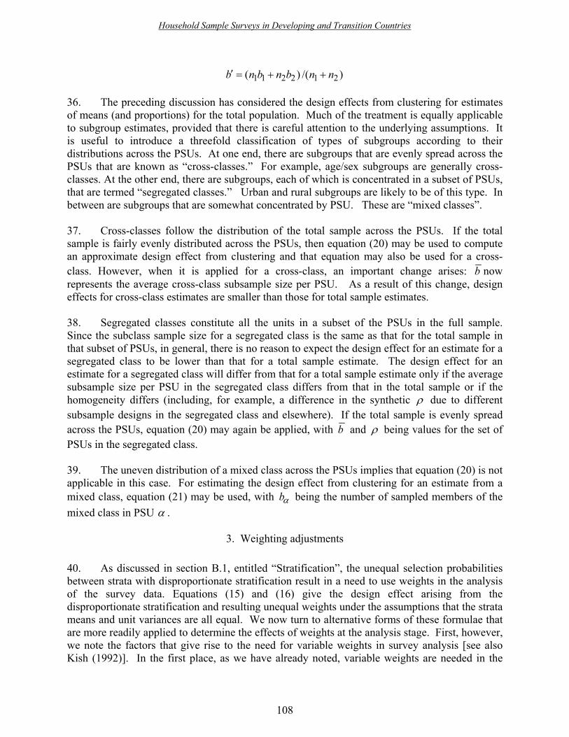
Household Sample Surveys in Developing and Transition Countries
108
1 1 2 2 1 2( ) /( )b n b n b n n′ = + +
36. The preceding discussion has considered the design effects from clustering for estimates of means (and proportions) for the total population. Much of the treatment is equally applicable to subgroup estimates, provided that there is careful attention to the underlying assumptions. It is useful to introduce a threefold classification of types of subgroups according to their distributions across the PSUs. At one end, there are subgroups that are evenly spread across the PSUs that are known as �cross-classes.� For example, age/sex subgroups are generally cross-classes. At the other end, there are subgroups, each of which is concentrated in a subset of PSUs, that are termed �segregated classes.� Urban and rural subgroups are likely to be of this type. In between are subgroups that are somewhat concentrated by PSU. These are �mixed classes�.
37. Cross-classes follow the distribution of the total sample across the PSUs. If the total sample is fairly evenly distributed across the PSUs, then equation (20) may be used to compute an approximate design effect from clustering and that equation may also be used for a cross-class. However, when it is applied for a cross-class, an important change arises: b now represents the average cross-class subsample size per PSU. As a result of this change, design effects for cross-class estimates are smaller than those for total sample estimates.
38. Segregated classes constitute all the units in a subset of the PSUs in the full sample. Since the subclass sample size for a segregated class is the same as that for the total sample in that subset of PSUs, in general, there is no reason to expect the design effect for an estimate for a segregated class to be lower than that for a total sample estimate. The design effect for an estimate for a segregated class will differ from that for a total sample estimate only if the average subsample size per PSU in the segregated class differs from that in the total sample or if the homogeneity differs (including, for example, a difference in the synthetic ρ due to different subsample designs in the segregated class and elsewhere). If the total sample is evenly spread across the PSUs, equation (20) may again be applied, with b and ρ being values for the set of PSUs in the segregated class.
39. The uneven distribution of a mixed class across the PSUs implies that equation (20) is not applicable in this case. For estimating the design effect from clustering for an estimate from a mixed class, equation (21) may be used, with bα being the number of sampled members of the mixed class in PSU α .
3. Weighting adjustments
40. As discussed in section B.1, entitled �Stratification�, the unequal selection probabilities between strata with disproportionate stratification result in a need to use weights in the analysis of the survey data. Equations (15) and (16) give the design effect arising from the disproportionate stratification and resulting unequal weights under the assumptions that the strata means and unit variances are all equal. We now turn to alternative forms of these formulae that are more readily applied to determine the effects of weights at the analysis stage. First, however, we note the factors that give rise to the need for variable weights in survey analysis [see also Kish (1992)]. In the first place, as we have already noted, variable weights are needed in the

Household Sample Surveys in Developing and Transition Countries
109
analysis to compensate for unequal selection probabilities associated with disproportionate stratification. More generally, they are needed to compensate for unequal selection probabilities arising from any cause. The weights that compensate for unequal selection probabilities are the inverses of the selection probabilities, and they are often known as base weights. The base weights are often then adjusted to compensate for non-response and to make weighted sample totals conform to known population totals. As a result, final analysis weights are almost always variable to some degree.
41. Even without oversampling of certain domains, sample designs usually deviate from epsem because of frame problems. For example, if households are selected with equal probability from a frame of households and then one household member is selected at random in each selected household, household members are sampled with unequal probabilities and hence weights are needed in the analysis in compensation. These weights give rise to a design effect component as discussed below. In passing, it may be noted that this weighting effect may be avoided by taking all members of selected household into the sample. However, this procedure introduces another stage of clustering, with an added clustering effect due to the similarity of many characteristics of household members [see Clark and Steel (2002) on the design effects associated with these alternative methods of selecting persons in sampled households].
42. Another common case of a non-epsem design resulting from a frame problem is that in which a two-stage sample design is used and the primary sampling units (PSUs) are sampled with probabilities proportional to estimated sizes (PPES). If the size measures are reasonably accurate, the sample size per selected PSU for an overall epsem design is roughly the same for all PSUs. However, if the estimated size of a selected PSU is a serious underestimate, the epsem design calls for a much larger than average number of units from that PSU. Since collecting survey data for such a large number is often not feasible, a smaller sample may be drawn, leading to unequal selection probabilities and the need for compensatory weights.
43. Virtually all surveys encounter some amount of non-response. A common approach used to reduce possible non-response bias involves differentially adjusting the base weights of the respondents. The procedure consists of identifying subgroups of the sample that have different response rates and inflating the weights of respondents in each subgroup by the inverse of the response rate in that subgroup (Brick and Kalton, 1996). These weighting adjustments cause the weights to vary from the base weights and the effect is often an increase in the design effect of an estimate.
44. When related population information is available from some other source, the non-response-adjusted weights may be further adjusted to make the weighted sample estimates conform to the population information. For example, if good estimates of regional population sizes are available from an external source, the sample estimates of these regional populations can be made to coincide with the external estimates. This kind of population weighting adjustment is often made by a post-stratification type of adjustment. It can help to compensate for non-coverage and can improve the precision of some survey estimates. However, it adds further variability to the weights which can adversely affect the precision of survey estimates that are unrelated to the population variables employed in the adjustment.

Household Sample Surveys in Developing and Transition Countries
110
45. With this background, we now consider a generalization of the design effect for disproportionate stratification to assess the general effects of variable weights. Kish (1992) presents another way of expressing the design effect for a stratified mean that is very useful for computing the effect of disproportionate stratification at the analysis stage. The following equation is simply a different representation of equations (15) and (16), and is thus based on the same assumptions of equal strata means and unit variances, particularly the latter. Since it is computed from the sample, the design effect is designated as 2 ( )std y and
( )
( )2
2 22( ) 1hih i
st hi
hih i
n wd y cv ww
∑ ∑= = +∑ ∑
(22)
where ( )hicv w is the coefficient of variation of the weights, ( ) ( )22 2/hi hicv nww w w= −∑ ∑ , and /hiw w n= ∑ ∑ is the mean of the weights. 46. A more general form of this equation is given by
( )
22 2
2( ) 1 ( )jjst j
jj
n wd y cv w
w
∑= = +
∑ (23)
where each of the n units in the sample has its own weight ( 1,jw j = 2, �, n). The design effect due to unequal weighting given by equation (23) depends on the assumption that the weights are unrelated to the survey variable. The equation can provide a reasonable measure of the effect of differential weighting for unequal selection probabilities if its underlying assumptions hold at least approximately [see Spencer (2000), for an approximate design effect for the case where the selection probabilities are correlated with the survey variable]. 47. Non-response adjustments are generally made within classes defined by auxiliary variables known for both respondents and non-respondents. To be effective in reducing non-response bias, the variables measured in the survey do need to vary across these weighting classes. The variation, however, is generally not great, particularly in the unit variance. As a result, equation (23) is widely used to examine the effect of non-response weighting adjustments on the precision of survey estimates. This examination may be conducted by computing equation (23) with the base weights alone or with the non-response adjustment weights. If the latter computation produces a much larger value than the former, this means that the non-response weighting adjustments are causing a substantial loss of precision in the survey estimates. In this case, it may be advisable to modify the weighting adjustments by collapsing weighting classes or trimming extremely large weights in order to reduce the loss of precision.
48. While equation (23) is reasonable with respect to most non-response sample weighting adjustments, it often does not yield a good approximation for the effect of population weighting adjustments. In particular, when the weights are post-stratified or calibrated to known control totals from an external source, then the design effect for the mean of y is poorly approximated by

Household Sample Surveys in Developing and Transition Countries
111
equation (23) when y is highly correlated with the one or more of the control totals. For example, assume the weights are post-stratified to control totals of the numbers of persons in a country by sex. Consider the extreme case where the survey data are used to estimate the proportion of women in the population. In this case of perfect correlation between the y variable and the control variable, the estimated proportion is not subject to sampling error and hence has zero variance. In practice, the correlation will not be perfect, but it may be sizeable for some of the survey variables. When the correlation is sizeable, post-stratification or calibration to known population totals can appreciably improve the precision of the survey estimates, but this improvement will not be shown through the use of equation (23). On the contrary, equation (23) will indicate a loss in precision.
49. The above discussion indicates that equation (23) should not be used to estimate the design effects from population weighting adjustments for estimates based on variables that are closely related to the control variables. In most general population surveys in developing countries, however, few, if any, dependable control variables are available, and the relationships between any that are available and the survey variables are seldom strong. As a result, the problem of substantially overestimating the design effects from weighting using equation (23) should not occur often. Nevertheless, the above discussion provides a warning that equation (23) should not be applied uncritically.
50. We conclude this discussion of the design effects of weighting with some comments on the effects of weighting on subgroup estimates. All the results presented in this section and section B.1 can be applied straightforwardly to give the design effects for subgroup estimates simply by restricting the calculations to subgroup members. However, care must be taken in trying to infer the design effects from weighting for subgroup estimates from results for the full sample. For this inference to be valid, the distribution of weights in the subgroup must be similar to that in the full sample. Sometimes this is the case, but not always. In particular, when disproportionate stratification is used to give adequate sample sizes for certain domains (subgroups), the design effects for total sample estimates will exceed 1 (under the assumptions of equal means and variances). However, the design effects from weighting for domain estimates may equal 1 because equal selection probabilities are used within domains.
C. Models for design effects 51. The previous section has presented some results for design effects associated with weighting and clustering separately, with the primary focus on design effects for means and proportions. The present section extends those results by considering the design effects from a combination of weighting and clustering and the design effects for some other types of estimates.
52. A number of models have been used to represent the design effects for these extensions. The models have been used in both the design and the analysis of complex sample designs (Kalton, 1977; Wolter, 1985). Historically, the models have played a major role in analysis. However, their use in analysis is probably on the wane. Their primary -- and important -- use in the future, in the planning of new designs, will be the focus of the present discussion.

Household Sample Surveys in Developing and Transition Countries
112
53. Recent years have seen major advances in computing power and in software for computing sampling errors from complex sample designs. Before these advances were achieved, computing valid sampling errors for estimates from complex samples had been a laborious and time-consuming task. It was therefore common practice to compute sampling errors directly for only a relatively small number of estimates and to use design effect or other models to infer the sampling errors for other estimates. The computing situation has now improved dramatically so that the direct computation of sampling errors for many estimates is no longer a major hurdle. Moreover, further improvements in both computing power and software can be expected in the future. Thus, the use of design effects models for this purpose can be expected to largely disappear.
54. Another reason for using sampling error models at the analysis stage is to provide a means for succinctly summarizing sampling errors in survey reports, thereby eliminating the need to present a sampling error for each individual estimate. In some cases, it may also be argued that the sampling error estimates from a model may be preferable to direct sampling error estimates because they are more precise. There are certain cases where this latter argument has some force (for instance, in estimating the sampling error for an estimate in a region in which the number of sampled PSUs is very small). However, in general, the use of models for reporting sampling errors for either of these reasons is questionable. The validity of the model estimates depends on the validity of the models and, when comparisons of direct and model-based sampling errors have been made, the comparisons have often raised serious doubts about the validity of the models [see, for example, Bye and Gallicchio (1989)]. Also, while sampling error models can provide a concise means of summarizing sampling errors in survey reports, they impose on users the undesirable burden of performing calculations of sampling errors from the models. Our overall conclusion is that design effect and other sampling error models will play a limited role in survey analysis in the future.
55. In contrast, design effect models will continue to play a very important role in sample design. Understanding the consequences of a disproportionate allocation of the sample and of the effects of clustering on the precision of different types of survey estimates is key to effective sample design. Most obviously, the determination of the sample size required to give adequate precision to key survey estimates clearly needs to take account of the design effect resulting from a given design. Also, the structure of an efficient sample design can be developed by examining the results from models for different designs. Note that estimates of unknown parameters, such as ρ , are required in order to apply the models at the design stage. This requirement points to the need for producing estimates of these parameters from past surveys, as illustrated in the next section.
56. We start by describing models for inferring the effects of clustering in epsem samples on a range of statistics beyond the means and proportions considered in section B.3, entitled �Weighting adjustments�. To introduce these models, we return to subgroup means as already discussed, with the distinction made between cross-classes, segregated classes, and mixed classes. For a cross-class, denoted as d, that is evenly spread across the PSUs, the design effect for a cross-class mean is given approximately by equation (20), which is written here as
2
:( ) 1 ( 1)cl d d dD y b ρ= + − (24)

Household Sample Surveys in Developing and Transition Countries
113
where db denotes the average cross-class sample size per PSU and dρ is the synthetic measure of homogeneity of y in the PSUs for the cross-class. A widely used model assumes that the measure of homogeneity for the cross-class is the same as that for the total population, in other words, that dρ ρ= . Then the design effect for the cross-class mean can be estimated by
2: �( ) 1 ( 1)cl d dd y b ρ= + − (25)
where �ρ is an estimate of ρ from the full sample given by
2( ) 1�
1cld y
bρ −
=−
(26)
57. A common extension of this approach is to compute �ρ �s for a set of comparable estimates involving related variables and, provided that the �ρ �s are fairly similar, to use some form of average of them to estimate ρ and hence also the dρ �s for subgroup estimates for all the variables. This approach has often been applied to provide design effect models for summarizing sampling errors in survey reports. It is also the basis of one form of generalized variance function (GVF) used for this purpose (Wolter, 1985, p. 204).
58. A special case of this approach occurs with survey estimates that are subgroup proportions falling in different categories of a categorical variable, such as the proportions of different subgroups that have reached different levels of education or that are in different occupational categories. It is often assumed that the values of ρ for the different categorizations are similar, so that the value of ρ needs to be estimated for only one categorization, and that once estimated, �ρ can then be applied for all the other categorizations. The assumption of a common ρ is mathematically correct when there are only two categories (for example, household with and household without electricity), but it need not hold when there are more than two categories. Consider, for example, estimates of the proportion of workers engaged in agriculture and in mining. The value of ρ for agricultural workers is almost certainly much lower than that for miners because mining is probably concentrated in a few areas. The assumption of a common ρ value for all categorizations should therefore not be applied uncritically.
59. When variances for cross-class means derived from equation (25) have been compared with those computed directly, they have been found to tend to be underestimates. This finding may be due to the fact that, even though classified as cross-classes, the subgroups are not distributed completely evenly across the PSUs. One remedy that has been used to address this problem is to modify equation (25) with the result that
2
: �( ) 1 ( 1)cl d d dd y k b ρ= + − (27)

Household Sample Surveys in Developing and Transition Countries
114
where 1dk > . Basing his work on many empirical analyses, Kish (1995) suggests values of 1.2dk = or 1.3; Verma and Lê (1996) allow dk to vary with the cross-class size (with dk
always greater than 1). A possible alternative remedy would be to replace db in (25) with 2 /d d db b bα α′ = Σ Σ in line with equation (21).
60. We now consider briefly design effects for analytic statistics. The simplest and most widely used form of analytic statistic is the difference between two subgroup means or proportions. It has generally been found that the design effect for the difference between two means is greater than 1 but less than that obtained by treating the two subgroup means as independent (Kish and Frankel, 1974; Kish, 1995). Expressed in terms of variances,
: : : : : :( ) ( ) ( ) ( ) ( )u d u d cl d cl d cl d cl dV y V y V y y V y V y′ ′ ′+ < − < + (28)
where d and d ′ represent the two subgroups. The variance of the difference in the means is typically lower than the upper bound when the subgroups are both represented in the same PSUs. This feature results in a covariance between the two means that is virtually always positive, and that positive covariance then reduces the variance of the difference. This effect does not occur when the subgroups are segregated classes that are in different sets of PSUs: in this case, the upper bound applies. Under the assumption that the unit variances in the two subgroups are the same (in other words, that 2 2
d dS S ′= ), this inequality reduces to
2 2
2 ( ) ( )1 ( ) d d d dd d
d d
n D y n D yD y yn n
′ ′′
′
+< − <
+
61. A special case of the difference between two proportions arises when the proportions are each based on the same multi-category variable, as occurs, for example, when respondents are asked to make a choice between several alternatives and the analyst is interested in whether one alternative is more popular than another. Kish and others (1995) examined design effects for such differences and found empirically that ( ) ( ) ( )[ ] 4/222
dddd ddpd ′′− += ρρρ in this special case.
62. The finding given above that design effects from clustering are typically smaller for differences in means than for overall means generalizes to other analytic statistics. See Kish and Frankel (1974) for some early empirical evidence and some modelling suggestions for design effects for multiple regression coefficients. The design effects for regression coefficients are like those for differences between means. That this is in line with expectation may be seen by noting that the slope of a simple linear regression of y on x may be estimated fairly efficiently by
( ) /( )u l u lb y y x x= − − , where the means of y and x are computed for the upper (u) and lower (l) thirds of the sample based on the x variable. See Skinner, Holt and Smith (1989) and Lehtonen and Pahkinen (1994) for design effects in regression and other forms of analysis, and Korn and Graubard (1999) for the effects of complex sample designs on precision in the analysis of survey data.

Household Sample Surveys in Developing and Transition Countries
115
63. We conclude this section with some comments on the taxing problem of decomposing an overall design effect into components due to weighting and to clustering. The calculation of the design effect 2 ( ) ( ) / ( )c ud y v y v y= encompasses the combined effects of weighting and clustering. However, in using the data from the current survey to plan a future survey, the two components of the design effect need to be separated. For example, the future survey may be planned as one using epsem whereas the current survey may have oversampled certain domains. Also, even if it used the same PSUs and stratification, the future survey might wish to change the subsample size per PSU. Kish (1995) discusses this issue, for which there is no single and simple solution. Here, we give an approach that may be used only when the weights are random or approximately so. In this case, the overall design effect can be decomposed approximately into a product of the design effects of weighting and clustering whereby
2 2 2( ) ( ). ( )w cld y d y d y= (29)
where 2 ( )wd y is the design effect from weighting as given by equation (23) and 2 ( )cld y is the design effect from clustering given by equations (20) or (21). There is little theoretical justification for equation (29); however, using a modelling approach, Gabler, Haeder and Lahiri (1999) derive the design effect given by equation (29) as an upper bound. Using equation (29) with equation (20), ρ is thus estimated by
2 2[ ( ) / ( )] 1�
1wd y d y
bρ −
=−
(30)
As will be seen below, for planning purposes, estimation of the parameter ρ is more important than estimation of the design effect from clustering because it is more portable across different designs. The design effect from clustering in one survey can be directly applied in planning another only if the subsample size per PSU remains unchanged.
D. Use of design effects in sample design
64. The models for design effects discussed in the earlier part of this chapter can serve as useful tools for planning a new sample design. However, they need to be supported by empirical data, particularly on the synthetic measure of homogeneity ρ . These data can be obtained by analysing design effects for similar past surveys. Accumulation of data on design effects is therefore valuable.
65. A substantial amount of data on design effects is available for demographic surveys of fertility and health from the extensive analyses of sampling errors that have been conducted for the World Fertility Surveys (WFS) and Demographic and Health Surveys (DHS) programmes. The WFS programme had conducted 42 surveys in 41 countries between 1974 and 1982. The DHS programme followed in 1984, with over 120 completed surveys in 66 countries having been conducted to date, with the surveys being repeated in most countries every three to five years. See Verma and Lê (1996) for analyses of DHS sampling errors, and Kish, Groves and

Household Sample Surveys in Developing and Transition Countries
116
Krotki (1976) and Verma, Scott and O�Muircheartaigh (1980) for similar analyses of WFS sampling errors. An important finding from the sampling error analyses for these programmes is that estimates of ρ for a given estimate are fairly portable across countries provided that the sample designs are comparable. Thus, in designing a new survey in one country, empirical data on sampling errors from a similar survey in a neighbouring country may be employed if necessary and if due care is taken to check on sample design comparability.
66. The example given below illustrates the use of design effects in developing the sample design for a hypothetical national survey. For the purposes of this illustration, we assume that the sample design will be a stratified two-stage PPS sample, say, with census enumeration districts as the PSUs and households as the second-stage units. We assume that the key statistic of interest is the proportion of households in poverty, which for planning purposes is assumed to be about 25 per cent, and to be similar for all the provinces in the country. The initial specifications are that the estimate of this proportion should have a coefficient of variation of no more that 5 per cent for the nation and no more than 10 per cent for each of the nation�s eight provinces. Furthermore, the sample should be efficient in producing precise estimates for a range of statistics for national subgroups that are spread fairly evenly across the eight provinces. If simple random sampling was used, the coefficient of variation would be
1 PCVnP−
=
where P is the proportion of households in poverty (25 per cent in this case). This formula can also be used with a complex sample design, but with n replaced by the effective sample size,
2/ ( )effn n D p= . 67. The first issue to be addressed is how the sample should be distributed across the provinces. Table VI.2 gives the distribution of the population across the provinces ( hW ), together with a proportionate allocation of the sample across the provinces, an equal sample size allocation for each province, and a compromise sample allocation that falls between the proportionate and equal allocations. An arbitrary total sample size of 5,000 households is used at this point. It can be revised later, if necessary.
Table VI.2. Distributions of the population and three alternative sample allocations across
the eight provinces (A �H) A B C D E F G H Total
hW 0.33 0.24 0.20 0.10 0.05 0.04 0.02 0.02 1.00 Proportionate allocation
1 650 1 200 1 000 500 250 200 100 100 5 000
Equal sample size allocation
625 625 625 625 625 625 625 625 5 000
Compromise sample allocation
1 147 879 767 520 438 427 411 411 5 000

Household Sample Surveys in Developing and Transition Countries
117
68. Other things being equal, the proportionate allocation is the most suitable for producing national estimates and subgroup estimates where the subgroups are evenly spread across the provinces. On the other hand, the equal sample size allocation is the most suitable for producing provincial estimates. As table VI.2 shows, these two allocations differ markedly, as a result of the very different sizes of the provinces given in the hW row. The proportionate allocation yields samples in the small provinces (E, F, G and H) that are too small to enable the computation of reliable estimates for them. On the other hand, the equal sample size allocation reduces the precision of national estimates. That loss of precision can be computed from equation (15), which, in this case, simplifies to 2 1.77hH WΣ = , where H is the number of provinces. Thus, by considering the effects of the disproportionate allocation only (that is to say, by excluding the effects of clustering), the sample size of 5,000 for national estimates is reduced to an effective sample size of 5,000 /1.77 2,825.=
69. Whether the large loss of precision for national estimates (particularly for subgroups) resulting from the use of the equal allocation is acceptable depends on the relative importance of national and provincial estimates. Often, national estimates are sufficiently important to render this loss too great to accept. In this case, a compromise allocation that falls between the proportionate and equal allocations may be found to satisfy the needs for both national and provincial estimates. The compromise allocation in the final row of table VI.2 is computed according to an allocation proposed by Kish (1976, 1988) for the situation where national and provincial estimates are of equal importance. That allocation, given by 2 2
h hn W H −∝ + , increases the sample sizes for the small provinces considerably over the proportionate allocation, but not as much as the equal allocation. The design effect for unequal weighting for this allocation is 1.22, as compared with 1.77 for the equal sample size allocation. We will assume that the compromise allocation is adopted for the survey.
70. The next issue to be addressed is how to determine the number of PSUs and the desired number of households to be selected per PSU. As discussed in chapter II, through the use of a simple cost model, the optimum number of households to select per sampled PSU is given by
(1 )*optb C ρ
ρ−
=
where C* is the ratio of the cost of adding a PSU to the sample to the cost of adding a household. The cost model is oversimplified, and the formula for optb should not be used uncritically; nevertheless, it can still give useful guidance. 71. Let us assume that the organizational structure of the survey fieldwork makes the use of the simple cost model reasonable and that an analysis of the cost structure indicates that *C is about 16. Furthermore, let us assume that a previous survey, using the same PSUs, has produced an estimate of 0.05ρ = for a characteristic that is highly correlated with poverty. Applying these numbers to the above formula gives � 17.4optb = , which, for the sake of simplicity, we round to 17. Often, in practice, the cost ratio *C is not constant across the country; for

Household Sample Surveys in Developing and Transition Countries
118
example, the ratio may be much lower in urban than in rural areas. If this is the case, different values may be used in different parts of the country. Such complexity will not be considered further here. Examples of such differences are to be found in several of the chapters in this publication that describe national sample designs.
72. With 0.05ρ = and 17b = , the design effect from clustering is
2 ( ) 1 ( 1) 1.80D p b ρ= + − =
This design effect needs to be taken into account in determining the precision of provincial estimates. For example, the effective sample size of 411 households in province H is 411/1.80 228= . Hence, the coefficient of variation for the proportion of households in poverty in province H is 0.11. If this level of precision was deemed inadequate, the sample size in province H (and also G) would need to be increased. 73. The design effect for national estimates needs to combine the design effects for clustering and the disproportionate allocation across provinces. Thus, for the overall national proportion of households in poverty, the estimated design effect may be obtained from equation (29) as 1.22 1.80 2.20× = . Hence, the effective sample size corresponding to an actual sample size of 5,000 households is 2,277 and the coefficient of variation for the national estimate of the proportion of households in poverty is 0.036. It is often the case that the overall sample size is more than adequate to satisfy the precision requirements for estimates for the total population. Of more concern is the precision levels for population subgroups. In this case, the design effect from clustering for cross-classes evenly distributed across the PSUs, is smaller than for the total sample, as described in section C. For example consider a cross-class that comprises one third of the population. In this case, applying formula (27) with 1.2dk = and 17 / 3db = gives a clustering design effect of 1.23. Combining the clustering design effect with that for the disproportionate allocation across provinces gives an overall design effect for the cross-class estimate of 1.22 1.23 1.50× = , and an effective sample size of 5000 /(3 1.50) 1111× = . The estimated coefficient of variation for the cross-class estimate is thus 0.05.
74. Calculations along the lines of those indicated above can be made to assess the likely precision of key survey estimates, and sample sizes can be modified to meet desired requirements. In the final estimates of sample sizes, allowances need to be made for non-response. For example, with a fairly uniform 90 per cent response rate across the country, the sample sizes calculated above need to be increased by 11 per cent. Also, the design effect may increase somewhat as a result of the additional variation in weights arising from non-response adjustments. In computing the sampling fractions to be used to generate the required sample sizes, allowance needs to be made for non-coverage. With a 90 per cent coverage rate, sampling fractions need to be increased by 11 per cent.

Household Sample Surveys in Developing and Transition Countries
119
E. Concluding remarks 75. An understanding of design effects and their components is valuable in developing sample designs for new surveys. For example:
• The magnitudes of the overall design effects for key survey estimates may be
used in determining the required sample size. The sample size needed to give the specified level of precision for each key estimate may be computed for an unrestricted sample, and this sample size may then be multiplied by the estimate�s design effect to give the required sample size for that estimate with the complex sample design. The final sample size may then be chosen by examining the required sample sizes for each of the estimates (perhaps, with the largest of these sample sizes being taken).
• When a disproportionate stratified sample design is to be used to provide domain
estimates of required levels of precision, the resultant loss of precision for estimates for the total sample and for subgroups that cut across the domains can be assessed by computing the design effect due to variable weights. If the loss is found to be too great, then a change in the domain requirements that leads to less variable weights may be indicated.
• If the design effect from clustering is very large for some key survey estimates,
then the possibility of increasing the number of sampled PSUs (a) with a smaller subsample size (b) should be considered.
76. While the formulas presented in this chapter are useful in sample design, they should not be applied uncritically. As noted in several places, the formulae are derived under a number of assumptions and simplifications. Users need to be sensitive to these features and to consider whether the formulae will provide reasonable approximations for their situation.
77. Estimating design effects from clustering requires estimates of ρ values for the key survey variables. These estimates are inevitably imperfect, but reasonable estimates may suffice. To err in the direction of the use of a value of ρ larger than predicted leads to the specification of a larger required sample size; hence, this is a conservative strategy.
78. Finally, it should be noted that the purpose of using these design effect models is to produce an efficient sample design. The failure of the models to hold exactly will result in some loss of efficiency. However, the use of inappropriate models to develop the sample design does not affect the validity of the survey estimates. With probability sampling, the survey estimates remain valid estimates of the population parameters.
Household Sample Surveys in Developing and Transition Countries
120
References Brick, J.M., and G. Kalton (1996). Handling missing data in survey research. Statistical
Methods in Medical Research, vol. 5, pp. 215-238. Bye, B., and S. Gallicchio (1989). A note on sampling variance estimates for Social Security
program participants from the Survey of Income and Program Participation. United States Social Security Bulletin, vol. 51, no. 10, pp. 4-21.
Clark, R.G., and D.G. Steel (2002). The effect of using household as a sampling unit.
International Statistical Review, vol. 70, pp. 289-314. Cochran, W.G. (1977). Sampling Techniques, 3rd ed. New York: Wiley. Gabler, S., S. Haeder and P. Lahiri (1999). A model based justification of Kish's formula for
design effects for weighting and clustering. Survey Methodology, vol. 25, pp. 105-106. Holt, D. H. (1980). Discussion of the paper by Verma, V., C. Scott and C. O�Muircheartaigh:
sample designs and sampling errors for the World Fertility Survey. Journal of the Royal Statistical Society, Series A, vol. 143, pp. 468-469.
Kalton, G. (1977). Practical methods for estimating survey sampling errors. Bulletin of the
International Statistical Institute, vol. 47, No. 3, pp. 495-514.
_________ (1979). Ultimate cluster sampling. Journal of the Royal Statistical Society, Series A, vol. 142, pp. 210-222.
Kish, L. (1965). Survey Sampling. New York: Wiley. _________ (1976). Optima and proxima in linear sample designs. Journal of the Royal
Statistical Society, Series A, vol. 139, pp. 80-95. _________ (1982). Design effect. In Encyclopedia of Statistical Sciences, vol. 2, S. Kotz and
N.L. Johnson, eds., New York: Wiley, pp. 347-348. _________ (1988). Multi-purpose sample designs. Survey Methodology, vol. 14, pp. 19-32. _________ (1992). Weighting for unequal iP . Journal of Official Statistics, vol. 8, pp. 183-200. _________ (1995). Methods for design effects. Journal of Official Statistics, vol. 11, pp. 55-77. __________, and M.R. Frankel (1974). Inference from complex samples. Journal of the Royal
Statistical Society, Series B, vol. 36, pp. 1-37. __________, and others (1995). Design effects for correlated ( )i jp p− . Survey Methodology,
vol. 21, pp. 117-124.

Household Sample Surveys in Developing and Transition Countries
121
__________, and others (1976). Sampling Errors in Fertility Surveys. World Fertility Survey Occasional Paper, No. 17. The Hague: International Statistical Institute.
Korn, E.L., and B.I. Graubard (1999). Analysis of Health Surveys. New York: Wiley. Lehtonen, R., and E.J. Pahkinen (1994). Practical Methods for Design and Analysis of Complex
Surveys, revised ed. Chichester, United Kingdom: Wiley. Lepkowski, J.M., and J. Bowles (1996). Sampling error software for personal computers.
Survey Statistician, vol. 35, pp. 10-17. Rust, K.F. (1985). Variance estimation for complex estimators in sample surveys. Journal of
Official Statistics, vol.1, pp. 381-397. __________ , and J.N.K. Rao (1996). Variance estimation for complex surveys using replication
techniques. Statistical Methods in Medical Research, vol. 5, pp. 283-310. Skinner, C.J., D. Holt and T.M.F. Smith, eds. (1989). Analysis of Complex Surveys. Chichester,
United Kingdom: Wiley. Spencer, B.D. (2000). An approximate design effect for unequal weighting when measurements
may correlate with selection probabilities. Survey Methodology, vol. 26, pp. 137-138. United Nations (1993). National Household Survey Capability Programme: Sampling Errors in
Household Surveys. UNFPA/UN/INT-92-P80-15E. New York: United Nations Statistics Division. Publication prepared by Vijay Verma.
Verma, V., and T. Lê (1996). An analysis of sampling errors for the Demographic and Health
Surveys. International Statistical Review, vol. 64, pp. 265-294. Verma, V., C. Scott and C. O�Muircheartaigh (1980). Sample designs and sampling errors for
the World Fertility Survey. Journal of the Royal Statistical Society, Series A, vol. 143, pp. 431-473.
Wolter, K.M. (1985). Introduction to Variance Estimation. New York: Springer-Verlag.

Household Sample Surveys in Developing and Transition Countries
122

Household Sample Surveys in Developing and Transition Countries
123
Chapter VII Analysis of design effects for surveys in developing countries
Hans Pettersson Statistics Sweden Stockholm, Sweden
Pedro Luis do Nascimento Silva Escola Nacional de Ciências Estadísticas/
Instituto Brasileiro de Geografia e Estatística (ENCE/IBGE)
Rio de Janeiro, Brazil
Abstract
The present chapter presents design effects for 11 household surveys from 7 countries and, for 3 surveys that are rather similar in design, compares design effects and rates of homogeneity (roh) for estimates of household consumption and possession of durables. It concludes with a discussion of the portability of estimates of roh across surveys.
Key terms: design effects, efficiency, rates of homogeneity, survey design, sample design, clustering.

Household Sample Surveys in Developing and Transition Countries
124
A. Introduction
1. It is not yet common practice to calculate design effects as standard output for household surveys in developing countries. An exception occurs with respect to some standardized surveys like the Living Standards Measurement Study (LSMS) surveys and the Demographic and Health Surveys (DHS). For those surveys, design effects have been calculated and compared across countries (see chaps. XXII and XXIII). An earlier extensive comparative analysis has been made on 35 surveys conducted under the World Fertility Survey (WFS) programme (Verma, Scott and O�Muircheartaigh, 1980).
2. The present chapter presents design effects for 11 surveys from 7 countries. The selection of surveys was subjective and was mainly based on easy availability. The surveys come from: Brazil (3), Cambodia (1), the Lao People�s Democratic Republic (1), Lesotho (1), Namibia (2), South Africa (2) and Viet Nam (1). The surveys are of different character and cover different topics. Among the surveys are multipurpose surveys, labour force surveys, a living standards survey and a demographic survey. Design effects have been calculated for a number of characteristics, mostly for survey planning purposes. The main purpose of this chapter is to give the reader a general idea of the levels of design effects experienced in various surveys.
3. For three surveys that are rather similar in design, a deeper analysis is made comparing design effects and rates of homogeneity for a few variables concerning household consumption and access to durables. The purpose is to examine the behaviour of (roughly) the same variable in different populations and to explore similarities and possible patterns in the findings.
B. The surveys
4. The surveys for which design effects are reported in this chapter are: • The Lao Expenditure and Consumption Survey 1997/98 (LECS) • The Cambodia Socio-Economic Survey 1999 (CSES) • The Namibia Household Income and Expenditure Survey 1993/94 (NHIES) • The Namibia Intercensal Demographic Survey 1995/96 (NIDS) • The Viet Nam Multipurpose Household Survey 1999 (VMPHS) • The Lesotho Labour Force Survey 1997 (LFS) • The October Household Survey 1999 of the Republic of South Africa (OHS) • The Labour Force Survey February 2000 of the Republic of South Africa • PNAD (Pesquisa Nacional por Amostra de Domicílios) 1999, Brazil • PME (Pesquisa Mensal de Emprego) for September 1999, Brazil • PPV (Pesquisa de Padrões de Vida) 1996/97, Brazil

Household Sample Surveys in Developing and Transition Countries
125
5. Table VII.1 summarizes the main design features of the 11 surveys. Standard two-stage probability proportional to size (PPS) designs were used in all the surveys except the Viet Nam survey where three stages are used. PNAD also employed three-stage sampling for small non-metropolitan municipalities, but these contained only about one third of the population covered by the survey. Most of the surveys used census enumeration areas as PSUs (with some modification of small EAs in some cases). Average PSU sizes of 90-150 households were common in these cases. Three surveys deviated from this pattern. The two surveys in Lesotho had much larger PSUs: the PSUs were groups of EAs with an average size of 340-370 households. At the other end, the rural PSUs in the Lao survey had on average only 50 households. 6. The sample sizes within PSUs (cluster sizes) were about 20 households for several of the surveys. The Namibia Intercensal Demographic Survey stands out with a large sample take of 50 households from each PSU. At the lower end were the Brazilian PPV survey where 8 households were selected per urban PSU, and the two South African surveys and the Cambodian survey with 10 households selected from each PSU. Most of the surveys had the same cluster sizes in urban and rural areas. 7. Most surveys were stratified explicitly on urban/rural areas within administrative divisions (provinces, regions). The Lesotho LFS had a further stratification in agroecological zones and the Lao LECS a further stratification on whether the village had road access or not. The Brazilian PNAD and PME surveys were stratified only implicitly into urban and rural, with systematic PPS selection of PSUs having taken place after sorting by location. 8. Systematic selection was used for selection of households within ultimate area units in all the surveys, except the PPV survey, where households were selected by simple random sampling. 9. An important feature of many of the sample designs is that they employed disproportionate sample allocations across provinces in order to produce provincial estimates of adequate precision. The weights needed in the analysis to compensate for the disproportionate allocations were very variable in some cases. For example, the ratio of largest to smallest sampling weight in the Brazilian PPV was about 40. Further details on the sample designs for the surveys are presented in the annex.

Household Sample Surveys in Developing and Transition Countries
126
Table VII.1. Characteristics of the 11 household surveys included in the study
Survey
Number of area stages
First-stage
sample: number
of PSUs selected to the
sample
PSU size: average
number of households
per PSU
Cluster size: number of households selected per
PSU (or SSU, if two area
stages)
Sample size: number of households
in the survey
Sample allocation
between strata
Lao Expenditure and Consumption Survey, 1997-1998
1 R: 348 U: 102
R: 51 U: 87
R: 20 U: 20
R: 6 960 U: 2 040
Disproportionate
Cambodia Socio-Economic Survey, 1999
1 R: 360 U: 240
R: 154 U: 243
R: 10 U: 10
R: 3 600 U: 2 400
Approximately proportionate
Namibia Household Income and Expenditure Survey, 1993-1994
1 R: 123 U: 96
R: 152 U: 148
R: 20 U: 20
R: 2 685 U: 1 712
Approximately proportionate
Namibia Intercensal Demographic Survey, 1995-1996
1 R: 120 U: 82
R: 152 U: 148
R: 50 U: 50
R: 5 600 U: 3 900
Approximately proportionate
Viet Nam Multipurpose Household Survey ,1999
2 839 PSUs, (2 SSUs
selected in each PSU)
R: 1 417 U: 2 579
SSUs: R: 99 U: 105
R: 15 U: 15
25 170 Disproportionate
Lesotho Labour Force Survey, 1997
1 R: 80 U: 40
R: 370 U: 341
R: 33 (average)
U: 25 (average)
R: 2 600 U: 1 000
Approximately proportionate
Labour Force Survey, 2000 of the Republic of South Africa
1 R: 426 U: 1 148
R: min 100 a/ U: min 100 a/
R: 10 U: 5
R: 4 059 U: 5 646
Disproportionate
October Household Survey, 1999 of the Republic of South Africa
1 R: 1 273 U: 1 711
R: 110-120 U: 80-100
R: 10 U: 10
R: 10 923 U: 15 211
Disproportionate
PNAD survey, 1999, Brazil
1 or 2 7 019 250 13 93 959 Disproportionate
PME survey for September 1999, Brazil
1 1 557 250 20 30 535 Disproportionate
PPV survey, 1996-1997, Brazil 1 554 250 R: 16 U: 8
4 944 Highly disproportionate
Note: R= rural, U=urban a/ Minimum of 100.

Household Sample Surveys in Developing and Transition Countries
127
C. Design effects
10. The design effects ( )(2 yd ) for a selection of estimates from each survey are shown in tables VII.2 through VII.6 (for a description on how the design effect is calculated, see chap. VI). The design effects have been calculated using Software for the Statistical Analysis of Correlated Data (SUDAAN) or StATA. In some cases, the design effects were provided by national statistical offices.21 11. The variation in design effects is substantial, as could be expected given the differences in sample design and variables among the surveys and the variation due to country-specific population conditions. Some effects are very high. Design effects in the range 6-10 for household variables are not unusual in the results displayed in tables VII.2-VII.6, and there are some effects in the range 10-15. Note that these design effects reflect the effects of the complex stratified clustered sample designs and the disproportionate allocations across provinces (where applicable). The tables of design effects presented in tables VII.2-V11.6 serve to illustrate the levels of design effects that have been experienced in some socio-economic and demographic household surveys in developing countries.
12. Table VII.2 presents estimates of design effects for seven surveys in Africa and South-East Asia for the national level and for urban and rural sub-domains. Most of the design effects concerned household socio-economic variables. Design effects from three of the surveys mainly concern labour-force variables on individual level. The overall average design effect on national level is 4.2. There is a rather wide variation in the effects, from 1.3 to 8.1, but most of the effects are in the range 2.0-6.0. The average design effects for the urban and rural sub-domains are 4.1 and 4.0, respectively. The differences in sample design and variables make it difficult to exploratorily search the results for any general differences between types of variables (for example, socio-economic/labour force) or domains (urban/rural) in the table. An attempt to compare some of the design effects is presented in table VII.7.
21 Professor David Stoker of Statistics South Africa compiled the design effects for the Labour Force Survey and October Household Survey of the Republic of South Africa. The design effects for the Viet Nam Multipurpose Household Survey were provided by Mr. Nguyen Phong, Director of Social and Environmental Statistics Department, General Statistics Office of Viet Nam. The design effects for the Namibia Household Income and Expenditure Survey were calculated by Mr. Alwis Weerasinghe, National Central Statistics Office of Namibia. The design effects for the Brazilian surveys were calculated by Dr. Pedro Silva, IBGE. For the other surveys, the design effects were calculated by Dr. Hans Pettersson based on data provided by the national statistical institutes.

Household Sample Surveys in Developing and Transition Countries
128
Table VII.2. Estimated design effects from seven surveys in Africa and South-East Asia Urban Rural National
Lao Expenditure and Consumption Survey, 1997-1998
Total monthly consumption per household
3.8
7.8
5.4 Monthly food consumption per household 4.4 6.8 5.8 Proportion of households with access to
motor vehicle
1.3
3.3
2.1 Proportion of households with access to TV 3.1 6.8 5.4 Proportion of households with access to
radio
2.7
4.8
4.5 Proportion of households with access to
video
3.9
6.1
5.5 Cambodia Socio-Economic Survey, 1999
Total monthly consumption per household
2.0
2.0
1.4
Monthly food consumption per household 3.1 3.2 3.2 Proportion of households with access to TV 2.4 2.2 2.6 Namibia Household Income and Expenditure Survey, 1993-1994
Total yearly household consumption
2.9
1.9
2.5 Total yearly household income 2.9 2.8 2.8 Proportion of households with access to TV 6.0 4.6 4.1 Proportion of households with access to
radio
2.7
2.1
2.4 Proportion of households with access to
telephone
6.2
4.6
4.5 Namibia Intercensal Demographic Survey
Proportion of households with access to TV
14.7
4.1
6.6
Proportion of households using electricity for lighting
4.4
3.9
4.2
Proportion of households experiencing a death of a household member during last 12 months
2.1
4.3
2.3 Viet Nam Multipurpose Household Survey, 1999 Poverty rate .. ..
7.1
Lesotho Labour Force Survey, 1997
Employment rate
5.6
3.1
6.6
Proportion of population ages 10 years and over that have not attended school
4.6
5.9
5.5
Proportion subsistence farmers 6.3 4.4 8.1 Proportion own account workers 3.0 1.4 2.4 October Household Survey, 1999, Republic of South Africa
Employment rate
4.0
3.6
3.8
Labour Force Survey, 2000, Republic of South Africa
Employment rate
2.5
3.4
2.8
Note: Two dots (..) indicate data not available.

Household Sample Surveys in Developing and Transition Countries
129
13. Table VII.3 presents estimates of design effects for a number of household-level estimates from the Brazilian PNAD.
Table VII. 3. Estimated design effects for country level and by type of area estimates for selected household estimates (PNAD 1999)
Variable
National Metropolitan
areas Large
municipalitiesOther areas
Proportion with general net water supply 9.80 6.60 6.74 10.73 Proportion with water from source 9.24 4.04 4.19 9.43 Proportion with adequate sewerage 9.04 6.36 5.87 11.59 Proportion with general net piped water 8.48 5.16 4.79 9.40 Proportion with at least one bathroom 8.34 1.51 7.20 7.76 Proportion with owned land 8.10 11.53 4.49 7.09 Proportion with electricity 7.92 1.03 4.43 7.27 Proportion with adequate wall material 7.43 6.17 5.01 6.84 Proportion with piped water at least one room 7.09 4.74 5.45 7.04 Proportion with adequate roof material 5.68 2.91 2.41 5.65 Average number of rooms per household 5.32 6.26 4.50 5.09 Proportion with telephone 4.80 5.59 4.44 5.91 Proportion with fridge 4.59 1.53 2.77 5.02 Proportion with washing machine 4.34 3.98 3.49 6.25 Proportion with color TV 4.31 1.77 2.76 4.88 Proportion with freezer 3.83 3.55 2.68 4.67 Proportion with water filter 3.39 2.50 2.07 4.37 Proportion with radio 3.01 1.46 1.62 3.29 Proportion with black and white TV 2.79 1.50 1.30 2.93 Average rent 2.52 3.09 2.01 3.39 Proportion of owned households 2.46 3.18 1.74 2.30 Proportion of rented households 2.32 2.71 1.78 2.51 Average number of rooms used as dormitories 2.14 2.37 1.72 2.09
14. Design effects vary between 2 and 10 for estimates at the national level, with an average value of 5.5. Design effects are higher for variables such as proportion of households with general net water supply, proportion with water from source, and proportion with adequate sewerage. This is expected, given the very high degree of clustering that these variables tend to display. Design effects are lower for some of the �economic� variables, such as average rent, proportion of owned or rented households, and average number of rooms used as dormitories. Also as expected, design effects are generally lower for the metropolitan areas and larger municipalities where the design is two-stage cluster sampling, than for the other areas, where the design is more clustered (three-stage cluster sampling).

Household Sample Surveys in Developing and Transition Countries
130
15. Design effects for a set of variables measured at the person level are presented in table VII.4.
Table VII.4. Estimated design effects for selected person-level characteristics at the national level and for various sub-domains (PNAD 1999)
Variable National Metropolitan areas
Large municipalities
Other areas
Proportion race=white 15.97 11.97 8.14 19.97 Proportion race=black or coloured 15.75 12.23 8.44 19.41 Proportion paid worker 8.44 4.45 5.81 7.49 Proportion self-employed 7.65 3.73 5.51 6.66 Proportion with social security 6.59 2.93 3.28 8.45 Proportion illiterate 6.33 3.67 4.37 7.10 Average income main occupation 5.54 7.16 4.45 6.38 Proportion housing benefit 5.23 3.80 3.00 5.54 Proportion transportation benefit 4.93 2.94 2.78 9.10 Proportion health benefit 4.90 3.76 2.29 8.79 Proportion working (10+ years) 4.79 1.97 1.67 7.08 Proportion food benefit 3.35 2.60 2.08 4.60 Proportion infants working (5-9 years) 3.27 1.25 2.04 3.00 Proportion employer 2.87 2.80 1.54 2.63 Proportion attending school 1.88 1.75 1.57 1.94 Proportion education benefit 1.87 1.85 1.74 2.22
16. Design effects for estimates at the national level vary from about 2 to 16, with an average of 6.2. Design effects are quite high for race variables, high for job- or income-related variables, and low for variables such as proportion attending school and proportion receiving education benefit. Again, design effects are higher for the other areas where the design is three-stage. Design effects for household variables are generally lower than those for person-level variables, which is expected because the number of persons is larger than the number of households surveyed per PSU. The substantial variations in design effects for different variables are expected because they display different degrees of clustering. These rather high design effects are also explained by the use of disproportionate sample allocation between strata, which leads to varying weights. 17. Design effects for the Brazilian PME are reported in table VII.5 for a selection of the estimates published every month. The values were obtained for September 1999, chosen because they have the same reference period as those for the PNAD 1999.

Household Sample Surveys in Developing and Transition Countries
131
Table VII.5. Estimated design effects for selected estimates from PME for September 1999
Variable Recife Salvador Belo Horizonte
Rio de Janeiro
São Paulo
Pôrto Alegre
All
Average income main occupation
3.43
4.47
2.49
4.44
4.89
4.79
6.23
Proportion employer 2.00 2.16 3.06 2.53 2.33 2.27 3.34 Proportion illiterate 4.23 4.43 1.86 2.69 2.11 2.13 3.24 Unemployment rate 1.64 2.62 1.98 2.06 1.65 1.67 2.43 Proportion with registered employment
1.61
1.87
1.66
1.50
1.40
1.75
2.02
Proportion economically active
1.59 1.99 1.78 1.61 1.31 1.40 1.96
Proportion paid worker 1.51 1.67 1.43 1.37 1.34 1.55 1.88 Proportion self-employed 1.53 2.26 1.60 1.47 1.19 1.14 1.78 Proportion attending school 1.41 1.57 1.64 1.24 1.26 1.49 1.72
18. Although not reported here, design effects for the same estimates were computed for other months in the series and found to vary little from month to month. The sample of enumeration areas is fixed throughout the decade and sample sizes also vary little in short periods of time. Design effects are larger for the average income in the main occupation and only moderate for the proportion illiterate and the proportion of employers. That these are in line with the values observed for similar estimates computed from PNAD for the metropolitan areas, is not surprising because essentially the same sample design was adopted for PME and PNAD, except for the larger sample take per PSU in PME. Design effects are below 2.5 for the other variables. That design effects for comparable variables estimated from PME are generally lower than those for PNAD, is due to the fact that the sample allocation is closer to proportional in PME than in PNAD.
19. Design effects for the Brazilian PPV are reported in table VII.6 for a small selection of the estimates obtained from that survey.
Table VII.6. Estimated design effects for selected estimates from PPV Estimated population parameter Deff estimate
Number of people older than 14 years of age who are illiterate 4.17 Proportion of people older than 14 years of age who are illiterate 3.86 Number of people who rated their health status as �bad� 3.37 Proportion of rented households 2.97 Average number of persons per household 2.64 Number of people between 7 and 14 years of age who are illiterate 2.64 Proportion of people between 7 and 14 years of age who are illiterate 2.46 Number of women aged 12-49 who had children born dead 2.03 Number of women aged 12-49 who had children 2.02 Number of women aged 12-49 who had children born alive 2.02 Dependence ratio (number aged 0-14 plus number aged 65 years or over, divided by number aged 15-64)
1.99
Average number of children born per woman aged 12-49 1.26

Household Sample Surveys in Developing and Transition Countries
132
20. For the estimates considered here, design effects vary between 1.3 and 4.2. The relatively small values of these design effects reflect the lower degree of clustering in PPV, where only 8 households were selected per PSU. They also reflect the fact that mostly variables in the demographic and educational blocks of the questionnaire were considered, plus two variables at the household level.
21. We now select, from tables VII.2 through VII.6, a set of estimates that appear in more than one survey. The design effects are presented in table VIII.7. The design effects have been grouped in three categories: (a) household consumption and household income; (b) household durables; and (c) employment and occupation. Within each category, we have grouped the estimates that have roughly the same definitions.
Table VII.7. Comparisons of design effects across surveys
Topic/characteristic
Urban
Rural
National
Comments Consumption, household income (household variables) - Total monthly consumption (Lao People�s Democratic Republic: LECS) - Total monthly consumption (Cambodia: CSES) - Total domestic household consumption (Namibia: NHIES) - Monthly food consumption (Lao People�s Democratic Republic: LECS) - Monthly food consumption (Cambodia: CSES)
3.8
2.0
2.9
4.4
2.5
7.7
2.0
1.9
6.8
3.3
5.4
1.4
2.5
5.8
3.3
The cluster size in CSES is half the cluster sizes in LECS and NHIES
Household durables (household variables) - Proportion of households with access to TV (Lao People�s Democratic Republic: LECS) - Proportion of households with access to TV (Cambodia: CSES) - Proportion of households with access to TV (Namibia: NHIES) - Proportion of households with access to TV (Namibia: NIDS)
3.1
2.4
6.0
14.7
6.8
2.2
4.6
4.1
5.4
2.6
4.1
6.6
The fact that the cluster size in NIDS is more than double that in the other surveys explains the large design effect in the urban areas (but not the low design effect for the rural areas)

Household Sample Surveys in Developing and Transition Countries
133
- Proportion of households with a color TV (Brazil: PNAD) - Proportion of households with access radio (Lao People�s Democratic Republic: LECS) - Proportion of households with access to radio (Cambodia: CSES) - Proportion of households with access to radio (Namibia: NHIES) - Proportion of households with access to telephone (Namibia: NHIES) - Proportion of households with access to telephone (Brazil: PNAD)
..
2.7
2.1
2.7
6.2 -
..
4.8
2.8
2.1
4.6 -
4.3
4.5
3.4
2.4
4.5
4.8
Employment, occupation (person variables) - Employment rate (South Africa: OHS) - Employment rate (South Africa: LFS) - Employment rate (Lesotho: LFS) - Employment rate (Brazil: PNAD)
4.0
2.5
5.6 -
3.6
3.4
3.1 -
3.8
2.8
6.6
4.8
The difference in design effects for the urban areas between the South African LFS and the South African OHS is an effect of the smaller cluster size in the urban domain in LFS (5 households as compared with 10 households in OHS)
Note: Two dots (..) indicate that data are not available. A hyphen (-) indicates that the item is not applicable. 22. The design effects for national-level estimates vary between 1.4 and 6.6 with a median value of 4.3. Some of the design effects are very high. One that stands out is the design effect of 14.7 for the proportion of urban households with access to television in the Namibia NIDS. The large cluster take of 50 households contributes to this high value; if the cluster take had been 20 as in NHIES then the design effect would have been 6.7, in line with the NHIES design effect of 6.0. This is still a high design effect and there is no appreciable contribution from variable weights in this case. The design effects for most of the rural estimates in LECS are also high. In NHIES, some of the urban design effects for durables are high. 23. In all the surveys except the two South African surveys and the Cambodia survey there are clear urban/rural differentials. In the Lao and Brazilian surveys (see tables VII.2 through VII.6), the urban design effects are generally lower than the rural design effects. In the Namibia and Lesotho surveys the urban design effects are higher than the rural design effects. (Most of the surveys had the same cluster size in urban and rural areas so that the differentials are not the effect of different cluster sizes.)

Household Sample Surveys in Developing and Transition Countries
134
24. The design effects include effects of stratification, unequal weighting, cluster size and the homogeneity of the clusters (see chap. VI for a detailed discussion of the effects). The surveys in table VII.7 may be broadly similar in their sample designs but there are distinct differences in stratification, cluster sizes, sample allocation, etc. This makes it difficult to compare the design effects across the surveys even for the same estimate. To achieve better comparability, it is desirable to remove the effects of cluster size and weighting from the design effects.
D. Calculation of rates of homogeneity
25. The analysis may be continued on a smaller set of surveys and variables, using a few estimates of household consumption and possession of durables from LECS, CSES and NHIES, three surveys that have similar sample designs. All surveys employed two-stage sample designs with EAs as primary sampling units. The PSUs were stratified in roughly the same way by provinces and urban/rural divisions within provinces. Households were selected by systematic sampling within EAs. Sample allocation over strata differed, however. The Lao survey had equal allocation over provinces, while the other two surveys had allocations close to proportional over provinces. The purpose of the analysis is to examine the effect of the complex sample designs on the precision of (roughly) the same estimate in different populations and to explore similarities and possible patterns in the rates of homogeneity. 26. A first step is to remove effects of unequal weights from the design effects. In table VII.8 the design effects have been separated into components due to weighting and clustering. These components are calculated using equations 23 and 20 in chapter VI. The equal sample sizes within provinces in LECS give a substantial variation in the sampling weights. Consequently, the design effects due to weighting are rather high for the LECS estimates. NHIES has some oversampling in less populous regions and in urban areas, resulting in design effects due to weighting above 1.0 but considerably lower than the effects for LECS. CSES also has oversampling in urban areas. 27. All three surveys used a design in which a constant number of households were selected from each PSU (using systematic sampling). These constant cluster sizes also contribute to the variation in the weights because imperfections in the measures of size of the PSUs will result in variation in the overall sampling weights.
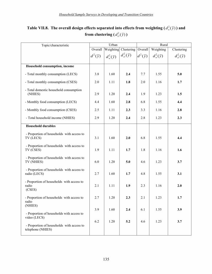
Household Sample Surveys in Developing and Transition Countries
135
Table VII.8. The overall design effects separated into effects from weighting ( )(2 ydw ) and from clustering ( )(2 ydcl )
Topic/characteristic Urban Rural
Overall
Weighting
Clustering
Overall Weighting Clustering
Household consumption, income - Total monthly consumption (LECS) - Total monthly consumption (CSES) - Total domestic household consumption (NHIES) - Monthly food consumption (LECS) - Monthly food consumption (CSES) - Total household income (NHIES)
3.8
2.0
2.9
4.4
2.5
2.9
1.60
1.11
1.20
1.60
1.11
1.20
2.4
1.8
2.4
2.8
2.3
2.4
7.7
2.0
1.9
6.8
3.3
2.8
1.55
1.16
1.23
1.55
1.16
1.23
5.0
1.7
1.5
4.4
2.8
2.3
Household durables - Proportion of households with access to TV (LECS) - Proportion of households with access to TV (CSES) - Proportion of households with access to TV (NHIES) - Proportion of households with access to radio (LECS) - Proportion of households with access to radio (CSES) - Proportion of households with access to radio (NHIES) - Proportion of households with access to video (LECS) - Proportion of households with access to telephone (NHIES)
3.1
1.9
6.0
2.7
2.1
2.7
3.9
6.2
1.60
1.11
1.20
1.60
1.11
1.20
1.60
1.20
2.0
1.7
5.0
1.7
1.9
2.3
2.4
5.2
6.8
1.8
4.6
4.8
2.3
2.1
6.1
4.6
1.55
1.16
1.23
1.55
1.16
1.23
1.55
1.23
4.4
1.6
3.7
3.1
2.0
1.7
3.9
3.7
)(2 yd )(2 yd w)(2 yd )(2 yd w )(2 ydcl
)(2 ydcl

Household Sample Surveys in Developing and Transition Countries
136
28. The design effects of clustering, )(2 ydcl , depend on the cluster sample size. The Lao and Namibia surveys had cluster sample sizes of 20 households while the Cambodia survey had 10 sampled households per cluster. To remove the effects of different cluster takes in comparing results across surveys, we have calculated rates of homogeneity (roh) for the estimates in table VII.8 (see equation 30 in chap.VI). The results are presented in table VII.9. The roh�s measure the internal homogeneity of the PSUs (enumeration areas) for the survey variables. The issue to be examined is whether there are similarities in the levels and patterns of roh�s across countries.
Table VII.9. Rates of homogeneity for urban and rural domains
Topic/characteristic
Urban Rural Ratio urban/rural
Household consumption, income
- Total monthly consumption (LECS) - Total monthly consumption (CSES) - Total domestic household consumption (NHIES) - Monthly food consumption (LECS) - Monthly food consumption (CSES) - Total household income (NHIES)
0.072
0.089
0.071
0.092
0.139
0.071
0.209
0.080
0.025
0.178
0.204
0.058
0.3
1.1
2.9
0.5
0.7
1.2
Household durables - Access to TV (LECS) - Access to TV (CSES) - Access to TV (NHIES) - Access to radio (LECS) - Access to radio (CSES)) - Access to radio (NHIES) - Proportion of households with access to video (LECS) - Access to phone (NHIES)
0.049
0.079
0.200
0.036
0.100
0.063
0.076
0.208
0.178
0.061
0.125
0.110
0.109
0.032
0.154
0.125
0.3
1.3
1.6
0.3
0.9
1.9
0.5
1.7

Household Sample Surveys in Developing and Transition Countries
137
29. Since the homogeneity of the clusters may differ between urban and rural clusters, the values of roh have been computed separately for these two parts of the population. The results are presented in table VII.9. There are some results that stand out in this table:
• The patterns of urban/rural differences in roh values are different in the three countries. The roh´s for the urban clusters in the Lao survey are consistently much lower than the roh´s for rural clusters. The average urban/rural ratio is 0.4. In the Namibian survey, the differences are in the opposite direction; the urban roh�s are on average larger than the rural roh�s by a factor of 1.9. In the Cambodian survey, there is no clear urban/rural pattern in the roh�s.
• The roh�s for rural clusters are high in the LECS (in the range of from 0.110 to
0.209, with a median value of 0.178). The roh�s for urban clusters are much lower (in the range 0.036 to 0.092, with a median value of 0.072).
• The roh for monthly food consumption is high in rural areas in Cambodia (0.204).
This roh is considerably higher than the roh for total monthly consumption and also higher than the roh�s for the household durables estimates.
30. The large differences between urban and rural roh´s in the Lao People�s Democratic Republic arise mainly because of the high roh�s for rural areas. These results are in line with results from a previous LECS survey in the country. High values of roh for the rural areas are not unreasonable considering the fact that the rural villages are small and rather homogeneous in socio-economic terms. Also, the urban areas have very little income-level segregation, making them rather mixed in socio-economic terms. The seasonality that is present for total monthly consumption and monthly food consumption may also be a contributing factor for these variables. Each PSU is visited for 1 month and the sample of PSUs is spread out over a 12-month period. Consequently, there is a �seasonal clustering� on top of the geographical clustering. There are reasons to believe that this seasonality is somewhat stronger in the rural areas. 31. In Namibia, many of the rural PSUs in the commercial farming areas are rather heterogeneous, containing mixtures of high-income farmer households and low-income farm labourer households. In the urban areas, on the other hand, there is a rather strong income-level segregation that has been taken care of only partly in the stratification. These circumstances may explain the larger roh´s for household consumption and household income in urban areas. 32. To the explanations above should be added two others. One is that the design effects (and consequently the roh�s) for the consumption variables are rather sensitive to values at the high end. Removal of a few of the highest values will, in some cases, change the design effect considerably. The other is that the roh values reflect more than simply measures of cluster homogeneity. They also capture interviewer variance effects, when different interviewers, or teams of interviewers, carry out the interviews in different PSUs.

Household Sample Surveys in Developing and Transition Countries
138
E. Discussion
33. It is not possible to discern any similarities between countries in levels or patterns of roh in table VII.9. The results offer little consolation for a sampling statistician who wants to use roh�s from a similar survey in another country when designing the sample for a survey. It seems that country-specific population conditions may play a strong role in determining the degree of cluster homogeneity for the kinds of socio-economic variables studied here. The study is admittedly very limited; the only general conclusion that can be drawn is to urge caution when �importing� a roh from a survey in another country. The results also draw attention to the need to calculate and document design effects and roh´s from the current survey so that they can be used for the design of the next one. 34. The findings in the study, however uncertain, are contrary to the usual findings. Studies of the DHS surveys have found that estimates of roh for a given estimate are fairly portable across countries provided that the sample designs are comparable (see chap. XXII). Likewise, the study conducted on a number of WFS surveys also concluded that there were similarities in patterns in roh across countries. It may be that roh�s for demographic variables are more �well behaved� and more portable than roh�s for socio-economic variables.

Household Sample Surveys in Developing and Transition Countries
139
Annex Description of the sample designs for the 11 household surveys
The sample designs for the 11 surveys are described briefly below:
Lao Expenditure and Consumption Survey 1997/98 (LECS)
Census enumeration areas (EAs) served as PSUs. The PSUs were stratified by 18 provinces and urban/rural areas. The rural EAs were further stratified by �access to road� and �no access to road�. Equal samples of 25 PSUs were selected with systematic PPS in each province (450 PSUs altogether) (Rosen, 1997). Twenty households were selected in each PSU, giving a sample of 9,000 households. The equal allocation of the sample over provinces resulted in a large variation in sampling weights on household level.
Cambodia Socio-Economic Survey 1999 (CSES)
Villages serve as PSUs. A few communes and villages were excluded because they could not be visited for security-related reasons; the excluded area amounted to 3.4 per cent of the total number of households in the country.
The villages were grouped into 5 strata based on ecological zones. Phnom Penh was
treated as a separate stratum, and the rural and urban sectors were treated as separate strata. Thus, 10 strata were created from the 4 geographical zones (Phnom Penh, Plains, Tonle Sap, Coastal and Plateau/Mountain). From each stratum, four independent subsamples of villages were drawn. The sample was allocated approximately proportionally to strata.
Six hundred villages were selected with circular systematic PPS sampling. Ten
households were selected within each village (National Institute of Statistics, Kingdom of Cambodia, 1999).
Namibia Household Income and Expenditure Survey 1993/94 (NHIES)
The PSUs were basically census enumeration areas. Some small EAs were combined with adjacent EAs before selection. The average PSU size was approximately 150 households. A primary stratification was carried out according to urban/rural divisions and 14 regions. A secondary stratification was effected in the urban domain where �urban� and "small urban" (semi-urban) strata were defined. The sample was allocated approximately proportionally to strata. However, a slight oversampling of urban areas was introduced. A sample of 96 urban and 123 rural PSUs was selected using a systematic PPS procedure (Pettersson, 1994).
Namibia Intercensal Demographic Survey 1995/96 (NIDS)
The design was the same as that for the NHIES. A sample of 82 urban and 120 rural PSUs was selected. For the NIDS, a rather large sample of 50 households was selected in each PSU, giving a total sample of 9,500 households (Pettersson, 1997).

Household Sample Surveys in Developing and Transition Countries
140
Viet Nam Multipurpose Household Survey 1999 (VMPHS)
Communes were used as PSUs in rural areas. In urban areas, wards served as PSUs. Stratification was carried out on urban/rural and province (61 provinces). Eight hundred thirty-nine communes were selected with PPS. The sample was basically equal-sized for each province, but the large provinces were allocated somewhat larger samples. The secondary sampling units (SSUs) were villages within communes and blocks within wards. Two SSUs were selected within each selected commune. In each SSU, 15 households were selected. In all, approximately 25,000 households were selected (Phong, 2001).
Lesotho Labour Force Survey 1997
The sample was a two-stage sample. Primary sampling units were groups of enumeration areas. The average PSU size was 370 households. The PSUs were stratified by urban/rural divisions, regions (10) and agro-economic zones (4), to produce 33 strata altogether. The sample was allocated proportionally to strata, with two exceptions: two small strata were heavily oversampled. A systematic PPS procedure was used to select 120 PSUs. Within PSUs, 15-40 households were selected using systematic random sampling to generate a total sample size of 3,600 households. All eligible household members were included in the survey (Pettersson, 2001).
October Household Survey 1999 of the Republic of South Africa (OHS)
Census enumeration areas (EAs) served as PSUs. During the selection process, EAs having less than 80 households were combined with neighbouring EAs on the list using a method proposed by Kish (1965). The average size of PSUs was 80-100 households for urban PSUs and 110-120 households for rural PSUs. The PSUs were stratified by nine provinces. The sample was allocated over strata with a square-root allocation. Within each province, a further stratification by district councils (and metropolitan councils) was carried out. A sample of 2,984 PSUs was selected by systematic PPS sampling, 1,711 in urban areas and 1,273 in rural areas. In each PSU, a systematic sample of 10 �visiting points� (approximately the same as households) was drawn (Stoker, 2001).
Labour Force Survey February 2000 of the Republic of South Africa
The Labour Force Survey February 2000 was the first survey to use a new master sample that had been constructed at the end of 1999 based on the 1996 census database. The sample consisted of 2,000 PSUs. (Later in the year, the sample was expanded to 3,000 PSUs.) Census enumeration areas served as PSUs, with EAs having less than 100 households being linked with neighbouring EAs. The PSUs were stratified by nine provinces. The sample was allocated over strata with a square-root allocation. In each PSU, clusters of size 10 visiting points were formed, each cluster spread over the entire PSU. A set of clusters was selected to be used in the future Labour Force Survey.
As a result of budget problems it was decided to scale down the labour-force survey to 10,000 visiting points. This was effected as follows: from all the urban PSUs, only five visiting

Household Sample Surveys in Developing and Transition Countries
141
points were selected from the identified cluster. For the rural sample, a PPS systematic subsample containing 50 per cent of the rural PSUs was drawn from the set of rural PSUs and in the drawn PSUs the entire identified cluster of 10 visiting points formed part of the sample (Stoker, 2001).
PNAD (Pesquisa Nacional por Amostra de Domicílios) 1999, Brazil
PNAD covers annually a sample of approximately 115,000 households, representing all of Brazil except the rural areas in the north (Amazon) region. Stratification was by geography into 36 explicit strata. The 36 strata comprised 18 of the States as one stratum each and the remaining 9 States as subdivided in two strata each. One stratum was then formed with PSUs located in the metropolitan area around the State capital, and one stratum was formed with the remaining PSUs in the State. In the strata formed by metropolitan areas, the design was a two-stage cluster sampling, where the PSUs were census enumeration areas, selected by systematic PPS sampling, with size measures equal to the number of private households as obtained in the latest population census. Prior to selection of PSUs, they were sorted by geography code, leading to an implicit stratification by municipality and by urban-rural status.
In the strata that were not metropolitan areas, the PSUs were municipalities. These were stratified by size and geography, forming strata of approximately equal population (using data from the latest available population census). Two municipalities (PSUs in these strata) were then selected in each stratum using systematic PPS sampling, with total population as the measure of size. Prior to systematic selection, some municipalities were declared to be �certainty� PSUs because of their large population, and were thus included in the sample of municipalities with certainty. Within each selected municipality, EAs were selected using systematic PPS sampling, with size measures equal to the number of private households as obtained in the latest population census. At the last stage of selection, households were selected within EAs by systematic sampling from lists updated yearly. Every member of selected households was included in the survey. A target sample of 13 households should have been selected from each EA. However, in order to reduce weight variation due to outdated measures of size, constant sampling fractions were used in each EA instead of constant sample sizes, yielding varying cluster takes.
The sample allocation was disproportional over the strata, and the ratio of largest to smallest weight was approximately equal to 8.
PME (Pesquisa Mensal de Emprego) for September 1999, Brazil
PME is a labour-force survey that covers a monthly sample of about 40,000 households in the six largest metropolitan areas in Brazil, from which the main current labour-force indicators are derived. The sample design is the same as for PNAD in the metropolitan area strata, except for the target cluster take, which is 20 for PME in contrast with 13 for PNAD.
PPV (Pesquisa de Padrões de Vida) 1996/97, Brazil
PPV targeted measurement of living standards, using the approach developed in the family of Living Standards Measurement Study (LSMS) surveys carried out in various countries

Household Sample Surveys in Developing and Transition Countries
142
under sponsorship of the World Bank (Grosh and Muñoz, 1996). The Brazilian survey, carried out in 1996-1997, investigated a large number of demographic, social and economic characteristics using a sample of 4,944 households selected from 554 EAs in the north-east and south-east regions of Brazil. The sample design was a two-stage stratified cluster sample. Stratification comprised two steps. First, 10 geographical strata were formed to identify the 6 metropolitan areas of Fortaleza, Recife, Salvador, Belo Horizonte, Rio de Janeiro and São Paulo, plus 4 other strata that covered the remainder of the north-east and south-east regions, subdivided into urban and rural enumeration areas. Within each of these 10 geographical strata, EAs were further subdivided into 3 strata according to average head of household income as recorded in the 1991 population census. Hence, a total of 30 strata were formed.
The total sample size was fixed at 554 EAs, 278 for the north-east region and 276 for the
south-east region. Allocation of the EAs within the strata was proportional to number of EAs in each stratum. Selection of EAs was carried out using a PPS with replacement procedure, with the number of private households per EA as the measure of size. In each selected urban EA, a fixed take of eight households was selected by simple random sampling without replacement. The survey take per rural EA was set at 16 households for cost-efficiency reasons.
Despite its small sample size when compared with PNAD and PME, the PPV survey provides useful information about design effects because it used direct income stratification of EAs, as well as smaller sample takes per EA than the other surveys. Another distinctive feature stems from the fact that estimation used only the standard inverse selection probability weights, and that no calibration to population projections was attempted. The variation of the sample weights for the PPV was substantial, with the largest weight over 40 times the smallest.

Household Sample Surveys in Developing and Transition Countries
143
References
Grosh, M., and Muñoz, J. (1996). A Manual for Planning and Implementing the Living Standards Measurement Study Survey. Living Standards Measurement Study Working Paper, No. 126. Washington, D.C.: World Bank.
Kish, L. (1965). Survey Sampling. New York: Wiley. National Institute of Statistics, Kingdom of Cambodia (1999). Cambodia Socio-Economic Survey
1999: Technical Report on Survey Design and Implementation. Phnom Penh. Pettersson, H. (1994). Master Sample Design: Report from a Mission to the National Central
Statistics Office, Namibia, May 1994. International Consulting Office, Statistics Sweden. _________ (1997). Evaluation of the Performance of the Master Sample 1992-96: Report from
a Mission to the National Central Statistics Office, Namibia, May 1997. International Consulting Office, Statistics Sweden.
_________ (2001). Sample Design for Household and Business Surveys: Report from a Mission
to the Bureau of Statistics, Lesotho May 21-June 2, 2001. International Consulting Office, Statistics Sweden.
Phong, N. (2001). Personal correspondence concerning sample design for the Viet Nam
Multipurpose Household Survey 1999. Rosen, B. (1997). Creation of the 1997 Lao Master Sample. Report from a Mission to the
National Statistics Centre, Lao PDR. International Consulting Office, Statistics Sweden. Stoker, D. (2001). Personal correspondence concerning sample design for the October
Household Survey and Labour Force Survey in the Republic of South Africa. Verma, V., C. Scott and C. O�Muircheartaigh (1980). Sample designs and Sampling Errors for
the World Fertility Survey. Journal of the Royal Statistical Society, Series A, vol. 143, part 4, pp. 431-473.

Household Sample Surveys in Developing and Transition Countries
144

Household Sample Surveys in Developing and Transition Countries
145
Section C
Non-sampling errors

Household Sample Surveys in Developing and Transition Countries
146
Introduction
James Lepkowski University of Michigan Ann Arbor, Michigan
United States of America 1. The previous sections and chapters of the present publication have examined, for the most part, sampling errors that arise when a representative probability sample is taken from a population. A number of other errors that arise in household surveys are considered in the present section. Some of these errors are, like sampling error, variable across possible samples, or across possible repetitions of the measurement process. Others are fixed, or systematic, and do not vary from one sample to the next. 2. In the sample design framework, variable errors are usually referred to as sampling variance. There are fixed sampling errors, some of which have already been mentioned, which are referred to as bias. For example, the deliberate exclusion of a subgroup of the population introduces non-coverage of the population subgroup, and an error that will be present, and of the same size, no matter which possible sample is selected. 3. Non-sampling errors involve non-observation errors when there is a failure to obtain data from a sampling unit or a variable, or measurement errors that arise when the values for survey variables are collected. Non-observation errors are usually fixed in nature, and lead to considerations about bias in survey estimates. Measurement errors are sometimes fixed, but they may also be variable. 4. Among non-observation errors, two sources of error are most important: non-coverage and non-response. In probability sampling, there must be a well-defined population of elements, each of which has a non-zero chance of selection. Non-coverage arises when an element in the population actually has no chance of selection; the element has no way to enter into the selected sample. Non-response refers to the situation where no data are collected for an element response that has been chosen into the sample. This may occur because a household or person refuses to cooperate at all, or because of a language barrier, a health limitation, or the fact that no one is at home during the survey period. 5. Measurement errors arise from more diverse sources -- from respondents, interviewers, supervisors and even data-processing systems. Respondent measurement errors may occur when a respondent forgets information needed and gives an incorrect response, or distorts information in response to a sensitive question. These respondent errors are likely to constitute a bias, because the respondent consistently forgets, or distorts an answer, in the same way, no matter when he or she is asked a question. These errors can also be variable. Some respondents may forget an answer at one moment, and remember it another. 6. There are four dimensions that survey designers consider in respect of these kinds of errors. One entails a careful definition of the error and an examination of the sources of the error in the survey process, encompassing what part of the survey process appears to be responsible
Household Sample Surveys in Developing and Transition Countries
147
for generating this kind of an error. The second entails how to measure the size of the error, a particularly difficult problem. Third, there are procedures to be developed to reduce the size of the error, although their implementation often requires additional survey resources. Last, non-sampling errors occur in every survey, and survey designers attempt to compensate for those errors in survey results.
7. Chapters VIII and IX in this section examine from a conceptual viewpoint non-observation and measurement error, respectively, providing some illustration of many different types of these errors. Chapters X and XI offer more detailed treatments of these errors, the former considering the overall impact on the quality of survey results, and the latter providing a case study of these kinds of errors in one country, Brazil.

Household Sample Surveys in Developing and Transition Countries
148

Household Sample Surveys in Developing and Transition Countries
149
Chapter VIII Non-observation error in household surveys in developing countries
James Lepkowski University of Michigan
Ann Arbor, Michigan, United States of America
Abstract
Non-observation in a survey occurs when measurements are not or cannot be made on some of the target population or the sample. The non-observation may be complete, in which case no measurement is made at all on a unit (such as a household or person), or partial, in which case some, but not all, of the desired measurements are made on a unit. The present chapter discusses two sources of non-observation, non-coverage and non-response. Non-coverage occurs when units in the population of interest have no chance of being selected for the survey. Non-response occurs when a household or person selected for the survey does not participate in the survey or does participate but does not provide complete information. The chapter examines causes, consequences and steps to remedy non-observation errors. Non-coverage and non-response can result in biased survey estimates when the part of the population or sample left out is different than the part that is observed. Since these biases can be severe, a number of remedies and adjustments for non-coverage and non-response are discussed. Key terms: non-response, non-coverage, bias, target population, sampling frame, response rates.

Household Sample Surveys in Developing and Transition Countries
150
A. Introduction
1. Non-observation in survey research is the result of failing to make measurements on a part of the survey target population. The failure may be complete, in which case no measurement is made at all, or partial, in which case some, but not all, of the desired measurements are made.
2. One obvious source of non-observation is the sampling process. Only in a census, which is a type of survey designed to make measurements on every element in the population, is there no non-observation arising from drawing a sample. Non-observation from sampling gives rise to sampling errors that are discussed in chapters VI and VII of the present publication. This source of non-observation will therefore not be treated here.
3. The present chapter will discuss two other sources of non-observation, namely, non-coverage and non-response. As will be explained in more detail later, non-coverage occurs when there are units in the population of interest that have no chance of being sampled for the survey; and non-response occurs when a sampled unit fails to participate in the survey, either completely or partially. The chapter will address the causes of these sources of non-observation, their potential consequences, steps that can be taken to minimize them, and methods that attempt to alleviate the bias in the survey estimates that they can generate. The consequences of non-coverage and non-response include the possibility of bias in the results obtained from the survey. If the part of the population that is left out is different than the part that is observed, there will be differences between the survey results and what is actually true in the population. The differences are non-observation biases, and they can be severe.
4. Of course, non-observation bias may not occur at all, even when measurements are not made on a portion of the population. While recording instances of non-observation is somewhat straightforward, detection of non-observation bias is difficult. This difficulty is what makes consideration of non-observation bias an infrequently researched topic. It is possible to find examples where non-observation makes no difference at all in an entire survey, or as regards most survey questions. It is also possible to find examples where non-observation has led to substantial bias in the survey estimate from a single question, or substantial biases in the estimates from a set of questions, in which case all the results from the survey become suspect.
5. There has been a great deal of research on non-observation. This chapter can provide only an introduction to the nature of non-coverage and non-response errors in household surveys. The reader is referred to the references provided for more detailed treatments. The next section provides a framework for distinguishing between non-coverage and non-response and is followed by separate sections on each source of error.
B. Framework for understanding non-coverage and non-response error
6. Knowing the difference between non-coverage and non-response requires an understanding of the nature of populations and sampling frames. The target population is the

Household Sample Surveys in Developing and Transition Countries
151
collection of elements for which the survey designer wants to produce survey estimates. For example, a survey designer may be called upon to develop a survey to study labour-force participation for persons aged 15 years or over living in a given country. The population clearly has geographical limits that are well defined (the borders of the country), and limits on the characteristics of the units, such as age restrictions. 7. There are other implicit aspects of the target population definition; for example, the meaning of a person living in the country. Many surveys use a definition of residence according to which a person must have lived in the country the majority of the past year or, having just moved into the country, must intend to stay there permanently. Some portions of the population may be out of scope for a certain survey topic. For example, persons living in prisons or jails, or other institutions such as the military, may be defined as out of scope for some surveys of economic conditions. Thus, institutions may be excluded because they contain persons who are not part of the conceptual basis for the measurement to be made. There is also an implied temporal dimension to the target population definition. The survey is probably interested in current labour-force participation and not historical patterns for the individual. If so, the survey is concerned to make estimates about the characteristics of the population as it exists at a particular point in time.
8. The target population is also the population of inference. The survey results will, in the end, be said to refer to a particular population. Surveys are often designed to measure the characteristics of persons in a given country. Regardless of whether some persons in the country are covered by the sampling process or not, the survey�s final report may make unqualified statements about the entire population. For example, even though the survey excluded persons living in institutions, the final report may state that the results of the survey apply to the population of persons living in the country. The uninformed reader may then assume that the results represent persons living in institutions, even though they were not covered by the sampling process. It is thus important in describing the survey to include careful and complete statements about the target and survey populations in publications about the survey.
9. The target population will often differ from another important population, the set of elements from which the sample is actually drawn, called the sampling frame The sampling frame is the collection of materials used to draw the sample, and it may not match exactly with the target population. For example, in some countries, address registries prepared and maintained by a public security agency, such as the police, are used as a sampling frame. But some households in the population are not in those administrative systems. The frame then differs from the target population.
10. In other instances, the frame differs from the target population for structural, or deliberate, reasons. A portion of the population may be left out of the frame for administrative or cost reasons. For example, there may be a region, several districts, or a province in a country where there is current civil unrest. Public security agencies may place restrictions on travel into and out of the region. The survey designer may deliberately leave the region out of the frame, even though materials exist to draw the sample in the region.

Household Sample Surveys in Developing and Transition Countries
152
11. Cost may also enter into a decision to exclude a portion of the population. In many countries, those living in remote and sparsely population areas are excluded from the sampling frame because of the high cost of surveying them if they are sampled. Furthermore, since in countries with many indigenous languages, separate translations and the hiring of interviewers who can speak all languages are expensive, survey designers may, in conjunction with survey sponsors, specifically exclude population members who do not speak one of the major languages in the country. In this case, it may not be possible to exclude a person until after a household has been identified and the language abilities of the persons in the household have been determined. The exclusion is made through a screening in the household.
12. On the other hand, survey designers may choose to classify this kind of a problem as non-response, that is to say, as non-coverage due to language exclusion or non-response due to inability to communicate. The decision about how to classify �language exclusions� depends in part on the size of the problem. For example, in one country the survey may be limited to populations who can speak one of several officially recognized languages. This decision may exclude substantial numbers of persons who do not speak those languages. In contrast, in another country, where nearly everyone speaks one of the official languages, small population groups speaking non-official languages for which questionnaire translations are not available may be contacted but not interviewed. In the former instance, it may be appropriate, with careful documentation, to classify the excluded language groups as non-coverage. In the latter, it is appropriate to classify the non-interviews as non-response.
13. Non-coverage arises when there are elements in the target population that do not correspond to listings in the sampling frame. In household surveys, typical non-coverage problems arise when housing units fail to be included in a listing prepared during field operations, when out-of-date or inaccurate administrative household listings are used, or when individuals within a household are omitted from a household listing of residents.
14. Non-coverage refers to a failure to give an element in the population a chance of being selected for the survey�s sample, whereas non-response is due to an unsuccessful attempt to collect survey data from a sampled eligible unit, a unit in the target population. Non-coverage arises due to errors or problems in the frame being used for sample selection; non-response arises after frames have been constructed, and sample elements selected from the frame. For example, suppose that in a sampled household a male resident of the household is absent at the time of interview because he is spending the week away at a temporary job outside of the village where the household is located. If that resident is not listed on a household roster during initial interviewing because the household informant forgot about him, non-coverage has occurred. On the other hand, if a resident is listed on the roster, but he is away during the interviewing period in the village and the survey accepted only self-reported data from the resident himself, and hence no data were collected from him, that resident is a non-respondent.
15. Non-coverage typically involves entire units, such as households or persons. Non-response can involve entire units, or individual data items. For example, non-coverage might involve the failure to list a household in a village roster because it is located above a retail shop. The entire unit is absent from the frame. Non-response might occur because the household, when listed, refuses to participate in the survey, or because some members of the household

Household Sample Surveys in Developing and Transition Countries
153
cooperate, and provide data, while others are not at home or refuse to respond to the survey entirely. These two forms of unit or total non-response, household or person, are in contrast to the case where a member of the household provides data in response to all survey questions except a subset. For example, a household respondent may refuse to provide data about his or her earnings in the informal economy, perhaps because of a concern about official administrative action on unreported income. This latter form of non-response is known as item non-response. Note that the type of non-response in this case also depends on whether the unit of analysis is the person or the household: person-level non-response is item non-response for analysis at the household level, but unit non-response for analysis at the person level.
16. It is also important to consider the trade-offs between non-coverage and non-response. While many sources of non-coverage or non-response might be identified for a given survey through careful study, and there may be a desire to reduce the size of either of these problems, reduction will require the expenditure of scarce, and limited, survey resources. There may then be a competition for these resources with respect to reducing these two sources of error.
17. For example, suppose that in a country with 40 major languages or dialects, the survey instrument is translated into 5 languages that are spoken in the households of 80 per cent of the population. The sixth most frequently spoken language group represents 3 per cent of the population. At the same time, suppose that survey operations specify two visits to a household over a two-day period in order to find someone at home, and that it is known that 10 per cent of the households visited twice will be non-responding because no one is at home during two days of the survey interviewing. The survey designer has a choice in terms of resources. More funds could be spent to translate the instrument into a sixth language to cover an additional 3 per cent of the population speaking the sixth language. Or more funds could be spent on having interviewers spend a third or fourth day in each village to conduct household visits to try to find a higher proportion of household members at home.
18. The decision about how to use any extra survey resources, for translation or for additional household visits, will depend on the size of the anticipated biases and the costs and resources involved. The biases depend on both the level of non-coverage or non-response and on the differences between covered and not-covered populations, or responding and non-responding sample persons.
19. These kinds of cost-error trade-offs occur frequently in survey design. It is beyond the scope of this chapter to consider in any detail the kind of data needed to make such trade-offs or how the trade-offs are made. In most surveys, such trade-offs are based on limited information and made informally.
C. Non-coverage error
1. Sources of non-coverage 20. The sources of non-coverage in household surveys depend on the frame materials used to select the sample. Since many household surveys in developing countries, and some transition

Household Sample Surveys in Developing and Transition Countries
154
countries, involve area sampling methods, the present discussion will limit the frame and non-coverage problems to household surveys based on area samples.
21. Area sampling is also usually coupled with multistage selection. Primary and sometimes secondary stages of selection involve geographical areas that can be considered clusters of households. In some subsequent stage of selection, a list of households must be obtained, or created, for a set of relatively small geographical areas. At the last stage of selection, a list of persons or residents in the household is created in each sampled area. There are thus three types of units that need to be considered when examining non-coverage in such surveys: geographical units, households, and persons. As discussed later, these units also may be separate sources of non-response in household surveys.
22. Non-coverage of geographical units as a result of deficiencies in the sampling frame is rare, because most area frames will be based on census materials that cover the entire geographical extent of a population. Non-coverage of a geographical area does arise, but in a more subtle form, as mentioned above. A survey may be designed to provide inferences to the entire population of a country or region within a country, and references to the population in the final report may indeed include the population living in the entire area, but the sample may not be selected from the entire country.
23. For example, during the survey design, the survey designers may identify some geographical areas with limited shares of the population that are extremely costly to cover. They may make a deliberate decision to exclude those geographical areas from the frame. Yet, in reporting results for the survey, the deletion of these areas is not mentioned, or only mentioned briefly. Report readers may have, or be given implicitly, the impression that survey results apply to the entire country or region, when in fact a portion of the population is not covered. In practice, the size of the non-coverage error arising in such situations is generally small, and typically ignored.
24. It is important to keep in mind that the distinction remains between a desired target population (that is to say, the population living in the entire geographical area of the country) and a restricted �survey population� living in the included geographical area. There is a danger, though, that through incomplete documentation, the user of the data may be under the impression that the survey sample covers the entire population, when in fact it does not.
25. A more important source of non-coverage occurs at the household level. Most surveys consider households to be the collection of persons who usually reside in a housing unit. Two components are thus important: the definition of a usual resident and the definition of a housing unit. 26. Housing unit definitions are complex, inasmuch as they take into account whether a physical structure is intended as living quarters, and whether the persons living in the structure live and eat separately from others in the same structure (as in multi-unit structures such as apartment buildings). Living separately implies that the residents have direct access to the living quarters from the outside of the structure, or from a shared lobby or hallway. The ability to �eat

Household Sample Surveys in Developing and Transition Countries
155
separately� usually involves the presence of a place to provide and prepare food, or the complete freedom of the residents to choose the food they eat.
27. Applying this kind of broad definition to the many diverse living situations across countries, or across regions of a country, is difficult. Most housing units are readily identified, such as single family or detached housing units, duplexes where separate housing units share a wall but have separate entrances, and apartments in multi-structure buildings. However, there are many housing units that are difficult to classify or find. For example, in urban slum areas, separate housing units may be difficult to identify when people are living in structures built from recycled or scrap materials. Housing units may be located in places that cannot be identified by casual inspection of entrances from a street, lane or pathway.
28. In rural areas, a structure intended for dwelling may be easily identified, but complex social arrangements within the structure may make separate housing unit identification difficult. For instance, in a tribal group, long-houses with a single entrance are used for housing; they contain separate compartments for family unit sleeping arrangements, but there is a common food preparation area for group or individual family meals, that is to say, the individual compartments are not themselves housing units, because they do not have a separate entrance or their own cooking and eating area. In such an arrangement, the notion of a household as the group of persons who usually reside in a specific housing unit is more difficult to apply. It is not clear whether the entire structure, or each compartment, should be treated as a housing unit. In practice, the entire longhouse is treated as a housing unit or dwelling and, if sampled, all households identified during the field listing of households are included in the survey. 29. There are also living quarters that are not considered housing units. Institutional quarters occupied by individuals under the care or custody of others, such as orphanages, prisons or jails, or hospitals, are not considered to be housing units. Student dormitories, monasteries and convents, and shelters for homeless persons are special types of living quarters that do not necessarily provide the care or custody associated with an institution. Living quarters for transitional or seasonal living are also a problem. For example, there may be separate housing units present in an agricultural area for housing seasonal labour, which are occupied for only one season, or a few seasons each year. Presumably, the seasonal residents usually live elsewhere, and should not be counted as part of a household in the seasonal unit.
30. Multistage area sampling in developing countries requires that at some point in the survey process lists of dwellings be created for small geographical areas, such as a block in a city or an enumeration area in a rural location. Non-coverage often arises when part-time survey staff are sent to the field to list housing units, and encounter the kinds of complex living quarters described above. Identification of most housing units is straightforward; but the missing of housing units may still be common to the extent that the part-time staff has limited experience applying to complex living quarter arrangements a definition that has several components. 31. The non-coverage problem in housing unit listing is made more difficult by the temporal dimension. A housing unit may be unoccupied at the time of listing, or under construction. If the survey is to be conducted at some point in the future, these types of units may need to be included in the listing. In surveys where housing unit listings are used across multiple waves of

Household Sample Surveys in Developing and Transition Countries
156
a single panel survey, or across several different surveys, it is common to try to include construction units that are unoccupied or under construction.
32. In surveys in transition countries, it may be possible to use a list already prepared by an administrative authority. However, the quality of those lists for household surveys needs to be carefully assessed. The same kinds of problems outlined here that could arise in survey listing are likely to occur in respect of administrative lists.
33. Thus, the housing unit listing process can generate non-coverage of certain types of households. This non-coverage may be difficult to identify without substantial investment of additional survey resources.
34. Finally, within a sampled housing unit, listing of persons who are usual residents is a part of the household listing process as well. Operational rules are required to instruct interviewers regarding whom to include in the housing unit as a usual resident. As in the case of housing units, most determinations are straightforward. Most persons encountered are staying at the housing unit at the time of contact, and it is their only place of residence. There are others who are absent at the time of contact, but for whom the residence is an only residence.
35. However, there are persons for whom the housing unit is one of several in which they live. A decision must be made in the field by part-time staff about whether the sampled housing unit is the usual place where this person resides. It is also difficult for household informants to report accurately on the living arrangements of some residents. This reported proxy information about another resident may not be completely accurate.
36. Informants may also have personal reasons for deliberately excluding persons whom they know to be usual residents. For example, a person may be living in a housing unit who would make the household ineligible for receiving the government benefits that it is already receiving. Also, an informant may deliberately exclude a resident who does not want to be identified by public or private agencies because of financial problems (such as debt) or legal problems (such as criminal activity).
37. Informants may also not include someone in the household for cultural or cognitive reasons. An informant may not report an infant less than one year of age because the culture does not consider these persons old enough to be regarded as persons. They may also exclude infants, because they believe that the survey organization is not interested in collecting data about young children; or they may simply forget to include someone, whether it is an infant or someone older. 38. Non-coverage in household surveys may thus arise from a variety of definition and operation circumstances. The concern must be the extent to which non-coverage leads to error in survey results.
2. Non-coverage error 39. Suppose that the survey is to estimate the mean for some characteristic Y for a population of N persons, ncN of whom are not covered by the survey�s sampling frame. Let the mean in the

Household Sample Surveys in Developing and Transition Countries
157
population of size N be Y , let cY , be the mean of those covered by the sampling frame, and let
ncY be the mean of those not covered by the frame. . The error associated with the non-coverage is referred to as the non-coverage bias of the sample mean, cy , which is based only on those covered in the sample, and which in fact estimates cY rather than Y .
40. The bias of the sample mean, cy , depends on two components, the proportion of the population that is not covered, ncN N , and the difference in the means of the characteristic Y between covered and not-covered persons. Hence,
( ) ( )( )c nc c ncB y N N Y Y= − 41. This formulation of the non-coverage bias is helpful in understanding how survey designers deal with non-coverage. In order to keep the error associated with non-coverage small, or to reduce its effect, the survey designer either must have small differences between covered and non-covered persons, or must have a small proportion of the persons who are not covered by the survey.
42. An important difficulty with this formulation is that, in most surveys, neither the difference ( )c ncY Y− nor the proportion ( )ncN N not covered is known. Further, the non-
coverage rate ( )ncN N may also vary across subclasses. The difference may vary across different variables and across subclasses of persons (such as a region, or a subgroup, defined by some demographic characteristic such as age). Thus, non-coverage error is a property not of the survey but of the individual characteristic, and of the statistic estimated.
43. In many government survey organizations, estimates of a total are frequently required. The non-coverage bias associated with a total depends on not only the differences between covered and non-covered units on the characteristic of interest but also on the number (and not the rate) of non-covered, that is to say, for an estimated total for respondents �
r rY Ny= , the bias
is ( ) ( )�r nc r mB Y N Y Y= − .
Reduction, measurement and reporting of non-coverage error 44. There are four possible means of handling non-coverage error in household surveys:
• Reducing the level of non-coverage through improved field procedures. • Creating procedures to measure the size of the non-coverage error and reporting
the level in the survey.
• Attempting to compensate for the non-coverage error through statistical adjustments.

Household Sample Surveys in Developing and Transition Countries
158
• Reporting non-coverage properties of the survey as fully as is possible in the survey report.
45. The reduction of non-coverage error in household surveys is usually attempted either through the use of multiple frames or through methods to improve the listing processes involved in the survey. Multiple frames are more likely to be used for housing units rather than persons. They require the availability of separate lists of housing units that pose particular problems for field listing.
46. For example, suppose that seasonal housing units for agricultural workers are known to be difficult to list properly in the field in a given country. Suppose also that an agency responsible for agricultural production, education, or social welfare has a list of the number and type of seasonal housing units on farms or enterprises where seasonal labour is employed and housed. The list of seasonal housing units from the alternative source may be used as a separate frame. Field interviewers preparing housing unit lists would be given a list of farms or enterprises where agency lists were already available in the area they are to list, and told not to list seasonal housing units there. Samples of housing units for the survey would then be selected from the housing unit list prepared by the interviewer and from the list maintained by the government agency. There will no doubt remain some non-coverage across both lists, and possibly some �over-coverage� may occur as well; but the use of both frames may reduce the level of non-coverage, and the error associated with it.
47. It is also important to consider methods to improve the listing processes. When housing unit lists are available from an administrative source, they may be checked by a field update before the sample is drawn. Interviewers may be sent to geographical areas with a list of housing units from the administrative source, and given instructions on how to check and add, or delete, housing units from the list as they examine the area.
48. Interviewers may also be trained to use a �half-open interval� procedure in the field to capture missed housing units from administrative lists or field lists that have missing units. The half-open interval procedure involves the selection of a housing unit from an address list, a visit by an interviewer to the sampled unit, and an implied or explicit list order. At the unit, the interviewer is instructed to enquire about any additional housing units that might be present between the selected housing unit and the next one on the list.
49. The next unit on the list is defined by some kind of pre-defined route through a geographical area. For example, on a city block, interviewers preparing a listing are instructed to start on a particular corner, and then proceed in a clockwise direction around the block. The housing unit list is to be assembled in that clockwise order.
50. If an interviewer finds a housing unit that is not on the list, and between the selected housing unit and the next on the list, he or she is instructed to add the missed housing unit to the sample and attempt an interview. If there are several such missed units, the interviewer may need to contact the survey central office for further instructions so as to avoid disruptions to field operations.

Household Sample Surveys in Developing and Transition Countries
159
51. Within households, improved listing procedures may involve question sequences administered by the interviewer to the housing unit informant to identify missed persons. For example, the survey interviewer may be instructed to ask about any infants who may have been left off the list of usual residents. The household listing may also be improved if interviewers are given guidelines about the choice of suitable informants or instructions to repeat the names on the list of persons to the informant to be sure no one was overlooked.
52. Measurement of non-coverage bias is also an important consideration, although a difficult problem to address. How does a survey organization identify units that are not included in any of its lists? As measurement of non-coverage can be an expensive survey task, it is one that is undertaken only occasionally.
53. A common way to assess non-coverage error is to compare survey results, for those variables for which comparisons can be made, with findings from external or independent sources. To assess the size of non-coverage, a survey may compare the age and gender distribution of its sample persons with the distribution obtained from a recent census, or from administrative records. Differences in the distributions will indicate non-coverage problems. To assess the non-coverage error associated with a variable, a comparison of values of the statistic of interest to an independent source may be made. For example, total wage and salary income reported in a survey, for the total sample and for key subgroups, may be compared to administrative reports on wage and salary income. In a classic study, Kish and Hess (1950) compared the distribution of housing units in a survey with recent census data on the distribution of housing units at the block level. The comparison provided insight into the nature of the non-coverage problem in the survey data collection.
54. A more expensive non-coverage error assessment can be made through dual system measurement, or related case matching procedures. Censuses employ dual system methods to assess coverage of a census operation [see, for example, Marks (1978)]. In a census, a separate survey is compared with census results to identify non-coverage problems. The assessment of the size of the non-coverage depends on a case-by-case matching of survey sample to census elements to determine which sample elements did not appear in the census. These procedures are closely related to the methods of �capture-recapture sampling� used in environmental studies of animal populations.
55. Since household surveys are universally affected by non-coverage error, many surveys will employ post-stratification or population control adjustments as statistical procedures to adjust survey results so as to compensate for non-coverage error. These adjustments are very similar to the method outlined above for assessing the size of the non-coverage error. The sample distribution by age and gender, for example, may be compared with the age and gender distribution from an outside source, such as a recent census or population projections. When the sample distribution is low (or high) for an age-gender group, a weight may be applied to all sample person data from that age-gender group to increase (decrease) their contribution to survey results. Weighted estimators will be required to properly handle the weights in analysis.
56. As a final consideration for non-coverage, good reporting is important for any statistical organization. Analytical reports ought to give clear definitions of the target population,

Household Sample Surveys in Developing and Transition Countries
160
including any exclusions. The frame should be described in enough detail for the reader to see how non-coverage might arise, and even make an informal assessment of the size of potential error. It would be helpful to include as references or appendices, any quality assessments of the frame, such as checks of the quality of housing unit lists or administrative lists, or comparison of original lists of persons within housing units with those lists obtained from reinterviews carried out for the purpose of quality control assessment.
57. A more difficult problem is the reporting of any coverage rates or non-coverage bias for the population and subclasses of the population. These kinds of assessments may be possible only for ongoing surveys where at some time there has been an attempt to assess the size of the non-coverage problem. It is very difficult if not impossible to make such assessments for one-time cross-sectional surveys.
58. Finally, if post-stratification or population control adjustments are made, the survey documentation must contain a description of the adjustment procedures and the magnitudes of the adjustments for important subgroups of the population.
D. Non-response error
59. Non-response error suggests a number of parallels with non-coverage error in terms of definitions, measurement, reduction, compensation and reporting. The organization of the present section is thus very similar to that of section C. It is important to make clear, however, that non-response and non-coverage are quite separate problems, having different sources and, in a few instances, different solutions. While in non-coverage survey designers almost never know anything other than the location and general characteristics of the non-covered portion of the population, in non-response they know at least frame information for non-respondents. Non-response is also believed to be more extensive in household surveys, and thus its contribution to the bias of survey estimates may be larger.
60. As noted above, two types of non-response are often identified in household surveys, namely, unit non-response and item non-response. These two types have quite different implications for survey results, and the methods used to measure, reduce and report them, and to compensate for them, are in some ways distinct as well. While a separate section could be devoted to each type, both will be addressed together in this section.
1. Sources of non-response in household surveys 61. In household surveys, unit non-response can occur for several different kinds of units. As is the case for non-coverage, non-response may occur for primary or secondary sampling units. For example, a primary sampling unit might consist of a district or sub-district in a country. Weather conditions or natural disasters may prevent survey operations from being conducted in a district or sub-district that has been selected at a primary, or secondary, stage of sampling. The unit is covered by the survey, but during the survey period, it is not possible to collect data from any of the households in the unit.

Household Sample Surveys in Developing and Transition Countries
161
62. Non-response is more frequent at the household level. A listed housing unit chosen for the sample may be found occupied, and an interview attempted. However, as the interviewer visits the housing unit, several adverse events may prevent data collection. A household member may refuse participation as an individual or as a representative of the entire unit.
63. Although a housing unit is occupied, its residents may be away from home during the entire survey period. In some developing countries, a considerable problem is encountered with housing units clearly lived in but locked during the entire data-collection period.
64. In many countries, although occupied housing units have individuals home at the time of data collection, language may pose a barrier. A version of the survey�s questionnaire may not have been translated into the language of the household, or the interviewer may not speak the local language. To avoid non-response, surveys may hire translators locally to accompany interviewers to the doorstep and translate interactively. Other surveys reject this practice because of concerns about whether the translation is correct, and whether the translation is consistent across households. Households that cannot provide responses, though, because of language difficulties, can be classified as non-responding units. As an alternative approach, it is the practice of some survey organizations to exclude from the survey households that do not speak a translated language. These households then become non-covered, rather than non-responding. The particular approach chosen by the survey organization, whether to handle such units as not covered or to handle them as non-responding, must be clearly described in the survey documentation.
65. Person-level unit non-response also may occur. For surveys that allow proxy reporting on survey questions, data can be collected from other household members for persons in the household who are not at home at the time of interview. For surveys, though, that require self-report for some or all questions, a person who is not at home during the survey, refuses to participate, or has another barrier (such as language) that precludes interviewing is a non-respondent. Health conditions, whether permanent, such as hearing impairment or blindness, or temporary, such as an episode of a severe acute illness, may preclude an individual from responding as well. 66. As for households with language problems, some survey organizations choose to classify persons with language barriers or permanent health conditions as not covered, and those with temporary conditions as non-responding (Seligson and Jutkowitz, 1994). There are no widely accepted rules for deciding how to make such a classification. For a survey of income or expenditures, persons with temporary health conditions are few enough in number for the organization to be able to treat them as not covered. For a survey of health conditions, though, the responses of these individuals may differ enough for there to be concern about excluding them. They may then be classified as non-response. In view of the lack of widely agreed practice, it is important that survey organizations report clearly in survey reports exactly how such cases have been handled in a given survey.

Household Sample Surveys in Developing and Transition Countries
162
2. Non-response bias 67. A great deal more research has been devoted to the problem of non-response in household surveys than to non-coverage [see for example, reviews by Groves and Couper (1998), and Lessler and Kalsbeek (1992)]. This increased emphasis in research is related to several factors.
68. Non-coverage is, in a certain sense, less visible than non-response. The non-covered households or persons are simply not available for study, while non-responding units can be observed and counted, and possibly persuaded to participate.
69. There is a presumption in developed countries that non-coverage is less important than non-response because the non-coverage rate is lower than the non-response rate. The opposite may be true for developing countries where non-response rates are lower and non-coverage rates much higher than in developed countries. Recall that non-coverage bias for a sample mean is attributable to two sources, the size of the non-coverage rate and the size of the difference between the means for the covered and not covered population groups. Similarly, for non-response, the size of the non-response bias for a sample mean can be attributed to the proportion of the population that does not respond and the size of the difference in population means between respondent and non-respondent groups.
70. Following the development for non-coverage, suppose that the survey is to estimate the mean for some characteristic Y, and that the mean in the population Y is composed of a mean for persons who respond, say rY , and a mean for those not responding, nrY . Let nrN denote the number of persons who would not respond if they were sampled. The bias of the sample mean for respondents ry is then ( ) ( )( )r nr r nrB y N N Y Y= − . As for non-coverage, the survey designer must either keep the non-response rate small, or anticipate small differences between responding and non-responding households and persons. This general framework can be used to understand further non-response at the item level. The problem of item non-response bias is more complicated, though, because often items are considered in combinations, and item non-response is the union of non-responses across several items. 71. While in non-coverage neither the difference nor the rate is known, for non-response, carefully designed surveys will provide good estimates of the non-response rate. Carefully designed surveys maintain detailed records of the disposition of every sample unit, whether household, person, or individual data item, that is selected for study. They can then estimate the non-response rate directly from survey data. They may also have data to observe if response rates differ across important subclasses, particularly geographical subclasses for households.
72. Evaluating differences between respondents and non-respondents requires more extensive data collection and measurement. It is often impossible during survey data collection to attempt measurement of characteristics of interest for survey non-respondents. Special studies designed to elicit responses from non-responding units can, however, be conducted during the course of a survey.

Household Sample Surveys in Developing and Transition Countries
163
73. Non-response in later waves of panel surveys provides more data for studying and adjusting for the effects of potential non-response bias than non-response in one-time or cross-sectional surveys. Panel surveys are ones in which the same units are followed and data are collected from the panel units repeatedly over time. A portion of the units can be lost to follow-up, leading to panel or attrition non-response over the course of the survey. Investigations of panel non-response can, however, use the data collected on previous panel waves to learn more about differences between respondents and non-respondents, and to serve as the basis for the kind of adjustments described below. Techniques for compensating for panel non-response are described in Lepkowski (1988).
74. The availability of slightly more information about non-respondents than about non-covered persons, and the potential use of behavioural models to study and compensate for non-response have also led to more research on non-response than on non-coverage. When careful records are kept on all sample units, and not just responding ones, comparisons between respondents and non-respondents can be made directly from sample data. Further, non-response is partly generated by household or person behavior: it is a self-selection phenomenon. The survey designer can turn to an extensive literature in sociology, psychology and social psychology to study how individuals and groups make decisions about participation in various activities. Behavioural models can be examined, provided some data are available for non-respondents, to understand the determinants of non-response in a survey.
3. Measuring non-response bias
75. Measurement of non-response bias requires measurement of non-response rates and measurement of differences between respondents and non-respondents on survey variables. Non-response rate calculation for households or persons from sample data in turn requires definition of possible outcomes for all sampled cases, and then specification of how those outcomes should be used to compute a rate. For example, completed and partial interviews (those that have sufficient data to provide information on key study concepts) are often grouped together.
76. Eligible non-interview cases are those that are in the population and identified through the survey operation, but from whom no data were collected. For example, if a survey is restricted to persons aged 15 years or over, then eligible non-interviews are those person aged 15 years or over for whom no data were collected. There are usually at least three sources of non-interviews: refusals (Ref) or persons or households that have been contacted, but will not participate in the study; non-contacts (NC) or eligible persons or households where contact cannot be established during the course of the data collection; and other (Oth) or those non-interviews occurring for some other reason, such as language difficulty or a health condition. Finally, there are also cases that are not eligible (Inelig) for the survey (for example, those under age 15), and those with unknown eligibility (Unk).
77. The response rate in this simplified set of outcomes can be computed in several different ways. A commonly accepted method of response rate calculation (where �Int� denotes the number of completed and partial interviews in a survey) is

Household Sample Surveys in Developing and Transition Countries
164
IntInt+Ref+NC+Oth+ Unk
Rε
=×
Here, some proportion, ε , of the unknown eligibility cases are estimated to be eligible. Often, this estimated eligibility is computed from the existing data by using the rate of known eligibility (those cases with outcomes Int, Ref, NC and Oth) among all cases for which eligibility has been determined. Hence
Int+Ref+NC+Oth�Int+Ref+NC+Oth+Inelig
ε =
78. Household surveys that repeatedly interview the same households, or a panel of persons selected from a household sample, have additional non-response considerations that affect the calculation of response rates. Such longitudinal panel surveys have unit non-response at the initial wave of interviewing as in a cross-sectional survey, and in addition may be unable to obtain data at later waves from some panel members. Response rate calculations must take into account the losses due to non-response for the initial as well as the subsequent waves of data collection. It is beyond the scope of the present publication to address the calculation of response rates in panel surveys. More on this subject can be found on the American Association for Public Opinion Research web site (http://www.aapor.org. Path: Survey Methods). 79. Measures of differences between respondent and non-respondent means, or other statistics, are more difficult to obtain. One can compare survey results with those of outside sources for some variables in order to assess whether there is a large difference between the survey and the external source in terms of the value of an estimate; this approach, however, may be difficult to apply because there may be differences in definitions and methodology between the survey and the external source that complicate interpretation of any observed difference. In other words, the difference between the survey estimates and the external source estimates may be attributed to causes other than non-response. 80. The measurement of differences between respondents and non-respondents is expensive. In principle, with sufficient resources, it is sometimes assumed that responses can be obtained from non-responding cases. However, the resources are seldom available for the attempt to obtain data from every non-responding case. As an alternative, a second phase or double sample can be drawn from among the non-respondents, and all remaining survey resources devoted to collecting data from this subsample.
81. Statistically, there is a modest literature about two-phase sampling for non-response concerning a number of design features (see, for example, Cochran, 1977, sect. 13.6). In the case when complete response is obtained from the two-phase non-response sample, it is possible to determine an optimal sampling fraction in the second phase, given cost constraints, that minimizes the sampling variance of a two-phase estimate of the mean.
4. Reducing and compensating for unit non-response in household surveys 82. Reducing unit non-response is, in many circumstances, achieved through ad hoc methods that appear to be sensible ways to reduce non-response rates. More recently, comprehensive

Household Sample Surveys in Developing and Transition Countries
165
theories based on sociological and psychological principles have been posited [see Groves and Couper (1998)], from which may flow non-response reduction methods based on a more complete understanding of how non-response operates in household surveys. It is beyond the scope of this chapter to describe these more comprehensive theoretical frameworks. Instead, several techniques that have been shown to be effective in reducing non-response in experimental studies are described.
83. Repeated visits, or �callbacks�, are a standard procedure in most sample surveys. Survey interviewers do not make just one attempt to contact a household, or an eligible person, but �callback� on the household or eligible person to try to obtain a completed interview. The number of callbacks to be made, callback scheduling, and interviewer techniques for persuading reluctant or difficult-to-contact respondents to participate are all subjects of research in the field. However, there is no single recommended standard for these survey features. Differences between countries in response rates, public acceptance of surveys, and population mobility make it impossible to establish a unified theory on callbacks. Public receptiveness to surveys on different topics makes it difficult to establish callback standards even in a single country across different kinds of surveys. However, it is always advisable to use the best interviewers for the difficult task of refusal conversion.
84. There is no empirical evidence that a single technique, including callbacks, yields high response rates in household surveys. Often a combination of techniques is employed. Interviewer-administered household surveys that use advance notification in the form of a telephone call or advance letter, personalization of correspondence, information about sponsorship of the surveys, and providing potential respondents with illustrations of how the data are being used have all been shown to increase response rates. Incentives are controversial in surveys in developing and transition countries, and they are discouraged in many countries. They are becoming widespread in surveys in developed countries [see Kulka (1995) for a review of research literature on the technique].
85. Response rates can also be improved through attention to interviewer technique. Interviewer training to prepare interviewers to tailor their approach to the different reactions they receive from respondents can appreciably improve response rates. Incentives paid to interviewers based on monitored production and quality of work exceeding survey goals have also had a beneficial impact on survey response rates.
86. It is inevitable in every household survey that there will be unit non-response. Survey designs often adjust for sample size for unit non-response, as well as compute compensatory weights to provide an adjustment in estimation and analysis.
87. The sample size adjustment for non-response requires estimation prior to data collection of an anticipated unit non-response rate. The estimation is often ad hoc or particular to a survey, based on data from past survey experience with the population of interest, the topic of the survey, and other factors. In a one-time cross-sectional survey, the estimation often requires assumptions that the experience from other surveys will be reproduced in the forthcoming survey. In repeated cross-section surveys where the same population is sampled at regular, or irregular, time intervals, the data for estimating anticipated response rates are readily available.

Household Sample Surveys in Developing and Transition Countries
166
In panel surveys, where the sample units are followed over time, the estimation requires anticipation not only of initial first-wave unit non-response but also of subsequent attrition non-response in which subjects who cooperated in earlier waves cannot be interviewed at later waves (owing to refusal, or the inability to locate them, or other factors).
88. The sample size adjustment increases sample size required for cost or precision reasons in order to have sufficient units in the sample to yield the desired outcome. Say, for example, that a final sample size of 1,000 completed interviews with households is required, and that there is an anticipated non-response of 20 per cent. In order to obtain the final 1,000 completed household interviews, the survey operation draws a sample of 1,000/(1-0.2) = 1,250. The final sample size will, to the extent that the anticipated response rate is correct, yield approximately the final required number of completed interviews. The interviewers are given an assignment of units to interview, and instructed to obtain responses from as many as possible. No substitution is allowed.
89. Another approach to handling unit non-response is substitution. This approach leaves the decision about whether to approach a unit to the interviewer, that is to say, it is subjective interviewer judgement, and not an objective probability selection, that determines which sample units are to be approached. Substitution methods for handling non-response can lead to exact sample sizes. However, there is substantial evidence [see, for example, Stephan and McCarthy (1958), who deal with a closely related non-probability procedure, quota sampling] that substitution methods lead to samples that do not match known population distributions well.
90. Statistical adjustments can be applied to the final survey data so as to compensate in part for the potential of non-response bias. The most common kind of compensation entails developing non-response adjustment weights. 91. Non-response adjustment weights require that the same information be available for all respondents and all non-respondents. Since little is known about non-respondents, the type of variables that are available for this kind of an adjustment is limited in most household surveys. In most cases, the primary information known about non-respondents is geographical location, that is to say, where the household was located.
92. For example, suppose that a household survey uses an area sampling method in which census enumeration areas are selected at the first stage of selection. During data collection, not all households chosen for the survey in a given enumeration area provide data. A simple non-response weighting adjustment scheme would assign increased weights to all responding households in an enumeration area in order to compensate for non-responding households in that area. If 90 per cent of the households in an enumeration area responded, then the weights of responding households in the area would be increased by a factor of 1/0.9 = 1.11. If in another area, 80 per cent responded, the factor would be 1/0.8 = 1.25. The weights of all responding households in the enumeration area are increased by the same factor. All non-responding households are dropped from the final sample, effectively weighting each of them by zero.
93. In some cases, weighting adjustments can be developed from a comparison of administrative data with survey respondent data. For example, administrative data may have
Household Sample Surveys in Developing and Transition Countries
167
been used to select the sample. The sample respondents can then be assigned weights that make the distributions of weighted respondents on some key variables correspond to the distributions reported in the administrative data.
94. Non-response adjustments can also be made on the basis of a model. When response status of sampled households in a survey as simply responded or not responded, and there are data available for responding and non-responding households, response status can be regressed on the available variables. Logistic regression coefficients may be then used to predict the probability of each household responding. The inverse of the predicted probabilities can be used, much as above, to compute a weight, sometimes referred to as a response propensity weight. Since the weights computed directly from predicted probabilities tend to be quite variable, the predicted probabilities are often grouped in classes, and a single weight is assigned to each class using the inverse of the midpoint, the median, or the mean-predicted probability, or the weighted response rate in the class, as the weight.
5. Item non-response and imputation 95. An area of more recent active research has been item non-response [see, for example, the recent review by Groves and others (2002)]. With item non-response, there is a great deal of data available for each non-responding case. These data afford the opportunity for more complete understanding of item non-response, and the potential for measurement, reduction and compensation based on more complex statistical models.
96. For example, suppose that 90 per cent of the respondents to a household survey on health and health-care service availability provide answers to all questions, but 10 per cent answer all questions except one about wage and salary earnings in the previous month. The information available from the 90 per cent providing complete data can be used to develop statistical models to understand the relationship between health and health care and wage and salary income. Those models can in turn be used to posit methods for reducing the level of non-response to wage and salary income to compensate, or to predict missing values of wage and salary income.
97. The replacement of item missing values is referred to as imputation, which has been used in surveys for decades now. See Kalton and Kasprzyk (1986) and Brick and Kalton (1996) for reviews of imputation procedures used in household and other surveys. Imputation is a procedure that has been used in surveys to compensate for missing item values for decades. The basic idea is to replace missing item values with a value that is predicted using other information available for the subject (household or person, for instance) or from other subjects in the survey.
98. Imputation can be implemented, for example, through a regression model. For a variable Y in a survey, a model may be proposed for Y that �predicts� Y using a set of p other variables
1, , pX XK from the survey. Such a model can be written as:
0 1 1i i p pi iY X Xβ β β ε= + + + +L This model is fitted to the set of subjects for whom the survey variable Y and the �predictor� variables 1, , pX XK are not missing. Then, the value of Y is predicted for the missing cases

Household Sample Surveys in Developing and Transition Countries
168
using the estimated parameters obtained from fitting the above model. The predicted value of the variable Y for the ith unit is given by:
0 1 1� � ��
i i p piY X Xβ β β= + + +L
99. This regression model for imputation is implemented in several forms. The regression prediction can include a predicted �residual� to be added to the predicted value. A technique called sequential hot deck imputation implements a form of the regression imputation that effectively adds a residual �borrowed� from another case in the data file with similar values on the 1, , pX XK as the case to be imputed.
100. Recent advances in the area of imputation have also considered the problem arising from the fact that imputation introduces additional variability into estimates that use the imputed values. This variability can be accounted for through variance estimation procedures such as the �jackknife� variance estimate, or through models for the imputation process, or through a multiple imputation procedure in which the imputation is repeated multiple times and variability among imputed values is included in variance estimation.
101. There are a few techniques that can be used to reduce the level of item non-response in a survey. Survey interviewers can be trained to probe any non-codable or incomplete answer provided to any question in the survey questionnaire. Survey designers do add scripted follow-up questions to selected items that probe further when an answer such as �I don�t know� or �I won�t answer that question� is obtained. For example, questions about income have higher item non-response rates than other items. Surveys concerning income sometimes add a sequence of questions for some income items that �unfold� a series of ranges within which income may be reported. If the respondent refuses to answer or does not know the income amount, the unfolding questions may be: Is the income more than XXX units?, between YYY units and XXX units?, etc. These questions allow the construction of ranges within which an income is reported to occur.
102. Organizations conducting household surveys should routinely examine the frequency of item non-response across survey items to gauge the importance of the problem in the survey. Item non-response rates are seldom published, except for a few key items. The user is often left to determine the extent to which item non-response would be a problem for their analysis. Survey documentation should include item non-response rates for key items and for items with high non-response rates. Acknowledgements
The author thanks Kenneth Coleman, Master of Science candidate in the University of Michigan Program in Survey Methodology, for his valuable assistance examining survey methods in Latin and South America.

Household Sample Surveys in Developing and Transition Countries
169
References Brick, J.M., and G. Kalton (1996). Handling missing data in survey research. Statistical
Methods in Medical Research, vol.5, pp. 215-238. Cochran, W.G. (1977). Sampling Techniques. 3rd ed. New York: John Wiley and Sons. Groves, R.M. (1989). Survey Errors and Survey Costs. New York: John Wiley and Sons __________ , and M.P. Couper (1998). Non-response in Household Interview Surveys. New
York: John Wiley and Sons. Groves, R.M., and others (2002). Survey Non-response. New York: John Wiley and Sons. Kalton, G., and D. Kasprzyk (1986). The treatment of missing survey data. Survey
Methodology, vol. 12, pp. 1-16. Kish, L., and I. Hess (1950). On non-coverage of sample dwellings. Journal of the American
Statistical Association, vol. 53, pp. 509-524. Kulka, R. (1995). The use of incentives to survey �hard-to-reach� respondents: a brief review of
empirical research and current research practices. Seminar on New Directions in Statistical Methodology. Statistical Policy Working Paper, no. 23. Washington, D.C.: U.S. Office of Management and Budget, pp. 256-299.
Lessler, J., and W. Kalsbeek (1992). Non-sampling Error in Surveys. New York: John Wiley
and Sons. Lepkowski, James M. (1988). The treatment of wave non-response in panel surveys. In Panel
Survey Design and Analysis, D. Kasprzyk, G. Duncan and M.P. Singh, eds. New York: Wiley and Sons
Marks, E.S. (1978). The role of dual system estimation in census evaluation. In Developments
in Dual System Estimation of Population Size and Growth, K.J. Krotki, ed. Edmonton, Alberta, University of Alberta Press.
Seligson, M.A., and J. Jutkowitz (1994). Guatemalan Values and the Prospects for Democratic
Development. Arlington, Virginia: Development Associates, Inc.

Household Sample Surveys in Developing and Transition Countries
170

Household Sample Surveys in Developing and Transition Countries
171
Chapter IX Measurement error in household surveys: sources and measurement
Daniel Kasprzyk Mathematica Policy Research
Washington, D.C., United States of America
Abstract
The present chapter describes the primary sources of measurement error found in sample surveys and the methods typically used to quantify measurement error. Four sources of measurement error - the questionnaire, the data-collection mode, the interviewer, and the respondent - are discussed, and a description of how measurement error occurs in sample surveys through these sources of error is provided. Methods used to quantify measurement error, such as randomized experiments, cognitive research studies, repeated measurement studies, and record check studies, are described and examples are given to illustrate the application of the method. Key terms: measurement error, sources of measurement error, methods to quantify measurement error.

Household Sample Surveys in Developing and Transition Countries
172
A. Introduction 1. Household survey data are collected through a variety of methods. Inherent in the process of collecting these data is the assumption that the characteristics and concepts being measured may be precisely defined, can be obtained through a set of well-defined procedures, and have true values independent of the survey. Measurement error is then the difference between the value of a characteristic provided by the respondent and the true (but unknown) value of that characteristic. As such, measurement error is related to the observation of the variable through the survey data-collection process, and, consequently, is sometimes referred to as an �observation error� (Groves, 1989). 2. The present chapter is based on a chapter on measurement error in a working paper prepared by a subcommittee on measuring and reporting the quality of survey data of the United States Federal Committee on Statistical Methodology (2001). As such, many of the references and examples refer to research in the United States of America and other developed countries. Nevertheless, the discussion applies to all surveys, no matter where they are conducted. The chapter should therefore be equally useful for those conducting surveys in developing and transition countries. 3. A substantial literature exists on measurement error in sample surveys [see Biemer and others (1991) and Lyberg and others (1997)] for reviews of important measurement error issues. Measurement error can give rise to both bias and variable errors (variance) in a survey estimate over repeated trials of the survey. Measurement bias or response bias occurs as a systematic pattern or direction in the difference between the respondents� answers to a question and the true values. For example, respondents may tend to forget to report income earned from a second or third job held, resulting in reported incomes lower than the actual incomes for some respondents. Variance occurs if values are reported differently when questions are asked more than once over the units (households, people, interviewers, and questionnaires) that are the sources of errors. Simple response variance reflects the random variation in a respondent�s answer to a survey question over repeated questioning (that is to say, respondents may provide different answers to the same question if they are asked the question several times). The variable effects interviewers may have on the respondents� answers can be a source of variable error, termed interviewer variance. Interviewer variance is one form of correlated response variance that occurs because response errors are correlated for sample units interviewed by the same interviewer. 4. Several general approaches for studying measurement error are evident in the literature. One approach compares the survey responses with potentially more accurate data from another source. The data could be at the individual sample unit level as in a �record check study�. As a simple example, if respondents were asked their ages, responses could be verified against birth records. However, we need to recognize that, even in this simple case, one cannot assume for certain that birth records are without errors. Nonetheless, one method of studying measurement error in a sample survey is to compare survey responses with data from other independent and valid sources. An alternative means of assessing measurement error using data from another source is to perform the analysis at the aggregate level, that is to say, to compare the survey-based estimates with population estimates from the other source. A second approach involves obtaining repeated measurements on some of the sample units. This typically is a survey

Household Sample Surveys in Developing and Transition Countries
173
reinterview programme and involves comparing responses from an original interview with those obtained in a second interview conducted soon after the original interview. A third approach to studying measurement error entails selecting random subsamples of the full survey sample and administering different treatments, such as alternative questionnaires or questions or different modes of data collection. Finally measurement error can also be assessed in qualitative settings. Methods include focus groups and controlled laboratory settings, such as the cognitive research laboratory. 5. This chapter describes the primary sources of measurement error found in sample surveys and their measurement. Setting up procedures to quantify measurement error is expensive and often difficult to implement. For this reason and because it is good practice, survey managers place more emphasis on attempting to control the sources of measurement error though good planning and good survey implementation practices. Such practices include testing of survey materials, questionnaires and procedures, developing and testing well-defined, operationally feasible survey concepts, making special efforts to address data-collection issues for difficult-to-reach subgroups, implementing high standards for the recruitment of qualified field staff, and developing and implementing intensive training programmes and well-specified and clearly written instructions for the field staff. The control of non-sampling error, and measurement error specifically, requires an extended discussion by itself. See, for example, the report issued by the United Nations (1982) that includes a �checklist� for controlling non-sampling error in household surveys. This chapter does not address this issue, but rather focuses on describing the key sources of measurement error in sample surveys, and the typical ways measurement error is quantified. 6. Following Biemer and others (1991), four sources of error will be discussed: the questionnaire, the data-collection mode, the interviewer, and the respondent. A significant portion of the chapter describes how measurement error occurs in sample surveys through these sources of error. It then discusses some approaches to quantifying measurement error. These approaches include randomized experiments, cognitive research studies, repeated measurement studies, and record check studies. Quantifying measurement error always requires taking additional steps prior to, during, and after the conduct of survey. Frequently cited drawbacks to initiating studies that quantify specific sources of measurement error are the time and expense required to conduct the study. However, studies of measurement error are extremely valuable both to quantify the level of error in the current survey and to indicate where improvements should be sought for future surveys. Such studies are particularly useful for repeated survey programmes.
B. Sources of measurement error
7. Biemer and others (1991) identify four primary sources of measurement error:
• Questionnaire: the effect of the questionnaire design, its visual layout, the topics it covers, and the wording of the questions.
• Data-collection method: the effect of how the questionnaire is administered to the
respondent (for example, mail, in person, or diary). Respondents may answer
Household Sample Surveys in Developing and Transition Countries
174
questions differently in the presence of an interviewer, by themselves, or by using a diary.
• Interviewer: the effect that the interviewer has on the response to a question. The
interviewer may introduce error in survey responses by not reading the items as intended, by probing inappropriately when handing an inadequate response, or by adding other information that may confuse or mislead the respondent.
• Respondent: the effect of the fact that respondents, because of their different
experiences, knowledge and attitudes, may interpret the meaning of questionnaire items differently.
8. These four sources are critical in the conduct of a sample survey. The questionnaire is the method of formally asking the respondent for information. The data-collection mode represents the manner in which the questionnaire is delivered or presented (self-administered or in person). The interviewer, in the case of the in-person mode, is the deliverer of the questionnaire. The respondent is the recipient of the request for information. Each can introduce error into the measurement process. Most surveys look at these sources separately, that is to say, if they address them at all. The sources can, however, interact with each other, for example, interviewers� and respondents� characteristics may interact to introduce errors not be evident from either source alone. The ways in which measurement error may arise in the context of these four error sources are discussed below.
1. Questionnaire effects
9. The questionnaire is the data collector�s instrument for obtaining information from a survey respondent. During the last 20 years, the underlying principles of questionnaire design, once thought to be more art than science, have become the subject of an extensive literature (Sirken and others, 1999; Schwarz, 1997; Sudman, Bradburn, and Schwarz, 1996; Bradburn and Sudman, 1991). The questionnaire or the characteristics of the questionnaire, that is to say, the way the questions are worded or the way the questionnaire is formatted may affect how an individual responds to the survey. In the present section, we describe ways in which the questionnaire can introduce error into the data-collection process. Specification problems 10. In the planning of a survey, problems often arise because research objectives and the concepts and information collected in the questionnaire are ambiguous, not well defined, or inconsistent. The questions in the questionnaire as formulated may be incapable of eliciting the information required to meet the research objectives. Data specification problems can arise because questionnaires and survey instructions are poorly worded, because definitions are ambiguous, or because the desired concept is difficult to measure. For example, a survey could ask about �the maternity care received during pregnancy� but not specify either which pregnancy or which period of time the question relates to. Ambiguity may arise in questions as basic as, how many jobs do you have?, if the nature of the job -- temporary or permanent jobs and/or full- or part-time -- is unspecified. Composite analytical concepts, such as total income for a person,

Household Sample Surveys in Developing and Transition Countries
175
may not be reported completely if the individual components of income are not identified and defined for the respondent. Question wording 11. The questions in the survey questionnaire must be precisely and clearly worded if the respondent is to interpret the question as the designer intended. Since the questionnaire is a form of communication between the data collector and the respondent, there are many potential sources of error. First, the questionnaire designer may not have clearly formulated the concept he/she is trying to measure. Next, even if the concept is clearly formulated, it may not be properly represented in the question or set of questions; and even if the concept is clear and faithfully represented, the respondent�s interpretation may not be that intended by the questionnaire designer. Language and cultural differences or differences in experience and context between the questionnaire designer and the respondent may contribute to a misunderstanding of the questions. These differences can be particularly important in developing and transition countries that have several different ethnic groups. Vaessen and others (1987) discuss linguistic problems in conducting surveys in multilingual countries. 12. There are at least two levels in the understanding of a question posed in a sample survey. The first level is that of the simple understanding of the question�s literal meaning. Is the respondent familiar with the words included in the question? Can the respondent recall information that matches his/her understanding of those words and provide a meaningful response? To respond to a question, however, the respondent must also infer the questionnaire�s intent; that is to say, to answer the question, the respondent must determine the pragmatic meaning of the question (Schwarz, Groves and Schuman, 1995). It is this second element that makes the wording of questions a more difficult and more complex task than that of just constructing items requiring a low reading level. To produce a well-designed instrument, respondents� input, that is to say, their interpretation and understanding of questions, is needed. Cognitive research methods offer a useful means of obtaining this input (see sect. C.2). Length of the questions 13. Common sense and good writing practice suggest that keeping questions short and simple will lead to clear interpretation. Research finds, however, that longer questions may elicit more accurate detail from respondents than shorter questions, at least in respect of reporting behaviour as related to symptoms and doctor visits (Marquis and Cannell, 1971) and alcohol and drug use (Bradburn, Sudman and Associates, 1979). Longer questions may provide more information or cues to help the respondent remember and more time to think about the information being requested. Length of the questionnaire 14. Researchers and analysts always want to ask as many questions as possible, while the survey methodologist recognizes that error may be introduced if the questionnaire is too long. A respondent can lose concentration or become tired depending on his/her characteristics (age or

Household Sample Surveys in Developing and Transition Countries
176
health status, for example), salience of the topic, rapport with the interviewer, design of the questionnaire, and mode of interview. Order of questions 15. Researchers have observed that the order of the questions affects response (Schuman and Presser, 1981), particularly in attitude and opinion surveys. Assimilation -- where subsequent responses are oriented in the same direction as those for preceding items, and contrast, where subsequent responses are oriented in the opposite direction from those for preceding items -- has been observed. Respondents may also use information derived from previous items regarding the meaning of terms to help them answer subsequent items. Response categories 16. Question response categories may affect responses by suggesting to the respondent what the developer of the questionnaire thinks is important. The respondent infers that the categories included with an item are considered to be the most important ones by the questionnaire developer. This can result in confusion as to the intent of the question if the response categories do not appear appropriate to the respondent. The order of the categories may also affect responses. Respondents may become complacent during an interview and systematically respond at the same point on a response scale, respond to earlier choices rather than later ones, or choose the later responses offered. 17. The effect produced by the order of the response categories may also be influenced by the mode in which the interview is conducted. If items are self-administered, response categories appearing earlier in the list are more likely to be recalled and agreed with (primacy effect), because there is more time for the respondent to process them. If items are interviewer-administered, the categories appearing later are more likely to be recalled (recency effect). Open and closed formats 18. A question format in which respondents are offered a specified set of response options (closed format) may yield different responses than that in which respondents are not given such options (open format) (Bishop and others, 1988). A given response is less likely to be reported in an open format than when included as an option in a closed format (Bradburn, 1983). The closed format may remind respondents to include something they would not otherwise remember. Response options may indicate to respondents the level or type of responses considered appropriate [see, for example, Schwarz, Groves and Schuman (1995) and Schwarz and Hippler (1991)]. Questionnaire format 19. The actual �look� of a self-administered questionnaire, that is to say, the questionnaire format and layout, may help or hinder accurate response. The fact that respondents may become confused by a poorly formatted questionnaire design could result in a misunderstanding of skip patterns, or contribute to misinterpretation of questions and instructions. Jenkins and Dillman

Household Sample Surveys in Developing and Transition Countries
177
(1997) provide principles for designing self-administered questionnaires for the population of the United States. Caution should be exercised in transferring these principles to another country without having considered the cultural and linguistic factors unique to that country.
2. Data-collection mode effects
20. Identifying the most appropriate mode of data collection entails a decision involving a variety of survey methods issues. Financial resources often play a significant role in the decision; however, the content of the questionnaire, the target population, the target response rates, the length of the data-collection period, and the expected measurement error are all important considerations in the process of deciding on the most appropriate data-collection mode. While advances in technology have led to increases in the use of the telephone as a means of data collection, the number of other modes of data-collection offer substantial variety of options in the conduct of a survey. Lyberg and Kasprzyk (1991) present an overview of different data-collection methods along with the sources of measurement error for these methods. A summary of this overview is presented below. Face-to-face interviewing 21. Face-to-face interviewing is the main method of data collection in developing and transition countries. In most cases, an interviewer administers a structured questionnaire to respondents and fills in the respondent�s answers on the paper questionnaire. The use of this paper and pencil personal interview (PAPI) method has had a long history. Recent advances in the production of lightweight laptop personal computers have resulted in face-to-face interviewing conducted via computer-assisted personal interviewing (CAPI). Interviewers visit the respondents� home and conduct interviews using laptop computers rather than paper questionnaires. See Couper and others (1998) for a discussion of issues related to CAPI. The most obvious advantage of the CAPI methodology relates to quality control and the reduction of response error. Interviewers enter responses into a computer file. The interview software ensures that questionnaire skip patterns are followed correctly and that responses are entered and edited for reasonableness at the time of interview; as a result, time and resources are saved at the data cleaning stage of the survey. 22. With face-to-face interviewing, complex interviews may be conducted, visual aids may be used to help the respondent answer the questions, and skillful, well-trained interviewers can build rapport and probe for more complete and accurate responses. However, the interviewers may influence respondents� answers to questions, thereby producing a bias in the survey estimates or an interviewer variance effect as discussed in section C.3. Interviewers can affect responses through a combination of personality and behavioural traits. A particular concern relates to socially undesirable traits or acts. Respondents may well be reluctant to report such traits or acts to an interviewer. DeMaio (1984) notes that the factor of social desirability seems to encompass two elements � the idea that some things are good and others bad, and the fact that respondents want to appear �good� and will answer questions to appear so. 23. Another possible source of measurement error connected with face-to-face interviewing in household surveys is the possible presence of other household members at the interview.

Household Sample Surveys in Developing and Transition Countries
178
Members of the household may affect a respondent�s answers, particularly when the questions are viewed as sensitive. For example, it may be difficult for a respondent to answer questions related to the use of illegal drugs truthfully when another household member is present. Even seemingly innocuous questions may be viewed as sensitive in the presence of another household member (for example, marital or fertility history-related questions asked in the presence of a spouse). Self-completion surveys 24. The sources of measurement error in self-completion surveys questionnaires are different from those in face-to-face interviewing. Self-administered surveys have, obviously, no interviewer effects and involve less of a risk of �social desirability� effects. They also provide a means of asking questions on sensitive or threatening topics without embarrassing the respondent. Another benefit is that they can, if necessary, be administered simultaneously to more than one respondent in a household (Dillman, 1983). On the other hand, self-completion surveys may suffer from systematic bias if the target population consists of individuals with little or no education, or individuals who have difficulty reading and writing. This bias may be observed in responses to �open-ended� questions which can be less thorough and detailed than those responses obtained in surveys conducted by interviewers. This method of data collection may be less than ideal in countries with low literacy rates; however, even if the target population has a reasonably high education level, respondents may misread and misinterpret questions and instructions. Generally, item response rates are lower in self-completion surveys, but when the questions are answered, the data tend to be of higher quality. Self-completion surveys, perhaps more than other data-collection modes, benefit from good questionnaire design and formatting and clearly written questionnaire items. One specific type of self-completion survey is the self-completion mail survey in which respondents are asked to complete by themselves a questionnaire whose delivery and retrieval is done by mail (Dillman, 1978; 1991; 2000). Diary surveys 25. Diary surveys are self-administered forms used for topics that require detailed reporting of behaviour over a period of time (for example, e.g., expenditures, time use, and television viewing). To minimize or avoid recall errors, the respondent is encouraged to use the diary and record responses about an event or topic soon after its occurrence. The diary mode�s success depends on the respondent�s taking an active role in recording information and completing a typically �burdensome� form. This mode also entails the requirement that the target population be capable of reading and interpreting the diary questions, a condition that will not apply in countries with low literacy rates. The data-collection procedure usually requires that interviewers contact the respondent to deliver the diary, gain the respondent�s cooperation and explain the data recording procedures. The interviewer returns after a predetermined amount of time to collect the diary and, if it has not been completed, to assist the respondent in completing it. 26. Lyberg and Kasprzyk (1991) identify a number of sources of measurement error for this mode. For example, respondents who pay little or no attention to recording events may fail to record events when fresh in their memories. The diary itself, because of its layout and format
Household Sample Surveys in Developing and Transition Countries
179
and the complexity of the question items, may present the respondent with significant practical difficulties. Furthermore, respondents may change their behaviour as a result of using a diary; for example, the act of having to list purchases in an expenditure diary may cause a respondent to change his/her purchasing behaviour. Discussions of measurement errors in expenditure surveys and, in particular, the diary aspect of the surveys, can be found in Neter (1970) and Kantorowitz (1992). Comparisons of data derived from face-to-face interviews and diary surveys are found in Silberstein and Scott (1991). Direct observation 27. Direct observation, as a data-collection method, requires the interviewer to collect data using his/her senses (vision, hearing, touching, testing) or physical measurement devices. This method is used in many disciplines, for example, in agricultural surveys to estimate crop yields (�eye estimation�) and in household surveys to assess the quality of respondents� housing. Observers introduce measurement errors in ways similar to those through which errors are introduced by interviewers; for example, observers may misunderstand concepts and misperceive the information to be recorded, and may change their pattern of recording information over time because of complacency or fatigue.
3. Interviewer effects 28. The interviewer plays a critical role in many sample surveys. As a fundamental part of the data-collection process, his/her performance can influence the quality of the survey data. The interviewer, however, is one component of the collection process whose performance the survey researcher/survey manager can attempt to control; consequently, strategies have evolved-- through selection and hiring, training, and monitoring of job performance -- to minimize the error associated with the role of the interviewer (Fowler, 1991). Because of individual differences, each interviewer will handle the survey situation in a different way; individual interviewers, for example, may not ask questions exactly as worded, follow skip patterns correctly or probe for answers in an appropriate manner. They may not follow directions exactly, either purposefully or because those directions have not been made clear. Without being aware, interviewers may vary their inflection or tone of voice, or display other changes in personal mannerisms. 29. Errors, both overreports and underreports, can be introduced by each interviewer. When overreporting and underreporting approximately cancel out across all interviewers, small overall interviewer bias will result. However, errors of individual interviewers may be large and in the same direction, resulting in large biases for those interviewers. Variation in the individual interviewer biases gives rise to what is termed interviewer variance, which can have a serious impact on the precision of the survey estimates. Correlated interviewer variance 30. In the early 1960s, Kish (1962) developed an approach using the intra-interviewer correlation coefficient, which he denoted by ρ , to assess the effect of interviewer variance on survey estimates. The quantity ρ , which is defined as the ratio of the interviewer variance

Household Sample Surveys in Developing and Transition Countries
180
component to the total variance of a survey variable, is estimated by a simple analysis of variance. 31. In well-conducted face-to-face surveys, ρ typically is about 0.02 for most variables. Although ρ is small, the effect on the precision of the estimate may be large. The variance of the sample mean is multiplied by 1 + ρ (n-1), where n is the size of the average interviewer workload. A ρ of 0.02 with a workload of 10 interviews increases the variance by 18 per cent, and a workload of 25 yields a variance 48 per cent larger. Thus, even small values of ρ can significantly reduce the precision of survey statistics. Based on practical and economic considerations, interviewers usually have large workloads. Thus, an interviewer who contributes a systematic bias will affect the results obtained from a sizeable number of respondents and the effect on the variance can be large. Interviewer characteristics 32. The research literature is not helpful in identifying characteristics indicative of good interviewers. In the United Kingdom of Great Britain and Northern Ireland, Collins (1980) found no basis for recommending that the recruitment of interviewers should be concentrated among women rather than men, or among middle-class persons, or among the middle-aged rather than the young or the old. Weiss (1968), studying a sample of welfare mothers in New York City, validated the accuracy of several items, and found that the similarity between interviewer and respondent with respect to age, education and socio-economic status did not result in better reporting. Sudman and others (1977) studied interviewer expectations of the difficulty of obtaining sensitive information and observed weak effects in respect of the relationship between expected and actual interviewing difficulties. Groves (1989) reviewed a number of studies and concluded, in general, that demographic effects may occur when measurements are related to the demographic characteristics, but not otherwise; for example, there may be an effect based on the race of the interviewer if the questions are related to race. Methods to control interviewer errors 33. To some extent, the survey manager can control interviewer errors through interviewer training, supervision or monitoring, and workload manipulation. A training programme of sufficient length to cover interview skills and techniques as well as provide information on the specific survey helps to bring a measure of standardization to the interview process (Fowler, 1991). Many believe standardizing interview procedures reduces interviewer effects. 34. Supervision and performance monitoring, the objectives of which are to monitor performance through observation and performance statistics and identify problem questions, constitute another component of an interviewer quality control system. Reinterview programmes and field observations are conducted to evaluate individual interviewer performance. Field observations are conducted using extensive coding lists or detailed observers� guides where the supervisor checks whether the procedures are properly followed. For instance, the observation could include the interviewer�s appearance and conduct, the introduction of himself/herself and of the survey, the manner in which the questions are asked and answers recorded, the use of

Household Sample Surveys in Developing and Transition Countries
181
show cards and neutral probes, and the proper use of the interviewers� manual. In other instances, tapes (either audio-visual or audio) can be made and interviewer behavior coded and analysed (Lyberg and Kasprzyk, 1991). 35. Another way to reduce the effect of interviewer variance is to lower the average workload; however, this assumes that additional interviewers of the same quality are available. Groves and Magilavy (1986) discuss optimal interviewer workload as a function of interviewer hiring and training costs, interview costs, and size of intra-interviewer correlation. Since the intra-interviewer correlation varies among statistics in the same survey, it is very difficult to ascertain what constitutes an optimal workload. 36. Interviewer effects can be reduced by avoiding questionnaire design problems, by giving clear and unambiguous instructions and definitions, by training interviewers to follow the instructions, and by minimizing reliance on the variable skills of interviewers with respect to obtaining responses.
4. Respondent effects 37. Respondents may contribute to error in measurement by failing to provide accurate responses. Groves (1989) notes both traditional models of the interview process (Kahn and Cannell, 1957) and the cognitive science perspectives on survey response. Hastie and Carlston (1980) identify five sequential stages in the formation and provision of answers by survey respondents:
• Encoding of information, which involves the process of forming memories or retaining knowledge.
• Comprehension of the survey question, which involves knowledge of the
questionnaire�s words and phrases as well as the respondent�s impression of the survey�s purpose, the context and form of the question, and the interviewer�s behaviour when asking the question.
• Retrieval of information from memory, which involves the respondent�s attempt to
search her/his memory for relevant information.
• Judgement of appropriate answer, which involves the respondent�s choice of alternative responses to a question based on the information that was retrieved;
• Communication of the response, which involves influences on accurate reporting after
the respondent retrieved the relevant information and the respondent�s ability to articulate the response.
38. Many aspects of the survey process affect the quality of the respondent�s answers emerging from this five-stage process. Examples of factors that influence respondent effects follow.

Household Sample Surveys in Developing and Transition Countries
182
Respondent rules 39. Respondent rules that define the eligibility criteria used for identifying the person(s) to answer the questionnaire play an important role in the response process. If a survey collects information about households, knowledge of the answers to the questions may vary among the different eligible respondents in the household. Surveys that collect information about individuals within sampled households may use self-reporting or proxy reporting. Self-reporting versus proxy reporting differences vary by subject matter (for example, self-reporting is better for attitudinal surveys). United Nations (1982) describes the result of a pilot test of the effects of proxy response on demographic items for the Turkish Demographic Survey. Blair, Menon, and Bickart (1991) present a literature review of research on self-reporting versus proxy reporting. Questions 40. The wording and complexity of the question and the design of the questionnaire may influence how and whether the respondent understands the question (see sect. B.1 for further details). The respondent�s willingness to provide correct answers is affected by the types of question asked, by the difficulty of the task in determining the answers, and by the respondent's view of the social desirability of the responses. Interviewers 41. The interviewer�s visual clues (for example, age, gender, dress, facial expressions) as well as audio cues (for example, tone of voice, pace, inflection) may affect the respondent�s comprehension of the question. Recall period 42. Time generally reduces ability to recall facts or events. Memory fades, resulting in respondents� having more difficulty recalling an activity when there is a long time period intervening between an event and the survey. For example, for some countries in the World Fertility Survey, recent births are likely to be dated more accurately than births further back in time (Singh, 1987). Survey designers may seek recall periods that minimize the total mean squared error in terms of the sampling error and possible biases; for example, Huang (1993) found the increase in precision obtained by increasing sample size and changing from a four-month reference period to a six-month reference period would not compensate for the increase in bias from recall loss. Eisenhower, Mathiowetz and Morganstein (1991) discuss the use of memory aids (for example, calendars, maps, diaries) to reduce recall bias. Mathiowetz (2000) reports the results of a meta-analysis testing the hypothesis that the quality of retrospective reports is a function of the length of recall period. Telescoping 43. Telescoping occurs when respondents report an event as being within the reference period when it actually occurred outside that period. Bounding techniques (for example, conduct of an initial interview solely to establish a reference date, or use of a significant date or event as

Household Sample Surveys in Developing and Transition Countries
183
the beginning of the reference period) can be used to reduce the effects of telescoping (Neter and Waksberg, 1964). Panel/longitudinal surveys 44. Additional respondent-related factors contribute to survey error in panel or longitudinal surveys. First, spurious measures of change may occur when a respondent reports different answers to the same or similar questions at two different points and the responses are due to random variation in answering the same questions rather than real change. Kalton, McMillen and Kasprzyk (1986) provide examples of measurement error in successive waves of a longitudinal survey. They cite age, race, sex, and industry and occupation, as variables where measurement error was observed in the United States Survey of Income and Program Participation. The United States Survey of Income and Program Participation Quality Profile discusses this and other measurement error issues identified in the survey (United States Bureau of the Census, 1998). Dependent interviewing techniques, in which the responses from the previous interview are used in the current interview, can reduce the incidence of spurious changes. Hill (1994) found dependent interviewing had resulted in a net improvement in measures of change in occupation and industry of employment, but it can also miss reports of true change, so selectivity in its use is necessary. Mathiowetz and McGonagle (2000) review current practices within a computer-assisted interviewing environment as well as empirical evidence of the impact of dependent interviewing on data quality. 45. Panel conditioning or �time-in-sample� bias is another potential source of error in panel surveys. Conditioning refers to the change in response occurring when a respondent has had one or more prior interviews. Woltman and Bushery (1977) investigated time-in-sample bias for the United States National Crime Victimization Survey, comparing victimization reports of individuals with varying degrees of panel experience (that is to say, number of previous interviews) who had been interviewed in the same month. They found generally declining rates of reported victimization as the number of previous interviews increased. Kalton, Kasprzyk and McMillen (1989) also discuss this source of error.
C. Approaches to quantifying measurement error 46. There exist several general approaches to quantifying measurement error. In order to study measurement biases, different treatments, such as alternative questionnaires or questions or a different mode of data collection, can be administered to randomly selected subsamples of the full survey sample. Measurement error can be studied in qualitative settings, such as focus groups, or cognitive research laboratories. Another approach involves repeated measurements on the sample unit, such as are undertaken in a survey reinterview programme. Finally, there are �record check studies�, which compare survey responses with more accurate data from another source to estimate measurement error. These approaches are discussed below.
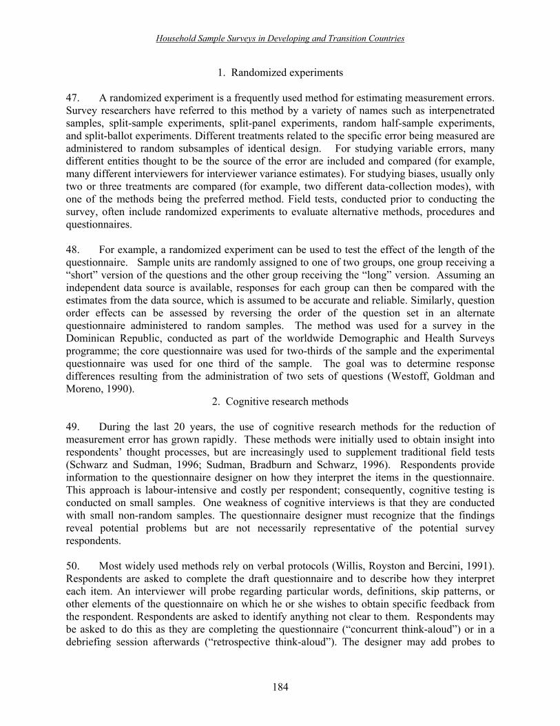
Household Sample Surveys in Developing and Transition Countries
184
1. Randomized experiments 47. A randomized experiment is a frequently used method for estimating measurement errors. Survey researchers have referred to this method by a variety of names such as interpenetrated samples, split-sample experiments, split-panel experiments, random half-sample experiments, and split-ballot experiments. Different treatments related to the specific error being measured are administered to random subsamples of identical design. For studying variable errors, many different entities thought to be the source of the error are included and compared (for example, many different interviewers for interviewer variance estimates). For studying biases, usually only two or three treatments are compared (for example, two different data-collection modes), with one of the methods being the preferred method. Field tests, conducted prior to conducting the survey, often include randomized experiments to evaluate alternative methods, procedures and questionnaires. 48. For example, a randomized experiment can be used to test the effect of the length of the questionnaire. Sample units are randomly assigned to one of two groups, one group receiving a �short� version of the questions and the other group receiving the �long� version. Assuming an independent data source is available, responses for each group can then be compared with the estimates from the data source, which is assumed to be accurate and reliable. Similarly, question order effects can be assessed by reversing the order of the question set in an alternate questionnaire administered to random samples. The method was used for a survey in the Dominican Republic, conducted as part of the worldwide Demographic and Health Surveys programme; the core questionnaire was used for two-thirds of the sample and the experimental questionnaire was used for one third of the sample. The goal was to determine response differences resulting from the administration of two sets of questions (Westoff, Goldman and Moreno, 1990).
2. Cognitive research methods 49. During the last 20 years, the use of cognitive research methods for the reduction of measurement error has grown rapidly. These methods were initially used to obtain insight into respondents� thought processes, but are increasingly used to supplement traditional field tests (Schwarz and Sudman, 1996; Sudman, Bradburn and Schwarz, 1996). Respondents provide information to the questionnaire designer on how they interpret the items in the questionnaire. This approach is labour-intensive and costly per respondent; consequently, cognitive testing is conducted on small samples. One weakness of cognitive interviews is that they are conducted with small non-random samples. The questionnaire designer must recognize that the findings reveal potential problems but are not necessarily representative of the potential survey respondents. 50. Most widely used methods rely on verbal protocols (Willis, Royston and Bercini, 1991). Respondents are asked to complete the draft questionnaire and to describe how they interpret each item. An interviewer will probe regarding particular words, definitions, skip patterns, or other elements of the questionnaire on which he or she wishes to obtain specific feedback from the respondent. Respondents are asked to identify anything not clear to them. Respondents may be asked to do this as they are completing the questionnaire (�concurrent think-aloud�) or in a debriefing session afterwards (�retrospective think-aloud�). The designer may add probes to

Household Sample Surveys in Developing and Transition Countries
185
investigate the clarity of different items or elements of the questionnaire in subsequent interviews. The advantage of the technique is that it is not subject to interviewer-imposed bias. The disadvantage is that it does not work well for respondents uncomfortable with, or not used to, verbalizing their thoughts (Willis, 1994). 51. A related technique involves the interviewer�s asking the respondent about some feature of the question immediately after the respondent completes an item (Nolin and Chandler, 1996). This approach is less dependent on the respondent�s comfort and skill level with respect to verbalizing his/her thoughts, but limits the investigation to those items the survey designer thinks he can ask about. The approach may also introduce an interviewer bias since the probes depend on the interviewer. Inasmuch as the probing approach is different from conducting an interview, some consider it artificial (Willis, 1994). 52. Other approaches allow the respondent to complete the survey instrument with questioning conducted in focus groups. Focus groups provide the advantage of the interaction of group members which may lead to the exploration of areas that might not be touched on in one-on-one interviews. 53. The convening of expert panels, a small group of experts brought in to critique a questionnaire, can be an effective way to identify problems in the questionnaire (Czaja and Blair, 1996). Survey design professionals and/or subject-matter professionals receive the questionnaire several days prior to a meeting with the questionnaire designers. In a group session, the individuals review and comment on the questionnaire on a question-by-question basis. 54. Cognitive research methods are now widely used in designing questionnaires and reducing measurement error in surveys in developed countries. Sudman, Bradburn and Schwarz (1996) summarize major findings as they relate to survey methodology. Tucker (1997) discusses methodological issues in the application of cognitive psychology to survey research.
3. Reinterview studies
55. A reinterview - a repeated measurement on the same unit in an interview survey - is an interview that asks the original interview questions (or a subset of them). Reinterviews are usually conducted with a small subsample (usually about 5 per cent) of a survey�s sample units. Reinterviews are conducted for one or more of the following purposes:
• To identify interviewers who falsify data
• To identify interviewers who misunderstand procedures and require remedial training
• To estimate simple response variance
• To estimate response bias 56. The first two purposes provide information on measurement errors resulting from interviewer effects. The last two provide information on measurement errors resulting from the

Household Sample Surveys in Developing and Transition Countries
186
joint effect of all four sources (namely, interviewer, questionnaire, respondent, and data-collection mode). 57. Specific design requirements for each of four types of reinterviews are discussed below [see Forsman and Schreiner (1991)]. In addition, some methods for analysing reinterview data along with limitations of the results are also presented. Interviewer falsification reinterview 58. Interviewers may falsify survey results in several ways; for example, an interviewer can make up answers for some or all of the questions, or an interviewer can deliberately not follow survey procedures. To detect the occurrence of falsification, a reinterview sample is drawn and the reinterviews are generally conducted by supervisory staff. A falsification rate, defined as the proportion of interviewers falsifying interviews detected through the falsification reinterview, can be calculated. Schreiner, Pennie and Newbrough (1988) report a 0.4 per cent rate for the United States Current Population Survey, a 0.4 per cent rate for the United States National Crime Victimization Survey, and a 6.5 per cent rate for the New York City Housing and Vacancy Survey, which are all conducted by the United States Bureau of the Census. Interviewer evaluation reinterview 59. Reinterview programmes that identify interviewers who do not perform at acceptable levels are called interviewer evaluation reinterviews. The purpose is to identify interviewers who misunderstand survey procedures and to target them for additional training. Most design features of this type of reinterview are identical to those of a falsification reinterview. Tolerance tables, based on statistical quality control theory, may be used to determine whether the number of differences in the reinterview after reconciliation exceeds a specific acceptable limit. Reinterview programmes at the United States Bureau of the Census use acceptable quality tolerance levels ranging between 6 and 10 per cent (Forsman and Schreiner, 1991). Simple response variance reinterview 60. The simple response variance reinterview is an independent replication of the original interview procedures. All guidelines, procedures and processes of the original interview are repeated in the reinterview to the fullest extent possible. The reinterview sample is a representative subsample of the original sample design. The interviewers, data-collection mode, respondent rules and questionnaires of the original interview are used in the reinterview. In practice, the assumptions are not always followed; for example, if the original questionnaire is too long, a subset of the original interview questionnaire is used. Differences between the original interview and the reinterview are not reconciled. 61. A statistic estimated from a simple response variance reinterview is the gross difference rate (GDR), which is the average squared difference between the original interview and reinterview responses. The GDR divided by 2 is an unbiased estimate of simple response variance (SRV). For characteristics that have two possible outcomes, the GDR is equal to the percentage of cases that had different responses in the original interview and the reinterview.

Household Sample Surveys in Developing and Transition Countries
187
Brick, Rizzo and Wernimont (1997) provide general rules for interpreting the response variance measured by the GDR. 62. Another statistic is the index of inconsistency (IOI), which measures the proportion of the total population variance attributed to the simple response variance. Hence,
s+sGDR= IOI
22
21
where s2
1 is the sample variance for the original interview and s22 is the sample variance for the
reinterview. 63. The value of the IOI is often interpreted as follows:
• An IOI of less than 20 is a low relative response variance
• An IOI between 20 and 50 is a moderate relative response variance
• An IOI above 50 is a high relative response variance 64. The response variance measures, the GDR and the IOI, provide data users with information on the reliability and response consistency of a survey�s questions. Examples of the use of the GDR and the IOI for selected variables from a fertility survey in Peru can be found in United Nations (1982) on non-sampling error in household surveys. As part of the second phase of the Demographic and Health Surveys programme, a reinterview programme to assess the consistency of responses at the national level was conducted in Pakistan on a subsample of women interviewed in the main survey (Curtis and Arnold, 1994). Westoff, Goldman and Moreno (1990) describe a reinterview study conducted as part of the Demographic and Health Surveys programme in the Dominican Republic, notable because of the need to adopt several compromises, such as restricting the reinterviews to a few geographical areas and a subset of the target population. Reinterview surveys in India, conducted with a response variance objective, are described in United States Bureau of the Census (1985), which examines census evaluation procedures. 65. Feindt, Schreiner and Bushery (1997) describe a periodic survey�s efforts to continuously improve questionnaires using a reinterview programme. When questions have high discrepancy rates as identified in the reinterview, questionnaire improvement research using cognitive research methods can be initiated. These methods may identify the cause of the problems and suggest possible solutions. During the next round of survey interviews, a reinterview can be conducted on the revised questions to determine whether reliability improvements have been made. This process is then repeated for the remaining problematic questions. Response bias reinterview 66. A reinterview to measure response bias aims to obtain the true or correct responses for a representative subsample of the original sample design. In order to obtain the true answers, the

Household Sample Surveys in Developing and Transition Countries
188
most experienced interviewers and supervisors are used. In addition, either the reinterview respondent used is the most knowledgeable respondent or the household members answer questions for themselves. The original interview questions are used for the reinterview, and the differences between the two responses are reconciled with the respondent to establish �truth.� Another approach uses a series of probing questions to replace the original questions in an effort to obtain accurate responses and then reconcile differences with the respondent. For a discussion of reinterview surveys conducted with the objective of obtaining estimates of response bias, see the report describing census evaluation procedures issued by the United States Bureau of the Census (1985). 67. Reconciliation to establish truth does have limitations. The respondents may knowingly report false information and consistently report this information in the original interview and the reinterview so that the reconciled reinterview will not yield the �true� estimates. In a study of the quality of the United States Current Population Survey reinterview data, Biemer and Forsman (1992) determined that up to 50 per cent of the errors in the original interview had not been detected in the reconciled reinterview. 68. Response bias is estimated by calculating the net difference rate (NDR), the average difference between the original interview response and the reconciled reinterview response assumed to represent the �true� answer. In this case,
)y - y( n1 = NDR TiOi
n
1 = i∑
where n is the reinterview sample size; yo is the original interview response; and yT is the reinterview response after reconciliation, assumed to be the true response. 69. The NDR provides information about the accuracy of a survey question and also identifies questions providing biased results. The existence of this bias needs to be considered when the data are analysed and results interpreted. Brick and others (1996) used an intensive reinterview to obtain a better understanding of the respondent�s perspective and reasons for his/her answers, leading to estimates of response bias. Although working with a small sample, the authors concluded that the method had potential for detecting and measuring biases. Bias-corrected estimates were developed, illustrating the potential effects on estimates when measures of bias are available.
4. Record check studies
70. A record check study compares survey responses for individual sample cases with values obtained from an external source, generally assumed to contain the true values for the survey variables. Such studies are used to estimate response bias resulting from the combined effect of all four sources of measurement error (interviewer, questionnaire, respondent and data-collection mode). 71. Groves (1989) describes the three kinds of record check study designs:
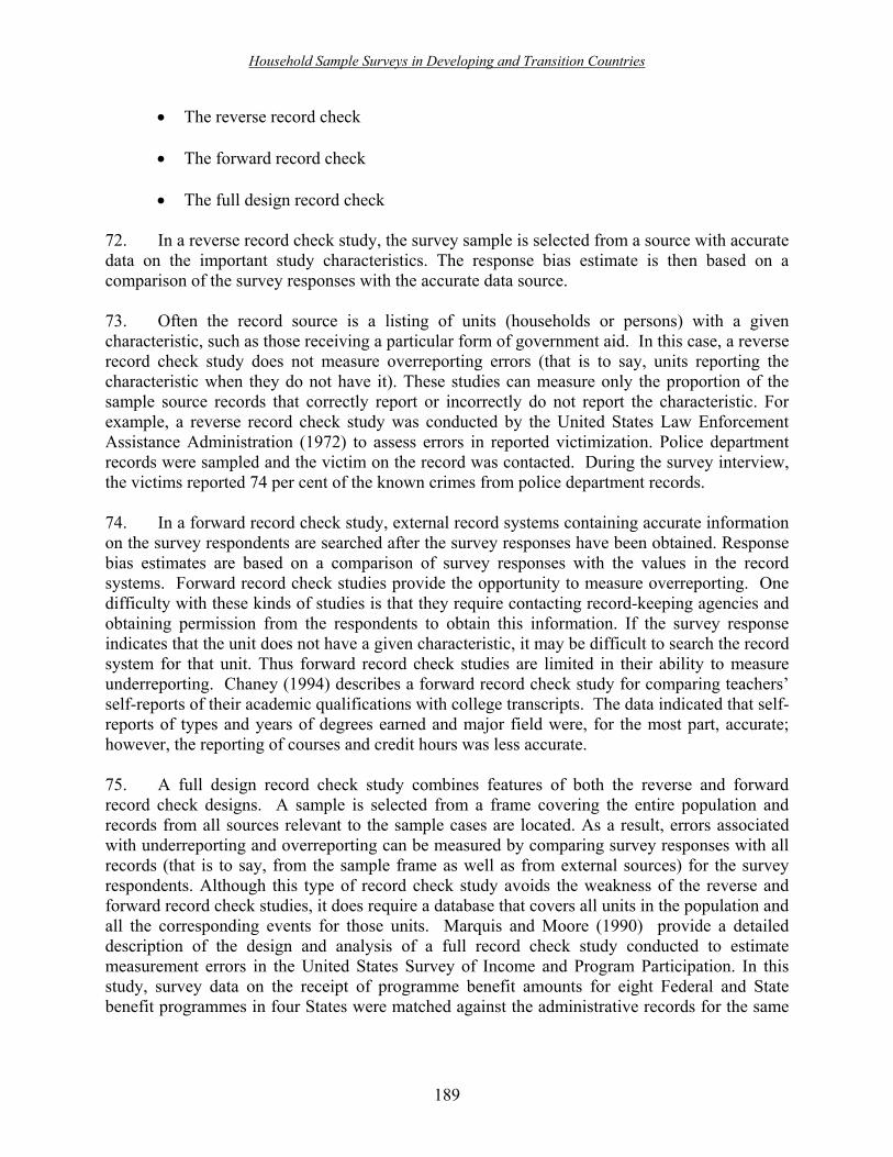
Household Sample Surveys in Developing and Transition Countries
189
• The reverse record check
• The forward record check
• The full design record check 72. In a reverse record check study, the survey sample is selected from a source with accurate data on the important study characteristics. The response bias estimate is then based on a comparison of the survey responses with the accurate data source. 73. Often the record source is a listing of units (households or persons) with a given characteristic, such as those receiving a particular form of government aid. In this case, a reverse record check study does not measure overreporting errors (that is to say, units reporting the characteristic when they do not have it). These studies can measure only the proportion of the sample source records that correctly report or incorrectly do not report the characteristic. For example, a reverse record check study was conducted by the United States Law Enforcement Assistance Administration (1972) to assess errors in reported victimization. Police department records were sampled and the victim on the record was contacted. During the survey interview, the victims reported 74 per cent of the known crimes from police department records. 74. In a forward record check study, external record systems containing accurate information on the survey respondents are searched after the survey responses have been obtained. Response bias estimates are based on a comparison of survey responses with the values in the record systems. Forward record check studies provide the opportunity to measure overreporting. One difficulty with these kinds of studies is that they require contacting record-keeping agencies and obtaining permission from the respondents to obtain this information. If the survey response indicates that the unit does not have a given characteristic, it may be difficult to search the record system for that unit. Thus forward record check studies are limited in their ability to measure underreporting. Chaney (1994) describes a forward record check study for comparing teachers� self-reports of their academic qualifications with college transcripts. The data indicated that self-reports of types and years of degrees earned and major field were, for the most part, accurate; however, the reporting of courses and credit hours was less accurate. 75. A full design record check study combines features of both the reverse and forward record check designs. A sample is selected from a frame covering the entire population and records from all sources relevant to the sample cases are located. As a result, errors associated with underreporting and overreporting can be measured by comparing survey responses with all records (that is to say, from the sample frame as well as from external sources) for the survey respondents. Although this type of record check study avoids the weakness of the reverse and forward record check studies, it does require a database that covers all units in the population and all the corresponding events for those units. Marquis and Moore (1990) provide a detailed description of the design and analysis of a full record check study conducted to estimate measurement errors in the United States Survey of Income and Program Participation. In this study, survey data on the receipt of programme benefit amounts for eight Federal and State benefit programmes in four States were matched against the administrative records for the same

Household Sample Surveys in Developing and Transition Countries
190
programmes. The Survey Quality Profile (United States Bureau of the Census, 1998) provides a summary of the design and analysis. 76. The three types of record check studies share limitations linked to the following three assumptions that, in practice, are unrealistic and are never justified: first, that record systems are free of errors of coverage, non-response, or missing data; second, that individual records in these systems are complete, accurate and free of measurement errors; and third, that matching errors (errors that occur as part of the process of matching the respondents� survey records) are non-existent or minimal. Response bias for a given characteristic can be estimated by the average difference between the survey response and the record check value for that characteristic, according to the following formula:
)(1Bias Response1
i
n
ii XY
n−= ∑
=
where: n is the record check study sample size; Yi = the survey response for the ith sample person; and Xi = the record check value for the ith sample person. 78. The response bias measures from a record check study provide information about the accuracy of a survey question and identify questions that produce biased estimates. These measures can also be used for evaluating alternatives for various survey design features such as questionnaire design, recall periods, data-collection modes, and bounding techniques. For example, Cash and Moss (1972) give the results of a reverse record check study in three counties of North Carolina regarding motor vehicle accident reporting. Interviews were conducted in households containing sample persons identified as involved in motor vehicle accidents in the 12-month period prior to the interview. The study showed that whereas only 3.4 per cent of the accidents occurring within 3 months of the interview had not been reported, over 27 per cent of those occurring between 9 and 12 months before the interview had not been reported.
5. Interviewer variance studies
79. To study interviewer variance, interviewer assignments must be randomized so that differences in results obtained by different interviewers can be attributed to the effects of the interviewers themselves. 80. Interviewer variance is estimated by assigning each interviewer to different but similar respondents, that is to say, respondents who have the same attributes with respect to the survey variables. In practice, this equivalency is assured through randomization. The sample is divided into random subsets, each representing the same population, and each interviewer then works on a different subset of the sample. With this design, each interviewer conducts a small survey with all the essential attributes of the large survey except its size. O�Muircheartaigh (1982) describes the methodology used in the World Fertility Survey to measure the response variance due to interviewers and provides estimates of the response variance for the surveys conducted in Peru (1984a) and Lesotho (1984b).

Household Sample Surveys in Developing and Transition Countries
191
81. In face-to-face interview designs, interpenetrated interviewer assignments are geographically defined to avoid large travelling costs. The assigned areas have sizes sufficient for one interviewer�s workload. Pairs of assignment areas are identified and assigned to pairs of interviewers. Within each assignment area, each interviewer of the pair is assigned a random half of the sample housing units. Thus, each interviewer completes interviews in two assignment areas and each assignment area is handled by two different interviewers. The design consists of one experiment (a comparison of results of two interviewers in each of two assignment areas) replicated as many times as there are pairs of interviewers. Bailey, Moore, and Bailar (1978) present an example of interpenetration for personal interviews in the United States National Crime Victimization Survey in eight cities.
6. Behaviour coding 82. Interviewer performance, while both in training and on-the-job, can be evaluated through the use of behaviour coding. Trained observers observe a sample of interviews, code aspects of the interviews or the sample of interviews are tape-recorded and the coding is done from the tapes. Codes are assigned to record interviewer�s major verbal activities and behaviours such as question asking, probe usage, and response summarization. For example, codes can classify how the interviewer reads the question, whether questions are asked correctly and completely, whether the questions are asked with minor changes and omissions, and whether the interviewer rewords the question substantially or does not complete the question. The coding system classifies whether probes directed the respondent to a particular response, further defined the question or were non-directive, whether responses were summarized accurately or inaccurately, and whether various other behaviours were appropriate or inappropriate. The coded results reflect to what extent the interviewer employed methods in which he/she had been trained, that is to say, an �incorrect� or �inappropriate� behaviour is defined as one that the interviewer had been trained to avoid. To establish and maintain a high level of coding reliability for each coded interview, a second coder should independently code a subsample of interviews. 83. A behaviour coding system can tell new interviewers which of their interviewing techniques are acceptable and which are not and may serve as a basis upon which interviewers and supervisors can review fieldwork and discuss the problems identified by the coding. Furthermore, it provides an assessment of an interviewer�s performance, which can be compared both with the performance of other interviewers and with the individual�s own performance during other coded interviews (Cannell, Lawson, and Hauser, 1975). 84. Oksenberg, Cannell and Blixt (1996) describe a study in which interviewer behaviour was tape-recorded, coded, and analysed for the purpose of identifying interviewer and respondent problems in the 1987 National Medical Expenditure Survey conducted by the United States Agency for Health Care Research and Quality. The study intended to see whether interview behaviour had differed from the principles and techniques covered in the interviewers� training. The authors reported that interviewers frequently had not asked the questions as worded, and at times they had asked them in ways that could influence responses. Interviewers had not probed as much as necessary; and when they did, the probes tended to be directive or inappropriate.

Household Sample Surveys in Developing and Transition Countries
192
D. Concluding remarks: measurement error
85. Measurement error occurs through the data-collection process. Four primary sources were identified as being part of that process: the questionnaire, the method or mode of data collection, the interviewer, and the respondent. Quantifying the existence and magnitude of a specific type of measurement error requires advance planning and thoughtful consideration. Unless small-scale (that is to say, limited sample) studies are conducted, special studies are necessary that require randomization of subsamples, reinterviews, and record checks. These studies are usually expensive to conduct and require a statistician for the data analysis. Nevertheless, if there is sufficient concern that the issue may not be adequately resolved during survey preparations or if the source of error is particularly egregious in the survey being conducted, survey managers should takes steps to design special studies to quantify the principal or problematic source of error. 86. The importance of conducting studies to understand and quantify measurement error in a survey cannot be overemphasized. This is particularly critical if the survey concepts being measured are new and complicated. The analyses that users conduct are dependent on their having both good-quality data and an understanding of the nature and limitations of the data. Measurement error studies require an explicit commitment of the survey programme, because they are costly and time-consuming. The commitment, however, does not end with the implementation and conduct of the studies. The studies must be analysed and results reported so that analysts can make their own assessment of the effect of measurement error on their results. Special studies that focus on analyses of tests and experiments and assessments of data quality are typically available in methodological and technical reports [see, for example, methodological and analytical reports produced by the Demographic and Health Surveys program (Stanton, Abderrahim and Hill, 1997; Institute for Resource Development/Macro Systems Inc., 1990; Curtis, 1995)]. Finally, results from measurement error studies are important for improving the next fielding of the survey. Significant measurement improvements rely, to a large extent, on knowledge and results of previous surveys. Future improvements in the quality of survey data require the commitment of survey research professionals. References Bailey, L., T. F. Moore and B.A. Bailar (1978). An interviewer variance study for the eight
impact cities of the National Crime Survey Cities Sample. Journal of the American Statistical Association, vol. 73, pp. 16�23.
Biemer, P.P., and G. Forsman (1992). On the quality of reinterview data with application to the
current population survey. Journal of the American Statistical Association, vol. 87: pp. 915�923.
Biemer, P.P., and others , eds. (1991). Measurement Errors in Surveys. New York: John Wiley
and Sons.

Household Sample Surveys in Developing and Transition Countries
193
Bishop, G.F. and others (1988). A comparison of response effects in self-administered and telephone surveys. In Telephone Survey Methodology, R.M. Groves and others, eds. New York: John Wiley and Sons, pp. 321�340.
Blair, J., G. Menon and B. Bickart (1991). Measurement effects in self vs. proxy responses to
survey questions: an information-processing perspective. In Measurement Errors in Surveys, P. Biemer and others, eds. New York: John Wiley and Sons, pp. 145�166.
Bradburn, N.M. (1983). Response Effects. In Handbook of Survey Research, P.H. Rossi, J.D.
Wright and A.B. Anderson, eds. New York: Academic Press, pp. 289�328. __________ , and S. Sudman (1991). The current status of questionnaire design. In
Measurement Errors in Surveys, P. Biemer and others, eds. New York: John Wiley and Sons, pp. 29-40.
__________ and Associates (1979). Improving Interviewing Methods and Questionnaire
Design: Response Effects to Threatening Questions in Survey Research. San Francisco, California: Jossey-Bass.
Brick, J.M., L. Rizzo and J. Wernimont (1997). Reinterview Results for the School Safety and
Discipline and School Readiness Components. Washington, D.C.: United States Department of Education, National Center for Education Statistics. NCES 97�339.
Brick, J.M., and others (1996). Estimation of Response Bias in the NHES: 95 Adult Education
Survey. Working Paper, No. 96-13. Washington, D.C., United States Department of Education, National Center for Education Statistics.
Cannell, C.F., S.A. Lawson and D.L. Hauser (1975). A Technique for Evaluating Interviewer
Performance. Ann Arbor, Michigan: University of Michigan, Survey Research Center. Cash, W.S., and A.J. Moss (1972). Optimum recall period for reporting persons injured in motor
vehicle accidents. Vital and Health Statistics, vol. 2, No. 50. Washington, D.C.: Public Health Service.
Chaney, B. (1994). The Accuracy of Teachers� Self-reports on Their Post Secondary Education:
Teacher Transcript Study, Schools and Staffing Survey. Working Paper, No. 94-04. Washington, D.C.: United States Department of Education, National Center for Education Statistics.
Collins, M. (1980). Interviewer variability: a review of the problem. Journal of the Market
Research Society, vol. 22, No. 2, pp. 77�95. Couper, M.P., and others, eds. (1998). Computer Assisted Survey Information Collection. New
York: John Wiley and Sons.

Household Sample Surveys in Developing and Transition Countries
194
Curtis, S.L. (1995). Assessment of the Data Quality of Data Used for Direct Estimation of Infant and Child Mortality in DHS-II Surveys. Occasional Papers, No. 3. Calverton, Maryland: Macro International, Inc.
__________ , and F. Arnold (1994). An Evaluation of the Pakistan DHS Survey Based on the
Reinterview Survey. Occasional Papers, No. 1. Calverton, Maryland: Macro International, Inc.
Czaja R., and J. Blair (1996). Designing Surveys: A Guide to Decisions and Procedures.
Thousand Oaks, California: Pine Forge Press (a Sage Publications company). DeMaio, T.J. (1984). Social desirability and survey measurement: a review. In Surveying
Subjective Phenomena, C.F. Turner and E. Martin, eds. New York: Russell Sage, pp. 257�282.
Dillman, D.A. (1978). Mail and Telephone Surveys: The Total Design Method. New York:
John Wiley and Sons. __________ (1983). Mail and other self-administered questionnaires. In Handbook of Survey
Research, P. Rossi, R.A. Wright and B.A. Anderson, eds. New York: Academic Press, pp. 359�377.
__________ (1991). The design and administration of mail surveys. Annual Review of
Sociology, vol. 17, pp. 225-249. __________ (2000). Mail and Internet Surveys: The Tailored Design Method. New York:
John Wiley and Sons. Eisenhower, D., N.A. Mathiowetz and D. Morganstein (1991). Recall error: sources and bias
reduction techniques. In Measurement Errors in Surveys, P. Biemer and others, eds. New York: John Wiley and Sons, pp.127�144.
Feindt, P., I. Schreiner and J. Bushery (1997). Reinterview: a tool for survey quality
management. In Proceedings of the Section on Survey Research Methods. Alexandria, Virginia: American Statistical Association, pp. 105�110.
Forsman, G., and I. Schreiner (1991). The design and analysis of reinterview: an overview. In
Measurement Errors in Surveys, P. Biemer and others, eds. New York: John Wiley and Sons, pp. 279�302.
Fowler, F.J. (1991). Reducing interviewer-related error through interviewer training, supervision
and other means. In Measurement Errors in Surveys, P. Biemer and others, eds. New York: John Wiley and Sons, pp. 259�275.
Groves, R.M. (1989). Survey Errors and Survey Costs. New York: John Wiley and Sons.

Household Sample Surveys in Developing and Transition Countries
195
__________ , and L.J. Magilavy (1986). Measuring and explaining interviewer effects. Public Opinion Quarterly, vol. 50, pp. 251�256.
Hastie, R, and D. Carlston (1980). Theoretical issues in person memory. In Person Memory:
The Cognitive Basis of Social Perception, R. Hastie and others, eds. Hillsdale, New Jersey: Lawrence Erlbaum, pp. 1�53.
Hill, D.H. (1994). The relative empirical validity of dependent and independent data collection
in a panel survey. Journal of Official Statistics, vol. 10, No. 4, pp. 359�380. Huang, H. (1993). Report on SIPP Recall Length Study. Internal United States Bureau of the
Census, Washington, D.C. Institute for Resource Development/Macro Systems, Inc. (1990). An Assessment of DHS-1 Data
Quality. Demographic and Health Surveys Methodological Reports, No. 1. Columbia, Maryland: Institute for Resource Development/Macro Systems, Inc.
Jenkins, C., and D. Dillman (1997). Towards a theory of self-administered questionnaire design.
In Survey Measurement and Process Quality, L. Lyberg and others, eds. New York: John Wiley and Sons, pp. 165�196.
Kahn, R.L., and C.F. Cannell (1957). The Dynamics of Interviewing. New York: John Wiley
and Sons. Kalton, G., D. Kasprzyk and D.B. McMillen (1989). Non-sampling errors in panel surveys.
In Panel Surveys, D. Kasprzyk and others, eds. New York: John Wiley and Sons, pp. 249�270.
Kalton, G., D. McMillen and D. Kazprzyk (1986). Non-sampling error issues in SIPP. In
Proceedings of the Bureau of the Census Second Annual Research Conference. Washington, D.C., pp.147-164.
Kantorowitz, M. (1992). Methodological Issues in Family Expenditure Surveys, Vitoria-Gasters,
autonomous community of Euskadi: Euskal Estatistika-Erakundea, Instituto Vasco de Estadistica.
Kish, L. (1962). Studies of interviewer variance for attitudinal variables. Journal of the
American Statistical Association, vol. 57, pp. 92�115. Lyberg, L., and D. Kasprzyk (1991). Data Collection Methods and Measurement Errors: An
Overview. In Measurement Errors in Surveys, P. Biemer and others, eds. New York: John Wiley and Sons, pp.237�258.
__________ , P. Biemer, M. Collins, E.D. DeLeeuw, C. Dippo, N. Schwartz and D. Trewin
(1997). In Survey Measurement and Process Quality. New York: John Wiley and Sons.

Household Sample Surveys in Developing and Transition Countries
196
Marquis, K.H., and C.F. Cannell (1971). Effects of some experimental techniques on reporting in the health interview. In Vital and Health Statistics, Washington, D.C.: Public Health Service, Series 2 (Data Evaluation and Methods Research), No. 41.
__________ , and J.C. Moore (1990). Measurement errors in SIPP program reports. In
Proceedings of the Bureau of the Census 1990 Annual Research Conference. Washington, D.C., pp. 721�745.
Mathiowetz, N. (2000). The effect of length of recall on the quality of survey data. In
Proceedings of the 4th International Conference on Methodological Issues in Official Statistics. Stockholm: Statistics Sweden. Available from http://www.scb.se/Grupp/Omscb/_Dokument/Mathiowetz.pdf (Accessed 3 June 2004).
__________ , and K. McGonagle (2000). An assessment of the current state of dependent
interviewing in household surveys. Journal of Official Statistics, vol. 16, pp. 401�418. Neter, J. (1970). Measurement errors in reports of consumer expenditures. Journal of Marketing
Research, vol. VII, pp. 11-25. __________ , and J. Waksberg (1964). A study of response errors in expenditure data from
household interviews. Journal of the American Statistical Association, vol. 59, pp. 8�55. Nolin, M.J., and K. Chandler (1996). Use of Cognitive Laboratories and Recorded Interviews in
the National Household Education Survey. Washington, D.C.: United States Department of Education, National Center for Education Statistics. NCES 96�332.
Oksenberg, L., C. Cannell and S. Blixt (1996). Analysis of interviewer and respondent behavior
in the household survey. National Medical Expenditure Survey Methods, 7. Rockville, Maryland: Agency for Health Care and Policy Research, Public Health Service.
O�Muircheartaigh, C. (1982). Methodology of the Response Errors Project. WFS Scientific
Reports, No. 28. Voorburg, Netherlands: International Statistical Institute. __________ (1984a). The Magnitude and Pattern of Response Variance in the Lesotho Fertility
Survey. WFS Scientific Reports, No. 70. Voorburg, Netherlands: International Statistical Institute.
__________ (1984b). The Magnitude and Pattern of Response Variance in the Peru Fertility
Survey. WFS Scientific Reports, No. 45. Voorburg, Netherlands: International Statistical Institute.
Schreiner, I., K. Pennie and J. Newbrough (1988). Interviewer falsification in Census Bureau
Surveys. In Proceedings of the Section on Survey Research Methods. Alexandria, Virginia: American Statistical Association, pp. 491�496.

Household Sample Surveys in Developing and Transition Countries
197
Schuman, H. and S. Presser (1981). Questions and Answers in Attitude Surveys. New York: Academic Press.
Schwarz, N. (1997). Questionnaire design: the rocky road from concepts to answers. In Survey
Measurement and Process Quality, L. Lyberg and others, eds. New York: John Wiley and Sons, pp. 29�46.
__________ , R.M. Groves and H. Schuman (1995). Survey Methods. Survey Methodology
Program Working Paper Series. Ann Arbor, Michigan, Institute for Survey Research, University of Michigan.
__________, and H. Hippler (1991). Response alternatives: the impact of their choice and
presentation order. In Measurement Errors in Surveys, P. Biemer and others, eds. New York: John Wiley and Sons, pp. 41�56.
__________, and S. Sudman (1996). Answering Questions: Methodology for Determining
Cognitive and Communicative Processes in Survey Research. San Francisco, California: Jossey-Bass.
Silberstein, A., and S. Scott (1991). Expenditure diary surveys and their associated errors. In Measurement Errors in Surveys, P. Biemer and others, eds. New York: John Wiley and
Sons, pp. 303-326. Singh, S. (1987). Evaluation of data quality. In The World Fertility Survey: An Assessment, J.
Cleland and C. Scott, eds. New York: Oxford University Press, pp. 618-643. Sirken, M. and others (1999). Cognition and Survey Research. New York: John Wiley and
Sons. Stanton, C., N. Abderrahim and K. Hill (1997). DHS Maternal Mortality Indicators: An
Assessment of Data Quality and Implications for Data Use. Demographic and Health Surveys Analytical Report, No. 4. Calverton, Maryland: Macro International, Inc.
Sudman, S., N. Bradburn and N. Schwarz (1996). Thinking about Answers: The Application of
Cognitive Processes to Survey Methodology. San Francisco, California: Jossey-Bass. __________, and others (1977). Modest expectations: the effect of interviewers� prior
expectations on response. Sociological Methods and Research, vol. 6, No. 2, pp. 171�182.
Tucker, C. (1997). Methodological issues surrounding the application of cognitive psychology
in survey research. Bulletin of Sociological Methodology, vol. 55, pp.67�92.
Household Sample Surveys in Developing and Transition Countries
198
United Nations (1982). National Household Survey Capability Programme: Non-sampling Errors in Household Surveys: Sources, Assessment, and Control: Preliminary Version
DP/UN/INT-81-041/2. New York: United Nations Department of Technical Co-operation for Development and Statistical Office.
United States Bureau of the Census (1985). Evaluating Censuses of Population and Housing.
Statistical Training Document. Washington, D.C. ISP-TR-5. __________ (1998). Survey of Income and Program Participation (SIPP) Quality Profile, 3rd
ed. Washington, D.C.: United States Department of Commerce. United States Federal Committee on Statistical Methodology (2001). Measuring and Reporting
Sources of Error in Surveys, Statistical Policy working Paper, No. 31. Washington, D.C.: United States Office of Management and Budget. Available from http://www.fcsm.gov (accessed 14 May 2004).
United States Law Enforcement Assistance Administration (1972). San Jose Methods Test of
Known Crime Victims. Statistics Technical Report No.1. Washington, D.C. Vaessen, M. and others (1987). Translation of questionnaires into local languages. In The
World Fertility Survey: An Assessment, J. Cleland and C. Scott, eds. New York: Oxford University Press, pp.173-191.
Weiss, C. (1968), Validity of welfare mothers� interview response. Public Opinion Quarterly,
vol. 32, pp. 622�633. Westoff, C., N. Goldman and L. Moreno (1990). Dominican Republic Experimental Study: An
Evaluation of Fertility and Child Health Information. Princeton, New Jersey: Office of Population Research; and Columbia, Maryland: Institute for Resource Development/Macro Systems, Inc.
Willis, G.B. (1994). Cognitive Interviewing and Questionnaire Design; A Training Manual.
Cognitive Methods Staff Working Paper, No. 7. Hyattsville, Maryland: National Center for Health Statistics.
__________ , P. Royston and D. Bercini (1991). The use of verbal report methods in the
development and testing of survey questions. In Applied Cognitive Psychology, vol. 5, pp. 251-267.
Woltman, H.F., and J.B.Bushery (1977). Update of the National Crime Survey Panel Bias Study.
Internal United States Bureau of the Census report, Washington, D.C.

Household Sample Surveys in Developing and Transition Countries
199
Chapter X Quality assurance in surveys:
standards, guidelines and procedures
T. Bedirhan Üstun, Somnath Chatterji, Abdelhay Mechbal and Christopher J.L. Murray
On behalf of the World Health Survey (WHS) Collaborators * World Health Organization
Evidence and Information for Policy Geneva, Switzerland
Abstract
The quality of a survey is of prime importance for accurate, reliable and valid results. Survey teams should implement systematic quality assurance procedures to prevent unacceptable practices and to minimize errors in data collection. Establishment of effective and efficient strategies towards improvement of the quality of a survey will help achieve the timely collection of high-quality data and the validity of the results. �Quality assurance� may also be viewed as an organizing tool for implementation with pre-defined operational standards regarding the structure, process and outcome of the survey. Survey teams should adhere to explicit standards of quality and follow prescribed procedures to achieve such standards. The procedures should be transparent, systematically monitored and carefully reported as part of the general documentation of the survey implementation and results. It is also important that the survey be measured and summarized by quantifiable indicators, to the extent practicable.
The present chapter outlines a systematic approach to achieving quality assurance
measures, going beyond simple control mechanisms. A large international survey -- the World Health Survey (WHS) implemented by multiple survey institutions in 71 different countries-- is used to illustrate the elaboration of the application of a total quality assurance programme. This survey was designed to gather comparable data to assess the different dimensions of health systems in participating countries using nationally representative samples. In accordance with the importance of the results of the WHS, rigorous quality assurance procedures were put in place utilizing international experts who were assembled to serve as an external peer review group and to support countries in achieving commonly agreed and feasible quality standards with regard to such matters as: sample selection methodology, achievement of acceptable response rates, treatment of missing data, calculation of measures of reliability and checks for comparability of the data across population subgroups and countries. Key terms: quality assurance, quality indicators, World Health Survey, missing data, response rate, sampling, reliability, cross-population comparability, international comparisons. __________ * The WHS Collaborators are listed in full on the WHS web site: (http://www.who.int/whs/).

Household Sample Surveys in Developing and Transition Countries
200
A. Introduction 1. One of the basic features in respect of the design and implementation of a survey is the survey�s �quality� (Lyberg and others, 1997). In every data-collection initiative, the results depend on the input; as the saying goes: garbage in-garbage out. In addition to the quality of the survey instruments and analytical techniques, the quality of the survey results depend mainly on the implementation of the survey including sound sampling methods and proper administration of the questionnaire. 2. To achieve maximum quality, every survey team should adhere to a standard set of guidelines on survey implementation. These guidelines identify the following:
(a) Quality standards that need to be adhered to at each step of a survey; (b) Quality assurance (QA) procedures that identify the explicit actions to be taken
for monitoring the survey implementation in actual settings; (c) Evaluation of the quality assurance process that measures the impact of quality
assurance standards on the survey results and procedures towards improving the relevance and efficiency of the overall quality assurance process (Biemer and others, 1991).
3. The overall aim of the guidelines is to provide support to improving quality rather than to audit the survey implementation. Since any survey is a large investment involving multiple parties with important results that have influence on the policies of a nation, it is essential that quality be a serious operational focus. Quality assurance is seen as an ongoing process throughout the survey from preparation and sampling through data collection and data analysis to report writing. The guidelines also aim to ensure a better understanding of the design of the survey among users. The purpose of establishing standard procedures is to help ensure that:
• The data collection is relevant and meaningful for the country's needs • The data can be compared within a country and across countries to identify the
similarities and differences across populations • The practical implementation of the survey follows accepted protocols • The errors in data collection are minimized • The data-collection capability is improved over time
B. Quality standards and assurance procedures 4. Quality assurance (Statistics Canada, 1998) is defined as any method or procedure for collecting, processing or analysing survey data that is aimed at maintaining or enhancing their

Household Sample Surveys in Developing and Transition Countries
201
reliability or validity. Quality assurance could be understood as having similar yet differing meanings. In the present chapter, we utilize the total quality management paradigm that examines the survey process at each step and try to outline an approach not only to reducing sampling and non-sampling errors but also to improving the relevance and feasibility of the survey as well as the capacity of the country to implement surveys. To achieve this aim, yet remain practical, this chapter will make use of the World Health Survey (WHS) quality standards and assurance procedures (World Health Organization, 2002) referring to all the steps including:
• Selection of survey institutions • Sampling • Translation • Training • Survey implementation • Data entry/data capturing • Data analysis • Indicators of quality • Country reports • Site visits
5. Figure X.1 depicts the overall WHS life cycle indicating the above-mentioned steps in every phase of survey implementation. The quality assurance guidelines which were drafted by a large number of WHS participants as well as international experts, aim to identify best practices whose implementation, in order to achieve and monitor a good-quality survey, is feasible. Each step of survey implementation involves a certain examination of quality. For example, it is important that the survey instruments have good measurement properties, that the sampling be representative of the target population, and that the data be clean and complete. 6. This set of procedures constitutes merely an example to demonstrate the "quality assurance approach" to survey design and implementation as a process and to improving the output of the survey in terms of its relevance, accuracy, coherence and comparability. Any survey team designing and implementing a survey could use a similar approach keeping in mind the specific aims of its own survey and the feasibility of the quality assurance standards proposed in this chapter. Most importantly, quality should be given distinct attention and should be guided and monitored within an operational context. The results of the quality assurance process should be reported both in quantitative terms using appropriate indicators where measurement is possible (for example, sampling ratios, response rates, missing data, test-retest reliability of the application) and in qualitative terms summarizing the structure, process and outcome of the survey.

Household Sample Surveys in Developing and Transition Countries
202
Figure X.1. WHS quality assurance procedures
WHRStatistical annexes
RESEARCHQUESTIONS
POLICYQUESTIONS
Indicators! Health
MortalityHealth
! Responsiveness! Financing! Health system functions
Coverage! Composite goals
Country reportsShort reportDetailed reportPolicy report
World Health Survey
Instrument design" Measurement properties" Scales" Reliability" Cultural comparability
QualityAssurance
Implementation" Sampling" Training" Fieldwork" Site visits
QualityAssurance
Data" Editing and entry" Checks" Cleaning and filing" Missing data" Archiving
QualityAssurance
Statistics" Descriptive" Multivariate" Hypothesis testing
QualityAssurance
C. Practical implementation of quality assurance guidelines: example of World Health Surveys
7. The overall quality assurance strategy described above has been implemented within the WHS to improve the quality of the surveys including in several developing countries in Asia and sub-Saharan Africa. The present section aims to make use of the quality assurance standards, procedures and reporting as a concrete guide. Other survey teams may use this example as it fits their purpose. To our knowledge this is the first-ever application of systematic application of quality assurance procedures in international surveys, and implementing agencies and collaborators have found them very useful in organizing and reporting their work. Initial data suggest that it was possible to detect errors early and prevent them, and increase completion, accuracy and efficiency of results. 8. The World Health Organization (WHO) has initiated the World Health Survey (WHS) as a real-life data-collection platform for obtaining information on the health of populations and health systems in a continuous manner (Üstün and others, 2003a, 2003b; Valentine, de Silva and Murray, 2000; World Health Organization, 2000). WHS responds to the need of countries for a detailed and sustainable health information system and gathers data through surveys to measure essential population health parameters; and brings together standard survey procedures and instruments for general population surveys in order to present comparable data across WHO

Household Sample Surveys in Developing and Transition Countries
203
member States. These methods and instruments are modular in structure and have been refined through scientific review of literature, extensive consultations with international experts and large-scale pilot tests conducted in more than 63 countries and 40 languages (Üstün and others, 2003a, 2003c; 2001). WHS is designed to evolve through its implementation by continuous input from collaborators including policy makers, survey institutions, scientists and other interested parties. The countries and WHO jointly own the data, and there is a commitment for long-term data collection, building local capacity and using the survey results to guide the development and implementation of health policy. 9. This chapter systematically reviews each step of the survey process, except questionnaire design and testing, which is reviewed elsewhere (see Üstün and others, 2003b), and introduces the WHS quality assurance standards in each area. These are desirable standards though which to increase efficiency and prevent unacceptable practices. Greater attention to quality is needed now more than ever because of the increasing importance of the WHS data for WHO member States and their implications for health policies. WHS has therefore formulated general guidelines for survey practice in order to enhance the reliability and validity of WHS surveys by reducing possible preventable errors. Quality assurance guidelines as adopted will become primary organizing tools for WHS and also serve in the organization of survey work and the preparation and planning for implementation. This chapter therefore provides an overall guide to the critical aspects that need particular attention so as to ensure collection of good-quality data. 10. These guidelines will also serve as an evaluation template for the survey managers and quality assurance advisers (a network of international experts with extensive survey experience who serve as peer reviewers of the whole process). They will make site visits to countries to support their efforts in implementing the WHS and undertake a structured and detailed assessment of the process, which will support countries in assessing quality in a systematic manner, and in identifying areas in survey activity that could be improved.
1. Selection of survey institutions 11. Carrying out a national survey requires extensive knowledge, skills, resources and expertise. These requirements have resulted in the organization of survey activity in accordance with different styles and traditions in different countries and sectors. To ensure that a competent survey group in a given country carries out the WHS, it is important to establish the identification of good survey institutions and the specifying of standards as the contractual conditions. WHS usual practice is to consult with the ministries of health, regional offices and WHO country representatives or liaison officers to identify such institutions. Given the size and complexity of the survey, the feasibility should be demonstrated by a contractual bidding process as required by WHO regulations. This process starts with a call for competent survey institutions to make their bid for the WHS In accordance with the technical specifications of the sampling, interviewing and data collection. [Technical specifications for the WHS is available on the WHS web site (www.who.int/whs)]. These bids are compared according to a number of criteria before the final selection is made.

Household Sample Surveys in Developing and Transition Countries
204
12. Criteria for assessing performance standards of potential institutions include:
• Their previous track record (that is to say, their experience with at least five large national surveys in the recent past with sample sizes of 3,000 or more).
• Their capacity to carry out the whole survey process (namely, sampling, training,
data collection and analysis). • Their experience in different modes of data collection including face-to-face
interviews (and other possible modes like telephone, mail, computer, etc.). • Documentation on former surveys (including the survey metrics of sample
representation, coverage of country population, quality of interviewing, cost and type of training, quality assurance and other survey procedures).
• Record of usual time lines for survey calendar and their ability to complete
surveys within an established time frame. • Their potential to develop and use a good infrastructure with regard to health
information systems, working closely with the ministry of health, national statistical bodies and other agencies.
13. The contractual bidding procedure is useful in identifying the best possible offer in terms of quality and costs, and allows for a comparative assessment of all possible providers in a country. In this way, WHO and the ministry of health can identify the best possible survey institution with a view to building capacity for further surveys and to incorporate WHS data into the health information system. The contractual process also allows for building in penalties for failure to deliver results and ensure adherence to quality. Consortium bids should be encouraged to ensure that relevant partners (for example, the ministry of health together with the national statistical office) work together to secure access to a good sampling frame. 14. A careful review of the different proposals submitted using the list of criteria described above should be undertaken. This comparative analysis should be documented. 15. In summary, it is important not only to identify a good agency that will meet the technical specifications of the desired survey in the country concerned but also to provide the agency with the necessary technical support in order to achieve the desired outcome. For large-scale national surveys, it is often necessary within a country to create a partnership of groups, institutions and persons that have the necessary expertise for design, training, implementation, data processing, analysis and report writing.
2. Sampling
16. A survey is only as good as its sample. If either sample design/or implementation or both are faulty, there is little one can do to make up for the sample design�s limited representativeness

Household Sample Surveys in Developing and Transition Countries
205
or to fill in missing information. The survey results will then be biased in unknown ways and often of unquantifiable magnitude. 17. Because there is a wide range of applications in the field, WHO and a group of international technical experts have identified a set of guidelines to secure a good sample for the WHS [WHS Sampling Guidelines for Participating Countries are available on the WHO web site (www.who.int/whs)]. Standards of scientific sampling are based on probability selection methods and are widely known and accepted (Üstün and others, 2001; Kish, 1995a). However, these are typically not followed because of poor operationalization, lack of supervision of the implementation of sampling procedures in the field and/or high costs of implementation in particular contexts and conditions. 18. WHO guidelines emphasize the scientific principles of survey sampling as explicit standards for quality, give examples of good sampling plans, and identify quality assurance standards for countries to adhere to. WHO and technical advisers will provide technical support to countries when needed. Important aspects of WHS sampling are outlined below:
(a) The WHS sample should target the de facto population (that is to say, all people living in that country including guest workers, immigrants and refugees) and not the de jure population (the citizens of that country alone). It is important to create good representation as the "miniature" of the country's overall population. To this end, it is essential to represent all people living in the country and have full geographical coverage of the country;
(b) The size of the sample must be adequate to provide good (robust) estimates of the
quantities of interest at national or subnational levels depending on the objectives of the survey; at the same time, survey managers must balance the need for larger sample sizes to achieve better estimates against the corresponding increase in survey costs. Large sample sizes do not make up for poor quality. For various purposes, it may be required to have adequate representation of minorities (for example, ethnic or other subgroups) which may require oversampling (that is to say, giving a higher probability of selection). If a subpopulation needs to be oversampled because of any scientific study question, then specifications for doing so must be clarified in detail. In case of oversampling, differential weighting at the data analysis stage should be applied to correct the distortion caused by oversampling;
(c) In the WHS, a sampling frame (that is to say, a list of the geographical areas,
households or individuals from which the sample is selected, such as could be derived from a computerized population list, a recent census, electoral roll, etc.) with 90 per cent coverage of all key subgroups of interest is considered acceptable. Countries should use the most recent sampling frame available. If it is two or more years out of date, enumeration or listing of households to update the frame at the penultimate stage of selection is often necessary. Quick count methods may be used to update measures of size for the primary sampling units prior to selection; such methods include counting in selected tracks where an up-to-date frame is unavailable owing to obsolete cartography or other reasons. Besides quick counting approaches in the selected sampling areas, other sources such as postal addresses from local post offices, lists from water or electricity billing companies, etc. can be used to update the frame. It is essential that the population be scientifically weighted back to the most recent census;

Household Sample Surveys in Developing and Transition Countries
206
(d) The WHS sample targets all adult members of the general population aged 18
years or over as its sample.22 In most cases, it is based on the most recent census data as its sampling frame. Households are selected using a multistage stratified cluster sampling procedure. One individual per household is then selected through a random selection procedure [for example, the Kish table method (Kish, 1995a), or alternative methods such as the last-birthday method, and the Trohdahl/Carter/Bryant method (Bryant, 1975)]. Random number tables could also be used at this stage provided that the selection numbers are carefully documented. Whatever selection technique is used, all attempts should be made to reduce selection bias during actual implementation in the field. Countries should seek to design the simplest sample plan possible that meets the measurement objectives of the survey. With respect to an overly complex design, implementation may be difficult and errors may be out of control. Feasibility and having the data trail to monitor sampling design are key to the quality;
(e) WHS uses the United Nations definition of household;23 however, there may be
variations in this definition owing to local circumstances. The possible impact of variations in the household definition on sampling should be elaborated in country reports. Should the countries use a sampling frame of households, it is suggested that they then use the same definition for a household in the survey as was used in the original frame;
(f) WHS uses a scientific sampling strategy, which encompasses a known non-zero
selection probability for any individual included in the survey. Use of strict probability methods at every stage of sampling is crucial, and makes it possible to extrapolate the sample data to the whole population. Otherwise, the survey results will not be representative and valid;
(g) The inclusion of institutionalized populations in a general population survey is
difficult because separate frames need to be developed. There are also many ethical implications in relation to interviewing in institutions (such as hospitals, nursing homes, army barracks and prisons). Given the wide ranges of differences in institutionalization in difference countries, a single solution cannot be found. As a possible solution, WHS attempts to include people who are institutionalized owing to their health condition if it is possible to interview them during the survey period. We then use the institutional population rates from the census to check the concordance of the rates obtained in the survey. This is of specific concern to the WHS, since persons living in institutions such as nursing homes, long-stay hospitals, etc. are likely to be in worse health than those who are not in institutions and therefore need to be included in the sample to reduce the potential for underestimating health conditions;
(h) WHS sampling guidelines clearly explain what is meant by unit non-response and
calculation of non-response rates in terms of target and achieved samples. The sampling strategy of the WHS does not allow substitution of non-responses by another household or individual;
22 Currently, the WHS only includes adults. Future work aims to develop a survey that will include children as well. 23 The United Nations defines a household as a group of persons that live under the same roof and share cooking and eating facilities (in other words, eat from the same source). For the WHS, a person is usually considered part of the household if he/she is currently in an institution because of a health condition. Such institutionalized people must be included in the household roster.
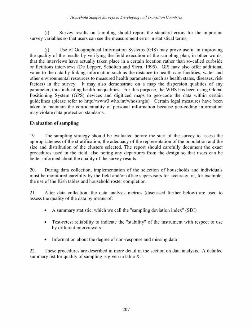
Household Sample Surveys in Developing and Transition Countries
207
(i) Survey results on sampling should report the standard errors for the important survey variables so that users can see the measurement error in statistical terms;
(j) Use of Geographical Information Systems (GIS) may prove useful in improving
the quality of the results by verifying the field execution of the sampling plan; in other words, that the interviews have actually taken place in a certain location rather than so-called curbside or fictitious interviews (De Lepper, Scholten and Stern, 1995). GIS may also offer additional value to the data by linking information such as the distance to health-care facilities, water and other environmental resources to measured health parameters (such as health states, diseases, risk factors) in the survey. It may also demonstrate on a map the dispersion qualities of any parameter, thus indicating health inequalities. For this purpose, the WHS has been using Global Positioning System (GPS) devices and digitized maps to geo-code the data within certain guidelines (please refer to http://www3.who.int/whosis/gis). Certain legal measures have been taken to maintain the confidentiality of personal information because geo-coding information may violate data protection standards.
Evaluation of sampling 19. The sampling strategy should be evaluated before the start of the survey to assess the appropriateness of the stratification, the adequacy of the representation of the population and the size and distribution of the clusters selected. The report should carefully document the exact procedures used in the field, also noting any departures from the design so that users can be better informed about the quality of the survey results. 20. During data collection, implementation of the selection of households and individuals must be monitored carefully by the field and/or office supervisors for accuracy, in, for example, the use of the Kish tables and household roster completion. 21. After data collection, the data analysis metrics (discussed further below) are used to assess the quality of the data by means of:
• A summary statistic, which we call the "sampling deviation index" (SDI) • Test-retest reliability to indicate the "stability" of the instrument with respect to use
by different interviewers • Information about the degree of non-response and missing data
22. These procedures are described in more detail in the section on data analysis. A detailed summary list for quality of sampling is given in table X.1.

Household Sample Surveys in Developing and Transition Countries
208
Table X.1. Summary list for quality of sampling
• Overview of population composition (urban/rural, minorities, languages,
oversampled groups) • Sampling frame and number of stages of sampling:
- Do(es) the sampling frame(s) cover all the target populations? - How recent is the sampling frame?
• Stratification within the sampling frame • Sampling units at each stage: known selection probability • Size of sampling units at each stage: ensure all sampling units have a measure of
size that exceeds a predetermined minimum • Checking of �on the ground� size of units and issues such as whether there is one
or more households per selected �address�, and how to select within these • Size of sample selected • Probability weight for household • Probability weight for respondent • Training in use of and proper implementation of Kish table (or alternative) • Checking on procedure for selection of respondent in household • Summary report on sampling on the actual implementation, deviations, weights,
standard errors
3. Translation 23. To make meaningful comparisons of data across cultures, one needs a relevant instrument that measures the same construct in different countries. The WHS instrument has been developed following scientific review of existing survey instruments, large-scale consultations with experts and systematic field-testing in a multi-country survey study (Üstün and others, 2003a). We have reported the survey instruments features, relevance and cultural applicability elsewhere (Üstün and others, 2003b). For any other survey, designers must aim to have the best instruments and measures and make certain that their instrument is fit for their purpose, has good measurement properties and has passed through pilot tests to assure its feasibility and stability. 24. Once you have a good survey instrument, then translation is one of the key features of ensuring the equivalent versions of questions in different languages. Given the multicultural societies that we live in, it is essential that we have good translations that measure the same concepts in the survey. 25. Often in one country, the instrument will be translated into multiple languages depending on the size of the different language groups within the country. It is suggested that any linguistic group that constitutes over 5 per cent of the population should be interviewed in its own language. For respondents who are interviewed in a language for which a formal translated version has not been produced, emphasis is placed on the understanding of key concepts. Interviewers work with one of the existing translations in the country to ask questions in the

Household Sample Surveys in Developing and Transition Countries
209
language without translation, using the overall guidelines. A further challenge faced by a large multi-country survey exercise is that in many African and Asian countries languages are not written and no scripts are available. It is recommended, in such cases, that a standard translation still be prepared in keeping with the guidelines and transliteration with a script from another familiar language in the country be used to prepare the written version. 26. Guidelines for the translation of the WHS instruments have arisen out of the extensive experience of WHO in developing and implementing international studies with multiple partners and linguistic experts. The WHS Translation Guidelines, which are available on the WHS web site (www.who.int/whs),emphasize the importance of maintaining the equivalence of concepts and ensure a procedure that identifies possible pitfalls and avoids distortion of the meaning. These guidelines stress that:
• Translation should aim to produce a locally understandable questionnaire • The original intent of the questions should be translated with the best possible
equivalent terms in the local language • Question-by-question specifications should aim to convey the original meaning of the
questions and pre-coded response options • The questionnaire should first be translated by health and survey experts who have a
basic understanding of the key concepts of the subject-matter content. A set of selected key terms and those that proved to be problematic during the first direct translation should be back-translated by linguistic experts who would then comment on all the possible interpretations of the terms and suggest alternatives. An editorial group under the supervision of the chief survey officer in that country should review the translation and the back-translation and report back to WHO about the quality of the translation.
• Focus groups and qualitative linguistic methods such as developing an inventory of
local expressions, and comparing expressions with those in other languages, should be used to improve quality. WHO has already undertaken systematic studies of translation and cognitive interviewing in certain languages and incorporated the results of these studies in the current text of the WHS questionnaire. It is still recommended that �cognitive interviews� (that is to say, further exploratory studies of what subjects understood to be the meaning of questions) using the translated questionnaire be undertaken with local subjects. It is mandatory to translate all the WHS documents (namely, the WHS questionnaire, question-by-question specifications, the survey manual and training manuals) into the local language. The data entry program may remain in English. If, however, the country has translated the WHS questionnaire using the electronic media following WHO specifications, the data entry program can automatically be generated in the other languages.
• Each WHS country should submit a report on the quality of the translation work at
the end of the pilot phase. For items that were found to be particularly difficult to

Household Sample Surveys in Developing and Transition Countries
210
translate, specific linguistic evaluation forms should be requested that describe the nature of difficulty of translation.
• Quality assurance advisers for the country should pay special attention to the
implementation steps in the translation process and should check the list of key terms with the chief survey officer in the country.
• In countries where there are many dialects and/or languages that are not available in
written format, specific translation protocols should be discussed with WHO.
Evaluation of translation 27. A full translation of the questionnaire should be submitted to WHO before the start of the pilot interviews in the WHS. This translation should be checked by relevant experts in the particular languages, and comments made to the country if required. 28. The list of key terms back-translated together with a report on the translation process and issues arising therefrom should be reviewed. The linguistic evaluation sheets (Üstün and others, 2001) should be systematically examined by the Country Survey manager and later by WHO to spot particularly problematic items and to enable a common solution across languages wherever feasible. 29. Discussions should be held with interviewers with respect to understanding the procedures employed in the field when a term, phrase or question is not understood. These discussions should review the extent to which interviewers are required to �explain� and �interpret� the questions to respondents.
Table X.2. Summary list for review of translation procedures
• Languages spoken in the country; coverage of major language groups • Who was involved in the translation process? • Were all the needed materials translated?
- Questionnaire - Appendix - Guide to administration (only when the interviewers do not know English) - Survey manual (only when the interviewers do not know English) - Result codes
• What issues came up in the translation? • What protocol was undertaken (for example, full translation sent to WHO or just
list of key items)? • Were linguistic evaluation forms completed?

Household Sample Surveys in Developing and Transition Countries
211
D. Training 30. Training of survey team is the key to quality. Training is an ongoing process that should be conducted before and during the data-collection process, and end with a detailed debriefing after the fieldwork period is completed. 31. Training should be provided at all levels of the survey team involved in the survey, from interviewers to trainers and supervisors, as well as to the central team overseeing the process nationally. This will ensure that all involved persons are clear with regard to their role in ensuring good quality of data. 32. The purpose of overall training is to:
• Ensure a uniform application of the survey materials • Explain the rationale of the study and study protocol • Motivate interviewers • Provide practical suggestions • Improve the overall quality of the data
33. To fulfil part of the training purpose, WHO has organized WHS regional training workshops for principal investigators from all participating countries and produced various training materials, including a training video and an educational compact disk covering all training issues.
Selection of interviewers 34. The use of experienced interviewers as well as people who are familiar with the topic of the survey is important. 35. Interviewers should have at least completed the full period of schooling within their country and be fluent in the main language of the country. Individual countries must decide what further level of education is required as well as what formal assessments will be carried out prior to selection. 36. The issue of whether the interviewers should be health workers or not is left to the individual countries to decide. The characteristics of the interviewers (age, sex, education, professional training, employment status, past survey experience, and so on) should be recorded on a separate database. This information can then be linked to the identification numbers of interviewers for each questionnaire completed and an analysis can be carried out of individual interviewer performance.
Length, methods and content of training 37. Training should be long enough for the interviewers to become familiar with not only the techniques for successful interviewing, but also the content of the questionnaire to be used. For experienced interviewers, the training will be shorter than for less experienced ones.

Household Sample Surveys in Developing and Transition Countries
212
38. The recommended length of training for the WHS is from three to five days, with three days being appropriate for experienced interviewers requiring training on the questionnaire only. The longer period of training is recommended for all other interviewers. 39. All the training should be carried out as far as possible by the same team to ensure a standard training either for all interviewers in one session or for different groups at different times and places. To cut down costs and provide for regional training, training may be decentralized and cascaded. However, these costing benefits are then outweighed by the disadvantages of a diluted or varying training. 40. A booster session is strongly recommended if it can be accommodated at some point during the data-collection period. It should preferably be held sometime towards the middle of the WHS data-collection period. The booster session serves to review various aspects of data collection, focusing on those undertakings that are proving complex and difficult or those guidelines that are not being adhered to sufficiently by interviewers. This session could also provide feedback on how much has been achieved and the positive aspects, including feedback from the supervisors and central survey team to the interviewers, as well as from interviewers to the supervisors and survey team. 41. The training methods should include as much role playing in interviews as possible (with a minimum of one per interviewer). This method provides assimilation of interviewing techniques more effectively. For role playing to be effective, different scripts must be prepared in advance of the training so that the different branching structures of the interview, the nature of explanations that are permitted, and anticipated problems during an interview with difficult respondents can be illustrated. 42. In addition to role playing, there should be at least one opportunity, before starting the actual data collection, to conduct an interview with a real-life respondent outside of the interviewer group. The practice interviews should be tape- or video-recorded as often as possible for review and feedback discussion during training sessions. WHS countries are encouraged to make a standard training video similar to the WHO video if this is possible. Feedback should be given after each role-play or practice interview. 43. Training materials should be provided to all interviewers to use as reference material. Any material provided should be comprehensively reviewed during the training and, where relevant, should be translated into the languages used in the country. 44. The content of training should include the following:
• Administrative issues • Planning of fieldwork • Review of all materials provided • Contacting procedures, consent forms and confidentiality

Household Sample Surveys in Developing and Transition Countries
213
Conducting an interview should encompass:
• Interview procedures in the field • Supervision in field and reporting procedures • Structure of the survey team and role of all members of the team
Evaluation of training 45. Evaluation of training should occur at a number of levels. The interviewers must be evaluated in order to determine whether they are capable of interviewing effectively and what, if any, particular support they require. The interviewers may in turn evaluate the training provided and the trainers. There should be ongoing evaluation during the initial data-collection period and at the conclusion of the fieldwork. 46. The supervisors must be similarly evaluated by the central survey team. It must be mentioned here that the nature of the training must be adapted to the tasks that the supervisors are expected to perform such as refusal conversions, cross-checking and verification of selected interviews and editing of interviews. Detailed protocols for these procedures must be drawn up and clearly explained during the training process. 47. The interviewers can be given a formal assessment at the end of training and some form of certification provided to each successful interviewer. This must be decided and implemented by each country individually.
Table X.3. Summary list for review of training procedures
• Number of training sessions • Number of days of training • Who did the training and what was their expertise in training and in the area of health
surveys? • What documentation was used? • Practical components: role playing observation in real context • Problems experienced in training • Evaluation of training
E. Survey implementation 48. To plan and manage survey implementation is a complex task, logistically and otherwise. It requires much preparation, scheduling and moving around of forces in the field to obtain the desired sample. Strategically, survey implementation is a key element that determines whether survey data is of a good quality or not. It is therefore of great importance to pay careful attention

Household Sample Surveys in Developing and Transition Countries
214
to the quality of implementation of the actual survey and monitor it in real time so that problems can be addressed while it is in progress. 49. How a survey is actually carried out in the field is the quality-determining step in the overall process. Good and strong central organization of the survey in each country will help ensure quality. Each step (that is to say, printing questionnaires, making sample lists, enrolling subjects, sending out interviewer teams, carrying out daily supervision in the field, editing the questionnaires, and so on) should be planned and reviewed carefully for quality. More specifically:
(a) Each survey team should prepare a central survey implementation plan and a task calendar in which the details of the survey logistics are laid out clearly. This plan should identify how many interviewers are needed to cover an identified portion of the sample in a given region with a given number of calls (including callbacks) and success rate. Accordingly, it should take into account the anticipated non-response rate and incomplete interviews, and the survey team's presence in a location;
(b) Each survey team should have a supervisor who oversees and coordinates the
work of the interviewers, as well as provides on-site training and support. The ideal supervisor-interviewer ratio for the WHS varies between 1:5 and 1:10 depending on the country and the different locations;
(c) Supervisors should set out the daily work at the beginning of the workday with
the interviewers and review the results at the end of the day. In this review, interviewers will brief their supervisors about their interviews and results. Supervisors must examine the completed interviews to make sure that the interviewers� selection of the respondents in the household has been done correctly and that the questionnaire is both complete and accurately coded;
(d) A daily logbook should be kept to monitor the progress of the survey work in
every WHS country survey center. The elements to be recorded are:
• The number of respondents approached, interviews completed and incomplete interviews
• The response, refusal and non-contact rates • The number of callbacks and outcomes of calls
Information must be maintained on each interviewer so that his/her work can be monitored by the supervisor on an ongoing basis. This interviewer base can then be used in order to give individual feedback and so that decisions with regard to future hiring can be made;
(e) Each country should conduct a pilot survey at the beginning of the WHS survey period, which should last a week or two. The pilot should be used as a dress rehearsal for the main survey. Fifty per cent of the pilot sample would then be reinterviewed by another interviewer to demonstrate the stability of application of the interview. The pilot period should be evaluated critically and discussed with WHO. The data from the pilot should be rapidly

Household Sample Surveys in Developing and Transition Countries
215
analysed to identify any particular implementation problems. Since the instrument to be used in the survey would already have undergone extensive pre-testing prior to the pilot, the intention of the pilot testing should be to identify minor linguistic and feasibility issues and enable better planning for the main phase. It would also be expected to identify some obvious particular mistakes in skip patterns, etc. in the survey. Feedback from the pilot will correct these errors and allow for minor adjustments to be made. After consultation with WHO, the main study should start;
(f) The helpfulness of the printing and practical collation of questionnaires (for example, colour coding of sets of rotations, lamination of respondent cards) should be recognized. All countries should send WHO a copy of the printed documents;
(g) Pursuant to WHS contract specifications, 10 per cent of the respondents should be
randomly checked again by supervisors or other teams. This check can be done by phone or in person, and is structured to ensure that the initial interview has been conducted properly. The recheck interview should cover the basic demographic information and any information not collected at the initial interview;
(h) Pursuant to WHS contract specifications, a randomly selected 10 per cent of the
total sample of respondents should be given the whole interview again by another interviewer within seven days of first interview so that the reliability of the questionnaire can be assessed (the re-tested respondents should not be the same as the check-back respondents, as specified in (g) above);
(i) Response rates should be monitored continuously and each centre should employ a combination of various strategies to increase participation in the survey and reduce non-response. For example, making public announcements in TV, radio, newspapers or local media channels, sending letters or cards to participants, asking assistance from local health workers, giving incentives for participation, negotiating with local traditional or other recognized authorities, etc. are all public relations techniques that may be used to maximize response. The use of particular methods is left to the individual centre;
(j) Each survey should aim towards the highest attainable response rate. WHS contract specifications require an overall response rate of at least 75 per cent. This threshold does not mean that 75 per cent should be a stop point in survey implementation. It simply denotes the minimum acceptable standard commonly agreed by WHS collaborators in view of the past surveys in many different countries. In many instances, WHS response rates have been higher. The response rate may vary across countries and has to be compared with that of other surveys in the same country. In calculating the response rate, the same definition of complete interview should be used in all countries. An algorithm is used during the data cleaning procedures to identify the completeness of an interview based on a set of key variables;
(k) Callbacks: Pursuant to WHS contract specifications, survey teams should attempt up to 10 callbacks (including phone calls, leaving notes or cards indicating that the interviewer called). The average number of these callbacks depends on the response rate and each centre

Household Sample Surveys in Developing and Transition Countries
216
should examine the gain in each additional callback and consult with WHO regarding the sufficient number for that particular country;
(l) Survey implementation depends heavily on the resources at hand. Each survey should be evaluated within the context of the country. It is essential to compare with other comparable surveys in the same country. Local customs and traditions must be taken into account in the evaluation. The trade-off between having fewer interviewers do more interviews over a longer study duration versus having a larger number of interviewers do fewer interviews over a shorter study period needs to be considered in terms of impact on quality.
Table X.4. Summary list for review of survey implementation
Pilot survey • Where was the pilot carried out? • What training was provided for the pilot? • Any data problems in data entry? • Data analysis: see results; and what problems were experienced? • Any changes in methodology arising from the pilot? • Any changes in translation arising from the pilot?
Main survey • Number of interviewers, supervisors and central coordinators:
- How is supervision conducted? Feedback • Logistic arrangements:
- Travel: how easy was it to travel to the household? What sort of transport was used?
- Team organization • Contact procedures:
- How easy was it to contact the respondent? - How many contact calls were made? - What was the refusal rate and what was the main reason for refusing to do the
interview? • Payment of interviewers • Consent form signing and recording (as part of questionnaire or separate sheet) • Checking procedures in field by supervisors • Checking procedures centrally • Return of questionnaires to central office and security • Final check on questionnaire and procedure for correcting errors • Checking procedures and supervision
- Weekly production status reports: • To assess interviewing process • To review response, refusal and non-contact rates: ensure response rate • To monitor results and ensure that data collection is implemented
Household Sample Surveys in Developing and Transition Countries
217
- Verification of records: • Is the number of contacts (contact/contact attempt) recorded in detail?
• Are at least 10 per cent of each interviewer�s interviews verified to ensure that some answers remain constant (age, education, household composition) and that the interview has been conducted? - Check number of interviews already conducted and planning of
interview schedule - Verify that final result codes for completed interviews and refusals
have been assigned correctly - Check that informed consent forms are signed
All identifying information detached from questionnaires and data entry program. Draft report with recommendations for any action to be taken.
F. Data entry 50. The everlasting output of the survey is the data. It is important to capture the data accurately and in a timely manner. The WHS data entry process is planned so that there is immediate local data entry and central coordination. It is essential that data be transferred to computer media as soon as possible after collection. In this way, standard routine checks can be easily conducted by use of local computers. Any errors found can then be dealt with while the survey is in progress in the field. 51. Figure X.2 below describes the data flow in the WHS and the quality assurance steps that relate to this data flow. The tasks that are performed at the country level are presented on the right-hand side and the tasks that are performed at WHO are presented on the left-hand side.

Household Sample Surveys in Developing and Transition Countries
218
Figure X.2. Data entry and quality monitoring process
data entryData entry program check: �Range� Logical consistency
Second data entryDouble data entry: � Compares the first and second � Identifies typing errors
Data checking algorithms
WHO Site
Program checks for: - Inconsistencies -Missing value - Identification numbers - Double data entry
Analytical checks Data analysts check: - Representativeness -Basic descriptive statistics - Outliers
Supervisor�s check: � Consistency � Quality
� Completeness.
Supervisor
Electronic data transfer web, email, disk, CD
Feedback
52. After the interview is administered, the following steps take place:
• Supervisor checks the questionnaire form before the data entry starts. • Data entry (or data capture/registration) is performed by using the WHO data entry
program. This program checks ranges (for example, the allowed response variable ranges) and checks to ensure logical consistency of related codes (for example, an illness cannot last longer than one's age, and men cannot have gynaecologic problems, etc.).
• Second data entry is performed for the purpose of identifying typing errors and
accidentally skipped questions.
• Data are sent to WHO in batches using email, CD-ROM or diskette.
• Once the data are at WHO, programs check for inconsistencies, missing values, problems with identification numbers or test/re-test cases. These programs produce a report to be sent back to the countries. Also, any corrections received from the site countries are applied to the data.
• Data analysts check for representativeness, basic descriptive statistics and outliers.
Representativeness is checked by comparing the age-sex distribution of the realized

Household Sample Surveys in Developing and Transition Countries
219
sample with the expected population distribution. Basic descriptive statistics are used to determine the response distributions and identify any skewed distributions, odd results and outliers.
• WHO sends feedback to the countries. The countries will send, if needed, corrections
and/or explanations in accordance with the feedback. 53. Important quality issues concerning the data entry:
• Data entry should be carried out done using a data entry program, which provides quality check features. Use of other programs that do not include these features may therefore be disadvantageous.
• The completed interview forms should be checked by the supervisor before the data
entry starts. • The data entry program is accessible only to the responsible team members and to no
one else. This is essential for the confidentiality of data. • Double data entry is required so as to avoid data typing or editing errors. The data
entry program identifies double data entry when the second entry is completed. • The countries should be very careful in entering the identification (ID) number . A list
of valid IDs is sent to the countries. The program has a checksum digit to make sure that the ID code is entered correctly. Using correct IDs is especially important for the re-test cases, since the ID is used to match the test cases with the re-test cases.
• Data must be submitted to WHO regularly, for example, on a daily or a weekly basis. • Once WHO starts receiving data from the countries, it is checked and feedback is sent
to the countries as the data collection continues. • Certain rules are applied to maintain the integrity and accuracy of data involving, for
example, checking to determine whether the same respondent is used twice and the extent of missing data.
54. Identifying information will be detached from questionnaires and the data entry program will keep confidential information in a separate file if entered. It is the country�s responsibility to maintain confidentiality. Security of data during transfer over the Internet is ensured through encryption. Evaluation of data entry 55. The following aspects should be carefully monitored and reviewed (see table X.5):
• The number of data entry personnel and their training

Household Sample Surveys in Developing and Transition Countries
220
• The number of forms entered per day per person, including error rates • Checking procedures and supervision of data entry • Time period between completion of the interview in the field and data entry • Number and regularity of completed interviews sent to WHO and problems
encountered with respect to the sending of the data 56. Though several problems with data entry can be minimized with computer-assisted interviews where the data are entered as the interview is in progress, these computer programs will require that checks be built in so as to ensure the correct application of the interview with all skip and branching rules and that consistent data within specified ranges are entered.
Table X.5. Summary list for the data entry process
• Who are the data entry personnel? • What is the completion and error rate by data entry personnel? Are there data entry
personnel who need retraining? • Observe data entry process. What is the system used for keeping track of the number of
questionnaires assigned to each interviewer? • Discuss data analysis and calculation of data quality matrix, and need for further support • Questionnaires: Choose several completed questionnaires from each interviewer and check that:
- Names are deleted from questionnaires - Coversheet has been detached from questionnaire - Household rosters have been randomized and completed appropriately - Handwriting is legible and neat - Options have been recorded appropriately (for example, options are circled, not
ticked, underlined or crossed out) - Open-ended questions are answered when they need to be - Open-ended questions are recorded verbatim - Questions are skipped correctly - Questions to be answered by women are answered only by women
• Double data entry. • Use of data entry program:
- Verify confidentiality and security of data - Is data double-entered? - Check coding in database against hard copy - Check range, consistency, routing and other errors - Check extent of missing data

Household Sample Surveys in Developing and Transition Countries
221
G. Data analysis 57. In advance of substantive data analysis of the WHS data, there are a number of systematic checks of data quality. The compilation of these checks is called the �WHS survey metrics� and provides summary indicators of data quality. 58. The components of survey metrics are:
• Completeness, which includes response rate (taking into account households whose
eligibility status may be unknown, in which case an estimate must be made of the proportion of eligible households or, if such households are excluded from the calculation of response rates, a clear justification must be provided for the assumption that these households had no eligible respondents) and incomplete questionnaires or item non-response. Frequencies of missing data are calculated at the level of items across respondents and at the level of each respondent across all items. This helps identify problems of survey implementation, particularly problematic items in the questionnaire.
• Sample deviation index (SDI), which is a measure of the degree to which the sample
deviates in representativeness from the target population. If this measure shows significant deviation then the analysis should be stratified. The SDI can be formally assessed using the chi-squared statistic. If some key subgroups have been intentionally oversampled, this should be taken into account so as to adjust the SDI by the intended oversampling factor.
• Reliability, which indicates replicability of results using the same measurement
instrument on the same respondent at different times and with different interviewers. This analysis uses the data from the test/re-test protocol undertaken in 50 per cent of the pilot interviews and in 10 per cent of the whole sample.
• Comparison with external validators, that is to say, comparison with other survey
results, such as the census, surveys and service data as well as private and public sector data.
59. These metrics are further elaborated in the next section. Data processing is conducted at the country level, where the necessary capacity is available, as well as at WHO headquarters. 60. Further country-level data analysis is seen as essential to ensure effective use of the results. WHO headquarters and regional offices will identify countries requiring support in the full analysis of the data and develop mechanisms for providing this support.

Household Sample Surveys in Developing and Transition Countries
222
Evaluation of data analysis 61. The evaluation of this aspect requires discussion on the availability of skills in the country to undertake the analysis and the level of support that is required or that can be provided by the country to other countries.
H. Indicators of quality
62. It is useful to summarize the quality assurance by ways of indicators. These indicators may later be used to evaluate other contextual factors that affect the quality of the survey and the quality cycle is then completed. To our knowledge, there has not been a systematic set of indicators proposed to monitor and report the quality of a survey in summary measures. The WHS uses certain quantifiable indicators explained below as well as a structured qualitative assessment by a peer review process as a quality assurance report. 63. In general, any household survey is subject to two kinds of errors: sampling error and non-sampling error. Sampling error occurs because a survey is carried out on a sample of the population rather than the entire population. It is affected by the sample size, the variability that occurs in the population for the quantities of interest and other aspects of the sample design such as stratification and clustering effects. Non-sampling errors, on the other hand, are affected by factors such as the nature of the subject-matter concepts, accuracy and degree of completeness of the sampling frame, fidelity of the actual selection procedures in the field vis-à-vis the intended sample design, and survey implementation errors. The last-mentioned factor entails such problems as poor design of the questionnaire, interviewer errors in asking the questions and respondent mistakes or misreporting in answering them, data entry and other processing errors, non-response and incorrect estimation techniques. Some of the non-sampling errors that lend themselves to measurement and quantification are illustrated below. 64. In respect of monitoring the end result of survey data, the following standard indicators are currently being used to monitor the WHS data quality.
1. Sample deviation index
65. Sample deviation index (SDI)24 shows the proportion of age and sex strata in the sample compared with population data from an independent source, with the latter assumed to be the standard. The WHS has used, as the independent source, the United Nations population database, but any other more recent and reliable population data source may be used instead. The SDI is one indicator of the quality of the sample data in terms of their representativeness (that is
24 ∑
=
−=a
aaindexSDI
11 , where a = age categories and the index is the ratio of the sample in the age category to
the population in the age category from the UN population database or other updated source such as the country census. This index indicates the extent to which the sample represents the population in terms of age or sex distribution. The index can be tested by the chi-square or the pi-star tests for homogeneity.

Household Sample Surveys in Developing and Transition Countries
223
0.42 0.41
0.63
0.81
1.14 1.18 1.151.26 1.32
1.54 1.611.46
1.98
1.29
0.120
0.5
1
1.5
2
2.5
3
3.5
4
18- 19 20-24 25-29 30- 34 35- 39 40-44 45-49 50-54 55-59 60-64 65-69 70-74 75-79 80-84 85+
Female (s ample size=1,170)Male (sample s ize=1,603)Total (sample s ize=2,773)
#In the populat ion, the rat io of male to female is 0.95.
#In the survey sample, the rat io of male to female is 1.37.
5149 4258
0
1
1
Male Femal e
Population
Survey
50
0
100Pe rcentage
Perc
enta
ge
to say, of how well the sample represents the overall population). A ratio of 1 shows that the survey sample matches the characteristics of the general population for an age or sex category, whereas deviations from 1 indicate oversampling or undersampling from that age or sex category. 66. The expected value of 1 (ideal representativeness) is rarely observed in surveys because of sampling errors. Figure X.3 presents the SDI for one of the surveys, showing underrepresentation at younger ages and overrepresentation at older ages, particularly for older men.
Figure X.3. Example of a sample deviation index
2. Response rate
67. Response rate shows the completion rate of interviews in the selected sample, that is to say, the number of completed interviews among persons or households eligible for inclusion (a selected �household� that turns out to be a vacant dwelling, for example, is not eligible). This indicator shows how well the survey has performed with respect to achieving the ideal of 100 per cent response. A response rate of 60 per cent is generally regarded as the minimum acceptable, though the WHS requests a response rate of at least 75 per cent.
3. Rate of missing data 68. The rate of missing data is defined as the proportion of missing items in a respondent's interview. The WHS measures the proportion of people failing to complete a

Household Sample Surveys in Developing and Transition Countries
224
minimum acceptable range of items (for example, 10 per cent in the household face-to-face interviews) to determine the quality of the interviews. Problematic items with a high level of missing responses (over 5 per cent) across eligible respondents are also identified.
4. Reliability coefficients for test-retest interviews 69. Reliability coefficients for test-retest interviews show the stability of interview administration with respect to response variability on two separate occasions. These are calculated as chance-corrected concordance rates (that is to say, kappa statistics for categorical, and intra-class correlation coefficients for continuous variables). This indicator refers to how well a given item/question in the survey interview yields the same results in repeat administrations of the interview. Generally, a score greater than 0.4 is considered acceptable; a score greater than 0.6 is considered fair and a score greater than 0.8 is considered excellent (Cohen, 1960; Fleiss, 1981). 70. The main indicator of a survey�s quality in terms of the error present in the data from the sampling component is the estimated standard error for each key statistic in the survey. It shows the estimated range of sampling error (for example, plus or minus 3 per cent) around a given estimate. A related measure, design effect coefficients for the multistage cluster samples of the WHS, are calculated when possible. This coefficient is the ratio of the variance from the actual sample to that of an assumed simple random sample of the same size. Since a true simple random sample is not practical in large-scale surveys owing to costs (including transportation costs), it is customary to calculate sampling variance (square of standard error) for comparison with a random sample (Kish, 1995b). A design effect of between 1 and 6 is generally considered to be acceptable for the indicators of interest to the WHS.
I. Country reports 71. An important feature of quality assurance relates to the final output in terms of reporting the data, because of the impact of the survey in terms of its added value to our knowledge base and the provision of further directions for policy. Proper reporting is obviously closely related to the relevance of the WHS to the country's needs. WHS results will be presented in a number of different types of reports, namely:
(a) Country reports for each individual WHS country:
(i) Executive summary for policy makers and the public; (ii) Detailed report for researchers and other scientific users;
(b) Regional and international reports on specific issues.
72. The initial template for a country report [71(a) above] includes:
• Introduction encompassing (for example, the information to drive policy and available information on health systems).

Household Sample Surveys in Developing and Transition Countries
225
• Discussion of survey implementation (encompassing, for example, the survey
description, sampling methods, training, data collection and processing, quality assurance procedures, description of survey metrics).
• Overview of survey results and implications for policy (entailing, for example, the
inputs to the health system, population and household characteristics, coverage of health interventions, health of the population, responsiveness of health systems; health expenditure).
• Conclusions: specific recommendations for health policy and monitoring the
Millennium Developing Goals in the country. 73. This template will be further developed in interactive collaboration with countries, regional offices and other interested parties. 74. A dissemination strategy for the country report needs to be clearly developed through the media, workshops and other events. It is necessary to involve different stakeholders in the use of the information generated from the survey in policy debates. 75. Countries themselves should be primarily responsible for generating their country reports. WHO will assist in providing the essential data and technical support and tools to prepare and discuss these country reports with production teams. 76. The WHS is useful in obtaining information on different aspects on the health of populations and health systems. These elements include many components of the health system performance assessment framework. Moreover, the surveys provide detailed information on other aspects such as specific risk factors, functions of health systems, specific disease epidemiology and health services. It is therefore important to extract the best possible information value from the WHS data. 77. Some countries may also wish to use WHS data for subnational analysis. In most cases, this may require larger sample sizes. In others, WHS data may be used together with other data sources such as the census and other surveys. 78. In the long run, it is expected that the modular structure of the WHS will allow for integration of various surveys on health and health systems into a single survey.
Evaluation of country reports 79. The analysis of the data and drafting of country reports is the culmination of the survey implementation. The quality of the reports and the manner in which the results are discussed will determine the way in which the future rounds of surveys are implemented as well as the impact the results will have on policy development and monitoring within the country.

Household Sample Surveys in Developing and Transition Countries
226
J. Site visits 80. WHS countries know in advance what is expected of them in terms of implementing the WHS and quality assurance procedures. It is important to document the fieldwork in this regard. To achieve this aim, WHO will contract independent quality assurance advisers who will make site visits in each country. These site visits will in effect constitute an external peer review of the survey implementation process and will independently record the adherence to QA standards. These site visits will also provide an opportunity to recognize any problems and solve them early in the process. The country team and the quality assurance adviser will then produce together a structured assessment of the overall survey quality along with the WHO guidelines. 81. Quality assurance is a process, and is not reducible to the single event of a site visit. The relationship between QA advisers and the country teams can be seen as a long-term process in three phases: before, during and after the site visit. 82. Before the site visit, countries and QA advisers should prepare a file for the visit, which will cover the basic format of the WHO QA guidelines as outlined in this document and include all aspects in the site visit checklist. Included in this file will be all background information available with regard to the site, survey institution, sampling design, local expertise, instruments and training package used locally, and template for the WHS country report. Information not available will be obtained during the site visit. 83. Country officers at WHO headquarters and the QA advisers will be in direct communication with the principal investigator or chief survey officer within the country to make the QA process an integral part of the survey implementation process. This will help build a culture of quality assurance in surveys. The aim of the QA process is not auditing or policing but achieving quality in the WHS through the provision of assistance and support. 84. In order for the site visit to have the most impact, it should be scheduled towards the end of the training and the beginning of data collection. The site visit should focus on all aspects of the survey process, that is to say, diagnose problems, suggest remedies, be sensitive to local context and provide support and build an ongoing relationship.
85. The role of the quality assurance advisers (QAAs) when visiting the countries, will be to diagnose the problems and note strengths within the survey implementation. Their main task is to examine the WHS implementation process used in the country and to identify any deviation from the expected QA standards. Their judgement as to whether this deviation is significant and how it could be remedied is essential. The QAA should also provide support directly through discussion with WHO headquarters or arrange for relevant support to be provided by another entity. 86. The QAAs will perform their evaluation according to a structured checklist that will include the various steps in their order of importance. This evaluation should include the analysis of the �survey metrics� (as long as there are some data entered by the time the site visit occurs) which includes indicators for quality of data.
Household Sample Surveys in Developing and Transition Countries
227
87. The QA evaluation will be jointly discussed with the country survey team and WHO. Countries should know in advance what is expected of them in terms of quality assurance procedures.
88. The site-visit report is succeeded by the WHS country report, which is the final product of the site visit and country support. The site visit should start the process of drafting the country report and explore specific strategies for its production, including how to use the findings in policy development.
K. Conclusions 89. Quality assurance is a core issue in survey implementation. It is necessary and possible to specify quality assurance mechanisms at each step of a survey. If these mechanisms are operationally defined, then they can be measured and an overall survey quality can be monitored. 90. The establishment of quality assurance requires a change in the mindset of survey implementers, since examination and evaluation of each step become mandatory. 91. The assessment of the quality indicators on an ongoing basis during the course of the entire survey is essential. The process should not be regarded merely as post hoc; it should also be used to make such midstream corrections as are warranted by detecting problems and intervening appropriately. This important continuous quality improvement or total quality management in the production process must be integrated into all surveys. 92. The availability of computer tools now makes it possible to develop a survey management and tracking system that allows the continuous tracking of the survey process, which helps instil confidence in the data.
93. It is important to document critical issues (for example, issues about survey implementation, training, etc.) in a systematic manner in terms of both qualitative reports and quantitative indicators (namely, the sample deviation index, response rates, missing data proportions, and test-re-test reliability) so as to give the users of data essential information about the quality of a survey.
94. The desired outcome of the quality assurance process is to produce a survey that yields better-quality data. The results can then be documented as being valid, reliable and comparable.
95. The continued implementation of these quality assurance procedures will set standards for acceptable international data-gathering exercises, and methods to monitor these standards will continue to evolve.

Household Sample Surveys in Developing and Transition Countries
228
Acknowledgements
We would like to gratefully acknowledge the participation of the following survey experts from various countries and institutions in the production of WHS quality assurance guidelines:
Dr. Farid Abolhassani, Islamic Republic of Iran Dr. Sergio Aguilar-Gaxiola, United States of America Dr. Atalay Alem, Ethiopia Dr. Lorna Bailie, Canada Dr. Russell Blamey, Australia Dr. Carlos Gomez-Restrepo, Colombia Dr. Oye Gureje, Nigeria Dr. Holub Jiri, Czech Republic Mr. Mark Isserow, South Africa Dr. Feng Jiang, China Mr. Jean-Louis Lanoe, France Professor Howard Meltzer, United Kingdom of Great Britain and Northern Ireland Mr. Steve Motlatla, South Africa Ms. Lipika Nanda, India Dr. Kültegin Őgel, Turkey Dr. Gustavo Olaiz Fernandez, Mexico Dr. Mhamed Ouakrim, Morocco Dr. Jorun Ramm, Norway Dr. Wafa Salloum, Syrian Arab Republic Dr. Shen Mingming, China Dr. Benjamin Vicente, Chile
Sampling consultants
Professor Steve Heeringa, University of Michigan, Institute of Social Research, United States of America Professor Nanjamma Chinnappa, India, ex-president of the International Association of Survey Statisticians
WHO regional advisers Mrs. M. Mohale M., Regional Adviser for WHO Regional Office for Africa Dr. Siddiqi Sameen, Regional Adviser for WHO Regional Office for the Eastern Mediterranean Dr. Amina Elghamry, Regional Adviser for WHO Regional Office for the Eastern Mediterranean Dr. Lars Moller, Regional Adviser for WHO Regional Office for Europe Dr. Myint Htwe, Regional Adviser for WHO Regional Office for South-East Asia Dr. Soe Nyunt-U, Regional Adviser for WHO Regional Office for the Western Pacific

Household Sample Surveys in Developing and Transition Countries
229
References Biemer, P.P., and others, eds. (1991). Measurement Errors in Surveys. New York: Wiley. Bryant, B.E. (1975). Respondent selection in a time of changing household composition.
Journal of Marketing Research, vol. 12, pp. 129-135. Cohen, J. (1960). A coefficient of agreement for nominal scales. Educational and
Psychological Measurement, vol. 20, pp. 37-46. DeLepper, M.H., H. Scholten and R. Stern, eds (1995). The Added Value of Geographical
Information Systems in Public and Environmental Health Dordrecht, Netherlands: Kluwer Academic Publishers.
Fleiss, J.L. (1981). Statistical Methods for Rates and Proportions, 2nd ed. New York: John
Wiley and Sons. Kish, L. (1995a). Survey Sampling. New York: John Wiley and Sons. __________ (1995b) Methods for design effects. Journal of Official Statistics, vol. 11, pp. 55-77. Lyberg, L.E., and others, eds. (1997). Survey Measurement and Process Quality. New York:
Wiley. Statistics Canada (1998). Quality Guidelines, 3rd ed. Ottawa. Üstün, T.B. and others (2001). Disability and Culture; Universalism and Diversity. Göttingen,
Germany: Hogrefe Huber. __________ (2003a). WHO Multi-country Survey Study on Health and Responsiveness 2000-
2001. In Health System Performance Assessment: Debates, Methods and Empiricim (C.J.L. Murray and D.B. Evans, eds.). Geneva: WHO.
__________ (2003b). The World Health Surveys. In Health System Performance Assessment:
Debates, Methods and Empiricism (C.J.L. Murray and D.B. Evans, eds.). Geneva: WHO. __________ (2003c). World Health Organization Disability Assessment Schedule II (WHO DAS
II): Development and Psychometric Testing. Geneva: WHO. In collaboration with WHO/National Institute of Health Joint Project Collaborators.
Valentine, N.B., A. de Silva and C.J.L. Murray (2000). Estimating Responsiveness Level and
Distribution for 191 Countries: Methods and Results. Global Programme on Evidence Discussion Paper Series, No. 22. Geneva: WHO.
World Health Organization (2000). World Health Report. Geneva: WHO.

Household Sample Surveys in Developing and Transition Countries
230
__________ (2002). World Health Survey: Quality Assurance and Guidelines: Procedures for Quality Assurance Implementation by Country Survey Teams and Quality Assurance Advise. Geneva: WHO.

Household Sample Surveys in Developing and Transition Countries
231
Chapter XI Reporting and compensating for non-sampling errors for surveys in Brazil:
current practice and future challenges
Pedro Luis do Nascimento Silva Escola Nacional de Ciências Estadísticas/
Instituto Brasileiro de Geografia e Estatística (ENCE/IBGE)
Rio de Janeiro, Brazil
Abstract
The present chapter discusses some current practices for reporting and compensating for non-sampling errors in Brazil, considering three classes of errors: coverage errors, non-response, and measurement and processing errors. It also identifies some factors that make it difficult to focus greater attention on the measurement and control of non-sampling errors. In addition, it identifies some recent initiatives that might help to improve the situation. Key terms: survey process, coverage, non-response, measurement errors, survey reporting, data quality.

Household Sample Surveys in Developing and Transition Countries
232
A. Introduction 1. The notion of error as applied to a statistic or estimate of some unknown target quantity (or parameter) must be defined. It refers to the difference between the estimate (say, Y� ) and the theoretical �true parameter value� (say, Y) that would be obtained or reported if all sources of error were eliminated. Perhaps, as argued by some, a better term would be deviation (see discussion in Platek and Särndal (2001, sect. 5). However, the term error is so entrenched that we shall not attempt to avoid it. Here, we are concerned with survey errors, that is to say, errors of estimates based on survey data. According to Lyberg and others (1997, p. xiii), �survey errors can be decomposed in two broad categories: sampling and non-sampling errors�. The discussion of survey errors, in modern terminology, is part of the wider discussion of data quality. 2. To illustrate the concept, suppose that the estimate of the average monthly income for a certain population reported in a survey is 900 United States dollars, and that the actual average monthly income for members of this population, obtained from a complete enumeration without errors of reporting and processing, is US$ 850. Then, in this example, the error of the estimate would be US$ +50. In general, survey errors are unobserved, because the true parameter values are unobserved (or unobservable). One instance in which at least the sampling errors of statistical estimates may be observed is that provided by sampling from computer records, where the differences between estimates and the values computed using the full data sets can then be computed, if required. Public use samples of records from a population census provide an example of practical application. In Brazil, samples of this type have been selected from population census records since 1970. However, situations like this are the exception, not the rule. 3. Sampling errors refer to differences between estimates based on a sample survey and the corresponding population values that would be obtained if a census was carried out using the same methods of measurement, and are �caused by observing a sample instead of the whole population� (Särndal, Swensson and Wretman, 1992, p. 16). �Non-sampling errors include all other errors� (ibid.) affecting a survey. Non-sampling errors can and do occur in all sorts of surveys, including censuses. In censuses and in surveys employing large samples, non-sampling errors are the main source of error that one must be concerned with. 4. Survey estimates may be subject to two types of errors: bias and variable errors. Bias refers to errors that affect the expected value of the survey estimate, taking it away from the true value of the target parameter. Variable errors affect the spread of the distribution of the survey estimates over potential repetitions of the survey process. Regarding sampling errors, bias is usually avoided or made negligible by using adequate sampling procedures, sample size and estimation methods. Hence, the spread is the main aspect of the distribution of the sampling error that one has to consider. A key parameter describing this spread is the standard error, namely, the standard deviation of the sampling error distribution.

Household Sample Surveys in Developing and Transition Countries
233
5. Non-sampling errors include two broad classes of errors (Särndal, Swensson and Wretman, 1992, p. 16): �errors due to non-observation� and �errors in observations�. Errors due to non-observation result from failure to obtain the required data from parts of the target population (coverage errors) or from part of the selected sample (non-response error). Coverage or frame errors refer to wrongful inclusions, omissions and duplications of survey units in the survey frame, leading to over- or undercoverage of the target population. Non-response errors are those caused by failure to obtain data for units selected for the survey. Errors in observations can be of three types: specification errors, measurement errors and processing errors. Biemer and Fecso (1995, chap. 15) define specification errors as those that occur when �(1) survey concepts are unmeasurable or ill-defined; (2) survey objectives are inadequately specified; or (3) the collected data do not correspond to the specified concepts or target variables�. Measurement errors concern having observed values for survey questions and variables after data collection that differ from the corresponding true values that would be obtained if ideal or gold standard measurement methods were used. Processing errors are those introduced during the processing of the collected data, that is to say, during coding, keying, editing, weighting and tabulating the survey data. All of these types of errors are dealt with in the subsections of section B, with the exception of specification errors. The exclusion of specification errors from our discussion does not mean that they are not important, but only that discussion and treatment of these errors are not well established in Brazil. 6. Other approaches to classifying non-sampling errors are discussed in a United Nations manual (see, United Nations, 1982). In some cases, there is no clear dividing line between non-response, coverage and measurement errors, as is the case in a multistage household sample survey when a household member is missed in an enumerated household: Is this a measurement error, a non-response or a coverage problem? 7. Non-sampling errors can also be partitioned into non-sampling variance and non-sampling bias. Non-sampling variance measures the variation in survey estimates if the same sample would be submitted to hypothetical repetitions of the survey process under the same essential conditions (United Nations, 1982, p. 20). Non-sampling bias refers to errors that result from the survey process and survey conditions, and would lead to survey estimates with an expected value different from the true parameter value. As an example of non-sampling bias, suppose that individuals in a population tend to underreport their income by an average 30 per cent. Then, irrespective of the sampling design and estimation procedures, without any external information, the survey estimates of average income would be on average 30 per cent smaller than the true value of the average income for members of the population. Most of the discussion in the present chapter deals with avoiding or compensating for non-sampling bias.
8. Data quality issues in sample surveys have received increased attention in recent years, with a number of initiatives and publications addressing the topic, including several international conferences (see sect. D). Unfortunately, the discussion is still predominantly restricted to developed countries, with little participation and contribution coming from developing and transition countries. This is the main conclusion one reaches after examining the proceedings and publications issued after these various conferences and initiatives. However, several papers have recently been published on this topic in respect of surveys in transition countries in the journal

Household Sample Surveys in Developing and Transition Countries
234
Statistics in Transition (Kordos, 2002), but this journal does not appear to have wide circulation in libraries across the developing world.
9. Regarding sampling errors, a unified theory of measurement and estimation exists [see, for example, Särndal, Swensson and Wretman (1992)], which is supported by the widespread dissemination of probability sampling methods and techniques as the standard for sampling in survey practice (Kalton, 2002), and also by standard generalized software that enables practical application of this theory to real surveys. If samples are properly taken and collected, estimates of the sampling variability of survey estimates are relatively easy to compute. This is already being done for many surveys in developing and transition countries, although this practice is still far from becoming a mandatory standard. 10. The dissemination and analysis of such variability measures lag behind, however. In many surveys, sampling error estimates are neither computed nor published, or are computed/published only for a small selection of variables/estimates. Generally, they are not available for the majority of the survey�s estimates because such a massive computational undertaking is involved. While this may make it difficult for an external user to assess the degree of sampling variability for a particular variable of interest, it is possible nevertheless to gauge its order of magnitude by comparing it with a similar variable for which the standard error was estimated. Commentary about survey estimates often ignores the degree of variability of the estimates. For example, the Brazilian Monthly Labour Force Survey (Instituto Brasileiro de Geografia e Estatística, 2002b), started in 1980, computes and publishes every month estimates of the coefficients of variation (CVs) of the leading indicators estimated from the survey. However, no estimates of standard errors are computed for differences of such indicators between successive months, or months a year apart. Yet, most of the survey commentary published every month together with the estimates is about change (variations in the monthly indicators). Only very recently were such estimates of standard errors for estimates of change computed for internal analysis [see Correa, Silva and Freitas (2002)], and these are not yet made available regularly for external users of survey results. The same is true when the estimates are �complex�, as is the case with seasonally adjusted series of labour-market indicators.
11. If the situation is far from ideal regarding sampling errors, where both theory and software are widely available, and a widespread dissemination of the sampling culture has taken place, treatment of non-sampling errors in household and other surveys in developing countries is much less developed. Lack of a widely accepted unifying theory [see Lyberg and others (1997, p. xiii); Platek and Särndal (2001)]; and subsequent discussion), lack of standard methods for compiling information about and estimating parameters of the non-sampling error components, and lack of a culture that recognizes the importance of measuring, assessing and reporting on these errors imply that non-sampling errors, and their measurement and assessment, receive less attention in surveys carried out in developing or transition countries. This is not to say that most surveys carried out in developing or transition countries are of low quality, but rather to stress that we know little about their quality levels. 12. With this background information on the status of the non-sampling error measurement and control for surveys carried out in developing and transition countries, we move on to discuss the status of current practice (sect. B) regarding the Brazilian experience. Although limited to

Household Sample Surveys in Developing and Transition Countries
235
what is found in one country (Brazil), we believe that this discussion is relevant for statisticians in other developing countries, given that literature on the subject is scarce. We then indicate what challenges lie ahead for improved survey practice in developing and transition countries (sect. C), again from the perspective of survey practice in Brazil.
B. Current practice for reporting and compensating for non-sampling errors in household surveys in Brazil
13. In Brazil, the main regular household sample surveys with broad coverage are carried out by Instituto Brasileiro de Geografia e Estatística (IBGE), the Brazilian central statistical institute. To help the reader understand the references to these surveys, we present their main characteristics, coverage and periods in table XI.1.
Table XI.1. Some characteristics of the main Brazilian household sample surveys
Survey name Period Population coverage Topic/theme Population Census Every 10
years (latest in 2000)
Residents in private and collective households in the country
Household items, marital status, fertility, mortality, religion, race, education, labour, income
National Household Sample Survey (PNAD)
Annual, except for census years
Residents in private and collective households in the country, except in rural areas of northern region
Household items, religion, race, education, labour, income and special supplements on varied topics
Monthly Labour Force Survey (PME)
Monthly Residents in private households in six large metropolitan areas
Education, labour, income
Household Expenditure Survey (POF)
1974-1975, 1986-1987, 1995-1996, 2002-2003
National in the 2002-2003 edition; 11 large metropolitan areas in two previous editions; national in 1974-1975 edition
Household items, family expenditure and income
Living Standards Measurement Survey (PPV)
1996-1997 Residents in private households in the north-east and south-east regions
Extensive coverage of topics relating to measurement of living standards
Urban Informal Economy Survey (ECINF)
1997 Residents involved in the informal economy in private households in urban areas
Labour, income and characteristics of business in the informal economy
Household Sample Surveys in Developing and Transition Countries
236
1. Coverage errors 14. Coverage errors refer to under- or overcoverage of survey population units. Undercoverage occurs when units in the target population are omitted from the frame, and thus would not be accessible for the survey. Overcoverage occurs when units not belonging to the target population are included in the frame and there is no way to separate them from eligible units prior to sampling, as well as when the frame includes duplicates of eligible units. Coverage errors may also refer to wrongful classification of survey units in strata due to inaccurate or outdated frame information (for example, when a household is excluded from the sampling process for not being occupied, when in fact it was occupied at the time the survey was carried out). Undercoverage is usually more damaging than overcoverage with respect to the estimates from a survey. There is no way we can recover missing units but units outside the universe can often be identified during the fieldwork or data processing and appropriately corrected or adjusted; the units outside the universe do, however, result in increased survey cost per eligible unit. 15. Coverage problems are often considered more important when a census is carried out than when a sample survey is carried out because, in a census, there are no sampling errors to worry about. However, this is a misconception. In some sample surveys, coverage can sometimes be as big a problem as sampling error, if not bigger. For example, sample surveys can sometimes exclude from the sampling process (hence giving them zero inclusion probability) units in certain hard-to-reach areas or in categories that are hard to canvass. This may occur for reasons of interviewer safety (for example, where surveying would involve areas of conflict or high-level violence) or of cost (for example, when travelling to parts of the territory for interviewing is prohibitively expensive or takes too long). If the definition of the target population does not describe such exclusions precisely, the resulting survey will lead to undercoverage problems. Such problems are likely to affect estimates in terms of bias, since the units excluded from the survey population will tend to be different from those that are included. When the survey intends to cover such hard-to-reach populations, special planning is required to make sure that the coverage is extended to include these groups in the target population, or the population for which inferences are to be drawn. 16. A related problem arises with some repeated surveys carried out in countries with poor telephone coverage and perhaps high illiteracy rates, where data collection must rely on face-to-face interviews. When these surveys have a short interviewing period, their coverage may often be restricted to easy-to-reach areas. In Brazil, for example, the Monthly Labour Force Survey (PME) is carried out in only six metropolitan areas (Instituto Brasileiro de Geografia e Estatística, 2002b). Its limited definition of the target population is one of the key sources of criticism of the relevance of this survey: with a target population that is too restricted for many uses, it does not provide information on the evolution of employment and unemployment elsewhere in the country. Although the survey correctly reports its figures as relating to the �survey population� living in the six metropolitan areas, many users wrongly interpret the figures for the sum of these six areas as if they relate to the overall population of Brazil. Redesign of the survey is planned in order to address this issue in 2003-2004. Similar issues arise in other surveys like, for example, the Brazilian Income and Expenditure surveys of 1987-1988 and 1995-1996 (coverage restricted to 11 metropolitan areas) and the Brazilian Living Standards

Household Sample Surveys in Developing and Transition Countries
237
Measurement Study (LSMS) survey of 1996-1997 (coverage restricted to the north-east and south-east regions only). To a lesser degree, this is also the case with the major �national� annual household sample survey carried out in Brazil (Instituto Brasileiro de Geografia e Estatística, 2002a). This survey does not cover the rural areas in the northern region of Brazil owing to prohibitive access costs. Bianchini and Albieri (1998) provide a more detailed discussion of the methodology and coverage of various household surveys carried out in Brazil. 17. Similar problems are experienced by many surveys in other developing and transition countries, where the coverage of some hard-to-reach areas of the country on a frequent basis may be too costly. An important rule to follow regarding this issue is that any publication based on a survey should include a clear statement about the population effectively covered by that survey, followed by a description of potentially relevant subgroups that have been excluded from it, if applicable. 18. Coverage error measures are not regularly published together with survey estimates to allow external users an independent assessment of the impact of coverage problems in their analyses. These measures may be available only when population census figures are published every 10 years or so and, even in this case, they are not directly linked to the coverage problem of the household surveys carried out in the preceding decade.
19. In Brazil, the only �survey� where more comprehensive coverage analysis is carried out is the population census. This is usually accomplished by a combination of post-enumeration sample surveys and demographic analysis. A post-enumeration sample survey (PES) is a survey carried out primarily to assess coverage of a census or similar survey, though in many country applications, the PES is often used to evaluate survey content as well. In Brazil, the PES following the 2000 population census sampled about 1,000 enumeration areas and canvassed them using a separate and independent team of enumerators who had to follow the same procedures as those followed by the regular census enumerators. After the PES data are collected, matching is carried out to locate the corresponding units in the regular census data. Results of this matching exercise are then used to apply the dual-system estimation method [see, for example, Marks (1973)], which produces estimates of undercoverage such as those reported in table XI.2 below. Demographic analysis of population stocks and flows based on administrative records of births and deaths can also be used to check on census population counts and assess their degree of coverage. In Brazil, this practice is fruitful only in some States in the south and south-east regions, where records of births and deaths are sufficiently accurate to provide useful information for this purpose. 20. A serious impediment towards generalized application of PES surveys for census coverage estimation and analysis is their high cost. These surveys need to be carefully planned and executed if their results are to be reliable. Also, it is important that they provide results disaggregated to some extent, or otherwise their usefulness will be quite limited. In some cases, the resources that would be needed for such a survey are not available, and in others, census planners may believe that those resources would be better spent in improving the census operation itself. However, it is difficult if not impossible to improve without measuring and detecting where the key problems are. The PES helps pinpoint the key sources of coverage problems and can provide information regarding those aspects of the data collection that need to
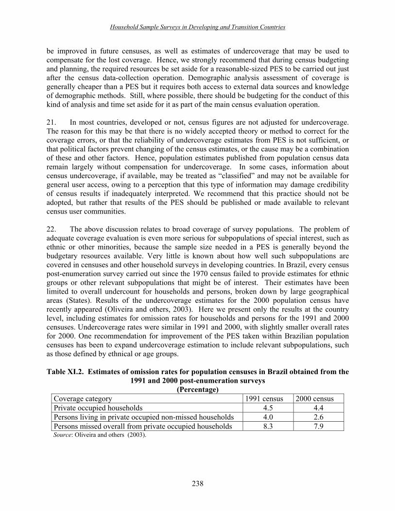
Household Sample Surveys in Developing and Transition Countries
238
be improved in future censuses, as well as estimates of undercoverage that may be used to compensate for the lost coverage. Hence, we strongly recommend that during census budgeting and planning, the required resources be set aside for a reasonable-sized PES to be carried out just after the census data-collection operation. Demographic analysis assessment of coverage is generally cheaper than a PES but it requires both access to external data sources and knowledge of demographic methods. Still, where possible, there should be budgeting for the conduct of this kind of analysis and time set aside for it as part of the main census evaluation operation.
21. In most countries, developed or not, census figures are not adjusted for undercoverage. The reason for this may be that there is no widely accepted theory or method to correct for the coverage errors, or that the reliability of undercoverage estimates from PES is not sufficient, or that political factors prevent changing of the census estimates, or the cause may be a combination of these and other factors. Hence, population estimates published from population census data remain largely without compensation for undercoverage. In some cases, information about census undercoverage, if available, may be treated as �classified� and may not be available for general user access, owing to a perception that this type of information may damage credibility of census results if inadequately interpreted. We recommend that this practice should not be adopted, but rather that results of the PES should be published or made available to relevant census user communities. 22. The above discussion relates to broad coverage of survey populations. The problem of adequate coverage evaluation is even more serious for subpopulations of special interest, such as ethnic or other minorities, because the sample size needed in a PES is generally beyond the budgetary resources available. Very little is known about how well such subpopulations are covered in censuses and other household surveys in developing countries. In Brazil, every census post-enumeration survey carried out since the 1970 census failed to provide estimates for ethnic groups or other relevant subpopulations that might be of interest. Their estimates have been limited to overall undercount for households and persons, broken down by large geographical areas (States). Results of the undercoverage estimates for the 2000 population census have recently appeared (Oliveira and others, 2003). Here we present only the results at the country level, including estimates for omission rates for households and persons for the 1991 and 2000 censuses. Undercoverage rates were similar in 1991 and 2000, with slightly smaller overall rates for 2000. One recommendation for improvement of the PES taken within Brazilian population censuses has been to expand undercoverage estimation to include relevant subpopulations, such as those defined by ethnical or age groups. Table XI.2. Estimates of omission rates for population censuses in Brazil obtained from the
1991 and 2000 post-enumeration surveys (Percentage)
Coverage category 1991 census 2000 census Private occupied households 4.5 4.4 Persons living in private occupied non-missed households 4.0 2.6 Persons missed overall from private occupied households 8.3 7.9
Source: Oliveira and others (2003).

Household Sample Surveys in Developing and Transition Countries
239
23. The figures in table XI.2 are higher than those reported for similar censuses in some developed countries. The omission rates reveal an amount of undercoverage that is non-negligible. To date, census results in Brazil are published, as is the case in the great majority of countries, without any adjustments for the estimated undercoverage. Such adjustments are made later, however, to population projections published after the census. There is a need for research to assess the potential impact of adjusting census estimates for undercoverage coupled with discussion, planning and decisions about the reliability required of PES estimates if they are to be used for this purpose.
2. Non-response 24. The term �non-response� refers to data that are missing for some survey units (unit non-response), for some survey units in one or more rounds of a panel or repeated survey (wave non-response) or even for some variables within survey units (item non-response). Non-response affects every survey, be it census or sample. It may also affect data from administrative sources that are used for statistical production. Most surveys employ some operational procedures to avoid or reduce the incidence of non-response. Non-response is more of a problem when response to the survey is not �at random� (differential non-response among important subpopulation groups) and response rates are low. If non-response is at random, its main effect is increased variance of the survey estimates due to sample size reduction. However, if survey participation (response) depends on some features and characteristics of respondents and/or interviewers, then bias is the main problem one needs to worry about, particularly for cases of larger non-response rates. 25. Särndal, Swensson and Wretman (1992, p. 575) state: �The main techniques for dealing with non-response are weighting adjustment and imputation. Weighting adjustment implies increasing the weights applied in the estimation to the y-values of the respondents to compensate for the values that are lost because of non-response ... Imputation implies the substitution of �good� artificial values for the missing values.� 26. Among the three types of non-response, unit non-response is the kind most difficult to compensate for, because there is usually very little information within survey frames and records that can be used for that purpose. The most frequent compensation method used to counter the negative effects of unit non-response is weighting adjustment, where responding units have their weights increased to account for the loss of sample units due to non-response; but even this very simple type of compensation is not always applied. Compensation for wave and item non-response is often carried out through imputation, because in such cases the non-responding units will have provided some information that may be used to guide the imputation and thus reduce bias (see Kalton, 1983; 1986).
27. Non-response has various causes. It may result from non-contact of the selected survey units, owing to such factors as the need for survey timeliness, hard-to-enumerate households and respondents� not being at home. It may also result from refusals to cooperate as well as from incapacity to respond or participate in the survey. Non-response due to refusal is often small in household surveys carried out in developing countries, mainly because, as citizen empowerment via education is less developed, potential respondents are less willing and able to refuse

Household Sample Surveys in Developing and Transition Countries
240
cooperation with surveys; and higher illiteracy implies that most data collection is still carried out using face-to-face interviewing, as opposed to telephone interviewing or mail questionnaires. Both factors operate to reduce refusal or non-cooperation rates, and both may also lead to differential non-response within surveys, with the more educated and wealthy having a higher propensity to become survey non-respondents. At the same time, response or survey participation does not necessarily lead to greater accuracy in reporting: in many instances, higher response may actually mask deliberate misreporting of some kinds of data, particularly income- or wealth-related variables, because of distrust of government officials. 28. Population censuses in developing countries are affected by non-response. In Brazil, the population census uses two types of questionnaire: a short form, with just a few questions on demographic items (sex, age, relationship to head of household and literacy), and a larger and more detailed form, with socio-economic items (race, religion, education, labour, income, fertility, mortality, etc.), that also includes all the questions on the short form. The long form is used for households selected by a probability sample of households in every enumeration area. The sampling rate is higher (1 in 5) for small municipalities and lower (1 in 10) for the municipalities with an estimated population of 15,000 or more in the census year. Overall unit non-response in the census is very low (about 0.8 per cent in the Brazilian 2000 census). However, for the variables of the short form (those requiring response from all participating households, called the universe set), no compensation is made for non-response. There are three reasons for this: first, non-response is considered quite low; second, there is very little information about non-responding households to allow for compensation methods to be effective; third, there is no natural framework for carrying out weighting adjustment in a census context. The alternative to imputing the missing census forms by some sort of donor method is also not very popular for the first two reasons, and also because of the added prejudice against imputation when performed in cases like this. For the estimates that are obtained from the sample within the census, weighting adjustments based on calibration methods are performed that compensate partially for the unit non-response. 29. A similar approach has been adopted in some sample surveys. Two of the main household surveys in Brazil, the annual National Household Sample Survey (PNAD) and the monthly Labour Force Survey (PME), use no specific non-response compensation methods (see Bianchini and Albieri, 1998). The only adjustments to the weights of responding units are performed by calibration to the total population at the metropolitan area or State level, hence they cannot compensate for differential non-response within population groups defined by sex and age, for example. The reasons for this are mostly related to operational considerations, such as maintenance of tailor-made software used for estimation that was developed long ago and the perceived simplicity of ignoring the non-response. Both surveys record their levels of non-response, but information about this issue is not released within the publications carrying the main survey results. However, microdata files are made available from which non-response estimates can be derived, because records from non-responding units are also included in such files with appropriate codes identifying the reasons for non-response. The PME was recently redesigned (Instituto Brasileiro de Geografia e Estatística, 2002b) and started using at least a simple reweighting method to compensate for the observed unit non-response. Further developments may include the introduction of calibration estimators that will try to correct for differential non-response on age and sex. However, the relevant studies, which were motivated

Household Sample Surveys in Developing and Transition Countries
241
by the observation that non-response is one of the probable causes of rotation group bias (Pfeffermann, Silva and Freitas, 2000) in the monthly estimates of the unemployment rate, are at an early stage. 30. A Brazilian survey that uses more advanced methods of adjustment for non-response is the Household Expenditure Survey (POF) (last round in 1995-1996, with the 2002-2003 round currently in the field). This survey uses a combination of reweighting and imputation methods to compensate for non-response (Bianchini and Albieri, 1998). Weight adjustments are carried out to compensate for unit non-response, whereas donor imputation methods are used to fill in the variables or blocks of variables for which answers are missing after data collection and edit processing. The greater attention to the treatment of non-response has been motivated by the larger non-response rates observed in this survey, when compared with the general household surveys. Larger non-response is expected given the much larger response burden imposed by the type of survey (households are visited at least twice, and are asked to keep detailed records of expenses during a two-week period). Survey methodology reports have included an analysis of non-response, but the publications presenting the main results have not. 31. Yet another survey carried out in Brazil, the Living Standards Measurement Survey (PPV), which was part of the Living Standards Measurement Study survey programme of the World Bank, used substitution of households to compensate for unit non-response. In Brazil, this practice is seldom used, and there are no other major household surveys that have adopted it.
32. After examining these various surveys carried out within the same country, a pattern emerges to the effect that there is no standard approach to compensating for, and reporting about, unit non-response. Methods and treatment for non-response vary between surveys, as a function of the non-response levels experienced, of the survey�s adherence to international recommendations, and of the perceived need and capacity to implement compensation methods and procedures. One approach that could be used to improve this situation is the regular preparation of �quality profile� reports for household surveys. This might often be more practical and useful than attempting to include all available information about methods used and limitations of the data in the basic census or survey publications. 33. Regarding item non-response, the situation is not much different. In Brazilian population censuses, starting from 1980, imputation methods were used to fill in the blanks and also to replace inconsistent values detected by the editing rules specified by subject-matter specialists. In 1991 and 2000, a combination of donor methods and Fellegi-Holt methods, implemented in software like DIA (Deteccíon e Imputacíon Automática de datos) (Garcia Rubio and Criado, 1990) and NIM (New Imputation Methodology) (Poirier, Bankier and Lachance, 2001), were used to perform integrated editing and imputation of census short and long forms. In 2000, in addition to imputation of the categorical variables, imputation of the income variables was also performed, by means of regression tree methods used to find donor records from which observed income values were then used to fill in for missing income items within incomplete records. This was the first Brazilian population census in which all census records in microdata files at the end of processing have no missing values. The population census editing and imputation strategy is well documented, although most of the information regarding how much editing and

Household Sample Surveys in Developing and Transition Countries
242
imputation was performed is available only in specialized reports. A recommendation for making access to these reports easier is their dissemination via the Internet. 34. The treatment of missing and suspicious data in other household surveys is not so well developed. In both the PNAD and the PME, computer programs are used for error detection, but there is still a lot of �manual editing�, and little use is made of computer-assisted imputation methods to compensate for item non-response. If items are missing at the end of the editing phase, they are coded as �unknown�. The progress made in recent years has focused on integrating editing steps with data entry, so as to reduce processing cost and time. The advent of cheaper and better portable computers has enabled IBGE to proceed towards even further integration. The revised PME for the 2000 decade started collection in October 2001 of a parallel sample, the same size as the one used in the regular survey, where data are obtained using computer-assisted (palmtop) face-to-face interviewing. There are no final reports on the performance of the palmtop computers yet, but after the first few months, the data collection was reported as running smoothly. This technology has enabled survey managers to focus on quality improvement in the source, by embedding all jump instructions and validity checks within the data-collection instrument, thus avoiding keying and other errors in the source. Non-response for income will be compensated using regression tree methods to find donors, as in the population census. However, the results of this new survey only recently became available and data collection ran in parallel with the old series for a whole year before they were released and the new series replaced the old one. A broader and more detailed assessment of the results of this new approach for data collection and processing is still under way. 35. In the PME, each household is kept in the sample for two periods of four months each, separated by eight months. Hence, in principle, data from previous complete interviews could be used to compensate for wave non-response whenever a household or household member was missed in any survey round after the first. This use of data does not occur in the old series nor is it planned for the new series, although it represents an improvement that might be considered by survey managers. 36. The pattern emerging from a cross-survey analysis of editing and imputation practices for item non-response and inconsistent or suspicious data is one of no standardization, with different surveys following different methodological paths. Censuses have clearly been the occasion for large-scale applications of automatic editing and imputation methods, with the smaller surveys not so often adopting similar methods. Perhaps there is a survey scale effect, in the sense that the investment in developing and applying acceptable methods and procedures for automatic imputation is justifiable for the censuses, but not for smaller surveys, which also have a shorter time to deliver their results. For a repeated survey like the Brazilian PME, although the time in which to deliver results is short, there would probably be a benefit to be derived from larger investment in methods for data editing and imputation because of the potential to exploit this investment over many successive survey rounds.

Household Sample Surveys in Developing and Transition Countries
243
3. Measurement and processing errors
37. Measurement and processing errors entail observed values for survey questions and variables after data collection and processing that differ from the corresponding true values that would be obtained if ideal or gold standard measurement and processing methods were used. 38. This topic is probably the one that receives the least attention in terms of its measurement, compensation and reporting in household surveys carried out in developing and transition countries. Several modern developments can be seen as leading towards improved survey practice towards reducing measurement error. First, the use of computer-assisted methods of data collection has been responsible for reducing transcription error, in the sense that the respondent�s answers are directly fed into the computer and are immediately available for editing and analysis. Also, the flow of questions is controlled by the computer and can be made to be dependent upon the answers, preventing mistakes introduced by the interviewer. The answers can be checked against expected ranges and even against previous responses from the same respondent. Suspicious or surprising data can be flagged and the interviewer asked to probe the respondent about them. Hence, in principle, data that are of better quality and less subject to measurement error may be obtained. However, there is little evidence of any quality advantages for computer-assisted interviewing over paper-and-pencil interviewing other than that of reducing the item missing-value rates and values-out-of-range rates. 39. Another line of progress has involved the development and application of generalized software for data editing and imputation (Criado and Cabria, 1990). As already mentioned in section B, population censuses have adopted automated editing and imputation software to detect and compensate for measurement error and some types of processing errors (for example, coding and keying errors), and, at the same time, item non-response. This has also occurred in some sample surveys. However, the type of compensation that is applied within this approach is capable of tackling only the so-called random errors. Systematic errors are seldom detected or compensated for using standard editing software. 40. Yet another type of development that may lead to reduction of processing errors in surveys has been the development of computer-assisted coding software, as well as data capture equipment and software.
41. Although prevention of measurement and processing errors may have experienced some progress, the same is not true of the application of methods for measuring, eventually compensating for, and reporting about measurement errors. Practice regarding measurement errors is mostly focused on prevention, and after doing what is considered important in this respect, it does not give much attention to assessment of how successful the survey planning and execution were. The lack of a standard guiding theory of measurement makes the task of setting quality goals and assessing the attainment of such goals a hard one. For example, although we do see survey sampling plans where sample size was defined with the goal of having coefficients of variation (relative standard errors) of certain key estimates below a specified value set forth in advance, we rarely see survey collection and processing plans that aim to keep item imputation levels below a specified level, or that aim at having observed measures within a specified tolerance (that is to say, maximum deviation) from corresponding �true values� with high

Household Sample Surveys in Developing and Transition Countries
244
probability. It may be impractical to expect that realistic quantitative goals for all types of non-sampling error could be set in advance; however, we advocate that survey organizations should at least make an effort to measure non-sampling errors and use such measures to set targets for future improvement and to monitor the achievement of those targets.
C. Challenges and perspectives
42. After over 50 years of widespread dissemination of (sample) surveys as a key observation instrument in social science, the concept of sampling errors and their control, measurement and interpretation have reached a certain level of maturity despite the fact that, as we have noted, the results of many surveys around the world are published without inclusion of any sampling error estimates. Much less progress has been made regarding non-sampling errors, at least for surveys carried out in developing countries. This has not been the case by chance. The problem of non-sampling errors in surveys is a difficult one. For one thing, they come from many sources in a survey. Efforts to counter one type of error often result in increased errors of another kind. Prevention methods depend not only on technology, but also on culture and environment, making it very hard to generalize and propagate successful experiences. Compensation methods are usually complex and expensive to implement properly. Measurement and assessment are hard to perform in a context of surveys carried out under very limited budgets, with publication deadlines that are becoming tighter and tighter to satisfy the increasing demands of our information-hungry societies. In a context like this, it is correct for priority to always be given to prevention rather than measurement and compensation, but this leaves little room for assessing how successful prevention efforts were, and thereby reduces the prospects for future improvement. 43. Some users who may have poor knowledge of statistical matters may misinterpret reports about non-sampling errors in surveys. Hence, publication of reports of this kind is sometimes seen as undesirable in some survey settings mainly because of the lack of well-developed statistical literacy and culture, whose development may be particularly challenging among populations that lack broader literacy and numeracy, as is the case in many developing countries. It is also often true that statistical expertise is lacking within the producing agencies as well, leading to difficulties in recognizing the problems and taking affirmative actions to counter them, as well as in measuring how successful such actions were. In any case, we encourage the preparation and publication of such reports, with the statistical agencies striving to make them as clear as possible and accessible to literate adults. 44. Even if the scenario is not a good one, some new developments are encouraging. The recent attention given to the subject of data quality by several leading statistical agencies, statistical and survey academic associations, and even multilateral government organizations, is a welcome development. The main initiatives that we shall refer to here are the General Data Dissemination System (GDDS) and the Special Data Dissemination Standard (SDDS) of the International Monetary Fund (IMF), which are trying to promote standardization of reporting about the quality of statistical data by means of voluntary adherence of countries to either of these two initiatives. According to IMF (2001): �The GDDS is a structured process through which Fund member countries commit voluntarily to improving the quality of the data produced

Household Sample Surveys in Developing and Transition Countries
245
and disseminated by their statistical systems over the long run to meet the needs of macroeconomic analysis.� Also according to IMF: �The GDDS fosters sound statistical practices with respect to both the compilation and the dissemination of economic, financial and socio-demographic statistics. It identifies data sets that are of particular relevance for economic analysis and monitoring of social and demographic developments, and sets out objectives and recommendations relating to their development, production and dissemination. Particular attention is paid to the needs of users, which are addressed through guidelines relating to the quality and integrity of the data, and access by the public to the data.� (ibid.). 45. The main contribution of these initiatives is to provide countries with: (a) a framework for data quality (see http://dsbb.imf.org/dqrsindex.htm) that helps to identify key problem areas and targets for data quality improvement; (b) the economic incentive to consider data quality improvement within a wide range of surveys and statistical output (in the form of renewing or gaining access to international capital markets); (c) a community sharing a common motivation through which they can advance the data quality discussion free from the fear of misinterpretation; and (d) technical support for evaluation and improvement programmes, when needed. This is not a universal initiative, since not every country is a member of IMF. However, 131 countries were contacted about it, and as at the present date, 46 countries have decided to adhere to the GDDS and 50 other countries have achieved the higher status of subscribers to the SDDS, having satisfied a set of tighter controls and criteria for the assessment of the quality of their statistical output. 46. A detailed discussion of the data quality standards promoted by IMF or other organizations is beyond the scope of this chapter, but readers are encouraged to pursue the matter with the references indicated here. Developing countries should join the discussion of the standards currently in place, decide whether or not to try to adhere to either of the above initiatives and, if relevant, contribute to the definition and revision of the standards. Most important, statistical agencies in developing countries can use these standards as starting points (if nothing similar is available locally) to promote greater quality awareness both among their members and staff, and within their user communities. 47. The other initiative that we shall mention here, particularly because it affects Brazil and other Latin American countries, is the Project of Statistical Cooperation of the European Union (EU) and the Southern Common Market (MERCOSUR).25 According to the goal of the project: �The European Union and the MERCOSUR countries have signed an agreement on �Statistical Cooperation with the MERCOSUR Countries�, the main purpose of which is a rapprochement26 in statistical methods in order to make it possible to use the various statistical data based on mutually accepted terms, in particular those referring to traded goods and services, and, generally, to any area subject to statistical measurement.� The Project �is expected to achieve at the same time the standardization of statistical methods within the MERCOSUR countries as well as between them and the European Union.� (For more details, visit the website: http://www.ibge.gov.br/mercosur/english/index.html). This project has already promoted a
25 MERCOSUR is the common market of the South, a group of countries sharing a free trade agreement that includes Brazil, Argentina, Paraguay and Uruguay. 26 The term is used here in the sense of harmonization.

Household Sample Surveys in Developing and Transition Countries
246
number of courses and training seminars and, in doing so, is contributing towards improved survey practice and greater awareness of survey errors and their measurement. 48. Initiatives like these are essential in respect of supporting statistical agencies in developing countries to improve their position: their statistics may be of good quality, but they often do not know how good they are. International cooperation from developed towards developing countries and also between the latter is essential for progress towards better measurement and reporting about non-sampling survey errors and other aspects of survey data quality.
D. Recommendations for further reading
49. Meetings recommended as subjects for further reading include:
• International Conference on Measurement Errors in Surveys, held in Tucson, Arizona in 1990 (see Biemer and others, 1991).
• International Conference on Survey Measurement and Process Quality, held in
Bristol, United Kingdom in 1995 (see Lyberg and others, 1997). • International Conference on Survey Non-response, held in Portland, Oregon in 1999
(see Groves and others, 2001). • International Conference on Quality in Official Statistics, held in Stockholm,
Sweden in 2001 (visit http://www.q2001.scb.se/). • Statistics Canada Symposium 2001, held in Ottawa, Canada, which focused on achieving data
quality in a statistical agency from a methodological perspective (visit http://www.statcan.ca/english/conferences/symposium2001/session21/s21c.pdf).
• Fifty-third session of the International Statistical Institute (ISI), held in Seoul, Republic of
Korea in 2001, where there was an invited paper meeting on �Quality programs in statistical agencies�, dealing with approaches to data quality by national and international statistical offices ( visit http://www.nso.go.kr/isi2001).
• Statistical Quality Seminar 2000, sponsored by IMF, held in Jeju Island, Republic
of Korea in 2000 (visit http://www.nso.go.kr/sqs2000/sqs12.htm). • International Conference on Improving Surveys, held in Copenhagen, Denmark in
2002 (visit http://www.icis.dk/).

Household Sample Surveys in Developing and Transition Countries
247
References Bianchini, Z.M., and S. Albieri (1998). A review of major household sample survey designs
used in Brazil. In Proceedings of the International Conference on Statistics for Economic and Social Development. Aguascalientes, Mexico, 1998: Instituto Nacional de Estadística, Geografía e Informática (INEGI).
Biemer, P.P., and R.S. Fecso (1995). Evaluating and controlling measurement error in business
surveys, Cox and others, eds. In Business Survey Methods, New York: John Wiley and Sons.
Biemer, P.P., and others (1991). Measurement Errors in Surveys. New York: John Wiley and
Sons. Correa, S.T., P.L. do Nascimento Silva and M.P.S. Freitas (2002). Estimação de variância para o
estimador da diferença entre duas taxas na pesquisa mensal de emprego. In 15o Simpósio Nacional de Probabilidade e Estatística. Aguas de Lindóia, Brazil, São Paulo, Brazil: Associação Brasileira de Estatística.
Criado, I.V., and M.S.B. Cabria (1990). Procedimiento de depuración de datos estadísticos,
cuaderno 20. Vitoria-Gasteiz, Spain: EUSTAT Instituto Vasco de Estadística. Garcia Rubio, E., and I.V. Criado (1990). DIA System: software for the automatic imputation of
qualitative data. In Proceedings of the United States Census Bureau Sixth Annual Research Conference (Arlington, Virginia). Washington, D.C.: United States Bureau of the Census.
Groves, R.M., and others (2001). Survey Non-response. New York: John Wiley and Sons. Instituto Brasileiro de Geografía e Estatística (2002a).
http://www.ibge.gov.br/home/estatistica/populacao/trabalhoerendimento/pnad99/metodologia99.shtm.
__________ (2002b).
http://www.ibge.net/home/estatistica/indicadores/trabalhoerendimento/pme/default.shtm. International Monetary Fund (2001). Guide to the General Data Dissemination System (GDDS).
Washington, D.C.: IMF Statistics Department. Available from http://dsbb/imf/org/applications/web/gdds/gddsguidelangs).
Kalton, G. (1983). Compensating for Missing Survey Data. Research Report Series. Ann Arbor,
Michigan: Institute for Social Research, University of Michigan. __________ (1986). Handling wave non-response in panel surveys. Journal of Official
Statistics, vol. 2, No. 3, pp. 303-314.

Household Sample Surveys in Developing and Transition Countries
248
__________ (2002). Models in the practice of survey sampling (revisited). Journal of Official Statistics, vol.18, No. 2, pp. 129-154.
Kordos, J. (2002). Personal communications. Lyberg, L., and others, eds. (1997). Survey Measurement and Process Quality. New York:
John Wiley and Sons. Marks, E.S. (1973). The role of dual system estimation in census evaluation. Internal report.
Washington, D.C.: United States Bureau of the Census. Oliveira, L.C., and others (2003). Censo Demográfico 2000: Resultados da Pesquisa de
Avaliação da Cobertura da Coleta. Textos para Discussão, No. 9. Rio de Janeiro: IBGE, Directoria de Pesquisas.
Pfeffermann, D., P.L. Nascimento de Silva and M.P.S. Freitas (2000). Implications of the
Brazilian Labour Force rotation scheme on the quality of published estimates. Internal report. Rio de Janeiro: IBGE, Departamento de Metodologia.
Platek, R., and C.E. Särndal (2001). Can a statistician deliver? Journal of Official Statistics, vol.
17, No. 1, pp. 1-20. Poirier, P., M. Bankier and M. Lachance (2001). Efficient methodology within the Canadian
Census Edit and Imputation System (CANCEIS). Paper presented at the Joint Statistical Meetings, American Statistical Association.
Särndal, C.E., B. Swensson and J. Wretman (1992). Model Assisted Survey Sampling. New
York: Springer-Verlag. United Nations (1982). National Household Survey Capability Programme: Non-sampling
errors in household surveys: sources, assessment and control: Preliminary Version. DP/UN/INT-81-041/2. New York: Department of Technical Cooperation for Development and Statistical Office.

Household Sample Surveys in Developing and Transition Countries
249
Section D
Survey costs

Household Sample Surveys in Developing and Transition Countries
250
Introduction
James Lepkowski University of Michigan Ann Arbor, Michigan
United States of America 1. In the previous sections, sampling and non-sampling errors that arise in household surveys were examined in order to gain a better understanding of the quality of survey estimates. In almost all types of such errors, there are methods that can be used to reduce the size of the error. The implementation of those methods, however, often entail an additional cost. Since surveys have fixed budgets to cover expenses, devoting additional resources to reduce one source of error means shifting resources from one area to another procedure. Survey design involves constantly trading off costs and survey error. 2. For example, suppose that in a particular household survey, there is a subgroup of the population speaking a language for which there is no translation of the survey questionnaire. The survey designers may decide initially to exclude this group from the survey, creating a coverage problem. Alternatively, they may decide to decrease the sample size to reduce survey costs, and then use the saved costs to translate the questionnaire into a new language, hire interviewers who speak that language, and bring those households back into the survey. 3. Given that survey design is often a series of such trade-offs, in order to make sound decisions, good information must be available about the nature and size of errors arising from different sources (such as sampling variance and non-coverage bias, in the previous example) and about the costs associated with different survey procedures. The previous sections examined error sources and sizes of errors. In the present section, the nature of survey costs will be examined. 4. Cost considerations in a survey arise at three levels. The first is in the planning phase of a survey when costs must be estimated in advance. Cost estimates in the planning or �budgeting� phase are difficult to obtain, unless one has prior experience to build on. Continuing survey operations can provide relevant cost data for planning new rounds of a survey, although cost considerations at the next level - the monitoring of survey costs - often interferes. 5. Survey organizations, or even others that conduct surveys occasionally, seldom have well-developed systems for tracking costs in such a way as to enable the cost data to be used for planning. Costs are assembled in an accounting system, but those systems do not categorize costs into the kind of categories that a survey designer needs for planning purposes. In instances where such cost monitoring is attempted, it may add to the cost of the survey itself if new systems must be added to the operations. 6. If costs are being monitored in an ongoing operation, it is possible to consider, more systematically, changes in survey design during data collection. Cost information can be used to

Household Sample Surveys in Developing and Transition Countries
251
project how large both the savings in one operation, and the impact of the reallocation of resources to another area, might be. 7. Reallocation of resources in survey planning is determined by considering trade-offs between cost level and error across multiple sources of error. Sample design development is one area where these trade-offs can be and are made formally to find an optimal solution to the resource allocation problem. 8. For example, as discussed in chapter II, surveys that are based on clusters drawn in an area probability sample from a widely spread population must consider limiting the number of clusters in order to reduce data-collection costs. Limiting the number of clusters however means that the number of observations made in each sample cluster must go up in order to maintain overall sample size. However, this increase in the size of the subsample in each cluster increases the variability of sample estimates. In other words, as costs go down, by taking fewer clusters, sampling variance goes up. What is needed is guidance on how many clusters to select so that the costs can be minimized, given that a specified level of precision is to be achieved, or that the sampling variance is to be kept as small as possible for a given cost. In sample design, there is a mathematical solution to this problem. 9. The cost-error trade-off arises in other aspects of survey design as well. For example, one method for reducing household non-response in a household survey is to visit more than once households for which no response is obtained on a single visit. An interviewer can be instructed to visit households during the survey data collection period as many as four or five times in order to obtain a response. Making repeated visits to some sample households reduces the number of sample households that can be included in the sample. The cost of repeated visits to reduce household non-response limits sample size. The cost of greater non-response reduction efforts to reduce non-response bias thus increases sampling variance. Again, the cost-reduction efforts in one area requires that resources be reallocated, and introduces the potential for an increase in error in another area of the survey design. 10. The chapters in this section consider a number of issues centred around planning, monitoring and reallocation of costs in survey design. They use data from household surveys in developing and transition countries to illustrate the types of costs incurred in survey data collection and, to some extent, the size of the costs. Since survey operations vary so widely from country to country, and even more so across continents, the specific cost information provided may not be useful for planning a survey in a given country. It is hoped, however, that the cost sources and cost levels presented in the following chapters will help survey designers across diverse settings understand survey costs and cost-error trade-offs more fully in their own surveys.

Household Sample Surveys in Developing and Transition Countries
252
Household Sample Surveys in Developing and Transition Countries
253
Chapter XII
An analysis of cost issues for surveys in developing and transition countries
Ibrahim S. Yansaneh* International Civil Service Commission
United Nations, New York
Abstract
The present chapter discusses, in general terms, the key issues related to the cost of designing and implementing household surveys in developing and transiton countries. The overall cost of a survey is decomposed into more detailed components associated with various aspects of its design and implementation. The cost factors are considered separately for countries with extensive survey infrastructure and those with little or no survey infrastructure. The issue of comparability of costs across countries is also examined. Key terms. Survey infrastructure, incremental cost per interview, efficiency, cost comparability, cost factors. __________ * Former Chief, Methodology and Analysis Unit, United Nations Statistics Division.

Household Sample Surveys in Developing and Transition Countries
254
A. Introduction
1. Criteria for efficient sample designs
1. In general, an efficient sample design has to satisfy one of two criteria: it must provide reasonably precise estimates under the constraint of a fixed budget, or minimize the cost of implementation for a specified level of precision. The present chapter focuses on the first criterion, which is concerned with the task of developing the most efficient design that can be implemented with costs that are consistent with available budgets and make reasonably efficient use of resources. In developing and transition countries, the cost of the surveys is one of the biggest constraints on the formulation of critical decisions about design and implementation. Designing a survey in developing and transition countries, as in developed countries, involves the usual trade-offs between the precision of survey estimates and the cost of implementation. Precision is generally measured in terms of the variances of the estimators of selected population quantities that are considered to be of principal interest. Other related measures of precision include mean squared error or total survey error, which also incorporates the bias component of error. 2. Formal mathematical development of the trade-offs between precision and cost typically involves optimization of well-behaved variance or cost functions subject to relatively simple constraints. However, owing to limitations in available cost and variance information, this optimization approach often should be viewed as providing only rough approximations towards the preferred design, or for the precision and cost values that will actually be achieved in implementation. These issues have been considered in depth for surveys carried out in developed countries. See, for example, Andersen , Kasper and Frankel (1979), Cochran (1977), Groves (1989), Kish (1965; 1976) and Linacre and Trewin (1993), and the references cited therein. In addition, for a broader discussion of cost and precision as two of many criteria for evaluation of national statistical systems, see de Vries (1999, p. 70) and the references cited therein. For empirical analyses of the costs of selected surveys in developing and transition countries, and a more detailed discussion of the cost/error trade-offs in the design of surveys in developing and transition countries, see chaps. XIII and XIV, and the introduction to Section D (Survey costs).
3. One major limitation in the design of surveys in developing and transition countries is the lack or insufficiency of information on costs associated with various aspects of survey implementation. Despite the above-mentioned limitations, one often finds some amount of common structure in costs across surveys that can be useful in the design of a new survey. In some cases, this common structure is limited to qualitative indications of the relative magnitudes of several cost components or sources. In other cases, actual costs are available that can be seen to be fairly homogeneous across a set of countries, particularly countries with similar population distributions and levels of survey infrastructure.
4. This chapter presents an analysis of issues of cost in the context of surveys in developing and transition countries and investigates the extent to which survey costs or related components for one country can be used to improve the design for a similar survey in another country. In other words, the chapter attempts to address the issue of the portability of survey costs across

Household Sample Surveys in Developing and Transition Countries
255
countries. The utility of such an analysis is twofold: First, it has the potential of providing a partial solution to the problem of scarcity of information on cost of surveys in developing and transition countries. Second, to the extent that there are similarities across countries in terms of sample designs, survey infrastructure, and population distributions, one might expect similarities in at least some components of the cost of surveys across these countries. Such cost information can be extracted from one survey in one country and used to design a new survey in a different country, or to improve the efficiency of the design of the same survey in the same country. In doing this, the survey designer must recognize the wide variability in survey cost structures across countries. Variable cost components are typically country-specific, whereas some fixed costs are likely to be comparable across countries.
2. Components of cost structures for surveys in developing and transition countries
5. In this chapter, we focus on the first criterion for an efficient survey design, that is to say, a design that generates reasonably precise survey estimates for a given budget allocation. Many surveys conducted in developing and transition countries are commissioned by international financial and development agencies that need the data for decision-making on developmental assistance projects or to support decision makers and policy makers in the beneficiary countries. Three prominent examples of developing country surveys are the Demographic and Health Surveys (DHS), conducted by ORC Macro for the United States Agency for International Development; the Living Standards Measurement Study (LSMS) surveys, conducted by the World Bank; and the Multiple Indicator Cluster Surveys (MICS), conducted by the United Nations Children�s Fund (UNICEF). In addition, many other surveys are conducted on a regular basis by national statistical offices and other agencies within national statistical systems. There is also a large number of smaller-scale surveys commissioned by donors and carried out by small, local organizations (for example, non-governmental organizations). Needless to say, the issue of cost is critical in the design work for these surveys as well.
6. In dealing with cost issues, it is important to recognize the fact that developing-country survey designs share many common features. For instance, most surveys are based on a multistage stratified area probability design. The primary sampling units (PSUs) are frequently constructed from enumeration areas identified and used in a preceding national population census. Secondary sampling units are typically dwelling units or households, and the ultimate sampling units are usually either households or persons. The strata and analytical domains are typically formed from the intersection of administrative regions and urban/rural sub-domains of these regions. Because of these similarities, and in keeping with the literature mentioned above in paragraph 2, it is of interest to study the extent to which one may identify common cost structures within groups of developing-country surveys. For some general background on the design and implementation of surveys carried out in developing and transition countries, see Section A of Part one (Section design) and the case studies in part two of this publication. For a more detailed treatment of cost components for a specific survey in a developing country, see chapter XIII. Empirical comparisons of the cost components of surveys conducted in selected developing and transition countries are presented in chapter XIV.
7. In this chapter, we shall restrict our attention to major national household surveys carried out by national statistics offices or other government agencies in the national statistical system.

Household Sample Surveys in Developing and Transition Countries
256
These include household budget surveys, income and expenditure surveys, and demographic and health surveys. Even though market surveys and other smaller-scale household surveys carried out by various organizations on an ad hoc basis provide a useful source of information and feed into national policy decisions and developmental plans, they are excluded from this discussion. However, the key issues raised in the discussion apply to these types of surveys as well. Most examples are based on the DHS and LSMS surveys, but the key issues are broadly applicable to all household surveys.
3. Overview of the chapter
8. The chapter is organized as follows: section B discusses the classical decomposition of the overall cost of a survey into more detailed components. The next three sections provide a qualitative description of some factors that influence the overall costs of surveys conducted in developing and transition countries. Section C reviews cost factors that may be important for cases in which a considerable amount of survey infrastructure is already in place. Section D considers cases in which there is limited or no prior survey infrastructure. Section E discusses changes in the cost structure that may result from modifications in survey goals. Section F provides some related cautionary remarks regarding interpretation of reported survey costs. Section G provides some concluding remarks, and a summary of some salient points that were not fully developed in the discussion. An example of a framework used in budgeting for the UNICEF multiple indicator cluster surveys (MICS) carried out in developing and transition countries, is given in the annex, as provided by Ajayi (2002).
B. Components of the cost of a survey 9. The mathematical underpinnings of survey costs generally postulate an overall cost, C, as a linear function of the numbers of selected primary sampling units and selected elements. An example of such a function is
hi
L
h
n
ihi
L
hhh cncncC
h
∑ ∑∑= ==
++=1 11
0 (1)
where c0 represents the fixed costs of initiating the survey; ch equals the incremental cost of collecting information from an additional primary sampling unit (PSU) within stratum h; nh is the number of sampled PSUs; chi equals the incremental cost of interviewing an additional household within PSU i in stratum h; and nhi is the number of sampled households in PSU i. See, for example, Cochran (1977, sects. 5.5 and 11.13-11.14) and Groves (1989, chap. 2). In general, the cost coefficients c0, ch and chi will depend on a large number of factors that may vary across countries and across surveys within countries. These factors are discussed in detail in the sections that follow. 10. Note that expression (1) is one of many possible cost functions that could be considered. For example, Cochran (1977, p. 313) discusses inclusion of a separate cost component associated with listing of secondary sampling units (as an intermediate stage prior to subsampling households for interview) within selected primary units, where that component depends on the

Household Sample Surveys in Developing and Transition Countries
257
number of secondary units in each primary unit. Also, for a three-stage design, that is to say, a design in which persons are randomly selected for interview from within households, there will be an extra term in (1) above, denoting the incremental cost associated with interviewing an additional person within a selected household.
11. Furthermore, a more realistic cost function is frequently a stepwise function rather than a linear function. For example, if 10 interviews can be conducted in a single day, then the addition of an eleventh interview requires an extra day of work and thus substantial cost, whereas the addition of a twelfth interview may add little to the overall cost. Also, it is important to note that decisions on such issues as the number of sample PSUs are sometimes influenced by practical considerations other than considerations of cost and precision. For example, it may be that one would want to spend a full week interviewing in a PSU. In that case, less than a week�s workload would not be feasible, although a double workload equivalent to two weeks of work might be possible. Thus, in such a situation, the number of sample PSUs would not be directly determined by consideration of costs and design effects, but by practical constraints on implementation. 12. In the next section, we discuss costs of surveys depending on the level of survey infrastructure in the country in question. The central message of that section is that there is a huge disparity in the overall costs of surveys between countries with substantive survey infrastructure and those with little or no infrastructure. However, it must be remembered that in developing and transition countries, one would have to assess the degree of infrastructure at the planning stage of a survey, rather than rely on the historical record. It is not uncommon for a country with superb survey infrastructure at some point to suffer a steady decline in infrastructure over time, to the point of migrating from the first group of countries (considered in sect. C) to the second (considered in sect. D).
C. Costs for surveys with extensive infrastructure available
1. Factors related to preparatory activities
13. Much of the cost of a one-time survey goes to the financing of preparatory activities [see, for example Grosh and Muñoz (1996, p. 199)], hence the funds for such activities are disbursed early in the survey process. Preparatory activities with relatively fixed costs include coordination of survey planning by multiple government agencies, frame development, sample design, questionnaire design, printing of questionnaires and other survey materials, and publicity directed towards potential respondents. Preparatory activity costs that depend on sample size (either at the primary unit or at the household level) include the hiring and training of field staff (for example, listers, interviewers, supervisors and translators).
14. The costs of preparatory activities depend on local factors such as the size of the survey staff and compensation rates, the type and amount of equipment, the prices of items such as stationery and other supplies and modes of transportation and communication. In addition, costs are heavily influenced by whether the survey is a cross-sectional study being done for the first time - where unit costs are comparatively higher - or part of a continuing survey - where the unit costs are lower.
Household Sample Surveys in Developing and Transition Countries
258
2. Factors related to data collection and processing 15. The costs of data collection and processing also involve both fixed and variable components; but for the most part, the costs of data collection are variable, that is to say, dependent on the number of primary sampling units and households selected. These costs include the costs of the listing of households within selected primary units or the listing of persons within selected households, interviewing and field supervision. The cost of data collection also includes the cost of travel both between and within PSUs. These data-collection costs depend on the organization of the interview operations, the length of the questionnaire, whether or not interpreters are used, and the number of units to be interviewed.
16. One option for reducing travel costs is to create national survey teams consisting of supervisors and interviewers and to move the teams around from region to region, as opposed to establishing regional teams. It is important to note that this option also improves the quality of the data. This approach can also be useful in situations where data collection is carried out on a rolling basis, or when survey operations involve the use of expensive equipment. The model of multiple survey teams has been used in many surveys in developing and transition countries, such as the LSMS series (Grosh and Muñoz, 1996, chap. 5). In developing and transition countries where languages change from region to region, it may be more efficient to have survey teams based on proficiency in the language spoken in each region.
17. A significant part of the costs of data collection and processing is related to the costs of coordination of field activities and survey materials. In a centralized data-collection and processing system, the costs associated with retrieving completed questionnaires and transmitting them to the headquarters could be substantial. Furthermore, the budget must take into account the potentially significant costs associated with monitoring survey activities and results, for example, listing and subsampling procedures carried out in the field, the response rates for key domains of interest against pre-specified levels, etc. Effective monitoring of such activities enables survey implementers to take corrective measures, if necessary, during data collection, instead of discovering deficiencies after data collection, when it might be too prohibitively expensive to compensate for them.
18. As part of data processing, data entry, edit and imputation work may involve a mixture of fixed and variable costs, depending on the degree of automation used in this process. The other principal costs of data processing are arguably fixed, and include the costs of computing equipment and software; and the development of weights, and variance estimators and other data analysis work. For instance, weights would be computed regardless of the number of PSUs or households sampled; and after a weighting procedure has been developed and programmed, the incremental cost of computing a weight for an additional household would be negligible.
19. The cost of data processing depends on how many levels of analysis are included in the budget. For some surveys, only preliminary analysis is carried out on the collected data in the form of tables. For other surveys like the DHS and LSMS, more detailed statistical analyses are conducted as a basis for policy recommendations for beneficiary Governments and donor agencies. For instance, both the DHS and the LSMS conduct various types of detailed analyses on their survey microdata, and publish their findings in a series of analytical and methodological

Household Sample Surveys in Developing and Transition Countries
259
reports (in the case of the DHS), and working papers (in the case of the LSMS). Some examples are included in certain of the reference cited below. Considerable costs are also incurred in report production and dissemination of results, as well as for various services to other analysts, which may include preparation of metadata and the organization of training workshops. D. Costs for surveys with limited or no prior survey infrastructure available
20. In a country with relatively little previous survey infrastructure, it is likely that the sponsoring agency will need to devote a substantial quantity of resources to capacity-building efforts that would not be required in a country with substantial survey infrastructure (Grosh and Muñoz, 1996, chap. 8). The costs of preparatory activities, field operations and data processing can all be substantially increased by a lack of infrastructure. 21. Capacity-building generally involves extensive initial training of personnel. In a country with limited or no prior survey infrastructure, compared with a country with well-developed infrastructure, there are usually substantial costs associated with the use of external expertise needed to develop the survey. In addition, the time of field personnel tends to be used more efficiently as a survey organization gains experience. Also, in countries with substantial previous survey experience, the need for travel is much lower because the statistical agencies in such countries are likely to have experienced regional data-collection teams, or to provide the means of transportation for survey field staff. These advantages result in savings in the cost of transportation, training and other personnel costs. Countries with no history of previous surveys usually include vehicles in the survey budget and this item may become a major part of the overall cost of the survey (Grosh and Muñoz, 1996, chap. 8). Other examples of budget items where the existence of some survey infrastructure or history of previous surveys has a substantial impact are computer equipment and maps for identification of households.
E. Factors related to modifications in survey goals
22. As noted above, many cost factors are linked to features of the survey design, including the sample size; the length of the questionnaire; the number of modules; and specific methods employed in sample selection and listing, pilot testing, and questionnaire design and translation. For a given design, some of the resulting costs are approximately constant across countries. 23. However, survey designs in developing and transition countries often have to be modified to accommodate ad hoc specifications by beneficiary governments or other stakeholders. For instance, a government may decide to broaden the objectives of the survey to include other national priorities. This in turn may lead to: (a) the inclusion of additional modules in the questionnaire; or (b) an increase in the number of reporting domains if estimates of key variables for subnational groups are desired at the same precision level as that for the national-level estimates. 24. These modifications can affect trade-offs between cost and data quality in several ways. First, they can lead directly to significant increases in the total amount of interviewer time

Household Sample Surveys in Developing and Transition Countries
260
required for data collection because of an increased mean length of an interview owing to the inclusion of additional questionnaire modules [para. 23 (a)] or because of an increase, by orders of magnitude, in the number of interviews owing to an increase in the number of reporting domains [para. 23 (b)]. Second, if a survey organization has available a relatively fixed number of well-trained interviewers and field supervisors, then modifications may lead to increased costs owing to the need to train additional interviewers plus the greater amount of supervisory time required per minute of interview time. Alternatively, the number of well-trained field staff may be held constant with the dual consequence of an elongated period of data collection and thus increased costs. Third, the above-mentioned increases can lead to an increase in the magnitude of non-sampling error relative to sampling error. For example, inclusion of extra modules in a questionnaire may inflate non-sampling error owing to inadequate question testing or respondent fatigue. Non-sampling error may also increase owing to the use of a larger number of relatively inexperienced interviewers, necessitated by an increase in the number of interviews or in the mean length of an interview.
F. Some caveats regarding the reporting of survey costs 25. Several factors need to be considered to ensure that comparisons of costs across surveys and countries are carried out on a reasonably common basis. First, surveys in developing and transition countries are sponsored by several different organizations, which often have different policies and accounting procedures. For instance, for some sponsoring agencies, it may be important to distinguish between the cost to the sponsoring agency and the overall cost of implementing the survey.
26. Second, it may be important to account comparably for survey support that is provided in kind, for example, vehicles for transportation of field personnel. In some cases, in-kind support may be provided by the national statistical office by, for instance, assigning its permanent field staff to an internationally sponsored survey. Although such costs may be considered in-kind and excluded from the itemized budget, they nevertheless represent an opportunity cost in so far as the survey exercise is an additional activity that takes time away from other potential work that could be performed by the national statistical office.
27. Similar comments apply to provision of external technical assistance. This item can be especially important in countries with no survey infrastructure or no history of conducting surveys. For many surveys, such technical assistance is provided in kind by international agencies that conduct or sponsor the surveys, and thus is not included directly in the survey budget. However, sometimes, such technical assistance is contracted out, and thus included in the budget. For instance, the 1998 Turkmenistan LSMS-type survey was conducted with technical assistance from the Research Triangle Institute (RTI), under contract to the World Bank.
28. Third, owing to the hierarchical cost structure (expression 1) given in section B, it is important to distinguish between the total cost for a survey and the cost per completed interview. For instance, owing to the availability of greater resources and a greater degree of interest in reliable estimates reported at a subnational level, larger developing and transition countries tend

Household Sample Surveys in Developing and Transition Countries
261
to use larger sample sizes in their surveys (United Nations Children�s Fund, 2000, chap. 4). Because of high costs associated with transportation and salaries of a larger number of survey staff, surveys in larger countries tend to have higher total costs than surveys in smaller countries. However, larger countries with higher overall costs may sometimes have lower costs per completed interview, because of economies of scale and the distribution of fixed costs over a larger sample.
29. Fourth, the evaluation of overall, and per-interview, costs may be complicated by special features of the sample design. For example, costs may be inflated by the use of oversampling or the use of screening samples to ensure achievement of precision goals for certain subpopulations that are small or difficult to identify from frame information (for example, households with children under age five). Finally, for surveys of populations with widely variable household sizes, it may also be important to distinguish between costs per contacted household and costs per completed interview.
G. Summary and concluding remarks
30. Most surveys in developing and transition countries are conducted in an environment of severe budget constraints and of uncertainties about the delivery of even the approved budget. Thus, the analysis of factors that influence the cost of surveys is one of the most important aspects of the survey design and planning process for developing and transition countries. This chapter has presented a framework for such an analysis and has also examined the extent to which survey costs and related components are portable across countries that are similar with respect to the design of the survey and the population distribution of households, and other factors.
31. Large-scale national surveys have been used to illustrate the key issues, but the discussion is applicable to the numerous other types of smaller-scale surveys carried out within the national statistical systems in developing and transition countries. To the extent that one is able to identify common cost structures in these surveys, one can use information on cost components for one survey in one country to provide useful guidelines for the design of a similar survey in another country, or to improve the efficiency of the design of a new survey in the same country. It has been pointed out that there is a large disparity in the costs of surveys between countries with extensive survey infrastructure at the time of the survey under consideration, and those with little or no infrastructure. Also given emphasis have been some caveats that should be taken into consideration in comparisons of overall costs of surveys across countries.
32. We conclude by reiterating points connected with some important issues related to the cost of surveys in developing and transition countries, namely, that:
(a) Even though a careful analysis of cost components can reveal common cost structures
across groups of countries or surveys, it should be recognized that survey budgets are often not only country-specific, but also time-specific. It is therefore important to compile cost data and prepare an administrative report documenting the various components of the cost of each stage of the survey process for each household survey. The same type of information should be

Household Sample Surveys in Developing and Transition Countries
262
documented for variances and components thereof. Such information on costs and variances can be useful in two ways: first, in making important budgetary and management decisions, and second, in demonstrating how various sample design decisions were influenced by different cost and variance components. In general, the documentation of costs and variances and their components, for each stage of the survey process, should be an integral part of the standard operating procedures for national statistical offices in developing and transition countries;
(b) Even though overall survey cost incorporates both fixed and variable costs, it is the
variable costs in the survey budget that need to be carefully controlled and manipulated in the process of designing a survey. Some fixed costs, such as those for coordination of survey planning by multiple government agencies, and for publicity directed towards potential respondents are often beyond the control of the survey designer and, in any case, too specific to the country, time and survey under consideration;
(c) As discussed in chapter XIV, there is a difference in budgeting considerations
between user-paid surveys and country-budgeted surveys. Whereas the former are well designed and are implemented comparatively smoothly and with all critical components paid for in advance, the latter are usually subject to the budget constraints and allocations of a country. For this type of survey, there is often a large disparity between the planned budget and the actual budget, which is determined not by precision considerations but by availability of funds for the survey vis-à-vis the other budgetary priorities in the country;
(d) Owing to the very stringent budgetary environment in which most surveys in
developing and transition countries are carried out, it is important for a survey designer to explore non-monetary ways of budgeting for a survey, or of implementing aspects of a survey without budgeting for them. For instance, it may be possible to share infrastructure with an existing survey; to use a subsample of units already selected for another survey; or to have one interviewer collect data for multiple surveys. Consideration should also be given to budgeting for certain aspects of a survey in terms of the amount of time required for them;
(e) In the foregoing, we have argued that the cost of a survey can be increased
significantly by the lack of survey infrastructure and general statistical capacity in a country. Building and strengthening survey infrastructure are therefore a worthwhile investment that could lead to lower budgets for surveys in the long term in developing and transition countries. One of the most effective approaches to building such survey infrastructure and for promoting general statistical development is through technical cooperation between national statistical offices in developing and transition countries and those of more developed statistical systems, in collaboration with international statistical and funding agencies and other stakeholders. However, in order to yield positive results for beneficiary countries, such technical cooperation efforts must be well conceived and well implemented. Practical guidelines for good practices for technical cooperation in statistics were outlined by the United Nations (1998, annex) and endorsed by the United Nations Statistical Commission at its thirtieth session on 4 March 1999.

Household Sample Surveys in Developing and Transition Countries
263
Acknowledgements
I am grateful for the very constructive comments of three referees and of participants at the Expert Group Meeting on the Analysis of Operating Characteristics of Surveys in Developing and Transition Countries, at United Nations Headquarters in New York in October 2002, which led to considerable improvements in the first draft of this chapter. However, the opinions expressed herein are mine and do not necessarily reflect the policies of the United Nations. References Ajayi, O.O. (2002). Budgeting framework for surveys. Personal communication. Andersen, R., J. Kasper and M.R. Frankel (1979). Total Survey Error. San Francisco,
California: Jossey-Bass. Cochran, W.G. (1977). Sampling Techniques, 3rd ed.. New York: Wiley. de Vries, W. (1999). Are we measuring up? questions on the performance of national statistical
systems. International Statistical Review, vol. 67, pp. 63-77. Grosh, M.E., and J. Muñoz (1996). A Manual for Planning and Implementing the Living
Standards Measurement Study Survey. Living Standards Measurement Study Working Paper, No. 126. Washington, D.C.: International Bank for Reconstruction and Development, World Bank.
Groves, R.M. (1989). Survey Errors and Survey Costs. New York: Wiley. Kish, L.(1965). Survey Sampling. New York: Wiley. __________ (1976). Optima and proxima in linear sample designs. Journal of the Royal
Statistical Society, Series A, vol. 139, pp. 80-95. Linacre, S.J. and D.J. Trewin (1993). Total survey design: application to a collection of the
construction industry. Journal of Official Statistics, vol. 9, pp. 611-621. United Nations (1998). Some guiding principles for good practices in technical co-operation for
statistics: note by the Secretariat. E/CN.3/1999/19. 15 October. United Nations Children�s Fund (2000). End-Decade Multiple Indicator Cluster Survey Manual.
New York: United Nations Children�s Fund. Yansaneh, I.S., and J.L Eltinge (2000). Design effect and cost issues for surveys in developing
countries. Proceedings of the Section on Survey Research Methods. Alexandria, Virginia: American Statistical Association, pp. 770-775.

Household Sample Surveys in Developing and Transition Countries
264
Annex Budgeting framework for the United Nations Children�s Fund (UNICEF) Multiple Indicator Cluster
Surveys (MICS)
Activity categories Cost categories Total
costs Preparation/ sensitization Pilot survey
Survey design and sample preparation
Training Main survey implementation Data input Data processing
and analysis Report writing Dissemination and further analysis
Personnel
Per diem
Transportation
Consumables
Equipment
Other costs
TOTAL COSTS
Implementing agencies (names)
Supplementary details
1. Sample size: number of households: _____________________________ number of clusters: _______________________ 2. Duration of enumeration: number of days: _________________________________ 3. Duration of training for enumerators: number of days: _______________________ 4. Numbers of field enumerator/supervisors: enumerators: ___________________ supervisors: _______________________ 5. Data entry: key strokes per questionnaire: number: _________________________ 6. UNICEF contribution: $ _________________________________________________

Household Sample Surveys in Developing and Transition Countries
265
Costing framework Items included in cost and activity categories
Cost categories Activity categories Personnel (salaries) Preparation/sensitization Consultants fees Preparation of questionnaire Field supervisors Preparation of dummy tables Interviewers/enumerators Translation and back translation Drivers Pre-testing of questionnaire Translators Publicity pre and post enumeration Local guides Data entry clerks Pilot survey Computer programmers Training Overtime payments Data collection Incentive allowance Data analysis Coordinating committee Report on the pilot survey Per diem (room and board) Survey design and sample preparation Field supervisors Planning Interviewers/enumerators Sample preparation Drivers Translators Training Local guides (meal allowance) Preparation of training materials Consultants/monitors Translation into training language Implementation of training Transportation Vehicle rental Main survey implementation Public transportation allowance Implementation Fuel Monitoring and supervision Maintenance costs Data retrieval Consultant visits Data input Consumables Data entry Stationery (papers, pencils, pens, etc.) Error checking Identification cards Envelopes for filing Data processing and analysis Computing; supplies (paper, diskettes, ribbons, cartridges)
Data processing Data cleaning
Indicator production Equipment Tables of analysis Anthropometric equipment (weighing scales, length meters, etc.)
Report writing Other costs Printing (questionnaire, etc.) Dissemination and further analysis Photocopies of maps, listings and instruction manuals
Equipment maintenance Report printing Communications (phone, fax, postage, etc.) Distribution Contracts (data processing, report writing) Feedback meetings Further analysis

Household Sample Surveys in Developing and Transition Countries
266

Household Sample Surveys in Developing and Transition Countries
267
Chapter XIII Cost model for an income and expenditure survey
Hans Pettersson Statistics Sweden Stockholm, Sweden
Bounthavy Sisouphanthong National Statistics Centre
Vientiane, Lao People�s Democratic Republic
Abstract The present chapter describes the work of setting up a cost model for an expenditure and
consumption survey in Lao People�s Democratic Republic. It begins with a brief discussion of cost models and the problems of estimating the components in the model, and then describes the design of the Lao Expenditure and Consumption Survey 2002. A cost model, which is developed based on budget estimates for the survey, is used for calculations of optimal cluster sizes under different assumptions on rates of homogeneity in the clusters. The chapter concludes with an analysis of the efficiency of the chosen sample design compared with efficiency under optimal conditions.
Key terms: survey design, survey costs, efficiency, cost model, optimum sample size.

Household Sample Surveys in Developing and Transition Countries
268
A. Introduction 1. The design of a multistage cluster sample involves a number of decisions. One important decision to be made is how to allocate the sample among sample stages in the best possible way. Clustering the sample generally has opposing influences on costs and variances: it reduces the costs and increases the variances. The economic design of a multistage sample requires the sampling statistician to estimate and balance these influences. For this task, he or she needs good information on the variances attributable to the different sampling stages and also information on the variable costs dependent on the sample size at each stage. 2. While variance models have been developed for many common multistage designs, the development of cost models has received less attention among statisticians. Nowadays, variances and design effects are compiled at least for the most important estimates in many surveys in developing countries. The use of cost models to design the sample is less common. Part of the problem is the scarcity of detailed information on survey costs in many national statistical institutes, which makes it difficult to prepare an accurate budget for a survey and to set up a realistic cost model. 3. In the present chapter, we briefly discuss cost models and describe how cost models are used together with variance models to find optimal sample size within primary sampling units (PSUs) in a two-stage design. We develop a cost model for an expenditure and consumption survey in the Lao People�s Democratic Republic and use the model to calculate optimal sample sizes within PSUs.
B. Cost models and cost estimates
Cost models 4. A simple cost model for a two-stage sample may be represented as
mnCnCCC ⋅⋅+⋅+= 210 (1) where n = the number of primary sampling units (PSUs) in the sample; m = the number of secondary sampling units (SSUs) (for example, households) in the sample from each PSU; 0C = the fixed costs of conducting the survey, independent of the number of sample PSUs and SSUs per PSU, including costs for survey planning, costs for development of the survey design, costs for preparatory work, costs for survey management, and costs for data processing, analysis and presentation of results (some of the costs for data processing are dependent on sample size and hence are not fixed costs, but this is disregarded here); = the average costs for adding a PSU to the sample, consisting of costs for travel by interviewers and supervisors between PSUs and home base or between PSUs (fuel costs, driver salaries) and interviewer salaries, including the cost of obtaining maps and other material for the PSU, the cost of establishing the survey in the local area, entailing, for example, meeting with and obtaining permission from local authorities, and the cost of listing and sampling of dwelling units/households within the PSU; = the average cost of including an extra household in the sample, including the costs for locating, contacting and interviewing a household, where the costs consist of interviewer and supervisor salaries and per diem, and also costs for travel by interviewers and supervisors within PSUs.

Household Sample Surveys in Developing and Transition Countries
269
5. This cost model is simple compared with the more sophisticated cost models that have been developed. Hansen, Hurwitz and Madow (1953) developed a model that isolated the between-PSU travel costs, in which
nCmnCnCCC ⋅+⋅⋅+⋅+= 3210 (2) The cost of adding a PSU ( 1C ) includes positioning travel cost (travel to the first PSU visited from the interviewer�s home base and then back to the home base from the last PSU visited during the data-collection trip) but not the cost of between-PSU travel which is covered by the term nC ⋅3 . Models isolating both between-PSU travel and positioning travel have also been proposed (Kalsbeek, Mendoza and Budescu, 1983). Groves (1989) provides a relatively broad discussion on cost models, including various complex forms, for example, non-linear, discontinuous, step-function cost expression. However, complexity in the mathematical form of cost models often makes the search for optimality more difficult. Furthermore, lack of accurate data often hampers the use of complex models. In this chapter, the simple model (1) will be used and it is assumed that the second-stage units are households. Cost estimates
6. The survey manager often has a good idea of the time required for specific survey operations based on information from previous surveys of a similar nature. Experiences from prior surveys (or from pilot surveys) could often be used for reasonable estimates of time per household required for locating and interviewing the household. In these cases, reasonable estimates of C2 could be compiled. More problematic, usually, is the estimate of C0, which involves the allocation of indirect costs and the costs for staff that work in several projects/activities. It is often difficult to make estimates for the time required for the administrative, professional and supervisory personnel. Usually, there are no good cost records from previous surveys indicating the costs for that kind of staff. Also, many surveys employ technical assistance (TA) provided by foreign donors. It may be difficult in many cases to separate out the time spent by TA consultants spent on a specific survey. 7. Computing a reasonable estimate of C1 is often difficult because it involves determining the effect of additional interviewer travel when a PSU is added to the sample. The travel depends on the size of the area being covered, the number of PSUs assigned to each interviewer, and the travel pattern of the interviewers. The travel includes between-PSU travel during a data- collection trip and positioning travel. 8. There is no easy way to overcome the difficulties inherent in making good cost estimates. Accurate and rather detailed cost accounting from previous surveys or a pilot survey is very valuable. In addition to prior experience and pilots, one might also obtain the cost data needed by instituting special cost monitoring capabilities in ongoing surveys, which is done, for example, in the National Health Interview Survey in the United States of America (Kalsbeek, Botman and Massey, 1994).

Household Sample Surveys in Developing and Transition Countries
270
C. Cost models for efficient sample design
9. Cost modelling can be used for two purposes:
• For budgetary purposes, to set up a survey budget based on the unit costs in the cost model and the planned sample sizes at different stages
• To find an efficient sample design by combining the cost model with a sampling error
model 10. In this chapter, our interest is mainly in the use of cost models to find an efficient design. We assume a two-stage design with households selected from PSUs in the second stage. The problem can be stated in this way: given the cost structure represented in the cost model, how should the sample be allocated over the two sampling stages. Separate cost models are usually prepared for urban and rural strata and in some cases for other strata. In that case, the problem also includes the allocation of the sample over urban and rural (and other) strata. 11. We do not have to consider the fixed costs (C0) when trying to work out an efficient design; the important part is the fieldwork costs: mnCnC ⋅⋅+⋅ 21 . The estimated fieldwork cost per interview (Cf ) is found by dividing the total field costs by the number of interviews ( mn ⋅ ), giving
Cf = C2 + C1/m (3) The variance for the design can be expressed as
))1(1( −+⋅= mrohVVar (4) where V is the variance under simple random sampling of households; ρ is the rate of homogeneity (Kish, 1965); see also chap. VI above); and m is the sample size within PSUs. It is clear from (3) that the fieldwork costs per interview (Cf) could be minimized by making m as large as possible. It is equally clear from (4) that the variance increases with a larger m (and that the variance is minimized by setting m = 1). The optimum number of households, mopt, is the value of m that minimizes fCVar ⋅ where
)/())1(1( 12 mCCmrohVCVar f +⋅−+⋅=⋅ (5)

Household Sample Surveys in Developing and Transition Countries
271
It has been shown (Kish, 1965) that the optimal sample size can be found by
( )ρ
ρ−⋅=
1
2
1
CC
mopt (6)
12. The first factor in equation (6), C1/C2, is the cost ratio between the unit costs in the first and second stages. The cost of including a new PSU in the sample (C1) will always be higher than the cost of including a new household in a selected PSU (C2), hence the cost ratio will always be well above 1.0. The higher the cost ratio, the more costly it is to select a new PSU compared with selecting more households in selected PSUs; consequently, we should select more households in already selected PSUs. 13. The quantity ρ measures the internal homogeneity of the PSU. When the internal homogeneity is high, it is not desirable to take a large sample of households in the PSU inasmuch as the information gain from each new household in the sample will be small (because the households are very similar). This is reflected in the second factor in (6). When ρ is high, this factor, and mopt, become small (for a given cost ratio). 14. The ρ values are often derived from design effects estimated from previous surveys. The ρ �s tend to be small -- often less than 0.01 -- for many demographic variables. For many socio-economic variables, the ρ �s may be above 0.1, and in some cases, as high as 0.2 or 0.3. 15. The cost ratio has also to be worked out from experiences in previous surveys. It should be pointed out that it is not necessary to express the ratio in terms of costs. Time (in terms of required interviewer days) is often used as the unit instead of costs: the mathematics will be approximately the same (some travel costs may be overlooked). The level of the cost ratio depends on the fieldwork design. For a survey where the time spent on the interview is very short, the cost ratio may be 20-50. If, for example, the time required per PSU independently of the household interviewing is three days and the interviewer is able to cover 10 households per day the cost ratio (calculated as the time ratio T1/T2) will be 30 (T1=3 days and T2=0.1 days). In surveys with very long interviews, the cost ratio may be below 10. 16. The mathematics employed in the calculations may give the impression that a precise and clear-cut answer can be obtained to the question how many households to select from each PSU. That is almost never the case, however, owing to several factors, namely:
• The cost model is a rather crude approximation of the reality. Simplification is needed
to make the cost model manageable (as discussed in sect. B). • The estimates of costs and ρ �s are subject to uncertainty. • The optimum applies to one survey variable out of many. If the important survey
variables in the survey have different levels of ρ , then there will be no single optimal cluster size but rather a number of different ones.

Household Sample Surveys in Developing and Transition Countries
272
17. The calculations will provide rather crude indications of what the optimum sample size is for different values of ρ . This information can be used to decide on a sample size within PSUs that suits all the important survey variables reasonably well. In respect of the final decision, there may also be other factors to consider, often related to practical constraints on the fieldwork.
D. Case study: the Lao Expenditure and Consumption Survey 2002
18. The National Statistics Centre (NSC) of the Lao People�s Democratic Republic has conducted two expenditure and consumption surveys in the last decade. The first Lao Expenditure and Consumption Survey (LECS-1) was conducted in 1992-1993; the second (LECS-2) in 1997-1998; and the third (LECS-3) in 2002-2003. The present section describes LECS-3. 19. Data from the surveys are used for a number of purposes, the most important being to produce national estimates of household consumption and production for the national accounts. This includes estimating production in household agricultural activities and business activities. Sample design for LECS-3
20. The sample consisted of 8,100 households selected through a two-stage sample design. Villages served as primary sampling units (PSU). The villages were stratified on 18 provinces and within provinces on urban/rural sector. The rural villages were further stratified on villages �with access to road� and �with no access to road�. The total first-stage sample consisted of 540 villages. The sample was allocated to provinces proportionally to the square root of the population size according to population census. The PSUs were selected with a systematic probability proportional to size (PPS) procedure in each province. 21. The households in the selected villages were listed prior to the survey. Fifteen households were selected with systematic sampling in each village, giving a sample of 8,100 households. The decision to select 15 households per village was primarily based on practical considerations. In section E, we compare the efficiency of the 15 household samples with optimum sample sizes under different assumptions on rates of homogeneity. Data collection in LECS-3 22. Data were collected by the means of (a) a household questionnaire; (b) a village questionnaire; and (c) a price collection form. The last two questionnaires mainly served as instruments with which to collect supplemental information for the household survey. 23. A large part of the household questionnaire remained the same as in previous surveys, except for some modifications in questions that had not worked well in the previous survey. Data on expenditure and consumption were collected for a whole month based on daily recording of all transactions. At the end of the month, the household was asked about purchases of durable goods during the preceding 12 months. During the month, each member of the household should

Household Sample Surveys in Developing and Transition Countries
273
have recorded the time use during a 24-hour period. The rice consumption of each member of the household was measured for one �yesterday� to get a more precise measure of intake at each meal for each person. 24. The village questionnaire, which was administered to the head of the village, covered such items as roads and transport, water, electricity, health facilities, local markets, schools, etc. The price collection form was used by the interviewers to collect data on local prices of 121 commodities. Fieldwork
25. The measurement of daily consumption through a diary kept by the household put a heavy burden not only on the households but also on the field interviewers. Many households, especially in the rural areas, needed frequent support in the task of keeping the diary. In order to secure an acceptable quality in the data, it had been deemed necessary to keep the interviewers in the village for the whole month rather than have them travel to the villages for repeated interviews and follow-up. This decision was also supported by the fact that many villages, especially in the mountainous areas, were difficult to access (access to some villages required travel by foot for several days). 26. In the previous surveys, teams of two interviewers in each village had carried out the fieldwork. For LECS-3, a single-interviewer design was considered. However, in the final analysis, factors related to interviewers security and well-being weighed in favour of having two interviewers in the village. The interviewers made several visits to the selected households during the four-week period. The interviewers also worked with the village leaders to complete the village questionnaire and to update the village registers. During the month, the interviewers also collected data on prices at the local market. 27. The field staff consisted of 180 interviewers organized in 90 two-member teams. Thirty-six supervisors from the provincial statistical offices and 10 central supervisors from the head office supervised the teams.
E. Cost model for the fieldwork in the 2002 Lao Expenditure and
Consumption Survey (LECS-3) Cost estimates 28. LECS-3 was, to a large extent, similar to the two previous LECS surveys. Experiences in respect of the time required for the fieldwork in the two previous surveys were therefore used for estimating the fieldwork costs in LECS-3. 29. Table XIII.1 contains estimates of required time for fieldwork in the villages for LECS-3. Separate estimates have been made for urban and rural areas.

Household Sample Surveys in Developing and Transition Countries
274
Table XIII.1. Estimated time for fieldwork in a village
Field travel
Introducing survey, listing and selecting
households in villages, collecting village
information
Household interview work
Urban (100 villages) No of days/ village No of days/ village No of days/ village
Province supervisors 1.5 0.5 3 Interviewers (teams of 2) 3 7 47 Rural (440 villages)
Province supervisors 3 0.5 3 Interviewers (teams of 2) 6 7 47
30. Table XIII.2 contains estimated costs for the fieldwork calculated on the basis of the time estimates in table XIII.1. The costs include travel costs (usually by car or bus) and field allowances (per diem) for the working time in the field. The staff working with the survey was without exception permanent staff of the NSC assigned to the survey as part of their ordinary duties. The cost items therefore do not include ordinary salaries.
Table XIII.2. Estimated costs for LECS-3 (US dollars per diem)
Field travel costs
(per diem for travel time and estimated
travel costs)
Introducing survey, listing and selecting
households in villages, collecting village
information
Household interview work
A B C Urban (100 villages)
Province supervisors 1 540 450 2 710 Interviewers (teams of 2) 2 490 5 060 33 970 Rural (440 villages)
Province supervisors 15 850 1 990 11 950 Interviewers (teams of 2) 25 560 22 260 149 460
Total 45 440 29 760 198 090
Cost model 31. Columns A and B in the table XIII.2 present costs related to the selection and preparation of the villages for the survey. The sum of the items in these columns divided by the number of villages constitutes the average cost (C1) in United States dollars of including a village in the

Household Sample Surveys in Developing and Transition Countries
275
survey: for urban areas: C1 = (1,540+2,490+450+5060)/100 = 95; and for rural areas: C1 = (15,850+25,560+1,990+22,260)/440 = 149. All travel is considered as between-village travel; all the travel costs are therefore included in C1. 32. Column C in table XIII.2 presents survey costs related to the interviews of the households. The main item is interviewer time. The sum of the items in this column divided by the number of households constitutes the average cost (C2), in United States dollars, of including a household in the survey: for urban areas: C2 = (2,710+33,970)/(100.15) = 24; and for rural areas: C2 = (11,950+149,460)/(440.15) = 24. When inserting the estimated values for C1 and C2, the cost function becomes
Urban: mnnC fieldwork ⋅⋅+⋅= 2495 (7)
Rural: mnnC fieldwork ⋅⋅+⋅= 24149 (8)
33. The fact that the personnel costs did not include permanent staff salaries results in an underestimate of C1 and C2, and consequently an underestimate of Cfieldwork. Most important for the optimization of the design, however, is the cost ratio C1/C2. We could expect the cost ratio to be only slightly affected by the omission of salaries, as the omission will have rather similar effects on C1 and C2. 34. The cost ratio between the first- and second-stage samples is C1/C2 = 95/24 = 3.9 for urban areas and 149/24 = 6.1 for rural areas. These cost ratios are rather low, reflecting the fact that the survey required considerable time for interview and follow-up per household over the month when the interviewer-supported diary method was used. LECS-3 was an unusual survey in that respect. Optimum sample size within villages
35. In the previous LECSs, the two interviewers had had a workload of 20 households in each village. For LECS-3, the sample size was reduced to 15 households. The reduction in workload from 20 to 15 households stemmed from the fact that the household interviews were considerably longer in LECS-3 as compared with the previous surveys. Also, LECS-3 contained a price questionnaire that had not been included in the previous surveys. 36. How efficient was the design with two interviewers in the village covering a sample of 15 households? The cost model, along with a variance model, could be used for an assessment of the relative efficiency of the 15 household samples. 37. In table XIII.3, the optimal value of m is presented for different values of ρ . The relative efficiency of our design is shown in rows three and four. It is computed as the ratio between the minimum of Var.Cf (see (5)) and the actual value of Var.Cf for a given ρ and a sample size of 15. The efficiency is reasonably high for ρ values up to 0.10; it is rather low and tends to deteriorate for ρ values equal to 0.2 and above.

Household Sample Surveys in Developing and Transition Countries
276
Table XIII.3. Optimal sample sizes in villages (mopt) and relative efficiency of the actual design (m=15) for different values of ρ
ρ =0.01 ρ =0.05 ρ =0.10 ρ =0.15 ρ =0.2 ρ =0.25
mopt, urban 20 9 6 5 4 4 mopt, rural 24 11 8 6 5 4 Relative efficiency (percentage) urban 99 94 82 73 66 61
Relative efficiency (percentage, rural 96 98 89 81 75 70
38. Calculations of ρ in the previous LECS had shown that there were clear urban/rural differentials in ρ for important LECS variables. The ρ ´s in urban areas are considerably lower than the ρ ´s in the rural areas. We could expect ρ to be in the range of 0.04-0.08 for many urban estimates in LECS, in which case a sample of eight to nine households would be optimal. Our design with a sample of 15 households per PSU will have a relative efficiency of 85-95 per cent. The ρ ´s in rural areas are in the range 0.11-0.20, in which case a sample of five to seven households would be optimal. Our sample will have a relative efficiency of 75-88 per cent. There is some uncertainty, especially concerning the ρ ´s we can expect in respect of important variables in LECS-3. Still, we can safely conclude that our sample of 15 households is above the optimum. 39. What are the practical implications of these results for the future LECS surveys? The efficiency losses are small in the urban areas; we may therefore decide to stay with the 15 households alternative. We would like to reduce the sample per PSU in rural areas. However, the present fieldwork set-up where the interviewers have to stay in the PSU for a full month makes it difficult to reduce the workload considerably. This means that the interviewers will not be fully occupied during the month. It may be possible to give the interviewers other tasks with which to fill the working time, for example, conducting community surveys in the area during the month. Whether that is a viable option has to be discussed.
F. Concluding remarks
40. A cost model for the fieldwork in LECS-3 has been developed and analysed. It shows that the cost ratio, C1/C2, for the survey was rather low. The main reason is the time-consuming interviewer-supported diary method that was used for LECS-3 where the interviewers stayed in the village for a whole month and gave the households all the assistance needed for the diary- keeping. In that respect, LECS-3 was a rather unusual survey compared with other household income and expenditure surveys where the interview time per household was usually lower.
Household Sample Surveys in Developing and Transition Countries
277
41. Calculations of optimum sample sizes within PSUs show that the present sample size of 15 households is above the optimum, especially in rural areas. However, practical constraints may make it difficult to reduce the sample size. 42. It should be pointed out that the cost model is only a crude approximation of the reality; whole complexity cannot be completely captured by any simple model. More complex models could be built including, for example, various step-function cost expressions. However, complexity in the mathematical form of cost models will often make it more difficult to determine optimality. References Groves, R. M. (1989). Survey Error and Survey Costs. New York: John Wiley and Sons. Hansen, M.H., W.N. Hurwitz and W.G. Madow ( 1953). Sample Survey Methods and
Theory, vol. I. New York: John Wiley and Sons. Kalsbeek, W., O.M. Mendoza and D.V. Budescu (1983). Cost models for optimum allocation in
multi-stage sampling. Survey Methodology, vol. 9, No. 2, pp. 154-177. Kalsbeek W.D., S.L. Botman and J.T. Massey (1994). Cost efficiency and the number of
allowable call attempts in the National Health Interview Survey. Journal of Official Statistics, vol. 10, No. 2, pp. 133-153.
Kish, L. (1965). Survey Sampling. New York: John Wiley and Sons.

Household Sample Surveys in Developing and Transition Countries
278

Household Sample Surveys in Developing and Transition Countries
279
Chapter XIV Developing a framework for budgeting for household surveys in developing
countries
Erica Keogh Statistics Department, University of Zimbabwe
Harare, Zimbabwe
Abstract
The present chapter aims to provide recommendations on careful and logical budgeting for a survey exercise. Readers are shown that there are two ways of viewing such a budget -- in terms of accounting categories or in terms of survey activities -- and are therefore encouraged to develop the budget using the approach of detailing accounting categories within each survey activity. The final product is a matrix of costs, which can also be used throughout the survey exercise to record real expenditure. Documenting and discussing real survey costs so as to provide input material for future exercises are greatly encouraged. The critical interplay between the design of, and the budgeting for, a sample survey, is emphasized throughout. Key terms: survey design, survey budgets, survey implementation.

Household Sample Surveys in Developing and Transition Countries
280
A. Introduction 1. A survey is a costly exercise in terms of both time and money; hence, it is imperative that one plans, in detail, the expenditures that one expects to incur from the start of the exercise to its end. Furthermore, one has to plan for contingencies, emergencies and unexpected economic changes, and to ensure that these unforeseeable events will be covered by the proposed budget. One way in which to plan for contingencies is to build into the survey process the ability to adjust the scope of work of the survey, including sample sizes, thereby allowing one the flexibility to deal more capably with unforeseen economic changes that may affect the survey implementation. A survey budget should be considered a dynamic part of the survey process, changing according to real needs during survey implementation. Tools for monitoring expenditure will be developed alongside the budget, and constantly updated to reflect real budgetary progress. 2. As the size of the budget and its allocation to various components within the survey exercise will have a direct impact on the quality of the survey results, one cannot emphasize too often the importance of detailed planning and budgeting. A detailed discussion of cost issues in the design of household surveys is presented in chapter XII. United Nations (1984) emphasizes the importance of balancing costs and quality as follows: �Ideally, priorities should be determined on the basis of analysis of costs and benefits of various alternative ways of using the scarce resources� (para. 1.5). Often, the budget for the survey is fixed and the sample designer is tasked with developing a design, with acceptable error levels, within this budget. 3. The setting up of a detailed budget for a proposed survey is often a cumbersome exercise, since it entails minuscule planning and preparation. In addition, survey planners are in a bit of a quandary at the time of planning, since the budget cannot be properly estimated until the final survey plan is in place, and yet the budgeting has to take place before the final survey planning/design. Here, experience with budgeting and costing in previous surveys plays an important role. It is also necessary to remember that optimal sample allocation cannot be considered without also considering the costs: for example, in stratified sampling, one can choose between minimizing cost for a fixed level of precision, or optimal precision for fixed costs (Scheaffer, Mendenhall and Ott, 1990). However, cost models often are not realistic, do not allow for changing circumstances which may arise during the course of the survey, and usually consider only errors in one variable. It is important, therefore, to maintain detailed records of budgeting and eventual expenditure, in order to support the growing advocacy that encourages survey practitioners to make cost information available so as to assist in future survey planning. 4. Traditionally, survey data are required for use in planning and/or policy decisions, and therefore results are required as soon as possible. Often, the survey will have to be carried out within a strict time frame, with deadlines for completion of various stages of the survey being specified by funding agencies. However, it must be remembered that using a little extra time can lead to the acquisition of data of much better quality; survey practitioners should therefore be prepared to argue for this at the budgeting stage of the exercise. For example, if, as is often the case, the time and/or the budget allocated to the management and analysis of data is/are insufficient, then the quality of the survey results may be in jeopardy. Thus, it is necessary at the

Household Sample Surveys in Developing and Transition Countries
281
budgeting stage to �juggle� time, costs and errors, in order to come up with the most appropriate framework within which to operate. 5. The present chapter aims to shed some light on:
• How to go about preparing a budget • Pitfalls to be expected at the time of survey implementation • Developing tools with which to manage and report on survey finances
with reference specifically to personal interview household surveys in developing countries.
B. Preliminary considerations
1. Phases of a survey
6. As a starting point, before examining in some detail the main components of the budget for a household survey, it is wise to remind oneself of the main phases of a survey, since the costs for each stage of the survey must be planned for and adhered to wherever possible. The phases of a survey can be summarized as follows:
• Survey design and preparation • Survey implementation • Survey reporting
The components of these phases have been expanded upon in some detail in previous chapters.
2. Timetable for a survey
7. A second essential item to consider when drawing up a budget is the timetable for the whole exercise. Usually, when one is planning a survey, funds will have been promised on the basis of a completion date and, possibly, various other imposed deadlines. In order for the survey processes to work well, it is essential that a realistic timetable be drawn up alongside the budgeting framework, and then adhered to during survey implementation. Example 1 8. Suppose one has been commissioned to carry out a survey in a large city in order to provide basic information on informal sector enterprises, their operation and success. Various donors are interested in the results since they wish to provide assistance in the form of business training and microfinance to deserving entrepreneurs. In particular, the donors would like to ensure that gender issues are addressed and, in the future, would want to monitor the impact of any assistance given. The donors are willing to allocate funds for a small survey for the purpose of interviewing 500 households/owners of small businesses in the city. A time period of three months will be allowed for completion of data collection, and an additional one month for production of a basic draft report. A proposed budget for this survey is to be submitted.

Household Sample Surveys in Developing and Transition Countries
282
9. Below is a first draft (Gantt chart) of a possible timetable for such a survey. When one considers the time available for particular tasks, one has to estimate the staff needed to carry out and complete those tasks within the allocated time, for example, if four weeks have been allocated to conducting 500 interviews, including callbacks, an allocation of about 24 interviews per day will be required. The length of the questionnaire, the number of interviews per day, and the distances between respondents will now dictate the field staff required.
Table XIV.1. Proposed draft timetable for informal sector survey
Week number Task 1 2 3 4 5 6 7 8 9 10 11 12 13 14 15 16 17Consultations with donors/publicity
● ● ● ● ● ● ● ● ●
Questionnaire design and testing
● ● ●
Sampling design and sample selection
● ● ● ● ●
Design of data entry ● ● Data analysis planning ● ● ● Field staff recruitment ● ● ● Training of enumerators and pilot
● ● ●
Printing of questionnaires ● ● ● Fieldwork and checking ● ● ● ● Data entry and validation ● ● ● ● ● ● Data cleaning and analysis ● ● ● ● ● ● ● Production of graphs and tables
● ● ●
Report preparation ● ● ● ● ● ● ● ● ● ● Archiving ● ● ● ● 10. The above chart shows:
• How phases of the survey overlap, for example, data entry design will take place at the same time as questionnaire finalization, data entry itself begins very soon after the first questionnaires become available, and data cleaning can start even before all the data has been entered.
• How some tasks continue to run throughout the survey period, for example, report
preparation should be an ongoing task for the survey coordinators since each step of the study has to be reported upon.
• How, in some cases, it is not possible to begin one stage before completing another,
for example, final printing of questionnaires cannot take place until piloting is complete and then the window for printing is short, occurring parallel to the main

Household Sample Surveys in Developing and Transition Countries
283
training (keeping in mind that it is always recommended to begin the interview process as soon as possible after training).
3. Type of survey
11. Budget development may depend on the type of survey to be conducted. In respect of budgeting, there are two main types of surveys to be considered here, namely, country-specific budgeted surveys, and user paid surveys. Country budgeted surveys 12. Each country has specific (government) departments that have the responsibility for conducting periodic surveys, for example, health and nutrition surveys, demographic household surveys, income, consumption and expenditure surveys, and agriculture and livestock surveys. Most of these studies are likely to have:
• Some common infrastructure that is in place and is used again and again in exercises of this nature, in other words, it is part of an �integrated� programme
• Been budgeted for by central government, although donors may be asked for
additional funding • Permanent staff to take part in the surveys • Available information technology equipment and transport facilities
and so on. In other words, these surveys are part and parcel of everyday life with respect to certain sections of the public sector and, as such, will rely heavily on previous studies for input into the budgeting of the current study. These surveys are usually carried out using a national representative sample, and often have a somewhat flexible timetable, with deadlines being expressed in months rather than in days. Some of the budgeting items presented in the remainder of this chapter may not be applicable to such surveys. User paid surveys 13. A user paid survey is not linked to any central government programme but is, rather, carried out by a private organization that will be funded by various non-governmental organizations and donors, both national and international. These surveys may be �one-off� exercises from which quality results are needed quickly. On the other hand, such surveys may be used for programme monitoring and, sometimes, extended data analysis may be required for modelling purposes to plan for future activities. Agencies conducting such surveys may have:
• Limited infrastructure upon which the survey process can rely • A pool of staff upon which to draw for such studies • Limited information technology equipment and transport facilities • Limited fixed resources

Household Sample Surveys in Developing and Transition Countries
284
or they may be well setup, having carried out a number of such studies during the recent past. Fixed resources and overheads have to be budgeted out and if the organization is private, profit considerations have to be taken into account. Sample sizes for such surveys are usually not too large and often the survey will be concentrated in only a few geographical areas of the country. Stringent timetables and deadlines are often a characteristic of these surveys and, unfortunately, data quality frequently suffers because of insufficiently realistic planning.
4. Budgets versus expenditure 14. Budgeting for a survey is carried out well before implementation of the survey begins and the budgeting framework has to be drawn up and submitted to funding organizations before the real planning begins. Consequently, certain basic assumptions about the survey design have to be made at the time of budget development. On the other hand, the actual survey expenditures reflect what really happens during the course of the study. Survey implementers need to aware of this distinction and to realize that the budget has to take care of the eventual costs. Expenditure is heavily dependent upon time in respect of such changes as inflation, exchange rates, etc., and, of course, will differ from country to country, sometimes quite substantially. It is recommended that budgeting be done in terms of man-days, distances travelled, etc., as well as in terms of forecast cost (using international currency), in order to better deal with soaring inflation and similar unexpected changes in macroeconomic conditions within a country. As mentioned previously, the survey budget is a dynamic entity, lending itself to constant updating, once the real expenditure during implementation has become a reality.
5. Previous studies 15. �One learns from past experience� is an adage with which we are all familiar. However, in the case of survey budgeting, this is a very much more difficult task than one would expect. It appears that, worldwide, there is a tendency to report rather badly/incompletely on survey costs, which means that retrieving information for planning of the next survey is a rather difficult task. When requesting cost information from organizations that had recently carried out surveys, the author discovered that only original budgets were most often available, and yet it was reported that actual cost allocations differed from budget allocations owing to a number of extraneous factors such as inflation. Actual costs did not seem to have been reported anywhere and all parties appeared to have accepted that this was normal and acceptable, as long as the exercise stayed within budget. A further problem in reviewing budgets from past surveys is the lack of reporting on hidden costs, for example, free use of vehicles, director�s salary, etc. The fact that such costs are often treated as overhead costs and do not enter into the survey budget exercise will thereby mislead the researcher in the future. 16. It is hoped that reading this chapter will encourage survey implementers to keep track of everyday costs and to document them fully so that researchers of the future can learn from past experience. Full documentation leading to cost per interview for the survey is tremendously valuable to those wishing to budget for similar exercises in the future. Cost per interview captures all aspects of actual survey costs, including design, fieldwork, data processing and reporting, and provides a nice overall summary of real costs.

Household Sample Surveys in Developing and Transition Countries
285
C. Key accounting categories within the budget framework
17. There are two ways in which one can view a survey budget and, eventually, survey expenditure, namely, according to survey activities or according to common accounting procedures. It is recommended that, when drawing up the budget framework, one does so by considering accounting categories separately within each survey activity. One can then summarize the accounting categories overall, drawing on the information from each activity, and bring them together for presentation to funding agencies. At the same time, it would be useful to show the funding agency the detailed budgeting for each survey activity, so as to emphasize the particular needs for each activity. Table XIV.2 below provides an example of such an approach, using a matrix to illustrate the need for budgeting from the two points of view.
Table XIV.2. Matrix of accounting categories versus survey activities
Consultations Design Sampling Fieldwork Data processing
Reporting Total
Personnel Transport Equipment Consumables Other Total
18. By comparing it with the timetable presented in the Gantt chart in table XIV.1, one observes that table XIV.2 aims to highlight the same survey activities as were shown in table XIV.1. Although, for reasons of space, some grouping has been done here, within each cell in table XIV.2 above, there would be a need for fine detailing of exactly how the costing arises. 19. The present section will focus on identifying accounting categories that are relevant to survey budgeting, while section D will focus on budgeting for survey activities and section E will �pull it all together�. The categories mentioned below are not exhaustive and it may be necessary to (re)define additional survey-specific categories.
1. Personnel 20. Wages and salaries for all staff should be carefully calculated and incorporated into the budget. Additional costs to be considered here include those that may arise if the survey extends over a long period of time: for example, rising inflation may necessitate a rise in salaries. One also has to plan for ill health and staff mobility. 21. Salaries paid to staff should be in line with local conditions but it should be remembered that since survey staff work long hours, including night-time and weekends, and that this will often consist of contract work, the remuneration should take this into account. Fringe benefits may be needed and must be included in the budgeting process. Remember that workers who feel they are not paid enough may tend to make mistakes, thus increasing the non-sampling errors. Depending on the length of the survey, one may wish to pay the staff by the day, by the week or by the month. It is essential that funds be available right from the start of the study, to pay

Household Sample Surveys in Developing and Transition Countries
286
salaries and wages on time and in full. Out-of-town allowances will be required if enumerators and team leaders are working away from home. Some survey implementers tend to pay field staff on the basis of �per completed interview�. However, this practice can lead to a good deal of bias and is not to be recommended. 22. All categories of staff, from the lowest to the highest, should be accounted for, including those who may be working only part-time on the project. The survey timetable will guide one in assessing the time to be worked by each potential staff member. 23. A staff loading chart is one way to draw up the salaries and wages section of the budget. This again uses the matrix approach to provide an overview of the possible time uses for each member of the survey team. An example is shown in table XIV.3 below. As above, additional detail within each cell will be needed during the planning process.
Table XIV.3. Matrix of planned staff time (days) versus survey activities
Number of man-days in each activity
Number of staff
Consultations Design Sampling Fieldwork Data processing
Reporting Total days
Manager Supervisor Team leader Enumerator Data clerk Analyst Secretarial Drivers Other Total days
24. Fieldworkers should be given a daily allowance (per diem) to cover their meals, drinks and other basic needs while on duty. The size of such an allowance should be within local limits, but perhaps somewhat larger than the usual, so as to cover situations where food is scarce and to ensure that funds are available for emergencies. 25. Accommodation costs of all staff who are working away from home have to be budgeted for and paid in a timely manner. In many cases the staff themselves prefer to find their own accommodation as they move from area to area; but in other cases, it will make sense for some central arrangements to be made.
2. Transport
26. Transport costs can be estimated fairly well if one knows the location of the respondents, that is to say, after the basic sample design has been established. Depending on the circumstances, one may advise enumerators to secure their own transport, recording costs for future refund, or one can choose to provide transport to each team of fieldworkers. The latter option is to be preferred since then the team will be working as a �team� and the team leader will find it much easier to keep track of the interview schedule. Additional costs that cannot be

Household Sample Surveys in Developing and Transition Countries
287
foreseen would include a rise in fuel prices, unexpected weather patterns rendering certain roads impassable, and so on, and such eventualities should be covered in the contingency costs. 27. Transport costs for regular meetings of team leaders with survey managers should also be budgeted for, once again aiming at adhering to consistent data-collection methods. 28. It may be necessary to buy or hire vehicles/motorbikes/bicycles for the fieldwork and budgeting for these can be difficult in situations of rising inflation.
3. Equipment
29. It is usually possible to provide good estimates of likely expenditure on equipment well in advance of the survey exercise. Problems that can arise with these aspects of the budget usually centre around rising prices and availability of needed items. If this is likely to be the case, one is advised to purchase items well in advance and to purchase enough to cover the whole survey exercise. Information technology, communications, photocopying and printing equipment will need to be considered here.
4. Consumables
30. Items to be considered under this portion of the budget include all kinds of stationery, software, fieldwork needs such as bags, maps, identifying documents and clipboards, other office facilities, and so on. Consumables for printing and duplicating will constitute a major portion of this section of the survey budget since it is essential to have 24-hour access to copying facilities throughout the survey period.
5. Other costs 31. There will always be a modicum of publicity and information costs during a survey exercise. The extent of these activities will be totally dependent on the nature and size of the survey and can take place at various times throughout the survey period. Examples of such activities include meetings or workshops with all interested parties, including community leaders and end-users, contacting respondents in advance, advertising, etc. Publicity should be ongoing throughout the survey as information is fed to interested parties in preparation for the final dissemination of results. 32. During some phases of the survey, large numbers of staff will be employed. It is essential that sufficient space be organized for lengthy meetings (for example, during training), for storage of questionnaires, for data entry clerks and supervisors to work in comfortable surroundings, etc. Sometimes it will be necessary to hire alternate venues, for example, ones that are closer to the fieldwork area, while at other times, one will have ready access to these venues. 33. Training costs can mount alarmingly unless adequate preparation is undertaken. Training costs include accommodation costs for training facilities and transportation costs for training interviews, plus per diem expenses for all involved. All these costs need to be taken into account.

Household Sample Surveys in Developing and Transition Countries
288
34. It is easy to forget about all the communications that are necessary when one carries out a survey. These will include use of telephones, e-mails, faxes and post. It is often difficult to budget for these items, since one never knows the quantities that will be needed. Generally, a lump-sum figure is arrived at, often as a percentage of the whole, which it is hoped will cover the real expenses. Ongoing communication with the teams in the field are essential so as to ensure both that unforeseen events can be dealt with quickly, and that consistent data-collection methods are adhered to. In countries where the cell/mobile phone network is reliable, these instruments provide an extremely useful means of instant communication. 35. �Hidden� costs refer to budgeting for items/infrastructure already �in place�, such as computers or office space. Other hidden facets of the budget that may not be too obvious include operating costs for personnel who are employed to carry out tasks in more than one project, and for transport and consumables that will be utilized over a number of different projects, each with its own budget. Usually, it is advisable to try to estimate the actual time/quantity that will be spent/used in the exercise being planned, although sometimes one can broadly estimate these additional overhead costs as a percentage of the whole. It is important that all of these hidden costs be identified and accounted for so that, in planning for future surveys, one is aware of them and can plan accordingly, even though the situation may have meanwhile changed.
6. Examples of account categories budgeting
36. As mentioned earlier, information about actual survey costs is extremely difficult to access. The first example below was provided courtesy of Ajayi (2002) and refers to costings collected from a number of African countries in respect of End-Decade Goals (EDG) surveys conducted in the lead-up to the United Nations request for indicators of child and maternal health and welfare. Example 2 37. Information on survey costs according to accounting categories was available from 12 countries. Examples of the categories used in country-budgeted surveys are displayed in table XIV. 4 below, which indicates the proportion of the total budget assigned to each.

Household Sample Surveys in Developing and Transition Countries
289
Table XIV.4. Costs in accounting categories as a proportion of total budget: End-Decade Goals surveys (1999-2000), selected African countries
(Percentage)
Country Personnel a/ Transport Equipment Consumables Other Sample size
Angola 62.7 22.2 9.6 1.3 4.2 6 000 Botswana 79.2 0 b/ 10.1 3.5 7.2 7 000 Eritrea 64.0 0 b/ 28.0 4.8 3.2 4 000 Kenya 62.3 22.8 3.3 4.7 6.9 7 000 Lesotho 75.1 5.2 5.8 2.3 11.6 7 500 Madagascar 31.2 6.5 33.3 12.8 16.1 6 500 Malawi 32.0 17.3 23.9 21.6 5.2 6 000 Somalia 43.8 17.7 5.0 1.0 32.5 2 200 South Africa 69.3 24.0 1.5 3.7 1.5 30 000 Swaziland 29.8 4.3 1.9 1.0 63.0 4 500 United Republic of Tanzania
77.9
12.8
1.6
1.2
6.5
3 000
Zambia 81.8 5.2 2.0 5.6 5.4 8 000 Overall 62.9 14.9 7.4 6.3 8.5 7 054
Source: Ajayi (2002) a/ Including per diems. b/ Indicating the impossibility of extracting this information separately. 38. It is clear from table XIV.4 that there is considerable variation in budgeting via accounting categories for similar surveys in different countries. We would expect increasing sample size to be accompanied by an increasing proportion of budget allocated to personnel costs; however, this does not appear to be the case, for example, when comparing South Africa with the United Republic of Tanzania. Nevertheless, it is probably true that most surveys are expected to use up to two thirds of their total budget on personnel costs, including per diems during fieldwork. For any national survey, the next most costly item is likely to be transport, which will of course vary according to the area needing coverage, and is likely to use up between 15 and 20 per cent of total budget. Financing for these surveys was provided by the United Nations Children�s Fund (UNICEF) and the Government concerned, with the proportions borne by UNICEF varying considerably from country to country. Example 3 39. The present example refers to budgeting for a household survey conducted in 1999 as part of the Assessing the Impact of Microenterprise Services (AIMS) studies (Barnes and Keogh, 1999; Barnes, 2001) investigating microfinance operations in Zimbabwe and thus refers to a user-paid survey [funded by Management Systems International (MSI) via United States Agency for International Development (USAID)]. 40. Table XIV.5 shows that a high proportion (75 per cent) of budget was assigned to personnel, including per diems. This arose, in part, from the survey design, which was a follow-
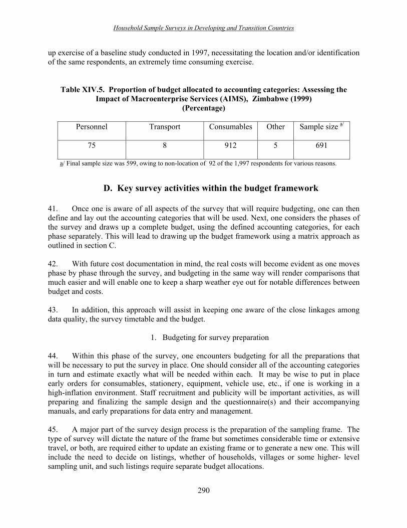
Household Sample Surveys in Developing and Transition Countries
290
up exercise of a baseline study conducted in 1997, necessitating the location and/or identification of the same respondents, an extremely time consuming exercise.
Table XIV.5. Proportion of budget allocated to accounting categories: Assessing the Impact of Macroenterprise Services (AIMS), Zimbabwe (1999)
(Percentage)
Personnel
Transport Consumables Other Sample size a/
75
8 912 5 691
a/ Final sample size was 599, owing to non-location of 92 of the 1,997 respondents for various reasons.
D. Key survey activities within the budget framework
41. Once one is aware of all aspects of the survey that will require budgeting, one can then define and lay out the accounting categories that will be used. Next, one considers the phases of the survey and draws up a complete budget, using the defined accounting categories, for each phase separately. This will lead to drawing up the budget framework using a matrix approach as outlined in section C. 42. With future cost documentation in mind, the real costs will become evident as one moves phase by phase through the survey, and budgeting in the same way will render comparisons that much easier and will enable one to keep a sharp weather eye out for notable differences between budget and costs. 43. In addition, this approach will assist in keeping one aware of the close linkages among data quality, the survey timetable and the budget.
1. Budgeting for survey preparation 44. Within this phase of the survey, one encounters budgeting for all the preparations that will be necessary to put the survey in place. One should consider all of the accounting categories in turn and estimate exactly what will be needed within each. It may be wise to put in place early orders for consumables, stationery, equipment, vehicle use, etc., if one is working in a high-inflation environment. Staff recruitment and publicity will be important activities, as will preparing and finalizing the sample design and the questionnaire(s) and their accompanying manuals, and early preparations for data entry and management. 45. A major part of the survey design process is the preparation of the sampling frame. The type of survey will dictate the nature of the frame but sometimes considerable time or extensive travel, or both, are required either to update an existing frame or to generate a new one. This will include the need to decide on listings, whether of households, villages or some higher- level sampling unit, and such listings require separate budget allocations.

Household Sample Surveys in Developing and Transition Countries
291
46. Other activities here that can take considerable time are the preparation of the questionnaires along with training and fieldwork manuals.
2. Budgeting for survey implementation 47. As survey implementation is likely to be the most costly aspect of the survey, careful budgeting within each accounting category, for each possible scenario, is extremely important. The time and budget allocated to the final printing of the questionnaires must be carefully thought through and planned well in advance with reliable sources. It is important to remember that, at the same time as the fieldwork begins to move forward, central office activities should be gearing up towards data entry. 48. As was emphasized before, the time allocated to the fieldwork should not be trimmed in order to fit within budget, since this can lead to the compromising of data quality owing to increases in non-sampling errors.
3. Budgeting for survey data processing 49. Budgets for data entry, validation, cleaning and analysis should be planned with all possible scenarios in mind, so as to ensure that these activities are not at risk of being rushed, leading to poor and incomplete reporting. A large amount of printing will be done during this stage and skimping on stationery will detract from the overall quality of the results. Adequate information technology facilities, including back-up facilities for entered data (CDs, disks), will also be required.
4. Budgeting for survey reporting 50. Once the fieldwork is complete and data entry well under way, one will be working within the next budgeting phase, namely, reporting and finalizing. Once again the survey design will play a part here, since it will have determined the extent of data analysis and the level of reporting required. Ongoing documentation throughout the survey exercise is highly recommended, since a daily diary of activities, decisions, problems, and costs will feed nicely into the descriptive sections of the report. Accounting categories should be considered carefully and adequate amounts assigned to each for this final survey phase.
5. Examples of budgeting for survey activities 51. The information in the examples presented in section C.6 above is presented here from a survey activity perspective. Example 4 52. Referring back to example 2 (EDG surveys), information is available here for costing of particular survey activities for 10 countries. Table XIV.6 below provides a summary.

Household Sample Surveys in Developing and Transition Countries
292
Table XIV.6. Costs of survey activities as a proportion of total budget: End-Decade Goals surveys (1999-2000), selected African countries
(Percentage)
Country Preparation Implementation a/ Data processing b/
Reporting c/ Sample size
Angola 0 d/ 83.6 6.1 10.3 6 000 Botswana 10.4 d/ 59.1 21.7 8.8 7 000 Kenya 0 d/ 93.9 2.6 3.5 7 000 Lesotho 0 d/ 73.2 18.6 8.8 7 500 Madagascar 0.3 78.6 3.0 18.1 6 500 Malawi 5.0 62.7 16.4 15.9 6 000 South Africa 1.3 93.1 2.9 2.7 30 000 Swaziland 63.0 23.4 7.5 6.1 4 500 United Republic of Tanzania
22.7
72.4
3.6
1.3
3 000
Zambia 0.4 92.0 6.4 1.2 8 000 Overall 7.0 81.0 6.0 6.0 7 054
Source: Ajayi (2002) a/ Including training, design, pilot and data collection. b/ Including data entry, management and analysis. c/ Including report production and dissemination. d/ Indicating the impossibility of extracting this information separately.
53. All countries, except for Swaziland, show the large proportion of costs that have to be assigned to survey implementation: it is probably reasonable to estimate that 70-90 per cent of budget will be devoted to this survey phase. Since (as may be recalled from table XIV.4) Malawi showed fairly high costings for equipment, this could explain the larger proportion allocated for data processing and reporting costs shown in table XIV.6. However, no explanation is available for the relatively high proportions allocated by Botswana and Lesotho for data-processing costs. In this case, countries were requested to provide a �matrix� of costs, showing accounting categories within survey activities; unfortunately, only the United Republic of Tanzania and Eritrea provide such a summary. Example 5 54. Referring back to example 3, information on costs by survey activity for the AIMS 1999 Zimbabwe survey is presented in table XIV. 7 below.

Household Sample Surveys in Developing and Transition Countries
293
Table XIV.7. Costs of survey activities as a proportion of total budget: AIMS Zimbabwe (1999)
(Percentage)
Preparation
Implementation a/ Data processing b/ Reporting c/ Sample size
4
85 8 3 599
a/ Including location of respondents, design, training, pilot, and data collection. b/ Including entry, management and cleaning. c/ Referring only to localized reporting up to production of clean data sets; detailed data analysis and final reporting were carried out under separate contracts.
55. The fairly high proportion of survey implementation costs in the total budget, as illustrated above in this user paid example, are likely to have stemmed from the fact that the sample for this AIMS survey consisted of 691 respondents being followed up from the previous (1997) survey, the costs of locating whom were fairly high (22 per cent of total budget).
E. Putting it all together 56. Once one has prepared costs within accounting categories for each type of survey activity, a matrix of accounting categories by survey activity can be drawn up with a view to facilitating a final consideration of the survey budget. Constructing such a matrix assists the survey planners in viewing the exercise on a global level, ironing out inconsistencies and overlaps, and highlighting the major costs to be expected; and assists funding agencies in comparing costs across various surveys, thus conducing to a better assessment of the validity of the proposed budget. 57. As mentioned above in example 4, only 2 out of the 21 countries involved in the EDG surveys actually produced the requested matrix of costs in accounting categories by survey activities. Therefore for this example, we cannot compile a matrix of accounting categories by survey activities. 58. However, the information for the AIMS survey is available and the cross-classification of tables XIV.5 and XIV.7 is shown in table XIV.8 below. Table XIV.8. Costs in accounting categories by survey activity as a planned proportion of
the budget: AIMS Zimbabwe (1999) (Percentage)
Preparation Implementation Data Reporting Overall Personnel 3 65 5 2 75 Transport 0 8 0 0 8 Consumables 0.9 9 2 0.1 12 Other 0.1 3 1 0.9 5 Overall 4.0 85 8 3 100
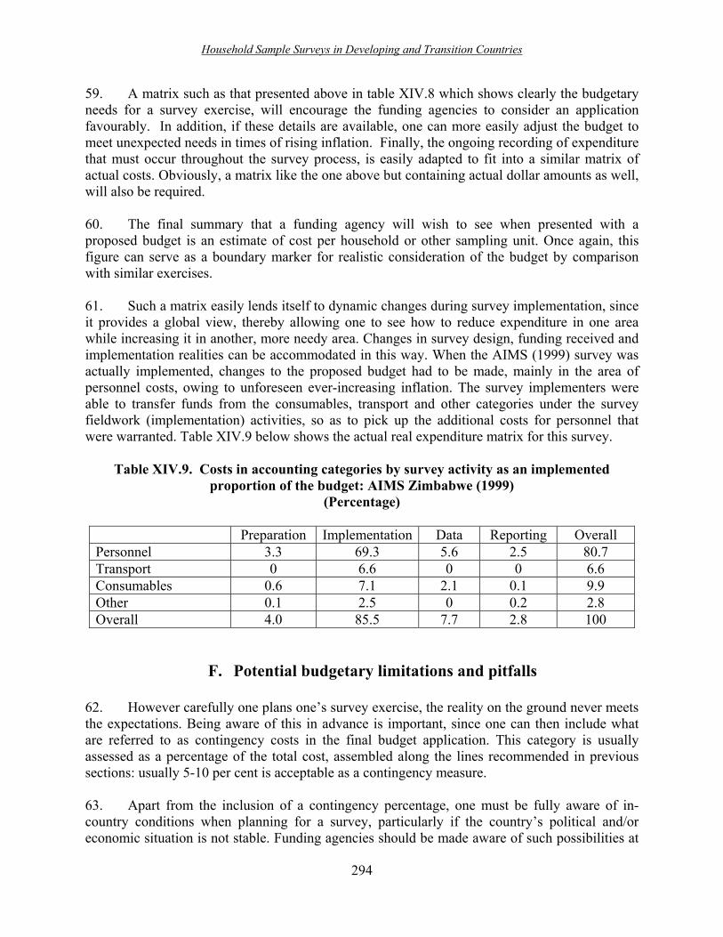
Household Sample Surveys in Developing and Transition Countries
294
59. A matrix such as that presented above in table XIV.8 which shows clearly the budgetary needs for a survey exercise, will encourage the funding agencies to consider an application favourably. In addition, if these details are available, one can more easily adjust the budget to meet unexpected needs in times of rising inflation. Finally, the ongoing recording of expenditure that must occur throughout the survey process, is easily adapted to fit into a similar matrix of actual costs. Obviously, a matrix like the one above but containing actual dollar amounts as well, will also be required. 60. The final summary that a funding agency will wish to see when presented with a proposed budget is an estimate of cost per household or other sampling unit. Once again, this figure can serve as a boundary marker for realistic consideration of the budget by comparison with similar exercises. 61. Such a matrix easily lends itself to dynamic changes during survey implementation, since it provides a global view, thereby allowing one to see how to reduce expenditure in one area while increasing it in another, more needy area. Changes in survey design, funding received and implementation realities can be accommodated in this way. When the AIMS (1999) survey was actually implemented, changes to the proposed budget had to be made, mainly in the area of personnel costs, owing to unforeseen ever-increasing inflation. The survey implementers were able to transfer funds from the consumables, transport and other categories under the survey fieldwork (implementation) activities, so as to pick up the additional costs for personnel that were warranted. Table XIV.9 below shows the actual real expenditure matrix for this survey.
Table XIV.9. Costs in accounting categories by survey activity as an implemented proportion of the budget: AIMS Zimbabwe (1999)
(Percentage)
Preparation Implementation Data Reporting Overall Personnel 3.3 69.3 5.6 2.5 80.7 Transport 0 6.6 0 0 6.6 Consumables 0.6 7.1 2.1 0.1 9.9 Other 0.1 2.5 0 0.2 2.8 Overall 4.0 85.5 7.7 2.8 100
F. Potential budgetary limitations and pitfalls
62. However carefully one plans one�s survey exercise, the reality on the ground never meets the expectations. Being aware of this in advance is important, since one can then include what are referred to as contingency costs in the final budget application. This category is usually assessed as a percentage of the total cost, assembled along the lines recommended in previous sections: usually 5-10 per cent is acceptable as a contingency measure. 63. Apart from the inclusion of a contingency percentage, one must be fully aware of in-country conditions when planning for a survey, particularly if the country�s political and/or economic situation is not stable. Funding agencies should be made aware of such possibilities at

Household Sample Surveys in Developing and Transition Countries
295
the time of budget submission, and by staying in constant communication with them during the course of the survey, one can quickly alert them to events that are causing the budget to move out of line. Such events include both man-made and environmental problems; and issues such as local politics, economics, weather patterns, migratory movements, etc., must also feed into the ongoing communication with those providing the funds and/or commissioning the survey. 64. For example, in the Zimbabwe 1999 AIMS study, inflation had been steadily rising for some months and the survey coordinators thought they had taken this into account when drawing up the survey budget. However, just as fieldwork was about to begin, the authorities froze the United States dollars exchange rate at an unrealistically low level, thus not matching the ever-increasing rate of inflation; planned costs then became totally unrealistic. Fortunately, Management Systems International was sympathetic and allowed a cost increase for completion of the exercise. 65. In cases such as the one above, it may be necessary for survey implementers to reduce staff, retaining only those who are most efficient, or to cut costs in other ways, for example, by using lower-cost stationery, public instead of hired transport, consolidating operations to reduce overheads, etc. Alternatively, it is advisable, if allowed by those funding the survey, to include in the statement of the survey process a note to the effect that the scope of the survey may be subject to alteration owing to unforeseen circumstances, which would allow, for example, a change in sample size so as to take account of rising costs.
G. Record-keeping and summaries
66. It was mentioned earlier that the ongoing daily recording of events during the survey exercise will be essential if one is to keep track of all the decisions made and the options considered when making those decisions. This includes recording expenditure. 67. The survey coordinators should, at the survey preparation stage, devise a series of forms for use by all employees in recording daily activities and expenditure in full detail. Such forms should include details of hours worked, tasks completed, interview details, transport details, etc., which can be summarized on a weekly basis. In this way, one will be able to both maintain a tight watch on the budget and identify possible problems at an early stage. In addition, a system of payment only upon production of valid receipts should be instituted wherever possible. 68. Monitoring and reporting actual daily survey activities, and their consequent costs, are a critical survey management responsibility. Different forms of recording are suitable for different phases of the survey. Survey design 69. During this phase, the survey manager will be in close touch with all activities, thus making the monitoring a fairly straightforward task. A daily diary is a useful way of logging who has done what, and this can be summarized in a weekly report. A parallel record of actual costs for transport, consumables, accommodation, etc. can be kept and will be supported by the weekly

Household Sample Surveys in Developing and Transition Countries
296
summary so as to provide a weekly cost report. Examples of forms for the maintaining of daily and weekly records are provided in the annex to this chapter. Survey implementation 70. During survey implementation, the survey manager will need to rely heavily on his fieldwork team leaders to provide him with their daily diarized activities plus actual costs and receipts recorded. Once again, the manager should make a weekly summary detailing all costs and days worked by team members, so that a check on percentage of budget used can be easily made. Examples of forms to be used are provided in the annex. Survey reporting 71. Once again the survey manager will be more closely in touch with the activities during this phase and a system of diarizing daily activities and costs will enable a weekly summary to be maintained. Forms to be used are provided in the annex. Tracking expenditure against budget 72. It is advisable for one person to be given the responsibility of undertaking ongoing tracking of expenditure against budget. He or she should provide a weekly overview of expenditure to date, together with budget allocations (see annex for an example). If this mechanism is in place from the start of the survey period, it will be fairly straightforward to foresee problems and, if necessary, apply for reallocations of budget. Survey practitioners should realize that increasing the budget once the survey has started is a very unusual occurrence and thus that adjustments are the key to success in producing the final product.
H. Conclusions 73. This chapter has aimed at providing some useful hints and advice in respect of planning a survey budget by means of detailed consideration of all components of the survey. A dynamic approach incorporating budgeting from two points of view has been recommended and illustrated by examples. 74. It remains to be emphasized that this detailed planning is crucial if one is to successfully carry out a transparent, reliable and high-quality study. Of similar importance is the need for the daily recording of all activities and actions, which can then smoothly feed into the accounting process and be maintained as a reliable record for future survey planning.

Household Sample Surveys in Developing and Transition Countries
297
Annex Examples of forms for the maintaining of daily and weekly records
Personnel daily activity log NAME Date Activity Location Time spent Total number of days
Daily interview log NAME of Enumerator Date Location Interview
Code No. Time spent
Result of interview/comments
Personnel weekly summary activity log NAME of team leader Date of report Personnel name
Activities summary Location Total number of days
Total number of days

Household Sample Surveys in Developing and Transition Countries
298
Personnel daily expenditure log
NAME Date Location Activity Details of expenditure Amount
(dollars) Receipt No.
Total amount (dollars)
Weekly expenditure log NAME of team leader Date of report Personnel Name
Location Activity Details of Expenditure Amount (dollars)
Receipt Nos.
Total amount (dollars)
Weekly expenditure summary NAME Item Week 1 Week 2 Week 3 Week 4 Week 5 Week 6Personnel Wages/salaries Accommodation Meals Other Transport Consumables Other

Household Sample Surveys in Developing and Transition Countries
299
Weekly expenditure summary * Item Budget Cumulative
expenditure Week 1
Week 2
Week 3
Week 4
Week 5
Week 6
Personnel Wages/salaries Accommodation Meals Other Transport Fuel Vehicles Public Other Equipment Consumables Other Total to date * Can be set up as a spreadsheet (for example, with EXCEL).

Household Sample Surveys in Developing and Transition Countries
300
References Ajayi, D. (2002). Personal communication. Barnes, C. (2001). An Assessment of Zambuko Trust Zimbabwe. Assessing the Impact of
Microenterprise Services (AIMS) project. Washington, D.C.: Management Systems International.
__________ , and E. Keogh (1999). An Assessment of the Impact of Zambuko�s Microfinance
Program in Zimbabwe: Baseline Findings. Assessing the Impact of Microenterprise Services (AIMS) paper, Washington, D.C.: Management Systems International.
Greenfield, T. (1996). Research Methods: Guidance for Postgraduates. New York: Arnold,
John Wiley and Sons, Inc., p. 306. Groves, R. M. (1989). Survey Errors and Survey Costs. New York: J. Wiley and Sons, Inc. __________ , and J. M. Lepkowski (1985). Dual frame mixed mode survey designs. Journal of
Official Statistics, vol. 1, No. 3, pp. 263-286. Scheaffer, R.L., W.Mendenhall and L. Ott (1990). Elementary Survey Sampling (4th ed.).
Belmont, California: Wadsworth, Inc., p. 97. United Nations (1984). Handbook of Household Surveys (Revised Edition). Studies in Methods,
No. 31, Sales No. E. 83. XVII.13.

Household Sample Surveys in Developing and Transition Countries
301
Section E
Analysis of survey data

Household Sample Surveys in Developing and Transition Countries
302
Introduction
Graham Kalton Westat
Rockville, Maryland United States of America
1. When the data for a survey have been collected, they need to be prepared for analysis. This step has three important components. First, as will be discussed in chapter XV, decisions need to be made on how to format the data most effectively for analysis, taking account of the computing facilities available and the analysis software to be used. The survey analyses often involve two or more different units of analysis: in particular, households and persons are separate units of analysis in many household surveys. The data file therefore needs to be able to handle hierarchic structures efficiently; for example, it needs to cater for the facts that persons are nested within households and that the number of persons varies between households. 2. The second component of data preparation is data cleaning or editing. Inevitably, the survey responses will contain identifiable errors of various forms, for example, responses that are inconsistent with other responses or that fall outside the range of possibilities. These errors need to be resolved before analyses can start (see chap. XV for details on data cleaning). 3. An important task in data cleaning is to finalize the analytic status of each sampled unit. All of the units selected for the sample need to be placed in one of the following categories: respondent, eligible non-respondent, ineligible unit, or non-responding unit of unknown eligibility (see chap. VIII). A classification as respondent generally requires more than just the presence of a questionnaire for the sampled unit. Usually a minimum amount of acceptable data has to be collected for the unit to be so classified. The assignment of response status thus necessitates a review of the questionnaires. Note, however, that even though a unit is to be retained in the analysis as a respondent, there may well be some items for which acceptable answers have not been obtained. To cope with this problem, some form of imputation method may be used to assign values for the missing responses. 4. The analytic statuses of all sampled units are required for the last step of data preparation: the computation of survey weights. Survey weights are computed for each of the units of analysis. Since the starting point in the construction of weights is to determine the selection probabilities be all the sampled units, it is vitally important that careful records of the selection probabilities be kept in the sample selection process. The initial, or base, weights for sampled units are computed as the inverses of the units� selection probabilities. The base weights for respondents are then adjusted to compensate for the eligible non-respondents and for a proportion of the non-respondents with unknown eligibility status. A further adjustment is often applied to make the adjusted weighted sample distributions for certain key variables conform to known distributions of these variables available from an external source. The development of weights is described in chapters XV and XIX.

Household Sample Surveys in Developing and Transition Countries
303
5. An important responsibility of data preparation is to ensure that the sampling information required for analysis is recorded on each respondent data record. Survey weights are needed for each responding unit of analysis in order that valid estimates of parameters of the survey population may be produced. Information on each responding unit�s PSU and stratum is needed in order that sampling errors may be computed correctly for the survey estimates (see chap. XXI). 6. Two considerations distinguish analyses of survey data from the analyses described in standard statistical texts. One is the need to use survey weights in survey analyses in order to compensate for unequal selection probabilities, non-response, and non-coverage. Failure to use weights in the analyses may well result in distorted estimates of population values.
7. The second distinguishing consideration of survey analyses is the need to compute sampling errors for survey estimates in a way that takes account of the survey�s complex sample design. The theory presented in standard statistical texts in effect assumes unrestricted sampling, whereas most household surveys employ stratified multistage sampling. In general, sampling errors for estimates from a stratified multistage sample are larger that those from an unrestricted sample of the same size, so that the application of the formulas in standard statistical texts will overstate the precision of the estimates (see chaps. VI, VII and XXI). This implies that standard statistical software packages produce invalid standard error estimates for survey estimates. Fortunately, however, there are now a sizeable number of survey analysis software packages that can be used to produce appropriate sampling error estimates from survey data obtained from complex sample designs. Chapter XXI contains a review of a number of these packages.
8. Much of the analysis conducted with government surveys is descriptive in nature. Often the results are reported in tabular form, with the table cells containing means, percentages or totals; sometimes, they are presented in graphical displays. In narrow statistical terms, the estimates involved are often very simple, the only issue being the need to make sure that the survey weights have been used. There are, however, important issues of definition and presentation to be considered. Careful attention needs to be given to defining the construct to be measured (for example, poverty: see chap. XVII), and to specifying the set of units for which it is to be measured, in suitable ways for the purpose in hand. Also, the results need to be presented in a fashion that clearly communicates what has been measured and for which set of units. Guidance on the presentation of simple descriptive estimates is given in chapter XVI.
9. Often, the construct to be measured can be defined in a relatively straightforward logical manner in terms of the survey responses. Sometimes, however, the construct is more complex and it may need to be measured by creating an index using multivariate statistical methods, such as cluster analysis and principal component analysis. Several examples are provided in chapter XVIII, including, for instance, one in which a �wealth� index was constructed using information on such variables as whether the household had electricity, the number of persons per sleeping room, and the principal type of drinking water.
10. Finally, it should be noted that, while the production of descriptive estimates remains the main form of survey analysis, there is increasing use of analytic techniques with survey data. These techniques are often applied to examine the relationships between variables and to explore

Household Sample Surveys in Developing and Transition Countries
304
possible cause-effect relationships. The most common form of this type of analysis is one in which a statistical model is constructed to best predict a dependent variable in terms of a set of independent (or predictor) variables. If the dependent variable is a continuous one (for example, household income), then multiple linear regression methods may be used. If it is a categorical variable with a binary response (for example, whether the household has or does not have running water), then logistic regression methods may be used. These methods, and the effects of the complex sample design on them, are described in chapters XIX and XX. Chapter XIX also describes the use of multilevel modelling in a survey context and chapter XX also discusses the effect of complex sample designs on standard chi-square tests of the associations between categorical variables.

Household Sample Surveys in Developing and Transition Countries
305
Chapter XV A guide for data management of household surveys
Juan Muñoz Sistemas Integrales
Santiago, Chile
Abstract
The present chapter describes the role of data management in the design and implementation of national household surveys. It starts by discussing the relationship between data management and questionnaire design, and then explores the past, present and future options for survey data entry and data editing, and their implications for survey management in general. The following sections provide guidelines for the definition of quality control criteria and the development of data entry programs for complex national household surveys, up to and including the dissemination of the survey data sets. The final section discusses the role of data management as a support for the implementation of the survey sample design.
Key terms: consistency check, data cleaning, data editing, data management, household survey, quality control criteria
Household Sample Surveys in Developing and Transition Countries
306
A. Introduction 1. Although the importance of data management in household surveys has often been emphasized, data management is still generally seen as a set of tasks related to the tabulation phase of the survey, in other words, activities that are conducted towards the end of the survey project, that use computers in clean offices at survey headquarters, and that are generally under the control of data analysts and computer programmers. 2. This restrictive vision of survey data management is changing. Experience from the past two decades shows that data management can and should play a critical role beginning with the very earliest stages of the survey effort. It is also becoming clear that data management does not terminate with the publication of the first statistical reports. 3. The clearest demonstration of effective data management efforts prior to the analytical phases has been given by the World Bank�s Living Standards Measurement Study and other surveys that have successfully integrated computer-based quality controls with survey field operations. Even when data entry is not implemented as a part of fieldwork, data managers should participate in the design of questionnaires to ensure that the statistical units observed by the survey are properly recognized and identified, that skip instructions for the interviewers are explicit and correct, and that deliberate redundancies are eventually incorporated into the questionnaires that can be later used to implement effective consistency controls. 4. At the other extreme of the survey project timeline, the notion that the end product expected from the survey is a printed publication, with a collection of statistical tables, has been replaced by the concept of a database that not only can be used by the statistical agency to prepare the initial tables, but will also be accessible to researchers, policymakers and the public in general. The descriptive summary report of survey results is no longer seen as the final step, but rather as the starting point of a variety of analytical endeavours that may last for many years after the project is officially closed and the survey team is disbanded. 5. The present chapter begins with a discussion of the relationships between survey data management and questionnaire design, followed by an exploration of the past, present and future options for survey data entry and data editing, and their implications for survey management in general. The subsequent sections provide guidelines for the definition of quality control criteria and the development of data entry programs for complex national household surveys, up to and including the dissemination of the survey data sets. The final section discusses the role of data management as a support for the implementation of the survey sample design.
B. Data management and questionnaire design
6. Survey data management begins concurrently with questionnaire design and may to a large extent influence the latter. The data manager should be consulted on each major draft of the questionnaire, since he or she will have an especially sharp eye for flaws in the definition of units of observation, skip patterns, etc. The present section explores some of the formal aspects of the questionnaire that deserve attention at this point.

Household Sample Surveys in Developing and Transition Countries
307
7. Nature and identification of the statistical units observed. Every household survey collects information about a major statistical unit - the household - as well as about a variety of subordinate units within the household - persons, budget items, plots, crops, etc. The questionnaire should be clear and explicit about just what these units are, and it should also ensure that each individual unit observed is properly tagged with a unique identifier. 8. The identification of the household itself generally appears on the cover page of the questionnaire. It sometimes consists of a lengthy series of numbers and letters that represent the geographical location and the sampling procedures used to select the household. Although it may seem self-evident, the use of all these codes as household identifiers should be critically assessed, because it is cumbersome, error-prone and expensive (often 20 digits or more may be needed to identify just the few hundred households in the sample); sometimes it does not even ensure unique identification of the unit as, for instance, when geographical codes on the cover page identify the dwelling but do not consider the case of multiple households in a dwelling. An easier and safer alternative is to identify the households by means of a simple serial number that can be handwritten or stamped on the cover page of the questionnaire, or even pre-printed by the print shop. Geographical location, urban/rural status, sampling codes and the rest of the data on the cover page then become important attributes of the household, which as such must be included in the survey data sets, but not necessarily for identification purposes. A good compromise between these two extremes (the list of all detailed sampling codes and a simple household serial number) is to give a three- or four-digit serial number to the primary sampling units (PSUs) used in the survey, and then a two-digit serial number to the households within each PSU. 9. The nature of the subordinate statistical units is often obvious (for instance, the members of the households are individual persons), but ambiguities may present themselves when what seems like an individual unit is in fact a multiplicity of units of a different kind. This may occur, for instance, when a man who has been asked to report on the main activity of his job conducts multiple, equally important activities at the same time or has more than one job in a given reference period. Similarly, ambiguity is possible when a woman who has been asked about the gender or weight of her last child gave birth to boy-girl twins with different weights. However, although such situations should of course be averted through good questionnaire design and piloting, they often arise in subtle ways, and this is where the critical vision of an experienced data manager can offer invaluable assistance to the subject matter specialists in spotting them. 10. Whatever its nature, subordinate units within the household should always be uniquely identified. This can be done by means of numerical codes assigned by the interviewer, but it is generally better to have these identifiers pre-printed in the questionnaire whenever possible. 11. Built-in redundancies. The design of the questionnaire may consider the inclusion of deliberate redundancies, intended to detect mistakes of the interviewer or data entry errors. The most common examples are:
• Adding a bottom line for �totals� under the columns that contain monetary amounts. Generating these totals may often be the interviewer�s task, but even when this is not the case, their inclusion is convenient because they are a very
Household Sample Surveys in Developing and Transition Countries
308
effective way (often the only way) of detecting data entry errors or omissions. In fact, totals may be added for quality control purposes at the bottom of any numerical column, even when the sum of the numbers does not represent a meaningful measure of magnitude (for instance, a total may be added at the bottom of a column containing the quantities (not the monetary amounts) of various food items purchased, even if that means adding heterogeneous numbers, such as kilos of bread and kilos of potatoes (or even litres of milk). This point is further elaborated in the discussion of typographic checks below.
• Adding a check digit to the codes of some important variables (such as the
occupation or activity of a person, or the nature of the consumption item). A check digit is a number or letter that can be deducted from the rest of the digits in the code by means of arithmetic operations performed at data entry time. A common check digit algorithm is the following: multiply the last digit in the code by 2, the second from last by 3, etc. (if the code is longer than six digits, repeat the sequence of multipliers 2, 3, 4, 5, 6, 7), and add the results. The check digit is the difference between this sum and the nearest higher multiple of 11 (the number 10 is represented by the letter K). Check digit algorithms are constructed so that the more common coding mistakes, such as transposing or omitting digits, will produce the wrong check digit.
C. Operational strategies for data entry and data editing
12. Many household surveys still consider data entry and editing as activities to be conducted in central locations, after the survey is fielded, whereas other surveys are already implementing the concept of integrating data entry into field operations. In the near future, the idea may evolve towards the application of computer-assisted interviewing. The present section discusses the organizational implications of the various strategies and the common and specific features of the data entry and data editing software developed under each alternative. 13. Centralized data entry. Centralized data entry was the only known option before the emergence of microcomputers, and it is still used today in many surveys. It considers data entry an industrial process, to be conducted in centralized data entry workshops after the end of the interviews. The objective of the operation is to convert the raw material (the information on the paper questionnaires) into an intermediate product (machine-readable files) that needs to be further refined (by means of editing programs and clerical processes) in order that a so-called clean database may be obtained as a final product. 14. During the initial data entry phase, the priorities are speed and ensuring that the information on the files perfectly reflects the information gathered in the questionnaires. Data entry operators are indeed not expected to �think� about what they are doing, but rather to just faithfully copy the data given to them. Sometimes, the questionnaires are submitted to double-blind data entry, in order to ascertain that this is done correctly.

Household Sample Surveys in Developing and Transition Countries
309
15. Until the mid-1970s, data entry was carried out with specialized machines having very limited capabilities. Although, at present, the process is almost always carried out with microcomputers that can be programmed with quality control checks, this capability is seldom used in practice. The prevalent belief is that few quality control checks should be included in the data entry process, since the operators are not trained to make decisions as to what to do if an error is found. Besides, the detection of errors and their solutions slow down the data entry process. This school of thought considers that quality control checks should be solely reserved for the editing process. 16. Data entry in the field. Starting in the mid-1980s, the integration of computer-based quality controls into field operations has been identified as one of the keys to improving the quality and timeliness of household surveys. These ideas were initially developed by the World Bank�s Living Standards Measurement Study (LSMS) surveys, and have been applied later to various other complex household surveys. Under this strategy, data entry and consistency controls are applied on a household-by-household basis as a part of field operations, so that errors and inconsistencies are solved by means of eventual revisits to the households. 17. The most important and direct benefit of integration is that it significantly improves the quality of the information, because it permits the correcting of errors and inconsistencies while the interviewers are still in the field rather than by office �cleansing� later. Besides being lengthy and time-consuming, office cleansing processes at best produce databases that are internally consistent but do not necessarily reflect the realities observed in the field. The uncertainty stems from the myriad of decisions - generally undocumented - that need to be made far from where the data are collected, and long after the data collection. 18. The integration of computer-based quality controls can also generate databases that are ready for tabulation and analysis in a timely fashion, generally just a few weeks after the end of field operations. In fact, databases may be prepared even as the survey is conducted, thus giving the survey managers the ability to effectively monitor field operations. 19. Another indirect advantage of integration is that it fosters the application of uniform criteria by all the interviewers and throughout the whole period of data collection, which is hard to achieve in practice with pre-integration methods. The computer indeed becomes an incorruptible and tireless assistant of the survey supervisors. 20. The integration of computer-based quality controls to field operations also has various implications for the organization of the survey, the most important being that it requires the field staff to be organized into teams. A field team is usually headed by a supervisor and includes a data entry operator in addition to two to four interviewers. 21. The organization of field operations depends on the technological options available. The two most used set-ups involve desktop and notebook computers and entail the following steps:
• Have the data entry operator work with a desktop computer in a fixed location
(generally a regional office of the statistical agency,) and organize fieldwork so that the rest of the team visits each survey location (generally a primary sampling

Household Sample Surveys in Developing and Transition Countries
310
unit) at least twice, so as to give the operator time to enter and verify the consistency of the data in between visits. During the second and subsequent visits, the interviewers will re-ask questions where errors, omissions or inconsistencies are detected by the data entry program.
• Have the data entry operator work with a notebook computer and join the rest of
the team in its visits to the survey locations. The whole team stays in the location until all the data are entered and certified as complete and correct by the data entry program.
22. Both options have external requirements that need to be carefully considered by the survey planners and managers. One of them entails ensuring a permanent power supply for the computers, which may be an issue in poorly electrified countries. If desktops in fixed locations are used, this may require installing generators and ensuring that fuel for the generators is always available. If mobile notebooks are used instead, this may require the use of portable solar panels. 23. An obvious but important difference between the two strategies is that if computer-based quality controls are to be integrated into fieldwork, the data entry and editing program needs to be developed and debugged before the survey starts. With centralized data entry, this is also convenient (so that data entry can proceed in parallel with field operations,) but not absolutely necessary. 24. Paperless interviews. The use of hand-held computers to get rid of the paper questionnaires altogether is very appealing because of the advantages of automating certain parts of the interviews, such as skip instructions. However, although the technology has been available for almost 20 years, very little has been done to seriously apply this strategy to complex household surveys in developing countries. In fact, even in the most advanced national statistical agencies, paperless questioning has so far been restricted to relatively simple exercises, such as employment surveys and the collection of prices for the consumer price index. 25. A possible reason for this is that although paperless questioning lends itself well to interviews that follow a linear flow, with a beginning and an end, many household surveys conducted in developing and transition countries may require instead multiple visits to each household, separate interviews with each member of the household, or other procedures that are less strictly structured. 26. In spite of the absence of real empirical experience, certain observations about what needs to be taken into consideration in the design and implementation of a paperless questionnaire can be made:
• The data entry program interface will in some cases consist of a series of questions appearing one after the other on the computer screen, but in other cases it will need to reproduce the structure and visual format of the paper questionnaires, showing many data entry fields at the same time. This seems to be particularly important in the modules on expenditure and consumption, where the interviewer needs to �see� many consumption items simultaneously. The interface

Household Sample Surveys in Developing and Transition Countries
311
must also allow for the possibility of marking questions in case of doubts, and it should also make it possible to return to the household for a second interview without repeating all questions.
• The questionnaire design process generally takes many months of work and
involves many different people (subject-matter specialists, survey practitioners, etc.). With a paper questionnaire, the process is carried out by preparing, distributing, discussing and piloting various �generations� of the questionnaire until the final version is agreed upon. The equivalent steps for something that will never actually appear on paper still need to be defined.
• Interviewer training will need to be redesigned around the new technology. We
know how to train interviewers to administer a paper questionnaire (theoretical sessions, simulations, mock interviews, training manuals, etc.,) but little work has been done to develop the equivalent techniques for a paperless survey.
• Finally, effective methods of supervision have to be developed. A large and rich
set of procedures (visual inspection of the questionnaires, check-up interviews, etc.) has evolved for over a half-century to verify the work done by interviewers in the field. All these have been elaborated around the concept of a paper questionnaire and need to be re-engineered for paperless interviewing. It is very likely that the new technologies will offer completely different -- and possibly much more powerful -- options for effective supervision; for instance, most hand-held computers have voice recording capabilities that could be used to automatically record random parts of the interview along with the data files. By adding Global Position System (GPS) capabilities, it may also be possible to automatically record the time and place of the interviews. Again, the details have yet to be defined, field-tested and incorporated into the general scheme of survey fieldwork.
D. Quality control criteria
27. Regardless of the strategy chosen for quality control, the data on the questionnaires need to be subjected to five kinds of checks: range checks, checks against reference data, skip checks, consistency checks and typographic checks. Here, we revise the nature of these checks and the way they can be implemented under the various operational set-ups. 28. Range checks are intended to ensure that every variable in the survey contains only data within a limited domain of valid values. Categorical variables can have only one of the values predefined for them on the questionnaire (for example, gender can be coded only as �1� for males or �2� for females); chronological variables should contain valid dates, and numerical variables should lie within prescribed minimum and maximum values (such as 0 to 95 years for age.)

Household Sample Surveys in Developing and Transition Countries
312
29. A special case of range checking occurs when the data from two or more closely related fields can be checked against external reference tables. Some common situations involve the following:
• Consistency of anthropometric data. In this case, the recorded values for height, weight and age are checked against the World Health Organization�s standard reference tables. Any value for the standard indicators (height-for-age, weight-for-age and weight-for-height) that falls more than three standard deviations from the norm should be flagged as a possible error so that the measurement can be repeated.
• Consistency of food consumption data. In this case, the recorded values for the
food code, the quantity purchased and the amount paid are checked against an item-specific table of possible unit prices.
30. Even when data are entered in centralized locations, it is generally convenient to detect and correct range errors in the initial data entry phase, rather than postpone this control for the editing phase, because range errors are often a result of the data entry operation itself rather than of interviewer mistakes. An error flag, such as a beep and a flashing field on the screen, may be set off when an out-of-range value is entered. If the error is merely typographical, the data entry operator can correct it immediately. It should, however, be possible to override the flag if the value entered represents what is on the questionnaire. In that case, an error report should be made so that the clerical staff can correct the error later by inspecting the questionnaire (or by the interviewer during a second interview, if the data are being entered in the field.) In the meantime, the suspect data item may be stored in a special format that registers its questionable status. 31. Skip checks. These verify whether the skip patterns have been followed appropriately. For example, a simple check verifies that questions to be asked only of schoolchildren are not recorded for a child who answered no to an initial question on school enrolment. A more complicated check would verify that the right modules of the questionnaire have been filled in for each respondent. Depending on his or her age and gender, each member of the household is supposed to answer (or skip) specific sections of the questionnaire. For instance, children less than 5 years of age should be measured in the anthropometric section but the questions about occupation are not asked of them. Women aged 15-49 years may be included in the fertility section but men may not be. 32. Sometime in the future, computer-assisted (paperless) interviews for surveys in developing countries may become common, and then the skipping scheme will possibly be controlled by the data entry program itself, at least in some cases. However, under the other operational set-ups (central data entry locations and data entry in the field), the data entry program should not actually follow the skip patterns on its own. For example, if the answer no is entered to the question, Are you enrolled in school?, the fields in which to enter data about the kind of school attended, grade in school and so on, should still be presented to the data entry operator. If there are answers actually recorded on the questionnaire, they can then be entered and the program will flag an incorrect skip. The supervisor or interviewer (or the centralized editing clerical staff) can determine the nature of the mistake at a later time. It may well be that

Household Sample Surveys in Developing and Transition Countries
313
the no was supposed to be a yes. If the data entry program had automatically skipped the following fields, the error would not have been detected or remedied. 33. Consistency checks. These checks verify that values from one question are consistent with values from another question. A simple check occurs when both values are from the same statistical unit, for example, the date of birth and age of a given individual. More complicated consistency checks involve comparing information from two or more different units of observation. 34. There is no natural limit imposed on the number of consistency checks that can exist. Well-written versions of the data entry program for a complex household survey may have several hundred of them. In general, the more checks that are defined, the higher the quality of the final data set. However, given that the time available to write the data entry and data editing programs is always limited (usually about two months), expertise and good judgement are required to decide exactly which should be included. Certain consistency checks that are applicable in almost all household surveys have proved to be particularly effective and thus have become something of a de facto standard. These encompass:
• Demographic consistency of the household. The consistency between the ages and genders of all household members is checked with a view to kinship relationships. For example, parents should be at least (say) 15 years older than their children, spouses should be of different genders, etc.
• Consistency of occupations. The presence or absence of certain sections should be
consistent with occupations declared individually by household members. For instance, the farming section should be present if and only if some household members are reported as farmers in the labour section.
• Consistency of age and other individual characteristics. It is possible to check
that the age of each person is consistent with personal characteristics such as marital status, relationship to the head of the household, grade of current enrolment (for children currently in school) or last grade obtained (for those who have dropped out). For example, an 8-year-old child should not be in a grade higher than third.
• Expenditures. In this case, several different consistency checks are possible. Only
in a household where one or more of the individual records show that a child is attending school should there be positive numbers in the household consumption record for items such as school books and schooling fees. Likewise, only households that have electrical service should report expenditures on electricity.
• Control totals. As said before, adding a control total wherever a list of numbers
can be added is a healthy questionnaire design principle. The data entry program should check that the control total equals the sum of the individual numbers.
Household Sample Surveys in Developing and Transition Countries
314
35. Typographical checks. In the early years of survey data processing, checking for typographical errors was almost the only quality control conducted at the time of data entry. This was generally achieved by simply having each questionnaire entered twice, by two different operators. These so-called double-blind procedures are seldom used nowadays, on the grounds that the other consistency controls that are now possible make them redundant. However, this may in some cases be wishful thinking rather a solid assumption. 36. A typical typographical error consists in the transposition of digits (like entering �14� rather than �41�) in a numerical input. Such a mistake for age might be caught by consistency checks with marital status or family relations. For example, the questionnaire of a married or widowed adult age 41 whose age is mistakenly entered as 14, will show up with an error flag in the check on age against marital status. However, the same error in the monthly expenditure on meat may easily pass undetected, since either $14 or $41 could be valid amounts. 37. This emphasizes the importance of incorporating data management perspectives into the questionnaire design phase of the survey. Control totals, for instance, can significantly reduce typographical errors, because asking the interviewer to add up the figures with a pocket calculator is akin to entering them with double-blind data procedures. Check-digits can similarly be used for this purpose in some important variables. It is also possible to implement real double-blind methods for entering the data of certain parts of the questionnaire, but doing this for the whole questionnaire is both unnecessary and impractical � among other reasons, because modern data entry strategies are generally based on the work of a single data entry operator, not two different operators.
E. Data entry program development
38. The development of a good survey data entry and editing program is both a technique and a craft. The present section discusses some of the development platforms that are available today to facilitate the technical aspects of the process and some of the subtler issues related to the design of interfaces for the data entry operators and the future users of the survey data sets. 39. Development platforms. There are many data entry and editing program development platforms available in the market, but few of them are specifically adapted to the data management requirements of complex household surveys. A World Bank review conducted in the mid-1990s had found that at that time two DOS-based platforms were adequate: the World Bank�s internally developed Living Standards Measurement Study (LSMS) package and the United States Bureau of the Census Integrated Microcomputer Processing System (IMPS) program. Both platforms have progressed since the review, in response to changing hardware and operating system environments. IMPS has been superseded by the Census and Survey Processing System (CSPro), a Windows-based application that provides some tabulation capabilities, besides serving in its primary role as a data entry and editing program development environment. The LSMS package has evolved towards LSD-2000, an Excel-based application that strives to develop the survey questionnaire and the data entry program simultaneously. 40. Both CSPro and LSD-2000 (or their ancestors) have proved their ability to support the development of effective data entry and editing programs for complex national household

Household Sample Surveys in Developing and Transition Countries
315
surveys in many countries. These platforms are also easy to obtain and use. Almost any programmer -- in fact, almost anybody with a basic familiarity with computers -- can be expected to acquire in a couple of weeks the technical ability needed to initiate the development of a working data entry program. 41. Design principles. Unfortunately, development platforms cannot advise the programmers on just what data entry program needs to be developed. It may even be argued that the user-friendliness of the platforms risks making the development of inadequate data entry programs too easy. Confusing the mastery of the tools with the craft of putting the tools to good use is a mistake that survey managers should avoid by integrating both experienced programmers and subject-matter specialists in the development of the survey data entry and editing programs. Certain practical guidelines can be helpful in this regard:
• Data entry screen design. Data entry screens should look as much as possible like
the corresponding pages of the questionnaire, but this rule has many exceptions. For example, if the questionnaire presents personal questions in the form of a matrix (with questions in rows and household members in columns, or the other way around), it is generally better to prepare a separate data entry screen for each person rather than to reproduce the paper grid on the computer screen. One reason for not reproducing the whole grid on the screen is that the number of respondents is variable. A stronger reason is that the statistical units observed are persons and not households.
• Distinguishing between impossible and unlikely situations. The data entry
program should of course flag as errors any situations that represent logical or natural impossibilities (such as a girl�s being older than her mother), but it should also react to situations that are not naturally impossible but very unlikely (such as a girl�s being less than 15 years younger that her mother). Ideally, the data entry program should assess the severity of the errors and react differently depending on how serious they are, much as a human supervisor would if she or he was visually inspecting the questionnaire. This kind of �smart� programming is particularly important when data entry is integrated into field operations. Unfortunately, some programmers do not invest enough effort in this issue. A revealing sign is the tendency to always define the upper range of quantitative variables as �999��(as many nines as the data entry field is long). The counterproductiveness of this practice is obvious: data entry fields should of course be long enough to input even the largest possible values, but the upper ranges should be small enough to flag unlikely values as possible outliers.
• Error reporting language. Some of the quality control criteria included in the data
entry program may report on the errors detected by relatively simple means that are either self-explanatory or require little training to be understood. For instance, the LSMS data entry program reports range-checking errors by showing blinking arrows pointing up �↑↑↑� or down �↓↓↓� along with the offending value, depending on whether it is considered to be too low or too high. However, the most complex consistency controls require much clearer and more explicit
Household Sample Surveys in Developing and Transition Countries
316
reporting. For instance, a check on the demographic consistency of the household could eventually produce a text such as �Warning: Lucy (ID Code 05, a girl 9 years old) is unlikely to be the daughter of Mary (ID Code 02, a woman 21 years old)�, ideally on a printout rather than on the computer screen only. This kind of �smart and literate� programming may take longer than seemingly simpler alternatives (such as using error codes), but it will save many hours of fieldwork and field staff training, and it will also free the programmers themselves from the burden of writing an error codebook.
• Variable codes. A complex household survey typically contains hundreds of
variables. The programmers in charge of the data entry program will need to refer to them by means of codes, according to the specific conventions of the development platform used. It is important that a rational and simple coding system be selected for this purpose from the beginning of the data entry program development process, because this will facilitate the communication between members of the development team, and also because it will save time in the subsequent steps of preparation and dissemination of the survey data sets. Finding a good coding system, however, can be harder than it seems. The process may start easily enough, with the first few variables getting codes such as �AGE�, �GENDER� and so forth, but may soon become unmanageable, as finding adequate mnemonic codes becomes harder. A good option is to simply refer to the section and question numbers on the questionnaire, without any intent to make the codes self-explanatory (for example, if �Age� and �Gender� are variables 4 and 5 of Section 1, they could be coded as �S1Q4� and �S1Q5�, respectively).
• Data entry workloads. When data entry is integrated into field operations, the
most natural work unit for data entry is the household. This is because under these conditions the data entry operator always has only one or just a few questionnaires to work with, and also because consistency controls and error reporting are conducted on a household-by-household basis. In a central data entry location, the workloads can be blocks of 10-20 households (such as survey localities or PSUs). The idea is that: (a) the block should be entered by a single data entry operator in a single computer in at most a couple of days; and (b) the corresponding pack of questionnaires should be easily stored and retrieved at all times.
F. Organization and dissemination of the survey data sets
42. The structure of the survey data sets must reflect the nature of the statistical units observed by the survey. In other words, the data from a complex household survey cannot be stored in the form presented in table XV.1 directly below, that is to say, as a simple rectangular file with one row for each household and columns for each of the fields on the questionnaire.

Household Sample Surveys in Developing and Transition Countries
317
Table XV.1. Data from a household survey stored as a simple rectangular file Variable 1 Variable 2 � Variable j � Variable m
Household 1 � � Household 2 � �
� � � � � � �
Household i � Datum i,j �
� � � � � � �
Household n � �
43. Such a structure (also known as a �flat file�) would be adequate if all of the questions referred to the household as a statistical unit, but as discussed before, this is not the case. Some of the questions refer to subordinate statistical units that appear in variable numbers within each household, such as persons, crops, consumption items and so forth. Storing the age and gender of each household member as different household-level variables would be both wasteful (because the number of variables required would be defined by the size of the largest household rather than by the average household size) and extremely cumbersome at the analytical stage (because even simple tasks such as obtaining the age-gender distribution would entail laboriously scanning a variable number of age-gender pairs in each household). 44. Both the CSPro and LSD-2000 platforms use a file structure that handles well the complexities that arise from dealing with many different statistical units, while minimizing storage requirements, and interfacing well with statistical software at the analytic phase. 45. The data structure maintains a one-to-one correspondence between each statistical unit observed and the records in the computer files, using a different record type for each kind of statistical unit. For example, to manage the data listed on the household roster, a record type would be defined for the variables on the roster and the data corresponding to each individual would be stored in a separate record of that type. Similarly, in the food consumption module, a record type would correspond to food items and the data corresponding to each individual item would be stored in separate records of that type. 46. The number of records in each record type is allowed to vary. This economizes the storage space required, since the files need not allow every case to be the largest possible. 47. In principle, only one record type is needed for each statistical unit, although sometimes more than one record type may be defined for the same unit for practical reasons. For instance, questions on education and health may be stored in two separate record types, even if the statistical unit is the person in both cases.

Household Sample Surveys in Developing and Transition Countries
318
48. Each individual record is uniquely identified by a code in three or more parts. The first part is the "record type", which appears at the beginning of each record. It tells whether the information is, for example, from the cover page, or the health module, or for food expenditures. The record type is followed - in all records - by the household number. In most record types, a third identifier will be necessary to distinguish between separate statistical units of the same kind within the household, for instance, the person's identification number or the code of the expenditure item. In a few cases, there will be only one unit for the level of observation and thus the third identifier will be unnecessary. For example, housing characteristics are usually gathered for only one home per household. In a few cases, there may be an additional, fourth code. For example, the third identifier might be the household enterprise, and the fourth code would apply to each piece of equipment owned for each enterprise. 49. After the identifiers, the actual data recorded by the survey for each particular unit follow, recorded in fixed-length fields in the same order as that of the questions in the questionnaire. All data are stored in the standard American Standard Code for Information Interchange (ASCII) format. 50. The survey data sets need to be organized only as separate flat files (one for each record type) for dissemination, because the fixed-length field format of the native structure is also adequate for transferring the data to standard Database Management Systems (DBMSs) for further processing, or to standard statistical software for tabulation and analysis. Transferring the data to DBMSs is very easy because the native structure translates almost directly into the standard database format (DBF) that is accepted by all of them as input for individual tables (in this case, the record identifiers act as natural relational links between tables.) 51. Dissemination also requires that the structure of each record type be properly documented in a so-called Survey Codebook, which needs to be given to any user interested in working with the data sets. The codebook should clearly specify the position and length of each variable in the record. For categorical variables, it should also specify the encoding. The figure XV.1 below presents a page of the Nepal Living Standards Survey codebook (the encodings of certain variables were abridged).

Household Sample Surveys in Developing and Transition Countries
319
52. Both the CSPro and LSD-2000 platforms permit producing the survey codebook as a by-product of the data entry program development process. LSD-2000 also provides interfaces to convert the data entry files into DBF files and to transfer the data into the most commonly used statistical software (Ariel, CSPro, SAS, SPSS and Stata). This emphasizes the importance of defining a variable encoding system carefully at the data entry program development phase: if this is done well, the survey analysts will be able to immediately use the survey data when the data sets become available.
G. Data management in the sampling process
53. The present section discusses the role of data management in the design and implementation of household survey samples. It contains recommendations for the computerization of sampling frames and for conducting the first stages of sampling selection, including practical methods for implicit stratification and sampling of primary sampling units (PSUs) with probability proportional to size (PPS). The development of a database with the penultimate sampling units as a by-product of the prior sampling stages is discussed, emphasizing its role as a management tool while the survey is fielded, and how its contents can
Record Type 002 Section 1, Part A1: Household Roster
VARIABLE CODE RT FROM LENGTH TYPEHousehold 2 4 5 QNTID CODE IDC 2 9 2 QNT
1 Name Q01 2 11 24 TYPD Ethnicity Q01A 2 35 3 QLN Chhatri 001
Brahmin Hill 002••• •••Others 102
2 Gender Q02 2 38 1 Male 1Female 2
3 Relationship Q03 2 39 2 Head 1Spouse 2Child 3••• •••Other relative 11Servant/Servant's relative 12Tenant/Tenant's relative 13Other Perbon non-related 14
4A District born in Q04A 2 41 2 QLN Taplejung 01Panchthar 02••• •••Other country 93
4B District born U/R Q04B 2 43 1 QLN Urban 1Rural 2
5 Age Q05 2 44 2 QNI6 Marital status Q06 2 46 1 QLN Married 1
Divorced 2Separated 3Widowed 4Never married 5
7 Spouse in list? Q07 2 47 1 QLN Yes 1No 2
8 ID Code of Spouse Q08 2 48 2 QNT9 Months at home Q09 2 50 2 QNT
10 Member or not? Q10 2 52 1 QLN Yes 1No 2
Figure XV.1. Nepal living standards survey II
Household Sample Surveys in Developing and Transition Countries
320
be updated with field-generated information (such as the results of the household listing operation and the data on non-response) in order to generate the sampling weights to be used at the analytical stage. 54. Organization of the first stage sampling frame. The first-stage sampling units for many household surveys are the census enumeration areas (CEAs) defined by the most recently available national census. Creating a computer file with the list of all CEAs in the country is a convenient and efficient way to develop the first-stage sampling frame. Except in countries where the number of CEAs is massive (such as Bangladesh with over 80,000), the best way to do this is with a spreadsheet program such as Excel, with one row for each CEA, and columns for all the information that may be required. It must include the full geographical identification of the CEA and a measure of its size (such as the population, the number of households or the number of dwellings). It is generally more convenient to create a different worksheet for each of the sample strata. Figure XV.2 below shows how a first-stage sampling frame could look in the �Forest� stratum of a hypothetical country (the Excel screen has been split into two windows to show the first and last CEAs simultaneously).

Household Sample Surveys in Developing and Transition Countries
321
Figure XV.2. Using a spreadsheet as a first-stage sampling frame
55. In this example, the 1,326 CEAs in the Forest stratum are identified by means of the geographical codes and names of the country�s administrative divisions (provinces and wards) and by a serial number within each ward. The sampling frame also contains the number of households and the population of each CEA at the time of the census, and indicates whether the CEA is urban or rural. 56. Before proceeding with the next steps of sampling selection, it is critical to verify that the sampling frame is complete and correct by checking the population figures with the census totals published by the statistical agency. It is also important to verify that the size of all CEAs is sufficiently large to permit their use as primary sampling units. If the sample design calls for

Household Sample Surveys in Developing and Transition Countries
322
penultimate-stage clusters of, for example, 25 households each, it will not be possible to meet that requirement in CEAs of fewer than 25 households. In that case, small CEAs should be combined with geographically adjacent CEAs to constitute primary sampling units. This process may be tedious if the quest for neighbouring CEAs has to be conducted by hand, by continuous reference to the census maps. However, since statistical agencies often assign the CEA serial numbers according to some geographical criterion (the so-called serpentine or �spiral� orderings), so that the CEAs that are neighbours in the spreadsheet are also neighbours in the territory, it is generally possible to make the combinations automatically in the spreadsheet. In our example, every CEA has over 30 households, so no grouping is needed. It should be noted, however, that the illustration above is somewhat unrealistic for effectuating this procedure because urban and rural CEAs are mixed in the numerical listing, a situation not likely to be encountered in an actual country. In other words, grouping of adjacent CEAs by computer cannot be effected when urban and rural CEAs are scattered in the list rather than grouped together. 57. Another step preceding the first sampling stage is deciding if the sampling frame needs to be sorted by certain design criteria in order to implicitly stratify the sample within each of the explicit strata. Administrative divisions are almost always used for this purpose but, in some cases, another criterion -- that is to say, urban/rural stratification -- may be considered even more important. Assuming that in our example, this is the case in respect of the urban/rural classification, the sampling frame needs to be sorted by urban/rural, then by province, after that by ward, and finally by the CEA serial number. This can be easily done with the �sort� command provided by the spreadsheet program in figure XV.3.

Household Sample Surveys in Developing and Transition Countries
323
Figure XV.3. Implementing implicit stratification
58. Selecting primary sampling units with probability proportional to size. Most household surveys select the primary sampling units using probability proportional to size (PPS). When it is available in the sampling frame, the number of households in the CEA is generally used as a measure of its size, but in some cases the population or the number of dwellings can be used instead. We will now illustrate the PPS procedure, assuming that the design calls for the selection of 88 CEAs with probability proportional to the number of households (column G of the worksheet) in the Forest stratum (see figure XV.4). 59. First, create a new column in the spreadsheet, with the cumulated size of the CEAs. Enter the formula =I1+G2 in cell I2 and copy it all the way down to the last row of column I (notice that the last row in column I will contain the total number of households in the Forest stratum (110,388).

Household Sample Surveys in Developing and Transition Countries
324
Figure XV.4. Selecting a PPS sample (first step)
60. Second, create another column with the scaled cumulated size of the CEAs, multiplying the values in column I by the scaling factor 88/110,388 (the idea is to have a column that grows from zero to the number of CEAs to be selected, proportionally to the size of the CEAs; see figure XV.5). Enter the formula =I2*88/110388 in cell J2 and copy it all the way down to the last row of column J:

Household Sample Surveys in Developing and Transition Countries
325
Figure XV.5. Selecting a PPS sample (second step)
61. Third, enter a uniformly distributed random number between 0 and 1 in the topmost cell of a new column and add it to all rows of column J, to create a new column with the randomly shifted scaled cumulated size (see figure XV.6). It is possible to select random numbers automatically within the spreadsheet, but it is better to select this random shift externally (using a table of random numbers, for instance) to prevent the system from selecting a different sample whenever the workbook is recalculated. Enter, for instance, the random number 0.73 in cell K1, then enter the formula =J2+K$1 in cell K2 and copy it all the way down column K.

Household Sample Surveys in Developing and Transition Countries
326
Figure XV.6. Selecting a PPS sample (third step)
62. The sample is defined by the rows where the integer part of the shifted scaled cumulated size change. In this example, the shifted scaled cumulated size changes from 0.97 to 1.02 for CEA number 17 in ward number 207 (Macondo) of province number 1 (West Tazenda), implying that this is the first CEA to be selected in the sample. The value changes again, from 1.99 to 2.09 in CEA number 01 of ward 226 (Balayan) of the same province, so that this is the second CEA selected. The selected sample can be flagged automatically by entering the formula =INT(K2)-INT(K1) in cell L2 and copying it all the way down column L. The sample is defined by the rows with a non-zero value in column L (see figure XV.7).

Household Sample Surveys in Developing and Transition Countries
327
Figure XV.7. Selecting a PPS sample (fourth step)
63. The list of all sampling units selected in the first stage should be transferred to a separate worksheet that will become a fundamental tool for the management of the survey. The survey managers can, for instance, add columns to record the particulars of all major activities in each PSU (expected and actual dates of fieldwork and data entry, identification of the responsible team, etc.).
64. The worksheet will be used, in particular, to compute the selection probabilities and the corresponding raising factors (or weights) required for obtaining unbiased estimates from the sample. This summary worksheet does not need to be separated by stratum. It is better to put all selected PSUs in a unique worksheet, specifying the stratum in one of the columns. In our

Household Sample Surveys in Developing and Transition Countries
328
example, the �sample� worksheet for the first 19 of the 88 selected CEAs is presented in figure XV.8.
Figure XV.8. Spreadsheet with the selected primary sampling units
65. Selection probabilities and sampling weights. The first-stage selection probabilities P(1) can be easily computed in the �sample� worksheet by multiplying the number of households in the sample PSU by the number of PSUs selected in each stratum (columns G and K in figure XV.9 below) and dividing the result by the total number of households in the stratum (column J). This is written as the formula =K2*G2/J2 in cell L2, copied all the way down column L.

Household Sample Surveys in Developing and Transition Countries
329
Figure XV.9. Computing the first-stage selection probabilities
66. The selection probabilities in the subsequent stages depend, of course, on the particulars of the sampling design. We will illustrate the computations for a two-stage sampling design with a fixed number of households selected with equal probability in each PSU in the second stage. This sampling design is in fact one of those most commonly used in practice. The number of households per PSU selected in the second stage may vary across strata; but in the hypothetical country of our example, we will assume 12 households per CEA in all strata. 67. This sampling stage generally requires that a household listing operation be conducted in each of the selected PSUs. The household listings do not need to be computerized, because the selection of the households to be visited by the survey can be carried out by hand from the paper listings. However, there are many advantages of having the listings entered into computer files (for instance, if the PSUs selected in the first stage constitute a so-called master sample that will be used for various surveys, or for various rounds of a panel survey). 68. The number of households actually found in each of the sampled PSUs at the time of the listing operation will generally be different from the �number of households� originally recorded by the census in the first-stage sampling frame. A column should be appended to the �sample� worksheet to record the number of households listed. If the listing forms are computerized, this column can be filled programmatically (using Excel macros, for instance.) Otherwise, filling
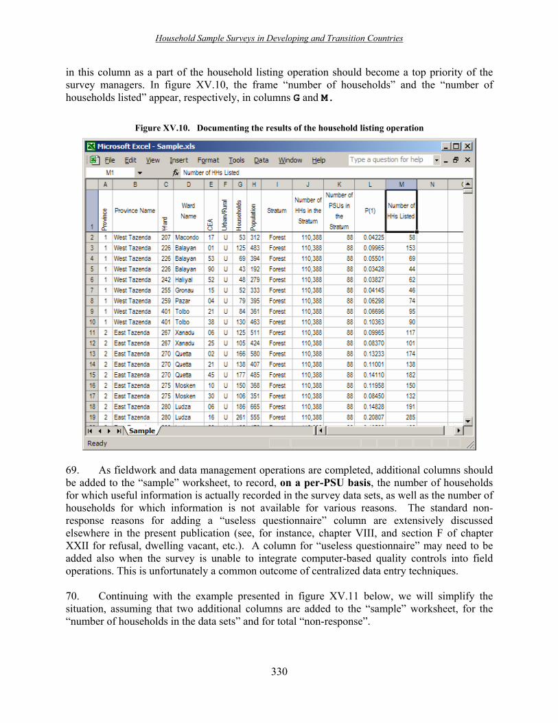
Household Sample Surveys in Developing and Transition Countries
330
in this column as a part of the household listing operation should become a top priority of the survey managers. In figure XV.10, the frame �number of households� and the �number of households listed� appear, respectively, in columns G and M.
Figure XV.10. Documenting the results of the household listing operation
69. As fieldwork and data management operations are completed, additional columns should be added to the �sample� worksheet, to record, on a per-PSU basis, the number of households for which useful information is actually recorded in the survey data sets, as well as the number of households for which information is not available for various reasons. The standard non-response reasons for adding a �useless questionnaire� column are extensively discussed elsewhere in the present publication (see, for instance, chapter VIII, and section F of chapter XXII for refusal, dwelling vacant, etc.). A column for �useless questionnaire� may need to be added also when the survey is unable to integrate computer-based quality controls into field operations. This is unfortunately a common outcome of centralized data entry techniques. 70. Continuing with the example presented in figure XV.11 below, we will simplify the situation, assuming that two additional columns are added to the �sample� worksheet, for the �number of households in the data sets� and for total �non-response�.

Household Sample Surveys in Developing and Transition Countries
331
Figure XV.11. Documenting non-response
71. Although there are no universally accepted models for non-response, a very common assumption is that the �useful� households in the final data sets are in fact an equal-probability sample of all the households listed in their respective PSUs (see chaps. II and VIII for an extensive discussion). Under this hypothesis, the probability P(2) of selecting each of these households in the second stage can be computed by simply dividing the number of useful households by the number of households listed. The total selection probability of each household in the PSU is the product P(1)*P(2) and the sampling weight is the inverse of that probability. 72. These formulae can be easily implemented in the spreadsheet (see figure XV.12). Write formula =N2/M2 in cell P2, formula =L2*P2 in cell Q2 and formula =1/Q2 in cell R2; then copy them all the way down columns P, Q and R.

Household Sample Surveys in Developing and Transition Countries
332
Figure XV.12. Computing the second-stage probabilities and sampling weights
73. The probability-based weights computed in this way apply to all households in each PSU. Some survey practitioners may use �post-stratification� techniques to further adjust these weights in order to ensure that the survey estimates match certain known population distributions (such as age and gender distributions, or total consumption figures obtained from sources external to the sample survey itself). These adjustments are made with specialized software directly in the survey data sets, not in the sampling spreadsheets, and they generally operate on a per-household or per-person basis rather than on a per-PSU basis.
H. Summary of recommendations 74. This chapter has aimed at shedding some light on the relevance of incorporating data management criteria at every stage of a survey, as opposed to deeming it a matter integral only to the last analytical phases. One of the clearest cases in point are the Living Standards Measurement Study surveys, which have taken it upon themselves to design their questionnaires, plan and carry out field operations, and deal with data entry and processing in such a way as to allow the data to be properly managed even before any of them are collected. The guiding principles behind that effort constitute the core of this chapter; and even as they take on different characteristics according to the specific application in a given country, those principles may still be condensed and codified as follows:
(a) Survey data management begins with questionnaire design, and within it deals with:
(i) Proper identification of the statistical units. The recommendation is to use a simple or upgraded three- or four-digit serial numbers for the survey�s PSUs, and then
Household Sample Surveys in Developing and Transition Countries
333
a two-digit serial number for each household within it, plus proper serial identification of each subordinate unit within the household;
(ii) Built-in redundancies. The design of the questionnaire should include deliberate redundancies, intended to detect mistakes of the interviewer or data entry errors. Examples of this are a bottom line for totals or adding a check digit to the codes of important variables.
(b) During field operations, the following should be taken into account:
(i) Operational strategies for data entry and data editing. It is recommended that countries give careful consideration to the option of entering all data in the field. This may be done through a data entry operator working in a fixed location other than that of the surveyed households, by an operator joining the rest of the interviewing team and entering data directly to a laptop computer in each household or by the as yet not properly researched paperless interview method using a palmtop (though this needs more research). Entering all data in the field versus centralized entry will go a long way towards ensuring quality and consistency; (ii) Quality control criteria. The data on the questionnaires needs to be subjected to five different control mechanisms: range checks, checks against reference tables, skip checks, consistency checks and typographical checks; (iii) Data entry technology. According to a 1995 World Bank review, two reliable data entry and editing platforms suitable for complex household surveys were the World Bank�s internally developed LSMS package and the IMPS program of the United States Bureau of the Census. Their updated versions are LSD-2000 and the CSPro, respectively. Allowing for existing expertise and other factors affecting each country�s own set of conditions, there are a few basic guidelines that should be taken into account when designing data entry and editing tools: exceptions aside, computer screens should resemble their corresponding questionnaire sections; data entry programs should discern impossible and unlikely situations and specifically flag each; error-type reporting language and expressions should be colloquial and easily understood; (iv) Organizing and disseminating the survey data sets. For these purposes, flat files are not suitable, since they do not deal properly with subordinate statistical units (persons, crops, consumption items, etc.) within the household. A structure with a different record type for each kind of statistical unit is to be preferred.
(c) Finally, data management may also prove instrumental in implementing the sampling
protocol, by guiding it through its main stages: organization of the first-stage sampling frame, usually created from the latest available set of census enumeration areas (CEAs); selection of primary sampling units with probability proportional to size, measured by the number of households, dwellings or the size of the population; and calculation of selection probabilities and the corresponding sampling weights.

Household Sample Surveys in Developing and Transition Countries
334
References Ainsworth, M., and J. Muñoz (1986). The Côte d'Ivoire Living Standards Survey: Design and
Implementation. Living Standards Measurement Study Working Paper, No. 26. Washington, D.C.: World Bank.
Blaizeau, D. (1998). Seven expenditure surveys in the West African Economic and Monetary
Union. In Proceedings of the Joint International Association of Survey Statisticians/International Association for Official Statistics (IASS/IAOS) Conference on Statistics for Economic and Social Development. Aguascalientes, Mexico: International Statistical Institute.
__________, and J.L. Dubois (1990). Connaître les Conditions de Vie des Ménages dans les
Pays en Développement. Paris: Documentation française. Blaizeau, D, and J. Muñoz (1998). LSD-2000. Logiciel de Saisie des Données: Pour Saisir les
Données d�une Enquête Complexe. Paris: Institut national de la statistique et des études économiques.
Grosh, M. and J. Muñoz (1996). A Manual for Planning and Implementing the Living Standards
Measurement Study Survey, Living Standards Measurement Study Working Paper, No. 126. Washington, D.C.: World Bank.
Muñoz, J. (1989). Data management of complex socioeconomic surveys: from questionnaire
design to data analysis. In Proceedings of the 47th Session of the International Statistical Institute. Paris: International Statistical Institute.
__________ (1996). Cómo mejorar la calidad de la información: opciones para mejorar la
organización del trabajo de campo, el sistema de entrada de datos, el análisis de consistencia y el manejo de la base de datos. In Reunión de Iniciación del Programa para el Mejoramiento de las Encuestas de Condiciones de Vida en América Latina y El Caribe. Asunción: Inter-American Development Bank.
__________ (1998). Budget-Consumption Surveys: New Challenges and Outlook. In
Proceedings of the Joint International Association of Survey Statisticians/International Association for Official Statistics (IASS/IAOS) Conference on Statistics for Economic and Social Development. Aguascalientes, Mexico: International Statistical Institute.
United States Bureau of the Census. CSPro Census and Survey Processing System, available
from http://www.census.gov/ipc/www/cspro/.

Household Sample Surveys in Developing and Transition Countries
335
Chapter XVI Presenting simple descriptive statistics from household survey data
Paul Glewwe Department of Applied Economics
University of Minnesota St. Paul, Minnesota, United States of America
Michael Levin United States Bureau of the Census
Washington, D.C., United States of America
Abstract
The present chapter provides general guidelines for calculating and displaying basic descriptive statistics for household survey data. The analysis is basic in the sense that it consists of the presentation of relatively simple tables and graphs that are easily understandable by a wide audience. The chapter also provides advice on how to put the tables and graphs into a general report intended for widespread dissemination. Key terms: descriptive statistics, tables, graphs, statistical abstract, dissemination.

Household Sample Surveys in Developing and Transition Countries
336
A. Introduction 1. The true value of household survey data is realized only when the data are analysed. Data analysis ranges from analyses encompassing very simple summary statistics to extremely complex multivariate analyses. The present chapter serves as an introduction to the next four chapters and, as such, it will focus on basic issues and relatively simple methods. More complex material is presented in the four chapters that follow. 2. Most household survey data can be used in a wide variety of ways to shed light on the phenomena that are the main focus of the survey. In one sense, the starting point for data analysis is basic descriptive statistics such as tables of the means and frequencies of the main variables of interest. Yet, the most fundamental starting point for data analysis lies in the questions that the data were collected to answer. Thus, in almost any household survey, the first task is to set the goals of the survey, and to design the survey questionnaire so that the data collected are suitable for achieving those goals. This implies that survey design and planning for data analysis should be carried out simultaneously before any data are collected. This is explained in more detail in chapter III. The present chapter will focus on many practical aspects of data analysis, assuming that a sensible strategy for data analysis has already been developed following the advice given in chapter III. 3. The organization of this chapter is as follows. Section B reviews types of variables and simple descriptive statistics; section C provides general advice on how to prepare and present basic descriptive statistics from household survey data; and section D makes recommendations on how to prepare a general report (often called a statistical abstract) that disseminates basic results from a household survey to a wide audience. The brief final section offers some concluding remarks.
B. Variables and descriptive statistics 4. Many household surveys collect data on a particular topic or theme, while others collect data on a wide variety of topics. In either case, the data collected can be thought of as a collection of variables, some of which are of interest in isolation, while others are primarily of interest when compared with other variables. Many of the variables will vary at the level of the household, such as the type of dwelling, while others may vary at the level of the individual, such as age and marital status. Some surveys may collect data that vary only at the community level; an example of this is the prices of various goods sold in the local market.27 5. The first step in any data analysis is to generate a data set that has all the variables of interest in it. Data analysts can then calculate basic descriptive statistics that let the variables 27 In most household surveys, the household is defined as a group of individuals who: (a) live in the same dwelling; (b) eat at least one meal together each day; and (c) pool income and other resources for the purchase of goods and services. Some household surveys modify this definition to accommodate local circumstances, but this issue is beyond the scope of this chapter. �Community� is more difficult to define, but for the purposes of this chapter, it can be thought of as a collection of households that live in the same village, town or section of a city. See Frankenberg (2000) for a detailed discussion of the definition of �community�.

Household Sample Surveys in Developing and Transition Countries
337
�speak for themselves�. There are a relatively small number of methods of doing so. The present section explains how this is done. It begins with a brief discussion of the different kinds of variables and descriptive statistics, and then discusses methods for presenting data on a single variable, methods for two variables, and methods for three or more variables.
1. Types of variables 6. Household surveys collect data on two types of variables, �categorical� variables and �numerical� variables. Categorical variables are characteristics that are not numbers per se, but categories or types. Examples of categorical variables are dwelling characteristics (floor covering, wall material, type of toilet, etc.), and individual characteristics such as ethnic group, marital status and occupation. In practice, one could assign code numbers to these characteristics, designating one ethnic group as �code 1�, another as �code 2�, and so on, but this is an arbitrary convention. In contrast, numerical variables are by their very nature numbers. Examples of numerical variables are the number of rooms in a dwelling, the amount of land owned, or the income of a particular household member. Throughout this chapter, the different possible outcomes for categorical variables will be referred to as �categories�, while the different possible outcomes for numerical variables will be referred to as �values�. 7. When presenting data for either type of variable, it is useful to make another distinction, regarding the number of categories or values that a variable can take. If the number of categories/values is small, say, less than 10, then it is convenient (and informative) to display complete information on the distribution of the variable. However, if the number of values/categories is large, say, more than 10, it is usually best to display only aggregated or summary statistics concerning the distribution of the variable. An example will make this point clear. In one country, the population may consist of a small number of ethnic groups, perhaps only four. For such a country, it is relatively easy to show in a simple table or graph the percentage of the sampled households that belong to each group. Yet, in another country, there may be hundreds of ethnic groups. It would be very tedious to present the percentage of the sampled households that fall into each of, say, 400 different groups. In most cases, it would be simpler and sufficiently informative to aggregate the many different ethnic groups into a small number of broad categories and display the percentage of households that fall into each of these aggregate categories. 8. The example above used a categorical variable, ethnic group, but it also applies to numerical variables. Some numerical variables, such as the number of days a person is ill in the past week, take on only a small number of values and so the entire distribution can be displayed in a simple table or graph. Yet many other numerical variables, such as the number of farm animals owned, can take on a large number of values and thus it is better to present only some summary statistics of the distribution. The main difference in the treatment of categorical and numerical variables arises from how to aggregate when the number of possible values/categories becomes large. For categorical variables, once the decision not to show the whole distribution has been made, one has no choice but to aggregate into broad categories. For numerical variables, it is possible to aggregate into broad categories, but there is also the option of displaying summary statistics such as the mean, the standard deviation, and perhaps the

Household Sample Surveys in Developing and Transition Countries
338
minimum and maximum values. The following subsection provides a brief review of the most common descriptive statistics.
2. Simple descriptive statistics 9. Tables and graphs can provide basic information about variables of interest using simple descriptive statistics. These statistics include, but are not limited to, percentage distributions, medians, means, and standard deviations. The present subsection reviews these simple statistics, providing examples using household survey data from Saipan, which belongs to the Commonwealth of the Northern Mariana Islands and from American Samoa.
10. Percentage distributions. Household surveys rarely collect data for exactly 100, or 1,000 or 10,000 persons or households. Suppose that one has data on the categories of a categorical variable, such as the number of people in a population that are male and the number that are female, or data on a numerical variable, such as the age in years of the members of the same population. Presenting the numbers of observations that fall into each category is usually not as helpful as showing the percentage of the observations that fall into each category. This is seen by looking at the first three columns of numbers in table XVI.1. Most users would find it more difficult to interpret these results if they were given without percentage distributions. The last three columns in table XVI.1 are much easier to understand if one is interested in the proportion of the population that is male and the proportion that is female for the different age groups. Of course, one may be interested in column percentages, that is to say, the percentage of men and the percentage of women falling into different age groups. This is shown in table XVI.2. (A third possibility is to show percentages that add up to 100 per cent over all age by sex categories in the table, but this is usually of less interest.) Both tables show that percentage distributions can be shown for either categorical or numerical variables.
Table XVI.1. Distribution of population by age and sex, Saipan, Commonwealth of the
Northern Mariana Islands, April 2002: row percentages
Numbers Row percentages Broad age group, in years Total Male Female Total Male FemaleTotal persons 67 011 29 668 37 343 100.0 44.3 55.7 Less than 15 16 915 8 703 8 212 100.0 51.5 48.5 15 to 29 18 950 5 765 13 184 100.0 30.4 69.6 30 to 44 20 803 9 654 11 149 100.0 46.4 53.6 45 to 59 8 105 4 458 3 648 100.0 55.0 45.0 60 years or over 2 239 1 088 1 150 100.0 48.6 51.4Source: Round 10 of the Commonwealth of the Northern Mariana Islands Current Labour-force Survey. Note: Data are from a 10 per cent random sample of households and all persons living in collectives.

Household Sample Surveys in Developing and Transition Countries
339
Table XVI.2. Distribution of population by age and sex, Saipan, Commonwealth of the
Northern Mariana Islands, April 2002: column percentages
Numbers Column percentages Broad age group, in years Total Male Female Total Male FemaleTotal persons 67 011 29 668 37 343 100.0 100.0 100.0 Less than 15 16 915 8 703 8 212 25.2 29.3 22.0 15 to 29 18 950 5 765 13 184 28.3 19.4 35.3 30 to 44 20 803 9 654 11 149 31.0 32.5 29.9 45 to 59 8 105 4 458 3 648 12.1 15.0 9.8 60 years or over 2 239 1 088 1 150 3.3 3.7 3.1Source: Round 10 of the Commonwealth of the Northern Mariana Islands Current Labour-force Survey. Note: Data are from a 10 per cent random sample of households and all persons living in collectives.
11. It is clear from table XVI.1 that the sex distribution differs across the age groups. This reflects something that cannot be seen in tables XVI.1 and XVI.2, namely that Saipan has many immigrant workers � particularly female workers � employed in its garment factories. While Saipan has slightly more males than females at the youngest ages, the next age group, those 15-29 years, has only 30 males for every 70 females. Age group 30-44 also has more females than males. This is consistent with the fact that most of Saipan�s garment workers are women between the ages of 20 and 40. In the next group, those 45-59 years of age, there are more males than females. The column percentages in table XVI.2 show that the largest age group for males was that of 30-44, while the largest age group for females was that of 15-29, the age group of females most likely to work in the garment factories.
12. Medians. The two most common statistical measures for numerical variables are means and medians. (By definition, categorical variables are not numerical and thus one cannot calculate means and medians for such variables.) The median is the midpoint of a distribution, while the mean is the arithmetic average of the values. The median is often used for variables such as age and income because it is less sensitive to outliers. As an extreme example, let us assume that there are 99 people in a survey with incomes between $8,000 and $12,000 per year, and symmetrically distributed around $10,000. Thus, the mean and the median would be $10,000. Now suppose one more person with an income of $500,000 during the year is included, then, the mean would be about $15,000 while the median would still be about $10,000. For many income variables, published reports often show both the mean and the median.
13. Returning to the data from Saipan, the median age for the Saipan population was 28.5 years in April 2002, that is to say, half the population was older than 28.5 years and half was younger than 28.5 years. The female median age was lower than the male median age (27.6

Household Sample Surveys in Developing and Transition Countries
340
versus 30.5), because of the large number of young immigrant females working in the garment factories.
14. Means and standard deviations. As noted above, the mean is the arithmetic average of a numerical variable. Means are often calculated for the number of children ever born (to women), income, and other numerical variables. The standard deviation measures the average distance of a numerical variable from the mean of that variable, and thus provides a measure of the dispersion in the distribution of any numerical variable.
15. Table XVI.3 shows medians and means for annual income obtained from the 1995 American Samoa Household Survey. The survey was a 20 per cent random sample of all households in the territory. The fact that household mean income was higher than the median income is not surprising, since some households earned significantly higher wages and derived higher income from other sources. Tongan immigrants are relatively poor, as seen by their low mean and low median income; while the high mean and high median income of �other ethnic groups� indicate that they are relatively well off.
Table XVI.3. Summary statistics for household income by ethnic group, American Samoa,
1994 Other ethnic
Annual income Total Samoan Tongan Groups Number of households surveyed
8 367 7 332 244 790Median (United States dollars)
15 715 15 786 7 215 23 072Mean (United States dollars)
20 670 20 582 8 547 25 260 Source: 1995 American Samoa Household Survey. Note: Data are an unweighted, 20 per cent random sample of households.
3. Presenting descriptive statistics for one variable 16. The simplest case when presenting descriptive statistics from a household survey is that where only one variable is involved. The present subsection explains how this can be produced for both categorical and numerical variables. 17. Displaying the entire distribution. Categorical or numerical variables that take a small number of categories or values, say 10 or less, are the simplest to display. A table can be used to show the entire (percentage) distribution of the variable by presenting the frequency of each of the categories or numerical values of the variable. An example of this is given in table XVI.4, which shows the (unweighted) sample frequency counts and percentage distribution for the main sources of lighting among Vietnamese households. Many household surveys require the use of weights to estimate the distribution of a variable in the population, in which case showing the raw sample frequencies may be confusing and thus is not advisable; the use of weights will be discussed in section C below. (The survey from Viet Nam was based on a self-weighting sample

Household Sample Surveys in Developing and Transition Countries
341
and thus no weights were needed.) A final point is that it is also useful to report the standard errors of the estimated percentage frequencies (see chap. XXI for a detailed discussion of this issue, which is complicated by the use of weights and by other features of the sample design of the survey). 18. In some cases, the number of categories or values taken by a variable may be large, but the major part of the distribution is accounted for by only a few categories or values. In such cases, it may not be necessary to show the frequency of each category or value. One option to prevent the amount of information from taxing the patience of the reader of a table is to combine rare cases into a general �other� category. For example, any category or value with a frequency of less than 1 per cent could go into this category. Indeed, this is what was done in table XVI.4, where �other� includes rare cases such as torches and flashlights. In some cases, there may be other natural groups. For example, in many countries, ethnic and religious groups can be divided into a large number of distinct categories, but there may be a much smaller number of broad groups into which these more precise categories fit. In many cases, it will be sufficient to present figures only for the more general groups. The main exception to this rule concerns categories that may be of particular interest even though they occur rarely. In general, such �special interest but rare� categories could be reported separately, but it is especially important to show standard errors in such instances because the precision of the estimates is lower for rare categories. 19. In many cases, presentation of data can be made more interesting and more intuitive if it is displayed as a graph or chart instead of as a table. For a single variable that has only a small number of categories or values, a common way to display data graphically is in a column chart or histogram, in which the relative frequency of each category or value is indicated by the height of the column. Figure XVI.1 provides an example of this, using the data presented in table XVI.4. Another common way of displayinig of the relative frequency of the categories or values of a variable is the pie chart, which is a circle showing the relative frequencies in terms of the size of the �slices� of the pie. An example of this is given in figure XVI.2, which also displays the information given in table XVI.4. See Tufte (1983) and Wild and Seber (2000) for detailed advice on how to design effective graphs.
Table XVI.4. Sources of lighting among Vietnamese households, 1992-1993
Method
Number of households
Percentage of households (standard error)
Electricity
2 333 48.6 (0.7)
Kerosene/oil lamp
2 386 49.7 (0.7)
Other
81 1.7 (0.2)
Total households in sample 4 800 100.0 Source: 1992-1993 Viet Nam Living Standards Survey. Note: Data are unweighted.
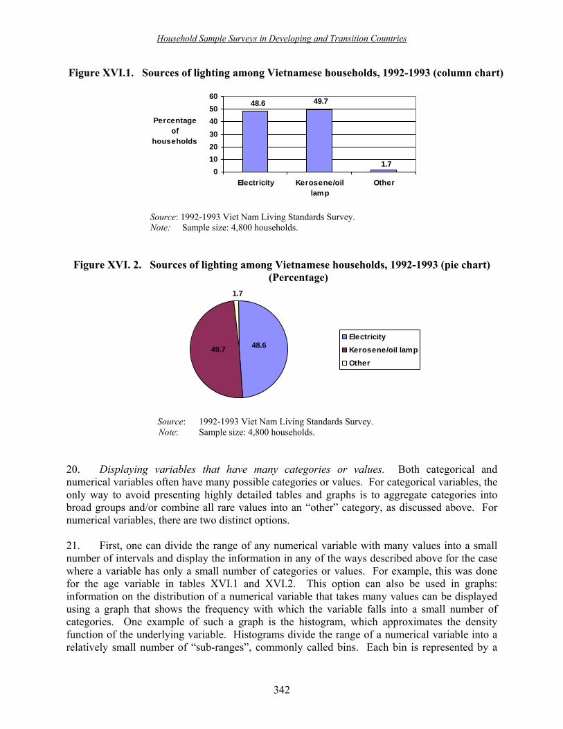
Household Sample Surveys in Developing and Transition Countries
342
Figure XVI.1. Sources of lighting among Vietnamese households, 1992-1993 (column chart)
1.7
49.748.6
0102030405060
Electricity Kerosene/oillamp
Other
Percentage of
households
Source: 1992-1993 Viet Nam Living Standards Survey. Note: Sample size: 4,800 households.
Figure XVI. 2. Sources of lighting among Vietnamese households, 1992-1993 (pie chart) (Percentage)
49.7
1.7
48.6 ElectricityKerosene/oil lampOther
Source: 1992-1993 Viet Nam Living Standards Survey. Note: Sample size: 4,800 households.
20. Displaying variables that have many categories or values. Both categorical and numerical variables often have many possible categories or values. For categorical variables, the only way to avoid presenting highly detailed tables and graphs is to aggregate categories into broad groups and/or combine all rare values into an �other� category, as discussed above. For numerical variables, there are two distinct options. 21. First, one can divide the range of any numerical variable with many values into a small number of intervals and display the information in any of the ways described above for the case where a variable has only a small number of categories or values. For example, this was done for the age variable in tables XVI.1 and XVI.2. This option can also be used in graphs: information on the distribution of a numerical variable that takes many values can be displayed using a graph that shows the frequency with which the variable falls into a small number of categories. One example of such a graph is the histogram, which approximates the density function of the underlying variable. Histograms divide the range of a numerical variable into a relatively small number of �sub-ranges�, commonly called bins. Each bin is represented by a

Household Sample Surveys in Developing and Transition Countries
343
column that has an area proportional to the percentage of the sample that falls in the sub-range corresponding to the bin. Figure XVI.3 does this for the age data in table XVI.2. The first bin is the sub-range from 0 to 14; the next is the sub-range from 15 to 29, and so on.28 Note that, unlike the column chart in figure XVII.1, there is no distance between the �columns� of the histogram. This is because the horizontal axis in a histogram depicts the range of the variable, and variables typically have no �gaps� in their range.
Figure XVI.3. Age distribution of the population in Saipan, April 2002 (histogram)
0
5
10
15
20
25
30
35
0-14 15-29 30-44 45-59 60-74 75-89 90-104
Age
Percentage of population
Source: Round 10 of the Commonwealth of the Northern Mariana Islands Current Labour-force Survey 22. The second, and perhaps most common, option for displaying a numerical variable that takes many values is to present some summary statistics of its distribution, such as its mean, median, and standard deviation. This can be done only by showing these statistics in a table; it is not possible to show summary statistics for a single numerical variable in a graph. In addition to the mean, median and standard deviation, it is also useful to present the minimum and maximum values, the values of the upper and lower quartiles,29 and perhaps a measure of skewness. An example of this is given in table XVI.5.
4. Presenting descriptive statistics for two variables.
23. Examination of the relationships between two or more variables often offers much more insight into the underlying topic of interest than examining a single variable in isolation. Yet, at the same time the possibilities for displaying the data increase by an order of magnitude. The
28 This histogram divides the population aged 60-99 into three groups (60-74, 75-89 and 90-104) each of which spans the same number of years, 15, as the population groups younger than 60. This is done to ensure that the area in each column of the histogram is proportional to the percentage of the population in each age group. 29 The lower quartile of a distribution is the value for which 25 per cent of the observations are less than the value and 75 per cent are greater than the value, and the upper quartile is the value for which 75 per cent of the observations are lower than the value and 25 per cent are higher than the value.

Household Sample Surveys in Developing and Transition Countries
344
present subsection describes common methods, distinguishing between variables that have a small number of categories or values and variables that take a large number of values.
24. Two variables with a small number of categories or values. The simplest case for displaying the relationship between two variables is that where both variables have a small number of categories or values. In a simple two-way tabulation, the categories or values of one variable can serve as the columns, while the categories or values of the other variable can serve as the rows. An example of this is shown in table XVI.6, which illustrates the use of different types of health service providers in urban and rural areas of Viet Nam. In this example, the columns sum to 100 per cent. As explained above, an alternative would be for the rows to sum to 100 per cent. In the example from Viet Nam, percentage figures that sum to 100 per cent across each row would indicate how the use of each type of health facility was distributed across urban and rural areas of Viet Nam. A third alternative would be for each �cell� of this table to give the frequency (in percentage terms) of the (joint) probability of a visit to a health-care facility by someone in a particular geographical region (urban or rural), in which case the sum of the percentages over all rows and columns would be 100 per cent. This is rarely used, however, since conditional distributions are usually more interesting. In any case, it is good practice to report sufficient data so that any reader can derive all three types of frequencies given the data provided in the table.
Table XVI.5. Summary information on household total expenditures: Viet Nam,
1992-1993 (Thousands of dong per year)
Mean 6 531 Standard deviation 5 375 Median 5 088 Lower quartile 3 364 Upper quartile 7 900 Smallest value 235 Largest value 100 478
Source: 1992-1993 Viet Nam Living Standards Survey. Note: Sample size: 4,799 households.
Table XVI.6. Use of health facilities among population (all ages) that visited a health facility in the past four weeks, by urban and rural areas of Viet Nam, in 1992-1993
Urban areas Rural areas
Place of consultation Frequency Percentage (std. error)
Frequency Percentage (std. error)
Hospital or clinic 251 45.0 (2.1) 430 25.0 (1.0) Commune health centre 30 5.4 (1.0) 318 18.5 (0.9) Provider�s home 213 38.2 (2.1) 595 34.6 (1.1) Patient�s home 50 9.0 (1.2) 376 20.1 (1.0) Other 14 2.5 (0.7) 29 1.7 (0.3) Total 558 100.0 1718 100.0
Source: 1992-1993 Viet Nam Living Standards Survey.

Household Sample Surveys in Developing and Transition Countries
345
25. There are several ways to use graphs to display information on the relationship between two variables that take a small number of values. When showing column or row percentages, one convenient method is to show several vertical columns that sum to 100 per cent. Each column represents a particular value of one of the variables, and the frequency distribution of the other variable is shown as shaded areas of each column. This is shown for the health facility data from Viet Nam in figure XVI.4. Spreadsheet software packages present many other variations that one could use.
Figure XVI.4. Use of health facilities among the population (all ages) that visited a health facility in the past four weeks, by urban and rural areas of Viet Nam, in 1992-1993
(Percentage)
5.418.5
38.234.6
20.1
45.025.0
2.5 1.7
0%10%20%30%40%50%60%70%80%90%
100%
Urban areas Rural areas
Other
Home of patient
Home of provider
Commune healthcenterHospital or clinic
9.0
Source: 1992-1993 Viet Nam Living Standards Survey. Note: Sample size: 2,276.
26. One variable with a small number of categories/values and a numerical variable with many values. Another common situation is one where there are two variables. One takes a small number of categories or values (perhaps after aggregating to reduce the number) and the other is a numerical variable that takes many values. Here the most common way to display the data is in terms of the mean of the numerical variable, conditional on each value of the variable that takes a small number of categories or values. One could also add other information, such as the median and the standard deviation. An example of this is seen in table XVI.7, which shows mean household total expenditure levels in Viet Nam in 1992-1993 with households being classified by the seven regions of that country. This could be put into a �profile plot� column graph, where each column (x-axis) represents a region and the lengths of the columns (y-axis) are proportional to the mean incomes for each region. 27. Another option is to transform the continuous variable into a discrete variable by dividing its range into a small number of categories. For example, it is sometimes convenient to divide households into the poorest 20 per cent, the next poorest 20 per cent, and so on, based on household income or expenditures. After this is done, one can use the same methods for displaying data for two discrete variables, as described above. A specific example is to modify figure XVI.4 to show five columns, one for each income quintile.

Household Sample Surveys in Developing and Transition Countries
346
28. Two numerical variables with many values. Statisticians often provide summary information on two numerical variables in terms of their correlation coefficient (the covariance of the two variables divided by the square root of the product of the variances). However, such statistics are often unfamiliar to a general audience. An alternative is to graphically display the data in a scatter-plot that has a dot for each observation. This could show, for example, the extent to which household income is correlated over two periods of time, using observations on the same households in two different surveys (one for each period of time).
Table XVI.7. Total household expenditures by region in Viet Nam, 1992-1993 (Thousands of dong per year)
Region Mean total expenditures
(standard errors in parentheses) Northern uplands 4 792 ( 95.5) Red River delta 5 306 (110.4) North central 4 708 (107.7) Central coast 7 280 (234.8) Central highlands 6 173 (373.7) South-east 10 786 (398.5) Mekong Delta 7 801 (167.4) All Viet Nam 6 531 (77.6)
Source: 1992-1993 Viet Nam Living Standards Survey. Note: Sample size: 4,799 households. 29. One problem with using scatter-plots is that when the sample size is large, the graph becomes too �crowded� to interpret easily. This can be avoided by drawing a random subsample of the observations (for example, one tenth of the observations) to keep the diagram from becoming too crowded. Another problem with scatter-plots is how to adjust them to account for sampling weights. One simple method is to create duplicate observations, with the sampling weight being the number of duplicates for each observation. This will almost certainly overcrowd the scatter-plot; hence after creating the duplicates, only a random subsample of the observations should be included in the scatter plot.
5. Presenting descriptive statistics for three or more variables
30. In principle, it is possible to display relationships between three or more variables using tables and graphs. Yet, this should be done rarely because it adds additional dimensions that complicate both the understanding of the underlying relationships and the methods for displaying them in simple tables or graphs. In practice, it is sometimes possible to show the descriptive relationships among three variables, but it is almost never feasible to show descriptive relationships among four or more variables.
31. For three variables, the most straightforward approach is to designate one variable as the �conditioning� variable. Either this variable will have a small number of discrete values or, if continuous, it will have to be �discretized� by calculating its distribution over a small number of

Household Sample Surveys in Developing and Transition Countries
347
intervals over its entire range. After this is done, separate tables or graphs can be constructed for each category or value of this conditioning variable. For example, suppose one is interested in showing the relationship among three variables: the education of the head of household, the income level of the household, and the incidence of child malnutrition. This could be done by generating a separate table or graph of the relationship between income and an indicator of children�s nutritional status (such as the incidence of stunting) for each education level. This may show, for example, that the association between income and child nutrition is weaker for households with more educated heads.
C. General advice for presenting descriptive statistics
1. Data preparation 32. Before any figures to be put into tables and graphs are generated, the data must be prepared for analysis. This involves three distinct tasks: checking the data to remove observations that may be highly inaccurate; generating complex (derived) variables; and thoroughly documenting the preparation of the �official� data set to be used for all analysis. In all three tasks, extra effort and attention to detail initially may save much time and many resources in the future. The present subsection presents a brief overview of these tasks; for a much more detailed treatment the reader should consult chapter XV. 33. Virtually every household survey, no matter how carefully planned and executed, will have some observations for some variables that do not appear to be credible. These problems range from item non-response (see chap. XI) and other clear errors -- for example, a three-year-old child who is designated as the head of household -- to much less clear cases, such as a household with very high income but an average level of household expenditures. In many cases, the errors are due to inaccurate data entry from paper questionnaires and so the paper questionnaire should be checked first. Such data entry errors can be easily fixed. If the strange data are on the questionnaire itself, there are several options. First, one could change the value of the variable to �missing�. If there are only a small number of such cases, those observations can be excluded when calculating any table or graph that uses that variable.30 If there are a large number of cases, the �missing� values can be calculated as a distinct category of a categorical variable, labelled �not reported� or �not stated�. Second, if most of the cases are concentrated in a small number of households, those households could be dropped. Third, if there are many questionable observations for many households for some variables, a decision may have to be made not to present results for that variable. 34. One approach to missing data is to �impute� missing values using one of several methods. Imputation methods assign values to unknown or �not reported� cases, as well as to cases with implausible values. Approaches include the hot deck imputation and nearest neighbour methods, which allow for a �best guess� for a response when none is available. The idea behind these methods is quite simple: households or people that are similar in some 30 This option has the disadvantage that the sample size will differ slightly for each table. While this could cause confusion, a note at the bottom of each table explaining that a few observations were dropped should provide sufficient clarification.
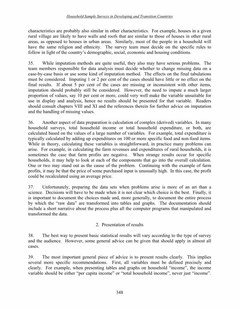
Household Sample Surveys in Developing and Transition Countries
348
characteristics are probably also similar in other characteristics. For example, houses in a given rural village are likely to have walls and roofs that are similar to those of houses in other rural areas, as opposed to houses in urban areas. Similarly, most of the people in a household will have the same religion and ethnicity. The survey team must decide on the specific rules to follow in light of the country�s demographic, social, economic and housing conditions. 35. While imputation methods are quite useful, they also may have serious problems. The team members responsible for data analysis must decide whether to change missing data on a case-by-case basis or use some kind of imputation method. The effects on the final tabulations must be considered. Imputing 1 or 2 per cent of the cases should have little or no effect on the final results. If about 5 per cent of the cases are missing or inconsistent with other items, imputation should probably still be considered. However, the need to impute a much larger proportion of values, say 10 per cent or more, could very well make the variable unsuitable for use in display and analysis, hence no results should be presented for that variable. Readers should consult chapters VIII and XI and the references therein for further advice on imputation and the handling of missing values. 36. Another aspect of data preparation is calculation of complex (derived) variables. In many household surveys, total household income or total household expenditure, or both, are calculated based on the values of a large number of variables. For example, total expenditure is typically calculated by adding up expenditures on 100 or more specific food and non-food items. While in theory, calculating these variables is straightforward, in practice many problems can arise. For example, in calculating the farm revenues and expenditures of rural households, it is sometimes the case that farm profits are negative. When strange results occur for specific households, it may help to look at each of the components that go into the overall calculation. One or two may stand out as the cause of the problem. Continuing with the example of farm profits, it may be that the price of some purchased input is unusually high. In this case, the profit could be recalculated using an average price. 37. Unfortunately, preparing the data sets when problems arise is more of an art than a science. Decisions will have to be made when it is not clear which choice is the best. Finally, it is important to document the choices made and, more generally, to document the entire process by which the �raw data� are transformed into tables and graphs. The documentation should include a short narrative about the process plus all the computer programs that manipulated and transformed the data.
2. Presentation of results 38. The best way to present basic statistical results will vary according to the type of survey and the audience. However, some general advice can be given that should apply in almost all cases. 39. The most important general piece of advice is to present results clearly. This implies several more specific recommendations. First, all variables must be defined precisely and clearly. For example, when presenting tables and graphs on household �income�, the income variable should be either �per capita income� or �total household income�, never just �income�.

Household Sample Surveys in Developing and Transition Countries
349
Complex variables such as income and expenditure should be defined clearly in the text and in footnotes to tables and graphs. Does income refer to income before or after taxes? Does it include the value of owner-occupied housing? Does income refer to income per week, per month or per year? This must be completely clear. For many variables, it is very useful to present in the text the wording in the household questionnaire from which the variable has been derived. For example, for data on adult literacy, it should be very clear how this variable has been defined. It may be defined by the number of years the person has attended school, or the person�s ability to sign his or her name, or the respondent�s statement that he or she can read a newspaper; or it may be based on some kind of test given to the respondent. Different definitions can give very different results. 40. A second specific recommendation regarding clarity is that percentage distributions of discrete variables should be very clear as to whether they are percentages of households or percentages of people (that is to say, of the population). In many cases, these will give different results. In many countries, better-educated individuals have relatively small families. This implies that the proportion of the population living in households with well-educated heads is smaller than the proportion of households that have a well-educated head. A third recommendation regarding clarity is that graphs should show the numbers underlying the graphical shapes. For example, the column chart in figure XVI.1 shows the percentages for each of three sources of lighting among Vietnamese households, and the same is true of the pie chart in figure XVI.2. 41. Finally, there are several other miscellaneous pieces of advice. First, reports should not present huge numbers of tables and a vast array of numbers in each table. Statistical agencies sometimes present hundreds of tables giving minute details that are unlikely to be of interest to most audiences, and a similar point often applies concerning the detail in a given table. Staff preparing reports should discuss the purpose of the various tables that are being prepared, and if little use can be perceived in presenting a particular table or the detailed information in a given table, then the extraneous information should be excluded. Second, estimates of sampling errors should be reported for a selection of the most important variables collected in the survey; in addition, it is highly useful to show the confidence intervals for key variables or indicators. This is an obvious point, but it is often overlooked. It emphasizes the importance of conveying to the reader the degree of precision of the information provided by the household survey. Third, the sample sizes should be given for each table.
3. What constitutes a good table 42. The present subsection offers specific advice about preparing tables that present information from a household survey. When preparing tables and graphs, the following general principle applies: the information the tables include should be sufficient to enable the user to interpret them correctly without having to consult the text of the report. This is highly important because many users of reports photocopy tables and later use them without reference to the accompanying text.
43. The advice given below is general in nature. For any survey, the survey team must decide which conventions are most appropriate. Once the conventions are chosen, they should

Household Sample Surveys in Developing and Transition Countries
350
be very strictly followed. However, in some cases, divergence from the conventions may be necessary to illustrate specific points or to display specific types of statistical analyses. A final point regarding this subsection is that almost all of these guidelines for tables also apply to graphs. 44. The various parts of a good table are included in table XVI.6. Each table should contain: a clear title; geographical designators (when appropriate); column headers; stub (row) titles; the data source; and any notes that are relevant. 45. Title. The title should provide a succinct description of the table. This description should include: (a) the table number; (b) the population or other universe under consideration (including the unit of analysis, such as households or individuals; (c) an indication of what appears in the rows; (d) an indication of what appears in the columns; (e) the country or region covered by the survey; and (f) the year(s) of the survey. 46. Regarding the table number, most statistical reports number their tables consecutively, starting with table XVI.1, and continuing through to the last table. Sometimes countries use letters and numbers for different tables sets, for example, H01, H02, etc., for housing tables, and P01, P02, etc., for population tables. While this procedure is simple and straightforward, it has the disadvantage that reports become locked into the numbering, making additions or deletions very cumbersome. 47. The universe is the population or housing base covered by the table. If all of the population is included in the table, then the universe can be omitted from the title: the total population is assumed. In contrast, if a table encompasses a subpopulation such as persons in the labour force, and the potential labour force is defined as persons aged 10 years or over, then the title might contain the phrase � Population aged 10 years or over�. 48. The title of table XVI.6 also includes an indication of what appears in the rows and what appears in the columns of the table. In particular, it states that the table presents information on types of health facilities used (the rows) and shows this information separately for urban and rural areas (the columns). Including the country or region in the title makes the geographical universe immediately apparent. This feature is most important for researchers comparing results between countries. Obviously, the country statistical office collecting the data will know its own country name; but persons using tables from different countries may need this information in order to distinguish between the countries.
49. Finally, the year(s) of the survey should be in the title to make the time frame immediately apparent. Sometimes, a country�s national statistics agency may want to show data from two or more different surveys in the same table. Then two dates may appear, for example �1990 and 2000� or �1980 through 2000�. The survey team must make a decision about whether it wants to write out a series of dates (for example, �1980, 1990 and 2000�, rather than the simpler, but less complete, �1980 through 2000�); once the decision has been made, however, the country should always follow its decision.

Household Sample Surveys in Developing and Transition Countries
351
50. Geographical designators. Whenever the same table is repeated for lower levels of geography, each table should have a geographical designator to clarify which table applies to which geographical region. For example, if table XVI.6 were repeated for each of Viet Nam�s seven regions, the name of the region could appear in parentheses in a second line immediately below the title of the table. �Non-geographical� designators could also be used. For example, a table might be repeated for major ethnic groups or nationalities.
51. Column headers. Each column of a table must be labelled with a �header�. Column headers can have more than one �level�; for example, in table XVI.6, the header for the first two columns is designated as �Urban areas� and the header for the last two is designated as �Rural areas�; and within both urban and rural areas, there are separate headers for the frequency of observations and for the percentage distribution of those observations. Another point pertains to columns of �totals� or �sums�, such as the first column of table XVI.3. The survey team should choose a convention with respect to where these columns will be placed. Traditionally, the total comes last, with all of the attributes shown first across the columns. However, if a table continues for multiple pages, with many columns of information, the survey team may prefer to have the total first (at the left) for the series of columns. When the total appears first, any user will immediately know the total for that series of columns, without having to page through all of the table.
52. Column headers and their associated columns of data should be spaced to minimize blank space on the page. Spacing of columns needs to take into account the number of digits in the maximum figures to appear in the columns, the number of letters in the names of the attributes appearing in the columns, and the total number of �spaces� allowed by the particular font being used. The font used is very important, and should be chosen early in the tabulation process.
53. Stub (row) titles. The survey team must also determine conventions to be used for stub (row) headings and titles. Stub �headings� should be left justified and only one variable should be listed on each line. Stub headings should consist of the names of variables displayed in the row. Stubs may include subcategories (nested variables). For example, a stub �group� may have two separate rows, one for male and one for female. Some conventions need to be established to distinguish between the different stub groups; the convention usually involves different indentation for different �levels� of variables.
54. Precision of numbers. Many tables suffer from presenting too many significant digits. When percentages are shown, it is almost always sufficient to include only one digit beyond the decimal point; presenting two or more digits rarely provides useful information and has three disadvantages: it distracts the reader, wastes space, and conveys a false sense of precision. Numbers with four or more digits rarely need any decimal point at all. When large numbers are displayed, they should appear in �thousands� or �millions,� so that no numbers of more than four or five digits appear.
55. Source. The source of the data should appear as the complete name of the survey, usually at the bottom of the table (as seen in table XVI.6). However, sometimes tabulations display more than one survey for a country, or surveys from more than one country. When this happens, the information in the sources becomes more important. The date should be included along with

Household Sample Surveys in Developing and Transition Countries
352
the name of the survey. If the source is a published report, it is useful to distinguish between the date of publication of the report and the year of data collection. For example, a country might have collected data in 1990, but published the data in 1992. Hence, the source might read �1990 Fertility Survey, 1992� with 1992 indicating the date of publication. 56. Notes. Notes provide immediate information with which to properly interpret the results shown in the table. For example, the notes to tables XVI.1 and XVI.2 indicate that the sampled population includes all persons living in either individual dwellings or collectives. In addition to notes at the bottom of a table, a series of definitions and explanations might appear in the text accompanying the tables. The text would include the definitions of the characteristics, for example, it would indicate that the birthplace referred to the mother�s living quarters just prior to going to the hospital to deliver, rather than to the hospital location. The text might also include explanations regarding how the data were obtained or are to be used. For example, if the date of birth and age were both collected, but date of birth superseded age when they were inconsistent, this information might assist certain users, like demographers, in assessing the best method of interpreting the data.
4. Use of weights
57. The present subsection provides a brief overview of the use of weights when producing tables and graphs using household survey data. For much more detailed treatment, see chapters II, VI, XIX, XX and XXI and the references therein. 58. With respect to survey weighting, the simplest type of household survey sample design is the �self-weighted� type. In such a case, no weights need actually be used in the analysis because each household in the population has the same probability of being selected in the sample. The 1992-1993 Viet Nam Living Standards Survey used in several of the examples in this chapter was such a survey. Yet, variation in response rates across different types of households usually implies that weights should be calculated to correct for such variation. More importantly, most household surveys are not self-weighted because they draw disproportionately large samples for some parts of the population that are of particular interest. For these surveys, weights must be used to reflect the differential probabilities of selection in order to properly calculate unbiased estimates of the characteristics of interest to the survey. 59. Accurate weights must incorporate three components. The first encompasses the �base weights� or �design weights�. These account for variation in the selection probabilities across different groups of households (that is to say, when the sample is not self-weighting) as stipulated by the survey�s initial sample design. The second component is adjustment for variation in non-response rates. For example, in many developing countries, wealthier households are less likely to agree to be interviewed than are middle-income and lower-income households. The base weights need to be �inflated� by the inverse of the response rate for all groups of households. Finally, in some cases, there may be �post-stratification adjustments�. The rationale for post-stratification is that an independent data source, such as a census, may provide more precise estimates of the distribution of the population by age, sex and ethnic group. If the survey estimates of these distributions do not closely correspond to those of the independent source, the survey data may be re-weighted to force the two distributions to agree.

Household Sample Surveys in Developing and Transition Countries
353
For a more detailed account of the second and third components, see Lundström and Särndal (1999).
D. Preparing a general report (abstract) for a household survey 60. Most household surveys first disseminate their results by publishing a general report which contains a modest amount of detail on all of the information collected in the survey. Such reports usually have much wider circulation than do more specialized reports that make full use of certain aspects of the data. These general reports are sometimes called �statistical abstracts�. The present section provides some specific recommendations for producing these reports, based on Grosh and Muñoz (1996).
1. Content 61. The main material in any general statistical report is a large number of tables and graphs. They should reflect all of the main kinds of information collected in the survey; in-depth analysis of more narrow topics should be left to more focused special reports. A small amount of text should accompany the tables, just enough to clarify the type of information in those tables. There is no need to draw particular policy conclusions, although possible interpretations can be suggested as fruitful areas for future research. 62. The most basic information can be broken down by geographical regions, by sex and, perhaps, by age. If the survey contains income or expenditure data, they can also be broken down by income or expenditure groups. In some countries, there will be large differences across these different groups, and the nature of these differences can be explored further in additional tables. In other countries, some of these differences will not be very large, so there will be no need to present more detail. 63. In addition to the results from the household survey data, the general report should have several pages describing the survey itself, including the sample size and the design of the sample, the date of the survey�s start and the date of its termination, and some detail on how the data were collected. The questionnaire or questionnaires used should be included as an annex to the main report.
2. Process 64. A good general statistical report is produced by a team of people, several of whom will ideally have had experience on previous reports. Some team members will focus on the technical aspects of generating tables and graphs, while others will mainly be responsible for the content and the text accompanying the tables. The more technically-oriented team members can choose the statistical software with which they are most familiar, since most statistical software are able to produce the figures needed for the tables and graphs. However, estimation of standard errors will likely require software specifically designed for that purpose, since household survey sample designs are virtually always too complex to be handled properly by standard statistical software packages (see chapter XXI for a discussion of these issues).

Household Sample Surveys in Developing and Transition Countries
354
65. The team members responsible for the content should meet with experts in government agencies regarding the topics to be included in the report. This will ensure that the tables and graphs present the data in a form most useful to those agencies. It might prove useful as well to consult international aid agencies, which could also find the data useful in planning their programmes (see chap. III for a more general discussion of how to form an effective survey team).
E. Concluding comments 66. This chapter has provided an introduction to the presentation of simple descriptive statistics using household survey data. The treatment has been very general, and undertaken at a very basic level. As much of what has been presented constitutes little more than common sense, data analysts should use their own common sense when facing particular issues regarding the analysis of their surveys. More sophisticated methods can also be used to analyse household survey data, some of which are discussed in later chapters. All things considered, the data analysis for any given household survey will have to be tailored to the main topics and objectives of the survey, and researchers will have to consult specialized books and journals to obtain guidance on issues specific to those topics. References Frankenberg, Elizabeth (2000). Community and price data. In Designing Household Survey
Questionnaires for Developing Countries: Lessons from 15 Years of the Living Standards Measurement Study, M. Grosh and P. Glewwe, eds. New York: Oxford University Press, for the World Bank.
Grosh, Margaret, and Juan Muñoz (1996). A Manual for Planning and Implementing the Living
Standards Measurement Study Survey�. Living Standards Measurement Study Working Paper, No. 126. Washington, D.C.: World Bank.
Lundström, S., and C. E. Särndal (1999). Calibration as a standard method for the treatment of
non-response in sample surveys�, Journal of Official Statistics, vol. 13, No. 2, pp. 305-327.
Tufte, Edward (1983). The Visual Display of Quantitative Information. Cheshire, Connecticut:
Graphics Press. Wild, C. J., and G. A. F. Seber (2000). Chance Encounters: A First Course in Data Analysis and
Inference. New York: Wiley.

Household Sample Surveys in Developing and Transition Countries
355
Chapter XVII Using multi-topic household surveys to improve poverty reduction policies in
developing countries
Paul Glewwe Department of Applied Economics
University of Minnesota St. Paul, Minnesota, United States of America
Abstract
The present chapter shows how household surveys can be used by researchers and government officials in developing countries to formulate policies to reduce poverty. It begins with relatively simple descriptive analyses, highlighting the key contribution of household survey data: they provide information on who is poor and on the characteristics of the poor. The chapter then discusses more complex multivariate analyses, which are based on multiple regression techniques. For each type of analysis, examples are provided on how household survey data can be used to formulate policies to reduce poverty. Key terms: Poverty, policy formulation, descriptive analyses, multivariate analyses.

Household Sample Surveys in Developing and Transition Countries
356
A. Introduction 1. Almost all developing countries accept the fact that a primary objective of economic and social development is the reduction, and eventual elimination, of poverty. While all Governments may have the same goal, the policies they implement to reduce poverty should not necessarily be the same. The nature of poverty, and the characteristics of the poor, will vary from one country to another, hence the appropriate policies should also vary. 2. The present chapter is much too brief to discuss in detail the many ways in which government policies can affect poverty in developing countries. See Lipton and Ravallion (1995) and World Bank (2001) for recent detailed treatments. Yet a general overview can be provided, and for the purposes of this chapter, it is convenient to divide government policies into four broad types. The first type comprises macroeconomic policies, which are economy-wide policies that have implications for economic growth and stability. The most important macroeconomic policies are the overall level of taxation and government spending, monetary policies (which influence interest rates and the inflation rate), international economic policies (which affect the exchange rate, foreign trade and foreign capital flows), and policies regarding banks and other financial institutions. The second type of government policies comprises those that affect prices, such as taxes and subsidies on specific goods and services. Government provision of public services and infrastructure, such as health clinics, schools and transportation and communication networks, represents the third general type of government policy. The last type comprises government programmes designed to provide direct assistance to the poor. Examples of these policies are Mexico�s Programa de Educación, Salud y Alimentación (PROGRESA), which provides cash grants to poor families if their children regularly attend school, and Jamaica�s food stamp programme, which provides poor families with vouchers that can be used to purchase food items in local shops. All four types of policies can have important effects on poverty. 3. The impact on poverty of any of these types of policies depends on the characteristics and behaviour of the poor and, in some cases, on the characteristics and behaviour of the non-poor population. For example, the impact on poverty of government subsidies for specific food items, which should lower the price of those items, depends on the extent to which the poor purchase those items. This implies that Governments need information on the characteristics and behaviour of the poor in their countries in order to choose policies that are most effective in reducing poverty. Household surveys provide this crucial information. 4. Almost all developing countries, even the poorest, conduct some kinds of household surveys, such as income and expenditure surveys, labour-force surveys, and demographic and health surveys. These surveys provide a wealth of information that can be used to better understand the nature of poverty and the likely effects of government policies on the poor. This chapter shows how household surveys from developing countries can be used to formulate policies to reduce poverty. Section B begins by showing what can be learned from simple descriptive statistics calculated from survey data. Section C discusses more complex methods based on multivariate analysis and is followed by a brief concluding section.

Household Sample Surveys in Developing and Transition Countries
357
B. Descriptive analysis 5. To ensure that government policies and programmes intended to help the poor are effective, information is needed on whether the policies are indeed reaching the poor and on the effect those policies are having. Unfortunately, such information is often lacking in developing countries. For example, policies that increase economic growth may raise the incomes of certain occupations more than others. There then arises the question which occupations are most common among the poor. A similar point applies regarding pricing policies. The impact on the poor of government plans to increase taxes on, say, petroleum products depends on whether poor households consume significant amounts of those products. The same issue arises regarding whether new schools or health clinics should be built in certain areas of the country: this raises the question whether those areas have a relatively high concentration of poor households. Finally, for any programme that provides direct benefits to the poor, whether services or in-kind or monetary transfers, programme administrators would like to know what proportion of the programme beneficiaries are poor, and what proportion of the poor benefit from the programme. 6. Unfortunately, many developing countries have little information about the location and characteristics of the poor, and thus they have very little idea about the extent to which the poor benefit from, or are harmed by, government policies and programmes. Household surveys can fill many of these information gaps. The present section discusses how this can be achieved, using many examples from developing countries. Although many of the uses of household survey data to understand poverty are very simple, amounting to the production of simple tables and graphs, this type of information is often much more useful than what can be obtained from more sophisticated analyses.
1. Defining poverty 7. Before investigating the impact of government policies on the poor, one must be clear on who is poor, which in turn requires a definition of poverty. People do not always agree on what poverty is. However, there is general agreement that there exists, in principle, a minimal "decent" standard of living that individuals and households should be able to attain if they are to have the opportunity to live a fulfilling life. Most discussions of poverty focus on material necessities, as opposed to political freedoms, human rights, and psychological well-being, and this chapter will do the same. The material necessities that are most obvious, and thus for which there is a large degree of consensus, are: (a) adequate diet; (b) basic shelter/housing; and (c) potable water and sanitary means of waste disposal. Most observers would also add basic education opportunities and simple preventative health care. Some would argue for an even larger "bundle" of goods and services, adding, for example, cultural or recreational activities, but on this point there is less consensus on what to include, or even whether to include these types of goods and services. 8. Philosophers, economists and other social scientists can, and often have, spent large amounts of time debating what is the appropriate minimal bundle of goods and services that an individual or household should have in order not to be considered poor. Once a bundle of goods and services is agreed upon, lack of consumption of particular components of the bundle can be used as an �indicator� of poverty. A more practical approach, taken by many economists, is to

Household Sample Surveys in Developing and Transition Countries
358
point out that almost all of the items in the bundle cost money, so that the real issue becomes not the exact composition of the bundle but its monetary cost. This approach sets a �poverty line� in terms of a given amount of money and then defines as poor any household whose income or expenditures are less than that amount. In fact, the starting point for many monetary poverty lines used in developing countries is a bundle of goods and services that meets minimal requirements. For example, one component would be a bundle of food items that meets minimal nutritional needs, and that also reflects national food consumption patterns. The next step would be to calculate the cost of this bundle. The remainder of this chapter will assume that this approach is followed; for a more detailed treatment of how such a poverty line can be drawn, see Ravallion (1998).
2. Constructing a poverty profile
9. Once a workable definition of poverty has been set in terms of household income or household expenditure, a description of the poor can be constructed using household survey data. Such a description is often called a �poverty profile�. This is carried out by using income and/or household expenditure data in the household survey to calculate each household�s total purchasing power (total income or total expenditures). The poor are defined as those households whose purchasing power is lower than the poverty line. 10. The above paragraph contains an implicit lesson and an implicit question. The lesson is that poverty analysis requires household survey data that include reasonably accurate information on total household income and/or total household expenditure. Without such data, poverty analysis is difficult because some other way will have to be found of classifying households as poor or non-poor. While some useful information could probably be obtained from a survey without such data, much more can be learned from household surveys that collect income and/or expenditure data. The question is, If one has a survey with both income and expenditure data, which should one use? In general, expenditure data are preferred because they are usually more accurate than income data and because consumption expenditures are, in theory, more closely tied to household welfare, since income is sometimes used to repay debts or to save for future consumption and, as such, does not necessarily reflect current welfare. 11. The first task when constructing a poverty profile is to describe who the poor are. Without household survey data, policy makers and other observers often have little idea of who the poor are and what characteristic they have. Even worse, some perceptions that they do have may be inaccurate. For example, many government officials and other observers spend most of their time in large urban areas and think of the poor in terms of what they see in those areas, yet in virtually all countries the incidence of poverty is much higher in rural areas. Thus, the first task in using household survey data is to estimate the incidence of poverty, describe the location of the poor in terms of urban versus rural areas and by region of the country, and calculate some basic characteristics of the poor. It is important to check the rates of poverty by ethnic and religious groups, by level of education, and by occupation. It is also useful to examine housing conditions among the poor, as well as ownership of any productive assets. With this and other information, one can begin to provide useful advice to policy makers.

Household Sample Surveys in Developing and Transition Countries
359
12. An example of some basic characteristics of the poor comes from a recent World Bank (1999) report on poverty in Viet Nam, where 37 per cent of the population were estimated to be poor in 1998. In Viet Nam, 79 per cent of the poor work in agricultural occupations; and almost all of them are self-employed. Another basic fact is that poverty is much higher among ethnic minority groups: although minority groups constitute only 14 per cent of the general population, they constitute 29 per cent of the poor in Viet Nam. 13. One of the most important characteristics of the poor is where they live. Ideally, policy makers would like to know the incidence of poverty in every city, town and rural district. Unfortunately, the sample size of a typical household survey is usually between 3,000 and 15,000 households, which is too small to provide precise estimates of poverty at such a disaggregated level. Yet if recent census data are also available, it is possible to combine those data with household survey data to obtain estimates of poverty for much smaller geographical areas. The basic idea is to estimate the relationship between various �predictor� variables and household income or expenditure, using the household survey data. The predictor variables used are variables that are also found in the census. The fact that, with an estimate of the predictive relationship, the census data can be used to simulate the distribution of expenditures in relatively small geographical areas, allows one to estimate the incidence of poverty in those areas. An example of this using data from Ecuador is Hentschel and others (1998). For more detailed discussions of the methods used, see Rao (2002) and Kalton (2002). 14. A final important point regarding the definition of poverty and the construction of poverty profiles is that one often wants to compare poverty at different points in time for the same country, or at the same point in time for different countries. When doing so, it is important that the data from the household survey used to define expenditures or income be collected in the same way over time or across countries. Very small differences in questionnaire design or other changes in the method of collecting the data can often lead to significant but completely spurious changes in the estimates, often in unanticipated ways. To be frank, it may not be possible to make such comparisons if the data collected or the way in which the data are analysed, or both, are not the same in the surveys being compared. Thus any changes in the way the data are collected for the variables that define poverty must be considered very carefully, in order to limit the potential for observed changes to be due merely to statistical procedures as opposed to actual change. Thus, it is usually best not to change the way in which the data are collected in any significant way.
3. Using poverty profiles for basic policy analysis 15. Knowledge of the location of the poor and some of their basic characteristics is the starting point for providing advice to policy makers. Of course, specific programmes to assist the poor must be located where the poor are most heavily concentrated, but much more can be accomplished, programmatically, if simple statistics about the poor are analysed properly. The present subsection describes four kinds of basic information on the poor that can be used to draw lessons on the impact of various policies on the poor.

Household Sample Surveys in Developing and Transition Countries
360
16. How the poor earn income. As explained above, one of the ways that government policies affect the poor is by affecting the incomes they earn. Thus an important question is what the poor do to earn a living. Perhaps the first question to ask is whether the poor are self-employed, as opposed to earning wages by working for an employer. In many countries, the vast majority of the poor are self-employed farmers, craftsmen or traders. By definition, those poor who are self-employed will not be directly affected by policies that affect wage earners, such as changes in minimum wage laws or the implementation of a �social security� or health insurance scheme that applies only to wage earners. 17. Because many of the poor are self-employed farmers, an important question is, What crops do they produce, and how much of what they produce is sold? A specific example of this comes from Côte-d�Ivoire. Glewwe and de Tray (1990) found that many poor Ivorian farmers produce cotton, while cotton production among non-poor farmers was quite rare. Thus government policies that affect the price of cotton will primarily affect the poor in that country. 18. Consumption patterns of the poor. The economic well-being of the poor is also determined by the prices of the goods and services that they consume. For example, in Ghana, less than 1 per cent of the poorest 20 per cent of the population own either a motorbike or an automobile (Glewwe and Twum-Baah, 1991). This implies that there will be little direct effect of an increase in the price of gasoline on poor Ghanaians, although there may be an indirect effect owing to rising public transportation costs. 19. More generally, data on the consumption of food and non-food items, and on the availability of electricity and piped water, provide a wealth of information for policy makers to consider. When a tax or subsidy is being considered on a particular type of good, the data should be examined to see to what extent the poor will be affected. Note also that exchange-rate policies will also affect prices, hence the extent to which the poor consume imported goods is also of interest. The example of Ghana given directly above is a case in point: all of Ghana�s petroleum products are imported. 20. Services used by the poor. Subsidies to health and education are often justified, at least in part, by the benefits that they provide to the poor. However, there are many kinds of health services and many different types and levels of education. Data on who uses those services provide an opportunity to check the poverty status of the beneficiaries of specific policies. 21. A recent example of this is from Viet Nam. Gertler and Litvack (1998) found that the typical person in the poorest 20 per cent of the population made about one outpatient visit per year to a government hospital and about two outpatient visits per year to a commune health centre. In contrast, a typical person in the wealthiest 20 per cent of the population made four or five outpatient visits per year to a government hospital and only about one outpatient visit to a commune health centre. The main reason for the disparity is that government hospitals are found primarily in urban areas, while about 90 per cent of the poor in that country live in rural areas. The obvious implication of these simple figures is that subsidies to commune health centres benefit the poor more than the non-poor, while subsidies to hospitals benefit the non-poor much more than the poor.

Household Sample Surveys in Developing and Transition Countries
361
22. Programme participation. A final straightforward use of household survey data is to examine who participates in various government programmes that are intended to help the poor. This requires a household survey with one or more specific questions on households� participation in programmes, as well as income or expenditure data that can be used to classify households as poor or non-poor. While such data were rare in the past, they are becoming increasingly common as survey designers recognize their value. 23. An example of the use of a household survey to assess the targeting of a programme comes from Jamaica (Grosh, 1991). Household survey data showed that food stamps were, perhaps not surprisingly, much more likely to be used by poor households than by non-poor households. Paradoxically, the benefits of general food subsidies tended to go primarily to better-off households. This information was presented to the Government in the late 1980s; and in the early 1990s, the food stamp programme�s benefits were doubled while food subsidies were ended. 24. A final general point about basic descriptive analysis is that almost all household surveys are based on complex sample designs rather than random samples. Accordingly, subpopulation groups of particular interest, such as the poor, are oversampled, which implies that sampling weights must be used to obtain unbiased estimates of basic descriptive statistics. In addition, calculation of standard errors must take the sample design into account. As these points are discussed in more detail in chapter XVI and in other chapters of this book, the reader should consult those chapters before undertaking descriptive analysis.
C. Multiple regression analysis of household survey data 25. The above examples of the use of household surveys are based on very simple statistics which may be calculated by anyone who can use a simple statistical software package. Yet, the policy lessons drawn from them may be too simplistic in that they ignore behavioural responses to those policies. For example, if a tax is removed from a particular agricultural product because it is commonly produced by the poor, non-poor households may also start to produce that crop as its price increases, so that some of the benefits of the policy could go to non-poor households.31 Similarly, a tax on a particular type of food item may appear to have a large negative effect on the poor if they consume large amounts of that good; but if there is another similar good that is not taxed, the poor may simply switch to that good with only a small reduction in their welfare. Another example concerns education. The fact that poor children in a given country rarely attend upper secondary school suggests that there is little benefit to the poor of reducing the tuition fees for those kinds of schools, but it is possible that such a reduction in tuition will greatly increase enrolment of poor children in those schools. This possibility in turn implies that looking at current enrolment patterns would underestimate the benefit to the poor of such a policy.
31 When the tax is in place, the price received by producers will be lower than the price paid by consumers, the difference being the amount of the tax. When the tax is removed, the producer price will be equal to the consumer price; and in almost all cases, this means that the price received by producers will increase and the price paid by consumers will decrease.

Household Sample Surveys in Developing and Transition Countries
362
26. Household surveys can be used to estimate how household behaviour changes in response to policy changes. This is not an easy task because it requires much more sophisticated types of analysis. The most common methods used to carry out such estimation are those of multiple regressions analysis. The most sophisticated methods often use data from specially designed household surveys that collect the precise data needed to carry out such an analysis. This is necessary because these methods often require data that are not found in typical household surveys. The present section describes three common ways to use household survey data to estimate how policies can influence household behaviour. For a more detailed treatment, see Deaton (1997).
1. Demand analysis
27. Economists often estimate the impact of prices and household income on purchases of goods and services. Such research is called demand analysis. The general concept is that for any good (i), the purchases of that good (qi) by a household are determined by the income (y) of the household, the price (pi), of that good and the prices of all other goods. This can be expressed as
qi = f(y, p1, p2, �pi, �pn) + ε ≈ β0 + β1p1 + β2p2 + ... + βipi + � βnpn + βn+1y + ε.
The function f(y, p1, p2, �pi, �pn) is a very general representation of how income and prices affect household demand, where ε reflects the impact of other causal factors (and perhaps a random variation in qi that has nothing to do with any causal factors). A common simplification in demand analysis is to assume a linear representation, which is shown here by the term to the right of the �≈� symbol, which indicates that this simplification is an approximation. If ε is uncorrelated with y and the price variables, then simple ordinary least squares (OLS) can be used to obtain unbiased estimates of the coefficients (the β�s) of the income (y) and prices (pi) in this linear relationship. In actual applications, this assumption may not hold, and many other estimation issues could complicate the analysis. For further information on demand system estimation, the classic reference is Deaton and Muellbauer (1980). More recent treatments are found in Pollack and Wales (1992) and Lewbel (1997). 28. To perceive how demand analysis provides information beyond the information obtained using simple descriptive statistics, consider the impact of a tax on an imported foodstuff, such as wheat. (Developing economies often tax imported items because such taxes are relatively easy to administer; and the tropical climate in many developing countries would suggest that imports are the only source of wheat.) Suppose the current price of one kilogram of wheat flour is 10, and that the typical poor household consumes 60 kilograms of wheat flour per year. Assuming that the import price is fixed at the international price, a 50 per cent tax on wheat imports would raise the price of wheat flour to 15, which implies that the typical poor household would pay 300 (5×60) in additional taxes. Of course, this analysis based on simple descriptive statistics assumes that poor households will continue to purchase the same amount of wheat flour after the tax is imposed. In fact, it is likely that households will decrease consumption of wheat flour and increase consumption of other staple crops (such as rice, maize or cassava) in response to the increased price of wheat flour. Demand analysis estimates allow one to calculate the size of this behavioural response. Suppose that the equation in the previous paragraph depicts the demand for wheat, so that qi represents kilograms of wheat flour purchased by households per year and pi

Household Sample Surveys in Developing and Transition Countries
363
represents the price of one kilogram of wheat flour. If βi = -3, then an increase in the price of wheat flour by 5 will reduce consumption of wheat flour by 15, so that annual consumption of an average poor household would be 45 kilograms. This in turn implies that the average poor household would pay 225 (5×45) in additional taxes, instead of 300. While this example is quite simple, it points to the need to take account of household behaviour when examining the impact of specific policies.
29. An example of the use of demand analysis to analyse the impact of government policies on the poor is that of Deaton, Parikh and Subramanian (1994). The authors estimate a system of demand equations for over 10 different kinds of food items. They calculate the overall impact of increases in food prices on national social welfare, as well as the extent to which the changes affect the welfare of the poor. One particularly interesting result is that increases in the price of rice have less negative effects on the welfare of the poor than do increases in the price of coarse grains, since the poor are more dependent on the latter. Thus, taxes on rice hurt the poor less than do taxes on coarse grains.
2. Use of social services
30. Health and education programmes can provide many benefits to poor households, but participation does not necessarily imply that substantial benefits have been received. Some of those programmes may be ineffective. In the area of health, policy makers would like to know whether participation actually improved individuals� health status. In education, they would like to know how much children actually learned by attending school. Many studies have been conducted using household survey data from developing countries that attempt to investigate how successful health and education programmes are in attaining their objectives.
31. One recent example that illustrates the use of multiple regression is an analysis of the impact of specific school characteristics on student learning, and thereby on future wages. Glewwe (1999) examined this question by estimating the impact of school and household characteristics on children�s academic performance, as measured by test scores, using household survey data from Ghana. The equation utilized was of the following form:
Ti = β0 + β1MEDi + β2FEDi + β3yi + β4IQi + β5SC1i + β6SC2i + � + ε,
where Ti is the test score of child i, MEDi and FEDi are the education levels of the child i�s mother and father, respectively, yi is the income of child i�s household, and the SC variables represent a large number of school and teacher characteristics. Estimation of such an equation is quite complicated (see Glewwe, 2002); but once the β�s are estimated, they provide information on how different school and teacher characteristics affect student achievement. Comparing these impacts with the costs of the various school and teacher characteristics provides guidance on which types of education spending are most cost-effective.
32. Glewwe�s analysis of data from Ghana found that repairing leaking roofs in classrooms and providing blackboards in classrooms that do not have them significantly raised student achievement and school attainment (years spent in school). Simple calculations of the financial

Household Sample Surveys in Developing and Transition Countries
364
rates of return on such �investments� in school quality showed those rates of return to be very high, sometimes 25 per cent or more.
3. Impact of specific government programmes 33. While it is easy to use household survey data to examine whether a particular household or individual participates in some kind of programme designed to help the poor, it is harder to determine the extent to which their participation actually raises their welfare. The problem here is that participation may have other effects that reduce welfare. For example, a �food for work� programme may provide employment to poor individuals, but the benefits of the increased income must be weighed against the cost of working, including the impact of working on their health. Similarly, when households are provided with food stamps in order to raise their food consumption, it is not necessarily the case that their use of those stamps to purchase food will increase food consumption, since they may well divert some or all of the money that would have been used to purchase that food to some other use. Assessing the impact of programmes on household behaviour requires careful and sophisticated econometric analysis to understand all the effects of programme participation and, ultimately, the overall impact of participation on household welfare. 34. A recent example of this is found in a paper by Jacoby (2002) that examined the impact of school feeding programmes in the Philippines. The paper examined whether provision of school lunches to children resulted in their parents� providing them with less food at home. While most economists would have expected such a reallocation of food eaten at home, Jacoby found no evidence of such a diversion. Instead, he found that participation in the school feeding programme had no effect on children�s consumption of food at home, which implies that overall food consumption among participating children increased by the amount of the food provided at schools.
D. Summary and concluding comments
35. Household surveys provide a rich source of information that can be used by policy makers and programme designers to evaluate whether policies and programmes benefit poor households. To be useful, a survey must contain income or expenditure data, in order to classify households as poor or non-poor, and data that indicate how the household will be affected by a particular policy or programme. Until recently, the household surveys used were often designed for other purposes. Yet in the 1980s and 1990s, new household surveys were developed with the explicit intention of providing this type of information. Among the most prominent of these were the Living Standards Measurement Study (LSMS) household surveys of the World Bank. A brief introduction to these surveys is provided in Grosh and Glewwe (1998) and an extremely detailed treatment is given in Grosh and Glewwe (2000). However, even standard surveys designed for other purposes can be made much more useful for poverty analysis by adding a few questions. For example, it would be very useful to add questions on participation in national poverty programmes (such as rural employment programmes or food stamp programmes) to a standard household income and expenditure survey.

Household Sample Surveys in Developing and Transition Countries
365
36. This chapter has provided the reader an overview of how to use household surveys to design policies that will reduce poverty in developing countries. The discussion is admittedly brief, owing to the space constraints in this publication. Readers who would like a more detailed
treatment should consult the books and papers cited in this chapter. References Deaton, Angus (1997). The Analysis of Household Surveys: A Microeconomic Approach to
Development Policy. Baltimore, Maryland: Johns Hopkins University Press. __________ , and John Muellbauer (1980). Economics and Consumer Behaviour. Cambridge,
United Kingdom and New York: Cambridge University Press. Deaton, Angus, Kirit Parikh and Shankar Subramanian (1994). Food demand patterns and
pricing policy in Maharashtra: an analysis using household-level survey data. Sarvekshana, vol. 17, pp. 11-34.
Gertler, Paul, and Jennie Litvack (1998). Access to health care during the transition: the role of
the private sector in Viet Nam. In Household Welfare and Viet Nam�s Transition, D. Dollar, P. Glewwe and J. Litvack, eds. Washington, D.C.: World Bank.
Glewwe, Paul (1999). The Economics of School Quality Investments in Developing Countries.
London: Macmillan. __________ (2002). Schools and skills in developing countries: education policies and
socioeconomic outcomes. Journal of Economic Literature, vol. 40, No. 2, pp. 436-482. __________, and Dennis de Tray (1990). The poor during adjustment: a case study of Côte
d�Ivoire. In Macroeconomic Policy Reforms, Poverty, and Nutrition, P. Pinstrup-Andersen, ed. Ithaca, New York: Cornell Food and Nutrition Policy Program Monograph, No. 3.
Glewwe, Paul, and Kwaku Twum-Baah (1991). The Distribution of Welfare in Ghana, 1987-88.
Living Standards Measurement Study Working Paper, No. 75. Washington, D.C.: World Bank.
Grosh, Margaret (1991). The Household Survey as a Tool for Policy Change: Lessons from the
Jamaican Survey of Living Conditions. Living Standards Measurement Study Working Paper, No. 80. Washington, D.C.: World Bank.
__________ , and Paul Glewwe (1998). Data watch: the World Bank�s Living Standards
Measurement Study Household Surveys. Journal of Economic Perspectives, vol. 12, No. 1, pp.187-196.

Household Sample Surveys in Developing and Transition Countries
366
__________ (2000). Designing Household Survey Questionnaires for Developing Countries: Lessons from 15 Years of the Living Standards Development Study. New York: Oxford University Press (for World Bank).
Hentschel, Jesko, and others (1998). Combining Census and Survey Data to Study the Spatial
Dimensions of Poverty. Policy Research Working Paper, No. 1928. Washington, D.C.: World Bank.
Jacoby, Hanan (2002). Is there an intra-household �flypaper effect�? evidence from a school
feeding programme.� Economic Journal, vol.112, No. 476 (January), pp. 196-221. Kalton, Graham (2002). Models in the practice of survey sampling (revisited). Journal of
Official Statistics, vol. 18, pp. 129-154. Lewbel, Arthur (1997). Consumer demand systems and household equivalence scales. In
Handbook of Applied Economics, vol. II, Microeconomics. H. Pesaran and P. Schmidt, eds. Oxford: United Kingdom: Blackwell.
Lipton, Michael, and Martin Ravallion (1995). Poverty and policy. In Handbook of
Development Economics, vol. 3. J. Behrman and T.N. Srinivasan, eds. North Holland. Pollak, Robert, and Terence Wales (1992). Demand System Specification and Estimation.
Oxford, United Kingdom: Oxford University Press. Rao, J. N. K. (2002). Small Area Estimation. New York: Wiley. Ravallion, Martin (1998). Poverty Lines in Theory and Practice. Living Standards
Measurement Study Working Paper, No. 133. Washington, D.C.: World Bank. World Bank (1999). Viet Nam: Attacking Poverty. Joint Report of the Government of Viet Nam
� Donor � NGO Poverty Working Group. Hanoi. __________ (2001). World Development Report 2000/2001: Attacking Poverty. New York:
Oxford University Press.

Household Sample Surveys in Developing and Transition Countries
367
Chapter XVIII Multivariate methods for index construction
Savitri Abeyasekera Statistical Services Centre
University of Reading Reading, United Kingdom of Great Britain and Northern Ireland
Abstract
Surveys, by their very nature, result in data structures that are multivariate. While recognizing the value of simple approaches to survey data analysis, the present chapter illustrates the benefits of a more in-depth analysis, for selected population subgroups through the application of multivariate techniques. Software packages are now available that make possible the application of these more advanced methods by survey researchers.
This chapter demonstrates a range of situations where multivariate methods have a role to play in index construction and in initial stages of data exploration with specific subsets of the survey data, before further analysis is carried out to address specific survey objectives. The focus is mainly on methods that involve the simultaneous study of several key variables. In this context, multivariate methods allow a deeper exploration into possible patterns that exist in the data, enable complex interrelationships among many variables to be represented graphically, and provide ways of reducing the dimensionality of the data for summary and further analysis. The discussion on index construction uses the broader interpretation of multivariate methods to include regression-type methods.
The emphasis throughout is on providing an overview of multivariate methods so that an appreciation of their value towards index construction can be obtained from a very practical point of view. It is aimed both at those engaged in large-scale household surveys and at survey researchers involved in research and development projects who may have little experience in the application of the analysis approaches described here. The use of these methods is illustrated with suitable examples and a discussion of how the results may be interpreted. Key terms: Index construction, multivariate methods, principal components, cluster analysis.

Household Sample Surveys in Developing and Transition Countries
368
A. Introduction
1. In analysing survey data, most survey analysts typically use straightforward statistical approaches. Commonest is the use of one-way, two-way or multi-way tables, and the use of graphical displays such as bar charts, line charts, etc. An overview of these approaches and a good discussion on aspects needing attention during the data analysis process can be found in Wilson and Stern (2001) and chapters XV and XVI of the present publication. In some cases, however, analysis procedures that go beyond simple summaries are desirable. One class of such procedures is discussed in the present chapter. 2. Multivariate methods deal with the simultaneous treatment of several variables (Krzanowski and Marriott, 1994a and 1994b; Sharma, 1996). In a strict statistical sense, they concern the collective study of a group of outcome variables, thus taking account of the correlation structure of variables within the group. Many researchers, however, also use the term �multivariate� in the application of multiple regression techniques because this involves several explanatory (predictor) variables along with the main outcome variable (for example, Ruel, 1999). Once again, the benefit of exploring several variables together is that it allows for intercorrelations. Regression approaches, which essentially involve modelling a key response variable, are discussed more fully in chapter XIX. Here we focus mainly on the joint study of several measurement variables as a preliminary step towards our broader interpretation of multivariate methods in the discussion of index construction. 3. Multivariate techniques are often perceived as �advanced� techniques requiring a high level of statistical knowledge. While it is true that the theoretical aspects of many multivariate procedures and their application can be quite daunting even to statisticians, they do have a useful role in analysing data from developing-country surveys. We first discuss the effective use of such methods: (a) as an exploratory tool with which to investigate patterns in the data; (b) to identify natural groupings of the population for further analysis; and (c) to reduce dimensionality in the number of variables involved. We view these as preliminary steps that lead to the construction of indices from household-level variables, for instance, to create indicators of poverty [see, for example, Sahn and Stifel (2000)]. 4. Section B provides a general overview of multivariate techniques as the collective study of a group of outcome variables. It is followed by four sections covering areas of application with a number of illustrative examples. Some conclusions on the value and limitations of these techniques are given in the final section. Technical details have been kept to a minimum and greater emphasis is given to understanding the concepts involved and the interpretation. The reader who wishes to acquire a more in-depth understanding of these techniques should consult Everitt and Dunn (2001); and Chatfield and Collins (1980).
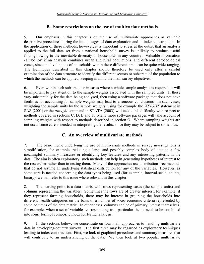
Household Sample Surveys in Developing and Transition Countries
369
B. Some restrictions on the use of multivariate methods
5. Our emphasis in this chapter is on the use of multivariate approaches as valuable descriptive procedures during the initial stages of data exploration and in index construction. In the application of these methods, however, it is important to stress at the outset that an analysis applied to the full data set from a national household survey is unlikely to produce useful findings owing to the inevitable diversity of households in any country. Valuable information can be lost if an analysis combines urban and rural populations, and different agroecological zones, since the livelihoods of households within these different strata can be quite wide-ranging. The techniques described in this chapter should therefore be used only after a careful examination of the data structure to identify the different sectors or substrata of the population to which the methods can be applied, keeping in mind the main survey objectives. 6. Even within such substrata, or in cases where a whole sample analysis is required, it will be important to pay attention to the sample weights associated with the sampled units. If these vary substantially for the data being analysed, then using a software package that does not have facilities for accounting for sample weights may lead to erroneous conclusions. In such cases, weighting the sample units by the sample weights, using for example the WEIGHT statement in SAS (2001) or the aweight command in STATA (2003) will tackle this difficulty with respect to methods covered in sections C, D, E and F. Many more software packages will take account of sampling weights with respect to methods described in section G. Where sampling weights are not used, some care is needed in interpreting the results, since they may be subject to some bias.
C. An overview of multivariate methods
7. The basic theme underlying the use of multivariate methods in survey investigations is simplification, for example, reducing a large and possibly complex body of data to a few meaningful summary measures or identifying key features and any interesting patterns in the data. The aim is often exploratory: such methods can help in generating hypotheses of interest to the researcher rather than in testing them. Many of the approaches use distribution-free methods that do not assume an underlying statistical distribution for any of the variables. However, as some care is needed concerning the data types being used (for example, interval-scale, counts, binary), we will refer to this issue where relevant in this chapter. 8. The starting point is a data matrix with rows representing cases (the sample units) and columns representing the variables. Sometimes the rows are of greater interest, for example, if they represent farming households, there may be interest in grouping the households into different wealth categories on the basis of a number of socio-economic criteria represented by some columns of the data matrix. In other cases, columns can be of primary interest themselves, for example, when a set of variables corresponding to a particular theme need to be combined into some form of composite index for further analysis. 9. In the sections below, we concentrate on four main approaches to handling multivariate data in developing-country surveys. The first three may be regarded as exploratory techniques leading to index construction. First, we look at graphical procedures and summary measures that will contribute to an understanding of the data. We then look at two popular multivariate

Household Sample Surveys in Developing and Transition Countries
370
procedures, cluster analysis and principal component analysis (PCA), since these are two of the key procedures that have a useful preliminary role to play in index construction. The latter procedure is discussed more fully in section G along with other ways in which indices can be constructed, taking the broader interpretation of �multivariate� methods as used by many researchers. Throughout, we assume that a suitable subset of the survey data has been selected for analysis and that the aim of subjecting these data to a multivariate procedure is to integrate an exploratory step into an analysis that is attempting to fulfil some broader survey objective. 10. There are of course many other multivariate methods that could be considered in specific situations. Table XVIII.1 shows a range of such methods, together with a brief description of each. This chapter is restricted to just the first three because the aim is to focus on data exploration as a necessary first step for index construction. These three methods are also likely to have the greatest relevance in survey data analysis. Together with the wider application of the term �multivariate� in our discussion on index construction, they form valuable additional methodological tools in survey data analysis. The remaining methods in table XVIII.1 may be useful on specific occasions when relevant to survey objectives. They are, however, beyond the scope of this chapter which proposes to provide only a broad introduction to some of the simpler methods.
Table XVIII.1. Some multivariate techniques and their purpose Multivariate technique Purpose of technique
1. Descriptive multivariate methods Data exploration; identifying patterns and relationships
2. Principal component analysis Dimension reduction by forming new variables (the principal components) as linear combinations of the variables in the multivariate set
3. Cluster analysis Identification of natural groupings among cases or variables
4. Factor analysis Modelling the correlation structure among variables in the multivariate response set by relating them to a set of common factors
5. Multivariate analysis of variance (MANOVA)
Extending the univariate analysis of variance to the simultaneous study of several variates. The aim is to partition the total sum of squares and cross-products matrix among a set of variates according to the experimental design structure
6. Discriminant analysis Determining a function that enables two or more groups of individuals to be separated
7 Canonical correlation analysis Studying the relationship between two groups. It involves forming pairs of linear combinations of the variables in the multivariate set so that each pair in turn produces the highest correlation between individuals in the two groups
8. Multidimensional scaling Constructing a �map� showing a spatial relationship between a number of objects, starting from a table of distances between the objects

Household Sample Surveys in Developing and Transition Countries
371
D. Graphs and summary measures 11. A preliminary understanding of the data is an essential initial stage whenever data analysis is undertaken. A careful look at the data will provide a feel for the meaning and distributional patterns of the data, identify possible outliers (observations not consistent with the pattern of the remaining data), show up data patterns, and provide the user with an idea of whether some variables have greater variability than others [see, for example, Tufte (1983) and Everitt and Dunn (2001)]. 12. As in a set of univariate analyses, summary measures such as means and standard deviations for measurement data and frequency tables for binary and categorical data are desirable. Pairs of variables may then be considered in order to identify associations between variables. At this preliminary stage, it would be reasonable to consider data in �bundles�, possibly two, one comprising quantitative data (continuous or discrete) and the other comprising qualitative data (categorical and binary). For the former, scatter plots (in pairs) would be meaningful, while for the latter, two-way tables, again in pairs, would be appropriate, possibly combined with some measures of association and the use of a chi-square test statistic. Where relevant, the scatter plots may also be displayed using different symbols to indicate subsets of the data identified by a categorical variable. 13. Most statistics software packages have facilities for matrix plots, for example, the PLOT procedure in SAS (2001), the Graph/Graphics menu in SPSS for Windows (SPSS, 2001) and GenStat for Windows (GenStat, 2002). These are graphical displays where scatter plots between all pairs of variables can be shown together, thus providing a quick judgement on how each variable is related to every other variable in the multivariate data set under consideration. 14. As an example, figure XVIII.1 presents a matrix plot, produced from SPSS (2001), that shows the relationships between four variables for 50 villages in Gujarat State in India, according to whether or not they had a dairy cooperative. The variables were: village population, area, and numbers of cattle and buffalo, these being just a few of a larger group of variables. The data come from a baseline study conducted prior to introducing a scheme to promote animal health training. The horizontal and vertical axes for each plot are determined by the axis that runs parallel to the diagonal cells. For example, the three plots in the first row all have village population as their vertical axis and area, cattle and buffalo numbers as their horizontal axes in turn. The same three plots appear in the first column but with their axes reversed. There is possibly one outlier in the data set, clearly seen in the cells in the first row corresponding to a village with a very high population. Some association is observed between all pairs of variables. It is also seen that large values for all variables under consideration are more likely with villages having a dairy cooperative than those without one. 15. If the matrix plot identifies particular pairs of variables that show interesting patterns or outliers, it would be well to repeat these as simple two-way scatter plots, but with attention to the sampling weights associated with each data point. Bubble plots, where each point is represented by a bubble with an area proportional to the sample weight (Korn and Graubard, 1998), are particularly helpful and provide a more meaningful interpretation. For example, an outlier with a large sampling weight will obviously have a greater impact than one with a small sampling

Household Sample Surveys in Developing and Transition Countries
372
weight. There are a variety of other ways of accounting for the sample design in scatter plots, for example, by subsampling the data with probability proportional to the sample weights and then plotting while ignoring the sample weights, or by applying kernal smoothing methods. The reader is directed to Korn and Graubard (1998) for further details. 16. Many other graphical approaches exist for displaying multivariate data. For example, Manly (1994) shows how several objects, described by several variables, can be drawn in three different ways to show the profile of variable values. Everitt and Dunn (2001) has an excellent chapter on many graphical displays including bivariate boxplots, coplots and trellis graphs, and Jongman, Ter Braak and Van Tongeren (1995) demonstrates the use of biplots. It is not possible to provide further details here but the reader is encouraged to look up the references cited above for further clarification. It is important to note, however, that such graphical procedures are of most value when used with specific subgroups of the population.
Figure XVIII.1. Example of a matrix plot among six variables
Vill. Population
Vill. Area
Cattle
BuffaloWith co-op
Without co-op

Household Sample Surveys in Developing and Transition Countries
373
E. Cluster analysis 17. Cluster analysis (Everitt, Landau and Leese, 2001) is a data-driven technique, generally aimed at identifying natural groupings among the sampling units (for example, respondents, farms, households) so that units within each group (cluster) are similar to one another while dissimilar units are in different groups. Situations also arise where clustering of variables is relevant, for example, the case where just one or two variables are selected from each cluster so that further analysis could be based on fewer variables. It is thus a useful tool in data exploration and/or data reduction. It can also be used to help in hypothesis generation and in other specific situations. Example 1
18. As an illustration, consider a study aimed at investigating the effectiveness of a range of low-cost pest management strategies for adoption by resource-poor farming households in a particular region. Suppose that a baseline survey of farmers who may participate in future on-farm trials is conducted with the aim of (a) giving a socio-economic profile of farming households; (b) determining farmers� current pest management practices; and (c) determining farmers� perceptions in respect of pests on the crops they grow. We concentrate here on the first of these three aims and consider how cluster analysis can be used to help determine an effective choice of different groups of farmers for the main study involving on-farm trials. 19. A large number of socio-economic variables were measured during the baseline survey. The aim was to stratify the farming households on the basis of these variables. One approach is to choose, for example, two key variables and form strata defined by combinations of categories associated with the two variables. For example, if the chosen variables were gender of the household head (male/female) and the household�s level of food security (low, medium, high), then six strata would result. 20. The disadvantage of this approach is that it ignores other socio-economic characteristics of the households. A multivariate approach allows many variables to be considered simultaneously. Cluster analysis, applied to the farming households on the basis of all relevant socio-economic variables, is a more effective way of stratifying households into a number of clusters so that each cluster represents a distinct socio-economic group of the farming population. This is important inasmuch as recommendations concerning pest management strategies will not necessarily be appropriate for all farming households. An initial classification of farmers into clusters is helpful in providing a basis for choosing different types of farmers to participate in exploring a range of pest management strategies. It also helps in focusing on characteristics specific to the clusters so that interactions between such characteristics and the recommended strategies can be investigated. An illustration is provided in Orr and Jere (1999). 21. To conduct a cluster analysis, two decisions have to be made. First, a measure of similarity (or distance) among the units being clustered must be determined. A similarity measure is one that uses the information from several variables to give a numerical value reflecting the degree of �closeness� between each pair of units. A distance measure is the opposite and reflects how far apart any pair of units is. When all variables are quantitative, or

Household Sample Surveys in Developing and Transition Countries
374
include at most a few ordered categorical variables in addition, the use of a Euclidean32 distance matrix may be appropriate. Survey data, however, often include binary and non-ordered categorical variables. For such data, various similarity measures have been proposed. For example, if a similarity measure is to be produced between two binary variables, the data may first be cross-tabulated by these two variables to give the 2 × 2 table below.
0 1
0 a b
1 c d 22. A possible measure of similarity is then (a+d)/(a+b+c+d), which is called the simple matching coefficient. Another is the Jaccard coefficient d/(b+c+d). A range of other measures can be found in Krzanowski and Marriott (1994b). See Gower (1971) for a suitable similarity measure when mixed data types are involved. In practice, if a large number of variables of different types are to be used in the clustering, it may be better to conduct a number of different cluster analyses, considering variables of the same type each time, and then determining whether the different sets of clusters that emerge are similar. This provides a cross-validation of the cluster membership. 23. Once a distance or similarity measure has been determined, a decision has to be made regarding the method of clustering. Again, many options are presented in statistics software. For example, SPSS (2001) offers seven options (for example, between group linkage, within group linkage, nearest neighbour, etc.). Some of these are agglomerative procedures where, initially, the n units being clustered form n clusters with one member per cluster, and these are then combined sequentially according to their similarity with members of other clusters. The alternative is a divisive process where all n units start as a single cluster, which is then divided in a sequential manner until a satisfying solution is obtained. In either case, some care is needed in making the right decision concerning the way in which the clusters are formed. An extensive discussion of these issues can be found in Everitt, Landau and Leese (2001). Example 2 24. A special case arises when all variables are binary. The procedure can be fairly simple using hierarchic clustering. For purposes of illustration, we will use just a few observations from a small survey involving 74 farmers in an on-farm research programme. Data for a number of variables recorded during farm visits are shown in table XVIII.2 for just eight farmers. The variables correspond to yes (+) and no (-) answers. One aim was to investigate whether the farms can be grouped into a few clusters on the basis of these characteristics.
32 Euclidean distance can be thought of simply as reflecting the normal meaning of �distance� as applied to a multidimensional space.
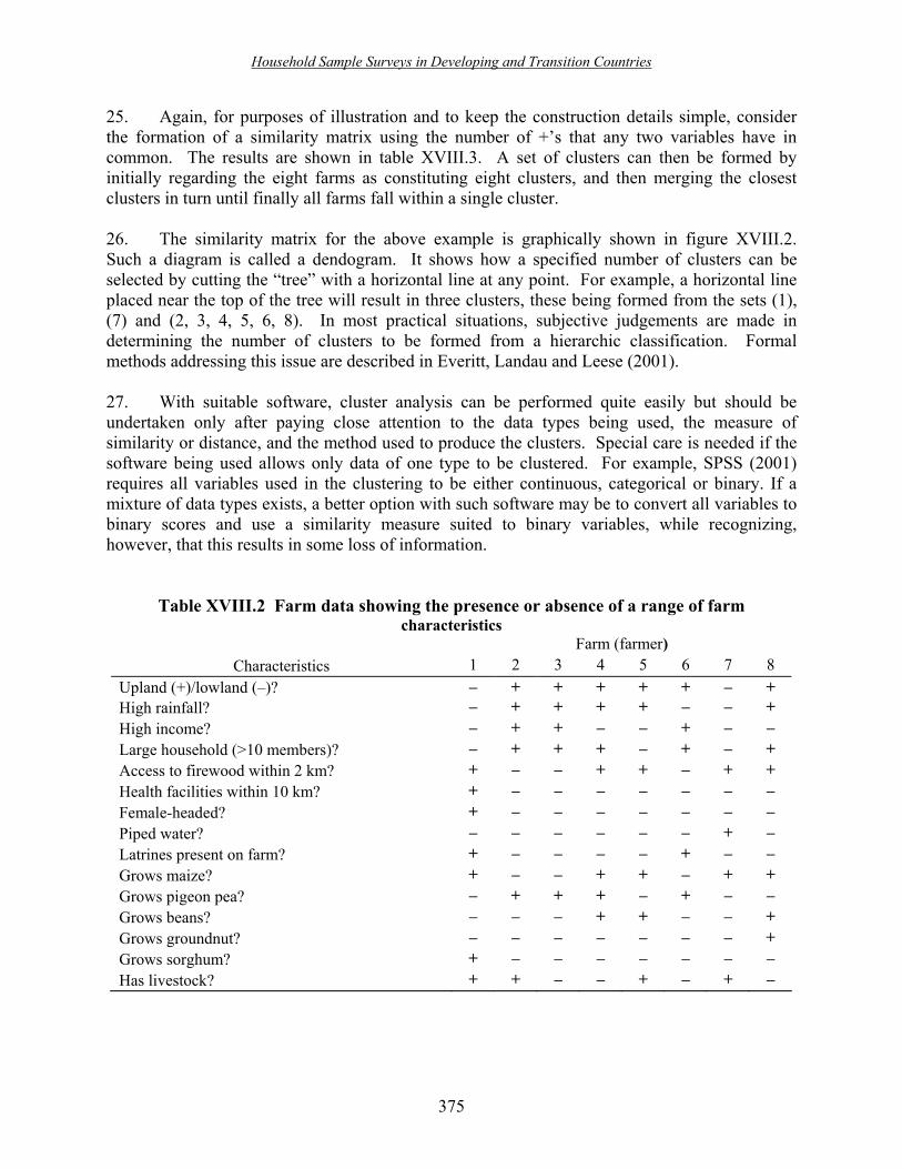
Household Sample Surveys in Developing and Transition Countries
375
25. Again, for purposes of illustration and to keep the construction details simple, consider the formation of a similarity matrix using the number of +�s that any two variables have in common. The results are shown in table XVIII.3. A set of clusters can then be formed by initially regarding the eight farms as constituting eight clusters, and then merging the closest clusters in turn until finally all farms fall within a single cluster. 26. The similarity matrix for the above example is graphically shown in figure XVIII.2. Such a diagram is called a dendogram. It shows how a specified number of clusters can be selected by cutting the �tree� with a horizontal line at any point. For example, a horizontal line placed near the top of the tree will result in three clusters, these being formed from the sets (1), (7) and (2, 3, 4, 5, 6, 8). In most practical situations, subjective judgements are made in determining the number of clusters to be formed from a hierarchic classification. Formal methods addressing this issue are described in Everitt, Landau and Leese (2001). 27. With suitable software, cluster analysis can be performed quite easily but should be undertaken only after paying close attention to the data types being used, the measure of similarity or distance, and the method used to produce the clusters. Special care is needed if the software being used allows only data of one type to be clustered. For example, SPSS (2001) requires all variables used in the clustering to be either continuous, categorical or binary. If a mixture of data types exists, a better option with such software may be to convert all variables to binary scores and use a similarity measure suited to binary variables, while recognizing, however, that this results in some loss of information.
Table XVIII.2 Farm data showing the presence or absence of a range of farm characteristics
Farm (farmer) Characteristics 1 2 3 4 5 6 7 8
Upland (+)/lowland (�)? � + + + + + � + High rainfall? � + + + + � � + High income? � + + � � + � � Large household (>10 members)? � + + + � + � + Access to firewood within 2 km? + � � + + � + + Health facilities within 10 km? + � � � � � � � Female-headed? + � � � � � � � Piped water? � � � � � � + � Latrines present on farm? + � � � � + � � Grows maize? + � � + + � + + Grows pigeon pea? � + + + � + � � Grows beans? � � � + + � � + Grows groundnut? � � � � � � � + Grows sorghum? + � � � � � � � Has livestock? + + � � + � + �
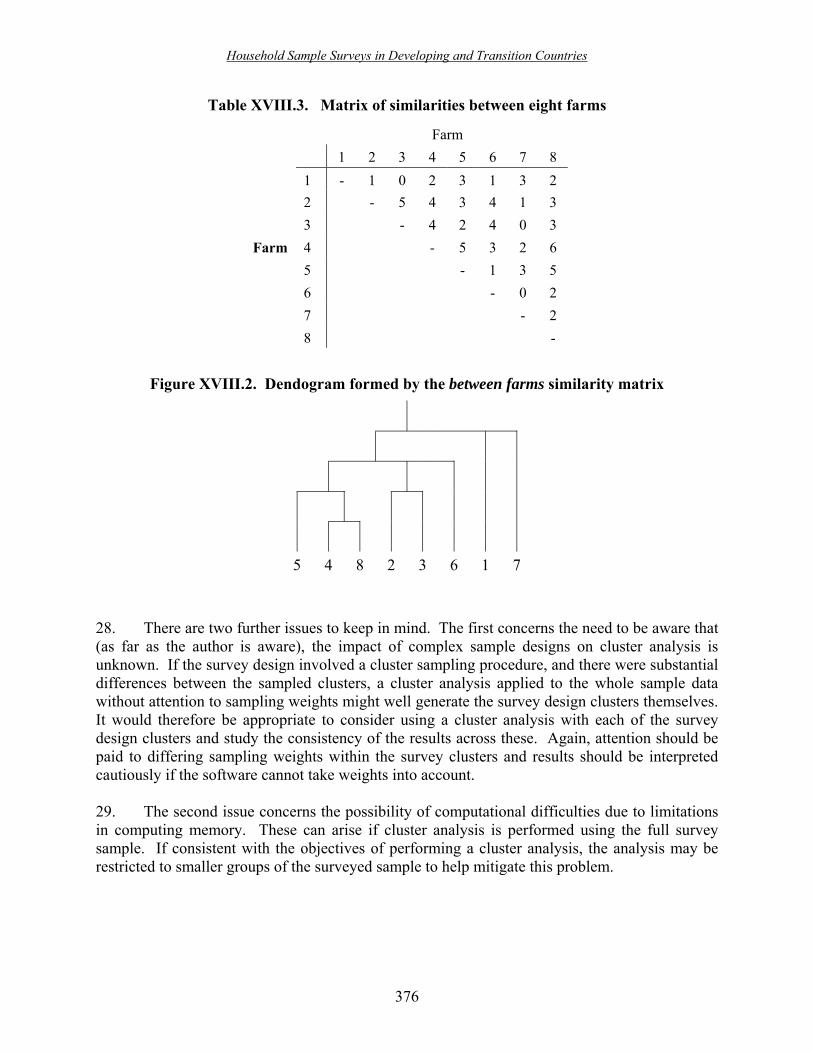
Household Sample Surveys in Developing and Transition Countries
376
Table XVIII.3. Matrix of similarities between eight farms
Farm 1 2 3 4 5 6 7 8 1 - 1 0 2 3 1 3 2 2 - 5 4 3 4 1 3 3 - 4 2 4 0 3 Farm 4 - 5 3 2 6 5 - 1 3 5 6 - 0 2 7 - 2 8 -
Figure XVIII.2. Dendogram formed by the between farms similarity matrix
5 4 8 2 3 6 1 7
28. There are two further issues to keep in mind. The first concerns the need to be aware that (as far as the author is aware), the impact of complex sample designs on cluster analysis is unknown. If the survey design involved a cluster sampling procedure, and there were substantial differences between the sampled clusters, a cluster analysis applied to the whole sample data without attention to sampling weights might well generate the survey design clusters themselves. It would therefore be appropriate to consider using a cluster analysis with each of the survey design clusters and study the consistency of the results across these. Again, attention should be paid to differing sampling weights within the survey clusters and results should be interpreted cautiously if the software cannot take weights into account. 29. The second issue concerns the possibility of computational difficulties due to limitations in computing memory. These can arise if cluster analysis is performed using the full survey sample. If consistent with the objectives of performing a cluster analysis, the analysis may be restricted to smaller groups of the surveyed sample to help mitigate this problem.

Household Sample Surveys in Developing and Transition Countries
377
F. Principal component analysis (PCA)
30. Suppose there are several variables, for instance, 12, which measure facets of one major issue in a survey. For example, in a nutrition survey, the nutrition status of children may be measured in terms of several anthropometric measurements, as well as by variables describing socio-economic characteristics of their families. Such variables are likely to be correlated, and the question then arises whether these variables could be reduced in some fashion to fewer variables that capture as much as possible of the variation in the original data set. Principal component analysis (PCA) aims to do this. The technique is strictly applicable to a set of measurements that are either quantitative or have an ordinal scale. However, as this is largely a descriptive technique, the inclusion of binary variables and/or a small number of nominal categorical variables is unlikely to be of practical consequence. 31. In PCA, a new set of variables is created as linear combinations33 of the original set. The linear combination that explains the maximum amount of variation is called the first principal component. A second principal component (another linear combination) is then created, independent of the first, that explains, as much as possible, the remaining variability. Further components are then created sequentially, each new component being independent of the previous ones. If the first few components, say, the first 3, explain a substantial amount, say, 90 per cent of the variability among the original set of 12 variables, then essentially, the number of variables to be analysed has been reduced from 12 to 3. 32. It is important to note that the principal component estimators can be severely biased if PCA is applied to the entire survey sample when it is non-self-weighting (Skinner, Holmes and Smith, 1986). As emphasized in section B, PCA is generally recommended in survey data analysis only for smaller subsets of the sample that have (at least approximately) the same sampling weights. If the data subset of interest has substantially differing sampling weights, then some caution should be exercised in interpreting the results. Example 3 33. Pomeroy and others (1997) applied PCA to data from a survey of 200 households where the respondents were asked to score 10 indicators, on a scale of 1-15, presented to them as rungs of a ladder, to show their perception of the changes that had taken place due to community-based coastal resources management projects in their area. The indicators are listed below, while the PCA results are presented in table XVIII.4.
33 If X1, X2, �., Xp are the original set of p variables, then a variable Y formed from a linear combination of these takes the form Y = a1X1 + a2X2 + �.+ apXp where the ai�s (i=1,2,�,p) are numbers, that is to say, the principal component coefficients.

Household Sample Surveys in Developing and Transition Countries
378
Table XVIII.4. Results of a principal component analysis
Component Variable PC1 PC2 PC3
1. Overall well-being of household 0.24 0.11 0.90 2. Overall well-being of the fisheries resources 0.39 0.63 0.02 3. Local income 0.34 0.51 0.55 4. Access to fisheries resources -0.25 0.72 0.17 5. Control of resources 0.57 0.40 0.12 6. Ability to participate in community affairs 0.77 0.13 0.29 7. Ability to influence community affairs 0.75 0.22 0.34 8. Community conflict 0.78 0.03 0.18 9. Community compliance and resource management 0.82 0.12 0.07 10. Amount of traditionally harvested resource in water 0.38 0.66 0.12 Percentage of variance explained 33 19 14
The first principal component is therefore given by:
PC1 = 0.24(household) +0.39(resource) � + 0.82(compliance) + 0.38(harvest). 34. This first component is described by Pomeroy and others (1997) as an indicator dealing with the behaviour of community members, the second component as relating to the fisheries resource, and the third component as an indicator of household well-being. They then use these components as the dependent variables in multiple regression analyses to investigate the effectiveness of a number of explanatory factors in explaining the variability of each indicator. 35. Although the interpretation of the variables is reasonable here, one may question the value of using (say) the first principal component in the form calculated above for further analysis. Only variables 5, 6, 7, 8 and 9 describe the behaviour of the community members and these are the variables that score highly on PC1. Rather than include all 10 variables in the calculation of the first principal component, it would be better to recalculate a new variable as a simple summary of the behaviour variables in the original data set, for example, by taking a simple arithmetical average of variables 5, 6, 7, 8 and 9, or a weighted average of these in which control of resources (variable 5) is given a slightly lower weight relative to the others. Likewise, the resource variables (variables 2, 3, 4 and 10) could be combined to given a simple summary, while variable 1 would stand on its own. Used in this manner, PCA identifies how the 10 indicators may be summarized in a simple way to give a new set of meaningful measures for further analysis, as, for example, Pomeroy and others (1997) have done through regression analysis to explore factors influencing each of their first three principal components.

Household Sample Surveys in Developing and Transition Countries
379
Example 4 36. The sustainable livelihoods framework adopted by the Department for International Development (DFID) of the Government of the United Kingdom of Great Britain and Northern Ireland provides another practical example. This framework considers five livelihood assets, namely, social capital, human capital, natural capital, physical capital and financial capital. A survey conducted to study household livelihoods would require each of these assets to be measured in terms of a number of subsidiary variables. For example, social capital may be measured in terms of the extent of reliance on networks of support, percentage of household income from remittances, extent of trust in the group, degree of participation in decision-making, etc.; human capital may be measured in terms of the level of education, health status, etc.; and physical capital in terms of ownership of a bicycle or radio, having piped water, electricity, etc. 37. The objective here is to determine a single variable, one for each of the five livelihood assets. This can be done in a straightforward manner for physical assets, for example, by obtaining a simple weighted average of the binary responses corresponding to whether or not items in a given list are owned by a household, using item prices as weights. Social capital, on the other hand, cannot be combined in such a simple way because allocating weights to variables describing social assets is much more difficult. Here we may have to accept data-derived weights via a PCA applied to a set of social variables. The results may be used to produce a suitable overall measure of social capital, again moving towards a simple weighted average after the relative weights of each variable in the first one or two principal components are known.
G. Multivariate methods in index construction
38. Index construction can have several different meanings. In a health study, for example, the nutritional status of children is typically measured by creating indices from anthropometric measurements, for example, weight-for-age, height-for-age and weight-for-height, these representing underweight, stunting and wasting, respectively. 39. In a more complex example, responses to items on breastfeeding, use of baby bottles, dietary diversity, the number of days the child receives selected food groups in past seven days, and feeding frequency, may be summed to create a child feeding index (Ruel and Menon, 2002). This is a second type of index where the researcher decides on the specific scores to be allocated, ensuring that the ordinal scale for each variable is such that high values always represent either �good� or �bad�. When binary variables are involved, as, for example, in ownership of a number of assets, the price of the asset could be used to give different weights to each item, as shown in example 4 (sect. F) above. 40. Another type of index can arise in the case where a survey involves determining attitudes or views, say, of the quality of access to health services. Here several questions may be asked, requiring answers on a scoring scale of 1-5 with 1 being �very poor� and 5 being �very good�. Again, the resulting scores could be summed across all relevant questions to provide an index reflecting householders� views of the value of health services.

Household Sample Surveys in Developing and Transition Countries
380
41. Our discussion here goes further to include situations where the data determine the form of the index by use of a multivariate procedure. This still retains the common interpretation of an index as being a single value that captures the information from several variables in one composite measure, typically taking the form:
Index = a1X1 + a2X2 + a3X3 + ��� + apXp where the ai terms are weights to be determined from the data and the Xi terms are an appropriate subset of p variables measured in the survey. We illustrate two ways in which the weights ai can be determined from the data (see below). Which one is more appropriate will usually depend on the objectives underlying index construction. 42. The first is based on a regression modelling approach; the second, on an application of PCA. These are discussed in relation to indices used for measuring proxy indicators of household wealth or socio-economic status in developing countries. There is a vast literature on this topic and a comprehensive overview can be found in Davis (2002). See also chapter XVII of the present publication which provides a useful discussion on the use of household survey data to understand poverty.
1. Modelling consumption expenditure to construct a proxy for income 43. An approach for modelling consumption expenditure as a proxy for income has been developed by Henstchel and others (2000) and Elbers, Lanjouw and Lanjouw (2001). It involves using data from a detailed household budget survey to identify variables indicative of poverty. This is done by using consumption expenditure as the dependent variable in a multiple linear regression model and a series of household-level variables (for example, assets owned by the household, quality of housing, access to facilities, etc.) as potential explanatory (predictor) variables in the model. The best small subset of the explanatory variables that explains maximum variation in the response (dependent) variable is used to predict consumption expenditure. If the explanatory variables have been collected in a population census, the resulting model equation can then be applied to census data to predict consumption expenditure for each census household. These can then be used to construct poverty maps on a national scale. If the household budget survey is conducted well before the expected date of the census, the appropriate set of predictor variables can be identified from the budget survey data and included in the census questionnaire. We present an example directly below to illustrate this approach. Example 5 44. The National Bureau of Statistics in the United Republic of Tanzania undertook a National Household Budget Survey (HBS) in 2000-2001 covering approximately 22,000 households. On the basis of details collected on household expenditure over a 28-day period, the total 28-day consumption expenditure per adult equivalent was calculated for each household. Regression modelling with preliminary data available from the HBS identified a series of potential household-level variables (separate sets for urban and rural areas) that explained a high proportion of the variability in consumption expenditure. These variables were included in a

Household Sample Surveys in Developing and Transition Countries
381
questionnaire administered to a census of households at three sentinel surveillance sites under study by the Adult Morbidity and Mortality Project (AMMP) team based in Dar es Salaam. The aim was to develop an index reflecting consumption expenditure using HBS data for each AMMP site, and to apply the index to households covered by the AMMP at each site. 45. Full details of the modelling approaches and an evaluation of the effectiveness of the models can be found in Abeyasekera and Ward (2002). Here we present a summary of the results for one rural region (see table XVIII.5) to show the variables that entered the model equation and the weights (regression coefficients) used in computing an index of consumption expenditure. 46. From the results of table XVIII.5, the index predicting consumption expenditure for households in Kilimanjaro region in the United Republic of Tanzania is the following:
Index of consumption expenditure =
9.79388+(0.11043*lamp)+(0.19950*sofa)+(0.12870*bicycle)+(0.11858*seed) +(0.16254*fertiliser)+(0.025824*landarea)+(0.088769*meat)+(0.076132*income4) +(0.13451*income3)+(0.098303*income2)+(0.27985*edu4)+(0.15878*edu3) -(0.0091977*edu2) - (0.0022552*age)+(0.010456*hhsize2)-(0.23902*hhsize)
47. The model explained 65 per cent of the variability in consumption expenditure. This is a significantly high figure given the complexity of livelihoods among rural households. The quality of this index at its development stage was judged by (a) comparing it with the true values of consumption expenditure; and (b) considering its ability to identify the true proportion of households below the basic needs poverty line of the United Republic of Tanzania. Method (a), utilized by graphing the index versus true values, showed a very good correspondence. It performed less well when the population of true values and the population of predicted values were categorized into five wealth quintiles, and tabulated against each other. Only 46 per cent of households were classified into the correct quintile. The classification by poverty line was better, with 87 per cent classified correctly as being above or below the poverty line. 48. Further examples of the modelling approach are presented in the final sections of chapter XIX.

Household Sample Surveys in Developing and Transition Countries
382
Table XVIII.5. Variables used and their corresponding weights in the construction of a predictive index of consumption expenditure for the Kilimanjaro region in the United
Republic of Tanzania Predictor variable Significance
probability Weight (model coefficient) (STATA estimate)
Household size 0.000 �0.239 Square of household size 0.000 0.0104 Age of household head (years) 0.038 �0.00226 Education of household head a/ 0.000 0, -0.00920, 0.159, 0.280 Main source of income b/ 0.017 0, .0983, 0.1345, 0.0761 Days meat eaten in past week 0.000 0.0888 Area of land owned by household 0.000 0.0258 Fertilizer c/ 0.000 0.1625 Seeds c/ 0.004 0.1186 Ownership of bicycle 0.000 0.1287 Ownership of sofa 0.000 0.1995 Ownership of lamp 0.001 0.1104 Constant in model equation 0.000 9.794 Sample size = 1,026 R2 = 0.651 Adjusted R2 = 0.646 a/ None; primary; secondary; tertiary and above. b/ Sale of crops; sale of livestock; business/wages/salaries; other sources. c/ If bought in past 12 months.
2. Principal components analysis (PCA) used to construct a �wealth� index 49. The methodology discussed in section G.1 above can be applied only if reliable data on consumption expenditure � the dependent variable - are available from a previous survey. The difficulty of collecting reliable information on consumption expenditure, combined with the high costs of data collection, has prompted some researchers to recommend the use of an asset-based poverty index, derived from conducting a PCA. The first principal component is used as an index of socio-economic status following previous research that has suggested that the asset-consumption relationship is a quite close one (Filmer and Pritchett, 1998). However, some caution must be exercised in interpreting the asset index as a poverty measure, since its effectiveness will depend on the choice of assets used and the particular set of data to which the PCA is applied. As an example of this approach, Gwatkin and others (2000) illustrate the PCA methodology for determining wealth quintiles in the United Republic of Tanzania, using the following set of mixed asset based variables and health-related:
• Whether the household has electricity, a radio, television, refrigerator, bicycle,
motorcycle, car (each coded as 1 = yes, 0 = no) • Number of persons per sleeping room (a quantitative response) • Principal household sources of drinking water (seven categories) • Principal type of toilet facility used by members of the household (five categories) • Principal type of flooring material in the household (six categories)

Household Sample Surveys in Developing and Transition Countries
383
50. The data they used come from information gathered through the Demographic and Health Survey (DHS) questionnaire. Appropriate sampling weights were used in the analysis. 51. The authors emphasized that theirs was an initial effort applied to a whole country sample, but that future attempts to examine population differences by socio-economic class would produce different results. They suggested that this might happen as a result of the use of some basis other than assets for defining socio-economic status, or as a result of sampling errors, etc. A more obvious reason would be wealth differentials across sites. Indeed, there was evidence of differences in wealth quintile cut-offs when their methodology was applied to three subpopulations in the United Republic of Tanzania, namely, the three regions referred to in section G.2, using data from the national Household Budget Survey (table XVIII.6). It is therefore advisable not to regard PCA results as being portable even within a single country over time or when applied to different strata of the population. 52. Researchers have also used the first principal component of a principal component analysis as a summary index for further analysis of the data. Ruel and Menon (2002), for example, constructed a socio-economic index from DHS data sets in order to categorize households into terciles for the purpose of controlling for socio-economic status in a multiple regression analysis carried out to determine factors affecting child nutritional status. They undertook separate analyses for urban and rural populations using seven data sets from five countries in Latin America. The variables used were water source, sanitation, housing materials (floor, wall, roof) and ownership of a list of assets. The values of these variables were ranked in ascending order (from worst to best) before subjecting them to a principal component analysis. Only variables with principal component coefficients greater than 0.5 were retained in the final index. The approach here was reasonable, the primary objective having been the construction of an index to correct for socio-economic differentials in a subsequent analysis.
Table XVIII.6. Cut-off points for separating population into five wealth quintiles
Wealth quintile
Dar es Salaam a/ (HBS)
Kilimanjaro a/ (HBS)
Morogoro a/ (HBS)
All United Republic of Tanzania a/
(HBS)
All United Republic of Tanzania b/
(DHS) 20th
percentile -1.2993 -0.8452 -0.9190 -1.0317 -0.5854
40th percentile
-0.7709 -0.6289 -0.6180 -0.5704 -0.5043
60th percentile
-0.1054 -0.2459 -0.3645 -0.3051 -0.3329
80th percentile
1.1603 0.3239 0.4586 0.4609 0.3761
a/ Household Budget Survey 2000-2001. b/ Demographic and Health Survey, 1996.
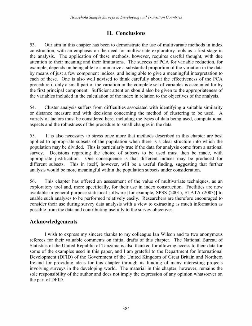
Household Sample Surveys in Developing and Transition Countries
384
H. Conclusions 53. Our aim in this chapter has been to demonstrate the use of multivariate methods in index construction, with an emphasis on the need for multivariate exploratory tools as a first stage in the analysis. The application of these methods, however, requires careful thought, with due attention to their meaning and their limitations. The success of PCA for variable reduction, for example, depends on being able to summarize a substantial proportion of the variation in the data by means of just a few component indices, and being able to give a meaningful interpretation to each of these. One is also well advised to think carefully about the effectiveness of the PCA procedure if only a small part of the variation in the complete set of variables is accounted for by the first principal component. Sufficient attention should also be given to the appropriateness of the variables included in the calculation of the index in relation to the objectives of the analysis. 54. Cluster analysis suffers from difficulties associated with identifying a suitable similarity or distance measure and with decisions concerning the method of clustering to be used. A variety of factors must be considered here, including the types of data being used, computational aspects and the robustness of the procedure to small changes in the data. 55. It is also necessary to stress once more that methods described in this chapter are best applied to appropriate subsets of the population when there is a clear structure into which the population may be divided. This is particularly true if the data for analysis come from a national survey. Decisions regarding the choice of subsets to be used must then be made, with appropriate justification. One consequence is that different indices may be produced for different subsets. This in itself, however, will be a useful finding, suggesting that further analysis would be more meaningful within the population subsets under consideration. 56. This chapter has offered an assessment of the value of multivariate techniques, as an exploratory tool and, more specifically, for their use in index construction. Facilities are now available in general-purpose statistical software [for example, SPSS (2001), STATA (2003)] to enable such analyses to be performed relatively easily. Researchers are therefore encouraged to consider their use during survey data analysis with a view to extracting as much information as possible from the data and contributing usefully to the survey objectives. Acknowledgements
I wish to express my sincere thanks to my colleague Ian Wilson and to two anonymous referees for their valuable comments on initial drafts of this chapter. The National Bureau of Statistics of the United Republic of Tanzania is also thanked for allowing access to their data for some of the examples used in this paper, and I am grateful to the Department for International Development (DFID) of the Government of the United Kingdom of Great Britain and Northern Ireland for providing ideas for this chapter through its funding of many interesting projects involving surveys in the developing world. The material in this chapter, however, remains the sole responsibility of the author and does not imply the expression of any opinion whatsoever on the part of DFID.
Household Sample Surveys in Developing and Transition Countries
385
References Abeyasekera, S., and P. Ward (2002). Models for Predicting Expenditure per Adult Equivalent
for AMMP Sentinel Surveillance Sites. Dar es Salaam: Adult Morbidity and Mortality, Ministry of Health of the United Republic of Tanzania. Available from www.ncl.ac.uk/ammp/tools_methods/socio.html.
Chatfield, C., and A.J. Collins (1980). Introduction to Multivariate Analysis. London: Chapman
and Hall. Davis, B. (2002). Is it possible to avoid a lemon? Reflections on choosing a poverty mapping method.
Available from http://www.povertymap.net/pub/Pov_mapping_methods_18-9-02.pdf. Elbers, C., J. Lanjouw and P. Lanjouw (2001). Welfare in villages and towns: micro-level
estimation of poverty and inequality. Mimeo.Vrije Universiteit, Yale University and World Bank.
Everitt, B.S., and G. Dunn (2001). Applied Multivariate Data Analysis. London: Arnold. Everitt, B.S., S., Landau and M. Leese (2001). Cluster Analysis. London: Arnold. Filmer, D., and L. Pritchett (1998). Estimating Wealth Effects without Expenditure Data�or
Tears: An Application to Educational Enrolments in States of India. Washington, D.C.: World Bank Policy Research Working Paper, No. 1994.
GenStat (2002). GenStat for Windows, 6th Ed. Oxford, United Kingdom: VSN International, Ltd. Gower , J.C. (1971). A general coefficient of similarity and some of its properties. Biometrics,
vol. 27, pp. 857-872. Gwatkin, D.R., and others (2000). Socio-economic Differences in Health, Nutrition and
Population in Tanzania. Washington, D.C.: Thematic Group on Health, Population, Nutrition and Poverty of the World Bank. Available from http://www.worldbank.org/poverty/health/data/tranzania/tanzania.pdf (accessed 30 June 2004).
Hentschel, J., and others (2000). Combining census and survey data to trace spatial dimensions
of poverty: a case study of Ecuador. The World Bank Economic Review, vol. 14, No. 1, pp. 147-165.
Jongman, R.H.G., C.J.F. Ter Braak and O.F.R. Van Tongeren (1995). Data Analysis in
Community and Landscape Ecology. Cambridge, United Kingdom: Cambridge University Press.
Korn, E.L., and B.I. Graubard (1998). Scatterplots with survey data. The American Statistician,
vol. 52, No. 1.

Household Sample Surveys in Developing and Transition Countries
386
Krzanowski, W.J., and F.H.C. Marriott (1994a). Multivariate Analysis, Part 1. Distributions,
Ordination and Inference. London: Arnold. __________ (1994b). Multivariate Analysis, Part 2. Classification, covariance structures and
repeated measurements. London: Arnold. Manly, B.F.J. (1994). Multivariate Statistical Methods: A Primer. 2nd ed. London: Chapman and
Hall. Orr, A., and P. Jere (1999). Identifying smallholder target groups for IPM in southern Malawi.
International Journal of Pest Management, vol. 45, No. 3, pp. 179-187. Pomeroy, R.S., and others (1997). Evaluating factors contributing to the success of community-
based coastal resource management: the Central Visayas Region Project-1, Philippines. Ocean and Coastal Management, vol. 36, Nos. 1-3, p. 24.
Ruel, M.T., and others (1999). Good Care Practices Can Mitigate the Negative Effects of
Poverty and Low Maternal Schooling on Children�s Nutritional Status: Evidence from Accra. Food Consumption and Nutrition Division Discussion Paper, No. 62, Washington, D.C.: International Food Policy Research Institute.
Ruel, M.T., and P. Menon (2002). Creating a Child Feeding Index Using the Demographic and
Health Surveys: an Example from Latin America. Food Consumption and Nutrition Division Discussion Paper, No. 130, Washington, D.C.: International Food Policy Research Institute.
Sahn, D.E., and D. Stifel (2000). Assets as a measure of household welfare in developing
countries. Working Paper 00-11. St. Louis, Missouri: Washington University, Center for Social Development.
SAS (2001). SAS Release 8.2. Cary, North Carolina: SAS Institute, Inc., SAS Publishing. Sharma, S. (1996). Applied Multivariate Techniques. New York: Wiley and Sons, Inc. Skinner, C.J., D.J. Holmes and T.M.F. Smith (1986). The effect of sample design on principal
component analysis. Journal of the American Statistical Association, vol. 81, Issue 395, pp. 789-798.
SPSS (2001). SPSS for Windows. Release 11.0. Chicago, Illinois: LEAD Technologies, Inc. STATA (2003). Intercooled Stata 8.0 for Windows. College Station, Texas: Stata Corporation. Tufte, E.R. (1983). The Visual Display of Quantitative Information. Chesire, Connecticut:
Graphics Press.

Household Sample Surveys in Developing and Transition Countries
387
Wilson, I.M., and R.D. Stern (2001). Approaches to the Analysis of Survey Data. Statistical Guideline Series supporting DFID Natural Resources Projects. Reading, United Kingdom: Statistical Services Centre, University of Reading. Available from http://www.reading.ac.uk/ssc (accessed 25 June 2004).

Household Sample Surveys in Developing and Transition Countries
388

Household Sample Surveys in Developing and Transition Countries
389
Chapter XIX Statistical analysis of survey data
James R. Chromy
Research Triangle Institute Research Triangle Park, North Carolina,
United States of America
Savitri Abeyasekera Statistical Services Centre
University of Reading Reading, United Kingdom of Great
Britain and Northern Ireland
Abstract
The fact that survey data are obtained from units selected with complex sample designs
needs to be taken into account in the survey analysis: weights need to be used in analysing survey data and variances of survey estimates need to be computed in a manner that reflects the complex sample design. The present chapter outlines the development of weights and their use in computing survey estimates and provides a general discussion of variance estimation for survey data. It deals first with what are termed �descriptive� estimates, such as the totals, means and proportions that are widely used in survey reports. It then discusses three forms of �analytic� approaches to survey data that can be used to examine relationships between survey variables, namely, multiple linear regression models, logistic regression models and multilevel models. These models form a set of valuable tools for analysing the relationships between a key response variable and a number of other factors. In this chapter, we give examples to illustrate the use of these modelling techniques and also provide guidance on the interpretation of the results. Key terms: complex survey design, analytic statistics, regression, logistic regression, hierarchical structures, multilevel modelling.

Household Sample Surveys in Developing and Transition Countries
390
A. Introduction 1. Household surveys utilize complex sample designs to control survey costs. Complete sampling frames that list all individuals or all households are usually not available; and even when population registries are available, the cost of implementing a household interview survey based on a simple random sample design would be prohibitively high. The Living Standards Measurement Study (LSMS) surveys discussed in chapter XXIII provide a good example of many of the complex features of household survey designs. 2. A typical household survey design structure is shown in table XIX.1. Most sample designs for household surveys use are complex and involve stratification, multistage sampling, and unequal sampling rates, as indicated above. Weights are needed in the analysis to compensate for unequal sampling rates and adjustments for non-response lead to more unequal weighting. The complex sample design needs to be taken into account in estimating the precision of survey estimates.
Table XIX.1. Typical household survey design structure
Features Possible definitions Implications Strata Regions
Community type (urban versus rural) May reduce standard errors of estimates. Control distribution of sample may lead to disproportionate sampling
First-stage sampling units Census enumeration areas or similar geographical areas Villages in rural strata
Facilitate clustering of the sample to control costs. Facilitate development of complete frames of housing unit addresses only in sampled areas. Selected with probability proportional to size.
Second-stage sampling units Housing unit addresses May contain none, one or more than one household or unrelated person. Selected with equal probability within first-stage sampling units.
Third-stage sampling units (when not all household members are automatically included in the sample)
Household members Sample selected from roster of household members obtained from a responsible adult household member. May lead to unequal weighting in order to account for household size.
Observational units Households Household members Agricultural or business enterprises operated by the household members Special files for subgroups, for example, adults in the workforce Events or episodes pertaining to household members Repeated measures over time (panel surveys)
May require more than one analytic file for special-purpose analyses.

Household Sample Surveys in Developing and Transition Countries
391
3. Section B of the present chapter outlines the development of weights for use in survey analysis and the use of weights for the production of simple �descriptive� estimates, such as the totals, means and proportions/percentages that are widely presented in survey reports. It also provides an overview of variance estimation for such estimates based on complex sample designs. 4. The remaining sections focus on three forms of �analytic� uses of survey data that explore the way in which a key response or dependent variable - for example, academic performance of a school-going child, poverty level of a household - is affected by a number of factors, often referred to as explanatory variables, or regressor variables. Multiple linear regression models are suitable when the key response is a quantitative measurement variable, while logistic regression models are applicable when the key response variable is binary, that is to say, when the response takes only two possible values (for example, yes/no, present/absent). These regression methods may be applied to a non-nested body of survey data, or to sampling units at a single level of the hierarchy of a multistage design. Alternatively, the analysis may need to take account of the different sources of variability occurring at the different hierarchical levels, and then multilevel modelling comes into play. This approach takes account of the correlation structure between sampling units at one level because they occur within units at different levels.
B. Descriptive statistics: weights and variance estimation 5. Household surveys are commonly designed to produce estimates of population totals, population means, or simple ratios of totals or means. Examples of totals might be total population, men in the workforce, women in the workforce, or the number of children five years of age or under. Examples of means might be average income for persons in the workforce, average income of women in the workforce, and average income of men in the workforce. Ratio estimates might be required to estimate the proportion of households with total income below the poverty level or the average household income for households whose principal wage earner is a female. 6. Household surveys produce national estimates, but may also be designed to yield estimates for geopolitical regions or for other cross-sectional domains. Furthermore, household surveys may be repeated to obtain periodic estimates (for example, annual or five-year estimates), which might be viewed as temporal domains. As long as the statistics produced consist simply of estimates of totals, means or rates even when produced for population domains (cross-sectional or temporal), we characterize the analysis required to produce these estimates as �descriptive�. Descriptive statistics include the estimates themselves as well as some measure of the precision of those estimates. Descriptive reports may include standard errors of estimates or interval estimates based on those standard errors. Estimation of the standard errors requires an analysis that takes account of the household survey sample design. Interval estimates require not only the appropriate design-based estimates of standard errors, but also knowledge of the degrees of freedom used in computation of the standard error estimates. These types of fairly simple descriptive statistics constitute the majority of the official statistics published to describe the results of household surveys.
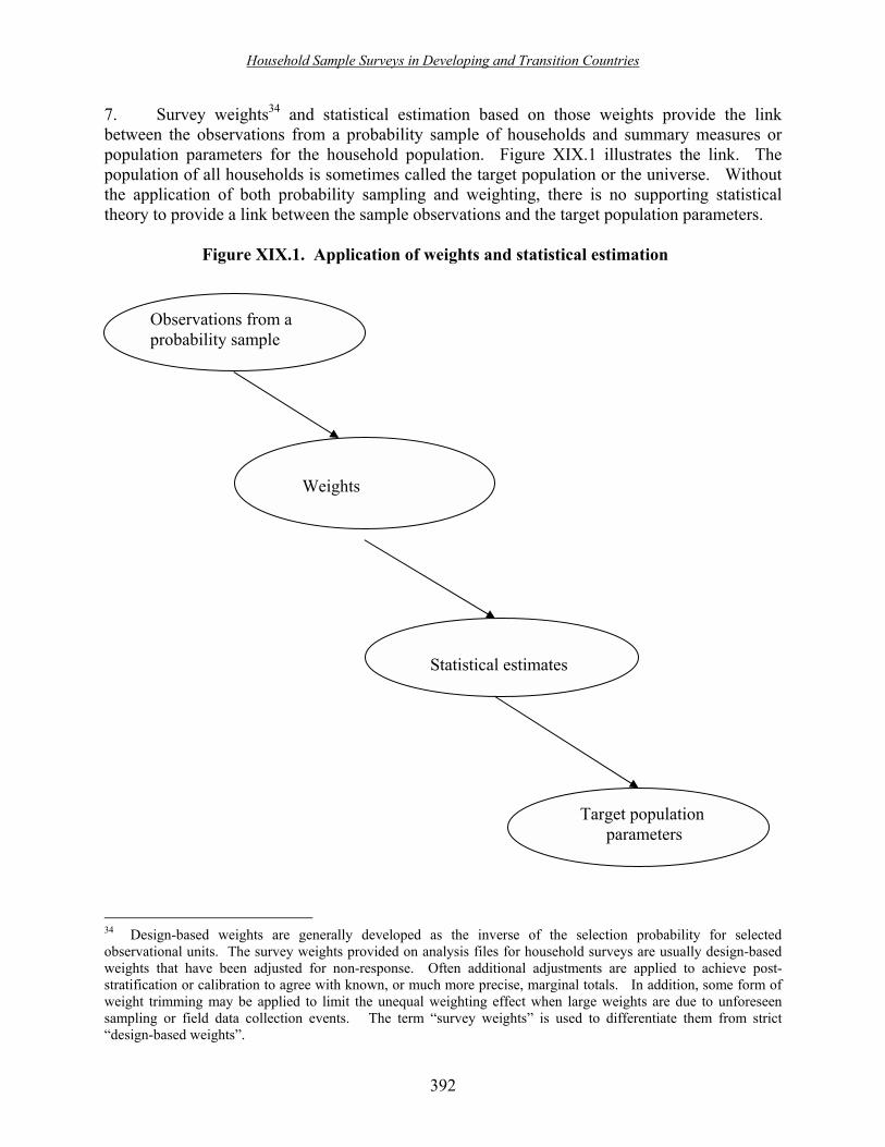
Household Sample Surveys in Developing and Transition Countries
392
7. Survey weights34 and statistical estimation based on those weights provide the link between the observations from a probability sample of households and summary measures or population parameters for the household population. Figure XIX.1 illustrates the link. The population of all households is sometimes called the target population or the universe. Without the application of both probability sampling and weighting, there is no supporting statistical theory to provide a link between the sample observations and the target population parameters.
Figure XIX.1. Application of weights and statistical estimation
34 Design-based weights are generally developed as the inverse of the selection probability for selected observational units. The survey weights provided on analysis files for household surveys are usually design-based weights that have been adjusted for non-response. Often additional adjustments are applied to achieve post-stratification or calibration to agree with known, or much more precise, marginal totals. In addition, some form of weight trimming may be applied to limit the unequal weighting effect when large weights are due to unforeseen sampling or field data collection events. The term �survey weights� is used to differentiate them from strict �design-based weights�.
Weights
Statistical estimates
Target population parameters
Observations from a probability sample

Household Sample Surveys in Developing and Transition Countries
393
8. Any analysis that ignores the sample design and the weights must be based on assumptions. If the sample is designed to generate an equal probability sample, then the weights for estimating means, rates or relationships among variables may be safely ignored. Kish (1965, pp. 20-21) called these designs epsem designs and noted that even complex multistage samples can be designed to be epsem for sampling units at the final or near final stage of the design. As noted later, adjustments for non-response might create unequal weights even if the design was initially epsem. If post-stratification or multidimensional calibration is applied to the data through adjustments to the weights, these processes will almost always create unequal weights adjustments and therefore unequal weights. 9. Some analysts, however, are willing to make the assumptions that would allow analysis of household survey data without weights or with equal weights. These assumptions are most tenable when applying models to the data to study relationships between a dependent variable and a number of independent explanatory variables. 10. For the theoretical case of surveys with complete response from all sample members, the use of design-based weights computed as the inverse of each observational unit�s probability of selection provides for unbiased estimates of population totals and other linear statistics (Horvitz and Thompson, 1952). In practice, household surveys always encounter some non-response, which can lead to bias in estimates if these observations are dropped from the analysis without any other action being taken (see chap. VIII). Techniques have been developed that attempt to reduce the bias due to non-response. The simplest approach involves partitioning the sample into weighting classes in order that within these classes the differences between the population parameters for respondents and non-respondents may be considered to be much smaller or ignorable (Rubin, 1987). Ratio adjustments to the weights are then performed within the weighting classes so that each class is represented in the adjusted estimates in the same proportion as that in which it would have been represented in the selected sample. 11. The process of probability sampling does not necessarily guarantee that the selected sample�s distribution on known characteristics will be identical to that of the total population. Stratification before sample selection can ensure that this condition holds for some characteristics, but it may not be possible for others if the classification variable is not available on the frame used to select the sample. Instead of conducting complex ratio adjustments for each estimate produced from the household survey data, there is often an incorporation of post-stratification as a one-time weight adjustment, which then automatically applies to all estimates produced using the adjusted weights. The simplest approach to post-stratification adjustment uses a partitioning of the sample similar to that used for weighting class non-response adjustment. 12. Calibration methods that control the weighted sample distribution in several dimensions simultaneously are sometimes used for weight adjustment for non-response, for post-stratification or for both (Deville and Särndal, 1992; Folsom and Singh, 2000). 13. Extremely large weights can inflate the variance of household survey estimates through a design effect (see chaps. VI and VII). Sometimes these weights are arbitrarily reduced or trimmed, particularly if the large weight is not a result of the planned sample design.

Household Sample Surveys in Developing and Transition Countries
394
14. The final weights attached to an analytic file produced from a household survey may contain the following factors:
• The design-based weight computed as the reciprocal of the overall probability of selection
• A non-response adjustment factor • A post-stratification adjustment factor • A weight-trimming factor
15. These factors should be documented so that any analyst can review them. The adjustment factors applied to the initial design-based weights involve some subjective and sometimes arbitrary judgements in the definition of weighting classes, in the selection of control totals for post-stratification adjustment, and in the extent of weight trimming applied to control the design effect. When unexpected results or apparent anomalies emerge in the survey estimates, it is not uncommon to thoroughly review the weighting process as well as all other aspects of the total survey design and implementation. 16. In general, the analytic uses of household survey data provide special challenges due to complex survey designs that include the use of weights and a design structure. Design effects due to complex survey design are discussed in several of the chapters in this handbook. Chapter XX, in particular, addresses the impacts of complex survey design on the results of analysis. For more thorough discussions of complex survey analysis or for more detail on selected topics, the reader may to wish refer to Skinner, Holt and Smith (1989); Korn and Graubard (1999); and Chambers and Skinner (2003). Chapter XX of the present publication also provides a more technical discussion regarding the analysis of complex surveys, and chapter XXI discusses software and provides examples of approaches to analysing survey data with real-data examples. 17. Non-linear statistics. Even simple statistics such as means become non-linear in complex surveys. To estimate a population mean from a complex survey, it is necessary to estimate a population total for the variable of interest, say, family income, and to estimate the size of the population, say, total number of families. The mean is then estimated as the ratio of the two estimates. Mean family income would be estimated as
familiesofnumbertotalofEstimateincomefamilytotalofEstimateincomefamilymeanofEstimate =
This estimated mean turns out to be a non-linear function (a ratio) of two linear statistics. In complex surveys, the sample size (number of observations of a particular type) is itself a random variable. These types of non-linear estimates are not unbiased for small samples, but are consistent in the trivial sense that if the sample size were increased to the finite population size, the non-linear estimate would exactly equal the comparable finite population value (Cochran, 1977, pp. 21, 153 and 190). If we allow ourselves to consider the finite population as arising from a hypothetical infinite population, then we can consider letting the sample size increase without limit. In this case, we can claim model-consistency when the non-linear estimate

Household Sample Surveys in Developing and Transition Countries
395
converges in probability to the super-population parameter as the sample size increases (see, for example, Skinner, Holt, and Smith, 1989, pp. 17-18). 18. Standard errors of non-linear statistics can be expressed only approximately using first-order Taylor series approximations. Estimates of the standard errors of non-linear statistics can be obtained using the first-order Taylor series approximations or replication methods such as balanced repeated replication or jackknife replication. 19. The same types of arguments carry over to analysis using �linear� models when the required linear functions of both the dependent and the independent variable are first estimated at the full population level. 20. In summary, the use of weights leads to unbiased linear estimates and consistent non-linear estimates. In practice, the use of consistent estimates is considered satisfactory for controlling estimation bias. Other types of biases and non-sampling errors such as those arising due to non-response, to interviewer error, or to respondent error are usually of much more practical significance, particularly when sample sizes become large. 21. Sample design structure in household surveys. In general, both the population and the sample design can have some structure. In household survey sample designs, a nested structure is generally imposed on the sampling frame, as was discussed in the preceding section and illustrated in table XIX.1. While the structure does not influence the construction of first-order statistical estimates such totals, means, ratios or model coefficients, it does affect second-order statistics (variance estimates), which allow analysts to estimate the standard errors of the first-order statistics and to construct tests of statistical significance concerning specified hypotheses. 22. The full expression for variance of estimates based on stratified multistage samples has components for each stage of the sample design. For example, if stratification is employed at the first stage only, an estimate �T of a population total T based on a three-stage design with area segments, households and household members might have a variance of the form
∑
++=
h h
hh
h
hh
h
hh n
Sfpc
nS
fpcnS
fpcTVar3
23
32
22
21
21
1)�(
where the terms within stratum h are defined as follows. The hifpc terms are finite population correction factors at the area segment selection (i=1), housing unit selection (i=2), and persons selection stages (i=3). The 2
hiS terms are variance components based on the weighted data at the three stages of sampling. The hin �s are the sample sizes of segments (i=1), households (i=2) and persons (i=3) within stratum h. In practice, it is not unusual for some of these variance components to be difficult to estimate or to be non-estimable; this can occur owing to subsamples of size 1 or for other reasons. Cochran (1977, p. 279) notes that if the finite population correction factor at the first stage (assumed to be 1) can be ignored, then estimates of the variance can be based on a much simpler analogue to this formula that involves only the first stage of sampling. The assumption of a first-stage finite population factor of 1 is often described

Household Sample Surveys in Developing and Transition Countries
396
as a �with replacement� sample design variance estimate to approximate the variance for a �without replacement� sample design. 23. To make this work for linear estimates of population totals for the three-stage design discussed above when the observational units are persons, we can define a new variable
∑∑=j k
hijkhijkhhi YwnZ 1
where hijkw and hijkY are the weight and the observed variable for person k of household j of area segment i within stratum h, respectively. Then, a reasonable estimate of the variance can be obtained as
∑∑
−
−=
h hh
ihhi
nn
ZZT
)1(
)()�var(
11
2
This works because with this formulation because the estimate of the population total can be written as
∑=h
hZT�
With appropriate choice of hiZ , the variances of non-linear as well as linear statistics can be estimated using first-order Taylor series approximations.35 This extends to the parameter estimates in regression or logistic regression. Note that variance contributions from subsequent stages need not be estimable for this to work. 24. If the first-stage finite population correction is appreciably less than 1, this formulation will overestimate the variance and lead to overstating the standard error of survey estimates. A small overestimate would lead to conservatively wide confidence intervals or it might lead to fewer declarations of statistical significance when hypothesis tests are being conducted. In that sense, the assumption of a first-stage finite population correction of 1 is said to be conservative statistically, since it will help protect against false declarations of statistical significance. It should be noted that the application both Taylor series-based and replication-based software is simplified by the assumption of a finite population correction factor of 1 at the first sampling stage (see chap. XXI).
C. Analytic statistics
25. In the present section, we move from consideration of simple descriptive estimates to what are termed �analytic statistics�, that is to say, statistics that examine the relationships among variables. In fact, the moment data users wish to compare estimates among domains, the nature of the required statistics becomes �analytic�. Simple analytic statistics may be based on differences among domains, as exemplified, for example, by a comparison of the proportion of
35 Woodruff (1971) shows how linearized variables can be developed to facilitate the computation of complex Taylor series variance approximations.

Household Sample Surveys in Developing and Transition Countries
397
households with total income below the poverty level in two geo-political subdivisions or a comparison of crop production over the last two years. Sometimes the estimates in a simple comparison are independent of one another, so that the standard error of the difference can be determined strictly from the standard error of the individual estimates. Under these circumstances, the standard error of the estimated difference between two domain means can be derived as
{ } { }22
2121 )()()( yseyseyyse +=−
This formula for the standard error of a difference assumes that the two estimates are independent and that, as a result, their estimates are uncorrelated. This form of the standard error of differences is convenient for data users, because they can derive the standard error of a difference from published standard errors of the individual estimates. However, with complex sample designs, domain estimates are often correlated. The variance of the difference of two domain estimates then includes a covariance term
{ } { } ),cov(2)()()( 212
22
121 yyyseyseyyse −+=− 26. The covariance term is generally positive, hence, it leads to a lower standard error of the difference estimate than in the independent case discussed above. Household surveys can be designed to take advantage of the covariance term in the standard errors of estimates of differences; longitudinal panel surveys achieve a high positive covariance among annual estimates by utilizing a common, continuing sample of individuals or households. Because the standard error of the difference cannot be derived from the published standard errors of the individual estimates, it becomes necessary to anticipate what comparisons are of greatest interest and to publish their standard errors also. 27. For strictly descriptive statistics about finite populations, the standard error of descriptive estimates is correctly reduced by the application of a finite population correction factor. In the simplest case of simple random sampling, the finite population correction factor is
Nnfpc −= 1
where n is the sample size and N is the population size. If the purpose of the analysis is analytic, then, even in the simplest case of statistical significance of the observed difference between two domain means, the use of the finite population correction factor is inappropriate (Cochran, 1977, pp. 34-35). This is because the form of the statistical significance test requires one to hypothesize whether both domain populations could have arisen from a common infinite hypothetical population (a single super-population).36 The use of finite population correction factors in a structured complex design is discussed later. 36 Cochran (1977, p. 39) states that use of the finite population correction factor is not appropriate for statistically testing for differences among domain means. The interpretation of this guideline becomes more ambiguous when applied to complex designs involving both stratification and clustering; Chromy (1998) discusses the problem with regard to sampling of students within schools when schools are stratified and sampled at high rates. Graubard and Korn (2002) provide a recent review of this issue.

Household Sample Surveys in Developing and Transition Countries
398
D. General comments about regression modelling 28. The methods covered in the remaining sections of this chapter involve a modelling technique that models the variation in a key response variable or dependent variable, and identifies which subset of a set of potential explanatory variables contributes most significantly to this variation. Choice of this �best� subset can be made by the application of appropriate variable selection procedures, or by using a sensible sequential procedure to explore a number of different models with close attention to the suitability, from a practical viewpoint, of the variables that enter or are removed from the model at each step of the analytical procedure. 29. We would like to stress that the techniques discussed in this chapter should be regarded as being supplementary to, rather than as replacing, simpler methods of analysis. Initial exploration of the data using simple descriptive summaries (means, standard deviations, etc.), graphical procedures (scatter plots, bar charts, box plots, etc.) and relevant data tabulations is highly valuable and should form the first stage of the data analysis. Sometimes, this may be all that is needed. Often, however, the survey objectives demand further analysis of the data, in which case modelling techniques are likely to become important. 30. The modelling methods discussed here are particularly relevant in cases where the approach is holistic, for example, when the analytic objective is to understand the rationale of existing farming systems and the way in which households manage their limited resources to meet both production and consumption needs. The emphasis throughout is on practical application of an appropriate modelling technique, with an appreciation of possible difficulties faced in developing-country field situations. Analysis limitations are highlighted to ensure that the approaches discussed are applied only after careful thought has been given to the appropriateness of the method being applied for the research setting in mind. 31. Regression models are used to develop a better understanding of the relationship between a dependent variable and a set of independent or explanatory variables. One must be cautioned, however, that it is usually impossible to assign a cause and effect relationship to any observed connections between a dependent variable and an explanatory variable, except in the case of well-designed controlled and randomized experiments.37 With this kept in mind, a great deal can be learned from applying regression models to the observed data obtained from household surveys. 32. As opposed to data derived from controlled experiments that employ randomization and control of auxiliary variables, household survey data are usually observational with little or no control over other factors that may influence the relationships among variables. Regression methods can sometimes remove the effects of these uncontrolled confounding variables, so that less biased estimates of the true relationship may be obtained. 33. Regression modelling is often exploratory in nature. A number of different models may be developed to explain the behaviour of a dependent variable of interest. The explanatory
37 Randomized experiments can be embedded in surveys. Often, these are methodological experiments in a pre-test sample or supplemental samples for an ongoing survey. Social experiments can also be conducted by recruiting subjects for a social experiment using a household survey sample.

Household Sample Surveys in Developing and Transition Countries
399
variables used in the model are restricted to those that are available on the survey data file; as a result, the variables selected to explain the variation in a dependent variable may only be strong correlates of the actual causative factor. There may be competing correlates of the causative factor, none of which logically seem to be related to the dependent variable. Analysts of household surveys should be guided by the substantive (for example, social or economic) theory in choosing explanatory variables and in determining the form of the relationship (for example, linear versus non-linear). 34. When substantive theory does not suggest strong theoretical relationships or when several competing explanatory variables may be suggested by the substantive theory, variable selection approaches from standard (non-survey) packages can be applied to identify potential explanatory variables. Forward and backward variable selection approaches are available in many non-survey software packages that help identify explanatory variables having linear relationships with the dependent variable. If the non-survey package allows, the use of survey weights even for this exploratory analysis is highly recommended. Survey weights may be normalized to sum the total sample so as to provide better estimates of error and more nearly correct tests of statistical significance (see chap. XXI for examples of this approach). After using non-survey statistical packages or programs to perform variable selection, it is a good practice to evaluate the model using a software package that uses the survey weights and recognizes the household survey design. 35. Model variables may be categorical variables, count variables, or continuous measurement variables. Linear regression models are used when the dependent variables are counts or continuous measurements; logarithmic transformations are advocated for count data. When the dependent count variable includes values of zero, the logarithmic transformation fails, but procedures such as the PROC LOGLINK (SUDAAN 2001) can be used to fit the expected value of the logarithm of a count variable. Logistic regression is used when the dependent variable is a categorical variable defined at two levels; multinomial regression models may also be applied to categorical dependent variables with more than two levels. For discussion purposes, we classify explanatory variables as categorical or continuous, because count and continuous (measurement) variables are treated in essentially the same way in a modelling context. Survey data may also be analysed using survival models and other multivariate techniques not discussed in this chapter. 36. The use of categorical explanatory variables, which define study domains, is analogous to constructing simple domain comparisons without using models. The use of models allows the analyst to simultaneously adjust for other possible explanatory variables. This is often called adjusting for covariates. When there is no adjustment for covariates, regression model coefficients reproduce simple domain comparisons and estimate the domain differences that exist in the population. When other variables are included in the model as covariates, the regression model coefficients estimate the domain differences that would hypothetically exist if the covariates were held at the same levels in all domains. 37. Regression model coefficients for continuous explanatory variables can also be obtained with or without adjustment for other covariates. Decisions about adjusting or not adjusting for covariates should be guided by the purpose of the analysis. Unadjusted estimates describe an

Household Sample Surveys in Developing and Transition Countries
400
empirical relationship between dependent and explanatory variables as they exist in the population. Adjusted estimates describe the same relationship if other variables are hypothetically held constant. If the other variables included in the model are also good predictors of the dependent variable, they can improve the precision of the predicted values for set levels of the key predictors under study. Choice of methods of analysis should depend on the purpose of the analysis. 38. Only simple models for continuous explanatory variables are discussed in the examples below. When the explanatory variables are continuous, the analyst should investigate the relationship of the dependent variable with potential explanatory variables. Simple plots can show that a linear relationship is inadequate for the purpose of properly relating variables. Depending on the observed plots, additional terms (quadratic or cubic terms) can be added to better capture the relationship. The dependent variable can then have linear relationships with an explanatory variable, with its square, and with its cubic or higher terms. Residual plots, after having included some of the potential explanatory variables, can be used to determine whether other variables or higher orders (squared or cubic terms) of included variables may be influencing the model fit. For explanatory variables with a wide range of values and differing effects on the dependent variable over that range, spline models that allow the relationship to change over subsets of the range are often useful. When a survey sample includes youth, middle-aged and elderly persons, the effects of age can often be exhibited by the use of regression spline models. 39. Other diagnostic procedures include the examination of the goodness of fit of proposed models and the examination of the statistical significance of regression parameters for added variables. Procedures from standard (non-survey) procedures can be adapted to weighted survey data. The concept of explained variation can be used with weighted survey data and linear regression. Contingency table approaches can be used to evaluate the fit of logistic regression models. Korn and Graubard (1999, chap. 3) provide a good discussion of the adaptation of diagnostic procedures to general survey data analysis. 40. The development of regression models based on the observed data clearly involves the concept of exploratory data analysis (Tukey, 1977). This type of analysis can lead to useful insights about the data and the relationship among observed variables, but the statistical significance of findings from such �unplanned� analysis should remain a topic for future confirmation or for validation by the study of other survey data.
E. Linear regression models 41. For the purposes of discussing linear regression models (the present sect.) and logistic regression models (sect. F), it is convenient to assume that sampling is �with replacement� at the first stage. We further assume that the analytic file of observation data includes index variables for strata, designated by h, and for primary sampling units (PSUs), designated by i. Additional structure variables do not need to be identified when we are willing to use the with-replacement design assumption at the first stage of sample selection as discussed in section B above. The full implications of using a complex household sample design are incorporated into the estimates of

Household Sample Surveys in Developing and Transition Countries
401
model coefficients and their standard errors only if we use a statistical package that properly accounts for the household survey design including the analytic weights and the design structure (strata and PSUs). When we discuss multilevel models, the focus will change to one incorporating the design structure into the model and the analysis will permit estimation of effects related to the structure variables. 42. A linear regression model that involves one continuous explanatory variable and one categorical explanatory variable can be expressed as
Model 1
hij
D
ddhijdhijhij xxxy εγβα +++= ∑
=12110
43. In model 1, observations are represented by the observed dependent variable, yhij; an intercept variable, xo, always set to 1; an observed continuous explanatory variable, x1hij; and a set of indicator variables, x2dhij, defining D levels of a categorical variable. The regression model parameters 1, , ( 1,2,..., )dand d Dα β γ = are termed regression coefficients and are estimated by the analysis. The final term in the model is the error term and measures the deviation from the model associated with the jth observation associated with the ith PSU of the hth stratum. This is a main effects model, since it contains no interaction effects. 44. Depending on the software being applied, the set of indicator variables can be specified as a single variable in a model statement; it may be necessary to define the variable as categorical and specify the number of levels with program statements or commands. The program then defines a vector of indicator variables. An indicator variable, say, dhijx2 is set to be 1 if observation hij belongs to category d, and set to be 0 otherwise. To avoid linear dependence among the explanatory variables, the analysis program re-parameterizes the indicators for the categorical variable. This is typically done by dropping the final category of the categorical variable; this category then becomes the reference category.38 Table XIX.2 shows some of the effects that can be estimated for model 1 when the dependent variable is household income from wages, the continuous explanatory variable is number of wage earners in the household, and the categorical variable defines four regional domains of the country (north, south, east and west).
38 It is also possible to estimate the coefficients of categorical variables by adding a linear constraint such as requiring that the sum of the effects be zero or that sum of the weighted effects be zero.

Household Sample Surveys in Developing and Transition Countries
402
Table XIX.2. Interpreting linear regression parameter estimates when the dependent
variable is household earnings from wages for model 1
Effect (as usually identified in program output)
Coefficient of Estimate of Interpretation
Intercept 10 =x α Salaried household income at reference cell or zero levels: 0 wage earners in the west region
Wage earners in household
hijx1 1β Change in household salaried income per additional wage earner (adjusted for region)
Region Regional differences in household earnings from wages (adjusted for wage earners in household)
North (d=1) hijhij xx 2421 − 412 γγβ −= North versus west
South (d=2) hijhij xx 2422 − 423 γγβ −= South versus west
East (d=3) hijhij xx 2423 − 434 γγβ −= East versus west West (reference domain, d=4)
02424 =− hijhij xx 044 =− γγ No estimate
45. The estimated regression coefficients for the domain variables are defined with regard to the difference between a domain and the reference domain. The statistical significance test of an estimated coefficient for the domain north actually tests whether north and west could be random samples from the same common super-population. If the coefficient for the north region is significantly different from 0 (based on a hypothesis test with significance level 0.05), then the analyst can conclude that it is highly unlikely (5 per cent chance or less) that household wages for the north and west regions are samples from the same super-population after adjusting for number of wage earners in the household. Statistical programs allow the users to specify different reference sets either by ordering the categories (so that the desired reference category is last) or by explicit specification. This can be a useful device in obtaining meaningful regression parameter estimates. Other comparisons can also be estimated through functions of the estimated coefficients. 46. Table XIX.3 shows some estimable model 1 functions based on estimates of the parameters shown in table XIX.2. Table XIX.3 shows model 1 estimates of household income from wages by region and number of wage earners in the household. This could easily be extended to three or more wage earners per household.

Household Sample Surveys in Developing and Transition Countries
403
Table XIX.3. Estimable household incomes from wages (model 1)
For households with Region
One wage earner Two wage earners North
21��� ββα ++ 21
��2� ββα ++ South
31��� ββα ++ 31
��2� ββα ++ East
41��� ββα ++ 41
��2� ββα ++ West
1�� βα + 1
�2� βα + 47. Let us examine the assumptions that the analyst must make in using model 1 for studying household earnings from wages. Perhaps the most critical assumption is that household earnings from wages are linearly related to number of wage earners. The linearity assumption states that the change in household earnings from wages increases by the same amount when increasing from 0 to one wage earner, from one to two wage earners, from two to three wage earners, etc. This assumption appears doubtful. Since categorical variables require fewer assumptions about the form of the relationship between the explanatory variable and the dependent variable, the analyst might decide to convert the number of wage earners into a categorical variable and thus use a model with only categorical variables.39 A variant of model 1 could be written as
Model 2
hij
D
ddhijd
D
ddhijdhij xxxy εγγα +++= ∑∑
==
21
122
1110
48. For model 2, the analyst might define as few as two wage earner categories or a much larger number depending on the distribution of the number of wage earners in the households. To limit the number of parameters to be estimated, the analyst may settle on four categories:
• Category 1: no wage earners • Category 2: one wage earner • Category 3: two wage earners • Category 4: three or more wage earners
49. This model is still a main effects model, but the number of regression parameters has now increased from five to seven. Table XIX.4 shows the interpretation of estimated regression coefficients under model 2. This model no longer requires the analyst to assume a linear relationship of household wage earnings to number of wage earners in the household. However, since there are no interaction terms in the model, the model does assume the following:
• The �wage earners in household� effect is the same in all four regions • The �region effect� is the same for all levels of �wage earners in household�
39 For additional discussions of methodology for assessing the goodness of fit of a linear regression model and for some other alternatives for non-linear relationships, readers may refer to Korn and Graubard (1999, pp. 95-100).

Household Sample Surveys in Developing and Transition Countries
404
Table XIX.4. Interpreting linear regression parameter estimates when the dependent variable is household earnings from wages, under model 2
Effect (as usually identified in program output)
Coefficient of Estimate of Interpretation
Intercept 10 =x α Household earnings from wages at the reference levels (no wage earners and the west region)
Wage earners in household
Change in household earnings from wages income per additional wage earner (adjusted for region)
One (d=1) hijhij xx 1411 − 14111 γγβ −= One versus none
Two (d=2) hijhij xx 1412 − 14122 γγβ −= Two versus none
Three or more (d=3)
hijhij xx 1413 − 14133 γγβ −= Three versus none
None (reference domain, d=4)
01414 =− hijhij xx 01414 =− γγ No estimate
Region Regional differences in household earnings from wages (adjusted for number of wage earners in household)
North (d=1) hijhij xx 2421 − 24214 γγβ −= North versus west
South (d=2) hijhij xx 2422 − 24225 γγβ −= South versus west
East (d=3) hijhij xx 2423 − 24236 γγβ −= East versus west West (reference domain, d=4)
02424 =− hijhij xx 02424 =− γγ No estimate
50. Most regression packages will allow you to test for interactions among categorical variables. In this case, there will be nine degrees of freedom for interaction. While interpreting the effects of regression models with two categorical main effects and an interaction is possible, we would recommend a different approach. First, test for interaction: in this case, model 2 could be augmented to include interaction between �wage earners in household� and �region�. If the statistical test for interaction indicates that interactions are present, incorporate the full model with 16 estimable parameters by implementing a simpler model with a single categorical variable defined at 16 levels. Call this model 3 and write it as

Household Sample Surveys in Developing and Transition Countries
405
Model 3 16
0 1 11
hij d dhij hijd
y x xα β ε=
= + +∑
51. The 16 levels of the new categorical variable and their estimates (in parentheses) are
• North, one wage earner ( 1�� βα + )
• North, two wage earners ( 2�� βα + )
• North, three or more wage earners ( 3�� βα + )
• North, no wage earners ( 4�� βα + )
• South, one wage earner ( 5�� βα + )
• South, two wage earners ( 6�� βα + )
• South, three or more wage earners ( 7�� βα + )
• South, no wage earners ( 8�� βα + )
• East, one wage earner ( 9�� βα + )
• East, two wage earners ( 10�� βα + )
• East, three or more wage earners ( 11�� βα + )
• East, no wage earners ( 12�� βα + )
• West, one wage earner ( 13�� βα + )
• West, two wage earners ( 14�� βα + )
• West, three or more wage earners ( 15�� βα + )
• West, no wage earners (α� )
52. With the sixteenth category defined as the reference cell, the model 3 intercept estimate �α corresponds to the estimated household earnings from wages for that cell (west, no wage
earners). The estimate of household earnings from wages for each of the other 15 cells is estimated as the sixteenth cell estimate plus the estimated regression coefficient for that cell. These 16 estimates could also be obtained from direct estimates. If the survey weights and the design structure are applied in appropriate survey software, the estimates and their estimated standard errors should be identical under the two approaches (model 3 or direct estimation). There is no gain in applying model 3 over developing 16 direct estimates. 53. If the sample sizes for some of the 16 cells are small, the precision of the estimates for these �small sample� cells will be poor. Using a main effects model (model 1 or 2) produces more precise estimates for the cells with small sample sizes by �borrowing� sample size from the marginal estimates and making a few more assumptions (as discussed above) about how the finite population derives from the hypothetical super-population.

Household Sample Surveys in Developing and Transition Countries
406
54. Analysts generally use models to adjust for a number of explanatory variables. Suppose that an analyst wishes to adjust for city or community characteristics such as urbanicity (percentage urban). The analysis may show that the region effect is reduced after taking account of, and standardizing for, percentage urban. In a main effects linear model, adjusting for percentage urban (as either a continuous or a categorical explanatory variable) provides estimates of region effects assuming the same (standard) percentage urban distribution within each region. Without adjustment for covariates, the model (or direct estimates) represents regional parameters as they exist; with a model adjustment for covariates, the model represents regional parameters as they would be if the covariate effects were removed. Korn and Graubard (1999, pp. 126-140) discuss the use of predictive margins as a method of standardization.
F. Logistic regression models
55. When the dependent variable is categorical, linear regression approaches do not apply. Although multinomial modelling procedures are available, we will be discussing only the binary (two-level) categorical variables that can be analysed using logistic regression models. In this sense, logistic regression is a special, simpler case of multinomial regression. 56. For a two-category or binary dependent variable coded as 0 or 1, linear regression approaches will work but they can produce predicted values outside the range of 0 to 1. Linear regression might be used as a preliminary step with a binary dependent variable to identify explanatory variables that are good predictors of the dependent variable, particularly if the software packages available to the analyst have variable selection procedures built into the linear regression software but not into the logistic regression software. 57. Numerical methods are used to fit the parameters of logistic regression models; therefore, they may sometimes have difficulty in converging to a solution. Users should be alert to any warnings given by the software when problems occur with convergence; generally, these cases can be resolved by simplifying the model. 58. A logistic regression model that involves one continuous explanatory variable and one categorical explanatory variable can be expressed as
Model 4
hij
D
ddhijdhij
hij
hij xxxxp
xpεγβα +++=
− ∑=1
2110)(1)(
log
59. Except for the dependent variable, the terms in model 4 are defined the same way as in model 1. To understand the logistic transformation, consider an example where )( hijxp is a function of the explanatory variables; designate it by p for convenience. Further assume that p is the probability that a household with a given set of values for the explanatory variables has an income level below the established poverty level. Then, p/(1-p) is called the odds of being in poverty, and log(p/1-p)) is the log odds of p, sometimes called logit(p). Model 4 tries to relate
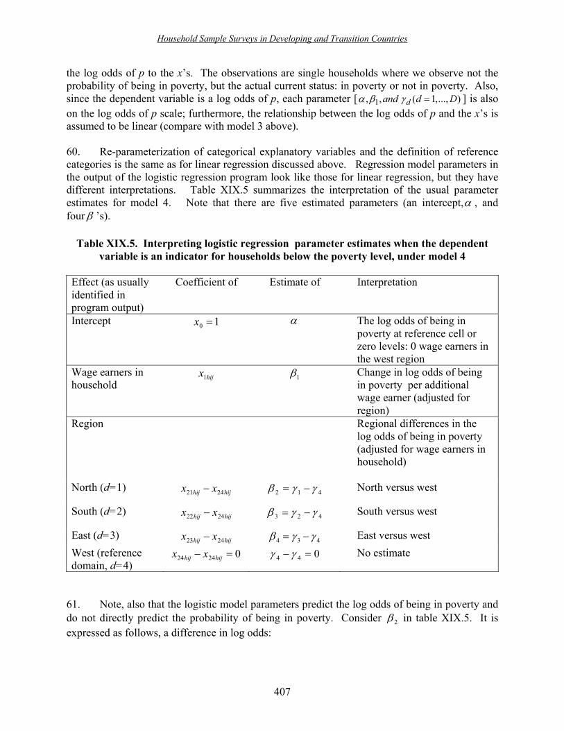
Household Sample Surveys in Developing and Transition Countries
407
the log odds of p to the x�s. The observations are single households where we observe not the probability of being in poverty, but the actual current status: in poverty or not in poverty. Also, since the dependent variable is a log odds of p, each parameter [ 1, , ( 1,..., )dand d Dα β γ = ] is also on the log odds of p scale; furthermore, the relationship between the log odds of p and the x�s is assumed to be linear (compare with model 3 above). 60. Re-parameterization of categorical explanatory variables and the definition of reference categories is the same as for linear regression discussed above. Regression model parameters in the output of the logistic regression program look like those for linear regression, but they have different interpretations. Table XIX.5 summarizes the interpretation of the usual parameter estimates for model 4. Note that there are five estimated parameters (an intercept,α , and four β �s).
Table XIX.5. Interpreting logistic regression parameter estimates when the dependent
variable is an indicator for households below the poverty level, under model 4
Effect (as usually identified in program output)
Coefficient of Estimate of Interpretation
Intercept 10 =x α The log odds of being in poverty at reference cell or zero levels: 0 wage earners in the west region
Wage earners in household
hijx1 1β Change in log odds of being in poverty per additional wage earner (adjusted for region)
Region Regional differences in the log odds of being in poverty (adjusted for wage earners in household)
North (d=1) hijhij xx 2421 − 412 γγβ −= North versus west
South (d=2) hijhij xx 2422 − 423 γγβ −= South versus west
East (d=3) hijhij xx 2423 − 434 γγβ −= East versus west West (reference domain, d=4)
02424 =− hijhij xx 044 =− γγ No estimate
61. Note, also that the logistic model parameters predict the log odds of being in poverty and do not directly predict the probability of being in poverty. Consider 2β in table XIX.5. It is expressed as follows, a difference in log odds:

Household Sample Surveys in Developing and Transition Countries
408
−
−
−
=)west(1
)west(log)north(1
)north(log2 pp
ppβ
By the properties of logarithms, it can also be expressed as the log of an odds ratio:
−
−=
)west(1)west(
)north(1)north(
log2
ppp
p
β
Standard output from logistic regression procedures routinely also provides the odds ratios, since they can be readily computed as:
−
−=
)west(1)west(
)north(1)north(
2
ppp
p
e β
In addition, individual household probabilities of being in poverty can be determined from the model as
)([log11)(
hijxpithij exp −+
=
62. When citing the results of logistic model-fitting, writers sometimes interpret an odds ratio of 2 as indicating that the probability of the event (poverty) in one domain (for example, north) is twice the probability of the event (poverty) in the other domain (for example, west). While this type of statement is approximately true for rare events (p near 0), it is far from true for more common events.
G. Use of multilevel models 63. We now turn to a discussion of multilevel modelling, and begin by emphasizing the need to recognize the survey data structure. Of relevance here is the structure imposed by surveys that are designed to be multistage. For example agroecological regions in a country may form strata, and from each, a number of administrative units may be selected. The latter will form the primary sampling units. Secondary units are then selected from each primary unit, subsequent units are selected from the secondary units, and so on. This leads to a hierarchic data structure. It can involve the use of stratification variables at one or more of the levels. 64. For example, a survey concerning farming households in a region may entail using the administrative divisions of the region as primary units, then choosing villages from each division and then selecting households from each village, perhaps ensuring that different wealth categories of households are included. Here, attention must be paid to the different sources of variability in the data collected at the household level. The overall variation incorporates variation between the administrative divisions, variation between villages, and variation between

Household Sample Surveys in Developing and Transition Countries
409
households within villages. Often data are also collected at each level of the hierarchy: here, at the household level, at the village level and at the administrative division level. It is then important to recognize and note which variables are measured at the village level (for example, existence of an extension officer; government subsidies for fertilizer) and which are measured at the household level (for example, socio-economic characteristics of the household). 65. For data analysis purposes, separate �flat� spreadsheet files may be prepared to hold the village-level information and the household-level information, using some key identifier to link these files. This is appropriate if the analysis objectives require data at village level to be analysed separately from data at the household level. However, it is not suitable if the analysis needs to combine village information with household-level information. Much more desirable is a relational database, that is to say, a database that allows data at different levels to be stored in one file, together with links that permit data at one level to be related to data at another level. The analysis must pull together the information from the multiple levels in order that the interrelationships between the different levels may be explored so as (for example) to enable an overall interpretation. 66. Multilevel modelling is the key statistical technique of relevance here. This modelling approach (Goldstein, 2003; Snijders and Bosker, 1999; Kreft and de Leeuw, 1998) is desirable because it allows relationships across and within hierarchic levels of a multistage design to be explored, taking account of the variability at different levels. Intercorrelations between variables at the same level are also taken into account. It also provides, through use of appropriate software, for example, MLwiN (Rashbash and others, 2001) and SAS (2001), model-based standard errors for estimates from complex survey designs. Such standard errors can serve as reasonable approximations for more exact standard errors that take account of stratification and clustering. It should be noted that MLwiN could also take account of sampling weights. This is important since unequal probabilities of selection in a multistage sampling design can induce bias in estimators of key parameters. Pfeffermann and others (1998) and Korn and Graubard (2003) discuss these issues more thoroughly. 67. It is worth highlighting briefly the consequences of ignoring the hierarchic structure at this point, which may occur when the data are aggregated to a higher level or disaggregated to a lower level. If the analysis is relevant and is required only at one level, there is no problem. However, care must then be taken that any inferences are made only at that level. It will not be possible to make inferences about one particular level of the hierarchy from data analysed at another level. Thus, an analysis ignoring the hierarchy will not permit cross-level effects to be explored. Another difficulty arises if data are analysed at their lowest level by regarding the higher- level units as a factor in the analysis. This is inefficient because it does not allow conclusions to be generalized to all higher-level units in the population: they will apply only to the sampled units. 68. We present below a scenario illustrating how the use of multilevel modelling can be beneficial in exploring relationships. Further examples can be found in Congdon (1998), Langford, Bentham and McDonald (1998) and Goldstein and others (1993).

Household Sample Surveys in Developing and Transition Countries
410
Example 1 69. In a study of factors contributing to successful community-based co-management of coastal resources among Pacific island countries, 31 sites across five countries were chosen and 133 interviews conducted with mini-focus groups comprising two to six respondents from different households (World Bank, 2000). Fiji, Palau, Samoa, Solomon Islands and Tonga were the countries chosen to represent a range of coastal management conditions. The 31 sites were selected to cover a range of conditions that were believed to influence management success. The study collected �perceptions of success� in terms of trends in perceived catch per unit effort (CPUE), condition of habitats, threats to the site, and an assessment of compliance. The first three indicators were measured on a five-point scale (5 = improving a lot; 1 = declining a lot), while compliance was measured on a four-point scale. 70. Data were also collected nationally from the fisheries and environmental ministries in each country, and at site level. Additionally, each focus group, comprising members of several households, was asked to give its perceptions for up to three resources (for CPUE), three habitats, three threats and five management rules for compliance. Thus, the information collected during this study resided at four levels: country, site, focus group and specific resource, habitat, threat or rule. 71. It is important, however, to note that this survey used non-probability sampling; it may therefore be argued that any analytical conclusions may not be generalizable to any clearly defined target population. However, for the purpose of this discussion, suppose that sampling had been conducted on a probability basis and that data at the focus group level would be analysed using a multilevel model - the particular variable of interest being the perception of CPUE trend, obtained by averaging the perception scores across the three resources. The country effect (at the top level of the hierarchy) could be included in the model as a factor (a fixed effect) since it is essentially a stratification variable. However, to enable results to be generalized across all co-managed sites, it is necessary to include sites as a random variable rather than as a fixed effect. Focus groups within sites would also enter the model as a random effect. The essence of multilevel modelling resides in the inclusion of a mixture of fixed effect variables and random effect variables. Such models also allow interactions among site-level variables and variables at the focus group level to be explored. 72. To illustrate the way in which a multilevel model can be formulated to answer specific survey questions, we use an example from a Food Production and Security Survey conducted in Malawi in 2000-2001 (Levy and Barahona, 2001). The survey aimed at evaluating a programme whose goal was to increase food security among rural smallholders through the distribution of a starter pack containing fertilizer, and maize and legume seed. Example 2 73. The Food Production and Security Survey was a national survey that used a stratified two-stage sampling scheme with districts as the strata. Four villages were selected from each of Malawi�s 27 districts, and about 30 households were selected from each village. Selection of villages was limited to those with more than 40 households (so that there would be enough

Household Sample Surveys in Developing and Transition Countries
411
households in the village to ensure that recipients of the starter pack could be interviewed) and those with less than 250 households (to make the team�s work possible within the time allowed according to resource availability).40 Within this restriction, the sampling at each stage was conducted at random. A total of 108 villages and 3,030 households were visited during the survey. 74. The data we consider for multilevel modelling comes from a household questionnaire completed during the survey. The subset of variables we will consider in our illustration are the district, village, household identification number, sex and age of household head, size of household, whether or not the household had received a starter pack, and two indices reflecting household assets41 and income.42 75. There are several multilevel models that can be fitted to this data. In formulating the model, the first step is to decide which variables are random and which are fixed effects. 76. In example 2, district is a stratification variable and would be regarded as a fixed effect. In general, any effect is regarded as fixed if repeats of the sampling process will result in the same set of selections. On the other hand, villages and households have been selected at random, so they form random effects in the model. 77. The basic model for analysing (say) the asset index (AI) is
Model 5
yijk = µ + dk + Ujk + εijk
where dk is the district effect (k = 1, 2, �., 27), and indices i and j correspond to the ith household and jth village, respectively. It is sometimes convenient to think of the district parameter as reflecting the deviation of the mean value of AI for district k from the overall mean value of AIs across all districts. However, software for modelling use a different parameterization and sets one of the district effects to zero. The remaining effects then provide comparisons between the AIs for each district with the AI of the district whose effect has been set to zero. 78. In this model, Ujk and εijk, denote random variables representing, respectively, the variation among all villages within district k (assumed to be the same for all districts), and the variation among all households in village j in district k (assumed to be the same for all village and district combinations). Ujk and εijk are random variables that are assumed in the model to be normally distributed variables with zero mean and constant variances σu
2 and σe2, respectively.
They are further assumed to be independent of each other. We may therefore write Ujk ~ N(0, σu
2) and εijk ~ N(0, σe2).
40 This constraint on the target population limited inference to the population residing in villages in this size range. 41 The asset index was a weighted average based on different livestock numbers and household assets, for example, radio, bicycle, oxcart, etc. 42 The income index was based on income from a range of different sources.

Household Sample Surveys in Developing and Transition Countries
412
79. Fitting this model provides estimates of σu2 and σe
2 and estimates for dk, along with relevant standard errors. The parameter estimates for dk (k=1, 2,�, 27), allow a comparison of the AI means across the 27 districts. 80. Now suppose that it was of interest to investigate how the variation in the AI was affected by the size of household (a quantitative variable) and whether or not the household received a starter pack (a binary variable). These would be included in the model in the same way as would be done in standard general linear modelling. The model would be given by
Model 6
yijk = µ + dk + Ujk + tp(ijk) + β xijk + εijk where tp(ijk) represents the effect corresponding to the receipt of the starter pack; xijk represents the size of the household and β represents the slope describing the relationship of xijk to yijk, that is to say, the relationship of household size (HHSIZE) to the asset index (AI). 81. Here both tp(ijk) and β are regarded as fixed effects, while Ujk and εijk are (as before) random effects. The form of this model assumes that the relationship of HHSIZE to AI is the same across all villages and districts. 82. The inclusion of both components of variation (village and household) in the above model means that the model takes account of the variability at two levels of the hierarchy. This means that standard errors associated with tp(ijk) and β are calculated correctly, as would be the results of tests of significance associated with these parameters. This would not have been the case if a general linear model had been fitted regarding villages as fixed effects. Even if survey software (which take account of sampling weights) was used, standard regression procedures would ignore the correlation structure between households within any one village. 83. There is another important benefit in treating villages as random effects. If villages had been regarded as fixed, then the conclusions from the analysis would have applied only to the set of villages visited during the survey. Regarding villages as random effects means that the conclusions concerning the relationship of household size to the AI, the comparison of the AI across households receiving or not receiving the starter pack, and the comparison across districts, can all be generalized to encompass the wider population of all villages. The interaction between the district level fixed effect dk and the starter pack recipient effect tp(ijk) can also be explored by including such an interaction term in the model. 84. A further useful model is obtained by regarding the slope term β in model 6 as a random variable that varies across the villages. This is often referred to as a random coefficient regression model. The model then becomes
Model 7
yijk = µ + dk + Ujk + tp(ijk) + βj xijk + εijk

Household Sample Surveys in Developing and Transition Countries
413
where βj is assumed N(β, σβ2). Further, since βj is random across villages, it may also be
considered to have a covariance with Ujk, say, σβu. 85. Thus, in the analysis presented here, testing the hypothesis that σβ
2 is zero effectively tells us whether there is variability in the slope of the AI-versus-HHSIZE relationship across villages. If this hypothesis cannot be rejected, then it may be concluded that the form of the relationship is the same for all villages. 86. It is possible to extend this model further to include village-level variables, for example, access to a clean water supply or the degree of availability of advice from agricultural extension officers. Here, the real benefits of multilevel modelling come into play since it would then be possible to explore relationships between such village-level variables and the household-level variables. Thus, the study of relationships between variables at different levels of a hierarchic sampling scheme becomes possible through multilevel modelling. The benefits lie in being able to take account of the correlation structure among lower-level units when variables at different levels are being analysed together. In the above example, further models could be considered, for example, models that include gender and age of the household head, and interactions between these and terms previously included in the model. 87. There are of course limitations associated with fitting multilevel models. As with all other modelling procedures, the hypothesized multilevel model is assumed to be �correct� to a reasonable degree and to conform to the sample design. Whether such assumptions are true is of course debatable.
H. Modelling to support survey processes 88. Even when a household survey is used strictly to provide descriptive statistics, there may be need for modelling to support other survey processes. Adjustments for non-response are often based directly or indirectly on statistical models: Groves and others (2002, pp. 197-443) discuss a variety of methods for accounting for non-response, all of which must assume some statistical model. Logistic regression models may be used to develop predicted response propensities for the purpose of non-response adjustment or to identify weighting classes based on similar response propensities [see, for example, Folsom (1991); Folsom and Witt (1994); or Folsom and Singh (2000)]. Predictive statistical models may also be used as part of the procedure for imputing missing data [see, for example, Singh, Grau and Folsom (2002)]. Finally, statistical models can be used to evaluate methodological experiments embedded in surveys [see, for example, Hughes and others (2002)].
I. Conclusions
89. Our aim in this chapter has been to discuss issues involved in the analysis of survey data. These issues include the use of survey weights and of appropriate variance estimation methods with both descriptive and analytic approaches to survey data. The chapter also provides an overview of practical situations where modelling techniques have a role to play in survey data

Household Sample Surveys in Developing and Transition Countries
414
analysis. They are useful tools but their application requires careful thought and attention to their underlying assumptions. 90. We have discussed the role of survey weights and recognition of the sample structure in developing both descriptive and analytic statistics from survey data. Survey data analysis software that use survey weights and take account of the sample structure may be used to estimate the parameters of both linear and logistic regression models based on survey data. The estimates based on the sample are estimates of what would be obtained from fitting the models to the entire finite population. Furthermore, standard errors of the estimates can also be obtained. The explanatory variables in regression models applied to survey data are almost always observed as they exist in the population rather than randomly assigned according to some experimental design. Analysts need to be clear that regression coefficients based on survey data simply reflect relationships that exist between the dependent variable and the explanatory variables in the population and do not necessarily imply causation. We have discussed how the parameters of regression and logistic regression models relate to simple descriptive statistics and how they may be interpreted for some relatively simple models. 91. Multilevel modelling, in particular, would generally be regarded as a rather �advanced� technique and is best carried out in consultation with a statistician familiar with the use and limitations of this technique. At present, multilevel models appear to be rarely used in analysing surveys in developing countries; however, their use would be highly desirable for the insights they can provide concerning interrelationships between variables at different levels and their ability to take account of variability among sampling units at different levels in a multistage design. 92. We have shown that the formulation of multilevel models is not too difficult for someone familiar with the application of general linear models (GLMs); but, again, there are assumptions associated with the models that need to be checked by carrying out residual analyses, as would be the case with GLMs. The multilevel modelling approach can also be undertaken when the main response of interest is binary, although we have not presented an example of such a case. Care is also needed in deciding which effects are random and which are fixed and how the model specification will help in answering specific survey objectives. 93. However, as with all statistical techniques, the modelling methods discussed in this chapter have various limitations which need to be recognized in their application. We have urged the use of survey weights and analysis software that recognizes the sample design structure. The difficulty of access to appropriate software that takes account of the sampling design must be recognized. Chapter XXI describes several software packages that pay attention to sampling design issues with respect to multiple regression and logistic regression procedures. Unfortunately however, these packages do not have facilities for fitting multilevel models. For this purpose, the user needs to turn to more general-purpose statistical software such as SAS (2001), GenStat (2002) and SPSS (2001), or to a specialist software package such as MLwiN (Rahbash and others, 2001). 94. This chapter has offered some modelling techniques that can serve as useful tools for survey data analysis. We recommend that survey analysts and researchers seriously consider

Household Sample Surveys in Developing and Transition Countries
415
these methods, where appropriate to survey objectives, during survey data analysis, with a view to extracting as much information as possible from expensively collected survey data. Acknowledgements
The authors wish to express their special thanks to the reviewers and editors for many useful comments and suggestions, and especially to Dr. Graham Kalton for the enhancements to the discussion on survey weighting.
The Department for International Development (DFID) of the Government of the United Kingdom of Great Britain and Northern Ireland is also thanked for providing ideas for this chapter through its funding of many interesting projects involving surveys in the developing world. The material in this chapter remains, however, the sole responsibility of the authors and does not imply the expression of any opinion whatsoever on the part of DFID. References Chambers, R.L., and C.J. Skinner (2003). Analysis of Survey Data. Chichester, United
Kingdom: Wiley. Chromy, James R. (1998). The Effects of Finite Sampling on State Assessment Sample
Requirements. Palo Alto, California: NAEP Validity Studies, American Institutes for Research.
Cochran, W. G. (1977). Sampling Techniques, 3rd ed. New York: John Wiley and Sons. Congdon, P. (1998). A multi-level model for infant health outcomes: maternal risk factors and
geographic variation. The Statistician, vol. 47, Part 1, pp. 159-182. Deville, J.C., and C.E. Sarndal (1992). Calibration estimating in survey sampling. Journal of
the American Statistical Association, vol. 87; pp. 87, pp. 376-382. Folsom, Ralph E., Jr. (1991). Exponential and logistic weight adjustments for sampling and non-
response error reduction. In Proceedings of the Social Statistics Section, American Statistical Association. Alexandria, Virginia: American Statistical Association, pp. 376-382.
Folsom, Ralph E., and Michael B. Witt (1994). Testing a new attrition non-response adjustment
method for SIPP. In Proceedings of the Survey Research Methods Section, American Statistical Association, pp. 428-433.
Folsom, R. E., and A.C. Singh (2000). The general exponential model for sampling weight
calibration for extreme values, non-response and post-stratification. In Proceedings of the Survey Research Methods Section, American Statistical Association. Indianapolis, Indiana.

Household Sample Surveys in Developing and Transition Countries
416
GenStat (2002). GenStat for Windows, 6th ed. Oxford, United Kingdom: VSN International, Ltd. Goldstein, H. (2003). Multi-level Statistical Models, 3rd ed. London: Arnold. __________ , and others (1993). A multi-level analysis of school examination results. Oxford
Review of Education, vol. 19, pp. 425-433. Graubard, B. I., and E.L. Korn ( 2002). Inferences for super-population�� Statistical Science,
vol. 17, pp. 73-96. Groves, Robert M., and others (2002). Survey non-response. New York: John Wiley and Sons,
Inc. Horvitz, D. G., and D.J. Thompson (1952). A generalization of sampling without replacement
from a finite universe. In Journal of the American Statistical Association, vol. 47, pp. 663-685.
Hughes, Arthur, and others (2002). Impact of interviewer experience on respondent reports of
substance use. In Redesigning an Ongoing National Household Survey: Methodological Issues, J. Gfoerer, J. Eyerman and J. Chromy, eds. DHHS Publication, No. SMA 03-3768. Rockville, Maryland: Substance Abuse and Mental Health Services Administration, Office of Applied Studies, pp. 161-184.
Kish, Leslie (1965). Survey Sampling. New York: John Wiley and Sons, Inc. Korn, E. L. and B.I. Graubard (1999). Analysis of Health Surveys. New York: John Wiley and
Sons. __________ (2003). Estimating variance components by using survey data. In Journal of the
Royal Statistical Society B, vol. 66, pp. 175-190. Kreft, I., and J. de Leeuw (1998). Introducing Multi-level Modeling. London. Langford, I.H., G. Bentham and A. McDonald (1998). Multi-level modeling of geographically
aggregated health data: a case study on malignant melanoma mortality and UV exposure in the European community. Statistics in Medicine, vol. 17, pp. 41-58.
Levy, S., and C.I. Barahona (2001). The targeted inputs programme, 2000-01: Main report.
Unpublished. Pfeffermann, D., and others (1998). Weighting for unequal selection probabilities in multi-level
models. In Journal of the Royal Statistical Society B, vol. 60, pp. 23-40. Rasbash, J., and others (2001). MLwiN Version 1.10.0007. Multi-level Models Project.

Household Sample Surveys in Developing and Transition Countries
417
London: Institute of Education, University of London. Research Triangle Institute (2002). SUDAAN User�s Manual, Release 8.0. Research Triangle
Park, North Carolina: Research Triangle Institute. Rubin, Donald B. (1987). Multiple Imputation for Non-response in Surveys. New York: John
Wiley and Sons. SAS (2001). SAS Release 8.2. Cary, North Carolina: SAS Institute, Inc., SAS Publishing. Singh, Avinash, Eric Grau and Ralph Folsom Jr. (2002). Predictive mean neighborhood
imputation for NHSDA substance use data. In Redesigning an Ongoing National Household Survey: Methodological Issues, J. Gfroerer, J. Eyerman and J. Chromy, eds. DHHS publication, No. SMA 03-3768. Substance Abuse and Mental Health Services Administration, Office of Applied Studies.
Skinner, C.J., D. Holt and T.M.F. Smith, eds. (1989). Analysis of Complex Surveys. New York:
Wiley. Snijders, T.A.B., and R.J. Bosker, R.J. (1999). Multi-level Analysis: An Introduction to Basic
and Advanced Multi-level Modelling. London: Sage. SPSS (2001). SPSS for Windows. Release 11.0. Chicago, Illinois: LEAD Technologies, Inc. Tukey, J. W. (1977). Exploratory Data Analysis. Reading, Massachusetts: Addison-Wesley. Woodruff, R. S. (1971). A simple method for approximating the variance of a complicated
sample. In Journal of the American Statistical Association, vol. 66, pp. 411-414. World Bank (2000). Voices from the Village: A Comparative Study of Coastal Management in
the Pacific Islands. Pacific Islands Discussion Paper Series, No. 9. Washington, D.C.: World Bank. Papua New Guinea and Pacific Islands Country Management Unit.

Household Sample Surveys in Developing and Transition Countries
418

Household Sample Surveys in Developing and Transition Countries
419
Chapter XX More advanced approaches to the analysis of survey data
Gad Nathan Hebrew University Jerusalem, Israel
Abstract
In the present chapter, we consider the effects of complex sample design used in practice in most sample surveys on the analysis of the survey data. The cases in which the design may or may not influence analysis are specified and the basic concepts involved are defined. Once a model for analysis has been set up, we consider the possible relationships between the model and the sample design. When the design may have an effect on the analysis and additional explanatory variable related to the design cannot be added to the analytical model, two basic methodologies may be used: classical analysis, which could be modified to take the design into account; or a new analytical tool, which could be developed for each design. Different approaches are illustrated with real-data applications to linear regression, linear models, and categorical data analysis. Key terms: complex sample design, analysis of survey data, linear regression, linear models, categorical data analysis, model-based analysis.
.

Household Sample Surveys in Developing and Transition Countries
420
A. Introduction
1. Sample design and data analysis
1. The primary purpose of the vast majority of sample surveys, both in developed and in developing countries, is a descriptive one, namely, to provide point and interval estimates of descriptive measures of a finite population, such as means, medians, frequency distributions and cross-tabulations of qualitative variables. Nevertheless, as demonstrated in chapters XV-XIX and as will be demonstrated in chapter XXI, there is increasing interest in making inferences about the relationships among the variables investigated, as opposed to simply describing phenomena. 2. In the present chapter, we shall try to assess the effects of commonly used complex sample designs on the analysis of survey data. We shall attempt to identify cases where the design can influence the analysis. Usually, the sample design has no effect on the analysis when the variables on which the sample design is based are included in the analytical model. Frequently, however, some design variables are not included in the model, either owing to mis-specification or to a lack of interest in those design variables as explanatory factors. This can result in serious biases. 3. There are two basic methodologies we shall discuss for handling data from a complex sample when additional design-related variables are not added to the analysis. The first modifies a classical analytical tool developed for handling data from a simple random sample. The second develops a new analytical tool for the specific complex design. 4. In what follows, we present some examples of the possible effects of sample design on analysis, define a few basic concepts, and discuss the role of design effects in the analysis of complex sample data. Section B describes the two basic approaches to the analysis of complex sample data. In sections C and D, we discuss examples relating to the analysis of continuous and categorical data, respectively. The final section contains a summary and some conclusions. Formal definitions and technical results are given in the annex.
2. Examples of effects (and of non-effect) of sample design on analysis 5. In order to demonstrate the potential effects of sample design on the analysis, we consider the following simple, but illuminating, example (for details, see Nathan and Smith, 1989). Let Y be the variable of interest and X be an auxiliary variable. Assume that the linear regression model iii XY εβα ++= , with ( )2,0N~| iindii X σε , holds for the population. The model
holds as well for any simple random sample selected from the population. Sometimes the assumption of independence across the ii X|ε is better suited for the simple random sample than the population from which it was drawn. In a human population, for example, iε values may be correlated for different members of the same household, while in a simple random sample of individuals, with a very small probability that more than a single individual is selected per household, the correlation would be negligible.

Household Sample Surveys in Developing and Transition Countries
421
6. Under simple random sampling the standard estimate of the regression coefficient is unbiased. The display in figure XX.1 plots Y against X for the total population; the display would look the same for a simple random sample. In the five displays of figures XX.2-XX.6, samples are selected from the population using methods very different from simple random sampling. Consider sample selection based entirely on the value of X, for instance, by truncating data points with X values beyond (or within) fixed limits as in figures XX.2 and XX.3. It is clear from these figures that the selection has no effect on the estimation of the intercept (α ) and slope ( β ) parameters of the regression (although it may effect the variance of the estimators). 7. Now consider sample selection based on the values of the target variable, Y, for instance, by truncating those data points with Y values beyond (or within) fixed limits as in figures XX.4-XX.6.
Figure XX.2Selection on X: XL<X<XU
-4
-3
-2
-1
0
1
2
3
4
-4 -2 0 2 4
X
Y
Figure XX.1No selection
-4
-3
-2
-1
0
1
2
3
4
-4 -2 0 2 4
X
Y
Figure XX.3Selection on X: X<XL; X>XU
-4
-3
-2
-1
0
1
2
3
4
-4 -2 0 2 4
X
Y
Figure XX.4Selection on Y: YL<Y<YU
-4
-3
-2
-1
0
1
2
3
4
-4 -2 0 2 4
X
Y
Figure XX.5Selection on Y: Y<YL;Y>YU
-4
-3
-2
-1
0
1
2
3
4
-4 -2 0 2 4
X
Y
Figure XX.6Selection on Y: Y>YU
-4-3-2-10
1234
-4 -2 0 2 4
X
Y

Household Sample Surveys in Developing and Transition Countries
422
In these cases, it is clear that the estimates of the slopes of the regression become biased. In the last case (figure XX.6), truncation is not symmetric, and the estimate of the intercept is also biased. These examples are extreme, since selection based on the truncation of the dependent variable is rare in sample surveys. It is quite common, however, in experimental or observational studies, such as case control studies in epidemiology or choice-based studies in economics [see, for example, Scott and Wild (1986) and Manski and Lerman (1977)]. Nevertheless, in many cases, samples are selected on the basis of design variables that may be closely related to the dependent variable. Thus, a common sampling procedure, widely used in surveys of establishments and of farms, is to select units with probability proportional to size. The size measure, say, the previous year�s production, will obviously be related to the variable of interest when that variable is the current year�s production. Standard estimates of model parameters, such as regression coefficients, can be biased when the sample design is ignored. 8. The examples above illustrate the dangers of carrying out an analysis based on complex sample data as if they came from simple random sampling. The examples reveal a need for identifying when it is likely that the design affects the analysis and for taking the design into account when it does.
3. Basic concepts 9. Most sample surveys are designed primarily for descriptive (or enumerative) purposes. They aim at estimating the values of finite population parameters, such as the median household income or the proportion of all adults with AIDS. These are statistics that, in principle, can be measured exactly if the whole population were included in the survey, that is to say, if a census of the population was enumerated rather than a random sample of the population. The standard theory of survey sampling ensures that data from a random sample can be used to provide unbiased estimates of the finite population parameters and of their sampling errors no matter how complex the sample design. This assumes that the sample design is a probability sample design, that is to say, each unit in the population has a known positive probability of being sampled. These classical methods of estimation of finite population parameters are known as design-based (or randomization-based) methods, since all inference is based on the properties of the sample design, via the sample probability distribution. It should be noted, however, that the efficiency of different estimation strategies (a sample design coupled with an estimation formula) can usually be evaluated only when extensive information about the population is available. This is usually not the case in practice. Thus, even classical sampling texts (for example, Cochran, 1977) often rely on models to justify specific methods of sampling or estimation. If the population values follow a simple regression model, for example, then the ratio estimator will be more efficient than the simple expansion estimator, under certain assumptions. Design-based methods are thus often model-assisted, but they are not model-based (or model-dependent): with model-assisted methods of sample design and estimation of descriptive statistics, model assumptions are not required for the nearly unbiased estimation of finite population parameters. 10. The model-based (or prediction theory) approach to sample design and estimation assumes that the finite population values are, in fact, realizations of a super-population distribution based on a hypothetical model with super-population (model) parameters. For further detail and discussion, see Brewer and Mellor (1973), Hansen, Madow and Tepping (1983),

Household Sample Surveys in Developing and Transition Countries
423
Särndal, Swensson and Wretman (1992) and Valliant, Dorfman and Royall (2000). In contrast with model-assisted estimation methods, the increased efficiency attained by model-based estimation methods relies on the validity of the assumed model. Thus, if there is any doubt about the validity of the model assumptions, the apparent reduction in mean square may not justify the use of purely model-based analysis. A good example of this is demonstrated in Hansen, Madow and Tepping (1983), where assuming no intercept in a regression model, even when the intercept is in fact very close to zero, results in invalid model-based inference. 11. Increasingly, surveys are being used for analytical purposes as well as descriptive ones. Often surveys are designed with their analytical uses in mind. This is because decision makers and researchers are interested in the processes underlying the raw data, in modelling the relationships among the variables investigated. Such analyses obviously require assumptions about models. The aim of an analysis is to confirm the validity of an assumed model and to estimate the model�s parameters rather than the parameters of the finite population. Thus analysis is inherently model-based. Inference about model parameters must, practically by definition, be based on the models of interest. 12. It should be pointed out, however, that when the population is very large and the hypothesized model indeed holds, there is in practice very little difference between the model parameters and their finite population counterparts. For instance, if the standard linear regression model iii XY εβα ++= , with ( )2,0N~| iindii X σε holds, and the population size is very
large, then the value of the standard population regression coefficient, B (see annex), will be very close to the value of the model parameter, β, because of to the Central Limit Theorem. Thus, although we shall focus on the estimation of model parameters in what follows, these parameters will sometimes be replaced by their finite-population counterparts. For the sake of simplicity in presentation, most of the examples in what follows will be formulated in terms of univariate distributions (that is to say, a single dependent variable and a single explanatory variable). The extension of the results to the multivariate case is usually straightforward. 13. To summarize, hypothetical models are an integral part of statistical analysis. In order to analyse data from sample surveys, the choice of a good model to fit the data is a critical part of the analysis. Researchers and analysts must have a good understanding of the models underlying the processes they wish to study before applying analytical methods. As we shall see in the following sections, the application to data from complex sample designs requires both an understanding of the underlying model and of the way in which the analysis can be affected by the complex design.
4. Design effects and their role in the analysis of complex sample data
14. The topics of design effects and their estimation have been treated extensively in chapters VI and VII, primarily in relation to their role in the design and estimation for enumerative surveys. We shall see in this chapter that they also play an important role in the analysis of data from complex sample surveys. The underlying idea is based on the fact that, assuming that the model assumptions hold, unbiased estimates of the model parameters and estimates of the variances of these estimates are readily available under simple random sampling. These estimates and variance estimates form the basis for testing hypotheses relating to the model

Household Sample Surveys in Developing and Transition Countries
424
parameters. For example, under simple random sampling and assuming the simple regression model iii XY εβα ++= , with ( )2,0N~| iindii X σε , the ordinary least squares sample estimator, b,
is an unbiased estimator of β, and an unbiased estimator of its variance, v(b), is available (see annex). The standard test of the null hypothesis that β=0 is then based on the test statistic
)(/ bvb , by invoking the Central Limit Theorem. When the sample design is a complex one, for example, a stratified cluster sample, the estimator b remains model-unbiased, if the regression model holds and the sample design does not depend on the values of Yi (for example, in constrast to the situation in figures XX.4-XX.6). By this we mean that under the specified regression model, the expected value of b is β, where the expectation is with respect to the super-population distribution of the values of Yi. As we shall see in section C.1, this may no longer be true if the model does not hold. However, even if the model assumptions hold, v(b) is no longer a valid estimator of the model variance of b and must be modified. Often, a direct estimator of the correct model variance can be computed, for example, by using one of the software packages described in chapter XXI, and can be used to replace v(b). If a direct estimator is not available, often a good estimator of the design effect, denoted by d2(b), can be obtained. This can be used for the modification of the test statistic to replace v(b) by d2(b) x v(b). We shall present further specific uses of the design effects to modify standard test statistics for other applications below.
B. Basic approaches to the analysis of complex sample data
1. Model specification as the basis of analysis 15. Correct specification of the underlying model is a fundamental step in any analysis. The consequences of model mis-specification - both of exclusion of relevant explanatory variables (or the inclusion of superfluous ones) and of using a wrong functional form (for example, linear instead of quadratic) - are well known and documented in standard texts. They can take the form of biases in the estimation of the model parameters (primarily the exclusion of relevant variables), losses of efficiency (mostly connected with erroneous inclusion of explanatory variables) and altered sizes and power in tests of hypotheses. These effects may be exacerbated when the mis-specification relates directly to sample design variables or to variables correlated with design variables. Nevertheless, it is important to realize that the survey design variables may not be relevant to the research objectives. Moreover, there may be no subject-matter justification for their inclusion in the analytical model. 16. There are two basic approaches to incorporating survey design variables in the model. The aggregated approach considers the model of interest to be at the population level and conceptually independent of the sample design employed to obtain the data. Under this approach, design variables would be included in the model only when they are relevant to the subject-matter analysis. For instance, say we wish to explain the binary variable employed/unemployed by the explanatory variable years of education, irrespective of geographical location. The sample is stratified, say, by geographical regions, for which different models may be relevant. This would be the case even had simple random sampling been used. As a result, the stratification can be included in the model (see the disaggregated approach discussed below) to reflect regional variations in the relationships among the model variables. If, by contrast, the stratification and

Household Sample Surveys in Developing and Transition Countries
425
the sample allocation to strata were carried out simply for operational reasons (convenience or cost), the sample weights would likely not be relevant to the population model. The incorporation of sampling weights into an analysis otherwise free of stratum effects will lead to some loss of efficiency. Nevertheless, it is susceptible to the easy interpretation of a model free from stratum effects, while being robust to model failure if some of the ignored stratum effects really exist. 17. The disaggregated approach extends the analyst�s model to include not only the survey variables of interest but also variables used in the survey design and those relating to the structure of the population reflected in the design. Design variables relating to the stratification and clustering are included in the model to reflect the complex structure of the population. For instance, in the previous example, the model would contain a different set of coefficients (both an intercept and a slope) for each geographical stratum. Inference under the disaggregated approach takes the sample design fully into account, assuming that all design variables are correctly included in the model. The large number of parameters that need to be estimated under this approach may cause difficulties and lead to less accurate estimates when compared with those of more parsimonious aggregated models. The disaggregated approach is appropriate only when the analyst believes that the hypothesized model is relevant for his purposes. 18. The appropriate approach to be used - the aggregated or disaggregated approach - will depend on the analyst�s aims. The aggregated approach is more suitable for studying factors affecting the population as a whole and, as such, may be more useful for evaluating national-policy actions. The disaggregated approach is more suitable for studying micro-effects and the effects of local and sector-specific decision-making. For further examples and discussion, see Skinner, Holt and Smith (1989) and Chambers and Skinner (2003).
2. Possible relationships between the model and sample design: informative and uninformative designs
19. It is important to draw a distinction between informative and non-informative sample designs when analysing complex survey data. Once a model has been hypothesized, the analyst must consider whether, after conditioning on the model covariates, the sample selection probabilities are related to the values of the response variable. A sampling process is informative if the joint conditional model distribution of the observations for the sample, given the values of the covariates in the model, differs from their conditional distribution in the population. Only when these distributions are identical is the sample design non-informative (or ignorable), in which case standard analytical methods can be employed as if the observations came from a simple random sample. When the sample design is informative, the model holding for the sample data is different from the population model. Ignoring the sampling process in such a case may yield biased point estimators and distort the analysis just as when variables are excluded from the model in a conventional analysis. Note that the correct inclusion of design-related variables in the model will ensure that the design is non-informative. 20. There are two major problems with including all design-related variables in a model. First, exactly which variables were used in the design may not be known or, if known, their values may not be available. Even when the design variables are identified and measured, the

Household Sample Surveys in Developing and Transition Countries
426
analyst may not know the exact form of the relationship (for example, linear or exponential) between them and the variable of interest. For instance, if the design is a stratified one, then the possibility that a regression relationship has different slopes and intercepts for the different strata will need to be checked. 21. Second, when design variables are correctly included in the model, resulting estimates may be of little value to the analyst, since the variables added are not of intrinsic subject-matter interest (recall the discussion on aggregated and disaggregated analysis). This implies that the effect of a complex sample design on analysis cannot always be dealt with solely by modifying the underlying model. In what follows, we shall consider both how to modify standard analytical methods to take a complex design into account and how to construct special design-specific methods of estimation and analysis.
3. Problems in the use of standard software analysis packages for analysis of complex samples
22. The nearly universal use of standard software for statistical analysis has led to widespread abuse of sound statistical practice. This abuse is frequently exacerbated when analysing complex sample survey data. 23. The advantages of statistical software in facilitating analysis unfortunately come with the possibilities for performing analysis without any basic understanding of the underlying principles involved. This has become a serious problem in quantitative work, especially in the social sciences. This problem is compounded by the fact that most commonly available software treats data as if they resulted from simple random sampling. As pointed out previously, this can lead to seriously biased inference when the design is informative. Nevertheless, with due care, standardized software can often be adapted to approximately capture or account for the effect of a complex design. In particular the SURVEYREG procedure in the latest versions of SAS (versions 8 and 9) features regression analysis that takes the sample design into account in ways similar to those described below [see An and Watts (2001)]. 24. For instance, consider the linear (heteroscedastic) regression model defined by:
iii XY εβα ++= , with ( )2,0N~| iindii X σε . Standard computer programmes ordinarily compute
b, the ordinary least squares (OLS) estimator of β, or the generalized least squares (GLS) estimator, bG, where sums and products are weighted by the reciprocals of 2
iσ , whose values (or relative values) are assumed to be known (see annex). Both of these are unbiased estimators for the parameter β, if the model holds, although bG is a more efficient estimator in the heteroscedastic case. The standard programmes also provide estimators of the variances of the OLS estimator, v(b), and of the GLS estimator, v(bG), which are each model-unbiased under the appropriate model (the homoscedastic model in the case of v(b)). 25. In many cases, there may be doubt about the validity of the model, so that instead of estimating β, it may be more appropriate to estimate the finite population counterpart of β, which we denote as B (see annex). Although b (the OLS estimator) is a model-unbiased estimator for β ≈ B, it is not in general design-unbiased. The sample-weighted (Horvitz-Thompson) estimator,

Household Sample Surveys in Developing and Transition Countries
427
bW, with cross-products and squares weighted by the reciprocals of the inclusion probabilities, is both design-consistent and model-unbiased, under appropriate conditions. Furthermore bW can be obtained from the weighted regression options of many standard programmes by using the values of wi as the weights. Alternatively bW can be obtained by unweighted regression of the transformed variables iiY π , iiX π with the intercept replaced by iπ1 . It must be emphasized, however, that under both these alternatives, the estimates of the variance-covariance matrix reported by most standard programmes are incorrect -- both as estimators for design mean squared error and as estimators for model variance -- except in unusual circumstances. 26. In summary, the use of standard software programmes that do not take into account complex survey design should be avoided unless it can be determined that the complex design does not have a serious effect on estimation. This can often be achieved through the suitable use of standard software. See the example in section C.2. The use of software packages specifically dealing with complex sample designs is recommended (see chap. XXI).
C. Regression analysis and linear models
1. Effect of design variables not in the model and weighted regression estimators
27. Regression analysis and linear modelling are very common applications where standard models developed for simple random samples are routinely applied to data from complex sample surveys. As already pointed out, this can often lead to erroneous analyses and conclusions. A key source of protection against error is the identification of variables determining or influencing the sample design, so that they can be included in the model. As we have seen, however, even when these variables are identified, their inclusion in the model may not be warranted from the subject-matter point of view. In the present subsection, we will study the effects on traditional estimators of not including design variables in the model and investigate the possibilities for modifying these estimators so as to take the complex design into account. For ease of exposition, we consider the case of a single dependent variable, Y (denoted in this section for technical reasons by X1), where the model of interest has a single explanatory variable (X2), and there is a single design variable (X3). The model of interest is therefore
( ) ( )221211E µβµ −+= XX , where 12β is the parameter of interest, rather than the full model, which includes the design variable, X3. See the annex for the formulae used in this subsection. 28. Under fairly general conditions specified in Nathan and Holt (1980), the standard OLS estimator for β12, 2
21212 ssb = , can be both (model-) biased conditional on X3 and on the sample, S, and biased unconditionally. Expressions for the conditional model expectation and its unconditional (joint model and design) expectation show that, in general, b12 is asymptotically biased, unless ρ23, the correlation between X2 and X3, is zero or if the simple sample variance of X3 is an unbiased estimator for its true variance. It can be shown that this second condition does hold asymptotically for a large number of equal probability (epsem) sample designs, but rarely for unequal probability designs (for example, non-proportional stratified sample designs).
Household Sample Surveys in Developing and Transition Countries
428
29. A corrected, asymptotically unbiased estimator based on the maximum likelihood estimator under normality, 12
�β , can be used instead of the OLS estimator. Expressions for the variances of b12 and of 12
�β are given in Nathan and Holt (1980). It should be noted that the usual estimator for the variance of b12, ( )12v b , may not be nearly unbiased, even when b12 is a consistent estimator for β12. This can happen when the iε �s are not independent and identically distributed among the observations in the sample. 30. Neither the estimator b12 nor 12
�β depends on the sample design, though their properties do. Information on the sample design may be useful for improving these estimators, either when information on values of the design variable X3 is not available for the whole population (so that
23S cannot be used for estimation) or when the analysts wishes to ensure robustness to departures
from the model. This can be done by using sample-weighted estimators based on Horvitz-Thompson estimation for each of the components of the unweighted estimators. One can replace the unweighted sample moments by their weighted versions in the expressions for b12 and for
12�β to obtain the weighed estimators, *
12b and *12
�β . 31. Note that *
12b can be used when the population variance of X3, 23S , is unknown, but that
*12
�β cannot be used in that situation. It is easily seen that, under fairly general conditions, both of these estimators are design-consistent estimators of the finite population parameter, 12B . 32. Empirical comparisons of the performance of these four estimators were made by Nathan and Holt (1980) for a population of N = 3,850 farms, about which data on crop land (X1), total acreage (X2), and total value of produce in previous year (X3), were available. Farms were stratified on the basis of the X3 values resulting in six strata of sizes 563, 584, 854, 998, 696 and 155. The following six sample designs were used to select samples of size n = 400 (see table XX.1):
(A) Simple random sampling;
(B) Proportional stratified simple random sampling;
(C) Fixed size stratified simple random sampling;
(D) Stratified simple random sampling with higher-than- proportional allocation to strata with high X3 values (25, 30, 60, 80, 130, 75);
(E) Stratified simple random sampling with U-shaped allocation (100, 80, 20, 20, 80, 100).
.

Household Sample Surveys in Developing and Transition Countries
429
Table XX.1. Bias and Mean square of ordinary least squares estimator and variances of unbiased estimators for population of 3,850 farms using various survey designs
Survey design E(b12)- β12 MSE(b12) V( 12
�β ) V( *12b ) V( *
12�β )
A 0-000 0-000214 0-000197 0-000226 0-000197 B 0-000 0-000200 0-000198 0-000222 0-000196 C 0-031 0-001102 0-000160 0-000222 0-000196 D 0-027 0-000879 0-000163 0-000220 0-000195 E 0-042 0-001877 0-000152 0-000225 0-000196
Source: Nathan and Holt (1980); table 1. 33. The results demonstrate the bias of b12 for the non-epsem designs (C,D,E), whereas the other estimators are either design-consistent or model-consistent (or both). They also demonstrate the advantage of 12
�β over the weighted estimators for all the designs considered. This holds even though the full model assumptions appear not to hold for the population. When
23S is unknown, however, the less efficient, but still consistent, b12
*, is a reasonable estimator. 34. To summarize, when data are based on unequal probability designs, it is worthwhile to consider both weighted and unweighted maximum likelihood estimators, rather than the simple OLS estimators. The unweighted estimator seems to be more efficient. In many applications, however, the analyst will not have the information needed to compute maximum likelihood estimators; and less efficient, but consistent, sample-weighted estimators are appropriate and, indeed, are routinely used [see Korn and Graubard (1999)].
2. Testing for the effect of the design on regression analysis
35. Many analysts prefer to use simple weighted or unweighted estimators of regression coefficients, which can be obtained from standard packages, rather than the modified estimators proposed in section C.1. We have seen that the simple OLS estimator is consistent when the design is non-informative or the effect of the design is negligible, but that its weighted counterpart is preferable when that is not the case. DuMouchel and Duncan (1983) proposed a simple test, based on standard software packages, for deciding whether weights should be used when based on data from a non-clustered sample. Consider the univariate case with a single explanatory variable. The extension to the multivariate case is straightforward. Letting
bbW −=∆� , the goal is to test the hypothesis: 0∆E∆^
=
= . DuMouchel and Duncan showed
that the test for 0=∆ is the same as the test for γ = 0, under the model iiii εZβXY +++= γα , where Zi = wiXi and ( )2,0N~| σε
indii X . The authors gave a numerical example for the multivariate
case involving a subset of data from the University of Michigan Survey Research Center�s Panel Study of Income Dynamics. The sample of 658 individuals was selected with varying probabilities, resulting in weights ranging from 1 to 83. The final model used to explain educational attainment included a constant and 17 explanatory variables, such as parents�

Household Sample Surveys in Developing and Transition Countries
430
education, income, age, race employment and interactions. The following analysis of variance (ANOVA) table is obtained:
Table XX.2. ANOVA table comparing weighted and unweighted regressions
Source df Sum of squares Mean square F Significance Regression 17 730.6 43.0 17.35 <.0001 Weights 18 43.3 2.5 .97 .494 Error 622 1542.2 2.5 Total 657 2315.9
36. Taken together, the 18 variables corresponding to Zi (the 17 explanatory variable and the constant, each multiplied by wi) have an F value of .97 and a significance level of only .494. Thus an unweighted regression is justified, even though it may entail some loss of power. 37. In general, analysts may be equally concerned about accepting the null hypothesis that
( ) 0∆�E∆ == , when it is false, as about rejecting it when it is true. As a result, they may decide to conduct a weighted analysis (with the appropriate software) or develop a less parsimonious model when the significance level is considerable larger that the standard .05. In the example above, the significance level is very close to 0.5, which suggests that the weights can be ignored. In an earlier version of the model, however, the significance level for the Zi was .056, at which point, DuMouchel and Duncan added some interaction terms. The final results are those displayed in the table. 38. The DuMouchel-Duncan test described above assumes that the iε �s are independent and identically distributed. Often survey data come from multistage sample designs. When the
iε values of observations from the same sample cluster are correlated or when the observations have an unknown heteroscedasticity regardless of the design, this test in inappropriate. Nevertheless, an analyst may feel that using sample weights adds unneeded variance to the resulting estimates. A Wald test along the lines proposed by Fuller (1984) can be employed. In practice this involves using software like SAS/SURVEYREG and entering each data point twice, once with the sample weight set to 1 and once with the sample weight set to the actual weight. 39. Pfeffermann and Sverchkov (1999) proposed an alternative set of weights for use when the linear model is correct and the errors are independent and identically distributed but the sample design is informative. The test described above can be used to assess their weights relative to the sample weights. For further discussion of the role of sampling weights when modelling survey data, see Pfeffermann (1993) and Korn and Graubard (1999).
3. Multilevel models under informative sample design
40. Recently, there has been increased use of multilevel models for the analysis of data from populations with complex hierarchic structures. For instance, in most household surveys, individuals nested within households are the units of investigation, and there is interest in both

Household Sample Surveys in Developing and Transition Countries
431
relationships among the individuals and among the households. Similar hierarchic structures exist for surveys of pupils within schools and employees within establishments. 41. The usual single-level linear models can easily be extended to take a hierarchy into account by using mixed (random and fixed effects) models with an error structure that reflects the hierarchic configuration. For example, what is known as the random intercept model can be formulated (for a single explanatory variable) as follows:
( ) ( )iijijijijoiij MjNixβxy ,,1;,,1;,0N~|; 2 KK ==++= εσεεβ where yij is the outcome variable for first-level unit j (say, individual) within second-level unit i (say, household), ijx is a known explanatory variable and β an unknown parameter. The intercept, oiβ , is here a random variable, which is further modelled as
( ) ( )Nizuuγz uiiiioi ,,1;,0N~|; 2 K=++= σαβ where iz is a known second-level unit explanatory variable and α and γ are unknown parameters. 42. Under simple random sampling, models of this type can be analysed using straightforward extensions of single-level linear model theory. Unfortunately, closed forms for the estimates of the model parameters (α, 22 ,,, uσσγβ ε , for the model above) are not available. Instead, an iterative procedure, Iterated Generalized Least Squares (IGLS), is used. It produces estimates that converge to maximum-likelihood solutions. Thus, the closed-form methods of adapting weighted least squares to take sample design into account cannot be employed in this case. A sample-weighted version of IGLS (PWIGLS), which weights the first- and second-level estimating equations by appropriate weights based on the selection probabilities, has been developed to obtain consistent estimators of the parameters [see Pfeffermann and others (1998) for the details]. 43. More recently, Pfeffermann, Moura and Silva (2001) have proposed a model-dependent (purely model-based) approach for multilevel analysis that accounts for informative sampling. The idea behind the proposed approach is to extract the hierarchic model holding for the sample data as a function of the population model and the first-order sample inclusion probabilities, and then fit the sample model using classical estimation techniques. The selection probabilities become additional outcome variables to be modelled and to thereby strengthen the performance of the estimators. Further detail is beyond the scope of this chapter but can be found in Pfeffermann, Moura and Silva (2001). A simulation experiment that follows closely the design of the Rio de Janeiro Basic Education Evaluation study of 1996 indicates that the results of applying the proposed method are promising.

Household Sample Surveys in Developing and Transition Countries
432
D. Categorical data analysis
1. Modifications to chi-square tests for tests of goodness of fit and of independence 44. Initial attempts to assess the effects of complex sample design on the analysis of categorical data (data such that each point falls into one of a finite number of categories or cells) concerned modifications to the chi-squared tests that are commonly employed either to assess the goodness of fit between the distribution of a single categorical variable and a hypothesized distribution or to test for independence between two categorical variables. Although several modified chi-squared tests have been proposed in the literature for data from proportionate stratified simple random sampling, the effect of that design is usually very small in practice. Thus, in a study of modified chi-square statistics in eight data sets from proportionate stratified samples in Israel, presented in table XX.3 [from Kish and Frankel (1974)], none of the final iteration statistics differed by more than 4 per cent from those that would have been obtained under simple random sampling (SRS) assumptions, and most differed by less than 1 per cent.
Table XX.3. Ratios of three iterated chi-squared tests to SRS tests a/
Nathan’s three tests
Data set
No. of strata
Row x columns
Sample size First
iteration Last iteration
X2 21χ G X2 2
1χ G 1 4 3x3 845 1·028 0·992 1·017 1·004 1·004 1·005 2 4 3x3 821 1·088 0·963 1·043 0·999 1·003 1·001 3 4 3x3 491 1·740 0·707 1·406 1·011 1·001 1·009 4 4 3x3 2 528 1·095 0·959 1·049 1·003 1·005 1·003 5 6 2x4 500 1·079 0·967 1·040 1·004 1·003 1·003 6 3 2x2 120 1·013 0·967 1·009 1·008 0·969 1·007 7 5 2x2 269 1·076 0·989 1·043 1·011 1·015 1·011 8 2 2x4 81 1·368 0·889 1·186 1·029 1·037 1·029
Source: Adapted from data in Nathan (1972). a/ Eight contingency tables based on proportionate stratified samples from Israel: Nos. 1-4 of savings, No. 5 of attitudes, No. 6 of hospital data, No. 7 of poultry medicament and No. 8 of perception experiments.
45. Although the impact of the design on categorical data analysis under proportionate stratified simple random sampling is usually small, this is often not the case under clustered sampling, as was demonstrated in a seminal paper by Rao and Scott (1981). When testing for goodness of fit, they showed that, under the null hypothesis, the usual chi-square statistic, X2
, is
distributed asymptotically as a weighted sum of k-1 independent 21χ (that is to say, squared
normal) random variables. The weights are the eigenvalues of a matrix D (see annex). The matrix can be viewed as a natural multivariate extension of the design effect for univariate statistics (see chaps. VI and VII). Its eigenvalues, 2
0iλ , are termed generalized design effects and can be shown to be the design effects for certain linear combinations of the design effects, 2
id , of
ip� (= the estimated proportion of the population in category i). A modified chi-square statistic,

Household Sample Surveys in Developing and Transition Countries
433
2CX , can be obtained by dividing the standard X2 statistics by the average of estimates of these
generalized design effects, denoted by 2�λ . This modification requires knowledge only about the design effects of the cell estimates. Although 2
CX does not have an asymptotic 21−kχ distribution
under the null hypothesis, it has the same asymptotic expected value as 21−kχ (that is to say, k-1),
but with a larger variance. It turns out that 2CX can be used empirically to test goodness-of-fit by
comparing the value of this statistic to the critical value of 21−kχ . This can be seen in table XX.4
[from Rao and Scott (1981)], which displays the true sizes of tests based on X2 and on 2CX ,
respectively, for six items of data from the 1971 General Household Survey of the United Kingdom of Great Britain and Northern Ireland. The survey had a stratified three-stage design.
Table XX.4. Estimated asymptotic sizes of tests based on X2 and on 2
CX for selected items from the 1971 General Household Survey of the United Kingdom of Great Britain and
Northern Ireland; nominal size is .05
Variable k m 2�⋅λ Size
(X2) Size
( 2CX )
G1: Age of building 3 33.1 3.42 .41 .05 G2: Ownership type 3 33.4 2.54 .37 .06 G3: Type of accommodation 4 27.7 2.17 .30 .06 G4: Number of rooms 10 34.6 1.19 .14 .06 G5: Household gross weekly income 6 26.6 1.14 .10 .06 G6: Age of head of household 3 34.6 1.26 .10 .05
The results show that the use of the standard chi-square statistic, X2, can be very misleading, whereas the modified statistic, 2
CX , performs very well. 46. Similar results hold when testing for independence in a two-way contingency table. For a contingency table with r columns and c rows, the null hypothesis of interest is
( )cjrippphH jiijij ,,1;,,10:0 KK ===−= ++ , where pij is the population proportion in the (i,j)th cell and ji pp ++ , are the marginal totals. The usual chi-square statistic for data from a
simple random sample, 2IX , is asymptotically distributed as chi-square with b=(r-1)(c-1) degrees
of freedom under the null hypothesis. This need not be true when the sample design is complex. In fact, the asymptotic distribution of 2
IX is a weighted sum of b independent 21χ random
variables, similar to the case when testing for goodness-of-fit. 47. A generalized Wald statistic can be constructed based on estimating the complete variance-covariance matrix of the estimates, jiijij ppph ++−= ���� [see details in Rao and Scott (1981)]. Fortunately, a first-order correction, which requires only estimates of the variances of
ijh� , ( )ijh�v� , seems to be an adequate approximation. The modified statistic is defined as
⋅= 222 �)(
δIXXCI
, where 2�⋅δ is a weighted average of the estimated design effects of ijh� . When

Household Sample Surveys in Developing and Transition Countries
434
estimates of these design effects are unavailable, as often happens with secondary analysis of published data, an alternative modification can be obtained by replacing 2�
⋅δ by 2�λ , a weighted average of the estimated design effects of the cell proportions, 2�
ijd . The adequacy of these approximations depends to a large extent on the relative variance of the design effects. A second-order correction is available for use when the relative variance is large. 48. Empirical results for 15 two-way contingency tables based on data from the General Household Survey of the United Kingdom of Great Britain and Northern Ireland are given in table XX.5 [from Rao and Scott (1981)]. They indicate again that: (a) the uncorrected chi-square statistic, 2
IX , performs very poorly in many cases; (b) the corrected statistic, 2)(CI
X , based on 2�⋅δ
attains the nominal size almost exactly; and (3) the corrected statistic based on 2�λ errs on the conservative side. Table XX.5. Estimated asymptotic sizes of tests based on 2
IX , ⋅22 �δIX , and on ⋅
22 �λIX for cross-classification of selected variables from the 1971 General Household Survey of the
United Kingdom of Great Britain and Northern Ireland; nominal size is .05
Cross Classification r + c 2�⋅δ 2�λ
Size ( 2
IX ) Size
( ⋅22 �δIX )
Size ( ⋅
22 �λIX ) G1 X G2 2 X 2 1.99 3.18 .16 .05 .01 G1 X G3 2 X 3 1.97 2.36 .22 .05 .03 G1 X G4 2 X 3 1.24 1.98 .09 .05 .01 G1 X G5 2 X 6 .91 1.23 .04 .05 .02 G1 X G6 2 X 3 .97 1.75 .05 .05 .01
G2 X G3 2 X 3 1.94 2.49 .21 .05 .03 G2 X G4 2 X 3 1.41 1.86 .12 .05 .02 G2 X G5 2 X 6 1.02 1.18 .06 .05 .03 G2 X G6 2 X 3 1.13 1.61 .08 .05 .02
G3 X G4 3 X 3 1.26 1.72 .11 .05 .01 G3 X G5 3 X 6 .93 1.14 .03 .05 .02 G3 X G6 3 X 3 .96 1.51 .05 .05 .01
G4 X G5 3 X 6 .94 1.05 .05 .05 .03 G4 X G6 3 X 3 .93 1.21 .04 .05 .02
G5 X G6 6 X 3 .85 .94 .03 .05 .04
2. Generalizations for log-linear models
49. The results above for two-way tables have been generalized by Rao and Scott (1984) to the log-linear model used in analysing multi-way tables. Denote by π the T-vector of population cell proportions, iπ , in the multi-way table with 1
1=∑T
tπ (for example, T = 4 for a 2 x 2 table). Denote the saturated log-linear model (that which includes all possible interactions)

Household Sample Surveys in Developing and Transition Countries
435
as M1. We consider testing of the hypothesis that a reduced nested sub-model, M2, is sufficient. Let π� be the pseudo maximum likelihood estimator of π under M1. This is defined as the solution of the sample estimate of the census likelihood equations (those that would have been obtained on the basis of the population data) and is based on a design-consistent estimator of π under the survey design (see annex). Similarly, let π�� be the pseudo maximum likelihood estimator of π under M2. The standard Pearson chi-square statistic for testing H0, based on π� , and on π�� , does not usually have an asymptotic chi-square distribution under the null hypothesis. This case is similar to that of the two-way table, inasmuch as the standard Pearson chi-square statistic�s asymptotic distribution is a weighted sum of u independent 2
1χ random variables with weights 2
iδ , which are the eigenvalues of a generalized design effect matrix (see annex for details). 50. In order to take the complex design into account, modified chi-square statistics, 2
.2 �δX ,
2.
2 �λX and 2.
2 �dX are proposed. Here 2.
�δ is the average of the estimated eigenvalues, 2.λ is
the average of the estimated design effects of pX �′ , and 2�⋅d , is the average of the estimated cell
design effects (see annex for details). It should be noted that 2.λ and 2�
⋅d do not depend on the
null hypothesis, H0, whereas 2.
�δ does. Furthermore, 2�⋅d requires knowledge only of the cell
design effects as does 2.λ when M1 is the saturated model.
51. In the important case of models admitting explicit solutions for π� and for π�� , Rao and Scott (1984) show that 2
.�δ can be computed knowing only the cell design effects and those of
their marginals. For instance, for the hypothesis of complete independence in a three-way I×J×K table, kjiijkH ++++++= ππππ:0 , where kji ++++++ πππ ,, are the three-way marginals, the value of
2.
�δ can be calculated explicitly as a function of the estimates of the design effects of the three-way marginals and of the estimates of the cell design effects. 52. The relative performances of these modified statistics and of the unmodified one are given in table XX.6 [from Rao and Scott (1984)] based on a 2×5×4 table from the Canada Health Survey 1978-1979. The variables are gender (I=2), drug use (J=5) and age group (K=4). The hypotheses tested were: (a) complete independence (denoted by 321 ⊗⊗ ); (b) partial independence (for example, 321 ⊗⇔= +++ jkiijk πππ ) and, similarly, ( )312 ⊗ and ( )213 ⊗ ;
(c) conditional independence (for example, 321 ⊗⇔= ++++ kjkkiijk ππππ ) and, similarly,
( )312 ⊗ and ( )213 ⊗ . The design was complex, involving stratification and multistage sampling. Moreover, post-stratification was used to improve the estimates.

Household Sample Surveys in Developing and Transition Countries
436
Table XX.6. Estimated asymptotic significance levels (SL) of X2 and the corrected statistics 2
.2 �δX , 2
.2 �λX , 2
.2 �dX . : 2 x 5 x 4 table and nominal significance level α = 0.05
Hypothesis (a) (b) (c)
321 ⊗⊗ 321 ⊗ 312 ⊗ 213 ⊗ 321 ⊗ 231⊗ 132 ⊗
SL (X2) 0.72 0.33 0.76 0.72 0.43 0.30 0.78 SL ( 2
.2 �δX ) 0.16 0.11 0.14 0.13 0.095 0.11 0.12
SL ( 2.
2 �λX ) 0.34 0.056 0.39 0.32 0.098 0.06 0.39
SL ( 2.
2 �dX ) 0.34 0.054 0.39 0.32 0.097 0.06 0.39
⋅δ� 2.09 1.40 2.25 2.09 1.63 1.39 2.31
C.V. ( iδ� ) 1.54 1.02 1.37 1.27 0.86 1.05 1.11
53. The comparisons relate the actual significance levels (SL) to the desired nominal level, α = 0.05. The results again show unacceptably high values of SL for the uncorrected statistic. The modified statistics 2
.2 �λX and 2
.2 �dX , which do not depend on the hypothesis, perform
very similarly with values of SL ranging from 0.06 to 0.39, which are too high. The modification based on marginal and cell design effects, 2
.2 �δX , has a more stable performance,
with SL values ranging from 0.095 to 0.16, all above the nominal level, probably owing to the large coefficient of variation (CV) of the s'� 2
iδ . 54. To summarize, correction methods are available for standard chi-squared test statistics in categorical data analysis. These corrections are often necessary for valid analysis, given a clustered sample, and can be applied with relative ease using estimated marginal and cell design effects. Details on available software to deal with the effects of complex sample design on chi-squared tests and logistic regression can be found in chapter XXI.
E. Summary and conclusions
55. In this chapter, we have illustrated methods for assessing the effects of commonly used complex sample designs on the analysis of survey data. The material is intended primarily as an introductory exposition of the issues rather than a prescriptive one. The assessment and treatment of the effects of sample design on analysis can be difficult and are not amenable to the formulation of easily applicable �how-to-do� rules. As we have shown, different problems can have different (or several different) possible methods of resolution. These are highly dependent on the hypothesized model and the validity of its underlying assumptions, on various aspects of the sample design (for example, unequal selection probabilities, clustering, etc.) and on the type of analysis contemplated. Knowledge about the relationship between the model and the sample design variables is imperative. Unfortunately, this information is not always readily available, which means that assumptions and approximations may have to be used instead.

Household Sample Surveys in Developing and Transition Countries
437
56. A first and fundamental step in any analysis is the correct specification of the underlying model. This is the responsibility of the subject-matter analyst, although the final identification of the model can and should be based on appropriate statistical techniques. The initial exploratory analysis needed to identify the appropriate model can be conducted using standard graphical and descriptive methods without taking into account the effects of the sample design. 57. Once an initial working model has been hypothesized, it is necessary to determine whether the design has a confounding influence on the analysis. This can be done, for example, with a test comparing the weighted and the unweighted estimates of linear regression coefficients (see sect. C.2). If the complex design needs to be incorporated into the analysis, then one must choose the appropriate method for doing that. The disaggregated approach simply adds variables to the model related to the sample design. 58. In many situations, however, the model cannot be modified to fully reflect the effects of sample design in a meaningful way. When this is the case and the aggregated approach is to be used, two basic methodologies have been proposed to deal with the potential impact of the sample design. One entails the modification of classical analytical tools to take the design into account. This is the method best suited for dealing with categorical data analysis, where standard chi-square statistics can be modified on the basis of generalized design effects. The second approach is the development of appropriately defined analytical tools especially for the design. Sample-weighted estimators and a large-sample Wald statistic have been proposed. A reliable estimator of the covariance matrix is needed before using the Wald statistic. This is not always available in practice. 59. Considerable research into the problems of handling the effects of complex sample design on analysis has produced practical methods, some of which have been described in this chapter. Further research is under way, and many of the existing methods have already been incorporated in new and existing software. Unfortunately, owing to the complexity of the problem, it is unlikely that any overall uniform method will be developed in the future. The available methods and software must be applied with extreme caution. Their application requires both basic knowledge of the underlying theory and thorough understanding and experience in practical model construction.

Household Sample Surveys in Developing and Transition Countries
438
Annex Formal definitions and technical results
Regression models (sects. B.2 and B.3) • Standard linear regression model: iii XY εβα ++= , with ( )2,0N~| σε
indii X
• Standard population regression coefficient: ( )
( )∑ −
∑ −=
=
=N
ii
N
iii
XX
XXYB
1
2
1
• Ordinary least squares (OLS) estimator of β: ( )
( )∑ −
∑ −=
=
=n
ii
n
iii
xx
xxyb
1
2
1
• Unbiased estimator of variance of b: ( )( )∑ −
=
=
n
ii xx
sb
1
2
2
v ,
where s2 is the unbiased estimator of σ2,
based on the variance of the estimated regression residuals.
• General linear (heteroscedastic) regression model: iii XY εβα ++= , with ( )2,0N~| iindii X σε
• Weighted population regression coefficient: ( )
( )∑
∑
=
=
−
−
=N
iii
N
iii
XX
XXY
Bi
1
22
1
2
*
σ
σ
σ
σ
,
where ∑
∑
=
==N
ii
N
iiiX
X
1
2
1
2
1 σ
σ
σ

Household Sample Surveys in Developing and Transition Countries
439
• Generalized least squares (GLS) estimator of β: ( )
( )∑
∑
=
=
−
−= n
iii
n
iii
G
xx
xxyb
i
1
22
1
2
σ
σ
σ
σ
,
where ∑
∑
=
==n
ii
n
iiix
x
1
2
1
2
1 σ
σ
σ
• Variance of the GLS estimator: ( )( )∑
=
−= n
iii
G
xxbv
1
22
1
σσ
• Design-weighted (Horvitz-Thompson) estimator: ( )
( )∑
∑
=
=
−
−
=n
iii
n
iii
xxw
xxyw
bi
1
2*
1
*
* , where ∑
=
=n
kk
iiw
1
1
/1
π
π ,
πi is the inclusion probability, and ∑=
=n
iii xwx
1
*
Effect of exclusion of design variables (sect. C.1) • Model of interest: ( ) ( )221211E µβµ −+= XX , where 12β is the
parameter of interest. • Full model with design variable, X3: ( ) ( ) ( )332132231211E µβµβµ −+−+= ⋅⋅ XXX
• Notation:
o Usual notation for multivariate analysis, for example, 312⋅β denotes the conditional regression coefficient of X1 on X2, given X3

Household Sample Surveys in Developing and Transition Countries
440
o First and second population moments of Xi: ∑==
N
jiji X
NX
1
1 ;
( )∑ −−
==
N
jiiji XX
NS
1
22
11 ;
o ( )( )∑ −−−
==
N
jikjiijik XXXX
NS
111 ;
o Sample moments: ∑==
n
jiji x
nx
1
1 ;
( )( )∑=
−−−
=n
jkkjiijik xxxx
ns
111 ; iii ss =2 , where we assume a sample, S, of
fixed size n, selected by any design, possibly dependent on X3.
• Standard OLS estimator of β12: 22
1212 s
sb =
• Asymptotic model conditional expectation of b12:
( ) ( )( ) ( )1
23
23
223
23
23231312
312 O11
1,E −+
−+−+
= ns
sXbM σρ
σβββS
• Unconditional (joint model and design) expectation:
( ) ( )( )[ ] ( )( )
( )1223
21
223
21223213
2
11212 O
11111
E −⋅ +−+
−−−+= n
bMρ
ρρρρσσ
β , where ( ) 23
23sE σ=Q
• OLS estimator, b12, is asymptotically biased, even unconditionally, unless ρ23 = 0 or
( ) 23
23sE σ= , that is to say, Q=1
• Corrected asymptotically unbiased estimator (maximum likelihood estimator (MLE) under normality):
( )( )( )( )1
1�23
23
23
223
23
23
23
23231312
12 −+−+
=sSsss
sSssssβ
• Weighted estimators: 2*2
*12*
12 ssb = ;
( )( )( )( )1
1�2*
323
2*3
2*23
2*3
2*3
23
2*3
*23
*13
*12*
12 −+−+
=sSssssSssss
β , where

Household Sample Surveys in Developing and Transition Countries
441
∑==
n
j j
iji N
xx
1
*
π; **
1
*ki
n
j j
kjijik xx
Nxx
s −= ∑= π
; *2*iii ss = , and
( )jj Xj 3p S∈=π are the sample inclusion probabilities. Note that ∑=
=n
j jN1
11π
under
stratified simple random sampling, which is the design we are assuming here. For more general designs, Nπj can be replaced by 1/wj, where
∑=
=n
kk
jjw
1
1
/1
π
π
• Result: ( ) ( ) ( )112
*12
*12 O�EE −+== nBb PP β , where EP denotes design expectation (that is to
say, the expectation over repeated sample selection). Categorical data analysis (sect. D) • Testing goodness-of-fit:
o Assume known multinomial distribution with probabilities ( )1,01,0 ,, −= kpp K0p , where k is the number of categories and 1
1 ,0 =∑kip .
o Under H0, chi-square statistic ( )
∑−
==
k
i i
ii
ppp
nX1 0
202 �
(where ip� are sample
estimates of ip0 ) is distributed asymptotically as: ( )1,0N~;ind.
21
1
20
2ii
k
ii ZZX ∑
−
=
= λ ,
where 20iλ are the eigenvalues of 0VPD 1
0−= , P0 is the variance matrix of the
sample estimates, under the null hypothesis for SRS, and V0 is their true variance matrix under H0.
o Modified chi-square statistic: )1/(�)�1(� ;�/ 21
1
2222 −−== ∑−
=
kdpXX i
k
iiC λλ , where
2�id are estimates of the design effects, 2
id , of ip� . • Test of independence in two-way contingency tables:
o Hypothesis of interest: ( )cjrippphH jiijij ,,1;,,10:0 KK ===−= ++ ,
where pij is the population proportion in the (i,j)th cell and
∑∑ == ++r
ijjc
iji pppp11
, are the marginal totals.

Household Sample Surveys in Developing and Transition Countries
442
o Usual chi-square statistic: ( )
∑ ∑−
== = ++
++c
j
r
i ji
jiijI pp
pppnX
1 1
22 �
where ijp� denotes the sample estimator of pij.
o 2IX is asymptotically distributed as weighted sum of b independent 2
1χ random variables.
o First order correction: 2.
22 �)(
δIXXCI
= , where:
∑∑=
+=
+ −−=r
ijij
c
ji bpp
1
2
1
2. /�)�1)(�1(� δδ , and
( ))�1)(�1(��
�v�� 2
jijii
ijij pppp
hn
++++ −−=δ , is the
estimated design effects of ijh� .
o Alternative modification obtained by replacing 2.
�δ
by ( )∑∑= =
−−
=r
i
c
jijij dp
rc 1 1
2.
��11
1�λ
• Generalisations for log-linear models
o Log-linear model: ( ) Xθ1θµ += u~ , where π is the T-vector of population cell proportions, iπ , µ is the T-vector of log probabilities tt πµ ln= , X is a known T×r matrix of full rank and 01X =′ , θ is an r-vector of parameters and
( ) ( )[ ]{ }Xθ1θ exp1ln~ ′=u is a normalizing factor.
o Hypothesis of interest: H0: θ2=0, where ( )21 , XXX = and ( ),21 θ,θθ = X1 is T×s and X2 is T×u, θ1 is s×1 and θ2 is u×1.
o Let π� be the pseudo maximum likelihood estimator of π , under M1, that is
the solution of the pseudo-likelihood equations: pXπX �� ′=′ , where p� is a
(design-) consistent estimator of π , under the survey design. Similarly let π�� be the pseudo maximum likelihood estimator of π , under M2.
o Standard Pearson chi-square statistic for testing H0:
( )
∑−
= t
t
ttnXπ
ππ��
���2
2 .
o Asymptotic distribution of X2: ( )1,0N~;ind.
2
1
22ii
u
ii ZZX ∑
=
= δ , where 2iδ are
the eigenvalues of a generalised design effect matrix.

Household Sample Surveys in Developing and Transition Countries
443
o Modified chi-square statistics: 2.
2 �δX , 2.
2 �λX and 2.
2 �dX where:
! 2.
�δ is the estimate of the average of the eigenvalues,
∑=i iu
22.
1 δδ
! 2
.�λ is the estimate of the average of the design effects of pX �′
! ∑=t td
Td 22
.�1� , where
( )( )tt
tt
pnd
ππ �1��v�� 2
−= is the estimated design
effect of cell t. o Example: for the hypothesis of complete independence in a three-way I×J×K
table, kjiijkH ++++++= ππππ:0 , where kji ++++++ πππ ,, are the three-way marginals,
the value of 2.
�δ is given by:
2
)(�)�1()(�)�1()(�)�1(�)���1(�
2222
2. +−−−
−−−−−−−=
∑ ∑ ∑ ∑ ∑∑ ++++++++++++
KJIIJK
ldcdrddi j k i k kkj jjiiijkkji ππππππ
δ
where ( ),� 2 rdi ( ),� 2 cd j and ( ),� 2 ldk are estimates of the design effects of the three-way
marginals and 2�ijkd is the estimate of the cell design effect.

Household Sample Surveys in Developing and Transition Countries
444
References An, A., and D. Watts (2001). New SAS Procedures for Analysis of Sample Survey Data. SAS
Users Group International (SUGI) paper, No. 23. Cary, North Carolina, SAS Institute, Inc. Available from http://www2.sas.com/proceedings/sugi23/stats/p247.pdf (accessed 2 July 2004).
Berthoud, R., and J. Gershuny, eds. (2000). Seven Years in the Lives of British Families:
Evidence on the Dynamics of Social Change from the British Household Panel Survey. Bristol, United Kingdom: The Policy Press.
Brewer, K.R.W., and R.W. Mellor (1973). The effect of sample structure on analytical surveys.
Australian Journal of Statistics, vol. 15, pp. 145-152. Chambers, R. L., and C.J. Skinner, eds. (2003). Analysis of Survey Data. New York: Wiley and
Sons, Inc. Cochran, W.G. (1977). Sampling Techniques, 3rd ed. New York: Wiley and Sons, Inc. DuMouchel, W.H., and G.J. Duncan (1983). Using sample survey weights in multiple regression
analyses of stratified samples. Journal of the American Statistical Association, vol. 78, pp. 535-543.
Duncan, G. J., and G. Kalton (1987). Issues of design and analysis of surveys across time.
International Statistical Review, vol. 55, pp. 97-l17. Feder, M., G. Nathan and D. Pfeffermann (2000). Time series multi-level modelling of complex
survey longitudinal data with time varying random effects. Survey Methodology, vol. 26, pp. 53-65.
Fuller, W.A. (1984). Least squares and related analyses for complex survey designs. Survey
Methodology, vol. 10, pp. 97-118. Hansen, M.H., W.G. Madow and B.J. Tepping (1983). An evaluation of model-dependent and
probability-sampling inferences in sample surveys. Journal of the American Statistical Association, vol. 78, pp. 776-793.
Kish, L., and M. Frankel (1974). Inference from complex samples. Journal of the Royal
Statistical Society B, vol. 36, pp. 1-37. Korn, E.L., and B.I. Graubard (1999). Analysis of Health Surveys. New York and Chichester,
United Kingdom: Wiley and Sons, Inc. Manski, C. F., and S.R. Lerman (1977). The estimation of choice probabilities from choice
based samples. Econometrica, vol. 45, pp. 1977-1988.

Household Sample Surveys in Developing and Transition Countries
445
Nathan, G. (1972). On the asymptotic power of tests of independence in contingency tables from stratified samples. Journal of the American Statistical Association, vol. 67, pp. 917- 920.
__________, and D. Holt (1980). The effect of survey design on regression analysis. Journal of
the Royal Statistical Society B, vol. 43, pp. 377-386. __________, and T.M.F. Smith (1989). The effect of selection on regression analysis. In
Analysis of Complex Surveys, C.J. Skinner, D. Holt and T.M.F. Smith, eds. Chichester, United Kingdom: Wiley and Sons, Inc., pp. 227-250.
Pfeffermann, D. (1993). The role of sampling weights when modeling survey data.
International Statistical Review, vol. 61, pp. 317-337. __________, and Sverchkov, M. (1999). Parametric and semi-parametric estimation of
regression models fitted to survey data. Sankhya, Series B, vol. 61, pt. 1, pp. 166-186. Pfeffermann, D., F. Moura and N.S. Silva (2001). Multi-level modelling under informative
probability sampling. Invited paper for the 53rd Session of the International Statistical Institute, Seoul.
Pfeffermann, D., and others (1998). Weighting for unequal selection probabilities in multi-level
models. Journal of the Royal Statistical Society B, vol. 60, pp. 23-40. Rao, J.N.K., and A.J. Scott (1981). The analysis of categorical data from complex sample
surveys: hi-squared tests for of fit and independence in two-way tables. Journal of the American Statistical Association, vol. 76, pp. 221-230.
__________ (1984). On chi-squared tests for multi-way contingency tables with cell proportions
estimated from survey data. Annals of Statistics, vol.12, pp. 46-60. Särndal, C-E., B. Swensson and J. Wretman (1992). Model Assisted Survey Sampling. New
York: Springer-Verlag. Scott, A.J., and C.J. Wild (1986). Fitting logistic models under case control or choice-based
sampling. Journal of the Royal Statistical Society B, vol. 48, pp. 170-182. Skinner, C.J., D. Holt and T.M.F. Smith, eds. (1989). Analysis of Complex Surveys. Chichester,
United Kingdom: Wiley and Sons, Inc. Valliant, R., A.H. Dorfman and R.M. Royall (2000). Finite Population Sampling and Inference:
A Prediction Approach. Chichester, United Kingdom, and New York: Wiley and Sons, Inc.

Household Sample Surveys in Developing and Transition Countries
446

Household Sample Surveys in Developing and Transition Countries
447
Chapter XXI Sampling error estimation for survey data*
Donna Brogan Emory University Atlanta, Georgia
United States of America
Abstract Complex sample survey designs deviate from simple random sampling, including aspects
such as unequal probability sampling, multistage sampling and stratification. Weighted analyses are necessary for unbiased (or nearly unbiased) estimates of population parameters. Variance estimation for estimators depends upon the sampling plan specifics and requires approximate methods, generally Taylor series linearization or replication techniques.
Standard statistical software packages generally cannot be used to analyse sample survey data since they typically assume simple random sampling of elements. These packages yield biased point estimates of population parameters (in an unweighted analysis) and/or underestimation of standard errors for point estimates. Using the sampling weight variable with standard packages yields appropriate point estimates of population parameters. However, estimated standard errors usually are still incorrect because the variance estimation procedure typically does not take into account the clustering and/or stratification of the sampling plan.
The present chapter gives an overview of eight software packages with capability for
sample survey data analysis, including approximate cost, variance estimation methods, analysis options, user interface, and advantages/disadvantages. Four of the packages are free, hence possibly of interest to developing countries that have a limited budget for software acquisition.
A complex sample survey data set from Burundi illustrates that incorrect analyses are obtained from standard statistical software. Annotated descriptive analyses with the Burundi survey for five of the eight reviewed packages (STATA, SAS, SUDAAN, WesVar and Epi-Info) show how to use these packages. Finally, numerical results from the five software packages are compared for common analytical objectives with the Burundi survey data. All five packages give equivalent variance estimation results whether Taylor series linearization or balanced repeated replication (BRR) is used. Key terms: Taylor series linearization, replication methods, ultimate cluster, variance estimation, complex sample surveys, software packages. __________ * This chapter includes an Annex (English only) containing illustrative and comparative analyses of data from the Burundi Immunization Survey using five statistical software packages. The contents of the CD-ROM, including program codes and output for each of the software packages, may be downloaded directly from the UN Statistics Division website (http://unstats.un.org/unsd/hhsurveys/) or the CD-ROM may be made available upon request from the UN Statistics Division ([email protected]).
Household Sample Surveys in Developing and Transition Countries
448
A. Survey sample designs 1. As illustrated in many chapters in the present publication, the sample designs for household surveys are complex ones, typically involving stratified multistage sampling. A consequence of the use of a complex sample design is that standard statistical methods and software cannot be applied uncritically for the analysis of household survey data. In particular, the responding units in a survey are assigned weights that compensate for unequal selection probabilities, unit non-response, and non-coverage and that may be used to make weighted survey distributions for certain variables conform to known distributions for those variables. These weights need to be employed in the survey analysis. Also, the computation of sampling errors for survey estimates needs to take into account the fact that the survey sample was selected using a complex sample design. Fortunately, there are now a number of specialist software packages for survey analysis that compute sampling errors correctly for weighted survey estimates from complex sample designs. The present chapter describes and reviews some of these packages. 2. As preparation for the discussion of the survey analysis packages, the next two sections review the issue of weighted analyses and methods of variance estimation with complex sample designs. The following sections compare eight software packages for variance estimation for estimates derived from complex sample survey data and illustrate the use of five of them with data from a sample survey in Burundi. The chapter ends with some conclusions and recommendations. The annex contained in the CD-ROM associated with this publication provides annotated data analyses for three analyses conducted with the selected five software packages.
B. Data analysis issues for complex sample survey data
1. Weighted analyses 3. In many household surveys the units of analysis - households or persons - are selected with unequal probabilities, and weights are needed to compensate for these unequal selection probabilities in the analyses. Further, even when the units are selected with equal probability, weights are often needed to compensate for unit non-response and also for benchmarking, such as post-stratification (see chap. XIX). These weights should be used in the analyses to estimate population parameters. Unweighted estimators (not recommended) may be badly biased for population parameters, depending upon the specific survey. The value of the sample weight variable, denoted by WTVAR, for a given respondent sample element R in the data set can be interpreted as the number of elements in the population represented by that R. The sum of the value of WTVAR over all Rs in the data set estimates the number of elements in the population. 4. Sometimes, the sampling weight variable WTVAR is “normed” by multiplying it by (number of Rs) / (sum of value of WTVAR over all Rs). The sum of the value of the “normed weight variable” WTNORM over all Rs is the sample size for analysis (number of Rs). It does not matter whether the sample weight variable WTVAR or the normed weight variable WTNORM is used to obtain a point estimate of an “average” population parameter such as a
Household Sample Surveys in Developing and Transition Countries
449
mean or proportion: both yield the same calculation. However, the normed weight variable WTNORM cannot be used to directly estimate population parameter totals, for example, the total number of malnourished children in the population.
2. Variance estimation overview
5. Variance estimation is important because it indicates precision of estimators, leading to confidence intervals for and testing hypotheses about population parameters. Variance estimation for estimators based on complex sample survey data must recognize the following factors: (a) most estimators are non-linear (a ratio of linear estimators is common); (b) estimators are weighted; (c) the sampling plan will generally have used stratification prior to first-stage sampling (and perhaps also at subsequent sampling stages); and (d) elements in the sample will generally not be statistically independent owing to multistage cluster sampling. In almost all cases, it is not possible to obtain a closed-form algebraic expression for the estimated variance. Thus, the research literature on variance estimation for complex sample survey data contains several approximate methods from which sample survey data analysts can choose.
6. The two most commonly used approaches to approximating the estimated variance are Taylor series linearization (TSL) (Wolter, 1985; Shah, 1998) and replication techniques (Wolter, 1985; Rust and Rao, 1996). These approaches are discussed more fully in section C. Most software packages that analyse sample survey data implement only one of these two methods. For estimators that are smooth functions of the sample data (for example, totals, means, proportions, differences between means/proportions, etc.), both methods give comparable variance estimates and neither is clearly preferred. For estimators that are non-smooth functions of the sample data (for example, medians), a particular replication procedure, balanced repeated replication, seems preferred over Taylor series linearization and jackknife, another replication method (Korn and Graubard, 1999). There is a substantial literature on comparison of variance estimation techniques, including particular instances where one method may be preferred over another [for example, see Korn and Graubard (1999) and their many references and, also, Kish and Frankel (1974)].
3. Finite population correction (FPC) factor(s) for without replacement sampling
7. For simplicity, consider initially the estimate of a population mean from a sample of size n selected with equal probability from a population of size N, and compare two sample designs. In one design, the elements are selected by simple random sampling, that is to say, they are selected without replacement. In the other design, they are selected by unrestricted sampling, that is to say, with replacement (also termed simple random sampling with replacement). The difference in the variance for the sample means with these two designs is that a finite population correction (fpc) term is included in the variance with the simple random sample but not in that with the unrestricted sample (see chap. VI). The fpc term is (1 )f− where /f n N= is the sampling fraction. The fpc is bounded above by 1.0 and reflects the reduction in variance resulting from sampling without replacement. If the sampling fraction f is small, the fpc term is close to 1.0 and has minimal impact on the variance. It can then be safely ignored in variance estimation. In other words, the without replacement sample may be treated as if it had been sampled with replacement. A small sampling fraction generally is considered to be up to 5 or 10
Household Sample Surveys in Developing and Transition Countries
450
per cent. On the other hand, if f is large, ignoring the fpc term when the sample is selected without replacement will lead to an overestimate of the variance. In a stratified random sample design with different sampling fractions in different strata, the fpc term may be small enough to be ignored in some strata but not others.
8. Most household surveys are based on complex sample designs applied to very large populations. The PSUs are generally selected using probability proportional to size (PPS) without replacement sampling, making the concept of “sampling fraction” more complex. However, the number of PSUs is often large and the PSU sampling fraction in each stratum is fairly small, giving a value close to 1.0 for all first-stage fpc terms. Thus, a common approximation in the analysis of complex sample survey data is one where the PSUs have been sampled with replacement in each stratum. If this approximation is made in the presence of some strata with large first-stage sampling fractions, the variance will be overestimated to some extent. Such overestimation is often accepted in view of the complexity of variance estimation without the approximation. Note that if sampling is done with replacement at the first stage of sampling in any stratum, there is no approximation involved for that stratum.
4. Pseudo-strata and pseudo-PSUs
9. For the purpose of variance estimation, sometimes the strata and PSUs are not identified as they actually were used in the sampling plan. Modifications in defining strata and PSUs for variance estimation may be made to make the sampling plan actually used fit into one of the sampling plan options available in a software package. When such modifications are made, the newly defined strata and PSU variables for variance estimation sometimes are called pseudo-strata and pseudo-PSUs.
10. A common example arises when a very large number of strata are defined prior to first-stage sampling, with only one PSU selected (sampled) within each stratum. Variance estimation is impossible with only one PSU per stratum, since between PSU variability within the stratum cannot be estimated. In this situation, two strata are collapsed or combined into one pseudo-stratum, thus giving two sample PSUs within that pseudo-stratum. Collapsing strata is carried out strategically, not arbitrarily, and is based on knowledge of the PSU stratification variable(s) and method of PSU sampling (Kish, 1965).
11. Another example arises with implicit stratification. A country may, for example, be stratified by north and south, with PSUs defined by villages. Within each stratum, the PSUs are ordered by geographical proximity, followed by selection of a probability sample of many (say, 30) PSUs within each stratum using systematic PPES (probability proportional to estimated size) sampling (Kish, 1965). The geographical ordering of the population PSUs within stratum, combined with systematic sampling, results in implicit geographical stratification of the villages (PSUs) within each of the north and south strata. In order to recognize the implicit stratification in variance estimation, the sampling plan typically would be described as encompassing 15 northern pseudo-strata and 15 southern pseudo-strata, each with two sampled PSUs or pseudo-PSUs. The first two PSUs sampled from the north sampling frame would go into the first pseudo-stratum, the next two PSUs sampled into the second pseudo-stratum, etc.

Household Sample Surveys in Developing and Transition Countries
451
12. Korn and Graubard (1999) give several additional examples where pseudo-strata and pseudo-PSUs are formed for variance estimation purposes, for example, to reduce the number of replicates and computational load. Also, appendix D of the WesVar User’s Guide (2002) gives guidance and examples in describing various sampling plans to variance estimation software based on replication methods.
5. A common approximation (WR) to describe many complex sampling plans
13. Complex sample surveys typically use multistage cluster sampling. In addition, stratification of population PSUs prior to first-stage sampling is usual. Further, stratification of second and subsequent stage units (within a sample PSU) may occur before sampling at these stages. However, the approximate methods of variance estimation commonly used for these complex designs do not need to take into account all stages of sampling and stratification. Complex sampling at later stages is automatically covered appropriately under the “with replacement” approximation for the first stage of sampling discussed above. In fact, few sample survey software packages have the capability to include all stages of sampling separately in variance estimation in cases where the first stage with replacement approximation is not made.
14. It is very common to use the ultimate cluster variance estimate (UCVE) for complex designs, first proposed by Hansen, Hurwitz and Madow (1953) and discussed also in Wolter (1985). The ultimate cluster variance estimate may be implemented with either Taylor series linearization or a replication technique. The UCVE approach treats the PSUs as if they were sampled with replacement within first-stage strata. Then, each R (sample respondent element in the data set) needs to be identified only by the first stage stratum and PSU (within stratum) from which it was selected. Information on sampling stages below the PSU level but before the element stage is not needed for the purpose of variance estimation. Thus, the description of the actual sampling plan is simplified so that it looks like stratified one-stage cluster sampling, that is to say, a stratified sample of completely enumerated ultimate clusters. This ultimate cluster approach yields a good approximation for estimating the variance provided that the first stage with replacement assumption is reasonable. This common approximation (UCVE) sometimes is denoted as WR (with replacement) in the sample survey literature, and WR is used with that meaning hereinafter.
15. Thus, when the sampling plan is described as WR, only three survey design variables are needed for variance estimation:
(a) The sample weight variable WTVAR (which is needed as well for point estimates); (b) The stratification variable (or pseudo-stratification variable) STRATVAR used prior to
first stage (PSU) sampling;
(c) The PSU (or pseudo-PSU) variable, denoted by PSUVAR.

Household Sample Surveys in Developing and Transition Countries
452
16. Each sample respondent R must have a value for each one of these three variables in the basic data file. For example, a particular R may represent 8,714 elements in the population (WTVAR has the value 8,714) and may have been selected from stratum or pseudo-stratum #6 (STRATVAR has the value 6) and from PSU or pseudo-PSU #3 within stratum 6 (value of 3 for PSUVAR, within STRATAVR = 6).
17. WR is the default or only sampling plan description for most sample survey software packages or procedures. For example, WR is default, with Taylor series linearization, in SUDAAN, SAS, STATA, Epi-Info, PC-CARP and CENVAR. WR is default, with BRR and jackknife, in WesVar and SUDAAN. Note that single-stage sampling of elements, such as simple random sampling or stratified random sampling, is a special case of multistage sampling where the population PSUs on the sampling frame are the population elements and each sample PSU contains only one element (in other words, no clustering of sample elements). Software packages that have only the WR sampling plan description available may provide the option of incorporating fpc terms in variance estimation when single stage without replacement sampling of elements is used (for example, SAS, STATA, WesVar).
18. Using WR to approximate the actual complex sampling plan may overestimate variances slightly. However, survey data analysts generally are willing to accept some degree of overestimation for the relative simplicity of the WR approximation. Note, though, that the overestimation may be appreciable if there are several strata where first-stage sampling is without replacement and with large sampling fractions. In this situation, it may be desirable to use a software option that can incorporate the first stage fpc factors.
6. Variance estimation techniques and survey design variables
19. Public release sample survey data sets typically are already set up for variance estimation using one of the two major approaches, Taylor series linearization or replication techniques. Occasionally a public release data set will be set up to use both variance estimation approaches. The relevant sample design variables for variance estimation should be included in the public release data set, with corresponding documentation on how these variables are defined and how to use them.
20. If Taylor series linearization is used for the data set, look for three survey design variables in the documentation: the sample weight variable WTVAR, the first stage stratification variable STRATVAR, and the PSU variable PSUVAR. (Of course, the variables will not have the names used here.) If a replication method is used for the data set, look for the sample weight variable WTVAR and several replicate weight variables, often named something like REPL01--REPL52 (for 52 replicate weight variables). It is not necessary to know the STRATVAR or PSUVAR variables if replicate weight variables are available in the data set.
21. Surveyors who field their survey and prepare their own data set for analysis need to include relevant survey design variables and assign a value to these variables for each sample respondent element (R) in the data set. The minimum set of variables needed is: sample weight variable WTVAR, first-stage stratification (or pseudo-stratification) variable STRATVAR, and PSU (or pseudo-PSU) variable PSUVAR within stratum. These three survey design variables

Household Sample Surveys in Developing and Transition Countries
453
approximate the actual sampling plan as WR and allow direct use of Taylor series linearization or allow personal or software calculation of replicate weights for replication techniques for variance estimation. If one wishes to incorporate fpc terms and/or additional stages of sampling or stratification into variance estimation, one needs additional survey design variables in the data set as well as sample survey software with these capabilities (for example, SUDAAN).
22. An unfortunately common situation is the acquisition of a sample survey data set that does not include any survey design variables or any replicate weight variables. Assuming that probability sampling was used, it is necessary to construct the survey design variables WTVAR for estimation, and STRATVAR and PSUVAR for variance estimation. Hopefully, enough details of the sampling plan can be obtained from written documentation or personal contact with the sampling personnel so that survey design variables can be constructed. If limited information is available, some crude approximations can be made. For example, if no selection probabilities can be reconstructed, it might be reasonable to assume an equal probability sample of elements and just use a post-stratification adjustment to obtain values for WTVAR. If PSUs cannot be exactly identified, proxy PSUs might be developed if certain geographical identifiers are known. Be aware in such cases of limitations of the data analysis if sample design variables are imprecise.
7. Analysis of complex sample survey data
23. There are many theoretical and practical issues involved in the analysis of complex sample survey data beyond conducting a weighted analysis and correctly estimating variances of estimators. These issues are well addressed and illustrated in the recent comprehensive book by Korn and Graubard (1999), including topics such as fitting models (for example, logistic regression) to sample survey data, goodness-of-fit for models, variance estimation for subpopulations, combining multiple surveys and forming pseudo-strata and pseudo-PSUs. See also other chapters in the present section of the present publication.
C. Variance estimation methods
1. Taylor series linearization for variance estimation 24. Assume a complex sampling plan with stratification of PSUs, multistage sampling, and unequal probability sampling of elements. The linear estimator Σ wiyi, a weighted sum, estimates the population total for the y variable, where wi is the value of the sample weight variable WTVAR for sample element i, yi is the value of the y variable for sample element i, and the summation Σ is over all elements in the sample, i=1, 2, …, m. If y is a dichotomous variable coded 1 for male diabetic and 0 otherwise, then the population total being estimated is the total number of male diabetics. The estimated variance of Σ wiyi can be obtained directly under the WR assumption discussed above.

Household Sample Surveys in Developing and Transition Countries
454
25. Now let xi be a dichotomous variable coded 1 for male and 0 for female. Then the estimated prevalence of diabetes among males is given by [Σ wiyi ] / [Σ wixi ], a ratio of two linear estimators (or two weighted sums). Under the WR assumption, the estimated variance of this ratio estimator cannot be obtained directly. Even if simple random sampling has been used as opposed to complex sampling methods, estimating the variance of this non-linear function, a ratio, is not direct and requires some approximate method.
26. The algebraic expression for the non-linear estimator above can be expanded in an infinite Taylor series centred at the (estimated) expected value of the numerator and the (estimated) expected value of the denominator. The non-linear estimator then is approximated algebraically by retaining only the leading terms in the infinite Taylor series, resulting in an algebraic expression that now is a linear (no longer non-linear) function of sample data; that is to say, the non-linear ratio estimator has been “linearized”. Now the estimated variance of the linearized function (including relevant covariance terms) can be obtained directly under the WR assumption, just as the estimated variance of Σ wiyi was obtained. In this process, the variance of the linearized function is estimated within each stratum separately (since sampling is independent across strata) and then the stratum specific estimated variances are summed to obtain the variance of the estimator.
27. When the Taylor series linearization approach is used, a unique approximate variance estimation formula needs to be derived and programmed not only for every different non-linear estimator, but also for each possible sampling plan where that estimator might be used (WR being one such sampling plan). This characteristic is viewed as a disadvantage of the Taylor series linearization approach to variance estimation. In fact, a given software package that analyses sample survey data with Taylor series linearization may not include the combination of the specific estimator that one wishes to use with the actual or approximate sampling plan that one has used.
28. All software programs using Taylor series linearization require the specification of the design variables WTVAR, STRATVAR and PSUVAR, as needed for the WR sampling plan approximation. Additional sampling plans may be available with Taylor series linearization, depending upon the software package; their use may require additional design variables.
2. Replication method for variance estimation
29. The replication method for variance estimation of sample survey estimators, although known theoretically for quite some time, has experienced increased utilization with the advent of high-speed computing capability. The replication method is computer-intensive but more flexible than the Taylor series linearization method in terms of the number of different estimators for which estimated variances can be computed.
30. The general idea of replication methods is as follows. First, the entire or full sample is used, as in the Taylor series method, to obtain a point estimate of the population parameter of interest; that is to say, the estimator formula for the population parameter is applied to the full sample. Only the sampling weight variable WTVAR is needed for this calculation.

Household Sample Surveys in Developing and Transition Countries
455
31. Second, in order to estimate the variance of this estimator, many different subsamples or “replicates” are formed from the full sample in such a manner that each replicate reflects the sampling plan and weighting procedures and adjustments of the full sample. Each replicate is defined by the value of a replicate weight variable. For example, REPWTj is the replicate weight variable for replicate #j, where j = 1, 2, 3, …, G (total number of replicates). An observation in the full sample has a value of zero for REPWTj if that observation is not included in replicate #j and a positive value if it is included in replicate #j. The sum of the values of REPWTj over the observations in the full sample is an estimate of the number of elements in the population.
32. Third, the estimator formula is applied to each replicate to obtain a point estimate of the population parameter of interest (the replicate estimate), yielding G replicate estimates of the same population parameter.
33. Fourth, based on the variability of the G replicate estimates, an estimated variance of the full sample estimator is computed.
34. Replicates can be formed in different ways, resulting in various replication techniques. Two major approaches to forming replicates, each with variations, are balanced repeated replication (BRR) and jackknife (both discussed below). Public release sample survey data sets that are set up for variance estimation with a particular replication method typically include the replicate weight variables with the data set. In this case, the secondary data analyst must use variance estimation software that includes the specific replication technique for which the replicate weights in the data set were generated.
35. However, one may wish to use a replication technique for variance estimation when the replicate weights are not already in the data set. Some software packages that implement replication variance estimation approaches also compute the replicate weights. The minimum survey design variables needed for a software package to form replicate weights are: sample weight variable WTVAR, stratification variable STRATVAR, and PSU variable PSUVAR within stratum. If the full sample has been adjusted for non-response and/or has been post-stratified, then this information may also be accepted as input by the software package in the calculation of replicate weights (for example, WesVar). One can always calculate replicate weights oneself (without a software package), but this strategy is recommended only for those who are knowledgeable about the details of replication techniques.
3. Balanced repeated replication (BRR)
36. Balanced repeated replication (BRR) is a specific replication technique that can be used for very general designs, namely, stratified multistage sampling. However, it was developed for the specific situation with exactly two PSUs selected (sampled) per stratum, generally sampled with unequal probability with or without replacement. It also is generally used with the WR approximation to the complex sampling plan (the UCVE approach).

Household Sample Surveys in Developing and Transition Countries
456
37. With BRR, each replicate contains exactly half of the sample PSUs, one PSU from each stratum; frequently each replicate is called a “half-sample”. The total number of possible different replicates is 2L, where L is the number of strata. However, it is not necessary to use all 2L replicates, which might require inordinate computing time. Rather, a smaller and “balanced” set of replicates can yield the same variance estimate that would be obtained from all possible replicates. G “balanced” replicates are formed, using a Hadamard matrix (Wolter, 1985), so that each sample PSU appears in the same number of replicates and each pair of sample PSUs from two different strata appears in the same number of replicates. The minimum number G of replicates required is the smallest integer that is greater than or equal to L but divisible by 4. For example, 49 strata, each with two sampled PSUs, would require 52 BRR replicates. Observations in sample PSUs that are not included in replicate j have a value of zero for the replicate weight variable REPWTj, and observations in sample PSUs that are included in replicate j have a value that is twice their sampling weight in the full sample, although this may be adjusted for non-response and/or post-stratification.
38. A common variation on the BRR technique defined above was developed by Fay (Judkins, 1990) because standard BRR can be problematic if estimation is desired for a small domain or for a population ratio when the denominator has few cases in the full sample. In Fay’s method, observations in the sample PSUs that are not chosen for replicate j are not zeroed out, as they are in standard BRR. Rather, their sampling weight is diminished by a multiplicative factor K (0 < K <1), whereas the observations in the sample PSUs chosen for the replicate have their sampling weight enhanced by the multiplicative factor (2 – K). Setting K = 0 yields the standard BRR technique. A commonly recommended value is K = 0.3 for Fay’s method.
4. Jackknife replication techniques (JK)
39. The general idea of jackknife techniques is to delete one sample PSU at a time to form replicates and then reweight each replicate as necessary so that it makes inference to the population represented by the full sample. A sample PSU could comprise a single element, as in the case of simple random sampling or stratified random sampling, or a sample PSU could contain several elements as in the approximate sampling plan WR.
40. Consider first the case where no stratification is used prior to PSU sampling and each of G sample PSUs (with approximately the same number of elements) resembles the full sample. A total of G replicates are formed by deleting one sample PSU at a time. For replicate j with the replicate weight variable REPWTj, observations in the deleted sample PSU #j have a value of zero for REPWTj. Each observation in the remaining (non-deleted) sample PSUs have a value for REPWTj that equals the sampling weight for that observation multiplied by the factor [ G / ( G – 1) ].
41. A second example is L strata with exactly two PSUs selected per stratum; this is to say, the design discussed above for BRR. Deleting one sample PSU at a time would result in 2L replicates. For each of the 2L replicates the remaining sample PSU in the stratum with the deleted sample PSU would have the sampling weight for each observation multiplied by 2 (and the deleted sample PSU would have the sampling weight for its observations multiplied by zero). However, this technique usually is implemented with only L replicates rather than 2L replicates,
Household Sample Surveys in Developing and Transition Countries
457
where only one sample PSU, chosen at random, is deleted within each of the L strata. For linear estimators, the variance estimator using only the L replicates is algebraically equivalent to the variance estimator using the 2L replicates.
42. The most general sampling plan is stratified multistage sampling with L strata (prior to PSU sampling) and two or more PSUs sampled per stratum. Each sample PSU is deleted to form a replicate; the number of replicates G is equal to the total number of sample PSUs in the full sample (n). Within stratum h, the value for the replicate weight variable REPWTj for each observation in the deleted sample PSU is the sample weight variable WTVAR multiplied by zero. The value of the variable REPWTj for each observation remaining in stratum h from which the sample PSU was deleted is the sample weight variable WTVAR multiplied up by the factor [ nh / ( nh – 1) ], where nh is the number of sample PSUs within stratum h in the full sample.
5. Some common errors made by users of variance estimation software
43. Several software packages require the user to sort the input data set by some of the survey design variables, for example, by STRATVAR and by PSUVAR within STRATVAR (as explained in para. 35). Forgetting to sort may yield incorrectly estimated variances, although most software programs will emit an error message if the data set is not sorted correctly.
44. Users of public release data sets may specify incorrect survey design variables because of an inadequate review of the sample survey documentation. An incorrectly specified sample weight variable will result in biased estimators and incorrectly estimated variances; that is to say, all analyses will be wrong. If the sample weight variable is correct but the stratification and/or PSU variable is incorrect, point estimates will be correct but estimated variances will be incorrect.
45. Some public release data sets have multiple data files with different survey design variables for different files. Different data files may have varying units of analysis, for example, person, household or family, so careful attention is needed to interpretation of output. Some survey variables may be measured on only a probability subsample of the full sample, requiring a different sample weight variable than variables measured on the entire sample. Careful and thorough reading of the documentation is essential for all sample surveys, whether the sampling plan is simple or inordinately complex.
D. Comparison of software packages for variance estimation
46. Web links to a full array of software packages for sample survey data packages, including the eight reviewed in this article, can be found at the informative web site www.fas.harvard.edu/~stats/survey-soft/survey-soft.html. See also Carlson (1998) for a review of software packages for complex sample survey data. Note that SPSS is not included among the software packages reviewed. As of early 2003, SPSS had had no capability for complex sample survey variance estimation but it did release an add-on module in late 2003 when this chapter was in press.

Household Sample Surveys in Developing and Transition Countries
458
47. The remainder of this chapter reviews and compares eight software packages for variance estimation with complex sample survey data: SAS, SUDAAN, STATA, Epi-Info, WesVar, PC-CARP, CENVAR and IVEware. The first five of the eight packages are illustrated with descriptive analyses using data from a sample survey conducted in Burundi in 1989; population proportions, means and totals are estimated and domains are compared on these parameters. Results from the Burundi analyses are summarized in the chapter in table XXI.1, and detailed tables and annotated example programs and output for each package are given in the annex on the CD-ROM. The annotated examples in the annex can help users learn how to use the first five variance-estimation software packages.
Table XXI.1. Comparison of PROCS in five software packages: estimated percentage and number of women who are seropositive, with estimated standard
error, women with recent birth, Burundi, 1988-1989 Software package and PROC
% Seropos
s.e. of % Seropos
95% CI % Seropos
Number Seropos
s.e. # Seropos
95% CI # Seropos
SAS 8.2 MEANS a/
No weight 74.88% wrong
2.12% wrong
N-APP N-APP N-APP N-APP
SAS 8.2 MEANS b/
With weight 67.20% 2.30%
wrong N-APP N-APP N-APP N-APP
SAS 8.2 SURVEYMEANS
67.20% 3.83% 59.38%, 75.02%
142,485 8848.10 124415, 160556
SUDAAN 8.0 CROSSTAB and DESCRIPT Taylor and BRR
67.20% 3.83% N-AV 142,485 8848.10 N-AV
STATA 7.0 Svymean
67.20% 3.83% 58.38%, 75.02%
N-AV N-AV N-AV
STATA 7.0 Svytotal
N-AV N-AV N-AV 142,485 8848.10 124415, 160556
Epi-Info 6.04d CSAMPLE c/
67.20% 3.83% 59.70%, 74.71% c/
N-AV
N-AV
N-AV
WesVar 4.2 67.20% 3.83% 59.38%, 75.02%
142,485 8848.10 124415, 160556
Note: Abbreviations used: CI = Confidence interval, N-APP = not applicable, N-AV = not available, s.e. = standard error. a/ Incorrectly specified analysis; ignores sampling weight, clustering and stratification. b/ Incorrectly specified analysis; sampling weight incorporated but not clustering and stratification. c/ Confidence interval given by Epi-Info 6.04d is narrower than that of other software packages. Epi-Info 6.04d used z=t=1.96 to construct the 95 per cent confidence interval, whereas the other software packages used t = 2.042 from the Student t-distribution with 30 ddf (denominator degrees of freedom for the sample survey, calculated as number of PSUs minus number of pseudo-strata). Using the actual survey ddf is preferred.
Household Sample Surveys in Developing and Transition Countries
459
48. Among the five packages illustrated with the Burundi survey data, three (STATA, SAS and Epi-Info) include sample survey procedures within a general statistical software package. All three use Taylor series linearization for variance estimation. The remaining two illustrated packages (WesVar and SUDAAN) were developed especially for sample survey variance estimation. WesVar uses replication methods and SUDAAN offers both Taylor series linearization and replication methods.
49. Three additional software packages (PC-CARP, CENVAR and IVEware) are reviewed but not illustrated with the Burundi survey data. PC-CARP and CENVAR both use Taylor series linearization for variance estimation. IVEware uses both Taylor series linearization and replication methods.
50. The eight packages reviewed here include many, but not all, of the possible options for sample survey variance estimation. Three (Epi-Info, CENVAR and WesVar 2) were chosen because they offer basic descriptive analyses and can be downloaded from the Web at no cost, an appealing feature for analysts with a limited or no budget for software purchases. Two (PC-CARP and WesVar 4) were chosen because, although not free, they are low in cost compared with to other options and offer descriptive analyses as well as design-based linear and logistic regression. Two moderately priced packages (SUDAAN and STATA) were chosen because they offer, along with descriptive analyses, comprehensive choices for design-based regression models. Although expensive, SAS was chosen because of its dominance in the data management and analysis arena and its relatively new PROCS for sample survey data analysis. Finally, the recently released IVEware (beta version) was chosen because it offers comprehensive descriptive analyses and design-based regression models, along with multiple imputation procedures. IVEware is free (downloadable from the Web) but runs as a SAS callable software application (thus requiring SAS).
51. Table XXI.2 summarizes all eight software packages on a wide variety of characteristics, including sampling plans covered, methods of variance estimation, and types of analyses.

Household Sample Surveys in Developing and Transition Countries
460
Table XXI.2. Attributes of eight software packages with variance estimation capability for complex sample survey data
ATTRIBUTE SAS 8.2 SUDAAN
8.0 STATA 8.0
Epi-Info 6.04d
WesVar 4.2
PC-CARP
CENVAR IVEware
Taylor series Yes Yes Yes Yes No Yes Yes Yes Desc
Replication methods BRR and JK
No BRR JK
No No BRR JK
No No JK Models
Replicate weights formed
No No-BRR Yes-JK
No No Yes BRR/JK
No No Yes JK
Input data set SAS SAS, SPSS, ASCII
STATA Epi-Info SAS, SPSS, STATA, ASCII, ODBC
ASCII ASCII SAS
Estimate total Yes Yes Yes No Yes Yes Yes No CI on total Yes No Yes No Yes Yes Yes No LC on totals No Yes Yes No Yes Yes Yes No Estimate mean Yes Yes Yes Yes Yes Yes Yes Yes CI on mean Yes No Yes Yes-
narrow Yes Yes Yes Yes
LC on means No Yes Yes Yes Yes Yes Yes Yes Estimate proportions
Yes Yes Yes Yes Yes Yes Yes Yes
CI on proportion
Yes No Yes Yes-narrow
Yes Yes Yes Yes
LC on proportions
No Yes Yes Yes- error
Yes Yes Yes Yes
Estimate ratio Yes Yes Yes No Yes Yes Yes No CI on ratio Yes No Yes No Yes Yes Yes No LC on ratios No Yes Yes No Yes Yes Yes No Domain analyses
Yes Yes Yes Yes Yes Yes Yes Yes
Compare domains
No-8.2 Yes-9.0
Yes Yes Yes Yes Yes Yes Yes
Subpopulation analyses
No Yes Yes No Yes Yes Yes Yes
Standardized rates/means
No-8.2 Yes-9.0
Yes Yes No Yes No No No
Chi-square tests No-8.2 Yes-9.0
Yes Yes No Yes Yes No No
Logistic regression
No Yes Yes No Yes Yes No Yes
Odds ratio No Yes Yes Yes Yes Yes No Yes Risk ratio No Yes Yes Yes Yes No No No Linear regression
Yes Yes Yes No Yes Yes No Yes
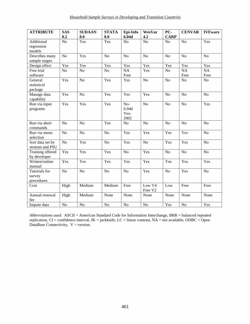
Household Sample Surveys in Developing and Transition Countries
461
ATTRIBUTE SAS 8.2
SUDAAN 8.0
STATA 8.0
Epi-Info 6.04d
WesVar 4.2
PC-CARP
CENVAR IVEware
Additional regression models
No Yes Yes No No No No Yes
Describes many sample stages
No Yes No No No No No No
Design effect Yes Yes Yes Yes Yes Yes Yes Yes Free trial software
No No No NA Free
Yes No NA Free
NA Free
General statistical package
Yes No Yes Yes No No No No
Manage data capability
Yes No Yes Yes Yes No No No
Run via input programs
Yes Yes Yes No-6.04d Yes-2002
No No No Yes
Run via short commands
No No Yes No No No No No
Run via menu selection
No No No Yes Yes Yes Yes No
Sort data set by stratum and PSU
No Yes No Yes No Yes Yes No
Training offered by developer
Yes Yes Yes No Yes No No No
Written/online manual
Yes Yes Yes Yes
Yes Yes Yes Yes
Tutorials for survey procedures
No No No No Yes No Yes No
Cost High Medium Medium Free Low V4 Free V2
Low Free Free
Annual renewal fee
High Medium None None None None None None
Impute data No No No No No Yes No Yes
Abbreviations used: ASCII = American Standard Code for Information Interchange, BRR = balanced repeated replication, CI = confidence interval, JK = jackknife, LC = linear contrast, NA = not available, ODBC = Open DataBase Connectivity, V = version.
Household Sample Surveys in Developing and Transition Countries
462
E. The Burundi sample survey data set
52. All numerical examples in this chapter use a data set from a tetanus toxoid (TT) immunization coverage sample survey conducted in Burundi in 1989. A brief summary of the Burundi sample survey design follows; more detail is provided in section I of the annex on the CD-ROM. For additional information on this survey’s methodology and its published results, see the report by the Expanded Programme on Immunization (EPI) (1996) of the World Health Organization (WHO).
1. Inference population and population parameters
53. The population of inference for this survey is women of Burundi who gave birth between Easter of 1988 and February/March of 1989. The population parameter of interest is percentage (or proportion) of women who were seropositive for tetanus antitoxin, thus protecting their newborn against neonatal tetanus.
2. Sampling plan and data collection 54. The sampling plan was a modification suggested by Brogan and others (1994) of the cluster sample survey methodology developed at the WHO for its Expanded Programme on Immunization. The modification yields a probability sample of dwellings or housing units and hence a probability sample of women, which the standard WHO EPI cluster sampling methodology may not do (ibid.).
55. Burundi was stratified into two geographical areas, the capital Bujumbura (urban stratum) and the rest of the country (rural stratum). Primary sampling units (PSUs) were geographical areas, collines within the rural stratum and quartiers or avenues within the urban stratum. The PSU sampling frame for each stratum was ordered by geographical proximity. Systematic ppes (probability proportional to estimated size) sampling was used to select 30 sample PSUs per stratum. Since 96 per cent of the inference population resides in rural Burundi, and since the same number of sample PSUs was allocated to each stratum, urban women were substantially oversampled. The specific ordering of the PSUs on the sampling frame, combined with systematic ppes sampling of PSUs, yields implicit geographical stratification within each stratum.
56. Further stages of probability sampling within sample PSUs were conducted to obtain a sample of occupied dwellings. All survey-eligible women within a sampled dwelling were selected for the sample. Seropositivity of tetanus antitoxin titre was determined from a finger prick blood sample. The survey response rate was essentially 100 per cent, an unusually high response rate. A total of 206 urban and 212 rural women were interviewed.
3. Weighting procedures and set-up for variance estimation 57. The sample weight variable W provided in the Burundi data set was revised to W2 so that the value of W2 for a sample respondent R is an estimate of the number of women in the inference population represented by that R. The value of W2 is approximate and used only to

Household Sample Surveys in Developing and Transition Countries
463
illustrate the estimation of population totals with the various software packages. Substantive conclusions regarding population totals for survey-eligible women in Burundi in 1989 should not be drawn from the analyses in this chapter. It is important to note that estimated proportions and means reported in this chapter agree with previously published results with this data set (Expanded Programme on Immunization, 1996) since the revised W2 is a scalar multiple of W that was used for previous analyses. The value of W2 was 959.3 for rural sample women and 42.0 for urban sample women, reflecting the substantial oversampling of urban women. The Burundi sampling plan was approximated by the common description WR for the purpose of variance estimation, that is to say, the UCVE approach with low first-stage sampling fractions.
58. Since PSUs were implicitly stratified, the sampling plan within each of the urban and rural strata was regarded as two PSUs sampled from each of 15 pseudo-strata. Describing the sampling plan as a total of 30 pseudo-strata, each with two sample PSUs, is preferred over describing it as 2 strata, each with 30 sample PSUs, because the former yields less biased variance estimation, since it takes the implicit stratification into account. The pseudo-stratification variable PSTRA was coded 1 through 30 and the pseudo-PSU variable PPSU was coded 1 or 2 within each pseudo-stratum.
59. When Taylor series linearization is used for variance estimation, only the variables W2, PSTRA and PPSU are needed. When replication techniques are used, however, replicate weights are required. WesVar was used to calculate BRR replicate weights from the variables W2, PSTRA and PPSU. These replicate weights calculated by WesVar were used both in WesVar and in SUDAAN for variance estimation using BRR.
4. Three examples for survey data analyses
60. The annex contains annotated data analyses for the three examples below, using five software packages for sample survey data (sects. II-VI). The examples below illustrate common descriptive and analytical analyses performed on sample survey data, namely, (a) estimation of proportions, totals and means for the entire population and for domains or strata; and (b) comparison of domains or strata on means or proportions. The inference population is survey-eligible women in Burundi in early 1989.
Example 1: Estimate number of women (population total) and percentage of women (population proportion/percentage) who were seropositive (IMMUNE variable, 1= seropositive, 2 = seronegative). The variable BLOOD (1 = seropositive, 0 = seronegative) is a recode of IMMUNE. Example 2: Estimate the population parameters of example 1 among urban and rural women (RUR_URB variable, coded 1 = rural, 2 = urban). Determine whether rural/urban residence is statistically independent of seropositivity (IMMUNE). Example 3: Estimate mean international units of antitoxin per millitre (ml) (IUML), for the inference population of women and by rural/urban residence. Determine whether rural/urban residence is related to mean IUML.

Household Sample Surveys in Developing and Transition Countries
464
Note: estimation of mean international units of antitoxin per millitre (ml) (IUML) may give misleading results because of the right skewed distribution of this variable. It might be better to use the median or to transform IUML before analysis, for example, to the natural logarithim of IUML. In this chapter, mean IUML (without transformation) is estimated to show the capabilities of the five software packages, not to illustrate substantive results concerning IUML.
F. Using non-sample survey procedures to analyse sample survey data
61. The present section illustrates that incorrect use of simple random sample formulae for analysis of complex sample survey data can result in biased point estimates and biased (usually too small) estimated standard errors. See Brogan (1998 and in press) for another illustration. Any statistical software package could have been used for this illustration, and answers comparable with those obtained with SAS (used in this section) would have been obtained.
62. The population parameter to be estimated is the proportion of women in the inference population who are seropositive. The indicator variable BLOOD is calculated and coded as 1 = seropositive and 0 = seronegative. Thus, the mean of BLOOD is the proportion of women who are seropositive. PROC MEANS in SAS estimates the mean of BLOOD as 0.74880, with estimated standard error of 0.02124 (row 1 of table XXI.1). These two calculations are biased because the incorrectly applied PROC MEANS ignores the sampling weight variable for estimating the population proportion and, in addition, ignores the sampling weight, PSU and stratification variables for calculating the estimated standard error of the point estimate.
63. PROC MEANS in SAS, then, is used with the sampling weight variable W2 on a WEIGHT statement. The mean of BLOOD is estimated as 0.67203, with estimated standard error (weighted) of 0.02299 (row 2 of table XXI.1). In this analysis PROC MEANS obtains an appropriate point estimate for the population proportion. However, the incorrectly applied PROC MEANS yields a biased estimated standard error because it ignores the PSU and stratification variables.
64. Finally PROC SURVEYMEANS in SAS is used to provide an appropriate analysis for complex sample survey data. (Details on how to use SURVEYMEANS appear in the next section.) The point estimate of the population proportion is 0.67203, with estimated standard error of 0.03830 (row 3 of table XXI.1). PROC SURVEYMEANS takes into account the sampling weight variable for calculating the point estimate and the sampling weight, PSU and stratification variables for calculating the estimated standard error.
65. A comparison of these three analyses in table XXI.1 shows that the unweighted (incorrect) point estimate of 0.7488 (74.88 per cent) differs quite a bit from the weighted (correct) point estimate of 0.6720 (67.20 per cent). The unweighted point estimate is too high because a higher proportion of urban women, compared with rural women, are seropositive (illustrated later in the chapter), and urban women are overrepresented in the sample since they were oversampled: they constitute about half of the sample but only 4 per cent of the inference population. Thus, in an unweighted analysis for making inference to the country, urban women

Household Sample Surveys in Developing and Transition Countries
465
are given much more influence than they should and bias upward the estimated population proportion.
66. A comparison of the two analyses that yield the correct weighted point estimate illustrates that, even with a WEIGHT statement, the incorrectly applied PROC MEANS in SAS seriously underestimates the standard error, an incorrect calculation of 0.02299 (2.30 per cent) compared with the correct PROC SURVEYMEANS calculation of 0.03830 (3.83 per cent). This occurs primarily because PROC MEANS, with or without a WEIGHT statement, ignores the clustering of women within sample PSUs, whereas SURVEYMEANS recognizes the clustering for variance estimation. Since the intra-class correlation coefficient is positive for most measured variables in complex sample surveys, correct variance estimation procedures that take into account the clustering usually yield larger estimated standard errors.
67. In general, biased point estimates of population parameters are obtained if sample survey data are not analysed with the appropriate sample weight variable. Further, even if the sample weight variable is incorporated into the analysis, yielding appropriate point estimates of population parameters, the standard errors typically are underestimated when sample elements are clustered in survey data and the clustering is not recognized in variance estimation. Underestimation of standard errors results in confidence intervals that are too narrow and statistical tests of significance with p-values that are too small, in other words, the level of statistical significance is overstated.
68. The magnitude of underestimation of variance by ignoring clustering of sample survey data is approximated by the expression [1 + ρ (b – 1)] where ρ is the intra-class correlation coefficient between population elements and b is the average number of sample elements per sample cluster (PSU) (see chap. VI). For example, if the value of the expression is 2, then taking the clustering into account approximately doubles the estimated variance that one would obtain by ignoring the clustering. Note that the Burundi PSU variable named PPSU identifies for the software what sample elements are clustered together within the same sample PSU (for a given stratum).
69. In addition to the impact of clustering on estimated variance, substantial variation in the value of the sampling weight variable across respondents increases estimated variance. Thus, if the sampling weight variable is ignored in the analysis, the estimated standard error is underestimated (and the estimator of the population parameter is biased).

Household Sample Surveys in Developing and Transition Countries
466
G. Sample survey procedures in SAS 8.2
1. Overview of SURVEYMEANS and SURVEYREG 70. Version 8.2 in SAS contains two recently developed procedures (they first appeared in V 8.0) for analysis of sample survey data: SURVEYMEANS and SURVEYREG. SAS includes the common sampling plan description WR for which the basic three survey design variables are required. Finite population correction terms can be applied for single-stage sampling designs such as stratified random sampling and simple random sampling. Taylor series linearization is used for variance estimation. SAS V9 contains two new PROCS for complex sample survey data, SURVEYFREQ for analysis of categorical variables and SURVEYLOGISTIC for logistic regression. Additional SAS procedures for sample survey data are under development.
71. The syntax for specifying the relevant survey design variables for WR is the same for both SURVEYMEANS and SURVEYREG. The keyword STRATA is used to designate the stratification variable, the keyword CLUSTER is used to designate the PSU variable, and the keyword WEIGHT is used to specify the sampling weight variable (as in other SAS procedures such as MEANS). These statements, appropriate for a given survey, must be in each SAS sample survey procedure and generally will not change as long as the same sample survey data set is being analysed. For the Burundi data set, the SAS statements below describe the sample survey design for SAS PROC SURVEYMEANS or PROC SURVEYREG:
STRATA PSTRA CLUSTER PPSU WEIGHT W2
72. If the STRATA statement is missing, SAS assumes the sampling plan had no stratification of PSUs prior to first-stage sampling. If the CLUSTER statement is missing, SAS assumes that the sample elements are not clustered, i.e., that each sample cluster contains exactly one element, i.e., that elements were sampled at the first (and only) stage of sampling, i.e., that simple random or stratified random sampling was used. If the WEIGHT statement is missing, SAS assumes that each R has the same value for the weighting variable and SAS assigns the value 1.0 to the weighting variable. If all three survey design statements (STRATA, CLUSTER, WEIGHT) are missing, this is equivalent to specifying simple random sampling from an infinite population, the assumption for most of the non-survey PROCS in SAS.
2. SURVEYMEANS 73. This procedure estimates population means and totals for continuous variables and population proportions and totals for categorical variables, using sample survey data. Estimated standard errors and coefficients of variation are provided for all point estimates, as well as confidence intervals for population parameters. Specific statistics can be requested on the PROC statement, or one can take the default printout for statistics, or one can use ALL on the PROC statement to obtain all statistics that can be calculated by SURVEYMEANS.

Household Sample Surveys in Developing and Transition Countries
467
74. Variables to be analysed (both continuous and categorical) appear on the VAR statement. The CLASS statement lists the variables on the VAR statement that are categorical; SAS then assumes that all other variables on the VAR statement are continuous.
75. The DOMAIN statement with one or more categorical variables is used to specify domains for analysis of all variables on the VAR statement. SAS automatically provides analyses for the marginal, in other words, the entire population, in addition to the domain analyses. A program without a DOMAIN statement provides estimates for the entire population only. Although the BY statement in SURVEYMEANS can be used to obtain estimates for domains, this is not recommended for sample survey data because the appropriate formulae for variance estimation are not used when the BY statement is used. Use the DOMAIN statement for analysis of domains.
76. SAS V8.2 does not have a statement that allows a subpopulation to be analysed, for example, only older women. However, subpopulation analyses can be conducted by first defining an indicator variable, for example, OLDERFEM, which indicates whether the sample element belongs to the subpopulation. Then, the statement DOMAIN OLDERFEM can be used to obtain the desired analyses; ignore the SAS output for the sample elements who are not older women. Do not use the SAS IF statement to subset the data set to women who are older before going into PROC SURVEYMEANS, since the standard errors may be calculated incorrectly inasmuch as SURVEYMEANS may not know the full number of strata and sample PSUs in the sample survey.
3. SURVEYREG 77. This procedure performs linear regression for sample survey data according to the design-based approach (Korn and Graubard, 1999), that is to say, the analysis takes into account the survey design variables. As with linear regression for non-survey data, the dependent variable is continuous (or assumed to be so), and the independent variables can be a mixture of continuous and categorical variables. The MODEL statement includes the dependent variable and all independent variables. Any categorical variable on the MODEL statement must also appear on the CLASS statement, and the CLASS statement must precede the MODEL statement in the SAS program. SURVEYREG forms dummy indicator variables (coded 1 or 0) for categorical independent variables, with the highest coded value of the variable defined as the reference group. Other options in SURVEYREG, as well as its output, are similar to the (non-survey) linear regression in SAS.
78. SAS Version 8.2 has no sample survey procedures to compare domains on means or proportions, although these capabilities are under development. An example question for this situation is, Do rural and urban women in the Burundi inference population differ on mean IUML units or on proportion who are seropositive? SURVEYFREQ in V9.0 can be used to conduct a chi-square test on the two variables residence (rural/urban) and seropositivity (yes/no). Until domain comparison procedures are full developed in SAS for sample survey data, SURVEYREG can be used as follows to compare domains.

Household Sample Surveys in Developing and Transition Countries
468
79. If it is desired to compare rural and urban women in the inference population on mean IUML, use the MODEL statement in SURVEYREG with the continuous variable IUML as the dependent variable and the domain variable designating rural/urban as the independent categorical variable. Part of the standard output from SURVEYREG is a test of the null hypothesis that the population regression coefficient for rural/urban (with one degree of freedom) is equal to zero. This null hypothesis regarding the regression coefficient is equivalent to the null hypothesis that rural and urban women in the inference population have the same mean IUML.
80. If it is desired to compare urban and rural women in the inference population on proportion who are seropositive (a dichotomous variable), use the indicator variable BLOOD (1= seropositive, 0=seronegative) as the dependent variable. (Note that BLOOD is simply a recode of the IMMUNE variable where 1=seropositive and 2=seronegative.) On the MODEL statement in SURVEYREG, define BLOOD as the dependent variable and the domain variable designating rural/urban as the independent categorical variable. The null hypothesis that the regression coefficient is zero is equivalent to the null hypothesis that the proportion seropositive is the same for rural and urban women in the population of inference.
4. Numerical examples
81. Section II of the annex on the CD-ROM illustrates the use of SURVEYMEANS and SURVEYREG to work the three examples listed in paragraph 60. Review of the annotated SAS programs (user-written) and annotated SAS output should prepare readers to write their own SAS programs for SURVEYMEANS and SURVEYREG and interpret the output.
82. Table XXI.1, row 3, summarizes the SURVEYMEANS output in section II of the annex for estimating the percentage and number of women in the Burundi inference population who are seropositive, with estimated standard error and confidence interval; most of these results were discussed in section F of this chapter. Table XXI.3, row 1 (in annex, sect. VII, on the CD-ROM), summarizes the SURVEYMEANS output for estimating the percentage seropositive for each of the two domains of rural and urban women, 66.51 per cent and 83.50 per cent, respectively. Table XXI.4, row 1 (in annex, sect. VII, on the CD-ROM), summarizes the SURVEYREG output that compares rural and urban women, yielding a t-value of -3.52, with a p-value of 0.0014 for testing the null hypothesis that rural and urban women do not differ on the percentage who are seropositive. Thus, rural and urban women in the inference population differ on percentage who are seropositive: urban women have a higher seropositivity prevalence rate.
5. Advantages/disadvantages/cost
83. If one already is a SAS/STAT user, then the sample survey procedures in SAS are available at no additional cost and use familiar syntax. Further, the full capabilities of SAS for data management and new variable formation are also available. Technical support and documentation for the sample survey procedures are subsumed under the regular system of SAS support. Compared with that of other sample survey packages reviewed, the cost of SAS is high.

Household Sample Surveys in Developing and Transition Countries
469
84. SAS 8.2 has no capability to compare domains to each other, although SURVEYREG can be used as a temporary solution for this type of analysis. The addition of SURVEYFREQ in V9.0 provides domain comparisons on categorical variables.
85. SAS uses only Taylor series linearization for variance estimation. For stratified multistage cluster sampling, it handles only the common sampling plan description WR. However, it can incorporate fpc terms into single-stage stratified random sampling or simple random sampling.
86. The capability of SAS 8.2 for sample survey data analysis is basic and descriptive and may fit the analysis needs of many users. The addition of SURVEYFREQ in V9.0 provides descriptive and analytical capability for categorical variables. Sample survey procedures still under development, for example, logistic regression, should make SAS more comparable in the future with other software packages that offer comprehensive sample survey analyses.
H. SUDAAN 8.0
1. Overview of SUDAAN
87. SUDAAN (Research Triangle Institute, 2001) is a specialty software package originally developed for the analysis of complex sample survey data, but now generalized for the analysis of correlated data using techniques such as longitudinal data analysis and generalized estimating equations (GEE). SUDAAN is an acronym for SUrvey DAta ANalysis. The procedures for descriptive and analytical statistics are DESCRIPT, CROSSTAB, and RATIO. Design-based modelling procedures include linear regression, logistic regression (including multinomial), log-linear regression and survival analysis.
88. SUDAAN 8.0 is programmed in C language, with user-provided command statements similar to those of SAS. Input data sets can be either SAS, SPSS or ASCII files. SUDAAN is available to run by itself (standalone SUDAAN) or in conjunction with SAS (SAS-callable SUDAAN). SAS users generally would prefer SAS-callable SUDAAN.
89. SUDAAN is the only sample survey package to include both of the two most common approaches to variance estimation: Taylor series linearization and replication methods. The latter approach in SUDAAN includes balanced repeated replication (BRR), with or without the Fay adjustment factor, and jackknife methods. All replication methods in SUDAAN assume the common sampling plan description referred to previously as WR. If BRR is used for variance estimation, the BRR replicate weights must be provided with the input data set; SUDAAN does not generate BRR replicate weights. SUDAAN will generate replicate weights for the jackknife delete one (PSU) method or will accept jackknife replicate weights provided with the input data set for the jackknife delete one method and variations on this method.
90. The sample survey design is described to SUDAAN in three statements: (a) by choosing an option for the DESIGN keyword on the PROC statement; (b) by specifying the stratification and clustering variables on the NEST statement; and (c) by specifying the sample weight variable on the WEIGHT statement. The input data set to SUDAAN must be sorted by all of the

Household Sample Surveys in Developing and Transition Countries
470
variables that appear on the NEST statement, generally the first-stage stratification variable and then the PSU variable within each stratum.
91. Unlike most other software packages with sample survey capability, second and subsequent stages of sampling and stratification in multistage sampling can be described to SUDAAN for variance estimation, alleviating the necessity of always using the common sampling plan description WR. In addition, SUDAAN has extensive capability for incorporating into variance estimation the finite population correction (fpc) terms at multiple stages of without replacement sampling. The SUDAAN manual, available in print or a pdf file, gives several examples of how to describe sampling plans to SUDAAN (see chap. III).
92. The default sampling plan for SUDAAN is WR as defined above, whether for Taylor series linearization, BRR or jackknife. Using the SUDAAN syntax DESIGN = WR on the PROC statement invokes not only the UCVE approach and first-stage sampling with replacement or without replacement but with small first-stage sampling fractions, but also the use of Taylor series linearization. With DESIGN = WR, the NEST statement contains one or more justification variables (usually just one) and one PSU variable. If the option DESIGN = is missing from the PROC statement, SUDAAN assumes DESIGN = WR.
93. The SUDAAN syntax DESIGN = BRR invokes the common sampling plan description WR (as discussed previously) with balanced repeated replication for variance estimation. The BRR replicate weight variables must be in the input data set, and the REPWGT statement in the SUDAAN program gives the variable names for the replicate weight variables.
94. The SUDAAN syntax DESIGN = JACKKNIFE, in the absence of JACKWGTS and JACKMULT statements, invokes the common sampling plan description WR with variance estimation by the delete one jackknife technique where SUDAAN generates the jackknife replicate weights. The SUDAAN syntax DESIGN = JACKKNIFE, with the JACKWGTS statement, invokes the common sampling plan description WR with the jackknife weights provided to SUDAAN as variables in the input data set.
95. The sample survey design for the Burundi survey and specification of Taylor series linearization for variance estimation are described to SUDAAN as follows:
PROC ………. DESIGN = WR …… NEST PSTRA PPSU WEIGHT W2
96. The sample survey design for the Burundi survey and specification of BRR (balanced repeated replication) for variance estimation are described to SUDAAN as follows:
PROC ………. DESIGN = BRR …… WEIGHT W2 REPWGT REPLWT01-REPLWT32

Household Sample Surveys in Developing and Transition Countries
471
Note above that the REPWGT statement identifies the replicate weight variables included in the input data set. These 32 replicate weight variables are based on the 30 pseudo-strata, with 2 PSUs per pseudo-stratum, and were obtained by using WesVar. Note also that the NEST statement is absent when BRR is used; SUDAAN does not need to know the stratification and PSU variables, since it uses only the replicate weight variables for variance estimation.
2. DESCRIPT 97. The DESCRIPT procedure estimates population totals and means for continuous variables as well as population totals and percentages for categorical variables. The VAR statement lists the variables (dependent) to be analysed. For a given DESCRIPT program, all variables on the VAR statement must be continuous or all variables must be categorical. If categorical variables are on the VAR statement, then the CATLEVEL statement must also be used to indicate for which levels of each categorical variable estimates are desired. For example, the two statements below estimate the percentage of the inference population in Burundi who are seropositive and not seropositive [assuming IMMUNE is coded 1, 2 or . (dot) for missing].
VAR IMMUNE IMMUNE CATLEVEL 1 2
98. Estimates are provided for domains by using a TABLES statement that contains one or more categorical variables. Domains can be compared with each other via linear contrasts using the CONTRAST, PAIRWISE or DIFFVAR statements. Standardized rates and means can be estimated, for example, an age-adjusted prevalence for disease, by using the STDVAR and STDWGT statements. Linear and higher-level (quadratic, etc.) trends on means or percentages can be assessed across levels of some categorical variable by using the POLY (POLYNOMIAL) statement; SUDAAN uses orthogonal polynomial linear contrasts for these analyses.
99. All variables on a TABLES, CONTRAST, PAIRWISE, DIFFVAR, STDVAR or POLY statement must also appear on a SUBGROUP statement, and a required LEVELS statement indicates the highest coded value in the analysis for each categorical variable on the SUBGROUP statement.
100. The SUBPOPN statement in SUDAAN, which can be used in all PROCS, restricts analyses to a subpopulation, for example, only older women. Use the SUBPOPN statement with the full sample survey data set input into SUDAAN instead of subsetting the input data set to the subpopulation of interest before using SUDAAN, since the latter procedure may result in incorrectly estimated standard errors inasmuch as some sample PSUs may be missing from the subsetted data set.
3. CROSSTAB 101. The CROSSTAB procedure is for categorical variables only. The TABLES statement in CROSSTAB indicates the one-way, two-way or multi-way tables for which population percentages and totals are estimated. Corresponding SUBGROUP and LEVELS statements are required for all variables on the TABLES statement.

Household Sample Surveys in Developing and Transition Countries
472
102. The TEST statement in CROSSTAB requests chi-square tests for testing the null hypothesis that two categorical variables are statistically independent. One chi-square test is based on a Pearson type test (CHISQ), using “observed minus expected” calculations on estimated population totals. The other chi-square test is based on estimated population odds (LLCHISQ). Odds ratios and relative risks (prevalence ratios, really), with confidence intervals, are estimated for 2 x 2 tables by using RISK = ALL on the PRINT statement. Finally, a Cochran-Mantel-Haenszel test (use CMH on the TEST statement) is available to assess statistical independence of two variables while controlling on (“stratifying” on) a third variable.
4. Numerical examples
103. Section III of the annex on the CD-ROM illustrates the use of CROSSTAB and DESCRIPT to work the three examples listed in paragraph 60, using SAS-CALLABLE SUDAAN (SAS Version 8.2 and SUDAAN Version 8.0). Both Taylor series linearization and BRR (balanced repeated replication) are used for variance estimation. Review of the annotated SUDAAN programs (user-written) and annotated SUDAAN output should aid readers in writing their own SUDAAN programs and interpreting the output. Only selected SUDAAN analyses discussed in TABLES 1, 3, 4, 5, and 6 are included and annotated in the annex, section III.
104. Table XXI.1, row 4 summarizes the CROSSTAB and DESCRIPT output in section III (annex) for estimating the percentage and number of women in the Burundi inference population who are seropositive, with estimated standard error. The CROSSTAB and DESCRIPT results from SUDAAN are identical for a given method of variance estimation (as expected), and the Taylor Series and BRR results are identical (not always true). The SUDAAN results agree with results from SAS SURVEYMEANS. Note that CROSSTAB and DESCRIPT do not calculate confidence intervals for estimated population percentages or totals.
105. Table XXI.3, row 2, in the annex, section VII (CD-ROM), shows that identical output is obtained from CROSSTAB and DESCRIPT (whether with Taylor series or BRR) for estimating the percentage who are seropositive, but for each of the two domains of rural and urban women. The SUDAAN CROSSTAB and DESCRIPT results agree with SAS SURVEYMEANS.
106. Table XXI.4, row 2 in the annex, section VII (CD-ROM), summarizes the DESCRIPT output (with Taylor series and BRR) that uses a linear contrast to compare rural with urban women on percentage who are seropositive. There is a negligible difference in the estimated standard error with Taylor series and BRR. The conclusion is: urban and rural women in the Burundi inference population differ on seropositivity prevalence; urban women have a higher prevalence. Note that the DESCRIPT linear contrast results agree with using SAS SURVEYREG to compare two domains.
107. Table XXI.5, rows 1 and 2, in the annex, section VII (CD-ROM), shows results from the two different chi-square tests available in CROSSTAB: Pearson (CHISQ) and log-linear (LLCHISQ). Results using Taylor Series and BRR are identical. The estimated seropositivity prevalence is significantly higher for urban women than for rural women (using CHISQ), and the estimated odds of seropositivity is significantly higher for urban women than for rural women (using LLCHISQ).

Household Sample Surveys in Developing and Transition Countries
473
108. Table XXI.6, row 1 in the annex, section VII (CD-ROM), shows the estimated odds ratio (0.393) and prevalence ratio (0.797) for seropositivity (rural to urban), each with a 95 per cent confidence interval. Taylor Series and BRR have negligible differences in the upper limit for the 95 per cent confidence interval on odds ratio. The estimated odds ratio and prevalence ratio differ in magnitude because the prevalence of seropositivity is not low.
5. Advantages/disadvantages/cost
109. SUDAAN is a comprehensive sample survey (and correlated data) software package with analytical strengths for both descriptive and modelling analyses. It has extensive capability to estimate and test user-specified contrast matrices on population parameters, including regression coefficients. It runs in both mainframe and PC environments. SAS users likely have an advantage in learning SUDAAN, since its syntax is similar to SAS. However, some of the syntax of SUDAAN is esoteric, perhaps requiring more learning time than other packages.
110. Compared with that of other software packages reviewed in this chapter, the cost of SUDAAN is high, especially if used as SAS-Callable SUDAAN because, then, SAS also is required. Technical support is provided for licensed users. The SUDAAN Users Manual for Version 8.0, primarily for reference as opposed to learning SUDDAN, has several detailed annotated examples of analyses with NHANES-III (National Health and Nutrition Examination Survey-III) data which can be useful for learning how to use SUDAAN.
111. SUDAAN is the only software package illustrated here that includes both major approaches to variance estimation, Taylor series linearization and replication methods. However, SUDAAN does not construct replicate weights for balanced repeated replication (BRR), requiring the user to provide these weights. SUDAAN constructs replicate weights for the jackknife delete one procedure and will also accept jackknife replicate weights if they are included in the input data set.
112. SUDAAN also is the only software package reviewed here that has extensive capability for describing several stages of sampling, stratification and fpc terms for incorporation into variance estimation. Further, it has several different definitions for design effect calculations to allow one to exclude from the design effect the effects of oversampling and/or of unequal weighting.
113. ASCII data input into SUDAAN is cumbersome, making the other two data input options preferable, namely, a SAS or SPSS data set. A SAS data set input into standalone SUDAAN must be SAS Version 6.04 or a SAS transport file. SAS-Callable SUDAAN can read any data set that SAS can read. SUDAAN output can be saved electronically to a SAS data file format for further use in SAS or spreadsheet software such as EXCEL. SUDAAN has very limited capability for recoding variables and no capability for data management. Thus, it is prudent to undertake any necessary recoding and formation of new variables in either SAS or SPSS (depending upon type of input data set) before using SUDAAN.

Household Sample Surveys in Developing and Transition Countries
474
I. Sample survey procedures in STATA 7.0
1. Overview of STATA
114. STATA is a general statistical software package that added extensive capability for sample survey data analysis in 1995. STATA 7.0 is illustrated here; Version 8.0 was released in 2003. Only Taylor series linearization is used for variance estimation. The common sampling plan description WR is default. STATA can incorporate fpc terms into variance estimation for single stage without replacement sampling plans (simple random sampling and stratified random sampling) and for one stage without replacement cluster sampling (stratified or not) where equal probability sampling is used for clusters (PSUs) within a stratum and all elements in a sampled PSU are included in the sample.
115. The breadth of sample survey analyses of STATA compares favorably with that of SUDAAN, with mathematical statistical capability for user-specified contrast matrices on population parameters, including regression coefficients. STATA runs interactively with short and simple commands, making it relatively easy to learn. However, user-written programs can be submitted in batch mode if desired. STATA is case-sensitive, and commands to STATA are typed in lower case. STATA allocates a default amount of memory into which it loads a copy of the input data set. If this memory is insufficient for large data sets, the memory can be increased with the set memory command.
116. The sample survey commands in STATA begin with the name svy (for survey). Descriptive commands are available for estimating a population mean (svymean), a population total (svytotal), a population proportion (svyprop), and percentages and totals in two-way tables (svytab). Confidence intervals on population proportions from svytab use a logit transform so that estimated lower and upper limits are constrained within (0,1). Eight different chi-square tests for sample survey data in two-way tables are available in svytab. Available modelling procedures include linear regression, logistic regression (including multinomial with a nominal or ordered variable), Poisson regression, and probit models.
117. The svyset command is used to specify the sampling plan to STATA. To describe the common sampling plan WR (default), three keywords for the command svyset are typed into STATA interactively. The keyword strata precedes the stratification variable name, the keyword psu precedes the PSU variable name, and the keyword pweight precedes the sampling weight variable name. Thus, the sampling plan for the Burundi survey is described to STATA V7 as:
svyset strata pstra svyset psu ppsu svyset pweight w2
118. As indicated earlier for the sample survey procedures in SAS, omission of the strata keyword in STATA implies no stratification of PSUs prior to first-stage sampling. Omission of the psu keyword implies one-stage sampling of elements and no clustering of sampled elements. Omission of the pweight keyword implies equally weighted sample elements, with a default

Household Sample Surveys in Developing and Transition Countries
475
value of 1.0 for the weighting variable. The syntax for the svyset command is revised in STATA V8.
119. The command svydes instructs STATA to output the survey design variables it has attached to the data set (from the svyset commands) and to summarize the number of strata, the number of PSUs per stratum, and the average number of observations per PSU within each stratum. This is a very useful summary of characteristics of the sample survey design.
2. SVYMEAN, SVYPROP, SVYTOTAL, SVYLC
120. The svymean command estimates a population mean, either for a continuous variable or for an indicator variable coded 1 or 0 (that is to say, an estimated population proportion). Output options include estimated standard error, estimated coefficient of variation, design effect and confidence interval on the population parameter.
121. The svyprop command is for categorical data: it estimates the proportion of the population that is at each level of the categorical variable, along with estimated standard error. Fewer output options are available with svyprop, compared with svymean.
122. The svytotal command estimates a population total for either a continuous or an indicator (0, 1) variable, with estimated standard error, estimated coefficient of variation, design effect and confidence interval.
123. Each of the three commands above can be used to estimate population parameters for domains by using the option by on the command line, for example, by (stra) or by (urb_rur) to analyse the two domains of rural and urban women in Burundi. STATA uses correct variance estimation formulae for domains with the by statement in its svy commands.
124. In addition, each of the three commands above can be used with a subpop option on the command line to perform estimation of population parameters for a subpopulation, for example, only older women. Do not use the STATA “if” statement for subpopulation analyses because estimated variances may be incorrect; use the subpop option.
125. The svylc command estimates user specified linear combinations of domain means, proportions or totals, along with estimated standard error, t-test, p-value, and confidence interval. This command can be used to compare domains with each other. In V8.0, the svylc command is replaced by lincom. The command svylc continues to work in V8.0 but is no longer documented.
3. SVYTAB 126. The svytab command in STATA is for two-way tables. It estimates population percentages (row, column or total) with estimated standard errors, population totals for table cells with estimated standard errors, and confidence intervals. A logit transform is used to obtain confidence intervals on population proportions so that estimated lower and upper limits are constrained to be in the interval (0, 1). Eight different chi-square tests are available to test the

Household Sample Surveys in Developing and Transition Countries
476
null hypothesis of statistical independence of the two categorical variables in the table. The command subpop is available for use with svytab.
4. Numerical examples
127. Section IV of the annex (CD-ROM) illustrates the use of STATA commands to work the three examples listed in paragraph 60. Each worked example is a log file of the interactive session with STATA. Review of the annotated STATA log (user commands and STATA output) should aid readers in using the sample survey commands in STATA and interpreting the output.
128. The commands svymean and svytotal were used with the indicator variable BLOOD (1=seropositive, 0=seronegative). Table XXI.1 (rows 5 and 6) shows the estimated number and percentage of women who are seropositive, with confidence intervals. The STATA calculations agree with SAS SURVEYMEANS and with SUDAAN DESCRIPT and CROSSTAB.
129. Table XXI.3 (row 3) in the annex, section VII (CD-ROM) shows the estimated percentage of women who are seropositive, by rural/urban residence. The STATA svytab point estimates and estimated standard errors agree with SAS SURVEYMEANS and with SUDAAN DESCRIPT and CROSSTAB. However, the confidence intervals for domains differ slightly between STATA svytab and SAS SURVEYMEANS because STATA svytab uses a logit transform to obtain confidence intervals.
130. Table XXI.4 (row 3) in the annex, section VII (CD-ROM), presents the STATA svylc results for the linear contrast that compares rural and urban women on percentage who are seropositive, indicating a significant difference between the two domains. The STATA results agree with SUDAAN DESCRIPT and with using SAS SURVEYREG for domain comparisons. 131. Table XXI.5 (rows 3 through 5) in the annex, section VII (CD-ROM), presents the STATA svytab results for three chi-square tests of the null hypothesis that seropositivity is statistically independent of rural/urban residence. All three svytab chi-square tests have similar (and small) p-values. The default chi-square test for STATA svytab (row 3) is a Pearson type chi-square test proposed by Rao and Scott (1981; 1984) with a second-order correction. The other two chi-square tests in svytab (rows 4 and 5) are the same chi-square tests as in SUDAAN CROSSTAB, and STATA and SUDAAN yield the same calculations for these two tests.
132. Since the svytab command in STATA does not produce odds ratios or prevalence ratios, the command svylogit was used to estimate odds ratio (urban to rural) for seropositivity. The STATA odds ratio, with confidence interval, is in table XXI.6 (row 2) in the annex, section VII (CD-ROM). The STATA svylogit command gives the same calculations as SUDAAN CROSSTAB for point estimate and confidence interval.
5. Advantages/disadvantages/cost 133. STATA is a comprehensive general statistical analysis package and also has extensive analytical capability for sample survey data, including descriptive and design-based modelling

Household Sample Surveys in Developing and Transition Countries
477
procedures. It provides many modelling procedures for sample survey data. STATA has received very good reviews as a statistical package, is relatively easy to learn, and has an active users group. Compared with other software packages reviewed in this chapter, its cost is moderate.
134. STATA accepts user-defined contrast matrices of estimated population parameters, including regression coefficients, for those who wish to test their own specific hypotheses or estimate combinations of population parameters. In general, it allows great flexibility in conducting statistical analyses for those with the requisite mathematical statistical background.
135. STATA uses only Taylor series linearization and is limited to the common sampling plan description WR. However, it can include in variance estimation for without replacement sampling the fpc terms for one-stage sampling of elements and for one-stage cluster sampling. It is somewhat difficult, but possible, to extract STATA analytical results (for example, unweighted sample sizes, point estimates, standard errors) for export to other data formats.
J. Sample survey procedures in Epi-Info 6.04d and Epi-Info 2002
1. Overview of Epi-Info 136. Epi-Info has been developed over many years by the Centers for Disease Control and Prevention (CDC) and the World Health Organization (WHO). This software is available at no cost as a download from the CDC web site: http://www.cdc.gov/epiinfo/. 137. Two versions of Epi-Info are available: the last DOS-based Epi-Info Version 6.04d and the most recent Windows-based Epi-Info 2002.
138. The capabilities of Epi-Info include development of a questionnaire or research data-collection form, customized data entry, data analysis and word processing. Its analytical and statistical capabilities are oriented towards epidemiologists worldwide. Output (analytical results) from Epi-Info analyses can be sent to the screen, to a printer, or to an electronic file.
139. Both versions of Epi-Info (DOS or Windows) have capability for basic descriptive analyses of complex sample survey data. Only the common sampling plan description WR is available. The input data set must be sorted by two of the three survey design variables: the stratification variable STRATVAR and by the PSU variable PSUVAR within stratum. Epi-Info does not incorporate any fpc terms into variance estimation. Also, it does not estimate population totals. Taylor series linearization is used for variance estimation.
140. The analytical capability of Epi-Info for complex sample survey data originally was developed for the Behavioral Risk Factor Surveillance System (BRFSS), a CDC-sponsored annual health sample survey programme for States in the United States of America (Brogan, 1998 and in press) and for the WHO cluster sample methodology used worldwide by the Expanded Programme on Immunization (EPI) to estimate vaccination coverage among children (Brogan and others, 1994). However, the sample survey procedures in Epi-Info may be used for any complex sample survey that can be described by the common sampling plan description WR.

Household Sample Surveys in Developing and Transition Countries
478
2. Epi-Info Version 6.04d (DOS), CSAMPLE module
141. Epi-Info for DOS was a joint development effort of CDC and WHO. Data input for Epi-Info 6.04d is a dBase file or an ASCII file which Epi-Info then converts into an Epi-Info data file *.rec. Software packages exist to convert SAS or SPSS or other types of data files into an Epi-Info *.rec file, for example, DBMS-COPY (http://www.dataflux.com/conceptual/). Epi-Info 6.04d runs as an interactive program and cannot be run in batch mode. The DOS version may be preferred over the Windows version by those who have older computers, older operating systems and/or limited hard-drive storage space.
142. The CSAMPLE module in Epi-Info Version 6.04d conducts analyses for complex sample survey data. CSAMPLE estimates a population mean (for a continuous variable or for an indicator variable coded 1/0) or a population percentage (for a categorical variable), along with estimated standard error, confidence interval(s) and design effect. These estimates also are provided for domains formed by levels of a categorical variable. In addition, CSAMPLE estimates the difference between domain means or domain percentages, with corresponding estimated standard error of the estimated difference and a confidence interval on the population difference. CSAMPLE estimates odds ratio and risk ratio for 2 x 2 tables. Note that CSAMPLE does not estimate population totals.
143. When the CSAMPLE module is opened in Epi-Info 6.04d, a data input screen appears where the user specifies variables to be used in the analysis. The user selects a variable for each of the three survey design boxes: STRATA (the stratification variable), PSU (the PSU or cluster variable) and WEIGHT (the sampling weight variable). For the Burundi survey, the specification to Epi-Info was as follows:
STRATA PSTRA PSU PPSU WEIGHT W2
144. The user specifies the analysis variable (or dependent variable) in the box called MAIN. This variable can be continuous, such as IUML, or categorical, such as IMMUNE. If the estimated population mean is desired for the continuous (or assumed to be continuous) variable specified in MAIN, then the user clicks on the option MEANS. If the estimated population percentages are desired for the categorical variable specified in MAIN, then the user clicks on the option TABLE.
145. If estimated means or percentages are desired for domains, then the variable that defines the domains is specified in the box called CROSSTAB and the analysis variable is specified in the MAIN box.
146. In addition, CSAMPLE can estimate the difference between two domains on the mean of an analysis variable. The user can specify the two levels of the CROSSTAB variable that define the two domains to be compared with each other.

Household Sample Surveys in Developing and Transition Countries
479
3. Epi-Info 2002 (Windows)
147. Epi-Info 2002, a Windows application, has been developed by CDC. Data input for Epi-Info 2002 data analysis is via a MicroSoft Access 1997 file (*.mdb) or a dBase file. Epi-Info 2002 can also read the *.rec files prepared for the DOS versions of Epi-Info. The software runs interactively but has an option to run in batch mode.
148. Epi-Info 2002 has three complex sample procedures located in the Analyze Data section under Advanced Statistics. Complex Sample Frequencies estimates a one-way percentage distribution for a categorical variable, with estimated standard error and confidence intervals. Complex Sample Tables estimates row and column percentages for a two-way table of categorical variables [labelled exposure (row) and outcome (column)], with estimated standard errors and confidence intervals for row percentages. If the table is 2 x 2, the procedure also estimates odds ratio and risk ratio, with confidence intervals. Complex Sample Means estimates the mean for a continuous variable, with estimated standard error and confidence interval, including estimation of mean for domains formed by a categorical variable. If the domain variable is at two levels, the difference between domain means also is estimated, with estimated standard error and confidence interval.
149. In all three complex sample procedures, the survey design variables are identified in three boxes labelled Weight, PSU and Stratify By (the sample survey stratification variable). In order to obtain estimated standard errors and confidence intervals as output, double click on OPTIONS:SET and then choose Statistics = Advanced.
4. Numerical examples
150. Section V of the annex (CD-ROM) illustrates the use of CSAMPLE in Epi-Info 6.04d to work the three examples in paragraph 60. Each worked example contains the output from Epi-Info, annotated with comments. Review of the annotated output should aid readers in interpreting the CSAMPLE output.
151. Table XXI.1 (row 7) gives the Epi-Info 6.04d estimate for percentage of women who are seropositive. The Epi-Info point estimate and estimated standard error agree with SAS SURVEYMEANS, STATA svymean and SUDAAN DESCRIPT and CROSSTAB. The 95 per cent confidence interval on seropositivity prevalence is narrower than the confidence intervals given by SAS SURVEYMEANS and STATA svymean. This occurs because Epi-Info uses z = 1.96 in its 95 per cent confidence interval calculation rather than the Student-t value of 2.042 with 30 df, the denominator degrees of freedom for the Burundi survey [number of PSUs (60) less number of pseudo-strata (30)].
152. Table XXI.3 (row 4) in section VII of the annex (CD-ROM) gives the Epi-Info estimates of seropositivity prevalence by rural/urban residence. The Epi-Info point estimates and estimated standard errors agree with SAS SURVEYMEANS, STATA svytab, and SUDAAN DESCRIPT and CROSSTAB. The Epi-Info domain confidence intervals are narrower compared with those from SAS SURVEYMEANS and STATA svytab because Epi-Info uses z = 1.96.

Household Sample Surveys in Developing and Transition Countries
480
153. Table XXI.4 (row 4) in section VII of the annex (CD-ROM) gives the result of the Epi-Info linear contrast that compares rural and urban women on seropositivity prevalence. The estimated contrast value (-16.99 per cent) agrees with SAS SURVEYREG, with SUDAAN DESCRIPT and with STATA svylc. Epi-Info does not give the estimated standard error of the estimated difference, and the 95 per cent confidence interval that Epi-Info gives on the contrast value is in error.
154. Table XXI.6 (row 3) in section VII of the annex (CD-ROM) gives the Epi-Info estimated odds ratio (urban to rural) and estimated prevalence ratio of seropositivity, with 95 per cent confidence interval. The Epi-Info point estimates agree exactly with SUDAAN CROSSTAB and with STATA svylogit, and the Epi-Info confidence intervals are in close agreement with SUDAAN and STATA.
5. Advantages/disadvantages/cost
155. A major advantage of Epi-Info is its cost: it can be downloaded free from the CDC web site. Further, it is available for both DOS and WINDOWS operating systems, permitting wide flexibility on hardware and software required to run Epi-Info. The sample survey capability of Epi-Info certainly would appeal to those who already are Epi-Info users for other types of epidemiological or statistical analyses.
156. Epi-Info uses only Taylor series linearization and handles only the common sampling plan description WR. The CSAMPLE module in the DOS release and its counterpart in the Windows release (three procedures under Advanced Statistics) are adequate for basic descriptive statistics for complex sample survey data. This includes estimation of population means or percentages for the entire population and for domains, as well as comparison of domains. Epi-Info has no sample survey capability for estimating population totals, for conducting chi-square tests, for incorporating the fpc (finite population correction) terms into variance estimation, or for design-based modelling analyses (for example, logistic regression or linear regression).
K. WesVar 4.2
1. Overview of WesVar
157. WesVar is a software package dedicated to the analysis of sample survey data. Replication methods (Rust and Rao, 1996) are used for variance estimation: BRR, including the optional Fay factor, and three jackknife variations. WesVar does not have capability for Taylor series linearization. Sample survey designs that lend themselves well to BRR have several strata and exactly two sample PSUs per stratum. Jackknife methods, like Taylor series linearization, can be applied to a design with any number (> = 2) of sample PSUs per stratum.
158. The default sampling plan for WesVar is the common sampling plan WR referred to earlier. WesVar has capability to include fpc factors in variance estimation, but only for jackknife techniques and only for one-stage sampling of elements.

Household Sample Surveys in Developing and Transition Countries
481
159. WesVar 4.2 can read the following types of input data sets: PC-SAS for DOS, SAS transport, SAS (versions 6-8), SPSS, STATA, ASCII, and ODBC-compliant files such as Microsoft Excel or Access. Consistent with the assumed common sampling plan WR, if replicate weights are to be constructed, WesVar requires the stratification, PSU and weight variables for each observation. Once the replicate weights are on the file, however, PSU and strata identifiers are not needed: this is a confidentiality advantage of replication methods for public use files. WesVar is the only package among those reviewed that can adjust basic survey weights for non-response, post-stratification and raking. After preparation of the input data set is completed, it is saved as a WesVar (*.var) file for data analysis and any future data management.
160. A full range of descriptive statistics is available: estimated population means, percentages, percentiles and totals, along with estimated standard error, coefficient of variation, confidence interval and design effect. A particular strength of WesVar, and replication methods in general, is the ability to obtain point estimates (with estimated standard error) of user-specified functions of population parameters, for example, prevalence ratios. Design-based regression analyses are available in WesVar: linear, logistic and multinomial logistic.
161. A download of WesVar Version 4 is available from the WESTAT web page for a thirty-day trial period. WesVar Version 2 is available for download from the web page and can be used for an unlimited time at no cost (see http://www.westat.com/wesvar). WesVar Version 4, compared with Version 2, accepts a wider variety of input data sets, has better capability for file handling and data management, adjusts replicated weights for non-response, and includes many more analytical options. A user could begin with WesVar Version 2 and then upgrade to Version 4, if needed.
2. Using WesVar Version 4.2
162. The user interacts with WesVar via pop-up menus in a Windows environment. When the WesVar software is opened, the first menu contains four options. The first option, new WesVar data file, (1) reads in an input data set that is not a WesVar data set; (2) creates replicate weights or accepts replicate weights already in the input data set; (3) recodes, transforms, labels and formats variables; (4) performs post-stratification, raking and non-response adjustments; (5) defines subpopulations for analysis; and (6) modifies the default ddf if requested, and then saves the data set as a WesVar file. The second option, open WesVar data file, reads in a WesVar data file and allows all of the six operations just listed above.
163. The third option, New WesVar Notebook, accepts analysis requests for a WesVar data file, runs the requests, displays the output, and saves the requests and output in a “notebook”, WesVar’s system for organizing requested analyses and resulting output. One of two types of analysis is requested: tables or regression (linear, logistic or multinomial). After the tables or regression choice is made, many options are available to specify the analysis. Navigating the menu screens for analysis and reading the output are not straightforward, but the WesVar User’s Guide has several useful examples to illustrate menu navigation and output organization.
164. If the requests and output from a previous WesVar session were saved in a notebook, then the fourth option on the first menu could be chosen: open WesVar Notebook. New

Household Sample Surveys in Developing and Transition Countries
482
analysis requests can be added to an existing notebook and then saved. All analyses related to a specific WesVar data file or to a specific project can be organized into one or more notebooks.
165. One of five replication methods in WesVar must be specified in order to construct replicate weights or to recognize replicate weights that already exist in the input data file. These replication methods are:
(a) Balanced repeated replication (BRR)-exactly two sample PSUs per stratum; (b) Fay’s perturbation method (FAY) with BRR; (c) Jackknife delete one with no explicit stratification (JK1); (d) Jackknife with exactly two sample PSUs per stratum (JK2); (e) Jackknife with two or more sample PSUs per stratum (JKn).
166. Appendices A and D in the WesVar User’s Guide contain an excellent overview of these five replication methods and illustrate via examples how to translate different sampling plans into one of these five methods.
3. Numerical examples
167. Since the Burundi input data set did not contain replicate weights, it was necessary to choose one of the five available replication techniques and then request WesVar to calculate the replicate weights. The Burundi survey design variables needed by WesVar were: PSTRA, PPSU and W2. Since the Burundi sampling plan is WR, with 30 pseudo-strata and exactly two sample PSUs per stratum, BRR or JK2 are the best choices. BRR was chosen with no Fay perturbation factor. Further, no non-response adjustments or post-stratification or raking was carried out for the replicates since these adjustments were not carried out on the full data set when Taylor series linearization was used.
168. Section VI (CD-ROM) illustrates the use of WesVar to work the three examples listed in paragraph 60. Each worked example contains the output from WesVar 4.1 or 4.2, although the input menu screens for the requested analyses are not shown. Review of the annotated WESVAR output should aid readers in interpreting the WesVar output.
169. Table XXI.1, row 8, shows that WesVar agrees with all other sample survey software packages on the estimated percentage and estimated number of women who are seropositive (with standard errors). The WesVar confidence intervals agree with SAS and STATA but not Epi-Info, which are too narrow.
170. Table XXI.3, row 5 in the annex (CD-ROM), shows that WesVar agrees with all other software packages on domain point estimates and estimated standard errors. The WesVar confidence intervals are very close to those of SAS SURVEYMEAS but differ slightly from STATA svytab (uses logit transform) and Epi-Info (uses z=1.96 rather than Student t-value).
171. Table XXI.4, row 5, in section VII of the annex (CD-ROM), shows the WesVar linear contrast result to compare rural and urban women on seropositivity prevalence. WesVar agrees with SAS SURVEYREG, SUDAAN DESCRIPT and STATA svylc on estimated standard error
Household Sample Surveys in Developing and Transition Countries
483
for the linear contrast and Student t-statistic. Confidence intervals on the linear contrast have negligible differences among SAS, STATA and WesVar.
172. Table XXI.5, rows 6 and 7, in section VII of the annex (CD-ROM), show the two Rao/Scott chi-square tests for complex sample survey data as implemented in WesVar. These calculations do not agree exactly with any of the other chi-square tests in other packages.
173. Table XXI.6, row 4 in section VII of the annex (CD-ROM), shows that the WesVar logistic regression procedure produces the same estimated odds ratio and essentially the same confidence interval as do SUDAAN CROSSTAB and STATA svylogit. Table XXI.6, row 5, shows that the WesVar estimated prevalence ratio (by using cell functions in TABLES) agrees with SUDAAN CROSSTAB and Epi-Info, with negligible differences in the confidence intervals between SUDAAN and WesVar.
4. Advantages/disadvantages/cost
174. WesVar uses only replication techniques for variance estimation. Secondary data analysts of public release data sets with replicate weights provided do not have to know details of the sample design (for example, the survey design variables STRATVAR and PSUVAR), although they do need to specify to WesVar the method that was used to obtain the replicate weights (information obtained from the survey documentation). If the user needs to use WesVar to construct replicate weights for the sample survey data set, some knowledge about replication methods is required and, in addition, the three survey design variables associated with the common sampling plan WR must be available (stratification variable STRATVAR, PSU variable PSUVAR within stratum, sample weight variable WTVAR).
175. WesVar has extensive capability for constructing replicate weights for a sample survey data set. Five different replication techniques are available, including the opportunity to adjust for non-response and to conduct post-stratification or raking. In addition, WesVar has options for incorporating a finite population correction term for single-stage sampling using jackknife techniques for variance estimation.
176. For those new to replication techniques for variance estimation, appendix A of the WesVar User’s Guide has an excellent overview of the theory and practice of replication techniques, although reading this material requires some background in mathematical statistics. Further, appendix D of the User’s Guide gives very useful guidance and several examples for choosing a replication method for a given sampling plan.
177. WesVar is capable of estimating user-defined functions of population parameters, something that is more difficult to do with the Taylor series linearization approach to variance estimation. Thus, it is inherently more flexible than the other software packages reviewed in this chapter in terms of the population parameters it is able to estimate. Although SUDAAN has BRR and jackknife replication methods available for variance estimation, SUDAAN does not allow the user to specify functions of population parameters to be estimated, as does WesVar.

Household Sample Surveys in Developing and Transition Countries
484
178. Direct output from WesVaris somewhat difficult to work with, compared with most other sample survey software. WesVar output contains one row for each cell of a requested table (as illustrated in section VI of the annex). However, a Table Viewer utility is available as a free download from the WesVar web site. This adjunct program converts the WesVar 4 output into a grid or tabular form to display on the screen or to print or produces an electronic file in this form for pasting into applications such as Microsoft Word or Excel.
179. Compared with that of other software packages reviewed in this chapter, the cost of WESVAR is low. Version 4 is available as a free download for a thirty-day trial period, and version 2 is available as a free download for unlimited use.
L. PC-CARP
180. PC-CARP is a standalone MS-DOS program developed at and available from Iowa State University (Statistics Department). It handles the common sampling plan WR discussed above and, for simpler designs, can incorporate fpc terms up to two stages of sampling. Taylor series linearization is used for variance estimation.
181. Point estimates, estimated standard errors and confidence intervals are constructed for population and subpopulation totals, means, proportions, quantiles, empirical distribution functions, ratios, and differences of ratios (and hence differences of means, proportions and totals). Also included are design-based linear regression and a two-way contingency table analysis, including a chi-square test. Design effect and coefficient of variation for point estimates are calculated. Three add-on modules are available: PC-CARPL for design-based logistic regression, POSTCARP for post-stratification of sample survey data, and EV CARP for regression analysis with measurement error in the explanatory variables.
182. The user interface is via keyboard-navigated text-based menu screens; mouse use is not supported. Only ASCII files are accepted as input where the input records may be space-delimited or fixed-length with a supporting format statement in FORTRAN syntax. There are no restrictions on number of observations in the data set, and most analyses can accept up to 50 variables. PC-CARP can run on older computer systems with DOS 5.0 or later and Windows 3.1x or Windows 95 or later. It takes only 3 metabytes (Mb) of hard-disk space and only 450 kilobytes (Kb) of random access memory (RAM). Any newer system must support DOS programs in order to run PC-CARP.
183. The one-time purchase price for PC-CARP, compared with that of other software packages reviewed, is low. No annual renewal fee is required. There is a small fee for each of the three add-on modules.
184. No example analyses of the Burundi survey with PC-CARP are reported in this chapter.

Household Sample Surveys in Developing and Transition Countries
485
M. CENVAR
185. CENVAR is one component of a comprehensive statistical software system called Integrated Microcomputer Processing System (IMPS) that was designed by the United States Bureau of the Census for processing, management and analysis of complex sample survey data. IMPS, including CENVAR, is available at no cost and can be downloaded from http://www.census.gov/ipc/www/imps/download.htm. As of early 2003, part of IMPS is Windows-based and part is still DOS-based. No discussion of IMPS is included in this chapter.
186. CENVAR is adapted from PC-CARP and thus has many of its characteristics. CENVAR supports the same sample designs as PC-CARP, that is to say, the common sampling plan WR as well as incorporation of fpc terms into variance estimation for simpler one- and two-stage designs using without replacement sampling. Taylor series linearization is used for variance estimation. The software is menu-driven and has no mouse support.
187. Point estimates, estimated standard errors, confidence intervals, coefficients of variation and design effects are constructed for population and subpopulation totals, means, proportions, ratios, and differences of ratios (and hence differences of means, proportions and totals). The remaining options in PC-CARP are not included, namely, design-based linear regression, a two-way contingency table analysis, and quantile estimation. The add-on modules in PC-CARP are not included in CENVAR.
188. The CENVAR User’s Guide (1995), about 100 pages long, can be downloaded from the web. It contains useful examples and training exercises from three sample surveys conducted by the Bureau of the Census. CENVAR accepts only ASCII data input and it requires the IMPS Data Dictionary software. The Data Dictionary must be created prior to running CENVAR. Thus, some familiarity with IMPS must be obtained in order to use CENVAR. CENVAR runs in a DOS 3.2 or higher environment on a PC. It requires 10 Mb of disk storage and 640K byes of available memory. No example analyses of the Burundi survey with CENVAR are reported in this chapter.
N. IVEware (Beta version)
189. IVEware (Imputation and Variance Estimation Software) is a SAS callable software application for sample survey data recently developed by the Survey Methodology Program at the University of Michigan. It handles the common sampling plan WR and uses either Taylor series linearization or replication methods, depending upon the procedure.
190. The IMPUTE module uses a multivariate sequential regression approach to impute item missing values, including multiple imputed data sets. The DESCRIBE module estimates population and subpopulation means and proportions, subgroup differences and linear contrasts of means and proportions; Taylor series linearization is used. The REGRESS module fits several design-based regression models (linear, logistic, etc.); the jackknife replication technique is used. The SASMOD module allows users to take into account complex sample design features when using several SAS PROCS for data analysis, for example, CATMOD, GENMOD, and MIXED.

Household Sample Surveys in Developing and Transition Countries
486
A multiple imputation analysis can be performed for the three data analysis modules (DESCRIBE, REGRESS, SASMOD).
191. IVEware runs with SAS V 6.12 or higher and is available for personal computers using Microsoft Windows or Linux operating systems; other platforms are available. Although users do not need to be familiar with the IVEware building blocks of SAS Macro Language, C and FORTRAN, they do need to have a moderate amount of SAS experience and, of course, SAS software. The IVEware software and documentation are available for free download from http://www.isr.umich.edu/src/smp/ive/. No example analyses of the Burundi survey with IVEware are reported in this chapter.
O. Conclusions and recommendations
192. Some data analysts may be surprised that specialized software is needed for variance estimation with complex sample survey data. Although some analysts may want to use software developed for simple random samples for variance estimation with complex sample survey data, we do not recommend this. There are several software options now for variance estimation, including some that are free. Reasons for choosing among these options are likely to be familiarity with the software, cost, ease of use, and whether one is interested in only basic descriptive analyses or more comprehensive analyses
193. If you already use a general statistical package that has sample survey variance estimation capability, then that package is an obvious choice, since the acquisition cost is already paid and the syntax is familiar. STATA users have comprehensive sample survey variance estimation capability in that package and should not need to look elsewhere unless the data set being analysed must use replication methods. SAS users, with the recently released Version 9.0, have increased capability for sample survey variance estimation compared with Version 8.2 and can expect additional capability in the future. However, if SAS V9.0 is not sufficient for your sample survey variance estimation purposes, using the free IVEware package with SAS may meet your needs. Epi-Info users have only basic sample survey data variance estimation capability in that package, but if that is all you need, it will suffice. SPSS, a widely used statistical analysis package, released a complex sample survey add-on module in late 2003, so that this is now a viable choice.
194. If your general statistical software package does not have the necessary sample survey variance estimation capability, then consider a specialized sample survey software package (for example, WesVar, SUDAAN, PC-CARP or CENVAR) or a different general statistical package (for example, STATA or SAS with/without IVEware or SPSS or perhaps Epi-Info). SUDAAN often appeals to SAS users because of its SAS-like syntax and the option to run it as SAS-callable SUDAAN, although in a standalone environment it also accepts SPSS input data sets. WesVar, PC-CARP and CENVAR are all stand-alone programs with their own unique organization, so familiarity with some other statistical package likely is not going to influence choice among these three. PC-CARP and CENVAR may appeal to those who must or prefer to operate in a DOS environment and may not appeal to those who prefer a Windows environment.

Household Sample Surveys in Developing and Transition Countries
487
195. If cost is a major factor in software selection, then some packages are definitely more preferable. Epi-Info, although free, is limited in the analytical options for sample survey variance estimation but may be fine for basic analyses. CENVAR, also free, has more analytical options than Epi-Info but no design-based regression procedures. WesVar Version 2 is also free. IVEware is free but must run in conjunction with SAS. Low-cost but comprehensive sample survey software includes WesVar Version 4 and PC-CARP. STATA and standalone SUDAAN are moderate in cost, and SAS is expensive.
196. Another factor in choosing software may be the variance estimation method that is used. For example, if you are analysing a public release data set that includes BRR or jackknife replicate weights and no stratum/PSU identifier variables, then a software package that uses only Taylor series linearization will not be useful for you. Among the packages reviewed here, SUDAAN and IVEware offer both Taylor series linearization and replication methods, WesVar offers only replication procedures, and STATA, SAS, PC-CARP, Epi-Info and CENVAR offer only Taylor series linearization.
197. Finally, the choice of software depends upon the analyses you wish to conduct. All of the eight packages reviewed here perform basic and descriptive analyses. Among these eight packages, the ones that go beyond basic analyses include STATA, SUDAAN, WesVar, PC-CARP and SAS (with or without IVEware). Table XXI.2 summarizes and compares many attributes of these eight software packages.
198. The five software packages compared empirically in this chapter (SAS, SUDAAN, STATA, Epi-Info and WesVar) provide the same point estimates for all descriptive and analytical examples, an expected finding. All five software packages produce essentially the same estimated standard errors, whether BRR or Taylor series linearization was used. There are slight variations among the five packages on some of the confidence interval calculations; reasons for this were discussed earlier. Thus, there is no compelling reason to choose among these five packages based on the benchmarking analyses reported in this chapter.
199. The market for specialized sample survey software packages (with focus on variance estimation) may disappear in the future. The trend seems to be to include these capabilities in the standard statistical packages (for example, STATA, SAS and SPSS). Thus, in the future it may be easier for data analysts to obtain and use appropriate software for variance estimation with complex survey data.

Household Sample Surveys in Developing and Transition Countries
488
Acknowledgements
Appreciation is extended to:
Michael S. Deming, MD, MPH, for providing the Burundi data set and its documentation, for careful reading of multiple manuscript drafts, and for valuable editing suggestions.
Kevin Sullivan, PhD, for instruction and valuable hints in navigating Epi-Info, for careful reading of multiple manuscript drafts, and for valuable editing suggestions.
Z. T. Daniels, MS, MBA, for formatting WesVar output and text tables and for locating Burundi population data on the web.
Graham Kalton, PhD and Ibrahim Yansaneh, PhD, for valuable organizational and editing suggestions.
James Chromy, PhD, for careful reading of manuscript drafts and valuable editing suggestions.
Several anonymous referees for careful reading of manuscript drafts and for valuable editing suggestions.
Paul Weiss, MS, for instruction and valuable hints in navigating WesVar.
Any errors in this chapter are the sole responsibility of the author. References
Brogan, Donna (1998 and in press). Software for sample survey data: misuse of standard
packages. Invited chapter in Encyclopedia of Biostatistics, Peter Armitage and Theodore Colton, eds.-in-chief. New York: John Wiley, vol. 5, pp. 4167-4174. Revised chapter in press for 2nd ed. Encyclopedia of Biostatistics, to be published in 2004.
Brogan, Donna, and others (1994). Increasing the accuracy of the expanded programme on
immunization's cluster survey design. Annals of Epidemiology, vol. 4, No. 4, pp. 302-311.
Carlson, Barbara L. (1998). Software for sample survey data. In Encyclopedia of Biostatistics,
vol. 5, Peter Armitage and Theodore Colton, eds.-in-chief, New York: John Wiley and Sons, pp. 4160-4167.
Cochran, William G. Sampling Techniques, 3rd ed. New York: John Wiley and Sons.
Household Sample Surveys in Developing and Transition Countries
489
Expanded Programme on Immunization (EPI) (1996). Estimating tetanus protection of women by serosurvey. Weekly Epidemiological Record. (World Health Organization), vol. 71, pp. 17-124.
Hansen, Morris H., William N. Hurwitz and William G. Madow (1953). Sample Survey Methods
and Theory, vol. I, Methods and Applications. New York: John Wiley and Sons. Judkins, D. (1990). Fay’s method for variance estimation. Journal of Official Statistics, vol. 6,
pp. 223-240. Kish, Leslie (1965). Survey Sampling. New York: John Wiley and Sons. __________, and M. R. Frankel (1974). Inference from complex samples. Journal of the Royal
Statistical Society, Series B, vol. 36, pp. 1-37. Korn, Edward L., and Barry I. Graubard (1999). Analysis of Health Surveys. New York: John
Wiley and Sons. Krotki, Karol P. (1998). Sampling in developing countries. In Encyclopedia of Biostatistics,
vol. 5, Peter Armitage and Theodore Colton, eds.-in-chief. New York: John Wiley and Sons, pp. 3939-3944.
Levy, Paul S., and Stanley Lemeshow (1999). Sampling of Populations: Methods and
Applications, 3rd ed., New York: John Wiley and Sons. Lohr, Sharon L. (1999). Sampling: Design and Analysis. Pacific Grove, California: Duxbury
Press, Brooks/Cole Publishing. Rao, J.N.K., and A. J. Scott (1981). The analysis of categorical data from complex sample
surveys: chi-squared tests for goodness of fit and independence in two-way tables. Journal of the American Statistical Association, vol. 76, pp. 221-230.
__________ (1984). On chi-squared tests for multiway contingency tables with cell proportions
estimated from survey data. Annals of Statistics, vol. 12, pp. 46-60. Rust, K.F., and J.N.K. Rao (1996). Variance estimation for complex surveys using replication
techniques. Statistical Methods in Medical Research, vol. 5, pp. 283-310. Shah, Babubhai V. (1998). Linearization methods of variance estimation. In Encyclopedia of
Biostatistics, vol. 3, Peter Armitage and Theodore Colton, eds.-in-chief, New York: John Wiley and Sons, pp. 2276-2279.
Som, R.K. (1995). Practical Sampling Techniques, 2nd ed. New York, Basel and Hong Kong:
Marcel Dekker. Wolter, Kirk M. (1985). Introduction to Variance Estimation. New York: Springer-Verlag.
Household Sample Surveys in Developing and Transition Countries
490
Software references:
CENVAR Variance Calculation System: IMPS Version 3.1: User’s Guide, 1995. Bureau of the Census, United States Department of Commerce, Washington, D.C. Available from http://www.census.gov/ipc/www/imps/download.htm.
Epi-Info. Available from http://www.cdc.gov/epiinfo/ for the software and documentation. IVEware. Available from http://www.isr.umich.edu/src/smp/ive/ for the software and
documentation. PC CARP (1986, 1989). User’s Manual, Wayne Fuller and others, eds. Statistical Laboratory,
Iowa State University, Ames, Iowa. Available from http://cssm.iastate.edu/software. Research Triangle Institute (2001). SUDAAN User’s Manual, Release 8.0. Research Triangle
Park, North Carolina: Research Triangle Institute. Available from www.rti.org/sudaan. SAS/STAT. Available from http://www.sas.com/technologies/analytics/statistics/stat/index.html
for information on SAS/STAT software that includes procedures for sample survey data. STATA. Available from http://www.stata.com for STATA, from
http://www.stata.com/help.cgi?svy for a discussion of the svy commands in STATA, and from http://www.stata.com/bookstore/ for reference manual availability.
WesVar 4.2 User’s Guide (2002). Rockville, Maryland: Westat. See also the web site
http://www.westat.com/WesVar/about/. Annex: This chapter includes an Annex (English only) containing illustrative and comparative analyses of data from the Burundi Immunization Survey using five statistical software packages. The contents of the CD-ROM, including program codes and output for each of the software packages, may be downloaded directly from the UN Statistics Division website (http://unstats.un.org/unsd/hhsurveys/) or the CD-ROM may be made available upon request from the UN Statistics Division ([email protected]).

Household Sample Surveys in Developing and Transition Countries
491
Part Two
Case Studies

Household Sample Surveys in Developing and Transition Countries
492
Introduction
Gad Nathan Hebrew University Jerusalem, Israel
1. In the first part of the present publication, an attempt was made to present the �state of the art� for the most important aspects of household survey design and analysis in developing and transition countries. The focus was on the general principles and methodologies in survey design, implementation and analysis, applicable to household surveys in developing and transition countries, with emphasis on the operating characteristics: design effects, survey costs and non-sampling errors. There have been a wide range of methods and techniques developed and applied to household surveys in developing and transition countries. The coverage in the preceding chapters was therefore as broad as possible to ensure the treatment of as many of them as possible. Many examples of applications were included in the chapters themselves and some specific applications to a variety of surveys in developing and transition countries were dealt with in separate chapters. Thus, chapter VII described the sample designs and presented data on design effects for 11 surveys in 7 countries. Similarly, chapter XI presented a case study with details of current practices for reporting, controlling, evaluating, and compensating for non-sampling errors in Brazil.
2. However, for practitioners, it is of the utmost importance to see how the various techniques and methods advocated combine in practice in a real-life application and to view concrete examples of the integration of the methods into a well-designed and analysed complete household survey. The specific conditions in each country and its infrastructure have an important influence on how the general principles are applied in practice and, in particular, on the way they are combined for a complete survey. Case studies are, in general, a fundamental learning tool for the study of any applied science, and the study of the application of theoretical statistical concepts and results to the design and analysis of statistical surveys by means of detailed case studies is especially fruitful. It is for this reason that we have devoted the second part of this publication to case studies. With the case studies, we hope to set the methods discussed in the first part in applied real-life contexts. This should exemplify not just the application of specific aspects of the techniques studied, but, above all, their integration into complete programmes of design and analysis for household surveys in developing and transition countries.
3. The four chapters in this part of the publication cover a very wide array of several hundred household surveys from all over the world in a variety of subject areas, under differing conditions and different designs, in varying degrees of detail. In most cases, the case studies describe the aims and scopes of the surveys, the population definition and sample design, the survey instruments, fieldwork design and implementation, non-response errors and evaluation, analysis, weighting and design effects. In some cases, the surveys described were standardized in respect of design parameters over a large number of surveys by international organizations. In other cases, there were similarities in the survey designs owing to similar conditions in neighbouring countries (for example, in the transition countries).
Household Sample Surveys in Developing and Transition Countries
493
4. Chapter XXII describes the general characteristics and design of the Demographic and Health Surveys (DHS) programme for over 100 surveys of households and of individuals in over 50 countries. Chapter XXIII describes the operating characteristics of the series of over 60 Living Standards Measurement Study (LSMS) surveys carried out under the aegis of the World Bank in over 40 countries. Chapter XXIV discusses a number of sample designs and measurement-related issues specific to household budget surveys (HBS), based on experiences with such surveys in a number of developing and transition countries. A case study of the Lao Expenditure and Consumption Survey 1997-1998 includes detailed descriptions of the general conditions for survey work, the survey instruments, measurement methods, sample design and fieldwork. An evaluation of the experiences in these areas has provided interesting conclusions. Finally, chapter XXV reviews the main aspects of the design and implementation of household surveys in 14 transition countries of Eastern Europe with detailed case-study descriptions of the household surveys in a selection of 6 of them. 5. Some of the features described have much in common. For instance, all the surveys were household surveys or had a household element in them. However, in many cases, the unit of analysis was primarily the individual - a single individual per household (for example, women in the Demographic and Health surveys) or all individuals in the household (for example, in the labour-fource surveys), often with response obtained by a proxy. Basic sample designs were quite similar in almost all the surveys described - multistage cluster sampling with large geographical units usually serving as primary sampling units (PSUs). Some stratification of PSUs was often attempted. Mostly, the designs were self-weighting at the household level. However, when a single individual was selected per household, the sample of individuals was no longer self-weighting. Practically all the designs were full probability designs, though the household budget surveys in the Czech Republic and in Slovakia still used quota sampling. 6. The aims and purposes of the surveys vary quite considerably. For instance, the Demographic and Health Surveys aim �to provide counties with the data needed to monitor and evaluate population, health and nutrition programmes.� The focus of the LSMS programme is on understanding, measuring and monitoring living conditions. The household budget surveys programme aims at measuring the important aspects of the everyday household budget - income and expenditures. The wide range of household surveys in transition countries have concentrated on the analysis of living conditions, the construction of consumer price indices and the labour-force statistics required for the transition from a State economy to a market economy. 7. The survey instruments used in these surveys were still based, in general, on field interviews with pencil and paper questionnaires. However a first attempt to use computer- assisted telephone interviewing (CATI) was reported for the Estonian labour-force survey (chap. XXV). Training and control of interviewers were given a high priority in many of the surveys reported and various attempts were made to reduce non-response and response errors. High response rates were reported for the DHS: 88-99 per cent for households and 87-99 per cent for women. LSMS surveys also reported high rates of overall response (74-99.7 per cent). However, high rates of missing income data were also reported, especially for the self-employed. The Lao Household Budget Survey had only a 3.1 per cent non-response rate. On the other hand, household budget surveys in the transition countries reported non-response rates ranging from 8 to 49 per cent. Response was somewhat better in the labour-force surveys for these

Household Sample Surveys in Developing and Transition Countries
494
countries, with non-response rates in the range of 4 to 29 per cent, and some countries having consistently attained less than a 10 per cent non-response. 8. There is much emphasis in many of the case studies on the efforts made at data cleaning, editing and imputation. Most of the processing and analysis was carried out by standard software packages - often without weighting. The transition countries did use weighting and calibration methods extensively. Many of the studies attempted to estimate design effects using standard methods. These estimates were used both in the analysis and for future design improvements. Thus, a review of LSMS design effects has indicated the necessity of using them in analysis but the large variations in design effects for different important variables have not made it possible to reach useful conclusions on the sample design, owing to the multi-topic nature of the surveys. 9. Beyond offering the possibilities for learning from the wide range of experiences presented here for a variety of different surveys in different countries, the reports reach important conclusions of their own for the types of surveys covered. These include the need to constantly update sample frames, the continuing emphasis on field training and interviewer control, the importance of quality data preparation, formulation and updating of data requirements and analysis, the use of design effects, and much more. In conjunction with the methods described in part one of this publication, these case studies form an important and integral component of what can be learned from this publication.

Household Sample Surveys in Developing and Transition Countries
495
Chapter XXII The Demographic and Health Surveys
Martin Vaessen
ORC Macro Calverton, Maryland
United States of America
Mamadou Thiam *
UNESCO Montreal, Canada
Thanh Lê *
WESTAT Rockville, Maryland
United States of America
Abstract
The present chapter provides an overview of the main procedures followed in the international Demographic and Health Surveys (DHS) programme in the execution of large-scale household and individual surveys. It provides an overview of the general content of the surveys, the sampling procedures, response rates and design effects, as well as a description of the procedures and approaches followed for all the important survey components, from training to data processing and report writing. The chapter also contains a listing of the main lessons learned so far, from executing this survey programme.
Key terms: household surveys, response rates, survey sampling, sampling errors, design effects, survey fieldwork. __________ * Both Mamadou Thiam and Thanh Lê were formerly with the DHS programme at ORC Macro.

Household Sample Surveys in Developing and Transition Countries
496
A. Introduction
1. The Demographic and Health Surveys (DHS) programme has been conducting household surveys in developing countries worldwide since 1984. The main purpose of the DHS surveys is to provide countries with the data needed to monitor and evaluate population, health and nutrition programmes on a regular basis. Increasing emphasis by donors and countries on the utilization of objective indicators to measure such progress has increased the reliance on regular household survey data, given the absence of appropriate information that is available from administrative statistics and other routine data-collection systems. In a DHS survey, a sample of households is selected throughout the entire country and then interviewed using a household questionnaire to collect housing characteristics, and to identify all household members and their basic characteristics. Women between the ages of 15 and 49 are also interviewed using a woman�s questionnaire to collect information mainly on background characteristics, reproductive behaviour, contraceptive knowledge and use, children and women�s health, and other issues. The average duration of an interview is about 35-40 minutes with a general spread of between 10 and 90 minutes, although some interviews take longer. Samples vary considerably in size, ranging from 5,000 to 30,000 women. In some countries, a sample of men between the ages of 15 and 59 are also interviewed. Often this is a subsample of the sample used for selecting the women. Interviews of men take an average of about 25 minutes to complete. The following sections present the history of the DHS programme along with the general content of its surveys, an overview of its sampling procedures and an analysis of unit non-response. Sampling design effects are also presented as well as the different phases of the survey implementation and lessons learned from conducting the Demographic and Health Surveys in developing countries.
B. History 2. The Demographic and Health Surveys are the follow-on to two earlier household survey programmes: the World Fertility Surveys (WFS) and Contraceptive Prevalence Surveys (CPS). The World Fertility Surveys took place from 1973 to 1984, and the Contraceptive Prevalence Surveys from 1977 to 1985. The WFS programme carried out surveys in 41 developing countries and collaborated on surveys in 20 developed countries. The World Fertility Surveys were geared mostly towards information on fertility, family planning and, to some extent, child health. The programme was funded jointly by the United States Agency for International Development (USAID) and the United Nations Population Fund (UNFPA), with assistance from the Governments of the United Kingdom of Great Britain and Northern Ireland, the Netherlands and Japan. 3. The CPS programme carried out 43 surveys in 33 countries and was more narrowly focused on family planning. It was funded by USAID, and surveys were limited to countries that had received development assistance from USAID. 4. The Demographic and Health Surveys started in 1984. By the end of 2003, about 150 surveys of women, 75 surveys of men and 10 surveys of health facilities would have taken place in about 70 countries. Surveys typically take place once every five years, although a few countries have surveys at lesser intervals. The surveys take place mostly in countries that receive
Household Sample Surveys in Developing and Transition Countries
497
assistance from USAID, although some countries have participated with funding from the World Bank or UNFPA. In many countries, the surveys enjoy the support of donors other than USAID, such as the Department for International Development (DFID) of the United Kingdom, the United Nations Children�s Fund (UNICEF), and the Governments of Japan and Sweden, among others. The Demographic and Health Surveys provide a comprehensive overview of population and maternal and child health issues in participating countries and the data are freely accessible to agencies for monitoring and evaluation purposes. The content of the surveys has changed over the years to adapt to changing circumstances and priorities.
C. Content
5. The core content of every round of the Demographic and Health Surveys is standard across countries in order to maximize the comparability of the information. In addition to this core content, countries can choose to add questionnaire modules that deal with issues of particular interest for each country. The core content of the questionnaires for countries in sub-Saharan Africa is somewhat different from that of other countries, mainly in terms of its complexity.
6. The core questionnaires for the period 1997-2002 covered the following: Household questionnaire. This questionnaire obtained basic data on age, sex, survivorship of the parents and schooling for members of the household. It also obtained information on water supply and household amenities. The household questionnaire also collected information on the height and weight of women aged 15-49 and children under age 5 as well as on their haemoglobin levels for the measurement of anaemia. Women�s questionnaire. This questionnaire, applied to women of fertile age, contained the following sections:
• Respondent�s background characteristics • Reproduction history • Contraception • Pregnancy, post-natal care and breastfeeding • Immunization, health and nutrition • Marriage and sexual activity • Fertility preferences • Husband�s background and woman�s work • HIV/AIDS and other sexually transmitted infections
Some surveys included testing for HIV/AIDS or syphilis or other biomarkers. 7. There also is a Men�s questionnaire. This questionnaire covers some of the same topics as the woman�s questionnaire. It is not applied in all countries. A questionnaire for family planning and health-care providers is also available, but it is separate from the household survey and administered instead to service providers. It is called the Service Provision Assessment (SPA)
Household Sample Surveys in Developing and Transition Countries
498
questionnaire. This questionnaire covers all aspects of service provision through questions to service providers and clients and observation of the delivery of services. 8. The DHS programme has developed a number of modules that countries can add to their questionnaire. Modules are available on:
• Female genital mutilation • Maternal mortality • Pill-taking behaviour • Sterilization experience • Consanguinity (marriage between blood relatives) • Verbal autopsy (detailed questions on cause of death) • HIV/AIDS • Children�s education • Women�s status • Domestic violence • Malaria • Household health expenditures
9. Owing to the length of the core instrument, it is generally not possible for a given country to add more than two or three modules, although this may vary with the length of the modules that are chosen (visit www.measuredhs.com for questionnaires and other materials).
D. Sampling frame 10. The issue of the availability of a suitable sampling frame is obviously addressed in the early stages of planning a Demographic and Health Survey. A Demographic and Health Survey collects data on individuals residing in private households, but an up-to-date list of such individuals or households is generally not available. The sampling frame used in most Demographic and Health Surveys is, by definition, a list of non-overlapping area units that cover the entire national territory. Essential characteristics of these units, for frame purposes, are well-defined boundaries and clearly delineated maps. Each area unit also has a unique identification code. It must also have a current or estimated measure of size (population and/or number of households). Other characteristics such as the urban/rural classification usually exist for each area unit and these may be used for stratification purposes.
11. In most countries, the desired area units correspond to census enumeration areas (EAs), which provide a convenient frame for the first sampling stage. In some countries, these EAs may be large in population size; in others, they may be small. Whatever their size, the EAs are usually the primary sampling units (PSUs). In some surveys, they also are the ultimate area units if small enough. If they are used as PSUs and are found to be too large in size (households or population), segmentation as an intermediate stage of selection is then introduced into the sample design.

Household Sample Surveys in Developing and Transition Countries
499
12. As mentioned above, the frame, whether comprising census EAs or other units, may not be current. Steps usually have to be taken either (a) to update the entire frame; or (b) to update it partially by compiling a current list of households in the penultimate stage of selection. 13. In some surveys, a pre-existing master sample is used as the sampling frame if it is determined that its design can accommodate the measurement objectives of the Demographic and Health Survey.
E. Sampling stages
14. As for any sample design, the characteristics of the sampling frame and the survey objectives determine the number of sampling stages. Although not standardized across countries, the sample design for each Demographic and Health Survey is guided by the same general principles: simplicity, probability sampling (non-zero known probability of selection), clustering and stratification. In the Demographic and Health Surveys, two or more stages of selection are usually required, depending on the measure of size of the area units in the sampling frame. 15. The basic design involves the selection of area units in the first stage with probability proportional to size, the size being the population counts or the number of households in each area unit. This first stage of selection marks the point beyond which the sampling operations move out of the office and into the field for mapping and, if necessary, household listing in the selected area units. Mapping consists of drawing a sketch map showing the boundaries of each selected PSU and the location of dwellings within the PSU. In countries where detailed and accurate maps of PSUs are available, mapping consists simply of updating the location of dwellings. When the frame is not thought to be completely up to date, current household lists are constructed in each selected PSU by listing all households in each occupied dwelling, including households that are absent at the time of the visit of the listing team. The lists obtained serve as the sampling frame for the systematic selection of households in the second stage.
16. The cluster size for any household survey (number of households/women to be selected per PSU or cluster) depends on the variable under consideration. For variables that are highly clustered with comparisons often required between geographical areas (such as contraceptive prevalence and its determinants), the optimum cluster size has been determined to be 15-20 women per cluster. Other fertility variables are less clustered, and when comparisons of interest are non-geographical (for example, comparisons between age groups or levels of education), the optimum cluster size can be higher. The DHS use a cluster size of about 30-40 women for the rural sector. In urban areas, the cost advantage of a large cluster size is generally smaller, and the DHS use cluster size of 20-25 women. Where a pre-existing recent household list is available, these figures are reduced, since the factor favouring large cluster size is saving in respect of listing operations (ORC Macro, 1996). As DHS also collects data on children�s health, and these children are of sampled women, the cluster size must also be sufficiently large to yield the required number of children for analysis.

Household Sample Surveys in Developing and Transition Countries
500
17. All eligible individuals in selected households are included in the final sample. Although in most DHS samples the number of households selected per PSU varies from one PSU to another, a fixed sample take has been used in some surveys. 18. Often, the selected PSUs are too large in size to be directly listed. Segmentation is introduced in the design to reduce the amount of listing and to keep an even workload between PSUs. Each large PSU is divided into segments of which one is retained in the sample with probability proportional to size (PPS). 19. The majority of DHS sample designs is clustered and stratified. Explicit stratification is usually based on geographical criteria such as the urban/rural breakdown and is introduced only at the first stage of sampling. PSUs are selected independently in each stratum. Implicit stratification is achieved through the use of the systematic selection technique. Typically, the number of PSUs is large, ranging from about 300 to 550 for a sample of 10,000 households. 20. The DHS strive to keep their sample design as simple as possible in order to facilitate accurate implementation of the design. However, the basic design is modified to meet the country�s specific conditions. These modifications include the use of the standard segment design with or without compact clusters; compact clusters are defined as those where each sample household is geographically contiguous to another, while geographically dispersed sample households define non-compact clusters. This is a variation of the sample design in which a predetermined standard segment size, that is to say, the ultimate area unit as specified, is as small as seems practical. Each PSU or enumeration area i in the country is allocated a number of segments si by dividing its census population by the standard segment size. The PSUs are then sampled with probability proportional to size (PPS) where the measure of size equals the number of segments si. Within each selected PSU, one segment is then selected at random. The case of the standard segment with compact cluster is that where segments are made of average size T, where T is the desired cluster size. In this way, a listing operation could be avoided by using the �take-all� approach (ORC Macro, 1996).
21. The DHS estimates are presented for both the country as a whole and for particular geographical domains such as urban, rural and region. Since the domains are often variable in population size, the sample is usually designed to oversample the small ones in order to provide adequate sample sizes needed for analysis. This, of course, introduces a potential bias in national estimates that is corrected by appropriately weighting the sample data. The main component of sample weights is the design weight based upon the probabilities of selection. Non-response at both household and individual levels is also taken into account in the weighting. A final stage of weighting may be used in which a post-stratification adjustment is made whenever an out-of-date area frame was used for sample selection, using population projections from reliable sources.
F. Reporting of non-response
22. The replacement of non-responding units (households or individuals) is not allowed in the DHS, which in this regard, are unlike many other surveys. In order to achieve the target number of sample units, non-response rates for sample units are estimated from past or similar

Household Sample Surveys in Developing and Transition Countries
501
surveys at the time of the sample design and are then used to determine the required number of units to be selected. Moreover, numerous efforts are made during fieldwork to ensure high response rates. A review of the DHS response rates follows, including a comparison of these rates over time and across the different regions. 23. As mentioned earlier, DHS data are collected at two levels: households and individuals. Eligible individuals are mostly women of childbearing ages, but in some countries men between the ages of 15 and 59 are also interviewed. In the Demographic and Health Surveys, non-response refers to the failure to interview households or individuals selected for the sample. Response rates for households and individuals are measured by keeping accurate accounts of all households and eligible individuals. The operational computation of response rates uses response codes that are entered on the questionnaires. The household questionnaire identifies all eligible individuals within each household. Only individuals who are eligible for the survey are assigned an individual questionnaire.
24. Response codes at the household level are:
1H Completed interview 2H No household member at home or no competent respondent at home 3H Entire household absent for extended period 4H Postponed 5H Refused 6H Dwelling vacant or address not a dwelling 7H Dwelling destroyed 8H Dwelling not found 9H Other
The household response rate is then
HR HH H H H H
=+ + + +
11 2 4 5 8
25. In DHS, those households with codes 3H, 6H, 7H and 9H are considered ineligible, and thus are not included in the denominator. 43 Code 9H is usually recoded by the supervisors into one of the explicit codes and is thus almost always non-existent. The few cases of households remaining 9H can be categorized as ineligible. It should be noted that owing to the lack of a good address system in many countries, the DHS listing operation first identifies dwellings in terms of the names of the occupying households, which names are then used in place of addresses. When a new household moves into a dwelling between the listing operation and the interview, this does not mean that a replacement of a sampling unit has occurred, because the 43 Since the households with code 3H ("entire household absent for extended period") are considered ineligible for DHS, this method of computing household response rate is comparable with the RR5 method established by the American Association for Public Opinion Research (AAPOR) 2000 standards. This method slightly overstates the true response rate in that a small number of those households coded 3H are eligible but are not included in the calculation.

Household Sample Surveys in Developing and Transition Countries
502
dwelling is the true basis for selection. Also, the case where a household moves out after the listing and another does not move in, does not constitute non-response.
26. Response codes at the individual level are:
1I Completed interview 2I Not at home 3I Postponed 4I Refused 5I Partly completed 6I Incapacitated 7I Other
The individual response rate is
IR II I I I I I I
=+ + + + + +
11 2 3 4 5 6 7
27. Unweighted household and individual response rates are calculated separately for each stratum or reporting domain and presented in the DHS country report along with overall response rates. The overall response rate is the product of the response rates at the household and individual levels. In Demographic and Health Surveys, response rates are similar across domains. Since the sample is usually approximately self-weighted within each domain, weighted and unweighted response rates for a country as a whole are very close. It should be noted that the above response codes have been used in most Demographic and Health Surveys but they are modified in some surveys to take into account the situation in a particular country.
G. Comparison of non-response rates 28. Using the above formulae, both household and woman response rates were computed for 66 surveys conducted in 44 countries between 1990 and 2000. The results are presented in the annex for the following regions of the world: Asia, Eurasia, Latin America, Near East and Sub-Saharan Africa.
29. The data show that the household response rates for these surveys ranged between 87.9 and 99.5 per cent with an average of 97.5 per cent, indicating that the vast majority of households identified in DHS samples were successfully interviewed. For the same surveys, the woman response rate was between 86.5 and 99.3 per cent with an average of 95 per cent. A complete interview was therefore obtained from most eligible women.
30. Except in Latin America, where the overall household response rate was 95 per cent, all other regions had an average household response rate of about 98 per cent. As for households, the average woman response rate was lower in Latin America than in the other regions covered

Household Sample Surveys in Developing and Transition Countries
503
by the DHS programme: 92 per cent versus 97 per cent. Within each region, both household and woman response rates varied little across countries, the coefficient of variation ranging between 0.4 and 3.7 per cent.
31. The average household response rate remained high at 97 per cent during the last three phases of the DHS programme (DH II, DHS III and MEASURE-DHS+)44, while the average woman response rate increased slightly from 94 to 96 per cent over time. 32. The high response rates at both household and individual levels in DHS surveys are the results of rigorous training of field staff and close supervision of the fieldwork. Moreover, in every survey care is taken to ensure that the time of the listing operation and that of the interviewing, are not too far apart. Also, as opposed to surveys in developed countries, household surveys in developing countries usually benefit from a high level of cooperation on the part of potential respondents. Over time, the average household and individual response rates have been remarkably similar in each region.
H. Sample design effects from the DHS 33. The present section provides a brief summary of some design effects and intra-class correlation coefficient values ( ρ ) found in the Demographic and Health Surveys [see Lê and Verma (1997) for more detail; and Kish, Groves and Krotki (1976) and Verma, Scott and O�Muircheartaigh (1980) for similar analyses of WFS sampling errors].
34. The design effect is the ratio of the sampling variance of any estimate obtained from a complex sample design to the variance of the same estimate that would apply with a simple random sample or unrestricted sample of the same sample size (Kish, 1965), that is to say
2 ( )( )
( )= complex
unrestricted
Var yD y
Var y
35. Design effects result from stratification, unequal selection probabilities, sample weighting adjustments (for non-response), population weighting adjustments (for non-coverage and for improved precision) and clustering all elements of a complex sample design.
36. The estimated design effect due to weighting can be computed from the sample as
2 2�( ) 1 ( )= + jd y cv w
where cv2 is the square of the coefficient variation of the sampling weights wj.
44 MEASURE is an overarching project of USAID, of which MEASURE DHS+ is a part. �MEASURE� stands for �Monitoring and Evaluation to Assess and Use Results�.

Household Sample Surveys in Developing and Transition Countries
504
37. The design effect due to the effect of clustering can be computed as
( )2 � 1 ( 1)ρ= + −D by
where b is the average cluster size and ρ is the intra-class correlation.
38. A complete discussion of design effects and intra-class correlation coefficients - definitions, components of design effects, use of design effects and intra-class correlation coefficients in designing sample surveys � is presented in chapter VI of this publication. To understand the effect of a complex sample design on standard errors, it is common to use the square root of the design effect, �( )d y .
39. As mentioned before, DHS surveys are based on nationally representative household samples with a standard multistage stratified probability sample design that includes a fairly large number of PSUs. Estimates are usually produced at the national level, for urban and rural areas, and smaller geographical regions usually coinciding with administrative regions in many countries.
40. Lê and Verma (1997) studied sampling errors in 48 Demographic and Health Surveys conducted between 1985 and 1993. For overall national estimates, the average root design effect
( )d y , where y was often a proportion averaged over 37 variables and 48 surveys, was about 1.50, with averages ranging from 1.13 for Trinidad and Tobago to 2.07 for Nigeria. This means that the clustering, weighting and other aspects of the designs increased the standard errors of the estimates by, on average, a factor of 1.5 (or the variances of the estimates by a factor of 2.25) over those for an unrestricted sample of the same size. 41. Similar cluster sizes were used in the urban and rural areas in most countries (average cluster size of 24 in urban areas and 30 in rural areas). As a result, the difference in the average urban and rural ( )d y values was small, 1.4 for urban and 1.5 for rural. This pattern was also seen in ( )d y values by geographical regions. Within each country, ( )d y values were very similar across different regions, being only marginally smaller than the corresponding total country ( )d y , again reflecting the same design used across all regions in the country. By contrast, ( )d y values were appreciably smaller than the national values for subgroups defined in terms of demographic and socio-economic characteristics of individual respondents. Since these subgroups cut across the PSUs, the relevant cluster sizes ( db ) were smaller than the cluster sizes for the total sample (b ), hence the subgroup design effects tended to be smaller. For example, in the Tunisia DHS, the ( )d y values for the variable �Ideal family size� were 1.56 and 1.70 for the subgroups of working women and non-working women, respectively, compared with the total sample ( )d y value of 1.79.
42. Differential sampling rates for urban and rural areas or for geographical regions in the Demographic and Health Surveys required weighting of the sample data. Weighting was also necessary to compensate for differential non-response and other shortcomings in sample implementation. Such weighting tended to inflate sampling errors. The design effect due to
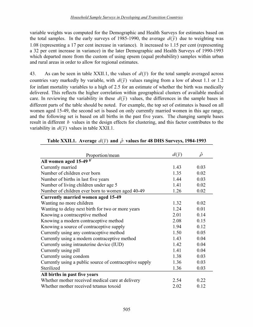
Household Sample Surveys in Developing and Transition Countries
505
variable weights was computed for the Demographic and Health Surveys for estimates based on the total samples. In the early surveys of 1985-1990, the average ( )d y due to weighting was 1.08 (representing a 17 per cent increase in variance). It increased to 1.15 per cent (representing a 32 per cent increase in variance) in the later Demographic and Health Surveys of 1990-1993 which departed more from the custom of using epsem (equal probability) samples within urban and rural areas in order to allow for regional estimates.
43. As can be seen in table XXII.1, the values of ( )d y for the total sample averaged across countries vary markedly by variable, with ( )d y values ranging from a low of about 1.1 or 1.2 for infant mortality variables to a high of 2.5 for an estimate of whether the birth was medically delivered. This reflects the higher correlation within geographical clusters of available medical care. In reviewing the variability in these ( )d y values, the differences in the sample bases in different parts of the table should be noted. For example, the top set of estimates is based on all women aged 15-49, the second set is based on only currently married women in this age range, and the following set is based on all births in the past five years. The changing sample bases result in different b values in the design effects for clustering, and this factor contributes to the variability in ( )d y values in table XXII.1.
Table XXII.1. Average ( )d y and �ρ values for 48 DHS Surveys, 1984-1993
Proportion/mean ( )d y �ρ All women aged 15-49 a/ Currently married 1.43 0.03 Number of children ever born 1.35 0.02 Number of births in last five years 1.44 0.03 Number of living children under age 5 1.41 0.02 Number of children ever born to women aged 40-49 1.26 0.02 Currently married women aged 15-49 Wanting no more children 1.32 0.02 Wanting to delay next birth for two or more years 1.24 0.01 Knowing a contraceptive method 2.01 0.14 Knowing a modern contraceptive method 2.08 0.15 Knowing a source of contraceptive supply 1.94 0.12 Currently using any contraceptive method 1.50 0.05 Currently using a modern contraceptive method 1.43 0.04 Currently using intrauterine device (IUD) 1.42 0.04 Currently using pill 1.41 0.04 Currently using condom 1.38 0.03 Currently using a public source of contraceptive supply 1.36 0.03 Sterilized 1.36 0.03 All births in past five years Whether mother received medical care at delivery 2.54 0.22 Whether mother received tetanus toxoid 2.02 0.12

Household Sample Surveys in Developing and Transition Countries
506
Child under age 5 Whether had diarrhoea in the last two weeks 1.34 0.03 Of above, whether child received ORS b/ treatment 1.25 0.12 Children aged 6-35 months Height for age less than 2 standard deviations below norm 1.33 0.05 Weight for age less than 2 standard deviations below norm 1.29 0.04 Weight for height less than 2 standard deviations below norm 1.19 0.02 Children aged 12-23 months Whether has health card 1.33 0.15 Of above, whether child is fully immunized 1.31 0.21 Children born 1-4 years or 5-9 years ago Infant mortality rate 1-4 years preceding the survey 1.23 0.02 Infant mortality rate 5-9 years preceding the survey 1.14 0.01 a/ In approximately one-fourth of the surveys, the sample, and hence all variables in this group, was restricted to ever-married women. b/ Oral rehydration salts.
44. The measure of homogeneity ρ is more useful than the design effect due to clustering for planning future surveys, since the design effect depends on both ρ and the cluster size b . The design effect for a past survey will be applicable to the new survey only if both these parameters are the same. However, the possibility of changing b should be considered, since the cluster size can be controlled by the sampler while the intra-class correlation cannot. If an estimate of ρ is available, the effect of changing b may be examined by computing the design effects from clustering for different values of b . Thus, ρ is the key factor of interest. Estimates of average ρ were computed from the Demographic and Health Surveys, and the results are also displayed in table XXII.1. As can be seen from the table, the ρ values vary considerably, ranging from a low of 0.01 to a high of 0.22. As expected, estimates that depend on the availability of local health facilities tend to have large ρ values.
45. An important finding from the sampling error analyses for the DHS programme is that estimates of ρ for a given estimate are fairly portable across countries, provided that the sample designs are comparable. Thus, in designing a new survey in one country, empirical data on sampling errors from a similar survey in a neighbouring country may be employed if necessary and if due care is taken to check on comparability.
I. Survey implementation 45 46. While much attention is paid to scientific sampling and the calculation of sampling errors, it should not be forgotten that there are multiple sources of errors in surveys. Errors related to sampling variability can typically be quantified while other errors typically cannot 45 Much of the mateial in the sections on survey organization and the characteristics of the Demographic and Health Surveys have been taken from the draft DHS Survey Organization Manual, drafted by one of the authors of the present chapter.

Household Sample Surveys in Developing and Transition Countries
507
easily be quantified. Nonetheless, non-sampling errors are often likely to be bigger than sampling errors. This is particularly the case if insufficient attention is paid to training and recruitment of field and data-processing staff. Thus, the control of non-sampling error is a major objective in every Demographic and Health Survey.
47. With respect to implementation, many Demographic and Health Surveys are carried out in countries where it is difficult to recruit highly qualified field staff and where fieldwork poses significant challenges of transportation, lodging, hygiene, food supply, etc. The need for field staff to travel around the country also opens up issues of security and supervision. These and others are the main reasons that the DHS programme pays great attention to the training of field staff and to supervision in the field and in the office. Yet, even with this emphasis on supervision, there have been instances where the systems were not properly implemented and issues of data quality arose. The steps below describe the typical steps that go into the implementation of a Demographic and Health Survey, emphasizing the need for detailed preparation, extensive training and supervision. 48. Another important aspect of surveys is the extent to which the survey data become available in a timely manner and are accessible to decision makers, programme managers and analysts. There are too many surveys, particularly in developing countries, that have never been properly analysed or disseminated. The DHS programme is geared towards ensuring that all surveys are analysed in a timely fashion, that the results are published and disseminated and that the data are available for further research. The process required to achieve this is described below.
J. Preparing and translating survey documents
49. The survey documents in each participating country typically consist of a household questionnaire, individual questionnaire(s) for women and/or men and corresponding manuals. The questionnaires include the DHS core questions, country-specific adaptations and optional modules. DHS staff work with local counterparts on the adaptation of questionnaires, bearing in mind the needs of the country. The DHS model questionnaires are lengthy, so that additions need to be carefully considered in view of the overall length of the instruments. Data quality is likely to suffer if the questionnaires become unwieldy and take too long to implement. The core Interviewer and Supervisor�s Manuals are adapted in each country to reflect the country-specific content of the questionnaire. 50. DHS policy is to have questionnaires translated into and printed in all the major local languages to ensure that the interviews are conducted in the language of the respondents. Any language group that constitutes 10 per cent or more of the sample should have its own translated questionnaire. The need for on-the-spot translation by the interviewer or someone else often cannot be avoided totally, as there may be no adequate language version of a questionnaire for some respondents who fall within the sample. However, the need for on-the-spot translation should be minimized.

Household Sample Surveys in Developing and Transition Countries
508
51. Translation is not an easy task and requires both strong linguistic skills as well as an understanding of terms and expressions that are typical in Demographic and Health Surveys. Seldom are all these skills to be found in only one person, particularly where multiple languages are to be used in the same country. 52. The DHS approach to translation entails having one person translate the DHS questionnaire into the required local language, using the English, French or Spanish version of the core questionnaire. In case there has been an earlier DHS or similar survey that was translated, that translation should certainly be taken into account. Typically, if the same questions are to be asked one would expect the translation to be the same as well, except in cases where the earlier translation was judged to be deficient. 53. The translated questionnaire is then translated back into its original language by an independent translator. It is important that the back-translation be carried out without reference to the original questionnaire, so as to ensure full independence of the two versions. The next step is to have the two translators and the senior survey staff get together to study the original and the back-translation with a view to resolving discrepancies. This is an important process particularly in the case of languages that are not commonly written, inasmuch as their translation is not a straightforward process. 54. This process should result in questionnaires that are well understood by the respondents who are to be interviewed in their language. However, it is also necessary to test the translations in the field before adopting them for the survey. It is not necessary to conduct a large number of interviews in the field, but at least from three to five should be carried out in each language, prior to finalizing the translations. It is important to remember that the purpose of the translation is to ensure that every respondent is asked the same question. This does not mean, however, that translation should be literal. A good translation will transmit the same meaning, although it may not be a word-for-word translation. Demographic and Health Surveys are often repeated in countries although the questionnaires for the different rounds may be somewhat different in content. Old translations of most questions and the experience gained during earlier pre-tests and fieldwork can therefore also be used. 55. Survey documentation such as interviewers� and supervisors� manuals should be translated into the language understood by all the field staff, if the English, French or Spanish versions cannot be used.
K. The pre-test 56. A pre-test constitutes a crucial means of testing the translations, the skip patterns in the questionnaire, the interviewers� and supervisors� manuals and other survey procedures. It is also a mechanism through which the senior survey staff may gain experience in training field staff prior to the main training course. The DHS country manager typically participates in the pre-test interviews. 57. For the pre-test, a small number of field staff is trained, usually for about two weeks. Training is provided through local staff, with assistance from the DHS country manager. It is
Household Sample Surveys in Developing and Transition Countries
509
DHS practice to train future supervisors as interviewers for the pre-test. They later attend interviewer training as supervisors. This ensures that they have very extensive training, that their role is already established during interviewer training, and that there is sufficient staff available to correct and guide the practice sessions and tests that take place during interviewer training. 58. The pre-test typically covers 100-200 households and interviewing takes about a week to complete. Pre-test interviews are carried out in urban and rural areas that have not been selected for the main survey in order to prevent contamination of the survey results. The body of experience that has accumulated in DHS with this type of survey is by now very extensive, so that the pre-test can be small and does not need to cover many different areas of the country. 59. Pre-test fieldwork follows the same procedures that will be followed during the main fieldwork. Thus, households are listed so that teams become acquainted with following procedures and using their control forms. The senior survey staff actively supervise all the stages of the pre-test so that they may become familiar with problems that are encountered and may recommend solutions. 60. The pre-test experience is the basis on which the survey questionnaires and manuals are revised. Errors need to be corrected and improvements made on the basis of the work observed during the pre-test. Key to this activity is the keeping of a running log of all the problems that are found during the training, the practices and the actual interviews. Problems found during the latter are documented through reports by the survey staff that observe pre-test interviews and through a daily debriefing of the pre-test interviewers. It is important that all staff involved in the pre-test take notes on what they observe. 61. Care is also taken to make sure that any post-pre-test revisions do not introduce new errors. Indeed, if extensive revision of the questionnaires is necessary, a few field interviews with the new instrument are conducted to ensure that the revisions are made correctly and no new problems were introduced.
L. Recruitment of field staff
62. The quality of a household survey depends to a significant extent on the quality of the field staff. Therefore, the best possible people are recruited for the job. In developing countries, few organizations have a permanent field force of interviewers and supervisors; and even if they do, the interviewers tend to be predominantly men. Female interviewers are required for a Demographic and Health Survey unless the survey is one of men. Therefore, a DHS is generally fielded with staff that have been especially recruited for the job. As the data-collection or fieldwork stage typically lasts from three to six months, recruits are usually people who are not currently holding jobs and who are willing and able to spend several months away from home. In some countries where surveys have more extensive health content, medical staff working for the Ministry of Health have been seconded as interviewers and supervisors. 63. Recruitment takes into account the number of staff needed to speak each of the languages in which the survey will be conducted. The number of trainees recruited is at least 10-15 per cent

Household Sample Surveys in Developing and Transition Countries
510
higher than the number needed for fieldwork to allow for attrition and dismissal of candidates who prove to be inadequate. Recruitment is based on an objective test of the candidates� abilities rather than any other characteristics. Candidates should be presentable, able to walk long distances and able to establish good rapport with the people they will need to interview. Having a good team spirit is a further necessary requirement. Under no circumstances should recruitment be based on the candidates� relationship to survey staff, favouritism or other unacceptable recruitment practices. 64. The supervisor and field editor positions require people that can be team leaders. They need self-confidence, strong motivation and excellent team spirit. All these characteristics are desirable in interviewer candidates as well. However, the main characteristics of a good interviewer are the ability to ask questions in a fluent and natural manner, the ability to put the respondent at ease and the ability to correctly record the answers that are given.
M. Interviewer training
65. Interviewer training is very similar to the pre-test training, except that it is generally from three to four weeks long, partly because of the larger number of trainees. Candidate interviewers complete at least 5-10 practice interviews in the field during training. Training is provided by local staff, who are assisted by the staff that was trained for the pre-test and the DHS country manager. 66. Final selection of interviewers is based on their performance on a series of written tests as well as on the observation of their performance during practice interviews in the office and the quality of their pre-test interviews. It is extremely important that the selection criteria be objective. In many places, there is much pressure on survey staff from other individuals to fill the available jobs with those individuals� particular choices. However, the only way to select staff is through a review of their qualifications for the job and an objective rating of their performance during training. Indeed, having objective written tests during training can help survey staff document the reasons why certain candidates could not be accepted.
N. Fieldwork 67. DHS policy calls for a team approach to fieldwork. The reasons for working in teams are many, but the main one is the ability to achieve a higher level of supervision of the work. An additional reason is the need for special means of transportation for most interviewers. In many countries, the need to safeguard to the well-being of the field staff is another important reason. 68. Teams generally consist of one supervisor (team leader), one female field editor, one health technician and from three to four female interviewers. If a survey of men is also incorporated, the team usually includes one male interviewer. In most countries, a vehicle is assigned to each team, accompanied by a driver. The size of the team is sometimes limited by the carrying capacity of the vehicles that are used.

Household Sample Surveys in Developing and Transition Countries
511
69. The supervisor is in overall charge of the team and the daily organization and supervision of the team�s work. The field editor is mainly in charge of checking the quality of the interviews. In actual practice, the supervisor and the field editor will need to share each other�s responsibilities in order to build and maintain a good interviewing team. 70. The main considerations in determining the number of teams are the number of PSUs, the size of the clusters and the anticipated duration of the fieldwork. However, other important considerations are the number of vehicles available, the number of capable interviewers and supervisors that can be recruited and the number of languages spoken in the country. Fieldwork should last from three to six months. Shorter durations are sometimes possible. However, to achieve good data quality, the number of interviewers is kept relatively low owing to constraints on training, availability of good candidates, etc. This in turn limits the number of teams that can be used and determines the duration of the fieldwork. 71. If possible, all teams start fieldwork in the same general geographical location (such as the same province), in order to make supervision of all teams by senior survey staff possible during the time that supervision is most needed. If teams scatter all across the country from the beginning, it is very difficult to visit all teams immediately. 72. Survey teams are assigned sample areas taking into account languages spoken and other requirements and the need to ensure that the travel times per team are minimized as much as possible. Generally, teams work six days per week and work away from home for several weeks or months at a time. 73. If an interview is not completed on the first visit, further attempts are made with the sampled household or respondent, up to three times and over three different days, before classifying the case as non-response. The subsequent contacts are scheduled at times when the respondent is more likely to be at home. When most members of the team have finished work, but one or two callbacks are remaining for another day, it is not uncommon for the team to move to a new cluster and to leave one interviewer behind to �clean up�. This is possible when the new cluster is not too distant and the team vehicle can pick up the clean-up interviewer. In other circumstances, the whole team stays until all work in the cluster is completed. As mentioned earlier, there is no replacement for households or individuals that refuse to be interviewed or are otherwise classified as non-response. 74. Teams need to have a sufficient supply of questionnaires and materials with them to ensure that work can continue at full speed at all times. Completed questionnaires need to be packed, protected from the elements and safeguarded until they can be transmitted to the home office, usually via the roving field supervisors who periodically visit each team. 75. Heavy emphasis on supervision is a hallmark of a Demographic and Health Survey. Experience suggests that without continuous supervision, data quality will suffer considerably. Therefore, several levels of supervision are employed. The team supervisor and the field editor are required to observe interviewers from time to time and check each questionnaire thoroughly for completeness and accuracy. Where major problems are found, interviewers are required to return to the interviewed person to obtain the correct information. Moreover, the supervisor is

Household Sample Surveys in Developing and Transition Countries
512
usually responsible for re-interviewing a subsample of about 10 per cent of selected households to ensure that the initial interview was conducted and that all eligible women were correctly identified. 76. The survey director and DHS staff provide further supervision during the fieldwork. Teams are visited in the field on a regular basis to check on the work of the interviewers, the editors and the supervisors. During this check, at least one or two questionnaires of each interviewer are scrutinized after the field editor has reviewed them. In this way, both interviewer and editor mistakes can be caught at the same time. Supervisory field visits are extremely important. It is not uncommon for some supervisors and editors not to be doing a really good job. This will affect the quality of the work of the interviewers and should be rectified as soon as possible. Field visits are the main mechanism through which this rectification is achieved. A helpful tool during these field visits are the �data quality tables� that are run at regular intervals during the fieldwork to pinpoint specific problems and problems with specific survey teams and interviewers. The data quality tables contain information on the age of the respondents and the age of small children that may be used to check that respondents were properly selected by the interviewers. In addition, they contain information on infant and child deaths in order to gauge the level of omission of dead children. Household and individual response rates are also included to gauge the productivity of each team and interviewer and to see if households and/or respondents are being willfully omitted from the survey. Problems found during the examination of these data quality tables are communicated to the field, so that they can be avoided in the future (see also sect. O below).
77. The household listing that is part of the household sampling stage is not described in the present section on fieldwork. It is a separate operation that takes place from two to three months before fieldwork by specialized household listing staff, as described in section E. Keeping the listing operation separate from the main fieldwork ensures that listing can be well supervised and that households can be sampled by qualified personnel in the office prior to the main fieldwork. Sample selection as an office operation helps avoid potential biases that often occur if households are selected by the field staff, especially when the �lister� and �sampler� are the same person.
O. Data processing
78. In Demographic and Health Surveys, data processing generally starts from one to two weeks after the start of fieldwork and is usually completed within a month after the completion of fieldwork. The data entry staff is trained on the questionnaires, by attending either part of the interviewer-training course or a special two- or three-day training. The data-processing coordinator typically attends the entire interviewer-training course. 79. Data entry takes place in a separate room, where the staff is not disturbed and where the questionnaires are secure. This room should be close to the space where completed questionnaires are stored. All questionnaires are handled several times during data entry and editing, and proximity between the storage and data entry facilities can considerably reduce workload and stress. Data entry staff does not work more than six hours per day, owing to the mechanically intense nature of the operation. Depending on the number of computers available

Household Sample Surveys in Developing and Transition Countries
513
for the data entry operation, more than one shift of data entry staff may be necessary in order to finish data entry and editing shortly after the end of fieldwork. Double shifts are avoided if possible, since they can lead to inconsistencies as a result of having multiple supervisors and office editors. 80. DHS policy is to enter the data from all questionnaires twice (�double entry�), compare the results and resolve any discrepancies. Such 100 per cent verification greatly reduces the amount of secondary editing needed to resolve inconsistencies and results in a cleaner, more accurate data set. Double data entry is carried out by two different data entry staff, to ensure the best results. During data entry, range, skip and consistency checks are performed on each questionnaire. 81. One aspect of the data entry and editing relates directly to the control of data quality. It is DHS procedure to produce a selected set of tables periodically during data entry and editing, with a view to checking for problems that cannot be easily identified during manual editing and data entry of individual questionnaires. These �field check tables� are geared towards discovering whether, for example, interviewers are manipulating the ages of respondents or their children in order reduce their workload, underreporting infant and child deaths, or correctly recording the age at death. These tables are run once a sufficient number of questionnaires have been entered, say, 300, and biweekly thereafter, so that deviant patterns of response or respondent's characteristics can be identified by the interviewer or interviewer team. Staff from the implementing organization and from DHS reviews these tables. Problems are communicated to the appropriate teams, so that corrective action can be taken. 82. The basic tabulations that are produced for each country are those that were designed on the basis of the data collected in the core questionnaire. Tabulations of data that are derived from questions that were added to the core questionnaire are designed in collaboration with the persons/institutions that requested these extra tables. This work needs to be done early on to ensure that the tabulation process is smooth. All tabulations are checked thoroughly, both by DHS staff and by country counterparts. 83. Because of the complexity of the data entry, editing, imputation, and tabulation programs, they are developed by DHS data-processing staff, who visit the country to install the programs and set up the process. Typically, the data processing specialist returns at the end of the data processing to help review the final data set, recode some variables, impute missing dates, attach the sample weighting factors, and run the previously designated set of tables for the preliminary and final reports. In tabulating the data, both weighted and unweighted numbers of cases are presented in the reports, although calculations always use final sample weights.
P. Analysis and report writing
84. The basis for the analysis is the set of DHS model tabulations as modified by the DHS country manager and host country staff to fit the questionnaires used. These tabulations are supplemented by country-specific tables that present the additional data that have been collected in each country. The analysis results in a comprehensive report on the survey data.
Household Sample Surveys in Developing and Transition Countries
514
85. A small report on key findings is also produced, with a view to achieving the widest possible dissemination of the data. The report on key findings is produced immediately after or concurrent with the main survey report and is available at the time of the national seminar (see sect. Q on dissemination below). 86. In addition to producing with these survey reports, DHS assists countries in conducting more in-depth �further analysis� of the survey data. These analyses typically result in a research paper of 30-60 pages and address topics of special interest to the country or funding agencies; but they can also consist of special tabulations and short analytic statements that permit a country to respond to policy-relevant and/or other issues.
Q. Dissemination 87. Dissemination of the survey results to all the relevant audiences is a key objective of the survey programme. The survey reports are distributed widely at the local level and are also made available to cooperating agencies and other institutions that work in the respective countries. Survey reports are also available for viewing and downloading on the DHS web site. Wall charts, chart books, calendars, posters and other materials are also developed in conjunction with the national seminar to achieve wider dissemination of the survey results. 88. In addition, a national seminar is held to present the main survey findings to policy makers, programme managers, researchers and representatives of donor organizations. The seminar is generally covered in the mass media, thus helping to generate utilization of these data for policy and programme purposes. Some countries organize regional seminars to ensure that the results are known and utilized beyond the national policy and programme level. 89. All DHS survey data are entered into the DHS data archive. Nearly all countries that participate in the programme have authorized the use of their data by responsible researchers worldwide. The data archive team at DHS tracks data requests and provides data and documentation to those who are authorized to use them. Data are now available without charge via the Internet, after proper electronic registration and authorization of each user. By the end of 2002, ORC Macro had provided access to DHS data files and sub-files more than 80,000 times. The web site address is: www.measuredhs.com. Further information on the DHS programme is also available on this web site.
R. Use of DHS data 90. DHS data are typically used to monitor and evaluate progress in maternal and child health and population programmes in participating countries. The availability of repeat-survey information provides countries with the trend data necessary to gauge progress. Data are sometimes used for immediate-action programmes entailing, for example, the provision of iron supplementation in places where anaemia is rampant. More often, they are used to shape policy and to change intervention programme objectives, as well as for long-term health and population

Household Sample Surveys in Developing and Transition Countries
515
planning. DHS data have been instrumental in galvanizing support for family planning programmes in sub-Saharan Africa and elsewhere by showing that change is possible and is occurring even in some of the poorest countries.
S. Capacity-building
46. 91. One of the aims of the DHS programme is to increase the capacity of participating countries to collect and analyse data through large-scale national-level household surveys. The main mechanism by which this is to be achieved is the development of state-of-the-art basic documentation, such as questionnaires and manuals; the development of software programs that facilitate survey processing in the context of developing countries, and on-the-job training of local counterparts during all stages of the country surveys. 92. A major contribution to capacity-building is the development of new software. Initially, DHS developed the Integrated System for Survey Analysis (ISSA) program for survey processing. The availability of that software was instrumental in achieving early availability of clean data files and reports. To adapt to new basic hardware and software developments, DHS has launched new survey data-processing software called Census and Survey Processing (CSPro), in collaboration with the United States Bureau of the Census and a software development firm. It is expected that this software will be very widely used and will supplant the variety of programs used by different institutions for the processing of large-scale surveys. The United States Bureau of the Census is already supporting extensive training programmes in the use of this software and it is envisaged that the software will become the standard in most developing countries. This will greatly help capacity-building efforts. 93. The DHS programme has always provided continuous training and feedback to local counterparts by means of detailed basic documentation for survey implementation, regular technical assistance visits (10-14 per country) and joint work on the preparation of the survey reports. The basic documentation includes manuals on all the important stages of survey execution. These three mechanisms remain the main vehicles for capacity-building in participating countries.
T. Lessons learned
94. Many valuable lessons for household surveys in developing countries have been learned during the execution of the DHS and its predecessors, for example:
• Sampling frames in many countries need costly field updating in order to be usable for surveys that intend to collect high-quality data. Household listings are often out of date or non-existent. Quality control makes it necessary to select the households in the office rather than leave the selection to field staff, thereby ensuring that all households have a known probability of selection. Selecting households in the office eliminates problems caused by the tendency of interviewers to visit those homes that are more accessible and to leave out those that are more remote. Selecting from a

Household Sample Surveys in Developing and Transition Countries
516
household list in the office provides un unbiased sampling of the listed households and also permits easy supervision of sample selection in the field.
• Sample updating, when done at the penultimate sampling stage, needs to be closely
supervised in order for a full listing of all households to be achieved. It has also been observed in a number of surveys that household listers may be tempted to leave out dwellings that are more remote or that are located in difficult or dangerous areas. Without good supervision, the listing produced by the household listers may be biased.
• Response rates are generally very good, both at the household and at the individual
respondent level (see sect. F on response rates). • Sampling errors and design effects must be calculated for a representative set of
survey items of every survey in order to evaluate the effectiveness of the sample design and the precision of the survey estimates.
• A cluster size of 15-20 women is optimum in Demographic and Health Surveys
where the need is to balance the variety of demographic and health items - some more clustered than others, some involving small children of sampled women - and the cost of data collection.
• The design effect due to clustering is an increasing function of the cluster size b and
the intra-class correlation coefficient ρ . Since ρ is fairly portable across countries with comparable sample designs, ρ , b and the design effects from one survey can be used to design a new comparable survey in another country, as described in chapter VI.
• Training interviewers and supervisors on complex surveys takes from three to four
weeks to accomplish. DHS training typically takes three weeks. However, there have been many occasions where training was extended for an additional week or more to achieve proper preparation of the field staff. Most of the problems with the surveys emanate from the field staff, not from the respondents. Proper training and supervision are the main tools with which to avoid those problems.
• Interviewers and supervisors can cause serious problems for a survey. Continuous
supervision and quality control are therefore necessary in order that sloppy work and/or deliberate manipulation of the sample or the interview by some interviewers and supervisors to lighten their workload, may be avoided. DHS surveys have provided ample evidence that interviewers have a tendency to code women and/or children out of eligible age ranges so as not to have to interview them. While this problem does not generally involve all the field staff, it does exist and often is confined to only a few of the interviewing teams. Continued vigilance during the whole of the fieldwork is a must.

Household Sample Surveys in Developing and Transition Countries
517
• An interview that, on average, takes no more than one hour should be striven for. This statement is based not on actual field experimentation with different survey durations, but rather on feedback from field staff. Demographic and Health Surveys vary enormously in length depending on the characteristics of the respondents and the ease with which they can recall dates and events. The duration can vary from as little as 10 minutes for a single woman without children and sexual activity to more than an hour and a half for women with a large number of children who do not easily recall the events that constitute the content of the survey.
• One of the major obstacles with respect to field logistics is associated with the
availability of suitable vehicles to transport the survey teams. Vehicles for fieldwork are expensive to acquire and operate because they need to be the large variety of an all-terrain vehicle in order to accommodate the whole survey team. Lack of proper vehicles costs time and impacts negatively on team morale. Even with proper vehicles, interviewers and supervisors will need to walk long distances to reach certain dwellings. Therefore, transporting them to the general survey area should be made as painless as possible.
• One of the most difficult aspects of field logistics is matching the right interviewer
with the right respondent and the right questionnaire in the case of countries where multiple languages are used for the interview. The composition of teams according to language capabilities, combined with a detailed deployment plan that takes into account the linguistic requirements for the teams, is a necessity for ensuring that most respondents are interviewed in their native language by an interviewer who speaks that language, using a questionnaire in that language.
• Data entry staff needs to follow the interviewer�s training course so as to be able to
handle data entry and editing. DHS questionnaires are quite complicated. Participation in interviewer�s training gives data entry staff a good understanding of the flow of the questionnaire and of how different parts of the questionnaire are related. They need this knowledge in order to make corrections during the interactive data entry and editing process.
• Double data entry will save time on editing, although it may appear to be costly. In
the early Demographic and Health Surveys, data were entered only once. The later surveys have used double data entry to detect those errors that cannot be detected through the range and consistency checking programs and to ensure that the minimum number of questionnaires will need corrections during the editing stage. DHS data-processing staff has decided that the beneficial impact of double data entry on data editing far outweighs its cost.
• Continuous feedback to the field about problems encountered in completed
questionnaires during data entry is necessary to achieve data of high quality. Particularly in the early stages of a survey, field staff needs to be told immediately what errors they are committing, so that those errors can be avoided in the future.

Household Sample Surveys in Developing and Transition Countries
518
Interactive data entry provides a very good mechanism for the early identification of field problems.
• It is necessary to run some tables to reveal response patterns that will not be obvious
from editing individual questionnaires. For example, do interviewers purposely code potential respondents as older or younger in order to avoid having to interview them? Only by studying age patterns of respondents over several hundred interviews can problems of this nature be clearly identified.
• In many countries, producing the survey report is one of the most challenging tasks.
Capacity-building in survey research is one of the aims of the Demographic and Health Survey programme. Report writing is one of the areas where a strong effort is made to build capacity through interactive work with local authors. More recently, report writing workshops, during which all authors work on chapters of the report with the collaboration of DHS staff, have come to be considered one of the more effective ways of transferring capacity. Nonetheless, report writing is also something of an art and not everyone, irrespective of any advanced degrees in demography or health, is equally good at it.
• Technical assistance is most needed in sampling, data processing and report writing.
For other areas, such assistance often takes the form of ensuring that the different survey steps are executed in a timely fashion. The above-mentioned areas have presented the greatest difficulties for local staff in many, if not most, of the Demographic and Health Surveys. In comparison, training and fieldwork are conducted very well by many local agencies. It is therefore necessary to make the needed technical assistance available in order that weaknesses in one or more of the more troublesome areas may be overcome.
• Countries are willing to share their survey data with responsible researchers. Plans
for this should be agreed upon prior to survey implementation. The Demographic and Health Surveys programme has been very successful in securing the approval of participating countries with respect to sharing their data with responsible researchers on future research projects. This has created a unique multi-country database which has become invaluable for countries and donors alike. To achieve this goal, agreements need to be reached with the authorities in participating countries at the time the survey is agreed upon. If such agreements are not reached at that time, it is often not possible to negotiate them later because the government may have changed and different people may be in charge of the government department(s) that were in place when the survey was initially being planned.

Household Sample Surveys in Developing and Transition Countries
519
Annex: Household and woman response rates for 66 surveys in 44 countries, 1990-2000, selected regions
Region
Country
Survey year
Phase
Number of households
Household response
rate (percentage)
Number of women
Woman response rate (percentage)
Asia Bangladesh 1994 DHS III 9 255 99.1 9 900 97.4 Bangladesh 1997 DHS III 8 762 99.1 9 335 97.8 Indonesia 1991 DHS II 27 106 99.1 23 470 97.6 Indonesia 1997 DHS III 34 656 98.8 29 317 98.3 Pakistan 1991 DHS II 7 404 97.2 6 910 95.7 Philippines 1993 DHS III 13 065 99.5 15 332 98.0 Philippines 1998 DHS III 12 567 98.7 14 390 97.2
Eurasia Kazakhstan 1995 DHS III 4 232 98.7 3 899 96.7 Kazakhstan 1999 MEASURE 5 960 98.1 4 906 97.8 Kyrgyzstan 1997 DHS III 3 695 99.4 3 954 97.3 Turkey 1993 DHS III 8 900 96.8 6 862 95.0 Turkey 1998 MEASURE 8 596 93.8 9 468 90.6 Uzbekistan 1996 DHS III 3 763 98.4 4 544 97.2
Latin America Bolivia 1994 DHS III 9 335 97.6 9 316 92.3 Bolivia 1997 DHS III 12 281 98.6 1 831 94.6 Brazil 1991 DHS II 6 416 94.5 6 864 90.7 Brazil 1996 DHS III 14 252 93.2 4 579 86.5 Colombia 1990 DHS II 8 106 91.4 9 715 89.0 Colombia 1995 DHS III 11 297 89.5 2 086 92.2 Colombia 2000 MEASURE 11 747 92.8 2 531 92.5 Dominican Republic 1991 DHS II 8 131 87.9 8 200 89.3
Dominican Republic
1996 DHS III
9 026
97.8
9 034
93.2
Guatemala 1995 DHS III 11 754 96.1 3 388 92.6 Haiti 1994 DHS III 4 944 97.5 5 709 93.8
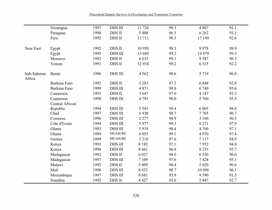
Household Sample Surveys in Developing and Transition Countries
520
Nicaragua 1997 DHS III 11 726 98.3 4 807 92.1 Paraguay 1990 DHS II 5 888 96.5 6 262 93.1 Peru 1992 DHS II 13 711 98.3 17 149 92.6 Near East Egypt 1992 DHS II 10 950 98.3 9 978 98.9 Egypt 1995 DHS III 15 689 99.2 14 879 99.3 Morocco 1992 DHS II 6 635 99.1 9 587 96.5 Yemen 1991 DHS II 12 934 99.2 6 515 92.2 Sub-Saharan Africa
Benin 1996 DHS III 4 562 98.6 5 719 96.0
Burkina Faso 1992 DHS II 5 283 97.3 6 848 92.8 Burkina Faso 1999 DHS III 4 871 98.8 6 740 95.6 Cameroon 1991 DHS II 3 647 97.0 4 147 93.3 Cameroon 1998 DHS III 4 791 98.0 5 760 95.5 Central African
Republic
1994 DHS III
5 583
99.4
6 005
98.0
Chad 1997 DHS III 6 930 98.7 7 705 96.7 Comoros 1996 DHS III 2 277 98.9 3 160 96.5 Côte d'Ivoire 1994 DHS III 5 977 99.3 8 271 97.9 Ghana 1993 DHS III 5 919 98.4 4 700 97.1 Ghana 1999 MEASURE 6 055 99.1 4 970 97.4 Guinea 1999 MEASURE 5 216 97.6 7 117 94.9 Kenya 1993 DHS III 8 185 97.1 7 952 94.8 Kenya 1998 DHS III 8 661 96.8 8 233 95.7 Madagascar 1992 DHS II 6 027 98.6 6 520 96.0 Madagascar 1997 DHS III 7 349 97.6 7 424 95.1 Malawi 1992 DHS II 5 409 98.4 5 020 96.6 Mali 1996 DHS III 8 833 98.7 10 096 96.1 Mozambique 1997 DHS III 9 681 95.9 9 590 91.5 Namibia 1992 DHS II 4 427 92.6 5 847 92.7

Household Sample Surveys in Developing and Transition Countries
521
Niger 1992 DHS II 5 310 98.7 6 750 96.3 Niger 1997 DHS III 6 007 98.7 7 863 96.4 Nigeria 1990 DHS II 9 173 98.1 9 200 95.4 Nigeria 1999 MEASURE 7 736 98.8 10 529 93.2 Rwanda 1992 DHS II 6 292 99.4 6 947 94.3 Senegal 1993 DHS II 3 563 99.0 6 639 95.0 Senegal 1997 DHS III 4 855 98.3 9 186 93.5 Togo 1998 DHS III 7 620 98.6 8 964 95.6 Uganda 1995 DHS III 7 671 98.4 7 377 95.8 United Republic of
Tanzania 1992 DHS II 8 560 97.3 9 647 95.8
United Republic of Tanzania
1996 DHS III 8 141 97.9 8 501 95.5
Zambia 1992 DHS II 6 245 99.4 7 247 97.4 Zambia 1996 DHS III 7 365 98.9 8 298 96.7 Zimbabwe 1994 DHS III 6 075 98.5 6 408 95.6 Zimbabwe 1999 MEASURE 6 512 97.8 6 208 95.2
Household Sample Surveys in Developing and Transition Countries
522
Acknowledgements
The authors acknowledge the valuable comments of members of an expert panel convened by the United Nations to discuss the draft publication, of the external reviewers and of Dr. Alfredo Aliaga of ORC Macro. References Cleland, J., and C. Scott, eds. (1987). The World Fertility Survey. An Assessment. New York:
Oxford University Press Institute for Resource Development/Macro Systems, Inc. (1990). An Assessment of DHS-I Data
Quality. Methodological Report, No. 1. Columbia, Maryland. __________ (1994). An Assessment of the Quality of Health Data in DHS-I Surveys.
Methodological Report, No. 2. Columbia, Maryland. Review, 56(3): 259-78. Kish, L. (1965). Survey Sampling. New York: Wiley. __________, R. Groves and K. Krotki (1976). Sampling Errors in Fertility Surveys. World
Fertility Survey Occasional Paper, No. 17, The Hague: International Statistical Institute. Lê, T., and V. Verma (1997). An Analysis of Sample Designs and Sampling Errors of the
Demographic and Health Surveys. DHS Analytical Reports, No. 3. Calverton, Maryland: Macro International, Inc.
ORC Macro (1996). Sampling Manual. DHS-III Basic Documentation, No. 6. Calverton,
Maryland. __________ (2001). Survey organizational manual. Draft. Calverton, Maryland. Scott, Christopher, and others (1988). Verbatim questionnaires versus field translation or
schedules: an experimental study. International Statistical Review, vol. 56, No. 3, pp. 259-278.
Vaessen, Martin, and others (1987). Translation of questionnaires into local languages. In The
World Fertility Survey: An Assessment. John Cleland and Chris Scott, eds. New York: Oxford University Press.
Verma, V., and T. Lê (1996). An analysis of sampling errors for the Demographic and Health
Surveys. International Statistical Review, vol. 64, pp. 265-294. Verma, V., C. Scott and C. O�Muircheartaigh (1980). Sample designs and sampling errors for the World
Fertility Survey. Journal of the Royal Statistical Society A, vol. 143, pp. 431-473.

Household Sample Surveys in Developing and Transition Countries
523
Chapter XXIII Living Standards Measurement Study Surveys
Kinnon Scott World Bank
Washington, D.C. United States of America
Diane Steele
World Bank Washington, D.C.
United States of America
Tilahun Temesgen
World Bank Washington D.C.
United States of America
Abstract
The Living Standards Measurement Study (LSMS) programme arose from the need to improve statistical data at the household level required for designing, implementing and evaluating social and economic policy in developing countries. The focus of the LSMS programme has been on understanding, measuring and monitoring living conditions, the interaction of government spending and programmes with household behaviour, ex ante and ex post assessments of policies, and the causes of observed social sector outcomes. The resulting LSMS surveys use multiple survey instruments to obtain data needed for these purposes and rely on significant quality control mechanisms to ensure high-quality relevant data. Especially in recent years, the LSMS programme has emphasized the process of involving data users in the design of the surveys and has worked on issues of sustainability. The present chapter provides an overview of what LSMS surveys are, and the key design and implementation methods used in the surveys, as well as the efforts to promote analytic capacity. An assessment of the costs of the survey and the quality of the data obtained is included, as are examples of the policy uses of LSMS survey data. The chapter also discusses computations of the average sample design effects and intra-class correlation coefficients of some household- and individual-level variables using selected LSMS surveys. Key terms: poverty measurement, living standards, survey methodology, design effect, intra-class correlation, quality control.

Household Sample Surveys in Developing and Transition Countries
524
A. Introduction
1. Public sector expenditures for social services and infrastructure represent significant amounts of resources, both in absolute and in relative terms. It is not unusual for health and education spending to each account for 3-4 per cent of gross domestic product (GDP). Depending on the country, this can range from several million to hundreds of millions of dollars. Major changes in economic policies concerning taxes and prices substantially alter both relative and absolute welfare levels. Yet often, owing to a lack of data, policies are designed, implemented and revised with little information on their overall effectiveness in improving the lives of the country�s population. The absence of appropriate household-level data forces policy makers to rely on administrative data that, while adequate for some purposes, often severely limits the ability to understand household behaviour, how government policies affect households and individuals and the determinants of observed social sector outcomes. Filling in such gaps in understanding is the role of household surveys. 2. The Living Standards Measurement Study (LSMS) surveys are one instrument that Governments can, and do, use to better understand the causes of observed outcomes as well as the impact of their policies. The LSMS survey goes beyond simply measuring outcomes to allowing connections to be made among the myriad factors that affect or cause these outcomes. Single-topic household surveys provide important and in-depth information on a specific topic of interest, but are inadequate for explaining why certain outcomes exist and the range of the factors are that affect them. The goal of the LSMS survey is to explore the linkages among the various assets and characteristics of the household on the one hand, and the actions of government on the other, and, thus to understand the forces affecting each sector, set of behaviours or outcomes. Deepening government�s understanding of the factors that affect living conditions serves to improve policies and programmes. In turn, this can lead to a more efficient and effective use of scarce government and private resources and better living standards. 3. LSMS surveys are a collaborative effort on the part of the country Governments that administer the surveys, the principal users of the data in the countries and the World Bank as well as other bilateral and multilateral donor organizations.46 While based on a core set of concepts, each LSMS survey is substantially customized to meet the specific needs of the individual Governments at a given point in time. The principal implementing agency is usually the national statistical office (NSO) which takes the lead in questionnaire design, sample design, and fieldwork methodology using the techniques found by the LSMS to be most effective. 4. The present chapter provides an overview of the Living Standards Measurement Study. First a short history of the programme is provided, followed by information on the key features of the LSMS survey. This, in turn, is followed by a section explaining how LSMS design features have affected the quality of the data collected. The final section provides some examples of ways in which LSMS survey data have been used.
46 Inter alia, other institutions that have partnered LSMS surveys are the Inter-American Development Bank, United Nations organizations such as the United Nations Development Programme, the United Nations Children�s Fund, the United Nations Population Fund, and bilateral donors from Canada, Denmark, the United Kingdom of Great Britain and Northern Ireland, Japan, Norway, Sweden and the United States of America.

Household Sample Surveys in Developing and Transition Countries
525
B. Why an LSMS survey? 5. The LSMS efforts to respond to the need of policy makers for quality data started in 1980. After a five-year period of work that included reviewing existing household surveys and extensive consultation with researchers and policy makers to determine the types of data needed, as well as with survey methodologists on how best to design the actual fieldwork procedures, the first LSMS surveys were piloted in Côte d�Ivoire and Peru in 1985. These two first surveys were, specifically, research projects testing the full methodology to determine the usefulness and quality of the data that could be obtained.47 The success of these first two surveys has been responsible for the over 60 LSMS surveys that have been carried out in over 40 countries since 1985 (see annex I for a complete list).
C. Key features of LSMS surveys 6. The following is a summary of key features of the LSMS. The reader is referred to the 1996 LSMS Manual for more detailed information about the surveys and how to implement them.48
1. Content and instruments used
7. Up to four separate survey instruments are part of the LSMS surveys. The instruments are: (a) a household questionnaire for collecting information at the household and individual levels, as well as at the level of household economic activities (agriculture and home businesses); (b) a community49 questionnaire for collecting data on the environment in which households function with a focus on the available services, economic activities, access to markets and, lately, social capital; (c) a price questionnaire administered in every area where households are located to allow cost of living adjustments;50 and (d) facility questionnaires administered to local service providers to obtain information on the types and quality of services available to households. Figure XXIII.1 relates the instruments used to the policy purposes of LSMS surveys and the variables needed.
47 For a more detailed account of the history of the LSMS, see Grosh and Glewwe (1995). 48 In Grosh and Muñoz (1996). 49 Note that this is not a �community� in the sociological sense, but rather a mechanism to collect information about the areas where the households selected for the survey are located. 50 National consumer price indices are often inadequate for this purpose, as they tend to be urban and even when rural areas are included, prices are not captured at the appropriate level of disaggregation.

Household Sample Surveys in Developing and Transition Countries
526
Figure XXIII.1. Relation between LSMS purposes and survey instruments
Purpose Indicators Instruments Individual and household measurement of welfare
Levels, distribution Consumption and correlates Income Household questionnaire Wealth, savings Price questionnaire Human capital Anthropometrics Analyse policy
Who benefits from programmes/public spending
Use of services Who receives services, transfers
Impact of public spending/programmes
Costs of services Impact of policies
Household questionnaire Community questionnaire
Availability of services Distance to nearest service Facility questionnaire Quality of services Types of service provided Price questionnaire Price of services Personnel, budget, other
inputs
Effect of economic policies Net transfers between sectors Identify determinants
Why observed outcomes occur Household composition, Household questionnaire What affects household behaviour human capital, welfare,
services available, etc. Community questionnaire Facility questionnaire Price questionnaire
8. The contents of the survey instruments reflect the priority data needs of the country implementing the survey at a given point in time. As the overarching concern is measuring living standards, in all their varied facets, the household survey instrument, in particular, aims to collect information on the wide range of topics affecting these. Table XXIII.1 shows the content of a typical LSMS survey, this one from Viet Nam in 1997-1998.
Table XXIII.1. Content of Viet Nam household questionnaire, 1997-1998
First visit
Second visit
Household roster Fertility Education Agriculture, forestry and fishing Health Non-farm self-employment Labor Food expenses and production Migration Non-food and durable goods Housing and utilities Income from remittances Borrowing, lending and savings Anthropometrics

Household Sample Surveys in Developing and Transition Countries
527
9. There is a high level of questionnaire customization for each country which has led to variations in the overall content of the survey instruments as well as the inclusion of new modules and topics over the years. For example, in Bosnia and Herzegovina in 2001, the health module was expanded to incorporate questions on depression in an effort to measure the incidence of this mental health ailment and identify the linkages between it and other aspects of welfare and labour-market participation. In Guatemala in 2000, a module on social capital was added to collect information on the social dimensions of poverty such as participation in community/government programmes and collective actions, causes of exclusion in the society, perceptions of welfare, and perceptions of, and access to, justice. In Albania, Brazil, Nepal, Jamaica, South Africa and Tajikistan, questions were added on subjective measures of poverty in an attempt to examine the relation of these to other measures.51 Table XXIII.2 presents a sample of modules that have been added in recent years. In summary, while a standard package of modules exists, each country�s LSMS survey reflects the country�s priorities, data needs or concerns at the time of the survey. A recent research project in the World Bank on �Improving the Policy Relevance of LSMS Surveys� has led to a new book outlining, by topic, the policy questions that can be addressed by LSMS data and providing guidance on questionnaire design. 52
Table XXIII.2. Examples of additional modules Topics Countries and year Activities of daily living Kosovo (2000), Kyrgyzstan (1993, 1996, 1997, 1998), Jamaica
(1995) Nicaragua (1993)
Disability Nicaragua, (1993)
Impact of AIDS-related mortality United Republic of Tanzania-Kagera (1991-1994)
Literacy and/or numeracy tests Viet Nam (1997-1998), Jamaica (1990), Morocco (1990-1991)
Mental health Bosnia and Herzegovina (2001)
Privatization Bosnia and Herzegovina (2001), Kyrgyzstan (1996, 1997)
Shocks/vulnerability Bolivia (1999, 2000), Guatemala (2000), Paraguay (2000-2001) Peru (1999)
Social capital Guatemala (2000), Kosovo (2000), Panama (1997), Paraguay
(2000-2001)
Subjective measures of poverty Albania (2002), Brazil (1996), Jamaica (1997), Nepal (1996), South Africa (1993), Tajikistan (1999)
Time-use Guatemala (2000), Nicaragua (1998), Jamaica (1993), Pakistan (1991) Morocco (1990-1991), United Republic of Tanzania-Kagera (1991-1994)
51 For more information on the social capital work in Guatemala, see World Bank (2002b). For further information on the subjective measures of poverty, see Pradhan and Ravallion (2000), Ravallion and Lokshin (2001), Ravallion and Lokshin (2002). Analysis of the Bosnia and Herzegovina data is ongoing. 52 In Grosh and Glewwe, eds. (2000).
Household Sample Surveys in Developing and Transition Countries
528
10. The questionnaire design phase is a process aimed at ensuring that relevant policy issues are identified and incorporated. In most countries, a Data Users� Group or Steering Committee is formed with members from different line ministries, donors and academics along with the National Statistical Office (NSO). This group is responsible for identifying the data needs for specific policies to ensure that the appropriate data are collected. On average, the questionnaire design phase takes about eight months and involves as many actors as possible. This rather lengthy process has the additional benefit of generating demand for, and ownership of, the resulting data. This, in turn, leads to a greater use of the data in policy than would otherwise obtain.
2. Sample issues 11. Typically, LSMS surveys are national surveys using multistage probability samples of households.53 The overall samples are small (relative to several other surveys), usually ranging from 2,000-5,000 households. There are two main reasons to limit the sample size. First, there is a concern for quality and the need to balance sampling error with non-sampling error (see sect. C.4. below for further discussion of this point). Second, the analytic focus of the LSMS surveys is on the determinants or relationships among characteristics of households and not on precise estimates of specific rates, ratios or means. For these reasons, LSMS samples are kept reasonably small and, usually, are not large enough for the survey results to be disaggregated to small geographical areas such as States, municipalities or departments. 12. Probability sampling is used in all LSMS surveys, although the actual design used varies by country and situation.54 Domains of study are identified (urban/rural, regions) and within each domain a stratified two-stage cluster design is used.55 As is the case in most household surveys, LSMS surveys use a cluster design in lieu of a simple random sample (SRS). This stems from cost considerations, even though cluster designs reduce the precision of the estimates (see sect. E.4 below for more on sample design effects that arise from using multistage sampling, as well as annex III). The primary sampling units (PSUs) are geographically defined area units selected with probability proportional to size. The sample frame is typically the most recent population census in the country, but alternatives have been used when the census was unavailable or irrelevant (see Basic Information Documents for the Nicaragua 1993 LSMS, where voting registers supplemented outdated census information; and the Bosnia and Herzegovina 2001 LSMS, where extensive listing operations were needed owing to the civil war, for examples). 13. Once the PSUs have been selected, an enumeration of these PSUs is carried out to ensure that an accurate and up-to-date listing of all dwellings and households is available. This listing operation is carried out as close in time as possible to the fieldwork for the actual survey. To avoid any potential biases, it is conducted not by the interviewers themselves but, instead, by the
53 Actually, as with most household surveys, it is the dwelling that is selected and then all households found in the selected dwelling are interviewed. Note that when a panel design is used, whether it is the dwelling or the household that is followed will depend on the purpose of the panel and logistic issues. 54 The Basic Information Document for each survey provides the details of the sample design for the individual survey. These can be found on the LSMS web site: http://www.worldbank.org/lsms/. 55 Three stage designs have been necessary in some countries, however.
Household Sample Surveys in Developing and Transition Countries
529
cartography department of the NSO. With a complete current list of all dwellings in the PSU, the secondary sampling units (households) are systematically selected, usually a fixed number of households within each PSU, typically from 12 to 18. Data are then collected from all members of the household. While the sample design of LSMS surveys is intended to encompass national coverage, in some cases, owing to civil conflict or natural disaster, specific areas may be excluded. 14. LSMS survey estimates generally require the use of sample weights. Even when the original sample design calls for a self-weighted scheme, for example, as in Ghana, Nicaragua (1993) and Tajikistan, varying non-response rates create the need for differential weights to be used in the analysis of the data. In fact, most of the sample designs are not self-weighted. Often, the design of the sample in a given country is affected by that country�s analytic considerations. For example, population subgroups that are small but of interest to the government (ethnic minorities, remote regions, those engaged in a particular economic activity or in an important government project area) may need to be oversampled to ensure that there are enough cases to permit a separate analysis of them. Again, such sample designs lead to the need for sample weights in the analysis of the data. A final point that must be kept in mind, given the sample designs used in LSMS surveys, is that statistical tests of significance carried out on the data must take into account the multistage nature of the design as well (see the chaps. in this publication on sample design effects for details on this issue).
3. Fieldwork organization
15. As seen above, the goals of LSMS surveys drive the structure and content of the surveys: they also are reflected in the fieldwork methods used. The fieldwork for an LSMS survey is designed so that data are collected by mobile interview teams which incorporate data entry activities and strong supervision.56 Each household is visited at least twice with a two-week period between visits. Figure XXIII.2 shows graphically the way in which fieldwork is carried out. Fieldwork is designed so that each interview team completes the interviews in two selected communities (PSUs) per month. The teams work in the first community in the first and third weeks of the month and in the second community in the second and fourth weeks. The first half of the questionnaire is completed in the first visit, made in week 1 or 2 depending on the community. Between visits, the data from the first visit are entered and checked for errors. The second visit is used to correct errors from the first visit, to administer the second half of the survey, and to provide a fixed time period for the information collected on food expenditures.57 Data are typically collected throughout a 12-month period, in order to allow seasonal adjustments where necessary, although many countries have opted for shorter periods.
56 See annex II for more details on the interview teams. 57 While two visits are formally scheduled, the use of direct informants for all sections of the questionnaire means that, in fact, interviewers visit each household as many times as are needed in order to interview all household members.
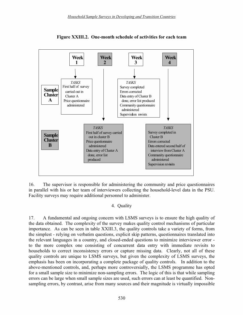
Household Sample Surveys in Developing and Transition Countries
530
Figure XXIII.2. One-month schedule of activities for each team
16. The supervisor is responsible for administering the community and price questionnaires in parallel with his or her team of interviewers collecting the household-level data in the PSU. Facility surveys may require additional personnel to administer.
4. Quality 17. A fundamental and ongoing concern with LSMS surveys is to ensure the high quality of the data obtained. The complexity of the survey makes quality control mechanisms of particular importance. As can be seen in table XXIII.3, the quality controls take a variety of forms, from the simplest - relying on verbatim questions, explicit skip patterns, questionnaires translated into the relevant languages in a country, and closed-ended questions to minimize interviewer error - to the more complex one consisting of concurrent data entry with immediate revisits to households to correct inconsistency errors or capture missing data. Clearly, not all of these quality controls are unique to LSMS surveys, but given the complexity of LSMS surveys, the emphasis has been on incorporating a complete package of quality controls. In addition to the above-mentioned controls, and, perhaps more controversially, the LSMS programme has opted for a small sample size to minimize non-sampling errors. The logic of this is that while sampling errors can be large when small sample sizes are used, such errors can at least be quantified. Non-sampling errors, by contrast, arise from many sources and their magnitude is virtually impossible
Sample Cluster A
TASKS First half of survey carried out in Cluster A Price questionnaire administered
Sample Cluster B
TASKS First half of survey carried o ut in cluster B Price questionnaire administered Data entry of Cluster A done, error list produced
TASKS Survey completed Errors corrected Data entry of Cluster B done, error list produced Community questionnaire administered SupervisiIon revists-
TASKS Survey completed in Cluster B Errors corrected Data entered second half of interview from Cluster A Community questionnaire administered Supervision revisits v
Week 1
Week 2
Week 3
Week 4

Household Sample Surveys in Developing and Transition Countries
531
to measure; it is well-known, however, that the totality of non-sampling error tends to increase as sample size increases. Thus, the decision was made to limit these non-sampling errors even if this would restrict the level of geographical disaggregation possible with the survey data. The emphasis in LSMS surveys on exploring the relationships among aspects of living standards, as opposed to measuring with great precision specific indicators or rates, means that this decision is less of a hindrance than it might be in other surveys.58 Finally, recent methods to link LSMS survey data (and others) to census data that allow an imputation of poverty within the census data, serves to reduce, to some extent, the small sample size issue, at least in terms of poverty and inequality measures.59
Table XXIII.3. Quality controls in LSMS surveys Area of quality control Controls Questionnaire Verbatim questions Explicit skip patterns Minimal use of open-ended questions Written translation into relevant languages a/ Sensitive topics placed at end Packaging: one form for all household and individual data
Pilot phase Formal pilot test of questionnaire and fieldwork
Direct informants Individuals and best informed
Concurrent data entry Check for range, consistency errors Revisits to households to make corrections
Two-round format Reduces fatigue Creates bounded recall period Allows for checking of data entry and correction with households
Training Intensive training of interviewers (one month), supervisors and
data entry staff
Decentralized fieldwork Mobile teams made up of supervisor, from two to three interviewers and data entry operator with computer and printer, and driver with car
Supervision One supervisor per two to three interviewers
Small sample size Limit non-sampling error
Data access policy Open use of data to all researchers and institutions
a/ In countries where some languages do not have a written form (indigenous languages in Panama, for example), bilingual interviewers are used instead. This is not a perfect solution and should be avoided unless absolutely necessary.
58 A labour-force survey, for example, which is supposed to show very small changes in unemployment rates over time, will require a much larger sample than that needed to analyse the determinants of unemployment, which would be more the focus of analysis of the LSMS survey. 59 See sect. E below on the uses of LSMS data for more on this technique.

Household Sample Surveys in Developing and Transition Countries
532
18. Another quality control mechanism incorporated by the LSMS surveys is the use of direct informants, also called self-respondents. This has two key advantages. It reduces the burden on any given respondent and thus lessens respondent fatigue. The household questionnaire is actually a series of short (10-15 minute) individual interviews, with only the best-informed respondents for consumption, agriculture and household businesses facing longer interview periods.60 The use of direct informants also improves the quality of the data obtained by ensuring that the most knowledgeable person is answering the questions.61 It is unreasonable to expect that any person in the household can give accurate and complete data on the health, education, labour, migration, credit and fertility status or activities of all other household members -- it is simply too much information. In addition, there may be incentives within a household to keep some information from other household members (credit, savings, earnings, and contraceptive use are all activities about which information might not be shared). Using direct informants is thus the only way to ensure accurate information on each household member. Interviewers are trained to, as far as possible, conduct the individual interviews in private. 19. Training of all staff involved in each LSMS survey is a further quality control mechanism. This takes the form of �on-the-job� training for the staff of the NSO, as well as more formal courses as needed. For the field staff, interviewers, supervisors and data entry operators, substantial resources are invested in formal training. Typically, the training for field staff is four weeks long and incorporates both theory and practical exercises. Upon completion of the training, field staff are selected based on their having passed the training course. A satisfactory result is usually based on a combination of successful participation during the course and the passing of a formal test at the end. 20. A final method to improve data quality that is often missed is promoting open access to the microdata resulting from the survey. Ensuring the widespread use of the data sets by a range of researchers and policy makers leads to careful checking of existing data; and by creating a feedback loop to data producers, this serves to increase the quality of future surveys. Open data access agreements have been reached for most LSMS survey data sets and efforts are made to help Governments disseminate such data. Although the World Bank does not own the LSMS survey data sets, permission has been given to the World Bank to directly disseminate over half of them (in fact, 30 per cent of all data sets can be downloaded directly from the LSMS web site).62 Of the remaining data sets, the majority can be distributed once the Government approves the individual request. Feedback from those who have requested this type of permission indicate that permission is granted in about 90 per cent of the cases.
60 Even for the �best informed� respondents, the actual interview time is kept to under one hour, as this is considered the maximum time during which one person should be interviewed. For some specific households, however, this time limit may be exceeded and care needs to be taken to avoid informant fatigue and the resulting decrease in data quality associated with it. 61 In the case of children under age 10 or age 12, or of household members unable to communicate, proxy respondents may be used. When proxy respondents are used, the identification code of the actual respondent is noted. 62 http://www.worldbank.org/lsms/.

Household Sample Surveys in Developing and Transition Countries
533
5. Data entry 21. Concurrent data entry entails using sophisticated data entry software that checks for range errors, inter- and intra-record inconsistencies and, when possible, even checking data against external reference tables (for example, those providing anthropometrics, crop yield data and prices). Data are entered in the field on laptop computers during the data-collection phase, and data entry operators are an integral part of the mobile survey teams. Data are entered immediately after each interview has been conducted and a list of errors, inconsistencies and missing information is produced from the data entry process. The interviewer then returns to the household to clarify, with the household members, any problems and to complete any missing information. This method avoids lengthy batch cleaning of data after the survey has terminated. Such cleaning is best avoided: although it tends to create internally consistent data sets, these are not the ones that best reflect each individual�s situation. It also requires substantial time, thus delaying the use of the data and, in the worst case, rendering some of them obsolete. With the advent of inexpensive, yet powerful, computers and new software developments, it is likely that some LSMS surveys will be carried out completely electronically using the computer-assisted personal interview (CAPI) methods. This is an avenue that is presently being explored given its potential for decreasing the time between fieldwork and publication as well for higher data quality.63
6. Sustainability 22. At the simplest level, the three greatest impediments to sustainability, to the long-term implementation of LSMS surveys and to the use of the resulting data in policy-making, are budget constraints, staff turnover and a lack of analytic capacity. While no blueprint for ensuring sustainability exists, experience with the LSMS has provided several pointers on how to increase the likelihood of achieving sustainability. The first highlights the importance of involving policy makers and data users in the design and analysis phase. This essentially begins the process of creating a demand for the LSMS results and the use of the data in policy decisions. As it is these end-users who benefit from the data (not the NSO per se), this is the group that has the most incentive to ensure that budget needs for future surveys are met during the budget allocation process within the government. Often, creating or identifying one or more �champions� of the survey and data outside of the statistical system is key to sustainability.64 23. The second key lesson is that achieving sustainability is a long-term process: investing in one-off surveys has little long-term impact. A more systematic effort over several years is needed to train a critical mass of staff, demonstrate the effectiveness and use of the instruments, create the linkages between producers and users, and adapt the methodology to a country�s needs and skills. Additionally, investment in proper documentation of survey efforts, archiving of data and dissemination activities help to ensure that institutional memory does not leave with any
63 The use of CAPI systems is one factor in the ability of the United States Bureau of the Census to publish results of its monthly labour-force survey (Current Population Survey) within 10 days of fieldwork. An experiment to compare the costs and benefits of CAPI with concurrent data entry for LSMS surveys is planned for Albania in 2003. 64 Jamaica offers one example of this approach. Demand originally came from the Prime Minister�s office and the Ministry of Planning has been involved in every stage of the survey design and use with the Statistical Office implementing the survey. The LSMS has been carried out annually since the late 1980s in Jamaica. See Grosh (1991) for more on this example.

Household Sample Surveys in Developing and Transition Countries
534
particular staff member. Close to 40 per cent of the countries that have conducted one LSMS survey have conducted multiple surveys. 24. Finally, building analytic capacity needs to be an explicit goal.65 This increases the use of data, thus helping to create demand for future data sets. In addition, increasing the skills of the NSO staff and, thus the NSO�s profile within government, may entice staff to stay on.66 Finally, outside forces may also help to increase the demand for data. The Poverty Reduction Strategies being designed by countries receiving concessionary lending from the World Bank and the International Monetary Fund (IMF), and the Millennium Development Goals, all require data on the measurement and monitoring of poverty and key social indicators. The long-term nature of such goals can help to foster monitoring and evaluation systems that rely heavily on household surveys such as the LSMS surveys along with administrative and project data.67 A recent evaluation of the Inter-American Development Bank-World Bank-Economic Commission for Latin America and the Caribbean (ECLAC) project to improve household surveys68 underlines the long-term nature of sustainability and raises the additional issue of transition from donor financing to local financing that must also be addressed.69
D. Costs of undertaking an LSMS survey 25. The attention to quality has serious implications for the costs, in both time and resources, of the surveys fielded. LSMS survey costs range from US$ 400,000 to US$ 1.5 million, depending on the country and the year. On a per-household basis, this is commensurate with other complex surveys such as Income and Expenditure Surveys and Demographic and Health Surveys. Costs, of course, vary based on the capacity of the NSO, the state of existing statistical infrastructure, the goals of the survey, and the difficulty of movement within the country. Costs are substantially lower in cases where the implementing agency already has good infrastructure and experienced staff. Funds for each survey typically come from a variety of sources: government budgets (for the NSO or from other agencies), bilateral donations and multilateral donations and credits. In some cases, the private sector has also funded part of the survey costs.70
65 A summary of lessons learned in LSMS surveys in terms of building analytic capacity can be found in Blank and Grosh (1999). 66 There is always a concern about maintaining the separation of data collectors from data analysts. Issues of credibility must be kept in mind when the barrier is relaxed. 67 The creation of the Partnership in Statistics for Development in the Twenty-first Century (PARIS21) initiative to support the improvement of data for such purposes underlines the importance of sustainable data collection, analysis and use. 68 The Inter-American Development Bank-World Bank-ECLAC project is entitled �Improving Surveys of Living Conditions�, but is more commonly known by its Spanish acronym: MECOVI. 69 See Ryten (2000). 70 For example, in Peru, a limited amount of space on the questionnaire is reserved for private firms or researchers who pay to have specific questions added to the questionnaire in any given quarter.

Household Sample Surveys in Developing and Transition Countries
535
26. In general, the cost of an LSMS survey reflects the methods adopted, the size of the sample, and the complexity of the fieldwork. Figure XXIII.3 shows the cost components of an LSMS survey and each one�s relative weight.71 (A simple exercise to help the reader start a budget for an LSMS survey can be found in annex II.)
Figure XXIII.3. Cost components of an LSMS survey (share of total cost)
Source: Based on Grosh and Muñoz (1996), table 8.2 27. The largest component of costs is for salaries. Almost three quarters of this cost is for field staff: interviewers, supervisors, data entry operators, anthropometrists and drivers. The field staff for LSMS surveys is large (relative to the sample size) owing to the high supervisor-to-interviewer ratios (typically 1 to 3), the size of the questionnaire and the use of direct informants which limits the number of households that can be visited per day, the inclusion of data entry in the field teams, and the provision of transport to each team member to ensure the mobility and integrity of the team by providing each with transport. Other salaries are for office staff: typically these are staff of the NSO, although a project coordinator may be contracted from outside if needed. 28. The second largest cost component is for materials and equipment. This covers computers and vehicles (either purchase or rental), and maintenance, as well as other office equipment. This is the component that varies the most widely based on existing infrastructure in the NSO or implementing agency. Also, funding sources can increase costs if vehicle purchases are prohibited: renting the needed vehicles can sometimes be significantly more expensive.
71 The present section on costs is based on Grosh and Muñoz (1996) and a presentation of Juan Muñoz at the World Bank course on poverty and inequality, 26-28 February 2002.
Base salaries 28 per cent
Per diems and travel costs
9 per cent Materials
23 per cent
Consultancy fees and travel 18 per cent
Other 11 per cent
Contingency 10 per cent
Printing & copying
1 per cent

Household Sample Surveys in Developing and Transition Countries
536
29. Technical assistance is the third major component of costs. Again, this will vary substantially depending on the existing skills and experience in the implementing agency. Countries carrying out second or third LSMS surveys obviously require much less technical assistance and equipment. Typically, the types of skills most needed from technical assistance are sampling, questionnaire design, data entry customization, fieldwork organization and analytic techniques. 30. The costs of an LSMS survey are, of course, justified if the result truly is better-quality data that may be used to improve policy. While costly in absolute terms, relative to the magnitude of spending on social policy, LSMS surveys are not expensive. The following section provides evidence from recent LSMS surveys for the quality of LSMS survey data. Examples of quality are given in terms of missing data, usefulness of data for LSMS purposes, internal consistency and design effects.
E. How effective has the LSMS design been on quality?
1. Response rates 31. A first measure of quality is the overall response rate to the survey: do households selected in the sample respond to the survey or are a substantial number not included, thus potentially biasing the final results?72 Examining response rates is useful, as these are an indicator of the quality of training, questionnaire design and interviewers as well as of the sample selection procedures (enumeration, updating of maps and the like). Many countries� LSMS surveys have achieved remarkably high response rates. Table XXIII.4 shows the response rates from recently completed LSMS surveys. However, LSMS surveys are not immune to the impact of country-specific situations. In post-conflict countries, where the expected levels of trust are low, response rates have also been lower as witnessed by the LSMS surveys in Bosnia and Herzegovina and Kosovo. The lower response rates in Jamaica, however, perhaps better illustrate the power of the quality control mechanisms. Jamaica has used fewer of the standard LSMS field techniques and quality control measures: this does appear to have translated into lower response rates.73 In Guatemala, the low response rate was probably due to the length of time between the date of completion of the listing of households and the dates during which the survey was in the field. For the later interviews, this period was nine to ten months.
72 Participation rates refer to the household as a whole, and not to individual members of that household. 73 See World Bank (2001) for more details on the fieldwork of the Jamaica Survey of Living Conditions.

Household Sample Surveys in Developing and Transition Countries
537
Table XXIII.4. Response rates in recent LSMS surveys
Country
Year
Number of
selected dwellings
Actual sample
size
Response rate a/
(percentage)
Bosnia and Herzegovina 2001 5 400 5 402 82.6
Ghana b/ 1998-1999 6 000 5 998 97.4
Guatemala 2000 8 940 7 468 83.5
Jamaica 1999 2 540 1 879 74.0
Kosovo 2000 2 880 2 880 82.0
Kyrgyzstan 1998 2 987 2 979 99.7
Nicaragua 1998-1999 4 370 4 209 96.3
Tajikistan 1999 2 000 2 000 ..
Viet Nam 1997/98 5 994 5 999 93.9
a/ Bosnia and Herzegovina, Ghana, Kosovo, Tajikistan and Viet Nam used replacement households. Response rate was based on completed interviews minus replacement households divided by planned sample size. In Bosnia and Herzegovina, 938 replacement households were used; in Ghana, 155; in Kosovo, 519; and in Vietnam, 372. The authors were unable to determine the number of replacement households in Tajikistan. b/ The Ghana survey was conducted in seven visits to each household. The final sample size figure is the number of households that participated in all seven visits. Note: Two dots (..) indicate data not available.
2. Item non-response
32. Calculating the percentage of item non-response is another indicator of quality. A review of this issue in the three earliest LSMS surveys showed item non-response to have been fairly insignificant (less than 1 per cent of responses were missing for 10 key variables).74 It is also of interest to compare rates of item non-response in LSMS surveys with those obtained in other surveys that do not have the same quality control mechanisms. This is not always possible; however, one small comparison is given here. A 1998 review of labour-force surveys in Latin America compiled information on the frequency of missing values for labour income of salaried workers, self-employed individuals and employers.75 Three of the countries cited also carried out LSMS surveys within a year of the labour-force surveys. As can be seen in table XXIII.5, in these countries, the LSMS surveys did substantially better than -- or at least as -- well as labour- force surveys, for most of the comparisons. While only a limited example, this appears to demonstrate the positive effect of the LSMS investment in quality controls.
74 In Grosh and Glewwe (1995). 75 In Feres (1998). While income is not the focus of either labour-force surveys or the LSMS surveys, income information is collected in similar fashions in the two types of surveys.

Household Sample Surveys in Developing and Transition Countries
538
Table XXIII.5. Frequency of missing income data in LSMS and LFS
Country Survey Percentage of missing income data for Salaried
workers Self-
employed
Employers
Percentage of
direct informants Ecuador LFS, 1997 6.3 6.7 13.2 .. LSMS, 1998 3.6 8.5 6.5 96.5 Nicaragua Urban LFS, 1997 1.0 1.4 5.7 .. LSMS, 1998 1.1 1.0 4.7 84.6 Panama LFS 1997 2.9 36.2 26.0 .. LSMS, 1996 1.0 3.5 8.4 98.7
Source: The information on Labour-force Surveys (LFS) is from Feres (1998); for the LSMS surveys, calculations by authors. Note: For Nicaragua, in the 1998 LSMS survey, the percentage of missing data did not include zeros, as the interviewer instructions had interviewers coding a zero response here if the person received income not in cash but in kind. In this category were subsistence farmers whose income was calculated elsewhere in the module in agricultural production.
Two dots (..) indicate data not available. 33. Instead of just toting up the number of missing responses, perhaps a better overall test of the quality of the data is the extent to which it can be used. For LSMS surveys, which have a main goal of measuring welfare, it is most relevant to determine the extent to which the collected data are adequate for this purpose. The most commonly used money-metric measure of welfare, for its theoretical and practical advantages, is total household consumption. This is a complex measure that requires data from a range of modules in the questionnaire: at both the individual and household levels. Typically, consumption data are taken from the housing module (use value of housing, utilities and other housing expenditures), the durable goods module (to calculate the value of the flow of services), the education module (private, out-of-pocket expenditures), the food consumption module (purchased, home-produced and gift foods), the agricultural module (for home-produced food consumed by household if not captured in the food consumption module) and the non-food expenditure modules (for items ranging from soap to household furnishings). 34. Table XXIII.6 shows the percentage of households for which it was possible to construct such a consumption aggregate. For most of the surveys, very few households had to be dropped from the analysis owing to lack of data. The exception is Ghana. It is not clear what the main problem was in the case of Ghana, 1998: the sample was a bit larger than others but not as dramatically so as in the Guatemala case. The fact that some food consumption data were collected via a diary (as opposed to use of the standard LSMS methodology) may have been a factor: unfortunately, the documentation on the survey does not address this issue.76
76 See Ghana Statistical Service (2000).

Household Sample Surveys in Developing and Transition Countries
539
Table XXIII.6. Households with complete consumption aggregates: examples from recent LSMS surveys
Households with complete
consumption aggregate Country
Year
Final sample
size (percentage) Bosnia and Herzegovina 2001 5 402 99.9
Ghana 1998-1999 5 998 87.7
Guatemala 2000 7 468 97.4
Jamaica 1999 1 879 99.8
Kosovo 2000 2 880 100.0
Kyrgyzstan 1998 2 979 99.4
Nicaragua 1998-1999 4 209 96.0
Tajikistan 1999 2 000 100.0
Viet Nam 1997-1998 5 999 100.0
3. Internal consistency checks
35. Ensuring the internal consistency of the data is also crucially important. The fact that the complexity of the survey instruments makes it difficult for interviewers to monitor this during the interview process, explains why so many of the quality controls address consistency issues. Three examples of internal consistency checks are shown in table XXIII.7. The first check determines how well the community questionnaire could be to be linked to the household data. The second check shows the percentage of children of pre-school or school age, as identified in the roster, that have complete information on their schooling/pre-schooling. The third check determines whether those identified as self-employed in the labour-force module have reported details of their activities in the non-agricultural household business module.

Household Sample Surveys in Developing and Transition Countries
540
Table XXIII.7. Internal consistency of the data: successful linkages between modules (Percentage) a/
Correct link between: Country
Household survey
and community survey a/
Roster and education
module b/
Employment module and non-agricultural household business
module c/ Pre-
school Primary
Bosnia and Herzegovina ... 99.5 99.8 90.4
Ghana 99.9 .. 96.5 70.2
Guatemala 100 100 100 93.0
Jamaica .. .. 96.4 ..
Kosovo 100 .. 100 58.6
Kyrgyzstan 100 86.5 98.4 93.1
Nicaragua .. 97.9 97.5 62.0
Tajikistan 100 .. 99.9 ..
Viet Nam 100 .. 99.6 98.1
Notes: Table refers to percentage of correct linkages. Bosnia and Herzegovina, Jamaica and Tajikistan did not include community questionnaires. Jamaica, Kosovo, Tajikistan and Viet Nam did not include a special module on pre-school. Jamaica and Tajikistan did not collect information on non-agricultural household businesses. Two dots (..) indicate data not available. a/ Comparison of the households with the communities in which they were located. b/ Comparison of the age variable from the roster with the presence of individuals in the education module. c/ Comparison of those indicating they were self-employed in the employment module with the presence of information in the non-agricultural household business module.
36. As can be seen from the table, the first two checks show data quality to have been quite high. The third check does, however, show problems. This indicates a lack of appropriate controls in the field between the two visits to the households. Only in the case of Viet Nam was an explicit question included for the interviewer in the second visit to ensure that this module would be completed. Clearly, a similar check is needed for all surveys.
4. Sample design effects
37. A final criterion for judging LSMS surveys concerns the sample size and design. When using data from any household survey based on a complex design with multiple stages, stratification and clustering, the true variance of the estimates is calculated by taking into account these features of the sample design as well as weighting. The design effect is the ratio of the true variance of an estimate, taking into account the multistage sample, to the variance of the

Household Sample Surveys in Developing and Transition Countries
541
estimate that would have been obtained if a simple random sample of the same size had been used.77 Thus, a design effect of 1 indicates that there has been no loss in precision in the sample estimates owing to use of a multistage design, while a design effect greater than 1 shows that use of the multistage design has lowered the efficiency of the sample and the precision of the estimates. 38. As part of the LSMS activities, a review of the design effects on key variables and indicators was carried out on some of the earlier LSMS surveys. The review, conducted by Temesgen and Morganstein (2000), highlighted several key points that must be taken into account when using LSMS survey data (and data from other households surveys using multistage sample designs of course) and designing appropriate samples.78 The main point was that the multi-topic nature of the LSMS surveys complicates the process of designing an efficient sample. Design effects vary widely among both individual-level and household-level variables, as can be seen in table XXIII.8, taken from the work of Temesgen and Morganstein (2000). In short, minimizing the design effect of one variable may well lead to increasing it for other variables. Second, the trade-off between non-sampling and sampling errors is clear. Design effects can be high in LSMS surveys. The table indicates that, to the extent that LSMS surveys are used to produce means, ratios and point estimates, it is critically important that the sample design be taken into account and that careful attention be paid to the proper use of the data.
Table XXIII.8. Examples of design effects in LSMS surveys Country Per capita consumption Access to health care Unemployment rate All Rural Urban All Rural Urban All Rural Urban Côte d-Ivoire, 1988
6.7
3.6
5.5
6.3
5.7
2.2
7.0
4.4
5.7
Ghana, 1987 1.9 3.1 1.8 2.9 3.0 5.0 1.7 1.5 2.0
Ghana, 1988 3.2 2.9 2.9 2.2 2.5 3.6 1.3 1.1 1.4
Pakistan, 1991 1.6 1.1 2.6 5.0 4.0 5.2 4.6 4.7 2.5
Source: Temesgen and Morganstein (2000). 39. As with other surveys, it is interesting to note that the design effect varies not just among variables, but also geographically within a country for the same variable and for a specific variable over time. Finally, the design effects can be hugely different between countries. A careful review of intra-class correlations and design effects in previous surveys, when these exist, will help in refining the design for future LSMS surveys. Care must be taken in presenting and interpreting the results of LSMS and other surveys using multistage samples because the sample design used can be complicated.
77 See annex III of this chap. or other chaps. in this publication for additional information on sample design issues. 78 Several of the tables from the report of Temesgen and Morganstein are included in annex III of this chapter.

Household Sample Surveys in Developing and Transition Countries
542
F. Uses of LSMS survey data 40. Over the years, LSMS survey data have been used for a wide variety of policy and research purposes. Some of these have been chronicled elsewhere79 and an extensive, albeit partial, bibliography of papers and reports based on LSMS survey data can be found by the interested reader on the LSMS web site. That bibliography shows the scope of the use of LSMS data for analytic purposes but the uses of the data are certainly not limited to what is found therein. The existence of ongoing research and questionnaire revisions and amendments mean that the range of uses is constantly changing. To demonstrate the variety of ways in which LSMS data have been used and combined with other data, it is perhaps more worthwhile to focus on one particular use � targeting of government programmes to the poor, for example � rather than to attempt a comprehensive examination of the uses of those data. 41. First, an early example from Jamaica shows how a simple analysis can provide a Government with clear information on the effects of targeting the poor using alternate programmes. In the Jamaica case, as outlined in Grosh (1991), three major nutrition programmes existed: generalized food subsidy, food stamps and school feeding programmes. The LSMS survey in Jamaica made it possible to quantify the value of the benefits received by poor households from the three programmes and showed that the food subsidy, unlike the other two programmes, was highly regressive. This analysis was one element in the decision to eliminate subsidies and to increase resources to the other two programmes. 42. A second tool that can be created using LSMS survey data is for geographical targeting to poor areas. By taking advantage of census data, the LSMS survey data can be used to construct poverty maps for allocating resources and programmes to poor areas.80 The method relies on the existence of an LSMS survey and census data within a few years of each other.81 The LSMS survey provides a solid welfare measure (total household consumption) but, owing to the small sample size, the ability to disaggregate the resulting poverty data is limited to only urban and rural areas, and a few large regional breakdowns of the country. Clearly, this does not meet all the needs of Governments trying to focus resources on poor areas nor does it help, in decentralized systems, in the allocation of resources to local government. Additionally, within large regions, there is often a great deal of heterogeneity in terms of poverty levels of the population that goes undetected in a small sample household survey. 43. To be able to provide poverty information at smaller levels of aggregation requires a data set with a sample size several orders of magnitude larger than that of an LSMS. The largest data set in any country is, of course, the population census. However, because it covers the whole population, a census collects very limited information from each household and is usually
79 See Grosh (1997), for example. 80 For more on the methodology of creating poverty maps using the welfare measure from surveys and linking to census data see: Hentschel and others (2000); Elbers, Lanjouw and Lanjouw (2002; 2003); Elbers and others (2001); and Demombynes and others (2001). Further work is being done on using this technique to link two surveys together; however, estimating correct standards errors from such a linkage is impossible. 81 Other household surveys can be used as long as they provide a robust money-metric measure of welfare such as total consumption or total income.
Household Sample Surveys in Developing and Transition Countries
543
conducted only once every 10 years. Thus, it is not possible to construct an adequate poverty measure from the census. An innovative vein of work that allows survey data and census data to be linked is being tested. This technique takes advantage of the LSMS-provided welfare measure and the census-provided coverage. The method entails estimating poverty in the LSMS survey data by using a vector of variables found in both the census and the survey. The parameters estimated from this are then used with the census data to predict the probability of being poor for each household and creating headcount ratios for small areas using the census data. The resulting poverty maps provide a tool for government in the allocation of resources. Examples of such poverty maps can be found in Ecuador, Guatemala, Madagascar, Nicaragua, Panama and South Africa. 44. A third example of the use of LSMS survey data for improving the targeting of social programmes is derived from an evaluation of the Emergency Social Investment Fund (or FISE, after its Spanish acronym) in Nicaragua. The evaluation addressed issues of targeting as well as the impact of the FISE investments in communities in the areas of water, latrines, education, health and sewerage. 82 In this case, a national-level LSMS survey was planned. An oversample of households was included consisting of households from FISE project areas as well as from similar communities without FISE programmes. The other source of data was project and administrative records that were used to evaluate the administrative costs of the project. 45. The oversample of households in FISE and similar non-FISE communities allowed the creation of both control and treatment groups to measure the impact of the FISE investments and the effectiveness of their targeting. In addition, the national sample from the LSMS survey was used to create a second control group (using propensity matching techniques) which increased the strength of scope of the evaluation. The evaluation of the effectiveness of targeting was carried out both at the community level (were FISE investments progressive in terms of the communities where projects were carried out?) and at the individual level (within communities with FISE projects, were the poorer segments of the population more or less likely to benefit from the FISE investment?). 46. The evaluation was able to show, with statistically significant results, the overall efficiency of targeting and allowed the main project types to be assessed based on targeting criteria. The study showed that sewerage projects were highly regressive, while latrines and primary education projects were systematically progressive, reaching the 17 per cent of the population classified as extremely poor. The immediate result of the evaluation was the suspension of sewerage projects and a decision to focus on improving the outreach to, and investments in, extremely poor communities. The cost of this very complex evaluation of the FISE project represented 1 per cent of the investments made by the project up to the date when the evaluation was done.
82 See World Bank (2000) for details on the goals of the evaluation, the methods employed and the results.

Household Sample Surveys in Developing and Transition Countries
544
G. Conclusions 47. The results of LSMS surveys have demonstrated the value of the approach. Data have been used by Governments to understand the effect of present policies, to redesign policies and to better target resources to groups and areas. The emphasis on quality has paid off in terms of lower levels of errors and greater usefulness of the data. There are, however, trade-offs involved with this approach. Costs are relatively high, the smaller sample size limits the level of disaggregation that can be obtained, and the upfront planning and design are time-consuming; however, data can be produced rapidly once work is begun and the links with policy makers increases the use of the data. 48. Clearly, there are advantages to incorporating LSMS surveys in a country�s system of household surveys. How often such a survey is needed will depend on several factors. First, the analytic needs of the country should drive the decision to carry out one or multiple surveys over time. While many government programmes can be evaluated with cross-sectional data (targeting, incidence, even impact using propensity matching score techniques), repeated cross-sections and panel data sets are needed for other types of analysis of changes over time and the impact of policies and events. 49. A second consideration, in terms of the frequency of implementing LSMS surveys, is that concerning the analytic capacity in the country. Data need to be analysed as an input to policy makers and in order that each future round of the survey may be improved based on the previous round�s findings. If the data cannot be analysed quickly, much of the investment in multiple rounds of the survey may be lost. In such a case, it may make sense to leave a significant time gap (three years, for example) between surveys. 50. Finally, budget and logistic issues are often as important as substantive ones in deciding how often or when to do specific surveys. Thus, the frequency with which any survey is conducted will reflect the act of balancing the importance of its results against those of other surveys. Also, it is important to remember that no one source of data is adequate for all needs. Administrative records, and project management information system (MIS) data, as well as a system of household surveys, are required by Governments for both macro and microeconomic policy. In conjunction with an overall system of surveys in a country, LSMS surveys can lead to a substantial improvement in the understanding of how a Government�s policy and spending affect the lives of its population.

Household Sample Surveys in Developing and Transition Countries
545
Annex I List of Living Standard Measurement Study surveys
Country
Year
Household count
Albania 1996 1 500 Albania 2002 3 600 Armenia 1996 4 920 Azerbaijan 1995 2 016 Bolivia 1999 ... Bolivia 2000 5 032 Bolivia 2001 .. Bosnia and Herzegovina 2001 5 402 Brazil 1996-1997 4 940 Bulgaria 1995 2 500 Bulgaria 1997 2 317 Bulgaria 2001 2 633 Cambodia 1997 6 010 China: Hebei and Liaoning 1995 and1997 780 Côte d'Ivoire 1985 1 588 Côte d'Ivoire 1986 1 600 Côte d'Ivoire 1987 1 600 Côte d'Ivoire 1988 1 600 Ecuador 1994 4 500 Ecuador 1995 5 500 Ecuador 1998 5 801 Ecuador 1998-1999 5 824 Gambia 1992 1 400 Ghana 1987-1988 3 200 Ghana 1988-1989 3 200 Ghana 1991-1992 4 565 Ghana 1998-1999 5 998 Guatemala 2000 7 276 Guinea 1994 4 705 Guyana 1992-1993 5 340 India: Uttar Pradesh and Bihar
1997-1998
2 250
Jamaica 1988-2000 (annual)
2 000-7 300
Kazakhstan 1996 1 996 Kosovo 2000 2 880 Kyrgyzstan 1993 2 000 Kyrgyzstan 1996 (spring) .. Kyrgyzstan 1996 (autumn) 1 951 Kyrgyzstan 1997 2 962 Kyrgyzstan 1998 2 979 Madagascar 1993 4 504 Malawi 1990 6 000 Mauritania 1987 1 600 Mauritania 1989 1 600

Household Sample Surveys in Developing and Transition Countries
546
Mauritania 1995 3 540 Morocco 1991 3 323 Morocco 1998 .. Nepal 1996 3 373 Nicaragua 1993 4 200 Nicaragua 1998-1999 4 209 Nicaragua 2001 4 290 Niger 1989 1 872 Niger 1992 2 070 Niger 1995 4 383 Pakistan 1991 4 800 Panama 1997 4 945 Papua New Guinea 1996 1 396 Paraguay 1997-1988 4 353 Paraguay 1999 5 101 Paraguay 2000-2001 8 131 Peru 1985 5 120 Peru (Lima only) 1990 1 500 Peru 1991 2 200 Peru 1994 3 500 Russian Federation a/ 1992 6 500 South Africa 1993 9 000 Tajikistan 1999 2 000 United Republic of Tanzania: Kagera
1991-1994
840
United Republic of Tanzania: national
1993
5 200
Tunisia 1995-1996 3 800 Uganda 1992 9 929 Viet Nam 1992-1993 4 800 Viet Nam 1997-1998 5 999 Note: Two dots (..) indicate data not available. a/ The 1992 Russian Longitudinal Monitoring Survey was conducted using World Bank financing. Subsequent surveys did not involve World Bank participation. For more information, see the Carolina Population Center web site: http: //www.cpc.unc.edu/projects/rlms/rlms_home.html.

Household Sample Surveys in Developing and Transition Countries
547
Annex II Budgeting an LSMS survey
As noted in the text of chapter XXIII, no two LSMS surveys are exactly alike, nor are
any two NSOs, or the costs associated with salaries, transportation, equipment, etc. in different countries. Thus, it is impossible to provide information on how much an LSMS survey will cost in a specific place at a specific time. The chapter provided an example of the share of different types of costs in the total cost of a survey. The following is a small exercise designed to help one get started on budgeting. It simply provides a quick guide to estimating the most basic salary costs for the fieldwork. Using this guide with real costs in the country of interest, one can obtain a very rough approximation of what an LSMS survey might cost.
On average, given the complexity of the survey instrument and the use of direct informants, an interviewer can complete two half-interviews per day (refer to figure XXIII.2 in the text on how the survey is implemented). In other words, he or she can complete one round of the survey in two households. If we assume a six-day workweek (whether the �day off� is taken every week or distributed in some other way per month), an interviewer can complete 24 households per month.
Let us assume that a sample of 4,000 households is needed. If each interviewer can complete 24 households per month, a total of 167 interviewer months are needed to carry out interviews of 4,000 households. If the fieldwork takes place over a 12-month period, then 14 interviewers are needed. For each pair of interviewers, one supervisor, one data entry person and a driver and car are needed. So the total fieldwork staff (not counting regional supervision by staff of the NSO) comprises:
14 interviewers 7 supervisors 7 data entry operators 7 drivers
If planners use the parameters set out below, then the salary costs of the fieldwork portion
of the survey will be: Item Cost per individual per month Number of
months Cost
14 interviewers 500 13 91 000 7 supervisors 575 13.5 54 338 7 data entry operators 525 14 51 450 7 drivers 300 13 27 300 Rough estimate of field salary costs
224 088
Note: While the fieldwork takes only 12 months, an extra month is added to cover cost of the training (where field staff are usually paid something) and/or any delays in the survey work. Data entry operators are often kept on an extra month to finalize and clean the data set if needed.

Household Sample Surveys in Developing and Transition Countries
548
According to figure XXIII.3, fieldwork staff costs, which represent three quarters of the total salary costs of the survey, in turn represent 28 per cent of the survey costs. Based on a simple calculation, in this case, a rough estimate of the cost of the survey is found to be 1,067,086.
Clearly this number is only a very rough approximation. Details on other costs such as those for technical assistance and so on are needed. However, this simple starting exercise can be useful in beginning the process of budgeting an actual survey. The reader is referred to chapter 8 of Grosh and Muñoz (1996) for a detailed presentation on how to design a realistic budget for an LSMS survey.

Household Sample Surveys in Developing and Transition Countries
549
Annex III
Effect of sample design on precision and efficiency in LSMS surveys83
A. Introduction
Other chapters in this publication provide detailed information on sampling issues and, particularly, the effect of complex or multistage sample designs on the variance of the estimates obtained. This so-called design effect is common to all surveys that do not use a simple random sample, such as the LSMS surveys. The design effect is one part of overall sampling error: the difference between an estimate obtained from a multistage cluster design and one that would be obtained using a simple, random sample design. In the present annex, we summarize the key issues and show the actual impact of sample design on several LSMS surveys.
B. Computation of sampling errors, design effects and related components
In a simple random sample, all sampled units have an identical and independent
probability of selection. Simple random sampling is almost never used for household surveys, however, owing to logistic and cost concerns. Instead, as in the LSMS surveys, more complex, multistage sample designs are used that incorporate stratification and clustering. This affects the calculation of the variance of the estimates and the efficiency of the sample itself. To compute sampling errors for sample designs that are implemented in more than one stage, it is necessary to know the variables that identify the strata, the primary sampling units (PSUs) and the weighting procedures (if any) used in the design. Once these variables are identified, a number of statistical packages can be used to compute the needed measures.84
The sampling error measures reported here for selected household- and individual-level variables in LSMS surveys include the standard error (SE) which is computed by taking into account the complexity of the sample design, the coefficient of variation (CV (%)), the sample size (n), the design effect, the intra-class correlation coefficient (ρ), the lower and upper boundaries of the confidence intervals (CI), and the effective sample size (EFFn). These terms are all defined in chapters II, VI, VII and other chapters.
83 The present annex draws heavily on previous work by Temesgen and Morganstein (2000). 84 The statistical software WESVAR was used in the computations here. Some of the other programs that can be used to estimate sampling variances and a variety of related statistics for complex survey designs include: CENVAR, CLUSTERS, Epi-Info, PC CARP, SUDAAN, VPLX and STATA. Some of these software packages can be downloaded from the WorldWide Web for free.

Household Sample Surveys in Developing and Transition Countries
550
C. Standard errors, design effects and intra-class correlation computed from LSMS
surveys
One important aspect of calculating sampling errors for survey variables involves comparing the efficiencies (precision) of the sample designs with each other; and with the precision that would have been yielded by a hypothetical simple random sample of the same size. In addition to indicating the reliability of existing survey data, such an exercise can be equally important in helping analysts to evaluate how well a particular design has performed and in providing information for the design of future surveys The three tables set out below compare the design effects and related measures for several variables in order to show the differences that exist (a) within a country across different variables; (b) within a country over time; and (c) between countries.85
As shown in table AIII.1, within a country, the same survey will generate substantially different design effects for different variables. The table is based on data from the 1987 LSMS conducted in Ghana and variables constructed at the household and individual levels. As can be seen, for some variables, such as per capita total expenditure, where the intra-class correlation is low, the design effect is not high (1.9); but for variables such as access to sanitation and water, where intra-class correlations are high (infrastructure tends to be concentrated in specific spatial areas), the design effects are high (7.8 and 8.0, respectively), and are even higher for urban or rural subpopulations.
85 For the full report, see Temesgen and Morganstein (2000).
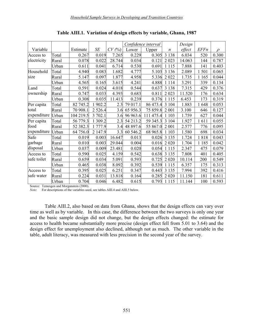
Household Sample Surveys in Developing and Transition Countries
551
Table AIII.1. Variation of design effects by variable, Ghana, 1987
Confidence intervalVariable Estimate SE CV (%) Lower Upper n
Design effect EFFn ρ
Total 0.267 0.019 7.265 0.229 0.305 3 138 6.034 520 0.300Rural 0.078 0.022 28.744 0.034 0.121 2 023 14.063 144 0.787
Access to electricity Urban 0.611 0.041 6.714 0.530 0.691 1 115 7.888 141 0.403
Total 4.940 0.083 1.682 4.777 5.103 3 136 2.089 1 501 0.065Rural 5.147 0.097 1.877 4.958 5.336 2 022 1.735 1 165 0.044
Household size
Urban 4.565 0.165 3.615 4.241 4.888 1 114 3.291 339 0.134Total 0.591 0.024 4.018 0.544 0.637 3 138 7.315 429 0.376Rural 0.747 0.033 4.393 0.683 0.811 2 023 11.520 176 0.634
Land ownership
Urban 0.308 0.035 11.413 0.239 0.376 1 115 6.453 173 0.319Total 82 745.2 1 902.2 2.3 79 017.1 86 473.4 3 104 1.883 1 648 0.053Rural 70 908.1 2 526.4 3.6 65 956.3 75 859.8 2 001 3.100 646 0.127
Per capita total expenditure Urban 104 219.5 3 702.1 3.6 96 963.6 111 475.4 1 103 1.759 627 0.044
Total 56 779.3 1 309.2 2.3 54 213.2 59 345.3 3 104 1.927 1 611 0.055Rural 52 382.3 1 777.9 3.4 48 897.6 55 867.0 2 001 2.577 776 0.095
Per capita food expenditure Urban 64 756.0 2 147.9 3.3 60 546.2 68 965.8 1 103 1.580 698 0.034
Total 0.019 0.003 16.647 0.013 0.026 3 135 1.724 1 818 0.043Rural 0.010 0.003 29.044 0.004 0.016 2 020 1.704 1 185 0.042
Safe garbage disposal Urban 0.037 0.009 23.481 0.020 0.054 1 115 2.347 475 0.079
Total 0.590 0.025 4.159 0.542 0.638 3 135 7.808 401 0.405Rural 0.659 0.034 5.091 0.593 0.725 2 020 10.114 200 0.549
Access to safe toilet
Urban 0.465 0.038 8.092 0.392 0.539 1 115 6.357 175 0.313Total 0.395 0.025 6.251 0.347 0.443 3 135 7.994 392 0.416Rural 0.224 0.031 13.818 0.164 0.285 2 020 11.150 181 0.611
Access to safe water
Urban 0.704 0.046 6.482 0.615 0.793 1 115 11.144 100 0.593Source: Temesgen and Morganstein (2000). Note: For descriptions of the variables used, see tables AIII.4 and AIII.5 below.
Table AIII.2, also based on data from Ghana, shows that the design effects can vary over
time as well as by variable. In this case, the difference between the two surveys is only one year and the basic sample design did not change, but the design effects changed: the estimate for access to health became substantially more precise (design effect fell from 5.01 to 3.64) and the design effect for unemployment also declined, although not as much. The other variable in the table, adult literacy, was measured with less precision in the second year of the survey.

Household Sample Surveys in Developing and Transition Countries
552
Table AIII.2. Variation in design effects over time, Ghana, 1987 and 1988
Ghana, 1987
Confidence interval
Variable Estimate SE CV (%) Lower Upper n Design effect EFFn ρ
Female 0.402 0.021 5.103 0.362 0.442 1 339 2.342 572 0.080 Male 0.613 0.018 2.953 0.578 0.649 1 381 1.910 723 0.054
Adult literacy
Total 0.509 0.016 3.192 0.477 0.541 2 720 2.875 946 0.112 Female 0.443 0.016 3.625 0.411 0.474 2 756 2.876 958 0.112 Male 0.423 0.017 4.017 0.390 0.457 2 542 3.011 844 0.120
Access to health services
Total 0.433 0.015 3.517 0.403 0.463 5 298 5.013 1 057 0.239 Female 0.039 0.004 10.063 0.031 0.047 4 011 1.655 2 424 0.039 Male 0.047 0.004 9.136 0.038 0.055 3 543 1.454 2 437 0.027
Unemployment
Total 0.043 0.003 7.666 0.036 0.049 7 554 1.983 3 810 0.059
Ghana, 1988
Confidence interval
Variable Estimate SE CV (%) Lower Upper n Design effect EFFn ρ
Female 0.390 0.022 5.526 0.348 0.432 1 289 2.519 512 0.090 Male 0.587 0.020 3.397 0.548 0.626 1 226 2.013 609 0.060
Adult literacy
Total 0.486 0.018 3.654 0.451 0.521 2 515 3.179 791 0.130 Female 0.375 0.013 3.558 0.348 0.401 2 921 2.215 1 319 0.072 Male 0.365 0.015 4.118 0.335 0.394 2 606 2.539 1 026 0.092
Access to health services
Total 0.370 0.012 3.346 0.346 0.394 5 527 3.635 1 521 0.157 Female 0.036 0.003 9.593 0.029 0.042 3 852 1.307 2 946 0.018 Male 0.034 0.003 9.885 0.027 0.041 3 260 1.123 2 904 0.007
Unemployment
Total 0.035 0.003 7.306 0.030 0.040 7 112 1.372 5 185 0.022 Source: Temesgen and Morganstein (2000). Note: For descriptions of the variables used, see tables AIII.4 and AIII.5 below.

Household Sample Surveys in Developing and Transition Countries
553
Finally, as expected, design effects across countries can vary significantly. Table AIII.3 shows how surveys in Côte d�Ivoire and Pakistan produced quite different design effects for the same variables. This result was a function both of the differing sample designs used in the countries and of the different characteristics of these countries.
Table AIII.3. Variation in design effects across countries
Côte d�Ivoire, 1988 Confidence interval
Variable Estimate SE CV ( %) Lower Upper n Design effect EFFn ρ
Total 0.567 0.031 5.538 0.506 0.629 1 660 6.676 249 0.378Rural 0.411 0.042 10.212 0.329 0.493 745 5.415 138 0.294
Adult literacy
Urban 0.738 0.024 3.217 0.691 0.784 915 2.661 344 0.111Total 0.417 0.029 6.883 0.361 0.473 1 849 6.260 295 0.351Rural 0.303 0.034 11.174 0.236 0.369 1 051 5.693 185 0.313
Access to health services
Urban 0.622 0.025 4.078 0.572 0.671 798 2.181 366 0.079Total 0.038 0.007 18.837 0.024 0.052 4 979 6.991 712 0.399Rural 0.007 0.003 50.457 0.000 0.013 2 529 4.357 580 0.224
Unemployment
Urban 0.081 0.013 16.218 0.055 0.107 2 450 5.679 431 0.312
Pakistan, 1991 Confidence interval
Variable Estimate SE CV ( %) Lower Upper n Design effect EFFn ρ
Total 0.5 0.013 2.5 0.48 0.53 6 834 4.335 1 577 0.222Rural 0.42 0.017 3.95 0.39 0.45 3 249 3.669 885 0.178
Adult literacy
Urban 0.68 0.018 2.616 0.64 0.71 3 585 5.156 695 0.277Total 0.5 0.012 2.329 0.48 0.52 9 238 5.02 1 840 0.268Rural 0.46 0.015 3.177 0.43 0.49 4 752 4.048 1 174 0.203
Access to health services
Urban 0.61 0.017 2.74 0.57 0.64 4 486 5.185 865 0.279Total 0.03 0.003 9.735 0.02 0.03 18 232 4.633 3 935 0.242Rural 0.02 0.003 14.955 0.02 0.03 8 934 4.706 1 898 0.247
Unemployment
Urban 0.03 0.003 8.956 0.03 0.04 9 298 2.539 3 662 0.103 Source: Temesgen and Morganstein (2000). Note: For descriptions of the variables used, see tables AIII.4 and AIII.5 below.
In summary, the small sample sizes used in LSMS surveys and the multistage nature of
the samples do involve a trade-off in terms of the precision of sample estimates. For example, the design effect value for �adult literacy� for all the individuals in the 1988 Côte d'Ivoire data is high at 6.7. This design effect signifies that the precision of the estimate with a sample size (n) of 1,660 is equivalent to that obtained using a SRS sample of only 249. If we consider the �urban� individuals only, however, we see that the design effect is a bit lower (2.7), although still higher than 1, meaning that a sample size of 915 persons has the precision equivalent to one of 344 persons using a SRS. The fact that the design effect can be quite large and the variation of

Household Sample Surveys in Developing and Transition Countries
554
such effects over variables, time and different countries makes it imperative that analysts recognize and take into account the sample design when using the data and especially when performing statistical tests of significance. This also highlights the difficulties in designing efficient samples for multi-topic household surveys. Trying to lower the design effect of one variable may very well result in a higher design effect for others. A rule of thumb here is to primarily consider the variable(s) of key importance to the survey, to the extent possible.
Table AIII.4. Description of analysis variables: individual level
Variable Description Population base Unemployment Adults currently unemployed but available for work and
looking for a job.
Persons aged 15-64 years
Access to health Services
Proportion of individuals who were sick during the month prior to the interview and who visited modern health facilities such as hospitals, clinics and health centres (but not midwives, faith healers, or other traditional medical practitioners).
Persons who were sick during the previous month
Adult literacy The proportion of adults who are literate (defined as those who could read a newspaper).
Persons aged 15-24 years
Table AIII.5. Description of analysis variables: household level Variable Description Access to safe water The proportion of households that have access to safe drinking water. At the
household level, this variable takes a value of one if the household obtains its drinking water from, for example, a tap, a pipe or a well with a pump. It takes a value of zero if the source of drinking water for the household -- such as a river, canal, open well, lake or marsh -- is considered potentially risky for health.
Land ownership The proportion of households that own land. For a household, this variable takes a value of one if the household owns land. Zero otherwise.
Access to electricity The proportion of households that have access to electricity. For a household, this variable takes a value of one if the household uses electricity for light and/or energy. Zero otherwise.

Household Sample Surveys in Developing and Transition Countries
555
References Blank, Lorraine,and Margaret Grosh (1999). Using household surveys to build analytic capacity.
The World Bank Research Observer, vol. 14, No. 2 (August), pp. 209-227. Demombynes, Gabriel, and others (2001). Producing an Improved Geographic Profile of
Poverty: Methodology and Evidence from Three Developing Countries. WIDER Discussion Paper, No.2002/39. Helsinki: World Institute for Development Economic Research/United Nations University.
Elbers, C., J. Lanjouw and P. Lanjouw (2002). Micro-level Estimation of Welfare. Policy
Research Working Paper, No. 2911. Washington, D.C.: World Bank. __________ (2003). Micro-level estimation of poverty and inequality. In Econometrica, vol.
71, No. 1, pp. 355-364. Elbers, C., and others (2001). Poverty and Inequality in Brazil: New Estimates from Combined
PPV-PNAD Data. Washington, D.C.: Development Economics Research Group, World Bank.
Feres, Juan Carlos (1998). Falta de respuesta a las preguntas sobre el ingreso: su magnitud y
efectos en las Encuestas de Hogares en América Latina. In Conference Proceedings from the 2o Taller Regional del Medición del Ingreso en las Encuestas de Hogares, Buenos Aires. November. Santiago de Chile: Comisión Económica para América Latina y el Caribe (CEPAL). Document LC/R.1886.
Ghana Statistical Service (2000). Ghana Living Standards Survey, Round Four (GLSS 4) 1998-
99: Data User�s Guide. Accra. Grosh, Margaret (1991). The Household Survey as a Tool for Policy Change: Lessons from the
Jamaican Survey of Living Conditions. Living Standards Measurement Study Working Papers, No. 80. Washington, D.C.:World Bank.
__________ (1997). The policymaking uses of multi-topic household survey data: a primer.
The World Bank Research Observer, vol. 12, No. 2, pp. 137-60. __________, and Paul Glewwe (1995). A Guide to Living Standards Measurement Study
Surveys and Their Data Sets. Living Standards Measurement Study Working Paper, No. 120. Washington, D.C.: World Bank.
_____, eds. (2000). Designing Household Survey Questionnaires for Developing Countries:
Lessons from 15 Years of the Living Standards Measurement Study Surveys. Washington, D.C.: World Bank.

Household Sample Surveys in Developing and Transition Countries
556
Grosh, Margaret and Juan Muñoz (1996). A Manual for Planning and Implementing the Living Standards Measurement Study Survey. Living Standards Measurement Study Working Paper, No.126. Washington, D.C.: World Bank.
J. Hentschel, and others (2000). Combining household data with census data to construct a
disaggregated poverty map: a case study of Ecuador. World Bank Economic Review, vol. 14, No. 1 (January).
Kish, Leslie (1965). Survey Sampling. New York: John Wiley and Sons, Inc. Pradhan, Menno, and Martin Ravallion (2000). Measuring poverty using qualitative perceptions
of consumption adequacy. Review of Economics and Statistics, vol. 82, pp. 462-471. Ravallion, Martin, and Michael Lokshin (2001). Identifying welfare effects using subjective
questions. Economica, vol. 68, pp. 335-357. __________ (2002). Self-rated economic welfare in Russia. European Economic Review, in
press. Ryten, Jacob (2000). The MECOVI Program: ideas for the future: a mid-term evaluation.
Unpublished paper prepared for Inter-American Development Bank. December. Skinner, C.J., D. Holt and T.M.F. Smith (1989). Analysis of Complex Surveys. Chichester,
United Kingdom: John Wiley and Sons. Temesgen, Tilahun, and David Morganstein (2000). Measurement of Sampling Errors:
Application to Selected Variables in LSMS Surveys. Washington, D.C.: Development Economics Research Group, World Bank.
World Bank (2000). Nicaragua: Ex-Post Impact Evaluation of the Emergency Social
Investment Fund (FISE). Report No. 20400-NI. Washington, D.C. __________ (2001). Jamaica Survey of Living Conditions (JLSC) 1988-98: Basic Information.
Washington, D.C.: Development Economics Research Group. __________ (2002a). Basic Information Document: Bosnia and Herzegovina Living Standards
Measurement Study Survey. Washington, D.C.: Development Economics Research Group.
__________ (2002b). Guatemala Poverty Assessment. Report No. 24221-GU. Washington, D.C. __________(2002c). The 1993 Nicaragua Living Standards Measurement Survey:
Documentation. Washington, D.C.: Development Economics Research Group.

Household Sample Surveys in Developing and Transition Countries
557
Chapter XXIV Survey design and sample design in household budget surveys
Hans Pettersson Statistics Sweden
Stockholm, Sweden
Abstract
The present chapter addresses some issues on survey design and sample design for household budget surveys. The focus is on surveys in developing countries. Problems of measuring consumption and income are discussed in some detail in section B. Section C contains a discussion on some crucial sample design issues, for example, stratification, and sample allocation in space (geographical) and in time (over the full season). Section D provides a description of the Lao Expenditure and Consumption Survey 1997/98 (LECS-2). In section E, some of the experiences from LECS-2 are discussed. Key terms: household budget survey, expenditure and consumption survey, measurement of expenditures, diary method.
Household Sample Surveys in Developing and Transition Countries
558
A. Introduction
1. �Household budget survey� serves as a generic term for a broad category of surveys. The surveys may be called �family expenditure surveys�, �expenditure and consumption surveys� or �income and expenditure surveys� but the common element is the attempt to capture important parts of the everyday �budget� for the household. Some surveys originally designed as household budget surveys have taken on the role of multi-purpose surveys. To the core of questions on household consumption, expenditures and income have been added additional modules covering, for example, health, nutrition and education. This way of integrating several subjects in one multipurpose survey is becoming common. In the present chapter, the focus is on surveys in which an important element is the measurement of the household budget, regardless of whether the survey is a multi-purpose survey or a more specialized budget survey. 2. Data on household consumption, expenditure and income serve a variety of uses. The survey data can be used for various studies of the socio-economic characteristics of the population and their distribution (for instance, the prevalence of poverty). When the surveys are carried out on a regular basis they can be used to monitor the welfare of various population groups. The World Bank Living Standard Measurement Study (LSMS) surveys have been specifically designed to measure poverty and living standard differentials in the population. In recent years, there has been a great deal of interest in the use of surveys to evaluate results of government interventions, especially the effects of poverty reduction projects. These data may also be used for policy decisions within the welfare and fiscal areas. 3. Data from household budget surveys constitute a very important input to the national economic statistics system and, especially, the national accounts. These surveys measure the consumption in the household sector and can also capture the production in household establishments and agricultural operations (a large part of the national production in poor countries). In the economic statistics system, the emphasis is on national aggregates. A survey mainly catering to the needs of the economic statistics system should be designed to provide estimates of totals at the national level. Such a design may in some cases be less efficient when the survey data are used for policy-oriented analysis and evaluation of interventions, where the interest is on differentials between various population groups or geographical areas. 4. In this chapter, the emphasis will be on budget surveys in developing countries as providers of data for the economic statistics system. The chapter has four main sections. Section B addresses some important problems relating to survey design, especially the difficult measurement problems and, in particular, the measurement of household consumption. Section C discusses sample design issues for household budget surveys. Section D discusses the Lao Expenditure and Consumption Survey, 1997/98 (LECS-2) as a case study. Experiences and lessons learned from the Lao Expenditure and Consumption Survey are discussed in section E.

Household Sample Surveys in Developing and Transition Countries
559
B. Survey design
1. Data-collection methods in household budget surveys 5. The main objective in household budget surveys is to measure total household consumption and its components. The traditional approach to the measurement problem, and the one still used in many surveys, is to collect information at a detailed level. The household is asked to report purchases separately for a large number of items, both in physical quantities and in monetary units. Another approach is to limit the collection of consumption data to a less detailed item list. This is the approach usually taken in the World Bank Living Standard Surveys (Deaton, 1997). 6. Consumption data can be collected in basically two ways:
• By household interviews consisting of retrospective questions regarding consumption.
• By the use of a household diary where the household records the consumption and
expenditure on a daily basis. 7. The diary method usually requires at least two visits to the household, one at the start and one at the end of the diary period. Often a mid-period visit is scheduled to make sure that the diary reporting is going well. The retrospective interview could be conducted in a single visit to the household but it is common to have two visits.
2. Measurement problems 8. How should household consumption be measured in an interview with retrospective questions? Should it be measured on a detailed level for a large number of items or on a less detailed level? The first approach produces more accurate detail than the second approach, but at a significantly higher cost. If we can do without the detail and mainly aim at estimating the total consumption, will the second approach with a small number of questions produce estimates as accurate as those produce by the detailed questionnaire? There are no definite conclusions regarding the accuracy. Deaton cites studies in recent years, among them a test survey in Indonesia covering 8,000 households where two questionnaires were tested (Deaton, 1997). The long questionnaire had 218 food items and 102 non-food items, whereas the short questionnaire had 15 food items and 8 non-food items. The estimates of total food expenditures differed little between the questionnaires. The estimates of non-food expenditures were about 15 per cent higher for the long questionnaire (World Bank, 1992, appendix 4.2). However, these results have not been reproduced in other tests. Similar tests in El Salvador (Joliffe and Scott, 1995) and Jamaica (Statistical Institute and Planning Institute of Jamaica 1996, appendix III) show larger differences between the questionnaires. The total expenditures were 40 per cent higher and the food expenditures 27 per cent higher for the long questionnaire in the El Salvador test. The test in Jamaica resulted in 26 per cent higher total expenditures for the long questionnaire. Deaton concludes: �Although the shorter questionnaire can sometimes lead to dramatic

Household Sample Surveys in Developing and Transition Countries
560
reductions in survey costs and times - in Indonesia from eighty minutes to ten - it seems that such savings come at a cost in terms of accuracy� (Deaton, 1997). 9. The diary method minimizes the reliance on respondents� memories. However, the method will be difficult to use when a substantial fraction of the population is illiterate. Even with a high literacy rate in the population, we could expect some problems with the diary method; for example, poorer households are less likely to be able to use diaries and many households that are able to use diaries in fact do not use them (Deaton and Grosh, 2000). The General Statistics Office of Viet Nam found that in urban areas many households would not fill out the diaries for the 1995 Viet Nam Multi-purpose Household Survey (Glewwe and Yansaneh, 2001). The length of the period of diary reporting is also an issue for consideration, with many surveys using two-week periods and some covering a whole month. Research indicates lower reporting of expenditures between the first and second week in two-week diaries, likely owing to a fatigue effect. 10. Many household budget surveys also collect data on household income. The measurement of household income presents even larger challenges than the measurement of consumption. Income is a sensitive topic to many respondents, especially in well-to-do areas. There is sometimes a suspicion among respondents that information on incomes could be used for taxation purposes, especially in the cases where the household operates a family business. 11. Incomes need to be recorded for all household members and for all kinds of incomes (incomes from household business or agriculture, informal incomes from part-time activities, returns on assets, etc.). Calculations of incomes are further complicated by gifts in cash and in kind, remittances and loans. Incomes from agriculture for smallholder households present special problems, as such households obtain part of their food from subsistence production. Also, some of the cash income may come from sales of agricultural produce that take place intermittently, making it difficult for that income to be captured properly in the interview. 12. It is probable and, in some cases, proved that these conceptual and practical difficulties in measuring household income lead to underestimation of household incomes. Experiences from income and expenditure surveys support this claim. It is often seen that estimates of income from the surveys are substantially lower than estimates of consumption, so much lower that it is difficult to explain the whole difference by households� using savings for the consumption. The alternative explanation � that the consumption is overestimated - is less probable. Research indicates that consumption is more likely to be underestimated than overestimated. Hence, there are reasons to believe that many survey estimates of income are too low
3. Reference periods
13. Closely related to the decision on measurement instrument (�long� or �short� questionnaire, diary method for the food consumption or recall questions, etc.) is the decision on reference period. The reference period that the respondent is asked to recall must not be too long, as this would increase the recall errors. The effect of increasing the length of the reference period was studied in an experiment in the Living Standards Survey in Ghana. The study showed that for 13 frequent items, reported expenditures decreased on average 2.9 per cent for

Household Sample Surveys in Developing and Transition Countries
561
every day added to the recall period (Scott and Amenuvegbe, 1990). There is some controversy among researchers over the effects of varying recall periods. An earlier study on the Indian National Sample Survey seems to indicate that, for certain food items, a one-month reference period produces less bias than a one-week reference period (Mahalanobis and Sen, 1954). Studies on Living Standard Surveys in recent years seem to confirm the results of Scott but it is unclear whether the results are due to recall failure over time in long-period data or boundary effects (telescoping) in short-period data (Deaton, 1997). 14. High-frequency items such as food usually have rather short reference periods, at most one-month recall. The situation is different for low-frequency items. Recall of expenditures on low-frequency items such as household durables must cover a relatively longer period because a period that is too short would result in large variances in the estimates of totals. The length of a suitable reference period will consequently differ between item groups.
4. Frequency of visits 15. Most income and expenditure surveys collect data through repeated visits to the sample households. The required frequency of visits to each household depends on the measurement method. The standard procedure for the retrospective method is two visits, roughly two weeks apart. In surveys using the diary method, one or two weeks between the follow-up visits to the households is recommended. 16. Repeated visits to the same household may cause respondent fatigue, leading to deterioration in the quality of reporting. The advantages of following the household for a longer time and keeping control of the data quality by frequent visits to the same household must be balanced against the fatigue that this may produce. 17. Another kind of repeated visit survey is one where the household is interviewed for two or more reference periods spread over the year. An example is the Ethiopian Household Income Consumption and Expenditure Survey 1995/96, where the households were visited two times in two different seasons and asked about the last month. This situation is discussed further in the section on sampling below.
5. Non-response 18. A distinguishing feature of household budget surveys is the heavy response burden put on the sample households. The rate of refusal is generally higher in budget surveys than in other surveys and it may be very high in some parts of the population. To the refusals from the start will be added dropouts during the survey. There is likely to be a higher dropout rate than in other surveys owing to the fatigue (or annoyance) experienced by the household when the interviewer makes repeated visits and undertakes detailed probes into incomes and expenditures. 19. There are no good comparative studies on the non-response levels in budget surveys in developing countries. The LSMS surveys have non-response rates of less than 20 per cent (Deaton and Grosh, 2000), which are considerably lower than those experienced in household budget surveys in Western Europe, where the levels may reach 40-50 per cent. There is probably a great deal of variation in non-response rates between developing countries. In countries with

Household Sample Surveys in Developing and Transition Countries
562
strong administrative control at the local community level, the non-response rate will likely be low.
C. Sample design
20. The demands on the sample design for a budget survey do not differ much from demands in other types of household surveys. Typically, a multistage sample is employed, the primary sampling units (PSUs) being census enumeration areas (EAs) or administrative units such as communes, villages or wards. A few issues specific to sample designs for budget surveys will be addressed in the present section.
1. Stratification, sample allocation to strata 21. Stratification of PSUs will usually be implemented using administrative regions (provinces, etc.) and, within regions, urban/rural parts. For household budget surveys, further stratification by income level will increase efficiency. In cities and larger towns, it is usually possible to identify two to three income-level strata and to make a crude classification of the PSUs into these strata (for example, high-, middle- and low-income areas). 22. A household budget survey has many users who place different demands on the results from the survey. This is even truer for a multi-purpose household survey of which the budget survey is a part. The survey planner often has to handle conflicting demands from important users. An important use of household budget data is for national accounts (NA). The NA requires, first and foremost, reliable national estimates of totals for the accounts. This calls for a sample design where the sample is allocated evenly over the population (self-weighting sample) or a design with some oversampling of middle- and high-income households where the economic activity is higher. 23. Other important users are government planners and policy analysts, who use the data for planning, welfare monitoring, and poverty analysis. For these uses, there is a need for reliable estimates for different parts of the country and for different population groups, rather than for good national estimates. The survey should have a sufficient number of households in all regions and important population groups (for example, households living in remote or poor villages). This calls for a sample design that allocates the sample more or less equally over the regions and, if possible, secures a sufficient sample in important population groups. 24. The conflicting demands described above must be handled through some sort of compromise. One compromise sometimes used in this situation is the square root allocation where the sample is allocated over the strata (regions) proportionally to the square root of the stratum size (in terms of population or number of households). Square root allocation has been used for the Viet Nam Household Living Standards Survey and the samples for the household surveys in South Africa.

Household Sample Surveys in Developing and Transition Countries
563
2. Sample size 25. The total sample sizes for budget surveys vary between countries. Many surveys have sample sizes in the range of 3,000-10,000 households; but in big countries, the sample sizes may be considerably larger. Local authorities may express a strong demand for results at a detailed geographical level, in some cases to the point where the quality of the survey data is put at risk. A large sample may �steal� resources from the equally important work of keeping the non-sampling errors at acceptable levels. The challenge is to find a balance between the demands from the subnational administrative agencies and the budgetary requirements with respect to keeping the sample size and non-sampling errors at manageable levels. Often, the survey designer must face the difficult task of explaining the need to maintain a balance between sampling and non-sampling errors to the users.
3. Sampling over time 26. The expenditure and income patterns of large population groups may vary considerably over seasons. The survey should preferably cover the various seasons with an adequate sample. Special consideration must be given to large holiday periods when the consumption patterns often deviate considerably from other periods. 27. One possible way to handle the seasonality problem is to use a one-year reference period. As we have seen, this is not a viable solution for most items and certainly not for food items. Better approaches are:
• Repeated visits (with repeated reference periods) for the same households spread over the year, including all seasons.
• Surveying the household for one period, for example, a month (possibly with several
visits during the period). The households are spread over the year according to a sampling plan that secures a sufficient sample in all seasons. The design assumes that by adding together monthly cross-sectional data (multiplied by 12), it is possible to reconstitute the year statistically.
28. The second approach probably offers the most common solution to the problem of seasonality. It is used in the expenditure surveys in, for example, the Lao People�s Democratic Republic, Namibia and Lesotho. 29. The first approach has been used in, for example, the Ethiopian Household Income, Consumption and Expenditure Survey 1995/96, where the households were visited two times in two different seasons and asked about the last month. 30. With the second approach, we take care of the seasonal variation but only at the aggregate level. Aggregates such as means and totals of annual household income or expenditure will be correctly estimated. Ordinary measures of dispersion, however, will be biased. Individual household monthly totals that are annualized by multiplication by 12 will contain seasonal variation (owing to the fact that only one month is surveyed) and random non-seasonal

Household Sample Surveys in Developing and Transition Countries
564
variation (owing to the fact that the household has different incomes and expenditures over the months that are not attributable to seasonal effects). This seasonal and non-seasonal variation in the annualized monthly totals increases the variation above what would have been obtained if yearly totals had been observed. Estimates of dispersion in yearly totals will consequently be biased if we use measures of dispersion in monthly totals as estimates. The seasonal variation can be estimated from the data and used to reduce the bias. It is not possible, however, to reduce the bias due to variation within household between months because we have data for only one month for each household. 31. For the analyst interested in the annual expenditure distribution across households, the one-month survey design presents problems because of the bias in the ordinary measures of dispersion (for example, the standard deviation). These problems affect, for example, poverty analysis, where individual households are identified as being below or above a poverty line and characteristics of these groups are analysed. If corrections are not made, the extent of poverty will be overstated if less than half of the population is poor, and understated if more than half of the population is poor. Scott shows through a model calculation that the standard deviation of annual expenditures is overestimated by 36 per cent in a survey that collects data for a single month from the households (Scott, 1992).
D. A case study: the Lao Expenditure and Consumption Survey 1997/98
32. The Lao People�s Democratic Republic has conducted two expenditure and consumption surveys in the last decade. The first Lao Expenditure and Consumption Survey (LECS-1) was conducted 1992/93. The second, LECS-2 was conducted 1997/98 (State Planning Committee, National Statistical Centre of Lao People�s Democratic Republic, 1999). A third survey, LECS-3, is under way.
1. General conditions for survey work 33. The Lao People�s Democratic Republic had a population of 4.5 million in the latest census (1995). Area-wise, it is a bit larger than Great Britain. The northern and eastern parts are mountainous. Transportation is difficult in many parts of the country: 57 per cent of the rural household lived in villages that had no access to roads, according to the 1995 census. The Lao People�s Democratic Republic is still a predominantly rural and agricultural society. The overwhelming majority of the population is self-employed in agriculture. The adult literacy rate is about 60 per cent. Although there are many languages in the Lao People�s Democratic Republic, the official language, Lao, is understood by most of the population. The villages are well-defined administrative units and there is even a formal subdivision within villages into �household groups� of 10-15 households. A somewhat crude (and subjective) assessment of the fieldwork conditions would consider that in the Lao People�s Democratic Republic, compared with the average developing country, it is more difficult to reach the households in the rural areas but that, once reached, households are more likely to cooperate.

Household Sample Surveys in Developing and Transition Countries
565
2. Topics covered in the survey, questionnaires 34. Large parts of the two macroeconomic measures �value added� and �labour input in production� concern household production in agriculture or informal household activities. In order to capture household production data, three new modules were introduced in the second LECS: (a) a �light� time diary, which was used to capture time use for one member of the household, enabling measurement of labour input in hours in the Lao economy; and (b) two modules on agricultural and household business operations. This makes it possible to calculate value added in household production in agriculture and informal business activities. 35. A general module on household composition, education, employment, fertility and child nutrition was administered in the first interview. A diary module was used to cover all household transactions during a month. Housing, access to durables, land and cattle were covered in the second interview. The questions on housing were used as a basis for imputing values on rent. At the end of the month, the household was asked about purchases of durable goods during the preceding 12 months. A village questionnaire was administered to the head of the village. The questionnaire covered roads and transport, water, electricity, health facilities, local markets, schools, etc.
3. Measurement methods 36. The fact that the diary method had been used in the first LECS for measuring household transactions argued for using this method in the new LECS, provided it had worked well. Changing the measurement method would compromise the comparability between the surveys. The diary method had worked well in the LECS-1 but only with substantial support to the households from the interviewers. Many households could not (or would not) fill in the diary properly without rather close and frequent support from the interviewer. Under these circumstances, the diary method seems to be a less favourable alternative. However, we must also consider the fact that many villages in the Lao People�s Democratic Republic are difficult to reach. Once the interviewer is in the village, it often pays to keep him/her there for the three interviews that are needed for each household, rather than have him/her travel several times between the village and home base. Furthermore, the interviewers would be available for frequent contacts with the households during their stay in the village. The National Statistical Centre finally opted for the �interviewer-supported diary method� for LECS-2. The interviewers would stay in the village for a whole month and give the households all the assistance needed for the diary keeping. 37. A special procedure was used for measuring the daily consumption of rice. The rice consumption of each member of the household was measured for one day to obtain a precise measure of intake at each meal for each person. The person was shown a leaflet with pictures of six plates with various amounts of rice (one �ball�, two �balls�, etc.) and was asked to indicate which picture was accurate. 38. During the month, a 24-hour period was selected for recording household time use. The time-use diary used in LECS-2 had been developed jointly by Statistics Sweden and the Economic and Social Research Council (ESRC) Research Centre on Microsocial Change at the University of Essex. A major objective was to make it �light� -- to have a diary format that

Household Sample Surveys in Developing and Transition Countries
566
could be used together with other survey instruments without overburdening the respondents. Only one (randomly selected) household member, 10 years of age or over, was asked to fill in the time-use diary for one designated day. The interviewer selected respondents randomly so that the number selected each day of the week was constant. 39. The time-use diary contained 22 predefined activities with an emphasis on economic activities. For some of these activities, the interviewer probed for additional information at the time when the diaries were collected. Those who answered �worked as employee� were asked whether they had worked as a farm worker, in the governmental sector, in the private sector, or somewhere else. Those who answered �for own business work� were asked what role they performed in their business. The answers were classified according to a list with about 50 categories based on the International Standard Industrial Classification of all Economic Activities (ISIC), and the System of National Accounts, 1993 [Commission of the European Communities, International Monetary Fund, Organisation for Economic Co-operation and Development, United Nations and World Bank (1993)].
4. Sample design, fieldwork
40. Census enumeration areas serve as primary sampling units (PSUs). The PSUs were stratified by 18 provinces and within provinces by urban/rural. The rural EAs were further stratified into EAs with �access to road� and �no access to road�. A sample of 25 PSUs was allocated to each province. A further allocation by urban/rural was implemented, the urban part being assigned a sampling fraction 50 per cent larger than that of the rural part. The PSUs were selected with a systematic probability proportional to size (PPS) procedure in each province, giving a sample of 450 PSUs. 41. The households in the selected PSUs were listed prior to the survey and 20 households were selected with systematic sampling in each PSU, resulting in a total sample of 9,000 households. Sampling over time was achieved by a random assignment of the provincial sample over the 12-month period, giving two (and, in one case, three) villages per month. 42. A team of two interviewers was required for the work in the village. Interviewers were selected among the permanent staff in the provincial statistics offices. Many had participated in the first LECS. Training was conducted over a two-week period.
E. Experiences, lessons learned
1. Measurement methods, non-response 43. The interviewers spent much time in the households assisting the respondents in their task of recording all transactions relating to the household as well as household businesses and agricultural operations. There are reasons to believe that this tedious and time-consuming work improved the quality of the responses. There is anecdotal evidence that the frequent visits to the household by the interviewer in many cases established a relaxed and trustful relation between the parties. They also gave the interviewers ample time to sort out the often complicated

Household Sample Surveys in Developing and Transition Countries
567
relations between household consumption and household production in agriculture or household businesses. 44. A few checks of quality were made. The estimates of rice consumption derived from the survey were checked against external agricultural production data and found to agree reasonably well. A check on consumption levels between the first and the second two-week diary period was also made. There was no indication of lower reporting during the second period, and there were small differences in the number of diary entries between the two periods. Also, the estimates of total consumption were comparable over the two periods. 45. The fact that there were very small differences in consumption on aggregate level between the first and the second two-week diary period raises the question whether a shorter diary period might have been sufficient to capture the consumption. 46. The reported non-response was low, only 3.1 per cent. The non-response was very low in urban areas, only 0.6 per cent, and higher, but still low, in the rural areas (3.9 per cent). The non-response was underestimated to some extent. Substitution for non-response was used but the routines for reporting outcomes of the interview were poor, so that it is difficult to assess the correct non-response level and also to differentiate between non-contacts and refusals. The number of refusals was very low. All experiences from Lao household surveys indicate that households feel obliged to participate in government surveys. In addition, they are told to participate by the village chairman.
2. Sample design, sampling errors
47. The analysis of variance and cost structures indicates that an optimal sample size within PSUs (enumeration areas) is in the range of 8-12 households. Thus, the sample size used in the survey, 20 households, was larger than the optimal level (Pettersson, 2001). 48. Calculations also show that the equal allocation of the sample over provinces resulted in sampling errors in national estimates that were approximately 20 per cent higher than what would have been achieved with proportional allocation. The coefficients of variation (CV) were generally below 5 per cent for national-level estimates. The sample in urban areas was smaller than the sample in rural areas (2,008 versus 6,874 households) but the CVs for urban estimates were comparable with the rural estimates, partly an effect of the lower design effects in urban areas. 49. The design effects were relatively high in rural areas, considerably higher than in the urban areas (see table XXIV.1). This was a reflection of the fact that the rural villages are socio-economically homogeneous. As most of the rural PSUs consist of one village, the PSUs would also be homogeneous. In the cities and towns, there is relatively little income-level segregation into rich and poor areas: rich households are living next to poor households in all parts of the city. Many urban PSUs therefore contain both rather rich households and rather poor households, making the urban PSUs relatively heterogeneous.

Household Sample Surveys in Developing and Transition Countries
568
Table XXIV.1. Design effects on household consumption and possession of durables National Urban Rural Total monthly consumption per household in Lao kip 5.4 3.8 7.7 Monthly food consumption per household in Lao kip 5.8 4.4 6.8 Proportion of households in possession of motor vehicle 2.1 1.3 3.3 Proportion of households in possession of TV 5.4 3.1 6.8 Proportion of households in possession of radio 4.5 2.7 4.8 Proportion of households in possession of video 5.5 3.9 6.1
50. Each sample household was surveyed for one month, the sample spread evenly over a twelve-month period. This caused problems when poverty rates were estimated from the survey (see sect. C.3). The seasonal variation was estimated from the data and used to remove the seasonal variation in the estimates. The random non-seasonal variation within household between months, however, could not be estimated. The result was that the dispersion of household consumption was overstated somewhat and the poverty rates were overestimated.
3. Experiences from the use of the time-use diary
51. The number of self- and interviewer-completed diaries are not known. There are, however, indications that the interviewers generally gave significant support to most respondents, though there might have been regional differences.
52. The random sampling of one person in the household did not work well. Calculation of age/sex distribution among the persons who filled in the time-use form indicate that interviewers and supervisors were not very successful in implementing the rules for random selection. It seems that in many cases the interviewer did not insist on using the randomly selected person but allowed substitutions, probably for practical reasons. Calculations indicate that men of active age (aged 15-64) were over-represented and the young (aged 10-14) of both sexes and the old (65 years or over), particularly women, were underrepresented in the selection (Johansson, 2000) (see table XXIV.2). Modification of the procedure is needed to secure better representativity of the time-use data. If the time-use survey module is designed to capture mainly economic activities, the youngest and the oldest may not need to be included. However, including these categories is relevant to a social programme with particular interest in child labour and the situation of the elderly.
Table XXIV.2. Ratio between actual and expected number of persons in the time-use diary sample
Ratio actual/expected
Age Men Women All 10-14 0.41 0.49 0.45 15-64 1.33 1.04 1.18 65+ 0.59 0.29 0.43 All 1.11 0.90 1.00

Household Sample Surveys in Developing and Transition Countries
569
4. The use of LECS-2 for estimates of GDP 53. The experiences from including modules that measures value data on household production and input costs, as well as time use, have been encouraging. It has considerably strengthened the statistical base for the estimates of gross domestic product (GDP). The survey now provides important data for the national accounts regarding: (a) value added in household production; (b) labour input in the total economy; and (c) level and structure of private consumption. 54. In the new base estimate of GDP for 1997, household production in agriculture and in informal economic activities accounted for 64 per cent of GDP and an even larger per cent of GDP from the use side. About 80 per cent of labour input in the total economy came from household production in agriculture and informal sector economic activities (Johansson, 2000).
F. Concluding remarks
55. This chapter has addressed issues concerning the design of surveys where the aim is to measure the �household budget�. The focus has been on surveys where the total household consumption as well as production is estimated and where these estimates in turn serve as input to the national accounts and the national economic statistics in general. For a more thorough treatment of the design issues, the interested reader is referred to other publications [see, for example, Deaton and Grosh (2000) and United Nations (1989)]. 56. The case study used in this chapter is somewhat unusual in terms of the amount of interviewer time spent per household. Considerations of measurement accuracy and fieldwork conditions argued for this resource-demanding design for the Lao survey. The use of the diary method in a population with a low literacy rate meant that support on a more or less daily basis would be required for many households. The interviewer-supported diary method was deemed necessary to accurately capture the consumption in the Lao households. Other, less costly, methods may result in estimates of acceptable quality in other countries. References Commission of the European Communities, International Monetary Fund, Organisation for
Economic Cooperation and Development. United Nations and World Bank (1993). System of National Accounts, 1993. Sales No. E.94.XVII.4. Deaton, A. (1997). The Analysis of Household Surveys. A Micro Econometric Approach to
Development Policy. Baltimore, Maryland, and London: Johns Hopkins University Press.
__________, and M. Grosh (2000). Consumption. In Designing Household Survey
Questionnaires in Developing Countries: Lessons from 15 Years of Living Standards Measurement Study, M. Grosh and P. Glewwe, eds. Washington, D.C.: World Bank.

Household Sample Surveys in Developing and Transition Countries
570
Glewwe, P., and Yansaneh, I. (2001). Recommendations for Multi-Purpose Household Surveys
from 2002 to 2010. Report of Mission to the General Statistics Office, Viet Nam. Johansson, S. (2000). A Household Survey Program for Lao PDR. Report on a Short-Term
Mission to Vientiane, August 7-21, 2000. Stockholm: International Consulting Office, Statistics Sweden.
Joliffe, D., and K. Scott (1995). The sensitivity of measures of household consumption to survey
design: results from an experiment in El Salvador. Washington, D.C.: Policy Research Department, World Bank.
Mahalanobis, P.C., and S. B. Sen (1954). On some aspects of the Indian National Sample
Survey. Bulletin of the International Statistical Institute, vol. 34. Pettersson, H. (2001). Sample Design for the Household Surveys: Report from a Mission to the
National Statistics Centre, Lao P.D.R. February 19-March 2, 2001. Stockholm: International Consulting Office, Statistics Sweden.
Rydenstam, K. (2000). The �light� time diary approach: report on some Lao PDR and Swedish
actions and experiences. Paper prepared for the United Nations Expert Group Meeting on Methods for Conducting Time-Use Surveys, 23-27 October 2001.
Scott, C. (1992). Estimation of annual expenditure from one-month cross-sectional data in a
household survey. Inter-Stat Bulletin, vol. 8, pp. 57-65. __________, and B. Amenuvegbe (1990). Effect of Recall Duration on Reporting of
Household Expenditures: An Experimental Study in Ghana. Social Dimensions of Adjustment in Sub-Saharan Africa Working Paper, No. 6. Washington, D.C.: World Bank.
State Planning Committee, National Statistical Centre of Lao People�s Democratic Republic
(1999). The household of Lao PDR: Social and economic indicators: Lao Expenditure and Consumption Survey 1997/98. Vientiane.
Statistical Institute and Planning Institute of Jamaica (1996). Jamaica Survey of Living
Conditions 1994. Kingston. United Nations (1989). National Household Survey Capability Programme: Household Income
and Expenditure Surveys: A Technical Study. DP/UN/INT-88-X01/6E. Department of Technical Co-operation for Development and Statistical Office.
World Bank (1992). Indonesia: public expenditures, prices and the poor. Indonesia Resident
Mission 11293-IND, Jakarta. Cited in Deaton (1997).

Household Sample Surveys in Developing and Transition Countries
571
Chapter XXV Household surveys in transition countries
Jan Kordos
Warsaw School of Economics, Central Statistical Office Warsaw, Poland
Abstract
The present chapter provides a review of the main aspects of design and implementation of household sample surveys (household sample surveys) in transition countries in the last decade, 1991-2000. In addition, the chapter presents information from 14 countries in transition on operational aspects of these surveys. Statistical offices of these countries delivered this information in 2001 by filling out special questionnaires and in some cases, they subsequently updated it.
This chapter consists of two sections: Section A provides a general assessment of household surveys in transition countries. Section B contains case studies of household sample surveys in selected transition countries.
Section A presents a synthesis of the main features of household surveys in transition countries. In particular, two main types of surveys are considered: the household budget survey (HBS), and the labour-force survey (LFS). The following features of the surveys are considered: sampling frame, sample design, size of samples, method of estimation, estimation of sampling errors, non-response rates, survey costs, and design effects. The transition countries already had a tradition of some experience with the HBS, although a redesign was needed in each country. The LFS is a completely new type of survey and has been introduced in different transition countries only in the last decade, in some cases with technical assistance from abroad. Section A concludes with recommendations for improving the household sample surveys in transition countries, taking into account 2000 censuses of population and housing.
Section B presents case studies of the following countries: Estonia, Hungary, Latvia, Lithuania, Poland and Slovenia. The descriptions outline the main features of the HBS, the LFS and other household surveys in each country. Key terms: household budget survey, labour-force survey, cost of the survey, design effect, sampling error, non-response rate.

Household Sample Surveys in Developing and Transition Countries
572
A. General assessment of household surveys in transition countries
1. Introduction 1. The purpose of the present section is to present certain aspects of design and implementation of household surveys in some transition countries, specifically certain of the Central and Eastern European countries and the Russian Federation, in the last decade. The fact that there are major differences between various kinds of household sample surveys (household sample surveys) in subject matter, units of response, periodicity, sample design and collection methodologies, leads to different levels of costs and non-response rates. The present chapter focuses on the design and implementation of two types of household sample surveys, namely, the household budget survey (HBS) and labour-force survey (LFS). However, other household surveys carried out by the countries in transition in the last decade are also mentioned.
2. Before considering the household sample surveys in transition countries in the last decade, a general description of household surveys in these countries previous to the transition period will be presented as a basis for understanding the further development of household surveys in these countries.
3. In preparing this chapter, a special questionnaire was constructed and sent to the following 14 countries in transition:
Belarus, Bulgaria, Croatia, Czech Republic, Estonia, Hungary, Latvia, Lithuania, Poland, Romania, Russian Federation, Slovakia, Slovenia and Ukraine.
4. Eight countries prepared comprehensive papers which were published in Statistics in Transition [vol. 5, No. 4 (June 2002)]. 5. Special attention is given to design and implementation of household sample surveys in these countries, focusing on issues such as sampling frames, sample design, sample size, methods of estimation of parameters and sampling errors, non-response rates, survey costs and cost components, design effects and their use in statistical analysis. The chapter also describes future plans for improving the surveys after the 2000 round of Censuses of Population and Housing Censuses.
2. Household sample surveys in Central and Eastern European countries and the USSR before the transition period (1991-2000)
6. It is not easy to objectively assess household sample surveys in Central and Eastern European countries and the USSR before the transition period. It is very well known that these countries had a centralized system of statistics, and complete reporting or censuses were the main form of data collection. However, there are publications describing household surveys in these countries in that period and it is known that conferences, seminars and working group meetings were held to discuss survey methods.

Household Sample Surveys in Developing and Transition Countries
573
7. The former communist countries, namely, the countries of Central and Eastern Europe and the Soviet Union, had a system of household sample surveys of which the most important were family budget surveys (FBS). Large-scale living condition surveys were also carried out periodically, as well as income surveys, microcensuses, health surveys, time-use surveys and different kinds of social and demographic sample surveys.
8. Starting in the 1950s, the family budget surveys were established according to the Soviet methodology based on the so-called branch approach (Postnikov, 1953). This involved choosing households from among employees in selected enterprises in each branch. The selected households that participated in the survey for several years kept income and expenditure diaries. The sample was not rotated and covered only households with persons employed in socialized enterprises, excluding those living too far from the selected enterprises. In each branch, households were selected according to a two-stage design. At the first stage of selection, a determined number of enterprises (or other units of the workplace) for the country were selected with a probability proportional to the total number of employees in the enterprises. In the second stage, in each selected enterprise the same number of households was systematically selected from a list of employees stratified by type of economic group. Each group was first ordered by size of wages or salaries. At each stage of selection, sampling units were selected systematically starting from the middle of the "sampling interval". It was assumed that such a method of sample selection was self-weighting for each branch. After selection, a special procedure was applied to check the sample for representativeness, using data on average wages and salaries. In the beginning, non-response rates were low and there were notable differences between countries.
9. In the years 1959-1962, special attention was given to the improvement and unification of the FBS. For this task, a Permanent Committee for Statistics of the Council for Mutual Economic Assistance (CMEA) established a special working group from among Central and Eastern European countries and the Soviet Union. Some progress was made in methodological areas such as concept definitions, classifications, and questionnaire design. Some countries questioned the branch approach, pointing out the disadvantages of having the same household in the survey for several years. In some countries, as non-response rates had increased steadily, it was suggested that a rotation method of sample selection be applied and that the length of participation of the same household in the survey be shortened. In the 1960s, some countries experimented with a �territorial approach�, essentially an area probability design, in which households were selected from census enumeration areas and dwellings stratified by region. The rotation of households in the sample shortened periods of participation of households in the survey [Glowny Urzad Statystyczny (GUS), 1971a; Kordos 1985, 1996].86 In some Central and Eastern European countries (Bulgaria, Czechoslovakia, Hungary, Poland, Romania), the methodology of HBS began to change.
10. After some experiments, in 1971, Poland accepted the territorial approach for the HBS in 1971 and in 1982 the rotation method was applied [Glowny Urzad Statystyczny (GUS), 1971a; Kordos, 1982, 1985; Lednicki, 1982].
86 GUS = Central Statistical Office of Poland.

Household Sample Surveys in Developing and Transition Countries
574
11. In Hungary, after the development of the Unified System of Household Surveys (USHS) in the mid-1970s, the household budget survey became a continuous survey for the period 1976-1982, in the period 1983-1991 it was carried out biennially, and since 1993, it has again become a continuous survey. The Income Surveys, introduced in 1963, were carried out twice per decade. There were a number of household surveys carried out within the frame of the USHS, especially in the 1980s, for example, a Time-use Survey, a Prestige Survey (prestige of the various occupations), a Survey on Living Conditions and Social Stratification, etc. (Mihalyffy, 1994; Éltetö and Mihalyffy, 2002).
12. There were other household surveys being conducted in these countries during the pre-transition period. The CMEA Permanent Committee for Statistics included in its 1968-1970 work plan a topic on �Possibilities of larger application of sampling methods in statistical investigations of the member countries of the Council for Mutual Economic Assistance�. In April 1970, Poland was responsible for organizing a seminar thereon and preparing the main paper (Kordos, 1970). Nine countries (Bulgaria, Czechoslovakia, the German Democratic Republic, Hungary, Mongolia, Poland, Romania, the Soviet Union and Yugoslavia) participated in the seminar. Each country presented a paper in Russian, and these papers were later published in Polish in a special volume [Glowny Urzad Statystyczny (GUS), 1971a]. Methodological papers were also presented, and published in a second volume [Glowny Urzad Statystyczny (GUS), 1971b]. From these papers, it is possible to assess generally what kind of household surveys were conducted in these countries until 1970.
13. There were also several international conferences devoted to household surveys, and particularly to household budget surveys. Polish statisticians participating in such international meetings prepared comprehensive reports, which were published in Polish statistical journals. The author participated in the European statistical seminar devoted to household surveys which was held in Vienna in 1961 (Kordos, 1963), and in the second international conference on methodology of household surveys which was held in Geneva in 1981 (Kordos, 1981).
14. Household surveys in these countries were discussed also at the International Conference on Economic Statistics for Economies in Transition: Eastern Europe in the 1990s, held in Washington, D.C., 14-16 February 1991 (Garner and others, 1993).
15. From the above-mentioned publications, it is possible to determine that sampling methods were also used for: speeding up data processing of censuses of population and housing (Bulgaria, Czechoslovakia, the German Democratic Republic, Poland, Yugoslavia); microcensuses (Czechoslovakia, Hungary, Poland, the USSR, Yugoslavia); living conditions (Bulgaria, Hungary, Poland, Romania, the USSR); post-enumeration surveys after population and housing censuses (Bulgaria, Czechoslovakia, Hungary, Mongolia, Poland, Romania, the USSR, Yugoslavia); and time-use surveys (Bulgaria, Hungary, Poland, Romania). There were great differences in statistical development in these countries, which had some impact on the progress of household surveys in the transition period.

Household Sample Surveys in Developing and Transition Countries
575
3. Household surveys in the transition period
16. The present section covers methodology and implementation of household sample surveys carried out in the transition period, namely, in 1991-2000. The surveys were considerably extended and modified in this period compared with the period before 1990. The household budget surveys were, and still are, being improved, and for the first time in each country a new survey, namely, a labour-force survey, has been, or is soon to be, introduced. Also, other new sample household surveys -- surveys on the well-being and health of the population, surveys of the living conditions of the population, and other demographic and social surveys -- are being launched. 17. We start with a discussion of HBSs and LFSs. Other periodic or one-time household surveys are also described in general terms. Next, special attention will be given to some methodological aspects common to all household surveys, such as sampling frame construction, a sample design, method of estimation, sampling error, design effect, costs of the survey, non-response, and plans for future improvement of household surveys. 18. In the last decade in nearly all transition countries, the HBS was redesigned and a new survey introduced. Since there were no LFSs before the transition period, new ones were designed and implemented. Table XXV.1 indicates the start year of the new HBS and of the new LFS, their periodicity and the last year of redesign. 19. As seen in table XXV.1, the new HBSs, after having been redesigned and adjusted to Statistical Office of the European Communities (Eurostat) requirements (Eurostat, 1997), were usually continuous surveys. The LFSs were introduced in the transition countries during the period 1992-1999.
4. Household budget surveys 20. The conduct of household budget surveys has a long tradition in transition countries. Much attention was paid to these surveys owing to their special role in the analysis of the living conditions of the population and in the calculation of consumer price indices. Various survey methods were experimented with and various attempts were made to improve methodology and organization. In some countries, such as Bulgaria, Hungary, Poland and Romania, improvements in survey methodology had begun in the 1970s and 1980s. At the beginning of the 1990s, other countries started to change the methodology of the HBS. The surveys were redesigned and adjusted to Eurostat requirements (Eurostat, 1997). Eurostat is committed to assisting member States, as well as other interested countries, in improving their survey methods and procedures through the provision of guidelines and direct technical support (Eurostat, 1995, 1996, 1998a, 1998b). Thus, new concepts, definitions and classifications have been adopted and new diaries and questionnaires constructed. For the first time, the surveys are also being used as an input into the building of national accounts for the purpose of measuring household final consumption at an aggregate level. 21. All HBSs are confined to the population residing in private households. Collective or institutional households (hospitals, old persons� homes, boarding houses, prisons, military

Household Sample Surveys in Developing and Transition Countries
576
barracks, etc.) are excluded. All of the 14 transition countries, except the Czech Republic and Slovakia, have redesigned the HBS.
Table XXV.1. New household budget surveys and labour-force surveys in some transition
countries, 1992-2000: year started, periodicity and year last redesigned
Country
Year started Periodicity Year last redesigned
HBS LFS HBS LFS HBS LFS Belarus 1995 - Quart. - 1995 -
Bulgaria 1992 1993 Cont. Quart. 2000 2001
Croatia 1998 1996 Cont. Twice 2000 2000
Czech Republic 1991 1993 Cont. Cont.a/ 1999 2000
Estonia 1995 1995 Cont. Cont. 1999 2000
Hungary 1976 1996 Cont. Cont. 1997 1997
Latvia 1995 1995 Cont. Twice 1998 1999
Lithuania 1992 1994 Cont. Twice 1996 1997
Poland 1982 1992 Cont. Cont. b/ 2000 c/ 1999
Romania 2001 1994 Cont. Cont. d/ 2000 2001
Russian Federation 1997 1992 Cont. e/ Quart. 1996 1998
Slovakia 2003 1993 Cont. f/ Cont. 2002 1999
Slovenia 1999 1993 Cont. Cont. 1997 Yearly g/
Ukraine 1999 1999 Cont. Quart. 2000 1999
Source: Data from questionnaires submitted by selected countries. Note: Quart. Means conducted quarterly; Cont. means conducted continuously; Twice means conducted biannually. Hyphen (-) means data not applicatle. a/ Since 2000. b/ Since fourth quarter of 1999. c/ Since 1982, redesigned three times. d/ Since 1996. e/ Continuous since 1952 but redesigned in 1996. New survey started in 1997. f/ Continuous since 1957, but redesigned in 2002. New survey starting from 2003. g/ Ad hoc questions added every year.
5. Labour-force surveys 22. For transition countries, the labour-force surveys is a new concept, developed only after 1992. Eurostat and representatives of the national statistical offices and ministries of labour, in discussing the technical aspects of these surveys, met regularly several times a year at the meetings of the Employment Statistics Working Party held in Luxembourg (Eurostat, 1998a,
Household Sample Surveys in Developing and Transition Countries
577
1998b). Thus, the LFSs were implemented according to International Labour Organization (ILO) recommendations and the methods and definitions of Eurostat (Eurostat, 1998a). 23. Since 1989, the ILO Bureau of Statistics had been actively involved in assisting Central and Eastern European countries and the former USSR in radically revising and restructuring their labour-force statistics systems in order to meet the new requirements emerging from their transition to a market economy. This technical assistance was provided in the form of a number of training sessions, seminars, conferences and expert visits. 24. With regard to the LFS, ILO experts carried out missions to the Russian Federation (twice in 1992 for the preparation of a pilot LFS and in May 1993 for a full-scale LFS); Ukraine (November 1991 and November 1992 for the preparation of a pilot LFS and in November 1993 to conduct a test survey); Bulgaria (December 1991, July and October 1992, April 1993 and February 1994); Slovenia (October 1993); Belarus (November 1993 and September 1994 for the preparation of a pilot survey and follow-up); Kazakhstan (March and June 1993 to examine the feasibility of launching a pilot LFS). In addition, three on-the-job training sessions on the preparation and conduct of an LFS were organized for Russian and Ukrainian specialists in Norway (1991) and Germany (1991 and 1992). 25. In 1994 (31 August - 2 September), ILO organized the International Conference on Restructuring of Labour Statistics in Transition Countries, in Minsk. The immediate objective of the conference was to take stock of what had been achieved and what still had to be done in order to produce reliable and consistent labour-market statistics for policy-making and information needs in transition countries. All documents prepared for this international conference were published in a special issue of Statistics in Transition (vol. 2, No. 1, March 1995). 26. There are some aspects of design and implementation of LFS in 14 transition countries that merit attention. As may be seen from table XXV.1, 13 of the transition countries have already started LFSs and Belarus is planning to start one soon. Seven out of 14 countries (the Czech Republic, Estonia, Hungary, Poland, Romania, Slovakia and Slovenia) carried out continuous surveys, which means that the reference weeks were evenly spread throughout the entire year. In three countries (Bulgaria, the Russian Federation and Ukraine), the survey was carried out quarterly and in three others (Croatia, Lithuania and Latvia) twice a year (semi-annually). In Estonia, until 1999, the survey was conducted annually (in the spring); but since 2000, it has been a continuous quarterly survey. All countries plan to redesign the LFS in the near future, using the results of the censuses of population and housing as a basis for improving the sampling frame, the sample design and the method of estimation.
6. Common features of the sampling designs and implementation of the HBS and the LFS
27. The HBS and the LFS constitute significantly different types of household surveys. However, inasmuch as some methodological and implementation features (such as sampling frame, sample design, method of estimation, sampling error estimation, design effect, cost, and non-response rates, and future plans for improving the surveys) are common to both, it is useful to consider them together.

Household Sample Surveys in Developing and Transition Countries
578
28. The different countries have followed fairly similar procedures for the recruitment and training of interviewers. Generally, the interviewers are not recruited and trained exclusively for the HBS or LFS, but shared with other household surveys in the country. In all HBSs, data collection involves a combination of (a) diaries maintained by households or individuals, generally on a daily basis; and (b) one or more interviews. 29. For the LFS, the face-to-face personal interview is the main mode of data collection. The "reference person" provides information on the household, and each individual fills out a personal questionnaire. Interview by proxy is rare but most countries consider it a valid source of data. In situations where the individual cannot be personally contacted, a majority of the countries allow for "self-administration", that is to say, the interviewer leaves the questionnaire to be completed by the respondent. Self-administration is the preferred mode over proxy interviewing. Given the content of the questionnaire, telephone interviewing has not been widely used but there are early attempts to use computer-assisted telephone interviewing (CATI) (Estonia). A majority of the countries use the conventional "paper and pencil" mode of interviewing. Sampling frame for the HBS and the LFS 30. Censuses of population and housing are the basis for a sampling frame construction of household surveys in several countries (Bulgaria, Hungary, Poland and Romania). Census data are used to create primary sampling units (PSUs) based on census enumeration areas (CEAs), usually adjusted to specific demands of the survey. In most cases, dwellings serve as secondary sampling units (SSUs). Usually, dwellings in selected PSUs are updated on an annual basis. The updating involved an estimate of the increase in the dwelling stock due to the completion of new buildings, and an estimate of the decrease of the dwelling stock due to the demolition of buildings and changes in the boundaries of districts as a result of changes in the administrative division of the country [Glowny Urzad Statystyczny (GUS), 1999; Kordos, 1982, 1996; Lednicki, 1982; Martini, Ivanova and Novosyolva, 1996; Mihalyffy, 1994]. 31. Some countries of the former Soviet Union, for example, Belarus, Estonia, Latvia and Lithuania, use population registers (PR) and addresses from the PR and other available administrative documentation as sampling frames (Lapins and Vaskis, 1996; Martini, Ivanova and Novosyolova, 1996; �niukstiene, Vanagaite and Binkauskiene, 1996; Traat, Kukk and Sostra, 2000). 32. In the Russian Federation, the 1994 microcensus was used effectively as the sampling frame for the HBS and the LFS (Goskomstat, 2000).
33. Generally, the target population covered includes all private households throughout the national territory of each country, with minor exceptions. In some cases, certain small population groups are not covered, mostly as a result of limitations in the coverage of the available sampling frame.

Household Sample Surveys in Developing and Transition Countries
579
34. There are plans to use the results of the 2000 round of censuses of population as sampling frames for the HBS and the LFS and other household surveys in the future (Éltető and Mihalyffy, 2002; Kordos, Lednicki and Zyra, 2002; Lapins and others, 2002; Kurvits, Sõstra and Traat, 2002). Sample size and allocation 35. For 2000, the range of sample sizes for HBS varied from 1,028 households in Slovenia and 1,300 in Slovakia to 36,163 in Poland and 48,675 in the Russian Federation. Table XXV.2 provides HBS and LFS sample sizes in transition countries in 2000. 36. Generally, larger countries, because of their greater need for disaggregated results and also their greater capacity, required larger sample sizes � but, of course, not in proportion to their size. Within some countries, the sample was distributed proportionately across geographical regions, so as to maximize the precision of estimates at the national level. However, three countries, namely Hungary, Poland and the Russian Federation, chose disproportionate allocations, sampling smaller regions at higher rates thus ensuring a minimum sample size for each region of the country. 37. In the year 2000
(a) HBS: Russian Federation had the largest sample size (48,675 households), followed
by Poland (36,163), Ukraine (12,534) and Hungary (11,862). The countries with the lowest sample size were Slovakia (1,300) and Slovenia (1,028);
(b) LFS: Russian Federation had the largest sample size (123,041), followed by Ukraine
(38,695), Hungary (36,500 quarterly), Poland (24,400 quarterly), Czech Republic (31,800), Bulgaria (24,000), Romania (17,600) and Slovakia (10,250). All other countries used sample sizes below 10,000.
Sample design and selection
38. Different sample designs for HBS and LFS were applied in transition countries in the last 10 years. Diverse criteria were used for the stratification of PSUs before selection. The most common criterion was geographical region and/or urban/rural environment. Stratification by population size of locality was also used in a number of countries (for example, Hungary, Poland, the Russian Federation and Ukraine). 39. Most of the surveys were based on two-stage sampling: the selection of primary sampling units (PSUs) at the first stage, followed by the selection of a small number of dwellings or households within each selected PSU at the second stage. Normally, selection probabilities at the two stages were balanced so as to obtain a "self-weighting'"' sample of households within domains, i.e., PSUs are selected with probability proportional to size (PPS), usually to the number of dwellings; and in selected PSUs the same number of secondary sampling units (SSUs) were chosen. Direct (single-stage) samples of dwellings, households or persons were used in large cities in Latvia and Lithuania. By contrast, in Hungary, for small localities, the sample was

Household Sample Surveys in Developing and Transition Countries
580
selected in three stages: large areas in the first stage, smaller clusters in the second stage, and addresses or households at the last stage. Sample rotation 40. Response burden among the households can be reduced by periodic sample rotation. However, rotation of units increases the cost of the survey because of additional sample maintenance, possible additional training of interviewers, extra costs of initially collecting baseline information, and difficulties in grooming new units to provide data. Partial rotation of sampled units at some fixed rate is undertaken as a compromise between total rotation, that is to say, replacement of 100 per cent of units, which is very expensive and gives poor estimates of change, and no rotation at all (in other words, a panel survey) which leads to an unacceptable distribution of response burden. The rotation schemes keep a unit in the sample for a given period after which the unit becomes ineligible for reselection by the same survey for a minimum period. 41. Some pattern of sample rotation is applied in both the HBS and the LFS in most transition countries. For example, in Estonia, Poland and Romania have applied the 2-(2)-2 pattern, that is to say, two quarters in the sample, two quarters out, two more quarters in the sample, and then exit.
Weighting of the results 42. Non-response rates in the HBS are usually high, and they change considerably the socio-economic structure of households in the sample. To minimize this impact, the sample results are weighted. Both the sampling error and the non-response error can be substantially reduced when powerful auxiliary information is available and is used in re-weighting by a calibration method. Hungary was the only country where calibration was used in both types of survey (Éltetö and Mihalyffy, 2002; see also Deville and Särndal, 1992). 43. Information on basic characteristics of units in the frame can be useful for the purpose of sample design and selection. Even more important, such information can be used to compute weights, which are applied to reduce the effect of non-response. For this purpose, the required information on characteristics of the units has to be available both for responding and for non-responding units in the survey.
44. First, each household in the sample is weighted by the inverse of the probability with which it was selected. Weighting for non-response involves the division of the sample into appropriate weighting classes, and within each weighting class, respondents are weighted to adjust for the non-responding cases in that class. In some cases, appropriate weights from external sources are used. Additionally, for the HBS, appropriate weights from the LFS (for size of households, and urban and rural relation) are applied (Poland). 45. In the Baltic States, special procedures are used to obtain a self-weighting sample of households from a population register (Lapins and Vaskis, 1996; �niukstiene, Vanagaite and Binkauskiene, 1996; Traat, Kukk and Sõstra, 2000).

Household Sample Surveys in Developing and Transition Countries
581
46. The LFS data are used simultaneously for analysis at the household and personal levels. It is necessary, therefore, to use a weighting procedure that ensures complete consistency in analysis involving both types of units. All weighting of the original sample is applied at the household level, that is to say, the procedure ensures that persons within a household all receive the same weight. 47. The weights are derived in sequence. At any step after the first, the weights are computed from sample values already weighted according to the results of all preceding steps. The final weight of a unit is the product of the weighting factors determined at each step. Weights computed at each step are normalized, in other words, they are scaled so that the average value per sample unit equals 1.0 and the sum of the weights is equal to the original sample size. Table XXV.2. Sample size, sample design and estimation methods in the HBS and the LFS,
2000, selected transition countries
Country Sample size
Sample design Estimation method
HBS LFS HBS LFS HBS LFS
Belarus
6 000
_
2-stage
_
Weighted
_
Bulgaria 6 000
24 000
2-stage PPS
2-stage PPS
Direct
Weighted
Croatia 2 865
12 843 2-stage PPS
2-stage PPS Weighted Direct
Czech Republic
3 250
31 800
Quota
2-stage PPS
Last microc.
Weighted
Estonia
9 840
9 127
PR PPS
PR Eq.Pr.
Weighted
Weighted
Hungary
11 862 a/
36 500 b/
3-stage PPS
3-stage c/PPS
Calibr.
Calibr.
Latvia
3 847
7 940
2-stage PPS
2-stage PPS
Weighted
Weighted
Lithuania
10 680
6 000
PPS person PPS person
Weighted
Weighted
Poland
36 163 d/
24 400 e/
2-stage PPS
2-stage PPS
Weighted LFS
Weighted demogr.
Romania
17 827
17 600
2-stage PPS
2-stage PPS
Weighted
Weighted

Household Sample Surveys in Developing and Transition Countries
582
Russian Federation
48 675
123 041
2-stage PPS
2-stage PPS
Weighted microc.
Weighted microc.
Slovakia
1 300
10 250
quota
2-stage PPS
_ Weighted
Slovenia
1 028
7 000 f/
2-stage PPS
1-stage person
Weighted
Weighted
Ukraine
12 534
38 695
2-stage PPS
2-stage PPS
Weighted
Weighted
Source: Data from questionnaires submitted by selected countries. Note: �Last microc.� was the 1995 microcensus; �weighted microc.� = weighted microcensus; �PR� = Population Register; �Weighted LFS = weights used in LFS; �Weighted demog.� = weights used from demographic projections-post-stratification control data; �calibr.� = calibration method; �Eq Pr.� = equal probability. Hyphen (-) = data not applicable. a/ The number of household that cooperated with the survey was 10,191. To achieve this result, the interviewer had to call as many as 17,243 addresses. b/ Selected quarterly. c/ Except for the self-representing cities, where selection was two-stage. d/ This sample size was achieved only in 2000. In the previous year, sample size amounted to about 32,000 households. e/ Quarterly number of selected dwellings. Each quarter, the same number of dwellings is selected. f/ Quarterly figure. 48. While a common set of procedures is used in all surveys, the specific variables involved at each step and the sources of the data used vary from one survey to another. Nevertheless, certain variables tend to be important in practically all circumstances, such as geographical location of the household, household size and composition, and distribution of the population by age, sex and other basic characteristics (Verma, 1995).
Estimation of standard errors 49. The majority of countries apply complex sample designs for the HBS and the LFS and thus are required to incorporate these complex features into the calculation of sampling variance (Wolter, 1985). Analytical variance expressions are not available for estimating the sampling error of complicated estimates; therefore approximation methods are used. Countries have used the random group method (for example, Poland for the HBS until 2000, and for the LFS until 1999), the jackknife method (Hungary), the Taylor series method (Poland for the LFS since the fourth quarter of 1999), the balanced half-sample method (Poland for the HBS since 2001) and a customized analytical method (the Russian Federation). Some countries (Estonia, Latvia and Slovenia) rely on Software for the Statistical Analysis of Correlated Data (SUDAAN), the well-known software package used for calculating standard errors for complex designs. Non-response rates in the HBS and the LFS 50. If we take HBS average non-response rates in some transition countries for the last four years, it is possible to identify the following three groups from the data in table XXV.3:

Household Sample Surveys in Developing and Transition Countries
583
(a) High non-response group (above 40 per cent): Estonia (43.6 per cent), Poland (43.4 per cent), Bulgaria (41.7 per cent) and Hungary (40.0 per cent); (b) Middle non-response group (above 20 and less than 30 per cent): Russian Federation (25.6 per cent), Ukraine (25.0 per cent), Latvia (24.5 per cent and Lithuania (22.2 per cent); (c) Low non-response group (below 20 per cent): Croatia (19.0 per cent), Slovenia (18.5 per cent) and Romania (11.0 per cent).
51. As may be seen from tables XXV.3 and XXV.4, non-response rates for the HBS were much higher than those for the LFS in all countries. In addition, in some countries, there was clear evidence of an increase of the non-response rates over time in both types of surveys. For the LFS, some increase of the non-response rates may be observed in:
(a) Poland (4.5 per cent in 1992 compared with 22.1 per cent in 2000);
(b) Bulgaria (10.1 per cent in 1993 compared with 17.2 per cent in 2000);
(c) Czech Republic (16 per cent in 1993 compared with 24 per cent in 2000);
(d) Croatia (6.3 per cent in 1996 compared with 15.7 per cent in 2000);
(e) Romania (2.6 per cent in 1994 compared with 8.9 per cent in 2000);
(f) Slovenia (9.0 per cent in 1992 compared with 12.0 per cent in 2000).
52. The data in table XXV.4 indicate that non-response rates differed considerably across countries, which may be divided into three groups based on the level on non-response:
(a) High non-response rate group (above 15 per cent): Ukraine (28.8 per cent), the Czech Republic (21.5 per cent), Bulgaria (16.1 per cent), Croatia ((15.7 per cent) and Poland (15.4 per cent);
(b) Middle non-response rate group (from 10 to 15 per cent): Estonia (12.5 per cent),
Slovenia (12.2 per cent), Hungary (11.2 per cent) and Latvia (10.4 per cent); (c) Low non-response rate group (below 10 per cent): Lithuania (9.1 per cent), Romania
(7.7 per cent), Slovakia (5.6 per cent) and Russian Federation (5.4 per cent).

Household Sample Surveys in Developing and Transition Countries
584
Table XXV.3. Non-response rates in the HBS in some transition countries, 1992-2000
Non-response rate in year Country 1992 1993 1994 1995 1996 1997 1998 1999 2000 Percentage
Bulgaria .. 33.0 34.2 35.6 37.9 49.0 41.1 39.7 37.0
Croatia .. .. .. .. .. .. 19.0 21.0 17.0
Czech Republic Not reported
Estonia .. .. .. 44.4 50.2 44.9 46.6 47.5 35.2
Hungary .. 36.7 40.4 32.6 43.3 40.6 40.9 39.6 39.0
Latvia .. .. .. .. 26.1 24.1 21.9 23.1 28.7
Lithuania .. .. .. .. 24.0 20.3 22.7 22.8 22.8
Poland 23.2 27.6 25.3 25.1 31.4 34.3 40.7 49.4 49.2
Romania .. .. .. 8.0 10.2 9.6 10.4 11.6 13.4
Russian Federation 10.4 10.5 5.9 11.5 31.4 47.5 25.0 13.9 16.0
Slovakia Not reported
Slovenia .. 24.6 22.1 28.0 34.6 19.5 18.4 17.6 18.6
Ukraine .. .. .. .. .. .. .. 24.2 25.7
Source: Special country questionnaires. Note: Two dots (..) indicate data not available.

Household Sample Surveys in Developing and Transition Countries
585
Table XXV.4. Non-response rate in LFS in some transition countries in 1992-2000
Non-response rate in year Country 1992 1993 1994 1995 1996 1997 1998 1999 2000 Percentage
Bulgaria .. 10.1 8.8 8.5 11.0 14.4 16.7 16.2 17.2
Croatia .. .. .. .. 6.3 14.0 18.1 15.0 15.7
Czech Republic .. 16 16 18 20 19 21 22 24
Estonia .. .. .. 7.4 .. 13.5 13.4 13.2 9.9
Hungary .. 10.3 8.1 11.4 13.6 14.3 12.2 8.9 9.2
Latvia .. .. .. 13.7 13.3 12.4 9.8 9.4 10.1
Lithuania .. .. .. .. .. 9.6 9.0 8.7 8.9
Poland 4.5 5.3 8.9 9.9 10.0 9.6 11.6 18.2 22.1
Romania .. .. 2.6 2.3 6.4 6.7 7.4 7.9 8.9
Russian Federation 4.6 6.8 5.9 4.5 5.5 5.8 5.8 5.3 4.5
Slovakia .. .. 6.2 5.9 5.1 5.0 5.6 5.9 5.7
Slovenia 9.0 7.9 9.8 9.7 10.0 12.5 12.4 11.7 12.0
Ukraine .. .. .. .. .. .. .. 29.2 28.3
Source: Special country questionnaires. Note: Two dots (..) indicate data not available. Costs of household surveys 53. In any sample survey, two important questions should be answered, namely:
(a) What is the total cost of the survey? (b) What is the degree of precision of the main estimates?
54. It is not easy to assess costs of household surveys in transition countries. Some countries give only the total direct cost of data collection, including interviewing, travel, material cost and services connected with data collection, but excluding other cost components such as survey preparation, means of methodological imputation, data processing, report writing and report publication.
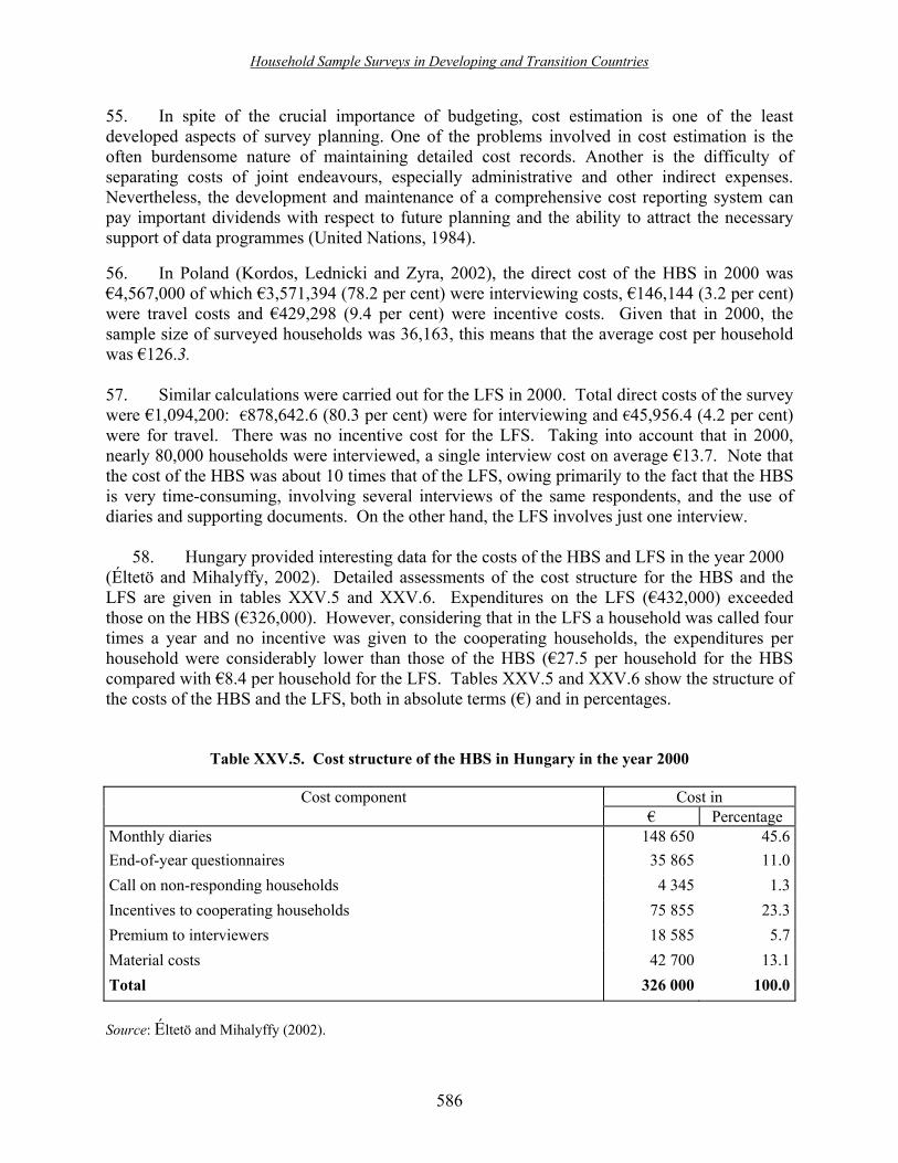
Household Sample Surveys in Developing and Transition Countries
586
55. In spite of the crucial importance of budgeting, cost estimation is one of the least developed aspects of survey planning. One of the problems involved in cost estimation is the often burdensome nature of maintaining detailed cost records. Another is the difficulty of separating costs of joint endeavours, especially administrative and other indirect expenses. Nevertheless, the development and maintenance of a comprehensive cost reporting system can pay important dividends with respect to future planning and the ability to attract the necessary support of data programmes (United Nations, 1984). 56. In Poland (Kordos, Lednicki and Zyra, 2002), the direct cost of the HBS in 2000 was �4,567,000 of which �3,571,394 (78.2 per cent) were interviewing costs, �146,144 (3.2 per cent) were travel costs and �429,298 (9.4 per cent) were incentive costs. Given that in 2000, the sample size of surveyed households was 36,163, this means that the average cost per household was �126.3. 57. Similar calculations were carried out for the LFS in 2000. Total direct costs of the survey were �1,094,200: �878,642.6 (80.3 per cent) were for interviewing and �45,956.4 (4.2 per cent) were for travel. There was no incentive cost for the LFS. Taking into account that in 2000, nearly 80,000 households were interviewed, a single interview cost on average �13.7. Note that the cost of the HBS was about 10 times that of the LFS, owing primarily to the fact that the HBS is very time-consuming, involving several interviews of the same respondents, and the use of diaries and supporting documents. On the other hand, the LFS involves just one interview.
58. Hungary provided interesting data for the costs of the HBS and LFS in the year 2000 (Éltetö and Mihalyffy, 2002). Detailed assessments of the cost structure for the HBS and the LFS are given in tables XXV.5 and XXV.6. Expenditures on the LFS (�432,000) exceeded those on the HBS (�326,000). However, considering that in the LFS a household was called four times a year and no incentive was given to the cooperating households, the expenditures per household were considerably lower than those of the HBS (�27.5 per household for the HBS compared with �8.4 per household for the LFS. Tables XXV.5 and XXV.6 show the structure of the costs of the HBS and the LFS, both in absolute terms (�) and in percentages.
Table XXV.5. Cost structure of the HBS in Hungary in the year 2000
Cost component Cost in � Percentage Monthly diaries 148 650 45.6End-of-year questionnaires 35 865 11.0Call on non-responding households 4 345 1.3Incentives to cooperating households 75 855 23.3Premium to interviewers 18 585 5.7Material costs 42 700 13.1Total 326 000 100.0 Source: Éltetö and Mihalyffy (2002).

Household Sample Surveys in Developing and Transition Countries
587
Table XXV. 6. Cost structure of the LFS in Hungary in the year 2000
Cost components Cost in � Percentage Calls on households Add
22 032 5.1Household questionnaires 65 232 15.1Activity questionnaires 212 110 49.1Supplementary questionnaires 42 336 9.8Premium to interviewers 33 695 7.8Material costs 56 595 13.1Total 432 000 100.0
Source: Éltetö and Mihalyffy (2002). Design effects 59. As can be seen from the description of household surveys in some transition countries, nearly all household sample surveys are based on a multistage. This means that the calculation of design effects is needed for statistical analysis of data from these surveys (Kish and Frankel, 1974). 60. We present an example from the Russian Federation (Goskomstat, 2000, pp. 219-220), in which the sample size for the quarterly LFS was determined for each region of the Russian Federation separately. The sample size was determined for various levels of the true unemployment rate. The desired level of precision of the estimate was set at 1.5 per cent, at 5 per cent and at 8 per cent for the Russian Federation, for larger and middle regions, and for small regions, respectively. The design effect was calculated in accordance with the formula in equation (7) of chapter VI, and on the basis of sample survey data on employment and unemployment in 1998. The calculated design effects were in the 1.52 to 2.14 range. Design effects were calculated for several characteristics of the HBS and the LFS. Some of the design effects are given in the annex to this chapter.
7. Concluding remarks
61. In this chapter, we have presented different aspects of sample design and implementation of household sample surveys, focusing on the most important surveys: the HBS and the LFS. From this general review of household surveys, it is possible to draw some conclusions. Household sample surveys in transition countries were redesigned and harmonized according to the new requirements of the market economy and the recommendations of Eurostat (1995; 1996; 1997; 1998a), with some differences between countries related to previous experiences and current possibilities. Although progress has been evident in household survey development, a number of problems need further attention at the statistical office level, such as calculation and presentation of standard errors, assessment of cost components, and calculation and publication of design effects and their use in statistical analysis. In addition, there are specific problems affecting particular countries, such as low response rates and less-than-adequate sample size for domains. These are very important and serious problems related to the comparability of the

Household Sample Surveys in Developing and Transition Countries
588
results between countries. It is the task of Eurostat to address these problems since they affect the integration and harmonization of household sample surveys conducted in various countries. The transition countries have their own plans for the further development of household surveys. One such plan entails utilization of results of the 2000 round of population and housing censuses. Their data offer opportunities for improving sampling frames, sample designs and estimation methods, mainly for small domains. 62. The several case studies of selected countries in transition provided below present a more detailed picture of the problems of the design, implementation and analysis of related to household surveys in these countries. The case studies are followed by a comprehensive list of references, which may be used to study different aspects of household surveys in transition countries.
B. Household sample surveys in transition countries: case studies
63. The case studies offered in the present section were prepared by authors from the following transition countries: Estonia, Hungary, Latvia, Lithuania, Poland and Slovenia. More comprehensive articles from eight countries in transition were published in Statistics in Transition, vol. 5, No. 4 (June 2002). The information on the main features of the HBS, the LFS and other household surveys in each country presented below serves as a supplement to the information provided in section A.
1. The Estonian Household Sample Survey 87 Introduction 64. The Statistical Office of Estonia implemented two major household surveys in 1995: the Estonian Labour Force Survey (LFS) and the Estonian Household Budget Survey (HBS). 65. The HBS is a continuous survey; its results are published quarterly and annually. In 1999, the survey was redesigned under a World Bank project, its diaries were changed, and the sampling and weighting procedures were more closely aligned with the most recently available data. The description of the survey is given in Traat, Kukk and Sõstra (2000) and in more detail in Traat (1999). 66. The LFS had been was a one-time survey in 1995. The next version, in 1997, was conducted with changed methodology. After that, it was executed on a quarterly basis until 2000 when it became a continuous survey. The survey is described in Kurvits, Sõstra and Traat (2002) and in Statistical Office of Estonia (1999). 67. In addition, the Statistical Office of Estonia has conducted many other household- or population-based surveys. These correspond to a series of similar studies in other European 87 Prepared by Imbi Traat, Institute of Mathematical Statistics, University of Tartu (e-mail: [email protected]).

Household Sample Surveys in Developing and Transition Countries
589
countries, and the resulting information has been used for national and international comparisons. These include the Adult Education Survey 1997, the Time-use Survey 1999�2000, the Living Conditions Survey 1994 and 1999, and the Health Behaviour of the Estonian Adult Population 2000 (Kurvits, Sõstra and Traat, 2002). 68. The Estonian Household Budget and Labour Force Surveys are described briefly below. Data content
69. The HBS is a diary-based survey. Each sampled household provides information on its food consumption and expenditure for one week, as well as on all other expenditure and income for one month. There is also a pre-interview concerning household composition and other background information, and a short post-interview about changes in the household composition.
70. The data-collection programme of the LFS has been more extensive than that for an ordinary labour-force survey, especially in 1995-1999 when retrospective information was collected. The respondent's labour-force status (employed, unemployed or inactive) was recorded for the time interval since the previous survey. The start and end dates and other relevant data were recorded for each status. The standard module of the labour-force surveys focuses on the reference week and asks the employed persons about occupation, usual and actual working time, the economic activity of the enterprise/organization, etc. Unemployed persons were asked about the steps taken to find a job, the continuity of job seeking, and the characteristics of the job they were looking for, etc. Data collection
71. The Interviewers Department (established in 1994) of the Statistical Office of Estonia is responsible for data collection for a variety of surveys. The 15 county coordinators organize the work of 130 interviewers, spread throughout the nation. In rural areas, an interviewer conducts, on average, 10-15 interviews per survey in one month, and in urban areas about 15-20; but in reality, their workload varies, depending on the regional sample sizes. The interviewing work is a second job for approximately half of the interviewers. They are paid for completed interviews as well as for attempts to contact non-respondents.
72. Data entry and coding are carried out in the Statistical Office using the survey processing system called Blaise. The first logical check is included in the data entry program. Data processing and more complex checks are performed using the Statistical Analysis System (SAS) software in the case of the LFS and FoxPro in the case of the HBS.
73. The total cost of the HBS and the LFS in 2000 was �153,000 and �128,000, respectively. The interviewers' salary, transportation, and communication represented approximately 70 per cent of the total cost and data entry about 15 per cent.

Household Sample Surveys in Developing and Transition Countries
590
Sample design 74. The target population of the HBS comprises all Estonian households, excluding institutes. The target population of the LFS comprises residents of Estonia aged 15-74 years.
75. The sampling frame for both surveys is the Population Register. The sampling units are persons and they are sampled systematically from the list of records in the Population Register. Strata (three for the HBS, four for the LFS) with different sampling rates are used to obtain better regional coverage. 76. In both surveys, auxiliary information from the frame is used. The frequency of the address in the frame determines the inclusion probability of that address. The sample is divided into two parts, handled by different rules: the address sample (the records with complete addresses) and the person sample (the records with unknown or incomplete addresses). Unknown or incomplete addresses exist in rural regions where the address is just the name of the village without any other information.
77. In the address sample, all households living at the sampled addresses are included in the sample. In the person sample, only households with selected persons are included in the sample. A proper household is traced within a county. About 15 per cent of the households are sampled via selected persons. 78. The sample design uses probability-proportional-to-size (PPS) sampling where the size is either the address frequency on the frame or the household size (learned from the household). For the HBS, this is the final sample. Its PPS inclusion probabilities are used in deriving estimators. For the LFS, this is a first-phase sample of households/addresses for which the number of working-age members, if not available from the Register, is determined with the help of local authorities. The aim of the second-phase sampling is to yield an equal-probability sample of households (and its members). All the households (addresses) with one working-age member and, by systematic sampling, half of the households with two working-age members, one third of the households with three working-age members, etc., are taken into the final sample. 79. The current HBS samples 820 households every month.
80. Since 2000, the households in LFS have been rotated according to a 2-2-2 rotation plan. The households are interviewed four times: during two consecutive quarters and, after a two-quarter hiatus, in the corresponding two quarters of the following year. According to this rotation plan, in any quarter, 25 per cent of the households are participating for the first time and 50 per cent are households that were interviewed in the preceding quarter. In this way, there is a 50 per cent overlap between neighbouring quarters and also between the same quarters of neighbouring years.

Household Sample Surveys in Developing and Transition Countries
591
Non-response 81. In diary-based surveys, the increased response burden tends to lead to higher non-response rates (see sect. A of the chapter).
82. In general, "refusals" represent about 50 per cent of total non-response and "not at homes" about 25 per cent. 83. The non-response rate in the LFS has always been much smaller than in the HBS. Furthermore, the refusal rate has been increasing owing to the time limits for the fieldwork as a result of the transition to the continuous survey approach. In addition, the inclusion of households four times in the LFS has led to increased non-response rates. Weighting
84. Weighting is used in both the HBS and the LFS. In the HBS, the weights are calculated for households; in the LFS, for persons. 85. In the HBS, response rates and income/expenditure levels determine the six weighting groups. The initial sampling weights are multiplied by the inverses of group response rates. Response weights are then calibrated by sex/age distributions (five classes) based on known demographic statistics.
86. In the LFS, the weights are formulated in a sequence of steps (Verma, 1995). The initial weight of a respondent is the size of the target population (persons between ages 15 and 74) divided by the number of respondents calculated within each of four strata. Then six regional weighting groups of reasonably uniform size with different response rates jR are formed. Within
each group, the correction factor of the weight of an individual respondent is jj RRw /)0( = , where R is the overall (average) response rate. After that, the raking-ratio method with five iterations is used to calibrate the sample distributions to population benchmarks using sex, age (five-year groups) and place of residence (15 counties and the capital city). Parameters and estimators
87. Most of the parameters estimated in the HBS and the LFS are totals and ratios. The weighted Horvitz-Thompson estimators or their ratios are used.
88. The variance estimates are calculated using SUDAAN. Since the software does not handle the exact design of the LFS and the HBS, the closest available design in SUDAAN � stratified with-replacement unequal-probability cluster sampling, with households as clusters, is used. Owing to the assumption of with-replacement sampling, the estimates slightly overestimate the true variances.

Household Sample Surveys in Developing and Transition Countries
592
Future developments
89. The 2000 Population Census provides a wealth of information about Estonian households and individuals. The weighting system of the HBS and the LFS will be reviewed in light of these available census data which reflect the demographic situation in Estonia more precisely than the data used earlier.
90. Efforts will also be made to improve other survey phases. For example, in 2002 a new data-collection method -- computer-assisted telephone interviewing (CATI) with 10 laptops -- was tested for the LFS. There will be a trial run of face-to-face interviewing at first contact and telephone interviewing for the three subsequent interviews.
2. Design and implementation of the Household Budget Survey and the Labour
Force Survey in Hungary88
Household Budget Survey
91. The HBS has a long tradition in Hungary. It began in the 1950s, based first on quota samples. It then used probability-based design as part of the Unified System of Household Surveys (USHS) in the mid-1970s. The sampling frame has always consisted of census enumeration districts (EDs), updated after every decennial census, most recently in 2002. Between 1976 and 1982, the HBS had been a continuous survey; between 1983 and 1991, it was carried out biennially; and since 1993, it has again been a continuous survey.
92. The sample of the HBS is selected in three stages, except for the self-representing cities, that is to say, cities with 7,000 or more dwellings, where the selection process consists of only two stages. In the case of non self-representing localities, the primary sampling units (PSUs) are the localities, the secondary units (SSUs) are EDs and the ultimate sampling units are the dwellings. In self-representing cities, the EDs are the PSUs.
93. Localities are stratified by size, resulting in eight strata, and also by county. The sample is, generally, not proportionately allocated to strata. The sampling rate is lower in smaller localities than in larger cities, especially Budapest. The annual sample size is distributed evenly over the months.
94. A household consenting to participate in the survey is asked to report its income and expenditures daily over a period of one month. During this period, interviewers collect additional data about the household such as age and occupational structure of the household, type, size and equipment of the dwelling, stock of consumer durables, etc. In addition, at the beginning of the following year, the interviewer again calls the household to ask the members about less frequent expenditures of high value during the whole year and certain types of annual income. 88 Prepared by Ödön Éltetö and László Mihalyffy, Central Statistical Office, P.O. Box 51, H-1525 Budapest, Hungary.

Household Sample Surveys in Developing and Transition Countries
593
95. The fact that, biennially, the interviewers call every household in their EDs to collect demographic and economic data, such as size of household, age, educational level, and economic activity of the head, constitutes an important aspect of the HBS. These data are used primarily for substitution purposes: owing to the rather high non-response rate, the use of substitute households (two in the larger cities and one elsewhere) is allowed. The substitute household is selected from the same stratum as the originally selected household and from the same ED assigned to the original interviewer.
96. Every year, the rotation of one third of the households is such that the sample size within each ED remains constant (six dwellings). Because non-responding households may be substituted, the actual number of households cooperating in the survey can be greater or fewer than the initial six. Thus, the rate of rotation in a given ED can be higher or lower than one third. A household that has participated in the survey for three consecutive years is rotated out permanently.
97. In 2000, the HBS sample covered nearly 1,980 EDs from 262 localities, and the number of initially selected households was 11,862. 98. As interviewers often encounter refusal or other types of non-response at the substitute addresses, too, the number of final interviews is smaller than the planned sample size. For example, in 2000, instead of the 11,862 (1,977 x 6) households, only 10,191 completed the survey; and to achieve this result, the interviewers had to call as many as 17,243 addresses. Non-response rates had increased after 1993, reaching 43.3 per cent in 1996, then decreased slightly. In 2000, the total non-response rate was 39 per cent with refusals accounting for nearly 27 per cent, and vacant dwellings, not-at-homes, invalid addresses and other factors accounting for the remainder. Given the problem of non-response, achieving the planned sample size is particularly difficult in the capital and in some large cities. Although until the end of 2002 cooperating households had received a monetary incentive for supplying their data, the amount was not large enough to motivate many households to cooperate with the survey and this incentive programme was terminated. However, a favourable change took place in the system of remuneration of the interviewers, inspiring them to increase their efforts to persuade households to cooperate in the survey. Overall, the refusal rate decreased from 34.4 per cent in 1996 to 26.9 per cent in 2000.
99. The design of the HBS sample ensures the conditions needed to make use of the familiar Horvitz-Thompson estimator. Totals are weighted sums of the observations, and the design weights are reciprocals of the inclusion probabilities. In each of the 98 design strata of the HBS sample, the design weight is unique, and is defined as the ratio of the number of non-vacant dwellings of the stratum in the population to the number of completed interviews. Because of the unit non-response, and also possible coverage deficiencies, the design weights are not suitable for computing the HBS data, hence calibrated weights should be used. In the course of the calibration process, the design weights are adjusted using the following auxiliary variables:
• Age-sex group (2 × 4 categories) • Economic activity (9 categories)

Household Sample Surveys in Developing and Transition Countries
594
• Level of education (3 categories) • Household type (3 categories)
100. In the case of quarterly data, calibration is carried out for three major areas: the capital city, cities with county rights and the rest of the country. For annual data, the area breakdown for calibration is more detailed. The seven regions of the country -- Nomenclature des Unités Territoriales Statistiques (NUTS) II-level regions in terms of Eurostat -- are also considered.
101. The calibrated weights of the HBS are computed using the generalized raking ratio weighting procedure.
102. Sampling error estimates for detailed income and expenditure items obtained from the HBS data are regularly computed and published. The computations are carried out using the stratified jackknife option of the VPLX software developed by R. E. Fay. In future applications, the use of the bootstrap method is envisaged, in particular in the case of estimated quantiles.
103. The HBS is one of the most costly surveys of the Central Statistical Office (CSO). In 2000, the direct expenditures on the survey - excluding salaries of the personnel in the central and county offices of the CSO - namely, remuneration of the interviewers, incentives for cooperating households and material costs, amounted to 84,769,000 Hungarian fortint (Ft), corresponding roughly to �326,000.
104. The design effect in 2000 was about 2 for net available income, 2.5 for food expenditures, and 2 for total personal expenditures.
105. The results of the survey are published yearly in bilingual form (Hungarian and English) with a short analysis of the data. The last publication containing the 2001 HBS data appeared in 2002 under the title Household Budget Survey: 2001 Annual Report (CSO, Budapest, 2002). The publication is also available on CD Rom. Labour Force Survey
106. The LFS is a new household survey introduced by the CSO in 1992. Its sample was selected in 1991 using the 1990 census as a frame. Self-representing cities were defined as those with 15,000 or more inhabitants. The initial sample for a quarter consisted of 9,960 EDs in 670 localities with 3 addresses from each ED, resulting in a quarter sample of 9,960 x 3 = 29,200 addresses. 107. In the second half of the 1990s, the demand for more detailed and reliable regional LFS data emerged, and the sample size was increased 40 per cent. The number of localities covered by the sample, especially the number of EDs, was also increased. In 2000, the sample contained 12,829 EDs from 754 localities and thus nearly 36,500 households were called quarterly. More details about the enlarged sample can be found in Éltetö (2000).

Household Sample Surveys in Developing and Transition Countries
595
108. Currently, data collection takes place each month, with the week containing the twelfth day of the month as the reference period, and the next week as the period for collecting the data. LFS data are collected mainly via face-to-face interviews using traditional paper questionnaires, although there are plans to increasingly use telephone interviews, especially for repeated interviews. At the sample addresses, all individuals aged 15-74 are eligible for the LFS and are interviewed. 109. According to the rotation system applied in the LFS, selected households remain in the sample through six consecutive quarters, then leave. That means that in each quarter one sixth of the sample is rotated out. 110. The design weights of the LFS sample are computed in the same way as in the HBS. The final weights of the LFS sample are also determined using the raking ratio approach. In the calibration of the LFS sample weights, the following auxiliary variables are used in the 19 counties as well as in the capital city:
• Age-sex (2×10 categories) • Residence in cities with county rights or elsewhere (2 categories)
111. Sampling errors for the LFS quarterly data in the �Main table� are run under the stratified jackknife model using VPLX software. Sampling errors for monthly data are also calculated but not published. In terms of sampling error, the LFS complies with the precision requirements of Eurostat as stated in Council Regulation (EC) No. 577/98 of 9 March 1998.
112. Non-response rates in the LFS - especially rates of refusals - are much lower than those in the HBS. From the beginning to 1997, a slight increase in the non-response rates had been reaching a maximum of 14.3 per cent. After 1997, the total non-response rate declined, reaching 9.2 per cent in 2000. Refusal rates also increased at first, reaching 7 per cent in 1996 and 1997, then decreased, reaching 3.2 per cent in 2000.
113. The LFS is an expensive operation. Direct expenditures on the survey in year 2000 were Ft 109,802,000 corresponding to �422,000. However, considering that a household is called four times a year and no incentive is given to the cooperating households, the expenditures per household are considerably lower than those in the HBS.
114. Mainly because the LFS sample contains many more PSUs than does the HBS, the design effect is considerably lower. In 2001, the design effect for total unemployment rate was 1.4, while for the female participation rate, the design effect was 0.8.
115. The LFS is supplemented by a module focusing on topics such as the situation of working women, questions concerning mothers on childcare leave, etc. These modules are included, on average, for three of the four quarters. One of the three modules, generally that for the second quarter of the year, covers the theme recommended by Eurostat for that year. Both the basic LFS questionnaires and those for the Eurostat modules contain all the information required by Eurostat.
116. Both quarterly and annual data of the LFS are published in bilingual bulletins.

Household Sample Surveys in Developing and Transition Countries
596
117. It can be concluded that both the HBS and the LFS are very important household surveys of the Hungarian CSO. HBS data are used not only to calculate weights for the consumer price index, but also to estimate the consumption of households within the national account computations for producing the quarterly and yearly gross domestic product (GDP) values. In addition, its data are of vital importance for research areas such as the living conditions of various social strata, expenditure patterns of various types of households and changes in them, consumer demand for different types of commodities, etc. It must be mentioned, furthermore, that in order to enhance compliance with Eurostat requirements, 2001 expenditures have been grouped according to the Classification of Individual Consumption According to Purpose (COICOP) system (United Nations, 2000, part three).
118. Though information on the number of registered unemployed persons is available from other sources, LFS data differ from those both in concept and in detail. The information on the actual situation and changes in the labour market provided by the LFS is indispensable for both central and local governments as well as for researchers. The official unemployment rate based on LFS data is one of the most important economical indicators.
3. Design and implementation of household surveys in Latvia89 Latvian Household Budget Survey 119. The Household Budget Survey (HBS) is a continuous survey which has been carried out since 1995. The survey was redesigned in May 2001. 120. The HBS was introduced with the technical assistance of the World Bank in September 1995. It had already been in the preparatory phase when a requirement was established that the results should conform to Eurostat requirements. Scope of survey 121. The target population of the HBS is all private households in Latvia. Persons living in institutional households (homes for the elderly, homes for disabled children, student hostels, hotels, barracks, hospitals, sanatoriums, penal institutions, etc.) and homeless people are excluded from the current survey. Sampling 122. The sample represents the whole population as well as its most typical groups. Every month, 342 households are surveyed. Each household included in the sample is surveyed only once.
89 Prepared by Janis Lapins, Statistics Department, Bank of Latvia; Edmunds Vaskis, Zaiga Priede, Central Statistical Bureau of Latvia; and Signe Balina, University of Latvia, Riga.

Household Sample Surveys in Developing and Transition Countries
597
123. Stratified two-stage probability sampling is applied. Households are stratified by the degree of urbanization and by geographical allocation. The sample allocation between strata is made proportional to the population sizes within strata. In urban areas the population register has been chosen as the sampling frame, while in rural areas, lists of households have been used. 124. Six administrative districts of Riga, the capital city, together with the six major cities, form 12 self-representing strata. All other towns are used as the PSUs in the remaining urban areas, which are distributed among 10 strata defined by combining 5 regions and 2 size groups. At the first stage of sampling, PSUs are selected within each stratum with probabilities proportional to the total number of inhabitants. At the second stage, persons aged 15 years or over are selected by simple random sampling. 125. In rural areas, households are distributed among five strata or geographical regions. As a rule, pagasts (civil parishes; the smallest administrative rural territories) are used as PSUs; some of the small pagasts are added to a neighbouring territory. Within each stratum, PSUs are selected with probabilities proportional to the number of households. At the second stage, households are selected using simple random sampling. Cost of the survey
126. The HBS is one of the most expensive statistical exercises. For the 2001 HBS, the survey cost per household was 24 Latvian lats (LVL) (approximately 40 US dollars). The main expenditure items are related to fieldwork. The compensation of interviewers reached 44 per cent of the total costs of the survey, followed by incentives to respondents (16 per cent), supervisors' salaries (14 per cent) and transportation costs (8 per cent).
Sampling error
127. In the HBS, the variances of selected estimates for the main domains of interest (capital city and six major cities, other towns and rural areas) are estimated using SUDAAN. On the basis of these estimates, the variances and design effects are estimated at the country level. Non-response
128. The total level of non-response was 26.1 per cent in 2000. The main reasons for non-response were refusals, including those from the households that stopped participation during the survey month (46.0 per cent of all non-response cases), followed by �not at home (31.8 per cent) and �not able to participate due to illness or being too old� (11.6 per cent). The non-response level was much higher in urban areas (31.9 per cent) than in rural areas (12.2 per cent).
129. Households that refuse to participate in the survey, or do not respond to the questions of the survey, as well as households that are not found at the given address, may have an impact on the precision of the acquired results which should not be neglected. In order to keep an effective sample size at the chosen level, the sequential sampling approach was applied. A refusing or non-responding household was replaced by another from the reserve list and surveyed.

Household Sample Surveys in Developing and Transition Countries
598
Redesign of the HBS in 2001-2002
130. The most recent redesign of the HBS sample was done on the basis of the population census, which was carried out in spring 2000. Survey instruments were significantly changed and the unified retrospective reference period of 12 months was introduced for durable goods, rarely made purchases and payments, seasonal income from paid work, and revenues from and expenditures in cash for agricultural production in the household. The previous HBS was terminated at the end of 2000.
131. Starting in January 2002, the samples of two surveys, the HBS and the LFS, were coordinated. For both surveys, the annual household sample is evenly distributed over time (the same number of households participates in the survey within each of the 52 weeks of the year). The sample of PSUs is also evenly distributed over territories within each quarter.
132. For the new HBS and the continuous LFS, the same interviewer network is used. Separate interviewer networks were used in the old HBS and LFS. Moreover, interviewers in rural areas are recruited from the local population. Under the new design, the interviewers are mobile and can work in different administrative territories. This allows for a distribution of the sample more widely over rural territories. (In the new HBS, the annual sample is spread over 208 different rural PSUs.) At the same time, the workload of interviewers is now more evenly distributed, and transportation is handled more economically. The reorganized interviewer structure of the Central Statistical Bureau (CSB) was instituted in January 2002. Latvian Labour Force Survey 133. During the period 1995-2001, the Latvian Labour Force Survey had been carried out biannually, in May and November. The redesigned continuous LFS was implemented in January 2002.
134. The Latvian LFS was prepared in accordance with the internationally approved labour-force survey methodology of the International Labour Organization (ILO) which ensures comparability of information with other countries (Eurostat, 1998a; 1998b). Scope of survey
135. The LFS survey population consists of all Latvian residents aged 15 years or over who reside in private households. Persons living in institutions such as homes for the elderly, homes for disabled children, hotels, barracks, hospitals, sanatoriums, penal institutions, etc., as well as homeless people, are excluded from the survey. 136. To follow the recommendations of Eurostat and to reduce the costs of the survey, all individuals of this age group who live in the same household with the sampled persons are also surveyed. The national sample size for one survey wave equals 7,940 households. 137. All questions in the survey refer to the calendar week (Monday to Sunday) before the day of the interview. Normally data are collected by means of face-to-face interviews using paper

Household Sample Surveys in Developing and Transition Countries
599
and pencil. If a respondent does not want to open the door, he or she is asked to give an interview by phone. Sampling
138. The sample for urban areas is drawn from the population register. The sample for rural areas is based on complete household lists. Since 1998, the rural sample has been based on the household register developed at the Central Statistical Bureau of Latvia. 139. The LFS covers 7 cities, 32 towns and all pagasts. In each survey wave, almost 16,000 persons are surveyed. For the construction of the sample, the procedure of one-stage sampling (in cities and rural areas) or two-stage sampling (in towns) is applied with stratification based on the administrative territorial division of the country. In urban areas, a simple random sample of persons aged 15 years or over is selected within each selected PSU. In rural areas, a simple random sample of households is selected within each pagast. 140. According to the rotation scheme for the sample of the LFS, persons from each household are included in the survey three times. Within each wave of the survey, the sample replacement rate is one third of the households in every city, town or pagast. Non-response
141. The total rate of non-response reached 10.1 per cent in 2000. The non-response rate in rural areas (only 8.5 per cent) was lower than in urban areas (11.4 per cent). The percentage of refusals in rural areas was particularly small, only about 0.5 per cent. Proxy interviews have been used as a method to increase the response rate. Approximately one third of the interviews were conducted using proxy respondents. Frame imperfections
142. Not all of the sampled persons were living at the address indicated in the register as their dwelling unit. Since tracking down and surveying these persons at the actual dwelling unit are costly, time consuming, and sometimes practically impossible, the interviewers have to survey households actually living at the sampled addresses. The analysis of non-participation cases showed that only 2.0 per cent of all non-participation cases (2.3 per cent in rural areas) were identified as being related to some frame imperfections (empty dwelling, demolished house, non-existent address, etc.). Redesign of the LFS in 2001-2002
143. The questionnaire for the LFS was redesigned in 2001 in full compliance with the requirements of the European Union (EU). The LFS is now carried out as a continuous survey.
144. Since January 2002, significant changes in the sample design for the LFS have also been introduced. For the LFS and the HBS, the same interviewer network is used. As a result, starting in January 2002, the samples of both surveys - the HBS and the LFS - were coordinated. It is

Household Sample Surveys in Developing and Transition Countries
600
expected that the coordination of samples of the two main household surveys, the HBS and the LFS, will promote more effective use of survey resources. 145. Training of the interviewers took place in December 2001. The continuous LFS started in January 2002. Other household surveys
146. The Living Conditions Survey (LCS) was launched in 1994 and 1999 within the framework of the NORBALT project that was financed by the Norwegian Government, and in close cooperation with the Fafo Institute (Institute for Applied Social Science, Oslo). 147. Several other household surveys were initiated in the second half of the 1990s, inter alia, the Family and Fertility Survey (1995), the Time-use Survey (1996), the Consumer Confidence Survey (1993-1999), the Survey of Energy Consumption by Households (1996), the Domestic Tourism Survey (1998), the Survey on the Use of Personal Computers in Households (1998), the Special Poverty Module Survey (1998) and the Survey of Attitudes to Suicide Problems (1999), etc.
148. Since 1996, the Traveller Border Survey has been conducted three or four times per year. Both traveller flows, that of the Latvian residents returning from abroad and that of the foreign travellers leaving Latvia, are surveyed.
149. As a rule, the results of the surveys are published in both Latvian and English and are available in printed and electronic form. For research purposes, the CBS has ensured access to the anonymous microdata files for data users in Latvia and abroad. Some concluding remarks
150. We expect that the development of the new highly professional and mobile interviewer service will make planning and execution of the new sample surveys and different ad hoc surveys more flexible.
151. The CSB is also planning to introduce modern data collection methodologies. One of the first steps will be to implement computer-assisted personal interview (CAPI) technology within the next few years.
4. Household sample surveys in Lithuania90
Introduction
152. The Household Budget Survey (HBS) was the first sample survey conducted in Lithuania. It was conducted for the first time over a 12-month period in 1936-1937. The HBS 90 Prepared by Danute Krapavickaite, Institute of Mathematics and Informatics, 4 Akademijos str., LT 2600 Vilnius and Lithuanian Department of Statistics, 29 Gedimino Avenue, 2746 Vilnius.

Household Sample Surveys in Developing and Transition Countries
601
was the only regular sample survey used to produce statistics for Lithuania�s planned economy. After Lithuania achieved independence in 1990, the national economy turned towards a market economy. A new questionnaire had to be introduced in order to collect more data, a new sample design was needed to cover the private sector, and published results had to redesigned to provide users with data comparable with results of other countries. The main redesign of the HBS was done with the help of World Bank experts in 1996, as described in �niuk�tiene, Vanagaite and Binkauskiene (1996). The sample design and estimation method remain unchanged. 153. The other regular household survey is the Labour Force Survey (LFS), which was started in 1994. The population register was modernized in 1996. Since then, it has been used for sample selection as a sampling frame for most household surveys, including the LFS.
154. Other household surveys, mainly one-time events, covered topics such as living conditions (1997), time-use (1998), the elderly (1999), household energy consumption (1997), accessibility of health-care service (1998) and providing households with computers (2000).
Estimates and errors in the Labour Force Survey Sample design 155. The population of the LFS consists of residents of Lithuania aged 15 years or over. The sample is constructed as follows: having selected a simple random sample of approximately 3,000 persons from the population register, the members of their households are added to the sample, even if they are not on the register. The proportion of respondents who are women has been 52.5 per cent. Sample rotation 156. In order to avoid major changes in the survey results from one survey to another, only one third of the sample is rotated for each survey. Each selected household participates in two surveys, rotates out for one survey, completes one more survey, and rotates out of the system. Estimates and their precision 157. The distribution of the survey respondents by urban/rural areas, age and sex differs slightly from the corresponding distributions based on census data. Post-stratification of the sample was processed by 12 age groups, 2 sex groups and 10 counties, for a total of 240 weighting groups. 158. Different weighting systems are used for the estimation of employed and unemployed persons. In order to improve the accuracy of estimates of the unemployed, the indices of the labour exchange are also used for the post-stratification. Variance estimation is described in Krapavickaitë, Klimavicius and Plikusas (1997) for fixed size sample design.

Household Sample Surveys in Developing and Transition Countries
602
Survey cost 159. The cost of one survey is about 70,000 Lithuania litai.91 Printing the questionnaires and delivering them to the respondents represent 14 per cent of the total cost and the remaining 86 per cent covers payment of interviewers, transport expenses of the interviewers, and costs of post office delivery of the completed questionnaires to Vilnius. Expenses connected with the methodological work associated with sample design and questionnaire preparation, sample selection, data entry, editing and processing are not included. Household budget survey Sample design 160. The HBS is carried out continuously. The sample is drawn once a year, divided into 12 parts and distributed for each month. Each household participates in the survey for one month. The population of private households in Lithuania is divided into three strata, according to the type of residence. A simple random sample of 4,476 persons aged 16 years or over is selected from the population register in the largest cities: Vilnius, Kaunas, Klaipėda, �iauliai and Panevė�ys. A random sample of 20 clusters with probabilities proportional to their size is drawn from all 140 such clusters in small towns, and a random sample of 33 clusters with probabilities proportional to their size is drawn from the population of 463 clusters at the first stage. A simple random sample of persons is drawn from each selected cluster. All persons residing in the selected households are surveyed. In case there are several households at the same address selected, the household of the person with the closest birthday is included in the sample. Estimates and their precision 161. Design weights are used for HBS estimation. The design effects of the estimates are larger than one. This suggests that auxiliary information should be used in future to obtain more accurate estimates.
Survey cost 162. The total yearly cost of the survey is approximately 900,000 litai broken down as follows: 61 per cent, payment to interviewers; 18 per cent, taxes; 14 per cent, payment to households; 5 per cent, transportation; and 2 per cent, other expenses. Dissemination of the results 163. The results of the surveys are published by Statistics Lithuania. The main results are published in the monthly journal Economic and Social Development in Lithuania. All results are published in special issues dedicated to topics such as the labour force, employment and unemployment (survey data), and household income and expenditure.
Concluding remarks 91 Exchange rate (2000 US dollars): 1 US dollar = 4 litai.

Household Sample Surveys in Developing and Transition Countries
603
164. Provisional results of the Population and Housing Census 2001 estimate the total Lithuanian population to be 3,491,000 usual residents. This figure is 202,000 persons less than that derived from demographic data published on 1 January 2001. After finalizing Census results, Statistics Lithuania will have more reliable demographic data as a basis for improving future household surveys. It is expected that the systematic error will be reduced in those surveys.
5. Household surveys in Poland in the transition period92
Introduction
165. Household surveys in Poland have a relatively long tradition [Glowny Urzad Statystyczny (Central Statistical Office of Poland, (GUS)], 1987, 1998a, 1999; Kordos, 1985, 1996; Lednicki, 1982). In the 1980s, the so-called Integrated System of Household Surveys (ISHS) was gradually implemented. It was launched in 1982 and completed in 1992 (GUS, 1987; Kordos, 1985).
166. The most important component of the ISHS was the household budget survey (HBS), which was based on two-phase sampling, quarterly rotation of households within a year, and one-third rotation of households in the three following years. This means that two thirds of households were included in the panel for four consecutive years. There was also a four-year cycle of the survey of subsamples. This survey programme was discontinued in 1992. At the same time, that is to say, during the period 1983-1992, subsamples selected for the HBS were used for over 30 social surveys employing topical modules.
167. The attempts to integrate household surveys conducted in the 1980s facilitated considerably the adjustment of household surveys to the European standards (GUS,1997). Further integration and improvement of the methodology of household surveys are needed (Kordos, 1998).
Household surveys in the transition period
168. The surveys were considerably extended and modified after 1990. The HBS is still being improved, and in 1992 for the first time a new LFS was introduced. Also, other new household surveys were launched including a survey on living conditions, a survey on the health status of households, a time-use survey, a population microcensus, and a variety of post-enumeration surveys. The Household Budget Survey
169. The household budget surveys have a tradition that started almost 45 years ago (GUS, 1999; Kordos, 1996; Lednicki, 1982). Various survey methods were experimented with and attempts were made to improve execution. At the beginning of the 1990s, the survey
92 Prepared by Jan Kordos, Warsaw School of Economics; and Bronislaw Lednicki and Malgorzata Zyra, Central Statistical Office, Al. Niepodleglosci 208, 00-925 Warsaw.

Household Sample Surveys in Developing and Transition Countries
604
methodology was changed. In the new method of conducting the HBS introduced in 1992, the classification of incomes and expenditure, as well as the classification of socio-economic types of the survey, was changed. For the first time all types of individual households in Poland encompassing about 32,000 households, were included in the survey. In 1997, efforts were made to improve the integration of household surveys.93 In 2000, the redesign of the HBS was implemented and some methodological components were changed (Kordos, Lednicki and Zyra, 2002). Further improvement of the HBS and its integration with other household surveys are planned, much of this work being motivated by the Eurostat recommendations (Eurostat, 1997).
The Labour Force Survey
170. The survey on the economic activity of the population was implemented in Poland for the first time in May 1992 and was repeated on a quarterly basis until the third quarter of 1999 (Szarkowski and Witkowski, 1994). It was prepared according to the ILO recommendations. In each quarter, about 24,000 households and persons aged 15 years or over who were members of those households were surveyed. Occasionally, modules on selected social topics were included in the survey, extending considerably the opportunity for social and economic analyses as well as the range of published results.
171. The survey results are published quarterly. Redesign of the LFS took place in 1999 to adjust the survey to the new administrative division of the country and to improve its efficiency according to Eurostat requirements (Eurostat, 1998b; Verma, 1995).
The 1995 Microcensus of Population and Housing
172. Several ad hoc household surveys were conducted in the last decade, the largest of which was the 1995 Microcensus. In May 1995, a large-scale sample survey (microcensus) of the population and housing was conducted (Bracha, 1996; GUS, 1998a). This survey was the third microcensus, two previous ones having been conducted in 1974 and 1984. It should be added that the censuses provide an opportunity to capture data on the disabled, migration and other social science topics.
173. The 1995 Microcensus covered 5 per cent of the population, that is to say, nearly 600,000 households. The complete Census of Population and Housing was conducted in May and June 2002; the previous one had taken place in 1988. Surveys of living conditions
174. Besides the HBS, starting in 1997, the decision was taken to conduct a multi-aspect survey of the living conditions of the population (Kordos, Lednicki and Zyra; 2002). The survey was carefully prepared in cooperation with experts from the French National Institute for
93 See internal regularion No. 20 of the President of the Central Statistical Office of 30 October 1997 on the establishment of the Working Group for the Improvement of the Methodology and Integration of Household Surveys.

Household Sample Surveys in Developing and Transition Countries
605
Statistics and Economic Studies [Institut national de la statistique et des études économiques (INSEE)] and conducted on a large sample for the first time in mid-1997. The survey was repeated on a smaller scale each year using panel subsamples and on a larger scale every few years.
175. In total, 12,524 households took part in the survey and the response rate in the case of households was 87 per cent, and for adult persons, 86 per cent. In mid-1998 the survey was repeated on a smaller scale.
176. The sample for 1999 consisted of two subsamples: the subsample selected in 1998 (panel) and a new subsample, the size of which was equal to the 1998 panel subsample. In this way, in each year there were a panel subsample and a new subsample selected from the updated sampling frame.
177. A new large-scale survey on living conditions was conducted in 2001, whose sample size was about 24,000 households, with 18,052 respondents and a non-response rate of 25 per cent. The survey is to be continued until the introduction of a new Income and Living Conditions Survey (EU-SILC), prepared according to the Eurostat programme (Eurostat, 2001), in 2005. Population health status survey
178. This survey was conducted in April 1996, covering 192,000 households. The response rate was 88.6 per cent. This was the first survey of the health status of the population in Poland conducted on such a large scale.
179. The health survey of the population was based on the World Health Organization (WHO) recommendations which allow comparison of the results with other European countries, especially the EU member States and the countries of the Economic Commission for Europe (ECE) region.
Time-use survey
180. GUS conducted time-use surveys in 1969, 1976 and 1984 (Kordos, 1988b). In 1996, GUS carried out a small-scale time-use survey with a sample of 1,000 households including persons aged 10 years or over. One objective of the survey, among others, was to verify the applicability of the methodology proposed by Eurostat (GUS, 1998b). A large-scale time-use survey is to be conducted in 2004. Common methodological aspects of household surveys Sampling frames
181. Population censuses are the basis for sampling frames used by household surveys in Poland. Primary sampling units (PSUs) are constructed using enumeration statistical districts (ESDs) or census enumeration areas (CEAs) usually adjusted to the specific demands of a survey. Dwellings usually serve as secondary sampling units (SSUs). Dwellings in ESDs or in

Household Sample Surveys in Developing and Transition Countries
606
CEAs are updated on an annual basis and the updating involves an increase of the dwelling stock due to the completion of new buildings, a decrease of the dwelling stock due to the demolition, and changes in the boundaries of districts due to the changes in the administrative division of the country. For each district, the sampling frame contains information on the addresses and estimates of the number of members of the population and the number of dwellings (GUS, 1998a).
182. For sample selection of the HBS and the LFS, it was necessary to merge neighbouring ESDs or CEAs to satisfy the minimum required size for each PSUs. For example, 29,172 PSUs were constructed for the HBS from 33,023 ESDs (from urban areas, PSUs had at least 250 dwellings, and from rural areas, 150 dwellings). The household survey sample designs 183. Usually in each household survey, two-stage sample selection is used and PSUs are selected with probability proportional to size (PPS). Stratification is based on region (voivodship), urban/rural areas and, in some cases, size of locality. For continuous surveys, such as the HBS and the LFS, a different rotation pattern has been used, and final results are weighted to minimize the impact of non-response. Sample designs for the HBS 184. Different sample designs for HBS were applied over the last 45 years (GUS,1999; Kordos, 1996; Lednicki, 1982). Here, we discuss the most recent HBS sample design, which has been in place since 2000. For the period 1992-2000, sample designs are described in detail in Kordos, Lednicki and Zyra (2002). 185. Since 2001, two subsamples of 675 PSUs have been selected from a total of 29,172 PSUs. PSUs are stratified by 16 voivodships, and in each voivodship, according to the class of size of localities. Large towns constitute separate strata. The number of strata in each voivodship ranges from 3 to 12. Altogether there are 96 strata. Allocation of the sample to strata is proportional to the total population of dwellings in each stratum. PSUs are selected with probability proportional to the number of dwellings according to the Hartley-Rao scheme. In each PSU, 24 dwellings are selected for two years (2 dwellings for each month, and the same dwellings are surveyed in both years). Additionally, in each PSU, 150 dwellings are selected independently as a reserve subsample, to be used in the case of non-response. Each year, a new subsample of 675 PSUs will be selected for two years. Weighting for HBS 186. Non-response rates in HBS are usually high, and they affect considerably the socio-economic structure of households in the sample. To minimize this impact, the sample results are weighted.
187. First, each household in the sample is weighted in inverse proportion to the probability with which it was selected. Weights from external sources are used. For the HBS, additional

Household Sample Surveys in Developing and Transition Countries
607
appropriate weights from the LFS (for size of households, and urban and rural proportions of the population) are applied. Method of standard error estimation 188. The random group method of standard error estimation was used until 2000. Since 2001, a method of balanced half-samples has been used. Sample design for LFS and its redesign in 1999
189. A sample for the LFS was selected in two stages with stratification. The PSUs were CEAs in towns; in rural areas, PSUs were ESDs. (In some cases, sampling units were created by collapsing two or more adjacent CEAs or ESDs, in order to achieve prespecified minimum size requirements.) Dwellings served as the second-stage sampling units (Szarkowski and Witkowski, 1994).
Redesign of the survey in 1999 190. Since the fourth quarter of 1999, the LFS has been carried out as a continuous survey. PSUs and SSUs were selected in the same way as in the previous survey, but sample allocation by 16 voivodships was changed. To achieve greater precision of estimates by voivodship, the size of the sample in a voivodship was allocated nearly proportional to the square root of the number of dwellings in the voivodship. The sizes of the strata created within voivodships were proportional to the sizes of localities. 191. PSUs within strata were selected with probability proportional to the number of dwellings in a PSU. Then, a determined number of dwellings (from four to nine) were selected from each PSU. Every 13 weeks in a quarter,94 interviewers visit a determined number of randomly sampled dwellings (1,880-1,900) and collect data concerning economic activity during the preceding week. The survey covers all people aged 15 years or over living in the selected dwellings. A sample of dwellings to be visited is changed every week. Weekly samples result from a random division of a quarterly sample into 13 parts. The quarterly sample ranges from 24,440 to 24,700 dwellings (GUS, 2000).
192. The following rotation pattern of households is applied: two quarters in the survey, two quarters out, followed by two quarters in, and finally rotating out of the system [2-(2)-2 rotation pattern].
94 According to Eurostat regulations, the term "quarter" as currently applied to the LFS is slightly different from the calendar quarter: every quarter in the LFS consists of 13 weeks and always starts on a Monday. Thus, the first quarter of 2000 lasted from 3 January to 3 April.

Household Sample Surveys in Developing and Transition Countries
608
Weighting the LFS results
193. Weighting is performed in three stages (for details, see Kordos, Lednicki and Zyra, 2002). Estimation of standard errors
194. Until 1999, standard errors of estimates were calculated according to the random group method. Since the redesign of the LFS in the fourth quarter of 1999, the Taylor linearization technique has been used.
Costs of household surveys 195. The Central Statistical Office of Poland has a system of household survey cost assessment. For each sample survey, the direct cost of the survey is assessed, using previous experiences in the field, and some administrative recommendations. Such cost survey assessment includes field interviewing costs, travel costs, material costs, services connected with the survey, incentives for increasing participation in the survey, taxes, etc. (GUS, 2001). Not included are coding and editing, computer runs, methodological contributions of indirect and overhead costs and the cost of personnel whose responsibilities extend over several projects. 196. As examples, costs elements for the HBS and the LFS in Poland in the year 2000 were presented in Section A of this chapter. Design effects 197. For the Polish household surveys, that is to say, for the HBS and the LFS, the design effects for several characteristics were calculated (Kordos, Lednicki and Zyra., 2002). As an exercise, and for comparison with other countries, design effects were calculated for several parameters for the years 2000 and 2001. 198. For some characteristics of the HBS, the design effects and the relative standard errors (as a percentage given in parentheses) were as follows: total income: 4.24 (1.1); total expenditure: 4.16 (1.0); food expenditure: 3.53 (0.4); clothing and shoes: 2.72 (1.5); maintenance of dwellings: 4.04 (1.3); personal health care: 3.28 (1.7); transport and communication: 2.16 (4.5); and education: 2.50 (3.9). 199. For the LFS, 2000 and 2001 design effects were calculated for the total number of unemployed for different cross-classification groups based on urban/ rural areas, size of localities (classes of towns) and level of education. The highest dispersion was for classes of towns with design effect levels ranging from 1.7 to 3.55. 200. As may be seen from the above estimates, design effects for the HBS and the LFS data were usually greater than 1, and for some characteristics were even greater than 4. Hence, standard errors based on simple random sample assumptions tended to underestimate the standard errors derived from the applied complex sample design.

Household Sample Surveys in Developing and Transition Countries
609
Non-response in household surveys 201. As discussed in Section A, non-response rates increased both for the HBS and for the LFS in the last decade. The main reasons for these increases were refusals and �not at homes�. For the HBS, refusal rates increased from 10.2 per cent in 1992 to 25.0 per cent in 2000, and not at home rates increased from 4.5 per cent in 1992 to 14.5 per cent in 2000. 202. On an annual average basis, non-response rates in the LFS were steadily increasing throughout most of the period 1992-2000, from 4.5 per cent in 1992 to 22.1 per cent in 2000, as were refusal rates, from 2.0 per cent in 1992 to 10.9 per cent in 2000. Non-response rates increased significantly in the years 1992-2000, the main reasons being refusals and not at homes.
203. Non-response rates for the LFS differ according to size of localities, the largest being in Warsaw, and the smallest in rural areas. For the year 2000, the weighted annual non-response rates by size of localities were as follows: Warsaw: 54.5 per cent; cities: (500,000 to 1 million inhabitants) 32.6 per cent; cities: (100,000 to 500,000 inhabitants) 33.3 per cent; towns: (20,000 to 100,000 inhabitants) 23.1 per cent; towns: (below 20,000 inhabitants) 19.0 per cent; and rural areas: 11.1 per cent. Concluding remarks 204. In this section, general descriptions of household surveys in the transition period of the Central Statistical Office of Poland (GUS) were presented, with special emphasis on two continuous surveys, namely, the HBS and the LFS. GUS has a long tradition of conducting household surveys and large experience in this area. This was helpful at the beginning of the transition period in redesigning the surveys and designing new ones.
205. Assimilating the results of the Population and Housing Census conducted in 2002 will constitute one of the most important tasks of household surveys in the coming years. The census will deliver not only updated sampling frames for household surveys but also auxiliary information for increasing precision of estimates and for small-area estimation methods which are now under study.
206. We have started preparing a new household survey -- EU-SILC, which is to be introduced in 2005 (Eurostat, 2001) -- and are improving current surveys to adjust them to EU standards.

Household Sample Surveys in Developing and Transition Countries
610
6. The Labour Force Survey and the Household Budget Survey in Slovenia95 Introduction
207. The Republic of Slovenia gained independence in the early 1990s. Before that, within the former Yugoslavia, statistical activities were centralized in the Federal Statistical Office. At that time, household surveys did not feature prominently in the national statistical programme. With independence, the Slovenian Statistical Office was rapidly transformed from a regional office to a national statistical one. The transition process was relatively smooth owing, in part, to the fact that senior management remained unchanged and in power for the entire transition period.
Labour Force Survey (LFS)
Background
208. The first LFS was implemented in 1989 by the Faculty of Social Science of the University of Ljubljana (Vehovar, 1997). The Statistical Office of the Republic of Slovenia took over full responsibility for the LFS survey in 1995.
209. The LFS samples for 1989-1995 were designed and conducted in a rather ad hoc manner largely because of uncertain annual budgets. Starting in 1992, the design was a three-stage cluster sample with 3,000 new households each year. The units stayed in the sample for three consecutive years, with the total sample size about 8,500 units. Redesign
210. In 1997, a major redesign took place owing to requests for more frequent (that is to say, quarterly) and more detailed (that is to say, regional) results. The Eurostat guidelines were also important stimuli for the redesign (Eurostat, 1998a).
211. The LFS was revised to become a continuous panel survey with quarterly sample selection and publication of results. Each quarterly sample is divided into six two-week intervals. The reference period for the interviews is the week (Monday to Sunday) prior to the interview. The rotation model 3-1-2 is applied, with households being interviewed for three consecutive quarters, then omitted for one quarter and included again for another two quarters. This model results in a 60 per cent overlap between two consecutive quarters and a 40 per cent overlap between two consecutive years.
212. The LFS sampling frame is the central register of the population combined with stratification information. The stratum definitions are based on 6 types of settlements (according 95 Prepared by Vasja Vehovar, Faculty of Social Sciences, University of Ljubljana; and Metka Zaletel, Tatjana Novak, Marta Arne� and Katja Rutar, Statistical Office of the Republic of Slovenia.

Household Sample Surveys in Developing and Transition Countries
611
to the size of the settlements and the proportion of the population that are farmers) and 12 geographical regions. After collapsing, there are a total of 47 strata.
213. In each stratum, the sample is selected using systematic sampling with a random start. Implicit stratification is implemented through a data sort by settlement, street, and building number. The sampling rate in each stratum is adjusted to account for the anticipated non-response rate. Field substitutions are not applied, as it has been shown that substitutions offer few advantages and entail considerable problems (Vehovar, 1999).
214. In each quarter, 2,000 new units are selected. In addition, about 5,000 (responding) households are included from the previous four quarters. Thus, approximately 7,000 households are selected per quarter (2,000 from the incoming sample and 5,000 from the continuing sample). Of these, about 6,000 are expected to be responding households. The total number of completed individual interviews is approximately 20,000.
Implementation
215. All households from the incoming quarterly sample are interviewed personally (face-to-face interview) with the help of computers (CAPI). There are about 30 experienced interviewers for the LFS, all equipped with portable computers. Repeated interviews are made from the telephone centre at the Statistical Office via CATI, except for non-telephone households and those unable to participate in a telephone interview. The national telephone coverage rate is about 95 per cent. Before interviewing, each household receives an advance letter with a description of the survey and a brochure with LFS results from previous surveys. Incentives are not offered.
216. For face-to-face interviews in the incoming part of the sample, non-response rates have been 17-18 per cent and refusal rates 12-13 per cent. In the repeated telephone interviewing for the households already in the panel, the non-response rates have been slightly lower (10-11 per cent) as have the refusal rates (6-7 per cent). The LFS non-response rate grew considerably starting in 1991 but has stabilized in the last four years. Sampling errors and publication
217. The data are weighted for unequal probability of selection and for unit non-response. Post-stratification is performed according to the known population distribution of age (8 groups), sex and region (12 regions). The fact that post-stratification is carried out at the individual level means that members of the same household can receive different weights.
218. The sampling errors and design effects are routinely estimated only for the key variables: unemployment rate and employment/population ratio. The design effects are relatively low, for example, the design effect is 1.3 for the unemployment rate.
Household Sample Surveys in Developing and Transition Countries
612
219. The coefficients of variation (CV) of the estimates are routinely calculated. The estimates with CV less then 10 per cent are published without any restrictions; estimates with CV between 10 and 20 per cent are published in a single bracket. CVs between 20 and 30 per cent are published with a double bracket. When the CV exceeds 30 per cent, the results are replaced with a dot (.) meaning �non-zero but unreliable�. 220. The results of the survey are published quarterly in the Statistical Rapid Reports, Statistical Yearbook, and several other Slovenian publications. The special series �Results of the Survey� provides detailed results of the survey and the methodology. Data also appear in publications of other organizations such the World Bank, the United Nations Children�s Fund (UNICEF) and Eurostat. Researchers outside the Statistical Office also analyse the microdata. Household Budget Survey (HBS) Background
221. The first survey on household consumption had been implemented in the 1960s. Until 1997, the survey was conducted according to the relatively advanced and innovative methodology designed by the Federal Statistical Office of Yugoslavia. The sample design encompassed a two-stage cluster sample with stratification of the PSUs at the first stage. Primary sampling units were enumeration areas (EAs), sampled with probability proportional to size (PPS). At the second stage, individuals were selected from the central register of population; they also determined the household. In each PSU, five households were interviewed. Until 1993, the substitution procedure was used to provide five responding units; however, starting in 1994, the �take� per cluster was increased from six to eight persons within each PSU, a design feature that required additional correction with weights. Two different HBS surveys were conducted regularly: one on a quarterly basis and another as an annual survey in five-year intervals. The last annual HBS included 3,270 households and the quarterly one included 1,000 households. In the annual survey, the interviewing was implemented at the end of the year for the whole year, while with the quarterly survey, sampled households were interviewed four times per year. Redesign of the HBS sample
222. The main motivation for the redesign was the new guidelines from Eurostat (Eurostat, 1997).
223. The population register is used to select the individual respondents. These persons also determine the households. Weights are used to adjust for unequal selection probabilities for persons and households. Institutional households are excluded. The annual sample size includes 1,200 responding households. Since this constitutes too small a sample to allow the application of the �Nordic� model, data from samples of three consecutive years are merged and recalculated to the middle year. In this way, a sample size of 3,600 households can be secured.
224. Proportionate allocation to 47 strata is used. Owing to the relatively small sample and the large number of strata, stratification is performed only implicitly. In small settlements (fewer

Household Sample Surveys in Developing and Transition Countries
613
than 1,000 inhabitants), the enumeration areas serve as PSUs and are selected with probability proportional to size (PPS). Four responding households are selected in each PSU. In larger towns and cities, the simple random sampling (SRS) method is applied. As a consequence, the design effects are relatively low, about 1.2 for key variables. The units are selected for each quarter separately and allocated into 12 weeks of the corresponding quarter. The thirteenth week is used for the remaining work with non-respondents. Imlementation 225. Advance letters are sent one week before the first visit together with the incentive: a pocket calculator. As this is a continuous survey, it can be implemented with a smaller number of interviewers (for example, 20).
226. The interviewers register all contacts/attempted contacts with a household on a special form. The status with respect to dwelling, household and reference person of each unit is thus very clear as well as the number of contacting attempts, number of filled diaries and potential reasons for non-response.
227. Data are collected using a questionnaire completed by the interviewer and diaries completed by household members. Almost all interviews are conducted via computers (CAPI).
228. The households keep the diary for 14 days. During this period, they regularly fill in their daily expenditure information. The households are considered to be responding if they complete at least the basic interview questionnaire because two thirds of the data are obtained from the questionnaire. Relatively high and stable response rates (about 81 per cent) are obtained at the level of interview questionnaires. However, the response rate for complete response, including diaries, is lower, at about 70 per cent. Sampling errors and publication
229. If all diaries for a given household unit are missing, the data are imputed using the hot- deck imputation method from a similar household donor. Missing item non-response is also imputed using hot-deck procedures. Each missing value is replaced with corresponding data from the previous respondent within the same imputation class defined by household size and sociodemographic characteristics. In particular, missing individual income is replaced with the income of a donor matching on employment status and education.
230. The method of calculation of the design weights and the post-stratification weights are similar to that for the LFS sample. In addition, specific expansion factors are developed to compensate for different reference periods. The coefficient of the recalculation is basically the ratio of the reference period of the survey (one-year) to the reference period of the individual variable. Special weights are also needed when combining the data for three consecutive years. The calculation for a specific date thus uses the three-year data with half of the data referring to the period before this date and half to the period after this date.

Household Sample Surveys in Developing and Transition Countries
614
231. The HBS methodology and results are described in the publications cited above for the LFS.
Conclusions 232. Before independence in 1991, household sample surveys were not a common tool of data collection in Slovenia. However, unlike other transition countries, Slovenia had regularly conducted HBS surveys starting in the mid 1960s and the series of annual LFS surveys starting in the late 1980s. 233. After independence, the Statistical Office of Slovenia underwent a smooth and effective transition. The Statistical Office now routinely conducts the standard series of household surveys. The basic socio-economic surveys (LFS, HBS) are almost completely harmonized with Eurostat requirements (Statistical Office of the Republic of Slovenia, 2001). A variety of other household surveys have also been conducted: Household Energy Consumption Survey (HECS), 1997; Time-use Survey (TUS), 2000/2001; Monthly Consumer Attitude Survey (CAS); Quarterly Survey on Travels of the Domestic Population (QSTDP); and Annual Crime and Victimization Survey (2000, 2001). 234. There remains room for further improvement of the household sample survey system. Slovenia has a rich and accurate registration-based statistical system (taxation data, database of employees, insurance databases, etc.) that can be linked efficiently and effectively to geographical systems and to census data. Thus, additional advantages can be derived for application in the design of optimal samples as well as for estimation. Acknowledgements The Presidents of the Central Statistical Offices of the following countries agreed to submit information about their household sample surveys: Belarus, Bulgaria, Croatia, the Czech Republic, Estonia, Hungary, Latvia, Lithuania, Poland, Romania, the Russian Federation, Slovakia, Slovenia and Ukraine. The author would like to express his gratitude for the submitted data and for the helpful comments provided by many colleagues in these countries. He would like also to express his gratitude to the authors of the contributions in section B that are designed to supplement the material presented in section A.
The author also extends his appreciation to some anonymous reviewers and to members of the Expert Group Meeting on the Analysis of Operating Characteristics of Surveys in Developing and Transition Countries, held, in New York from 8 to 11 October 2002, for their helpful comments and suggestions.

Household Sample Surveys in Developing and Transition Countries
615
References Bracha, Cz. (1996). Schemat losowania próby do Mikrospisu 1995 (Sample design for the 1995
microcensus). Wiadomosci Statystyczne, No. 3, pp. 12-18. Deville, J.-C., and C.E. Särndal (1992). Calibration estimators in survey sampling. Journal of
the American Statistical Association, vol. 87, pp. 376-382. Éltetö, Ö. (2000). Enlargement of the sample of the Hungarian LFS to get reliable small area
estimates for labour market indicators. Statistics in Transition, vol. 4, No. 4, pp. 549�563.
__________, and L. Mihalyffy (2002). Household surveys in Hungary. Statistics in Transition,
vol. 5, No. 4, pp. 521-540. European Union (1998). Council regulation No. 577/98 of 9 March 1998 on the organisation of
a labour force sample survey in the Community. Official Journal of the European Communities, 14/3/98, pp. I.77/3-I.77/7.
Eurostat (1995). The Future of European Social Statistics: Guidelines and Strategies.
Luxembourg. __________(1996). The Future of European Social Statistics: Use of Administrative Registers
and Dissemination Strategies. Luxembourg. __________(1997). Family Budget Surveys in the EC: Methodology and Recommendations for
Harmonisation. Population and Social Conditions 3, Methods E. Luxembourg. __________(1998a). Labour Force Survey: Methods and Definitions. Luxembourg.
__________(1998b). Labour Force Survey in Central and Eastern European Countries. Methods and Definitions (Provisional). Luxembourg
__________(2001). Meeting of the Working Party Statistics on Income and Living Conditions
(EU-SILC), 10 and11 December 2001. Luxembourg. Working document.
Garner, T.I., and others (1993). Household surveys of economic status in Eastern Europe: an evaluation. In Economic Statistics for Economies in Transition: Eastern Europe in the 1990s. Washington, D.C.: United States. Bureau of Labour Statistics, pp. 309-353.
Glowny Urzad Statystyczny (GUS) (Central Statistical Office of Poland) (1971a). Badania
statystyczne metodą reprezentacyjną w krajach socjalistycznych (Sampling surveys in socialist countries). Biblioteka Wiadomości Statystycznch, tom 14 (Warszawa), p. 220.

Household Sample Surveys in Developing and Transition Countries
616
__________(1971b). Wybrane problemy metodologiczne badań reprezentacyjnych (Some methodological problems of sampling surveys). Biblioteka Wiadomości Statystycznch, tom 15 (Warszawa), p.151.
__________(1987). Problemy integracji statystycznych badan gospodarstw domowych
(Problems of integration of statistical household surveys). Biblioteka Wiadomości Statystycznch, tom 34 (Warszawa).
__________(1997). Stan dostosowania polskiej statystyki publicznej do standardów Unii
Europejskiej. Harmonogram prac dostosowawczych (Status of harmonisation of Polish statistics with European Union standards). Warszawa. Mimeograph.
__________(1998a). Metodologia i organizacja mikrospisów (Methodology and organisation of
microcensuses). Statystyka w Praktyce. Warszawa. __________(1998b). Budzet czasu ludnosci 1996 (The 1996 Time-use Survey). In Studia i
Analizy Statystyczne. Warszawa. __________(1999). Metodyka badania budzetów gospodarstw domowych (Methodology of the
household budget survey). In Zeszyty Metodyczne i Klasyfikacje). Warszawa. __________(2000a). Aktywnosc ekonomiczna ludnosci Polski: I kwartał 2000 (Labour Force
Survey in Poland: I quarter 2000). Informacje i Opracowania Statystyczne. Warszawa. __________(2001). Zasady wyceny kosztów prac statystycznych realizowanych przez służby
statystyki publicznej w roku 2003 (Principle of cost assessment of statistical work in official statistics in 2003). Warszawa. Mimeograph.
Goskomstat (2000) Methodologitcheskie polojenia po statistike (Methodological principle of
statistics), Vypusk treti (3rd ed.). Moskva, pp. 294. Groves, R.M. (1989). Survey Errors and Survey Costs. New York: John Wiley and Sons. __________, and M.P. Couper (1998). Non-response in Household Interview Surveys. New
York: John Wiley and Sons. Kish, L., and M.R. Frankel (1974). Inference from complex samples (with discussion). Journal
of the Royal Statistical Society, series B, vol. 36, pp. 1-37. Kordos, J. (1963). Seminarium statystyczne w Wiedniu (Statistical seminar in Vienna). Przegląd
Statystyczny, No. 2, pp. 307-310. __________(1970). Mozliwosci szerszego stosowania metody reprezentacyjnej w badaniach
statystycznych krajów-czlonków RWPG (Possibilities of larger application of sampling methods in statistical investigations of the member-countriers of the Council for Mutual Economic Assistance). Przeglad Statystyczny, No. 1, pp. 33-50.

Household Sample Surveys in Developing and Transition Countries
617
__________(1981). Problemy badań gospodarstw domowych: drugie spotkanie statystyków
europejskich w Genewie (Problems of household surveys: the second meeting of European statisticians). Wiadomosci Statystyczn, No. 11, pp. 36-38.
__________(1982). Metoda rotacyjna w badaniach budzetow rodzinnych w Polsce (Rotation
method in Household Budget Surveys in Poland). Wiadomosci Statystyczne, No. 9. __________(1985). Towards an integrated system of household surveys in Poland. Bulletin of
the International Statistical Institute (Amsterdam), vol. 51, book 2, pp. 13-18. __________(1988a). Jakość danych statystycznych (Quality of statistical data). Państwowe
Wydawnictwo Ekonomiczne (Warszawa), pp. 204. __________(1988b). Time-use surveys in Poland. Statistical Journal of the United Nations
ECE, vol. 5, pp. 159-168. __________(1996). Forty years of the household budget surveys in Poland. Statistics in
Transition, vol. 2, No. 7, pp. 1119-1138. __________(1998). Social Statistics in Poland and its Harmonisation with the European Union
Standards, Statistics in Transition, vol. 3, No.4, pp. 617�639. __________(2001). Some data quality issues in statistical publications in Poland. Statistics in
Transition, vol. 5, No. 3, pp. 475�489. __________, B. Lednicki and M. Zyra (2002). The household sample surveys in Poland.
Statistics in Transition, vol. 5, No. 4, pp. 555�589. Krapavickaitë, D. (2002). The household sample surveys in Lithuania. Statistics in Transition,
vol. 5, No. 4, pp. 591�603. __________, G. Klimavicius and A. Plikusas (1997). On some estimators in cluster sampling.
Proceedings of the XXXVIII Conference of the Lithuanian Mathematical Society, pp. 298-303.
Kurvits, M.A., K. Sõstra and I. Traat (2002). Estonian household surveys: focus on the labour
force survey. Statistics in Transition, vol. 5, No. 4. Lapins, J.,and E. Vaskis (1996). The new household budget survey in Latvia. Statistics in
Transition, vol. 2, No. 7, pp. 1085-1102. Lapins, J, and others (2002). Household sample surveys in Latvia. Statistics in Transition, vol. 5,
No. 4, pp. 617�641.

Household Sample Surveys in Developing and Transition Countries
618
Lednicki, B. (1982). Schemat losowania i metoda estymacji w rotacyjnym badaniu budzetów gospodarstw domowych (Sampling design and estimation method in the household budget rotation survey). Wiadomosci Statystyczne, No. 9.
Martini, A., A. Ivanova and S. Novosyolova (1996). The income and expenditure survey of
Belarus: design and implementation. Statistics in Transition, vol. 2, No. 7, pp. 1063-1084.
Mihalyffy, L. (1994). The unified system of household surveys in the decade 1992-2001.
Statistics in Transition, vol. 1, No. 4, pp. 443-462. Postnikov, S. (1953). O metodach otbora semei rabocich, sluja�cich i kolchoznikov dla obsledovanjia ich budjeta (On methods of selection of families of workers, non-worker emploees and co-operative employees for investigation their budgets). Vestink Statistiki, No. 3, pp. 14-25 Särndal, C-E., B.I. Swensson and J. Wretman (1992). Model Assisted Survey Sampling. New
York: Springer-Verlag. �niukstiene, Z., G. Vanagaite and G. Binkauskiene (1996). Household Budget Survey in
Lithuania. Statistics in Transition, vol. 2, No. 7, pp. 1103-1117. Statistical Office of Estonia (1999). Estonian Labour Force Survey 1998: Methodological
Report, Tallinn. Statistical Office of the Republic of Slovenia (2001). Slovenian Statistical System: A Global
Assessment, 2001. A Phare project. Ljubljana. Szablowski, J., J. Wesolowski and R. Wieczorkowski (1996). Indeks zgodnosci jako miara
jakosci danych: na podstawie wyników spisu kontrolnego do Mikrospisu 1995 (Index of fitting as a measure of data quality: on the basis of the post-enumeration survey of the microcensus, 1995). Wiadomosci Statystyczne, No. 4. pp. 43-49.
Szarkowski, A., and J. Witkowski (1994). The Polish Labour Force Survey. Statistics in
Transition, vol. 1, No. 4, pp. 467-483. Traat, I. (1999). Redesign of the Household Budget Survey: Final Report of the Sampling Group.
Tallinn: Statistical Office of Estonia. __________, A. Kukk and K. Sõstra (2000). Sampling and estimation methods in the Estonian
household budget survey. Statistics in Transition, vol. 4, No. 6, pp. 1029�1046. United Nations (1964). Recommendations for the Preparation of Sample Survey Reports (Provisional
Issue). Statistical Papers, Series C, No. 1, Rev. 2. ST/STAT/SER.C/1/Rev.2. New York. __________(1984). Handbook of Household Surveys (Revised Edition), Studies in Methods,

Household Sample Surveys in Developing and Transition Countries
619
No. 31. New York. Sales No. E.83.XVII.13. __________(2000). Classifications of Expenditure According to Purpose: Classification of the
Functions of Government (COFOG). Classification of Individual Consumption According to Purpose (COICOP). Classification of the Purposes of Non-Profit Institutions Serving Households (COPNI). Classification of the Outlays of Producers According to Purpose (COPP). Statistical Papers, No. 84. Sales No. E.00.XVII.6.
Vehovar, V. (1997). The Labour Force Survey in Slovenia. Statistics in Transition, vol. 3, No. 1
(June), pp. 191-199. __________(1999). Field substitution and unit non-response. Journal of Official Statistics, vol.
15, No. 2, pp. 335-350. __________, and M. Zaletel (1995). Non-response trends in Slovenia. Statistics in Transition,
vol. 2, No. 5, pp. 775-788. Verma, V.(1995). Technical Report on the Turkey Labour Force Survey. Project TUR/86/081.
Geneva: International Labour Organization. Wolter, K.M. (1985). Introduction to Variance Estimation. New York: Springer-Verlag.