arX

iv:a

stro

-ph/

9909

473v

1 2

8 Se

p 19

99

To appear in The Astrophysical Journal (1999 November 10 issue)

HOT MOLECULAR CORES AND THE FORMATION OF MASSIVE STARS

Mayra Osorio, Susana Lizano

Instituto de Astronomıa, Unidad Morelia, UNAM, J.J Tablada 1006,

Col. Lomas de Santa Marıa, 58090 Morelia, Michoacan, MEXICO

and

Paola D’Alessio

Instituto de Astronomıa, UNAM, Apdo Postal 70-264, Cd. Universitaria,

04510 Mexico D. F., MEXICO

ABSTRACT

It has been proposed that some hot molecular cores (HMCs) harbor a young

embedded massive star, which heats an infalling envelope and accretes mass at a rate

high enough to “choke off” an incipient HII region. This class of HMCs would mark

the youngest phase known of massive star formation. In order to test this hypothesis,

we model this type of object calculating the radiative transfer through a spherically

symmetric dusty envelope infalling onto a central OB star, with accretion rates from

M = 6 × 10−4 to 10−3 M⊙ yr−1. The dust thermal spectrum from infrared to radio

wavelengths is derived and is compared with the observed fluxes of several hot cores

which may be internally heated. We find that the data are best fitted using an envelope

with the density distribution resulting from the collapse of a singular logatropic sphere,

instead of that of a singular isothermal sphere. We conclude that several of these

sources may be undergoing an intense accretion phase and find in all the cases that the

accretion luminosity exceeds the stellar luminosity. We discuss the implications of this

phase on the formation of massive stars.

Subject headings: stars: formation — dust — HII regions — ISM: individual (G34.24

+ 0.13MM, W3(H2O), Orion hot core, IRAS 23385+6053) — radiative transfer

1. INTRODUCTION

One of the most interesting results of the past few years in the study of massive star formation

is the discovery of Hot Molecular Cores (HMCs) which are small (∼< 0.1 pc), dense (n ∼ 106 -

108 cm−3), hot (T ∼ 100 - 300 K) and dark (Av ∼ 103 mag) molecular clumps. They are generally

– 2 –

found in the proximity of ultra-compact HII (UCHII) regions, and are probably directly related to

the formation of high mass stars. The best known example is the Orion-KL hot core (e.g., Genzel

& Stutzki 1989; Kaufman, Hollenbach & Tielens 1998 and references therein) but several other

cores have been observed with qualitatively similar characteristics: the core near G31.41+0.31

(Cesaroni et al. 1994b), G9.62+0.19F (Hofner et al. 1996), G34.24+0.13MM (Hunter et al.

1998, hereafter H98), W3(H2O) (Turner & Welch 1984), and IRAS 23385+6053 (Molinari et al.

1998; hereafter M98) among others. These sources have not been detected as free-free emitters

at centimeter wavelengths; rather, their presence is established, and their physical properties

determined through millimeter-wave and molecular line observations (see the review of Kurtz et

al. 1999).

It is not yet understood what heats the gas in HMCs to a temperature higher than 100

K. In some cases, the heating source might be a nearby star, facing the clump. This seems to

be the case of the warm ammonia clumps associated with the source G61.48+0.09 (Gomez et

al. 1995). Alternatively, Walmsley (1995) proposed that the heating source could be a recently

formed OB-type star (or stars) inside the core undergoing an intense accretion phase. Following

Yorke (1984), he suggested that high mass accretion rates of the infalling material could quench

the development of an UCHII region, so that the free-free emission from the ionized material

would be undetectable at centimeter wavelengths. Observationally, Cesaroni et al. (1994a) found

that several HMCs seen in NH3(4,4) are coincident with groups of water masers, which are known

signposts of massive star formation. Thus, these sources are of particular interest because they

may represent the youngest phase yet observed in the life of a massive star, and they could help

us understand the process of high-mass star formation.

Kaufman et al. (1998) modeled the temperature distributions of internally and externally

heated molecular cores and calculated the column density of hot dust and gas inside the cores.

They considered constant density distributions and collapsing density distributions (ρ ∝ r−3/2) for

the cores. In the latter case, they did not discuss explicitly the effect of the accretion luminosity in

the core heating. They applied their models to the Orion hot core with mass Mcore ∼ 15 M⊙, and

size rcore ∼ 0.01 pc (i.e. a column density of N(H2) > 5 × 1024 cm−2). These authors concluded

that an internal energy source is necessary to heat up the entire column density of the core to

the observed temperatures, T > 200 K, since the nearest known source (Radio Source “I”) is not

luminous enough to externally illuminate and produce the observed high temperatures of the gas

and dust.

In this paper, we calculate the intrinsic dust thermal spectrum from infrared to radio

wavelengths for a simple theoretical construct of the temperature profile of a HMC: a central

massive star undergoing spherical accretion of a free falling envelope of gas and dust. The central

heating source has two components, the stellar luminosity and the accretion luminosity.

We compare the spectrum of our model with the observed fluxes in several sources to

determine the physical size of the HMC, the mass accretion rate of the envelope, and the spectral

– 3 –

type of the central star. We present in §2 the parameters and the assumptions made in our model,

in §3 the model results, in §4 a comparison with the available observations, in §5 a discussion our

results, and in §6 the conclusions.

2. THE MODEL

Inspired by the scenario proposed by Walmsley (1995), we model a HMC as an envelope of

gas and dust that is freely falling onto a recently formed massive central star. The young star is

embedded within the dense core and interacts with it through its radiation, heating the core from

inside.

We assume that the system consists of a central heating source, with a total bolometric

luminosity Lcore, surrounded by a spherically symmetric envelope, with inner radius Rd and outer

radius Rcore. The inner radius of the envelope is set by the dust destruction radius (see §2.4 ).

The luminosity of the heating source, Lcore = L∗ + Lacc, has two components, the luminosity

of the central star (considered to be a ZAMS massive star), L∗, and the accretion luminosity,

Lacc = GM∗M/R∗, where G is the gravitational constant, M∗ is the stellar mass, M is the mass

accretion rate, and R∗ is the stellar radius.

The effect of an energetic stellar wind is not taken into account. In spherical symmetry this

is justified as long as the mass accretion rate is larger that the wind mass loss rate, Macc > Mw,

since the wind terminal speed is of the order of the free-fall velocity. In this case the ram pressure

of the accretion flow will prevent the wind from escaping from the stellar surface. More likely, the

angular momentum of the infalling envelope will deviate the flow from spherical accretion and the

material will be deposited in a circumstellar disk around the star. In this case, the stellar winds

could escape more easily through the poles. Our models will still be valid if the stellar winds are

ejected in narrow bipolar cones, coexisting with the accreting envelope as in the case of low mass

proto-stars (Adams, Lada & Shu 1987), as long as these cones of missing material represent only

a small fraction of the total core material and provided the axis of the bipolar outflow is not close

to the line-of-sight. Also, the deviations of the envelope density profile from spherical symmetry

will be important only within the centrifugal radius (Adams & Shu 1986). This region does not

make a significant contribution to the emergent flux as long as it is small compared to the size of

the core. Since this is the case expected for our models, the predicted spectra will be appropriate.

To calculate the emergent dust thermal spectrum, we ignore the interaction of radiation from

the central object with envelope matter located inside Rd. We calculate the flux received from

the source by an observer at a distance D by integrating the equation of radiative transfer along

rays for different impact parameters (e.g. Mihalas 1978). We take the volume emissivity of the

dust to equal the LTE value ρκνBν(T ), where ρ is the matter density, κν is the monochromatic

absorption opacity per unit mass, Bν is the Planck function, and T is the local dust temperature.

In order to solve the transfer equation, a knowledge of ρ, κν and T is needed.

– 4 –

2.1. Density Distribution

Two different types of density distributions are considered: one resulting from the collapse

of the singular isothermal sphere (SIS; Shu 1977), and the other from the collapse of the

singular logatropic sphere (SLS; McLaughlin & Pudritz 1997). The logatropic equation of state,

P = P0 ln(ρ/ρ0), has been invoked to explain the linewidth-size relation observed in molecular

clouds (Lizano & Shu 1989; Myers & Fuller 1992; McLaughlin & Pudritz 1996) since the sound

speed, cs, given by c2s = dP/dρ = P0/ρ, behaves like the observed velocity dispersion in these

clouds. In the above equations, P0 has a constant value and ρ0 is an arbitrary reference density.

The logatropic and isothermal collapses occur in the same general fashion: an expansion

wave moves outward into a cloud at rest and the gas behind the wave falls into the central

proto-star. The infalling matter close to the center has free-fall density and velocity profiles given

by ρ = M(32π2GM∗)−1/2 r−3/2, and v = −(2GM∗)

1/2r−1/2, respectively, while in the outer region

the density profile tends towards the hydrostatic equilibrium configuration: ρ(r) = a2(2πG)−1r−2

for the SIS, where a is the isothermal sound speed, and ρ(r) = (P0/2πG)1/2r−1 for the SLS.

Nevertheless, there are important differences in the behavior of both types of collapsing clouds.

The mass accretion rate is constant for the SIS collapse: M i = mi0a

3/G, where the reduced mass

is mi0 = 0.975. For the SLS collapse, however, the mass accretion rate is a steep function of time

given by

M =(2πGP0)

3/2

4Gm0t

3, (1)

and the reduced mass is m0 = 0.0302.

For a given stellar mass, M∗, and present mass accretion rate, M , the age of the system in

the SIS is given by tiage = M∗/M , while it is longer for the SLS

tage = 4M∗

M= 4tiage. (2)

Furthermore, for a given central star, the mass of the infalling envelope is given by

Menv = M∗

(

m(x)

m0− 1

)

, (3)

where m(x) is the dimensionless mass function of the dimensionless variable x. For the SIS,

x = r/at, where r is the distance to the central star, while x = 4(2πGP0)−1/2rt−2, for the SLS. For

tage, the location of the expansion wave, rew, occurs at x = 1. Then, one has the infalling density

distribution within rew and the hydrostatic density distribution outside this radius. In particular,

at the expansion wave, m(1) = 2 for the SIS and m(1) = 1 for the SLS. Thus, at a given time,

within the expansion wave, the SLS has only 3 % of the mass in the star and the rest is contained

in the envelope. In contrast, for the SIS, mi0 = 0.975, so about half of the mass is in the star and

half in the envelope. Also, eqns. (2) and (3) imply that, for a given M∗ and M , the isothermal

envelope has less mass than the logatropic envelope. For simplicity, we assume that the density

distribution is not affected by effects of the finite core size.

– 5 –

2.2. Dust Opacity

We assume that the dust in the core is a mixture of 4 types of grains: graphite, silicates, iron

and water ice, with optical constants and abundances taken from D’Alessio (1996; see references

therein), and a MRN-type size distribution (Mathis, Rumpl & Nordsieck 1977). Water ice only

contributes to the opacity for T < 100 K. For higher temperature we assume it has sublimated

(Sandford & Allamandola 1993). Since little is known about grain opacities in the sub mm range,

we adopt a power law of the form, κλ ∝ λ−β, with 1 ≤ β ≤ 2 for λ ≥ 200 µm. With these

monochromatic opacities, the Rosseland mean opacity, χR, and the Planck mean opacity, κP,

are calculated in the wavelength range 0.1 < (λ/µm) < 105. In this range, the monochromatic

opacities for the low and high temperatures in the envelope (∼ 20 - 2000 K), are well represented.

2.3. Temperature Profile of the Dust Envelope

Kenyon, Calvet & Hartmann (1993) made detailed models of the temperature structure and

emission of dusty infalling envelopes around low mass proto-stars. They proposed a simplified

calculation of the temperature profile which we have adopted to calculate the temperature

distribution in our model. The basic idea of this approximate treatment considers radiative

equilibrium for the outer optically thin dusty envelope and assumes the standard diffusion

approximation in the inner optically thick region. The radius that divides the optically thin and

thick regions is called the “photospheric radius”, Rph. The total luminosity is conserved at this

radius, thus, Lcore = 4πR2phσT 4

ph, where σ is Stefan-Boltzmann constant and Tph = T (Rph). We

also require that τR(Tph) = 2/3, where τR(Tph) is the Rosseland mean optical depth weighted by

the Planck function evaluated at Tph. Both, the optical depth and the luminosity conservation

conditions are used to determine Rph and Tph. Unlike the SIS collapse density distribution, in

the collapse of a SLS the photospheric radius changes for different external radii of the envelope

because the external part of the SLS envelope has an appreciable optical depth.

The equation for radiative equilibrium is

∫

∞

0κνBν [T (r)]dν =

∫

∞

0κνJνdν. (4)

For the optically thin outer region, the mean intensity, Jν(r), is approximated as

Jν(r) = W (r)Bν(Tph), where W (r) is the dilution factor: W (r) = 12 (1 − [1 − (Rph/r)2]

12 ).

Thus, one accounts for the geometric dilution of the radiation field of the envelope’s photosphere

but not the exponential attenuation of this emission which, by assumption, is less than e−2/3.

Therefore, we consider that the grains in this region are heated only by the energy from the

photosphere and we neglect the heating by the diffuse field from the optically thin region. Using

the Planck mean opacities, the thermal balance equation for the dust becomes

T 4κP(T ) = W (r)T 4phκP(Tph). (5)

– 6 –

where the Planck mean opacity, κP(T ), is evaluated at the local dust temperature, T , and κP(Tph)

is evaluated at Tph. Once the photospheric temperature is known, the implicit eqn. (5) determines

the temperature distribution, T (r) in the outer region.

The innermost regions of the accreting dust envelope (inside the photospheric radius) are

optically thick. In such regions the temperature gradient is determined by the standard diffusion

approximation

Lcore = −64πσr2T 3

3χRρ

dT

dr. (6)

For a given density ρ(r) and Rosseland mean opacity χR(T ), one solves this equation for the

temperature distribution T (r), using a Runge-Kutta integration technique subject to the boundary

condition T (Rph) = Tph. The approximation used here to obtain the temperature distribution is a

very simplified approach since a full angular and frequency-dependent radiative transfer treatment

is beyond the scope of this paper.

2.4. Dust Destruction Radius

The dust is sublimated for temperatures higher than ∼ 1200 K (e.g. Adams & Shu 1985),

producing an inner dust free cavity. The dust destruction radius is calculated following the

evolution of an average sized dust particle (ag = 0.1 µm) until it disappears, neglecting particle

accretion onto the grains. The equation for the grain radius variation is given by

(dag

dt

)

sub=

−1

ρg

√

3µgmH

16kT (r)Pvap, (7)

where ρg is the grain mass density, µg is the mean molecular weight of the gas and dust material,

mH is the hydrogen mass and Pvap is the vapor pressure, taken from Lamy (1974). Pvap depends on

the dust grain composition, which we have assumed to be pure silicate. With this approximation

one obtains T (Rd) ∼ 1200 K, where the dust destruction radius, Rd, is of order tens of AUs (see

Tables 1a, 1b and 3). In a more rigorous analysis one should calculate the destruction radius of

each one of the components and sizes of the dust grain mixture.

2.5. Central Stars

To determine the total luminosity, we must specify not only the stellar mass and mass

accretion rate but also the radius and luminosity of the central star. It is unclear whether a star

formed under very high accretion rates, will have a normal ZAMS radius. In fact, Adams & Shu

(1985), using the results of Stahler, Shu & Taam (1980) for the formation of low mass stars, found

that the stellar radius is an increasing function of accretion rate: R∗ ∝ M0.33. Furthermore,

Stahler, Palla & Salpeter (1986) studying the formation of primordial massive stars, found the

– 7 –

same type of behavior: R∗ ∝ M0.41. In addition, Beech & Mitalas (1994) and Bernasconi &

Maeder (1996) have studied the formation of massive stars with solar abundances and under

constant accretion rates. These authors do not discuss enlarged radii, maybe because they studied

only accretion rates < 10−4M⊙ yr−1. It is then quite probable that OB stars, formed under

intense accretion flows inside HMCs, will have radii larger than the ZAMS values since they have

not had time to get rid of excess internal energy. We consider two possibilities: stars with ZAMS

radii of Thompson (1984) (see also Vacca, Garmany, & Shull 1996), and stars with stellar radii

R∗ = 1012 cm. This last value for the radius is a factor of ∼ 2-5 larger than the ZAMS radii for

the central B0-B3 stars considered in our models and is within the range of radii found by the

authors mentioned above. Finally, we adopt the ZAMS luminosities of Thompson (1984; see also

Vacca, Garmany, & shull 1996), even though, the luminosities of massive stars forming under

intense accretion rates are also uncertain.

3. MODEL RESULTS

This section presents the results obtained for a set of models with different values of the

mass accretion rate, the external radius of the envelope, and the spectral type of a ZAMS central

star. We discuss the effects in the spectrum, when the above parameters are changed, assuming

the collapse density distribution of the SLS and SIS. For both cases, a distance of 4.9 kpc was

assumed for the model source, namely the distance to IRAS 23385+6053, which is one of the

studied HMCs.

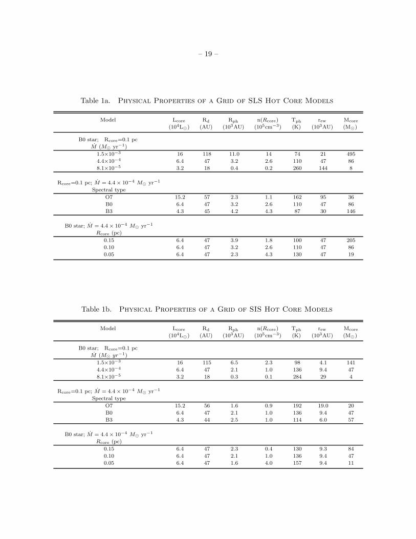
The summary of the physical properties of the SLS models is given in Table 1a and its general

trends are shown in Figure 1a. The top panel of Figure 1a shows the spectra obtained for three

different values of the mass accretion rate (M = 1.5 × 10−3, 4.4 × 10−4 and 8.1 × 10−5 M⊙ yr−1),

for a B0 central star with a radius R∗ = 4 × 1011 cm (Thompson 1984), and an envelope with an

external radius Rcore = 0.1 pc. As seen in the figure, the peak flux density increases and shifts to

longer wavelengths as the accretion rate increases. This behavior can be explained as a result of

the increase of the optical depth in the envelope, because of the overall density increase for higher

accretion rates. As a consequence of the increase in opacity, the flux tends to be redistributed

towards longer wavelengths, where the envelope is optically thinner, producing a shift of the peak

of the spectrum. This also has the effect of increasing the depth of the silicate absorption feature

at 10 µm. The total luminosity, Lcore, increases with the mass accretion rate because of the

increase in the accretion luminosity. This results in higher values of the peak flux density. Table 1a

shows that the photospheric radius increases and its temperature decreases with increasing mass

accretion rates.Again this is easily understood as a result of the overall density increase in the

envelope that moves the photospheric radius to outer (and thus cooler) regions, as the accretion

rate increases. Table 1a also indicates that the dust destruction radius, Rd, increases with the

accretion rate, since the central luminosity, Lcore, increases.

The middle panel of Figure 1a shows the spectra for different spectral types of the central

– 8 –

star (O7, B0 and B3), for an envelope with external radius of 0.1 pc, and an accretion rate of

4.4 × 10−4 M⊙ yr−1. The peak flux density of the spectrum shifts to longer wavelengths for later

spectral types. This happens because, for the models presented in this figure, Rcore < rew (see

column 7 in Table 1a), thus, the mass of the envelope is given by eqn. (3), where m(x) ∝ x1.84,

and x ∝ M−1∗ M2/3. Hence, the envelope mass is inversely proportional to the stellar mass, i.e.

Menv ∝ M−0.84∗ (see last column in Table 1a). Therefore, the opacity of the envelope increases for

later spectral types and the emission is redistributed towards longer wavelengths.

Finally, the bottom panel of Figure 1a illustrates the trends of the spectra for different

external radii of the envelope (Rcore = 0.15, 0.10 and 0.05 pc), for a central star with spectral type

B0 and an accretion rate of 4.4×10−4 M⊙ yr−1. As seen in the figure, the flux at long wavelengths

increases slightly, while it decreases slightly at short wavelengths, as the external radius increases.

This effect can be also understood as a consequence of the redistribution of the flux density to

longer wavelengths, because of the increase of the optical depth for larger external radii. Note

that, the photospheric radius increase with increasing external radii, as discussed in § 2.3.

The summary of the physical properties of the SIS models is given in Table 1b and its

general trends are shown in Fig 1b. The SIS models in each panel were computed with the same

parameters that the SLS models (see columns 1 and 2 in Tables 1a and 1b). As one can see from

Figures 1a and 1b, that the general behavior of the SIS models in each panel is the same the

SLS models. However, one can also see that the spectra resulting of the SIS models have smaller

millimeter fluxes and greater infrared fluxes than the SLS. This happens because the mass of the

SIS envelope, Menv = M(18GM∗)−1/2R

3/2core, is always smaller than that of the SLS envelope (see

last columns in Tables 1a and 1b). Thus, the SIS envelope is optically thinner and emits most of

the radiation at shorter wavelengths than the SLS envelopes.

In summary, the spectrum at all frequencies is very sensitive to the mass accretion rate;

infrared flux densities are sensitive to the spectral type of the central star, and the value of the

external radius has only a small effect on the spectrum for the parameters explored in Figures 1a

and 1b.

4. COMPARISON OF THE MODEL WITH OBSERVATIONS

To date, about 20 candidate HMCs have been proposed (Kurtz et al. 1999). In general, these

objects are associated with nearby or embedded FIR sources and/or UCHII regions. Thus, it is

very likely that the observed fluxes are contaminated by these nearby sources and overestimate

the actual contribution of the HMC, making it difficult to fit the intrinsic spectrum. For this

reason, we selected relatively isolated objects, and among them, those with the most complete

data sets available in order to constrain, as much as possible, the parameters of our model. With

these restrictions, we chose the sources: G34.24+0.13MM, W3(H2O), Orion hot core and IRAS

23385+6053 as a representative sample to test the model.

– 9 –

In order to match the sources, fits using both the SLS and SIS density distributions have

been considered. Figure 2 shows the observed fluxes of the source G34.24+0.13MM (H98)

and the results of three model spectra for HMCs with Rcore = 0.07 pc and a central B3

star with 10 M⊙. The dotted line corresponds to the SIS collapse density distribution with

M = 1.0 × 10−3 M⊙ yr−1, while the dot-dashed line corresponds to the SLS collapse density

distribution with M = 6.5 × 10−4 M⊙ yr−1. For both models we used a ZAMS stellar radius,

R∗ = 2.0 × 1011 cm (Thompson 1984). In order to match the observed fluxes at mm wavelengths,

massive envelopes with high accretion rates are required. In particular, for a given mass accretion

rate, the envelope is less massive for the SIS than the SLS, so one requires a higher mass accretion

rate, producing a flux density at 20 µm several orders of magnitude higher than the upper limit

on the flux at this wavelength (see discussion in § 3). The logatropic collapse model, on the other

hand, has a smaller excess emission at 20 µm which can be attenuated invoking a high external

extinction to the HMC, AV ∼ 100 mag. This value of the external extinction is somewhat high,

even though HMCs are found inside dense regions in molecular clouds. More generally accepted

values are AV ∼< 30 mag (e.g. Testi et al 1998).

The solid line in Figure 2 shows the spectrum of the SLS model discussed above, but for a star

of radius R∗ = 1012 cm, as discussed in § 2.5. Clearly, the excess of emission at 20 µm is reduced,

and now fits the constraint at 20 µm, with no external extinction required, since the accretion

luminosity decreases for this large stellar radius. Note that if this large stellar radius were used

for the SIS density distribution, one still requires AV > 100 mag to attenuate the excess emission

at 20 µm.

A similar result is found for the remaining sources, so, for these, we present only models for

a SLS collapse distribution. In addition, the central stars are assumed to have radii R∗ = 1012

cm, and any external extinction is neglected. It is likely that in reality, a combination of some

external extinction (AV ∼< 30 mag) plus a star with a radius larger than its ZAMS value, could

be responsible for the observed spectrum. Finally, similar trends, as those shown in Figure 1, are

found for these type of central stars with large radii.

4.1. G34.24 + 0.13MM

The source G34.24 + 0.13MM discovered by Hunter et al. (1998), is located 84′′ (1.5 pc)

southeast of the UCHII region G34.26 + 0.15, within the G34.3 + 0.2 HII region complex, which

is at a distance of 3.7 kpc (Kuchar & Bania 1994). H98 identified G34.24 + 0.13 MM as a massive

proto-stellar object, which coincides with a methanol maser. This source has upper limits on the

centimeter continuum emission of Sν ∼< 0.8 mJy at 15 GHz, and Sν ∼< 0.6 mJy at 8.3 GHz (Goss

1999, personal communication). From observations at 1.3 mm and 2.7 mm, H98 measured an

angular diameter of 2′′ (0.037 pc). They also obtained near-infrared images and photometry at

10 and 20 µm, but no infrared source was detected coincident with the millimeter position. H98

estimated a total luminosity in the range of 1600 - 6300 L⊙. These authors argue that because

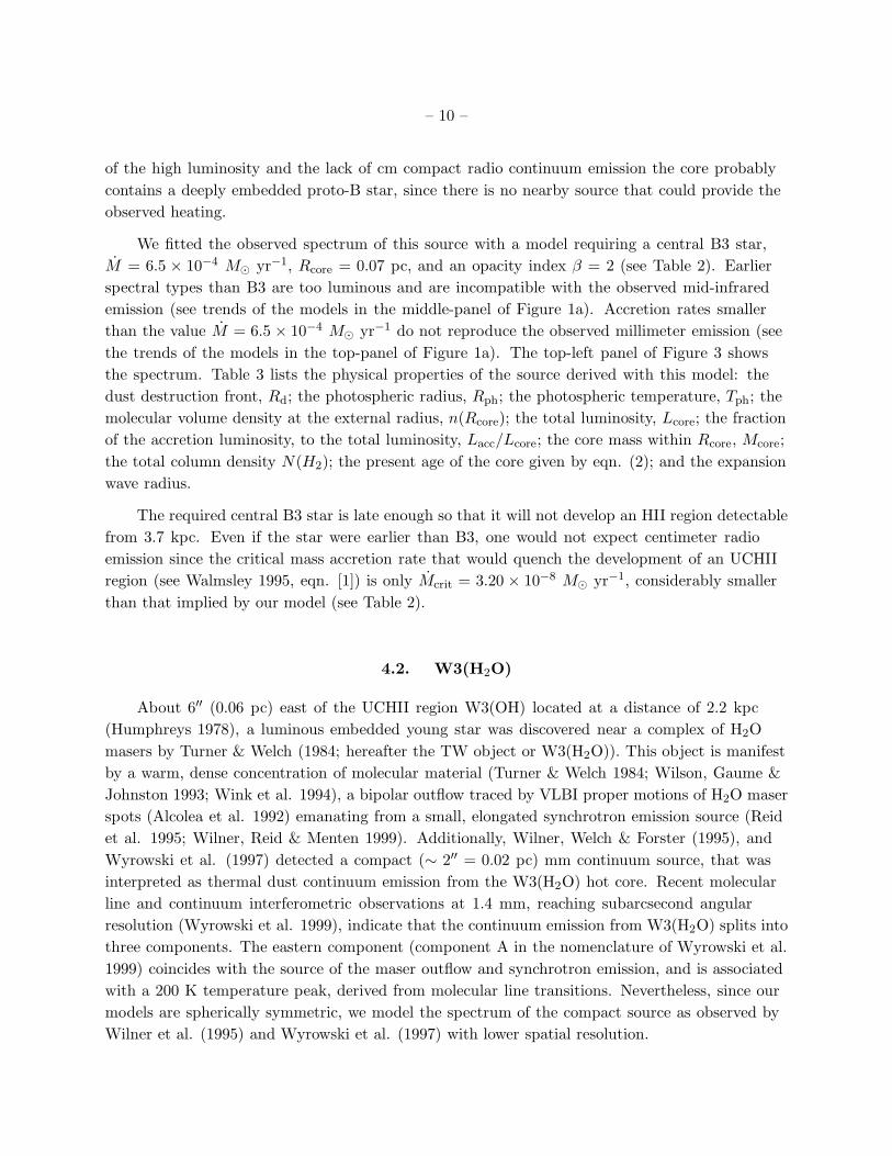
– 10 –

of the high luminosity and the lack of cm compact radio continuum emission the core probably

contains a deeply embedded proto-B star, since there is no nearby source that could provide the

observed heating.

We fitted the observed spectrum of this source with a model requiring a central B3 star,

M = 6.5 × 10−4 M⊙ yr−1, Rcore = 0.07 pc, and an opacity index β = 2 (see Table 2). Earlier

spectral types than B3 are too luminous and are incompatible with the observed mid-infrared

emission (see trends of the models in the middle-panel of Figure 1a). Accretion rates smaller

than the value M = 6.5 × 10−4 M⊙ yr−1 do not reproduce the observed millimeter emission (see

the trends of the models in the top-panel of Figure 1a). The top-left panel of Figure 3 shows

the spectrum. Table 3 lists the physical properties of the source derived with this model: the

dust destruction front, Rd; the photospheric radius, Rph; the photospheric temperature, Tph; the

molecular volume density at the external radius, n(Rcore); the total luminosity, Lcore; the fraction

of the accretion luminosity, to the total luminosity, Lacc/Lcore; the core mass within Rcore, Mcore;

the total column density N(H2); the present age of the core given by eqn. (2); and the expansion

wave radius.

The required central B3 star is late enough so that it will not develop an HII region detectable

from 3.7 kpc. Even if the star were earlier than B3, one would not expect centimeter radio

emission since the critical mass accretion rate that would quench the development of an UCHII

region (see Walmsley 1995, eqn. [1]) is only Mcrit = 3.20 × 10−8 M⊙ yr−1, considerably smaller

than that implied by our model (see Table 2).

4.2. W3(H2O)

About 6′′ (0.06 pc) east of the UCHII region W3(OH) located at a distance of 2.2 kpc

(Humphreys 1978), a luminous embedded young star was discovered near a complex of H2O

masers by Turner & Welch (1984; hereafter the TW object or W3(H2O)). This object is manifest

by a warm, dense concentration of molecular material (Turner & Welch 1984; Wilson, Gaume &

Johnston 1993; Wink et al. 1994), a bipolar outflow traced by VLBI proper motions of H2O maser

spots (Alcolea et al. 1992) emanating from a small, elongated synchrotron emission source (Reid

et al. 1995; Wilner, Reid & Menten 1999). Additionally, Wilner, Welch & Forster (1995), and

Wyrowski et al. (1997) detected a compact (∼ 2′′ = 0.02 pc) mm continuum source, that was

interpreted as thermal dust continuum emission from the W3(H2O) hot core. Recent molecular

line and continuum interferometric observations at 1.4 mm, reaching subarcsecond angular

resolution (Wyrowski et al. 1999), indicate that the continuum emission from W3(H2O) splits into

three components. The eastern component (component A in the nomenclature of Wyrowski et al.

1999) coincides with the source of the maser outflow and synchrotron emission, and is associated

with a 200 K temperature peak, derived from molecular line transitions. Nevertheless, since our

models are spherically symmetric, we model the spectrum of the compact source as observed by

Wilner et al. (1995) and Wyrowski et al. (1997) with lower spatial resolution.

– 11 –

We fit the spectrum of this source with a model requiring a central B0 star,

M = 1.2 × 10−3 M⊙ yr−1, Rcore = 0.05 pc, and an opacity index β = 1.6 (see Table 2).

Table 3 lists the physical properties of this model and the resulting spectrum is shown in the

upper right panel of Figure 3. Because of the few data points available for this source, the model

fit was not unique, and we selected the model solution with the spectral type of the central star

and the index of the opacity law in accordance with those inferred by Wyrowski et al. (1997,

1999). High angular resolution observations at mid- and far-infrared wavelengths are necessary to

constrain the total luminosity of this source, and the spectral type of the central star.

4.3. Orion hot core

Because of its proximity (D = 480 pc; Genzel et al. 1981), the most studied region of

high-mass star formation is the Orion molecular cloud (OMC-1). Line studies of the central

portion of OMC-1 (i.e., the Kleinmann-Low nebula) showed that it was separated into a number

of velocity components that were subsequently associated with several spatial components as

very high-resolution mapping became available (see Wright et al. 1996 and references therein).

Prominent at the center of this region is a dense condensation of gas and dust known as the

“Orion hot core” which has a gas density n(H2) ∼> 107 cm−3 and a temperature of 150-300 K (see

Kaufman et al. 1998 for references). Whether this source is heated either externally (Blake et al.

1996, Wright, Plambeck & Wilner 1996) or internally (Masson & Mundy 1988) is still a matter

of great debate. In addition, Chandler & Wood (1997) suggested that there is an HII region

associated with Radio Source “I”, located to the northwest of the hot core ( 2′′ away). This source

has been proposed to be the heating source of the Orion hot core. Nevertheless, as discussed in

§1, Kaufman et al. (1998) modeled the physical conditions in the Orion hot core, and concluded

that an internal energy source is more likely, since the Radio Source “I” is not luminous enough

to externally heat the core up to the observed temperatures. Although high resolution molecular

line and continuum studies have found evidence of substructure within the core (Migenes et al.

1989; Blake et al. 1996), we apply our spherically symmetric model as a first approximation to

this source.

The parameters of our best-fit model are: a mass accretion rate M = 1.1 × 10−3 M⊙ yr−1, a

B3 central star, an outer radius of the envelope Rcore = 0.025 pc, and an opacity index β = 1.6

(see Table 2). The mass accretion rate is determined mainly by the mm and submm data. The

spectral type of the star is constrained by the measured flux density at 30 µm (Wynn-Williams

et al. 1984), since an spectral type earlier than B3 would have too much flux at this wavelength.

Furthermore, the convolved image of the model at 1.3 mm has a FWHM of ∼ 3′′, as observed

by Blake et al. (1996; Figure 2, top panel). The total luminosity given by our model is

Lcore = 2.5 × 104 L⊙, being most of this due to the accretion. It is worth noting that this value

exceeds the minimum luminosity required by the models of Kaufman et al. (1998) to explain the

observed high temperature in the Orion hot core.

– 12 –

4.4. IRAS 23385+6053

IRAS 23385+6053 has a quite broad data set available, spanning from centimeter to near

infrared wavelengths (see M98). No emission is detected at centimeter wavelengths above 3-σ

level of ∼ 0.5 mJy. At 3.4 mm, M98 detected a compact source with a deconvolved angular size

of 4.′′5 × 3.′′6 (or 0.048 pc for an assumed distance of 4.9 kpc). They estimated a bolometric

luminosity for this source L ∼ 1.6 × 104 L⊙. They also detected a compact outflow in SiO and

HCO+ lines that is centered on the millimeter source.

In order to explain the lack of a detectable HII region associated with this source, M98

consider two possibilities: a heavily obscured B0 star with residual accretion, or a proto-star

undergoing very intense accretion with M = 10−3M⊙ yr−1. For the latter case, using the

relation found by Stahler et al. (1986), discussed in §2.5, they proposed a central proto-star with

M∗ = 39 M⊙ and R∗ = 70 R⊙, and assumed that the observed luminosity is dominated by the

accretion luminosity.

Our best-fit (model I) to the observed spectrum is shown in the lower right panel of Figure

3 and upper left panel of Figure 4. This model I (whose parameters are given in Table 2) has a

central B2 star, an accretion rate of 10−3 M⊙ yr−1, an external radius Rcore = 0.1 pc, and an

opacity index β= 1.6. The physical properties of this model are given in Table 3. The lower left

panel of Figure 4 shows the intensity profile at 3.4 mm predicted by our model and the observed

intensity profiles along the major and minor axes of the 3.4 mm map given in Figure 1 of M98

(dot-dashed line). As can be seen in the figure, the agreement is very good. The intensity profile

of the model was obtained by convolving (in two dimensions) the intensity distributions at 3.4

mm given by the model with a Gaussian beam of FWHM = 3.′′8 (corresponding to the size of the

beam in the observations of M98). Note that no fit was done to the observed intensity profile at

3.4 mm; only the observed flux densities (that are integrated values, with no information on the

spatial distribution) were fitted with a model spectrum (upper panel of Fig. 4). It is remarkable

that the predicted 3.4 mm model intensity profile, obtained from the parameter set that provide

the best-fit to the spectrum, is in such a good agreement with the observed intensity profile (lower

panel of Fig. 4).

The right panels of Figure 4 shows the predictions for an alternative HMC model, similar to

the one proposed by M98 (model II), namely a core with a central proto-star with M∗ = 39 M⊙,

R∗ = 70 R⊙, and Lcore = Lacc. This model has M = 1.6 × 10−3M⊙ yr−1, Rcore = 0.19 pc and

β = 2. Even though the observed spectrum can be fitted by this model, the predicted intensity

profile at 3.4 mm is too broad and its peak intensity is too low to be detectable above the rms noise

of the map (see lower right panel in Fig. 4). This difference is due the large value of Rcore, with

respect to that of Model I. Therefore, this model appears to be in conflict with the observations.

We conclude that a B2 star is most likely embedded in the IRAS 23385+6053 core, as indicated

by model I (Table 2 and 3 and left panel of Fig 4).

– 13 –

4.5. Temperature Profiles of HMC models

Figure 5 shows the temperature profiles for the models presented in Figure 3 (from Rd

to Rcore). The different sources are labeled in each panel. These temperature profiles are

discontinuous at the photospheric radius, Rph, because the dilution factor, W (Rph) = 1/2, and,

in our approximation, eqn. (5) then gives T < Tph at this radius. Instead, there should be a

smooth transition between the optically thin and the optically thick regimes and hence a smooth

temperature profile. With our simplified treatment for the temperature profile, the difference

between the total luminosity of the spectra of model and the input luminosity, Lcore, is less than

15 - 20 %. It can be seen that the temperature distributions in the optically thick region have

a steeper dependence with radius than in the optically thin region, as discussed by Adams &

Shu (1985) and Kenyon et al. (1993). Finally, for all cases, at the external radius, Rcore, the

temperatures are T > 30K.

5. DISCUSSION

5.1. General Discussion

The model studied here, of an envelope infalling onto a central massive star, reproduces

very well the currently available observational data for the sources selected in our sample. We

have explored two possible density distributions for the structure of the infalling envelope and

concluded that a SLS collapse density distribution provides a better agreement with the available

observational data, than a SIS density distribution. In order to fit the observations of these

sources, our model requires massive, early B-type central stars (10-16 M⊙), with high values of the

mass accretion rate (∼ 10−3 M⊙ yr−1), and core radii ∼< 0.1 pc. The values of the mass accretion

rate obtained exceed by a large factor the “critical” value required to quench the development of

a detectable UCHII region, which for an early B-type central star (the proposed central stars), is

∼< 10−7 M⊙ yr−1. Therefore, the model lacks a detectable HII region. Furthermore, very small

flux densities from dust thermal emission are predicted at centimeters wavelengths.

The values that we have obtained for the radius of the cores are roughly consistent with those

inferred from the observations. However, a detailed comparison is not yet possible, since most of

the observations give only upper limits for the source sizes. Only in the case of the 3.4 mm map

of IRAS 23385+605 (M98), was it possible to compare the intensity distribution predicted by the

model with that observed, and we found a remarkably good agreement with the observed total

flux, source size and peak intensity. Additional maps of good S/N and high angular resolution

are required for a larger number of sources and wavelengths. In this manner, continuum intensity

profiles may be able to discriminate between possible models. Similarly, high angular resolution

FIR images are needed. Our model predicts a peak flux density > 103 Jy at ∼ 100 µm. Thus,

infrared fluxes around this wavelength, obtained with higher angular resolution than currently

– 14 –

available to avoid contamination with nearby objects, would be specially relevant in order to

further constrain the parameters of the modeled sources.

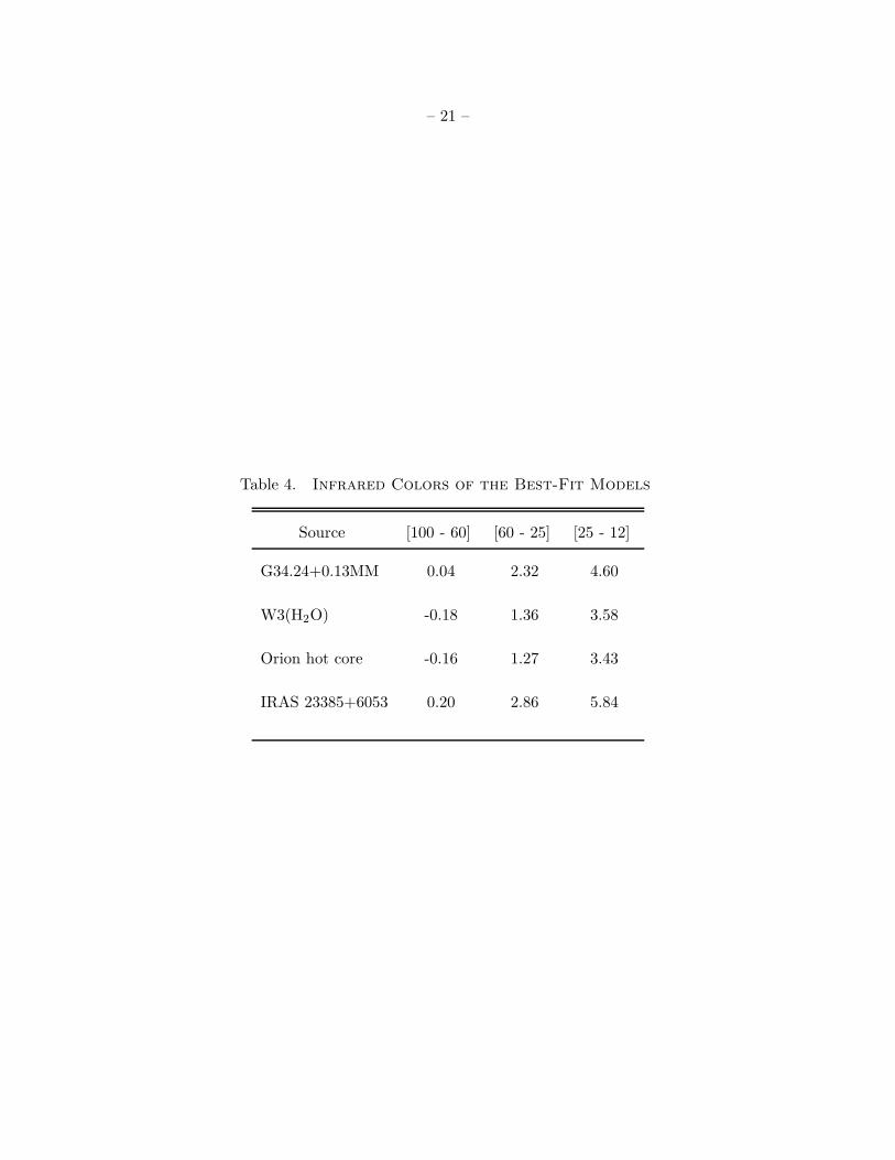
The intrinsic infrared colors [100-60], [60-25] and [25-12] predicted by our models (see Table

4) are very different from those of observed UCHII regions, [100-60]=0.26, [60-25]=0.87, and

[25-12]=0.91 (Wood & Churchwell 1989). In particular, a color criterion [60-25] > 1.3 could be use

to find isolated HMCs, when their fluxes are not contaminated by nearby sources.

Furthermore, for all the sources, the accretion luminosity clearly exceed, the stellar luminosity

(see Table 3). This result points out the relevance of the energy released in the accretion process

at this early evolution stage, a basic ingredient that should not be ignored when modeling this

kind of object.

5.2. Radiation Pressure Onto Dust Grains

The radiation pressure onto dust grains imposes an upper limit to the amount of mass that

can accrete onto a massive star. It is therefore important to assess whether or not this effect can

halt the collapse of the envelopes that we consider in our models. Kahn (1974) found that the

radiation pressure of the diffuse infrared radiation field inside a dusty envelope around a massive

proto-star decelerates the flow allowing a maximum luminosity to mass ratio L/M∗ = 5436 L⊙/M⊙,

although this number depends on the properties of the dust grains. Wolfire & Cassinelli (1987;

hereafter WC87) revised the calculations of the maximum mass that an accreting proto-star can

accumulate taking into account updated properties of the interstellar grains. Jijina & Adams

(1996) reexamined this problem including the effect of angular momentum. In this section, we

ensure that our models of hot cores fulfill the general constraint that guarantee that inflow will

proceed towards the central proto-star.

At the outer boundary of the inflow, the outward radiative acceleration must be less than the

inward gravitational acceleration of the gas. This condition can be written as (WC87, eqn. [10])

Γ =κpr

H Lcore

4πcGM(Rcore)< 1, (8)

where κprH is the flux mean radiation pressure coefficient, c is the speed of the light, M(Rcore) is

the total mass inside Rcore (star plus core mass), and Lcore = L∗ + Lacc is the total luminosity

available to heat and push the core material. Our models have Lcore ∼< 6 × 104 L⊙, typical core

masses M(Rcore) ∼ 130 M⊙, and we approximate the flux mean opacity with the dust Planck

mean opacity evaluated at the photospheric temperature. The photospheric temperatures we find

are Tph ∼ 100 K, therefore, κP ∼ 2 cm2 g−1. For this range of values

Γ = 0.07

(

κP

2 cm2 g−1

) (

Lcore

6 × 104 L⊙

) (

M(Rcore)

130 M⊙

)−1

< 1, (9)

– 15 –

and the fluid at the outer boundary can flow inward.

On the other side, at the dust destruction front, Rd, where the direct stellar radiation is

absorbed, the momentum rate of the flow must be greater or equal to the pressure of the stellar

radiation field

M ≥L

udc, (10)

where ud is the velocity of the flow at the dust destruction front, Rd. This condition is satisfied for

our model (M∗ ∼ 10 − 16 M⊙, M ∼ 6 × 10−4 − 10−3 M⊙ yr−1) as can be seen in Fig. 5 of WC87.

Their figure also shows that our cores have less than the Eddington luminosity, LEdd, where the

accretion is halted by radiation pressure on free electrons with an opacity given by Thompson

scattering.

Considering an optically thick dusty cocoon plus an optically thin envelope, and assuming

an analytic form for the Rosseland mean opacity χR = χR0(T/Ts)2, Kahn (1974) obtained the

maximum luminosity to mass ratio L/M∗ = 5436 L⊙/M⊙, mentioned above. His eqn. [65] implies

that this ratio is inversely proportional both to the cube of the dust sublimation temperature,

T 3sub, and to χR0, the Rosseland mean opacity for radiation at a color temperature Ts = 22, 000 K.

Kahn used Tsub = 3675 K and χR0 = 600 cm2 g−1. We find that the sublimation temperature

for the grain mixture in our models (see §2.4) is Tsub ∼ 1200 K. Also, the value of χR0 must be

increased by a factor of ∼ 8 to agree with our value for the Rosseland mean opacity at T ∼ 1000

K. These modifications, due to the currently accepted properties of the standard grain mixture

used in this work, imply that the maximum luminosity to mass ratio derived by Kahn would

currently be L/M∗ ∼ 20, 000 L⊙/M⊙. This result contrasts with the detailed modeling of the dust

destruction process carried out by WC87. They found that very massive stars can only be formed

with modifications of the standard MRN grain mixture for accretion onto massive stars with M∗ =

60, 100 and 200 M⊙, in which the luminosity to mass ratios are larger than L/M∗ = 8974 L⊙/M⊙.

On the other hand, Jijina & Adams (1996) found that the maximum luminosity to mass ratio is

less restrictive for a rotating collapse than for the spherical infall. In any case, all our models have

luminosity to mass ratios Lcore/M∗ < 4300 L⊙/M⊙, which implies that accretion can continue

onto the central star.

We therefore consider that radiation pressure onto dust grains will not stop the accretion flow

onto the central proto-star for the modeled HMCs discussed in this work. For simplicity, we have

not considered any deviations of the flow from the dynamics of a logatropic collapsing core.

5.3. End of the Accretion Phase

The luminosity to mass ratios of the modeled HMCs discussed in this work are high but still

remain below the critical ratios for radiation pressure onto dust grains needed to halt the accretion

– 16 –

(see §5.2). Nevertheless, this ratio, given by

Lcore

M∗

=L∗

M∗

+GM∗

R∗

, (11)

will increase with time both because the luminosity of the central star increases with time, and

because the mass accretion rate increases as M ∝ t3 (eqn. [1]) in the logatropic model. Therefore,

radiation pressure could eventually halt the collapse of matter onto the central star. This is only

a transient process since, as the accretion is shut off, so is the accretion luminosity, an important

contributor to the total luminosity. Thus, one is tempted to speculate that, if a stellar wind can

turn on after the flow is impulsively reversed, the wind could help clear out the accreting flow. An

HII region can then be produced, although in this scenario its evolution would be governed by the

reversal of the accretion flow, a complex problem worth studying in detail.

If this process occurs on a short time scale compared to the accretion time scale, one can make

a simple estimate of the final masses of the central stars inside the HMCs when the accretion flow

is halted by radiation pressure. We assume a main sequence mass-luminosity relation, L∗ ∝ M3∗ ,

and mass-radius relation, R∗ ∝ M0.73∗ (e.g. Bowers & Deeming 1984), even though, as discussed in

§ 2.5, it is not clear if these relations hold for massive stars formed under intense accretion rates

which increase steeply with time, considered in this work. Figure 6 shows the luminosity to mass

ratio as function of the dimensionless time t/tage, where tage is the present age of the HMC (solid

line). We have assumed a 12.6 M⊙ central star and a mass accretion rate M = 1× 10−3 M⊙ yr−1,

at the dimensionless time t/tage = 1. These values correspond to the model for IRAS 23385+6053

which has tage = 5 × 104 yr (see Tables 2 and 3). The dot-dashed line is the stellar contribution

to the luminosity to mass ratio and the dashed line is the accretion contribution to this ratio.

The triangles show the mass of the central star (M∗ ∝ t4, see eqn. [1]) labeled on the right

hand vertical axis. Independently of the exact critical value for the luminosity to mass ratio for

radiation pressure to halt the accretion flow (see discussion in §5.2), this figure shows that the

evolution of this ratio is very fast so one would expect that in less than 105 yr the accretion of

mass onto the central star of the HMC should stop and an ultracompact HII region should develop

inside these cores.

Finally, if all OB stars are formed within HMCs under high accretion rates, one can estimate

the expected number of HMCs in this phase. Taking the rate of formation of O stars in the

Galaxy N ∼ 1/300 yr−1 (Wood & Churchwell 1989), and the time in the HMC phase when the

central star is a late B star, ∆t ∼ 105 yr, one should expect to find ∼ 300 HMCs at the present

time. On the other hand, the period of time that a core contains an early O star is very small,

∆t ∼< 2×104 yr, so less than 60 HMCs with very luminous massive stars inside should be expected.

The number of expected HMCs can increase by a factor of 10 if a higher star formation rate of O

stars, ∼ 4 × 10−2 yr−1 (Gusten & Mezger 1983), is used.

– 17 –

6. CONCLUSIONS

Our main results can be summarized as follows:

1. The observed spectra of several HMCs (G34.24 + 0.13MM, W3(H20), the Orion hot core and

IRAS 23385+6053) can be reproduced by massive envelopes accreting onto young massive

central stars. In order to fit the available data, we require early B-type stars with high mass

accretion rates, M ∼> 6 × 10−4M⊙ yr−1, and time-scales tage ∼< 105 yr. The main heating

agent is the accretion luminosity (Lacc > L∗; see Table 3).

2. The spectra are strongly dependent on the assumed envelope density profile. Isothermal

collapsing envelopes have less mass in the envelope for a given mass accretion rate, with

respect to the logatropic collapsing envelopes. Therefore, they require very high accretion

rates (> 10−3M⊙ yr−1) in order to reproduce the observed millimeter emission. Nevertheless,

high accretion rate SIS models predict strong mid-infrared emission which is, in general, not

observed.

3. Models of the structure of massive stars formed under intense mass accretion rates that

increase with time, discussed in this work, are necessary to determine the characteristics

(e.g. radius, intrinsic luminosity) of this type of object. In particular, we have used central

stars with radii larger than the ZAMS radii in order to avoid excess fluxes at mid infrared

wavelengths with respect to those observed.

4. High angular resolution mid and far IR observations (which avoid contamination by nearby

massive stars) are crucial to constrain the total luminosity of the HMCs.

5. The critical mass accretion rate required to quench the development of an UCHII region is

very small compared to the accretion rates required by all the HMC models studied here.

Therefore, at this stage the HMCs have no detectable HII region.

6. We speculate that when a critical luminosity to mass ratio is achieved, the infall will be

halted by a powerful stellar wind and a detectable UCHII region can appear.

We are greatly indebted with Javier Ballesteros, Marıa Eugenia Contreras, and Rosa Izela

Dıaz-Miller with whom we originally discussed the work presented here. We also thank Guillem

Anglada, Riccardo Cesaroni, Guido Garay, William Henney, Stan Kurtz, Sergio Molinari, Luis F.

Rodrıguez, Leonardo Testi, Malcom Walmsley and Alan Watson for useful discussions and helpful

suggestions. We thank Leonardo Testi for providing us the original data for IRAS 23385+6053.

Thanks too to Robert Estalella for providing a program to convolve our results with the observing

beam. M. O., S. L. and P. D. acknowledge support from DGAPA/UNAM and CONACYT. S.

L. also acknowledges support from the Simon Guggenheim Memorial Foundation. M. O. also

– 18 –

acknowledges partial support from the Programa de Cooperacion Cientıfica con Iberoamerica

(Spain).

– 19 –

Table 1a. Physical Properties of a Grid of SLS Hot Core Models

Model Lcore Rd Rph n(Rcore) Tph rew Mcore

(104L⊙) (AU) (103AU) (105cm−3) (K) (103AU) (M⊙)

B0 star; Rcore=0.1 pc

M (M⊙ yr−1)

1.5×10−3 16 118 11.0 14 74 21 495

4.4×10−4 6.4 47 3.2 2.6 110 47 86

8.1×10−5 3.2 18 0.4 0.2 260 144 8

Rcore=0.1 pc; M = 4.4 × 10−4 M⊙ yr−1

Spectral type

O7 15.2 57 2.3 1.1 162 95 36

B0 6.4 47 3.2 2.6 110 47 86

B3 4.3 45 4.2 4.3 87 30 146

B0 star; M = 4.4 × 10−4 M⊙ yr−1

Rcore (pc)

0.15 6.4 47 3.9 1.8 100 47 205

0.10 6.4 47 3.2 2.6 110 47 86

0.05 6.4 47 2.3 4.3 130 47 19

Table 1b. Physical Properties of a Grid of SIS Hot Core Models

Model Lcore Rd Rph n(Rcore) Tph rew Mcore

(104L⊙) (AU) (103AU) (105cm−3) (K) (103AU) (M⊙)

B0 star; Rcore=0.1 pc

M (M⊙ yr−1)

1.5×10−3 16 115 6.5 2.3 98 4.1 141

4.4×10−4 6.4 47 2.1 1.0 136 9.4 47

8.1×10−5 3.2 18 0.3 0.1 284 29 4

Rcore=0.1 pc; M = 4.4 × 10−4 M⊙ yr−1

Spectral type

O7 15.2 56 1.6 0.9 192 19.0 20

B0 6.4 47 2.1 1.0 136 9.4 47

B3 4.3 44 2.5 1.0 114 6.0 57

B0 star; M = 4.4 × 10−4 M⊙ yr−1

Rcore (pc)

0.15 6.4 47 2.3 0.4 130 9.3 84

0.10 6.4 47 2.1 1.0 136 9.4 47

0.05 6.4 47 1.6 4.0 157 9.4 11

– 20 –

Table 2. Model Parameters Determined from Spectral Fits to Individual Sources

Source Ma∗ Lb

∗ M Rcore β Dc

(M⊙) (L⊙) (M⊙ yr−1) (pc) (kpc)

G34.24+0.13MM 10.0 1.0×103 6.5×10−4 0.07 2.0 3.7

W3(H2O) 15.8 2.5×104 1.2×10−3 0.05 1.6 2.2

Orion Hot Core 10.0 1.0×103 1.1×10−3 0.02 1.6 0.5

IRAS 23385+6053 12.6 2.8×103 1.0×10−3 0.10 1.6 4.9

a R∗ = 1012 cm is assumed.

b Taken from Thompson (1984), for a given M∗.

c The adopted distances are taken from Kuchar & Bania 1994, Humphreys

1978, Genzel et al. 1981, and Molinari et al. 1998.

Table 3. Physical Properties of Best-Fit Models to Individual HMCs

Source Rd Rph Tph n(Rcore) Lcore Lacc/Lcore Mcore N(H2) tage rew

(AU) (103 AU) (K) (106 cm−3) (104 L⊙) (%) (M⊙) (1024 cm−2) (104 yr) (103 AU)

G34.24+0.13MM 35 3.8 72 1.0 1.6 94 131 34 6.1 20

W3(H2O) 74 5.3 87 2.0 6.7 62 83 48 5.3 24

Orion hot core 52 3.2 88 5.0 2.5 96 27 55 3.7 16

IRAS 23385+6053 54 7.0 62 1.1 3.1 91 382 47 5.0 21

– 21 –

Table 4. Infrared Colors of the Best-Fit Models

Source [100 - 60] [60 - 25] [25 - 12]

G34.24+0.13MM 0.04 2.32 4.60

W3(H2O) -0.18 1.36 3.58

Orion hot core -0.16 1.27 3.43

IRAS 23385+6053 0.20 2.86 5.84

– 22 –

REFERENCES

Alcolea, J., Menten, K. M., Moran, J. M. & Reid, M. J. 1992, in Astrophysical Masers, ed. A. W.

Clegg & G. E. Nedoluha (Berlin: Springer-Verlag), 225

Adams, F. C., Lada, C. J. & Shu, F. H. 1987, ApJ, 312, 788

Adams, F. C., & Shu, F. H. 1985, ApJ, 296, 655

Adams, F. C., & Shu, F. H. 1986, ApJ, 308, 836

Beech, M., & Mitalas, R. 1994, ApJS, 95, 517

Bernasconi, P. A. & Maeder, A. 1996, A&A, 307, 829

Blake, G. A., Mundy, L. G., Carlstrom, J. E., Padin, S., Scott, S. L., Scoville, N. Z., & Woody, D.

P. 1996, ApJ, 472, L49

Bowers, R., & Deeming, T. 1984, Astrophysics I, Stars (Boston: Jones and Bartlett Publishers,

Inc.)

Cesaroni, R., Churchwell, E., Hofner, P., Walmsley, C. M.& Kurtz, S. 1994a, A&A, 288, 903

Cesaroni, R., Olmi, L., Walmsley, C. M., Churchwell, E.& Hofner, P. 1994b, ApJ, 435, L137

Chandler, C. J.& Wood, D. O. S. 1997, MNRAS, 287, 445

D’Alessio, P. 1996, Ph.D. Thesis, Universidad Nacional Autonoma de Mexico

Genzel, R., & Stutzki, J. 1989, ARA&A, 27, 41

Genzel, R., Reid, M.J., Moran, J.M., & Downes, D. 1981, ApJ, 244, 884

Gomez, Y., Garay, G., & Lizano, S. 1995, ApJ453, 727

Gusten, R., & Mezger, P. G. 1983 Vistas in Astronomy, 26, 159

Hofner, P., Kurtz, S., Churchwell, E., Walmsley, C. M., & Cesaroni, R. 1996, ApJ, 460, 359

Hunter, T. R., Neugebauer, G., Benford, D. J., Matthews, K., Lis, D. C., Serabyn, E., & Phillips,

T. G. 1998, ApJ, 493, L97 (H98)

Humphreys, R. M. 1978, ApJS, 38, 309

Jijina, J., & Adams, F. C. 1996, ApJ, 462, 874

Kahn, F. D. 1974, A&A, 37, 149

Kaufman, M. J., Hollenbach, D. J. & Tielens, A.G.G.M. 1998, ApJ, 497, 276

Kenyon, S., Calvet, N., & Hartmann, L. 1993, ApJ, 414, 676

Kuchar, T. A., & Bania, T. M. 1994, ApJ, 436, 117

Kurtz, S., Cesaroni, R., Churchwell, E., Hofner, P., & Walmsley, C. M. 1999, in Protostars &

Planets IV, ed. V. Mannings, A. P. Boss, & S. S. Russell (Tucson: Univ. of Arizona Press),

in press.

Lamy, Ph. L. 1974, A&A, 35, 197

– 23 –

Lizano, S., & Shu, F. H. 1989, ApJ, 342, 834

Mathis, J. S., Rumpl, W., & Nordsieck, K. H. 1977, ApJ, 217, 425

Masson, C. R., & Mundy, L. G. 1988, ApJ, 324, 538

McLaughlin, D. E.,& Pudritz, R. E. 1996, ApJ, 469, 194

McLaughlin, D. E.,& Pudritz, R. E. 1997, ApJ, 476, 750

Mezger, P. G., Wink, J. E., & Zylka, R. 1990, A&A, 228, 95

Migenes, V., Johnston, K. J., Pauls, T. A., & Wilson, T. L. 1989, ApJ, 347, 294

Mihalas, D. 1978, Stellar Atmospheres (New York: Freeman, 2nd edition)

Molinari, S., Testi, L., Brand, J., Cesaroni, R., & Palla, F. 1998, ApJ, 505, L39 (M98)

Murata, Y., Kawabe, R., Ishiguro, M., Hasegawa, T., & Hayashi, M. 1991, in IAU Symp. 147,

Fragmentation of Molecular Clouds and Star Formation, ed. E. Falgarone, F. Boulanger, &

G. Duvert (Dordrecht: Kluwer), 357

Myers, P. C.,& Fuller, G. A. 1992, ApJ, 396, 631

Reid, M. J., Argon, A. L., Masson, C. R., Menten, K. M. & Moran, J. M. 1995, ApJ, 443, 238

Sandford, S. A. & Allamandolla, L. J. 1993, ApJ, 417, 815

Shu, F. H. 1977, ApJ, 214, 488

Stahler, S. W., Shu, F. H., & Taam, R. E. 1980, ApJ, 241, 637

Stahler, S. W., Palla, F., & Salpeter, E. E. 1986, ApJ, 302, 590

Testi, L., Felli, M., Persi, P., & Roth, M. 1998, A&A, 329, 233 (T98)

Thompson, R. I. 1984, ApJ, 283, 165

Turner, J. L. & Welch, W. J. 1984, ApJ, 287, L81

Vacca, W. D., Garmany, C. D. & Shull, J. M. 1996, ApJ, 460, 914

Walmsley, C. M. 1995, RevMexAA Serie de Conf., 1, 137

Wilner, D. J., Welch, W. J. & Forster, J. R. 1995, ApJ, 449, L73

Wilner, D. J., Reid, M. J. & Menten, K. M. 1999, ApJ, 513, 775

Wilson, T. L., Gaume, R. A. & Johnston, K. J. 1993 ApJ, 402, 230

Wink, J. E., Duvert, G., Guilloteau, S., Gusten, R., Walmsley, C. M. & Wilson, T. L. 1994, A&A,

281, 505

Wolfire, M. G., & Cassinelli, J. P. 1987, ApJ, 319, 850 (WC87)

Wood, D. O. S. & Churchwell, E. 1989, ApJ, 340, 265

Wright, M. C. H., Sandell, G., Wilner, D. J. & Plambeck, R. L. 1992, ApJ, 393, 225

Wright, M. C. H., Plambeck R. L. & Wilner, D. J. 1996, ApJ, 469, 216

– 24 –

Winn-Williams, C. G., Genzel, R., Becklin, E. E., & Downes, D. 1984, ApJ, 281 172

Wyrowski, F., Hofner, P., Schilke, P., Walmsley, C. M., Wilner, D. J. & Wink, J. E. 1997, A&A,

320, L17

Wyrowski, F., Schilke, P., Walmsley, C. M., & Menten, K. 1999, ApJ, 514, L43

Yorke, H. 1984, Workshop on Star Formation, ed. R. D. Wolstencroft (Edinburgh: Royal

Observatory), p. 63

This preprint was prepared with the AAS LATEX macros v4.0.

– 25 –

Fig. 1.— (a) Spectra for different sets of the SLS collapse density distribution HMC models. The

top panel shows the trends of the spectra obtained for three different values of the mass accretion

rate, for a B0 central star and an external radius Rcore = 0.1 pc. The middle panel shows models

with different spectral types of the central star, for a given external radius Rcore = 0.1 pc and

accretion rate of M = 4.4×10−4 M⊙ yr−1. The bottom panel shows models with different external

radii of the envelope, for a central B0 star and an accretion rate M = 4.4 × 10−4 M⊙ yr−1. (b)

Same as 1(a) but for the SIS collapse density distribution HMC models. In all cases, a distance of

4.9 kpc were adopted.

Fig. 2.— Observed flux densities of the source G34.24+0.13MM (Hunter et al. 1998; Goss 1999,

personal communication). Three modeled spectra with Rcore = 0.07 pc and a central B3 star

(10 M⊙) are also shown. The dotted line corresponds to the collapse density distribution of the

SIS, with M = 1.0 × 10−3 M⊙ yr−1, and the dot-dashed line corresponds to the collapse density

distribution of the SLS, with M = 6.5 × 10−4 M⊙ yr−1, when ZAMS radii are adopted. The solid

line shows the spectrum of the SLS model but with a star that has a large radius, R∗ = 1012 cm.

Fig. 3.— Observed flux densities for the sources G34.24+0.13MM (Hunter et al. 1998; Goss 1999,

personal communication), W3(H2O) (Wyrowski et al. 1997; Wilner et al. 1995), Orion hot core

(Wright et al. 1992; Murata et al. 1991; Masson et al. 1985; Mezger et al. 1990; The fluxes and

errorbars at 30 µm and 1.3 mm was estimated from the maps of Wynn-Williams et al. 1984 and

Blake et al. 1996, respectively), and IRAS 23385+6053 (Molinari et al. 1998; IRAS-PSC2), and

model spectra. The parameters of each model are listed in Table 2.

Fig. 4.— Observed flux densities (Molinari et al. 1998; IRAS-PSC2) and two models for the source

IRAS 23385+6053. The upper left panel shows the spectrum for a model I, with B2 central star,

M = 10−3 M⊙ yr−1, Rcore = 0.1 pc, and β = 1.6. The lower left panel shows the intensity profile

of the 3.4 mm emission given by the model (solid line) and the observed intensity profiles along the

major and minor axes of the 3.4 mm map given in Fig. 1 of M98 (dot-dashed lines). The upper

right and lower right panels correspond to model II with M = 1.6× 10−3 M⊙yr−1, Rcore = 0.19 pc,

and β = 2, and a central proto-star with M∗ = 39 M⊙ and R∗ = 70 R⊙ (for this model, Lcore = Lacc

and L∗ is neglected)

Fig. 5.— Temperature profiles in the range Rd < r < Rcore, for the models shown in Figure 3.

The different sources are labeled in each panel. The parameters of each model are given in Table 2.

The dust destruction radius, Rd, the photospheric radius, Rph, and the photospheric temperature,

Tph, for each source are given in Table 3.

Fig. 6.— Luminosity to mass ratio as function of the dimensionless time t/tage (solid line). The dot-

dashed line is the stellar contribution to this ratio and the dashed line is the accretion contribution.

The triangles show the mass of the central star, labeled on the right hand vertical axis.