Statistical Analyses of Massive Stars andStellar Populations

Dissertationzur

Erlangung des Doktorgrades (Dr. rer. nat.)der

Mathematisch-Naturwissenschaftlichen Fakultätder

Rheinischen Friedrich-Wilhelms-Universität Bonn

vorgelegt vonFabian Schneider

ausDuisburg

Bonn 2014

Angefertigt mit Genehmigung der Mathematisch-Naturwissenschaftlichen Fakultät der Rheini-schen Friedrich-Wilhelms-Universität Bonn

1. Gutachter: Prof. Dr. Norbert Langer2. Gutachter: Prof. Dr. Robert G. Izzard

Tag der Promotion:Erscheinungsjahr:

I, a universe of atoms,an atom in the universe.

(Richard P. Feynman)

Abstract

Massive stars, i.e. stars more massive than about ten times that of the Sun, are key agents inthe Universe. They synthesise many of the chemical elements that are so important for lifeon Earth, helped reionising the early Universe and end their lives in spectacular supernovaexplosions that are visible out to large distances. Because of their important role for muchof astrophysics, accurate and reliable stellar evolution models are essential. However, recentdevelopments regarding wind mass loss rates, internal mixing processes and duplicity seriouslychallenge our understanding of massive stars and stellar populations.It is now established that most, if not all, massive stars reside in binaries or higher order

multiple systems such that more than two-thirds of all massive stars are expected to interactthrough mass transfer with a binary companion during their lives. We investigate the conse-quences of this finding for coeval stellar populations and show that the most massive stars instar clusters are likely all rejuvenated binary products that may seriously bias the determinationof cluster ages. We further find that wind mass loss from stars and binary mass transfer leavetheir fingerprints in the high mass end of stellar mass functions. Using these fingerprints, we areable to age-date the young Arches and Quintuplet star clusters with far reaching consequencesfor the stellar upper mass limit that we revise to be in the range 200–500 M. Such an uppermass limit would allow for pair-instability supernovae in the local Universe.Large spectroscopic surveys such as the VLT-FLAMES Tarantula Survey (VFTS) deliver

many atmospheric parameters of hundreds of massive stars that are ideal to probe and calibratethe physics used in stellar models. To make use of such data, we develop the Bayesian codeBonnsai and make it available through a web-interface. With Bonnsai we are able to matchall available observables of stars including their uncertainties simultaneously to stellar modelsto determine fundamental stellar parameters like mass and age while taking prior knowledgesuch as initial mass functions into account. A key aspect of Bonnsai is that it allows us toidentify stars that cannot be reproduced by stellar models. We use Bonnsai to test the MilkyWay stellar models of Brott et al. (2011) with eclipsing binaries and find good agreement.We further use Bonnsai in combination with data from the VFTS to study the massive O

and WNh stars in one of the largest starburst regions known to date, 30 Doradus. In particularwe investigate their age distributions to learn about their formation history. The VFTS starsin our sample are mostly found outside clusters and associations and we do not find spatiallycoherent age patterns. The stars either formed continuously over the 30 Doradus field or inclusters and associations from where they were ejected to their current positions. The agedistributions of our sample stars are consistent with the existence of at least two to four coevalstellar populations which would imply that most of the VFTS stars in our sample formed inclusters and associations.

v

Contents

Contents ix

1 Introduction 11.1 Towards a modern picture of stellar evolution . . . . . . . . . . . . . . . . . . . . 21.2 Modern massive star evolution . . . . . . . . . . . . . . . . . . . . . . . . . . . . 6

1.2.1 Stellar wind mass loss . . . . . . . . . . . . . . . . . . . . . . . . . . . . . 61.2.2 Interior mixing and rotation . . . . . . . . . . . . . . . . . . . . . . . . . . 81.2.3 Binary star evolution . . . . . . . . . . . . . . . . . . . . . . . . . . . . . . 10

1.3 This thesis . . . . . . . . . . . . . . . . . . . . . . . . . . . . . . . . . . . . . . . . 121.3.1 Role of binary star evolution in coeval stellar populations . . . . . . . . . 131.3.2 The Bonnsai project . . . . . . . . . . . . . . . . . . . . . . . . . . . . . 14

2 Evolution of mass functions of coeval stars through wind mass loss and binary inter-actions 192.1 Introduction . . . . . . . . . . . . . . . . . . . . . . . . . . . . . . . . . . . . . . . 202.2 Method . . . . . . . . . . . . . . . . . . . . . . . . . . . . . . . . . . . . . . . . . 21

2.2.1 Rapid binary evolution code . . . . . . . . . . . . . . . . . . . . . . . . . . 212.2.2 Initial distribution functions . . . . . . . . . . . . . . . . . . . . . . . . . . 232.2.3 Binary parameter space . . . . . . . . . . . . . . . . . . . . . . . . . . . . 242.2.4 Construction of mass functions . . . . . . . . . . . . . . . . . . . . . . . . 29

2.3 Modulation of mass functions by stellar evolution . . . . . . . . . . . . . . . . . . 292.3.1 Single star populations . . . . . . . . . . . . . . . . . . . . . . . . . . . . . 292.3.2 Binary star populations . . . . . . . . . . . . . . . . . . . . . . . . . . . . 332.3.3 Stellar populations with varying binary fractions . . . . . . . . . . . . . . 362.3.4 Quantification of evolutionary effects on the PDMF . . . . . . . . . . . . 37

2.4 Blue straggler stars . . . . . . . . . . . . . . . . . . . . . . . . . . . . . . . . . . . 402.4.1 Expected and observed blue straggler star frequencies . . . . . . . . . . . 402.4.2 Binary fraction of blue straggler stars . . . . . . . . . . . . . . . . . . . . 432.4.3 Apparent ages of blue straggler stars . . . . . . . . . . . . . . . . . . . . . 45

2.5 Determination of star cluster ages . . . . . . . . . . . . . . . . . . . . . . . . . . 462.6 Conclusions . . . . . . . . . . . . . . . . . . . . . . . . . . . . . . . . . . . . . . . 472.7 Supplementary material . . . . . . . . . . . . . . . . . . . . . . . . . . . . . . . . 49

2.7.1 Binary parameter space continued . . . . . . . . . . . . . . . . . . . . . . 492.7.2 Uncertainties in the models . . . . . . . . . . . . . . . . . . . . . . . . . . 562.7.3 Unresolved binary stars . . . . . . . . . . . . . . . . . . . . . . . . . . . . 572.7.4 Stochastic sampling . . . . . . . . . . . . . . . . . . . . . . . . . . . . . . 58

vii

3 Ages of young star clusters, massive blue stragglers and the upper mass limit ofstars 613.1 Introduction . . . . . . . . . . . . . . . . . . . . . . . . . . . . . . . . . . . . . . . 623.2 Methods and observational data . . . . . . . . . . . . . . . . . . . . . . . . . . . 63

3.2.1 Rapid binary evolution code . . . . . . . . . . . . . . . . . . . . . . . . . . 633.2.2 Initial distribution functions for stellar masses and orbital periods . . . . 643.2.3 Monte Carlo experiments . . . . . . . . . . . . . . . . . . . . . . . . . . . 643.2.4 Observations . . . . . . . . . . . . . . . . . . . . . . . . . . . . . . . . . . 653.2.5 Binning procedure of mass functions . . . . . . . . . . . . . . . . . . . . . 66

3.3 Analyses of the Arches and Quintuplet clusters . . . . . . . . . . . . . . . . . . . 663.3.1 The Arches and Quintuplet mass functions . . . . . . . . . . . . . . . . . 663.3.2 The ages of Arches and Quintuplet . . . . . . . . . . . . . . . . . . . . . . 69

3.4 Stochastic sampling of binary populations . . . . . . . . . . . . . . . . . . . . . . 703.5 The stellar upper mass limit . . . . . . . . . . . . . . . . . . . . . . . . . . . . . . 733.6 Uncertainties . . . . . . . . . . . . . . . . . . . . . . . . . . . . . . . . . . . . . . 75

3.6.1 Modelling uncertainties . . . . . . . . . . . . . . . . . . . . . . . . . . . . 753.6.2 Observational uncertainties . . . . . . . . . . . . . . . . . . . . . . . . . . 783.6.3 Dynamical interactions in star clusters . . . . . . . . . . . . . . . . . . . . 803.6.4 Star formation histories . . . . . . . . . . . . . . . . . . . . . . . . . . . . 80

3.7 Conclusions . . . . . . . . . . . . . . . . . . . . . . . . . . . . . . . . . . . . . . . 813.8 Supplementary material . . . . . . . . . . . . . . . . . . . . . . . . . . . . . . . . 83

3.8.1 Star formation histories cont. . . . . . . . . . . . . . . . . . . . . . . . . . 86

4 BONNSAI: a Bayesian tool for comparing stars with stellar evolution models 894.1 Introduction . . . . . . . . . . . . . . . . . . . . . . . . . . . . . . . . . . . . . . . 904.2 Method . . . . . . . . . . . . . . . . . . . . . . . . . . . . . . . . . . . . . . . . . 91

4.2.1 Bayes’ theorem . . . . . . . . . . . . . . . . . . . . . . . . . . . . . . . . . 914.2.2 Bayesian stellar parameter determination . . . . . . . . . . . . . . . . . . 924.2.3 Likelihood function . . . . . . . . . . . . . . . . . . . . . . . . . . . . . . . 934.2.4 Prior functions . . . . . . . . . . . . . . . . . . . . . . . . . . . . . . . . . 934.2.5 Stellar model grids . . . . . . . . . . . . . . . . . . . . . . . . . . . . . . . 954.2.6 Goodness-of-fit . . . . . . . . . . . . . . . . . . . . . . . . . . . . . . . . . 954.2.7 Our new approach in practice . . . . . . . . . . . . . . . . . . . . . . . . . 98

4.3 Testing Bonnsai with mock stars . . . . . . . . . . . . . . . . . . . . . . . . . . . 994.3.1 Mock Star A . . . . . . . . . . . . . . . . . . . . . . . . . . . . . . . . . . 994.3.2 Mock Star B . . . . . . . . . . . . . . . . . . . . . . . . . . . . . . . . . . 102

4.4 Testing stellar evolution models with eclipsing binaries . . . . . . . . . . . . . . . 1044.4.1 Description of our test . . . . . . . . . . . . . . . . . . . . . . . . . . . . . 1084.4.2 The role of rotation in Milky Way binaries . . . . . . . . . . . . . . . . . 1094.4.3 The ages of primary and secondary stars . . . . . . . . . . . . . . . . . . . 1104.4.4 Effective temperatures and bolometric luminosities . . . . . . . . . . . . . 115

4.5 Conclusions . . . . . . . . . . . . . . . . . . . . . . . . . . . . . . . . . . . . . . . 117

5 The age distribution of massive O and WN stars in 30 Doradus 1195.1 Introduction . . . . . . . . . . . . . . . . . . . . . . . . . . . . . . . . . . . . . . . 1205.2 Method . . . . . . . . . . . . . . . . . . . . . . . . . . . . . . . . . . . . . . . . . 121

5.2.1 Atmosphere modelling . . . . . . . . . . . . . . . . . . . . . . . . . . . . . 121

viii

5.2.2 BONNSAI . . . . . . . . . . . . . . . . . . . . . . . . . . . . . . . . . . . . 1235.2.3 Sample selection . . . . . . . . . . . . . . . . . . . . . . . . . . . . . . . . 1245.2.4 Incompleteness correction . . . . . . . . . . . . . . . . . . . . . . . . . . . 125

5.3 Our sample of massive VFTS stars . . . . . . . . . . . . . . . . . . . . . . . . . . 1265.3.1 Hertzsprung–Russell diagram . . . . . . . . . . . . . . . . . . . . . . . . . 127

5.4 The ages of the massive VFTS stars . . . . . . . . . . . . . . . . . . . . . . . . . 1295.4.1 The whole 30 Dor region . . . . . . . . . . . . . . . . . . . . . . . . . . . . 1295.4.2 The R136 region . . . . . . . . . . . . . . . . . . . . . . . . . . . . . . . . 1325.4.3 The NGC 2060 region . . . . . . . . . . . . . . . . . . . . . . . . . . . . . 1365.4.4 Stars outside R136 and NGC 2060 . . . . . . . . . . . . . . . . . . . . . . 1385.4.5 The age of the central R136 cluster . . . . . . . . . . . . . . . . . . . . . . 1385.4.6 The overall star formation process . . . . . . . . . . . . . . . . . . . . . . 140

5.5 Discussion . . . . . . . . . . . . . . . . . . . . . . . . . . . . . . . . . . . . . . . . 1435.5.1 The ages of our sample stars in context of previous investigations . . . . . 1435.5.2 Massive star formation in isolation . . . . . . . . . . . . . . . . . . . . . . 1445.5.3 Runaway stars . . . . . . . . . . . . . . . . . . . . . . . . . . . . . . . . . 1445.5.4 Binary products . . . . . . . . . . . . . . . . . . . . . . . . . . . . . . . . 146

5.6 Conclusions . . . . . . . . . . . . . . . . . . . . . . . . . . . . . . . . . . . . . . . 1475.7 Supplementary material . . . . . . . . . . . . . . . . . . . . . . . . . . . . . . . . 148

5.7.1 Discrepant stars . . . . . . . . . . . . . . . . . . . . . . . . . . . . . . . . 148

6 Outlook 155

Curriculum Vitae 159

List of publications 161

Acknowledgements 165

Bibliography 167

ix

CHAPTER 1

Introduction

Twinkle, twinkle, little star,How I wonder what you are.Up above the world so high,Like a diamond in the sky.

(Jane Taylor)

Since the dawn of mankind, people have looked into the dark night sky, watching the starsand wondering what they are. Stars helped navigating on sea and land, and played a majorrole in ancient mythology and religion. The movement of stars over the course of a year toldpeople when to plant and harvest. In ancient Egypt, the day when Sirius, the brightest star inthe night sky, became visible just before sunrise indicated the annual flooding of the river Nileand was therefore a pivotal element of the Egyptian calender and mythology. The apparentposition of the Sun on the celestial sphere still defines the worldwide used Gregorian calender.But what are these fascinating, twinkling lights in the night sky? This question has kept

mankind busy for millennia. For a long time, stars have been considered to be lights fixedon the outermost sphere of a finite universe with the Earth, the Sun and the other planets ofour solar system being located inside this sphere. Only in 1584, Giordana Bruno proposed aninfinite universe with an infinite number of stars that are like the Sun but far away from us. Heeven envisioned that many of these stars host planets just like our Earth (Gatti 2002). He wasburnt at the stake in 1600 by the Roman inquisition for his views1. In 1838, Friedrich Bessellmeasured the first parallax distance, 293 mas and 11.1 lightyears respectively, to the star 61 Cyg(Unsöld & Baschek 2001), thereby proving that stars are like our Sun but far away. Bessell’sparallax measurement is still in excellent agreement with those of the Hipparcos satellite2.Bessell not only influenced science in general with his extensive work but also the astronomical

research in Bonn. His lectures in 1818 in Königsberg (Kaliningrad) attracted the young FriedrichWilhelm August Argelander. Fascinated by Bessell’s lectures, Argelander switched his fieldof study from economics to astronomy and later became Bessell’s PhD student. In 1836,1 “Giordano Bruno.” Encyclopaedia Britannica. Encyclopaedia Britannica Online Academic Edition. Ency-clopædia Britannica Inc., 2014. Web. 26 Jun. 2014.http://www.britannica.com/EBchecked/topic/82258/Giordano-Bruno.

2 61 Cyg is actually a wide binary star for which parallaxes of πA = 286.82±6.78 mas and πB = 285.88±0.54 masare determined from Hipparcos observations for the binary components A and B, respectively (van Leeuwen2007).

1

1 Introduction

Argelander was offered the directorship of the newly founded astronomical institute at theUniversity of Bonn, which is nowadays named after him. During his time in Bonn, specificallyfrom 1852 to 1863, he and his colleagues Schmidt, Thormann, Schönfeld and Krüger createdthe first, modern catalogue of stars in the northern hemisphere, the Bonner Durchmusterung(BD). The original catalogue contained about 325,000 stars up to an apparent magnitude ofabout 9.5 and was extended in the Córdoba Durchmusterung (CD) and the Cape PhotographicDurchmusterung (CPD) to also cover stars in the southern hemisphere. These catalogues arestill in use and many stars are named after them (the BD-, CD- and CPD-numbers). TheBonner Durchmusterung and the applied techniques made Argelander famous3.

1.1 Towards a modern picture of stellar evolutionDiscovery of the Hertzsprung–Russell diagram Since Bessell measured the first distance toa star, it took yet further 100 years to establish what stars and particularly the Sun reallyare and how they work. A great breakthrough in the understanding of stars was accomplishedwith the discovery of the Hertzsprung–Russell (HR) diagram by E. Hertzsprung in 1909 andindependently by H.N. Russell in 1913 (see e.g. Russell 1914b but also Rosenberg 1910 for thevery first published HR diagram inspired by ideas of E. Hertzsprung and K. Schwarzschild).When E. Hertzsprung and H.N. Russell plotted the luminosity of stars against their effectivetemperatures, they found that stars predominantly cluster around a band, the main-sequence,and a region called the red giant branch. These correlations were the starting point in a longand ongoing journey of understanding the evolution of stars. The HR diagram is still themost frequently used diagram to compare the predictions of stellar evolution calculations toobservations.

The energy source of stars A central question was still unanswered: how do stars producethe energy to shine? One idea was that stars shine because they radiate energy released bygravitational contraction. Maybe partly because of that did H.N. Russell suggest that starsevolve down the red giant branch and then down the main-sequence while contracting, coolingand releasing gravitational energy (Russell 1914a). Nowadays we know that stars evolve ratherin the opposite direction and are visible as red giants in the end phases of their lives. Accordingto the contraction theory, the lifetime of the Sun, τ, can be approximated by dividing thetotal available energy, Etot, by the rate at which energy is being released, E, i.e. by the solarluminosity, L, such that

τ ≈Etot

E= GM2

2RL

≈ 16 Myr, (1.1)

where G is the gravitational constant, M the solar mass and R the solar radius. With thediscovery of radioactivity by H. Becquerel, M. Curie and P. Curie and the determination of theage of our solar system to be about 4.5 billion years from the radioactive decay of long-livedisotopes, it soon became clear that gravitational contraction is not the main source of energyof the Sun and other stars.Already in 1919/1920, J. Perrin and A.S. Eddington suggested that the fusion of hydrogen

to helium may provide the required energy to power the luminosity of the Sun. H. Betheand C.F.v. Weizsäcker further elaborated on this idea and, in 1938, a detailed theory was3 For more information about Argelander, his life and work see, e.g., Batten (1991) and http://www.astro.uni-

bonn.de/~geffert/ge/arg/arg.htm

2

1.1 Towards a modern picture of stellar evolution

established explaining how hydrogen is converted to helium either by successive proton capturesfirst forming deuterium and in the end helium (pp-chain) or by proton capture on catalysts suchas carbon, nitrogen and oxygen (CNO cycle; Weizsäcker 1937, 1938; Bethe & Critchfield 1938;Bethe 1939). H. Bethe was awarded the Nobel Prize in physics in 1967 partly for this discovery.

Major advances in stellar modelling Further big steps in the understanding of the interiorsof stars have been accomplished by S. Chandrasekhar, F. Hoyle and M. Schwarzschild. The oldpicture of A.S. Eddington that all the hydrogen in a star is burnt to helium had to be revised.Schönberg & Chandrasekhar (1942) showed that only about 10% of the whole hydrogen contentof a star is converted into helium and paved the way to explain the transition from main-sequence to red giant stars. Thanks to the growing computing power and refined numericalmethods to solve the stellar structure equations such as the Henyey scheme (Henyey et al. 1959,1964), stellar evolution models of ever improving accuracy could be computed, boosting ourunderstanding of stars. The Henyey scheme is still state of the art.

The origin of the elements It was also during that time that Burbidge, Burbidge, Fowler, &Hoyle (1957) in their seminal B2FH paper could explain the formation of the chemical elementsin the Universe because of the advanced understanding of nuclear physics and the processesoccurring in the interior of stars. After the Big Bang, there was mainly hydrogen, deuterium,helium and some traces of lithium. Burbidge et al. (1957) proposed that all the other elementssuch as the oxygen we breath every day, the iron in our blood and the carbon constituting thebuilding blocks of life as we know it were once synthesised in the interior of stars and thrown outinto space in dramatic supernova explosions and through strong stellar winds. These discoveriesand the advances in the theory of stellar evolution led to Nobel Prizes for W.A. Fowler andS. Chandrasekhar in 1983.

Discovery of stellar winds Besides supernova explosions, stellar winds are crucial to expel thechemical elements synthesised in stellar interiors into the interstellar medium from which newgenerations of stars and planets form. Massive, hot stars, i.e. main-sequence stars with initiallymore than 10 M, radiate most strongly in the UV regime which is inaccessible by ground-based observatories because of the, fortunately, strong absorption of the Earth atmosphere.The stellar winds of massive stars were thus only discovered in 1967 when it became possibleto investigate UV radiation from outer space with spectrographs on board balloons and rockets(Morton 1967a,b).

Soon after their discovery, the first complete theories of how these strong and fast stellar windsare driven were published by Lucy & Solomon (1970) and Castor et al. (1975). The stellar windsof hot stars are driven by momentum transfer because of the absorption of photons by atomsin the stellar atmosphere. The importance of stellar winds not only for the evolution andfate of stars but also for the evolution and chemical enrichment of galaxies was soon realised(e.g. Chiosi & Maeder 1986). Stellar winds significantly change the evolution of stars, help tounderstand strange objects such as Wolf–Rayet stars, affect supernova explosions and give riseto strong feedback in terms of kinetic energy imparted into the interstellar medium.

Stellar evolution: a solved problem—or not? In the 1990s, stellar evolution was, exceptfor some second order effects, thought to be a nearly solved problem: stars are single, slowlyrotating spheres of plasma powered by nuclear fusion in their cores. In massive stars, this picture

3

1 Introduction

Figure 1.1: Artist’s impression of mass transfer in an O-type main-sequence binary. The donor star(right) and accretor (left) have an initial mass of 20 M and 15 M, respectively. The mass gainer isspun up by accretion resulting in significant deformation. Credit: ESO/M. Kornmesser/S.E. de Mink.

was soon revised when realising that several observations are in stark contrast with predictionsof stellar evolution. For example, stellar evolution predicts a gap in the HR diagram after theend of the main-sequence evolution, the so-called Hertzsprung gap, but observations of massivestars show that this gap is densely filled with stars (e.g. Fitzpatrick & Garmany 1990; Evanset al. 2006). Another problem is posed by stars whose surfaces are highly enriched in hydrogenburning products such as helium and nitrogen, which was not expected from the theory ofstellar evolution at that time (e.g. Herrero et al. 1992). Furthermore, many stars show whatis known as the “mass-discrepancy”: stellar masses inferred from evolutionary models disagreewith those inferred from spectroscopy (e.g. Herrero et al. 1992). Also the ratio of blue to redsupergiants as a function of metallicity shows the opposite trend to what models predict (e.g.Langer & Maeder 1995; Eldridge et al. 2008). All these problems persist until today and awaita solution.

New challenges It became evident that the interiors of stars are more complex than generallybelieved and that aspects of stellar evolution widely regarded as second order effects such asrotation and duplicity must be considered (e.g. Langer 1992; Vanbeveren et al. 1998). Rotationand the corresponding rotational mixing was subsequently investigated in detail and led to arevision of massive star evolution. Massive star evolution is considered no longer only a functionof initial mass and metallicity but also of rotation (e.g. Maeder & Meynet 2000; Heger et al.2000).

In 2012, the picture of massive star evolution was once more revolutionised. It was alreadyknown that many stars do not live alone but have at least one companion. For example,

4

1.1 Towards a modern picture of stellar evolution

Figure 1.2: Temporal evolution of the light echo of V838 Mon, a good candidate system for a binary starcaught in the act of merging. The eruption of the central, reddish object V838 Mon in 2002 released anoutward moving flash of light that illuminated subsequently more distant parts of the previously unknownsurrounding nebula structure. Credit: NASA, ESA, and The Hubble Heritage Team (AURA/STScI)

α Centaurus, the closest star to Earth, is a multiple system. However, the breakthrough wasmade when Sana et al. (2012) could show that the fraction of binary stars among the mostmassive stars in the Universe, i.e. of O stars with an initial mass of ≥ 15 M, is about 70%and that the orbital period distribution of these binaries is more strongly biased toward shortperiods than previously thought. The implications of this discovery are far reaching. Sana et al.(2012) estimate that about 71% of all O stars witness a phase where mass is transferred fromone star to the other or where both components merge (see Fig. 1.1 for an artist’s impressionof binary mass transfer). The resulting consequences of binary mass transfer and mergers forstellar evolution are dramatic and not yet fully explored.Mergers have even been directly observed. In V1309 Sco, the decay of a ∼ 1.4 day orbit of

a binary in which both stars are in physical contact is seen, implying a merger (Tylenda et al.2011). The merger is accompanied by an outburst (brightening of about 5 mag in the I-band)of the “V838 Mon type eruption” (Munari et al. 2002), suggesting that also the eruptions ofV838 Mon and V4332 Sgr (Martini et al. 1999) were due to stellar mergers (Fig. 1.2). Suchtransients, typically called luminous red novae, are observed frequently in distant galaxies(Kulkarni et al. 2007; Kasliwal 2011) and future wide field transient surveys such as that usingthe Large Synoptic Survey Telescope (LSST) are likely to find more of these objects. This willhelp to shed light onto this interesting evolutionary phase.

5

1 Introduction

Another big challenge for massive star evolution is posed by ongoing large stellar surveys suchas the Magnetism in Massive Stars (MiMeS) and the B-fields in OB stars (BOB) projects thatinvestigate the surface magnetic fields in massive stars. Preliminary results show that about 7%of massive, main-sequence stars possess strong (up to several kG), large scale magnetic fields(Wade et al. 2014). The origin of these fields is unknown as is their influence on the final fatesof stars but magnetic fields may influence the mixing in the interior of stars and rotationalvelocities by torquing stars if the magnetic field is coupled to a stellar wind. It is suspiciousthat only a small fraction of massive stars show such strong fields, implying that somethingspecial must have happened to them. One hypothesis is that these fields are produced in strongbinary interactions such as stellar mergers (Ferrario et al. 2009; Langer 2012). The discoveryof a strong B-field in the mass-accreting secondary star of the O-type binary HD 47129, alsoknown as Plaskett’s star, may be a smoking gun for this scenario (Grunhut et al. 2013). Arethe highly magnetic neutron stars, the so-called magnetars, the descendants of these massivemagnetic main-sequence stars and can they explain some of the newly discovered superluminoussupernovae?

1.2 Modern massive star evolution

Today, massive stars are recognised as key agents in the Universe (Langer 2012). Their feedbackin terms of chemical elements, ionising radiation and kinetic energy injected by their strongstellar winds and violent explosions drives the evolution of galaxies (Ceverino & Klypin 2009;Schaye et al. 2010; Vogelsberger et al. 2014) and the chemical enrichment of the Universe(Burbidge et al. 1957). Stellar feedback helps to reionise the Universe during the dark ages(Haiman & Loeb 1997; Loeb & Barkana 2001; Conroy & Kratter 2012), triggers the formation ofnew stars (Elmegreen 2011; Walch 2014) and is essential to explain the structure of disk galaxies(Ceverino & Klypin 2009; Vogelsberger et al. 2014). Massive stars die as the most powerfulexplosions in the Universe such as gamma-ray bursts (GRBs) and pair-instability supernovae(PISNe), which are visible up to large distances and hence are probes of the early Universe(Savaglio et al. 2009; Tanvir et al. 2009; Cucchiara et al. 2011; Whalen et al. 2013b,a; Kozyrevaet al. 2014). Compact objects, i.e. white dwarfs, neutron stars and black holes, are born at theend of a star’s life and give rise to spectacular transients such as type Ia supernovae, X-raybinaries, pulsars and magnetars, and allow us to probe fundamental physics like the expansionof the Universe, gravity and the equation of state of ultra-compact matter (Riess et al. 1998;Perlmutter et al. 1999; Lattimer & Prakash 2004; Antoniadis et al. 2013). Mergers of thecompact remnants of massive stars are thought to produce gravitational waves that might bedetectable with ground-based laser interferometers (Sathyaprakash & Schutz 2009).Despite the importance of massive stars to a large variety of astrophysical fields, our un-

derstanding of their lives is seriously incomplete, mainly because of stellar wind mass loss(Sec. 1.2.1), interior mixing (Sec. 1.2.2) and duplicity (Sec. 1.2.3).

1.2.1 Stellar wind mass lossMass loss from single stars is mainly driven in three ways (e.g. Smith 2014): (1) by heating andsubsequent evaporation if particles gain enough energy to overcome the gravitational pull of thestar, e.g. the solar wind being heated by magnetic reconnection, (2) by absorption of photonswhich transfer momentum such that particles are accelerated beyond the escape velocity, e.g.by dust in cool giants or by iron atoms in hot massive stars (line-driven wind), and (3) by

6

1.2 Modern massive star evolution

Figure 1.3: Hubble Space Telescope image of the bipolar Homunculus Nebula surrounding the centralbinary star η Car. The Homunculus Nebula is thought to have been ejected in the “Great Eruption”of η Car in the middle of the 19th century when it became the second brightest star in the night sky.Smith et al. (2003) estimate that η Car may have ejected about 10–20 M over a timescale of decadesin its giant eruption. Credit: ESA/Hubble and NASA

pulsations and eruptions, e.g. in Luminous Blue Variables such as η Car (Fig. 1.3) but also inclassical variable stars such as Cepheids. In the massive main-sequence stars dealt with in thisthesis, line-driven winds are most important.The accumulated wind mass loss over the lifetime of stars initially more massive than 20 M,

∆Mloss =∫M dt (M being the mass loss rate), can make up a significant fraction of the stellar

mass (Chiosi & Maeder 1986). For example, an initially 120 M, non-rotating Milky Way starmodel of Ekström et al. (2012) loses about 90 M, i.e. three quarters of the initial mass, duringits life. Besides mass, angular momentum is also lost from stars in stellar winds (Langer 1998).Given that the mass and angular momentum of stars are deterministic parameters of stellarevolution, wind mass loss has profound consequences for a star’s life. Mass loss affects theluminosity, lifetime, core mass and spins of stars and therefore directly their further fates as,for example, Wolf–Rayet stars, supernovae, GRBs or PISNe (e.g. Heger et al. 2003).The problem with stellar winds is that their rates are quite uncertain. Line-driven winds

of O-type stars may be uncertain by about ±30% (Puls et al. 2008; Smith 2014), but, more

7

1 Introduction

importantly, inhomogeneities (clumps) in the wind lead to an observational reduction of inferredmass loss rates for O stars by about a factor of 2–3 (e.g. Smith 2014). This reduction is not yetincorporated in state-of-the-art stellar models of O stars.Furthermore there is the “weak wind problem” at the lower luminosity end of the O star

regime (logL/L . 5.2 corresponding to O7 dwarfs). For these stars, the standard predictionsof line-driven wind mass loss rates are larger by up to a factor of 100 than empirically measuredrates (e.g. Puls et al. 2008; Muijres et al. 2012; Gvaramadze et al. 2012). Another challenge arisesat the high luminosity end of the O star regime, i.e. towards Wolf–Rayet stars (logL/L & 6.0).These stars approach the Eddington limit and it is found theoretically as well as observationallythat their mass loss rates depend on how close they are to the Eddington limit (Gräfener &Hamann 2008; Gräfener et al. 2011; Vink et al. 2011; Bestenlehner et al. 2014). In the mostmassive and evolved stars, line-driven winds may transition into continuum-driven winds whenradiation pressure becomes more and more important. This may result in giant eruptions duringwhich several solar masses of material can be ejected (e.g. giant eruptions in Luminous BlueVariables; cf. Fig. 1.3). The consequences of all of these findings for massive star evolution areyet unexplored and pose a major uncertainty for their evolution and especially final fates.

1.2.2 Interior mixing and rotation

The internal mixing of stars, i.e. the mixing of chemical elements and angular momentum, isa crucial aspect of stellar evolution. For example, mixing occurs because of convection andconvective core overshooting and possibly also because of gravity waves, magnetic fields androtational mixing. Mixing can prolong the life of stars by bringing fresh fuel into the coresand may be essential for the progenitor stars of long duration GRBs. The mixing processesin stars involve turbulence and therefore are inherently complicated. They are incorporated instellar models in an approximate way, typically by defining diffusion coefficients for all mixingprocesses that are then plugged into diffusion equations describing the transport of chemicalelements and angular momentum through the interior of a star (e.g. Heger et al. 2000).The mixing of chemical elements and angular momentum is essential to explain the abun-

dances of those stars whose surfaces are enriched with products of core hydrogen burning suchas helium and nitrogen, and to explain the rotation rates of the cores of stars as probed by aster-oseismology, young white dwarfs and neutron stars. As of today, stellar models have difficultiesto explain the surface abundances of some stars with rotational mixing alone (Hunter et al.2008b; Brott et al. 2011b) as well as the transport of angular momentum through the interiorof stars although magnetic fields, which give rise to an extra coupling between the stellar coreand envelope, help to explain some observations (Heger et al. 2005; Suijs et al. 2008; Beck et al.2012; Mosser et al. 2012; Cantiello et al. 2014). Altogether, these shortcomings may imply asubstantial lack of knowledge concerning the mixing of the interior of stars but they could alsohave a different physical origin. In the following we focus on rotationally induced mixing anddo not discuss mixing because of other physical processes such as gravity waves, magnetic fieldsor convective core overshooting.Rotation influences stars mainly in two ways. First, the associated centrifugal force helps

to counteract gravity such that stars behave as if they had less mass and, second, it resultsin rotationally induced mixing. The latitudinal dependence of the centrifugal force results inthe deformation of a star such that the equator feels the centrifugal force strongest, hence ispushed farthest away from the core and is cooler than the poles. Consequently, a thermalimbalance between the poles and the equator arises, leading to mixing (meridional circulation).

8

1.2 Modern massive star evolution

6.8

7

7.2

7.4

7.6

7.8

8

0 50 100 150 200 250 300 350

12 +

log [N

/H]

v sini [km/s]

M ≤ 10 Msun10 < M ≤ 12 Msun

12 < M ≤ 15 Msun15 < M ≤ 20 Msun

M > 20 Msunbinary

1

10

100

1000

Num

ber

of sim

ula

ted s

tars

per

bin

Box 1(a)

(b)

Box 2 Box 4

Box 3

Box 5

Figure 1.4: Hunter diagram, i.e. surface nitrogen abundance, log(N/H) + 12, as a function of projectedrotational velocity, v sin i, of B stars in the Large Magellanic Cloud (Hunter et al. 2008b). The back-ground colour coding shows the expected number of rotating, single stars (Brott et al. 2011b). Trianglesdenote binary stars, circles are for apparent single stars and the colours indicate the approximate massranges of the stars. Two classes of stars, the rapid rotating, nitrogen normal (Box 1) and the slowlyrotating, nitrogen enriched stars (Box 2), defy the predictions of rotational mixing in single stars. Figureadopted from Brott et al. (2011b).

During the evolution of a star, the core contracts while the envelope expands. In rotating stars,this leads to differential rotation and hence shear mixing because of friction at the interfacesbetween differentially rotating layers.

Rotationally induced mixing can bring products of nuclear burning, e.g. helium and nitrogen,formed in the cores of stars to their surfaces. Rotational mixing is expected to be strongerthe faster a star rotates. At sufficiently high rotation rates, mixing is faster than nuclearburning such that stars are homogeneously mixed throughout their main-sequence evolution(Maeder 1987; Langer 1992). The helium synthesised in the core and mixed throughout thestar reduces the number of free electrons per gram of material and hence the electron-scattering-dominated opacity of the stellar interior. Instead of becoming a cool giant, such stars heat upand become brighter because of a lower opacity and a larger average mean molecular weight.At low metallicity, they may retain enough angular momentum to produce long duration GRBs(Yoon & Langer 2005; Woosley & Heger 2006) when the stellar core collapses to a black hole(collapsar scenario; Woosley 1993). If there is enough angular momentum to form an accretiondisc, a powerful jet may be launched giving rise to a fireball exploding the star and producinggamma rays when interacting with the outer layers of the star. If the jet happens to pointtowards an observer, a long duration GRB is observed.

9

1 Introduction

However, the picture of rotational mixing is seriously challenged by observations of B starsin the Large Magellanic Cloud (LMC; Fig. 1.4) in which 15% of the B stars are found to rotatevery quickly while showing no significant chemical enrichment at their surface (Box 1) andanother 15% are found to exhibit strong enrichment while rotating slowly (Box 2; Hunter et al.2008b; Brott et al. 2011b). This puzzle remains unsolved.

1.2.3 Binary star evolution

Stars expand while ageing. This is neither surprising nor worrisome when thinking of singlestars. In binary stars, however, this changes everything. In the case of two orbiting stars, thepotential describing their mutual attraction, the Roche potential, is given by the gravitationalpotential of each individual star and the (effective) centrifugal repulsion. The Roche potentiallimits the growth of a star in a binary to a maximum radius after which the outer layers of astar are more strongly attracted by its companion than by itself. The critical limit is called theRoche lobe radius and corresponds to the radius of a sphere that has the same volume as theRoche lobe of the corresponding star. Eggleton (1983) approximated the Roche lobe radius,RL, by

RL = 0.49q2/3

0.6q2/3 + ln(1 + q1/3)a, (1.2)

where a is the orbital separation and q the ratio of the mass of the star whose Roche radius wewish to compute to the mass of its companion. Once a star fills its Roche volume, i.e. if theradius of a star, R, becomes larger than its Roche lobe radius, R > RL, the outer layers aretransferred into the gravitational potential of the companion and a phase of Roche lobe overflow(RLOF) is initiated. Roche lobe overflow can be either initiated by an expanding star or by adecreasing Roche lobe radius, e.g. in orbits decaying because of gravitational wave radiation.Roche lobe overflow is responsible for a wide variety of spectacular phenomena. For example,

in X-ray binaries, stars transfer mass onto a neutron star or a black hole unleashing energyby matter falling into the gravitationally potential of the compact object (Psaltis 2006; Tauris& van den Heuvel 2006) and in type Ia supernovae white dwarfs overcome the Chandrasekharmass by mass accretion or merging leading to thermonuclear explosions (Hillebrandt & Niemeyer2000; Podsiadlowski 2010; Maoz & Mannucci 2012; Wang & Han 2012) that are so importantfor cosmology and lead to the discovery of the accelerated expansion of the Universe (Riesset al. 1998; Perlmutter et al. 1999). Binary stars play also a key role in classical novae (Bode& Evans 2012), the formation of planetary nebulae (Hall et al. 2013), the large variety ofsupernova classes and probably also in long duration GRBs, PISNe and the newly discoveredclass of super-luminous supernovae (Podsiadlowski et al. 1992; Langer 2012; Podsiadlowski2013).The outcome of mass transfer phases can be diverse and depends critically on the reaction

of the donor and the accretor upon mass loss and gain, respectively (see Ivanova 2014, for areview). In the following we briefly discuss our current understanding of the main consequencesof initiating RLOF, namely stable mass transfer, merging of binaries and common envelopeevolution. In addition we briefly discuss other forms of mass transfer that recently gained moreattention (e.g. Mohamed & Podsiadlowski 2007; Abate et al. 2013). However, several aspectsof binary evolution are theoretically uncertain and large regions of the binary parameter space,such as mergers, are not yet systematically explored with detailed state-of-the-art models.Altogether this leaves a large gap in our understanding of massive stars and their final fates.

10

1.2 Modern massive star evolution

Stable mass transfer During stable mass transfer, mass is flowing from one star to the other(Fig. 1.1). The donor star is stripped of its hydrogen-rich envelope and layers processed bynuclear burning are exposed. If massive enough, the star explodes as a type Ib/c supernova,i.e. as a supernova with no hydrogen or helium lines in its spectrum. The accreting star spinsup because, besides mass, angular momentum is transferred as well. The accreted materialmay be rich in the ashes of nuclear burning that took place in the interior of the donor star.The spin-up of the star may be such that the star starts to evolve chemically homogeneously,leading to a long duration GRB (Cantiello et al. 2007).

Mass transfer episodes are also responsible for the Algol paradox. Algol, the demon star, isa close binary in which the more massive star is a main-sequence star while the less massivecompanion has already evolved off the main-sequence. This is a paradoxical situation because,according to single star evolution, more massive stars evolve faster and the more massive starin Algol should therefore be the post main-sequence object. This paradox is resolved whenrealising that mass transfer inverted the mass ratio, i.e. that the currently less massive, postmain-sequence star in Algol transferred mass onto the nowadays more massive component.

Contact binaries and stellar mergers It may also happen that both stars fill their Rochelobes such that their surfaces are in direct contact, likely resulting in a merger of both starsbecause of orbital energy losses, e.g., because of friction or the Darwin instability. A contactphase may arise either if the mass transfer rate is so fast that the accretor is brought out ofthermal equilibrium such that it expands until both stars get into physical contact or if theinitial orbit is so close that also the accretor overfills its Roche lobe because of its expansion dueto nuclear burning (e.g. Pols 1994; Wellstein et al. 2001). According to these studies, binarieswith an initial mass ratio of q = M2/M1 . 0.6 in which mass transfer is initiated while thedonor is a main-sequence star evolve into contact to finally merge. Hence, more than 50% ofthese binaries are expected to merge, meaning that a substantial fraction of stars in the MilkyWay, about 10%, are merger products (e.g. Podsiadlowski et al. 1992; de Mink et al. 2014).The merger product is expected to rotate rapidly because of the angular momentum contained

in the binary progenitor (spin and orbital angular momentum) unless material ejected in themerger takes away the majority of the angular momentum. From detailed merger simulations(e.g. Lombardi et al. 1995; Sills et al. 1997, 2001; Glebbeek & Pols 2008; Glebbeek et al. 2013),it is expected that nuclear burning products such as helium and nitrogen are brought to thesurface and that some fresh hydrogen is mixed into the cores of stars, increasing the available fueland hence prolonging the star’s life (rejuvenation). Because of the strong shear, magnetic fieldsmay be generated (Tout et al. 2008; Ferrario et al. 2009; Langer 2012, 2014; Wickramasingheet al. 2014), which, when coupled to out-flowing material or a stellar wind, may torque the star,spinning it down (magnetic braking). This channel might be able to explain the nitrogen rich,slowly rotating LMC B stars in Fig. 1.4 (Box 2).Besides the previously mentioned V1309 Sco, V838 Mon and V4332 Sgr systems, the nearby,

fast rotating, magnetic O6.5f?p star HD 148937 with its massive, quickly expanding bipolarnebula (Leitherer & Chavarria-K. 1987; Langer 2012) and the over-luminous B[e] supergiant R4in the Small Magellanic Cloud, which also has a massive bipolar nebula (Pasquali et al. 2000),are promising post merger candidates. In the case of HD 148937, the mass of the nebula isestimated to about 2 M, i.e. to about 5% of the merger mass (Leitherer & Chavarria-K. 1987).The surrounding bipolar nebulae are in both cases enriched with nitrogen and appear to besimilar to nebulae of some Luminous Blue Variable stars (cf. Fig. 1.3 Pasquali et al. 2000). Are

11

1 Introduction

some of these objects and their bright eruptions such as the giant eruption of η Car also relatedto stellar mergers? May it even be that some of these eruptions are the massive counterpart ofluminous red novae?

Common envelope evolution Stars with fully convective envelopes tend to expand upon massloss, thereby overfilling their Roche lobes even more, resulting in more mass transfer and fasterradius expansion and so on—a viscous circle that is thought to lead to an engulfment of thecompanion by the donor star, a phase called common envelope evolution (Paczynski 1976; Taam& Sandquist 2000). In such a situation, there are two possible outcomes. Either the stars mergeor the binary survives after ejecting the common envelope. A leading idea is that orbital energyis injected into the common envelope by the in-spiral of the engulfed star and, if the energy isenough to unbind the envelope, the envelope is ejected and the two stars avoid merging. Thisprocess is important to explain the short orbits of binaries with compact objects (e.g. X-raybinaries).The yellow hypergiant HR 5171 A may be caught in a common envelope phase (Chesneau

et al. 2014). From the lightcurve of the binary eclipses a possible contact system is inferred.According to the analysis of Chesneau et al. (2014), the 1304± 6 day binary has a total mass of39+40−22 M where the yellow hypergiant is at least 10 times more massive than the companion.

This and related systems might turn out to be a key to get a deeper insight into the stilluncertain physics of common envelope evolution.

Other forms of mass transfer Mass can be transferred in a binary not only because of RLOFbut also through stellar winds (Boffin 2014). In the classical Bondi–Hoyle–Lyttleton accretion(Hoyle & Lyttleton 1941; Bondi 1952), a star accretes from a homogeneous surrounding medium,e.g. produced by the wind of its companion. If the wind velocity is comparable to the orbitalvelocity, e.g. in wide binaries with giants having slow winds, the orbital movement is imprintedinto the gas flow because the winds are too slow to restore the classical flow before the starspass by again. In such situations, another form of mass transfer, “wind RLOF”, may applythat can be 100 times more efficient than the Bondi–Hoyle–Lyttleton accretion (Mohamed &Podsiadlowski 2007). In wind RLOF, the star itself does not fill its Roche lobe but its slowwind does, if the wind acceleration radius, i.e. the radius at which the wind reaches the terminalvelocity, is larger than the Roche radius. The wind is then gravitationally channelled throughthe inner Lagrangian point into the potential well of the companion. Observational support ofthis new mass transfer mechanism comes from binaries that show the classical Algol paradoxbut in which the donor star significantly underfills its Roche lobe (e.g. SS Leporis, Blind et al.2011). Both, Bondi–Hoyle–Lyttleton accretion and wind RLOF, may be enhanced by tidesreducing the effective gravity of stars and thereby enhancing the stellar wind (Tout & Eggleton1988). Wind mass transfer and tidal wind enhancement also apply to massive stars and maybe important for stars close to the Eddington limit and rapidly rotating stars.

1.3 This thesis

As discussed above, mass loss, rotation and duplicity play a major role in massive stars andpose challenges for the theory of stellar evolution. In light of recent developments, we want toadvance our understanding of massive stars and stellar populations by confronting state-of-the-art theoretical models with observations. To that end, we investigate the consequences of our

12

1.3 This thesis

Figure 1.5: Fraction of all Milky Way O stars that end their lives as effectively single stars (either as agenuinely single star or in a wide binary), merge with a companion, accrete & spin-up and are strippedoff their envelopes (Sana et al. 2012). The percentages are in terms of all stars born as O-type stars,including genuinely single O stars and O stars in binaries. The insets are artist’s impressions of thedifferent evolutionary channels. Figure courtesy of Selma de Mink.

current picture of stars, in particular of duplicity and mass loss, for coeval stellar populationsand compare our predictions to observations of Galactic star clusters (Sec. 1.3.1). Furthermore,we develop a Bayesian statistical method to match detailed observations of individual stars tostellar models. This new method allows us to probe, with statistical significance, the physicsimplemented in stellar evolutionary models and to deepen our understanding of observed starsand stellar populations (Sec. 1.3.2).

1.3.1 Role of binary star evolution in coeval stellar populations

Thanks to recent surveys and large observational campaigns, it is now established that amongstmassive stars binaries are way more frequent than previously thought and that they play animportant role in stellar evolution and stellar populations. The multiplicity fraction, i.e. thenumber of multiple systems divided by the total number of systems, is at least 40% in solar likestars and exceeds 70% in the most massive stars (e.g. Bastian et al. 2010; Duchêne & Kraus2013). The vast majority of O stars undergo a phase of mass transfer, where about 24% of allO stars merge with a companion, about 14% accrete mass thereby spinning up or go through acommon envelope phase and about 33% of all O stars are stripped of their envelopes (Fig. 1.5;Sana et al. 2012). As described in the previous sections, mass transfer phases heavily alter theevolution of stars and lead to spectacular phenomena. But what are the consequences of thisdominant role of binary star evolution for massive star populations, e.g. in star clusters, andmassive stars in general?Stellar wind mass loss and binary mass transfer heavily alter the masses of individual stars

and hence also the distribution of stellar masses in populations of stars, i.e. the mass function.Mass transfer in binaries not only alters stellar masses but also rejuvenates the mass accretorssuch that they may appear younger than they really are. Central questions are therefore: Howdoes stellar evolution shape stellar mass functions and thereby influences the determination

13

1 Introduction

of the initial mass function, i.e. the birth distribution of stellar masses, that is so importantfor many areas in astrophysics, and how does rejuvenation affects the ages inferred for starclusters?State-of-the-art predictions were lacking, so we conducted population synthesis computations

to investigate these questions. To that end we equipped the rapid binary evolution code ofIzzard et al. (2004, 2006, 2009) with the newest relevant stellar physics and simulated theevolution of millions of single and binary stars to model realistic stellar populations. In thisthesis (Chapters 2 and 3), we investigate coeval stellar populations such as those found in starclusters. Stellar populations that formed with a constant star formation rate in the past, e.g.the Galactic stellar population, are studied with the same techniques in de Mink et al. (2014).For star clusters, we find that stellar wind mass loss creates a peak at the high mass end of

mass functions and that binary mass exchange forms a tail that extends the single star massfunction by up to a factor of two in mass. Based on these fingerprints of stellar evolution in massfunctions, we develop a new method to age-date young star clusters. Classical blue stragglerstars, i.e. stars extending the main-sequence turn-off in the HR diagram towards hotter effectivetemperatures and brighter luminosities, are formed by binary mass transfer and mergers, andprimarily populate the mass function tail. We characterise this population of blue stragglersin terms of their frequency, apparent ages and binary fraction, and compare to observations(Chapter 2). The comparison with the observations reveals a fundamental mismatch betweenthe predicted and observed frequency of blue straggler stars as a function of cluster age and wepropose modifications to the adopted physics of the evolution of binary stars that may solvethis discrepancy. Most importantly, we find that the most massive stars in sufficiently oldstar clusters are all products of binary mass transfer and that ages derived from these starssignificantly underestimate the true cluster age because of rejuvenation arising from binarymass transfer.Equipped with this knowledge, we probe observed mass functions of the young Galactic

Arches and Quintuplet star clusters for signs of massive single and binary star evolution. Weare able to find the fingerprints of stellar wind mass loss and binary mass transfer in the massfunctions and use our new method to age-date these two clusters. From the features foundin the mass functions and additional Monte Carlo experiments, we conclude that the mostmassive stars in Arches and Quintuplet, the nitrogen and hydrogen rich Wolf–Rayet stars, arelikely rejuvenated binary products (Chapter 3). Our findings solve two major problems: (1)the age problem in young clusters in which the most massive stars appear to be younger thanless massive cluster members (Martins et al. 2008; Liermann et al. 2012) and (2) the maximummass problem. Observationally, a tentative stellar upper mass limit of 150 M is proposed(Figer 2005) whereas more massive stars are observed in 30 Doradus (Crowther et al. 2010;Bestenlehner et al. 2011) and are inferred for the progenitor of supernova 2007bi (Gal-Yamet al. 2009). Our analysis of the Arches cluster questions the 150 M limit and revises theupper mass limit of stars to be in the range 200–500 M. Such an upper mass limit allows forpair-instability supernovae in the local Universe that would add yet unaccounted contributionsto the chemical enrichment of galaxies and are visible up to large distances.

1.3.2 The Bonnsai project

Large stellar surveys such as the VLT Flames Tarantula survey (VFTS; Evans et al. 2011) andGaia-ESO (Gilmore et al. 2012) take spectra of thousands of stars. Within the VFTS multi-epoch spectra of more than 1000 OB stars in 30 Doradus (Fig. 1.6), the largest resolved star

14

1.3 This thesis

Figure 1.6: The central R136 star cluster in the heart of the gigantic starburst region 30 Doradus inthe Large Magellanic Cloud. Once hypothesized to be a supermassive single star of 2500 M (Cassinelliet al. 1981), R136 is now resolved to be a star cluster that still hosts some of the most massive stars everobserved, e.g. the four stars R136a1-a3 and R136c with inferred initial masses of 165–320 M (Crowtheret al. 2010). Credit: NASA, ESA, and F. Paresce (INAF-IASF, Bologna, Italy), R. O’Connell (Universityof Virginia, Charlottesville), and the Wide Field Camera 3 Science Oversight Committee

15

1 Introduction

forming complex known to date, have been taken. These observations comprise an unprece-dented data set that is analysed with detailed atmosphere models to derive stellar parameterssuch as surface gravity, luminosity, effective temperature, surface chemical abundances etc. foreach star. Such plentiful information is ideally suited to, e.g., determine empirical prescriptionsfor stellar wind mass loss from some of the most massive stars known and to test and calibrateimportant physics in stellar models such as rotationally induced mixing.Classically, observations of stars are compared to stellar models in the Hertzsprung–Russell

diagram. However, this is no longer possible when many more stellar parameters than just lu-minosity and effective temperature are known as is the case in modern surveys such as VFTS.To that end, we develop the Bayesian code Bonnsai that is capable of matching all observ-ables simultaneously to theoretical models to derive fundamental stellar parameters such asinitial mass and age while taking prior knowledge like the initial mass function into account(Chapter 4). Currently Bonnsai supports the rotating, single star models of Brott et al.(2011a) and Köhler et al. (2014). A key feature of Bonnsai is that we can securely identifystars that cannot be reproduced by stellar models, i.e. we can thoroughly test state-of-the-artstellar evolutionary models. Only with such statistical methods are we able to find shortcom-ings in current models. We further make our method available through a web interface athttp://www.astro.uni-bonn.de/stars/bonnsai.In a first application, we use Bonnsai to test the stellar models of Brott et al. (2011a) with

some of the most accurately measured masses and radii of Galactic eclipsing binary stars. Thestellar models reproduce these observations well but we find that the observed temperaturesof stars hotter than 25 kK are, on average, warmer by 1.1 ± 0.3 kK (95% CI) than predictedby the models. This systematic discrepancy in temperature results in a systematic offset be-tween observed and predicted luminosities. In cooler stars, the observed and predicted effectivetemperatures and luminosities are in agreement.In a second application of Bonnsai (Chapter 5), we match the atmospheric parameters

derived for the massive VFTS O and WNh stars to the stellar models of Brott et al. (2011a) andKöhler et al. (2014) to (1) probe the models and (2) determine fundamental stellar parameterssuch as mass and age to investigate the formation process of these stars in 30 Doradus. Thelatter is a key step to understand the age structure of this local template of more distant andunresolved starbursts.With Bonnsai we identify two stars that cannot be reproduced by the models because they

are likely binary products. We further find that the models have difficulties in explainingthe evolution of the most massive stars. According to the models, more than 50% of theWNh stars must initially rotate faster than 300 km s−1 to simultaneously explain the observedluminosities, effective temperatures and large surface helium mass fractions. We consider sucha large fraction of rapid rotators unrealistic given that only less than 20% of the less massiveOB stars are observed to rotate that fast. Furthermore, the stellar models predict stars in aregion of the HR diagram (Teff . 35 kK and logL/L & 6.1) where no stars are observed. Bothproblems indicate that additional physics is needed to explain the evolution of these massivestars. We propose that stronger stellar winds and the inclusion of binary star evolution mayhelp solving these discrepancies.The VFTS stars in our sample are mostly field stars that are spread over the whole region.

We find no spatially coherent age pattern, meaning that these stars either formed continuouslyin apparent isolation in various regions of 30 Doradus or in distinct star clusters and associationsfrom where they were then ejected. To further investigate these formation scenarios, we computeage probability distributions of our sample stars to identify potential coeval stellar populations

16

1.3 This thesis

by their ages. We find two peaks at about 2.7 and 4.5 Myr in the age distributions that mayindicate the existence of at least two coeval stellar populations. From independent age estimatesfor the most active site of recent star formation, the central R136 cluster, we conclude that, ifR136 hosts a coeval stellar population whose ejected stars form a peak in our age distributions,it must be associated with the 2.7 Myr group of stars. Stars of the 4.5 Myr group are mainlyfound 1.2 arcmin outside R136 and may be associated with the second most obvious site ofrecent star formation, NGC 2060. If these two groups of stars indeed belong to two stellarpopulations, our age distributions reveal at least two further groups of 3.6 and 5.3 Myr stars.The 3.6 Myr stars are only found in the vicinity of R136 and may belong to the north-eastclump suggested by Sabbi et al. (2012) to merge with R136. If true, these findings imply thatmost of our sample stars formed in clusters and associations from which they ejected. However,in order to prove this scenario, future proper motion measurements are required to trace backthe formation sites of stars in the different age groups.

17

CHAPTER 2

Evolution of mass functions of coeval starsthrough wind mass loss and binary interactions

F.R.N. Schneider, R.G. Izzard, N. Langer and S.E. de MinkThe Astrophysical Journal, 2014, submitted

Abstract Accurate determinations of stellar mass functions and ages of stellar populations arecrucial to much of astrophysics. We analyse the evolution of stellar mass functions of coevalmain sequence stars including all relevant aspects of single- and binary-star evolution. Weshow that the slope of the upper part of the mass function in a stellar cluster can be quitedifferent to the slope of the initial mass function. Wind mass loss from massive stars leads toan accumulation of stars which is visible as a peak at the high mass end of mass functions,thereby flattening the mass function slope. Mass accretion and mergers in close binary systemscreate a tail of rejuvenated binary products. These blue straggler stars extend the single starmass function by up to a factor of two in mass and can appear up to ten times younger thantheir parent stellar cluster. Cluster ages derived from their most massive stars that are closeto the turn-off may thus be significantly biased. To overcome such difficulties, we propose theuse of the binary tail of stellar mass functions as an unambiguous clock to derive the clusterage because the location of the onset of the binary tail identifies the cluster turn-off mass. It isindicated by a pronounced jump in the mass function of old stellar populations and by the windmass loss peak in young stellar populations. We further characterise the binary induced bluestraggler population in star clusters in terms of their frequency, binary fraction and apparentage.

19

2 Evolution of mass functions of coeval stars through wind mass loss and binary interactions

2.1 Introduction

Stellar mass functions are important for population studies, both nearby and at high redshift.Mass functions are not static but change their shape when the frequencies of stars or theirmasses are altered over time (Scalo 1986; Kroupa et al. 2013). Possible causes include theevaporation of stars and mass segregation in star clusters (de Grijs et al. 2002; McLaughlin &Fall 2008; Harfst et al. 2010; Habibi et al. 2013) and mass loss in the course of stellar evolution(Langer 2012). These mechanisms leave characteristic fingerprints in mass functions from whichinsights into the evolutionary status of stellar populations and the mechanisms themselves canbe gained.Massive stars are subject to strong stellar wind mass loss, which decreases their masses

already on the main-sequence (MS), directly affecting mass functions. Furthermore, it emergesthat binary stars play an important role in stellar populations of various ages and even dominatethe evolution of massive stars (Sana et al. 2012). The multiplicity fraction, i.e. the number ofmultiple stars divided by the total number of stellar systems, is larger for higher masses (e.g.Bastian et al. 2010; Duchêne & Kraus 2013): it exceeds 40% for solar like stars (F, G andK stars) and 70% for the most massive stars (O-stars). In close binaries, mass is exchangedbetween the binary components during Roche lobe overflow (RLOF) or in stellar mergers,directly affecting stellar masses and hence the mass function. The mass gainers are rejuvenatedand can appear much younger than they really are. Some mass gainers may also be visible asblue straggler stars (Braun & Langer 1995; Dray & Tout 2007; Geller & Mathieu 2011).The determination of stellar ages is a fundamental task in stellar astrophysics (Soderblom

2010) that can be biased by rejuvenated binary products. Various methods are used to deter-mine stellar ages. The surface properties of individual stars can be compared with evolutionarymodel predictions, e.g. luminosity, surface temperature or surface gravity (Holmberg et al.2007; Schneider et al. 2014a), rotation rates in low mass stars (Barnes 2007) or surface nitrogenabundances in massive stars (Köhler et al. 2012). In star clusters, the most widely used agedetermination method compares the main sequence turn-off with theoretical isochrones (e.g.Naylor & Jeffries 2006; Monteiro et al. 2010). Close binary evolution such as mass transfer andstellar mergers leads to spurious or inaccurate results in all of these methods. To derive un-ambiguous age estimates one must be able to distinguish between rejuvenated binary productsand genuinely single stars.In this paper we investigate how the modulation of stellar mass functions by single and binary

star evolution can be used both to identify binary products and to derive unambiguous stellarages. More generally, we explore what can be learned about stellar evolution and the evolu-tionary status of whole stellar populations from observed mass functions. We also investigatequantitatively how single and binary star evolution influence the determination of initial massfunctions. To that end, we perform detailed population synthesis calculations of coeval stellarpopulations using a rapid binary evolution code.We describe our method in Sec. 2.2 and present mass functions of coeval single and binary

star populations of ages ranging from 3 Myr to 1 Gyr in Sec. 2.3. Through binary interactions,blue straggler stars are formed in our models. We characterise their binary fraction and ages,and compare their predicted frequencies to those found in Galactic open star clusters in Sec. 2.4.Blue straggler stars predominantly populate the high mass end of mass functions and may biasdeterminations of stellar cluster ages. We show how to use mass functions to overcome suchbiases when determining cluster ages in Sec. 2.5 and conclude in Sec. 2.6.

20

2.2 Method

2.2 Method

We compute the evolution of single and close, interacting binary stars and construct, at prede-fined ages, mass functions by counting how many stars of certain masses exist. This approachensures that we factor in all the relevant single and binary star physics to investigate theirinfluence on the present-day mass function (PDMF).The initial parameter space of binaries is large compared to that of single stars, which essen-

tially consists of the initial mass. In binaries, there are two masses, the orbital separation, theeccentricity of the orbit and the relative orientation of the spin axis of both stars. We applysome standard simplifications to reduce this huge parameter space: we impose circular orbitsand that both stellar spins are aligned with the orbital angular momentum. All our models arecalculated for a metallicity Z = 0.02 (unless stated otherwise). Furthermore we focus on themain-sequence because stars spend typically 90% of their life in this evolutionary stage. Still,we need to follow the evolution of a large number of stellar systems to sample the remainingbinary parameter space and to resolve effects at the high mass end of the PDMF. Hence, wework with a rapid binary evolution code.

2.2.1 Rapid binary evolution code

We use the binary population and nucleosynthesis code of Izzard et al. (2004, 2006, 2009) withmodifications due to de Mink et al. (2013) which is based on the rapid binary evolution codeof Hurley et al. (2002). This code uses analytic formulae (Hurley et al. 2000) fitted to detailedsingle star evolutionary models (Pols et al. 1998) to approximate the evolution of single starsfor a wide range of masses and metallicities.The fitting formulae of Hurley et al. (2000) are based on detailed stellar model sequences of

stars with mass up to 50 M (Pols et al. 1998). The evolution of stars with mass in excess of50 M is thus based on extrapolations of the original fitting formulae. The MS lifetime, τMS, isparticularly inaccurately extrapolated by the appropriate fit, so we replace it with a logarithmictabular interpolation of the main sequence lifetimes taken directly from the models of Pols et al.(1998) in the mass range 20 ≤ M ≤ 50 M. More massive than this we extrapolate the finaltwo masses in the grid of detailed models (Pols et al. 1998). This results in a reduction of theMS lifetime of e.g. a 100 M star at Z = 0.02 from 3.5 Myr to 2.9 Myr, i.e. in a reduction of17%, which is in agreement with state-of-the-art non-rotating detailed stellar models of Brottet al. (2011a) and Ekström et al. (2012).Stellar wind mass loss for stars with luminosities L > 4000 L is given by Nieuwenhuijzen &

de Jager (1990). This recipe is modified by a factor Z0.5 according to Kudritzki et al. (1989)to mimic the impact of the metallicity Z on wind mass loss rates.

Binary stars can exchange mass either by Roche lobe overflow (RLOF), wind mass transferor merging. Roche lobe overflow occurs when one star (hereafter the donor) fills its Rochelobe and transfers mass to its companion (hereafter the accretor) through the inner Lagrangianpoint. Depending on the physical state of the donor star one distinguishes between Case A, Band C mass transfer. Following the definition of Kippenhahn & Weigert (1967), Case A masstransfer occurs during core hydrogen burning, Case B after the end of core hydrogen burningand Case C, defined by Lauterborn (1970), after the end of core helium burning.Our binary evolution code differs from Hurley et al. (2002) in its treatment of RLOF. For

stable mass transfer it is expected that the stellar radius R adjusts itself to the Roche loberadius RL, i.e. R ≈ RL. Whenever RLOF occurs (R > RL) we remove as much mass as

21

2 Evolution of mass functions of coeval stars through wind mass loss and binary interactions

needed to shrink the donor star back into its Roche lobe. The resulting mass transfer and massaccretion rates are capped by the thermal timescales of the donor and accretor, respectively.We follow Hurley et al. (2002) to determine the occurrence of common envelope evolution

and contact phases that lead to stellar mergers. Main-sequence mergers are expected either ifthe initial orbital separation is so small that both stars fill their Roche lobes and thus comeinto physical contact or if the mass ratio of the accretor to the donor star falls below a certainlimit at the onset of mass transfer, q = M2/M1 < qcrit, which drives the accretor out of thermalequilibrium and hence results in a contact system (e.g. Ulrich & Burger 1976; Kippenhahn& Meyer-Hofmeister 1977; Neo et al. 1977; Wellstein et al. 2001). The critical mass ratio isapproximately qcrit,MS = 0.56 for MS stars (de Mink et al. 2007), qcrit,HG = 0.25 if the donorstar is a Hertzsprung gap star and is given by a fitting formula if the donor star has a deepconvective envelope (Hurley et al. 2002).Mass transfer because of either stable RLOF or during a stellar merger makes the mass gainers

appear younger than they really are (Braun & Langer 1995; van Bever & Vanbeveren 1998; Dray& Tout 2007). Such rejuvenated stars may stand out as blue stragglers in Hertzsprung Russelldiagrams. Rejuvenation is handled following Tout et al. (1997) and Hurley et al. (2002) butwith improvements as described in Glebbeek & Pols (2008) and de Mink et al. (2013). Theapparent age T of a star is given by the amount of burnt fuel compared to the total available.For a star with MS lifetime τMS we therefore have (in a linear approximation) T = fburntτMSwhere fburnt = Mburnt/Mavailable is the mass ratio of the burnt to totally available fuel. Aftermass transfer onto a MS star with a convective core, the mass of the already burnt fuel is givenby the fraction of burnt material, fburnt, times the convective core mass before mass transfer,Mc (primes indicate quantities after mass transfer). After mass transfer, the convective coreand hence the available fuel of the accretor grow in mass, i.e.M ′c > Mc, because the total stellarmass increases (and vice versa for the donor star). Thus, the fraction of burnt fuel after masstransfer is f ′burnt = fburntMc/M

′c and the apparent age, T ′ = f ′burntτ

′MS, is

T ′ = McM ′c

τ ′MSτMS

T. (2.1)

This equation holds for the accretor and also for the donor when settingMc = M ′c (no burnt fuelis mixed out of the core upon mass loss from the stellar surface) and shows that the accretingstars rejuvenate upon mass transfer (T ′ < T becauseM ′c ≥Mc and τ ′MS < τMS) while the donorstars age (T ′ > T because τ ′MS > τMS). The accretor and donor will have burnt less (more)fuel than a single star of the same mass that did not accrete (lose) mass. If stars do not haveconvective cores, e.g. stars with initial masses in the range 0.3 ≤M/M ≤ 1.3 or Hertzsprunggap stars which have radiative cores, we set Mc = M ′c because no fresh fuel is expected to bemixed into their cores.To model the rejuvenation of MS mergers we follow de Mink et al. (2013): first, we assume

that a fraction floss of the total mass M3 = M1 + M2 is lost during the merger; we adoptfloss = 0.1. Second, we approximate the core mass fraction fc of MS stars according to fittingfunctions (Glebbeek & Pols 2008) and estimate the apparent age T3 of the newly formed mergedstar from,

T3 = τMS,3 ·fc,1 · T1

τMS,1+ fc,2 · T2

τMS,2

f effc,3

, (2.2)

where T1 and T2 are the effective ages, fc,1 and fc,2 are the core mass fractions of the progenitor

22

2.2 Method

stars and τMS denotes the MS lifetime of the corresponding star. The denominator contains theeffective core mass fraction f eff

c,3 = fc,3 + fmix · (1 − fc,3) of the merger product which is givenby its core mass fraction modified by an additional mixing of fmix = 10% of the hydrogen-richenvelope. The resulting rejuvenation is less than in the original Hurley et al. (2002) code, whereit is assumed that the whole star is mixed, and closer to that seen in hydrodynamic and SPHsimulations of stellar mergers (e.g. Lombardi et al. 1995; Sills et al. 1997, 2001; Glebbeek &Pols 2008; Glebbeek et al. 2013).

2.2.2 Initial distribution functions

We set up a grid of stellar systems to cover the parameter space of single and binary stars andassign each stellar system j a probability of existence δpj . The probabilities δpj are calculatedfrom δpj = Ψδ lnV where Ψ is a distribution function of the initial masses and the initialorbital periods and δ lnV is the volume of the parameter space filled by the stellar system j.The initial distribution function, Ψ, reads,

Ψ =ψ(lnm) single stars,ψ(lnm1)φ(lnm2)χ(lnP ) binary stars,

(2.3)

where m1 and m2 are the initial masses of the primary and secondary star in binaries, respec-tively, and P is the initial orbital period. The functions ψ(lnm1), φ(lnm2) and χ(lnP ) are theinitial mass functions of the primary and secondary star and the distribution function of theinitial orbital period, respectively. Stellar masses m are given in solar masses.Single stars and also the primaries of binary stars, i.e. the initially more massive component,

are distributed according to a Salpeter initial mass function (IMF) (Salpeter 1955). The initialmass function ψ(lnm1) is then

ψ(lnm1) ≡ dpd lnm1

= m1dp

dm1= AmΓ

1 (2.4)

with Γ = −1.35 the slope of the mass function and A the normalization constant such that∫ mu

ml

dpdm1

dm1 = 1. (2.5)

The lower and upper mass limits are chosen such that we do not exceed the validity of thefitting functions used in the code, hence ml = 0.1 and mu = 100.Duchêne & Kraus (2013) review stellar multiplicity (multiplicity fractions, mass ratio distri-

butions and orbital separations distributions) and its dependence on primary mass and environ-ment. A complete picture is yet lacking (e.g. for MS primary stars in the mass range 8–16 M)but it seems that a flat mass ratio distribution,

φ(lnm2) = dpd lnm2

= qdpdq ∝ q, (2.6)

is reasonable maybe except at the lowest primary masses (. 1 M). We adopt this as thedistribution function of the initial mass ratios, meaning that all mass ratios q are equallyprobable (dp/dq = const.). We adopt a minimum mass ratio, qmin = 0.1/m1.In terms of orbital separations, we are only interested in close binaries, i.e. binaries that

23

2 Evolution of mass functions of coeval stars through wind mass loss and binary interactions

can interact by mass exchange at some point during their life. Our binary systems thereforehave initial orbital separations a between 3 R and 104 R (∼ 46 AU). In practice it turns outthat only binaries with initial orbital separations less than about 3× 103 R ≈ 15 AU interact.Initially wider binaries are effectively single stars. The distribution function χ(lnP ) of theinitial orbital periods P is given by Sana et al. (2012) for binaries with O-type companions (i.e.m1 ≥ 15) and mass ratios q > 0.1 and by a flat distribution in lnP for all other binaries, i.e.f(P ) dP ∝ dP/P (Öpik 1924),

χ(lnP ) ∝

(logP )−0.55 , 0.15 ≤ logP/d ≤ 3.5const. otherwise.

(2.7)

The lower boundary of the initial orbital separations, al = 3 R, is increased if a star fills itsRoche lobe on the zero age main-sequence (ZAMS) such that stars cannot interact immediatelyby RLOF.For our mass function calculations, we evolve a total of 2, 500, 000 binary and 250, 000 single

stars. The overall mass range of 1–100 M is subdivided in 10 equally spaced mass intervals.Each of the 10 mass intervals covers 2500 single stars of different initial masses and 100× 50×50 (m1 × q × a) binaries. Masses and orbital separations are distributed equidistantly on alogarithmic grid while the mass ratios are distributed equidistantly on a linear grid.

2.2.3 Binary parameter space

To understand the influence of binary interactions on the PDMF, we need to know quantitativelyhow much mass is transferred and accreted during binary mass exchange. Given an initialprimary mass m1, we investigate the binary parameter space spanned by the initial secondarymass m2 (< m1) and initial orbital separation a to calculate the amount of transferred andaccreted mass because of RLOF (∆Mtrans and ∆Macc respectively) during the MS evolution ofthe secondary star. We further compute the mass transfer efficiency,

β = ∆Macc∆Mtrans

, (2.8)

during the different mass transfer Cases A, B and C. ∆Macc and ∆Mtrans are then the accretedand the transferred mass, respectively, during the different mass transfer cases.In Fig. 2.1 we show the mass transfer efficiency β (Eq. 2.8) in binaries with 10 M primary

stars as a function of initial mass ratio, qini, and initial orbital separation, aini. Binaries interactby Case A mass transfer if the initial orbital separation is less than about 20-30 R. They firstinteract by Case B mass transfer if the initial orbital separation is longer than the boundaryfor Case A mass transfer and shorter than 800–1000 R. They first interact by Case C masstransfer if the initial orbital separation is longer than 800–1000 R. They do not interact byRLOF at all if the initial orbital separation is longer than about 2000 R. The boundariesdepend on the initial mass ratio: if the mass ratio is larger (for a fixed orbital separation),the primary overflows its Roche lobe earlier in its evolution because the Roche lobe is smaller.The boundaries between the different mass transfer cases therefore shift to longer initial orbitalseparations for larger mass ratios.There is a small zone/gap above the Case C mass transfer region for large initial mass ratios

(q & 0.95) where stars interact by Case C mass transfer, but only after the secondary has leftthe MS, hence the gap.

24

2.2 Method

Figure 2.1: Mass transfer efficiency β = ∆Macc/∆Mtrans in binaries with M1 = 10 M primary stars asa function of initial orbital separation aini and initial mass ratio qini = m2/m1. The black, dotted linesindicate the boundaries between the three different mass transfer Cases A, B and C. The white areahatched from bottom-left to top-right shows binaries that result in stellar mergers whereas those hatchedfrom bottom-right to top-left show binaries that go through at least one common envelope phase duringtheir evolution. Binary evolution is followed until the secondary stars leave the MS.

In Fig. 2.1, we also mark those binaries as mergers which start RLOF on the ZAMS (we donot treat these binaries in our simulations). We assume that stars enter a contact phase if theirmass ratio at the onset of Case A mass transfer is less than 0.56 (Sec. 2.2.1). Only the productsof these Case A mergers are MS stars and only these contribute to our analysis of the PDMF.There are two more critical mass ratios visible in Fig. 2.1: we assume that stars enter common

envelope evolution at the onset of Case B RLOF if the donor star is a Hertzsprung gap star andthe mass ratio is below 0.25. For giant-like donor stars, i.e. donor stars with a deep convectiveenvelope (e.g. red supergiants), we use a formula (Eq. 57 in Hurley et al. 2002) to calculate thecritical mass ratio. Mass loss from a star with a deep convective envelope leads to an increaseof its radius, hence to even more mass transfer and is thus dynamically unstable. The giant-likedonor star engulfs its companion and the binary enters common envelope evolution. If all thesecriteria do not apply for the binary star at the onset of RLOF we use the critical mass ratioqc = 0.33.

The transferred mass ∆Mtrans from a 10 M primary star during RLOF is shown in Fig. 2.2.The transferred mass is very similar in all interacting binaries that do not enter a contact phaseCase A mass transfer is caused by increasing stellar radii due to nuclear evolution during corehydrogen burning. MS stars with masses larger than 1.25 M have radiative envelopes in ourmodels. Mass transfer from stars with radiative envelopes is stable, i.e. such stars shrink backinto their Roche lobe as a reaction to mass loss. Case A RLOF starts earlier and lasts longerfor smaller initial orbital separations, hence the smaller the initial orbital separation the largerthe mass lost by the donor, i.e. the transferred mass ∆Mtrans. During Case B and C masstransfer, RLOF is driven by the expansion of the stellar envelope. Stars stop overfilling theirRoche lobes only after losing (nearly) their whole envelope. The envelope mass of the 10 Mdonor stars of the Case B binaries which do not enter a CE evolution is always about the same,hence is the total transferred mass in Fig. 2.2.

25

2 Evolution of mass functions of coeval stars through wind mass loss and binary interactions

Figure 2.2: The mass ∆Mtrans transferred from 10 M donor stars by RLOF during the MS evolution ofthe secondary star as a function of the initial mass ratio and the initial orbital separation. The hatchedregions have the same meaning as in Fig. 2.1.

Figure 2.3: As Fig. 2.2 but for the total mass accreted by the secondary star, ∆Macc, during RLOF.

26

2.2 Method

Figure 2.3 shows how much of the mass transferred from the 10 M donor stars is accreted bythe secondary stars during their MS evolution. The only limit on mass accretion in our modelsis the thermal timescale of the accretor which ensures that the accretors remain in thermalequilibrium, an implicit assumption when using fitting functions for single star evolution. Thethermal (Kelvin-Helmholtz) timescale is given by

τKH ≈ 107M/MMenv/MR/RL/L

yr, (2.9)

where M is the total mass, Menv the mass of the envelope (Menv = M for MS stars), R theradius and L the luminosity of the star. Nearly all transferred mass is accreted during Case Amass transfer. Mass transfer during the Hertzsprung gap, i.e. Case B mass transfer, proceedson the thermal timescale of the primary. At longer initial orbital separations, the thermaltimescale of the primary is shorter because the primaries have larger radii when they overfilltheir Roche lobes (mass and luminosity are nearly constant in the Hertzsprung gap). Thethermal timescale of the MS secondary at the same time is inversely proportional to a powerof its mass (τKH ∝ M−x , x > 0). We therefore expect less accretion at longer initial orbitalseparations (because of shorter thermal timescales of the donor stars and hence faster masstransfer) and for smaller initial secondary masses (because of longer thermal timescales of lessmassive accretors). This causes the gradient visible in the Case B region of Figs. 2.1 and 2.3.Combining the results of the transferred and accreted mass during RLOF reveals the mass

transfer efficiency as shown in Fig. 2.1. Mass transfer is nearly conservative during Case A, i.e.almost all transferred mass is accreted (β ≈ 1), and becomes non-conservative during Case Band C mass transfer.Next, we analyse the binary parameter space for different primary masses. Figures 2.17–2.22

in Appendix 2.7.1 contain the mass transfer efficiency, transferred and accreted mass as inFigs. 2.1, 2.2 and 2.3 but for primary masses of 2, 5, 20, 50, 70 and 100 M. Binaries in whichthe primary star once filled its Roche lobe are called interacting binaries. From the data ofFig. 2.1, we compute the ratios of the number of binaries that go through a common envelopephase, merge on the MS and transfer mass stably by RLOF to the number of interactingbinaries and the ratio of the number of interacting to simulated binaries. We plot these ratiosas a function of primary mass in Fig. 2.4 taking into account the initial distribution functionsof binaries discussed in Sec. 2.2.2. The overall trend is that the more massive the primary starthe larger the fraction of stars that transfer mass stably by RLOF, the larger the fraction ofstars that merge on the MS and hence the smaller the fraction of binaries that go through acommon envelope phase.The number of interacting binaries decreases rapidly around 50 M because more massive

stars cross the Humphreys-Davidson limit (Humphreys & Davidson 1979) after their MS evo-lution and are subject to strong wind mass loss. The mass loss widens the orbits such thatbinaries cannot interact by RLOF (cf. Vanbeveren 1991). Consequently, the fraction of MSmergers increases because it is normalized by the number of interacting binaries while thenumber of Case B binaries that go through a common envelope phase (qini < 0.25) decreases.The fraction of interacting binaries shows a kink around 8 M because this is the mass

above which stars explode as supernovae. Our 7 M model reaches a maximum radius thatis larger than that of e.g. our 8 M model because the latter star explodes before reachinga similarly large radius. The parameter space for interaction is therefore smaller in binarieswith 8 M primary stars. From thereon, the number of interacting binaries gradually increases

27

2 Evolution of mass functions of coeval stars through wind mass loss and binary interactions

0.0

0.2

0.4

0.6

0.8

1.0

1 10 100

Fra

ctio

n o

f b

ina

rie

s

Initial primary mass M1 / M⊙

Ninteract / NsimulatedNMS merger / Ninteract

Nstable RLOF / NinteractNCE / Ninteract

Figure 2.4: Fraction of simulated binaries that interact by RLOF during the MS of the secondary starsand fraction of interacting binaries that merge on the MS, that transfer mass stably by RLOF and thatgo through a common envelope (CE) phase as a function of the mass of the primary stars. The numberof simulated binaries is given by Nsimulated, the number of interacting binaries by Ninteract, the numberof binaries that merge on the MS by NMS merger, the number of binaries that transfer mass stably byRLOF by Nstable RLOF and the number of binaries that go through a CE phase by NCE. By interactingbinaries, we mean that the primary overfills its Roche lobe resulting in mass transfer or a merger.

with primary mass because more massive primary stars reach larger maximum radii. Above∼ 13 M, the maximum radius is larger than that of a 7 M star and so is the fraction ofinteracting binaries.Between 2 and 10 M the fraction of binaries that transfer mass stably by RLOF increases

while the fraction of systems that go through a common envelope phase decreases. Stars moremassive than about 2 M expand significantly while crossing the Hertzsprung-Russell diagramand the chance of interaction by Case B mass transfer is therefore larger. Less massive stars arecooler and develop convective envelopes, ascending the giant branch (GB), after little expansion.Mass transfer from such stars is dynamically unstable leading to a common envelope phase.The more massive stars are, the larger the Hertzsprung gap, the larger the number of stars thatinteract by Case B mass transfer while having a radiative envelope and the fewer the numberof binaries that enter a common envelope phase.Stars with M & 13 M ignite helium in the core during the Hertzsprung gap in our models

and only slightly climb the giant branch, meaning there is only a limited range of initial orbitalseparations that leads to stars that interact as giants and thus enter a common envelope phase.Contrarily, the fraction of binaries that transfer mass stably by RLOF plateaus for primarymasses greater than 10 M because the available range of separations to transfer mass from astar without a fully convective envelope does not change significantly.Binaries in which the primary star is more massive than about 22 M do not experience

Case C mass transfer because the primary stars lose their envelopes through strong stellarwinds during core helium burning which widens the orbit and prevents the star from furtherexpansion. As a consequence, the star cannot overfill its Roche lobe after core helium burning

28

2.3 Modulation of mass functions by stellar evolution

and there is no Case C mass transfer.Binaries with O-type primaries, i.e. with M1 ≥ 15 M are distributed according to the initial

orbital period distributions of Sana et al. (2012). This enhances the number of stellar mergerson the MS and the occurrence of Case A mass transfer because there are more binaries withshort orbital periods according to the orbital period distribution of Sana et al. (2012) than fora distribution that is flat in logP as used for less massive stars. The change of the perioddistribution leads to the abrupt increase in the fraction of MS mergers around 15 M and thedecrease of the fraction of binaries transferring mass stably by RLOF because the emphasis isnow on binaries in the closest orbits which preferentially merge (see Figs. 2.1 and 2.17–2.22).We discuss uncertainties in our models regarding single and binary star evolution and the

initial distribution functions in Appendix 2.7.2.

2.2.4 Construction of mass functions

Constructing the mass function of a population of single stars is straightforward: we bin themasses and count the number of stars per mass bin. In the case of binary stars we constructthree different mass functions according to:

1. The primary masses only.

2. The secondary masses only.

3. An observed mass reconstructed from the total stellar luminosity.

In the latter case we derive masses from the total luminosity of binaries: we add the luminositiesof both components and numerically invert the mass-luminosity (ML) relation given by ourfitting formula (Eq. 12 of Hurley et al. 2000). We call mass functions constructed in this wayobserved mass functions, because it comes closest to mass functions from photometry whereluminosities are directly translated into masses and binaries are unresolved. We emphasizeagain that we only consider MS stars in our analysis.

2.3 Modulation of mass functions by stellar evolution

2.3.1 Single star populations

Two phenomena influence the mass functions of a population of single stars. First, stars haveshorter lives the more massive they are. When stars leave the MS, they disappear from ourmass functions. Second, massive stars lose mass through stellar winds. This reduces stellarmasses and hence changes the mass function. In Fig. 2.5 we show PDMFs of coeval single starpopulations of different ages. The mass functions are constructed from the theoretically knownstellar masses (approach 1 in Sec. 2.2.4). The dashed vertical lines mark the initial mass ofstars that have a MS lifetime equal to the age of the population. Over-plotted in black is theinitial distribution of stellar masses, i.e. the Salpeter (1955) IMF.The most massive stars leave the MS first which causes a truncation close to the dashed

vertical lines. From here on we call this truncation the turn-off because stars at the truncationof the mass function are located at the turn-off in the Hertzsprung-Russell (HR) diagram of astar cluster. Stars at the turn-off are called ‘turn-off stars’ and their mass the ‘turn-off mass’.Younger than about 10 Myr the turn-off and the dashed lines do not coincide, they are displaced

29

2 Evolution of mass functions of coeval stars through wind mass loss and binary interactions

-5

-4

-3

-2

-1

0

0 0.2 0.4 0.6 0.8 1 1.2 1.4 1.6 1.8 2

log

( m

ass-f

un

ctio

n )

[lo

g(d

p/d

log

M)]

log M/M⊙

0 Myr3 Myr5 Myr

10 Myr100 Myr

1000 MyrSalpeter IMF

Figure 2.5: Present-day mass functions of coeval single star populations of different ages. Dashed verticallines correspond to the mass of stars with a MS lifetime equal to the age of the population. The mostmassive stars have the shortest MS lifetime and hence disappear first. Stellar wind mass loss creates thepeaks at the high mass end most prominently seen in the 3.0 Myr old population.

from each other. The displacement is caused by stellar wind mass loss and amounts to ∼ 40 Min the 3.0 Myr PDMF for our adopted mass loss recipes.We use a maximum initial stellar mass of 100 M. Such stars have MS lifetimes of about

3.0 Myr, so the upper mass boundary plays no role in populations older than 3.0 Myr becauseall stars with initially masses larger than 100 M have left the MS. Our results are influencedby boundary effects at ages younger than 3.0 Myr.

A prominent feature in the PDMF is the accumulation of stars close to the turn-off becauseof mass loss through stellar winds. The more massive a star the more mass is lost during itsMS evolution. Stars with masses close to the turn-off mass are the currently most massivestars in the cluster and will soon leave the MS, so the greatest accumulation of stars in thePDMF is found close to the turn-off. In our calculations, stars initially less massive than 9 Mat Z = 0.02 (τMS & 30 Myr) lose less than 1% of their initial mass via winds during the MS —the accumulation of stars in the PDMF disappears totally and the initial and the present-dayturn-off masses are the same (the dashed vertical lines coincide with the turn-off). Note thatwe do not see a sharp truncation as indicated by the dashed vertical lines because of the finitesize of our mass bins.The magnitude of the wind mass loss peak in the PDMF depends on how many stars are

shifted to lower masses and by how much. It therefore depends on the strength of stellarwind mass loss, i.e. also on the metallicity, and the slope of the IMF. In Fig. 2.6 we show thisdependence at the high mass end of PDMFs (≥ 10 M) on a linear scale where the size of thebump is more apparent: the higher the metallicity, i.e. the stronger the wind mass loss, thebigger the peak. Similarly, the flatter the mass function, i.e. the more high mass stars existcompared to lower mass stars, the bigger the peak. The number of stars in the highest-massbin of the 3 Myr mass function is increased compared to the IMF by 127% for Γ = −1.35 and

30

2.3 Modulation of mass functions by stellar evolution

0

20

40

60

80

100

1.0 1.2 1.4 1.6 1.8 2.0

# s

tars

pe

r b

in

log M/M⊙

(c)

N1

N2

Γ = -0.90

0

20

40

60

80

100

1.0 1.2 1.4 1.6 1.8 2.0

# s

tars

pe

r b

in

log M/M⊙

(c)

N1

N2

Z = 0.02

1.0 1.2 1.4 1.6 1.8 2.0

log M/M⊙

(d)

N1

N2

Γ = -0.90

1.0 1.2 1.4 1.6 1.8 2.0

log M/M⊙

(d)

N1

N2

Z = 0.01

(b)

N1

N2

Γ = -1.35

(b)

N1

N2

Z = 0.01

0

40

80

120

160

200

240#

sta

rs p

er

bin

(a)

N1

N2

Γ = -1.35

0

40

80

120

160

200

240#

sta

rs p

er

bin

(a)

N1

N2

Z = 0.02

3.0 Myr 5.0 Myr 7.0 Myr 11.0 Myr

Figure 2.6: High mass end (≥ 10 M) of mass functions of coeval stellar populations with IMF slopes Γand metallicities Z. The panels show (a) a population drawn from a Salpeter IMF Γ = −1.35 at solarmetallicity Z = 0.02, (b) as (a) with Z = 0.01, (c) as (a) with Γ = −0.9 and (d) as (c) with Z = 0.01.The black dotted line shows the IMF and the filled regions labelled N1 indicate the accumulation of starsbecause of stellar wind mass loss at an age of 3 Myr. Because the area labelled N1 contains those starsthat depopulated the mass function for masses beyond the mass function peak, it contains the samenumber of stars as the area labelled N2. The wind mass loss peaks are stronger the flatter, i.e. the morepositive, the IMF slope and the stronger the wind mass loss (i.e. the higher the metallicity).

by 162% for Γ = −0.9 at a metallicity Z = 0.02 and by about 55% for Γ = −1.35 and 70% forΓ = −0.9 at Z = 0.01.

The wind mass loss peak allows us to determine the overall mass lost by stars during theirmain-sequence evolution. In practice, it may be necessary to model luminosity functions ratherthan mass functions with different mass loss recipes to match observed luminosity functions.Only by doing so can one overcome the inherent problem that masses derived from observedluminosities rely implicitly on the mass loss prescription used to derive the applied mass-luminosity relations.Figures 2.5 and 2.6 show that the wind mass loss peak is only visible in sufficiently young

clusters in which stellar winds are strong. We now investigate the age and metallicity range ofstellar populations whose mass functions are likely to show the wind mass loss peak. Let Mto,pbe the present-day turn-off mass in the star cluster and N1 the number of excess stars in thepeak compared to the initial mass function which is a power-law with slope Γ (Eq. 2.4). Wecan then redistribute these stars such that the peak is removed by filling up the IMF from thetop end, thereby obtaining the initial mass of the turn-off stars, Mto,i. Let ∆M be the masslost by turn-off stars over their main-sequence evolution, i.e. ∆M = Mto,i−Mto,p. Because the

31

2 Evolution of mass functions of coeval stars through wind mass loss and binary interactions

log

( m

eta

llicity Z

)

log( Mini / M⊙ )

Main-sequence lifetime (Z=0.02) / Myr

-4.0

-3.5

-3.0

-2.5

-2.0

-1.5

1.0 1.2 1.4 1.6 1.8 2.0

24.5 16.6 11.8 8.9 7.0 5.7 4.9 4.3 3.8 3.3 3.0

0.01

0.1

∆M

/ M

ini

5% (Γ=-1.35)

10% (Γ=-1.35)

15% (Γ=-1.35)

Z=0.020

Z=0.010

Z=0.004

Figure 2.7: Fractional initial mass loss, ∆M/Mini, of stars during the main-sequence as a function ofinitial mass and metallicity Z. The solid and dotted lines show the criterion of the visibility of the windmass loss peak in mass functions from Eq. (2.11) for N1/Nimf = 5%, 10% and 15%, respectively, andan IMF slope of Γ = −1.35. According to our criterion, a wind mass loss peak is likely visible in stellarpopulations to the right of the solid, 10% line (see text for more details).

number of excess stars N1 equals the number of stars N2 between Mto,p (Fig. 2.6), we have,

N1 = N2 =∫Mto,p+∆MMto,p

ψ(M) dM = N2

= AΓM

Γto,p

[(1 + ∆M

Mto,p

)Γ− 1

]. (2.10)

To judge whether the accumulation of N1 stars is enough to see a wind mass loss peak, we haveto compare N1 to the number of stars expected from the IMF in a mass range that is slightlyless massive than the turn-off, Nimf . We define Nimf to be the number of stars in the massrange from fMto,p to Mto,p where f < 1. For f = 0.75, we require that N1 has to exceed 10%of Nimf to be able to see the wind mass loss peak. The 10% requirement and the value for f arechosen such that a visible wind mass loss peak is predicted in the 7 Myr but not 11 Myr stellarpopulations at Z = 0.01 and Z = 0.02 (cf. Fig. 2.6). Analogously to Eq. (2.10), we computeNimf and find that,

N1Nimf

= (1 + ∆M/Mto,p)Γ − 11− fΓ > 10% for f = 0.75 (2.11)

in order for the wind mass loss peak to be visible. This criterion translates into a relative windmass loss of,

∆MMto,p

≥[N1Nimf

(1− fΓ

)+ 1

]1/Γ− 1. (2.12)

According to our criterion, the minimum relative mass loss is 3.7% for Γ = −1.35 and 3.3% forΓ = −0.7.

32

2.3 Modulation of mass functions by stellar evolution

In Fig. 2.7, we show how much mass is lost by stars through stellar winds during theirmain-sequence evolution as a function of initial mass and metallicity. We further indicate thecorresponding main-sequence lifetimes for Z = 0.02 on the top and plot the criterion fromEq. 2.11 for N1/Nimf = 5%, 10% and 15%. The mass functions of stellar populations of agesand metallicities to the right of the N1/Nimf = 10% line are likely to show the wind mass losspeak. As a rule of thumb, the mass functions of stellar populations younger than about 10 Myrat Z = 0.02 are likely to show a visible wind mass loss peak. Note that our criterion is a ratherrough estimate and depends on the wind mass loss prescription and its metallicity scaling.

2.3.2 Binary star populations

Two processes additionally influence the mass functions of binary star populations compared tothose of single stars. First, stars can merge during their evolution and, second, stars can accretemass by RLOF. In what follows we discuss three different mass functions to disentangle theseeffects: we present mass functions of primary stars, of secondary stars and those constructedfrom the mass-luminosity inversion method (observed mass functions) as discussed in Sec. 2.2.4.The primary star is initially more massive than the secondary star, so it evolves faster and

is the donor star during RLOF. Analogously, the secondary star is the mass gainer. In thetop panel of Fig. 2.8 we show the mass functions of primary stars, i.e. stars that have not yetinteracted, that have lost mass by mass transfer or that have merged. The mass functions in themiddle panel of Fig. 2.8 show secondary stars that have not interacted yet and that have gainedmass by RLOF. The observed mass function in the bottom panel of Fig. 2.8 is a combinationof all stellar evolutionary effects.The primary stars are initially distributed according to the Salpeter IMF (Eq. 2.4) and the

secondary stars according to

dpd lnm2

=∫ ln 100

lnm2ψ(lnm1)φ(lnm2) d lnm1 ·

∫ln a

χ(ln a) d ln a︸ ︷︷ ︸=1

≈ A

Γ− 1m2(100Γ−1 −mΓ−1

2

), (2.13)

where ψ(lnm1), φ(lnm2) and χ(ln a) are the initial distribution functions of the primary andsecondary masses and the orbital separations as defined in Sec. 2.2.2 (we assume qmin ≈ 0.0 inthe last step). Compared to the IMF of primary stars, the initial mass distribution of secondarystars is lowered by a factor (1−Γ)−1 (≈ 0.43). The decline of the secondary initial mass functionat the high mass end is caused by the maximum initial mass (cf. the first term on the right-handside of Eq. 2.13: the maximum initial mass in our calculations is 100 M). The overall slope isΓ = −1.35 again because of the flat mass ratio distribution.In single stars, no star is more massive than the turn-off. Including binary stars it is possible

to populate a tail of stars that extends the high mass end of single star PDMFs by about afactor of two in mass.In the top panel of Fig. 2.8 only stellar mergers populate the PDMF tail (i.e. the PDMF on

the right-hand side of the vertical dashed lines). The relative number of mergers in the tail islower the older the population as expected from our analysis of the binary parameter space inwhich the fraction of binary stars that merge on the MS increases with the initial mass of theprimary star (Fig. 2.4).

33

2 Evolution of mass functions of coeval stars through wind mass loss and binary interactions

-5

-4

-3

-2

-1

0

0 0.2 0.4 0.6 0.8 1 1.2 1.4 1.6 1.8 2

log M/M⊙

All stars (obs.)

-5

-4

-3

-2

-1

0

log

( m

ass-f

un

ctio

n )

[lo

g(d

p/d

log

M)]

Secondaries and mass gainers

-5

-4

-3

-2

-1

0

Primaries and mergers

0 Myr3 Myr

5 Myr10 Myr

100 Myr1000 Myr

Figure 2.8: Temporal evolution of PDMFs of all primary stars and mergers (top panel), all secondarystars (middle panel) and for observed masses for all stars (bottom panel; see Sec. 2.2.4). By construction,merged stars appear in the PDMFs in the top panel and mass gainers of RLOF in the PDMFs in themiddle panel. The vertical dashed lines indicate the mass of stars having a MS lifetime equal to theage of the population, i.e. they indicate the initial mass of the turn-off stars. Contrary to a populationmade only of single stars, stars more massive than the initial mass of the turn-off stars exist. The blacksolid lines are the Salpeter IMF and the initial distribution function of the secondary stars (Eq. 2.13)respectively.

The maximum mass of stellar mergers is reached by initially equal-mass binaries in which thefinal mass is the total mass of the binary minus a fraction of 10% that we assume is lost duringa merger (Sec. 2.2.1). This corresponds to a mass increase by a factor of 1.8 or a shift of about0.26 dex on the logarithmic mass scale. The PDMF at 10 Myr extends slightly further becauseof the rejuvenation of the merged stars. The mass of the merged star is not increased by morethan a factor of 1.8 relative to the primary mass, but fresh hydrogen is mixed into its core.This decreases the fraction of burnt fuel and hence the apparent age of the star. Compared togenuine single stars of comparable mass, i.e. stars which have not interacted, the stellar mergerhas more available fuel and thus stays longer on the MS. Rejuvenated stars can thus appear tobe shifted by more than 0.26 dex because the turn-off mass decreases simultaneously.

The PDMF tails in the middle panel of Fig. 2.8 contain secondary stars that have accretedmass. The PDMFs again extend to slightly larger masses than expected from mass accretion

34

2.3 Modulation of mass functions by stellar evolution

alone because of rejuvenation. Mass accretion in young stellar populations (ages . 10 Myr)forms PDMF tails that even exceed the initial distribution of the secondary stars. At latertimes, the relative number of stars in the tail is less because the number of interacting binariesthat transfer mass stably by RLOF decreases for initially less massive primary stars (Fig. 2.4)as does the overall mass transfer efficiency, β, which is coupled to the thermal timescale ofthe mass gainers during Case B mass transfer. The thermal timescales of stars become morecomparable for larger masses because the mass-luminosity and mass-radius relations are lesssteep the larger the mass.In populations younger than 3.0 Myr, the effect of mass accretion on the PDMF is modest

because the most massive stars in our models have just left the MS and hence there is nocontribution from Case B mass transfer to the PDMF (Case C does not occur for primarymasses larger than about 22 M, see Sec. 2.2.3). The number of interacting binaries dropsstrongly for primary masses larger than about 50 M because of the Humphreys-Davidsonlimit (Sec. 2.2.3). This is important in stellar populations younger than ∼ 4.3 Myr which is theMS lifetime of 50 M stars in our models.In the bottom panel of Fig. 2.8 we use the mass-luminosity inversion method (approach 3 in

Sec. 2.2.4) to construct the PDMFs. Both, mergers and accretors show up in the PDMF tails.The star with the highest mass in each population is formed by RLOF. However, the differencebetween the highest mass achieved by stellar mergers and by RLOF is small — at most onebin-width, i.e. ∆ logm = 0.04 dex — and depends on the assumed mass loss in stellar mergersand the mass transfer efficiency. Only at early times (. 3.5 Myr) does the star with the highestmass originate in a stellar merger. Unresolved binaries also contribute to the tail of the observedPDMFs but their contribution is small (at most 30% of the tail stars are unresolved binaries inyoung, . 3–4 Myr populations) and greatest for the largest masses because of a flatter mass-luminosity relation of high mass stars compared to lower masses. Unresolved binaries extendthe single star mass function by at most ∼ 20% in mass for 1 . . . 2 M stars and by at most∼ 50% in mass for 60 . . . 100 M stars (cf. Eq. 2.15 in Sec. 2.3.4).

In Fig. 2.9 we show the PDMF of secondary stars at three different times — 5, 20 and100 Myr. Case B mass transfer is the dominant contribution after 3 Myr, therefore the masslosing star has left the MS and is no longer included in the PDMFs of the primary stars in thetop panel of Fig. 2.8. The Case A mass losers are difficult to find. Nevertheless some of themcan be found by comparing the PDMFs of populations of single (Fig. 2.5) and binary stars only(top panel of Fig. 2.8). The mass losers are easiest to spot by the difference in the magnitudeof the accumulation of stars because of wind mass loss e.g. in the PDMFs of the 5 Myr oldpopulations. Populations made only of single stars show a larger accumulation of stars thanthose made of binary stars, because some donor stars that would appear in the wind mass losspeak lose additional mass during Case A mass transfer. In practice it is very hard to detectthe primaries after they have lost mass (de Mink et al. 2014).Case C mass transfer is typically highly non-conservative in our models (Sec. 2.2.3 and

Appendix 2.7.1). The secondary stars of such systems therefore do not gain enough mass tomake any significant contribution to the tail.The stars in the tail of the mass functions are rejuvenated binary products and hence appear

younger than the real age of the population — they are blue stragglers. We further characterisethese blue straggler stars in Sec. 2.4 in terms of their binary fraction and apparent ages andcompare their frequencies to observations.

35

2 Evolution of mass functions of coeval stars through wind mass loss and binary interactions

-5

-4

-3

-2

-1

0

0 0.2 0.4 0.6 0.8 1 1.2 1.4 1.6 1.8 2

log M/M⊙

100 Myr

-5

-4

-3

-2

-1

0

log

( m

ass-f

un

ctio

n )

[lo

g(d

p/d

log

M)]

20 Myr

-5

-4

-3

-2

-1

0

5 Myr

Case A Case B Case C

Figure 2.9: Mass functions at 5, 20 and 100 Myr for secondary stars, i.e. mass accretors. The curves showthe contributions of the mass transfer Cases A, B and C (as defined in Sec. 2.2.1) to the total PDMFof secondaries (black squares). Case B mass transfer is the dominant contribution to the tail stars for& 3 Myr, hence the mass loser is not a MS star and therefore not present in the PDMFs of primaries inthe top panel of Fig. 2.8. This is why the mass gainers are seen clearly in the PDMFs whereas the masslosers are not.

2.3.3 Stellar populations with varying binary fractions

We use the PDMFs of populations of single and binary stars presented in Secs. 2.3.1 and 2.3.2to build stellar populations composed of a mixture of coeval single and binary stars. Let fB bethe binary fraction at birth, i.e. the number of binary systems divided by the number of totalstellar systems (fB = NB/[NS +NB] with NB the number of binary systems and NS the numberof single stars). The considered binaries have initial orbital separations shorter than 104 R —initially wider binaries are treated as single stars in our models (Sec. 2.2.2). The mass functionof a population with this binary fraction is then,

dpd logm = (1− fB) ·

( dpd logm

)s

+ fB ·( dp

d logm

)b. (2.14)

Here (dp/d logm)s is the mass function of single stars only and correspondingly (dp/d logm)bis the mass function of binary stars only. In Fig. 2.10 we show the observed mass functionsof stellar populations with a primordial binary fraction of fB = 0.5 (i.e. two out of three stars

36

2.3 Modulation of mass functions by stellar evolution

-5

-4

-3

-2

-1

0

0 0.2 0.4 0.6 0.8 1 1.2 1.4 1.6 1.8 2

log

( m

ass-f

un

ctio

n )

[lo

g(d

p/d

log

M)]

log M/M⊙

0 Myr3 Myr5 Myr

10 Myr100 Myr

1000 MyrSalpeter IMF

Figure 2.10: As the bottom panel of Fig. 2.8, but for a population of stars with a primordial binaryfraction of fB = 0.5. As discussed in Sec. 2.3.3 the number of stars in the binary tails are halvedcompared to a pure binary star population.

initially born in binaries). In comparison to Fig. 2.8, the number of stars in the binary tailin the PDMFs (Sec. 2.3.2) is attenuated. The tail of the mass functions of stellar populationswith a binary fraction of 50% is decreased by 0.3 dex, i.e. by a factor of two, compared to thosewith a binary fraction of 100%.

2.3.4 Quantification of evolutionary effects on the PDMF

The stellar wind mass-loss peak at the high mass end flattens the mass function. We quantifythe flattening by computing the PDMF slopes as a function of stellar mass. We fit straight linespiecewise to three mass bins at a time by a Levenberg-Marquardt method (Levenberg 1944;Marquardt 1963) and show the slopes β of the single star PDMFs in Fig. 2.11. The errorsare statistical 1σ deviations from the best fit. The more massive a star the more mass is lostby stellar winds, hence the accumulation and resulting flattening of the PDMF is strongest inthe 3 Myr population. The slope at the high mass end of the mass function of young stellarpopulations (. 10 Myr) is much shallower than the Salpeter IMF, Γ = −1.35. We find extremesof the PDMF slope of β ≈ −0.45 ± 0.20 at the highest masses around 50 M (logM/M ≈1.7 dex) in the 3 Myr population. The flattening is still significant for 10 Myr populations atmasses more than 10 M for which the slope flattens to values of up to β ≈ −0.95 ± 0.09. Inother words, not accounting for wind mass loss when determining the slope of the IMF for themost massive stars may lead to IMF slopes that are biased by up to 1 dex.We further quantify the wind mass loss peak and the binary tail by dividing the PDMFs of

populations consisting purely of single stars, purely of binary stars and of a mixture of singleand binary stars by the initial distribution functions (Eqs. 2.4 and 2.13) in order to determinethe relative importance of the evolutionary effects compared to the initial distribution of stellarsystems. First, we construct PDMFs from the theoretically known stellar masses and not usingthe mass-luminosity inversion method and show the ratio of PDMF to IMF in Fig. 2.12. This

37

2 Evolution of mass functions of coeval stars through wind mass loss and binary interactions

-2.0

-1.5

-1.0

-0.5

0.0

0 0.2 0.4 0.6 0.8 1 1.2 1.4 1.6 1.8 2

PD

MF

slo

pe

β

log M/M⊙

flatter...

steeper... ...than Salpeter (β=-1.35)

0 Myr3 Myr

5 Myr10 Myr

100 Myr1000 Myr

Figure 2.11: Slopes of the PDMF of single stars (Sec. 2.3.1) as a function of logarithmic mass. Stellarwind mass loss flattens the high mass end of the PDMFs.

enables us to distinguish between the effects of single and binary star physics and of unresolvedbinaries on the PDMF. Again, the truncations of the PDMFs are due to finite stellar lifetimes.

The PDMF of the 5 Myr single star population reaches a level of more than 120% of theIMF because of an accumulation of stars caused by wind mass loss (blue solid line close to theturn-off mass of logm ≈ 1.5 dex). The wind mass loss peak becomes weaker with age until itcompletely disappears in stellar populations older than 30 Myr (at a metallicity of Z = 0.02with a Salpeter IMF; see also Sec. 2.3.1).

Stellar mergers and mass transfer by RLOF shift stars towards higher masses. The numberof stars that are slightly less massive than the turn-off stars is therefore less than the initialnumber of stars, i.e. PDMF/IMF < 1 (with no wind mass loss). The tail of the 5 Myr binarypopulation reaches an average level of more than 30% of the initial distribution function, i.e.on average about one third of the IMF in a mass range from about 40 M (logm ≈ 1.6 dex)to 80 M (logm ≈ 1.9 dex) is re-populated by binary evolution. This level gradually decreasesthe older the population and the smaller the binary fraction.

Being unable to resolve binaries shifts the observed mass function to larger masses (Fig. 2.13).This is well known (Sagar & Richtler 1991; Kroupa et al. 1993; Maíz Apellániz 2008; Weidneret al. 2009) and is evident from the initial mass distribution of pure binary star populations(0 Myr binary population in Fig. 2.13). In a single star population there is no difference betweenthe observed initial mass function and the Salpter IMF. With unresolved binaries, the PDMFexceeds the IMF and the ratio of PDMF to IMF increases with larger binary fractions. Instellar populations with fB = 0.5 there are 5 − 10% more stellar systems than expected fromthe Salpeter IMF and up to ∼ 20% more for pure binary populations (fB = 1). The increaseis mass dependent: it is greater for larger masses and is understood from the mass-luminosityrelation, which can be approximated as L = L0M

x. In unresolved binaries with equal masses

38

2.3 Modulation of mass functions by stellar evolution

0

0.2

0.4

0.6

0.8

1

1.2

1.4

1.6

0 0.2 0.4 0.6 0.8 1 1.2 1.4 1.6 1.8 2

PD

MF

/ I

MF

log M/M⊙

single starsbinary stars

fB=0.5

0

0.2

0.4

0.6

0.8

1

1.2

1.4

1.6

0 0.2 0.4 0.6 0.8 1 1.2 1.4 1.6 1.8 2

PD

MF

/ I

MF

log M/M⊙

0.0 Myr5.0 Myr

10.0 Myr100.0 Myr

Figure 2.12: Ratio of the PDMFs to IMFs for different ages and primordial binary fractions. The PDMFsare constructed from the known stellar masses (approaches 1 and 2 in Sec. 2.2.4).

0

0.2

0.4

0.6

0.8

1

1.2

1.4

1.6

0 0.2 0.4 0.6 0.8 1 1.2 1.4 1.6 1.8 2

PD

MF

/ I

MF

log M/M⊙

single starsbinary stars

fB=0.5

0

0.2

0.4

0.6

0.8

1

1.2

1.4

1.6

0 0.2 0.4 0.6 0.8 1 1.2 1.4 1.6 1.8 2

PD

MF

/ I

MF

log M/M⊙

0 Myr5 Myr

10 Myr100 Myr

Figure 2.13: As Fig. 2.12 but constructed using the mass-luminosity inversion method (approach 3 inSec. 2.2.4).

39

2 Evolution of mass functions of coeval stars through wind mass loss and binary interactions

M the observed mass Mobs is

Mobs =(L1 + L1L0

)1/x= 21/xM, (2.15)

i.e. larger than M by a factor of 21/x. Low mass stars have a larger exponent x than highmass stars, hence the larger the mass M the larger the factor by which the observed mass isincreased (e.g. L ∝ M4.5 for 1 ≤ M/M ≤ 2 and L ∝ M1.8 for 60 ≤ M/M ≤ 100 zero agemain sequence stars, Tout et al. 1996). This translates into an increase of the mass function bya factor of

ψ(lnM)ψ(lnMobs)

= 2−Γ/x = 1.23 . . . 1.68, (2.16)

where Γ is the IMF slope. Unresolved binaries flatten the PDMF most strongly at the largeststellar masses (under the assumption that Γ is constant in the considered mass range). Wediscuss the effect of unresolved binaries on mass functions with respect to previous work inmore detail in Appendix 2.7.3.Figure 2.13 shows that unresolved binaries flatten the PDMF at masses less than the turn-off

mass instead of steepening the PDMF as was the case for resolved binaries. The wind mass-losspeaks in the PDMF reach a level of up to ∼ 140% of the IMF. The tail of the 5 Myr binarypopulation is re-populated by on average & 40% and with maximum levels of about 55% of theIMF. The number of stars in the binary tail is halved in populations with a binary fraction offB = 0.5.

We have shown above that stellar wind mass loss, binary products and unresolved binariesre-shape the high mass end of mass functions which may complicate IMF determinations. Toavoid biased IMF slope determinations in young as well as old clusters, we suggest to eitherexclude those parts of the mass function that are expected to be affected by stellar winds, binaryproducts and/or unresolved binaries or to correct for these effects. As evident from Fig. 2.13,this concerns roughly the mass ranges from 0.5–0.6 to twice the turn-off mass in our models(about ±0.3 dex around the turn-off).

2.4 Blue straggler starsThe stars in the tail of mass functions are mainly rejuvenated binary products — they areclassical blue straggler stars. We define a blue straggler as a star whose mass is larger than thatof the turn-off stars. This definition does not include all blue stragglers because there are alsorejuvenated binary products that are less massive than the turn-off. In the following sectionswe characterise the blue straggler stars in the binary tail and make predictions about theirfrequencies, binary fractions and ages as a function of cluster age and compare to observationsto test our predictions and to finally improve our understanding of binary evolution.Because our stellar evolution code cannot evolve stars more massive than 100 M (Sec. 2.2.1),

boundary effects for ages . 3 Myr are expected. This age range is indicated by hatched regionsin Figs. 2.14, 2.15 and 2.16.

2.4.1 Expected and observed blue straggler star frequencies

Blue straggler stars and their frequencies have been investigated in the past using populationsynthesis calculations including binary stars (e.g. Collier & Jenkins 1984; Pols & Marinus 1994;

40

2.4 Blue straggler stars

van Bever & Vanbeveren 1998; Hurley et al. 2001, 2005; Chen & Han 2009; Chatterjee et al.2013). Qualitatively, population synthesis calculations show that binary star evolution formsstars that appear as blue stragglers in colour magnitude diagrams through binary mass transferand mergers. Quantitatively however, the picture is more complicated. Some models predictblue straggler frequencies in agreement with observations (e.g. Collier & Jenkins 1984; Pols &Marinus 1994; Hurley et al. 2001, 2005; Chatterjee et al. 2013) while others disagree (e.g. Chen& Han 2009; Geller et al. 2013). This problem is not yet fully resolved.Ahumada & Lapasset (2007) present a catalogue of blue stragglers in Galactic open star

clusters of various ages. They count the number of blue straggler stars and the number ofstars down to two magnitudes below the turn-off based on colour-magnitude diagrams. Thisis a complicated task because of observational uncertainties such as field contamination. Inaddition, the turn-off and age of the cluster are uncertain, in particular for the younger clusterwhere only a few stars define the turn-off.In our models, the number of blue stragglers, Nbss, is given by the number of stars more

massive than the turn-off mass. The number of stars two magnitudes below the turn-off, N2,is computed from the number of stars with luminosities in the range 10−5/4Lto to Lto, whereLto is the turn-off luminosity (the factor 10−5/4 corresponds to two magnitudes).

Sills et al. (2013) show that the number of blue straggler stars selected from their positionin an observed HR diagram following the prescription of Leigh et al. (2011) can be less by afactor of about two than the number of blue stragglers selected from models based on stellarmasses. The reason for the difference is that the criteria of Leigh et al. (2011) that are usedto identify blue stragglers observationally in an HR diagram of a modelled star cluster do notcover all blue stragglers produced in that model (cf. Fig. 1 of Sills et al. 2013). Ahumada& Lapasset (2007) identify blue stragglers differently in HR diagrams. They count stars asblue stragglers that lie between the ZAMS and an isochrone appropriate for the cluster. It istherefore likely that the number of observationally and theoretically identified blue stragglersdo not differ by a factor of two in our case — we expect the difference to be smaller but can notrule out systematic differences. Sills et al. (2013) further show that there is a strong correlationbetween the number of observationally and theoretically identified blue stragglers such that therelative number of blue straggler stars as a function of cluster age may be compared directly.From the catalogue of Ahumada & Lapasset (2007), we put the number of blue straggler stars,

Nbss, and stars down to two magnitudes below the turn-off, N2, in age bins of size 0.25 dexand plot the ratio Nbss/N2 as a function of cluster age in Fig. 2.14. Additionally, we show theindividual datapoints for every cluster and our model predictions. In some clusters, no bluestraggler star is found. These clusters are not visible on the logarithmic scale used in Fig. 2.14but do contribute to the binned data.In our models, the ratio Nbss/N2 decreases in older populations. Binary evolution is more

efficient in producing blue stragglers in high mass, young binaries than in low mass, old binaries.This is because the number of binaries that produce blue straggler stars by MS mergers andby stable mass transfer, i.e. the number of binaries that do not go through a common envelopephase, is larger in high mass than in low mass binaries (cf. Figs. 2.4 and 2.17–2.22). Thepeak in the predicted ratio Nbss/N2 around 10 Myr (log τcl/yr = 7) is due to a change in thedistribution functions of the initial orbital periods from Öpik’s law to the results of Sana et al.(2012) for O-star binaries (Sec. 2.2.2). The orbital period distribution of Sana et al. (2012)favours tight over wide binaries more than Öpik’s law does and thus binaries that form massiveblue straggler stars.A similar decreasing blue straggler ratio Nbss/N2 in older clusters is predicted from binary

41

2 Evolution of mass functions of coeval stars through wind mass loss and binary interactions

0.001

0.01

0.1

1

6.0 6.5 7.0 7.5 8.0 8.5 9.0 9.5 10.0

Nb

ss / N

2

log( τcl / yr )

3 M

yr AL07, raw

AL07, binnedPrediction

Figure 2.14: Ratio of the number of blue straggler stars, Nbss, to the number of stars two magnitudesbelow the turn-off, N2, as a function of cluster age, τcl. The raw observational data for each Galacticopen cluster of the blue straggler catalogue of Ahumada & Lapasset (2007), AL07, is given by the greytriangles, while the same data binned by cluster age is given by blue squares. Note that no blue straggleris found in 66% of the clusters younger than 500 Myr. These clusters are not on the logarithmic scale butcause the decreasing blue straggler frequency of the binned observational data with younger cluster ages.Our model predictions are overlayed in black dots. The grey regions indicate ages for which boundaryeffects play a role.

evolution calculations by Chen & Han (2009) but our ratios are larger by factors of 3–5. Chen& Han notice a similar difference (of a factor of at most two) between their predicted bluestraggler frequencies and those computed with the population synthesis code of Hurley et al.(2002). Chen & Han find that the difference is related to how they treat binaries in counting thenumber of stars two magnitudes below the turn-off. We count each binary as one stellar systembecause binaries are unresolved in the colour-magnitude diagrams from which the observedblue straggler frequencies are deduced. We notice another difference that might explain thediscrepancy: we use a maximum initial orbital separation of 104 R while Chen & Han (2009)use 5.75× 106 R. Hence, our models contain more interacting binaries (cf. Fig. 2.4) that canform blue straggler stars. In other words, our effective binary fraction is larger.The observations indicate an opposite trend to our models: the ratio Nbss/N2 increases with

cluster age. There are complications that render a direct comparison between the observed andour predicted ratio Nbss/N2 difficult. There exist two classes of star clusters in the catalogue ofAhumada & Lapasset (2007): clusters with and without blue straggler stars. The bi-modalityis mainly found in clusters younger than about 500 Myr. There is no blue straggler star in 3%of their star clusters older than 500 Myr, in 38% of star clusters with ages between 100 Myr and500 Myr and in 80% of star clusters younger than 100 Myr. This bi-modality is not understoodbut causes the observed decreasing blue straggler frequency with younger cluster ages.Stochastic sampling (Schneider et al. 2014b and Appendix 2.7.4), i.e. lower number statistics

in young clusters compared to older clusters because of the IMF, cannot explain this bi-modality.Stochastic sampling is expected to increase the scatter between the blue straggler frequencies of

42

2.4 Blue straggler stars

clusters of similar ages but not to create a bi-modal distribution. However, stochastic samplingmay possibly complicate the accurate determination of the turn-off.Supernova kicks (e.g. Lai 2001) might be part of the solution to this discrepancy. The binary

companion of a blue straggler star that formed by RLOF, i.e. the former mass donor, will explodeif it is massive enough to undergo core collapse. The supernova can break up the binary suchthat the blue straggler leaves the cluster as a runaway star, thereby reducing the number ofblue stragglers observed in the cluster. Some clusters might lose all their blue stragglers inthis way, giving rise to the observed bi-modality. The observed bi-modality is found in starclusters younger than 500 Myr. However, supernova explosions occur only in young star clusters(. 40–50 Myr) with massive stars (& 7–8 M). Supernova kicks can therefore explain only partof the discrepancy.The primordial binary fraction in our models is 100%. A smaller binary fraction linearly de-

creases the number of blue stragglers and hence the ratio Nbss/N2. Our predictions are thereforelikely upper limits, implying that our models underpredict the observed blue straggler frequen-cies in & 100 Myr star clusters and that additional channels for the formation of blue stragglersare required. Geller & Mathieu (2011) find carbon-oxygen white dwarfs as companions to bluestragglers in NGC 188. The white dwarf mass and period distributions appear to be consistentwith a Case C RLOF formation scenario in which an asymptotic giant branch star transfersmass to a MS star. In our models, RLOF from giants typically leads to common envelopeevolution and thus not to the formation of blue stragglers. However, Chen & Han (2008) showthat Case B and C mass transfer from giants to MS stars can form blue stragglers. Dynamicalcluster evolution also produces blue stragglers in stellar collisions (e.g. Geller et al. 2013) andis expected to be more efficient the higher the density of the star cluster (e.g. Chatterjee et al.2013). Another form of mass transfer, wind Roche lobe overflow from asymptotic giant branchstars, might be efficient enough to also form blue straggler stars (e.g. Mohamed & Podsiad-lowski 2007; Abate et al. 2013). All three contributions, the Case B and C formation scenarios,mergers due to collisions and wind RLOF, are missing in our predictions and might potentiallyhelp explaining the too low BSS predictions in & 100 Myr star clusters (see also Geller et al.2013).

2.4.2 Binary fraction of blue straggler stars

A further testable prediction from our models is the binary fraction among blue straggler stars.The blue stragglers that form from stable mass transfer by RLOF can potentially be observedas binary stars whereas those that form from stellar mergers are observed as single stars. Itis, however, difficult to observationally find the companions of blue stragglers that formed bystable mass transfer because the companions can be much fainter than the blue straggler (oreven be a compact object) and the binary orbits are often wide such that most searches forradial velocity variations in blue stragglers cannot detect them (e.g. Collier & Jenkins 1984;Pols & Marinus 1994). The blue straggler binary might even be disrupted if the companion starexplodes. In general, post-interaction binaries can often not be identified as such from radialvelocity variations and mostly appear to be single stars (de Mink et al. 2014).In our models, the binary fraction of blue straggler stars is independent of the primordial

binary fraction in star clusters because only the sub-sample of primordial binaries can produceblue stragglers. The binary fraction among blue straggler stars is thus purely determinedthrough binary evolution.In Fig. 2.15 we show the binary fraction fB of blue straggler and hence tail stars in our PDMFs

43

2 Evolution of mass functions of coeval stars through wind mass loss and binary interactions

0

0.2

0.4

0.6

0.8

1

1 10 100 1000 10000

Bin

ary

fra

ctio

n f

B a

mo

ng

BS

S

Cluster age τcl / Myr

3 M

yr

Figure 2.15: Binary fraction among blue straggler stars as a function of cluster age, τcl, corresponding tostars in the tail of our PDMFs. The given binary fractions are upper limits because we neglect supernovakicks that may disrupt binaries. The grey regions indicate ages for which boundary effects play a role.

as a function of cluster age. In our simulations we assume that all binaries with a mass ratio lessthan 0.56 merge at the onset of Roche lobe overflow during Case A mass transfer (Sec. 2.2.1),i.e. mass transfer from a MS star. Because of the assumed flat mass ratio distribution, atleast 56% of all Case A binaries merge and are thus observed as single stars (fB ≤ 44%). Ouranalysis of the binary parameter space (Figs. 2.17–2.22) reveals that more than 56% of allbinaries merge during Case A mass transfer because even binaries with a mass ratio greaterthan 0.56 come into contact if they are initially in close orbits (e.g. Wellstein et al. 2001). Inbinaries younger than 2 Myr, only the primary stars of very short orbit binaries overfill theirRoche lobes. Most of them, regardless of the mass ratio, merge, leading to binary fractions≤ 10%. Later, the binary fraction increases with time because also binaries in initially widerorbits interact, producing blue straggler stars by stable Case A and B mass transfer withoutmerging, i.e. leaving behind a blue straggler in a binary.Case A mass transfer predominantly forms blue stragglers by merging in more than 56%

of all Case A binaries in our simulations. Contrarily, Case B mass transfer purely createsblue straggler star binaries (neglecting binary disruption by supernova explosions). The binaryfraction in Fig. 2.15 therefore reaches a maximum of ∼ 60–70% and stays at this level after allCase B binaries have enough time to interact to contribute blue straggler binaries.In our models, Case B mass transfer in binaries with primary stars more massive than 5 M

leads to fewer common envelope phases and consequently more blue stragglers than in binarieswith less massive primary stars (cf. Case B regions of binaries with 2 M and 5 M primarystars in Figs. 2.17 and 2.18, respectively). The binary fraction of blue straggler stars thereforedecreases in populations older than the lifetime of 5 M stars, i.e. older than ∼ 100 Myr, andis given by the fraction of stars that merge during Case A (and early Case B) mass transfer.Our blue straggler star binary fractions are upper limits because we neglect supernova kicks

that might disrupt binaries and because the companions might be hard to detect observationally.We exclude supernova kicks because they introduce a random process that can only be fully

44

2.4 Blue straggler stars

1

10

100

1000

10000

1 10 100 1000 10000

Ap

pa

ren

t ste

llar

ag

e τ

* /

Myr

Cluster age τcl / Myr

3 M

yr

τ * =

τ cl

τ * =

0.1 x τ cl

τ* of apparently youngest BSS

τ* of most massive BSS

Figure 2.16: Apparent stellar age, τ∗, of the most massive and the apparently youngest blue stragglerstar as a function of cluster age, τcl. The grey regions indicate ages for which boundary effects play arole.

taken into account by many repeated calculations which is impractical in our approach.

2.4.3 Apparent ages of blue straggler starsMass gainers and mergers appear to be younger than other cluster members because theyare rejuvenated by mass accretion (Sec. 2.2.1). The age of a cluster is given by the main-sequence lifetime of the turn-off stars, τMS(Mto) ∝ M1−x

to , where x is the exponent of themass-luminosity relation, L ∝ Mx. The most massive blue straggler stars have a mass ofabout twice the mass of the turn-off stars in our models. Their apparent age is thus a factorτMS(2Mto)/τMS(Mto) = 21−x smaller than their true age if we neglect mixing of fresh fuel intoconvective cores which makes stars look even younger than the analytic approximation givenhere. The mass-luminosity relation of MS stars is flatter, i.e. has a smaller exponent x, at highmasses. The exponent approaches x = 1 in stars close to the Eddington limit and is as largeas x = 4–5 in low mass stars (∼ 1–2 M). The most massive blue straggler with exponentx = 4, i.e. a blue straggler of lower mass in older clusters, appears to be rejuvenated by a factor1/8 (the cluster appears 8 times as old as the blue straggler). Contrarily, the most massiveblue straggler with an exponent x = 2, i.e. a blue straggler of higher mass in younger clusters,appears to be rejuvenated by only a factor of 1/2 (the cluster appears twice as old as the bluestraggler).In Fig. 2.16 we show the apparent stellar age, τ∗, of the most massive and of the apparently

youngest blue straggler star in our simulations as a function of cluster age, τcl. The abovementioned trend for the most massive blue straggler is recovered, i.e. the most massive bluestraggler in young star clusters appears to be less rejuvenated than in old ones: in a 10 Myrstar cluster, the most massive blue straggler appears to be younger than the cluster by a factorof 0.48 while this factor is smaller, only 0.17, at 1 Gyr.The most massive blue straggler is not the one that appears youngest (Fig. 2.16). The

apparently youngest blue straggler forms from accretion onto a relatively unevolved star which

45

2 Evolution of mass functions of coeval stars through wind mass loss and binary interactions

then becomes a blue straggler. In our models, the apparently youngest blue straggler is about40% more massive than the turn-off and forms from late Case A/early Case B mass transfer ina binary with a mass ratio 0.5–0.6. The mass ratio ensures that the secondary star is relativelyunevolved. Mass accretion then brings the secondary mass above the mass of the turn-off,forming a blue straggler close to the ZAMS, i.e. apparently very young — the apparent age isof the order of 7% of the cluster age (cf. Fig. 2.16).

The apparent age of the most massive blue straggler depends on how massive blue stragglerscan get through mergers and stable RLOF, and on how much fresh fuel is mixed into convectivecores during these processes. The apparent age of the most massive blue straggler is youngerthe more massive the star gets and the more mixing occurs. The apparent age of the seeminglyyoungest blue straggler depends on the choice of the critical mass ratios, qcrit, and the masstransfer efficiency because these parameters determine how small the initial mass ratio can bein order to accrete enough mass to form a blue straggler star. The smaller the mass ratio, theless evolved is the progenitor of the blue straggler and hence the younger the blue stragglerappears. Note that the mass ratio can also not be too small: there has to be enough transferredmass such that the secondary mass can exceed the turn-off mass.

2.5 Determination of star cluster ages

As shown in Sec. 2.4.3, a stellar population can be ten times older than some of its most massivestars appear to be. Such rejuvenated stars can bias the age determination of stellar populationsbecause it is not always clear whether a star was influenced by binary mass transfer in the pastor not. Especially in young clusters with OB stars, the most luminous and hence most massivestars are often investigated in detail because they are easiest to observe. Their ages are thensometimes interpreted as the cluster age although the most massive stars are likely rejuvenatedbinary products.To avoid potential biases and confusion of stars with rejuvenated binary products such as

stellar mergers, stars at least half the mass of the most massive cluster members should be usedto determine ages of stellar populations. This rule of thumb is implicitly taken into accountwhen dismissing blue stragglers from fitting the turn-off of well-populated star clusters in colourmagnitude or HR diagrams.The turn-off may be blurred by binary products and it is sometimes, especially in young star

clusters, challenging to determine its location. In such cases, the mass function may providea promising alternative because possibly rejuvenated binary products can be identified by thebinary tail and the age of the stellar population can be directly determined by reading-off theturn-off mass.First, we consider single star mass functions to clarify the general approach to determine

cluster ages from mass functions. Single star mass functions are truncated at the present-dayturn off mass, Mto,p, because of finite stellar lifetimes. The present-day and initial mass of theturn off stars in old stellar populations are the same because stars have negligible stellar winds.The age of old populations therefore follows directly from the main-sequence age of stars withan initial mass of that of the turn-off. In young stellar populations, stars lose mass by stellarwinds and a peak forms in the mass function. The present-day mass of the turn off stars thatis read-off from the truncation of the mass function is no longer equal to their initial massbecause of stellar winds. However, without further modeling or the need of stellar models, wecan correct for wind mass loss by redistributing the number of excess stars in the wind mass loss

46

2.6 Conclusions

peak, N1, such that the mass function is filled up to the initial mass of the turn off stars, Mto,i(cf. Fig. 2.6 and Sec. 2.3.1). Rewriting the mass lost by stellar winds on the main-sequence,∆M = Mto,i −Mto,p, in Eq. (2.10), we have for the number of excess stars in the wind massloss peak,

N1 = A

Γ(MΓ

to,i −MΓto,p

), (2.17)

from which we find the initial mass of the turn-off stars,

Mto,i =(N1ΓA

+MΓto,p

)1/Γ, (2.18)

in the cluster. The age of the star cluster follows from the main-sequence lifetime of the turnoff stars with initial mass Mto,i.The mass function of binary stars allows us to determine the age of the stellar population

in a similar way. The difference is that the binary star mass functions are not truncated atthe turn-off mass but rather at about twice this mass. In practice the mass function may betruncated at less than twice the turn-off mass because of stochastic sampling. Consequently,another indicator of the turn-off mass than the truncation of the mass function is required todetermine the age of the stellar population. We use the onset of the binary tail for that purpose.In old stellar populations, the onset of the binary tail, i.e. the turn-off mass, is indicated bya steep decrease in the number of stars. In young stellar populations, the number of starsin our models do not change that strongly at the onset of the binary tail. In such cases, wepropose the use of the wind mass loss peak to indicate the onset of the binary tail and henceto determine the turn-off mass and the age of the stellar population. The number of excessstars in the peak can be influenced by unresolved binaries and binary evolution (Sec. 2.3.2).The correction for stellar wind mass loss to derive the initial mass of the turn off stars maytherefore not be possible without the use of stellar models that provide the mapping of massesat the end of the main-sequence to initial masses.The advantage of this over other methods to determine stellar ages is that it is not biased by

apparently younger, rejuvenated binary products. Instead, the proposed method identifies andexplicitly uses rejuvenated binary products to determine the turn-off mass and hence to derivethe cluster age.This new method is used by Schneider et al. (2014b) to determine the ages of the young

Arches and Quintuplet star clusters in the Galactic centre. The mass functions of Arches andQuintuplet show a wind mass loss peak from which it is possible to identify the binary tail andderive an unambiguous age. The age from the wind mass loss peak results in older cluster agesthan previously derived for these clusters from the most luminous stars. The most luminousstars belong to the binary tail of the mass function and are thus likely rejuvenated binaryproducts.

2.6 ConclusionsWe use a rapid binary evolution code to investigate how single and binary star evolution shapepresent day mass functions (PDMFs) with time. To that end, we set up coeval populationsof single and binary stars, follow their evolution in time and construct mass functions at agesranging from Myr up to Gyr. Our code incorporates all the relevant single and binary starphysics that directly alters stellar masses — wind mass loss, mass transfer in binaries by Roche

47

2 Evolution of mass functions of coeval stars through wind mass loss and binary interactions

lobe overflow (RLOF) and by winds, stellar mergers and rejuvenation of stars.Finite stellar lifetimes truncate the mass functions and wind mass loss results in an accumu-

lation of stars in the PDMF creating a peak at the high mass end. The magnitude of the peakdepends on the strength of stellar winds, i.e. on stellar mass and metallicity, and the slope ofthe IMF: the flatter the IMF the stronger the peak. The peak can thus be used to constrainstellar wind mass loss. We investigate the age and mass ranges of stellar populations for whichwe expect a wind mass loss peak in their mass functions. Typically, the peak is present in stel-lar populations younger than about 10 Myr at Z = 0.02 corresponding to stars initially moremassive than about 18 M (Figs. 2.6 and 2.7). Less massive stars have too weak stellar winds.The peak flattens the PDMF slopes at the high mass end by up to 60% in 5 Myr old stellarpopulations with a Salpeter IMF (IMF slope Γ = −1.35; Fig. 2.11).Binary interaction, i.e. mass transfer and stellar mergers, reshape the PDMF at the high

mass end, forming a tail which extends the PDMF of single stars by a factor of two in mass.The PDMF tail consists of rejuvenated binary products that are not expected to exist fromsingle star evolution and are better known as blue stragglers. Binary interactions are moreefficient in producing the binary tail at high masses (Sec. 2.2.3). The number of rejuvenatedbinary products in young star clusters (∼ 5 Myr) reaches more than 30% of the initial numberof stars in the mass range corresponding to the tail (Figs. 2.12 and 2.13). Binary interactionsare therefore efficient in repopulating the high mass end of PDMFs even in star clusters thatare only a couple of million years old.Unresolved binaries flatten the slope of the PDMF. The slope is flattened by about 0.1 in our

zero-age populations, which is in agreement with previous work on unresolved multiple systems.Altogether, stellar winds, mass exchange in binary systems and unresolved binaries reshape thehigh mass end of mass functions within ±0.3 dex of the turn-off mass and can therefore biasIMF determinations.We compare our predicted blue straggler frequencies to those from the blue straggler catalogue

of Galactic open star clusters (Ahumada & Lapasset 2007). Our models predict a decreasingblue straggler frequencies with increasing cluster age — in contrast to the observations. Theobserved blue straggler frequency drops with younger ages because there are no blue stragglersidentified in two-thirds of the open clusters younger than 500 Myr but only in 3% of clustersolder than that. Our models predict about the right amount of blue stragglers in young clusters(. 100 Myr) but too few in older clusters. Additional blue straggler formation channels, suchas mergers resulting from stellar collisions and wind Roche-lobe overflow from AGB stars, arelikely required to explain the observed frequency of blue stragglers in older clusters. Also, thetreatment of Case B and C mass transfer may need revision in our models to allow for theformation of blue stragglers from RLOF of giants to main-sequence stars.The binary fraction among the blue straggler stars in the tail of our PDMFs varies between

40% and 70%, depending on cluster age. It is largest in young (∼ 10 Myr) and smallest in oldstellar populations (∼ 5000 Myr). Our binary fractions are upper limits because we neglectsupernova kicks that may disrupt binaries.The most massive blue stragglers in the binary tail have apparent ages that are younger by

factors of 0.17–0.48 than the real cluster age, i.e. cluster ages inferred from the most massivestars would be too young by factors of 2–6. Some of the less massive blue stragglers mayshow apparent ages that are even younger by a factor of ten. Cluster ages derived from themost luminous stars should therefore be treated with caution because of a likely confusion withrejuvenated binary products. If in doubt, and to avoid potential confusion, cluster ages shouldnot be based on the most luminous cluster members. Instead, we propose the use of mass

48

2.7 Supplementary material

functions to identify rejuvenated binary products and to derive cluster ages. This is possiblebecause the turn-off mass and hence the cluster age can be directly determined from massfunctions.In old stellar populations, the turn-off mass is best indicated by a steep decrease of the

number of stars at the onset of the binary tail. In younger populations, this decrease of thenumber of stars is less and the wind mass loss peak may be used instead to determine theturn-off mass. Stellar mass functions and especially the wind mass loss peak constitute a newand unambiguous clock to age-date star clusters. This technique is applied by Schneider et al.(2014b) to the Arches and Quintuplet star clusters to determine unambiguous cluster ages byidentifying likely binary products and thereby resolved the apparent age discrepancies amongthe most luminous members in both clusters.The binary products in the tail of young PDMFs have potentially far-reaching consequences.

So far, they have mostly been neglected when computing the feedback from stellar populations.However, the stars in the tail are the most massive stars in a stellar population and can thereforecontribute significantly to the ionising radiation, the mechanical feedback from stellar windsand supernovae explosions and to the chemical enrichment. In the youngest star clusters,binary products might even become so massive that they explode as pair-instability supernovae,thereby contributing significantly to the metal production in the Universe (Heger & Woosley2002; Gal-Yam et al. 2009; Langer 2012).

Acknowledgements We thank the anonymous referee for thoughtful and constructive com-ments that helped to improve the paper. F.R.N.S. acknowledges the fellowships awarded bythe German National Academic Foundation (Studienstiftung) and the Bonn-Cologne GraduateSchool of Physics and Astronomy. R.G.I. would like to thank the Alexander von Humboldtfoundation. S.d.M. acknowledges support by the Einstein Fellowship program through grantPF3-140105 awarded by the Chandra X-ray Center, which is operated by the SmithsonianAstrophysical Observatory for NASA under the contract NAS8-03060.

2.7 Supplementary material

2.7.1 Binary parameter space continuedIn Sec. 2.2.3 we describe how much mass is transferred and accreted in our binary models with10 M primary stars to understand quantitatively how binary evolution shapes the high massend of PDMFs. Here, we continue this description by providing figures equivalent to Figs. 2.1,2.2 and 2.3 but for primary masses of 2, 5, 20, 50, 70 and 100 M (Figs. 2.18–2.22, respectively).These analyses enable us to fully understand the quantitative results presented in this paper.The top panels (a) contain the mass transfer efficiency β as defined in Eq. (2.8), the middlepanels (b) the mass transferred from the primary to the secondary stars during stable RLOFand the bottom panels (c) the mass accreted by the secondary stars during stable RLOF.

49

2 Evolution of mass functions of coeval stars through wind mass loss and binary interactions

M1 = 2 M

Figure 2.17: Mass transfer efficiency β (top panel a), transferred mass from primary to secondary duringstable RLOF (middle panel b) and mass accreted by secondary star during stable RLOF (bottom panelc) as functions of the initial mass ratio qini (i.e. initial secondary mass) and initial orbital separation ainifor 2 M primary stars. The shaded regions have the same meaning as in Fig. 2.1 and indicate binarieswhich merge and/or go through a common envelope phase.

50

2.7 Supplementary material

M1 = 5 M

Figure 2.18: As Fig. 2.17 but for 5 M primary stars.

51

2 Evolution of mass functions of coeval stars through wind mass loss and binary interactions

M1 = 20 M

Figure 2.19: As Fig. 2.17 but for 20 M primary stars.

52

2.7 Supplementary material

M1 = 50 M

Figure 2.20: As Fig. 2.17 but for 50 M primary stars.

53

2 Evolution of mass functions of coeval stars through wind mass loss and binary interactions

M1 = 70 M

Figure 2.21: As Fig. 2.17 but for 70 M primary stars.

54

2.7 Supplementary material

M1 = 100 M

Figure 2.22: As Fig. 2.17 but for 100 M primary stars.

55

2 Evolution of mass functions of coeval stars through wind mass loss and binary interactions

2.7.2 Uncertainties in the models

2.7.2.1 Single star evolution

Stars more massive than 10 M accumulate in a peak at the high mass end of PDMFs becauseof stellar wind mass loss (Sec. 2.3.1). The magnitude of the accumulation depends on the IMFslope Γ and on the strength of stellar winds, i.e. on the wind mass loss prescription and themetallicity. Our wind mass loss prescription for MS stars (Nieuwenhuijzen & de Jager 1990;Kudritzki et al. 1989) tends to slightly underestimate stellar wind mass loss compared to Vinket al. (2000, 2001). We compare our initial and end-of-MS stellar masses to the latest non-rotating stellar models of Brott et al. (2011a) and Ekström et al. (2012) and find that the turn-off masses agree within 1–3% for stars less massive than about 50 M and that we overestimatethe turn-off masses by up to 20% for more massive stars. This deviation is primarily becauseof the Wolf-Rayet wind mass loss rates used in Brott et al. (2011a) and Ekström et al. (2012)for massive MS stars which we only apply for post-MS stars. Increasing the wind mass loss forstars ≥ 50 M to match the turn-off masses of the latest detailed stellar models results intostronger peaks at the high mass end of PDMF younger than about 4.3 Myr. Older populationsare not affected.The wind mass loss peak flattens PDMFs (Sec. 2.3.4). Whether this effect needs to be taken

into account when deriving the IMF from observations depends on how mass functions areconstructed from a measured sample of stars. If, on the one hand, measured stellar luminositiesare converted to masses by means of a suitable mass luminosity relation, the flattening ofthe PDMF by wind mass loss needs to be taken into account. If, on the other hand, theobserved stars are compared individually to stellar evolution tracks to find their initial masses,this effect does not need to be corrected for because stellar tracks usually include wind massloss. Alternatively, the mass function slope can be determined omitting the high mass end andtherefore the wind mass loss peak.

2.7.2.2 Uncertain binary physics

In this section we discuss changes in the treatment of binary interactions and their importancefor the PDMFs. Besides mass, angular momentum is transferred during RLOF. Packet (1981)found that a uniformly rotating star needs to accrete only 5 to 10% of its initial mass througha disc to reach a critical (Keplerian) velocity at the equator such that the outermost layers areno longer bound to the star (see also Petrovic et al. 2005). This point of view is debated andthere are several arguments regarding accretion and decretion disks which might be able todissipate angular momentum such that stars stay always below critical rotation and thus canaccrete much more mass (Lin & Pringle 1976; Popham & Narayan 1991; Krtička et al. 2011).If a star is spun up to over-critical rotation it probably sheds as much mass as is needed torotate below critical. Mass is lost from the system and takes away angular momentum from thestar. In the case of RLOF this means that not all transferred mass is accreted, mass transfer isnon-conservative and typically only a few percent of the transferred mass is accreted (Langer2012). Low mass transfer efficiencies reduce the PDMF binary tail. For stellar mergers weassume that 10% of the system mass is lost and takes away the excess angular momentum.This is likely rather an upper limit because detailed collision simulations of massive MS starsshow that < 10% is lost even in equal-mass merger events (Glebbeek et al. 2013).

Detailed binary models find mass transfer efficiencies of about 100% for Case A and of theorder of 40–100% for early Case B mass transfer (Wellstein et al. 2001). Also, tides in short

56

2.7 Supplementary material

period binaries and magnetic fields in combination with mass loss (e.g. by a stellar wind),i.e. magnetic braking, are efficient in dissipating angular momentum such that stars do notreach critical rotation during RLOF. Magnetic fields seem to be even generated by strong shearbecause of mass accretion (see e.g. Plaskett’s star, Grunhut et al. 2013) and stellar mergers(Tout et al. 2008; Ferrario et al. 2009; Langer 2012).It is mentioned by Hurley et al. (2002) that the critical mass ratio qcrit = m2/m1 = 0.25 that

determines whether stars come into contact during thermal timescale mass transfer, e.g. whenthe primary star is a Hertzsprung gap star, is rather approximate. Case B mass transfer canlead to a contact phase for extreme mass ratios because the mass transfer timescale becomesfaster than the thermal timescale of the accretor (e.g. Ulrich & Burger 1976; Kippenhahn &Meyer-Hofmeister 1977; Neo et al. 1977; Pols & Marinus 1994; Wellstein et al. 2001). Weimplement a similar criterion with the consequence that nearly all binary systems undergoingCase B mass transfer go through a contact phase in which both stars merge or eject theircommon envelopes. Merging stars results in a post-MS object and hence a reduction of MSsecondary stars. Ejecting envelopes terminates any mass transfer such that the initial secondarystars cannot accrete any matter — in other words the mass transfer efficiency is 0% for mostCase B binaries. The resulting changes to our PDMFs are small, because we already limit massaccretion to the thermal timescale of the accretors.The initial distribution functions of secondary masses (or mass ratios) and orbital periods

are also important for our results. We assume an initially flat mass ratio distribution, i.e. allmass ratios are equally probable. Small initial mass ratios often lead to contact phases (see thediscussion of the binary parameter space in Sec. 2.2.3). A distribution function of initial massratios which favours equal mass binaries enhances the effect of mass transfer and reduces theeffect of MS coalescence. Also the Case B contribution, which is the dominant mass transferchannel at later times (Fig. 2.9), is increased because the Case B mass transfer efficiency ishigher for larger mass ratios. If the initial orbital separation distribution favours small initialorbital separations compared to Öpik’s law, Case A and B mass transfer (including stellarmergers) occur more frequently which increases the magnitude of the tail of the PDMFs.Different IMF slopes Γ enhance or reduce the importance of binary physics. Binary evolution

usually increases the mass of stars: let this increase be given by a multiplicative factor α, i.e.the increased mass is αM . If we increase all stellar massesM by the same factor α, we enhancethe mass function at the increased mass αM by the factor,

ψ(lnM)ψ(lnαM) = α−Γ. (2.19)

The steeper the slope of the IMF, i.e. the more negative Γ, the bigger the effect of any massgain. Also the flattening of the PDMF because of unresolved binaries is more important forsteeper IMF slopes and less important for flatter IMF slopes (Sec. 2.3.4). This trend is oppositeif mass is lost e.g. by stellar winds: then, a flatter IMF enhances and a steeper one reduces theaccumulation of stars.

2.7.3 Unresolved binary starsBinaries in photometric studies are usually unresolved which leads to an overestimation of theirmasses (see Eq. 2.15). A mass function, even at zero age, thus looks different compared tothe IMF. We find changes in the slope of the mass function of the order of ∆β ≈ 0.1 towardsflattened mass functions for zero age populations. The flattening because of unresolved binaries

57

2 Evolution of mass functions of coeval stars through wind mass loss and binary interactions

is more important for larger masses because of the mass dependence of the power law indexof the mass luminosity relation (Sec. 2.3.4). The problem of unresolved binaries is well known(Sagar & Richtler 1991; Kroupa et al. 1993; Maíz Apellániz 2008; Weidner et al. 2009). Tocompare with their results it is important to know how they distributed stars in binaries (seee.g. the review by Bastian et al. 2010).Sagar & Richtler (1991), for example, do not use a flat mass ratio distribution, but they draw

both binary components randomly from one IMF. For an initial IMF slope of Γ = −1.5 (ourinitial IMF slope is Salpeter, i.e. Γ = −1.35) and a binary fraction of 50% they derive a PDMFslope of β = −1.16; for a binary fraction of 100% they arrive at β = −1.10. These changesoccur according to their analysis in a mass range of 2–14 M and are larger than we find. Themajor difference between their calculation and ours is the assumed distribution function of starsin binaries (mass ratios and IMF slope).Maíz Apellániz (2008) not only investigates unresolved binary stars but also higher order

multiples and chance superpositions in dense clusters. Taking only the effect of binary starsinto account they conclude “that for most cases the existence of unresolved binaries has onlya small effect on the massive-star IMF slope” of the order of |∆β| ≈ 0.2. They use the samemass ratio distribution as in our analysis but slightly different IMF slopes.Weidner et al. (2009) investigate the effect of unresolved binaries and higher order multiples

for different pairing methods. None of their pairing methods correspond to our flat mass ratiodistribution. A steepening of the observed PDMF by ∆β = 0.1 is reported. Their PDMFis steeper because they take a certain number of stars given by their IMF and pair themrandomly into binaries (their RP method). The probability of finding a massive star groupedwith another massive star is therefore less than to find it grouped with a lower mass companion,hence estimated system masses do not change significantly for massive stars. At lower masses itis opposite: relatively more binaries with stars of similar masses are found and the companionslead to higher system mass estimates. In total this leads to a steepening of the PDMF.All in all it seems that unresolved binaries have limited influence on the PDMF of zero

age populations. Pairing stars which are randomly sampled from an IMF steepens the massfunction, whereas a flat mass ratio distribution flattens the mass function as is shown in ouranalysis. Observations of massive, i.e. O-type binaries favour a flat mass ratio distribution(Sana et al. 2012), so the high mass end of PDMFs of young stellar populations with O-typestars is expected to be flattened if binaries are unresolved.

2.7.4 Stochastic sampling

The statement that the most massive stars are likely blue stragglers has to be treated withcaution, because it is only valid in “rich” (i.e. massive) clusters where there are enough starsto sample the binary parameter space well — this problem is known as stochastic sampling.Binary evolution e.g. re-populates the 5 Myr PDMF on average by more than 40% of the IMFabove 40 M (logm ≈ 1.6). If there is initially only one star in this mass range, we expectabout 0.4 stars to be re-populated by binary evolution — if there are initially ten stars (if thecluster is a factor of ten more massive), we expect to find about 4 binary products. So if thecluster is not massive enough, there might be no blue straggler star at a certain age. It will alsotake some time until binary star evolution produces the first blue straggler stars. This againdepends on the cluster richness and on how binaries are distributed: the shorter the initialperiod, the earlier the binary interaction. When the initially most massive stars in a clusterevolve towards the end of core hydrogen burning we know that blue stragglers can be produced

58

2.7 Supplementary material

by MS mergers and Case A mass transfer. So the whole contribution of MS mergers and Case Amass transfer products of binaries with initial 100 M primary stars to the blue straggler starpopulation is expected to be present after about 3 Myr. Blue stragglers can be even present atyounger ages — this is just a matter of stochastic sampling which is investigated in more detailin Schneider et al. (2014b).

59

CHAPTER 3

Ages of young star clusters, massive bluestragglers and the upper mass limit of stars:Analysing age-dependent stellar mass functions

F.R.N. Schneider, R.G. Izzard, S.E. de Mink, N. Langer, A. Stolte, A. de Koter,V.V. Gvaramadze, B. Hußmann, A. Liermann and H. Sana

The Astrophysical Journal, 2014, 780, 117

Abstract Massive stars rapidly change their masses through strong stellar winds and masstransfer in binary systems. The latter aspect is important for populations of massive starsas more than 70% of all O stars are expected to interact with a binary companion duringtheir lifetime. We show that such mass changes leave characteristic signatures in stellar massfunctions of young star clusters that can be used to infer their ages and to identify productsof binary evolution. We model the observed present-day mass functions of the young GalacticArches and Quintuplet star clusters using our rapid binary evolution code. We find that theshaping of the mass function by stellar wind mass loss allows us to determine the clusterages as 3.5 ± 0.7 Myr and 4.8 ± 1.1 Myr, respectively. Exploiting the effects of binary massexchange on the cluster mass function, we find that the most massive stars in both clustersare rejuvenated products of binary mass transfer, i.e. the massive counterpart of classical bluestraggler stars. This resolves the problem of an apparent age spread among the most luminousstars exceeding the expected duration of star formation in these clusters. We perform MonteCarlo simulations to probe stochastic sampling, which support the idea of the most massivestars being rejuvenated binary products. We find that the most massive star is expected to bea binary product after 1.0 ± 0.7 Myr in Arches and after 1.7 ± 1.0 Myr in Quintuplet. Today,the most massive 9± 3 stars in Arches and 8± 3 in Quintuplet are expected to be such objects.Our findings have strong implications for the stellar upper mass limit and solve the discrepancybetween the claimed 150 M limit and observations of four stars with initial masses of 165–320 M in R136 and of supernova 2007bi, which is thought to be a pair-instability supernovafrom an initial 250 M star. Using the stellar population of R136, we revise the upper masslimit to values in the range 200–500 M.

61

3 Ages of young star clusters, massive blue stragglers and the upper mass limit of stars

3.1 Introduction

Massive stars play a key role in our universe. They drive the chemical evolution of galaxiesby synthesising most of the heavy elements. Their strong stellar winds, radiation feedback,powerful supernova explosions and long gamma ray bursts shape the interstellar medium. Theyare thought to have played an essential role in reionising the universe after the dark ages andare visible up to large distances.

Unfortunately, our understanding of the formation and evolution of the most massive starsin the local universe is incomplete (Langer 2012). Recently, it was established that most ofthe massive stars in the Milky Way are actually part of a binary star system and that morethan 70% of them will exchange mass with a companion during their life (Sana et al. 2012).Our understanding of these stars is further hampered by two major controversies. The firstone, the cluster age problem, concerns the ages of the youngest star clusters. Emerging starclusters are expected to form stars in a time span shorter than the lifetime of their most massivemembers (Elmegreen 2000; Kudryavtseva et al. 2012). In contrast, the most luminous stars intwo of the richest young clusters in our Galaxy, the Arches and Quintuplet clusters, show anapparently large age range. Their hydrogen- and nitrogen-rich Wolf–Rayet (WNh) stars appearsignificantly younger than most of their less luminous O stars (Martins et al. 2008; Liermannet al. 2012). Similar age discrepancies are observed in other young stellar systems (Massey2003), such as the Cyg OB2 association (Herrero et al. 1999; Gvaramadze & Bomans 2008a;Negueruela et al. 2008) and the star clusters Pismis 24 (Gvaramadze et al. 2011) and NGC 6611(Hillenbrand et al. 1993; Gvaramadze & Bomans 2008b).

The second controversy, the maximum stellar mass problem, concerns the stellar upper masslimit. Such an upper mass limit is theoretically motivated by the Eddington limit which mayprevent stellar mass growth by accretion above a certain mass (Larson & Starrfield 1971).Observationally, an upper mass limit of about 150 M is derived from the individual stellarmass distributions of the Arches and the R136 clusters (Weidner & Kroupa 2004; Figer 2005;Koen 2006) and from a broader analysis of young stellar clusters (Oey & Clarke 2005). Thisresult is questioned by a recent analysis of very massive stars in the core of R136, in whichstars with initial masses of up to about 320 M are found (Crowther et al. 2010). Furthermore,recently detected ultraluminous supernovae in the local universe are interpreted as explosionsof very massive stars (Langer et al. 2007); for example, SN 2007bi is well explained by a pair-instability supernova from an initially 250 M star (Gal-Yam et al. 2009; Langer 2009).

Here we show that both controversies can be resolved by considering a time-dependent stellarmass function in young star clusters that accounts for stellar wind mass loss and binary massexchange. We perform detailed population synthesis calculations of massive single and binarystars that include all relevant physical processes affecting the stellar masses and compare themto observed present-day mass functions of the Arches and Quintuplet clusters. Our methodsand the observations of the mass functions of the Arches and Quintuplet clusters are describedin Sec. 3.2. We analyse the Arches and Quintuplet clusters in Sec. 3.3 to derive cluster agesand identify possible binary products by fitting our models to the observed mass functions.Stochastic sampling effects are investigated in Sec. 3.4 and the implications of our findings forthe upper mass limit are explored in Sec. 3.5. We discuss our results in Sec. 3.6 and give finalconclusions in Sec. 3.7.

62

3.2 Methods and observational data

3.2 Methods and observational data

We analyse the Arches and Quintuplet clusters in two steps. First, we model their observedstellar mass functions to determine, e.g., the initial mass function (IMF) slopes and the clusterages. We set up a dense grid of single and binary stars, assign each stellar system in the grida probability of existence given the initial distribution functions (see Sec. 3.2.2) and evolvethe stars in time using our rapid binary evolution code described (see Sec. 3.2.1). Present-daymass functions are then constructed from the individual stellar masses at predefined ages. Thisensures that all the relevant physics such as stellar wind mass loss and binary mass exchange,which directly affects stellar masses, is factored in our mass functions.Second, we investigate stochastic sampling effects to compute, e.g., the probability that the

most massive stars in the Arches and Quintuplet clusters are binary products. To that end,we randomly draw single and binary stars from initial distribution functions until the initialcluster masses are reached and, again, evolve the drawn stellar systems with our rapid binaryevolution code. The setup of these Monte Carlo experiments is described in detail in Sec. 3.2.3.The initial distribution functions used in the above-mentioned steps are summarised in

Sec. 3.2.2 and an overview of the observations of the Arches and Quintuplet clusters to whichwe compare our models is given in Sec. 3.2.4. We bin mass functions in a nonstandard way tocompare them to observations; the binning procedure is described in Sec. 3.2.5.

3.2.1 Rapid binary evolution code

The details of our population synthesis code are described in Schneider et al. (subm.) and deMink et al. (2013). Here we briefly summarise the most important methods and assumptionsthat are used to derive our results.We use a binary population code (Izzard et al. 2004, 2006, 2009) to evolve single and binary

stars and follow the evolution of the stellar masses and of other stellar properties as a functionof time. Our code is based on a rapid binary evolution code (Hurley et al. 2002) that usesanalytic functions (Hurley et al. 2000) fitted to stellar evolutionary models with convectivecore overshooting (Pols et al. 1998) to model the evolution of single stars across the wholeHertzsprung–Russell diagram. We use a metallicity of Z = 0.02.Stellar wind mass loss (Nieuwenhuijzen & de Jager 1990) is applied to all stars with lumi-

nosities larger than 4000 L (Hurley et al. 2000). The mass accretion rate during mass transferis limited to the thermal rate of the accreting star (Wellstein et al. 2001). Binaries enter acontact phase and merge if the mass ratio of accretor to donor is smaller than a critical value atthe onset of Roche lobe overflow (de Mink et al. 2013). When two main-sequence stars merge,we assume that 10% of the total mass is lost and that 10% of the envelope mass is mixed withthe convective core (de Mink et al. 2013).Photometric observations of star clusters cannot resolve individual binary components. In

order to compare our models to observations we assume that binaries are unresolved in ourmodels and determine masses from the combined luminosity of both binary components utilisingour mass–luminosity relation. Hence, unresolved, preinteraction binaries contribute to our massfunctions.We concentrate on main sequence (MS) stars because stars typically spend about 90% of

their lifetime in this evolutionary phase; moreover, our sample stars used for comparison areobservationally colour selected to remove post-MS objects. If a binary is composed of a post-MSand a MS star, we take only the MS component into account.

63

3 Ages of young star clusters, massive blue stragglers and the upper mass limit of stars

3.2.2 Initial distribution functions for stellar masses and orbital periods

We assume that primary stars in binaries and single stars have massesM1 distributed accordingto a power-law IMF with slope Γ,

ξ(M1) = dNdM1

= AMΓ−11 , (3.1)

in the mass range 1–100 M (where A is a normalisation constant). Secondary star masses M2are taken from a flat mass-ratio distribution; that is, all mass ratios q = M2/M1 ≤ 1 are equallyprobable (Sana et al. 2012). The initial orbital periods for binaries with at least one O star, i.e.a primary star with M1 & 15 M, mass ratio q ≥ 0.1 and a period 0.15 ≤ log(P/days) ≤ 3.5are taken from the distribution of stars in Galactic open clusters (Sana et al. 2012). The initialperiods of all other binaries follow a flat distribution in the logarithm of the orbital period (Öpik1924). Orbital periods are chosen such that all interacting binaries are taken into account; thatis, the maximum initial orbital separation is 104 R (≈ 50 AU). Binaries with wider orbitswould be effectively single stars.

3.2.3 Monte Carlo experiments

To address stochastic sampling, we perform Monte Carlo simulations of star clusters and in-vestigate the probability that the most massive star in a star cluster is a product of binaryevolution as a function of cluster mass, age, binary fraction and IMF slope.We assume that all stars are coeval and that every star cluster forms from a finite supply

of mass, with stellar masses stochastically sampled from initial distribution functions. Whilesingle stars are sampled from the IMF, binary stars are chosen from a larger parameter spaceof primary and secondary masses and orbital periods. This larger parameter space is bettersampled in clusters of higher mass.We draw single and binary stars for a given binary fraction from the initial distribution

functions of primary mass, secondary mass and orbital period until a given initial cluster mass,Mcl, is reached. Here we consider only stars with masses in the range of 1–100 M. Thetrue cluster masses are therefore larger if stars below 1 M are added. Including these starsaccording to a Kroupa IMF (Kroupa 2001) increases the true cluster mass by 20% and 89% forhigh-mass (≥ 1 M) IMF slopes of Γ = −0.70 and Γ = −1.35, respectively.After the stellar content of a cluster is drawn, we evolve the stars in time to analyse whether

the most massive stars at a given cluster age result from close binary interaction. Repeatingthis experiment 1000 times provides the probability that the most massive cluster star formedfrom binary interactions, how long it takes, on average, until the most massive star is a productof binary evolution 〈τB〉 and how many stars have, on average, a mass larger than that of themost massive cluster star (MS) which did not accrete from a companion, 〈N(M > MS)〉. Themost massive star that did not accrete from a companion can be a genuine single star or a starin a binary where binary mass transfer has not yet happened. From here on we refer to thisstar as “the most massive genuine single star”. We evolve and distribute stars as described inSecs. 3.2.1 and 3.2.2.To compare our Monte Carlo simulations with observations of the Arches and Quintuplet

clusters, we need to know the corresponding cluster massesMcl in our Monte Carlo experiments.We use IMF slopes of Γ = −0.7 as later determined in Sec. 3.3.1 for both clusters. Theobservations used for comparison (Stolte et al. 2005; Hußmann et al. 2012) are complete for

64

3.2 Methods and observational data

masses > 10 M, corresponding to 234 and 134 stellar systems in the Arches and Quintupletand integrated masses of stars more massive than 10 M of 7200 and 3100 M, respectively.

Our best-fitting Monte Carlo models of the central regions of the Arches and Quintuplet withprimordial binary fractions of 100% and 60% have 225± 10 stellar systems with an integrated(initial) mass of (7993 ± 361) M and 136 ± 10 stellar systems with an integrated initial massof (3240 ± 244) M, respectively. These models correspond to initial cluster masses of Mcl ≈1.5× 104 M and Mcl ≈ 0.9× 104 M, respectively, in stars with 1 ≤M/M ≤ 100.We assume that binaries are resolved in our Monte Carlo calculations, contrary to when we

model mass functions in order to compare to observed mass functions. This is because we maketheoretical predictions and are thus interested in individual masses of all stars whether or notthey are in a binary.

3.2.4 Observations

The observed present-day mass functions of the Arches and Quintuplet clusters were obtainedfrom NAOS/CONICA (NACO) photometry at the Very Large Telescope. The Arches clusterwas observed in 2002 over a field of view (FOV) of 27′′. The centre of the Quintuplet clusterwas imaged with NACO over a FOV of 40′′ in 2003 and 2008, which allowed the constructionof a membership source list from proper motions. Both data sets were obtained in the H(λc = 1.66µm) and Ks (λc = 2.18µm) passbands. The colour information is used to removelikely blue foreground interlopers, red clump and giant stars towards the Galactic Center lineof sight. Details can be found in Stolte et al. (2005) for the Arches cluster and in Hußmannet al. (2012) for the Quintuplet cluster.In the case of the Arches cluster, the known radial variation of the extinction is removed prior

to individual mass determination (Stolte et al. 2002) by employing the extinction law of Rieke &Lebofsky (1985). Masses are then derived from the Ks magnitudes of each star by comparisonwith a 2 Myr Geneva isochrone (Lejeune & Schaerer 2001). In the case of Quintuplet, thebetter photometric performance allowed all sources to be individually dereddened to a 4 MyrPadova MS isochrone (Marigo et al. 2008, and references therein) using the recently updatednear-infrared extinction law toward the Galactic Center line of sight (Nishiyama et al. 2009).As detailed in Hußmann et al. (2012), isochrone ages of 3 and 5 Myr do not significantly alterthe shape and slope of the constructed mass function. All mass determinations are based onsolar metallicity evolution models.With the aim to minimise any residual field contamination, only the central r < 10′′, or 0.4 pc,

of the Arches and r < 12.5′′, or 0.5 pc, of the Quintuplet (at an assumed distance of 8.0 kpc tothe Galactic Center; Ghez et al. 2008) were selected to construct the mass functions. For theArches cluster, this radial selection corresponds approximately to the half-mass radius, whichimplies that the mass projected into this annulus is of the order of ∼ 104 M (see Espinozaet al. 2009; Clarkson et al. 2012; Habibi et al. 2013). In the Quintuplet cluster, the total massis estimated to be 6000 M within the considered 0.5 pc radius (Hußmann et al. 2012). Themass functions in the central regions of Arches and Quintuplet have slopes that are flatter thanthe usual Salpeter slopes, most likely because of mass segregation (Harfst et al. 2010; Habibiet al. 2013).The most massive stars in the Arches and Quintuplet clusters are hydrogen- and nitrogen-rich

WNh stars. As reliable masses cannot be derived for these WR stars from photometry aloneand as several of the WRs in Quintuplet suffered from saturation effects, the most massive starsare excluded from the mass functions. This affects six WNhs stars with uncertain masses in

65

3 Ages of young star clusters, massive blue stragglers and the upper mass limit of stars

Arches and three (plus seven post-MS, carbon-rich WR stars) in Quintuplet. These WNh starsare expected to contribute to the high-mass tail of the Arches and Quintuplet mass functions.

3.2.5 Binning procedure of mass functions

Following Stolte et al. (2005), we employ a binning procedure that renders the observed massfunctions independent of the starting point of the bins. We shift the starting point by one-tenthof the bin size and create mass functions for each of these starting points. We use a fixed binsize of 0.2 dex to ensure that the number of stars in each bin is not too small and does notintroduce a fitting bias (Maíz Apellániz & Úbeda 2005). Each of these 10 mass functions withdifferent starting points is shown when we compare our mass functions to observations.This procedure results in lowered number counts in the highest-mass bins because only the

most massive stars will fall into these bins as seen in the power-law mass function (blackdotted lines in Fig. 3.2) where a kink is visible around logM/M ≈ 1.85 (left panel) andlogM/M ≈ 1.45 (right panel; see the convolution of a truncated horizontal line with a boxfunction with the width of the bins). This kink is caused by the binning procedure. Importantly,the observations, our models and the power-law mass functions in Figs. 3.2 and 3.8 are binnedidentically to render the mass functions comparable.

3.3 Analyses of the Arches and Quintuplet clustersFor a meaningful comparison of the modelled to the observed mass functions, the star clusterand the observations thereof need to fulfil certain criteria. They should be (1) between ∼ 2 Myrand ∼ 10 Myr in age such that the wind mass loss peak in the mass function is present (seebelow and Schneider et al. subm.), (2) massive enough such that the mass function samplesthe largest masses and (3) homogeneously analysed, with a complete present-day mass functionabove ∼ 10 M. Both the Arches and Quintuplet clusters fulfil all criteria and are thereforechosen for our analysis.

Other possible star clusters, which can be analysed in principle, are the Galactic Centercluster, NGC 3603 YC, Westerlund 1 and R136 in the Large Magellanic Cloud. Trumpler 14and Trumpler 16 in the Galactic Carina nebula are not massive enough and rather are OB starassociations with stars of different ages. For Westerlund 1 (Lim et al. 2013) and NGC 3603 YC(Pang et al. 2013), present-day mass functions were recently derived. A brief inspection ofthese results shows that both clusters may be suitable for an analysis as performed here for theArches and Quintuplet clusters. We will investigate this further in the near future. Possibly,NGC 3603 YC is too young such that its mass function is not yet altered enough by stellarevolution to apply our analysis.

3.3.1 The Arches and Quintuplet mass functions

The initially most massive stars in a cluster end their life first. This depopulates the high-mass end of the stellar mass function. Before that, however, massive stars lose a significantfraction of their initial mass because of strong stellar winds; for example, our 100 M star atsolar metallicity loses about 40 M during core hydrogen burning. Stellar wind mass loss shiftsthe top of the mass function toward lower masses and a peak accumulates near its high-massend (Figs. 3.1a and 3.1b). The location of the peak depends strongly on the cluster age andprovides a clock to age-date a star cluster.

66

3.3 Analyses of the Arches and Quintuplet clusters

Figure 3.1: Stellar mass functions, i.e. number of stars per logarithmic stellar mass bin, predicted by ourpopulation synthesis models for MS (a) single and (b) binary stars. Circles and triangles show the massfunction at 3.5 and 4.8 Myr, respectively. The black dotted line shows the adopted initial mass function(Γ = −0.7). The peaks in the mass functions caused by stellar wind mass loss are apparent in both plotsat about 32 M (logM/M ≈ 1.5) and 50 M (logM/M ≈ 1.7) respectively. The tail of stars affectedby binary evolution in (b) is highlighted by the hatched regions. The tail extends to about twice themaximum mass expected from single star evolution, which is indicated by the vertical dashed lines.

Stars in close binary systems exchange mass with their companion either by mass transfer orin a stellar merger. A fraction of stars gain mass, producing a tail at the high mass end of themass function (hatched regions in Fig. 3.1b) that extends beyond the most massive single stars(Fig. 3.1a) by up to a factor of about 2. The mass gainers appear younger than genuine singlestars because their convectively mixed stellar core grows upon mass accretion and mixes freshfuel into their centre, thereby turning their clock backward (van Bever & Vanbeveren 1998).Furthermore, the most massive gainers reach masses that, when interpreted as single stars, havelifetimes that are shorter than the cluster age — they are the massive counterpart of classicalblue straggler stars (Schneider et al. subm.).The mass functions of the cores of the Arches (r . 0.4 pc) and Quintuplet (r . 0.5 pc) clusters

(Stolte et al. 2005; Hußmann et al. 2012) reveal both the stellar wind mass loss peak and thetail because of binary mass exchange. Compared to a power law, we find that the Arches andQuintuplet mass functions are overpopulated in the ranges 32 to 50 M (logM/M = 1.5–1.7)and 20 to 32 M (logM/M = 1.3–1.5), respectively (Fig. 3.2).These peaks are well reproduced by our models (Figs. 3.1 and 3.2). We can thus determine the

cluster age because among the stars in the peak are the initially most massive stars that are (a)still on but about to leave the main sequence and (b) unaffected by binary interactions (we referto them as turn-off stars in analogy to their position close to the turn-off in a Hertzsprung–Russell diagram). The majority of stars in the peak are turn-off stars but there are smallcontributions from unresolved and postinteraction binaries (see Schneider et al. subm.). Acorrection for wind mass loss then reveals the initial mass of the turn-off stars and hence theage of the cluster.We can correct for wind mass loss by redistributing the number of excess stars in the peak

N such that the mass function is homogeneously filled for masses larger than those of the peakstars up to a maximum mass, the initial mass of the turn-off stars Mto,i. The number of excess

67

3 Ages of young star clusters, massive blue stragglers and the upper mass limit of stars

Figure 3.2: Observed stellar mass functions for a bin size of 0.2 dex of (a) the Arches cluster (Stolteet al. 2005) compared to our 3.5 Myr binary population model from Fig. 3.1b (primordial binary fraction100%) and (b) the Quintuplet cluster (Hußmann et al. 2012) compared to our 4.8 Myr model (primordialbinary fraction 60%). The peak and tail of the mass functions are well reproduced by our models. Grayshaded regions around the observed mass functions give Poisson uncertainties and show that the observedpeaks deviate by 1σ–2σ from the power-law mass functions. We plot simple power-law mass functionsas dotted lines, binned in the same way as the observations and our models (Sec. 3.2.5). The kinks inthe power-law mass functions result from our binning procedure.

stars is thenN =

∫ Mto,i

Mto,pξ(M) dM (3.2)

where Mto,p is the present-day mass of the turn-off stars, which can be directly read-off fromthe higher-mass end of the peak, and ξ(M) the initial mass function as defined in Eq. (3.1).The initial mass of the turn-off stars Mto,i and hence the cluster age follows from integratingEq. (3.2),

Mto,i =(NΓA

+MΓto,p

)1/Γ. (3.3)

The normalisations, A, of the mass functions to be filled up with the excess stars, N , (dot-ted, power-law functions in Fig. 3.2) are A = 964 and A = 639 for Arches and Quintuplet,respectively, with slopes of Γ = −0.7 in both cases (see discussion below for why the massfunctions are so flat). It is difficult to read off the exact value of Mto,p from the observed massfunctions because of the binning. However, from binning our modelled mass functions in thesame way as the observations, we know that Mto,p corresponds to the mass shortly after thepeak reached its local maximum (see the vertical dashed lines in Figs. 3.1 and 3.2). Dependingon the exact value ofMto,p, logMto,p/M = 1.70–1.74 in Arches and logMto,p/M = 1.50–1.54in Quintuplet, we find 12–14 and 7–10 excess stars in the peaks of the Arches and Quintupletmass functions, respectively. These numbers of excess stars result in turn-off masses Mto,i of62–72 M and 36–43 M and hence ages of 3.8–3.5 Myr and 5.2–4.7 Myr for the Arches andQuintuplet clusters, respectively. These are only first, rough age estimates that will be refinedbelow and their ranges stem from the uncertainty in reading off Mto,p from the observed massfunctions.From the difference between the initial and present-day masses of the turn-off stars in Arches

and Quintuplet, we can directly measure the amount of mass lost by these stars through stellar

68

3.3 Analyses of the Arches and Quintuplet clusters

winds. The turn-off stars in Arches lost about 12–17 M and the turn-off stars in Quintupletlost about 4–8 M during their MS evolution. This is a new method to measure stellar windmass loss that does not require measurements of stellar wind mass loss rates and can thereforebe used to constrain these.More accurately, we determine the ages of the Arches and Quintuplet clusters by fitting our

population synthesis models (Sec. 3.2) to the observed mass functions. First, we fit power-law functions to the observed mass functions in mass regimes in which they are observationallycomplete and not influenced by stellar wind mass loss (10 .M/M . 32 and 10 .M/M . 20,respectively). Binary effects are also negligible because stars with such masses are essentiallyunevolved at the present cluster ages. This fit gives the normalisation and a first estimate ofthe slope of the mass function. We then vary the mass function slope, the cluster age and theprimordial binary fraction in our models simultaneously such that the least squares deviationfrom the observations is minimised. Our best-fit models are shown in Fig. 3.2 together withthe observed mass functions.We find slopes of Γ = −0.7, ages of 3.5 ± 0.7 Myr and 4.8 ± 1.1 Myr and primordial binary

fractions of 100% and 60% for the Arches and Quintuplet clusters, respectively. The binaryfractions are less robust and may be the same within uncertainties because we do not takethe uncertain masses of the WNh stars into account. While our mass function fits contributeto the age uncertainties by only ±0.3 Myr, its major part, ±0.6 Myr and ±1.1 Myr for Archesand Quintuplet, respectively, is due to observational uncertainties in stellar masses of ±30%(Sec. 3.6).Massive stars tend to sink toward the cluster cores because of dynamical friction (mass

segregation), thereby flattening the mass function of stars in the core. The derived massfunction slopes of Γ = −0.7 are flatter than the typical Salpeter slope of Γ = −1.35 (Salpeter1955) because we investigate only the mass-segregated central regions of both clusters (seeHabibi et al. 2013, as well as Sec. 3.6.3), i.e. a subsample of stars biased toward larger masses.In our models (Fig. 3.1), the tail of the Arches mass function contains about 30% unresolved,

preinteraction binaries with logM/M ≥ 1.76 (M ≈ 58 M) and about 20% with logM/M ≥1.80 (M ≈ 63 M). For Quintuplet, the fraction of unresolved, pre-interaction binaries is about20% with logM/M ≥ 1.56 (M ≈ 36 M) and about 10% with logM/M ≥ 1.60 (M ≈ 40 M).The binary fraction among the rejuvenated binary products in the tails is about 55% in ourArches model and 70% in our Quintuplet model, where the remaining stars are single-starbinary products, i.e. merger stars.

3.3.2 The ages of Arches and Quintuplet

Previously estimated ages for the Arches and Quintuplet clusters lie in the range 2–4.5 Myr(Blum et al. 2001; Figer et al. 2002; Martins et al. 2008) and 2–5 Myr (Figer et al. 1999;Liermann et al. 2010, 2012), respectively. Within these ranges, the age discrepancy betweenthe most luminous cluster members, the WN and the less luminous O stars, accounts for about1 Myr and 1.5 Myr, respectively (Martins et al. 2008; Liermann et al. 2012), which is eliminatedby our method. Our ages of 3.5 ± 0.7 Myr and 4.8 ± 1.1 Myr for the Arches and Quintupletclusters, respectively, agree with the ages derived from the O stars and dismiss the proposedyounger ages from the brightest stars as a result of neglecting binary interactions. The mostfamous member of the Quintuplet cluster, the Pistol star, is such an example because it appearsto be younger than 2.1 Myr assuming single-star evolution (Figer et al. 1998).

69

3 Ages of young star clusters, massive blue stragglers and the upper mass limit of stars

3.4 Stochastic sampling of binary populationsThe initial mass of the primary star, the mass ratio and the orbital period of a binary systemdetermine when mass transfer starts, with more massive and/or closer binaries interactingearlier. Stochastic effects caused by the limited stellar mass budget prevent the formation ofall possible binaries in a stellar cluster, i.e. binaries with all possible combinations of primarymass, mass ratio and orbital period. The likelihood that a binary in a given cluster interacts,e.g., after 2 Myr and that the binary product becomes then the most massive star depends thuson the number of binary stars in that cluster and hence on the total cluster mass. Using MonteCarlo simulations, we investigate the influence of stochastic sampling and binary evolution onthe most massive stars in young star clusters (see Sec. 3.2.3).The Galactic star cluster NGC 3603YC contains NGC 3603-A1, a binary star with component

masses (116 ± 31) M and (89 ± 16) M in a 3.77 d orbit (Schnurr et al. 2008). An initially120 + 90 M binary in a 3.77 d orbit starts mass transfer ∼ 1.4 Myr after its birth accordingto the nonrotating models of Ekström et al. (2012). This is the time needed for the 120 Mprimary star to fill its Roche lobe as a result of stellar evolutionary expansion. This timeprovides an upper age estimate for NGC 3603 YC. After mass transfer, the secondary star willbe the most massive star in the cluster. Were NGC 3603-A1 in a closer orbit, it could alreadybe a binary product today.To find the probability that the most massive star in a cluster of a given age is a binary

product, we investigate how many close binaries are massive enough to become the most massivestar by mass transfer. Were the cluster a perfect representation of the initial stellar distributionfunctions, we could use these functions to derive the probability directly. However, the finitecluster mass and hence sampling density must be considered for comparison with real clusters.Returning to the example of NGC 3603 YC, if the cluster had larger total mass, its binaryparameter space would be better sampled and its most massive star might already be a binaryinteraction product. For perfect sampling, i.e. infinite cluster mass, the time until a binaryproduct is the most massive star tends toward zero.The idea that the most massive star in a star cluster may be a binary product resulted from

the first discovery of blue straggler stars (Sandage 1953). It was proposed that blue stragglersmight stem from binary mass transfer and/or stellar collisions (McCrea 1964; Hills & Day1976). Stellar population synthesis computations including binary stars then showed that thisis indeed possible (e.g. Collier & Jenkins 1984; Pols & Marinus 1994; van Bever & Vanbeveren1998; Hurley et al. 2001; Chen & Han 2009). Here, we show, using the binary distributionfunctions of Sana et al. (2012), that the formation of blue stragglers by binary interactionsprevails up to the youngest and most massive clusters and we quantify it for the Arches andQuintuplet clusters.In Fig. 3.3, we show the average time 〈τB〉 after which the most massive star in a star cluster

is a product of binary evolution as a function of the cluster massMcl for two different primordialbinary fractions fB. The error bars are 1σ standard deviations of 1000 Monte Carlo realisations.The slope of the mass function is Γ = −0.7, appropriate for the mass-segregated central regionsof both Arches and Quintuplet. The more massive a star cluster is, i.e. the more stars thatpopulate the multidimensional binary parameter space, the shorter this average time is becausethe probability for systems that interact early in their evolution is increased. For less massiveclusters 〈τB〉 increases and the statistical uncertainty grows. For example, if Mcl = 103 M,there are only about 16 ± 3 binaries in which at least one star has a mass above 10 M (forΓ = −0.7 and fB = 100%). The same reasoning holds for different binary fractions: the higher

70

3.4 Stochastic sampling of binary populations

0

1

2

3

4

5

6

103

104

105

<τB>

, A

ge [M

yr]

Mcl [M⊙]

Γ=-0.70

fB=0.60

fB=1.00

Arches

Quintuplet

Figure 3.3: Average time 〈τB〉 until the most massive star in a star cluster is a product of close binaryevolution as a function of cluster mass for two primordial binary fractions, fB, and a mass functionslope Γ = −0.7. For steeper, Salpeter-like mass functions see Fig. 3.4. The error bars are the standarddeviation of 1000 realisations of each cluster. The star symbols indicate the age and central cluster massof Arches and Quintuplet as derived in this work.

the binary fraction is, the more binaries there are and hence the shorter the average time isuntil the most massive star results from binary interactions.With a Salpeter mass function (Γ = −1.35, Salpeter 1955) the average time until the most

massive star is a binary product increases compared to Γ = −0.7 (Fig. 3.4) because fewermassive binaries interact to form the most massive star. Assume a 4 Myr old star cluster hasa mass function slope of Γ = −1.35, a total mass in stars above 1 M of Mcl = 104 M (i.e. atrue cluster mass of 1.9× 104 M if stars below 1 M follow a Kroupa IMF; see Sec. 3.2.3) anda primordial binary fraction of fB = 60%. From Fig. 3.4, we can then read off after which timethe most massive star is expected to be a binary product, namely after 2.5± 1.1 Myr.

The central regions of the Arches and Quintuplet clusters have masses of Mcl = 1.5×104 Mand 0.9 × 104 M in stars more massive than 1 M (Sec. 3.2.3) and ages of 3.5 ± 0.7 and4.8 ± 1.1 Myr (Sec. 3.3.1), respectively. From Fig. 3.3, we expect that the most massive staris a binary product after 1.0 ± 0.7 Myr in the Arches cluster and after 1.7 ± 1.0 Myr in theQuintuplet cluster.In Fig. 3.5 we show the probability that the most massive star is a binary product and the

average number of stars that are more massive than the most massive genuine single star asa function of cluster age for different cluster masses and two different binary fractions. TheIMF slope is Γ = −0.7. The corresponding probabilities and average numbers for a Salpeter(Γ = −1.35) mass function are shown in Fig. 3.6. Again, the error bars are 1σ standarddeviations from 1000 Monte Carlo experiments. Returning to the above-mentioned examplestar cluster (Mcl = 104 M): from Fig. 3.6, we find that the most massive star is a binaryproduct with a probability of 88% and that the most massive 2.1± 1.4 stars are expected to bebinary products for the exemplary cluster age of 4 Myr.Given the ages of the Arches and Quintuplet clusters, we find a probability of > 99.9% that

71

3 Ages of young star clusters, massive blue stragglers and the upper mass limit of stars

0

1

2

3

4

5

6

7

8

9

10

103

104

105

<τB>

[M

yr]

Mcl [M⊙]

Γ=-1.35

fB=0.60

fB=1.00

Figure 3.4: As Fig. 3.3, but for a steeper mass function with a Salpeter slope of Γ = −1.35. The binaryparameter space spanned by the initial mass ratios and initial orbital separations for massive primarystars is now less populated, resulting in increased average times until the most massive star is a binaryproduct. Similarly, the standard deviations increase.

1

10

100

0 2 4 6 8 10

<N

(M>

MS)>

Age / Myr

(c) fB=1.0

1

10

100

0 2 4 6 8 10

<N

(M>

MS)>

Age / Myr

(c) fB=1.0

1

10

100

0 2 4 6 8 10

<N

(M>

MS)>

Age / Myr

(c) fB=1.0

0 2 4 6 8 10

Age / Myr

(d) fB=0.6

0 2 4 6 8 10

Age / Myr

(d) fB=0.6

0.0

0.2

0.4

0.6

0.8

1.0

Pro

babili

ty

(a) fB=1.0

Arc

he

s

Qu

intu

ple

t

0.0

0.2

0.4

0.6

0.8

1.0

Pro

babili

ty

(a) fB=1.0

Arc

he

s

Qu

intu

ple

t

1.0×103 M⊙

5.0×103 M⊙

1.0×104 M⊙

5.0×104 M⊙

1.0×105 M⊙

(b) fB=0.6

Arc

he

s

Qu

intu

ple

t

Γ=-0.70

(b) fB=0.6

Arc

he

s

Qu

intu

ple

t

Γ=-0.70

Figure 3.5: (a, b) Probability that the most massive star in a young star cluster is a product of binaryevolution and (c, d) average number of stars more massive than the most massive genuine single star〈N(M > MS)〉 as a function of age for several cluster masses Mcl. The left panels have a binary fractionof 100% whereas the right panels have a binary fraction of 60%. The symbols represent different clustermasses Mcl and the error bars correspond to the 1σ standard deviation of 1000 realisations per clustermass. The vertical dashed lines indicate the ages of the Arches and the Quintuplet clusters. The adoptedIMF slope is Γ = −0.7.

72

3.5 The stellar upper mass limit

1

10

100

0 2 4 6 8 10

<N

(M>

MS)>

Age / Myr

(c) fB=1.0

1

10

100

0 2 4 6 8 10

<N

(M>

MS)>

Age / Myr

(c) fB=1.0

0 2 4 6 8 10

Age / Myr

(d) fB=0.6

0.0

0.2

0.4

0.6

0.8

1.0

Pro

babili

ty

(a) fB=1.0

1.0×103 M⊙

5.0×103 M⊙

1.0×104 M⊙

5.0×104 M⊙

1.0×105 M⊙

(b) fB=0.6

Γ=-1.35

Figure 3.6: As Fig. 3.5, but with a Salpeter mass function, i.e. slope of Γ = −1.35. The relative fractionof massive stars in each cluster is reduced compared to Γ = −0.7.

the most massive star in each cluster is a binary product, with the most massive 9.2± 3.0 and7.5± 2.8 stars being products of binary evolution in Arches and Quintuplet, respectively. Thisis compatible with the number of WNh stars in the cores of Arches and Quintuplet, which arethe most luminous and hence most massive stars in these clusters, implying they are massiveblue stragglers.

3.5 The stellar upper mass limit

Data from two star clusters provide the current evidence for the existence of an upper stellarmass limit around 150 M: the Arches cluster in the Galactic Center (Figer 2005) and theR136 cluster in the Large Magellanic Cloud (Weidner & Kroupa 2004; Oey & Clarke 2005;Koen 2006). However, according to our analysis an upper mass limit cannot be derived fromthe Arches cluster because (1) it is too old, hence the most massive stars already exploded, and(2) its present-day high-mass star population is dominated by binary products. The situationmight be different in the R136 cluster: current age estimates lie in the range 1–4 Myr (Hunteret al. 1995; Massey & Hunter 1998; de Koter et al. 1998; Andersen et al. 2009; Crowther et al.2010). In the following we assume that the cluster is young enough such that even the mostmassive stars have not yet evolved off the main sequence, to explore what we can learn fromR136 about a possible stellar upper mass limit.Four stars in R136 with initial masses of 165–320 M appear to exceed the currently discussed

upper mass limit of 150 M (Crowther et al. 2010). Either these stars were born with massesexceeding 150 M or gained mass from other stars, e.g. by binary interactions (this work) ordynamically induced stellar mergers (Portegies Zwart et al. 1999; Banerjee et al. 2012b).From our Monte Carlo simulations (Sec. 3.4), we cannot judge with high enough confidence

whether the most massive star in R136 is expected to be a binary product or not because of

73

3 Ages of young star clusters, massive blue stragglers and the upper mass limit of stars

the uncertain age of R136. R136 has an IMF with approximately a Salpeter slope Γ = −1.35(Massey & Hunter 1998) and its cluster mass is 5–10 × 104 M (Hunter et al. 1995; Andersenet al. 2009; Hénault-Brunet et al. 2012). From our Monte Carlo simulations of star clusters withbinary fractions of 60% and cluster masses Mcl of 5 × 104 M and 105 M (Fig. 3.6), we findthat the most massive star is expected to be a binary product after 1 Myr with probabilitiesof 42% and 63%, respectively. The probabilities increase to 74% and 92%, respectively, for acluster age of 2 Myr and are larger than 98% for an age of 3 Myr. So if the cluster is older thanabout 2 Myr, the most massive star is likely a binary product (note that our calculations arefor a metallicity of Z = 0.02, whereas the R136 cluster in the Large Magellanic Cloud has alower metallicity — so the above numbers will slightly change for the appropriate metallicitybut are good enough for this estimate). Because it is not clear whether the most massive starin R136 is a binary product or not, we explore both possibilities.With Monte Carlo simulations, we investigate the likelihood of finding the observed 280–

320 M stars (Crowther et al. 2010) in R136. We randomly sample R136-like star clusters fordifferent adopted stellar upper mass limitsMup using the observed IMF slope (Massey & Hunter1998) of Γ = −1.35, a binary fraction of 70% and the fact that R136 contains about 650 stellarsystems more massive than 10 M (Hunter et al. 1997). We then compute the average numberof stars that are initially more massive than a given mass M , 〈N≥M 〉, and the probabilitythat at least one star is more massive than M , P≥M , by repeating each experiment 1000 times(the quoted errors are 1σ standard deviations). The average numbers and probabilities for thecase that binary interactions did not yet take place are summarised in Table 3.1. For the casewhere binary interactions already took place, we assume that all massive binaries with initialperiods Pi ≤ 5 days interact by mass transfer (which happens within 2–3 Myr) and that thepostinteraction mass is 90% of the total binary mass. The corresponding average numbers andprobabilities for this case can be found in Table 3.2. In both Tables. 3.1 and 3.2, we also givethe results for less massive clusters with 100 and 350 stellar systems initially exceeding 10 M.

Through binary mergers, stars of up to 300 M can be produced if the star formation processstops at an upper mass of 150 M. However, this scenario requires equal-mass O-type binaries,which are rare (Sana et al. 2012, 2013). We find that with an upper mass of 150 M, theprobability of forming stars in excess of 275 M in R136 is zero1. With an upper mass limit of175 M, the probability of forming at least one star of mass M ≥ 275 M increases to 7.0%,and for an upper mass limit of ∼ 200 M, the probability of forming at least one star exceeding275 M and 300 M is 22.8% and 10.6%, respectively. Thus, 200 M provides a lower limit onthe maximum stellar birth mass.It is also unlikely that the upper mass limit exceeds 350 M because then the probability of

forming one star above 350 M by binary mass transfer increases to 50.5% but such massivestars are not observed. We conclude that an upper mass limit in the range of about 200–350 Mis needed to explain the most massive stars in R136 by binary evolution.Dynamically induced stellar coalescence was proposed as a mechanism to produce the very

massive stars in R136 (Portegies Zwart et al. 1999; Banerjee et al. 2012b). However, N -bodysimulations of dynamically induced stellar coalescence typically only produce one to two stars,in one case up to four, exceeding 200 M for R136 when adopting an upper mass limit of 150 M(Banerjee et al. 2012b), i.e. fewer than observed in R136. Furthermore, the rate of dynamicallyinduced mergers in these simulations should be viewed as an upper limit only. Observational

1 Given our assumptions, the maximum achievable postinteraction mass is 90% of the total system mass, i.e.270 M for Mup = 150 M

74

3.6 Uncertainties

results indeed favour a larger half-mass radius (Hunter et al. 1995; Hénault-Brunet et al. 2012),hence a lower density compared to the simulation assumptions. Similarly, adopting the recentmeasurements of the orbital distributions of massive binaries (Sana et al. 2012, 2013) furtherdecreases the number of possible dynamical mergers that can overcome the 150 M limit by afactor of 3.5 to 4.0. It appears thus unlikely that dynamically induced stellar coalescence issufficiently efficient to explain the origin of the very massive stars in R136 if the upper masslimit is 150 M.

As mentioned above, it is also possible that the four massive stars in R136 were born withtheir deduced initial masses and did not gain mass by other means. This provides then anupper limit on the maximum stellar birth mass. The most massive star found in R136 hasan initial mass of 320+100

−40 M (Crowther et al. 2010) — hence, the upper mass limit has tobe at least of this order, i.e. & 280 M. This initially 320 M star allows us to exclude anupper mass limit of Mup = 104 M with 96% confidence because we expect to find 3.2 ± 1.8stars that initially exceed 500 M in this case, although no such star is observed. However, itbecomes more difficult to exclude an upper mass limit of 500 M or less because the probabilityof finding no star that initially exceeds 350 M (1 − P≥350) is about 13%; in other words, nostar would initially exceed 350 M in about every tenth R136-like star cluster for an upper masslimit of 500 M. The probability increases further to 39% for an upper mass limit of 400 M.We conclude that stochastic sampling effects are important even in the richest massive starclusters in the Local Group.Altogether, we find that current data do not exclude an upper mass limit as high as 400–

500 M if binary interactions are neglected. However, the most massive star in R136 is abinary product with a probability of & 40–60%. Including effects of close binary evolution, aninitial stellar upper mass limit of at least 200 M is required to explain the observed stars withapparent initial masses of about 300 M. The upper mass limit is thus in the range 200–500 M,thereby solving the maximum mass problem.

3.6 UncertaintiesThere are several sources of uncertainty that affect theoretical and observed mass functions andhence e.g. our cluster ages derived from them. It is important to understand the uncertaintiesto estimate their influence on our conclusions and the derived quantities. The conclusionthat binary effects shape the upper end of the stellar mass function remains unaffected. InSec. 3.6.1, we discuss modelling uncertainties because of the fitting procedure, stellar windmass loss, binary star evolution and rotation. Observational uncertainties such as the influenceof different reddening laws on derived stellar masses of stars in the Galactic Center are discussedin Sec. 3.6.2. We discuss the influence of dynamical interactions on stellar mass functions inSec. 3.6.3. Star formation histories that are different from single starbursts are considered inSec. 3.6.4 to investigate whether such scenarios are also consistent with the observed age spreadamong the most massive stars and the resulting stellar mass functions.

3.6.1 Modelling uncertainties

3.6.1.1 Fitting uncertainties

Stars in the wind mass loss peak of the mass function will very soon leave the main sequence.The mass of these turn-off stars is a sensitive function of cluster age especially for massive

75

3 Ages of young star clusters, massive blue stragglers and the upper mass limit of stars

stars, which radiate close to the Eddington limit. Massive stars have lifetimes that depend onlyweakly on mass and hence a small change in age corresponds to a large change in mass. Wecannot reproduce the observed mass functions of Arches and Quintuplet if we change the ageof our models in Fig. 3.2 by more than 0.2–0.3 Myr. We therefore adopt 0.3 Myr as the ageuncertainty associated with our fitting.The initial binary fraction is best constrained by the number of stars in the mass function

tail because it consists only of either postinteraction or preinteraction, unresolved binaries. Incontrast, the wind mass loss peak changes little with the binary fraction. Our observationalsample is limited by the exclusion of WNh stars in both Arches and Quintuplet because noreliable masses of the WNh stars could be determined (see Sec. 3.2.4. We thus cannot determinethe primordial binary fractions accurately, especially because the tail of the Quintuplet massfunction is not very pronounced. Increasing the age of our Quintuplet model by 0.1 Myr allowsfor 100% binaries while maintaining a satisfactory, albeit slightly inferior to the best, fit tothe mass function. Both clusters are thus consistent with having the same primordial binaryfraction.

3.6.1.2 Stellar wind mass loss

Our wind mass loss prescription (Nieuwenhuijzen & de Jager 1990) slightly underestimatesstellar winds compared to the latest predictions (Vink et al. 2000, 2001). Compared to themost recent stellar evolution models of Ekström et al. (2012), which use the prescriptions ofVink et al. (2000, 2001), we find that our turn-off masses agree to within 2 − 3% for initialmasses . 50 M, while in more massive stars our turn-off mass is up to 15% larger, mainlybecause of the applied Wolf–Rayet wind mass loss rates in Ekström et al. (2012).The widths of the bins in our model mass functions are 0.04 dex; that is masses differ by about

10% from bin to bin. The observed mass functions have bin sizes of 0.2 dex; that is masses aredifferent by 59% from bin to bin. Wind mass loss prescriptions that lead to stellar masses at theend of the MS that differ by only a few percent result in indistinguishable mass functions — ourmass functions and conclusions are therefore essentially independent of whether the empiricalwind mass loss prescription of Nieuwenhuijzen & de Jager (1990) or the theoretical prescriptionof Vink et al. (2000, 2001) is used.Augmenting our wind loss rate by 70%, we find that an initially 85 M star has a turn-

off mass of about 49 M which matches the recent stellar models by Ekström et al. (2012)(compared to ∼ 58 M in our standard model). With the enhanced wind mass loss rate, theArches wind mass loss peak corresponds to an initially ∼ 85 M star with a main sequencelifetime of 3.3 Myr, compared to 70 M and 3.5 Myr, respectively, in our standard model. TheQuintuplet wind mass loss peak comes from initially ∼ 40 M stars for which the uncertaintyin wind mass loss is < 3%. Our Quintuplet age estimate is thus robust with respect to the windmass loss rate uncertainty.

3.6.1.3 Binary star evolution

Our understanding of binary star evolution in general is subject to uncertainties. Uncertaintiesthat directly influence the shape of the mass function tails are discussed in Schneider et al.(subm.). A further, more quantitative discussion of uncertainties in binary star evolution isfound in de Mink et al. (2013) and de Mink et al. (2014). Here, we restrict ourselves to MSstars, i.e. to mergers of two MS stars and mass transfer onto MS stars. Mergers that involve a

76

3.6 Uncertainties

post-MS star form a post-MS object and are thus not considered here.We assume that two MS stars merge if the mass ratio of the accretor to donor star is less

than 0.56. This threshold is calibrated against the detailed binary models of de Mink et al.(2007) and is of limited relevance to our results: if a binary does not merge but instead transfersmass (or vice versa), the accretor becomes massive because the mass transfer efficiency of MSstars is high (e.g. Wellstein et al. 2001; Langer 2012). In either case, the mass gainer will be amassive star (de Mink et al. 2013). The expected binary fraction of stars in the tail of the massfunctions however changes: a lower critical mass ratio leads to fewer MS mergers and hence toa higher binary fraction and vice versa.The amount of rejuvenation of MS mergers is determined by the amount of mixing of fresh

fuel into the core of the merger product and determines by how much the lifetime of the mergerproduct is prolonged. The more rejuvenation there is, the longer the remaining MS lifetimeis and the more mergers are expected to be found. We assume that a fraction of 10% of theenvelope is mixed into the core, resulting into fairly short remaining MS lifetimes of the mergerproducts compared to the assumption of complete mixing used in the original Hurley et al.(2002) code. Recent simulations of massive mergers seem to support the mild mixing as usedin our work (Glebbeek et al. 2013, and references therein).The mass transfer efficiency is important for our results. The more the transferred mass

is accreted during RLOF, the larger the final mass of the accreting star is. The maximumreachable mass of any accretor is given by the total mass of the binary (i.e. at most twicethe mass of the donor star) and the larger the overall mass transfer efficiency, the more binaryproducts exceed the most massive genuine single star. In our models, we limit the mass accretionrate to the thermal timescale of the accretor, which results in higher mass transfer efficienciesthe larger the mass ratio is and the closer the binary is (see Schneider et al. subm.). This ideais motivated by detailed binary evolution models (e.g. Ulrich & Burger 1976; Kippenhahn &Meyer-Hofmeister 1977; Neo et al. 1977; Pols & Marinus 1994; Wellstein et al. 2001).The initial distributions of primary masses, mass ratios and orbital separations determine the

relative fraction of stars that will merge, transfer mass etc. It turns out that the distribution oforbital separations influences the incidence of binary products most (de Mink et al. 2013, 2014)because initially close binaries transfer mass, on average, more efficiently than wider binaries.A distribution of initial orbital separations that favours close binaries therefore leads to, onaverage, more massive binary products than distribution functions that favour initially widerbinaries.A more quantitative assessment of the above-quoted uncertainties in binary evolution and

initial binary distribution functions reveals that a population of MS stars with luminositiesL > 104 L (i.e. O and B stars) contains about 30+10

−15% binary products if continuous starformation is assumed (de Mink et al. 2014). All in all, depending on the exact assumptionsregarding binary evolution, there will be more or fewer stars in the tail of the mass function.However, the peak–tail structure never disappears unless it is assumed that neither MS mergersnor RLOF are able to increase stellar masses which is unphysical.

3.6.1.4 Stellar rotation

Mixing induced by stellar rotation increases the fuel available to a star and increases its lifetime.The amount of mixing grows with increasing mass, increasing rotation rate and decreasingmetallicity and may contribute to the observed age spreads and mass function tails in Archesand Quintuplet. The models of Brott et al. (2011a) show that the MS lifetime of a 60 M

77

3 Ages of young star clusters, massive blue stragglers and the upper mass limit of stars

star lengthens by 0.2 Myr and 0.6 Myr for initial rotational velocities of 300 and 500 km s−1,respectively. Assuming that the present-day distribution of rotational velocities of Galactic Oand B stars approximately represents the initial distribution, no more than 10% and less than1% of stars would have initial rotation rates exceeding 300 and 500 km s−1, respectively, andare thus expected to be influenced significantly by rotational mixing (see Table 2 in de Minket al. 2013, and references therein). This is small compared to the 40% of all O stars thatundergo strong binary interaction during their main sequence evolution (Sana et al. 2012). Thepresent-day distribution of rotational velocities is probably altered e.g. by binary star evolutionsuch that some of the fast rotators are expected to have gained their fast rotation by binaryinteractions (de Mink et al. 2013, but see also Ramírez-Agudelo et al. 2013). In this respect, theexpected fraction of genuine Galactic single stars that are significantly affected by rotationalmixing is even smaller than the above-quoted fractions. The effect of rotation is thus only oflimited relevance to our results compared to binary star interactions.

3.6.2 Observational uncertainties

There are two steps involved in determining stellar masses from photometric observations thatcontribute to the uncertainties of the derived individual stellar masses. The first step involvesthe conversion of the observed apparent magnitudes (fluxes) to absolute magnitudes and lu-minosities, respectively, taking, among other things, the distance and extinction into account.The second step involves the conversion of luminosities to stellar masses. This step relies uponmass–luminosity relations that depend on (in general a priori unknown) stellar ages and theapplied stellar models. In this section, we estimate the uncertainty on individual stellar massesintroduced by these two steps for stars in Arches and Quintuplet. Once we know the uncer-tainties, we can apply them to the turn-off masses derived from the wind mass loss peak in themass function to find the corresponding uncertainty in cluster age.In the top panel of Fig. 3.7 we show main sequence mass–luminosity relations of Milky Way

stars of different ages as used in our code (based on Hurley et al. 2000). Not knowing the exactage of a star, but only a probable age range (here 2.0–3.5 Myr), introduces an uncertainty ∆Mon the derived individual stellar masses (cf. lower panel in Fig. 3.7). The more evolved and themore massive a star is, the larger the uncertainty is. If we additionally include the uncertaintyin the luminosity (here ±0.2 dex; see below) the uncertainty in the stellar mass grows to ∆M ′.The uncertainty in luminosity is the dominant contribution here.The uncertainties presented in Fig. 3.7 are tailored to stars in the Arches cluster where stellar

masses have been derived by Stolte et al. (2005) using a 2 Myr isochrone (mass–luminosityrelation) whereas our analysis reveals an age of about 3.5 Myr — hence the 2.0–3.5 Myr agerange for the mass–luminosity relations. Deriving individual stellar masses using two differentextinction laws, Habibi et al. (2013) find that stellar masses can deviate by up to 30% wheneither a Nishiyama et al. (2009) extinction law or the traditional Rieke & Lebofsky (1985) lawtoward the Galactic Center are used. As the appropriate extinction law toward the GalacticCenter line of sight is still a matter of debate, we adopt uncertainties of ±0.2 dex on luminositiesto be in line with the work of Habibi et al. (2013). The situation is similar in Quintuplet: we findslightly smaller uncertainties on derived stellar masses than given in Fig. 3.7 for uncertaintiesof ±0.2 dex on luminosities and an age range of 4–5 Myr. To be conservative, we adopt anuncertainty of ±30% (i.e. ∆M ′/M = 60%) for individual stellar masses in both clusters, whichagrees with the diversity of mass estimates in the literature for stars in Arches.Habibi et al. (2013) find stellar masses that are up to 30% less than those of our analysis for

78

3.6 Uncertainties

0.0

0.1

0.2

0.3

0.4

0.5

0.6

1.1 1.2 1.3 1.4 1.5 1.6 1.7 1.8 1.9 2.0

Rela

tive m

ass u

ncert

ain

ty

log( Present day mass M / M⊙ )

∆M / M∆M’ / M

4.0

4.5

5.0

5.5

6.0

log(

Lum

inosity L

/ L

⊙ )

∆M

∆M’

0.0 Myr2.0 Myr3.5 Myr5.0 Myr

Figure 3.7: Uncertainties on derived individual stellar masses introduced by unknown a priori stellar ages,∆M/M , and by the combined effect of unknown stellar ages and uncertain luminosities, ∆M ′/M . Thetop panel illustrates how we estimate these uncertainties for a star with luminosity logL/L = 5.7± 0.2using the main-sequence mass–luminosity relations of different ages from our code (Hurley et al. 2000).The bottom panel shows the uncertainties as a function of mass.

a Nishiyama et al. (2009) extinction law. An independent study of the Arches present-day massfunction (Kim et al. 2006) shows a similar peak–tail structure at the high-mass end using adifferent extinction law and the derived masses are comparable to those of our analysis (Stolteet al. 2005). Masses in excess of 150 M— i.e. larger than our masses — have been suggested forthe most luminous stars in the Arches cluster by Crowther et al. (2010). Hence, an uncertaintyof ±30% applied to our adopted stellar masses covers the complete range of suggested massesfor stars in Arches.The overall structure of the mass functions of Arches and Quintuplet — a stellar wind peak

and binary tail — is robust to the mentioned uncertainties. We also find the peak–tail structurein the mass function of Habibi et al. (2013) and in mass functions constructed from the pho-tometric data of Stolte et al. (2005) and Hußmann et al. (2012), respectively, using isochronesof different ages. The whole mass functions shift in mass, but the relative structure stays thesame. The reason is that different extinction laws or isochrones systematically influence allstars in a similar way and do not introduce differential effects.Applying ±30% uncertainties on stellar masses leads to turn-off masses of the Arches and

Quintuplet of about 70± 21 M and 40± 12 M, with associated age uncertainties of ±0.6 and

79

3 Ages of young star clusters, massive blue stragglers and the upper mass limit of stars

±1.1 Myr, respectively.

3.6.3 Dynamical interactions in star clusters

The observed present-day mass functions are influenced by dynamical cluster evolution (Harfstet al. 2010, and references therein). Flat mass function slopes of the order of Γ = −0.7,compared to a Salpeter IMF slope of Γ = −1.35, are likely a consequence of mass segregation inwhich massive stars sink toward the cluster center For the Arches cluster, Habibi et al. (2013)show that a dynamical model with a standard Salpeter IMF explains the steepening of the IMFslope toward larger distances from the cluster center. While the conclusion is more elusive forthe dispersed Quintuplet population, the similarity of the mass function slopes in the innerregions of both clusters and the older age of Quintuplet suggest that similar processes haveshaped the present-day mass function of this cluster as well.We further investigate whether dynamical interactions in star clusters can also cause the

peak in the observed mass functions. Mass segregation flattens the high-mass end of the massfunction without producing a peak (Portegies Zwart et al. 2007) while dynamical ejection ofstars works on all stars with an ejection efficiency monotonically increasing with mass (Fujii &Portegies Zwart 2011; Perets & Šubr 2012; Banerjee et al. 2012a) as confirmed by the observedGalactic fraction of runaway O stars which is larger than that of runaway B stars (Gies &Bolton 1986; Stone 1991). Such a smoothly increasing ejection efficiency does not create a peakin the mass function but can give rise to a tail that is, however, not seen in the mass functionsof N -body simulations of the Arches cluster (Portegies Zwart et al. 2007; Harfst et al. 2010).

3.6.4 Star formation histories

Star formation is not an instantaneous process but lasts a finite amount of time. Observationsshow that there is an empirical relationship between the duration of star formation and thecrossing time of star clusters (Elmegreen 2000). For example, in Westerlund 1 and NGC 3603YCthe age difference among stars less massive than about 11.5 M and 6.5 M shows that theywere formed within at most 0.4 and 0.1 Myr (Kudryavtseva et al. 2012), respectively, whichcompares well to the cluster crossing times of 0.3 Myr (Brandner et al. 2008) and 0.1 Myr (Panget al. 2010).The core of the Arches cluster has a radius of about 0.23 pc (Figer et al. 2002) and a velocity

dispersion of 5.7 km s−1 (Clarkson et al. 2012) at a distance of 8.0 kpc corresponding to acrossing time, and hence a duration of star formation, of about 0.04 Myr. A similar estimatefor the Quintuplet cluster is more uncertain because the core radius and especially the velocitydispersion are not well known. If we assume that the observed central region of Quintupletwith a radius of about 0.5 pc (Hußmann et al. 2012) corresponds to the core radius and thatthe velocity dispersion is about 17 km s−1 (Liermann et al. 2009), the crossing time is 0.03 Myr.The mass functions produced by such short periods of star formation are indistinguishable froman instantaneous starburst. The apparent age spread among the most luminous stars in Archesand Quintuplet is about 1–1.5 Myr (Martins et al. 2008; Liermann et al. 2012) and hence muchlarger than the estimated star formation periods.In the Sec. 3.8.1 we investigate whether a star formation history that is different from a single

starburst can also explain the observed peak–tail structure in the mass functions of Arches andQuintuplet. We find that this is possible with e.g. a two-stage starburst but the age spreadamong the most massive stars would then be inconsistent with observations.

80

3.7 Conclusions

3.7 ConclusionsMassive stars rapidly change their mass, thereby altering the stellar mass function. Stellarwind mass loss reduces stellar masses such that stars accumulate near the high-mass end ofpresent-day mass functions, creating a bump whose position reveals the mass of the turn-offstars and hence the age of young star clusters (Schneider et al. subm.). Binary stars are frequentand important for massive star evolution because of binary mass exchange (Sana et al. 2012):mass transfer and stellar mergers increase stellar masses and create a tail of rejuvenated binaryproducts at the high-mass end of mass functions (Schneider et al. subm.). We model theobserved mass functions of the young Arches and Quintuplet star clusters (Stolte et al. 2005;Hußmann et al. 2012) using a rapid binary evolution code (Hurley et al. 2002; Izzard et al.2004, 2006, 2009) to identify these two features and to address two pressing controversies:

1. The cluster age problem. The most massive stars in Arches and Quintuplet, the WNhstars, appear to be younger than the less massive O stars (Martins et al. 2008; Lier-mann et al. 2012). This is not expected from star cluster formation (Elmegreen 2000;Kudryavtseva et al. 2012) but is well known in older clusters under the blue stragglerphenomenon.

2. The maximum mass problem. A stellar upper mass limit of 150 M is observationallydetermined (Weidner & Kroupa 2004; Figer 2005; Oey & Clarke 2005; Koen 2006). Incontrast, SN 2007bi is thought to be a pair-instability supernova from an initially 250 Mstar (Gal-Yam et al. 2009; Langer 2009) and four stars greatly exceeding this limit arefound in the R136 cluster in the Large Magellanic Cloud (Crowther et al. 2010).

We identify the peak and tail in the observed mass functions of the Arches and Quintupletclusters. By fitting our models to the observations, we determine the ages of Arches andQuintuplet to be 3.5 ± 0.7 Myr and 4.8 ± 1.1 Myr, respectively. This solves the age problembecause the most massive stars in Arches and Quintuplet are rejuvenated products of binarymass transfer and the ages derived from these stars are therefore significantly underestimated.While our age error bars are still large, mostly because of uncertain absolute magnitudes, ourmethod removes the ambiguity in the age determination. For the age determination of olderstar clusters, blue stragglers are eminently disregarded when isochrones are fitted to the turn-offin Hertzsprung–Russell diagrams. Our analysis shows that for young star clusters, where thehigher fraction of interacting binaries produces even more blue stragglers, they obviously needto be disregarded as well in order to derive the correct cluster age.Even without modelling the observed mass functions, the ages and also the mass lost by the

turn-off stars during their main-sequence evolution can be determined from the mass functionalone. Refilling the mass function above the present-day mass of the turn-off stars with thenumber of excess stars in the wind mass loss peak gives the initial mass of the turn-off starsand hence the cluster age. The derived ages agree with the more accurate ages from detailedmodelling of the observed mass functions. According to this new method, the turn-off starslost 12–17 M of their initial 62–72 M in Arches and 4–8 M of their initial 36–47 M inQuintuplet. This is the first direct measurement of stellar wind mass loss that does not rely onderivations of stellar wind mass loss rates.Monte Carlo experiments to investigate the effects of stochastic sampling show that the most

massive star in the Arches and Quintuplet clusters is expected to be a rejuvenated product ofbinary mass transfer after 1.0 ± 0.7 Myr and 1.7 ± 1.0 Myr, respectively. At their present age,

81

3 Ages of young star clusters, massive blue stragglers and the upper mass limit of stars

the probability that the most massive star in Arches and Quintuplet is a product of binarymass exchange is > 99.9% and the most massive 9.2 ± 3.0 and 7.5 ± 2.8 stars in Arches andQuintuplet, respectively, are expected to be such rejuvenated binary products.Our findings have implications for the maximum mass problem. The Arches cluster is older

than previously thought and its most massive stars are most likely binary products. Themass function is thus truncated by finite stellar lifetimes and not by an upper mass limit. Toconstrain a potential stellar upper mass limit, we consider the massive cluster R136 in theLarge Magellanic Cloud which is thought to be so young that its initially most massive starsare still alive today. We find that the most massive star is a binary product with a probabilityof > 40%, depending on the exact, albeit uncertain cluster age (Sec. 3.5). Assuming binariesalready interacted, a stellar upper mass limit of at least 200 M is needed to form the observed165–320 M stars in R136. It can also not exceed 350 M because then the probability offorming stars above e.g. 350 M becomes larger than about 50% — but such stars are notobserved. Assuming that no binary interactions changed the masses of the very massive starsin R136, a stellar upper mass limit of up to 400–500 M cannot be fully excluded because ofstochastic sampling even in this rich star cluster. The upper mass limit is thus likely in therange 200–500 M, thereby solving the maximum mass problem.We conclude that the most massive stars in the universe may be the rejuvenated products of

binary mass transfer. Because of their extreme mass and luminosity, radiation feedback fromthese stars is crucial to observable properties of young stellar populations, to the state of theinterstellar medium around young stellar clusters and even to the reionization of the universeafter the big bang. Our results have strong implications for understanding star-forming regionsnearby and at high redshift as observationally derived fundamental properties like initial massfunctions are based on the assumption that the brightest stars are single and less massive than150 M. These very massive stars are thought to die as pair-instability supernovae and producehuge, so far unaccounted for contributions to the chemical enrichment of nearby and distantgalaxies (Langer 2012) and their final explosions may be observable throughout the universe.Understanding the most massive stars in young nearby star clusters is an essential step towardinvestigating these exciting phenomena that shape our cosmos.

Acknowledgements We thank the referee, Dany Vanbeveren, for carefully reading our manuscriptand constructive suggestions. F.R.N.S. acknowledges the fellowships awarded by the GermanNational Academic Foundation (Studienstiftung) and the Bonn-Cologne Graduate School ofPhysics and Astronomy. R.G.I. thanks the Alexander von Humboldt foundation. S.d.M. ac-knowledges support by NASA through Hubble Fellowship grant HST-HF-51270.01-A awardedby the Space Telescope Science Institute, which is operated by the Association of Universitiesfor Research in Astronomy, Inc., for NASA under contract NAS 5-26555 and the Einstein Fel-lowship program through grant PF3-140105 awarded by the Chandra X-ray Center, which isoperated by the Smithsonian Astrophysical Observatory for NASA under contract NAS8-03060.B.H. and A.S. acknowledge funding from the German science foundation (DFG) Emmy Noetherprogram under grant STO 496-3/1.

82

3.8 Supplementary material

3.8 Supplementary material

Table 3.1: Results of our Monte Carlo simulations to determine the stellar upper mass limit withoutbinary interactions. Given are the average number of stars 〈N≥M 〉 initially more massive than M andthe probability P≥M that at least one star is initially more massive than M for stochastically sampledstar clusters as a function of the stellar upper mass limit, Mup, and the number of stars, N10, moremassive than 10 M. The corresponding total cluster masses, Mcl, extrapolated with a Kroupa IMF(Kroupa 2001) down to 0.08 M are also provided. All stars are assumed to be effectively single, i.e.that no binary interactions took place.

N10 = 100 N10 = 350 N10 = 650Mcl ≈ 2× 104 M Mcl ≈ 7× 104 M Mcl ≈ 105 M

Mup/M M/M 〈N≥M 〉 P≥M 〈N≥M 〉 P≥M 〈N≥M 〉 P≥M

10000 150 2.6± 1.6 92.0% 9.0± 3.0 99.9% 16.9± 4.1 > 99.9%200 1.7± 1.3 81.8% 6.1± 2.5 99.8% 11.3± 3.3 > 99.9%250 1.3± 1.1 71.5% 4.5± 2.1 98.2% 8.3± 2.9 > 99.9%300 1.0± 1.0 63.4% 3.4± 1.8 96.8% 6.5± 2.6 99.9%350 0.8± 0.9 55.1% 2.8± 1.6 94.1% 5.2± 2.3 99.6%400 0.7± 0.8 48.5% 2.3± 1.5 90.6% 4.4± 2.1 99.2%450 0.6± 0.7 43.0% 2.0± 1.4 86.1% 3.7± 1.9 98.1%500 0.5± 0.7 38.5% 1.7± 1.3 81.4% 3.2± 1.8 96.3%

1000 150 2.5± 1.5 92.5% 8.3± 2.8 > 99.9% 15.4± 3.9 > 99.9%200 1.6± 1.2 81.3% 5.4± 2.3 99.5% 10.0± 3.2 > 99.9%250 1.1± 1.0 69.1% 3.8± 2.0 97.5% 7.0± 2.7 99.9%300 0.8± 0.9 58.0% 2.8± 1.7 93.2% 5.2± 2.3 99.3%350 0.6± 0.7 48.4% 2.1± 1.4 87.8% 4.0± 2.1 97.3%400 0.5± 0.7 40.0% 1.6± 1.2 80.3% 3.1± 1.8 94.4%450 0.4± 0.6 32.8% 1.3± 1.1 72.6% 2.5± 1.6 91.2%500 0.3± 0.5 27.4% 1.0± 1.0 65.0% 2.0± 1.4 86.4%

500 150 2.2± 1.5 88.5% 7.3± 2.6 > 99.9% 13.3± 3.5 > 99.9%200 1.3± 1.2 73.0% 4.4± 2.1 98.5% 8.0± 2.7 > 99.9%250 0.9± 0.9 57.4% 2.8± 1.7 94.5% 5.1± 2.2 99.5%300 0.5± 0.7 42.5% 1.9± 1.3 84.8% 3.3± 1.8 96.3%350 0.3± 0.6 28.7% 1.1± 1.0 68.1% 2.0± 1.4 87.3%400 0.2± 0.4 18.0% 0.7± 0.8 48.9% 1.1± 1.0 68.7%450 0.1± 0.3 7.9% 0.3± 0.5 24.6% 0.5± 0.7 39.0%500 0.0± 0.0 0.0% 0.0± 0.0 0.0% 0.0± 0.0 0.0%

400 150 1.9± 1.4 84.2% 6.7± 2.5 99.9% 12.6± 3.5 > 99.9%200 1.0± 1.0 64.9% 3.7± 1.9 97.8% 7.1± 2.7 > 99.9%250 0.6± 0.8 43.1% 2.2± 1.4 88.6% 4.1± 2.1 97.5%300 0.3± 0.6 26.5% 1.1± 1.0 69.2% 2.2± 1.5 89.9%350 0.1± 0.3 11.4% 0.5± 0.7 36.3% 0.9± 1.0 60.6%400 0.0± 0.0 0.0% 0.0± 0.0 0.0% 0.0± 0.0 0.0%

Table continued on next page

83

3 Ages of young star clusters, massive blue stragglers and the upper mass limit of stars

Table 3.1: continued

N10 = 100 N10 = 350 N10 = 650Mcl ≈ 2× 104 M Mcl ≈ 7× 104 M Mcl ≈ 105 M

Mup/M M/M 〈N≥M 〉 P≥M 〈N≥M 〉 P≥M 〈N≥M 〉 P≥M

300 150 1.7± 1.3 81.5% 5.6± 2.3 99.7% 10.4± 3.2 > 99.9%200 0.8± 0.9 53.8% 2.6± 1.6 93.1% 4.9± 2.2 99.1%250 0.3± 0.6 26.2% 1.0± 1.0 61.4% 1.8± 1.3 84.9%300 0.0± 0.0 0.0% 0.0± 0.0 0.0% 0.0± 0.0 0.0%

200 150 0.9± 0.9 56.7% 3.0± 1.7 95.9% 5.7± 2.4 99.8%200 0.0± 0.0 0.0% 0.0± 0.0 0.0% 0.0± 0.0 0.0%

Table 3.2: Results of our Monte Carlo simulations to determine the stellar upper mass limit with binaryinteractions. As in Table 3.1 but now it is assumed that binary interactions took place in all massivebinaries with initial orbital periods shorter than 5 d such that higher masses than the stellar upper masslimit can be achieved because of binary mass transfer. Stars with masses smaller than the upper masslimit are either (effectively) single stars or again products of binary mass exchange in binaries with initialorbital periods shorter than 5 d.

N10 = 100 N10 = 350 N10 = 650Mcl ≈ 2× 104 M Mcl ≈ 7× 104 M Mcl ≈ 105 M

Mup/M M/M 〈N≥M 〉 P≥M 〈N≥M 〉 P≥M 〈N≥M 〉 P≥M

400 150 2.2± 1.5 87.7% 7.6± 2.8 99.9% 14.2± 3.6 > 99.9%200 1.3± 1.1 70.9% 4.4± 2.2 98.4% 8.1± 2.8 > 99.9%250 0.8± 0.9 51.4% 2.6± 1.6 92.9% 4.8± 2.2 99.3%300 0.5± 0.7 36.1% 1.5± 1.2 79.1% 2.8± 1.7 93.3%350 0.2± 0.5 20.8% 0.8± 0.9 56.2% 1.5± 1.2 75.2%400 0.1± 0.3 7.1% 0.3± 0.5 24.6% 0.5± 0.7 39.8%450 0.0± 0.2 4.7% 0.2± 0.5 18.5% 0.3± 0.6 26.2%500 0.0± 0.2 2.7% 0.1± 0.3 11.5% 0.2± 0.4 16.3%550 0.0± 0.1 1.6% 0.1± 0.3 6.2% 0.1± 0.3 9.4%600 0.0± 0.1 0.7% 0.0± 0.2 2.9% 0.0± 0.2 4.3%650 0.0± 0.1 0.3% 0.0± 0.1 0.8% 0.0± 0.1 1.5%700 0.0± 0.0 0.1% 0.0± 0.0 0.2% 0.0± 0.0 0.1%750 0.0± 0.0 0.0% 0.0± 0.0 0.0% 0.0± 0.0 0.0%800 0.0± 0.0 0.0% 0.0± 0.0 0.0% 0.0± 0.0 0.0%

Table continued on next page

84

3.8 Supplementary material

Table 3.2: continued

N10 = 100 N10 = 350 N10 = 650Mcl ≈ 2× 104 M Mcl ≈ 7× 104 M Mcl ≈ 105 M

Mup/M M/M 〈N≥M 〉 P≥M 〈N≥M 〉 P≥M 〈N≥M 〉 P≥M

350 150 2.1± 1.4 87.0% 7.2± 2.6 > 99.9% 13.6± 3.6 > 99.9%200 1.1± 1.1 68.4% 3.9± 1.9 98.2% 7.6± 2.6 99.9%250 0.6± 0.8 46.9% 2.1± 1.4 88.2% 4.2± 2.0 98.8%300 0.3± 0.5 24.4% 1.1± 1.0 66.1% 2.1± 1.5 88.0%350 0.1± 0.3 8.3% 0.3± 0.6 28.2% 0.7± 0.8 50.5%400 0.0± 0.2 4.2% 0.2± 0.4 16.4% 0.4± 0.6 33.0%450 0.0± 0.1 2.1% 0.1± 0.3 8.3% 0.2± 0.5 20.7%500 0.0± 0.1 1.1% 0.0± 0.2 3.2% 0.1± 0.3 10.4%550 0.0± 0.1 0.3% 0.0± 0.1 1.6% 0.0± 0.2 2.9%600 0.0± 0.0 0.0% 0.0± 0.0 0.0% 0.0± 0.0 0.0%650 0.0± 0.0 0.0% 0.0± 0.0 0.0% 0.0± 0.0 0.0%700 0.0± 0.0 0.0% 0.0± 0.0 0.0% 0.0± 0.0 0.0%

300 150 1.9± 1.4 86.5% 6.5± 2.5 > 99.9% 12.3± 3.5 > 99.9%200 1.0± 0.9 63.8% 3.3± 1.7 97.5% 6.1± 2.5 99.8%250 0.5± 0.7 38.4% 1.5± 1.2 79.1% 2.8± 1.7 93.0%300 0.1± 0.4 12.7% 0.4± 0.6 33.7% 0.7± 0.8 51.5%350 0.1± 0.3 7.7% 0.2± 0.5 19.1% 0.4± 0.6 30.4%400 0.0± 0.2 3.7% 0.1± 0.3 10.1% 0.2± 0.4 15.4%450 0.0± 0.1 1.5% 0.0± 0.2 3.3% 0.1± 0.2 5.5%500 0.0± 0.1 0.4% 0.0± 0.1 0.7% 0.0± 0.1 0.8%550 0.0± 0.0 0.0% 0.0± 0.0 0.0% 0.0± 0.0 0.0%600 0.0± 0.0 0.0% 0.0± 0.0 0.0% 0.0± 0.0 0.0%

250 150 1.6± 1.3 78.2% 5.5± 2.5 99.8% 10.6± 3.3 > 99.9%200 0.7± 0.8 47.2% 2.4± 1.6 89.8% 4.4± 2.1 98.5%250 0.1± 0.4 12.7% 0.5± 0.7 39.6% 1.0± 1.0 61.6%300 0.1± 0.2 4.8% 0.2± 0.5 20.5% 0.4± 0.7 36.1%350 0.0± 0.1 1.6% 0.1± 0.3 7.9% 0.2± 0.4 15.4%400 0.0± 0.1 0.3% 0.0± 0.1 1.7% 0.0± 0.2 2.8%450 0.0± 0.0 0.0% 0.0± 0.0 0.0% 0.0± 0.0 0.0%500 0.0± 0.0 0.0% 0.0± 0.0 0.0% 0.0± 0.0 0.0%

200 150 1.2± 1.1 69.2% 4.1± 2.0 98.4% 7.5± 2.8 > 99.9%200 0.2± 0.4 20.1% 0.8± 0.9 52.9% 1.4± 1.1 76.3%250 0.1± 0.3 8.0% 0.3± 0.5 23.7% 0.5± 0.7 38.5%300 0.0± 0.1 1.8% 0.1± 0.3 6.7% 0.1± 0.4 10.6%350 0.0± 0.0 0.1% 0.0± 0.0 0.2% 0.0± 0.0 0.2%400 0.0± 0.0 0.0% 0.0± 0.0 0.0% 0.0± 0.0 0.0%

150 150 0.3± 0.5 23.6% 1.1± 1.0 66.7% 2.0± 1.4 87.8%200 0.1± 0.3 7.2% 0.3± 0.5 24.9% 0.5± 0.7 39.6%250 0.0± 0.1 0.6% 0.0± 0.1 1.7% 0.0± 0.2 3.5%300 0.0± 0.0 0.0% 0.0± 0.0 0.0% 0.0± 0.0 0.0%

85

3 Ages of young star clusters, massive blue stragglers and the upper mass limit of stars

Table 3.3: Star formation (SF) scenarios used to compute the mass functions that are compared toobservations in Fig. 3.8. Given are the primordial binary fraction fB for each model as well as theleast-square deviation χ2

tot in the total mass range (1.1 ≤ logM/M ≤ 2.0) and χ2peak in a mass region

around the wind-mass-loss peak (1.4 ≤ logM/M ≤ 1.8 for Arches and 1.3 ≤ logM/M ≤ 1.6 forQuintuplet). The best fit models are A2, A4, Q2 and Q4.

SF model t1/Myr t2/Myr fB χ2tot χ2

peak Description

A1 — — — 1.19 1.59 power law mass function truncated atthe most massive observed star; powerlaw index Γ = −0.7

A2 3.5 — 100% 0.57 0.36 single starburst at t1A3 3.2 3.3 0% 1.85 0.31 constant SF between t1 and t2A4 0.7 3.3 0% 0.49 0.69 two starbursts at t1 and t2Q1 — — — 2.11 4.23 power law mass function truncated at

the most massive observed star; powerlaw index Γ = −0.7

Q2 4.8 — 60% 0.56 0.36 single starburst at t1Q3 4.8 — 0% 0.70 0.97 single starburst at t1Q4 4.5 4.7 0% 0.43 0.46 constant SF between t1 and t2

3.8.1 Star formation histories cont.

Here we investigate changes in the mass function due to a star formation scenario that deviatesfrom a true starburst in order to understand whether the observed mass functions of Archesand Quintuplet can be reproduced without binaries. We analyse two scenarios: (1) a period ofprolonged but constant star formation rate and (2) two instantaneous starbursts separated intime. The latter scenario represents not only a two stage starburst within one cluster but alsotwo merged star clusters where stars in each cluster are coeval. This situation most probablyapplies to the massive star cluster R136 in the Large Magellanic Cloud, which is thought to bea double cluster in the process of merging (Sabbi et al. 2012). We compute mass functions forstar formation scenarios 1 and 2 (which include single, true starbursts) and search for parametervalues that minimise the least squares deviation, of the modelled (ymodel,i) from the observed(yobs,i) mass functions of the Arches and Quintuplet clusters assuming Poisson uncertainties,i.e. σ2

obs,i = yobs,i,

χ2 = 1N

N∑i=1

(ymodel,i − yobs,i)2

σ2obs,i

, (3.4)

where N is the number of mass bins. Exemplary star formation scenarios are described inTable 3.3 and the resulting mass functions are compared to observations in Fig. 3.8. Amongthese examples are those star formation scenarios that lead to the best fits (models A2, A4, Q2and Q4).From Table 3.3 and the top panels of Fig. 3.8 it is evident that simple power-law mass

functions (models A1 and Q1) fit the observed mass functions of Arches and Quintuplet muchworse than the best single-starburst models including binary stars (A2 and Q2). Particularlythe mass region around the wind mass loss peak is not fitted well by models A1 and Q1 (see

86

3.8 Supplementary material

0

20

40

60

80

1.2 1.4 1.6 1.8 2.0

# s

tars

pe

r b

in

log M/M⊙

(c)No Binaries

0

20

40

60

80

1.2 1.4 1.6 1.8 2.0

# s

tars

pe

r b

in

log M/M⊙

(c)No Binaries

A3

A4

0

20

40

60

80

# s

tars

pe

r b

in

Arches

(a)True Starburst

0

20

40

60

80

# s

tars

pe

r b

in

Arches

(a)True Starburst

A1

A2

0

20

40

60

1.2 1.4 1.6 1.8

log M/M⊙

(d)No Binaries

0

20

40

60

1.2 1.4 1.6 1.8

log M/M⊙

(d)No Binaries

Q3

Q4

0

20

40

60

Quintuplet

(b)True Starburst

0

20

40

60

Quintuplet

(b)True Starburst

Q1

Q2

Figure 3.8: Modelled mass functions using different star formation scenarios compared to observations ofthe (a, c) Arches and (b, d) Quintuplet clusters. In the top panels, we compare the observations to ourbest-fitting starburst models including binary stars and to simple power-law mass functions truncatedat the observed maximum mass. In the bottom panels, we show mass functions composed only of singlestars with more complex star formation scenarios. The individual star formation models A1–A4 andQ1–Q4 are explained in Table 3.3 together with their least squares deviation χ2 (see Eq. 3.4). Allmodelled mass functions are binned in the same way as the observations (see Sec. 3.2.5).

χ2peak in Table 3.3). The mass functions of the Arches and Quintuplet clusters do not follow

simple power laws.In the bottom panels of Fig. 3.8, we also present models of the observed mass functions of

the Arches and Quintuplet clusters without binary stars. We do not find satisfactory modelsthat fit peak and tail simultaneously with a single starburst without binaries. Model A3, forexample, fits the peak due to mass loss well (χ2

peak = 0.31) but fails to explain the high-massend of the observed mass function (χ2

tot = 1.85).We can improve this situation by adding a younger stellar population that fits the tail. Such

a scenario is given by model A4, which fits the peak and the total mass function. However, thistwo-component model has an age spread of 2.6 Myr which is more than twice as large as theobserved age discrepancy of about 1 Myr in the Arches cluster (Martins et al. 2008) and muchlarger than the expected star formation duration.A two-component solution is not needed to model the observed mass function of the Quin-

tuplet cluster because the tail of the mass function is not very pronounced. Consequently ourmodels Q3 and Q4 predict no or a too small age spread — contrary to the observations.The age spread of 0.2 Myr of model Q4 might be compatible with the above-estimated star

formation duration given the quite uncertain core radius and velocity dispersion of Quintuplet.The single-starburst model, Q3, is shown to illustrate the difference between the mass functionswith (Q2) and without (Q3) binaries. The tail of the mass function is, however, underestimated

87

3 Ages of young star clusters, massive blue stragglers and the upper mass limit of stars

in the observed mass function in Fig. 3.8 because no self-consistent mass determination for thethree WNh stars in the core of Quintuplet is available (Hußmann et al. 2012). If the tail werevisible, we could, of course, model it by an additional younger population as is in Arches.In summary, we conclude that we can reproduce the mass functions of Arches and Quintuplet

without binaries but with freedom in the star formation history. However, the best-fit starformation parameters (e.g. the age spread of 2.6 Myr) are inconsistent with other observables.Our single-starburst models which include binaries are thus the only models that fulfil allobservational constraints. These models are also consistent with a star formation duration ofthe order of the crossing time of the cluster.

88

CHAPTER 4

BONNSAI: a Bayesian tool for comparing starswith stellar evolution models

F.R.N. Schneider, N. Langer, A. de Koter, I. Brott, R.G. Izzard and H.H.B. LauAstronomy & Astrophysics, 2014, in press

Abstract Powerful telescopes equipped with multi-fibre or integral field spectrographs com-bined with detailed models of stellar atmospheres and automated fitting techniques allow for theanalysis of large number of stars. These datasets contain a wealth of information that requirenew analysis techniques to bridge the gap between observations and stellar evolution models. Tothat end, we develop Bonnsai1 (BONN Stellar Astrophysics Interface), a Bayesian statisticalmethod, that is capable of comparing all available observables simultaneously to stellar modelswhile taking observed uncertainties and prior knowledge such as initial mass functions and dis-tributions of stellar rotational velocities into account. Bonnsai can be used to (1) determineprobability distributions of fundamental stellar parameters such as initial masses and stellarages from complex datasets, (2) predict stellar parameters that were not yet observationallydetermined and (3) test stellar models to further advance our understanding of stellar evolu-tion. An important aspect of Bonnsai is that it singles out stars that cannot be reproducedby stellar models through χ2 hypothesis tests and posterior predictive checks. Bonnsai can beused with any set of stellar models and currently supports massive main-sequence single starmodels of Milky Way and Large and Small Magellanic Cloud composition. We apply our newmethod to mock stars to demonstrate its functionality and capabilities. In a first application,we use Bonnsai to test the stellar models of Brott et al. (2011a) by comparing the stellar agesinferred for the primary and secondary stars of eclipsing Milky Way binaries of which the com-ponents range in mass between 4.5 and 28 M. Ages are determined from dynamical massesand radii that are known to better than 3%. We show that the stellar models must includerotation because stellar radii can be increased by several percent via centrifugal forces. Wefind that the average age difference between the primary and secondary stars of the binariesis 0.9 ± 2.3 Myr (95% CI), i.e. that the stellar models reproduce the Milky Way binaries well.The predicted effective temperatures are in agreement for observed effective temperatures forstars cooler than 25, 000 K. In hotter stars, i.e. stars earlier than B1–2V and more massive1 Bonnsai is available through a web-interface at http://www.astro.uni-bonn.de/stars/bonnsai.

89

4 BONNSAI: a Bayesian tool for comparing stars with stellar evolution models

than about 10 M, we find that the observed effective temperatures are on average hotter by1.1 ± 0.3 kK (95% CI) than predicted by the stellar models. The hotter temperatures conse-quently result in bolometric luminosities that are larger by 0.06±0.02 dex (95% CI) than thosepredicted by the models.

4.1 Introduction

Stars are the building blocks of galaxies and hence the Universe. Our knowledge of their evolu-tion is deduced from detailed comparisons of observations to theoretical models. The interface,where observations meet theory, is often provided by the Hertzsprung-Russell (HR) diagramand its relative, the colour-magnitude diagram. In an HR diagram, two surface properties ofstars, the effective temperature and the luminosity, are compared to stellar evolutionary mod-els to, e.g., determine fundamental stellar parameters like initial mass and age that are bothinaccessible by observations alone and of utmost importance to modern astrophysics.With the advent of large spectroscopic surveys2 such as the Gaia-ESO survey (Gilmore et al.

2012), SEGUE/SDSS (Yanny et al. 2009), GOSSS (Maíz Apellániz et al. 2011, 2013), RAVE(Steinmetz et al. 2006), OWN (Barbá et al. 2010), IACOB (Simón-Díaz et al. 2011a; Simón-Díaz & Herrero 2014), the VLT FLAMES Survey of Massive Stars (Evans et al. 2005, 2006)and the VLT-FLAMES Tarantula Survey (Evans et al. 2011), much more is known about starsthan just their positions in the HR diagram: surface abundances, surface gravities, surfacerotational velocities and more. Such a wealth of information not only allows the determinationof fundamental stellar parameters with high precision but also to thoroughly test and thus ad-vance our understanding of stellar evolution. However, bridging the gap between such manifoldobservations and stellar models requires more sophisticated analysis techniques than simplycomparing stars to models in the HR diagram because the comparison needs to be performedin a multidimensional space.Bayesian inference is widely applied in determining cosmological parameters and offers a

promising framework to infer stellar parameters from observations. Steps into this directionhave been taken by Pont & Eyer (2004) and Jørgensen & Lindegren (2005) to infer stellar agesand masses from colour-magnitude diagrams. Since then, Bayesian modelling has been usedby several authors to infer a wide range of stellar parameters from spectroscopy, photometry,astrometry, spectropolarimetry and also asteroseismology (e.g. da Silva et al. 2006; Takeda et al.2007; Shkedy et al. 2007; Burnett & Binney 2010; Casagrande et al. 2011; Gruberbauer et al.2012; Petit & Wade 2012; Bazot et al. 2012; Serenelli et al. 2013; Schönrich & Bergemann 2014).Bayesian inference is further used to derive properties of stellar ensembles such as cluster ages,mass functions and star formation histories (e.g. von Hippel et al. 2006; De Gennaro et al. 2009;van Dyk et al. 2009; Weisz et al. 2013; Walmswell et al. 2013; Dib 2014). The big advantageof a Bayesian approach is the knowledge of full probability distribution functions of stellarparameters that take observational uncertainties and prior knowledge into account.Incorporating prior knowledge may be essential because the determination of stellar param-

eters can otherwise be biased (e.g. Pont & Eyer 2004). For example, the evolution of starsspeeds up with time such that stars spend different amounts of time in various evolutionary2 Sloan Digital Sky Survey (SDSS), Sloan Extension for Galactic Understanding and Exploration(SEGUE/SDSS), Galactic O Star Spectroscopic Survey (GOSSS), RAdial Velocity Experiment (RAVE), Spec-troscopic Survey of Galactic O and WN stars (OWN), Instituto de Astrofísica de Canarias OB star survey(IACOB)

90

4.2 Method

Table 4.1: Initial mass ranges Mini, age ranges and initial rotational velocity ranges vini of the BonnMilky Way (MW), Large Magellanic Cloud (LMC) and Small Magellanic Cloud (SMC) stellar models(Brott et al. 2011a; Köhler et al. 2014). The models contain main-sequence single stars. We discuss themetallicities of the models in Sec. 4.4.3.

Stellar models Mini/M Age / Myr vini/km s−1

Bonn MW 5–50 0–100 0–600Bonn LMC 5–500 0–100 0–600Bonn SMC 5–60 0–100 0–600

phases (this even holds for stars on the main-sequence). This knowledge is typically neglectedwhen determining stellar parameters from the position of stars in an HR diagram and may thusresult in biased stellar parameters.In this paper, we present a method that simultaneously takes all available observables, their

uncertainties and prior knowledge into account to determine stellar parameters and their fullprobability density distributions from a set of stellar models. This method further allowsus to predict yet unobserved stellar properties like rotation rates or surface abundances. Byapplying sophisticated goodness-of-fit tests within our Bayesian framework, we are able tosecurely identify stars that cannot be reproduced by the chosen stellar models which will helpto improve our understanding of stellar evolution.Currently, Bonnsai supports the Bonn stellar models for the Milky Way (MW), Large Mag-

ellanic Cloud (LMC) and Small Magellanic Cloud (SMC; Brott et al. 2011a; Köhler et al. 2014)with initial mass and rotational velocity ranges given in Table 4.1. We plan to integrate furtherstellar model grids in the future and make Bonnsai available through a web-interface3.We describe the Bonnsai approach in Sec. 4.2 and apply it to mock stars in Sec. 4.3 to

show its functionality and to demonstrate its capabilities. In Sec. 4.4 we apply Bonnsai tohigh-precision observations of Milky Way binaries to thoroughly test the Milky Way stellarmodels of Brott et al. (2011a) and conclude in Sec. 4.5.

4.2 Method

Besides the observables, there are two main ingredients in Bonnsai. On the one hand, thereis the statistical method and on the other hand there are the stellar models. The statisticalmethod uses the stellar models to derive stellar parameters from a given set of observables. Inthe following, we describe our statistical method (Secs. 4.2.1–4.2.4 and 4.2.6–4.2.7) and the sofar implemented stellar models (Sec. 4.2.5).

4.2.1 Bayes’ theorem

Bayes’ theorem directly follows from the definition of conditional probabilities. Let P (M |D) bethe conditional probability that an event M occurs given that an event D already took place,i.e. P (M |D) = P (M ∩D)/P (D) where P (M ∩D) is the joint probability of both events and

3 http://www.astro.uni-bonn.de/stars/bonnsai

91

4 BONNSAI: a Bayesian tool for comparing stars with stellar evolution models

P (D) 6= 0 the probability for the occurrence of event D. We then arrive at Bayes’ theorem,

P (M |D) =P (M∩D)P (M) P (M)P (D) = P (D|M)P (M)

P (D) . (4.1)

In the context of Bayesian inference, M is the model parameter, D is the (observed) data and

• P (M |D) is the posterior probability function, i.e. the probability of the model parametergiven the data,

• P (D|M) is the likelihood, i.e. the probability of the data given the model parameter,

• P (M) is the prior function, i.e. the probability of the model parameter,

• and P (D) is the evidence that serves as a normalisation constant in this context becauseit does not depend on the model parameter.

The likelihood function per se is not a probability distribution of the model parameters that weseek to derive but it describes how likely each value of an observable is given a model. To derivethe probability distribution of the model parameters, i.e. the posterior probability distribution,we apply Bayes’ theorem. In case of a uniform prior function, P (M) = const., the likelihood isthe posterior probability distribution and Bayesian inference reduces to a maximum likelihoodapproach.

4.2.2 Bayesian stellar parameter determinationIn the case of stellar parameter determination, the data d are now an nobs-dimensional vectorcontaining the nobs observables like luminosities L, effective temperatures Teff , surface abun-dances etc.4 The model parameter m for rotating single stars is a 4-dimensional vector consist-ing of the initial massMini, the initial rotational velocity at the equator vini, the initial chemicalcomposition/metallicity Z and the stellar age τ . Further physics that alters the evolution ofstars, like magnetic fields or duplicity, may be added to the stellar models and hence to themodel parameters if needed. The model parameters uniquely map to the observables; e.g. stellarmodels predict luminosities, effective temperatures, etc. for given stellar initial conditions andage, m = (Mini, vini, Z, τ) → d(m) = (L, Teff , . . .). The reverse mapping is not always uniqueas evident from Fig. 4.2 where stellar tracks of different stars cross each other in the HRD, i.e.different model parameters, m, can predict the same observables d.

Bayes’ theorem in terms of probability density functions reads, analogously to Eq. 4.1,

p(m|d) ∝ p(d|m)p(m). (4.2)

The proportionality constant follows from the normalisation condition,∫mp(m|d) dm = 1, (4.3)

where dm = dMini dvini dZ dτ . To compute p(m|d) we must define the likelihood and priorfunctions, which we do in the following two sections.4 What we call observables are actually not observables but quantities derived from observations, e.g. frommodelling of stellar spectra. For clarity we nevertheless use the phrase observables in this paper.

92

4.2 Method

4.2.3 Likelihood function

We assume two-piece Gaussian likelihood functions to compute the posterior probability distri-bution according to Bayes’ theorem, Eq. 4.1. The probability density function of an observedquantity di with 1σ uncertainties +σp,i and −σm,i is then,

p(di|m) ≡ Li = 2√2π(σm,i + σp,i)

exp[−(di − di(m))2

2σ2i

], (4.4)

with

σi =σm,i, di ≤ di(m),σp,i, di > di(m).

(4.5)

If σm,i = σp,i, the likelihood function (Eq. 4.4) reduces to the usual Gaussian distribution func-tion. We assume that all nobs observables are statistically independent, i.e. they are assumedto be uncorrelated. The full likelihood function p(d|m) needed in Eq. (4.2) is then the prod-uct of the individual probability density functions Li of the observed data di given the modelparameters m,

p(d|m) =nobs∏i=1

Li . (4.6)

We further define the usual χ2,

χ2 =nobs∑i=1

(di − di(m))2

σ2i

, (4.7)

which is useful later on.Whenever only lower or upper limits of observables are known, we use a step function as the

likelihood instead of the Gaussian function from Eq. 4.4. This means that all values above thelower limit and all values below the upper limit, respectively, are equally probable.In Eq. 4.6 we assume that the observables are not correlated, which may lead to a loss of

information. For example, effective temperatures and surface gravities that are inferred frommodels of stellar spectra calculated with a stellar atmosphere code are typically correlated.They are correlated in the sense that fitting a spectral line equally well with a hotter effectivetemperature requires a larger gravity. Such correlations are not accounted for in our currentapproach because the needed information is usually not published. The correlations are valuablebecause they contain information to constrain stellar parameters better and may thus result insmaller uncertainties. In principle correlations can readily be incorporated in our approach byincluding the covariance matrix in the likelihood function.

4.2.4 Prior functions

The prior functions contain our a priori knowledge of the model parameters m (i.e.Mini, vini , Z, τ).The prior functions do not include our knowledge of stellar evolution such as how much timestars spend in different evolutionary phases. This knowledge, that essentially is also a priori,enters our approach through the stellar models (Sec. 4.2.5). As for the likelihood function,we assume that the individual model parameters are independent such that the prior function

93

4 BONNSAI: a Bayesian tool for comparing stars with stellar evolution models

splits into a product of four individual priors for the four model parameters,

p(m) = ξ(Mini) θ(vini)ψ(Z) ζ(τ). (4.8)

Our a priori knowledge of initial masses, i.e. the initial mass prior ξ(Mini), is given by theinitial mass function. The initial mass function is commonly expressed as a power-law function,

ξ(Mini) ∝Mγini, (4.9)

with slope γ. The slope is γ = −2.35 for a Salpeter initial mass function (Salpeter 1955),meaning that lower initial masses are more probable/frequent than higher. Alternative param-eterisations of the initial mass function may be used as well (see e.g. the review by Bastianet al. 2010). A uniform mass function, i.e. ξ(Mini) = const., may be used if no initial mass shallbe preferred a priorly.As an initial rotational velocity prior, θ(vini), we use observed distributions of stellar rota-

tional velocities such as those found by Hunter et al. (2008a) for O and B-type stars in theMilky Way and Magellanic Clouds. For MW and LMC stars, the observed Hunter et al. (2008a)distributions follow a Gaussian distribution with mean of 100 km s−1 and standard deviation106 km s−1 and for SMC stars a Gaussian distribution with mean 175 km s−1 and standard devi-ation 106 km s−1. Other observed rotational velocity distributions of OB stars are equally wellsuited as priors; e.g. the distributions found by Conti & Ebbets (1977), Howarth et al. (1997),Abt et al. (2002), Martayan et al. (2006, 2007), Penny & Gies (2009), Huang et al. (2010),Dufton et al. (2013) or Ramírez-Agudelo et al. (2013). We note that the observed distributionsof rotational velocities are not necessarily the initial distributions that are actually required asprior function (see de Mink et al. 2013). A uniform prior, i.e. every initial rotational velocityis a priori equally probable, may be used as well.

The metallicity prior ψ(Z) has yet no influence because the metallicity is not a free modelparameter in the currently supported stellar model grids. In principle, any probability distri-bution such as a uniform or Gaussian distribution is suited to describe a priori knowledge ofthe metallicity of a star under investigation. The prior can, for example, encompass knowledgeof a spread in metallicity of a population of stars (e.g. Bergemann et al. 2014).The age prior ζ(τ) is set by the star formation history of the region to which an observed star

belongs. If the observed star is a member of a star cluster that formed in a single starburst, theage prior may be a Gaussian distribution with mean equal to the age of the cluster and widthcorresponding to the duration of the star formation process. A uniform age prior correspondsto assuming a constant star formation rate in the past such that all ages are a priori equallyprobable.It is typically assumed that the inclination of a star with respect to our line-of-sight does

not affect observables except for projected rotational velocities, v sin i. This assumption breaksdown for rapid rotators because their equators are cooler than their poles as a result of a distor-tion of the otherwise spherically symmetric shape of a star by the centrifugal force. The inferredeffective temperature and luminosity are then a function of the inclination angle of the star to-wards our line-of-sight The latter effect is beyond the scope of this paper. However, projectedrotational velocities are often determined from stellar spectra. Whenever v sin i measurementsare compared to stellar models, we take the equatorial rotational velocities of the models andcombine them with any possible orientation of the star in space, i.e. with any possible inclina-tion angle, to derive the v sin i values. By doing so, we introduce a fifth model parameter, the

94

4.2 Method

inclination angle i, and have to define the appropriate inclination prior, φ(i). Our assumptionthat the rotation axes of stars are randomly oriented in space results in inclination angles thatare not equally probable. It is, for example, more likely that a star is seen equator-on (i = 90)than pole-on (i = 0) because the solid angle of a unit sphere, dΩ ∝ sin i di, of a region aroundthe equator is larger than that of a region around the pole. The inclination prior is then,

φ(i) = sin i, (4.10)

and the full prior in Eq. (4.2) reads

p(m) = ξ(Mini) θ(vini)ψ(Z) ζ(τ)φ(i). (4.11)

Note that the functional form of the priors may predict non-zero probabilities for values ofthe model parameters that are physically meaningless. A Gaussian vini prior may result innon-zero probabilities for negative rotational velocities and a Gaussian age prior in non-zeroprobabilities for negative ages. Ideally, the prior functions should be properly truncated andrenormalised to allow only for meaningful values of the model parameters. However, we canskip this step because the stellar model grids ensure that we only analyse physically meaningfulvalues of the model parameters and the application of Bayes’ theorem as in Eq. (4.2) requires aproper renormalisation anyhow such that we can simply work with priors that are not properlynormalised but describe relative differences correctly.By default, Bonnsai assumes a Salpeter initial mass prior, uniform priors in vini, Z and age

and that stellar rotation axes are randomly oriented in space.

4.2.5 Stellar model grids

Currently, Bonnsai supports the stellar models of Brott et al. (2011a) and Köhler et al. (2014)summarised in Table 4.1. Bonnsai follows a grid-based approach, i.e. we compute the posteriorprobability distribution by sampling models from a dense, precomputed and interpolated grid.The model grids have a resolution in initial mass of ∆Mini = 0.2 M, in age of ∆τ = 0.02 Myrand in initial rotational velocity of ∆vini = 10 km s−1. The model grids Bonn MW, LMCand SMC with their different initial mass coverage contain about 7.5, 20 and 8 million stellarmodels, respectively. If projected rotational velocities are matched to stellar models, we probeten inclination angles from 0 to 90. The model grids are computed by a linear interpolation ofthe stellar models of Brott et al. (2011a) and Köhler et al. (2014) with the technique describedin Brott et al. (2011b).The stellar model grids contain our (a priori) knowledge of stellar evolution. For example,

the density of the stellar models is indicative of the time spent by the models in differentevolutionary phases and thus ensures that this knowledge is properly taken into account in ourapproach.

4.2.6 Goodness-of-fit

A crucial aspect of any fitting procedure is to check the goodness of the fit (e.g. when fitting astraight line to data points that may actually follow an exponential distribution). Typically theχ2 of the fit is used as the goodness of the fit. Similarly, we have to check whether the stellarmodels fitted to observations are a good representation of the observations for the determinedmodel parameters m.

95

4 BONNSAI: a Bayesian tool for comparing stars with stellar evolution models

(a) (b) (c)

Figure 4.1: Hypothetical model grid coverage of three observations. The resolution of the model grid ishigh compared to the observed uncertainties in the left panel (a) and the models sample the observationwell. The model grid is sparse in the middle panel (b) such that the model density is not enough toresolve the 1σ uncertainties of the observations — reliable model parameters cannot be determined. Inthe right panel (c), the models are physically unable to match the observations, i.e. the resolution of themodel grid is high compared to the observed uncertainties but the models do not probe the observedregion of the parameter space.

As an example, consider a star in the HR diagram that lies more than 5σ bluewards of thezero-age main-sequence and is compared to non-rotating, main-sequence single star models.Our Bayesian approach presented so far would return model parameters although the modelsare actually unable to reach the observed position of the star in the HR diagram.In general, the stellar models may fail to match an observation because

• the star is not covered by the underlying stellar model grid,

• physics is missing in the stellar models, e.g. magnetic fields, a different treatment ofrotation and rotational mixing or duplicity,

• there are problems with the calibrations of e.g. convective core overshooting, the efficiencyof rotational mixing or stellar winds,

• there are difficulties with the methods from which observables like the surface gravity arederived (e.g. stellar atmosphere models),

• there are problematic observations like unseen binary companions that lead to misinter-pretation of fluxes and spectra.

The goodness of a fit is often checked by eye. Besides a by-eye method, we develop objectiveand robust tests that allow us to reject the determined model parameters for a given significancelevel. By default, we use a significance level of α = 5% in our tests as commonly adopted instatistics.Within our approach, stellar models might be unable to match observations not only because

of the reasons given above but also because of a too low resolution of the model grid. Weillustrate these cases in Fig. 4.1. The left panel of Fig. 4.1 contains a hypothetical observationincluding error bars and a hypothetical coverage of the observed parameter space by a stellarmodel grid. It is evident that the models densely cover the observation. The resolution ofthe model grid, i.e. the average distance between adjacent models, is small compared to theobservational uncertainties. In the middle panel of Fig. 4.1, the stellar model grid in principlecovers the observations but the model grid is sparse compared to the observational uncertainties.In order to determine reliable model parameters, the resolution of the model grid needs to be

96

4.2 Method

increased. Such situations are encountered whenever the observational uncertainties are soaccurate that the observations including their error bars fall in between model grid points. Inthe right panel of Fig. 4.1, the model grid is dense compared to the observational uncertaintiesbut the models are unable to match the observations. The resolution of the model grid couldbe infinite but the models would still not reproduce the observations. We not only want toidentify situations as in Figs. 4.1b and c but also want to be able to distinguish between thesesituations.To test whether the resolution of the stellar model grid is sufficient to determine reliable

model parameters, we investigate the average spacing of those ten models that are closest tothe best-fitting model. We take the nearest neighbours of each of the eleven models and computethe average differences of each observable and the average χ2 of these pairs. We define as ourresolution criterion that the average differences are less than one fifth of the corresponding 1σuncertainties. This ensures that there are about ten models within 1σ of each observable andthat we know how significant the χ2 of the best fitting model is with respect to the resolutionof the stellar model grid.Once it is ensured that the resolution of the model grid is sufficient, we test whether the stellar

models are able to match the observations. One straightforward way to judge the goodness ofthe estimated parameters is to do a classical χ2-hypothesis test (Pearson’s χ2-hypothesis test).The χ2 of the best-fitting model, χ2

best, is compared to the maximum allowable χ2max for a given

significance level α, where the maximum allowable χ2max is such that the integrated probability

of the χ2-distribution for χ2 ≥ χ2max is equal to the significance level. This means that there is a

probability less than α that χ2best ≥ χ2

max for the best-fitting stellar model. The χ2-distributionis defined by the degrees of freedom which, in our case, is given by the number of observables.If some observables are dependent on each other, i.e. if some observables can be derived fromothers as is the case for surface gravity, mass and radius or luminosity, effective temperatureand radius, the χ2-test gives a too large χ2

max, i.e. the test is performed with an effectivelysmaller significance level.The χ2-test only incorporates the best-fitting stellar model. In a Bayesian analysis there are

not only the model parameters of the best-fitting stellar model but the full posterior probabilitydistribution of the model parameters that do not necessarily peak at the best-fitting modelparameters. We make use of this by conducting a posterior predictive check. The idea isto compare the predictions of the stellar models for the estimated model parameters to theobservations to check whether the predictions are in agreement with the observations. If theyare not in agreement, the estimated model parameters and hence the stellar models cannotreproduce/replicate the observations. In Bayesian statistics, the predictions of the models forthe observables are called replicated observables, drep, and are computed from the full posteriorprobability distribution, p(m|d),

p(drep|d) =∫

mp(drep|m)p(m|d) dm, (4.12)

where p(drep|d) is the probability distribution of the replicated observables (given the originalobservables) and p(drep|m) is the probability of the replicated parameters drep given a stel-lar model with parameters m (i.e. p(drep|m) consists, in our case, of delta-functions). Fromthe likelihood function (Eq. 4.6) and the posterior predictive probability distribution of thereplicated observables (Eq. 4.12), we compute the probability distributions p(∆di|d) of the dif-ferences between the replicated and original observables, ∆di ≡ drep,i−di. If the stellar models

97

4 BONNSAI: a Bayesian tool for comparing stars with stellar evolution models

can reproduce the observations, the differences between replicated and original observables haveto be consistent with being zero. We define the differences to be consistent with zero if theintegrated probabilities for ∆di > 0 and ∆di < 0 are both larger than the significance level αfor all observables di, i = 1 . . . nobs, i.e.∫

∆di<0p(∆di|d) ddi ≥ α ∧

∫∆di>0

p(∆di|d) ddi ≥ α, ∀i . (4.13)

In other words, we say that the stellar models cannot reproduce the observations if the prob-ability that the model prediction of any quantity is larger or smaller than the observationalvalue is ≥ 95% (≥ 1− α with α = 5%).Besides these automated and objective tests, we check the coverage of the observed parameter

space graphically in diagrams similar to the illustrations in Fig. 4.1. We place one dot foreach stellar model together with the observables and their uncertainties into two-dimensionalprojections of the parameter space of the observables. This results in nobs(nobs+1)/2 projectionsfor nobs observables from which the resolution can be assessed as well as whether the modelsare able to reproduce the observations (see Fig. 4.6 below for an example).

4.2.7 Our new approach in practice

In practice we perform the following steps:

1. We select all stellar models from a database (model grid) that are within 5σi of all observ-ables. The pre-selection reduces the parameter space of the stellar models (Mini, vini, Z, τ, i)that needs to be scanned and thus accelerates the analysis.

2. We scan the pre-selected model parameter space and compute for each model the posteriorprobability according to Eq. (4.2). The posterior probability consists of the likelihoodfrom Eq. (4.6) and a weighting factor that gives the probability of finding a stellar modelwith the given model parameters, m. The weighting factor consists of two contributions:first, it takes into account the prior function from Eq. 4.11 factoring in our a prioriknowledge about the probability of finding a particular stellar model and, second, thevolume ∆V = ∆Mini ∆vini ∆Z ∆τ ∆i that a particular stellar model covers in the modelgrid. The latter allows us to use non-equidistant model grids.

3. We renormalise the posterior probabilities such that Eq. (4.3) is fulfilled and create 1Dand 2D probability functions/maps for the model parameters m by marginalisation, i.e.by projecting the posterior probability distribution onto, e.g., the Mini axis or into thevini −Mini plane. Additionally we use Eq. (4.12) to derive probability functions/maps ofany stellar parameter to e.g. predict yet unobserved surface nitrogen abundances of thestellar models for the estimated model parameters.

4. The resolution and goodness-of-fit tests are conducted.

5. The 1D probability functions are analysed to compute the mean, median and mode in-cluding their 1σ uncertainties.

98

4.3 Testing Bonnsai with mock stars

5.2

5.4

5.6

5.8

6.0

4.24.34.44.54.64.74.84.95.0

log

( L

/ L

⊙ )

log( Teff / K )

SMC

vini = 569 km/s

424 km/s

0 km/s

0 km/s

585 km/s A

B"Observations"

Mini = 20 M⊙Mini = 35 M⊙Mini = 50 M⊙

Figure 4.2: Position of the mock stars, Star A and Star B, in the HR diagram compared to rotating andnon-rotating stellar evolutionary models of Brott et al. (2011a) of SMC composition. The dots on thestellar tracks are equally spaced by 0.25 Myr.

4.3 Testing Bonnsai with mock starsIn the following sections, we apply Bonnsai to the two SMC mock stars, Star A and Star B,whose position in the HR diagram is shown in Fig. 4.2 together with SMC stellar evolutionarymodels of Brott et al. (2011a). We analyse Star A in Sec. 4.3.1 and Star B in 4.3.2.

4.3.1 Mock Star AMock Star A has an effective temperature of Teff = 43200 ± 2500 K and a luminosity oflogL/L = 5.74 ± 0.10 (Fig. 4.2). Its position in the HR diagram is equally well matchedby an initially rapidly (424 km s−1) rotating 35 M star and a non-rotating 50 M star. Theinitial rapid rotator starts out evolving chemically homogeneously. Rotationally induced mix-ing brings helium, synthesized by hydrogen burning in the stellar core, to the surface which inturn reduces the electron scattering opacity. Therefore, it stays more compact, evolves towardshotter effective temperatures and becomes more luminous than its non-rotating counterpart.It is tempting to conclude that both evolutionary scenarios are equally likely because both fitthe position of the star in the HR diagram equally well. However, this is a biased view thatdoes not take a priori knowledge of stars and stellar evolution into account — we can actuallyexclude the rapidly rotating 35 M star with more than 95% confidence as we show below.There are two different sources of a priori knowledge, namely that of (a) the model parameters,

i.e. what we know about the initial mass, age, initial rotational velocity and metallicity of thestar before analysing it, and (b) stellar evolution. The former enters our approach throughthe prior functions (Sec. 4.2.4) and the latter through the stellar models used to compute thelikelihood (Sec. 4.2.3). From the point of view of the prior functions, 35 M models are preferredover 50 M because of the IMF, but moderately rotating 50 M models over rapidly rotating35 M stars because of observed distributions of stellar rotation rates. From the point of viewof stellar models, the 50 M track is preferred because the 50 M model spends more time at

99

4 BONNSAI: a Bayesian tool for comparing stars with stellar evolution models

Pro

babili

ty d

ensity

Mini / M⊙

1σ (68.3%)2σ (95.5%)3σ (99.7%)

0

0.01

0.02

0.03

0.04

0.05

0.06

0.07

0.08

30 35 40 45 50 55 60

Mean: 48.3+5.7-5.2 M⊙ (68.3%)

Median: 48.5+5.5-5.4 M⊙ (68.3%)

Mode: 48.6+5.4-5.5 M⊙ (68.3%)

Figure 4.3: Initial mass posterior probability distribution of mock Star A from Fig. 4.2. The shadedregions give the 1σ, 2σ and 3σ confidence regions.

the observed position in the HR diagram than the 35 M model that is close to the end of itsmain-sequence evolution where evolution is more rapid. The 50 M models are also preferredbecause there are many models of that mass with different initial rotational velocities that reachthe observed position in the HR diagram while there is only a narrow range of initial rotationrates of 35 M models that match the observations.The a priori knowledge allows us to quantify how likely both models are. Only additional

observables that are sensitive to rotation enable us to fully resolve the degenerate situation.In the following, we match Star A against the SMC models of Brott et al. (2011a), choose

a Salpeter mass function as initial mass prior and a uniform age prior. We vary the initialrotational velocity prior and use an additional constraint on the surface helium abundanceto show their influence on the posterior probability distributions. The resolution test, theχ2-hypothesis test and the posterior predictive checks are passed in all cases. We present asummary of our test cases in Table 4.2.

4.3.1.1 Uniform initial rotational velocity prior

At first we apply a uniform vini prior, i.e. we assume that all initial rotational velocities area priori equally probable. The resulting posterior probability distribution of the initial massis shown in Fig. 4.3 as a histogram with a binwidth of 0.2 M. The mean, median and modeare given with their 1σ uncertainties (the confidence level is indicated in parentheses). Themost probable initial mass is 48.6+5.4

−5.5 M, the most probable age is 2.3+0.5−0.6 Myr and the initial

rotational velocity is unconstrained, i.e. its posterior probability distribution is uniform untilit steeply drops-off at vini & 400 km s−1 (left panel in Fig. 4.4). The likelihood of a 35 M staris small. It is only within the 3σ uncertainty despite the Salpeter IMF prior that prefers lowerinitial masses. The reason why the 50 M models are favoured over rapidly rotating 35 Mstars is best seen in the vini −Mini plane of the posterior probability distribution in Fig. 4.4.Only a small subset of 35 M fast rotators, those with vini & 400 km s−1, reach the observed

100

4.3 Testing Bonnsai with mock stars

0

100

200

300

400

500

0.0

000

0.0

005

0.0

010

0.0

015

0.0

020

0.0

025

vin

i / k

m s

-1

Prob. density

30 35 40 45 50 55 600.00

0.02

0.04

0.06

0.08

Pro

b. density

Mini / M⊙

0.0 x 100

5.0 x 10-5

1.0 x 10-4

1.5 x 10-4

2.0 x 10-4

2.5 x 10-4

Pro

babili

ty d

ensity

Figure 4.4: Posterior probability map of the vini −Mini plane (middle panel) adopting a Salpeter initialmass function as Mini prior and a uniform prior for vini. One dimensional posterior probability distri-butions of initial rotational velocities vini (left panel) and initial masses Mini (bottom panel) are alsogiven.

position in the HR diagram and thus contribute to the posterior probability distribution of theinitial mass in Fig. 4.3. The range of initial rotational velocities of stars around 50 M thatcontribute to the posterior probability is much larger and has thus a correspondingly largerweight (Fig. 4.4). In conclusion, both the 35 and 50 M models reproduce the position in theHR diagram equally well but it is much more likely that the star is a 50 M star: 35 M modelsare excluded with a confidence of more than 97.5%.

As evident from this example, the (marginalised) posterior distributions contain a wealth ofinformation that is partly lost when looking only at the summary statistics, e.g. the mode andconfidence levels. We therefore encourage all Bonnsai users to first inspect the marginalisedposterior probability distributions before making use of the summary statistics.

4.3.1.2 Gaussian initial rotational velocity prior

We now change the initial rotational velocity prior to show its influence on the posterior proba-bility. We use the observationally determined distribution of rotational velocities of SMC earlyB-type stars from Hunter et al. (2008a) as a prior. This distribution is well approximatedby a Gaussian with mean 〈vrot〉 = 175 km s−1 and standard deviation σv = 106 km s−1. Thedistribution disfavours slow (. 100 km s−1) and fast rotators (& 250 km s−1) compared to theuniform vini prior. This is reflected in the vini − Mini plane of the posterior probability inFig. 4.5. Slow and fast rotators are now less likely than before with the uniform vini prior.The posterior probability function of the initial mass and age are however nearly unaffected:the most likely initial mass is 48.8+5.4

−5.1 M. Fast-rotating 35 M stars are now even less likelybecause the chosen prior favours moderate rotators. The most likely initial rotational velocitynow is 170+99

−94 km s−1, i.e. it follows the vini prior both in the mean value and the uncertaintybecause it is otherwise unconstrained in this example (Sec. 4.3.1.1).

101

4 BONNSAI: a Bayesian tool for comparing stars with stellar evolution models

0

50

100

150

200

250

300

350

400

450

0.0

00

0.0

01

0.0

02

0.0

03

0.0

04

0.0

05

vin

i / k

m s

-1

Prob. density

30 35 40 45 50 55 600.00

0.02

0.04

0.06

0.08

Pro

b. density

Mini / M⊙

0.0 x 100

5.0 x 10-5

1.0 x 10-4

1.5 x 10-4

2.0 x 10-4

2.5 x 10-4

3.0 x 10-4

3.5 x 10-4

Pro

babili

ty d

ensity

Figure 4.5: As Fig. 4.4 but using as vini prior the observed distribution of rotational velocities of SMCearly B-type stars from Hunter et al. (2008a).

4.3.1.3 Including the surface helium mass fraction

The degeneracy in HR diagrams (Fig. 4.2) that arises from rotational mixing can be removedif observables that are sensitive to rotation are incorporated in the analysis. We use observedsurface helium mass fractions, Y , as an additional constraint to demonstrate this (the initialmass fraction of the SMC models of Brott et al. (2011a) is Yini = 0.2515). The surface heliumabundance is sensitive to rotation as rotational mixing brings more helium to the surface thefaster the star rotates.A surface helium mass fraction of Y ≤ 0.3 rules out rapid rotators (& 350 km s−1) because

their surfaces are enriched in helium to more than 30% in mass. When assuming a uniform viniprior, the most likely initial mass is 49.2+4.7

−5.5 M, i.e. slightly larger than before because rapidrotators are totally excluded and not only suppressed as in Sec. 4.3.1.2 without the additionalsurface helium mass fraction constraint and a Gaussian vini prior.Contrarily, a surface helium mass fraction of Y ≥ 0.4 allows only for rapid rotators because

stars rotating initially slower than about 350 km s−1 do not enrich their surfaces by more than40% in helium at the observed position in the HR diagram. So even assuming that the initialrotational velocities are distributed according to Hunter et al. (2008a) — a Gaussian distributionthat highly suppresses rapid rotators — results in a most likely initial rotational velocity of400+14−15 km s−1. Consequently, the most likely initial mass is lower, namely 39.4+5.7

−3.2 M, and themost likely age is older, namely 3.9+0.8

−0.7 Myr.

4.3.2 Mock Star B

Next we consider the mock Star B with a luminosity of logL/L = 5.45 ± 0.10, effectivetemperature Teff = 60200±3500 K and surface helium mass fraction Y = 0.25±0.05 (Fig. 4.2).Only rapid rotators evolving chemically homogeneously reach the position of Star B in theHR diagram. Main-sequence SMC models of Brott et al. (2011a) at that position in the HR

102

4.3 Testing Bonnsai with mock stars

Table 4.2: Summary of the assumptions, additional constraints and resulting model parameters of ourmock Star A (Secs. 4.3.1.1–4.3.1.3).

Add. constraint vini prior Mini (M) τ (Myr) vini (km s−1)

– uniform 48.6+5.4−5.5 2.3+0.5

−0.6 unconstr.– Hunter ’08 48.8+5.4

−5.1 2.3+0.4−0.5 170+99

−94Y ≤ 0.3 uniform 49.2+4.7

−5.5 2.3+0.4−0.5 ≤ 350

Y ≥ 0.4 Hunter ’08 39.4+5.7−3.2 3.9+0.8

−0.7 400+14−15

diagram are significantly enriched with helium at their surface, Y = 0.89+0.05−0.09 (Yini = 0.2515).

Contrarily, our mock Star B has the initial helium abundance, thus the stellar models cannotreproduce the star. In the following, we show how such situations are robustly identified withinBonnsai using the goodness-of-fit criteria from Sec. 4.2.6 after ensuring that the resolution ofthe model grid is sufficiently high.

4.3.2.1 Resolution and χ2-hypothesis test

In Fig. 4.6 we show the stellar model coverage of the parameter space of the observables. Asdescribed in Sec. 4.2.7, stellar models are chosen within 5σ of the observations from the modeldatabase, i.e. the luminosities of the stellar models are in the range logL/L = 4.95–5.95,the effective temperatures in Teff = 42700–77700 K and the surface helium mass fractions inY = 0.00–0.50. There are no stellar models in the direct vicinity of the observation becauseonly those stars that are highly enriched with helium at their surface (Y = 0.89+0.05

−0.09) are foundat the observed position in the HR diagram.Projections like those in Fig. 4.6 can not be readily used as a criterion to accept a Bonnsai

solution but should only be used as an analysis tool. The best-fitting stellar model might befar away from the observation (e.g. 5σ) while all projections homogeneously and densely coverthe observation. This can happen whenever the stellar models cover the surface of the nobs-dimensional parameter space but not the inside. The projections are then homogeneously filledwith stellar models but the closest model is still far away from the observation.In the present case, the automatic resolution test as described in Sec. 4.2.6 confirms the

visual impression of Fig. 4.6 that the resolution of the stellar model grid is sufficiently high,i.e. that the observables, including their error bars, do not fall between model grid points. Aninsufficient resolution as a reason for not finding stellar models close to the observation can beexcluded and the results of our analysis do not suffer from resolution problems.The maximum allowable χ2 for a significance level α = 5% and three degrees of freedom is

χ2max ≈ 7.8. The χ2 of the best-fitting stellar model is χ2

best ≈ 10.2. We therefore conclude thatthe stellar models are unable to explain the observables with a confidence of ≥ 95%.

4.3.2.2 Posterior predictive check

In a Bayesian analysis we not only test the best fitting model but use the full posterior prob-ability distribution to evaluate the goodness of the fit. From the obtained model parameters,we compute the model predictions, i.e. the probability distributions, of the observables effectivetemperature, luminosity and surface helium mass fraction, that are called replicated observ-ables. The probability distributions of the replicated observables are then compared to those

103

4 BONNSAI: a Bayesian tool for comparing stars with stellar evolution models

Figure 4.6: Coverage of the projected parameter space of the observables of our mock Star B (Sec. 4.3.2).One dot for each stellar model and the observables including their 1σ uncertainties are plotted.

of the original observations, i.e. to the individual likelihood functions, Li (Eq. 4.4), to checkwhether the predictions of the models for the obtained model parameters are in agreement withthe observations. To that end, we compute the probability distributions of the differences ofreplicated and original observables which we show in Fig. 4.7. We find that the effective temper-atures deviate by ∆Teff = Teff,rep−Teff,obs = −11, 920±3, 735 K such that the replicated effectivetemperatures are cooler than the observed temperatures in more than 99% of the cases — thestellar models can clearly not reproduce the observations. The replicated luminosities and sur-face helium mass fractions are in agreement with the observations (∆ logL/L = 0.10 ± 0.13and ∆Y = −0.01± 0.06; Fig. 4.7).

4.4 Testing stellar evolution models with eclipsing binaries

In the previous sections we show that our new method provides stellar parameters includingrobust uncertainties and reliably identifies stars that cannot be reproduced by stellar modelswhen applied to mock data (Sec. 4.3). One of the primary goals of Bonnsai is to test thephysics in stellar models by matching the models to observations in a statistically sound way.For that it is necessary to have well determined stellar parameters that — ideally — do notrely on extensive modelling and/or calibrations. Eclipsing, double-lined spectroscopic binariesand interferometric observations of single stars are prime candidates for this purpose.We use Bonnsai in combination with precise measurements of stellar masses and radii of

Milky Way binaries (Torres et al. 2010) to test the Milky Way stellar models of Brott et al.

104

4.4 Testing stellar evolution models with eclipsing binaries

0.0 x 100

2.0 x 10−5

4.0 x 10−5

6.0 x 10−5

8.0 x 10−5

1.0 x 10−4

1.2 x 10−4

−35000

−30000

−25000

−20000

−15000

−10000

−5000

0 5000

10000

Pro

babili

ty d

ensity

∆Teff / K

<∆Teff / K> = −11921 ± 3735

p(x<0) = 100%

p(x>0) = 0%

0.0

0.5

1.0

1.5

2.0

2.5

3.0

3.5

−0.8−0.6

−0.4−0.2

0 0.2 0.4

0.6 0.8

1

Pro

babili

ty d

ensity

∆log( L / L⊙)

<∆log( L / L⊙)> = 0.10 ± 0.13

p(x<0) = 22%

p(x>0) = 78%

012345678

−0.3−0.2

−0.1 0 0.1

0.2 0.3

0.4 0.5

Pro

babili

ty d

ensity

∆Y

<∆Y> = 0.01 ± 0.06

p(x<0) = 42%

p(x>0) = 58%

Figure 4.7: Probability distributions of the differences of the replicated and original observables of ourmock Star B (left panel: effective temperature; middle panel: luminosity; right panel: surface heliummass fraction). The stellar models predict effective temperatures that are significantly cooler than theobservations and are thus not able to reproduce the star.

(2011a). The stellar masses and radii of the Milky Way binary components are determined fromobserved radial-velocity curves and light curves. We call masses and radii determined in thisway dynamical masses and dynamical radii. The surface gravities, log g, follow directly from themeasured dynamical masses and radii. Additionally, the stellar bolometric luminosities followfrom the Stefan-Boltzmann law if the effective temperatures are known as well. The lattertypically rely on multi-band photometry and calibrations, individual spectra or a comparisonof the spectral energy distributions obtained by narrow band filters with stellar atmospheremodels (spectro-photometry).The Torres et al. (2010) sample of Milky Way binary stars is an updated extension of the

sample of Andersen (1991). All binary stars are analysed homogeneously and dynamical massesand radii are known to better than 3%. We work with a subsample of the Torres et al. (2010)sample, namely with all stars that are within the mass range covered by our Milky Way stellarmodels. We extend the published stellar models of Brott et al. (2011a) by unpublished onesdown to 4 M to increase our binary sample size by three. We describe our method to test thestellar models in Sec. 4.4.1, explain why stellar rotation needs to be accounted for in Sec. 4.4.2,present the results of our test in Sec. 4.4.3 and compare effective temperatures and bolometricluminosities predicted by the models to the observed values in Sec. 4.4.4.

105

4 BONNSAI: a Bayesian tool for comparing stars with stellar evolution models

Table4.3:

Observedstellarp

aram

eterso

ftho

seMilk

yWay

bina

riesinthesampleof

Torres

etal.(2010)t

hatw

euseto

test

Bon

nsai

andthestellar

mod

elsof

Brottet

al.(

2011a).Listed

aretheorbitalp

eriodP

(sem

imajor

axisain

parentheses),t

hedy

namical

massM

dynan

dradius

Rdy

n,

theprojectedrotatio

nalv

elocity

vsin

i,thespectral

type

SpT,t

heeff

ectiv

etempe

ratureT

eff,o

bs,t

hesurfa

cegrav

itylo

ggob

san

dthebo

lometric

luminosity

logL

obs.

Bina

ryP

(days)

SpT

Mdy

n(M)

Rdy

n(R)

vsin

i(k

ms−

1 )T

eff,o

bs(K

)lo

ggob

s(cgs)

logL

obs(L)

V39

03Sg

r1.74

AO7V

27.27±

0.55

8.08

8±0.08

623

0±23

38,000±19

004.05

8±0.01

65.08

8±0.08

7(21.9

R)

BO9V

19.01±

0.44

6.12

5±0.06

017

0±17

34,100±17

004.14

3±0.01

34.65

8±0.08

8EM

Car

3.41

AO8V

22.83±

0.32

9.35

0±0.17

015

0±20

34,000±20

003.85

5±0.01

65.02

1±0.10

4(33.7

R)

BO8V

21.38±

0.33

8.35

0±0.16

013

0±15

34,000±20

003.92

5±0.01

64.92

2±0.10

4V10

34Sc

o2.44

AO9V

17.21±

0.46

7.50

7±0.08

1...

33,200±90

03.92

3±0.00

84.78

9±0.04

8(22.8

R)

BB1

.5V

9.59±0.27

4.21

7±0.08

9...

26,330±90

04.17

0±0.01

33.88

5±0.06

2V47

8Cyg

2.88

AO9.5V

16.62±

0.33

7.42

6±0.07

2...

30,479±10

003.91

7±0.00

74.63

1±0.05

8(27.3

R)

BO9.5V

16.27±

0.33

7.42

6±0.07

2...

30,549±10

003.90

8±0.00

84.63

5±0.05

7AH

Cep

1.77

AB0

.5Vn

15.26±

0.35

6.34

6±0.07

118

5±30

29,900±10

004.01

7±0.00

94.46

1±0.05

9(18.9

R)

BB0

.5Vn

13.44±

0.25

5.83

6±0.08

518

5±30

28,600±10

004.03

4±0.01

24.31

1±0.06

2V57

8Mon

2.41

AB1

V14

.50±

0.12

5.14

9±0.09

111

7±5

30,000±74

04.17

6±0.01

54.28

5±0.04

5(22.0

R)

BB2

V10

.26±

0.08

4.21

0±0.10

094±4

26,400±60

04.20

0±0.02

13.88

8±0.04

5V45

3Cyg

3.89

AB0

.4IV

13.82±

0.35

8.44

5±0.06

810

9±3

27,800±40

03.72

5±0.00

64.58

3±0.02

6(30.2

R)

BB0

.7IV

10.64±

0.22

5.42

0±0.06

898±5

26,200±50

03.99

7±0.01

04.09

4±0.03

5CW

Cep

2.73

AB0

.5V

13.05±

0.20

5.64

0±0.12

0...

28,300±10

004.05

0±0.01

94.26

3±0.06

4(24.0

R)

BB0

.5V

11.91±

0.20

5.14

0±0.12

0...

27,700±10

004.09

2±0.02

14.14

5±0.06

7DW

Car

1.33

AB1

V11

.34±

0.18

4.56

1±0.05

018

2±3

27,900±10

004.17

5±0.00

94.05

4±0.06

3(14.3

R)

BB1

V10

.63±

0.20

4.29

9±0.05

817

7±3

26,500±10

004.19

8±0.01

13.91

3±0.06

7QX

Car

4.48

AB2

V9.25±0.12

4.29

1±0.09

112

0±10

23,800±50

04.13

9±0.01

83.72

5±0.04

1(29.8

R)

BB2

V8.46±0.12

4.05

3±0.09

111

0±10

22,600±50

04.15

0±0.01

93.58

5±0.04

3V13

88Ori

2.19

AB2

.5IV

-V7.42±0.16

5.60

0±0.08

012

5±10

20,500±50

03.81

2±0.01

63.69

7±0.04

4(16.5

R)

BB3

V5.16±0.06

3.76

0±0.06

075±15

18,500±50

04.00

0±0.01

53.17

2±0.04

9V53

9Ara

3.17

AB3

V6.24±0.07

4.51

6±0.08

475±8

18,100±50

03.92

4±0.01

63.29

3±0.05

1(20.5

R)

BB4

V5.31±0.06

3.42

8±0.08

348±5

17,100±50

04.09

3±0.02

12.95

5±0.05

5CV

Vel

6.89

AB2

.5V

6.09±0.04

4.08

9±0.03

619±1

18,100±50

03.99

9±0.00

83.20

7±0.04

9(35.0

R)

BB2

.5V

5.98±0.04

3.95

0±0.03

631±2

17,900±50

04.02

2±0.00

83.15

8±0.04

9Ta

blecontinue

don

next

page

106

4.4 Testing stellar evolution models with eclipsing binariesTa

ble4.3:

continue

d

Bina

ryP

(days)

SpT

Mdy

n(M)

Rdy

n(R)

vsin

i(k

ms−

1 )T

eff,o

bs(K

)lo

ggob

s(cgs)

logL

obs(L)

AG

Per

2.03

AB3

.4V

5.35±0.16

2.99

5±0.07

194±23

18,200±80

04.21

3±0.02

02.94

6±0.07

9(14.7

R)

BB3

.5V

4.89±0.13

2.60

5±0.07

070±9

17,400±80

04.29

6±0.02

32.74

7±0.08

3U

Oph

1.68

AB5

V5.27±0.09

3.48

4±0.02

112

5±5

16,440±25

04.07

6±0.00

42.90

1±0.02

7(12.8

R)

BB6

V4.74±0.07

3.11

0±0.03

411

5±5

15,590±25

04.12

8±0.00

92.71

0±0.02

9DIH

er10

.55

AB5

V5.17±0.11

2.68

1±0.04

6...

17,000±80

04.29

5±0.01

52.73

2±0.08

3(43.2

R)

BB5

V4.52±0.07

2.47

8±0.04

6...

15,100±70

04.30

5±0.01

52.45

7±0.08

2V76

0Sc

o1.73

AB4

V4.97±0.09

3.01

5±0.06

695±10

16,900±50

04.17

6±0.01

92.82

3±0.05

5(12.9

R)

BB4

V4.61±0.07

2.64

1±0.06

685±10

16,300±50

04.25

8±0.02

12.64

5±0.05

8MU

Cas

9.65

AB5

V4.66±0.10

4.19

5±0.05

821±2

14,750±80

03.86

1±0.01

22.87

4±0.09

6(40.0

R)

BB5

V4.58±0.09

3.67

0±0.05

722±2

15,100±80

03.96

9±0.01

32.79

8±0.09

4

107

4 BONNSAI: a Bayesian tool for comparing stars with stellar evolution models

4.4.1 Description of our test

The primary and secondary stars in binaries can be assumed to be coeval. We use this conditionto test stellar models by comparing the ages determined individually for the primary andsecondary star of each binary. The ages inferred for the primary and secondary star maydeviate if the physics and calibrations of the stellar models are not accurate. This or a similartest is often applied to binaries in order to test stellar evolution and investigate convective coreovershooting (see e.g. Andersen 1991; Schroder et al. 1997; Pols et al. 1997; Clausen et al. 2010;Torres et al. 2010, 2014, and references therein).In case of observed dynamical masses and radii, the stellar ages are constrained through the

time dependence of stellar radii because the masses of stars in the binary sample of Torres et al.(2010) hardly change with time. However, stellar radii, R, depend not only on age but on avariety of parameters,

R = R(M, τ, vrot, Z, αML, lov, . . . ),

such as — in addition to age τ — mass M , rotational velocity vrot, metallicity Z and thetreatment of convection, indicated here by the convective mixing length parameter αML andthe convective core overshooting length lov. The mixing length parameter, αML, plays only aminor role in the hot stars considered here. Besides the dynamically measured masses and radii,we use, if available, the observed projected rotational velocities v sin i to determine stellar ages(Table 4.3). The parameters radius, mass and rotational velocity are fixed within their uncer-tainties by the observations and the derived stellar ages depend on the remaining parameters.That is, our test probes the chemical composition (metallicity) and the implementation andcalibration of rotation and convection in the stellar models. The metallicities are also knownto a certain degree because the binary sample consists of Milky Way stars.Because of the precise observations, we use denser stellar model grids than those available

by default in the Bonnsai web-service. With the higher resolution our resolution test, theχ2-hypothesis test and our posterior predictive check are passed by all stars.

Our test loses significance if the stars in a binary have very similar masses and radii becausethe ages derived for such similar stars have to be the same no matter which stellar modelsand calibrations are used. In the following we therefore cite the mass ratios q of secondary toprimary star to easily spot binaries with similar stellar components.We compare the stars in the binaries to stellar evolutionary models of single stars. This

assumption is good as long as the past evolution of the stars is not influenced significantlyby binary interactions. Past mass transfer episodes are not expected to have occurred in ourbinary sample because all the stars are on the main-sequence and presently do not fill theirRoche lobes. Tidal interactions, however, have influenced the binaries and affect stellar radii intwo ways: (1) tides spin stars up or down which consequently changes their radii by rotationalmixing and centrifugal forces; (2) tides dissipate energy inside stars, thereby giving rise to anadditional energy source that might increase stellar radii. All binary stars in Torres et al. (2010)whose radii are larger than about 25% of the orbital separation are circularised, implying thatthe stellar rotation periods are synchronised with the orbital periods because synchronisationis expected to precede circularisation. Once the binaries are synchronised and circularised, notorques act on the stars and tides no longer influence the evolution until stellar evolution eitherchanges the spin period of the stars or the orbit by e.g. wind mass loss such that tides are activeagain. We have to keep this in mind when comparing the observations to single star modelsthat do not take tidal evolution into account.

108

4.4 Testing stellar evolution models with eclipsing binaries

0.00

0.05

0.10

0.15

0.20

0 50 100 150 200 250 300 350 400

∆R

/ R

vini / km s-1

3% limit of Torres et al.

1%

Mini = 5 M⊙Mini = 10 M⊙Mini = 20 M⊙Mini = 40 M⊙

Figure 4.8: Relative radius difference of zero-age, rotating and non-rotating stellar models from Brottet al. (2011a) as a function of initial rotational velocity vini and initial stellar mass Mini.

4.4.2 The role of rotation in Milky Way binaries

The stars with known rotation rates in our sample have projected rotational velocities v sin ibetween 20 and 230 km s−1. The associated centrifugal forces lead to larger stellar radii. Withinthe Roche model, we approximate by how much stellar radii change as a function of rotationalvelocity. The Roche potential ψ(r, ϑ) of a star with massM rotating with frequency Ω = 2π/Ps(Ps being the rotation period) is given by

ψ(r, ϑ) = −Gmr

r− 1

2Ω2r2 sinϑ, (4.14)

where r is the radial distance and ϑ the polar angle, G is the gravitational constant and mr isthe mass within radius r. The Roche potential evaluated at the stellar pole (r = Rp, ϑ = 0)and at the stellar equator (r = Re, ϑ = π/2) are equal because the stellar surface is on anequipotential. Equating ψ(R, 0) = ψ(R, π/2), introducing the break-up or critical rotationalfrequency Ωcrit =

√GM/R3

e (i.e. Keplerian frequency at the equator) and Γ = Ω/Ωcrit, we havefor the relative difference of the equatorial and polar radius

∆RR≡ Re −Rp

Rp= Γ2

2 . (4.15)

The polar radius Rp is not explicitly affected by rotation and hence it can be viewed as theradius of a star in absence of rotation (centrifugal forces do not act in the direction of therotation axis). Hence, Eq. 4.15 provides an estimate of the relative increase in equatorial radiusof stars rotating with a fraction Γ of critical rotation. The equatorial radius increases by 3% ifthe star rotates with about 25% of critical rotation.In Fig. 4.8 we show the increase of the equatorial stellar radii of rotating zero-age main-

sequence stars compared to non-rotating stars (∆R/R ≡ [Rrot −Rnon−rot] /Rnon−rot) as a func-tion of initial rotational velocity vini and initial stellar mass Mini. Stars that have masses

109

4 BONNSAI: a Bayesian tool for comparing stars with stellar evolution models

≤ 10 M and rotate with about 100 km s−1 have radii increased by about 1%. The radii areincreased by more than 3% if stars rotate faster than about 200 km s−1. Given that dynamicalradii in Torres et al. (2010) are all known to better than 3% and often to about 1%, our esti-mates show that, at such accuracies, rotation has to be considered to accurately test the stellarmodels.

4.4.3 The ages of primary and secondary starsWe determine stellar parameters of the binary stars from dynamical masses, dynamical radiiand projected rotational velocities (Table 4.3). The latter are not available for the binariesV1034 Sco, V478 Cyg, CW Cep and DI Her, so we determine their stellar parameters from theirdynamical masses and radii alone. Our determined initial mass, age, initial rotational velocity,effective temperature, surface gravity and luminosity are summarised in Table 4.4 includingtheir (mostly) 1σ uncertainties (see caption of Table 4.4). We also indicate the approximatefractional main-sequence age, τ/τMS, of the stars in 5% steps. The main-sequence lifetimes,τMS, of the stellar models are determined from the obtained initial mass and initial rotationalvelocity.

110

4.4 Testing stellar evolution models with eclipsing binariesTa

ble4.4:

Evolutiona

rypa

rametersof

theMilk

yWay

bina

riesfro

mTa

ble4.3as

determ

ined

with

Bon

nsai.Weprovidetheinitial

stellarmass

Min

i,thestellarageτ,t

heinitial

rotatio

nalv

elocity

v ini,t

hefra

ctiona

lmain-sequ

ence

ageτ/τ M

S,t

heeff

ectiv

etempe

ratureT

eff,t

heo,

thesurfa

cegravity

logg

theo

andthebo

lometric

luminosity

logL

theo,including

their(m

ostly

)1σ

(68.3%

)confi

denceintervals.

Notethat

theconfi

dencelevel

ofthesurfa

cegravity

ofCV

VelA

is71.5%,t

hatof

theinitial

rotatio

nalv

elocity

ofV1034

ScoB

is76.3%

andthat

oftheeff

ectiv

etempe

ratures

ofCW

Cep

Aan

dCW

Cep

Bare81.8%

and87.0%,respe

ctively(becau

seof

broadpo

steriord

istrib

utions

that

dono

tallo

wus

tocompu

tesm

aller

confi

denceintervals).

Bina

ryM

ini(M)

τ(M

yr)

v ini

(km

s−1 )

τ/τ

MS

Teff,t

heo(K

)lo

ggth

eo(cgs)

logL

theo

(L)

V39

03Sg

rA

27.7

0+0.

60−

0.62

2.0+

0.3

−0.

224

0.0+

101.

8−

36.1

30%

37,4

75+

402

−42

44.

08+

0.02

−0.

045.

08+

0.03

−0.

04B

19.0

2+0.

44−

0.44

1.9+

0.4

−0.

418

0.0+

116.

4−

40.4

20%

33,2

75+

506

−59

04.

12+

0.04

−0.

034.

62+

0.03

−0.

05EM

Car

A23.2

8+0.

34−

0.36

4.3+

0.2

−0.

216

0.0+

85.5

−34.6

60%

33,4

25+

327

−33

13.

88+

0.02

−0.

054.

97+

0.04

−0.

03B

21.6

6+0.

35−

0.35

4.2+

0.2

−0.

214

0.0+

85.4

−37.5

55%

33,3

75+

319

−38

63.

92+

0.03

−0.

034.

88+

0.04

−0.

03V10

34Sc

oA

17.3

0+0.

49−

0.46

5.7+

0.6

−0.

552

0.0+

4.9

−35

0.1

45%–6

0%30,3

75+

581

−61

13.

92+

0.03

−0.

034.

62+

0.05

−0.

04B

9.56

+0.

26−

0.28

5.7+

2.0

−2.

642

0.0+

48.9

−31

8.7

20%

24,2

75+

536

−10

034.

17+

0.03

−0.

043.

73+

0.06

−0.

06V47

8Cyg

A16.7

0+0.

36−

0.32

6.1+

0.5

−0.

552

0.0+

6.7

−34

6.3

45%–6

0%29,8

75+

488

−52

23.

92+

0.02

−0.

034.

58+

0.06

−0.

02B

16.3

6+0.

34−

0.34

6.4+

0.5

−0.

552

0.0+

7.5

−34

6.7

50%–6

0%29,4

75+

518

−49

93.

92+

0.02

−0.

044.

58+

0.04

−0.

04AH

Cep

A15.2

8+0.

37−

0.35

5.3+

0.5

−0.

420

0.0+

90.5

−52.8

45%

29,4

75+

478

−44

74.

03+

0.03

−0.

034.

42+

0.05

−0.

03B

13.4

6+0.

24−

0.26

6.2+

0.5

−0.

520

0.0+

91.5

−52.7

45%

27,9

75+

386

−51

24.

03+

0.03

−0.

034.

28+

0.03

−0.

05V57

8Mon

A14.5

0+0.

13−

0.11

2.3+

0.6

−0.

512

0.0+

87.3

−33.9

20%

29,9

75+

244

−27

04.

17+

0.03

−0.

034.

28+

0.03

−0.

03B

10.2

6+0.

09−

0.08

4.0+

1.1

−1.

110

0.0+

66.0

−34.4

20%

25,4

75+

218

−20

84.

17+

0.06

−0.

013.

83+

0.03

−0.

03V45

3Cyg

A13.8

4+0.

37−

0.34

10.2

+0.

5−

0.6

120.

0+71.0

−37.2

80%

26,0

25+

449

−49

23.

73+

0.02

−0.

024.

47+

0.03

−0.

05B

10.6

4+0.

22−

0.22

10.9

+0.

8−

0.9

100.

0+78.5

−31.4

55%

24,9

25+

368

−43

93.

98+

0.05

−0.

024.

03+

0.02

−0.

06CW

Cep

A13.0

6+0.

21−

0.20

6.2+

0.6

−0.

752

0.0+

30.0

−32

7.0

35%–4

0%27,8

25+

308

−1,

285

4.08

+0.

01−

0.06

4.22

+0.

03−

0.07

B11.9

2+0.

20−

0.20

5.9+

1.1

−1.

252

0.0+

30.0

−30

5.0

30%–3

5%25,4

75+

1,74

6−

373

4.08

+0.

05−

0.02

4.08

+0.

03−

0.09

DW

Car

A11.3

4+0.

17−

0.19

3.7+

0.7

−0.

820

0.0+

83.6

−47.0

20%

26,4

75+

333

−46

54.

17+

0.02

−0.

023.

98+

0.02

−0.

06B

10.6

2+0.

19−

0.21

3.3+

1.0

−1.

018

0.0+

87.5

−30.7

15%

25,6

75+

396

−41

24.

17+

0.05

−0.

023.

88+

0.02

−0.

06QX

Car

A9.

24+

0.13

−0.

118.

4+1.

2−

1.5

140.

0+71.8

−49.6

30%

23,8

25+

293

−32

74.

12+

0.04

−0.

033.

73+

0.03

−0.

04B

8.46

+0.

12−

0.12

9.6+

1.6

−1.

712

0.0+

75.5

−37.5

30%

22,7

75+

267

−34

54.

12+

0.06

−0.

013.

58+

0.06

−0.

03V13

88Ori

A7.

44+

0.16

−0.

1729.4

+1.

9−

1.7

140.

0+95.7

−36.0

75%

19,2

75+

383

−44

63.

83+

0.03

−0.

043.

58+

0.06

−0.

04B

5.16

+0.

07−

0.06

51.6

+3.

0−

3.3

80.0

+76.3

−33.6

60%

16,4

75+

188

−24

93.

98+

0.06

−0.

012.

98+

0.03

−0.

04Ta

blecontinue

don

next

page

111

4 BONNSAI: a Bayesian tool for comparing stars with stellar evolution modelsTa

ble4.4:

continue

d

Bina

ryM

ini(M)

τ(M

yr)

v ini

(km

s−1 )

τ/τ

MS

Teff,t

heo(K

)lo

ggth

eo(cgs)

logL

theo

(L)

V53

9Ara

A6.

26+

0.06

−0.

0838.0

+1.

8−

1.8

80.0

+78.4

−33.3

65%

18,1

25+

206

−25

63.

92+

0.03

−0.

033.

27+

0.05

−0.

03B

5.32

+0.

06−

0.06

38.4

+3.

5−

3.8

60.0

+49.2

−40.9

50%

17,2

25+

177

−22

74.

08+

0.05

−0.

022.

98+

0.03

−0.

04CV

Vel

A6.

10+

0.04

−0.

0536.0

+1.

0−

1.2

20.0

+39.8

−18.2

60%

18,2

75+

118

−11

94.

03+

0.03

−0.

043.

23+

0.02

−0.

03B

5.98

+0.

05−

0.03

35.6

+1.

0−

1.2

40.0

+37.9

−33.0

60%

18,1

75+

121

−94

4.03

+0.

02−

0.02

3.17

+0.

02−

0.02

AG

Per

A5.

34+

0.15

−0.

1719.4

+5.

8−

5.7

100.

0+69.9

−35.5

25%

17,6

25+

396

−44

24.

22+

0.03

−0.

052.

88+

0.06

−0.

04B

4.86

+0.

14−

0.12

9.6+

5.7

−5.

280.0

+45.5

−35.8

10%

17,0

25+

347

−37

84.

28+

0.05

−0.

022.

73+

0.03

−0.

07U

Oph

A5.

28+

0.09

−0.

1039.8

+3.

7−

4.1

140.

0+82.0

−39.0

50%

16,8

75+

324

−28

64.

08+

0.02

−0.

022.

92+

0.07

−0.

02B

4.74

+0.

07−

0.08

43.2

+4.

6−

5.0

120.

0+85.3

−31.6

40%

16,0

25+

255

−28

14.

12+

0.02

−0.

022.

77+

0.02

−0.

06DIH

erA

5.14

+0.

12−

0.10

6.8+

3.9

−4.

260.0

+15

5.2

−45.0

10%

17,5

75+

302

−37

54.

28+

0.04

−0.

032.

77+

0.05

−0.

03B

4.52

+0.

06−

0.07

8.7+

4.5

−5.

640.0

+16

2.2

−25.6

5%16,2

25+

243

−25

54.

33+

0.02

−0.

052.

58+

0.04

−0.

03V76

0Sc

oA

4.96

+0.

10−

0.09

31.1

+5.

1−

5.6

100.

0+72.1

−32.1

35%

16,7

25+

288

−28

74.

17+

0.03

−0.

032.

83+

0.02

−0.

06B

4.60

+0.

08−

0.07

19.5

+6.

0−

6.4

100.

0+50.9

−40.5

15%

16,2

25+

275

−20

44.

28+

0.02

−0.

052.

62+

0.05

−0.

03MU

Cas

A4.

66+

0.09

−0.

1081.2

+5.

3−

4.8

20.0

+45.7

−16.9

70%

14,7

25+

269

−27

63.

88+

0.03

−0.

042.

88+

0.04

−0.

05B

4.58

+0.

08−

0.10

73.3

+5.

2−

4.7

20.0

+45.5

−16.6

60%

15,0

75+

271

−24

43.

98+

0.03

−0.

032.

77+

0.06

−0.

02

112

4.4 Testing stellar evolution models with eclipsing binaries

The ages τA and τB of the primary and secondary star of binaries from Table 4.4 are plottedagainst each other in Fig. 4.9. If the stellar models were a perfect representation of the observedstars, the ages of the binary components should agree within their 1σ uncertainties in 68.3%,i.e. in 12–13 of the 18 cases. A first inspection reveals that the ages of the binary componentsagree well within their uncertainties, except for one > 6σ outlier, V1388 Ori. We do not havean explanation for the discrepant ages of V1388 Ori. Perhaps the metallicity of this star differsfrom solar, which may induce an age difference. Alternatively, the formation history of thesystem may be peculiar.Stellar radii grow only slowly in the beginning of a stellar life but more quickly when ap-

proaching the end of the main-sequence evolution. For example, a non-rotating 10 M MilkyWay star of Brott et al. (2011a) has increased its radius by about 40% at half of its main-sequence life but by about 230% towards its end. Hence, the accuracy with which ages can bedetermined from dynamical masses and radii depends strongly on the fractional main-sequenceage of stars and becomes better the more evolved a star is. Because of this the age of CV Vel(τ/τMS ≈ 60%) is determined to about 3% whereas the age of DI Her (τ/τMS ≈ 5–10%) is onlydetermined to about 50–60%, despite an accuracy of 1–2% in stellar masses and radii in bothcases.We quantify the age differences, ∆τ = τA − τB, of the primary and secondary stars and

evaluate whether the age differences deviate significantly from zero. As noted in Sec. 4.4.1,our test loses significance if both stars in a binary are too similar, therefore we exclude thosebinaries from our analysis that have mass ratios larger than 0.97. This holds for the binariesV478 Cyg, CV Vel and MU Cas (the largest mass ratio of the remaining binaries, namely that ofEM Car and DW Car, is 0.94). We also exclude the outlier V1388 Ori. The mean, relative agedifference of the remaining 14 binaries is 〈∆τ/δ∆τ〉 = −0.09 ± 0.43 (95% CI), where δ∆τ arethe 1σ uncertainties of the age differences ∆τ and the uncertainty ±0.43 is the 95% confidenceinterval of the standard error σ/

√n with σ = 0.82 being the standard deviation of the relative

age differences and n = 14 the sample size. Further χ2- and t-tests confirm, with a confidencelevel of 95% (p-values of 0.85 and 0.47, respectively), that the age differences are consistentwith being zero (mean age difference 〈∆τ〉 = 0.9± 2.3 Myr, 95% CI).Convective core overshooting influences stellar radii most strongly towards the end of the

main-sequence evolution and has little influence on unevolved stars. A test with a 5 M MilkyWay star with an overshooting of 0.5 pressure scale heights compared to no overshooting showsthat the stellar radii differ by less than 3%–4% for fractional main-sequence ages younger than30%–40%. The maximum radii reached during the main-sequence evolution at fractional main-sequence ages of 98%–99% differ by 53%, i.e. the model with overshooting has a radius largerby a factor of 1/(1 − 0.53) ≈ 2.1. In the following we assume that stars with fractional main-sequence ages less than 35% can be viewed as being unaffected by convective core overshooting.Hence, by restricting the test to those binaries in which the primary stars have fractional main-sequence ages younger than about 35%, i.e. to the binaries V3903 Sgr, V578 Mon, DW Car,QX Car, AG Per, DI Her and V760 Sco, we mainly probe the combination of metallicity androtation in our models. The mean, relative age difference of this subsample of binary stars is〈∆τ/δ∆τ〉 = 0.14 ± 0.73 (95% CI) and χ2- and t-tests confirm, with a 95% confidence level(p-values of 0.54 and 0.30, respectively), that the age differences are consistent with zero (meanage difference 〈∆τ〉 = 2.4± 4.2 Myr, 95% CI). We find no significant evidence for a correlationbetween the inferred age- and observed mass-differences of the binary stars.Our test with the subsample of binaries that are not expected to be influenced by convective

core overshooting shows that the Milky Way stellar models of Brott et al. (2011a), with their

113

4 BONNSAI: a Bayesian tool for comparing stars with stellar evolution models

0.0

2.0

4.0

6.0

8.0

10.0

12.0

0.0 2.0 4.0 6.0 8.0 10.0 12.0

τB / M

yr

τA / Myr

V3903 Sgr

V578 Mon

DW Car

EM Car

CW Cep

V478 CygAH Cep

V1034 Sco

QX Car

V453 CygDI Her

0.5

0.6

0.7

0.8

0.9

1.0

Mass r

atio M

B / M

A

0.0

10.0

20.0

30.0

40.0

50.0

60.0

70.0

80.0

90.0

0.0 10.0 20.0 30.0 40.0 50.0 60.0 70.0 80.0 90.0

τB / M

yr

τA / Myr

V1388 Ori

V539 AraCV Vel

AG Per

U Oph

MU Cas

V760 ScoMdyn, Rdyn, vsini

Mdyn, Rdyn

0.5

0.6

0.7

0.8

0.9

1.0

Mass r

atio M

B / M

A

Figure 4.9: Ages of primary (τA) and secondary (τB) stars determined from dynamical masses, dynamicalradii and (if available) projected rotational velocities v sin i. The colour coding indicates the mass ratiosof secondary (MB) to primary (MA) stars. Squares and filled circles show binaries for which v sin imeasurements are available and are lacking to derive stellar ages, respectively. The bottom panel is azoom into the age range 0–12.5 Myr of the top panel.

114

4.4 Testing stellar evolution models with eclipsing binaries

Table 4.5: Iron abundances, total metallicities ZBrott as given in Brott et al. (2011a) and the correspond-ing metallicities Zκ of the opacity tables used in the Brott et al. (2011a) models.

MW LMC SMC

log(Fe/H) + 12 7.40 7.05 6.78ZBrott 0.0088 0.0047 0.0021Zκ 0.0143 0.0065 0.0035

metallicity and calibration of rotation, reproduce the massive (4.5–28 M) Milky Way binariesin the sample of Torres et al. (2010). This might come as a surprise because the models arecomputed for a metallicity of Z = 0.0088, which is small compared to current estimates ofthe metallicity of the Sun (Z = 0.014–0.020; Grevesse & Sauval 1998; Asplund et al. 2009).Though the total metallicity in the models of Brott et al. (2011a) is rather low compared tothat of the Sun, the iron abundance is not. The opacities in the models are interpolated linearlyin the iron abundances from standard OPAL opacity tables (Iglesias & Rogers 1996). The ironabundance in the Brott et al. (2011a) models is log(Fe/H) + 12 = 7.40 (Table 4.5) which isclose to the iron abundance of log(Fe/H) + 12 ≈ 7.50 in the Sun (e.g. Grevesse & Sauval 1998;Asplund et al. 2009), hence the structures of stars from Brott et al. (2011a) follow those of starswith a solar-like composition.Rotation increases the stellar radii at a level which is comparable to that of the uncertainties

of the radii (Fig. 4.8) and thus must be accounted for when testing stellar models (Sec. 4.4.2).Rotating stars are larger than non-rotating stars and hence reach the observed radii earlier intheir evolution. Stellar ages inferred from rotating stellar models are therefore systematicallyyounger than those inferred from non-rotating stellar models. To quantify the systematicage shift, we determine the ages of all 36 stars in our sample using only the non-rotatingMilky Way stellar models of Brott et al. (2011a). We find a mean, relative age difference of〈(τrot − τnon−rot) /τnon−rot〉 = −7.4±1.2% (95% CI) where the error is again the 95% confidenceinterval of the standard error. The ages inferred from rotating stellar models are younger thanthose from non-rotating models for all stars.

4.4.4 Effective temperatures and bolometric luminosities

The effective temperatures of stars in the Milky Way binary sample of Torres et al. (2010) are in-dependent observables. The effective temperatures mainly follow from multi-band photometry,calibrations with respect to spectral types and colours, individual stellar spectra and spectralenergy distributions. Once the effective temperatures are known, the bolometric luminositiesare derived using the Stefan Boltzmann law and the dynamical radii. Besides determining, e.g.,stellar ages, we further compute the posterior probability distributions of the effective temper-atures of stars from the measured dynamical masses, radii and projected rotational velocities.We then compare the predictions of the stellar models in terms of effective temperatures andbolometric luminosities to the observations (Fig. 4.10). In the following we exclude V1388 Oribecause our stellar models cannot reproduce this binary.We find that the observed effective temperatures and hence bolometric luminosities of our

stars are in agreement with the predictions of the stellar models of Brott et al. (2011a)for observed effective temperatures Teff,obs < 25, 000 K (〈∆Teff〉 = 133 ± 188 K, 95% CI;

115

4 BONNSAI: a Bayesian tool for comparing stars with stellar evolution models

15000

20000

25000

30000

35000

40000

15000 20000 25000 30000 35000 40000

Te

ff,t

he

o /

K

Teff,obs / K

(a)

τ/τMS < 35%τ/τMS > 35%

−2000

−1000

0

1000

2000

3000

4000

5000

15000 20000 25000 30000 35000 40000

(Te

ff,o

bs −

Te

ff,t

he

o)

/ K

Teff,obs / K

(b) V1388 Ori

−0.2

−0.1

0.0

0.1

0.2

0.3

15000 20000 25000 30000 35000 40000log

(Lo

bs/L

⊙)

− lo

g(L

the

o/L

⊙)

Teff,obs / K

(c)

Figure 4.10: Comparison of observed Teff,obs with predicted effective temperatures Teff,theo for stars inour Milky Way binary sample and its consequence for stellar luminosities (cf. Tables 4.3 and 4.4).Panel (a) shows a direct comparison of the observed and predicted effective temperatures, panel (b)the differences of these temperatures ∆Teff = Teff,obs − Teff,theo as a function of observed effectivetemperature and panel (c) the resulting differences of the observed and predicted bolometric luminosities∆ logL = logLobs− logLtheo. The squares show stars with fractional main-sequence ages τ/τMS youngerthan 35% (models not influenced by core overshooting) while the filled circles represent τ/τMS > 35%(models influenced by core overshooting).

116

4.5 Conclusions

〈∆ logL/L〉 = 0.01 ± 0.02 dex, 95% CI). However, the observed effective temperatures areon average hotter by 1062± 330 K (95% CI) and the bolometric luminosities are consequentlylarger by 0.06± 0.02 dex (95% CI) for Teff,obs > 25, 000 K than predicted by the stellar models.

The convective core overshooting in our models is not responsible for the discrepant effectivetemperatures for Teff,obs > 25, 000 K. The average difference between observed and predictedeffective temperatures of those stars whose radii are not influenced yet by convective coreovershooting (stars with fractional main-sequence ages τ/τMS ≤ 35%) is −88 ± 377 K (95%CI) for Teff,obs < 25, 000 K and 758 ± 371 K (95% CI) for Teff,obs > 25, 000 K. The averagedifferences in effective temperatures of stars expected to be influenced by core overshooting(τ/τMS > 35%) are 183 ± 496 K (95% CI) for Teff,obs < 25, 000 K and 1213 ± 461 K (95% CI)for Teff,obs > 25, 000 K.

The cause of the discrepant effective temperatures in stars hotter than 25, 000 K, i.e. earlierthan B1–2V or more massive than about 10 M, is unknown. We speculate that the discrep-ancy is partly explained by calibrations becoming less accurate for more massive stars. Tounderstand this, we recall how such calibrations are obtained in practice. In cool stars, fun-damental effective temperatures, i.e. that do not rely on any modelling, can be determinedfrom bolometric fluxes Fbol that are derived from spectral energy distributions and from in-terferometric measurements of stellar angular diameters θ (Fbol = [θ/2]2σT 4

eff , where σ is theStefan Boltzmann constant). Such fundamental measurements of effective temperatures aremore complicated and practically impossible in hot stars because they radiate a substantialfraction of their light in the ultraviolet (UV) that is difficult to access observationally (mostUV space telescopes cannot observe shortward of 90 nm which is the wavelength at which ablack body of Teff ≈ 32, 000 K radiates most of its energy). Bolometric fluxes of hot stars aretherefore difficult to measure directly and stellar atmosphere models are often used to predictthe flux in the far UV. Instead of this procedure, model atmosphere computations are applied toinfer effective temperatures directly from spectra and to establish the calibrations with spectraltypes and colours. The derived effective temperatures are therefore dependent on the treatmentof, for instance, non-LTE effects, line blanketing, and stellar winds. Compared to these modelatmospheres, the boundary conditions of the stellar structure models are relatively simple andthis may be a cause of the discrepant effective temperatures.

4.5 ConclusionsWith the advent of large stellar surveys on powerful telescopes and advances in analysistechniques of stellar atmospheres more is known about stars than just their position in theHertzsprung-Russell (HR) diagram — rotation rates, surface gravities and abundances of manystars are derived. Therefore, the comparison of observations to theoretical stellar models toinfer essential quantities like initial mass or stellar age and to test stellar models has to bedone in a multidimensional space spanned by all available observables. To that end we developBonnsai5, a Bayesian method that allows us to match all available observables simultaneouslyto stellar models taking the observed uncertainties and prior knowledge like mass functionsproperly into account. Our method is based on Bayes’ theorem from which we determine full(posterior) probability distributions of the stellar parameters such as initial mass and stellarage. The probability distributions are analysed to infer the model parameters including robustuncertainties. Bonnsai securely identifies cases where the observed stars are not reproduced5 The Bonnsai web-service is available at http://www.astro.uni-bonn.de/stars/bonnsai.

117

4 BONNSAI: a Bayesian tool for comparing stars with stellar evolution models

by the underlying stellar models through χ2-hypothesis tests and posterior predictive checks.We test Bonnsai with mock data to demonstrate its functionality and to show its capabilities.We apply Bonnsai to the massive star subsample (≥ 4 M) of the Milky Way binaries of

Torres et al. (2010). The masses and radii of the binaries are known to better than 3%. For eachof the 36 binary components in this sample, we determine the initial masses, ages, fractionalmain-sequence ages and initial rotational velocities from the observed masses, radii and, ifavailable, projected rotational velocities applying the stellar models of Brott et al. (2011a).Wefind that the Milky Way stellar models of Brott et al. (2011a) result in stellar ages for 17 binariesthat are equal within the uncertainties. There is no statistically significant age difference (95%confidence level). We find that Bonnsai, in combination with the Milky Way stellar models ofBrott et al. (2011a), can not fit one binary, V1388 Ori, for which the ages of both stars differby > 6σ.

We further compare the effective temperatures predicted by the stellar models to the ob-served effective temperatures. The predicted effective temperatures agree with the observedwithin their uncertainties for observed effective temperatures Teff,obs ≤ 25, 000 K. The observedeffective temperatures are hotter by 1063± 330 K (95% CI) than the effective temperatures ofthe models when Teff,obs > 25, 000 K. The cause of this discrepancy is unknown but may beconnected to the complexities of the atmospheres of hot OB stars. The systematically hottertemperatures result in stars being brighter by 0.06± 0.02 dex (95% CI) compared to the stellarmodels.The Bonnsai approach is flexible and can be easily extended and applied to different fields

in stellar astrophysics. In its current form, Bonnsai allows us to compare observed stellarsurface properties to models of massive, rotating, main-sequence single stars. Asteroseismologynowadays offers a look into the interiors of stars. By extending the stellar models to astero-seismic observables, Bonnsai could make use of these observables as well to constrain stellarmodels. Similarly, Bonnsai can be extended to also match pre main-sequence stars, post main-sequence stars, low mass stars, binary stars, stars of varying metallicities etc. to correspondingstellar models. Our statistical approach also enables the calibration of stellar parameters suchas convective core overshooting including robust uncertainties and to analyse whole stellar pop-ulations to, e.g., unravel initial mass functions and star formation histories in a statisticallysound way while properly taking observable uncertainties into account.

Acknowledgements We thank Selma de Mink, Luca Fossati, Jonathan Mackey, Oscar Ramírez-Agudelo, Hugues Sana, Richard Stancliffe, Frank Tramper and the VFTS consortium for stim-ulating discussions, constructive feedback and testing the Bonnsai web-service. In particular,we thank Claudia McCain for her help regarding the web-service. We further thank an anony-mous referee for constructive suggestions that helped to improve the presentation of the paper.FRNS acknowledges the fellowship granted by the Bonn-Cologne Graduate School of Physicsand Astronomy (BCGS) through the excellence initiative of the German Research Foundation(DFG). RGI and HHBL thank the Alexander von Humboldt foundation.

118

CHAPTER 5

The age distribution of massive O and WNstars in 30 Doradus

F.R.N. Schneider, O.H. Ramírez-Agudelo, F. Tramper, J.M. Bestenlehner, S. Simón-Díaz,C. Sabín-Sanjulían, N. Langer, N. Castro, R.G. Izzard, H. Sana and N.R. Walborn

Astronomy & Astrophysics, in preparation

Abstract The 30 Doradus (30 Dor) nebula in the Large Magellanic Cloud is a unique nearbystellar nursery hosting more than 1000 OB stars and several star clusters. Within the VLT-FLAMES Tarantula Survey (VFTS), the spectra of nearly 200 massive O and WN stars aremodelled with state-of-the-art stellar atmosphere codes. We use these data to match the derivedobservables against stellar models using the Bayesian code Bonnsai to determine fundamentalstellar parameters such as initial mass and age. Our aim is to study the recent massive starformation in 30 Dor and the age structure of this prototype starburst. The stars in our sampleare mainly field stars and we find no spatially coherent age pattern. Hence the stars eitherformed continuously in the whole 30 Dor region or in clusters and associations of various agesand then moved to their currently observed positions. To distinguish between these scenarios,we infer age probability distributions of various subsamples of stars in 30 Dor to identify groupsof stars by their ages. We find two peaks in the age distributions at about 2.7 and 4.5 Myrthat may correspond to two coeval stellar populations. If R136, the central star cluster in30 Dor, hosts a coeval stellar population that is visible in our age distributions, it must beassociated with the ≈ 2.7 Myr old stars because we can limit the R136 cluster age to 1–3 Myrfrom the high masses and enhanced surface helium mass fractions of some of its WNh stars.The ≈ 4.5 Myr old stars are mainly found outside 1.2 arcmin of R136, suggesting they formedelsewhere, e.g. in NGC 2060, the second most obvious site of recent massive star formationin 30 Dor. The age distribution of stars that do not belong to the potential 2.7 and 4.5 Myrpopulations reveals three further age groups at . 2, 3.6 and 5.3 Myr. The 3.6 Myr group isfound around R136 and may be associated with the north-east clump identified by Sabbi et al.(2012) in this part of 30 Dor while the . 2 and 5.3 Myr groups are rather found at distanceslarger than 1.2 arcmin from R136. Altogether, the age distribution of our sample stars may beexplained by at least four distinct starbursts but continuous star formation cannot be ruled outwithout proper motion information.

119

5 The age distribution of massive O and WN stars in 30 Doradus

5.1 Introduction

30 Doradus (30 Dor) in the Large Magellanic Cloud (LMC) was once thought to be a singlestar—the 30th brightest in the constellation of Doradus—until Nicolas Louis de Lacaille realisedits nebular structure in 17511. Today we know that 30 Dor is a highly complex nebula and thebrightest HII region in the Local Group (Kennicutt 1984) illuminated by the central massivestar cluster R136 that contains some of the most massive stars known to date (Crowther et al.2010; Bestenlehner et al. 2011; Hainich et al. 2014). Several other extreme objects such as thefastest rotating star VFTS-102 (Dufton et al. 2011), the fastest rotating and most energeticyoung pulsar PSR J0537-6910 (Chen et al. 2006) and the very massive runaway star VFTS-016(Evans et al. 2010) reside within 30 Dor.At a distance of about 50 kpc (Pietrzyński et al. 2013), 30 Dor is a unique starburst region

which can be used to study massive star evolution, star formation and cluster evolution in greatdetail. It is a template for distant, unresolved starbursts and can be used to explore their role ingalaxies and the overall cosmos. The central cluster R136 is thought to be a young counterpartof relatively low-mass globular clusters (e.g. Kennicutt & Chu 1988; Meylan 1993; O’Connellet al. 1994; Hunter et al. 1995; Andersen et al. 2009; Bosch et al. 2009) and the star formationand stellar populations in this region may be key to understanding the multiple main-sequencesand abundance anomalies observed in globular clusters (see e.g. Gratton et al. 2012). It is thusessential to investigate the age structure of giant starburst regions such as 30 Dor.30 Dor is a complicated region. Its stars range in age up to at least 20–30 Myr (Grebel & Chu

2000; De Marchi et al. 2011). The main constituents of 30 Dor are the star clusters Hodge 301,R136, SL 639 and the NGC 2060 nebula connected to the LH99 stellar association. Besidesthese clusters and associations, Sabbi et al. (2012) found a second cluster just north-est of R136that may be in the process of merging with R136. In the bright nebular filaments surroundingR136 to the north and west, several spots with ongoing star formation and embedded O starsare found, likely forming the next generation of stars (e.g. Walborn & Blades 1987; Hylandet al. 1992; Walborn & Blades 1997; Rubio et al. 1998; Brandner et al. 2001; Walborn et al.2002; Maercker & Burton 2005). Dense, sub-parsec molecular clumps are found in the sameregion by sub-millimeter and radio observations (Indebetouw et al. 2013; Anderson et al. 2014).Walborn & Blades (1997) further suggest the existence of a loose association of stars aroundthe luminous blue variable R143, about 2.2 arcmin (≈ 32 pc) south/south-east of R136. Starformation in 30 Dor is currently being further explored within the Hubble Tarantula TreasuryProject (Sabbi et al. 2013), a panchromatic imaging survey of 30 Dor using the Hubble SpaceTelescope.In the Milky Way, Getman et al. (2014a,b) use data from the MYStIX2 project (Feigelson

et al. 2013) to unravel the age structure of 15 massive star forming regions, among them theOrion and Carina nebulae, using X-ray luminosities and near infrared photometry of pre main-sequence stars. They find that unclustered stellar populations are, on average, older than thosein sub-clustered populations. Some star forming regions show coherent spatial age gradientsindicating that a wave of star formation moved through the molecular cloud whereas no coherentage gradients are found in other regions (Getman et al. 2014b). For example, in the Orion andFlame nebulae (NGC 2024), Getman et al. (2014a) find a core–halo age structure, i.e. stars

1 See e.g. notes on 30 Dor also known as NGC 2070 in the Messier and NGC catalogues(http://www.messier.obspm.fr/xtra/ngc/n2070.html).

2 Massive Young Star-Forming Complex Study in Infrared and X-Ray

120

5.2 Method

towards the cluster core are on average younger than those in the outskirts. A similar featureis also suggested to be present in and around R136 (e.g. Selman et al. 1999).The VLT FLAMES Tarantula Survey (VFTS; Evans et al. 2011) offers the unique possibility

to study the age distribution of massive stars in 30 Dor. Within the VFTS, multi-epoch opticalspectra of more than 800 OB stars have been taken, of which 342 are classified as O stars(Walborn et al. 2014), six as O2-3.5 If*/WN5-7, called “slash” stars from here on, (Crowther& Walborn 2011) and 17 as Wolf–Rayet (WR) stars (two earlier and 12 later than WN 5 andthree WCs; see e.g. Doran et al. 2013, for the whole WR star population in 30 Dor). Fora significant fraction of these massive stars (> 200), detailed atmosphere models have beencomputed (Sabín-Sanjulián et al. 2014; Bestenlehner et al. 2014; Ramírez-Agudelo et al. inprep.). In combination with stellar evolutionary models and sophisticated statistical methods,these datasets allow us to determine fundamental stellar parameters such as initial mass andage for each star and hence to follow the star formation process in 30 Dor during the last fewmillion years.We describe how we determine age probability distributions of individual and of samples of

stars from the observed VFTS spectra using detailed atmosphere modelling and the Bayesiancode BONNSAI3 (Schneider et al. 2014a) in Sec. 5.2. In Sec. 5.3 we discuss the sample ofstars analysed in this work in relation to their evolutionary status and distribution in theHertzsprung–Russell (HR) diagram. We present the age distributions of our sample stars inSec. 5.4 for all our stars in the 30 Dor field and for those around R136, NGC 2060 and outsidethese regions. We discuss our results with respect to previous investigations of star formation in30 Dor, the hypothesis of massive star formation in isolation (Bressert et al. 2012), the 30 Dorrunaway population (Sana et al. in prep.) and the influence of possible rejuvenated binaryproducts in Sec. 5.5. Conclusions are drawn in Sec. 5.6.

5.2 Method

There are two major steps involved in determining stellar parameters and their probabilitydistributions. First, stellar effective temperatures and surface gravities, including their uncer-tainties, are derived from the modelling of observed spectra. Second, the derived parametersare matched against stellar evolutionary models to determine probability distributions andsummary statistics of, e.g., stellar masses and ages of individual stars. The individual ageprobability distributions are then combined to derive those of whole stellar populations. In thefollowing we briefly describe these two major steps (Secs. 5.2.1 and 5.2.2), our sample selection(Sec. 5.2.3) and incompleteness correction (Sec. 5.2.4).

5.2.1 Atmosphere modelling

Within the VFTS, atmospheric modelling of the O dwarfs is mainly carried out by the Tenerifegroup (Sabín-Sanjulián et al. 2014), the O giants by the Amsterdam group (Ramírez-Agudeloet al. in prep.), and the slash and WN stars by the Armagh group (Bestenlehner et al. 2014).The groups apply different analysis techniques and use different atmosphere codes to modelspectra which we briefly discuss in the following sections.

3 The BONNSAI web-service is available at http://www.astro.uni-bonn.de/stars/bonnsai.

121

5 The age distribution of massive O and WN stars in 30 Doradus

5.2.1.1 Dwarfs

The stellar parameters of most of the dwarfs and sub-giants in the sample are determined bymeans of the Iacob-gbat package (Simón-Díaz et al. 2011b), a χ2-fitting algorithm based ona large grid of pre-computed Fastwind (Puls et al. 2005) models, and standard techniquesfor the hydrogen/helium analysis of O-type stars (see e.g. Herrero et al. 1992; Repolust et al.2004). Details of the grid and strategy followed for the spectroscopic analysis of the VFTSobservations can be found in Sabín-Sanjulián et al. (2014).The sample considered here also includes a few OIV stars not present in the study of Sabín-

Sanjulián et al. (2014) but analysed in the same way as described there. The dwarfs VFTS-404, 455 and 532 are analysed by Bestenlehner et al. (2014) with the techniques described inSec. 5.2.1.3. The dwarfs VFTS-102, 190 and 406 are runaway stars and are analysed by Sanaet al. (in prep.) with the techniques described in Sec. 5.2.1.2.

5.2.1.2 Giants

The stellar parameters of the giants and supergiants in the sample are derived by Ramírez-Agudelo et al. (in prep.) using a genetic algorithm (Mokiem et al. 2005; Tramper et al. inprep.). This method uses the algorithm Pikaia (Charbonneau 1995) to fit synthetic line profilesgenerated by the non-LTE atmosphere code Fastwind to the observed spectrum.The genetic algorithm uses a selection of hydrogen, He i and He ii lines to derive the effective

temperature, Teff , the surface gravity, log g, the mass-loss rate, M , the exponent of the windacceleration law, β, the surface helium abundance, NHe, the microturbulent velocity, vtur, andthe projected rotational velocity, v sin i. To calculate the errors on these values, the χ2 of allmodels are scaled such that the best fitting model has a reduced χ2 of one. We accept modelsthat have a χ2 probability P (χ2, ν) > 0.05 with ν the degrees of freedom (Tramper et al. 2011).

We have extensively compared parameters found by both the genetic algorithm and Iacob-gbat for a representative subsample of stars. The parameters are in good agreement, i.e. thereis no bias and the parameters agree within the uncertainties.The sample of Bestenlehner et al. (2014) contains further O-type giants that are not analysed

by Ramírez-Agudelo et al. (in prep.). Unfortunately, Bestenlehner et al. (2014) fix the surfacegravity to log g = 4.0 which is likely too large for giants. Their derived effective temperaturesand luminosities are therefore probably too high which results in systematically too youngages and too large masses. Thus, we discard these giants from our analysis to avoid spuriouscontributions to the age distributions. The giants all have logL/L & 5.5 and would likelyhave added valuable age constraints.Bestenlehner et al. (2014) further model the spectrum of Mk 42, an O2 If* supergiant not

observed within the VFTS. As for the slash/WN stars (below), the surface gravity does notinfluence its spectral modelling. The derived stellar parameters are robust despite the fixedsurface gravity of log g = 4.0 (see also Sec. 5.2.1.3).

5.2.1.3 Slash and WN stars

The slash and WNh stars require complex non-LTE stellar atmosphere models using the radia-tive transfer code Cmfgen (Hillier & Miller 1998). Unlike the methods described in Secs. 5.2.1.1and 5.2.1.2, Bestenlehner et al. (2014) perform a grid analysis using a tailored merit functionthat mimics a least-square fit method applied on temperature, mass loss and helium abundancediagnostics. The luminosities and reddening parameters are determined by matching B, V

122

5.2 Method

and Ks photometry with model spectral energy distributions reddened with the law of Cardelliet al. (1989) as described in Bestenlehner et al. (2011, 2014). To reduce the computation timea limited number of parameters is varied; for example, log g is fixed at 4.0 dex. A constantsurface gravity hardly influences the results for the slash and WNh stars, but it may lead tohigher temperatures and luminosities for the O giants and supergiants and to lower values forthe O dwarfs, respectively. In the study of Bestenlehner et al. (2014) a fixed surface gravity isnot critical. However, in the current work it may result in younger ages and higher masses forthe O giants and supergiants and vice versa for the O dwarfs. Uncertainties and systematicerrors are discussed in detail in Bestenlehner et al. (2014). Relevant to our study are the 1σuncertainties in effective temperature, luminosity and surface helium mass fraction that aredetermined individually for each star.

5.2.2 BONNSAI

We use BONNSAI4 (Schneider et al. 2014a), a Bayesian method, to determine the stellar ageprobability distribution of each star in our sample by simultaneously matching all availableobservables to stellar models while taking observed uncertainties and prior knowledge, like theinitial mass function, properly into account. BONNSAI uses Bayes’ theorem,

p(m|d) ∝ p(d|m)p(m), (5.1)

to determine the posterior probability distribution, p(m|d), of the model parameters, m, fromthe likelihood function, p(d|m), of the observed data, d, given a model, m, and the priorfunction, p(m). We assume that the observables are independent of each other and that theprobability distributions of the values of each observable follow a Gaussian (Schneider et al.2014a). We match the observables against the rotating, single star models of Brott et al. (2011a)and Köhler et al. (2014). The model parameters m = (Mini, vini, τ, i) are the initial mass, Mini,initial rotational velocity, vini, stellar age, τ , and inclination towards our line of sight, i. Foreach model parameter we assign a prior function to specify our knowledge about the modelparameter before we incorporate the observations. A priori we assume that initial masses aredistributed according to a Salpeter (1955) initial mass function, initial rotational velocitiesfollow the observed distribution of rotational velocities of the VFTS O stars (Ramírez-Agudeloet al. 2013), all ages are equally probable and all rotation axes are randomly oriented in space.The posterior probability distribution of the stellar age, p(τ |d), then follows from marginal-

ising p(m|d) over the model parameters initial mass, Mini, initial rotational velocity, vini, andinclination, i,

p(τ |d) =∫p(m|d) dMini dvini di. (5.2)

For each star j, we obtain a posterior age probability distribution, pj(τ |d). Adding the in-dividual pj(τ |d) results in the probability distribution of stellar age of (sub-)samples of stars.With this procedure, we can determine the age distribution of subsamples of stars to investigatespatially distinct stellar populations.Our determined age probability distributions of stellar samples are not star formation histo-

ries: we can only determine the present-day age distribution. For example, some stars will havealready ended their lives and their contribution to the star formation history is thus lacking.In principle it is possible to correct for that but this is not required for our analysis because we4 The BONNSAI web-service is available at http://www.astro.uni-bonn.de/stars/bonnsai.

123

5 The age distribution of massive O and WN stars in 30 Doradus

want to identify distinct stellar populations by age to find out how stars formed in the last fewmillion years.It should also be noted here that all our ages are only apparent ages derived from the rotating,

single star evolutionary models of Brott et al. (2011a) and Köhler et al. (2014). A different setof stellar models may result in different ages and the ages inferred for, e.g., binary productsare likely too young because of rejuvenation. In the following we mostly omit “apparent” forsimplicity but caution the reader that we can only provide apparent and not necessarily truestellar ages.Another important aspect of BONNSAI is that it allows us to securely identify stars that

cannot be reproduced by the chosen stellar models. To that end, BONNSAI conducts a Pear-son’s χ2-hypothesis test to check the goodness-of-fit of the best-fitting model and posteriorpredictive checks that take the posterior probability distribution into account to test whetherthe predictions of the stellar models for the determined model parameters are in agreementwith the observations. In both tests, we use a significance level of 5%, i.e. if one or both testsfail we are confident at ≥ 95% that the stellar models are unable to reproduce all observablessimultaneously within the observed uncertainties.

5.2.3 Sample selection

Walborn et al. (2014) find at least four stars within the aperture of the fibre pointing at VFTS-468. The observed spectrum of VFTS-468 further shows weak He i lines that should not bethere given its O2 spectral type and the star is a X-ray source (Walborn et al. 2014). Thislikely biases the derivation of the observables and thus results in an unreliable age. Similarproblems are found for, e.g., VFTS-303 and 621, which are multiples of two and three stars,respectively (Walborn et al. 2014). VFTS-506 shows radial velocity variations (SB1s) and isa X-ray source (Walborn et al. 2014). Its full resolution spectrum shows weak He i lines thatshould not be there given its ON2 spectral type; the spectrum is therefore likely a composite.Bestenlehner et al. (2014) discard the He i line and find an effective temperature of 47.3 kKfrom the ratio of the N iii, N iv and Nv lines. This temperature is cooler by about 7.7 kK thanwhat is found with the analysis techniques for dwarfs described in Sec. 5.2.1.1. Our derivedage is therefore unreliable. VFTS-599 shows radial velocity variations (SB1s) and its spectrumis nearly identical to that of VFTS-566 (Walborn et al. 2014). Despite this similarity of thespectra, the effective temperature derived for VFTS-599 is hotter by 13.3 kK than that derivedfor VFTS-566 (and too hot for an O3 star). Hence, the stellar parameters determined fromspectral modelling and also the derived age are unreliable.To avoid such problems and that spurious ages contaminate the distributions, we select only

those O, slash and WN stars from the VFTS sample for which robust observables could bedetermined. Two criteria must be fulfilled to obtain robust stellar parameters from spectralmodelling. First, the spectra must be of high quality and, second, they must not be pollutedby possible companions, chance superpositions or nearby bright stars.To ensure a high quality of the spectra, we follow Walborn et al. (2014) and exclude all VFTS

stars with a lower-rated (“BBB”) spectral classification from our analysis (e.g. because of a rel-atively low signal-to-noise ratio and/or severe nebular contamination). To remove stars witha potential composite spectrum, we discard all stars that Walborn et al. (2014) mark as VMn(visual multiple of n components) and SB(l,s,vs), SB1(l,s,vs), SB2 or SB2?, spectroscopic bina-

124

5.2 Method

ries with large (l), small (s) or very small (vs) radial velocity variations5 (the SB classificationis from Sana et al. 2013).The above mentioned selection criteria do not apply to the slash and WN stars. From the

sample of Bestenlehner et al. (2014), we only exclude stars with uncertain stellar parameters,i.e. the WN stars VFTS-147, 402 and 509 (see their Table 6).Because of the above selection criteria, 79 stars analysed by Sabín-Sanjulián et al. (2014) and

Ramírez-Agudelo et al. (in prep.) are excluded from our analysis such that the final samplecontains 119 O-type, slash and WN stars. Among the excluded stars may be some with robuststellar parameters. To ensure that we do not remove important information and features in thederived age distributions, we check the contributions of these excluded stars and find that theydo not alter our conclusions.Given that we exclude stars for which visual multiples are found within the aperture of the

FLAMES fibres, our sample stars are preferentially located outside crowded regions such as thedense cores of stellar clusters and associations. Furthermore, the VFTS does not cover starsin the core of R136. This implies that our stellar sample is essentially made of field stars andthat no potential coeval star forming site can be directly analysed. Hence, most of our samplestars either moved away from clusters (e.g. as runaways), formed in isolation or inside low-massclusters/associations that have yet not been recognised as such.By removing binary candidates, we restrict our sample to apparently single stars. As shown

by de Mink et al. (2014), a sample of apparently single stars contains more binary products suchas mergers than a sample that contains only binary stars. Under the assumption of constantstar formation, de Mink et al. (2014) predict that 30% of a sample of main-sequence stars arebinary products. These binary products are rejuvenated upon mass transfer (e.g. Schneideret al. 2014b, subm.) and the age distribution of a sample of apparently single stars is hencelikely biased towards younger ages. We discuss this issue further in Sec. 5.5.4.

5.2.4 Incompleteness correction

In total, our final stellar sample contains 82 out of the 194 O-type dwarfs, 23 out of the 110O-type giants and 14 out of the 17 slash/WN stars observed within the VFTS. For another 35O stars, no luminosity class could be assigned.Given that the completeness of the three stellar groups (dwarfs, giants and slash/WN) is

different, we need to correct for this when determining age distributions. Whenever we selectsamples of stars, e.g. stars in a certain region of 30 Dor, we compute the completeness factorof the three groups, i.e. the number of stars in our sample divided by the total number of starsin that region, and weight the age distributions of dwarfs, giants and slash/WNs by the inverseof their respective completeness factors. We further weight the O-type dwarfs and giants withthe inverse of the completeness factor of O stars with known luminosity class. In all cases theage distributions computed with and without incompleteness correction are very similar—thecontribution of the slash/WN stars are slightly lowered while the contribution of the O-typegiants is enhanced when correcting for incompleteness.By correcting the incompleteness in this way, we implicitly assume that the ages of, e.g.,

the dwarfs not analysed are distributed in the same way as the ages of the dwarfs which areanalysed. This assumption breaks down if a representative age distribution cannot be derivedfrom the existing stars, e.g. in case of low number statistics.5 (l) means radial velocity variations > 20 km s−1, (s) 10–20 km s−1 and (vs) < 10 km s−1.

125

5 The age distribution of massive O and WN stars in 30 Doradus

The 30 Dor region contains O and WR stars that are not observed within the VFTS. Weare not correcting for this bias because the VFTS sample is randomly chosen (except for theexclusion of stars in the innermost core of R136) and a bias correction is therefore unnecessary.

5.3 Our sample of massive VFTS stars

We match as many observed stellar parameters as available to stellar models to obtain thebest possible age constraints. In most cases, we match luminosities, logL/L, effective tem-peratures, Teff , surface gravities, log g, and projected rotational velocities, v sin i, against thesingle, rotating main-sequence star models with Large Magellanic Cloud composition of Brottet al. (2011a) and Köhler et al. (2014) using BONNSAI. The stellar models cover a mass rangeof 5–500 M and an initial rotational velocity range of about 0–600 km s−1. From the stellarmodels, we determine posterior probability distributions of the initial mass, Mini, initial rota-tional velocity, vini, and age. We further predict the present-day masses, Mpresent, radii, R,surface helium mass fractions, Y , and surface nitrogen abundances, log N/H + 12, of the VFTSstars. All observables including their 1σ uncertainties and summary statistics of the BONNSAIresults are given in Table 5.6 for stars included in our analysis.For five dwarfs, VFTS-014, 483, 554, 582 and 704, there is, as yet, no photometry and hence

no luminosity available, meaning we only match Teff , log g and v sin i against the stellar models.From the stellar models we predict luminosities including 1σ error bars and provide these valuesin Table 5.6. The luminosities are used to place the stars in the HR diagram (Fig. 5.1).Surface gravities cannot be determined for the slash and WN stars from atmospheric mod-

elling (Sec. 5.2.1.3). Also, for some of these stars, no v sin i measurements are possible or onlyupper limits can be determined. As opposed to the O dwarfs and giants, surface helium massfractions are known for all slash and WN stars (Bestenlehner et al. 2014). For the slash andWN stars, we match luminosities, effective temperatures, surface helium mass fraction and, ifavailable, v sin i constraints against the stellar models. As effective temperatures, we use T?provided in Table 5 of Bestenlehner et al. (2014) because their Teff values are defined in the windand are thus not comparable to the effective temperatures of our stellar models. Bestenlehneret al. (2014) define T? close to the hydrostatic surface of the stars which is comparable to whatis provided by the stellar models.In total, two stars with robust stellar parameters, VFTS-190 and 285, and eight of the

excluded stars, VFTS-102, 160, 188, 303, 389, 451, 711 and 787, cannot be reproduced by ourstellar models. In Appendix 5.7.1 we comment in detail on possible reasons for the discrepanciesof VFTS-190, 285 and 102. In summary, these stars rotate too fast to be covered by the appliedstellar models. The fast rotation of these stars is likely due to past binary mass transfer suchthat the found discrepancy is of physical origin.Stars removed from our sample include seven stars that cannot be explained by our stellar

models and for which there is no obvious computational or physical explanation for the dis-crepancy. These seven stars can likely not be reproduced because of lower quality or compositespectra leading to spurious stellar parameters. Contrarily, there is no such case in the sampleof stars that we use to derive age distributions. This substantiates our selection criteria to workonly with the highest quality data to ensure robust age distributions.

126

5.3 Our sample of massive VFTS stars

4.0

4.5

5.0

5.5

6.0

6.5

7.0

15202530354045505560

log(

L / L

⊙ )

Teff / kK

15 M⊙

20 M⊙

30 M⊙

40 M⊙

60 M⊙

100 M⊙

150 M⊙

200 M⊙

ZAMS

1 Myr

2 Myr

3 Myr

4 Myr

6 Myr

8 Myr

HD limit

DwarfsGiants

Slash/WN

Figure 5.1: Hertzsprung–Russell diagram of the VFTS O, slash and WN stars in 30 Doradus analysedin this paper together with non-rotating stellar evolutionary tracks (solid lines) and isochrones (dashedlines) of Brott et al. (2011a) and Köhler et al. (2014) with Large Magellanic Cloud composition. TheHumphreys–Davidson (HD) limit is shown by the dot-dashed line in the top-right. The light blue squaresindicate those dwarfs for which we determined luminosities from BONNSAI because no photometry isavailable. The two dwarfs in black, VFTS-190 and 285, cannot be reproduced by the stellar models.

5.3.1 Hertzsprung–Russell diagram

In Fig. 5.1, we show the position of the VFTS O, slash and WN stars used in this work in theHR diagram together with stellar evolutionary models and isochrones of Brott et al. (2011a)and Köhler et al. (2014). Except for the late O-type giants VFTS-046, 165 and 777 withTeff ≈ 29 kK, there is no star in our sample with an effective temperature cooler than about30 kK—consequently, we can only probe the formation of massive stars within the last 6–8 Myr.The HR diagram for Teff . 30 kK is populated with B stars for which no complete stellaratmosphere modelling is yet accomplished within the VFTS.There seems to be a dearth of stars with luminosities around logL/L = 5.8. This gap may

be populated by O supergiants that we discard in our analysis because of the fixed gravityin the spectral modelling of Bestenlehner et al. (2014) and the correspondingly likely too hottemperatures and too bright luminosities (Sec. 5.2)—these are the stars VFTS-422, 603, 1018and 1021. Further stars with uncertain stellar parameters in Table 6 of Bestenlehner et al.(2014) that we discard from our analysis and some of the removed stars may help filling thisgap.The coolest and brightest O supergiant not shown in the HR diagram, VFTS-1021, has an

effective temperature Teff ≈ 40 kK and luminosity logL/L ≈ 6.3 (Bestenlehner et al. 2014).Taking also the two brightest B supergiants into account, VFTS-003 and 591 with effective

127

5 The age distribution of massive O and WN stars in 30 Doradus

temperatures of about 21 kK and 25 kK and luminosities of logL/L ≈ 6.0 and logL/L ≈ 6.1,respectively (McEvoy et al. in prep.), there are no stars in the VFTS sample cooler thanabout 35 kK and at the same time brighter than logL/L ≈ 6.1. This is consistent with theHumphreys–Davidson limit (Humphreys & Davidson 1979, 1994) as indicated in Fig. 5.1.Our stellar models predict stars at effective temperatures cooler than 35 kK and brighter than

logL/L = 6.1 which is in contradiction with the massive stars in 30 Dor. Initial 100–200 Mmoderately rotating (. 100 km s−1) models of Köhler et al. (2014) spend about 30–40% of theirmain-sequence lifetime at effective temperatures cooler than 35 kK and luminosities brighterthan logL/L = 6.1. Given that there are 16 stars hotter than 35 kK and brighter thanlogL/L = 6.1, our models predict 5–6 stars in a region of the HR diagram where no staris observed. This is a > 2σ mismatch assuming Poisson uncertainties and a constant starformation rate in the last 2–3 Myr.

Our stellar models in this region of the HR diagram have inflated envelopes (Köhler et al.2014). Inflated envelopes are found in all models of Brott et al. (2011a) and Köhler et al. (2014)brighter than logL/L ≈ 6.0 and already develop in some models brighter than logL/L ≈5.5 (Sanyal et al. in prep.). The inflation occurs because stars approach or even exceed theEddington limit in their interiors. The inflation may be reduced or may even be removed ifeither the convective energy transport in the super Eddington outer layers is more efficient orif the inflated envelope cannot build up due to strong mass loss.The inflated envelopes of stars with logL/L ≈ 6.0 influence the determined ages. Ages

inferred from models with inflated envelopes are younger than those inferred from modelswithout that may reach such large radii only later in their evolution. This may apply to theslash and WN stars and also to some of the luminous giants and dwarfs, i.e. to the most massiveand hence the youngest stars (. 2 Myr).Surface helium enrichment is obtained in two ways in our stellar models: first, by the removal

of the hydrogen envelope through stellar winds which exposes material processed by nuclearburning in the stellar core and, second, by rotational induced mixing. An initial rotationalvelocity of faster than 300 km s−1 is required in 7–10 of the 14 slash/WN stars, i.e. in morethan 50%, to explain the high surface helium mass fractions because the stellar wind in ourmodels is not efficient enough, on its own, to enrich the stellar surfaces to the observed values.According to our models, all these stars evolve chemically homogeneously at the beginningof the main-sequence before losing so much angular momentum through stellar winds thatthey turn back to a normal redward evolution. We consider such a large fraction of initiallyfast rotators as implausible given that less than 20% of OB stars rotate that fast (Duftonet al. 2013; Ramírez-Agudelo et al. 2013). Hence, the stellar models may lack physics to fullydescribe the evolution of stars in the upper part of the HR diagram. Possible solutions are thatthe stellar wind mass loss in the models of such stars is underestimated and/or that some ofthem are binary products (as suggested by Schneider et al. 2014b for some of the Arches andQuintuplet WNh stars). A wind enhancement for stars close to the Eddington limit is found byBestenlehner et al. (2014) and may help to remove the discrepancy between the stellar modelsand observations in this part of the HR diagram. We discard the possibility that all of them arepost main-sequence objects because for each post main-sequence object we should find aboutnine main-sequence stars. This nicely shows the power of the VFTS that allows us for thefirst time to observationally constrain, improve and calibrate the physics of such massive starmodels.A quantitative comparison of the massive VFTS stars with another set of stellar evolutionary

models is difficult because of the scarcity of LMC high mass tracks of various initial rotational

128

5.4 The ages of the massive VFTS stars

velocities. Yusof et al. (2013) provide non-rotating, initially 150 and 500 M models of LMCcomposition but no models in between. Their non-rotating 150 M model reaches effectivetemperatures of about 20–25 kK towards the end of core hydrogen burning, similar to the non-rotating models of Köhler et al. (2014). The models presented in Crowther et al. (2010) arealso computed with a recent version of the Geneva evolution code and indicate that non-rotating models of initially 200 and 300 M reach effective temperatures cooler than 35 kKduring core hydrogen burning. We cannot say how cool they get because the end of the corehydrogen burning phase is not shown. We therefore speculate that also the models of Yusofet al. (2013) predict too many too cool and luminous stars (Teff < 35 kK and logL/L > 6.1)that have not been observed within the VFTS. The rotating models of Yusof et al. (2013)(vini ≈ 400–470 km s−1) of initially 150, 200 and 300 M stay hotter than 50 kK during corehydrogen burning and are thus unable to explain most of the luminous (logL/L > 6.0) VFTSstars. As is the case for the Köhler et al. (2014) models, there seems to be physics lacking inthe models to adequately describe the observed, luminous VFTS stars.Another intriguing object is the WN7h star VFTS-108. Its observables match an initially

35 M star evolving chemically homogeneously because of an initial rotational velocity of about500 km s−1. If true, VFTS-108 is viewed at an inclination angle of . 24 and may be a promisingcandidate for a long gamma-ray burst. However, VFTS-108 may simply be a post main-sequencestar, i.e. a classical WR star (Bestenlehner et al. 2014). If VFTS-108 is a post main-sequencestar, the stellar parameters determined with BONNSAI are meaningless. In any case, the ageof about 6.3 Myr inferred for VFTS-108 does not influence our overall conclusions.Five stars, Mk 42, VFTS-682, 695, 1022 and 1025, have luminosities logL/L & 6.5 and

likely exceed an initial mass of 150 M. VFTS-1025 is also known as R136c and is part of thegroup of four stars found by Crowther et al. (2010) that question the tentative stellar uppermass limit of 150 M (e.g. Weidner & Kroupa 2004; Figer 2005; Oey & Clarke 2005; Koen2006). As discussed by Schneider et al. (2014b), these stars are either born that massive andhence violate the proposed stellar upper mass limit or they gained mass, e.g., by mass transferor merging in binary systems and became that massive during their evolution (see also Banerjeeet al. 2012b).

5.4 The ages of the massive VFTS stars

5.4.1 The whole 30 Dor regionIn Fig. 5.2, we show the positions of the stars in our sample in 30 Dor. Their ages are colourcoded and the positions of all VFTS O stars, early type WR/WC stars and the LBV R143 areshown as well. Most of the O stars in 30 Dor are close to the central cluster R136, circled inred, and the NGC 2060 region, circled in blue. The energetic 16 ms X-ray pulsar PSR J0537-6910 and its supernovae remnant N157B reside in the centre of the NGC 2060 region (Chenet al. 2006). Hodge 301, a 20 ± 5 Myr old star cluster (Grebel & Chu 2000) hosting three redgiants and VFTS B stars, lies about 3 arcmin (≈ 44 pc) north-west of R136, and the star clusterSL 639, hosting B stars but no red giants, about 7.5 arcmin (≈ 110 pc) south-east of R136.

The age distribution of all our sample stars is computed as described in Sec. 5.2.2 anddepicted in Fig. 5.3. The ±1σ estimate displays the standard deviation in each bin of the agedistribution computed with a bootstrapping method. The ±1σ errors are correlated becauseof the normalisation of the probability distributions, e.g. because increasing the probability inone age range of the age distribution means decreasing it in another. The shown errors are

129

5 The age distribution of massive O and WN stars in 30 Doradus

Figure 5.2: Age map of the massive VFTS stars in our sample. As in Fig. 5.1, squares are dwarfs,diamonds are giants and circles are slash/WN stars. The open, small circles show the positions of theother VFTS O stars, the orange star symbols the position of early type WR/WC stars taken from Doranet al. (2013) and the green plus sign the position of the LBV R143 (Parker et al. 1993). The runawaystars in our sample identified by Sana et al. (in prep.) are indicated by plus signs and the position of thepulsar PSR J0537-6910 by a black asterisk. Stars mentioned in the text are marked with their VFTSnumber or other names. The red and blue circles show regions of 1.2 arcmin or 17.5 pc around R136 and3 arcmin or 43.6 pc around NGC 2060 (the pulsar), respectively, assuming a distance of 50 kpc to theLMC (Pietrzyński et al. 2013). The stars in black are apparently older than 6 Myr. The backgroundimage of 30 Dor is an optical (B, V, O iii and Hα) composite taken with the Wide Field Imager (WFI)at the MPG/ESO 2.2-m telescope on La Silla under programme ID 076.C-0888, processed and releasedby the ESO VOS/ADP group.

130

5.4 The ages of the massive VFTS stars

Pro

babili

ty d

ensity

Age / Myr

AllAll (119 stars)± 1σ estimate

Dwarfs (82 stars)Giants (23 stars)

Slash/WN (14 stars)

0.00

0.05

0.10

0.15

0.20

0.25

0.30

0 1 2 3 4 5 6

12

24

36

48

60 72

84

96

108

Figure 5.3: Probability density distribution of the apparent ages of all the stars in our sample. Thecontributions of the dwarfs, giants and slash/WN stars are shown separately. There is one vertical linefor each star in the sample and cumulative number counts are given every 12th star, i.e. about every10%, on top of the corresponding vertical line to give a feeling for the number statistics. The blue shadedarea is a bootstrapped ±1σ estimate of the age distribution.

therefore only thought to indicate the potential scatter of the age distribution to judge whichpeaks and wiggles are likely real and which are likely noise.The age map already shows that 30 Dor, and also the central region around R136, is complex

with stars of different ages spread over the place (Fig. 5.2). This picture is reflected in the agedistribution of the sample stars (Fig. 5.3). Our sample stars all formed during the last 6 Myrbut in unknown places. An over-abundance of apparently 2.7 Myr and 4.5 Myr-old massivestars indicates enhanced star formation during these times. These two ages either correspondto spatially localised star formation in, e.g., star clusters or stellar associations, or to a spatiallynon-localised, coincident enhanced star formation in the whole 30 Dor region.The age distribution decreases for ages younger than about 2.0 Myr. Given the dearth of stars

in the HR diagram around a luminosity of logL/L ≈ 5.8 (Fig. 5.1; see also the discussion inSec. 5.3.1), we may expect that there are more stars younger than about 3.0 Myr than currentlyincluded in the age distribution. This young part of the age distribution may therefore be alteredif these luminous, missing stars are considered.The bootstrapped 1σ error estimates indicate that the first peak in the age distribution at

2.7 Myr is significant at about a 1σ level. The second peak mentioned above at 4.5 Myr fallsinside the 1σ bootstrap error estimate and is therefore not significant at a 1σ or higher level.However, we will see in Sec. 5.4.4 that this peak corresponds to a well defined and significantpeak in the age distribution of stars that are located 1.2 arcmin away from R136 and 3.0 arcminaway from NGC 2060. All other wiggles in the age distribution of all stars in our sample(Fig. 5.3) are not significant.In the following, we investigate the ages of our sample stars in spatially localised regions,

namely around R136, NGC 2060 and outside these regions to further disentangle and understand

131

5 The age distribution of massive O and WN stars in 30 Doradus

Pro

babili

ty d

ensity

Age / Myr

1.2’ around R136 All (38 stars)± 1σ estimate

Dwarfs (25 stars)Giants (4 stars)

Slash/WN (9 stars)

0.00

0.05

0.10

0.15

0.20

0.25

0.30

0.35

0.40

0.45

0 1 2 3 4 5 6

4

8

12

16

2024

28

32

36

Figure 5.4: As Fig. 5.3 but for stars within 1.2 arcmin (≈ 17.5 pc) of R136.

the age distribution in Fig. 5.3 and its two peaks.

5.4.2 The R136 region

Within the VFTS, the core of the R136 star cluster was not observed with FLAMES becauseof crowding. It was partially observed with UVES and is subject to follow up observations withSTIS aboard Hubble (PI, P. Crowther). Consequently, our stellar sample lacks stars belongingto R136 and it is therefore not clear how well our age distributions capture its age.In Fig. 5.4 we show the apparent age distribution of our sample stars within 1.2 arcmin

(≈ 17.5 pc) of R136. More than 80% of the stars (about 31 out of 38) appear to be younger than4 Myr. The age distribution suggests three characteristic ages of about 0.8, 2.6 and 3.6 Myr.However, given the bootstrapped 1σ uncertainty estimates, the peak around 0.8 Myr is notsignificant on its own and the latter two at 2.6 and 3.6 Myr may actually correspond to onlyone broad peak at about 3.0 Myr. The error estimates at different ages are correlated becauseof the normalisation of the probability distribution and it is therefore not straightforward tosay whether there are two peaks at 2.6 and 3.6 Myr or just one at about 3.0 Myr. We discussthis further in Sec. 5.4.6.The stars belonging to the 0.8 Myr peak in the age distribution consist of those slash/WN

stars that are not enriched with helium on their surface by more than 40% in mass and thegiant Mk 42. The ages of these and other luminous stars are more uncertain than indicated inthe age distribution for the following reasons:

• As explained in Sec. 5.3.1, the stellar models for logL/L & 6.0 have significantly inflatedenvelopes which may result in too young ages for these stars.

• The most luminous stars in any cluster have a high probability of being a binary product(Schneider et al. 2014b), meaning that their real age may be older than that inferred here.

132

5.4 The ages of the massive VFTS stars

Figure 5.5: As Fig. 5.2 but zoomed in to the R136 region. The four circles around R136 have radii of0.4 (5.8), 0.8 (11.6), 1.2 (17.5) and 1.6 arcmin (23.3 pc) and the age distributions of stars within thesecircles are shown in Fig. 5.6.

The slash/WN stars that are more enriched in helium by more than 40% are, according to themodels, quite old (up to 3.5 Myr) because they would have first evolved chemically homoge-neously before reaching their currently observed surface helium enrichment and position in theHR diagram. As noted in Sec. 5.3.1 the stellar models may require a stronger mass loss thatwould reduce the inferred ages of these slash/WN stars. If this is so, the age distribution of theslash and WN stars in Fig. 5.4 may be narrower than we predict.In any case, if these luminous stars are genuinely single, they cannot be older than 2–3 Myr

because of their high masses and correspondingly short lifetimes. These very luminous andhence massive stars are concentrated towards R136. Eight of nine stars more luminous thanlogL/L = 6.0 are found within 0.4 arcmin (≈ 5.8 pc) of R136 showing that the most massivestars around R136 are clustered in the innermost region.To further disentangle the contributions of different stars to the age distribution in Fig. 5.4, we

investigate the spatial location and age distributions of stars within circles of radii of 0.4 (5.8),

133

5 The age distribution of massive O and WN stars in 30 Doradus

0.8 (11.6), 1.2 (17.5) and 1.6 arcmin (23.3 pc) around R136 in Figs. 5.5 and 5.6, respectively.When drawing conclusions from the age map and the age distributions, we have to bear in mindthat we see the projection of a complex 3D stellar distribution.We do not correct the age distributions in Fig. 5.6 for incompleteness because of low number

statistics, especially within the innermost region. We distinguish between age distributionsthat include and that discard stars above logL/L = 6.0 to study the influence of potentiallybiased age estimates because of physics lacking in the stellar models (Sec. 5.3.1). Figure 5.6e,in comparison to Fig. 5.4, shows how our incompleteness correction alters the age distribution.Without the incompleteness correction, the slash and WN stars contribute more, primarilyincreasing the first peak at about 1 Myr, while the giants’ contribution at 3.6 Myr lowers.Most of the stars in our sample surrounding R136 may have not formed where they are

observed currently and given our sample selection we are biased towards field stars (Sec. 5.2.3).This complicates the interpretation of the star formation process around R136. However, theage map in Fig. 5.5 and the age distributions in Fig. 5.6 show that the apparently youngeststars (< 2 Myr) are located closer to the R136 star cluster while older stars are preferentiallyfound in the outskirts. In the following we go through the R136 region in more detail and relateindividual and groups of stars to the various features seen in the age distributions.

The innermost 0.4 arcmin contains most of the very luminous and hence most massive stars(logL/L > 6.0, Mini & 90 M). It cannot be proven whether all of these massive stars belongto R136 but it seems to be a reasonable assumption that such massive stars are born in sucha nearby massive star cluster. The situation is less clear for the four dwarfs in this region andtheir inferred ages may not be representative of the true R136 cluster age.The ages inferred for the most massive stars (logL/L > 6.0) may be biased because of

physics missing in the stellar models (see Sec. 5.3.1) or past binary mass exchange. The ob-served surface helium mass fractions of these stars may serve as lower limits for the true R136cluster age. The surface helium mass fractions inferred by Bestenlehner et al. (2014) for theWN6(h) star VFTS-1001 and WN5h star VFTS-1025 (also known as R136c) are 0.85 ± 0.05and 0.70 ± 0.05, respectively. Given the observed luminosity of about logL/L ≈ 6.2 andeffective temperature of about Teff ≈ 42.2 kK of VFTS-1001, it falls on an initially 100 Mstellar track. Such stars have main-sequence lifetimes of about 2.6 Myr, meaning VFTS-1001must be older than 1.9 Myr with 84% confidence and 1.7 Myr with 98% confidence6. VFTS-1025 with an observed luminosity of about logL/L ≈ 6.6 and effective temperature of aboutTeff ≈ 42.2 kK is close to an initially 200 M track that has a main-sequence lifetime of about2.1 Myr. Hence, VFTS-1025 is older than 1.1 Myr with 84% confidence and older than 1.0 Myrwith 98% confidence.Within a radius of 0.8 arcmin are all stars of the north-east clump (Sabbi et al. 2012) and

several stars in the dusty arc-like structure that surrounds R136. The age distributions aresimilar to those within 0.4 Myr with the exception of the addition of some older stars that giverise to the little features in the age distributions (c) and (d) in Fig. 5.6 at ages > 3 Myr. Asmentioned previously, we cannot say where our sample stars formed and it is therefore notfeasible to provide an age estimate of the north-east clump from individual or small groups of6 The lower age limits are derived by assuming that the helium core mass fraction, Ycore, is the same asthat observed at the surface and that the core helium mass fraction scales linearly with age, i.e. t/τMS =(Ycore − Yini) / (1− Yini) with t being the age of the star, Yini ≈ 0.26 the initial helium mass fraction and τMSthe main-sequence lifetime. The confidence levels are derived from the uncertainties of the observed surfacehelium mass fraction. The lower age limits become larger if the star was initially rotating faster, prolongingthe main-sequence, or if the star is a binary product in which case it was likely rejuvenated.

134

5.4 The ages of the massive VFTS stars

0.00

0.05

0.10

0.15

0.20

0.25

0.30

0.35

0.40

0.45

0 1 2 3 4 5 6

Pro

babili

ty d

ensity

Age / Myr

(g) R<=1.6’, 46 stars

0.00

0.05

0.10

0.15

0.20

0.25

0.30

0.35

0.40

0.45

0.50

0 1 2 3 4 5 6

Pro

babili

ty d

ensity

Age / Myr

(h) R<=1.6’, 36 stars

0.00

0.05

0.10

0.15

0.20

0.25

0.30

0.35

0.40

0.45

0 1 2 3 4 5 6

Pro

babili

ty d

ensity

(e) R<=1.2’, 38 stars

0.00

0.05

0.10

0.15

0.20

0.25

0.30

0.35

0.40

0.45

0 1 2 3 4 5 6

Pro

babili

ty d

ensity

(f) R<=1.2’, 29 stars

0.00

0.10

0.20

0.30

0.40

0.50

0.60

0 1 2 3 4 5 6

Pro

babili

ty d

ensity

(c) R<=0.8’, 23 stars

0.00

0.10

0.20

0.30

0.40

0.50

0.60

0 1 2 3 4 5 6

Pro

babili

ty d

ensity

(d) R<=0.8’, 15 stars

0.00

0.10

0.20

0.30

0.40

0.50

0.60

0.70

0.80

0.90

0 1 2 3 4 5 6

Pro

babili

ty d

ensity

All stars

(a) R<=0.4’, 12 stars

All± 1σ estimate

0.00

0.20

0.40

0.60

0.80

1.00

1.20

1.40

0 1 2 3 4 5 6

Pro

babili

ty d

ensity

Stars with log L/L⊙ < 6.0

(b) R<=0.4’, 4 stars

All± 1σ estimate

Figure 5.6: Age distributions of stars around R136 within circles of radii of 0.4 (5.8), 0.8 (11.6), 1.2(17.5) and 1.6 arcmin (23.3 pc; see Fig. 5.5). The age distributions on the left side are for all stars in oursample and those on the right side only for stars less luminous than logL/L = 6.0 to remove stars withpossibly biased ages because of physics lacking in the stellar models (Sec. 5.3.1). The age distributionsare not incompleteness corrected because of the low number statistics within the innermost region.

135

5 The age distribution of massive O and WN stars in 30 Doradus

stars.The north-east clump extends up to the dusty shells north of R136 and to the brightest X-ray

source in 30 Dor, the multiple star system containing the WC4 star R140a1. Another threeO stars surround the R140 star system and together they may form an association of stars.Three to five O stars are found close to the position of the 3.0+0.5

−0.6 Myr star VFTS-564 andmay form another small association just as five O stars that cluster around the position of the2.8+0.6−0.9 Myr giant VFTS-513. All together this may suggest that R136 is surrounded by further

stellar associations along the dusty shell to its north/north-west.Increasing the radius to 1.2 arcmin adds stars that primarily fall in the age range 2–4 Myr,

thereby explaining the (potential) double peak in the age distributions (e) and (f) in Fig. 5.6. Sixout of eleven stars are found about 1 arcmin south of R136 and contain the WN8(h) star VFTS-427 and the O3.5 If*/WN7 star VFTS-457. The WN8(h) star has a surface helium mass fractionof 0.93 ± 0.05 that is hard to reproduce with our stellar models given the observed positionin the HR diagram—our stellar models predict a surface helium mass fraction of 0.84 ± 0.04.From its high helium surface mass fraction we conclude that the star is either close to the endof the main sequence or already burning helium in the core. The high surface helium massfractions further indicates that VFTS-427 is older than 2.2 Myr with 84% confidence given thatits position in HR diagram corresponds to that of an initially moderate rotator of about 100 M(see also above discussion on the age of VFTS-1001 and 1025).Within 1.2 arcmin are also the two dwarfs VFTS-609 and 660 with ages of 6.5+1.1

−1.0 Myr and6.3+2.1−2.4 Myr, respectively. The latter star, located about 0.9 arcmin east/north-east of R136, is

a rapid rotator with an observed projected rotational velocity v sin i ≈ 520 km s−1. Accordingto our stellar models, the star is not massive enough to mix helium synthesised in its core tothe surface and hence is predicted to show nitrogen but no helium surface enrichment. Its veryfast rotation makes VFTS-660 a promising candidate for a binary product in which case itsinferred age is unreliable. The origin of the other old dwarf, VFTS-609, remains unclear.Increasing the radius further to 1.6 arcmin includes a group of stars about 1.4 arcmin north

of R136 that add a little bump to the age distributions (g) and (h) in Fig. 5.6 at about 5.2 Myr.The rest of the age distribution is very similar to those within 1.2 arcmin.

5.4.3 The NGC 2060 region

The second most obvious site of star formation is the NGC 2060 region. We show an age map ofthat region in Fig. 5.7 and the age distribution of stars within 3 arcmin (≈ 43.6 pc) of the 16 mspulsar PSR J0537-6910 in Fig. 5.8. The age distribution shows two broad features at about 2.3and 4.8 Myr. According to the bootstrapped 1σ uncertainty estimates, the other wiggles andpeaks in the age distribution are insignificant.The number of stars in our sample in this region is rather low so it is challenging to understand

the star formation process around NGC 2060 in detail. Overall the stars are less luminous thanthose around R136—the two most luminous stars of our sample in that region are the dwarfVFTS-216 with logL/L ≈ 5.8 and the WN7h star VFTS-108 with logL/L ≈ 5.7. Hence, oursample stars around NGC 2060 are less massive, initially up to about 60 M, and on averageolder than the stars around R136.Besides the pulsar PSR J0537-6910 and the rapidly rotating runaway star VFTS-102, that

may be physically linked to each other (Dufton et al. 2011), the region in Fig. 5.7 contains severalinteresting stars and stellar populations such as the WN7h star VFTS-108 about 2.5 arcminnorth/north-west of the pulsar PSR J0537-6910 (see discussion on its evolutionary state in

136

5.4 The ages of the massive VFTS stars

Figure 5.7: As Fig. 5.2 but zoomed in to NGC 2060. The age distribution of the stars is shown inFig. 5.8. The position of the pulsar PSR J0537-6910 is indicated by an asterisk and is the centre of theblue circle.

Sec. 5.3.1). In the north-west part of the region is the WN4b/WCE star VFTS-079 (Br 70a)indicated by the yellow star symbol. About 1.1 arcmin south-east of VFTS-079 and 1.2 arcminnorth of the pulsar PSR J0537-6910 lies the stellar association TLD1 that hosts several OB starsand the WN6(h) star VFTS-147 (Testor et al. 1988; Bica et al. 1999, 2008). The 4.7+0.4

−0.4 Myr oldgiant VFTS-165 just east of this association is identified by Sana et al. (in prep.) as a runawaystar, so its age may not be representative of the association. Within the TLD1 associationare the O dwarf VFTS-154 and the O giants VFTS-141, 151 and 153. The giants have BBBspectral classifications and VFTS-151 and 153 are visual multiples of at least five and threestars, respectively (Walborn et al. 2014). Their inferred ages are therefore highly uncertain andwe are unable to provide a robust age for this association.About 0.6 arcmin south-west from the pulsar PSR J0537-6910 are the three dwarfs VFTS-

110, 117 and 130 with ages of 2.7+0.3−0.3 Myr, 1.3+0.7

−1.0 Myr and 3.4+0.7−1.0 Myr, respectively. Some of

them may belong to a group of stars in this part of NGC 2060 given their spatial coincidence

137

5 The age distribution of massive O and WN stars in 30 Doradus

Pro

babili

ty d

ensity

Age / Myr

3’ around NGC 2060All (21 stars)± 1σ estimate

Dwarfs (13 stars)Giants (7 stars)

Slash/WN (1 stars)

0.00

0.10

0.20

0.30

0.40

0.50

0 1 2 3 4 5 6

2

4 6 8

10

12

1416

18

Figure 5.8: As Fig. 5.3 but for stars within 3.0 arcmin of NGC 2060.

with a small cluster like association of stars seen in the optical image of NGC 2060 at thatlocation.

5.4.4 Stars outside R136 and NGC 2060About half of our sample stars are within 1.2 arcmin of R136 and 3 arcmin of NGC 2060 (59 outof 119 stars) while another 60 stars surround these two regions. We show the age distributionof these 60 stars in Fig. 5.9. The age distribution has two remarkable features: peaks at about2.7 and 4.5 Myr. The first peak is not significant at a 1σ or higher level but the second is. Bothfeatures are also present in the age distributions of the R136 and NGC 2060 regions (Figs. 5.4,5.6 and 5.8). The age distribution of stars in the vicinity of R136 shows no peak at 4.5 Myrbut a single or even double peak at 2.7 Myr (Fig. 5.4). The opposite is true for stars in theNGC 2060 region: a clear peak at about 4.5 Myr is visible in their age distribution while ayounger peak of 2.7 Myr is not that prominent (Fig. 5.8). These findings may suggest that thestars in our sample of about 2.7 Myr formed primarily close to (or even in) R136 while an oldergroup of about 4.5 Myr stars primarily formed in the NGC 2060 region. This may be the casefor 27 stars that have ages consistent with 2.4–2.9 Myr within 1σ and for 22 stars with ages thatare within 1σ in the age range 4.2–4.8 Myr. However, only future proper motion measurementswill confirm or disprove this scenario by tracing back the formation sites of these stars.

5.4.5 The age of the central R136 clusterPrevious age estimates of the R136 cluster range from less than 1–2 Myr up to 4 Myr dependingon which stars are analysed (e.g. Hunter et al. 1995; Brandl et al. 1996; de Koter et al. 1997;Massey & Hunter 1998; Selman et al. 1999; Andersen et al. 2009; Crowther et al. 2010; Sabbiet al. 2012). Ages derived from the most massive stars are the youngest while average ages for alarger sample of stars tend to be older. These findings are in agreement with our results showingthat stars projected onto the central region of R136 have apparent ages up to 4 Myr (Fig. 5.4

138

5.4 The ages of the massive VFTS stars

Pro

babili

ty d

ensity

Age / Myr

Stars outside of R136 & NGC 2060All (60 stars)± 1σ estimate

Dwarfs (44 stars)Giants (12 stars)

Slash/WN (4 stars)

0.00

0.05

0.10

0.15

0.20

0.25

0.30

0.35

0 1 2 3 4 5 6

7

14

21

2835

42

49

56

Figure 5.9: As Fig. 5.3 but for stars outside of R136 (> 1.2 arcmin) and NGC 2060 (> 3.0 arcmin), i.e.outside the red and blue circles in Fig. 5.2.

and Sec. 5.4.2). With the data at hand we cannot give a definite age for the R136 clusterbecause our sample stars are mostly outside of the R136 core and their cluster membership isnot yet established. However, there are three different constraints that may serve as hints tothe real age of the central cluster.The central region hosts stars whose initial masses greatly exceed 100 M and even reach

200 M (Fig. 5.1). Crowther et al. (2010) finds stars in the innermost core of R136 that mayhave been initially as massive as 300 M. The derived ages of these stars are uncertain giventhe uncertainties in the physics of stellar models at such high masses and a large fraction ofthem may even be rejuvenated binary products (Sec. 5.4.2 and Schneider et al. 2014b). Howevergiven that such massive stars live only for 2–3 Myr, we can set an upper age limit on the R136cluster age of about 3 Myr.

A lower age limit may be derived from the observed surface helium mass fractions of themassive WNh stars in our sample that are spatially concentrated towards R136. In Sec. 5.4.2we discuss that the WN6(h) star VFTS-1001 and the WN5h star VFTS-1025 must be olderthan 1.7 Myr and 1.0 Myr, respectively, in order to produce the large amount of helium observedin their spectra. This restricts the potential R136 cluster age to the range 1.0–3.0 Myr. If futureobservations can show that VFTS-1001 is a member of R136, the potential age range narrowsto 1.7–3.0 Myr.The third hint comes from the two characteristic ages of about 2.7 and 4.5 Myr found in

the age distributions of our sample stars. The strongest recent star formation took place inR136 and if R136 formed a coeval stellar population that is also represented in our sample ofstars, the R136 cluster age would be linked to the strongest and youngest age signal, i.e. tothe peak found around 2.4–2.9 Myr in our age distributions. This feature stands out in theage distribution of our sample stars in the whole 30 Dor region (Fig. 5.3) as well as in theR136 region (Fig. 5.4) and outside of R136 and NGC 2060 (Fig. 5.9). A cluster age of about2.7 Myr is consistent with the 1.0–3.0 Myr estimate derived from the most massive stars near

139

5 The age distribution of massive O and WN stars in 30 Doradus

Pro

babili

ty d

ensity

Age / Myr

All All (41 stars)± 1σ estimate

Dwarfs (24 stars)Giants (10 stars)

Slash/WN (7 stars)

0.00

0.05

0.10

0.15

0.20

0.25

0.30

0.35

0.40

0 1 2 3 4 5 6

4 812

16

20

24

28

32

36

Figure 5.10: As Fig. 5.3 but stars that have ages within 1σ of 2.4–2.9 Myr and 4.2–4.8 Myr have beenremoved.

the core of R136. We note however that these constraints are rather indirect and that onlyfuture observations and detailed modelling of stars in the core of R136 will settle the discussionon the true R136 cluster age.

5.4.6 The overall star formation process

As stressed earlier, our stellar sample consists mostly of field stars that may have formed faraway from where they are currently observed. They may originate from dissolving clusters orassociations, have formed in apparent isolation or have been kicked out of clusters as runawaystars. To discriminate between these origins, i.e. between continuous star formation over thewhole 30 Dor field and star formation in discrete, spatially localised regions, we try to identifygroups of stars that may have formed together and are now spread over 30 Dor by their inferredages.All the age distributions discussed so far (Figs. 5.3, 5.4, 5.6, 5.8 and 5.9) indicate the existence

of a stellar population in the age range 2.4–2.9 Myr that we suggest formed in the R136 starcluster (Sec. 5.4.5). The other stellar population identified by its age consists of stars withapparent ages in the range 4.2–4.8 Myr. This population cannot be found in the R136 region(Fig. 5.4) but rather in the NGC 2060 region (Fig. 5.8) and the outskirts of R136 and NGC 2060(Fig. 5.9). Of our 119 sample stars, 53 (45%) have an age that is consistent within 1σ in therange 2.4–2.9 Myr (Table 5.1), 35 (29%) have an age that is consistent with the age range4.2–4.8 Myr (Table 5.2) and 41 (35%) have ages that are not consistent with either of the twoage ranges (Table 5.3). Note that some stars have so large age uncertainties that they maybelong to both age ranges.If we remove stars that apparently do not belong to either of the two age ranges within their

1σ uncertainties from the age distribution in Fig. 5.3, we obtain that shown in Fig. 5.10. Thisage distribution suggests the existence of three further stellar groups: stars that are younger

140

5.4 The ages of the massive VFTS stars

Table 5.1: Sample stars that have an age within 1σ of 2.4–2.9 Myr (53 out of 119 stars, i.e. 45%).

VFTS No. Age (Myr) VFTS No. Age (Myr) VFTS No. Age (Myr)

065 2.4+0.9−1.4 470 2.8+0.3

−0.6 617 2.1+0.4−0.3

067 2.0+1.3−1.6 483 4.3+0.8

−1.7 620 3.3+1.3−1.6

074 2.1+1.2−1.7 488 2.5+0.2

−0.2 627 4.2+0.8−1.3

089 2.5+0.4−0.8 491 2.6+0.2

−0.2 663 2.5+1.3−1.7

110 2.7+0.3−0.3 505 1.8+1.1

−1.2 704 4.2+1.1−2.1

130 3.4+0.7−1.0 513 2.8+0.6

−0.9 706 3.5+1.5−0.9

132 2.3+0.9−1.2 537 3.3+0.5

−0.5 724 3.6+1.4−2.6

149 2.9+1.3−1.9 542 2.2+0.3

−0.4 737 2.1+0.7−1.0

168 3.0+0.5−0.7 549 2.2+0.6

−1.1 746 2.8+0.4−0.4

249 2.7+0.9−1.3 550 3.3+0.5

−0.4 751 3.8+1.1−2.0

250 3.0+0.9−1.4 560 2.6+1.5

−1.9 755 1.8+1.7−0.8

266 3.0+0.3−0.6 564 3.0+0.5

−0.6 758 2.2+0.4−0.2

356 2.6+0.6−0.9 566 2.7+0.1

−0.2 770 3.2+0.9−1.6

369 4.4+1.2−1.8 577 2.1+0.5

−0.7 775 2.3+1.2−1.5

382 3.0+0.4−0.4 581 3.0+0.4

−0.3 778 3.9+1.1−1.9

406 3.3+1.6−0.4 592 2.5+1.2

−1.6 1001 3.3+0.1−0.5

427 3.1+0.3−0.3 601 2.6+0.2

−0.2 1017 2.2+0.4−0.4

457 2.4+0.2−0.4 611 1.9+0.9

−1.2

Table 5.2: Sample stars that have an age within 1σ of 4.2–4.8 Myr (35 out of 119 stars, i.e. 29%).

VFTS No. Age (Myr) VFTS No. Age (Myr) VFTS No. Age (Myr)

012 5.3+0.4−0.6 406 3.3+1.6

−0.4 679 4.7+0.9−1.7

021 5.0+0.5−0.6 419 4.9+0.6

−0.5 704 4.2+1.1−2.1

091 5.1+0.5−0.5 435 3.9+0.6

−0.6 706 3.5+1.5−0.9

103 4.4+0.2−0.2 436 4.6+0.8

−0.8 717 4.4+0.3−0.2

165 4.7+0.4−0.4 466 4.5+0.2

−0.2 722 3.9+2.0−0.8

185 4.0+0.3−0.3 483 4.3+0.8

−1.7 724 3.6+1.4−2.6

210 5.1+0.7−0.9 498 5.0+0.7

−0.9 751 3.8+1.1−2.0

251 4.7+0.5−0.8 597 4.0+0.5

−0.6 778 3.9+1.1−1.9

280 4.7+0.3−0.3 620 3.3+1.3

−1.6 782 4.6+0.3−0.3

290 4.7+0.5−0.6 627 4.2+0.8

−1.3 807 5.0+0.7−0.5

306 4.3+0.3−0.3 639 4.1+0.7

−1.1 892 3.8+0.5−0.7

369 4.4+1.2−1.8 660 6.3+2.1

−2.4

141

5 The age distribution of massive O and WN stars in 30 Doradus

Table 5.3: Sample stars that have an age that is not consistent within 1σ to be in the ranges 2.4–2.8 Myrand 4.2–4.8 Myr (41 out of 119 stars, i.e. 35%).

VFTS No. Age (Myr) VFTS No. Age (Myr) VFTS No. Age (Myr)

016 0.5+0.1−0.2 472 1.5+0.6

−0.9 682 1.1+0.2−0.3

046 6.2+0.5−0.5 482 1.3+0.2

−0.2 695 2.2+0.1−0.3

072 0.4+1.9−0.4 484 3.8+0.3

−0.3 710 1.1+1.1−1.0

076 5.3+0.3−0.3 493 1.5+0.9

−1.0 753 5.6+0.6−0.7

108 6.3+1.2−0.9 517 5.2+0.3

−0.3 761 1.2+0.6−0.8

117 1.3+0.7−1.0 536 0.9+0.7

−0.8 777 5.2+0.5−0.4

123 1.4+0.6−0.9 545 1.1+0.2

−0.2 797 1.9+0.3−0.3

169 1.4+0.3−0.3 546 5.7+0.4

−0.4 819 3.5+0.4−0.6

216 2.0+0.3−0.2 554 0.4+1.7

−0.4 843 5.9+0.7−1.0

252 1.1+0.8−0.8 582 0.4+1.5

−0.4 849 1.5+0.6−0.9

361 3.5+0.3−0.5 586 1.5+0.4

−0.6 1022 1.2+0.2−0.2

380 1.7+0.7−0.9 609 6.5+1.1

−1.0 1025 1.8+0.4−0.2

392 3.4+0.3−0.3 638 1.0+0.9

−0.8 MK42 0.8+0.2−0.2

418 1.4+0.6−0.9 664 3.7+0.3

−0.2

than about 2 Myr, one group that is about 3.6 Myr old and one that is about 5.3 Myr old.The . 2 Myr stars are mainly composed of dwarfs that are primarily located outside the R136region while four of the six apparently young (< 3 Myr) slash and WN stars and one of thetwo young (. 1 Myr) giants are found within 1.2 arcmin of R136. Consequently, most of theseapparently young stars are found outside 1.2 arcmin of R136. Contrarily, the potential 3.6 Myrstellar population is, except for VFTS-819 (Fig. 5.2), solely found within 1.2 arcmin of R136.Together with the 2.7 Myr old stars, this population makes up the potential double peak inthe age distribution of stars around R136 (Fig. 5.4). Assuming the 2.7 Myr stars belong toR136, the 3.6 Myr stars would have to belong to another, distinct stellar population in theR136 region. The north-east clump suggested by Sabbi et al. (2012) to be in the process ofmerging with R136 may be a good candidate for the origin of this population if these starsindeed formed together in one place. Stars of about 5.3 Myr are only present outside 1.2 arcminof R136 but are found within 3 arcmin of NGC 2060. Their origin remains obscure and it is notclear whether they formed together in a spatially localised region of 30 Dor or not.Overall the following picture may emerge: 30 Dor contains a 2.7 Myr population that is

possibly linked to R136 and a 4.5 Myr population that may have formed within the NGC 2060region. Stars younger than 2 Myr could be rejuvenated binary products that belong to the2.7 Myr population, i.e. possibly to R136, and stars that formed recently in 30 Dor such asthose found in the dense knots in the filamentary structure to the north and north-west ofR136. In this picture, the age distribution of stars around R136 shows a double peak insteadof one broad peak, where the 2.7 Myr component belongs to stars from R136 and the 3.6 Myrcomponent makes up a distinct stellar population that may correspond to stars from the north-east clump found by Sabbi et al. (2012). The origin of the remaining stars, i.e. those withapparent ages of about 5.3 Myr, remains obscure. There are several possible formation sitesbut we have no evidence that clearly points to one of them. However, we note that continuousformation of our sample stars in relative isolation over the whole 30 Dor field cannot be ruled

142

5.5 Discussion

out with the current data.

5.5 Discussion

5.5.1 The ages of our sample stars in context of previous investigations

30 Dor is a complex starburst region and so far most attention has been devoted to the centralionising cluster R136. The oldest stars in 30 Dor are 20–30 Myr old (Grebel & Chu 2000; DeMarchi et al. 2011) whereas the youngest stars are still embedded in dense molecular clumps,primarily found to the north and west of R136 (e.g. Walborn & Blades 1987; Hyland et al.1992; Walborn & Blades 1997; Rubio et al. 1998; Brandner et al. 2001; Walborn et al. 2002;Maercker & Burton 2005). Just a couple of million years ago, the star formation rate reachedits maximum when giving birth to R136 and the stars in NGC 2060. Besides the clearly visibleclusters Hodge 301, NGC 2060, R136 and SL 639, further distinct groups and associations ofstars are thought to have formed together:

• the stars in knots 1–3 (Walborn & Blades 1997),

• the stars surrounding the LBV R143 (Walborn & Blades 1997),

• the stars in field 15 of Brandner et al. (2001),

• the stars in the north field of Walborn et al. (2002), right at the edge of the filamentbetween R136 and Hodge 301

• and the stars in the north-east clump that may be even merging with R136 (Sabbi et al.2012).

Using ALMA and the Australia Telescope Compact Array, respectively, Indebetouw et al. (2013)and Anderson et al. (2014) find molecular clumps in the filamentary structure north of R136,i.e. in the region of knots 1 and 2, that seem to be gravitationally unstable and are likely tocollapse to form the next generation of stars.De Marchi et al. (2011) investigate the spatial distribution of pre main-sequence stars around

R136. They find that pre main-sequence stars younger than 4 Myr primarily cluster aroundR136 and towards its north whereas those older than about 12 Myr are rather found east/south-east of R136. These two groups overlap in the outskirts of R136, indicative of the 3D structureof the 30 Dor nebula.From photometry of stars near R136, Brandl et al. (1996) and Selman et al. (1999) deter-

mine stellar age distributions similar to ours in Sec. 5.4.2. They also find three distinct peaksalbeit at slightly different ages suggesting that the region around R136 consists not only of onestellar population but rather of several. Selman et al. (1999) find that the youngest stars areconcentrated towards the core of R136, in agreement with our findings. Similar core–halo agegradients are found in other star forming regions, e.g. in the Orion nebula, the Flame nebula(NGC 2024) and W40 (Getman et al. 2014a,b) and seem to be a ubiquitous feature of starformation that can have several origins as discussed by Getman et al. (2014a) but is not yetunderstood.

143

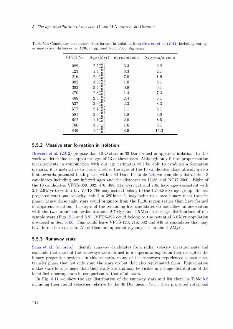
5 The age distribution of massive O and WN stars in 30 Doradus

Table 5.4: Candidates for massive stars formed in isolation from Bressert et al. (2012) including our ageestimates and distances to R136, dR136, and NGC 2060, dNGC2060.

VFTS No. Age (Myr) dR136/arcmin dNGC2060/arcmin

089 2.5+0.4−0.8 6.3 2.2

123 1.4+0.6−0.9 8.3 2.1

216 2.0+0.3−0.2 7.0 1.9

382 3.0+0.4−0.4 1.0 6.1

392 3.4+0.3−0.3 0.9 6.1

470 2.8+0.3−0.6 1.4 7.3

488 2.5+0.2−0.2 2.4 5.1

537 3.3+0.5−0.5 2.3 8.3

577 2.1+0.5−0.7 1.1 6.1

581 3.0+0.4−0.3 1.8 8.0

682 1.1+0.2−0.3 2.0 8.5

706 3.5+1.5−0.9 1.6 8.1

849 1.5+0.6−0.9 8.9 15.3

5.5.2 Massive star formation in isolationBressert et al. (2012) propose that 16 O stars in 30 Dor formed in apparent isolation. In thiswork we determine the apparent ages of 13 of these stars. Although only future proper motionmeasurements in combination with our age estimates will be able to establish a formationscenario, it is instructive to check whether the ages of the 13 candidates alone already give ahint towards potential birth places within 30 Dor. In Table 5.4, we compile a list of the 13candidates including our inferred ages and the distances to R136 and NGC 2060. Eight ofthe 13 candidates, VFTS-089, 382, 470, 488, 537, 577, 581 and 706, have ages consistent with2.4–2.9 Myr to within 1σ. VFTS-706 may instead belong to the 4.2–4.8 Myr age group. Its fastprojected rotational velocity, v sin i ≈ 380 km s−1, may point to a past binary mass transferphase, hence these eight stars could originate from the R136 region rather than have formedin apparent isolation. The ages of the remaining five candidates do not allow an associationwith the two prominent peaks at about 2.7 Myr and 4.5 Myr in the age distributions of oursample stars (Figs. 5.3 and 5.9). VFTS-392 could belong to the potential 3.6 Myr populationdiscussed in Sec. 5.4.6. This would leave VFTS-123, 216, 682 and 849 as candidates that mayhave formed in isolation. All of them are apparently younger than about 2 Myr.

5.5.3 Runaway starsSana et al. (in prep.) identify runaway candidates from radial velocity measurements andconclude that most of the runaways were formed in a supernova explosion that disrupted thebinary progenitor system. In this scenario, many of the runaways experienced a past masstransfer phase that not only spun the stars up but that also rejuvenated them. Rejuvenationmakes stars look younger than they really are and may be visible in the age distribution of theidentified runaway stars in comparison to that of all stars.In Fig. 5.11 we show the age distribution of the runaway stars and list them in Table 5.5

including their radial velocities relative to the 30 Dor mean, δvrad, their projected rotational

144

5.5 Discussion

Pro

babili

ty d

ensity

Age / Myr

Runaways All (14 stars)± 1σ estimate

Dwarfs (10 stars)Giants (4 stars)

Slash/WN (0 stars)

0.00

0.10

0.20

0.30

0.40

0.50

0 1 2 3 4 5 6

2

4

6 8

10

12

Figure 5.11: As Fig. 5.3 but for the runaway stars in our sample identified by Sana et al. (in prep.). Therunaway stars in our sample are marked by additional plus signs in Figs. 5.2, 5.5 and 5.7.

velocities, v sin i, their inferred ages and initial masses, Mini. Of the 24 runaway stars identifiedby Sana et al. (in prep.), one is a known binary for which no atmospheric modelling is available,seven have been removed from our sample mainly because of their BBB spectral classificationand two cannot be reproduced by the stellar models because the stars are rotating too fast(Sec. 5.3). The age distribution shows three interesting features—peaks at about 0.5, 1.9 and4.5 Myr.The 0.5 Myr peak is due to VFTS-016, a runaway with a bow shock that is thought to have

been ejected from R136 (Evans et al. 2010). Its position in the HR diagram (Fig. 5.1) is veryclose to the zero-age main-sequence and its age of 0.5+0.1

−0.2 Myr is significantly younger than anystellar population found in this work. Hence, from its apparent age we conclude that VFTS-016is a rejuvenated binary product. However, its large relative radial velocity of δvrad = 78.3 km s−1

rather points towards a star that has been dynamically ejected from R136 (Sana et al. in prep.).We therefore propose that VFTS-016 is a binary product that either accreted mass or mergedwith a companion prior to its dynamical ejection from R136 or it was ejected as a binary andmerged later on. Such an object is expected to rotate rapidly. Its relatively low v sin i of about94 km s−1 may therefore be due to an unfavourable inclination angle or the generation of amagnetic field because of past mass accretion or merging that spun the star down (magneticbraking). Evans et al. (2010) find that the surface nitrogen mass fraction of VFTS-016 isenhanced by a factor of five and Bestenlehner et al. (2014) report a partial surface nitrogenenhancement though note that the stellar surface is not strongly enriched with nitrogen. Thismay be in favour of a binary merger origin (e.g. Glebbeek et al. 2013) but is not yet conclusive.The 1.9 Myr peak is intriguing. Either the peak contains stars that were dynamically ejected

from R136 and hence is indicative of the true cluster age of R136 or it contains stars that belongto the 2.7 Myr population found around R136 and were rejuvenated by binary mass transferbefore being ejected by the supernova explosion of their companion. The peak is mainly formedby the stars VFTS-755 and 797. If these runaways are rejuvenated binary products, we expect

145

5 The age distribution of massive O and WN stars in 30 Doradus

Table 5.5: Runaway candidates from Sana et al. (in prep.), their radial velocities relative to the mean ofthe 30 Dor population, δvrad, projected rotational velocities, v sin i, inferred ages and initial mass, Mini.

VFTS δvrad v sin i Age MiniNo. km s−1 km s−1 Myr M

012 48.6 306 5.3+0.4−0.6 19.0+1.0

−1.0016 78.3 94 0.5+0.1

−0.2 100.0+13.9−10.6

102 56.2 610 . . . . . .

165 61.6 75 4.7+0.4−0.4 31.2+3.6

−3.0168 36.6 39 3.0+0.5

−0.7 23.6+1.2−1.2

190 45.0 444 . . . . . .285 38.6 622 . . . . . .

306 33.4 71 4.3+0.3−0.3 31.4+3.3

−2.7356 70.3 211 2.6+0.6

−0.9 28.2+3.2−2.9

406 35.7 356 3.3+1.6−0.4 38.6+3.3

−7.3418 30.6 133 1.4+0.6

−0.9 34.2+4.6−3.9

661 26.4 . . . . . . . . .

663 37.2 90 2.5+1.3−1.7 20.6+2.0

−1.6722 38.8 404 3.9+2.0

−0.8 23.6+2.0−2.5

724 28.6 369 3.6+1.4−2.6 22.0+5.2

−4.0755 33.7 286 1.8+1.7

−0.8 51.6+4.8−11.9

761 98.8 111 1.2+0.6−0.8 28.0+1.6

−1.6797 29.2 138 1.9+0.3

−0.3 49.0+7.5−6.3

them to rotate rapidly. If they were dynamically ejected from R136, they may show relativeradial velocities of δvrad > 60 km s−1 (Sana et al. in prep.). Both stars have δvrad < 60 km s−1

but VFTS-755 rotates with a projected rotational velocity of v sin i ≈ 285 km s−1, suggestive ofbeing a rejuvenated binary product. Unfortunately, its age is not constrained well enough togive a definite answer to its origin.The 4.5 Myr peak in Fig. 5.11 is produced by VFTS-165 and 306. Their projected rotational

velocities suggest that they are not binary products and the relative radial velocity of 61.6 km s−1

of VFTS-165 points towards a dynamical ejection (Sana et al. in prep.), explaining why thispeak is not shifted towards younger (rejuvenated) ages compared to the corresponding peak of4.5 Myr in the age distribution of stars in the surroundings of R136 and NGC 2060 (Fig. 5.9).

5.5.4 Binary products

Sana et al. (2013) show that close binaries are frequent among the O stars in 30 Dor and thatmore than 50% of them will exchange mass with a binary companion during their life. Fromobservations, post mass-transfer binaries are hard to distinguish from genuinely single starssuch that a sample of apparent single O stars may contain more binary products than a sampleof binary stars. This is because stars detected as binaries from radial velocity measurements aremostly pre-interaction binary stars (de Mink et al. 2014). The stellar sample used in this workis chosen to exclude potential composite spectra, i.e. binaries, but is still expected to contain asignificant fraction of binary products. Within a coeval stellar population, binary products are

146

5.6 Conclusions

preferentially found among the most massive stars because these stars evolve fastest (Schneideret al. subm.). The O stars in our sample are younger than about 6 Myr which corresponds tothe main-sequence lifetime of a moderately rotating, initially 27 M star (Brott et al. 2011a).We therefore expect to find an increasing fraction of binary products in our sample stars froman initial mass of about 27 M and greater.When analysing binary products with single star models, the inferred ages are younger than

the real stellar ages because of rejuvenation (e.g. Schneider et al. 2014b, subm.). We alreadysuggest that the 2 Myr group among the runaways (Sec. 5.5.3) and the . 2 Myr stars fromSec. 5.4.6 may be such rejuvenated binary products. In Sec. 5.4.5 we conclude that the centralR136 cluster must be older than 1.7 Myr if VFTS-1001 is a genuine cluster member. Giventhat we do not find any spatially localised population that is younger than that in R136,a significant fraction of stars that are apparently younger than 1.7 Myr may be rejuvenatedbinary products. Within 1σ, the dwarf VFTS-536, the giants VFTS-016 and Mk42 and theslash/WN stars VFTS-482, 545, 682 and 1022 are younger than 1.7 Myr and thus are potentialbinary products. Given that the ages of stars in the upper part of the HR diagram are notrobust (Sec. 5.3.1), further binary product candidates are VFTS-072, 617 and 1017 because oftheir proximity to the zero age main-sequence in the HR diagram (Fig. 5.1).VFTS-682 sticks out not just because of its young age but also because it is found in apparent

isolation (Bestenlehner et al. 2011). VFTS-682 either formed in isolation, hence it is young, orit is a binary product.Identifying further binary products older than about 2.0–2.5 Myr purely from inferred ages

is difficult because of the broad age distribution of all stars and the overlap with older stellarpopulations (Fig. 5.3). Unusually rapid rotation, surface nitrogen or helium enrichment, and/orthe clear association of apparently young stars to older stellar populations may be furtherindicators of binary products. For the latter, the membership probability of stars needs to beassessed which likely requires full 3D stellar velocity information.

5.6 Conclusions

The atmospheric parameters of 198 massive O, slash and WN stars observed and modelledwithin the VLT FLAMES Tarantula Survey (VFTS; Evans et al. 2011) have been matchedagainst the rotating, main-sequence star models of Large Magellanic Cloud composition ofBrott et al. (2011a) and Köhler et al. (2014) to derive stellar ages and other parameters such asinitial mass. All inferred ages, and also all other parameters, have to be considered as apparentages because we expect that our sample of stars contains a non-negligible fraction of rejuve-nated binary products for which we infer too young ages. We derive stellar age probabilitydistributions for each star using the Bayesian tool BONNSAI7 (Schneider et al. 2014a) andcombine them to construct age distributions of the massive VFTS stars to analyse their forma-tion process in 30 Dor. Out of the 198 stars, 79 are removed from further analysis because theirspectra are of lower quality and/or are potential composites because of chance superpositionsand duplicity that may result in biased atmospheric parameters when modelled with the meth-ods of Sabín-Sanjulián et al. (2014) and Ramírez-Agudelo et al. (in prep.). The stars of oursample are mainly located outside of known clusters and associations—a fact that is importantto take into account when interpreting the derived age distributions.

7 The BONNSAI web-service is available at http://www.astro.uni-bonn.de/stars/bonnsai.

147

5 The age distribution of massive O and WN stars in 30 Doradus

The spatial distribution of our sample stars shows no obviously coherent age pattern. MassiveO stars of various ages are spread over the whole 30 Dor region. Given that our sample containsmainly field stars, this means that our sample stars either formed continuously over the whole30 Dor field or in distinct clusters and/or associations from which they have been released toreach their currently observed positions. A mixture of both formation scenarios is also possible.The age distribution of the 119 sample stars shows two prominent peaks at ages of about 2.7

and 4.5 Myr. The first group of stars is found in the whole 30 Dor region whereas the latteris mainly found outside 1.2 arcmin (≈ 17.5 pc) of R136. Stars inside 1.2 arcmin of R136 aremostly younger than 4 Myr, with stars being on average younger the closer they are to R136.The R136 cluster age cannot be determined straightforwardly because our sample stars do

not cover the innermost region of R136. However, from the high masses and consequently shortlifetimes of the massive WNh stars in R136 and the observed high surface helium mass fractionsof VFTS-1001 and 1025, we estimate that they, and R136 (if it consists of coeval stars), are1–3 Myr old. If VFTS-1001 is a genuine cluster member, R136 has an age of at least 1.7 Myr.If stars in R136 are coeval and produce a peak in our age distribution, the only possible

peak associated with that is at 2.7 Myr. If this is the case, the age distribution of stars within1.2 arcmin of R136 shows a double and not a single peak that, besides the 2.7 Myr stars, containsa distinct group of 3.6 Myr stars. These stars might be associated with the north-east clumpfound by Sabbi et al. (2012).If also the group of 4.5 Myr stars belong to one stellar population—they may originate from

NGC 2060, the second most obvious site of recent star formation after R136—, our age distribu-tions reveal at least two further groups of . 2 and 5.3 Myr stars, whose formation sites remainunknown. In that picture, most of our sample stars would have formed in at least four distinctclusters or associations and moved to their currently observed positions. Future proper motionmeasurements in combination with our ages will help to trace back the formation sites of starsand to settle the question to which extent stars formed continuously in the whole 30 Dor regionand to which extent in star clusters and associations.

Acknowledgements We thank the VFTS collaboration for fruitful and stimulating discussions.F.R.N.S. acknowledges the fellowship awarded by the Bonn–Cologne Graduate School of Physicsand Astronomy. R.G.I thanks the Alexander von Humboldt foundation.

5.7 Supplementary material

5.7.1 Discrepant starsTwo of our sample stars, VFTS-190 and 285, and one of the excluded stars, VFTS-102, cannotbe reproduced by the stellar models because the fast rotation rates of these stars are not coveredby the stellar models. In the following we discuss these stars in more detail to point out thatthis discrepancy is likely of physical nature and not just a problem of the stellar models.

VFTS-190 is a runaway star and a fast rotator with v sin i ≈ 450 km s−1. The observablesplace it in a sparsely populated region of our model parameter space because of its fastrotation. The resolution test and the posterior predictive checks conducted by BONNSAIfail because the stellar models are initially not rotating fast enough to model this star. Itmay be that this star was spun-up by mass transfer in a binary. This hypothesis is sup-ported by its runaway nature and fast rotation. Mass transfer from a former companion

148

5.7 Supplementary material

spun the star up and the supernova explosion ejected the star, releasing it as a runaway(Sana et al. in prep.).

VFTS-285 is also a runaway and with a v sin i of about 600 km s−1 one of the fastest spinningstars ever observed. As for VFTS-190, the resolution test and the posterior predictivechecks fail. The stellar models of Brott et al. (2011a) and Köhler et al. (2014) are com-puted for vini ≤ 600 km s−1 and it is therefore impossible to reproduce this star. However,given its runaway nature and extreme rotation, the star may be a binary product thatwas spun up by mass transfer from a former companion or in a merger (de Mink et al.2013; Sana et al. in prep.).

VFTS-102 is yet another extremely fast-rotating runaway star (v sin i ≈ 600 km s−1) andDufton et al. (2011) propose that it was spun up by mass transfer from the progeni-tor of the pulsar PSR J0537-6910. As with VFTS-190 and 285, our resolution test andthe posterior predictive check fail because of a lack of stellar models with initial rotationalvelocities & 500–600 km s−1.

149

5 The age distribution of massive O and WN stars in 30 Doradus

Table5.6:

Derived

observab

les,

bolometric

luminosity

logL

/lsun,eff

ectiv

etempe

ratureT

eff,surfa

cegravity

logg

,projectedrotatio

nalv

elocity

vsin

ian

dsurfa

ceheliu

mmassfra

ctionY

obs,

from

spectral

fittin

gan

dstellarpa

rameters,

initial

massM

ini,initial

rotatio

nalv

elocity

v ini,a

ge,

present-da

ymassM

pres

ent,

radius

R,s

urface

heliu

mmassfra

ctionY

andsurfa

cenitrogen

abun

dance

logN

/H+

12,d

etermined

from

thestellar

mod

elso

fBrott

etal.(2011a)

andKöh

lere

tal.(2014)

usingBO

NNSA

I.The

spectral

type

s,Sp

T,a

refro

mWalbo

rnet

al.(2014)a

ndtheprovided

uncertaintiesare

1σconfi

dencelevels

ifno

tstated

otherw

ise.

VFT

SSp

Tlo

gL/L

Teff

logg

vsi

ni

Yob

sM

ini

v ini

Age

Mpr

esen

tR

Ylo

gN/H

+12

No.

(K)

(cgs)

(km

s−1)

(M)

(km

s−1)

(Myr)

(M)

(R)

(dex)

MK42

O2If*

6.60

+0.

10−

0.10

4731

5+17

00−

1700

–<

200

0.33

+0.

05−

0.05

184.

8+37

.4−

30.3

120+

85−

520.

8+0.

2−

0.2

173.

4+35

.8−

29.1

28.5

+4.

2−

3.9

...*

8.22

+0.

26−

0.57

(68%

)(2)

012

O9.5IIIn

4.79

+0.

10−

0.10

3240

0+61

2−

500

3.93

+0.

10−

0.11

306+

31−

31–

19.0

+1.

0−

1.0

310+

48−

445.

3+0.

4−

0.6

18.8

+1.

0−

0.9

7.6+

0.7

−0.

8...*

7.70

+0.

21−

0.15

(68%

)(1)

016

O2III-If*

6.16

+0.

10−

0.10

5200

0+94

4−

500

4.07

+0.

10−

0.10

104+

30−

30–

100.

0+13

.9−

10.6

110+

57−

400.

5+0.

1−

0.2

97.2

+14

.4−

9.0

14.3

+1.

4−

1.4

...*

6.89

+0.

44−

0.02

(68%

)(1)

021

O9.5IV

4.86

+0.

14−

0.14

3384

0+88

0−

880

3.90

+0.

10−

0.10

40+

30−

30–

20.0

+1.

6−

1.5

70+

39−

385.

0+0.

5−

0.6

19.6

+1.

7−

1.2

7.8+

0.9

−0.

9...*

6.89

+0.

04−

0.01

(68%

)(3)

046

O9.7II((n))

5.10

+0.

10−

0.10

2885

0+84

2−

689

3.33

+0.

10−

0.10

172+

30−

30–

22.8

+1.

9−

1.9

180+

52−

426.

2+0.

5−

0.5

23.4

+0.

6−

2.9

14.8

+1.

8−

1.3

...*

7.37

+0.

30−

0.11

(68%

)(1)

065

O8V(n)

4.80

+0.

15−

0.15

3705

0+10

79−

1079

4.06

+0.

16−

0.16

165+

30−

30–

22.2

+1.

8−

1.6

170+

48−

462.

4+0.

9−

1.4

22.2

+1.

7−

1.6

6.2+

0.9

−0.

5...*

6.89

+0.

20−

0.01

(68%

)(3)

067

O9.5Vz

4.56

+0.

17−

0.17

3520

0+11

00−

1100

4.12

+0.

19−

0.19

40+

30−

30–

18.6

+1.

5−

1.4

70+

38−

382.

0+1.

2−

1.6

18.6

+1.

5−

1.4

5.5+

0.6

−0.

6...*

6.89

+0.

01−

0.01

(71%

)(3)

072

O2V-III(n)((f*))

6.07

+0.

13−

0.13

5400

0+15

00−

1500

4.00

+0.

10−

0.10

185+

30−

30–

80.0

+31

.7−

14.4

460+

0−

0a

0.4+

1.9

−0.

494.0

+17

.2−

35.6

13.4

+2.

0−

1.9

...*

8.98

+0.

05−

0.79

(68%

)(3)

074

O9Vn

4.69

+0.

15−

0.15

3514

0+13

49−

1349

4.18

+0.

21−

0.21

265+

30−

30–

19.6

+1.

8−

1.4

270+

61−

452.

1+1.

2−

1.7

19.6

+1.

8−

1.4

6.0+

0.6

−0.

6...*

6.90

+0.

61−

0.01

(68%

)(3)

076

O9.2III

5.09

+0.

10−

0.10

3250

0+66

3−

500

3.59

+0.

10−

0.10

86+

30−

30–

23.6

+1.

9−

1.6

100+

41−

375.

3+0.

3−

0.3

23.2

+1.

9−

1.4

11.3

+1.

3−

1.0

...*

6.93

+0.

14−

0.05

(68%

)(1)

089

O6.5V((f))z

Nstr

5.09

+0.

18−

0.18

3970

0+70

0−

700

4.02

+0.

12−

0.12

50+

30−

30–

28.0

+2.

6−

1.9

70+

45−

322.

5+0.

4−

0.8

28.0

+2.

2−

2.0

7.5+

1.2

−0.

8...*

6.89

+0.

04−

0.01

(68%

)(3)

091

O9.5IIIn

4.82

+0.

10−

0.10

3285

0+51

0−

663

3.92

+0.

10−

0.10

306+

30−

30–

19.4

+1.

1−

1.0

310+

47−

435.

1+0.

5−

0.5

19.2

+1.

1−

0.9

7.8+

0.7

−0.

7...*

7.72

+0.

19−

0.16

(68%

)(1)

103

O8.5III((f))

5.23

+0.

10−

0.10

3470

0+50

0−

500

3.89

+0.

10−

0.10

112+

30−

30–

25.2

+2.

0−

1.6

120+

44−

394.

4+0.

2−

0.2

24.8

+1.

8−

1.5

10.2

+1.

1−

0.9

...*

6.93

+0.

24−

0.05

(68%

)(1)

108

WN7h

5.70

+0.

10−

0.10

5308

8+19

07−

1907

–<

200

0.78

+0.

05−

0.05

35.0

+1.

6−

6.3

500+

30−

186.

3+1.

2−

0.8

26.2

+4.

0−

3.3

7.7+

1.5

−0.

80.

81+

0.02

−0.

049.

06+

0.03

−0.

10(68%

)(2)

110

O6V((n))z

5.40

+0.

20−

0.20

3985

0+10

49−

1049

3.86

+0.

10−

0.10

175+

30−

30–

34.4

+5.

0−

4.0

180+

52−

432.

7+0.

3−

0.3

33.4

+4.

8−

3.5

10.6

+1.

5−

1.5

...*

7.35

+0.

35−

0.23

(68%

)(3)

117

O6:

Vz5.

02+

0.26

−0.

2641

300+

1500

−15

004.

14+

0.16

−0.

1675

+30−

30–

29.2

+3.

7−

3.2

90+

41−

371.

3+0.

7−

1.0

29.0

+3.

7−

3.1

6.9+

1.2

−0.

6...*

6.89

+0.

04−

0.01

(69%

)(3)

123

O6.5Vz

4.99

+0.

13−

0.13

4040

0+68

0−

680

4.10

+0.

12−

0.12

65+

30−

30–

28.2

+1.

6−

1.6

80+

44−

331.

4+0.

6−

0.9

28.0

+1.

6−

1.5

6.9+

0.7

−0.

5...*

6.89

+0.

03−

0.02

(70%

)(3)

130

O8.5V((n))

5.06

+0.

12−

0.12

3650

0+13

30−

1330

4.09

+0.

19−

0.19

170+

30−

30–

24.2

+2.

1−

1.9

170+

54−

413.

4+0.

7−

1.0

24.0

+2.

1−

1.8

7.6+

1.1

−1.

0...*

6.90

+0.

40−

0.01

(68%

)(3)

132

O9.5Vz

4.71

+0.

13−

0.13

3564

0+68

0−

680

4.18

+0.

10−

0.10

40+

30−

30–

19.8

+1.

1−

0.9

70+

39−

382.

3+0.

9−

1.2

19.8

+1.

1−

0.9

5.7+

0.6

−0.

4...*

6.90

+0.

01−

0.01

(68%

)(3)

149

O9.5V

4.68

+0.

15−

0.15

3499

5+13

95−

1395

4.12

+0.

24−

0.24

125+

30−

30–

19.0

+1.

7−

1.5

130+

44−

402.

9+1.

3−

1.9

19.0

+1.

7−

1.5

5.8+

0.8

−0.

6...*

6.90

+0.

06−

0.01

(68%

)(3)

165

O9.7Iab

5.49

+0.

10−

0.10

2865

0+76

5−

765

3.26

+0.

10−

0.10

75+

30−

30–

31.2

+3.

6−

3.0

100+

40−

414.

7+0.

4−

0.4

29.8

+3.

5−

2.3

21.0

+2.

9−

1.8

...*

6.99

+0.

16−

0.10

(68%

)(1)

168

O8.5Vz

4.92

+0.

11−

0.11

3727

0+51

0−

510

4.02

+0.

10−

0.10

40+

30−

30–

23.6

+1.

2−

1.2

70+

38−

383.

0+0.

5−

0.7

23.4

+1.

2−

1.1

7.0+

0.8

−0.

6...*

6.89

+0.

02−

0.02

(70%

)(3)

169

O2.5V(n)((f*))

5.91

+0.

13−

0.13

4700

0+15

00−

1500

3.90

+0.

10−

0.10

200+

30−

30–

64.8

+12

.0−

8.6

210+

71−

471.

4+0.

3−

0.3

62.0

+11

.2−

7.9

13.7

+1.

7−

1.8

...*

7.98

+0.

31−

0.40

(68%

)(3)

185

O7.5III((f))

5.31

+0.

10−

0.10

3505

0+50

0−

500

3.51

+0.

10−

0.10

124+

30−

30–

30.8

+3.

1−

2.4

130+

49−

384.

0+0.

2−

0.3

30.4

+2.

3−

2.6

13.1

+1.

6−

1.1

...*

6.95

+0.

40−

0.03

(68%

)(1)

190

O7Vn

n((f))p

5.28

+0.

10−

0.10

3570

0+50

0−

500

3.45

+0.

10−

0.10

444+

44−

44–

––

––

––

–(1)

210

O9.7II-III((n))

4.61

+0.

10−

0.10

3230

0+50

0−

536

4.05

+0.

10−

0.10

166+

30−

30–

16.8

+0.

8−

0.8

170+

48−

445.

1+0.

7−

0.9

16.8

+0.

8−

0.8

6.2+

0.6

−0.

5...*

6.92

+0.

25−

0.03

(68%

)(1)

216

O4V((fc))

5.83

+0.

13−

0.13

4300

0+15

00−

1500

3.80

+0.

10−

0.10

100+

30−

30–

55.4

+9.

0−

7.5

110+

48−

362.

0+0.

3−

0.2

52.8

+8.

3−

6.6

14.4

+1.

9−

1.8

...*

6.99

+0.

47−

0.10

(73%

)(3)

249

O8Vn

4.78

+0.

14−

0.14

3648

0+75

9−

759

4.04

+0.

11−

0.11

300+

30−

30–

22.4

+1.

4−

1.4

300+

74−

432.

7+0.

9−

1.3

22.2

+1.

4−

1.3

6.4+

0.8

−0.

5...*

7.63

+0.

41−

0.39

(68%

)(3)

250

O9.2V((n))

4.76

+0.

12−

0.12

3541

5+80

5−

805

4.12

+0.

15−

0.15

155+

30−

30–

20.2

+1.

3−

1.1

160+

47−

453.

0+0.

9−

1.4

20.2

+1.

2−

1.1

6.1+

0.7

−0.

6...*

6.90

+0.

16−

0.01

(68%

)(3)

251

O9.5IV

4.72

+0.

11−

0.11

3371

0+55

9−

559

4.01

+0.

10−

0.10

40+

30−

30–

18.4

+1.

1−

0.8

70+

39−

384.

7+0.

5−

0.8

18.6

+0.

8−

0.9

6.7+

0.6

−0.

7...*

6.89

+0.

03−

0.01

(68%

)(3)

150

5.7 Supplementary materialTa

ble5.6:

continued.

VFT

SSp

Tlo

gL/L

Teff

logg

vsi

ni

Yob

sM

ini

v ini

Age

Mpr

esen

tR

Ylo

gN/H

+12

No.

(K)

(cgs)

(km

s−1)

(M)

(km

s−1)

(Myr)

(M)

(R)

(dex)

252

O8.5Vz

4.73

+0.

12−

0.12

3695

5+50

0−

500

4.21

+0.

10−

0.10

100+

30−

30–

21.6

+1.

0−

0.8

110+

40−

391.

1+0.

8−

0.8

21.6

+1.

0−

0.8

5.8+

0.5

−0.

3...*

6.89

+0.

02−

0.02

(70%

)(3)

266

O8V((f))z

5.05

+0.

12−

0.12

3804

5+50

0−

500

4.01

+0.

10−

0.10

40+

30−

30–

25.6

+1.

7−

1.4

70+

39−

383.

0+0.

3−

0.6

25.4

+1.

6−

1.3

7.6+

0.9

−0.

7...*

6.90

+0.

03−

0.02

(69%

)(3)

280

O9V((n))

4.88

+0.

12−

0.12

3436

0+56

0−

560

3.82

+0.

10−

0.10

150+

30−

30–

21.4

+1.

6−

1.3

150+

48−

394.

7+0.

3−

0.3

21.2

+1.

6−

1.3

8.3+

0.9

−0.

8...*

6.92

+0.

34−

0.02

(68%

)(3)

285

O7.5Vn

nn4.

77+

0.20

−0.

2035

280+

919

−91

93.

63+

0.10

−0.

1060

0+60−

60–

––

––

––

–(3)

290

O9.5IV

4.76

+0.

10−

0.10

3395

0+50

0−

500

3.99

+0.

10−

0.10

40+

30−

30–

19.0

+1.

0−

0.8

70+

39−

384.

7+0.

5−

0.6

19.2

+0.

7−

1.0

6.9+

0.7

−0.

6...*

6.91

+0.

02−

0.02

(70%

)(3)

306

O8.5II((f))

5.42

+0.

10−

0.10

3240

0+50

0−

500

3.43

+0.

10−

0.10

88+

30−

30–

31.4

+3.

3−

2.7

100+

48−

334.

3+0.

3−

0.3

30.8

+2.

5−

2.9

16.1

+2.

0−

1.5

...*

6.96

+0.

23−

0.06

(68%

)(1)

356

O6:

V(n)z

5.14

+0.

20−

0.20

3925

0+12

50−

1250

3.99

+0.

13−

0.13

215+

30−

30–

28.2

+3.

2−

2.9

220+

58−

462.

6+0.

6−

0.9

28.0

+3.

0−

2.9

8.0+

1.1

−1.

3...*

7.56

+0.

22−

0.46

(68%

)(3)

361

O8.5V

5.27

+0.

15−

0.15

3689

5+67

4−

674

4.07

+0.

10−

0.10

70+

30−

30–

25.2

+2.

2−

1.8

80+

48−

303.

5+0.

3−

0.5

25.2

+1.

8−

2.0

8.2+

1.1

−0.

9...*

6.90

+0.

08−

0.01

(68%

)(3)

369

O9.7V

4.67

+0.

14−

0.14

3336

0+12

00−

1200

4.10

+0.

18−

0.18

40+

30−

30–

17.6

+1.

4−

1.3

70+

39−

384.

4+1.

2−

1.8

17.6

+1.

4−

1.3

5.8+

0.9

−0.

7...*

6.90

+0.

01−

0.01

(70%

)(3)

380

O6-7Vz

4.92

+0.

15−

0.15

3912

0+68

0−

680

4.13

+0.

10−

0.10

65+

30−

30–

25.6

+1.

7−

1.3

80+

44−

331.

7+0.

7−

0.9

25.6

+1.

5−

1.3

6.6+

0.7

−0.

5...*

6.91

+0.

02−

0.01

(71%

)(3)

382

O4-5V((fc))z

5.31

+0.

13−

0.13

4000

0+15

00−

1500

3.80

+0.

10−

0.10

75+

30−

30–

32.8

+4.

0−

3.3

90+

42−

363.

0+0.

4−

0.4

32.2

+3.

7−

3.1

10.3

+1.

4−

1.1

...*

6.90

+0.

13−

0.01

(68%

)(3)

392

O6-7V((f))z

5.11

+0.

23−

0.23

3756

0+84

0−

840

3.87

+0.

10−

0.10

40+

30−

30–

27.0

+3.

3−

2.6

70+

39−

383.

4+0.

3−

0.3

26.2

+3.

6−

2.0

9.2+

1.3

−1.

4...*

6.91

+0.

04−

0.01

(69%

)(3)

406

O6Vn

n5.

55+

0.10

−0.

1037

800+

500

−56

13.

54+

0.10

−0.

1035

6+36−

36–

38.6

+3.

3−

7.3

380+

46−

463.

3+1.

6−

0.4

37.4

+3.

4−

7.2

13.8

+1.

7−

1.1

0.27

+0.

20−

0.02

b 8.47

+0.

26−

0.40

(91%

)(1)

418

O5V((n))((fc))z

5.24

+0.

18−

0.18

4322

0+17

40−

1740

4.09

+0.

13−

0.13

135+

30−

30–

34.2

+4.

6−

3.9

140+

48−

431.

4+0.

6−

0.9

33.8

+4.

6−

3.6

7.8+

1.1

−0.

7...*

6.90

+0.

21−

0.01

(68%

)(3)

419

O9:

V(n)

5.07

+0.

24−

0.24

3310

0+89

9−

899

3.61

+0.

10−

0.10

145+

30−

30–

24.4

+3.

5−

2.9

150+

48−

414.

9+0.

6−

0.5

25.0

+2.

3−

3.6

11.3

+2.

2−

1.4

...*

7.33

+0.

08−

0.39

(70%

)(3)

427

WN8(h)

6.10

+0.

10−

0.10

4168

7+14

97−

1497

–<

200

0.93

+0.

05−

0.05

90.4

+9.

5−

17.9

410+

18−

373.

1+0.

3−

0.3

c53.2

+12

.3−

2.1

d27.6

+2.

9−

4.6

0.84

+0.

04−

0.04

9.09

+0.

22−

0.08

(68%

)(2)

435

O7-8V

5.12

+0.

13−

0.13

3600

0+15

00−

1500

3.90

+0.

10−

0.10

80+

30−

30–

24.6

+2.

7−

2.1

90+

45−

333.

9+0.

6−

0.6

24.4

+2.

5−

2.1

8.9+

1.1

−0.

9...*

6.91

+0.

11−

0.01

(68%

)(3)

436

O7-8V

4.87

+0.

13−

0.13

3500

0+15

00−

1500

3.90

+0.

10−

0.10

60+

30−

30–

20.8

+1.

9−

1.8

80+

40−

364.

6+0.

8−

0.8

20.4

+2.

1−

1.5

7.8+

0.9

−0.

8...*

6.90

+0.

04−

0.01

(68%

)(3)

457

O3.5If*

/WN7

6.20

+0.

10−

0.10

3981

1+14

30−

1430

–<

200

0.40

+0.

05−

0.01

78.6

+18

.9−

12.3

320+

23−

132.

4+0.

2−

0.4

68.6

+16

.7−

11.6

e26.0

+3.

8−

3.7

0.41

+0.

05−

0.03

f 8.52

+0.

05−

0.04

(79%

)(2)

466

O9III

5.24

+0.

10−

0.10

3425

0+50

0−

500

3.72

+0.

10−

0.10

86+

30−

30–

26.4

+2.

2−

1.9

100+

41−

384.

5+0.

2−

0.2

25.8

+2.

4−

1.5

11.4

+1.

2−

1.0

...*

6.95

+0.

15−

0.05

(68%

)(1)

470

O6:

V((f))z

4.97

+0.

18−

0.18

3933

0+63

0−

630

3.93

+0.

10−

0.10

75+

30−

30–

28.0

+2.

6−

1.9

90+

41−

372.

8+0.

3−

0.6

27.8

+2.

4−

1.8

8.1+

1.1

−0.

9...*

6.90

+0.

08−

0.01

(68%

)(3)

472

O6Vz

5.01

+0.

15−

0.15

4036

5+85

5−

855

4.12

+0.

12−

0.12

40+

30−

30–

28.0

+2.

0−

1.8

70+

39−

381.

5+0.

6−

0.9

27.8

+2.

1−

1.7

6.9+

0.8

−0.

6...*

6.91

+0.

02−

0.01

(69%

)(3)

482

O2.5If*

/WN6

6.40

+0.

10−

0.10

4217

0+15

15−

1515

–<

200

0.33

+0.

05−

0.05

124.

4+24

.9−

19.2

100+

102

−36

1.3+

0.2

−0.

211

3.8+

22.8

−17

.728.1

+4.

4−

3.7

...*

8.23

+0.

02−

1.06

(74%

)(2)

483

O9V

4.59

+0.

15−

0.13†33

655+

854

−85

44.

09+

0.11

−0.

1140

+30−

30–

17.4

+1.

6−

1.3

70+

38−

384.

3+0.

8−

1.7

17.4

+1.

6−

1.3

5.8+

0.9

−0.

8...*

6.91

+0.

01−

0.01

(70%

)(3)

484

O6-7V((n))

5.41

+0.

14−

0.14

3568

0+68

0−

680

3.67

+0.

10−

0.10

120+

30−

30–

31.6

+3.

9−

3.3

130+

45−

403.

8+0.

3−

0.3

31.0

+3.

4−

3.1

12.7

+1.

9−

1.4

...*

6.96

+0.

49−

0.06

(81%

)(3)

488

O6V((f))z

5.33

+0.

25−

0.25

4070

0+65

9−

659

3.87

+0.

10−

0.10

55+

30−

30–

35.4

+5.

4−

3.8

80+

39−

382.

5+0.

2−

0.2

34.6

+5.

0−

3.3

10.3

+1.

7−

1.5

...*

6.90

+0.

08−

0.02

(68%

)(3)

491

O6V((fc))

5.43

+0.

16−

0.16

4036

0+79

9−

799

3.84

+0.

10−

0.10

50+

30−

30–

36.4

+4.

7−

3.7

70+

46−

312.

6+0.

2−

0.2

35.4

+4.

5−

3.3

10.9

+1.

5−

1.4

...*

6.90

+0.

07−

0.01

(68%

)(3)

493

O9V

5.06

+0.

16−

0.16

3705

0+95

0−

950

4.28

+0.

10−

0.10

200+

30−

30–

23.4

+1.

6−

1.6

200+

64−

421.

5+0.

8−

1.0

23.2

+1.

8−

1.4

6.3+

0.6

−0.

5...*

6.90

+0.

31−

0.01

(68%

)(3)

498

O9.5V

4.88

+0.

14−

0.14

3323

0+81

0−

810

4.12

+0.

15−

0.15

40+

30−

30–

18.6

+1.

4−

1.3

70+

39−

385.

0+0.

7−

0.9

18.6

+1.

3−

1.2

6.9+

0.9

−1.

0...*

6.90

+0.

02−

0.01

(69%

)(3)

505

O9.5V-III

4.66

+0.

13−

0.13

3404

0+68

0−

680

4.30

+0.

10−

0.10

100+

30−

30–

17.8

+0.

9−

0.8

110+

41−

391.

8+1.

1−

1.2

17.8

+0.

9−

0.8

5.3+

0.5

−0.

4...*

6.89

+0.

02−

0.01

(70%

)(3)

513

O6-7II(f)

4.93

+0.

10−

0.10

3660

0+50

0−

500

4.16

+0.

10−

0.10

114+

30−

30–

22.4

+1.

1−

1.0

120+

45−

392.

8+0.

6−

0.9

22.4

+0.

9−

1.0

6.6+

0.7

−0.

5...*

6.89

+0.

08−

0.02

(69%

)(1)

517

O9.5V-III((n))

5.09

+0.

10−

0.10

3300

0+50

0−

500

4.01

+0.

10−

0.10

120+

30−

30–

21.0

+1.

5−

1.2

120+

51−

345.

2+0.

3−

0.3

20.8

+1.

6−

1.1

8.9+

0.9

−0.

8...*

6.92

+0.

24−

0.03

(68%

)(3)

536

O6Vz

5.19

+0.

17−

0.17

4150

0+15

40−

1540

4.24

+0.

15−

0.15

40+

30−

30–

30.4

+3.

5−

2.8

70+

39−

380.

9+0.

7−

0.8

30.2

+3.

5−

2.7

7.1+

0.9

−0.

6...*

6.89

+0.

02−

0.01

(69%

)(3)

537

O5V((fc))z

5.19

+0.

13−

0.13

3900

0+15

00−

1500

3.80

+0.

10−

0.10

60+

30−

30–

29.4

+3.

3−

2.9

80+

41−

363.

3+0.

5−

0.5

29.0

+3.

0−

2.8

9.8+

1.2

−1.

1...*

6.90

+0.

07−

0.01

(68%

)(3)

542

O2If*

/WN5

6.20

+0.

10−

0.10

4466

8+20

06−

2006

–<

200

0.47

+0.

05−

0.05

81.4

+17

.3−

13.4

340+

16−

312.

2+0.

3−

0.4

71.4

+15

.8−

11.4

20.3

+3.

2−

3.1

0.44

+0.

06−

0.04

8.57

+0.

07−

0.06

(68%

)(2)

151

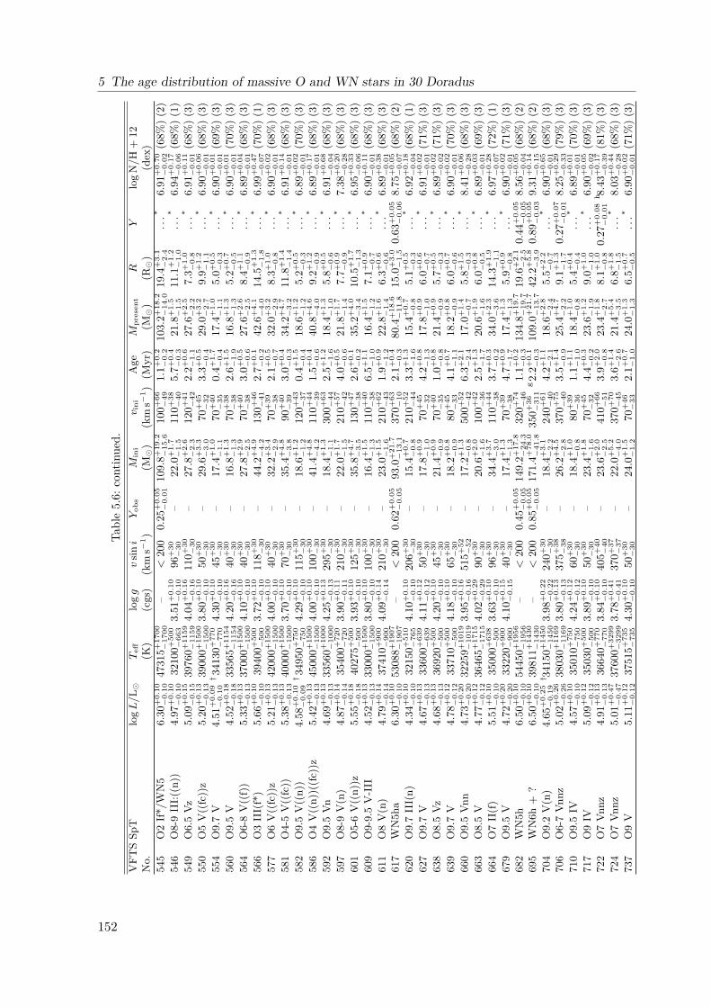
5 The age distribution of massive O and WN stars in 30 Doradus

Table5.6:

continued.

VFT

SSp

Tlo

gL/L

Teff

logg

vsi

ni

Yob

sM

ini

v ini

Age

Mpr

esen

tR

Ylo

gN/H

+12

No.

(K)

(cgs)

(km

s−1)

(M)

(km

s−1)

(Myr)

(M)

(R)

(dex)

545

O2If*

/WN5

6.30

+0.

10−

0.10

4731

5+17

00−

1700

–<

200

0.25

+0.

05−

0.01

109.

8+19

.2−

15.6

100+

66−

491.

1+0.

2−

0.2

103.

2+18

.2−

14.0

19.4

+3.

1−

2.4

...*

6.91

+0.

70−

0.02

(68%

)(2)

546

O8-9III:(

(n))

4.97

+0.

10−

0.10

3210

0+50

0−

663

3.51

+0.

10−

0.10

96+

30−

30–

22.0

+1.

7−

1.5

110+

38−

405.

7+0.

4−

0.3

21.8

+1.

5−

1.5

11.1

+1.

2−

1.0

...*

6.94

+0.

17−

0.06

(68%

)(1)

549

O6.5Vz

5.09

+0.

15−

0.15

3976

0+11

59−

1159

4.04

+0.

16−

0.16

110+

30−

30–

27.8

+2.

6−

2.3

120+

41−

422.

2+0.

6−

1.1

27.6

+2.

5−

2.2

7.3+

1.0

−0.

8...*

6.91

+0.

11−

0.01

(68%

)(3)

550

O5V((fc))z

5.20

+0.

13−

0.13

3900

0+15

00−

1500

3.80

+0.

10−

0.10

50+

30−

30–

29.6

+3.

3−

3.0

70+

45−

323.

3+0.

5−

0.4

29.0

+3.

2−

2.7

9.9+

1.2

−1.

1...*

6.90

+0.

06−

0.01

(68%

)(3)

554

O9.7V

4.51

+0.

09−

0.10†34

130+

770

−77

04.

30+

0.10

−0.

1045

+30−

30–

17.4

+1.

0−

1.1

70+

40−

350.

4+1.

7−

0.4

17.4

+1.

0−

1.1

5.0+

0.5

−0.

3...*

6.90

+0.

01−

0.01

(69%

)(3)

560

O9.5V

4.52

+0.

18−

0.18

3356

5+11

54−

1154

4.20

+0.

16−

0.16

40+

30−

30–

16.8

+1.

3−

1.3

70+

38−

382.

6+1.

5−

1.9

16.8

+1.

3−

1.3

5.2+

0.7

−0.

5...*

6.90

+0.

01−

0.01

(70%

)(3)

564

O6-8V((f))

5.33

+0.

13−

0.13

3700

0+15

00−

1500

4.10

+0.

10−

0.10

40+

30−

30–

27.8

+2.

9−

2.5

70+

40−

383.

0+0.

5−

0.6

27.6

+2.

6−

2.5

8.4+

1.1

−0.

9...*

6.89

+0.

04−

0.01

(68%

)(3)

566

O3III(f*)

5.66

+0.

10−

0.10

3940

0+50

0−

500

3.72

+0.

10−

0.10

118+

30−

30–

44.2

+4.

9−

4.2

130+

46−

412.

7+0.

1−

0.2

42.6

+4.

1−

4.0

14.5

+1.

3−

1.8

...*

6.99

+0.

47−

0.07

(70%

)(1)

577

O6V((fc))z

5.21

+0.

13−

0.13

4200

0+15

00−

1500

4.00

+0.

10−

0.10

40+

30−

30–

32.2

+3.

4−

2.9

70+

39−

382.

1+0.

5−

0.7

32.0

+3.

2−

2.9

8.3+

1.0

−0.

8...*

6.90

+0.

02−

0.01

(68%

)(3)

581

O4-5V((fc))

5.38

+0.

13−

0.13

4000

0+15

00−

1500

3.70

+0.

10−

0.10

70+

30−

30–

35.4

+4.

8−

3.8

90+

40−

393.

0+0.

4−

0.3

34.2

+4.

7−

3.2

11.8

+1.

4−

1.4

...*

6.91

+0.

14−

0.01

(68%

)(3)

582

O9.5V((n))

4.58

+0.

10−

0.09†34

950+

750

−75

04.

29+

0.10

−0.

1011

5+30−

30–

18.6

+1.

2−

1.2

120+

43−

370.

4+1.

5−

0.4

18.6

+1.

2−

1.2

5.2+

0.5

−0.

3...*

6.89

+0.

02−

0.01

(70%

)(3)

586

O4V((n))((fc))z

5.42

+0.

13−

0.13

4500

0+15

00−

1500

4.00

+0.

10−

0.10

100+

30−

30–

41.4

+4.

8−

4.2

110+

44−

391.

5+0.

4−

0.6

40.8

+4.

6−

4.0

9.2+

1.2

−0.

9...*

6.89

+0.

17−

0.01

(68%

)(3)

592

O9.5Vn

4.69

+0.

13−

0.13

3356

0+10

00−

1000

4.25

+0.

13−

0.13

295+

30−

30–

18.4

+1.

3−

1.1

300+

63−

442.

5+1.

2−

1.6

18.4

+1.

3−

1.0

5.8+

0.5

−0.

6...*

6.91

+0.

68−

0.04

(68%

)(3)

597

O8-9V(n)

4.87

+0.

14−

0.14

3540

0+72

0−

720

3.90

+0.

11−

0.11

210+

30−

30–

22.0

+1.

7−

1.5

210+

57−

424.

0+0.

5−

0.6

21.8

+1.

7−

1.4

7.7+

0.9

−0.

9...*

7.38

+0.

20−

0.28

(68%

)(3)

601

O5-6V((n))z

5.55

+0.

18−

0.18

4027

5+50

0−

500

3.93

+0.

10−

0.10

125+

30−

30–

35.8

+4.

7−

3.5

130+

47−

382.

6+0.

1−

0.2

35.2

+4.

0−

3.4

10.5

+1.

7−

1.3

...*

6.95

+0.

33−

0.06

(68%

)(3)

609

O9-9.5V-III

4.52

+0.

13−

0.13

3300

0+15

00−

1500

3.80

+0.

10−

0.10

100+

30−

30–

16.4

+1.

5−

1.3

110+

40−

386.

5+1.

1−

1.0

16.4

+1.

5−

1.2

7.1+

0.9

−0.

7...*

6.90

+0.

11−

0.01

(68%

)(3)

611

O8V(n)

4.79

+0.

14−

0.14

3741

0+90

0−

900

4.09

+0.

14−

0.14

210+

30−

30–

23.0

+1.

5−

1.6

210+

62−

431.

9+0.

9−

1.2

22.8

+1.

6−

1.4

6.3+

0.6

−0.

6...*

6.89

+0.

38−

0.01

(68%

)(3)

617

WN5h

a6.

30+

0.10

−0.

1053

088+

1907

−19

07–

<20

00.

62+

0.05

−0.

0593.0

+21

.7−

13.1

370+

63−

102.

1+0.

4−

0.3

80.4

+18

.6−

11.8

15.0

+3.

0−

1.5

0.63

+0.

05−

0.06

8.75

+0.

05−

0.07

(68%

)(2)

620

O9.7III(n)

4.34

+0.

10−

0.10

3215

0+51

0−

765

4.10

+0.

10−

0.10

206+

30−

30–

15.4

+0.

7−

0.8

210+

52−

443.

3+1.

3−

1.6

15.4

+0.

7−

0.8

5.1+

0.5

−0.

3...*

6.92

+0.

18−

0.04

(68%

)(1)

627

O9.7V

4.67

+0.

13−

0.13

3360

0+63

9−

639

4.11

+0.

12−

0.12

50+

30−

30–

17.8

+0.

9−

1.0

70+

45−

324.

2+0.

8−

1.3

17.8

+0.

9−

1.0

6.0+

0.6

−0.

7...*

6.91

+0.

02−

0.01

(71%

)(3)

638

O8.5Vz

4.68

+0.

13−

0.13

3692

0+50

0−

500

4.20

+0.

10−

0.10

45+

30−

30–

21.4

+0.

9−

0.9

70+

40−

351.

0+0.

8−

0.8

21.4

+0.

9−

0.9

5.7+

0.5

−0.

3...*

6.89

+0.

02−

0.02

(71%

)(3)

639

O9.7V

4.78

+0.

12−

0.12

3371

0+50

0−

500

4.18

+0.

10−

0.10

65+

30−

30–

18.2

+0.

8−

0.9

80+

45−

334.

1+0.

7−

1.1

18.2

+0.

8−

0.9

6.0+

0.7

−0.

6...*

6.90

+0.

02−

0.01

(70%

)(3)

660

O9.5Vn

n4.

73+

0.20

−0.

2032

259+

1019

−10

193.

95+

0.16

−0.

1651

5+52−

52–

17.2

+1.

3−

0.8

500+

52−

426.

3+2.

1−

2.4

17.0

+1.

4−

0.7

5.8+

1.5

−0.

3...*

8.41

+0.

06−

0.28

(68%

)(3)

663

O8.5V

4.77

+0.

12−

0.12

3646

5+17

15−

1715

4.02

+0.

29−

0.29

90+

30−

30–

20.6

+2.

0−

1.6

100+

42−

362.

5+1.

3−

1.7

20.6

+1.

9−

1.6

6.0+

0.8

−0.

5...*

6.89

+0.

03−

0.01

(69%

)(3)

664

O7II(f)

5.51

+0.

10−

0.10

3500

0+63

8−

500

3.63

+0.

10−

0.10

96+

30−

30–

34.4

+3.

7−

3.0

110+

44−

383.

7+0.

3−

0.2

34.0

+2.

3−

3.6

14.3

+1.

9−

1.1

...*

6.97

+0.

28−

0.07

(72%

)(1)

679

O9.5V

4.72

+0.

20−

0.20

3322

0+90

0−

900

4.10

+0.

15−

0.15

40+

30−

30–

17.4

+1.

3−

1.3

70+

39−

384.

7+0.

9−

1.7

17.4

+1.

3−

1.3

5.9+

0.9

−0.

8...*

6.90

+0.

02−

0.01

(71%

)(3)

682

WN5h

6.50

+0.

10−

0.10

5445

0+19

56−

1956

–<

200

0.45

+0.

05−

0.05

149.

2+17

.8−

24.3

320+

74−

461.

1+0.

2−

0.3

134.

8+19

.7−

19.7

19.6

+2.

1−

2.5

0.44

+0.

05−

0.05

8.56

+0.

05−

0.04

(68%

)(2)

695

WN6h

+?

6.50

+0.

10−

0.10

3981

1+14

30−

1430

–<

200

0.85

+0.

05−

0.05

171.

4+78

.0−

41.8

350+

36−

311

g2.

2+0.

1−

0.3

109.

0+21

.7−

13.7

42.2

+5.

8−

3.9

0.89

+0.

05−

0.03

9.31

+0.

14−

0.15

(68%

)(2)

704

O9.2V(n)

4.65

+0.

25−

0.19† 3

4150

+14

50−

1450

3.98

+0.

22−

0.22

240+

30−

30–

18.4

+3.

1−

2.2

240+

61−

404.

2+1.

1−

2.1

18.6

+2.

8−

2.4

5.5+

2.2

−0.

7...*

6.90

+0.

65−

0.01

(68%

)(3)

706

O6-7Vn

nz5.

02+

0.26

−0.

2638

030+

1169

−11

693.

80+

0.13

−0.

1337

5+38−

38–

26.2

+4.

5−

2.8

370+

75−

403.

5+1.

4−

0.9

25.4

+4.

7−

2.2

9.1+

1.3

−1.

70.

27+

0.07

−0.

018.

25+

0.29

−0.

33(79%

)(3)

710

O9.5IV

4.57

+0.

10−

0.10

3501

0+75

0−

750

4.24

+0.

12−

0.12

60+

30−

30–

18.4

+1.

0−

0.8

80+

39−

361.

1+1.

1−

1.0

18.4

+1.

0−

0.8

5.4+

0.4

−0.

4...*

6.89

+0.

01−

0.01

(70%

)(3)

717

O9IV

5.09

+0.

12−

0.12

3503

0+50

0−

500

3.89

+0.

10−

0.10

50+

30−

30–

23.4

+1.

8−

1.6

70+

45−

324.

4+0.

3−

0.2

23.6

+1.

2−

1.9

9.0+

1.0

−1.

0...*

6.90

+0.

05−

0.02

(69%

)(3)

722

O7Vn

nz4.

91+

0.13

−0.

1336

640+

770

−77

03.

84+

0.10

−0.

1040

5+40−

40–

23.6

+2.

0−

2.5

410+

66−

513.

9+2.

0−

0.8

23.4

+1.

8−

2.7

8.1+

1.0

−0.

80.

27+

0.08

−0.

01h 8.

43+

0.17

−0.

39(81%

)(3)

724

O7Vn

nz5.

01+

0.47

−0.

4737

600+

3299

−32

993.

78+

0.41

−0.

4137

0+37−

37–

22.0

+5.

2−

4.0

370+

70−

453.

6+1.

4−

2.6

21.4

+5.

4−

3.5

6.8+

1.8

−1.

5...*

8.03

+0.

44−

0.28

(68%

)(3)

737

O9V

5.11

+0.

12−

0.12

3751

5+73

5−

735

4.30

+0.

10−

0.10

50+

30−

30–

24.0

+1.

5−

1.2

70+

46−

332.

1+0.

7−

1.0

24.0

+1.

3−

1.3

6.5+

0.7

−0.

5...*

6.90

+0.

02−

0.01

(71%

)(3)

152

5.7 Supplementary materialTa

ble5.6:

continued.

VFT

SSp

Tlo

gL/L

Teff

logg

vsi

ni

Yob

sM

ini

v ini

Age

Mpr

esen

tR

Ylo

gN/H

+12

No.

(K)

(cgs)

(km

s−1)

(M)

(km

s−1)

(Myr)

(M)

(R)

(dex)

746

O6Vn

n5.

29+

0.24

−0.

2439

885+

1154

−11

543.

86+

0.10

−0.

1027

5+30−

30–

33.0

+5.

5−

3.9

290+

54−

482.

8+0.

4−

0.4

32.2

+5.

1−

3.5

10.1

+1.

5−

1.5

...*

7.90

+0.

25−

0.24

(70%

)(3)

751

O7-8Vn

nz5.

01+

0.31

−0.

3136

045+

1494

−14

943.

90+

0.25

−0.

2536

0+36−

36–

22.0

+3.

4−

2.3

360+

67−

443.

8+1.

1−

2.0

22.0

+3.

1−

2.3

6.4+

2.2

−0.

7...*

7.98

+0.

46−

0.24

(73%

)(3)

753

O9.7II-III

4.78

+0.

10−

0.10

3230

0+86

7−

765

4.02

+0.

11−

0.10

38+

30−

30–

17.8

+1.

2−

0.9

60+

48−

295.

6+0.

6−

0.7

18.0

+0.

9−

1.1

7.1+

0.7

−0.

7...*

6.90

+0.

02−

0.01

(69%

)(1)

755

O3Vn

((f*))

5.65

+0.

13−

0.13

4600

0+15

00−

1500

3.90

+0.

10−

0.10

285+

30−

30–

51.6

+4.

8−

11.9

410+

38−

147

i 1.8+

1.7

−0.

8j

50.2

+5.

1−

12.8

k11.1

+1.

5−

1.2

0.27

+0.

15−

0.02

8.65

+0.

09−

0.71

(85%

)(3)

758

WN5h

6.40

+0.

10−

0.10

4731

5+17

00−

1700

–<

200

0.78

+0.

05−

0.05

133.

4+17

.1−

35.1

420+

35−

282.

2+0.

4−

0.2

82.4

+18

.3−

14.0

l24.6

+2.

3−

4.0

0.79

+0.

04−

0.05

8.97

+0.

11−

0.08

(68%

)(2)

761

O6.5V((n))((f))zNstr

4.99

+0.

13−

0.13

4028

0+68

0−

680

4.15

+0.

10−

0.10

110+

30−

30–

28.0

+1.

6−

1.6

120+

40−

421.

2+0.

6−

0.8

27.8

+1.

6−

1.4

6.9+

0.6

−0.

6...*

6.89

+0.

05−

0.02

(69%

)(3)

770

O7Vn

n4.

98+

0.27

−0.

2737

815+

1125

−11

253.

95+

0.15

−0.

1535

0+35−

35–

25.0

+3.

0−

2.6

350+

75−

413.

2+0.

9−

1.6

24.8

+3.

0−

2.4

7.0+

1.5

−0.

9...*

7.92

+0.

55−

0.16

(75%

)(3)

775

O9.2V

4.72

+0.

12−

0.12

3594

0+13

29−

1329

4.14

+0.

20−

0.20

40+

30−

30–

20.0

+1.

6−

1.4

70+

38−

382.

3+1.

2−

1.5

20.0

+1.

5−

1.4

5.8+

0.7

−0.

5...*

6.90

+0.

01−

0.01

(70%

)(3)

777

O9.2II

5.31

+0.

10−

0.10

2930

0+50

0−

663

3.28

+0.

10−

0.12

152+

30−

30–

27.2

+2.

7−

2.4

160+

55−

385.

2+0.

5−

0.4

25.8

+3.

1−

1.6

18.3

+1.

6−

2.2

...*

7.41

+0.

21−

0.28

(68%

)(1)

778

O9.5V

4.81

+0.

18−

0.18

3421

5+13

75−

1375

4.18

+0.

21−

0.21

125+

30−

30–

19.0

+1.

9−

1.7

130+

45−

403.

9+1.

1−

1.9

19.0

+1.

8−

1.7

5.9+

1.1

−0.

7...*

6.90

+0.

10−

0.01

(68%

)(3)

782

O8.5III

5.22

+0.

10−

0.10

3380

0+63

8−

500

3.57

+0.

10−

0.10

78+

30−

30–

27.2

+2.

3−

2.2

90+

46−

334.

6+0.

3−

0.3

25.6

+3.

1−

0.9

12.2

+1.

5−

1.0

...*

6.96

+0.

10−

0.09

(68%

)(1)

797

O3.5V((n))((fc))

5.60

+0.

13−

0.13

4500

0+15

00−

1500

3.80

+0.

10−

0.10

140+

30−

30–

49.0

+7.

5−

6.3

150+

55−

501.

9+0.

3−

0.3

47.8

+6.

7−

6.1

12.1

+1.

4−

1.5

...*

6.94

+0.

69−

0.04

(68%

)(3)

807

O9.5IIINstr

4.86

+0.

10−

0.10

3380

0+66

3−

1199

3.92

+0.

10−

0.12

20+

30−

30–

19.6

+1.

4−

1.1

50+

47−

305.

0+0.

7−

0.5

19.4

+1.

4−

1.1

7.7+

0.9

−0.

7...*

6.90

+0.

02−

0.01

(69%

)(1)

819

ON8III((f))

4.88

+0.

10−

0.10

3675

0+74

0−

536

3.81

+0.

12−

0.10

66+

30−

30–

23.4

+1.

3−

1.3

80+

44−

323.

5+0.

4−

0.6

23.0

+1.

5−

1.1

7.5+

0.8

−0.

7...*

6.90

+0.

05−

0.02

(68%

)(1)

843

O9.5IIIn

4.46

+0.

10−

0.10

3065

0+71

4−

500

3.93

+0.

10−

0.10

312+

30−

30–

15.8

+0.

7−

0.8

310+

54−

375.

9+0.

7−

1.0

15.8

+0.

7−

0.8

6.2+

0.6

−0.

5...*

7.65

+0.

17−

0.18

(68%

)(1)

849

O7Vz

5.02

+0.

13−

0.13

3980

0+63

9−

639

4.16

+0.

11−

0.11

95+

30−

30–

27.2

+1.

6−

1.4

100+

47−

331.

5+0.

6−

0.9

27.2

+1.

4−

1.4

6.8+

0.7

−0.

6...*

6.90

+0.

03−

0.02

(69%

)(3)

892

O9V

4.85

+0.

12−

0.12

3576

5+59

5−

595

3.98

+0.

10−

0.10

40+

30−

30–

21.4

+1.

4−

1.1

70+

38−

383.

8+0.

5−

0.7

21.2

+1.

4−

1.0

7.1+

0.8

−0.

7...*

6.91

+0.

02−

0.01

(70%

)(3)

1001

WN6(h)

6.20

+0.

10−

0.10

4217

0+15

15−

1515

–<

200

0.85

+0.

05−

0.05

78.2

+20

.7−

7.9

410+

20−

333.

3+0.

1−

0.5

53.2

+13

.8−

2.6

24.9

+5.

0−

1.9

0.81

+0.

04−

0.05

8.98

+0.

18−

0.06

(68%

)(2)

1017

O2If*

/WN5

6.20

+0.

10−

0.10

5011

9+18

00−

1800

–<

200

0.55

+0.

05−

0.05

75.8

+20

.1−

7.1

360+

22−

242.

2+0.

4−

0.4

66.6

+18

.3−

6.1

15.7

+2.

5−

2.3

0.53

+0.

06−

0.05

m 8.64

+0.

06−

0.05

(68%

)(2)

1022

O3.5If*

/WN7

6.50

+0.

10−

0.10

4217

0+15

15−

1515

–<

200

0.25

+0.

05−

0.01

148.

0+29

.4−

23.7

100+

59−

491.

2+0.

2−

0.2

135.

6+26

.5−

22.0

31.6

+4.

8−

4.1

...*

8.08

+0.

16−

0.64

(68%

)(2)

1025

WN5h

6.60

+0.

15−

0.15

4217

0+18

94−

1894

–<

200

0.70

+0.

05−

0.05

198.

8+32

.6−

85.0

n36

0+39−

171.

8+0.

4−

0.2

102.

4+77

.2−

29.2

o 37.9

+7.

2−

6.3

0.73

+0.

04−

0.06

8.87

+0.

07−

0.08

(68%

)(2)

(1)Amsterda

m,(

2)Arm

agh,

(3)Te

nerife

(a)97%

CI,(b)83%

CI,(c)69%

CI,(d)72%

CI,(e)72%

CI,(f)86%

CI,(g)93%

CI,(h)71%

CI,(i)

85%

CI,(j)70%

CI,(k)70%

CI,(l)

69%

CI,(m

)70%

CI,(n)78%

CI,(o)91%

CI

(*)no

ten

riche

din

heliu

mon

surface,

i.e.t

hemod

elspredictY≈

0.26

(†)luminosity

pred

ictedby

thestellarmod

els

153

CHAPTER 6

Outlook

The important thing is not to stopquestioning.

(Albert Einstein)

Massive stars are key agents in the Universe and important for many aspects of astrophysicssuch as the reionisation of the early Universe and the chemical enrichment and evolution ofgalaxies. However, as discussed in this thesis, their evolution is seriously hampered by uncertainwind mass loss rates, interior mixing and duplicity (Sec. 1.2). Improving these aspects ofmassive star evolution is therefore of utmost importance. As is done in this thesis, a continuouscomparison of theoretical predictions with observations is essential to improve the models aswell as our understanding of observed stars and stellar populations. The statistical methodsdeveloped in this thesis will be of great help as a starting point to accomplish these aims. Inthe following we want to illustrate possible ways to tackle some of the open questions of massivestar evolution and how results and methods described in this thesis may contribute to theseefforts.As discussed in Sec. 1.2.1, our theoretical understanding of the winds of massive stars is

incomplete. There is the “weak-wind” problem for early B and late O stars, the likely over-estimated wind mass loss rates of O stars because of wind clumping and the challenge withthe high wind mass loss rates of the most massive stars because of their proximity to the Ed-dington limit. Current state-of-the-art stellar evolutionary models typically use wind mass lossprescriptions that do not account for these new empirical constraints. One way to update thewind mass loss rates used in stellar evolutionary computations would be to use robust empiricalconstrains as a function of effective temperature and luminosity, and of the surface helium massfraction for the most massive stars. There are currently probably not enough robust empiricalconstraints available to obtain a complete picture of wind mass loss for massive stars but it maybe worth starting to build a table of wind mass loss rates in which one can interpolate to fillsome gaps and implement this table into stellar models. With time and help from wind expertsit could then be possible to construct a flexible system that can be easily updated whenevernew constraints are available. The transition to other metallicities may be accomplished bythe usual scaling of the wind mass loss rates with a factor that depends on a power of themetallicity.Another big challenge for massive star evolution is the internal mixing of chemical elements

155

6 Outlook

and angular momentum. There are various physical processes that may lead to mixing, e.g.convection, internal gravity waves and magnetic fields, but we focus on rotational inducedmixing here. The Hunter diagram, i.e. the diagram showing the surface nitrogen abundance ofstars as a function of projected rotational velocity (Fig. 1.4), is thought to be an excellent probeof rotational mixing in stellar models. The slowly rotating, nitrogen enhanced and rapidlyrotating, nitrogen normal stars pose a serious challenge for our understanding of rotationalmixing (Hunter et al. 2008b; Brott et al. 2011b; Aerts et al. 2014; Maeder et al. 2014). Withthe statistical methods developed in this thesis, we already have the tools at hand to testthe hypothesis that some of these stars are binary products and therefore may not follow theexpectations of rotational mixing in single stars. As mentioned in Sec. 1.2.3, mergers areexpected to be enriched in nitrogen on their surface and may produce magnetic fields thathave the potential to efficiently spin-down stars. This may be a viable channel to explain someof the slowly rotating, nitrogen enriched stars. The structure of merger products may notdiffer greatly from genuine single stars, making it hard to distinguish between single stars andbinary products. However, merger products are expected to be rejuvenated as discussed in thisthesis (Chapters 2 and 3). So if the slowly rotating, nitrogen enriched stars are indeed mergerproducts, we may expect that their average age is younger than that of the slowly rotating,non-enriched stars. Hence, computing the age probability distributions of stars in the differentboxes of the Hunter diagram (Fig. 1.4) as done in Chapter 5 for the stars in the VLT-FLAMESTarantula Survey and comparing their average ages may be a direct probe of the binary mergerhypothesis. Such computations likely have to be accompanied by Monte Carlo calculations tocheck the odds of obtaining different average ages just by chance.Identifying some of the stars in the Hunter diagram as potential binary products would be a

great step forward but can yet not tell us whether our understanding of rotational mixing is cor-rect or not. Improving upon the complex interplay between rotational mixing and binary masstransfer is not straightforward because rotationally induced mixing and binary mass transferresult, in some regards, in similar observational consequences. For example, a trend of highernitrogen enrichment with faster rotational velocities is expected to occur because of rotationalmixing as well as binary mass transfer and both mechanisms can prolong stellar lives. It istherefore essential to disentangle these degenerate physical processes. There may be at leasttwo possible ways of doing so and both complement each other:

• On the observational site, a sample of genuine single stars, i.e. those stars for whichpast binary mass transfer can be for sure excluded, has to be selected to remove thesignal of binary star evolution. This may be achieved by picking a sample of detachedmain-sequence binary stars or cluster stars that are below the main-sequence turn-offbecause they are mostly pre-interaction binaries as shown in Chapter 2. The drawbackin the latter case is that these cluster members may yet not be evolved enough to showsigns of rotational mixing. The drawback in the former case is that analysing compositespectra is difficult and likely requires new techniques. There are already methods todisentangle spectra and it is also possible to combine Monte Carlo sampling techniqueswith pre-computed grids of atmosphere models to determine the best-fitting atmosphericparameters of composite spectra. Having a sample of genuine single stars is probably theonly way to obtain a clean observational picture of single star evolution, e.g. in the Hunterdiagram as well as Hertzsprung–Russell diagram to tackle some problems in massive starresearch.

• On the theoretical site, detailed population synthesis predictions of single and binary

156

stars need to be made. Population synthesis models of single stars are already availablebut similar predictions for binary stars are yet lacking. In a first step, a grid of binarystars has to be computed. However, this is not enough because about half of the binariesinteracting by mass transfer from a main-sequence donor are expected to merge. Hence, acomplete grid of binary stars would also have to take mergers into account which is a verychallenging problem. Entropy sorting techniques may be applied to take some first stepsin this direction. In any case, at least two population synthesis models have to be made,one model with and one without rotational mixing. A comparison with observations willthen allow us to conclude whether rotational mixing is needed at all or whether binarystar evolution is sufficient to explain the observations.

Computing detailed models of massive binary stars is a very pressing problem given that thereis a lack of such models and that binary stars are now recognized to be such an important partof massive star evolution. There are many open questions in binary star evolution, for examplehow efficient is mass transfer, which binaries merge and how does common envelope evolutionwork. Once we have a complete picture of single and binary star evolution, Bonnsai (Chapter 4)can be extended to binary stars opening up possibilities never seen before. For example it wouldbe possible to assess the likelihood of individual stars being binary products and to highlightshortcomings in our models. This would yet be another way to disentangle genuine single starsfrom binary products. Actually, there already exists an extension of Bonnsai to binary starsthat is not described in this thesis because it has yet not been tested thoroughly. However, theextension of Bonnsai to binary stars shows that it may be beneficial to drop the grid approachand move to a Monte Carlo technique and efficient interpolation routines to sample the hugebinary parameter space.

There are further key ingredients of stellar evolution, such as the extent of convective coreovershooting, that can yet not be derived from first principles or sophisticated state-of-the-art simulations but are very important for the mixing of stars. For example, the extent ofconvective core overshooting is uncertain and may even be mass dependent (e.g. Castro et al.2014). Given the immense progress of observations and newly developed statistical methodslike Bonnsai we are in the fortunate situation that we can calibrate stellar models with thehelp of observations. Detached main-sequence binaries with accurately measured masses andradii are ideally suited for this purpose (e.g. the sample of Milky Way binaries of Torres et al.2010). Making the metallicity and the extent of convective core overshooting free parametersbeside mass and age in a grid of stellar models will enable us to determine the overshootingparameter including robust uncertainties from a large sample of binary stars using Bonnsaiand to study a possible mass dependence. Efforts in this direction are already underway.Besides these suggested paths to advance our understanding of massive star evolution, this

thesis reveals further shortcomings of current models and suggests solutions that may be worthinvestigating in the future. For example, the criterion for stable mass transfer from giant-like stars in binary population synthesis models likely needs to be modified (Chapter 2). Themodification has the potential to explain the observed trend of the frequency of blue stragglerstars with cluster age and the observed blue straggler star binaries with white dwarf companionsin wide orbits in NGC 188 (e.g. Chen & Han 2008; Geller & Mathieu 2011; Geller et al. 2013).The comparison of the observed massive stars (logL/L & 6.0) in the VLT-FLAMES Taran-

tula Survey with theoretical models in Chapter 5 shows that the models lack important physicsto properly describe the observations. A first step could be updating the wind mass loss pre-scriptions for these stars such that the models follow the observed and theoretically predicted

157

6 Outlook

trend of stronger winds when approaching the Eddington limit.Furthermore Bonnsai opened up a totally new dimension of comparing observed stars to

theoretical models but this method is currently limited to massive stars. Hence, an extensionof Bonnsai to stars below 5 M is desirable as well as the inclusion of other widely used stellarmodels to enable comparisons between different models to, e.g., asses uncertainties in inferredstellar parameters that are purely related to the calibrations and numerics applied in differentstellar codes.In the future, new instruments such as Gaia, the European Extremely Large Telescope (E-

ELT), the James Webb Space Telescope (JWST), the Square Kilometre Array (SKA) and theLarge Synoptic Survey Telescope (LSST) will bring unprecedented observations of stars in theGalaxy, massive stars up to large distances, the explosions of the first stars, the reionisationof the Universe and transients over the whole sky. We should expect the unexpected and beprepared for big discoveries that will trigger innovative developments, provide novel insightsand demand improved models on our way to unravel the laws of nature.

158

Curriculum Vitae

Personal Details

Name Fabian SchneiderDate of Birth 4th November 1985, Duisburg, Germany

Email fschneid@astro.uni-bonn.de

Education

2011– PhD in Astrophysics, Rheinische Friedrich-Wilhelms-Universität, Bonn,Germany

2009–2011 Master of Science in Astrophysics Rheinische Friedrich-Wilhelms-Universität, Bonn, Germany

2006–2009 Bachelor of Science in Physics, Rheinische Friedrich-Wilhelms-Universität,Bonn, Germany

2005–2006 Alternative national service (civil service), Städt. Förderschule Am Röns-bergshof, Schwerpunkt Geistige Entwicklung, Duisburg, Germany

1996–2005 Abitur, Max-Planck Gymnasium Duisburg, Germany

Professional Experience

2014 Local Organising Committee, 568. WE Heraeus-Seminar “Nucleosynthesisin AGB stars”, Bad Honnef, Germany

2011–2014 Research assistant, Argelander Institut für Astronomie, RheinischeFriedrich-Wilhelms-Universität Bonn, Germany

Teaching Experience

2012 Supervision of a Bachelor student, Seminar on Presentation Skills, Rheinis-che Friedrich-Wilhelms-Universität, Bonn, Germany

2011–2013 Teaching assistant, “Stars and Stellar Evolution” and “Nucleosynthesis”,Rheinische Friedrich-Wilhelms-Universität, Bonn, Germany

2010–2011 Teaching assistant, “Introduction into Astronomy” and “Introductioninto Extragalactic Astronomy”, Rheinische Friedrich-Wilhelms-Universität,Bonn, Germany

Curriculum Vitae

Awards, prices and fellowships

2009–2014 Stipendiary Fellowship (honours branch) of the Bonn-Cologne GraduateSchool of Physics and Astronomy (BCGS)

2007–2011 Stipendiary Fellowship of the German National Academic Foundation (Stu-dienstiftung des Deutschen Volkes)

2005 Book-award of the German Physical Society (Deutsche PhysikalischeGesellschaft, DPG)

160

List of publications

Refereed publications

1. Fossati, L., Castro, N., Morel, T., Langer, N., Briquet, M., Carroll, T. A., Hubrig, S.,Nieva, M. F., Oskinova, L. M., Przybilla, N., Schneider, F. R. N., Schöller, M., Simón-Díaz, S., Ilyin, I., de Koter, A., Reisenegger, A., Sana, H. & the BOB collaboration 2014,A&A submitted, B fields in OB stars (BOB): on the detection of weak magnetic fieldsin the two early B-type stars βCMa and εCMa—Possible lack of a “magnetic desert” inmassive stars

2. Neilson, H. R., Schneider, F. R. N., Izzard, R. G., Evans, N. R. & Langer, N. 2014,A&A submitted, The occurrence of classical Cepheids in binary systems

3. Clark, J. S., Taylor, W. D., Townsley, L. K., Walborn, N. R., Bird, A. J., Sana, H.,Broos, P. S., de Mink, S. E., Dufton, P. L., Evans, C. J., Langer, N., Maíz Apellániz,J., Schneider, F. R. N. & Soszyński, I. 2014, A&A submitted, The VLT-FLAMESTarantula Survey XIX. The nature of the X-ray bright emission line star VFTS 399

4. Schneider, F. R. N., Izzard, R. G., Langer, N. & de Mink, S. E. 2014, ApJ submitted,Evolution of mass functions of coeval stars through wind mass loss and binary interactions

5. Castro, N., Fossati, L., Langer, N., Simón-Díaz, S., Schneider, F. R. N. & Izzard, R. G.2014, A&A Letter, in press, The spectroscopic Hertzsprung–Russell diagram of Galacticmassive stars

6. Schneider, F. R. N., Langer, N., de Koter, A., Brott, I., Izzard, R. G. & Lau, H. H. B.2014, A&A, in press, BONNSAI: a Bayesian tool for comparing stars with stellar evolutionmodels

7. Lau, H. H. B., Izzard, R. G. & Schneider, F. R. N. 2014, A&A, in press, NumericalTests of Rotational Mixing in Massive Stars with the new Population Synthesis CodeBONNFIRES

8. Bestenlehner, J. M., Gräfener, G., Vink, J. S., Najarro, F., de Koter, A., Sana, H.,Evans, C. J., Crowther, P. A., Hénault-Brunet, V., Herrero, A., Langer, N., Schneider,F. R. N., Simón-Díaz, S., Taylor, W. D. & Walborn, N. R. 2014, A&A, in press, TheVLT-FLAMES Tarantula Survey XVII. Physical and wind properties of massive stars atthe top of the main sequence

161

List of publications

9. Koenigsberger, G., Morrell, N., Hillier, D. J., Gamen, R., Schneider, F. R. N., González-Jiménez, N., Langer, N. & Barbá, R. 2014, AJ, 148, 62, The HD 5980 multiple system:masses and evolutionary status

10. de Mink, S. E., Sana, H., Langer, N., Izzard, R. G. & Schneider, F. R. N. 2014, ApJ,782, 7, The Incidence of Stellar Mergers and Mass Gainers among Massive Stars

11. Fossati, L., Zwintz, K., Castro, N., Langer, N., Lorenz, D., Schneider, F. R. N.,Kuschnig, R., Matthews, J. M., Alecian, E., Wade, G. A., Barnes, T. G. & Thoul, A.A. 2014, A&A, 562, 143, Two spotted and magnetic early B-type stars in the young opencluster NGC 2264 discovered by MOST and ESPaDOnS

12. Schneider, F. R. N., Izzard, R. G., de Mink, S. E., Langer, N., Stolte, A., de Koter,A., Gvaramadze, V. V., Hußmann, B., Liermann, A. & Sana, H. 2014, ApJ, 780, 117,Ages of Young Star Clusters, Massive Blue Stragglers, and the Upper Mass Limit of Stars:Analyzing Age-dependent Stellar Mass Functions

13. Doran, E. I., Crowther, P. A., de Koter, A., Evans, C. J., McEvoy, C., Walborn, N. R.,Bastian, N., Bestenlehner, J. M., Gräfener, G., Herrero, A., Köhler, K., Maíz Apellániz,J., Najarro, F., Puls, J., Sana, H., Schneider, F. R. N., Taylor, W. D., van Loon, J.Th. & Vink, J. S. 2013, A&A, 558, 134, The VLT-FLAMES Tarantula Survey. XI. Acensus of the hot luminous stars and their feedback in 30 Doradus

14. Sana, H., van Boeckel, T., Tramper, F., Ellerbroek, L. E., de Koter, A., Kaper, L., Moffat,A. F. J., Schnurr, O., Schneider, F. R. N. & Gies, D. R. 2013, MNRAS, 432, L26, R144revealed as a double-lined spectroscopic binary

15. Sana, H., de Mink, S. E., de Koter, A., Langer, N., Evans, C. J., Gieles, M., Gosset, E.,Izzard, R. G., Le Bouquin, J.-B. & Schneider, F. R. N. 2012, Science, 337, 444, BinaryInteraction Dominates the Evolution of Massive Stars

Non-refereed Publications

1. Morel, T., Castro, N., Fossati, L., Hubrig, S., Langer, N., Przybilla, N., Schöller, M.,Carroll, T., Ilyin, I., Irrgang, A., Oskinova, L., Schneider, F. R. N., Simón-Díaz, S.,Briquet, M., González, J. F., Kharchenko, N., Nieva, M.-F., Scholz, R.-D., de Koter, A.,Hamann, W.-R., Herrero, A., Maíz Apellániz, J., Sana, H., Arlt, R., Barbá, R., Dufton,P., Kholtygin, A., Mathys, G., Piskunov, A., Reisenegger, A., Spruit, H. & Yoon, S.-C.2014, in proceedings of IAU Symposium 307, New Windows on Massive Stars (Geneva,June 2014), The B Fields in OB Stars (BOB) Survey

2. Schneider, F. R. N., Langer, N., Lau, H. H. B. & Izzard, R. G. 2013, in EAS Pub-lications Series, Vol. 64, EAS Publications Series, 423–424, The BONNSAI Project: AStatistical Comparison of Stars with Stellar Evolution Models

3. Lau, H. H. B., Izzard, R. G. & Schneider, F. R. N. 2013, in EAS Publications Series,Vol. 64, EAS Publications Series, 55–58,Modelling binary rotating stars by new populationsynthesis code BONNFIRES

162

4. de Koter, A., Bestenlehner, J. M., de Mink, S. E., Evans, C. J., Gräfener, G., Izzard, R.G., Langer, N., Ramírez-Agudelo, O. H., Sana, H., Schneider, F. R. N., Simón-Díaz, S.& Vink, J. S. 2013, in EAS Publications Series, Vol. 64, EAS Publications Series, 21–28,On the possibility that the most massive stars result from binary mergers

5. Sana, H., de Mink, S. E., de Koter, A., Langer, N., Evans, C. J., Gieles, M., Gosset,E., Izzard, R. G., Le Bouquin, J.-B. & Schneider, F. R. N. 2013, in AstronomicalSociety of the Pacific Conference Series, Vol. 470, 370 Years of Astronomy in Utrecht,ed. G. Pugliese, A. de Koter, & M. Wijburg, 141, Multiplicity of massive O stars andevolutionary implications

163

Acknowledgements

I can no other answer make, but,thanks, and thanks, and everthanks.

(William Shakespeare)

When starting to write these acknowledgements I really realised for the first time: I madeit! Three years of hard work are brought to an end and written up in this thesis. However, itis not just the work of three years that culminates in this moment but rather all the work andeffort since I began to study physics in Bonn with the distant aim of conducting professionalresearch and finishing a PhD. Back then, the way to the PhD looked endless with many hurdleswaiting to be taken—and to be honest, I am still wondering how I managed to pass some ofthem. Now, when looking back, it feels as if it was yesterday when I attended the “VorkursMathematik und Physik” in preparation for the upcoming studies and sat together with severalcolleagues in the library desperately trying to solve some hard exercises. Since then I met manywonderful people without whom I would have never managed to get that far. I hope I do notforget to mention anybody but I am more or less sure that it will happen unintentionally—myhonest apology.First of all, I want to express my deepest gratitude to my advisers Norbert and Rob. They

guided me through my Master project and also my PhD. It is my absolute pleasure to workwith you and I learned so much from you. Norbert, your support and advise in every possiblerespect is outstanding. You gave me a lot of freedom to follow my own ideas and I very muchappreciate that. From the first day on when I joined your group I felt at home. Science is alabyrinth in which it is easy to get lost but you have the ability to always see the bigger picturewhile still finding the details that will show the way out and bring us one step ahead. Youhave been a never drying up source of ideas and knowledge. Rob, your skills are astonishingand I tried my best to acquire a tiny part of them. Your innovative and efficient computing isadmirable, just as is your smartness and concise writing.From my first day on, when doing a small project during a four week internship before starting

to work on myMaster thesis, I experienced support from several people that immediately treatedme as one of their colleagues and helped me a lot in various respects. In particular, I would liketo thank Selma, Alex and Hugues for many useful discussions, inspiration, help and support. Iam not overstating when saying that you became something like third advisers to me but alsoclose colleagues and friends.I also want to thank all our group members in Bonn that made working a joy. In no special

order these are Hilding, Enrique, Matteo, Vincent, Jonathan M., Jonathan B., Shazrene, Tyl,Sung-Chul, Thomas, Selma, Herbert, Karen, Sasha, Luis, Dominique, Denise, Sutirtha, Stefan

165

Acknowledgements

K., Alina, Pablo, Dori, Debashis, Luca G., Nico, Elvjis, Patrick, Jean-Claude, Norberto, LucaF., Ilka, Zhengwei, Takashi, Jo, Richard, Joachim, Claudia, Elisabeth, Maryam, Benjamin,Michael G., Andrea, Rob and Norbert. There are also many people from the AIfA that madeworking very enjoyable. Especially the table soccer sessions (and tournaments) were great inorder to refresh the mind, get rid of some anger whenever the code tried to fool me again (it isalways the code’s fault!) or just when there was the need for a quick break. I will also alwaysremember the Astroclub and the public outreach seminar and all our great activities. For thesereasons I want to thank (in random order) Alina, Luca G., Luca F., Philipp W., Dominik,Alex T., Alex B., Gerrit, Alberto, Matthias, Joachim, Katharina, Denise, Nadya, Miko, Malte,Daniela, Nina, Michael G. and many others that I forgot now.My thanks also go to the people of the VLT FLAMES Tarantula Survey. This collaboration

is like a big family from which I learned so much. Since my first attendance on you treatedme just as any other member. The meetings and discussions are always very fruitful and ahighlight each year. Special thanks to Danny, Chris, Oscar, Frank, Carolina, Sergio, Artemio,Paco, Jo, Paul C., Saida, Joachim, Götz, Jorrick, Jesus, Miriam, Mark, Vincent, William andNolan.I should not miss the chance at this place to thank some very special people I met during

my PhD, some becoming good friends. Alina and Pablo, you are great office mates and friendsthat I do not want to miss. I would share an office with you any time again. And Alina, I thinkI won the kicker battle (18:17)! Special thanks to Jean-Claude, our chef Luca G., Debashis,Luca F., Norberto, Herbert and Richard for all the great time we had and good work we did.Let the helicopter fly!I also want to thank some very good friends without which I would have never managed to get

that far. Philipp, I will never forget the shear endless work we had with the lab reports—butin the end we managed to complete all of them! Katrin and Dominik, I am very glad to haveyou as my friends and grateful for your support.Last but not least, möchte ich mich bei meinen Eltern Marlis and Reinhard, meinem Bruder

Nico and meiner Liebsten Isabel für all die Unterstützung bedanken. Ich konnte und kann michimmer voll auf euch verlassen. Ohne euch wäre ich niemals in der Lage gewesen diese Arbeitzu schreiben. Ich danke euch von ganzem Herzen!

166

Bibliography

Abate, C., Pols, O. R., Izzard, R. G., Mohamed, S. S., & de Mink, S. E. 2013, A&A, 552, A26

Abt, H. A., Levato, H., & Grosso, M. 2002, ApJ, 573, 359

Aerts, C., Molenberghs, G., Kenward, M. G., & Neiner, C. 2014, ApJ, 781, 88

Ahumada, J. A., & Lapasset, E. 2007, A&A, 463, 789

Andersen, J. 1991, A&A Rev., 3, 91

Andersen, M., Zinnecker, H., Moneti, A., et al. 2009, ApJ, 707, 1347

Anderson, C. N., Meier, D. S., Ott, J., et al. 2014, ApJ, 793, 37

Antoniadis, J., Freire, P. C. C., Wex, N., et al. 2013, Science, 340, 448

Asplund, M., Grevesse, N., Sauval, A. J., & Scott, P. 2009, ARA&A, 47, 481

Banerjee, S., Kroupa, P., & Oh, S. 2012a, ApJ, 746, 15

—. 2012b, MNRAS, 426, 1416

Barbá, R. H., Gamen, R., Arias, J. I., et al. 2010, in Revista Mexicana de Astronomia y As-trofisica Conference Series, Vol. 38, Revista Mexicana de Astronomia y Astrofisica ConferenceSeries, 30–32

Barnes, S. A. 2007, ApJ, 669, 1167

Bastian, N., Covey, K. R., & Meyer, M. R. 2010, ARA&A, 48, 339

Batten, A. H. 1991, JRASC, 85, 43

Bazot, M., Bourguignon, S., & Christensen-Dalsgaard, J. 2012, MNRAS, 427, 1847

Beck, P. G., Montalban, J., Kallinger, T., et al. 2012, Nature, 481, 55

Bergemann, M., Ruchti, G. R., Serenelli, A., et al. 2014, A&A, 565, A89

Bestenlehner, J. M., Vink, J. S., Gräfener, G., et al. 2011, A&A, 530, L14

Bestenlehner, J. M., Gräfener, G., Vink, J. S., et al. 2014, A&A, in press, arXiv:1407.1837

Bethe, H. A. 1939, Physical Review, 55, 434

167

6 Bibliography

Bethe, H. A., & Critchfield, C. L. 1938, Physical Review, 54, 248

Bica, E., Bonatto, C., Dutra, C. M., & Santos, J. F. C. 2008, MNRAS, 389, 678

Bica, E. L. D., Schmitt, H. R., Dutra, C. M., & Oliveira, H. L. 1999, AJ, 117, 238

Blind, N., Boffin, H. M. J., Berger, J.-P., et al. 2011, A&A, 536, A55

Blum, R. D., Schaerer, D., Pasquali, A., et al. 2001, AJ, 122, 1875

Bode, M. F., & Evans, A. 2012, Classical Novae

Boffin, H. M. J. 2014, ArXiv e-prints, arXiv:1406.3473

Bondi, H. 1952, MNRAS, 112, 195

Bosch, G., Terlevich, E., & Terlevich, R. 2009, AJ, 137, 3437

Brandl, B., Sams, B. J., Bertoldi, F., et al. 1996, ApJ, 466, 254

Brandner, W., Clark, J. S., Stolte, A., et al. 2008, A&A, 478, 137

Brandner, W., Grebel, E. K., Barbá, R. H., Walborn, N. R., & Moneti, A. 2001, AJ, 122, 858

Braun, H., & Langer, N. 1995, A&A, 297, 483

Bressert, E., Bastian, N., Evans, C. J., et al. 2012, A&A, 542, A49

Brott, I., de Mink, S. E., Cantiello, M., et al. 2011a, A&A, 530, A115

Brott, I., Evans, C. J., Hunter, I., et al. 2011b, A&A, 530, A116

Burbidge, E. M., Burbidge, G. R., Fowler, W. A., & Hoyle, F. 1957, Reviews of Modern Physics,29, 547

Burnett, B., & Binney, J. 2010, MNRAS, 407, 339

Cantiello, M., Mankovich, C., Bildsten, L., Christensen-Dalsgaard, J., & Paxton, B. 2014, ApJ,788, 93

Cantiello, M., Yoon, S.-C., Langer, N., & Livio, M. 2007, A&A, 465, L29

Cardelli, J. A., Clayton, G. C., & Mathis, J. S. 1989, ApJ, 345, 245

Casagrande, L., Schönrich, R., Asplund, M., et al. 2011, A&A, 530, A138

Cassinelli, J. P., Mathis, J. S., & Savage, B. D. 1981, Science, 212, 1497

Castor, J. I., Abbott, D. C., & Klein, R. I. 1975, ApJ, 195, 157

Castro, N., Fossati, L., Simón-Díaz, S., et al. 2014, A&A, in press

Ceverino, D., & Klypin, A. 2009, ApJ, 695, 292

Charbonneau, P. 1995, ApJS, 101, 309

168

6 Bibliography

Chatterjee, S., Rasio, F. A., Sills, A., & Glebbeek, E. 2013, ApJ, 777, 106

Chen, X., & Han, Z. 2008, MNRAS, 387, 1416

—. 2009, MNRAS, 395, 1822

Chen, Y., Wang, Q. D., Gotthelf, E. V., et al. 2006, ApJ, 651, 237

Chesneau, O., Meilland, A., Chapellier, E., et al. 2014, A&A, 563, A71

Chiosi, C., & Maeder, A. 1986, ARA&A, 24, 329

Clarkson, W. I., Ghez, A. M., Morris, M. R., et al. 2012, ApJ, 751, 132

Clausen, J. V., Frandsen, S., Bruntt, H., et al. 2010, A&A, 516, A42

Collier, A. C., & Jenkins, C. R. 1984, MNRAS, 211, 391

Conroy, C., & Kratter, K. M. 2012, ApJ, 755, 123

Conti, P. S., & Ebbets, D. 1977, ApJ, 213, 438

Crowther, P. A., Schnurr, O., Hirschi, R., et al. 2010, MNRAS, 408, 731

Crowther, P. A., & Walborn, N. R. 2011, MNRAS, 416, 1311

Cucchiara, A., Levan, A. J., Fox, D. B., et al. 2011, ApJ, 736, 7

da Silva, L., Girardi, L., Pasquini, L., et al. 2006, A&A, 458, 609

De Gennaro, S., von Hippel, T., Jefferys, W. H., et al. 2009, ApJ, 696, 12

de Grijs, R., Gilmore, G. F., Johnson, R. A., & Mackey, A. D. 2002, MNRAS, 331, 245

de Koter, A., Heap, S. R., & Hubeny, I. 1997, ApJ, 477, 792

—. 1998, ApJ, 509, 879

De Marchi, G., Paresce, F., Panagia, N., et al. 2011, ApJ, 739, 27

de Mink, S. E., Langer, N., Izzard, R. G., Sana, H., & de Koter, A. 2013, ApJ, 764, 166

de Mink, S. E., Pols, O. R., & Hilditch, R. W. 2007, A&A, 467, 1181

de Mink, S. E., Sana, H., Langer, N., Izzard, R. G., & Schneider, F. R. N. 2014, ApJ, 782, 7

Dib, S. 2014, MNRAS, 444, 1957

Doran, E. I., Crowther, P. A., de Koter, A., et al. 2013, A&A, 558, A134

Dray, L. M., & Tout, C. A. 2007, MNRAS, 376, 61

Duchêne, G., & Kraus, A. 2013, ARA&A, 51, 269

Dufton, P. L., Dunstall, P. R., Evans, C. J., et al. 2011, ApJ, 743, L22

Dufton, P. L., Langer, N., Dunstall, P. R., et al. 2013, A&A, 550, A109

169

6 Bibliography

Eggleton, P. P. 1983, ApJ, 268, 368

Ekström, S., Georgy, C., Eggenberger, P., et al. 2012, A&A, 537, A146

Eldridge, J. J., Izzard, R. G., & Tout, C. A. 2008, MNRAS, 384, 1109

Elmegreen, B. G. 2000, ApJ, 530, 277

Elmegreen, B. G. 2011, in EAS Publications Series, Vol. 51, EAS Publications Series, ed.C. Charbonnel & T. Montmerle, 45–58

Espinoza, P., Selman, F. J., & Melnick, J. 2009, A&A, 501, 563

Evans, C. J., Lennon, D. J., Smartt, S. J., & Trundle, C. 2006, A&A, 456, 623

Evans, C. J., Smartt, S. J., Lee, J.-K., et al. 2005, A&A, 437, 467

Evans, C. J., Walborn, N. R., Crowther, P. A., et al. 2010, ApJ, 715, L74

Evans, C. J., Taylor, W. D., Hénault-Brunet, V., et al. 2011, A&A, 530, A108

Feigelson, E. D., Townsley, L. K., Broos, P. S., et al. 2013, ApJS, 209, 26

Ferrario, L., Pringle, J. E., Tout, C. A., & Wickramasinghe, D. T. 2009, MNRAS, 400, L71

Figer, D. F. 2005, Nature, 434, 192

Figer, D. F., McLean, I. S., & Morris, M. 1999, ApJ, 514, 202

Figer, D. F., Najarro, F., Morris, M., et al. 1998, ApJ, 506, 384

Figer, D. F., Najarro, F., Gilmore, D., et al. 2002, ApJ, 581, 258

Fitzpatrick, E. L., & Garmany, C. D. 1990, ApJ, 363, 119

Fujii, M. S., & Portegies Zwart, S. 2011, Science, 334, 1380

Gal-Yam, A., Mazzali, P., Ofek, E. O., et al. 2009, Nature, 462, 624

Gatti, H. 2002, Giordano Bruno and Renaissance Science, 1st edn. (Cornell University Press)

Geller, A. M., Hurley, J. R., & Mathieu, R. D. 2013, AJ, 145, 8

Geller, A. M., & Mathieu, R. D. 2011, Nature, 478, 356

Getman, K. V., Feigelson, E. D., & Kuhn, M. A. 2014a, ApJ, 787, 109

Getman, K. V., Feigelson, E. D., Kuhn, M. A., et al. 2014b, ApJ, 787, 108

Ghez, A. M., Salim, S., Weinberg, N. N., et al. 2008, ApJ, 689, 1044

Gies, D. R., & Bolton, C. T. 1986, ApJS, 61, 419

Gilmore, G., Randich, S., Asplund, M., et al. 2012, The Messenger, 147, 25

Glebbeek, E., Gaburov, E., Portegies Zwart, S., & Pols, O. R. 2013, MNRAS, 434, 3497

170

6 Bibliography

Glebbeek, E., & Pols, O. R. 2008, A&A, 488, 1017

Gräfener, G., & Hamann, W.-R. 2008, A&A, 482, 945

Gräfener, G., Vink, J. S., de Koter, A., & Langer, N. 2011, A&A, 535, A56

Gratton, R. G., Carretta, E., & Bragaglia, A. 2012, A&A Rev., 20, 50

Grebel, E. K., & Chu, Y.-H. 2000, AJ, 119, 787

Grevesse, N., & Sauval, A. J. 1998, Space Sci. Rev., 85, 161

Gruberbauer, M., Guenther, D. B., & Kallinger, T. 2012, ApJ, 749, 109

Grunhut, J. H., Wade, G. A., Leutenegger, M., et al. 2013, MNRAS, 428, 1686

Gvaramadze, V. V., & Bomans, D. J. 2008a, A&A, 485, L29

—. 2008b, A&A, 490, 1071

Gvaramadze, V. V., Kniazev, A. Y., Kroupa, P., & Oh, S. 2011, A&A, 535, A29

Gvaramadze, V. V., Langer, N., & Mackey, J. 2012, MNRAS, 427, L50

Habibi, M., Stolte, A., Brandner, W., Hußmann, B., & Motohara, K. 2013, A&A, 556, A26

Haiman, Z., & Loeb, A. 1997, ApJ, 483, 21

Hainich, R., Rühling, U., Todt, H., et al. 2014, A&A, 565, A27

Hall, P. D., Tout, C. A., Izzard, R. G., & Keller, D. 2013, MNRAS, 435, 2048

Harfst, S., Portegies Zwart, S., & Stolte, A. 2010, MNRAS, 409, 628

Heger, A., Fryer, C. L., Woosley, S. E., Langer, N., & Hartmann, D. H. 2003, ApJ, 591, 288

Heger, A., Langer, N., & Woosley, S. E. 2000, ApJ, 528, 368

Heger, A., & Woosley, S. E. 2002, ApJ, 567, 532

Heger, A., Woosley, S. E., & Spruit, H. C. 2005, ApJ, 626, 350

Hénault-Brunet, V., Evans, C. J., Sana, H., et al. 2012, A&A, 546, A73

Henyey, L. G., Forbes, J. E., & Gould, N. L. 1964, ApJ, 139, 306

Henyey, L. G., Wilets, L., Böhm, K. H., Lelevier, R., & Levee, R. D. 1959, ApJ, 129, 628

Herrero, A., Corral, L. J., Villamariz, M. R., & Martín, E. L. 1999, A&A, 348, 542

Herrero, A., Kudritzki, R. P., Vilchez, J. M., et al. 1992, A&A, 261, 209

Hillebrandt, W., & Niemeyer, J. C. 2000, ARA&A, 38, 191

Hillenbrand, L. A., Massey, P., Strom, S. E., & Merrill, K. M. 1993, AJ, 106, 1906

Hillier, D. J., & Miller, D. L. 1998, ApJ, 496, 407

171

6 Bibliography

Hills, J. G., & Day, C. A. 1976, Astrophys. Lett., 17, 87

Holmberg, J., Nordström, B., & Andersen, J. 2007, A&A, 475, 519

Howarth, I. D., Siebert, K. W., Hussain, G. A. J., & Prinja, R. K. 1997, MNRAS, 284, 265

Hoyle, F., & Lyttleton, R. A. 1941, MNRAS, 101, 227

Huang, W., Gies, D. R., & McSwain, M. V. 2010, ApJ, 722, 605

Humphreys, R. M., & Davidson, K. 1979, ApJ, 232, 409

—. 1994, PASP, 106, 1025

Hunter, D. A., Shaya, E. J., Holtzman, J. A., et al. 1995, ApJ, 448, 179

Hunter, D. A., Vacca, W. D., Massey, P., Lynds, R., & O’Neil, E. J. 1997, AJ, 113, 1691

Hunter, I., Lennon, D. J., Dufton, P. L., et al. 2008a, A&A, 479, 541

Hunter, I., Brott, I., Lennon, D. J., et al. 2008b, ApJ, 676, L29

Hurley, J. R., Pols, O. R., Aarseth, S. J., & Tout, C. A. 2005, MNRAS, 363, 293

Hurley, J. R., Pols, O. R., & Tout, C. A. 2000, MNRAS, 315, 543

Hurley, J. R., Tout, C. A., Aarseth, S. J., & Pols, O. R. 2001, MNRAS, 323, 630

Hurley, J. R., Tout, C. A., & Pols, O. R. 2002, MNRAS, 329, 897

Hußmann, B., Stolte, A., Brandner, W., Gennaro, M., & Liermann, A. 2012, A&A, 540, A57

Hyland, A. R., Straw, S., Jones, T. J., & Gatley, I. 1992, MNRAS, 257, 391

Iglesias, C. A., & Rogers, F. J. 1996, ApJ, 464, 943

Indebetouw, R., Brogan, C., Chen, C.-H. R., et al. 2013, ApJ, 774, 73

Ivanova, N. 2014, ArXiv e-prints, arXiv:1406.3475

Izzard, R. G., Dray, L. M., Karakas, A. I., Lugaro, M., & Tout, C. A. 2006, A&A, 460, 565

Izzard, R. G., Glebbeek, E., Stancliffe, R. J., & Pols, O. R. 2009, A&A, 508, 1359

Izzard, R. G., Tout, C. A., Karakas, A. I., & Pols, O. R. 2004, MNRAS, 350, 407

Jørgensen, B. R., & Lindegren, L. 2005, A&A, 436, 127

Kasliwal, M. M. 2011, PhD thesis, California Institute of Technology

Kennicutt, Jr., R. C. 1984, ApJ, 287, 116

Kennicutt, Jr., R. C., & Chu, Y.-H. 1988, AJ, 95, 720

Kim, S. S., Figer, D. F., Kudritzki, R. P., & Najarro, F. 2006, ApJ, 653, L113

Kippenhahn, R., & Meyer-Hofmeister, E. 1977, A&A, 54, 539

172

6 Bibliography

Kippenhahn, R., & Weigert, A. 1967, ZAp, 65, 251

Koen, C. 2006, MNRAS, 365, 590

Köhler, K., Borzyszkowski, M., Brott, I., Langer, N., & de Koter, A. 2012, A&A, 544, A76

Köhler, K., Langer, N., de Koter, A., et al. 2014, A&A, submitted

Kozyreva, A., Blinnikov, S., Langer, N., & Yoon, S.-C. 2014, A&A, 565, A70

Kroupa, P. 2001, MNRAS, 322, 231

Kroupa, P., Tout, C. A., & Gilmore, G. 1993, MNRAS, 262, 545

Kroupa, P., Weidner, C., Pflamm-Altenburg, J., et al. 2013, The Stellar and Sub-Stellar InitialMass Function of Simple and Composite Populations, ed. T. D. Oswalt & G. Gilmore, 115

Krtička, J., Owocki, S. P., & Meynet, G. 2011, A&A, 527, A84+

Kudritzki, R. P., Pauldrach, A., Puls, J., & Abbott, D. C. 1989, A&A, 219, 205

Kudryavtseva, N., Brandner, W., Gennaro, M., et al. 2012, ApJ, 750, L44

Kulkarni, S. R., Ofek, E. O., Rau, A., et al. 2007, Nature, 447, 458

Lai, D. 2001, in Lecture Notes in Physics, Berlin Springer Verlag, Vol. 578, Physics of NeutronStar Interiors, ed. D. Blaschke, N. K. Glendenning, & A. Sedrakian, 424

Langer, N. 1992, A&A, 265, L17

—. 1998, A&A, 329, 551

—. 2009, Nature, 462, 579

—. 2012, ARA&A, 50, 107

Langer, N. 2014, in IAU Symposium, Vol. 302, IAU Symposium, 1–9

Langer, N., & Maeder, A. 1995, A&A, 295, 685

Langer, N., Norman, C. A., de Koter, A., et al. 2007, A&A, 475, L19

Larson, R. B., & Starrfield, S. 1971, A&A, 13, 190

Lattimer, J. M., & Prakash, M. 2004, Science, 304, 536

Lauterborn, D. 1970, A&A, 7, 150

Leigh, N., Sills, A., & Knigge, C. 2011, MNRAS, 415, 3771

Leitherer, C., & Chavarria-K., C. 1987, A&A, 175, 208

Lejeune, T., & Schaerer, D. 2001, A&A, 366, 538

Levenberg, K. 1944, Quart. Applied Math., 2, 164

173

6 Bibliography

Liermann, A., Hamann, W.-R., & Oskinova, L. M. 2009, A&A, 494, 1137

—. 2012, A&A, 540, A14

Liermann, A., Hamann, W.-R., Oskinova, L. M., Todt, H., & Butler, K. 2010, A&A, 524, A82

Lim, B., Chun, M.-Y., Sung, H., et al. 2013, AJ, 145, 46

Lin, D. N. C., & Pringle, J. E. 1976, in IAU Symposium, Vol. 73, Structure and Evolution ofClose Binary Systems, ed. P. Eggleton, S. Mitton, & J. Whelan, 237–+

Loeb, A., & Barkana, R. 2001, ARA&A, 39, 19

Lombardi, Jr., J. C., Rasio, F. A., & Shapiro, S. L. 1995, ApJ, 445, L117

Lucy, L. B., & Solomon, P. M. 1970, ApJ, 159, 879

Maeder, A. 1987, A&A, 178, 159

Maeder, A., & Meynet, G. 2000, ARA&A, 38, 143

Maeder, A., Przybilla, N., Nieva, M.-F., et al. 2014, A&A, 565, A39

Maercker, M., & Burton, M. G. 2005, A&A, 438, 663

Maíz Apellániz, J. 2008, ApJ, 677, 1278

Maíz Apellániz, J., Sota, A., Walborn, N. R., et al. 2011, in Highlights of Spanish AstrophysicsVI, ed. M. R. Zapatero Osorio, J. Gorgas, J. Maíz Apellániz, J. R. Pardo, & A. Gil de Paz,467–472

Maíz Apellániz, J., & Úbeda, L. 2005, ApJ, 629, 873

Maíz Apellániz, J., Sota, A., Morrell, N. I., et al. 2013, in Massive Stars: From alpha to Omega

Maoz, D., & Mannucci, F. 2012, PASA, 29, 447

Marigo, P., Girardi, L., Bressan, A., et al. 2008, A&A, 482, 883

Marquardt, D. W. 1963, SIAM Journal on Applied Mathematics, 11, 431

Martayan, C., Frémat, Y., Hubert, A.-M., et al. 2006, A&A, 452, 273

—. 2007, A&A, 462, 683

Martini, P., Wagner, R. M., Tomaney, A., et al. 1999, AJ, 118, 1034

Martins, F., Hillier, D. J., Paumard, T., et al. 2008, A&A, 478, 219

Massey, P. 2003, ARA&A, 41, 15

Massey, P., & Hunter, D. A. 1998, ApJ, 493, 180

McCrea, W. H. 1964, MNRAS, 128, 147

McEvoy et al., C. in prep.

174

6 Bibliography

McLaughlin, D. E., & Fall, S. M. 2008, ApJ, 679, 1272

Meylan, G. 1993, in Astronomical Society of the Pacific Conference Series, Vol. 48, The GlobularCluster-Galaxy Connection, ed. G. H. Smith & J. P. Brodie, 588

Mohamed, S., & Podsiadlowski, P. 2007, in Astronomical Society of the Pacific ConferenceSeries, Vol. 372, 15th European Workshop on White Dwarfs, ed. R. Napiwotzki & M. R.Burleigh, 397

Mokiem, M. R., de Koter, A., Puls, J., et al. 2005, A&A, 441, 711

Monteiro, H., Dias, W. S., & Caetano, T. C. 2010, A&A, 516, A2

Morton, D. C. 1967a, ApJ, 150, 535

—. 1967b, ApJ, 147, 1017

Mosser, B., Goupil, M. J., Belkacem, K., et al. 2012, A&A, 548, A10

Muijres, L. E., Vink, J. S., de Koter, A., Müller, P. E., & Langer, N. 2012, A&A, 537, A37

Munari, U., Henden, A., Kiyota, S., et al. 2002, A&A, 389, L51

Naylor, T., & Jeffries, R. D. 2006, MNRAS, 373, 1251

Negueruela, I., Marco, A., Herrero, A., & Clark, J. S. 2008, A&A, 487, 575

Neo, S., Miyaji, S., Nomoto, K., & Sugimoto, D. 1977, PASJ, 29, 249

Nieuwenhuijzen, H., & de Jager, C. 1990, A&A, 231, 134

Nishiyama, S., Tamura, M., Hatano, H., et al. 2009, ApJ, 696, 1407

O’Connell, R. W., Gallagher, III, J. S., & Hunter, D. A. 1994, ApJ, 433, 65

Oey, M. S., & Clarke, C. J. 2005, ApJ, 620, L43

Öpik, E. 1924, Publications of the Tartu Astrofizica Observatory, 25, 1

Packet, W. 1981, A&A, 102, 17

Paczynski, B. 1976, in IAU Symposium, Vol. 73, Structure and Evolution of Close BinarySystems, ed. P. Eggleton, S. Mitton, & J. Whelan, 75

Pang, X., Grebel, E. K., Allison, R. J., et al. 2013, ApJ, 764, 73

Pang, X., Grebel, E. K., & Altmann, M. 2010, in IAU Symposium, Vol. 266, IAU Symposium,ed. R. de Grijs & J. R. D. Lépine, 24–28

Parker, J. W., Clayton, G. C., Winge, C., & Conti, P. S. 1993, ApJ, 409, 770

Pasquali, A., Nota, A., Langer, N., Schulte-Ladbeck, R. E., & Clampin, M. 2000, AJ, 119, 1352

Penny, L. R., & Gies, D. R. 2009, ApJ, 700, 844

Perets, H. B., & Šubr, L. 2012, ApJ, 751, 133

175

6 Bibliography

Perlmutter, S., Aldering, G., Goldhaber, G., et al. 1999, ApJ, 517, 565

Petit, V., & Wade, G. A. 2012, MNRAS, 420, 773

Petrovic, J., Langer, N., & van der Hucht, K. A. 2005, A&A, 435, 1013

Pietrzyński, G., Graczyk, D., Gieren, W., et al. 2013, Nature, 495, 76

Podsiadlowski, P. 2010, Astronomische Nachrichten, 331, 218

—. 2013, Supernovae and Gamma-Ray Bursts, ed. T. D. Oswalt & M. A. Barstow, 693

Podsiadlowski, P., Joss, P. C., & Hsu, J. J. L. 1992, ApJ, 391, 246

Pols, O. R. 1994, A&A, 290, 119

Pols, O. R., & Marinus, M. 1994, A&A, 288, 475

Pols, O. R., Schroder, K.-P., Hurley, J. R., Tout, C. A., & Eggleton, P. P. 1998, MNRAS, 298,525

Pols, O. R., Tout, C. A., Schroder, K.-P., Eggleton, P. P., & Manners, J. 1997, MNRAS, 289,869

Pont, F., & Eyer, L. 2004, MNRAS, 351, 487

Popham, R., & Narayan, R. 1991, ApJ, 370, 604

Portegies Zwart, S., Gaburov, E., Chen, H.-C., & Gürkan, M. A. 2007, MNRAS, 378, L29

Portegies Zwart, S. F., Makino, J., McMillan, S. L. W., & Hut, P. 1999, A&A, 348, 117

Psaltis, D. 2006, Accreting neutron stars and black holes: a decade of discoveries, ed. W. H. G.Lewin & M. van der Klis, 1–38

Puls, J., Urbaneja, M. A., Venero, R., et al. 2005, A&A, 435, 669

Puls, J., Vink, J. S., & Najarro, F. 2008, A&A Rev., 16, 209

Ramírez-Agudelo, O. H., Simón-Díaz, S., Sana, H., de Koter, A., & Sabín-Sanjulían, C. in prep.

Ramírez-Agudelo, O. H., Simón-Díaz, S., Sana, H., et al. 2013, A&A, 560, A29

Repolust, T., Puls, J., & Herrero, A. 2004, A&A, 415, 349

Rieke, G. H., & Lebofsky, M. J. 1985, ApJ, 288, 618

Riess, A. G., Filippenko, A. V., Challis, P., et al. 1998, AJ, 116, 1009

Rosenberg, H. 1910, Astronomische Nachrichten, 186, 71

Rubio, M., Barbá, R. H., Walborn, N. R., et al. 1998, AJ, 116, 1708

Russell, H. N. 1914a, The Observatory, 37, 165

—. 1914b, Popular Astronomy, 22, 275

176

6 Bibliography

Sabbi, E., Lennon, D. J., Gieles, M., et al. 2012, ApJ, 754, L37

Sabbi, E., Anderson, J., Lennon, D. J., et al. 2013, AJ, 146, 53

Sabín-Sanjulián, C., Simón-Díaz, S., Herrero, A., et al. 2014, A&A, 564, A39

Sagar, R., & Richtler, T. 1991, A&A, 250, 324

Salpeter, E. E. 1955, ApJ, 121, 161

Sana, H., Ramírez-Agudelo, O. H., Simón-Díaz, S., de Koter, A., & Sabín-Sanjulían, C. in prep.

Sana, H., de Mink, S. E., de Koter, A., et al. 2012, Science, 337, 444

Sana, H., de Koter, A., de Mink, S. E., et al. 2013, A&A, 550, A107

Sandage, A. R. 1953, AJ, 58, 61

Sanyal et al., D. in prep.

Sathyaprakash, B. S., & Schutz, B. F. 2009, Living Reviews in Relativity, 12, 2

Savaglio, S., Glazebrook, K., & Le Borgne, D. 2009, ApJ, 691, 182

Scalo, J. M. 1986, Fund. Cosmic Phys., 11, 1

Schaye, J., Dalla Vecchia, C., Booth, C. M., et al. 2010, MNRAS, 402, 1536

Schneider, F. R. N., Izzard, R. G., Langer, N., & de Mink, S. E. subm., ApJ

Schneider, F. R. N., Langer, N., de Koter, A., et al. 2014a, A&A, in press, arXiv:1408.3409

Schneider, F. R. N., Izzard, R. G., de Mink, S. E., et al. 2014b, ApJ, 780, 117

Schnurr, O., Casoli, J., Chené, A.-N., Moffat, A. F. J., & St-Louis, N. 2008, MNRAS, 389, L38

Schönberg, M., & Chandrasekhar, S. 1942, ApJ, 96, 161

Schönrich, R., & Bergemann, M. 2014, MNRAS, 443, 698

Schroder, K.-P., Pols, O. R., & Eggleton, P. P. 1997, MNRAS, 285, 696

Selman, F., Melnick, J., Bosch, G., & Terlevich, R. 1999, A&A, 347, 532

Serenelli, A. M., Bergemann, M., Ruchti, G., & Casagrande, L. 2013, MNRAS, 429, 3645

Shkedy, Z., Decin, L., Molenberghs, G., & Aerts, C. 2007, MNRAS, 377, 120

Sills, A., Faber, J. A., Lombardi, Jr., J. C., Rasio, F. A., & Warren, A. R. 2001, ApJ, 548, 323

Sills, A., Glebbeek, E., Chatterjee, S., & Rasio, F. A. 2013, ApJ, 777, 105

Sills, A., Lombardi, Jr., J. C., Bailyn, C. D., et al. 1997, ApJ, 487, 290

Simón-Díaz, S., Castro, N., Garcia, M., Herrero, A., & Markova, N. 2011a, Bulletin de laSociete Royale des Sciences de Liege, 80, 514

177

6 Bibliography

Simón-Díaz, S., Castro, N., Herrero, A., et al. 2011b, Journal of Physics Conference Series, 328,012021

Simón-Díaz, S., & Herrero, A. 2014, A&A, 562, A135

Smith, N. 2014, ARA&A, 52, 487

Smith, N., Gehrz, R. D., Hinz, P. M., et al. 2003, AJ, 125, 1458

Soderblom, D. R. 2010, ARA&A, 48, 581

Steinmetz, M., Zwitter, T., Siebert, A., et al. 2006, AJ, 132, 1645

Stolte, A., Brandner, W., Grebel, E. K., Lenzen, R., & Lagrange, A.-M. 2005, ApJ, 628, L113

Stolte, A., Grebel, E. K., Brandner, W., & Figer, D. F. 2002, A&A, 394, 459

Stone, R. C. 1991, AJ, 102, 333

Suijs, M. P. L., Langer, N., Poelarends, A.-J., et al. 2008, A&A, 481, L87

Taam, R. E., & Sandquist, E. L. 2000, ARA&A, 38, 113

Takeda, G., Ford, E. B., Sills, A., et al. 2007, ApJS, 168, 297

Tanvir, N. R., Fox, D. B., Levan, A. J., et al. 2009, Nature, 461, 1254

Tauris, T. M., & van den Heuvel, E. P. J. 2006, Formation and evolution of compact stellarX-ray sources, ed. Lewin, W. H. G. & van der Klis, M., 623–665

Testor, G., Llebaria, A., & Debray, B. 1988, The Messenger, 54, 43

Torres, G., Andersen, J., & Giménez, A. 2010, A&A Rev., 18, 67

Torres, G., Vaz, L. P. R., Sandberg Lacy, C. H., & Claret, A. 2014, AJ, 147, 36

Tout, C. A., Aarseth, S. J., Pols, O. R., & Eggleton, P. P. 1997, MNRAS, 291, 732

Tout, C. A., & Eggleton, P. P. 1988, MNRAS, 231, 823

Tout, C. A., Pols, O. R., Eggleton, P. P., & Han, Z. 1996, MNRAS, 281, 257

Tout, C. A., Wickramasinghe, D. T., Liebert, J., Ferrario, L., & Pringle, J. E. 2008, MNRAS,387, 897

Tramper, F., Ramírez-Agudelo, O. H., Sana, H., & de Koter, A. in prep.

Tramper, F., Sana, H., de Koter, A., & Kaper, L. 2011, ApJ, 741, L8

Tylenda, R., Hajduk, M., Kamiński, T., et al. 2011, A&A, 528, A114

Ulrich, R. K., & Burger, H. L. 1976, ApJ, 206, 509

Unsöld, A., & Baschek, B. 2001, The new cosmos : an introduction to astronomy and astro-physics

178

6 Bibliography

van Bever, J., & Vanbeveren, D. 1998, A&A, 334, 21

van Dyk, D. A., Degennaro, S., Stein, N., Jefferys, W. H., & von Hippel, T. 2009, Annals ofApplied Statistics, 3, 117

van Leeuwen, F. 2007, A&A, 474, 653

Vanbeveren, D. 1991, A&A, 252, 159

Vanbeveren, D., De Loore, C., & Van Rensbergen, W. 1998, A&A Rev., 9, 63

Vink, J. S., de Koter, A., & Lamers, H. J. G. L. M. 2000, A&A, 362, 295

—. 2001, A&A, 369, 574

Vink, J. S., Muijres, L. E., Anthonisse, B., et al. 2011, A&A, 531, A132

Vogelsberger, M., Genel, S., Springel, V., et al. 2014, Nature, 509, 177

von Hippel, T., Jefferys, W. H., Scott, J., et al. 2006, ApJ, 645, 1436

Wade, G. A., Grunhut, J., Alecian, E., et al. 2014, in IAU Symposium, Vol. 302, IAU Sympo-sium, 265–269

Walborn, N. R., & Blades, J. C. 1987, ApJ, 323, L65

—. 1997, ApJS, 112, 457

Walborn, N. R., Maíz-Apellániz, J., & Barbá, R. H. 2002, AJ, 124, 1601

Walborn, N. R., Sana, H., Simón-Díaz, S., et al. 2014, A&A, 564, A40

Walch, S. K. 2014, in Astrophysics and Space Science Proceedings, Vol. 36, The Labyrinth ofStar Formation, ed. D. Stamatellos, S. Goodwin, & D. Ward-Thompson (Springer Interna-tional Publishing), 173

Walmswell, J. J., Eldridge, J. J., Brewer, B. J., & Tout, C. A. 2013, MNRAS, 435, 2171

Wang, B., & Han, Z. 2012, New A Rev., 56, 122

Weidner, C., & Kroupa, P. 2004, MNRAS, 348, 187

Weidner, C., Kroupa, P., & Maschberger, T. 2009, MNRAS, 393, 663

Weisz, D. R., Fouesneau, M., Hogg, D. W., et al. 2013, ApJ, 762, 123

Weizsäcker, C. F. v. 1937, Physikalische Zeitschrift, 38, 176

—. 1938, Physikalische Zeitschrift, 39, 633

Wellstein, S., Langer, N., & Braun, H. 2001, A&A, 369, 939

Whalen, D. J., Joggerst, C. C., Fryer, C. L., et al. 2013a, ApJ, 768, 95

Whalen, D. J., Even, W., Frey, L. H., et al. 2013b, ApJ, 777, 110

179

6 Bibliography

Wickramasinghe, D. T., Tout, C. A., & Ferrario, L. 2014, MNRAS, 437, 675

Woosley, S. E. 1993, ApJ, 405, 273

Woosley, S. E., & Heger, A. 2006, ApJ, 637, 914

Yanny, B., Rockosi, C., Newberg, H. J., et al. 2009, AJ, 137, 4377

Yoon, S.-C., & Langer, N. 2005, A&A, 443, 643

Yusof, N., Hirschi, R., Meynet, G., et al. 2013, MNRAS, 433, 1114

180