Stability of metal-rich very massive stars

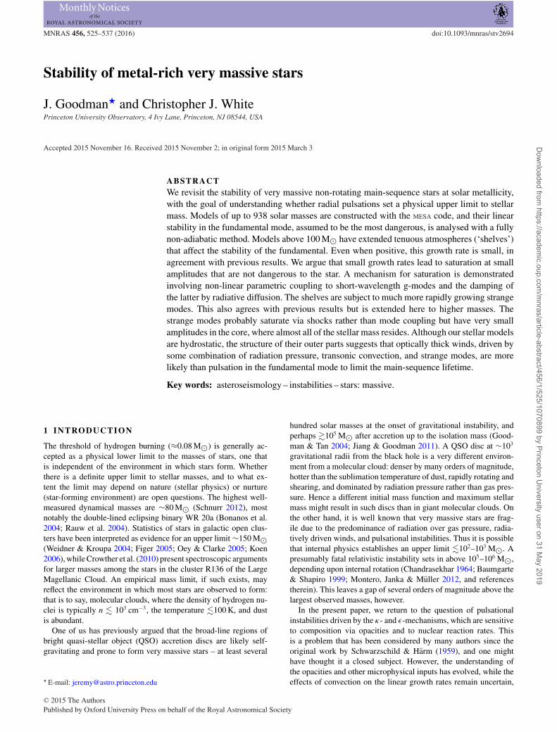
MNRAS 456, 525–537 (2016) doi:10.1093/mnras/stv2694

Stability of metal-rich very massive stars

J. Goodman‹ and Christopher J. WhitePrinceton University Observatory, 4 Ivy Lane, Princeton, NJ 08544, USA

Accepted 2015 November 16. Received 2015 November 2; in original form 2015 March 3

ABSTRACTWe revisit the stability of very massive non-rotating main-sequence stars at solar metallicity,with the goal of understanding whether radial pulsations set a physical upper limit to stellarmass. Models of up to 938 solar masses are constructed with the MESA code, and their linearstability in the fundamental mode, assumed to be the most dangerous, is analysed with a fullynon-adiabatic method. Models above 100 M� have extended tenuous atmospheres (‘shelves’)that affect the stability of the fundamental. Even when positive, this growth rate is small, inagreement with previous results. We argue that small growth rates lead to saturation at smallamplitudes that are not dangerous to the star. A mechanism for saturation is demonstratedinvolving non-linear parametric coupling to short-wavelength g-modes and the damping ofthe latter by radiative diffusion. The shelves are subject to much more rapidly growing strangemodes. This also agrees with previous results but is extended here to higher masses. Thestrange modes probably saturate via shocks rather than mode coupling but have very smallamplitudes in the core, where almost all of the stellar mass resides. Although our stellar modelsare hydrostatic, the structure of their outer parts suggests that optically thick winds, driven bysome combination of radiation pressure, transonic convection, and strange modes, are morelikely than pulsation in the fundamental mode to limit the main-sequence lifetime.

Key words: asteroseismology – instabilities – stars: massive.

1 IN T RO D U C T I O N

The threshold of hydrogen burning (≈0.08 M�) is generally ac-cepted as a physical lower limit to the masses of stars, one thatis independent of the environment in which stars form. Whetherthere is a definite upper limit to stellar masses, and to what ex-tent the limit may depend on nature (stellar physics) or nurture(star-forming environment) are open questions. The highest well-measured dynamical masses are ∼80 M� (Schnurr 2012), mostnotably the double-lined eclipsing binary WR 20a (Bonanos et al.2004; Rauw et al. 2004). Statistics of stars in galactic open clus-ters have been interpreted as evidence for an upper limit ∼150 M�(Weidner & Kroupa 2004; Figer 2005; Oey & Clarke 2005; Koen2006), while Crowther et al. (2010) present spectroscopic argumentsfor larger masses among the stars in the cluster R136 of the LargeMagellanic Cloud. An empirical mass limit, if such exists, mayreflect the environment in which most stars are observed to form:that is to say, molecular clouds, where the density of hydrogen nu-clei is typically n � 103 cm−3, the temperature �100 K, and dustis abundant.

One of us has previously argued that the broad-line regions ofbright quasi-stellar object (QSO) accretion discs are likely self-gravitating and prone to form very massive stars – at least several

� E-mail: [email protected]

hundred solar masses at the onset of gravitational instability, andperhaps �105 M� after accretion up to the isolation mass (Good-man & Tan 2004; Jiang & Goodman 2011). A QSO disc at ∼103

gravitational radii from the black hole is a very different environ-ment from a molecular cloud: denser by many orders of magnitude,hotter than the sublimation temperature of dust, rapidly rotating andshearing, and dominated by radiation pressure rather than gas pres-sure. Hence a different initial mass function and maximum stellarmass might result in such discs than in giant molecular clouds. Onthe other hand, it is well known that very massive stars are frag-ile due to the predominance of radiation over gas pressure, radia-tively driven winds, and pulsational instabilities. Thus it is possiblethat internal physics establishes an upper limit �102–103 M�. Apresumably fatal relativistic instability sets in above 105–106 M�,depending upon internal rotation (Chandrasekhar 1964; Baumgarte& Shapiro 1999; Montero, Janka & Muller 2012, and referencestherein). This leaves a gap of several orders of magnitude above thelargest observed masses, however.

In the present paper, we return to the question of pulsationalinstabilities driven by the κ- and ε-mechanisms, which are sensitiveto composition via opacities and to nuclear reaction rates. Thisis a problem that has been considered by many authors since theoriginal work by Schwarzschild & Harm (1959), and one mighthave thought it a closed subject. However, the understanding ofthe opacities and other microphysical inputs has evolved, while theeffects of convection on the linear growth rates remain uncertain,

C© 2015 The AuthorsPublished by Oxford University Press on behalf of the Royal Astronomical Society

Dow

nloaded from https://academ

ic.oup.com/m

nras/article-abstract/456/1/525/1070899 by Princeton University user on 31 M

ay 2019

mailto:[email protected]

526 J. Goodman and C. J. White

as do the mechanisms responsible for non-linear saturation of thepulsations if they grow at all.

We focus on the fundamental radial mode, on the assumption thatit is most dangerous. Glatzel & Kiriakidis (1993, hereafter GK93)have analysed the stability of solar metallicity stars up to 120 M�and found a host of higher order modes that grow more quicklythan the fundamental. However, the energies of these modes areconcentrated in the outer parts of the star, so that they can be ex-pected to reach non-linear amplitudes before the bulk of the massis much affected. The fundamental involves the entire star. Its char-acter and scaling with mass are unlike those of other modes. Thepulsation period increases ∝ M1/2, whereas those of higher orderradial modes scale ∝ M1/4. This is due to the predominance of radia-tion pressure, Prad/Pgas ∝ M1/2 for M � 100 M�, which makes verymassive non-rotating stars almost neutrally stable against changesin radius even in the adiabatic approximation. Thus at large ampli-tudes (δr/r � 1), the fundamental mode might disrupt or collapsethe entire star. The former requires unbinding the star which be-comes less difficult with increasing mass because of the predomi-nance of radiation pressure and the attendant near-cancellation ofgravitational and potential energies in hydrostatic equilibrium. (In-deed, spontaneous disruptions occurred in the simulations of AGNdisc fragmentation by Jiang & Goodman 2011, though they werecaused by numerical energy errors rather than pulsations.) Collapsemight occur under extreme compression due to electron–positronpairs at central temperatures approaching 109 K, or due to rela-tivistic corrections to gravity at masses >104 M� (Zeldovich &Novikov 1971).

Recently, Shiode, Quataert & Arras (2012, hereafter SQA) haverevisited the ε-mechanism. Applying a quasi-adiabatic analysis toequilibrium models constructed with the MESA code (Paxton et al.2011, 2013), they concluded that the instability is suppressed bythe effective viscosity due to turbulent convection, at least for starsof masses �1000 M�. However, they did not consider any modelsabove 100 M� with solar or higher metallicity. Since QSO discs ap-pear to be metal rich, with metallicities perhaps up to 10 times solar(Hamann & Ferland 1999; Dietrich et al. 2003; Matsuoka et al. 2011;Dhanda Batra & Baldwin 2014), one motivation for the present workwas to repeat SQA’s analysis at higher metallicities and masses>102 M�. We also wanted to perform a fully non-adiabatic ratherthan quasi-adiabatic analysis. This is arguably less important forthe ε-mechanism because it is driven deep within the star where thethermal time is very long. However, SQA also found evidence forinstabilities driven by opacity variations in the envelope which theydid not fully explore, perhaps because they had less confidence inthe quasi-adiabatic approximation for those modes. Also, at leastwith modern opacities, the envelopes of high-mass stellar models atsolar metallicity differ strikingly from those of corresponding Popu-lation III models, and this has interesting consequences for the modestructures.

Linear stability analysis is only a first step towards answeringthe question posed above. If instabilities are found, one must con-sider how they may saturate in order to decide whether they arelikely to shorten the main-sequence lifetime. Early attempts to ad-dress the saturation of instabilities driven by the ε-mechanism gaveconflicting results (Appenzeller 1970; Papaloizou 1973b), but lit-tle work has been done along these lines in recent decades. Wewill argue that even if the uncertain damping effects of convec-tion are neglected, the linear growth rates are so small comparedto the real part of the pulsation frequency that the pulsations willsaturate by one or another weakly non-linear mechanism at smallamplitudes that do not threaten the survival of these stars, at least

Table 1. Basic properties of our ZAMS models.

M/M� L/L� R/R� Teff (K) Xc

10.0 5.118 × 103 3.922 24 688 0.72721.5 4.841 × 104 5.998 34 983 0.72746.4 2.962 × 105 9.279 44 236 0.727100 1.244 × 106 15.27 49 360 0.729215 4.054 × 106 30.88 46 638 0.726464 1.135 × 107 75.29 38 635 0.728938 2.686 × 107 274.3 25 106 0.727

not before they have lived out most of the nominal minimum main-sequence lifetime (∼3 × 106 yr). Instead, in view of the structureof our hydrostatic models, as well as a recent body of work onWolf–Rayet and O-star winds, radiatively driven mass loss seemsmore likely than pulsational instabilities to limit the lifetimes of themost massive metal-rich stars. We hope to explore the scaling ofthe mass-loss time-scale (i.e. |M/M|) with stellar mass in a futurepaper.

The outline of this paper is as follows. Section 2, supplemented byAppendix A, presents the equilibrium MESA models and our methodsfor the linear stability analysis. Section 3 highlights the extendedatmosphere or ‘shelf’ seen in the higher mass models. Results forthe growth rates and eigenfunction of the fundamental are given inSection 4, with particular emphasis on non-adiabatic effects in theshelf. GK93’s intrinsically non-adiabatic ‘strange modes’ are shownto extend to higher masses, where they have longer periods than thefundamental. Section 5 examines non-linear saturation of the fun-damental through three-mode or parametric coupling to high-ordernon-radial g-modes, and (more briefly) saturation of strange modesin shocks. Since the stably stratified zones of our most massivemodels are relatively small, and would perhaps disappear entirelyat some higher mass, the explicit estimates in Section 5 are in-tended to be illustrative of a larger class of weak non-linearities thatwill limit the amplitude of the fundamental when its growth rateis small. A summary of our conclusions and a discussion of futuresteps follows in Section 6.

2 M E T H O D

2.1 Equilibrium models and initial estimates

Like SQA, we generated zero-age main sequence (ZAMS) stellarmodels using the stellar evolution code MESA. Here we highlight theconfiguration settings used when they deviate from the defaults.

The initial mass is specified, with initial abundances (X, Y, Z) =(0.73, 0.25, 0.02). The simulation begins in the pre-main-sequencephase at a large radius and low central temperature. The atmo-sphere is modelled as a ‘simple photosphere’. Convective mixingis implemented following Henyey, Vardya & Bodenheimer (1965)in regions determined to be convectively unstable by the Ledouxcriterion.

The star is evolved until it is determined to lie on the main se-quence, defined by the minimum photospheric radius. (MESA hasits own way of deciding when the model has reached the main se-quence, but we found its decisions unreliable for our higher massmodels.) The nuclear and photospheric luminosities are then in equi-librium, and the central hydrogen abundance is only very slightlydepleted. Table 1 lists some properties of the models, which aresimilar to those of GK93 (within 5 per cent in L and 1 per cent inTeff), except that theirs were limited to 40–120 M�. The effective

MNRAS 456, 525–537 (2016)

Dow


ic.oup.com/m


ay 2019

Stability of metal-rich massive stars 527

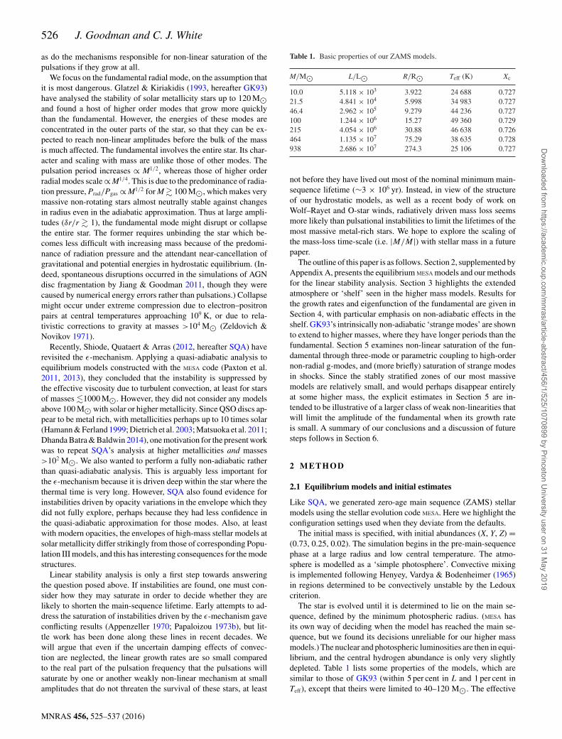
Figure 1. Luminosity (star symbols, left-hand scale) and photospheric ra-dius (circles, right-hand scale) versus stellar mass for our MESA models. Thinsolid line is the Eddington limit for this composition (Y = 0.25, Z = 0.02).Thin dashed line shows R ∝ M1/2, as would be expected for homologousradiation-pressure-dominated models.

temperature peaks at 4.95 × 104 K near 120 M�: more massiveare cooler because of their distended atmospheric ‘shelves’ drivenby iron opacities (Section 3). Luminosities and radii for additionalmodels are shown in Fig. 1.

Once the star has reached its ZAMS phase, the model is savedand the data are analysed with the ADIPLS package (Christensen-Dalsgaard 2008), which computes adiabatic pulsational modesgiven one-dimensional stellar models. The output from ADIPLS isa set of eigenfrequencies and corresponding mode shapes in theform of radial displacements from equilibrium. We use these out-puts in our own routine, which finds mode frequencies and shapeswithout the adiabatic assumption. We turn to this method now.

2.2 Non-adiabatic analysis

For the purpose of analysing the pulsational modes in a non-adiabatic framework, we began by adopting the method outlinedin Castor (1971), with mass fraction as the independent variable,and a Henyey-type relaxation scheme for finding the eigenfrequen-cies. Despite extensive efforts and algorithmic variations, this didnot give numerically stable results for the growth rate of the fun-damental mode, possibly because of the many orders of magnitudeseparating the dynamical and thermal time-scales in the core, and theenormous radial variation in the ratio of these time-scales throughthe star.

We therefore adopted a sort of shooting method designed forvery stiff equations (Appendix A). The basic linearized equationsare

∂

∂rδPgas = ρ

[ω2δr + grad

(δκ

κ+ δLrad

Lrad

)+ 4geff

δr

r

], (1a)

r−2 ∂

∂r(r2δr) = − δρ

ρ, (1b)

∂

∂rδPrad = −ρgrad

(δκ

κ+ δLrad

Lrad− 4

δr

r

), (1c)

∂

∂rδL = iω4πr2ρT δS + 4πr2ρ

δε

ε. (1d)

Here grad = κLrad/4πr2c is the radiative force per unit mass,geff = GMr/r2 − grad is the residual between the gravitationaland radiative accelerations, δ represents Lagrangian perturbation(first-order variation at fixed interior mass), and all other sym-bols have their usual meaning. We define dimensionless linearizedvariables

y0 ≡ δr

r, y1 ≡ δρ

ρ, y2 ≡ δT

T, y3 ≡ δLrad

L. (2)

Notice that L not Lrad appears in the denominator of y3.In principle δL = δLrad + δLconv. However, since there is no

generally accepted prescription for time-dependent convective lu-minosity – especially in the radiation-pressure-dominated regime –we adopt δLconv = 0 (‘frozen convection’). Nor have we allowedfor a turbulent convective viscosity in the linearized momentumequation (1a).

Then in terms of our dimensionless variables, with primesfor d/dr and writing f ≡ Lrad/L, κT = (∂ ln κ/∂ ln T )ρ , κρ =(∂ ln κ/∂ ln ρ)T , and similarly for εT and ερ , equations (1)become

ry ′0 = −3y0 − y1, (3a)

y ′1 + y ′

2 = ρ

Pgas[ω2ry0 + grad(κρy1 + κT y2 + f −1y3)

+ geff (4y0 + y1 + y2)], (3b)

y ′2 = −ρgrad

4Prad[κρy1 + κT y2 + f −1y3 − 4y0 − 4y2], (3c)

ry ′3 = 4πr3ρ

L{iωCV T [y2 − (�3 − 1)y1]

+ ε(ερy1 + εT y2 − y3)}. (3d)

The system of equations is closed by choosing four boundaryconditions. Physically, one expects δr = δL = δLrad = 0 at r = 0.This does not require y0 or y3 to vanish at the centre, but from thefirst of equations (3), one sees that non-singular behaviour requires

3y0 + y1 → 0 as r → 0. (4)

Similarly, regularity of the last of equations (3) implies

iωCV T

ε[y2 − (�3 − 1)y1] + ερy1 + εT y2 − y3 → 0 as r → 0.

(5)

The factor in front of the square brackets is ∼tKH/tdyn 1 ifω ∼ t−1

dyn, so to a first approximation the behaviour near the originis adiabatic, δ ln T ≈ (�3 − 1)δ ln ρ. But since we are interested ingrowth or decay rates ωI ∼ t−1

KH, we use equation (5) as written.The outer heat equation requires a more general analysis than

is given by Castor, as the equations in that work only hold underthe assumption that radiation pressure is negligible compared togas pressure at the outer boundary. This condition clearly does nothold for very massive stars. We therefore turn to the equation forradiation pressure in the Eddington approximation:

Prad = F

c

(τ + 2

3

),

where F is the radiative flux and τ is the optical depth at the locationbeing considered. In more familiar variables,

Prad = Lrad

4πr2c

(κm

4πr2+ 2

3

), (6)

MNRAS 456, 525–537 (2016)

Dow


ic.oup.com/m


ay 2019


where m is the mass exterior to the point being considered, if thedensity scale height is �r. Linearizing yields

δPrad

Prad= δLrad

L− 4

(τ + 1/3

τ + 2/3

)δr

r+

(τ

τ + 2/3

)δκ

κ,

or in dimensionless variables,

−4

(τ + 1

3

)y0 + τκρy1 + τκT y2 +

(τ + 2

3

)(y3 − 4y2) = 0.

(7)

We replace Lrad with L here because in practice the model extendsfar enough into the tenuous atmosphere as to make the contributionof Lconv negligible.

The outer momentum equation is closed as follows. The totalpressure at a point near the surface, under a mass m and at aradius r, is

P = m

4π

(r

r2+ GM

r4

)+ L

6πcr2, (8)

if the mass shell m is thin and effectively hydrostatic in its accel-erated frame. The last term in equation (8) is the radiation pressureextrapolated to the outer surface of the shell, where τ = 0. Subtract-ing equation (6) from equation (8) yields

Pgas = m

4π

(r

r2+ GM

r4− κLrad

4πr4c

). (9)

Perturbing this yields

δPgas

Pgas= − δr

r

(4 + ω2r3

βGM

)− 1 − β

β

(δL

L+ δκ

κ

),

or equivalently,(4 + ω2R3

βGM

)y0 + 1 − β

β(y3 + κρy1 + κT y2)

− y1 − y2 = 0, (10)

where β is defined in terms of the Eddington luminosity LEdd =4πGMc/κ by L = (1 − β)LEdd.

3 TH E S H E L F

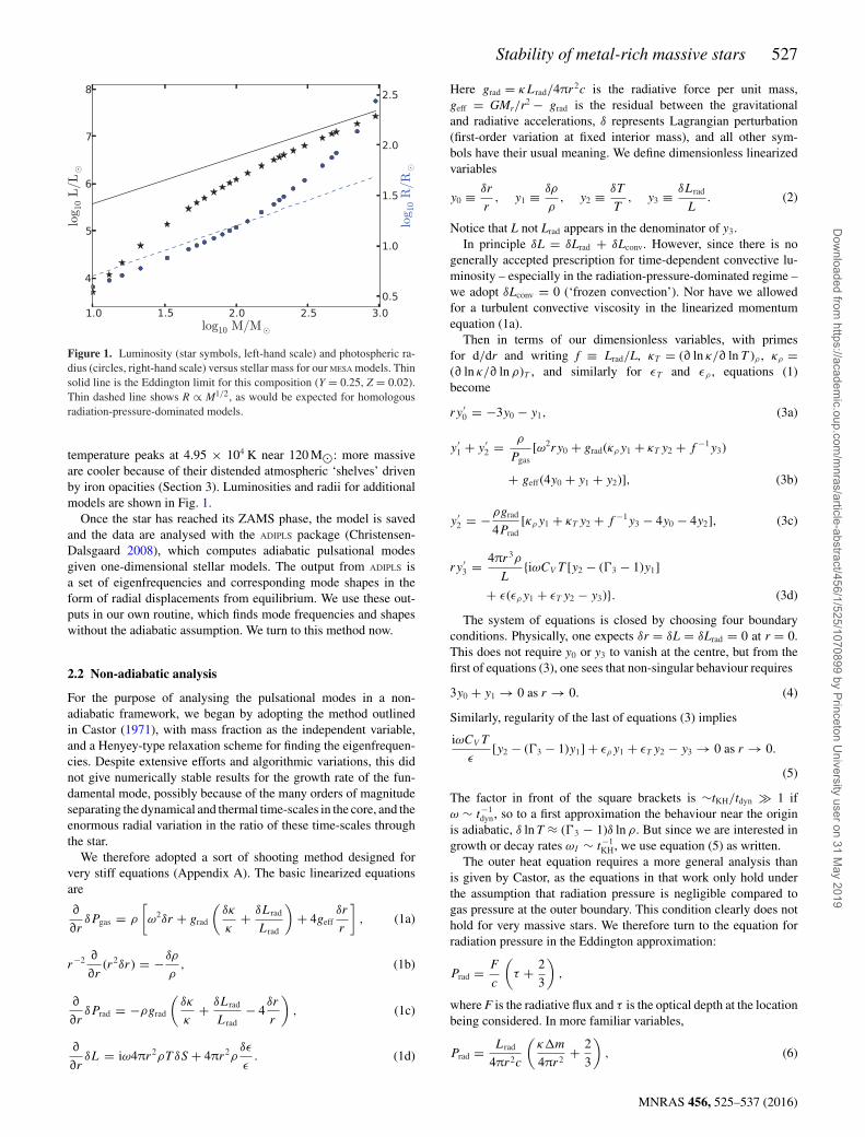
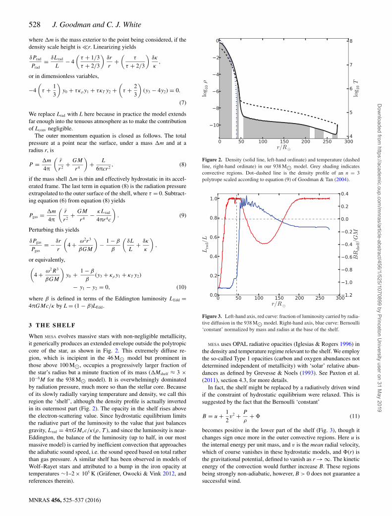
When MESA evolves massive stars with non-negligible metallicity,it generically produces an extended envelope outside the polytropiccore of the star, as shown in Fig. 2. This extremely diffuse re-gion, which is incipient in the 46 M� model but prominent inthose above 100 M�, occupies a progressively larger fraction ofthe star’s radius but a minute fraction of its mass (Mshelf ≈ 3 ×10−6M for the 938 M� model). It is overwhelmingly dominatedby radiation pressure, much more so than the stellar core. Becauseof its slowly radially varying temperature and density, we call thisregion the ‘shelf’, although the density profile is actually invertedin its outermost part (Fig. 2). The opacity in the shelf rises abovethe electron-scattering value. Since hydrostatic equilibrium limitsthe radiative part of the luminosity to the value that just balancesgravity, Lrad = 4πGM∗c/κ(ρ, T ), and since the luminosity is near-Eddington, the balance of the luminosity (up to half, in our mostmassive model) is carried by inefficient convection that approachesthe adiabatic sound speed, i.e. the sound speed based on total ratherthan gas pressure. A similar shelf has been observed in models ofWolf–Rayet stars and attributed to a bump in the iron opacity attemperatures ∼1–2 × 105 K (Grafener, Owocki & Vink 2012, andreferences therein).

Figure 2. Density (solid line, left-hand ordinate) and temperature (dashedline, right-hand ordinate) in our 938 M� model. Grey shading indicatesconvective regions. Dot–dashed line is the density profile of an n = 3polytrope scaled according to equation (9) of Goodman & Tan (2004).

Figure 3. Left-hand axis, red curve: fraction of luminosity carried by radia-tive diffusion in the 938 M� model. Right-hand axis, blue curve: Bernoulli‘constant’ normalized by mass and radius at the base of the shelf.

MESA uses OPAL radiative opacities (Iglesias & Rogers 1996) inthe density and temperature regime relevant to the shelf. We employthe so-called Type 1 opacities (carbon and oxygen abundances notdetermined independent of metallicity) with ‘solar’ relative abun-dances as defined by Grevesse & Noels (1993). See Paxton et al.(2011), section 4.3, for more details.

In fact, the shelf might be replaced by a radiatively driven windif the constraint of hydrostatic equilibrium were relaxed. This issuggested by the fact that the Bernoulli ‘constant’

B = u + 1

2v2 + P

ρ+ � (11)

becomes positive in the lower part of the shelf (Fig. 3), though itchanges sign once more in the outer convective regions. Here u isthe internal energy per unit mass, and v is the mean radial velocity,which of course vanishes in these hydrostatic models, and �(r) isthe gravitational potential, defined to vanish as r → ∞. The kineticenergy of the convection would further increase B. These regionsbeing strongly non-adiabatic, however, B > 0 does not guarantee asuccessful wind.

MNRAS 456, 525–537 (2016)

Dow


ic.oup.com/m


ay 2019


Figure 4. Plot of the lowest frequency adiabatic modes for the 464 M�model. The curves show the square root of the mode kinetic energy per unitlength, normalized independently. The modes have radial mode number nequal to 1 (red), 2 (orange), 3 (green), 4 (cyan), 5 (blue), 6 (magenta), or 7(black), only the latter of which is not evanescent in the core.

For a precise definition of the base of the shelf, we use the radiusor mass fraction corresponding to the local minimum in the pressurescale height, HP. For the model shown in Fig. 2, this is Rshelf =46.3 R�. Within our suite of models, such a minimum occurs onlyfor M � 50 M�.

4 R ESULTS

4.1 Adiabatic calculations

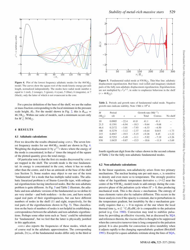
First we describe the results obtained using ADIPLS. The seven low-est frequency modes for our 464 M� model are shown in Fig. 4.Weighting the displacement δr by ρ1/2r shows where the energy ofthe mode is concentrated, in that ω2 times the integral of the squareof the plotted quantity gives the total energy.

Of particular note is that the first six modes discovered by ADIPLS

are trapped in the shelf. The seventh mode is the true fundamen-tal: its energy is concentrated in the core, where it has no nodesother than the centre, and it has an antinode at the base of the shelf(see Section 3). Some readers may object to our use of the term‘fundamental’ for a mode that has multiple radial nodes. The adia-batic linearized problem is of Sturm–Liouville type, with orthogo-nal eigenfunctions having interleaved nodes. But the non-adiabaticproblem is quite different. As Fig. 5 and Table 2 illustrate, the adia-batic and non-adiabatic versions of the fundamental (as we define it)are very similar – and both nodeless – in the core, and have nearlyequal real parts of their eigenfrequencies, but can have differentnumbers of nodes in the shelf (11 and eight, respectively, for thereal parts of the eigenfunctions shown in Fig. 5). Thus classifica-tion on the basis of numbers of nodes is not helpful in establishing acorrespondence between the adiabatic and non-adiabatic eigenfunc-tions. Perhaps some other term such as ‘basic’ could be substitutedfor ‘fundamental’, but we feel that the latter is physically justifiedin this application.

ADIPLS also reports the frequencies of these modes, which areof course real in the adiabatic approximation. The correspondingperiods, 2π/ω, of the fundamental modes differ only in the third or

Figure 5. Fundamental radial mode at 938 M�. Thin blue line: adiabaticdisplacement eigenfunction. Red lines: real (solid) and imaginary (dashed)parts of the fully non-adiabatic displacement eigenfunction. Eigenfunctionsare not multiplied by r2ρ1/2, in order to emphasize behaviour in the shelf(r > 46 R�).

Table 2. Periods and growth rates of fundamental radial mode. Negativegrowth rates indicate stability. Note 1 Md ≡ 106 d.

M Period Growth rate (Md−1)(M�) (d) ε κ Total Convec. No shelf

10 0.0905 −22.4 41.0 41.1 41.1 –21.5 0.1391 −6.94 −10.3 −9.64 −9.68 –46.4 0.2172 −3.01 −7.93 −6.33 −6.50 –100 0.3279 −3.12 −2.37 +0.44 0.015 −1.73215 0.4947 −19.5 −5.15 +9.28 8.45 +1.22464 0.7253 −5.49 −11.1 −5.92 −7.19 +3.26938 1.0435 −9.87 −15.5 −10.6 −11.9 +3.69

fourth significant digit from the values shown in the second columnof Table 2 for the fully non-adiabatic fundamental modes.

4.2 Non-adiabatic calculations

In the linear equations, non-adiabaticity arises from two primarymechanisms. The nuclear heating rate per unit mass, ε, is sensitiveto density and even more so to temperature. The strongly positivevalue of the logarithmic temperature derivative εT (≈12 near thecentre of the 938 M� model) tends to add entropy during the com-pressive phase of the pulsation cycle when δT > 0, thus producingmechanical work. This is the classic ε-mechanism. The entropy ofmass elements varies also by radiative diffusion. This occurs in thelinear analysis even if the opacity is constant, due to perturbations inthe temperature gradient, but instability by the κ-mechanism gen-erally requires that κT > 0 in regions of the star where the localthermal time tth ≡ L−1CVHPdMr/dr is comparable to the pulsationperiod (e.g. Cox 1980). Convection may tend to stabilize pulsa-tions by providing an effective viscosity, but as discussed by SQAand references therein, the viscous effect is thought to be suppressedwhen the convective turnover time is long compared to the pulsationperiod. It is also possible for convection to drive instability whenit adjusts rapidly to the changing superadiabatic gradient (Brickhill1991). Except for a quasi-adiabatic estimate along the lines of SQA,

MNRAS 456, 525–537 (2016)

Dow


ic.oup.com/m


ay 2019


we have generally neglected these convective effects, even thoughthese stars are in fact largely convective.

When applying the numerics described in Section 2.2, we arefree to set any of εT, ερ , κT, and κρ to zero throughout the model.In this way we can separate the two effects. Thus the third columnof Table 2 lists the growth rates obtained when the derivatives of κ

are neglected, and similarly the fourth column gives the rates whenthe derivatives of ε are set to zero, while the fifth column retains allderivatives.

The effects of the non-adiabatic mechanisms on the growth rateare not entirely additive, as they would be in the quasi-adiabatic ap-proximation. This is because the opacity derivatives have a substan-tial effect on the shape of the eigenfunction near the photosphere(or in the shelf), which is also the region mainly responsible fordriving or damping. However, the ε-mechanism does appear to beadditive, as might be expected since it acts only in the core wherethe quasi-adiabatic approximation is excellent. That is to say, ifω

(ε)I , ω(κ)

I , and ωI represent the growth rates in the third through fifthcolumns of Table 2, while ω

(0)I is the growth rate obtained when all

of εT, ερ , κT, κρ are neglected (this is not shown in the table), thenwe do find that ω

(ε)I − ω(0) ≈ ωI − ω

(κ)I for all of the models except

perhaps the first (10 M�), in which the ε-mechanism is very weak.The sixth column in Table 2 differs from the fifth by including a

quasi-adiabatic work-integral estimate of convective viscous damp-ing, following equations (11) and (12) of SQA. Since the quasi-adiabatic method depends upon the adiabatic eigenfunction, andsince the adiabatic and non-adiabatic eigenfunctions differ stronglyin the shelf region, we truncate the work integrals at the local mini-mum in the pressure scale height.

It can be seen that the two most massive models are stable with-out the convective correction. This appears to be due to radiativedamping in the shelf. In Fig. 5, the first two nodes of the real partof the displacement occur r ≈ 87 and 141 R�, where the imaginarypart is close to a local maximum and minimum, respectively. (Re-call that the shelf begins at 46 R�.) Thus the phase increases withradius, as for an outward-propagating acoustic wave. Evidently thiswave is damped almost completely, because if it were not, thenupon reflection from the photosphere a standing wave would resultwith real and imaginary parts in phase. The escaping acoustic powercan be estimated as Eac = 2πr2ρcs|δv|2, where δv = −iωδr is theradial velocity perturbation and cs ≡ (�1P/ρ)1/2 is the adiabaticsound speed. Evaluating this at the first node and dividing by twicethe total mode energy, 2Emode = 4π

∫ρr2|δv|2dr , yields an esti-

mate for the damping rate of the mode amplitude: 11 Md−1. Thisagrees well with the directly calculated growth rate shown for thismodel in the fifth column of Table 2. Of course the calculations arenot independent because the estimate above uses the non-adiabaticeigenfunction. But it does suggest that the non-adiabatic calcula-tion is self-consistent, and also that acoustic radiation into the shelfis the dominant loss mechanism at our highest masses. As furtherevidence of this, the final column of Table 2 shows growth ratescalculated when the ‘photospheric’ boundary conditions (7) and(10) are imposed at the local minimum of the pressure scale height(which does not exist in the two least massive models), thus ef-fectively discarding the shelf region from the linear analysis. Thisresults in a small positive growth rate.

4.3 Strange modes

In addition to the fundamental mode, there are in principle an infinitenumber of other radial modes. Some, like the fundamental itself, are

Figure 6. Real (first panel) and imaginary (second panel) parts of the lowestlying modes versus stellar mass. (Positive imaginary parts indicate instabil-ity.) Solid circles mark the fundamental. Other modes are marked by thenumber of nodes of δr/r in the core. M/M� ∈ {10, 13, 16, 21.5, 33, 46.4,53, 60, 70, 80, 90, 100, 120, 150, 183, 200, 215, 250, 300, 400, 465, 500,700, 983}.

slight modifications of adiabatic counterparts and are concentratedin the core (the region below the local minimum of the pressurescale height). The real parts of the frequencies of these increasewith the number of nodes in the displacement eigenfunction (δr/r),while the imaginary parts tend to become more negative (i.e. moredamped) but are generally small because of the long thermal timein the core.

Besides these, there are modes that have no obvious adiabaticcounterpart, and which are probably the strange modes discussedby GK93 and Papaloizou et al. (1997). Though some of these aredamped, others have positive growth rates [Im(ω) > 0] whose re-ciprocals approach the dynamical time. Their energies are stronglyconcentrated in the tenuous shelf region and thus are not likely toaffect directly the bulk of the star. This is discussed more quantita-tively below (Section 5.2).

Fig. 6 shows the complex eigenfrequencies versus mass for themodels in Table 1 and Fig. 6. For each mass, we show the fouror five modes with smallest real part – at least among those we

MNRAS 456, 525–537 (2016)

Dow


ic.oup.com/m


ay 2019


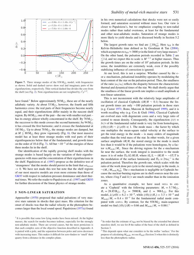
Figure 7. Three strange modes of the 938 M� model, with frequenciesas shown. Solid and dashed curves show real and imaginary parts of theeigenfunctions, respectively. Thin vertical dashed line divides the core fromthe shelf (see Fig. 2). Note eigenfunctions are not weighted by r2ρ1/2.

have found.1 Below approximately 50 M�, these are of the nearlyadiabatic variety. At about 53 M�, however, the fourth and fifthharmonics cross: the real parts of their frequencies become nearlyequal, and their eigenfunctions differ mainly in the nascent shelfregion. By 60 M�, one of the pair – the one with smaller real part –has its energy almost wholly concentrated in the shelf. By 70 M�,the successor to this mode crosses the second harmonic; by 94 M�it has crossed the first harmonic; and it crosses the fundamental at183 M�. Up to about 70 M�, the strange modes are damped, butat M ≥ 80 M� they grow vigorously (Fig. 6). Our most massivemodel has at least three strange modes with real parts of theireigenfrequencies below that of the fundamental, and growth timeson the order of 10 d (Fig. 7). All but ∼10−8 of the energies of thesethree modes lie in the shelf.

Our identification of the rapidly growing shelf modes with thestrange modes is based largely on the variation of their eigenfre-quencies with mass and the concentration of their eigenfunctions inthe shelf. Papaloizou et al. (1997) propose as the definitive test of‘strangeness’ that the modes should persist in the limit that ωtthermal

→ 0. We have not made this test but note that the shelf regionsof our most massive models are even more extreme than those ofGK93 with respect to radiation-pressure dominance and short ther-mal times. We refer the reader to Papaloizou et al. (1997) and GK93for further discussion of the linear physics of strange modes.

5 N O N - L I N E A R SATU R AT I O N

Appenzeller (1970) proposed that radial pulsations of very mas-sive stars saturate in shocks that eject mass. His criterion for theonset of shocks was that the radial velocity at the photosphere be-comes larger than the local sound speed. Papaloizou (1973a) found

1 It is possible that some low-lying modes have been missed. At the highermasses, the search for modes becomes tedious, especially for the stronglynon-adiabatic modes. There are several causes, but the most pernicious isthat each complex zero of the objective function described in Appendix Ais paired with a pole, and the separation between poles and zeros decreaseswith increasing mass. This makes it difficult for zero-finders to ‘smell’ theirquarry from a distance in the complex plane.

in his own numerical calculations that shocks were not so easilyformed, and saturation occurred without mass loss. Our view iscloser to Papaloizou’s, but we emphasize coupling to non-radialmodes rather than radial overtones, at least for the fundamentaland other near-adiabatic modes. Saturation of strange modes ismore likely to yield shocks and is discussed briefly in Section 5.2below.

The largest growth rates we find are �10t−1KH. Here tKH is the

Kelvin–Helmholtz time defined as by Goodman & Tan (2004),which asymptotes to tKH ≈ 3000 yr in the limit of very large masses.2

On the other hand, the pulsation periods recorded in Table 2 are�1 d, and we expect this to scale ∝ M−1/2 at higher masses. Thusthe growth times are on the order of 105 pulsation periods. In thissense, the instabilities are extremely weak, even if the possiblystabilizing influence of convection is ignored.

At one level, this is not a surprise. Whether caused by the ε-or κ-mechanism, pulsational instability operates by modulating theheat content of the star on the pulsation period. Thus, the smallnessof the ratio |ωi/ωr| reflects the disparity between the characteristicthermal and dynamical times of the star. We shall shortly argue thatthe smallness of the linear growth rate implies a small amplitude atnon-linear saturation.

This is not inconsistent with the relatively large amplitudes ofoscillation of classical Cepheids (δR/R ∼ 0.1) because the lin-ear growth times are only ∼100 pulsation periods in those stars(e.g. Castor 1971; Bono, Marconi & Stellingwerf 1999), and it isworth recalling why (e.g. Cox & Giuli 1968). Classical Cepheidsare evolved stars with degenerate cores and a very large ratio ofcentral to mean density. Consequently, the eigenfunction ζ (r) ≡δr/r of the fundamental radial mode is very far from homologous,ζ (0)/ζ (R) ∼ ρ/ρ(0) � 1. The mode mass – the factor by whichone multiplies the mean-square radial velocity at the surface toget the total energy in the mode – is many orders of magnitudesmaller than the total mass of the star. In other words, for a givensurface amplitude δR/R, the stored energy in the mode is muchless than it would be if the pulsations were homologous, by a fac-tor ∝Mmode/M∗. Since the driving regions for the κ-mechanismlie near the surface, the work integral is insensitive to the modemass: it is of order �0 δL δR/R, where δL/L ∼ δR/R ∼ −δT/T isthe modulation of the surface luminosity and �0 ≡ 2πω−1

r is thepulsation period. Therefore the growth rate, which scales with theratio of the work done per cycle to the stored energy in the mode, is∼(M∗/Mmode)t−1

KH. The ε-mechanism is negligible in Cepheids be-cause the nuclear-burning regions are in shell sources near the cen-tre, where δ log T and δr/r are much smaller than in the ionizationzones.

As a quantitative example, we have used MESA to cre-ate a ‘Cepheid’ with the following parameters: M∗ = 5.7 M�,R∗ = 28.85 R�, Teff = 5900 K, and L = 906 L�. For thismodel, ρ/ρ(0) = 6.2 × 10−8, while ζ (0)/ζ (R∗) = 3.3 × 10−6 andMmode/M∗ = 8.4 × 10−5 for the fundamental radial mode com-puted with ADIPLS. By contrast, for the 938 M� main-sequencemodel we find ζ (0)/ζ (R) = 0.66 and Mmode/M∗ = 0.061.3

2 In order that the estimate of tKH not be biased by the extended but almostmassless shelf, we use for R the radius of the base of the shelf as defined inSection 3.3 This depends upon what one considers to be the stellar ‘surface.’ For thepurpose of calculating Mmode, we use Rshelf (Section 3) when this is distinctlyless than the photospheric radius.

MNRAS 456, 525–537 (2016)

Dow


ic.oup.com/m


ay 2019


Thus the fundamental mode is approximately homologous and in-volves a significant fraction of the star’s mass. We expect Mmode/M∗to be nearly constant and comparable to this for larger masses be-cause of the similarity of these models to isentropic n = 3, �1 =4/3 polytropes. Thus we also expect the growth rates of the funda-mental radial mode to remain �10t−1

KH, due to the relatively homo-geneous structure and homologous pulsation of these very massivemain-sequence models, regardless of the details of the excitationmechanisms and of the shelf or wind.

5.1 Saturation of the fundamental via three-mode coupling

As a general rule, instabilities with smaller linear growth rates satu-rate at lower amplitudes. A simple model equation for the amplitudeenvelope A > 0 might be

dA

dt= ωiA − νAn+1, (12)

in which ωi is the linear growth rate, while ν and n describe the non-linearities. If ωi, ν, and n are all positive, then equilibrium is reachedat Asat = (ωi/ν)1/n. As noted above, pulsations in classical Cepheidsgrow relatively rapidly. Saturation in these stars and in RR Lyraesoccurs via shocks and non-linear modification of the conditionsin the driving (ionization) zones (Christy 1966). Because of theirmuch smaller dimensionless growth rates (ωi/ωr ∼ 10−6 insteadof ∼10−3), the massive main-sequence stars considered here maysaturate at lower amplitudes, where more delicate non-linearitiesmay be effective.

Dziembowski (1982) suggested that three-mode coupling is re-sponsible for saturation in dwarf Cepheids, and that this explainswhy they oscillate at lower amplitudes than do classical Cepheids.He worked directly from non-linear equations of motion. But if dis-sipation is weak, an action principle, which is necessarily adiabatic,can be efficient in describing mode couplings. The Lagrangian den-sityL(ξ, ξ) is expanded in powers of the displacement ξ and its timederivative ξ. The quadratic terms (L2) yield the linearized equationsof motion, while cubic and higher terms (L3 + L4 + · · ·) describenon-linear couplings. When the amplitude of the primary/‘parent’mode grows slowly from small amplitudes, the cubic non-linearitiesare the first to come into play. The most important couplings arethose that are resonant, meaning that the linear eigenfrequenciesof the parent and daughter modes satisfy ωp ≈ ωd1 + ωd2, so thatsecular transfers of energy can occur.4 However, the correspond-ing Hamiltonian density H2 + H3 cannot be positive definite sincethe components of ξ can have either sign, so that the higher ordernon-linearities must dominate if the amplitudes pass some thresh-old, perhaps leading to shocks and a breakdown of the Lagrangiandescription. Actually, even when the amplitudes remain small, dis-sipative terms must be added to the equations of motion to describethe linear damping of the daughter modes. In application to pul-sating stars, the growth rate of the parent is also represented bya non-adiabatic term. The daughter modes are usually smaller inwavelength than the parent and therefore more easily damped byradiative diffusion or (perhaps) eddy viscosity.

Landmark applications of three-mode coupling to the saturationof stellar instabilities include those by Wu & Goldreich (2001) (towhite dwarf/ZZ Ceti stars), as well as Schenk et al. (2002) andArras et al. (2003) (to rapidly rotating neutron stars). Papaloizou

4 In resonance conditions such as this, all frequencies are understood to bereal and non-negative.

(1973a) argued that pulsations of very massive stars driven by theε-mechanism can saturate via direct resonant couplings: that is, thecoupling of a quadratic or higher power of the fundamental modeto a higher frequency radial p mode (overtone), so that nωf ≈ ωd

for some integer n > 1. Non-radial daughter modes offer manymore possibilities for resonance, however, g-modes are necessar-ily non-radial and have low frequencies, which is important forresonances of the type ωp ≈ ωd1 + ωd2 because the frequency ofthe fundamental, ωf, is somewhat lower relative to the character-istic dynamical frequency ω∗ ≡ (GM∗/R3

∗)1/2 than in less massivestars, the ratio ωf/ω∗ scaling as M−1/2 (Goodman & Tan 2004).Therefore we focus on couplings of this type. When the parent isthe radial fundamental mode, the strongest three-mode couplingsare usually parametric subharmonic, meaning that the two daughtermodes are two copies of the same mode, with frequency ωd ≈ ωf/2.The eigenfunction of a typical daughter mode is high order, withmany nodes in radius and angle, but its square is non-negative andhence may have a significant three-mode coupling with the node-less radial fundamental. Parametric subharmonic destabilization ofg-modes and internal waves has been studied experimentally aswell as theoretically (Benielli & Sommeria 1998, and referencestherein).

We use our most massive (938 M�) model as an example. Mostof the star convects, but there is a radiative zone at 29 � r/R� ≤41 containing 0.026M. (There is also a second radiative zone at r ≥44 R�, and still others in the shelf, but these contain much less mass,so we neglect them here.) The peak of the Brunt–Vaisala frequencyis Nmax = 2.94ω∗, whereas the frequency of the fundamental radialmode is ωf = 1.1446ω∗ ≈ 7.116 × 10−5 rad s−1 according to ADIPLS

(which computes only the real part), in good agreement with ournon-adiabatic code. Thus there are many g-modes with frequencies∼ωf/2. Using the approximate Wentzel–Kramers–Brillouin (WKB)dispersion for high-order g-modes,√

l(l + 1)

ωln

∫N (r)

dr

r≈ π

(n − 1

2

)(13)

(where n ≥ 1 counts radial nodes) and the profile of the Brunt–Vaisala frequency in the radiative zone, N(r), we estimate that n/l ≈0.34 for ωln ≈ ωf/2 and l, n 1. For a non-rotating spherical star, sothat the eigenfrequency is independent of spherical-harmonic orderm, the number of mode frequencies in a given interval ω near ωf/2that correspond to g-modes of degree l′ ≤ l scales as 0.17 l2log ω

when l 1. Inverting this, the minimum l at which one expects tofind modes in the interval ω is

lmin(ω) ≈ 2.4

(ω

ω

)−1/2

. (14)

The distance ω from exact subharmonic resonance at whichdaughter modes can grow depends upon the linear damping rateof these modes, the amplitude of the parent, and the three-modecoupling coefficient. For the damping time of high-order g-modesby radiative diffusion, we apply equation (4.8) of Dziembowski(1982) to our 938 M� model:

tdamp = γ −1d ≈ 1.0

(30

l

ωf

2ω

)2

yr. (15)

We evaluate the three-mode coupling coefficient from equation(A8) of Kumar & Goldreich (1989). Their formula assumes thatthe adiabatic exponent �1 is constant and neglects the Eulerian per-turbation to the gravitational potential, which, although essentialfor the eigenfrequency of the fundamental mode, is unimportantfor the coupling since most of the stellar mass lies interior to the

MNRAS 456, 525–537 (2016)

Dow


ic.oup.com/m


ay 2019


propagation region of the g-modes in our case. We make thefurther approximation that the fundamental mode is exactly ho-mologous, meaning that its radial displacement is given by δr(r,t) = ζ r cos (ωft), with ζ spatially constant but growing slowlyas exp (ωit). We approximate the daughter mode eigenfunctionsusing WKB, neglecting terms of relative order (krHP)−1, wherekr ≈ √

l(l + 1)N/ωr is the radial wavenumber and HP the pressurescale height, and find that∫

H3d3x = · · · +(

3�1 − 1

2

)ζ cos ωf t

∫N2δr2

d dM . (16)

Here ‘···’ represents all three-mode coupling other than the one ofinterest, while δrd = qd(t)ξ r,d(r)Ylm(θ , φ) is the radial displacementof the daughter mode, with time-dependent amplitude qd(t). Forsimplicity, we set �1 = 4/3, though the mass-averaged value of �1

in the 938 M� model is ≈1.37.The integrand of equation (16) is twice the potential energy per

unit mass of the g-mode. The coupling term can therefore be treatedas though it were a time-dependent correction to the linear dynamicsof the daughter mode, whose amplitude evolves according to

qd + 2γdqd + ω2d [1 + 3ζ cos(ωf t)] qd = 0. (17)

As usual with such Mathieu equations, if ζ and γ d/ωd are bothsmall, then the solutions for qd(t) are approximately sinusoidal butwith envelopes varying as exp (st):

s = −γd ± 3ζωd

4

√1 −

(4ωd

3ζωd

)2

, ωd ≡ ωd − 1

2ωf . (18)

Thus in order that the daughter mode should grow even at exactresonance (ωd = 0), we must have ζ > 4γ d/3ωd. Since γ d ∝ l2

(equation 15), this sets an upper bound to the degrees of daughtermodes that can be destabilized when the amplitude of the fun-damental is δR/R = ζ � 1. Yet l must be large enough so thatit is probable to find eigenfrequencies within the range |ωd| ≤3ζωd/4 for which the square root in equation (17) is real. Thus ineffect we must evaluate γ d at the degree lmin that is found by settinglog ω ≈ ζ in equation (14). Then γd ∝ l2

min ∝ ζ−1, so that therequirement 3

4 ζωd > γd for growth leads to an inequality of theform ζ > Cζ−1. Evaluating the numerical factor C, we find thatthe threshold for exciting daughter modes is approximately(

δR

R

)min

≈ 3 × 10−3, ld ≈ 45. (19)

Since the mode frequencies are sensitive to details of the stellarmodel, the occurrence of resonance is effectively probabilistic, andtherefore the threshold for subharmonic instability will vary some-what. In fact, for the particular model considered here, ADIPLS findsωd/ωd ≈ 4 × 10−4 at ld = 26, which is some 20 times closer toresonance than would be expected from the statistical estimate (14).

The threshold (19) of subharmonic instability involves only thecurrent amplitude of the fundamental mode, not its rate of growth,ωi. The latter is important for deciding whether the daughter modescan actually accept and dissipate energy from the parent faster thanthe non-adiabatic work integral increases that energy. Arras et al.(2003) state as a rule of thumb that the condition for this is simplyγ d >ωi, a regime they call ‘weak driving’. Clearly this would sufficefor non-linear saturation of the unstable parent mode if a daughtermode could reach energy equipartition with the parent, but that isunlikely in our case. The wavelength of the first daughters to gounstable is much smaller than the radius of the star, roughly by afactor 2/l when one accounts for both the radial and angular compo-nents of the wavenumber. Also the mass of the g-mode propagation

zone is only 0.026M, whereas the effective mass of the fundamentalmode is 0.061M, as previously discussed. Therefore if a daughtermode at, say, ld = 45 were to have the same energy as the funda-mental, it would have a strain rate (spatial derivative of velocity)roughly 2π(l/2)

√0.061/0.026 ≈ 5. l times larger than the parent.

At such a strain rate, the daughter mode would destabilize still othermodes (granddaughters) and probably transfer energy to them morequickly than it could receive energy from the parent. Thereforeequipartition is unlikely.

On the other hand, γ d ωi in the present case, so that the rate oflinear dissipation by daughter modes could balance the growth of theparent even if the daughters’ energies were well below equipartitionwith the parent. Because of the degeneracy of the eigenfrequenciesin a non-rotating star, 2ld + 1 daughter modes grow at the same rate.When the average energy per mode reaches a value Ed, the totallinear dissipation rate becomes 2(2ld + 1)γdEd. Setting this equalto the rate at which the fundamental mode gains energy from itsown linear instability, 2ωiEf, shows that saturation is possible whenEd/Ef ≈ (2ld + 1)−1(ωi/γd). Evaluating this for ld = 45, γ −1

d ≈0.46 yr (cf. equation 15), and ωi = (500 yr)−1 leads to Ed/Ef ≈10−5. The ratio of strain rates is then

1

2

√Ed

Ef4.6ld ≈ 0.3 (ld ≈ 45) (20)

(a factor of 1/2 reflects the lower frequency of the daughters). Sincethis is less than unity, saturation of the parent/fundamental mode islikely at daughter amplitudes too small to excite granddaughters.

We conclude that it is indeed likely that three-mode couplingwill saturate the growth of the fundamental radial mode. However,some caveats are in order regarding rotation, which we have so farneglected.

There are at least two rotational regimes to consider: slow andfast. Slow rotation at an angular velocity � � l−1

d ω∗ but �Nmax

will lift the degeneracy with respect to spherical-harmonic orderm, while preserving the degree l as a useful approximate quantumnumber. Since there are more distinct eigenfrequencies, subhar-monic resonance becomes possible at smaller l: equation (14) isreplaced by lmin ≈ 1.6(ω/ω)−1/3 → 0.6ζ−1/3. Otherwise follow-ing the same steps as before, the threshold of instability occursat ζ ≈ 5.4 × 10−4 and ld ≈ 20 (both lower than before). Now asingle, non-degenerate daughter mode first goes unstable, so the re-quired balance at saturation if this daughter only is active becomes2γdEd = 2ωiEf , and the ratio of strain rates (daughter:parent) worksout to ≈3 instead of 0.3. Hence non-linear coupling of the daughterto granddaughters may occur, limiting the energy of the former andcomplicating the analysis. On the other hand, the number of unsta-ble daughters will increase rapidly (∝ ζ 5/2) as the amplitude of theparent increases above the first subharmonic threshold, so withouthaving analysed the situation carefully, we still expect saturation tooccur.

By fast rotation, we mean fast enough so that inertial oscilla-tions – approximately incompressible motions restored by Coriolisrather than buoyancy forces – can have resonant three-mode cou-plings with the parent, as considered by Schenk et al. (2002) andArras et al. (2003) for neutron stars. Since the maximum frequencyof inertial oscillations is 2�, a necessary condition for subharmonicinstability of the fundamental mode is � > ωf/4. In the 938 M�model, this translates to � > 0.286ω∗, which is half or less ofthe mass-shedding limit for an n = 3 polytrope, depending howone defines ω∗ for a non-spherical body (Hurley & Roberts 1964).Rapid rotation is not unreasonable for a body recently formed by

MNRAS 456, 525–537 (2016)

Dow


ic.oup.com/m


ay 2019


fragmentation of an active galactic nucleus (AGN) accretion disc.Furthermore, ωf/ω∗ scales as M−1/2 with increasing stellar mass.5

Unlike g-modes, inertial oscillations propagate in convection zones,so that they may be destabilized throughout these (largely convec-tive) massive stars. This is salient because we are not sure how themass fraction of the radiative zones should scale at masses above103 M� and supersolar metallicities. Even when the condition � >

ωf/4 is not satisfied, the imposition of rotation on vigorous convec-tion will surely lead to magnetic fields, perhaps in rough equipar-tition with the convection, so that radial pulsations may couplenon-linearly to small-scale Alfvenic modes.

5.2 Saturation of strange modes

Because of their large growth rates, strange modes are unlikely tosaturate via three-mode couplings of the sort discussed above. Theywill grow to large amplitudes and probably saturate via shocks.

As a conservative criterion for the amplitude at which a shockappears, we take |∂δr/∂r|max ≥ 1, since this would predict shellcrossing in the absence of shocks. For the fastest growing strangemode of the 938 M� model, |∂δr/∂r|max = 25.9δR/R. The max-imum is achieved at r = 0.984R. Shocks may then appearwhen the surface amplitude δR/R = (25.9)−1 ≈ 4 per cent. At thispoint, the amplitude of the displacement eigenfunction at the surfaceof the core (r ≈ 0.169R) will be only 1.4 × 10−6. The correspond-ing numbers for the other two strange modes of this model are 2 ×10−6 and 7 × 10−6. Given the smallness of these numbers, it seemsinconceivable that strange modes could threaten the survival of thestar on dynamical time-scales.

Whether finite-amplitude strange modes drive mass loss fromthe shelf is a different and difficult question. On the one hand, themaximum radial velocity at shock onset is rather small (�5 per cent)compared to the escape velocity vesc = (2GM/R)1/2. On the otherhand, the residual between gravitational and radiative accelerationsis relatively small, so that escape may be possible at v � vesc.Furthermore, line-driven steady winds are likely even without theassistance of shocks. If the mass-loss rate of such a wind is highenough, it may tend to suppress the linear instability of the strangemodes. All of this we leave for later investigation.

6 SU M M A RY A N D D I S C U S S I O N

We have re-examined the stability of the fundamental radial mode ofvery massive main-sequence stars. Although non-radial and higherorder radial modes may also be unstable, we focus on the radial fun-damental because collapse or explosion of these radiation-pressure-dominated objects would begin with this mode at linear order. Inagreement with SQA, we find that the linear growth rate is sensitiveto turbulent convective damping. We have extended their results tohigher masses at solar metallicity, and we have used a fully non-adiabatic rather than quasi-adiabatic method, which allows us totreat the κ-mechanism more reliably. The ε-mechanism is moreimportant for our most massive models we consider, however.

5 Uniform rotation at the mass-shedding limit may set a lower limit toωf/ω∗ because rotational energy behaves somewhat like gas pressure inthe time-dependent virial theorem. Because of the central concentration ofn = 3 polytropes, however, we estimate that this limit comes into effect onlyfor M � 105 M�, where relativistic corrections must also be considered(Baumgarte & Shapiro 1999).

The linear growth rates remain uncertain not only because of theturbulent bulk viscosity, but also because of the tenuous (and pos-sibly unphysical) envelopes possessed by all of our models above100 M�. In fact we find negative growth rates even without con-vection, apparently due to radiative damping in the shelf. Neverthe-less, the growth rate should in any case be extremely small even ifpositive, ωi/ωr ∼ �0/tKH, due to the relatively low central concen-trations of these stars and correspondingly large mode masses.

We have then argued from the smallness of the linear growth rate(in case this is positive) that the radial fundamental should saturateat a small amplitude due to any one of a number of weak non-linearities. To support this claim, we have estimated the saturationamplitude that would result if parametric coupling to high-order g-modes were the most important non-linearity. For our most massivemodel, the estimate is δR/R ≈ 3 × 10−3. Other non-linear cou-plings may stop the growth at even smaller amplitudes, but thosewe identify would depend on uncertain parameters such as the star’srotation rate or magnetic field.

We have also shown that our models, like those of GK93, aresubject to a class of intrinsically non-adiabatic modes having muchlarger growth rates but confined to the shelf: strange modes. Thesewe estimate to saturate at fractional surface displacements of a fewper cent via shocks. Their contribution to mass loss, if any, canbe reliably estimated only in the context of a time-dependent windmodel that includes a number of other non-linear effects, such asline driving. However, even at saturation, the energy of the strangemodes in the stellar core is negligible, and therefore they probablyaffect the bulk of the star only secularly.

A number of physical simplifications and compromises have beenmade: restriction to solar metallicity; neglect of rotation; and neglectof perturbations to the convective flux. Increased metallicity mightproduce even more extended ‘shelves’ in the equilibrium models,and larger growth rates for the modes driven by the ε-mechanism.However, presuming that the growth rates of the fundamental modevaried roughly linearly with Z, they would remain very small com-pared to the dynamical time even at metallicities 10 times solar,such as may obtain in AGN discs (Dietrich et al. 2003; Nagao, Mar-coni & Maiolino 2006). Rotation is expected to have a stabilizinginfluence on the fundamental mode at very high masses because itcontributes to the perturbed energy under homologous changes inradius somewhat like gas rather than radiation pressure (Baumgarte& Shapiro 1999). This could be important for very massive starsformed in an AGN disc, and perhaps continually accreting from thatdisc, since such objects would probably rotate rapidly (Goodman &Tan 2004; Jiang & Goodman 2011). Neglect of perturbations to theconvective flux has surely caused quantitative errors in the growthrates. Guzik & Lovekin (2012), using a prescription for such per-turbations that incorporates a time delay in the convective response,find that super-Eddington luminosities can occur during part of thepulsation cycle, perhaps leading to mass loss. However, their anal-ysis is limited to the outer parts of the star. More importantly, theirprescription relies on mixing-length theory, which may not be re-liable in the extremely radiation-pressure-dominated shelf regions(Jiang et al. 2015).

Despite these simplifications and uncertainties, it seems likelythat the growth rate of the fundamental mode must be extremelysmall compared to the reciprocal of the dynamical time, and there-fore that pulsations in the fundamental will saturate non-linearly atsmall amplitudes too small to disrupt or collapse the star – at leaston the main sequence. We conclude that thermally driven pulsationsof the radial fundamental mode do not limit the main-sequence life-times of very massive stars. The tenuous outer envelopes of the more

MNRAS 456, 525–537 (2016)

Dow


ic.oup.com/m


ay 2019


massive MESA models, however, which stem from an opacity bumpat ∼105 K, lead us to suspect that these stars would have powerfulwinds if the hydrostatic constraint were lifted, and that the mass-losstime-scale (M∗/M) may be much less than 1 Myr, though necessar-ily longer than the Kelvin–Helmholtz time-scale (≈3000 yr). Thelower bound would be achieved only if all of the stellar luminositywere converted to the mechanical energy of a wind with vanishingasymptotic velocity at infinity. For a very massive star embedded ina dense AGN disc, continued accretion from the disc might easilyexceed the wind losses, perhaps causing it to grow to such a massas to undergo relativistic instability.

These results suggest a few directions for future research. Itwill be relatively straightforward to explore the effect of super-solar metallicities on the linear growth rates. Changes in the growthrates as the models evolve away from the ZAMS could also bestudied, although we have not yet succeeded in evolving our mostmassive MESA models to the end of their main-sequence phases.Probably more important, but also more challenging, will be todetermine the mass-loss time-scale. Several physical mechanismswill have to be considered, including line-driven winds (Castor, Ab-bott & Klein 1975); inhomogeneous optically thick winds (Owocki2015); and perhaps winds driven by non-linear strange modes orother radiation-driven instabilities. Still more mechanisms may op-erate in late stages of stellar evolution, such as wave-driven winds(Quataert et al. 2015). The range of possibilities is narrowed ifone focuses on mechanisms that operate early in the life of a starand that are capable of removing much of its initial mass in muchless than the nominal main-sequence lifetime. Even so, multidi-mensional calculations with frequency-dependent radiative transfermay be required.

AC K N OW L E D G E M E N T S

This project made extensive use of the MESA stellar evolution codeand the ADIPLS asteroseismology package.

R E F E R E N C E S

Appenzeller I., 1970, A&A, 9, 216Arras P., Flanagan E. E., Morsink S. M., Schenk A. K., Teukolsky S. A.,

Wasserman I., 2003, ApJ, 591, 1129Baumgarte T. W., Shapiro S. L., 1999, ApJ, 526, 941Benielli D., Sommeria J., 1998, J. Fluid Mech., 374, 117Bonanos A. Z. et al., 2004, ApJ, 611, L33Bono G., Marconi M., Stellingwerf R. F., 1999, ApJS, 122, 167Brickhill A. J., 1991, MNRAS, 251, 673Castor J. I., 1971, ApJ, 166, 109Castor J. I., Abbott D. C., Klein R. I., 1975, ApJ, 195, 157Chandrasekhar S., 1964, ApJ, 140, 417Christensen-Dalsgaard J., 2008, Ap&SS, 316, 113Christy R. F., 1966, ApJ, 144, 108Cox J. P., 1980, Theory of Stellar Pulsation. Princeton Univ. Press, Princeton,

NJCox J. P., Giuli R. T., 1968, Principles of Stellar Structure. Gordon & Breach,

New YorkCrowther P. A., Schnurr O., Hirschi R., Yusof N., Parker R. J., Goodwin

S. P., Kassim H. A., 2010, MNRAS, 408, 731Davey A., 1983, J. Comput. Phys., 51, 343Dhanda Batra N., Baldwin J. A., 2014, MNRAS, 439, 771Dietrich M., Hamann F., Shields J. C., Constantin A., Heidt J., Jager K.,

Vestergaard M., Wagner S. J., 2003, ApJ, 589, 722Drury L. O., 1980, J. Comput. Phys., 37, 133Dziembowski W., 1982, Acta Astron., 32, 147Figer D. F., 2005, Nature, 434, 192

Glatzel W., Kiriakidis M., 1993, MNRAS, 262, 85 (GK93)Goodman J., Tan J. C., 2004, ApJ, 608, 108Grafener G., Owocki S. P., Vink J. S., 2012, A&A, 538, A40Grevesse N., Noels A., 1993, Phys. Scr. T, T47, 133Guzik J. A., Lovekin C. C., 2012, Astron. Rev., 7, 13Hamann F., Ferland G., 1999, ARA&A, 37, 487Henyey L., Vardya M. S., Bodenheimer P., 1965, ApJ, 142, 841Hurley M., Roberts P. H., 1964, ApJ, 140, 583Iglesias C. A., Rogers F. J., 1996, ApJ, 464, 943Jiang Y.-F., Goodman J., 2011, ApJ, 730, 45Jiang Y.-F., Cantiello M., Bildsten L., Quataert E., Blaes O., 2015, ApJ, 813,

74Koen C., 2006, MNRAS, 365, 590Kumar P., Goldreich P., 1989, ApJ, 342, 558Matsuoka K., Nagao T., Marconi A., Maiolino R., Taniguchi Y., 2011, A&A,

527, A100Montero P. J., Janka H.-T., Muller E., 2012, ApJ, 749, 37Nagao T., Marconi A., Maiolino R., 2006, A&A, 447, 157Oey M. S., Clarke C. J., 2005, ApJ, 620, L43Owocki S. P., 2015, in Vink J. S., ed., Astrophysics and Space Science

Library, Vol. 412, Very Massive Stars in the Local Universe. Springer-Verlag, Switzerland, p. 113

Papaloizou J. C. B., 1973a, MNRAS, 162, 143Papaloizou J. C. B., 1973b, MNRAS, 162, 169Papaloizou J. C. B., Alberts F., Pringle J. E., Savonije G. J., 1997, MNRAS,

284, 821Paxton B., Bildsten L., Dotter A., Herwig F., Lesaffre P., Timmes F., 2011,

ApJS, 192, 3Paxton B. et al., 2013, ApJS, 208, 4Quataert E., Fernandez R., Kasen D., Klion H., Paxton B., 2015, preprint

(arXiv e-prints)Rauw G. et al., 2004, A&A, 420, L9Schenk A. K., Arras P., Flanagan E. E., Teukolsky S. A., Wasserman I.,

2002, Phys. Rev. D, 65, 024001Schnurr O., 2012, in Drissen L., Rubert C., St-Louis N., Moffat A. F. J., eds,

ASP Conf. Ser. Vol. 465, Proceedings of a Scientific Meeting in Honorof Anthony F. J. Moffat. Astron. Soc. Pac., San Francisco, p. 187

Schwarzschild M., Harm R., 1959, ApJ, 129, 637Shiode J. H., Quataert E., Arras P., 2012, MNRAS, 423, 3397 (SQA)Weidner C., Kroupa P., 2004, MNRAS, 348, 187Wu Y., Goldreich P., 2001, ApJ, 546, 469Zeldovich Y. B., Novikov I. D., 1971, Relativistic Astrophysics. Vol. 1, Stars

and Relativity. University of Chicago Press, Chicago

A P P E N D I X A : M E T H O D F O R ST I F F L I N E A RB O U N DA RY-VA L U E PRO B L E M S

The method described here is similar to that of Drury (1980) andDavey (1983), but different in detail and slightly simpler, at least inderivation. One wants to solve

d ydx

= A y, (A1)

y being a column vector of length n representing the dependentvariables, and A an n × n matrix depending upon an eigenvalueto be determined, and usually also on the independent variable, x.In our case n = 4, and the eigenvalue is the complex frequencyof pulsation, ω. There are p homogeneous boundary conditions tobe satisfied at the left-hand boundary, x = xmin, and n − p at theright-hand boundary, x = xmax. These are represented by p × n and(n − p) × n matrices B(xmin) and C(xmax):

B(xmin) y(xmin) = 0, C(xmax) y(xmax) = 0. (A2)

One expects non-zero solutions for y(x) only for discrete values ofω, which are to be determined.

MNRAS 456, 525–537 (2016)

Dow


ic.oup.com/m


ay 2019

http://arxiv.org/abs/e-prints


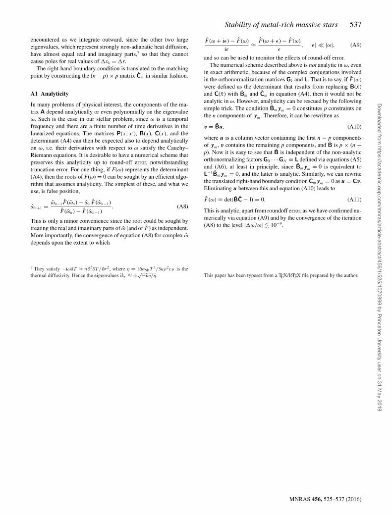
Figure A1. Real (solid) and imaginary (dashed) parts of the four eigenval-ues of A in the 938 M� model. Vertical scale is linear within the interval

(−R−1� , R−1� ), and logarithmic outside it.

The difficulty in solving this boundary-value problem is that the ncomplex eigenvalues of A(x, ω) may differ widely in size (Fig. A1).In our problem, they vary over 4–6 orders of magnitude in the innerparts of the star, due to the large ratio of thermal to dynamical time.6

Furthermore, since the eigenfunction corresponding to λ behavesas ∼exp (

∫xλdx), direct integration of equation (A1) can overflow

or underflow machine precision if the real part of λ is large. Thishappens in our stellar problem, and both signs of Real(λ) occursimultaneously. It therefore proves impractical to use a conventionalshooting method in which one iteratively makes guesses for theunconstrained components of y at both boundaries (and for ω) andintegrates towards a fitting point. As described above, a relaxation(Henyey-type) method also failed.

Instead, we propagate the boundary conditions themselves tothe fitting point. For a given choice of ω and for any x and x′

between the boundaries, equation (A1) has the formal solutiony(x) = P(x, x ′) y(x ′) if the ‘propagator’ P satisfies

∂P

∂x(x, x ′) = A(x)P(x, x ′),

∂P

∂x ′ (x, x ′) = −P(x, x ′)A(x ′),

P(x, x ′) = P(x, x ′′)P(x ′′, x ′), P(x, x) = I,

(A3)

I being the n × n identity. The left-hand boundary condition (A2) canthen be restated as B(x) y(x) = 0 with B(x) ≡ B(xmin)P(xmin, x).Similarly C(x) y(x) = 0 with C(x) ≡ C(xmax)P(xmax, x). In otherwords, the solution y(x) at any intermediate x between xmin andxmax must belong to the subspace annihilated by B(x), and also tothe subspace annihilated by C(x). Since the dimensions of thesetwo subspaces add up to n, their intersection is only y = 0 unless ω

is a root of

det{B(x),C(x)} = 0, (A4)

{B,C} meaning the n × n matrix whose first p rows coincide withthose of B and whose last n − p rows those of C.

6 The eigenvalues {λ1, . . . , λn} of A at a particular x should not be confusedwith the eigenvalue ω of the entire boundary-value problem. It might bebetter to speak of wavenumbers kx ≡ −iλ. Since A depends upon ω as wellas x, the λs and kxs do as well.

This reformulation may appear pointless since it is no easier tosolve for P by direct integration of equation (A2) than to solve equa-tion (A1) itself. The same difficulties with stiffness and overflowoccur. Furthermore, as the separation between x and xmin increases,the rows of B(x) are dominated by the fastest growing eigenvectorof A, so that they quickly become linearly dependent when esti-mated in finite-precision arithmetic. A key observation, however,is that the constraint B(x) y(x) = 0 is equivalent to LB(x) y(x) = 0for any non-singular p × p matrix L. This can be exploited to keepthe rows of LB(x) linearly independent, in fact orthonormal.

In practice one integrates equation (A1) or equation (A2) on adiscrete grid xmin = x0 < x1 < x2··· < xN = xmax. Let xm be the fittingpoint, 0 < m < N. The values of B(xk) could be defined iterativelyaccording to

B(xk+1) = B(xk)P(xk, xk+1), B(x0) = B(xmin).

Instead of this, however, we solve

Bk+1 = Gk+1BkPk,k+1, B0 = B(xmin). (A5)

Here Pk,k+1 is a discrete approximation to P(xk, xk+1) – a suitablechoice will be given presently – while Gk+1 is chosen at each stepto make the rows of Bk+1 orthonormal. For example, if p = 2 andthe rows of BkPk,k+1 are a and b, then

Gk+1 =(

1 0

0 γ

)(1 0

−β 1

)(α 0

0 1

), (A6)

with α ≡ |a|−1, β ≡ αba†, and γ = |b − αβa|−1. This representsthe Gram–Schmidt process, which can be extended to any num-ber of rows. It is clear that if Pk+1 = P(xk, xk+1), then Bm =G0G1 · · ·GmB(xm), so that det B(xm) = 0 if and only if det Bm = 0.

We now discuss a suitable approximation for P(xk, xk+1). If Awere constant over the interval [xk, xk+1], then Pk,k+1 = exp[(xk+1 −xk)A] would be exact, and otherwise if A is evaluated at the midpointxk+1/2 ≡ (xk + xk+1)/2, then the exponential approximation formallysecond order in xk ≡ xk+1 − xk. However, in our problem, thelargest eigenvalue of Ak+1/2 can be so large that on a reasonablemesh (we typically interpolate the MESA model with splines at ∼103–104 uniformly spaced radii), the matrix exponential can overflow,or at least cause substantial loss of precision. We therefore adoptthe Crank–Nicholson approximation:

Pk,k+1 =(

I + 1

2xkAk+1/2

) (I − 1

2xkAk+1/2

)−1

. (A7)

Eigenvalues of Ak+1/2 with positive (negative) real part, correspond-ing to behaviours that grow (decay) with increasing x, are mappedto eigenvalues of Pk,k+1 inside (outside) the unit circle, presumingxk < xk+1; very large eigenvalues of xkAk+1/2 are mapped to eigen-values of Pk,k+1 close to −1. It is still necessary to use a mesh fineenough so that the behaviours that should decay with the iteration(A5) do so quickly enough; the growing behaviours are controlledby the orthonormalization. In practice this is determined by varyingthe mesh resolution and monitoring the effect on the estimated rootof equation (A4) for ω.

Another constraint on the mesh is that the Crank–Nicholson ap-proximation (A7) for P(xk, xk+1) encounters a pole if Ak+1/2 has2/xk+1/2 as an eigenvalue. In fact, the eigenvalue represented bythe blue lines in Fig. A1 is nearly real and diverges towards thecentre of the star. This corresponds approximately to the singularsolution of the adiabatic equation, ∝ r−3 as r → 0. To controlthis, we start the integration at a non-zero but small radius rmin

with a mesh spacing r � rmin/3. This ensures that no poles are

MNRAS 456, 525–537 (2016)

Dow


ic.oup.com/m


ay 2019


encountered as we integrate outward, since the other two largeeigenvalues, which represent strongly non-adiabatic heat diffusion,have almost equal real and imaginary parts,7 so that they cannotcause poles for real values of xk = r.

The right-hand boundary condition is translated to the matchingpoint by constructing the (n − p) × p matrix Cm in similar fashion.

A1 Analyticity

In many problems of physical interest, the components of the ma-trix A depend analytically or even polynomially on the eigenvalueω. Such is the case in our stellar problem, since ω is a temporalfrequency and there are a finite number of time derivatives in thelinearized equations. The matrices P(x, x ′), B(x), C(x), and thedeterminant (A4) can then be expected also to depend analyticallyon ω, i.e. their derivatives with respect to ω satisfy the Cauchy–Riemann equations. It is desirable to have a numerical scheme thatpreserves this analyticity up to round-off error, notwithstandingtruncation error. For one thing, if F(ω) represents the determinant(A4), then the roots of F(ω) = 0 can be sought by an efficient algo-rithm that assumes analyticity. The simplest of these, and what weuse, is false position,

ωn+1 = ωn−1F (ωn) − ωnF (ωn−1)

F (ωn) − F (ωn−1). (A8)

This is only a minor convenience since the root could be sought bytreating the real and imaginary parts of ω (and of F ) as independent.More importantly, the convergence of equation (A8) for complex ω

depends upon the extent to which

7 They satisfy −iωδT ≈ η∂2δT /∂r2, where η = 16σSBT 3/3κρ2cP is thethermal diffusivity. Hence the eigenvalues ikr ≈ ±√−iω/η.

F (ω + iε) − F (ω)

iε≈ F (ω + ε) − F (ω)

ε, |ε| � |ω|, (A9)

and so can be used to monitor the effects of round-off error.The numerical scheme described above is not analytic in ω, even

in exact arithmetic, because of the complex conjugations involvedin the orthonormalization matrices Gk and L. That is to say, if F (ω)were defined as the determinant that results from replacing B(x)and C(x) with Bm and Cm in equation (A4), then it would not beanalytic in ω. However, analyticity can be rescued by the followingsimple trick. The condition Bm ym = 0 constitutes p constraints onthe n components of ym. Therefore, it can be rewritten as

v = Bu, (A10)

where u is a column vector containing the first n − p componentsof ym, v contains the remaining p components, and B is p × (n −p). Now it is easy to see that B is independent of the non-analyticorthonormalizing factors G0 · · ·GN ≡ L defined via equations (A5)and (A6), at least in principle, since Bm ym = 0 is equivalent toL−1Bm ym = 0, and the latter is analytic. Similarly, we can rewritethe translated right-hand boundary condition Cm ym = 0 as u = Cv.Eliminating u between this and equation (A10) leads to

F (ω) ≡ det(BC − I) = 0. (A11)

This is analytic, apart from roundoff error, as we have confirmed nu-merically via equation (A9) and by the convergence of the iteration(A8) to the level |ω/ω| � 10−9.

This paper has been typeset from a TEX/LATEX file prepared by the author.

MNRAS 456, 525–537 (2016)

Dow


ic.oup.com/m


ay 2019

Stability of metal-rich very massive stars

Documents

Transcript of Stability of metal-rich very massive stars