Higher frequency risk pricing for - Yeshiva University

15 seconds to alpha: Higher frequency riskpricing for commercial real estate

securities

Andreas D. Christopoulos∗and Joshua G. Barratt†‡

11th October 2021

Abstract

In this paper we introduce a new and generalizable method to estimate reduced formrisk decompositions at daily and intraday frequencies. Our estimates of CMBX riskpartitions for liquidity and excess liquidity are significant in explaining daily effectivebid-ask spreads historically, from 11/2007-4/2019, and in 20-day forecasts. We increasethe frequency of the daily model to intraday frequencies of 15 second intervals across 240days (4/2020-4/2021) during the Covid pandemic. There, we observe intraday patternsof risk partition volatility in the cross-section. We fuse CMBX risk partitions to REITprices in 54 automated trading strategies during the pandemic. 96% of the tradingstrategies produced significant alphas, and 63% produced abnormal cumulative returnsranging between 0.73% and 48.74%. The study contributes to our understanding ofprice formation of commercial real estate securities and supports risk partitioning athigher frequencies with our new method.

Key Words: High Frequency Trading, Liquidity, Microstructure, REITs, SecuritizationJEL Codes: C58, E10, G17, R30

∗e-mail: [email protected], Yeshiva University, Sy Syms School of Business, New York, NY10033.

†email: [email protected], Barratt Consulting, Wildenbruchstrasse 84 12045 Berlin, Germany.‡The authors would like to thank the organizers, discussants and participants at the 5th Annual HFE

Conference (Ecole Hôtelière de Lausanne), the 2021 Derivatives Conference (Auckland Centre for FinancialResearch), and the 2021 Summer Research Seminar Series (Yeshiva University, Sy Syms School of Business).The comments and insights we received have helped us improve this paper.

1

Introduction

Microstructure bid-ask spread estimation is not the only theoretical measure of liquidity.

Work in the area of Corporate bond risk characterization can be found in Longstaff, Mithal

and Neis (2005), Bao, Pan and Wang (2011) and Gilchrist and Zakrajsek (2012) who have

identified compensation within observable risk premia apart from default risk. Motivated

by these earlier works, Christopoulos (2017) introduced the technique to project fair value

prices onto observed risk premia in the market in basis points (bps) for commercial mortgage

backed securities indexed credit default swaps (CMBX) classes. In Christopoulos (2017) and

Christopoulos and Jarrow (2018), the reduced form simulations in those studies first allowed,

and then restricted, simulation of default. This allowed for isolation of theoretical compens-

ation for default and interest rate risks which were both explicitly modelled. The pricing

of residual risk premia identified in those two works are interpreted as distinct partitions of

liquidity and excess liquidity availability.

In the two earlier studies focusing on CMBX risk partitioning, the frequency of capture

is monthly. In this work we resolve to increase the frequency of risk partitioning for CMBX

from monthly to daily, and then to intraday frequency, in keeping with the frequency of more

developed markets. To do this we introduce two models to estimate the risk partitions at

daily and intraday frequency. In so doing, we disclose insights into the price formation of

CMBX and the related Real Estate Investment Trust (REIT) market.

First we consider, daily, the liquidity of CMBX from two perspectives: risk partitions

and microstructure. Both perspectives on liquidity are new to the literature concerning

CMBX and REITs and we provide some reconciliation between the two views of liquidity.

We begin by introducing the ‘Daily Model’ which estimates the reduced form liquidity and

excess liquidity partitions. To do this, we construct a linear estimation model using principal

component and OLS techniques with the training data the monthly market variables of the

VIX, interest rates, and REIT prices which represent the economy and the monthly simulated

values of risk partitions from Christopoulos and Jarrow (2018) serving as the dependent

variables.

Next, we establish the daily liquidity assessments for CMBX using the classical micro-

structure models of Roll (1984), Thompson and Waller (1987) and variants suggested by

2

Harris (1990), Hasbrouck (2009), Foucault, Pagano and Roell (2013), and Christopoulos

(2020). The CMBX market still does not provide reliable intraday recorded bid-ask spreads,

mid-market spreads, corresponding trade executions prices, or transaction volumes. As such,

the classic microstructure models are well suited to CMBX liquidity assessment for instru-

ments limited to end of day mark to market data.

With these two different perspectives on CMBX liquidity established, we test their re-

lationships to validate the Daily Model. Specifically, we use risk partitions of liquidity

to compare to the microstructure perspective on liquidity articulated in effective bid-ask

spreads. These comparisons yield our first two main results.

First, liquidity risk partitions play a significant role in CMBX price formation for AAA

and BBB credits over 2828 daily observations from 11/2007 - 4/2019. We establish this

result through the use of multivariate OLS of risk premia changes regressed onto changes

in the macroeconomy for observed market risk premia over 5-day rolling estimation periods.

Estimates of reduced form liquidity and excess liquidity measures are being communicated

into effective bid-ask spreads.

Second, estimated reduced form liquidity measures have a significant effect on future

effective bid-ask spreads over 20 day forecast periods. We establish this result in time-

series analyses using vector autoregression (VAR), Granger causality techniques and impulse

response functions (IRF) to project effective bid-ask spreads in response to shocks of liquidity

and excess liquidity.

With the Daily Model validated by our first two main results, we then increase the

frequency of risk estimation to intraday with the ‘Intraday Model’. Over 240 trading days

during the Covid-19 pandemic period between 4/2020-4/2021 we compute in 15 second

intervals estimated risk partitions in response to changing market variables. This analysis

gives rise to our third main result.

Third, during the pandemic, we find considerably greater volatility in risk partition pri-

cing at the start of each trading day for all risk partitions compared to the end of each

trading day. We establish this result by conducting a cross-sectional evaluation of millions

of cumulative intraday changes in CMBX risk partitions in 15 second intervals during the

pandemic. We note that REITs, like CMBX, are also exposed to commercial real estate risks.

Additionally, REIT trading frequency more closely matches the frequency of estimation of

3

the risk partitions. With these insights we investigate into the relationship between CMBX

risk partition signals and REIT pricing. This investigation leads to our fourth main result.

Fourth, well constructed intraday trading strategies using CMBX risk partitions as relat-

ive value signals applied to the related REIT market can result in substantial extraordinary

returns. We establish this fourth main result by fusing the cross-sectional insights into

CMBX risk partition estimation with the more frequently traded REIT sector in a set of

54 long/short day trading strategies during the Covid pandemic for each of the investment

grade credit rating classes (AAA, AJ/AS, AA, A, BBB and BBB-). The strategies exploit

regular and systematic aberrations in volatility in both CMBX risk partitions and REIT pri-

cing. Using use the Intertemporal Capital Asset Pricing Model (ICAPM) of Merton (1990)

we find 96% of the strategies produced positive and statistically significant α′s. 65% of those

strategies also exhibited positive cumulative returns over the Covid-19 crisis period ranging

from 0.73% to 48.74% with very good Sharpe ratios. These third and fourth main results

validate the Intraday Model.

CMBX and commercial mortgage backed securities (CMBS) sectors total approximately

$600 billion, while the US REIT sector stands at approximately $1.3 trillion. Our paper

establishes that CMBX risk partitions at daily and intraday frequencies provide new insights

into the liquidity for CMBX and REIT sectors with a combined value of about $2 trillion.

As such, we provide a new perspective on the pricing of liquidity risks for two large and

related sectors within real estate capital markets.

The remainder of this paper is organized as follows: Section 1 provides a brief literature

review while Section 2 discusses the data used in this study. Section 3 introduces the Daily

Model and discusses methods and results used in validation. Section 4 introduces the Intra-

day Model presenting cross-sectional visualizations, and trading strategy results. Section 5

summarizes with suggestions for future work. The Online Appendix provides supplementary

information.

1 Literature review

This section discusses some of the literature related to liquidity pricing relevant to our study.

4

1.1 Bid-ask measures of liquidity

Bid-ask spreads represent the difference between the quotes of where market-makers stand

ready to buy (bid-side) and sell (ask-side aka ‘offered-side’) securities at a specific point

in time. While bid-ask spreads provide a rich measure of a security’s liquidity, it stands

to reason, that infrequently traded securities (where bid-ask spreads are less frequently ob-

servable) may present investors with greater opacity with respect to trading information

which may, in turn, compound their illiquidity as noted in Hasbrouck (2009) and Fong,

Holden and Trzcinka (2017). Despite their size relative to equities, US fixed income markets

can suffer from considerable illiquidity, particularly during times of stress as noted in Bao,

Pan and Wang (2011) and Bao, O’Hara and Zhou (2018). This may be due to the over-

the-counter (OTC) trading mechanism as discussed in Campello, Chen and Zhang (2008)

and the comparatively less frequently traded characteristic for much of credit sensitive fixed

income compared with equities as noted in Goldstein, Jiang and Ng (2017). Some data im-

provement in the area of Corporates has helped to advance the fixed income microstructure

literature 1 and there have also been some advances in data and analysis for securitizations

as discussed in Hollified, Nekyudov and Spatt (2017). At the same time, limited information

for dealers on weekly trading volumes and inventories with lags under the Securities and

Exchange Commission (SEC) embargo of 90 days and sporadic trading in the credit sens-

itive fixed income instruments, such as CMBX, still leave pockets of uncertainty regarding

liquidity.

Many of the classical microstructure models that investigate into issues of illiquidity are

based on price and volume information content, as introduced in Kyle (1985), Easley, et al

(1996), and O’Hara (1997). As a result, most studies in microstructure focus on products

such as publicly traded equities where price and volume data is available for empirical evalu-

ation. However, this rich data is simply unavailable for many credit sensitive fixed income in-

struments, particularly in the securitized sector. One sector in the fixed income market with

such limited pricing information is CMBS and its indexed derivatives, CMBX. CMBX are

OTC indexed credit default swaps which do not trade on electronic exchanges.2 Communic-1See Hotchkiss and Ronen (2002), Bao, Pan and Wang (2011), Han and Zhou (2016), Haddad, Moreira

and Muir (2020), Gilchrist etal (2021) among others.2This contrasts with Corporate bonds, which are increasingly traded electronically and which are required

to post execution prices and volumes on the Trade Reporting and Compliance Engine (TRACE).

5

ation between market makers (dealers) and investors is done principally through Bloomberg

terminal posts and sporadically.3 Since there is reliable recording of day-end mark-to-market

values since 2007 for CMBX through Markit, the technology to estimate bid-ask spreads for

CMBX from a microstructure perspective is restricted to Roll (1984), Harris (1990), Has-

brouck (2009), Thompson and Waller (1987) and, most recently, Christopoulos (2020). In

this study, we implement these models to compare to estimated reduced form theoretical

liquidity measures. A more detailed summary of these classical microstructure models is

provided in the Online Appendix Section A.2.

1.2 Non-bid/ask measures of liquidity

While bid-ask spreads represent one measure of securities liquidity, there are others. For ex-

ample, Amihud (2002) and Gilchrist and Zakrajsek (2012) each identify measures of liquidity

for credit sensitive fixed income securities. In particular, certain areas of the literature are fo-

cused on disclosing default and liquidity components. Longstaff, Mithal and Neis (2005) find

substantial concentration of default risk in corporate bond spreads that vary across credit

ratings informed by implementing a theoretical model similar in class to Christopoulos and

Jarrow (2018). Bao, Pan and Wang (2011) for example isolate factors apart from credit risk

to be attributable to overall risk premia for that sector. They find illiquidity in Corporate

bonds to increase with volatility and to be highly time varying. Gilchrist and Zakrajsek

(2012) reveal statistically the excess bond premia in excess of default risk estimated using

firm specific variables and the distance to default framework of Merton (1974). Their res-

ults indicate significant explanatory power for both the isolated default partition and the

excess bond risk premia for several economic indicators including the civilian unemployment

rate (UER). Broto and Lamas (2016) use principal component analysis (PCA) to construct

liquidity indices for US fixed income demonstrating the use of PCA in this domain.

1.2.1 Christopoulos (2017) and Christopoulos and Jarrow (2018)

While similar in motivation to the earlier work, Christopoulos (2017) takes a different mod-

elling approach and has a different focus on CMBS. Christopoulos (2017) articulates risk3See the Online Appendix Section A.1.

6

components for CMBS and CMBX transforming simulated risk-neutral pricing into observ-

able market pricing of default risk, rate risk, liquidity availability and excess liquidity avail-

ability. The reduced form theoretical liquidity and excess liquidity partitions of CMBS, first

introduced in Christopoulos (2017) and then indexed in Christopoulos and Jarrow (2018),

provide insights into CMBS liquidity.

The reduced form modelling approach in both studies simulated an economy consisting

of 11 forward interest rates, 48 NCREIF property x regional property indices, and 6 property

specific REIT indices under risk neutral conditions. The interest rate process used a simu-

lation using high performance computing which consisted of forward rates following Heath,

Jarrow and Morton (1992) and correlated Brownian Motion for all 65 factors. The simulation

implemented loan-level credit state transitions using the Cox Process as motivated by Lando

(1998). The state transitions of the loans reflected the historical state transitions of 1.92

million loan life observations over the period November 2007 to December 2014. The risk

adjusted loan level cashflows were first aggregated to the trust level and then allocated to the

bond classes. This resulted in the capture of risk adjusted bond level cashflows. Prepayment

risk was reasonably omitted in the asset pricing model due to the prepayment restrictions

for commercial real estate loans which serve as collateral for CMBS. Since the simulation of

the economy was conducted under risk neutral conditions, the valuation of the bond classes

were also risk neutral, generating fair value prices, independent of market prices.

Because fair value pricing is risk neutral, there are indeed instances empirically where

fair value pricing so exceeds the market price, that an additional risk premia, in excess

of observed risk premia, is required for reconciliation of fair value to market prices in the

transformations. This additional compensation above observable risk premia is interpreted

as excess liquidity availability. Excess liquidity, in excess of observed market risk premia,

indicates the amounts in bps by which market risk premia could instantaneously increase

(widen) before the security experienced deterioration in regular liquidity availability. In this

study we implement estimations of the reduced form risk partitions for CMBX to compare

to estimated liquidity revealed in effective bid/ask spreads.

7

2 Data

In this section we discuss the data used throughout this study. The study uses data from

three time frames: the training period, the daily period, and the intraday period.

1. The training period consists of 92 monthly observations from 11/2007-6/2015 in whichtraining data is used to train the Daily Model in Section 3.

2. The daily period consists of 2828 daily observation in which data are used to producerisk partition estimates with the Daily Model in Section 3 from 11/2007-4/2019 andare used in OLS, VAR, Granger and IRF analyses.

3. The intraday period consists of 246 dates during the Covid-19 pandemic in whichtime stamped intraday data are used to produce estimates of risk partitions with theIntraday Model in Section 4 from 4/2020-4/2021 which are used in cross-sectionalanalyses and ICAPM trading tests at the open and close of the trading days.

Tables and figures summarizing the data and results are introduced in the relevant sections

throughout the paper where the data are used.

2.1 Private data - CMBX risk premia

The private data was generously donated to us by one of the largest asset managers for

our research. Like CMBS, CMBX trade on a ‘Spread’ basis, where Spreads are mid-market

risk premia St, in excess of US Treasury swap spreads. These Spreads are contributed

by dealers to Markit at the close of each trading day. For all daily observation dates, t,

the risk premium, St, captures the drivers of uncertainty on CMBX derivatives in excess

of the relevant risk-free rate. The underlying collateral tranches securing CMBX used in

this study represent approximately $400 billion (bn) of the ~$600 bn CMBS market. As

a securitized credit default swap, as described in Driessen and Van Hemert (2012) and

Christopoulos and Jarrow (2018), series of CMBX classes (or tranches) capture the cashflows

of 25 reference asset CMBS tranches for corresponding credit ratings. A Bloomberg post and

primer discussion of CMBX bid-ask spreads is provided in the Online Appendix Section A.1.

To our knowledge, such indications of CMBX liquidity are only available as sporadic posts

by dealers to clients and are not regularly recorded and verified with time stamps intraday.

8

2.2 Public data

2.2.1 Monthly

We use prices for 25 representative publicly traded REITs obtained from Yahoo! Finance that

we use for the estimation of the Daily Model in Section 3 and the estimation of the Intraday

Model in Section 4, through RapidAPI. We select these REITs due to their similarity to

CMBX on a few dimensions. Table 1 lists the names of the 25 REITs used in this study along

with their property type, ticker, factor name (proptype_ticker), and market capitalization

as of 6/27/2021. The market capitalization of these 25 REITs selected total $478.45 billion.

According to the National Association of Real Estate Investment Trusts (NAREIT), the

total market capitalization (market cap) of US REITs was $1249.19 billion as of December

31, 20204, and so our sample captures about 38% of the US REIT sector by market cap.

NAREIT also states that the total number of US REITs is 223, and so by counts, our sample

represents about 11% of the US REIT sector. These REITs also are well distributed across

multiple property types as shown in a further summary of the REIT sample in our study

broken down by property type in Table 2. Our estimated economy also captures most of

the REITs used in the prior study of Christopoulos and Jarrow (2018) and for continuity

with the simulation, we also use these REITs. Finally, as the CMBX in our sample represent

approximately $400 billion of CMBS underlying, the size of our REIT sample and our CMBX

sample are of similar market magnitude.4See https://www.reit.com/data-research/reit-market-data/us-reit-industry-equity-market-cap

9

Table 1: Sample REITsPropType Ticker Factor Name REIT Name Market Cap ($bn)

Industrial (IN) DRE IN_DRE Duke Realty $18.04FR IN_FR First Industrial Realty Trust $6.90PLD IN_PLD Prologis, Inc. $90.25SELF IN_SELF Global Self Storage, Inc. $54.28

Hotel (LO) HST LO_HST Host Hotels & Resorts, Inc. $12.41MAR LO_MAR Marriott International, Inc. $45.64WH LO_WYND Wyndam Hotels & Resorts, Inc. $6.82MGM LO_MGM MGM Resorts International $21.53

Multifamily (MF) AVB MF_AVB Avalon Bay Communities, Inc. $29.87ELS MF_ELS Equity LifeStyle Properties, Inc. $13.81EQR MF_EQR Equity Residential $29.39UDR MF_UDR UDR, Inc. $14.80

Office (OF) BXP OF_BXP Boston Properties, Inc. $18.70CLI OF_CLI Mack-Cali Realty Corporation $1.55HIW OF_HIW Highwoods Properties, Inc. $4.85SLG OF_SLG SL Green Realty Corp. $5.72VNO OF_VNO Vornado Realty Trust $9.24

Mixed Use/Other (OT) BKD OT_BKD Brookdale Senior Living Inc. $1.54NNN OT_NNN National Retail Properties, Inc. $8.41PSB OT_PSB PS Business Parks, Inc. $4.15WPC OT_WPC W.P. Carey Inc. $13.93

Retail (RT) KIM RT_KIM KIMCO Realty Corporation $9.14REG RT_REG Regency Centers Corporation $11.05SPG RT_SPG Simon Property Group $43.06TCO RT_TCO Taubman Centers Inc. $3.40

This table summarizes the 25 REITs used in this study. The market capitalization of the REITs are $478.45 billion as of 6/27/2021. The firstcolumn provides the property type and groups the REITs by property type separated by borders. The six property types are Industrial (IN), Hotel(LO), Multifamily (MF), Office (OF), Mixed Use/Other (OT), and Retail (RT). The second column provides the stock market ticker symbol. Thethird column provides the factor name composite of the property type with the ticker. The fourth column provides the name of the REIT, whilethe fifth column the market capitalization.

Table 2: Aggregate Summary of Sample REITs

Property Type Market Cap ($bn) % Market Cap Count US Count Sample % of US

Industrial (IN) $169.47 35.42% 4 13 30.77%Hotel (LO) $86.39 18.06% 4 13 30.77%

Multifamily (MF) $87.86 18.36% 4 20 20.00%Office (OF) $40.06 8.37% 5 19 26.32%

Mixed Use/Other (OT) $28.02 5.86% 4 126 3.17%Retail (RT) $66.65 13.93% 4 32 12.50%

Total $478.45 100.00% 25 223 100.00%

This table aggregates values related to the 25 REITs used in this study. The first column gives the property type and total labels. The six propertytypes are Industrial (IN), Hotel (LO), Multifamily (MF), Office (OF), Mixed Use/Other (OT), and Retail (RT). The second column provides themarket capitalization (Market Cap). The third column provides proportion of each property type Market Cap compared to the total Market Capin the sample. The fourth column provides the counts of the REITs by property type in the sample. The fifth column the number of REITs byproperty type in the US. The sixth column captures the proportion of the sample count to the US count of REITs.

While no sample selection is perfect, we feel our selection is broadly representative of the

US REIT sector. The 25 REITs are included in the training data and then used in the Daily

and Intraday Models to estimate CMBX risk partitions.

10

2.2.2 Daily

For the period 11/2007-4/2019, we also have public daily time series from the Federal Reserve

Bank of St. Louis FRED system. These data include benchmark corporate bond credit

spreads for AAA and BBB ratings, the VIX volatility index, constant maturity (CMT) US

Treasury yields to maturity. Following the estimation of the Daily Model, we also provide

summary statistics for the public, private and estimated data of CMBX bid-ask spreads and

CMBX risk partitions later in Section 3 Table 9. Finally, for the trading strategies and

related ICAPM testing conducted during the Covid-19 pandemic period (246 days between

4/2020-4/2021) we obtain daily values of the market portfolio (Mkt-Rf, which consists of all

NYSE, AMEX, and NASDAQ firms), small minus big (SMB), high minus low (HML), and

momentum (MOM) indices from Ken French’s website.5

2.2.3 Intraday

During the Covid-19 pandemic period of 4/2020-4/2021 we captured the daily values of the

VIX, US Treasuries, and REITs during this period using the RapidAPI application with

Yahoo! Finance. These data are summarized later in Section 4 Tables 14 and 15 at the start

and at the end of the trading days during this period. We poll the data in 15 second intervals

and the average delay over this period is about 1.15 seconds. The data is always ‘most-recent’

and reflective of updates driven by trading in the marketplace. The data polling for each

day starts at approximately 9:30:15am EST and ends at approximately 4:15:00pm EST.

There were some delays in reporting due to electronic communication lags on the internet

in the application of up to 2 seconds. Additionally, some delays in reporting can take up

to 15 minutes for the VIX at the start of each trading day. All Federal holidays and are

excluded with trading only taking place on days when both bond and stock markets are

open. Reporting terminates early with early market closings market circuit breaker triggers.5See https://mba.tuck.dartmouth.edu/pages/faculty/ken.french/.

11

3 The Daily Model (and its results)

This section introduces and validates the Daily Model of risk partition estimation. The Daily

Model is based on findings of the reduced form technique in the prior literature applied to

CMBX that is then fused with daily market information. We then validate the Daily Model

with data generated from four bid-ask microstructure models we implement.

3.1 Indices of CMBX

Christopoulos and Jarrow (2018) create indices of CMBX market spreads and the CMBX risk

partitions introduced in Christopoulos (2017) for tractability. These indices of CMBX serve

as sector-wide risk benchmarks for the CMBX sector. In Christopoulos and Jarrow (2018),

for each of the six investment grade credit tranches k ∈ {AAA,AJ/AS,AA,A,BBB,BBB-}

there were seven different issued CMBX series, l ∈= 1, . . . , 7 (ie. CMBX Series 1, CMBX

Series 2, ...CMBX Series 7). The prior work computed six average tranched CMBX market

spreads (one for each of the six credit ratings) aggregated across seven CMBX Series, Sk(t),as

Sk(t) = 17

7∑l=1

Skl(t). (1)

plus a sector level indexed CMBX market spread benchmark across all k credit ratings,

computed as

S(t) =6∑

k=1wkSk(t) (2)

where wk is the weight of the kth credit rating tranche determined by its subordination

level. The weights based on subordination levels across all indices are ωAAA =0.8222,

ωAJ/AS =0.0514, ωAA =0.0514, ωA =0.0257, ωBBB =0.0339 and ωBBB− =0.0154.

In this paper we take a different approach with the construction of a set of ‘on-the-run’

CMBX time series. In fixed income parlance, the most recent new issue security is considered

the ‘on-the-run’ security and is also referred to as the ‘current-coupon’ as is typical in fixed-

income sectors. The terminology borrows from the US Treasury vocabulary as discussed

in Fleming (2001) and the residential mortgage market as discussed in Bhattacharjee and

Hayre (2006). The on-the-run security is typically the most liquid of all outstanding similar

12

issues within a sector, and coupons on securities for individual bonds (Treasuries) or tranches

(within securitized capital structures) will be closest to the benchmark par/new-issue pricing

for the sector. Additionally, loans underlying CMBS (which, in turn, collateralize CMBX)

have interim principal payments (and sometimes losses of principal) prior to maturity as

discussed in Christopoulos (2017). This is due to principal amortization and manifestations

of default in the form of loss and as well as default driven prepayments. They also may exhibit

restricted prepayments of principal subject to prepayment lockout and prepayment penalties.

It is well-known that default and prepayment of mortgage collateral exhibit statistically

positive relationships with loan age early on in the life of the loan with loans exhibiting

less frequency of default or prepayment the closer they are to the origination date. As such,

on-the-run issues are less likely to exhibit idiosyncratic changes in promised payment profiles

the more recent the issue is to its origination date.6

The selection date for the on-the-run risk premium, S, with series classification, l, for

credit rating class (aka ‘tranche’), k ∈ [AAA, AJ/AS, AA, A, BBB, BBB-], for all daily

observation dates, t, is defined as follows:

Slkt =

l = Series 4, t ∈ [11/1/2007, 5/22/2008]l = Series 5, t ∈ [5/23/2008, 1/24/2013]l = Series 6, t ∈ [1/25/2013, 1/26/2014]l = Series 7, t ∈ [1/27/2014, 1/25/2015]l = Series 8, t ∈ [1/26/2015, 1/24/2016]l = Series 9, t ∈ [1/25/2016, 1/24/2017]l = Series 10, t ∈ [1/25/2017, 1/29/2018]l = Series 11, t ∈ [1/30/2018, 1/28/2019]l = Series 12, t ∈ [1/29/2019, 1/31/2020]

(3)

For on-the-run schedule dates, the differences in observations across tranches are due to

normal amortization, maturity and default driven prepayments and losses from underlying

loan collateral underlying the bonds, as well as different timing of series new issuance. For

example, the AAA tranches for CMBX Series 1 paid off in late 2015, while CMBX Series 12

was not issued until 1/29/2019. Because of changes in issuance frequency, resulting effective

bid-ask spreads based may introduce some noise relative to the underlying fundamental

health of the collateral and market sentiment pricing. During the Great Financial Crisis,6See for example Hayre, et al (1995, 2000), Christopoulos and Jarrow (2018), and Bond Market Associ-

ation (2017) among others.

13

for example, over the period 5/23/2008-2/7/2013, CMBX Series 5 served as the on-the-

run issue for 5 consecutive years. This is an unavoidable artefact of the market itself (and

corresponding data) as no new CMBX Series were issued over this period. Additionally,

as noted, unlike Christopoulos and Jarrow (2018) we do not have the underlying loan and

bond cashflow data which precludes us from simulating directly. We only have CMBX credit

spreads, their changes and dates of observation. As such, our choice to construct ‘on-the-run’

time series of Spreads is the best we can do for this type of approach.

We use the issuance schedule in Eq. (3) to create the time series of ‘on the run’ CMBX

market spreads and select Skl(t) values noted in Eq. (1) from the previous work. For each

of the four CMBS risk factors j ∈ {default, rates, reglq, xslq} four indexed risk partitions

indices, Sjk(t), across all CMBX series, are given by

Sjk(t) = 17

7∑l=1

Sjkl(t). (4)

This gives us 24 indexed risk partitions, one for each of the k ∈= 1, . . . , 6 credit rating classes

for each of j ∈= 1, . . . , 4 risk factors. To create the composite CMBX sector level risk factor

indices, we take the weighted sum across all credit ratings

Sj(t) =6∑

k=1wkSjk(t) (5)

where wk is the weight of the kth credit rating tranche determined by its subordination level.

As with CMBX market spreads, we also create ‘on-the-run’ time series risk partitions which

use Eq. (3) to select the time series of CMBX risk partition values, Sjkl(t) in Eq. (1).

14

3.2 Reduction of dimension

Table 3: Summary of Daily Model PCA training data

type_ticker mean median min max variance stdev countVIX 22.1251 19.3000 10.7300 69.9600 115.4094 10.7429 92

IN_DRE 15.5298 14.3950 5.6200 32.6700 25.1089 5.0109 92IN_FR 14.4922 12.7050 2.0900 40.5800 73.8958 8.5963 92IN_PLD 34.9227 35.5300 10.8800 64.8000 117.6452 10.8464 92IN_SELF 3.7005 3.7800 2.3800 4.4500 0.1826 0.4273 92LO_HST 15.6474 16.2642 3.5732 23.7400 20.1085 4.4843 92LO_MAR 38.7738 35.6409 12.8553 82.8000 285.1512 16.8864 92LO_WYND 18.8808 15.4538 1.5214 41.0384 125.1303 11.1862 92LO_MGM 19.9279 13.7750 2.6200 91.7100 297.1436 17.2379 92MF_AVB 115.1334 122.1300 43.7600 173.2800 1013.2613 31.8318 92MF_ELS 15.9899 15.8763 6.8750 27.3750 23.7395 4.8723 92MF_EQR 50.1745 53.9450 17.9100 77.7000 210.1242 14.4957 92MF_UDR 22.8744 24.2100 7.9700 32.9900 32.5518 5.7054 92OF_BXP 94.9709 101.1400 34.0400 142.2200 577.5131 24.0315 92OF_CLI 27.6958 28.0650 14.6800 40.6800 40.0223 6.3263 92OF_HIW 33.5559 33.2700 17.8200 46.3100 34.6371 5.8853 92OF_SLG 76.3286 80.6000 11.1900 127.8500 809.1747 28.4460 92OF_VNO 61.5884 61.5832 22.9945 91.3581 186.2377 13.6469 92OT_BKD 22.6844 22.4500 3.0100 38.7200 73.2452 8.5583 92OT_NNN 27.3768 26.4400 10.5300 42.0900 49.3787 7.0270 92OT_PSB 62.3994 58.9550 32.3200 86.5300 175.0194 13.2295 92OT_WPC 43.4868 38.5000 18.3400 71.2900 272.3761 16.5038 92RT_KIM 20.9846 19.4900 7.4900 42.0900 59.1813 7.6929 92RT_REG 47.7711 46.8450 24.3900 71.5700 124.9783 11.1794 92RT_SPG 114.7762 108.8476 27.2503 196.5700 1909.6103 43.6991 92RT_TCO 57.3334 58.6900 15.6000 86.9500 349.8780 18.7050 92TSY_3MO 0.3285 0.0700 0.0050 3.8400 0.5240 0.7239 92TSY_5YR 1.7756 1.6805 0.6140 4.0350 0.6180 0.7862 92TSY_10YR 2.8003 2.7190 1.5040 4.3890 0.5643 0.7512 92TSY_30YR 3.7164 3.6970 2.5560 4.7630 0.4430 0.6656 92

This table summarizes the 92 monthly observations of training data used in the Daily Model for the principal component analysis. The VIX is theCBOE volatility index. This is followed by the 25 REITs with the ticker a composite of the 6 property types industrial (IN), hotel/lodging (LO),multifamily (MF), mixed use/other (OT), office (OF) and retail (RT). Following the REITs are US Treasury yields with ticker representing the 4maturities of 3 month, 5 year, 10 year and 30 year.

Table 3 provides a summary of the 92 training observations of the variables proxying for

the simulated economy over the period 11/2007 thru 6/2015 that make up the economy in

the Daily Model. They are used for the Daily Model estimation. From the training data

summarized in Table 3 we estimate the risk partitions daily with the Daily Model, over the

sample period of 11/2007-4/2019. The Daily Model uses a standard linear regression on the

logs of the risk partitions reported in the monthly training set of Christopoulos and Jarrow

(2018) against a digest of market data (25 REITs, 4 US Treasuries, and the VIX volatility

index). Throughout the estimation of the Daily Model and (later the Intraday Model), for

arithmetic reasons, we use the logarithm of these values as our starting point. Although the

number of observations for the training set (92) is limited, these variables have a high degree

of correlation among them. It is thus possible to create a lower-dimensional set of factors

which contain enough information to explain most of the variance in the original set of 30.

15

To remove the cointegration we perform a principal components analysis (PCA), retaining

enough factors to preserve 96% of the total variance at the observed dates.

For PCA in general form, let xq(t) be the value of the q-th explanatory variable at time

t. For PCA loadings piq, i ∈ [1, 5], q ∈ [1, 30]. Assuming, we have all 30 factors, then the

elements of the i x q matrix of principal components of the observed explanatory variables

xq(t) for all observed t, there exists a set of factors fi(t) such that

xq(t) =30∑i=1

piqfi(t) (6)

with each explanatory variable a linear combination of the factors fi at all times t. But we

want to reduce dimension because we have only 92 observations. And so when we reduce

the number of components below 30 observable variables, to 5 variables, we determine the

factors with matrix multiplication as

fi(t) =30∑q=1

piqxq(t), i ∈ {1...5} (7)

The factors fi(t) are uncorrelated7, such that the partial sum is an unbiased estimator of

xq(t),

xq(t) =5∑i=1

piqfi(t) + εn(t), E[εn] = 0 (8)

where the error term E[εn] = ∑30i=6 piqfi(t), which is the minimal possible error that can

be introduced in a 1:1 transformation with the technique. For highly correlated series of

variables xq(t), the proportion of their internal variance explained by even small partial

sums can be large. From the covariance matrix of the explanatory variables we calculate the

(30x30) matrix of eigenvectors and their corresponding eigenvalues. In Table 4, we report the

eigenvalues all 30 principal components. Since none of the eigenvalues are less than zero, the

variance covariance matrix is said to be positive semi-definite. As the first five eigenvalues

have cumulative variance of 96.11%, we are comfortable with restricting our model to these

first five principal components.

We transform our 30 variables into a digest of just 5 variables with xq(t) the value of the7See the proof of this in the Online Appendix Section A.3.

16

Table 4: EigenvaluesPrincipal Components (1:30) eigenvalue variance (%) cumulative variance (%)

Dim.1 18.1849 60.6163 60.6163Dim.2 7.0359 23.4529 84.069Dim.3 1.7472 5.8239 89.8932Dim.4 1.2534 4.1778 94.0711Dim.5 0.6139 2.0463 96.1174Dim.6 0.3176 1.0588 97.1762Dim.7 0.2173 0.7243 97.9005Dim.8 0.1257 0.4190 98.3196Dim.9 0.1012 0.3374 98.6571Dim.10 0.0853 0.2842 98.9413Dim.11 0.0647 0.2155 99.1568Dim.12 0.0444 0.1481 99.3049Dim.13 0.0387 0.1288 99.4338Dim.14 0.0341 0.1136 99.5475Dim.15 0.0223 0.0744 99.6219Dim.16 0.0174 0.0580 99.6800Dim.17 0.0154 0.0514 99.7314Dim.18 0.0132 0.0438 99.7752Dim.19 0.0122 0.0406 99.8159Dim.20 0.0115 0.0382 99.8541Dim.21 0.0105 0.0349 99.8890Dim.22 0.0080 0.0267 99.9158Dim.23 0.0061 0.0202 99.9361Dim.24 0.0044 0.0145 99.9507Dim.25 0.0043 0.0144 99.9651Dim.26 0.0035 0.0116 99.9768Dim.27 0.0028 0.0093 99.9861Dim.28 0.0024 0.0078 99.9940Dim.29 0.0012 0.0039 99.9979Dim.30 0.0006 0.0020 100.0000

This table summarizes the eigenvalues associated with the covariance matrix and eigenvectors.

Table 5: Eigenvectors of five principal components

Type PropType Ticker Factor Name PC1 PC2 PC3 PC4 PC5VIX NA VIX VIX 0.1748 0.0107 -0.3148 -0.2332 -0.4369REIT Industrial DRE IN_DRE -0.1406 -0.2886 -0.097 -0.0937 -0.0245REIT Industrial FR IN_FR -0.1334 -0.2833 -0.1556 -0.1863 0.1269REIT Industrial PLD IN_PLD -0.1622 -0.2605 0.0067 -0.1089 0.1225REIT Industrial SELF IN_SELF -0.1163 -0.0726 0.5916 -0.1331 0.1507REIT Hotel HST LO_HST -0.2184 -0.0537 0.0704 0.1801 -0.0047REIT Hotel MAR LO_MAR -0.2091 0.0519 -0.1853 0.2272 -0.1395REIT Hotel WYND LO_WYND -0.2161 0.1097 -0.122 0.107 0.1364REIT Hotel MGM LO_MGM -0.0578 -0.3335 -0.1355 -0.1244 0.1721REIT Multifamily AVB MF_AVB -0.2207 0.0755 0.1151 -0.0826 -0.1916REIT Multifamily ELS MF_ELS -0.2157 0.1168 -0.0943 0.0968 -0.0964REIT Multifamily EQR MF_EQR -0.2135 0.1001 0.1302 -0.0469 -0.3028REIT Multifamily UDR MF_UDR -0.2201 -0.0111 0.0938 -0.0807 -0.3541REIT Office BXP OF_BXP -0.2296 -0.0055 0.0615 -0.0646 -0.1693REIT Office CLI OF_CLI 0.0629 -0.2369 0.514 -0.0331 -0.1139REIT Office HIW OF_HIW -0.2195 -0.0137 0.0278 0.2056 -0.089REIT Office SLG OF_SLG -0.2249 -0.0927 -0.0024 0.0316 -0.068REIT Office VNO OF_VNO -0.2131 -0.0941 0.0421 0.1063 -0.3489

REIT Mixed/Other BKD OT_BKD -0.2124 -0.0833 -0.0401 0.2277 0.1163REIT Mixed/Other NNN OT_NNN -0.2213 0.0892 -0.0338 0.0709 0.1337REIT Mixed/Other PSB OT_PSB -0.2124 0.0861 -0.0613 0.1464 0.2303REIT Mixed/Other WPC OT_WPC -0.2079 0.1098 -0.1229 0.0496 0.3096REIT Retail KIM RT_KIM -0.116 -0.3012 -0.0986 -0.2131 -0.0795REIT Retail REG RT_REG -0.1783 -0.2091 -0.1494 -0.1061 -0.0406REIT Retail SPG RT_SPG -0.2247 0.0994 -0.0166 -0.0345 0.0524REIT Retail TCO RT_TCO -0.2183 0.0611 0.1079 -0.1874 0.1506

Treasury NA 3MO TSY_3MO 0.0137 -0.347 -0.0736 -0.2146 0.1305Treasury NA 5YR TSY_5YR 0.0803 -0.311 -0.1406 0.3288 -0.1094Treasury NA 10YR TSY_10YR 0.1142 -0.2744 -0.0077 0.4121 -0.0729Treasury NA 30YR TSY_30YR 0.1228 -0.2373 0.1884 0.4231 0.0084

This table summarizes the principal component loadings (rotations). The first column indicates the type of the variable (REIT, VIX, or Treasury).The second column indicates the property type which is indicated for REITs and not applicable (NA) for the other variables. The third columnprovides the ticker symbol for the REITs and indication of VIX or the maturity for the Treasuries. The fourth column is the internal data nameof the variable. The fifth through ninth columns (PCA1, ... PCA5) indicates the principal component loadings determined from the eigenvaluesand eigenvectors.

17

q-th economic variable at time t. The eigenvectors consisting of the principal component

loadings (aka ‘rotations’) are summarized in Table 5. This five-dimensional digest is used to

construct our factor volatility explanatory variables (described below) for the risk component

estimates. To expand on Eq. (7), the factor volatilities fit are a function of the PCA loadings

in Table 5 and the explanatory variables observed at time t.

Table 6: Summary of market spreads and simulated risk partitions as dependent variables

type_ticker mean median min max variance stdev countmarket spread AAA 118.1295 99.9420 25.0000 550.7100 8084.8459 89.9158 92market spread AJ 473.0770 390.9575 55.1621 1703.7300 81736.2628 285.8955 92market spread AA 981.0831 1000.9948 76.1364 2525.8600 261721.8298 511.5876 92market spread A 1555.3875 1609.9502 89.0328 3667.6336 604157.4778 777.2757 92

market spread BBB 3053.6276 2703.6012 162.1271 10491.7654 3845199.4134 1960.9180 92market spread BBBm 4252.5810 3952.0150 207.4319 14720.7284 8199398.1483 2863.4591 92

def_AAA 8.0555 1.6607 0.0277 195.8856 790.1596 28.1098 92rates_AAA 52.8702 37.4083 1.6727 263.6903 2712.6277 52.0829 92reglq_AAA 57.2037 44.8207 6.7286 262.8916 2294.4850 47.9008 92xslq_AAA 134.1662 134.5824 0.0000 294.3972 8930.3539 94.5005 92def_AJ 56.0297 3.3434 0.0488 1146.3424 42838.9678 206.9758 92rates_AJ 211.9356 164.1067 0.5000 1251.9229 37946.1184 194.7976 92reglq_AJ 200.6518 221.3317 0.0000 432.8215 10881.9687 104.3167 92xslq_AJ 0.5256 0.0000 0.0000 22.5208 9.9243 3.1503 92def_AA 284.7420 159.6041 30.4583 1735.0750 107892.5071 328.4699 92rates_AA 561.9648 617.7424 0.0000 1506.2897 111677.9404 334.1825 92reglq_AA 134.3763 123.8860 0.0000 385.7624 13602.5250 116.6299 92xslq_AA 0.0000 0.0000 0.0000 0.0000 0.0000 0.0000 92def_A 577.6416 535.7316 3.2881 1959.6544 170249.2845 412.6128 92rates_A 721.9083 708.1810 0.0000 1788.8356 293804.1400 542.0370 92reglq_A 255.8375 0.0000 0.0000 2564.8621 210292.7394 458.5769 92xslq_A 0.0000 0.0000 0.0000 0.0000 0.0000 0.0000 92def_BBB 965.0640 740.0350 7.5201 2687.1501 710113.0550 842.6821 92rates_BBB 1180.3222 920.4655 0.0000 5171.6783 1298837.7798 1139.6656 92reglq_BBB 908.2413 0.0000 0.0000 5811.4664 1878471.1005 1370.5733 92xslq_BBB 0.0000 0.0000 0.0000 0.0000 0.0000 0.0000 92def_BBBm 2583.6984 2682.1252 207.4319 4683.3151 1266031.2743 1125.1806 92rates_BBBm 527.5114 0.0000 0.0000 6610.2034 1342570.6397 1158.6935 92reglq_BBBm 1141.3713 0.0000 0.0000 7660.1845 4407188.9990 2099.3306 92xslq_BBBm 0.0000 0.0000 0.0000 0.0000 0.0000 0.0000 92

This table summarizes the 92 monthly observations of the markets spreads (mktsprd) and the simulated risk partitions indexed in Christopoulosand Jarrow (2018) in spread (bps) form. As noted in Eq. (10), the market spreads in this table serve as independent variables while the simulatedrisk partitions serves as dependent variables. The ticker is a composite of the 4 types of risk partitions default (def), interest rates (rates), liquidity(reglq) and excess liquidity (xslq) combined with the credit rating class names of AAA, AJ, AA, A, BBB and BBB- (BBBm).

Let RT be the 5x30 PCA loadings matrix, and ET the 30x92 matrix of the 30 variables

over 92 observation dates, whose elements are xq(t). Then the factor matrix, F, calculated

using matrix multiplication as the product of RT and ET , is

F = RTET =

f1,1 · · · ft,5... . . . ...

f92,1 · · · f92,5

(9)

which yields a 92x5 matrix, the elements of which are the factors, fti that we use to capture

18

the volatility in our model. We switch the notation fti ≡ fit for the remaining calculations.

The factor volatility we determine from the PCA is vi(t) ≡ [fi(t)− fi(t− 1)]2. For each

month, t, to estimate the risk partition we begin with an opening value based on the previous

two one-month volatilities of the variables vi(t) and vi(t−1) and the CMBX indexed market

spread Sk(t) for each credit rating class, as these are the values available to us for training

purposes. Table 6 provides a summary of the market spreads used as independent variables

and the risk partitions used as dependent variables for the OLS. The risk partitions are

the proportional results from the 92 monthly simulations and indexing of Christopoulos and

Jarrow (2018) over the period 11/2007 thru 6/2015. The initial risk component yjk(t0), j ∈

{def, rate, ...}, k ∈ {AAA,AJ/AS, ...}, is given by

yjk(t) = αjk +5∑i=1

βijkvi(t) + γijkvi(t− 1) + δijk [vi(t)− vi(t− 1)]2 + ψkSk(t) + εjk(t) (10)

The coefficients {αjk, βijk, γijk, δijk, ψk} are determined through OLS by minimizing the sum

of the squared error ∑t εjk(t) with t indexed in months with E[εjk(t)] = 0. In total, 16

coefficients are estimated, one for each of the 15 separate volatility components, and one for

the indexed market spread corresponding to the credit rating class. Tables 7 and 8 capture

the results of the 28 OLS in Eq (10). The OLS capture 90 monthly observations over the

period 12/2007 - 6/2015. The panels in each table are organized by j-th risk partition and

capture k = 6 investment grade ratings classes and the indexed aggregation across all credit

ratings classes. 26 of 28 regressions are significant as measured by the F-test. Adjusted R-

squared values range from -0.11 to 0.95. Generally, the market spread is highly significant,

but not always. The volatility factors also exhibit instances of significance from 0.10% to

10.00% as well as many instances of insignificance. The third principal component for all

three volatilities vi(t), vi(t − 1), and [vi(t)− vi(t− 1)]2 appears to be consistently more

significant across all regressions compared with other principal components. Interestingly,

looking back to the third principal component in Table 5 we note the VIX is the largest value

suggesting a large influence on the third principal component. Our purpose in this portion

of the paper is to synthetically increase the frequency of risk partitions. These results are

acceptable to that task and are next used to estimate the risk partitions, daily.

19

Table 7: OLS of default and rate risk partitions

Panel A, default defAAA defAJ defAA defA defBBB defBBBm defALL

alpha -10.7767* -61.8278. 22.6571 590.1731*** 993.1729*** 121.6843 50.5395***(4.1368) (35.8692) (74.1767) (108.5017) (102.68) (115.3387) (12.9274)

vPC1 6.5726** 43.0815** 26.1433 2.574 40.8001 86.041* 10.6503*(2.2568) (14.8203) (25.8927) (36.5177) (30.0269) (34.8689) (4.4446)

vPC2 -10.9708. -45.7803 -26.6861 -26.8434 -209.1309* -210.8679* -20.9231.(6.3299) (41.1619) (72.0341) (103.1963) (86.2198) (99.733) (12.3307)

vPC3 12.4146 145.5318 540.8874*** 901.7894*** 682.7787*** 539.3425** 111.771***(13.7431) (90.7345) (146.2545) (196.6739) (161.0751) (186.1063) (24.0677)

vPC4 -12.5255 -140.2799* -116.8911 37.1549 140.519 -140.3293 -20.232(10.4518) (68.8229) (118.749) (166.813) (137.3145) (159.1696) (20.0894)

vPC5 -9.6894 21.136 201.2984 -91.5091 -327.7452 133.0946 -14.9287(19.4001) (127.7155) (221.7927) (311.7747) (259.3555) (300.3334) (37.4276)

vm1PC1 5.7167* 25.5661 6.1495 3.3371 27.5806 61.3883 7.0571(2.4355) (16.0857) (28.2306) (39.6899) (32.4783) (37.6898) (4.8548)

vm1PC2 -1.9859 11.382 66.1957 15.3863 -129.5663. -94.7728 0.3806(5.7632) (37.0799) (65.329) (93.4886) (77.6678) (90.0697) (11.1128)

vm1PC3 -28.6259** -59.0789 271.0683* 504.6081*** 331.9641** 65.3341 22.4011(10.0256) (63.9269) (103.9853) (145.0704) (119.445) (139.1512) (17.4612)

vm1PC4 -13.4965 -80.9366 -77.608 88.963 104.68 -96.5376 -16.9641(10.9315) (71.8723) (124.0292) (174.2153) (143.3167) (166.195) (20.9625)

vm1PC5 5.2977 68.0332 307.9458 77.2959 -316.3798 142.7753 11.1588(22.9842) (150.0821) (258.6374) (363.3975) (300.6296) (348.8222) (43.7195)

vvm1PC1 0.1493 0.9124 1.6063 3.2727. 3.2997* 2.1411 0.5178*(0.1067) (0.7051) (1.2157) (1.702) (1.4014) (1.6201) (0.2048)

vvm1PC2 0.6574 -3.3348 -10.3103 -13.4763 0.9685 4.0089 -0.8307(1.0164) (6.5063) (11.1916) (15.8043) (13.0475) (15.1449) (1.8922)

vvm1PC3 -1.2238 -16.1888 -65.566** -115.4626*** -86.9145*** -69.1465** -13.729***(1.8167) (12.0746) (19.4756) (26.1569) (21.416) (24.7358) (3.1985)

vvm1PC4 4.6921 81.5522* 76.0035 20.7611 57.2081 174.8484* 17.5748.(4.9887) (32.829) (56.7403) (79.8132) (65.7941) (76.3209) (9.6051)

vvm1PC5 -27.798 -179.6284 -526.2122* -607.3429. -58.3076 -413.3655 -88.5667*(22.5853) (144.9092) (245.7735) (344.6383) (285.52) (331.9571) (41.4507)

mktsprd_k 0.1318*** 0.1184* 0.051 -0.0474 0.1798*** 0.3498*** 0.1496***(0.0258) (0.0501) (0.0464) (0.0382) (0.0215) (0.0196) (0.0298)

F-test 13.46 7.108 5.59 3.91 13.76 36.07 12.940 0 0 0 0 0 0

Adj. Rsq 0.6914 0.5234 0.4521 0.3435 0.6964 0.8631 0.6822

Panel B, rates ratesAAA ratesAJ ratesAA ratesA ratesBBB ratesBBBm ratesALL

alpha 0.7599 14.7093 -56.8643 -610.7355*** -1370*** -727.7179*** -37.0003***(2.3686) (27.5605) (75.5302) (117.5056) (151.7) (154.6173) (7.4369)

vPC1 1.2789 -22.3523. 3.1219 12.529 -8.244 -24.0701 -4.5644.(1.2922) (11.3873) (26.3652) (39.5481) (44.38) (46.7435) (2.5569)

vPC2 -11.0221** 2.2831 -65.0849 -19.3482 151.7 103.2575 1.9126(3.6243) (31.6272) (73.3485) (111.76) (127.4) (133.6971) (7.0936)

vPC3 3.5193 -32.378 -504.5734** -852.9238*** -1019*** -985.9521*** -50.3539***(7.8689) (69.7169) (148.9232) (212.9947) (238) (249.4849) (13.8457)

vPC4 12.9372* 98.5707. 94.672 8.6312 -109.9 34.8594 15.5986(5.9844) (52.8809) (120.9158) (180.6559) (202.9) (213.3749) (11.557)

vPC5 -8.1576 36.4812 -92.4278 216.7334 650. 284.9899 -2.5607(11.1079) (98.1316) (225.8397) (337.6472) (383.3) (402.612) (21.5314)

vm1PC1 1.0172 -8.2242 16.5593 13.804 -1.232 -26.5671 -3.0305(1.3945) (12.3597) (28.7457) (42.9835) (48) (50.525) (2.7929)

vm1PC2 -6.8769* -36.4399 -109.1081 -57.646 73.94 50.1415 -3.653(3.2998) (28.4907) (66.521) (101.2467) (114.8) (120.743) (6.393)

vm1PC3 -0.9608 58.8951 -296.5544** -509.8478** -583.4** -407.5405* -20.991*(5.7403) (49.119) (105.8827) (157.109) (176.5) (186.5392) (10.0451)

vm1PC4 4.9163 78.5986 73.4133 -4.9955 -38.09 20.884 6.1253(6.259) (55.2239) (126.2923) (188.6725) (211.8) (222.7928) (12.0593)

vm1PC5 -14.7768 7.9833 -197.0646 39.5006 540 113.6629 -15.0279(13.16) (115.3173) (263.3566) (393.5539) (444.3) (467.6137) (25.151)

vvm1PC1 0.0954 -0.3552 -1.4311 -3.043 -4.396* -3.5722 -0.1345(0.0611) (0.5418) (1.2379) (1.8433) (2.071) (2.1719) (0.1178)

vvm1PC2 0.5601 3.7786 14.6394 15.4617 5.816 3.5045 1.1716(0.5819) (4.9992) (11.3958) (17.1159) (19.28) (20.3025) (1.0885)

vvm1PC3 -0.1488 2.6962 63.071** 109.5375*** 132*** 131.8938*** 6.3621***(1.0402) (9.2776) (19.8309) (28.3275) (31.65) (33.1596) (1.84)

vvm1PC4 -5.9098* -54.4616* -50.1199 -33.0714 -78.64 -116.4152 -14.7355**(2.8564) (25.2245) (57.7756) (86.4365) (97.24) (102.312) (5.5256)

vvm1PC5 10.0181 95.6128 498.4666. 518.6177 131.5 561.9252 40.7162.(12.9316) (111.3426) (250.2581) (373.238) (422) (445.0051) (23.8458)

mktsprd_k 0.3738*** 0.4311*** 0.6047*** 0.7357*** 0.6704*** 0.5004*** 0.5991***(0.0148) (0.0385) (0.0473) (0.0413) (0.0318) (0.0262) (0.0172)

F-test 116.9 15.29 15.38 28.31 38.92 33.63 1030 0 0 0 0 0 0

Adj. Rsq 0.9542 0.7197 0.7211 0.8308 0.8721 0.8544 0.9483

This Table 7 summarizes the estimates of the OLS in Eq. (10) of the form yjk(t) = αjk+∑5

i=1βijkvi(t)+γijkvi(t−1)+δijk [vi(t)− vi(t− 1)]2+

ψkSk(t) + εjk(t). The dependent variables are the risk partitions of default (Panel A) and rates (Panel B) for each of the investment grade creditrating classes AAA thru BBB- as well as the aggregation sector wide CMBX benchmark across all classes. The independent variables are thevolatilities vi(t), vi(t − 1), and [vi(t)− vi(t− 1)]2 labeled vPC#, vm1PC# and vvm1PC#, respectively. The other covariate is the observedCMBX spread for such ratings, Sk(t). The estimates are provided for each row with the standard error of the estimate immediately below inparentheses. The F-test statistic and p-value and the Adjusted R-squared are provided in the final three rows. The columns indicate the creditrating class. The significance codes of ’***’, ’**’, ’*’, and ’.’ indicate statistical significance at the 0.001, 0.01, 0.05 and 0.1 levels, respectively.

20

Table 8: OLS of liquidity and excess liquidity risk partitions

Panel A, regular liquidity rglqAAA rglqAJ rglqAA rglqA rglqBBB rglqBBBm rglqALL

alpha 18.4029*** 118.9706*** 1.7014 -313.2145*** -612.6711*** -688.2123*** -13.5367.(4.2406) (19.9913) (44.0622) (88.309) (111.1486) (80.0271) (7.6505)

vPC1 -4.8539* -3.8118 3.0006 20.6221 7.3018 -25.764 -6.0858*(2.3134) (8.2599) (15.3807) (29.7215) (32.5034) (24.1936) (2.6304)

vPC2 13.5444* -8.5059 -16.3051 -37.9445 49.0844 131.2454. 19.0093*(6.4887) (22.9411) (42.7894) (83.9909) (93.3309) (69.1991) (7.2974)

vPC3 -12.5931 -145.3003** -385.2747*** -603.8999*** -510.9596** -411.5784** -61.4267***(14.0879) (50.5699) (86.8776) (160.0719) (174.36) (129.1287) (14.2434)

vPC4 6.6246 62.5189 35.5547 -52.19 -91.4001 29.2656 4.6369(10.714) (38.3577) (70.5389) (135.7683) (148.6397) (110.4389) (11.889)

vPC5 6.8217 -93.1821 -64.7353 110.5509 407.0535 489.4531* 17.4923(19.8867) (71.1808) (131.7486) (253.7519) (280.7463) (208.3845) (22.1499)

vm1PC1 -2.9833 1.9172 7.891 12.1455 11.1894 -2.9167 -4.0258(2.4966) (8.9652) (16.7695) (32.3034) (35.157) (26.1508) (2.8731)

vm1PC2 0.8198 -34.084 -53.6298 -32.8496 23.6343 51.3935 3.2702(5.9078) (20.666) (38.8065) (76.0899) (84.0736) (62.4943) (6.5766)

vm1PC3 27.6438** -43.2358 -242.5588*** -367.3343** -300.0991* -198.4602* -1.4145(10.2771) (35.629) (61.769) (118.0721) (129.2964) (96.5492) (10.3337)

vm1PC4 16.0564 38.2344 32.2554 -65.7412 -55.6258 60.6023 10.8392(11.2057) (40.0572) (73.6754) (141.793) (155.137) (115.3134) (12.4057)

vm1PC5 -1.2835 -109.2202 -121.3679 -9.8251 353.6387 509.7061* 3.8662(23.5607) (83.6466) (153.6349) (295.7674) (325.4245) (242.0282) (25.8734)

vvm1PC1 -0.2354* -0.379 -1.0069 -2.0164 -2.2893 -2.2005. -0.3834**(0.1094) (0.393) (0.7221) (1.3853) (1.517) (1.1241) (0.1212)

vvm1PC2 -0.7587 1.7791 7.6116 10.2662 4.0287 0.0264 -0.3405(1.0419) (3.6262) (6.648) (12.8631) (14.1237) (10.5082) (1.1198)

vvm1PC3 1.0583 17.6926* 48.6955*** 79.6236*** 67.6857** 52.3923** 7.3681***(1.8623) (6.7296) (11.5688) (21.289) (23.1823) (17.1628) (1.8929)

vvm1PC4 1.4512 -14.8557 -11.3304 14.7181 -20.0621 -128.8652* -2.8393(5.1139) (18.2969) (33.7047) (64.9596) (71.2205) (52.9548) (5.6844)

vvm1PC5 30.8461 186.1648* 319.9671* 399.533 41.9613 -157.6773 47.8575.(23.1518) (80.7635) (145.9936) (280.4994) (309.0687) (230.3264) (24.5308)

mktsprd_k 0.1689*** 0.1252*** 0.2053*** 0.2918*** 0.221*** 0.2394*** 0.2513***(0.0265) (0.0279) (0.0276) (0.0311) (0.0233) (0.0136) (0.0177)

F-test 12.84 3.418 6.791 9.217 8.12 25.98 15.660 0.0002 0 0 0 0 0

Adj. Rsq 0.6803 0.303 0.51 0.5963 0.5614 0.8179 0.725

Panel B, excess liquidity xslqAAA xslqAJ xslqAA xslqA xslqBBB xslqBBBm xslqALLalpha 113.6527*** 0.3828* 0.1516*** 0.193*** 0.2314*** 0.1223. 17.3036

(9.0347) (0.1481) (0.0196) (0.0173) (0.0178) (0.0651) (11.2882)vPC1 9.3319. -0.0308 -0.0108 -0.0074 -0.0063 -0.0306 0.4606

(4.9288) (0.0612) (0.0068) (0.0058) (0.0052) (0.0197) (3.881)vPC2 -22.0347 -0.0215 0.0403* 0.023 0.0115 0.0585 -11.4069

(13.8245) (0.1699) (0.019) (0.0165) (0.0149) (0.0563) (10.7671)vPC3 -0.4144 0.4244 0.0889* 0.0736* 0.068* 0.0254 -85.719***

(30.0148) (0.3746) (0.0386) (0.0314) (0.0279) (0.1051) (21.0158)vPC4 -7.3099 -0.2611 -0.0178 -0.0141 -0.0093 -0.0566 -12.0873

(22.8266) (0.2842) (0.0313) (0.0267) (0.0238) (0.0899) (17.542)vPC5 -55.9739 0.0404 0.0289 0.0101 -0.0232 0.1019 -31.214

(42.3695) (0.5273) (0.0585) (0.0498) (0.0449) (0.1696) (32.6817)vm1PC1 9.2152. -0.0497 -0.0097 -0.0056 -0.0051 0.0077 -3.0403

(5.3191) (0.0664) (0.0074) (0.0063) (0.0056) (0.0213) (4.2392)vm1PC2 -13.8536 0.0573 0.0359* 0.0204 0.0121 -0.009 -8.2156

(12.5868) (0.1531) (0.0172) (0.0149) (0.0135) (0.0509) (9.7037)vm1PC3 -6.8977 0.3309 0.0677* 0.0476* 0.0431* -0.0252 -49.0566**

(21.8958) (0.2639) (0.0274) (0.0232) (0.0207) (0.0786) (15.2471)vm1PC4 -20.5648 -0.4027 -0.0238 -0.0197 -0.0171 0.0589 -16.1122

(23.8742) (0.2967) (0.0327) (0.0278) (0.0248) (0.0939) (18.3044)vm1PC5 -31.2948 -0.1524 0.0488 0.0375 -0.0012 0.3677. -52.344

(50.1971) (0.6197) (0.0682) (0.0581) (0.0521) (0.197) (38.1757)vvm1PC1 0.158 0.0011 0.0001 0.0001 0.0002 0.0002 -0.0722

(0.2331) (0.0029) (0.0003) (0.0003) (0.0002) (0.0009) (0.1789)vvm1PC2 -0.6102 0.0014 -0.0033 -0.0018 -0.0009 0.001 1.3111

(2.2197) (0.0269) (0.003) (0.0025) (0.0023) (0.0086) (1.6522)vvm1PC3 -0.0805 -0.0589 -0.0123* -0.0103* -0.0096* -0.0035 11.0896***

(3.9677) (0.0499) (0.0051) (0.0042) (0.0037) (0.014) (2.7929)vvm1PC4 16.1625 0.1147 -0.0036 0.0003 0.0038 -0.018 9.1813

(10.8953) (0.1355) (0.015) (0.0128) (0.0114) (0.0431) (8.3871)vvm1PC5 39.3148 0.0093 -0.1213. -0.0907 -0.0515 -0.2458 95.7047*

(49.326) (0.5983) (0.0648) (0.0551) (0.0495) (0.1875) (36.1947)mktsprd_k -0.2838*** -0.0002 0*** 0*** 0*** 0 0.1644***

(0.0564) (0.0002) (0) (0) (0) (0) (0.0261)F-test 5.556 0.2605 2.654 5.419 7.988 0.4475 7.052

0 0.9979 0.0025 0 0 0.9631 0Adj. Rsq 0.4502 -0.1533 0.2292 0.4427 0.5568 -0.1103 0.5211

This Table 8 summarizes the estimates of the OLS in Eq. (10) of the form yjk(t) = αjk+∑5

i=1βijkvi(t)+γijkvi(t−1)+δijk [vi(t)− vi(t− 1)]2+

ψkSk(t) + εjk(t). The dependent variables are the risk partitions of regular liquidity (reglq, Panel A) and excess liquidity (xslq Panel B) for eachof the investment grade credit rating classes AAA thru BBB- as well as the aggregation sector wide CMBX benchmark across all classes. Theindependent variables are the volatilities vi(t), vi(t− 1), and [vi(t)− vi(t− 1)]2 labeled vPC#, vm1PC# and vvm1PC#, respectively. The othercovariate is the observed CMBX spread for such ratings, Sk(t). The estimates are provided for each row with the standard error of the estimateimmediately below in parentheses. The F-test statistic and p-value and the Adjusted R-squared are provided in the final three rows. The columnsindicate the credit rating class. The significance codes of ’***’, ’**’, ’*’, and ’.’ indicate statistical significance at the 0.001, 0.01, 0.05 and 0.1levels, respectively.

21

After determining the estimates in Eq. (10) we then predict the daily spread risk decom-

positions using Eq. (11) combining the estimates and 2828 daily on the run observations

selected with Eq. (3). We adjust the lookback of the factor volatilities with 22 trading days

equal to one month from the date of the daily observations for the updated calculations.

We re-express the estimation model for the daily predicted model as follows. For all trading

days, u, we compute predicted values on the left hand side based on the principal component

volatilities, market spreads and estimated coefficients on the right hand side as is given by

yjk(u) = αjk +5∑i=1

βijkvi(u) + γijkvi(u− 22) + δijk [vi(u)− vi(u− 22)]2 + ψkSk(t) (11)

with the final risk composition then computed as a proportion of the total for the bond:

yjk(u) = yjk(u)∑j yjk(u) (12)

We calculate all four risk components as the proportions of Eq. (12) for the CMBX sector

across all credits in Figure 1.

Figure 1: Daily Indexed CMBX Risk Partitions

This figure depicts the estimated risk partitions defined in Eq. (12) for all four risk components of default, interest rates, liquidity and excessliquidity on a daily basis in the plot on the left from 11/2007 thru 4/2019. These estimates are based on the monthly training set of 92 weightedobservations of risk partitions for the CMBX sector overall across all credits as depicted in Fig. (9) in Christopoulos and Jarrow (2018). Thex-axis capture the trading days over the sample period and the y-axis captures the proportions of risk.

The time series is a weighted average across all on-the run investment grade credit ratings

22

classes with the weights the subordination levels as shown in Eq. (5). We see default, interest

rate, liquidity availability and excess liquidity availability indices for the CMBX as introduced

and defined in Christopoulos (2017). Since this paper is focused on liquidity for CMBX and

REITs, as measured by effective bid-ask spreads compared with estimated reduced form

liquidity measures, we extract the values for liquidity and excess liquidity depicted in Figure

1 and use them as independent variables in the evaluation of CMBX liquidity.

3.3 Validation of the Daily Model

To validate the daily estimation approach, we use the effective bid/ask spreads determined

from the microstructure models discussed below as measures of CMBX liquidity from the

perspective of the market and compare to the perspective revealed by the risk partitions. In

this section we restrict the analysis to AAA and BBB8 CMBX to correspond to the AAA

and BBB corporate bond spreads used in this analysis. We incorporate that data with the

daily estimated reduced form liquidity estimates from the Daily Model. We use ordinary

least squares (OLS), vector autoregressive (VAR), Granger causality (Granger) and impulse

response function (IRF) techniques. These analyses allow us to assess the liquidity of the

CMBX sector with our approach historically and, in so doing, to validate the Daily Model

approach. The explanatory factors influencing bid-ask spreads we consider are changes in US

Treasuries, corporate bond spreads, the VIX volatility index and the exogenously determined

reduced form liquidity indices for the CMBX sector.

3.3.1 Microstructure models to validate Daily Model

We implement the microstructure models applied to CMBX. In all cases, we substitute the

daily mark-to-market spread, Ct, for Pt in Roll (1984) to accommodate bid-ask spreads of

risk premia (bid-ask spreads of Spreads) as permitted by i.i.d. and in keeping with the way

in which such fixed income spread products are traded.9

In Model 1 (Roll), we implement Roll (1984) for end-of-day mid-market spread risk

premia.8BBB CMBX are often split rated based on selection for CMBX 1 thru 5 of BBB and for CMBX 6-12

BBB-. For our on the run selection, they are simply BBB.9Further detail on the microstructure models used is provided in the Online Appendix Section A.1.

23

ct = 2√−COV(∆Ct,∆Ct−1) (13)

To address positive autocovariance in the implementation we follow Harris (1990)

ct =

c+t = −2

√COV(∆Ct,∆Ct−1) for COV(∆Ct,∆Ct−1) > 0

c−t = 2√−COV(∆Ct,∆Ct−1) for COV(∆Ct,∆Ct−1) ≤ 0

(14)

which preserves the sign of autocovariance resulting in negative bid-ask spreads.

In Model 2 (Restricted Roll) we restrict Model 1, by simply dropping (or ‘zeroing’ in

depictions, not the statistics) the observations with positive autocovariance as suggested by

Harris (1990), Hasbrouck (2009) and Foucault, Pagano and Roell (2013).

In Model 3 (Absolute Roll), the Absolute Roll Measure for risk premia (aka ‘Spreads’) is

given by

Ct = 2√|−COV (∆Ct,∆Ct−1)| (15)

following Christopoulos (2020).10

In Model 4 (Thompson and Waller), we implement the model of Thompson and Waller

(1987) and restate their absolute value of 5-day moving average price changes to 5-day

moving average of changes in mid-market credit risk premia (aka ‘Spreads’) defined as

|∆Ct| =15

5∑t=1|∆Ct| (16)

with Ct the observed mid-market credit spread at time t. The bid-side spread is given by

Bt = Ct +(|∆Ct|

2

)(17)

and the ask-side spread11 is given by

At = max (0, Ct − (Bt − Ct)) (18)10As described further in the the Online Appendix Section A.1.11The lower boundary of zero ensures offer side spreads cannot be negative. The boundary is never reached

in this study.

24

such that the bid-ask spread, ct, of mid-market fixed income Spreads is given by

ct = Bt − At (19)

Consistent with the earlier findings of Roll (1984), Harris (1990) and Hasbrouck (2009),

we too find positive autocovariance to be frequently observable in our study. In our sample

of 2828 observations for AAA and BBB CMBX credit tranches: 1164 (41%) of the AAA

observations and 1076 (38%) of the BBB observations exhibited positive autocovariance. To

give some context for the implementation of the models, we depict their implementation for

the AAA CMBX in Figure 2. Figure 2a shows an example of the application of Model 1

to AAA CMBX risk premia above the risk-free rate with splits in application according to

domains described in Eq. (14). The x-axis captures the range of values for the autocovariance

while the y-axis captures the range of values for c. There we indeed observe negative bid-ask

spreads corresponding to positive autocovariances. Model 2, drops observations that exhibit

positive autocovariance in the statistical analysis as suggested in the prior literature.

Figure 2b shows an implementation of Model 2 for the same series for AAA CMBX.

Dropped values are ‘zeroed’ for visual emphasis to the right of the origin in the graph. This

implementation eliminates about 41% of the sample in the statistical analysis. Figure 2c

shows the implementation of Model 3 in Eq. (15). We see a strictly positive bid-ask spread

for all CMBX AAA observations, as expected. The positive autocovariance values to the

right of the origin on the x-axis in Figure 2c exhibit positive bid-ask spreads on the y-axis

in contrast to Figure 2a and Figure 2b. Figure 2d shows the bid-ask spreads for AAA for

Thompson and Waller (1987) (Model 4) described in Eq. (19) utilizing the autocovariance

from the prior three models as a characteristic, even though it is not included in the Model

4 structure. As is evident, the Absolute Roll Measure and the Thompson-Waller methods

yield very different results at the same observation date. This is interesting.

25

Figure 2: AAA CMBX bid-ask estimates

(a) Roll (1984), ‘Preserve sign’ (b) Roll (1984), Restricted (‘zeroed’)

(c) Christopoulos (2020), ‘Absolute Roll’ (d) Thompson & Waller (1987)

This figure depicts the effective bid-ask spread of risk premia (aka. bid-ask spread of ‘Spreads’) for on-the-run AAA CMBX tranche for 2828 dailyobservations of end of day mark to market values mid market spreads from 11/2007-4/2019. The x-axis for all plots show the autocovariancesand the y-axis for all plots shows the effective bid-ask spread of spreads (in bps). Fig. (2a) depicts the effective bid-ask spread for Roll (1984)with the positive autocovariance preserved resulting in negative bid-ask spreads. Fig. (2b). shows the effective bid-ask spread for Roll (1984)with the restriction suggested in the prior literature of zeroing or omitting observations of positive autocovariance (we zero those observations foremphasis). Fig. (2c) shows the effective bid ask spreads using the Absolute Roll Measure of Christopoulos (2020) depicting strictly non-negativeeffective bid-ask spreads. Fig. (2d) shows the effective bid-ask spread using the technique of Thompson and Waller (1987). These daily values areused as the dependent variables in the OLS and VAR models described in Eq. (20) and Eq. (21), respectively.

Figure 3 shows the time series of on-the-run AAA and BBB bid-ask spreads for Model 3

and Model 4 over the sample period. Figure 3a depicts the modelled bid-ask estimates for

AAA while Figure 3b exhibits the estimates for BBB. As expected, the AAA bid-ask spreads

are categorically narrower than the BBB bid-ask spreads. This is due to the fact that virtually

all non-agency CMBS are structured in senior subordinate sequential pay capital structures.

As such, losses from defaults are deducted from the bottom of the capital structure with

the lowest credit rated tranches being impacted first (Unrated,...,BBB,...,AAA). Since BBB

securities will be impacted by losses from defaults before AAA, credit speculators betting

against the sector using CMBX will opt to ‘buy protection’ by paying a fixed premium

26

and receiving floating. As credit spreads widen, the short position will increase in value on

a mark-to-market basis. Thus, even if defaults don’t materialize, investor expectations of

defaults will cause the short leg of lower rated tranches to increase in value more rapidly

than higher rated tranches when credit spreads widen.12

Figure 3: CMBX bid-ask spreads

(a) AAA bid-ask spreads (b) BBB bid-ask spreadsThis figure depicts the daily time series of effective bid-ask spread of risk premia (aka. bid-ask spread of ‘Spreads’) for on-the-run AAA CMBXtranche for 2828 daily observations of end of day mark to market values mid market spreads from 11/2007-4/2019. The on-the-run AAA CMBXand BBB/BBB- effective bid-ask spreads are depicted using the on-the-run selection method and modeled using the Absolute Roll Measure ofChristopoulos (2020) and Thompson and Waller (1987) methods. The x-axis for all plots show the date and the y-axis for all plots shows theeffective bid-ask spread of spreads (in bps). Fig. (3a) depicts AAA bid-ask spreads while Fig. (3b) depicts BBB/BBB- bid-ask spreads.

3.3.2 Statistical summary

We construct a number of new measures in this paper which are summarized in Table 9.

To address the regime shifts in data surrounding the halting of CMBX series issuance from

5/2008 - 1/2013, we provide statistical summary the daily public data, the Daily Model, and

the microstucture effective bid-ask spreads in Table 9 in three panels. Panel A (11/1/2007-

4/17/2019) captures the entire sample. Panel B captures the beginning of the sample to the

end of the temporary halt in CMBX issuance (11/1/2007-1/24/2013). Panel C captures the

period 2/4/2013-4/17/2019. As expected, BBB spreads are larger (wider) than AAA spreads

which are smaller (tighter). This is due to additional risk premia required by investors in

subordinate BBB securities who are more exposed to loss than senior AAA counterparts.12See An, Deng, Nichols and Sanders (2015), Riddiough and Zhu (2016), and Christopoulos (2017) among

others.

27

Table 9: Daily Data, Bid-Ask, Risk Partition ModelsPanel A: 11/16/07-4/2/19 mean median min max variance stdev n

VIX 19.74 17.00 9.14 80.86 91.15 9.55 282210yr Tsy 2.64 2.56 1.37 4.30 0.46 0.68 28222yr Tsy 1.02 0.75 0.16 3.33 0.62 0.78 2822

Tsy Slope (10s-2s) 161.90 163.00 11.00 291.00 5278.17 72.65 2822Corp Baa 284.43 274.00 156.00 616.00 6335.29 79.59 2822Corp Aaa 171.01 174.00 84.00 300.00 1211.61 34.81 2822

Credit Slope (Baa-Aaa) 113.42 100.00 53.00 350.00 2755.99 52.50 2822CMBX Baa 2172.00 561.42 290.95 6924.08 4398624.78 2097.29 2822CMBX Aaa 158.38 106.95 44.45 847.50 17164.78 131.01 2822

CMBX CrdSlope 2013.62 458.34 214.28 6314.59 4047916.97 2011.94 2822Bid/Ask TWBaa 88.63 6.48 0.00 3161.76 63301.09 251.60 2822

Bid/Ask ABSRollBaa 22.93 8.44 0.05 507.96 1504.61 38.79 2822Bid/Ask TWAaa 2.56 0.87 0.00 142.83 44.27 6.65 2822

Bid/Ask ABSRollAaa 5.20 1.70 0.03 193.37 116.00 10.77 2822CJdef_pct 0.13 0.13 0.00 0.87 0.00 0.07 2822CJrates_pct 0.32 0.26 0.00 0.87 0.03 0.17 2822CJreglq_pct 0.26 0.25 0.00 0.97 0.01 0.11 2822CJxslq_pct 0.30 0.33 0.00 0.96 0.04 0.21 2822

Panel B: 11/16/07-1/24/13 mean median min max variance stdev n

VIX 25.52 22.44 12.43 80.86 118.41 10.88 129610yr Tsy 2.96 3.17 1.43 4.30 0.63 0.79 12962yr Tsy 0.92 0.75 0.16 3.33 0.56 0.75 1296






Panel C: 2/6/13-4/2/19 mean median min max variance stdev n

VIX 14.84 13.81 9.14 40.74 15.68 3.96 152610yr Tsy 2.37 2.37 1.37 3.24 0.17 0.41 15262yr Tsy 1.10 0.75 0.20 2.98 0.64 0.80 1526






This table summarizes the daily data used in the paper. Panel A summarizes for the entire sample period 11/2007-4/2019. Panel B summarizesfrom 11/2007-1/2013. Panel C summarizes from 2/2013-4/2019. The split account for the temporary halt for 5 years of CMBX issuance from 2008to 2013. The VIX is the CBOE volatility index. Next, 10 year and 2 year Treasury yields are captured as well as their difference in the TreasurySlope (10s-2s). Then the Corporate Bond Spreads (in bps) of Baa and AAA ratings are captured along with their difference, the Corporate BondCredit Slope (Baa-Aaa). Then aggregations for on the CMBX Spreads (in bps) based on the selection criteria in Eq. (3) are captured for Aaaand Baa credits as well as their differences the CMBX Credit Slope (Baa-Aaa). These are followed by the effective bid-ask spreads of Spreads(in bps) for Baa CMBX using Model 4 Thompson Waller (Bid/Ask TWBaa) and then Model 3 Absolute Roll (Bid/Ask ABSRollBaa), with thecorresponding values for Aaa CMBX immediately following them. Finally, the estimated proportions of risk partitions using the Daily Modelfor the on-the-run CMBX sector index weighted across all CMBX credit ratings in Eq. (5) is provided for default (CJdef_pct), interest rates(CJrates_pct), liquidity (CJreglq_pct), and excess liquidity (CJxslq_pct). The columns to the right of the label report mean, median, min, max,variance, standard deviation (stdev) and the number of observations.

Additionally, there may also be embedded partitions of the risk premia associated with

risks other than default for all CMBX including rate risk, liquidity availability and excess

liquidity availability as discussed previously. The absolute value of the ratio of the mean

to the standard deviation also suggests that AAA securities (1.21) are less volatile than

28

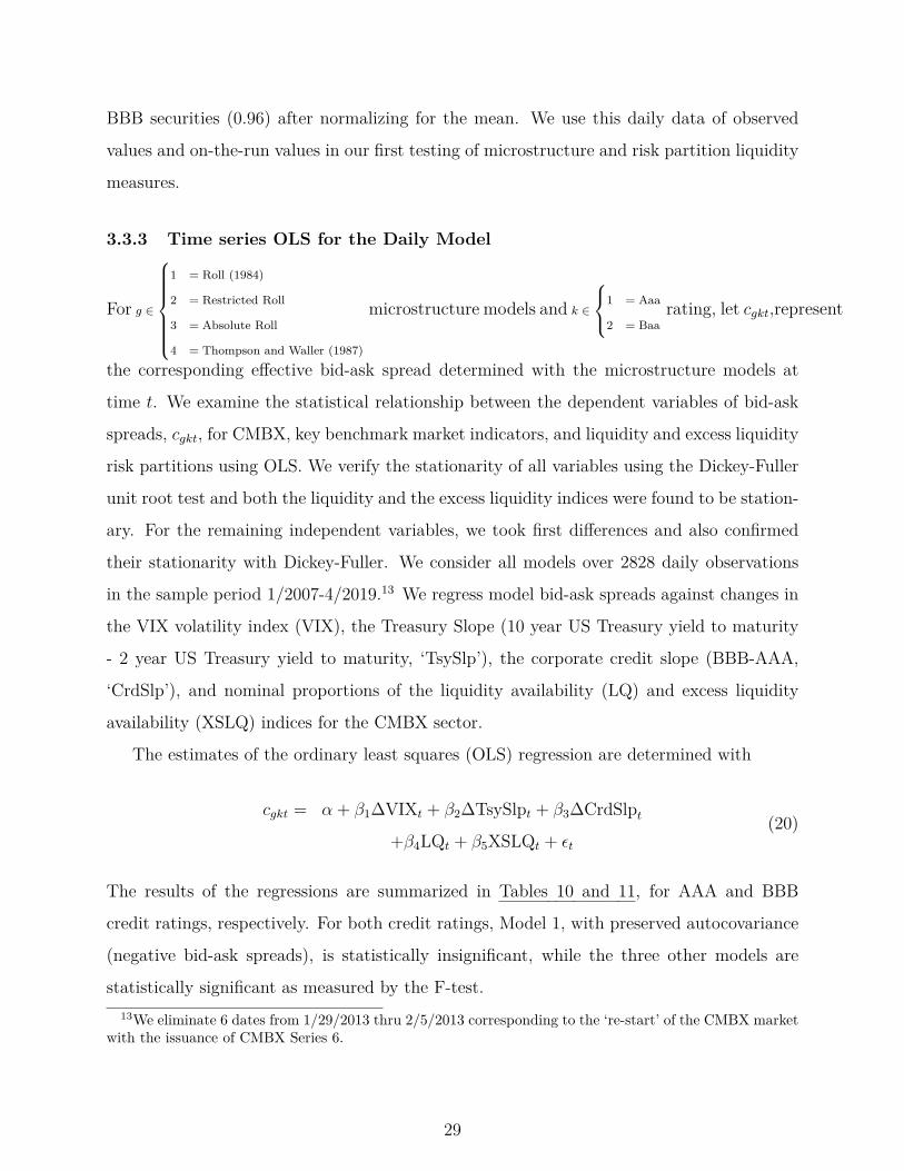
BBB securities (0.96) after normalizing for the mean. We use this daily data of observed

values and on-the-run values in our first testing of microstructure and risk partition liquidity

measures.

3.3.3 Time series OLS for the Daily Model

For g ∈

1 = Roll (1984)

2 = Restricted Roll

3 = Absolute Roll

4 = Thompson and Waller (1987)

microstructure models and k ∈

1 = Aaa

2 = Baarating, let cgkt,represent

the corresponding effective bid-ask spread determined with the microstructure models at

time t. We examine the statistical relationship between the dependent variables of bid-ask

spreads, cgkt, for CMBX, key benchmark market indicators, and liquidity and excess liquidity

risk partitions using OLS. We verify the stationarity of all variables using the Dickey-Fuller

unit root test and both the liquidity and the excess liquidity indices were found to be station-

ary. For the remaining independent variables, we took first differences and also confirmed

their stationarity with Dickey-Fuller. We consider all models over 2828 daily observations

in the sample period 1/2007-4/2019.13 We regress model bid-ask spreads against changes in

the VIX volatility index (VIX), the Treasury Slope (10 year US Treasury yield to maturity

- 2 year US Treasury yield to maturity, ‘TsySlp’), the corporate credit slope (BBB-AAA,

‘CrdSlp’), and nominal proportions of the liquidity availability (LQ) and excess liquidity

availability (XSLQ) indices for the CMBX sector.

The estimates of the ordinary least squares (OLS) regression are determined with

cgkt = α + β1∆VIXt + β2∆TsySlpt + β3∆CrdSlpt+β4LQt + β5XSLQt + εt

(20)

The results of the regressions are summarized in Tables 10 and 11, for AAA and BBB

credit ratings, respectively. For both credit ratings, Model 1, with preserved autocovariance

(negative bid-ask spreads), is statistically insignificant, while the three other models are

statistically significant as measured by the F-test.13We eliminate 6 dates from 1/29/2013 thru 2/5/2013 corresponding to the ‘re-start’ of the CMBX market

with the issuance of CMBX Series 6.

29

Table 10: Time series OLS, AAARoll (1) Restricted Roll (2) ABSRoll (3) TW (4)

Intercept -0.36589 17.97386*** 19.85028*** 8.04411***0.95751 0.73358 0.76557 0.50276

chgVIX -0.1203 -0.2673** -0.16294 . -0.075440.11786 0.08985 0.09423 0.06188

chgTsySlp 0.09272 -0.01474 -0.11751** -0.022230.05491 0.04257 0.0439 0.02883

chgCrdSlp -0.08124 0.19366** 0.28591*** 0.08836 .0.09726 0.07077 0.07776 0.05107

Lq 2.40796 -21.30327*** -24.37286*** -7.33146***2.55098 1.94928 2.0396 1.33945

XSLq 0.19045 -25.47087*** -28.0375*** -12.05928***1.301 0.97257 1.04019 0.68312

df 2822 1658 2822 2822F-test p-val 0.2703 0.00 0.00 0.00Adj-Rsq 0.0004919 0.3017 0.2114 0.1075

This table summarizes the results from the AAA OLS regression cgkt = α + β1∆VIXt + β2∆TsySlpt + β3CrdSlpt + β4LQt + β5XSLQt + εt asdefined in Eq. (20). The dependent variable considered are the AAA effective bid-ask spreads, cgkt determined using the four microstructuremodels of Roll (1984) with positive autocovariance preserved for observations, Roll (1984) augmented with observations of positive autocovarianceeliminated, Christopoulos (2020), and Thompson and Waller (1987). The five independent variables are the change in the VIX volatility index(‘chgVIX’), the change in the Treasury slope (‘chgTsySlope’) of 10year - 2year yields, the change in the corporate credit slope (‘chgCrdSlp’) ofBBB-AAA risk premia, the estimated CMBX sector wide indices weighted across all ratings and tranches for liquidity (‘Lq’) and excess liquidity(‘XSLq’) as depicted in Fig. (1). The significance codes of ’***’, ’**’, ’*’, and ’.’ indicate statistical significance at the 0.001, 0.01, 0.05 and 0.1levels, respectively.

Table 11: Time series OLS, BBBRoll (1) Restricted Roll (2) ABSRoll (3) TW (4)

Intercept 8.2623 399.7197*** 68.1094*** 388.1854***7.3778 23.1303 6.9989 18.3606

chgVIX 0.4042 1.5045 -0.1384 0.1580.9081 2.8203 0.8615 2.2599

chgTsySlp 0.5833 0.3842 0.2917 0.38940.4231 1.2611 0.4014 1.0529

chgCrdSlp 0.5793 -0.8997 0.65 -1.83480.7494 2.2132 0.7109 1.865

Lq 2.3037 -536.5333*** -63.1772*** -484.008***19.6558 61.9319 18.6463 48.9159

XSLq -3.866 -592.9525*** -86.4366*** -587.0661***10.0244 30.6485 9.5096 24.9471

df 2822 1746 2822 2822F-test p-val 0.7238 0.00 0.00 0..00Adj-Rsq -0.0007627 0.1801 0.02843 0.1676

This table summarizes the results from the BBB OLS regression cgkt = α + β1∆VIXt + β2∆TsySlpt + β3CrdSlpt + β4LQt + β5XSLQt + εt asdefined in Eq. (20). The dependent variable considered are the BBB effective bid-ask spreads, cgkt determined using the four microstructuremodels of Roll (1984) with positive autocovariance preserved for observations, Roll (1984) augmented with observations of positive autocovarianceeliminated, Christopoulos (2020), and Thompson and Waller (1987). The five independent variables are the change in the VIX volatility index(‘chgVIX’), the change in the Treasury slope (‘chgTsySlope’) of 10year - 2year yields, the change in the corporate credit slope (‘chgCrdSlp’) ofBBB-AAA risk premia, the estimated CMBX sector wide indices weighted across all ratings and tranches for liquidity (‘Lq’) and excess liquidity(‘XSLq’) as depicted in Fig. (1). The significance codes of ’***’, ’**’, ’*’, and ’.’ indicate statistical significance at the 0.001, 0.01, 0.05 and 0.1levels, respectively.

30

AAA For AAA bid-ask spreads as dependent variable, wider bid-ask spreads correspond

to lower volatility as measured by the VIX. This would suggest a lagging response in market

pricing compared with observed volatility. This intuition is corroborated in the significant

Models 2, 3 and 4. As bid-ask spreads widen (greater uncertainty) changes in the Treasury

slope become more muted (negative) reflecting a general flight to quality. Simultaneously, the

changes in the credit slope are increasing (positive), also reflecting market wide concerns over

credit. Finally, the signs of both liquidity and excess liquidity indices are negative suggesting

that when bid-ask spreads widen, there may be less sector-wide liquidity embedded within

market prices. The Adjusted R-squared value of 0.3017 for Model 214 exhibits the best

explanatory value for the bid-ask estimates, but its scope is limited. In contrast, Model 3

with its Adjusted R-squared value of 0.2114 provides consistently significant estimators for

each of the covariates. Model 4 provides less insight.

BBB CMBX In general, the finding for the BBB OLS are worse than the AAA case. The

stand-out results are the signs and significance of the liquidity and excess liquidity indices

which are negative, and highly significant for Models 2, 3 and 4. The other covariates are

insignificant though, in the case of Model 3 the coefficient signs are mostly similar to the

AAA case. The exception is in the change of the Treasury slope which exhibits a positive

sign. This is encouraging as the credit sensitive portion of the capital structure (BBB) should

be less influenced by yield curve dynamics than corresponding senior (AAA) credits.

Discussion As in the AAA case, Model 2 model provides the highest explanatory value as

measured by the Adjusted R-squared of 0.1801, but it again suffers from the limited sample

of 38% less observations than are considered by the other three models. Interestingly, we

see lower incidence of positive autocovariance in BBB than AAA. In Model 2 for AAA there

are 1164 incidents (2822-1658) while in BBB there are 1082 incidents (2822-1746). This

could suggest that investors have more idiosyncratic risk information about loan and bond

collateral and are somewhat less apt to simply engage in follow-on pricing exhibited in the

more commoditized AAA classes which are protected from default driven losses through sub-

ordination. AAA securities are categorically more liquid than BBB’s which, as subordinate14Model 2 has 43% less observations than the other models due to dropped values exhibiting positive

autocovariance.

31

classes, exhibit categorically wider bid-ask spreads, wider mid-market spreads, and smaller

liquidity and excess liquidity partitions than AAA’s. This may be due in part to idiosyn-

cratic concerns over the risk of default on underlying collateral. As such, the regressions for

the BBB class of CMBX suggest that other drivers are materially influencing pricing of the

securities, which in turn influences the bid-ask spread estimates. It is thus not surprising

that the Adjusted R-squared values for the BBB regressions are categorically lower than for

AAA. It is interesting that the Adjusted- R-squared value for Model 4 of 0.16786 is higher

than the Adjusted R-squared for Model 3 of 0.02843. These statistics seem to support the

distinctions between the senior AAA and the subordinate BBB securities and the presence

of an influence of liquidity and excess liquidity embedded within market pricing which is our

first main result.

3.3.4 VAR, Granger and IRF for the Daily Model

While the OLS results are good, they are somewhat coarse to the task of liquidity evalu-

ation. OLS relationships are contemporaneous and do not control for autoregressive behavior

amongst covariates. In contrast, VAR and IRF techniques do provide such controls and are

applied here to CMBX liquidity evaluation.

VAR With VAR, we estimate the ‘true’ value of the bid-ask spread, ct, as the dependent

variable at time t explained by its own lagged variables, ct−n, and lagged market variables,

Mt−n. The VAR we implement is of the form

ct = α +N∑n=1

βnct−n +N∑n=1

γnMt−n + εt (21)

The n-period lagged ∑Nn=1 βnct−n term serves as the sum of first-differenced bid-ask spread

variables while the ∑Nn=1 γnMt−n term captures the sum of first differenced market variables.

In all cases, the n-period lags are determined by Akaike Information Criteria (AIC), and

we permit up to n = 10 daily lags (2 weeks of trading). Each market variable has one

equation. The current time t observation of each variable depends upon lagged values of

bid-ask spread estimates as well as lagged values for the market variable. Ivanov and Kilian

(2005) conclude that n-order lag selections are ultimately discretionary to the project. As

32

our lags comport with those found in the earlier literature, we are comfortable with this

choice. In the OLS, the liquidity measures categorically exhibit statistical significance and

intuitively correct signs, and so we focus on those market variables to generate the IRFs.

We restrict the analysis to Model 3 and Model 4 due to their reliability across the sample.

The results of the VARs are provided in the Online Appendix in Tables 22 and 23. They are

as expected with high Adjusted R-squared values ranging from 0.73 to 0.84 and statistical

significance for lagged bid-ask dependent variable as independent variable for both models

across AAA and BBB credits. Interestingly, lagged values for excess liquidity indices exhibit

greater statistical significance than liquidity indices in Model 3 (AbsRoll) but less so in

Model 4 (ThompsonWaller).

Granger As with the VARs, the Granger tests are restricted to Models 3 and 4 and only

test relationships between bid-ask spread and liquidity measures. In Panel B, for Models 3

and 4, we find strong statistical evidence at the 0.10% significance level with excess liquidity

Granger causing AAA bid-ask spreads. For BBB bid-ask spreads only Model 4 exhibits

statistical significance (0.10%) for excess liquidity Granger causing BBB bid-ask spreads,

while Model 3 is insignificant. We find weaker evidence of liquidity Granger causing AAA or

BBB bid-ask spreads for the exact same relationship across both models in Panel A. Panels

C and D exhibit strong statistical support for bid-ask spreads Granger causing liquidity and

excess liquidity, which is not surprising given both liquidity and excess liquidity are residual

measures. These results are summarized below in Table 12.

IRF IRFs describe a response variable’s evolution over a projected time horizon following

a one standard deviation exogenous random shock to the initial values of the endogenous

variables in VAR using the bootstrapping method. It is a statistical assessment of sensitivity

(response) to a one-standard deviation shock (impulse) within the VAR and is conducted as a

post-estimation analysis. Following Lütkepohl (2005), a moving average representation (also

referred to as a forecast error impulse response, or FEIR, Φi = ∑im=1 Φm−1Am, i = 1, 2, ...)

is an iterative formulation for Φi with Φ0 = IK and Am the coefficient vector for lag m. To

correctly account for the contemporaneous correlation between residuals of the covariates

in the VAR, which is not accounted for in the coefficient vectors Ai, we orthogonalize the

33

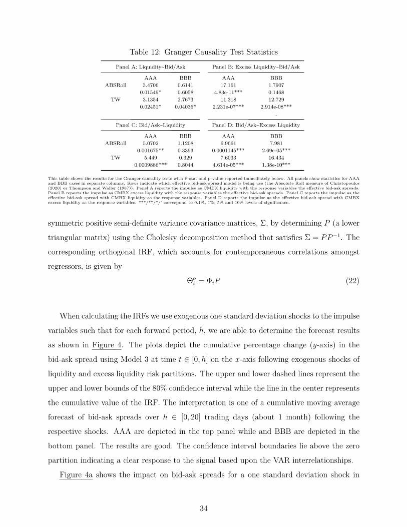
Table 12: Granger Causality Test Statistics

Panel A: Liquidity~Bid/Ask Panel B: Excess Liquidity~Bid/Ask

AAA BBB AAA BBBABSRoll 3.4706 0.6141 17.161 1.7907

0.01549* 0.6058 4.83e-11*** 0.1468TW 3.1354 2.7673 11.318 12.729

0.02451* 0.04036* 2.231e-07*** 2.914e-08***.

Panel C: Bid/Ask~Liquidity Panel D: Bid/Ask~Excess Liquidity

AAA BBB AAA BBBABSRoll 5.0702 1.1208 6.9661 7.981

0.001675** 0.3393 0.0001145*** 2.69e-05***TW 5.449 0.329 7.6033 16.434

0.0009886*** 0.8044 4.614e-05*** 1.38e-10***

This table shows the results for the Granger causality tests with F-stat and p-value reported immediately below. All panels show statistics for AAAand BBB cases in separate columns. Rows indicate which effective bid-ask spread model is being use (the Absolute Roll measure of Christopoulos(2020) or Thompson and Waller (1987)). Panel A reports the impulse as CMBX liquidity with the response variables the effective bid-ask spreads.Panel B reports the impulse as CMBX excess liquidity with the response variables the effective bid-ask spreads. Panel C reports the impulse as theeffective bid-ask spread with CMBX liquidity as the response variables. Panel D reports the impulse as the effective bid-ask spread with CMBXexcess liquidity as the response variables. ***/**/*/’ correspond to 0.1%, 1%, 5% and 10% levels of significance.

symmetric positive semi-definite variance covariance matrices, Σ, by determining P (a lower

triangular matrix) using the Cholesky decomposition method that satisfies Σ = PP−1. The

corresponding orthogonal IRF, which accounts for contemporaneous correlations amongst

regressors, is given by

Θoi = ΦiP (22)

When calculating the IRFs we use exogenous one standard deviation shocks to the impulse

variables such that for each forward period, h, we are able to determine the forecast results

as shown in Figure 4. The plots depict the cumulative percentage change (y-axis) in the

bid-ask spread using Model 3 at time t ∈ [0, h] on the x-axis following exogenous shocks of

liquidity and excess liquidity risk partitions. The upper and lower dashed lines represent the

upper and lower bounds of the 80% confidence interval while the line in the center represents

the cumulative value of the IRF. The interpretation is one of a cumulative moving average

forecast of bid-ask spreads over h ∈ [0, 20] trading days (about 1 month) following the

respective shocks. AAA are depicted in the top panel while and BBB are depicted in the

bottom panel. The results are good. The confidence interval boundaries lie above the zero

partition indicating a clear response to the signal based upon the VAR interrelationships.

Figure 4a shows the impact on bid-ask spreads for a one standard deviation shock in

34

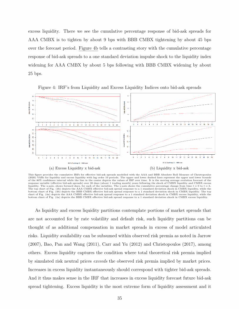
excess liquidity. There we see the cumulative percentage response of bid-ask spreads for

AAA CMBX is to tighten by about 9 bps with BBB CMBX tightening by about 45 bps

over the forecast period. Figure 4b tells a contrasting story with the cumulative percentage

response of bid-ask spreads to a one standard deviation impulse shock to the liquidity index

widening for AAA CMBX by about 5 bps following with BBB CMBX widening by about

25 bps.

Figure 4: IRF’s from Liquidity and Excess Liquidity Indices onto bid-ask spreads

(a) Excess Liquidity x bid-ask (b) Liquidity x bid-askThis figure provides the cumulative IRFs for effective bid-ask spreads modelled with the AAA and BBB Absolute Roll Measure of Christopoulos(2020) VARs for liquidity and excess liquidity with lag order 10 periods. The upper and lower dashed lines represent the upper and lower boundsof the 80% confidence interval while the line in the center depicts the values of IRF over time. It is the moving average evolution forecast of theresponse variable (effective bid-ask spreads) over 20 days (about 1 trading month) years following the shock of CMBX liquidity and CMBX excessliquidity. The x-axis, shows forward days, for each of the variables. The y-axis shows the cumulative percentage change from time t = 0 to t = h.The top chart of Fig. (4b) depicts the AAA CMBX effective bid-ask spread response to a 1 standard deviation shock in CMBX liquidity, while thebottom chart of Fig. (4b) depicts the BBB CMBX effective bid-ask spread response to a 1 standard deviation shock in CMBX liquidity. The topchart of Fig. (4a) depicts the AAA CMBX effective bid-ask spread response to a 1 standard deviation shock in CMBX excess liquidity, while thebottom chart of Fig. (4a) depicts the BBB CMBX effective bid-ask spread response to a 1 standard deviation shock in CMBX excess liquidity.

As liquidity and excess liquidity partitions contemplate portions of market spreads that

are not accounted for by rate volatility and default risk, such liquidity partitions can be

thought of as additional compensation in market spreads in excess of model articulated

risks. Liquidity availability can be subsumed within observed risk premia as noted in Jarrow

(2007), Bao, Pan and Wang (2011), Carr and Yu (2012) and Christopoulos (2017), among

others. Excess liquidity captures the condition where total theoretical risk premia implied

by simulated risk neutral prices exceeds the observed risk premia implied by market prices.

Increases in excess liquidity instantaneously should correspond with tighter bid-ask spreads.

And it thus makes sense in the IRF that increases in excess liquidity forecast future bid-ask

spread tightening. Excess liquidity is the most extreme form of liquidity assessment and it

35

is plausible that even if excess liquidity is not actively revealed to the market as yet, that

other signals correlated with excess liquidity are signalling to market actors, resulting in

assessments that the bonds are inexpensive relative to their risks.

The more nuanced case is in revealed liquidity availability. If, as a theoretical measure,

liquidity availability increases and the market is unaware of this, it can suggest that market

is simply uncertain of the underlying risks of the securities. This would be consistent with

the findings of Bao, O’Hara and Zhou (2018) where the impact results in more restrictive

risk policy not substantiated by underlying risks. If market spreads are widening in excess of

the theoretical assessment of default and rate risks then, mechanically, liquidity availability

will increase. But if no one knows about the partitioning, then all the market sees is market

spreads widening. It is thus plausible that the liquidity shock in the IRF will correspond to

future uncertainty evidenced by projected bid-ask spread widening.

Discussion As shown in the OLS, liquidity risk partitions play a significant role in CMBX

price formation (our first main result). They give rise to our time series analyses with VAR,

Granger and IRFs. These analyses produces our second main result that liquidity partitions

have a significant effect on future observed CMBX liquidity as measured by projected effective

bid-ask spreads. Finally, we note that the Daily Model is well specified because the four

elements of the Daily Model are not collinear. The proof of this is found in the Online

Appendix Section A.3. These results establishes a theoretical relationship for CMBX between

microstructure estimates of liquidity in effective bid-ask spreads and estimated reduced form

assessments of liquidity. Together these results validate the Daily Model.

4 The Intraday Model (and its results)

This section introduces the Intraday Model and uses all indexed investment grade CMBX

classes in the validation of the risk partitions. As discussed in Section 2, there are no observ-

able CMBX intraday prices (spreads). And so it is not possible to validate the risk partitions

with observed market prices or, even theoretical effective bid-ask spreads. However, the the-

oretical underpinning of CMBX risk partitions provide insights into the related REIT sector.

We disclose that relationship in this section and use it to validate with ICAPM.

36

4.1 Instantaneous changes

With the exception of CMBX market spreads, the Daily Model, validated in the previous

section, is based on changes in explanatory variables in Eq. (24) which capture the economy

of REITs, US Treasuries and the VIX. There is nothing in principle that prevents us from

increasing the frequency of estimation for all risk components from daily, to shorter intervals

intraday. In this section we increase the frequency of linear estimation from daily to 15

second intervals, intraday, for each trading day in the Covid-19 pandemic in our sample (the

‘Intraday Model’).

For the Intraday Model, all mathematics apply to all trading days u and time t is the

intraday time index with t ∈ [1, 1560] 15 second intervals from 9:30:15am to 4:15:00pm EST

for each trading day u. Once the daily initial conditions have been determined, for each

trading day u intraday changes in risk composition are then modelled as a zero-centered

function of the evolution of the factors

∆yjk(t) =5∑i=1

ηijk∆fi(t) + ε∆jk(t) (23)

for the j-th risk partition of the k-th bond at time t. We compute a covariance matrix

such that ηijk is the covariate of the i-th factor with the corresponding bond’s corresponding

risk component. The coefficients ηijk are determined through OLS and ε∆jk(t) has expected

mean zero with standard deviation √η0jk. We normalize the sum of the proportions for the

intraday risk decomposition to 1 as was done previously for daily observations in Eq. (12).

The final risk composition is then calculated using the initial condition and the instant-

aneous changes:

yjk(t) = yjk(t0) +t∑

t′=1∆yjk(t′) (24)

where the intraday estimation of risk components yjk(t) is the j-th component of the risk

partition for bond k at time t on trading day u. The first term on the righthand side, yjk(t0),

is the initial value of the risk component intraday and the second term ∑tt′=1 ∆yjk(t′) the

intraday sum of the changes in the risk component defined in Eq. (23).

37

Figure 5: CMBX intraday risk decomposition (15 second intervals)

(a) CMBX intraday, 20200417

(b) CMBX intraday, 20201204This figure provides proportional intraday CMBX risk decomposition in 1560, 15 second intervals. The four components of risk modelled aredefault, interest rates, liquidity and excess liquidity. The x-axis capture the time intervals from 9:30:15am to 4:15:00pm.EST The y-axis capturesthe estimated proportion of CMBX risk embedded within CMBS spreads as determined in Eq. (12). Fig. (5a) captures the intraday evolution ofCMBX proportional risk decompositions on April 17, 2020 and Fig. (5b) captures the intraday evolution of CMBX proportional risk decompositionson December 4, 2020. Separate evolutions are provided for each of the investment grade CMBX tranches, as well as for the weighted averagecomposite index across all investment grade CMBX as shown monthly in Christopoulos and Jarrow (2018).

38

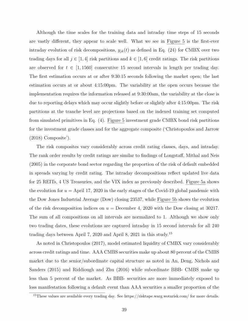
Although the time scales for the training data and intraday time steps of 15 seconds

are vastly different, they appear to scale well. What we see in Figure 5 is the first-ever

intraday evolution of risk decompositions, yjk(t) as defined in Eq. (24) for CMBX over two

trading days for all j ∈ [1, 4] risk partitions and k ∈ [1, 6] credit ratings. The risk partitions

are observed for t ∈ [1, 1560] consecutive 15 second intervals in length per trading day.

The first estimation occurs at or after 9:30:15 seconds following the market open; the last

estimation occurs at or about 4:15:00pm. The variability at the open occurs because the

implementation requires the information released at 9:30:00am, the variability at the close is

due to reporting delays which may occur slightly before or slightly after 4:15:00pm. The risk

partitions at the tranche level are projections based on the indexed training set computed

from simulated primitives in Eq. (4). Figure 5 investment grade CMBX bond risk partitions

for the investment grade classes and for the aggregate composite (‘Christopoulos and Jarrow

(2018) Composite’).

The risk composites vary considerably across credit rating classes, days, and intraday.

The rank order results by credit ratings are similar to findings of Longstaff, Mithal and Neis

(2005) in the corporate bond sector regarding the proportion of the risk of default embedded

in spreads varying by credit rating. The intraday decompositions reflect updated live data

for 25 REITs, 4 US Treasuries, and the VIX index as previously described. Figure 5a shows

the evolution for u = April 17, 2020 in the early stages of the Covid-19 global pandemic with

the Dow Jones Industrial Average (Dow) closing 23537, while Figure 5b shows the evolution

of the risk decomposition indices on u = December 4, 2020 with the Dow closing at 30217.

The sum of all compositions on all intervals are normalized to 1. Although we show only

two trading dates, these evolutions are captured intraday in 15 second intervals for all 240

trading days between April 7, 2020 and April 8, 2021 in this study.15

As noted in Christopoulos (2017), model estimated liquidity of CMBX vary considerably

across credit ratings and time. AAA CMBS securities make up about 80 percent of the CMBS

market due to the senior/subordinate capital structure as noted in An, Deng, Nichols and

Sanders (2015) and Riddiough and Zhu (2016) while subordinate BBB- CMBS make up

less than 5 percent of the market. As BBB- securities are more immediately exposed to

loss manifestation following a default event than AAA securities a smaller proportion of the15These values are available every trading day. See https://risktape.warg.wotnrisk.com/ for more details.

39

risk compensation above the risk free rate for BBB- securities should be associated with

liquidity availability when compared with AAA. This dynamic is confirmed in Christopoulos

(2017) and Christopoulos and Jarrow (2018) in indexed form from 2007-2015 in monthly

simulations and is confirmed again in the results of this paper with bid-ask comparisons

with such measures daily (as previously discussed), and now as evident, intraday.

4.2 Validation of the Intraday Model

4.2.1 Statistical summary for the Intraday Model

Table 13: Summary statistics of cumulative changes of intraday CMBX risk partitions

Panel A: Default AAA AJ AA A BBB BBB-min 0.483416 0.338351 0.494514 0.609670 0.717165 0.823893max 1.820368 8.403204 6.036482 6.121692 1.913765 1.400509mean 1.000102 1.000104 1.000046 1.000039 1.000012 1.000005median 1.000000 1.000000 1.000000 1.000000 1.000000 1.000000variance 0.000212 0.000380 0.000156 0.000147 0.000020 0.000006stdev 0.014562 0.019491 0.012485 0.012127 0.004425 0.002384obs 275370 275370 275370 275370 275370 275370

Panel B: Rate risk AAA AJ AA A BBB BBB-min 0.702365 0.610945 0.530693 0.583500 0.476037 0.599777max 1.518098 1.742393 2.244835 1.871355 1.976362 1.469975mean 1.000010 1.000137 1.000058 1.000042 1.000061 1.000024median 1.000000 1.000000 1.000000 1.000000 1.000000 1.000000variance 0.000019 0.000281 0.000123 0.000086 0.000123 0.000041stdev 0.004340 0.016768 0.011092 0.009273 0.011089 0.006433obs 275370 275370 275370 275370 275370 275370

Panel C: Liquidity AAA AJ AA A BBB BBB-min 0.735970 0.330755 0.030144 0.016780 0.275537 0.134313max 1.707165 8.456980 9.348418 27.908990 2.411473 6.462325mean 1.000036 1.000466 1.000559 1.000738 1.000176 1.000397median 1.000000 1.000000 1.000000 1.000000 1.000000 1.000000variance 0.000078 0.001217 0.001370 0.007370 0.000361 0.000976stdev 0.008806 0.034890 0.037017 0.085848 0.019004 0.031240obs 275370 275370 275370 275370 275370 275370

Panel D: XS liquidity AAA AJ AA A BBB BBB-min 0.346666 0.136986 0.508825 0.508825 0.508825 0.140683max 3.379393 7.812876 2.413748 2.413748 2.413748 6.325317mean 1.000147 1.000329 1.000074 1.000074 1.000074 1.000184median 1.000000 1.000000 1.000000 1.000000 1.000000 1.000000variance 0.000333 0.000868 0.000152 0.000152 0.000152 0.000719stdev 0.018239 0.029465 0.012328 0.012328 0.012328 0.026816obs 275370 275370 275370 275370 275370 275370

This table provides summary statistics of intraday CMBX risk partitions. The columns show the investment grade credit rating class and therows the summary statistics of minimum (min), maximum (max), mean, median, variance, standard deviation (stdev), kurtosis and the number ofobservation (obs). Panel A summarizes for default risk, Panel B summarizes for interest rate risk, Panel C summarizes for liquidity, while PanelD summarizes for excess (XS) liquidity.

Table 13 provides a statistical summary across all observations intraday for default, rates,

40

liquidity and excess liquidity risk partitions. The summary results generally follow intuition

with some new insights and we exhibit all investment grade classes. Focusing first on intraday

default risk pricing, we observe AAA CMBX appear to exhibit substantially greater volatility

than BBB-, with only the AJ exhibiting greater volatility. Rates volatility pricing intraday

is much calmer than default intraday pricing across most credits with the exception of the

BBB class. Again, as with default, the AJ class appears to exhibit higher volatility than

the AAA class. This relatively higher volatility for the AJ class compared with the AAA

class repeats across all four risk measures. Finally, as we are concentrating on liquidity, the

low nominal amounts of both liquidity and excess liquidity in BBB- classes should result

in higher volatility estimates reflective of scarce liquidity availability. Min and max values

follow intuition suggesting that the capital structure allocation concentrates mispricing in

the mid-section with the endpoints of AAA and BBB- exhibiting more regular behavior.

4.2.2 Cross sectional visualizations for the Intraday Model

While the summary information in Table 13 is interesting from an academic perspective, it is

fundamentally limited for two reasons. First, the values estimated intraday still must use an

initial set of simulated values and market spreads. The simulated risk decomposition studies

of Christopoulos (2017) and Christopoulos and Jarrow (2018), reflecting actual cashflow and

updated credit and prepayment profiles, end in 2015.

Second, the initialized spread value informing these evolutions are restricted to only

March 18, 2020 because no additional daily CMBX pricing data was made available to us

after that date. In this sense, the intraday results depicted are essentially cross-sectional

intraday stress tests of the response of risk decompositions holding market spreads as of

March 18, 2020 held constant. Although the limitations of the initialization restrict the

validity of the intraday time series across dates, they will reveal insights in cross sectional

analysis. Each day is a valid time series and the collection of all dates represents the set

for cross section evaluation. At the same time, because the real time estimations are price

independent, observing their changes over time yields some unique insights. One way to

approach the evaluation of cross section of daily time series is through the heat map approach

using binning. We want to cast the daily risk pricing data against both time and a relevant

variable. The VIX provides such a variable as a dominant explanatory variable in the

41

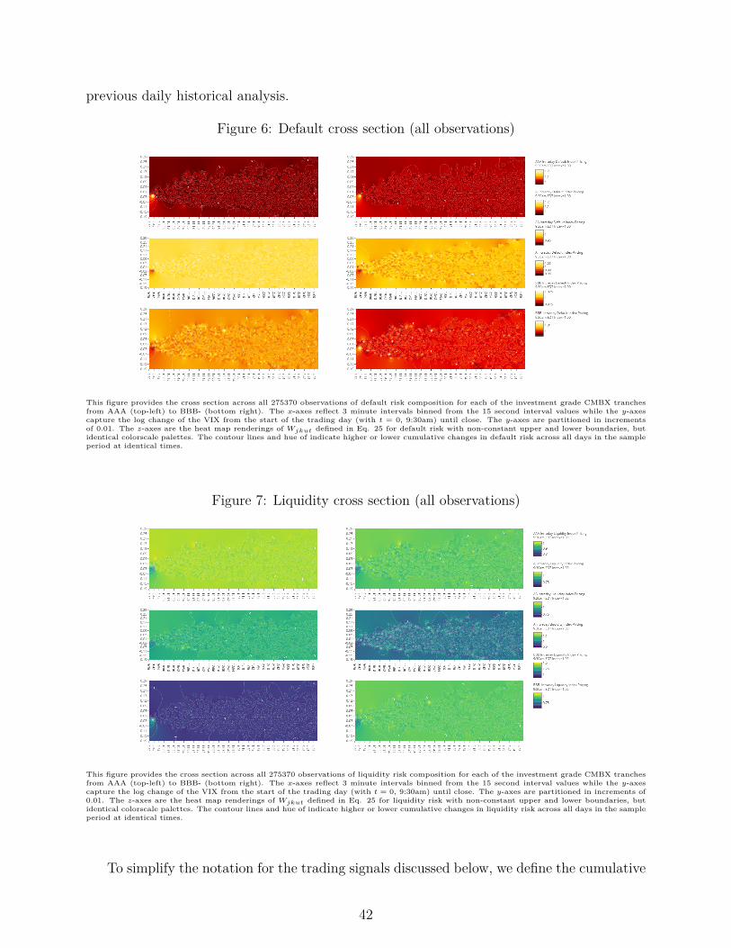
previous daily historical analysis.

Figure 6: Default cross section (all observations)

This figure provides the cross section across all 275370 observations of default risk composition for each of the investment grade CMBX tranchesfrom AAA (top-left) to BBB- (bottom right). The x-axes reflect 3 minute intervals binned from the 15 second interval values while the y-axescapture the log change of the VIX from the start of the trading day (with t = 0, 9:30am) until close. The y-axes are partitioned in incrementsof 0.01. The z-axes are the heat map renderings of Wjkut defined in Eq. 25 for default risk with non-constant upper and lower boundaries, butidentical colorscale palettes. The contour lines and hue of indicate higher or lower cumulative changes in default risk across all days in the sampleperiod at identical times.

Figure 7: Liquidity cross section (all observations)

This figure provides the cross section across all 275370 observations of liquidity risk composition for each of the investment grade CMBX tranchesfrom AAA (top-left) to BBB- (bottom right). The x-axes reflect 3 minute intervals binned from the 15 second interval values while the y-axescapture the log change of the VIX from the start of the trading day (with t = 0, 9:30am) until close. The y-axes are partitioned in increments of0.01. The z-axes are the heat map renderings of Wjkut defined in Eq. 25 for liquidity risk with non-constant upper and lower boundaries, butidentical colorscale palettes. The contour lines and hue of indicate higher or lower cumulative changes in liquidity risk across all days in the sampleperiod at identical times.

To simplify the notation for the trading signals discussed below, we define the cumulative

42

intraday change for each risk partition as

Wjkut ≡t∑

t′=1∆yjku(t′) (25)

This is the second term Eq. (24), now also indexed for the u-th trading day, and so defined

for j risk partitions, of k credit rating classes, for u trading days and t intraday trading

times. Figure 6 shows 275370 observations computed for each of the intraday default risk

partition pricings. We use a double binning method to observe. The x-axes reflect 3 minute

intervals binned from the 15 second interval values while the y-axes capture the log change

of the VIX from the start of the trading day (with t = 0, 9:30am) until close. The y-

axes are partitioned in increments of 0.01. The z-axes are the heat map renderings of

Wjkut defined in Eq. 25. The depiction have non-constant upper and lower boundaries, but

identical colorscaling . This is purposeful, as each of the classes may have inherently different

sensitivities to market indicators. The plots represent the data for each of the CMBX classes

with AAA in the upper left, AJ upper right, and so forth, with BBB- in the bottom right.

The color saturation produced for each plot is interesting during the Covid period. Together

they suggest somewhat lower intraday default risk pricing for AAA, AJ and BBB- classes

compared with the AA, A and BBB classes. In Figure 7 we take the same vantage point

but for liquidity availability. Here, we see somewhat greater intraday liquidity availability

for AAA with the least liquidity available for A and BBB classes as indicated by the color

palettes and contour lines.

These perspectives document some important facts in theoretical observation of CMBX

risk pricing during the Covid period, one of the most interesting being an apparent regular

‘spot’ of volatility in the first 15 minutes of trading in the cross section. This repeats across

all instruments and risk partitions in our sample. Figure 8 zooms in on this interval for each

of the risk partitions for all classes to revealing more detail of the phenomenon. There we see

‘peaks’ as indicated by the contour lines exceeding 1, and ‘valleys’ as indicated by contour

lines less than one clustered about 9:39am. The subplots depict risk pricing for default,

liquidity, excess liquidity and rates indices for all investment grade credit rating classes.

For example, consider in Figure 8 the case of intraday liquidity availability pricing in the

second composite of six plots on the top right. At about 9:39am we observe considerable

43

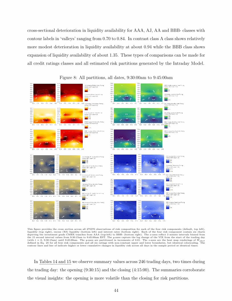
cross-sectional deterioration in liquidity availability for AAA, AJ, AA and BBB- classes with

contour labels in ‘valleys’ ranging from 0.70 to 0.84. In contrast class A class shows relatively

more modest deterioration in liquidity availability at about 0.94 while the BBB class shows

expansion of liquidity availability of about 1.35. These types of comparisons can be made for

all credit ratings classes and all estimated risk partitions generated by the Intraday Model.

Figure 8: All partitions, all dates, 9:30:00am to 9:45:00am

This figure provides the cross section across all 275370 observations of risk composition for each of the four risk components (default, top left),liquidity (top right), excess (XS) liquidity (bottom left) and interest rates (bottom right). Each of the four risk component contain six chartsdepicting the investment grade CMBX tranches from AAA (top-left) to BBB- (bottom right). The x-axes reflect 3 minute intervals binned fromthe 15 second interval values from 9:30:15am to 9:45:00am EST. The y-axes capture the log change of the VIX from the start of the trading day(with t = 0, 9:30:15am) until 9:45:00am. The y-axes are partitioned in increments of 0.01. The z-axes are the heat map renderings of Wjkutdefined in Eq. 25 for all four risk components and all six ratings with non-constant upper and lower boundaries, but identical colorscaling. Thecontour lines and hue of indicate higher or lower cumulative changes in liquidity risk across all days in the sample period at identical times.

In Tables 14 and 15 we observe summary values across 246 trading days, two times during

the trading day: the opening (9:30:15) and the closing (4:15:00). The summaries corroborate

the visual insights: the opening is more volatile than the closing for risk partitions.

44

Table 14: Open Summary during Covidvariable mean median min max variance stdev nVIX 26.7659 25.6000 16.5500 47.3400 31.88860 5.6470 246

IN_DRE 37.9874 38.5400 30.4000 43.0600 6.83532 2.6144 246IN_FR 41.0038 41.5825 33.1700 47.3700 8.22299 2.8676 246IN_PLD 98.7801 99.5750 81.4700 109.7950 35.65076 5.9708 246IN_SELF 4.0519 4.0000 3.5200 5.0500 0.08360 0.2891 246LO_HST 12.8944 11.8875 9.1400 18.4200 4.94857 2.2245 246LO_MAR 109.4389 100.5550 72.7600 155.7419 495.52655 22.2604 246LO_WYND 37.0577 33.4700 21.0900 51.7500 93.63226 9.6764 246LO_MGM 24.6343 22.3325 12.1100 41.7300 63.82471 7.9890 246MF_AVB 162.0976 159.2000 133.1000 193.5300 145.65429 12.0687 246MF_ELS 62.7243 62.7025 55.8600 68.2900 5.18841 2.2778 246MF_EQR 60.1919 59.3700 46.0100 75.9600 37.04669 6.0866 246MF_UDR 37.7456 37.4550 29.9100 45.6700 11.21798 3.3493 246OF_BXP 91.4597 91.0200 70.7300 108.5900 74.19748 8.6138 246OF_CLI 14.0493 13.8825 10.4000 18.5100 2.23470 1.4949 246OF_HIW 37.9485 38.0200 29.4500 45.1700 10.21290 3.1958 246OF_SLG 54.5778 50.6400 36.8300 77.1200 93.46684 9.6678 246OF_VNO 38.3335 37.5750 29.9550 49.0300 16.31488 4.0392 246OT_BKD 3.8272 3.3900 2.4400 6.7500 1.36962 1.1703 246OT_NNN 37.3254 36.8075 27.1050 45.8552 17.25113 4.1534 246OT_PSB 133.0409 131.7250 110.3200 159.8700 106.10071 10.3005 246OT_WPC 67.5772 68.2300 54.5500 75.0000 12.15876 3.4869 246RT_KIM 13.6444 12.6550 8.3400 19.7200 8.91863 2.9864 246RT_REG 45.0055 44.4750 34.0300 59.8800 38.80736 6.2296 246RT_SPG 78.3857 69.6225 49.7200 120.4975 364.88435 19.1019 246RT_TCO 40.0019 40.4050 28.1450 46.8000 13.19712 3.6328 246TSY_3MO 0.0854 0.0880 0.0030 0.2350 0.00149 0.0386 246TSY_5YR 0.4095 0.3600 0.2060 0.9710 0.02983 0.1727 246TSY_10YR 0.8936 0.7735 0.5260 1.7490 0.10170 0.3189 246TSY_30YR 1.6290 1.5460 1.1380 2.4960 0.11141 0.3338 246AAA_def 1.0131 1.0015 0.6218 1.8204 0.01493 0.1222 246AAA_rates 1.0015 1.0001 0.8004 1.5181 0.00313 0.0560 246AAA_reglq 1.0046 0.9995 0.7360 1.3345 0.00616 0.0785 246AAA_xslq 1.0118 0.9994 0.3467 3.1465 0.04744 0.2178 246AJ_def 1.0457 1.0008 0.5545 8.4032 0.23584 0.4856 246AJ_rates 1.0023 0.9998 0.8048 1.3263 0.00365 0.0604 246AJ_reglq 1.0303 0.9959 0.3308 2.8615 0.10486 0.3238 246AJ_xslq 1.0308 0.9975 0.1370 4.5724 0.11270 0.3357 246AA_def 1.0277 1.0000 0.5937 6.0365 0.10726 0.3275 246AA_rates 1.0082 1.0003 0.6064 2.2448 0.01458 0.1207 246AA_reglq 1.0092 0.9982 0.0301 3.0219 0.07331 0.2708 246AA_xslq 1.0087 0.9992 0.5088 2.4137 0.02058 0.1435 246A_def 1.0219 0.9997 0.6108 6.1217 0.11167 0.3342 246A_rates 1.0084 0.9995 0.7212 1.8714 0.00939 0.0969 246A_reglq 1.0013 1.0004 0.0168 3.4114 0.05614 0.2369 246A_xslq 1.0087 0.9992 0.5088 2.4137 0.02058 0.1435 246BBB_def 1.0050 0.9999 0.7172 1.9138 0.00514 0.0717 246BBB_rates 1.0101 1.0001 0.6726 1.4887 0.00836 0.0914 246BBB_reglq 0.9934 0.9982 0.3555 1.9290 0.02679 0.1637 246BBB_xslq 1.0087 0.9992 0.5088 2.4137 0.02058 0.1435 246BBBm_def 1.0029 1.0001 0.9184 1.4005 0.00095 0.0308 246BBBm_rates 1.0012 1.0000 0.5998 1.3887 0.00533 0.0730 246BBBm_reglq 1.0430 0.9956 0.1343 5.0141 0.15543 0.3942 246BBBm_xslq 1.0062 0.9992 0.3763 2.7905 0.03548 0.1884 246

This table summarizes the observations of intraday data at the open of the trading day 9:30:15ET for 246 trading days during the pandemic (4/2020- 4/2021). The first column provides the abbreviation for the variable name. The VIX is the CBOE volatility index. This is followed by the pricesof 25 REITs with the name a composite made up of the property type (industrial (IN), hotel/lodging (LO), multifamily (MF), mixed use/other(OT), office (OF) and retail (RT)) and the REIT’s stock market ticker. Following the REITs are US Treasury yields with ticker representing the4 maturities of 3 month, 5 year, 10 year and 30 year. The remaining values are the simulated risk partitions indexed in Christopoulos and Jarrow(2018) in cumulative change form. The ticker is a composite of the 4 types of risk partitions default (def), interest rates (rates), liquidity (reglq)and excess liquidity (xslq) combined with the credit rating class names of AAA, AJ, AA, A, BBB and BBB- (BBBm). Each of the columns to theright of the ticker report statistics across all 246 observations.

45

Table 15: Close Summary during Covidvariable mean median min max variance stdev nVIX 26.6096 25.6550 16.9900 45.4300 29.64890 5.4451 246

IN_DRE 38.0191 38.4550 30.4000 43.0300 6.75872 2.5998 246IN_FR 41.0291 41.6200 33.3500 47.4500 8.21028 2.8654 246IN_PLD 98.7703 99.6100 82.8500 109.5300 36.53448 6.0444 246IN_SELF 4.0505 4.0000 3.5622 5.0500 0.08343 0.2888 246LO_HST 12.8848 11.9275 9.4500 18.4200 4.91837 2.2177 246LO_MAR 109.2835 100.3450 75.2600 157.5000 492.77623 22.1986 246LO_WYND 37.0491 33.2800 21.3900 51.7500 92.64766 9.6254 246LO_MGM 24.6201 22.0400 12.6800 42.2000 63.62672 7.9766 246MF_AVB 161.9634 159.0800 132.7800 193.6100 143.79254 11.9914 246MF_ELS 62.7417 62.6450 56.1500 68.2900 5.27037 2.2957 246MF_EQR 60.1311 59.3700 46.2300 74.9600 37.29848 6.1072 246MF_UDR 37.7246 37.5050 29.6000 45.5600 11.21592 3.3490 246OF_BXP 91.4361 91.2000 71.1500 108.6600 73.53062 8.5750 246OF_CLI 14.0223 13.8000 10.4100 18.6900 2.24609 1.4987 246OF_HIW 37.9085 38.0250 29.7050 45.2300 10.27220 3.2050 246OF_SLG 54.5360 51.1750 36.8200 77.7900 92.16894 9.6005 246OF_VNO 38.2630 37.4800 30.1900 49.0100 16.01428 4.0018 246OT_BKD 3.8215 3.4050 2.4350 7.0500 1.37638 1.1732 246OT_NNN 37.3067 36.7350 27.6000 45.6000 16.87934 4.1084 246OT_PSB 133.0165 131.8750 110.3100 159.9100 107.41229 10.3640 246OT_WPC 67.5539 68.1400 54.5600 74.3100 11.90968 3.4510 246RT_KIM 13.6380 12.7100 8.3000 19.7000 8.91577 2.9859 246RT_REG 44.9848 44.4500 34.0500 59.6500 38.49700 6.2046 246RT_SPG 78.2918 69.4800 51.2000 121.1400 363.46241 19.0647 246RT_TCO 40.0404 40.4700 32.8700 46.6900 12.51065 3.5370 246TSY_3MO 0.0850 0.0880 0.0030 0.2100 0.00149 0.0386 246TSY_5YR 0.4094 0.3620 0.1950 0.9410 0.02932 0.1712 246TSY_10YR 0.8942 0.7630 0.5150 1.7460 0.10130 0.3183 246TSY_30YR 1.6306 1.5450 1.1620 2.4760 0.11075 0.3328 246AAA_def 0.9997 0.9999 0.9806 1.0272 0.00002 0.0039 246AAA_rates 1.0001 1.0000 0.9971 1.0066 0.00000 0.0010 246AAA_reglq 1.0001 1.0001 0.9745 1.0138 0.00001 0.0032 246AAA_xslq 1.0006 1.0000 0.9696 1.0326 0.00004 0.0060 246AJ_def 1.0001 1.0000 0.9913 1.0217 0.00001 0.0026 246AJ_rates 1.0002 1.0001 0.9666 1.0247 0.00002 0.0040 246AJ_reglq 1.0001 1.0000 0.9176 1.0409 0.00009 0.0092 246AJ_xslq 0.9988 1.0000 0.9528 1.0172 0.00006 0.0079 246AA_def 1.0000 1.0000 0.9866 1.0188 0.00000 0.0018 246AA_rates 1.0004 1.0003 0.9775 1.0225 0.00002 0.0043 246AA_reglq 0.9992 1.0000 0.9347 1.0215 0.00004 0.0066 246AA_xslq 0.9995 1.0000 0.9776 1.0071 0.00001 0.0033 246A_def 1.0000 1.0000 0.9870 1.0065 0.00000 0.0014 246A_rates 1.0003 1.0002 0.9824 1.0169 0.00001 0.0034 246A_reglq 0.9998 1.0000 0.9441 1.0294 0.00003 0.0054 246A_xslq 0.9995 1.0000 0.9776 1.0071 0.00001 0.0033 246BBB_def 0.9999 1.0000 0.9952 1.0030 0.00000 0.0009 246BBB_rates 1.0001 1.0000 0.9827 1.0273 0.00002 0.0042 246BBB_reglq 1.0000 0.9999 0.9785 1.0248 0.00002 0.0047 246BBB_xslq 0.9995 1.0000 0.9776 1.0071 0.00001 0.0033 246BBBm_def 1.0000 1.0000 0.9953 1.0029 0.00000 0.0008 246BBBm_rates 0.9999 1.0000 0.9877 1.0059 0.00000 0.0012 246BBBm_reglq 0.9993 1.0000 0.9467 1.0170 0.00003 0.0056 246BBBm_xslq 0.9996 1.0000 0.9665 1.0092 0.00001 0.0033 246

This table summarizes the observations of intraday data at the close of the trading day 4:15:00ET for 246 trading days during the pandemic (4/2020- 4/2021). The first column provides the abbreviation for the variable name. The VIX is the CBOE volatility index. This is followed by the pricesof 25 REITs with the name a composite made up of the property type (industrial (IN), hotel/lodging (LO), multifamily (MF), mixed use/other(OT), office (OF) and retail (RT)) and the REIT’s stock market ticker. Following the REITs are US Treasury yields with ticker representing the4 maturities of 3 month, 5 year, 10 year and 30 year. The remaining values are the simulated risk partitions indexed in Christopoulos and Jarrow(2018) in cumulative change form. The ticker is a composite of the 4 types of risk partitions default (def), interest rates (rates), liquidity (reglq)and excess liquidity (xslq) combined with the credit rating class names of AAA, AJ, AA, A, BBB and BBB- (BBBm). Each of the columns to theright of the ticker report statistics across all 246 observations.

46

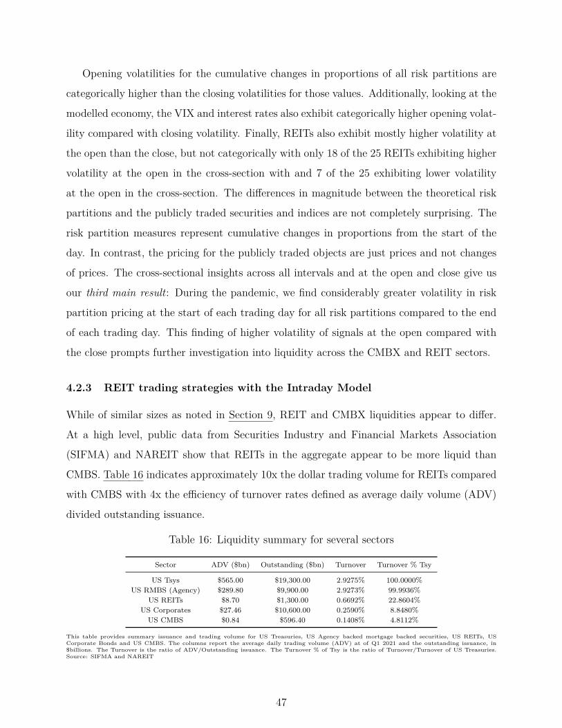
Opening volatilities for the cumulative changes in proportions of all risk partitions are

categorically higher than the closing volatilities for those values. Additionally, looking at the

modelled economy, the VIX and interest rates also exhibit categorically higher opening volat-

ility compared with closing volatility. Finally, REITs also exhibit mostly higher volatility at

the open than the close, but not categorically with only 18 of the 25 REITs exhibiting higher

volatility at the open in the cross-section with and 7 of the 25 exhibiting lower volatility

at the open in the cross-section. The differences in magnitude between the theoretical risk

partitions and the publicly traded securities and indices are not completely surprising. The

risk partition measures represent cumulative changes in proportions from the start of the

day. In contrast, the pricing for the publicly traded objects are just prices and not changes

of prices. The cross-sectional insights across all intervals and at the open and close give us

our third main result: During the pandemic, we find considerably greater volatility in risk

partition pricing at the start of each trading day for all risk partitions compared to the end

of each trading day. This finding of higher volatility of signals at the open compared with

the close prompts further investigation into liquidity across the CMBX and REIT sectors.

4.2.3 REIT trading strategies with the Intraday Model

While of similar sizes as noted in Section 9, REIT and CMBX liquidities appear to differ.

At a high level, public data from Securities Industry and Financial Markets Association

(SIFMA) and NAREIT show that REITs in the aggregate appear to be more liquid than

CMBS. Table 16 indicates approximately 10x the dollar trading volume for REITs compared

with CMBS with 4x the efficiency of turnover rates defined as average daily volume (ADV)

divided outstanding issuance.

Table 16: Liquidity summary for several sectors

Sector ADV ($bn) Outstanding ($bn) Turnover Turnover % Tsy

US Tsys $565.00 $19,300.00 2.9275% 100.0000%US RMBS (Agency) $289.80 $9,900.00 2.9273% 99.9936%

US REITs $8.70 $1,300.00 0.6692% 22.8604%US Corporates $27.46 $10,600.00 0.2590% 8.8480%US CMBS $0.84 $596.40 0.1408% 4.8112%

This table provides summary issuance and trading volume for US Treasuries, US Agency backed mortgage backed securities, US REITs, USCorporate Bonds and US CMBS. The columns report the average daily trading volume (ADV) at of Q1 2021 and the outstanding issuance, in$billions. The Turnover is the ratio of ADV/Outstanding issuance. The Turnover % of Tsy is the ratio of Turnover/Turnover of US Treasuries.Source: SIFMA and NAREIT

47

Additionally, as discussed in Section 2.2.1, publicly traded REITs trade on electronic

equity exchanges and thus have a similar frequency of price updates as our intraday risk

measures. Finally, REITs, like CMBS and CMBX, have similar underlying exposure to

commercial real estate risk, and so estimated CMBX risk partitions may carry relevance to

REIT pricing in the marketplace. As previously mentioned, CMBX as an OTC product does

not trade electronically.16 That means that the estimated risk partitions in this study update

more rapidly than the pricing of actual CMBX securities and the pricing of their underlying

CMBS collateral. In earlier studies the CMBX risk partitions gave many profitable insights

into the buy/sell decision-making within the CMBX market. In this study, we also find

that the risk partitions reveal insights into the related REIT sector intraday, with matching

trading frequency.

4.2.4 Scope and notation for trading strategies

Note that unlike default, liquidity and excess liquidity partitions, the interest rate risk parti-

tion is a bit more difficult to interpret in the trading context with respect to REITs. Higher

interest rate risk compensation for higher future rate volatility may affect REITs differently,

depending on leverage and asset composition. Thus, to keep things tractable, we focus our

trading strategies with REITs to the risk partitions of default, liquidity and excess liquidity.

Below we fuse the change in the intraday values of the risk partitions, Wjkut as defined in

Eq. 25, with REITs to construct two trading signals.

Trading Signal 1 For ι ∈ [1, 25] one of the 25 REITs in our sample, let ∆Rιut be defined

as

∆Rιut = Rιut

Rιt=4:15:00pm,u−1(26)

which represents the proportion of cumulative changes in REIT prices from the close of the

prior trading day t =4:15:00 pm to the time of trade execution for the ι-th REIT. With this,

define Trading Signal 1, L1ιjkut, as

L1ιjkut = |∆Rιut −Wjkut| (27)

16For further information see the Online Appendix Section A.1.

48

which captures the absolute value of the difference between the observed proportional cu-

mulative change in prices for the ι-th REIT, ∆Rιut, and the cumulative change in prices for

one of the risk partitions, Wjkut.

As an absolute value of differences in cumulative changes, L1ιjkut gives the magnitude

of differences. If those differences are influenced by liquidity effects we appear to capture

in the cross section, trading opportunities may arise. Eq. (26) does not provide a clear

direction for the trading strategy. We borrow from differences between fair value estimates

and market prices where large differences may indicate buying opportunities. Large differ-

ences necessarily correspond to differences in the theoretical risk measures and perspectives

on risk projected by market actors onto market prices. While there is a theoretical basis

for long/short trading direction in comparisons between fair value and market prices17, the

elements ∆Rιut andWjkut of Eq. (27) do not carry such ex-ante trade directional indications.

Trading Signal 2 We address some arbitrariness in Trading Signal 1’s lack of direction

with our second trading signal, Trade Signal 2, L2ιjkut, defined as

L2ιjkut = ∆Rιut

Wjkut

(28)

This trading signal L2ιjkut has several interesting interpretations and provides clear theoretical

interpretations with respect to trading direction.

As noted in Christopoulos (2017), both the liquidity and excess liquidity measures have

the interpretation of liquidity availability. And thus large values for those risk neutral meas-

ures (which are then projected onto market spreads) suggest that compensation in market

spreads exceeds (wider than) what is required fair compensation from the perspective of

the model technology. In the case of the current technology which does not benefit from

market prices to project onto, the risk composition estimated reflect cumulative intraday

changes in the measure from the opening bell. As such, higher values for cumulative changes

intraday in the liquidity and excess liquidity pricing measures, suggest ‘cheaper’ pricing for

the underlying derivatives and potentially a healthier commercial real estate environment.

The opposite is true for default risk pricing. There, higher cumulative values for the pricing17See, for example, the relative value measure theta defined in Eq. (23) in Christopoulos and Jarrow

(2018) where fair value prices greater/less than market prices indicate buy/sell signals, among others.

49

of default indicates greater default risk while lower cumulative values suggest lower default

risk. We capture the interpretation above in the proportional trading signal, L2ιjkut and

summarize below in Table 17 fifteen numerical examples which capture all types of changes

in the components of the signal. Although the trading strategy involve the ratio of 1 the

statistical analysis shows the mean and median for the ratios to be strongly clustered about

1, thereby justifying this choice.

Table 17: Trade Signal Examples

Ex # type ∆R W L = ∆R/W W = XSLQ W= LQ W= DEF1 ∆R ↑, W↑ 1.250 1.250 1.0000 no trade no trade no trade2 ∆R ↓, W↓ 0.990 0.990 1.0000 no trade no trade no trade3 ∆R ↑, W↑ 1.250 1.200 1.0417 sell sell buy4 ∆R ↓, W↓ 0.990 0.980 1.0102 sell sell buy5 ∆R ↑, W0 1.500 1.000 1.5000 sell sell buy6 ∆R↑, W↓ 1.200 0.999 1.2012 sell sell buy7 ∆R0, W↓ 1.000 0.900 1.1111 sell sell buy8 ∆R0, W0 1.000 1.000 1.0000 no trade no trade no trade9 ∆R0, W↑ 1.000 1.500 0.6667 buy buy sell10 ∆R ↓, W↑ 0.800 1.500 0.5333 buy buy sell11 ∆R ↓, W0 0.900 1.000 0.9000 buy buy sell12 ∆R ↓, W↓ 0.960 0.970 0.9897 buy buy sell13 ∆R ↑, W↑ 1.020 1.100 0.9273 buy buy sell14 ∆R ↓, W↓ 0.960 0.960 1.0000 no trade no trade no trade15 ∆R ↑, W↑ 1.020 1.020 1.0000 no trade no trade no trade

This table summarizes the logic underlying the direction (long/buy or short/sell) for Trading Signal 2, L2ιjkut

. The 15 examples show possibletrading signal impact, numerically, for different cumulative changes in REIT prices, ∆R, and different cumulative changes in the risk partition,W . The rows capture the different examples and the columns the combination of changes (type), the individual changes (∆Rand W ) the signal(L = ∆R/W ), and the different types of risk partition tested in the trading strategies: excess liquidity (W = XSLQ), liquidity (W = LQ), anddefault (W = DEF). The rowwise indication of ‘no trade’ indicates that no valid trade signal is observed for L at that time. The indication of‘sell’ is a signal to allocate the REIT corresponding to R into the short portfolio, while an indication of ‘buy’ is a signal to allocate to the REITcorrespond to R into the long portfolio.

For liquidity and excess liquidity measures, higher values of L2ιjkut > 1 correspond to

‘sell’ signals while lower values of L2ιjkut < 1 correspond to ‘buy’ signals. Values of L2

ιjkut = 1

indicate no trade signal. It is important to see that the relative rate of change between the

numerator and denominator come into play and the signal picks up these subtleties. For

example, consider in Table 17 Examples 3 and 13, ∆R ↑,W↑. Both instances correspond

to simultaneous increases in both the numerator and the denominator, indicated by the

upward pointing arrows. In Example 3, the cumulative proportional liquidity measure W

is increasing more slowly (1.20) than the cumulative proportional REIT price change ∆R

(1.25). Since liquidity availability is lagging price increases, the trade signal suggests ‘sell’

as prices are moving higher than justified relative to the liquidity measure (L = 1.25/1.20 =

1.0417 > 1 → ’sell’). In contrast, in Example 13, also ∆R ↑,W↑, since liquidity (1.10) is

50

increasing more rapidly than the cumulative price increases in the REIT (1.02), the trade

signal suggests a buying opportunity (L = 1.02/1.10 = 0.9273 < 1 → ’buy’). Finally, while

liquidity and excess liquidity availability generate the same directional signalling, the default

risk measure generates exactly the opposite signal, because higher default risk decompositions

correspond to higher default risk as noted in Christopoulos (2017).18

Trading Strategies with Trading Signals 1 and 2 On each day we consider the set of

all 25 REITs with the Trading Signals L1ιjkut and L2

ιjkut for all risk partitions for all credits.

We ‘buy’ securities into the long portfolio and ‘sell’ securities into the short portfolio. We

assume execution at mid-market prices for the REITs when we enter and exit trades and do

not, in this initial study, make adjustments for bid/ask spreads of REITs which were not

provided. We execute all our trading (long and short positions) at the first trade of the

day at approximately t =9:30:15 am EST. We unwind all positions at end of the day at the

close of the day approximately t =4:15:00pm EST.19 For all strategies we rank order the

REITs based on the values of L1ιjkut and L2

ιjkut and buy or sell them instantaneously into

their respective portfolios at the price which contributes to the signals. In this paper, long

and short portfolios are assumed to make price weighted contributions to the long/short

portfolio components with the daily returns on long/short components equally weighted.

Trading Strategy 1 For Trading Strategy 1 we use trade signal 1, L1ιjkut. We consider

two alternatives: i.) an even split of 12 long and 12 short positions assumed to make and ii.)

a top-3/bottom-3 strategy (close to deciles) with an even split of 3 long and 3 short positions.

The selection based on the rank order of the REITs based on the signals assumes that larger

differences (greater magnitude) between ∆Rιut and Wjkut represent buying opportunities

(long portfolio) and smaller differences selling opportunities (short portfolio).

Trading Strategy 2 For Trading Strategy 2 we use L2ιjkut. We consider the rank order

of the REITs based on the signals with interpretations given in Table 17. For liquidity and

excess liquidity risk availability portfolios, for those REITs with values of L2ιjkut > 1 we ‘sell’

18While we also capture the rates uncertainty partition we do not focus on it in these strategies which isleft to future research.

19On occasion there are small differences of a few seconds due to latency. All trading times are timestamped.

51

those securities in the short portfolio; and for those REITs with values L2ιjkut < 1 we ‘buy’

those securities into the long portfolio. In the case of the default risk partition portfolio we

buy (long) REITs with values of L2ιjkut < 1 and sell (short) REITs with values of L2

ιjkut > 1.

Values of L2ιjkut = 1 indicate no trade signal in all cases.

It is certainly the case in this strategy that on any given day we may be 100% directionally

long or short, but we are never more than 50% weighted long/short. In the instances where

100% of the values L2ιjkut are in the same direction (Eg. all > 1 or all< 1), then the

corresponding portfolio is allocated 50% to the direction given by the uniform signal on that

day and 50% into cash (0% Return). For example, if all 25 REITs had a buy-signal based on

L2ιjkut then all 25 would be purchased into the long position. The return for the day would

be calculated based on the change in value between 9:30:15am (when they were purchased)

and 4:15:00pm (when they were sold). However, in such cases 50% of the portfolio is said to

have been moved to cash with assumed 0% return for that day. On all other days, when the

signals are mixed 50% of the returns are generated by the long leg of the portfolio and 50%

are generated by the short leg of the portfolio, regardless of how many signals indicate long

and short on such date. The risk management of the portfolio is enforced in cases where

only one direction is signalled, with a 50% allocation to cash imposed. Additionally, the

time horizon of mandatory unwind of all positions by the end of the day ensures that each

portfolio horizon is only one trading session. The obvious artifice is the forcing trades to

close at the end of the day instead exploiting the intraday changes observable in Figures 5, 6,

7 and 8. Investigation of such tactical intraday exploitation of CMBX risk partition pricing

is outside the scope of this paper and left to future work.

4.2.5 Results from Trading Strategies 1 and 2

The trading strategies were implemented for excess liquidity, liquidity and default risk meas-

ures for all ratings classes summarized in Table 18. The best results were found with the

excess liquidity risk strategy returns of 48.74% for AAA using L1 1010 (Panel A). The worst

result was -50.13% 12-month returns for A using L2 (Panel D). Sharpe ratios, Hω, for the

52

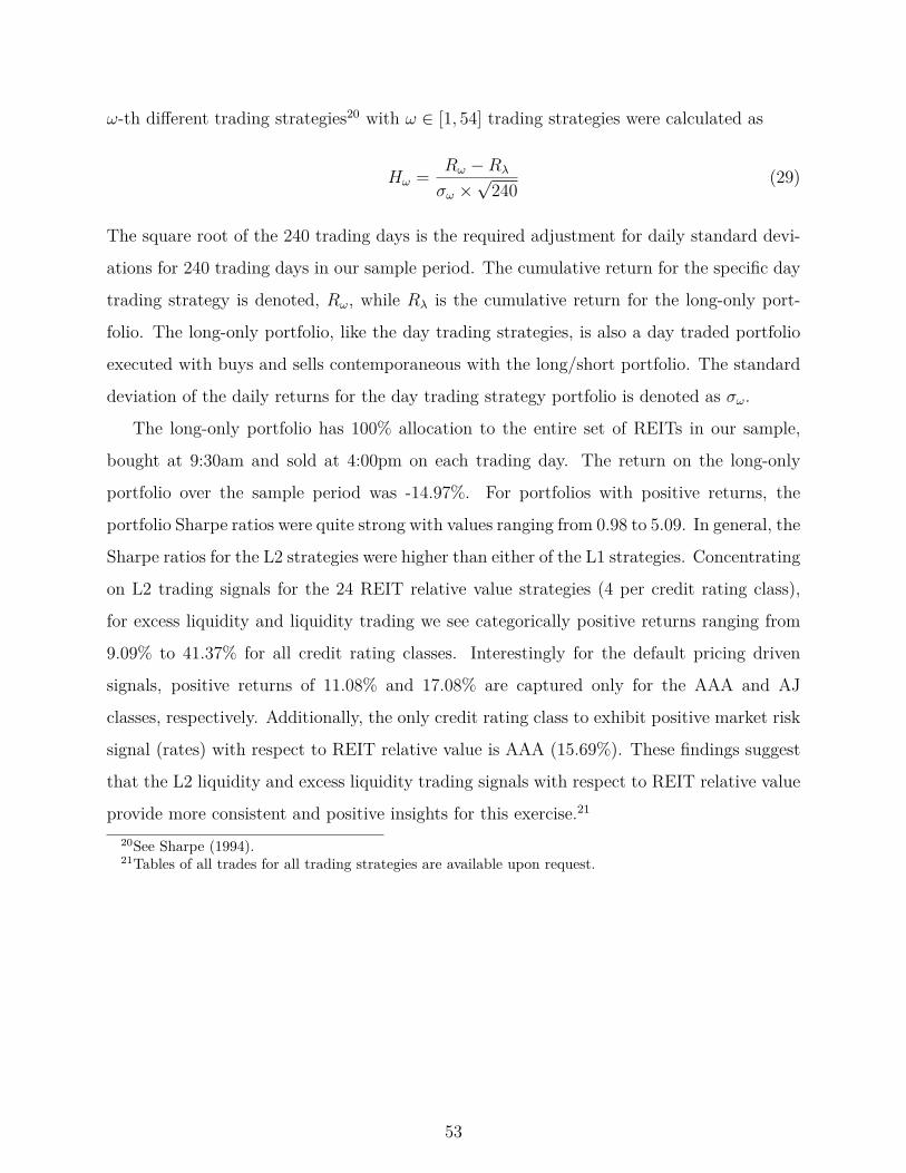
ω-th different trading strategies20 with ω ∈ [1, 54] trading strategies were calculated as

Hω = Rω −Rλ

σω ×√

240(29)

The square root of the 240 trading days is the required adjustment for daily standard devi-

ations for 240 trading days in our sample period. The cumulative return for the specific day

trading strategy is denoted, Rω, while Rλ is the cumulative return for the long-only port-

folio. The long-only portfolio, like the day trading strategies, is also a day traded portfolio

executed with buys and sells contemporaneous with the long/short portfolio. The standard

deviation of the daily returns for the day trading strategy portfolio is denoted as σω.

The long-only portfolio has 100% allocation to the entire set of REITs in our sample,

bought at 9:30am and sold at 4:00pm on each trading day. The return on the long-only

portfolio over the sample period was -14.97%. For portfolios with positive returns, the

portfolio Sharpe ratios were quite strong with values ranging from 0.98 to 5.09. In general, the

Sharpe ratios for the L2 strategies were higher than either of the L1 strategies. Concentrating

on L2 trading signals for the 24 REIT relative value strategies (4 per credit rating class),

for excess liquidity and liquidity trading we see categorically positive returns ranging from

9.09% to 41.37% for all credit rating classes. Interestingly for the default pricing driven

signals, positive returns of 11.08% and 17.08% are captured only for the AAA and AJ

classes, respectively. Additionally, the only credit rating class to exhibit positive market risk

signal (rates) with respect to REIT relative value is AAA (15.69%). These findings suggest

that the L2 liquidity and excess liquidity trading signals with respect to REIT relative value

provide more consistent and positive insights for this exercise.21

20See Sharpe (1994).21Tables of all trades for all trading strategies are available upon request.

53

Table 18: Cumulative returns for Trading Strategies 1 and 2

Panel A: AAA L1 5050 L1 1010 L2 Panel B: AJ L1 5050 L1 1010 L2XSLiquidity 19.21% 48.74% 9.09% XSLiquidity -8.22% -12.47% 41.37%stdev port 0.61% 1.18% 0.78% stdev port 0.63% 1.26% 0.71%

Sharpe Ratio 3.61 3.50 1.99 Sharpe Ratio 0.69 0.13 5.09Liquidity 2.02% -5.63% 37.69% Liquidity 6.80% 16.93% 22.80%stdev port 0.62% 1.11% 1.09% stdev port 0.63% 1.23% 1.09%

Sharpe Ratio 1.77 0.54 3.12 Sharpe Ratio 2.24 1.67 2.23Default -3.52% -18.21% 11.08% Default 1.53% -8.01% 17.08%

stdev port 0.63% 1.20% 0.80% stdev port 0.64% 1.28% 0.72%Sharpe Ratio 1.17 -0.17 2.11 Sharpe Ratio 1.66 0.35 2.87Panel C: AA L1 5050 L1 1010 L2 Panel D: A L1 5050 L1 1010 L2XSLiquidity 0.73% -5.79% 37.62% XSLiquidity 0.73% -5.79% 37.62%stdev port 0.62% 1.22% 0.78% stdev port 0.62% 1.22% 0.78%

Sharpe Ratio 1.64 0.48 4.37 Sharpe Ratio 1.64 0.48 4.37Liquidity 5.55% 3.58% 14.34% Liquidity 7.14% 19.81% 34.89%stdev port 0.64% 1.22% 0.74% stdev port 0.64% 1.20% 0.75%

Sharpe Ratio 2.09 0.98 2.57 Sharpe Ratio 2.24 1.88 4.30Default 1.09% -0.09% -5.23% Default 12.38% 6.23% -13.02%

stdev port 0.63% 1.23% 0.79% stdev port 0.62% 1.24% 0.73%Sharpe Ratio 1.64 0.78 0.80 Sharpe Ratio 2.86 1.10 0.17Panel E: BBB L1 5050 L1 1010 L2 Panel F: BBB- L1 5050 L1 1010 L2XSLiquidity 0.73% -5.79% 37.62% XSLiquidity 11.00% 18.50% 15.09%stdev port 0.62% 1.22% 0.78% stdev port 0.61% 0.97% 0.76%

Sharpe Ratio 1.64 0.48 4.37 Sharpe Ratio 2.75 2.23 2.57Liquidity 4.32% -2.47% 39.95% Liquidity -0.01% -1.59% 21.03%stdev port 0.64% 1.23% 0.77% stdev port 0.63% 1.25% 0.72%

Sharpe Ratio 1.95 0.66 4.63 Sharpe Ratio 1.53 0.69 3.24Default 16.12% 13.10% -34.67% Default 6.23% 11.98% -32.53%

stdev port 0.61% 1.24% 0.84% stdev port 0.64% 1.20% 0.86%Sharpe Ratio 3.27 1.47 -1.52 Sharpe Ratio 2.14 1.44 -1.31

This table provides the cumulative returns over 240 consecutive trading days over the sample period for Trading Strategies 1 and 2 using the fourdifferent risk partitions of default, liquidity and excess liquidity as embedded within Eqs. (27 and 28). The columns show results for TradingStrategy 1 for upper and lower 50% (L1 5050), Trading Strategy 1 for upper and lower deciles (L1 1010), and Trading Strategy 2. Each of the rowswithin the Panels A thru E show the returns for the risk partitions in the order Excess (XS) Liquidity, Liquidity, and Default with the standarddeviation for the portfolio and the Sharpe Ratio for the portfolio.***/**/*/’ correspond to 0.1%, 1%, 5% and 10% levels of significance. Panel A,shows the results for AAA, Panel B shows the results for AJ, Panel C shows the results for AA, Panel D shows the results for A, Panel E showsthe results for BBB and Panel F shows the results for BBB-.

4.2.6 ICAPM

To test for skill in the trading strategies we use the ICAPM of Merton (1990). We choose

this approach as a standard approach for equity asset pricing tests of skills. An alternative

approach was introduced by Acharya and Pedersen (2005) which includes the Amihud (2002)

ILLIQ measure. However, ILLIQ is dependent on observed volumes. Since no observed

volumes were provided for CMBX, ILLIQ cannot be implemented as an ICAPM factor in

this study. However, the key findings of Acharya and Pedersen (2005) concerning flight to

liquidity do appear to be confirmed in this study, in particular in our trading strategies that

exploit the estimated reduced form measures of liquidity and excess liquidity.

54

Following Christopoulos and Jarrow (2018) the final regression model to test for abnormal

returns in our trading strategies is given by:

Rωu −Rλu = α +M∑i=2

βωi(Riu − ru) + εu (30)

with u ∈ [1, 240] trading days, Rωu the daily returns of the trading strategy portfolio, Rλu

the returns of the long-only trading portfolio, Riu the i-th portfolio equity risk factor, and

ru the risk-free rate. Positive and significant α implies these trading strategies generate ab-

normal returns. We use the standard risk factors to evaluate equity based trading strategies

introduced in Fama and French (1993) including: (i) the market portfolio, (ii) the SMB

equity index, and (iii) the HML index as well as the MOM risk factor introduced in Carhart

(1997). We test 54 different trading strategies with results summarized in Tables 19 and 20.

For each of the six credit rating classes we conduct nine daily trading strategies across 240

trading dates from u = 4/8/2020 thru u = 3/31/2021. Trading Strategy 1 implements 50th

percentile (‘5050’) and decile (‘1010’) variations. The results are quite strong. All strategies

were statistically significant overall based on the F-test. Adjusted R-squared values ranged

from 0.1885 to 0.5052. All strategies produced positive α′s. 52 of 54 total trading strategies

(96.30%) produced statistically significant α′s ranging from 0.001 to 0.100 levels significance,

with 35 of 54 (64.81%) producing statistically significant α′s ranging from 0.001 to 0.010. In

all strategies the market portfolio was statistically significant at the 0.001 level and negat-

ive. The MOM risk factor was generally insignificant and varied in sign. SMB varied in sign

and insignificant across all strategies. HML was categorically negative exhibiting statistical

significance ranging from 0.001 to 0.010. 65.38% of the statistically significant α strategies

(34/52) also exhibited positive abnormal returns.

55

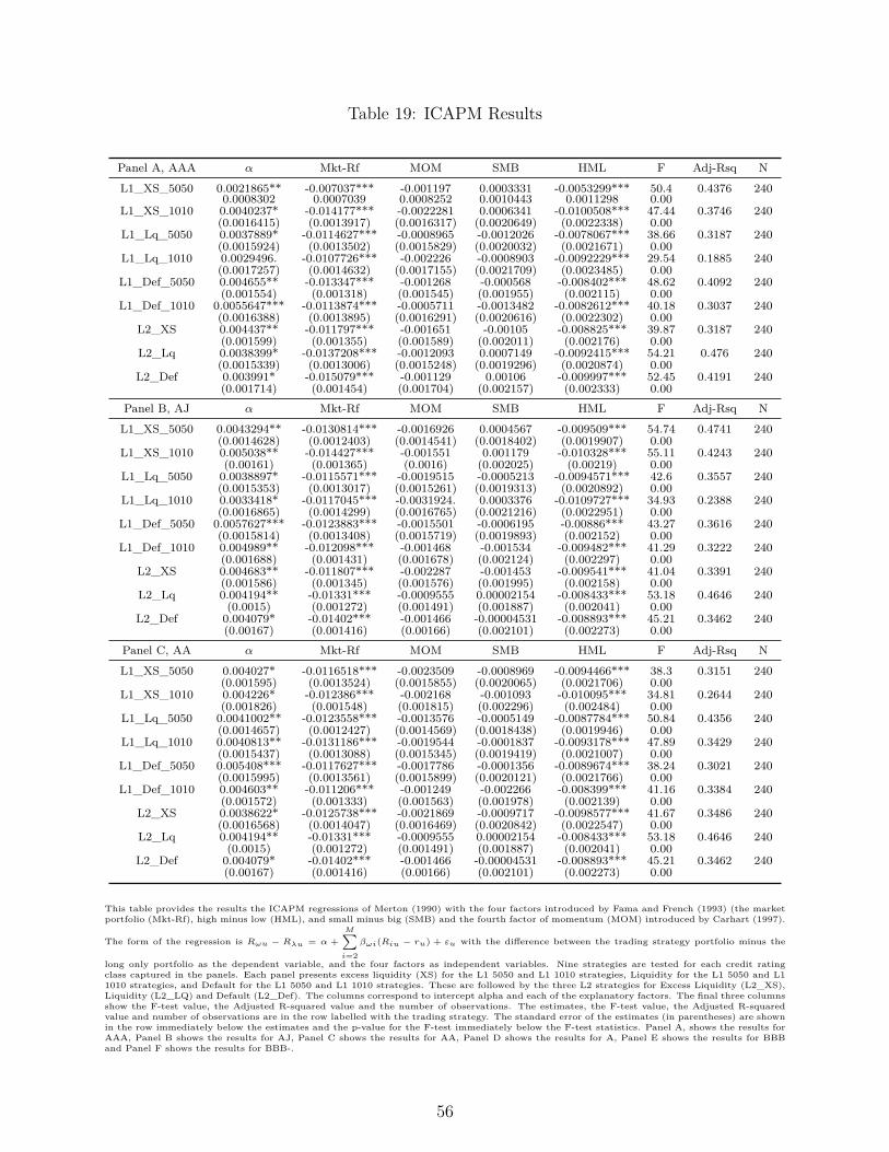
Table 19: ICAPM Results

Panel A, AAA α Mkt-Rf MOM SMB HML F Adj-Rsq N

L1_XS_5050 0.0021865** -0.007037*** -0.001197 0.0003331 -0.0053299*** 50.4 0.4376 2400.0008302 0.0007039 0.0008252 0.0010443 0.0011298 0.00

L1_XS_1010 0.0040237* -0.014177*** -0.0022281 0.0006341 -0.0100508*** 47.44 0.3746 240(0.0016415) (0.0013917) (0.0016317) (0.0020649) (0.0022338) 0.00

L1_Lq_5050 0.0037889* -0.0114627*** -0.0008965 -0.0012026 -0.0078067*** 38.66 0.3187 240(0.0015924) (0.0013502) (0.0015829) (0.0020032) (0.0021671) 0.00

L1_Lq_1010 0.0029496. -0.0107726*** -0.002226 -0.0008903 -0.0092229*** 29.54 0.1885 240(0.0017257) (0.0014632) (0.0017155) (0.0021709) (0.0023485) 0.00

L1_Def_5050 0.004655** -0.013347*** -0.001268 -0.000568 -0.008402*** 48.62 0.4092 240(0.001554) (0.001318) (0.001545) (0.001955) (0.002115) 0.00

L1_Def_1010 0.0055647*** -0.0113874*** -0.0005711 -0.0013482 -0.0082612*** 40.18 0.3037 240(0.0016388) (0.0013895) (0.0016291) (0.0020616) (0.0022302) 0.00

L2_XS 0.004437** -0.011797*** -0.001651 -0.00105 -0.008825*** 39.87 0.3187 240(0.001599) (0.001355) (0.001589) (0.002011) (0.002176) 0.00

L2_Lq 0.0038399* -0.0137208*** -0.0012093 0.0007149 -0.0092415*** 54.21 0.476 240(0.0015339) (0.0013006) (0.0015248) (0.0019296) (0.0020874) 0.00

L2_Def 0.003991* -0.015079*** -0.001129 0.00106 -0.009997*** 52.45 0.4191 240(0.001714) (0.001454) (0.001704) (0.002157) (0.002333) 0.00

Panel B, AJ α Mkt-Rf MOM SMB HML F Adj-Rsq N

L1_XS_5050 0.0043294** -0.0130814*** -0.0016926 0.0004567 -0.009509*** 54.74 0.4741 240(0.0014628) (0.0012403) (0.0014541) (0.0018402) (0.0019907) 0.00

L1_XS_1010 0.005038** -0.014427*** -0.001551 0.001179 -0.010328*** 55.11 0.4243 240(0.00161) (0.001365) (0.0016) (0.002025) (0.00219) 0.00

L1_Lq_5050 0.0038897* -0.0115571*** -0.0019515 -0.0005213 -0.0094571*** 42.6 0.3557 240(0.0015353) (0.0013017) (0.0015261) (0.0019313) (0.0020892) 0.00

L1_Lq_1010 0.0033418* -0.0117045*** -0.0031924. 0.0003376 -0.0109727*** 34.93 0.2388 240(0.0016865) (0.0014299) (0.0016765) (0.0021216) (0.0022951) 0.00

L1_Def_5050 0.0057627*** -0.0123883*** -0.0015501 -0.0006195 -0.00886*** 43.27 0.3616 240(0.0015814) (0.0013408) (0.0015719) (0.0019893) (0.002152) 0.00

L1_Def_1010 0.004989** -0.012098*** -0.001468 -0.001534 -0.009482*** 41.29 0.3222 240(0.001688) (0.001431) (0.001678) (0.002124) (0.002297) 0.00

L2_XS 0.004683** -0.011807*** -0.002287 -0.001453 -0.009541*** 41.04 0.3391 240(0.001586) (0.001345) (0.001576) (0.001995) (0.002158) 0.00

L2_Lq 0.004194** -0.01331*** -0.0009555 0.00002154 -0.008433*** 53.18 0.4646 240(0.0015) (0.001272) (0.001491) (0.001887) (0.002041) 0.00

L2_Def 0.004079* -0.01402*** -0.001466 -0.00004531 -0.008893*** 45.21 0.3462 240(0.00167) (0.001416) (0.00166) (0.002101) (0.002273) 0.00

Panel C, AA α Mkt-Rf MOM SMB HML F Adj-Rsq N

L1_XS_5050 0.004027* -0.0116518*** -0.0023509 -0.0008969 -0.0094466*** 38.3 0.3151 240(0.001595) (0.0013524) (0.0015855) (0.0020065) (0.0021706) 0.00

L1_XS_1010 0.004226* -0.012386*** -0.002168 -0.001093 -0.010095*** 34.81 0.2644 240(0.001826) (0.001548) (0.001815) (0.002296) (0.002484) 0.00

L1_Lq_5050 0.0041002** -0.0123558*** -0.0013576 -0.0005149 -0.0087784*** 50.84 0.4356 240(0.0014657) (0.0012427) (0.0014569) (0.0018438) (0.0019946) 0.00

L1_Lq_1010 0.0040813** -0.0131186*** -0.0019544 -0.0001837 -0.0093178*** 47.89 0.3429 240(0.0015437) (0.0013088) (0.0015345) (0.0019419) (0.0021007) 0.00

L1_Def_5050 0.005408*** -0.0117627*** -0.0017786 -0.0001356 -0.0089674*** 38.24 0.3021 240(0.0015995) (0.0013561) (0.0015899) (0.0020121) (0.0021766) 0.00

L1_Def_1010 0.004603** -0.011206*** -0.001249 -0.002266 -0.008399*** 41.16 0.3384 240(0.001572) (0.001333) (0.001563) (0.001978) (0.002139) 0.00

L2_XS 0.0038622* -0.0125738*** -0.0021869 -0.0009717 -0.0098577*** 41.67 0.3486 240(0.0016568) (0.0014047) (0.0016469) (0.0020842) (0.0022547) 0.00

L2_Lq 0.004194** -0.01331*** -0.0009555 0.00002154 -0.008433*** 53.18 0.4646 240(0.0015) (0.001272) (0.001491) (0.001887) (0.002041) 0.00

L2_Def 0.004079* -0.01402*** -0.001466 -0.00004531 -0.008893*** 45.21 0.3462 240(0.00167) (0.001416) (0.00166) (0.002101) (0.002273) 0.00

This table provides the results the ICAPM regressions of Merton (1990) with the four factors introduced by Fama and French (1993) (the marketportfolio (Mkt-Rf), high minus low (HML), and small minus big (SMB) and the fourth factor of momentum (MOM) introduced by Carhart (1997).

The form of the regression is Rωu − Rλu = α +M∑i=2

βωi(Riu − ru) + εu with the difference between the trading strategy portfolio minus the

long only portfolio as the dependent variable, and the four factors as independent variables. Nine strategies are tested for each credit ratingclass captured in the panels. Each panel presents excess liquidity (XS) for the L1 5050 and L1 1010 strategies, Liquidity for the L1 5050 and L11010 strategies, and Default for the L1 5050 and L1 1010 strategies. These are followed by the three L2 strategies for Excess Liquidity (L2_XS),Liquidity (L2_LQ) and Default (L2_Def). The columns correspond to intercept alpha and each of the explanatory factors. The final three columnsshow the F-test value, the Adjusted R-squared value and the number of observations. The estimates, the F-test value, the Adjusted R-squaredvalue and number of observations are in the row labelled with the trading strategy. The standard error of the estimates (in parentheses) are shownin the row immediately below the estimates and the p-value for the F-test immediately below the F-test statistics. Panel A, shows the results forAAA, Panel B shows the results for AJ, Panel C shows the results for AA, Panel D shows the results for A, Panel E shows the results for BBBand Panel F shows the results for BBB-.

56

Table 20: ICAPM Results

Panel D, A α Mkt-Rf MOM SMB HML F Adj-Rsq N

L1_XS_5050 0.0042909** -0.0125106*** -0.0016312 -0.0002349 -0.0094443*** 46.2 0.3982 240(0.0015688) (0.0013301) (0.0015594) (0.0019735) (0.0021348) 0.00

L1_XS_1010 0.004902** -0.012716*** -0.0009979 -0.0001228 -0.0091501*** 39.08 0.3026 240(0.0017638) (0.0014954) (0.0017532) (0.0022188) (0.0024002) 0.00

L1_Lq_5050 0.00454** -0.012023*** -0.001855 -0.001405 -0.00898*** 47.11 0.4028 240(0.001491) (0.001264) (0.001482) (0.001876) (0.002029) 0.00

L1_Lq_1010 0.004231** -0.012184*** -0.002705. -0.00114 -0.009916*** 41.87 0.2924 240(0.00158) (0.00134) (0.001571) (0.001988) (0.002151) 0.00

L1_Def_5050 0.005408*** -0.0117627*** -0.0017786 -0.0001356 -0.0089674*** 38.24 0.3021 240(0.0015995) (0.0013561) (0.0015899) (0.0020121) (0.0021766) 0.00

L1_Def_1010 0.005718*** -0.013031*** -0.002128 -0.001359 -0.010209*** 47.62 0.4112 240(0.00163) (0.001382) (0.00162) (0.00205) (0.002218) 0.00

L2_XS 0.003497* -0.012009*** -0.002309 -0.001462 -0.010016*** 42.67 0.3593 240(0.00161) (0.001365) (0.0016) (0.002025) (0.002191) 0.00

L2_Lq 0.004194** -0.01331*** -0.0009555 0.00002154 -0.008433*** 53.18 0.4646 240(0.0015) (0.001272) (0.001491) (0.001887) (0.002041) 0.00

L2_Def 0.004079* -0.01402*** -0.001466 -0.00004531 -0.008893*** 45.21 0.3462 240(0.00167) (0.001416) (0.00166) (0.002101) (0.002273) 0.00

Panel E, BBB α Mkt-Rf MOM SMB HML F Adj-Rsq N

L1_XS_5050 0.0038162* -0.0117119*** -0.0024842 0.0005267 -0.0100017*** 35.93 0.2936 240(0.0016434) (0.0013934) (0.0016336) (0.0020674) (0.0022365) 0.00

L1_XS_1010 0.003713* -0.0120828*** -0.002494 0.0006448 -0.0109529*** 31.68 0.2385 240(0.0018763) (0.0015908) (0.0018651) (0.0023603) (0.0025533) 0.00

L1_Lq_5050 0.004766** -0.012471*** -0.00194 -0.001338 -0.00944*** 50.23 0.4355 240(0.001503) (0.001274) (0.001494) (0.00189) (0.002045) 0.00

L1_Lq_1010 0.0046653** -0.0129274*** -0.0025898 -0.0009711 -0.0099328*** 42.18 0.3085 240(0.0016414) (0.0013917) (0.0016316) (0.0020649) (0.0022337) 0.00

L1_Def_5050 0.005408*** -0.0117627*** -0.0017786 -0.0001356 -0.0089674*** 38.24 0.3021 240(0.0015995) (0.0013561) (0.0015899) (0.0020121) (0.0021766) 0.00

L1_Def_1010 0.00561*** -0.011541*** -0.001856 -0.001621 -0.009152*** 44.03 0.3589 240(0.001526) (0.001294) (0.001517) (0.00192) (0.002077) 0.00

L2_XS 0.0025332 -0.0120336*** -0.0023626 -0.0006994 -0.0098406*** 38.99 0.3121 240(0.0016395) (0.0013901) (0.0016297) (0.0020625) (0.0022311) 0.00

L2_Lq 0.004575** -0.0128342*** -0.0006617 -0.0003317 -0.0079207*** 52.7 0.459 240(0.0014701) (0.0012464) (0.0014613) (0.0018493) (0.0020005) 0.00

L2_Def 0.005056** -0.0134311*** -0.0003629 -0.0002725 -0.0077591*** 51.39 0.4141 240(0.0015477) (0.0013123) (0.0015385) (0.001947) (0.0021063) 0.00

Panel F, BBB- α Mkt-Rf MOM SMB HML F Adj-Rsq N

L1_XS_5050 0.004217** -0.013495*** -0.001041 0.000192 -0.008697*** 58.21 0.5052 240(0.001453) (0.001232) (0.001444) (0.001828) (0.001977) 0.00

L1_XS_1010 0.004322** -0.015282*** -0.001788 0.001642 -0.009734*** 56.21 0.4296 240(0.00158) (0.00134) (0.001571) (0.001988) (0.00215) 0.00

L1_Lq_5050 0.004165** -0.011688*** -0.001834 -0.001053 -0.009192*** 40.45 0.3382 240(0.001591) (0.001349) (0.001582) (0.002002) (0.002166) 0.00

L1_Lq_1010 0.0043642* -0.0116363*** -0.0019992 -0.0008662 -0.0091518*** 33.42 0.2301 240(0.0017165) (0.0014554) (0.0017063) (0.0021593) (0.0023359) 0.00

L1_Def_5050 0.0044753** -0.0118264*** -0.0023004 -0.0003724 -0.0100502*** 42.17 0.3458 240(0.0015752) (0.0013356) (0.0015658) (0.0019816) (0.0021436) 0.00

L1_Def_1010 0.0048238** -0.0124841*** -0.00216 -0.0006673 -0.0094188*** 42.97 0.3586 240(0.001581) (0.0013405) (0.0015716) (0.0019889) (0.0021515) 0.00

L2_XS 0.002663 -0.012487*** -0.003047. -0.001407 -0.010772*** 40.39 0.3351 240(0.001682) (0.001426) (0.001672) (0.002116) (0.002289) 0.00

L2_Lq 0.0066207** -0.0180265*** -0.0027309 -0.0004056 -0.0140932*** 46.3 0.4231 240(0.0022618) (0.0019177) (0.0022483) (0.0028453) (0.003078) 0.00

L2_Def 0.0078028*** -0.0181336*** -0.0023276 -0.0000474 -0.0137304*** 43.97 0.3912 240(0.0023297) (0.0019753) (0.0023158) (0.0029307) (0.0031704) 0.00

This table provides the results the ICAPM regressions of Merton (1990) with the four factors introduced by Fama and French (1993) (the marketportfolio (Mkt-Rf), high minus low (HML), and small minus big (SMB) and the fourth factor of momentum (MOM) introduced by Carhart (1997).

The form of the regression is Rωu − Rλu = α +M∑i=2

βωi(Riu − ru) + εu with the difference between the trading strategy portfolio minus the

long only portfolio as the dependent variable, and the four factors as independent variables. Nine strategies are tested for each credit ratingclass captured in the panels. Each panel presents excess liquidity (XS) for the L1 5050 and L1 1010 strategies, Liquidity for the L1 5050 and L11010 strategies, and Default for the L1 5050 and L1 1010 strategies. These are followed by the three L2 strategies for Excess Liquidity (L2_XS),Liquidity (L2_LQ) and Default (L2_Def). The columns correspond to intercept alpha and each of the explanatory factors. The final three columnsshow the F-test value, the Adjusted R-squared value and the number of observations. The estimates, the F-test value, the Adjusted R-squaredvalue and number of observations are in the row labelled with the trading strategy. The standard error of the estimates (in parentheses) are shownin the row immediately below the estimates and the p-value for the F-test immediately below the F-test statistics. Panel A, shows the results forAAA, Panel B shows the results for AJ, Panel C shows the results for AA, Panel D shows the results for A, Panel E shows the results for BBBand Panel F shows the results for BBB-.

57

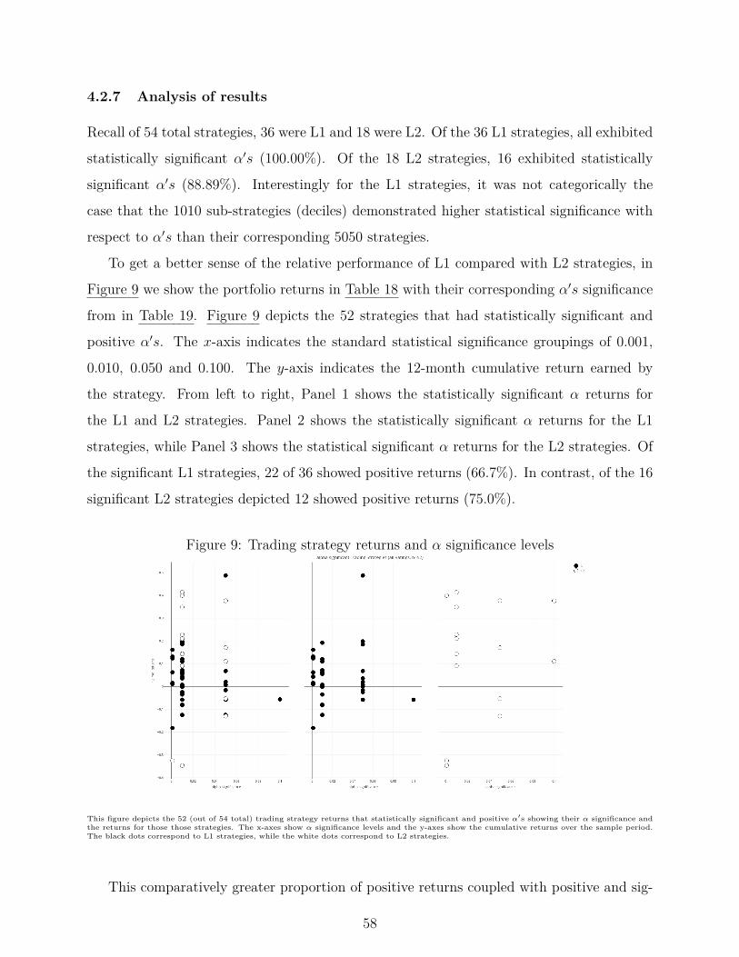
4.2.7 Analysis of results

Recall of 54 total strategies, 36 were L1 and 18 were L2. Of the 36 L1 strategies, all exhibited

statistically significant α′s (100.00%). Of the 18 L2 strategies, 16 exhibited statistically

significant α′s (88.89%). Interestingly for the L1 strategies, it was not categorically the

case that the 1010 sub-strategies (deciles) demonstrated higher statistical significance with

respect to α′s than their corresponding 5050 strategies.

To get a better sense of the relative performance of L1 compared with L2 strategies, in

Figure 9 we show the portfolio returns in Table 18 with their corresponding α′s significance

from in Table 19. Figure 9 depicts the 52 strategies that had statistically significant and

positive α′s. The x-axis indicates the standard statistical significance groupings of 0.001,

0.010, 0.050 and 0.100. The y-axis indicates the 12-month cumulative return earned by

the strategy. From left to right, Panel 1 shows the statistically significant α returns for

the L1 and L2 strategies. Panel 2 shows the statistically significant α returns for the L1

strategies, while Panel 3 shows the statistical significant α returns for the L2 strategies. Of

the significant L1 strategies, 22 of 36 showed positive returns (66.7%). In contrast, of the 16

significant L2 strategies depicted 12 showed positive returns (75.0%).

Figure 9: Trading strategy returns and α significance levels

This figure depicts the 52 (out of 54 total) trading strategy returns that statistically significant and positive α′s showing their α significance andthe returns for those those strategies. The x-axes show α significance levels and the y-axes show the cumulative returns over the sample period.The black dots correspond to L1 strategies, while the white dots correspond to L2 strategies.

This comparatively greater proportion of positive returns coupled with positive and sig-

58

nificant α is echoed when we break down returns by credit rating class as seen in Figure 10.

Figure 10: Trading strategy returns and alpha significance levels by ratings

This figure depicts the 52 (out of 54 total) trading strategy returns with statistically significant and positive α′s showing their α significance andthe returns for those those strategies, broken out by credit rating class. The x-axes show α significance levels and the y-axes show the cumulativereturns over the sample period. The top panel of 6 sub charts capture the 36 results for the L1 trading strategies, while the bottom panel of 6subcharts capture the 16 results for the L2 trading strategies. The credit ratings begin with AAA in the upper left corner and descend rowwisefrom left to right ending with BBB- in the bottom right corner.

The plots are read from left to right by descending credit rating class beginning with AAA

(blue) in the top left and BBB- (red) in the bottom right. The top chart of 6 panels depict

the statistically significant α L1 trading strategies. The bottom chart of 6 panels depicts the

statistically significant L2 trading strategies. L2 strategies for the higher credits generally

outperform with respect to returns at higher α significance levels for AAA, AJ, AA, and A

classes. For BBB and BBB- classes, L1 appears to relatively outperform L2 in the REIT

59

strategies tested. Across all strategies and credits, the L2 strategies for the AJ class (green)

appear to perform best while L1 strategies, also for AJ class, appear to perform worst.

Additionally, L1 shows a proportionately larger number of statistically significant strategies

driven by BBB and BBB- classes than L2 which relatively dominates on a proportional basis

within the higher credit classes. This capital structure differences are consistent with the

earlier literature22 that finds idiosyncratic risk of collateral in CMBX is comparatively more

important for lower credit rated tranches than higher rated tranches. Interestingly, as noted

in An, Deng, Nichols and Sanders (2015) the pricing of credit risk alone is insufficient to

explain subordination impact on pricing. As such, the logic underlying L2 trading strategies,

previously discussed and summarized in Table 17, may be somewhat obscured for BBB and

BBB- classes. While theWjkut values in Eq. (28) signals are picking up risk tranching effects,

and are differentiating across different types of risks, they nevertheless are not directly pricing

the idiosyncratic risks of CMBX collateral with reduced form simulation and current data

as shown in Christopoulos (2017) and Christopoulos and Jarrow (2018). This is a limitation

to be explored in future work where computational costs and data are made available.

Table 21: Summary of L1 and L2 ICAPM strategies (all ratings)Panel A: L2 >=0 <0 significant insignificant all % >= & significant avg return median ret min ret max ret

XS 4 0 4 2 6 100% 31.43% 37.62% 9.09% 41.37%Lq 6 0 6 0 6 100% 28.45% 28.85% 14.34% 39.95%Def 2 4 6 0 6 33% -9.56% -9.16% -34.67% 17.08%

Panel B: L1 1010 >=0 <0 significant insignificant all % >= & significant avg return median ret min ret max ret

XS 2 4 6 0 6 33% 6.23% -5.79% -12.47% 48.74%Lq 2 4 6 0 6 33% 0.21% -2.03% -12.47% 19.81%Def 3 3 6 0 6 50% 0.83% 3.07% -18.21% 13.10%

Panel C: L1 5050 >=0 <0 significant insignificant all % >= & significant avg return median ret min ret max ret

XS 5 1 6 0 6 83% 4.03% 0.73% -8.22% 19.21%Lq 5 1 6 0 6 83% 4.30% 4.94% -0.01% 7.14%Def 5 1 6 0 6 83% 5.64% 3.88% -3.52% 16.12%

This table summarize depicts L1 and L2 ICAPM strategies for all ratings. Each of the rows in the panel capture risk partitions of excess liquidity(XS), liquidity (Lq) and default (Def). The columns provide the counts of those strategies with non-negative returns (>=0), negative returns(<0), number of significant, insignificant, and all. Then the percentage of non-negative with significant alpha strategies are calculated for therisk partition as well as the average, median, minimum (min), and maximum (max) returns. Panel A summarizes for the L2 strategies. Panel Bsummarizes for the L1 1010 strategies. Panel C summarizes for the L1 5050 strategies.

Finally we compress the ICAPM significant trading strategies across all ratings in Table

21. There again we observe the L2 strategies outperforming the L1 1010 and L1 5050

strategies in excess liquidity and liquidity strategies compared with default. Across all ratings

100% of significant excess liquidity and liquidity strategies for L2 also exhibited positive22See for example Riddiough and Zhu (2016), among others.

60

returns ranging from 9.09% to 41.37% for excess liquidity and 14.34% to 39.95% for liquidity

strategies. In contrast, the default strategies for L2 were positive in only 33% of the cases

ranging from -34.67% to 17.08%. In the case of the L1 strategies, the 1010 decile strategies

performed somewhat comparatively worse than the 5050 strategies overall with 33% to 50%

of the strategies positive and significant for the 1010 decile strategies compared with 83%

for the 5050. The returns statistics for 5050 strategies compared with 1010 strategies were

generally better overall.

CMBX liquidity and excess liquidity risk pricing by definition, as discussed in Chris-

topoulos (2017) and Christopoulos and Jarrow (2018), provide insights into sentiments of

CMBX pricing risks apart from idiosyncratic risks associated with CMBX collateral pools.

This is because CMBX risk pricing of liquidity and excess liquidity are residual measures

apart from explicitly modelled risks of default, loss and interest rate volatility at the loan

level, aggregated to the bond level using fair value techniques. Liquidity and excess liquidity

risk pricing provides insights into investor sentiment of risk apart from rate volatility and

default experiences as captured in the loan level historical state transitions as discussed in

Christopoulos and Barratt (2016). In this sense, at the securities level following fair value

aggregation, the liquidity and excess liquidity measures articulate investor sentiment of real

estate securities more broadly than the historical analysis of default and rates and their

relationship in current CMBX collateral vis a vis simulation. As such, the positive and sig-

nificant performance for REIT trading strategies using excess liquidity and liquidity CMBX

measures makes sense, particularly for the L2 strategies.

As shown in the cross-sectional analysis, we find considerably greater volatility in risk

partition pricing at the start of each trading day for all risk partitions compared to the end

of each trading day, which contrast with the much more muted volatility for REITs from the

start to end of the trading day. This suggests that the monthly and daily analysis supporting

insights provided by the theoretical liquidity risk partitions persist at the intraday level (our

third main result). Finally, the success of the trade strategies and their significance confirm

that the insights of CMBX risk partitions bring valuable insights to the related REIT sector,

which is our fourth main result. This expands the application of CMBX risk partitions,

intraday, to a broader array of commercial real estate securities. Together these main and

supporting results completes the validation of the Intraday Model.

61

5 Summary

Despite their size and importance in capital markets, near real time information content

for credit sensitive US fixed income has only recently come into focus in the microstructure

literature. CMBX is one segment of the fixed income market where sparsity of meaningful

real time data obscures insights into underlying risk pricing effects of the underlying asset

class. Because of that, there is value in understanding the intraday risk composition of the

$600 billion CMBS sector and its CMBX derivatives. In this first study into CMBX micro-

structure we provide such daily and intraday insights into CMBX liquidity with crossover

insights into the related $1.3 trillion REIT sector before and during the Covid-19 pandemic.

By addressing some of the gaps in the frequency and accuracy of risk information in

the CMBX market, we contribute to the literature with reconciliation between classical

microstructure and reduced form assessments of liquidity daily frequency. We find risk

partitions to play a statistically signifcant role in bid-ask formation historically, and in

forecasts. We extend our analysis to estimate, intraday, CMBX risk decompositions for all

investment grade credits in 15 second intervals. This reveals suprisingly, apparent regular

volatility pockets of risk partition pricing in the cross-section over the sample period. If

broader real estate risk sentiments of investors are embedded within the CMBX residual

risk partitions of liquidity and excess liquidity, it would make sense if those measures also

revealed pricing insights into real estate risk in securities apart from CMBX. We find this

to be true. By fusing the CMBX risk partition signals with REIT pricing in 54 day trading

strategies over 240 trading days, we achieved significant ICAPM α′s in about 96% of the

strategies and positive cumulative returns ranging from 0.73% to 48.74% in about 65% of

the strategies during the Covid pandemic. By our results, the fusion of CMBX risk partition

signals and REIT pricing, appears to capture broader investor sentiment with respect to the

pricing of real estate securities risks from the idiosyncratic risks of default and rate risks in

specific collateral pools underlying CMBX or balance sheets of REITs.

The method in this paper is generalizable to all fixed income securities. In this particular

case, the risk partition signals are commercial real estate based (CRE) based as embedded

within CMBX and REIT pricing. As such, they disclose crossover liquidity sentiment with

respect to commercial real estate securities in general and their pricing in the mind of the

62

market, apart from modelled idiosyncratic risks of specific collateral underlying CMBX. To

our knowledge, this is the first study of its kind to investigate projections of reduced form

CMBX risk decompositions on a daily and intraday basis. Since the pace of our intraday

risk partitions exceeds the typical pace of CMBX trading, our good results validate the

theoretical insights of CMBX with respect to REITs.

In future work, considering post-optimality analysis of different trading strategies for

each of the risk partition signals, would also be interesting, this might be achieved with

some calibration techniques using MLE or other techniques. Additionally, given the rapid

pacing of interest rates, such analysis applied with specific focus on the interest rate risk

pricing partitions in conjunction with REITs would build on the extensive prior work in the

literature related to interest rate term structure models. Establishing further connections

between intraday risk partition pricing and actual CMBX pricing would also be exciting, and

that line of inquiry is purely an issue of data accessibility as the method in this work applies.

Similarly, extending the general approach introduced here and applying it to the Corporate

bond sector would be facinating with new good work in that area on an intraday basis.

Finally, from a policy perspective, investigating into the longer term relationship (if any)

between intraday signals of risk partitions and manifestation of actual hazards in the real

estate asset classes (and Corporates) would be an interesting area for exploration. Lending

criteria, risk retention, and capital constraints all have links to capital markets. Research

inquiries into the nature of those links, with the intraday approach we introduce, before

hazards manifest, seems a natural next level of inquiry that could be accomplished with

the simulation approach of Christopoulos (2017) and Christopoulos and Jarrow (2018) with

availability of highly costly comprehensive data at loan, bond and deal levels and expensive

high performance computing resources. This is left to future research.

References

Acharya, Viral V., and Lasse Heje Pedersen. "Asset pricing with liquidity risk." Journal ofFinancial Economics 77.2 (2005): 375-410.

Amihud, Yakov. "Illiquidity and stock returns: cross-section and time-series effects." Journalof Financial Markets 5.1 (2002): 31-56.

63

An, Xudong, Yongheng Deng, Joseph B. Nichols, and Anthony B. Sanders. "What is sub-ordination about? Credit risk and subordination levels in commercial mortgage-backedsecurities (CMBS)." The Journal of Real Estate Finance and Economics 51, no. 2 (2015):231-253.

Bao, Jack, Maureen O’Hara, and Xing Alex Zhou. "The Volcker Rule and corporate bondmarket making in times of stress." Journal of Financial Economics 130.1 (2018): 95-113.

Bao, Jack, Jun Pan, and Jiang Wang. "The illiquidity of Corporate bonds." The Journal ofFinance 66, no. 3 (2011): 911-946.

Bhattacharjee, Ranjit, and Lakhbir S. Hayre. "The term structure of mortgage rates: Citig-roup’s MOATS model." The Journal of Fixed Income 15.4 (2006): 34-47.

Bond Market Association. ”Standard Formulas for the Analysis of Mortgage-Backed Securities and Other Related Securities. (https://www.sifma.org/wp-content/uploads/2017/08/chsf.pdf)” August 2017.

Broto, Carmen, and Matías Lamas. "Measuring market liquidity in US fixed income markets:A new synthetic indicator." The Spanish Review of Financial Economics 14.1 (2016): 15-22.

Campello, Murillo, Long Chen, and Lu Zhang. "Expected returns, yield spreads, and assetpricing tests." The Review of Financial Studies 21.3 (2008): 1297-1338.

Carhart, Mark M. "On persistence in mutual fund performance." The Journal of Finance52.1 (1997): 57-82.

Carr, Peter, and Jiming Yu. "Risk, return, and Ross recovery." The Journal of Derivatives20.1 (2012): 38-59.

Christopoulos, Andreas D. "The composition of CMBS risk." Journal of Banking & Finance76 (2017): 215-239.

Christopoulos, Andreas D. "The Absolute Roll Measure." Working Paper, 2020.

Christopoulos, Andreas D., and Joshua G. Barratt. "Credit risk findings for commercial realestate loans using the reduced form." Finance Research Letters 19 (2016): 228-234.

Christopoulos, Andreas D., and Robert A. Jarrow. "CMBS market efficiency: The crisis andthe recovery." Journal of Financial Stability 36 (2018): 159-186.

Driessen, Joost, and Otto Van Hemert. "Pricing of commercial real estate securities duringthe 2007–2009 financial crisis." Journal of Financial Economics 105.1 (2012): 37-61.

Easley, David, Nicholas M. Kiefer, Maureen O’Hara, and Joseph B. Paperman. "Liquidity,information, and infrequently traded stocks." The Journal of Finance 51, no. 4 (1996):1405-1436.

Fama, E.F. and French, K.R., 1993. Common risk factors in the returns on stocks and bonds.Journal of Financial Economics, 33(1): 3-56.

64

Fabozzi, Frank J., ed. The Handbook of Mortgage-Backed Securities. Oxford UniversityPress, 2016.

Fleming, Michael J. "Measuring treasury market liquidity." FRB of New York Staff Report133 (2001).

Foucault, Thierry, Marco Pagano, Ailsa Roell, and Ailsa Röell. Market Liquidity: Theory,Evidence, and Policy. Oxford University Press, 2013.

Fong, Kingsley YL, Craig W. Holden, and Charles A. Trzcinka. "What are the best liquidityproxies for global research?." Review of Finance 21.4 (2017): 1355-1401.

Gilchrist, Simon, and Egon Zakrajšek. "Credit spreads and business cycle fluctuations."American Economic Review 102, no. 4 (2012): 1692-1720.

Gilchrist, S., Wei, B., Yue, V.Z. and Zakrajšek, E., The Term Structure of the Excess BondPremium: Measures and Implications. Atlanta Federal Reserve NO. 12–2021 September2021.

Goldstein, Itay, Hao Jiang, and David T. Ng. "Investor flows and fragility in corporate bondfunds." Journal of Financial Economics 126.3 (2017): 592-613.

Haddad, Valentin, Alan Moreira, and Tyler Muir. When selling becomes viral: Disruptionsin debt markets in the covid-19 crisis and the fed’s response. No. w27168. National Bureauof Economic Research, 2020.

Han, Song, and Hao Zhou. "Effects of liquidity on the non-default component of corporateyield spreads: Evidence from intraday transactions " Quarterly Journal of Finance 6.03(2016): 1650012.

Harris, Lawrence. "Statistical properties of the Roll serial covariance bid/ask spread estim-ator." The Journal of Finance 45.2 (1990): 579-590.

Hasbrouck, Joel. "Trading costs and returns for US equities: Estimating effective costs fromdaily " The Journal of Finance 64.3 (2009): 1445-1477.

Hayre, Lakhbir S., Sharad Chaudhary, and Robert A. Young. "Anatomy of prepayments."The Journal of Fixed Income 10.1 (2000): 19-49.

He, An and Bruce Mizrach. “Analysis of securitized asset liquidity - Research Note” FINRAOffice of the Chief Economist (2017).

Heath, David, Robert Jarrow, and Andrew Morton. "Bond pricing and the term structureof interest rates: A new methodology for contingent claims valuation." Econometrica:Journal of the Econometric Society (1992): 77-105.

Hollifield, Burton, Artem Neklyudov, and Chester Spatt. "Bid-ask spreads, trading networks,and the pricing of securitizations." The Review of Financial Studies 30 (2017), 3048-3085.

Hotchkiss, Edith S., and Tavy Ronen. "The informational efficiency of the corporate bondmarket: An intraday analysis." The Review of Financial Studies 15.5 (2002): 1325-1354.

65

Ivanov, Ventzislav, and Lutz Kilian. "A practitioner’s guide to lag order selection for VARimpulse response analysis." Studies in Nonlinear Dynamics & Econometrics 9.1 (2005).

Jarrow, Robert. "A Tutorial on Zero Volatility and Option Adjusted Spreads." Advances inMathematical Finance. Birkhäuser Boston, 2007. 85-95.

Jarrow, Robert A., David Lando, and Stuart M. Turnbull. "A Markov model for the termstructure of credit risk spreads." The review of financial studies 10.2 (1997): 481-523.

Kyle, Albert S. "Continuous auctions and insider trading." Econometrica: Journal of theEconometric Society (1985): 1315-1335.

Lando, David. "On Cox processes and credit risky securities." Review of Derivatives research2.2-3 (1998): 99-120.

Lo, Andrew W., and Jiang Wang. "Trading volume: definitions, data analysis, and implica-tions of portfolio theory." The Review of Financial Studies 13.2 (2000): 257-300.

Longstaff, Francis A., Sanjay Mithal, and Eric Neis. "Corporate yield spreads: Default riskor liquidity? New evidence from the credit default swap market." The journal of finance60.5 (2005): 2213-2253.

Lütkepohl, Helmut. New introduction to multiple time series analysis. Springer Science &Business Media, 2005.

Merton, Robert C. "On the pricing of corporate debt: The risk structure of interest rates."The Journal of Finance 29.2 (1974): 449-470.

Merton, R.C., 1990. Continuous Time Finance. Cambridge, MA. Blackwell.

O’Hara, Maureen. Market Microstructure Theory. Wiley, 1997.

Riddiough, Timothy J. and Jun Zhu. "Governance and Capital Structure: Theory andEvidence from the CMBS Market (September 13, 2016)." Available at SSRN: ht-tps://ssrn.com/abstract=2838597 or http://dx.doi.org/10.2139/ssrn.2838597.

Roll, Richard. "A simple implicit measure of the effective bid-ask spread in an efficientmarket." The Journal of Finance 39.4 (1984): 1127-1139.

Sharpe, William F. "The Sharpe ratio." Journal of Portfolio Management 21.1 (1994): 49-58.

Simon, Carl P., and Lawrence Blume. Mathematics for Economists. Vol. 7. New York:Norton, 1994.

Thompson, Sarahelen R., and Mark L. Waller. "The execution cost of trading in commodityfutures markets." Food Research Institute Studies 20.1387-2016-116196 (1987): 141-163.

66

Higher frequency risk pricing for - Yeshiva University

Documents

Transcript of Higher frequency risk pricing for - Yeshiva University