nanomaterials

Article

High-Yield Production of Selected 2D Materials byUnderstanding Their Sonication-AssistedLiquid-Phase Exfoliation

Freskida Goni, Angela Chemelli * and Frank Uhlig

�����������������

Citation: Goni, F.; Chemelli, A.;

Uhlig, F. High-Yield Production of

Selected 2D Materials by

Understanding Their Sonication-

Assisted Liquid-Phase Exfoliation.

Nanomaterials 2021, 11, 3253.

https://doi.org/10.3390/

nano11123253

Academic Editors: Gwan-Hyoung

Lee, Alberto Bianco and

Saulius Kaciulis

Received: 19 October 2021

Accepted: 26 November 2021

Published: 30 November 2021

Publisher’s Note: MDPI stays neutral

with regard to jurisdictional claims in

published maps and institutional affil-

iations.

Copyright: © 2021 by the authors.

Licensee MDPI, Basel, Switzerland.

This article is an open access article

distributed under the terms and

conditions of the Creative Commons

Attribution (CC BY) license (https://

creativecommons.org/licenses/by/

4.0/).

Institute of Inorganic Chemistry, Faculty of Technical Chemistry, Chemical and Process Engineering,Biotechnology, Graz University of Technology, Stremayrgasse 9, 8010 Graz, Austria;freskida.goni@tugraz.at (F.G.); frank.uhlig@tugraz.at (F.U.)* Correspondence: angela.chemelli@tugraz.at

Abstract: Liquid-phase exfoliation (LPE) is a widely used and promising method for the productionof 2D nanomaterials because it can be scaled up relatively easily. Nevertheless, the yields achievedby this process are still low, ranging between 2% and 5%, which makes the large-scale production ofthese materials difficult. In this report, we investigate the cause of these low yields by examiningthe sonication-assisted LPE of graphene, boron nitride nanosheets (BNNSs), and molybdenumdisulfide nanosheets (MoS2 NS). Our results show that the low yields are caused by an equilibriumthat is formed between the exfoliated nanosheets and the flocculated ones during the sonicationprocess. This study provides an understanding of this behaviour, which prevents further exfoliationof nanosheets. By avoiding this equilibrium, we were able to increase the total yields of graphene,BNNSs, and MoS2 NS up to 14%, 44%, and 29%, respectively. Here, we demonstrate a modified LPEprocess that leads to the high-yield production of 2D nanomaterials.

Keywords: 2D materials; liquid-phase exfoliation; high-yield production; graphene; boron nitridenanosheets; molybdenum disulfide nanosheets

1. Introduction

Two-dimensional (2D) nanomaterials have gained worldwide attention in recentyears because of their outstanding properties due to their structure and dimensionality.Graphene was the first 2D material that was successfully isolated and studied in 2004 byAndre Geim and Konstantin Novoselov [1]. Graphene consists of sp2-hybridised carbonatoms that are hexagonally arranged in a honeycomb lattice. This unique structure isresponsible for many of graphene’s excellent mechanical, electrical, thermal, and opticalproperties [1–10]. Due to these properties, graphene can be used in a variety of applications,ranging from nanoelectronics and energy storage to sensors and medicine [8,9,11–16]. Overthe last decade, there has been an increasing interest in other 2D materials as well, e.g.,hexagonal boron nitride (h-BN) [17,18], transition metal dichalcogenides (TMDs suchas MoS2, TiS2, TaS2, WS2, etc.) [19,20], layered metal oxides [21–23], etc. Boron nitridenanosheets (BNNSs) have a similar structure to that of graphene, but this material consistsof alternating boron and nitrogen atoms instead of carbon atoms. Similar to graphene,BNNSs exhibit outstanding properties [24–30], which makes this material very interestingand useful for a wide range of applications [31–36]. In contrast to graphene and BNNSs, aTMD monolayer itself contains three layers of atoms (X-M-X), where the transition metalM, for example, molybdenum, is “sandwiched” between two layers of the nonmetal atomX, for example, sulfur in the case of MoS2 [20]. Similar to other 2D nanomaterials, TMDscan also be used in a wide variety of applications [37–42] due to their properties [38,43–47].In addition, 2D nanosheets have the potential to revolutionise technology. However, thelarge-scale production of these materials still remains a major challenge. A very promising

Nanomaterials 2021, 11, 3253. https://doi.org/10.3390/nano11123253 https://www.mdpi.com/journal/nanomaterials

Nanomaterials 2021, 11, 3253 2 of 15

method is the liquid-phase exfoliation (LPE) because it allows the possibility of upscalingand increasing the yields [22,48–51]. Many articles on understanding the mechanismof LPE and advancing the yields of 2D materials have already been published [52–59],The sonication-assisted LPE is a method in which layered materials are exfoliated byconcentrated energy that is released in the dispersion due to the cavitational implosionof the ultrasound [60]. In the right solvent, by minimising the interfacial tension, the vander Waals force between the layers can be overcome, and the exfoliated nanosheets aredispersed stably in the solvent [51,61]. Liquid cascade centrifugation (LCC) [62,63] hasalso been shown to be effective in the production of 2D materials with controlled sizeand thickness but at the cost of low yield. LPE is a promising and powerful method forlarge-scale production of 2D materials, the obtained yields (0.04% [64] and 3% [48] forgraphene, 2% [22] and 2.6% [65] for BNNSs, and 4.8% for MoS2 NS [66]) are still low andso far, there has been no explanation as to why. Yuan et al. have reported a yield of 26% forBNNSs by using sonication [67]; however, they start from a hydroxyl-functionalised boronnitride. Hernandez et al. [49] have also reported an increased yield by bath sonicationrecycling (12% for graphene); however, they use NMP as a solvent. The aim of our studyis to increase the yield by using green solvents [68], such as acetone for graphene and2-propanol for BNNSs and MoS2 NS, as well as by starting from their non-modified bulkcounterpart, by first understanding the physical–chemical phenomenon that appears in thedispersion during the sonication process. The behaviour of the nanosheets in the solventprovides an insight into the cause of the current low yields. Experimental analyses wereperformed to investigate and study the production of graphene, BNNSs, and MoS2 byusing the sonication-assisted LPE method.

2. Materials and Methods

The bulk materials used for the production of 2D nanosheets are as follows: graphitewas purchased from Alfa Aesar GmbH & Co KG (Karlsruhe, Germany); hexagonal boronnitride (h-BN), purchased from ESK Ceramics (3M Deutschland GmbH, Neuss, Germany);molybdenum disulfide (MoS2), purchased from Sigma-Aldrich Chemie GmbH (Steinheim,Germany). The 3D bulk materials are in the µm range. The exfoliation solvents were 2-propanol (purity (GC) ≥ 99.9%) was purchased from Carl Roth GmbH + Co. KG (Karlsruhe,Germany); acetone (purity (GC) ≥ 99.8%), purchased from Carl Roth GmbH + Co. KG(Karlsruhe, Germany); N-methyl-2-pyrrolidone (purity (GC) ≥ 99.5%), purchased fromMerck KGaA (Darmstadt, Germany). All solvents were used without further purification.Poly(ethylene oxide) with an M.W of 100,000 was purchased from Sigma-Aldrich ChemieGmbH (Steinheim, Germany).

2.1. Probe-Type Sonication

For this procedure, 1 g of the starting bulk material was dispersed in 100 mL 2-propanol and sonicated for a total of 21 h for boron nitride and 26 h molybdenum disulfide,and 1 g of the starting bulk material graphite was dispersed in 100 mL acetone and sonicatedfor a total of 17 h. The sonication was performed at an amplitude of 30% and with anOn/Off pulse of 0.5/0.5 s. The probe-type sonicator that was used was Sonics & Materials,400 Watt-Model with a variable power of max. 400 W and a frequency of 20 kHz. Theprobe was a standard horn 1

2 ” (13 mm) with a threaded end and replaceable tip 12 ” (13 mm)

and made of titanium alloy (Ti-6Al-4V). The sample was cooled with an ice bath during thesonication process. The experiments were performed in triplicates. Therefore, three smallsamples were taken every hour, in order to determine the yield and follow the productionof the nanosheets, which are separated from their non-exfoliated bulk materials by a 10 mincentrifugation at 4500 rpm. The centrifuge that was used was the Heraeus Labofuge 400Rwith a swinging bucket rotor (max. radius 17.4 cm) from Kendro Laboratory ProductsGmbH (Osterode, Germany).

Nanomaterials 2021, 11, 3253 3 of 15

2.2. Diluting and Stirring

During this stage, 1 g of the starting bulk material was dispersed in 100 mL 2-propanoland sonicated for a total of 21 h for boron nitride and 26 h for molybdenum disulfide, and1 g of the starting bulk material graphite was dispersed in 100 mL acetone and sonicatedfor a total of 17 h. The same sonication parameters as above were used. The sample wasthen diluted with the following dilution ratios: 1:1; 1:10 and 1:100. In the case of graphene,a solvent exchange from acetone to N-methyl-2-pyrrolidone (NMP) was performed. Thediluted samples were stirred for one hour and the exfoliated nanosheets were separated bya 10 min centrifugation at 4500 rpm. For comparison, all three materials were also stirredwithout previous sonication. Parameters such as initial concentration (10 mg/mL) andsolvent (2-propanol for boron nitride and molybdenum disulfide and NMP for graphite)were the same as above.

2.3. Recycling

Briefly, 100 mg bulk material (boron nitride and molybdenum disulfide) was dispersedin 10 mL 2-propanol, and 100 mg graphite was dispersed in 10 mL acetone. The materialswere sonicated for one hour using the same sonication parameters as above, and theexfoliated nanosheets were separated from the bulk material by a 10 min centrifugation at4500 rpm. The non-exfoliated material was redispersed in fresh solvent (2-propanol forboron nitride and molybdenum disulfide and acetone for graphite) and further sonicatedfor another hour. This process was repeated for a total of 12 h.

2.4. Enhanced Liquid-Phase Exfoliation

During one cycle, 100 mg bulk material (boron nitride and molybdenum disulfide)was dispersed in 10 mL 2-propanol, and 100 mg graphite was dispersed in 10 mL acetone.The materials were sonicated for one hour using the same sonication parameters as above.They were then diluted with a 1:10 ratio and stirred for one hour. The exfoliated nanosheetswere separated from the bulk material by a 10 min centrifugation at 4500 rpm. The non-exfoliated material was redispersed in fresh solvent (2-propanol for boron nitride andmolybdenum disulfide and acetone for graphite) and recycled. This process was repeatedfor a total of 5 cycles.

2.5. Ultraviolet–Visible Spectroscopy (UV–Vis) Measurements

The yield was determined using UV–Vis spectroscopy and the Lambert–Beer law.The photometer that was used was the Aligent Cary 60 Spectrophotometer (Aligent Tech-nologies Österreich GmbH, Vienna, Austria) with the following electrical specifications:standard 3.2 A/12 V plug pack as the main supply; spectrophotometer: 90–265 V AC and afrequency of 47–63 Hz. The absorption coefficients are 2474 L g−1m−1 at λ = 660 nm forgraphene, 2354 L g−1m−1 at λ = 300 nm for h-BN and 3302 L g−1m−1 at λ = 672 nm forMoS2 [51].

2.6. Dynamic Light Scattering (DLS) Measurements

The instrument comprised a goniometer, a diode laser working at λ = 532 nm (CoherentVerdi V5) with single fiber detection optics (OZ from GMP, Zürich, Switzerland), anALV/SO-SIPD/DUAL photomultiplier with pseudo-cross-correlation mode, and an ALV7004 digital multi-tau real-time correlator (ALV, Langen, Germany). The AVL softwarepackage was used to record and store the correlation functions. These were averagedwith 10 measurements of 30 s at a scattering angle of 90◦ and a temperature of 25 ◦C. Thehydrodynamic radius was calculated by the optimised regulation technique software [69].

2.7. Small Angle X-ray Scattering (SAXS) Measurements

The SAXS instrument consisted of a SAXSpoint 2.0 (Anton-Paar GmbH, Graz, Austria)that contained a Primux 100 micro microfocus X-ray source operating at λ = 0.154 nm(Cu Kα). The samples were filled into a 1 mm diameter capillary and measured 10 times,

Nanomaterials 2021, 11, 3253 4 of 15

for 180 s. Two-dimensional scattering patterns that were recorded by a 2D EIGER serieshybrid photon counting (HPC) detector (Dectris Ltd., Baden-Daettwil, Switzerland), wereaveraged and edited by correcting the cosmic X-ray impacts. All measurements wereperformed at 20 ◦C. Water was used as a secondary standard in order to achieve the absolutescale calibration [70]. All SAXS data have been evaluated by a generalised indirect Fourier-transform (GIFT) method [71–73] to determine the pair distance distribution function ofthe thickness pt(r) [74].

2.8. Atomic Force Microscopy (AFM) Measurements

The instrument used was the atomic force microscope ToscaTM 400 (Anton-PaarGmbH, Graz, Austria) with a power supply of 100 to 240 V ± 10%, frequency of 50 to60 Hz, power consumption of 200 W, and fuse T 3.6 AH. The tapping mode was used forimaging the sample surface at 10 µm resolution. The cantilever had a force constant of42 N and a resonance frequency of 285 kHz.

3. Results

Despite the liquid-phase exfoliation being a promising method for the large-scaleproduction of 2D materials, yields achieved by continuous sonication in previous studiesare low. Understanding what occurs during the sonication process would be the first steptowards increasing the yields.

3.1. Probe-Type Sonication

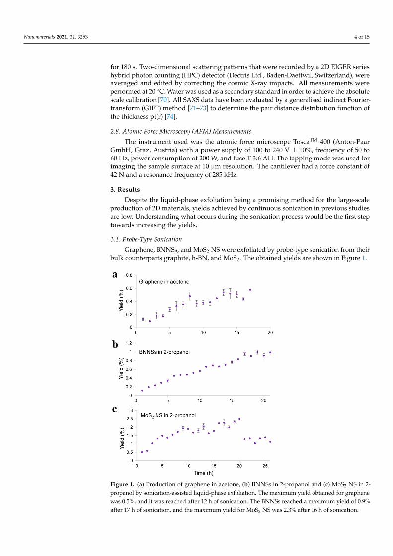
Graphene, BNNSs, and MoS2 NS were exfoliated by probe-type sonication from theirbulk counterparts graphite, h-BN, and MoS2. The obtained yields are shown in Figure 1.

Nanomaterials 2021, 11, x FOR PEER REVIEW 4 of 16

for 180 s. Two-dimensional scattering patterns that were recorded by a 2D EIGER series hybrid photon counting (HPC) detector (Dectris Ltd., Baden-Daettwil, Switzerland), were averaged and edited by correcting the cosmic X-ray impacts. All measurements were per-formed at 20 °C. Water was used as a secondary standard in order to achieve the absolute scale calibration [70]. All SAXS data have been evaluated by a generalised indirect Fou-rier-transform (GIFT) method [71–73] to determine the pair distance distribution function of the thickness pt(r) [74].

2.8. Atomic Force Microscopy (AFM) Measurements The instrument used was the atomic force microscope ToscaTM 400 (Anton-Paar

GmbH, Graz, Austria) with a power supply of 100 to 240 V ± 10%, frequency of 50 to 60 Hz, power consumption of 200 W, and fuse T 3.6 AH. The tapping mode was used for imaging the sample surface at 10 μm resolution. The cantilever had a force constant of 42 N and a resonance frequency of 285 kHz.

3. Results Despite the liquid-phase exfoliation being a promising method for the large-scale

production of 2D materials, yields achieved by continuous sonication in previous studies are low. Understanding what occurs during the sonication process would be the first step towards increasing the yields.

3.1. Probe-Type Sonication Graphene, BNNSs, and MoS2 NS were exfoliated by probe-type sonication from their

bulk counterparts graphite, h-BN, and MoS2. The obtained yields are shown in Figure 1.

Figure 1. (a) Production of graphene in acetone, (b) BNNSs in 2-propanol and (c) MoS2 NS in 2-propanol by sonication-assisted liquid-phase exfoliation. The maximum yield obtained for gra-phene was 0.5%, and it was reached after 12 h of sonication. The BNNSs reached a maximum yield

Figure 1. (a) Production of graphene in acetone, (b) BNNSs in 2-propanol and (c) MoS2 NS in 2-propanol by sonication-assisted liquid-phase exfoliation. The maximum yield obtained for graphenewas 0.5%, and it was reached after 12 h of sonication. The BNNSs reached a maximum yield of 0.9%after 17 h of sonication, and the maximum yield for MoS2 NS was 2.3% after 16 h of sonication.

Nanomaterials 2021, 11, 3253 5 of 15

The yield of the exfoliated 2D materials was initially increased with sonication time.However, longer sonication times led to a flattening of the curve. The maximum yieldobtained for graphene was 0.5%, and it was reached after 12 h of sonication, as shown inFigure 1a. The BNNSs reached a yield of 0.9% after 17 h of sonication, as shown in Figure 1b,and the maximum yield of MoS2 NS was 2.3%, and it was reached after 16 h of sonication,as shown in Figure 1c. The sonication time needed to achieve maximum yields varieddepending on the material and the exfoliation solvent. The different molecular structuresled to different amounts of energy that were necessary in order to exfoliate the nanosheetsfrom their bulk material. The chosen solvent also had an effect on the exfoliation andstabilisation of the nanosheets. 2-Propanol is a promising solvent [22] and has shown ahigh exfoliation efficiency for boron nitride and molybdenum disulfide. In the case ofgraphene, N-methyl-2-pyrrolidone (NMP) would have been a good solvent, but it couldnot be used for the probe-type sonication because of its sonochemical degradation [75].Therefore, acetone was chosen as an exfoliation solvent, because the ratio of surface tensioncomponents (polar component/dispersive component) of acetone is closest to that ofNMP as demonstrated by Shen et al. [51]. Regardless of different sonication times neededto achieve the maximum yield, one common behaviour observed for all three materialswas that there was no significant increase in the yield after a certain concentration of thenanosheets in the sample was reached. Furthermore, in the case of MoS2 NS, the yield wasdecreased. This behaviour was also found in other studies [76–79]. Thus far, no explanationwhy this occurs has been reported. This raises the question of whether the exfoliation ofnanosheets from their bulk counterpart stops despite further sonication, or whether theyare continuously being exfoliated from the bulk material but reaggregate.

3.2. Diluting and Stirring

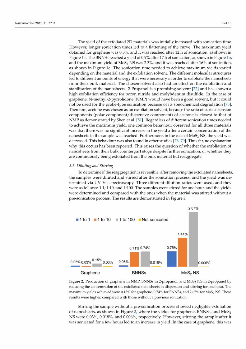
To determine if the reaggregation is reversible, after removing the exfoliated nanosheets,the samples were diluted and stirred after the sonication process, and the yield was de-termined via UV–Vis spectroscopy. Three different dilution ratios were used, and theywere as follows: 1:1; 1:10, and 1:100. The samples were stirred for one hour, and the yieldswere determined and compared with the ones when the material was stirred without apre-sonication process. The results are demonstrated in Figure 2.

Nanomaterials 2021, 11, x FOR PEER REVIEW 5 of 16

of 0.9% after 17 h of sonication, and the maximum yield for MoS2 NS was 2.3% after 16 h of soni-cation.

The yield of the exfoliated 2D materials was initially increased with sonication time. However, longer sonication times led to a flattening of the curve. The maximum yield obtained for graphene was 0.5%, and it was reached after 12 h of sonication, as shown in Figure 1a. The BNNSs reached a yield of 0.9% after 17 h of sonication, as shown in Figure 1b, and the maximum yield of MoS2 NS was 2.3%, and it was reached after 16 h of soni-cation, as shown in Figure 1c. The sonication time needed to achieve maximum yields varied depending on the material and the exfoliation solvent. The different molecular structures led to different amounts of energy that were necessary in order to exfoliate the nanosheets from their bulk material. The chosen solvent also had an effect on the exfolia-tion and stabilisation of the nanosheets. Moreover, 2-Propanol is a promising solvent [22] and has shown a high exfoliation efficiency for boron nitride and molybdenum disulfide. In the case of graphene, N-methyl-2-pyrrolidone (NMP) would have been a good solvent, but it could not be used for the probe-type sonication because of its sonochemical degra-dation [75]. Therefore, acetone was chosen as an exfoliation solvent, because the ratio of surface tension components (polar component/dispersive component) of acetone is closest to that of NMP as demonstrated by Shen et al. [51]. Regardless of different sonication times needed to achieve the maximum yield, one common behaviour observed for all three ma-terials was that there was no significant increase in the yield after a certain concentration of the nanosheets in the sample was reached. Furthermore, in the case of MoS2 NS, the yield was decreased. This behaviour was also found in other studies [76–79]. Thus far, no explanation why this occurs has been reported. This raises the question of whether the exfoliation of nanosheets from their bulk counterpart stops despite further sonication, or whether they are continuously being exfoliated from the bulk material but reaggregate.

3.2. Diluting and Stirring To determine if the reaggregation is reversible, after removing the exfoliated

nanosheets, the samples were diluted and stirred after the sonication process, and the yield was determined via UV–Vis spectroscopy. Three different dilution ratios were used, and they were as follows: 1:1; 1:10, and 1:100. The samples were stirred for one hour, and the yields were determined and compared with the ones when the material was stirred without a pre-sonication process. The results are demonstrated in Figure 2.

Figure 2. Production of graphene in NMP, BNNSs in 2-propanol, and MoS2 NS in 2-propanol by reducing the concentration of the exfoliated nanosheets in dispersion and stirring for one hour. The maximum yields achieved were 0.15% for graphene, 0.74% for BNNSs, and 2.67% for MoS2 NS. These results were higher, compared with those without a previous sonication.

Figure 2. Production of graphene in NMP, BNNSs in 2-propanol, and MoS2 NS in 2-propanol byreducing the concentration of the exfoliated nanosheets in dispersion and stirring for one hour. Themaximum yields achieved were 0.15% for graphene, 0.74% for BNNSs, and 2.67% for MoS2 NS. Theseresults were higher, compared with those without a previous sonication.

Stirring the sample without a pre-sonication process showed negligible exfoliationof nanosheets, as shown in Figure 2, where the yields for graphene, BNNSs, and MoS2NS were 0.03%, 0.018%, and 0.006%, respectively. However, stirring the sample after itwas sonicated for a few hours led to an increase in yield. In the case of graphene, this was

Nanomaterials 2021, 11, 3253 6 of 15

very low, almost non-significant, with values such as 0.05%, 0.03%, and 0.15%. The reasonfor this might be the overall lower efficiency of acetone in comparison with NMP as anexfoliation solvent for this material, as the maximum yield of graphene obtained after 12 hof sonication was only 0.5%. Although for the stirring process, a solvent exchange fromacetone to NMP was performed, this did not seem to have an effect on yield. The resultswere more promising for boron nitride nanosheets and molybdenum disulfide nanosheets,with yields up to 0.74% and 2.67%, respectively.

3.3. Recycling

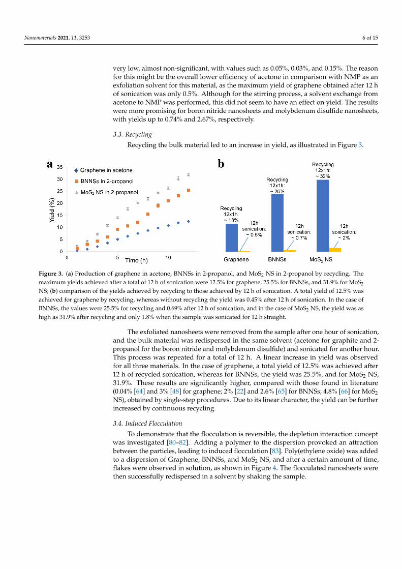
Recycling the bulk material led to an increase in yield, as illustrated in Figure 3.

Nanomaterials 2021, 11, x FOR PEER REVIEW 6 of 16

Stirring the sample without a pre-sonication process showed negligible exfoliation of nanosheets, as shown in Figure 2, where the yields for graphene, BNNSs, and MoS2 NS were 0.03%, 0.018%, and 0.006%, respectively. However, stirring the sample after it was sonicated for a few hours led to an increase in yield. In the case of graphene, this was very low, almost non-significant, with values such as 0.05%, 0.03%, and 0.15%. The reason for this might be the overall lower efficiency of acetone in comparison with NMP as an exfo-liation solvent for this material, as the maximum yield of graphene obtained after 12 h of sonication was only 0.5%. Although for the stirring process, a solvent exchange from ace-tone to NMP was performed, this did not seem to have an effect on yield. The results were more promising for boron nitride nanosheets and molybdenum disulfide nanosheets, with yields up to 0.74% and 2.67%, respectively.

3.3. Recycling Recycling the bulk material led to an increase in yield, as illustrated in Figure 3.

Figure 3. (a) Production of graphene in acetone, BNNSs in 2-propanol, and MoS2 NS in 2-propanol by recycling. The maximum yields achieved after a total of 12 h of sonication were 12.5% for graphene, 25.5% for BNNSs, and 31.9% for MoS2 NS; (b) comparison of the yields achieved by recycling to those achieved by 12 h of sonication. A total yield of 12.5% was achieved for graphene by recycling, whereas without recycling the yield was 0.45% after 12 h of sonication. In the case of BNNSs, the values were 25.5% for recycling and 0.69% after 12 h of sonication, and in the case of MoS2 NS, the yield was as high as 31.9% after recycling and only 1.8% when the sample was sonicated for 12 h straight.

The exfoliated nanosheets were removed from the sample after one hour of soni-cation, and the bulk material was redispersed in the same solvent (acetone for graphite and 2-propanol for the boron nitride and molybdenum disulfide) and sonicated for an-other hour. This process was repeated for a total of 12 h. A linear increase in yield was observed for all three materials. In the case of graphene, a total yield of 12.5% was achieved after 12 h of recycled sonication, whereas for BNNSs, the yield was 25.5%, and for MoS2 NS, 31.9%. These results are significantly higher, compared with those found in literature (0.04% [64] and 3% [48] for graphene; 2% [22] and 2.6% [65] for BNNSs; 4.8% [66] for MoS2 NS), obtained by single-step procedures. Due to its linear character, the yield can be further increased by continuous recycling.

3.4. Induced Flocculation To demonstrate that the flocculation is reversible, the depletion interaction concept

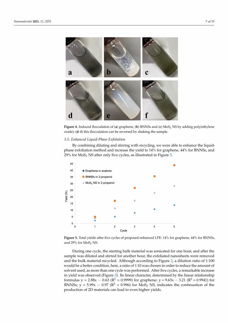
was investigated [80–82]. Adding a polymer to the dispersion provoked an attraction be-tween the particles, leading to induced flocculation [83]. Poly(ethylene oxide) was added to a dispersion of Graphene, BNNSs, and MoS2 NS, and after a certain amount of time, flakes were observed in solution, as shown in Figure 4. The flocculated nanosheets were then successfully redispersed in a solvent by shaking the sample.

Figure 3. (a) Production of graphene in acetone, BNNSs in 2-propanol, and MoS2 NS in 2-propanol by recycling. Themaximum yields achieved after a total of 12 h of sonication were 12.5% for graphene, 25.5% for BNNSs, and 31.9% for MoS2

NS; (b) comparison of the yields achieved by recycling to those achieved by 12 h of sonication. A total yield of 12.5% wasachieved for graphene by recycling, whereas without recycling the yield was 0.45% after 12 h of sonication. In the case ofBNNSs, the values were 25.5% for recycling and 0.69% after 12 h of sonication, and in the case of MoS2 NS, the yield was ashigh as 31.9% after recycling and only 1.8% when the sample was sonicated for 12 h straight.

The exfoliated nanosheets were removed from the sample after one hour of sonication,and the bulk material was redispersed in the same solvent (acetone for graphite and 2-propanol for the boron nitride and molybdenum disulfide) and sonicated for another hour.This process was repeated for a total of 12 h. A linear increase in yield was observedfor all three materials. In the case of graphene, a total yield of 12.5% was achieved after12 h of recycled sonication, whereas for BNNSs, the yield was 25.5%, and for MoS2 NS,31.9%. These results are significantly higher, compared with those found in literature(0.04% [64] and 3% [48] for graphene; 2% [22] and 2.6% [65] for BNNSs; 4.8% [66] for MoS2NS), obtained by single-step procedures. Due to its linear character, the yield can be furtherincreased by continuous recycling.

3.4. Induced Flocculation

To demonstrate that the flocculation is reversible, the depletion interaction conceptwas investigated [80–82]. Adding a polymer to the dispersion provoked an attractionbetween the particles, leading to induced flocculation [83]. Poly(ethylene oxide) was addedto a dispersion of Graphene, BNNSs, and MoS2 NS, and after a certain amount of time,flakes were observed in solution, as shown in Figure 4. The flocculated nanosheets werethen successfully redispersed in a solvent by shaking the sample.

Nanomaterials 2021, 11, 3253 7 of 15Nanomaterials 2021, 11, x FOR PEER REVIEW 7 of 16

Figure 4. Induced flocculation of (a) graphene, (b) BNNSs and (c) MoS2 NS by adding poly(ethylene oxide); (d–f) this flocculation can be reversed by shaking the sample.

3.5. Enhanced Liquid-Phase Exfoliation By combining diluting and stirring with recycling, we were able to enhance the liq-

uid-phase exfoliation method and increase the yield to 14% for graphene, 44% for BNNSs, and 29% for MoS2 NS after only five cycles, as illustrated in Figure 5.

Figure 5. Total yields after five cycles of proposed enhanced LPE: 14% for graphene, 44% for BNNSs, and 29% for MoS2 NS.

During one cycle, the starting bulk material was sonicated for one hour, and after the sample was diluted and stirred for another hour, the exfoliated nanosheets were removed and the bulk material recycled. Although according to Figure 2, a dilution ratio of 1:100 would be a better condition, here, a ratio of 1:10 was chosen in order to reduce the amount of solvent used, as more than one cycle was performed. After five cycles, a remarkable increase in yield was observed (Figure 5). Its linear character, determined by the linear relationship formulas y = 2.88x − 0.63 (R2 = 0.9999) for graphene; y = 9.63x − 3.21 (R2 = 0.9941) for BNNSs; y = 5.99x − 0.97 (R2 = 0.996) for MoS2 NS, indicates the continuation of the pro-duction of 2D materials can lead to even higher yields.

Figure 4. Induced flocculation of (a) graphene, (b) BNNSs and (c) MoS2 NS by adding poly(ethyleneoxide); (d–f) this flocculation can be reversed by shaking the sample.

3.5. Enhanced Liquid-Phase Exfoliation

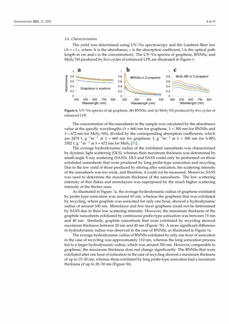
By combining diluting and stirring with recycling, we were able to enhance the liquid-phase exfoliation method and increase the yield to 14% for graphene, 44% for BNNSs, and29% for MoS2 NS after only five cycles, as illustrated in Figure 5.

Nanomaterials 2021, 11, x FOR PEER REVIEW 7 of 16

Figure 4. Induced flocculation of (a) graphene, (b) BNNSs and (c) MoS2 NS by adding poly(ethylene oxide); (d–f) this flocculation can be reversed by shaking the sample.

3.5. Enhanced Liquid-Phase Exfoliation By combining diluting and stirring with recycling, we were able to enhance the liq-

uid-phase exfoliation method and increase the yield to 14% for graphene, 44% for BNNSs, and 29% for MoS2 NS after only five cycles, as illustrated in Figure 5.

Figure 5. Total yields after five cycles of proposed enhanced LPE: 14% for graphene, 44% for BNNSs, and 29% for MoS2 NS.

During one cycle, the starting bulk material was sonicated for one hour, and after the sample was diluted and stirred for another hour, the exfoliated nanosheets were removed and the bulk material recycled. Although according to Figure 2, a dilution ratio of 1:100 would be a better condition, here, a ratio of 1:10 was chosen in order to reduce the amount of solvent used, as more than one cycle was performed. After five cycles, a remarkable increase in yield was observed (Figure 5). Its linear character, determined by the linear relationship formulas y = 2.88x − 0.63 (R2 = 0.9999) for graphene; y = 9.63x − 3.21 (R2 = 0.9941) for BNNSs; y = 5.99x − 0.97 (R2 = 0.996) for MoS2 NS, indicates the continuation of the pro-duction of 2D materials can lead to even higher yields.

Figure 5. Total yields after five cycles of proposed enhanced LPE: 14% for graphene, 44% for BNNSs,and 29% for MoS2 NS.

During one cycle, the starting bulk material was sonicated for one hour, and after thesample was diluted and stirred for another hour, the exfoliated nanosheets were removedand the bulk material recycled. Although according to Figure 2, a dilution ratio of 1:100would be a better condition, here, a ratio of 1:10 was chosen in order to reduce the amount ofsolvent used, as more than one cycle was performed. After five cycles, a remarkable increasein yield was observed (Figure 5). Its linear character, determined by the linear relationshipformulas y = 2.88x − 0.63 (R2 = 0.9999) for graphene; y = 9.63x − 3.21 (R2 = 0.9941) forBNNSs; y = 5.99x − 0.97 (R2 = 0.996) for MoS2 NS, indicates the continuation of theproduction of 2D materials can lead to even higher yields.

Nanomaterials 2021, 11, 3253 8 of 15

3.6. Characterisation

The yield was determined using UV–Vis spectroscopy and the Lambert–Beer law(A = ε l c, where A is the absorbance, ε is the absorption coefficient, l is the optical pathlength in cm and c is the concentration). The UV–Vis spectra of graphene, BNNSs, andMoS2 NS produced by five cycles of enhanced LPE are illustrated in Figure 6.

Nanomaterials 2021, 11, x FOR PEER REVIEW 8 of 16

3.6. Characterisation The yield was determined using UV–Vis spectroscopy and the Lambert–Beer law (A

= ε l c, where A is the absorbance, ε is the absorption coefficient, l is the optical path length in cm and c is the concentration). The UV–Vis spectra of graphene, BNNSs, and MoS2 NS produced by five cycles of enhanced LPE are illustrated in Figure 6.

Figure 6. UV–Vis spectra of (a) graphene, (b) BNNSs, and (c) MoS2 NS produced by five cycles of enhanced LPE.

The concentration of the nanosheets in the sample was calculated by the absorbance value at the specific wavelengths (λ = 660 nm for graphene, λ = 300 nm for BNNSs and λ = 672 nm for MoS2 NS), divided by the corresponding absorption coefficients, which are 2474 L g−1m−1 at λ = 660 nm for graphene; L g−1m−1) at λ = 300 nm for h-BN; 3302 L g-1m-1) at λ = 672 nm for MoS2 [51].

The average hydrodynamic radius of the exfoliated nanosheets was characterised by dynamic light scattering (DLS), whereas their maximum thickness was determined by small-angle X-ray scattering (SAXS). DLS and SAXS could only be performed on those exfoliated nanosheets that were produced by long probe-type sonication and recycling. Due to the low yield of those produced by stirring after sonication, the scattering intensity of the nanosheets was too weak, and therefore, it could not be measured. Moreover, SAXS was used to determine the maximum thickness of the nanosheets. The low scattering in-tensity of thin flakes and monolayers was superposed by the much higher scattering in-tensity of the thicker ones.

As illustrated in Figure 7a, the average hydrodynamic radius of graphene exfoliated by probe-type sonication was around 65 nm, whereas the graphene that was exfoliated by recycling, where graphite was sonicated for only one hour, showed a hydrodynamic ra-dius of around 100 nm. Monolayer and few-layer graphene could not be determined by SAXS due to their low scattering intensity. However, the maximum thickness of the graphite nanosheets exfoliated by continuous probe-type sonication was between 15 nm and 40 nm. Similarly, graphite nanosheets that were exfoliated by recycling showed max-imum thickness between 20 nm and 40 nm (Figure 7b). A more significant difference in hydrodynamic radius was observed in the case of BNNSs, as illustrated in Figure 8a.

Figure 6. UV–Vis spectra of (a) graphene, (b) BNNSs, and (c) MoS2 NS produced by five cycles ofenhanced LPE.

The concentration of the nanosheets in the sample was calculated by the absorbancevalue at the specific wavelengths (λ = 660 nm for graphene, λ = 300 nm for BNNSs andλ = 672 nm for MoS2 NS), divided by the corresponding absorption coefficients, whichare 2474 L g−1m−1 at λ = 660 nm for graphene; L g−1m−1 at λ = 300 nm for h-BN;3302 L g−1m−1 at λ = 672 nm for MoS2 [51].

The average hydrodynamic radius of the exfoliated nanosheets was characterisedby dynamic light scattering (DLS), whereas their maximum thickness was determined bysmall-angle X-ray scattering (SAXS). DLS and SAXS could only be performed on thoseexfoliated nanosheets that were produced by long probe-type sonication and recycling.Due to the low yield of those produced by stirring after sonication, the scattering intensityof the nanosheets was too weak, and therefore, it could not be measured. Moreover, SAXSwas used to determine the maximum thickness of the nanosheets. The low scatteringintensity of thin flakes and monolayers was superposed by the much higher scatteringintensity of the thicker ones.

As illustrated in Figure 7a, the average hydrodynamic radius of graphene exfoliatedby probe-type sonication was around 65 nm, whereas the graphene that was exfoliatedby recycling, where graphite was sonicated for only one hour, showed a hydrodynamicradius of around 100 nm. Monolayer and few-layer graphene could not be determinedby SAXS due to their low scattering intensity. However, the maximum thickness of thegraphite nanosheets exfoliated by continuous probe-type sonication was between 15 nmand 40 nm. Similarly, graphite nanosheets that were exfoliated by recycling showedmaximum thickness between 20 nm and 40 nm (Figure 7b). A more significant differencein hydrodynamic radius was observed in the case of BNNSs, as illustrated in Figure 8a.

The average hydrodynamic radius of BNNSs exfoliated by only one hour of sonicationin the case of recycling was approximately 110 nm, whereas the long sonication processled to a larger hydrodynamic radius, which was around 350 nm. However, comparable tographene, the maximum thickness does not change significantly. The BNNSs that wereexfoliated after one hour of sonication in the case of recycling showed a maximum thicknessof up to 15–30 nm, whereas those exfoliated by long probe-type sonication had a maximumthickness of up to 20–30 nm (Figure 8b).

Nanomaterials 2021, 11, 3253 9 of 15

Nanomaterials 2021, 11, x FOR PEER REVIEW 8 of 16

3.6. Characterisation The yield was determined using UV–Vis spectroscopy and the Lambert–Beer law (A

= ε l c, where A is the absorbance, ε is the absorption coefficient, l is the optical path length in cm and c is the concentration). The UV–Vis spectra of graphene, BNNSs, and MoS2 NS produced by five cycles of enhanced LPE are illustrated in Figure 6.

Figure 6. UV–Vis spectra of (a) graphene, (b) BNNSs, and (c) MoS2 NS produced by five cycles of enhanced LPE.

The concentration of the nanosheets in the sample was calculated by the absorbance value at the specific wavelengths (λ = 660 nm for graphene, λ = 300 nm for BNNSs and λ = 672 nm for MoS2 NS), divided by the corresponding absorption coefficients, which are 2474 L g−1m−1 at λ = 660 nm for graphene; L g−1m−1) at λ = 300 nm for h-BN; 3302 L g-1m-1) at λ = 672 nm for MoS2 [51].

The average hydrodynamic radius of the exfoliated nanosheets was characterised by dynamic light scattering (DLS), whereas their maximum thickness was determined by small-angle X-ray scattering (SAXS). DLS and SAXS could only be performed on those exfoliated nanosheets that were produced by long probe-type sonication and recycling. Due to the low yield of those produced by stirring after sonication, the scattering intensity of the nanosheets was too weak, and therefore, it could not be measured. Moreover, SAXS was used to determine the maximum thickness of the nanosheets. The low scattering in-tensity of thin flakes and monolayers was superposed by the much higher scattering in-tensity of the thicker ones.

As illustrated in Figure 7a, the average hydrodynamic radius of graphene exfoliated by probe-type sonication was around 65 nm, whereas the graphene that was exfoliated by recycling, where graphite was sonicated for only one hour, showed a hydrodynamic ra-dius of around 100 nm. Monolayer and few-layer graphene could not be determined by SAXS due to their low scattering intensity. However, the maximum thickness of the graphite nanosheets exfoliated by continuous probe-type sonication was between 15 nm and 40 nm. Similarly, graphite nanosheets that were exfoliated by recycling showed max-imum thickness between 20 nm and 40 nm (Figure 7b). A more significant difference in hydrodynamic radius was observed in the case of BNNSs, as illustrated in Figure 8a.

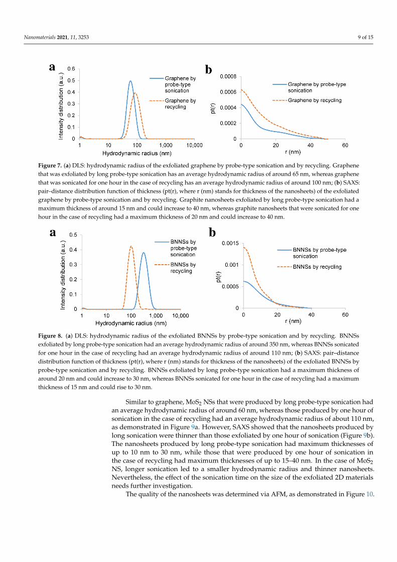
Figure 7. (a) DLS: hydrodynamic radius of the exfoliated graphene by probe-type sonication and by recycling. Graphenethat was exfoliated by long probe-type sonication has an average hydrodynamic radius of around 65 nm, whereas graphenethat was sonicated for one hour in the case of recycling has an average hydrodynamic radius of around 100 nm; (b) SAXS:pair–distance distribution function of thickness (pt(r), where r (nm) stands for thickness of the nanosheets) of the exfoliatedgraphene by probe-type sonication and by recycling. Graphite nanosheets exfoliated by long probe-type sonication had amaximum thickness of around 15 nm and could increase to 40 nm, whereas graphite nanosheets that were sonicated for onehour in the case of recycling had a maximum thickness of 20 nm and could increase to 40 nm.

Nanomaterials 2021, 11, x FOR PEER REVIEW 9 of 16

Figure 7. (a) DLS: hydrodynamic radius of the exfoliated graphene by probe-type sonication and by recycling. Graphene that was exfoliated by long probe-type sonication has an average hydrodynamic radius of around 65 nm, whereas gra-phene that was sonicated for one hour in the case of recycling has an average hydrodynamic radius of around 100 nm; (b) SAXS: pair–distance distribution function of thickness (pt(r), where r (nm) stands for thickness of the nanosheets) of the exfoliated graphene by probe-type sonication and by recycling. Graphite nanosheets exfoliated by long probe-type soni-cation had a maximum thickness of around 15 nm and could increase to 40 nm, whereas graphite nanosheets that were sonicated for one hour in the case of recycling had a maximum thickness of 20 nm and could increase to 40 nm.

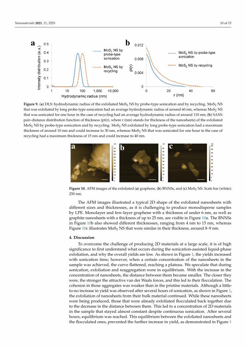
Figure 8. (a) DLS: hydrodynamic radius of the exfoliated BNNSs by probe-type sonication and by recycling. BNNSs exfo-liated by long probe-type sonication had an average hydrodynamic radius of around 350 nm, whereas BNNSs sonicated for one hour in the case of recycling had an average hydrodynamic radius of around 110 nm; (b) SAXS: pair–distance distribution function of thickness (pt(r), where r (nm) stands for thickness of the nanosheets) of the exfoliated BNNSs by probe-type sonication and by recycling. BNNSs exfoliated by long probe-type sonication had a maximum thickness of around 20 nm and could increase to 30 nm, whereas BNNSs sonicated for one hour in the case of recycling had a maximum thickness of 15 nm and could rise to 30 nm.

The average hydrodynamic radius of BNNSs exfoliated by only one hour of soni-cation in the case of recycling was approximately 110 nm, whereas the long sonication process led to a larger hydrodynamic radius, which was around 350 nm. However, com-parable to graphene, the maximum thickness does not change significantly. The BNNSs that were exfoliated after one hour of sonication in the case of recycling showed a maxi-mum thickness of up to 15–30 nm, whereas those exfoliated by long probe-type sonication had a maximum thickness of up to 20–30 nm (Figure 8b).

Similar to graphene, MoS2 NSs that were produced by long probe-type sonication had an average hydrodynamic radius of around 60 nm, whereas those produced by one hour of sonication in the case of recycling had an average hydrodynamic radius of about 110 nm, as demonstrated in Figure 9a. However, SAXS showed that the nanosheets pro-duced by long sonication were thinner than those exfoliated by one hour of sonication (Figure 9b). The nanosheets produced by long probe-type sonication had maximum thick-nesses of up to 10 nm to 30 nm, while those that were produced by one hour of sonication in the case of recycling had maximum thicknesses of up to 15–40 nm. In the case of MoS2 NS, longer sonication led to a smaller hydrodynamic radius and thinner nanosheets. Nev-ertheless, the effect of the sonication time on the size of the exfoliated 2D materials needs further investigation.

Figure 8. (a) DLS: hydrodynamic radius of the exfoliated BNNSs by probe-type sonication and by recycling. BNNSsexfoliated by long probe-type sonication had an average hydrodynamic radius of around 350 nm, whereas BNNSs sonicatedfor one hour in the case of recycling had an average hydrodynamic radius of around 110 nm; (b) SAXS: pair–distancedistribution function of thickness (pt(r), where r (nm) stands for thickness of the nanosheets) of the exfoliated BNNSs byprobe-type sonication and by recycling. BNNSs exfoliated by long probe-type sonication had a maximum thickness ofaround 20 nm and could increase to 30 nm, whereas BNNSs sonicated for one hour in the case of recycling had a maximumthickness of 15 nm and could rise to 30 nm.

Similar to graphene, MoS2 NSs that were produced by long probe-type sonication hadan average hydrodynamic radius of around 60 nm, whereas those produced by one hour ofsonication in the case of recycling had an average hydrodynamic radius of about 110 nm,as demonstrated in Figure 9a. However, SAXS showed that the nanosheets produced bylong sonication were thinner than those exfoliated by one hour of sonication (Figure 9b).The nanosheets produced by long probe-type sonication had maximum thicknesses ofup to 10 nm to 30 nm, while those that were produced by one hour of sonication inthe case of recycling had maximum thicknesses of up to 15–40 nm. In the case of MoS2NS, longer sonication led to a smaller hydrodynamic radius and thinner nanosheets.Nevertheless, the effect of the sonication time on the size of the exfoliated 2D materialsneeds further investigation.

The quality of the nanosheets was determined via AFM, as demonstrated in Figure 10.

Nanomaterials 2021, 11, 3253 10 of 15Nanomaterials 2021, 11, x FOR PEER REVIEW 10 of 16

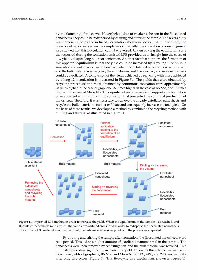
Figure 9. (a) DLS: hydrodynamic radius of the exfoliated MoS2 NS by probe-type sonication and by recycling. MoS2 NS that was exfoliated by long probe-type sonication had an average hydrodynamic radius of around 60 nm, whereas MoS2 NS that was sonicated for one hour in the case of recycling had an average hydrodynamic radius of around 110 nm; (b) SAXS: pair–distance distribution function of thickness (pt(r), where r (nm) stands for thickness of the nanosheets) of the exfoliated MoS2 NS by probe-type sonication and by recycling. MoS2 NS exfoliated by long probe-type sonication had a maximum thickness of around 10 nm and could increase to 30 nm, whereas MoS2 NS that was sonicated for one hour in the case of recycling had a maximum thickness of 15 nm and could increase to 40 nm.

The quality of the nanosheets was determined via AFM, as demonstrated in Figure 10.

Figure 10. AFM images of the exfoliated (a) graphene, (b) BNNSs, and (c) MoS2 NS. Scale bar (white): 250 nm.

The AFM images illustrated a typical 2D shape of the exfoliated nanosheets with dif-ferent sizes and thicknesses, as it is challenging to produce monodisperse samples by LPE. Monolayer and few-layer graphene with a thickness of under 6 nm, as well as graphite nanosheets with a thickness of up to 25 nm, are visible in Figure 10a. The BNNSs in Figure 10b also showed different thicknesses, ranging from 4 nm to 15 nm, whereas Figure 10c illustrates MoS2 NS that were similar in their thickness, around 8–9 nm.

4. Discussion To overcome the challenge of producing 2D materials at a large scale, it is of high

significance to first understand what occurs during the sonication-assisted liquid-phase exfoliation, and why the overall yields are low. As shown in Figure 1, the yields increased with sonication time; however, when a certain concentration of the nanosheets in the sam-ple was achieved, the curve flattened, reaching a plateau. We speculate that during soni-cation, exfoliation and reaggregation were in equilibrium. With the increase in the con-centration of nanosheets, the distance between them became smaller. The closer they were, the stronger the attractive van der Waals forces, and this led to their flocculation. The cohesion in those aggregates was weaker than in the pristine materials. Although a little-to-no increase in yield was observed after several hours of sonication, as shown in Figure 1, the exfoliation of nanosheets from their bulk material continued. While these

Figure 9. (a) DLS: hydrodynamic radius of the exfoliated MoS2 NS by probe-type sonication and by recycling. MoS2 NSthat was exfoliated by long probe-type sonication had an average hydrodynamic radius of around 60 nm, whereas MoS2 NSthat was sonicated for one hour in the case of recycling had an average hydrodynamic radius of around 110 nm; (b) SAXS:pair–distance distribution function of thickness (pt(r), where r (nm) stands for thickness of the nanosheets) of the exfoliatedMoS2 NS by probe-type sonication and by recycling. MoS2 NS exfoliated by long probe-type sonication had a maximumthickness of around 10 nm and could increase to 30 nm, whereas MoS2 NS that was sonicated for one hour in the case ofrecycling had a maximum thickness of 15 nm and could increase to 40 nm.

Nanomaterials 2021, 11, x FOR PEER REVIEW 10 of 16

Figure 9. (a) DLS: hydrodynamic radius of the exfoliated MoS2 NS by probe-type sonication and by recycling. MoS2 NS that was exfoliated by long probe-type sonication had an average hydrodynamic radius of around 60 nm, whereas MoS2 NS that was sonicated for one hour in the case of recycling had an average hydrodynamic radius of around 110 nm; (b) SAXS: pair–distance distribution function of thickness (pt(r), where r (nm) stands for thickness of the nanosheets) of the exfoliated MoS2 NS by probe-type sonication and by recycling. MoS2 NS exfoliated by long probe-type sonication had a maximum thickness of around 10 nm and could increase to 30 nm, whereas MoS2 NS that was sonicated for one hour in the case of recycling had a maximum thickness of 15 nm and could increase to 40 nm.

The quality of the nanosheets was determined via AFM, as demonstrated in Figure 10.

Figure 10. AFM images of the exfoliated (a) graphene, (b) BNNSs, and (c) MoS2 NS. Scale bar (white): 250 nm.

The AFM images illustrated a typical 2D shape of the exfoliated nanosheets with dif-ferent sizes and thicknesses, as it is challenging to produce monodisperse samples by LPE. Monolayer and few-layer graphene with a thickness of under 6 nm, as well as graphite nanosheets with a thickness of up to 25 nm, are visible in Figure 10a. The BNNSs in Figure 10b also showed different thicknesses, ranging from 4 nm to 15 nm, whereas Figure 10c illustrates MoS2 NS that were similar in their thickness, around 8–9 nm.

4. Discussion To overcome the challenge of producing 2D materials at a large scale, it is of high

significance to first understand what occurs during the sonication-assisted liquid-phase exfoliation, and why the overall yields are low. As shown in Figure 1, the yields increased with sonication time; however, when a certain concentration of the nanosheets in the sam-ple was achieved, the curve flattened, reaching a plateau. We speculate that during soni-cation, exfoliation and reaggregation were in equilibrium. With the increase in the con-centration of nanosheets, the distance between them became smaller. The closer they were, the stronger the attractive van der Waals forces, and this led to their flocculation. The cohesion in those aggregates was weaker than in the pristine materials. Although a little-to-no increase in yield was observed after several hours of sonication, as shown in Figure 1, the exfoliation of nanosheets from their bulk material continued. While these

Figure 10. AFM images of the exfoliated (a) graphene, (b) BNNSs, and (c) MoS2 NS. Scale bar (white):250 nm.

The AFM images illustrated a typical 2D shape of the exfoliated nanosheets withdifferent sizes and thicknesses, as it is challenging to produce monodisperse samplesby LPE. Monolayer and few-layer graphene with a thickness of under 6 nm, as well asgraphite nanosheets with a thickness of up to 25 nm, are visible in Figure 10a. The BNNSsin Figure 10b also showed different thicknesses, ranging from 4 nm to 15 nm, whereasFigure 10c illustrates MoS2 NS that were similar in their thickness, around 8–9 nm.

4. Discussion

To overcome the challenge of producing 2D materials at a large scale, it is of highsignificance to first understand what occurs during the sonication-assisted liquid-phaseexfoliation, and why the overall yields are low. As shown in Figure 1, the yields increasedwith sonication time; however, when a certain concentration of the nanosheets in thesample was achieved, the curve flattened, reaching a plateau. We speculate that duringsonication, exfoliation and reaggregation were in equilibrium. With the increase in theconcentration of nanosheets, the distance between them became smaller. The closer theywere, the stronger the attractive van der Waals forces, and this led to their flocculation. Thecohesion in those aggregates was weaker than in the pristine materials. Although a little-to-no increase in yield was observed after several hours of sonication, as shown in Figure 1,the exfoliation of nanosheets from their bulk material continued. While these nanosheetswere being produced, those that were already exfoliated flocculated back together dueto the decrease in the distance between them. This led to a concentration of 2D materialsin the sample that stayed almost constant despite continuous sonication. After severalhours, equilibrium was reached. This equilibrium between the exfoliated nanosheets andthe flocculated ones, prevented the further increase in yield, as demonstrated in Figure 1

Nanomaterials 2021, 11, 3253 11 of 15

by the flattening of the curve. Nevertheless, due to weaker cohesion in the flocculatednanosheets, they could be redispersed by diluting and stirring the sample. The reversibilitywas demonstrated by the induced flocculation shown in Section 3.4. Furthermore, thepresence of nanosheets when the sample was stirred after the sonication process (Figure 2)also showed that this flocculation could be reversed. Understanding the equilibrium statethat occurred during the sonication-assisted LPE provided us an insight into the cause oflow yields, despite long hours of sonication. Another fact that supports the formation ofthis apparent equilibrium is that the yield could be increased by recycling. Continuoussonication did not increase yield; however, when the exfoliated nanosheets were removed,and the bulk material was recycled, the equilibrium could be avoided, and more nanosheetscould be exfoliated. A comparison of the yields achieved by recycling with those achievedby a long 12 h sonication is illustrated in Figure 3b. The yields that were obtained byrecycling procedure and those obtained by continuous sonication were approximately28 times higher in the case of graphene, 37 times higher in the case of BNNSs, and 18 timeshigher in the case of MoS2 NS. This significant increase in yield supports the formationof an apparent equilibrium during sonication that prevented the continual production ofnanosheets. Therefore, it was necessary to remove the already exfoliated nanosheets andrecycle the bulk material to further exfoliate and consequently increase the total yield. Onthe basis of these results, we developed a method by combining the recycling method withdiluting and stirring, as illustrated in Figure 11.

Nanomaterials 2021, 11, x FOR PEER REVIEW 11 of 16

nanosheets were being produced, those that were already exfoliated flocculated back to-gether due to the decrease in the distance between them. This led to a concentration of 2D materials in the sample that stayed almost constant despite continuous sonication. After several hours, equilibrium was reached. This equilibrium between the exfoliated nanosheets and the flocculated ones, prevented the further increase in yield, as demon-strated in Figure 1 by the flattening of the curve. Nevertheless, due to weaker cohesion in the flocculated nanosheets, they could be redispersed by diluting and stirring the sample. The reversibility was demonstrated by the induced flocculation shown in Section 3.4. Fur-thermore, the presence of nanosheets when the sample was stirred after the sonication process (Figure 2) also showed that this flocculation could be reversed. Understanding the equilibrium state that occurred during the sonication-assisted LPE provided us an insight into the cause of low yields, despite long hours of sonication. Another fact that supports the formation of this apparent equilibrium is that the yield could be increased by recy-cling. Continuous sonication did not increase yield; however, when the exfoliated nanosheets were removed, and the bulk material was recycled, the equilibrium could be avoided, and more nanosheets could be exfoliated. A comparison of the yields achieved by recycling with those achieved by a long 12 h sonication is illustrated in Figure 3b. The yields that were obtained by recycling procedure and those obtained by continuous soni-cation were approximately 28 times higher in the case of graphene, 37 times higher in the case of BNNSs, and 18 times higher in the case of MoS2 NS. This significant increase in yield supports the formation of an apparent equilibrium during sonication that prevented the continual production of nanosheets. Therefore, it was necessary to remove the already exfoliated nanosheets and recycle the bulk material to further exfoliate and consequently increase the total yield. On the basis of these results, we developed a method by combin-ing the recycling method with diluting and stirring, as illustrated in Figure 11.

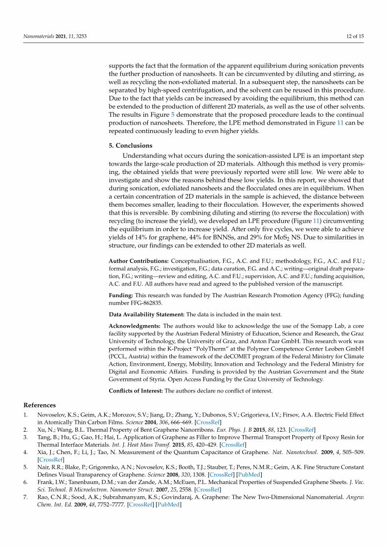
Figure 11. Improved LPE method in order to increase the yield. When the equilibrium in the sample was reached, and flocculated nanosheets were created, the sample was diluted and stirred in order to redisperse the flocculated nanosheets. The exfoliated 2D material was then removed, the bulk material was recycled, and the process was repeated.

Figure 11. Improved LPE method in order to increase the yield. When the equilibrium in the sample was reached, andflocculated nanosheets were created, the sample was diluted and stirred in order to redisperse the flocculated nanosheets.The exfoliated 2D material was then removed, the bulk material was recycled, and the process was repeated.

By diluting and stirring the sample after sonication, the flocculated nanosheets wereredispersed. This led to a higher amount of exfoliated nanomaterial in the sample. Thenanosheets were then removed by centrifugation, and the bulk material was recycled. Thismulti-step procedure significantly increased the yield. Following this scheme, we were ableto achieve yields of graphene, BNNSs, and MoS2 NS to 14%, 44%, and 29%, respectively,after only five cycles (Figure 5). This five-cycle LPE mechanism, shown in Figure 11,

Nanomaterials 2021, 11, 3253 12 of 15

supports the fact that the formation of the apparent equilibrium during sonication preventsthe further production of nanosheets. It can be circumvented by diluting and stirring, aswell as recycling the non-exfoliated material. In a subsequent step, the nanosheets can beseparated by high-speed centrifugation, and the solvent can be reused in this procedure.Due to the fact that yields can be increased by avoiding the equilibrium, this method canbe extended to the production of different 2D materials, as well as the use of other solvents.The results in Figure 5 demonstrate that the proposed procedure leads to the continualproduction of nanosheets. Therefore, the LPE method demonstrated in Figure 11 can berepeated continuously leading to even higher yields.

5. Conclusions

Understanding what occurs during the sonication-assisted LPE is an important steptowards the large-scale production of 2D materials. Although this method is very promis-ing, the obtained yields that were previously reported were still low. We were able toinvestigate and show the reasons behind these low yields. In this report, we showed thatduring sonication, exfoliated nanosheets and the flocculated ones are in equilibrium. Whena certain concentration of 2D materials in the sample is achieved, the distance betweenthem becomes smaller, leading to their flocculation. However, the experiments showedthat this is reversible. By combining diluting and stirring (to reverse the flocculation) withrecycling (to increase the yield), we developed an LPE procedure (Figure 11) circumventingthe equilibrium in order to increase yield. After only five cycles, we were able to achieveyields of 14% for graphene, 44% for BNNSs, and 29% for MoS2 NS. Due to similarities instructure, our findings can be extended to other 2D materials as well.

Author Contributions: Conceptualisation, F.G., A.C. and F.U.; methodology, F.G., A.C. and F.U.;formal analysis, F.G.; investigation, F.G.; data curation, F.G. and A.C.; writing—original draft prepara-tion, F.G.; writing—review and editing, A.C. and F.U.; supervision, A.C. and F.U.; funding acquisition,A.C. and F.U. All authors have read and agreed to the published version of the manuscript.

Funding: This research was funded by The Austrian Research Promotion Agency (FFG); fundingnumber FFG-862835.

Data Availability Statement: The data is included in the main text.

Acknowledgments: The authors would like to acknowledge the use of the Somapp Lab, a corefacility supported by the Austrian Federal Ministry of Education, Science and Research, the GrazUniversity of Technology, the University of Graz, and Anton Paar GmbH. This research work wasperformed within the K-Project “PolyTherm” at the Polymer Competence Center Leoben GmbH(PCCL, Austria) within the framework of the deCOMET program of the Federal Ministry for ClimateAction, Environment, Energy, Mobility, Innovation and Technology and the Federal Ministry forDigital and Economic Affairs. Funding is provided by the Austrian Government and the StateGovernment of Styria. Open Access Funding by the Graz University of Technology.

Conflicts of Interest: The authors declare no conflict of interest.

References1. Novoselov, K.S.; Geim, A.K.; Morozov, S.V.; Jiang, D.; Zhang, Y.; Dubonos, S.V.; Grigorieva, I.V.; Firsov, A.A. Electric Field Effect

in Atomically Thin Carbon Films. Science 2004, 306, 666–669. [CrossRef]2. Xu, N.; Wang, B.L. Thermal Property of Bent Graphene Nanorribons. Eur. Phys. J. B 2015, 88, 123. [CrossRef]3. Tang, B.; Hu, G.; Gao, H.; Hai, L. Application of Graphene as Filler to Improve Thermal Transport Property of Epoxy Resin for

Thermal Interface Materials. Int. J. Heat Mass Transf. 2015, 85, 420–429. [CrossRef]4. Xia, J.; Chen, F.; Li, J.; Tao, N. Measurement of the Quantum Capacitance of Graphene. Nat. Nanotechnol. 2009, 4, 505–509.

[CrossRef]5. Nair, R.R.; Blake, P.; Grigorenko, A.N.; Novoselov, K.S.; Booth, T.J.; Stauber, T.; Peres, N.M.R.; Geim, A.K. Fine Structure Constant

Defines Visual Transparency of Graphene. Science 2008, 320, 1308. [CrossRef] [PubMed]6. Frank, I.W.; Tanenbaum, D.M.; van der Zande, A.M.; McEuen, P.L. Mechanical Properties of Suspended Graphene Sheets. J. Vac.

Sci. Technol. B Microelectron. Nanometer Struct. 2007, 25, 2558. [CrossRef]7. Rao, C.N.R.; Sood, A.K.; Subrahmanyam, K.S.; Govindaraj, A. Graphene: The New Two-Dimensional Nanomaterial. Angew.

Chem. Int. Ed. 2009, 48, 7752–7777. [CrossRef] [PubMed]

Nanomaterials 2021, 11, 3253 13 of 15

8. King, A.; Johnson, G.; Engelberg, D.; Ludwig, W.; Marrow, J. Observations of Intergranular Stress Corrosion Cracking in aGrain-Mapped Polycrystal. Science 2008, 321, 382–385. [CrossRef]

9. Cao, J.; Zhang, Y.; Men, C.; Sun, Y.; Wang, Z.; Zhang, X.; Li, Q. Programmable Writing of Graphene Oxide/Reduced GrapheneOxide Fibers for Sensible Networks with in Situ Welded Junctions. ACS Nano 2014, 8, 4325–4333. [CrossRef]

10. Wang, F.; Zhang, Y.; Tian, C.; Girit, C.; Zettl, A.; Crommie, M.; Shen, Y.R. Gate-Variable Optical Transitions in Graphene. Science2008, 320, 206–209. [CrossRef]

11. Shelke, M.V.; Gullapalli, H.; Kalaga, K.; Rodrigues, M.-T.F.; Devarapalli, R.R.; Vajtai, R.; Ajayan, P.M. Facile Synthesis of 3D AnodeAssembly with Si Nanoparticles Sealed in Highly Pure Few Layer Graphene Deposited on Porous Current Collector for Long LifeLi-Ion Battery. Adv. Mater. Interfaces 2017, 4, 1601043. [CrossRef]

12. Sensale-Rodriguez, B.; Fang, T.; Yan, R.; Kelly, M.M.; Jena, D.; Liu, L.; Xing, H. Unique Prospects for Graphene-Based TerahertzModulators. Appl. Phys. Lett. 2011, 99, 113104. [CrossRef]

13. Li, J.; Niu, L.; Zheng, Z.; Yan, F. Photosensitive Graphene Transistors. Adv. Mater. 2014, 26, 5239–5273. [CrossRef]14. Li, G.; Zhang, X.; Wang, J.; Fang, J. From Anisotropic Graphene Aerogels to Electron- and Photo-Driven Phase Change Composites.

J. Mater. Chem. A 2016, 4, 17042–17049. [CrossRef]15. Xu, Z.; Shi, X.; Zhai, W.; Yao, J.; Song, S.; Zhang, Q. Preparation and Tribological Properties of TiAl Matrix Composites Reinforced

by Multilayer Grapheme. Carbon 2014, 67, 168–177. [CrossRef]16. Boparai, H.K.; Joseph, M.; O’Carroll, D.M. Cadmium (Cd2+) Removal by Nano Zerovalent Iron: Surface Analysis, Effects of

Solution Chemistry and Surface Complexation Modeling. Environ. Sci. Pollut. Res. 2013, 20, 6210–6221. [CrossRef]17. Lin, Y.; Williams, T.V.; Connell, J.W. Soluble, Exfoliated Hexagonal Boron Nitride Nanosheets. J. Phys. Chem. Lett. 2010, 1, 277–283.

[CrossRef]18. Khan, M.H.; Liu, H.K.; Sun, X.; Yamauchi, Y.; Bando, Y.; Golberg, D.; Huang, Z. Few-Atomic-Layered Hexagonal Boron Nitride:

CVD Growth, Characterization, and Applications. Mater. Today 2017, 20, 611–628. [CrossRef]19. Huang, X.; Zeng, Z.; Zhang, H. Metal Dichalcogenide Nanosheets: Preparation, Properties and Applications. Chem. Soc. Rev.

2013, 42, 1934–1946. [CrossRef]20. Chhowalla, M.; Shin, H.S.; Eda, G.; Li, L.J.; Loh, K.P.; Zhang, H. The Chemistry of Two-Dimensional Layered Transition Metal

Dichalcogenide Nanosheets. Nat. Chem. 2013, 5, 263–275. [CrossRef]21. Osada, M.; Sasaki, T. Exfoliated Oxide Nanosheets: New Solution to Nanoelectronics. J. Mater. Chem. 2009, 19, 2503–2511.

[CrossRef]22. Coleman, J.N.; Lotya, M.; O’Neill, A.; Bergin, S.D.; King, P.J.; Khan, U.; Young, K.; Gaucher, A.; De, S.; Smith, R.J.; et al.

Two-Dimensional Nanosheets Produced by Liquid Exfoliation of Layered Materials. Science 2011, 331, 568–571. [CrossRef][PubMed]

23. Novoselov, K.S.; Jiang, D.; Schedin, F.; Booth, T.J.; Khotkevich, V.V.; Morozov, S.V.; Geim, A.K. Two-Dimensional Atomic Crystals.Proc. Natl. Acad. Sci. USA 2005, 102, 10451–10453. [CrossRef] [PubMed]

24. Watanabe, K.; Taniguchi, T.; Kanda, H. Direct-Bandgap Properties and Evidence for Ultraviolet Lasing of Hexagonal BoronNitride Single Crystal. Nat. Mater. 2004, 3, 404–409. [CrossRef]

25. Golberg, D.; Bando, Y.; Huang, Y.; Terao, T.; Mitome, M.; Tang, C.; Zhi, C. Boron Nitride Nanotubes and Nanosheets. ACS Nano2010, 4, 2979–2993. [CrossRef]

26. Weng, Q.; Wang, X.; Wang, X.; Bando, Y.; Golberg, D. Functionalized Hexagonal Boron Nitride Nanomaterials: EmergingProperties and Applications. Chem. Soc. Rev. 2016, 45, 3989–4012. [CrossRef] [PubMed]

27. Lindsay, L.; Broido, D.A. Enhanced Thermal Conductivity and Isotope Effect in Single-Layer Hexagonal Boron Nitride. Phys. Rev.B Condens. Matter Mater. Phys. 2011, 84, 155421. [CrossRef]

28. Song, L.; Ci, L.; Lu, H.; Sorokin, P.B.; Jin, C.; Ni, J.; Kvashnin, A.G.; Kvashnin, D.G.; Lou, J.; Yakobson, B.I.; et al. Large ScaleGrowth and Characterization of Atomic Hexagonal Boron Nitride Layers. Nano Lett. 2010, 10, 3209–3215. [CrossRef]

29. Pacil, D.; Meyer, J.C.; Girit, Ç.; Zettl, A. The Two-Dimensional Phase of Boron Nitride: Few-Atomic-Layer Sheets and SuspendedMembranes. Appl. Phys. Lett. 2008, 92, 133107. [CrossRef]

30. Paine, R.T.; Narulat, C.K. Synthetic Routes to Boron Nitride. Chem. Rev. 1990, 90, 73–91. [CrossRef]31. Weng, Q.; Wang, B.; Wang, X.; Hanagata, N.; Li, X.; Liu, D.; Wang, X.; Jiang, X.; Bando, Y.; Golberg, D. Highly Water-Soluble,

Porous, and Biocompatible Boron Nitrides for Anticancer Drug Delivery. ACS Nano 2014, 8, 6123–6130. [CrossRef] [PubMed]32. Chen, X.; Wu, P.; Rousseas, M.; Okawa, D.; Gartner, Z.; Zettl, A.; Bertozzi, C.R. Boron Nitride Nanotubes Are Noncytotoxic and

Can Be Functionalized for Interaction with Proteins and Cells. J. Am. Chem. Soc. 2009, 131, 890–891. [CrossRef] [PubMed]33. Song, W.L.; Wang, P.; Cao, L.; Anderson, A.; Meziani, M.J.; Farr, A.J.; Sun, Y.P. Polymer/Boron Nitride Nanocomposite Materials

for Superior Thermal Transport Performance. Angew. Chem. Int. Ed. 2012, 51, 6498–6501. [CrossRef]34. Yu, J.; Mo, H.; Jiang, P. Polymer/Boron Nitride Nanosheet Composite with High Thermal Conductivity and Sufficient Dielectric

Strength. Polym. Adv. Technol. 2015, 26, 514–520. [CrossRef]35. Cho, H.B.; Nakayama, T.; Suzuki, T.; Tanaka, S.; Jiang, W.; Suematsu, H.; Niihara, K. Linear Assembles of BN Nanosheets,

Fabricated in Polymer/BN Nanosheet Composite Film. J. Nanomater. 2010, 2011, 693454. [CrossRef]36. Wang, X.; Zhi, C.; Weng, Q.; Bando, Y.; Golberg, D. Boron Nitride Nanosheets: Novel Syntheses and Applications in Polymeric

Composites. Proc. J. Phys. 2013, 471, 012003. [CrossRef]

Nanomaterials 2021, 11, 3253 14 of 15

37. Chang, H.Y.; Yogeesh, M.N.; Ghosh, R.; Rai, A.; Sanne, A.; Yang, S.; Lu, N.; Banerjee, S.K.; Akinwande, D. Large-Area MonolayerMoS2 for Flexible Low-Power RF Nanoelectronics in the GHz Regime. Adv. Mater. 2016, 28, 1818–1823. [CrossRef] [PubMed]

38. Wang, Q.H.; Kalantar-Zadeh, K.; Kis, A.; Coleman, J.N.; Strano, M.S. Electronics and Optoelectronics of Two-DimensionalTransition Metal Dichalcogenides. Nat. Nanotechnol. 2012, 7, 699–712. [CrossRef]

39. Radisavljevic, B.; Radenovic, A.; Brivio, J.; Giacometti, V.; Kis, A. Single-Layer MoS2 Transistors. Nat. Nanotechnol. 2011, 6,147–150. [CrossRef] [PubMed]

40. Lee, G.H.; Yu, Y.J.; Cui, X.; Petrone, N.; Lee, C.H.; Choi, M.S.; Lee, D.Y.; Lee, C.; Yoo, W.J.; Watanabe, K.; et al. Flexible andTransparent MoS2 Field-Effect Transistors on Hexagonal Boron Nitride-Graphene Heterostructures. ACS Nano 2013, 7, 7931–7936.[CrossRef]

41. Zhang, W.; Cao, Y.; Tian, P.; Guo, F.; Tian, Y.; Zheng, W.; Ji, X.; Liu, J. Soluble, Exfoliated Two-Dimensional Nanosheets as ExcellentAqueous Lubricants. ACS Appl. Mater. Interfaces 2016, 8, 32440–32449. [CrossRef] [PubMed]

42. Ho, W.; Yu, J.C.; Lin, J.; Yu, J.; Li, P. Preparation and Photocatalytic Behavior of MoS2 and WS2 Nanocluster Sensitized TiO2.Langmuir 2004, 20, 5865–5869. [CrossRef]

43. Han, S.W.; Kwon, H.; Kim, S.K.; Ryu, S.; Yun, W.S.; Kim, D.H.; Hwang, J.H.; Kang, J.S.; Baik, J.; Shin, H.J.; et al. Band-GapTransition Induced by Interlayer van Der Waals Interaction in MoS2. Phys. Rev. B Condens. Matter Mater. Phys. 2011, 84, 045409.[CrossRef]

44. Cheng, R.; Jiang, S.; Chen, Y.; Liu, Y.; Weiss, N.; Cheng, H.C.; Wu, H.; Huang, Y.; Duan, X. Few-Layer Molybdenum DisulfideTransistors and Circuits for High-Speed Flexible Electronics. Nat. Commun. 2014, 5, 5143. [CrossRef]

45. Splendiani, A.; Sun, L.; Zhang, Y.; Li, T.; Kim, J.; Chim, C.Y.; Galli, G.; Wang, F. Emerging Photoluminescence in Monolayer MoS2.Nano Lett. 2010, 10, 1271–1275. [CrossRef] [PubMed]

46. Yoon, Y.; Ganapathi, K.; Salahuddin, S. How Good Can Monolayer MoS2 Transistors Be? Nano Lett. 2011, 11, 3768–3773. [CrossRef][PubMed]

47. Mak, K.F.; Lee, C.; Hone, J.; Shan, J.; Heinz, T.F. Atomically Thin MoS2: A New Direct-Gap Semiconductor. Phys. Rev. Lett. 2010,105, 136805. [CrossRef] [PubMed]

48. Paton, K.R.; Varrla, E.; Backes, C.; Smith, R.J.; Khan, U.; O’Neill, A.; Boland, C.; Lotya, M.; Istrate, O.M.; King, P.; et al. ScalableProduction of Large Quantities of Defect-Free Few-Layer Graphene by Shear Exfoliation in Liquids. Nat. Mater. 2014, 13, 624–630.[CrossRef] [PubMed]

49. Hernandez, Y.; Nicolosi, V.; Lotya, M.; Blighe, F.M.; Sun, Z.; De, S.; McGovern, I.T.; Holland, B.; Byrne, M.; Gun’ko, Y.K.; et al.High-Yield Production of Graphene by Liquid-Phase Exfoliation of Graphite. Nat. Nanotechnol. 2008, 3, 563–568. [CrossRef]

50. Varrla, E.; Backes, C.; Paton, K.R.; Harvey, A.; Gholamvand, Z.; McCauley, J.; Coleman, J.N. Large-Scale Production of Size-Controlled MoS2 Nanosheets by Shear Exfoliation. Chem. Mater. 2015, 27, 1129–1139. [CrossRef]

51. Shen, J.; He, Y.; Wu, J.; Gao, C.; Keyshar, K.; Zhang, X.; Yang, Y.; Ye, M.; Vajtai, R.; Lou, J.; et al. Liquid Phase Exfoliation ofTwo-Dimensional Materials by Directly Probing and Matching Surface Tension Components. Nano Lett. 2015, 15, 5449–5454.[CrossRef]

52. Xu, Y.; Cao, H.; Xue, Y.; Li, B.; Cai, W. Liquid-Phase Exfoliation of Graphene: An Overview on Exfoliation Media, Techniques, andChallenges. Nanomaterials 2018, 8, 942. [CrossRef] [PubMed]

53. Li, Z.; Young, R.J.; Backes, C.; Zhao, W.; Zhang, X.; Zhukov, A.A.; Tillotson, E.; Conlan, A.P.; Ding, F.; Haigh, S.J.; et al. Mechanismsof Liquid-Phase Exfoliation for the Production of Graphene. ACS Nano 2020, 14, 10976–10985. [CrossRef] [PubMed]

54. Chacham, H.; Santos, J.C.C.; Pacheco, F.G.; Silva, D.L.; Martins, R.M.; Del’boccio, J.P.; Soares, E.M.; Altoé, R.; Furtado, C.A.;Plentz, F.; et al. Controlling the Morphology of Nanoflakes Obtained by Liquid-Phase Exfoliation: Implications for the MassProduction of 2D Materials. ACS Appl. Nano Mater. 2020, 3, 12095–12105. [CrossRef]

55. Jawaid, A.; Nepal, D.; Park, K.; Jespersen, M.; Qualley, A.; Mirau, P.; Drummy, L.F.; Vaia, R.A. Mechanism for Liquid PhaseExfoliation of MoS2. Chem. Mater. 2016, 28, 337–348. [CrossRef]

56. Wei, Y.; Sun, Z. Liquid-Phase Exfoliation of Graphite for Mass Production of Pristine Few-Layer Graphene. Curr. Opin. ColloidInterface Sci. 2015, 20, 311–321. [CrossRef]

57. Manna, K.; Huang, H.N.; Li, W.T.; Ho, Y.H.; Chiang, W.H. Toward Understanding the Efficient Exfoliation of Layered Materialsby Water-Assisted Cosolvent Liquid-Phase Exfoliation. Chem. Mater. 2016, 28, 7586–7593. [CrossRef]

58. Amiri, A.; Naraghi, M.; Ahmadi, G.; Soleymaniha, M.; Shanbedi, M. A Review on Liquid-Phase Exfoliation for Scalable Productionof Pure Graphene, Wrinkled, Crumpled and Functionalized Graphene and Challenges. FlatChem 2018, 8, 40–71. [CrossRef]

59. Güler, Ö.; Tekeli, M.; Taskın, M.; Güler, S.H.; Yahia, I.S. The Production of Graphene by Direct Liquid Phase Exfoliation of Graphiteat Moderate Sonication Power by Using Low Boiling Liquid Media: The Effect of Liquid Media on Yield and Optimization.Ceram. Int. 2021, 47, 521–533. [CrossRef]

60. Bang, J.H.; Suslick, K.S. Applications of Ultrasound to the Synthesis of Nanostructured Materials. Adv. Mater. 2010, 22, 1039–1059.[CrossRef]

61. Liu, Y.; Li, R. Study on Ultrasound-Assisted Liquid-Phase Exfoliation for Preparing Graphene-like Molybdenum DisulfideNanosheets. Ultrason. Sonochem. 2020, 63, 2764–2766. [CrossRef]

62. Mihai, C.; Sava, F.; Galca, A.C.; Velea, A. Low Power Non-Volatile Memory Switching in Monolayer-Rich 2D WS2 and MoS2Devices. AIP Adv. 2020, 10, 025102. [CrossRef]

Nanomaterials 2021, 11, 3253 15 of 15

63. Backes, C.; Szydłowska, B.M.; Harvey, A.; Yuan, S.; Vega-Mayoral, V.; Davies, B.R.; Zhao, P.L.; Hanlon, D.; Santos, E.J.G.;Katsnelson, M.I.; et al. Production of Highly Monolayer Enriched Dispersions of Liquid-Exfoliated Nanosheets by Liquid CascadeCentrifugation. ACS Nano 2016, 10, 1589–1601. [CrossRef]

64. Zhang, X.; Coleman, A.C.; Katsonis, N.; Browne, W.R.; van Wees, B.J.; Feringa, B.L. Dispersion of Graphene in Ethanol Using aSimple Solvent Exchange Method. Chem. Commun. 2010, 46, 7539–7541. [CrossRef] [PubMed]

65. Zhou, K.G.; Mao, N.N.; Wang, H.X.; Peng, Y.; Zhang, H.L. A Mixed-Solvent Strategy for Efficient Exfoliation of InorganicGraphene Analogues. Angew. Chem. Int. Ed. 2011, 50, 10839–10842. [CrossRef] [PubMed]

66. Li, Y.; Yin, X.; Wu, W. Preparation of Few-Layer MoS2 Nanosheets via an Efficient Shearing Exfoliation Method. Ind. Eng.Chem. Res. 2018, 57, 2838–2846. [CrossRef]

67. Yuan, F.; Jiao, W.; Yang, F.; Liu, W.; Liu, J.; Xu, Z.; Wang, R. Scalable Exfoliation for Large-Size Boron Nitride Nanosheets by LowTemperature Thermal Expansion-Assisted Ultrasonic Exfoliation. J. Mater. Chem. C 2017, 5, 6359–6368. [CrossRef]

68. Capello, C.; Fischer, U.; Hungerbühler, K. What Is a Green Solvent? A Comprehensive Framework for the EnvironmentalAssessment of Solvents. Green Chem. 2007, 9, 927–993. [CrossRef]

69. Schnablegger, H.; Glatter, O. Optical Sizing of Small Colloidal Particles: An Optimized Regularization Technique. Appl. Opt. 1991,30, 4889–4896. [CrossRef]

70. Orthaber, D.; Bergmann, A.; Glatter, O. SAXS Experiments on Absolute Scale with Kratky Systems Using Water as a SecondaryStandard. J. Appl. Crystallogr. 2000, 33, 218–225. [CrossRef]

71. Glatter, O. A New Method for the Evaluation of Small-Angle Scattering Data. J. Appl. Crystallogr. 1977, 10, 415–421. [CrossRef]72. Glatter, O. The Interpretation of Real-Space Information from Small-Angle Scattering Experiments. J. Appl. Crystallogr. 1979, 12,

166–175. [CrossRef]73. Frühwirth, T.; Fritz, G.; Freiberger, N.; Glatter, O. Structure and Order in Lamellar Phases Determined by Small-Angle Scattering.

J. Appl. Crystallogr. 2004, 37, 703–710. [CrossRef]74. Glatter, O. Evaluation of Small-Angle Scattering Data from Lamellar and Cylindrical Particles by the Indirect Transformation

Method. J. Appl. Crystallogr. 1980, 13, 577–584. [CrossRef]75. Yau, H.C.; Bayazit, M.K.; Steinke, J.H.G.; Shaffer, M.S.P. Sonochemical Degradation of N-Methylpyrrolidone and Its Influence on

Single Walled Carbon Nanotube Dispersion. Chem. Commun. 2015, 51, 16621–16624. [CrossRef]76. Johnson, D.W.; Dobson, B.P.; Coleman, K.S. A Manufacturing Perspective on Graphene Dispersions. Curr. Opin. Colloid

Interface Sci. 2015, 20, 367–382. [CrossRef]77. Khan, U.; Porwal, H.; Óneill, A.; Nawaz, K.; May, P.; Coleman, J.N. Solvent-Exfoliated Graphene at Extremely High Concentration.

Langmuir 2011, 27, 9077–9082. [CrossRef]78. Guardia, L.; Paredes, J.I.; Rozada, R.; Villar-Rodil, S.; Martínez-Alonso, A.; Tascón, J.M.D. Production of Aqueous Dispersions

of Inorganic Graphene Analogues by Exfoliation and Stabilization with Non-Ionic Surfactants. RSC Adv. 2014, 4, 14115–14127.[CrossRef]

79. Yin, X.; Li, Y.; Wu, W.; Chu, G.; Luo, Y.; Meng, H. Preparation of Two-Dimensional Molybdenum Disulfide Nanosheets byHigh-Gravity Technology. Ind. Eng. Chem. Res. 2017, 56, 4736–4742. [CrossRef]

80. Vrij, A. Polymers at Interfaces and the Interactions in Colloidal Dispersions; Pergamon Press: Oxford, UK, 1976; Volume 48, pp. 471–483.81. Asakura, S.; Oosawa, F. Interaction between Particles Suspended in Solutions of Macromolecules. J. Polym. Sci. 1958, 33, 183–192.

[CrossRef]82. Asakura, S.; Oosawa, F. On Interaction between Two Bodies Immersed in a Solution of Macromolecules. J. Chem. Phys. 1954, 22,

183–192. [CrossRef]83. Grillo, I.; Morfin, I.; Combet, J. Chain Conformation: A Key Parameter Driving Clustering or Dispersion in Polyelectrolyte—

Colloid Systems. J. Colloid Interface Sci. 2020, 561, 426–438. [CrossRef] [PubMed]