PARALLEL COMPUTING

ELSMIER Parallel Computing 23 (1997) 219-233

High speed simulation of discrete event systems by mixing process oriented and equational approaches

Bruno Gaujal * , Alain Jean-Marie, Philippe Mussi, Giinther Siegel INRIA Sophiu Antipolis, 2004 route des Lucioles. B.P. 93. 06902 Sophiu Antipolis Cedex. Frunce

Abstract

This paper shows how the Prosit system, a new C + +-based framework for both sequential and distributed discrete event simulation, developed at INRIA-Sophia-Antipolis, makes an easy and efficient integration of classical discrete event simulation and of new high speed simulation techniques based on evolution equations possible. This demonstrates in particular the feasibility of distributed simulations involving simulators of different nature. Important applications of these techniques may be found in the simulation of communication switches, as illustrated in an example.

Keywor~Ls: Discrete event simulation; Object-oriented simulation; Distributed simulation; High performance computing

1. Introduction

Discrete event simulation and object-oriented languages have a long common history - probably started back in 1967 with the Simula language [9]. By using the object-ori- ented paradigm in the construction of simulation models, there is the hope of taking advantage of its features, at the modeling level (in particular modularity and reusability) and at the execution level (organization of the simulation, distribution, etc.).

In an opposite direction, a novel technique to simulate discrete event systems has recently appeared in the papers of Greenberg et al. 171, and Baccelli and Canales [I]. Here, the simulation is no longer based on the events occurring in the system but on evolution equations describing the dynamics of the system. Such a simulation is called ‘equational’. It turns out that this technique is parallelizable and may give several orders of magnitude of speed-up when simulating highly structured systems such as ATM

switches or multi-stage interconnection networks. Even sequential implementations of

* Corresponding author. E-mail: bruno.gaujal@sophia.inria.fr.

01674 I91 /97/S 17.00 Copyright 0 I997 Elsevier Science B.V. All rights reserved.

Pii SOl67-8191(96)00106-8

220 B. Guujul c! ul./Purullel Compuring 23 (1997) 219-233

equational simulations prove generally faster than conventional (i.e., event-list based) simulations.

However, this technique is highly specific and applies only to particular classes of discrete event systems. As a result, it is generally difficult to model complete systems by means of equational techniques. For many elementary constructs used by the modelers, efficient evolution equation are not known. Therefore multi-paradigm simulators based on joint classtcal and equational methods would be desirable.

The purpose of this paper is to show how such a combined simulation is possible within PROSIT, a new object oriented application framework for discrete event simula- tion. Seamless integration of equational and process oriented simulation techniques, as made possible by PROSIT, may open new interesting fields to discrete event simulation, by allowing thorough performance evaluation of highly complex systems.

In particular, it is hoped that using suitable object libraries and the fact that distributed simulation is at the core of the PROSIT concept, the modeler will be able to take advantage of the efficiency of equational simulation in a distributed context.

The rest of this paper is organized as follows. For the sake of completeness, we briefly introduce the two simulation techniques we are combining. We begin, in Section 2, by presenting equational simulation and in Section 3, we review the Prosit system. Section 4 details the integration of both paradigms and shows the results of preliminary experiments. Section 5 discusses the parallelization of simulations. Final comments, conclusions and future work are proposed in Section 6.

2. Equational simulation

The equational simulurion of a system consists in using recursive evolufion equa- rions for computing the successive states of a system. The general principle is as follows. Assume that the nth state of the system is described in some vector X(n), and that there exist a function f such that:

X(n+ 1) =f(X(n)).

Then the simulation algorithm computes the sequence X(1 ), X(2), . . . , X(N), from which statistical estimators of the performance of the system can be gathered,

This approach is different from the standard discrete event simulation in several respects. First, it dispenses with the use of a sorted time list. Actually, it may happen that during an equational simulation, the ‘simulation time’ is not increasing. Secondly, the fact that the simulation is reduced to a computation with a known structure allows the development of specific parallelization methods, depending on this structure.

Naturally, equational simulation only applies to discrete event systems for which a system of evolution equations such as Eq. (1) is known. This is presently the case for classes of stochastic Petri Nets: event graphs [2] and free choice nets 131. The equations used in the example of Section 4.3 are extensions of those derived in [3], and we describe them below.

The class of systems considered is that of simple Petri Nets, without weighted arcs or inhibitor arcs. For the sake of brevity, we shall not formally describe Petri Nets and their vocabulary, but refer instead to standard references such as [l I]. Details of the technical

B. Guujul er ul./ Porullel Comnpurrt~~ 23 f 19971219-233 221

while(/*not end of simulation*/) {

for( i transition ) {

compute the number of tokens arrived in the input places: mP

increment the routing functions H+( mp)

compute the new firing count x’,(n) with (2)

ni+;

Fig. I. Basic loop of the equational simulation of a Petri Net.

assumptions and of the derivation of the evolution equations can be found in [4,3]. Petri nets considered here are timed: the firing of transition i is assumed to take T; units of time. Likewise, tokens have a minimum holding time of aj in place j. All these durations are constant and assumed to be multiple of a common time unit 6, taken as unity in the following. When a place has several output transitions, we say that a choice exists. If this is the case, then the conditions imposed on the net are: . tokens may be roured to the transitions (see [3]), either randomly or cyclically; - if not, then there must be a priority order among conflicting transitions. The tokens

are then assigned to the enabled transition with the higher priority. The state variables used are Xi(n), the number of firings initiated at transition i at

time n. Under the above conditions, these quantities obey the following relations:

X,(n) = min H,,; pE 0;

c X,(“-q;,-‘j) +M,P

9 .P

Here, M,, is the initial number of tokens in place p and the key quantity is the routing fincrion H,,,(m) which counts how many, among the first m tokens to enter place p, were routed to transition i. This function is readily computable under the assumptions above.

A difficulty arises if some of the 7j or a,, are zero, which is common in real models. It can be shown that if no cycle with a zero total time exist in the network, the equations above may be ordered and computed iteratively. The resulting computation runs as indicated in Fig. 1.

To conclude this section, note that the simulation described above is of the rime driven family, in that its clock evolves of one time unit at each loop. However, this is not always the case in equational simulation.

3. Prosit: Sequential and distributed object oriented simulation

PROSIT is a sequential and distributed application framework for discrete event simulation developed in the SLOOP team at INRIA Sophia-Antipolis. The PROSIT

222 B. Gaujul et ul./Pordlrl Compurin# 23 (1997) 219-233

approach specifies both a modeling process and an execution architecture, and is based on several ideas and techniques stemming from contemporary distributed system and object programming research. It provides an active object programming model in which the simulated entities interact via reified function calls in the simulated time. Distributed simulation is achieved through remote service call and active object migration. Different synchronization protocols are currently being implemented. The flexible system design of PROSIT seamlessly supports various simulation paradigms.

3. I. Motiuarions and objectives

PROSIT provides a programming environment which can be used at the same time by the simulationist to study his models and by the researcher as a workbench to test and validate his research results. A presentation of the design philosophy can be found in [lo]. Two objectives are of particular interest here: take advantage of the object paradigm and performance.

Several in&resting features are naturally derived from the use of the object paradigm: modularity and reusability, allowing both PROSIT programmers and end-users to develop high-level model libraries. These libraries may include sub-models for high-level subsystems, or highly optimized simulation classes for commonly used sub-systems. In particular, it is possible to develop dedicated libraries implementing new simulation paradigms; target independence: distributed simulation, in both optimistic [81 and conservative [6] variants, and parallel replication are implemented in such a way that application programmers do not have to take it into account. Furthermore, new simulators must be able to cope with the detailed analysis of very

large and complex systems (telecommunication networks, VLSI components, etc.). In order to reduce the execution time, the PROSIT system is designed from the ground up with distributed simulation in mind. As we show in this paper, another source of performance comes from the capacity to support several simulation paradigms adapted to each type of system to be simulated.

Base classes of Prosit environment Prosit system

@G-j EJ ..+lz/ J

-1 Library Programmer

Final user Simulationist

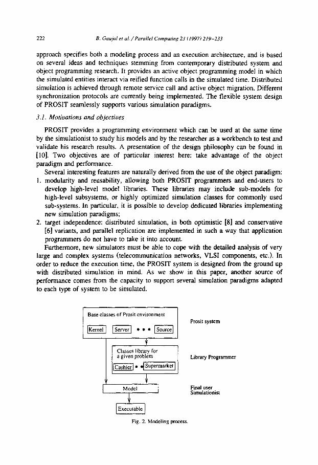
Fig. 2. Modeling process.

B. Guujul rr ol./ Purull~l Computing 23 f 1997) 219-233 223

3.2. Design issues

In this section we address simulator design as well as model design. We first describe the simulator generation process, and go on to describe the model architecture. A discussion on how to build a simulation follows.

3.2. I. Modeling process Using an object-oriented language completely defines the modeling process as being

an assembly of class instances, using dedicated class libraries and user-defined classes suited to the problem being modeled. Therefore coding a simulation consists in building the interacting entities and constructing the model by instantiating and initializing the components. The whole process is described by Fig. 2. The PROSIT framework includes the following base classes: - simulation classes used to build the simulation engine; - modeling classes used to program models.

To mask the simulation paradigm to the final user of the simulator, a library programmer defines a set of classes for a specific field of application. These classes, gathered in a library, allow a model to be built at a higher description level than the one corresponding to the simulation paradigm. For example, in the simulation of a supermar- ket, the modeler manipulates cashiers instead of FIFO servers.

3.2.2. Model architecture We have selected the process oriented approach that views the simulation in terms

of the individual entities involved, and we have decided to revert the control of execution from the server to the customer. The customers (in the usual sense of queuing networks) are active entities in the model. We call this structure the customer architec- ture in contrast to the classical passive customer approach. In particular, customers choose their path of transit in the set of servers. In a more object-oriented fashion, the user programs the customer with a body( ) method which describes the behavior of a customer of that type.

For instance, in a supermarket simulation, the objects entrance, shelves,. . . , butcher, exit being servers, the body( ) method of a customer (a supermarket client in that case) could be defined as in Fig. 3.

This inversion provides more reusability (the servers don’t have the path followed by the customers embedded within their code) and eases the collection of statistics: for instance, end-to-end and client statistics can be placed in the client itself.

PROSIT also supports the passiue customer architecture and the euent scheduling approach, and these paradigms may be easily mixed.

3.2.3. Building a simulation A PROSIT simulation can be thought of as a collection of concurrently active objects

interacting, via service calls, in the simulated time. An active object encapsulates both the specification and the behavior of the modeled entity.

The behavior of an entity consists in the internal management of services and the interactions with other active objects. Service management includes the management of

224 B. Coujul et ol./ Powllel Computing 23 f 1997) 219-233

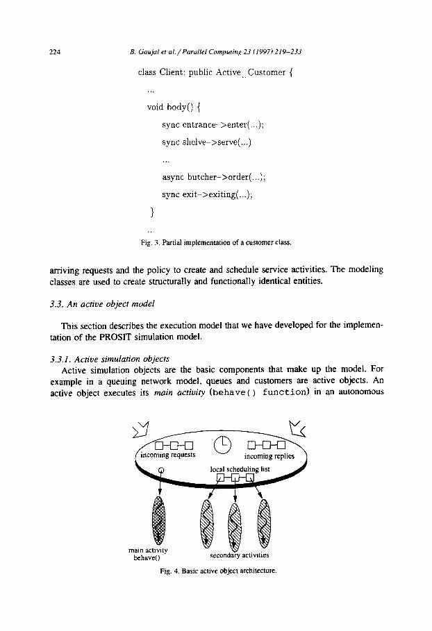
class Client: public Active_Customer {

void body0 {

sync entrance->enter(...);

sync shelve->serve(. ..)

.

async butcher->order(...);

sync exit->exiting(...);

Fig. 3. Partial implementation of a customer class.

arriving requests and the policy to create and schedule service activities. The modeling classes are used to create structurally and functionally identical entities.

3.3. An active object model

This section describes the execution model that we have developed for the implemen- tation of the PROSIT simulation model.

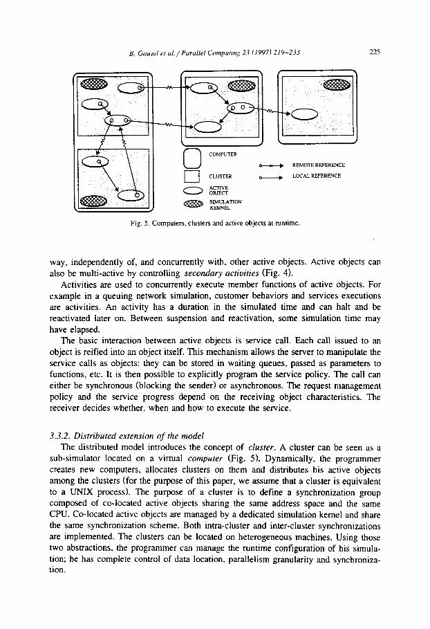
3.3.1. Active simulation objects Active simulation objects are the basic components that make up the model. For

example in a queuing network model, queues and customers are active objects. An active object executes its main activity (behave( ) function) in an autonomous

main activity behave0 secondary activilles

Fig. 4. Basic active object architecture.

B. &,UJUl rr al./ Purullel Compur~n~ 23 (19971219-233 225

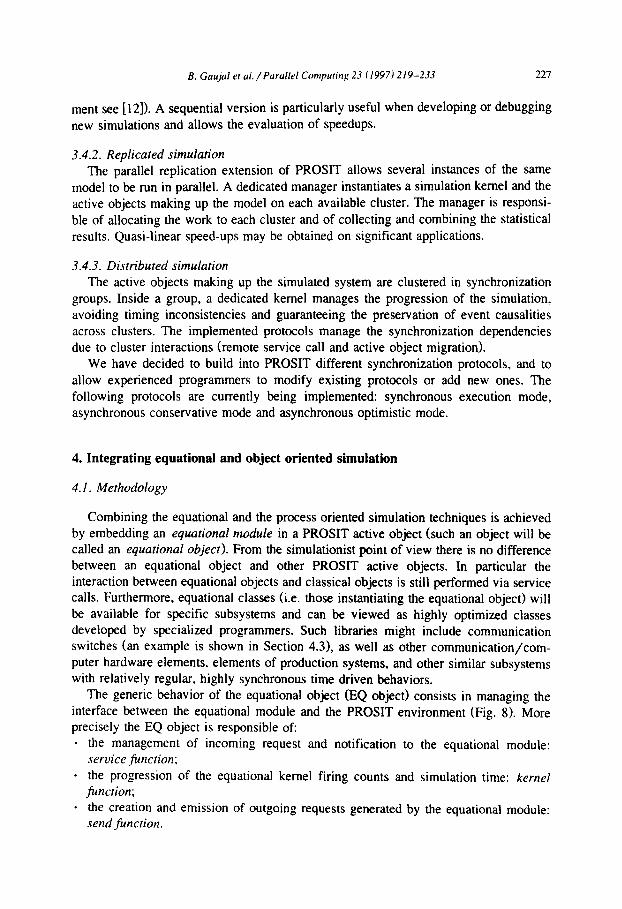
(c--*3 REMOTE REFERENCE

- LOCAL REFERENCE

B SIMULATION KERNEL

way, independently of, and concurrently with, other active objects. Active objects can also be multi-active by controlling secondary acriuiries (Fig. 4).

Fig. 5. Computers, clusters and active objects at nmtime.

Activities are used to concurrently execute member functions of active objects. For example in a queuing network simulation, customer behaviors and services executions are activities. An activity has a duration in the simulated time and can halt and be reactivated later on. Between suspension and reactivation, some simulation time may have elapsed.

The basic interaction between active objects is service call. Each call issued to an object is reified into an object itself. This mechanism allows the server to manipulate the service calls as objects: they can be stored in waiting queues, passed as parameters to functions, etc. It is then possible to explicitly program the service policy. The call can either be synchronous (blocking the sender) or asynchronous. The request management policy and the service progress depend on the receiving object characteristics. The receiver decides whether. when and how to execute the service.

3.3.2. Distributed extension of the model

The distributed mode1 introduces the concept of cluster. A cluster can be seen as a sub-simulator located on a virtual computer (Fig. 5). Dynamically, the programmer creates new computers, allocates clusters on them and distributes his active objects among the clusters (for the purpose of this paper, we assume that a cluster is equivalent to a UNIX process). The purpose of a cluster is to define a synchronization group composed of co-located active objects sharin g the same address space and the same CPU. Co-located active objects are managed by a dedicated simulation kernel and share the same synchronization scheme. Both intra-cluster and inter-cluster synchronizations are implemented. The clusters can be located on heterogeneous machines. Using those two abstractions, the programmer can manage the runtime configuration of his simula- tion; he has complete control of data location, parallelism granularity and synchroniza- tion.

226 B. Guujul rt ul./Purullel Compuring 23 (19971219-233

Computer *computer1 = new Computer(“huba”,“uranus.solar.fr”);

Computer *computer2 = new Computer(LLhop”,‘Lneptune.solar.fr”);

Cluster *cluster1 = new(Computer::current()) Cluster;

Cluster *cluster2 = new(computer2) Cluster;

Cluster *cluster3 = new(“huba”) Cluster;

Door *entrance = new Door;

Door *exit = new(cluster1) Door;

Butcher *butcher = Butcher::bind(“delicatessen”);

Fig. 6. Creation of computers, clusters and active objects.

Each active object is mapped into a cluster which can be indicated, at creation, by the programmer or selected at runtime according to a load balancing and synchronization scheme. When an active object owns a handle on another active object, it is able to invoke any of its member functions independently of the object’s location (Fig. 6).

We have also added migration capability to the active objects. During its execution, the object can explicitly migrate to another cluster by using the primitive migrate (Cluster * ) (Fig. 7). In addition to migration, the runtime system updates the context of the active object: the passive objects are copied and references on active objects are updated. The migrant object continues execution transparently, as if on its original cluster. This approach entails the migration of a requesting entity with its time-stamp to the remote cluster hosting the requested server. Major advantages of migration include load balancing, memory management, synchronization optimization and increased locality reference.

3.4. Sequential, replicated and distributed simulation

3.4.1. Sequential simulation In sequential simulation all the active

scheduled according to their logical clock

if (entrance->is_remote())

objects are located on the same cluster and (for a presentation of the sequential environ-

migratc(entrancc->get_cluster());

sync entrance->enter(...); //this is a local service call

Fig. 7. Explicit active object migration.

B. Gaujul et ul./Porullel Conrpuring 23 (1997) 219-233 221

ment see [ 121). A sequential version is particularly useful when developing or debugging new simulations and allows the evaluation of speedups.

3.4.2. Replicated simulation The parallel replication extension of PROSIT allows several instances of the same

model to be run in parallel. A dedicated manager instantiates a simulation kernel and the active objects making up the model on each available cluster. The manager is responsi- ble of allocating the work to each cluster and of collecting and combining the statistical results. Quasi-linear speed-ups may be obtained on significant applications.

3.4.3. Distributed simulation The active objects making up the simulated system are clustered in synchronization

groups. Inside a group, a dedicated kernel manages the progression of the simulation, avoiding timing inconsistencies and guaranteeing the preservation of event causalities across clusters. The implemented protocols manage the synchronization dependencies due to cluster interactions (remote service call and active object migration).

We have decided to build into PROSIT different synchronization protocols, and to allow experienced programmers to modify existing protocols or add new ones. The following protocols are currently being implemented: synchronous execution mode, asynchronous conservative mode and asynchronous optimistic mode.

4. Integrating equational and object oriented simulation

4. I. Methodology

Combining the equational and the process oriented simulation techniques is achieved by embedding an equational module in a PROSIT active object (such an object will be called an equational object). From the simulationist point of view there is no difference between an equational object and other PROSIT active objects. In particular the interaction between equational objects and classical objects is still performed via service calls. Furthermore, equational classes (i.e. those instantiating the equational object) will be available for specific subsystems and can be viewed as highly optimized classes developed by specialized programmers. Such libraries might include communication switches (an example is shown in Section 4.31, as well as other communication/com- puter hardware elements, elements of production systems, and other similar subsystems with relatively regular, highly synchronous time driven behaviors.

The generic behavior of the equational object (EQ object) consists in managing the interface between the equational module and the PROSIT environment (Fig. 8). More precisely the EQ object is responsible of: * the management of incoming request and notification to the equational module:

service function; * the progression of the equational kernel firing counts and simulation time: kernel

function; * the creation and emission of outgoing requests generated by the equational module:

send function.

228 B. Guujul et ul./Purullel Compuring 23 (1997) 219-233

ACTIVE 0 OBJECT

e EQUATIONAL OBJECT

Fig. 8. Interaction of equational objects with other objects inside PROSIT.

The main activity of an equational object will be an endless loop between these three functions, as represented in Fig. 9.

Particular behaviors of specific equational classes will differ in the nature of the subnetwork embedded into it, but also in the way the internal evolution depends on the nature of requests (in particular, the routing functions) and the nature of incoming requests it will handle and outgoing requests it will produce.

4.2. Integration overview/ inzplententation highlights

As we have seen in the previous section, the integration of an equational module to PROSIT is performed through the coding of dedicated equational classes (Fig. 9.) with a specific activity.

As we said before, the main activity is composed of three modules which are now presented in more details. Remember that an equational object evolves in discrete time. Let S be this time step. - The servicefunction is the main new feature of an EQ object. First, due to the nature

of the equational module, the equational objects can only handle asynchronous

void behave0 {

while(/*not end of simulation*/) {

deliver to equational module incom.ing requests

make equational modllle increm.ent local firin,g counts

consult equational module and generate output requests

increment equational time

wait(ti);

Fig. 9. Equational object behavior.

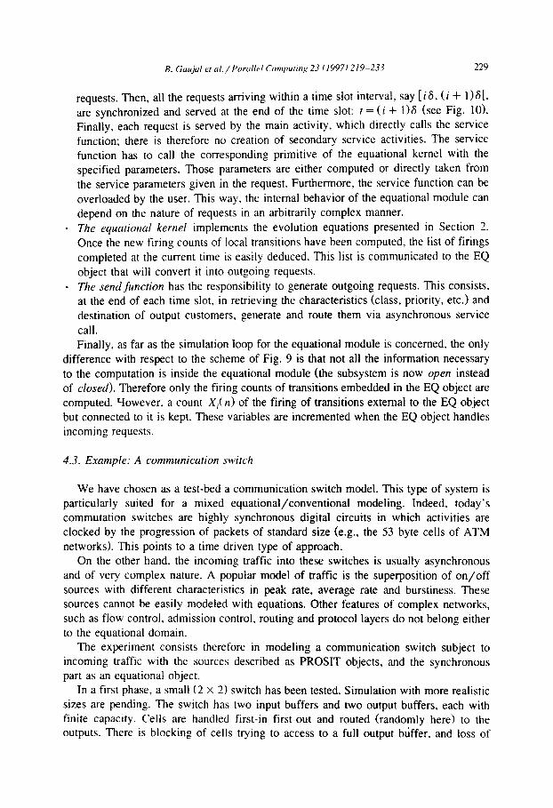
R. Guujul et 01. / Portrllel Computtn~ 23 (lY97J 219-233 229

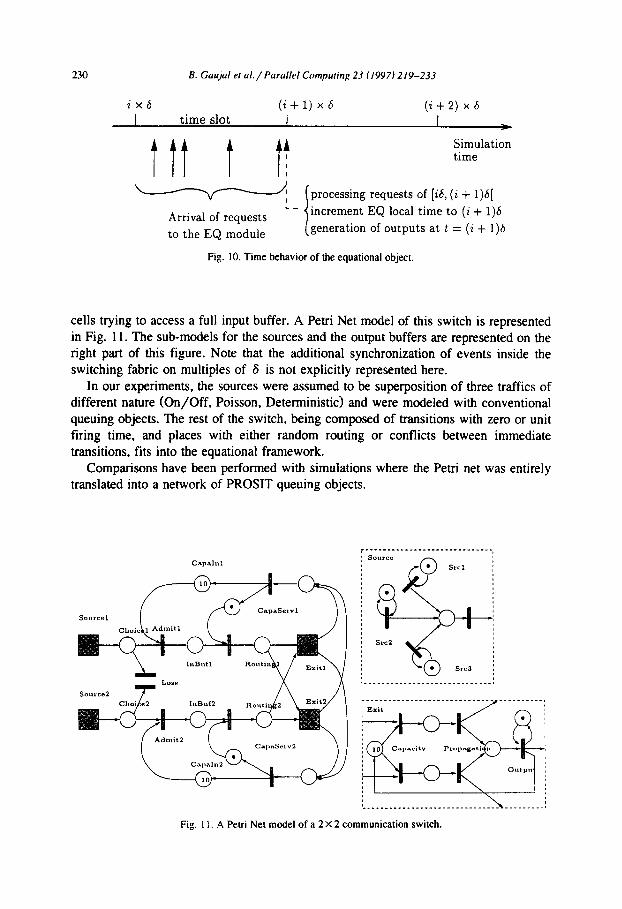
requests. Then, all the requests arrivin, 0 within a time slot interval, say [is, (i + l)S[, are synchronized and served at the end of the time slot: t = (i + 1)s (see Fig. 10). Finally, each request is served by the main activity, which directly calls the service function; there is therefore no creation of secondary service activities. The service function has to call the corresponding primitive of the equational kernel with the specified parameters. Those parameters are either computed or directly taken from the service parameters given in the request. Furthermore, the service function can be overloaded by the user. This way, the internal behavior of the equational module can depend on the nature of requests in an arbitrarily complex manner.

. The equarional kernel implements the evolution equations presented in Section 2. Once the new firing counts of local transitions have been computed, the list of firings completed at the current time is easily deduced. This list is communicated to the EQ object that will convert it into outgoing requests.

* The send&n&m has the responsibility to generate outgoing requests. This consists, at the end of each time slot, in retrieving the characteristics (class, priority, etc.) and destination of output customers, c oenerate and route them via asynchronous service call. Finally, as far as the simulation loop for the equational module is concerned, the only

difference with respect to the scheme of Fig. 9 is that not all the information necessary to the computation is inside the equational module (the subsystem is now open instead of closed). Therefore only the firing counts of transitions embedded in the EQ object are computed. Yowever, a count X,(n) of the firing of transitions external to the EQ object but connected to it is kept. These variables are incremented when the EQ object handles incoming requests.

4.3. Example: A communication switch

We have chosen as a test-bed a communication switch model. This type of system is particularly suited for a mixed equational/conventional modeling. Indeed. today’s commutation switches are highly synchronous digital circuits in which activities are clocked by the progression of packets of standard size (e.g., the 53 byte cells of ATM networks). This points to a time driven type of approach.

On the other hand. the incoming traffic into these switches is usually asynchronous and of very complex nature. A popular model of traffic is the superposition of on/off sources with different characteristics in peak rate, average rate and burstiness. These sources cannot be easily modeled with equations. Other features of complex networks, such as flow control, admission control, routing and protocol layers do not belong either to the equational domain.

The experiment consists therefore in modeling a communication switch subject to incoming traffic with the sources described as PROSIT objects, and the synchronous part as an equational object.

In a first phase, a small (2 X 2) switch has been tested. Simulation with more realistic sizes are pending. The switch has two input buffers and two output buffers, each with finite capacity. Cells are handled first-in first-out and routed (randomly here) to the outputs. There is blocking of cells trying to access to a full output buffer, and loss of

230 6. Guujul er ul./ Purullrl Computing 23 f 1997) 219-233

ix6 (i + 1) x 6 (i+2) x6

ttt t Tt Simulation time

processing requests of [i6, (i + 1)6[

Arrival of requests increment EQ local time to (i + 1)6

to the EQ module generation of outputs at t = (i + 1)6

Fig. IO. Time behavior of the equational object.

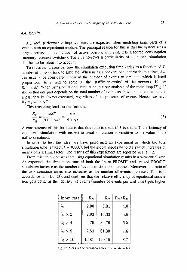
cells trying to access a full input buffer. A Petri Net model of this switch is represented in Fig. 11. The sub-models for the sources and the output buffers are represented on the right part of this figure. Note that the additional synchronization of events inside the switching fabric on multiples of 6 is not explicitly represented here.

In our experiments, the sources were assumed to be superposition of three traffics of different nature (On/Off, Poisson, Deterministic) and were modeled with conventional queuing objects. The rest of the switch, being composed of transitions with zero or unit firing time, and places with either random routing or conflicts between immediate transitions, fits into the equational framework.

Comparisons have been performed with simulations where the Petri net was entirely translated into a network of PROSIT queuing objects.

Fig. I 1. A Petri Net model of a 2 X 2 communication switch.

231 B. Guujul er al. / Porollel Compufinx 23 (1997) 219-233

4.4. Results

A priori, performance improvements are expected when modeling large parts of a system with an equational module. The principal reason for this is that the system sees a large decrease in the number of active objects, implying less resource consumption (memory, context switches). There is however a particularity of equational simulation that has to be taken into account.

To illustrate it, consider how the simulation execution time varies as a function of T, number of units of time to simulate. When using a conventional approach, this time, R,,

can usually be considered linear in the number of events to simulate, which is itself proportional to T and to some A, the ‘traffic intensity’ of the network. Hence: R, = ahT. When using equational simulation, a close analysis of the main loop (Fig. 1) shows that one part depends on the total number of events as above, but also that there is a part that is always executed, regardless of the presence of events. Hence, we have R, = PAT + yT.

This reasoning leads to the formula:

RC CXhT ffh =-

R,=pT+yAT P+yA’ (3)

A consequence of this formula is that this ratio is small if A is small. The efficiency of equational simulation with respect to usual simulation is sensitive to the value of the traffic simulated.

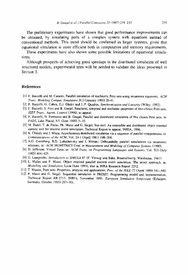
In order to test this idea, we have performed an experiment in which the total simulation time is fixed (T = lOOOO>, but the global input rate to the switch increases by means of a scaling factor. The results of this experiment are reported in Fig. 12.

From this table, one sees that using equational simulation results in a substantial gain. As expected, the simulation time of both the ‘pure PROSIT’ and ‘mixed PROSIT’ simulators increase as the number of events to simulate increases. Moreover, the ratio of the two execution times also increases as the number of events increases. This is in accordance with Eq. (3), and confirms that the relative efficiency of equational simula- tion gets better as the ‘density’ of events (number of events per unit time) gets higher.

Input rate RE Rc &IRE

2.00 8.01 4.0

2.93 16.33 5.6

4.70 30.76 6.0

7.80 61.30 7.6

13.81 120.16 8.7

Fig. 12. Measures of execution times of simulations (s).

232 B. Goujul er (11. / Purullcl Compuring 23 (1997) 219-233

5. Parallelization

The distributed version of PROSIT being currently in beta-testing, we were unable to perform a full evaluation of combined asynchronous distributed executions. Neverthe- less, we are optimistic of achieving good speedups for the following reasons: * The equational objects are directly integrated in the distributed simulation framework

of PROSIT; at execution time, they will be mapped on available clusters. Early experiments of queuing networks simulations, with the distributed prototype, give positive results.

- In many simulations it will be possible, when setting the model architecture and the active objects mapping, to have a feed-forward system at the cluster level. Simulating feed-forward systems requires almost no synchronization overhead.

- Likewise, the computation of statistics can be separated from the simulation itself, and distributed with minimal synchronization requirements. This is the principle of the companion package STAT-TOOL we are developing 151.

- Distributed equational simulation using Eq. (2) is not efficient unless the granularity of sub-models and the grouping of objects is well chosen [4]. And as we have seen (Section 3.3.2). PROSIT gives complete control of parallelism granularity and data location.

* Also, the choice of a proper time scale for equational object is an important issue: as we have seen in the previous section, if the ‘clock’ of the object is too fast compared to the pace of the rest of the network, it is inefficient. Grouping objects with respect to their time scale and distributing them may be a good source of improvements. On the other hand, the equational objects have certain properties that may make them

compatible with the common mechanisms of distributed simulation. Concerning conser- vative simulation, one remarks that the discrete time nature of these systems allows the computation of the minimum time between an input event and its first output conse- quence. This time may be used as lookahead. As for optimistic simulation, the main problem is the management of rollback. The

equational engine uses table of event dates as its basic data structure. From these tables, it is possible to reconstruct the trajectory of the system in the past, including all the events sent to the outside of the equational part. Therefore, the principal ingredients for being able to roll back in time and undoin, 0 what has been done in the meantime, are already present. The amount of memory necessary is directly proportional to the amount of time the object can go back, and the frequency of checkpoints (global synchroniza- tions) and the number of objects embedded in the equational module.

6. Conclusion

We have demonstrated how the flexible concept of PROSIT allows the integration of simulators of different nature. This work is the first validation of the idea that our approach to the design of complex simulators gives the possibility to re-use existing simulators, by embedding them in a suitable PROSIT object.

B. Guujul et ul. / Purullel CO~~UIIII,~ 23 (19971 219-233 233

The preliminary experiments have shown that good performance improvements can be obtained, by simulating parts of a complex system with equations instead of conventional methods. This trend should be confirmed in larger systems. given that equational simulation is more efficient both in computation and memory requirements.

These experiments have also shown some possible limitations of equational simula- tions.

Although prospects of achievin g good speedups in the distributed simulation of well structured models, experimental tests will be needed to validate the ideas presented in Section 5.

References

[I] F. Baccelli and M. Canales. Parallel simulation of stochastric Petri nets using recurrence equations, ACM

Truns. Modding Compuf. Simuhrion 3( I) (January 1993) 20-41.

[2] F. Baccelli. G. Cohen, G.J. Olsder and J.-P. Quadrat, Synchmni:ucrtion utul Lineuriry (Wiley. 1992).

[3] F. Baccelli, S. Foss and B. Gaujal, Structural, temporal and stochastic properties of free-choice Petri nets,

IEEE Truns. Autom. Control ( 1996). to appear.

(41 F. Baccelli, N. Furmento and B. Gaujal, Parallel and distributed simulation of free choice Petri nets, in:

PADS, Lake Placid, NY (June 1995) 3-10.

151 M. Badel. T. de Pretto, Ph. Mussi and G. Siegel, Stat-tool: An extensible and distributed object oriented

statistic tool for discrete event simulation. Technical Report to appear, INRIA, 1996.

[6] K. Chandy and J. Misra, Asynchronous distributed simulation via a sequence of parallel computations. in,

Communicurion.\ r!f rhe ACM, Vol. 24-l (April 198 I) 198-206.

[7] A.G. Greenberg, B.D. Lubachevsky and 1. Mitrani, Unboundedly parallel simulations via recurrence

relations, in: ACM SIGMETRICS Conj: in Meusuremenr unrl Modeling c$ Cornpurer Sysfem.~ ( 1990).

181 D. Jefferson, Virtual Time, in: ACM Truns. on Propmvnin~ Lunptugcs unrl Sysrem.s. Vol. 7(3) (July

1985) 404-425.

[9] G. Lamprecht. Introduction 10 SIMUU 67 (F. Vieweg und Sohn, Braunschweig, Wiesbaden, 1981).

[IO] L. Mallet and P. Mussi, Object oriented parallel discrete event simulation: The prosit approach, in:

Modelling U& Simulation, Lyon (June 1993). also in INRA Research Report 2232.

[I 11 T. Murata. Petri nets: Propenies. analysis and applications, Pruc. of‘rhr lEEE 77 (April 1989) 54 I -580. [I21 P. Mussi and G. Siegel, Sequential simulation in PROSIT: Programming model and implementation,

Technical Report RR-27 I.?, INRIA. November 1995; Europrun Simukurion Sympo.\ium (Erlanzen.

Germany, October 1995) 297-301.