
High-level Estimation and Exploration of Reliability for MPSoC
208
High-level Estimation and Exploration of Reliability for Multi-Processor System-on-Chip Von der Fakultät für Elektrotechnik und Informationstechnik der Rheinisch–Westfälischen Technischen Hochschule Aachen zur Erlangung des akademischen Grades eines Doktors der Ingenieurwissenschaften genehmigte Dissertation vorgelegt von M. Sc. Zheng Wang aus Tianjin, China Berichter: Universitätsprofessor Dr.-Ing. Anupam Chattopadhyay Universitätsprofessor Dr.-Ing. Tobias G. Noll Tag der mündlichen Prüfung: 02.12.2015 Diese Dissertation ist auf den Internetseiten der Hochschulbibliothek online verfügbar.
-
Upload
khangminh22 -
Category
Documents
-
view
0 -
download
0
Transcript of High-level Estimation and Exploration of Reliability for MPSoC

High-level Estimation and Exploration of Reliability forMulti-Processor System-on-Chip
Von der Fakultät für Elektrotechnik und Informationstechnikder Rheinisch–Westfälischen Technischen Hochschule Aachen
zur Erlangung des akademischen Gradeseines Doktors der Ingenieurwissenschaften
genehmigte Dissertation
vorgelegt vonM. Sc. Zheng Wangaus Tianjin, China
Berichter: Universitätsprofessor Dr.-Ing. Anupam Chattopadhyay
Universitätsprofessor Dr.-Ing. Tobias G. Noll
Tag der mündlichen Prüfung: 02.12.2015
Diese Dissertation ist auf den Internetseitender Hochschulbibliothek online verfügbar.


Acknowledgements
This thesis is the result of my work as research assistant at the Institute for Commu-nication Technologies and Embedded Systems (ICE) at the RWTH Aachen University.During this time I have been accompanied and supported by many people. It is mygreat pleasure to take this opportunity to thank them.
My most sincere thanks go to my advisors, Prof. Anupam Chattopadhyay andProf. Tobias Noll. Anupam has been extremely helpful and tremendously inspiringthroughout my PhD study. Prof. Noll has been impressively knowledgeable while pa-tient with my ideas and mistakes. Their thoughtful advices have greatly contributedto this work and influenced me for my future career.
Special thanks go to my defense committee members, Prof. Andrei Vescan andProf. Renato Negra for spending their time, offering oral exam, giving me feedback,and attending my defense session.
Several colleagues in ICE and EECS have assisted and encouraged me duringthe past five years for my work and personal life. Among them I would like toshow my deep appreciation to Ayesha Khalid, Zoltán Rákossy and Michael Meixner.Furthermore, I would like to thank my students Xiao Wang, Chao Chen, Lai Wang,Renlin Li, Hui Xie, Liu Yang, Saumitra Chafekar, Alessandro Littarru, Shazia Kanwal,Kolawole Soretire, Emmanuel Ugwu, Dan Yue, Kapil Singh, Piyush Sharma and SaiRama Usha Ayyagari for their consistent contribution.
I would also like to thank my family: My parents and parents-in-law for support-ing me spiritually throughout writing this thesis and my life in general. And finally,infinite gratitude to my beloved wife as well as my son.
Zheng Wang, in February 2016


Abstract
Continuous technology scaling in semiconductor industry forces reliability as a seri-ous design concern in the era of nanoscale computing. Traditional device and circuitlevel reliability estimation and error mitigation techniques neither address the hugedesign complexity of modern system nor consider architecture and system-level errormasking properties. An alternative approach is to accept and expose the unreliabil-ity to all layers of computing and possibly mitigate the errors with device-, circuit-,architectural or software techniques. To enable cross-layer exploration of reliabilityagainst other performance constraints, it is essential to accurately model the errorsin nanoscale technology and develop a smooth tool-flow at high-level design abstrac-tions so that error effects can be estimated, which assists the development of high-levelfault-tolerant techniques. In this dissertation, a high-level reliability estimation andexploration framework for MPSoC is developed.
To estimate reliability at early design stages, a high-level fault simulation frame-work is constructed for generic architecture models and integrated into a commercialprocessor design environment. The fault injector is further extended for system-levelmodules. A power/thermal/timing error co-simulation framework is demonstratedfor integrating fault injection with simulation of physical properties. To further speedup reliability estimation, an analytical method is proposed to calculate vulnerabilityof individual logic blocks, from which application level error probabilities are de-duced. A formal technique is introduced to predict error effects by tracking errorpropagation. Finally, design diversity metric is utilized to quantify the robustness ofredundancy in system-level computing elements.
The contributions in reliability exploration include several novel architectural fault-tolerant techniques. Opportunistic redundancy detects errors by re-executing theinstructions only if there are underutilized resources. Asymmetric redundancy un-equally protects memory elements based on criticality analysis of data and instruc-tions. Error confinement replaces any erroneous result with the best available esti-mate from statistical characteristics. For system-level fault tolerance, a core reliability-aware task mapping algorithm is demonstrated on a heterogeneous multiprocessorplatform. A theoretical approach to construct ad-hoc fault tolerant network for arbi-
5

6
trary task graph with optimal amount of connecting edges is elaborated and verifiedby exhaustive search based algorithm.
The methodologies proposed in this dissertation are going to be critical for fu-ture semiconductor technology nodes, where reliability is going to be a permanentproblem. Further research directions are outlined to take this research forward.

Contents
1 Introduction 1
1.1 Contribution . . . . . . . . . . . . . . . . . . . . . . . . . . . . . . . . . . . 2
1.2 Outline . . . . . . . . . . . . . . . . . . . . . . . . . . . . . . . . . . . . . . 4
2 Background 5
2.1 Reliability Definition . . . . . . . . . . . . . . . . . . . . . . . . . . . . . . 5
2.2 Fault, Error and Failure . . . . . . . . . . . . . . . . . . . . . . . . . . . . 5
2.3 Hardware Faults . . . . . . . . . . . . . . . . . . . . . . . . . . . . . . . . . 6
2.3.1 Origins . . . . . . . . . . . . . . . . . . . . . . . . . . . . . . . . . . 6
2.3.2 Fault Models . . . . . . . . . . . . . . . . . . . . . . . . . . . . . . . 8
2.4 Soft Error . . . . . . . . . . . . . . . . . . . . . . . . . . . . . . . . . . . . . 8
2.4.1 Evaluation Metrics . . . . . . . . . . . . . . . . . . . . . . . . . . . 8
2.4.2 Scaling Trends . . . . . . . . . . . . . . . . . . . . . . . . . . . . . . 9
3 Related Work 11
3.1 Fault Injection and Simulation . . . . . . . . . . . . . . . . . . . . . . . . . 11
3.1.1 Physical Fault Injection . . . . . . . . . . . . . . . . . . . . . . . . . 11
3.1.2 Simulated Fault Injection . . . . . . . . . . . . . . . . . . . . . . . 12
3.1.3 Emulated Fault Injection . . . . . . . . . . . . . . . . . . . . . . . . 15
3.2 Analytical Reliability Estimation . . . . . . . . . . . . . . . . . . . . . . . 16
3.2.1 Architecture Vulnerability Factor Analysis . . . . . . . . . . . . . 16
3.2.2 Probablistic Transfer Matrix . . . . . . . . . . . . . . . . . . . . . . 17
3.2.3 Design Diversity Estimation . . . . . . . . . . . . . . . . . . . . . . 18
3.3 Architectural Fault-tolerant Techniques . . . . . . . . . . . . . . . . . . . 19
3.3.1 Traditional Fault-tolerant Techniques . . . . . . . . . . . . . . . . 19
i

ii CONTENTS
3.3.2 Approximate Computing . . . . . . . . . . . . . . . . . . . . . . . 22
3.4 System-level Fault Tolerant Techniques . . . . . . . . . . . . . . . . . . . 26
3.4.1 Reliability-aware Task Mapping . . . . . . . . . . . . . . . . . . . 26
3.4.2 Fault-tolerant Network Design . . . . . . . . . . . . . . . . . . . . 27
4 High-level Fault Injection and Simulation 29
4.1 Architectural Fault Injection . . . . . . . . . . . . . . . . . . . . . . . . . . 29
4.1.1 Methodologies . . . . . . . . . . . . . . . . . . . . . . . . . . . . . . 30
4.1.2 LISA-based Fault Injection . . . . . . . . . . . . . . . . . . . . . . . 32
4.1.3 Timing Fault Injection . . . . . . . . . . . . . . . . . . . . . . . . . 37
4.1.4 Experimental Results . . . . . . . . . . . . . . . . . . . . . . . . . . 39
4.1.5 Summary . . . . . . . . . . . . . . . . . . . . . . . . . . . . . . . . . 44
4.2 System-level Fault Injection . . . . . . . . . . . . . . . . . . . . . . . . . . 44
4.2.1 Fault injection for system modules . . . . . . . . . . . . . . . . . . 45
4.2.2 Experimental results . . . . . . . . . . . . . . . . . . . . . . . . . . 46
4.2.3 Summary . . . . . . . . . . . . . . . . . . . . . . . . . . . . . . . . . 48
4.3 High-level Processor Power/Thermal/Delay Joint Modelling Framework 49
4.3.1 High-level Power Modeling and Estimation . . . . . . . . . . . . . 50
4.3.2 LISA-based Thermal Modeling . . . . . . . . . . . . . . . . . . . . 59
4.3.3 Thermal-aware Delay Simulation . . . . . . . . . . . . . . . . . . . 63
4.3.4 Automation Flow and Overhead Analysis . . . . . . . . . . . . . . 67
4.3.5 Summary . . . . . . . . . . . . . . . . . . . . . . . . . . . . . . . . . 69
5 Architectural Reliability Estimation 71
5.1 Analytical Reliability Estimation Technique . . . . . . . . . . . . . . . . . 71
5.1.1 Operation Reliability Model . . . . . . . . . . . . . . . . . . . . . . 72
5.1.2 Instruction Error Rate . . . . . . . . . . . . . . . . . . . . . . . . . 73
5.1.3 Application Error Rate . . . . . . . . . . . . . . . . . . . . . . . . . 74
5.1.4 Analytical Reliability Estimation for RISC Processor . . . . . . . . 75
5.1.5 Summary . . . . . . . . . . . . . . . . . . . . . . . . . . . . . . . . . 77
5.2 Probabilistic Error Masking Matrix . . . . . . . . . . . . . . . . . . . . . . 78
5.2.1 Logic Masking in Digital Circuits . . . . . . . . . . . . . . . . . . . 80
5.2.2 PeMM for Processor Building Blocks . . . . . . . . . . . . . . . . . 81

CONTENTS iii
5.2.3 PeMM Characterization . . . . . . . . . . . . . . . . . . . . . . . . 84
5.2.4 Approximate Error Prediction Framework . . . . . . . . . . . . . 86
5.2.5 Results in Error Prediction . . . . . . . . . . . . . . . . . . . . . . . 89
5.2.6 Summary . . . . . . . . . . . . . . . . . . . . . . . . . . . . . . . . . 93
5.3 Reliability Estimation using Design Diversity . . . . . . . . . . . . . . . . 94
5.3.1 Design Diversity . . . . . . . . . . . . . . . . . . . . . . . . . . . . 95
5.3.2 Graph-based Diversity Analysis . . . . . . . . . . . . . . . . . . . 97
5.3.3 Results in Diversity Estimation . . . . . . . . . . . . . . . . . . . . 103
5.3.4 Summary . . . . . . . . . . . . . . . . . . . . . . . . . . . . . . . . . 107
6 Architectural Reliability Exploration 109
6.1 Opportunistic Redundancy . . . . . . . . . . . . . . . . . . . . . . . . . . 109
6.1.1 Opportunistic Protection . . . . . . . . . . . . . . . . . . . . . . . . 110
6.1.2 Implementation . . . . . . . . . . . . . . . . . . . . . . . . . . . . . 112
6.1.3 Experimental Results . . . . . . . . . . . . . . . . . . . . . . . . . . 117
6.1.4 Summary . . . . . . . . . . . . . . . . . . . . . . . . . . . . . . . . . 121
6.2 Processor Design with Asymmetric Reliability . . . . . . . . . . . . . . . 122
6.2.1 Asymmetric Reliability . . . . . . . . . . . . . . . . . . . . . . . . . 123
6.2.2 Asymmetric Reliability Exploration . . . . . . . . . . . . . . . . . 126
6.2.3 Summary . . . . . . . . . . . . . . . . . . . . . . . . . . . . . . . . . 133
6.3 Approximate Computing with Statistical Error Confinement . . . . . . . 134
6.3.1 Proposed Error Confinement Method . . . . . . . . . . . . . . . . 135
6.3.2 Realizing the Proposed Error Confinement in a RISC Processor . 136
6.3.3 Case Study and Statistical Analysis . . . . . . . . . . . . . . . . . 138
6.3.4 Results . . . . . . . . . . . . . . . . . . . . . . . . . . . . . . . . . . 140
6.3.5 Summary . . . . . . . . . . . . . . . . . . . . . . . . . . . . . . . . . 144
7 System-level Reliability Exploration 147
7.1 System-level Reliability Exploration Framework . . . . . . . . . . . . . . 147
7.1.1 Platform and Task Manager Firmware . . . . . . . . . . . . . . . . 148
7.1.2 Core Reliability Aware Task Mapping . . . . . . . . . . . . . . . . 151
7.1.3 Experimental Results . . . . . . . . . . . . . . . . . . . . . . . . . . 153
7.1.4 Summary . . . . . . . . . . . . . . . . . . . . . . . . . . . . . . . . . 156

iv CONTENTS
7.2 Reliable System-level Design using Node Fault Tolerance . . . . . . . . . 156
7.2.1 Node Fault Tolerance in Graph . . . . . . . . . . . . . . . . . . . . 157
7.2.2 Construct NFT for Arbitrary Graph . . . . . . . . . . . . . . . . . 158
7.2.3 Verify NFT Graphs using Task Mapping . . . . . . . . . . . . . . 160
7.2.4 Experiments for Node Fault Tolerance . . . . . . . . . . . . . . . . 163
7.2.5 Summary . . . . . . . . . . . . . . . . . . . . . . . . . . . . . . . . . 164
8 Conclusion and Outlook 167
8.1 Conclusion . . . . . . . . . . . . . . . . . . . . . . . . . . . . . . . . . . . . 167
8.2 Outlook . . . . . . . . . . . . . . . . . . . . . . . . . . . . . . . . . . . . . . 168
Glossary 171
List of Figures 175
List of Tables 179
Bibliography 181

Chapter 1
Introduction
The last few decades have witnessed continuous scaling of CMOS technology, guidedby Moore’s Law [133], to support devices with higher speed, less area and less power.Though there have been varying arguments on how long the scaling can be continued,it is undisputed that there is a reach of classical physics on supporting determinis-tic circuit behavior, which is limited by the thickness of an atom. The current sub-micron CMOS technology generation is already facing several challenges, resulting ina broad class of problems known as reliability. According to International TechnologyRoadmap for Semiconductors (ITRS) [11], reliability and resilience across all designlayers constitute a long-term grand challenge.
Reliability is influenced by several trends. First, soft errors caused by external ra-diation are increasingly reported, even at ground conditions [53]. Second, increasingpower dissipation leads to thermal stress which affects design lifetime as well as softerror rates [37]. Third, continuous technology scaling gives rise to increased perma-nent errors caused by process variation [183]. Fourth, frequency and voltage over-scaling targeting timing margin exploration save power and performance budgets butalso introduce timing errors [57]. Finally, new kinds of innovative fault-based attacksagainst cryptographic modules [175] make fault-tolerant design important. Besides,fault tolerance is always mandatory for safety-critical application domains such asaerospace, biomedical, automotive and infrastructure.
The effects of reliability challenges can only be accurately modelled at low levelsof design abstractions. For instance, at device level the the vulnerability of a tran-sistor against striking particles is analysed according to its physical properties. Thedeviation on the threshold voltage caused by process variation and temperature shiftis evaluated by diffusion effects of chemical elements. At circuit level the genera-tion, propagation and attenuation of the transient current pulse are simulated usingSPICE. However, despite its accuracy, low level reliability analysis and simulationare extremely time consuming which can not address the huge design complexity ofmodern computing system with hundreds of computing elements.
Furthermore, error mitigation techniques at low levels ignore the architectural andapplication-level error masking abilities which result in conservative design choicesaffecting performance. An alternative approach is to accept and expose the unreli-ability to all the layers of computing and mitigate the error effects with high-leveltechniques. For example, an aggressive voltage scaling of the device may lead tohigher runtime performance at the cost of timing errors, which can be corrected byarchitectural techniques [57]. An uncorrected data error representing the color of apixel in an image can be intrinsically tolerated by the limit of human perception [17].
1

2 Chapter 1. Introduction
ApplicationsApplications
Faults
Config
Faults
Config
Instruction &
Application
Error Rates
Instruction &
Application
Error Rates
Approximate
Error
Prediction
Approximate
Error
Prediction
Design Diversity
Analyzer
Design Diversity
Analyzer
System
Mean-time-to-
Failure
System
Mean-time-to-
Failure
Processor
Model
(SystemC)
Processor
Model
(SystemC)
L H L
L L L
L L L
L L L
L
L
L
L
Heterogeneous SoC
with mixed reliability
MPSoC Task,
Mapping
Heuristics
MPSoC Task,
Mapping
Heuristics
Fault Injection Reliability Estimation
Speed &
Accuracy
Benchmarking
Speed &
Accuracy
Benchmarking
Fault Tracking
Engine
Fault Tracking
Engine
Analytical
Analyzer
Analytical
Analyzer
ISS/RTL with
Fault Injection
ISS/RTL with
Fault Injection
Reliability Exploration
System-level Exploration
Processor
Description
(ADL)
Processor
Description
(ADL)
Architecture Exploration
Graphical
Interface
Graphical
Interface
User
Defined
Faults
User
Defined
Faults
Configurable
Faults
Timing
Analysis
Timing
Analysis
Timing
Variation
Fuction
Timing
Variation
Fuction
Delay Faults
Thermal
Estimation
Thermal
Estimation
FloorplanFloorplan
Reliable
Network
Topology
Reliable
Network
Topology
Power
Modeling
Power
Modeling
Bit Error
Rate
Bit Error
Rate
Task ManagerTask Manager
Autmatic
Generation
Autmatic
Generation
Opportunism;
Asymmetry;
Approximation
Figure 1.1: Overall flow of high-level reliability estimation and exploration
1.1 Contribution
A key ingredient of successful cross-layer exploration of reliability against other per-formance constraints (e.g. power, temperature, speed) is to accurately model the er-rors in nanoscale technology and develop a smooth tool-flow at high-level design lay-ers to estimate error effects, which assists the development of high-level fault-toleranttechniques. In this thesis, multiple challenges for developing the reliability-estimationand exploration framework are tackled. Figure 1.1 shows the overall flow with de-tailed discussion on individual blocks in the following.
• High-level Fault Injection and SimulationFault injection, which is an important setup for reliability exploration, is dis-cussed in Chapter 4. Section 4.1 presents the fault injection tool for genericcycle-accurate architecture models which has been integrated into commercialprocessor design framework. The faults can be injected at both combinationallogic and memory cells while achieve similar accuracy as state-of-the-art RTLfault injection. Two modes of fault injection are supported. In the configurablemode, faults are defined based on user’s configuration through graphical inter-face. In the timing mode, logic delay faults are injected based on the statisticsfrom low level timing analysis and variation function. In Section 4.2 the faultinjector is extended for system-level modules described in SystemC language.An interesting case study is to relate delay faults injection with power consump-tion and runtime temperature variation, while the co-simulation framework forpower, temperature and delay faults is proposed in Section 4.3.

1.1. Contribution 3
• High-level Reliability EstimationArchitectural reliability can be fast estimated through analytical methods, whichare discussed in Chapter 5. Section 5.1 presents an analytical estimation tech-nique based on graph representation of processor architecture. The vulnerabilityand logic masking capability of vertexes in the graph representing logic blockscan be fast characterized. The edges in the graph which link the vertexes directthe estimation of instruction and application-level error probability. In Section5.2 such analytical method is further extended as a formal algorithmic approachto predict error effects by tracking error propagation and attenuation in a graphnetwork representing dynamic processor behavior. A different reliability es-timation technique is proposed in Section 5.3 to quantify the robustness of aredundant system against common mode failure using design diversity. As-sisted by a graph indicating exclusiveness information of architecture modules,the approach quantifies the potential of fault tolerance for different computingelements using MTTF metric.
• Architectural Reliability ExplorationThree novel architectural fault-tolerant techniques are proposed in Chapter 6.The first technique, named as opportunistic redundancy in Section 6.1, intro-duces a passive error detection policy for algorithmic units by re-executingthe instruction only if there exists underutilized resources, which incurs verysmall performance penalty. The approach is benchmarked with aggressive pol-icy where all instructions are double executed to verify the correctness of results.The second technique, named as asymmetric redundancy in Section 6.2, presentsan unequal error protection technique for storage elements based on criticalityanalysis. Different schemes of asymmetric protection are investigated for in-struction and data words, with static or dynamic criticality assignment. Thelast technique, named as error confinement in Section 6.3, exploits the statisti-cal characteristics of any target application and replaces any erroneous data inmemory with the best available approximation of that data rather than correct-ing every single error. All techniques are demonstrated on embedded processorswith customized architecture extension.
• System-level Reliability ExplorationIn Chapter 7 fault tolerant techniques in system-level design are presented whichfocus on reliability-aware task mapping and reliable network design. Section 7.1introduces a heuristic task mapping algorithm which jointly considers task reli-ability requirement and core reliability level. The mapping technique is demon-strated on a heterogeneous multiprocessor platform with customized firmwarelayer for fault injection, topology exploration and task management. Section 7.2presents a theoretical approach to construct ad-hoc fault tolerant network forarbitrary task graph, which contains an optimal amount of connecting edges.Exhaustive search based graph verification algorithm is demonstrated and realworld tasks are applied to show the generic feature of proposed technique.

4 Chapter 1. Introduction
1.2 Outline
The dissertation is organized as following. Chapter 2 presents the background ofrecent reliability issues. Chapter 3 provides a summary on the related work of relia-bility estimation and exploration. Chapter 4 describes the fault injection frameworkwhich targets both architectural and system-level design. Chapter 5 elaborates severalreliability estimation techniques for architecture components. Chapter 6 concentrateson different fault tolerant techniques for error resilience in architecture level. Chapter7 illustrates proposed system-level techniques enhancing reliability. The conclusionand outlook of this dissertation are presented in Chapter 8.

Chapter 2
Background
In this chapter, fundamental knowledge on reliability are discussed, including relia-bility definition, fault classification and fault models. In the next soft error and itsevaluation metrics are elaborated, which is heavily used in the following chapters.
2.1 Reliability Definition
Reliabilty is in a broad sense one attribute of dependability, which describes the abilityof the system to deliver its intended service [51]. Reliability measures the capabilityof continuous delivery of correct service. Formally, reliability R(t) at time instance tdefines the probability that system performs without failure in time range [0, t], pro-vided that system functions correctly at time 0. Reliability is a function of time, wherelonger time will reduce the system reliability. Another attribute of dependabilities isavailability. Availability A(t) defines the probability that system performs correctlyat time t, which is often used when occurrence of failures is tolerated. For instance,system down time per year in network application is a measure of availability, sinceshort failure time in network is allowed by the users.
2.2 Fault, Error and Failure
The definition of reliability shows its strong relationship with failure, which indicatesthe occurrence of unexpected behavior of a system. The definition of failure differswith the scope of the system. In a software system, the failure can be defined as awrong value in the program outputs. In a hardware system such as the architecture ofa processor, the failure can be interpreted as a mismatch value of the values stored intomemories. Generally, failure is strong correlated with the system under discussion.
Error is a wrong value during computation, which is the cause of failure. Forinstance, error can be viewed from architecture perspective as a logic value whichdiffers the state of the circuits from the correct one. Explicitly, an error occurs whenthe sequential logic of the circuits exhibits an unexpected value. The sequential logicincludes register file and pipeline registers. Not all errors lead to failure. For instance,the erroneous values in register file is overwritten before stored into the data memory.An error in the pipeline register can be ignored when the computation never uses suchoperand. Generally, errors can result in different effects, such as benign fault, SilentData Corruption (SDC), Detected Unrecoverable Error (DUE) and system crash. Theauthor in [204] illustrates various system-level effects of error.
5

6 Chapter 2. Background
Fault from hardware perspective is the physical defect or temporal malfunctions,which is the cause of error. Fault can be also defined from software perspectivesuch as a bug in the program due to incorrect specification or human mistakes. Thedissertation concentrate on hardware related faults. Not all faults can result in errors.Generally, four masking mechanisms prevent the faults in outputs of combinatorialgates from forming errors in the storages:
• Electrical Masking: The fault in the form of current pulse attenuates its elec-trical strength during the propagation through logic network. The durationof the pulse increases while the amplitude decreases. When the pulse reachesthe sequential logic, the attenuated amplitude may not be strong enough to belaunched into the storage cell. A technique to model electrical masking is pre-sented in [137].
• Logic Masking: Combinatorial logic has its intrinsic masking ability. For in-stance an 2-to-1 AND gate which has one input of value zero, will mask thefault on the other input.
• Timing Masking: The faulty current pulse propagates to the input of sequentiallogic with enough strength. However, it can not be latched into the flip-flopsince it does not arrive within the timing window for data latching. The timingwindow is the sum of setup and hold time of the flip-flop [8].
2.3 Hardware Faults
2.3.1 Origins
2.3.1.1 Transient Fault
Transient fault, which are often named as soft fault or glitches, is temporal hardwarefault which keeps active for a limited time duration. Transient fault is no longerpresent when its driving source disappears. The causes of radioactive related transientfaults can be alpha particles, cosmic arrays and thermal neutrons. When such particlesstrike the transistors, electron-hole pairs are formed and collected by the transistor’ssource and drain area. Once the charges are stronger enough, a current pulse occursand can potentially flip the value of the memory cell, which resulted in a Single EventUpset (SEU) or produce glitches named Single Event Transient (SET) to the logic output.The smallest amount of charge to cause the SEU is called critical charge Qcrit. HigherQcrit will reduce the probability of SEU, however, also reduce the speed of the logictransition for the circuits.
• Alpha Particle consists of two protons and two neutrons. They are usually fromradioactive nuclei during their decay. The emitters of alpha particles are usuallythe impurities in the device package, which can potentially affect the activeregion. As the progress of packaging technologies such as 3D packaging, the

2.3. Hardware Faults 7
active region has become very close to the solder bumps so that alpha particleswith low energy can also cause transient faults.
• Cosmic Rays are the main source of transient faults for chips applied in ter-restrial domain. Cosmic array is a high energy neutron flux, whose density ismainly determined by altitude and locations. Neutrons are uncharged particleswhich do not interact with charged electrons or holes. Consequently they arehighly penetrating and cause low protection efficiency by shielding. Recently,SEU caused by cosmic array are increasingly reported, even at ground condi-tions [53].
• Thermal Neutrons In contrast to the high energy neutrons from cosmic rays,thermal neutrons are the terrestrial neutron flux from the surrounding environ-ment. Recently, the circuits become sensitive to the thermal neutron flux due tothe appliance of boron-based glasses in manufacturing [48].
2.3.1.2 Permanent Fault
Permanent faults refer to the faults which are unrecoverable. For CMOS technologythey can be classified as extrinsic and intrinsic faults. Extrinsic faults are causedduring device manufacturing by contamination or burn-in testing. Intrinsic faultsare directly related to the CMOS ageing effects, where the performance of devicedegrades through time. Several ageing effects are briefly reviewed as following.
• Electromigration (EM) refers to the mechanism that causes void region in metallines or devices, which prevents the further movement of electrons. Electronshit the metal atoms during the movement through metal wires. With sufficientmomentum of the electrons, the atoms can be displaced in the direction of elec-tron movement. High temperature increases the momentum of electrons whichleads to faster displacement of atoms. Such mechanism finally result in a voidregion in the metal wire.
• Hot Carrier Injection (HCI) degrades the maximal operating frequency of thechip. HCI originates from the ionization effect when the electrons in the channelhit the atoms around the drain-substrate interface. The electron-hole pairs withsufficient energy, which are caused during ionization, can potentially enter theoxide to occur damage. Such effect raises the threshold voltage of transistor andreduces the operating frequency by 1% to 10% during the device lifespan of 15years.
• Negative Bias Temperature Instability (NBTI) also degrades operating frequencyby increasing the threshold voltage of PMOS transistor. The negative bias underhigh temperature cause the stress to the PMOS transistor, which results in thebreaking of silicon-hydrogen bonds in the oxide interface. The free hydrogenatoms create traps at oxide-channel interface by combining with oxygen or ni-trogen atoms. This finally leads to the reduction in holes mobility and negative

8 Chapter 2. Background
shift of PMOS threshold voltage. NBTI is predicted to be the most critical ageingeffect for CMOS technology under 45nm technology [21].
2.3.2 Fault Models
To investigate the effects of physical faults on higher level of design abstractions, faultsare usually modelled with predefined behaviors. Several prevalent fault models arepresented in the next. In practice, the effects of physical fault are modelled using thecombination of different fault models below.
• Stuck-at Fault is used to model the effect when the memory cells or logic gatespermanently stuck at the logic value zero or one. Stuck-at faults are the mostcommon type of fault model.
• Single Bit-flip Fault is used to model the transition of logic value to anothervalue. It can be classified as simple bit-flip, where the logic value changes whenthe fault is injected, and bit-flip within the time window, where the value flipsback to its original value after the duration of the fault.
• Multiple Bit-flip Fault is used to model the simultaneous change of logic valuesfor multiple bits. It can also model the coupling fault, such as short betweenmultiple logic cells or wires.
2.4 Soft Error
Most of the work in this dissertation focuses on analysis and tolerance of transientfaults, which manifest into soft errors. Soft error is a synonym of SEU, which rep-resents the bit-flip of logic value in a memory cell or flip-flop. It results from eitherthe strike of radioactive particles in the memory/flip-flop cell or the latched erroneousvalue from SET of logic faults. According to the location of errors effected by the fault,SEU can be further classified as Single Bit Upset (SBU), Multiple Bit Upset (MBU) andMultiple Cell Upset (MCU) [92]. Recently, MBU and MCU become important threatsfor nanoscale technologies [86]. In this section, the evaluation metrics for soft errorand its scaling trend are introduced.
2.4.1 Evaluation Metrics
• Mean-Time-to-Failure (MTTF) represents the average time between two errorsor failures. Assume n components exist in the system, the system MTTF iscomputed from MTTF from individual component using:
MTTFsys =1
n∑i=1
1MTTFi
(2.1)

2.4. Soft Error 9
(a) SER vs Design rule (b) Per unit area SER vs Design rule
Figure 2.1: SER scale trend for SRAM and DRAM [176] Copyright ©2010 IEEE
• Failure-in-Time (FIT) FIT with is more favorable than MTTF since it is additive incomputation. One FIT indicates an error within 109 hours. If the components inthe system are independent, the system FIT is the addition of FIT for individualcomponents using:
FITsys =n∑
i=1
FITi (2.2)
FIT is a typical representation of Soft Error Rate (SER).
2.4.2 Scaling Trends
The drastic reduction of technology size and supply voltage has significant impact onSER of different components. The SER scaling trends for SRAM, DRAM (Figure 2.1a)and b)) and combinatorial logic (Figure 2.2) are presented.
• SRAM has a flat decreasing SER trend as technology scales. This is due tothe fact that both Qcrit of the SRAM cell and the cell area for the particles tostrike decrease, which leads to a saturation for the SRAM SER. Figure 2.1b) alsoshows the SRAM SER per unit area indicating the per chip SER, which is evenincreasing. Another trend shows the fast increment of MCU, where the rationof MCU to SBU grows from a few percent at 250nm to 50% at 22nm [87]. Thework in [64] also investigates the MBU rate for 65nm.
• DRAM reduces its SER significantly for new technologies. The reason is thatwith reduced cell area, the Qcrit for DRAM cell remains roughly constant, whichmakes the particles difficult in upsetting the cell. DRAM vendors achieve thisby implementing deeper trenches, more tracks and larger capacitors.

10 Chapter 2. Background
Figure 2.2: SER scale trend for combinatorial logic [171] Copyright ©2002 IEEE
• Combinatorial logic Figure 2.2 shows the predicted trend of logic SER rate fromShivakumar [171] from 600nm till 50nm technology, where the logic SER ap-proaches SRAM. The SER is also predicted to increase with running frequency.Such prediction is based on simulation, where recent work in [66] presents thatthe logic SER is below 30% of nominal latch SER for 32nm fabricated chips.

Chapter 3
Related Work
In this chapter, the related work of this dissertation is elaborated. Initially, fault injec-tion techniques are discussed. Following that, major high-level reliability estimationtechniques are briefly illustrated. Afterwards, traditional and state-of-the-art archi-tectural fault tolerant techniques are selectively presented. Finally, several designapproaches to enhance system-level reliability are explained.
3.1 Fault Injection and Simulation
Fault injection (FI) has been applied over several decades to validate the device de-pendability under faulty conditions. The benefits of FI include but are not limited tothe following:
• Track the propagation of faults and their consequences in the system.
• Verify the system behavior under tolerated range of faults, which is documentedin the device specification.
• Explore efficient fault tolerant techniques in specific faulty environment.
• Estimate fault coverage of testing mechanism in device.
• Understand the behavior of real physical faults and benchmark with high-levelfault injection techniques.
Hardware related FI techniques is the focus of this dissertation. According totheir implementation mechanism, FI techniques are classified into physical FI, simulatedFI and emulated FI. A survey of techniques from individual domain follows in thissection.
3.1.1 Physical Fault Injection
Physical FI or hardware FI involves the fault injection using physical sources suchas neutron flux or through processor pins. Physical FI can be further classified intocontact technique and non-contact technique. The contact technique usually uses pinsas the inputs of faults, which can only test selective faults. The non-contact techniqueinvolves no direct contact with the source of faults, such as radiation rays, so that theinjection location can spread over the device. The physical FI techniques are very fastin speed and able to accurately model low-level faults. The major disadvantages are
11

12 Chapter 3. Related Work
the large setup cost, low controllability and observability. Representative physical FItools are listed in the following.
• MESSALINE [9] adopts both active probes and sockets to inject faults throughpins of device. It is able to inject multiple fault types including stuck-at, bridgingand open faults, while can also control the duration of faults. The injectionmodule can select up to 32 injection points. Test sequences are automaticallygenerated by a manager module, which also performs fault analysis.
• RIFLE [121] presents a pin-level FI tool for processor architectures. It is based onthe idea of trigger and tracing, which records extensive behavioral informationafter faults. No feedback circuits are needed for the mismatch detection. RIFLEfocuses on its ability for fault analysis, which has been applied to analyse theprotection efficiency of multiple fault tolerant modules.
• FIST [98] create transient faults to the system using both contact and non-contacttechniques. The device is exposed under a radiation environment. Transientfaults are created using heavy-ion radiations and injected in random locations.The test system, which includes two computers and the radiation source, isplaced inside a vacuum chamber. FIST also supports the injection of powerdisturbance faults through a MOS transistor locating between the power lineand the Vcc pin to mimic the power fluctuation.
• MARS [63] uses not only heavy-ion radiation but also electromagnetic fields toperform non-contact FI, which is realized by either a chip near a charged probeor a circuit board between two charged plates. MARS also uses dangling wiresas antennas to generate the electromagnetic field to test the effect for the pins ofdevice.
• Van@2011 [190] was proposed recently in the domain of crypto-analysis. Thiswork tries to inject fault through very focused optical beams due to the fact thatCMOS transistor is sensitive when facing optical pulse to switch its value. Itallows very fine focusing of the optical beam to individual architecture compo-nents of the micro-controller.
3.1.2 Simulated Fault Injection
Simulated FI changes the runtime states of the simulator. Compared with physi-cal fault injection, simulated FI does not require a produced chip for testing so thatvery low cost is incurred. Simulated FI has been adopted heavily in the verificationphase of chip. Recently, the emergence of virtual prototyping also shows its usagein system-level design for reliability purpose [198]. Simulated FI achieves maximalcontrollability and observability due to the available description of architecture. Themodel under FI can be from multiple design abstractions such as circuit and gatelevel, register transfer level and system level, where model from higher abstractionimplies less controllability for fault injection while faster in simulation speed. In [35]

3.1. Fault Injection and Simulation 13
the author demonstrates the inaccuracy of high-level error injection techniques com-pared with low level ones, which indicates that the cross layer masking effects playan significant role in fault simulation and analysis.
Generally, simulated fault injection can be classified as code-modification (CM)and simulator commands (SC) technique. Within the CM category, Saboteurs and Mu-tant [91] [18] are the most common ones. While Saboteurs add new components tothe HDL model, Mutant replaces the original model with a modified one. Both ofthese methods have the limitation that they must modify the source code so that re-compilation is needed. The SC technique takes advantage of the simulator commandsto modify the signal and variable values of the HDL model during simulation. Suchmethod has the advantage that no recompilation is needed so that extra time causedby fault injection is greatly reduced. The main problem of the SC technique lies inits controllability over the injected places, which means not all of the signals andvariables within the architecture can be reached by the simulator commands. Fur-thermore, the portability among different simulators raises another issue for the SCtechnique.
In this section, representative simulated FI approaches are shown according totheir design abstractions.
3.1.2.1 Gate-level and Register-transfer-level Techniques
Simulated FI techniques for both gate-level and RTL work on the simulation model ineither VHDL or Verilog languages, which are discussed together.
• VERIFY [172] provides a language extension to VHDL language supportingfaults description which enables hardware manufacturers to implement theirtechnology dependent faults as libraries. Multi-threaded fault simulation is ap-plied to increase the speed of fault injection and comparison with golden simu-lation.
• MEFISTO-L [26] uses Saboteurs technique to augment the original VHDL mod-ule with fault injection capabilities. Automated paring, injection and result ex-traction blocks are designed to speed up fault simulation. Another tool variationis named MEFISTO-C [62], which applies simulator command method to injectfault on the fly. The Vantage Optium VHDL Simulator has been used for parallelsimulation on the network of UNIX workstations.
• GSTF [18] is an automatic and model independent fault simulation tool whichsupports main FI techniques such as SC, mutants and saboteurs. A wide rangeof fault models can be injected. The tool is able to automatically analyse the re-sult from fault configurations in order to validate the fault tolerant mechanisms.
• FIT [56] introduces a tool for automatic insertion of hardware redundant andinformation redundant fault tolerant structures as synthesizable VHDL compo-nents and performs fault injection to demonstrate the usability. The designer

14 Chapter 3. Related Work
provides guidelines for the tool to update the original model. The fault tolerantcomponents are pre-developed as library modules.
• Berrojo@2002 [20] describes techniques for speeding-up FI on fault tolerant cir-cuits at RTL. The faults are collapsed with several optimization techniques toreduce the time required for FI.
• INJECT [212] is able to inject faults for all design abstraction layers includingswitch level modules in Verilog modules, which can not be described in VHDLlanguage. Mutants are adopted for fault injection.
• David@2009 [42] extends the standard Verilog simulator with fault injection ca-pability through Verilog Programming Interface (VPI). The faults are configuredusing XML files and scheduled/injected during runtime accordingly. A genericSC based technique for Verilog modules is introduced.
3.1.2.2 System-level Techniques
System-level fault injection techniques works on the simulator models described inhigh-level languages such as C++ and SystemC. It provides efficient solution for thedesign of fault tolerant techniques in MPSoC architectures.
• Chang@2007 [30] presents the Saboteurs based FI technique for SystemC anddemonstrates the usability for different levels of Transaction Level Models (TLM).
• Misera@2007 [129] proposes FI techniques for SystemC modules by Saboteursand Mutant. The work also introduces SC based simulation by extension of Sys-temC library, which can consequently access the public signals and variables.Several optimization techniques in parallel computing are presented to acceler-ate the simulation speed. Besides, switch level fault simulation is also presentedin the work.
• Shafik@2008 [169] proposes a general FI approach for SystemC by replacingthe original variable types with FI enabler types. Consequently, the originalfunctions are intact and design modifications are less intrusive. Experimentsalso show a speed-up in simulation with new data types.
• Beltrame@2009 [19] introduces a complete non-intrusive SC-based FI techniquefor SystemC modules without kernel and module extension. The work is basedon the technique named reflective wrapper from the Python language, where apython layer is integrated between SystemC modules and kernels to allow theaccess of SystemC members and variables. Such elements can be manipulatedthrough command line or parsed from a fault configuration XML file.
• Lu@2011 [116] proposes the fault simulation in SystemC by concurrent and com-parative simulation (CCS), which was originally applied in functional verifica-tion. CCS speeds up simulation by concurrent simulation of many machines

3.1. Fault Injection and Simulation 15
with different fault configurations compared to a reference fault-free one. Themodule is transformed into a high-level decision diagram, where each node inthe diagram is injected with a complex pattern keeping fault free and a set offaulty values. The pattern propagates through the network on all machines torealize parallel simulation. The experiments show a speed-up upto 665x fortransient faults.
3.1.3 Emulated Fault Injection
Recently, emulated FI technique has become an active research field due to its fasterexperiment speed as physical FI, as well as good controllability and observabilityas simulation technique. Typically, fault injection is implemented on FPGA-basedhardware modules through the available HDL codes. It achieves additional bene-fits in hardware prototyping before the actual deposition of final designs. Selectedapproaches are presented in the following.
• FIDYCO [147] introduces an FI technique in combined hardware/software en-vironment. The hardware side is implemented in FPGA while the software sideis in the host machine. Both the design under test and golden node can be im-plemented in FPGA to speed up FI experiment. The tool provides a flexible andopen system for testing further components.
• FT-UNSHADES [4] uses the technique of partial reconfiguration from FPGA forFI and capture-feedback mechanism for error observation. Special configura-tion circuits are used for change values of flip-flops. Bit-flip errors injection arespeeded up by direct manipulation of bitstreams.
• FITVS [214] demonstrates the library-replace-modelling technique to insert sabo-teurs in the library modules for FI. Real time emulation is performed withoutFPGA reconfiguration. Gate-level netlists are manipulated such as the transfor-mation of flip-flop into 8 gates implementation for FI.
• FuSE [90] proposes the fault simulation using SEmulator, where both simula-tion based FI and FPGA accelerated FI can be switched. The integration istransparent so that both fault propagation and huge number of FI experimentsare realized simultaneously.
• FLIPPER [7] presents the FPGA emulation platform for SEU in the configurationmemory. Proton irradiation is performed for FI during ground test. The effectsof various protection mechanism are tested in the radiation environment.
• DFI [123] is designed for SER estimation of SEUs in memory cells of LEON3processor cores during emulation. Saboteurs for memory cells and flip-flopsare adopted for FI purpose, where the emulation results are instantaneouslyavailable in the host PC from Ethernet link port. FI can be performed in singleclock cycle when processor runs an application.

16 Chapter 3. Related Work
• NETFI [122] presents a netlist level emulated FI tool, where the FPGA built-inlibrary after FPGA-based logic synthesis is automatically modified to generatenetlist with cells capable of SEU and SET injection.
• Cho@2013 [35] evaluates the accuracy of various FI techniques compared withemulation technique, which injects errors into flip-flops of LEON3 processor.Error checkers are inserted at different design modules to track the error propa-gation. Based on the experiments of this work, the author further discusses thenecessity for conventional FI techniques in [127].
3.2 Analytical Reliability Estimation
Despite of the ability for reliability estimation, fault injection consumes large cost inexperiment setup, simulation and system configuration. As an alternative, analyti-cal reliability estimation techniques are proposed to perform fast analysis of systembehavior under faults using either statistical data collected from fault simulation orprobabilistic analysis of circuits behavior. In this section, three representative analyti-cal reliability estimation techniques are briefly discussed, whose theories are adoptedin this dissertation for further proposals.
3.2.1 Architecture Vulnerability Factor Analysis
Architecture Vulnerability Factor (AVF) was proposed in [135] to calculate the probabil-ity that a fault within a certain architecture unit (mainly for storage units) will lead touser visible errors. AVF is computed using the processor state bits of ArchitecturallyCorrect Execution (ACE). A hardware storage contains ACE bits when they are furtherloaded and processed by instructions which potentially commit values into architec-tural registers and memories, and un-ACE bits when their values do not affect thefollowing execution of processor. Under pessimistic estimation, the author assumesinitially all bits are ACE and removes the ones only if they are shown to be un-ACE.Un-ACE bits can be classified from microarchitectural perspective as idle state bits,mis-speculated state bits, predictor structure bits and Ex-ACE state bits. From ar-chitectural perspective, NOP instructions, performance-enhancing instructions, pred-icated fault instructions and dynamically dead instructions will produce un-ACE bits.The readers are suggested to refer [135] for details of un-ACE bits.
The calculation of ACE bits involves an performance simulator, where perfor-mance counters are used to profile and track the instructions. This is demonstratedusing Asim framework [54] of IA64 architecture [101] to estimate AVF for instructionqueues and execution units. The instruction profiling result, which contains the per-centage of committed instructions which contain ACE bits (ACE IPC) and the averagecycles of ACE bits’ residence time (ACE latency), are provided to the AVF calcula-tion methodology using Little’s Law [105], which result in architecture and applicationdependent AVF values.

3.2. Analytical Reliability Estimation 17
The generic pessimistic ACE model is further optimized to reduce the non-vulnerabletime interval using specific behavior of architecture components, which leads to lessconservative techniques for instruction cache [197], data cache [74], L2 cache [31] andregister file [132]. However, the author in [65] pointed out that an 6.6x over-estimatederror on average is indicated by benchmarking the AVF estimation with ACE analysisand fault injection. Such huge inaccuracy comes from several factors.
• The bitflip fault model assumed originally in ACE analysis is inaccurate withtechnology scaling, since MBU and MCU are much more prevalent in nanoscaleCMOS devices.
• The simple bitflip model is advised to be replaced by biflip with certain prob-ability, since the time instance and location of particle strike directly affect thechances of bitflip.
• Precise classification of ACE bits cannot be made until execution time. Originalapproach identifies all bits to be ACE unless proved as un-ACE using predefinedinstructions and architecture states. The potential error defined as the valuecommitted to architecture registers also increases the estimation gap, since mostof such errors are later masked due to the program nature itself. It is advised inSection 5.2 [201] of this dissertation that ACE bits can be accurately identifiedthrough probabilistic fault tracking analysis in a architectural simulator, whichconsiders fine-grained logic masking effect.
In parallel with architectural ACE analysis, other works take advantage of ACEfor analysis of software reliability. [150] proposed compiler optimization techniquesto generate reliable code which minimizes the ACE latencies of program variable. Thework is further extended in [151] to jointly consider functional correctness and timingreliability. In [204] several software and hardware techniques are proposed to reducethe soft error rate based on fault tracking and ACE analysis.
In summary, despite its fast estimation speed which corresponding to one pro-gram run in fault injection technique, ACE analysis incurs significant overestimationwhich prohibits its application for architectural reliability estimation. Also, ACE anal-ysis can only be applied to storage elements but not combinatorial logic. Anotherapproach for AVF calculation is to perform statistical characterization for architecturecomponents using fault injection, following with the graph-based AVF analysis withAVFs of individual components. Such approach is proposed in Section 5.1 [210].
3.2.2 Probablistic Transfer Matrix
Krishnaswamy [160] introduced Probabilistic Transfer Matrix (PTM) as an circuit-levelreliability estimation technique. For a given gate-level circuit, the truth table, whichdescribes the circuit behavior, can be viewed as a matrix contains only zero and oneas its elements. The rows of the matrix indicates the binary combination of the inputsof circuits, while the column indices correspond to the outputs. Such matrix is named

18 Chapter 3. Related Work
as Ideal Transfer Matrix (ITM). PTM is obtained from the ITM by allowing its entryelement to exhibit real value in the range of [0, 1]. Error probability of the circuitis defined to be the deviation of PTM element from its counterpart in ITM. PTM forentire circuits can be derived from PTM of individual gates and connecting wires. Todo this, PTM algebra is illustrated which contains operators such as normal matrixproduct for serial connected circuits, tensor product for parallel connected circuits andswap operator for wire swapping. Additional operators such as fidelity is introducedfor analyzing logic masking effects for the circuits input with error probabilities. Anextension of PTM algebra is also presented in [160] which models the electrical mask-ing effects due to error glitch attenuation through the logic gates [137]. The elementsin PTM are replaced using attenuation probability, which is derived from the glitchduration relative to the gate propagation delay.
PTM provides an accurate methodology for error estimation in the outputs of cir-cuits when error probabilistic of specific cells inside the circuit is known as a priori.The approach is accurate compared with ACE based AVF analysis since the derivationcomes from low level probabilistic analysis. Although mainly applied for small scalecircuits, PTM algebra can handle large circuits under an automated analysis frame-work. However, PTM suffers from scalability problem for large circuits since the sizeof the PTM is 2n × 2m where n and m imply the total number of bits for inputs andoutputs. Although optimization techniques are proposed in [159] to compress the sizeof PTM using algebraic decision diagram (ADD), the derivation of PTM from individ-ual gates is extremely time consuming and impractical. Besides, PTM is applied forhandling masking effects in pure hardware, where a processor like architecture needsa joint software and hardware analysis tool for accurate error propagation analysis.Such issue is addressed in Section 5.2 [201] where the dimension of PTM is reducedto n × m where n and m imply the total number of signals for inputs and outputs.The fault propagation is also considered in the simulator with cycle accurate stateinformation of the processor.
3.2.3 Design Diversity Estimation
Redundancy is the fundamental idea for the error detection of fault tolerant system.A redundant system consists of multiple implementations of the same function. Pro-viding the same data as common inputs, the results from each implementation arecompared for error detection. A Common Mode Failure (CMF) implies the error/fail-ure which can affect each implementation in the same fashion, which is undetectableby the redundant system. Examples of such failure are the power disturbance andelectromagnetic coupling, which affects all implementations simultaneously. A re-dundant system should minimize the chances of CMF. Design diversity, which wasoriginally proposed in [13], is used to protect redundant system from CMF by in-dependent generation of two or more hardware/software components. For instance,N-version programming [14] is applied to attain diversity. Hardware diversity is ap-plied in the Primary Flight Computer (PFC) system of Boeing 777 [153] by usingprocessors from different vendors. The principle behind is that the redundant system

3.3. Architectural Fault-tolerant Techniques 19
with different implementations is prone to have different erroneous outputs whenfacing errors, which is easier to be detected.
Design diversity is further extended as an quantitative evaluation metric for theredundant system [130], which is defined as a rated average of design diversity for allfault pairs in the system. Design diversity is directly related to system reliability. Itis concluded in [130] that for a high rate of CMF, a small quantity of design diversitycan significantly increase system reliability. When CMF rate is low, large design di-versity is required to improve reliability. Fault injection experiments prove the usageof design diversity as an reliability evaluation metric. Efficient diversity estimationtechniques for combinatorial circuits are proposed in [131], which works on circuitstructures showing regularity features. For arbitrary circuit, reduction techniques byfault equivalence and fault dominance are adopted to significantly reduce the numberof fault pairs for calculation of design diversity.
Compared with ACE and PTM, design diversity is specialized in the analysis ofredundant systems which are frequently implemented by spatial redundancy such asTriple Modular Redundancy [117]. Other than a pure theoretical methodology, designdiversity needs to be calculated using fault injection experiments, which need to beperformed exhaustively for all potential fault pairs in the redundant system. Conse-quently, design diversity also faces scalability issue for the analysis of modern system.Furthermore, both spatial and temporal redundancy exist in modern processor archi-tecture. To exploit such redundancy, not only circuit level design diversity analysisis needed but also micro-architectural analysis which considers whether redundantcomponents can potentially execute simultaneously. The original quantitative metricis extended into system-level analysis based on activation graph structure of arbitraryprocessor architectures, which partially addresses the scalability problem of designdiversity. The analysis is presented in Section 5.3.1 [202].
3.3 Architectural Fault-tolerant Techniques
In this section prevalent fault tolerant techniques in architecture-level are presented.First, the traditional hardware techniques which ensure the correction of errors onceupon their detection are discussed. After that, a recently hot research topic namely ap-proximate computing is investigated, where the reduction in quality-of-service (QoS)can be tolerated for power/energy saving.
3.3.1 Traditional Fault-tolerant Techniques
3.3.1.1 Redundant Execution
Redundant execution involves the techniques to compare the outputs of redundanthardware modules which execute same instruction streams. A mismatch of the com-pared values triggers the error correction mechanism such as checkpointing [50]. Thedisscusion in the section focuses on the error detection mechanism. Dual-modular Re-dundancy (DMR) contains the replication of two modules, while the Triple-modular

20 Chapter 3. Related Work
Redundancy (TMR) involves three redundant threads. In [158] the concept Sphere ofReplication is introduced to formally define the scale of hardware redundancy, whichcan be classified as Lockstepping and Redundant Multithreading (RMT) techniques ac-cordingly. In Lockstepping, a cycle by cycle comparison is performed for each in-struction. The redundant hardware copy within the sphere is synchronized with theoriginal one. Every signal from the two copies are compared in each cycle. In con-trast, RMT only compares the outputs of committed instructions so that the stateswithin each instruction can be different.
Lockstepping provides a large fault coverage for the errors within each imple-mentation. The realization of lockstepping is straightforward since no sophisticatedcontrol between two copies are required. However, this comes at the cost of two ma-jor drawbacks. First, Lockstepping cause increased amount of CMF errors, since thedesign diversity of the same implementations are very low. Second, large resourceoverheads are involved for Lockstepping since most such techniques are based on thecore level redundancy. In contrast, RMT saves huge redundant resources since it canbe implemented in a single chip using multiple hardware threads, but it comes withincreased design and verification efforts on the controlling between the copies. RMTis more robust than Lockstepping against CMF errors due to the high design diversityfrom modules with different realizations. In the following, prevalent implementationsusing both techniques are presented.
• Stratus ftServer [177] targets mission critical applications which have very lowSDC and DUE rates. The lockstepped system adopts its sphere of replicationincluding off-the-shelf cores, main memories, I/O subsystem and fault detectionmodules. It supports the configurations of both DMR and TMR modes.
• Hewlett-Packard NonStop Himalaya [207] is implemented using LocksteppedMIPS microprocessors. The sphere of replication includes the MIPS cores, sec-ondary caches and ASIC interfaces for fault detection by signal comparison. Themain memory and I/O subsystem are out of such sphere. The Hewlett-Packardserver takes advantage of the Lockstepping by process pairs in the kernel of itsoperating system.
• IBM Z-series [179] defines the replication sphere to be the processor pipeline,including instruction fetch/decode and execution units. The fault detection unitis moved out of the sphere to reduce the critical path. The authors in [179]estimate an area overhead of 35% from this Lock-stepped implementation.
• AR-SMT [154] is a single-core implementation of RMT technique incorporatingtwo threads: the active A-thread and redundant R-thread. The committed datavalues from A-thread are kept in a delay buffer to be checked by the instructionstream from the R-thread. The sphere of replication includes the register fileand the main memory, which achieves good memory fault coverage at the costof two physical memories.

3.3. Architectural Fault-tolerant Techniques 21
• DIVA [12] achieves RMT with a simple checker processor to detect errors ina superscalar core. The checker core incurs a relatively small area overhead,which is 6% for an Alpha processor [203]. The independent checker core enablesDIVA to detect design failures, thus named as dynamic implementation verificationarchitecture. One drawback in the design of DIVA is that the checker core isalways assumed to be correct. In case of mismatch the result of the checker coreis adopted. Transient faults in the checker core itself is not addressed. Besides,DIVA cannot detect error from the decode stage.
• Argus [124] applies similar technique as DIVA by the extension of a simple RISCcore. Instead of replicating all instructions, it only verifies control flow, data flow,computation and memory interfacing instructions. The experiment shows thatonly 17% area overhead of the RISC processor overhead is imposed to achievethe fault coverage of 98%.
• URISC [148] realizes the RMT protection by a ultra-reduced instruction-set co-processor, which has only one turing complete instruction subleq from the MIPSISA. Different instructions in the main core is protected by different sequencesof subleq instructions. URISC achieves 30% area overhead than its original MIPScore. Due to URISC’s difference in decoding instruction sequences of the maincore, it achieves good fault coverage for errors in the decoder.
Most previous works achieve hardware redundancy by core-level duplication whilesome exploits multi-thread implementation within single core. However, techniquesin AR-SMT are still expensive for the embedded processors since it does not supportmultithreading mechanism. A low-cost implementation of SRT for embedded RISCand VLIW processors is presented using the concept of opportunistic redundancy bythe existing resources. The details are presented in Section 6.1 [211].
3.3.1.2 Information Redundancy
Information redundancy or coding technique, has been widely used for protectionof memory-like structures, which is projected to exceed 70% of the die area by 2017and cause most reliability related problems [168]. Parity and Single Error CorrectionDouble Error Detection (SECDED) are two fundamental techniques in the realm ofError Correction Code (ECC) due to their simple implementation. Parity bit is onesingle bit for counting whether the encoded data word contains even or odd numberof ones, which is used only for error detection. SECDED is encoded and decoded byusing generation and checker matrix in linear time. In case of an detected error bit,the syndrome is calculated to detect the error location in order to correct it by flippingits value. A typical implementation of SECDEC is Hamming code. For 32 bits data, 6bits of hamming codes are necessary. For details in coding theory and its applicationthe readers are referred to the book by Peterson and Weldon [141].
ECC has been investigated heavily for the mainstream processors. IBM introducesthe concept of Chipkill-correct [46], which interleaves the ECC coding such that two

22 Chapter 3. Related Work
consecutive data bits are encoded in two different code words. The approach is ableto protect the memory data facing complete damage of single memory bank. AMDfurther develops such technique to reduce the required memory rank while achievesthe same level of protection [22]. In [189] novel implementations of Chipkill-levelreliability are proposed for efficient future memory devices. Other than the traditionalSECDED codes, other coding techniques such as BCH codes are proposed to protectthe memory system from more bit errors [205]. An efficient implementation of BCHis presented in [111].
In Section 6.2 [200] an alternative technique for multi-bit correction is presentedby extending the standard SECDEC for fine-grained data segments according to theircriticality. Different schemes of asymmetric protection are illustrated and demon-strated on embedded RISC and VLIW processors.
3.3.2 Approximate Computing
Recent research shows the trend towards exploring the energy-QoS trade-off basedon the observation that huge amount of energy has been spent on guaranteeing ex-act correctness. However, exact correctness is not always required due to severalcharacteristics of the applications. For example, computational intensive applicationssuch as recognition, data mining and synthesis (RMS) use probabilistic algorithms,which use probability values or probability densities to compute or represent infor-mation. The effects of inaccuracies can be reduced over many iterations or by usinga large number of samples [72]. Furthermore, applications such as video and audioprocessing exhibit the feature of cognitive resilience due to the limitation of humanperception. In [33] an framework to characterize application resilience is presented.Consequently, approximate computing or inexact computing techniques, which ex-ploit application-level characteristics for energy saving, become prevalent in research.In this section a survey on the relevant techniques from different design abstractionsare illustrated.
3.3.2.1 Circuits-level Techniques
• Kahng@2012 [95] presents an accuracy-configurable approximate adder (ACA)where the accuracy of results is configurable during runtime. Due to its recon-figurability, the ACA adder can operate in both approximate mode and accuratemode. The result shows that the ACA adder achieves 30% power reductioncompared to the conventional adder with the relaxed accuracy requirement.
• IMPACT [70] proposes various approximate full adders with reduced complex-ity at the transistor level, and utilize them to design approximate multi-bitadders. The reduction in switch capacitance also gives in shorter critical pathwhich provides additional chances for frequency scaling. Results which adoptproposed adder for image and video compression algorithms indicate the powersavings of 60% and area savings of 37% with a small loss in output quality.

3.3. Architectural Fault-tolerant Techniques 23
• Miao@2012 [126] introduces a novel approximate adder structure using an aligned,fixed internal-cary structure for higher significant bits. It also proposes condi-tional bounding as an optimization technique for synthesis of lower significantbits. The proposed adder achieves up to 60 % energy saving compared to theconventional timing-starved adder.
• Kulkarni@2011 [102] presents a 2x2 under-designed multiplier block and showsits usage for building arbitrarily large power efficient inaccurate multipliers. Thearchitecture is tunable while the errors can be corrected at the cost of power.The approximate multipliers achieve an average power saving up to 45.4% overconventional multiplier with an average error up to 3.32%.
• Razor [57] demonstrates a novel pipeline structure which enables dynamic volt-age scaling by monitoring the error rate during circuit operation. The goal is toeliminate the need for voltage margins based on the instruction and data depen-dence of circuit delay. A Razor flip-flop is proposed to double-sample pipelinestage values by a fast clock and a delayed clock. The value in the fast flip-flop iscompared with the one from the delayed flip-flop to check metastability error. Apipeline mispeculation recovery mechanism recovers correct program state onceupon a timing error is detected.
• Constantin@2015 [36] proposes an approximate processor pipeline structurewith dynamically adjustable clock, which is set according to dynamic timinganalysis of different instructions and operands. The approach enables frequencyoverscaling without timing errors. Results show that 38% of speed increment or24% power reduction is achieved.
3.3.2.2 Architectural Techniques
• ERSA [72] presents Error Resilient System Architecture targeting RMS applica-tions. The proposed heterogeneous multi-core system has several features. First,cores are designed with asymmetric reliability which contain super reliable core(SRC) and relaxed reliable core (RRC). ERSA uses expensive SRC for execut-ing non-error-resilient portion of applications, while cheap RRC for portions ofapplication which contain approximate features. Second, low cost boundarycheckers are adopted for memory access and timeout errors. Third, softwaretechniques are introduced to modify the applications with minimal intrusive-ness. The prototype of ERSA shows that 90% of output accuracy is achievedunder a very high soft error rate.
• Chippa@2010 [34] implements accuracy scaling mechanisms from high-level ab-stractions using control knob in the architecture. Three types of accuracy con-trol are applied which are voltage over-scaling at circuit level, dynamic preci-sion control at architectural level and significance-driven algorithmic truncationat application level. Greater energy saving are gained by synergistically co-optimizing across different abstractions.

24 Chapter 3. Related Work
• Chippa@2011 [32] proposes a general framework by dynamically regulatingscaling mechanisms according to the quality requirement. Low-overhead sen-sors are used to estimate output quality, while a feedback control mechanismtries to maintain output quality within a specified range using the control knobssimilar as the ones in [34].
• Georgios@2012 [97] tunes the degree of voltage over-scaling for individual blockof the DSP system based on user specifications and severity of process variation-s/channel noise. Minimum system power is ensured while adequate quality isprovided. Cross layer approaches of unequal error protection are applied fortuning both logic and memory modules. 69% improvement in power consump-tion is achieved for reasonable image quality.
• Banerjee@2007 [17] designs an novel DCT architecture which tolerates strongprocess variations. The key idea is to limit the erroneous effect of process vari-ation under voltage over-scaling to the long paths which contribute less to thePNSR improvement, yet offering a large improvement to power dissipation withsmall PSNR degradation. The results show a 62.8% of power saving, which isachieved by a gradual quality degradation under large process variation andlow supply voltage.
3.3.2.3 Synthesis Techniques
• SALSA [194] exploits quality trade-off during logic synthesis of generic circuits.The approach encodes quality constraints as Q-functions which takes advantageof the Approximation Don’t Cares (ADC) from the primary outputs. ADC basedanalysis enables the circuits simplification using the traditional Don’t Care basedlogic optimization techniques. Significant area and power savings are achievedthrough the approach.
• ASLAN [149] is the first approach to synthesize approximate sequential circuits.ASLAN formulates the quality based synthesis as a sequential model check-ing problem by identifying liveness and safety properties in the circuits whichguarantee the correctness of the approximate circuits. It also maximizes energysaving for a given output quality using SALSA-based technique for synthesizingthe combinational blocks.
• MACACO [195] proposes a systematic methodology to analyse the behaviorsof approximate circuits using metrics such as worst case error, average error,error probability and error distribution. The approach is taken by conventionalBoolean analysis techniques such as SAT solver and BDD for an untimed circuitrepresenting behavior of the approximate circuit. SAT solver predicts the worstcase error while BDD gives the error distribution.
• GALS [125] formulates that the approximate logic synthesis problem un-constrainedby the frequency of errors is isomorphic to the Boolean relations minimization

3.3. Architectural Fault-tolerant Techniques 25
problem, which is then solved by algorithms of Boolean relations for the errormagnitude-only constrained approximate synthesis problem. Furthermore, aheuristic algorithm is proposed to iteratively refine the magnitude-constrainedsolutions with the purpose to finally make the solution satisfying the error fre-quency constraint. Experiments show that 60% of literal reduction is achievedfor tight error magnitude and frequency constraints.
• SASIMI [193] provides another optimization technique during logic synthesisby identifying signal pairs in the circuit which exhibit the same value with highprobability and substituting one for the other correspondingly. The fanout cir-cuits of the logic being removed is consequently downsized due to extra timingslack. The approach ensures the input quality constraints and iteratively per-forms substitution automatically.
• Probabilistic Pruning [113] first introduces a ranking function to rank the sig-nificance and activity of nodes in the circuits. After that, the logic pruningis performed by iteratively removing nodes with least ranking until target er-ror bound is achieved. Results on a 64-bit adder show up to 7.5x gain in theEnergy-Delay-Area product with up to 10% of error percentage compared withconventional design.
• Probabilistic Logic Minimization [114] is another ranking based optimizationtechnique during logic synthesis by intentionally bit-fliping elements in the logiclook-up-table to achieve potential literal and operator minimization. The bits forflipping are selected based on the ranking of lowest input combination proba-bilities from the application-level characteristics. Results on a 16-bit ripple carryadder and array multiplier show up to 9.5x gain in the Energy-Delay-Area prod-uct with up to 1% of error percentage compared with conventional design.
3.3.2.4 Programming and Compilation Techniques
• EnerJ [164] proposes type qualifier for variables involved in approximate com-puting. Such variables are automatically mapped to low-power storage, opera-tions and energy-efficient algorithms. The system isolates the precise variablesfrom the approximate ones, where the users can explicitly control the castingfrom approximate type to precise type of the variables. Using EnerJ in Javaprograms leads up to 50% of energy saving with little accuracy cost.
• Truffle [58] proposes another microarchitecture design supporting instruction ex-tensions for quality aware programming. The quality selection is implementedby dual-voltage operations. The architecture contains approximate executionunits, registers, caches and main memories, which are exposed to selection oninstruction-level granularity. Energy saving of up to 43% is demonstrated forseveral benchmarks.

26 Chapter 3. Related Work
• QUORA [192] presents an energy efficient, quality programmable vector pro-cessor using hardware based precision scaling and error compensation mech-anisms. QUORA contains a separate set of instructions implementing qualityaware instructions. The architecture contains approximate processing elementsand accuracy processing elements for different computing accuracy require-ments. Simulation result shows up to 1.7x energy saving with less than 0.5%loss in application quality.
• GREEN [16] introduces a systematic approximate programming approach withtwo phases of operation.The calibration phase builds a model of the QoS lossproduced by the approximation, which is applied in the operational phase tomake approximation decisions based on the QoS constraints. An adaptationfunction is included in the operational phase which monitors the runtime behav-ior and updates the approximation decisions to guarantee statistical QoS. Theproposed approximation techniques and language extensions are integrated intothe Phoenix compilation framework and demonstrated for the energy saving ongraphics, machine learning, signal processing and web searching applications.
• Shafique@2013 [170] takes advantage of program-level error masking and prop-agation properties to perform reliability-driven instruction prioritization and se-lective protection during compilation. Statistical instruction-level error maskingmodels are developed for estimating error propagation probabilities. Signifi-cant reliability improvement is achieved compared with state-of-the-art reliabil-ity techniques during program compilation.
In Section 6.3, the state-of-the-art programming and architecture techniques areenhanced by an alternative method for mitigating memory failures and presenting thenecessary software and hardware features for its realization within a RISC processor.By focusing on memory faults, rather than correcting every single error, the proposedmethod exploits the statistical characteristics of any target application and replacesany erroneous data with the best available estimate of that data.
3.4 System-level Fault Tolerant Techniques
The advent of multi-processor system-on-chip provides new design opportunities forapplications with high performance and low power requirements. At the same time,system-level fault tolerant techniques address the reliability issues for MPSoC in par-allel with architectural and circuit-level techniques. In this section, two classes ofsystem level fault tolerant techniques are briefly discussed which are reliability-awaretask mapping and reliable network design.
3.4.1 Reliability-aware Task Mapping
Continuous performance scaling tends to decompose applications on MPSoC intosmall tasks, which can be executed in parallel on the multiple cores and communicate

3.4. System-level Fault Tolerant Techniques 27
with each other. The problem of task mapping involves an optimal task depositionand scheduling mechanism in favour of performance/power/reliability constraint.Generally, task mapping approaches can be viewed from different perspectives. First,according to the time instance when mapping takes place they can be categorizedas design-time mapping which is used for static workloads and run-time mappingwhich includes dynamic workloads. Second, based on the types of architecture com-ponents they can be sorted as homogeneous and heterogeneous mapping. Besides,for dynamic workloads task managers are required, where the control mechanismsof task manager can be either centralized or distributed. Furthermore, intensive com-putation efforts are required to compute the decision of run-time mapping especiallyfor many-core processor systems. Such computation would place strong performanceoverheads for the task manager if it is performed online. An alternative solution isto calculate the mapping results by design time analysis and to book-keep such re-sults in the storage of task manager, so that the mapping scenarios are read directlywhen decisions need to be made. A survey from [173] is referred to for details on thevarious mapping strategies.
Within the large amount of research for task mapping methodologies, reliability-aware mapping becomes a hot research topic in nanoscale computing recently. Withregard to the techniques improving device lifetime, [44] discusses the proper approachesto address the lifetime optimization in terms of mean time to failure. Coskun et al. [39]discusses temperature-aware mapping that leads to increased lifetime. A wear-basedheuristic is proposed in [78] to improve the system lifetime. On the other hand, sev-eral works target the field of reliable mapping for transient faults where the cores aretemporarily corrupted. In [106] the author proposes reliable remapping techniqueaiming at determining task migrations with the minimum cost while minimize thethroughput degradation. In [166] a scenario-based design flow for mapping stream-ing applications onto heterogeneous on-chip many-core systems is presented. Thetask manager moves the tasks on the failure core onto available cores allocated dur-ing design time. [47] demonstrates several fault tolerant mapping algorithms by usingInteger Linear Programming (ILP) under faulty core constraints. The algorithms tendto minimize the communication traffic and the total execution time caused by thepermanent failures. ERSA architecture [72] introduces the asymmetric mapping tech-nique which allocates critical task portion to highly reliable core while the rest taskportions to less reliable cores manually from application designers. Enlightened fromERSA, in Section 7.1 [198] a heuristic mapping algorithm considering various taskcriticality and core reliability levels is proposed and demonstrated in a system-levelreliability exploration framework.
3.4.2 Fault-tolerant Network Design
In contrast to task mapping techniques where the network topology for the MPSoCis predefined, fault-tolerance in network design involves the reliability evaluation ofnetwork topology according to its graph structure from theoretical perspectives. Dif-ferent reliability targets are presented in the literatures such as ensuring connectivity,

28 Chapter 3. Related Work
least routing overheads, distance guarantee and ensuring graph isomorphism in pres-ence of failure nodes or edges. Selective works in this fields are presented in thefollowing.
• Group graphs [5] presents the reliability analysis of a set of graphs namedGroup Graphs, which are constructed based on symbol permutations. The workdemonstrates that most group graphs exhibit optimal fault tolerance in the sensethat each node in the graph is still able to connect to all other nodes whend− 1 nodes are removed from its neighbouring nodes, where d is the amountof its neighbouring nodes. Besides, the symmetric property of group graphsautomatically alleviates many interconnection problems such as congestion andmessage-routing.
• Generalized de Bruijn Graph [80] discusses its fault-tolerant properties in termsof the latency and energy consumption cost by a link failure. The work demon-strates that such latency of Generalized de Bruijn Graph is much less comparedto Mesh and Torus style topologies. The reason lies in the logarithmic relation-ship between the diameter of the graph and the number of nodes in the graph.Besides, the graph’s Hamiltonian nature also contributes to its fault toleranceability.
• Graphs with Distance Guarantees [75] addresses the graph reliability by find-ing the subgraph structure named as k-spanners from an arbitrary graph. K-spanners gives an upper bound to the graph distance between any nodes inthe graph, which is applied to construct fault tolerant graphs that guaranteeconstant delays even if a multiple number of edges fail.
• Node fault tolerance [77] approaches the problem of constructing reliable net-work topology by designing a supergraph which is isomorphic to the task graphwhen any of its nodes and connecting edges is removed. To find such super-graph with smallest amount of edges is the problem of optimal node fault toler-ance (NFT). Harary proposes several techniques to build optimal NFT graph forselective graphs, including path, circle and a set of tree structures. Such tech-niques are generic in the sense that the supergraph can tolerate any number offailing nodes.
• Edge fault tolerance [76] addresses a similar problem as in [77] to find optimalEdge fault tolerance (EFT) supergraph from a given task graph, which containssmallest amount of edges out of all EFT supergraphs. Families of optimal EFTgraphs are presented for n-node path or cycle with k edge tolerance.
In Section 7.2, the methodology in [77] is extended to construct optimal NFT forarbitrary graphs by decomposing them into small graphs which are individually han-dled using the original NFT theory. An exhaustive search based heuristic algorithm isdesigned to verify the correctness of the proposed approach and reduces the searchingspace for optimal NFT graph significantly.

Chapter 4
High-level Fault Injection andSimulation
In this chapter the fault injection technique for generic architecture models is pre-sented, which provides an experimental setup for reliability estimation and explo-ration. First the architectural fault injector is illustrated in Section 4.1. After thatthe system-level fault injector is presented in Section 4.2. Finally a case study whichconnects fault injection with power and thermal simulation is described in Section 4.3.
4.1 Architectural Fault Injection
Although faults can be simulated accurately only at the circuit level of abstraction,there have been many proposals to inject faults at high levels of abstraction. Faultinjection techniques can be divided into three categories, i) physical fault injection,ii) software fault injection and iii) simulated fault injection. Physical fault injectionintroduces the fault in the hardware by emulating a faulty environment [88] or bydoing ground testing [145]. Software-based fault injection techniques alter the pro-cessor state (memory, register) to simulate a fault. Detailed account of such methodsare presented at [15]. Simulated fault injection approaches simulate the microarchi-tecture, usually at Register Transfer Level. Several fault injection tools in this categoryare proposed [42] [91] [18]. While pure software fault injectors suffer from restrictedview of the microarchitecture, RTL-based simulated fault injectors are usually slowand in some cases need to be recompiled. In order to strike a balance, fault injec-tion can be performed during instruction-set simulation. Processor instruction setsimulators offer different degrees of accuracy and speed trade-off. This is leveragedby creating a fault injection set up based on cycle-accurate instruction-set simulatorin [120] and [118].
The lack of generic tools for fault injection at architectural level enforces the de-signer to include at least the RTL abstraction in the design space exploration flow orstick to a specific processor design environment, which impedes early design spaceexploration. Error detection and correction mechanisms at architectural level cur-rently do not fully exploit the processor knowledge. For example, the reliability re-quirement at the processor decoder, processor datapath and the processor storage canbe different. Software-based fault detection and protection mechanisms also needto be aware of the available hardware methods much like the traditional compiler-microarchitecture design problem. These issues can only be addressed by consideringreliability at early design space exploration phase. For high-level processor design,
29

30 Chapter 4. High-level Fault Injection and Simulation
a large body of research work is presented. In particular, with the entry of Archi-tecture Description Languages (ADLs), processor design has not only become easierbut it also offers high-level design space exploration capabilities. This has shown toimprove design quality and productivity tremendously, thereby gaining widespreadcommercial acceptance [182] [184].
Contribution This work attempts to keep the system generic so that arbitrary pro-cessor architecture can be modelled and simulated with proposed fault injectionframework. More importantly, the fault injection is designed in a high-level pro-cessor design environment based on ADL LISA (Language for Instruction Set Archi-tecture) [2], which is used for early design space exploration. One can add a faultprotection mechanism in hardware or in software and quickly evaluate the corre-sponding area or timing overhead as well as test the efficacy of the protection. Al-though experimented using ADL LISA, the proposed techniques are general enoughto be applicable to any high-level processor design environment.
4.1.1 Methodologies
The proposed fault injection technique is presented in this section. Brief overview ofLISA language is first introduced, which is followed by the description of fault modelscovered in this work. The fault injection approach on LISA processor model is thenexplained. After that the method of error evaluation is presented.
4.1.1.1 Brief Overview of LISA
In LISA, the OPERATION is the key element to describe the instruction set, timingand behavior of the processor. One instruction can be hierarchically split into severalOPERATIONs, each of which describes one part of the instruction. The OPERATIONcontains several sections such as CODING, SYNTAX and BEHAVIOR which representthe encoding, syntax and behavior of the instruction respectively. The BEHAVIORsection encloses plain C codes so that arbitrary functionalities can be specified. The Ccode allows user-defined data types such as bit types.
The declarations for processor resources such as pipeline stages, registers, mem-ories and ports are located in the global RESOURCE section of LISA and they canbe accessed from the LISA OPERATION. To describe the microarchitecture, structuralinformation can be added by assigning the operations to different pipeline stagesoutside the RESOURCE section. This essentially covers the scheduling. The microar-chitecture and the Instruction Set Architecture (ISA) are completely described by RE-SOURCEs and OPERATIONs. For further information on LISA language please referto [2] [182].
4.1.1.2 Fault Models
To represent physical faults which occur in real integrated circuits, several fault typesare currently implemented which are presented in Table 4.1. In the table, t is the

4.1. Architectural Fault Injection 31
evaluation time, which is the time between fault starting time ts and fault ending timete. V(t) is the original signal value before fault injection and F(t) is the signal valueafter fault injection. While Table 4.1 explains the implemented transient fault types,the permanent faults can be easily realized by setting te to the end of the simulationtime. Three kinds of bit-flip faults are implemented. Instantaneous bit-flip assigns theresource with faulty value at specific time instance and then instantaneously releasesthe control of that resource to the simulator. SEU can be modelled using this fault.Bit-flip with duration keeps the faulty value for several clock cycles before releases thecontrol to the simulator, which resembles intentional fault injections such as in faultattacks. For the toggling bit-flip fault type, the faulty value toggles with the originalvalue at each clock cycle during the fault injection period. This is different from theother bit-flip faults where the faulty value is the inverted value of the signal at thefault starting time. Other fault models can be easily extended through the interfaceof fault modules.
Table 4.1: Currently implemented fault types
Fault Type Expression for fault value (ts < t < te)Stuck-at 0 F(t) = 0
Stuck-at 1 F(t) = 1
Instantaneous bit-flip F(ts) = Not(V(ts))
Bit-flip with duration F(t) = Not(V(ts))
Toggling bit-flip F(t) = Not(V(t))Indetermination F(t) = X
High Impedance F(t) = Z
4.1.1.3 Fault Injection Method
In this work, simulated fault injection technique on LISA simulator is developed. Toovercome the inefficiencies of the SC method, a hybrid approach which combinesboth SC and CM methods is adopted. In the instruction set simulator generatedby the LISA compiler the reachable signals from the simulator are limited to theprocessor resources defined in LISA resource sections. While SC technique can beapplied to change values of such resources through simulator interfaces, the localvariables which reside in the LISA operations are still unreachable. To solve thisproblem, additional LISA signals are declared which help the simulator to reach thelocal variables. Such signals work as disturbance to the local variables inside theLISA operations. In this approach the controllability of SC method of LISA simulatoris extended. Depending on the usability of fault simulation, user can choose whetherSC technique is used standalone or the hybrid approach is needed.

32 Chapter 4. High-level Fault Injection and Simulation
4.1.1.4 Error Evaluation Method
The Error Manifestation Rate (EMR) [42] is used as a metric for the evaluation of faultsimulation. Suppose one fault is injected randomly both in time and location into thedevice model or a component of such device in each experiment, EMR is defined asthe percentage of experiments which detects error on the memory interfaces to whichthe faults propagate. Mathematically, given the number of total experiments as Ni,
EMR = Ne/Ni × 100% (4.1)
where Ne is the number of experiments with error detected. Normally, the EMRincreases with the duration and number of injected faults. For the same fault dura-tion and number among different components, larger EMR value reflects higher errorprobability, which means less reliability of the faulty component. The interface valuesare traced and compared with values from fault free golden simulation for error de-tection. Besides, user can define their tracing signals for further analysis of the targetarchitecture under faulty environment.
Note that EMR does not directly determine the percentage of user visible errorwhich is highly dependent on the application characteristics. However, it reflects thearchitecture level error resilience ability within the processor. In case that no tim-ing perturbation is caused by pipeline stall and rollback, the cycle-based comparisonof interface signal values with the ones from golden simulation indicates the errormanifestation.
4.1.2 LISA-based Fault Injection
Based on the technique in previous section, LISA-based fault simulation framework isdiscussed here in detail. Figure 4.1 shows an overview of the framework. It consistsof the following three phases.
4.1.2.1 The setup phase
In this phase, the processor model and fault configuration for the simulation and errorevaluation are generated. By using LISA compiler, simulation models for the LISAprocessor descriptions are generated. From the processor model, all the declared re-sources such as registers, memories and signals are exposed to fault injection. Incase of hybrid fault injection, the declarations of disturbance signals and modifica-tions inside the behavior sections of LISA operations are required. Figure 4.2 showssuch code-modification method by an example which performs add operation in theEX pipeline stage of a RISC processor. Specifically, all the read identifiers in eachbehavioral statement can be masked by simple logic operations with the disturbancesignals, whose values are assigned later according to user configurations. The mask-ing operations can be easily modified through pragmas so that different fault typescan be realized. In Figure 4.2 this is the case how signals alu_in1 and alu_in2 aremasked to realize the bit-flip type of fault.

4.1. Architectural Fault Injection 33
LISA Simulation
Faults Scheduling
LISA
Models
User
Fault
Configuration Simulation
Models
Golden
Simulation
Trace File
Fault
Simulation
Trace File
Prepare Tracing
Fault Config Parsing
Result
Faults
Library
LISA
Compiler
Fault Config
Generator
Result
Analyzer
Se
tup
Ph
ase
Sim
ula
tion
Ph
ase
Ev
alu
atio
n P
ha
se
Figure 4.1: LISA-based fault injection and evaluation flow
Besides LISA behavior sections, the activation signals used to implement schedul-ing for LISA operations can also be disturbed. A single bit disturbance signal is testedto determine whether the target operation would be activated. This is also shown inFigure 4.2.
To generate the fault configuration file a graphical user interface is developed,which converts user defined fault properties into a configuration file in XML format.Figure 4.3 takes a snapshot of the graphical interface. A list of implemented faultproperties is presented in Table 4.2. The fault injection tool also supports the capa-bility to annotate the Bit Error Rate (BER) for each bit of the resources. The BER canbe characterized from low-level simulation or taped-out circuits. For instance, underdifferent run-time frequencies, the probability of delay faults on individual logic pathdiffers. Fault injection with resource specific fault probabilities facilitates architecturedesign with real physical parameters.
The unit for injection time and durations are the number of clock cycles due to theusage of cycle-accurate simulation. Several fault properties are specified in a range

34 Chapter 4. High-level Fault Injection and Simulation
OPERATION add IN pipe.EX
{
BEHAVIOR
{
alu_out = alu_in1 + alu_in2;
}
ACTIVATION
{ write_back }
}
#define FT ^ // Options: s-t-1: |, s-t-0: &~ , bitflip: ^
RESOURCE
{
uint32 fault_add_1; // Disturbance signals declarations
uint32 fault_add_2;
bit[1] ft_activation_add_1;
}
OPERATION add IN pipe.EX
{
BEHAVIOR
{ // Disturb the original signals
alu_out = alu_in1 FT fault_add_1 + alu_in2 FT fault_add_2;
}
ACTIVATION
if (!ft_activation_add_1) {write_back}
}
With
ou
t Fau
lt Inje
ction
With
Fau
lt Inje
ction
Figure 4.2: Logic fault injection through disturbance signals
between the minimal value and the maximal value. The purpose of doing this is tofacilitate statistical fault injection where properties of the faults are determined statis-tically to model faults with distribution. An additional option associated with eachspecified range is created to select the distribution functions. Currently uniform andnormal distributions are supported while extensions are easily achievable throughuser defined probability density function. The location of injected fault can be fine-grained into one specific bit. Such implementation eases the experiments such asbit-level fault attack. If no injection location is specified, the tool will randomly selectthe location from all the processor resources. The fault types can be chosen from thelist specified in Table 4.1 which are defined in the fault library. Further extensions tothe fault types can also be made by adding new faults in the fault library. The dis-tributions for several fault properties can be specified to facilitate probabilistic faultinjection.

4.1. Architectural Fault Injection 35
Figure 4.3: Graphical user interface for fault configuration and evaluation
Besides configurations of fault injection, Table 4.2 also shows the configurationsfor the error evaluation, where simulation time and total number of experiments pro-vided as user inputs. The resource list for Value Change Dump(VCD) tracing providesa convenient interface to define error condition based on user needs. By default, theenable, address and data signals from all instruction and data memories are traced todetect potential errors. List 4.1 presents an example of fault configuration file in XMLformat.
To facilitate fault injection on generic LISA models, user can specify the targetarchitecture model and the application file. An architecture specific fault simulatorwill be generated based on the configurations.
4.1.2.2 The simulation phase
In this phase the fault injection is performed during behavioral simulation. The Syn-opsys Processor Designer provides convenient programming interface [182] for theuser to simulate and interact with the processor models. In this work, several meth-ods such as model initialization, cycle based execution, resource value tracing, getand set resources values are used to inject the faults based on user configurations.The simulation phase consists of four steps.
First, the fault configuration file is parsed, where data structures are created forboth fault simulation and evaluation. Each defined fault is allocated a data structureto store its information such as inject time, duration and location. All such structuresare appended onto a wait fault list while another active fault list is initialized to be

36 Chapter 4. High-level Fault Injection and Simulation
Table 4.2: Fault properties in configuration file
Purpose ContentsGeneral Target architecture model
Running application file
Fault injection Injection time range (unit clock cycles)Fault duration range (unit clock cycles)
Fault typesFault locations
Bits range of resourceArray range of resource
Number of injected faultsProbability distribution of fault properties
Fault Evaluation Simulation time (unit clock cycles)Total number of experiments
List of tracing resources
<ConfigFaultSim>< C o n f i g F a u l t I n j e c t i o n >
<ConfigPlacesAndFaults InjectionMode=" P r o b a b i l i t y "><Conf igFaul ts>
<Mode>EMR Trend with F a u l t s Duration</Mode><InjectCycleLower>50000</InjectCycleLower><InjectCycleUpper>50100</InjectCycleUpper><DensityFunOfInjectTime>Uniform</DensityFunOfInjectTime><FaultsNumberLower>10</FaultsNumberLower><FaultsNumberUpper>10</FaultsNumberUpper><DensityFunOfFaultNo>Uniform</DensityFunOfFaultNo><FaultsDurationLower>1</FaultsDurationLower><FaultsDurationUpper>1</FaultsDurationUpper><DensityFunOfFaultDuration>Uniform</DensityFunOfFaultDuration><ConfigInjectPlaceName>R</ConfigInjectPlaceName><ConfigIn jectPlaceIndexLower>4</ConfigIn jectPlaceIndexLower><ConfigIn jectPlaceIndexUpper>4</ConfigIn jectPlaceIndexUpper><ConfigFaultType> B i t _ F l i p _ T r a n s i e n t </ConfigFaultType>
</Conf igFaul ts></ConfigPlacesAndFaults>
</ C o n f i g F a u l t I n j e c t i o n >
<Conf igFaul tAnalys is><DumpVcdFileName> l i s a .dump</DumpVcdFileName><Simulat ionCycles>1200</Simulat ionCycles><TracedResources>
<ResourceName>R</ResourceName></TracedResources>
</Conf igFaul tAnalys is></ConfigFaultSim>
Listing 4.1: Example of fault configuration File in XML

4.1. Architectural Fault Injection 37
empty. The wait fault list is sorted in ascending order of injection time. Second,the tracing resources specified in the configuration file are added to the tracing listof Processor Designer. When the simulation starts, a scheduler is triggered to injectthe faults based on the injection time of the elements in the wait fault list. Whenthe simulation reaches the cycle instance when a fault needs to be injected, the datastructure of such fault is moved from the wait list to the active list. For each clockcycle when a fault is injected, the remaining injection time of such fault is reduced byone. The fault is deleted from the active fault list when its remained injection timereaches zero. When both the wait list and the active list become empty, the injectionof all specified faults are completed. The executed program finally runs until thesimulation time is over. The golden simulation is easily realized by emptying the waitfault list at the beginning of the simulation.
4.1.2.3 The evaluation phase
In this phase the tracing results of interface signals are compared and analysed. To getthe value of EMR for a number of experiments, the toggling information on the portsof processor interface is traced and stored into VCD file during each experiment. Also,the VCD file for the golden simulation without fault injection is traced to comparewith the faulty one to detect potential errorss. After each experiment, the result ofsuch comparison is recorded and the total number of experiments with error detectionis updated. When all experiments are completed, the EMR is calculated according toEquation 4.1.
The evaluation results contain the EMR, a logfile recording the fault injectionevents and comparison of VCD files between golden and faulty simulation for eachexperiment.
4.1.3 Timing Fault Injection
In most high-level simulation frameworks, clock cycle is adopted as the notion of time,which is the smallest time unit which maintains a stable processor state. Such frame-work lacks the ability for physical timing simulation, which is usually generated for apost-layout circuit netlist. To integrate low-level timing as a constraint for delay-basedfault injection, LISA-based processor simulator is extended with timing annotation ofthe logic paths, which are extracted from the timing analysis files. Such annotatedpath timing will be compared with runtime clock period, so that delay faults can beinjected. This subsection illustrates the simulator extension for timing fault injection.
4.1.3.1 Simulation kernel
To facilitate timing fault injection, the simulation kernel is extended by the modulesin Figure 4.4.
• Initial timing for logic paths. It shows the bitwise logic delay from initial flip-flopto the end flip-flop of a logic path, which are analysed during logic synthesis

38 Chapter 4. High-level Fault Injection and Simulation
Simulate next
clock cycle
Update runtime
timing
Timing
Violation
?
Delay fault
injection
TF
Simulation kernel
Timing
variation
model
STA
path timing
Potential
delay fault
Frequency
constraint
Figure 4.4: Simulator extension for injection of delay faults
or placement and routing using Static Timing Analysis (STA) [79]. Such bit-wise delay information is back-annotated as extra information for the hardwareresources in instruction-set simulator.
• Timing variation model, which updates the runtime delay based on initial delayand user provided timing variation function. For instance, temperature awaretiming variation function is provided when the path timing is changed throughtemperature and time. In Dynamic Timing Analysis (DTA), this could be thetiming look-up-table which stores information on instruction dependent pathtiming variation.
• Running frequency, which is defined by the user to compare with the runtimedelay, so that a fault could be injected. A runtime adjustable frequency can beapplied to model Dynamic Frequency Scaling (DFS).

4.1. Architectural Fault Injection 39
For each simulation clock cycle, the simulator first updates the clock cycle timeusing the initial delay and timing variation function for all annotated paths. In thenext, the simulator checks timing violation for all annotated logic paths. In case thereis a timing mismatch, the simulator overwrites the current value in the target resourceby a random value which is either zero or one to model metastability or the valuefrom previous clock cycle to model a delayed logic latching. Otherwise, the simulatorstores the current resource values which may be used as fault injection value for thefollowing clock cycles.
4.1.4 Experimental Results
Two case studies are presented in this section. To demonstrate the effectiveness of thefault injection framework it is first benchmarked with a state-of-the-art HDL-basedfault injection. Using an example of RISC processor customized for cryptographicapplication, the second case study shows how fault prevention techniques can bequickly explored with the help of the proposed framework.
4.1.4.1 Benchmarking with HDL-based Fault Injection
In [42] an HDL-based fault injection framework is presented, which is based on Ver-ilog Programming Interface. The fault injection is realized by scheduling events in theevent queue of Verilog simulator. By providing gate-level netlist and standard cell li-brary the framework in [42] can perform gate-level fault simulation. For cycle-accuratesimulation on ADL abstraction such gate-level refinement is missing. Consequently,the proposed technique is compared with the RTL fault simulation provided by theirwork.
Experiments are carried out on a RISC and a processor with 5 pipeline stages,which are parts of IPs distributed with Synopsys Processor Designer. The testingapplication is Sieve of Eratosthenes which is used to generate prime number in a spec-ified range of numbers. After compilation of the LISA descriptions, LISA-based faultinjection can be applied directly on the generated processor simulator. To use theHDL-based fault injection framework, the Verilog codes are generated from the LISAdescriptions by the processor generator. In the following the comparison with regardto the accuracy and speed is discussed.
Accuracy To demonstrate the fault injection accuracy for the RISC processor a groupof fault configurations are specified. Bit-flip type of faults are injected into 6 Verilogmodules randomly in time and location. The number of single bit bit-flip faults in eachexperiment is changing from 1 to 6 while the fault duration is kept at 1 clock cycle.The simulation time is set to 1200 clock cycles. Each measurement point averages3,000 fault injection experiments for an adequate statistical estimation.
Figure 4.6 shows the EMR trends with number of faults. It can be observed thatLISA-based fault simulation framework provides similar results as RTL fault simula-tion. Differences in absolute values for the same fault number are due to two factors.

40 Chapter 4. High-level Fault Injection and Simulation
First, since both injection frameworks generate their faults information independently,two random sets of experiments at LISA and RTL differ from each other with regardto injection time and location. Second, in most cases LISA fault injection gives slightlyhigher value than RTL injection. This happens because signals which have minor ef-fects in fault simulation are missing in LISA description, but are still available for theRTL injection, which reduces average EMR values.
50.00%
60.00%
70.00%
80.00%
90.00%
100.00%
1 2 3 4 5 6
Fetch LISA
Fetch RTL
0.00%
10.00%
20.00%
30.00%
40.00%
50.00%
1 2 3 4 5 6
Register File LISA
Register File RTL
0.00%
10.00%
20.00%
30.00%
40.00%
50.00%
1 2 3 4 5 6
ALU_DC LISA
ALU_DC RTL
0.00%
10.00%
20.00%
30.00%
40.00%
50.00%
1 2 3 4 5 6
WRITEBACK LISA
WRITEBACK RTL
0.00%
10.00%
20.00%
30.00%
40.00%
50.00%
1 2 3 4 5 6
LDST_MEM LISA
LDST_MEM RTL
0.00%
10.00%
20.00%
30.00%
40.00%
50.00%
1 2 3 4 5 6
ALU_EX LISA
ALU_EX RTL
Err
or
Manifesta
tion
Rate
Duration of Faults
Figure 4.5: Exemplary EMR with increasing duration of fault (RISC)
It is observed that the EMR increases faster with increasing number of faults thanincreasing duration. This happens because multiple bits of injected faults are uncor-related with each other in both injected time and location. However, single bit faultwith long duration has a constrained injected location which limits its increment oferror probabilities compared with the multiple bits fault.
With regard to individual hardware modules, Fetch unit is most vulnerable amongall six modules. This is because a fault inside it can potentially influence all instruc-tions. Besides, WRITEBACK module gives lower EMR even though it is activatedby most instructions. The reason is that during execution operands of instructionsare mostly bypassed from pipeline registers other than obtained from the registerfiles. Therefore an error in architectural register unnecessarily leads to an error on thememory interface due to architectural masking effect.
In order to verify the accuracy of fault simulation among different architectures,faults are also injected in VLIW processor for the same application. Figure 4.7 shows

4.1. Architectural Fault Injection 41
50.00%
60.00%
70.00%
80.00%
90.00%
100.00%
1 2 3 4 5 6
Fetch LISA
Fetch RTL
0.00%
10.00%
20.00%
30.00%
40.00%
50.00%
1 2 3 4 5 6
Register File LISA
Register File RTL
0.00%
10.00%
20.00%
30.00%
40.00%
50.00%
1 2 3 4 5 6
ALU_DC LISA
ALU_DC RTL
0.00%
10.00%
20.00%
30.00%
40.00%
50.00%
1 2 3 4 5 6
WRITEBACK LISA
WRITEBACK RTL
0.00%
10.00%
20.00%
30.00%
40.00%
50.00%
1 2 3 4 5 6
LDST_MEM LISA
LDST_MEM RTL
0.00%
10.00%
20.00%
30.00%
40.00%
50.00%
1 2 3 4 5 6
ALU_EX LISA
ALU_EX RTL
Err
or
Manifesta
tion
Rate
Number of Faults
Figure 4.6: Exemplary EMR with increasing number of fault (RISC)
its trend of EMR with fault duration. Besides similar EMR trends and accuracy, EMRvalues at the same evaluation points compared with RISC processor are reduced forall hardware modules except register file. The reason is that VLIW processor has fourparallel datapaths and usually not all of them are busy during runtime. Faults ran-domly injected on the idle datapaths do not lead to an error. However, the number ofregisters in the register file are almost the same which affects the EMR less comparedto the datapaths. The increased gap between EMRs for the register file is caused bythe large number of access ports in the register file for VLIW architecture, which arenot available in LISA resource section. The faults injected on the ports in RTL sim-ulation are currently modelled as faults on the LISA resources. However, this maycause non-equivalent behaviors since a fault on the resource interface does not equalto a fault on the resource value itself. This leads to a simulation mismatch betweenLISA and RTL when the same resource value is accessed in the following cycles. Suchgap is reduced for RISC processor when the number of ports are far less than that ofVLIW.
Speed Speed is a major metric in the evaluation of any fault injection framework.Table 4.3 presents the time required to complete 3,000 experiments by both frame-works. Simulations are done on the same host machine while the simulation time forthe application is 1200 clock cycles.

42 Chapter 4. High-level Fault Injection and Simulation
0.00%
10.00%
20.00%
30.00%
40.00%
50.00%
1 2 3 4 5 6
ALU_DC LISA
ALU_DC RTL
0.00%
10.00%
20.00%
30.00%
40.00%
50.00%
1 2 3 4 5 6
WRITEBACK LISA
WRITEBACK RTL
0.00%
10.00%
20.00%
30.00%
40.00%
50.00%
1 2 3 4 5 6
LDST_MEM LISA
LDST_MEM RTL
0.00%
10.00%
20.00%
30.00%
40.00%
50.00%
1 2 3 4 5 6
ALU_EX LISA
ALU_EX RTL
0.00%
20.00%
40.00%
60.00%
80.00%
100.00%
1 2 3 4 5 6
Fetch LISA
Fetch RTL
0.00%
10.00%
20.00%
30.00%
40.00%
50.00%
1 2 3 4 5 6
Register File LISA
Register File RTL
Err
or
Ma
nife
sta
tion
R
ate
Duration of Faults
Figure 4.7: Exemplary EMR with increasing duration of fault (VLIW)
Table 4.3: Comparison of fault simulation speed
Frameworks Time duration (3000 exps)LISA-based Fault Simulation 935 sec
HDL-based Fault Simulation 9963 sec
It can be observed that LISA-based fault simulation achieves a 10x speed-up com-pared with the HDL-based one. This is due to the fact that simulations at higherabstraction levels are orders of magnitude faster [109].
4.1.4.2 Exploring Reliability using Fault Injection
LISA-based fault injection framework enables fast reliability exploration by high-levelcustomization on hardware models. The automatic generation of instruction-set sim-ulator also enables reliability exploration by software techniques. In this section, thisis demonstrated by protecting a customized RISC processor from fault attack on Ad-vance Encryption Standard (AES) [43] application.

4.1. Architectural Fault Injection 43
The selected AES implementation is from Brian [27]. By the C compiler generatedfrom Synopsys Processor Designer the source code is compiled into binary code whichcan be run on the RISC processor model. The bit-level fault model from [175] isused, where single bits of the temporary cipher result at the beginning of the finalencryption round are flipped to get the cipher key. By using this method, the 128-bitAES key can be obtained by using less than 50 faulty cipher texts. The reliability isexplored in following steps.
Vulnerable Resources Identification Methods have to be taken first to identify thevulnerable resources where the temporal cipher results between encryption round 9and 10 are stored. The identification takes advantage of the fault-free simulation bywhich the executed assembly instructions and debugging information can be easilyobserved. It is found that such intermediate results are kept in register R[5], R[6],R[10] and R[11] during run-time.
Architecture Exploration First the fault protection based on software technique isquickly explored by directly modifying source code in C. The last 2 encryption roundsare executed twice and their results are compared to decide if an attack happened.Fault free simulation shows that the total execution time for encryption is increased by1%. However, simulation also shows that the temporal cipher results of the additional9th round are stored in the same registers as the original one. Thus the fault attackwhich lasts for a time period long enough to effect the results of both intermediaterounds is still undetectable.
To solve such problem, an alternative hardware based protection technique is ap-plied, where the target registers which store temporal cipher text are simply dupli-cated. For this aim, 4 additional registers are declared in the resource section ofprocessor model. To implement the protection mechanism, new features in logic op-erations are added. All logic operations writing to the target registers also write thesame value to the duplicated registers. Besides, all operations reading from the targetregisters also read from the associated duplicated registers. Both read results are thencompared with each other. The processor simply halts itself when mismatch is de-tected. Aforementioned architecture customizations are done in Processor Designer inonly several minutes of time. After that, the updated processor simulator is generatedautomatically.
Fault Simulation Using the simulation framework, single bit-flips are injected ontothe targeted registers to emulate real fault attacks. Result shows that the attack onlyon the target registers can not be successful but halts the processor, which demon-strates the efficiency of applied hardware reliability extensions.
HDL Generation and Logic Synthesis The HDL descriptions for the RISC processoris generated by the Processor Generator. To verify the results of protection HDL-basedfault simulation [42] can then be applied. The architecture is synthesized using fara-

44 Chapter 4. High-level Fault Injection and Simulation
day 90nm technology library [59] by Synopsys Design Compiler [181]. Table 4.4 showsthe synthesis result of both unprotected and protected architectures. Result shows a3% increment in critical path length, 43% in area and 30% in power consumptioncompared with the unprotected architecture. The large amount of additional area iscaused by the fault detection logic in the pipeline (contributed 24.5% of area incre-ment) and protection registers (contributed 18.5%). The result reflects the trade-offbetween performance and security.
Table 4.4: Comparison of Synthesis Result
Architectures Critical path Area Power(ns) (KGates) (mW)
RISC 1.41 23.0 11.5
RISC(hardware protection) 1.45 32.9 15.0
4.1.5 Summary
In this work, a LISA-based fault injection technique has been introduced. Both simulator-command and code-modification methods have been applied in this technique to in-crease fault simulation accuracy. The comparison with a state-of-the-art RTL levelfault injection framework has shown the result of comparable accuracy and signifi-cantly less simulation time. By applying such framework, reliability exploration canbe easily performed at the ADL abstraction, which facilitates fast prototyping of reli-able architecture.
4.2 System-level Fault Injection
As the design complexity grows, Multi-Processor System-on-Chip (MPSoC) becomesthe state-of-the-art architecture solution for high performance and low power applica-tions. The design trend of complex, multi-core systems puts stronger focus on system-atic high-level design flow than traditional Register Transfer Level (RTL)-based designflow. To this end, SystemC, which is a library of C++ functions supporting concurrentprocess simulation, has become the standard design approach for complex SoC mod-elling. On top of SystemC kernels, several platform simulation tools are proposedby Electronic System Level (ESL) tool vendors. It is necessary to integrate reliabilityexploration in system-level design. While there exists dedicated processor-specificfault-injection studies [35] [150], generic system-level fault injection is relatively lessexplored [119].
Contribution In this work, an efficient fault injection technique is presented for SoCcomponents, such as processor IPs, bus and memory. The fault injection tools devel-

4.2. System-level Fault Injection 45
Figure 4.8: System-level fault injection on virtual prototype
oped are convenient to use for system-level reliability exploration. For processors IPssuch as ARM9 [10], fault injection is realized by the integrated high-level program-ming interface of SystemC components, which is inherited directly from the platformsupport package of abstract processor models. With regard to bus and memories, newfault injection interfaces are inserted to facilitate runtime fault injection.
4.2.1 Fault injection for system modules
Figure 4.8 shows a snapshot of the system-level design environment where individ-ual components are subject to fault injection. Fault injection techniques of differentmodules including processor, bus and memory are discussed in the following.
4.2.1.1 Processor fault injection
For processor-level fault injection, a commercial processor design flow [182] is adopted,which is based on the architecture description language LISA. Fault injection forLISA-based processors has been proposed in Section 4.1, where the LISA Applica-tion Programming Interface (API) is used for modifying the processor states duringexecution. To integrate LISA processor model into the platform, a SystemC wrap-

46 Chapter 4. High-level Fault Injection and Simulation
per is constructed which inherits all the methods including the API functions of theprocessor model. Taking advantage of LISA API interfaces, high-level processor mod-els are subject to fault injection with sufficient accuracy. The system-level techniquesapply the same methodology so that similar accuracy is achieved.
4.2.1.2 Bus fault injection
Compared to the processor model, fault injection in the system bus is considerablysimplified due to its few communication states. The transmitted data is provided asan argument of the function for data transaction. Even without the API support, suchtransmitted data can be subjected to fault injection by changing its value at specifictime instances directly. Similar to the processor models, faults are specified in theconfiguration file. During model initialization, the fault configuration is parsed andsorted into the fault queue according to their injection time. When data transportfunction is called, the scheduler detects whether a fault needs to be injected into thedata before the actual data transmission according to the fault injection time.
4.2.1.3 Memory fault injection
Unlike processor and bus models, memory models in SystemC specification are notrequired to be clock-sensitive for a pure behavioral simulation. However, decision offault injection needs to be made according to the current simulation time. For thispurpose, an extra clock-sensitive SystemC method which maintains a clock counter iscreated for time-based fault injection, where the clock counter is continuously checkedagainst the fault injection time. The proposed method can also be applied to otherclock-insensitive modules. In the fault configuration phase, user needs to provide de-tailed memory array index for fault injection target or select a statistical distribution.
4.2.2 Experimental results
The Operating System Application Specific Instruction-set Processor (OSIP) [29] is ahardware accelerator of OS kernel providing support for task scheduling and syn-chronization in heterogeneous MPSoC. OSIP-based MPSoC system is used to verifythe effects of system level fault injection. Modelled using Synopsys Platform Archi-tect [1], the platform consists of seven ARM926EJ-S processors as PEs and one OSIP.Two applications on multi-processor have been investigated.
4.2.2.1 H.264 decoder
The application decodes H.264 data into video stream. ARM PEs dynamically gettheir task assignments from the OSIP. Fault configurations are parsed into the Sys-temC models of PEs. Note that currently no faults are injected into the OSIP. Figure4.9 shows the impacts of faulty simulation compared with fault free simulation, whereseveral effects are shown such as pixel error, thread error and fail to process.

4.2. System-level Fault Injection 47
(a) Fault free
(c) Pixel error
(b) One thread error
(d) Fail
Figure 4.9: H.264 decoder with fault injection
4.2.2.2 Median filter
Median filter implementation on OSIP reduces image noise by using PEs. Figure4.10a) and 4.10b) show the original image with noise and the image after filteringrespectively. A fault-tolerant implementation of median filter is executed on OSIP,which schedules additional tasks to other PEs whenever one PE is unresponsive.Downcount timers are implemented to restart the unresponsive PEs so that they getnew tasks from the OSIP to continue processing. Currently the downcount time is setas 3× of the regular processing time for one data token. Within such time if no pixelhas been processed, the PE is considered to be unresponsive. Several experiments areconducted which are shown in Figure 4.11. The first experiment runs without faultinjection, whereas for the rest experiments 100 bit-flip faults are injected on one PE.It can be observed from the Figure 4.11 that without monitoring timers, the process-ing overhead increases significantly as the number of hanging PEs grows. However,only a slight overhead occurs when timers are equipped, which is caused during taskre-allocation.

48 Chapter 4. High-level Fault Injection and Simulation
(a) Input (b) Output
Figure 4.10: Median filter: original and filtered image
0
1
2
3
4
5
6
7
8
9
10
0 1 2 3
Ex
ecu
tio
n t
ime
(k
ilo
cy
cle
s)
Number of hanging PEs
w/o timer with timer
Figure 4.11: Median filter: reliability exploration
4.2.3 Summary
A system-level fault injection technique for SoC components is proposed during thedesign of MPSoC. Faults on SystemC modules such as processor IPs, bus and memorycan be efficiently injected. Using the proposed technique, system reliability is fastexplored for applications running on multiprocessor system.

4.3. High-level Processor Power/Thermal/Delay Joint Modelling Framework 49
4.3 High-level Processor Power/Thermal/Delay JointModelling Framework
As reliability becomes an essential factor in the design of nanoscale digital system, itis important to integrate reliability as a design constraint in the traditional processordesign flow, where instruction-set simulator plays an important role in architecturevalidation and performance estimation. The fault injection technique in Section 4.1provides an user configurable approach to simulate processor behavior under fault.However, reliability effects, especially ageing and soft errors, have direct relationshipwith other design parameters such as runtime, power and temperature. There isstrong need to link reliability with other physical metrics in a high-level processordesign environment, where realistic estimation of reliability effects can be simulatedtogether with power and thermal footprints.
Processor power estimation techniques have been continuously a hot topic inboth research and industry. Instruction level power model is proposed by Tiwariet al. [187] [188], where each instruction is provided with an individual power model.The run-time power can be determined through the profiling of executed instructions.Wattch [41] introduces architecture-level power model which decompose main proces-sor units into categories based on their structures, and separates each of the units intostages and forms RC circuits for each stage. McPAT [110] models all dynamic, staticand short-circuit power while providing joint modelling capability of area and timing.To increase modelling accuracy, a hybrid FLPA(functional level power analysis) andILPA(instruction level power analysis) model [24] is elaborated which advantageouslycombines the lower modelling and computational efforts of an FLPA model and thehigher accuracy of an ILPA model. The trade-off is further explained in [139] with a3-D LUT and a tripartite hyper-graph.
The heat dissipation from power consumption leads to increased and un-evenlydistributed temperature which causes potential reliability problems [6] [96], wherethe research committee demands highly for architecture-level thermal managementtechniques. Consequently, accurate architecture level thermal modelling has receivedhuge interests. In this domain, HotSpot [174] is the de facto standard, where thethermal effects for individual architecture blocks can be fast estimated. HotSpot iseasy to integrate with any source level power simulator, which spreads its applianceinto huge research bodies [84] [49].
Recently, there is an emerging research trend for multi-domain simulation, wherephysical factors in more than one system such as electrical, chemical and mechanicalare jointly simulated [60]. In the domain of digital processor design, Cacti [136] es-timates power, area and timing specifically for memory system. McPAT [110] jointlymodels power, area and timing for individual system-level blocks including cores andmemories. [82] applies a joint performance, power and thermal simulation frameworkfor the design of network-on-chip. [185] extends the work with the ability to simu-late optimization techniques such as Dynamic Voltage Frequency Scaling (DVFS) andPower Gating.

50 Chapter 4. High-level Fault Injection and Simulation
However, the previous work simulates the physical behaviors using off the shelf li-braries on a higher abstraction level for individual blocks, which did not deal with thecomplexity of processor architecture itself. An Application-specific Integrated Proces-sor (ASIP) can have arbitrary logic blocks which need detailed block level modellingof physical parameters. Previous work also lacks the ability to accurately estimatepower/temperature with application specific switching activities. The reason is thatmodelling and simulation are treated as separate issues, where the modelling partis more tent to be provided from IP vendors as technology dependent databases.Furthermore, to the best knowledge, no work has been ever attempted to integratereliability issue directly into the joint simulation framework. Such issues still remainopen to be addressed.
Contribution In this work, a joint modelling framework is demonstrated by in-tegrating power, thermal and logic delay in a high-level processor design environ-ment, where both accurately modelling through low-level characterization and cross-domain simulation using instruction-set simulator are fast realized. The reliabilitysimulation is achieved as an extension to the high-level fault injection technique [209],where faults are modelled as delay variation on logic paths resulted from instanta-neous power and thermal footprints. By automating the complete modelling and sim-ulation flow, the processor designer can easily perform architectural and application-level design space exploration with power, temperature and reliability issues.
The work is organized in following manner. Section 4.3.1 discusses the approachof high-level power modelling and estimation for LISA based processor design frame-work. Section 4.3.2 illustrates the thermal modelling and integration using HotSpotpackage. Section 4.3.3 introduces the approach of high-level delay simulation. Section4.3.4 focuses on the automation flow and analyses its runtime overhead.
4.3.1 High-level Power Modeling and Estimation
High-level power estimation flow characterizes and generates power models for LISAunits (operations and resources) from low level power simulation. Such power modelsare applied later in instruction-set simulator to produce run-time power for targetedapplications. The whole procedure is independent of PrimeTime based low-levelpower simulation so that significant less efforts are spent. The simulation accuracydepends on the efforts in power model characterization. This section covers the pro-posed flow. First, an overall introduction on the power modelling flow is presented.Second, the method of power model construction is discussed. After that, techniquesto resolve power related factors such as inter-instruction effect are explained.
4.3.1.1 Flow Overview
Figure 4.12 explains the proposed power estimation flow which consists of simulation,characterization, estimation and exploration phases.

4.3. High-level Processor Power/Thermal/Delay Joint Modelling Framework 51
Testbenches
LISA-level
VCD (Test)
RTL
VCDGate-level
VCD
Gate-level
Netlist
Cycle-
accurate
power
PrimeTime PX
Tech
Library(.db)
LISA-based
Power
Simulation
Cycle-
accurate
power
Resource Mapping
and
Signal Extraction
Power
Characterization
with MATLAB
Power
Coefficient
s LUTs
Error
Analysis
If not acceptable
Application
LISA-level
VCD (App)
Phase 1
Simulation
Phase 2
Characterization
Phase 3
Estimation
Phase 4
Exploration
optional
Figure 4.12: LISA-based power modelling and simulation flow
Simulation High level power models are usually characterized by the data from lowlevel simulation. In this phase, cycle accurate power data for special testbenches aregathered according to PrimeTime-based power simulation which can be performed ateither RTL, gate-level or layout. Currently gate level is chosen for trade-off betweensimulation accuracy and modelling efforts. Each simulation testbench consists of sin-gle type of instructions such as ALU, Load/Store and Branch types. The testbenchesare composed in such a way that operands and immediate values are randomly dis-tributed. Special instruction features such as operand bypassing are also covered ac-cording to the target architecture. Larger coverage of instruction modes and operandvalues leads to enhanced accuracy of power modelling.
Characterization Besides cycle accurate power data, the inputs of characterizationphase also take into account the switching activities from instruction-set simulation.Both data are used to characterize the coefficients for the unit level power modelswhich are detailed in the next section. Multivariate curve fitting technique is appliedfor extraction of coefficient values. Exploration between accuracy and extraction effortof coefficients can be explored through linear and polynomial modes in curve fitting.
Estimation The power models are applied on target applications to estimate powerconsumption. The run-time switching activities from cycle accurate instruction setsimulator (ISS) are gathered and provided to the power simulator. Due to the nature

52 Chapter 4. High-level Fault Injection and Simulation
Figure 4.13: Hierarchical representation of RISC processor architecture
of unit-based power modelling, instantaneous power consumption for each hardwareunit is calculated and recorded in the PrimeTime recognized power format.
Exploration The ISS-level run-time power is compared with low level simulation todetermine the estimation accuracy. Based on the user requirements the unit-basedpower models can be further improved taking advantage of the techniques in thesimulation and characterization phases.
4.3.1.2 Power Modelling
Finer granularity of power models from instruction level to architecture level enhancesthe power estimation accuracy. In an ADL-based processor simulation environmentit is convenient to construct different levels of power models. An example is shownin Figure 4.13 where the hardware modules of a 5 pipeline stage RISC processor arelisted in a hierarchical manner. The single module on level 0 represents the processorcore. The instruction level power model can be created by power profiling and char-acterization according to different execution states/instructions of the processor core.

4.3. High-level Processor Power/Thermal/Delay Joint Modelling Framework 53
Operation/
RegisterFile/
PipeReg
Signal 1
Signal 2
Signal 3
Signal 4
Signal i
...
: estimated power, HDi: Hamming Distance for signal i,
i: Power coefficient for signal i, 0: Base power coefficient
y = -2E-10x6 + 3E-08x5 - 1E-06x4 + 3E-05x3 - 0.0003x2 + 0.0016x + 0.003
y = 0.0001x + 0.0059
4.00E-003
5.00E-003
6.00E-003
7.00E-003
8.00E-003
0 5 10 15 20 25
Power(W)
HDLinear and polynomial interpolation for single power coefficient
Power
Polynomial fit
Linear fit
Figure 4.14: Unit-level power model
Architectural power model for level 1 and level 2 hardware modules are constructeddepending on the granularity of the components. The proposed unit-based flow fur-ther expands logic modules on level 2 into logic operations listed in level 3 whilekeeps the storage resources such as pipeline registers and register file unexpanded.However, without module expansion, high level processor which has significant dif-ferences in runtime power consumption due to internal signal switching activities areextremely difficult to model accurately. A case of this is the inter-instruction effect.The advantage of such unit-based power model also lies in its ability in modellinggeneric architectures since all processor modules can be decomposed into several op-eration units and storage resources which can be individually characterized.
The concept of unit-based power model can be viewed from Figure 4.14 where theblock represents either a logic operation or a storage cell. Read and write signals areconnected to the unit which charge and discharge unit capacitance. The RTL equiv-alent names of read/write signals are automatically acquired from the resource tableduring model compilation. In Synopsys Processor Designer, signal names outputtedfrom RTL generator are uniquely defined by the unit name, access resource name and

54 Chapter 4. High-level Fault Injection and Simulation
IF
sub.EX
mul.EX
store.EX
DmemDmem
DmemDmem
add.EX
Reg
File
Dmem
DE MEM WB
Instr
Mem
insn
op
1o
p2
da
taa
dd
r
va
lue
ind
ex
load.EX
Unit\Resource Regfile insn op1 op2 addr data index value
Decode (DE) Read Read Write Write
add Read Read Write
sub Read Read Write
store Read Read Write Write
MEM Read Read Write Write
Writeback (WB) Write Read Read
Figure 4.15: Processor resource table for HDL generation
access types (read or write). It is indicated in Figure 4.15, where a RISC processor isused to illustrate the resource table. For multiple similar accesses of same type withinsame logic unit, the names are resolved using sequential index numbers as suffixes.Further information on resource generation is explained in [2].
The power model for each unit is constructed using the toggling of extracted readand write signals which are represented by their Hamming Distances between clockcycles. The run-time power of individual unit is modelled based on the weightedsummation of the power contributed from individual signals, where the weights ofsignals are extracted from low level power simulations in the form of coefficients byusing characterization testbenches. Cycle accurate power consumption and signalhamming distances from the simulation phase are used to extract such coefficients.
Figure 4.14 also shows an example of coefficient extraction using interpolationtechniques [99] for single coefficient. Both linear and polynomial fitted curves areindicated with their formula. This process is automatically performed to characterizeall processor units. It is obvious that the order of the formula directly relates to itsestimation accuracy, which also trades off for the timing overhead. In this work, linearcurve fitting is applied to acquire all power coefficients.
However, the model constructed from weighted hamming distances is insufficientfor accurately characterizing power consumption of hardware units. For logic opera-tions one significant factor is the activation conditions. An inactivated logic operation

4.3. High-level Processor Power/Thermal/Delay Joint Modelling Framework 55
Register Unit
Operation
Active
Inactive
Operation Unit
Figure 4.16: Separate modes for power models
with same hamming distances of signals consumes one order lower power than theactivated operation since no logic operations are actually performed inside the oper-ation. With regard to registers, two modes also need to be separately addressed forresource write and read. Gate-level simulation shows that the write causes one orderhigher power consumption than read on the registers. Such effects are addressed bymodelling both operations and registers by using two power models which is shownin Figure 4.16. Based on the activation situation of operation units, the power simula-tor selects either activate or inactivate model for power calculation. The power valueof registers is always the addition of both write and read power.
4.3.1.3 Power Related Factors
Inter-instruction Effect One key challenge for the accuracy of instruction level powermodelling is the inter-instruction effect (IIE), where the power consumption caused byinstruction transition varies among different instruction pairs. Previous work tries tocharacterize power consumption for all instruction pairs in the processor ISA whichrequires significant efforts. Besides, the difficulty of pair modelling scales exponen-tially with the increasing instruction set. An example is VLIW processor where in-structions usually consist of several slots which increase the number of instructionpairs even more.
The unit level power model addresses the IIE problem from finer architecturalgranularity. The instruction transition is investigated through signal transitions fordifferent units. Connecting instruction pairs would possibly activate different logicoperations in each pipeline stage. Since the instruction level power model alreadyconsiders the activation power of current operations, the IIE power is the deactivatingpower for previous operations which can be derived from the inactivate mode ofoperation power models. For registers, the read and write power are calculated ineach clock cycle to cover the resource transition power including IIE power.

56 Chapter 4. High-level Fault Injection and Simulation
Custom Instructions For a processor with N instructions, a new implemented cus-tom instruction which adds one unit in the architecture would increase the numberof instruction pairs by 2N. However, only small amount of additional units need to becharacterized in the proposed flow, which demonstrates the flexibility of unit powermodel compared with instruction level power models.
4.3.1.4 Experimental Results in Power Modeling
Instruction-level Power The target RISC processor is synthesized at 500MHz under90nm technologies. To evaluate the accuracy, firstly specific testbenches used in powercharacterization are considered. Average error of power estimated by proposed powermodels and that with PrimeTime are calculated and the results are summarized in Ta-ble 4.5. Except ld_rr, power difference for all instruction groups are below 5%. Powerfor memory loading is relatively inaccurate with a difference of 7.89% because of thelimited information about unit MemoryFile at the LISA level. Besides, MemoryFileunit implements the memory interface where the actual memory implementation isnot characterized currently.
Table 4.5: Power estimation accuracy for each instruction group
Instruction Difference Instruction Differencealu_rri 2.55% cmp_ri 3.03%
alu_rrrr 0.36% cmp_rr 3.63%
alu_rrri 1.62% st_rr 2.86%
alu_rrr 1.99% ld_rr 7.89%
ldc_ri 3.48% bra 2.28%
lui_ri 3.64% brau 0.53%
Instruction-level power models are easy to extend to other processors. Powermodels for another RISC processor with mixed 16/32 bits ISA under four technologiesare further characterized using testbenches with random operators. The processor issynthesized at 25MHz. Figure 4.17 presents the instruction level power consumption.
Application-level Power Six embedded applications are simulated to test the powerestimation flow. The application profiling based on instruction groups are shownin top half of Figure 4.18 while the comparison for average power and simulationspeed is documented in bottom half. The LISA-based power simulation results showa close approximation to the PrimeTime-based simulation. The relative higher errorfor Sieve application results from its large amount of memory load instructions whichcan be observed by application profiling. This can be reasoned from table 4.5 wherethe memory loading leads to higher inaccuracies than other instructions. In termsof power simulation speed, current implementation achieves in average 28x faster

4.3. High-level Processor Power/Thermal/Delay Joint Modelling Framework 57
0
0.5
1
1.5
2
2.5
3
3.5
4
4.5
5
Po
we
r (1
e-0
4 w
att
)
PD_RISC Instructions
Instruction-level Power Consumption for 4 Technologies
Faraday 130nm Faraday 90nm Faraday 65nm Nangate 45nm
Figure 4.17: Instruction-level power for RISC processor
for target applications compared with gate-level simulation. The factors for LISA-level power simulation overhead include intensive calculation for signal hammingdistances, power coefficients addressing and the dumping of power data. Noted thathigh-level power simulation has its limitation in reducing the accuracy gap, whichis caused by the significantly reduced number of signals compared with gate-levelsimulation. Consequently, the contribution of power consumption from many gate-level signals can not be tracked in high-level simulator, which reveals the trade-offbetween accuracy and simulation speed.
The snapshots of instantaneous power consumption for high-level and PrimeTimesimulation for selected applications are shown in Figure 4.19. The waveforms show agood run-time power estimation which implies the usage of proposed flow for appli-cation and architecture level power analysis.
Power for Custom Instruction To demonstrate the flexibility of the proposed flowfor modelling custom instructions, the Zero Overhead Loop (ZOL) instruction is im-plemented for the RISC processor. ZOL is used to execute a number of subsequentinstructions for specified number of iterations. In LISA model, one additional ZOL_-control operation for setting program counter based on the loop count value is createdwhereas the FETCH operation is updated for checking the ZOL branch conditions.Power modelling for ZOL instruction targets on the characterization of ZOL_controland the updated FETCH operations based on the testbenches. Comparison betweenLISA level power estimation and PrimeTime in Table 4.6 shows a modelling error of3.63% with the model characterization time of around 10 minutes.

58 Chapter 4. High-level Fault Injection and Simulation
LMS sobel cordic conv3x3 sieve FFT
Branch 26.64% 13.36% 13.57% 28.83% 12.10% 21.25%
Load/Store 16.51% 16.74% 10.85% 11.60% 42.07% 25.59%
ALU 56.85% 69.90% 75.58% 59.57% 45.83% 53.16%
0%
10%
20%
30%
40%
50%
60%
70%
80%
90%
100%
App
Average Power(mW)
Error
Speed(s)
FasterLISA-based
Simulation
Gate level
Simulation
LISA-based
Simulation
Gate level
Simulation
LMS 8.70 8.80 1.40% 1.23 40.57 X 32.97
sobel 9.20 9.70 5.04% 2.56 66.35 X 25.87
cordic 8.20 8.40 2.75% 0.79 32.59 X 41.02
conv3x3 8.70 8.84 1.58% 13.60 219.29 X 16.13
sieve 8.30 9.61 13.99% 11.40 215.81 X 18.92
FFT 8.80 9.30 5.38% 22.00 726.27 X 33.01
Average X 27.99
Figure 4.18: Application profiling and average power
Table 4.6: Power estimation for custom instruction
Instruction LISA-based power Gate-level power DifferenceZOL 5.1mw 5.3mw 3.63%

4.3. High-level Processor Power/Thermal/Delay Joint Modelling Framework 59
LMS conv3x3
FFTSobel
High level Simulation
PrimeTime Simulation
LEGEND
Figure 4.19: Instantaneous power for selected applications
4.3.2 LISA-based Thermal Modeling
4.3.2.1 Thermal Modelling using HotSpot
HotSpot is an opensource package for temperature estimation of architecture-levelunits. It has been applied in both academia and industry for architecture-level thermalmodelling and management. HotSpot is easily integrated into any performance/powersimulator by providing the floorplan and instantaneous power information. By trans-forming the floorplan into an equivalent thermal RC circuits which is called compactmodels, HotSpot calculates instantaneous temperature by solving the thermal differ-ential equation using a fourth-order Runge-Kutta method. The temperature for eachblock is updated by each call to the RC solver. For details of applying HotSpot forthermal modelling please refer to [84].
4.3.2.2 Integration of Power Simulator with HotSpot
The integration of LISA power simulator with HotSpot generally follows the guidelinein [81]. Two phases are required, the initialization and runtime phases, which arebriefly explained in the following.

60 Chapter 4. High-level Fault Injection and Simulation
Figure 4.20: Floorplan information for input of HotSpot framework
• The initialization phase, where the RC equivalent circuits are first initializedbased on user provided floorplan and thermal configurations, such as param-eters for heat sink and heat spread. Afterwards, the initial temperature is setby the user. For instance, 60 degree is initialized for starting temperature while45 degree is set as ambient temperature. Figure 4.20 shows an example of thefloorplan information of a RISC processor, which contains 5 pipeline stages and4 stages of pipeline registers. Such file could be obtained from commercial phys-ical synthesis tool such as Cadence SoC Encounter or derived according to thearea report from logic synthesize. The data in Figure 4.20 are calculated accord-ing to the area of individual architectural units.
• The runtime phase, where the simulator iteratively calls the temperature com-puting routine to update the block temperatures. Such routine does not needto be called during each clock cycle due to the nature of slow changing tem-perature. In practice, a sampling interval of 10 Kilocycles at 3 GHz is adapted,which corresponds a time of 3.33 microseconds. For different clock frequency,the same interval is maintained to make fair comparison. The power valueswhich provide to HotSpot are the average values among the previous samplinginterval.
4.3.2.3 Temperature Simulation and Analysis
Figure 4.21 shows an example of the runtime temperature simulation for BCH appli-cation under a synthesis frequency of 500 MHz. The unit of time is in nanosecondwhile the temperature is in Degree Celsius.
Table 4.7 shows the temperature and power consumption for architectural unitswith different design frequencies, where BCH application runs on the processor. Thesame floorplan as in Figure 4.20 is applied for all frequencies. As the power increasesdramatically with frequency, the temperature shows slightly increment for most of the

4.3. High-level Processor Power/Thermal/Delay Joint Modelling Framework 61
Figure 4.21: Instantaneous temperature generated by HotSpot
units such as DC, MEM and WB. Rapid increment lies between 100MHz and 500MHzfor units FE and FE_DC, even though their power consumptions are relatively smallcompared with other units. On the contrary, units such as RegisterFile which incurhigher power consumption shows only a slight increment in temperature. The reasonbehind this is the high power density on such units due to their small area providedby the floorplan.
Table 4.7 shows the temperature for BCH application using different floorplans.The first floorplan as in Figure 4.20 adopts the ratio of unit size from logic synthesistools. However, the runtime temperature shows strong differences among differentarchitectural units, which has the potential to incur temperature related reliabilityissues. Floorplan 2 tries to increase the sizes of units with high power density so thatthe power density will be significantly reduced. As seen from the thermal simulation,the temperature of hot units reduces dramatically so that the thermal footprints ofpipeline registers and RegisterFile are finalizing at similar values. To prevent largearea overhead, a slight increment to the area of registers is introduced due to theirinitially large size. The area of FE is also increased to achieve uniform temperaturefor all logic between pipeline stages. Overall a 38.6% area overhead is incurred toachieve the thermal footprints where all units show temperature under 68 degree.In other words, it reflects a maximal power density around 2.00 W/m2 for arbitrary

62 Chapter 4. High-level Fault Injection and Simulation
Frequencies 25MHz 100MHz 500MHzUnits temp(0C) power(mW) temp(0C) power(mW) temp(0C) power(mW)
FE 63.90 3.19e-3 69.39 9.08e-3 84.25 3.88e-2DC 60.16 2.56e-2 60.43 7.18e-2 61.15 2.99e-1EX 60.23 4.91e-2 60.60 1.40e-1 62.11 7.06e-1
MEM 60.17 3.88e-3 60.63 9.53e-3 61.48 3.72e-2WB 60.05 2.69e-3 60.20 8.47e-3 60.66 3.86e-2
FE_DC 62.16 2.71e-2 68.44 1.05e-1 89.04 4.93e-1DC_EX 60.74 5.72e-2 62.66 2.08e-1 67.68 1.08
EX_MEM 60.74 4.09e-2 62.40 1.50e-1 67.66 7.61e-1MEM_WB 60.45 2.32e-2 61.74 8.73e-2 66.89 4.36e-1
RegisterFile 61.09 2.39e-1 63.25 7.54e-1 69.79 3.52
Table 4.7: Temperature and power of LT_RISC at different frequencies running BCHapplication
Units Power Floor plan 1 Floorplan 2@500MHz size power density temp size power density temp
(mW) (mm2) (W/m2) (0C) (mm2) (W/m2) (0C)FE 3.88e-2 0.01 4.95 84.25 1.00 0.04 60.19DC 2.99e-1 1.24 0.24 61.15 1.24 0.24 61.15EX 7.06e-1 1.50 0.47 62.11 1.50 0.47 62.11
MEM 3.72e-2 0.28 0.13 61.48 0.28 0.13 61.37WB 3.86e-2 0.27 0.14 60.66 0.27 0.14 60.66
FE_DC 4.93e-1 0.08 6.03 89.04 1.00 0.49 62.40DC_EX 1.08 0.69 1.57 67.68 0.76 1.43 67.02
EX_MEM 7.61e-1 0.48 1.59 67.66 0.49 1.55 67.42MEM_WB 4.36e-1 0.26 1.65 66.89 0.30 1.45 66.17
RegisterFile 3.52 1.74 3.52 69.79 2.25 2.02 67.57Total - 6.55 - - 9.08 - -
Table 4.8: Temperature of LT_RISC running BCH application using different floor-plans
logic units. According to the strong relationship of temperature with power density,further thermal optimization techniques could be purposed.
Table 4.9 shows the temperature of processor units by end of the simulation timefor 10 embedded benchmarks using the initial floorplan in Figure 4.20. The tempera-ture differs among applications mainly due to the difference in execution time of theapplications. For instance the BCH application which runs for 900 µs is significantlyhotter on most of the units than other short applications. For applications with similarexecution time such as CRC32 and Sieve, no huge differences in temperature amongall units is detected. Note that change in temperature is a slow process comparedwith power consumption, where application dependent thermal effects will exhibitfor long execution time. For instance, with 91.4% execution time of median applica-tion, viterbi achieves a slightly higher temperature in EX units, which is due to thenature of more ALU instructions. Assembly level profiling shows that viterbi incurs

4.3. High-level Processor Power/Thermal/Delay Joint Modelling Framework 63
Units Temperature (0C) for different applicationsbch cordic crc32 fft idct median qsort sieve sobel viterbi
FE 84.25 60.38 61.10 60.57 61.70 73.67 72.62 61.27 60.73 72.65DC 61.15 60.02 60.06 60.03 60.09 60.70 60.65 60.06 60.04 60.69EX 62.11 60.05 60.15 60.06 60.20 61.50 61.51 60.07 60.10 61.69
MEM 61.48 60.03 60.07 60.03 60.09 60.94 60.95 60.02 60.04 60.80WB 60.66 60.02 60.05 60.02 60.06 60.50 60.52 60.03 60.03 60.48
FE_DC 89.04 60.44 61.29 60.66 62.04 76.01 75.13 61.51 60.86 75.50DC_EX 67.68 60.12 60.34 60.17 60.55 64.25 64.02 60.37 60.23 64.06
EX_MEM 67.66 60.12 60.36 60.18 60.54 64.32 64.14 60.38 60.25 64.22MEM_WB 66.89 60.14 60.39 60.19 60.57 64.42 64.31 60.39 60.27 64.22
RegisterFile 69.79 60.15 60.44 60.22 60.70 65.33 65.17 60.48 60.30 65.10Finish time (µs) 900.2 6.7 20.0 10.0 33.3 350.1 333.4 23.3 13.3 320.1
Table 4.9: Temperature of LT_RISC at 500MHz for different applications
59,739 ALU instructions (37.12% of all instructions) while median has the amount of46,301 (26.39% of all instructions), which verifies viterbi’s hotter temperature in EXpipeline unit than that for median.
4.3.3 Thermal-aware Delay Simulation
The effects of temperature on the logic delay of nanoscale CMOS technology havebeen heavily investigated such as Negative-bias Temperature Instability (NBTI) [6]and Inverted Temperature Dependence (ITD) [96]. Most of previous work focus ondevice and gate-level. Such effects can be modelled using the architectural level ther-mal simulation framework proposed in this work, so that an thermal-delay simulatorfor generic processor architecture could be easily generated and explored.
Figure 4.22 shows the integration framework with power and thermal simulator tomodel the delay fault. As discussed in Section 4.3.2, the LISA-level temperature sim-ulator is generated using power simulator, HotSpot package and architectural floor-plan. Thermal directed delay fault is modelled by combining the thermal simulatorand the high-level timing fault injection discussed in Section 4.1.3, where the runtimedelay of individual logic paths is updated using temperature and a user provided de-lay variation model. In this section, the effects of delay change with temperature aremodelled according to a second order polynomial model for 65nm technology. Theeffect of ITD for different applications running on a RISC processor is also presented.
4.3.3.1 Inverted Temperature Dependence
Propagation delay of CMOS transistor is widely modelled using the Alpha-power law[163] as:
Delay ∝CoutVdd
Id=
CoutVddµ(T)(Vdd −Vth(T))α
(4.2)

64 Chapter 4. High-level Fault Injection and Simulation
LISA Processor
Models
Gate-level
Netlist
SoC Encounter
STA
path timing
Delay fault
Simulation
Error Reports
Application,
Frequency
constraint
Technology
Parameters
Timing Delay
Variation model
LISA-level
Temperature
Simulator
Power
Modeling
LISA-level
Power
Simulator
Architecture
Floorplan
Figure 4.22: Thermal-aware fault injection
where Cout is the load capacitance, α is a constant, µ(T) is the temperature de-pendent carrier mobility, Vth(T) is the temperature dependent threshold voltage. Thetemperature affects the delay in two ways: at high voltage Vdd, delay is less sensitiveto the term Vth(T) but to the mobility, while at low temperature the thermal effects onthreshold voltage dominates the delay change. As a consequence, for advanced tech-nology which has small driving voltage, the increment in temperature could reducethe propagation delay rather than increase it for technologies with higher voltage.Such effect is named as Inverted Temperature Dependence (ITD) and the voltage whichinverts the trend of thermal dependent, is the Zero-temperature coefficient (ZTC) volt-age.
4.3.3.2 Timing Variation Function for Inverted Temperature Dependence
The effects of ITD for 65nm technology are modelled using the trend of delay changefor clock tree network in [165]. Two assumptions are made to simplify the high-levelmodelling:
1. The delay of logic path follows the same ration of temperature/voltage depen-dency of individual logic buffer.
2. The temperature within one architecture block is uniform.
3. Other thermal effects on the change of threshold voltage such as NBTI is notmodelled currently.
Figure 4.23 shows two critical paths for he RISC processor and their transversearchitectural blocks, which are generated by the STA tools. The delay of the completelogic path equals to the sum of path delay of individual logic blocks on the path.For instance, the critical path 1 which gets two operands from pipeline register andRegisterFile transverse in order the following block: MEM_WB, DC, BYPASS_DC, DC,

4.3. High-level Processor Power/Thermal/Delay Joint Modelling Framework 65
EX_MEM
data_out
FE_DC
Fetch
ALU_DC
BRANCH_
DC
BYPASS_
DC
CTRL_DC
LDST_DC
CMP_DC
ALU_EX
BRANCH_
EX
LDST
_MEMWRITE
BACK
RegisterFile
Memory
Interface
DC_EX
MEM_WB
FE EX MEM WBDC
CMP_EX
BYPASS_
EX
Critical path 1
Critical path 2
data_out
operand
Figure 4.23: Critical paths and transverse blocks
RegisterFile, DC, ALU_DC, DC, DC_EX. The critical path 2 transverses EX_MEM, EX,BYPASS_EX, EX, ALU_EX, EX, EX_MEM. The delay within individual architecturalunits are updated using its own running temperature, which is generated from thethermal simulation. In extreme case, each cell uses its own running thermal footprintsto update its delay, which can only be simulated using gate-level thermal analysis.
With the above assumption and the referred data for 65nm technology in [165],the second order polynomials shown in Figure 4.24 are interpolated to represent therelationship between supply voltage, instantaneous temperature and propagation de-lay.
It is observed that the trend of propagation delay with temperature differs withsupply voltage. For 1.0V and 1.1V the delay increases with temperature while de-creases at 0.9V. In [165] the ZTC voltage is known to be 0.95 V for 65nm technologyfrom STMicroelectronics, which proves the effect of ITD for advanced technology.
4.3.3.3 Case Study for ITD Simulation
The polynomials are used as the path timing variation models for the RISC processorand to test the change of critical path running embedded applications. Figure 4.25shows the runtime delay of the critical path for the RISC processor running BCH ap-plication. Curves are plotted for both frequency of 25MHz and 500MHz. The supplyvoltage is simulated using 0.9V, 0.95V, 1.0V and 1.1V. The initial delay of critical pathextracted out of the timing analysis tool is for the worst case condition under 1250C,

66 Chapter 4. High-level Fault Injection and Simulation
y = 0.3168x2 - 0.6371x + 1.3214
y = 0.875
y = 0.3202x2 - 0.2821x + 0.7873
y = 0.3754x2 - 0.3581x + 0.6763
0.5
0.6
0.7
0.8
0.9
1
1.1
0.4 0.5 0.6 0.7 0.8 0.9 1 1.1
Ra
tio
of
de
lay
wit
h r
esp
ect
to
0.9
V,
12
5°C
Ratio of temperature with respect to 125 °C
Path Delay Variation Function
0.9 V
0.95 V
1.0 V
1.1 V
Figure 4.24: Delay variation function under several conditions
3.475
3.48
3.485
3.49
3.495
3.5
3.505
3.51
3.515
2 20 200 2000 20000
De
lay
(n
s)
Time (μs)
1.1V
4.215
4.22
4.225
4.23
4.235
4.24
4.245
4.25
4.255
2 20 200 2000 20000
De
lay
(n
s)
Time (μs)
1.0V
4.6
4.605
4.61
4.615
4.62
4.625
4.63
4.635
4.64
2 20 200 2000 20000
De
lay
(n
s)
Time (μs)
0.95V
5.482
5.484
5.486
5.488
5.49
5.492
5.494
5.496
2 20 200 2000 20000
De
lay
(n
s)
Time (μs)
0.9V
25MHz 500MHz
Figure 4.25: Runtime delay of critical path for BCH application

4.3. High-level Processor Power/Thermal/Delay Joint Modelling Framework 67
Testbench
generation
Resource
table
extraction
Power LUT
extraction
Power
Simulation
Delay Fault
Simulation
Thermal
Simulation
Architecture
Description
Runtime/Avg.
Power
Runtime/Avg.
Temperature
Runtime
Path Delay
Behavioral
simulation
Power Characterization
Applications
Power/Thermal/Delay Co-simulation
Figure 4.26: Automation flow of power/thermal/logic delay co-simulation
0.9V. It is observed that for high supply voltage such as 1.1V and 1.0V, the delayincreases with temperature till a saturation point then slightly decreases accordingto the characteristics of the application. For low voltage of 0.9V, the inverse trendis shown where the delay decreases with temperature till the saturation point andthen slightly increases. Under the ZTC voltage which is 0.95V, the delay is not ef-fected by the temperature as expected. The effect of ITD shows potential of frequencyoverscaling under lower voltage, which is predicted for 65nm and further technolo-gies in [213]. With regard to different running frequencies, the processor runningat 500MHz consumes higher power which leads to higher temperature compared tothe data at 25MHz. Consequently, the speed of delay change shows more significantdependence on temperature for higher frequencies.
4.3.4 Automation Flow and Overhead Analysis
In this section the purposed automated estimation flow for Power/Thermal/Delay isbriefly documented, which functions as a simulator wrapper to the Synopsys Proces-sor Designer [182]. Furthermore, the overheads for both characterization and simula-tion are discussed.
4.3.4.1 Flow Summary
Figure 4.26 illustrates the complete analysis framework, where the architecture de-scription and application of interests are provided as inputs. The framework consistsof characterization and simulation phase. The power characterization phase consistsof 4 modules, which are briefly explained:

68 Chapter 4. High-level Fault Injection and Simulation
Testbench generation is used to generate processor specific testbenches for powercharacterization. This module parses the syntax section of processor description toproduce instructions with random operands. One testbench is generated for eachtype of instruction, which runs for a predefined simulation clock cycles.
Resource table extraction gets the hierarchical information of the architecture andextracts input and output signals for each architecture unit. Read and write powermodels in the form of interpolated polynomial will be generated to each unit.
Behavioral simulation dumps the runtime hamming distance of input/output sig-nals per architecture unit, which is used for power coefficient extraction.
Power LUT extraction interpolates power coefficients in the form of LUT using ham-ming distance and data from low-level power simulation. The interpolation itself iscarried out using Matlab tool.
Power simulation takes loops to simulate processor behavior and power consump-tion until end of the simulation cycles. In each control step the simulator calculatespower consumption based on the architecture unit specific instruction type, runtimehamming distances of the pins and power coefficient of the architecture units. Insteadof list based implementation of power LUT, hash container is applied to increase thespeed of instruction-architecture specific LUT addressing. The hierarchical powerdata according to Figure 4.13 is dumped during simulation. More modelling archi-tecture units lead to higher overhead of power estimation.
Thermal and delay simulations are automatically generated once upon power sim-ulator is ready, since no further characterization steps is required for thermal anddelay simulation.
The proposed flow is demonstrated by using Synopsys Processor Designer andis portable to any high-level architecture simulation environment and architectures.Further work includes the porting of the framework into other ADL such as SystemC.
4.3.4.2 Overhead Analysis
Table 4.10 shows the timing and accuracy for power characterization phase under twogroups of testbenches, where 10 architecture units are modelled. The first group con-sists of 14 types of instructions to cover the most generalized processor instructions.For instance, ALU instructions such as add, sub and and which operate on 2 registeroperands and 1 immediate are grouped together in one instruction type. The secondgroup consists of 33 types of instructions where each instruction type consists of exactone operational mode. The characterization is performed on the machine with IntelCore i7 CPU at 2.8 GHz. Each instruction file is running for 2,000 clock cycle.

4.3. High-level Processor Power/Thermal/Delay Joint Modelling Framework 69
As shown in the Table 4.10, group one achieves faster characterization time thangroup two. However, group two achieves higher estimation accuracy when bench-marked with gate-level power estimation. Generally, the power characterization timein the range of several minutes is acceptable for power modelling of embedded pro-cessors.
Number of testbenches 14 instructions 33 instructions
Time (minutes) 3 8
Average error (%) 21.3 8.6
Table 4.10: Time and accuracy of power characterization for testbench groups
Table 4.11 represents the runtime overhead of different simulation mode includ-ing pure behavioral simulation, power estimation, thermal estimation and delay sim-ulation, where 10 architecture units are modelled. It is observed that the runtimeoverhead significantly lies in the power estimation compared with behavioral simula-tion, on which details have been discussed in Section 4.3.1.4. The thermal simulatorachieves only 1.2% of overhead compared with power simulator, which is due to thelight weight implementation of HotSpot package and smooth integration with powersimulator. The delay simulation achieves in average 6.3% of overhead compared withthermal simulator, which is mainly due to the parsing of delay information fromtiming analysis file which contains delay of the longest 1,000 paths.
Simulator Behavior Power times Thermal +% Delay +%Applications (sec) (sec) (sec) (sec)
BCH 2.04 124.94 61x 125.47 0.4 129.72 3.4
Viterbi 0.82 43.49 53x 44.37 2.0 47.86 7.9
Median 0.87 49.40 57x 49.45 0.1 53.00 7.2
Qsort 0.81 45.45 56x 46.65 2.6 48.53 4.0
IDCT 0.19 5.17 27x 5.22 1.0 5.69 9.0
Average - - 51x - 1.2 - 6.3
Table 4.11: Runtime overhead for different simulation modes
4.3.5 Summary
In this work, a processor power/thermal/delay joint modelling framework is pre-sented for ADL LISA-based processor design environment. Detailed experiments areconducted which explore the usability of the framework with several design param-eters such as applications, technologies and layouts. An automatic setup has beenconstructed which performs estimation and analysis according to such parameters.

70 Chapter 4. High-level Fault Injection and Simulation
The proposed framework helps processor designer to explore the physical effects inearly design stage.

Chapter 5
Architectural Reliability Estimation
In this chapter three reliability estimation techniques are illustrated which fast char-acterize the effects of errors on processor architecture. In Section 5.1 an analyticalestimation technique is presented to quantify the vulnerability and logic masking ca-pability of individual circuit elements while calculating instruction and applicationlevel error rates. In Section 5.2 Probabilistic Error Masking Matrice is introduced topredict error effects through the graph network of dynamic processor behavior. InSection 5.3 design diversity metric is illustrated to evaluate the robustness of redun-dant system against common mode failures for system-level processing components.
5.1 Analytical Reliability Estimation Technique
Complementing the simulation techniques using fault injection, analytical techniqueshave also been proposed to investigate behavior of circuits under faults. Mukherjee etal. [135] introduced the concept of architecturally correct execution (ACE) to computethe vulnerability factors of faulty structures. In [23] the authors performed the ACEanalysis to compute architectural vulnerability factors for cache and buffers. Recently,Rehman et. al [150, 162] extended the ACE concepts to instruction vulnerability anal-ysis and proposed reliability-aware software transformations. The vulnerability ofthe instruction is analysed in this work by studying the constituent logic blocks andpossibly connect with the circuit-level reliability analysis [160]. While the instructionvulnerability index model proposed at [150] includes the logical masking effects, thedetails of derivation of the masking effect are not mentioned. The simulation accuracyis compared with other software-level reliability estimation flows [150].
Contribution In this work, an analytical technique is proposed to estimate the ap-plication dependent reliability of embedded processors and benchmark its usage onfault evaluation with instruction set simulation-based fault simulation technique inSection 4.1. Figure 5.1 shows the contributions where the novel modules are filledin dark color. The simulation-based reliability estimation technique is performed forboth RTL and ADL abstraction layers. The analytical technique takes the instructionprofiling of the target application and fault simulation results at either abstractionlayer as inputs. Such results are used to calculate the operation fault properties andInstruction Error Rate (IER) which are then processed by the reliability estimator topredict the Application Error Rate (AER). Users can improve LISA models and targetapplications to tune the AER, which closes the reliability estimation/exploration loop.
71

72 Chapter 5. Architectural Reliability Estimation
LISA
Models
User
LISA Fault
Config
RTL Fault
Simulation
Results
LISA Fault
Simulation
Results
LISA-based
Fault Simulator
Reports on
EMR, speed
LISA
Compiler
Fault Config
Generator
Benchmarking
HDL
Generator
Verilog
Models
VPI-based
Fault Simulator
Verilog
Testbench
Wrapper
App.
App.
Profiler
IER
Analyzer
C,M,IER
Instruction
Profile
Reliability
Estimator
Simulation
Models
Reports on
AER
E
X
P
L
O
R
A
T
I
O
N
LEGEND
New
Module
Existing
Module
Simulation Technique Analytical Technique
Figure 5.1: ADL driven reliability estimation flow
To present the analytical technique, the operation reliability model is explainedfirst, which is applied in the following to calculate instruction error rate. Then theapplication error rates are derived by profiling the target applications. The exemplaryanalysis is carried on the 5-pipeline stages RISC processor model, which is availablevia [182].
5.1.1 Operation Reliability Model
Directed Acyclic Graph (DAG) is used to represent the activation chain of LISA oper-ations. To represent fault injection and error propagation, data flows have to be addedin the DAG. Figure 5.2 shows the data flow graph for the ALU instruction. While thenodes represent LISA operations the edge between them shows the data flow withan individual index and corresponding signal names. When a transient fault is in-jected into an operation, it needs to first manifest on the operation’s output edges andthen propagate through following operations until it manifests on the output of theWriteback operation to result in an instruction level error. Notice that not all faultswill result in an instruction level error due to logic masking effect. Consequently,

5.1. Analytical Reliability Estimation Technique 73
the operation error probability and masking probability are proposed to model suchprocess.
ALU_DC
Fetch
Decode
ALU_EX
Writeback
FE stage
DC stage
EX stage
WB stage
1. insn
4. src1,src2
3. opcode,
mode
5. op1, op2, op3
2. dst
6. WBV
7. R[0]~R[15]
Program
Memory
R[0]~R[15] or
bypass signals
Figure 5.2: Data flow graph for ALU instruction
Operation error probability Ceop is the probability of a detected error on the output
edge e of an operation when a fault is injected inside its operation.Operation masking probability Me_in,e_out
op is the probability of a detected error on theoutput edge e_out of an operation when a fault is injected in its input edge e_in.
Each operation has both Ceop and Me_in,e_out
op to represent the situation of fault injec-tion on it and error propagation through it respectively. For a particular architecturemodel, single bit fault is injected through disturbance signals inside of each operationrandomly in time and location. By tracing the output edges and comparing the tracedvalue with golden simulation, it is easy to get Ce
op when large number of simulationsare performed to counter the randomness. Me_in,e_out
op can also be acquired whenfaults are injected to the input edges while output edges are traced and compared.Pure analysis on the data flow graph of combinational logic inside each operationinstead of simulation method can also predict its Ce
op and Me_in,e_outop value, which will
be proposed in the future work.
5.1.2 Instruction Error Rate
The path error probability is the product of Ceop and the Me_in,e_out
op of its followingoperations on the same path from the fault injected operation to the sink operation.

74 Chapter 5. Architectural Reliability Estimation
The instruction error rate IERop_ f aultyinsn for operation op_ f aulty and for instruction insn
is defined as the summation of all path error probabilities. For example Equation 5.1shows the instruction error rate when operation Fetch in Figure 5.2 is fault injected.The edges in the equation are labelled by their indexes.
IER f etchalu =C1
f etchM1,2decodeM2,7
writeback+
C1f etchM1,3
decodeM3,6alu_ex M6,7
writeback+
C1f etchM1,4
decodeM4,5alu_dcM5,6
alu_ex M6,7writeback
(5.1)
The method above to calculate the instruction error rate can be applied to all in-structions which are defined as a chain of activated operations in LISA. An instructionerror can be resulted from a fault injected in each preceding operation in the instruc-tion data flow graph. So that the error rates for a particular instruction constitute aset of IERop_ f aulty
insn where op_ f aulty is one of the activated operations for insn. Besidesthe operations the edges between them can also be faulty, which resembles the situ-ation when fault is injected on storage resources such as signals and registers. Suchresources have essentially both error and masking probabilities equal to one since nomasking effect exist for the resources, so that they propagate any encountering fault.In this work the SEU errors caused within the resources are not considered since theanalysis primarily is focused on those caused inside combinational logic.
5.1.3 Application Error Rate
The application error rate AERop_ f aultyapp represents the error probability when a fault is
injected inside operation op_ f aulty during the execution of a specific application app.When the error rates for all the instructions are known, the application error rate isdefined to be the weighted average of all instruction error rates, where the weight ofeach instruction is its execution counts versus the total instruction counts of the wholeapplication. Figure 5.3 shows the DAG for all instructions of the RISC processormodel. Several instructions which have similar operand behaviors are grouped intothe same operation for simplicity. Each instruction corresponds to a path starting fromoperation Fetch to its sink operations, which interact with resources such as registerfile or memories. The weights of instructions are labelled as pi, which can be acquiredfrom the application profiler. As an example, the application error rate of alu_rrr_exoperation is shown in Equation 5.2. The summation happens since the operation ison the activation chain of two instructions alu_rrr and alu_rrri.
AERalu_rrr_exapp = p1
app IERalu_rrr_exalu_rrri + p2
app IERalu_rrr_exalu_rrr (5.2)
The application error here is detected through the mismatch of instruction re-sults, either committed values to register files or load/store values to memories, withthe golden simulation. This provides a conservative estimate of the error rate in pro-gram’s output, which is normally the value sent by the processor through I/O instruc-

5.1. Analytical Reliability Estimation Technique 75
tions. The error in the current setup may not lead to an I/O error. This can be causedby several factors. First, the erroneous value committed to architecture registers canbe masked by following instructions before I/O access. Second, affected operationswhich are not activated can be irrelevant to the value finally sent through I/O. Be-sides, the hardware bypass features in the processor can also silent the interface errorsince the source of operands can be the bypassed value from pipeline registers in-stead of architecture registers. In this case an error occurring at the writeback valueafter it is bypassed to later instructions may also not result in an error. However, theproposed analysis offers a fast method to determine to what extent a fault injectedoperation can potentially influence the program output so that engineers can adoptsoftware or hardware measures to improve system reliability.
alu
_rrri
Fetch
Decode
alu_rrr
_ex
writeback
_dst
FE stage
DC stage
EX stage
WB stage
alu
_rrr
alu
_rri
alu_rri
_ex
MEM stage
ldc
_rilui
_ri
ld
_rr
st
_rr
ld_m
em
st_m
em
address
_gen
brabrai brau
branch
writeback
branch
execute
cmp
_rr
cmp_rr
_ex
nop
R[0]~R[15]
load_address_pinload_data_pin
store_address_pin
store_data_pin
pmem_address_pin
pmem_data_pin
R[15]
p1 p2 p3 p4 p5 p6 p7 p8 p9 p10 p11 p12
Figure 5.3: Operation graph for all instructions in RISC processor
5.1.4 Analytical Reliability Estimation for RISC Processor
In this section, the reliability analysis based on the proposed methodology is pre-sented. First, the estimation of IER for individual operation is shown. In the nextAER is calculated from IER and application dependent weights of instructions. Theestimated values are compared with experimental values.

76 Chapter 5. Architectural Reliability Estimation
5.1.4.1 IER
A set of testbenches are developed to get individual IERop_ f aultyinsn . Each testbench con-
tains the same type of instructions with different modes and random operands. Singlebit-flip fault with duration 1 clock cycle targeting a specific operation is then injectedduring each simulation. Mismatches can be easily detected when both faulty andgolden simulations are performed. Each operation specific IERop_ f aulty
insn is obtainedfrom 3000 simulations. The IER can also be derived analytically from Equation 5.1,where Ce
op and Me_in,e_outop need to be obtained based on fault simulations. Here the
experimental value is simply applied for higher estimation accuracy.Table 5.1 shows IERop_ f aulty
insn s of instruction alu_rrr as an example. Table 5.1 alsoshows the application dependent weights of instructions for Sobel. The weights areused to calculate p · IER, which constitutes one portion of the AER in Equation 5.2.Such weights can be obtained directly by the profiling tools of Processor Designer.Note that alu_rrr_dc and alu_rrr_ex operations are subdivided into several modes.This is because different modes of the same instruction type have distinct IERs andweights. The IER among different modes is the weighted average of IERs for allmodes.
Table 5.1: Instruction-level reliability estimation
Operation Mode IERop_ f aultyinsn pinsn
sobel p · IER
fetch 0.512 0.148 0.0760
decode 0.623 0.148 0.0924
alu_rrr_dc Total 0.199 0.148 0.0295add 0.268 0.081 0.0218sub 0.133 0.010 0.0013and 0.064 1e-4 6e-6or 0.111 0.056 0.0062
xor 0.169 0.002 0.0003
alu_rrr_ex Total 0.246 0.148 0.0547add 0.256 0.081 0.0208sub 0.249 0.010 0.0024and 0.109 1e-4 1e-5or 0.232 0.056 0.0130
xor 0.215 0.002 0.0003
writeback_dst 0.853 0.148 0.1265

5.1. Analytical Reliability Estimation Technique 77
5.1.4.2 AER
When IERop_ f aultyinsn s for all operations and instructions are obtained from the test-
benches, equation 5.2 is applied to estimate AERappop_ f aulty based on the application
profiling. Table 5.2 shows the estimation, experimental values and also relative devia-tion between both values averaged for three selected applications. In each experiment,one single bit fault with duration 1 clock cycle is injected randomly in time and lo-cation into the target operation. All analytical reliability estimation values can beobtained through one single simulation which consumes negligible amount of timewhile each experimental value comes from 10,000 LISA level fault simulation exper-iments, which requires around five hours each for Sobel and FFT and 12 hours forIDCT. This is a significant improvement in the productivity and facilitates explorationby the application developer like the optimizations proposed in [162]. Naturally, forany change in the processor datapath or storage, the analytical model parametersneed to be recomputed via benchmarking against instruction-set simulation-based orRTL-based reliability estimation flow.
Generally, for all three applications the estimated and experimental AER valuesof the same operation are close to each other. Regarding individual AERapp
op_ f aulty,fetch, decode and writeback_dst operations are apparently more vulnerable than theothers since they reside on the paths of many operations. Besides, address_generationshows highest AER among all other operations, this happens since it is activated byload and store operations with direct access to the resources. Nop shows 0 error ratessince it contributes nothing to the program execution. Compared among differentapplications, ldc_ri_dc is more vulnerable in FFT since coefficients are more frequentlyloaded in FFT than the others, while Sobel suffers more from faults in alu_rri_dcand alu_rri_ex since the compiler generates more assembly codes for calculation withimmediate values.
For estimation accuracy, the results for operations with higher AER values showbetter matches. This happens since frequently called operations are more robust tothe randomness during fault injection. Besides, AERs of operations which involveconditional behaviors such as cmp_rr and bra are highly dependent on the applica-tion characteristics, which makes it difficult to predict from IERs obtained using astandard testbench.
5.1.5 Summary
In this work, an analytical reliability estimation technique is presented, which facil-itates fast reliability estimation for the target processor architecture with sufficientaccuracy compared with instruction-set simulation-based estimation. The estimationaccuracy of both the techniques are demonstrated through several embedded applica-tions on a RISC processor and by benchmarking against an high-level fault injection.

78 Chapter 5. Architectural Reliability Estimation
Table 5.2: Reliability estimation for selected applications
Operation AERappop_ f aulty Rel.
Sobel FFT IDCT Dev.Est. Exp. Est. Exp. Est. Exp.
fetch 0.533 0.533 0.524 0.527 0.526 0.514 0.01
decode 0.629 0.635 0.595 0.606 0.610 0.616 0.01
writeback_dst 0.514 0.518 0.426 0.426 0.417 0.420 0.01
alu_rrr_dc 0.029 0.024 0.022 0.023 0.025 0.024 0.09
alu_rrr_ex 0.054 0.054 0.036 0.034 0.051 0.051 0.03
alu_rri_dc 0.041 0.043 0.020 0.018 0.018 0.018 0.05
alu_rri_ex 0.040 0.039 0.019 0.019 0.018 0.018 0.02
alu_rrri_dc 0.015 0.016 0.005 0.004 0.012 0.010 0.12
ld_rr_dc 0.074 0.070 0.056 0.055 0.083 0.078 0.05
address_gen 0.082 0.082 0.069 0.068 0.112 0.106 0.02
ld_mem 0.024 0.024 0.018 0.020 0.027 0.028 0.06
ldc_ri_dc 0.002 0.002 0.044 0.053 0.002 0.003 0.16
lui_ri_dc 0.003 0.005 0.004 0.005 0.003 0.004 0.35
st_rr_dc 0.026 0.025 0.024 0.024 0.042 0.041 0.02
st_mem 0.021 0.018 0.019 0.019 0.034 0.037 0.08
cmp_rr_dc 0.005 0.004 0.009 0.012 0.003 0.005 0.31
cmp_rr_ex 0.014 0.016 0.025 0.029 0.009 0.011 0.15
bra 0.025 0.018 0.041 0.035 0.031 0.028 0.17
branch_exe 0.011 0.011 0.021 0.021 0.011 0.015 0.11
branch_wb 0.012 0.012 0.014 0.014 0.015 0.015 4e-3
brau 0.023 0.023 0.024 0.023 0.022 0.024 0.04
brai 0.006 0.007 0.006 0.008 0.007 0.007 0.13
nop 0 0 0 0 0 0 0
5.2 Probabilistic Error Masking Matrix
In presence of reliability estimation techniques, design of reliable system is still achallenging problem. Designing a reliable processor requires thorough understand-ing of all the causes of failures such as external radiation, electromigration and ther-mal cycles. Furthermore, reliability brings forth trade-off with other design dimen-sions [3, 57, 89, 158]. Recent research treats reliability as a cross-layer design issue [45].This stresses the fact that separate error mitigation techniques from individual design

5.2. Probabilistic Error Masking Matrix 79
abstractions may result in an over-protected system. The design should take the sup-port of architectural and algorithmic error resilience [72, 143]. However, this requiresstrong understanding of the fault propagation through different design abstractions,based on which resultant error properties such as location, timing and probabilitiescould be predicted. Such knowledge are difficult to acquire through analytical or faultinjection techniques [35].
In particular approximate error prediction is an issue when algorithmic reliability isexplored or when inexact, probabilistic computing [138] is performed. Similar researchwas pursued earlier for floating-to-fix point conversion in DSP design [73]. However,the error localities were restricted to variables (sizes of fixed points) and operators(saturation, rounding effects) without any architecture-level concern. Krishnaswamyet al. proposed a framework called Probabilistic Transfer Matrix (PTM) [160] whichcaptures the probabilistic behavior of the circuit while estimates the approximate errorprobability of faults inside the circuit. Analytical study of error propagation couldbe potentially addressed using PTM. However, PTM suffers from scalability problemfor large design due to its bit-level accuracy and is not initially designed for handlingerror masking effects. In [128] a statistical error tracking approach named RAVENis introduced to analysis error effects across multiple design layers. The work isdemonstrated on the IVM processor where the DUE (Detected Unrecoverable Error)and SDC (Silent Data Corruption) outcomes for soft error candidates are predicted.However, RAVEN analyses error propagation of large micro-architecture blocks suchas a pipeline stage using averaged masking statistics, which implies increased amountof error due to various logic masking effects which depend on runtime processorbehaviors.
Contribution In this work, a new algebraic representation named Probabilistic errorMasking Matrix (PeMM) is first introduced to investigate the masking effects on errorsoccurring at the inputs of the circuits. Compared with PTM, PeMM has a reducedcalculation complexity due to the scope of error focusing on coarse-grained signallevel. Next PeMM algebra is integrated into a high-level processor design frameworkand represent logic error as an abstract data structure named token. The proposedapproach is illustrated using soft error occurring at registers and memories, which aremore susceptible to transient fault than combinational logic circuits [167]. An auto-mated analysis flow is presented where the token propagation can be predicted usingcycle-accurate instruction-set simulator while the error masking effects are carefullyaddressed using PeMM for individual micro-architecture unit. Fine-grained PeMMis also proposed which calculates nibble-wise or byte-wise error probabilities on datasignals. Compared with RAVEN, several optimization techniques are introduced toincrease the accuracy of prediction for runtime logic masking effects. Consequently,the significance of logic faults through design abstractions could be approximatelypredicted in earlier design phases.

80 Chapter 5. Architectural Reliability Estimation
5.2.1 Logic Masking in Digital Circuits
Faults within logic circuits are masked with certain probability before propagating tothe circuits’ outputs as visible errors. Such masking effects are seen due to severalreasons as:
• Logic primitives performing algorithmic calculations have inherent ability ofmasking faults at inputs, which give error-free outputs.
• Micro-architecture features such as inter-stage data bypass can neglect the faultyinput by replacing it with fault free input as a feedback from other pipelinestages.
• Faulty resources of processor such as registers and memory elements can neverbe read by computational circuit, giving always a fault free output.
• The faulty value of storage element or wires are overwritten before being read.
PTM [160] calculates the error probability of circuits’ output by considering thelogic circuits as a white box with faults inside logic blocks, which is the case in Figure5.4a). The approach suffers from scalability problem for large circuits since the sizeof the PTM is 2n × 2m where n and m imply the total number of bits for inputs andoutputs. Besides, for large scale circuits the derivation of PTM can be extremely timeconsuming since PTMs of individual logic gates needs to be accumulated.
a) Faults inside circuit b) Faulty inputs
Figure 5.4: Faults in logic circuits
Probabilistic error Masking Matrix (PeMM) is proposed to address the scalabilityissue, where the faults reside in inputs of circuits only as in Figure 5.4b). In contrastto PTM, PeMM has the size of m× n for a circuit with n bits input and m bits output.The size of matrix can be further reduced depending on the level of error existence.For instance, n and m represent number of input and output signals when signal levelerror existence is considered.
5.2.1.1 PeMM Definition
Consider a circuit with n inputs and m outputs. The n inputs are labelled as in0, ...inn−1and the m outputs as out0, ...outm−1. The PeMM P of the circuit is a matrix with di-mension m× n. Each entry in P(outi, inj) represents error masking probability Mouti
inj,

5.2. Probabilistic Error Masking Matrix 81
Figure 5.5: Probabilistic error Masking Matrix (PeMM)
where i ∈ [0, m− 1] and j ∈ [0, n− 1]. It shows the error masking effect on output outiwith regard to input inj, where 0 means the error has been completely masked while1 implies no masking effect at all. Note that eouti ∈ [0, 1] so that value larger than 1will be truncated. The inputs of the circuits are represented by a column vector I withdimension n × 1. Entry in I(j) represents the error probability einj associated withinput inj. When the input vector is left multiplied with P, resultant output vector isrepresented by a column vector O with dimension m× 1, whose entry shows the errorprobability eouti associated with output of circuits. Figure 5.5 visualizes the abstractcircuit model with its PeMM.
Besides the entire circuit, PeMMs can also represent error masking effects of in-dividual micro-architecture units. Such divide and conquer approach considers thecircuit PeMM as the concatenation of PeMMs for architecture units. Figure 5.6 showsthe architecture units for executing the ALU instructions and data signals betweenlogic operations. The dimensions of selected PeMMs are shown based on the countsof input and output signals. In case that input faults are not completely masked, theunit outputs errors with certain probability.
5.2.2 PeMM for Processor Building Blocks
5.2.2.1 Combinational Logic Blocks
PeMM performs a transformation of error masking probability from logic inputs tooutputs for linear circuits. However, such approach is not applicable for logic blockswith internal data dependencies. To address such issue, larger circuits are decom-posed into logic sub-blocks with individual PeMMs. Figure 5.7 indicates PeMMdecomposition based on data dependencies, where the large logic block alu_ex issplit into 3 sub-blocks. Signals alu_in1 and alu_in2 connect first two sub-blocks whilealu_out connects the last two sub-blocks. PeMMs for sub-blocks are characterizedindividually. The intra-token pool is used to keep the temporary tokens with errorprobabilities for processing by following logic sub-blocks.

82 Chapter 5. Architectural Reliability Estimation
ALU_DC
Fetch
Decode
ALU_EX
Writeback
FE stage
DC stage
EX stage
WB stage
1. insn
4. src1,src2
3. opcode,
mode
5. op1, op2, op3
2. dst
6. WBV8. Inter stage data bypass
Reg
File
Prog
Mem
Error with probability
PeMM (2x3)
PeMM (1x3)
PeMM (3x2)
Figure 5.6: Logic blocks involved for ALU instruction
5.2.2.2 Control Flow inside Logic Block
The other factor contributes to the inaccuracy of PeMM estimation is the dynamiccontrol flow within logic blocks. The run-time circuits masking capability showssignificant difference compared with purely random characterization. This can beseen from the behavioral description of circuits shown in Figure 5.8, where a 3-to-1multiplexer is generated during logic synthesis for the if/else statements. During ex-ecution, various active path shows different PeMM for the same logic block whichleads to exclusive elements in PeMM. Random characterization results in a PeMM el-ements of [0.33 0.33 0.33] indicating error probability on each path is statically maskedto 33%. To increase accuracy, additional helper_signal is adopted to indicate selectedbranch dynamically and fill the corresponding elements in PeMM. In Figure 5.8, vec-tor [1 0 0] is filled into PeMM when the first branch of if statement is selected. Suchapproach reviews trade-off between accuracy of characterization and modelling ef-forts.
5.2.2.3 Sequential Logic and Memory
Other than combinational logic, sequential logic and memory exhibit no internal errormasking effects on their inputs. Such elements have equal number of inputs and out-puts whose PeMM can be modelled using identity Matrix Im×m, where m is the num-ber of inputs and outputs. For pipeline registers, errors on input ports are mappedconsistently to corresponding output ports during pipeline shift. For RegisterFile, in-put errors are stored for write access while same errors are loaded during read access.

5.2. Probabilistic Error Masking Matrix 83
M00M01
M10M11
EX_MEM_WBV
EX_MEM_BPR
=
alu_out
dst
PeMM ofalu_ex_3
M00 M01 M02alu_out =
alu_in1
alu_in2
opcode
PeMM ofalu_ex_2
EX_MEM_BPR
DC_EX_rs1
EX_MEM_WBV
MEM_WB_BPR
MEM_WB_WBV
DC_EX_op1
DC_EX_op2
M00 M01 M02 M03 M04 M05 M06
M10 M11 M12 M13 M14 M15 M16
alu_in1
alu_in2=
PeMM ofalu_ex_1
PeMM ofalu_ex
Intra token pool
EX_MEM_BPR
DC_EX_rs1
EX_MEM_WBV
MEM_WB_BPR
MEM_WB_WBV
DC_EX_op1
EC_EX_op2
alu_ex_1alu_ex_2
alu_ex_3
opcode
dst
alu_in1
EX_MEM_WBV
alu_in2
alu_out
EX_MEM_BPR
alu_ex
Figure 5.7: Decomposition of large logic block using PeMM
Similarly, PeMM for memory is modelled as identity matrix with m equalling to thenumber of storage cells inside the memory. PeMM does not model error occurringinside sequential logic, which can be alternatively addressed using PTM [160].
5.2.2.4 Inputs with Multiple Faults
Multiple faults on the inputs of the circuit also affects PeMM characteristics. Matrixmultiplication sums up the contribution of each input error after individual mask-ing effects, which achieves good masking accuracy for non-algorithmic operations.For algorithmic operations multiple input faults can strongly vary the values of Mouti
inj
compared with fault on single input, especially in the case of correlated faults whichare completely or partially originated from the same fault. Correlated faults are pos-sible to inversely affect each other and even cancel the resultant errors depending onthe algorithmic operation, such as in the case of XOR operator with bit-flip faults onboth inputs.

84 Chapter 5. Architectural Reliability Estimation
BEHAVIOR
{
if(BYPASS_ACTIVE(MEM.IN.BPR,IN. rs1))
{
alu_in1=MEM.IN.WBV;
helper_signal =1;
}
else
{
if(BYPASS_ACTIVE(WB.IN.BPR.IN.rs1))
{
alu_in1=WB.IN.WBV;
helper_signal =2;
}
else
{
alu_in1=IN.op1;
helper_signal =3;
}
}
alu_in2=IN.op2;
}
helper_signal MEM.IN.WBV WB.IN.WBV IN.op1
1 1 0 0
2 0 1 0
3 0 0 1
PeMMLUTw.r.t.valueofhelpersignal
M00 M01 1 M03 0 0 M06
M10 M11 M12 M13 M14 M15 M16
EX_MEM_BPR
DC_EX_rs1
EX_MEM_WBV
MEM_WB_BPR
MEM_WB_WBV
DC_EX_op1
DC_EX_op2
alu_in1
alu_in2
=
M02 =PeMM(alu_in1,EX_MEM_WBV,helper_signal=1)
M04 =PeMM(alu_in1,MEM_WB_WBV,helper_signal=1)
M05 =PeMM(alu_in1,DC_EX_op1,helper_signal=1)
DynamicalupdateofPeMMvalues
Behavioraldescriptionoflogicblock
Figure 5.8: Control flow handling for PeMM
5.2.3 PeMM Characterization
PeMM elements are characterized through high-level behavioral simulation whereprimary inputs of logic blocks are subject to fault injection. For a specific circuit withrandom data inputs, the masking probability Mouti
injcan be acquired by averaging the
error probability on outi among multiple experiments, where single bit-flip fault isinjected onto input inj in each experiment.
5.2.3.1 Accuracy of PeMM Characterization
The characterization testbench compares the fault-free (golden) simulation resultswith fault injection on the specific inputs. To characterize each element in PeMMwith a required confidence level and confidence interval, the number of experimentsis determined by all the possibilities of bit flips in given input space (population) ac-cording to [40]. For a circuit with n inputs of m bits each, the size of input space is2m×n, the overall size of possible experiments equals 2m×n ×m with the possibilitiesof random bit-flip in a given input space. For instance, a circuit with 2 inputs, each 32

5.2. Probabilistic Error Masking Matrix 85
bits wide, requires 9604 experiments to achieve 95% confidence level with confidenceinterval of 1.
5.2.3.2 Fine-grained PeMM
As stated previously, granularity of PeMM varies depending on the level of error ex-istence. When the input vectors represent signal-level error probabilities, non-zerovalues in output vectors indicate the existence of errors in particular signals. An in-stinctive extension to the approach would be the focus of error existence in smallergranularity such as byte or nibble level, where PeMM predicts not only signal-levelerror existence but also in which byte/nibble the error exists. This could be of par-ticular importance in the field of approximate application, where the achieved QoScould be traded off with other design metrics such as power consumption and areaoverhead.
Fine-grained PeMM can be created using additional look-up-table for values ofMouti
injas in Table 5.3, where byte-level masking probabilities for selected algorithmic
operations are listed. The first column represents the targeted operations while thesecond column forms a Key variable showing in which bytes the faults locate for bothinputs of logic primitives. For instance, key 13 shows faults in 1st byte of first inputand 3rd byte of second input while key 10 shows no fault in second input but only 1st
byte of the first input. The byte-wise Moutiinj
shows the probabilities of error existencein particular output bytes. Depending on targeted field of application, granularity canbe further fine-grained, which requires additional efforts for characterization. Suchas single input fault in 1st byte of SUB operation can result in errors in 2nd or even3rd bytes with reduced probability, whereas for AND operation no cross bytes errorcould be resulted from single input fault. When faults exist in multiple bytes of thesame input, expected masking probabilities could be interpolated based on byte-levelerror probabilities.
Operation Key Byte-wise Moutiinj
SUB 10 1.000000 0.126830 0.000520 0.000000OR 22 0.000000 0.721690 0.000000 0.000000
AND 10 0.499030 0.000000 0.000000 0.000000AND 13 0.500400 0.000000 0.499900 0.000000XOR 33 0.000000 0.000000 0.873990 0.000000
Table 5.3: Examples of PeMM elements with byte-level granularity
Figure 5.9 and 5.10 shows the examples of byte-level and nibble-level PeMM. Eachsingle element in word level PeMM is expanded as 4 × 4 sub-matrix in byte-levelPeMM and 8× 8 sub-matrix in nibble-level PeMM. The indexing label out/in repre-sents the sub-matrix with regard to the input signal in and output signal out. The

86 Chapter 5. Architectural Reliability Estimation
Figure 5.9: Byte-level PeMM
overall error probabilities on a specific segment of signal out is the sum of contribu-tion from propagated error through all sub-matrix which has the same output signaland segment. Take the element alu_out/alu_in1 for instance, it is observed that the ex-pansion of error into neighbour segments with reduced error probabilities once uponfault is injected in a single segment. Further more, nibble-level PeMM shows thecross-section error propagation more clearly since mismatches on finer segments arecharacterized.
5.2.4 Approximate Error Prediction Framework
The approximate error prediction framework is proposed using PeMMs for individuallogic blocks. In this work it is integrated with LISA-based processor design flow[182] while the approach is generic for any architecture simulator such as Verilog andSystemC simulators. Figure 5.11 shows an overview of the framework.
The flow consists of the preparatory and execution stage. In preparatory stage,cycle accurate instruction-set simulator (ISS) running specific applications is first gen-erated from processor description using ADL LISA [2]. With the simulator extension,ISS is prone to fault injection where user can configure fault information using graph-

5.2. Probabilistic Error Masking Matrix 87
Figure 5.10: Nibble-level PeMM
ical interfaces. An extra LISA code parser is used to translate LISA description intoabstract circuit models, which contain the information on the directed acyclic graph(DAG) of LISA operations and the inputs and outputs resources for individual archi-tecture units. The PeMM characterization module translates the behavior of processorarchitecture units into C-based functions with signal inputs and output as function ar-guments. Testbenches are generated to inject random faults to function inputs, wherePeMMs are fast characterized. Special language directives are checked by the LISAparser for finer PeMM characterization according to techniques in section , 5.2.2.2 and5.2.3.2.
The execution stage starts with the creation of token by user using a graphicalinterface. The token represents the fault in terms of error probability, along withother fields representing the micro-architectural and timing information required totrack the token as it propagates. The cycle accurate error tracker works for genericprocessor models, which tracks the token propagation with possible masking effectsapplying PeMMs for architecture units. The reports on predicted errors are gener-ated by the error tracker, which documents detailed paths of token propagation andvarious masking effects through architecture units.

88 Chapter 5. Architectural Reliability Estimation
LISA
Models
LISA
Models
UserUser
LISA
Compiler
LISA
Compiler
Abstract Circuit
Model
Abstract Circuit
Model
AppApp
ISS with fault
injection
ISS with fault
injection
Architecture PeMM
Characterization
Architecture PeMM
Characterization
Pre
pa
rato
ry S
tag
eP
rep
ara
tory
Sta
ge
Exe
cuti
on
Sta
ge
Exe
cuti
on
Sta
ge
Token
generator
Token
generator
Predicted errorsPredicted errors
Instr. set
simulator
Instr. set
simulator
Fine-grained
PeMM
Data Base
Fine-grained
PeMM
Data Base
Cycle accurate
error tracker
Cycle accurate
error tracker
LISA
Code Parser
LISA
Code Parser
PeMM
lookup
PeMM
lookup
Tok
en
s
LEGEND
New
Module
New
Module
Existing
Module
Existing
Module
Figure 5.11: Error tracking and prediction framework
5.2.4.1 Error Representation
In contrast to fault injection method where the value of resources is changed dy-namically, token is created as an abstract data structures which does not change theresource values. Instead, error probability is updated during token propagation. Errorprobability is initially set to 1 during token creationWhen error probability is maskedto 0 the token is removed. Hardware resource ID and memory array index are associ-ated with each token so that the PeMM addresses the corresponding token correctly.Specific resources are possible to contain multiple sub-tokens, for instance the instruc-tion register, which consists of multiple decoding fields such as opcode, source anddestination operands.
5.2.4.2 Token Tracking
Since no actual faults are injected but only abstract tokens, the simulator maintainscorrect execution flow while indicates potential errors. Algorithm 1 shows the tokentracker routine called between consecutive processor control steps. The routine startswith the activation analysis of LISA operations. If any operations whose inputs con-tain tokens are activated, the tokens are updated by PeMMs and propagate to theoutputs of the operation by the end of the cycle. Due to synchronized register be-

5.2. Probabilistic Error Masking Matrix 89
Algorithm 1 Token tracking routine1: function trackToken(∗op, ∗token, ∗PeMM)2: for all op_id do . Create tokens by activation analysis3: if op[op_id] is active then4: if ∃token[tk_id] in op[op_id].inputs then5: Update with PeMM[op_id] for op[op_id];6: Schedule to create tokens in op[op_id].outputs;7: New tokens labelled as high priority;8: end if9: end if
10: end for11: for all tk_id do . Create tokens by pipeline behaviors12: if token[tk_id] is in pipeline registers then13: Schedule to remove token[tk_id];14: if token[tk_id] is not in last pipeline stage then15: Schedule forwarding token in next stage as low priority;16: end if17: end if18: end for19: Remove_tokens();20: Create_tokens(); . Create/remove tokens at end of the control step21: end function
22: function Create_tokens
23: for all tokens in schedule creating list do24: if ∃old token in new location then25: Overwrite old token;26: end if . Overwrite existing tokens27: if multiple tokens are scheduled in the same location then28: Create token with high priority;29: else . Forwarded tokens have less priority30: Create token;31: end if32: end for33: end function
haviors, the tokens cannot be immediately created or removed before the completionof analysis for the current cycle, but are scheduled for creation and removal. Afteractivation analysis for operations, the tokens in pipeline registers are forwarded tothe next pipeline stage. However, forwarded tokens have less priority compared withthe ones created from the active operations. For memory and register files, old tokensare overwritten by new arriving ones.
5.2.5 Results in Error Prediction
To demonstrate the usability of the approximate error prediction flow, several casestudies using an embedded RISC processor from Synopsys Processor Designer [182]are presented. The processor has five pipeline stages with fully bypassing and for-warding functionality. Verilog models are generated automatically for fault injectionexperiments.

90 Chapter 5. Architectural Reliability Estimation
5.2.5.1 Accuracy and Speed-up
The predicted error probability is compared with Verilog-based fault injection exper-iments [42], where the faults can be injected into physical resources such as pipelineregisters, RTL signals, register file and memory arrays of the processor in Verilogrepresentation.
Accuracy Comparison among PeMM Configurations In the first experiment, a sim-ple testbench containing all types of instructions for the RISC processor is designed,which processes data in a loop using general purpose register arrays and stores thefinal data into memory. Error prediction results using different modes of PeMM con-struction are compared with RTL fault injection. In each fault injection experimentsingle bit-flip fault is randomly injected among 32 bits of register containing inputdata of the testbench. 1,000 such fault injection experiments with random input val-ues are performed to calculate the average error probabilities on selected hardwareresources. On the contrary, proposed error prediction analysis is performed only onceto show the predicted error probabilities with the same fault configuration.
Figure 5.12 shows the prediction results using different PeMM configurations onselected hardware resources, which include general purpose registers R[1] to R[15]and program output value to data memory. It is indicated that the initial PeMMwithout matrix decomposition achieves least similarity compared with fault injection,while proper PeMM decomposition and appliance of assistant signals for control flowprediction shorten the gap significantly. When assistant signals are inserted for controlpaths in all logic blocks, the predicted error probabilities and locations perfectly matchthe results from fault injection.
Error Prediction for Embedded Applications Several embedded benchmarks areused for demonstrating the accuracy and timing of error prediction framework againstRTL fault injection. For both groups of experiments, one token/bit-flip fault is creat-ed/injected in the same resource location at same time instances. For benchmarkingpurpose, the hardware locations which result in errors in register file or data memo-ries are targeted on purpose, instead of being masked during propagation. Table 5.4shows the word level error probability on selected hardware registers and data mem-ory locations upon completion of applications. The advance mode of PeMM usingboth helper signal and decomposition is adopted for prediction.
It is noted that the error probabilities from fault injection experiments approachesthe predicted values as number of experiments grows. The exhaustive data input pat-terns and random faults generation during PeMM characterization phase contributeto the prediction accuracy. Table 5.4 also shows the speed comparison between pre-diction and RTL simulation with 2,000 experiments. Token tracker takes only severalseconds against scale of hours consumed by fault injection experiments. On average,token tracking achieves 25,000x speed-up compared with RTL simulation with 2,000experiments.

5.2. Probabilistic Error Masking Matrix 91
0
0.1
0.2
0.3
0.4
0.5
0.6
0.7
0.8
0.9
1
R[1] R[2] R[3] R[4] R[5] R[6] R[7] R[8] R[9] R[10] R[11] R[12] R[13] R[14] R[15] Output
Erro
rdP
rob
abili
ty
ProcessordResources
ErrordpredictiondaccuracydfordseveraldmodesdofdPeMMdagainstdRTLdfaultdinjection
Faultdinjection Decomposedgdfulldasst.dsignalsdPeMMDecomposedgdpartialdasst.dsignalsdPeMM DecomposedonlydPeMMInitialdPeMM
Figure 5.12: Comparison of error prediction accuracy for different modes of PeMMagainst fault injection [42]
Token tracker Verilog fault injection [42]Apps Traced Array Error Time Error Time
Resource Index Prob (sec) Prob (hours)one Number of experiments
token 1000 2000 3000 2000Cordic R 12 0.75 2.5 0.89 0.81 0.79 17.31CRC dmem 0x100017 0.03 3.4 0.07 0.04 0.03 23.43IDCT dmem 0x100034 0.98 2.9 1.00 1.00 0.99 19.41
Rijndael dmem 0x10002F 0.48 3.9 0.61 0.66 0.59 28.24Sobel R 7 0.24 2.4 0.30 0.28 0.29 16.63
Viterbi dmem 0x100078 0.90 4.4 0.98 0.95 0.93 33.30
Table 5.4: Speed and accuracy using proposed framework
5.2.5.2 Timing Overhead for Token Tracking
Overhead of Preparatory Stage The preparatory stage consists of two phases, theparsing stage analyses processor model and converted into C-based characterizationtestbenches, while the characterization phase generates PeMM elements based on thepre-defined PeMM modes. The parsing phase splits larger logic blocks and inserts

92 Chapter 5. Architectural Reliability Estimation
helper signals based on user defined language constructs to decomposed larger logicblocks.
The preparatory stage analyses 42 operations for the RISC processor. Table 5.5shows the timing overhead for the preparatory stage on the host machine with IntelCore i7 CPU at 2.8 GHz. In this experiment, 100,000 characterizations are performedfor each element in PeMM. It is observed that analysis of advance PeMM modesconsumes more time in both phases.
Initial PeMM Split only PeMM Split+full ass-signals(sec) (sec) PeMM (sec)
Parsing 0.14 0.17 0.26Characterization 2.80 2.85 4.75
Table 5.5: Processing time for automated PeMM preparation
Timing Analysis against Token Counts The token tracking framework is an ex-tension of the cycle accurate instruction-set simulator from Synopsys Processor De-signer [182]. Table 5.6 shows the timing overhead caused by the token tracking againstoriginal simulation using several embedded benchmarks. Analysis without any tokenadds in average 28.4% simulation overhead due to the additional analysis for opera-tion activation in each clock cycle. When there is one token created, the tracking rou-tine consumes 6.7% overhead. When 20 tokens are created, in average 79.3% overheadis added. The exact overheads differs among experiments due to the host machineusage and randomness in both injected location and time instance, where in most ofthe cases tokens are masked during execution. Tracking of multiple tokens scales thesimulation time in a linear fashion due to the fact that tokens are managed in theunordered hash map with timing complexity of O(1) for element searching [38].
Apps Original Token trackersimulator [182] 0 token 1 token 20 tokensNo fault (sec) (sec) +% (sec) +% (sec) +%
Cordic 1.7 2.3 35 2.5 9 3.3 32CRC 2.1 3.2 52 3.4 6 6.2 82IDCT 2.5 2.8 12 2.9 4 7.0 141
Rijndael 2.3 3.5 52 3.9 11 5.8 49Sobel 1.8 2.1 17 2.4 14 6.4 167
Viterbi 3.3 4.3 30 4.4 2 8.1 84Average - - 28.4 - 6.7 - 79.3
Table 5.6: Timing overhead analysis against architecture simulator
Timing Analysis among Modes of PeMM Figure 5.13 shows time consumed byseveral embedded benchmarks using different modes of PeMM. It is observed thatrun-time efforts of error prediction using split PeMM with helper signals increase,which shows a trade-off between prediction accuracy and analysis time.

5.2. Probabilistic Error Masking Matrix 93
0.00
0.50
1.00
1.50
2.00
2.50
3.00
3.50
4.00
4.50
5.00
Cordic CRC IDCT Rijndael Sobel Viterbi
An
aly
sis
Tim
e (
sec)
Applications
Intial PeMM
Split only PeMM
Split+full ass-signals
Figure 5.13: Run-time among different PeMM modes
5.2.5.3 Prediction of Application-level Error Locations
The advantage of error prediction is far more than its speed and accuracy. Faultinjection is impossible to track where exactly the errors result in the huge memoryaddress space. The ability to predict error locations especially in memory array assiststhe designer to find the potential error effects in application-level. The feature ofdata prediction is demonstrated using the median filter [83] where both input andoutput images are shown in Figure 5.14. When two tokens are injected in the memorylocation which contains the input image, the affective regions are predicted in theoutput image accordingly. Such prediction matches the algorithm specification in [83],where the value of each pixel in the output image is related to the median value ofthe pixel at the same position and its surrounding 8 values in the input image.
5.2.6 Summary
In this work, probabilistic error masking matrix is introduced to investigate the errormasking effects of logic circuits. A fast and approximate error prediction frameworkis introduced which tracks the paths of error propagation and estimates error prob-abilities. Vulnerability of hardware resources can be easily estimated, while locationand significance of errors are predicted. Benchmarking with state-of-the-art RTL faultinjection indicates that the proposed framework achieves high accuracy of error pre-diction and significant speed-up.

94 Chapter 5. Architectural Reliability Estimation
XX X
XX
Original 16x16 image with injected token Image after median filter with predicted errors
X XX
XX
XX
X
X
X
Figure 5.14: Error prediction for median filter application
5.3 Reliability Estimation using Design Diversity
Many reliability enhancement techniques across design abstractions have been pro-posed [100], among which redundancy is widely applied for increasing the data in-tegrity which indicates the probability that the system either produces correct outputor detects incorrect outputs. Redundancy takes advantage of repeated execution ofsame program on multiple hardware copies to verify the correctness of the results.In simultaneous multi-threaded processor, redundant Multi-Threading (RMT) [154]are exploited to take advantage of the idle hardware threaded. In [134] the authorextended RMT approach to multiprocessor architectures, which is known as Chip-level Redundant Threading (CRT), where a leading thread in one core is verified bya trailing thread in another core. Besides hardware redundancy techniques, softwarebased redundant execution takes advantage of the idle instruction slots for on-lineverification [152]. Large performance overhead is expected for the shadow programto fill the available instructions slots.
The key idea of a redundant system is duplication, where two modules are usedto verify the correctness of the outputs based on a comparator. However, the duplexsystem suffers from common-mode failures (CMFs) when a single type of failureaffects more than one module at the same time [115].
Strong need is required to quantify the effects against CMFs of a redundant sys-tem. Several reliability estimation techniques have been proposed to investigate thebehavior of circuits under faults, which utilize either fault injection [88] or analyti-cal prediction [23]. However, neither technique provides a quantifiable metric for aredundant system. The problem has been addressed for circuit-level design usingdesign diversity, which was initially proposed in [13] to protect the duplex systemagainst CMFs and has been applied in [104] [153] for design of robust systems. Mitraet al. [130] further develops design diversity as a quantifiable metric for evaluation ofduplicated system.

5.3. Reliability Estimation using Design Diversity 95
Module
i
Module
j
Module
l
Module
k
Comparator
Input
Error Output
...Module
i
Module
j
Comparator
Input
Output Error
Duplex System Multiplex System
Figure 5.15: Duplex and multiplex redundant systems
Simulation-based reliability estimation methods fail to generate confidence re-garding the accuracy [35]. Existing circuit-level reliability techniques does not scaleto architectural abstraction and on the other hand, due to growing number of di-verse architectural blocks in modern SoC, there is a strong need to understand thearchitectural reliability metrics combined with circuit-level models.
Contribution In this work, design diversity is utilized as a metric for architecture-level reliability evaluation which is validated on diverse processing architectures. Anovel graph-based analysis is proposed which jointly quantifies circuit-level designdiversity and architecture-level operator exclusiveness. The proposed techniques areuseful to evaluate the reliability of diverse classes of architectures. Case studies onseveral embedded computing architectures are demonstrated through the analysis onarchitecture and application-level design diversity, as well as estimation of the systemMean-Time-to-Failure.
5.3.1 Design Diversity
In a duplex system as shown in left side of Figure 5.15, two modules are used toverify the correctness of the outputs which may suffer from CMFs. Design diversityindicates that a duplex system with different implementations of its modules willprobably result in different error outputs facing CMFs, which is detectable by com-paring the outputs. For a system consisting of more than two replicated modules asin a duplex system, it is named as a multiplex system as shown in right side of Figure5.15.

96 Chapter 5. Architectural Reliability Estimation
Diversity di,j with respect to fault pair ( fi, f j) is defined in Equation 5.3. The factorki,j represents the joint detectability, which is the number of input combinations thatproduce identical erroneous output in the duplex system. n is the number of inputbits, thus 2n is the amount of all input combinations.
di,j = 1−ki,j
2n (5.3)
For a given faulty duplex system, the design diversity metric is defined to be theexpected value of the diversity with respect to all the possible fault pairs, which canbe shown in Equation 5.4. In the formula, di,j is the diversity with respect to fault pair( fi, f j). P( fi, f j) is the probability that fault pair ( fi, f j) happens.
∑( fi, f j)
collects all thepossible fault pairs in the duplex system. Thus the system diversity D represents theprobability that a duplex system produces either correct outputs or detectable errorswhen two modules are affected by faults. Consequently, system error probability Eshows the probability that a duplex system generates undetectable erroneous outputas shown in Equation 5.5.
D =∑( fi, f j)
P( fi, f j)di,j (5.4)
E = 1− D (5.5)
The design diversity metric is extended as in Equation 5.6 for a multiplex system,where di,j,..,k is the diversity with respect to fault set ( fi, f j, .., fk). The design diversityof a multiplex system represents the probability that a multiplex system produceseither correct outputs or detectable errors when all its modules are affected by faults.
D =∑
( fi, f j,.., fk)
P( fi, f j, .., fk)di,j,..,k (5.6)
Design diversity for duplex system can be calculated through exhaustive sim-ulation. Efficient diversity estimation techniques are proposed in [131]. [130] alsoperforms reliability analysis using diversity metric with extensive case studies oncircuit-level duplex system, which shows that diversely implemented duplex pair issignificantly reliable against the one containing the same implementation.
Figure 5.16 shows 2 types of implementation of 1 bit full adder and full subtracter,while the design diversity metric calculated using Equation 5.4 under worst case con-dition [130] is listed in Table 5.7. The calculation is based on exhaustive simulationunder fault injection on all possible fault pairs. For both circuits, the duplex sys-tem with different types of implementation achieves better design diversity, whichindicates the high reliability against faults.

5.3. Reliability Estimation using Design Diversity 97
1-bit full adder
Type 1
Type 2
1-bit full subtractor
Type 1
Type 2
Figure 5.16: Implementation for Full Adder (FA) and Full Subtractor (FS)
Logic function vs Duplex type T1 + T1 T2 + T2 T1 + T2
Full adder 0.4637 0.3608 0.6026
Full subtracter 0.4028 0.2504 0.5238
Table 5.7: Design diversity for duplex pairs in Figure 5.16
5.3.2 Graph-based Diversity Analysis
In previous work, design diversity is applied for circuits level reliability analysis. Inthis work it is extended into architecture-level analysis. Reliability analysis on majorSoC building blocks such as RISC and VLIW processors, as well as reconfigurablearchitectures like CGRA, are presented. A two phase analysis flow is proposed asfollowing:
1. For each type of operator, quantify number of conflict functional units which canbe executed simultaneously using architectural exclusiveness analysis as shownin this section.
2. Quantify circuit-level diversity for the conflict functional units with regard toeach type of operator using technique in section 5.3.1.
The proposed analysis method indicates the maximal design diversity that the ar-chitecture can achieve, which jointly considers duplication techniques in architecture

98 Chapter 5. Architectural Reliability Estimation
Fetch
Decode
Writeback
FE stage
DC stage
EX stage
WB stage
Add
MEM stage
And Or
Ld St
Ld
mem
St
mem
Addr
gen
Jmp Bra
Branch
writeback
Sub
Arith Mem CtrlLogic
All_insn
00 Add_Sub 01 And_Or 10 Ld_St 11 Jmp_Bra
00 11 00 11
00 11 00 11
Figure 5.17: Directed acyclic graph with ISA coding for ADL model
and circuit-level. To facilitate the proposed analysis, the estimation flow is designedin a high-level architecture design framework using ADL LISA. In this section, ADLLISA is first discussed from graphical perspective, followed by the graph-based rep-resentation and diversity analysis.
5.3.2.1 Graph Representation in LISA Language
LISA 2.0 [2] has been used to describe various architecture variants. An arbitraryLISA model is represented as a Directed Acyclic Graph (DAG) D =< V, E >. Vindicates functional unit where E represents activation of the child units from theparent ones. Figure 5.17 shows the DAG for a 5 pipeline stage RISC processor model,which consists of 4 groups of instructions e.g. Arith, Logic, Memory and Control. Theinstruction encoding for specific operators is shown in gray boxes, which is describedas different coding fields. Each coding field is either a terminal field containing bitsof ‘0‘ or ‘1‘, or a non-terminal field referring to the coding of child operators.
5.3.2.2 Exclusiveness Analysis
Exclusiveness of operators represents whether the operators can be executed in thesame clock cycle. The analysis was performed in [206] for resource sharing of mutu-ally exclusive operators. The exclusiveness information for LISA-based architecturedescriptions can be extracted from the instruction encoding fields and activation edgesin DAG, which is represented in a conflict graph as shown in Figure 5.18. In the conflict

5.3. Reliability Estimation using Design Diversity 99
Decode
Arith
Logic
Add Sub
OrAndBra
Ctrl
Jmp
St
Mem
Ld
DC stage operation
EX stage operation
Figure 5.18: Conflict graph for selected operators in Figure 5.17
graph, an edge between 2 function blocks indicates that they are not mutually exclu-sive, which is also called conflict. Operators from different pipeline stages, which arerepresented in different colors, are always conflict and for simplicity, edges betweenthose are not shown. In Figure 5.18, operator Arith is conflict with Decode, Add, Sub,And and Or but exclusive with the rest operators.
5.3.2.3 Diversity Analysis
A duplex redundant system requires the simultaneous execution of same logic functionon duplicated hardware copies. The information on simultaneous execution can beextracted from the conflict graph using exclusiveness analysis, while the informationon functions of logic blocks are directly acquired from LISA DAG. A novel graphrepresentation, named as Conflict Multiplex Graph (CMG), is proposed for illustratingfollowing information:
Theorem 5.3.1 CMG represents exclusiveness by colors, where the operators with same colorare mutually exclusive.
Theorem 5.3.2 CMG represents functionality by edges, where solid edge between operatorsindicates identical duplex and dashed edge shows diverse duplex.
An example of CMG with the corresponding DAG for RISC processor is shownin Figure 5.19. For simplicity, only CMG for EX pipeline stage is presented whichcontains 7 operators. Compared with Figure 5.17, decode unit activates 2 additionaloperators based on the coding field Chk, which is applied for checking Arith andLogic operators. Since All_insn and Chk originate from different coding fields in ISA,the checking operators are conflicting with Arith and Logic operators, which are rep-resented in different colors. By carefully providing the input operands, Mac operatoris capable to perform the functionality of Add, Mul and Sub with a diverse logic

100 Chapter 5. Architectural Reliability Estimation
Fetch
Decode
Writeback
FE stage
DC stage
EX stage
WB stage
Add
MEM stage
And1 OrSub
Arith Logic
All_insn
00 Add_Sub_Mul 01 And_Or
00 11 00 11
Chk
And2 Mac00 11
Add
And1
Mul
Sub
Mac
And2
Mul01 Or
Operation
Graph
Conflict
Duplex Graph
Decode
Arith Logic
Writeback
Fetch
Figure 5.19: Directed acyclic graph and conflict multiplex graph
implementation so that they are connected by dash edges. And1 and And2 opera-tors are identical implementation and conflict with each other, which is connected bysolid edge. No further edges exist in CMG since the rest pairs of operators are eithermutually exclusive or not able to perform the same functionality.
To quantify architecture-level diversity, the amount of duplex pairs for specificfunctions are identified using CMG, while the design diversity for each pair is cal-culated based on the technique in Section 5.3.1. Table 5.8 summarizes the performedlogic functions and implementation of duplex pairs from CMG in Figure 5.19. Thediversity value for each pair is calculated using exhaustive simulation.
Logic function Implementation Design diversity
Add Op_Add + Op_Mac 0.7243
Sub Op_Sub + Op_Mac 0.7481
Mul Op_Mul + Op_Mac 0.6160
And Op_And1 + Op_And2 0.4287
Table 5.8: Duplex pairs for EX pipeline stage in Figure 5.19

5.3. Reliability Estimation using Design Diversity 101
FE
Ld St
DC
Add1
Sub1
WB
Add2
Or
And
SrlSll
EX stage
Add3 Sub2 Sub3
Figure 5.20: Conflict multiplex graph for TMR Architecture
5.3.2.4 CMG for Several Architecture Variants
In this section CMGs for several architecture variants are presented while the cor-responding duplex systems are identified. Note that the analysis of CMG-based di-versity quantification identifies the potential of functional duplication for differentarchitectures. However, huge engineering efforts are required to fully use such du-plications in the run-time, which mainly result from the techniques during softwaredesign and/or compiler optimization flow. The detailed optimization techniques willbe part of the future work.
TMR Triple Modular Redundancy uses three copies of logic units for verificationof the protected function. Figure 5.20 shows an example of TMR scheme applyingto Add and Sub operators. Other than a duplex system, TMR creates a multiplexsystem containing three implementations, which can be either identical or diverse.For instance, Add2 and Add3 are identical while Add1 differs from them as a resultof different gate-level implementation. The design diversity for multiplex systemis calculated using Equation 5.6. The multiplex system consists of three modulesfor TMR scheme. Note that even though Add2 and Add3 are conflict with all blueoperators, the micro-architecture limit them from forming duplex pairs with operatorsother than Add1.
URISC URISC is proposed in [148] which adopts the Turing complete instructionsubleq in the co-processor for diverse duplication of logic instructions in the MIPSprocessor core. Figure 5.21 presents the CMG graph for URISC architecture wherethe subleq operator in co-processor forms duplex pairs with conflict operators in theMIPS core. Taking advantage of Turing completeness, subleq makes pairs of all EXstage operators in the MIPS core.

102 Chapter 5. Architectural Reliability Estimation
FE
UD
Ld St
UW
DC
Add
Sub
WB
Sub
leq
Or
And
SrlSllEX stage
• • •
UF
Figure 5.21: Conflict multiplex graph for URISC Architecture
32 bits
alu nop cmp mem branchsyllable0
syllable1
syllable2
syllable3
Figure 5.22: Conflict multiplex graph for VLIW Architecture
VLIW In VLIW processor, multiple instruction syllables are used for parallel exe-cution. Figure 5.22 shows the CMG for VLIW architecture with four syllables. Theoperators activated in each instruction syllable are conflict with the operators fromthe other ones so that multiplex system can be formed. For instance, Add1 can formidentical duplex pair with Add2, Add3 and Add4, while also non-identical pair withSub2, Sub3 and Sub4.
CGRA Coarse-Grained Reconfigurable Architecture consists of large number of pro-cessing tiles interconnected by a specific network topology. Each processing tile con-tains several pre-fabricated functional units (FUs) which are reconfigured by the syn-thesis tool. The run-time functions in each tile e.g. Add or Sub, are selected by hard-ware multiplexer using configuration bits, so that they are mutually exclusive. Onthe other hand, FU in one tile is conflict with FUs from other tiles since each tile hasfreedom in decision of its functions. Figure 5.23 shows the CMG for a CGRA archi-tecture with six tiles, where multiplex system with huge amounts of implementationsis formed for each logic function.

5.3. Reliability Estimation using Design Diversity 103
Add1 Sub1 Add2 Sub2
Sub4
Add4
Add5 Sub5 Add6 Sub6
Add3
Sub3
• • • • • •
• • • • • •
• • •
• • •
• • •
•••
•••
Figure 5.23: Conflict multiplex graph for CGRA Architecture
5.3.3 Results in Diversity Estimation
In this section the case studies of diversity estimation for several embedded architec-tures are first presented. In the next application-level design diversity is investigatedbased on instruction statistics. Furthermore, architectural design diversity is utilizedto estimate the system MTTF metric.
5.3.3.1 Architecture Diversity Evaluation
The evaluation results are presented for three architectures including RISC, VLIW andCGRA, which are listed in Table 5.9. Four operators implemented on all architecturesare selected as evaluation targets, which are Add, Sub, Sll, Srl. For each architecture,two variants are chosen which contain either identical or diverse modules of the se-lected operators. In case of diverse system, equal number of both module types isconsidered. Equation 5.6 is used for diversity evaluation on the multiplex systems.
Figure 5.24 shows the estimated architecture diversity values. Diversity of alloperators shows similar trend among architecture variants. It is obvious that moremodules in a multiplex system lead to higher diversity value. With the same num-ber of modules, systems with diverse implementation achieve higher diversity valuesthan the identical ones. Note that the RISC architecture with two diverse modules iscomparable with VLIW with four identical modules with regard to diversity.

104 Chapter 5. Architectural Reliability Estimation
No. modules No. modulestype 1 / operator type 2 / operator
RISC - Identical 2 0
RISC - Diverse 1 1
VLIW - Identical 4 0
VLIW - Diverse 2 2
CGRA - Identical 6 0
CGRA - Diverse 3 3
Table 5.9: Architecture variants of design diversity evaluation
0
0.1
0.2
0.3
0.4
0.5
0.6
0.7
0.8
add sub sll srl
Div
ers
ity
Operations
CGRA - Diverse CGRA - Identical VLIW - Diverse
VLIW - Identical RISC - Diverse RISC - Identical
Figure 5.24: Design diversity of architecture variants
5.3.3.2 Application-level Diversity Evaluation
The architectural design diversity of logic operators also provides a design metric forapplication analysis. Application-level design diversity is proposed in Equation 5.7,where Pop,app is the probability of operator op among all operators in application app.∑
op collects contribution of diversity from all targeted operators. To achieve a highapplication-level design diversity thus a low error probability according to Equation5.5, it is essential to match the operator op with high percentage in an application toa multiplex system with high architecture diversity with regard to op.
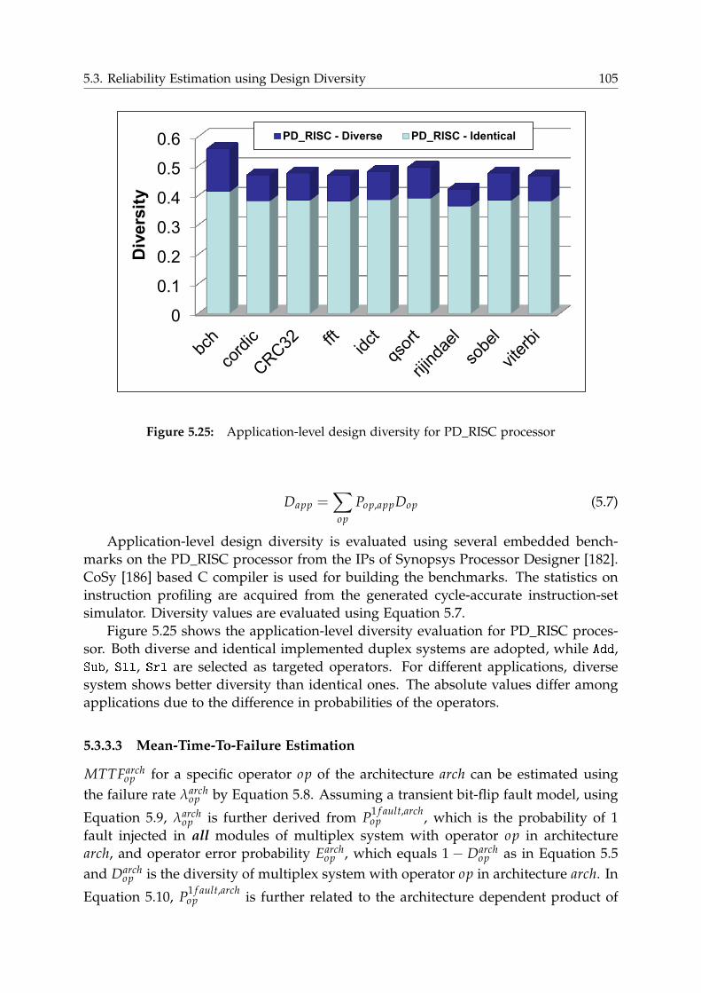
5.3. Reliability Estimation using Design Diversity 105
0
0.1
0.2
0.3
0.4
0.5
0.6D
ivers
ity
PD_RISC - Diverse PD_RISC - Identical
Figure 5.25: Application-level design diversity for PD_RISC processor
Dapp =∑op
Pop,appDop (5.7)
Application-level design diversity is evaluated using several embedded bench-marks on the PD_RISC processor from the IPs of Synopsys Processor Designer [182].CoSy [186] based C compiler is used for building the benchmarks. The statistics oninstruction profiling are acquired from the generated cycle-accurate instruction-setsimulator. Diversity values are evaluated using Equation 5.7.
Figure 5.25 shows the application-level diversity evaluation for PD_RISC proces-sor. Both diverse and identical implemented duplex systems are adopted, while Add,Sub, Sll, Srl are selected as targeted operators. For different applications, diversesystem shows better diversity than identical ones. The absolute values differ amongapplications due to the difference in probabilities of the operators.
5.3.3.3 Mean-Time-To-Failure Estimation
MTTFarchop for a specific operator op of the architecture arch can be estimated using
the failure rate λarchop by Equation 5.8. Assuming a transient bit-flip fault model, using
Equation 5.9, λarchop is further derived from P1 f ault,arch
op , which is the probability of 1fault injected in all modules of multiplex system with operator op in architecturearch, and operator error probability Earch
op , which equals 1− Darchop as in Equation 5.5
and Darchop is the diversity of multiplex system with operator op in architecture arch. In
Equation 5.10, P1 f ault,archop is further related to the architecture dependent product of

106 Chapter 5. Architectural Reliability Estimation
module-level fault probability P1 f aultop,i . It corresponds to the division of area estimation
of the operator Aop,i by the constant A1 f ault/hour, which is the size of area that 1 faulthappens per hour under a specific environmental condition. Such condition can beestimated by the reciprocal of Failure-in-Time (FIT) [69] in Equation 5.11. In this work,The FIT is assumed for instance as 10−4cph/µm2, where the unit stands for fault countper hour (cph) per unit area (µm2).
MTTFarchop =
1λarch
op(5.8)
λarchop = P1 f ault,arch
op Earchop = P1 f ault,arch
op (1− Darchop ) (5.9)
P1 f ault,archop =
arch∏i
P1 f aultop,i =
arch∏i
(Aop,i/A1 f ault/hour) (5.10)
A1 f ault/hour =1
FIT(5.11)
Aop,i and P1 f aultop,i for four operators are estimated in Table 5.10 based on 90nm
Faraday technology library [59]. Note that the area for routing wires is ignored in theestimation.
Add Sub Sll Srl
Gate-counts 256 224 128 104(NAND equivalence)
Aop,i (µm2) 1280 1120 640 560
P1 f aultop,i per hour 0.128 0.112 0.064 0.056
Table 5.10: Failure rate estimation for four operators
Combined with Dop from Figure 5.24, the estimated MTTFarchop under logarithmic
scale for four operators on several architecture variants is shown in Figure 5.26. Gen-erally, CGRA architecture naturally provides more reliability than VLIW, which is inturn more robust than RISC architecture.
For the same operator, MTTF increases with both the increasing number of mod-ules in the system and the increasing diversity of the modules. Compared with Figure5.24, RISC architecture with two diverse modules achieves far less MTTF than VLIWwith four identical modules. This is due to the fact that P1 f ault
op for VLIW is signifi-cantly smaller than RISC, since more modules in the multiplex system correspond toa lower probability that 1 fault happens in each module. The trend is the same in caseof CGRA. Among all four operators, Sll shows the highest MTTF which results fromits small fault probability due to its size and relatively high design diversity.

5.3. Reliability Estimation using Design Diversity 107
add
sub
sll
srl
0
1
2
3
4
5
6
7
8
CGRA -
DiverseCGRA -
IdenticalVLIW -
Diverse VLIW -
Identical RISC -
Diverse RISC -
Identical
LgM
TT
F (l
gh
ou
rs)
Architecture Variants
7-8
6-7
5-6
4-5
3-4
2-3
1-2
0-1
Figure 5.26: Mean-time-to-failure of architecture variants
5.3.4 Summary
Design diversity was proposed as a quantifiable metric in reliability evaluation forcircuit-level designs. In this work, design diversity is extended as an architecture-leveldesign metric to quantify reliability of different processing architectures in modernSoC. The approach is demonstrated on several architecture variants, where designdiversity and system Mean-Time-to-Failure are estimated quickly.

108 Chapter 5. Architectural Reliability Estimation

Chapter 6
Architectural Reliability Exploration
In this Chapter, three architecture-level fault tolerant techniques are presented. InSection 6.1 opportunistic redundancy is proposed to protect the algorithmic unitsof embedded processor with low performance penalty. In Section 6.2 asymmetricredundancy is proposed to protect the memory elements with the feature of unequalerror protection based on information criticality. In Section 6.3 error confinementtechnique is proposed to correct errors in memory with statistical data, which reachessimilar protection level with faster performance and less power consumption thantraditional techniques.
6.1 Opportunistic Redundancy
Architectural fault tolerant techniques targeting transient faults in mainstream proces-sors can be categorized into spatial and temporal redundancies. Spatial redundancyrequires additional hardware for protection, in the form of either information en-coding such as ECC [112] for protecting memory elements or simultaneous multipleexecution for combinatorial logic such as Triple Modular Redundancy (TMR) [196].Temporal redundancy involves instruction re-execution on the same hardware suchas Simultaneous and Redundantly Threaded (SRT) [154] processors at different clockcycle. Error detection is performed by comparing results from both executions. Theprocessor is either backward corrected by rolling back to its previously correct stateor forward corrected with the value from majority votes and ECC decoder.
In contrast to mainstream processors, reliability techniques for embedded proces-sors have reduced design space. Area and power constraints limit spatial redundancywith less amount of execution units and storage buffers while the opportunities fortemporal re-execution of instructions are also restricted due to real-time constraint.Expensive hardware units for out-of-order execution and multi-threading are seldomapplied. However, redundancy, which still exists, has been neither completely elim-inated nor fully utilized due to dynamic hardware usage and compiler complexity.Consequently, underutilized computational resources in embedded processors areexpected to be opportunistically used i.e., protect when possible, to achieve best-effort reliability enhancement. Besides, it is cost effective to reduce the granularity ofreplicated execution into micro-architecture level instead of the whole instruction toachieve less performance penalty.
Contribution In this work, a protection approach is proposed which considers dif-ferent policies for opportunistic redundant execution. In most aggressive policy, the
109

110 Chapter 6. Architectural Reliability Exploration
protected micro-architecture units are always double executed to ensure computa-tional correctness with large degraded performance. On the other hand, passive pol-icy re-executes only if there exists underutilized resources, which incurs no perfor-mance penalty when no errors are detected. Depending on the target application,policies can be chosen in order to balance reliability tolerance with performance. Thiswork also contributes several novel implementation features for reliability enhance-ment of embedded processors with less area and power overheads. Embedded RISCprocessor without out-of-order execution capability explores temporal redundancy inALU units whenever possible. VLIW processor takes advantage of its empty instruc-tion slots for spatial redundant execution. Using ADL based processor design flow,the proposed architectures and protection policies are efficiently explored throughhigh level fault injection. Synthesis results are provided to show the additional areaand power cost.
6.1.1 Opportunistic Protection
This section introduces the concept of opportunistic protection. First, an embeddedRISC processor is modeled in the form of Directed Acyclic Graph (DAG). Second, theprotection level used in this work is derived based on the DAG. The applied policieswhich facilitate opportunistic protection are explained next.
6.1.1.1 Processor Modeling
The processor modelling methodology from ADL LISA [2] is applied in this work. Thecomplete instruction set is represented by DAGs of LISA operations which describethe instruction behaviors. The directed links between operations show the activationconditions. When operations are associated within pipeline stages, the activationof operations implies the timing information of instructions. LISA operations areimplemented as HDL processes during RTL generation. Figure 6.1 shows the DAGfor a 5-pipeline stage RISC processor.
The Decode operation implements the coding root which activates correspondingsub-operations based on the instruction word from Fetch stage. The sub-operationsin Decode stage prepare the operands for calculation in Execute stage. Results fromExecute stage are further passed onto memory operations such as load and store ordirectly to Writeback operation. Note that alu_ex is shared by alu and bit as activatedoperation which is shown by the solid line. Besides such intra-instruction dependency,the dashed lines show inter-instruction dependencies since other types of instructionsdepend on the operand values from previous alu or bit type of instructions.
6.1.1.2 Protection Level
Protection level is critical to the whole design as it directly influences the error cover-age and performance overhead. The RMT processors have instruction level protection.To reduce the large performance overhead caused by instruction level duplication, theproposed protection is restricted on micro-architecture level. Figure 6.1 shows that the

6.1. Opportunistic Redundancy 111
Fetch
Decode
nop alu bit memcontrol
alu_ex addr_gencmp_ex
cmp
ld st
Write back
Fetch stage
Decode stage
Execute stage
Memory stage
Write back stage
Figure 6.1: Directed acyclic graph of embedded RISC processor
error in computational result of alu_ex operation directly influences alu and bit instruc-tions while indirectly affecting other instructions. The importance of protection foralu_ex can also be indicated from application profiling. Figure 6.2 shows the instruc-tion distribution averaged from 12 applications of MiBench [71] on the RISC processormodel. It is noticeable that alu and bit account for 51% of all the instructions whilecontrol, compare and memory account for 37%. The rest instructions are NOPs whichare not relevant for protection.
Consequently, the architecture unit alu_ex is double executed with the same inputsto ensure its correctness. However, instead of connected execution, the verified execu-tion is only performed when the alu_ex operation is un-activated, which implies thatcurrently other type of instructions are activated in Execute pipeline stage. Additionalprotection buffers are used to store the operands to be verified, while commit buffersare applied to ensure the correct commit sequence of instructions. When mismatch isdetected, the pipeline is rolled back to execute the faulty instruction for error correc-tion. The proposed protection method tries to duplicate the execution of vulnerablearchitecture units when there is opportunity for doing it. In contrast, instruction levelduplication doubles the execution of the complete instruction. For embedded proces-sors with single ALU unit this scheme would manifest large performance overhead.

112 Chapter 6. Architectural Reliability Exploration
33,28%
17,65%
11,45%
21,37%
9,01% 7,25%
0%
5%
10%
15%
20%
25%
30%
35%
alu_insn bit_insn nop_insn mem_insn control_insn cmp_insn
Figure 6.2: Average instruction distribution for MiBench
6.1.1.3 Protection Features and Policies
Different applications have various requirements in reliability. In Figure 6.3 severalfeatures and policies which explore the reliability-performance trade-off are intro-duced. Figure 6.3a) shows the basic approach for re-execution of add instruction inline 2 when line 3 has no ALU instructions. An improved version of this would bethe re-execution of several instructions based on a protection buffer which recordsunprotected instructions. This is shown in Figure 6.3b). The program flow may pro-hibit connected protections when there are not enough redundancies for protectingprevious instructions. In such cases, the following ALU instructions are continuouslypushed into the protection buffer and wait for chances of re-execution. However,when the buffer is full or in case of no protection buffer, decision for protection needsto be made in either passive policy such as Figure 6.3c) or aggressive policy in Fig-ure 6.3d). Passive policy ignores the protection of oldest instruction while aggressivepolicy stalls the processor pipeline for acquiring one clock cycle of in-activated alu_exoperation for duplicated execution. With regard to the VLIW processor which hasparallel execution syllables, spatial redundancies can be explored as shown in Fig-ure 6.3e) to take advantage of the underutilized execution resources.
6.1.2 Implementation
In this section, the proposed design methodology is demonstrated on embedded RISCand VLIW processors using ADL LISA. Intrinsic temporal and spatial redundancywithin processor models are explored to leverage reliability.

6.1. Opportunistic Redundancy 113
1 …
2 add R3, R1, R2
3 nop (protect line 2)
4 nop
5 …
1 …
2 add R3, R1, R2
3 add R4, R5, R6
4 nop (protect line 2)
5 nop (protect line 3)
1 …
2 add R3, R1, R2
3 add R4, R5, R6
4 nop (protect line 3)
5 sub R6, R5, R2
1 …
2 add R3, R1, R2
3 add R4, R5, R6
4 nop (protect line 3)
5 sub R6, R5, R2
Stall pipeline
line 2 protectedline 2 uncovered
Instruction buffering
line 2 and 3 protectedline 2 protected
c) passive policy d) aggressive policy
a) protect 1 insn b) protect 2 insns
c) passive
policy
d)
aggressive
policy
1 …
2 add R3, R1, R2; add R4, R1, R0; sub R5, R1, R2; nop
3 add R3, R1, R2; add R4, R1, R0; nop; nop
4 …
e) spatial redundancy for VLIW processor
Figure 6.3: Protection features and policies
6.1.2.1 RISC Model
PD_RISC_32p6 processor model from Synopsys IPs is improved targeting reliability,which is a fully bypassed 32-bits embedded processor with 6 pipeline stages. Withfull support of C compiler, applications are compiled to run on the cycle-accurate in-struction set simulator generated from LISA compiler. Figure 6.4 explains the generalprotection flow.
Within each clock cycle, the protection unit begins to check the activation con-dition of the ALU unit to identify whether redundant operations can be performed.A free ALU unit signals to execute previously oldest recorded instruction from theprotection buffer. Results from both executions are compared to decide whether errorrecovery operation needs to be activated. In case of no error detected, the checkedinstruction is committed from the commit buffer together with its dependent instruc-tions. In contrast, when the ALU unit is occupied in the current control cycle, decision

114 Chapter 6. Architectural Reliability Exploration
check alu
availability
protection buffer
empty?
Free
Yes
fetch to re-
execute
No
check results
Protection type
Occupied
protection buffer
status && policy
Yes (HARD)
Full && passive
stall pipeline
Full && aggressive
add to protection
buffer
Protection buffer not full
overwrite
Error recovery
Mismatch
add to commit
buffer &&
commit checked
insn
Match
NONE
SOFT
All insns that dependent on the uncommit
data should put into commit table
pipeline flush,
control table reset,
program flow
rollback
Figure 6.4: Flow of protection unit
is made on whether to push current instructions into the protection buffer based ontheir types. Table 6.1 shows three types of instructions where HARD and SOFT typesare recorded for protection. Other instructions are committed without further pro-tection. While the writeback values of SOFT instructions are recorded in the commitbuffer directly, HARD type of instructions need further processing based on their pro-tection modes. When the protection buffer is full, aggressive policy tries to stall thepipeline for earning one extra cycle of free ALU usage for re-execution. Otherwise,passive mode overwrites the oldest entry in the protection buffer with the new onewithout stalling the pipeline.
Figure 6.5 visualizes the protected ALU unit in EX pipeline stage. Several archi-tecture features are explained next.
Protection Buffer The protection buffer stores the opcode, operands and writebackvalues of the protected instructions. A checkState tag bit is used to indicate whethersuch instruction has been verified, so that the entry in both protection and commitbuffer can be deleted in the next clock cycle. The protection buffer is implemented as

6.1. Opportunistic Redundancy 115
Table 6.1: Handling methods of different instruction types
Types DefinitionHARD Protected instructions
SOFT Instructions have data depen-dency on HARD type
NONE Other instructions
alu_in1
alu_in2
alu_out
opcode
protect
info
ER
RO
R
ERROR_PC
commit
commit
Register file
pipe_flush
IN.PC PC
data
bypassfrom commit
from Register file
FE EX WB
To EX from mem
MEMDC
from ex
To DC
PC dst wbv statePC opcode operand1 operand2 result checkState
Figure 6.5: PD_RISC_32p6 processor with protection modification
a circular buffer which wraps around to the beginning when the boundary of bufferentries is reached. The buffer size is adjustable during simulation, which reveals thedesign trade-off between reliability and area/power. One specific control register isused for management of protection buffer, which periodically gets updated in DCpipeline stage.

116 Chapter 6. Architectural Reliability Exploration
Delayed Commit Unit A delayed commit unit is used for keeping the return valuesof both HARD and SOFT types of instructions. To ensure the correct value is usedfor subsequent instructions, the data bypass mechanism is adjusted accordingly toestablish a new path from commit buffer to the EX pipeline stage. The new pathhas higher priority in data bypass unit than the one from the register file. Searchingdata matches is done through register indexes which are stored along with write backvalues in the commit buffer. The search starts from the newest entity in the commitbuffer afterwards to ensure the correct order of value updates.
Error Correction When a mismatch of data values is detected, error is correctedbased on the rollback of processor state to the previously correct point. It is achievedby fetching the new instruction based on the value of program counter (PC) stored inthe protection buffer. Meanwhile, both the pipeline registers and buffers flush theirvalues.
6.1.2.2 VLIW model
The LT_VLIW_32p5x4 processor model from Synopsys IP is adapted for error pro-tection. The model contains 5 pipeline stages with 4 parallel instruction syllables.The EX stage of each syllable contains individual ALU unit. The major differencefrom RISC processor is that a VLIW processor contains intrinsic spatial redundancieswhich can be used for parallel execution. Due to application properties, such redun-dant instruction slots are not fully explored by the VLIW compiler. The modifiedarchitecture is shown in Figure 6.6. Three units are added into the architecture, acentralized Protection admin, Operand routing and Post processing units. The protectionbuffer and control register are the same as for PD_RISC processor model while a newregister alu_ctrl_reg is introduced for guiding the mapping of operation and operandsamong four ALU units in EX pipeline stage. Operand routing and Post processing unitsadjust their behaviors accordingly based on the contents in this register.
ALU Control Register The alu_ctrl_reg register contains 16 bits which are dividedinto four fields, each controls a ALU unit respectively. The higher 2 bits of each fieldrepresent the operation mode, while the lower 2 bits represent table pointers as shownin Table 6.2. Figure 6.7 shows an example on how this register directs the operationof each ALU. alu0 and alu1 contain ALU instructions while alu2 and alu3 slots arefree in this clock cycle. The value of alu_ctrl_reg is set by the Protection admin unit inthe decode stage. According to Table 6.2, alu0 duplicates its execution in slot alu2,while slot alu3 re-executes previously recorded operation from protection buffer entry1. The computation from alu1 is performed and backuped in the protection bufferentry 2 for later verification. Through such operands mapping, efficient managementof redundant resources is achieved to utilize both spatial and temporal redundancy.
Commit Unit For VLIW model the delayed commit unit is not necessary since theinstruction will be either executed twice or overwritten by another instruction due to

6.1. Opportunistic Redundancy 117
Operand
rounting
alu0
alu1
alu2
alu3
Post
processing
Figure 6.6: VLIW architecture with protection modification
Table 6.2: ALU control register
Modes 2 MSBs 2 LSBs
Normal execution 00 –
Save to table 01 table write pointer
Fetch from table 11 table read pointer
Fetch from syllable 10 syllable pointer
the protection policies before it enters the write back stage. This is due to the internalparallel architecture of VLIW processors while detailed timing analysis is ignoredhere in case of simplicity.
6.1.3 Experimental Results
Experiments on two processor models are documented in this section. First, perfor-mance overheads are presented based on several embedded applications. High-levelfault injection experiments are used to show the protection efficiency. Lastly the syn-thesis results of proposed design are provided.

118 Chapter 6. Architectural Reliability Exploration
alu0
PC opcode operand1 operand2 result
alu1 alu2 alu3
From syllable
From tableSave to table
0000 0110 1000 1101
0
12
alu control register
Figure 6.7: VLIW control register
6.1.3.1 Benchmarking
Several applications from MiBench are ported to our simulation environment basedon the Synopsys Processor Designer tool flow [182]. Figure 6.8 shows the coveragesof protected instructions for both policies on PD_RISC processor, where both the pro-tection and commit buffers are configured to store 3 entries of protected operations.It is shown that aggressive policy always achieves more coverage than passive policy.For aggressive policy, performance degradation is incurred by pipeline stall when nofree entry exists in protection buffer. The cost of such effect varies due to differentproperties of applications. For computationally intensive applications such as sha andrijndael the performance degradation is higher than others. With regard to passivepolicy, redundant execution is done in an opportunistic way, therefore no performanceoverhead is incurred with decreased instruction coverage. For the VLIW processor theinstruction coverage shows similar values which are not presented.
6.1.3.2 Fault injection experiment
To demonstrate the efficiency of error detection and correction of proposed architec-tures, a state-of-the-art high-level fault injection flow has been adopted [209] whichis integrated into LISA based processor design environment. Bit-flip faults are in-jected into the ALU units randomly during simulation time. Error Manifestation Rate(EMR) [42] is used as the method for error evaluation. EMR represents the percentageof detected fault on the program/data memory interface of the processor core. TheEMR value indicates the error resilience ability of an architecture.
10,000 experiments are performed to get the EMR value for a fixed count of in-jected faults. Sieve and IDCT applications are selected for fault simulation. Figure 6.9shows the EMR trends with increased count of injected faults for RISC and VLIWprocessor respectively.
For both processor models, protected architectures in passive mode achieve lowerEMR values than unprotected ones. Aggressive mode results in 0 EMR values regard-

6.1. Opportunistic Redundancy 119
0%
10%
20%
30%
40%
50%
60%
70%
80%aggressive coverage
passive coverage
performance degradation
(aggressive)
Figure 6.8: Instruction coverages and performance degradation
0
10
20
30
40
50
60
70
80
90
1 2 3 4 5 6 7 8 9 10 11 12 13 14 15
EM
R(%
)
RISC: Injected fault count
0
2
4
6
8
10
12
14
16
18
20
1 2 3 4 5 6 7 8 9 10 11 12 13 14 15VLIW: Injected fault count
sieve_org idct_org
sieve_passive idct_passive
sieve_aggressive idct_aggressive
Figure 6.9: EMR with increased count of faults for RISC/VLIW processor

120 Chapter 6. Architectural Reliability Exploration
less of the faults count which means all of the injected faults are resilient. Combinedwith the performance degradation for aggressive policy in Figure 6.8, it reflects thetrade-off between reliability and performance. Among different architectures VLIWprocessor achieves much less EMR than RISC processor under same amount of in-jected faults. This happens due to the reason that same amount of faults are dis-tributed onto 4 individual ALU units in VLIW processor which reduces the probabil-ity of interface error.
Optimization levels of the C compiler have impact on the run-time execution ofthe generated assembly codes, which affects the efficiency of the passive protectionmode. Figure 6.10 shows the optimization impacts on EMR for Sieve and IDCT appli-cations. The compiler is generated by the CoSy compiler development system [186].Basic features of optimization levels are briefly explained. For detailed informationregarding optimization flags please refer to [142]. It is obvious that effects of opti-mization levels vary among different applications. Compiler level theoretical analysisto cope with opportunistic protection is beyond the scope of the work.
• O0: No optimization, as applied in Figure 6.8 and 6.9
• O1: Alias analysis and control flow simplification
• O2: Function inlining and object propagation
• O3: Loop level optimizations
• O4: Software pipelining
0
0.02
0.04
0.06
0.08
0.1
0.12
0.14
0.16
Sieve Idct
EM
R(%
)
6 bit-flip faults injected on PD_RISC processor
Compiler Optimization Levels
O0 O1 O2 O3 O4
Figure 6.10: Effects of C compiler optimization levels on EMR for passive mode

6.1. Opportunistic Redundancy 121
6.1.3.3 Synthesis result
Based on the HDL generation flow of Synopsys Processor Designer [182] the pro-posed architectures are synthesized under 90nm Faraday technology library by usingSynopsys Design Compiler, topographical mode. Table 6.3 shows the gate-level syn-thesis results on area and power overheads for both processor models, where thepower values are averaged from the MiBench applications. The major extra area andpower contributors are the protection and commit buffers which are implemented asarchitectural registers. For error detection only, no commit buffer is required for RISCprocessor so that power and area are smaller than the results in error recovery mode.Error recovery for VLIW processor does not require extra area overhead since commitbuffer is not required. VLIW requires relatively more overheads than RISC due to theoperand routing unit which connects four ALU units and large amount of registerports to the protection buffer.
Table 6.3 also shows the performance and energy overheads under fault free sim-ulations. The passive mode achieves 0 performance overheads for both architectureswhereas the aggressive mode achieves varies overheads among different applications.
Table 6.3: Design overheads for proposed architectures
Area Overhead Power Overheaddetection recovery detection recovery
RISC 8%+ 12%+ 17.43%+ 25.48%+
VLIW 16.86%+ 16.86%+ 29.23%+ 31.23%+
Performance Overhead Energy Overhead(fault-free simulation) (recovery enabled)passive aggressive passive aggressive
RISC 0% 2%-20%+ 25.48%+ 28.0%-50.6%+
VLIW 0% 2%-12%+ 31.23%+ 33.9%-47.0%+
6.1.4 Summary
In this work a best-effort design method to increase reliability of embedded processorsagainst soft errors is presented. Redundancies of processor ALU units are exploredopportunistically based on several protection features and policies. Taking advantageof the proposed design, protection overhead can be reduced significantly. Synthesisresults are provided to show the trade-off between reliability and performance.

122 Chapter 6. Architectural Reliability Exploration
6.2 Processor Design with Asymmetric Reliability
Recent research on reliable system design reflects two trends. First, reliability istreated as a cross-layer design issue [45]. This stresses the fact that separate error miti-gation techniques may result in an over-designed system. The design can and shouldtake the support of architectural and algorithmic error resilience [143]. This approachcan reap significant benefits and requires establishment of design metrics and strongunderstanding of all the design layers. The second trend is to offer asymmetric relia-bility, where different parts of the system are protected unequally [72]. Consequently,the upper design layers, e.g., the application can select the level of reliability staticallyor dynamically during execution based on the task criticality.
The existing works on reliable storage implementation for embedded processorsis essentially a channel coding problem in noisy communication. Based on that, errordetection and correction methods in unreliable processor microarchitecture can be ap-plied to the storage. The storage include registers, data memory, instruction memoryand pipeline registers. The aspect of asymmetric reliability can be further probed forsuch information theoretic model. Though it is well accepted in the research com-munity that asymmetric reliability leads to more design trade-offs and possibly betterPareto-optimal curves [72, 97, 108], it is yet to be fully explored in the context of em-bedded processors. While unequal error protections for register file and data memoryare proposed by different schemes [108], the reliability issues of instruction words andprogram memory remain relatively less studied. Instruction-level vulnerability anal-ysis is presented in [161] though, the asymmetry is addressed by software mappingflow only. Naturally, protection of instruction and data demands different techniques.The scope and impact of all aspects of asymmetric reliability are not systematicallyexplored and studied to the best of our knowledge.
Though the availability of rich literature in channel coding aids our work, thereare two important challenges, one needs to solve. First, designing hardware-basedunequal error detection/correction requires efficient implementation of channel en-coder/decoder. A few works [93, 156] discuss applying Hamming codes for on-chipstorage but, efficiency of the encoder/decoder in terms of area and runtime is stillan important problem. This is particularly needed since, the error detection and cor-rection impacts the critical path of the processor. Second, Borade et al. [157] tookan information theoretic view on unequal error protection and there exists manypapers [103, 155] on applying unequal error-protection in diverse application areas.Interestingly, all of them consider different error probability for different bit-positionsand this distribution is the same for all the messages. Here, on the other hand, it isadvocated that some instructions in a processor are more important than the othersand hence demand more protection - thereby requiring a different view of asymmetry.These problems are addressed in this work.
Contribution In short, the contributions of this work are following.
• An asymmetric processor reliability model.

6.2. Processor Design with Asymmetric Reliability 123
• Novel schemes for performing reliability trade-off with other design constraints.
• Detailed experiments using a high-level embedded processor design framework.
6.2.1 Asymmetric Reliability
Any practical communication channel is exposed to several noise sources and there-fore the message received by the receiver may be different from the message sent bythe sender, causing transmission errors. The seminal paper of Shannon [28] laid thefoundation of the theory of error-correcting codes (ECC), which deals with how todetect and correct transmission errors at the receiver end. The basic idea is that eachmessage m is transformed into a particular codeword c before being sent. The set ofcodewords constitute a code. If an error is introduced in the communication channel,the received word r would be different from the codeword c. A convenient codingmethod for binary channels is [n, k] linear block code where the message is dividedinto blocks of k consecutive bits and each such k-bit message is encoded into an n-bit(n > k) codeword.
In Figure 6.11, a classification of asymmetric reliability schemes is proposed. Theunequal error protection for different channels in a microarchitecture can be eitherstatic or dynamic. For statically asymmetric reliability, the error protection schemesare fixed before program execution. For dynamic, it can be altered depending onthe varying criticality of tasks/data/instructions. For both static and dynamic asym-metric reliability, the error protection can be distributed across or within differentmessages. If only the higher order bits of a data are protected for every data then, thereliability distribution is bit-wise. If the protected regions vary for different data/in-struction then, it is termed as message-wise asymmetric reliability. For example, astatic error detection and correction framework is investigated for the processor in-struction set using message-wise asymmetry. The program memory is viewed as achannel, where linear codes are needed.
It turns out that the general decoding problem of linear codes is NP-complete [52].Though there are particular classes of linear-time encodable and decodable error-correcting codes [180], the time required to decode a codeword may adversely affectthe critical path of the microarchitecture. Hamming code [146] is therefore utilizedwhich can be decoded in a single cycle.
For each integer r, there is a Hamming code with codeword length n = 2r − 1 andmessage length k = 2r − r− 1. It has a k× n generator matrix G so that for a message(considered as a row-vector) u, the corresponding codeword is given by v = uG. Notethat r = n− k denotes the number of parity bits when G is written in systematic form(i.e., has a submatrix Ik in the left part). The r× n parity check matrix H contains allthe 2r − 1 non-zero r-bit binary vectors and the syndrome vector s = vT H gives theposition of the error in case of single-bit error. If s = 0, it indicates that no error hasoccurred. An extra parity bit can be added to form what is called an extended Hammingcode that provides an additional facility of detection of double bit-error. However, forproof of concept, only single bit-error correcting Hamming codes are used. In fact,

124 Chapter 6. Architectural Reliability Exploration
Asymmetric
Error
Detection/Correction
Static Dynamic
Message-Wise Bit-Wise
transmitter receiver
noise
source
channel transmitter receiver
noise
source
channel
Figure 6.11: Asymmetric encoding and decoding
our asymmetric reliability framework is generic in the sense that any error-correctioncomponent (that is fast enough) can be used as its subsystem. For memory word sizeof 32 bits, r = 6 parity bits are needed to correct a single bit error, leading to 38-bitcodewords. This scheme is denoted by H1[38, 32].
6.2.1.1 Divide and Conquer Method for Higher Bit-Error Correction
For double-bit error-correction, one could use BCH codes as in [140] or LDPC/turbocode as in [144]. However, the state-of-the-art decoding algorithms and circuits forthese codes are suitable for memory protection but are not fast enough to be used inthe instruction pipeline.
Note that the total number of possible errors in a 32-bit message is 232 − 1. Outof this, the direct application of Hamming code, i.e., the scheme H1[38, 32] covers(32
1 ) = 32 cases. To tackle higher bit errors, a novel method of dividing the messageinto multiple segments and apply Hamming encoding and decoding on each partparallel is proposed. For example, when a 32-bit word is divided into two halves,each of 16 bits and apply Hamming code with r = 5 parity bits on each half, then

6.2. Processor Design with Asymmetric Reliability 125
((160 ) + (16
1 ))2 − 1 = 288 cases can be covered. This scheme is denoted by H2[42, 32].
Similarly, the 32-bit word can be divided into four parts each of 8-bits and apply aHamming code with r = 4 parity bits on each part to achieve partial four-bit error-correctability. This scheme is referred as H4[48, 32] and covers ((8
0) + (81))
4 − 1 = 1295cases. Though the schemes H2[42, 32] and H4[48, 32] cannot correct arbitrary doubleor four bit-errors, by further division into segments of size 4 bits, 2 bits and so on,in the limit, one can correct any number of errors in the whole word. This scheme iscalled as Divide and Conquer Hamming or DCH.
Suppose a m = kl-bit message is divided into l parts each of k bits and apply asingle-error correcting Hamming Code on each part. For a k-bit message, the numberof parity bits needed is given by the minimum integer rk such that, 2rk − rk − 1 ≥ k.The total number of parity bits for all the l parts are given by rkl. The resulting partiall-bit correcting DCH scheme is denoted by Hl[kl + rkl, kl]. Table 6.4 shows the typicalparameter values for different choices of l and k assuming m = kl = 32.
Table 6.4: DCH schemes from different message partitioning
l k rk rkl DCH Scheme
1 32 6 6 H1[38, 32]2 16 5 10 H2[42, 32]4 8 4 16 H4[48, 32]8 4 3 24 H8[56, 32]
16 2 3 48 H16[80, 32]32 1 2 64 H32[96, 32]
The following result states how many out of total 2m − 1 = 2kl − 1 non-zero errorvectors are corrected by such a scheme.
Theorem 6.2.1 Hl[kl + rkl, kl] scheme can correct (k+ 1)l− 1 many different errors in kl-bitmessages.
Proof: In each of the k-bit part, there can be (k1) = k single bit errors. Adding
to this the case of no error, each of the l parts can contribute k + 1 cases, giving atotal of (k + 1)l cases. But this include the case where no error occurs in each part.Thus, excluding the all zero error-vector, the total number of errors covered is givenby (k + 1)l − 1.
It is easy to see that with m = kl fixed, as the number l of parts increases, theindividual part-length k decreases and the quantity (k + 1)l − 1 increases. In the limit,when there are m parts each of length 1, the resulting Hm[3m, m] scheme can correctall the 2m − 1 error vectors. This is exactly the point of the following corollary.
Corollary 6.2.2 Hm[3m, m] scheme can correct all the 2m − 1 errors in m-bit messages.

126 Chapter 6. Architectural Reliability Exploration
Proof: In Theorem 6.2.1, when l = m and k = 1, there exists (k + 1)l − 1 = 2m − 1.
There are two main points in which the proposed scheme for instruction worddiffers from the traditional coding schemes in communication systems.
• First, in coding theory, increment in block size tends to increase the coding ef-ficiency. However, for instruction word, increment in block size would increasethe error-correction time as well. Our method works on multiple blocks in par-allel and therefore decoding the whole word takes the same time as decoding asingle block.
• Secondly, the proposed DCH coding cannot be applied to general communi-cation systems. The reason is in typical communication scenario, the issues offraming, packetization, synchronization and real time constraints force the re-ceiver to decode the incoming bitstream as and when it arrives. The receivercannot afford to wait for the entire message to arrive and then perform divideand conquer. On the other hand, in instruction memory, the whole word isavailable for applying the divide and conquer technique.
6.2.2 Asymmetric Reliability Exploration
With the proposed techniques multiple sets of experiments are performed using theenvironments described in this section. First, the efficiency of the proposed Hammingencoder/decoder is studied together with its impact for different levels of protection.Second, a comparative study between static and dynamic protection modes is done.Third, the effect of different asymmetric reliability techniques for VLIW processor isinvestigated. Finally, a comparison of message-wise and bit-wise asymmetric reliabil-ity is performed.
6.2.2.1 Experiment Setup
For all the experiments, Synopsys Processor Designer [182], version 2012.06-SP1 isused. The processor descriptions, used in this work, are developed from the basicprocessor templates provided with the tool. The first processor, denoted LT_RISC_-32p5, is based on a RISC instruction set with 5-stage pipeline. The second processor,denoted LT_VLIW_32p5x4, contains a 5-stage pipeline and can have up to 128-bit in-struction word distributed over four parallel 32-bit instruction slots. The instruction-set supports the basic RISC instructions as available in LT_RISC_32p5 model. Both themodels are fully synthesizable and provides readily available retargeted C Compiler.Changes to the microarchitecture can be easily performed for both the models, withfast automatic retargeting of the software tools and generation of synthesizable RTL.For gate-level synthesis, Synopsys Design Compiler, version G-2012.06, targeting a90nm technology CMOS technology library is used. The applications for our experi-ments are chosen from different types of embedded applications including multime-dia and wireless algorithms.

6.2. Processor Design with Asymmetric Reliability 127
Technique in [209] is applied to efficiently inject fault in cycle-accurate instructionset simulator generated from Processor Designer. A user friendly GUI is designed forfaults configuration. The Error Manifestation Rate (EMR) [42] is used as a metric for theevaluation of fault simulation. For a set of fault injection experiments, EMR is definedas the percentage of experiments which detects error on the memory interfaces towhich the faults propagate. Normally, EMR value increases with the duration andnumber of injected faults. For the same fault duration and number, larger EMR valueindicates less reliable component.
Insn
Pip
ere
g
Prog
mem
ECC
mem1source
Compiler
*.out
Encoder
RISC core
. . .
Fetch Stage
ECC
mem2
ECC
mem3MUX
ECC
Decoder
Mode
Selection
Figure 6.12: ECC encoding and decoding
6.2.2.2 Efficient ECC for Message-wise Protection
Figure 6.12 shows the work flow for asymmetric protection for program memory.The application is initially compiled, assembled and linked to prepare the binaryexecutable. The instructions are encoded into code words for different ECC modes.The code words are loaded into multiple ECC memories. A hardware-based decoderwhich detects and corrects possible faults in the program memory is integrated intothe fetch pipeline stage of the processor. To facilitate runtime asymmetric protection,the decoder selects the code words from several ECC memories to enable differentlevel of protection. The protected instruction word is then forwarded onto the nextpipeline stage.
The current modes of protection for 32 bits instruction words include H1[38, 32],H2[42, 32] and H4[48, 3] that can achieve a maximum of of 1, 2 and 4-bit error-correction respectively. To demonstrate the protection efficiency by applying differentmodes, the fault injection experiments are carried out with bit-flip faults injected intoboth program memory and ECC memories randomly. The example application run-ning on the processor is sieve of Eratosthenes which requires a program memory size of512 Bytes. Figure 6.13 shows the EMR for different protection modes with increasingnumber of bit-flip faults. Each evaluation point is averaged from 1000 experimentswhile each experiment lasts for 1,200 clock cycles. With increased protection level

128 Chapter 6. Architectural Reliability Exploration
0%
10%
20%
30%
40%
50%
60%
70%
80%
90%
100%
10 20 30 40 50 60
EM
R
Number of Bit-flip faults
H1 [38,32]
H2 [42,32]
H4 [48,32]
No Protection
Figure 6.13: EMR with different protection modes (Sieve application on RISC pro-cessor)
the EMR values drop at the same evaluation point, which shows an increased protec-tion ability. All EMR values increase with increased number of faults where higherprotection level shows better EMR performances.
Table 6.5 shows the trade-off between power and area for the RISC processor withdifferent protection levels. All the architectures are synthesizable with a maximalfrequency of 200MHz. The power consumption increases slightly with increased pro-tection level. The RISC core area reflects an inverse trend since the decoder whichdecodes the complete 32-bit instruction costs more than twice the area of 16-bit de-coder. The same trend between the 16-bit and the 8-bit decoder is also observed. TheECC memory size increases with increased protection level.
Table 6.5: Performances for different protection modes
Protection LevelArea ECC Size Power
(KGates) (Bytes) (mW)
No Protection 27.53 0 9.03H1[38, 32] 27.94 96 9.26H2[42, 32] 27.93 160 9.28H4[48, 32] 27.92 256 9.30

6.2. Processor Design with Asymmetric Reliability 129
6.2.2.3 Static and Dynamic Asymmetric Reliability
Experiments have been carried out to investigate the impact of varying instruction re-liability. Static and dynamic approaches are proposed in the assignment of instructioncriticality. The static approach based on the observation that different instructions re-flects different criticality. For instance, branch is more critical than alu instructions dueto the effect of altering the program flow. To characterize the criticality of individualinstructions, simulations are performed by injecting random faults onto the same setof instructions with random operand values. Figure 6.14 collects the simulation re-sults where Instruction Vulnerability Factor (IVF) are characterized. We estimate IVFby the instruction error rates (IER) defined in Section 5.1.2. For a specific instruction,the IER values for all logic operations on the activation path of such instruction isaveraged to calculate the IVF, where each IER value is collected from 10,000 singlebit-flip fault injection experiments. Note that, different techniques of obtaining theinstruction criticality can be conceived, including a user-driven criticality assignment.
0
0.1
0.2
0.3
0.4
0.5
0.6
0.7
0.8
arithmetic load-store branch
Exp
eri
men
tal IV
F
criticality level 3
criticality level 2
criticality level 1
Figure 6.14: Static instruction criticality assignment
The dynamic approach assigns the protection level based on the situation of run-time fault detection, which reduces the power consumption of the ECC decoder when

130 Chapter 6. Architectural Reliability Exploration
less faults are detected. Figure 6.15 shows the approach in the form of a Finite StateMachine (FSM). Initially protection level one is assigned to all the instructions. If afault is detected the processor updates to level three for the following instructions,which lasts for at least 10 clock cycles. After that time period, decision is made againbased on whether faults are detected and protection may reduce to level two. If a faultis detected at level two, the protection level is increased for the following instructions.
Experiments are performed to compare the protection efficiency of both ap-proaches. The ECC decoder which supports three modes are integrated into the RISCprocessor. For static approach, the coding of instructions are indexed with two ECCmode bits according to Figure 6.14 for runtime mode selection. For dynamic approacha state machine module according to Figure 6.15 is designed. A flag register is usedto switch between static and dynamic modes.
Figure 6.16 shows that static approach excels the dynamic one when several singlebit-flip faults are injected randomly into whole memory blocks. However, when adja-cent instructions in memory array are bit-flipped, dynamic approach achieves betterprotection since high protection level covers all adjacent instructions. The dynamicapproach contributes especially when the faults happen inside loop kernels wheresequential instructions are defended using maximal protection.
Level 1
(Initial) H1[38,32]
Level 2 H2[42,32]
Level 3 H4[48,32]
Detected
Not detected
In 10 cycles
De
tec
ted
Figure 6.15: FSM for dynamic, asymmetric reliability
6.2.2.4 Asymmetric Reliability for VLIW Processor
VLIW architectures provide further opportunities for asymmetric protection. Instruc-tions generated by the VLIW compiler leave certain slots empty, when sufficientinstruction-level parallelism is not detected in the application. These slots are po-tentially to be utilized to place the parity bits for protecting the instruction words. To

6.2. Processor Design with Asymmetric Reliability 131
0.00%
5.00%
10.00%
15.00%
20.00%
25.00%
10 20 30 40 50 60
EM
R
Number of Bit-flip faults
Static Random Location Dynamic Random Location
0.00%
20.00%
40.00%
60.00%
80.00%
10 20 30 40 50 60
EM
R
Number of Bit-flip faults
Static Connected Location Dynamic Connected Location
Figure 6.16: Comparing static and dynamic protection
simplify the design complexity, two slots are fixed for protection when no instructionsreside in. Figure 6.17 visualizes the scheme.
To enable asymmetric protection for VLIW instructions, each slot is filled withparity bits of different modes. Ideally in a 32-bit instruction slot, all the three types ofparity bits corresponding to H1[38, 32], H2[42, 32] and H4[48, 32] can be exactly filledin. However, in our target VLIW model one bit for each slot is reserved to mark theend of VLIW instruction. Therefore, parity bits from two ECC types are used. In eachslot one extra bit is used to indicate whether it contains an instruction or parity bits.
As it can be observed from Table 6.6, both the area and the power consumptionincreases with increased protection levels. In this experiment, the parity bits for each32-bit instruction is generated and filled in the VLIW slots. This required us to intro-duce empty slots in the application, when there is none. This resulted in an increaseof the application runtime. To better study the effect of application runtime increase,two different protection modes are conceived. In the first mode, named opportunis-tic [199], parity bits for instructions are fitted in, only if empty slots are present. Foranother, compulsory protection mode, parity bits are introduced for all the instructions.
Table 6.6: Reliability vs. power/area trade-off
Protection LevelArea Power (mW)
(KGates) Cordic Sobel FFT CRC32
No Protection 79.09 4.93 4.89 4.91 5.00H1[38, 32] 79.85 5.18 5.13 5.17 5.25H1[38, 32]
80.49 5.40 5.34 5.38 5.45and H4[48, 32]
The EMR results of this experiment are shown in Figure 6.18 where the corre-sponding application runtime is provided in Table 6.7. Note that larger differences in

132 Chapter 6. Architectural Reliability Exploration
128 bits instruction word
ECC
Decoder
1
ECC
Decoder
2
INSN1 ECC1 INSN2 ECC2
INSN1 NOP INSN2 NOP
Fetch
Stage
. . .VLIW core
H(32, 38) H(32, 48)
Figure 6.17: ECC in VLIW slots
clock cycles between two protection modes lead to larger gab of EMR. This shows aninteresting trade-off between available parallelism, area, runtime, power and reliabil-ity.
Table 6.7: Application runtime for various VLIW protection modes
ApplicationCycles Increase
Opportunistic Compulsory (%)
Sobel 2671 2748 2.8
Cordic 1074 1317 22.63
CRC32 32278 32279 3e-5
FFT 1433 1440 0.49
6.2.2.5 Bit-wise Asymmetric Reliability for Data Memory
In contrast to the instruction words, data words can be protected with bit-wise pro-tection schemes, e.g., higher order bits can play a more important role in correctcomputation than lower order bits. Based on such principle bit-wise asymmetric en-coding is explored for data memory. Figure 6.19 shows the proposed flow where,an asymmetric encoder is integrated into the store pipeline stage. The parity bits arestored into an ECC data memory in parallel with store instruction. Decoding andcorrection for the same data is performed in the stage load.
To compare the protection efficiency, bit-wise symmetric encoding scheme is alsoimplemented and tested where 4 bytes within 32 bits use the same level of encoding.

6.2. Processor Design with Asymmetric Reliability 133
0.00%
20.00%
40.00%
60.00%
80.00%
100.00%
4 8 12 16 20 24
EM
R
Number of Bit-flip faults
Sobel
0.00%
20.00%
40.00%
60.00%
80.00%
100.00%
4 8 12 16 20 24
EM
R
Number of Bit-flip faults
CRC32
0.00%
20.00%
40.00%
60.00%
80.00%
100.00%
4 8 12 16 20 24
EM
R
Number of Bit-flip faults
FFT
0.00%
20.00%
40.00%
60.00%
80.00%
100.00%
4 8 12 16 20 24
EM
R
Number of Bit-flip faults
Cordic
Figure 6.18: EMR for different protection modes: VLIW
To compare the performance of asymmetric against symmetric reliability distribu-tion for data memory, two different applications are subjected to fault injection inthe data words and traced against golden simulation. Figure 6.20 shows the EMRtrends, which reflect that asymmetric protection wins over symmetric protection un-der the same evaluation points. It is interesting to note that in general, the asymmetricmode of reliability provides higher protection against bit errors though, at a slightlyincreased area cost (18 instead of 16 parity bits). However, the EMR trends for asym-metric and symmetric mode are very close for Cordic application, indicating that exactchoice of reliability mode is application-specific.
6.2.3 Summary
In this work, an asymmetric design framework for exploring reliability of embeddedprocessors is adopted. Based on that, different design variants for multiple architec-tures are explored to trade off reliability for other performance metrics.

134 Chapter 6. Architectural Reliability Exploration
23-16 15-8 7-0
32 bits data word
27-2431-28
En
co
der
H(4
,7)
Encoder
H(8,12)
Encoder
H(8,12)
Encoder
H(8,12)
En
co
der
H(4
,7)
11-8 7-4 3-014-1217-15
Store Stage
18 bits code word
Data ECC Memory
Figure 6.19: Bit-wise asymmetric encoding
0.00%
5.00%
10.00%
15.00%
20.00%
25.00%
30.00%
35.00%
40.00%
10 20 30 40 50 60
EM
R
Number of Bit-flip faults
Sobel
0.00%
10.00%
20.00%
30.00%
40.00%
50.00%
60.00%
10 20 30 40 50 60
EM
R
Number of Bit-flip faults
Cordic
Figure 6.20: Comparing symmetric and asymmetric bit-wise protection
6.3 Approximate Computing with Statistical ErrorConfinement
The aggressive shrinking of transistors have made circuits and especially memorycells more prone to parametric variations and soft errors that are expected to dou-ble for every technology generation [25], thus threatening their correct functionality.The increasing demand for larger on-chip memory capacity, predicted to exceed 70%of the die area in multiprocessors by 2017 is expected to further worsen the failurerates [168], thus indicating the need for immediate adoption of effective fault toleranttechniques.

6.3. Approximate Computing with Statistical Error Confinement 135
Techniques such as Error Correcting Codes (ECC) [55] and Checkpointing [50]may have helped in correcting memory failures, however they incur large area, per-formance and power overheads ending up wasting resources and contracting withthe high memory density requirements. With an effort to limit such overheads, recentapproaches exploit the tolerance to faults/approximations of many applications [33]and relax the requirement of 100% correctness. The main idea of such methods isthe restricted use of robust but power hungry bit-cells and methods such as ECC toprotect only the bits that play a more significant role in shaping the output qual-ity [208] [107]. Few very recent approaches exist also that extend generic instructionsets with approximation features and specialized hardware units [58] [192] [164]. Al-though such techniques are very interesting and showcase the available possibilities incertain applications, they are still based on redundancy and have neglected to exploitsome more fundamental characteristics of the application data.
Contribution In this work, the state-of-the-art is enhanced by proposing an alter-native system level method for mitigating memory failures and presenting the nec-essary software and hardware features for realizing it within a RISC processor. Theproposed approach, instead of adding circuit level redundancy to correct memoryerrors tries to limit the impact of those errors in the output quality by replacing anyerroneous data with the best available estimate of those data. The proposed approachis realized by enhancing a common programming model and a RISC processor withcustom instructions and low cost hardware support modules. The low overhead er-ror mitigation ability of the proposed approach is demonstrated by on the differentalgorithmic stages of JPEG and comparing with the extensively used Single ErrorCorrection Double Error Detection (SECDED) method. Overall, the proposed schemeoffers better error confinement since it is based on application specific statistical char-acteristics, while allowing to mitigate single and multiple bit errors with substantiallyless overheads.
6.3.1 Proposed Error Confinement Method
Assume that a set of data d ∈ D = {d1, . . . , dK} being produced by an applicationare distributed according to the probability mass function Pd(dk) = Pr(d = dk). Suchdata are being stored in a memory, which is affected by parametric variations causingerrors (i.e. bit flips) in some of the bit-cells. Sure errors eventually result in erroneousdata leading to a new data distribution P̄dk
. The impact of such faults can be quantifiedby using a relevant error cost metric which in many cases is the mean square error(MSE) defined as
C(d̄) , E{(d− d̄)2} (6.1)
with the expectation taken over the memory input d. The proposed method fo-cuses on minimizing the MSE between the original stored data d and the erroneousdata d̄ in case of a-priori information about the error F through an error-mitigationfunction d∗ = g(F ) which can be obtained by solving the following optimizationproblem:

136 Chapter 6. Architectural Reliability Exploration
d∗ = g(F ) , arg mind̄
C(d̄ | F ). (6.2)
where,C(d̄ | F ) , E
{(d− d̄)2 | F
}(6.3)
Basic arithmetic manipulations show that the resulting correction function is givenby gMMSE = E{d[n] |F}. This essentially corresponds to the expected value of theoriginal fault-free data. Such expected values can be eventually determined offlinethrough Monte-Carlo simulations or analytically in case that the reference data distri-bution is known already as in many DSP applications. Note that the above functiondepends on the applied cost metric that is relevant for the target application and otherfunctions may exist that can be found by following the above procedure. In this work,MSE is focused on which is relevant for many applications and especially for the casestudy discussed later.
6.3.2 Realizing the Proposed Error Confinement in a RISCProcessor
The proposed Error-Confinement function requires a scheme for detecting a memoryerror in order to provide the needed a-priori information F and a look up table forstoring the expected reference values, which are to be used for replacing the erro-neous data. Obviously the realization of such a scheme in a processor requires i) theintroduction of custom instructions and ii) micro-architectural enhancements whichare discussed next.
The proposed enhancements are implemented on the RISC processor core IP fromSynopsys Processor Designer [182], which consists of five pipeline stages as depictedin Figure 6.21, supports mixed 16/32 bits instructions, while the HDL implementationof the core is fully synthesizable. Note that for the detection of an error required inthe proposed scheme, a single parity bit is used within each word which is sufficientfor detecting a single error. By doing so the required overhead is limited as opposedto ECC methods that require the addition of several parity bits for the detection andcorrection of a single or more errors.
6.3.2.1 Custom Instructions
At the assembly level 4 new instructions are introduced, which can be used either instandalone assembly or be embedded as inline assembly in a high-level language suchas C/C++. To begin with the start address and the word size of the memory blockwhich is going to be protected need to be specified. It indicates the place in the lookup table (LUT) as well its size, where the expected value to be used in case of an erroris stored. To this end the following instruction is introduced: set_data @{data_start}@{data_size} @{lut_start} @{lut_size}in which all arguments are provided using general purpose registers.

6.3. Approximate Computing with Statistical Error Confinement 137
DATA
MEM
FE
_D
C
FETCH
ALU_DC
QoS_DC
ALU_EX
BRANCH_
EX
LDST
MEM
MEMORY INTERFACE
REGISTER FILE
MEMORY
ACCESS
DC
_E
X
EX
_M
EM
ME
M_
WB
PRE
/FE
EX MEM WBDC
PROG
MEM
BRANCH_
DC
BYPASS_
DC
TRAP_DC
LDST_DC
Data flow
QoS_EX QoS_MEM QoS_WB
LDST
EX
Gen_parity
WRITE
BACK
QoS_
Registers
Figure 6.21: Microarchitecture of RISC processor with enhancements for statisticalbased error confinement
Furthermore, the instruction chk_load @{dst} @{src} @{index} is introduced forstatistically confining the error in specific memory blocks while performing memoryreads . In particular, before reading the protected data, this instruction detects anyerror within the read data in the register @{src} and in case i) of an error it replacesthe erroneous data with the reference expected value stored in the position @{index}of the LUT and loads the value into the register @{dst}, while ii) in case of no errorthe register @{dst} is assigned directly to the correct value kept in the register @{src}.
Finally, to enable the protection of specific memory write accesses the instruc-tion en_parity is introduced as well as the instruction dis_parity for disabling theprotection of any data if needed. The above instructions are incorporated in thenewly constructed LLVM based C compiler (through the use of Synopsys ProcessorDesigner [182]) , which supports instruction set extensions using inline assembly.
6.3.2.2 Micro-Architectural Enhancements
The introduced instructions require the enhancement of the microarchitecture of thetarget RISC processor with customized modules which are highlighted in Figure 6.21.The detailed functionality of the logic functions within each module in each pipelinestage is described in detail in Figure 6.22.

138 Chapter 6. Architectural Reliability Exploration
QoS_DC
DC stage module to decode 4 new instructions in ISA:
1. en_parity_st: Enable parity encoding
2. dis_parity_st: Disable parity encoding
3. set_data: Register protected data range and reference LUT
4. chk_ld: Check the data using parity value
QoS_EX
EX stage module, implement following operation:
1. chk_ld_ex: Activated by chk_ld, verify parity bit of the incoming data. In case of
missmatch, activate chk_ld_mem in MEM, otherwise activate chk_ld_wb_correct
Gen_
parityEX stage module, implement following operation:
1. parity in MEM stage is activated in case the stored data lies in the protected range
QoS_
MEM
MEM stage module, implement following operations:
1. parity: Main parity encoding logic. Each 32 bits data generates 1 bit parity. Encode 32
words as 1 word parity, activate partiy_st logic in WB stage 32 bits parity are ready
2. chk_ld_mem: When a parity missmatch is detected, get the address of corresponding
LUT element and issue memory read. Activate chk_ld_wb_wrong in WB stage
QoS_WBWB stage module, implement following operations:
1. parity_st: Store 32 bits parity as one data word into data memory
2. Chk_ld_wb_wrong: In case of parity missmatch, return the reference value from LUT
3. Chk_ld_wb_correct: No parity missmatch, return the input value from instruction
QoS_
Registers
Special registers in RegisterFile,
1. set and re-set the processor state for load check.
2. Record the location for LUT and runtime offset to access the reference data.
Figure 6.22: Introduced modules and their functionalities
6.3.3 Case Study and Statistical Analysis
6.3.3.1 Case Study - JPEG
To demonstrate the efficacy of the proposed scheme, JPEG is used as case study, whichis a widely used lossy compression technique of digital images that became a pop-ular application example among error resilient techniques. JPEG consists of severalstages including color space transformation and down sampling. This work focuseson the subsystem shown in Figure 6.23 which consists of four major procedures. Inparticular an input image of size 512× 512 is decomposed into 4,096 matrices of thesize 8× 8. Then each matrix is being processed individually by the 2D Discrete Co-sine Transformation (2-D DCT) [68] that essentially transforms the image into thefrequency domain producing the DCT coefficients as output which are then finallybeing quantized. For the reconstruction of the image De-quantization and 2D InverseDiscrete Cosine Transformation (2-D IDCT) are applied. In general, the quality of theoutput image compared to the original one is evaluated using the peak signal to noiseration (PSNR) [85] and a typical PSNR value for a lossy image is 30 dB.

6.3. Approximate Computing with Statistical Error Confinement 139
DCT QuantizationDe-
quantizationIDCT
Figure 6.23: Subsystem in JPEG application
(a) Average 8x8 matrix after DCT operation
(b) Average 8x8 matrix after Quantization
Figure 6.24: Reference matrix for DCT and Quantization Coefficients
6.3.3.2 Statistical Analysis of JPEG
Following the steps of the proposed approach, the different stages of JPEG are statis-tically analysed by performing several simulations with different images. Simulationsshow that the output matrices of DCT and quantization share a similar pattern; theelements at the top-left corner of both DCT and quantization output matrix are largerin magnitude compared to the rest which in most cases are close to zero. Figure 6.24shows the expected value of each element in the DCT and quantization output matrixafter averaging their values across 4,096 individual matrices for over 10 images. Suchvalues are used as the reference expected values for replacing the erroneous data incase of a detected memory error in the approach. Note that these values are stored ina LUT that was described in Section III.

140 Chapter 6. Architectural Reliability Exploration
Figure 6.25: Programming example with custom instructions for DCT
6.3.4 Results
6.3.4.1 Experimental Setup
The RISC processor is modified and enabled the injection of bit flips in the memorylocations storing the images and intermediate results of the JPEG. Note that no er-rors are injected on instruction cache and other registers which are assumed to beadequately protected.
For detecting errors each of the 32-bit data of the application is encoded with asingle parity bit which is sufficient for detecting a single fault. Following the proposedmethod, the new instructions were used as inline assembly to describe JPEG as shownin Figure 6.25. In this example an array containing the reference expected values forthe DCT coefficients is defined. Within the DCT function, before performing a storeto the memory, parity encoding is enabled, which is turned off after a write-storeoperation. Within the quantization function, the load check is performed whenever avalue is read out from the array where the DCT coefficients are stored for replacing itwith the relevant expected value in case of an error.

6.3. Approximate Computing with Statistical Error Confinement 141
The above code was compiled and executed on the modified processor and theperformance, power and quality were measured under different error rates as dis-cussed next. Note that for comparison a similar infrastructure is replicated by usinga conventional SECDED Hamming code scheme H[38, 32] for the protection of thespecific memories (protected by the proposed scheme), which requires 6 parity bitsfor encoding each 32 bit memory word.
6.3.4.2 Evaluation of Quality
Figure 6.26 shows the output images and corresponding PSNR values with differentnumbers of injected bit-flips according to typical error rates in 65nm process tech-nology. The results show that in case of 800 and 1000 bit-flips, the output image isdegraded by 7.6% and 41.2% compared to the error free case.
The reason for such a large degradation in case of 1000 bit-flips is that two bit-flips in the same data word are allowed which cannot be detected by the single bitparity. Careful examination of the simulations indicated that some of such doublebit-flips affected words that relate to the first 20 DCT coefficients of the 8× 8 matrix(remember there are 4092 such matrices in each image). As other works have alsoshown such coefficients control almost 85% of the overall image quality and thus ifthey get affected by errors and these are not tackled by any means as in this case, theylead to significant quality degradation.
As mentioned the quality achieved by the proposed approach is compared with aSECDED ECC. Figure 6.27 shows the obtained results in case of protecting the outputof DCT and quantization coefficients with the two schemes under different numberof single bit-flips. It is observed that as the number of the injected single bit-flipsincreases, the output quality (in terms of PSNR) achieved by using the proposed ap-proach is slightly less than that achieved by using the ECC scheme. This can beattributed to the fact that in some cases the correct value of the erroneous data thatis being substituted by the expected value may indeed lie in the tale of the distribu-tion and thus may be far from the used reference expected value. In these cases thereplacement will not be as accurate and thus the quality achieved by the proposedapproach may not be as perfect. In any case the proposed approach tries to confinethe impact of memory errors by essentially approximating erroneous data with theirexpectation and sometimes such an approximation may not be as good. However,note that the proposed approach still achieves to provide output images with PSNRabove 36 dB even under 800 bit-flips, closely approximating the error free image.
It is observed that above 800 bit-flips (when double bit-flips are allowed in eachword) both methods fail to produce a good enough image, since neither scheme isable to detect and mitigate from multiple bit-flips in single data word. In particular,on one side the SECDED ECC intrinsically cannot correct more than one error ina word and on the other side the single parity bit used to in the proposed schemecannot detect two bit-flips in a word and thus it does not engage the replacement ofthe erroneous data.

142 Chapter 6. Architectural Reliability Exploration
(c) 100 faults
PSNR 39.12 dB
Protected
(d) 500 faults
PSNR 38.51 dB
Protected
(e) 800 faults
PSNR 36.24 dB
Protected
(f) 1000 faults
PSNR 23.68 dB
Protected
(b) 100 faults
PSNR -89.94 dB
No protection
(a) 1 fault
PSNR -0.03 dB
No protection
Figure 6.26: Output images under different schemes of error injection
The results reveal also a different aspect in the JPEG application. In particular, it isobserved that in case of more than 800 bit-flips when double bit-flips are taking placein each word then any untreated error in quantization coefficients are far more severe(causing large quality degradation) compared to untreated errors in DCT coefficients.This can be attributed to the sparse nature of the quantization coefficients (i.e. mostof them are zero) and the fact that any untreated error will significantly alter theexpected distribution of these data.
In addition to the above experiments, the ability of the proposed approach toaddress multiple bit-flips in a single data word is also evaluated by replacing it withthe expected reference value. Figure 6.27c) shows the achieved PSNR under differentnumber of bit-flips in each word. It is observed that the proposed scheme helps toobtain a PSNR of more than 38dB (for the particular image) in case of odd number offaulty bit cells (when the parity bit can detect the error) while the PSNR degrades a lotin case of even number of faulty bit cells (which cannot be detected by a single paritybit). On the contrary, note that the SECDED ECC even with the use of 6 parity bits failto address any number of multi bit-flips requiring more complex ECC schemes withmuch more parity bits. All in all, the proposed approach even with the use of singleparity bit is able to address adequately the cases of odd multi bit-flips in a singleword. The addition of another parity could be employed to improve the capability of

6.3. Approximate Computing with Statistical Error Confinement 143
-160
-140
-120
-100
-80
-60
-40
-20
0
20
40
60
0 200 400 600 800 1000
PS
NR
(d
B)
Number of injected single bit-flip faults to
quantization coefficients
Error Confinement ECC No Protection
-120
-100
-80
-60
-40
-20
0
20
40
60
0 1 2 3 4 5 6 7 8 9 10
PS
NR
(d
B)
Number of faulty bits of multiple bit-flip faults
(100 fauls to DCT coefficients)
Error Confinement ECC No Protection
-120
-100
-80
-60
-40
-20
0
20
40
60
0 200 400 600 800 1000
PS
NR
(d
B)
Number of injected single bit-flip faults to
DCT coefficients
Error Confinement ECC No Protection
(a) (b)
(c)
Figure 6.27: PSNR under no protection, proposed scheme and ECC
error detection which is left for future experimentation. The essential conclusion isthat the replacement of erroneous data with an expected value suffices to confine theimpact of single or even multi memory bitflips.
6.3.4.3 Performance and Power Results
The proposed enhanced processor is synthesized in 65nm Faraday technology and thepower, performance and area results compared to the original processor are shownin Table 6.8. Note that the reference processor in this case does not employ any pro-tection scheme and the results in this paragraph try to reveal the overheads involvedin enabling preferential protection of specific parts of a memory with special instruc-tions as well as the cost of the proposed data replacement scheme. It can be observedthat the performance is decreased by only 4.2% but the instruction extensions for real-ization of the proposed scheme by a generic programming environment have resultedin large power and area overheads. The extra logic and registers for specifying theprotected memory addresses (which is a unique and desirable feature in current errorresilient systems enabled by the proposed extensions), the added LUT and the 1-bitparity encoding are responsible for such overheads. However, note that implementing

144 Chapter 6. Architectural Reliability Exploration
the same instruction extensions by using six parity bits as needed by a H(38,32) ECCwill result in much larger overheads.
Table 6.8: Results for the proposed architecture extensions compared to the refer-ence unprotected processor
Area Power Critical(NAND equiv.) (µWatt) pathComb. Seq. Dynamic Leakage (ns)
Original 11789 6187 206 65 6.12
Proposed extensions 26519 10663 349 124 6.38
Increase (%) 124.9 72.3 69.4 90.8 4.2
To compare with the SECDED ECC, the total time required for executing the JPEGapplication on a processor instance that involves the proposed scheme and on anotherthat implements the ECC are presented. Figure 6.28 depicts the overall executiontime of the JPEG application after processing images of different sizes from 8× 8 till1, 024× 1, 024 and correcting randomly injected errors (in same locations) with ECCand the proposed scheme.
For small images both methods take similar time since the modules other than theones shown in Figure 6.23 dominate the execution time. For images larger than 64×64, ECC takes significantly longer time compared to proposed scheme. In particular,for an image of size 1, 024 × 1, 024, ECC takes 3.5× more time than the proposedscheme. Note that such overhead will further increase for larger images and moreinjected errors.
Although the architecture extension achieves large power overhead, the energyconsumption ratio between proposed approach and ECC reduces as image size grows,which is illustrated in Figure 6.29. This is because ECC takes longer time to finish.Starting from image size of 128× 128, the proposed approach consumes less energythan ECC, while the energy benefit increases even further for larger images.
Another interesting comparison to discuss is the difference in terms of memoryusage. As indicated in Figure 6.28 the proposed approach uses far less memorycompared to SECDED ECC scheme which incurs 18.75% memory overhead in eachprotected data word. In particular, for an image of size 1, 024× 1, 024, ECC requires5.99× more memory than the proposed error confinement approach.
6.3.5 Summary
In this work, a low cost error confinement technique is proposed which exploits thestatistical characteristics of target applications and replaces any erroneous data withthe best available estimate of that data. The architecture of a RISC processor withcustom instructions supporting proposed approach is presented. The benchmarking

6.3. Approximate Computing with Statistical Error Confinement 145
8x8 16x16 32x32 64x64 128x128 256x256 512x512 1024x1024
DG 27 29 30 33 57 143 488 1881
ECC 30 31 32 55 132 433 1594 6554
0
1000
2000
3000
4000
5000
6000
7000
Exe
cuti
on
tim
e (
ms)
8x8 16x16 32x32 64x64 128x128 256x256 512x512 1024x1024
DG 264 288 384 768 2304 8448 33024 131328
ECC 48 192 768 3072 12288 49152 196608 786432
0.00E+00
1.00E+05
2.00E+05
3.00E+05
4.00E+05
5.00E+05
6.00E+05
7.00E+05
8.00E+05
9.00E+05
Ex
tra
me
mo
ry s
ize
(B
yte
)
Figure 6.28: Execution time, data memory usage for error confinement vs. ECC
0
0.2
0.4
0.6
0.8
1
1.2
1.4
1.6
1.8
8x8 16x16 32x32 64x64 128x128 256x256 512x512 1024x1024
En
erg
y r
ati
o:
Err
or
Co
nfi
ne
me
nt/
EC
C
Image size
Figure 6.29: Energy ratio between error confinement and ECC vs. image size
result shows that the proposed approach achieves far less performance and memoryusage overhead than ECC based error detection and correction, while also consumesless energy as image size grows. Further application-level studies using the proposedmethodology will be presented in the future.

146 Chapter 6. Architectural Reliability Exploration

Chapter 7
System-level Reliability Exploration
In this chapter two techniques to enhance reliability in system-level design are pro-posed. First, a system-level exploration framework is presented in Section 7.1 whichsupports integration of heterogeneous processing elements and topology exploration.A novel task mapping algorithm targeting reliability is proposed and demonstratedon the platform. Second, an approach for reliable network design is illustrated inSection 7.2 based on the graph theoretical problem of Node Fault Tolerance.
7.1 System-level Reliability Exploration Framework
As task complexity increases, Multi-Processor System-on-Chip (MPSoC) becomes thestate-of-the-art architecture for high performance and low power applications. System-level modelling techniques for MPSoC such as Transaction Level Modelling (TLM) us-ing SystemC language are proposed due to their fast simulation speed and the abilityto model systems with large number of processing units. Consequently, system-levelreliability techniques which are compatible with architecture-level techniques gaintheir importance. To explore reliability in system-level design, efficient supports intools, platforms and task mapping algorithms are essential.
System-level design tightly couples with task mapping techniques on MPSoC,which have been intensively investigated in recent past. A detailed survey on MPSoCtask mapping can be found in [173]. With regard to the techniques improving devicelifetime, [44] discusses approaches for addressing the lifetime optimization in termsof Mean-Time-To-Failure (MTTF). Coskun et al [39] presented a temperature-awaremapping that leads to increased lifetime. A wear-based heuristic is proposed in [78]to improve the system lifetime.
On the other hand, several papers target reliable mapping in presence of transientfaults. In [106] the authors propose a remapping technique aimed towards determin-ing task migrations with the minimum cost while minimizing the throughput degra-dation. In [166] a scenario-based design flow for mapping streaming applications ontoheterogeneous on-chip many-core systems is presented. [47] evaluates several remap-ping algorithms for single fault scenarios by using Integer Linear Programming (ILP)under faulty core constraints. Several proposed heuristics also perform optimizationto minimize communication traffic and total execution time.
Though reliability is treated by several research works for efficient task manage-ment, the proposed mapping techniques have not yet considered the intrinsic differ-ences of reliability levels among different processing units. This is presumably due tothe lack of system-level reliability exploration frameworks. The ERSA architecture [72]
147

148 Chapter 7. System-level Reliability Exploration
addresses this issue by adopting one Super Reliable Core (SRC) and multiple RelaxedReliable Cores (RRCs) and manages the probabilistic applications according to thevulnerability of the cores. Application-level asymmetric reliability requirements havebeen considered during task mapping. However, no generic task mapping algorithmsjointly consider reliability levels of task and core have been proposed.
Contribution In this work, a heterogeneous multiprocessor platform consisting ofprocessor IPs and customized modules for executing Kahn Process Network (KPN)-like [94] streaming applications is introduced. The processing elements and commu-nication channels are equipped with fault injection properties proposed in Section4.2. Executing on the centralized task manager, a novel firmware initializes user-defined KPN task graph and dynamically updates system interconnect topology. Thetask-mapping algorithm can be easily integrated through function interface in thefirmware, thereby scheduling KPN applications accordingly. The mapping techniqueis further investigated in the presence of various reliability requirements among KPNtasks and different levels of reliability among heterogeneous processing elements. Acombined task/core-reliability-aware task mapping heuristic is then presented.
7.1.1 Platform and Task Manager Firmware
In this section, the reliability exploration platform and task management method-ologies are introduced. Figure 7.1 illustrates an exemplary heterogeneous MPSoCplatform with a mapping example of KPN application. It is noted that KPN nodeshave different reliability levels due to the application properties, which can be de-fined by software developer. For instance, higher reliability levels can be assignedto node P3 and P6 in Figure 7.1 due to higher degree of edges. From the architec-ture side, the ability to integrate customized processor helps improving core-levelreliability. In Figure 7.1 the PD_RISC processors are protected with architecture-levelfault tolerance features such as Error Correction Code (ECC) and Triple Modular Re-dundancy (TMR). During task mapping, task with high reliability level are preferredto be mapped on more reliable cores. To realize initial task mapping and run-timeremapping, the run-time manager core, which is protected by both ECC and TMR,executes a firmware for task scheduling and monitoring under fault injection. Thefirmware is novel in the sense that it supports arbitrary platform topology and userdefined task graphs through its API. Timer on individual processor informs the man-ager core whether the monitored processor is in unresponsive state and requires to bereset. The shared memory implements channels containing data tokens for commu-nication between processors with synchronization features. Several novel features ofthe platform are presented in the following.
7.1.1.1 Customized processor integration
Taking advantage of Synopsys Processor Designer [182], customized processor in bothRTL and SystemC package can be automatically generated from high-level descrip-

7.1. System-level Reliability Exploration Framework 149
PE 0
Timer
ARM968ES
Local Mem
Shared
Memory
PE 1
Timer
ARM968ES
Local Mem
PE 2
Timer
ARM968ES
Local Mem
PE 3
Timer
ARM968ES
Local Mem
PE 4
Timer
PD_RISC
(ECC)
Local Mem
BUS
PE 5
Timer
PD_RISC
(ECC)
Local Mem
Runtime
Manager
PD_RISC
(ECC+TMR)
Local Mem
P2P1
P3
P5P4
P6
Critical
node
Critical
node
Architecture
Application
Figure 7.1: KPN tasks mapping to MPSoC considering node reliability level
tions. The PD_RISC core used as run-time manager and reliable processing elements(PEs) is a mixed 16 and 32 bits instruction set processor with 6 pipeline stages. Re-liability extensions are implemented via additional LISA operations and resources.The processor-bus interface can be chosen among TLM 2.0 and AHB types depend-ing on the applied bus system. Fault injection technique in Section 4.1 is applied forindividual processor.
7.1.1.2 Run-time manager firmware
The extensibility of MPSoC platform requires support from the run-time manager fora dynamic platform topology specification, which considers not only system inter-connects but also core reliability indexes due to intrinsic differences of fault tolerantabilities among heterogeneous cores. Both KPN application and platform topologyare defined by the APIs shown in Figure 7.2.
Application graph Basic fields are used to describe the KPN task graph such asprocess ID and connecting processes. The firmware also maintains a look-up-table inthe local memory of each PE for the function definition corresponding to the processID. For reliability-directed mapping, user can provide reliability level for each processmanually. A successful task mapping assigns PE IDs to all processes.
Platform topology Specific fields are required to represent the platform topology foreach PE such as neighbouring PE nodes and connecting channels. For instance, busbased platform in Figure 7.1 is configured as a processor network with full connection.Architectural reliability index for each core is defined according to the EMR metric

150 Chapter 7. System-level Reliability Exploration
Figure 7.2: Data structures for platform initialization
in Section 4.1.1.4. Detailed EMR evaluation for heterogeneous processors is referredin [199]. Besides, fault configuration is provided on each core for the purpose of faultinjection.
Channels Channels implement not only inter-PE communication but also data syn-chronizations. Token type and buffer sizes are defined based on user inputs. Re-garding the implementation, channels can be realized in different ways dependingon the emulation platform. A NoC platform relates channels directly to its physi-cal links. For a bus-based platform, channels are implemented as data structures inshared memory according to the topology to emulate generic styles of interconnects,which gets automatically analysed from topology graph. Fault injection in channelsare implemented as bit manipulation in the data elements of channel structure, wherea fault configuration file is provided for each channel. A specific token state field isused to pass the current task execution state to the following channels. It can be real-ized as an integer, whose value is incremented each time the start node (P1 in Figure7.2) processes one token. When the same token is finished processing by the end node(P4), its value is updated in the shared memory. Such mechanism helps retrieving theprocessing state when run-time task remapping happens. After remapping, the startnode can directly process the next token.
State transition Upon system initialization, the manager initializes KPN processes,topology and channels according to user-provided information while PEs wait for task

7.1. System-level Reliability Exploration Framework 151
Update
platform
topology
TRUE
FALSE PE
Hang?
FALSE
TRUE
State
Finish?
Re-
Mapping
FALSE
Success
?
Finish
program
Terminate
program
Initialize task,
topology and
channels
Initial
Mapping
TRUE
Detect all
PEs status
Retrieve
token state
Figure 7.3: Run-time manager state transition
assignment. After a successful initial mapping, the PEs begin to perform individualtasks and token state begins to pass down the channels. The manager keeps checkingthe status of all PEs. The worst case is considered that unresponsive PE is not ableto be restarted. Under such case whenever one PE is unresponsive, the platformtopology is updated by removing the faulty PE and its edges from the topology graph.A task re-mapping phase then follows up. In case of mapping failure, the run-timemanager terminates the system. A successful mapping will interrupt all PEs for taskswitching while current token state is retrieved to continue processing the erroneoustoken. The mapping algorithm can be realized as either complete run-time mappingor based on design-time analysis [173].
7.1.2 Core Reliability Aware Task Mapping
Focusing on core reliability-aware task mapping, the performance/power metricsamong heterogeneous processors are currently disregarded. Besides, it is limited thatonly one task can be mapped to one PE, which implies a static global communica-tion cost for a fixed KPN system. The focus of the remapping algorithm is to acceptthe core/task reliability constraint and generate a mapping with low overhead. Aheuristic recursive mapping algorithm is developed in Algorithm 2. It maps taskssequentially. Once a task is mapped successfully, the mapping of next dependent taskin the task graph starts. Otherwise, the task will be mapped to other remaining pro-cessors. If such a task cannot be mapped to any remaining processor, the recursivealgorithm returns and changes the previous task mapping. The algorithm stops whena successful mapping for all tasks are achieved.

152 Chapter 7. System-level Reliability Exploration
Algorithm 2 Mapping task to platform recursivelyINPUTS: PE: Topology graph TA: Task graphOUTPUT: PE⇔ TA1: function runMap(PE, TA)2: sort_PE_node3: sort_TA_node4: status = recursiveMap(0) . init recursive mapping5: return status6: end function7:8: function recursiveMap(task_id)9: if task_id == task_Count then
10: return Success . last task has been mapped11: end if12: for pe_id = 1 to PE_Count do13: if mapT2P(task_id, pe_id) then . mapping plug-in14: binding(PE[pe_id], TA[task_id])15: if recursiveMap(task_id + 1) == Success then16: return Success . recursive mapping success17: else18: PE(pe_id)→ t_id = null19: end if . recursion fail, clear parent decision20: end if21: end for22: return Fail23: end function
Algorithm 3 shows the procedure which decides Task-PE mapping according tothe constraints. Two constraints are presented while further ones considering otherperformance can be easily integrated.
Algorithm 3 Decision with edges and reliability constraints1: function mapT2P(task_id, pe_id)2: if PE(pe_id)→ Degree < TA(task_id)→ Degree then3: return Fail . meet task edges constraint4: end if5: if PE(pe_id)→ relia_ind < TA(task_id)→ relia_lev then6: return Fail . meet reliability requirement7: end if8: neighbors_ids = get_task_neighbors(task_id)9: for all neighbors_ids do
10: pe_neb_id = TA(neighbors_ids)→ p_id11: if pe_neb_id! = null then12: if is_pe_neighbors(pe_neb_id, pe_id) then13: else14: return Fail15: end if16: end if . ensure task neighbors are topological neighbors17: end for18: return Success19: end function
Task degree constraint The 1-to-1 mapping constraint implies a possible mappingonly when the count of node edges in task graph is not larger than the count of PEedges in topology graph. Besides, connecting tasks in KPN graph should also betopological neighbours. The search procedure in Algorithm 2 starts by sorting both

7.1. System-level Reliability Exploration Framework 153
processes and PEs in descending order of their degrees, which reduces the time forfinding a possible mapping. During mapping, if the number of PE edges is smallerthan required, the mapping fails. Otherwise, the task will check whether its depen-dent tasks, which have already been mapped, can reach it as topological neighbours.
Core reliability constraint A successful mapping ensures that the reliability indexesof all PEs are not less than the tasks’ reliability level, which is considered every timebefore the mapping decision.
7.1.3 Experimental Results
In this section, several experimental studies are presented with the proposed tech-niques. Real-world KPN tasks are implemented on the customized MPSoC platform.Consequently, the effectiveness of run-time manager and core/task reliability-awaremapping is illustrated.
The efficacy of the mapping technique is explored with an audio processing appli-cation, shown as a KPN graph in Figure 7.4. The application is mapped onto a hete-rogeneous MPSoC platform with 16 PEs. The filter block task is assigned with a highreliability constraint according to its degree. To demonstrate the usage of proposedmapping algorithm, the platform consists PD_RISC processors with ECC protectionon its program counter register (PC-register) , which is labelled as ‘H’ while the restARM processors are labelled as ‘L’.
Source
FFT_l
FFT_r
IFFT_l
IFFT_r
SinkFilter
L L L
L L H
L L L
L L L
L
L
L
L
L L L
L L H
L L L
L L L
L
L
L
L
L L L
L L H
L L L
L L L
L
L
L
L
a) Initial mapping b) Remapping w/o core
reliability constraint
c) Remapping with core
reliability constraint
KPN for audio processing with parallel FFT/IFFT
X X
Figure 7.4: KPN tasks mapping onto 16 PE platform

154 Chapter 7. System-level Reliability Exploration
7.1.3.1 Algorithm constraints
Initially a fixed mapping as in 7.4a) is forced for all the tasks. Once single bit-flip isinjected into the PC register, the ARM processor without ECC protection is likely tofall into unresponsive state which activates the run-time manager for task remapping.When only edge count constraint is applied, the tasks are mapped as in Figure 7.4b),where the filter task is still prone to the faults on an unreliable PE. However, a core-reliability-aware mapping schedules tasks as in Figure 7.4c), where further single bit-flip fault injection on the filter application does not hang the system due to the ECCprotected program counter. Table 7.1 shows the required cycles of fault simulation toprocess 10 data tokens using different mapping algorithms. When the core reliabilityconstraint is considered, an overhead of 1.2% is caused by task migration, while thesystem hangs when only edge count constraint is applied.
Mapping Cycles count Cycle count Cycleconstraints w/o faults with faults increased
edge count only 18,173k Hang Hangedge count+core reliability 18,173k 18,387k 1.2%
Table 7.1: Mapping exploration with different algorithm constraints
7.1.3.2 Topology and PE types
Further mapping explorations with different topology and PE types are performedas in Figure 7.5. A platform with mesh topology suffers from 3 unresponsive PEs asin 7.5e). One extra high reliable core does not facilitate further remapping as shownin 7.5f). In the contrary, a topology with more links such as nearest neighbour (NN)realizes further mappings, where up to 5 unresponsive PEs are tolerant as in 7.5i).When further highly reliable core is deployed, remapping is still achieved with 6hanging PEs as shown in 7.5k). No further mapping is possible with 7 hanging PEs.
Experiments are conducted where single bit-flip faults are injected to the PC reg-isters of PEs as shown in Figure 7.5. Table 7.2 shows the required cycles to process10 data tokens with regard to various topologies and PE types where up to 7 PEsbecome unresponsive during execution. It is shown that NN topology with 2 highlyreliable PEs can tolerate up to 6 hanging PEs whereas Mesh suffers from 3 hangingPEs. The remapping task itself takes 143 kilo cycles on the supervisor core for 16-PE Mesh topology and 138 kilo cycles for the same using NN topology. In NN it iseasier and faster to find a possible mapping according to the task degree constraintsince all processor nodes have more edges than those in Mesh for executing the sameKPN task. However, the increased amount of channels implies the trade-off betweentopology complexity and possibility of successful mapping. The overhead differencescaused by varying number of reliable cores for the same topology and number ofhanging PEs are minor since only difference of a few cycles is incurred during PEinitialization.
The approach of design time analysis [166] is adopted and keep the mapping re-sults in the local memory of task manager, so that mapping decisions can be directly

7.1. System-level Reliability Exploration Framework 155
L L L
L L H
L L L
L L L
L
L
L
LXX L L L
L L H
L L L
L L L
L
L
L
L
XX
X
L L L
L L H
L L L
L L L
L
L
L
LXX X L L L
L L H
L L L
L L L
L
L
L
LXX XX L L L
L L H
L L L
L L L
L
L
L
LXX XX
X
L L L
L H H
L L L
L L L
L
L
L
LXX XX
XX
d) Mesh: 2 PEs hang e) Mesh: 3 PEs hang
Mapping fail
g) NN: 3 PEs hang h) NN: 4 PEs hang i) NN: 5 PEs hang
k) NN+2H: 6 PEs hang
L L L
L L H
L L L
L L L
L
L
L
L
X XX
Xj) NN: 6 PEs hang
Mapping fail
X
L L L
L H H
L L L
L L L
L
L
L
L
X XXX
Xj) NN+2H: 7 PEs hang
Mapping fail
X
X
L L L
L H H
L L L
L L L
L
L
L
L
XX
X
f) Mesh+2H: 3 PEs hang
Mapping fail
X
Figure 7.5: Mapping exploration for 7 KPN nodes
Hanging Cycle count (kcycles)PE Mesh NN
count 1H PE 2H PEs +(%) 1H PE 2H PEs +(%)0 18,173 18,173 0 18,168 18,168 01 18,387 18,387 1.2 18,375 18,375 1.12 18,621 18,621 2.5 18,602 18,602 2.43 Hang Hang - 18,831 18,831 3.64 Hang Hang - 19,063 19,063 4.95 Hang Hang - 19,297 19,297 6.26 Hang Hang - Hang 19,542 7.67 Hang Hang - Hang Hang -
Table 7.2: Exploration with topology and PE types
retrieved with least computation overhead. Therefore, the task re-mapping overheadfor NN topology compared with Mesh is increased less significantly, while the over-head differences caused by varying number of reliable cores for the same topologyand number of hanging PEs are minor.

156 Chapter 7. System-level Reliability Exploration
7.1.4 Summary
In this work a system-level reliability exploration framework is presented based ona commercial design flow. A mapping algorithm for process networks consideringreliability level of individual tasks is illustrated. A heterogeneous MPSoC platformwith user-defined architecture topology and its ability of integrating customized pro-cessors with reliability extension demonstrate the usability of the proposed mappingtechnique.
7.2 Reliable System-level Design using Node FaultTolerance
System-level reliability exploration mainly addresses the problem of executing spe-cific applications correctly on predefined multi-core platforms. Literature on suchissues can be classified in two directions: reliable task mapping and reliable net-work design. While task mapping techniques have been heavily investigated in thepast decade [173], design of reliable network topologies according to the application-level task pattern receives relatively less focus. The problem is partially addressedin the domain of Network-on-Chip (NoC), where different NoC topologies have beenevaluated according to its robustness of successful message routing facing brokennodes/links and the ability to minimize routing delay. Representative NoC topolo-gies are Mesh [191], Torus and Tree [178] which have been widely adopted in industry.Custom topologies such as de Bruijn graph [80] detour a faulty link while incurringless latency and energy consumption compared to Mesh and Torus. A survey onvarious NoC topologies can be referred in [61]. However, general network topologyis either limited to ensure the reliable execution of specific applications or over de-signed with more links than necessary. An ad-hoc reliable topology customized forgiven task is highly demanded.
To program complex applications onto MPSoC, large applications are usuallydecomposed into smaller tasks, which runs on individual cores and communicatesthrough on chip networks. Formally, such applications can be represented usinggraph structures with connected nodes such as Kahn Process Networks (KPN) [67].Consequently, constructing reliable network topology can be derived from graph the-oretical perspective, where the supergraph is isomorphic to the task graph when anyof its nodes and connecting edges is removed. To find such supergraph with smallestamount of edges is the problem of Node Fault Tolerance (NFT). However, previoustheory [77] handles only a subset of graphs, which limits its application for reliablead-hoc network design.
Contribution In this work, the approach to construct NFT graphs is proposed bydecomposing generic graph into basic subgraphs which can be individually handledusing the theory in [77] and merged by manipulating the adjacency lists of subgraphs.The correctness of the proposed approach is further verified using exhaustive search

7.2. Reliable System-level Design using Node Fault Tolerance 157
based task mapping algorithm and shows that a local optimal graph with least num-ber of edges is achieved for the demonstrative task graph. Finally, the tasks are ex-ecuted on the ad-hoc network topology and perform failure injection to indicate theefficiency of proposed approach using the framework in Section 7.1.
7.2.1 Node Fault Tolerance in Graph
In this section the system-level fault tolerance techniques are explored according to thegraph-based theoretical models proposed by Harary and Hayes [77]. In the domainof Node Fault Tolerance (NFT), two graphs are involved in the discussion which areG and G*. Graph G is always embedded in G* even if the faults take out certain nodesand connecting edges out of G*. Formally, G* is the k-node-fault-tolerance graph of G,denoted as k-NFT(G) when a maximal of k nodes failure can be tolerant in G*. The G*is not unique since many supergraphs which have k nodes more than G are k-NFT(G).The problem of great interest is to find the G* with minimal number of edges amongall k-NFT(G) graphs. Such G* is named as optimal k-NFT(G). Note that optimal k-NFT(G) graphs are not unique. However, they all have same amount of nodes andedges. The problems of focus are formally stated as following:
• Given a graph G representing tasks and interconnects, construct supergraph G*which is k-NFT(G).
• Find the optimal G* which has minimal number of edges among all G* graphs.
For example, let a circle with 5 nodes indicated as C5 in Figure 7.6(a) be theoriginal task graph. A 1-NFT(C5) graph is shown in Figure 7.6(b) consisting of a sparenode (s). When the node denoted as (f) fails, C5 is embedded in the supergraph G*using the spare node, which is shown as the bold circle. Such G* has in total 10 edges.Figure 7.6(c) gives the optimal 1-NFT(C5) graph which has 9-edges. Figure 7.6(d)shows us the optimal 2-NFT(C5) graph which has 14-edges.
Figure 7.6: (a) circle C5; (b) non-optimal 1-NFT(C5); (c) optimal 1-NFT(C5); (d) opti-mal 2-NFT(C5); [77] Copyright ©1996 John Wiley & Sons, Inc.

158 Chapter 7. System-level Reliability Exploration
7.2.1.1 Optimal Node Fault Tolerance
Harary and Hayes [77] proposes the approach to achieve optimal k-NFT graph forcircles and simple paths, which are illustrated in the following:
Harary-Hayes Theorem 1: The two Hamiltonian-connected (n+1)-node supergraphs de-picted in Figure 7.7 (a) and (b) represent an optimal 1-NFT (Cn) for odd and even number ofn.
Figure 7.7: (a) 1-NFT(Cn) n odd; (b) 1-NFT(Cn) n even; (C) k-NFT(Cn) k even, n odd;(d) k-NFT(Cn) k odd, n even; [77] Copyright ©1996 John Wiley & Sons,Inc.
Let k = 2h when k is even and k = 2h + 1 when k is odd. Cmn represents the power
graph obtained by adding edges to each node i of Cn which connects i to all nodes atdistance m or less.
Harary-Hayes Theorem 2: When k is even, the power graph Ch+1h+k shown in Figure 7.7 (c)
is an optimal k-NFT (Cn). When k is odd, the graph obtained by adding [(n+k+1)/2] bisectoredges to Ch+1
h+k as shown in Figure 7.7 (d),is an optimal k-NFT (Cn).
Harary-Hayes Theorem 3: Let Pn be the simple path with n nodes. For any k ≥ 1, k-NFT(Pn)=(k-1)-NFT(Cn+1).
Follow Theorem 3, the optimal k-NFT graph of paths can be constructed usingTheorem 1 and 2.
7.2.2 Construct NFT for Arbitrary Graph
The proposed algorithm of exploring node fault tolerance for complicated graph isbased on an extension of the Harary and Hayes’ theorems. The heuristic algorithmmake uses the concept of divide and conquer to obtain a near-optimal k-NFT super-graph. It works on arbitrary task graph consisting of elementary paths Pe and circlesCe which can be individually solved by Harary and Hayes’ theorems. The elementarycircles are the minimal circles which do not contain further circles inside.

7.2. Reliable System-level Design using Node Fault Tolerance 159
1
6
4
2
7
385
9
Figure 7.8: The task graph G with nine nodes
Algorithm 4 shows the proposed divide and conquer approach to construct k-NFT graph for complicated task graph. After initializing the G∗ as empty, the graphG is decomposed to individual elementary graphs Ge, whose k-NFT supergraph G∗e isfurther constructed. After that the G∗ is assigned by merging the G∗e and current G∗.
Algorithm 4 Constructing k-NFT(G) for arbitrary graph GINPUTS: G: Task graph; k: NFT levelOUTPUT: G∗: k-NFT graph G∗
1: function nft(G, k)2: initialize G∗ as empty3: decompose G into elementary graph Ge4: for each Ge do5: build G∗e = k− NFT(Ge) . according to Section 7.2.16: G∗ = merge(G∗e , G∗)7: end for8: return G∗9: end function
The construct of G∗e from Ge follows the approach from Section 7.2.1. Here theroutine of graph merging is described using the example shown in Figure 7.8 with 9nodes, where 6 elementary circles exist.
Figure 7.9 represents the C3 and C4 graphs with their 1-NFT and 2-NFT super-graphs which can be constructed using Harary-Hayes Theorem 1 and 2. The sparenodes are shown in black color. Since no other elementary graphs are identified in7.8, other constructions of NFT graphs are not listed. To represent the graph, theconcept of adjacency list [38] is adopted, where the neighbour nodes of each one isrepresented as a list such as the one shown in Figure 7.10(a). For instance, Figure7.10(b) represent the 1-NFT(C4) graph in Figure 7.9(e).
Figure 7.10 shows three adjacency list representations of 1-NFT graphs for ele-mentary circles and the list merging procedure represented as matrix operation. Tomerge two list A and B starting with the same node, it is only required to fill theabsent element in list B into list A. The fault tolerant node 0 is the spare node for all

160 Chapter 7. System-level Reliability Exploration
1
6
7
5
1
6
7
5 0
6
BA
5
1
7
9
38
9
3
0
8
9
38
BA
(d) C4
(a) C3 (b) 1-NFT(C3) (c) 2-NFT(C3)
(e) 1-NFT(C4) (f) 2-NFT(C4)
Figure 7.9: Optimal 1-NFT and 2-NFT graphs for C3 and C4
elementary circles which is put in the beginning of all lists. The merging is performedfor all nodes in both graphs.
Follow the iterative procedure in Algorithm 4, all NFT graphs are merged whichresult in a final list representation of the supergraph G∗. The procedure is irrespectiveof the number of spare nodes k. Figure 7.11 illustrates the adjacency lists of the final1-NFT and 2-NFT graphs for G in Figure 7.8. On the right side the correspondingnetwork topologies are shown where the spare nodes are highlighted. For the 2-NFTcase, node A and B are used to represent the spare nodes instead of node 0. Theconstruct of final NFT graph does not depend on the order of circle selection andadjacency list transversal, which implies a robust algorithmic design.
It is obvious that a fully connected network topology G∗ where each node connectsto all other nodes can ensure both 1-NFT and 2-NFT of the original graph G. Com-pared with a full connection which incurs 45 edges for the network of 10 nodes and55 edges for that of 11 nodes, the proposed approach results in 23 edges for 1-NFT(G)and 32 edges for 2-NFT(G). The saving of edges is 48.9% and 41.8% respectively.
7.2.3 Verify NFT Graphs using Task Mapping
The algorithm proposed in Section 7.2.2 analytically construct a k-NFT graph G∗ usingdivide-and-conquer approach. To verify the optimality and even further reduce thenumber of edges in G∗ while ensure the NFT condition, Algorithm 5 is proposed

7.2. Reliable System-level Design using Node Fault Tolerance 161
��1∗=
� 1 2 4 6
0 2 6 −
0 1 4 −
� 0 2 6 −
� 0 1 4 −
�∗=
� 1 2 4 6
0 2 6 −
0 1 4 −
� 0 2 6 −
� 0 1 4 −
− − − − −
� 1 5 6 7
0 5 6 −
� 0 1 7 −
� 0 1 7 −
� 0 5 6 −
− − − − −
� 6 9 7 −
� 0 7 9 −
� 0 6 9 −
� 0 6 7 −
=
� 1 2 4 6 5 7
0 2 6 5 − −
0 1 4 − − −
� 0 2 6 − − −
� 0 1 4 7 − −
� 0 1 7 − − −
� 0 5 6 − − −
− − − − − − −
� 6 9 7 − − −
� 0 7 9 − − −
� 0 6 9 − − −
� 0 6 7 − − −
=
� 1 2 4 6 5 7 9
0 2 6 5 − − −
0 1 4 − − − −
� 0 2 6 − − − −
� 0 1 4 7 9 − −
� 0 1 7 − − − −
� 0 5 6 9 − − −
� 0 6 7 − − − −
��2∗=
� 1 5 6 7
0 5 6 −
� 0 1 7 −
� 0 1 7 −
� 0 5 6 −
(a) (b)
(d)
��3∗=
� 6 7 9
� 0 7 9
� 0 6 9
� 0 6 7
(c)
Figure 7.10: Merge of three 1-NFT graphs
1 − ���(�) =
1 2 4 6 5 7 9 8 3
� 0 2 6 5 − − − − −
� 0 1 4 3 − − − − −
� 0 2 6 8 − − − − −
� 0 1 4 7 9 − − − −
� 0 1 7 − − − − − −
� 0 5 6 9 − − − − −
� 0 6 7 8 3 − − − −
� 0 4 9 3 − − − − −
� 0 2 8 9 − − − − −
2 − ���(�) =
� � 1 2 3 4 5 6 7 8 9
� 1 2 3 4 6 7 8 9 −
� � 2 4 5 6 − − − −
� � 1 3 4 − − − − −
� � 1 2 3 6 8 − − −
� � 1 4 5 7 8 9 − −
� 1 6 7 − − − − − −
� � 5 6 9 − − − − −
� � 3 6 7 8 − − − −
� � 4 6 3 9 − − − −
� � 2 4 8 9 − − − −
8
1
5
3
92
0 6
4
7
8
5
A
B
4
6
7
2
9
1
3
Figure 7.11: Final 1-NFT(G) and 2-NFT(G)

162 Chapter 7. System-level Reliability Exploration
which takes advantage of the recursive task mapping routines from Algorithm 2 and3 in Section 7.1.2.
Algorithm 5 Reduce number of edges in graph GINPUTS: G: Task graph; G∗: Output task graph from Algorithm 4OUTPUT: G∗opt: Local optimal k-NFT graph1: function nft_reduction(G, G∗)2: status = nft_verify(G, G∗, k)3: if status == Success then4: Gold = G∗5: for each edge e in G∗ do6: G∗ = G∗ − e . remove edge e from G∗7: Gnew=nft_reduction(G, G∗)8: if |E(Gnew)| < |E(Gold)| then . compare count of edges from Gnew and Gold9: Gold = Gnew
10: end if11: end for12: G∗ = Gold13: end if14: return G∗15: end function16:17: function nft_verify(G, G∗, k = 1) . Assume k = 1 for simplicity18: for each node n in G∗ do19: Gchk = G∗ − n . remove node n from G∗20: status=runMap(Gchk, G) . Algorithm 2 and 3 in Section 7.1.221: if status == Fail then return Fail22: end if23: end for24: return Success25: end function
Algorithm 5 consists of two routines, the nft_reduction which reduces numberof edges and nft_verify which verifies the NFT condition for given G and G∗.
• nft_verify: tries to remove k nodes and their connecting edges from G∗ andapplies the task mapping routine to map G onto the new G∗. The new G∗ is k−NFT(G) if any selection of k nodes and connecting edges in G∗ are removablewhile at least one mapping is found.
• nft_reduction: provided that G∗ is k − NFT(G), this routine tries to removeone edge per iteration out of all edges and check if the resulted graph is stilledge reducible. The recursive function ensures a local optimal G∗opt according tothe initial graph G∗.
In contrast to the k-NFT graph G∗ resulted from Algorithm 4, Algorithm 5 canalso take a fully connected graph G∗ so that the global optimal graph G∗opt will beachieved. However, such exhaustive search can take recursively up to 245 choices toremove edges in nft_reduction for the fully connected graph with 10 nodes, whichresulted in unacceptable time and complexity even for constructing an 1-NFT graph.By providing G∗ from the analytical approach, the maximal number of choices re-duces to 223 since only 23 edges remains in 1− NFT(G) graph from Figure 7.11. Incontrast to the function of edge reduction, the exhaustive search based graph verifica-

7.2. Reliable System-level Design using Node Fault Tolerance 163
Faulty Task indexUnits T0 T1 T2 T3 T4 T5 T6 T7 T8
P0 P1 P2 P3 P4 P5 P6 P7 P8 P9P1 P0 P2 P3 P4 P5 P6 P7 P8 P9P2 P1 P0 P3 P4 P5 P6 P7 P8 P9P3 P2 P4 P6 P8 P1 P0 P5 P7 P9P4 P2 P1 P6 P5 P3 P0 P8 P7 P9P5 P1 P2 P3 P4 P6 P0 P7 P8 P9P6 P1 P2 P3 P4 P5 P0 P7 P8 P9P7 P1 P6 P9 P4 P5 P2 P0 P8 P3P8 P1 P2 P3 P4 P5 P6 P7 P0 P9P9 P6 P4 P8 P2 P7 P1 P5 P3 P0
Table 7.3: Task remapping for faulty PEs under 1-NFT topology
tion function achieves a time complexity of O(nk), which increases exponentially withthe NFT requirement factor k.
The combination of the analytical approach and exhaustive search method is uti-lized to find a local minimal G∗opt. It is interesting that no edge among the 23 edges inG∗ is detected to be removable which still satisfies the 1-NFT condition. Consequently,the 1− NFT(G) graph in Figure 7.11 represents the local optimal graph for task G.The conclusion that it is also the global optimal 1-NFT graph can not be reached dueto the huge searching space and time using the exhaustive search algorithm.
7.2.4 Experiments for Node Fault Tolerance
To explore system-level reliability using node fault tolerance, the processor network isconstructed according to Section 7.2.2 and map the task in Figure 7.8. Fault injectionexperiments are conducted on individual core to change it into the state of unrespon-siveness. The firmware detects such situation and initiate the task mapping routineaccording to Section 7.1.1.2. Table 7.3 and 7.4 show the remapping schemes under1-NFT and 2-NFT condition respectively using the supergraph in Figure 7.11. For the1-NFT scheme, 1 faulty core is presented with the tasks and remapping cores. Forthe 2-NFT scheme, a pair of faulty cores are presented for the selected schemes. It isfound that under all faulty cases, a successful task remapping scheme is found.
Figure 7.12(c) and (d) visualize the 1-NFT based task mapping where 1 out of 10processing elements is faulty. The mapping reflects the schemes is Table 7.3.
Finally, tasks are assigned with real operators and execute them using the system-level reliability exploration framework in Section 7.1. The platform consists of onetask manager ARM9 core and 11 ARM9 as processing elements. Figure 7.13(a) showsthe directed task graph with extra input and output signals which match exactly thegraph pattern in Figure 7.8. The corresponding operators for each task are shown inFigure 7.13(b). Only simple operators are applied to avoid the long simulation timefor real world tasks. 100 data tokens are provided to task 4 as input and outputs are

164 Chapter 7. System-level Reliability Exploration
Faulty Task index Faulty Task indexUnits T0 T1 T2 T3 T4 T5 T6 T7 T8 Units T0 T1 T2 T3 T4 T5 T6 T7 T8P0,P1 P10 P4 P3 P9 P8 P7 P6 P5 P2 P3,P2 P7 P9 P10 P5 P6 P0 P8 P4 P1P0,P2 P7 P5 P9 P3 P6 P1 P8 P4 P10 P3,P4 P2 P1 P5 P10 P6 P0 P8 P9 P7P0,P3 P2 P5 P9 P4 P6 P1 P8 P10 P7 P3,P5 P10 P8 P7 P6 P4 P0 P9 P2 P1P0,P4 P9 P10 P7 P8 P5 P1 P3 P6 P2 P3,P6 P4 P5 P9 P2 P10 P0 P8 P7 P1P0,P5 P9 P10 P7 P8 P4 P1 P3 P6 P2 P3,P7 P2 P5 P4 P9 P6 P0 P8 P10 P1P0,P6 P4 P10 P9 P8 P3 P1 P2 P7 P5 P3,P8 P7 P5 P9 P4 P6 P0 P2 P10 P1P0,P7 P8 P10 P4 P9 P6 P1 P2 P5 P3 P3,P9 P2 P7 P5 P10 P6 P0 P8 P4 P1P0,P8 P7 P9 P5 P10 P6 P1 P2 P4 P3 P3,P10 P5 P2 P7 P6 P4 P0 P9 P8 P1P0,P9 P4 P10 P7 P8 P3 P1 P5 P6 P2 P4,P2 P9 P7 P10 P6 P5 P0 P3 P8 P1
P0,P10 P2 P3 P5 P4 P6 P1 P8 P9 P7 P4,P5 P6 P7 P8 P9 P2 P0 P3 P10 P1P1,P2 P10 P4 P9 P3 P8 P0 P6 P5 P7 P4,P6 P5 P7 P9 P8 P3 P0 P2 P10 P1P1,P3 P2 P5 P9 P4 P6 P0 P8 P10 P7 P4,P7 P10 P1 P3 P9 P8 P0 P6 P5 P2P1,P4 P9 P10 P7 P8 P5 P0 P3 P6 P2 P4,P8 P6 P7 P5 P10 P2 P0 P3 P9 P1P1,P5 P3 P2 P7 P6 P4 P0 P9 P8 P10 P4,P9 P2 P7 P10 P6 P3 P0 P5 P8 P1P1,P6 P4 P10 P9 P8 P3 P0 P2 P7 P5 P4,P10 P3 P2 P7 P6 P5 P0 P9 P8 P1P1,P7 P10 P4 P3 P9 P8 P0 P6 P5 P2 P5,P6 P4 P10 P9 P8 P3 P0 P2 P7 P1P1,P8 P6 P7 P9 P10 P2 P0 P3 P4 P5 P5,P7 P6 P8 P1 P10 P2 P0 P3 P9 P4P1,P9 P10 P4 P5 P3 P8 P0 P6 P2 P7 P5,P8 P6 P7 P9 P10 P2 P0 P3 P4 P1
P1,P10 P2 P3 P5 P4 P6 P0 P8 P9 P7 P5,P9 P2 P7 P10 P6 P3 P0 P4 P8 P1
Table 7.4: Selected task remapping for faulty PEs under 2-NFT topology
read out from task 1. Each data token consists of the flag section and data section.The flag section is used by the firmware on the PE to synchronize data execution.
An infinite loop is used on the faulty PE to imitate the state of unresponsiveness.The manager core detects such unresponsiveness using the down count timer perPE and initiate the task remapping routine. The core reset is deactivate to ensurethe NFT style task mapping. Task mapping table is stored in Table 7.3 and 7.4 asLook-up-Table so that new mapping patterns can be retrieved in small amount oftime. Figure 7.13(c) and (d) represent the execution cycles to finish processing 100data tokens under faulty conditions. Compared with golden simulation, each time ofremapping consumes around 1,000 clock cycles for both 1-NFT and 2-NFT cases. Withthe approach proposed in this work, the processor network survives fault injectionsand produce correct data outputs, regardless of which cores are faulty.
7.2.5 Summary
In this work, task pattern in Figure 7.8 is applied as example to show the divide-and-conquer technique of NFT graph construction and its verification. Following the sameapproach a ad-hoc NFT network can be analytically constructed for arbitrary graphsconsisting of elementary circle and paths. The graph verification function achieves atiming complexity of O(nk), which applies the exhaustive search method.

7.2. Reliable System-level Design using Node Fault Tolerance 165
T0
T5
T3
T1
T6
T2T7
T4
T8
P8
P1P5
P3
P9P2
P0 P6
P4
P7
P8
T7
P1
T0 P5
T4
P3
T2
P9
T8
P2
T1
P0P6
T5
P4
T3
P7
T6
P8
T7
P1
T0P5
T4
P3
T2
P9
T8
P2
T1
P0
T5P6
P4
T3
P7
T6
(b) 1-NFT Process element network
(c) Remapping PE0 faulty (d) Remapping PE6 faulty
(a) Process network
Figure 7.12: NFT mapping schemes with one faulty core

166 Chapter 7. System-level Reliability Exploration
Faulty
PE index
Cycle count to process 100
data tokens
P0 15,123
P1 15,201
P2 15,110
P3 15,324
P4 15,100
P5 15,157
P6 15,121
P7 15,159
P8 15,113
P9 15,005
No fault 14,115
Faulty
PE index
Cycle count to process 100
data tokens
P0,P1 15,969
P2,P3 15,911
P4,P5 16,072
P6,P7 16,118
P8,P9 16,094
No faults 14,115
(c) Tasks execution with 1-NFT (d) Tasks execution with 2-NFT
OUT
IN
T0
T5
T3
T1
T6
T2T7
T4
T8
Node Operator
T0 in1 << 2
T1 OUT = in1 * in2 * in3
T2 in1 & in2
T3 in1 ^ in2
T4 IN >> 2
T5 in1 | in2
T6 in1 mod 2 ^ 5
T7 in1 * 8
T8 in1 + in2 (a) Directed process network
(b) Exemplary operator for each process node
Figure 7.13: Task execution time under 1-NFT and 2-NFT

Chapter 8
Conclusion and Outlook
8.1 Conclusion
Continuous technology scaling in semiconductor industry forces reliability as a seri-ous design concern in the era of nanoscale computing. Traditional low level reliabilityestimation and fault tolerant techniques neither address the huge design complexityof modern system-on-chip nor consider architectural and system-level error mask-ing properties. According to International Technology Roadmap for Semiconductors(ITRS), reliability and resilience across all design layers constitute a long-term grandchallenge.
To enable cross-layer exploration of reliability against other performance con-straints, it is essential to accurately model the errors in nanoscale technology anddevelop a smooth tool-flow at high-level design layers to estimate error effects, whichassists the development of high-level fault-tolerant techniques. In this dissertation,several challenges are tackled for developing an high-level reliability estimation andexploration framework, which are identified as following.
• High-level Fault Injection and SimulationA high-level fault injection tool is constructed for generic cycle-accurate architec-ture models which has been integrated into commercial processor design frame-work. Two modes of fault injection are supported which are the user config-urable mode and timing error mode. The fault injector is further extended forsystem-level modules. A power/thermal/logic delay co-simulation frameworkis presented as a case study for integrating fault injection with simulation ofphysical properties.
• High-level Reliability EstimationThree techniques are proposed to estimate the reliability for computing ele-ments. The analytical method utilizes Directed Acyclic Graph to calculate vul-nerability and error masking capability of individual logic blocks. Instructionand application-level error probabilities are further calculated through the graphstructure. A formal algorithmic technique is introduced to predict error effectsby tracking error propagation in a graph network representing dynamic proces-sor behavior. The traditional design diversity metric is extended to quantify therobustness of major computing elements using Conflict Multiplex Graph.
• Architectural Reliability ExplorationThree architectural fault-tolerant techniques are proposed. Opportunistic re-dundancy presents a passive error detection approach for algorithmic units by
167

168 Chapter 8. Conclusion and Outlook
re-executing the instruction only if there exists underutilized resources, whichincurs very small performance penalty. Asymmetric redundancy introduces anunequal error protection technique for storage elements based on criticality anal-ysis of instruction and data. Error confinement exploits the statistical charac-teristics of target application and replaces any erroneous result with the bestavailable estimate rather than correcting every single error. All techniques aredemonstrated on embedded processors with customized architecture extension.
• System-level Reliability ExplorationSystem-level fault tolerant techniques are presented which focus on reliability-aware task mapping and reliable network design. A heuristic task mappingalgorithm which jointly considers task reliability requirement and core relia-bility level is demonstrated on a heterogeneous multiprocessor platform withcustomized firmware layer for fault injection, system topology and task man-agement. A theoretical approach to construct ad-hoc fault tolerant network forarbitrary task graph with optimal amount of connecting edges is presented andverified using exhaustive search based algorithm.
8.2 Outlook
The techniques proposed in this dissertation assist further research in high-level reli-ability estimation and exploration. Several future research directions are outlined inthe following.
• System-level Impact of Physical ErrorsA wide range of physically characterized fault models can be integrated intothe proposed fault simulator, which is based on instruction-set simulation andachieves orders of speed-up compared with RTL and Gate-level simulations.This facilitates the investigation of fault effects on application level. For in-stance, to which extend can the errors imposed by dynamic frequency scalingbe tolerated for machine learning algorithm? What is the system-level impact ofvoltage variation? How does the ageing of gates caused by NBTI reduce the im-age quality under processing? To solve such question the fault simulation basedon realistic physical models needs to be performed with acceptable simulationspeed.
• High-level Design and Synthesis for ReliabilityThe reliability estimation techniques can be fluently integrated into a high-levelarchitecture design and synthesis framework. For instance, high-level synthe-sizer can select hardware modules with sufficient reliability level according touser’s constraints. Designer can fast estimate the reliability of individual mod-ules through fault injection and PeMM, while exploring the trade-off betweenreliability and area using design diversity. Processor designer can always updatethe instruction error properties using the analytical technique for any customlogic and instruction.

8.2. Outlook 169
• Software and Compiler Techniques for Fault ToleranceThe architectural fault tolerance techniques can be directly involved with soft-ware and compiler optimizations. Opportunistic redundancy indicates the trade-off between code length with spatial redundancy, which can be of particular in-terests in the code generation phase for parallel structures such as VLIW. Errorconfinement gives the possibility of low cost protection according to the impor-tance of data word, which can be customized by software designer. System-leveldesigner can guide multiprocessor task mapping according to the reliability re-quirement and robustness of individual cores.
• Novel Techniques in Approximate ComputingMany proposals in this dissertation are inspired by approximate computing.Asymmetric redundancy protects most important data with highest redundancylevel. Error confinement takes advantage of application characteristics to con-fine the error using statistical mean value. Such techniques save huge process-ing power compared with traditional error detection and correction techniquessuch as ECC and check-pointing. Since approximate computing is a rising topicwhich are still mainly investigated in low-levels, it is believed that the proposedhigh-level framework will definitely assist researchers for further development.
• Fault Tolerance in Network DesignThe proposed divide-and-conquer approach of reliable network design basedon Node Fault Tolerance can find its usage in the domain of manycore andsuper computing. Instead of aggressive task migration in a complex networkof processing elements which imposes large processing power, the ad-hoc NFTnetwork with relative smaller amount of edges can guarantee the functionalstate facing pre-defined amount of failure cores. A partner idea focusing onEdge Fault Tolerance is also worth investigating for arbitrary process networks.

170 Chapter 8. Conclusion and Outlook

Glossary
AcronymsACE Architecturally Correct ExecutionADL Architecture Description LanguageAER Application Error RateAES Advance Encryption StandardALU Arithmetic Logic UnitAPI Application Programming InterfaceASIC Application Specific Integrated CircuitASIP Application-Specific Integrated ProcessorAVF Architecture Vulnerability FactorBDD Binary Decision DiagramBER Bit Error RateCCS Concurrent and Comparative SimulationCGRA Coarse Grained Reconfigurable ArchitectureCM Code ModificationCMF Common Mode FailureCMG Conflict Multiplex GraphCMOS Complementary Metal Oxide SemiconductorCRT Chip-level Redundant ThreadingDAG Directed Acyclic GraphDCH Divide and Conquer HammingDCT Discrete Cosine TransformationDFS Dynamic Frequency ScalingDMR Dual-modular RedundancyDRAM Dynamic Random Access MemoryDSP Digital Signal ProcessingDTA Dynamic Timing AnalysisDUE Detected Unrecoverable ErrorECC Error Correcting CodeEFT Edge Fault Tolerance
171

172 Glossary
EM ElectromigrationEMR Error Manifestation RateESL Electronic System LevelFI Fault InjectionFIT Failure-in-TimeFPGA Field Programmable Gate ArrayFSM Finite State MachineHCI Hot Carrier InjectionIDCT Inverse Discrete Cosine TransformationIER Instruction Error RateIIE Inter-Instruction EffectILP Integer Linear ProgrammingIP Intellectual PropertyISA Instruction Set ArchitectureISS Instruction Set SimulatorITD Inverted Temperature DependenceITM Ideal Transfer MatrixITRS International Technology Roadmap for SemiconductorsIVF Instruction Vulnerability FactorJPEG Joint Photographic Experts GroupKPN Kahn Process NetworkLISA Language for Instruction Set ArchitectureLLVM Low Level Virtual MachineLUT Look-Up TableMBU Multiple Bit UpsetMCU Multiple Cell UpsetMPSoC Multi-Processor System-on-ChipMSE Mean Square ErrorMTTF Mean-Time-to-FailureNBTI Negative Bias Temperature InstabilityNFT Node Fault ToleranceNN Nearest NeighbourNoC Network-on-ChipNOP No OperationOSIP Operating System Application Specific Instruction-set ProcessorsPC-register Program Counter RegisterPE Processing ElementPeMM Probabilistic error Masking Matrix

Glossary 173
PSNR Peak Signal to Noise RatioPTM Probabilistic Transfer MatrixRC-circuit Resistor–Capacitor circuitRISC Reduced Instruction Set ComputerRMS recognition, mining and synthesisRMT Redundant MultithreadingRRC Relaxed Reliable CoreRTL Register Transfer LevelSAT Boolean SatisfiabilitySBU Single Bit UpsetSC Simulator CommandsSDC Silent Data CorruptionSECDED Single Error Correction Double Error DetectionSER Soft Error RateSET Single Event TransientSEU Single Event UpsetSPICE Simulation Program with Integrated Circuit EmphasisSRAM Static Random Access MemorySRC Super Reliable CoreSRT Simultaneous and Redundantly ThreadedSTA Static Timing AnalysisTLM Transaction Level ModelingTMR Triple-modular RedundancyVCD Value Change DumpVLIW Very Long Instruction WordVPI Verilog Programming InterfaceZOL Zero Overhead LoopZTC Zero-Temperature Coefficient

174 Glossary

List of Figures
1.1 Overall flow of high-level reliability estimation and exploration . . . . . 2
2.1 SER scale trend for SRAM and DRAM [176] Copyright ©2010 IEEE . . . 92.2 SER scale trend for combinatorial logic [171] Copyright ©2002 IEEE . . 10
4.1 LISA-based fault injection and evaluation flow . . . . . . . . . . . . . . . 334.2 Logic fault injection through disturbance signals . . . . . . . . . . . . . . 344.3 Graphical user interface for fault configuration and evaluation . . . . . . 354.4 Simulator extension for injection of delay faults . . . . . . . . . . . . . . 384.5 Exemplary EMR with increasing duration of fault (RISC) . . . . . . . . . 404.6 Exemplary EMR with increasing number of fault (RISC) . . . . . . . . . 414.7 Exemplary EMR with increasing duration of fault (VLIW) . . . . . . . . 424.8 System-level fault injection on virtual prototype . . . . . . . . . . . . . . 454.9 H.264 decoder with fault injection . . . . . . . . . . . . . . . . . . . . . . 474.10 Median filter: original and filtered image . . . . . . . . . . . . . . . . . . 484.11 Median filter: reliability exploration . . . . . . . . . . . . . . . . . . . . . 484.12 LISA-based power modelling and simulation flow . . . . . . . . . . . . . 514.13 Hierarchical representation of RISC processor architecture . . . . . . . . 524.14 Unit-level power model . . . . . . . . . . . . . . . . . . . . . . . . . . . . 534.15 Processor resource table for HDL generation . . . . . . . . . . . . . . . . 544.16 Separate modes for power models . . . . . . . . . . . . . . . . . . . . . . 554.17 Instruction-level power for RISC processor . . . . . . . . . . . . . . . . . 574.18 Application profiling and average power . . . . . . . . . . . . . . . . . . 584.19 Instantaneous power for selected applications . . . . . . . . . . . . . . . 594.20 Floorplan information for input of HotSpot framework . . . . . . . . . . 604.21 Instantaneous temperature generated by HotSpot . . . . . . . . . . . . . 614.22 Thermal-aware fault injection . . . . . . . . . . . . . . . . . . . . . . . . . 644.23 Critical paths and transverse blocks . . . . . . . . . . . . . . . . . . . . . 654.24 Delay variation function under several conditions . . . . . . . . . . . . . 664.25 Runtime delay of critical path for BCH application . . . . . . . . . . . . 664.26 Automation flow of power/thermal/logic delay co-simulation . . . . . . 67
5.1 ADL driven reliability estimation flow . . . . . . . . . . . . . . . . . . . . 725.2 Data flow graph for ALU instruction . . . . . . . . . . . . . . . . . . . . . 735.3 Operation graph for all instructions in RISC processor . . . . . . . . . . 75
175

176 LIST OF FIGURES
5.4 Faults in logic circuits . . . . . . . . . . . . . . . . . . . . . . . . . . . . . 805.5 Probabilistic error Masking Matrix (PeMM) . . . . . . . . . . . . . . . . . 815.6 Logic blocks involved for ALU instruction . . . . . . . . . . . . . . . . . 825.7 Decomposition of large logic block using PeMM . . . . . . . . . . . . . . 835.8 Control flow handling for PeMM . . . . . . . . . . . . . . . . . . . . . . . 845.9 Byte-level PeMM . . . . . . . . . . . . . . . . . . . . . . . . . . . . . . . . 865.10 Nibble-level PeMM . . . . . . . . . . . . . . . . . . . . . . . . . . . . . . . 875.11 Error tracking and prediction framework . . . . . . . . . . . . . . . . . . 885.12 Comparison of error prediction accuracy for different modes of PeMM
against fault injection [42] . . . . . . . . . . . . . . . . . . . . . . . . . . . 915.13 Run-time among different PeMM modes . . . . . . . . . . . . . . . . . . 935.14 Error prediction for median filter application . . . . . . . . . . . . . . . . 945.15 Duplex and multiplex redundant systems . . . . . . . . . . . . . . . . . . 955.16 Implementation for Full Adder (FA) and Full Subtractor (FS) . . . . . . 975.17 Directed acyclic graph with ISA coding for ADL model . . . . . . . . . . 985.18 Conflict graph for selected operators in Figure 5.17 . . . . . . . . . . . . 995.19 Directed acyclic graph and conflict multiplex graph . . . . . . . . . . . . 1005.20 Conflict multiplex graph for TMR Architecture . . . . . . . . . . . . . . . 1015.21 Conflict multiplex graph for URISC Architecture . . . . . . . . . . . . . . 1025.22 Conflict multiplex graph for VLIW Architecture . . . . . . . . . . . . . . 1025.23 Conflict multiplex graph for CGRA Architecture . . . . . . . . . . . . . . 1035.24 Design diversity of architecture variants . . . . . . . . . . . . . . . . . . . 1045.25 Application-level design diversity for PD_RISC processor . . . . . . . . 1055.26 Mean-time-to-failure of architecture variants . . . . . . . . . . . . . . . . 107
6.1 Directed acyclic graph of embedded RISC processor . . . . . . . . . . . . 1116.2 Average instruction distribution for MiBench . . . . . . . . . . . . . . . . 1126.3 Protection features and policies . . . . . . . . . . . . . . . . . . . . . . . . 1136.4 Flow of protection unit . . . . . . . . . . . . . . . . . . . . . . . . . . . . . 1146.5 PD_RISC_32p6 processor with protection modification . . . . . . . . . . 1156.6 VLIW architecture with protection modification . . . . . . . . . . . . . . 1176.7 VLIW control register . . . . . . . . . . . . . . . . . . . . . . . . . . . . . . 1186.8 Instruction coverages and performance degradation . . . . . . . . . . . . 1196.9 EMR with increased count of faults for RISC/VLIW processor . . . . . . 1196.10 Effects of C compiler optimization levels on EMR for passive mode . . . 1206.11 Asymmetric encoding and decoding . . . . . . . . . . . . . . . . . . . . . 1246.12 ECC encoding and decoding . . . . . . . . . . . . . . . . . . . . . . . . . 1276.13 EMR with different protection modes (Sieve application on RISC pro-
cessor) . . . . . . . . . . . . . . . . . . . . . . . . . . . . . . . . . . . . . . 1286.14 Static instruction criticality assignment . . . . . . . . . . . . . . . . . . . 1296.15 FSM for dynamic, asymmetric reliability . . . . . . . . . . . . . . . . . . . 1306.16 Comparing static and dynamic protection . . . . . . . . . . . . . . . . . . 1316.17 ECC in VLIW slots . . . . . . . . . . . . . . . . . . . . . . . . . . . . . . . 1326.18 EMR for different protection modes: VLIW . . . . . . . . . . . . . . . . . 133

LIST OF FIGURES 177
6.19 Bit-wise asymmetric encoding . . . . . . . . . . . . . . . . . . . . . . . . . 1346.20 Comparing symmetric and asymmetric bit-wise protection . . . . . . . . 1346.21 Microarchitecture of RISC processor with enhancements for statistical
based error confinement . . . . . . . . . . . . . . . . . . . . . . . . . . . . 1376.22 Introduced modules and their functionalities . . . . . . . . . . . . . . . . 1386.23 Subsystem in JPEG application . . . . . . . . . . . . . . . . . . . . . . . . 1396.24 Reference matrix for DCT and Quantization Coefficients . . . . . . . . . 1396.25 Programming example with custom instructions for DCT . . . . . . . . 1406.26 Output images under different schemes of error injection . . . . . . . . . 1426.27 PSNR under no protection, proposed scheme and ECC . . . . . . . . . . 1436.28 Execution time, data memory usage for error confinement vs. ECC . . . 1456.29 Energy ratio between error confinement and ECC vs. image size . . . . 145
7.1 KPN tasks mapping to MPSoC considering node reliability level . . . . 1497.2 Data structures for platform initialization . . . . . . . . . . . . . . . . . . 1507.3 Run-time manager state transition . . . . . . . . . . . . . . . . . . . . . . 1517.4 KPN tasks mapping onto 16 PE platform . . . . . . . . . . . . . . . . . . 1537.5 Mapping exploration for 7 KPN nodes . . . . . . . . . . . . . . . . . . . . 1557.6 (a) circle C5; (b) non-optimal 1-NFT(C5); (c) optimal 1-NFT(C5); (d) op-
timal 2-NFT(C5); [77] Copyright ©1996 John Wiley & Sons, Inc. . . . . . 1577.7 (a) 1-NFT(Cn) n odd; (b) 1-NFT(Cn) n even; (C) k-NFT(Cn) k even, n
odd; (d) k-NFT(Cn) k odd, n even; [77] Copyright ©1996 John Wiley &Sons, Inc. . . . . . . . . . . . . . . . . . . . . . . . . . . . . . . . . . . . . . 158
7.8 The task graph G with nine nodes . . . . . . . . . . . . . . . . . . . . . . 1597.9 Optimal 1-NFT and 2-NFT graphs for C3 and C4 . . . . . . . . . . . . . . 1607.10 Merge of three 1-NFT graphs . . . . . . . . . . . . . . . . . . . . . . . . . 1617.11 Final 1-NFT(G) and 2-NFT(G) . . . . . . . . . . . . . . . . . . . . . . . . . 1617.12 NFT mapping schemes with one faulty core . . . . . . . . . . . . . . . . 1657.13 Task execution time under 1-NFT and 2-NFT . . . . . . . . . . . . . . . . 166

178 LIST OF FIGURES

List of Tables
4.1 Currently implemented fault types . . . . . . . . . . . . . . . . . . . . . . 314.2 Fault properties in configuration file . . . . . . . . . . . . . . . . . . . . . 364.3 Comparison of fault simulation speed . . . . . . . . . . . . . . . . . . . . 424.4 Comparison of Synthesis Result . . . . . . . . . . . . . . . . . . . . . . . . 444.5 Power estimation accuracy for each instruction group . . . . . . . . . . . 564.6 Power estimation for custom instruction . . . . . . . . . . . . . . . . . . . 584.7 Temperature and power of LT_RISC at different frequencies running
BCH application . . . . . . . . . . . . . . . . . . . . . . . . . . . . . . . . . 624.8 Temperature of LT_RISC running BCH application using different floor-
plans . . . . . . . . . . . . . . . . . . . . . . . . . . . . . . . . . . . . . . . 624.9 Temperature of LT_RISC at 500MHz for different applications . . . . . . 634.10 Time and accuracy of power characterization for testbench groups . . . 694.11 Runtime overhead for different simulation modes . . . . . . . . . . . . . 69
5.1 Instruction-level reliability estimation . . . . . . . . . . . . . . . . . . . . 765.2 Reliability estimation for selected applications . . . . . . . . . . . . . . . 785.3 Examples of PeMM elements with byte-level granularity . . . . . . . . . 855.4 Speed and accuracy using proposed framework . . . . . . . . . . . . . . 915.5 Processing time for automated PeMM preparation . . . . . . . . . . . . . 925.6 Timing overhead analysis against architecture simulator . . . . . . . . . 925.7 Design diversity for duplex pairs in Figure 5.16 . . . . . . . . . . . . . . 975.8 Duplex pairs for EX pipeline stage in Figure 5.19 . . . . . . . . . . . . . . 1005.9 Architecture variants of design diversity evaluation . . . . . . . . . . . . 1045.10 Failure rate estimation for four operators . . . . . . . . . . . . . . . . . . 106
6.1 Handling methods of different instruction types . . . . . . . . . . . . . . 1156.2 ALU control register . . . . . . . . . . . . . . . . . . . . . . . . . . . . . . 1176.3 Design overheads for proposed architectures . . . . . . . . . . . . . . . . 1216.4 DCH schemes from different message partitioning . . . . . . . . . . . . . 1256.5 Performances for different protection modes . . . . . . . . . . . . . . . . 1286.6 Reliability vs. power/area trade-off . . . . . . . . . . . . . . . . . . . . . 1316.7 Application runtime for various VLIW protection modes . . . . . . . . . 1326.8 Results for the proposed architecture extensions compared to the refer-
ence unprotected processor . . . . . . . . . . . . . . . . . . . . . . . . . . 144
179

180 LIST OF TABLES
7.1 Mapping exploration with different algorithm constraints . . . . . . . . 1547.2 Exploration with topology and PE types . . . . . . . . . . . . . . . . . . . 1557.3 Task remapping for faulty PEs under 1-NFT topology . . . . . . . . . . . 1637.4 Selected task remapping for faulty PEs under 2-NFT topology . . . . . . 164

Bibliography
[1] Synopsys platform architect introduction. Accessed: 2013-07-21. [On-line]. Available: http://www.synopsys.com/Systems/ArchitectureDesign/Pages/PlatformArchitect.aspx
[2] A. Chattopadhyay, H. Meyr and R. Leupers, LISA: A Uniform ADL for Embedded ProcessorModelling, Implementation and Software Toolsuite Generation. Morgan Kaufmann, jun 2008,ch. 5, pp. 95–130.
[3] A. Kahng, S. Kang, R. Kumar, and J. Sartori, “Designing Processors from the Groundup to Allow Voltage/Reliability Tradeoffs,” in HPCA, 2010.
[4] M. A. Aguirre, J. N. Tombs, V. Baena, F. Muñoz-Chavero, A. Torralba, A. Fernández-León, and F. Tortosa, “Ft-unshades: A new system for seu injection, analysis and di-agnostics over post synthesis netlist,” Proc. NASA Military and Aerospace ProgrammableLogic Devices, MAPLD, Washington, DC, 2005.
[5] S. B. Akers and B. Krishnamurthy, “On group graphs and their fault tolerance,” Com-puters, IEEE Transactions on, vol. 100, no. 7, pp. 885–888, 1987.
[6] M. A. Alam and S. Mahapatra, “A comprehensive model of pmos nbti degradation,”Microelectronics Reliability, vol. 45, no. 1, pp. 71–81, 2005.
[7] M. Alderighi, F. Casini, S. D’Angelo, M. Mancini, D. M. Codinachs, S. Pastore, C. Poivey,G. R. Sechi, G. Sorrenti, and R. Weigand, “Experimental validation of fault injectionanalyses by the flipper tool,” IEEE Transactions on Nuclear Science, vol. 4, no. 57, pp.2129–2134, 2010.
[8] D. Alexandrescu, E. Costenaro, and M. Nicolaidis, “A practical approach to single eventtransients analysis for highly complex designs,” in Defect and Fault Tolerance in VLSI andNanotechnology Systems (DFT), 2011 IEEE International Symposium on. IEEE, 2011, pp.155–163.
[9] J. Arlat, Y. Crouzet, and J.-C. Laprie, “Fault injection for dependability validation offault-tolerant computing systems.” in FTCS, 1989, pp. 348–355.
[10] http://www.arm.com/products/processors/classic/arm9/index.php, ARM.
[11] S. I. Association et al., “International technology roadmap for semiconductors (itrs), 2003edition,” Hsinchu, Taiwan, Dec, 2003.
[12] T. Austin et al., “DIVA: A reliable substrate for deep submicron microarchitecture de-sign,” in International Symposium on Microarchitecture, 1999, pp. 196–207.
181

182 BIBLIOGRAPHY
[13] A. Avizienis and J. P. Kelly, “Fault tolerance by design diversity: Concepts and experi-ments,” Computer, vol. 17, no. 8, pp. 67–80, 1984.
[14] A. Avizienis and L. Chen, “On the implementation of n-version programming for soft-ware fault tolerance during execution,” in Proc. IEEE COMPSAC, vol. 77, 1977, pp.149–155.
[15] B. Nicolescu and R. Velazco, “Detecting Soft Errors by a Purely Software Approach:Method, Tools and Experimental Results,” in DATE ’03: Proceedings of the conference onDesign, Automation and Test in Europe. Washington, DC, USA: IEEE Computer Society,2003.
[16] W. Baek and T. M. Chilimbi, “Green: a framework for supporting energy-consciousprogramming using controlled approximation,” in ACM Sigplan Notices, vol. 45, no. 6.ACM, 2010, pp. 198–209.
[17] N. Banerjee, G. Karakonstantis, and K. Roy, “Process variation tolerant low power dctarchitecture,” in Proceedings of the conference on Design, automation and test in Europe. EDAConsortium, 2007, pp. 630–635.
[18] J. C. Baraza, J. Gracia, D. Gil, and P. J. Gil, “A prototype of a vhdl-based fault injectiontool: description and application,” Journal of Systems Architecture, vol. 47, no. 10, pp.847–867, 2002.
[19] G. Beltrame, L. Fossati, and D. Sciuto, “Resp: a nonintrusive transaction-level reflec-tive mpsoc simulation platform for design space exploration,” Computer-Aided Design ofIntegrated Circuits and Systems, IEEE Transactions on, vol. 28, no. 12, pp. 1857–1869, 2009.
[20] L. Berrojo, F. Corno, M. S. Reorda, G. Squillero, L. Entrena, C. Lopez et al., “New tech-niques for speeding-up fault-injection campaigns,” in Design, Automation and Test inEurope Conference and Exhibition, 2002. Proceedings. IEEE, 2002, pp. 847–852.
[21] S. Bhardwaj, W. Wang, R. Vattikonda, Y. Cao, and S. Vrudhula, “Predictive modeling ofthe nbti effect for reliable design,” in Custom Integrated Circuits Conference, 2006. CICC’06.IEEE. IEEE, 2006, pp. 189–192.
[22] A. BIOS, “kernel developer’s guide for amd npt family 0fh processors, jul. 2007,” URLhttp://support. amd. com/us/Processor_TechDocs/32559. pdf.
[23] A. Biswas, P. Racunas, J. S. Emer, and S. S. Mukherjee, “Computing Accurate AVFsusing ACE Analysis on Performance Models: A Rebuttal,” Computer Architecture Letters,vol. 7, no. 1, pp. 21–24, 2007.
[24] H. Blume, D. Becker, M. Botteck, J. Brakensiek, and T. Noll, “Hybrid functional and in-struction level power modeling for embedded processors,” Embedded Computer Systems:Architectures, Modeling, and Simulation, pp. 216–226, 2006.
[25] S. Borkar, “The exascale challenge,” Proc. VLSI-DAT, 2010.
[26] J. Boué, P. Pétillon, and Y. Crouzet, “Mefisto-l: a vhdl-based fault injection tool for theexperimental assessment of fault tolerance,” in Fault-Tolerant Computing, 1998. Digest ofPapers. Twenty-Eighth Annual International Symposium on. IEEE, 1998, pp. 168–173.
[27] AES implementation in Chttp://gladman.plushost.co.uk/oldsite/, Brian Gladman.

BIBLIOGRAPHY 183
[28] C. E. Shannon, “Communication in the Presence of Noise,” in Proceedings of Institute ofRadio Engineers, vol. 37, 1949, pp. 10–21.
[29] J. Castrillon, D. Zhang, T. Kempf, B. Vanthournout, R. Leupers, and G. Ascheid, “Taskmanagement in mpsocs: an asip approach,” ser. ICCAD’09.
[30] K.-J. Chang and Y.-Y. Chen, “System-level fault injection in system design platform,” inISIS 2007 PROCEEDINGS OF THE 8TH SYMPOSIUM ON ADVANCED INTELLIGENTSYSTEMS, 2007, pp. 354–359.
[31] Y. Cheng, M. Anguo, and M. Zhang, “Accurate and simplified prediction of l2 cache vul-nerability for cost-efficient soft error protection,” IEICE TRANSACTIONS on Informationand Systems, vol. 95, no. 1, pp. 56–66, 2012.
[32] V. Chippa, A. Raghunathan, K. Roy, and S. Chakradhar, “Dynamic effort scaling: Man-aging the quality-efficiency tradeoff,” in Proceedings of the 48th Design Automation Con-ference. ACM, 2011, pp. 603–608.
[33] V. K. Chippa, S. T. Chakradhar, K. Roy, and A. Raghunathan, “Analysis and character-ization of inherent application resilience for approximate computing,” in Proceedings ofthe 50th Annual Design Automation Conference. ACM, 2013, p. 113.
[34] V. K. Chippa, D. Mohapatra, A. Raghunathan, K. Roy, and S. T. Chakradhar, “Scal-able effort hardware design: exploiting algorithmic resilience for energy efficiency,” inProceedings of the 47th Design Automation Conference. ACM, 2010, pp. 555–560.
[35] H. Cho, S. Mirkhani, C.-Y. Cher, J. A. Abraham, and S. Mitra, “Quantitative evaluation ofsoft error injection techniques for robust system design,” in Design Automation Conference(DAC), 2013, pp. 1–10.
[36] J. Constantin, L. Wang, G. Karakonstantis, A. Chattopadhyay, and A. Burg, “Exploitingdynamic timing margins in microprocessors for frequency-over-scaling with instruction-based clock adjustment,” in Proceedings of the 2015 Design, Automation & Test in EuropeConference & Exhibition. EDA Consortium, 2015, pp. 381–386.
[37] C. Constantinescu, “Trends and challenges in vlsi circuit reliability,” IEEE Micro, vol. 23,no. 4, pp. 14–19, 2003.
[38] T. H. Cormen, Introduction to algorithms. MIT press, 2009.
[39] A. K. Coskun, T. S. Rosing, and K. C. Gross, “Temperature management in multiproces-sor socs using online learning,” ser. DAC ’08.
[40] D. R. Cox and D. V. Hinkley, Theoretical statistics. CRC Press, 1979.
[41] D. Brooks, V. Tiwari, M. Martonosi, “Wattch: a framework for architectural-level poweranalysis and optimizations,” in ISCA ’00: Proceedings of the 27th annual international sym-posium on Computer architecture. New York, NY, USA: ACM, 2000, pp. 83–94.
[42] D. Kammler, J. Guan, G. Ascheid, R. Leupers and H. Meyr, “A fast and flexible Plat-form for Fault Injection and Evaluation in Verilog-based Simulations,” in Proc. 3rd IEEEInternational Conference on Secure Software Integration and Reliability Improvement (SSIRI),2009.

184 BIBLIOGRAPHY
[43] J. Daemen and V. Rijmen, The Design of Rijndael: AES - The Advanced Encryption Standard.Springer, 2002.
[44] A. Das, A. Kumar, and B. Veeravalli, “Reliability-driven task mapping for lifetime ex-tension of networks-on-chip based multiprocessor systems,” in Conference on Design,Automation and Test in Europe, ser. DATE ’13.
[45] A. DeHon, H. M. Quinn, and N. P. Carter, “Vision for cross-layer optimization to addressthe dual challenges of energy and reliability,” in DATE. IEEE, 2010, pp. 1017–1022.
[46] T. J. Dell, “A white paper on the benefits of chipkill-correct ecc for pc server mainmemory,” IBM Microelectronics Division, pp. 1–23, 1997.
[47] O. Derin, D. Kabakci, and L. Fiorin, “Online task remapping strategies for fault-tolerant network-on-chip multiprocessors,” in Fifth ACM/IEEE International Symposiumon Networks-on-Chip, ser. NOCS ’11.
[48] L. Dirk, M. E. Nelson, J. F. Ziegler, A. Thompson, and T. H. Zabel, “Terrestrial thermalneutrons,” Nuclear Science, IEEE Transactions on, vol. 50, no. 6, pp. 2060–2064, 2003.
[49] J. Donald and M. Martonosi, “Techniques for multicore thermal management: Classi-fication and new exploration,” in ACM SIGARCH Computer Architecture News, vol. 34,no. 2. IEEE Computer Society, 2006, pp. 78–88.
[50] X. Dong, N. Muralimanohar, N. Jouppi, R. Kaufmann, and Y. Xie, “Leveraging 3d pcramtechnologies to reduce checkpoint overhead for future exascale systems,” in Proceedingsof the Conference on High Performance Computing Networking, Storage and Analysis. ACM,2009, p. 57.
[51] E. Dubrova, “Fault tolerant design: An introduction,” Department of Microelectronics andInformation Technology, Royal Institute of Technology, Stockholm, Sweden, 2008.
[52] E. Berlekamp, R. McEliece and H. van Tilborg, “On the Inherent Intractability of CertainCoding Problems,” IEEE Trans. on Information Theory, vol. 24, no. 3, pp. 384–386, 1978.
[53] E. Normand, “Single event upset at ground level,” IEEE Transactions on Nuclear Science,vol. 43, no. 6, pp. 2742–2750, 1996.
[54] J. Emer, P. Ahuja, E. Borch, A. Klauser, C.-K. Luk, S. Manne, S. S. Mukherjee, H. Patil,S. Wallace, N. Binkert et al., “Asim: A performance model framework,” Computer,vol. 35, no. 2, pp. 68–76, 2002.
[55] Y. Emre and C. Chakrabarti, “Techniques for compensating memory errors inJPEG2000,” IEEE Trans. VLSI Syst., vol. 21, no. 1, pp. 159–163, 2013. Online:http://dx.doi.org/10.1109/TVLSI.2011.2180407
[56] L. Entrena, C. López, and E. Olías, “Automatic generation of fault tolerant vhdl designsin rtl,” in FDL (Forum on Design Languages). Citeseer, 2001.
[57] D. Ernst, N. S. Kim, S. Das, S. Pant, R. Rao, T. Pham, C. Ziesler, D. Blaauw, T. Austin,K. Flautner et al., “Razor: A low-power pipeline based on circuit-level timing specula-tion,” in Microarchitecture, 2003. MICRO-36. Proceedings. 36th Annual IEEE/ACM Interna-tional Symposium on. IEEE, 2003, pp. 7–18.

BIBLIOGRAPHY 185
[58] H. Esmaeilzadeh, A. Sampson, L. Ceze, and D. Burger, “Architecture support for dis-ciplined approximate programming,” in ACM SIGPLAN Notices, vol. 47, no. 4. ACM,2012, pp. 301–312.
[59] UMC Free Library 90 nm Processhttp://freelibrary.faraday-tech.com/, Faraday.
[60] M. Faruque, V. Dinavahi, M. Steurer, A. Monti, K. Strunz, J. Martinez, G. Chang,J. Jatskevich, R. Iravani, and A. Davoudi, “Interfacing issues in multi-domain simulationtools,” Power Delivery, IEEE Transactions on, vol. 27, no. 1, pp. 439–448, 2012.
[61] E. Fernandez-Alonso, D. Castells-Rufas, J. Joven, and J. Carrabina, “Survey of noc andprogramming models proposals for mpsoc,” International Journal of Computer ScienceIssues, vol. 9, no. 2, pp. 22–32, 2012.
[62] P. Folkesson, S. Svensson, and J. Karlsson, “A comparison of simulation based and scanchain implemented fault injection,” in Fault-Tolerant Computing, 1998. Digest of Papers.Twenty-Eighth Annual International Symposium on. IEEE, 1998, pp. 284–293.
[63] E. Fuchs, “An evaluation of the error detection mechanisms in mars using software-implemented fault injection,” in Dependable Computing—EDCC-2. Springer, 1996, pp.73–90.
[64] G. Georgakos, P. Huber, M. Ostermayr, E. Amirante, and F. Ruckerbauer, “Investigationof increased multi-bit failure rate due to neutron induced seu in advanced embeddedsrams,” in 2007 IEEE Symposium on VLSI Circuits, 2007.
[65] N. J. George, C. R. Elks, B. W. Johnson, and J. Lach, “Transient fault models and avfestimation revisited,” in Dependable Systems and Networks (DSN), 2010 IEEE/IFIP Interna-tional Conference on. IEEE, 2010, pp. 477–486.
[66] B. Gill, N. Seifert, and V. Zia, “Comparison of alpha-particle and neutron-induced com-binational and sequential logic error rates at the 32nm technology node,” in ReliabilityPhysics Symposium, 2009 IEEE International. IEEE, 2009, pp. 199–205.
[67] K. Gilles, “The semantics of a simple language for parallel programming,” in In Infor-mation Processing’74: Proceedings of the IFIP Congress, vol. 74, 1974, pp. 471–475.
[68] R. C. Gonzalez, Digital image processing. Pearson Education India, 2009.
[69] M. S. Gordon, P. Goldhagen, K. P. Rodbell, T. Zabel, H. Tang, J. Clem, and P. Bailey,“Measurement of the flux and energy spectrum of cosmic-ray induced neutrons on theground,” IEEE Transactions on Nuclear Science, vol. 51, no. 6, pp. 3427–3434, 2004.
[70] V. Gupta, D. Mohapatra, S. P. Park, A. Raghunathan, and K. Roy, “Impact: impreciseadders for low-power approximate computing,” in Proceedings of the 17th IEEE/ACMinternational symposium on Low-power electronics and design. IEEE Press, 2011, pp. 409–414.
[71] M. Guthaus, J. Ringenberg, D. Ernst, T. Austin, T. Mudge, and R. Brown,“MiBench: A free, commercially representative embedded benchmark suite,”in Proceedings of the Fourth Annual IEEE International Workshop on WorkloadCharacterization. WWC-4 (Cat. No.01EX538). IEEE, pp. 3–14. Online: http://ieeexplore.ieee.org/xpl/articleDetails.jsp?arnumber=990739

186 BIBLIOGRAPHY
[72] H. Cho, L. Leem and S. Mitra, “ERSA: Error Resilient System Architecture for Proba-bilistic Applications,” IEEE Trans. on CAD of Integrated Circuits and Systems, vol. 31, no. 4,pp. 546–558, 2012.
[73] M. W. H. Keding, F. Hürtgen and M. Coors, “Transformation of floating-point into fixed-point algorithms by interpolation applying a statistical approach,” in Proc. Int. Conf. onSignal Processing Application and Technology (ICSPAT), Toronto, sep 1998.
[74] A. Haghdoost, H. Asadi, and A. Baniasadi, “System-level vulnerability estimation fordata caches,” in Dependable Computing (PRDC), 2010 IEEE 16th Pacific Rim InternationalSymposium on. IEEE, 2010, pp. 157–164.
[75] D. Handke, “Graphs with distance guarantees,” Ph.D. dissertation, 1999.
[76] F. Harary and J. P. Hayes, “Edge fault tolerance in graphs,” Networks, vol. 23, no. 2, pp.135–142, 1993.
[77] F. Harary and J. P. Hayes, “Node fault tolerance in graphs,” Networks, vol. 27, no. 1, pp.19–23, 1996.
[78] A. S. Hartman and D. E. Thomas, “Lifetime improvement through runtime wear-basedtask mapping,” ser. CODES+ISSS ’12.
[79] R. B. Hitchcock Sr, “Timing verification and the timing analysis program,” in Proceedingsof the 19th Design Automation Conference. IEEE Press, 1982, pp. 594–604.
[80] M. Hosseinabady, M. R. Kakoee, J. Mathew, and D. K. Pradhan, “Reliable network-on-chip based on generalized de bruijn graph,” in High Level Design Validation and TestWorkshop, 2007. HLVDT 2007. IEEE International. IEEE, 2007, pp. 3–10.
[81] Documentationhttp://lava.cs.virginia.edu/HotSpot/documentation.htm, HotSpot 6.0.
[82] M.-y. Hsieh, A. Rodrigues, R. Riesen, K. Thompson, and W. Song, “A framework forarchitecture-level power, area, and thermal simulation and its application to network-on-chip design exploration,” ACM SIGMETRICS Performance Evaluation Review, vol. 38,no. 4, pp. 63–68, 2011.
[83] T. Huang, G. Yang, and G. Tang, “A fast two-dimensional median filtering algorithm,”IEEE Trans. Acoust., Speech, Signal Processing, vol. 27, no. 1, pp. 13–18, 1979.
[84] W. Huang, S. Ghosh, K. Sankaranarayanan, K. Skadron, and M. R. Stan, “Hotspot:Thermal modeling for cmos vlsi systems,” IEEE Transactions on Component Packaging andManufacturing Technology, pp. 200–205, 2005.
[85] Q. Huynh-Thu and M. Ghanbari, “Scope of validity of psnr in image/video qualityassessment,” Electronics letters, vol. 44, no. 13, pp. 800–801, 2008.
[86] E. Ibe, H. Taniguchi, Y. Yahagi, K. Shimbo, and T. Toba, “Scaling effects on neutron-induced soft error in srams down to 22nm process,” in Third Workshop on Dependable andSecure Nanocomputing, 2009.
[87] E. Ibe, H. Taniguchi, Y. Yahagi, K.-i. Shimbo, and T. Toba, “Impact of scaling on neutron-induced soft error in srams from a 250 nm to a 22 nm design rule,” Electron Devices, IEEETransactions on, vol. 57, no. 7, pp. 1527–1538, 2010.

BIBLIOGRAPHY 187
[88] J. A. Clark and D. K. Pradhan, “Fault injection: a method for validating computer-system dependability,” IEEE Computer, vol. 28, no. 6, pp. 47–56, 1995.
[89] J. Srinivasan, S. V. Adve, P. Bose and J. A. Rivers, “The Case for Lifetime Reliability-Aware Microprocessors,” SIGARCH Comput. Archit. News, vol. 32, no. 2, p. 276, 2004.
[90] M. Jeitler, M. Delvai, and S. Reichör, “Fuse-a hardware accelerated hdl fault injectiontool,” in Programmable Logic, 2009. SPL. 5th Southern Conference on. IEEE, 2009, pp.89–94.
[91] E. Jenn, J. Arlat, M. Rimén, J. Ohlsson, and J. Karlsson, “Fault injection into vhdl models:The mefisto tool,” in FTCS, 1994, pp. 66–75.
[92] J. S. JESD89A, “Measurement and reporting of alpha particle and terrestrial cosmic ray-induced soft errors in semiconductor devices,” JEDEC solid state technology association,2006.
[93] K. Amir and B. Eric, “Fast, Minimal Decoding Complexity, System Level, Binary Sys-tematic (41, 32) Single-Error-Correcting Codes For On-chip DRAM Applications,” inProceedings of the 2001 IEEE International Symposium on Defect and Fault Tolerance in VLSISystems, pp. 308–313.
[94] G. Kahn, “The semantics of simple language for parallel programming.” in IFIP Congress’74.
[95] A. B. Kahng and S. Kang, “Accuracy-configurable adder for approximate arithmeticdesigns,” in Proceedings of the 49th Annual Design Automation Conference. ACM, 2012,pp. 820–825.
[96] K. Kanda, K. Nose, H. Kawaguchi, and T. Sakurai, “Design impact of positive tem-perature dependence on drain current in sub-1-v cmos vlsis,” Solid-State Circuits, IEEEJournal of, vol. 36, no. 10, pp. 1559–1564, 2001.
[97] G. Karakonstantis, D. Mohapatra, and K. Roy, “Logic and Memory Design Based on Un-equal Error Protection for Voltage-scalable, Robust and Adaptive DSP Systems,” SignalProcessing Systems, vol. 68, no. 3, pp. 415–431, 2012.
[98] J. Karlsson, P. Liden, P. Dahlgren, R. Johansson, and U. Gunneflo, “Using heavy-ionradiation to validate fault-handling mechanisms,” IEEE micro, no. 1, pp. 8–11, 1994.
[99] J. Kiusalaas, Numerical methods in engineering with MATLAB®. Cambridge universitypress, 2010.
[100] I. Koren and C. M. Krishna, Fault-tolerant systems. Morgan Kaufmann, 2010.
[101] K. Krewell, “Intel’s mckinley comes into view,” Microprocessor Report, vol. 15, no. 10,p. 1, 2001.
[102] P. Kulkarni, P. Gupta, and M. Ercegovac, “Trading accuracy for power with an under-designed multiplier architecture,” in VLSI Design (VLSI Design), 2011 24th InternationalConference on. IEEE, 2011, pp. 346–351.
[103] L. Myint and P. Supnithi, “Unequal Error Correction Strategy for Magnetic RecordingSystems with Multi-track Processing,” J. Appl. Phys., vol. 111, 2012.

188 BIBLIOGRAPHY
[104] J. H. Lala and R. E. Harper, “Architectural principles for safety-critical real-time appli-cations,” Proceedings of the IEEE, vol. 82, no. 1, pp. 25–40, 1994.
[105] E. D. Lazowska, J. Zahorjan, G. S. Graham, and K. C. Sevcik, Quantitative system per-formance: computer system analysis using queueing network models. Prentice-Hall, Inc.,1984.
[106] C. Lee, H. Kim, H. Park, S. Kim, H. Oh, and S. Ha, “A task remapping technique forreliable multi-core embedded systems,” ser. CODES/ISSS ’10.
[107] I. Lee, J. Kwon, J. Park, and J. Park, “Priority based error correction code (ECC) for theembedded SRAM memories in H.264 system,” Signal Processing Systems, vol. 73, no. 2,pp. 123–136, 2013. Online: http://dx.doi.org/10.1007/s11265-013-0736-4
[108] J. Lee and A. Shrivastava, “A Compiler-Microarchitecture Hybrid Approach to Soft Er-ror Reduction for Register Files,” IEEE Trans. on CAD of Integrated Circuits and Systems,vol. 29, no. 7, pp. 1018–1027, 2010.
[109] R. Leupers and O. Temam, Processor and System-on-Chip Simulation. Springer, Sep 2010,ISBN: 978-1-44196-174-7.
[110] S. Li, J. H. Ahn, R. D. Strong, J. B. Brockman, D. M. Tullsen, and N. P. Jouppi, “Mcpat: anintegrated power, area, and timing modeling framework for multicore and manycore ar-chitectures,” in Microarchitecture, 2009. MICRO-42. 42nd Annual IEEE/ACM InternationalSymposium on. IEEE, 2009, pp. 469–480.
[111] S. Li, K. Chen, M.-Y. Hsieh, N. Muralimanohar, C. D. Kersey, J. B. Brockman, A. F.Rodrigues, and N. P. Jouppi, “System implications of memory reliability in exascalecomputing,” in Proceedings of 2011 International Conference for High Performance Comput-ing, Networking, Storage and Analysis. ACM, 2011, p. 46.
[112] S. Lin and D. Costello, Jr., Error Control Coding: Fundamentals and Applications. PrenticeHall, Englewood Cliffs, NJ., 1983.
[113] A. Lingamneni, C. Enz, J.-L. Nagel, K. Palem, and C. Piguet, “Energy parsimoniouscircuit design through probabilistic pruning,” in Design, Automation & Test in EuropeConference & Exhibition (DATE), 2011. IEEE, 2011, pp. 1–6.
[114] A. Lingamneni, C. Enz, K. Palem, and C. Piguet, “Parsimonious circuits for error-tolerant applications through probabilistic logic minimization,” in Integrated Circuit andSystem Design. Power and Timing Modeling, Optimization, and Simulation. Springer, 2011,pp. 204–213.
[115] B. Littlewood, “The impact of diversity upon common mode failures,” Reliability Engi-neering & System Safety, vol. 51, no. 1, pp. 101–113, 1996.
[116] W. Lu and M. Radetzki, “Efficient fault simulation of systemc designs,” in Digital SystemDesign (DSD), 2011 14th Euromicro Conference on. IEEE, 2011, pp. 487–494.
[117] R. E. Lyons and W. Vanderkulk, “The use of triple-modular redundancy to improvecomputer reliability,” IBM Journal of Research and Development, vol. 6, no. 2, pp. 200–209,1962.

BIBLIOGRAPHY 189
[118] M. Li, P. Ramachandran, S. K. Sahoo, S. V. Adve, V. S. Adve and Y. Zhou, “Understand-ing the Propagation of Hard Errors to Software and Implications for Resilient SystemDesign,” in In Proc. Intl. Conf. on Architectural Support for Programming Languages andOperating Systems(ASPLOS), 2008.
[119] M. Michael and D. Große and R. Drechsler, “Analyzing dependability measures at theElectronic System Level,” in Forum on Specification & Design Languages, ser. FDL ’11.
[120] M. Sugihara, T. Ishihara, K. Hashimoto and M. Muroyama, “A Simulation-based SoftError Estimation Methodology for Computer Systems,” in 7th International Symposiumon Quality Electronic Design, 2006, march 2006.
[121] H. Madeira, M. Rela, F. Moreira, and J. G. Silva, “Rifle: A general purpose pin-levelfault injector,” in Dependable Computing—EDCC-1. Springer, 1994, pp. 197–216.
[122] W. Mansour and R. Velazco, “An automated seu fault-injection method and tool forhdl-based designs,” Nuclear Science, IEEE Transactions on, vol. 60, no. 4, pp. 2728–2733,2013.
[123] W. Mansour and R. Velazco, “Seu fault-injection in vhdl-based processors: A casestudy,” Journal of Electronic Testing, vol. 29, no. 1, pp. 87–94, 2013.
[124] A. Meixner, M. E. Bauer, and D. Sorin, “Argus: Low-cost, comprehensive error detectionin simple cores,” ser. MICRO 40.
[125] J. Miao, A. Gerstlauer, and M. Orshansky, “Approximate logic synthesis under generalerror magnitude and frequency constraints,” in Computer-Aided Design (ICCAD), 2013IEEE/ACM International Conference on. IEEE, 2013, pp. 779–786.
[126] J. Miao, K. He, A. Gerstlauer, and M. Orshansky, “Modeling and synthesis of quality-energy optimal approximate adders,” in Proceedings of the International Conference onComputer-Aided Design. ACM, 2012, pp. 728–735.
[127] S. Mirkhani, H. Cho, S. Mitra, and J. A. Abraham, “Rethinking error injection for ef-fective resilience,” in Design Automation Conference (ASP-DAC), 2014 19th Asia and SouthPacific. IEEE, 2014, pp. 390–393.
[128] S. Mirkhani, S. Mitra, C.-Y. Cher, and J. Abraham, “Efficient soft error vulnerabilityestimation of complex designs,” in Proceedings of the 2015 Design, Automation & Test inEurope Conference & Exhibition. EDA Consortium, 2015, pp. 103–108.
[129] S. Misera, H. T. Vierhaus, and A. Sieber, “Fault injection techniques and their acceleratedsimulation in systemc,” in Digital System Design Architectures, Methods and Tools, 2007.DSD 2007. 10th Euromicro Conference on. IEEE, 2007, pp. 587–595.
[130] S. Mitra, N. R. Saxena, and E. J. McCluskey, “A design diversity metric and analysis ofredundant systems,” IEEE Transactions on Computers, vol. 51, no. 5, pp. 498–510, 2002.
[131] S. Mitra, N. R. Saxena, and E. J. McCluskey, “Efficient design diversity estimation forcombinational circuits,” IEEE Transactions on Computers, vol. 53, no. 11, pp. 1483–1492,2004.
[132] P. Montesinos, W. Liu, and J. Torrellas, “Using register lifetime predictions to protectregister files against soft errors,” in Dependable Systems and Networks, 2007. DSN’07. 37thAnnual IEEE/IFIP International Conference on. IEEE, 2007, pp. 286–296.

190 BIBLIOGRAPHY
[133] G. E. Moore, “Cramming more components onto integrated circuits, volume 38, number8, april 19, 1965, pp. 114 ff.” IEEE Solid-State Circuits Newsletter, vol. 3, no. 20, pp. 33–35,2006.
[134] S. S. Mukherjee, M. Kontz, and S. K. Reinhardt, “Detailed design and evaluation ofredundant multi-threading alternatives,” in Proceedings. 29th Annual International Sym-posium on Computer Architecture, 2002, pp. 99–110.
[135] S. S. Mukherjee, C. T. Weaver, J. S. Emer, S. K. Reinhardt, and T. M. Austin, “A systematicmethodology to compute the architectural vulnerability factors for a high-performancemicroprocessor,” in MICRO, 2003, pp. 29–42.
[136] N. Muralimanohar, R. Balasubramonian, and N. P. Jouppi, “Cacti 6.0: A tool to modellarge caches,” HP Laboratories, pp. 22–31, 2009.
[137] M. Omana, G. Papasso, D. Rossi, and C. Metra, “A model for transient fault propagationin combinatorial logic,” in On-Line Testing Symposium, 2003. IOLTS 2003. 9th IEEE. IEEE,2003, pp. 111–115.
[138] K. Palem and A. Lingamneni, “Ten years of building broken chips: The physics andengineering of inexact computing,” ACM Trans. Embed. Comput. Syst., vol. 12, no. 2s,pp. 87:1–87:23, May 2013. Online: http://doi.acm.org/10.1145/2465787.2465789
[139] Y. Park, S. Pasricha, F. Kurdahi, and N. Dutt, “A multi-granularity power modelingmethodology for embedded processors,” Very Large Scale Integration (VLSI) Systems,IEEE Transactions on, vol. 19, no. 4, pp. 668–681, 2011.
[140] S. Paul, F. Cai, X. Zhang, and S. Bhunia, “Reliability-Driven ECC Allocation for MultipleBit Error Resilience in Processor Cache,” IEEE Trans. Computers, vol. 60, no. 1, pp. 20–34,2011.
[141] W. W. Peterson and E. J. Weldon, Error-correcting codes. MIT press, 1972.
[142] Processor Designer: C Compiler Reference Manual 2013.06.
[143] R. Hegde and N.R. Shanbhag, “Energy-efficient Signal Processing via AlgorithmicNoise-tolerance,” ser. ISLPED ’99.
[144] R. Naseer, “Parallel Double Error Correcting Code Design to Mitigate Multi-bit Upsetsin SRAMs,” in ESSCIRC, 2008, pp. 222–225.
[145] R. Velazco, S. Karoui, T. Chapuis, D. Benezech and L.H. Rosier, “Heavy Ion Tests forthe 68020 Microprocessor and the 68882 Coprocessor,” in IEEE Transactions on NuclearScience, vol. 39, no. 3, 1992.
[146] R. W. Hamming, “Error Detecting and Error Correcting Codes,” The Bell System TechnicalJournal, vol. XXVI, no. 2, pp. 147–160, 1950.
[147] B. Rahbaran, A. Steininger, and T. Handl, “Built-in fault injection in hardware-the fidycoexample,” in Field-Programmable Technology, 2004. Proceedings. 2004 IEEE InternationalConference on. IEEE, 2004, pp. 327–332.
[148] A. Rajendiran, S. Ananthanarayanan, H. D. Patel, M. V. Tripunitara, and S. Garg, “Re-liable computing with ultra-reduced instruction set co-processors,” in Proceedings of the49th Design Automation Conference, 2012, pp. 697–702.
BIBLIOGRAPHY 191
[149] A. Ranjan, A. Raha, S. Venkataramani, K. Roy, and A. Raghunathan, “Aslan: synthesisof approximate sequential circuits,” in Proceedings of the conference on Design, Automation& Test in Europe. European Design and Automation Association, 2014, p. 364.
[150] S. Rehman, M. Shafique, F. Kriebel, and J. Henkel, “Reliable software for unreliablehardware: embedded code generation aiming at reliability,” in CODES+ISSS, 2011, pp.237–246.
[151] S. Rehman, A. Toma, F. Kriebel, M. Shafique, J.-J. Chen, and J. Henkel, “Reliable codegeneration and execution on unreliable hardware under joint functional and timing reli-ability considerations,” in Real-Time and Embedded Technology and Applications Symposium(RTAS), 2013 IEEE 19th. IEEE, 2013, pp. 273–282.
[152] G. A. Reis, J. Chang, N. Vachharajani, R. Rangan, and D. I. August, “Swift: Softwareimplemented fault tolerance,” in Proceedings of the International Symposium on Code Gen-eration and Optimization, 2005, pp. 243–254.
[153] R. Riter, “Modeling and testing a critical fault-tolerant multi-process system,” in Fault-Tolerant Computing, FTCS-25., 1995, pp. 516–521.
[154] E. Rotenberg, “AR-SMT: A microarchitectural approach to fault tolerance in micropro-cessors,” in FTCS. IEEE COMPUTER SOCIETY PRESS, 1999, pp. 84–93.
[155] S. Ahmed, “Unequal Error Protection Using Fountain Codes With Applications to VideoCommunication,” IEEE Trans. on Multimedia, vol. 13, no. 1, pp. 92–101, 2011.
[156] S. Baloch, T. Arslan and A. Stoica, “Efficient Error Correcting Codes for On-Chip DRAMApplications for Space Missions,” in IEEE Aerospace, 2005, pp. 1–9.
[157] S. Borade, B. Nakiboglu and L. Zheng, “Unequal Error Protection: An Information-theoretic Perspective,” IEEE Transactions on Information Theory, vol. 55, no. 12, pp. 5511–5539, 2009.
[158] S. K. Reinhardt and S. S Mukherjee, “Transient Fault Detection via Simultaneous Multi-threading,” ser. ISCA ’00, 2000, pp. 25–36.
[159] S. Krishnaswamy, G. F. Viamontes, I. L. Markov, and J. P. Hayes, “Accurate ReliabilityEvaluation and Enhancement via Probabilistic Transfer Matrices,” in DATE ’05: Proceed-ings of the conference on Design, Automation and Test in Europe. Washington, DC, USA:IEEE Computer Society, 2005, pp. 282–287.
[160] S. Krishnaswamy, G. F. Viamontes, I. L. Markov and J. P. Hayes, “Probabilistic transfermatrices in symbolic reliability analysis of logic circuits,” ACM Trans. Design Autom.Electr. Syst., vol. 13, no. 1, 2008.
[161] S. Rehman, M. Shafique and J. Henkel, “Instruction scheduling for reliability-aware compilation,” ser. DAC ’12. ACM, 2012, pp. 1292–1300. Online: http://doi.acm.org/10.1145/2228360.2228601
[162] S. Rehman, M. Shafique, F. Kriebel and J. Henkel, “RAISE: Reliability-Aware InstructionSchEduling for unreliable hardware,” in ASP-DAC ’12, 30 2012-feb. 2 2012, pp. 671 –676.
[163] T. Sakurai et al., “Alpha-power law mosfet model and its applications to cmos inverterdelay and other formulas,” Solid-State Circuits, IEEE Journal of, vol. 25, no. 2, pp. 584–594,1990.

192 BIBLIOGRAPHY
[164] A. Sampson, W. Dietl, E. Fortuna, D. Gnanapragasam, L. Ceze, and D. Grossman, “En-erj: Approximate data types for safe and general low-power computation,” in ACMSIGPLAN Notices, vol. 46, no. 6. ACM, 2011, pp. 164–174.
[165] A. Sassone, A. Calimera, A. Macii, E. Macii, M. Poncino, R. Goldman, V. Melikyan,E. Babayan, and S. Rinaudo, “Investigating the effects of inverted temperature depen-dence (ITD) on clock distribution networks,” in 2012 Design, Automation & Test in EuropeConference & Exhibition, DATE 2012, 2012, pp. 165–166.
[166] L. Schor, I. Bacivarov, D. Rai, H. Yang, S. Kang, and L. Thiele, “Scenario-based designflow for mapping streaming applications onto on-chip many-core systems,” ser. CASES’12.
[167] N. Seifert, B. Gill, S. Jahinuzzaman, J. Basile, V. Ambrose, Q. Shi, R. Allmon, andA. Bramnik, “Soft error susceptibilities of 22 nm tri-gate devices,” Nuclear Science, IEEETransactions on, vol. 59, no. 6, pp. 2666–2673, 2012.
[168] T. Semiconductor, “Soft errors in electronic memory-a white paper,” 2004.
[169] R. A. Shafik, P. Rosinger, and B. M. Al-Hashimi, “Systemc-based minimum intrusivefault injection technique with improved fault representation,” in On-Line Testing Sympo-sium, 2008. IOLTS’08. 14th IEEE International. IEEE, 2008, pp. 99–104.
[170] M. Shafique, S. Rehman, P. V. Aceituno, and J. Henkel, “Exploiting program-level mask-ing and error propagation for constrained reliability optimization,” in Proceedings of the50th Annual Design Automation Conference. ACM, 2013, p. 17.
[171] P. Shivakumar, M. Kistler, S. W. Keckler, D. Burger, and L. Alvisi, “Modeling the effectof technology trends on the soft error rate of combinational logic,” in Dependable Systemsand Networks, 2002. DSN 2002. Proceedings. International Conference on. IEEE, 2002, pp.389–398.
[172] V. Sieh, O. Tschache, and F. Balbach, “Verify: Evaluation of reliability using vhdl-modelswith embedded fault descriptions,” in Fault-Tolerant Computing, 1997. FTCS-27. Digest ofPapers., Twenty-Seventh Annual International Symposium on. IEEE, 1997, pp. 32–36.
[173] A. Singh, M. Shafique, A. Kumar, and J. Henkel, “Mapping on multi/many-core sys-tems: survey of current and emerging trends,” ser. DAC ’13.
[174] K. Skadron, M. R. Stan, W. Huang, S. Velusamy, K. Sankaranarayanan, and D. Tarjan,“Temperature-aware microarchitecture,” ACM SIGARCH Computer Architecture News,vol. 31, no. 2, pp. 2–13, 2003.
[175] S. P. Skorobogatov and R. J. Anderson, “Optical fault induction attacks,” in CHES, ser.Lecture Notes in Computer Science, B. S. K. Jr., Çetin Kaya Koç, and C. Paar, Eds., vol.2523. Springer, 2002, pp. 2–12.
[176] C. Slayman, “Soft errors—past history and recent discoveries,” in Integrated ReliabilityWorkshop Final Report (IRW), 2010 IEEE International. IEEE, 2010, pp. 25–30.
[177] J. Somers, F. Director, and S. Graham, “Stratus ftserver–intel fault tolerant platform,” inRap. tech. Intel Developer Forum, Fall, 2002.

BIBLIOGRAPHY 193
[178] V. Soteriou, N. Eisley, H. Wang, B. Li, and L.-S. Peh, “Polaris: a system-level roadmap-ping toolchain for on-chip interconnection networks,” Very Large Scale Integration (VLSI)Systems, IEEE Transactions on, vol. 15, no. 8, pp. 855–868, 2007.
[179] L. Spainhower and T. A. Gregg, “Ibm s/390 parallel enterprise server g5 fault tolerance:A historical perspective,” IBM Journal of Research and Development, vol. 43, no. 5.6, pp.863–873, 1999.
[180] D. A. Spielman, “Linear-Time Encodable and Decodable Error-Correcting Codes,” IEEETransactions on Information Theory, vol. 42, pp. 388–397, 1996.
[181] Design Compilerhttp://www.synopsys.com/products/logic/design_compiler.html, Synopsys.
[182] Processor Designerhttp://www.synopsys.com/Systems/BlockDesign/processorDev, Synopsys.
[183] X. Tang, V. K. De, and J. D. Meindl, “Intrinsic mosfet parameter fluctuations due torandom dopant placement,” Very Large Scale Integration (VLSI) Systems, IEEE Transactionson, vol. 5, no. 4, pp. 369–376, 1997.
[184] http://www.target.com, Target Compiler Technologies.
[185] F. Terraneo, D. Zoni, and W. Fornaciari, “An accurate simulation framework for thermalexplorations and optimizations,” in Proceedings of the 2015 Workshop on Rapid Simulationand Performance Evaluation: Methods and Tools. ACM, 2015, p. 5.
[186] CoSy Compiler Development Systemwww.ace.nl/compiler/cosy.html, The ACE Companies.
[187] V. Tiwari, S. Malik, and A. Wolfe, “Power analysis of embedded software: a first steptowards software power minimization,” Very Large Scale Integration (VLSI) Systems, IEEETransactions on, vol. 2, no. 4, pp. 437–445, 1994.
[188] V. Tiwari, S. Malik, A. Wolfe, and M. Tien-Chien Lee, “Instruction level power analysisand optimization of software,” The Journal of VLSI Signal Processing, vol. 13, no. 2, pp.223–238, 1996.
[189] A. N. Udipi, N. Muralimanohar, N. Chatterjee, R. Balasubramonian, A. Davis, and N. P.Jouppi, “Rethinking dram design and organization for energy-constrained multi-cores,”ACM SIGARCH Computer Architecture News, vol. 38, no. 3, pp. 175–186, 2010.
[190] J. G. Van Woudenberg, M. F. Witteman, and F. Menarini, “Practical optical fault injectionon secure microcontrollers,” in Fault Diagnosis and Tolerance in Cryptography (FDTC), 2011Workshop on. IEEE, 2011, pp. 91–99.
[191] S. R. Vangal, J. Howard, G. Ruhl, S. Dighe, H. Wilson, J. Tschanz, D. Finan, A. Singh,T. Jacob, S. Jain et al., “An 80-tile sub-100-w teraflops processor in 65-nm cmos,” Solid-State Circuits, IEEE Journal of, vol. 43, no. 1, pp. 29–41, 2008.
[192] S. Venkataramani, V. K. Chippa, S. T. Chakradhar, K. Roy, and A. Raghunathan, “Qualityprogrammable vector processors for approximate computing,” in Proceedings of the 46thAnnual IEEE/ACM International Symposium on Microarchitecture. ACM, 2013, pp. 1–12.

194 BIBLIOGRAPHY
[193] S. Venkataramani, K. Roy, and A. Raghunathan, “Substitute-and-simplify: a unifieddesign paradigm for approximate and quality configurable circuits,” in Proceedings ofthe Conference on Design, Automation and Test in Europe. EDA Consortium, 2013, pp.1367–1372.
[194] S. Venkataramani, A. Sabne, V. Kozhikkottu, K. Roy, and A. Raghunathan, “Salsa: sys-tematic logic synthesis of approximate circuits,” in Proceedings of the 49th Annual DesignAutomation Conference. ACM, 2012, pp. 796–801.
[195] R. Venkatesan, A. Agarwal, K. Roy, and A. Raghunathan, “Macaco: Modeling and anal-ysis of circuits for approximate computing,” in Proceedings of the International Conferenceon Computer-Aided Design. IEEE Press, 2011, pp. 667–673.
[196] J. von Neumann, “Probabilistic logics and synthesis of reliable organisms from unreli-able components,” in Automata Studies, C. Shannon and J. McCarthy, Eds. PrincetonUniversity Press, 1956, pp. 43–98.
[197] S. Wang, “Characterizing system-level vulnerability for instruction caches against softerrors,” in Defect and Fault Tolerance in VLSI and Nanotechnology Systems (DFT), 2011 IEEEInternational Symposium on. IEEE, 2011, pp. 356–363.
[198] Z. Wang, C. Chen, P. Sharma, and A. Chattopadhyay, “System-level reliability explo-ration framework for heterogeneous mpsoc,” in Proceedings of the 24th edition of the greatlakes symposium on VLSI. ACM, 2014, pp. 9–14.
[199] Z. Wang, R. Li, and A. Chattopadhyay, “Opportunistic redundancy for improving relia-bility of embedded processors,” in 8th International Design and Test Symposium, IDT 2013,Marrakesh, Morocco, 2013, pp. 1–6.
[200] Z. Wang, G. Paul, and A. Chattopadhyay, “Processor design with asymmetric reliabil-ity,” in VLSI (ISVLSI), 2014 IEEE Computer Society Annual Symposium on. IEEE, 2014,pp. 565–570.
[201] Z. Wang, H. Xie, S. Chafekar, R. U. A. Sai, and A. Chattopadhyay, “Architectural errorprediction using probabilistic error masking matrices,” in Asia Symposium on QualityElectronic Design (ASQED). IEEE, 2015.
[202] Z. Wang, L. Yang, and A. Chattopadhyay, “Architectural reliability estimation usingdesign diversity,” in Quality Electronic Design (ISQED), 2015 16th International Symposiumon. IEEE, 2015, pp. 112–117.
[203] C. Weaver and T. Austin, “A fault tolerant approach to microprocessor design,” in De-pendable Systems and Networks, 2001. DSN 2001. International Conference on. IEEE, 2001,pp. 411–420.
[204] C. Weaver, J. Emer, S. S. Mukherjee, and S. K. Reinhardt, “Techniques to reduce the softerror rate of a high-performance microprocessor,” in ACM SIGARCH Computer Architec-ture News, vol. 32, no. 2. IEEE Computer Society, 2004, p. 264.
[205] C. Wilkerson, A. R. Alameldeen, Z. Chishti, W. Wu, D. Somasekhar, and S.-l. Lu, “Re-ducing cache power with low-cost, multi-bit error-correcting codes,” ACM SIGARCHComputer Architecture News, vol. 38, no. 3, pp. 83–93, 2010.

BIBLIOGRAPHY 195
[206] E. M. Witte, A. Chattopadhyay, O. Schliebusch, D. Kammler, R. Leupers, G. Ascheid,and H. Meyr, “Applying resource sharing algorithms to adl-driven automatic asip im-plementation,” in ICCD 2005, 2005, pp. 193–199.
[207] A. Wood, R. Jardine, and W. Bartlett, “Data integrity in hp nonstop servers,” in Workshopon SELSE, 2006.
[208] W. Yueh, M. Cho, and S. Mukhopadhyay, “Perceptual quality preserving SRAMarchitecture for color motion pictures,” in Design, Automation and Test in Europe,DATE 13, Grenoble, France, March 18-22, 2013, 2013, pp. 103–108. Online:http://dl.acm.org/citation.cfm?id=2485315
[209] Z. Wang, C. Chen and A. Chattopadhyay, “Fast reliability exploration for embeddedprocessors via high-level fault injection,” in ISQED, 2013, pp. 265–272.
[210] Z. Wang, K. Singh, C. Chen and A. Chattopadhyay, “Accurate and efficient reliabilityestimation techniques during ADL-driven embedded processor design,” in DATE, 2013,pp. 547–552.
[211] Z. Wang, R. Li and A. Chattopadhyay, “Opportunistic redundancy for improving re-liability of embedded processors,” in 8th IEEE International Design and Test Symposium(IDT), 2013.
[212] H. R. Zarandi, S. G. Miremadi, and A. Ejlali, “Fault injection into verilog models fordependability evaluation of digital systems,” in null. IEEE, 2003, p. 281.
[213] W. Zhao and Y. Cao, “New generation of predictive technology model for sub-45 nmearly design exploration,” Electron Devices, IEEE Transactions on, vol. 53, no. 11, pp.2816–2823, 2006.
[214] H. Zheng, L. Fan, and S. Yue, “Fitvs: A fpga-based emulation tool for high-efficiencyhardness evaluation,” in Parallel and Distributed Processing with Applications, 2008.ISPA’08. International Symposium on. IEEE, 2008, pp. 525–531.


Curriculum Vitae
Name Zheng WangDate of birth 13 Dec. 1983Place of birth Tianjin, China
since Oct. 2015 Research associate at School of Electrical and Electronic En-gineeringNanyang Technological University, Singapore
Sept. 2010 – Sept. 2015 Research assistant at Institute of Multi-Processor System-on-Chip Architectures (MPSoC)RWTH-Aachen University, Germany
Oct. 2007 – Sept. 2009 Master of Science at Institute for Electronic Design Au-tomation (EDA)Technische Universität München, GermanyMaster thesis at Infineon Technology, Munich, Germany“Pfair Scheduling Algorithm on ARM Multiprocessor”
Sept. 2002 – Aug. 2007 Bachelor of Science at Department of PhysicsShanghai Jiao Tong University, China
Singapore, October 2015 Zheng Wang