Hierarchical Real-Time Recognition of Compound Objects in ...
159
Institut f ¨ ur Photogrammetrie und Kartographie der Technischen Universit¨ at M ¨ unchen Lehrstuhl f ¨ ur Photogrammetrie und Fernerkundung Hierarchical Real-Time Recognition of Compound Objects in Images Dissertation Markus Ulrich
-
Upload
khangminh22 -
Category
Documents
-
view
0 -
download
0
Transcript of Hierarchical Real-Time Recognition of Compound Objects in ...
Institut fur Photogrammetrie und Kartographieder Technischen Universitat Munchen
Lehrstuhl fur Photogrammetrie und Fernerkundung
Hierarchical Real-Time Recognition ofCompound Objects in Images
Dissertation
Markus Ulrich

Institut fur Photogrammetrie und Kartographieder Technischen Universitat Munchen
Lehrstuhl fur Photogrammetrie und Fernerkundung
Hierarchical Real-Time Recognition ofCompound Objects in Images
Markus Ulrich
Vollstandiger Abdruck der von der Fakultat fur Bauingenieur- und Vermessungswesender Technischen Universitat Munchen zur Erlangung des akademischen Grades eines
Doktor-Ingenieurs (Dr.-Ing.)
genehmigten Dissertation.
Vorsitzender: Univ.-Prof. Dr.rer.nat. E. Rank
Prufer der Dissertation:
1. Univ.-Prof. Dr.-Ing. H. Ebner
2. Univ.-Prof. Dr.-Ing. habil. Th. Wunderlich
Die Dissertation wurde am 30.4.2003 bei der Technischen Universitat Muncheneingereicht und durch die Fakultat fur Bauingenieur- und Vermessungswesen am10.6.2003 angenommen.

Abstract
This dissertation proposes a novel approach for the recognition of compound 2D objects in images underreal-time conditions. A compound object consists of a number of rigid object parts that show arbitrary relativemovements. The underlying principle of the approach is based on minimizing the overall search effort, andhence the computation time. This is achieved by restricting the search according to the relative movements ofthe object parts. Minimizing the search effort leads to the use of a hierarchical model: only a selected rootobject part, which stands at the top of the hierarchy, is searched within the entire search space. In contrast, theremaining parts are searched recursively with respect to each other within very restricted search spaces. Byusing the hierarchical model, prior knowledge about the spatial relations, i.e., relative movements, betweenthe object parts is exploited already in an early stage of the recognition. Thus, the computation time can bereduced considerably. Another important advantage of the hierarchical model is that it provides an inherentdetermination of correspondence, i.e., because of the restricted search spaces, ambiguous matches are avoided.Consequently, a complicated and computationally expensive solution of the correspondence problem is notnecessary. The approach shows additional remarkable features: it is general with regard to the type of object, itshows a very high robustness, and the compound object is localized with high accuracy. Furthermore, severalinstances of the object in the image can be found simultaneously.
One substantial concern of this dissertation is to achieve a high degree of automation. Therefore, a methodthat automatically trains and creates the hierarchical model is proposed. For this, several example images thatshow the relative movements of the object parts are analyzed. The analysis automatically determines the rigidobject parts as well as the spatial relations between the parts. This is very comfortable for the user because acomplicated manual description of the compound object is avoided. The obtained hierarchical model is usedto recognize the compound object in real-time.
The proposed strategy for recognizing compound objects requires an appropriate approach for recognizingrigid objects. Therefore, the performance of the generalized Hough transform, which is a voting scheme torecognize rigid objects, is further improved by applying several novel modifications. The performance of thenew approach is evaluated thoroughly by comparing it to several other rigid object recognition methods. Theevaluation shows that the proposed modified generalized Hough transform fulfills even stringent industrialdemands.
As a by-product, a novel method for rectifying images in real-time is developed. The rectification is based onthe result of a preceding camera calibration. Thus, a very fast elimination of projective distortions and radiallens distortions from images becomes possible. This is exploited to extend the object recognition approach inorder to be able to recognize objects in real-time even in projectively distorted images.
I

II

Zusammenfassung
In der vorliegenden Arbeit wird ein neues Verfahren vorgestellt, mit dem zusammengesetzte 2D Objekte inBildern unter Echtzeit-Anforderungen erkannt werden k¨onnen. Ein zusammengesetztes Objekt besteht ausmehreren starren Einzelteilen, die sich relativ zueinander in beliebiger Art bewegen k¨onnen. Das dem Ver-fahren zugrunde liegende Prinzip basiert auf der bestm¨oglichen Verringerung des Suchaufwandes und dientsomit dem Ziel, die Berechnungszeit w¨ahrend der Erkennungsphase zu minimieren. Die Umsetzung diesesZieles wird durch die Einschr¨ankung der Suche entsprechend der relativen Bewegungen der Objektteile er-reicht. Dies fuhrt zu der Verwendung eines hierarchischen Modells: Lediglich das Objektteil, das an derSpitze der Hierarchie steht, wird innerhalb des gesamten Suchraumes gesucht. Die verbleibenden Objektteilewerden hingegen innerhalb eingeschr¨ankter Suchr¨aume relativ zueinander unter Verwendung eines rekur-siven Verfahrens gesucht. Durch den Einsatz des hierarchischen Modells kann Vorwissen ¨uber die raumlichenBeziehungen, d.h. die relativen Bewegungen, zwischen den Objektteilen bereits in einer sehr fr¨uhen Phaseder Erkennung genutzt werden. Dadurch wird die Rechenzeit entscheidend reduziert. Ein weiterer großerVorteil des hierarchischen Modells ist die inh¨arente Bestimmung der Zuordnung: Durch die eingeschr¨ank-ten Suchr¨aume werden Probleme, die durch auftretende Mehrdeutigkeiten hervorgerufen werden w¨urden,vermieden. Eine komplizierte und rechenintensive L¨osung des Zuordnungs-Problems w¨ahrend der Erken-nungsphase er¨ubrigt sich somit. Das vorgestellte Verfahren besitzt weitere bemerkenswerte Eigenschaften: Esist nicht auf eine bestimmte Objektart beschr¨ankt, sondern ist nahezu auf beliebige Objekte anwendbar. DasVerfahren zeichnet sich außerdem durch eine hohe Robustheit aus und erm¨oglicht es, das zusammengesetzteObjekt mit hoher Genauigkeit im Bild zu lokalisieren. Dar¨uber hinaus k¨onnen auch mehrere Instanzen einesObjektes im Bild simultan gefunden werden.
Ein wesentliches Anliegen dieser Arbeit ist es, einen hohen Automatisierungsgrad zu erzielen. Aus diesemGrund wird eine Methode entwickelt, die es erlaubt, das hierarchische Modell automatisch zu trainieren undaufzubauen. Hierf¨ur werden einige Beispielbilder, in denen die relativen Bewegungen der Objektteile zu sehensind, analysiert. Durch die Analyse k¨onnen sowohl die starren Objektteile als auch die Relationen zwischenden Teilen automatisch ermittelt werden. Dieses Vorgehen ist ¨außerst komfortabel, da sich eine kompliziertemanuelle Beschreibung des zusammengesetzten Objektes durch den Benutzer er¨ubrigt. Das somit abgeleitetehierarchische Modell kann schließlich f¨ur die Erkennung in Echtzeit genutzt werden.
Die in dieser Arbeit vorgeschlagene Strategie zur Erkennung zusammengesetzter Objekte setzt die Nutzungeines Verfahrens zur Erkennung starrer Objekte voraus. Deshalb werden einige neue Modifikationen der gene-ralisierten Hough-Transformation, einem Voting-Mechanismus zur Erkennung starrer Objekte, vorgestellt, diedie Leistungsf¨ahigkeit der generalisierten Hough-Transformation verbessern. Die erzielte Leistungsf¨ahigkeitwird durch einen Vergleich mit weiteren Erkennungsverfahren f¨ur starre Objekte eingehend evaluiert. Es zeigtsich, dass die modifizierte generalisierte Hough-Transformation strengen industriellen Anforderungen gen¨ugt.
Gleichsam als ein Nebenprodukt der vorliegenden Arbeit wird eine neue Methode zur Rektifizierung vonBildern in Echtzeit vorgestellt. Die Rektifizierung basiert auf dem Ergebnis einer zuvor durchgef¨uhrtenKamerakalibrierung. Dadurch ist es m¨oglich, sowohl projektive Verzerrungen als auch radiale Verzeich-nungen des Kameraobjektives in Bildern sehr effizient zu eliminieren. Die Rektifizierung kann dann genutztwerden, um das Objekterkennungsverfahren dahingehend zu erweitern, Objekte auch in projektiv verzerrtenBildern in Echtzeit zu erkennen.
III

IV

Contents
1 Introduction 1
2 Scope 32.1 Example Applications and Motivation . . . . . . . . . . . . . . . . . . . . . . . . . . . . . . 32.2 Requirements . . . . . . . . . . . . . . . . . . . . . . . . . . . . . . . . . . . . . . . . . . . 92.3 Concept . . . . . . . . . . . . . . . . . . . . . . . . . . . . . . . . . . . . . . . . . . . . . . 122.4 Background .. . . . . . . . . . . . . . . . . . . . . . . . . . . . . . . . . . . . . . . . . . . 142.5 Overview . . . . . . . . . . . . . . . . . . . . . . . . . . . . . . . . . . . . . . . . . . . . . 15
3 Camera Calibration and Rectification 173.1 Short Review of Camera Calibration Techniques . . . . . . . . . . . . . . . . . . . . . . . . . 173.2 Camera Model and Parameters . . . . . . . . . . . . . . . . . . . . . . . . . . . . . . . . . . 193.3 Camera Calibration . . . . . . . . . . . . . . . . . . . . . . . . . . . . . . . . . . . . . . . . 213.4 Rectification . . . . . . . . . . . . . . . . . . . . . . . . . . . . . . . . . . . . . . . . . . . . 22
3.4.1 Computation of the Rectification Map . . . . . . . . . . . . . . . . . . . . . . . . . . 223.4.2 Rectification Process . . .. . . . . . . . . . . . . . . . . . . . . . . . . . . . . . . . 25
3.5 Example . . . . . . . . . . . . . . . . . . . . . . . . . . . . . . . . . . . . . . . . . . . . . . 25
4 Recognition of Rigid Objects 294.1 Previous Work . . . . . . . . . . . . . . . . . . . . . . . . . . . . . . . . . . . . . . . . . . . 29
4.1.1 Classification of Object Recognition Approaches. . . . . . . . . . . . . . . . . . . . 294.1.1.1 Approaches Using Intensity Information . . . . . . . . . . . . . . . . . . . 314.1.1.2 Approaches Using Low Level Features . . . . . . . . . . . . . . . . . . . . 334.1.1.3 Approaches Using High Level Features . . . . . . . . . . . . . . . . . . . . 40
4.1.2 Methods for Pose Refinement. . . . . . . . . . . . . . . . . . . . . . . . . . . . . . 414.1.3 General Methods for Speed-Up . . .. . . . . . . . . . . . . . . . . . . . . . . . . . 424.1.4 Conclusions . . . . . . . . . . . . . . . . . . . . . . . . . . . . . . . . . . . . . . . . 43
4.2 Modified Generalized Hough Transform (MGHT) . . .. . . . . . . . . . . . . . . . . . . . . 444.2.1 Generalized Hough Transform. . . . . . . . . . . . . . . . . . . . . . . . . . . . . . 44
4.2.1.1 Principle . . . . . . . . . . . . . . . . . . . . . . . . . . . . . . . . . . . . 444.2.1.2 Advantages . . . . . . . . . . . . . . . . . . . . . . . . . . . . . . . . . . 474.2.1.3 Drawbacks . . . . . . . . . . . . . . . . . . . . . . . . . . . . . . . . . . . 48
4.2.2 Computation of theR-tables . . . . . . . . . . . . . . . . . . . . . . . . . . . . . . . 504.2.3 Increasing the Efficiency .. . . . . . . . . . . . . . . . . . . . . . . . . . . . . . . . 51
4.2.3.1 Multi-Resolution Model . .. . . . . . . . . . . . . . . . . . . . . . . . . . 514.2.3.2 Domain Restriction. . . . . . . . . . . . . . . . . . . . . . . . . . . . . . 544.2.3.3 Tiling the Model. . . . . . . . . . . . . . . . . . . . . . . . . . . . . . . . 57
4.2.4 Pose Refinement . . . . . . . . . . . . . . . . . . . . . . . . . . . . . . . . . . . . . 584.2.5 Quantization Effects . . . . . . . . . . . . . . . . . . . . . . . . . . . . . . . . . . . 59
V

4.2.5.1 Rotation . . . . . . . . . . . . . . . . . . . . . . . . . . . . . . . . . . . . 594.2.5.2 Translation . . . . . . . . . . . . . . . . . . . . . . . . . . . . . . . . . . . 614.2.5.3 Gradient Direction . . . . . . . . . . . . . . . . . . . . . . . . . . . . . . . 614.2.5.4 Tile Structure . . . . . . . . . . . . . . . . . . . . . . . . . . . . . . . . . 66
4.2.6 Implementation Details . . . . . . . . . . . . . . . . . . . . . . . . . . . . . . . . . . 674.2.7 Conclusions . . . . . . . . . . . . . . . . . . . . . . . . . . . . . . . . . . . . . . . . 69
4.3 Shape-Based Matching (SBM) . .. . . . . . . . . . . . . . . . . . . . . . . . . . . . . . . . 704.3.1 Similarity Measure. . . . . . . . . . . . . . . . . . . . . . . . . . . . . . . . . . . . 704.3.2 Implementation Details . . . . . . . . . . . . . . . . . . . . . . . . . . . . . . . . . . 714.3.3 Least-Squares Pose Refinement . . . . . . . . . . . . . . . . . . . . . . . . . . . . . 72
4.4 Performance Evaluation of the MGHT and the SBM . . . . . . . . . . . . . . . . . . . . . . . 734.4.1 Additionally Evaluated Object Recognition Methods . . .. . . . . . . . . . . . . . . 73
4.4.1.1 Sum of Absolute Differences . . . . . . . . . . . . . . . . . . . . . . . . . 734.4.1.2 Normalized Cross Correlation . . . . . . . . . . . . . . . . . . . . . . . . . 744.4.1.3 Hausdorff Distance . . . . . . . . . . . . . . . . . . . . . . . . . . . . . . 744.4.1.4 Geometric Model Finder .. . . . . . . . . . . . . . . . . . . . . . . . . . 744.4.1.5 PatMax and PatQuick . . . . . . . . . . . . . . . . . . . . . . . . . . . . . 75
4.4.2 Robustness . . . . . . . . . . . . . . . . . . . . . . . . . . . . . . . . . . . . . . . . 754.4.3 Accuracy . . . . . . . . . . . . . . . . . . . . . . . . . . . . . . . . . . . . . . . . . 824.4.4 Computation Time . . . . . . . . . . . . . . . . . . . . . . . . . . . . . . . . . . . . 854.4.5 Conclusions . . . . . . . . . . . . . . . . . . . . . . . . . . . . . . . . . . . . . . . . 87
5 Recognition of Compound Objects 895.1 Previous Work . . . . . . . . . . . . . . . . . . . . . . . . . . . . . . . . . . . . . . . . . . . 895.2 Strategy . . . . . . . . . . . . . . . . . . . . . . . . . . . . . . . . . . . . . . . . . . . . . . 915.3 Training the Hierarchical Model . . . . . . . . . . . . . . . . . . . . . . . . . . . . . . . . . 97
5.3.1 Initial Decomposition . .. . . . . . . . . . . . . . . . . . . . . . . . . . . . . . . . 975.3.2 Rigid Models for the Components . .. . . . . . . . . . . . . . . . . . . . . . . . . . 995.3.3 Pose Determination of the Components. . . . . . . . . . . . . . . . . . . . . . . . . 101
5.3.3.1 Rating of Matches . . . . . . . . . . . . . . . . . . . . . . . . . . . . . . . 1035.3.3.2 Identification of Physical Instances . . . . . . . . . . . . . . . . . . . . . . 1055.3.3.3 Building the Bipartite Graph. . . . . . . . . . . . . . . . . . . . . . . . . 1065.3.3.4 Bipartite Graph Matching using Linear Programming . .. . . . . . . . . . 107
5.3.4 Extraction of Object Parts . . . . . . . . . . . . . . . . . . . . . . . . . . . . . . . . 1105.3.5 Analysis of Relations between Object Parts . . . . . . . . . . . . . . . . . . . . . . . 114
5.4 Creating the Hierarchical Model . . . . . . . . . . . . . . . . . . . . . . . . . . . . . . . . . 1155.4.1 Rigid Models for the Object Parts . . . . . . . . . . . . . . . . . . . . . . . . . . . . 1155.4.2 Optimum Search Trees . . . . . . . . . . . . . . . . . . . . . . . . . . . . . . . . . . 1165.4.3 Root Part Ranking . . . . . . . . . . . . . . . . . . . . . . . . . . . . . . . . . . . . 119
5.5 Object Recognition . . .. . . . . . . . . . . . . . . . . . . . . . . . . . . . . . . . . . . . . 1205.5.1 Principle of Hierarchical Object Recognition .. . . . . . . . . . . . . . . . . . . . . 1205.5.2 Practical Extensions . . . . . . . . . . . . . . . . . . . . . . . . . . . . . . . . . . . 122
5.5.2.1 Missed Object Parts. . . . . . . . . . . . . . . . . . . . . . . . . . . . . . 1225.5.2.2 Multiple Matches . . . . . . . . . . . . . . . . . . . . . . . . . . . . . . . 1235.5.2.3 Elimination of Overlapping Matches . . . . . . . . . . . . . . . . . . . . . 1245.5.2.4 Missed Root Part. . . . . . . . . . . . . . . . . . . . . . . . . . . . . . . 125
5.6 Examples . . . . . . . . . . . . . . . . . . . . . . . . . . . . . . . . . . . . . . . . . . . . . 127
6 Conclusions 133
VI

Chapter 1
Introduction
Using a hierarchical model for the recognition of compound objects provides higher efficiency and inherentdetermination of correspondence in contrast to standard methods, and hence facilitates real-time applications.This is the thesis of this dissertation.
The high relevance of the increasing automation process in the field of industrial production is undisputed.The already available high potential of automation can be attributed, amongst other things, to the progressin computer vision in general and in machine vision in particular. One of the most important topics in ma-chine vision, and hence in industrial automation, is object recognition, i.e., objects of the real world must beautomatically recognized and localized in digital images by a computer.
The thesis refers to the recognition of compound objects in real-time. To emphasize the novel aspects ofthis dissertation and to explain the basic idea behind it, definitions of the two decisive terms “real-time” and“compound objects” are given:
The term “real-time” is used in many applications with different semantics. A definition of real-time from acomputer science point of view is given in (SearchSolaris.com 2002):
“Real-timeis a level of computer responsiveness that a user senses as sufficiently immediateor that enables the computer to keep up with some external process (for example, to presentvisualizations of the weather as it constantly changes). . . . Real-time describes a human ratherthan a machine sense of time.”
Based upon this definition it is obvious that the upper boundary for the length of the processing time intervalthat makes a process real-time capable is application dependent (Russ 2000). Thus, operating in real-time isnot about being “real fast” because the time interval may range from microseconds to megaseconds (Jensen2002). In the field of video processing, for example, often the video frame rate (about 30 ms) is decisive,whereas, in remote sensing one would rather speak of online processing instead of real-time. This is becausethe image sequences that are dealt with in remote sensing are based on arbitrary time patterns and are notnecessarily equidistant in time. Hence, it is not unusual that the real-time or online analysis of remotelysensed data takes several minutes or even hours.
In this dissertation “real-time” primarily demands from the object recognition process a computation time thatenables the computer to keep up with an external process. The object recognition approach, however, shouldnot be related to any specific application. I.e., the time constraint must be derived from an external processthat is application independent. Since the process of image acquisition is an indispensable step in everyapplication, it is reasonable to take the video frame rate of common off-the-shelf cameras as reference, whichtypically is 1/30th of a second. In a multitude of applications new information is available not in each framebut only in each third or fifth frame, for example. With this it is possible to give at least a coarse definition ofwhat “real-time” means in this dissertation: the computation time of the object recognition process should be
1
2 CHAPTER 1. INTRODUCTION
in the range of a few hundredths of a second to a few tenths of a second using common standard hardware.This requirement considerably complicates the development of an appropriate object recognition method. Byusing a hierarchical model, as it is proposed in this dissertation, the gain in efficiency facilitates real-timeapplications.
In contrast, the definition of “compound object” is considerably simpler. First of all, it should be pointed outthat in this dissertation 2D objects are considered because the recognition of 3D objects, as it is performedin the field of robotics, for example, is not necessary for most applications in industry. The term “compoundobject” implies that the object consists of a number of object parts. Furthermore, the object parts are allowed tomove with respect to each other in an arbitrary way. The term “movement”, in a mathematical sense, describesa translation and a rotation. Following this definition, objects can be classified into the two classes:compoundobjectsand non-compound orrigid objects. Rigid objects may also consist of several object parts, but theconstellation of the parts is fixed, i.e., the parts do not move with respect to each other. In contrast, compoundobjects consist of several object parts that are rigid objects. Additionally, the constellation of the object parts isvariable. For instance, a wheel of a car can be seen as a rigid object consisting of the two parts, the rim and thetire. The car itself can be seen as a compound object consisting of the body and the four moving wheels: thewheels rotate and change their distance to the body because of the shock absorbers. Because the movementsof the object parts, and hence the appearance of the compound object, is not known `a priori, an efficientrecognition of compound objects in images is complicated dramatically in contrast to the recognition of rigidobjects. Furthermore, a correspondence problem arises when dealing with compound objects that additionallyhampers the recognition: even if the wheels of the car have been recognized, it is not immediately clear whichof the four wheels is the front left wheel, for example. Therefore, this correspondence problem must be solvedin a subsequent step taking into account the constellation of all object parts. For example, one is unable toassign the label “front left” to one of the four wheels until the body of the car is recognized. Unfortunately,solving this correspondence problem is complicated and computationally expensive, especially for compoundobjects that consist of a large number of similar object parts. Consequently, real-time computation wouldbe impossible. By using a hierarchical model, however, additionally to the gain in efficiency an inherentdetermination of the correspondence is ensured, and hence the correspondence problem becomes dispensable.
To summarize, the main novel aspect described in this dissertation is the development of an approach thatcombines the ability to recognize compound objects with the ability to perform the recognition in real-time.
Chapter 2
Scope
In this chapter the scope of this dissertation is introduced. The conceptual formulation for the work is illus-trated by giving several example applications that are discussed in detail (Section 2.1). At first, the require-ments for the object recognition approach are derived from the example applications, and are completed byadditional constraints (Section 2.2). The concept of the object recognition approach that is described in thisdissertation is subsequently introduced (Section 2.3). After that, the background of the work, which considersthe general conditions under which the dissertation has originated, is explained (Section 2.4). The chapteris concluded by a short overview in which the structure of this dissertation is described. This may help thereader to arrange the single sections of this work into an entire framework and to understand the interrelation-ship between individual working steps without losing touch with the central theme (Section 2.5).
2.1 Example Applications and Motivation
2D object recognition is used in many computer vision applications. It is particularly useful for machinevision, where often an image of an object must be aligned with a (well-defined)modelof the object. Ingeneral, the model contains a certain description of the object that can be used for recognition. For instance,a model can be represented by a CAD model, a gray scale image, extracted features like points, lines, orelliptic arcs, or any other description. In most cases, the result obtained by the object recognition approachdirectly represents the transformation of the model to the image of the object. Object recognition deliversthe transformation parameters of a predefined class of transformations, e.g., translation, rigid transformations,similarity transformations, or general 2D affine transformations (which are usually taken as an approximationof the true perspective transformations an object may undergo). This definition implies that object recognitionnot only means recognizing an object, i.e., deciding whether the object is present in the image or not, butadditionally means localizing it, i.e., getting its transformation parameters. The transformation refers to anarbitrary reference point of the model and is often referred to asposein the literature (Rucklidge 1997). In theremainder of this dissertation no distinction will be made between the two separate processes of recognitionand localization: recognition will always include the process of localization.
The pose that is returned by the object recognition approach can then be used for various tasks, ranging fromalignment, quality control, inspection tasks over character recognition to complex robot vision applicationslike pick and place operations. In the following, several example applications are introduced in order toelaborate the conceptual formulation for this dissertation and to derive the most important requirements thatshould be fulfilled.
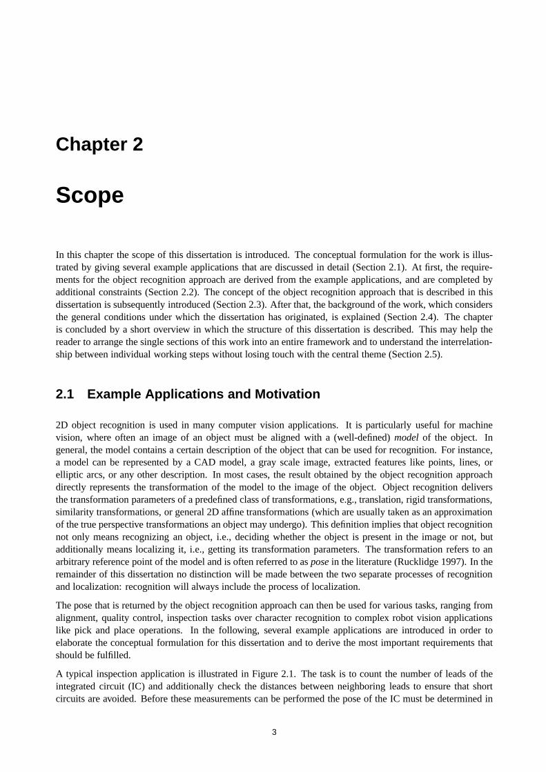
A typical inspection application is illustrated in Figure 2.1. The task is to count the number of leads of theintegrated circuit (IC) and additionally check the distances between neighboring leads to ensure that shortcircuits are avoided. Before these measurements can be performed the pose of the IC must be determined in
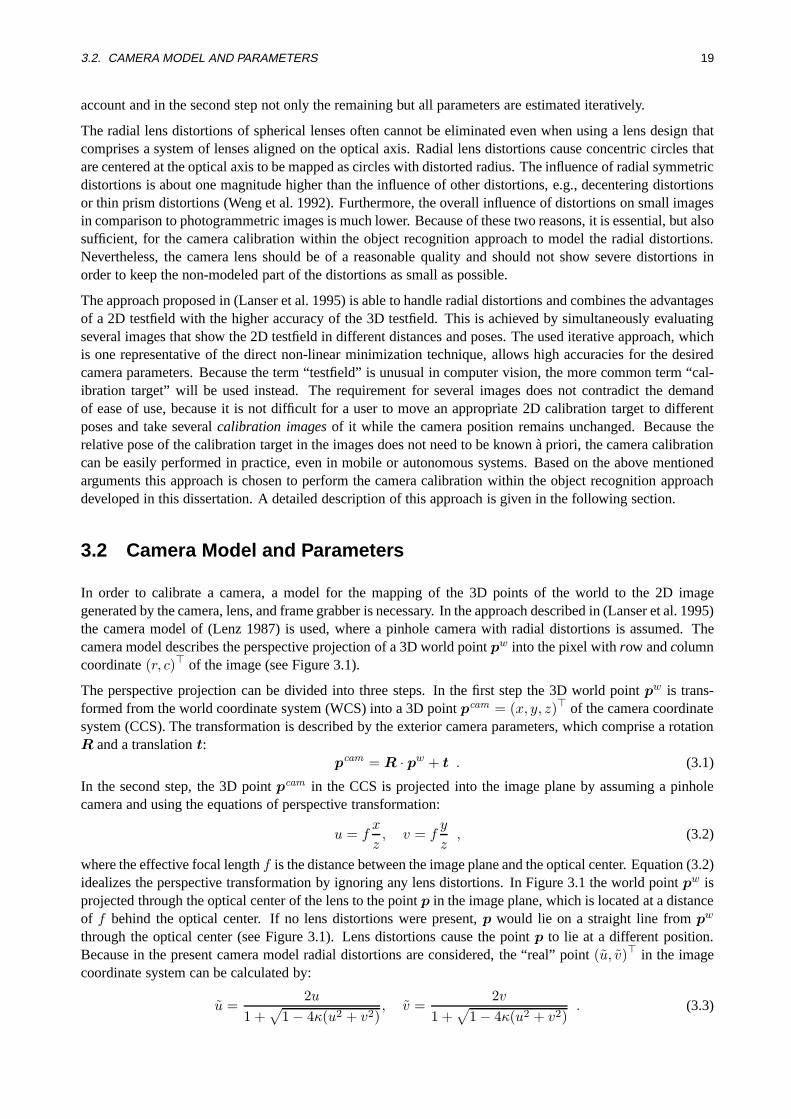
3
4 CHAPTER 2. SCOPE
(a) Input image (b) Inspected leads of the IC
Figure 2.1: Example that illustrates the role of object recognition in inspection tasks. The leads of the integrated circuit(IC) in (a) are to be inspected. The measurement windows (black), the extracted edges of the single leads (white), andthe results of the measurement are shown in (b).
the image by using an object recognition approach. In this case, the print on the IC is an obvious distinct objectthat can be used to build a model for the recognition process. A single image of the object should be sufficientto automatically build the model in order to keep the model creation as simple as possible. Because the relativeposition of the leads with respect to the print is approximately constant and known `a priori, two measurementwindows can be opened, which include the leads on both sides of the IC. This can be done after the pose of theprint has been determined by the recognition approach. Within the measurement windows subpixel preciseedges are computed and used to count the leads and to measure the distances between neighboring leads (seeFigure 2.1(b)). If one takes a closer look at Figure 2.1(a), a non-uniform illumination can be observed in theimage, which is due to a light source that was not perfectly mounted, leading to a stronger illumination ofthe lower left corner of the image. A uniform illumination that additionally is constant over time is highlydesirable in most applications. Unfortunately, sometimes a controlled illumination is hard to achieve if onerefrains from using an expensive set-up. Thus, it becomes obvious that the object recognition method must berobust against these kind of illumination conditions. For visualization purposes only, the contrast of the imagein Figure 2.1(b) is lowered. This auxiliary visualization step is performed whenever additional information isplotted within a gray scale image and the original image contrast makes it necessary. Therefore, this must notbe confused with a meaningful image processing operation under any circumstances.
Figure 2.2 illustrates one possible role of object recognition in the field of optical character recognition (OCR).Here, the task is to read the digits below the “disc” label. In many implementations, object recognition is notdirectly applied to recognize the characters. Instead, OCR is performed as a classification process, in whichsample characters are trained and used to derive a set of classification parameters for each character. Often,these parameters are not rotationally invariant. Hence, it is only possible to read characters that have the sameorientation as the characters used for training. In general, this assumption regarding the orientation is notvalid. A brute-force solution is to train the characters in all possible orientations. However, the computationtime for training and recognizing the characters increases. Additionally, the recognition rate decreases sincethe risk of confusion is higher. For example, it is not immediately possible to distinguish the letters “d” and“p” if they may appear in arbitrary orientation. A more sophisticated approach uses object recognition in apreliminary stage. In the example of Figure 2.2, the parameters are trained using characters that have beenhorizontally aligned. The CD label shown in Figure 2.2(a), however, may appear in arbitrary orientation.Therefore, the image must be rotated back to a horizontal orientation before the OCR can be applied. Thisprocess is often callednormalization. Object recognition can be used to obtain the orientation angle by whichthe image must be rotated. Because the digits below the “disc” label are not known, but must be determined,they cannot serve as object for the recognition process. In contrast, the appearance of the “disc” label itselfis constant and is an ideal pattern that can be searched in the image. As can be seen from this example, the

2.1. EXAMPLE APPLICATIONS AND MOTIVATION 5
(a) Input image (b) Result of the OCR
Figure 2.2: Example that illustrates the role of object recognition in optical character recognition (OCR). The digits belowthe “disc” label in (a) are to be read. To simplify the classification of the characters, the image is horizontally alignedaccording to the orientation of the recognized “disc” label (b).
recognition approach should be robust against a moderate degree of image noise. After the label has beenrecognized, the image is normalized, i.e., horizontally aligned by rotating it by the negative orientation ofthe found label. The result is shown in Figure 2.2(b). Although in this case the entire image is rotated fordemonstration purposes, normally, it is sufficient to only rotate the part below the disc label to speed up theprocess. Finally, the region of interest, i.e., the part of the image, in which the OCR is to be performed, canbe restricted to the image region directly below the label. Based on these two examples, it can be postulatedthat the recognition approach must be invariant to object orientation.
Another frequently arising problem is to check the quality of various kinds of prints. For example, it is es-tablished by law that food must have an appropriate durability indication, e.g., “Best Before:”, “Best BeforeEnd:”, or “Use By:”, followed by the corresponding date. Therefore, it is important that the date on foodpackagings is easy to read, and hence the corresponding print must not have severe quality faults. To men-tion another example, companies are very intent on handing out their products only with a perfectly printedcompany logo, because otherwise the imperfections of the logo are directly attributed to possible imperfectionof the company by the potential customer. Figure 2.3(a) shows the print on a pen clip that represents thecompany logo “MVTec”. In this example, the rightmost character “c” shows a substandard print quality inthe upper part of the character. A typical way to examine the print quality is to compare the gray values ofthe print that is to be checked with the gray values of an ideal template, which holds a perfect instance of theprint (Tobin et al. 1999). Absolute gray value differences that exceed a predefined threshold are interpreted assevere quality faults and returned by the program. The alignment of the ideal template over the print that is tobe checked can be achieved using object recognition by selecting, for example, the entire print as the object tobe found. From this it can be reasoned that even if parts of the object are missing, as is the case when dealingwith print faults, the recognition method must still be able to find the object. This is a hard but importantrequirement, since the case of missing parts is anything but rare, especially in the field of industrial qualitycontrol. Furthermore, especially in the field of quality control the colors of the object may vary, for example,depending on the used pressure during the print, on the amount of ink on the stamps, or on the color mixture.Thus, not only a non-uniform illumination but also the change of the object itself affects the gray values ofthe object in the image. Therefore, the object recognition approach should be robust against general changesin brightness of the object. Finally, the returned pose of the object can then be used to transform the idealtemplate to the desired position and orientation. Especially in this application the real-time aspect becomesimportant since the operational capacity in the pen production is very high, and hence fast computation for theobject recognition is demanded.
Based on this example, another demand on the recognition method can be derived which deals with sub-pixel object translations. The principle of the effect of subpixel translation is shown in Figure 2.4(a) using

6 CHAPTER 2. SCOPE
(a) Input image (b) Result of the print quality control
Figure 2.3: Example that illustrates the role of object recognition in quality control. The quality of the print on the labelof the pen clip in (a) is to be checked. An ideal template of the print is transformed according to the result of the objectrecognition and compared to the input image. Gray value differences that exceed a predefined threshold are returned aserrors (b).
Vertical subpixel object translation [pixel]
Ver
tica
lgra
yval
ue
pro
file
-0.5 -0.4 -0.3 -0.2 -0.1 0 +0.1 +0.2 +0.3 +0.4 +0.5
Subpixel accurateobject position
Pixel accurateobject position
1
2
3
4
M
(a) Effect of subpixel translation
−0.5 −0.4 −0.3 −0.2 −0.1 0 0.1 0.2 0.3 0.4 0.50
20
40
60
80
100
120
140
Vertical subpixel object translation [pixel]
Max
imum
abs
olut
e gr
ay v
alue
diff
eren
ce
(b) Induced error
Figure 2.4: The effect of subpixel translation on the gray values is shown in (a). Pixel precise object recognition methodsinduce errors in the case of subpixel translations (b).
a synthetic example, where a horizontal edge of the letter “M” is considered. For the ideal template a whitebackground (gray value 255) and a black foreground (gray value 0) are assumed. Let the horizontal edge ofthe letter exactly fall on the border between two neighboring vertically arranged pixels. Then a sharp hori-zontal edge with a gray value jump from 0 to 255 arises. If the letter is translated in a vertical direction by1/2 pixel in both directions using a step width of 1/10 pixel, the gray value of the corresponding pixel smoothlychanges. Consequently, the originally sharp horizontal edge becomes more and more blurred. When usinga pixel precise object recognition method, the subpixel translation would be undetectable, leading to a max-imum difference of 1/2 pixel between the true vertical location and the vertical location that is returned bythe recognition method. The resulting absolute gray value difference between the print and the incorrectlytransformed ideal template are plotted in Figure 2.4(b). The gray value differences, in this case, reach am-plitudes of 127, which make a reliable detection of defects in the print almost impossible. In contrast, sucheffects are avoided when using a subpixel precise object recognition method. Further examples that show theneed for subpixel precise object recognition can be found in image registration and feature location measure-ments in photogrammetry, remote sensing, image sequence analysis, or nondestructive evaluation (Tian andHuhns 1986).
The example application illustrated in Figure 2.5 introduces further important aspects to be considered inobject recognition. Here, the three metal parts shown in Figure 2.5(a) must be picked by a robot. From thisexample it follows that the object recognition method should also be able to recognize several instances of

2.1. EXAMPLE APPLICATIONS AND MOTIVATION 7
(a) Input image (b) Pick points for the robot
Figure 2.5: Example that illustrates the role of object recognition in pick and place applications. The metal parts shownin (a) are to be picked by a robot. The pick points are marked in (b). It is important to note that the recognition approachmust cope with projective distortions and overlapping objects.
the object in the image at the same time. Additionally, the different metal parts may overlap each other, andhence the recognition approach must also be able to handle occlusions up to a certain degree. This problemis equivalent to the situation where parts of the object are missing, as occurred in the example applicationof Figure 2.3. Furthermore, the image plane of the camera is not parallel to the plane in which the objectslie during image acquisition. This deviation from the nadir view leads to projective image distortions thatconsequently influence the appearance of the objects in the image and make the recognition much moredifficult. After the metal parts have been localized by the recognition method, the world coordinates of thepick points (see Figure 2.5(b)) are transmitted to the robot. More common pick and place applications can befound in the semiconductor industry where circuit boards are automatically equipped using robots.
Up to now, only examples with non-compound objects have been introduced. In the following, the motivationfor recognizing compound objects will be elaborated based upon further example applications. These exam-ples are also useful to elaborate the definition of compound objects that was given in Chapter 1. Because inthe following rigid objects must be distinguished from compound objects, the model representation of a rigidobject is referred to asrigid modeland the model of a compound object ascompound modelin the remainderof this dissertation.
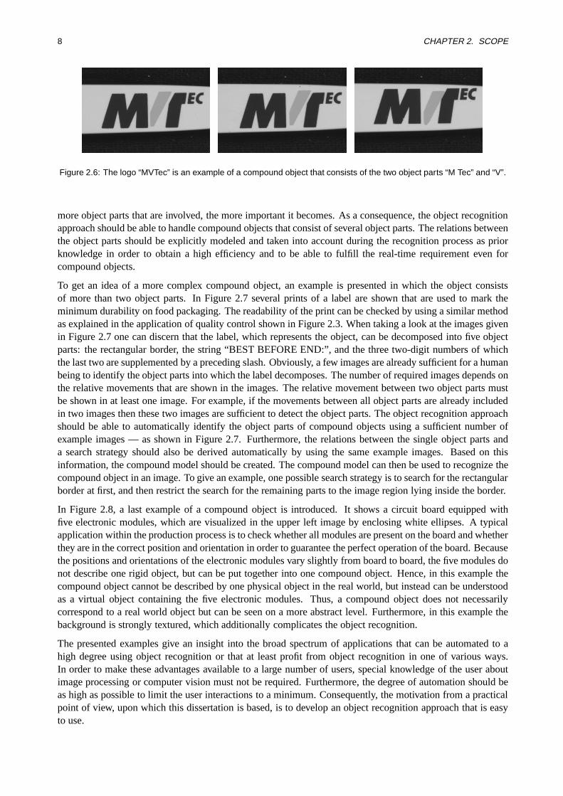
To give a first example, the application of quality control shown in Figure 2.3 is used. However, in contrastto the previously discussed example, now the considerations are extended to multiple occurrences of thepen clip (see Figure 2.6). Because the printing process of the logo was performed in two steps by applyingtwo independent stamps, one for each color, misalignments within the print may occur between the darkgray letters “M Tec” and the light gray letter “V”. Keeping the application of quality control in mind, itis necessary to perfectly align the ideal template to the print. The misalignment within the print, however,causes a discrepancy between the appearance of the print in the image and the object description in the modelthat is used to recognize the object. This discrepancy cannot be described by one global 2D transformation— which is typically used in the recognition process — because different parts of the object are transformedindividually. This leads to difficulties during object recognition and during the detection of print quality faults.One solution is to split the object, i.e., the entire print, into two separate objects, one representing the dark grayletters and the other the light gray letter, respectively. The object recognition approach is then started twice(once for each object), resulting in two independent poses for the two objects in the image. The drawback ofthis solution is that available information regarding the relations between the two objects is not exploited. Inthis example, such information could be, e.g., that the letter “V” is somewhere in between “M” and “Tec”.The consequence of ignoring this information is a loss of efficiency, since both objects must be searched inthe image without prior knowledge. This loss in most cases is already important when dealing with objectsthat consist of two separate object parts — as in this example. Considering the real-time requirement, the
8 CHAPTER 2. SCOPE
Figure 2.6: The logo “MVTec” is an example of a compound object that consists of the two object parts “M Tec” and “V”.
more object parts that are involved, the more important it becomes. As a consequence, the object recognitionapproach should be able to handle compound objects that consist of several object parts. The relations betweenthe object parts should be explicitly modeled and taken into account during the recognition process as priorknowledge in order to obtain a high efficiency and to be able to fulfill the real-time requirement even forcompound objects.
To get an idea of a more complex compound object, an example is presented in which the object consistsof more than two object parts. In Figure 2.7 several prints of a label are shown that are used to mark theminimum durability on food packaging. The readability of the print can be checked by using a similar methodas explained in the application of quality control shown in Figure 2.3. When taking a look at the images givenin Figure 2.7 one can discern that the label, which represents the object, can be decomposed into five objectparts: the rectangular border, the string “BEST BEFORE END:”, and the three two-digit numbers of whichthe last two are supplemented by a preceding slash. Obviously, a few images are already sufficient for a humanbeing to identify the object parts into which the label decomposes. The number of required images depends onthe relative movements that are shown in the images. The relative movement between two object parts mustbe shown in at least one image. For example, if the movements between all object parts are already includedin two images then these two images are sufficient to detect the object parts. The object recognition approachshould be able to automatically identify the object parts of compound objects using a sufficient number ofexample images — as shown in Figure 2.7. Furthermore, the relations between the single object parts anda search strategy should also be derived automatically by using the same example images. Based on thisinformation, the compound model should be created. The compound model can then be used to recognize thecompound object in an image. To give an example, one possible search strategy is to search for the rectangularborder at first, and then restrict the search for the remaining parts to the image region lying inside the border.
In Figure 2.8, a last example of a compound object is introduced. It shows a circuit board equipped withfive electronic modules, which are visualized in the upper left image by enclosing white ellipses. A typicalapplication within the production process is to check whether all modules are present on the board and whetherthey are in the correct position and orientation in order to guarantee the perfect operation of the board. Becausethe positions and orientations of the electronic modules vary slightly from board to board, the five modules donot describe one rigid object, but can be put together into one compound object. Hence, in this example thecompound object cannot be described by one physical object in the real world, but instead can be understoodas a virtual object containing the five electronic modules. Thus, a compound object does not necessarilycorrespond to a real world object but can be seen on a more abstract level. Furthermore, in this example thebackground is strongly textured, which additionally complicates the object recognition.
The presented examples give an insight into the broad spectrum of applications that can be automated to ahigh degree using object recognition or that at least profit from object recognition in one of various ways.In order to make these advantages available to a large number of users, special knowledge of the user aboutimage processing or computer vision must not be required. Furthermore, the degree of automation should beas high as possible to limit the user interactions to a minimum. Consequently, the motivation from a practicalpoint of view, upon which this dissertation is based, is to develop an object recognition approach that is easyto use.

2.2. REQUIREMENTS 9
Figure 2.7: The compound object decomposes into five object parts: the rectangular border, the string “BEST BEFOREEND:”, and the three two-digit numbers, of which the last two are supplemented by a preceding slash.
Figure 2.8: The five electronic modules, which are visualized in the upper left image (white ellipses), slightly vary theirposition and orientation on the circuit boards. They can be represented by one compound object.
2.2 Requirements
Following the discussion of the example applications (Section 2.1), the requirements that an object recognitionapproach should fulfill will now be summarized. They are completed by additional requirements that have tobe considered in industry.
However, before listing the demands some general remarks must be mentioned. Firstly, one of the aims of thisdissertation is to develop an object recognition approach for a broad spectrum of applications. Consequently,there must be no special requirements on the necessary hardware in order to maximize the field of possibleapplications. Usually, only three hardware components should be necessary for real-time object recognition:a camera, a computer, and a frame grabber. Starting with the first component, it should be sufficient to use
10 CHAPTER 2. SCOPE
Image plane
Projection center
(a) Image plane and object planeε′ are not parallel
Ori
gin
alim
age
Rec
tifi
edim
age
ε'
(b) Rectification
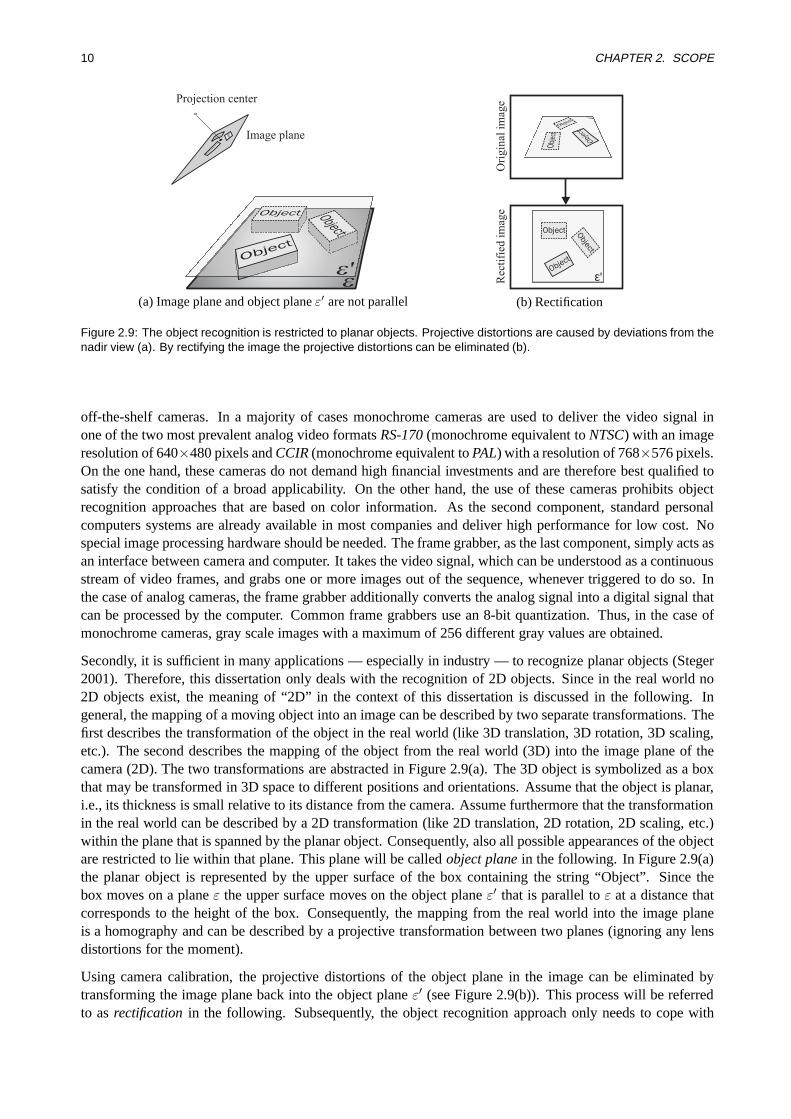
Figure 2.9: The object recognition is restricted to planar objects. Projective distortions are caused by deviations from thenadir view (a). By rectifying the image the projective distortions can be eliminated (b).
off-the-shelf cameras. In a majority of cases monochrome cameras are used to deliver the video signal inone of the two most prevalent analog video formatsRS-170(monochrome equivalent toNTSC) with an imageresolution of 640×480 pixels andCCIR(monochrome equivalent toPAL) with a resolution of 768×576 pixels.On the one hand, these cameras do not demand high financial investments and are therefore best qualified tosatisfy the condition of a broad applicability. On the other hand, the use of these cameras prohibits objectrecognition approaches that are based on color information. As the second component, standard personalcomputers systems are already available in most companies and deliver high performance for low cost. Nospecial image processing hardware should be needed. The frame grabber, as the last component, simply acts asan interface between camera and computer. It takes the video signal, which can be understood as a continuousstream of video frames, and grabs one or more images out of the sequence, whenever triggered to do so. Inthe case of analog cameras, the frame grabber additionally converts the analog signal into a digital signal thatcan be processed by the computer. Common frame grabbers use an 8-bit quantization. Thus, in the case ofmonochrome cameras, gray scale images with a maximum of 256 different gray values are obtained.
Secondly, it is sufficient in many applications — especially in industry — to recognize planar objects (Steger2001). Therefore, this dissertation only deals with the recognition of 2D objects. Since in the real world no2D objects exist, the meaning of “2D” in the context of this dissertation is discussed in the following. Ingeneral, the mapping of a moving object into an image can be described by two separate transformations. Thefirst describes the transformation of the object in the real world (like 3D translation, 3D rotation, 3D scaling,etc.). The second describes the mapping of the object from the real world (3D) into the image plane of thecamera (2D). The two transformations are abstracted in Figure 2.9(a). The 3D object is symbolized as a boxthat may be transformed in 3D space to different positions and orientations. Assume that the object is planar,i.e., its thickness is small relative to its distance from the camera. Assume furthermore that the transformationin the real world can be described by a 2D transformation (like 2D translation, 2D rotation, 2D scaling, etc.)within the plane that is spanned by the planar object. Consequently, also all possible appearances of the objectare restricted to lie within that plane. This plane will be calledobject planein the following. In Figure 2.9(a)the planar object is represented by the upper surface of the box containing the string “Object”. Since thebox moves on a planeε the upper surface moves on the object planeε′ that is parallel toε at a distance thatcorresponds to the height of the box. Consequently, the mapping from the real world into the image planeis a homography and can be described by a projective transformation between two planes (ignoring any lensdistortions for the moment).
Using camera calibration, the projective distortions of the object plane in the image can be eliminated bytransforming the image plane back into the object planeε′ (see Figure 2.9(b)). This process will be referredto asrectification in the following. Subsequently, the object recognition approach only needs to cope with

2.2. REQUIREMENTS 11
the remaining 2D transformation of the planar object in the real world. In the example applications presentedso far, the 2D transformation can be described by a rigid motion (translation and rotation). In practice, itis sufficient that the 3D object has at least an approximately planar surface: although a minor unevennessintroduces additional perspective distortions that cannot be eliminated by the rectification these distortions arenegligible as long as the deviation from the nadir view is also sufficiently small. What is important is that alltransformations the 3D object may undergo must lead to a 2D transformation of the planar object surface. Inthe following, the object will be equated with its planar surface since the 3D object as a whole is irrelevant forfurther considerations in this work. To give some examples, in Figure 2.1 the IC represents the 3D object withthe print on the IC as the planar object surface, in Figure 2.2 the CD cover represents the 3D object with the“disc” label as the planar object surface, in Figure 2.3 the pen clip represents the 3D object, with the logo asthe planar object surface, and in Figure 2.5 a metal part represents both the 3D object and the (approximately)planar object surface.
Now, after the general conditions have been stated, the requirements for an object recognition approach aregiven:
• The object recognition approach should be able to handle compound objects.Compound objects shouldnot be treated as a set of independent objects that ignore the relations between them but should be explic-itly modeled leading to an increased computational efficiency. Furthermore, the correct correspondenceof the object parts should be given by the approach.
• Objects should be recognized in real-time.This is strongly connected with the previous requirementbecause without modeling the relations between object parts, real-time computation is hard to achievewhen dealing with compound objects. Nevertheless, this requirement additionally implies the existenceof an object recognition approach that is able to recognizerigid objects in real-time since a rigid objectcan be seen as a degenerated compound object with only one object part. Because the computationalcomplexity of object recognition approaches depends on the image size, the real-time demand must berelated to a maximum occurring image size. Bearing the above considered hardware requirements inmind, RS-170 or CCIR images are assumed in this dissertation. Hence, objects should be recognized inreal-time when using images that have a size of not substantially larger than 768× 576 pixels.
• The model representation of a rigid object should be computed from an example image of the object.Keeping in mind the claim that the object recognition approach should be easy to use, the computationof the rigid model should only ask for a single model image of the object. This is the most comfortableway because usually it is too costly or time consuming to compute a more complicated model, e.g, aCAD model, or to transform a given CAD model into a model representation that can be used for objectrecognition.
• The model representation of a compound object should be computed from several example images ofthe compound object.In contrast to the previous requirement, the model representation of compoundobjects is more complicated to compute since movements between object parts cannot be detected froma single example image. Nevertheless, in order to keep the model computation as simple as possiblefor the user, it should be sufficient to make several example images available. The object recognitionapproach should then be able to automatically derive the relations between the object parts from thegiven example images and to derive the compound model.
• The object recognition approach should be general with regard to the type of object.The approachshould not be restricted to a special type of object. Thus, the model, which represents the object, shouldbe able to describe arbitrary objects. For example, if straight lines or corner points were chosen asfeatures to describe the object it would be impossible to recognize ellipse-shaped objects.
• The object recognition approach should be robust against occlusions up to a certain degree.This isoften highly desirable in cases where several objects may overlap each other or in cases where objectparts are missing.
12 CHAPTER 2. SCOPE
• The object recognition approach should be robust against changes in brightness of an arbitrary typeup to a certain degree.Illumination changes often cannot be avoided and are, for instance, caused bynon-uniform illumination over the entire field of view, changing light (position, direction, intensity),objects with non-Lambertian surfaces, etc. Furthermore, changes in the color of the object itself alsolead to changes in brightness in the image.
• The object recognition approach should be robust against clutter.Clutter in this context means anyadditional information in the image, aside from the object that is to be recognized. This informationcan, for example, be a strongly textured background or additional objects that are visible in the image,and which are possibly similar to the object of interest.
• The object recognition approach should be robust against image noise.Since noise cannot be avoidedin the image, the approach should be robust against noise up to a certain degree.
• Objects under rigid motion should be recognized.This is closely related to the requirement of real-time computation. In general, the more degrees of freedom the transformation of an object includesthe higher the complexity of the recognition approach and therefore the higher the computation time torecognize the object. Hence, the real-time demand is coupled with the allowable degrees of freedom.In this dissertation rigid motion (translation and rotation) is considered, i.e., the object recognition ap-proach should be able to find the object at arbitrary position and orientation. This does not imply that theapproach cannot be extended to more general transformations like similarity transformations or affinetransformations. However, there is a trade-off between the real-time demand and the transformationclass.
• The approach should cope with deviations from the nadir view.Often, it is not possible to mount thecamera with a viewing direction perpendicular to the plane in which the object appears. The resultingprojective distortions should be managed by the recognition approach.
• The returned pose parameters should be of high accuracy.This means that the pose parameters shouldnot be restricted to discretely sampled values but go beyond any quantization resolution. For example,the position parameters of the object should not be restricted to the pixel grid but should be subpixelprecise. The same holds for the object’s orientation.
• Finally, all instances of an object should be found in the image.The approach should not only find the“best” instance of an object in an image but return all instances that fulfill a predefined criterion. In theremainder of this dissertation found object instances in an image will be referred to asmatches.
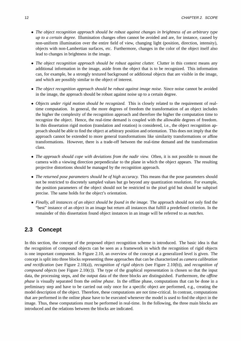
2.3 Concept
In this section, the concept of the proposed object recognition scheme is introduced. The basic idea is thatthe recognition of compound objects can be seen as a framework in which the recognition of rigid objectsis one important component. In Figure 2.10, an overview of the concept at a generalized level is given. Theconcept is split into three blocks representing three approaches that can be characterized ascamera calibrationand rectification(see Figure 2.10(a)),recognition of rigid objects(see Figure 2.10(b)), andrecognition ofcompound objects(see Figure 2.10(c)). The type of the graphical representation is chosen so that the inputdata, the processing steps, and the output data of the three blocks are distinguished. Furthermore, theofflinephaseis visually separated from theonline phase. In the offline phase, computations that can be done in apreliminary step and have to be carried out only once for a specific object are performed, e.g., creating themodel description of the object. Therefore, these computations are not time-critical. In contrast, computationsthat are performed in the online phase have to be executed whenever the model is used to find the object in theimage. Thus, these computations must be performed in real-time. In the following, the three main blocks areintroduced and the relations between the blocks are indicated.
2.3. CONCEPT 13
Images ofCalibration Target
Camera Calibration andComputation of Rectification Map
Input Image
Rectification
Rectification Map
Rectification MapRectified Image
InputO
ffli
ne
Processing OutputO
nli
ne
(a) Approach for camera calibration and rectification
Model Image
Search Image
Rectification
Rigid Model Generation Rigid Model
Rectification
Rigid Object Recognition Rigid Object Pose
Rectification Map
Rectification Map
Input Processing Output
Off
lin
eO
nli
ne
(b) Approach for recognition of rigid objects
Model Image
Search Image
Rectification
Rectification
HierarchicalModel
Hierarchical Model Training and CreationRectification Map
RectificationExample Images
Rectification Map
Rigid Model Generation for Each Part
Analysis of Example Images
Rigid Modelfor Each Part
Relations
Search Strategy
Extraction of Rigid Object Parts
Rectification MapHierarchical Object Recognition Compound Object
Pose
Poses of AllObject PartsRigid Object Recognition of Each Part
Successive Search SpaceComputation for Each Part
HierarchicalModel
Rigid Modelfor Each Part
Relations
Search Strategy
Input Processing Output
Off
lin
eO
nli
ne
(c) Approach for recognition of compound objects
Figure 2.10: The concept of the object recognition described in this dissertation
14 CHAPTER 2. SCOPE
The first block represents the camera calibration and the rectification (see Figure 2.10(a)). It is only relevant ifthe camera was not mounted perpendicular to the plane in which the objects lie or the camera exhibits severeradial distortions. Otherwise this block can be omitted. The idea behind the calibration is to eliminate pro-jective distortions by rectifying distorted images before the images are passed to further processing steps (seeFigure 2.10(b) and Figure 2.10(c)). This has the considerable advantage that all further processing steps donot need to concern themselves with projective distortions at all. The disadvantage is that an additional imagetransformation and a re-sampling step have to be performed, which are, in general, very time consuming. Inorder to reduce this additional computation time, this process of rectification is split into an offline phase andan online phase. In the offline phase, the camera calibration is computed using several images of a knowncalibration target and arectification mapis derived from the calibration data. This is a time consuming step,but it has to be performed only once for a specific camera pose and a specific object plane. The rectificationmap can be seen as a kind of look-up table that facilitates a fast rectification of an input image in the onlinephase. The resulting rectified image is free of radial and projective distortions.
In the second block the general design of an approach for recognizing rigid objects is described (see Fig-ure 2.10(b)). Here, in the offline phase, the rigid model is derived from an image of the object. The image partthat shows the object is referred to asmodel imageand — if necessary — has been rectified in a precedingstep using the rectification map. The rigid model can then be used in the online phase to recognize the objectin one or more (rectified)search images. While the rectification of the model image in the offline phase is nottime-critical the rectification of the search images in the online phase must be performed in real-time.
The third block describes the concept of the approach for recognizing compound objects (see Figure 2.10(c)).Generally, the model of a compound object is referred to as compound model. In the proposed approach thecompound model shows a hierarchical structure, which is also indicated by the thesis “Using ahierarchi-cal modelfor the recognition of compound objects provides higher efficiency and inherent determination ofcorrespondence in contrast to standard methods, and hence facilitates real-time applications”. Therefore, thecompound model that is generated during the offline phase will also be referred to ashierarchical model. Thehierarchical model generation comprises the extraction of rigid object parts on the basis of the model imageand several example images. The most important thing to note is that for each rigid object part a rigid modelis generated by employing the offline phase of the recognition of rigid objects (see Figure 2.10(b)). Hence, theoffline phase of recognizing rigid objects is embedded in the offline phase of recognizing compound objects.Consequently, the resulting hierarchical model holds a rigid model for each part of the compound object. Therelations between the parts and the search strategy for the online phase are automatically derived by analyzingthe example images and complete the hierarchical model. Analogous to the offline phase, the online phaseof recognizing rigid objects is embedded in the online phase of recognizing compound objects. An importantcharacteristic of the online phase for compound objects is, however, the computation of an individual searchspace for each object part in order to minimize the search effort. This computation is based on the hierarchicalmodel using the relations between the parts and the derived search strategy.
Consequently, the concept of recognizing compound objects represents a framework in which an approach forrecognizing rigid objects is embedded as a substantial part. This modularity facilitates the interchangeabilityof the latter approach without affecting the concept of recognizing compound objects. Thus, the concept ofrecognizing compound objects is independent from the chosen embedded approach. As another consequence,the requirements listed in Section 2.2 that do not explicitly refer to compound objects have to be fulfilled,not only by the approach for recognizing compound objects, but also by the approach for recognizing rigidobjects.
2.4 Background
In this section, the background and the general external conditions from which the dissertation has originatedand under which it was developed are explained. This is essential because these conditions influence severalaspects of the work.
2.5. OVERVIEW 15
The author’s work has been supported by the software companyMVTec Software GmbH(Munich, Germany).Their main product,HALCON, represents a machine vision tool that is based on a large library of imageprocessing operators (MVTec 2002). The implementation of the presented approach is partly based on imageprocessing operations that are provided by the HALCON library. The motivation for MVTec Software GmbHin supporting the author’s work was, on the one hand, to extend their existing knowledge in the field ofobject recognition in general. On the other hand, a new approach for the recognition of compound objectsthat can be directly included in the HALCON library should be developed and implemented. HALCON ismainly applied to specific tasks that arise in industry. A selection of the typical example applications aredemonstrated in Section 2.1. Thus, the requirements listed in Section 2.2, and hence the derived concept ofthis work introduced in Section 2.3, are indirectly influenced by industrial demands.
Two approaches for recognizing rigid objects have been developed approximately simultaneously with the aimof fulfilling the established requirements: on the commercial side, theshape-based matching(Steger 2002) hasbeen developed at MVTec Software GmbH, and on the scientific side, the author has developed themodifiedgeneralized Hough transformin the context of this dissertation (Ulrich et al. 2001b). Because of these closerelationships, the developments have not been completely independent of each other but have overlapped ina few areas. Both approaches are introduced in the dissertation, where the main focus is on the modifiedgeneralized Hough transform. The overlapping points will only be explained once. However, the approachfor recognizing compound objects is then built on the basis of the shape-based matching because the latter hasalready been thoroughly tested and included in the HALCON library.
2.5 Overview
In the following, a brief overview of the dissertation is given. According to to the concept outlined in Fig-ure 2.10 the next three chapters correspond to the three main tasks. Chapter 3 describes the camera calibrationand the rectification. It comprises the introduction of the used camera model, the calibration, as well as thenovel rectification process. This chapter is then concluded with a small example. Chapter 4 addresses therecognition of rigid objects. An extensive review of recognition methods is carried out and the generalizedHough transform (Ballard 1981) as a promising candidate is selected and further examined. The drawbacks ofthe generalized Hough transform are elaborated and analyzed. In the following sections, several novel mod-ifications are introduced to eliminate the drawbacks. The respective modifications are applied, resulting in amodified generalized Hough transform. Finally, after the shape-based matching is introduced, an extensiveperformance evaluation compares the modified generalized Hough transform and the shape-based matchingwith several other approaches for the recognition of rigid objects. In Chapter 5 the new approach for recog-nizing compound objects is explained. A review of the respective literature is followed by an overview thatbroadly describes the pursued strategy. A more detailed description of the single processing steps is subse-quently given focusing on the main novel aspects of this work. This chapter is then concluded with severalexamples that show the advantages of the new approach. Finally, in Chapter 6 some conclusions are given.

16 CHAPTER 2. SCOPE
Chapter 3
Camera Calibration and Rectification
Geometric camera calibration is a prerequisite for the extraction of precise 3D information from imagery incomputer vision, robotics, photogrammetry, and other areas.
Since in this dissertation only 2D objects are considered, the benefit of using 3D camera calibration for thepurpose of 2D object recognition should be addressed first. The first point has already been discussed inChapter 2 and must be considered when the image plane is not parallel to the plane in which the objectsoccur, which results in an homographic mapping between the two planes. In order to eliminate the resultingprojective distortions in the image, one has to know the 3D poses of both planes in the real world. The secondpoint addresses the problem of lens distortions, i.e., the physical reality of a camera geometrically deviatesfrom the ideal perspective geometry. Therefore, whenever precise measurements must be derived from theimage data, these deviations must be considered. In the case of compound objects, quantitative statementsabout the relative poses of the object parts in the real world must be made. This is important in order tofacilitate a correct automatic computation of the hierarchical model. Hence, it is essential to perform a cameracalibration in a preceding step. The remainder of this chapter is organized as follows: In Section 3.1, a shortreview of camera calibration techniques is given in order to select the appropriate method for the task ofrecognizing compound objects. Section 3.2 describes the applied camera model and the involved parametersand in Section 3.3 the calibration process is briefly explained. In Section 3.4, a novel way to rectify imagesbased on the calibration result that facilitates real-time computation is introduced. The rectified images arefree of lens distortions and free of projective distortions of the object plane. Finally, Section 3.5 concludeswith an example.
3.1 Short Review of Camera Calibration Techniques
One aspect of camera calibration is to estimate the interior parameters of the camera. These parameters de-termine how the image coordinates of a 3D object point are derived, given the spatial position of the pointwith respect to the camera. The estimation of the geometrical relation between the camera and the scene isalso an important aspect of calibration. The corresponding parameters that characterize such a geometricalrelation are called exterior parameters or camera pose. Thus, the camera parameters describe the interior andexterior orientation of the camera. In this work, camera calibration means to determine all camera parameters.It should be noted that sometimes camera calibration only comprises the determination of the interior cameraparameters, as in the field of photogrammetry and remote sensing. Literature provides several methods ofcamera calibration. In photogrammetry two basic approaches can be distinguished: laboratory methods andfield methods (Heipke et al. 1991). The interior orientation of metric cameras is usually determined underlaboratory conditions. The interior orientation of metric cameras is constant and the image coordinate systemis defined by special fiducial marks within the camera. Field methods can be further subdivided into testfieldcalibration, simultaneous self calibration, and system calibration. Testfield calibration is carried out for non-
17

18 CHAPTER 3. CAMERA CALIBRATION AND RECTIFICATION
and semi-metric cameras prior to image acquisition. The object coordinates of several control points withinthe testfield are known and used to derive the orientation of the camera within a photogrammetric block adjust-ment. In (Ebner 1976), a simultaneous self calibration is presented where the interior orientation parametersare determined simultaneously with the desired object space information. Finally, system calibration com-bines testfield and simultaneous self calibration where images are acquired that show both the testfield and theobject and that are evaluated in one step (Kupfer 1987).
In machine vision, mainly non-metric digital cameras (e.g., off-the-shelf CCD cameras) come into operationbecause of their lower prices, higher flexibility, and manageable size in contrast to metric and semi-metriccameras. Because their interior orientation is not known `a priori and cannot be assumed to be constant, therequirement for laboratory calibration methods is not fulfilled. Hence, in most cases, cameras are calibratedusing field methods. The advantages of simultaneous self calibration are its high accuracy and that no controlpoint coordinates in object space need to be known `a priori (Wester-Ebbinghaus 1983). However, severalimages taken from different camera poses must be acquired in order to perform the calibration. This contra-dicts the claim of the object recognition approach to be simple and easy to use. Camera calibration shouldbe possible in industry, even during system operation without unmounting the camera. Another limitation ofsimultaneous self calibration is that it requires a high number of corresponding points in the images, whichare not available in all cases. The requirements for testfield calibration are less stringent than the requirementsfor simultaneous self calibration. Nevertheless, high accuracies are also possible. The geometric quality ofsolid-state imaging sensors was already verified in (Gruen and Beyer 1987), where an accuracy of 1/10th ofthe pixel spacing was achieved with a planar testfield. In (Heipke et al. 1991), it was shown that the calibrationusing a 3D testfield even fulfills the stringent accuracy requirements of photogrammetric tasks. Accuracies upto 1/50th of the pixel spacing could be verified with a 3D testfield in (Beyer 1987). Also in (Beyer 1992) and(Godding 1993) 3D testfields are applied for camera calibration. Unfortunately, the construction of the 3Dtestfield and the precise determination of the object coordinates of the control points within the testfield arevery time consuming and costly. Generally, the assignment of the measured image coordinates to the controlpoints must be done manually because the correspondence problem in 3D is difficult to solve. The uncomfort-able handling of such targets is another drawback that rules out the use of 3D testfields in this work. Althoughin general, the accuracy achieved by a planar 2D testfield is lower in comparison to 3D testfields, there areseveral arguments for preferring the use of a 2D testfield for calibration: it is more robust, much easier toproduce, less expensive to gauge, and simpler to transport. Furthermore, the extraction and assignment of thecontrol points in the image can be done automatically since the correspondence problem in 2D is much easierto solve.
In order to perform the camera calibration, one has to select an appropriate camera model where the imple-mented parameters describe the physical mapping process with sufficient accuracy. According to the literature,different approaches for camera calibration are suitable for different camera models. In (Weng et al. 1992), theexisting techniques are classified into three categories.Direct non-linear minimizationrelates the parametersto be estimated with the 3D coordinates of control points and their image plane projections and minimizesthe residual errors using an iterative algorithm (Brown 1966, Faig 1975, Wong 1975). The advantages of thistype of technique are that the camera model can be very general to cover many types of distortions, and that ahigh accuracy can be achieved. However, because of the non-linearity of the resulting equations, a good initialguess is required for the iteration. Inclosed-form solutions, parameter values are computed directly througha non-iterative algorithm by defining intermediate parameters that can be determined by solving linear equa-tions. The final parameters are subsequently computed from the intermediate parameters (Abdel-Aziz andKarara 1971, Wong 1975, Faugeras and Toscani 1986). On the one hand this enables a fast computation, onthe other hand, in general, distortion parameters cannot be considered and poor results are obtained in thepresence of noise. In (Abdel-Aziz and Karara 1971), the direct linear transformation (DLT) has been extendedto incorporate distortion parameters. However, the corresponding formulation is not exact. Finally,two-stepmethodsinvolve a direct solution for most of the calibration parameters and some iterative solution for theremaining parameters. In (Tsai and Lenz 1988), a two-step method is presented that is able to handle radialdistortions. In (Weng et al. 1992), the two-step approach is extended to also take more general distortions into
3.2. CAMERA MODEL AND PARAMETERS 19
account and in the second step not only the remaining but all parameters are estimated iteratively.
The radial lens distortions of spherical lenses often cannot be eliminated even when using a lens design thatcomprises a system of lenses aligned on the optical axis. Radial lens distortions cause concentric circles thatare centered at the optical axis to be mapped as circles with distorted radius. The influence of radial symmetricdistortions is about one magnitude higher than the influence of other distortions, e.g., decentering distortionsor thin prism distortions (Weng et al. 1992). Furthermore, the overall influence of distortions on small imagesin comparison to photogrammetric images is much lower. Because of these two reasons, it is essential, but alsosufficient, for the camera calibration within the object recognition approach to model the radial distortions.Nevertheless, the camera lens should be of a reasonable quality and should not show severe distortions inorder to keep the non-modeled part of the distortions as small as possible.
The approach proposed in (Lanser et al. 1995) is able to handle radial distortions and combines the advantagesof a 2D testfield with the higher accuracy of the 3D testfield. This is achieved by simultaneously evaluatingseveral images that show the 2D testfield in different distances and poses. The used iterative approach, whichis one representative of the direct non-linear minimization technique, allows high accuracies for the desiredcamera parameters. Because the term “testfield” is unusual in computer vision, the more common term “cal-ibration target” will be used instead. The requirement for several images does not contradict the demandof ease of use, because it is not difficult for a user to move an appropriate 2D calibration target to differentposes and take severalcalibration imagesof it while the camera position remains unchanged. Because therelative pose of the calibration target in the images does not need to be known `a priori, the camera calibrationcan be easily performed in practice, even in mobile or autonomous systems. Based on the above mentionedarguments this approach is chosen to perform the camera calibration within the object recognition approachdeveloped in this dissertation. A detailed description of this approach is given in the following section.
3.2 Camera Model and Parameters
In order to calibrate a camera, a model for the mapping of the 3D points of the world to the 2D imagegenerated by the camera, lens, and frame grabber is necessary. In the approach described in (Lanser et al. 1995)the camera model of (Lenz 1987) is used, where a pinhole camera with radial distortions is assumed. Thecamera model describes the perspective projection of a 3D world pointpw into the pixel withrow andcolumncoordinate(r, c)> of the image (see Figure 3.1).
The perspective projection can be divided into three steps. In the first step the 3D world pointpw is trans-formed from the world coordinate system (WCS) into a 3D pointpcam = (x, y, z)> of the camera coordinatesystem (CCS). The transformation is described by the exterior camera parameters, which comprise a rotationR and a translationt:
pcam = R · pw + t . (3.1)
In the second step, the 3D pointpcam in the CCS is projected into the image plane by assuming a pinholecamera and using the equations of perspective transformation:
u = fx
z, v = f
y
z, (3.2)
where the effective focal lengthf is the distance between the image plane and the optical center. Equation (3.2)idealizes the perspective transformation by ignoring any lens distortions. In Figure 3.1 the world pointpw isprojected through the optical center of the lens to the pointp in the image plane, which is located at a distanceof f behind the optical center. If no lens distortions were present,p would lie on a straight line frompw
through the optical center (see Figure 3.1). Lens distortions cause the pointp to lie at a different position.Because in the present camera model radial distortions are considered, the “real” point(u, v)> in the imagecoordinate system can be calculated by:
u =2u
1 +√
1− 4κ(u2 + v2), v =
2v1 +
√1− 4κ(u2 + v2)
. (3.3)
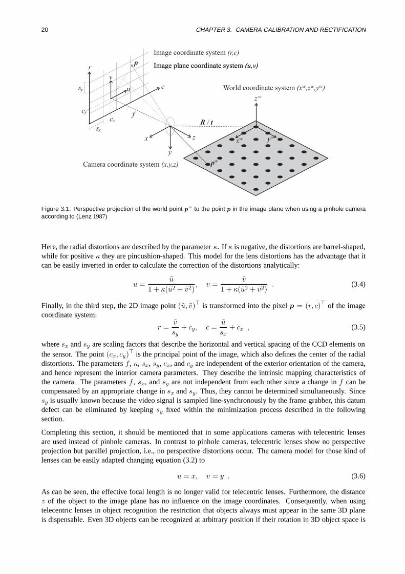
20 CHAPTER 3. CAMERA CALIBRATION AND RECTIFICATION
p
c
r
sy
v
u
cy
cxf
R t/
x
y
zx y
zw
w w
pw
Image coordinate system (r,c)
Image plane coordinate system (u,v)Image plane coordinate system (u,v)
Camera coordinate system (x,y,z)
World coordinate system (x ,z ,y )w w w
sx
Figure 3.1: Perspective projection of the world point pw to the point p in the image plane when using a pinhole cameraaccording to (Lenz 1987)
Here, the radial distortions are described by the parameterκ. If κ is negative, the distortions are barrel-shaped,while for positiveκ they are pincushion-shaped. This model for the lens distortions has the advantage that itcan be easily inverted in order to calculate the correction of the distortions analytically:
u =u
1 + κ(u2 + v2), v =
v
1 + κ(u2 + v2). (3.4)
Finally, in the third step, the 2D image point(u, v)> is transformed into the pixelp = (r, c)> of the imagecoordinate system:
r =v
sy+ cy, c =
u
sx+ cx , (3.5)
wheresx andsy are scaling factors that describe the horizontal and vertical spacing of the CCD elements onthe sensor. The point(cx, cy)
> is the principal point of the image, which also defines the center of the radialdistortions. The parametersf , κ, sx, sy, cx, andcy are independent of the exterior orientation of the camera,and hence represent the interior camera parameters. They describe the intrinsic mapping characteristics ofthe camera. The parametersf , sx, andsy are not independent from each other since a change inf can becompensated by an appropriate change insx andsy. Thus, they cannot be determined simultaneously. Sincesy is usually known because the video signal is sampled line-synchronously by the frame grabber, this datumdefect can be eliminated by keepingsy fixed within the minimization process described in the followingsection.
Completing this section, it should be mentioned that in some applications cameras with telecentric lensesare used instead of pinhole cameras. In contrast to pinhole cameras, telecentric lenses show no perspectiveprojection but parallel projection, i.e., no perspective distortions occur. The camera model for those kind oflenses can be easily adapted changing equation (3.2) to
u = x, v = y . (3.6)
As can be seen, the effective focal length is no longer valid for telecentric lenses. Furthermore, the distancez of the object to the image plane has no influence on the image coordinates. Consequently, when usingtelecentric lenses in object recognition the restriction that objects always must appear in the same 3D planeis dispensable. Even 3D objects can be recognized at arbitrary position if their rotation in 3D object space is

3.3. CAMERA CALIBRATION 21
restricted to rotations around the viewing direction of the camera, because then the resulting mapping in theimage can be described by a simple rigid motion. The diameter of telecentric lenses, however, must have atleast the same size as the parallel projection of the extent of the object. The following considerations refer topinhole cameras but can be easily adapted for the use of telecentric lenses.
3.3 Camera Calibration
In this section, the approach for camera calibration proposed in (Lanser et al. 1995), which uses the modelintroduced in the previous section, is briefly explained. This approach extends the single image calibration(SIC) to a multi image calibration (MIC) and is able to handle numerous images of the calibration target. Atfirst, the calibration using single images is introduced, and afterwards, the necessary modifications for themulti image calibration are explained.
In the SIC a single image of a 2D calibration target withN circular black colored marks is used (see Fig-ure 3.2). The centers of the circular marks represent the 3D control points. The 2D coordinates of the controlpoints in the planar calibration target are known with high accuracy. The coordinate system of the controlpoints also defines the coordinate system, in which the pose of the camera, i.e., the exterior orientation, iscomputed. The square border allows the inner part of the calibration target to be found automatically. Circu-lar marks are used because their center point can be determined with high accuracy. The circular marks aremapped to ellipses under projective transformations. It should be noted that, in general, the extracted centersof the ellipses do not coincide with the projected centers of the circular marks. Therefore, an analytical cor-rection must be applied in order to increase the accuracy (Kager 1981). Finally, the array layout of the rowsand columns of the circles facilitates the determination of the correspondence of the control points and theirprojections in the image.
Figure 3.2: 2D calibration target with 49 circular marks
The approach is based on minimizing the sum of squared distancese between the projected 3D centers of themarks and the extracted 2D centers in the image by using a parameter adjustment. Letmi be the 3D centersof the marks andmi the extracted 2D centers in the image. Eachmi is projected into a (sub)pixel point inthe image using the projectionπ : R3 7→ R
2, which is a function ofx = (R, t, f, κ, sx, sy, cx, cy)> and
comprises equations (3.1), (3.2), (3.3), and (3.5):
e(x) =N∑
i=1
‖mi − π(mi,x)‖2 −→ min . (3.7)
Because of the given non-linear relationship, suitable starting values for the unknown camera parameters mustbe known. Starting values for the interior camera parameters can be obtained from the specifications of the

22 CHAPTER 3. CAMERA CALIBRATION AND RECTIFICATION
CCD sensor and the lens. For the calculation of the starting values for the exterior camera parameters theinterested reader should refer to (Lanser et al. 1995).
The exact camera parameters can then be calculated using standard linear least-squares optimization routines(Koch 1987) or preferably non-linear methods, e.g., based on the Levenberg-Marquardt algorithm (Levenberg1944, Marquardt 1963, Press et al. 1992), because of their better convergence behavior, and hence highertolerance to unprecise starting values.
During the minimization process within the SIC, flat minima often occur because of correlations between thecamera parameters. This problem occurs, for example, if the 3D plane of the calibration target is approxi-mately parallel to the image plane. In order to stabilize the result and to improve the accuracy, the SIC isextended to evaluate several calibration images of the calibration target simultaneously resulting in the MIC.A similar approach can also be found in (Beardsley et al. 1992).
To get an accurate result, several images (in practice, 10–15 images are sufficient) should be taken, in whichthe calibration target is moved so that all degrees of freedom are used while the camera remains fixed. Thedetection of the marks in the image and the calculation of the starting values of the exterior camera parametersis performed independently for each calibration image. It is important to note that, although the cameraremains fixed, the exterior camera parameters are specific for each image. This is because the world coordinatesystem, in which the pose of the camera is described, is defined by the calibration target, which moves fromimage to image. During the adjustment within the MIC, the different exterior camera parameters of all imagesand the constant interior camera parameters are estimated simultaneously using one of the above mentionedoptimization routines. The experiments in (Lanser et al. 1995) showed that the maximum distance betweenthe projected 3D centers of the marks and the corresponding image points was about 1/10th of a pixel afterthe adjustment. A camera with a 2/3 inch sensor, a 12.5 mm lens, and images of size 768× 576 was used inthese experiments.
3.4 Rectification
In this section, the novel method for rectifying images in real-time is introduced. The rectification is based onthe previously determined camera parameters and eliminates projective as well as radial lens distortions. Toachieve real-time computation, the projection is split into two phases. In the offline phase, the mapping of theprojection is computed based upon the camera parameters, and stored within a look-up table, which is calledrectification map. In the online phase, the rectification map can be applied to an image (original image) inorder to rectify the image in a very short period of time.
3.4.1 Computation of the Rectification Map
The rectification process corresponds to a projection of the image onto a 3D projection plane in the WCS.
The projection plane, which corresponds to the rectified image, is defined in the WCS with respect to the3D plane of the calibration target as shown in Figure 3.3. Thus, the calibration target should be placed onthe object plane in at least one of the images that are used for calibration. The origin of the WCS can betranslated by a vectoro = (ox, oy, oz)
> to an arbitrary position that defines the position of the upper left pixelof the rectified image. If an appropriate value foroz is chosen, planes parallel to the calibration target can berectified. Therefore, it is, for example, possible to take the thicknesst of the calibration target into account: inorder to rectify the object plane and not the plane described by the calibration target,oz must be set to−t. Inorder to complete the definition of the rectified image, one has to specify the pixel sized in world units and thesize of the rectified image by the number of rowsR and the number of columnsC. In general, the value ford should be chosen according to the information content of the original image, i.e., the pixels in the rectifiedimage should approximately have the same size (in object space) as in the original image on average. This
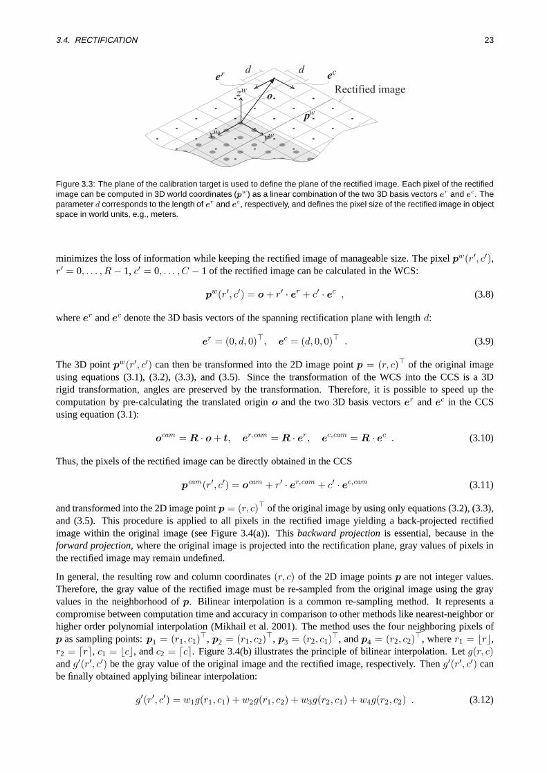
3.4. RECTIFICATION 23
Figure 3.3: The plane of the calibration target is used to define the plane of the rectified image. Each pixel of the rectifiedimage can be computed in 3D world coordinates (pw) as a linear combination of the two 3D basis vectors er and ec. Theparameter d corresponds to the length of er and ec, respectively, and defines the pixel size of the rectified image in objectspace in world units, e.g., meters.
minimizes the loss of information while keeping the rectified image of manageable size. The pixelpw(r′, c′),r′ = 0, . . . , R− 1, c′ = 0, . . . , C − 1 of the rectified image can be calculated in the WCS:
pw(r′, c′) = o + r′ · er + c′ · ec , (3.8)
whereer andec denote the 3D basis vectors of the spanning rectification plane with lengthd:
er = (0, d, 0)>, ec = (d, 0, 0)> . (3.9)
The 3D pointpw(r′, c′) can then be transformed into the 2D image pointp = (r, c)> of the original imageusing equations (3.1), (3.2), (3.3), and (3.5). Since the transformation of the WCS into the CCS is a 3Drigid transformation, angles are preserved by the transformation. Therefore, it is possible to speed up thecomputation by pre-calculating the translated origino and the two 3D basis vectorser andec in the CCSusing equation (3.1):
ocam = R · o + t, er,cam = R · er, ec,cam = R · ec . (3.10)
Thus, the pixels of the rectified image can be directly obtained in the CCS
pcam(r′, c′) = ocam + r′ · er,cam + c′ · ec,cam (3.11)
and transformed into the 2D image pointp = (r, c)> of the original image by using only equations (3.2), (3.3),and (3.5). This procedure is applied to all pixels in the rectified image yielding a back-projected rectifiedimage within the original image (see Figure 3.4(a)). Thisbackward projectionis essential, because in theforward projection, where the original image is projected into the rectification plane, gray values of pixels inthe rectified image may remain undefined.
In general, the resulting row and column coordinates(r, c) of the 2D image pointsp are not integer values.Therefore, the gray value of the rectified image must be re-sampled from the original image using the grayvalues in the neighborhood ofp. Bilinear interpolation is a common re-sampling method. It represents acompromise between computation time and accuracy in comparison to other methods like nearest-neighbor orhigher order polynomial interpolation (Mikhail et al. 2001). The method uses the four neighboring pixels ofp as sampling points:p1 = (r1, c1)
>, p2 = (r1, c2)>, p3 = (r2, c1)
>, andp4 = (r2, c2)>, wherer1 = brc,
r2 = dre, c1 = bcc, andc2 = dce. Figure 3.4(b) illustrates the principle of bilinear interpolation. Letg(r, c)andg′(r′, c′) be the gray value of the original image and the rectified image, respectively. Theng′(r′, c′) canbe finally obtained applying bilinear interpolation:
g′(r′, c′) = w1g(r1, c1) + w2g(r1, c2) + w3g(r2, c1) +w4g(r2, c2) . (3.12)
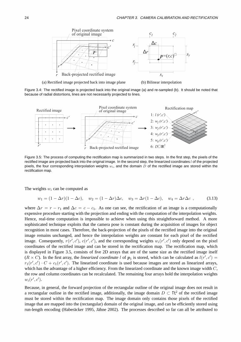
24 CHAPTER 3. CAMERA CALIBRATION AND RECTIFICATION
r
c
Pixel coordinate systemof original image
Back-projected rectified image
pc'
r'
(a) Rectified image projected back into image plane
p= r,c( ) sy
sx
∆c
∆r
c1c2
r1
r2
⊥
(b) Bilinear interpolation
Figure 3.4: The rectified image is projected back into the original image (a) and re-sampled (b). It should be noted thatbecause of radial distortions, lines are not necessarily projected to lines.
Rectified imageRectification map
w1
w2
w3
w4
l
(r',c')
(r',c')
(r',c')
(r',c')
(r',c')
r'
c'
c'
r'
r
c
Pixel coordinate systemof original image
Back-projected rectified image
c'
r'
1:
2:
3:
4:
5:
6: D∈ RI2
Figure 3.5: The process of computing the rectification map is summarized in two steps. In the first step, the pixels of therectified image are projected back into the original image. In the second step, the linearized coordinates l of the projectedpixels, the four corresponding interpolation weights wi, and the domain D of the rectified image are stored within therectification map.
The weightswi can be computed as
w1 = (1−∆r)(1−∆c), w2 = (1−∆r)∆c, w3 = ∆r(1−∆c), w4 = ∆r∆c , (3.13)
where∆r = r − r1 and∆c = c − c1. As one can see, the rectification of an image is a computationallyexpensive procedure starting with the projection and ending with the computation of the interpolation weights.Hence, real-time computation is impossible to achieve when using this straightforward method. A moresophisticated technique exploits that the camera pose is constant during the acquisition of images for objectrecognition in most cases. Therefore, the back-projection of the pixels of the rectified image into the originalimage remains unchanged, and hence the interpolation weights are constant for each pixel of the rectifiedimage. Consequently,r(r′, c′), c(r′, c′), and the corresponding weightswi(r′, c′) only depend on the pixelcoordinates of the rectified image and can be stored in the rectification map. The rectification map, whichis displayed in Figure 3.5, consists of five 2D arrays that are of the same size as the rectified image itself(R × C). In the first array, thelinearized coordinatel of p1 is stored, which can be calculated asl(r′, c′) =r1(r′, c′) · C + c1(r′, c′). The linearized coordinate is used because images are stored as linearized arrays,which has the advantage of a higher efficiency. From the linearized coordinate and the known image widthC,the row and column coordinates can be recalculated. The remaining four arrays hold the interpolation weightswi(r′, c′).
Because, in general, the forward projection of the rectangular outline of the original image does not result ina rectangular outline in the rectified image, additionally, the image domainD ⊂ R
2 of the rectified imagemust be stored within the rectification map. The image domain only contains those pixels of the rectifiedimage that are mapped into the (rectangular) domain of the original image, and can be efficiently stored usingrun-length encoding (Haber¨acker 1995, J¨ahne 2002). The processes described so far can all be attributed to

3.5. EXAMPLE 25
Figure 3.6: Deviations from the nadir view cause projective distortions in the object plane.
the offline phase and only need to be executed once for a specific camera and object plane configuration. Inthe following, the online phase of the rectification is described.
3.4.2 Rectification Process
The input data of the online phase, i.e., in the rectification process, are the image that must be rectified and therectification map that holds all necessary information for the rectification. The derivation of the rectificationmap already implies the process of computing the output data, i.e., the rectified image. Therefore, only someshort remarks are given. At first, a new image is created where the image domain is set to the image domainof the rectification mapD. Then, for each pixel(r′, c′)> within the image domain the gray valueg′(r′, c′) iscomputed only from the four corresponding gray values of the original imageg(r, c), g(r, c+ 1), g(r + 1, c),andg(r + 1, c + 1) multiplied by the respective weightswi(r′, c′), i = 1, . . . ,4, using equation (3.12). Thecoordinatesr andc are obtained from the linearized coordinatel(r′, c′) and the image width. Thus, this ex-tremely lean computation comprises the entire process of rectification in a compressed form and facilitatesreal-time computation. The rectified image is not only free of radial and projective distortions in the objectplane but — as an additional feature — also exhibits square pixels since the pixel spacing is estimated inde-pendently during camera calibration in each direction. Non-square pixels would also lead to deformations ofan object in the image. This deformation is not constant but dependents on the object orientation, and henceis critical for object recognition.
3.5 Example
In this section, an example is given, not only to prove the high efficiency of the rectification method, but alsoto accentuate the need for considering the radial distortions within the camera model.
The label of the example application of Figure 2.7 in Section 2.1 is taken as the test object. Here, it is assumedthat it is not possible to mount the camera perpendicular to the object plane. This causes projective distortionsof the object plane as can be seen from Figure 3.6, where the “deformation” of the label depends on the poseof the label in the image.
In order to rectify the images, the camera must be calibrated. Here, a calibration target of size 3 cm× 3 cmwas used and images that show the target in 15 different poses were taken. Figure 3.7 shows three of the15 calibration images (640× 482 pixels). The 3D coordinates of the center points of the black circles areknown and used as control points within the camera calibration as described in Section 3.4. The computationtime for the whole camera calibration was about 2 s on a 2 GHz Pentium 4, including the segmentation ofthe calibration target, the calculation of the starting values in all images, and the final parameter estimationusing the Levenberg-Marquardt method (Press et al. 1992). The resulting interior camera parameters in thisexample aref = 13 mm,κ = −1095.2 [1/m2] (i.e, slightly barrel-shaped distortions),sx = 7.3µm, sy =

26 CHAPTER 3. CAMERA CALIBRATION AND RECTIFICATION
Figure 3.7: Three examples of the 15 calibration images that were taken from the calibration target. The extracted ellipsecenters of the projected marks are assigned to the given 3D circle centers of the calibration target and used to estimatethe camera parameters. The calibration target in the left image is used to define the object plane to be rectified.
Figure 3.8: Rectified versions of the images shown in Figure 3.6. The average rectification time was 8.3 ms on a 2 GHzPentium 4.
7.3µm, cx = 321.422 pixels, andcy = 236.303 pixels. To get an impression of the achieved accuracy ofthe estimation, the 3D control points are projected back into the image using the estimated parameters andcompared to the extracted ellipse centers resulting in a mean distance of 0.027 pixels.
Now, the rectified image can be defined. The pose of the calibration target in the left image of Figure 3.7defines a plane that is offset from the object plane by the thicknesst = 0.63 mm from the calibration target.Therefore, thez component of the originoz must be set to−0.63 mm in order to correctly rectify the objectplane. Additionally, the pixel sized is chosen to be 0.32 mm to obtain a suitable size of the rectified image.To ensure that the upper left pixel of the original image is contained in the image domainD of the rectifiedimage,ox andoy are set to -9.4 cm each. Finally, the heightR and widthC are chosen appropriately (R =527,C = 515). Now, the computation of the rectification map can be performed using the interior cameraparameters, the exterior camera parameters according to the left image of Figure 3.7, and the chosen valuesfor o, d, R, andC. In the example it took approximately 120 ms to compute the rectification map.
Since all time-consuming computations of the offline phase have been completed, now, in the online phaseimages can be rectified in real-time. The three example images of Figure 3.6 are rectified by applying thecomputed rectification map in an average time of only 8.3 ms per image. The result is shown in Figure 3.8.
Finally, two experiments are carried out to show that firstly, the achievable accuracy of the camera parametersdepends on the number of acquired calibration images and that secondly, it is essential to include the radialdistortions within the camera model.
For the first experiment, a basic set of 10 selected calibration images out of the entirety of 15 images is formed.Then the number of imagesnI is varied from 1 to 10 and for eachnI , 10 sub-sets containingnI images aretaken from the basis set. It should be noted that only one sub-set of 10 images can be formed ifnI = 10.The camera calibration is then performed for the different number of images for each of the 10 sub-sets. The

3.5. EXAMPLE 27
1 2 3 4 5 6 7 8 9 100
0.5
1
1.5
2
Number of images
Sta
ndar
d de
viat
ion
of fo
cal l
engt
h [m
m]
(a) Standard deviation off
1 2 3 4 5 6 7 8 9 100
200
400
600
800
1000
1200
1400
1600
1800
Number of images
Sta
ndar
d de
viat
ion
of r
adia
l dis
tort
ion
[1/m
2 ]
(b) Standard deviation ofκ (c) Effect of radial distortions
Figure 3.9: Standard deviation of the estimated effective focal length (a) and the radial distortions (b) versus the numberof images. In (c) subpixel precise edges are shown, once taking the radial distortions into account (white solid), and onceignoring the radial distortions (white dashed).
standard deviation of the estimated interior camera parameters are then calculated for eachnI . As an exampleof the result, the standard deviation of the effective focal lengthf and of the parameterκ, which describes theradial distortions, are plotted in Figure 3.9(a) and Figure 3.9(b), respectively. From both plots it appears thateven for a small number of calibration images, the accuracy of the camera calibration increases considerablyin comparison to the SIC. In this example, the calibration using only a single image is not meaningful: thestandard deviation ofκ is σκ = 1782.0 1/m2, which is too high for precise measurements. This is becausethe used calibration target is relatively small and the radial distortions within a small part of the image areapproximately constant, and hence hard to determine. Therefore, it is essential to base the calibration onseveral images where the calibration target should appear in different parts of the image. The same holdsfor the effective focal length (f = 13 mm), the standard deviation of which isσf = 2 mm. Generally, theachievable accuracy depends on the number of used images and on the accuracy of the extracted ellipse centersin the calibration images. However, it is also apparent from the plots, that continuously increasing the numberof images does not necessarily increase the accuracy much. The maximum achievable accuracy is restrictedby the distortions that are not considered in the camera model.
For the second experiment, the rectified image of the label that is displayed in Figure 3.8 on the right is usedto demonstrate the effect of radial distortions. In Figure 3.9(c), the enlarged detail of the image containingthe upper right corner of the label is shown. This image part is far enough away from the principal point toexhibit significant radial distortions. Subpixel precise edges are extracted in the image using the approachpresented in (Steger 1998) and visualized as white solid lines. In a second step, the image is rectified withκ set to 0 when computing the rectification map. In the resulting rectified image, subpixel precise edges areagain extracted and overlaid on the image of Figure 3.9(c) as white dashed lines. From the displacement ofthe edges, it is obvious that ignoring the radial distortions in this example would lead to position errors of upto 2 pixels. In general, the position errors induced by radial distortions are in the range of 1 to 4 pixels usingoff-the-shelf lenses. Thus, it is absolutely essential to model and eliminate the radial distortions in the images.

28 CHAPTER 3. CAMERA CALIBRATION AND RECTIFICATION
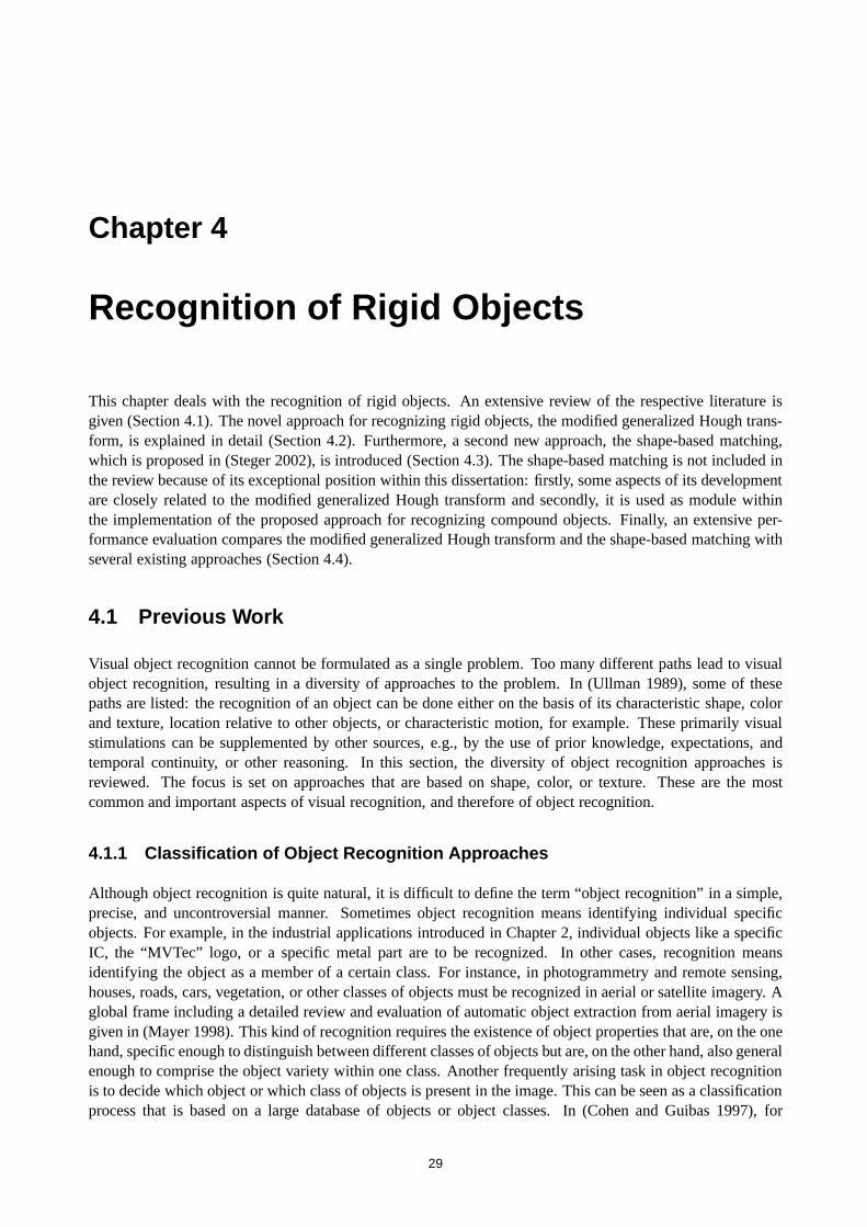
Chapter 4
Recognition of Rigid Objects
This chapter deals with the recognition of rigid objects. An extensive review of the respective literature isgiven (Section 4.1). The novel approach for recognizing rigid objects, the modified generalized Hough trans-form, is explained in detail (Section 4.2). Furthermore, a second new approach, the shape-based matching,which is proposed in (Steger 2002), is introduced (Section 4.3). The shape-based matching is not included inthe review because of its exceptional position within this dissertation: firstly, some aspects of its developmentare closely related to the modified generalized Hough transform and secondly, it is used as module withinthe implementation of the proposed approach for recognizing compound objects. Finally, an extensive per-formance evaluation compares the modified generalized Hough transform and the shape-based matching withseveral existing approaches (Section 4.4).
4.1 Previous Work
Visual object recognition cannot be formulated as a single problem. Too many different paths lead to visualobject recognition, resulting in a diversity of approaches to the problem. In (Ullman 1989), some of thesepaths are listed: the recognition of an object can be done either on the basis of its characteristic shape, colorand texture, location relative to other objects, or characteristic motion, for example. These primarily visualstimulations can be supplemented by other sources, e.g., by the use of prior knowledge, expectations, andtemporal continuity, or other reasoning. In this section, the diversity of object recognition approaches isreviewed. The focus is set on approaches that are based on shape, color, or texture. These are the mostcommon and important aspects of visual recognition, and therefore of object recognition.
4.1.1 Classification of Object Recognition Approaches
Although object recognition is quite natural, it is difficult to define the term “object recognition” in a simple,precise, and uncontroversial manner. Sometimes object recognition means identifying individual specificobjects. For example, in the industrial applications introduced in Chapter 2, individual objects like a specificIC, the “MVTec” logo, or a specific metal part are to be recognized. In other cases, recognition meansidentifying the object as a member of a certain class. For instance, in photogrammetry and remote sensing,houses, roads, cars, vegetation, or other classes of objects must be recognized in aerial or satellite imagery. Aglobal frame including a detailed review and evaluation of automatic object extraction from aerial imagery isgiven in (Mayer 1998). This kind of recognition requires the existence of object properties that are, on the onehand, specific enough to distinguish between different classes of objects but are, on the other hand, also generalenough to comprise the object variety within one class. Another frequently arising task in object recognitionis to decide which object or which class of objects is present in the image. This can be seen as a classificationprocess that is based on a large database of objects or object classes. In (Cohen and Guibas 1997), for
29

30 CHAPTER 4. RECOGNITION OF RIGID OBJECTS
instance, Chinese characters are recognized in images by comparing them to a database of images comprising500 possible characters.
In the scope of the present work, object recognition means identifying individual specific objects and notclasses of objects and, furthermore, is not interpreted as a classification process. Nevertheless, even in thisrestricted domain, several terms are commonly used in the literature. The terms imply different applications,but can all be summarized under “object recognition”. In Table 4.1, some examples are listed where the terms“object” and “recognition” are treated separately: each of the two terms can be replaced by one of variousexpressions. For example, “object” is often substituted by “image”, “pattern”, or “target”, while “recognition”is often substituted by “alignment”, “matching”, or “detection”. These expressions can be combined arbitrarilywithin the same row of Table 4.1, resulting in various paraphrases for the term “object recognition”. The tablefurther discriminates between terms that imply a 2D approach (first row) and terms that are used in both, 2Dand 3D approaches (second row). For example, “image alignment” assumes a 2D approach, while the term“target recognition” is used in 2D and 3D approaches.
object recognition
2D imagealignment / registration /
retrieval / comparison / matching
2D / 3Dobject / pattern /
template / target / shaperecognition / matching /
localization / detection / alignment
Table 4.1: “Object recognition” — a term including various semantics
Apart from the classification of object recognition approaches that distinguishes between 2D and 3D ap-proaches, several other classification schemes are possible. In (Ullman 1989), object recognition approachesare divided intoinvariant properties methods, object decomposition methods, andalignment methods, wherealso combinations between the methods are allowed. In invariant properties methods, the overall recognitionprocess is broken down into the extraction of a number of different properties (that are invariant to a particularkind of transformation), followed by a final decision based on these properties. Object decomposition meth-ods rely on the decomposition of objects into constituent parts, where in a first stage the parts are recognizedand in a second stage the initial classification of the individual parts is used to recognize the object itself byincluding knowledge about the relations between the parts. For example, in the first stage, straight lines aresearched in the image, which can be used in the second stage to recognize rectangles by exploiting knowledgeabout the relations between the lines. Finally, alignment methods try to find a particular transformation thatwill maximize somesimilarity measure. The similarity measure is often calledsimilarity metric if it fulfillsthe requirements for a metric, i.e., non-negativity, symmetry, and triangle inequality (Bronstein et al. 2001).The similarity measure describes the similarity between the transformed model and the image. The modelis systematically compared to the image using all degrees of freedom of the chosen class of transformations.The maxima of the similarity measure are used to decide whether an object is present in the image and todetermine its pose.
Another way to classify object recognition methods in general, and alignment methods in particular, is to usethe criteriafeature space, search space, search strategy, andsimilarity metric(Brown 1992). Feature spacedescribes the information that is used for object recognition (e.g., gray values, points, lines, elliptic arcs, etc.).Search space is the class of transformation the object is allowed to undergo in the image. Search strategydescribes how to find the correct transformation within the search space and, finally, similarity metric is usedto evaluate the transformations.
In the following, the criterionfeature spaceis used to classify the reviewed approaches intointensity-based,low level feature-based, andhigh level feature-based. In intensity-based approaches, the raw gray values areused as feature, low level features are, e.g., edge pixels, points, or gray value gradients, and high level features

4.1. PREVIOUS WORK 31
comprise lines, polygons, elliptic arcs, or object parts for instance. The approaches that use intensity or lowlevel features are further subdivided into those that use area-based and non-area-based strategies, respectively.In area-based strategieseach pixel in the model image and in the search image is involved in the matchingprocess, whereas innon-area-based strategies, objects are represented in a more efficient way. The advan-tage of this classification is that, in general, the algorithm’s complexity and the computational complexity ofthe object recognition approach can be directly deduced from its corresponding class. While intensity-basedapproaches often use simple algorithms, low and especially high level features often demand a more com-plex class of object recognition approaches. Furthermore, approaches that involve area-based strategies areoften connected with a high computational complexity, while non-area-based strategies in general facilitatefaster computations. Since in this dissertation it is differentiated between the recognition of rigid objects andthe recognition of compound objects there are two sections about previous approaches. In the following, onlyapproaches dealing with the recognition of rigid objects will be reviewed, while approaches dealing with com-pound objects will be reviewed in Chapter 5. Because of the almost unlimited number of different approaches,in the following subsections only the most important approaches for recognizing rigid objects will be includedin this review.
4.1.1.1 Approaches Using Intensity Information
The simplest class of object recognition methods is based on the raw intensity information of the modelimage and the search image. In the case of 8-bit gray scale images, the intensity information is given bythe gray values in the image. These methods are also often calleddirect methodsbecause they recover theunknown pose parameters directly from the measurable image quantities at each pixel in the images (Irani andAnandan 1999). This is in contrast to the feature-based methods, which first extract a set of distinct featuresfrom the images, and then recover and analyze their correspondences.
Alignment methods are probably the most popular methods that are used for object recognition. They can beused in both intensity-based approaches as well as in feature-based approaches. A comprehensive survey isgiven in (Brown 1992). The principle of alignment methods will be explained in the following. LetIm bethe model image with area of definitionDm ⊂ R2 andIs the search image with area of definitionDs ⊂ R2,respectively1. The alignment method transformsIm andDm to all discrete transformationsTi ∈ T withina specific transformation classT (e.g., translations, rigid, similarity, affine, or perspective transformations)and computes the similarity measureM(Ti) between the transformed model imagesIm = Ti(Im) withinDm = Ti(Dm) and the search image for each of the discrete transformations. Thus, a high similarity results ina peak inM . The transformationsTi that result in local maxima ofM(Ti) and that exceed a certain thresholdare treated as matches and represent the poses of the object instances in the image. Consequently, the run timecomplexity of alignment methods can be formalized asO(|Ti|om), where|Ti| denotes the number of discretetransformations andom the number of operations performed in the respective similarity measure. What alsofollows is that the accuracy of the obtained pose parameters is restricted to the resolution of the samplingthat is applied toT in order to get the discrete transformationsTi. This is insufficient for many applications(cf. Section 2.2). Unfortunately, the resolution of the sampling cannot be chosen arbitrarily fine because thefiner the chosen resolution the more discrete transformations must be computed and checked for similarity,which leads to an increasing computation time. There are several more practical methods to refine the poseparameters. Some of them will be introduced in Section 4.1.2. Furthermore, it is often useful to separate thetranslation partT t of T from the remaining transformationsT \ T t when dealing with alignment methods.The model image that has been transformed by the remaining transformations is translated according to thepixel grid of the search image. This avoids unfavorable gray value re-sampling. In order to simplify furtherdiscussions,T is assumed to only represent translations. Consequently,M only depends on the translationparameters(x, y)> ∈ Ds that translate the model image within the search image.
1Throughout the remainder of this dissertation the area of definition will also be referred to asdomainor region of interest(ROI)

32 CHAPTER 4. RECOGNITION OF RIGID OBJECTS
Area-Based Strategies. One of the most frequently applied intensity-based similarity measures in align-ment methods is thecross correlation(Brown 1992). It is calculated using the following expression:
CC (x, y) =∑
(u,v)∈Dm
Im(u, v)Is(x+ u, y + v) . (4.1)
This corresponds to an image convolution ofIs with a non-mirrored convolution maskIm and approximatelydescribes the squared Euclidian gray value distance (Cha 2000). The run time complexity of this kind ofalignment methods isO(nsnm), wherenm = |Dm| andns = |Ds| denote the number of image points(pixels) in the domain of the model image and the search image, respectively (|Ti| = ns, om = nm). Onthe one hand, this similarity measure always returns a high value for bright search image regions, no matterhow similar the images are. On the other hand, it is not invariant to changes in brightness. Therefore, in mostapplications its normalized version (NCC ) is applied: the meanµ and the standard deviationσ of the grayvalues in the model image and in the search image, respectively, are incorporated to achieve invariance tolinear changes in brightness, i.e.,NCC (x, y) = 1⇒ Is(x+ u, y + v) = aIm(u, v) + b, (a > 0):
NCC (x, y) =1nm
∑(u,v)∈Dm
(Im(u, v) − µm
σm· I
s(x+ u, y + v)− µs(x, y)σs(x, y)
). (4.2)
This zero-mean normalized cross correlation, which corresponds to the well-knowncorrelation coefficient,has the additional advantage that it maps the similarity between images to an interval of[−1,+1], where 1denotes a perfect match. It will be simply referred to asnormalized cross correlationin the following. Otherforms of normalizing the cross correlation can also be found in literature, e.g., (Aschwanden and Guggenb¨uhl1992, Martin and Crowley 1995), each with its own characteristics.
The computation of the normalized cross correlation is relatively expensive. Because of its convolution char-acter, the computation of the unnormalized cross correlation can be accelerated by transformingIm andIs
into the Fourier domain (e.g., by using the FFT (Fast Fourier Transformation) (Ballard and Brown 1982))and multiplying the resulting Fourier transforms (Anuta 1970):CC = F−1F(Is)F∗(Im), whereF andF−1 are the Fourier transform and the inverse Fourier transform, respectively.F∗ symbolizes the conjugatecomplex and accomplishes the reversal ofIm to get a mirrored filter mask. Unfortunately, the normalizedform of cross correlation does not have a simple and efficient frequency expression and is therefore muchmore difficult to compute. Several methods that try to overcome this problem have been developed, e.g.,high-pass filtering(Lewis 1995, J¨ahne 2002),phase correlation(Kuglin and Hines 1975, Foroosh et al. 2002), ora subsequent normalization after the convolution (Lewis 1995). Because of the problems that occur whendealing with correlation in the frequency domain, the normalized cross correlation is still computed in thespatial domain in most cases (Gonzalez and Woods 1992). Thus, several methods have been investigated tospeed up the computation in the spatial domain, e.g., by appropriately rearranging (4.2) or by using apseudo-correlation (Radcliffe et al. 1993). However, the major drawback of approaches using the normalized crosscorrelation is its limited robustness against occlusions and clutter as well as against non-linear changes inbrightness. Attempts have been made to improve the alignment reliability by utilizing image preprocessingprior to the execution of the normalized cross correlation (Bacon 1997). Unfortunately, there is no suitablepreprocessing strategy that is appropriate for the general case. Furthermore, the robustness against cluttercannot be improved by such methods.
Another class of alignment methods uses thesum of absolute or squared gray value differences(Brown 1992)or one of its various derivatives. For instance, the sum of absolute gray value differencesSAD is computedas follows:
SAD(x, y) =1nm
∑(u,v)∈Dm
|Im(u, v) − Is(x+ u, y + v)| . (4.3)
Thus,SAD indicates the average difference of the gray values and therefore represents a measure that mapsthe dissimilarity between two images to a positive value that is not limited by an upper boundary (apart fromthe maximum gray value that can occur). This complicates making statements about the quality of matches.

4.1. PREVIOUS WORK 33
In contrast to the correlation it is a measure of dissimilarity. Nevertheless, it will subsequently be referredto as similarity measure because simple negation or inversion can be applied to straighten out this dilemma.Like the normalized cross correlation, the sum of gray value differences is also sensitive to occlusions andclutter. However, it is faster to compute. Additionally, some speed-ups can be incorporated. For example, in(Cha 2000), a method that quickly eliminates most transformations from consideration is proposed. Hence,the computation of the sum of gray value differences can be restricted to the remaining transformations.
In contrast to cross correlation, the sum of gray value differences can be made invariant only either to ad-ditive changes in brightness (e.g.,
∑ |(Im(u, v)− µm)− (Is(x+ u, y + v)− µs)|) or to local multiplicativechanges (e.g.,
∑ |Im(u, v) − µm/µsIs(x+ u, y + v)|). However, linear changes in brightness cannot betaken into account in a simple way. In (Lai and Fang 1999c), the sum of gray value differences is made robustagainst linear changes in brightness by modeling the varying brightness with low-order polynomials. Robust-ness against a moderate amount of occlusion and clutter is obtained by computing the similarity measure in astatistically robust manner.
Several experimental results of a comparative study regarding the normalized cross correlation and the sum ofgray value differences can be found in (Aschwanden and Guggenb¨uhl 1992). Also different modifications andnormalization techniques are included in the study. They analyze the robustness of the similarity measuresby simulating different types of image distortions. It is shown that similarity measures that are based on thenormalized cross correlation are more robust against all types of tested distortions than similarity measuresthat are based on gray value differences. In particular, changes in lighting conditions cause problems whenusing difference-based measures. An alleviation to this problem is found in the use of more complicatednormalization techniques. However, under certain assumptions the computational requirements to implementthese functions are only slightly better than for the normalized cross correlation.
Non-Area-Based Strategies. Intensity-based approaches that are combined with non-area-based strate-gies can lead to less computational effort and higher robustness. The principle is that not all pixels withinthe model image and the search image are used to calculate the intensity based similarity measure. Instead,only a small selected fraction is used. For example, in (Edwards and Murase 1998), the region of overlapbetween modeled objects is determined and excluded from the calculation to increase the robustness againstocclusions. However, an expensive iterative processing is needed since the region of overlap is not knowna priori. Furthermore, occlusions that occur because of missing object parts or because of an overlap withnon-modeled objects cannot be taken into account. In (Li et al. 1997), the computation of the cross correlationis restricted to only a few pixels dependent on the image contrast in these pixels. This not only decreases thecomputation time but also increases the robustness against occlusions and clutter. However, applying the FFTfor efficiently computing the correlation is no longer possible.
4.1.1.2 Approaches Using Low Level Features
There are two main motivations for using features in object recognition approaches, which can be directlyconcluded from the weak points of most intensity-based approaches. The first motivation arises from therelatively high sensitivity to occlusions and clutter of most intensity-based approaches. Several features canbe found that enable higher robustness against such variations. The second motivation can be attributedto the fact that features combined with non-area-based strategies are able to represent an object in a morecompressed, and hence efficient form. Recognition approaches can take advantage of this property in order toachieve less computational effort.
When regarding alignment methods, a difference in the approaches that use features and approaches that useintensity information should be mentioned. In feature-based approaches, there are, in general, two ways foran alignment method to obtain the features of the transformed model image using the discrete transformationsTi. The first possibility is to transform the model image and to calculate the features in the transformed model

34 CHAPTER 4. RECOGNITION OF RIGID OBJECTS
image. In the second possibility, features are only calculated in the untransformed model image and merely thefeatures themselves are transformed. While the second method is faster, it usually suffers from quantizationeffects or unpleasant properties of the feature extractor (e.g, inaccuracy or non-isotropy).
Area-Based Strategies. A first class of feature-based alignment methods concentrates on gray valuestatistics. For example, gray value histograms (Ballard and Brown 1982) that are derived from images canbe interpreted as features that are used to compute the similarity between the images, since the raw grayvalue information is not directly used within the similarity measure. A similarity measure that is based on thedifference between two histograms is invariant to rotations. Histograms of angular measurements are used in(Cha and Srihari 2000) to recognize handwritten characters. In (Bhat and Nayar 1998), a similarity measure isproposed that uses an ordinal measure as feature, where images are represented by their gray value ranks. Forillustration purposes, the gray values of an imageI are written sequentially, e.g.,I = (5,10,50,40). Then thegray values are sorted and the image is represented by its rankingsπ = (1,2,4,3). This representation can beused in alignment methods, where, not the gray values themselves, but the rankings of the model image andthe respective part of the search image are compared by applying a rank correlation coefficient (Gideon andHollister 1987). Similarity measures that are based on gray value rankings have the advantage that they areinvariant to changes in brightness that do not affect the ranking such as linear changes. Another advantage isthat the ranking is less sensitive to outliers, which leads to a higher robustness against occlusions and clutterin comparison to the normalized cross correlation or the sum of gray value differences. However, in general,the mapping of an image to its gray value statistics is not an injective function: for example, when usinghistograms, the spatial arrangement of the pixels is lost. This may lead to a large number of false positivematches, i.e., a high similarity value between obviously dissimilar images, especially in the case of imageclutter.
In (Kaneko et al. 2002), a similarity measure for alignment methods is proposed that is based on theincrementsign correlation. In the first step, the two images to be compared are encoded into corresponding binaryimages. For this, a procedure is applied that maps local gray value changes into 1 if the gray value of aneighboring pixel (e.g., the right neighbor) is higher than the gray value of the current pixel, and into 0otherwise. This increment sign is used as the feature to represent the images. In the second step, a binarycorrelation coefficient is computed based on the binary representations of both images. It is shown that thismeasure is robust against occlusions and changes in brightness. The disadvantage of this method is the highreduction of information from (in general) 8 bit to 1 bit. This results in an increased number of false positivematches, especially in the case of small model images, where the discriminative power of the increment signcorrelation is poor. Furthermore, in the case of model images showing regions of approximately constant grayvalues, the increment sign is more or less random. This reduces the correlation coefficient even if the imagesare similar.
Another class of approaches performs an intensity-based similarity measure not directly on the raw gray valuesbut on derivatives of the gray values. For example, in (Martin and Crowley 1995), the cross correlation and thesum of gray value differences are computed on the first derivative magnitude (gradient magnitude) and the sumof second derivatives (Laplacian). It is shown that the decision whether one should use the raw gray values,the gradient magnitude, or the Laplacian for applying the cross correlation depends on the requirements ofthe task. In the frequency domain, an ideal first derivative grows linearly with increasing frequency, whilea second derivative grows quadratically. Therefore, a correlation of first derivatives has a more precise peakthan a correlation of raw intensity images, but is more sensitive to high frequency noise. A second derivativedoubles the effect. Experiments in (Martin and Crowley 1995) showed that using the gradient magnitudeusually provides more stable results in comparison to the use of raw intensity values or of the Laplacian.The approaches presented in (Scharstein 1994, Crouzil et al. 1996, Fitsch et al. 2002) extend the principle ofthese ideas by using the gradient direction as feature. For example, in (Fitsch et al. 2002), angles betweengradient directions are used as similarity measure. This results in invariance to changes in brightness, since,the gradient directions are unaffected by changing brightness. It also shows robustness against occlusions andclutter. In this approach, however, the object representation by the chosen feature is not very efficient since

4.1. PREVIOUS WORK 35
for each pixel in the model image the orientation is computed and used in the similarity measure. Thus, thenumber of features is equal to the number of pixels. Therefore, there is no real improvement regarding thecomputation time in comparison to the intensity-based approaches.
Non-Area-Based Strategies. The number of features that are involved in the matching process of non-area-based strategies is less than the number of pixels. Several classes of feature-based object recognitionmethods that are reviewed in this section use the object’s edges as geometric feature, which will also bereferred to as the objectshapein the following discussions. A review of edge extraction algorithms is notgiven here. Instead, the reader should refer to standard text books (Ballard and Brown 1982, Gonzalez andWoods 1992, Haber¨acker 1995, J¨ahne 2002). Usually, the edge pixels are defined as pixels in the imagewhere the magnitude of the gradient is maximum in direction of the gradient. In most cases, edges areextracted in two steps. At first, the image is convolved using an edge filter that provides the first partialderivatives of the gray values in row and column direction. An edge filter responds to gray value changes inthe image by taking the neighboring gray values into account, e.g., theRoberts(Gonzalez and Woods 1992),Sobel(Gonzalez and Woods 1992),Canny(Canny 1983, Canny 1986),Deriche (Deriche 1987), orLanser(Lanser and Eckstein 1992) filters. The edge magnitudeγ can be computed from the first partial derivativeswhen using a gradient-based edge detection:
γ =
√(∂I(x, y)∂x
)2
+(∂I(x, y)∂y
)2
. (4.4)
In the second step, a threshold is applied on the edge magnitude, which is a measure of the contrast in theimage. This results in the segmented edge regions of the image.
Other recognition methods use points as geometric features. They can also be extracted from an image in var-ious ways, e.g., using so-calledinterest operators. For a comprehensive overview and evaluation of differentinterest operators the interested reader should refer to (Heipke 1995, Schmid et al. 2000).
The first class of non-area-based strategies does not use the shape of the object, but is based on global imagetransforms. Both the model image and the search image are transformed into the frequency domain, e.g., usinga wavelet-based transformation (Bronstein et al. 2001, Wang 2001): the original images can be representedas a linear combination of the respective wavelet functions. By truncating the wavelet coefficients below acertain magnitude, image data can be sparsely represented. However, a loss of detail must be expected. Aset of such coefficients can be used as feature vector for object recognition. Approaches that use wavelettechniques can be found in (Jacobs et al. 1995) and (Wang et al. 1995), for example. The major drawback ofthese methods is that because of their global nature, it is difficult to compare the model image to only a part ofthe search image. Consequently, robustness against occlusions or clutter is hard to achieve when using globalimage transforms.
The second class of approaches works on an object as a whole, i.e., on a complete object area or shape.Therefore, these methods are often called global object methods. The use of geometric moments is a verypopular representative of this class (Teh and Chin 1988). Geometric moments are used in several objectrecognition applications as features, e.g., (Liao and Pawlak 1996). By combining moments of different orders,one can find features that are invariant to rotation, scaling, or other transformations of the objects. Someexamples are area, circularity, eccentricity, compactness, major axis orientation, Euler number (Veltkamp andHagedorn 1999). These invariant features can be computed in the model image as well as in the searchimage and can be represented in a feature vector. The feature vector of both images can then be used tocompute the similarity between both images using an appropriate distance measure. The main advantage ofobject recognition based on moments is that the class of transformationsT can be reduced by transformationsthat are covered by the invariants of the selected moments themselves. Thus, the computational effort canbe reduced considerably. Unfortunately, the computation of the moments itself is very time consuming ingeneral. This often annihilates the advantage of the reduced parameter space. A closely related method usesthe principle component analysis, which decomposes the object shape into an ordered set of eigenvectors (also
36 CHAPTER 4. RECOGNITION OF RIGID OBJECTS
called eigenshapes). The eigenvectors of the object in the model image and in the search image can be used tocompute a similarity measure to recognize the object. Finally, in another global object method, the shape ofthe object is represented by its contour parameterized by the arc-length (Mokhtarian et al. 1996). The contouris successively smoothed using a Gaussian kernel. The characteristic behavior of the contour while applyingthe smoothing is exploited and used as an object-specific feature. This feature is invariant to orientation andmoderate scale changes of the object and robust to noise. However, an important drawback of all global objectmethods is that the complete object to be found in the search image must be clearly segmented, which is initself an ill-posed problem. Consequently, most of these methods fail in the case of occlusions and clutter.
Another class of approaches performs object recognition using alignment methods. The most elementarysimilarity measure that can be applied to alignment methods based on image edges is binary correlation.Here, the intersection of edge pixels in the transformed model image and the search image is a measureof similarity. The advantage of a simple computation is overshadowed by a high sensitivity to small edgedisplacements. I.e., a high similarity measure is only obtained if the edges of model and search image arealmost perfectly identical. A method that relaxes this stringent requirement, and hence is less sensitive to smalledge displacements, is presented in (Borgefors 1988). The algorithm matches points in the transformed modelimage and the search image by minimizing a generalized distance between them. Although the algorithm isdesigned to cope with arbitrary binary images, in most cases edges are used as features. The result of theedge extraction are two sets of pointsPm 3 pm
i , i = 1, . . . , nm andPs 3 psj , j = 1, . . . , ns, representing the
edge pixels in the transformed model image (model edges) and the search image (search edges), respectively,wherenm andns are the number of edge pixels in the corresponding images. The average distance betweenthe two sets of pixelsPm andPs is then used as similarity measure to find the pose of the object in the image.Unfortunately, the distance computation between two point sets is computationally expensive. Therefore, in(Borgefors 1988) a more efficient solution is applied that exploits the distance transform (J¨ahne 2002) for thematching: in the search image, each non-edge pixel is assigned a value that is a measure of the distance to thenearest edge pixel. The edge pixels have a value of zero. Fast algorithms using iterative local operations areavailable for computing the distance transform (Soille 1999). Since the true Euclidean distance is expensiveto compute, it is approximated by using integer values (Danielsson 1980, Borgefors 1984). Assuming that thehorizontal and vertical distance of neighboring pixels isd and the diagonal distance isdd, then integer valuesfor d anddd are chosen appropriately in order to approximate the Euclidean distance, i.e.,dd/d ≈
√2. Well
known combinations are, for instance,d = 1, dd = 2 (city block distance),d = 1, dd = 1 (chess boarddistance), andd = 3, dd = 4 (chamfer distance). To compute the average distance betweenPm andPs, theedge pixelsPm of the transformed model image are superimposed on the distance-transformed search imageand the distance values of the pixels in the distance image that are hit byPm are added. In (Borgefors 1988),the distance measureB between two sets of points is computed using the chamfer distance and the root meansquare average:
B(Pm,Ps) =13
√√√√ 1nm
nm∑i=1
v2i , (4.5)
wherevi = minpsj∈Ps ‖pm
i − psj‖ are the distance values hit by the model edges, and‖ · ‖ is the underlying
norm of the chosen distance metric. To compensate the unit distance of 3 in the chamfer distance, the averageis divided by 3. For speed reasons, the implementation of (Borgefors 1988) uses a hierarchical structure byapplying image pyramids. The principle of image pyramids will be explained in Section 4.1.2. There aresome major drawbacks, which are inherently connected with this similarity measure. It is not a symmetricmeasure. I.e., a different similarity value is obtained depending on which point set is used to compute thedistance transform and which point set is superimposed on the distance-transformed image. If the distancetransform is computed on the search image, then the distance measure is not robust against partial occlusions.The reason for this is that some missing edge pixels in the search image cause the corresponding edge pixelsof the model to get a high distance value. This increases the root mean square average in a non-proportionalway. Additionally, the distance measure is not sensitive to even severe clutter, which would be desirable.E.g., if all pixels in the search image would represent edge pixels, then the distances of all model edge pixelswould be zero. Assume now that the distance transform is computed on the model image. Then, on the one
4.1. PREVIOUS WORK 37
hand, the distance measure is not robust against moderate clutter. On the other hand, it is not sensitive to evensevere occlusions, which would also be desirable when considering the case that no edge pixels are presentin the search image. Concluding, a good distance measure (similarity measure) should be, on the one hand,sensitive to occlusions and clutter, i.e., the distance measure (similarity measure) should increase (decrease)when occlusions and clutter increases. On the other hand, it should be robust against occlusion and clutter,i.e., the distance measure (similarity measure) should not increase (decrease) in a non-proportional way. TheHausdorff distanceproposed in (Huttenlocher et al. 1993) and (Rucklidge 1997) tries to remedy the abovementioned shortcomings. In (Huttenlocher et al. 1993) the Hausdorff distanceH is defined as
H(Pm,Ps) = max(h(Pm,Ps), h(Ps,Pm)) , (4.6)
whereh(Pm,Ps) = max
pmi ∈Pm
minps
j∈Ps‖pm
i − psj‖ (4.7)
andminpsj∈Ps ‖pm
i − psj‖ again can be efficiently obtained by computing the distance transform onPs. The
functionh(Pm,Ps) is called thedirectedHausdorff distance fromPm toPs. It identifies the pointpmi ∈ Pm
that is farthest from any point ofPs and measures the distance frompmi to its nearest neighbor inPs. By
computing the directed Hausdorff distance in both directions and taking the maximum of both, the Hausdorffdistance is a symmetric measure. Furthermore, it is sensitive to both occlusions and clutter in the search imagebecause one of both directed Hausdorff distances is affected and the maximum of both is taken. However, sincethe maximum of all edge distances is taken in (4.7) it still shows no robustness against occlusions and clutter.Therefore, in (Rucklidge 1997) thepartial directed Hausdorff distance is proposed:
hf (Pm,Ps) = fthpm
i ∈Pmmin
psj∈Ps
‖pmi − ps
j‖ , (4.8)
wherefthx∈X g(x) denotes thef -th quantile value ofg(x) over the setX , for values off between zero andone. Hence,f denotes the fraction of points that are used to compute the partial directed Hausdorff distance.For example, the 1-th quantile value is the maximum and the 1/2-th quantile value is the median. Thus, whenf = 1, the partial directed Hausdorff distance corresponds to the unmodified directed Hausdorff distance.Consequently, the partial undirected Hausdorff distance is defined as
HfF fR(Pm,Ps) = max(hfF (Pm,Ps), hfR(Ps,Pm)) . (4.9)
Here,fF andfR are theforward fractionandreverse fraction, respectively, and define the fractions for theevaluation of the directed distances. This measure is robust against 100(1− fF )% occlusions and 100(1−fR)% clutter in the image.
The Hausdorff distance has undergone several further improvements and extensions, including, for example,sophisticated search strategies, computational shortcuts, and enhanced robustness (Huttenlocher et al. 1993,Olson and Huttenlocher 1996, Paumard 1997, Rucklidge 1997, Huttenlocher et al. 1999, Kwon et al. 2001,Sim and Park 2001). To enhance the robustness against clutter, attempts have been made to also includethe angle difference between the model edges and the search edges into the Hausdorff distance (Olson andHuttenlocher 1995, Olson and Huttenlocher 1996, Olson and Huttenlocher 1997, Sim and Park 2001). Unfor-tunately, the computation is based on several distance transforms, and hence is too computationally expensivefor real-time object recognition.
Another class of feature-based object recognition methods are summarized under the termvoting schemes.One of the most important representatives of this class ispose clustering, also known as thegeneralized Houghtransform(GHT) (Ballard 1981), which uses the edge position and direction as features. Its principle is basedon the well-knownHough transform(Hough 1962), which is a voting scheme to detect analytical curvesin images. Comprehensive surveys of different Hough transform techniques are given in (Illingworth andKittler 1988) and (Leavers 1993). Because an analytical description of objects is not always available, ornot even possible, the conventional Hough transform is only of limited use for object recognition. Therefore,

38 CHAPTER 4. RECOGNITION OF RIGID OBJECTS
Ballard (1981) generalizes the Hough transform to detect arbitrary shapes. Here, the parameters that describethe analytical curve in the classical Hough transform are replaced by parameters that define the class of allowedtransformationsT . By taking the edge direction into account, not only the number of false positives is reduced,but also a speed-up is obtained. Strictly speaking, the gradient direction is computed instead of the (tangential)edge direction. Letθm
i andθsj be the associated gradient directions at the model edge pointpm
i and the searchedges pointps
j , respectively. Similar to the edge magnitude (4.4) the gradient direction of the edge can becomputed, for example, from the partial derivatives obtained from an arbitrary gradient-based edge filter:
θ = arctan∂I(x, y)/∂y∂I(x, y)/∂x
. (4.10)
To perform the GHT, in the offline phase a look-up table (R-table) is computed by using information aboutthe edge positions and the corresponding gradient directions in the model image. TheR-table is generated asfollows: At first, an arbitrary reference pointom, e.g., the centroid of all model edge points, is chosen. Thenthedisplacement vectorsri = om − pm
i are calculated for all edge pointspmi , i = 1, . . . , nm. Finally, ri is
stored as a function ofθmi in the R-table. Informally speaking, theR-table contains the position of all edge
points in the model image with respect to a reference point sorted by their corresponding gradient direction.
For the online phase a two dimensional accumulator arrayA is set up over the domain of translations. Thus,A represents the sampled parameter space ofT . In general, each cell of this array corresponds to a certainpixel position of the reference pointos in the search image. For each edge pixelps
j in the search image thedisplacement vectorsri that are stored under the corresponding gradient directionθm
i = θsj are selected from
theR-table. For the selected vectors, the cellspsj +ri inA receive a vote, i.e., they are incremented by 1. Thus,
at each edge pixel in the search image all possible candidates for the reference point are calculated. This isrepeated for all edge pixels in the search image. Finally, each cell inA has a value that specifies the likelihoodthat the reference point is located in the cell. Thus, local maxima inA that exceed a certain threshold representobject instances found in the search image.
The advantage of the GHT is the high robustness against occlusions, clutter, and against changes in brightnessof an arbitrary type. The GHT is more efficient in comparison to conventional alignment methods because itdoes not explicitly compute all translations of the model image to test the similarity. In contrast, it restricts thesearch to the relevant information in the search image, i.e., the edge information. This is achieved by usingthe relative position of the model edges with respect to the reference point (i.e., the displacement vectors) astranslation invariant feature. Thus, the transformation classT of the alignment method can be reduced by thesub-class of translations. For example, if the class of rigid transformations is chosen then the model imageneeds to be only rotated to all possible object orientations. Nevertheless, in the conventional form the GHTrequires large amounts of memory for the accumulator array and long computation times to recognize theobject if more general transformation classes than translations are considered.
Many algorithms have been suggested to reduce the computational load associated with the GHT. Davis(1982) proposes a hierarchical Hough transform in which sub-patterns, i.e., simple geometric objects, suchas line segments, instead of edge points are used as basic units. In a similar way, a local classification of theinstances of detected contours is performed in (Cantoni and Carrioli 1987). The implementations of theseapproaches are complicated since local classifications of sub-patterns are required. It is also difficult to findthe desired sub-patterns in a search image accurately, especially in the presence of noise. In (Ballard andSabbah 1983), a two-level approach is proposed that takes similarity transformations into account, in whichthe factors of scaling and rotation are estimated first from the lengths and directions of the line segmentsin the search image before the GHT is applied. However, accurate extraction of line segment data fromthe image is a difficult task. A fast GHT is described in (Jeng and Tsai 1990), where the basic GHT isperformed on a sub-sampled version of the original image and a subsequent inverse GHT operation is usedto finally determine the pose in the original image. In this approach the edge direction is ignored during theinverse GHT. Thus the robustness against clutter is reduced. The method proposed in (Thomas 1992) usesdisplacement vectors relative to the gradient direction to achieve orientation invariance. Hence, besides theinvariance of the conventional GHT to translations, invariance to rigid motion is obtained because one more
4.1. PREVIOUS WORK 39
degree of freedom withinT is eliminated. This method is extended to scale invariance in (Kassim et al. 1999)without adding an extra dimension in parameter space. This is obtained by incrementing a line of cells inthe accumulator array that correspond to a range of defined scales instead of incrementing a single cell. In(Lo and Tsai 1997), even a perspective transformation invariant GHT is proposed using only a 2D parameterspace. However, the solution is connected with long computation times for the recognition of perspectivelydistorted planar objects. This prohibits a use for real-time applications. Furthermore, when using one of thesemethods, which are based on the projection of the parameter space to fewer dimensions, information aboutthe projected dimensions, e.g., orientation and scale of the object, is lost and must be reconstructed using asubsequent computation step. In (Ma and Chen 1988), analytical features that consist of local curvature andslope are used to reduce the 4D parameter space of similarity transformations to two 2D parameter spaces.This approach reduces the computational complexity but also has some limitations. The memory requirementis as high as in the case of the conventional GHT, the accuracy of the curvature estimator and the gradientoperator can adversely affect the performance, additional computations in the image space are required, andthe algorithm fails for shapes that are composed mainly of straight lines (i.e., zero curvature).
Another voting scheme that is also often applied isgeometric hashing(Wolfson 1990, Cohen and Guibas1997). Here, the object is represented as a set of geometric features, such as edges or points, and their geo-metric relations are encoded using minimal sets of such features under the allowed transformation class. Thegeometric hashing method described in (Wolfson 1990) is illustrated for a 2D object using affine transfor-mation as transformation class. The object is described by interest points, which are invariant under affinetransformation, e.g., corners, points of sharp concavities and convexities, or points of inflection. Thus, twosets of interest points are obtained, one in the (untransformed) model image (model points) and one in thesearch image (search points). In the offline phase, a model description is constructed from the model pointsby choosing any triplet of non-collinear pointse00, e10, ande01. The point triplet defines an affine basis, intowhich all other model points can be transformed by representing each model pointpm
i as a linear combinationof the affine basis:
pmi = αi(e10 − e00) + βi(e01 − e00) + e00 . (4.11)
The obtained coordinate pair(αi, βi) is invariant under affine transformations. The(α, β)-plane is quantizedinto a two-dimensional hash-table and the chosen point triplet is recorded in all cells of the table that areassociated with(αi, βi). To achieve robustness against occlusions, the calculation must be repeated for severaldifferent affine basis triplets while using the same hash-table. In the online phase, an arbitrary triplet ofnon-collinear search points(e′00,e
′10,e
′01) is chosen and used to express the other search points as linear
combination of this affine basis. Thus, for each search pointpsj a coordinate pair (αj, βj ) is obtained. Each
triplet (e00,e10,e01) in the cell of the hash-table that is associated with(αj , βj) receives a vote. The affinetransformation that maps the triplet(e′00,e
′10,e
′01) to the triplet(e00,e10,e01) that received the most votes
is assumed to be the transformation between the model points and the search points. The advantage of suchmethods is that several different objects can be searched simultaneously without affecting the computationtime of the online phase. However, in the case of clutter there is a high probability for choosing a point tripletin the search image that is not represented in the model image. Thus, to achieve a higher robustness, also inthe online phase several point triplet must be selected subsequently. This increases the computational effort.
Another approach that is closely related to geometric hashing but is not a real voting scheme is described in(Hartley and Zisserman 2000). It is based on a robust estimator RANSAC (RANdom SAmple Consensus).Continuing the example of affine transformations, a sample point triplet is selected randomly in the modelimage and in the search image and the affine transformation is computed between these two triplets. Thesupport for this candidate transformation is measured by the number of points in the search image that liewithin some distance threshold to the transformed model points. This random selection is repeated a numberof times and the transformation with most support is deemed the searched transformation between the modeland the search points. Hartley and Zisserman (2000) showed that RANSAC can cope with a high rate ofoutliers, e.g., clutter in the search image, even for a relatively small number of randomly selected samples.
40 CHAPTER 4. RECOGNITION OF RIGID OBJECTS
4.1.1.3 Approaches Using High Level Features
A prominent class of object recognition methods represents an object not only by isolated features but alsotakes the relations between the features into account. The relations between features can be seen as self-contained high level features. In (Li 1999), for example, invariants under a certain class of transformationsserve as features and relations. The approach further distinguishes between invariants of order one, (represent-ing a single feature, i.e., an invariant property or invariant unary relation), invariants of order two (representingrelations between two features, i.e., an invariant binary relation), invariants of order three (representing rela-tions between three features, i.e., an invariant ternary relation), and so on. For each class of transformations,invariant relations of different order can be found. Under rigid motion, the curvature (e.g., of a curve or asurface) is an invariant unary relation, whereas the distance between two points is an invariant binary relation.Under similarity transformations, the length ratio between two lines or the angle between two lines are pre-served and are therefore invariant binary relations, whereas the three angles in a triangle constitute an invariantternary relation. The cross-ratio for four points on a line is an invariant quaternary relation that is preservedunder perspective transformation, and so on. This information can be represented in a graph, where the nodesrepresent the unary relations and the edges between the nodes represent the relations of higher order. Thus, theobject recognition problem is transformed into the problem of determining the similarity of graphs, which isalso known asgraph matching. In (Bunke 2000), it is shown that graphs are a versatile and flexible represen-tation formalism suitable for a wide range of object recognition tasks. Unfortunately, the complexity of graphmatching is NP-complete, i.e., it cannot be solved in polynomial time. Therefore, several algorithms havebeen developed that try to minimize the computational effort by finding either optimal solutions, which in theworst-case take exponential time (Ullmann 1976, Messmer and Bunke 1998), or approximate solutions, whichare not guaranteed to find the optimum solution (Christmas et al. 1995). To give an example application, in(Kroupnova and Korsten 1997) an algorithm is proposed to recognize electronic components on printed circuitboards using graph matching, where the nodes in the respective graph represent region attributes (color, shape)and the edges in the graph represent spatial relations between the regions (adjacent to, surrounds). However,because graph matching algorithms either are extremely slow or fail to find the optimum solution, they are notreally well suited for a robust real-time object recognition system.
Some of the approaches that use high level features can be interpreted as a natural extension of the approachesthat deal with low level features as introduced in the previous section. Geometric hashing, for instance, canbe extended to cope with higher level features like lines, for example. In (Procter and Illingworth 1997), 3Dobjects are recognized using edge-triple features. 3D polyhedral objects can be decomposed into triples ofconnected straight edges, which are projected as three straight, connected lines into the image. The two anglesformed by these three consecutive lines are invariant under 2D similarity transformations. Images of the objectare taken from different viewing angles to build the hash table. For each edge-triple the two angles are usedto index the hash table. In the corresponding cell of the hash table the current viewing angle of the model isstored. In the search image connected line triples are extracted and used to vote for the viewing angles storedin the associated cell of the hash table. The viewing angle that receives most votes can be used to compute thetransformation of the object in the search image. By using high level features, namely edge-triples, insteadof points, objects can be represented by a smaller number of more meaningful structures. This reduces thecomputational effort of the voting process and also the sensitivity to noise. However, the preprocessing, i.e.,the extraction of the lines, is computationally more expensive than the use of low level features. Furthermore,the method is restricted to polyhedral or partially polyhedral objects.
To climb the next rung on the ladder of feature hierarchy, in (Vosselman and Tangelder 2000) complete 3DCAD models are used to describe the object. An approach is designed to recognize parts of industrial instal-lations like straight pipes, curved pipes, T-junctions, and boxes. CAD models of these parts can be composedfrom simpler CAD model primitives like cylinders, boxes, cones, and spheres. The CAD models are projectedinto the image using a hidden line algorithm and fitted to the extracted edges in the search image using aconstrained least-squares adjustment, resulting in accurate pose parameters. However, the requirement for theexistence of a CAD model contradicts the requirement for an easy model generation.
4.1. PREVIOUS WORK 41
4.1.2 Methods for Pose Refinement
For many applications it is insufficient to determine the pose of an object with an accuracy that is limitedto the chosen quantization of the transformation class. Therefore, several methods have been developed torefine the discrete pose parameters of alignment methods in a subsequent step. Often the pose refinement isrestricted to the transformation class of translations. In general, the sampling of translations is done accordingto the pixel grid, and hence methods to refine the translation parameters are referred to assubpixelrefinementmethods. In (Tian and Huhns 1986), four different subpixel refinement methods are distinguished: correlationinterpolation, intensity interpolation, differential methods, and phase correlation.
In correlation interpolation the similarity measures at the sampled pixel positions are used to locally fit aninterpolation surface. Often a second-order interpolation function can provide an accurate representation(Tian and Huhns 1986). In the refinement step the maximum of the surface is analytically computed, yieldinga subpixel precise object position.
Intensity interpolation locally adapts the parameter quantization. If a position accuracy of 0.1 pixel is desired,then the model image is successively translated by 0.1 pixel steps in the neighborhood of a found match.Because of the subpixel translation, the gray values of the translated model image must be computed byre-sampling the original gray values.
The idea behind differential methods can be also interpreted as exploiting the well-knownoptical flow (cf.,e.g., (Jahne 2002)) for the use of object recognition. The optical flow was originally applied in the analysis ofimage sequences in order to detect object motion. It is based on thebrightness constancy assumption
I0(x+ ∆x, y + ∆y) = I1(x, y) , (4.12)
whereI0 andI1 are two images taken at timet0 and t1 and (∆x,∆y)> is the displacement vector, whichdescribes the object movement during the timet1 − t0 at a location(x, y)>. This equation assumes that thegray values in imageI1 are identical to those inI0 but occur at a different position in the image as it happenswhen projecting object movement into the image plane. Transferring this relationship to object recognition,I0
corresponds toIm andI1 to Is, respectively, and the displacement vector represents the desired pose param-eters. In order to incorporate changes in brightness, a generalized brightness model is used in (Szeliski andCoughlan 1997):I0(x + ∆x, y + ∆y) = aI1(x, y) + b, wherea andb model the global linear change inbrightness. However, this model cannot account for spatially varying brightness variations. To overcomethis restriction, a dynamic model is applied in (Negahdaripour 1998), which describes the parametersa(x, y)andb(x, y) as a function of location. This model is, for example, applied in (Lai and Fang 1999a, Lai andFang 1999b) for object recognition, using affine transformations as transformation class. This is achieved bywriting the displacement vector(∆x,∆y)> as a function of the affine transformation parameters and substi-tuting this, together witha(x, y) andb(x, y), into (4.12). The transformation parameters, and hence the objectpose, can then be accurately calculated by using a robust estimation. Good starting values for the parametersare needed, because there is a non-linear relationship between the observed gray values in both images andthe unknown transformation parameters. This requirement is less problematic when dealing with image se-quences where the object pose in two consecutive image frames changes only slightly. However, it is of moreimportance in object recognition, because in general no such prior information is available. Therefore, opticalflow is an ideal candidate for pose refinement when starting values for the parameters are obtained from anyother pixel precise recognition method.
Phase correlation can be used to detect subpixel shifts with a higher accuracy than it is possible with theoriginal normalized cross correlation when using correlation interpolation methods. It exploits the fact thata shift in the spatial domain is transformed in the Fourier domain into linear phase differences (cf., e.g.,(Stocker 1995)). In (Foroosh et al. 2002), a more sophisticated method is proposed that is based on the ideathat in down-sampled images phase correlation does not concentrate in a single peak but rather in severalcoherent peaks mostly adjacent to each other and centered at the (subpixel) object position. The position andthe magnitude of the peaks can then be used to determine the exact object pose.
42 CHAPTER 4. RECOGNITION OF RIGID OBJECTS
Another class of refinement approaches tries to minimize the geometrical distance between the features in themodel and the search image by using robust parameter estimation (Wallack and Manocha 1998). As for theabove described minimization of gray value differences (Lai and Fang 1999c) also here starting parameters areneeded, which can be obtained by a preceding pixel precise recognition method. The advantage of minimizingthe geometrical distance between features is the inherent robustness against changes in brightness. Thus, it isdispensable to model the changes in brightness as required in approaches that use intensity information, as in(Szeliski and Coughlan 1997), for example.
4.1.3 General Methods for Speed-Up
Some general improvements that can be used to speed up object recognition approaches and that are notrestricted to a special approach are introduced in the following.
In alignment methods, for example, most similarity measures can be computed using a recursive implemen-tation when dealing with rectangular model image domainsDm, which makes the computational complexityindependent of the size of the model image.
Another way to speed up the computation is to introduce stopping criteria (Barnea and Silverman 1972): thecomputation of the similarity measure for a certain model image transformation can be immediately stoppedas soon as it is certain that the predefined threshold for the similarity measure cannot be reached for thistransformation. In this way, the computational cost is decreased considerably.
Reducing the number of discrete model image transformations is also often desirable, especially when dealingwith transformation classes that are more general than translations. Therefore, it can be reasonable to combinesimilar model transformations into one common representative transformation. The similarity measure is thenonly computed for the representative instead of for all transformations separately. The combination of similartransformed model images can be achieved, e.g., applying the Karhunen-Loeve decomposition proposed in(Uenohara and Kanade 1997), or any other principal component analysis.
Furthermore, the search for objects is usually done in a coarse-to-fine manner, e.g., by using image pyramids.Often objects can be more easily recognized in images that have a very low sampling rate. There are twomain reasons for this (Ballard and Brown 1982). Firstly, the computations are fewer because of the reducedimage size. Secondly, confusing details, which are present in the high resolution version of the image, maydisappear at the reduced resolution. However, to be able to accurately determine the pose of an object, detailedimage information is required, which is only revealed at the higher resolutions. This naturally leads to the useof image pyramids in object recognition, where the search for objects is started at a low resolution withsmall image size, and refined at increasing resolutions until the highest resolution at the original image sizeis reached. The basic idea to compute an image pyramid is based on the Nyquist theorem. This theoremstates that the highest frequency that can be represented in a sampled version of a signal is less than one-half of the sampling rate. Thus, in the original image only frequencies below 1/2 [1/pixel] are represented.In a first step the original image is smoothed using a low pass filter that eliminates frequencies exceeding1/4 [1/pixel], e.g., by applying a Gaussian filter kernel (J¨ahne 2002). In a second step the smoothed imagecan be sub-sampled using a sampling interval of 2 pixels, without violating the Nyquist theorem, i.e., withoutcreated aliasing artifacts. These two steps are repeated iteratively, which results in a series of images with animage area successively reduced to one fourth. This series is called aGaussian Pyramid(Jahne 2002) and canbe seen as a multi-scale representation of the original image (Lindeberg 1994). As a matter of course, alsoother smoothing filters can be applied. Because in real-time object recognition the computation time playsa decisive role, often the mean filter is used instead of the Gaussian filter because it is less computationallyexpensive and serves as a sufficiently accurate approximation to the Gaussian filter. The few artifacts comingfrom the deviation of the mean filter from the optimum low-pass filter are accepted for the gain in speed.
In (Tanimoto 1981), some possible techniques are introduced to apply image pyramids to alignment methods.In general the object is searched in an image pyramid usingrecursive descent: the search is started in a coarse
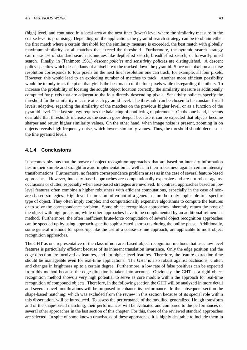
4.1. PREVIOUS WORK 43
(high) level, and continued in a local area at the next finer (lower) level where the similarity measure in thecoarse level is promising. Depending on the application, the pyramid search strategy can be to obtain eitherthe first match where a certain threshold for the similarity measure is exceeded, the best match with globallymaximum similarity, or all matches that exceed the threshold. Furthermore, the pyramid search strategycan make use of standard search techniques like depth-first search, breadth-first search, or forward-prunedsearch. Finally, in (Tanimoto 1981)descent policiesand sensitivity policiesare distinguished. A descentpolicy specifies which descendants of a pixel are to be tracked down the pyramid. Since one pixel on a coarseresolution corresponds to four pixels on the next finer resolution one can track, for example, all four pixels.However, this would lead to an exploding number of matches to track. Another more efficient possibilitywould be to only track the pixel that yields the best match of the four pixels while disregarding the others. Toincrease the probability of locating the sought object location correctly, the similarity measure is additionallycomputed for pixels that are adjacent to the four directly descending pixels. Sensitivity policies specify thethreshold for the similarity measure at each pyramid level. The threshold can be chosen to be constant for alllevels, adaptive, regarding the similarity of the matches on the previous higher level, or as a function of thepyramid level. The last strategy requires the balancing of conflicting requirements. On the one hand, it seemsdesirable that thresholds increase as the search goes deeper, because it can be expected that objects becomesharper and return higher similarity values. On the other hand, when image noise is present, zooming in onobjects reveals high-frequency noise, which lowers similarity values. Thus, the threshold should decrease atthe fine pyramid levels.
4.1.4 Conclusions
It becomes obvious that the power of object recognition approaches that are based on intensity informationlies in their simple and straightforward implementation as well as in their robustness against certain intensitytransformations. Furthermore, no feature correspondence problem arises as in the case of several feature-basedapproaches. However, intensity-based approaches are computationally expensive and are not robust againstocclusions or clutter, especially when area-based strategies are involved. In contrast, approaches based on lowlevel features often combine a higher robustness with efficient computations, especially in the case of non-area-based strategies. High level features are often not of a general nature but only applicable to a specifictype of object. They often imply complex and computationally expensive algorithms to compute the featuresor to solve the correspondence problem. Some object recognition approaches inherently return the pose ofthe object with high precision, while other approaches have to be complemented by an additional refinementmethod. Furthermore, the often inefficient brute-force computation of several object recognition approachescan be speeded up by using approach-specific sophisticated short-cuts during the online phase. Additionally,some general methods for speed-up, like the use of a coarse-to-fine approach, are applicable to most objectrecognition approaches.
The GHT as one representative of the class of non-area-based object recognition methods that uses low levelfeatures is particularly efficient because of its inherent translation invariance. Only the edge position and theedge direction are involved as features, and not higher level features. Therefore, the feature extraction timeshould be manageable even for real-time applications. The GHT is also robust against occlusions, clutter,and changes in brightness up to a certain degree. Furthermore, a low rate of false positives can be expectedfrom this method because the edge direction is taken into account. Obviously, the GHT as a rigid objectrecognition method shows a very high potential to serve as core module within the approach for real-timerecognition of compound objects. Therefore, in the following section the GHT will be analyzed in more detailand several novel modifications will be proposed to enhance its performance. In the subsequent section theshape-based matching, which was excluded from the review in this section because of its special role withinthis dissertation, will be introduced. To assess the performance of the modified generalized Hough transformand of the shape-based matching, their performances will be evaluated and compared to the performances ofseveral other approaches in the last section of this chapter. For this, three of the reviewed standard approachesare selected. In spite of some known drawbacks of these approaches, it is highly desirable to include them in

44 CHAPTER 4. RECOGNITION OF RIGID OBJECTS
the evaluation because they are widespread methods and used in the majority of industrial object recognitionapplications. By this, a common denominator is created that facilitates the comparability of the presentedevaluation with other evaluations that also include one of the three approaches. Additionally, three commercialhigh-end recognition tools will be evaluated. They have not been included in the review since no detailedinformation about their principle is available. Nevertheless, their performance helps to emphasize the highpotential of the new approaches.
4.2 Modified Generalized Hough Transform
The principle of the GHT as well as some inherent advantages have already been addressed in Section 4.1.1.2.However, the discussion has been done on a very coarse level of detail. On the one hand, this level of detailshould be sufficient to understand the general principle and to compare the GHT to other object recognitionapproaches. On the other hand, it is not detailed enough to enable the reader to obtain a comprehensive im-pression of the GHT. However, a comprehensive impression is essential to understand the modifications thathave been applied within the scope of this dissertation in order to improve the GHT. The goal of the mod-ifications is to make the GHT fulfill the requirements concerning the recognition of rigid objects introducedin Section 2.2. Therefore, in the following the principle of the GHT is explained in more detail. Further-more, the inherent advantages and drawbacks of the GHT are elaborated and used as basis for the proposedmodifications. Some modifications are based on the ideas of the previously introduced methods concerningpose refinement (cf. Section 4.1.2) and speed-up (cf. Section 4.1.3). These ideas are picked up and are furtherextended.
4.2.1 Generalized Hough Transform
4.2.1.1 Principle
The conventional Hough transform (HT) is a standard method to efficiently detect analytical curves (e.g.,lines, circles, ellipses) in images. Although the GHT is built on the idea of the HT, they both are independentmethods. Therefore, in this dissertation only the idea of the HT and its relations to the GHT are introduced. Forfurther details, the interested reader should refer to (Hough 1962) or to standard text books like (Ballard andBrown 1982, J¨ahne 2002).
To introduce the HT, the problem of detecting straight lines in images is considered. A straight line can bedescribed by the points(x, y)> that fulfill
r = x · cosϕ+ y · sinϕ . (4.13)
Thus, the line is represented by its distance to the originr and its orientationϕ (see Figure 4.1(a)). Fig-ure 4.1(b) shows an image after edge segmentation in which lines should be detected. Each edge pixel inthe(x, y) image space describes a sinusoidal curve in the(r, ϕ) parameter space, which is also referred to asHough spacein the literature. This can be seen from (4.13) by treatingx andy as fixed and lettingr andϕvary. Thus, the corresponding sinusoidal curve in the parameter space represents all lines in image space thatmeet in the same image point(x, y)>. In Figure 4.1(c) the sinusoidal curves of the two example edge pixelsshown in Figure 4.1(b) are displayed. All image points on the same line intersect at the same point in theparameter space. This relation between image space and parameter space is exploited in the HT. For this, theparameter space is divided into rectangular cells and represented by an accumulator array. In the first stage,each edge pixel is transformed into the Hough space and the corresponding cells are incremented. The secondstage is an exhaustive search for maxima in the accumulator array. The maxima represent the parameters ofthe straight lines in the image. Figure 4.1(d) shows the resulting accumulator array, where higher values of thecells are visualized by brighter gray values. The maximum represents the found straight line. The extension of
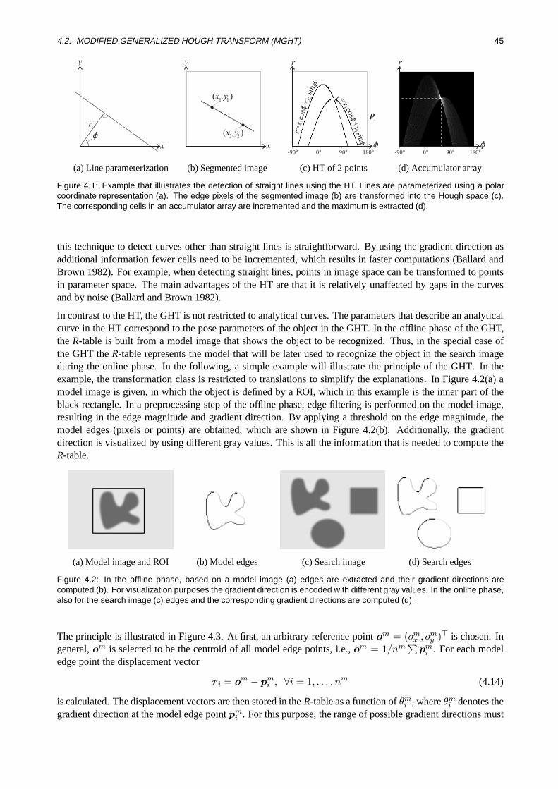
4.2. MODIFIED GENERALIZED HOUGH TRANSFORM (MGHT) 45
ϕr
y
x
(a) Line parameterization
( )x ,y
y
x
1 1
( )x ,y2 2
(b) Segmented image
r
ϕ-90° 180°0° 90°
p1
2
2
r=x
cosϕ
+y
sinϕ
r=x
cosϕ+
ysinϕ
1
1
(c) HT of 2 points
r
ϕ-90° 180°0° 90°
(d) Accumulator array
Figure 4.1: Example that illustrates the detection of straight lines using the HT. Lines are parameterized using a polarcoordinate representation (a). The edge pixels of the segmented image (b) are transformed into the Hough space (c).The corresponding cells in an accumulator array are incremented and the maximum is extracted (d).
this technique to detect curves other than straight lines is straightforward. By using the gradient direction asadditional information fewer cells need to be incremented, which results in faster computations (Ballard andBrown 1982). For example, when detecting straight lines, points in image space can be transformed to pointsin parameter space. The main advantages of the HT are that it is relatively unaffected by gaps in the curvesand by noise (Ballard and Brown 1982).
In contrast to the HT, the GHT is not restricted to analytical curves. The parameters that describe an analyticalcurve in the HT correspond to the pose parameters of the object in the GHT. In the offline phase of the GHT,theR-table is built from a model image that shows the object to be recognized. Thus, in the special case ofthe GHT theR-table represents the model that will be later used to recognize the object in the search imageduring the online phase. In the following, a simple example will illustrate the principle of the GHT. In theexample, the transformation class is restricted to translations to simplify the explanations. In Figure 4.2(a) amodel image is given, in which the object is defined by a ROI, which in this example is the inner part of theblack rectangle. In a preprocessing step of the offline phase, edge filtering is performed on the model image,resulting in the edge magnitude and gradient direction. By applying a threshold on the edge magnitude, themodel edges (pixels or points) are obtained, which are shown in Figure 4.2(b). Additionally, the gradientdirection is visualized by using different gray values. This is all the information that is needed to compute theR-table.
(a) Model image and ROI (b) Model edges (c) Search image (d) Search edges
Figure 4.2: In the offline phase, based on a model image (a) edges are extracted and their gradient directions arecomputed (b). For visualization purposes the gradient direction is encoded with different gray values. In the online phase,also for the search image (c) edges and the corresponding gradient directions are computed (d).
The principle is illustrated in Figure 4.3. At first, an arbitrary reference pointom = (omx , o
my )> is chosen. In
general,om is selected to be the centroid of all model edge points, i.e.,om = 1/nm∑pmi . For each model
edge point the displacement vector
ri = om − pmi , ∀i = 1, . . . , nm (4.14)
is calculated. The displacement vectors are then stored in theR-table as a function ofθmi , whereθm
i denotes thegradient direction at the model edge pointpm
i . For this purpose, the range of possible gradient directions must

46 CHAPTER 4. RECOGNITION OF RIGID OBJECTS
be quantized using quantization intervals of size∆θ. In general, the gradients occur in arbitrary direction,and hence the range of possible gradient directions corresponds to the interval of[0,360[. Each rowk oftheR-table is then assigned one quantization intervalΘk, k = 0, . . . , nθ − 1, leading to an overall number ofnθ = 2π
∆θ rows. Finally, the displacement vectorri of the model edge pointpmi is recorded in the row of the
R-table that contains the associated gradient directionθmi .
The exampleR-table in Figure 4.4 is built by using four selected model edge points. Here, the quantizationinterval for the gradient directions was set to∆θ = 60. Since the gradient directions at the two pointspm
2andpm
3 are identical, both associated displacement vectors are recorded in the same row within theR-table.
p
y
x
o
riim
θim
m
(a) Model edges
k Θk ri
0 [ 0, ∆θ[ ri | θmi ∈ Θ0
1 [ ∆θ, 2∆θ[ ri | θmi ∈ Θ1
2 [2∆θ, 3∆θ[ ri | θmi ∈ Θ2
......
...
(b) R-table
Figure 4.3: Information about the model edges (a) is used to build the R-table (b).
y
x
r θ1
m1r4
r2r3
θ3
m
θ4
m
θ2
mpm2
pm3
pm4 pm
1
om
(a) Four selected example model edge points
k Θk ri
0 [ 0, 60[1 [ 60, 120[ r2, r3
2 [120, 180[3 [180, 240[ r4
4 [240, 300[ r1
5 [300, 360[
(b) ExampleR-table with∆θ = 60
Figure 4.4: Example that illustrates the offline phase of the GHT. The gradient directions at the four selected examplemodel edge points are θm
1 = 280, θm2 = 65, θm
3 = 65, θm4 = 200. The associated displacement vectors ri are
recorded in the appropriate row of the R-table according to their gradient direction.
For the online phase a two dimensional accumulator arrayA is set up over the domain of translations, repre-senting the sampled parameter space or Hough space ofT . Figure 4.5 shows the principle of an accumulatorarray for the example search image of Figure 4.2. This is similar to the HT, however, each cell of this arraynow corresponds to a certain range of positions of the reference pointos = (os
x, osy)> in the search image. In
general, the size of the cells is adapted to the pixel grid, i.e., each cell represents one pixel. The accumulatorarray is initialized by setting the values of all cells to 0. For each edge pixelps
j in the search image the rowk intheR-table that corresponds to the gradient directionθs
j is selected. Each displacement vector that is recordedwithin the selected row represents the position of one reference point candidateo = (ox, oy)> relative tops
j

4.2. MODIFIED GENERALIZED HOUGH TRANSFORM (MGHT) 47
in the search image. Formally, the displacement vectors are added topsj in order to obtain the reference point
candidates:oi,j = ps
j + ri, ∀j = 1, . . . , ns, ∀i|θmi ∈ Θk, k|(θs
j ∈ Θk) . (4.15)
Finally, each cell in the accumulator arrayA that is hit by one reference point candidate receives a vote, i.e., itsvalue is incremented by one. After the voting process, each cell inA has a value that describes the likelihoodthat the reference point is located in this cell. Thus, local maxima inA that exceed a certain threshold representfound object instances in the search image. Figure 4.5 shows the principle of the online phase by means ofseven selected search edge points. In Figure 4.5(a) the cells of the accumulator array are overlaid on thesearch image of Figure 4.2. For illustration purposes, in this case one cell covers several pixels. For example,the edge directionθs
1 at pointps1 is 65. In the R-table of Figure 4.4(b) the respective gradient interval is
Θ1 = [60,120[, and hencek = 1. The two displacement vectorsr2 andr3 that are recorded in rowk = 1are added to the point positionps
1 and the two obtained reference point candidates are used to increment thetwo corresponding cells. Figure 4.5(b) shows the final accumulator array after the voting process, where thenumber of votes are entered in each cell. The cell with maximum number of votes represents the position ofthe reference point, and hence the found object instance in the search image.
c
r
y
x
ps3
ps2
ps4
θ2s
θ3s θ4
s
ps6
ps7
ps5
θ6s
θ5s
θ7sr1
r2 r3
r4
r1r4
r2r3
θ1sps
1
r2r3
(a) Accumulator array and voting process
c
r
41 1
11
1
1y
x
(b) Final votes (empty cells have zero votes)
Figure 4.5: Example that illustrates the online phase of the GHT. The gradient directions at seven selected examplesearch edge points are θs
1 = 65, θs2 = 65, θs
3 = 200,θs4 = 280, θs
5 = 65, θs6 = 200, and θs
7 = 280 (a). According tothe gradient direction the displacement vectors in the respective row of the R-table are added to the point positions, andthe corresponding cells receive a vote (b).
4.2.1.2 Advantages
The GHT shows several inherent advantages already in its original form. In contrast to alignment methods thatuse an arbitrary similarity measure, it is not necessary to translate the model image to all possible positions ofthe object in the search image. Instead, the translation is regarded implicitly since the model edges are storedrelative to the reference point. This saves significant computation time.
Further savings in computation time are achieved by taking the gradient direction information into account.Thus, for one edge point in the search image only the model edge points with similar gradient direction insteadof all model edge points are used for incrementing the respective cells. Considering the gradient direction leadsto another important advantage. The robustness against clutter is increased considerably, i.e., the probabilityof false positive matches is decreased. This effect is illustrated in Figure 4.6, which shows the accumulatorarray after the voting process. In contrast to Figure 4.5, now one cell corresponds to one pixel. The number ofvotes in each cell is visualized as height in the 3D plots. Figure 4.6(a) shows the result of the voting process in

48 CHAPTER 4. RECOGNITION OF RIGID OBJECTS
the case that no gradient direction information is taken into account. This can be simulated by creating anR-table that consists of only a single row, i.e.,∆θ = 360. Consequently, for each edge pixel in the search imageall displacement vector are used for voting, independent of their associated gradient direction. Although theartificially created search image is free of noise and the two additional objects differ from the searched object,the accumulator array shows noisy regions and some additional (albeit small) peaks. The signal-to-noise-ratio(SNR), calculated as the peak-signal-to-peak-noise in this case is 3.3. In Figure 4.6(b) the same situation isapplied, however, the gradient direction was quantized using an interval size of∆θ = 5. One can see thatthe noise in the accumulator array has diminished significantly. The almost doubled SNR of 6.5 confirms thevisual impression. In this example, an acceptable SNR is obtained even if no gradient direction is considered,and hence the intrinsic peak can be easily distinguished from the noise in the accumulator array. However,one can imagine the problems when dealing with noisy, highly textured images, which contain additionalobjects that are similar to the object to be found. In such cases the gradient direction is an absolutely essentialinformation.
(a) Neglecting gradient direction (b) Considering gradient direction
Figure 4.6: The accumulator array shows several peaks after the voting process. The signal-to-noise ratio (SNR) can besignificantly increased by considering the gradient direction information. In this example, the SNR almost doubles from3.3 (a) to 6.5 (b).
Another advantage of the GHT is its high robustness against occlusions. At first glance, one may think thatocclusions in the search image affect the position of the reference point (e.g., the centroid), and hence causethe voting process to fail. However, this is not the case. In contrast to moment-based approaches, for example,which require the object as a whole to be present in the image, the GHT is tolerant against a certain degree ofocclusions. Looking at the principle of the GHT again, the reference point in the search image is not computedas the centroid of all edge points but is the result of the maximum search after the voting process. If someof the edge pixels in the search image are missing because of partial occlusions, the peak height is merelyreduced in proportion to the fraction of occluded edge pixels. This is a rather intuitive behavior.
Furthermore, the GHT is robust against changes in brightness of an arbitrary type up to a certain degree.Since the recognition is based on the image edges instead of the raw gray value information, changes inbrightness do not affect the recognition unless the edge magnitude falls below the threshold that is appliedto edge segmentation. The features that are used in the GHT are edge position and gradient direction. Bothfeatures do not change dramatically when the brightness or the contrast in the image changes. However, if thecontrast is too low in some object parts of the search image fewer edges will be segmented. This leads to thesame effect as partial occlusions. Nevertheless, if the contrast is too low in the entire image the GHT fails torecognize the object, unless the segmentation threshold is set to a lower value.
4.2.1.3 Drawbacks
In this dissertation objects must be found under the transformation class of rigid motion. Unfortunately, theGHT was originally designed to cope with object translations only. If one wants to recognize objects that may

4.2. MODIFIED GENERALIZED HOUGH TRANSFORM (MGHT) 49
appear in an arbitrary orientation the GHT must be extended accordingly: now for each possible orientationϕs of the object in the search image a separateR-table is generated by using a certain orientation step∆ϕ tosample the range of possible orientations. Depending on∆ϕ and the orientation range in which the object mayappear, a number ofR-tables is generated at discrete orientationsϕr, r = 0, . . . , nϕ − 1, wherenϕ denotesthe number of discrete orientations, and hence the number ofR-tables. Finally, eachR-table is labeled withits associated orientationϕr. In the online phase,nϕ separate 2D accumulator arrays are built, one for eachR-table. All single 2D arrays can be put together into one 3D accumulator array. The first two dimensionsrepresent the position of the reference pointos and the third dimension represents the orientation of the objectϕs in the search image. The voting process is then performed for eachR-table separately, where the votes areentered in the respective 2D hyperplane of the accumulator array that is associated with the currentR-table.The position of local maxima in the 3D array that exceed a threshold describe the position and orientationof found object instances. Obviously, the computational effort in the online phase increases linearly with thenumber ofR-tables, and hence with the number of rotation steps.
Thus, one weakness of the GHT algorithm is the — in general — huge parameter space represented by the3D accumulator arrayA when allowing rigid motion. Assume an image of size 768× 576, a rotation stepof ∆ϕ = 1, and an object that may appear at an arbitrary orientation. Hence, the number of discernedorientation stepsnϕ is 360. Consequently, the accumulator array would contain 768× 576× 360= 159· 106
cells. This involves large amounts of memory to store the accumulator array as well as high computationalcosts in the online phase for the initialization of the array and the search for local maxima after the votingprocess.
Another crucial part is the large number of voting eventsnvote that have to be performed. The average numberof voting events is
nvote = nϕnsnm
nθ, (4.16)
wherenθ = 2π∆θ again is the number of different gradient direction intervals, and hence the number of rows
in theR-tables. Assuming a non-cluttered search image, i.e., no additional edges are present, and thusns =nm, the effort for incrementing the respective cells in the accumulator array increases quadratically with thenumber of model edge pixelsnm. This behavior hinders real-time performance, especially for large or highlytextured objects.
Additionally, the conventional GHT is sensitive to image noise. Although the edge position is relativelyunaffected by a moderate degree of noise, the gradient direction is much more sensitive. Since the gradientdirection is directly involved as feature within the GHT, image noise also has an impact on the performanceof GHT. Especially, when the size of the gradient direction intervals∆θ is chosen small, the robustness maysignificantly decrease.
Finally, the properties of the GHT lead to the fact that the accuracies achieved for the returned pose parametersdepend on the quantization of the transformation class of rigid motion. Thus, in the mentioned example theaccuracy of object position is limited to the pixel size and the accuracy of object orientation is limited to 1.Unfortunately, in practice the quantization cannot be chosen arbitrarily fine because of memory requirementsand computation time. Furthermore, the robustness against clutter would decrease considerably when increas-ing the resolution of the accumulator array. This is because the peak would be dispersed over an increasingnumber of cells in the accumulator array.
In the following, the mentioned problems will be tackled, resulting in a modified Generalized Hough Trans-form (MGHT) (Ulrich et al. 2001b, Ulrich et al. 2001a): a multi-resolution model and search strategy incombination with an effective limitation of the search space is introduced in order to increase the efficiency,and hence meet the real-time requirements. Furthermore, a technique for refining the returned pose parameterswithout noticeably decelerating the online phase is presented. In addition, some crucial quantization problemsand their solutions to increase the robustness of the GHT are discussed.
50 CHAPTER 4. RECOGNITION OF RIGID OBJECTS
4.2.2 Computation of the R-tables
First of all, some general comments on the computation of theR-tables for the different object orientationsshould be made. Feature extraction is a prerequisite for applying the principle of the GHT for object recog-nition. In this dissertation the edge magnitude and the gradient direction are computed using the Sobel filter.This filter represents a good compromise between computation time and accuracy: it can be computed in lesstime than, for instance, the Lanser or Canny filters. Its anisotropic response and its worse accuracy can bebalanced by the proposed approach: it will be shown in this section that the effect of the anisotropy can bereduced considerably by selecting an appropriate method for the computation of theR-tables. The residualanisotropy and the worse accuracy can be balanced by choosing an adequate quantization∆θ of the gradientdirections, which will be explained in Section 4.2.5. Both the edge magnitudeγ and the gradient directionθare computed from the first partial gray value derivatives inx andy direction, which are returned by the Sobelfilter. The edge pixels are segmented by applying a thresholdγmin on the edge magnitude. This thresholdmust be set by the user because it is highly correlated with the task of the application and with the type ofobject to be recognized. A subsequent non-maximum suppression eliminates the edge pixels that are no localmaxima in the direction of the gradient. For this, the current edge pixel is compared to the two adjacent pixelsin the gradient direction. However, because of the discrete structure of the image, still two pixel wide edgesmay occur. Therefore, the number of edge pixels can be further reduced by computing the skeleton based ona medial axis transform (Ballard and Brown 1982). Thus, by using only the most representative edge pixelsin theR-table the computational effort during the online phase can be kept small.
To allow object rotation, for each object orientationϕ a separateR-table must be built. In general, this canbe accomplished by following one of four possibilities. The four possibilities arise by combining one of twomethods to build theR-tables with the decision whether theR-tables are built within the offline phase or withinthe online phase.
The first method to build theR-tables is to compute theR-table for the model image as described before,yielding a prototypeR-table. TheR-tables of all discrete orientationsϕr are then obtained by applying simpletransformations on the prototypeR-table, as proposed in (Ballard 1981). For this, the limits of all gradientintervalsΘk, 0 ≤ k < nθ of the prototypeR-table are just incremented by the current rotation angleϕr.Furthermore, all displacement vectors within the prototypeR-table are rotated byϕr. The second methodto build theR-tables is to rotate the model image itself and generate anR-table based on each of the rotatedmodel images. When using the Sobel filter the latter method has a crucial advantage. By deriving theR-tablesfrom the rotated model images the error caused by the anisotropy of the Sobel filter can be eliminated sincethe anisotropy is the same in the rotated model image and in the search image, and hence the error cancels out.In contrast, the advantage of the first method is its lower computational effort, since only a “small” number ofdisplacement vectors must be rotated but not the entire image.
Furthermore, both methods can be applied either in the offline phase or in the online phase leading to fourdifferent combinations. Pre-computing theR-tables in the offline phase is more memory-intensive since allrotatedR-tables must be stored in memory. However, it facilitates a substantially more efficient object recog-nition during the online phase since no rotations must be performed online. In this dissertation theR-tablesare derived from the rotated model image in the offline phase. This, on the one hand, optimizes the com-putation time of the online phase and, on the other hand, eliminates the anisotropy error. Hence, the secondcomputation method is combined with computing theR-tables offline.
Table 4.2 summarizes the four possibilities and additionally points out the respective advantages and draw-backs. The combination used in this work is emphasized in bold type.
It should be noted that in some applications it might be less important to achieve real-time computation but tokeep the required memory amount as small as possible. Then it would be preferable to compute the requiredR-tables online. Furthermore, in such cases it might be desirable to use the first computation method to allowa reasonable computation time of the online phase even though the anisotropy error must be accepted.
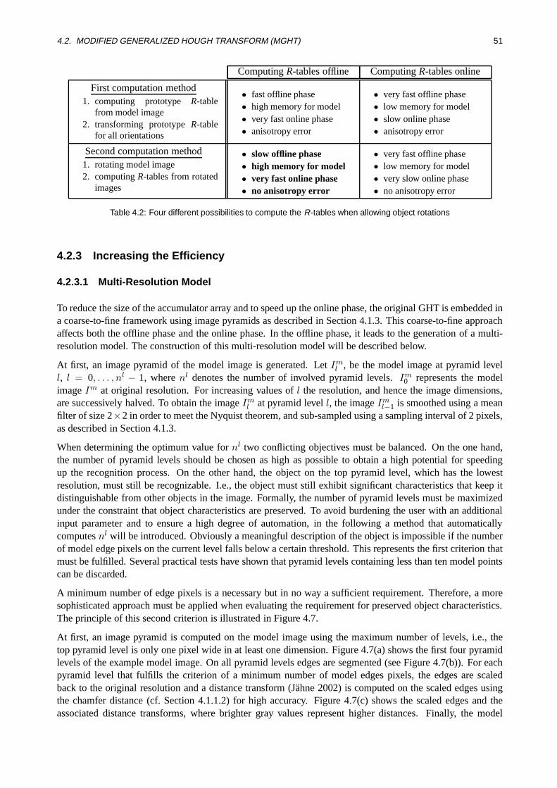
4.2. MODIFIED GENERALIZED HOUGH TRANSFORM (MGHT) 51
ComputingR-tables offline ComputingR-tables online
First computation method1. computing prototype R-table
from model image2. transforming prototypeR-table
for all orientations
• fast offline phase• high memory for model• very fast online phase• anisotropy error
• very fast offline phase• low memory for model• slow online phase• anisotropy error
Second computation method1. rotating model image2. computingR-tables from rotated
images
• slow offline phase• high memory for model• very fast online phase• no anisotropy error
• very fast offline phase• low memory for model• very slow online phase• no anisotropy error
Table 4.2: Four different possibilities to compute the R-tables when allowing object rotations
4.2.3 Increasing the Efficiency
4.2.3.1 Multi-Resolution Model
To reduce the size of the accumulator array and to speed up the online phase, the original GHT is embedded ina coarse-to-fine framework using image pyramids as described in Section 4.1.3. This coarse-to-fine approachaffects both the offline phase and the online phase. In the offline phase, it leads to the generation of a multi-resolution model. The construction of this multi-resolution model will be described below.
At first, an image pyramid of the model image is generated. LetIml , be the model image at pyramid level
l, l = 0, . . . , nl − 1, wherenl denotes the number of involved pyramid levels.Im0 represents the model
imageIm at original resolution. For increasing values ofl the resolution, and hence the image dimensions,are successively halved. To obtain the imageIm
l at pyramid levell, the imageIml−1 is smoothed using a mean
filter of size 2×2 in order to meet the Nyquist theorem, and sub-sampled using a sampling interval of 2 pixels,as described in Section 4.1.3.
When determining the optimum value fornl two conflicting objectives must be balanced. On the one hand,the number of pyramid levels should be chosen as high as possible to obtain a high potential for speedingup the recognition process. On the other hand, the object on the top pyramid level, which has the lowestresolution, must still be recognizable. I.e., the object must still exhibit significant characteristics that keep itdistinguishable from other objects in the image. Formally, the number of pyramid levels must be maximizedunder the constraint that object characteristics are preserved. To avoid burdening the user with an additionalinput parameter and to ensure a high degree of automation, in the following a method that automaticallycomputesnl will be introduced. Obviously a meaningful description of the object is impossible if the numberof model edge pixels on the current level falls below a certain threshold. This represents the first criterion thatmust be fulfilled. Several practical tests have shown that pyramid levels containing less than ten model pointscan be discarded.
A minimum number of edge pixels is a necessary but in no way a sufficient requirement. Therefore, a moresophisticated approach must be applied when evaluating the requirement for preserved object characteristics.The principle of this second criterion is illustrated in Figure 4.7.
At first, an image pyramid is computed on the model image using the maximum number of levels, i.e., thetop pyramid level is only one pixel wide in at least one dimension. Figure 4.7(a) shows the first four pyramidlevels of the example model image. On all pyramid levels edges are segmented (see Figure 4.7(b)). For eachpyramid level that fulfills the criterion of a minimum number of model edges pixels, the edges are scaledback to the original resolution and a distance transform (J¨ahne 2002) is computed on the scaled edges usingthe chamfer distance (cf. Section 4.1.1.2) for high accuracy. Figure 4.7(c) shows the scaled edges and theassociated distance transforms, where brighter gray values represent higher distances. Finally, the model
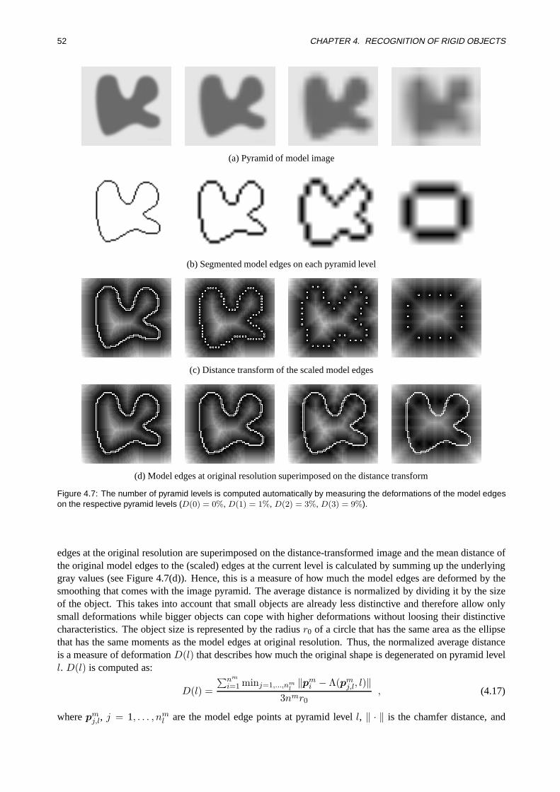
52 CHAPTER 4. RECOGNITION OF RIGID OBJECTS
(a) Pyramid of model image
(b) Segmented model edges on each pyramid level
(c) Distance transform of the scaled model edges
(d) Model edges at original resolution superimposed on the distance transform
Figure 4.7: The number of pyramid levels is computed automatically by measuring the deformations of the model edgeson the respective pyramid levels (D(0) = 0%, D(1) = 1%, D(2) = 3%, D(3) = 9%).
edges at the original resolution are superimposed on the distance-transformed image and the mean distance ofthe original model edges to the (scaled) edges at the current level is calculated by summing up the underlyinggray values (see Figure 4.7(d)). Hence, this is a measure of how much the model edges are deformed by thesmoothing that comes with the image pyramid. The average distance is normalized by dividing it by the sizeof the object. This takes into account that small objects are already less distinctive and therefore allow onlysmall deformations while bigger objects can cope with higher deformations without loosing their distinctivecharacteristics. The object size is represented by the radiusr0 of a circle that has the same area as the ellipsethat has the same moments as the model edges at original resolution. Thus, the normalized average distanceis a measure of deformationD(l) that describes how much the original shape is degenerated on pyramid levell. D(l) is computed as:
D(l) =∑nm
i=1 minj=1,...,nml‖pm
i − Λ(pmj,l, l)‖
3nmr0, (4.17)
wherepmj,l, j = 1, . . . , nm
l are the model edge points at pyramid levell, ‖ · ‖ is the chamfer distance, and
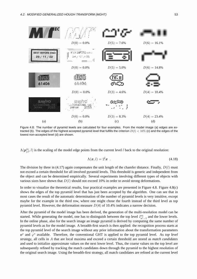
4.2. MODIFIED GENERALIZED HOUGH TRANSFORM (MGHT) 53
D(0) = 0.0% D(5) = 7.6% D(6) = 16.1%
D(0) = 0.0% D(5) = 5.0% D(6) = 14.8%
D(0) = 0.0% D(3) = 4.6% D(4) = 10.4%
D(0) = 0.0% D(3) = 8.3% D(4) = 23.4%
(a) (b) (c) (d)
Figure 4.8: The number of pyramid levels are calculated for four examples. From the model image (a) edges are ex-tracted (b). The edges of the highest accepted pyramid level that fulfills the criterion D(l) < 10% (c) and the edges of thelowest non-accepted level (d) are shown.
Λ(pmj,l, l) is the scaling of the model edge points from the current levell back to the original resolution:
Λ(x, l) = 2lx . (4.18)
The division by three in (4.17) again compensates the unit length of the chamfer distance. Finally,D(l) mustnot exceed a certain threshold for all involved pyramid levels. This threshold is generic and independent fromthe object and can be determined empirically. Several experiments involving different types of objects withvarious sizes have shown thatD(l) should not exceed 10% in order to avoid strong deformations.
In order to visualize the theoretical results, four practical examples are presented in Figure 4.8. Figure 4.8(c)shows the edges of the top pyramid level that has just been accepted by the algorithm. One can see that inmost cases the result of the automatic determination of the number of pyramid levels is very intuitive, exceptmaybe for the example in the third row, where one might chose the fourth instead of the third level as toppyramid level. However, the deformation measureD(4) of 10.4% indicates a narrow decision.
After the pyramid of the model image has been derived, the generation of the multi-resolution model can bestarted. While generating the model, one has to distinguish between the top levelIm
nl−1 and the lower levels.In the online phase, also for the search image an image pyramid is derived by computing the same number ofpyramid levels as for the model image. A breadth-first search is then applied: the recognition process starts atthe top pyramid level of the search image without any prior information about the transformation parametersos andϕs available. Therefore, the conventional GHT is applied to the top pyramid level. Astop levelstrategy, all cells inA that are local maxima and exceed a certain threshold are stored asmatch candidatesand used to initialize approximate values on the next lower level. Thus, the coarse values on the top level aresubsequently refined by tracking the match candidates down through the pyramid to the highest resolution ofthe original search image. Using the breadth-first strategy, all match candidates are refined at the current level
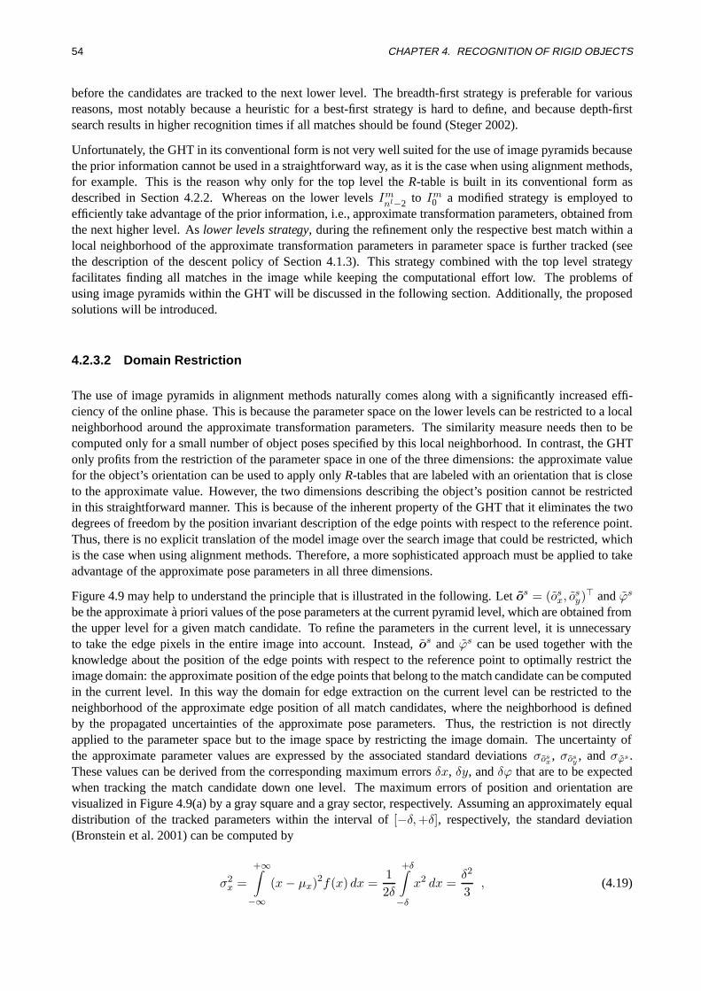
54 CHAPTER 4. RECOGNITION OF RIGID OBJECTS
before the candidates are tracked to the next lower level. The breadth-first strategy is preferable for variousreasons, most notably because a heuristic for a best-first strategy is hard to define, and because depth-firstsearch results in higher recognition times if all matches should be found (Steger 2002).
Unfortunately, the GHT in its conventional form is not very well suited for the use of image pyramids becausethe prior information cannot be used in a straightforward way, as it is the case when using alignment methods,for example. This is the reason why only for the top level theR-table is built in its conventional form asdescribed in Section 4.2.2. Whereas on the lower levelsIm
nl−2 to Im0 a modified strategy is employed to
efficiently take advantage of the prior information, i.e., approximate transformation parameters, obtained fromthe next higher level. Aslower levels strategy, during the refinement only the respective best match within alocal neighborhood of the approximate transformation parameters in parameter space is further tracked (seethe description of the descent policy of Section 4.1.3). This strategy combined with the top level strategyfacilitates finding all matches in the image while keeping the computational effort low. The problems ofusing image pyramids within the GHT will be discussed in the following section. Additionally, the proposedsolutions will be introduced.
4.2.3.2 Domain Restriction
The use of image pyramids in alignment methods naturally comes along with a significantly increased effi-ciency of the online phase. This is because the parameter space on the lower levels can be restricted to a localneighborhood around the approximate transformation parameters. The similarity measure needs then to becomputed only for a small number of object poses specified by this local neighborhood. In contrast, the GHTonly profits from the restriction of the parameter space in one of the three dimensions: the approximate valuefor the object’s orientation can be used to apply onlyR-tables that are labeled with an orientation that is closeto the approximate value. However, the two dimensions describing the object’s position cannot be restrictedin this straightforward manner. This is because of the inherent property of the GHT that it eliminates the twodegrees of freedom by the position invariant description of the edge points with respect to the reference point.Thus, there is no explicit translation of the model image over the search image that could be restricted, whichis the case when using alignment methods. Therefore, a more sophisticated approach must be applied to takeadvantage of the approximate pose parameters in all three dimensions.
Figure 4.9 may help to understand the principle that is illustrated in the following. Letos = (osx, o
sy)> andϕs
be the approximate `a priori values of the pose parameters at the current pyramid level, which are obtained fromthe upper level for a given match candidate. To refine the parameters in the current level, it is unnecessaryto take the edge pixels in the entire image into account. Instead,os and ϕs can be used together with theknowledge about the position of the edge points with respect to the reference point to optimally restrict theimage domain: the approximate position of the edge points that belong to the match candidate can be computedin the current level. In this way the domain for edge extraction on the current level can be restricted to theneighborhood of the approximate edge position of all match candidates, where the neighborhood is definedby the propagated uncertainties of the approximate pose parameters. Thus, the restriction is not directlyapplied to the parameter space but to the image space by restricting the image domain. The uncertainty ofthe approximate parameter values are expressed by the associated standard deviationsσos
x, σos
y, andσϕs .
These values can be derived from the corresponding maximum errorsδx, δy, andδϕ that are to be expectedwhen tracking the match candidate down one level. The maximum errors of position and orientation arevisualized in Figure 4.9(a) by a gray square and a gray sector, respectively. Assuming an approximately equaldistribution of the tracked parameters within the interval of[−δ,+δ], respectively, the standard deviation(Bronstein et al. 2001) can be computed by
σ2x =
+∞∫−∞
(x− µx)2f(x) dx =12δ
+δ∫−δ
x2 dx =δ2
3, (4.19)

4.2. MODIFIED GENERALIZED HOUGH TRANSFORM (MGHT) 55
y
x
os∼
ϕ s∼
2δx
2δy
2δϕ
ps∼i
-R r( ) iϕ s∼
(a)
unscalederror ellipse
y
x
os∼
unscalederror ellipse
error ellipsescaled by 3.44
99.7%39%
(b)
y
x
envelope
(c)
Figure 4.9: Approximate pose parameters are obtained from the upper pyramid level and can be used to calculateapproximate edge positions (a). The uncertainty of the pose propagates to the edge position (b). The envelope of theerror ellipses thus obtained for all edge points describes a region in which edge points lie with a certain probability (c).
finally leading to
σosx
=δx√
3, σos
y=
δy√3, σϕs =
δϕ√3. (4.20)
The values for the maximum errors have been derived from several tests. During the tests it turned out that itis sufficient to setδx andδy to 3 pixels andδϕ to 3∆ϕ. The approximate position of each model edge pixel inthe search imageps
i = (xsi , y
si )> can be obtained by transforming the associated negated displacement vector
according to the approximate pose parameters (see Figure 4.9(a)):
psi = os −R(ϕs)ri . (4.21)
Here,ri represents the displacement vectors obtained from the non-rotated model image. The covariancematrix for the two coordinates ofps
i is easily computed by applying the law of error propagation. The corre-sponding error ellipse (Gotthardt 1968) is obtained from the eigenvectors and eigenvalues of the covariancematrix (see Figure 4.9(b)). The error ellipse represents the boundary of a confidence region in whichps
i lieswith a probability of 39%. A more appropriate probability can be obtained by scaling the axis of the ellipseby a factor of 3.44 leading to a confidence of 1− e−(3.442/2) = 99.7% (Gotthardt 1968). Finally, the envelopeof all single confidence regions describes the image domain that the edge segmentation can be restricted to forthe current match candidate, where on average only 0.3% of the edge pixels are missed (see Figure 4.9(c)).
Unfortunately, the exact computation of the envelope region, as is was described above, is extremely timeconsuming. Furthermore, the assumption of the equal error distribution is not entirely correct. Therefore, itis advisable and meaningful to simplify the computations. The strategy is illustrated in Figure 4.10. Againthe approximate position of the model edge pixels in the search image is given (see Figure 4.10(a)). Theidea is based on blurring the model edges according to the maximum errors of position and orientation. Themaximum errors in positionδx, δy are taken into account by dilating the edges using a structuring element ofsize(2δx+1)× (2δy+1) (see Figure 4.10(b)). A dilation is a morphological region operation that efficientlyexpands the input region using a certain structuring element (Soille 1999). Assuming thatδ = δx = δythe dilation provides a region that is expanded byδ in both directions. The resulting dilated region is thensuccessively rotated in both directions until the two extremes of the maximum error in orientation±δϕ arereached. The final region is obtained by merging all rotated regions (see Figure 4.10(c)). Since the sequenceof the blurring affects the result, the blurring is done a second time by starting with the rotation and dilatingin the second step. The two resulting blurred regions are merged by computing the union of the two regions.
The blurred region can be pre-computed in the offline phase, where for each pyramid level different fromthe top level and for each discerned orientation one region is computed. For the top pyramid level no blurredregions need to be computed because no prior information will be available. In the online phase, the respectiveblurred region is selected according to the pyramid level and the approximate object orientationϕs and is
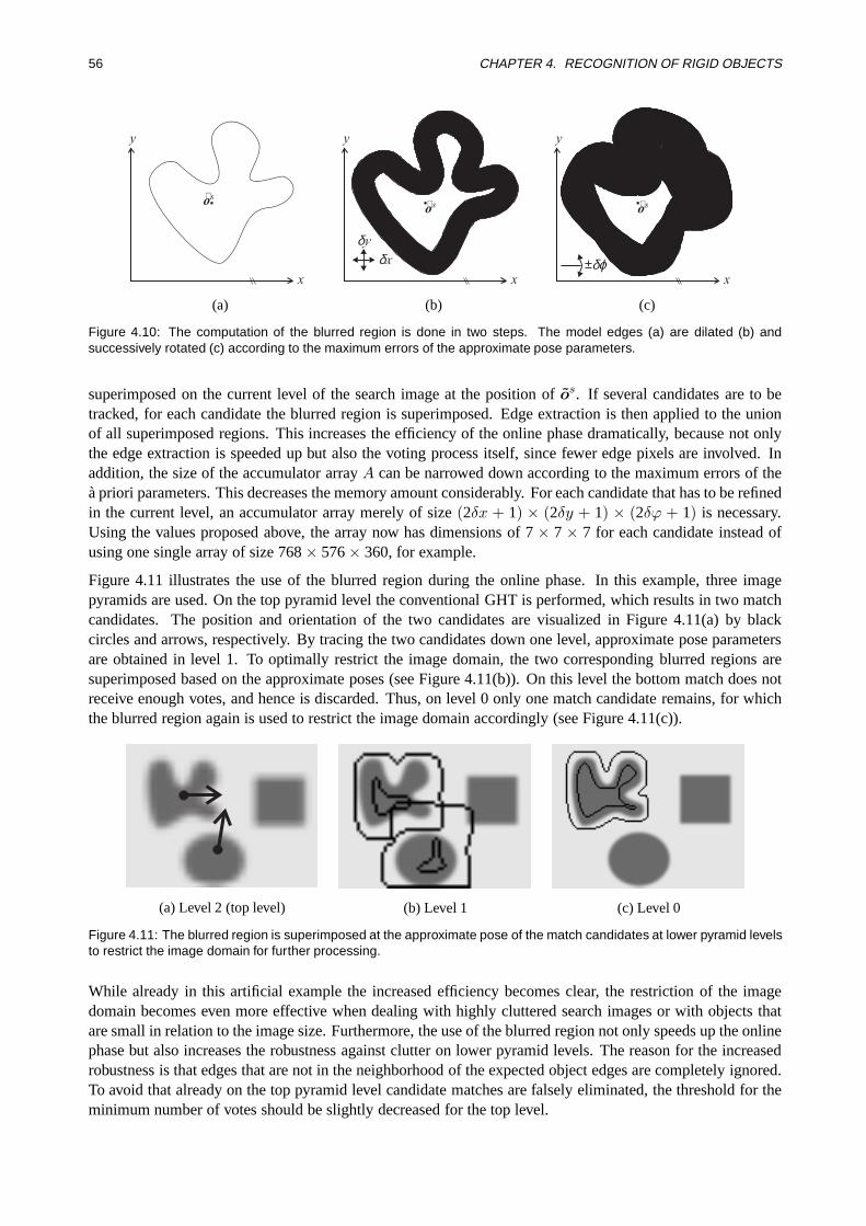
56 CHAPTER 4. RECOGNITION OF RIGID OBJECTS
y
x
os∼
(a)
y
x
os∼
δx
δy
(b)
y
x
os∼
δϕ±
(c)
Figure 4.10: The computation of the blurred region is done in two steps. The model edges (a) are dilated (b) andsuccessively rotated (c) according to the maximum errors of the approximate pose parameters.
superimposed on the current level of the search image at the position ofos. If several candidates are to betracked, for each candidate the blurred region is superimposed. Edge extraction is then applied to the unionof all superimposed regions. This increases the efficiency of the online phase dramatically, because not onlythe edge extraction is speeded up but also the voting process itself, since fewer edge pixels are involved. Inaddition, the size of the accumulator arrayA can be narrowed down according to the maximum errors of thea priori parameters. This decreases the memory amount considerably. For each candidate that has to be refinedin the current level, an accumulator array merely of size(2δx + 1) × (2δy + 1) × (2δϕ + 1) is necessary.Using the values proposed above, the array now has dimensions of 7× 7× 7 for each candidate instead ofusing one single array of size 768× 576× 360, for example.
Figure 4.11 illustrates the use of the blurred region during the online phase. In this example, three imagepyramids are used. On the top pyramid level the conventional GHT is performed, which results in two matchcandidates. The position and orientation of the two candidates are visualized in Figure 4.11(a) by blackcircles and arrows, respectively. By tracing the two candidates down one level, approximate pose parametersare obtained in level 1. To optimally restrict the image domain, the two corresponding blurred regions aresuperimposed based on the approximate poses (see Figure 4.11(b)). On this level the bottom match does notreceive enough votes, and hence is discarded. Thus, on level 0 only one match candidate remains, for whichthe blurred region again is used to restrict the image domain accordingly (see Figure 4.11(c)).
(a) Level 2 (top level) (b) Level 1 (c) Level 0
Figure 4.11: The blurred region is superimposed at the approximate pose of the match candidates at lower pyramid levelsto restrict the image domain for further processing.
While already in this artificial example the increased efficiency becomes clear, the restriction of the imagedomain becomes even more effective when dealing with highly cluttered search images or with objects thatare small in relation to the image size. Furthermore, the use of the blurred region not only speeds up the onlinephase but also increases the robustness against clutter on lower pyramid levels. The reason for the increasedrobustness is that edges that are not in the neighborhood of the expected object edges are completely ignored.To avoid that already on the top pyramid level candidate matches are falsely eliminated, the threshold for theminimum number of votes should be slightly decreased for the top level.
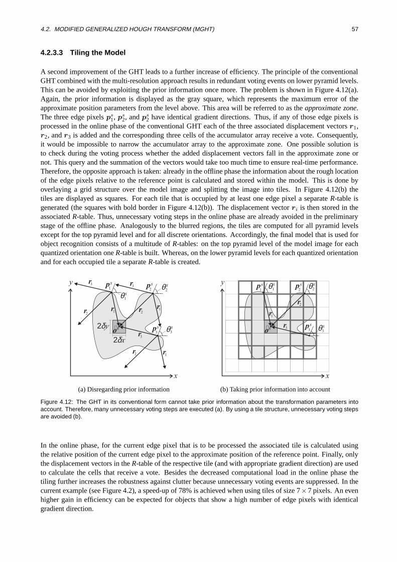
4.2. MODIFIED GENERALIZED HOUGH TRANSFORM (MGHT) 57
4.2.3.3 Tiling the Model
A second improvement of the GHT leads to a further increase of efficiency. The principle of the conventionalGHT combined with the multi-resolution approach results in redundant voting events on lower pyramid levels.This can be avoided by exploiting the prior information once more. The problem is shown in Figure 4.12(a).Again, the prior information is displayed as the gray square, which represents the maximum error of theapproximate position parameters from the level above. This area will be referred to as theapproximate zone.The three edge pixelsps
1, ps2, andps
2 have identical gradient directions. Thus, if any of those edge pixels isprocessed in the online phase of the conventional GHT each of the three associated displacement vectorsr1,r2, andr3 is added and the corresponding three cells of the accumulator array receive a vote. Consequently,it would be impossible to narrow the accumulator array to the approximate zone. One possible solution isto check during the voting process whether the added displacement vectors fall in the approximate zone ornot. This query and the summation of the vectors would take too much time to ensure real-time performance.Therefore, the opposite approach is taken: already in the offline phase the information about the rough locationof the edge pixels relative to the reference point is calculated and stored within the model. This is done byoverlaying a grid structure over the model image and splitting the image into tiles. In Figure 4.12(b) thetiles are displayed as squares. For each tile that is occupied by at least one edge pixel a separateR-table isgenerated (the squares with bold border in Figure 4.12(b)). The displacement vectorri is then stored in theassociatedR-table. Thus, unnecessary voting steps in the online phase are already avoided in the preliminarystage of the offline phase. Analogously to the blurred regions, the tiles are computed for all pyramid levelsexcept for the top pyramid level and for all discrete orientations. Accordingly, the final model that is used forobject recognition consists of a multitude ofR-tables: on the top pyramid level of the model image for eachquantized orientation oneR-table is built. Whereas, on the lower pyramid levels for each quantized orientationand for each occupied tile a separateR-table is created.
y
x
r1
θ3
sos∼
2δx
2δyr3
r2
θ2
s
θ1
s
ps1
ps2
ps3
r1
r1r2
r2
r3r3
(a) Disregarding prior information
y
x
r1
θ3
sos∼ r3
r2
θ2
sθ1
sps1
ps2
ps3
(b) Taking prior information into account
Figure 4.12: The GHT in its conventional form cannot take prior information about the transformation parameters intoaccount. Therefore, many unnecessary voting steps are executed (a). By using a tile structure, unnecessary voting stepsare avoided (b).
In the online phase, for the current edge pixel that is to be processed the associated tile is calculated usingthe relative position of the current edge pixel to the approximate position of the reference point. Finally, onlythe displacement vectors in theR-table of the respective tile (and with appropriate gradient direction) are usedto calculate the cells that receive a vote. Besides the decreased computational load in the online phase thetiling further increases the robustness against clutter because unnecessary voting events are suppressed. In thecurrent example (see Figure 4.2), a speed-up of 78% is achieved when using tiles of size 7×7 pixels. An evenhigher gain in efficiency can be expected for objects that show a high number of edge pixels with identicalgradient direction.

58 CHAPTER 4. RECOGNITION OF RIGID OBJECTS
Summarizing the most important points, the conventional GHT is not suited for the use of image pyramidsin a straightforward way. However, by applying a multi-resolution model that includes the domain restrictionwith the blurred region and the avoidance of unnecessary voting steps with the tile structure, the advantagesof image pyramids also become accessible to the GHT. The multi-resolution model reduces the memoryrequirements in the online phase drastically and facilitates real-time object recognition. Several tests that showthe correctness of the latter statement will be described in the performance evaluation, which is presented inSection 4.4. Furthermore, another important advantage of the proposed multi-resolution model is the increasedrobustness against clutter.
4.2.4 Pose Refinement
In this section, a method for pose refinement that breaks the limits on the achievable accuracy that are inducedby the quantization of the parameter space is described. After the voting process on the lowest pyramidlevel, matches that correspond to cells in the accumulator array and that are local maxima exceeding a certainthreshold of votes are obtained. Therefore, the accuracy of the position parametersos
x andosy is limited to the
cell size used in the accumulator array on the lowest pyramid level, which in general corresponds to the pixelgrid. Analogously, the accuracy of the orientation parameterϕs is limited to the step size∆ϕ that is used torotate the model image on the lowest pyramid level. The proposed refinement method is based on the idea ofcorrelation interpolation (Tian and Huhns 1986) that was introduced in Section 4.1.2. However, the proposedmethod is not restricted to refine the object position, as it is the case in (Tian and Huhns 1986), but is ableto simultaneously refine position and orientation. Furthermore, not a correlation measure but the votes in theaccumulator array are used for interpolation. To refine the position and orientation, thefacet model principle(Haralick and Shapiro 1992) is applied. It states that an image can be thought of as a continuous gray levelintensity surface, where the acquired digital image is a noisy sampling of a distorted version of this surface.To apply this principle to pose refinement, the 3D parameter space is assumed to be a 3D continuous intensitysurfacef(x, y, ϕ), where the intensitiesf describe the likelihood that the object is present in the image atpose(x, y, ϕ)>. The accumulator array is the sampled version off , in which the intensities correspond to thenumber of votes in the cells. To represent the discrete accumulator array by a continuous function, a secondorder polynomial is locally fitted to the accumulator array at the position of the discrete local maximum, whichalso defines the origin of the local coordinate system:
f(x, y, ϕ) = k0 + k1x+ k2y + k3ϕ+ k4x2 + k5xy + k6xϕ+ k7y
2 + k8yϕ+ k9ϕ2 . (4.22)
The coefficientsk0, . . . , k9 can be determined efficiently using the 3D facet model masks presented in (Steger1998), where for each coefficient a 3×3×3 filter mask is designed. Thus, the votes in a 3×3×3 neighborhoodof the local maximum inA are used to estimate the ten parameters (see Figure 4.13(a)). The pose refinementcan finally be obtained by analytically computing the maximum of the continuous function (4.22). For this,fis rewritten as:
f(x, y, ϕ) = (x, y, ϕ)
k4
12k5
12k6
12k5 k7
12k8
12k6
12k8 k9
x
yϕ
+ (x, y, ϕ)
k1
k2
k3
+ k0 . (4.23)
The maximum is defined as the point where the gradient off vanishes:
∇f(x, y, ϕ) =
2k4 k5 k6
k5 2k7 k8
k6 k8 2k9
x
yϕ
+
k1
k2
k3
= 0 . (4.24)
Finally, the subpixel precise position of the maximum in the local coordinate system is obtained by solving(4.24) with respect to(x, y, ϕ). This corresponds to the problem of solving a 3× 3 linear equation system:
xyϕ
=
2k4 k5 k6
k5 2k7 k8
k6 k8 2k9
−1 −k1
−k2
−k3
. (4.25)

4.2. MODIFIED GENERALIZED HOUGH TRANSFORM (MGHT) 59
The obtained values for(x, y, ϕ) should lie in the range of[−12,+
12]× [−1
2,+12]× [−1
2,+12] to be accepted as
a meaningful result. The final refined pose is then obtained by adding the coordinates of the maximum in thelocal coordinate system to the discrete pose parameters (see Figure 4.13(b)). The reason for choosing a secondorder polynomial is that it represents the shape of the maximum in the accumulator array sufficiently enough.Furthermore, the existence of a unique extremum, in which one is interested in, is ensured. Because the abovecomputations are only applied to local maxima in the discrete accumulator array, it is ensured that the fittedpolynomial always exhibits a maximum rather than a minimum. Only the final matches on the lowest pyramidlevel need to be refined. This is the reason why the additional computation time for the pose refinement isalmost negligible.
x
y
ϕ
1
0
-1
10-1 1
10
-1
(a) 3× 3× 3 sub-cube ofA
x
y
ϕMaximumof ( , , )f x y ϕ
Corrections forpose refinement
(b) Extracted maximum
Figure 4.13: Applying a 3D facet model mask on the 3×3×3 neighborhood of a local maximum in the discrete parameterspace A (a). The object pose is refined by adding the coordinates of the maximum to the discrete pose parameters (b).
4.2.5 Quantization Effects
When applying the principle of the GHT several problems are caused by the quantization of the parameters inthe accumulator array and of the gradient directions in theR-tables. A similar difficulty occurs when using thetile structure described in Section 4.2.3.3. In this section, these problems will be analyzed and the respectivesolutions will be proposed.
4.2.5.1 Rotation
Two contrary objectives must be balanced for the determination of the orientation step size∆ϕ when rotatingthe model image during model creation. On the one hand,∆ϕ should be chosen large to reduce the number ofR-tables, and hence the computational load in the online phase. On the other hand, if∆ϕ is chosen too large,objects that appear between two discrete orientation steps may be missed in the online phase. Informallyspeaking, the peak height in the parameter space must not drop down considerably if the object appears inthe middle of two sampled orientation steps. The optimum value for∆ϕ depends on the object, especiallyon its size. More precisely,∆ϕ can be increased for decreasing object size. Formalizing the statements, inthe optimum case all displacement vectorsri of the model should hit the same cell ofA in the online phase,independent of the object orientation. For this, the positions of the reference point candidateso, which areobtained by adding the displacement vectors, may only vary within the range of one cell. Assuming that onecell corresponds to one pixel, the maximum allowable distanceε of o from the center of the cell is 1/2 pixel inx andy, respectively. The maximum allowable value for∆ϕ can be written as a function ofε (see Figure 4.14):
∆ϕ ≤ 2 arcsinε
rmax≈ 2
ε
rmax, (4.26)

60 CHAPTER 4. RECOGNITION OF RIGID OBJECTS
o
Cell in accumulator array(corresponds to 1 pixel)
Object edge at ϕ
ε0.5 pixel
=ϕr
Object edge at ( )/2= ϕr
Object edge at ϕr+1
ϕr+1+
ϕ
ϕ
=ϕ
∆ϕ∆ 2/
ri
|r |i
pmi
ri
pmi
m
ε
Figure 4.14: The orientation step ∆ϕ depends on the distance of the model edge points pmi from the reference point om.
(a) Model edges
0 20 40 60 80 100 1200
10
20
30
40
50
||ri||
Num
ber
ofm
odeledge
poin
ts
(b) Histogram of‖ri‖
0 0.5 1 1.5 2 2.5 30
0.2
0.4
0.6
0.8
1
∆ϕ [deg]
η
chosen value for η
resulting value for ∆ϕ
(c) Weakening factorη
Figure 4.15: In (a), the model image, the reference point (white dot), and the extracted model edges (white) are shown.The optimum orientation step for an object is computed based on the histogram of the displacement vector lengths (b).For a chosen allowable weakening factor η the associated orientation step can be computed (c).
withrmax = max
i=1,...,nm‖ri‖ . (4.27)
Thus,rmax is the farthest distance of all model edge points to the reference pointom, which serves as thefixed point of the rotation.
The drawback of equation (4.26) is that the worst-case of only one isolated model edge point with a high dis-tance to the reference point is already sufficient to cause a very fine quantization of the orientation. However,a coarser quantization would only decrease the peak height by one vote if the distance of the remaining edgepixels is significantly smaller. Because of the resulting large memory amounts and time consuming computa-tions caused by a very fine quantization, a more tolerant computation of∆ϕ is required. Here, the distances ofall model edge pixels are taken into account instead of using onlyrmax as representative for the whole object.As previously mentioned, if∆ϕ is chosen too large, the peak in the corresponding cell inA will be weakenedbecause some of the reference point candidates will miss the cell. By solving (4.26) with respect tormax onecan compute for a given orientation step∆ϕ the maximum allowable distance of the edge points from thereference point in order not to weaken the peak. Consequently, the weakening factorη can be formalized asthe fraction of displacement vectors that have a length that does not exceed the maximum allowable distance:
η(∆ϕ) =
∣∣∣ri
∣∣∣‖ri‖ ≤ 2ε∆ϕ
∣∣∣nm
. (4.28)
whereε = 0.5. The maximum possible peak heightΓmax that corresponds to the number of model points andthat is achieved when (4.26) is fulfilled, will then be reduced to
Γ(∆ϕ) = η(∆ϕ) · Γmax . (4.29)

4.2. MODIFIED GENERALIZED HOUGH TRANSFORM (MGHT) 61
By evaluatingη(∆ϕ) or, optionally,Γ(∆ϕ) for different values of the orientation step∆ϕ, a characteristiccurve for the current object is obtained, as shown in Figure 4.15. One possibility to choose an appropriatevalue for∆ϕ is to specify a minimum value forη or Γ that is still tolerable in the online phase. Becauseη isa fractional value, and hence is limited to the range of[0,1], it is more intuitive for the user to specify a valuefor η rather than forΓ. Settingη to 1 means that the same value for∆ϕ as when using (4.26) is obtained.However, the use of (4.28) instead of (4.26) facilitates a more intuitive and flexible calculation of the optimumorientation step for a specific application.
The proposed computation is either executed for all pyramid levels separately, or as an approximation, onlyfor the original resolution, where∆ϕ is successively doubled for the next higher pyramid level.
4.2.5.2 Translation
Unfortunately, the height of the peak inA also depends on subpixel translations of the object. Under idealconditions the peak in the parameter space is equal tonm. If the object in the search image is translated bysubpixel values inx andy relative to its position in the model image the peak height decreases because thevotes are dispersed over more than one cell. This effect reaches its maximum at a subpixel translation of1/2 pixel in each direction, which diminishes the peak to 25% of its original height. Figure 4.16(a) illustratesthis behavior.
Under the assumption that the neighborhood of the peak is rotationally symmetric the peak height can bemade independent of subpixel translations by smoothing the 2D hyperplanes of the accumulator array, i.e.,ϕ = const., by a mean filter of size 2× 2. In Figure 4.16(b) the effect is illustrated. Although, in general,the number of votes per cell is reduced because of the smoothing, the peak height is independent of thesubpixel translation of the object. However, the threshold for the extraction of local maxima must be adaptedaccordingly.
subpixeltranslation
100%
25% 25%
25% 25%
(a) Without mean filtering
subpixeltranslation
25% 25%
2 2 mean filter×
(b) Applying a 2× 2 mean filter
Figure 4.16: Subpixel translations of 1/2 pixel in both directions disperse the original peak (100%) over four adjacentcells, leading to a diminished peak height of 25% in each of the four cells (a). This effect is eliminated by applying a2×2 mean filter to the votes in the 2D accumulator arrays, which results in peak heights that are independent of subpixeltranslations (b).
4.2.5.3 Gradient Direction
The optimum quantization of the gradient direction within theR-tables depends on various factors. Thesize∆θ of the gradient direction intervals defines the range of gradient directions that are treated as equalduring the voting process. The smaller the interval, the faster the computation, because, on average, fewerdisplacement vectors are contained in the same row of theR-table. Hence, fewer voting events must beperformed for a given gradient direction in the search image. However, an interval that is chosen too smallleads to instable results. This problem will be discussed in the following. The discussion is based on thecomputation of the maximum gradient direction error that is expected to occur in the search image. From thiserror conclusions about the optimum value of∆θ can be drawn.
62 CHAPTER 4. RECOGNITION OF RIGID OBJECTS
The first point to consider is the error of the gradient directions due to noise in the image. The gradientdirections are computed from the first partial directional derivatives inx andy direction returned by the Sobelfilter:
θ = arctan∂I(x, y)/∂y∂I(x, y)/∂x
, (4.30)
where
∂I(x, y)∂x
=: Ix =1NS
I(x, y) ∗
1 0 −1
2 0 −21 0 −1
(4.31)
and
∂I(x, y)∂y
=: Iy =1NS
I(x, y) ∗
−1 −2 −1
0 0 01 2 1
. (4.32)
NS is the normalization factor for the Sobel filter. In the scope of this dissertationNS is set to 4, withoutany restrictions, in order to obtain intuitive edge magnitudes. The derivative inx, for example, is explicitlycomputed as follows (it is important to note that the filter masks are mirrored during convolution):
Ix =1NS
(−I(x− 1, y + 1) + I(x+ 1, y + 1)− (4.33)
−2I(x− 1, y) + 2I(x+ 1, y)−−I(x− 1, y − 1) + I(x+ 1, y − 1)) .
The derivative iny is computed accordingly. Now, assume that the gray values are independent from eachother and show a constant standard deviationσI in the image. Then the standard deviation ofIx can bedetermined by applying the law of error propagation to (4.33). Finally,σ2
Ixandσ2
Iyare obtained as:
σ2Ix
= σ2Iy
=12
(NS)2σ2
I . (4.34)
In order to derive the standard deviation of the gradient directionθ, the partial derivatives of (4.30) with respectto Ix andIy must be computed:
∂θ
∂Ix= − Iy
Ix2 + Iy
2 ,∂θ
∂Iy=
Ix
Ix2 + Iy
2 . (4.35)
Applying the law of error propagation to (4.30) results in:
σ2θ =
(∂θ
∂Ix
)2
σ2Ix
+
(∂θ
∂Iy
)2
σ2Iy. (4.36)
By plugging (4.34) and (4.35) into (4.36) and applying some simplification steps, finally, the standard devia-tion of the gradient direction is obtained:
σθ =2√
3
NS√I2x + I2
y
σI . (4.37)
It is obvious thatσθ increases with lower edge magnitudesγ (=√I2x + I2
y ). Fortunately, during edge segmen-
tation only pixels with an edge magnitude exceeding the thresholdγmin are selected for further processing.Therefore, an upper boundary forσθ can be computed (assumingNS = 4):
σθ ≤√
32γmin
σI . (4.38)

4.2. MODIFIED GENERALIZED HOUGH TRANSFORM (MGHT) 63
0 10 20 30 40 50 60 700
5
10
15
20
25
30
γ
σ θ [deg
]Analytically computed values Experimentally obtained values
(a)σI = 2.0
0 10 20 30 40 50 60 700
5
10
15
20
25
30
γ
σ θ [deg
]
Analytically computed values Experimentally obtained values
(b) σI = 4.0
Figure 4.17: The standard deviation σθ of the gradient direction obtained from the Sobel filter depends on the edge mag-nitude γ. The experimentally obtained values show a very good correspondence with the values computed analyticallyfrom (4.38).
The standard deviationσI depends on the utilized camera and can be determined experimentally. For this,several images (e.g., 50) of the same scene under identical exterior circumstances are acquired. For each pixelthe gray value standard deviation can be computed over the collection of images. An empirical value forσI
can then be obtained by computing the average standard deviation over all pixels. This procedure needs to beexecuted only once for a specific camera (assuming a constant integration time) and therefore does not hamperthe applicability of the proposed approach. Off-the-shelf cameras of higher quality show typical values forσI
in the range of[1.5,2]. The practical correctness of the analytically derived values forσθ was experimentallyconfirmed. An artificial image showing a gray value edge with a length of 1000 pixels was created. Randomnoise with Gaussian distribution was added to the image usingσI as standard deviation. The gradient directionwas computed using the Sobel filter and the standard deviation of the gradient direction was derived over the1000 edge pixels. This procedure was repeated 100 times and a mean standard deviation was computed. Theexperiment was executed for edge magnitudesγ in the range of[1,70]. Figure 4.17 displays the mean standarddeviations obtained from the experiments for two selected values ofσI in dependence on the edge magnitude.Additionally, the values obtained analytical from (4.38) are plotted. Evidently, theory and practice show avery good correspondence.
After having derived the standard deviation of the gradient direction, the maximum error induced by noise inthe image can be determined. By assuming an approximately normal distribution of the computed gradientdirection, one can specify the desired percentage of gradient directions that should lie within a certain interval.For example, if at least 95 percent should fall inside the interval then its boundaries are[−2σθ,+2σθ], i.e., themaximum gradient direction errorξn induced by noise in the image is
ξn = 2σθ . (4.39)
Practical experiments have confirmed that assuming a confidence interval of 95 percent was sufficient for alltested examples.
The second influence that must be taken into account is the inherent absolute accuracy of the Sobel filter,i.e., the difference between the real partial derivatives and the Sobel response. Since the Sobel filter is ananisotropic filter, its absolute accuracy depends on the current gradient direction. The anisotropy error iseliminated to a high degree by rotating the model image instead of the displacement vectors when derivingtheR-tables for the different object orientations, as proposed in Section 4.2.2. However, the anisotropy errorwithin the range of one orientation step∆ϕ still remains. The error of the gradient directioneθ depends onthe frequency in the image and on the actual gradient direction itself, and can be computed with the following

64 CHAPTER 4. RECOGNITION OF RIGID OBJECTS
formula (Jahne 2002):
eθ(f , θ) ≈ −(πf)2
48sin 4θ +O(f4) , (4.40)
where f ∈ ]−1,1[ is the frequency normalized to the maximum frequency that can be sampled (Nyquistfrequency). Therefore, errors with highest magnitude of about 11.8 degrees are obtained. This is the case whenapplying the Sobel filter to image structures with frequencies close to the Nyquist frequency, i.e.,f → 1, andwith gradient directions ofθ = π
4 (z + 12), z ∈ Z. Although the casef = 1 cannot occur in practice because
the Sobel filter would return zero edge magnitude, the assumptionf → 1 is reasonable in order to representthe asymptotically worst-case scenario. The anisotropy errors are eliminated when calculating theR-tables inthe proposed way. Thus, if the object appears in the search image in exactly the same orientation from whichanR-table was computed, using a sampled orientationϕr, the errors cancel out. In general, objects do not careabout the sampled orientations but appear in arbitrary orientations. Consequently, each sampled orientationϕr must represent a range of object orientations[ϕr − ∆ϕ
2 , ϕr + ∆ϕ2 ]. Therefore, it is of interest, how much
the error of the gradient direction changes within this range of orientations. For this, (4.40) is differentiatedwith respect toθ. Ignoring higher order terms and assuming the worst-case by settingf to 1 one obtains:
e′θ(θ) =π2
12cos 4θ . (4.41)
Accordingly, the maximum change of the gradient error isπ2
12, obtained atθ = z π4 , z ∈ Z. Assuming an
orientation step of∆ϕ, the maximum change of the anisotropy errorξa that may occur within one range oforientations[ϕr − ∆ϕ
2 , ϕr + ∆ϕ2 ] with respect to the reference orientationϕr is
ξa =∆ϕ2
maxθ
(e′θ(θ)) = ∆ϕπ2
24. (4.42)
The third and most evident influence on the gradient direction directly arises from the orientation step∆ϕitself. Assume that anR-table was generated at the discrete orientationϕr. If the object appears at orientationϕr ± ∆ϕ
2 in the search image all gradient directions at corresponding edge points also change by the samevalue±∆ϕ
2 in comparison to the gradient directions that are stored in theR-table. Therefore, the maximumerror on the gradient direction that is caused by the quantization of the object orientation is given by
ξ∆ϕ =∆ϕ2
. (4.43)
Finally, the resulting maximum errorξ of the gradient direction is the sum of all single errors (see Fig-ure 4.18(a)):
ξ = ξn + ξa + ξ∆ϕ (4.44)
= 2σθ +
(12
+π2
24
)∆ϕ ≈ 2σθ + 0.91∆ϕ .
Imagine that in the offline phase the displacement vectorri is stored in rowk of the R-table, and hence theassociated gradient directionθm
i is in the intervalΘk. Furthermore, assume thatθmi exactly lies at the upper
boundary of the intervalΘk. Because of the error of the gradient directions, in the online phase the gradientdirection at the corresponding edge point in the search image may change toθm
i + ξ in the worst-case andtherefore leave the intervalΘk. Consequently, in the conventional GHT the displacement vectors of the wrongrow in theR-table are used to increment the cells. In contrast, the correct displacement vectorri would re-main unconsidered. Thus, whenever a certain gradient direction occurs in the search image, it is not knownwhether it is distorted by an error or not. This means that it is impossible to reliably compute the correct rowof theR-table. The optimum solution to this problem would be to consider all those displacement vectors forvoting where the associated gradient direction at most differs by±ξ from the computed gradient direction in
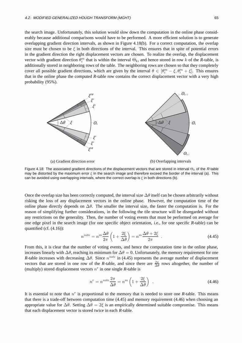
4.2. MODIFIED GENERALIZED HOUGH TRANSFORM (MGHT) 65
the search image. Unfortunately, this solution would slow down the computation in the online phase consid-erably because additional comparisons would have to be performed. A more efficient solution is to generateoverlapping gradient direction intervals, as shown in Figure 4.18(b). For a correct computation, the overlapsize must be chosen to beξ in both directions of the interval. This ensures that in spite of potential errorsin the gradient direction the right displacement vectors are chosen. To realize the overlap, the displacementvector with gradient directionθm
i that is within the intervalΘk, and hence stored in rowk of theR-table, isadditionally stored in neighboring rows of the table. The neighboring rows are chosen so that they completelycover all possible gradient directions, which are given by the intervalθ ∈ [θm
i − ξ, θmi + ξ]. This ensures
that in the online phase the computedR-table row contains the correct displacement vector with a very highprobability (95%).
ξ n
ξ aξ ∆ϕ
∆θ ξ Θ
ξ ∆ϕ
ξ a
ξ n
k
(a) Gradient direction error
Θk
Θk-1
Θk+1
∆θ ξ
(b) Overlapping intervals
Figure 4.18: The associated gradient directions of the displacement vectors that are stored in interval Θk of the R-tablemay be distorted by the maximum error ξ in the search image and therefore exceed the border of the interval (a). Thiscan be avoided using overlapping intervals, where the correct overlap is ξ in both directions (b).
Once the overlap size has been correctly computed, the interval size∆θ itself can be chosen arbitrarily withoutrisking the loss of any displacement vectors in the online phase. However, the computation time of theonline phase directly depends on∆θ. The smaller the interval size, the faster the computation is. For thereason of simplifying further considerations, in the following the tile structure will be disregarded withoutany restrictions on the generality. Then, the number of voting events that must be performed on average forone edge pixel in the search image (for one specific object orientation, i.e., for one specificR-table) can bequantified (cf. (4.16)):
nvote = nm ∆θ2π
(1 +
2ξ∆θ
)= nm ∆θ + 2ξ
2π. (4.45)
From this, it is clear that the number of voting events, and hence the computation time in the online phase,increases linearly with∆θ, reaching its minimum for∆θ = 0. Unfortunately, the memory requirement for oneR-table increases with decreasing∆θ. Sincenvote in (4.45) represents the average number of displacementvectors that are stored in one row of theR-table, and since there are2π
∆θ rows altogether, the number of(multiply) stored displacement vectorsnr in one singleR-table is
nr = nvote 2π∆θ
= nm(
1 +2ξ∆θ
). (4.46)
It is essential to note thatnr is proportional to the memory that is needed to store oneR-table. This meansthat there is a trade-off between computation time (4.45) and memory requirement (4.46) when choosing anappropriate value for∆θ. Setting∆θ = 2ξ is an empirically determined suitable compromise. This meansthat each displacement vector is stored twice in eachR-table.
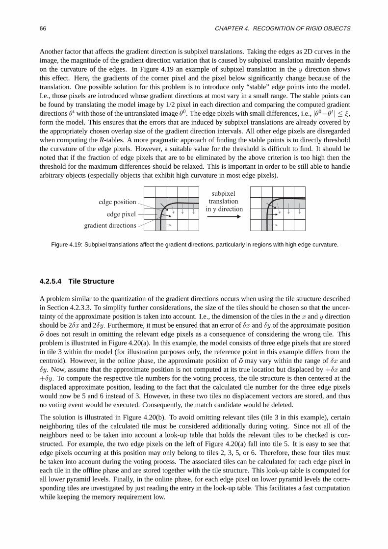
66 CHAPTER 4. RECOGNITION OF RIGID OBJECTS
Another factor that affects the gradient direction is subpixel translations. Taking the edges as 2D curves in theimage, the magnitude of the gradient direction variation that is caused by subpixel translation mainly dependson the curvature of the edges. In Figure 4.19 an example of subpixel translation in they direction showsthis effect. Here, the gradients of the corner pixel and the pixel below significantly change because of thetranslation. One possible solution for this problem is to introduce only “stable” edge points into the model.I.e., those pixels are introduced whose gradient directions at most vary in a small range. The stable points canbe found by translating the model image by 1/2 pixel in each direction and comparing the computed gradientdirectionsθt with those of the untranslated imageθ0. The edge pixels with small differences, i.e.,|θ0−θt| ≤ ξ,form the model. This ensures that the errors that are induced by subpixel translations are already covered bythe appropriately chosen overlap size of the gradient direction intervals. All other edge pixels are disregardedwhen computing theR-tables. A more pragmatic approach of finding the stable points is to directly thresholdthe curvature of the edge pixels. However, a suitable value for the threshold is difficult to find. It should benoted that if the fraction of edge pixels that are to be eliminated by the above criterion is too high then thethreshold for the maximum differences should be relaxed. This is important in order to be still able to handlearbitrary objects (especially objects that exhibit high curvature in most edge pixels).
edge position
gradient directions
edge pixel
subpixeltranslation
in y direction
Figure 4.19: Subpixel translations affect the gradient directions, particularly in regions with high edge curvature.
4.2.5.4 Tile Structure
A problem similar to the quantization of the gradient directions occurs when using the tile structure describedin Section 4.2.3.3. To simplify further considerations, the size of the tiles should be chosen so that the uncer-tainty of the approximate position is taken into account. I.e., the dimension of the tiles in thex andy directionshould be 2δx and 2δy. Furthermore, it must be ensured that an error ofδx andδy of the approximate positiono does not result in omitting the relevant edge pixels as a consequence of considering the wrong tile. Thisproblem is illustrated in Figure 4.20(a). In this example, the model consists of three edge pixels that are storedin tile 3 within the model (for illustration purposes only, the reference point in this example differs from thecentroid). However, in the online phase, the approximate position ofo may vary within the range ofδx andδy. Now, assume that the approximate position is not computed at its true location but displaced by+δx and+δy. To compute the respective tile numbers for the voting process, the tile structure is then centered at thedisplaced approximate position, leading to the fact that the calculated tile number for the three edge pixelswould now be 5 and 6 instead of 3. However, in these two tiles no displacement vectors are stored, and thusno voting event would be executed. Consequently, the match candidate would be deleted.
The solution is illustrated in Figure 4.20(b). To avoid omitting relevant tiles (tile 3 in this example), certainneighboring tiles of the calculated tile must be considered additionally during voting. Since not all of theneighbors need to be taken into account a look-up table that holds the relevant tiles to be checked is con-structed. For example, the two edge pixels on the left of Figure 4.20(a) fall into tile 5. It is easy to see thatedge pixels occurring at this position may only belong to tiles 2, 3, 5, or 6. Therefore, these four tiles mustbe taken into account during the voting process. The associated tiles can be calculated for each edge pixel ineach tile in the offline phase and are stored together with the tile structure. This look-up table is computed forall lower pyramid levels. Finally, in the online phase, for each edge pixel on lower pyramid levels the corre-sponding tiles are investigated by just reading the entry in the look-up table. This facilitates a fast computationwhile keeping the memory requirement low.
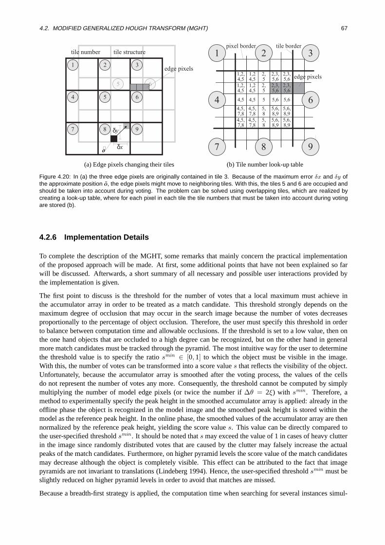
4.2. MODIFIED GENERALIZED HOUGH TRANSFORM (MGHT) 67
5 6
7
4
1
8
5
2
9
6
3
δx
δy
edge pixels
tile number
o∼
tile structure
(a) Edge pixels changing their tiles
7 8 9
4
1 2
6
3
5,6,8,9
5,6,8,9
5,6
2,3,5,6
2,3,5,6
5,6,8,9
5,6,8,9
5,6
2,3,5,6
2,3,5,6
5,8
5,8
5
2,5
2,5
4,5,7,8
4,5,7,8
4,5
1,24,5
1,24,5
4,5,7,8
4,5,7,8
4,5
1,2,4,5
1,2,4,5
pixel border tile border
edge pixels
(b) Tile number look-up table
Figure 4.20: In (a) the three edge pixels are originally contained in tile 3. Because of the maximum error δx and δy ofthe approximate position o, the edge pixels might move to neighboring tiles. With this, the tiles 5 and 6 are occupied andshould be taken into account during voting. The problem can be solved using overlapping tiles, which are realized bycreating a look-up table, where for each pixel in each tile the tile numbers that must be taken into account during votingare stored (b).
4.2.6 Implementation Details
To complete the description of the MGHT, some remarks that mainly concern the practical implementationof the proposed approach will be made. At first, some additional points that have not been explained so farwill be discussed. Afterwards, a short summary of all necessary and possible user interactions provided bythe implementation is given.
The first point to discuss is the threshold for the number of votes that a local maximum must achieve inthe accumulator array in order to be treated as a match candidate. This threshold strongly depends on themaximum degree of occlusion that may occur in the search image because the number of votes decreasesproportionally to the percentage of object occlusion. Therefore, the user must specify this threshold in orderto balance between computation time and allowable occlusions. If the threshold is set to a low value, then onthe one hand objects that are occluded to a high degree can be recognized, but on the other hand in generalmore match candidates must be tracked through the pyramid. The most intuitive way for the user to determinethe threshold value is to specify the ratiosmin ∈ [0,1] to which the object must be visible in the image.With this, the number of votes can be transformed into a score values that reflects the visibility of the object.Unfortunately, because the accumulator array is smoothed after the voting process, the values of the cellsdo not represent the number of votes any more. Consequently, the threshold cannot be computed by simplymultiplying the number of model edge pixels (or twice the number if∆θ = 2ξ) with smin . Therefore, amethod to experimentally specify the peak height in the smoothed accumulator array is applied: already in theoffline phase the object is recognized in the model image and the smoothed peak height is stored within themodel as the reference peak height. In the online phase, the smoothed values of the accumulator array are thennormalized by the reference peak height, yielding the score values. This value can be directly compared tothe user-specified thresholdsmin . It should be noted thats may exceed the value of 1 in cases of heavy clutterin the image since randomly distributed votes that are caused by the clutter may falsely increase the actualpeaks of the match candidates. Furthermore, on higher pyramid levels the score value of the match candidatesmay decrease although the object is completely visible. This effect can be attributed to the fact that imagepyramids are not invariant to translations (Lindeberg 1994). Hence, the user-specified thresholdsmin must beslightly reduced on higher pyramid levels in order to avoid that matches are missed.
Because a breadth-first strategy is applied, the computation time when searching for several instances simul-

68 CHAPTER 4. RECOGNITION OF RIGID OBJECTS
taneously does not dramatically increase in contrast to searching only for one single instance. Consequently,a second point that should be remarked concerns the number of matches that should be found during objectrecognition. Here, the user can choose between two options. The first option is to return all matches that havea score exceeding the specified thresholdsmin . The second option allows the user to introduce additional in-formation about the maximum numbernmatch of objects instances that may appear in the search image. Thisinformation can be used in the breadth-first search to eliminate a high number of match candidates during thetracking through the pyramid. This results in a high gain of computational efficiency. One way to eliminatematch candidates is to count the number of candidates that exceed the thresholdsmin on the current pyramidlevel. If this number is higher than the user-defined maximum number of object instances, extra match candi-dates with lower score values are excluded from further processing. The score values of the candidates do notbehave in a predictable manner during the tracking through the pyramid. Thus, a candidate with lower scoreon a higher pyramid level can turn into a candidate with higher score on a lower pyramid level. For this reason,a more tolerant heuristic is applied. A match candidate is only eliminated if it additionally fulfills the condi-tion that its score is significantly lower than the lowest score of non-eliminated match candidates. Finally, onthe lowest pyramid level only thenmatch best match candidates that additionally fulfill the requirement for theminimum score are returned as matches.
The last point to mention is the mutual overlapping of matches. In practice, sometimes one instance of anobject in the search image returns more than one match. For example, when dealing with objects that exhibitsymmetries, several matches are returned at similar positions, but at different orientations. In order to avoidthis behavior, the user can specify a fraction by which two returned matches are allowed to overlap each otherat most. The actual overlap fraction between two matches is approximated by the overlap between the twosmallest enclosing rectangles of the two objects at the pose of the respective matches. If the computed overlapfraction exceeds the user-specified maximum overlap, the match with lower score value is eliminated.
In the following, all necessary and possible user interactions or parameter settings of the MGHT are summa-rized.
• Input data passed to the offline phase (model generation):
– The model image in which the object is defined by an arbitrary region of interestmustbe pro-vided. Usually, the ROI is specified by the user. Another possibility would be to generate the ROIautomatically using suitable segmentation techniques.
– The usermustspecify the threshold for the minimum edge magnitudeγmin that is used for edgesegmentation. As previously mentioned, this value depends on the application and cannot bedetermined automatically.
– The camera-specific noiseσI of the gray values in the imagemustalso be provided in order toautomatically compute the optimum quantization of the gradient direction intervals used in theR-tables.
– Optionally, the domain of the transformation classmaybe restricted by the user, i.e., the rangeof possible object orientations can be restricted to a certain interval to avoid unnecessaryR-tablegenerations. Thus, the memory requirement of the model and the computational effort in theonline phase is reduced.
– In general, the automatically determined values for the reference pointom, the number of pyramidlevelsnl, the orientation step∆ϕ, and the size of the gradient quantization intervals∆θ are suit-able for most applications. Nevertheless, the usermayoptionally overwrite these values in orderto receive a higher flexibility.
• Input data passed to the online phase (object recognition):
– The search imagemustbe provided, where an arbitrary ROImayrestrict the image domain for edgeextraction. Thus, the user may introduce additional prior knowledge about the object position as

4.2. MODIFIED GENERALIZED HOUGH TRANSFORM (MGHT) 69
well as the object orientation, which can be specified during model generation, to speed up therecognition.
– The minimum scoresmin mustbe provided to specify the minimum peak height for match candi-dates.
– Also in the search image edge extraction is performed. Therefore, the minimum edge magnitudecan be optionally specified if it differs from the value set in the online phase. It is important tonote that the automatic computation of∆θ is based onγmin , which was specified in the offlinephase.
– The maximum number of matchesnmatch canbe specified in order to speed up the computation.
– The maximum allowable overlap between different matchescanbe specified to eliminate multiplyfound object instances.
Finally, for each match the object pose and the associated score value is returned. The pose is represented bythe object positionos
x, osy, and the object orientationϕs, whereϕs is 0 if the orientation of the object in the
search image is identical to its orientation in the model image.
4.2.7 Conclusions
To give an idea of the improvement of the MGHT in comparison to the conventional GHT, the memoryrequirement and the computational complexity of both methods are computed for a typical practical example.For this, a search image size of 600× 600 pixels, a tile size of 7× 7 pixels, 3000 model points at the originalresolution, and four image pyramid levels are assumed. The result is summarized in Table 4.3. For the MGHTthe memory requirement of the model increases from 4.3 MB to 30.8 MB in comparison to the conventionalGHT, which is mainly caused by the tile structure. However, in the online phase, the memory requirementshrinks from 480 MB to 0.5 MB because of the use of image pyramids. Since image pyramids are used and thecomputation time is optimized by the proposed approach the computational complexity of the online phaseis reduced considerably: theoretically, the MGHT is about 16.000 times faster than the conventional GHTin this example. However, in practice the recognition time is reduced from 45.60 s to 0.07 s on a 400 MHzPentium II, which corresponds to a factor of still 650. The difference to the theoretical value can be explainedby the increased memory access within the MGHT in contrast to the conventional GHT. Nevertheless, atremendous improvement is still observable.
GHT MGHT
Memory Requirement [MB] (Offline) 4.3 30.8
Memory Requirement [MB] (Online) 480 0.5
Computation Time [s] 45.60 0.07
Table 4.3: Improvement of the modified generalized Hough transform (MGHT) in comparison to the conventional gener-alized Hough transform (GHT) according to memory requirement and computation time
In summary, the MGHT that has been presented in this section eliminates the major drawbacks of the conven-tional GHT while keeping its inherent advantages and fulfills the stated requirements concerning the recogni-tion of rigid objects listed in Section 2.2. A comprehensive performance evaluation, including a comparisonwith other rigid object recognition methods, will be presented in Section 4.4 in order to support the theoreti-cally derived improvements. Although the descriptions in this section have been restricted to deal with rigidmotion as the transformation class, the MGHT can be easily extended in a straight forward way to be able tocope with more general transformations, like similarity or affine transformations. Therefore, also applicationsthat require parameter spaces of higher dimensions can benefit from the proposed modifications.

70 CHAPTER 4. RECOGNITION OF RIGID OBJECTS
4.3 Shape-Based Matching
As mentioned in Section 2.4, simultaneously to the development of the MGHT, a new similarity measurehas been developed. This similarity measure is already included in the HALCON library and is referred toasshape-based matching(SBM). In this section, the new similarity measure, an improved method for poserefinement, and some implementation details are described. Further details can be found in (Steger 2001,Ulrich and Steger 2002, Steger 2002).
4.3.1 Similarity Measure
The model of the SBM consists of a set of model pointspmi = (xm
i , ymi )> as in the case of the MGHT.
Additionally, the model is complemented by the associated gradient direction vectorsdmi = (ti, ui)>, i =
1, . . . , nm, whereti = Imx
∣∣∣pmi
andui = Imy
∣∣∣pmi
. Figure 4.21 illustrates the principle of this similaritymeasure by means of the example that has already been introduced in Section 4.2.1. Here, the third pyramidlevel is displayed (see Figures 4.2, 4.7(a), and 4.7(b)). In the offline phase, edges are extracted from the modelimage, which is shown in Figure 4.21(a), and their associated gradient direction vectors are computed. Theresulting edges and the normalized gradient direction vectors (white arrows) are shown in Figure 4.21(b).
(a) Model image
model edge pixels mi
gradient direction vectorsof the model image at
the model edge pixels
mid
p
(b) Model edges
gradient direction vectors of search imagesd ( , )x y
(c) Search image
Figure 4.21: In the shape-based matching edges are extracted and the associated gradient direction vectors are com-puted (b) from the model image (a). The search image is edge filtered, resulting in a gradient direction vector at eachmodel edge pixel (c).
The search image, which is shown in Figure 4.21(c), can be transformed into a representation in which agradient direction vectords(x, y) = (v(x, y), w(x, y))> is obtained for each image point(x, y)>. In thematching process, the transformed model must be compared to the search image at a particular location usinga certain similarity measure. The basic idea behind the similarity measure within the SBM is to sum thenormalized dot products of the gradient direction vectors of the transformed model and the search image overall model points. From this, a matching scores is obtained at each point(x, y)> in the search image. InFigure 4.21(c) the normalized gradient direction vectors are displayed as black arrows at each pixel in thesearch image. A threshold on the similarity measure has to be specified by the user. For this, a similaritymeasure with a well-defined range of values is desirable. The following similarity measure achieves this goal:
s(x, y) =1nm
nm∑i=1
〈dmi ,d
s(x+ xmi , y + ym
i )〉‖dm
i ‖ · ‖ds(x+ xmi , y + ym
i )‖ (4.47)
=1nm
nm∑i=1
tiv(x+ xmi , y + ym
i ) + uiw(x+ xmi , y + ym
i )√t2i + u2
i ·√v(x+ xm
i , y + ymi )2 + w(x+ xm
i , y + ymi )2
,

4.3. SHAPE-BASED MATCHING (SBM) 71
where〈·, ·〉 represents the dot product between two vectors. Therefore,s(x, y) represents the averaged cosineof the angle differences between the gradient directions of the transformed model points and the respectivegradient directions in the search image. The cosine takes into account that the gradient direction is influencedby image noise. The effect of the resulting small angle differences on the similarity measure is reduced by thelow sensitivity of the cosine to small arguments, which yields a high robustness against noise. Figure 4.21(c)also shows the calculation of the matching scores(x, y) for two example positions of the object in the searchimage. At the true position (upper left) the angle differences between the direction vectors are small, and thusthe cosine will be close to 1 at each model edge pixel. The reason for the small differences can be attributedto artificially added noise in the search image. At the second example position (lower right) the correspondinggradient directions show significantly higher differences, leading to cosine values that are much smaller than 1.
This similarity measure shows several inherent advantages. Because of the normalization of the gradientdirection vectors, the similarity measure is invariant to arbitrary changes in brightness since all vectors arescaled to length one. It is essential to note that edge filtering is applied to the search image, but no segmentationis performed, i.e., no threshold on the edge magnitude is applied. This has the advantage that the similaritymeasure not only exhibits robustness but true invariance against changes in brightness of an arbitrary type:there is no risk that any edge pixel falls below an edge threshold if the contrast is too low. This constitutesthe major advantage in comparison to all the object recognition methods that rely on segmented features inthe search image, like, for instance, the Hausdorff distance or the GHT. Furthermore, this measure is robustagainst occlusion and clutter because in case of missing features, either in the model or in the search image,noise will lead to random gradient direction vectors, which, on average, will contribute nothing to the sum(see (Steger 2002) for further discussions concerning this topic).
Focusing on (4.47) again, the similarity measure will return a high score if all the direction vectors of the modeland the search image align, i.e., have the same direction. A score of 1 indicates a perfect match between thetransformed model and the search image. Furthermore, the score roughly corresponds to the portion of theobject that is visible in the search image.
4.3.2 Implementation Details
An important feature of this similarity measure is that it does not need to be evaluated completely when objectrecognition is based upon a thresholdsmin for the similarity measure. Letsj denote the partial sum of the dotproducts up to thej-th model point:
sj(x, y) =1nm
j∑i=1
〈dmi ,d
s(x+ xmi , y + ym
i )〉‖dm
i ‖ · ‖ds(x+ xmi , y + ym
i )‖ . (4.48)
Obviously, all the remaining terms of the sum are all smaller or equal to 1. Therefore, the partial score cannever reach the required scoresmin if sj < smin − 1 + j/nm, and hence the evaluation of the sum can bediscontinued after thej-th element whenever this condition is fulfilled. This criterion speeds up the recognitionprocess considerably.
Nevertheless, further speed-ups are highly desirable. Another criterion is to set the condition that at eachpartial sum the score is better thansmin , i.e., sj ≥ sminj/nm. When this criterion is used, the search willbe very fast, but it can no longer be ensured that the object recognition finds the correct instances of theobject. This is because if missing parts of the object are checked first, then the partial score will be belowthe required score. To speed up the recognition process with a very low probability of missing the object, thefollowing heuristic can be used: the first part of the model points is examined with a relatively safe stoppingcriterion, while the remaining part of the model points is examined with the hard thresholdsminj/nm. Theuser can specify a parameterg, which represents the fraction of the model points that are examined with thehard threshold. This parameter will be referred to asgreedinessbelow. If g = 1, all points are examinedwith the hard threshold, while forg = 0, all points are examined with the safe stopping criterion. With this,
72 CHAPTER 4. RECOGNITION OF RIGID OBJECTS
the evaluation of the partial sums is stopped wheneversj < min(smin − 1 + ζj/nm, sminj/nm), whereζ = (1− gsmin)/(1− g). The term greediness is chosen because it appropriately reflects the intention of theparameter: ifg is set to 1 the search is very greedy, i.e., the search strongly tends to early abort the evaluationof less promising transformations in order to reduce the computation time. However, the risk of missing amatch is high.
To further speed up the recognition process, the model is generated in multiple resolution levels, which areconstructed by generating an image pyramid from the original image — in the same way as in the MGHT.Because of runtime considerations, again the Sobel filter is used for feature extraction. To take rigid transfor-mations into account the model is also created for different object orientations. For this,2/rmax has provento be an appropriate value for the orientation step size∆ϕ (cf. Section 4.2.5.1). In the online phase, an imagepyramid is constructed for the search image. To identify potential matches, an exhaustive search is performedfor the top level of the pyramid. With the termination criteria using the thresholdsmin , this seemingly brute-force strategy actually becomes extremely efficient. After the potential matches have been identified, they aretracked through the resolution hierarchy until they are found at the lowest level of the image pyramid.
Furthermore, the same method for pose refinement that is applied to the MGHT can be used in the SBM(cf. Section 4.2.4): once the object has been recognized on the lowest level of the image pyramid, its poseparameters position and orientation are extracted to a resolution better than the discretization of the searchspace by fitting again a second order polynomial (in the three pose variables) to the similarity measure valuesin a 3× 3× 3 neighborhood around the maximum score.
4.3.3 Least-Squares Pose Refinement
If an even higher accuracy is desirable than the accuracy that can be achieved by using the pose refinementdescribed in Section 4.2.4, a least-squares adjustment can be applied. Here, the sum of squared distances be-tween the transformed model points and the points in the search image is minimized. For this, it is necessary toextract the model points as well as the corresponding points in the search image with subpixel accuracy. How-ever, an algorithm that performs a least-squares adjustment based on closest point distances would not improvethe accuracy much since the points would still have an average distance significantly larger than 0 tangentiallybecause the model and search points are not necessarily samples at the same points and distances. Therefore,for each transformed model point the closest point in the search image is found and the squared distance ofthat point to a line defined by the corresponding model point and the corresponding tangent to the model pointis minimized. I.e., the directions of the model points are taken to be correct and are assumed to describe thedirection of the object’s border. The tangents are defined by the edge pointspm
i = (xmi , y
mi )> in the model im-
age and the perpendicular to the corresponding normalized gradient direction vectorsdmi /‖dm
i ‖ = (ti, ui)>.Hence, the tangents are given by the points(x, y)> that satisfyti(x − xm
i ) + ui(y − ymi ) = 0. The Hessian
normal form is used to compute the distance between each tangent and the potential corresponding edge pointps
j = (xsj , y
sj )> in the search image. Finally, the sum of squared distances is minimized:
d2(a) =nm∑i=1
[ti(xsj(a)− xm
i ) + ui(ysj (a)− ym
i )]2 → min . (4.49)
Here,a represents the vector of the unknown (inverse) pose parameters andxsj(a), ys
j (a) the transformedcorresponding edge point of the search image. It should be noted that instead of transforming the tangents atthe model points by the pose parameters, the points in the search image are transformed back using the inversepose parametersa in order to simplify the calculations.
The potential corresponding edge pointspsj in the search image are obtained by a non-maximum suppression
of the edge magnitude in gradient direction and are further extrapolated to subpixel accuracy (Steger 2000).Thus, a segmentation of the search image is further avoided in order to maintain invariance against changesin brightness. The model points are transformed according to the pose parameters that have been obtained
4.4. PERFORMANCE EVALUATION OF THE MGHT AND THE SBM 73
from the polynomial fitting (cf. Section 4.2.4). Because the points in the search image are not segmentedand correspondence is based on smallest euclidian distance, spurious points in the search image may bebrought into correspondence with model points. Therefore, to make the adjustment robust, only those edgepoints in the search image perpendicular to the local tangent direction are taken into account. Furthermore,corresponding edge points that have a distance larger than a statistically computed threshold are ignored inthe adjustment. Since the point correspondences may change by the newly estimated pose, an even higheraccuracy can be gained by iterating the correspondence search and the parameter adjustment. Typically, afterthree iterations the accuracy of the pose no longer improves.
4.4 Performance Evaluation of the MGHT and the SBM
In this section, an extensive empirical performance evaluation of the two developed approaches, the MGHTand SBM, is presented.
To assess the performance of the two approaches, they are compared to six different 2D object recognitiontechniques that are already available. For this purpose, three standard similarity measures are chosen becausethey are frequently used methods in industry and therefore are rather well known: the sum of absolute dif-ferences (SAD) and the normalized cross correlation (NCC) as two standard intensity-based approaches andthe Hausdorff distance (HD) as a standard feature-based approach. They constitute a common basis that fa-cilitates the comparability of the subsequent evaluation with other evaluations that also include one of thesestandard approaches. Furthermore, including the three standard approaches in the performance evaluation isscientifically interesting because no direct comparison of the three approaches could be found in literature.Additionally, to be able to evaluate the potential of the two new approaches, three commercial high-end recog-nition tools have been included in the evaluation: theGeometric Model Finder(GMF) developed byMatroxElectronic Systems Ltd.(Matrox 2002) as well asPatMaxR© (PM) andPatQuickR© (PQ), both developed byCognex (Cognex 2000). The analysis of the performance characteristics of rigid object recognition methodsis an important issue (cf. (Ulrich and Steger 2001)). Firstly, it helps to identify breakdown points of the al-gorithms, i.e., areas where the algorithms cannot be used because some of their underlying assumptions areviolated. Secondly, it makes an algorithm comparable to other algorithms, thus helping users to select theappropriate method for the task they have to solve. In the special case of this dissertation a performanceevaluation of rigid object recognition methods is essential in order to select the approach that is best suited toserve as a module within the approach to recognize compound objects.
The remainder of the chapter is organized as follows. After a short introduction of the respective methods,several criteria that allow an objective evaluation of object recognition approaches are introduced. Threemain criteria are used to evaluate the performance and to build a common basis that facilitates an objectivecomparison (cf. (Ulrich and Steger 2002)): the robustness, the accuracy of the returned pose parameters,and the computation time. Thereby, it is distinguished between the robustness against occlusions and clutterand the robustness against arbitrary changes in brightness. Experiments on real images are used to apply theproposed criteria. For this, in a first step, the experimental set-up for the evaluation measurements is explainedin detail. In a second step, the results are illustrated and analyzed.
4.4.1 Additionally Evaluated Object Recognition Methods
4.4.1.1 Sum of Absolute Differences
The special implementation that has been investigated to evaluate the sum of absolute gray value differencesconsiders rigid motion and makes use of image pyramids to speed up the recognition process. The averagedistance is used as dissimilarity measure using the formula given in (4.3). Since the SAD is a measure ofdissimilarity, the resulting average difference is also denoted as errore in the following. Hence, in contrast to
74 CHAPTER 4. RECOGNITION OF RIGID OBJECTS
all other methods this measure is not normalized to a certain interval, but can take arbitrary values, where anerror of 0 denotes a perfect match. The position and orientation of the best match, i.e., the match with smallesterror, is returned. Additionally, it is possible to specify the maximum erroremax of the match to be tolerated,similar to smin when using a similarity measure. The loweremax is chosen, the faster the recognition isperformed, since fewer matches must be tracked down the pyramid. Subpixel accuracy of position and therefinement of the discrete orientation are calculated by interpolating the minimum ofe.
4.4.1.2 Normalized Cross Correlation
For the purpose of evaluating the performance of the normalized cross correlation the implementation of theMatrox Imaging Library(MIL) — as one typical representative — was used. The MIL is a software develop-ment toolkit ofMatrox Electronic Systems Ltd.(Matrox 2001). Some specific implementation characteristicsshould be explained to ensure the correct appraisal of the evaluation results: The algorithm is able to find a pre-defined object under rigid motion. A hierarchical search strategy using image pyramids is used to speed up therecognition. The quality of the match is returned by calculating a score value ass = max(NCC ,0)2 ∈ [0,1],whereNCC is the value of the NCC as it is obtained when using (4.2). The subpixel accuracy of the objectposition is achieved by a surface fit to the match scores around the peak. The refinement of the object ori-entation is not comprehensively explained in the documentation. However, it is supposed that the refinementof the obtained discrete object orientation is realized by a finer resampling of the orientation in the angleneighborhood of the maximum score and recalculating the NCC at each refined orientation.
4.4.1.3 Hausdorff Distance
The original implementation by Rucklidge (Rucklidge 1997) was utilized to rate the performance of the Haus-dorff distance. The core of the implementation uses the partial HD (cf. (4.8) and (4.9)). The program expectsthe forward and the reverse fraction as well as the thresholds for the forward and the reverse distance as inputparameter. Both, the model image and the search image must be passed in binary form to the algorithm.Therefore, edges are extracted in advance using a minimum edge magnitudeγmin by applying the same pre-processing steps as in the case of the MGHT and the SBM to ensure a high comparability of the approaches.Since the method of (Rucklidge 1997) returns all matches that fulfill the given score and distance criteria, thebest match was selected based on the minimum forward distance. If more than one match had the same min-imum forward distance, the match with the maximum forward fraction was selected as the best match. Theforward fraction was interpreted as score values ∈ [0,1] during the evaluation in order to measure the qualityof the match. A score of 1 denotes a perfect match in the sense that all model pixels fulfill the selected forwarddistance. The implementation is not able to recognize rotated objects but only allows to recognize translatedobjects with fixed orientation. Furthermore, no subpixel refinement is included. Generally, it seems to bevery difficult to compute a refinement of the returned parameters directly based upon the forward or reversefraction. Although the parameter space is treated in a hierarchical way there is no use of image pyramids,which makes the algorithm very slow.
4.4.1.4 Geometric Model Finder
The Geometric Model Finder uses edge-based geometric features to find objects in images. Unfortunately, nodetailed information about the principle of the GMF is available from its documentation (Matrox 2002). Thedefault threshold that is used for edge extraction in the model image as well as in the search image can beinfluenced by a parameter that allows to chose the detail level, and hence whether a medium (default), a high,or a very high number of edges are to be extracted. This parameter of the GMF is similar to the thresholdfor the minimum edge magnitudeγmin used in the MGHT, the SBM, and the HD. To measure the qualityof a match, a score values ∈ [0,1] is computed and returned. The minimum score that must be reached by

4.4. PERFORMANCE EVALUATION OF THE MGHT AND THE SBM 75
a match candidate can be set by choosingsmin . Finally, the object pose is returned with subpixel accuracy.However, as a last important parameter to mention, the accuracy level can be controlled choosing between amedium and a high accuracy. The high accuracy is gained at the expense of a slower computation.
4.4.1.5 PatMax and PatQuick
As described in their documentation (Cognex 2000), PatMaxR© and PatQuickR© use geometric information.The main difference between the two approaches is that PQ is a faster but less accurate version of PM. Bothmethods apply a three-step geometric measurement process to an object: At first, it identifies and isolatesthe key individual features within the model image and measures characteristics such as shape, dimensions,angle, arcs, and shading. Then, it matches the key features of the model and the search image, encompassingboth distance and relative angle. By analyzing the geometric information from both the features and spatialrelationships, PM and PQ are able to determine the object’s position and orientation precisely, i.e., the accuracyis not limited to a quantized sampling grid.
The model representation, however, which can be visualized by PM and PQ, apparently consists of subpixelprecise edge points and respective edge directions. From this, one can be led to conclude that the two ap-proaches use similar features as the SBM, in contrast to their documentation.
To speed up the search, a coarse-to-fine approach is implemented. Indeed, there is no parameter that enablesusers to explicitly specify the number of image pyramids to be used. Instead, the parametercoarse grain limitcan be used to control the size of the features to be used during recognition and, therefore, the depth of thehierarchical search. This parameter has a similar meaning as the number of pyramid levels, but it cannot beequated with. To indicate the quality of the match, a scores ∈ [0,1] is computed, where 1 again represents aperfect match.
4.4.2 Robustness
The first criterion to be considered is therobustnessof the approaches. This includes the robustness againstocclusions and clutter as well as the robustness against arbitrary changes in brightness.
Experimental Set-Up. For all subsequent experiments an IC (see Figure 4.22(a)) was chosen as the objectto be found. Only the part within the bounding box of the print on the IC is used as ROI, from which themodels of the different recognition approaches are created (see Figure 4.22(b)). For the recognition methodsthat segment edges during model creation (MGHT, SBM, HD), the threshold for the minimum edge magnitudeγmin in the model image was set to 30 for all experiments. The detail level of the GMF was set to medium,which is the default value and results in approximately the same edges that are obtained when applying athreshold of 30 to the edge magnitude. All images that were used for the evaluation are of size 652× 494pixels. The experiments were performed on a 400 MHz Pentium II. For those recognition methods that useimage pyramids (MGHT, SBM, SAD, NCC), four pyramid levels were used to speed up the search. Thealgorithm presented in Section 4.2.3.1 found this number of levels to be the optimum for the IC. This numberalso agrees with human intuition. For PQ and PM the automatically determined value for the parametercoarsegrain limit was assumed to be the optimum one, and hence no manual setting was applied.
To apply the criterion of robustness, two image sequences were taken, one for testing the robustness againstocclusions and clutter, the other for testing the robustness against changes in brightness. The recognition ratewas defined as the number of images in which the object was recognized at the correct pose divided by thetotal number of images, and hence is an indicator for robustness against occlusions. The false alarm ratewas defined as the number of images, in which the object was recognized at an incorrect pose divided by thetotal number of images, and thus is an indicator for robustness against clutter. Such matches are called falsepositives.

76 CHAPTER 4. RECOGNITION OF RIGID OBJECTS
(a) Model image (b) ROI
Figure 4.22: An IC is used as the object to be recognized (a). The model is created from the print on the IC using arectangular ROI (b).
Figure 4.23: Six of the 500 images that were used to test the robustness against occlusions
The first sequence contains 500 images of the IC, in which the IC was kept at a fixed position and orientationand was occluded to various degrees with various objects, so that in addition to occlusion, clutter of variousdegrees was created in the images. Figure 4.23 shows six of the 500 images. In the corresponding modelimage of this sequence, the size of the bounding box that defines the ROI is 180× 120 pixels at the lowestpyramid level and contains 2127 edge pixels extracted by the Sobel filter. For the approaches that segmentedges in the search image (MGHT, HD, and GMF) the parameter to control the edge extraction was set to thesame value as in the model image.
Additionally, the relation between the actual degree of occlusion and the returned score value is examined,because the correlation between the visibilityv of the object and the scores can also be seen as an indicatorfor robustness. If, for example, only half of the object is visible in the image then, intuitively, also the scoreshould be 0.5, i.e., one would expect a very high correlation in the ideal case. For this purpose, an effortwas made to keep the IC in exactly the same position in the image in order to be able to measure the degreeof occlusion. The true amount of occlusion was determined by extracting edges from the search images andintersecting the edge region with the edges within the ROI in the model image. Since the objects that occludethe IC generate clutter edges, this actually underestimates the occlusion.

4.4. PERFORMANCE EVALUATION OF THE MGHT AND THE SBM 77
Figure 4.24: Three of the 200 images that were used to test the robustness against arbitrary changes in brightness
To test the robustness, the transformation class was restricted to translations, in order to reduce the timerequired to execute the experiment. However, the allowable range of the translation parameters was notrestricted, i.e., the object was searched in the entire image. It should be noted that the recognition rate wouldbe lower and the false alarm rate would be higher when allowing rigid motion instead of translations only.This is because the probability for an arbitrarily rotated model to match a clutter object is higher than for themodel at a fixed orientation. Nevertheless, restricting the experiment to translations is legitimate because itcan be assumed that the resulting percentage change in both rates compared to rigid motion is approximatelythe same for all approaches. Consequently, a qualitative comparison is ensured. For the MGHT, the SBM,the NCC, the HD, PQ, and PM different values for the parameter of the minimum score were applied. Aspreviously mentioned, in the case of the HD the forward fraction was interpreted as score value. Initial testswith the forward and reverse fractions set to 0.3 resulted in run times of more than three hours per image.Therefore, the reverse fraction was set to a constant value of 0.5 and the forward fraction was successivelyincreased from 0.5 to 0.9 using an increment of 0.1. The parameters for the maximum forward and reversedistance were set to 1 pixel. For the other three approaches the minimum scoresmin was varied from 0.1 to0.9. In the case of the SAD the maximum mean erroremax instead of the minimum score was varied. Since themean errore is not limited to an interval,emax was varied from 10 to 50 using an increment of 10. Toleratinghigher values fore would result in hardly meaningful matches, i.e., an occluded object instance could not bedistinguished from clutter in the search image. Furthermore, extremely expensive computations would be theconsequence, which would make the algorithm unsuitable for practical use. Since the robustness of the SBMdepends on the parameter greediness, additionally the value for greediness was varied in the range of 0 to 1using increments of 0.2.
To test the robustness against arbitrary changes in brightness, a second image sequence of the IC was taken.The sequence contains 200 images including various illumination situations, e.g., spot lights, reflections, non-uniform illumination, different ambient light intensity, etc. Three example images are displayed in Figure 4.24.Because of the smaller distance between the IC and the camera, the ROI is now 255×140 pixels and contains3381 model points on the lowest pyramid level. The parameter settings of all methods are equivalent to thesettings for testing the robustness against occlusions. However, since the MGHT segments the search image,additionally the threshold for the minimum edge magnitude in the online phase is varied from 5 to 30 using anincrement of 5. The same holds for the GMF, where the detail level was set to medium, high, and very high,respectively. Furthermore, in the case of the SAD the range of values for the maximum mean erroremax waslimited from 10 to 30 since higher values showed no significant improvements.
Results. At first, the sequence of the occluded IC was tested. A complete comparison of all approachesconcerning the robustness against occlusion is shown in Figure 4.25. The recognition rate is plotted versusthe minimum scoresmin and the maximum erroremax , respectively. For the SBM the greediness was set to 0at first, in order to receive the best obtainable recognition rate. As one would expect, the number of correctlyrecognized objects decreases with increasing minimum score for all approaches. Thus, the higher the degree
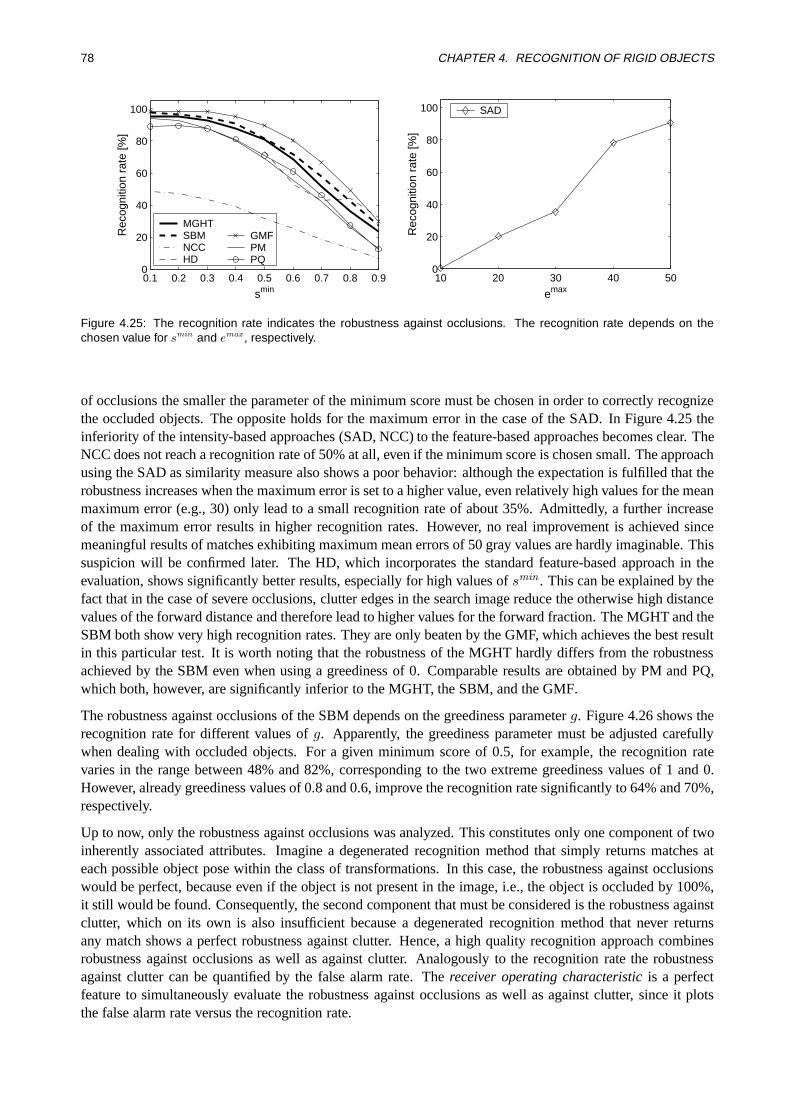
78 CHAPTER 4. RECOGNITION OF RIGID OBJECTS
0.1 0.2 0.3 0.4 0.5 0.6 0.7 0.8 0.90
20
40
60
80
100
smin
Rec
ogni
tion
rate
[%]
MGHTSBM NCC HD
GMFPM PQ
10 20 30 40 500
20
40
60
80
100
emax
Rec
ogni
tion
rate
[%]
SAD
Figure 4.25: The recognition rate indicates the robustness against occlusions. The recognition rate depends on thechosen value for smin and emax , respectively.
of occlusions the smaller the parameter of the minimum score must be chosen in order to correctly recognizethe occluded objects. The opposite holds for the maximum error in the case of the SAD. In Figure 4.25 theinferiority of the intensity-based approaches (SAD, NCC) to the feature-based approaches becomes clear. TheNCC does not reach a recognition rate of 50% at all, even if the minimum score is chosen small. The approachusing the SAD as similarity measure also shows a poor behavior: although the expectation is fulfilled that therobustness increases when the maximum error is set to a higher value, even relatively high values for the meanmaximum error (e.g., 30) only lead to a small recognition rate of about 35%. Admittedly, a further increaseof the maximum error results in higher recognition rates. However, no real improvement is achieved sincemeaningful results of matches exhibiting maximum mean errors of 50 gray values are hardly imaginable. Thissuspicion will be confirmed later. The HD, which incorporates the standard feature-based approach in theevaluation, shows significantly better results, especially for high values ofsmin . This can be explained by thefact that in the case of severe occlusions, clutter edges in the search image reduce the otherwise high distancevalues of the forward distance and therefore lead to higher values for the forward fraction. The MGHT and theSBM both show very high recognition rates. They are only beaten by the GMF, which achieves the best resultin this particular test. It is worth noting that the robustness of the MGHT hardly differs from the robustnessachieved by the SBM even when using a greediness of 0. Comparable results are obtained by PM and PQ,which both, however, are significantly inferior to the MGHT, the SBM, and the GMF.
The robustness against occlusions of the SBM depends on the greediness parameterg. Figure 4.26 shows therecognition rate for different values ofg. Apparently, the greediness parameter must be adjusted carefullywhen dealing with occluded objects. For a given minimum score of 0.5, for example, the recognition ratevaries in the range between 48% and 82%, corresponding to the two extreme greediness values of 1 and 0.However, already greediness values of 0.8 and 0.6, improve the recognition rate significantly to 64% and 70%,respectively.
Up to now, only the robustness against occlusions was analyzed. This constitutes only one component of twoinherently associated attributes. Imagine a degenerated recognition method that simply returns matches ateach possible object pose within the class of transformations. In this case, the robustness against occlusionswould be perfect, because even if the object is not present in the image, i.e., the object is occluded by 100%,it still would be found. Consequently, the second component that must be considered is the robustness againstclutter, which on its own is also insufficient because a degenerated recognition method that never returnsany match shows a perfect robustness against clutter. Hence, a high quality recognition approach combinesrobustness against occlusions as well as against clutter. Analogously to the recognition rate the robustnessagainst clutter can be quantified by the false alarm rate. Thereceiver operating characteristicis a perfectfeature to simultaneously evaluate the robustness against occlusions as well as against clutter, since it plotsthe false alarm rate versus the recognition rate.
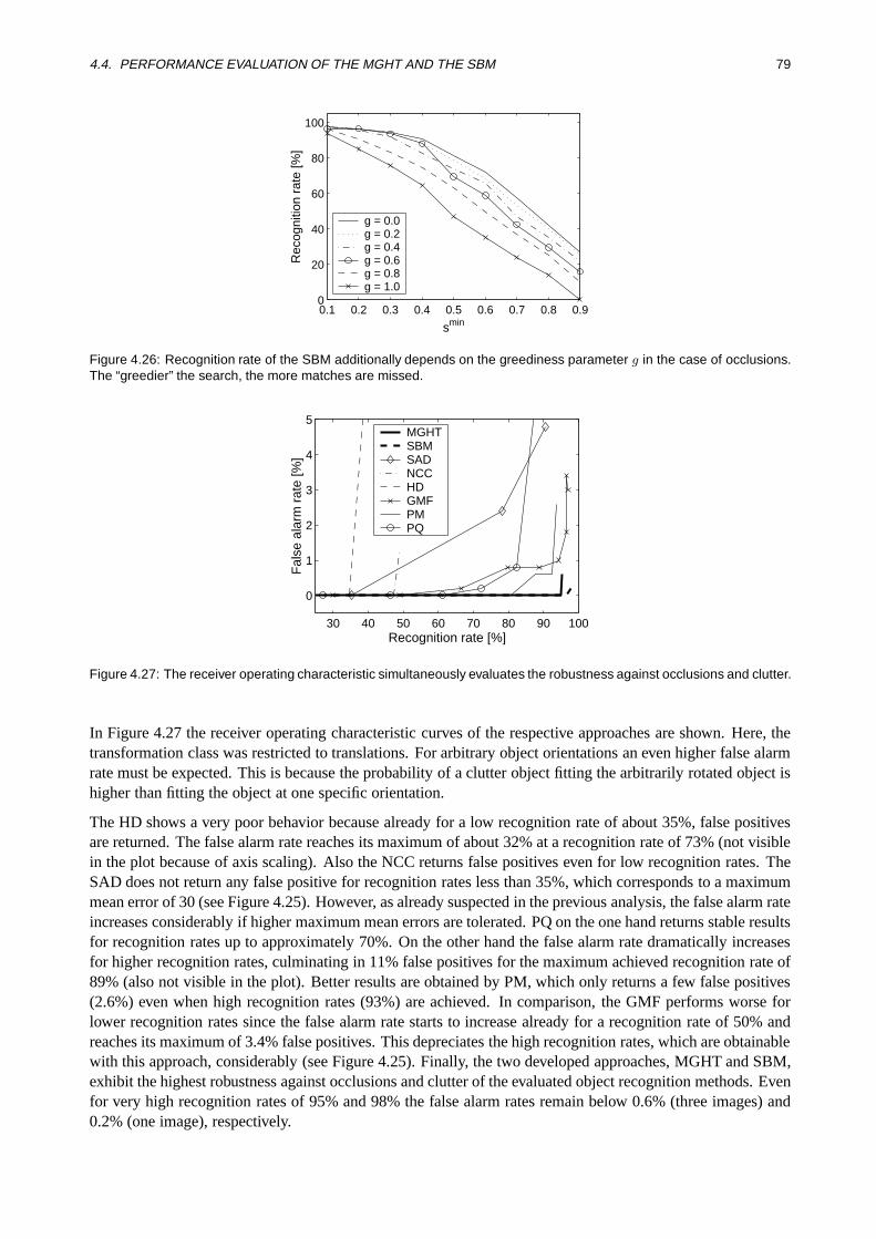
4.4. PERFORMANCE EVALUATION OF THE MGHT AND THE SBM 79
0.1 0.2 0.3 0.4 0.5 0.6 0.7 0.8 0.90
20
40
60
80
100
Rec
ogni
tion
rate
[%]
smin
g = 0.0g = 0.2g = 0.4g = 0.6g = 0.8g = 1.0
Figure 4.26: Recognition rate of the SBM additionally depends on the greediness parameter g in the case of occlusions.The “greedier” the search, the more matches are missed.
30 40 50 60 70 80 90 100
0
1
2
3
4
5
Recognition rate [%]
Fal
se a
larm
rat
e [%
]
MGHTSBM SAD NCC HD GMF PM PQ
Figure 4.27: The receiver operating characteristic simultaneously evaluates the robustness against occlusions and clutter.
In Figure 4.27 the receiver operating characteristic curves of the respective approaches are shown. Here, thetransformation class was restricted to translations. For arbitrary object orientations an even higher false alarmrate must be expected. This is because the probability of a clutter object fitting the arbitrarily rotated object ishigher than fitting the object at one specific orientation.
The HD shows a very poor behavior because already for a low recognition rate of about 35%, false positivesare returned. The false alarm rate reaches its maximum of about 32% at a recognition rate of 73% (not visiblein the plot because of axis scaling). Also the NCC returns false positives even for low recognition rates. TheSAD does not return any false positive for recognition rates less than 35%, which corresponds to a maximummean error of 30 (see Figure 4.25). However, as already suspected in the previous analysis, the false alarm rateincreases considerably if higher maximum mean errors are tolerated. PQ on the one hand returns stable resultsfor recognition rates up to approximately 70%. On the other hand the false alarm rate dramatically increasesfor higher recognition rates, culminating in 11% false positives for the maximum achieved recognition rate of89% (also not visible in the plot). Better results are obtained by PM, which only returns a few false positives(2.6%) even when high recognition rates (93%) are achieved. In comparison, the GMF performs worse forlower recognition rates since the false alarm rate starts to increase already for a recognition rate of 50% andreaches its maximum of 3.4% false positives. This depreciates the high recognition rates, which are obtainablewith this approach, considerably (see Figure 4.25). Finally, the two developed approaches, MGHT and SBM,exhibit the highest robustness against occlusions and clutter of the evaluated object recognition methods. Evenfor very high recognition rates of 95% and 98% the false alarm rates remain below 0.6% (three images) and0.2% (one image), respectively.

80 CHAPTER 4. RECOGNITION OF RIGID OBJECTS
20 40 60 80 1000
0.2
0.4
0.6
0.8
1
v [%]
s
(a) MGHT (ρ = 0.94)
20 40 60 80 1000
0.2
0.4
0.6
0.8
1
v [%]
s
(b) SBM (ρ = 0.95)
20 40 60 80 1000
10
20
30
40
v [%]
e
(c) SAD (ρ = −0.76)
20 40 60 80 1000
0.2
0.4
0.6
0.8
1
v [%]
s
(d) NCC (ρ = 0.78)
20 40 60 80 1000
0.2
0.4
0.6
0.8
1
v [%]
s
(e) HD (ρ = 0.95)
20 40 60 80 1000
0.2
0.4
0.6
0.8
1
v [%]
s
(f) GMF (ρ = 0.97)
20 40 60 80 1000
0.2
0.4
0.6
0.8
1
v [%]
s
(g) PM (ρ = 0.88)
20 40 60 80 1000
0.2
0.4
0.6
0.8
1
v [%]
s
(h) PQ (ρ = 0.79)
Figure 4.28: Returned values for score s and error e, respectively, plotted versus the visibility v of the object. In the idealcase the correlation coefficient ρ should be 1 (in the case of the score values) and −1 (in the case of the error values),respectively.
Figure 4.28 displays the returned values for the scores and mean errore, respectively, plotted versus theestimated visibilityv of the object. I.e., the correlation between these two quantities is visualized. For theplots,smin was set to 30 (50 in the case of the HD) andemax was set to 40. False positive matches are notvisualized in the plots. To facilitate the visual evaluation, additionally, for the approaches returning a scorevalue, the ideal curves representing 100% correlation are plotted, i.e.,sideal = v/100. In the case of the NCCthe score value is computed ass = max(NCC ,0)2, and hence the associated ideal curve issideal = (v/100)2
(cf. Section 4.4.1.2). Images in which no match was found are denoted by a score or error value of 0, i.e.,the corresponding points lie on thex axis of the plots. To precisely measure the correlation, additionally thecorrelation coefficientρ (Bronstein et al. 2001) is computed from corresponding values of correctly foundobjects.
It can be seen from the plot regarding the SAD that the error is negatively correlated with the visibility —as expected. The corresponding value forρ = −0.76 proves the visual impression. Nevertheless, the pointsare widely spread and far from an ideal virtual line with negative gradient. In addition, despite of a very highdegree of visibility many objects were not recognized. One possible reason for this behavior could be that insome images the clutter object does not occlude the IC yet, but casts its shadow onto the IC, which stronglyinfluences this metric. The magnitude of the correlation coefficient obtained for the NCC is comparable tothat obtained for the SAD. Furthermore, also here the points in the plot are widely spread and many objectswith high visibility were not recognized.
Most of the remaining approaches show a significantly higher positive correlation. This again confirms thehigher robustness of the feature-based approaches compared to the area-based approaches. As the rules ex-ception, the correlation coefficient obtained for PQ has a relatively low value. The plot of PM shows a betterbehavior, leading to a higher value forρ. However, also here the points are not close to the ideal line butspread by a higher amount in comparison to the MGHT, the SBM, the HD, and the GMF. These approachesall show similar results and a point distribution that is much closer to the ideal one. In addition, objects withhigh visibility are recognized with a high probability. However, again it becomes clear that in a few cases

4.4. PERFORMANCE EVALUATION OF THE MGHT AND THE SBM 81
0.1 0.2 0.3 0.4 0.5 0.6 0.7 0.8 0.90
20
40
60
80
100
smin
Rec
ogni
tion
rate
[%]
MGHTSBM NCC HD
GMFPM PQ
10 15 20 25 300
20
40
60
80
100
emax
Rec
ogni
tion
rate
[%]
SAD
Figure 4.29: The recognition rate indicates the robustness against arbitrary changes in brightness. The recognition ratedepends on the chosen value for smin and emax , respectively.
of higher object visibility the MGHT and the SBM cannot recognize the object. Conversely, the HD and theGMF can recognize the objects. But one has to keep in mind the corresponding false alarm rates.
In the following, the robustness against arbitrary changes in brightness is analyzed. Figure 4.29 shows acomparison of the recognition rates of the respective approaches. For the MGHT, the SBM, and the GMF, therespective best parameter settings are applied, i.e., the threshold for the edge extraction for the MGHT was setto the smallest value of 5, the greediness of the SBM was set to 0, and the highest detail level was used for theGMF.
The SAD shows even worse recognition rates than in the case of occlusions: now, the best recognition ratethat could be obtained using a maximum error of 30 was only 11%. By comparing this value to the resultobtained for a maximum error of 20, which is also 11%, it is obvious that even by further increasing themaximum allowable error no meaningful improvement can be reached. In contrast, the recognition rate of theNCC is substantially better. Obviously, the robustness of the NCC against changes in brightness is higher thanagainst occlusions. This can be attributed to its normalization, which compensates at least global changes inbrightness. The result obtained by the HD is superior to that of the NCC. Especially, in the case of large valuesfor the minimum score it shows good results. However, for lower values it cannot reach the performance ofthe remaining approaches. If the minimum score is set low enough, the recognition rate of the MGHT evensurpasses that of the SBM, PQ, and PM, reaching a result comparable to the GMF. For higher values itsrecognition rate decreases rapidly. PM and PQ show approximately equivalent results, both of which areinferior to the SBM for almost all values ofsmin . Also here, the GMF achieves a very high and approximatelyconstant recognition rate even for large values ofsmin .
In the case of the MGHT and the GMF the recognition rate additionally depends on the chosen thresholdfor the edge extraction in the search image. As in the case of occlusions the recognition rate of the SBMadditionally is influenced by the greediness parameter. Therefore, Figure 4.30 shows the recognition rates ofthe three approaches for different parameter settings.
The MGHT (see Figure 4.30(a)) allows to specify the minimum edge magnitudeγmin . The recognition rateof the MGHT strongly depends on the chosen threshold for edge extraction in the search image. As expected,higher recognition rates are obtained for lower values of the minimum edge magnitude, because fewer edgepixels fall below the thresholdγmin . The higher the minimum edge magnitude, the more edge pixels aremissed, because dimming the light as well as stronger ambient illumination reduces the contrast. Thus, thiseffect is comparable to the effect of higher occlusion. Therefore, a high recognition rate can be obtainedby setting the minimum score to a lower value or by choosing a lower threshold for the edge magnitude. Forexample, a minimum score of 0.5 and an edge threshold of 10 leads to a recognition rate of 84%. Nevertheless,the true invariance of the SBM against changes in brightness could not be reached by the MGHT. In the case of

82 CHAPTER 4. RECOGNITION OF RIGID OBJECTS
0.1 0.2 0.3 0.4 0.5 0.6 0.7 0.8 0.90
20
40
60
80
100
Rec
ogni
tion
rate
[%]
smin
γmin = 5γmin = 10γmin = 15γmin = 20γmin = 25γmin = 30
γmin = 5γmin = 10γmin = 15γmin = 20γmin = 25γmin = 30
(a) MGHT
0.1 0.2 0.3 0.4 0.5 0.6 0.7 0.8 0.90
20
40
60
80
100
Rec
ogni
tion
rate
[%]
smin
detail level = medium detail level = high detail level = very high
(b) GMF
0.1 0.2 0.3 0.4 0.5 0.6 0.7 0.8 0.90
20
40
60
80
100
Rec
ogni
tion
rate
[%]
smin
g = 0.0g = 0.2g = 0.4g = 0.6g = 0.8g = 1.0
(c) SBM
Figure 4.30: The recognition rate in case of changes in brightness additionally depends on the threshold for edge extrac-tion in the search image. The threshold can be set by γmin for the MGHT (a) and by the detail level for the GMF (b). Forthe SBM (c) the greediness g influences the recognition rate.
the GMF (see Figure 4.30(b)) the influence of the edge extraction is less distinct. Nevertheless, if the mediumdetail level is chosen, the recognition rate decreases by more than 15%. The recognition rate of the SBM (seeFigure 4.30(c)) in the case of changing brightness is less sensitive to the chosen greediness parameterg than inthe case of occlusions. Only, when settingg to 1 and choosing high values forsmin a significant deteriorationin the recognition rate is observable. Disregarding the result obtained with greediness set to 1, the discrepancyis smaller than 10%.
4.4.3 Accuracy
The second evaluation criterion is theaccuracyof the approaches. The accuracy is determined by comparingthe exact (known) position and orientation of the object with the returned pose parameters of the differentcandidates. Since the HD does not return the object position with subpixel accuracy this criterion is onlyapplied to the remaining candidates. Additionally, the least-squares pose refinement (LSPR), which has beenpresented in Section 4.3.3, is taken into account in order to evaluate the gain in accuracy that is achievedby this method. Therefore, in the following the results denoted by SBM refer to the pose refinement that isobtained by the polynomial fitting, whereas LSPR implies the additional improvement of the pose parametersthat is obtained by the least-squares adjustment in the SBM.

4.4. PERFORMANCE EVALUATION OF THE MGHT AND THE SBM 83
Experimental Set-Up. To evaluate the accuracy, the IC was mounted onto a table that can be shifted withan accuracy of 1µm and can be rotated with an accuracy of 0.7’ (0.011667). Figure 4.31 illustrates theexperimental set-up. Three image sequences were acquired: In the first sequence, the IC was shifted in 10µmincrements to the left in the horizontal direction, which resulted in shifts of about 1/7 pixel in the image. Atotal of 40 shifts were performed, while 10 images were taken for each position of the object. The IC wasnot occluded in this experiment and the illumination was approximately constant. In the second sequence,the IC was shifted in the vertical direction with upward movement in the same way. In this case, a total of50 shifts were performed. The intention of the third sequence was to test the accuracy of the returned objectorientation. For this purpose, the IC was rotated 50 times for a total of 5.83. Again, 10 images were taken ateach orientation.
∆ µ=10 m
Figure 4.31: To test the accuracy, the IC was mounted on a precise xyϕ-stage, which can be shifted with an accuracy of1 µm and can be rotated with an accuracy of 0.7’ (0.011667).
The search angle for the object orientation was restricted to the range of[−30; +30] for all approaches,whereas the object position again was not restricted. Since no occlusions were presentsmin could be uniformlyset to 0.8 for all approaches. For the SADemax was specified to be 25. The greediness parameter of the SBMwas set to 0.5, which represents a good compromise between recognition rate and computation time. For theGMF, the accuracy level was varied from medium to high.
Results. To assess the accuracy of the extracted object position, a straight line was fitted to the meanextracted coordinates of position. This is legitimated by the linear variation of the position and orientationof the IC in the world, which can be assumed when using the precisexyϕ-stage. Because the IC is shiftedin world units (µm) while the recognition approaches return the position of the IC in pixel coordinates, theexact position of the IC is only known in world units but not in pixel coordinates. Because this scaling isunknown, the slope of the straight line cannot be set to 1 but must be estimated during the line fit. In contrast,to assess the accuracy of the extracted object orientation the straight line does not need to be estimated butcan be computed directly. This is because the unit in which the IC is rotated on the stage and the unit inwhich the recognition approaches return the object orientation are identical, and hence no scaling needs to beconsidered. The residual errors, i.e., the differences of the extracted position and orientation to the straightlines, shown in the Figures 4.32 and 4.33, are a well suited indication of the achievable accuracies.
As can be seen from Figure 4.32, the position accuracy of the MGHT, the SBM, the LSPR, the NCC, theGMF (both accuracy levels), and PM are very similar. The corresponding errors are in most cases smallerthan 1/20 pixel. The conspicuous peaks in both error plots of Figure 4.32 occur for all these approaches withsimilar magnitude. Therefore, and because of the nearly identical lines, it is probable that the IC was notshifted accurately enough, and hence the error must be attributed to a deficient acquisition. Nevertheless, itcan be concluded that the error in position in most cases must at least be smaller than 1/20 pixel, which issufficient for most applications. However, the high and oscillating error of about 1/10 pixel when using theSAD cannot be attributed to this deficient acquisition. This error occurs because of subpixel translations that
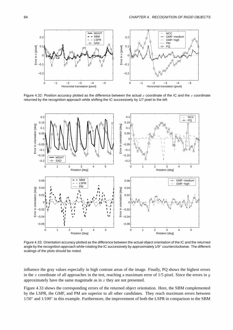
84 CHAPTER 4. RECOGNITION OF RIGID OBJECTS
−5−4−3−2−10
−0.2
−0.1
0
0.1
0.2
Horizontal translation [pixel]
Err
or in
x [p
ixel
]MGHTSBM LSPRSAD
−5−4−3−2−10
−0.2
−0.1
0
0.1
0.2
Horizontal translation [pixel]
Err
or in
x [p
ixel
]
NCC GMF−mediumGMF−high PM PQ
Figure 4.32: Position accuracy plotted as the difference between the actual x coordinate of the IC and the x coordinatereturned by the recognition approach while shifting the IC successively by 1/7 pixel to the left
0 1 2 3 4 5
−0.2
−0.15
−0.1
−0.05
0
0.05
0.1
0.15
0.2
Rotation [deg]
Err
or in
orie
ntat
ion
[deg
]
MGHTSAD
0 1 2 3 4 5
−0.2
−0.15
−0.1
−0.05
0
0.05
0.1
0.15
0.2
Rotation [deg]
Err
or in
orie
ntat
ion
[deg
]NCCPQ
0 1 2 3 4 5
−0.06
−0.04
−0.02
0
0.02
0.04
0.06
Rotation [deg]
Err
or in
orie
ntat
ion
[deg
]
SBM LSPRPM
0 1 2 3 4 5
−0.06
−0.04
−0.02
0
0.02
0.04
0.06
Rotation [deg]
Err
or in
orie
ntat
ion
[deg
]
GMF−mediumGMF−high
Figure 4.33: Orientation accuracy plotted as the difference between the actual object orientation of the IC and the returnedangle by the recognition approach while rotating the IC successively by approximately 1/9 counterclockwise. The differentscalings of the plots should be noted.
influence the gray values especially in high contrast areas of the image. Finally, PQ shows the highest errorsin thex coordinate of all approaches in the test, reaching a maximum error of 1/5 pixel. Since the errors inyapproximately have the same magnitude as inx they are not presented.
Figure 4.33 shows the corresponding errors of the returned object orientation. Here, the SBM complementedby the LSPR, the GMF, and PM are superior to all other candidates. They reach maximum errors between1/50 and 1/100 in this example. Furthermore, the improvement of both the LSPR in comparison to the SBM
4.4. PERFORMANCE EVALUATION OF THE MGHT AND THE SBM 85
and the high accuracy level of the GMF in comparison to the medium accuracy level becomes visible. Theerror of the SBM is reduced to 42% when using the LSPR. Similarly, the high accuracy level of the GMFresults in orientation errors that are about 84% in magnitude of the errors when using the medium accuracylevel. The remaining approaches return a less accurate object orientation. The corresponding maximum errorsof the MGHT, the SAD, the NCC, and PQ are about 1/6 (10’) in this example. However, it should be remarkedthat the accuracy of the MGHT can be easily improved by the LSPR in a similar way as the SBM because thesame features (edge position and orientation) are used in both methods. Thus, a similar accuracy level can beexpected when applying the LSPR to the MGHT.
4.4.4 Computation Time
The computation timerepresents the third evaluation criterion. Indeed, it is very hard to compare differentrecognition methods with this criterion because the computation time strongly depends on the individualimplementation of the recognition methods. Nevertheless, in conjunction with the achievable robustness andaccuracy the associated computation times at least allow a qualitative comparison. The HD was excludedfrom this test because the implementation does not use image pyramids, which results in unreasonably longrecognition times. This would lead to an unfair comparison.
Experimental Set-Up. In order to test the third criterion, the configurations that were used for testingthe robustness against occlusions (cf. Section 4.4.2) and for testing the accuracy (cf. Section 4.4.3) are used.The computation time of the recognition processes was measured on a 400 MHz Pentium II for each imageof the sequences and for each recognition method. Therefore, one has to keep in mind that the measuredrecognition times would reduce to a fraction on current computers (e.g., a 2.8 GHz Pentium 4). However, itcan be assumed that the relation of the recognition times between different approaches approximately remainsunchanged.
The computation time of the SBM was measured for two greediness values of 0 and 1 with using the se-quence for testing the robustness in order to be able to estimate the increase in computational cost for a gainin robustness. Furthermore, in order to assess the correlation between the size of parameter space and compu-tation time, the two sequences for testing the accuracy (horizontal shift and rotation) are used a second timewithout restricting the angle interval to[−30,30], but searching the object in the full range of orientations([0,360[).
In this context it should be noted that the MGHT and the GMF are the only candidates whose implementa-tions are able to recognize the object even if it partially lies outside the search image. The other approachesautomatically restrict the range of possible object positions to those at which the object completely lies withinthe search image. Therefore, particularly in the case of large objects both methods are disadvantaged whencomparing their computation times to those of the remaining approaches. This should be kept in mind whenanalyzing the results.
Results. At first, the computation time of the respective approaches during the robustness test is analyzed.In Figure 4.34 the mean computation timeT over the 500 images of the sequence is plotted for three differentvalues ofemax (SAD) andsmin (others), respectively. This facilitates an easy assignment of the computationtimes to the recognition rates displayed in Figure 4.25. Because for real-time applications the maximum timeto find the object is often of interest, additionally, the maximum computation time is plotted. One can see thatthe approaches can be divided into two groups, where the approaches within the same group exhibit similarrecognition times. In the first group (MGHT, SBM, NCC, PM, PQ) the mean recognition time varies in therange from 18 to 59 ms. In general, the lowersmin is chosen, the higher the robustness against occlusions(see Figure 4.25), but the higher the computation time. It also becomes evident that PQ is faster than PM.Furthermore, a greediness value of 1 speeds up the SBM in comparison to a greediness value of 0, especially

86 CHAPTER 4. RECOGNITION OF RIGID OBJECTS
MGHT SBM SBM NCC PM PQ0
10
20
30
40
50
60
70
80
90
(g=0) (g=1)
T [m
s]smin=20smin=50smin=80Maximum
SAD GMF0
1000
2000
3000
4000
5000
6000
7000
8000
9000
10000
T [m
s]
emax=50 / smin=20emax=30 / smin=50emax=20 / smin=80Maximum
Figure 4.34: Mean and maximum recognition times of the respective approaches when applying the sequence for testingthe robustness against occlusions. The computation time of each approach is represented by three bars, each associatedwith a certain value for emax (SAD) and smin (others), respectively. The different scalings of the two plots should be noted.
if smin is chosen small, i.e., a high number of match candidates must be tracked through the pyramid. In thesecond group (SAD, GMF) the mean recognition time is much higher. Even ifemax of the SAD is set to therelatively small value of 30, where the associated recognition rate is only 34%, the maximum computationtime already exceeds one second. If higher recognition rates should be obtained (at the expense of higher falsealarm rates) the computation time may even reach several seconds. The high recognition rates of the GMFhave already been depreciated by the associated high false alarm rates. Additionally, its computation timereaches several seconds. Hence, the performance of the GMF suffers from a further depreciation. However,in contrast to all other approaches the computation time increases ifsmin is set to a higher value. Duringevaluation it became obvious that the GMF is slowed down considerably if the object cannot be found or ifthe scores is nearsmin . From this, it can be deduced that the implementation of the SAD and the GMF arenot suited for real-time object recognition.
Figure 4.35 shows the respective mean and maximum computation times when applying the accuracy test.Again, the MGHT, the SBM, PM, and PQ show fast computations. Furthermore, the mean computation timeof the SBM extended by the LSPR only marginally increases in comparison to the SBM. The computationtime of the LSPR, which is represented as the difference between the computation time of “SBM+LSPR” and“SBM” in the plots, does not depend on the size of the parameter space: it is constant for a given object, andis 8 ms in the case of the translation sequence and 10 ms using the rotation sequence. Therefore, the largerthe parameter space the smaller the influence of this constant part becomes. In contrast, again the SAD andthe GMF are substantially slower. However, because the object does not show partial occlusions in the twosequences, the GMF is not slowed down to a high degree as in the occlusion case. This is becausesmin was setto 0.8 and the score hardly differs from 1. Becauseemax was set to 25, the robustness of the SAD would be verypoor. Thus, also the SAD would show much longer recognition times if higher robustness was desired. Whenlooking at the result of the NCC an increase of computation time is noticeable when searching the rotatedobject. During evaluation it became evident that the more the IC is rotated relative to the reference orientationin the model image the longer the computation time of the NCC became. Obviously, the implementation of(Matrox 2001) does not scan the whole orientation range at the highest pyramid level before the matches aretracked through the pyramid, but starts with a narrow angle range close to the reference orientation. Hence,the computation time of the NCC is not directly comparable to the other approaches, because the orientationrange of[−30; +30] and[0; 360[ is not really scanned. Hence, a comparable computation time would bestill higher.
From the time increase∆T when extending the angle search range from[−30; +30] to [0; 360[ con-clusions can be drawn about the ability of the approaches to deal with more general transformation classes.
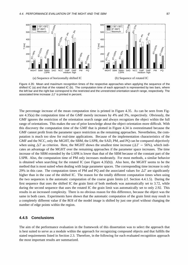
4.4. PERFORMANCE EVALUATION OF THE MGHT AND THE SBM 87
MGHT SBM SBM+ SAD NCC GMF GMF PM PQ0
100
200
300
400
500
600
LSPR medium high
T [m
s]
∆T=
56%
∆T=1
21%
∆T=1
05%
∆T=1
43%
∆T=1
13%
∆T=
4%
∆T=
3%
∆T=
60%
∆T=1
00%
[−30°;+30°][0°;360°[ Maximum
(a) Sequence of horizontally shifted IC
MGHT SBM SBM+ SAD NCC GMF GMF PM PQ0
100
200
300
400
500
600
LSPR medium high
T [m
s]
∆T=
29%
∆T=1
00%
∆T=
83%
∆T=
97%
∆T=
27%
∆T=
4%
∆T=
4%
∆T=1
41%
∆T=2
00%
[−30°;+30°][0°;360°[ Maximum
(b) Sequence of rotated IC
Figure 4.35: Mean and maximum recognition times of the respective approaches when applying the sequence of theshifted IC (a) and that of the rotated IC (b). The computation time of each approach is represented by two bars, wherethe left bar and the right bar correspond to the restricted and the unrestricted orientation search range, respectively. Theassociated time increase ∆T is printed in percent.
The percentage increase of the mean computation time is printed in Figure 4.35. As can be seen from Fig-ure 4.35(a) the computation time of the GMF merely increases by 4% and 3%, respectively. Obviously, theGMF ignores the restriction of the orientation search range and always recognizes the object within the fullrange of orientations. This makes the use of prior knowledge about the object orientation more difficult. Withthis discovery the computation time of the GMF that is plotted in Figure 4.34 is overestimated because theGMF cannot profit from the parameter space restriction as the remaining approaches. Nevertheless, the com-putation is much too slow for real-time applications. Because of the implementation characteristics of theGMF and the NCC, only the MGHT, the SBM, the LSPR, the SAD, PM, and PQ can be compared objectivelywhen using∆T as criterion. Here, the MGHT shows the smallest time increase (∆T = 56%), which indi-cates an advantage of the MGHT over the remaining approaches if the parameter space increases. The timeincrease of the SBM extended by the LSPR is lower than that of the SBM because of the constant part of theLSPR. Also, the computation time of PM only increases moderately. For most methods, a similar behavioris obtained when searching for the rotated IC (see Figure 4.35(b)). Also here, the MGHT seems to be themethod that is most suited when dealing with large parameter spaces. The corresponding time increase is only29% in this case. The computation times of PM and PQ and the associated values for∆T are significantlyhigher than in the case of the shifted IC. The reason for the totally different computation times when usingthe two sequences is the automatic computation of the coarse grain limits (cf. Section 4.4.1.5). During thefirst sequence that uses the shifted IC the grain limit of both methods was automatically set to 3.72, whileduring the second sequence that uses the rotated IC the grain limit was automatically set to only 2.92. Thisresults in an increased complexity. There is no obvious reason for this difference, because the object was thesame in both cases. Experiments have shown that the automatic computation of the grain limit may result ina completely different value if the ROI of the model image is shifted by just one pixel without changing thenumber of edge points within the region.
4.4.5 Conclusions
The aim of the performance evaluation in the framework of this dissertation was to select the approach thatis best suited to serve as a module within the approach for recognizing compound objects and that fulfills thestated requirements listed in Section 2.3. Therefore, in the following for each evaluated recognition approachthe most important results are summarized.
88 CHAPTER 4. RECOGNITION OF RIGID OBJECTS
There are two main reasons why the HD is unsuited regarding the stated criteria. Its strong trend to returnfalse positive matches leads to a very low robustness against clutter. Furthermore, there is no easy wayto refine the pose of the HD directly from the distance values by interpolation. No fair statements aboutthe computation time can be made because of the mentioned implementation characteristics. As a positiveproperty, the acceptable robustness against occlusions should be mentioned, which, however, is depreciatedby the bad receiver operating characteristic.
The SAD also exhibits several drawbacks. A reasonable robustness against occlusions is only obtained incombination with increasing false alarm rates and dramatically long computation times, which make real-timeapplications impossible. Furthermore, it is in no way robust against changes in brightness. This could alreadybe derived from the corresponding formula (4.3). Finally, the accuracy obtained by interpolating the scorevalues is only mediocre.
In contrast, the robustness against changes in brightness of the NCC is higher because of its normalization.However, the low robustness against occlusions as well as the trend to false positive matches limit its applica-bility decisively. While the position accuracy is very high the returned object orientation is less accurate.
The GMF achieves the highest robustness of all approaches against both occlusions and changes in brightness.Unfortunately, the associated high false alarm rates and a computation time that reaches several seconds aresubstantial arguments against the use of the GMF.
PM shows a good compromise between robustness, accuracy, and computation time. However, its receiveroperating characteristic is significantly worse than that of the MGHT and the SBM. The obtained accuracy isvery high and the computation time is also satisfactory.
Although PQ is faster than PM, its receiver operating characteristic is worse. This must be attributed to itstendency to return false positive matches. Furthermore, the speed-up is won at the cost of a reduced accuracy.Especially, the position accuracy is the worst in the test.
Finally, the two developed approaches MGHT and SBM both show a very well balanced behavior regardingrobustness, accuracy, and computation time. The receiver operating characteristics of both are the best of allapproaches in the test. They combine highest robustness against occlusions with highest robustness againstclutter. Also, the robustness against changes in brightness of the SBM is only beaten by the GMF. If smallerscore values are tolerated the MGHT also shows high robustness against changes in brightness, which, how-ever, cannot keep up with the true invariance of the similarity measure used within the SBM. Both methodsshow highest position accuracy in the test. The accuracy in orientation of the SBM is already high and canbe further increased by the LSPR. The MGHT shows lower orientation accuracy, which, however can keepup with the SAD, NCC, and PQ, and could be further improved by using the LSPR. Finally, the computationtime of the MGHT and the SBM on average is the fastest of all approaches in the test. Here, the MGHT seemsto be best suited for extending the parameter space to further dimensions.
Aside from these conclusions, it should be pointed out that some of the results might change if, for example,other implementations of the approaches, other parameter constellations, or other image sequences are chosen.Therefore, the presented evaluation is more of a qualitative nature than of a quantitative one. Nevertheless,the results are very objective and help to find the optimum approach for a specific application.
The approach for recognizing compound objects, which will be introduced in the following chapter, hasa modular design and is therefore independent of the used module for recognizing rigid objects. For theimplementation of the approach for compound objects the SBM was selected because, apart from the argumentthat the SBM is already part of a commercial software and thoroughly tested, its true invariance againstchanges in brightness is a second argument to prefer the SBM to the MGHT. The advantage of the MGHTwhen dealing with higher dimensional parameter spaces is less important since only rigid motion is consideredin this dissertation.

Chapter 5
Recognition of Compound Objects
This chapter describes the novel approach for recognizing compound objects. At first, a review of the respec-tive literature is given (Section 5.1). After a coarse description of the approach (Section 5.2), the single stepsare described in detail (Sections 5.3–5.5). Finally, several examples show the high performance of the newapproach (Section 5.6).
5.1 Previous Work
Approaches dealing with the recognition of compound objects are rarer to find in literature than those dealingwith rigid objects. In the following, the most important approaches will be described.
A prominent class of object recognition methods deals with constrained objects in general and articulatedobjects in particular. Although approaches of this kind mainly deal with the recognition of 3D objects it isworth to include them in the present review because some of the proposed ideas might be also useful in 2D.A constraint object is an object that is composed of a set of rigid object parts. The constellation of the partsis restricted by constraints of an arbitrary type. In articulated objects these constraints are special kinematicconstraints, e.g., rotational or translational joints.
Most methods that deal with the recognition of articulated objects like (Grimson 1989, Lowe 1991, Li andLee 2002) are too restrictive for the recognition of compound objects because the presence of joints in com-pound objects cannot be assumed in general. Several methods try to recognize articulated objects by decom-posing the object into its parts and estimating the pose of each part separately. In a subsequent step the con-straints between the parts are checked (Grimson 1987, Grimson 1989, Kratchounova et al. 1996). Althoughthese approaches are attractive because of their simplicity, the performance suffers: the information aboutthe constraints is not exploited during the recognition process. Also, solving the correspondences would becomputationally expensive because of its combinatorial character. In (Hel-Or and Werman 1994a, Hel-Or andWerman 1994b), an approach is presented that covers articulated or other more general constrained models.Here, the process of solving the correspondence problem is fused with the process of checking the constraints.This is done in a recursive process where the pose of the current object part is predicted using a Kalmanfilter. The prediction is based on the poses of the parts for which the correspondence problem has alreadybeen solved. The predicted pose is then compared to all matches of the current part by computing a distancemeasure. The match with minimum distance is selected. The whole process is repeated for all object parts.By successively selecting the best match for all object parts, the computational effort that is associated withthe correspondence problem is reduced considerably. However, in some cases it might be dangerous to fix thepose of the current part in an early stage. Especially, if the prediction relies on the poses of only a few partsthis may cause problems. The major drawback of these methods is that the recognition process itself ignoresthe information about the constraints between the parts. Thus, approaches of this kind assume that all possiblematches of all object parts are already given as input data.
89

90 CHAPTER 5. RECOGNITION OF COMPOUND OBJECTS
The approach presented in (Li and Lee 2002) is able to recognize articulated objects. Each rigid objectpart is represented by an attributed graph. Also from the search image one attributed graph is generated andautomatically partitioned into small subgraphs. In general, the subgraphs do not coincide with the object parts.Graph matching is then performed between one of the subgraphs and the graphs that represent the object parts.The graph matching is performed using a Hopfield network. Alternatively, other optimization techniques canbe applied to the problem of graph matching, e.g., genetic algorithms (Suganthan 2002). The matching resultsare stored and a different subgraph is selected. Another matching is performed and the result is added to theprevious ones and so on. A decision on the final result is made by interpreting all accumulated results. Theobtained poses are clustered to eliminate spurious matches. By accumulating the results of several matches therobustness against noise, occlusions, and ambiguities is increased. Unfortunately, the graph matching processis very time consuming, and hence unsuitable for real-time object recognition. Furthermore, information aboutthe constraints is not exploited during the recognition process but only considered afterwards.
In (Felzenszwalb and Huttenlocher 2000), an object is represented by a collection of parts arranged in adeformable configuration. The deformable configuration is represented by spring-like connections betweenpairs of parts. The globally best match in an image is found. This is done by minimizing an energy functionthat takes into account both the “spring” forces between the parts and the match quality for each part. Thus,the approach is able to solve the correspondence problem efficiently. However, information about the relationsbetween the parts is ignored during the recognition process itself. Hence, there is no speed-up in comparisonto simply matching each part separately: it takes several seconds to find the object, which is too slow for real-time applications. Furthermore, the model must be set up manually, which prevents the practical use. Anotherdrawback is that only the best match can be found, and hence the approach fails if more than one instance ofthe object is present in the image.
A hierarchical recognition of articulated 3D objects is presented in (Hauck et al. 1997). They assume that thepose of a static part is given and determine the poses of the remaining parts recursively. The relations betweenthe object parts are represented by rotational or translational joints. By making use of the relations andalready obtained information the efficiency of the recognition is increased. For this, the possible 3D poses ofthe remaining parts are successively predicted and projected into the image using a hierarchical representationof the object parts. Thus, self-occlusions of the object parts can be taken into account by eliminating possiblyoccluded image features from the recognition process. Additionally, the search space is restricted to thepredicted poses, which increases the efficiency. However, the manual generation of the 3D model is complexand time consuming. Furthermore, only articulated objects can be handled by the approach. Moreover, the3D pose of the static part must be known `a priori in the camera coordinate system in order to correctly projectthe 3D poses of the remaining parts. Finally, the approach fails if object parts are undetectable because thenthe pose prediction is impossible. Nevertheless, the idea of the hierarchical representation together with therecursive search promises to increase the efficiency also of 2D object recognition approaches.
Another category of approaches deals with the recognition of elastic, flexible, or deformable objects (Jain et al.1996, Pilu and Fisher 1997, Lee and Street 2000, Duta et al. 2001, Sclaroff and Liu 2001, Belongie et al. 2002).These approaches are mainly used to recognize natural objects that slightly change their appearance. Oftenthis change in appearance cannot be modeled by a global transformation but requires to take into account localdeformations. For example, in medical imaging these approaches can be applied to the registration of MRI(magnetic resonance imaging), CT (computed tomography), PET (positron emission tomography), FMRI(functional magnetic resonance imaging), ultrasound imaging, etc. Apart from human organs, a recognitionof plants or animals is facilitated by these methods. However, these methods fail to model compound objects,which do not show real deformations because their object parts themselves are rigid.
Another approach for recognizing deformable objects is given in (Gavrila and Philomin 1999). Here, a de-tection method for objects with varying shape is described. The method uses a shape hierarchy to capturethe variety of object shapes. It is based on the idea that similar object shapes can be grouped together andrepresented by a prototype shape. Thus, in the offline phase a hierarchy is computed from a set of trainingshapes using stochastic optimization techniques. In the online phase, matching is performed with this proto-

5.2. STRATEGY 91
type, rather than with the individual shapes. This is done by involving a simultaneous coarse-to-fine approachover the shape hierarchy and over the transformation parameters. To increase the performance, the existing setof training shapes can be extended with generated “virtual shapes” (Gavrila and Giebel 2001). This improvesthe representational capability of the prototype shapes. Approaches of this kind are suitable for compoundobjects that consist of only a few parts with only small relative movements. The relative movements could beseen as shape variations of the compound object. However, more object parts with even moderate movementswould lead to a combinatorial explosion of the number of required models.
5.2 Strategy
The approach for recognizing compound objects proposed in this dissertation is based on a hierarchical modelrepresentation of the compound object (Ulrich et al. 2002). The strategy behind the approach can be splitinto three stages. Figure 5.1 displays a flowchart for each stage in a very condensed form. In the first stagethe hierarchical model is trained based on several example images (see Figure 5.1(a)). Here, the rigid objectparts of the compound object are extracted and the relations between single object parts are derived. It shouldbe noted that the result of training the hierarchical model is not the hierarchical model itself: in fact, onlythe relations between the object parts are trained. The relations represent one essential component of thehierarchical model. This should be kept in mind during further discussions. The second stage incorporatesthe actual creation of the hierarchical model based upon the trained relations (see Figure 5.1(b)). Here, adistinguishedroot part is selected from all object parts using certain criteria. Furthermore, the optimumhierarchical search strategy is found, with the root part at the top of this hierarchy. Finally, in the third stagethe hierarchical model is used to find the compound object in the search image (see Figure 5.1(c)): In orderto achieve real-time capability, only the root part is searched within the full parameter space. Whereas, theremaining parts are searched with respect to each other only within a restricted parameter space accordingto the extracted relations. Consequently, the offline phase includes the first two stages, while the third stagerepresents the online phase. In this section, a coarse description of the three stages will be given in orderto introduce the underlying strategy. The description will then be elaborated on a finer level of detail in thefollowing three sections.
Outp
ut
Inp
ut
Pro
cess
ing
ExampleImages
ModelImage
Extraction ofObject Parts
Extraction ofRelations
RelationsRelations
(a)
Find OptimumRoot Part
Find OptimumHierarchical Search Strategy
Relations
HierarchicalModel
(b)
Recognition of Root Partwithin Full Parameter Space
Recognition of Remaining Partswithin Restricted Parameter Space
HierarchicalModel
SearchImage
RelationsPoses of All
Object Parts
(c)
Figure 5.1: Condensed flow charts represent the three stages of the proposed approach for recognizing compound ob-jects. The offline phase includes training (a) and creating (b) the hierarchical model. The object recognition (c) representsthe online phase.
In Figure 5.2 the detailed flowchart of the algorithm to train the hierarchical model is presented. A modelimageIm, in which the compound object is defined by a ROI, and several example imagesIe
i , i = 1, . . . ne

92 CHAPTER 5. RECOGNITION OF COMPOUND OBJECTS
represent the major input data to the algorithm. To enhance the illustrative power of the following expla-nations, an artificial example is used, which further clarifies the intermediate processing steps and results.Figure 5.3 shows the input data of the example. All images are of size 512× 512. Taking a closer look atthe example images two inherently connected observations can be immediately made. Firstly, the compoundobject (man) obviously consists of several rigid object parts (head, upper body, two arms, two hands, twolegs, and two feet). Secondly, the parts move with respect to each other to different degrees. The objectiveof the first offline phase, i.e., the training of the hierarchical model, exactly is to simulate the human visualperception. This process includes extracting the rigid object parts together with the relations that describe themutual movements.
Therefore, analyzing the process of visual perception may help to reproduce the human observations. Forthe following discussions it is essential to strictly distinguish between components and parts: One object partconsists of one or more components. The components that belong to the same object part do not show anyrelative movements, while different parts move with respect to each other. Assume that there is no priorknowledge about the compound object. Consequently, if one focuses on the model image and disregards theexample images, one is unable to determine the rigid object parts since no information about the movementis available. However, it is possible to decompose the object into small components. In this example, thefollowing components are perceptible: hat, face, two arms, two hands, two legs, two feet, square margin ofthe upper body, and six components, one for each letter printed on the upper body. This means, that in thisexample the decomposition is done on the basis of image regions that exhibit a homogenous gray value. Whenextending the field of view to the example images, a human tries to match the corresponding components ofthe model image in the example images. Finally, the components that do not move with respect to each otherin all example images are unconsciously and immediately merged into rigid object parts by the human brain.
With this knowledge it is possible to model the extraction of rigid object parts as shown in Figure 5.2. Atfirst, the domain of the model image defined by the ROI is initially decomposed into small components. Theresultingnc components are described bync ROIs that refer to the model image. For each of the components arigid model is generated using an arbitrary suitable object recognition approach. The pose of each componentis then determined by the recognition approach in each example image and stored in thecomponent posematrix of sizene × nc. From the component pose matrix the components that do not show any relativemovement in all example images are determined. The rigid object parts can then be extracted by merging theROIs of the respective components. Also, for the resultingnp(≤ nc) object parts, rigid models are generatedand used to determine the pose of each part in each example image in an analogous way as for the components.This results in thepart pose matrixof sizene × np. Finally, the relations between the parts can be extractedby analyzing the part pose matrix. The relations are stored in the squarerelation matrixof sizenp × np. I.e.,for an arbitrary pair of object parts(p, q) the relative movement of partq with respect to partp is stored in rowp and columnq. The relation matrix together with the ROIs of the extracted model parts represent the outputdata of the training process.
As an example, Figure 5.4 shows the relations of the left arm and the upper body, respectively, to all otherobject parts, i.e., the two corresponding rows of the relation matrix are visualized. Hence, the relative move-ments of the object parts with respect to the left arm and the upper body are displayed. For visualizationpurposes, these movements are projected back into the model image. The object parts are symbolized by theirreference points. The relative positions of the part’s reference points is symbolized by enclosing rectangles,and the relative orientations by circle sectors. A relative orientation of 0 is localized at the “3” of a clock’sdial and the center of the clock’s dial is visualized at the mean position of the respective part. For example,when looking at Figure 5.4(a) one can see that the relative movement of the left hand with respect to theleft arm is smaller than the relative movements of the other parts. Furthermore, the relative movements withrespect to the upper body displayed in Figure 5.4(b) on average are smaller than the movements with respectto the left arm.
In the second stage of the offline phase the information trained in the first stage is used to create the hierarchicalmodel. The process is illustrated in the flowchart of Figure 5.5 in a generalized form. The model image and
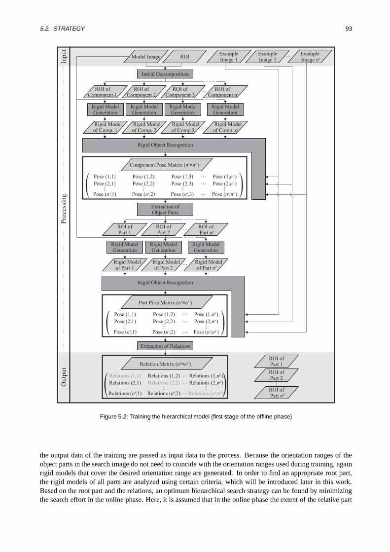
5.2. STRATEGY 93
Inp
ut
Outp
ut
Pro
cess
ing
Initial Decomposition
Rigid ModelGeneration
Rigid ModelGeneration
Rigid ModelGeneration
Rigid ModelGeneration
ROI ofComponent 3
ROI ofComponent 2
ROI ofComponent 1
ROI ofComponent n
C
Extraction ofObject Parts
ROI ofPart 2
ROI ofPart 1
ROI ofPart n
Rigid Modelof Comp 3
Rigid Modelof Comp. 2
Rigid Modelof Comp. nc
Pose (1,1) Pose (1,2) Pose (1,3) Pose (1, )n
Pose (2,1) Pose (2,2) Pose (2,3) Pose (2, )n
Pose ( ,1)n Pose ( ,2)n Pose ( ,3)n Pose ( , )n n
p
Rigid ModelGeneration
Rigid ModelGeneration
Rigid ModelGeneration
Rigid Modelof Part 2
Rigid Modelof Part 1
Rigid Modelof Part np
Rigid Object Recognition
Rigid Object Recognition
Extraction of Relations
ExampleImage 1
ExampleImage 2
ExampleImage ne
c
c
ce e e e
Component Pose Matrix ( )n n× ce
( (
Part Pose Matrix ( )n n× pe
Pose (1,1) Pose (1,2) Pose (1, )n
Pose (2,1) Pose (2,2) Pose (2, )n
Pose ( ,1)n Pose ( ,2)n Pose ( , )n n
p
p
pe e e( (
Relations (1,1) Relations (1,2) Relations (1, )n
Relations (2,1) Relations (2,2) Relations (2, )n
Relations ( ,1)n Relations ( ,2)n Relations ( , )n n
p
p
pp p p( (
……
… … ……
……
… … ……
……
… … ………
Relation Matrix ( )n n×
Model Image ROI
c
pp
…
…
…
…
…
ROI ofPart 1
ROI ofPart 2
ROI ofPart nP
…
Rigid Modelof Comp. 1
Figure 5.2: Training the hierarchical model (first stage of the offline phase)
the output data of the training are passed as input data to the process. Because the orientation ranges of theobject parts in the search image do not need to coincide with the orientation ranges used during training, againrigid models that cover the desired orientation range are generated. In order to find an appropriate root part,the rigid models of all parts are analyzed using certain criteria, which will be introduced later in this work.Based on the root part and the relations, an optimum hierarchical search strategy can be found by minimizingthe search effort in the online phase. Here, it is assumed that in the online phase the extent of the relative part
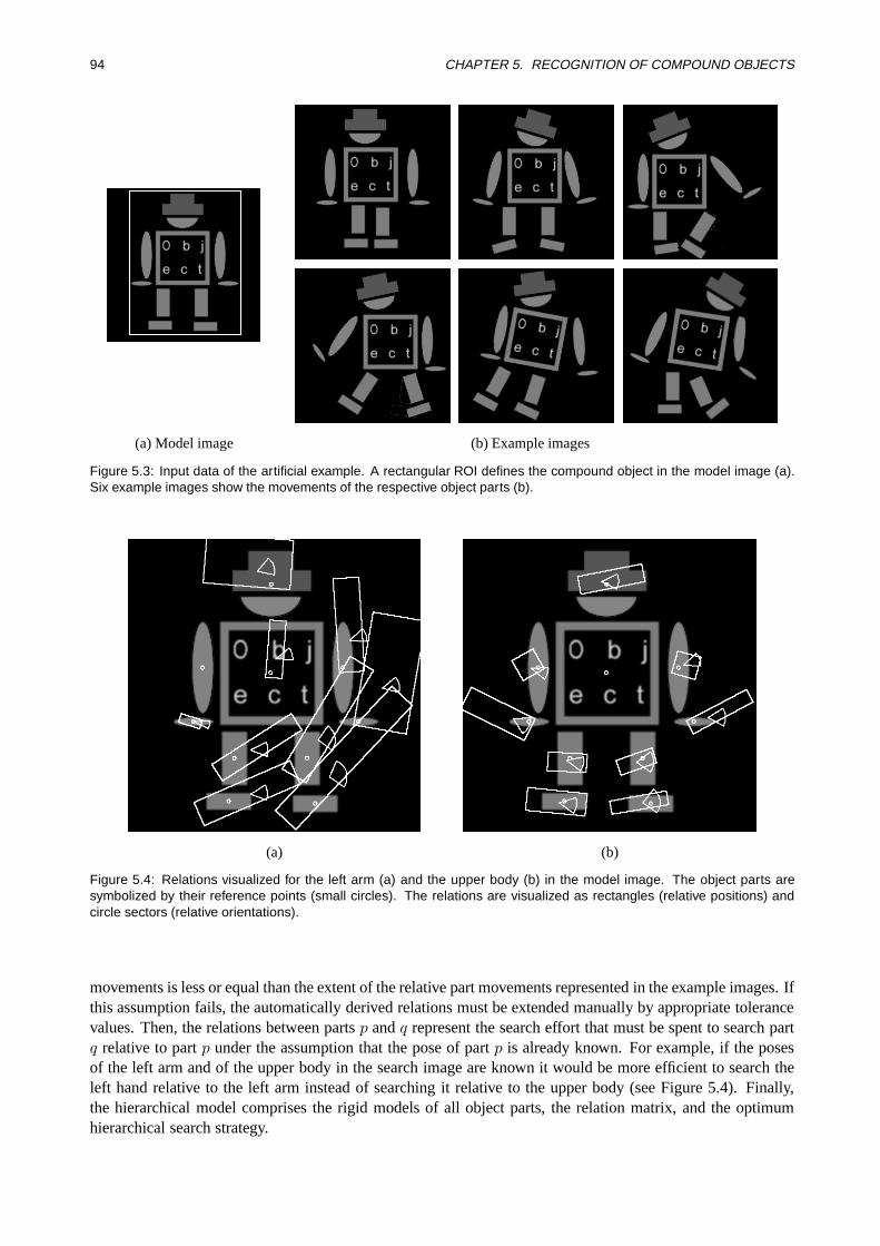
94 CHAPTER 5. RECOGNITION OF COMPOUND OBJECTS
(a) Model image (b) Example images
Figure 5.3: Input data of the artificial example. A rectangular ROI defines the compound object in the model image (a).Six example images show the movements of the respective object parts (b).
(a) (b)
Figure 5.4: Relations visualized for the left arm (a) and the upper body (b) in the model image. The object parts aresymbolized by their reference points (small circles). The relations are visualized as rectangles (relative positions) andcircle sectors (relative orientations).
movements is less or equal than the extent of the relative part movements represented in the example images. Ifthis assumption fails, the automatically derived relations must be extended manually by appropriate tolerancevalues. Then, the relations between partsp andq represent the search effort that must be spent to search partq relative to partp under the assumption that the pose of partp is already known. For example, if the posesof the left arm and of the upper body in the search image are known it would be more efficient to search theleft hand relative to the left arm instead of searching it relative to the upper body (see Figure 5.4). Finally,the hierarchical model comprises the rigid models of all object parts, the relation matrix, and the optimumhierarchical search strategy.
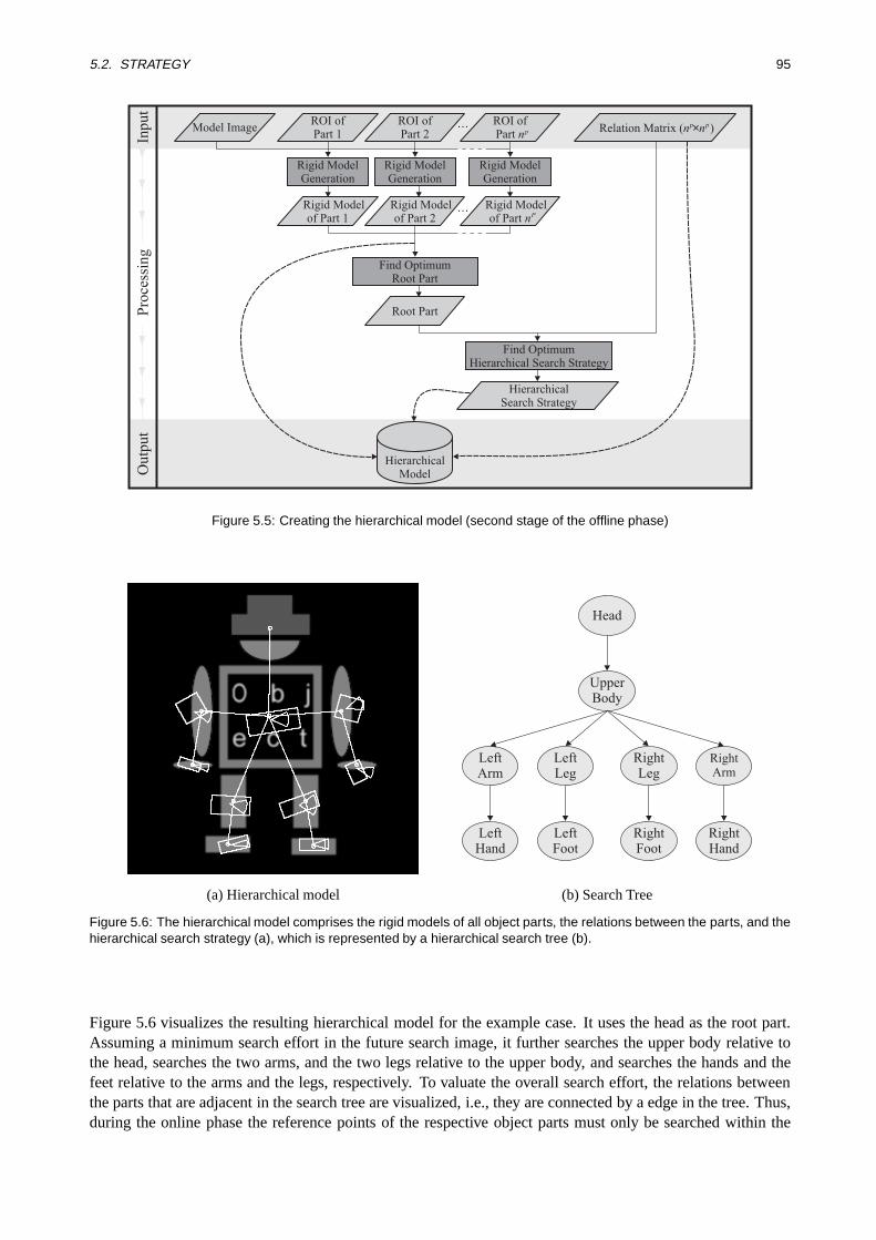
5.2. STRATEGY 95
Inp
ut
Ou
tpu
tIn
pu
tP
roce
ssin
gModel Image
ROI ofPart 2
ROI ofPart 1
ROI ofPart np
Rigid ModelGeneration
Rigid ModelGeneration
Rigid ModelGeneration
Root Part
Rigid Modelof Part 1
Rigid Modelof Part nP
…
…
Relation Matrix ( )n n× pp
Find OptimumHierarchical Search Strategy
HierarchicalSearch Strategy
Find OptimumRoot Part
Rigid Modelof Part 2
HierarchicalModel
Figure 5.5: Creating the hierarchical model (second stage of the offline phase)
(a) Hierarchical model
UpperBody
Head
RightLeg
RightFoot
RightArm
RightHand
LeftArm
LeftHand
LeftLeg
LeftFoot
(b) Search Tree
Figure 5.6: The hierarchical model comprises the rigid models of all object parts, the relations between the parts, and thehierarchical search strategy (a), which is represented by a hierarchical search tree (b).
Figure 5.6 visualizes the resulting hierarchical model for the example case. It uses the head as the root part.Assuming a minimum search effort in the future search image, it further searches the upper body relative tothe head, searches the two arms, and the two legs relative to the upper body, and searches the hands and thefeet relative to the arms and the legs, respectively. To valuate the overall search effort, the relations betweenthe parts that are adjacent in the search tree are visualized, i.e., they are connected by a edge in the tree. Thus,during the online phase the reference points of the respective object parts must only be searched within the
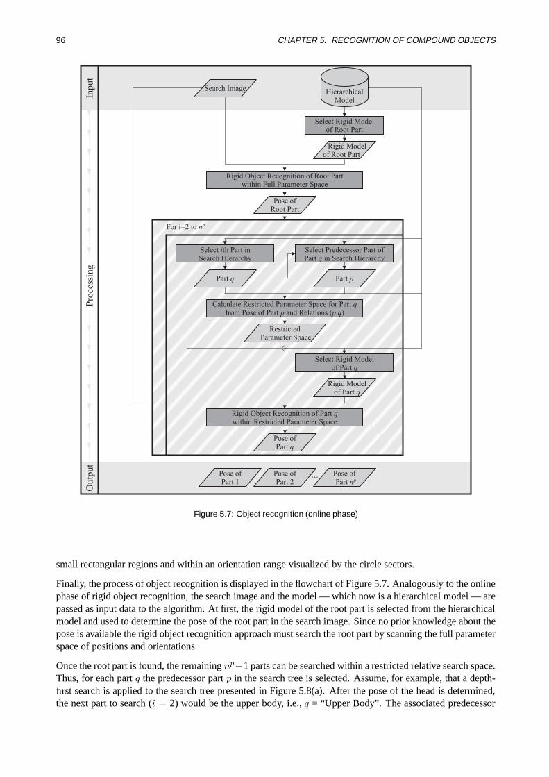
96 CHAPTER 5. RECOGNITION OF COMPOUND OBJECTS
Inp
ut
Outp
ut
Inp
ut
Pro
cess
ing
For i=2 to n
Part p
Search Image
Select Rigid Modelof Root Part
HierarchicalModel
Rigid Modelof Root Part
Rigid Object Recognition of Root Partwithin Full Parameter Space
Pose ofRoot Part
Calculate Restricted Parameter Space for Partfrom Pose of Part and Relations ( , )
qp p q
Part q
Select th Part inSearch Hierarchy
i Select Predecessor Part ofPart in Search Hierarchyq
RestrictedParameter Space
Rigid Object Recognition of Partwithin Restricted Parameter Space
q
p
Select Rigid Modelof Part q
Pose ofPart q
Rigid Modelof Part q
Pose ofPart 2
Pose ofPart 1
Pose ofPart np
…
Figure 5.7: Object recognition (online phase)
small rectangular regions and within an orientation range visualized by the circle sectors.
Finally, the process of object recognition is displayed in the flowchart of Figure 5.7. Analogously to the onlinephase of rigid object recognition, the search image and the model — which now is a hierarchical model — arepassed as input data to the algorithm. At first, the rigid model of the root part is selected from the hierarchicalmodel and used to determine the pose of the root part in the search image. Since no prior knowledge about thepose is available the rigid object recognition approach must search the root part by scanning the full parameterspace of positions and orientations.
Once the root part is found, the remainingnp−1 parts can be searched within a restricted relative search space.Thus, for each partq the predecessor partp in the search tree is selected. Assume, for example, that a depth-first search is applied to the search tree presented in Figure 5.8(a). After the pose of the head is determined,the next part to search (i = 2) would be the upper body, i.e.,q = “Upper Body”. The associated predecessor

5.3. TRAINING THE HIERARCHICAL MODEL 97
UpperBody
Head
RightLeg
RightFoot
RightArm
RightHand
LeftArm
LeftHand
LeftLeg
LeftFoot
1
2
3 5 7 9
4 6 8 10
(a) Depth-first search (b) Search image and found object instance
Figure 5.8: A depth-first search is applied to the search tree. In (a) the search order is indicated by numbers. In (b) anexample search image and the corresponding found object instance is displayed. The poses of the individual object partsare visualized by superimposing the edges of the parts at the returned pose in white.
part in the search tree is the head, and hencep = “Head”. The parameter space that must be scanned by therecognition approach to search partq is defined by the pose of partp and the relation between the partsp andq. The rigid model of partq is selected from the hierarchical model and used to determine the pose of partqwithin the restricted parameter space. The whole process is repeated for each part, finally obtaining the posesof all object parts. An example search image of size 512×512 and the corresponding found object instance isdisplayed in Figure 5.8(b). It should be noted that it is not necessary that the absolute orientation of the objectin the search image is covered within the example images, since only relative movements between object partsare trained.
To give an impression of the advantage when using the proposed hierarchical model, the recognition timefor this example was 20 ms on a 2 GHz Pentium 4. In contrast, the brute-force method that would search allparts in the entire search space independently from each other would take 310 ms (using the SBM in bothcases). The second obvious advantage should also be pointed out here: because of the inherently determinedcorrespondence, which is provided by the hierarchical model, the returned match of the compound objectimplicitly covers a topologically sound representation. In contrast, when searching the parts independently,it is not immediately possible to distinguish between the matches of the left and the right arm, for example.Furthermore, if several object instances are present in the image, it is hard to assign a match of a certain objectpart to the correct instance of the compound object.
Although the basic idea of the approach seems to be very simple, several difficulties that are not obvious atfirst glance occur. They will be discussed in the following sections together with the detailed explanation ofthe previously introduced steps.
5.3 Training the Hierarchical Model
5.3.1 Initial Decomposition
In the first step, the compound object must initially be broken up into small components. The conditionthe initial decomposition must fulfill is that each object part must be represented by at least one component.
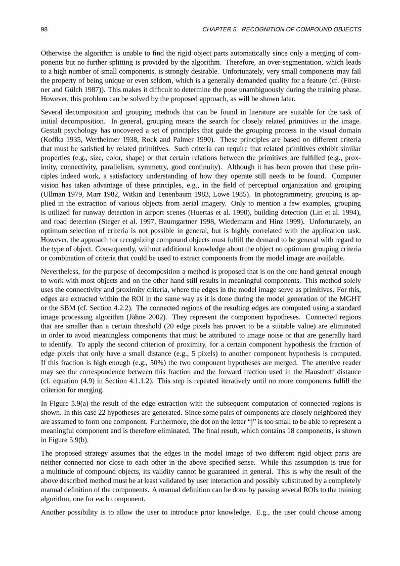
98 CHAPTER 5. RECOGNITION OF COMPOUND OBJECTS
Otherwise the algorithm is unable to find the rigid object parts automatically since only a merging of com-ponents but no further splitting is provided by the algorithm. Therefore, an over-segmentation, which leadsto a high number of small components, is strongly desirable. Unfortunately, very small components may failthe property of being unique or even seldom, which is a generally demanded quality for a feature (cf. (F¨orst-ner and G¨ulch 1987)). This makes it difficult to determine the pose unambiguously during the training phase.However, this problem can be solved by the proposed approach, as will be shown later.
Several decomposition and grouping methods that can be found in literature are suitable for the task ofinitial decomposition. In general, grouping means the search for closely related primitives in the image.Gestalt psychology has uncovered a set of principles that guide the grouping process in the visual domain(Koffka 1935, Wertheimer 1938, Rock and Palmer 1990). These principles are based on different criteriathat must be satisfied by related primitives. Such criteria can require that related primitives exhibit similarproperties (e.g., size, color, shape) or that certain relations between the primitives are fulfilled (e.g., prox-imity, connectivity, parallelism, symmetry, good continuity). Although it has been proven that these prin-ciples indeed work, a satisfactory understanding of how they operate still needs to be found. Computervision has taken advantage of these principles, e.g., in the field of perceptual organization and grouping(Ullman 1979, Marr 1982, Witkin and Tenenbaum 1983, Lowe 1985). In photogrammetry, grouping is ap-plied in the extraction of various objects from aerial imagery. Only to mention a few examples, groupingis utilized for runway detection in airport scenes (Huertas et al. 1990), building detection (Lin et al. 1994),and road detection (Steger et al. 1997, Baumgartner 1998, Wiedemann and Hinz 1999). Unfortunately, anoptimum selection of criteria is not possible in general, but is highly correlated with the application task.However, the approach for recognizing compound objects must fulfill the demand to be general with regard tothe type of object. Consequently, without additional knowledge about the object no optimum grouping criteriaor combination of criteria that could be used to extract components from the model image are available.
Nevertheless, for the purpose of decomposition a method is proposed that is on the one hand general enoughto work with most objects and on the other hand still results in meaningful components. This method solelyuses the connectivity and proximity criteria, where the edges in the model image serve as primitives. For this,edges are extracted within the ROI in the same way as it is done during the model generation of the MGHTor the SBM (cf. Section 4.2.2). The connected regions of the resulting edges are computed using a standardimage processing algorithm (J¨ahne 2002). They represent the component hypotheses. Connected regionsthat are smaller than a certain threshold (20 edge pixels has proven to be a suitable value) are eliminatedin order to avoid meaningless components that must be attributed to image noise or that are generally hardto identify. To apply the second criterion of proximity, for a certain component hypothesis the fraction ofedge pixels that only have a small distance (e.g., 5 pixels) to another component hypothesis is computed.If this fraction is high enough (e.g., 50%) the two component hypotheses are merged. The attentive readermay see the correspondence between this fraction and the forward fraction used in the Hausdorff distance(cf. equation (4.9) in Section 4.1.1.2). This step is repeated iteratively until no more components fulfill thecriterion for merging.
In Figure 5.9(a) the result of the edge extraction with the subsequent computation of connected regions isshown. In this case 22 hypotheses are generated. Since some pairs of components are closely neighbored theyare assumed to form one component. Furthermore, the dot on the letter “j” is too small to be able to represent ameaningful component and is therefore eliminated. The final result, which contains 18 components, is shownin Figure 5.9(b).
The proposed strategy assumes that the edges in the model image of two different rigid object parts areneither connected nor close to each other in the above specified sense. While this assumption is true fora multitude of compound objects, its validity cannot be guaranteed in general. This is why the result of theabove described method must be at least validated by user interaction and possibly substituted by a completelymanual definition of the components. A manual definition can be done by passing several ROIs to the trainingalgorithm, one for each component.
Another possibility is to allow the user to introduce prior knowledge. E.g., the user could choose among
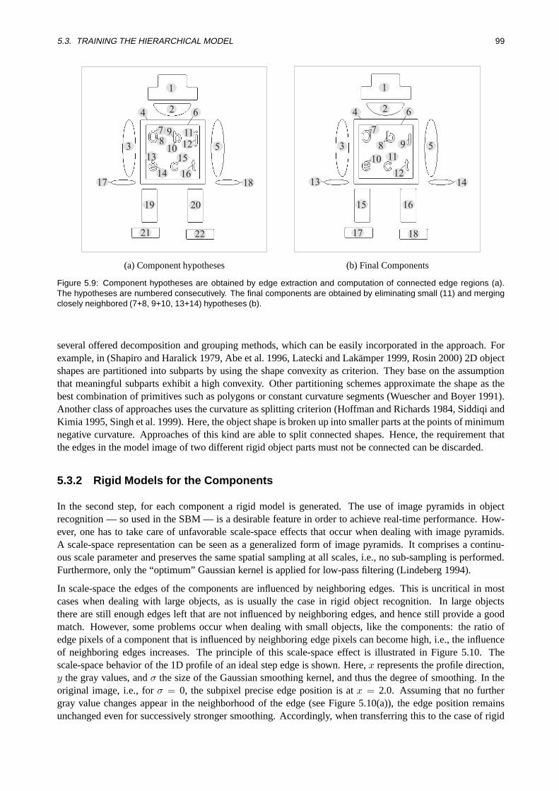
5.3. TRAINING THE HIERARCHICAL MODEL 99
1
2
3
17
19
4 6
78
9 1112
13
14
155
18
20
21 22
16
10
(a) Component hypotheses
1
2
3
13
15
4 6
7
8 9
10 11
1214
16
17 18
5
(b) Final Components
Figure 5.9: Component hypotheses are obtained by edge extraction and computation of connected edge regions (a).The hypotheses are numbered consecutively. The final components are obtained by eliminating small (11) and mergingclosely neighbored (7+8, 9+10, 13+14) hypotheses (b).
several offered decomposition and grouping methods, which can be easily incorporated in the approach. Forexample, in (Shapiro and Haralick 1979, Abe et al. 1996, Latecki and Lak¨amper 1999, Rosin 2000) 2D objectshapes are partitioned into subparts by using the shape convexity as criterion. They base on the assumptionthat meaningful subparts exhibit a high convexity. Other partitioning schemes approximate the shape as thebest combination of primitives such as polygons or constant curvature segments (Wuescher and Boyer 1991).Another class of approaches uses the curvature as splitting criterion (Hoffman and Richards 1984, Siddiqi andKimia 1995, Singh et al. 1999). Here, the object shape is broken up into smaller parts at the points of minimumnegative curvature. Approaches of this kind are able to split connected shapes. Hence, the requirement thatthe edges in the model image of two different rigid object parts must not be connected can be discarded.
5.3.2 Rigid Models for the Components
In the second step, for each component a rigid model is generated. The use of image pyramids in objectrecognition — so used in the SBM — is a desirable feature in order to achieve real-time performance. How-ever, one has to take care of unfavorable scale-space effects that occur when dealing with image pyramids.A scale-space representation can be seen as a generalized form of image pyramids. It comprises a continu-ous scale parameter and preserves the same spatial sampling at all scales, i.e., no sub-sampling is performed.Furthermore, only the “optimum” Gaussian kernel is applied for low-pass filtering (Lindeberg 1994).
In scale-space the edges of the components are influenced by neighboring edges. This is uncritical in mostcases when dealing with large objects, as is usually the case in rigid object recognition. In large objectsthere are still enough edges left that are not influenced by neighboring edges, and hence still provide a goodmatch. However, some problems occur when dealing with small objects, like the components: the ratio ofedge pixels of a component that is influenced by neighboring edge pixels can become high, i.e., the influenceof neighboring edges increases. The principle of this scale-space effect is illustrated in Figure 5.10. Thescale-space behavior of the 1D profile of an ideal step edge is shown. Here,x represents the profile direction,y the gray values, andσ the size of the Gaussian smoothing kernel, and thus the degree of smoothing. In theoriginal image, i.e., forσ = 0, the subpixel precise edge position is atx = 2.0. Assuming that no furthergray value changes appear in the neighborhood of the edge (see Figure 5.10(a)), the edge position remainsunchanged even for successively stronger smoothing. Accordingly, when transferring this to the case of rigid

100 CHAPTER 5. RECOGNITION OF COMPOUND OBJECTS
model generation, the edge position would be the same on each pyramid level. Unfortunately, this assumptionis not valid in general. If, for example, a rigid model is to be created from the component that represents theleft arm (see component number 3 in Figure 5.9(b)) the outer square of the upper body (component number 4)influences the scale-space behavior, and hence the model creation on higher pyramid levels. In Figure 5.10(b)a second step edge is added to the profile and the edge position in scale-space is computed again. It canbe seen that the higher the smoothing is, the larger the displacement of the original edge position becomes.This is uncritical if the left arm would always appear at the same relative pose with respect to the upperbody because the edge displacement in scale-space would be the same in the model image and in all exampleimages. However, in some example images the left arm moves with respect to the upper body, and hence therepresentation of the left arm in the pyramid of the example image differs from the representation in the modelimage. Especially, in the case of small components this may lead to a severe dissimilarity on higher pyramidlevels between the information stored in the model and that represented in the search image. This possiblycauses the recognition method not to find the component.
σ
(a) Undisturbed model edge
σ
(b) Disturbed model edge
Figure 5.10: Scale-space behavior of an ideal 1D edge profile. For homogeneous gray values in the neighborhood, theedge position remains constant in scale-space (a). In contrast, the edge position is disturbed if gray value changes appearthat are close to the edge, e.g., caused by a neighboring edge (b).
The problem could be avoided if no image pyramids were applied in the recognition method. However, thelong computation times involved are definitely unsuitable for the practical use, even for the offline phase.Therefore, an alternative solution is proposed: the disturbing gray value inhomogeneities in the neighborhoodof the model edges are eliminated. This is achieved by successively expanding the gray values of the modelimage that are adjacent to a component edge pixel in the direction of the edge gradient.
Figure 5.11(a) shows the principle of gray value expansion. The component edge region is dilated by onepixel, obtaining the pixels that are adjacent to the edge region. The gray values of the adjacent pixels are usedas seed values that are expanded to the neighborhood. Thus, the gray values of the edge pixels and those ofthe adjacent pixels remain unchanged to ensure an extraction of the component edges that is the same as in theoriginal image when applying the Sobel filter. For the gray value expansion, the already dilated edge regionis successively dilated by one pixel. After each dilation, the gray values of the pixels that are added by thedilation are calculated from the already available gray values of the preceding dilation step. For this purpose,the gray values of the preceding dilation that are within a 3× 3 neighborhood are averaged. Furthermore,to avoid artifacts that would lead to pseudo edges during model generation, a 1D smoothing of the newlycalculated gray values is applied in a second step. In Figure 5.11(b) the part of the model image showing theleft arm is displayed. The edges of the upper body and of the left hand would influence the model generationfor the component representing the left arm. Figure 5.11(c) shows the result after applying the gray valueexpansion. The neighboring image structure, and hence the disturbing influences are eliminated.
To guarantee that all disturbing influences are eliminated, the size of the expansion must be chosen appropri-
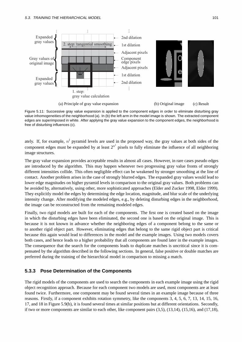
5.3. TRAINING THE HIERARCHICAL MODEL 101
Gray values oforiginal image
…
…
Expandedgray values
Expandedgray values
……
Adjacent pixels
1st dilation
2nd dilation
Adjacent pixels
1st dilation
2nd dilation
……
2. step: tangential smoothing
1. step:gray value calculation
Componentedge pixels
(a) Principle of gray value expansion (b) Original image (c) Result
Figure 5.11: Successive gray value expansion is applied to the component edges in order to eliminate disturbing grayvalue inhomogeneities of the neighborhood (a). In (b) the left arm in the model image is shown. The extracted componentedges are superimposed in white. After applying the gray value expansion to the component edges, the neighborhood isfree of disturbing influences (c).
ately. If, for example,nl pyramid levels are used in the proposed way, the gray values at both sides of thecomponent edges must be expanded by at least 2nl
pixels to fully eliminate the influence of all neighboringimage structures.
The gray value expansion provides acceptable results in almost all cases. However, in rare cases pseudo edgesare introduced by the algorithm. This may happen whenever two progressing gray value fronts of stronglydifferent intensities collide. This often negligible effect can be weakened by stronger smoothing at the line ofcontact. Another problem arises in the case of strongly blurred edges. The expanded gray values would lead tolower edge magnitudes on higher pyramid levels in comparison to the original gray values. Both problems canbe avoided by, alternatively, using other, more sophisticated approaches (Elder and Zucker 1998, Elder 1999).They explicitly model the edges by determining the edge location, magnitude, and blur scale of the underlyingintensity change. After modifying the modeled edges, e.g., by deleting disturbing edges in the neighborhood,the image can be reconstructed from the remaining modeled edges.
Finally, two rigid models are built for each of the components. The first one is created based on the imagein which the disturbing edges have been eliminated, the second one is based on the original image. This isbecause it is not known in advance whether the neighboring edges of a component belong to the same orto another rigid object part. However, eliminating edges that belong to the same rigid object part is criticalbecause this again would lead to differences in the model and the example images. Using two models coversboth cases, and hence leads to a higher probability that all components are found later in the example images.The consequence that the search for the components leads to duplicate matches is uncritical since it is com-pensated by the algorithm described in the following sections. In general, false positive or double matches arepreferred during the training of the hierarchical model in comparison to missing a match.
5.3.3 Pose Determination of the Components
The rigid models of the components are used to search the components in each example image using the rigidobject recognition approach. Because for each component two models are used, most components are at leastfound twice. Furthermore, one component may be found several times in an example image because of threereasons. Firstly, if a component exhibits rotation symmetry, like the components 3, 4, 5, 6, 7, 13, 14, 15, 16,17, and 18 in Figure 5.9(b), it is found several times at similar positions but at different orientations. Secondly,if two or more components are similar to each other, like component pairs (3,5), (13,14), (15,16), and (17,18),
102 CHAPTER 5. RECOGNITION OF COMPOUND OBJECTS
in general each component is found at its correct pose as well as at the pose of the similar component(s).This also includes partial similarities, i.e., one component is similar to a fraction of another component. Thecomponent representing the left leg (15), for example, will be found four times in each example image becauseof its rotation symmetry of 180 and its similarity to the right leg (16). Thirdly, a component may also showsimilarities to image clutter, where, in general, smaller components are more likely to show similarities toclutter than larger components. Consequently, the result of the component search is not unique.
In the following section, an approach that solves the ambiguities by selecting the most likely pose for eachcomponent in each example image is presented. Here, the component poses that are able to represent thecompound object in a least “deformed” way in comparison to the compound object in the model image aresupposed to be more likely. The deformation is caused by the relative movement of the components. In(Ullman 1979), this problem is called the correspondence problem, where correspondence is the process thatidentifies elements in different views as representing the same object (component) at different times (in differ-ent images), thereby maintaining the perceptual identity of objects in motion or change. Thus, the movementof the components that is introduced when comparing their poses in the model image and in an exampleimage is interpreted as apparent motion. Ullman (1979) proposes to solve the correspondence problem byminimizing the overall apparent motion. This is the basis for further considerations.
In the following, the exact solution for solving the ambiguities is presented. Upon closer examination, theproblem of finding the most likely poses turns out to be a graph matching problem between a model graphGm and a search graphGs. The model graph represents the compound object in the model image, wherethe nodes in the graph represent the components, which are labeled with the associated component number.Furthermore, each node is linked to all other nodes by arcs, where an arc between two nodes is labeled by therelative position and orientation between the two associated components in the model image. Accordingly,Gs represents the poses of the component matches in an example image. In general, the number of nodes inGs is higher than inGm because of ambiguous matches. Furthermore, only the nodes inGs that correspondto poses of distinct components are linked by arcs. Again the arcs are labeled by the relative poses of thecomponents. Finally, the task of solving the ambiguities corresponds to findingGm within Gs. The specialclass of graph matching that can be applied to this problem is often calledinexact subgraph isomorphism(Kroupnova and Korsten 1997) orerror-correcting subgraph isomorphism(Messmer 1996) in the literature.A comprehensive introduction to graph matching is given in (Messmer 1996). Agraph isomorphismis abijection between the nodes of two graphs. Asubgraph isomorphismof Gm andGs tries to find a subgraphGs′ of Gs and a graph isomorphism fromGm toGs′. An efficient algorithm is presented in (Ullmann 1976).Finally, anerror-correcting subgraph isomorphismis more tolerant and is able to find an optimum subgraphisomorphism even if the two graphs are different to each other. The solution is often realized by introducinggraph edit operations with associated costs. The goal is to find a sequence of edit operations with minimumcost that must be applied toGm for a subgraph isomorphism to exist.
In the present case, because the number of nodes inGs is higher than inGm, a subgraph isomorphism mustbe found. Furthermore, the subgraph to find inGs differs from the model graphGm because the componentsmay move with respect to each other. Hence, an error-correcting subgraph isomorphism is the right choice.The graph edit operations comprise modifying the relative poses between the components and deleting nodesfor the case that a component is missing in the example image. Unfortunately, finding an error-correctingsubgraph isomorphism is known to be NP-complete, and thus its time complexity is exponential in the numberof nodes. In (Messmer and Bunke 1998), an algorithm is presented that reduces the computational load atthe cost of exponentially increasing memory requirement. Both alternatives are not suitable for a practicalsolution of the ambiguities. Therefore, in the following an approach is presented that on the one hand showsonly polynomial time complexity and on the other hand provides acceptable results. The idea is based onrating the single component matches, where matches that lead to less plausible configurations are penalized.The problem of solving the ambiguities can then be seen as uniquely assigning a match to each componentsuch that the overall rating is maximized, while simultaneously considering certain constraints. For this, thecomponent matches are represented as a bipartite graph (i.e., a graph with two subsets of nodes). The solutionis then obtained by applying bipartite graph matching using linear programming.
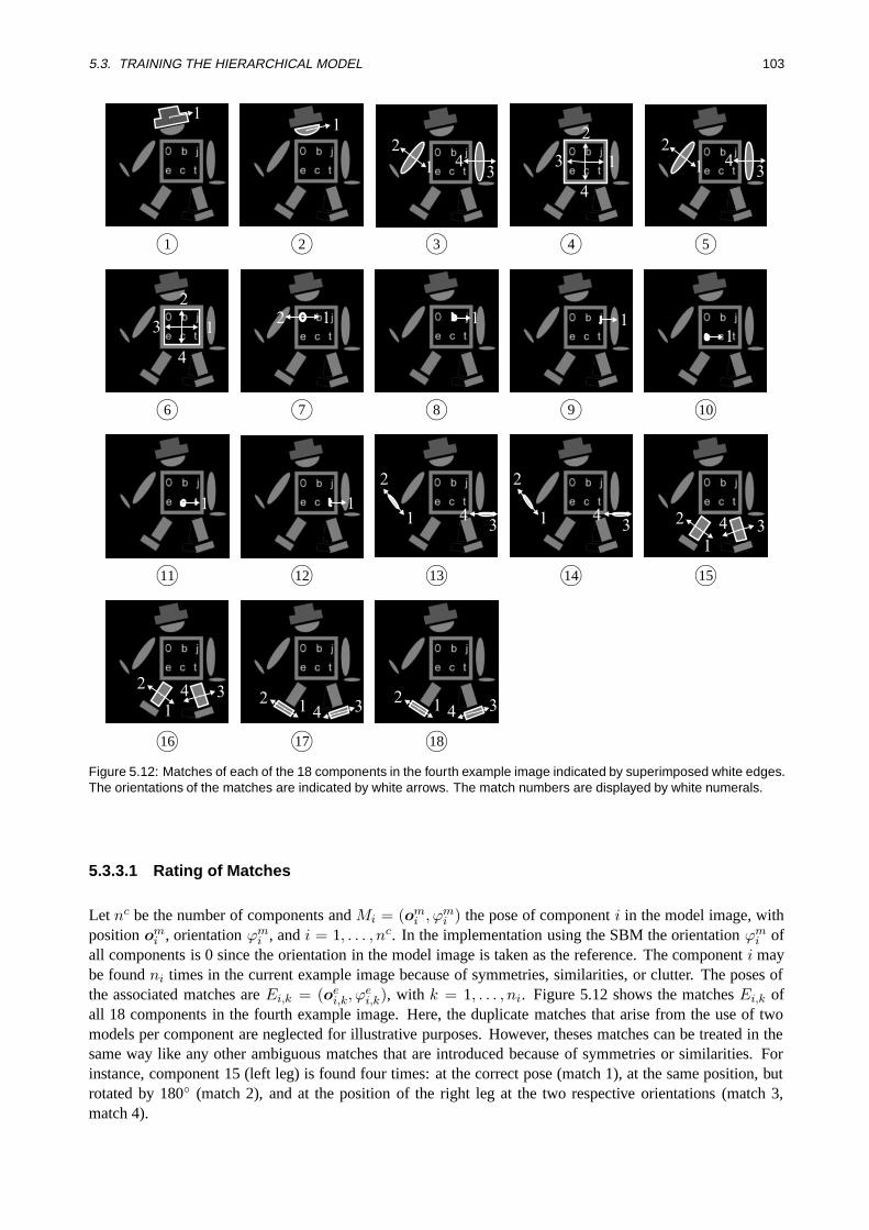
5.3. TRAINING THE HIERARCHICAL MODEL 103
11
1
2
34 1
2
3
4
1
2
34
1m 2m 3m 4m 5m
1
2
3
4
12 1 11
6m 7m 8m 9m 10m
1 11
2
34 1
2
34
1
2 34
11m 12m 13m 14m 15m
1
234
12
34 12
34
16m 17m 18m
Figure 5.12: Matches of each of the 18 components in the fourth example image indicated by superimposed white edges.The orientations of the matches are indicated by white arrows. The match numbers are displayed by white numerals.
5.3.3.1 Rating of Matches
Let nc be the number of components andMi = (omi , ϕ
mi ) the pose of componenti in the model image, with
positionomi , orientationϕm
i , andi = 1, . . . , nc. In the implementation using the SBM the orientationϕmi of
all components is 0 since the orientation in the model image is taken as the reference. The componenti maybe foundni times in the current example image because of symmetries, similarities, or clutter. The poses ofthe associated matches areEi,k = (oe
i,k, ϕei,k), with k = 1, . . . , ni. Figure 5.12 shows the matchesEi,k of
all 18 components in the fourth example image. Here, the duplicate matches that arise from the use of twomodels per component are neglected for illustrative purposes. However, theses matches can be treated in thesame way like any other ambiguous matches that are introduced because of symmetries or similarities. Forinstance, component 15 (left leg) is found four times: at the correct pose (match 1), at the same position, butrotated by 180 (match 2), and at the position of the right leg at the two respective orientations (match 3,match 4).

104 CHAPTER 5. RECOGNITION OF COMPOUND OBJECTS
The decisive point of the idea behind the approach for finding the most likely match of each component in theexample image is based on rating the associated poses of all matches. The rating is performed by penalizingthe matches that are less plausible by using a cost value. For this, the (unambiguous) poses of the componentsin the model image are taken as the reference, forming the reference component configuration. In the exampleimage, a match receives a cost value that describes the quantified change in the component configuration thatwould be introduced when this match is assumed to be correct. This follows the above described principle ofminimizing the overall apparent motion, where the apparent motion corresponds to the overall configurationchange.
In the following, the single steps that are used to compute the cost valueΨi0,k0 of thek0-th match of componenti0 will be explained. At first, the parameters of the 2D rigid transformation that transform poseMi0 intoEi0,k0
are computed, resulting in a rotation matrixR with rotation angleα and a translationt:
α = ϕei0,k0
− ϕmi0 (5.1)
t = oei0,k0
−R(α) · omi0 . (5.2)
In the second step, the reference component configuration is projected into the example image by transformingthe poses of all componentsi, providing the projected posesM ′
i = (omi′, ϕm
i′):
omi′ = R(α) · om
i + t (5.3)
ϕmi′ = ϕm
i + α . (5.4)
Figure 5.13 shows the projection of the reference component configuration into the example image for eachof the four matchesk0 = 1, . . . ,4 of componenti0 = 3.
(a) Match 1 (b) Match 2
(c) Match 3 (d) Match 4
Figure 5.13: Projection of the reference component configuration into the example image for each of the four matches ofcomponent 3 (left arm)
5.3. TRAINING THE HIERARCHICAL MODEL 105
The projected pose of componenti can then be compared to a certain matchk (k = 1, . . . , ni) of the compo-nenti in the example image by computing a distance measureψ:
ψ(M ′i , Ei,k) =
√‖om
i′ − oe
i,k‖2 + w2(ϕmi′ − ϕe
i,k)2 , (5.5)
where‖ ·‖ denotes the euclidian vector length andw is a weighting factor to balance the difference in positionand orientation. A suitable value forw can be obtained, for example, based on the quantization of the objectorientation∆ϕ. Assuming a position quantization of 1 pixel,w could be set to 1/∆ϕ, for example. Becausethe correct match of componenti is not knowna priori, the distance measureψ(M ′
i , Ei,k) is computed for allmatchesk. The match with minimum distance is assumed to be correct and is used to compute the cost valueΨi0,k0. This assumption is the only difference to the exact computation using the previously explained error-correcting subgraph isomorphism, and is uncritical unless the true component configuration in the currentexample image does not differ extremely from the reference component configuration. Finally, the associateddistance value is used in the computation of the cost valueΨi0,k0 of matchk0 of componenti0:
Ψi0,k0 =nc∑i=1
mink=1,...,ni
ψ(M ′i , Ei,k) . (5.6)
The computation of the cost value is repeated for each matchk0 and each componenti0 by applying (5.1)–(5.6). In some applications it might be desirable to apply a threshold on the cost value and eliminate thecorresponding matches in order to reduce the sensitivity to outliers. The cost values are then used in thefollowing algorithm to find the most likely match of each component using a global optimization.
5.3.3.2 Identification of Physical Instances
A simple way to get the most likely match of componenti would be to select the matchk, whereΨi,k
is minimal for k = 1, . . . , ni. Although this local optimizationwould assign one unique match to eachcomponent, one important condition would be neglected. It would be still possible that several matches ofdifferent components are assigned to the samephysical instancein the example image. A physical instancerepresents an arbitrary structure in the example image to which components are matched. The problem isillustrated in Figure 5.14, where the compound object from the previous examples is reduced to an upper bodyand two legs in order to keep the explanations as clear and simple as possible. Furthermore, a clutter objecthas been added to the example image. Thus, four physical instances are present in the example image: theupper body, the two legs, and the clutter object.
If the match with the lowest cost value would be selected for each component, components 2 and 3 matchthe same physical instance (the actual instance of the right leg) in the example image. However, a desirableresult would assign component 2 to match 1 and component 3 to match 3. Therefore, the task of aglobaloptimizationis to find for each componenti the matchki such that
nc∑i=1
Ψi,ki−→ min (5.7)
subject to the constraint that multiple matches are avoided, i.e., that at most one component is matched to acertain physical instance.
A prerequisite to solve the proposed minimization is to check whether two or more matches are assigned tothe same physical instance. For this purpose, the similarities and symmetries of the components are analyzedin a preliminary stage. This is achieved by a pairwise matching of the single components to each other. Allordered pairs of components are selected. From the edges of the first component an artificial gray valueimage is generated by applying the algorithm of gray value expansion explained in Section 5.3.2. The second

106 CHAPTER 5. RECOGNITION OF COMPOUND OBJECTS
component is searched within the artificially generated image. If there are any matches then the relativepose of the second component with respect to the first component is computed and stored as the result of theanalysis. After the relative poses of all pairs have been computed, the matches in the example image can beexamined. If the relative pose of two components in the example image is identical to the relative pose that hasbeen obtained as the result of the previous analysis (within a certain tolerance), it is known that the matchesare assigned to the same physical instance. For example, if the right leg is searched within the artificial imagecreated from the left leg two matches are returned. Because in this example the two components are identical,the two resulting relative poses are((0,0)>,0) and((0,0)>,180). With this information the respective sixmatches of each of the both components in the example image can be assigned to three physical instances.
1
2 3
(a) Model image (b) Components
(c) Example image
412
3 1
2
6
3
4
5
1
2
6
3
5
4
(d) (e) (f)
1
3 3
(g) (h) (i)
Figure 5.14: Example to illustrate the problem of multiple matches. From the model image (a) components are ex-tracted (b) and searched in the example image (c). The matches of the components 1–3 are shown in (d)–(f), respec-tively, by white numerals. The match with respective minimum cost is selected for each component and displayed in(g)–(i). Components 2 and 3 match the same physical instance in the image.
5.3.3.3 Building the Bipartite Graph
Based on the previous considerations, a bipartite graph with the set of nodesV can be generated, whichrepresents the problem in a structured form. A bipartite graph is distinguished by the property thatV satisfiesV = V1 ∪ V2, whereV1 ∩ V2 = ∅, and each arc connects a node inV1 to a node inV2. Hence, no pairof nodes that are within the same setV1 or V2 are directly connected. The graph representing the currentexample is shown in Figure 5.15. Here, three set of nodes are displayed. The first two setsV c andV mat
represent the components and the matches of the components in the example image, respectively. Each arcis weighted by anaffinity valueΨi,k = −Ψi,k, i.e., the higher the affinity value the more likely the match.Thus, minimizing the overall cost is equivalent to maximizing the overall affinities. Furthermore, the matchesare grouped according to their associated physical instance, leading to the third set of nodesV phys , wherenphys ≤ nmat . Here,nphys = |V phys | is the number of physical instances andnmat = |V mat | =
∑nc
i=1ni isthe total number of matches in the example image. Finally, the bipartite graph is formed by the two sets ofnodesV c andV phys , and is displayed in Figure 5.16(a). Consequently, each node inV phys may be the headof several arcs.
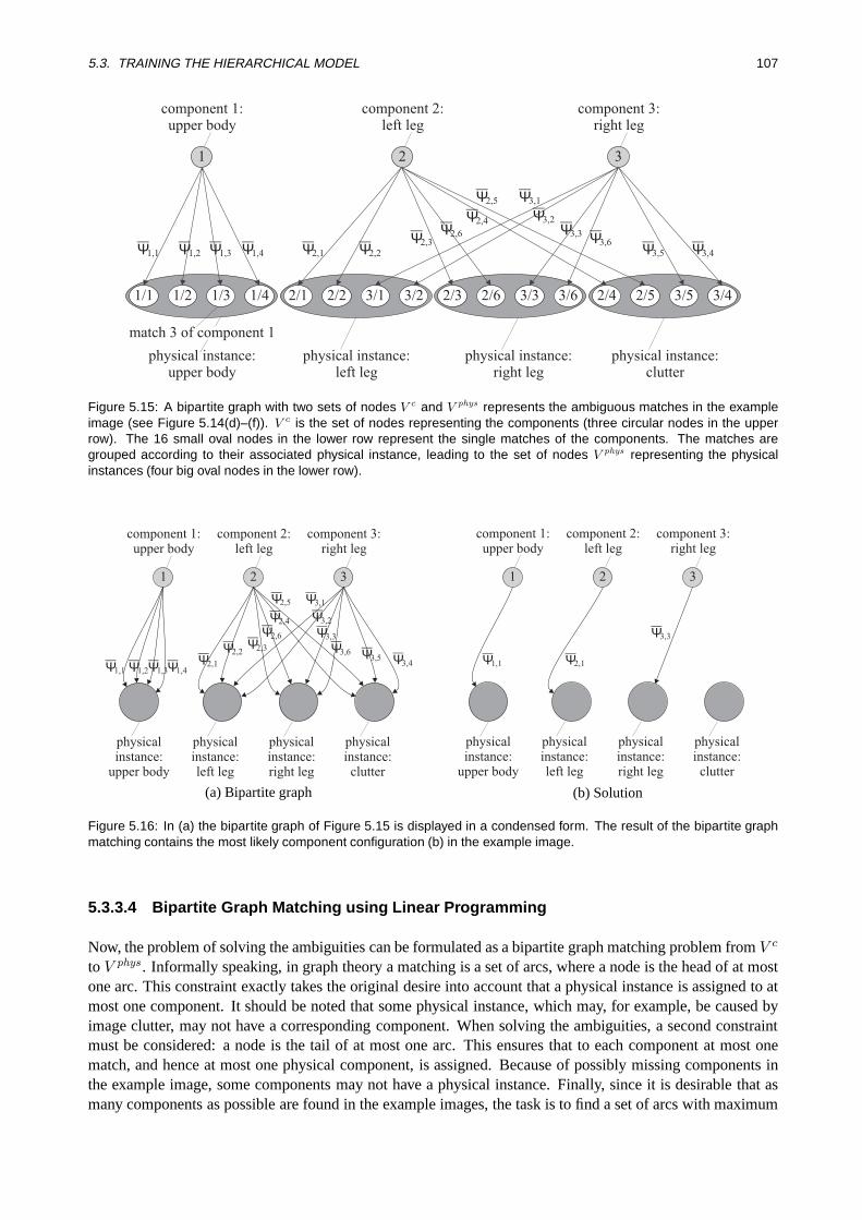
5.3. TRAINING THE HIERARCHICAL MODEL 107
1
1/1 1/2 1/3 1/4 2/1 2/2 3/1 3/2 2/3 2/6 3/3 3/6 2/4 2/5 3/5 3/4
2 3
physical instance:upper body
physical instance:left leg
physical instance:right leg
physical instance:clutter
match 3 of component 1
component 1:upper body
component 2:left leg
component 3:right leg
Ψ1,1 Ψ1,2 Ψ1,3 Ψ1,4 Ψ2,1 Ψ2,2
Ψ2,3Ψ2,6
Ψ2,4
Ψ2,5
Ψ3,5 Ψ3,4
Ψ3,1
Ψ3,2
Ψ3,3 Ψ3,6
Figure 5.15: A bipartite graph with two sets of nodes V c and V phys represents the ambiguous matches in the exampleimage (see Figure 5.14(d)–(f)). V c is the set of nodes representing the components (three circular nodes in the upperrow). The 16 small oval nodes in the lower row represent the single matches of the components. The matches aregrouped according to their associated physical instance, leading to the set of nodes V phys representing the physicalinstances (four big oval nodes in the lower row).
1 2 3
physicalinstance:
upper body
component 1:upper body
component 2:left leg
component 3:right leg
Ψ1,1 Ψ1,2Ψ1,3Ψ1,4Ψ2,1
Ψ2,2Ψ2,3
Ψ2,6
Ψ2,4
Ψ2,5
Ψ3,5 Ψ3,4
Ψ3,1
Ψ3,2
Ψ3,3
Ψ3,6
physicalinstance:left leg
physicalinstance:right leg
physicalinstance:clutter
1 2 3
physicalinstance:
upper body
component 1:upper body
component 2:left leg
component 3:right leg
Ψ1,1 Ψ2,1
Ψ3,3
physicalinstance:left leg
physicalinstance:right leg
physicalinstance:clutter
(a) Bipartite graph (b) Solution
Figure 5.16: In (a) the bipartite graph of Figure 5.15 is displayed in a condensed form. The result of the bipartite graphmatching contains the most likely component configuration (b) in the example image.
5.3.3.4 Bipartite Graph Matching using Linear Programming
Now, the problem of solving the ambiguities can be formulated as a bipartite graph matching problem fromV c
to V phys . Informally speaking, in graph theory a matching is a set of arcs, where a node is the head of at mostone arc. This constraint exactly takes the original desire into account that a physical instance is assigned to atmost one component. It should be noted that some physical instance, which may, for example, be caused byimage clutter, may not have a corresponding component. When solving the ambiguities, a second constraintmust be considered: a node is the tail of at most one arc. This ensures that to each component at most onematch, and hence at most one physical component, is assigned. Because of possibly missing components inthe example image, some components may not have a physical instance. Finally, since it is desirable that asmany components as possible are found in the example images, the task is to find a set of arcs with maximum
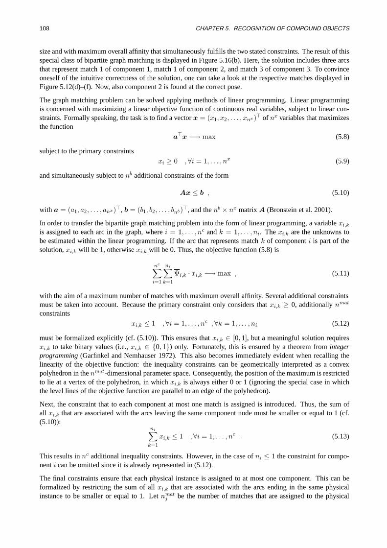
108 CHAPTER 5. RECOGNITION OF COMPOUND OBJECTS
size and with maximum overall affinity that simultaneously fulfills the two stated constraints. The result of thisspecial class of bipartite graph matching is displayed in Figure 5.16(b). Here, the solution includes three arcsthat represent match 1 of component 1, match 1 of component 2, and match 3 of component 3. To convinceoneself of the intuitive correctness of the solution, one can take a look at the respective matches displayed inFigure 5.12(d)–(f). Now, also component 2 is found at the correct pose.
The graph matching problem can be solved applying methods of linear programming. Linear programmingis concerned with maximizing a linear objective function of continuous real variables, subject to linear con-straints. Formally speaking, the task is to find a vectorx = (x1, x2, . . . , xnx)> of nx variables that maximizesthe function
a>x −→ max (5.8)
subject to the primary constraints
xi ≥ 0 ,∀i = 1, . . . , nx (5.9)
and simultaneously subject tonb additional constraints of the form
Ax ≤ b , (5.10)
with a = (a1, a2, . . . , anx)>, b = (b1, b2, . . . , bnb)>, and thenb × nx matrixA (Bronstein et al. 2001).
In order to transfer the bipartite graph matching problem into the form of linear programming, a variablexi,k
is assigned to each arc in the graph, wherei = 1, . . . , nc andk = 1, . . . , ni. Thexi,k are the unknowns tobe estimated within the linear programming. If the arc that represents matchk of componenti is part of thesolution,xi,k will be 1, otherwisexi,k will be 0. Thus, the objective function (5.8) is
nc∑i=1
ni∑k=1
Ψi,k · xi,k −→ max , (5.11)
with the aim of a maximum number of matches with maximum overall affinity. Several additional constraintsmust be taken into account. Because the primary constraint only considers thatxi,k ≥ 0, additionallynmat
constraints
xi,k ≤ 1 ,∀i = 1, . . . , nc ,∀k = 1, . . . , ni (5.12)
must be formalized explicitly (cf. (5.10)). This ensures thatxi,k ∈ [0,1], but a meaningful solution requiresxi,k to take binary values (i.e.,xi,k ∈ 0,1) only. Fortunately, this is ensured by a theorem fromintegerprogramming(Garfinkel and Nemhauser 1972). This also becomes immediately evident when recalling thelinearity of the objective function: the inequality constraints can be geometrically interpreted as a convexpolyhedron in thenmat -dimensional parameter space. Consequently, the position of the maximum is restrictedto lie at a vertex of the polyhedron, in whichxi,k is always either 0 or 1 (ignoring the special case in whichthe level lines of the objective function are parallel to an edge of the polyhedron).
Next, the constraint that to each component at most one match is assigned is introduced. Thus, the sum ofall xi,k that are associated with the arcs leaving the same component node must be smaller or equal to 1 (cf.(5.10)):
ni∑k=1
xi,k ≤ 1 ,∀i = 1, . . . , nc . (5.13)
This results innc additional inequality constraints. However, in the case ofni ≤ 1 the constraint for compo-nenti can be omitted since it is already represented in (5.12).
The final constraints ensure that each physical instance is assigned to at most one component. This can beformalized by restricting the sum of allxi,k that are associated with the arcs ending in the same physicalinstance to be smaller or equal to 1. Letnmat
j be the number of matches that are assigned to the physical

5.3. TRAINING THE HIERARCHICAL MODEL 109
(a) Model image (b) Example images
Figure 5.17: Ambiguities solved by linear programming. The model image and the reference component configuration isshown in (a). Similar components are distinguished by different line widths for visualization purposes. For each exampleimage the result of the linear programming assigns an unambiguous pose to each component (b).
instancej and letxi,k(j, l) be the variablexi,k that represents thel-th match that is assigned to the physicalinstancej. Then the constraint can be formalized as (cf. (5.10)):
nmatj∑
l=1
xi,k(j, l) ≤ 1 ,∀j = 1, . . . , nphys . (5.14)
Thus, the resulting linear programming problem is described by the objective function (5.11), which mustbe maximized subject to the constraints described by (5.12)–(5.14). Several efficient standard algorithms areavailable in the literature for linear programming. One of the most popular representatives is thesimplexmethod(Press et al. 1992, Bronstein et al. 2001). Although it has been proven that its theoretically worstcase runtime complexity is exponential, it merely shows polynomial time complexity on average for practicalproblems. Nevertheless, several “true” polynomial-time algorithms have been developed, e.g., (Karmarkar1984). Since the description of one of these algorithms would go beyond the scope of this dissertation thereader is referred to the literature. Finally, the result of the linear programming provides a value for eachxi,k
that is either 0 or 1. In the present example, allxi,k are returned as 0 exceptx1,1, x2,1, andx3,3, which arereturned as 1, as one would expect (see Figure 5.16(b)).
It should be noted that the algorithm is able to handle missing components by choosing the constraints inthe proposed way. However, it requires that at most one instance of the compound object is present in eachexample image since otherwise the algorithm would pick out the best component matches from differentinstances.
Returning to the original example, the ambiguities are solved for each example image individually accordingto the above described method. Hence, a unique pose for each component in each example image is obtained.The final result for all example images is shown in Figure 5.17. The unique poses are stored within thene×nc
component pose matrix.
By solving the ambiguities during the training of the hierarchical model the correspondence problem thatwould arise during the online phase when searching the object parts independently from each other is already

110 CHAPTER 5. RECOGNITION OF COMPOUND OBJECTS
implicitly solved within the hierarchical model. Thus, one can say that the correspondence problem is shiftedfrom the online to the offline phase with the considerable advantage that a real-time recognition of compoundobjects is made possible.
5.3.4 Extraction of Object Parts
The rigid parts of the compound object may be represented by several single components because of theover-segmentation during the initial decomposition. Therefore, the initial components that belong to the samerigid object part, and hence exhibit identical apparent movement over all example images, can be mergedby analyzing the unique poses obtained in the previous section. The merged components represent the rigidobject parts. The strategy comprises two steps. In the first step, for each pair of componentsi1 and i2 theprobability that the two components belong to the same object part is computed in a statistically foundedmanner, resulting in a square probability matrix of sizenc × nc. In the second step, the probability matrix isclustered using a pairwise clustering algorithm. The obtained clusters represent the desired object parts.
Let Mi1 = (omi1, ϕm
i1) with position om
i1= (xm
i1, ym
i1)> be the pose of componenti1 in the model image
andEi1 = (oei1, ϕe
i1) with positionoe
i1= (xe
i1, ye
i1)> the corresponding unique pose in the example image.
Accordingly, the poses of a second componenti2 areMi2 andEi2, respectively. Furthermore, assume thataccuracy information is available for each pose. The accuracies are represented by the 3× 3 covariancematricesKe
i1andKe
i2, which contain the variances and covariances ofx, y, andϕ. If the used recognition
method does not return any accuracy information for the pose parameters, the accuracy must be specifiedempirically (e.g., by applying tests with various objects of different size and shape). The reference position andorientation of the components in the model image are assumed to be error-free. Starting with this information,the probability that the two components belong to the same object part can be computed.
At first, the parametersα andt of the rigid transformation that transformMi1 intoEi1 are computed (cf. (5.1)and (5.2) in Section 5.3.3.1). By applying the transformation to the poseMi2 the projected poseE′i2
ofcomponenti2 in the example image is obtained (cf. (5.3) and (5.4) in Section 5.3.3.1). The assumptionthat both components belong to the same object part would require that componenti1 and i2 have movedidentically with respect to the model image, and henceE′i2
= Ei2. In general, this requirement is not fulfilled,even for components of the same object part because of the limited accuracy of the object recognition method.One method to get a kind of probability value for the current pair of components is to compute a distancemeasure betweenE′i2
andEi2. The drawback of this method is that it is hard to decide up to which distancethe components can be treated as belonging to the same part. A better result can be obtained by computing areal probability valuepi1,i2 ∈ [0,1]. This is achieved by applying methods of hypothesis testing. Stating thehypothesisE′i2
= Ei2 requires
xei2′ − xe
i2 = 0 (5.15)
yei2′ − ye
i2 = 0 (5.16)
ϕei2′ − ϕe
i2 = 0 . (5.17)
The hypothesis can be rewritten in matrix formHx = w, where
H =
1 0 0 −1 0 0
0 1 0 0 −1 00 0 1 0 0 −1
,x = (xe
i2′, ye
i2′, ϕe
i2′, xe
i2 , yei2 , ϕ
ei2)
>,w =
0
00
. (5.18)
For further processing, the covariance matrixKei2
′ of the projected poseE′i2is needed. It can be obtained
by applying the law of error propagation to the covariance matrixKei1
with respect to equations (5.1)–(5.4):Ke
i2
′ = AKei1A>. Here,A is the 3× 3 Jacobian matrix, which contains the partial derivatives of the pose

5.3. TRAINING THE HIERARCHICAL MODEL 111
parameters inE′i2with respect to the pose parameters inEi1. After some simplifications,A reads as follows:
A =
1 0 ∆x1,2 sin ∆ϕm,e + ∆y1,2 cos ∆ϕm,e
0 1 −∆x1,2 cos ∆ϕm,e + ∆y1,2 sin ∆ϕm,e
0 0 1
, (5.19)
with ∆x1,2 = xmi2− xm
i1, ∆y1,2 = ym
i2− ym
i1, and∆ϕm,e = ϕe
i1− ϕm
i1. Now, the associated covariance matrix
of x can be composed:
Kxx =
(Ke
i2′ 0
0 Kei2
), (5.20)
where0 represents a 3× 3 zero matrix.
With the results obtained by the previous calculations all information to perform the actual hypothesis testingis available. At first, a test valueT is computed (Koch 1987):
T =1r(Hx)>(HKxxH>)−1Hx , (5.21)
wherer = 3 denotes the number of equations in the hypothesis (5.15)–(5.17). The test valueT ∼ Fm,n hasa (Fisher)F -distribution with the parametersm andn denoting the degrees of freedom. The parametermcorresponds to the number of equationsr and the parametern to the redundancy involved in computing theaccuracies of the pose parameters. If a value forn is not available, e.g., because the accuracy informationhas been obtained by empirically tests instead of a preceding parameter adjustment, it is assumed that theaccuracies have been determined by using an infinite large set of samples. Consequently,n → ∞ and theF distribution degenerates to theχ2-distribution withT · r ∼ χ2
r. Hence, the probabilitypi1,i2 that the twocomponents belong to the same object part can be written as
pi1,i2 = 1−T∫
−∞Fr,n(t) dt n→∞= 1−
T ·r∫−∞
χ2r(t) dt , (5.22)
with Fr,n(t) andχ2r(t) representing the probability density function of the respective distributions. For prac-
tical considerations, the evaluation of (5.22) can be reduced to the calculation of the associated incompletegamma function (Press et al. 1992).
The probability matrix that is obtained by repeating the computations for each directed pair of components isnot symmetric, i.e.,pi1,i2 6= pi2,i1. This at first glance non-intuitive observation becomes evident when exam-ining the transformation described by (5.1)–(5.4) more closely. The small example in Figure 5.18 facilitatesthe discussion. Assume that the pose of the two components shown in Figure 5.18(a) are determined in theexample image shown in Figure 5.18(b). In the first step, the poses of component 1 in the model image andthe example image, respectively, are used to compute the rigid transformation parameters (i.e.,i1 = 1). Inthe second step, component 2 is projected into the example image using the calculated transformation (i.e.,i2 = 2). The projected pose of component 2 only differs in orientation from its true pose (see Figure 5.18(c)).A different observation can be made if component 2 is used to compute the transformation parameters andcomponent 1 is projected accordingly (i.e.,i1 = 2, i2 = 1). The projected pose of component 1 not onlydiffers in orientation but additionally differs in position from its true pose. Hence, in the second case the asso-ciateddirectedprobability value is significantly lower. In order to receive a symmetricundirectedprobabilitymeasure, the minimum of both corresponding directed probabilities is taken since a rigid object simultane-ously requires that both directed probability values are small. Finally, because a high probability value isrequired for components of the same object part in all images, either the minimum value or a more robustquantile value over all example images is computed. Consequently, another demand on the example imagescan be derived. Assume that the minimum probability value is decisive. If in all example images two objectparts accidently move in the same manner, then the algorithm will mistakenly assume that the two parts can

112 CHAPTER 5. RECOGNITION OF COMPOUND OBJECTS
1
2
(a) Model image (b) Example image (c) i1 = 1 (d) i1 = 2
Figure 5.18: Non-symmetry of relative movement. The poses of the two components that are extracted from the modelimage (a) are uniquely determined in the example image (b). In (c) component 2 is projected according to the pose ofcomponent 1. The true and projected pose only differ in orientation. However, when projecting component 1 according tothe pose of component 2, additionally a translation difference occurs (d).
1.00.80.60.40.20.0
(1)(2)(3)(4)(5)(6)(7)(8)(9)
(10)(11)(12)(13)(14)(15)(16)(17)(18)
HatFace
Left armOuter square
Right armInner square
"O""b""j""e""c""t"
Left handRight hand
Left legRight legLeft foot
Right foot
(2)
(3)
(4)
(5)
(6)
(7)
(8)
(9)
(10
)(1
1)
(12
)(1
3)
(14
)(1
5)
(16
)(1
7)
(18
)
Fac
eL
eft
arm
Ou
ter
squ
are
Rig
ht
arm
Inn
ersq
uar
e"O
""b
""j
""e
""c
""t
"L
eft
han
dR
igh
th
and
Lef
tle
gR
igh
tle
gL
eft
foo
tR
igh
tfo
ot
(1)
Hat
3
1 2
4
9
5 6
7 8
10
(a) Probability matrix (b) Object parts
Figure 5.19: The symmetric probability matrix contains information about the probability that a pair of components belongsto the same rigid object part (a). After clustering the matrix, ten rigid object parts are obtained (b). It should be noted thatthe numbers in (a) representing the components and the numbers in (b) representing the obtained object parts must notbe confused.
be combined in one rigid part. Therefore, different object parts must show a relative movement in at least oneexample image in order to be detected as two separate object parts.
In Figure 5.19(a) the finally obtained symmetric probability matrix is shown after computing the minimumover all example images. One can see that the pairwise probability for belonging to the same object part ishigh for the hat and the face as well as for the components forming the upper body. In contrast, the remainingprobabilities are approximately zero.
In the second step the components are partitioned into groups, orclusters, such that the probability betweencomponents in the same cluster is high and the probability between components in different clusters is small.

5.3. TRAINING THE HIERARCHICAL MODEL 113
The clusters finally represent the rigid object parts. In the following, the computed probability matrix is alsoreferred to as a similarity matrix, where the similarity expresses the rigidity between components. Manydifferent clustering algorithms for similarity matrices, or dissimilarity matrices, respectively, have becomeavailable. A comprehensive overview is given in (Jain et al. 1999). To find the rigid object parts, a hierarchicalagglomerative clustering algorithm is applied to the similarity matrix (actually, it is sufficient to take the uppertriangular matrix into account):
1. Initializenc clusters, each containing one component.2. Find the maximum entry in similarity matrix. If the maximum similarity is less than a thresholdpmin ,
return clusters and stop calculation.3. Merge associated pair of clusters into one cluster.4. Update similarity matrix to reflect the merge operation.5. If at least two clusters are left, go to step 2, else return clusters.
The update of the similarity matrix stated in step 3 means recalculating the similarity values between thenew cluster and the remaining clusters using a certainlinkage metric. The linkage metric characterizes thesimilarity between a pair of clusters. The most popular methods either use thesingle-link, average-link, orcomplete-linkalgorithm (Berkhin 2002). In the single-link algorithm, the similarity between two clusters isthe maximum of the similarities between all pairs of components drawn from the two clusters. Accordingly,the complete-link algorithm takes the minimum similarity and the average-link algorithm the average similar-ity. On the one hand, the complete-link algorithm is too stringent, and hence often fails to link componentsbelonging to the same object part. On the other hand, the single-link algorithm suffers from a chaining effect:in spite of a very low probability value the two associated components may be merged into the same clusterif the low probability is bridged by other components. In contrast, the average-link algorithm has proven tobe a suitable compromise, and hence is applied to cluster the components. Finally, the number of returnedclusters specifies the number of rigid object partsnp within the compound object. The result is shown inFigure 5.19(b), where the probability matrix of Figure 5.19(a) has been clustered using a thresholdpmin forthe probability of 0.5 (cf. step 2 of the clustering algorithm). The 18 components have been clustered into 10object parts. Now the hat and the face form one object part. Furthermore, the components of the upper bodybelong to the same object part.
Finally, for the object parts that consist of exactly one component the pose of the component is adopted bythe object part in each example image. For those object parts that consist of more than one component theposes must be explicitly determined. Simply taking the average pose over all involved components withina cluster would introduce errors. To avoid these errors, a new rigid model is created for the correspondingobject parts from the model image and used to search the object parts in all example images. This can berealized in a similar manner as for the components. However, the search can be focused on a very restrictedparameter space since an approximate pose is known. Therefore, the computational effort is negligible and noambiguities must be solved. After this step, for each rigid object part the pose parameters in each image areavailable and stored within thene × np part pose matrix for further analysis.
Some concluding remarks concerning the image rectification should be mentioned. In order to ensure a correctcomputation of the probability values, it is necessary that the model image and all example images are free ofdistortions. Therefore, it is essential that all images are rectified with the approach presented in Chapter 3 inorder to eliminate radial and projective distortions. Otherwise the distortions would lead to pseudo-movementsbetween components that belong to the same rigid object part, and hence would result in small probabilityvalues. Consequently, also the search images in the subsequent online phase must be rectified because theextraction of the relations, which will be described in the following section, is also based on the (rectified)example images. Nevertheless, in some very time-critical practical cases it may be desirable to refrain fromimage rectification. Therefore, if no significant projective distortions are present one can compensate existingradial distortions using one of two possibilities. The first possibility is to appropriately reduce the thresholdpmin for the probability value. The second possibility is to appropriately increase the standard deviations of

114 CHAPTER 5. RECOGNITION OF COMPOUND OBJECTS
the pose parameters, which are used in the hypothesis test. Consequently, small relative movements betweenobject parts cannot be distinguished from effects caused by the radial distortions any longer. However, ifno small movements must be expected and detected this is a suitable possibility in practice to avoid therectification and to further speed up the online phase.
5.3.5 Analysis of Relations between Object Parts
Now that the poses of the object parts are available in each example image, information about the relationsor the relative movements between the single object parts can be extracted. To compute the relation betweenobject partsi1 andi2, the pose of object parti2 is computed in the local coordinate system of object parti1.Let (oi1, ϕi1) and(oi2, ϕi2) be the poses of the two object parts in an example image or in the model image.The transformation into the local coordinate system can be described by a rotation matrixR with rotationangleα and a translationt:
α = −ϕi1 (5.23)
t = −R(α) · oi1 . (5.24)
The pose(oi2′, ϕi2
′) of object parti2 in the local coordinate system is obtained as:
oi2′ = R(α) · oi2 + t (5.25)
ϕi2′ = ϕi2 + α . (5.26)
If equations (5.23)–(5.26) are applied in the model image and all example images the relative movement ofparti2 with respect toi1 becomes available.
The extraction of the relations between two object parts is exemplified in Figure 5.20. Here, the pose of theright leg defines a local coordinate system into which the pose of the left arm is transformed for all images.The reference point of the transformed left arm describes a movement within the local coordinate system. Toquantify the position relation, the convex hull of the transformed reference points could be used. Hence, thepolygon of the convex hull would describe the border of the area within which the reference point of the leftarm is assumed to appear in the local coordinate system. Furthermore, the enclosing angle interval of theorientation of the transformed left arm is assumed to describe the orientation relation. On the one hand, theseassumptions imply that the example images cover the extrema of all possible relative movements. If it is notguaranteed that this requirement is fulfilled it is advisable to add appropriate tolerance values manually tothe automatically computed relations. Otherwise object parts could be missed during the search in the onlinephase. On the other hand, even one outlier could unnecessarily inflate the convex hull and the enclosing angleinterval, respectively. This would result in a sub-optimal online phase because of an increased computationtime. Although this is less critical in comparison to missing object parts, it sometimes is desirable to avoidoutliers by applying a statistically robust elimination of single extreme poses.
In the later online phase the left arm only needs to be searched within the parameter range described by therelations if the right leg has been found before. The number of polygon points in the convex hull may takevalues that correspond to the number of used images. Thus, the use of the convex hull would be accompaniedby a high computational load within the online phase. This is because all polygon points would have tobe transformed appropriately in order to compute the ROI in which the reference point is to be searched.Therefore, the smallest enclosing rectangle of arbitrary orientation is used instead to describe the positionrelation. Although the convex hull would be able to describe the relations in a less wasteful way, the rectangleis preferable also because the negligible loss in efficiency is justified by relaxed demands on the exampleimages.
Finally, the computations are repeated for each directed object pair and the extracted smallest rectangle and theorientation angle interval are stored within thenp × np relation matrix. The smallest rectangle is representedby its centroidcr
i1,i2, its semi axesar
i1,i2and bri1,i2
, and its orientationβri1,i2
. The orientation angle interval

5.4. CREATING THE HIERARCHICAL MODEL 115
i ,i1 2
r,max
i ,i1 2
r,minϕ
i ,i1 2
r
i ,i1 2
r
i ,i1 2
rb βi ,i1 2
r
Model imageExampleimage 1
Exampleimage 2
Exampleimage 3
Exampleimage 4
Exampleimage 5
Exampleimage 6
Transformation to local coordinate system of part 1
Convexhull
Smallest enclosingrectangle
Reference points
3
5
Model image
2
6
7
1
Relative positions Relative orientations
c
a
ϕ
Calculation of relative movement of part 2 (position and orientation)
Figure 5.20: Example showing the extraction of the relative movement of the left arm (i2) with respect to the right leg (i1).The position relation is described by the smallest enclosing rectangle of the reference points, the orientation relation bythe smallest enclosing angle interval.
is represented by its boundariesϕr ,mini1,i2
andϕr ,maxi1,i2
. Apart from the position and the orientation relationadditional information about the mean and the standard deviation of the relative movements are stored. Theresult is shown in Figure 5.21.
After this step, the training of the hierarchical model is completed. The result comprises the relation matrixas well as the ROIs of the object parts. Each ROI refers to the associated edge region of one object part in themodel image. The result represents the input data for creating the hierarchical model.
5.4 Creating the Hierarchical Model
5.4.1 Rigid Models for the Object Parts
The first step to create the hierarchical model is to generate a rigid model for each object part. Althoughalready during the training models have been created, the orientation range for which the models have beenbuilt does not necessarily coincide with the desired orientation range during the online phase. For example,the user may introduce prior knowledge about the possible orientation of the compound object in the search

116 CHAPTER 5. RECOGNITION OF COMPOUND OBJECTS
1m 2m 3m 4m 5m
6m 7m 8m 9m 10m
Figure 5.21: The relations of all pairs of object parts are visualized. Each picture represents an object part i1 for whichthe relative movements of the remaining parts i2 are displayed.
image. This is similar to the model creation for rigid object recognition (cf. Section 4.2.6) and may helpto keep the memory requirement of the model small. However, when dealing with compound objects thequestion arises how the orientation of a compound object is defined. In this dissertation the orientation of thecompound object is equated with the orientation of a user-specified reference object part. For the referencepart the user may specify the orientation range for which the associated rigid model should be created. Theorientation ranges of the remaining object parts are then automatically defined by the relations between theparts. Because the search order is unknown `a priori, a worst case estimation is used to get the orientationranges of the remaining object parts.
5.4.2 Optimum Search Trees
Based on the relations, an optimum hierarchical search strategy can be found by minimizing the computationalsearch effort in the online phase. One major part of the optimum hierarchical search strategy is representedby the optimum search trees. In this section, the definition and computation of the search trees is explained.
The relation between parti1 andi2 is used to compute the relative search effortΩri1,i2
that must be spent inorder to search parti2 relative to parti1. The computation of the search effort depends on the kind of appliedrigid object recognition method. If either the MGHT or the SBM is used the search effort is approximatelygiven by:
Ωri1,i2 = 2ar
i1,i2 · 2bri1,i2 · (ϕ
r ,maxi1,i2
− ϕr ,mini1,i2
) ·nm,top
i2
4nli2−1 ·∆ϕtop
i2
. (5.27)
The search effortΩri1,i2
is proportional to the area of the rectangle multiplied by the size of the orientation angleinterval, both given by the relations. Hence, this product represents the size of the continuous 3D parameterspace to be scanned. Because of the quantization of the parameter space and the use of image pyramids,the search effort of parti2 is reduced by a factor that depends on the number of pyramid levelsnl
i2and the
quantization of the orientation on the top pyramid level given by the orientation step∆ϕtopi2
. Finally, the search
effort increases linearly with the number of model edge pointsnm,topi2
that remain at the top pyramid level. Itshould be noted that the search effort is not symmetric, i.e.,Ωr
i1,i26= Ωr
i2,i1(for details see Figures 5.18 and
Figure 5.21 of Sections 5.3.4 and 5.3.5, respectively).
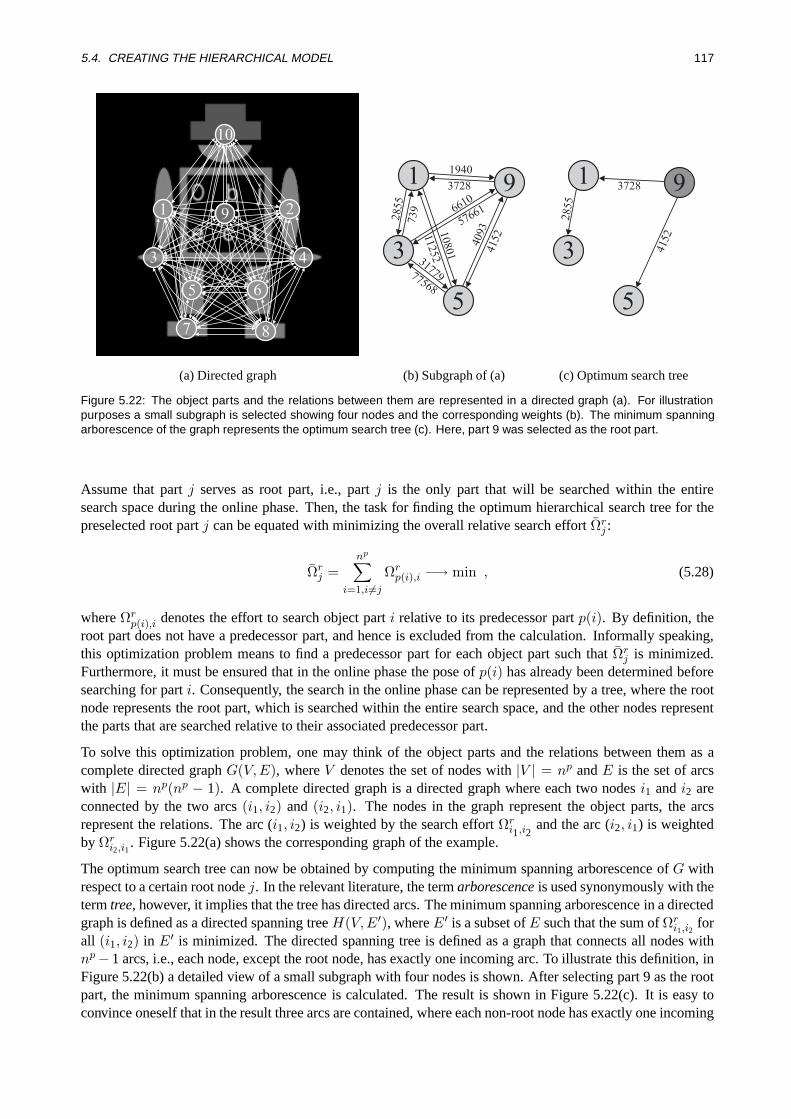
5.4. CREATING THE HIERARCHICAL MODEL 117
1 2
3 4
5 6
7 8
10
9
1
3
5
91940
2855
10801 4
152
77568
31779
739
3728
4093576616610
11252
1
3
5
9
2855
4152
3728
(a) Directed graph (b) Subgraph of (a) (c) Optimum search tree
Figure 5.22: The object parts and the relations between them are represented in a directed graph (a). For illustrationpurposes a small subgraph is selected showing four nodes and the corresponding weights (b). The minimum spanningarborescence of the graph represents the optimum search tree (c). Here, part 9 was selected as the root part.
Assume that partj serves as root part, i.e., partj is the only part that will be searched within the entiresearch space during the online phase. Then, the task for finding the optimum hierarchical search tree for thepreselected root partj can be equated with minimizing the overall relative search effortΩr
j :
Ωrj =
np∑i=1,i 6=j
Ωrp(i),i −→ min , (5.28)
whereΩrp(i),i denotes the effort to search object parti relative to its predecessor partp(i). By definition, the
root part does not have a predecessor part, and hence is excluded from the calculation. Informally speaking,this optimization problem means to find a predecessor part for each object part such thatΩr
j is minimized.Furthermore, it must be ensured that in the online phase the pose ofp(i) has already been determined beforesearching for parti. Consequently, the search in the online phase can be represented by a tree, where the rootnode represents the root part, which is searched within the entire search space, and the other nodes representthe parts that are searched relative to their associated predecessor part.
To solve this optimization problem, one may think of the object parts and the relations between them as acomplete directed graphG(V,E), whereV denotes the set of nodes with|V | = np andE is the set of arcswith |E| = np(np − 1). A complete directed graph is a directed graph where each two nodesi1 andi2 areconnected by the two arcs(i1, i2) and (i2, i1). The nodes in the graph represent the object parts, the arcsrepresent the relations. The arc (i1, i2) is weighted by the search effortΩr
i1,i2and the arc (i2, i1) is weighted
by Ωri2,i1
. Figure 5.22(a) shows the corresponding graph of the example.
The optimum search tree can now be obtained by computing the minimum spanning arborescence ofG withrespect to a certain root nodej. In the relevant literature, the termarborescenceis used synonymously with thetermtree, however, it implies that the tree has directed arcs. The minimum spanning arborescence in a directedgraph is defined as a directed spanning treeH(V,E′), whereE′ is a subset ofE such that the sum ofΩr
i1,i2for
all (i1, i2) in E′ is minimized. The directed spanning tree is defined as a graph that connects all nodes withnp− 1 arcs, i.e., each node, except the root node, has exactly one incoming arc. To illustrate this definition, inFigure 5.22(b) a detailed view of a small subgraph with four nodes is shown. After selecting part 9 as the rootpart, the minimum spanning arborescence is calculated. The result is shown in Figure 5.22(c). It is easy toconvince oneself that in the result three arcs are contained, where each non-root node has exactly one incoming

118 CHAPTER 5. RECOGNITION OF COMPOUND OBJECTS
1
3
5
9 1
3
5
9 1
3
5
9 1
3
5
9 1
3
5
91
3
5
9 1
3
5
9 1
3
5
9
1
3
5
9 1
3
5
9 1
3
5
9 1
3
5
9 1
3
5
9 1
3
5
9 1
3
5
9 1
3
5
9
Figure 5.23: All possible spanning arborescences of the subgraph shown in Figure 5.22(b) with part 9 as root part
arc and that the overall sum of weights associated with the result is 10735. This is the minimum weight amongall possible directed spanning arborescences rooted at part 9. For illustrative purposes Figure 5.23 shows allpossible spanning arborescences of the respective subgraph. As can be seen, there are 16 different ways toconnect the three nodes to the root node. The result of Figure 5.22(c) suggests that after the upper body (part 9)is found in the image, it is most efficient to search the left arm (part 1) and the left leg (part 5) relative to theupper body and to search the left hand (part 3) relative to the left arm.
The minimum spanning arborescence can be seen as the equivalent to the well-known minimum spanningtree in an undirected graph (ifΩr
i2,i1would be symmetric one would obtain a undirected graph). The two
most prominent algorithms to efficiently compute the minimum spanning tree are the Kruskal and the Primalgorithm (Graham and Hell 1985, Clark and Holton 1994). Unfortunately, these algorithms cannot be usedor even extended to cope with directed graphs. Solving the problem of finding the minimum spanning ar-borescence in a directed graph is much more complicated in comparison to solving the equivalent undirectedproblem. A polynomial algorithm for the minimum spanning arborescence was independently proposed in(Chu and Tseng-Hong 1965), (Edmonds 1967), and (Bock 1971). In (Tarjan 1977) and (Gabow et al. 1986),efficient implementations of the algorithm are presented. The implementation used in this dissertation is pre-sented in (Fischetti and Toth 1993). It makes use of simple data structures leading to a run time complexity ofonlyO(n2), wheren is the number of nodes in the graph. For a detailed description of the algorithm or of theimplementation the interested reader should refer to the cited literature.
Root Root
Root RootRoot
Ωr1 = 27 · 103 Ωr
2 = 28 · 103 Ωr3 = 25 · 103 Ωr
4 = 26 · 103 Ωr5 = 29 · 103
Root
Root Root
Root
Root
Ωr6 = 39 · 103 Ωr
7 = 29 · 103 Ωr8 = 39 · 103 Ωr
9 = 29 · 103 Ωr10 = 30 · 103
Figure 5.24: The minimum spanning arborescences for each of the ten object parts serving as root part and the associatedoverall search efforts are shown. Additionally, the relations between two adjacent nodes are superimposed.

5.4. CREATING THE HIERARCHICAL MODEL 119
It is obvious that for different root partsj different minimum spanning arborescences are obtained with dif-ferent overall weightsΩr
j . Therefore, for each root part the associated minimum spanning arborescence iscomputed. Figure 5.24 shows the result for each of the ten object parts serving as root part. It should benoted that although in this example the same two object parts are directly connected in all minimum spanningarborescences it is not necessarily the case in general.
5.4.3 Root Part Ranking
To complete the optimum hierarchical search strategy, the question remains, which part to choose as the rootpart. One criterion for a suitable root part is a small overall search effortΩr
j of the associated minimumspanning arborescences.
However,Ωrj only describes the search effort that must be spent during the relative search. Therefore, the
effort Ωrootj that must be spent to search the root partj itself must be considered as a second criterion:
Ωrootj = R · C · (ϕmax
j − ϕminj ) ·
nm,topj
4nlj−1 ·∆ϕtop
j
, (5.29)
whereR andC are the number of rows and columns in the search image, and hence describe the positionsearch range for the root object part, while(ϕmax
j − ϕminj ) describes the orientation angle search range.
As a third criterion the uniqueness of the root part must be considered. The root part should exhibit as fewsymmetries and as few similarities to other object parts as possible. Assume that the left leg (part 5) serves asroot part in the online phase and is searched within the full orientation search range. Because of its rotationsymmetry and its similarity to the right leg, it would be found at four different poses (ignoring possible clutterin the search image). When looking at the associated search tree the upper body and the left foot must besearched relative to each of the four poses of the left leg. Consequently, the search effort in the online phaseincreases with the number of symmetries and similarities. Therefore, the symmetries and similarities of allobject parts are determined using the analysis described in Section 5.3.3.2, which matches object partj toitself and to all other object parts. Assume that object partj has been foundnsym
j times on itself andnsimj
times on other object parts during the analysis. Then, the search effort of the relative searchΩrj must be
multiplied by (nsymj + nsim
j ) in order to approximately estimate the influence of the non-uniqueness of theroot part on the search effort. One could argue that it is sufficient to only multiply the relative search effort ofthe parts that are adjacent to the root part since the search can be aborted if the adjacent parts are not found.However, the multiplication of the overall relative search effort is legitimated since the object recognition,which will be described in Section 5.5, should be able to cope with occlusions. Thus, the search cannot bestopped if one object part is missing.
Finally, the search effortΩj that is associated with the root partj is obtained:
Ωj = Ωrootj + (nsym
j + nsimj )Ωr
j . (5.30)
By sorting the possible root parts with respect toΩj in ascending order one obtains a root part ranking thatexpresses the suitability of all object parts to serve as the root part. In Table 5.1 the respective ranking ofthe example is presented. It can be seen that the head (part 10) and the upper body (part 9) are best suitedto serve as the root part. This is because they both do not show any rotation symmetry or similarity to otherobject parts and because five pyramid levels can be used during the search. In contrast, taking one of the twohands (part 3 or part 4) as root part would result in the highest search effort: they both exhibit symmetries andmutual similarities. Furthermore, only three pyramid levels can be used because of their small size.
After this step, the creation of the hierarchical model is completed. However, a manual selection of the rootpart by the user is still reasonable. This is because the selection of a suitable root part also depends on theapplication (cf. Section 5.5.1). Therefore, the root part ranking is returned in order to help the user to select the
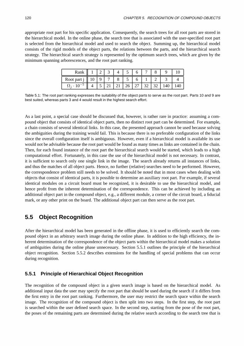
120 CHAPTER 5. RECOGNITION OF COMPOUND OBJECTS
appropriate root part for his specific application. Consequently, the search trees for all root parts are stored inthe hierarchical model. In the online phase, the search tree that is associated with the user-specified root partis selected from the hierarchical model and used to search the object. Summing up, the hierarchical modelconsists of the rigid models of the object parts, the relations between the parts, and the hierarchical searchstrategy. The hierarchical search strategy is represented by the optimum search trees, which are given by theminimum spanning arborescences, and the root part ranking.
Rank 1 2 3 4 5 6 7 8 9 10
Root part j 10 9 7 8 5 6 1 2 3 4
Ωj · 10−5 4 5 21 21 26 27 32 32 140 140
Table 5.1: The root part ranking expresses the suitability of the object parts to serve as the root part. Parts 10 and 9 arebest suited, whereas parts 3 and 4 would result in the highest search effort.
As a last point, a special case should be discussed that, however, is rather rare in practice: assuming a com-pound object that consists of identical object parts, then no distinct root part can be determined. For example,a chain consists of several identical links. In this case, the presented approach cannot be used because solvingthe ambiguities during the training would fail. This is because there is no preferable configuration of the linkssince the overall configuration itself is ambiguous. However, even if a hierarchical model is available its usewould not be advisable because the root part would be found as many times as links are contained in the chain.Then, for each found instance of the root part the hierarchical search would be started, which leads to a highcomputational effort. Fortunately, in this case the use of the hierarchical model is not necessary. In contrast,it is sufficient to search only one single link in the image. The search already returns all instances of links,and thus the matches of all object parts. Hence, no further (relative) searches need to be performed. However,the correspondence problem still needs to be solved. It should be noted that in most cases when dealing withobjects that consist of identical parts, it is possible to determine an auxiliary root part. For example, if severalidentical modules on a circuit board must be recognized, it is desirable to use the hierarchical model, andhence profit from the inherent determination of the correspondence. This can be achieved by including anadditional object part in the compound object, e.g., a different module, a corner of the circuit board, a fiducialmark, or any other print on the board. The additional object part can then serve as the root part.
5.5 Object Recognition
After the hierarchical model has been generated in the offline phase, it is used to efficiently search the com-pound object in an arbitrary search image during the online phase. In addition to the high efficiency, the in-herent determination of the correspondence of the object parts within the hierarchical model makes a solutionof ambiguities during the online phase unnecessary. Section 5.5.1 outlines the principle of the hierarchicalobject recognition. Section 5.5.2 describes extensions for the handling of special problems that can occurduring recognition.
5.5.1 Principle of Hierarchical Object Recognition
The recognition of the compound object in a given search image is based on the hierarchical model. Asadditional input data the user may specify the root part that should be used during the search if it differs fromthe first entry in the root part ranking. Furthermore, the user may restrict the search space within the searchimage. The recognition of the compound object is then split into two steps. In the first step, the root partis searched within the user defined search space. In the second step, starting from the pose of the root part,the poses of the remaining parts are determined during the relative search according to the search tree that is

5.5. OBJECT RECOGNITION 121
associated with the specified root part. As another parameter, the search order that is applied to the searchtree can be chosen to be, e.g., breadth-first search or depth-first search (see Figure 5.8(a) in Section 5.2). Thesearch order assigns each object part a number that describes its position within the search order.
Despite the automatically computed root part ranking, a manual selection of the root part may still be rea-sonable. This is because the computation of the root part ranking is only based on the endeavor to minimizethe search effort. However, the selection of the root part not only affects the computation time, but the rootpart plays another decisive role in the case of occlusions or missing object parts: it is important that the rootpart of the compound object instance in the search image is recognized. If the root part cannot be recognized,e.g., because of occlusions or because it is missing in the search image, then the recognition of the remainingparts becomes more difficult. Therefore, in case severe occlusions or missing parts must be expected, theuser should ensure to select a root part that is not only accompanied by a small search effort but also by ahigh possibility to be recognized. Because this selection depends on the object and the application, and thusrequires background information, it cannot be automated. Nevertheless, for the case that no such prominentobject part can be specified, e.g., because all object parts are approximately equal, in Section 5.5.2.4 a solutionthat is able to cope with the case of a missing root part is proposed.
In the following, the principle of the hierarchical recognition is explained in more detail. Letqi, i = 1, . . . , np
be the object part at positioni within the search order andpi, i = 2, . . . , np be the associated predecessor partwithin the search tree. For example, the root part is at the first position within the search order, and hence isrepresented byq1. It should be noted that the root part does not have a predecessor part in the search tree.The aim of the recognition is to return one hierarchical match for each instance of the compound object in thesearch image. A hierarchical match comprises the matches of all object parts that belong to the same objectinstance. Therefore, it contains at most one pose for each object part. Each match of the root part instantiatesone hierarchical match, which at this time only contains the respective pose of the root part. Then, accordingto the search order the next object partqi is successively selected. The search space for partqi is calculatedbased on the pose of the associated predecessor partpi. The search space is split into the position searchspace for the reference point and the orientation search space. The position search space is described by therectangle that is given by the position relation between partpi andqi transformed according to the pose of partpi. Accordingly, the orientation search space is given by the transformed orientation relation. Let(os
pi, ϕs
pi) be
the pose of the predecessor part in the search image. Then the position search space for partqi is representedby the rectangle that is described by the parameterscqi , aqi , bqi , andβqi :
cqi = ospi
+ R(ϕspi
)crpi,qi
(5.31)
aqi = arpi,qi
(5.32)
bqi = brpi,qi(5.33)
βqi = ϕspi
+ βrpi,qi
. (5.34)
The orientation search space is described by the angle interval[ϕminqi
, ϕmaxqi
]:
ϕminqi
= ϕspi
+ ϕr ,minpi,qi
(5.35)
ϕmaxqi
= ϕspi
+ ϕr ,maxpi,qi
. (5.36)
Finally, partqi is searched by scanning the computed search space. The obtained pose is stored within thehierarchical match. If there are several hierarchical matches (e.g., because multiple instances of the rootpart have been found) the search space is computed for each hierarchical match separately. This process issuccessively repeated for all object parts.
To rate the quality of the hierarchical match, a score values is computed by weighting the returned scorevaluessqi of the single object parts:
s =np∑i=1
fqisqi , (5.37)
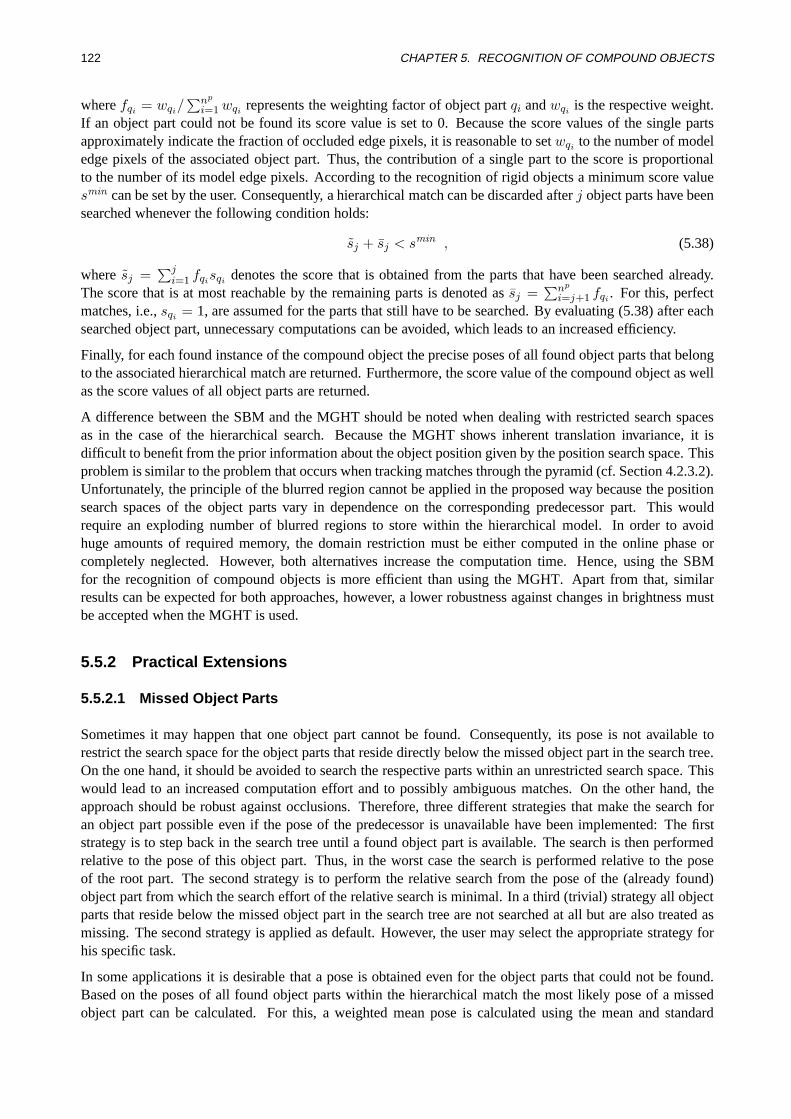
122 CHAPTER 5. RECOGNITION OF COMPOUND OBJECTS
wherefqi = wqi/∑np
i=1wqi represents the weighting factor of object partqi andwqi is the respective weight.If an object part could not be found its score value is set to 0. Because the score values of the single partsapproximately indicate the fraction of occluded edge pixels, it is reasonable to setwqi to the number of modeledge pixels of the associated object part. Thus, the contribution of a single part to the score is proportionalto the number of its model edge pixels. According to the recognition of rigid objects a minimum score valuesmin can be set by the user. Consequently, a hierarchical match can be discarded afterj object parts have beensearched whenever the following condition holds:
sj + sj < smin , (5.38)
wheresj =∑j
i=1 fqisqi denotes the score that is obtained from the parts that have been searched already.The score that is at most reachable by the remaining parts is denoted assj =
∑np
i=j+1 fqi . For this, perfectmatches, i.e.,sqi = 1, are assumed for the parts that still have to be searched. By evaluating (5.38) after eachsearched object part, unnecessary computations can be avoided, which leads to an increased efficiency.
Finally, for each found instance of the compound object the precise poses of all found object parts that belongto the associated hierarchical match are returned. Furthermore, the score value of the compound object as wellas the score values of all object parts are returned.
A difference between the SBM and the MGHT should be noted when dealing with restricted search spacesas in the case of the hierarchical search. Because the MGHT shows inherent translation invariance, it isdifficult to benefit from the prior information about the object position given by the position search space. Thisproblem is similar to the problem that occurs when tracking matches through the pyramid (cf. Section 4.2.3.2).Unfortunately, the principle of the blurred region cannot be applied in the proposed way because the positionsearch spaces of the object parts vary in dependence on the corresponding predecessor part. This wouldrequire an exploding number of blurred regions to store within the hierarchical model. In order to avoidhuge amounts of required memory, the domain restriction must be either computed in the online phase orcompletely neglected. However, both alternatives increase the computation time. Hence, using the SBMfor the recognition of compound objects is more efficient than using the MGHT. Apart from that, similarresults can be expected for both approaches, however, a lower robustness against changes in brightness mustbe accepted when the MGHT is used.
5.5.2 Practical Extensions
5.5.2.1 Missed Object Parts
Sometimes it may happen that one object part cannot be found. Consequently, its pose is not available torestrict the search space for the object parts that reside directly below the missed object part in the search tree.On the one hand, it should be avoided to search the respective parts within an unrestricted search space. Thiswould lead to an increased computation effort and to possibly ambiguous matches. On the other hand, theapproach should be robust against occlusions. Therefore, three different strategies that make the search foran object part possible even if the pose of the predecessor is unavailable have been implemented: The firststrategy is to step back in the search tree until a found object part is available. The search is then performedrelative to the pose of this object part. Thus, in the worst case the search is performed relative to the poseof the root part. The second strategy is to perform the relative search from the pose of the (already found)object part from which the search effort of the relative search is minimal. In a third (trivial) strategy all objectparts that reside below the missed object part in the search tree are not searched at all but are also treated asmissing. The second strategy is applied as default. However, the user may select the appropriate strategy forhis specific task.
In some applications it is desirable that a pose is obtained even for the object parts that could not be found.Based on the poses of all found object parts within the hierarchical match the most likely pose of a missedobject part can be calculated. For this, a weighted mean pose is calculated using the mean and standard
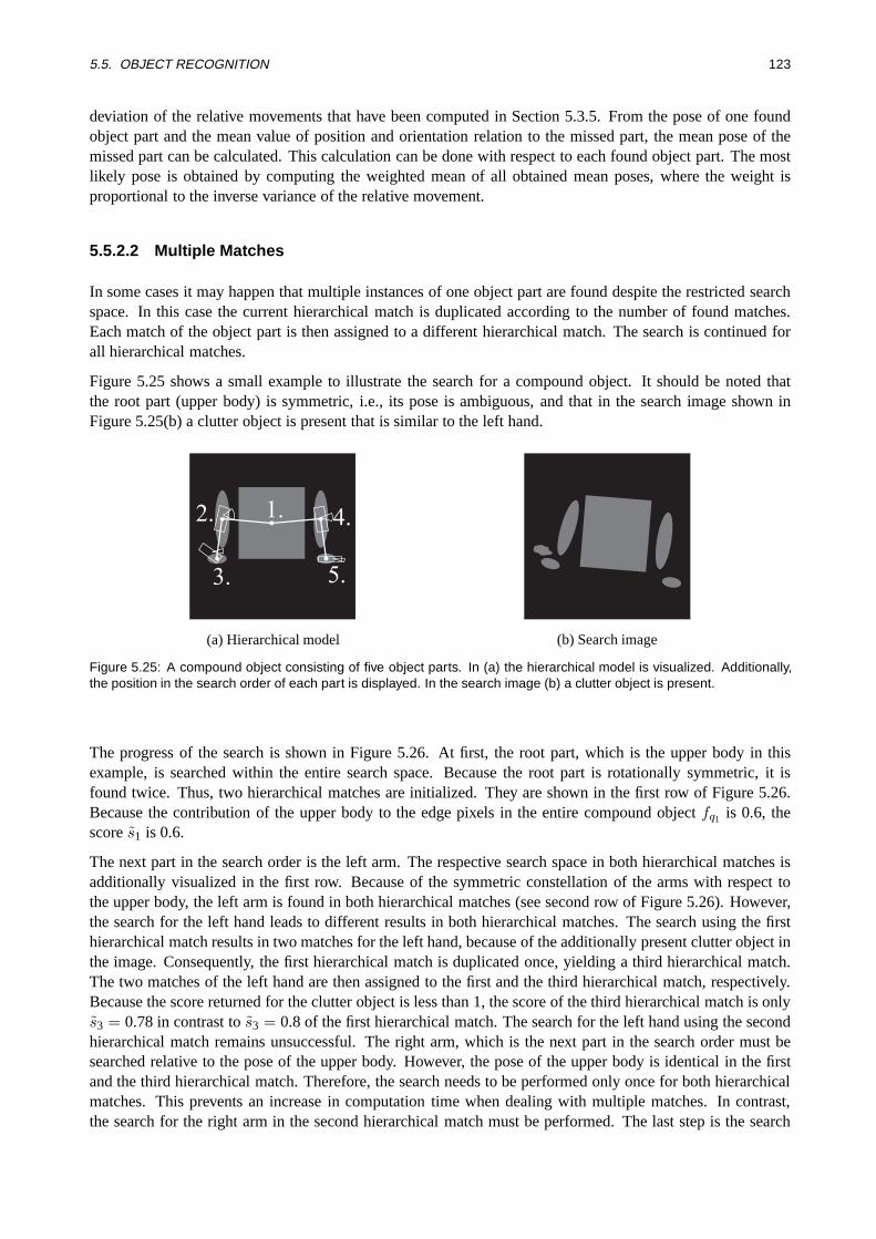
5.5. OBJECT RECOGNITION 123
deviation of the relative movements that have been computed in Section 5.3.5. From the pose of one foundobject part and the mean value of position and orientation relation to the missed part, the mean pose of themissed part can be calculated. This calculation can be done with respect to each found object part. The mostlikely pose is obtained by computing the weighted mean of all obtained mean poses, where the weight isproportional to the inverse variance of the relative movement.
5.5.2.2 Multiple Matches
In some cases it may happen that multiple instances of one object part are found despite the restricted searchspace. In this case the current hierarchical match is duplicated according to the number of found matches.Each match of the object part is then assigned to a different hierarchical match. The search is continued forall hierarchical matches.
Figure 5.25 shows a small example to illustrate the search for a compound object. It should be noted thatthe root part (upper body) is symmetric, i.e., its pose is ambiguous, and that in the search image shown inFigure 5.25(b) a clutter object is present that is similar to the left hand.
1.
3.
2. 4.
5.
(a) Hierarchical model (b) Search image
Figure 5.25: A compound object consisting of five object parts. In (a) the hierarchical model is visualized. Additionally,the position in the search order of each part is displayed. In the search image (b) a clutter object is present.
The progress of the search is shown in Figure 5.26. At first, the root part, which is the upper body in thisexample, is searched within the entire search space. Because the root part is rotationally symmetric, it isfound twice. Thus, two hierarchical matches are initialized. They are shown in the first row of Figure 5.26.Because the contribution of the upper body to the edge pixels in the entire compound objectfq1 is 0.6, thescores1 is 0.6.
The next part in the search order is the left arm. The respective search space in both hierarchical matches isadditionally visualized in the first row. Because of the symmetric constellation of the arms with respect tothe upper body, the left arm is found in both hierarchical matches (see second row of Figure 5.26). However,the search for the left hand leads to different results in both hierarchical matches. The search using the firsthierarchical match results in two matches for the left hand, because of the additionally present clutter object inthe image. Consequently, the first hierarchical match is duplicated once, yielding a third hierarchical match.The two matches of the left hand are then assigned to the first and the third hierarchical match, respectively.Because the score returned for the clutter object is less than 1, the score of the third hierarchical match is onlys3 = 0.78 in contrast tos3 = 0.8 of the first hierarchical match. The search for the left hand using the secondhierarchical match remains unsuccessful. The right arm, which is the next part in the search order must besearched relative to the pose of the upper body. However, the pose of the upper body is identical in the firstand the third hierarchical match. Therefore, the search needs to be performed only once for both hierarchicalmatches. This prevents an increase in computation time when dealing with multiple matches. In contrast,the search for the right arm in the second hierarchical match must be performed. The last step is the search

124 CHAPTER 5. RECOGNITION OF COMPOUND OBJECTS
search 1st part
search 2nd part
search 3rd part
search 4th part
search 5th part
s=
0.7
52 s=
0.7
52
s=
0.7
53
s=
0.9
04
s=
0.6
01 s=
0.6
01
s=
0.8
03 s=
0.7
83
s=
0.9
34s=
0.9
54
ss
=1.0
0=
5
1(q )
2(q )
3(q )
4(q )
5(q )
start search
1 2
1 2
1 23
1 23
1 23
number of thehierachical match
∼∼ ∼
∼
∼ ∼ ∼∼∼∼
∼
ss
=0.9
8=
5∼ 5∼s
s=
0.9
=
Figure 5.26: Search for the compound object using the hierarchical model. Found instances of object parts are rep-resented by white edges. The orientation of the match is displayed as a white arrow. The search space is displayedusing white rectangles and circle sectors. After the j-th part has been searched, the score sj is computed (fq1 = 0.60,fq2 = 0.15,fq3 = 0.05, fq4 = 0.15, and fq5 = 0.05).
for the right hand. Finally, three hierarchical matches are returned. The first and the third hierarchical matchonly differ in the match of the left hand. Therefore, the two corresponding scores (s = 1.00 ands = 0.98)differ only slightly. The second hierarchical match represents a rotated instance of the compound object withoccluded hands. Consequently, the corresponding score is lower (s = 0.90).
5.5.2.3 Elimination of Overlapping Matches
Sometimes it is desirable that hierarchical matches that represent the same instance of the object are elim-inated. In the previous example (cf. Section 5.5.2.2), only the first hierarchical match should be returned.

5.5. OBJECT RECOGNITION 125
Therefore, in a subsequent step after the search, the hierarchical matches are checked for mutual overlap.If the overlap fraction between two hierarchical matches exceeds a user-specified threshold the hierarchicalmatch with the lower score is eliminated. To compute the overlap fraction, the object part matches are rep-resented by their smallest enclosing rectangle. For each hierarchical match the union region of the smallestenclosing rectangles of all object part matches is computed. The overlap is computed by intersecting the unionregions of two hierarchical matches. The overlap fraction is then obtained by dividing the area of the intersec-tion region by the area of the smaller of both union regions. In order to save computation time, one can takeprofit of the fact that the overlap fraction for duplicated matches is 1 at the time of duplication. Therefore, itis sufficient to only check those object part matches for overlap that are different. Furthermore, the smallestenclosing rectangles for each object part can be computed in the offline phase. For the overlap check in theonline phase they only need to be transformed according to the pose parameters of the object part matches.This facilitates an efficient computation of the overlap fraction.
5.5.2.4 Missed Root Part
An important point to discuss is the treatment of a missed root part. In some applications it cannot be ensureda priori that the root part of each instance of the compound object is found. Thus, the hierarchical searchcannot be started. Consequently, the compound object cannot be found by the approach even if all object partsexcept the root part are visible.
Therefore, if the user specifies that the root part may be missing a special extension of the approach is applied.In this extension the search is not restricted to the use of a single root part. In contrast, the search is performedby successively selecting different root parts in accordance with the root part ranking. For each selected rootpart the associated search tree is used to search the remaining parts. The number of root parts that must be usedcan either be selected by the user or determined automatically based on the minimum score. If, for example,k root parts have been searched it is still possible that some instances of the compound object have not beendetected yet. This is possible for object instances with exactly thesek object parts occluded. Consequently,the score that can maximally be achieved for such object instances corresponds to the sum of weighting factorsof the remainingnp − k root parts. Thus, no further root part needs to be searched when this sum is smallerthan the user-specified minimum score.
Some particularities that arise when using several root parts should be discussed in the following. Firstly, theincreasing computational effort must be mentioned. Fortunately, some matches of the current root part canbe immediately eliminated without instantiating a new hierarchical match. This is done by checking whethera match of the current root part is identical to an already found match during the relative search of a previ-ously used root part. The respective matches of the current root part can then be eliminated without the riskof missing an instance of the compound object. Thus, the computational effort can be reduced considerably.Nevertheless, the effort is still higher in comparison to the use of only a single root part. Therefore, the com-putation time is compared to the brute-force method that searches all object parts in the entire search space:Let Ω be the average computational effort of searching an object part in the entire search space. Accordingly,let Ωr be the average computational effort of searching an object part relative to another part in a restrictedsearch space, and henceΩr Ω, in general. Furthermore, letninst be the number of object instances in thesearch image. The computational effort using the proposed hierarchical model with the extension of missingroot parts can then be estimated as:
(1− smin)npΩ + ninst(np − 1)Ωr . (5.39)
Here,(1− smin)np is the number of root parts that must be searched within the entire search space to ensurethat all object instances with a score exceedingsmin are found. For each found instance the relative searchmust be performed fornp − 1 object parts. In contrast, the computational effort using the brute-force methodcan be estimated as:
npΩ . (5.40)
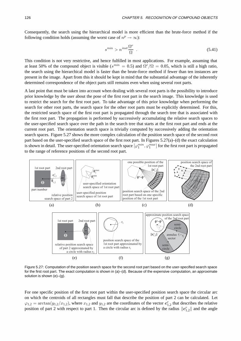
126 CHAPTER 5. RECOGNITION OF COMPOUND OBJECTS
Consequently, the search using the hierarchical model is more efficient than the brute-force method if thefollowing condition holds (assuming the worst case ofnp →∞):
smin > ninst Ωr
Ω. (5.41)
This condition is not very restrictive, and hence fulfilled in most applications. For example, assuming thatat least 50% of the compound object is visible (smin = 0.5) andΩr/Ω = 0.05, which is still a high ratio,the search using the hierarchical model is faster than the brute-force method if fewer than ten instances arepresent in the image. Apart from this it should be kept in mind that the substantial advantage of the inherentlydetermined correspondence of the object parts still remains even when using several root parts.
A last point that must be taken into account when dealing with several root parts is the possibility to introduceprior knowledge by the user about the pose of the first root part in the search image. This knowledge is usedto restrict the search for the first root part. To take advantage of this prior knowledge when performing thesearch for other root parts, the search space for the other root parts must be explicitly determined. For this,the restricted search space of the first root part is propagated through the search tree that is associated withthe first root part. The propagation is performed by successively accumulating the relative search spaces tothe user-specified search space over the path in the search tree that starts at the first root part and ends at thecurrent root part. The orientation search space is trivially computed by successively adding the orientationsearch spaces. Figure 5.27 shows the more complex calculation of the position search space of the second rootpart based on the user-specified search space of the first root part. In Figures 5.27(a)–(d) the exact calculationis shown in detail. The user-specified orientation search space[ϕmin
1 , ϕmax1 ] for the first root part is propagated
to the range of reference positions of the second root part.
1st root part 2nd root part
relative positionsearch space of part 2
1 2
part number
ϕ1,2
c r1,2
user-specified orientationsearch space of 1st root part
user-specified positionsearch space of 1st root part
ϕmax1
ϕmin1
position search space of the 2ndroot part based on one specificposition of the 1st root part
ϕ −ϕe s
one possible position of the1st root part
||c ||r1,2
position search space ofthe 2nd root part
(a) (b) (c) (d)
relative position search spaceof part 2 approximated by
a circle with radius r
1st root part 2nd root part
2
1 2
position search space of the1st root part approximated bya circle with radius r1
1r
r + r12
annulussector
semi-circle
semi-circle
ϕ −ϕe s
approximate position search spaceof the 2nd root part
||c ||r1,2
(e) (f) (g)
Figure 5.27: Computation of the position search space for the second root part based on the user-specified search spacefor the first root part. The exact computation is shown in (a)–(d). Because of the expensive computation, an approximatesolution is shown (e)–(g).
For one specific position of the first root part within the user-specified position search space the circular arcon which the centroids of all rectangles must fall that describe the position of part 2 can be calculated. Letϕ1,2 = arctan(y1,2/x1,2), wherex1,2 andy1,2 are the coordinates of the vectorcr
1,2 that describes the relativeposition of part 2 with respect to part 1. Then the circular arc is defined by the radius‖cr
1,2‖ and the angle
5.6. EXAMPLES 127
interval[ϕs, ϕe], with the start angleϕs = ϕ1,2 +ϕmin1 and the end angleϕe = ϕ1,2 +ϕmax
1 . At each point onthe circular arc the rectangle that describes the relative position search range of part 2 is superimposed. Theenvelope of all rectangles describes the position search space of the second root part based on one specificposition of the first root part (see Figure 5.27(c)). To take all possible positions of the first root part intoaccount, the resulting image region must be enlarged by using the Minkowski addition (Pratt 2001) with theuser-specified position search space of the first root part as structuring element. The reference point of thestructuring element must correspond to the previously specified position of the first part. The result is shownin Figure 5.27(d). One can see that the exact computation of the position search space is rather expensive.Therefore, an approximate solution is proposed. The single steps are shown in Figures 5.27(e)–(g). Theuser-specified search space for the root part as well as the relative search spaces are approximated by thesmallest enclosing circles with radiusr1 andr2. Consequently, the search region for the second root part canbe represented by an annulus sector with an inner radius of‖cr
1,2‖−r1−r2, an outer radius of‖cr1,2‖+r1+r2
and an angle interval of[ϕs, ϕe]. Finally, two semi-circles with radiusr1 + r2 must be appended at bothends of the annulus sector. Although the resulting approximate position search space is larger than the exactsolution, it can be computed much more efficiently. Therefore, one can take profit from the user-specifiedprior information about the position and orientation of the first root part even when using other root parts.
5.6 Examples
Because of the novelty of the proposed approach for recognizing compound objects, there exist no compara-ble recognition methods, and hence a comparison with the performance of other approaches is not possible.Fortunately, many properties of the compound object recognition approach are inherited from the underlyingrigid object recognition approach. I.e., in principle the results of the evaluation in Section 4.4 can be trans-ferred. However, a remark on the robustness should be annotated. The calculation of the score value of thecompound object differs from the calculation in the rigid case. This influences the robustness of the approachsince the score value is used to decide on the presence of an object instance. Furthermore, the user-specifiedparameters influence the robustness of the approach: depending on the selected treatment of missed objectparts, and depending on the handling of missing root parts, the robustness against occlusions changes. Thisshould be kept in mind by the user when specifying the corresponding parameters. Nevertheless, it is possibleto evaluate the computation time in comparison to the brute-force method that searches all object parts inthe entire search space independently from each other. In this section, selected examples that emphasize theconsiderable advantages of the proposed approach are presented. The image size in all examples is 640×482.All computations are performed on a 2 GHz Pentium 4.
In the first example (see Figure 5.28), the company logo that was already introduced in Figure 2.6 is used asthe compound object. The model image, a ROI that contains the entire print on the pen clip, and 10 exampleimages are passed as input data to the process of training the hierarchical model. The example images showthe relative movement of the light gray letter with respect to the dark gray letters. As the first intermediateresult the automatically found components are visualized in Figure 5.28(a) by superimposing their edges onthe model image in white. For each letter a separate component was detected. During the pose determinationof the components in the example images no ambiguities occurred because the components are free of anysimilarities or symmetries. In Figure 5.28(b) the extracted object parts that are obtained from clustering thesimilarity matrix are shown. The threshold for the minimum probabilitypmin was set to 0.5. As one wouldexpect, the dark gray letters are clustered into one rigid object part. Although no rectification was applied tothe images in this example, the relative movement between both parts was large enough to be easily separatedfrom pseudo movements that are caused by the radial distortions. The complete training process took 25 s.
In the next step, the hierarchical model was created. Because the logo is expected to appear only in a verylimited orientation range, the model was created in a small angle interval. This was done by restricting theexpected orientation angle of the part that represents the dark gray letters to[−20,+20]. In Figure 5.28(c)the object parts are represented by their reference points. The part that represents the dark gray letters was

128 CHAPTER 5. RECOGNITION OF COMPOUND OBJECTS
1 2 3 4 5 1
21
2
Root part:
(a) Components (b) Object parts (c) Hierarchical model
(d) Search image 1 (e) Search image 2 (f) Search image 3 (g) Search image 4
Figure 5.28: Recognition of the print on a pen clip. The pose of the light gray letter varies with respect to the dark grayletters.
selected as root part by the approach. One can see that the relative movement of the light gray letter is verysmall in position as well as in orientation. Because only two object parts are involved in this example, thesearch tree is degenerated to only two nodes with one single connection (displayed as a bold black line).Generating the hierarchical model took 6 s.
Finally, the hierarchical model was used to search the object in 20 different search images that are distinct fromthe example images that were used to train the hierarchical model. Figures 5.28(d)–(g) show four examples,in which the returned poses of the parts are visualized by their edges superimposed in white. The averagecomputation time of the recognition process was 21 ms if one object instance was present in the image and27 ms if two instances were present (as, e.g., in Figures 5.28(f) and (g)). The recognition of the root part took15 ms, the recognition of the second part for each instance about 6 ms. In contrast, the independent recognitionof both parts without using the hierarchical model would take about 30 ms (one instance) and 37 ms (twoinstances), respectively. Therefore, a speed-up of about 40% is received when using the hierarchical model.Although in this case the improvement in computation time that is obtained by the use of the hierarchicalmodel is not enormous, there is still the additional advantage of the inherently determined correspondence.Thus, whenever more than one object is present in the image, the correspondence between the found objectpart instances and the correct compound object is implicitly given.
The second example (see Figure 5.29) deals with the circuit board that was introduced in Figure 2.8. In thisexample, the object parts are specified manually by the user because obviously an automatic extraction ofthe components using the proposed approach would fail. Therefore, instead of one ROI, now five ROIs arepassed to the algorithm, each representing one object part (see Figure 5.29(a)). The associated object parts’edges are shown in Figure 5.29(b). To train the hierarchical model, 12 example images were provided. Alsoin this example no rectification was needed. Because two of the five electronic modules are identical (part 3and part 5), the approach had to solve the occurring ambiguities during the training. It took 24 s to train thehierarchical model. The creation of the hierarchical model was restricted to an orientation angle interval of[−45,+45]. The final hierarchical model is displayed in Figure 5.29(c). Part 2 was recommended by theapproach to serve as the root part, from which part 4 is searched. The pose of part 4 is then exploited to restrictthe search space of part 1, from which finally part 3 and part 5 are searched. Because of the relatively smallsize of the object parts, the model creation only took 3 s.
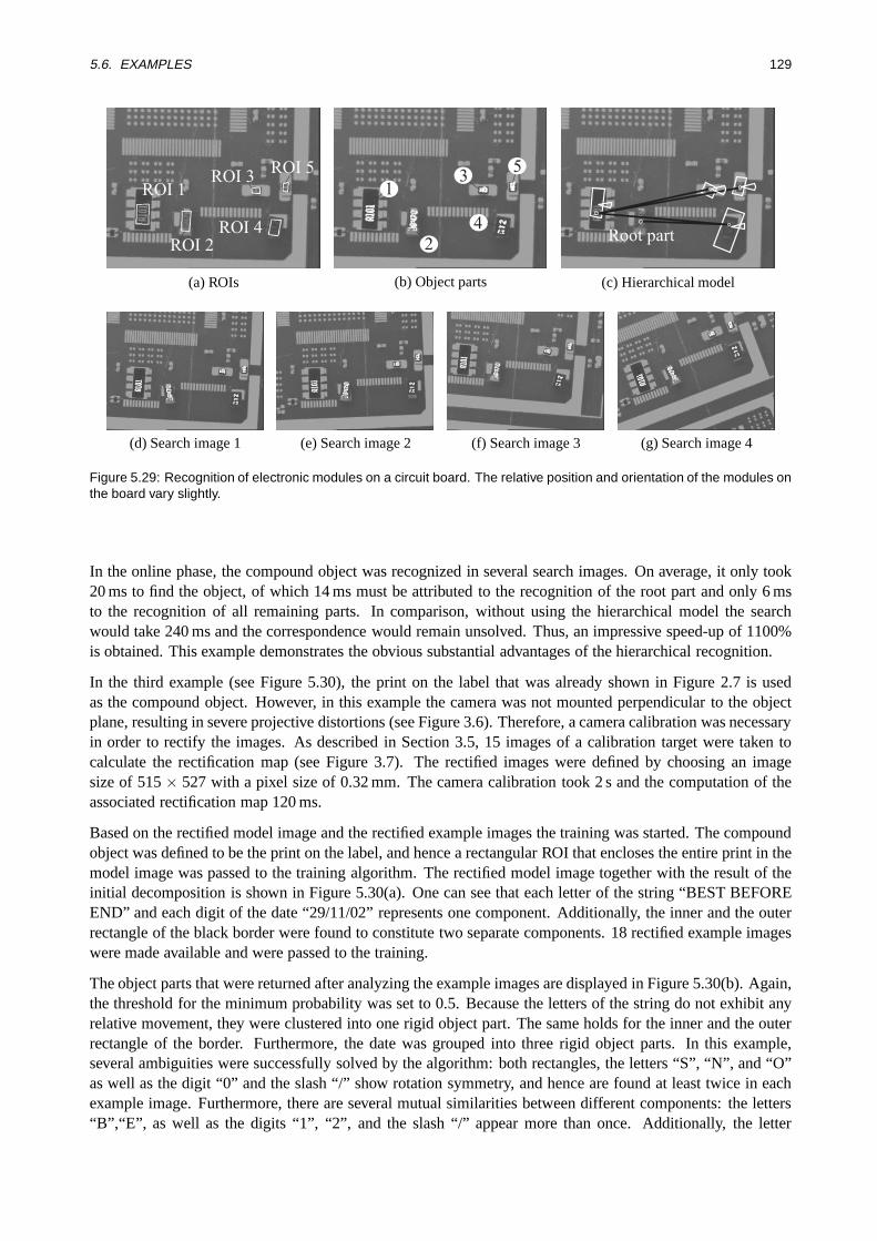
5.6. EXAMPLES 129
ROI 1
ROI 2ROI 4
ROI 3ROI 5
1
2
3
4
5
Root part
(a) ROIs (b) Object parts (c) Hierarchical model
(d) Search image 1 (e) Search image 2 (f) Search image 3 (g) Search image 4
Figure 5.29: Recognition of electronic modules on a circuit board. The relative position and orientation of the modules onthe board vary slightly.
In the online phase, the compound object was recognized in several search images. On average, it only took20 ms to find the object, of which 14 ms must be attributed to the recognition of the root part and only 6 msto the recognition of all remaining parts. In comparison, without using the hierarchical model the searchwould take 240 ms and the correspondence would remain unsolved. Thus, an impressive speed-up of 1100%is obtained. This example demonstrates the obvious substantial advantages of the hierarchical recognition.
In the third example (see Figure 5.30), the print on the label that was already shown in Figure 2.7 is usedas the compound object. However, in this example the camera was not mounted perpendicular to the objectplane, resulting in severe projective distortions (see Figure 3.6). Therefore, a camera calibration was necessaryin order to rectify the images. As described in Section 3.5, 15 images of a calibration target were taken tocalculate the rectification map (see Figure 3.7). The rectified images were defined by choosing an imagesize of 515× 527 with a pixel size of 0.32 mm. The camera calibration took 2 s and the computation of theassociated rectification map 120 ms.
Based on the rectified model image and the rectified example images the training was started. The compoundobject was defined to be the print on the label, and hence a rectangular ROI that encloses the entire print in themodel image was passed to the training algorithm. The rectified model image together with the result of theinitial decomposition is shown in Figure 5.30(a). One can see that each letter of the string “BEST BEFOREEND” and each digit of the date “29/11/02” represents one component. Additionally, the inner and the outerrectangle of the black border were found to constitute two separate components. 18 rectified example imageswere made available and were passed to the training.
The object parts that were returned after analyzing the example images are displayed in Figure 5.30(b). Again,the threshold for the minimum probability was set to 0.5. Because the letters of the string do not exhibit anyrelative movement, they were clustered into one rigid object part. The same holds for the inner and the outerrectangle of the border. Furthermore, the date was grouped into three rigid object parts. In this example,several ambiguities were successfully solved by the algorithm: both rectangles, the letters “S”, “N”, and “O”as well as the digit “0” and the slash “/” show rotation symmetry, and hence are found at least twice in eachexample image. Furthermore, there are several mutual similarities between different components: the letters“B”,“E”, as well as the digits “1”, “2”, and the slash “/” appear more than once. Additionally, the letter
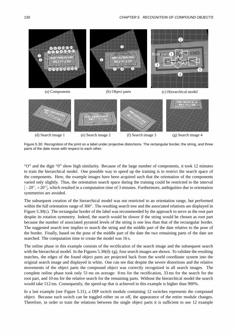
130 CHAPTER 5. RECOGNITION OF COMPOUND OBJECTS
16 17 18 19 20 21 22 23
4 6 8 10 12 14
1513119753
1
2
3 4 5
2
1
2
54
3
Root part: 1
(a) Components (b) Object parts (c) Hierarchical model
(d) Search image 1 (e) Search image 2 (f) Search image 3 (g) Search image 4
Figure 5.30: Recognition of the print on a label under projective distortions. The rectangular border, the string, and threeparts of the date move with respect to each other.
“O” and the digit “0” show high similarity. Because of the large number of components, it took 12 minutesto train the hierarchical model. One possible way to speed up the training is to restrict the search space ofthe components. Here, the example images have been acquired such that the orientation of the componentsvaried only slightly. Thus, the orientation search space during the training could be restricted to the interval[−20,+20], which resulted in a computation time of 3 minutes. Furthermore, ambiguities due to orientationsymmetries are avoided.
The subsequent creation of the hierarchical model was not restricted to an orientation range, but performedwithin the full orientation range of 360. The resulting search tree and the associated relations are displayed inFigure 5.30(c). The rectangular border of the label was recommended by the approach to serve as the root partdespite its rotation symmetry. Indeed, the search would be slower if the string would be chosen as root partbecause the number of associated pyramid levels of the string is one less than that of the rectangular border.The suggested search tree implies to search the string and the middle part of the date relative to the pose ofthe border. Finally, based on the pose of the middle part of the date the two remaining parts of the date aresearched. The computation time to create the model was 16 s.
The online phase in this example consists of the rectification of the search image and the subsequent searchwith the hierarchical model. In the Figures 5.30(d)–(g), four search images are shown. To validate the resultingmatches, the edges of the found object parts are projected back from the world coordinate system into theoriginal search image and displayed in white. One can see that despite the severe distortions and the relativemovements of the object parts the compound object was correctly recognized in all search images. Thecomplete online phase took only 51 ms on average: 8 ms for the rectification, 33 ms for the search for theroot part, and 10 ms for the relative search for the remaining parts. Without the hierarchical model the searchwould take 512 ms. Consequently, the speed-up that is achieved in this example is higher than 900%.
In a last example (see Figure 5.31), a DIP switch module containing 12 switches represents the compoundobject. Because each switch can be toggled either on or off, the appearance of the entire module changes.Therefore, in order to train the relations between the single object parts it is sufficient to use 12 example
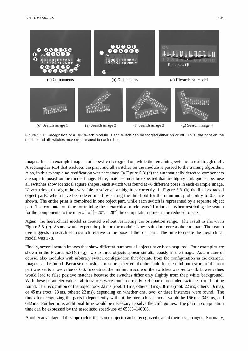
5.6. EXAMPLES 131
29
28
26 272523
242221
201917
181615
3
1
2 4 6 8 10 12 141311975
13
1
3 5 7 9 112 4 6 8 10 12
Root part: 13
(a) Components (b) Object parts (c) Hierarchical model
(d) Search image 1 (e) Search image 2 (f) Search image 3 (g) Search image 4
Figure 5.31: Recognition of a DIP switch module. Each switch can be toggled either on or off. Thus, the print on themodule and all switches move with respect to each other.
images. In each example image another switch is toggled on, while the remaining switches are all toggled off.A rectangular ROI that encloses the print and all switches on the module is passed to the training algorithm.Also, in this example no rectification was necessary. In Figure 5.31(a) the automatically detected componentsare superimposed on the model image. Here, matches must be expected that are highly ambiguous: becauseall switches show identical square shapes, each switch was found at 48 different poses in each example image.Nevertheless, the algorithm was able to solve all ambiguities correctly. In Figure 5.31(b) the final extractedobject parts, which have been determined by setting the threshold for the minimum probability to 0.5, areshown. The entire print is combined in one object part, while each switch is represented by a separate objectpart. The computation time for training the hierarchical model was 11 minutes. When restricting the searchfor the components to the interval of[−20,+20] the computation time can be reduced to 31 s.
Again, the hierarchical model is created without restricting the orientation range. The result is shown inFigure 5.31(c). As one would expect the print on the module is best suited to serve as the root part. The searchtree suggests to search each switch relative to the pose of the root part. The time to create the hierarchicalmodel was 17 s.
Finally, several search images that show different numbers of objects have been acquired. Four examples areshown in the Figures 5.31(d)–(g). Up to three objects appear simultaneously in the image. As a matter ofcourse, also modules with arbitrary switch configuration that deviate from the configuration in the exampleimages can be found. Because occlusions must be expected, the threshold for the minimum score of the rootpart was set to a low value of 0.6. In contrast the minimum score of the switches was set to 0.8. Lower valueswould lead to false positive matches because the switches differ only slightly from their white background.With these parameter values, all instances were found correctly. Of course, occluded switches could not befound. The recognition of the object took 22 ms (root: 14 ms, others: 8 ms), 38 ms (root: 22 ms, others: 16 ms),or 45 ms (root: 23 ms, others: 22 ms), depending on whether one, two, or three instances were found. Thetimes for recognizing the parts independently without the hierarchical model would be 166 ms, 346 ms, and682 ms. Furthermore, additional time would be necessary to solve the ambiguities. The gain in computationtime can be expressed by the associated speed-ups of 650%–1400%.
Another advantage of the approach is that some objects can be recognized even if their size changes. Normally,

132 CHAPTER 5. RECOGNITION OF COMPOUND OBJECTS
(a) White pads on a die
1
24
3
(b) Parts (c) Metal angles
12
3
4
56
(d) Parts
Figure 5.32: Recognition of objects with varying size. The white pads on the die in (a) can be represented by four cornersthat move with respect to each other (b). Analogously, the metal angles in (c) can be represented by six corners (d).
this would require a recognition approach that is able to handle similarity transformations. However, theproposed approach can model the changes in scale as relative movements. Figure 5.32 shows two examples.In the first example the white pads on the die must be recognized. The pads may occur at different sizes. Fourappropriate model parts can be defined by passing four ROIs to the training. Each ROI contains one corner ofthe rectangle. Hence, by choosing the corners of the rectangle as model parts exploits the fact that angles arepreserved under similarity transformations. It is sufficient to train the model with two example images oneshowing the smallest occurring pad and one showing the largest occurring pad. Thus, the trained relationsbetween the parts cover all possible object scales. Analogously, in the second example metal angles must berecognized. Here, six object parts that represent the six corners are involved. Again, two example images areenough to train the model. Actually, it would be sufficient to recognize only two object parts in both examplesto determine the pose of the object. The scale of the object can be determined from the distance between thetwo object parts. If more than two object parts are used the computation of the scale becomes ambiguous. Inthis case the scale can be determined in a least-squares adjustment by minimizing the distances between thescaled model and the returned poses of the object parts. In a similar way objects that are transformed by moregeneral transformation classes can be recognized. However, instead of angles other appropriate geometricinvariants must be found.

Chapter 6
Conclusions
In this dissertation, a novel approach for recognizing compound objects in real-time is proposed. A compoundobject is defined as a number of rigid object parts that show arbitrary relative movements. The basic ideabehind the approach is to minimize the search effort, and hence the computation time, by restricting thesearch in accordance with the relative movements of the object parts. This naturally leads to the use of ahierarchical model: only the root object part, which stands at the top of the hierarchy, is searched within theentire search space. In contrast, the remaining parts are searched recursively with respect to each other withinvery restricted search spaces. By using the hierarchical model, prior knowledge about the spatial relations,i.e., relative movements, between the object parts is exploited already in an early stage of the recognition.Thus, the computation time is reduced dramatically. Furthermore, the hierarchical model provides an inherentdetermination of the correspondence, i.e., because of the restricted search spaces, ambiguous matches areavoided. Therefore, a complicated and expensive solution of the correspondence problem is not necessary.
The proposed strategy for recognizing compound objects requires an appropriate approach for recognizingrigid objects. In an extensive review of rigid object recognition methods, the generalized Hough transformproves to be one of the most promising candidates. Its inherent translation invariance, as well as the high ro-bustness, are the most important advantages. Nevertheless, it is shown that there are still several modificationsnecessary to fulfill industrial demands. The method is extended to recognize objects at arbitrary orientations.This leads to high computation times and large amounts of required memory. Therefore, several effective ex-tensions to increase the efficiency are proposed. The use of image pyramids, which leads to a multi-resolutionmodel with an associated coarse-to-fine search, is a major improvement. It is shown that the benefit achievedby the use of the multi-resolution model can be further augmented: a method for optimally restricting theimage domain that is processed during the coarse-to-fine search is proposed. By splitting the model into tiles,redundant processing steps are avoided and the gain in efficiency is further increased. Additionally, severalnew methods to enhance the degree of automation and robustness are proposed. Finally, the obtained dis-crete values for the object position and orientation are analytically refined to achieve a high accuracy. It isshown that this modified generalized Hough transform is about 650 times faster than the conventional gener-alized Hough transform in a standard example. The performance of the new approach is evaluated thoroughlyby comparing it to three standard approaches and three high-end recognition tools. Furthermore, a secondnew approach, the shape-based matching (Steger 2002), which was developed simultaneously to the modifiedgeneralized Hough transform, is introduced and included in the evaluation. The evaluation shows that bothnew approaches are considerably superior to existing standard approaches. Their behavior with respect torobustness, accuracy, and computation time is better balanced in comparison to all other approaches, exceptfor one high-end recognition tool, which shows comparable results. From this discussion it can be seen thatboth approaches fulfill the industrial requirements discussed in Section 2.2. Furthermore, it follows that themodified generalized Hough transform is more than simply a by-product of this dissertation. In contrast, itcan be seen as one of the best stand-alone recognition approaches for rigid objects. The field of applicationsthat can benefit from this new approach is almost unlimited. Not only applications that use the conventional
133
134 CHAPTER 6. CONCLUSIONS
generalized Hough transform can be improved, but most applications that require rigid object recognition canachieve a high performance with this approach.
The shape-based matching is chosen to serve as a module within the approach for recognizing compoundobjects because it has already been thoroughly tested and included in a commercial software library. Further-more, in contrast to the modified generalized Hough transform, it shows true invariance against changes inbrightness. To achieve a high degree of automation, the hierarchical model is automatically trained. For this,some example images that show the relative movements of the object parts are automatically analyzed andused to determine the rigid object parts as well as the spatial relations between the parts. This is very com-fortable for the user because a complicated manual description of the compound object is avoided. Duringthe subsequent creation of the hierarchical model, the optimum hierarchical search strategy is automaticallyderived. The strategy includes a rating of the ability of each object part to serve as the root part: parts thatfacilitate a fast search when used as root part receive a good rating. Additionally, for each part that mightbe selected as the root part, an associated search tree, which represents the hierarchical search, is automati-cally computed. The hierarchical model that is finally obtained is used to recognize the compound object inreal-time. By default, the part with the best rating is selected as root part. However, in order to exploit priorknowledge about possibly occluded object parts, the root part may be selected by the user and passed as inputparameter to the search. In this case, the ratings of the root parts may assist the user while specifying thedesired root part. The search is then performed in accordance with the search tree that is associated with thespecified root part.
The training of the hierarchical model is performed in several steps by following the principle of human visualperception. At first, the compound object is split into several small components. Then, the components arerecognized in the example images. Components that do not exhibit any relative movements are merged intorigid object parts. Finally, the relations between the parts are determined. It is shown that the high degreeof automation during the training of the hierarchical model is accompanied by several problems that must besolved. One major problem is the non-uniqueness of the components, which, e.g., can be caused by rotationsymmetries or mutual similarities of the components. Thus, one component may be recognized several timesin the same example image. To solve this correspondence problem, a new method that uses a global criterionis proposed to estimate the likelihood of the found instances. Finally, it is shown that the correspondenceproblem can be transformed into a bipartite graph matching problem, which can be solved efficiently usinglinear programming. Thus, for each component, the most likely instance is obtained with respect to the globalcriterion. Because the correspondence problem is already solved during the training, the resulting hierarchicalmodel provides an inherent determination of the correspondence. Consequently, solving the correspondenceduring the object recognition is unnecessary, which is a considerable advantage of the proposed approach. Toobtain the rigid object parts, the probability that two components belong to the same object part is computed.This computation is performed in a statistically sound manner by using hypotheses testing. The resultingsquare probability matrix is clustered and the corresponding components are merged into object parts.
The creation of the hierarchical model includes the derivation of the search trees that minimize the searcheffort. It is shown that this problem can be translated into the problem of finding the minimum spanningarborescence in a directed graph. This guarantees an exact and efficient solution. Finally, several practi-cal extensions that must be considered during the hierarchical search conclude the approach for recognizingcompound objects.
Furthermore, as a by-product a method for rectifying images in real-time is proposed. By combining thismethod with camera calibration, a very fast elimination of projective distortions and radial lens distortionsfrom images becomes possible. Thus, the recognition of compound objects is extended to deal with projectivetransformations of the object plane. It is shown that the rectification is performed in less than 10 ms on standardhardware using RS-170 or CCIR-sized images. Thus, it facilitates the real-time recognition of objects evenunder severe projective distortions. The new method is not restricted to object recognition but could alsobe used in several other applications that require fast computations. Whenever more than one image mustbe rectified with the same mapping, a gain in computation time can be achieved by the proposed method.
135
Moreover, the method can be used to eliminate arbitrary distortions that are not necessarily caused by lensdistortions or projective distortions. For example, distortions that are caused by non-planar object surfacescan be eliminated. Once the rectification map is built the image of the curved surface can be unwrapped intoa plane in real-time. Consequently, the further processing needs to focus only on “planar” algorithms, andhence can be simplified significantly.
Several examples show that the proposed approach for recognizing compound objects fulfills the real-timerequirement. The computation time varies between 20 ms and 51 ms in the presented examples, which corre-sponds to an improvement of up to 1400% in comparison to standard recognition methods.
To summarize, the approach is able to recognize compound objects, to perform the recognition in real-time,and to provide an inherent determination of the correspondence between object parts. Furthermore, it exhibitsa very high degree of automation. The approach is general with regard to the type of object, and shows a veryhigh robustness against occlusions, clutter, and changes in brightness. The pose parameters of all object partsare returned with high accuracy. Even objects under projective distortions can be recognized. Finally, severalinstances of the object in the image can be found simultaneously. There is no other approach available thatdemonstrates comparable features.
Nevertheless, the proposed approach shows room for some promising extensions that are worth mentioning.They are discussed in the following.
The first point concerns the accuracy of the pose parameters that are returned by the rigid object recognitionapproach. Although the accuracy is not precisely known, the approach for training the hierarchical modelrequires such accuracy information. For the current implementation, the accuracy values have been determinedempirically and set to a constant value. Unfortunately, the accuracy depends on several factors that were nottaken into account. For example, the accuracy depends on object characteristics like the object size, thenumber of model points, the object shape, the histogram of the gradient directions, or object symmetries. Oneway to make accuracy information available would be to perform several empirical tests while using objectswith different characteristics, determining the achieved accuracy, and model the accuracy as a function ofthe characteristics. Other influences that are not correlated with object characteristics cannot be consideredby this method. Another possibility would be to derive the accuracy based on the score values in parameterspace. For example, the curvature of the local maximum could be an indicator of the achievable accuracy.Unfortunately, initial tests have shown that this is a very weak indicator.
A second possible extension would be to merge object parts that only show a small relative movement intoone rigid object part on higher pyramid levels. This is because the relative movement decreases for higherpyramid levels with respect to the quantization of the parameter space. The resulting larger object parts wouldincrease the robustness because, in general, larger objects can be found with higher reliability. Furthermore,it would enhance the efficiency because larger object parts allow the use of more pyramid levels.
Another improvement deals with the rectification. When using recognition approaches that perform a segmen-tation of the search image during the online phase (like the modified generalized Hough transform) a furtherspeed-up could be achieved when dealing with image distortions: the rectification in the online phase can berestricted to the features, like edge position or edge orientation, in order to avoid the complete rectification ofthe entire image. This would, however, result in only a moderate speed-up of the entire recognition processsince the contribution of the proposed rectification to the overall computation time is small. Unfortunately,the shape-based matching is not suited to take advantage of this improvement because no segmentation of thesearch image is performed, and hence no speed-up can be achieved.
Finally, in some applications it is desirable to recognize an object under more general transformations thanrigid transformations. For example, if the distance between camera and object is variable, or if the object itselfoccurs in different sizes, an additional scaling must be considered, which results in similarity transformations.The recognition of rigid objects and compound objects can be extended in a straightforward way to takescaling into account. However, extending the automatic training of the hierarchical model turns out to bemore complex. The rigidity assumption of object parts must be relaxed. Consequently, the rating of the

136 CHAPTER 6. CONCLUSIONS
matches during the solution of the ambiguities would have to be redesigned.
In conclusion, it should be pointed out that the principle of the proposed approach for recognizing compound2D objects can be applied to the recognition of 3D objects from 2D images as well. There are differentapproaches for recognizing 3D rigid objects, e.g., (Procter and Illingworth 1997, Vosselman and Tangelder2000, Pope and Lowe 2000, Blask´o and Fua 2001). By using one of these approaches, the training and thecreation of the hierarchical model can be performed in the same way as in the 2D case. Consequently, alsothe recognition of compound 3D objects can benefit from the use of the proposed hierarchical recognition.The computation time is reduced considerably. This is especially important in 3D because, in general, morecomplex and time consuming algorithms are involved than in 2D. Furthermore, the correspondence problem,which is much more complicated in 3D, must be only solved once during the training but not during therecognition process itself. Thus, real-time applications in 3D, e.g., in the field of autonomous mobile systems(Lanser et al. 1997), augmented reality (Blask´o and Fua 2001), or 3D object tracking (Torre et al. 2000) canprofit from the proposed approach.
Bibliography
Abdel-Aziz, Y. I. and Karara, H. M. (1971): Direct linear transformation into object space coordinates inclose-range photogrammetry,Symposium on Close-Range Photogrammetry, 1–19.
Abe, K., Arcelli, C., Hisajima, T. and Ibaraki, T. (1996): Parts of planar shapes,Pattern Recognition29(10): 1703–1711.
Anuta, P. E. (1970): Spatial registration of multispectral and multitemporal digital imagery using fast Fouriertransform techniques,IEEE Transactions on Geoscience Electronics8(4): 353–368.
Aschwanden, P. and Guggenb¨uhl, W. (1992): Experimental results from a comparative study on correlation-type registration algorithms,in W. Forstner and S. Ruwiedel (editors),Robust Computer Vision: Qualityof Vision Algorithms, Wichmann, Karlsruhe, 268–289.
Bacon, D. (1997): Image preprocessing to improve the reliability of normalized correlation,in A. R. Rao andN. Chang (editors),Machine Vision Applications in Industrial Inspection V, Proc. SPIE 3029, 195–199.
Ballard, D. H. (1981): Generalizing the Hough transform to detect arbitrary shapes,Pattern Recognition13(2): 111–122.
Ballard, D. H. and Brown, C. M. (1982):Computer Vision, Prentice-Hall International, Inc., Englewood Cliffs,NJ.
Ballard, D. H. and Sabbah, D. (1983): Viewer independent shape recognition,IEEE Transactions on PatternAnalysis and Machine Intelligence5(6): 653–659.
Barnea, D. I. and Silverman, H. F. (1972): A class of algorithms for fast digital image registration,IEEETransactions on Computers21: 179–186.
Baumgartner, A. (1998): Extraction of roads from aerial imagery based on grouping and local context,Inter-national Archives of Photogrammetry and Remote Sensing, volume XXXII part 3/1, 196–201.
Beardsley, P., Murray, D. and Zisserman, A. (1992): Camera calibration using multiple images,in G. San-dini (editor), European Conference on Computer Vision, volume 588 ofLecture Notes in ComputerScience, Springer-Verlag, Berlin, 312–320.
Belongie, S., Malik, J. and Puzicha, J. (2002): Shape matching and object recognition using shape contexts,IEEE Transactions on Pattern Analysis and Machine Intelligence24(4): 509–522.
Berkhin, P. (2002): Survey of clustering data mining techniques,Technical report, Accrue Software, San Jose,CA.
Beyer, H. A. (1987): Some aspects of the geometric calibration of CCD-cameras,ISPRS IntercommissionConference on Fast Processing of Photogrammetric Data, Interlaken, Switzerland, 68–81.
Beyer, H. A. (1992): Accurate calibration of CCD-cameras,Computer Vision and Pattern Recognition, 96–101.
137

138 BIBLIOGRAPHY
Bhat, D. N. and Nayar, S. K. (1998): Ordinal measures for image correspondence,IEEE Transactions onPattern Analysis and Machine Intelligence20(4): 415–423.
Blasko, G. and Fua, P. (2001): Real-time 3D object recognition for automatic tracker initialization,4th Inter-national Symposium on Augmented Reality.
Bock, F. (1971): An algorithm to construct a minimum directed spanning tree in a directed network,in B. Avi-Itzhack (editor),Developments in Operations Research, Gordon and Breach, New York, NY, 29–44.
Borgefors, G. (1984): Distance transformation in arbitrary dimensions,Computer Vision, Graphics, and ImageProcessing27: 321–345.
Borgefors, G. (1988): Hierarchical chamfer matching: A parametric edge matching algorithm,IEEE Trans-actions on Pattern Analysis and Machine Intelligence10(6): 849–865.
Bronstein, I. N., Semendjajew, K. A., Musiol, G. and M¨uhlig, H. (2001):Taschenbuch der Mathematik, 5thedn, Harri Deutsch, Thun, Frankfurt am Main.
Brown, D. C. (1966): Decentering distortion of lenses,Photogrammetric Engineering & Remote Sensing32(3): 444–462.
Brown, L. G. (1992): A survey of image registration techniques,ACM Computing Surveys24(4): 325–376.
Bunke, H. (2000): Graph matching for visual object recognition,Spatial Vision13(2/3): 335–340.
Canny, J. (1983): Finding edges and lines in images,Technical Report 720, MIT Artificial Intelligence Labo-ratory, Cambridge, MA.
Canny, J. (1986): A computational approach to edge detection,IEEE Transactions on Pattern Analysis andMachine Intelligence8(6): 679–698.
Cantoni, V. and Carrioli, L. (1987): Structural shape recognition in a multiresolution environment,SignalProcessing12: 267–276.
Cha, S.-H. (2000): Efficient algorithms for image template and dictionary matching,Journal of MathematicalImaging and Vision12: 81–90.
Cha, S.-H. and Srihari, S. N. (2000): Distance between histograms of angular measurements and its applica-tion to handwritten character similarity,15th International Conference on Pattern Recognition, volume 2,21–24.
Christmas, W. J., Kittler, J. and Petrou, M. (1995): Structural matching in computer vision using probabilisticrelaxation,IEEE Transactions on Pattern Analysis and Machine Intelligence17(8): 749–764.
Chu, Y. J. and Tseng-Hong, L. (1965): On the shortest arborescence of a directed graph,Scientia Sinica14(10): 1396–1400.
Clark, J. and Holton, D. A. (1994):Graphentheorie: Grundlagen und Anwendungen, Spektrum AkademischerVerlag, Heidelberg.
Cognex (2000):Cognex MVS-8000 Series - CVL Vision Tool Guide, Cognex Corporation: CVL 5.5.1.
Cohen, S. D. and Guibas, L. J. (1997): Shape-based image retrieval using geometric hashing,ARPA ImageUnderstanding Workshop.
Crouzil, A., Massip-Pailhes, L. and Castan, S. (1996): A new correlation criterion based on gradient fieldssimilarity, 13th International Conference on Pattern Recognition, volume 1, 632–691.

BIBLIOGRAPHY 139
Danielsson, P. E. (1980): Euclidean distance mapping,Computer Graphics and Image Processing14: 227–248.
Davis, L. S. (1982): Hierarchical generalized Hough transforms and line-segment based generalized Houghtransforms,Pattern Recognition15(4): 277–285.
Deriche, R. (1987): Using Canny’s criteria to derive a recursively implemented optimal edge detector,Inter-national Journal of Computer Vision1: 167–187.
Duta, N., Jain, A. K. and Dubuisson-Jolly, M.-P. (2001): Automatic construction of 2D shape models,IEEETransactions on Pattern Analysis and Machine Intelligence23(5): 433–446.
Ebner, H. (1976): Self calibrating block adjustment,International Archives of Photogrammetry21(3): 1–17.
Edmonds, J. (1967): Optimum branchings,Journal of Research of the National Bureau of Standards71B(4): 233–240.
Edwards, J. L. and Murase, H. (1998): Coarse-to-fine adaptive masks for appearance matching of occludedscenes,Machine Vision and Applications10: 232–242.
Elder, J. H. and Zucker, S. W. (1998): Local scale control for edge detection and blur estimation,IEEETransactions on Pattern Analysis and Machine Intelligence20(7): 699–716.
Elder, J. (1999): Are edges incomplete?,International Journal of Computer Vision34(2): 97–122.
Faig, W. (1975): Calibration of close-range photogrammetric systems: Mathematical formulation,Pho-togrammetric Engineering & Remote Sensing41(12): 1479–1486.
Faugeras, O. D. and Toscani, G. (1986): Calibration problems for stereo,Computer Vision and Pattern Recog-nition, 15–20.
Felzenszwalb, P. F. and Huttenlocher, D. P. (2000): Efficient matching of pictorial structures,Computer Visionand Pattern Recognition, volume 2, 66–73.
Fischetti, M. and Toth, P. (1993): An efficient algorithm for the min-sum arborescence problem on completedigraphs,ORSA Journal of Computing5(4): 426–434.
Fitsch, A. J., Kadyrov, A., Christmas, W. J. and Kittler, J. (2002): Orientation correlation,British MachineVision Conference, volume 1, 133–142.
Foroosh, H., Zerubia, J. B. and Berthod, M. (2002): Extension of phase correlation to subpixel registration,IEEE Transactions on Image Processing11(3): 188–200.
Forstner, W. and G¨ulch, E. (1987): A fast operator for detection and precise location of distinct points, cornersand centres of circular features,ISPRS Intercommission Workshop, Interlaken, Switzerland, 281–305.
Gabow, H. N., Galil, Z., Spencer, T. and Tarjan, R. E. (1986): Efficient algorithms for finding minimumspanning trees in undirected and directed graphs,Combinatorica6(2): 109–122.
Garfinkel, R. S. and Nemhauser, G. L. (1972):Integer Programming, John Wiley & Sons, Inc., New York,NY.
Gavrila, D. M. and Giebel, J. (2001): Virtual sample generation for template-based shape matching,ComputerVision and Pattern Recognition, 676–681.
Gavrila, D. M. and Philomin, V. (1999): Real-time object detection for “smart” vehicles,7th InternationalConference on Computer Vision, volume I, 87–93.
140 BIBLIOGRAPHY
Gideon, R. A. and Hollister, R. A. (1987): A rank correlation coefficient,Journal of the American StatisticalAssociation82(398): 656–666.
Godding, R. (1993): Ein photogrammetrisches Verfahren zurUberprufung und Kalibrierung digitaler Bildauf-nahmesysteme,Zeitschrift fur Photogrammetrie und Fernerkundung2: 82–90.
Gonzalez, R. C. and Woods, R. E. (1992):Digital Image Processing, Addison-Wesley Publishing Company.
Gotthardt, E. (1968):Einfuhrung in die Ausgleichungsrechnung, Wichmann, Karlsruhe.
Graham, R. L. and Hell, P. (1985): On the history of the minimum spanning tree problem,Annals of theHistory of Computing7(1): 43–57.
Grimson, W. E. L. (1987): Recognition of object families using parameterized models,International Confer-ence on Computer Vision, 93–101.
Grimson, W. E. L. (1989): On the recognition of parametrized 2-D objects,International Journal of ComputerVision2(4): 353–372.
Gruen, A. W. and Beyer, H. A. (1987): Real-time photogrammetry at the digital photogrammetric station(DIPS) of ETH Zurich,The Canadian Surveyor41(2): 181–199.
Haberacker, P. (1995):Praxis der Digitalen Bildverarbeitung und Mustererkennung, Carl Hanser VerlagMunchen Wien.
Haralick, R. M. and Shapiro, L. G. (1992):Computer and Robot Vision, volume I, Addison-Wesley PublishingCompany, Reading, MA.
Hartley, R. I. and Zisserman, A. (2000):Multiple View Geometry in Computer Vision, Cambridge UniversityPress, Cambridge.
Hauck, A., Lanser, S. and Zierl, C. (1997): Hierarchical recognition of articulated objects from single per-spective views,Computer Vision and Pattern Recognition, 870–876.
Heipke, C. (1995): Digitale photogrammetrische Auswertestationen, Habilitationsschrift, Fakult¨at furBauingenieur- und Vermessungswesen, Technische Universit¨at Munchen: Deutsche Geod¨atische Kom-mision, Reihe C, Heft Nr. 450, M¨unchen.
Heipke, C., Stephani, M., Strunz, G. and Lenz, R. (1991): Accuracy potential of a digital CCD camerafor photogrammetric applications,in B. Radig (editor),Mustererkennung, Informatik Fachberichte 290,Springer-Verlag, Berlin, 320–327.
Hel-Or, Y. and Werman, M. (1994a): Constraint-fusion for interpretation of articulated objects,ComputerVision and Pattern Recognition, 39–45.
Hel-Or, Y. and Werman, M. (1994b): Model based pose estimation of articulated and constraint objects,ThirdEuropean Conference on Computer Vision, 199–204.
Hoffman, D. and Richards, W. (1984): Parts of recognition,Cognition18: 65–96.
Hough, P. V. C. (1962): Method and means for recognizing complex patterns,U.S. Patent 3,069,654.
Huertas, A., Cole, W. and Nevatia, R. (1990): Detecting runways in complex airport scenes,Computer Vision,Graphics, and Image Processing51: 107–145.
Huttenlocher, D. P., Klanderman, G. A. and Rucklidge, W. J. (1993): Comparing images using the Hausdorffdistance,IEEE Transactions on Pattern Analysis and Machine Intelligence15(9): 850–863.
BIBLIOGRAPHY 141
Huttenlocher, D. P., Lilien, R. H. and Olson, C. F. (1999): View-based recognition using an eigenspace ap-proximation to the Hausdorff measure,IEEE Transactions on Pattern Analysis and Machine Intelligence21(9): 951–955.
Illingworth, J. and Kittler, J. (1988): A survey of the Hough transform,Computer Vision, Graphics, and ImageProcessing44: 87–116.
Irani, M. and Anandan, P. (1999): All about direct methods,in W. Triggs, A. Zisserman and R. Szeliski (edi-tors), International Workshop on Vision Algorithms, 267–277.
Jacobs, C. E., Finkelstein, A. and Salesin, D. H. (1995): Fast multiresolution image querying,Proc. SIG-GRAPH ’95, 277–286.
Jahne, B. (2002):Digital Image Processing, 5th edn, Springer-Verlag.
Jain, A. K., Murty, M. N. and Flynn, P. J. (1999): Data clustering: A review,ACM Computing Surveys31(3): 264–323.
Jain, A. K., Zhong, Y. and Lakshmanan, S. (1996): Object matching using deformable templates,IEEETransactions on Pattern Analysis and Machine Intelligence18(3): 267–278.
Jeng, S.-C. and Tsai, W.-H. (1990): Fast generalized Hough transform,Pattern Recognition Letters11: 725–733.
Jensen, D. (2002): Real-time for the real world: URL accessed October 2002.*http://www.real-time.org/
Kager, H. (1981):Bundeltriangulation mit indirekt beobachteten Kreiszentren, Dissertation, Institut f¨ur Pho-togrammetrie, Technische Universit¨at Wien: Geowissenschaftliche Mitteilungen, Heft Nr. 19, Wien.
Kaneko, S., Murase, I. and Igarashi, S. (2002): Robust image registration by increment sign correlation,Pattern Recognition35(10): 2223–2234.
Karmarkar, N. (1984): A new polynomial-time algorithm for linear programming,Combinatorica4(4): 373–395.
Kassim, A. A., Tan, T. and Tan, K. H. (1999): A comparative study of efficient generalised Hough transformtechniques,Image and Vision Computing17: 737–748.
Koch, K. R. (1987):Parameterschatzung und Hypothesentests in linearen Modellen, Dummler, Bonn.
Koffka, K. (1935):Principles of Gestalt Psychology, Harcourt Brace, New York.
Kratchounova, T., Krebs, B. and Korn, B. (1996): Erkennung und Bestimmung der aktuellen Konstellationvon Objekten mit Scharniergelenken,in B. Jahne, P. Geißler, H. Haußecker and F. Hering (editors),Mustererkennung, Informatik aktuell, Springer-Verlag, Berlin, 502–509.
Kroupnova, N. H. and Korsten, M. J. (1997): Object recognition algorithm based on inexact graphs matchingand its application in a color vision system for recognition of electronic components on PCB’s,in A. R.Rao and N. Chang (editors),Machine Vision Applications in Industrial Inspection V, Proc. SPIE 3029,37–48.
Kuglin, C. and Hines, D. (1975): The phase correlation image alignment method,International Conference ofCybernetics and Society, 163–165.
Kupfer, G. (1987): Volle geometrische Systemkalibrierung metrischer Luftbildkammern - Das Testfeld Brech-erspitze,Bildmessung und Luftbildwesen55: 151–154.

142 BIBLIOGRAPHY
Kwon, O.-K., Sim, D.-G. and Park, R.-H. (2001): Robust Hausdorff distance matching algorithms usingpyramidal structures,Pattern Recognition34(10): 2005–2013.
Lai, S.-H. and Fang, M. (1999a): Accurate and fast pattern localization algorithm for automated visual in-spection,Real-Time Imaging5: 3–14.
Lai, S.-H. and Fang, M. (1999b): A FLASH system for fast and accurate pattern localization,in K. W.Tobin and N. S. Chang (editors),Machine Vision Applications in Industrial Inspection VII, Proc. SPIE3652, 164–173.
Lai, S.-H. and Fang, M. (1999c): Robust and efficient image alignment with spatially varying illuminationmodels,Computer Vision and Pattern Recognition, volume II, 167–172.
Lanser, S. and Eckstein, W. (1992): A modification of Deriche’s approach to edge detection,11th InternationalConference on Pattern Recognition, volume III, 633–637.
Lanser, S., Zierl, C. and Beutlhauser, R. (1995): Multibildkalibrierung einer CCD-Kamera,in G. Sagerer,S. Posch and F. Kummert (editors),Mustererkennung, Informatik aktuell, Springer-Verlag, Berlin, 481–491.
Lanser, S., Zierl, C., Munkelt, O. and Radig, B. (1997): MORAL — a vision-based object recogntion sys-tem for autonomous mobile systems,Computer Analysis of Images and Patterns ’97, Lecture Notes inComputer Science, Springer-Verlag, Berlin, 33–41.
Latecki, L. J. and Lak¨amper, R. (1999): Convexity rule for shape decomposition based on discrete contourevolution,Computer Vision and Image Understanding73(3): 441–454.
Leavers, V. F. (1993): Which Hough transform?,Computer Vision, Graphics, and Image Processing: ImageUnderstanding58(2): 250–264.
Lee, K.-M. and Street, W. N. (2000): Generalized Hough transforms with flexible templates,InternationalConference on Artificial Intelligence, 1133–1139.
Lenz, R. (1987): Linsenfehlerkorrigierte Eichung von Halbleiterkameras mit Standardobjektiven f¨ur hochge-naue 3D-Messungen in Echtzeit,in E. Paulus (editor),Mustererkennung, Informatik Fachberichte 149,Springer-Verlag, Berlin, 212–216.
Levenberg, K. (1944): A method for the solution of certain non-linear problems in least squares,QuarterlyJournal of Applied Mathematics2(2): 164–168.
Lewis, J. P. (1995): Fast template matching,Vision Interface, 120–123.
Li, B. C., Zhao, D., Vilallabos, R. and Cabrera, S. (1997): Robust statistic-based template matching,in A. R.Rao and N. Chang (editors),Machine Vision Applications in Industrial Inspection V, Proc. SPIE 3029,195–199.
Li, S. Z. (1999): Shape matching based on invariants,in O. Omidvar (editor),Shape Analysis, volume 6 ofProgress in Neural Networks, Ablex, 203–228.
Li, W.-J. and Lee, T. (2002): Object recognition and articulated object learning by accumulative Hopfieldmatching,Pattern Recognition35(9): 1933–1948.
Liao, S. X. and Pawlak, M. (1996): On image analysis by moments,IEEE Transactions on Pattern Analysisand Machine Intelligence18(3): 254–266.
Lin, C., Huertas, A. and Nevatia, R. (1994): Detection of buildings using perceptual grouping and shadows,Computer Vision and Pattern Recognition, 62–69.

BIBLIOGRAPHY 143
Lindeberg, T. (1994):Scale-Space Theory in Computer Vision, Kluwer Academic Publishers, Dordrecht.
Lo, R.-C. and Tsai, W.-H. (1997): Perspective-transformation-invariant generalized Hough transform for per-spective planar shape detection and matching,Pattern Recognition30(3): 383–396.
Lowe, D. G. (1985):Perceptual Organization and Visual Recognition, Kluwer Academics, Boston.
Lowe, D. G. (1991): Fitting parametrized 3-D models to images,IEEE Transactions on Pattern Analysis andMachine Intelligence13(5): 441–450.
Ma, D. and Chen, X. (1988): Hough transform using slope and curvature as local properties to detect arbitrary2D shapes,9th International Conference on Pattern Recognition, 511–513.
Marquardt, D. W. (1963): An algorithm for least-squares estimation of nonlinear parameters,SIAM Journalof Applied Mathematics11(2): 431–441.
Marr, D. (1982):Vision, W. H. Freeman and Company, San Francisco, CA.
Martin, J. and Crowley, J. (1995): Experimental comparison of correlation techniques,IAS-4, InternationalConference on Intelligent Autonomous Systems, Karlsruhe.
Matrox (2001):Matrox Imaging Library - User Guide, Matrox Electonic Systems Ltd: Version 6.1.
Matrox (2002):Matrox Imaging Library - User Guide, Matrox Electonic Systems Ltd: Version 7.0.
Mayer, H. (1998): Automatische Objektextraktion aus digitalen Luftbildern, Habilitationsschrift, Fakult¨atfur Bauingenieur- und Vermessungswesen, Technische Universit¨at Munchen: Deutsche Geod¨atischeKommision, Reihe C, Heft Nr. 494, M¨unchen.
Messmer, B. T. (1996):Efficient Graph Matching Algorithms for Preprocessed Model Graphs, PhD thesis,University of Bern, Switzerland.
Messmer, B. T. and Bunke, H. (1998): A new algorithm for error-tolerant subgraph isomorphism detection,IEEE Transactions on Pattern Analysis and Machine Intelligence20(5): 493–504.
Mikhail, E. M., Bethel, J. S. and McGlone, J. C. (2001):Introduction to Modern Photogrammetry, John Wiley& Sons, Inc.
Mokhtarian, F., Abbasi, S. and Kittler, J. (1996): Efficient and robust retrieval by shape content through cur-vature scale space,International Workshop on Image Databases and Multi-Media Search, Amsterdam,35–42.
MVTec (2002):HALCON Version 6.1 - Programmer’s Manual, MVTec Software GmbH.
Negahdaripour, S. (1998): Revised definition of optical flow: integration of radiometric and geometric cues fordynamic scene analysis,IEEE Transactions on Pattern Analysis and Machine Intelligence20(9): 961–979.
Olson, C. F. and Huttenlocher, D. P. (1995): Recognition by matching dense, oriented edge pixels,Interna-tional Symposium on Computer Vision, 91–96.
Olson, C. F. and Huttenlocher, D. P. (1996): Recognition by matching with edge location and orientation,Image Understanding Workshop, 1167–1173.
Olson, C. F. and Huttenlocher, D. P. (1997): Automatic target recognition by matching oriented edge pixels,IEEE Transactions on Image Processing6(1): 103–113.
Paumard, J. (1997): Robust comparison of binary images,Pattern Recognition Letters18(10): 1057–1063.

144 BIBLIOGRAPHY
Pilu, M. and Fisher, R. B. (1997): Model-driven grouping and recognition of generic object parts from singleimages,Journal of Robotics and Autonomous Systems21: 107–122.
Pope, A. R. and Lowe, D. G. (2000): Probabilistic models of appearance for 3-D object recognition,Interna-tional Journal of Computer Vision40(2): 149–167.
Pratt, W. K. (2001):Digitial Image Processing, 3rd edn, John Wiley & Sons, Inc., New York, NY.
Press, W. H., Teukolsky, S. A., Vetterling, W. T. and Flannery, B. P. (1992):Numerical Recipes in C: The Artof Scientific Computing, 2nd edn, Cambridge University Press, Cambridge.
Procter, S. and Illingworth, J. (1997): Foresight: Fast object recognition using geometric hashing with edge-triple features,International Conference on Image Processing, volume 1, Washington, D.C., 889–892.
Radcliffe, T., Rajapakshe, R. and Shalev, S. (1993): Pseudo-correlation: A fast, robust, absolute grey levelimage alignment algorithm,in M. H. Loew (editor),Medical Imaging 1993: Image Processing, Proc.SPIE 1898, 134–145.
Rock, I. and Palmer, S. (1990): The legacy of Gestalt psychology,Scientific American263: 84–90.
Rosin, P. L. (2000): Shape partitioning by convexity,IEEE Transactions on Systems, Man, and Cybernetics30(2): 202–210.
Rucklidge, W. J. (1997): Efficiently locating objects using the Hausdorff distance,International Journal ofComputer Vision24(3): 251–270.
Russ, J. C. (2000):The Image Processing Handbook, 3rd edn, Springer-Verlag, Heidelberg.
Scharstein, D. (1994): Matching images by comparing their gradient fields,12th International Conference onPattern Recognition, volume 1, 572–575.
Schmid, C., Mohr, R. and Bauckhage, C. (2000): Evaluation of interest point detectors,International Journalof Computer Vision37(2): 151–172.
Sclaroff, S. and Liu, L. (2001): Deformable shape detection and description via model-based region grouping,IEEE Transactions on Pattern Analysis and Machine Intelligence23(5): 475–489.
SearchSolaris.com (2002): Definitions - real time: URL accessed October 2002.*http://searchsolaris.techtarget.com/sDefinition/0,,sid12gci214344,00.html
Shapiro, L. G. and Haralick, R. M. (1979): Decomposition of two-dimensional shapes by graph-theoreticclustering,IEEE Transactions on Pattern Analysis and Machine Intelligence1(1): 10–20.
Siddiqi, K. and Kimia, B. B. (1995): Parts of visual form: Computational aspects,IEEE Transactions onPattern Analysis and Machine Intelligence17(3): 239–251.
Sim, D.-G. and Park, R.-H. (2001): Two-dimensional object alignment based on the robust oriented Hausdorffsimilarity measure,IEEE Transactions on Image Processing10(3): 475–483.
Singh, M., Seyranian, G. D. and Hoffman, D. D. (1999): Parsing silhouettes: the short-cut rule,Perception &Psychophysics61: 636–660.
Soille, P. (1999):Morphological Image Analysis, Principles and Applications, Springer-Verlag, Heidelberg.
Steger, C. (1998):Unbiased Extraction of Curvilinear Structures from 2D and 3D Images, Dissertation,Fakultat fur Informatik, Technische Universit¨at Munchen: Herbert Utz Verlag, M¨unchen.
Steger, C. (2000): Subpixel-precise extraction of lines and edges,International Archives of Photogrammetryand Remote Sensing, volume XXXIII, part B3, 141–156.

BIBLIOGRAPHY 145
Steger, C. (2001): Similarity measures for occlusion, clutter, and illumination invariant object recognition,inB. Radig and S. Florczyk (editors),Mustererkennung 2001, Springer, Munchen, 148–154.
Steger, C. (2002): Occlusion, clutter, and illumination invariant object recognition,in R. Kalliany andF. Leberl (editors),International Archives of Photogrammetry, Remote Sensing, and Spatial Informa-tion Sciences, volume XXXIV, part 3A, Graz, 345–350.
Steger, C., Mayer, H. and Radig, B. (1997): The role of grouping for road extraction,in A. Gruen, E. Balt-savias and O. Henricsson (editors),Automatic Extraction of Man-Made Objects from Aerial and SpaceImages (II), Birkhauser Verlag, Basel, 245–256.
Stocker, H. (1995):Taschenbuch Mathematischer Formeln und moderner Verfahren, 3rd edn, Harri Deutsch,Thun, Frankfurt am Main.
Suganthan, P. N. (2002): Structural pattern recognition using genetic algorithms,Pattern Recognition35(9): 1883–1893.
Szeliski, R. and Coughlan, J. (1997): Spline-based image registration,International Journal of ComputerVision22(3): 199–218.
Tanimoto, S. L. (1981): Template matching in pyramids,Computer Graphics and Image Processing16: 356–369.
Tarjan, R. E. (1977): Finding optimum branchings,Networks7: 25–35.
Teh, C.-H. and Chin, R. T. (1988): On image analysis by methods of moments,IEEE Transactions on PatternAnalysis and Machine Intelligence10(4): 496–513.
Thomas, A. D. H. (1992): Compressing the parameter space of the generalized Hough transform,PatternRecognition Letters13(2): 107–112.
Tian, Q. and Huhns, M. N. (1986): Algorithms for subpixel registration,Computer Vision, Graphics, andImage Processing35: 220–223.
Tobin, K. W., Karnowski, T. P. and Ferrell, R. K. (1999): Image retrieval in the industrial environment,IP&T/SPIE’s 11th International Symposium on Electronic Imaging: Science and Technology, Proc. SPIE3652, San Jose Convention Center, 508–518.
Torre, R., Balcisoy, S., Fua, P. and Thalmann, D. (2000): Interaction between real and virtual humans: Playingcheckers,Eurographics Workshop on Virtual Environments.
Tsai, R. Y. and Lenz, R. K. (1988): Techniques for calibration of the scale factor and image center for high ac-curacy 3D machine vision metrology,IEEE Transactions on Pattern Analysis and Machine Intelligence10(5): 713–720.
Uenohara, M. and Kanade, T. (1997): Use of Fourier and Karhunen-Loeve decomposition for fast patternmatching with a large set of templates,IEEE Transactions on Pattern Analysis and Machine Intelligence19(8): 891–898.
Ullman, S. (1979):The Interpretation of Visual Motion, MIT Press, Cambridge, MA.
Ullman, S. (1989): Aligning pictorial descriptions: An approach to object recognition,Cognition32: 193–254.
Ullmann, J. R. (1976): An algorithm for subgraph isomorphism,Journal of Association for Computing Ma-chinery23(1): 31–42.

146 BIBLIOGRAPHY
Ulrich, M. and Steger, C. (2001): Empirical performance evaluation of object recognition methods,in H. I.Christensen and P. J. Phillips (editors),Empirical Evaluation Methods in Computer Vision, IEEE Com-puter Society Press, Los Alamitos, CA, 62–76.
Ulrich, M. and Steger, C. (2002): Performance evaluation of 2D object recognition techiques,Technical ReportPF-2002-01, Lehrstuhl fur Photogrammetrie und Fernerkundung, Technische Universit¨at Munchen.
Ulrich, M., Baumgartner, A. and Steger, C. (2002): Automatic hierarchical object decomposition for objectrecognition,International Archives of Photogrammetry and Remote Sensing, volume XXXIV, part 5,99–104.
Ulrich, M., Steger, C., Baumgartner, A. and Ebner, H. (2001a): Real-time object recognition in digital imagesfor industrial applications,5th Conference on Optical 3-D Measurement Techniques, Vienna, 308–318.
Ulrich, M., Steger, C., Baumgartner, A. and Ebner, H. (2001b): Real-time object recognition using a modifiedgeneralized Hough transform,21. Wissenschaftlich-Technische Jahrestagung der DGPF, volume 10,Konstanz, 571–578.
Veltkamp, R. C. and Hagedorn, M. (1999): State-of-the-art in shape matching,Technical Report UU–CS–1999–27, Department of Computing Science, Utrecht University, Utrecht, The Netherlands.
Vosselman, G. and Tangelder, J. W. H. (2000): 3D reconstruction of industrial installations by constrainedfitting of CAD models to images,in G. Sommer, N. Kr¨uger and C. Perwass (editors),Mustererkennung,Informatik aktuell, Springer-Verlag, Berlin, 285–292.
Wallack, A. and Manocha, D. (1998): Robust algorithms for object localization,International Journal ofComputer Vision27(3): 243–262.
Wang, J. Z. (2001): Wavelets and imaging informatics: A review of the literature, 34(2): 129–141.
Wang, J. Z., Wiederhold, G., Firschein, O. and Wei, S. X. (1995): Wavelet-based image indexing techniqueswith partial sketch retrieval capability,Proceedings of the Fourth Forum on Research and TechnologyAdvances in Digital Libraries, 13–24.
Weng, J., Cohen, P. and Herniou, M. (1992): Camera calibration with distortion models and accuracy evalua-tion, IEEE Transactions on Pattern Analysis and Machine Intelligence14(10): 965–980.
Wertheimer, M. (1938): Laws of organization in perceptual forms,in W. Ellis (editor), A source book ofGestalt psychology, Routledge & Kegan Paul, 71–88.
Wester-Ebbinghaus, W. (1983):Einzelstandpunkt-Selbstkalibrierung — ein Beitrag zur Feldkalibrierungvon Aufnahmekammern, Habilitationsschrift, Hohe Landwirtschaftliche Fakult¨at, Rheinische Friedrich-Wilhelms-Universitat: Deutsche Geod¨atische Kommision, Reihe C, Heft Nr. 289, M¨unchen.
Wiedemann, C. and Hinz, S. (1999): Automatic extraction and evaluation of road networks,InternationalArchives of Photogrammetry and Remote Sensing, volume 32, part 3–2W5, 95–100.
Witkin, A. and Tenenbaum, J. M. (1983): On the role of structure in vision,in A. Rosenfeld (editor),Humanand Machine Vision, Academic Press, Inc.
Wolfson, H. J. (1990): Model-based object recognition by geometric hashing,in O. D. Faugeras (editor),European Conference on Computer Vision, volume 427 ofLecture Notes in Computer Science, Springer-Verlag, Berlin, 526–536.
Wong, K. W. (1975): Mathematical formulation and digital analysis in close-range photogrammetry,Pho-togrammetric Engineering & Remote Sensing41(11): 1355–1373.
Wuescher, D. M. and Boyer, K. L. (1991): Robust contour decomposition using a constant curvature criterion,IEEE Transactions on Pattern Analysis and Machine Intelligence13(1): 41–51.

Acknowledgements
First of all, I would like to cordially thank my thesis advisor, Prof. Dr.-Ing. Heinrich Ebner, head of theChair for Photogrammetry and Remote Sensing at the Technische Universit¨at Munchen, for encouraging meand giving me the opportunity to work on this dissertation. I also appreciate his assistance during valuablediscussions, his ability to impart knowledge about working scientifically, and his support for keeping me onschedule during the preparation of the dissertation.
Furthermore, I would like to express my thanks to Prof. Dr.-Ing. Thomas Alexander Wunderlich, head of theChair for Geodesy at the Technische Universit¨at Munchen, for being the second reporter on this dissertation.He also significantly improved my work by giving helpful comments.
I owe a great debt to the management of the MVTec Software GmbH, Dr. rer. nat. Wolfgang Eckstein, Dr.rer. nat. Olaf Munkelt, and Dr. rer. nat. Carsten Steger, who provided financial and technical support for thisdissertation and gave me the creative as well as the temporal freedom for my scientific work. I am verygrateful to Dr. rer. nat. Wolfgang Eckstein and most notably to Dr. rer. nat. Carsten Steger for their stimulatingdiscussions and the exchange of ideas. They also took the time to proofread this dissertation, even thoughtheir schedules were extremely tight. Furthermore, I extend many thanks to all my colleagues at the MVTecSoftware GmbH for the extremely inspiring and friendly atmosphere. I would especially like to thank ThorstenBandlow, Dr. rer. nat. Gerhard Blahusch, Dr.-Ing. Alexa Zierl, and Christoph Zierl, who were always preparedto assist me in various ways.
Another substantial contribution to the successful preparation of this work can be attributed to the creative,motivating, and warm atmosphere at the Chair for Photogrammetry and Remote Sensing. I am very indebtedin particular to Dr.-Ing. Albert Baumgartner, who always found the time for helpful discussions, and henceis responsible for the success of the work to a great extent. He also helped me greatly by proofreadingthis dissertation. Furthermore, I want to express my thanks to my other colleagues Konrad Eder, ChristineElmauer, Stefan Hinz, Heinz Kozlowski, Franz Kurz, Franz Meyer, Hermann Rentsch, Michael Spiegel, Dr.-Ing. Manfred Stephani, Dr.-Ing. Christian Wiedemann, and Birgit Wessel who contributed to this work bydiscussions, ideas, or by simply cheering me up. I am especially grateful to Franz Meyer, who also proofreadthis dissertation.
Finally, I want to express my sincere gratitude to Dorith for her patience and support and for being simplywonderful. Last, but not least, I am also very grateful to my parents for laying the foundation of my scientificeducation by arousing my interest on geodetic engineering, and by supporting my studies. Their love andconstant encouragement have been more important than anything else.


Biography
Personal Data
Name: Markus Eric UlrichDate of Birth: 16th December 1974Place of Birth: Kronach, GermanyNationality: German
Education
Sept. 1981 – Jul. 1985 Volksschule Weißenbrunn, GermanySept. 1985 – Jun. 1994 Frankenwald Gymnasium Kronach, GermanyJun. 1994 Graduated with Abitur
Basic Military Service
Jul. 1994 – Jun. 1995 Panzerartilleriebataillon 395, Erfurt, Germany
Studies
Nov. 1995 – Mar. 2000 Technische Universit¨at Munchen, Germany:Vermessungswesen (Geodesy and Geoinformation)
Nov. 1999 – Mar. 2000 Diploma thesis at the Deutsches Geod¨atisches Forschungsinstitut, Munich,Germany: Vorhersage der Erdrotationsparameter mit Hilfe NeuronalerNetze (Prediction of the Earth Orientation Parameters by Neural Networks)
Mar. 2000 Graduated with a Dipl.-Ing. degree (M.Sc.) with honours
Professional Experience
Jun. 2000 – present Scientific collaborator at the Chair for Photogrammetry and Remote Sens-ing of the Technische Universit¨at MunchenSoftware engineer at MVTec Software GmbH, Munich, Germany
Award
2000 Harbert-BuchspendeDeutscher Verein f¨ur Vermessungswesen