CHAPTER 9

HHT ANALYSIS OF THE NONLINEAR AND NON-STATIONARY ANNUAL CYCLE

OF DAILY SURFACE AIR TEMPERATURE DATA

Samuel S. P. Shen, Tingting Shu, Norden E. Huang, Zhmhua Wu, Gerald R. North, Thomas R. Karl and David R. Easterling

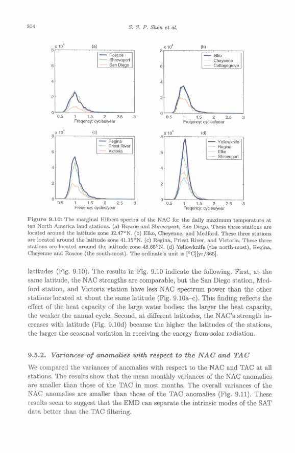
The empirical mode decomposition (EMD) method is used to analyze the nonlin- ear and non-stationary annual cycle (NAC) in climate data. The NAC is defined as an intrinsic mode function generated in the EMD process and has a mean pe- riod equal to a year. Both Hilbert and Fourier spectra of the NAC are examined to validate the power density at the frequency of one cycle per year. The NAC differs from the strictly periodic thirty-year-mean annual cycle (TAC), which is now commonly used in climate anomaly analysis. It is shown that the NAC has a stronger signal of the annual cycle than that of the TAC. Thus, the anomalies derived from the NAC have less spectral power at the frequency of one cycle per year than those from the TAC. The marginal Hilbert spectra of the maximum daily surface air temperature of ten North America stations demonstrate the ex- pected characteristics of an annual cycle: the NAC’s strength is proportional to the latitude of the station location and inversely proportional to the heat capac- ity of the Earth’s surface materials around a station. The NAC of the Nifio3.4 sea surface temperature analysis indicates that El Nifio events correspond to a weaker annual cycle, as suggested by wavelet analysis.

9.1. Introduction

Conventionally, when studying climate change via surface air temperature (SAT) data, one analyzes anomaly data, which are the departures of the observed SAT from its normal value called “climate normal” or “climatology.” The climatology of a station is often defined as the thirty-year mean of the station’s data for each month. The 30-year period progresses as time passes. Currently, 1961-1990 is com- monly used as the climatology period, whereas 1951-1980 was used in the 1980s and the early 1990s. Thus, the January climatology is the simple mean of the January temperatures from 1961-1990. This climatology is the expected monthly temper- ature throughout a year and is the so-called “annual cycle,” or “seasonal cycle.” Thus, the annual cycle of climate data describes the expected climate’s regular os- cillation from the winter cold to the summer heat and back to the winter cold. This fixed cycle, marked by the spring, summer, fall, and winter seasons, reflects the relative positions of the sun and the Earth, and the heat capacity of the Earth’s surface (land or ocean) , and some topographic characteristics. The commonly used

187

190 S. S. P. Shen et al.

still contain some apparent signal of the annual cycle because the TAC cannot completely filter out the annual signal from the climate data. Due to the nonlinear nature of the climate system, the spectral power of the TAC is not monotone at the one cycle per year; rather, it is distributed in a frequency interval that contains the annual cycle of one cycle per year. Thus, when the annual cycle in the residue of data minus the TAC is strong, the calculations of the linear trends of the seasonal or monthly climate changes can be affected because the non-monotonic “annual cycles” in the anomaly data are not synchronized to have peaks and valleys at the same month or season. Thus, the anomalies with respect to the TAC can lead to much uncertainty in a linear trend that is being used to measure the local, monthly climatic changes.

In contrast, the NAC reflects not only the periodic variation of the solar irradi- ance but also the nonlinear and non-stationary processes of atmospheric motions. Since the NAC is obtained through a sifting process, the sum of the last few IMFs can be regarded as the nonlinear and non-stationary trend. The nonlinear trend assessment of the monthly, local climatic changes is more robust and useful for attribution studies of the climatic changes.

Why do we want to remove the annual cycle? Although removing it is not important to the linear trend when a data stream is sufficiently long, the removal of this cycle becomes necessary when the data stream is shorter than 30 or 20 years. For a short stream of data, if we want to get a long-term linear trend for the regional or global average SAT, the seasonal variation will influence the trend, because only the departures from the “climate normal” in a cold area, such as Alberta, and a hot area, such as Arizona, can be compared in the spatial average. The annual cycle defined by the TAC assumes that the climate system can settle down into a “normal” pattern in a sufficiently long time period, say, 30 years. This assumption is a good approximation for many applications, yet when nonlinearity and non-stationarity have to be carefully considered, the assumption becomes problematic, since even in a low dynamic nonlinear chaotic system, such as the Lorenz attractor, the signal will not ever repeat itself. When the annual cycle appears to be an intrinsic property of a climate system, an adaptive approach, rather than a priori functional method, should be used to find the annual cycle. Furthermore, a successful removal-operation of annual cycles should satisfy the following criteria: (1) the anomaly data should have no spectral power peaks around the period of a year, and (2) the annual cycle should carry some physically meaningful signal, such as El Niiio. Criterion (1) reflects the variation of the solar irradiance, and criterion (2) reflects some major interactions between the dynamic components of a climate which is appropriate for a linear system, cannot satisfy even criterion (I), much less (2). The El Niiio signal is left in the anomaly data. Thus, the EMD approach is a natural way to define the annual cycle, that is the NAC. However, the NAC is not immune from uncertainties due to different sifting parameters, while the TAC’s uncertainties are caused by different period of 30 years. The contents of this chapter are arranged as follows:

Annual Cycle of Daily Surface A i r Temperature Data 191

Section 9.2 describes the method used in this research, regarding the end-point conditions, spectral representation, intermittence test, and stop criterion. Section 9.3 describes the daily and monthly data used in the analysis. Section 9.4 performs the time analysis of the NAC and analyzes the NAC’s robustness with respect to the length of the data stream, sifting parameters, and end-point algorithms. Section 9.5 performs the frequency analysis of both the NAC and the TAC. Section 9.6 contains conclusions and a discussion.

9.2. Analysis method and computational algorithms

The analysis method used here follows mainly that of Huang et al. (1998), a time domain analysis using EMD, and a frequency domain analysis using Hilbert and Fourier spectra. However, both the time and frequency analyses of Huang et al. (1998, 1999, 2003) have flexibilities in the computing details. Thus, we will specify our computing details to help others repeat our results.

The key problem in time-frequency analysis is to find the instantaneous fre- quency of a time series. Several ways are available to find instantaneous frequencies, including the wavelet transform (WT) and Hilbert transform (HT) (Mallat 1998, pp. 91-110; Boashash 1992a). The popular WT spectrum does not have a good res- olution for nonlinear processes and hence cannot effectively discern the nonlinear signals. The EMD pre-processed signals allow high-resolution Hilbert-spectra even for nonlinear signals. However, the HT often cannot be directly applied to a time series. For example, the HT was applied to the analysis of nonlinear vibration mo- tions (Feldman 1997), but the instantaneous frequency could not be found from the original time series. The possible problems were with the phase function, which are non-differentiable, or have unbounded derivatives, or are non-physical. H98 showed examples of these. The problem, thus, becomes how to find a differentiable and physically meaningful phase function so that the instantaneous frequencies are well defined, and their implications can be explained for the system where the data come from. Huang and his colleagues established their EMD-HAS (empirical mode decomposition-Hilbert spectral analysis), i.e., the HHT, based upon the belief that a physically meaningful mode should be self-coherent, namely, either quasi-periodic and quasi-symmetric, or quasi-monotone. Mathematically, phase functions and their derivatives are well defined for these types of functions by using HT. The quasi- periodic and quasi-symmetric functions, or quasi-monotone functions are the IMFs that satisfy the following two conditions:

(1) In the temporal domain of data, the number of extrema and the number of

(2) At any point, the mean value of the envelope defined by the local maxima and zero-crossings must either be equal or differ at most by one, and

the envelope defined by the local minima is zero.

With these requirements, an IMF oscillates in a narrow frequency band, a reflection of quasi-periodicity and nonlinearity. Of course, the non-constant frequency means

192 S. S. P. Shen et al.

non-stationarity. When an IMF c( t ) is found, its HT, N [ c ( t ) ] , can be found. Then

c( t ) + iX[c(t)] = a ( t ) exp(iw(t)]

is well defined. For a given t , this equation yields a frequency w( t ) and an amplitude ~ ( t ) . The triplet (t,w,u) forms the Hilbert spectral power described in Huang et al. (1998). The procedures for finding an IMF c ( t ) can be found in Chapter 1 of this book. However, the conditions of the end points, stopping criterion and intermittence are still flexible up to certain subjective decisions. The details of our algorithm are described below.

The envelopes of local maxima and minima require the extrapolation of the original time series outside the two temporal end points: the first point and the last point of the time series. However, usually no physical laws can be easily used to make the extrapolation. Various spline extrapolation methods have been devel- oped. We used two extrapolation methods to deal with the end effect: the signal extension approach by Wu and Huang (2004) and the extrema-prediction approach. The signal-extension approach includes two steps: the signal extension step and the signal-damping step. In the first step, the targeted time series, fi, i = 1 , . . . , N , is extended by using the anti-symmetric extension. In the second step, the extended signal is damped at the two ends. One can also use a one-step signal extension approach: a simple reflection extension. Apparently, many other signal-extension methods can be used. The physical nature of a problem is helpful in determining which methods are appropriate for the problem.

Due to the use of cubic splines, each EMD sifting step requires two extrema points outside of the data’s temporal domain (possibly including the first end data point) and before the first extrema point. Similarly, each step requires two extrema points after the last extreme point. These four extrema must be predicted.

Many possible approachs can be used for predicting these extrema. For example, Coughlin and Tung (2003) extended the signal by adding a characteristic wave at each end of the sifted data stream. Our approach is as follows: Let us denote the first data point by (0, x o ) , the first two extrema by (t l , q) and ( t 2 , 2 2 ) , where 0 < t i < t 2 ,

and the predicted extrema by (tpl, zpl) and ( t p 2 , x,2). Setting t,l = min(0,2ti - t 2 )

and t,2 = t,l - ( t 2 - t l ) , then xpl = 2 2 if t,l < 0; otherwise, xpl = 20. On the other hand, xp2 always equals 2 1 . The two extrema after the last data point are predicted in a similar manner.

The stopping criterion, determining when the EMD sifting stops for an IMF mode, is another important component for the sifting process. A stopping criterion through the standard deviation (SD) is proposed in H98. The sifting process for an IMF is stopped if this SD value is between 0.2 and 0.3. However, this SD value depends on the length of the time series. An alternative stop criterion is that the number of zero crossings and extrema remains the same for N successive sifting steps (Huang et al. 1999,2003). The choice of N is subjective, and many trials have to be made to find the best N suitable for a certain time series. The stopping

Annual Cycle of Daily Surface Air Temperature Data 193

criterion used here is that the sifting process stops when

where hi, i = 1,. . . , N, are the data of the step of being stopped, and mi, i = 1 , . . . , N, are the mean of the envelope of maxima and that of the mimima of the data hi, i = 1 , . . . , N .

Mode mixture, a phenomenon of different time scales mixed in a single IMF component, often occurs in a practical sifting process. The intermittency test is used to separate the intrinsic mode in the sifting process to prevent the modes from mixing. The intermittence criterion adopted in this study is a number M selected as the limit to the distances between each pair of the three successive maxima. If these distances are both greater than M , the points between the two zero crossings among the three extrema are assigned as zero. The M value ranges between 120 and 150 for the station SAT anomaly data in this research.

Our HT is computed by using the Fourier transform (Marple 1999). The sig- nal z( t ) and its HT forms an analytic signal z ( t ) = z( t ) + i'H[z(t)]. The N-point spectrum Z ( m ) of the discrete analytic signal z ( t ) is computed by

{ 0,

2 X ( m ) , 0 < m < N/2 ,

N/2 < m < N , Z ( m > = X ( m > , m = 0, N / 2 , (9.3)

where X ( m ) is the Fourier transform of z ( t ) . The discrete-time analytic signal z[n] is then computed by using the N-point inverse discrete Fourier transform, and the imaginary part of z[n] is IFl[z(t)].

The amplitude and phase of z ( t ) are a ( t ) = d [ ~ ( t ) ] ~ + {IFl[z(t)]}2 and O(t) = arctan{'H[z(t)]/z(t)}. The instantaneous frequency of a continuous signal is defined as (Boashash 1992a)

1 dQ(t) 2~ d t

w(t) = -- . (9.4)

Computationally, for a discrete-time analytic signal z [n] , we can compute the am- plitude a[n] and the angle O[n]. The discrete-time instantaneous frequency w[n] is computed by using the central difference scheme

1 Q[n + 11 - O[n - 11 2T 2T

4.1 = - 1 (9.5)

where T is the time interval (Boashash 1992b). Thus, a given time n corresponds to a frequency w[n] and an amplitude a[n] . Thus, on the (n,w)-plane, each point corresponds to an amplitude that is a function of both time n and frequency w, but the time n and frequency w are not independent; rather, they are related by a function w [ n ] . The triplet (n, w [ n ] , a [ n ] ) determines a point in the three-dimensional space ( n , w , a ) . For a given n, find a point w [ n ] , hence a point on the (n, w)-plane.

194 S. S. P. Shen et al.

From this point, find the corresponding amplitude a[n]. One can find this a[.] for all IMFs and hence for many amplitudes on the (n, w)-plane. These amplitudes form the discrete Hilbert-spectra. They are then smoothed by a 9-point grid, moving average on the (n, w)-plane to yield a series of smooth ridges in the three-dimensional space (n, w, a ) , and each ridge corresponds to an IMF (see Figs. 9.2a and 9.4b for two examples of Hilbert spectra). For more examples, see Huang et al. (1998).

9.3. Data

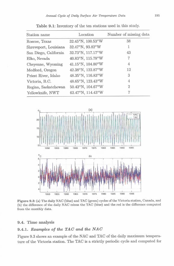
The dataset used in this study is the daily maximum surface air temperature data at 10 land stations of different latitude in USA and Canada in the time interval of 1 January 1946 to 31 December 2000. The data are from the Global Daily Climatology Network (GDCN) dataset of the US National Climatic Data Center (NCDC). The GDCN (v1.0) is a global dataset and contains different records of 32 857 locations around the world but covers mainly the northern hemisphere. The earliest and the latest dates of observation are 1 March 1840 and 30 November 2001, respectively, and most stations have missing records. All of the GDCN data have gone through an extensive set of quality-control procedures viz. simple datum checks and the statistical analysis of sets of observations to locate and identify potential outliers and/or erroneous data. However, the station data have not been homogenized. To demonstrate the NAC properties, we selected 10 stations in the United States and Canada that have few missing data and are distributed at four different latitude lev- els and from a coast to an area inland. Among the ten stations, three are distributed around the latitude zone 32.47'N, three around 41.15"N, three around 48.65'N, and one on 62.47'N. Among these stations, San Diego, Medford, and Victoria are close to the Pacific. They have few missing data in 55 years: from 1 January 1946 to 31 December 2000. Since the number of missing data is small with respect to the length of the entire data, the missing data are interpolated by using cubic spline fitting. The inventory of the ten stations is shown in Table 9.1.

The land stations at different latitudes were chosen to show the increase of the strength of the annual cycle as the latitude gets higher. It is also important to determine the annul cycle for the equatorial area where the incoming solar irradiance does not vary according to seasons. While no clear annual cycle is apparent on the equator, the climatology and climate anomalies are routinely computed for the SST data in both climate research and forecasting. To investigate the annual cycle of the equatorial area, we processed the SST data, not the SST anomaly data, over the Niiio 3.4 region (5"N-5"S1 12OoW-17O0W) from January 1950 to March 2003. The data are from the National Centers for Environmental Prediction (NCEP) data repository. The El Niiio and La Niiia events defined by Trenberth (1997) are used to compare the ENS0 signal carried by the NAC.

Annual Cycle of Daily Surface A i r Temperature Data 197

The difference of the NAC minus the TAC is shown in Fig. 9.3b (blue line). As shown in Fig. 9.1, the decomposed daily TAC has jumps from the last day of the previous month to the first day of the current month. These jumps cause a large difference. When using the monthly data to find the NAC, the difference of the NAC minus the monthly TAC is smaller (the red line in Fig. 9.3b). In both cases, there is no apparent drift of the differences away from zero.

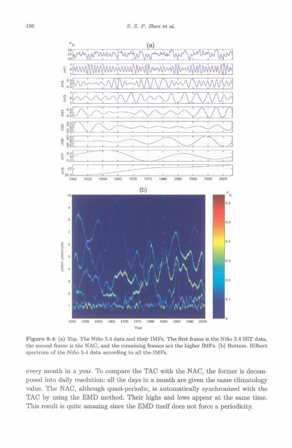
The IMFs of the Nifio 3.4 data are shown in Fig. 9.4. The first IMF is the NAC, and the second IMF corresponds to the biennial cycle. The third to fifth IMFs are the three- to seven-year cycles. The sixth IMF is the decadal cycle. The seventh IMF is the multi-decadal cycle. The last one is a warming trend. The strength of the NAC is found to have been enhanced during three strong La Niiia events in 1955- 1956, 1970-1971, and 1974-1975, and weakened during most El Niiio events before 1990. Similar results have been found by using the wavelet transform (Wang 1994, Wang and Wang 1996). The influence of the ENSO on the annual cycle appears to have changed after 1990. The prolonged El Nifio events from 1991 to 1995 did not change the amplitude of the NAC, but the NAC still appeared to be strong during the latest La Niiia period from 1998 to 2000. The smaller amplitude of the NAC in the second panel of Fig. 9.4a corresponds to the smaller amplitude of the lowest smoothed bright line around the frequency of one cycle yr-‘ in Fig. 9.4b. To clearly explain the Niiio 3.4 SST data, their NAC, its NAC and TAC anomalies, we display them in Fig. 9.5. It is quite surprising that the EMD-derived NAC is quasi-periodic and oscillates in the frequency of one cycle per year, because the incoming solar radiation does not have an apparent annual cycle. Of course, the NAC’s amplitude is small with a high-low difference within 2 degrees. We also calculated the TAC, and the anomalies with respect to the NAC and TAC. The anomalies are almost the same. The TAC anomalies have been commonly used to define El Niiio events (Trenberth 1997). The comparison of the NAC’s and the TAC’s anomalies seems to suggest that the NAC anomalies can also be used to define El Niiio. If so, the definition of El Niiio is more natural and the nonlinearity of the ENSO dynamics is explicitly reflected in the statistical computing of the ENSO index. However, this conclusion needs further justification, and the EMD method for describing the ENSO dynamics requires a thorough investigation.

9.4.2. Temporal resolution of data

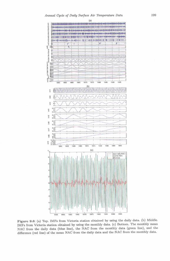
The NAC is in an annual time scale and is expected to be independent of the daily or monthly data resolution. This expectation was confirmed by analyzing the daily and monthly data of the ten stations. We performed sifting processing on the daily and monthly SAT data. The resulting daily NAC is averaged in each month, and the difference between the mean daily NAC and the monthly NAC is small. Figure 9.6a shows the IMFs derived from the daily maximal temperature of the Victoria station. The IMFll is the NAC, which is compared with the NAC derived from the monthly data (imfl in Fig. 9.6b). The difference, shown in Fig. 9.6c, oscillates around

200 S. S. P. Shen et al.

The above result does not mean that the daily resolution data are not important. On contrary, they are very important in reflecting the nonlinear interactions of the climate components in different time scales, but the interactions are reflected in the anomalies derived from the NAC.

9.4.3. Robustness of the EMD method

Another important aspect concerning our confidence in the NAC results is the robustness of the IMFs. Two questions are involved: (1) can the EMD lead to the separation of a given signal in a dataset? and (2) are the EMD-derived IMFs insensitive to the length of the data streams, the perturbation of the end conditions, the intermittency test, and the stop criterion? Huang et al. (2003) addressed some aspects of this problem. More examples are given below.

9.4.3.1. EMD separation of a known signal an a synthetic dataset

A dataset of 7300(= 365 x 20) data points, uniformly spaced in time t , has three signal components and a noise component and is expressed by the following:

where w[n] is a sequence of white noise with mean zero and variance gt = (1.5)’ and n = 1,. . . ,20 x 365 (Fig. 9.7a). The dataset mimics a 20-yr climate data of two periodic components at the frequency of one cycle yr-’ and $ cycles yr-’, a quadratic trend, and white noise. The annual cycle is much stronger than the 5-yr cycle. The nonlinear trend is very weak. This signal is contaminated by white noise. The signal-extension approach was applied to mitigate the end effect. The sifting results show the IMFs representing dyadically-filtered white noise (Flandrin et al. 2003, Wu and Huang 2004), the annual cycle component, and the low-frequency components, and the last two IMFs are trends (Fig. 9.7b). We used the sum of the low-frequency components to reconstruct the 5-yr cycle component in the signal and the sum of the last two IMFs to reconstruct the trend component. The results show that, as one expects, the EMD can accurately recover the strong annual component. The recovery of the weak 5-yr cycle is also very good except in the neighborhoods of the end points. The end-point effects are carried to the trend recovery. The EMD- derived trends from 0 to 2 300 and from 4 500 to 7 300 are apparently deviating away from the original trend. See Fig. 9 . 7 ~ . These results call for further revisions of the end-point conditions.

9.4.3.2. Robustness with respect to data length

The full dataset of the daily maximum temperature data at Victoria station is from 1 January 1946 to 31 December 2000. In order to test the IMF’s robustness with

Annual Cycle of Daily Surface Air Temperature Data 201

0 1000 2000 3000 4000 5000 €000 7000 10

I 0 1000 2000 3000 4000 5000 €000 7000 8000

101

~, -i

2 0 1000 2000 3000 4000 5000 €000 7000 8000

2-

1.5

Figure 9.7: (a) Top. Synthesized data s[n]. (b) Middle. IMFs of s[n] from the sifting process. (c) Bottom. Comparisons of the IMFs with the three signal components.

Annual Cycle of Daily Surface Air Temperature Data 207

Table 9.2: The ratio of the energy around one cycle yr-' of anomaly data with respect to the TAC and the NAC and that of the annual cycles at all stations.

Roscoe Shreveport San Diego Elk0 Cheyenne Medford Priest River Victoria Regina Yellowknife

3.6 6.2 4.1 8.0 5.6 1.4 8.5 18.7 17.3 2.3

0.93 0.96 0.95 0.99 0.98 1.02 0.99 0.94 0.96 0.98

9.6. Conclusions and discussion

We have used the EMD method to derive the nonlinear non-stationary annual cycle for both the SAT at land stations in North America and the SST in the Niiio 3.4 region. The nonlinear and non-stationary annual cycle compared with the commonly used thirty-year-mean annual cycle (TAC). The NAC allows daily resolution and is robust with respect to the length of a data stream and the end conditions of the EMD method. The EMD procedure used in the paper can accurately separate the annual cycle in a synthetic dataset composed of multiple harmonics, a nonlinear trend, and white noise. Comparison of the NAC and TAC in spectral space indicates that the NAC is a cleaner filter for the annual cycle than the TAC.

Many problems involving annual cycles are worth investigation. Three are listed here:

Can one use the NAC anomalies of the Niiio 3.4 SST data or the buoy data in the same area to define the El Niiio events? If the NAC anomalies are calculated from the 5" x 5" grid boxes for the NCAR/NCEP Reanalysis data and the EOFs are computed from these anoma- lies, then are the ENS0 patterns distributed in the same way as those calculated from the commonly used TAC anomalies? Discrete wavelet analysis can also yield modes of different scales. Is a systematic method available for comparing the modes derived from the EMD, wavelet analysis, and even some dynamical models?

208 S. S. P. Shen et al.

Acknowledgements

This work was supported by the NOAA Office of Global Programs. Shen also thanks the US National Research Council for the Associateship award, MITACS (Mathe- matics of Information Technology and Complex Systems) for a research grant, and the Chinese Academy of Sciences for an Overseas Assessor's research grant and for the Well-Known Overseas Chinese Scholar award.

References

Boashash, B., 1992a: Estimating and interpreting the instantaneous frequency of a signal. Part 1: Fundamentals. Proc. IEEE, 80, 520-538.

Boashash, B., 199213: Estimating and interpreting the instantaneous frequency of a signal. Part 2: Algorithms and applications. Proc. IEEE, 80, 539-568.

Coughlin, K. T., and K. K. Tung, 2003: ll-year solar cycle in the lower stratosphere extracted by the empirical mode decomposition method. Adv. Space Res., 34,

Feldman, M., 1997: Non-linear free vibration identification via the Hilbert trans- form. J. Sound Vib., 208, 475-489.

Flandrin, P., G. Rilling, and P. GonCalvBs, 2004: Empirical mode decomposition as a filter bank. IEEE Signal Process. Lett., 11, 112-114.

Gloersen, P., and N. E. Huang, 2003: Comparison of interannual intrinsic modes in hemispheric sea ice covers and other geophysical parameters. IEEE Trans. Geosci. Remote Sens., 41, 1062-1074.

Huang, N. E., Z. Shen, and S. R. Long, 1999: A new view of nonlinear water waves: The Hilbert spectrum. Annu. Rev. Fluid Mech., 31, 417-457.

Huang, N. E., Z. Shen, S. R. Long, M. C. Wu, H. H. Shih, Q. Zheng, N-C. Yen, C. C. Tung, and H. H. Liu, 1998: The empirical mode decomposition and the Hilbert spectrum for nonlinear and non-stationary time series analysis. Proc. R. SOC. London, Ser. A, 454, 903-995.

Huang, N. E., M. C. Wu, S. R. Long, S. S. P. Shen, N. H. Hsu, D. Xiong, W. Qu, and P. Gloersen, 2003: On the establishment of a confidence limit for the empirical mode decomposition and Hilbert spectral analysis, Proc. R. SOC. London, Ser.

323-329.

A, 459, 2317-2345. Mallat, S., 1998: A Wavelet Tour of Signal Processing. Academic Press, 637 pp. Marple, S. L., 1999: Computing the discrete-time analytic signal via FFT. IEEE

Trenberth, K. E., 1997: The definition of El Niiio. Bull. Amer. Meteor. SOC., 78,

Wang, B., and Y. Wang, 1996: Temporal structure of the Southern Oscillation as

Wang, B., 1994: On the annual cycle in the tropical eastern-central Pacific.

Trans. Signal Process., 47, 2600-2603.

2771-2777.

revealed by waveform and wavelet analysis. J. Climate, 9, 1586-1598.

J. Climate, 7, 1926-1942.

Annual Cycle of Daily Surface Air Temperature Data 209

Wu, Z., and N. E. Huang, 2004: A study of the characteristics of white noise using the empirical mode decomposition method. Proc. R. SOC. London, Ser. A, 460, 1597-161 1.

Samuel S. P. Shen Department of Mathematical and Statistical Sciences, University of Alberta, Edmonton, Alberta T6G 2G1, Canada shen@ualberta. ca

Tingting Shu Department of Mathematical and Statistical Sciences, University of Alberta, Edmonton, Alberta T6G 2G1, Canada ttshu@ualberta. ca

Norden E. Huang Goddard Institute for Data Analysis, Code 971, NASA/Goddard Space Flight Center, Greenbelt, MD 20771, USA norden. e. huang@nasa.gov

Zhaohua Wu Center for Ocean-Land-Atmosphere Studies, 4041 Powder Mill Rd., Suite 302, Calverton, MD 20705-31 06, USA zhwu@cola. ages. org Gerald R. North Department of Atmospheric Science, Texas A&M University, College Station, TX 77843, USA north@csrp.tamu. edu

Thomas R. Karl NOAA/National Climatic Data Center, Asheville, NC 28801, USA tlcarl@ncdc. noaa.gov

David R. Easterlang NOAA/National Climatic Data Center, Asheville, NC 28801, USA deasterl@ncdc. noaa.gov