Heat Transfer Investigations in a Modern Diesel Engine - CORE
204
This thesis may not be consulted, photocopied or lent to other libraries without the permission of the author and Federal Mogul for three years from the date of acceptance of the thesis. Heat Transfer Investigations in a Modern Diesel Engine Carlos Adolfo Finol Parra A thesis submitted for the degree of Doctor of Philosophy University of Bath Department of Mechanical Engineering February 2008 COPYRIGHT Attention is drawn to the fact that copyright of this thesis rests with its author. This copy of the thesis has been supplied on condition that anyone who consults it is understood to recognise that its copyright rests with its author and that no quotation from the thesis and no information derived from it may be published without the prior written consent of the author.
-
Upload
khangminh22 -
Category
Documents
-
view
0 -
download
0
Transcript of Heat Transfer Investigations in a Modern Diesel Engine - CORE

This thesis may not be consulted, photocopied or lent to other libraries without the permission of the author and Federal Mogul for three years from the date of acceptance of the thesis.
Heat Transfer Investigations in a Modern Diesel Engine
Carlos Adolfo Finol Parra
A thesis submitted for the degree of Doctor of Philosophy
University of Bath
Department of Mechanical Engineering
February 2008
COPYRIGHT
Attention is drawn to the fact that copyright of this thesis rests with its author. This copy of the thesis has been supplied on condition that anyone who consults it is understood to recognise that its copyright rests with its author and that no quotation from the thesis and no information derived from it may be published without the prior written consent of the author.

ii
Summary
An experimental investigation has been undertaken to study operating temperatures and
heat fluxes in the cylinder walls and cylinder head of a modern diesel engine.
Temperatures were measured under a wide range of speed and torque at more than one
hundred locations in the block and cylinder head of the engine employing conventional
thermocouples arranged to obtain one-dimensional metal thermal gradients and
subsequently deduce the corresponding heat fluxes and surface temperatures. Results
observed in the cylinder bores revealed that in addition to heat transferred by convection
and radiation from combustion gases, the temperature and heat flux distributions are
considerably affected by heat conduction from piston rings and skirt through the oil
film, and by frictional heat generated at these components. The heat fluxes and surface
temperatures obtained in the cylinder head combined with gas pressure measurements
were used to evaluate existing formulae to predict heat transfer coefficients from
combustion gases to the chamber walls. The evaluation confirmed the significant
variation previously observed between the various methods. As a consequence, a
modified correlation has been proposed to estimate the gas-side heat transfer coefficient.
This new correlation is considered to be an improved tool for estimating the heat
transfer coefficients from combustion gases in modern diesel engines. Additionally, the
results observed in the cylinder bores were used to develop a simple model from first
principles to estimate the heat transferred from piston rings and skirt to the cylinder
wall.

iii
Acknowledgements
This research work has been possible thanks to the collaboration of many people within
the Department of Mechanical Engineering and the Powertrain and Vehicle Research
Centre (PVRC) of the University of Bath, as well as the support of The Ford Motor
Company and Federal Mogul.
Within the Department of Mechanical Engineering, special gratitude is given to
Professor Gary Hawley for his support and friendship and to Professor Alec Parker,
whose enthusiasm and contribution in the last two years has been invaluable. Also
thanks to Dr Kevin Robinson for his supervision and to the following people whose
assistance throughout this work is sincerely recognised: Eric Brain, Alan Jeffries, Vijay
Rajput, Allan Cox, Sam Hurley, Dr Sam Akehurst and Professor Frank Wallace.
Finally, I would like to say thank you Julie for your endless support, encouragement and
understanding over the last few years.

iv
Contents
Notation vii
List of Figures x
List of Tables xvi
Chapter 1. Introduction 1
1.1. General Background 1
1.2. Aims and Objectives 2
1.3. Scope of Thesis 3
Chapter 2. Estimating the Heat Transferred from Combustion Gases 6
2.1. Introduction 6
2.2. General Concepts 6
2.3. Heat Transfer Correlations used in Internal Combustion Engines 7
2.3.1. Correlations for the Time-Averaged Coefficient 8
2.3.2. Correlations for the Instantaneous Spatially-Averaged Coefficient 11
2.3.3. Correlations for the Instantaneous Local Coefficient 25
2.4. Discussion of Application of Existing Correlations to Modern Diesel 29
Engines
Chapter 3. Experimental Set-Up 32
3.1. Introduction 32
3.2. Detailed Thermal Survey 32
3.2.1. Measuring Technique 32
3.2.2. Engine Instrumentation 33
3.2.2.1. Engine Block 33
3.2.2.2. Cylinder Head 39
3.2.3. Methodology Evaluation 44
3.2.4. Coolant Temperatures and Coolant Flows 49
3.3. Crank Angle Based Measurements 51
3.3.1. In-Cylinder Pressure 51
3.3.2. Instantaneous Temperatures 52
3.4. Testing Equipment 54
3.4.1. Test Engine 54
3.4.2. Test Facilities 55
3.4.3. Data Acquisition Systems 56
3.5. Engine Set-Up 57
3.6. Test Programme 58
3.6.1. Map of Engine Speed and Torque 59
3.6.2. Variation of Parameters 61
Chapter 4. Data Processing 63
4.1. Introduction 63
4.2. Methodology 63
4.2.1. Processing Criteria 63
4.2.2. Control Variables 63
4.2.3. Data Processing Routines 70

Contents
v
4.3. Computation of Temperature Gradients, Wall Surface Temperatures, 75
Heat Fluxes and Heat Transfer Coefficients
4.4. Data Validation 81
4.4.1. Inspection of Temperature Data 81
4.4.2. Statistical Parameters 95
4.4.3. Evaluation of the Coolant-Side Heat Transfer Coefficient 99
4.4.4. Repeatability 102
Chapter 5. Experimental Results 105
5.1. Introduction 105
5.2. Cylinder Bores 105
5.2.1. Surface Temperature 106
5.2.2. Heat Flux 111
5.3. Cylinder Head 113
5.3.1. Surface Temperature 114
5.3.2. Heat Flux 117
5.4. Uncertainty Analysis 117
5.5. Influence of Variation of Parameters on Surface Temperature and 124
Heat Flux
5.5.1. Exhaust Gas Recirulation (EGR) Effect 124
5.5.2. Inlet Manifold Temperature Effect 127
5.5.3. Injection Timing Effect 129
Chapter 6. Evaluation of Heat Transfer Correlations 132
6.1. Introduction 132
6.2. Data Requirements 133
6.2.1. Cylinder Gas Pressure 133
6.2.2. Mean Piston Speed and Combustion Chamber Geometry 134
6.2.3. Gas Properties 136
6.2.4. Mean Gas Temperature 137
6.3. Heat Transfer Coefficient Results 142
6.4. Proposal for a Modified Heat Transfer Correlation 149
6.5. Summary 153
Chapter 7. Model from First Principles to Estimate the Heat Flux in the 154
Cylinder Bore
7.1. Introduction 154
7.2. Heat Transfer from Combustion Gases to the Cylinder Bore 155
7.3. A Simple Piston Model 156
7.3.1. Piston Velocity and Acceleration 157
7.3.2. Determination of Forces 159
7.4. Conductive Heat Transfer 166
7.4.1. Deduction of the Oil Film Thickness 168
7.4.2. Heat Conduction from the Piston Rings 170
7.4.3. Heat Conduction from the Piston Skirt 172
7.5. Heat Generation by Friction 173
7.5.1. Piston Rings 174

Contents
vi
7.5.2. Piston Skirt 175
7.6. Results and Discussion 177
7.7. Concluding Remarks 180
Chapter 8. Conclusions and Further Work 182
References 185
Appendices 189
Appendix A. Instruments and Materials Specifications 189
A.1 K-Type Thermocouples 189
A.2 Fast Response Thermocouples 189
A.3 Platinum Resistance Thermometer (RTD) 189
A.4 Flow Meters 189
A.5 Data Loggers 189
A.6 Pressure Sensor 189
A.7 AVL 620 Indiset Measuring Configuration 190
A.8 Epoxy Resin 190
Appendix B. Engine Characteristics 191
B.1 Limiting Torque Curve (LTC) and Power Curve 191
B.2 Valve Data 192
Appendix C. Test Facilities 194
C.1 Test Cell Schematic Layout 194
C.2 Test Cell Equipment 195
Appendix D. Data Processing Routines 196
D.1 Testing Sequence 196
D.2 Logging Times 196
D.3 Trace File Data Stripper 197
D.4 Temperature Data Stripper 201
D.5 Thermal Gradients, Wall Surface Temperature and Heat Flux 209
in the Engine Block
D.6 Thermal Gradients, Wall Surface Temperature and Heat Flux 213
in the Cylinder Head
D.7 Gas Temperature 217
D.8 Heat Transfer Coefficient Correlations 224
D.9 Piston Model 227
Appendix E. Uncertainty Analysis Equations 238
E.1 Wall Surface Temperature 238
E.2 Heat Flux 239
Appendix F. Piston and Lubricant Data 241
F.1 Piston Dimensions 241
F.2 First Compresssion Ring 242
F.3 Second Compresssion Ring 242
F.4 Oil Control Ring 243
F.5 Piston Temperature Distribution at Maximum Power 244
F.6 Lubricant Oil 244

vii
Notation
a crank radius (m)
a, b, c, m, n experimental coefficients, parameters, exponents
A instantaneous surface area exposed to heat transfer (m2)
surface area (m2)
Ap piston area, bore area times number of cylinders (m2)
Ar reference area (m2)
B cylinder bore or diameter (m)
length of an area in the direction of motion (m)
Cd valve discharge coefficient
CDF valve discharge coefficient (forward flow)
CDR valve discharge coefficient (reverse flow)
Cp constant-pressure specific heat (J/kg K)
Cu peripheral gas velocity (m/s)
C1, C2, C3 constants
de equivalent diameter (m)
dp piston diameter (m)
ds sphere diameter (m)
f friction coefficient
F heat flux distribution factor
force (N)
Fi heat flux distribution factor
G gas mass flow rate per unit of piston area (kg m-2
s-1
)
h heat transfer coefficient (W/m2 K)
hc convective heat transfer coefficient (W/m2 K)
he over-all engine heat transfer coefficient (W/m2 K)
k thermal conductivity (W/m K)
l length of the connecting rod (m)
L instantaneous chamber height (m)
piston stroke (m)
length of an area at right angles to the direction of motion (m)
m gradient
mp piston equivalent mass (kg)
m& mass flow rate (kg/s)

Notation
viii
fm& fuel mass flow rate (g/hr)
n engine rotational speed (rev/min)
Nan swirl anemometer speed (rad/min)
Nu Nusselt number
p instantaneous cylinder gas pressure (bar)
pL air pressure before inlet valve (bar)
pme brake mean effective pressure (bar)
Pr Prandtl number
q& heat flux rate (heat transfer per unit area per unit time), (W/m2)
Q& heat transfer rate (heat transfer per unit time), (W)
r radial distance from the cylinder axis (m)
R gas constant of air (287 J/kg K)
ratio of connecting rod length to crank radius (l/a)
Re Reynolds number
s distance from crank axis to piston pin axis (m)
s& piston velocity (m/s)
s&& piston acceleration (m/s2)
t time (s)
T temperature (K)
force in the connecting rod (N)
Twr wall surface temperature at radius r (K)
U instantaneous gas velocity (m/s)
velocity of a sliding surface (m/s)
Vp mean piston speed (m/s)
V instantaneous cylinder volume (m3)
Vs swept volume (m3)
W load (N)
x distance measured along one particular coordinate (m)
αscaling scaling factor
∆x difference in distance (m)
∆T difference in temperature (K)
ε emissivity of radiating agent
ϕ angle between cylinder axis and connecting rod (degrees)
γ ratio of constant-pressure to constant-volume specific heats

Notation
ix
µ dynamic viscosity (kg/m s)
ν kinematic viscosity (m2/s)
θ crank angle (degrees)
ρ density (kg/m3)
σ Stefan-Boltzmann constant (5.67x10⁻⁸
W/m2 K
4)
ω angular rotational speed of the crankshaft (rad/s)
ωg angular velocity of cylinder gases (rad/s)
Subscripts
a indicates ambient conditions
b refers to the cylinder bore
c denotes coolant
g denotes gas
i denotes inertia
m indicates motored condition
p denotes pressure
r indicates a reference state or refers to the radial direction
s denotes combustion space surface
t denotes side thrust
T refers to the condition immediately after a flow restriction
w denotes wall surface
x denotes reference to one particular coordinate
0 refers to stagnation conditions
1, 2 refer to coordinate values or crank angle steps
Please note that all of the quantities and coefficients used in the equations of this thesis
have been calculated on the basis that the dimensions of all the constituent terms are
those given in the Notation. Thus, for example, in Equation 2.8 (Eichelberg correlation)
the dimensions of AQ /& are W/m2 and the coefficient 2.43 is correct provided that Vp is
in m/s, p is in bar, and Tg and Ts are in K.

x
List of Figures
Chapter 2 Estimating the Heat Transferred from Combustion Gases 6
Figure 2.1. An example of a correlation of time-averaged heat transfer measurements for several engines (Annand, 1986).
10
Figure 2.2. Observed heat fluxes compared with predictions by correlations from (a) Annand (1963), and (b) Annand and Ma (1970-71).
16
Figure 2.3. Local, local-mean heat transfer coefficient, and time-resolved curve according to Woschni’s equation (Sihling and Woschni, 1979).
18
Figure 2.4. Computed heat flux rate versus crank position (Hohenberg, 1979) 20
Figure 2.5. Comparison of predicted heat transfer coefficients and measured data (Han et al., 1997).
22
Figure 2.6. Comparison of measured spatially-averaged heat flux and predictions from several global models (Chang et al., 2004).
23
Figure 2.7. Heat flux variation with speed (a) spatially-averaged measured heat flux and (b) modified Woschni. Adapted from Chang et al. (2004)
24
Figure 2.8. Comparison of predicted heat transfer coefficients (Watson and Janota, 1982).
25
Figure 2.9. Extension of motored correlation to fired operation at (a) TC-1 and at (b) TC-2. Adapted from LeFeuvre et al. (1969).
26
Figure 2.10. Comparison of measured mean heat fluxes on piston crown (annular region) with prediction by flat plate equation using bulk mean gas temperature at 1050 rev/min fired operation (Dent and Suliaman, 1977).
28
Figure 2.11. Temperature field and heat flux through the cylinder liner of a supercharged diesel engine at 1500 rev/min and pme = 11 bar. Adapted from Woschni (1979).
30
Chapter 3 Experimental Set-Up 32
Figure 3.1. Schematic installation of a set of thermocouples in the cylinder wall. 34
Figure 3.2. General orientation of arrays of thermocouples in the engine block. 34
Figure 3.3. Schematic location of thermocouple sets in the engine block. 35
Figure 3.4. Thermocouple installation on locations A (a) and F (b), together with holes drilled ready for thermocouples on locations B (a) and G (b).
36
Figure 3.5. Thermocouples being installed on the inlet side (a) and completed installation on the exhaust side (b).
36
Figure 3.6. Schematic installation of a set of thermocouples in the cylinder head.
40
Figure 3.7. Thermocouple sets locations in the cylinder head. 40
Figure 3.8. Cylinder head during instrumentation. 43
Figure 3.9. Thermocouples already installed on the head before (a) and after (b) reassembling the valve train.
43
Figure 3.10. Instrumented cylinder head. 44

List of Figures
xi
Figure 3.11. Temperature distribution in a cylindrical section of the cylinder wall: (a) undisturbed situation and (b) section with holes.
46
Figure 3.12. Predicted temperatures. 48
Figure 3.13. Errors in predicted temperatures. 49
Figure 3.14. Engine cooling circuit. 50
Figure 3.15. Fast response thermocouple and adaptor. 53
Figure 3.16. Engine test bed. 58
Figure 3.17. Test sequence at 2500 rev/min. 60
Chapter 4 Data Processing 63
Figure 4.1. Variation of speed, torque, fuelling and injection timing during a test at 3000 rev/min and 50% LTC (approximately 143 Nm).
64
Figure 4.2. Variation of speed and torque at test conditions 1000 rev/min and 30% LTC, 1500 rev/min and 10% LTC, 3500 rev/min and 40% LTC, and 4000 rev/min and 70% LTC.
65
Figure 4.3. Variation of speed, torque, bottom hose temperature and air charge temperature during a test at 3000 rev/min and 50% LTC (approximately 143 Nm).
66
Figure 4.4. Effect of increasing speed on the control of inlet coolant temperature (a) and air charge temperature (b).
67
Figure 4.5. Effect of increasing torque on the control of inlet coolant temperature (a) and air charge temperature (b), at an engine speed of 3500 rev/min.
68
Figure 4.6. Effect of variations of inlet coolant and air charge temperatures on metal measured temperatures in the block (location A2C) and cylinder head (location C1D), at 4000 rev/min and 70% LTC (approximately 158 Nm).
69
Figure 4.7. Test sequence at 4000 rev/min. 71
Figure 4.8. Test point at 4000 rev/min and 40% LTC (approximately 68 Nm). 72
Figure 4.9. Schematic representation of the one-dimensional heat flux and temperature distribution in the cylinder walls.
78
Figure 4.10. Average measured temperature at locations A1 to A4 on the exhaust-side of cylinder two, for all torque values tested at 2500 rev/min.
82
Figure 4.11. Average measured temperature at locations A5 to A7 on the exhaust-side of cylinder two, for all torque values tested at 2500 rev/min.
83
Figure 4.12. Average measured temperature at locations B1 to B4 on the exhaust-side of cylinder two, for all torque values tested at 2500 rev/min.
84
Figure 4.13. Average measured temperature at locations C1 and C2 on the exhaust-side of cylinder two, for all torque values tested at 2500 rev/min.
85
Figure 4.14. Average measured temperature at locations D1 and D2 on the exhaust-side of cylinder three, for all torque values tested at 2500 rev/min.
86

List of Figures
xii
Figure 4.15. Average measured temperature at location E2 on the exhaust-side of cylinder four, for all torque values tested at 2500 rev/min.
86
Figure 4.16. Average measured temperature at locations F1 to F4 on the inlet-side of cylinder two, for all torque values tested at 2500 rev/min.
87
Figure 4.17. Average measured temperature at locations F5 to F7 on the inlet-side of cylinder two, for all torque values tested at 2500 rev/min.
88
Figure 4.18. Average measured temperature at locations G1 to G4 on the inlet-side of cylinder two, for all torque values tested at 2500 rev/min.
89
Figure 4.19. Average measured temperature at locations H2 to H4 (sets of two thermocouples on the rear of cylinder four), for all torque values tested at 2500 rev/min.
90
Figure 4.20. Average measured temperature at locations I1 and J1 on the rear-side of cylinder four), for all torque values tested at 2500 rev/min.
91
Figure 4.21. Average measured temperature at locations A, B and C (exhaust-inlet valves bridge) in the cylinder head for all torque values tested at 2500 rev/min.
93
Figure 4.22. Average measured temperature at location D (inlet valves bridge) in the cylinder head for all torque values tested at 2500 rev/min.
94
Figure 4.23. Average measured temperature at location E and F (inlet-exhaust valves bridge) in the cylinder head for all torque values tested at 2500 rev/min.
94
Figure 4.24. Average measured temperature at location G and H (exhaust valves bridge) in the cylinder head for all LTC test points at 2500 rev/min.
95
Figure 4.25. Standard deviation of controlled variables for all torque values tested at 2500 rev/min.
95
Figure 4.26. Standard deviation of temperature measurements in the engine block (locations A, B, and C) for all torque values tested at 2500 rev/min.
96
Figure 4.27. Standard deviation of temperature measurements in the engine block (locations D, E, F, G, H, I and J) for all torque values tested at 2500 rev/min.
97
Figure 4.28. Standard deviation of temperature measurements in the cylinder head for all torque values tested at 2500 rev/min.
98
Figure 4.29. Variation of physical properties with temperature of a 50-50 mixture of water and antifreeze. Adapted from Robinson et al. (2007).
99
Figure 4.30. Convective heat transfer coefficient on the coolant-side evaluated at location A (7 sets of thermocouples on the exhaust-side of cylinder two) at 2500 rev/min.
100
Figure 4.31. Convective heat transfer coefficient on the coolant-side of the cylinder head at locations A, B and C (exhaust-inlet valve bridge) at 2500 rev/min.
101
Figure 4.32. Comparison of temperature data obtained in the engine block from experiments at various combinations of speed and torque.
102
Figure 4.33. Comparison of temperature data obtained in the cylinder head from experiments at various combinations of speed and torque.
103

List of Figures
xiii
Chapter 5 Experimental Results 105
Figure 5.1. Predicted wall surface temperature at selected locations A, B and C in the engine block at 2000 rev/min and all torque conditions.
106
Figure 5.2. Predicted wall surface temperature at selected locations D, F and G in the engine block at 2000 rev/min and all torque conditions.
107
Figure 5.3. Predicted wall surface temperature at selected locations A, B and C in the engine block at 4000 rev/min and all torque conditions.
108
Figure 5.4. Predicted wall surface temperature at selected locations D, F and G in the engine block at 4000 rev/min and all torque conditions.
109
Figure 5.5. Predicted heat flux at locations A at 2000 rev/min and all torque conditions.
111
Figure 5.6. Predicted heat flux at locations A at 4000 rev/min and all torque conditions.
112
Figure 5.7. Predicted wall surface temperature in the cylinder head at 2000 rev/min and all torque conditions.
115
Figure 5.8. Predicted wall surface temperature in the cylinder head at 4000 rev/min and all torque conditions.
116
Figure 5.9. Predicted heat flux in the cylinder head at 2000 rev/min and all torque conditions.
118
Figure 5.10. Predicted heat flux in the cylinder head at 4000 rev/min and all torque conditions.
119
Figure 5.11. Uncertainty in the predicted surface temperature at selected locations in the engine block, at 4000 rev/min and 100% LTC.
121
Figure 5.12. Uncertainty in the predicted surface temperature at location A in the engine block, at 4000 rev/min and 100% LTC.
121
Figure 5.13. Uncertainty in the predicted heat flux at selected locations in the engine block, at 4000 rev/min and 100% LTC.
123
Figure 5.14. Uncertainty in the predicted heat flux at location A in the engine block, at 4000 rev/min and 100% LTC.
123
Figure 5.15. Effect of EGR on predicted wall surface temperature at location A in the engine block at 1500 rev/min.
125
Figure 5.16. Effect of EGR on predicted heat flux at location A in the engine block at 1500 rev/min.
126
Figure 5.17. Effect of inlet manifold temperature on predicted wall surface temperature at location A in the engine block.
127
Figure 5.18. Effect of inlet manifold temperature on predicted heat flux at location A in the engine block.
128
Figure 5.19. Effect of injection timing on predicted wall surface temperature at location A in the engine block.
129
Figure 5.20 Effect of injection timing on predicted heat flux at location A in the engine block.
130
Figure 5.21 Effect of injection timing on predicted wall surface temperature and heat flux at locations A, B and C in the cylinder head, at 2000 rev/min and 100% LTC.
131

List of Figures
xiv
Chapter 6 Evaluation of Heat Transfer Correlations 132
Figure 6.1. Cylinder pressure measurements at 4000 rev/min. 134
Figure 6.2. Instantaneous area of the combustion chamber and cylinder volume.
135
Figure 6.3. Instantaneous density in the combustion chamber at 4000 rev/min and 100% LTC.
137
Figure 6.4. Gas temperature obtained at 4000 rev/min and 100% LTC. 137
Figure 6.5. Valve-lift timing diagram and flow area for inlet and exhaust valves. 140
Figure 6.6. Mass flow through valves at 4000 rev/min and 100% LTC. 141
Figure 6.7. Mass of gas in the cylinder predicted at 4000 rev/min and 100% LTC.
141
Figure 6.8. Comparison of heat transfer coefficients predicted by several correlations at 4000 rev/min and 100% LTC.
142
Figure 6.9. Comparison of heat transfer coefficients predicted by several correlations at 4000 rev/min and 70% LTC (top) and 40% LTC (bottom).
143
Figure 6.10. Cycle-averaged heat transfer coefficients compared with the experimental steady-state coefficient obtained in the cylinder head at 4000 rev/min.
145
Figure 6.11. Comparison of heat transfer coefficients predicted by the modified correlations at 4000 rev/min and 100% (top) and 40% LTC (bottom). The correlations were adjusted to equal the experimental steady-state coefficient at 100% LTC.
147
Figure 6.12. Comparison of heat transfer coefficients predicted by the proposed equation and the other selected correlations at 4000 rev/min and 100% LTC.
151
Figure 6.13. Comparison of heat transfer coefficients predicted by the proposed equation and the other selected correlations at 4000 rev/min and 70% LTC (top) and 40% LTC (bottom).
152
Chapter 7 Model from First Principles to Estimate the Heat Flux in the Cylinder Bore
154
Figure 7.1. Heat flux from the cylinder gases estimated at location A in the cylinder wall, at 4000 rev/min and 100% LTC.
155
Figure 7.2. Simplified piston- cylinder diagram. 156
Figure 7.3. Piston velocity at 4000 rev/min. 158
Figure 7.4. Piston acceleration at 4000 rev/min. 158
Figure 7.5. Piston gas pressure force at 4000 rev/min and 100% LTC. 160
Figure 7.6. Piston inertia force at 4000 rev/min. 160
Figure 7.7. Measured cylinder gas pressure and the predicted inter-ring gas pressure at 4000 rev/min and 100% LTC.
162
Figure 7.8. Engine lubrication regimes on the Stribeck diagram. Adapted from Stone (1998).
162
Figure 7.9. Schematic of the piston rings or skirt as a rectangular tilting pad thrust bearing. Adapted from Cameron (1966) and Heywood (1988).
163
List of Figures
xv
Figure 7.10. Predicted friction coefficient for the piston rings during the engine
cycle (expansion stroke starts at 360°) at 4000 rev/min and 100% LTC.
164
Figure 7.11. Predicted friction force on piston rings at 4000 rev/min and 100% LTC.
164
Figure 7.12. Predicted side thrust at 4000 rev/min and 100% LTC. 166
Figure 7.13. Predicted skirt friction force at 4000 rev/min and 100% LTC. 166
Figure 7.14. Predicted oil film thickness between piston rings and cylinder wall
during the engine cycle (expansion stroke starts at 360°) at 4000 rev/min and 100% LTC.
169
Figure 7.15. Predicted oil film thickness between piston skirt and cylinder wall at 4000 rev/min and 100% LTC.
169
Figure 7.16. Predicted conductive heat flux between the piston rings and the cylinder wall on the thrust side of the bore at 4000 rev/min and 100% LTC.
171
Figure 7.17. Predicted conductive heat flux between the piston skirt and the cylinder wall on the thrust side of the bore at 4000 rev/min and 100% LTC.
172
Figure 7.18. Predicted heat flux due to friction between piston rings and the cylinder wall at 4000 rev/min and 100% LTC.
175
Figure 7.19. Predicted heat flux due to friction between the piston skirt and the thrust side of the cylinder wall at 4000 rev/min and 100% LTC.
176
Figure 7.20. Comparison between the total heat flux predicted by the model (conduction and friction) plus the heat flux from combustion gases with the experimentally derived heat flux for the thrust side of the bore at 4000 rev/min and 100% LTC.
178
Figure 7.21. Comparison between the total heat flux predicted by the model plus the heat flux from combustion gases with the experimental heat flux for the thrust side of the bore at 4000 rev/min and 100% LTC.
180

xvi
List of Tables
Chapter 3 Experimental Set-Up 32
Table 3.1. Thermocouples installed in the engine block. 38
Table 3.2. Thermocouples installed in the cylinder head. 42
Table 3.3. Engine characteristics. 54
Table 3.4. Engine block, cylinder head and cooling system data. 55
Table 3.5. Engine set-up conditions. 59
Table 3.6. Map of engine speed and torque. 61
Table 3.7. Test conditions for the EGR experiments. 61
Table 3.8. Variation of inlet manifold temperature. 62
Table 3.9. Variation of injection timing. 62
Chapter 4 Data Processing 63
Table 4.1. Test bed average data at 4000 rev/min. 74
Table 4.2. Selected average temperature (ºC) measured in the engine block at 4000 rev/min.
76
Table 4.3. Average temperature (ºC) measured in the cylinder head at 4000 rev/min.
77
Chapter 6 Evaluation of Heat Transfer Correlations 132
Table 6.1. Data requirements for the selected correlations. 133
Table 6.2. Specific heat at constant pressure, dynamic viscosity and thermal conductivity of air at atmospheric pressure. Adapted from Incropera and DeWitt (1990).
136

1
1 Introduction
1.1 General Background
In recent years there has been an increasing demand for improved internal combustion
engines in terms of fuel consumption and exhaust emissions. This situation is a natural
consequence of rising oil prices and growing environmental concern in modern society.
In response, the automotive industry has gradually developed more efficient and cleaner
engines and vehicles to comply with ever more strict emission regulations. Several
manufacturers have even brought in alternative or complementary solutions to the
internal combustion engine as a way of improving fuel efficiency and reducing
emissions. For instance, a few electric and hybrid cars are already in the market, and
considerable research is being done to overcome the significant problems of hydrogen
powered vehicles. Whilst hydrogen powered fuel cells are believed by many to offer the
best long term solution, it might take some time to introduce economical and practical
solutions to onboard hydrogen storage and widespread hydrogen generation and
distribution. In the mean time, however, the internal combustion engine continues to
dominate the automobile and commercial vehicle market.
Regardless of the existing economical and practical advantages of the internal
combustion engine, its continuous improvement has been a prerequisite for its dominant
presence in the transport market. In the particular case of diesel engines, remarkable
progress has been made, demonstrated by the fact that sales of diesel vehicles have
recently overtaken gasoline car sales in Europe. This progress in diesel engines has been
a positive result of the introduction of new technologies. Examples of such technologies
include, high pressure common rail and variable fuel injection strategies including
retarded injection for nitrogen oxides (NOx) emission control; exhaust gas re-circulation
(EGR); high levels of intake boost pressure provided by a single or double stage
turbocharger and inter-cooling; multiple valves per cylinder; and advanced engine
management systems. In addition to the engine improvements, exhaust gas treatment
technologies have played a major role in making vehicles much cleaner.
The use of some of the new diesel engine technologies has also resulted in a
considerable increase in specific power. For instance, a high performance production
engine from the 1970s produced around 20 kW per litre of displaced volume, whereas
the engine used in this research produces nearly 50 kW per litre. This is an important
fact because higher specific powers mean higher operating temperatures and
consequently larger thermal loads, and irrespective of technological advances, the

1 Introduction
2
durability and output potential of such engines is still strongly linked to the operating
temperature of several fundamental components, such as cylinder bores, exhaust valves,
valve bridges, valve seats and piston crowns. The maximum operating temperatures of
these components are the highest in the engine, and consequently, controlling the
corresponding thermal stresses is critical and equally important as adequate lubrication
in the engine in order to guarantee a long and reliable engine life. Another significant
factor affecting engine durability is bore distortion. Distortions of the engine block and
cylinder head are known to be caused by mechanical loads imposed during engine
assembly, and also by the in-cylinder operating pressure. Combined with mechanical
loads there is the more important effect of thermal deformation of the engine block and
cylinder head, as a consequence of variable operating temperatures and thermal
expansion coefficients.
Besides durability issues, component temperatures are also known to influence engine
emissions, particularly with respect to hydrocarbons (HC) and NOx; and also engine
friction is sensitive to temperature in the cylinder bores and accounts for a significant
proportion of the engine fuel consumption. Therefore, accurate temperature predictions
are an essential requirement for the continuing development of internal combustion
engines, with emphasis on the need for high quality predictive tools.
Existing methods for predicting heat fluxes and operating temperatures in diesel
engines, namely correlations to estimate the heat transfer coefficient, are based on
methodology developed over the past 50 years, often updated in view of more recent
experimental data. Therefore, the application of these methods to modern diesel engines
is questionable, mainly because key features found in today’s engines did not exist or
were not widely used when those methods were developed. This suggests a need for
improved predicting tools of thermal conditions, in particular temperature and heat flux
profiles in the engine block and cylinder head.
1.2 Aims and Objectives
With the aim of improving prediction methods to estimate thermal operating conditions,
an experimental and analytical study using a modern high-speed, turbocharged, direct-
injection diesel engine has been undertaken. The specific objective of the research was
to develop an enhanced method to predict the heat transferred from the in-cylinder gases
to the combustion chamber walls of a modern diesel engine, considering the spatial
variation of heat fluxes. This new method should be supported by a research
methodology comprising the application of thermodynamic principles and the

1 Introduction
3
fundamental equations of heat transfer. Also, on the analysis of experimental
measurements obtained over a wide range of operating conditions of a current
production diesel engine, having most of the aforementioned existing technologies.
The justification for undertaking this research on heat transfer in engines is based on the
potential benefits of this kind of investigation. The possible benefits from more accurate
predictions of operating temperatures and heat fluxes in the cylinder walls include:
enhanced cooling systems, specifically smaller and lighter coolant pumps and heat
exchangers, optimized cooling galleries, and development of precision cooling which
intends to provide coolant flows better suited to the engine heat rejection. Also,
advances in engine modelling and simulation by providing more accurate boundary
conditions necessary for the application and validation of current design and simulation
tools, such as computational fluid dynamics (CFD) and finite element analysis (FEA).
Another possible outcome is to decrease thermal bore distortion in engines, which is the
main cause of deformation in the engine block. This would be partly a result associated
with the advances in FEA and CFD applications as well as in cooling systems.
Reducing bore distortion improves engine block to cylinder head conformability, and
more importantly is a major factor in optimizing the piston-ring-cylinder assembly,
which has the beneficial effects of lowering friction and blow-by of combustion gases to
the crank case. Ultimately, it is believed that these benefits will certainly contribute to a
decrease in fuel consumption and to lower emissions of motor vehicles.
1.3 Scope of Thesis
The investigation was organized into three main sections; namely, a literature review, an
experimental part, and the analysis and modelling stage. The work done during each of
these stages is presented in this thesis in Chapters 2 to 8, including conclusions and
recommendations. The specific content of these chapters is given in the following
paragraphs.
A review of the relevant literature is presented in Chapter 2. The basic modes of heat
transfer from combustion gases to the chamber walls are illustrated initially. This is
followed by a detailed description of several correlations used to estimate coefficients of
heat transfer in internal combustion engines. In this section, the best known equations in
the existing literature are discussed along with others that represented a different or
interesting approach at the time when they were developed. The last section of this
chapter gives a discussion on the application of existing correlations to modern diesel

1 Introduction
4
engines. Most of the information given in this chapter has been published by the author
in the form of a review paper (Finol and Robinson, 2006a).
Chapter 3 reports the experimental phase of the research and is organized in six
sections. A brief introduction leads to the second section, which describes the measuring
technique used to obtain a steady-state thermal survey of the engine. The principles,
justification and evaluation of the method used are presented, illustrating its
implementation at multiple locations in the engine block and cylinder head. The third
section contains the description of the crank angle based measurements performed
during the experiments. The fourth section is used to describe the experimental
equipment, which includes the instrumented engine and test facilities. Section five
focuses on engine set-up, specifically on the modifications introduced to the engine
layout necessary to run the engine stationary and to achieve the required experimental
conditions. In the final section of Chapter 3, the programme followed during testing is
presented. This programme comprised two parts: experiments to produce a map of
steady-state operating conditions, and a group of tests to explore the influence of EGR,
inlet manifold temperature and injection timing on the estimated wall surface
temperature and heat flux.
The presentation of the analytical part of the investigation starts in Chapter 4. A general
overview of the chapter is followed by a discussion of the criteria to process and
organize the experimental information. Part of this discussion centres on the analysis of
variation of the controlled parameters during the experiments. Also in this section, the
various routines used to process the data are explained. The third section of Chapter 4
contains the calculation procedures to obtain thermal gradients in the metal, estimate
wall surface temperatures and heat fluxes, and to evaluate the heat transfer coefficients
in the cylinder walls and cylinder head. In the fourth section of Chapter 4, the validation
of the experimental data is discussed. The validation method considers an initial
selection of experimental data by inspection of temperature measurements, the
discussion of the experimental scatter of the data, an evaluation of steady-state coolant-
side heat transfer coefficients, and finally a view of the repeatability of experiments.
In Chapter 5, results of estimated gas-side wall surface temperatures and heat fluxes are
presented. The results are organized in two separate sections: cylinder head and cylinder
walls. In each section graphs of estimated gas-side surface temperature and heat flux
produced at various operating conditions are discussed. Particular emphasis is given to
those results obtained at maximum torque and maximum power. Some of these results

1 Introduction
5
have already been published by the author (Finol and Robinson, 2006b), which also
included extracts from the measuring technique and the experimental set-up (Chapter 3).
In the fourth section of Chapter 5, the uncertainties in the estimation of wall surface
temperature and heat flux are discussed. The final section of this chapter presents results
from the experiments performed to explore the influence of EGR, inlet manifold
temperature and injection timing on gas-side temperature and heat flux.
In Chapter 6, the experimental data and results obtained from the analysis of these data
are used to evaluate some of the most common existing heat transfer correlations to
predict the gas-side instantaneous heat transfer coefficient in internal combustion
engines. Initially, the data required for the evaluation is described and calculation details
are explained. Then, results from the evaluations of the formulae are presented and
discussed. In the next section of this chapter, a new equation is proposed on the basis of
averaged heat fluxes obtained from experiments undertaken in the test engine and
results from the previous evaluation of the existing correlations.
Chapter 7 contains the development and proposal of a simple model to estimate the heat
transferred to the cylinder bores of the engine. The model is an attempt to predict the
axial distribution of the heat flux observed in the cylinders. The proposed model is
based on first principles of piston dynamics, heat conduction and convection, and
hydrodynamic lubrication. An introduction to the chapter is followed by four sections in
which the various forms of heat transfer considered in the model (convection and
radiation from the gases to the cylinder wall, conduction from piston rings and skirt
through the oil film and frictional heat generation by rings and the skirt) are deduced.
The determination of the heat transferred by conduction through the lubricating oil and
the heat generated by friction require knowledge of the forces acting on the rings and
skirt. These forces are evaluated as part of the analysis of the piston-cylinder assembly
given in the third section of the chapter. In the sixth part of Chapter 7, the various heat
contributions found in the previous sections are added to obtain the total predicted heat
flux. This heat flux is compared with the axial heat flux distribution derived from the
experimental measurements and the main observations arising from this comparison are
explained. In the final part of this chapter, concluding remarks about the model and its
results are given.
Finally, the conclusions drawn from this research are given in Chapter 8. Also in this
chapter the author suggests some recommendations that might be valuable for future
studies of heat transfer in internal combustion engines.

6
2 Estimating the Heat Transferred from Combustion Gases
2.1 Introduction
The review of the literature focuses on the study of the existing correlations to estimate
coefficients of heat transfer in internal combustion engines. Initially, the basic modes of
heat transfer from combustion gases to the chamber walls are illustrated. This section is
followed by a detailed description of several heat transfer equations used in internal
combustion engine. Some of the correlations studied are well know within the existing
literature, others represented interesting or innovative approaches when they were
developed. The information provided in this section is discussed in a review paper
already published by the author (Finol and Robinson, 2006a). Finally, a discussion on
the application of the existing correlations to modern diesel engines is given in the last
section of this chapter.
2.2 General Concepts
The heat transfer from combustion gases to the coolant in reciprocating internal
combustion engines represents between one quarter and one third of the total energy
released by the mixture of fuel and air during combustion. The entire heat rejection to
the cooling fluid depends mainly on engine type and operating conditions.
Approximately half of the heat is transferred through the cylinder bore walls and most
of the remaining heat passes to the coolant in the cylinder head, with the highest rates
near the exhaust valve seats. There is also some heat transferred indirectly from the
gases to the coolant by the lubricant oil (Heywood, 1988), and heat dissipated by
friction between the bore and piston rings and skirts.
In the process of heat transfer from the gases to the coolant through the metal
components, the three modes of heat transfer are involved. From the gases to the metal,
heat is transferred mainly by forced convection with a contribution by radiation. It is
known that the radiative contribution is more significant in compression-ignition
engines than in spark-ignition engines, due to the formation of highly radiative soot
particles during combustion (Stone, 1999). In diesel engines heat radiation might
account for more than one fifth of the in-cylinder heat transfer, while in conventional
gasoline engines radiation is less important (Stone, 1999). However, modern engines
have smaller soot particles due to high fuel injection pressure. Heat from the gases is
also transferred to the cylinder bores indirectly by conduction through piston rings and
skirts (Heywood, 1988). Through the metal, heat is conveyed entirely by conduction,
and from the metal surface, in the cooling galleries, heat passes to the coolant

2 Estimating the Heat Transferred from Combustion Gases
7
essentially by forced convection (Heywood, 1988), which may also include changes of
phase (boiling) at higher load operating conditions.
Heat transfer in reciprocating engines is a non-uniform and unsteady phenomenon since
heat fluxes between fluids and metal surfaces vary during the engine operating cycle in
time and space. In-cylinder heat fluxes oscillate between a few MW/m2 during
combustion and near zero or even negative values during intake (Heywood, 1988).
Naturally aspirated engines generally take heat from the chamber walls during intake,
while in turbo or supercharged engines, heat can be gained or lost depending on the
degree of after cooling employed (Ferguson, 1986).
2.3 Heat Transfer Correlations used in Internal Combustion Engines
Over the last forty years, several empirical correlations have been developed to estimate
heat fluxes from the combustion chambers of internal combustion engines. Some of
these expressions are based on correlations to compute the Nusselt number for forced
convection in turbulent flow inside circular tubes. Frequently, correlations to predict in-
cylinder heat fluxes have a single term that includes both convection and radiation, but
in some cases, an additional term is included to cover the radiation part (Stone, 1999).
The fundamental suitability of this kind of empirical model in representing the highly
complex processes of in-cylinder heat transfer is questionable, but in practice the
models have steadily improved due to contributions from numerous investigators. Other
equations have less theoretical basis than those of the Nusselt number form. Formulae
of this type have been obtained from the application of simple statistical techniques to
large data sets, taking into account several engine operational parameters, and engine
types.
Numerous models of varying complexity in representing the heat flux variation have
been proposed to quantify heat fluxes arising from combustion. The models can be
grouped depending on the heat flux they intend to predict and the specific purpose of
the calculation (Heywood, 1988). Accordingly, there are correlations to predict the
time-averaged heat flux; correlations to predict the instantaneous spatially-averaged
heat flux; and correlations to predict the instantaneous local heat fluxes.
A correlation to predict the time-averaged heat flux to the combustion chamber walls is
presented in Section 2.3.1. The time-averaged heat transfer coefficient is useful to
estimate component temperatures and the overall heat given up by the gases, which is
used in heat balance calculations (Taylor, 1985). In Section 2.3.2 various correlations to

2 Estimating the Heat Transferred from Combustion Gases
8
obtain the instantaneous spatially-averaged heat transfer coefficient are discussed.
Instantaneous coefficients are used in predicting power output, efficiency and exhaust
emissions, for which the temporal variation of heat flux is needed, while the spatial
distribution is less important. Time-dependent heat losses are necessary for the
calculations of net heat release, which is used for emissions analysis. The accuracy
required for the instantaneous spatially-averaged heat flux to the chamber walls is not
necessarily very high. As reported by Stone (1999), engine performance parameters are
not very sensitive to heat transfer predictions. A 10% error in the evaluation of in-
cylinder heat transfer leads to a 1% error in the predicted power and efficiency.
However, emissions are sensitive to temperature; in particular NOx formation depends
on gas temperature and NOx emissions are known to increase with combustion chamber
surface temperature (Stone, 1999). Likewise, the prediction of surface temperature
within the chamber is also affected by the heat flux as well as by the coolant heat
transfer coefficient.
Three correlations to estimate local instantaneous heat transfer coefficients are given in
Section 2.3.3. Local heat fluxes are required for the thermal analysis of engine
components as well as engine modelling and they need to be accurately predicted.
Given the ever-increasing use of computer programs in heat transfer simulation, there is
a corresponding demand for knowledge of the boundary conditions essential for solving
the relevant equations within the combustion chamber. The thermal evaluation, in
particular, demands a detailed distribution of instantaneous as well as time-averaged
local heat fluxes, in order to prevent thermal failure at critical locations, for instance
exhaust valves and valve bridges, piston crowns, and spark plug locations in
conventional gasoline engines. An accurate prediction of the temperature distribution in
the engine block and cylinder head is required to improved engine designs in terms of
bore distortion; this means less friction losses and blow-by, with consequently reduced
fuel consumption and improved durability.
2.3.1 Correlations for the Time-Averaged Coefficient
Measurements of coolant flow rates and increases in temperature at different engine
operating conditions can be used to calculate time-averaged overall heat flow rates, and
then to derive a time-averaged heat transfer coefficient. This simple approach is the
basis of establishing empirical correlations for an overall heat transfer coefficient in the
cooling system. Using this approach heat transfer coefficients can be expressed in terms

2 Estimating the Heat Transferred from Combustion Gases
9
of dimensionless number groups. The results obtained by this method from several
engines can be used to predict the coolant thermal load in future designs.
Taylor and Toong (1957) proposed a relationship between Nu and Re based on heat
transfer measurements taken from nineteen commercial engines of various sizes and
configurations within three different types; namely, water-cooled compression-ignition
engines, water-cooled spark-ignition engines and air-cooled spark-ignition engines. As
commented by Heywood (1988) and also by Annand (1986), data obtained from the
engines, over a wide range of piston speeds, inlet densities and fuel-air ratios were
correlated and an expression of the following type was proposed:
maReNu = (2.1)
where Pr has been omitted for the reason that it varies little in gases, thus, its effect can
be included in the coefficient a; Nu and Re are defined, here, as:
( )cgpg TTAk
BQNu
−=
&
(2.2)
pg
g
A
BmRe
µ
&
= (2.3)
In this case Q& is the heat transfer rate to the coolant, gm& is the charge mass flow rate,
Ap is the piston projected area, B is the cylinder bore, and Tg represents a mean effective
gas temperature for the engine cycle. The numerical values of Tg, and corresponding µg
and kg were taken as functions of the overall fuel-air ratio, and Q& was obtained
considering the heat transfer to the oil and frictional heating, whenever data were
available. The factors a and m, were chosen to obtain the best agreement with
experimental results. The authors suggested a value of 0.75 for parameter m while
quantity a varied from 7.7 to 15.5 approximately, depending on engine type. It was
higher for compression-ignition water-cooled engines than for spark-ignition water-
cooled engines, and lowest for compression-ignition air-cooled engines. In the original
plot of Nu vs. Re presented by Taylor and Toong (1957), three different lines
corresponding to each engine group can be identified, as observed by Annand (1986)
and shown in Figure 2.1.
The fact that heat transfer coefficients are larger for liquids than for gases explains why
the overall Nu, which involved the coolant-side of the engines, were generally higher
for water-cooled engines than for air-cooled engines. Regarding differences between the
compression-ignition engines and spark-ignition water-cooled engines, higher heat

2 Estimating the Heat Transferred from Combustion Gases
10
transfer rates are expected in the former group since compression ratios in diesel
engines are considerably higher and consequently gas temperatures are also higher. In
addition, the gas-side component of the overall heat transfer coefficient includes the
radiation contribution, which is known to be important in diesel engines due to soot
particles.
Taylor and Toong found later that the following expression, presented by Taylor (1985),
corresponded very well to the average line:
75.04.10 ReNu = (2.4)
thus, the factor a has taken an averaged value based on the experimental data and Nu
and Re are given by:
g
e
k
BhNu = ,
g
GBRe
µ= (2.5)
where Re is defined as a gas-side parameter, G is the gas mass rate of flow divided by
the piston area Ap, and he is defined by:
( )cgp
eTTA
Qh
−=
&
(2.6)
By combining the above expressions with all physical quantities given in consistent
units, the following correlation for a time-averaged overall heat flux was derived:
( )75.0
4.10
−=
g
cg
g
p
GBTT
B
k
A
Q
µ
&
(2.7)
The above correlation can be used to predict gas-side engine heat transfer providing the
fuel-air ratio and the mass flow are known or can be estimated. It also requires values of
Figure 2.1. An example of a correlation of time-averaged heat transfer measurements for several engines (Annand, 1986).

2 Estimating the Heat Transferred from Combustion Gases
11
Tg as a function of the fuel-air ratio, which are difficult to estimate. Details of the
method used to obtain the values of Tg can be found in Taylor (1985).
The above correlation is typical of the forced convection type, in which accuracy in
predicting heat flux coefficients depends mainly on the selection of the critical
parameters; that is speed, characteristic length and thermodynamic properties. Ideally,
the choice of speed should account for the contribution of combustion and not only the
effect of piston movement. It is also worth mentioning that the values used for viscosity
and thermal conductivity of the gas, which strongly depend on temperature, were those
of air at Tg.
In developing this correlation, the values of heat loss were obtained from measurements
of the heat to the coolant, plus heat to the oil, less heat of friction; however, in many
cases only heat to the coolant was measured. Thus, the energy balance was incomplete.
As commented by Shayler et al. (1997), in the best case, no indirect heat contributions
were considered. In this later work, better predictions of steady-state heat transfer rate
were obtained by improving the energy balance of heat transfer from and to the engine.
The idea of using a single correlation to estimate the overall steady-state heat flux of
different types of engines is rather ambitious. The fact that parameter a depends on
engine type showed the prospect of obtaining better results simply by adapting the
correlation for a specific engine group. For instance, in the case of compression-
ignition engines, the radiation contribution to the heat flux should be separately
considered.
Although estimation of the overall heat transfer rate to the coolant does not demand
high precision, more accurate thermal load predictions should lead to improved cooling
systems. The possibility of using smaller coolant pumps and heat exchangers provides
an incentive for further improvements in predicting time-averaged heat fluxes.
2.3.2 Correlations for the Instantaneous Spatially-Averaged Coefficient
The idea of an instantaneous heat transfer coefficient is based on the assumption of
considering the in-cylinder heat transfer process as quasi-steady. Thus, at any instant the
heat transfer rate can be regarded as proportional to the temperature difference between
the working fluid and the metal surface. It also supposes a uniform distribution of the
instantaneous gas temperature in the cylinder. Although this method has been accepted,
a quasi-steady analysis of the process is not justifiable from any rigorous theoretical or
experimental point of view, as stated by Annand (1963). The reason for this statement is

2 Estimating the Heat Transferred from Combustion Gases
12
the fact that heat transfer in a reciprocating engine varies cyclically. In addition, a phase
lag caused by the heat capacity of the fluid exists between the leading gas-to-wall
temperature difference and the corresponding heat fluxes.
Within the instantaneous approach, the correlation proposed by Eichelberg (1939) was
one of the early attempts to quantify the heat loss to the cylinder walls in reciprocating
engines. This equation has been reviewed by Stone (1999), Annand (1986) and Woschni
(1967), and is presented here as follows:
( ) ( )sggp TTpTV
A
Q−= 2/13/1
43.2&
(2.8)
where A is the instantaneous surface of the combustion chamber, Tg is the instantaneous
bulk gas temperature, Ts is the mean surface temperature, p is the instantaneous cylinder
pressure, and Vp is the mean piston speed. Thus, h is given by:
( )sg TTA
Qh
−=
&
or ( ) 2/13/143.2 gp pTVh = (2.9)
Although this correlation was the result of measurements of instantaneous heat transfer
in operating reciprocating engines, it is based on the formula obtained by Nusselt in
1923 to interpret the heat transfer in a spherical bomb where combustion of a quiescent
mixture of air and fuel took place. The Nusselt formula accounted for convection and
radiation separately while the Eichelberg version did not include an explicit term for
radiation. The convective part of the heat transfer coefficient proposed by Nusselt is
shown below as presented by Woschni (1967).
( )( ) 3/125 24.111014.1 gpc TpVh +×= − (2.10)
It can be noticed that Eichelberg acknowledged the importance of the pTg term but
modified the exponents of p and Tg as a way of giving more importance to the
temperature and therefore accounting for the radiation effect in a combined form.
Essentially, both of these formulae interpret heat transfer under conditions of free
convection, which is in principle a different physical process from heat transfer in a
reciprocating engine. In an internal combustion engine, heat is transferred from the
gases mainly by forced convection, with a contribution of radiation after ignition and
during the expansion stroke. Therefore, this kind of formula is not theoretically suitable
to model the in-cylinder heat transfer process, in particular during combustion, as stated
by Woschni (1967).

2 Estimating the Heat Transferred from Combustion Gases
13
In addition to the lack of theoretical soundness, Eichelberg’s correlation, as commented
by Stone (1999), is not dimensionally consistent and units must be carefully used as
indicated, otherwise a different value for the proportionality constant in the right-hand
side of the equation would be required. These correlations have the advantage of being
relatively simple to use since they only require a value of the mean surface temperature,
providing that pressure data and the corresponding gas temperatures are available.
However, these data are usually difficult to obtain, particularly in the context of new
engine designs.
The disadvantages associated with equations of the Nusselt type include the fact that
they are based on correlations for forced convection in turbulent flow inside circular
tubes (Incropera and DeWitt, 1990):
nm PraReNu = (2.11)
This relationship is the result of the application of dimensional analysis using mass,
length, time and temperature as independent dimensions to reduce the number of
relevant variables to a few non-dimensional groups. In forced convection, the
significant groups are Nu, Re and Pr. When dealing with gases it is valid to neglect Pr
given that its variation is small and can be taken as a constant, thus the expression for
gases can be written as:
maReNu = (2.12)
The above expression can be used to relate the in-cylinder gas-to-wall heat transfer
coefficient h to the gas properties kg, ρg, µg, and characteristic velocity and length.
Because the fluid motion within the combustion chamber is not known in detail,
arbitrary definitions of velocity and length have been adopted. These are usually the
mean piston speed and the cylinder bore.
The first widely used correlation of the forced convection type was proposed by Annand
(1963). This expression also included an explicit radiation term, thus the heat flux was
represented by:
( ) ( )44
sgsg
bgTTcTTRe
B
ka
A
Q−+−=
&
(2.13)
where Tg represents a gas temperature remote from the wall and Ts is a local wall
temperature.

2 Estimating the Heat Transferred from Combustion Gases
14
To obtain this formula Annand reviewed the existing correlations and analysed the
available data at the time, which included results from experiments in two different
compression-ignition engines, one being a two-stroke and the other a four-stroke. Gas
properties were taken at the mean-bulk temperature, derived from cylinder pressure,
charge mass and cylinder volume. Coefficients a, b and c, were estimated to fit the
given data by statistical regression methods. Between the two engines b and c were not
significantly different, however a, which represents the level of convective heat transfer,
varied from 0.26 for the four-stroke to 0.76 for the two-stroke; thus it depends on engine
geometry and can be used as a scaling factor. Besides, the value of a increases with the
intensity of motion, depending on the region being considered. As pointed out by
Watson and Janota (1982), the large variation of parameter a confirmed that significant
factors were still ignored and presumably the relationship between piston speed and gas
velocity was not strong enough. Suggested values for parameters a, b and c, are
summarized by Watson and Janota (1982) as follows:
a = 0.25 to 0.8
b = 0.7
c = 0.576σ for compression-ignition engines
c = 0.075σ for spark-ignition engines.
Parameter c equals zero during intake, compression and exhaust, when radiation is
negligible. Watson and Janota (1982) proposed that c should equal zero only during the
charge exchange periods and take the values given above during combustion and
expansion.
The next correlation, proposed by Annand and Ma (1970-71) can be seen as an
improved version of the previous one. It was intended to overcome the significant
variation observed in the heat flux with time and location in the combustion chamber.
Heat transfer measurements at various locations were taken in the cylinder head of a
naturally-aspirated, direct-injection, air-cooled, single-cylinder diesel engine with
moderate air induction swirl provided by the inlet port. Engine tests were completed at
five different operating conditions depending on engine speed and fuel-air ratio. The
analysis of results showed that the phase lag between temperature change and heat flux
variation should be considered in the equation by including a term that represents the
rate of change of temperature. Accordingly, the time derivative of the bulk mean
temperature was added to compensate in an empirical way for the unsteady nature of the
flow.

2 Estimating the Heat Transferred from Combustion Gases
15
( ) ( )447.0
sg
g
sg
gTTc
dt
dTbTTaRe
B
kq −+
−−= σω
& (2.14)
where Tg denotes the bulk mean temperature of the working fluid, Ts is a local wall
surface temperature, and ω represents the angular rotation rate of the crankshaft. The
averaged coefficients a, b and c to best fit the five operating conditions were found to be
0.12, 0.20 and 1.50 respectively, with the radiation coefficient c set to zero up to the
ignition time.
The value of Re in the equation was obtained with a reference velocity different from
the customary mean piston speed. Instead, the energy-mean-velocity proposed by
Knight (1964-65) for indirect-injection diesel engines was used. As reviewed by
Borman and Nishiwaki (1987), the energy-mean-velocity was calculated from the mean
kinetic energy per unit mass of the gas, obtained by adding the kinetic energy of the
inflowing gas and subtracting that of the out flowing gas, considering valve flows and
pre-chamber flows in the gas-flow rate analysis. Borman and Nishiwaki (1987)
concluded that this model might be appropriate for well-mixed flow fields, such as the
one developed by using a pre-chamber. This is perhaps one of the reasons why, as
shown in Figure 2.2, regardless of the improvements and additional complexity, the heat
fluxes predicted with this correlation (dotted line in Figure 2.2b) were not substantially
better than those provided by the original equation (dotted line in Figure 2.2a), when
compared with the measured values (solid lines).
However, the energy-mean-velocity approach seems to work well during the gas
exchange process where predicted results satisfactorily followed measured trends. This
is noticeable in Figure 2.2b, where some improvement can be observed in terms of time
correspondence between the predicted and experimental combustion events. Evidently,
the improvement represents the effect of the mean temperature time derivative factor in
reducing the phase lag between variations in temperature and corresponding changes in
heat flux.
Another well-known correlation widely used to estimate instantaneous heat fluxes is the
one by Woschni (1967). This equation is also based on the power law expression for
steady force convective heat transfer in turbulent flow (Incropera and DeWitt, 1990).
8.0035.0 ReNu = (2.15)

2 Estimating the Heat Transferred from Combustion Gases
16
(a)
(b)
Figure 2.2. Observed heat fluxes compared with predictions by correlations from (a) Annand (1963), and (b) Annand and Ma (1970-71).
The exponent for Re is the same as for turbulent flow in pipes, the characteristic length
was taken as the cylinder bore, and the unknown gas velocity in the cylinder was
empirically defined in order to correlate with measured data of the total heat transfer
obtained from a heat balance in a test engine under motored and firing conditions. The
heat transfer coefficient given as follows was found to represent the heat transfer data
adequately.
( )8.0
21
53.08.02.09.129
−+= −−
m
rr
rspg pp
Vp
TVCVCTpBh (2.16)
In this expression, p and Tg correspond to instantaneous in-cylinder conditions and pr
and Tr are known working values corresponding to a volume Vr of a reference state,
such as inlet valve closure or beginning of combustion. The constants C1 and C2 are
necessary to consider changes in gas velocity over the engine cycle. Nevertheless, C1
and C2 must have consistent physical units, the same as in Annand’s equation. The
recommended values for C1 and C2 are as follows:

2 Estimating the Heat Transferred from Combustion Gases
17
For the scavenging period: C1 = 6.18, C2 = 0
For the compression: C1 = 2.28, C2 = 0
For combustion and expansion: C1 = 2.28, C2 = 3.24x10⁻³
The term associated with C2 represents the effect of combustion on the gas velocity
superimposed on the motion caused by the mean piston speed. This is taken into
account by considering the pressure difference between motoring and firing conditions.
There is not an explicit term for radiation; instead it was assumed that radiation effects
were included in the additional combustion term in a lumped form during combustion
and expansion, i.e. during the periods when the radiation contribution is significant.
A disadvantage of this correlation is the need for evaluation of the motored pressure pm
during combustion and expansion. In Watson and Janota (1982), a method of computing
this pressure from the energy equation is presented; however, it is also proposed that
assuming isentropic compression and expansion processes, with suitable index, to
calculate pm from the known reference conditions introduces no significant error and is
simpler.
The constants C1 and C2 were later modified to account for the effect of the charge swirl
variation on the velocity field. Watson and Janota (1982) provide the following
equations for these parameters:
C1 = 6.18+0.417Cu/Vp for the gas exchange process
C1 = 2.28+0.308Cu/Vp for the rest of the cycle
with: Cu = πBNan/60
and Nan obtained at 0.7B below the cylinder head in a steady flow test.
The final form of this correlation was used by Sihling and Woschni (1979) in an
experimental investigation on a high-speed diesel engine. The water-cooled, four-stroke,
single-cylinder test engine was externally supercharged, with four valves and direct
injection. The aim was to determine whether the time-resolved heat transfer coefficient
calculated using Woschni’s equation corresponded with the measured local heat transfer
coefficient averaged over a large number of cycles; provided that Woschni’s correlation
was obtained using average values of the measured heat balance, integrated over one
cycle.
The local-averaged coefficients were obtained from instantaneous wall surface
temperature measurements of the combustion chamber, combined with the application
of the convection and conduction equations for the heat flux, and the solution of the

2 Estimating the Heat Transferred from Combustion Gases
18
one-dimensional unsteady temperature distribution for a periodically varying
temperature at one of the solid wall surfaces. To minimize the effect of cycle to cycle
variation, the mean values of surface temperature at each location were obtained from a
large number of consecutive cycles. Surface thermocouples were used at five locations
in the combustion chamber. The thermocouples were embedded in a special water-
cooled flat test plate installed in the place of one of the two exhaust valves. The use of a
flat plate was an attempt to approximately replicate one-dimensional heat flux
conditions in the cylinder head.
Results for the instantaneous heat transfer coefficient at three locations, the time curve
from Woschni’s correlation, and the arithmetical local mean curve based on the three
local time curves are presented in Figure 2.3 for one set of test conditions.
In the figure, a discrepancy between local junction positions denoted 1, 2 and 3 (solid
lines) and Woschni’s correlation (dotted line) during the scavenging period is large.
This can be explained by the complexity of the transient turbulent process during intake
and exhaust, which cannot be properly described by the Woschni model. The result also
shows a considerable variation of the heat transfer coefficient among the three locations,
which can be attributed to the irregular velocity field. When the arithmetic mean-local
curve (segmented line) is compared against the correlation curve, it is noticeable that
Woschni’s formula under-predicted the heat transfer coefficient during the gas exchange
process and over-predicted its peak value; however, reasonable agreement is observed
in form and time between the curves during most of the combustion period. Sihling and
Figure 2.3. Local, local-mean heat transfer coefficient, and time-resolved curve according to Woschni’s equation (Sihling and Woschni, 1979).

2 Estimating the Heat Transferred from Combustion Gases
19
Woschni (1979) attributed the discrepancies during the scavenging phase to limitations
of the surface thermocouples method, which requires the differentiation of the measured
temperature variation; also to the non-homogeneous gas field during this period.
Several equations have been derived from Woschni’s correlation and also from
Annand’s original equation. For instance Sitkei and Ramanaiah (1972) proposed a
correlation with separated convection and radiant terms like Annand (1963),
recognizing the importance of radiative heat transfer in diesel engines. Similar to
Annand’s equation, the index of Re was 0.7, although an additional parameter in the
convection term was introduced to account for the particular type of engine combustion
chamber. Therefore the intensity of the charge motion, and an equivalent diameter de,
was used instead of the cylinder bore as the characteristic length. Thus, the heat transfer
coefficient was given by:
( )sg
sg
eg
p
TT
TT
dT
Vpbh
−
−++= −
44
8
3.02.0
7.07.0
10)1(46 εσ (2.17)
where the additional parameter b was found to change as follows:
For direct combustion chamber: b = 0 to 0.03
For piston chamber: b = 0.05 to 0.1
For swirl chamber: b = 0.15 to 0.25
For pre-combustion chamber: b = 0.25 to 0.35
And de was defined by the following relationship:
A
Vd e
4= (2.18)
The variable de was thought more appropriate than the cylinder bore to represent the
geometry of the combustion space, which continuously varies with crank angle. Also, it
should be mentioned that a power not greater than 0.7 for Re was used because the
radiation contribution to heat transfer was considered separately.
Results from experiments conducted by Sitkei and Ramanaiah (1972) on a single-
cylinder, pre-combustion chamber type diesel engine demonstrated that radiant heat
transfer accounted for up to 30% of the total heat transfer at full load. The research
involved radiation measurements and a comprehensive analysis of the emissivity ε.
Unfortunately, no comparisons were established with previous correlations.
The next correlation, proposed by Hohenberg (1979) and based on experimental
observations, was obtained after detailed examination of Woschni’s original formula. A

2 Estimating the Heat Transferred from Combustion Gases
20
simplified expression resulted from the analysis of the individual terms and
comparisons against measured data. For instance, the author found it more appropriate
to use the diameter of a sphere as the characteristic length whose volume corresponded
to the momentary cylinder volume V. In other words, the characteristic length was
reduced by a power of 1/3 and similarly to Sitkei and Ramanaiah (1972), it was variable
with crank angle. The modified correlation is shown below.
( ) 8.0
2
4.08.006.0
1 CVTpVCh pg += −− (2.19)
where p is the indicated pressure given in bar, Tg is the mean gas temperature, and:
3
6sdV
π= (2.20)
The mean values of the constants C1 and C2 were given as:
C1 = 130
C2 = 1.4
It is worth mentioning that the modified exponents and constants were the result of
extensive experimental work in four different direct-injection diesel engines. Systematic
and comprehensive measurements of heat flux, heat balance and temperature of various
engine components were taken. The results showed good agreement between predicted
values of heat flux and measurements at various speed and load conditions. The
investigation confirmed that in the case of high-speed diesel engines, Woschni’s
correlation underestimates the heat flux during the compression and expansion phases
and overestimates the maximum value of the heat flux induced by combustion. Results
presented by Hohenberg (1979) revealed improvements in those respects as shown in
Figure 2.4.
Figure 2.4. Computed heat flux rate versus crank position (Hohenberg, 1979).

2 Estimating the Heat Transferred from Combustion Gases
21
Interestingly, a simpler correlation which considered a constant combustion term and a
variable characteristic length, with a small adjustment of the temperature index,
predicted better values during scavenging and avoided overestimating the maximum
heat flux during combustion in direct-injection diesel engines. This can be explained by
the availability of considerable experimental data obtained for that particular type of
engine, which allowed a better calibration of the model to best fit the experimental
results.
The following empirical formula to estimate the instantaneous heat transfer coefficient
of the gas in a spark-ignition engine was developed by Han et al. (1997).
465.025.075.075.0
1
−−= gTBUpCh (2.21)
Similar to previous correlations, in deriving this equation dimensional analysis was
applied to obtain the significant dimensionless numbers. Results from experiments, in
addition to the review of published work, were used to determine the empirical
parameters. In this formula, the characteristic velocity U is a function of the crank angle
θ and is given by:
++=θθ
γθd
Vdp
d
pdVCVCU p 32)( (2.22)
where γ is the ratio of specific heats, θ is in degrees of crank angle (0 to 720) and
constants C1, C2 and C3 have the values: 687, 0.494 and 7.3x10⁻⁷
respectively.
Like Woschni (1967) and Hohenberg (1979), the authors introduced a specific term to
take into account the significance of the gas velocity variation due to combustion. In
this case, it was assumed that the increase of gas velocity during the combustion stroke
is caused by the heat released from the chemical reaction of the gas mixture (the value
of γ used was 1.35). However, the variation of gas velocity during the gas exchange
periods was ignored, based on the fact that most of the heat transfer occurs during
combustion. Figure 2.5 compares some results obtained by using this formula at three
different engine speeds with experimental data.
It can be observed in Figure 2.5 that the assumptions made by the authors explain why
this correlation predicted well the instantaneous heat flux during combustion, but
seemed not to correspond well with measurements for the rest of the engine cycle. The
equation overestimated the heat transfer coefficient during compression and
underestimated it during expansion; also this trend increased with speed. A timing lag

2 Estimating the Heat Transferred from Combustion Gases
22
between measured and calculated values is also observed, in particular at the lower
speed. Thus, like in Woschni’s model, a variable combustion term, even under a more
complex approach did not describe the heat transfer coefficient during the full cycle
particularly well.
The last correlation presented is this section was obtained by Chang et al. (2004) to
model heat transfer in an experimental gasoline homogeneous charge compression
ignition (HCCI) engine. During this investigation, heat flux measurements at various
locations on the piston and cylinder head revealed little variation, which confirmed the
relatively homogeneous in-cylinder conditions in a HCCI engine with fully pre-mixed
charge. A known characteristic of HCCI engines is that combustion takes place
simultaneously at multiple locations in the combustion chamber and the turbulent flame
propagation process is less important than chemical kinetic effects.
The observed uniformity of thermal conditions justified the use of a spatially-averaged
heat flux to represent the global heat transfer process in HCCI engines. The solution of
the one-dimensional time-dependent temperature profile based on instantaneous surface
temperature measurements, as highlighted by Sihling and Woschni (1979), and heat
release analysis, provided a spatially-averaged heat flux. The subsequent comparison of
some empirical models against the spatially-averaged heat flux, shown in Figure 2.6,
lead to the modification of the original Woschni correlation to obtain the following
formula:
( )8.0
21
73.08.02.0
6)()()(
−+= −−
m
rr
rspgscaling pp
Vp
TVCVCTtptLth α (2.23)
Figure 2.5. Comparison of predicted heat transfer coefficients and measured data (Han et al., 1997).

2 Estimating the Heat Transferred from Combustion Gases
23
The main differences in relation to Woschni’s equation are: the characteristic length is
taken as the instantaneous chamber height constrained to be less than the cylinder
radius, the temperature exponent is now 0.73, and constant C2 is reduced to 1/6 of its
original value. As in Woschni’s formula, a factor αscaling is used to suit the particular
engine geometry. In addition, the equation is only applicable during compression and
expansion since the spatially-averaged heat flux model relies on the assumption of a
closed control volume.
Although the equation is not applicable to the gas exchange process, the results
presented for the rest of the cycle in Figure 2.6 were useful to validate predictions
obtained with some of the best known correlations applied to this particular
experimental engine. Woschni’s equation, as observed before, estimated a higher peak
heat flux during combustion and lower values during compression. The models by
Annand (1963) and by Hohenberg (1979) agreed relatively well with the measured
values during compression and combustion. The three models predicted a higher heat
flux during expansion and failed to agree on the instant at which maximum heat flux
occurred, probably due to the phase lag between temperature change and heat flux
variation previously noticed by Annand and Ma (1970-71).
Figure 2.7 compares the spatially-averaged measured heat flux (a) with predictions
obtained with the modified Woschni equation (b) at different speeds. In general, an
improvement in the prediction of heat fluxes was observed, which demonstrated the
ability of the proposed equation to predict the heat transfer in HCCI engines. However,
Figure 2.6. Comparison of measured spatially-averaged heat flux and predictions from several global models (Chang et al., 2004).

2 Estimating the Heat Transferred from Combustion Gases
24
a trend to overestimate the heat flux, which seemed to decrease as the engine speed
increases, was also noticed. In addition, the measured peak heat flux values showed to
some extent larger spread and retarded phasing, as observed in Figure 2.6 for previous
models, compared to the predicted profiles.
The review of some of the most common correlations for the case of instantaneous heat
fluxes illustrates the different methods and experimental approaches used to derive and
validate the equations. Unsurprisingly, comparisons among the heat fluxes estimated by
some of these correlations have revealed a large variation within the predicted values.
The comparison shown in Figure 2.8, presented by Watson and Janota (1982),
demonstrated a 2:1 variation, which is partially attributed to the use of data obtained
from different types of engine and even different experimental conditions. This is
observed in the range of constant and index values used in the equations. In addition,
the variation can be explained by the choice of significant parameters, such as flow
velocity, characteristic length and fluid properties; and the assumptions made in
defining gas and wall temperatures.
In spite of the limitations of empirical formulae in predicting the instantaneous heat
transfer coefficient over the engine cycle, correlations based on zero-dimensional
models in which the flow field is not adequately considered are still the benchmark for
heat transfer simulation in engines and for the development of more complex models,
mainly because of their simplicity. For instance, in a recent work by Schubert et al.
(2005), a heat transfer model described by the authors as quasi-dimensional was
(a) (b)
Figure 2.7. Heat flux variation with speed (a) spatially-averaged measured heat flux and (b) modified Woschni. Adapted from Chang et al. (2004).
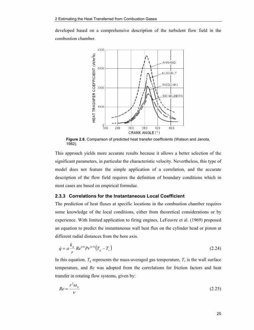
2 Estimating the Heat Transferred from Combustion Gases
25
developed based on a comprehensive description of the turbulent flow field in the
combustion chamber.
This approach yields more accurate results because it allows a better selection of the
significant parameters, in particular the characteristic velocity. Nevertheless, this type of
model does not feature the simple application of a correlation, and the accurate
description of the flow field requires the definition of boundary conditions which in
most cases are based on empirical formulae.
2.3.3 Correlations for the Instantaneous Local Coefficient
The prediction of heat fluxes at specific locations in the combustion chamber requires
some knowledge of the local conditions, either from theoretical considerations or by
experience. With limited application to firing engines, LeFeuvre et al. (1969) proposed
an equation to predict the instantaneous wall heat flux on the cylinder head or piston at
different radial distances from the bore axis.
( )sg
gTTPrRe
r
kaq −= 33.08.0
& (2.24)
In this equation, Tg represents the mass-averaged gas temperature, Ts is the wall surface
temperature, and Re was adopted from the correlations for friction factors and heat
transfer in rotating flow systems, given by:
ν
ω grRe
2
= (2.25)
Figure 2.8. Comparison of predicted heat transfer coefficients (Watson and Janota, 1982).

2 Estimating the Heat Transferred from Combustion Gases
26
The characteristic length for any position on the cylinder head or piston was r, the
significant gas velocity was the swirl velocity, obtained as the product of r and ωg,
which was assumed to be constant during the cycle; ν and the other properties were
calculated at the averaged boundary layer temperature, and a consistent set of physical
units was used in the calculations.
The value of a was 0.047. It was obtained by least-square error method to fit motored
data based on temperature readings from surface thermocouples at two locations, TC-1
and TC-2, in the cylinder head of a direct-injection, supercharged diesel engine. This
correlation was intended for convective heat transfer and therefore was not expected to
predict the total heat flux in a fired engine with high accuracy. However, the equation
was then used to estimate the heat transfer at the same two locations as for the motored
case under fired conditions. The results for 2000 rev/min and injection at 20ºBTDC,
which LeFeuvre et al. (1969) defined as standard operating conditions, are shown in
Figure 2.9.
The results revealed reasonable agreement between experimental data (solid line) and
calculated values (segmented line) only at location TC-1, Figure 2.9a. At TC-2, Figure
2.9b, the correlation over-predicted the heat flux for most of the cycle, and particularly
during combustion. In order to understand the observed variation in the heat flux
between locations, it is worth mentioning that the single-cylinder diesel engine
employed had two valves and a combustion chamber positioned offset in relation to the
injector tip. While both thermocouples were located outside the perimeter of the piston
(a) (b)
Figure 2.9. Extension of motored correlation to fired operation at (a) TC-1 and at (b) TC-2. Adapted from LeFeuvre et al. (1969).

2 Estimating the Heat Transferred from Combustion Gases
27
bowl approximately equidistant from its centre, TC-1 was placed symmetrically
between the valves and TC-2 on the opposite side of the chamber, closer to the exhaust
valve. Thus higher gas velocities and metal temperatures are expected around location
TC-1. The observed differences in heat transfer between the two locations challenges
the assumptions of mass-averaged gas properties and uniform gas temperature
throughout the cylinder being used as the source temperature for heat flux to the
cylinder walls.
Dent and Suliaman (1977) proposed a correlation identical in form to the previous one,
but with coefficient a equal to 0.023 after allowing for Pr to be taken as constant and
equal to 0.73.
( )wrg
gg
r TTr
r
kq −
=
8.02
023.0ν
ω& (2.26)
This investigation included extensive measurements of convective and radiant heat
transfer in an air-cooled, direct-injection diesel engine with three cylinders in line and
two valves per cylinder. In this engine higher swirl ratios than those reported by
LeFeuvre et al. (1969) have been previously observed. Thus, the different coefficient a
can be explained by the higher swirl velocity along with different engine specifications,
and the consideration of radiation heat transfer.
Although the two expressions are almost identical, this equation was derived from the
correlation for turbulent forced convective heat transfer along a flat plate surface. The
correlation was applied to a swirling force vortex flow, using the tangential velocity at
the specific radius ωgr as the relevant velocity, and the corresponding circumference
2πr as the characteristic length. The gas properties ν and kg were evaluated at the
instantaneous gas temperature Tg, and Twr was the instantaneous measured surface
temperature at each particular location. The equation can be used to obtain the
instantaneous heat flux at any radius in the combustion chamber space providing that
swirl data on a crank angle base from a motored test is available for the engine. It also
requires a measured or estimated value of Twr.
Based on results from motored and fired operation, Dent and Suliaman (1977)
concluded that the local instantaneous heat flux and the spatially-averaged instantaneous
values in the cylinder head and piston crown were well represented by this correlation,
in which the cylinder air motion was used as an input. However, in fired conditions,
swirl increases and variation in local gas temperature within the piston bowl and in the

2 Estimating the Heat Transferred from Combustion Gases
28
adjacent squish zones due to combustion must be considered; otherwise the equation
under-predicted the peak heat flux. This conclusion is illustrated in Figure 2.10, where
calculated and measured heat fluxes in the piston crown are compared in fired operation
at different loads (no load, 40% and 80%). Since no allowance had been made for
enhanced swirl and temperature variation, maximum heat flux was under-predicted, and
the difference increased with engine load.
With regard to radiant heat transfer, Dent and Suliaman (1977) found similar trends to
those reported by Annand (1963), and also by Sitkei and Ramanaiah (1972). However,
lower magnitudes were observed which were attributed to the higher swirl velocities
existing in the engine used in their study.
The following correlation applied by French (1969) to diesel engines, also presented by
Owen et al. (1993), was derived from an original equation first proposed by Alcock et
al. (1957). This is a completely empirical formula based on measurements of component
temperatures and temperature gradients in more than 200 different engines.
= −
a
b
n
b
a
m
p
f
T
T
p
p
A
mFq
&&
610 (2.27)
where q& denotes a local heat flux for a given value of the distribution factor F; fm& is the
fuel flow, and Ap is the bore area times the number of cylinders. The exponents m and n
take different values depending on the type of engine, i.e.:
Figure 2.10. Comparison of measured mean heat fluxes on piston crown (annular region) with prediction by flat plate equation using bulk mean gas temperature at 1050 rev/min fired operation (Dent and Suliaman, 1977).

2 Estimating the Heat Transferred from Combustion Gases
29
For four-stroke spark-ignition engines: m = 0.6, n = 0.3
For four-stroke compression-ignition engines: m = 0.75, n = 0.3
In order to define the spatial variation of the heat flux in the combustion chamber, a
value of F, appropriate for the particular engine type, is required. This factor also
depends on the combustion chamber geometry and is a function of the location in the
cylinder head, liner or piston top. Other correction factors, not shown in the correlation,
have been introduced to account for variables known to affect the heat flux, such as air-
fuel ratio, swirl, or ignition timing in the case of spark-ignition engines.
The correlation is simple to use in existing engines if enough data are available for the
particular engine under consideration. However, its application to a new engine design
is restricted since it relies on previous experience with similar engines. It is also
restricted by the lack of any theoretical basis.
2.4 Discussion of Application of Existing Correlations to Modern Diesel Engines
At this point, it is worth making a few comments on the applicability of the existing
correlations to modern engines. With regard to the correlation to estimate the overall
heat transfer coefficient, proposed by Taylor and Toong (1957), one would expect that
the various constants based on data collected on engines from fifty years ago would be
different if data from more efficient modern engines were used. Thus, updating this
equation would lead to more accurate heat balance calculations and improved
definitions of engine cooling requirements, even at the design stage.
The effort of the investigations reviewed in this chapter has focused on predicting the
instantaneous local and instantaneous spatially-averaged heat transfer coefficients. Most
of the correlations intended for this purpose are based on measurements on the cylinder
head and pistons, for instance Annand (1963), Woschni (1967), Dent and Suliaman
(1977), and Hohenberg (1979). This is understandable given that maximum
temperatures are observed at these parts of an engine and heat transfer to the cylinder
head and pistons can be predicted in the absence of friction. Also, reliable estimates of
local heat transfer coefficients at locations like valve bridges and valve seats are
necessary to define the cooling requirements of these critical components.
More attention should be given to the distribution of heat flux along the cylinder bore,
where friction is involved, and important design aspects like the size of cooling galleries
and jackets could be improved. A better knowledge of the heat transfer coefficient in
these zones of the combustion space, either time dependant or steady-state will
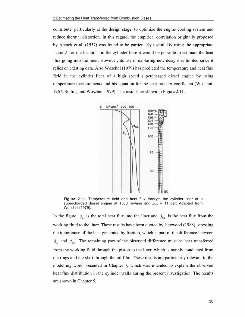
2 Estimating the Heat Transferred from Combustion Gases
30
contribute, particularly at the design stage, to optimize the engine cooling system and
reduce thermal distortion. In this regard, the empirical correlation originally proposed
by Alcock et al. (1957) was found to be particularly useful. By using the appropriate
factor F for the locations in the cylinder bore it would be possible to estimate the heat
flux going into the liner. However, its use in exploring new designs is limited since it
relies on existing data. Also Woschni (1979) has predicted the temperature and heat flux
field in the cylinder liner of a high speed supercharged diesel engine by using
temperature measurements and his equation for the heat transfer coefficient (Woschni,
1967; Sihling and Woschni, 1979). The results are shown in Figure 2.11.
In the figure, Lq& is the total heat flux into the liner and GLq& is the heat flux from the
working fluid to the liner. These results have been quoted by Heywood (1988), stressing
the importance of the heat generated by friction, which is part of the difference between
Lq& and GLq& . The remaining part of the observed difference must be heat transferred
from the working fluid through the piston to the liner, which is mainly conducted from
the rings and the skirt through the oil film. These results are particularly relevant to the
modelling work presented in Chapter 7, which was intended to explain the observed
heat flux distribution in the cylinder walls during the present investigation. The results
are shown in Chapter 5.
Figure 2.11. Temperature field and heat flux through the cylinder liner of a supercharged diesel engine at 1500 rev/min and pme = 11 bar. Adapted from Woschni (1979).

2 Estimating the Heat Transferred from Combustion Gases
31
Finally, it should be mentioned that although the best known of these models, proposed
by Annand (1963) and by Woschni (1967) over thirty years ago, have been validated by
other authors against more recent data, the application of these correlations to modern
engines is questionable. Current compression-ignition engines feature high pressure
common rail devices with variable fuel injection strategies, exhaust gas re-circulation
and retarded injection for NOx emission control, high levels of boost pressure and inter-
cooling, multiple valves per cylinder, high swirl and other modern technologies which
are known to affect combustion and consequently the convective and radiative heat
transfer in the engine. In most cases these features were not considered in the
formulation of the existing correlations, simply because they did not exist or were not
widely used in engines at the time when these equations were proposed.

32
3 Experimental Set-Up
3.1 Introduction
The experimental approach was intended to obtain a comprehensive picture of the
steady-state as well as the instantaneous thermal operating conditions of the engine. On
the one hand, a detailed thermal survey was obtained by measuring steady-state metal
temperatures in the engine block and cylinder head using single-point thermocouples.
Based on these temperatures, metal thermal gradients were calculated in the cylinder
head and cylinder walls. Besides metal temperatures, other variables necessary to
complete the thermal survey of the engine were also measured on a time-averaged basis.
These quantities were test cell temperature, inlet and exhaust manifold pressure, inlet
and exhaust manifold temperature, intake air mass flow rate, fuel mass flow rate,
coolant temperature and coolant flow rate at various key points in the cooling circuit.
On the other hand, instantaneous measurements of gas pressure, gas temperature, and
wall surface temperature within the combustion chamber were attempted. For this,
cylinder pressure measurements were taken in one cylinder on a crank angle basis, at
each test condition. In addition, two fast response, ‘erodable’ type thermocouples were
installed in the cylinder head with the purpose of measuring instantaneous gas
temperature and gas-side surface temperature. The objective was to synchronise the
instantaneous temperature measurements with the in-cylinder pressure values, thus
providing instantaneous measurements of pressure and temperature throughout the
engine cycle, that is in time or crank angle domain. Subsequently, this would lead to
instantaneous heat flux calculations.
3.2 Detailed Thermal Survey
3.2.1 Measuring Technique
The thermal survey consisted of steady-state measurements designed to reveal the
spatial variation of temperature and heat flux over a wide range of operating conditions.
The engine was instrumented at a number of locations in the cylinder walls and cylinder
head with sets of either three or two fixed, single-point, K-type thermocouples of 1 mm
diameter. By using a measuring technique based on arrays of three or two
thermocouples at a given location it was possible to obtain the local one-dimensional
temperature gradient. Basically, the gradient is the difference between temperature
readings per unit of distance separating the thermocouples. Subsequently, it is possible
to calculate the corresponding one-dimensional heat flux in the metal, which is the main
purpose of the thermal survey. Details of the calculation procedures to evaluate thermal

3 Experimental Set-Up
33
gradients and heat fluxes are given in Section 4.3. The method used to instrument the
engine is explained in the following section.
3.2.2 Engine Instrumentation
With regard to the implementation of the measuring technique, the sets of
thermocouples were positioned to provide maximum spatial resolution of the data in one
inner cylinder of the engine (cylinder two). The locations were chosen after detailed
consideration of the practicalities involved in the instrumentation of the engine. These
included drilling the holes in the machining shop, fitting the thermocouples to the metal
using an epoxy-type adhesive (resin), and then sealing the holes once the thermocouples
were installed. These operations had to be done within the practical constraints imposed
by the design features of the engine block and cylinder head, in particular cooling and
lubricant galleries. Details of the test engine are given in Section 3.4.1 and the
specifications of the thermocouples, other instruments, and material used in the
investigation are given in Appendix A.
The instrumentation method consisted in fitting the thermocouples of each set as close
as possible to each other in the same plane, but with their tips at different distances from
the gas-side surface. Although the basis of the measuring technique was the same for
the cylinder head and the engine block, the approaches used to instrument each
component differed to some extent.
3.2.2.1 Engine Block
In the instrumentation of the engine block a total of 93 thermocouples were used. They
were mainly arranged in arrays of three thermocouples; each array installed as shown in
Figure 3.1. The thermocouples were fitted on the cylinder wall along concentric lines
with their tips at different radii from the gas surface, 2.5º apart circumferentially and
passing through holes drilled on the outer wall of the engine block. The centre
thermocouple of each set was located at a distance (radially) of 2 mm from the bore, the
one to the right at 3.5 mm, and the one to the left at 5 mm, from the gas-side cylinder
surface. The cylinder wall thickness at most locations was about 7 mm, providing
enough material to secure the thermocouples in the holes. The measurements taken in
this way were the basis for obtaining the one-dimensional temperature gradient in the
cylinder wall in the radial direction.
Following the method explained above, twenty nine sets of three thermocouples and
three sets of two thermocouples were installed in the engine block. Figure 3.2 shows the
general orientation of the arrays of thermocouples in the engine block, including their

3 Experimental Set-Up
34
designation and number of sets at each location. Figure 3.3 illustrates the location of
each set of thermocouples installed in the engine block.
Figure 3.1. Schematic installation of a set of thermocouples in the cylinder wall.
Figure 3.2. General orientation of arrays of thermocouples in the engine block.

3 Experimental Set-Up
35
The arrays of three thermocouples were fitted mainly at twenty two locations in the
walls of cylinder two; half of the sets on the inlet side and the other half on the exhaust
side of the engine. On each side two groups, one of seven sets (locations A and F), and
another of four sets (locations B and G), were arranged vertically every 15 mm in two
circumferential directions 20º apart. These four locations can be seen in Figure 3.4. The
photographs show thermocouples already fitted in their holes at locations A and F. The
remaining seven sets of three thermocouples were used to explore cylinder-to-cylinder
variations at equivalent locations to A in the other cylinders; also to complement the
survey on cylinder two with measurements on cylinder four (outer cylinder) at places
that were inaccessible in the inner cylinders (see Figures 3.2 and 3.3).
In the evaluation of cylinder-to-cylinder temperature variations two sets were installed
at location C (cylinder one), two at D (cylinder three), and one set at E (cylinder four).
The other two arrays of three thermocouples on cylinder four were fitted at locations I
and J. Additionally on cylinder four, the only three sets of two thermocouples used in
the block were installed at location H. At this location the cylinder wall was found to be
significantly thinner than in most places (less than 6 mm), and consequently it was not
possible to fit the left thermocouple (at 5 mm from the gas surface) of each of these sets.
DISTANCE FROM
TOP DECK
CYL 4 CYL 3
CYL 2 CYL 1
10 mm 25 mm 40 mm 55 mm 70 mm 85 mm
100 mm
EXHAUST SIDE
A1
CYL 2
CYL 2
CYL 2
CYL 2
CYL 2
CYL 2
CYL 2
A2
A3
A4
A5
A6
A7
F7
F6
F5
F4
F3
F2
F1
B1
G1
B2
B3
B4
G2
G3
G4
D1
C1
I1
J1
C2
D2 E2 H2
H3
H4
TOP DECK
10 mm
25 mm
40 mm
55 mm
70 mm
85 mm
100 mm
0
Figure 3.3. Schematic location of thermocouple sets in the engine block.

3 Experimental Set-Up
36
In order to drill the holes for the thermocouples on the cylinder wall, first it was
necessary to drill access holes of 10 mm in diameter on the outer wall of the engine
block (see Figure 3.4). Once the thermocouples were in place, the holes were sealed
with steel plugs fitted with epoxy adhesive to the outer wall. The plugs had a smaller
hole in the centre, just enough for the thermocouples to pass through. This can be seen
schematically in Figure 3.1 and also in Figures 3.4a and 3.5a. During the drilling of the
access holes, three of them cut through an oil passage and opened a gap to the adjacent
cooling gallery. The gaps were sealed by using plugs with a slightly different shape also
fitted with epoxy resin. The procedure proved to be successful since no leaks or
contamination of oil were found during testing.
(a) (b)
Figure 3.4. Thermocouple installation on locations A (a) and F (b), together with holes drilled ready for thermocouples on locations B (a) and G (b).
(a) (b)
Figure 3.5. Thermocouples being installed on the inlet side (a) and completed installation on the exhaust side (b).

3 Experimental Set-Up
37
The sealing method of the engine block worked well in general and only minor external
leaks were observed during testing. Because the situation was not particularly critical
and had no significant effect on the engine operation, it was not necessary to have them
repaired. The final results of the instrumentation are shown in Figure 3.5b at locations A
and B.
The installation procedure required a reasonable separation between access holes, which
provided sufficient material to guarantee adequate sealing of the external wall of the
block, although reducing the spatial resolution of the measurements. This requirement
determined a vertical distance of 15 mm between sets of thermocouples. The first or top
set of thermocouples at most locations was installed at approximately 10 mm from the
top deck, the second one 15 mm further down the wall, the third one 30 mm further
down, and so on. In this way the seventh or bottom set at A and F were at 100 mm from
the top deck, and the intermediate sets were at 25, 40, 55, 70 and 85 mm. At locations B
and G the bottom or fourth set was at 55 mm from the top deck, as the equivalent set at
A or F; and correspondingly the intermediate sets were at 25 and 40 mm. At some
locations it was not possible to fit an array at 10 mm; in those cases the top set was then
at 25 mm, which corresponded to the second one at most locations. This information is
summarised in Table 3.1.
As mentioned above, the separation between the top deck and the first array of
thermocouples at most locations was 10 mm. This was the minimum distance at which
it was assumed to be safe to drill the access hole without compromising the integrity of
the top deck, and consequently the critical function of the cylinder head gasket. The
location of the top set of thermocouples was also planned to coincide with the position
of the first piston ring at top dead centre (TDC), which was approximately 10 mm from
the top deck. This was found to be useful in developing the heat transfer model
presented in Chapter 7; however, it would have been beneficial to evaluate the thermal
gradient at a location closer to the top deck where the combustion process begins.
For identification purposes, each array was designated with the letter giving its location
followed by a number indicating its vertical position, that is to say A1 to A7, B1 to B4
and so on. For example, A3 identifies the set at 40 mm from top deck at location A. In
addition, the thermocouples in each set were named as centre (C), right (R) and left (L).
For instance, the centre thermocouple of the top set at location A was identified as A1C.
By following this simple convention every single temperature signal could be identified
and therefore located in the engine block.

3 Experimental Set-Up
38
Designation
A1L, A1C, A1R to A7L, A7C, A7R
B1L, B1C, B1R to B4L, B4C, B4R
C1L, C1C, C1R and C2L, C2C, C2R
D1L, D1D, D1R and D2L, D2D, D2R
E2L, E2C, E2R
F1L, F1C, F1R to F7L, F7C, F7R
G1L, G1C, G1R to G
4L, G4C, G4R
H2C, H2R to H
4C, H4R
I1L, I1C, I1R
J1L, J1C, J1R
Distance from top deck
9.7 to 99.7 m
m every 15 m
m
9.7 to 54.7 m
m every 15 m
m
9.7 and 24.7 m
m
9.7 and 24.7 m
m
24.7 m
m
9.7 to 99.7 m
m every 15 m
m
9.7 to 54.7 m
m every 15 m
m
24.7 to 54.7 m
m every 15 m
m
9.7 m
m
9.7 m
m
Number
of sets
7 4 2 2 1 7 4 3 1 1
Distance from
cylinder surface
5.0 - 2.0 -3.5 m
m
5.0 - 2.0 -3.5 m
m
5.0 - 2.0 -3.5 m
m
5.0 - 2.0 -3.5 m
m
5.0 - 2.0 -3.5 m
m
5.0 - 2.0 -3.5 m
m
5.0 - 2.0 -3.5 m
m
2.0 -3.5 m
m
5.0 - 2.0 -3.5 m
m
5.0 - 2.0 -3.5 m
m
Angle from
transverse direction
7.5° - 5.0° - 2.5°
27.5° - 25° - 22.5°
7.5° - 5.0° - 2.5°
7.5° - 5.0° - 2.5°
7.5° - 5.0° - 2.5°
7.5° - 5.0° - 2.5°
27.5° - 25° - 22.5°
90° - 87.5°
67.5° - 65° - 62.5°
117.5° - 115° - 112.5°
Therm
ocouples
per set
3 3 3 3 3 3 3 2 3 3
Location
A - C
ylinder tw
o/Exhaust side
B - C
ylinder tw
o/Exhaust side
C - C
ylinder one/Exhaust side
D - C
ylinder three/Exhaust side
E - C
ylinder four/Exhaust side
F - Cylinder tw
o/Inlet side
G - C
ylinder two/Inlet side
H - C
ylinder four/Rear side
I - C
ylinder four/Rear side
J - C
ylinder four/Rear side
Table 3.1. Therm
ocouples installe
d in the engine block.

3 Experimental Set-Up
39
3.2.2.2 Cylinder Head
In the cylinder head, sets of two thermocouples each were used to measure temperature
in the flame deck of cylinder two. Similarly to the engine block, the two temperature
measurements from each set allowed the determination of the local one-dimensional
temperature gradient. This method and its limitations are discussed in Section 4.3.
Because of space constraints only two thermocouples per set were used in the head. The
complicated design of the cylinder head, especially its four valves per cylinder and
swirl-generating inlet ports, made the instrumentation procedure remarkably difficult.
The available room to drill openings in order to access the flame deck from the top of
the head was significantly restricted; mainly by inlet and exhausts ports, valve guides,
the injector port and cooling galleries, but also by the valve train on the top deck.
Therefore, to prevent damaging the integrity of the cylinder head, the access openings to
drill the holes for the thermocouples and subsequently fit them in the flame deck had to
be of a smaller diameter. This limited the number of thermocouples that was possible in
practice to install at each location in the flame deck of the cylinder head.
The two thermocouples of each set were installed 2 mm apart in the radial direction and
5 mm apart in the vertical direction. One thermocouple was at 2 mm from the gas
surface and the other at 7 mm. The diagram in Figure 3.6a illustrates the relative
position of the thermocouples of each set in the flame deck. The thermocouple at 2 mm
from the surface was in every case the one closer to the centre. Figure 3.6b is a
photograph of a cylinder head section cut from a spare head where the parallel paths of
the thermocouples (red lines) have been superimposed. This picture shows how the
thermocouples were fitted in the flame deck, namely by inserting them through
openings drilled on the top of the head and passing them through the cooling galleries.
After careful consideration of the restriction previously discussed, the cylinder head was
instrumented with pairs of thermocouples fitted to the flame deck at the points indicated
in Figure 3.7. As shown in this figure, eight sets of thermocouples were installed over
four circumferential directions and at three different radii. In total 16 thermocouples
were installed in the cylinder head. The arrays were identified with the letters A to H,
and the thermocouples of each pair were given a number (1 or 2) and an extra letter (D
for the deep and S for shallow) following the designation of the location. For instance,
A1D identified the thermocouple at location A installed at 15 mm from the centre and at
2 mm from the gas surface; A2S designated the thermocouple at 17 mm from the centre
and at 5 mm from the gas surface.

3 Experimental Set-Up
40
(a) (b)
Figure 3.6. Schematic installation of a set of thermocouples in the cylinder head.
Figure 3.7. Thermocouple sets locations in the cylinder head.
The configuration was intended to explore temperature and heat flux variations in the
regions of the valve bridges in certain radial directions. For instance, the sets at
locations A, B and C were placed with their deeper thermocouple at 15, 22.5 and
34.5 mm from the centre. In addition to design restrictions, these locations were chosen
Inlet
valve
r=15mm
r=22.5mm
r=34.5mm
Inlet
valve
Exhaust
valve
Exhaust
valve B A
C
D
G
E F
H

3 Experimental Set-Up
41
with reference to the radius of the piston bowl (22.5 mm). In this way the survey
included, at least in the region of one valve bridge, measurements of temperature in the
flame deck within the area corresponding to the piston bowl lip (location A), on the
edge of it (location B) and outside this area (location C). This is important, knowing that
during combustion, significant temperature gradients occur in the region of the piston
bowl lip; and therefore measurements should reveal its effect on the heat flux in the
corresponding section of the flame deck. For four valve engines, the bowl lip and the
centre of the valve bridges occur at approximately the same radius.
It was not possible to fit three sets of thermocouples as described before in the other
valve bridges; however, a set was installed at 22.5 mm on the other three radial
directions (points D, E and H), one set was fitted at 34.5 mm almost opposite to C
(location F), and one set was installed at 15 mm in the exhaust valve bridge (location
G). Of particular interest were the measurements in the exhaust valve bridge (sets G and
H) where maximum metal temperatures were expected (Heywood, 1988). Table 3.2
summarises the information about the location of thermocouples in the cylinder head
(see also Figure 3.7).
In the head, the holes were also sealed with metal plugs as in the engine block. In this
case the plugs were made of aluminium and they had a tapered thread, which
complemented the epoxy resin in securing them in their places amongst the valve train.
This additional precaution was taken after consideration of the catastrophic
consequences that a loose metallic plug among moving parts could have on the engine,
and also to minimise the possibility of oil contamination with coolant, which could also
cause severe damage to the entire engine.
The cylinder head during instrumentation is shown in Figure 3.8. The photograph on the
left (a) shows the head with the valve train of cylinder two removed and thermocouples
already in place; the photograph on the right (b) is a closer view of the thermocouples
with the plugs being installed.
Once the thermocouple tips were fitted into their holes and the access holes were sealed,
as shown in Figure 3.9a, the valves were reassembled (Figure 3.9b) and then the
thermocouple leads were directed out of the cylinder head towards both sides of the
engine. The leads came out through slots made in between the head and the cam carrier
frame. The slots were later sealed with epoxy resin.

3 Experimental Set-Up
42
Designation
A1D, A2S
B1D, B2S
C1D, C2S
D1D, D2S
E1D, E2S
F1D, F2S
G1D, G2S
H1D, H2S
Radius to centre
of access hole
16.0 m
m
23.5 m
m
35.5 m
m
23.5 m
m
23.5 m
m
34.3 m
m
16.0 m
m
23.5 m
m
Radius to
therm
ocouple
15.0 and 17.0 m
m
22.5 and 24.5 m
m
34.5 and 36.5 m
m
22.5 and 24.5 m
m
22.5 and 24.5 m
m
33.3 and 35.3 m
m
15.0 and 17.0 m
m
22.5 and 24.5 m
m
Distance from
flame deck
2 and 7 m
m
2 and 7 m
m
2 and 7 m
m
2 and 7 m
m
2 and 7 m
m
2 and 7 m
m
2 and 7 m
m
2 and 7 m
m
Angle from transverse
or axial direction
27°
27°
27°
25°
6°
7°
16°
16°
Number of
Therm
ocouples
2 2 2 2 2 2 2 2
Location
A - Exhaust Valve-Inlet Valve Bridge
B - Exhaust Valve-Inlet Valve Bridge
C - Exhaust Valve-Inlet Valve Bridge
D - Inlet Valves Bridge
E - Inlet Valve-Exhaust Valve Bridge
F - Inlet Valve-Exhaust Valve Bridge
G - Exhaust Valves Bridge
H - Exhaust Valves Bridge
Table 3.2. Therm
ocouples installed in the cylinder head.

3 Experimental Set-Up
43
In order to avoid any possible contact between the thermocouples and moving parts,
they were fixed with epoxy resin to the cylinder head under the camshafts at several
points. This can be seen in Figure 3.10, which shows the cylinder head once its
instrumentation had been completed.
It is worth mentioning that the instrumentation procedure of the cylinder head proved to
be safe and adequate. Regular inspections of the engine oil during testing did not reveal
any contamination by coolant leaked from the cooling galleries. In addition, all
thermocouples in the head provided consistent temperature readings throughout the
experiments.
(a) (b)
Figure 3.8. Cylinder head during instrumentation.
(a) (b)
Figure 3.9. Thermocouples already installed on the head before (a) and after (b) reassembling the valve train.

3 Experimental Set-Up
44
3.2.3 Methodology Evaluation
As mentioned in Sections 3.2.1 and 3.2.2, temperature measurements in the metal from
an array of three or two thermocouples can be used to estimate thermal gradients. The
difference in temperature per unit of distance between thermocouples installed on
parallel lines in the case of the cylinder head, or concentric lines as in the cylinder walls,
provides an approximate one-dimensional thermal gradient. Ideally, the actual gradient
could only be obtained by measuring temperatures along a single axis without using an
intrusive device. In practice, this is not possible to achieve with any existing technique
because of the necessary drilling in the metal of a finite diameter to install the probe,
which creates a discontinuity of the heat flow. Even in the case of built-in sensors
embedded in the casting, certain disruption is caused to the thermal profile due to the
changes in conductivity.
Although laborious in practice, the instrumentation technique used to measure
temperature was preferred after consideration of two other steady-state methods, namely
traversing thermocouples and multi-point thermocouples. The first of these techniques,
as described by Owen et al. (1993) is accurate (within 2.5% of the true gradient) and has
been used in the past by the author (Finol, 1999). However, the necessary space to
install and operate the traversing mechanism made it unsuitable for this application
where spatial resolution of heat fluxes in small areas was the main requirement.
Traversing thermocouples also need settling time in between measurements and have to
be operated in the unsafe environment of the test cell, which is a major drawback if
many of them are required. The second method, a multi-point thermocouple, as
explained by Hart et al. (1999) is a patented probe still under development, which has
Figure 3.10. Instrumented cylinder head.

3 Experimental Set-Up
45
given similar results to the traversing thermocouple. Nevertheless, it was decided not to
pursue this approach mainly because the probe was still a prototype not yet available for
purchase.
In order to evaluate the intrusiveness of the measuring technique, steady-state numerical
simulations were performed using a three-dimensional finite-difference conduction
model previously developed by the author (Finol and Damia, 1993). This model is an
extension of a programme by Patankar (1991) for the computation of conduction and
duct flow heat transfer. The model compares the temperature distribution for the
undisturbed situation (no drilled holes) used as reference, with that obtained by
considering the holes required to install the thermocouples in a metal section of the
cylinder wall.
In the model, a simple three-dimensional conduction situation in a cylindrical section of
circumferential length π/18 radians (10°), radial thickness 7 mm and axial length 5 mm
was simulated in axisymmetric coordinates. Adiabatic boundary conditions were
assumed along the radial faces; the temperature was fixed at the top and bottom faces,
and known heat fluxes were considered in the radial direction. The heat fluxes assumed
on the gas-side and coolant-side were representative values of actual engines and input
to the programme via the heat transfer coefficient and the temperature of the fluid and
the wall surface.
The undisturbed temperature distribution was obtained for a solid section with a single
thermal conductivity value of 45 W/m K (typical of cast iron). For the situation with
holes in the cylinder wall, the temperature profile was obtained assuming three holes of
1 mm in diameter and a depth of 5, 3.5 and 2 mm, corresponding to the position of the
centre, right and left thermocouples. The holes were modelled by assigning the
conductivity of atmospheric air at 300 K (0.03 W/m K) to most nodes representing
them, and the conductivity of the epoxy resin (0.582 W/m K) necessary to seal the holes
to those nodes within 1 mm from the coolant-side surface. For the rest of the domain,
the thermal conductivity of the metal was the same as for the undisturbed case. The
resulting temperature profiles for the two situations are shown in Figure 3.11. These
contour plots show the temperature distribution on the centre plane of the cylindrical
section (with reference to the axial coordinate), which is the one containing the axes of
the thermocouples. In Figure 3.11b, these axes are shown and the ideal position of the
tips of the thermocouples is indicated by arrows.

3 Experimental Set-Up
46
The contour plot for the reference situation (Figure 3.11a) shows the expected circular
isothermal lines with a falling temperature distribution along the radial direction, from
the gas-side surface (bottom) to the coolant-side surface (top). The lines are
symmetrical in the tangential coordinate as a result of the adiabatic boundary conditions
(zero heat flux) assumed in this direction. In contrast, the circular lines are not observed
in the contour plot shown in Figure 3.11b and there is no symmetry because of the
difference in depth between the left and right holes. Although adiabatic conditions still
existed on the left and right edges, the disruption caused by the holes on the radial heat
flow created temperature gradients in the tangential direction, which made the
isothermal lines different from the ideal circular shape. The holes having a lower
conductivity value acted as an impediment, holding the heat up from flowing otherwise
undisturbed from the gas-side to the coolant-side.
K380 400 420 440 460 480 (a)
K380 400 420 440 460 480
TL
TC
TR
(b)
Figure 3.11. Temperature distribution in a cylindrical section of the cylinder wall: (a) undisturbed situation and (b) section with holes.

3 Experimental Set-Up
47
As one might expect, higher temperatures at equivalent locations were in general found
in the cylinder wall section with holes. An exception to this is observed in the holes near
the coolant-side, where temperatures are lower than for the undisturbed section. This
can be explained by the smaller difference between the heat flow resistance for
conduction in the cylinder section and the resistance for convection to the coolant for
the case when holes were considered. In both situations the convective heat transfer
coefficient and the coolant temperature were identical, thus the thermal resistances for
convection were the same. However, the thermal resistance for conduction in the holes
was higher than for the undisturbed case since the thermal conductivity used for the
nodes representing the holes was significantly lower than that of cast iron. Therefore,
the effect of the convective part of the heat transfer process was more noticeable in the
situation modelled with holes.
The actual maximum increments in temperature observed at the relevant points in the
metal of the heat flow situation with holes were in the order of 5 K. These points are in
fact the locations where the tips of the thermocouples would be making contact with the
metal. It is also at these points where the change in thermal conductivity occurred,
which explains why peak differences in temperature between the two situations were
observed at these locations. The results obtained from the numerical simulations
revealed that the temperature at these points was 1 to 6 K higher for the cylinder wall
section with holes than the temperature at equivalent locations in the totally solid
section. This is shown in Figure 3.12.
In the figure, the temperatures obtained in the model that would correspond to the actual
readings from a set of thermocouples in the cylinder wall are denoted TC, TR and TL.
The notations also indicate the position of the tips of the thermocouples installed in the
centre, right and left holes respectively (red, blue and green lines). These represent in
the real situation the values used to calculate the local thermal gradient. As mentioned
before, these values were higher than for the reference case (black line) as a
consequence of the change in thermal conductivity. However, the differences should be
smaller in the actual situation since the thermocouples have a better thermal
conductivity than the air, thus decreasing the relative thermal resistance. In addition, the
effect of the differences on the estimated thermal gradients would be less since the
gradients were obtained by subtracting one temperature from another affected in a
similar way.

3 Experimental Set-Up
48
It should be noticed that there was no reason for concern with regard to predicted
temperatures in the holes near the coolant surface, where differences with the reference
line were significant (radius greater than 48.5 mm). Firstly, these temperatures have no
effect whatsoever on the estimated gradients (i.e. they are not used in the calculations);
secondly, the discrepancies are likely to decrease in the real situation due to the thermal
conductivity issues discussed above.
The predicted metal temperatures in the spaces between the holes (pink and cyan lines)
are also shown in Figure 3.12. The results showed that these temperatures were virtually
the same with and without holes (reference line), demonstrating the small effect of the
measuring technique on the cylinder wall temperature distribution.
Figure 3.13 shows the predicted relative errors in the measured temperatures caused by
the measuring method used in this research. In the metal, the observed errors are less
than 2.5% at the points where measurements were taken.
Although the results were obtained for an ideal one-dimensional situation, which differs
from actual conditions in an engine, particularly in the cylinder head, the simulation
helped to quantify the intrusiveness of the measuring technique. In terms of heat flow
disruption, similar results would be obtained using other measuring methods, namely
traversing thermocouples or multi-point thermocouples, since their installation also
require drilling a hole in the metal.
43 44 45 46 47 48 49 50380
400
420
440
460
480
500
Radius (mm)
Temperature (K)
reference
right hole
right-centre space
centre hole
centre-left space
left hole
TC TRTL
Figure 3.12. Predicted temperatures.

3 Experimental Set-Up
49
It is expected that the accuracy of the measuring technique would reduce as the
conditions depart from the one-dimensional situation; however, this would happen to
other methods too.
3.2.4 Coolant Temperatures and Coolant Flows
The temperature of the coolant as well as the coolant flow rate was measured at several
points in the cooling system during every experiment. The temperatures and mean flows
were measured using platinum resistance thermometers (PRTs) and turbine flow meters
respectively. The specification of these instruments can be found in Appendix A.
Figure 3.14 shows the locations in the cooling circuit where temperature and flow rate
measurements were taken.
In the figure, the red dots indicate the positions of the PRTs, which were located at the
inlet and outlet of every component exchanging heat with the coolant in the circuit. The
PRT positions were thus: radiator inlet (top hose), radiator outlet (bottom hose), engine
inlet (at the pump discharge), engine outlet (before the thermostat), EGR cooler inlet
and outlet, and oil cooler inlet and outlet. The flow meters (turbine type) were
positioned to quantify the coolant flow passing through these components; specifically,
at the engine outlet (FM1), after the EGR cooler (FM2) and after the oil cooler (FM3).
By using this layout it was possible to estimate the total heat rejection to the coolant as
well as the heat rejected in the engine (block and cylinder head) and the various heat
exchangers. Notice that the cabin heater (red dashed box) was removed only to facilitate
43 44 45 46 47 48 49 50-20
-16
-12
-8
-4
0
4
Radius (mm)
% Error [100(T-To)/To]
right hole
right-centre space
centre hole
centre-left space
left hole
TCTLTR
Figure 3.13. Errors in predicted temperatures.

3 Experimental Set-Up
50
the heat rejection measurements and calculations. Also, the radiator was replaced by a
heat exchanger (not shown in the figure) where the coolant transferred heat to the test
cell service water. This approach facilitated the control of the inlet coolant temperature,
which was one of the controlled variables during the experiments.
Coolant temperature measurements were taken mainly to obtain a spatial and time-
averaged estimate of the actual temperature of the coolant, particularly in the engine
block and cylinder head, at each test condition. This value was necessary to evaluate the
convective heat transfer coefficient on the coolant-side of the cylinder walls. This
coefficient is one of the criteria used in the validation of results presented in
Section 4.4.3, and the procedure for its calculation is given in Section 4.3. Coolant flow
rates were required, combined with coolant temperature, to perform heat balance
calculations in the engine. The heat rejection from the engine block and the cylinder
head obtained in this way can be used to validate the heat obtained by integration of the
experimental heat flux over the corresponding area. This justified the additional
instrumentation for measuring coolant flow rates and inlet and outlet temperatures of the
EGR and oil coolers.
Figure 3.14. Engine cooling circuit.

3 Experimental Set-Up
51
3.3 Crank Angle Based Measurements
As mentioned in Section 3.1, crank angle or time resolved measurements of cylinder
pressure, gas temperature and wall surface temperature in the combustion chambers of
the engine were part of the planned experimental work. The purpose of these
measurements was to obtain synchronised pressure and temperature data from the
combustion chamber throughout the engine operating cycle. This would allow the heat
flux variation within the cycle to be explored. However, only cylinder pressure was
successfully measured; details of these pressure measurements are given in
Section 3.3.1.
With regard to gas and surface temperatures, it was considered appropriate to write a
few comments on the approach followed in attempting to measure these variables; also
to explain the reasons why no results were obtained from these attempts. These
comments are given in Section 3.3.2.
The specifications of the instruments and equipment used for the crank angle based
measurements are included in Appendix A.
3.3.1 In-Cylinder Pressure
The measurements of the instantaneous cylinder pressure were taken in the combustion
chamber of cylinder two. The pressure was measured using a quartz piezoelectric
transducer Kistler Type 6123A. This type of transducer generates an electric charge
proportional to the cylinder pressure. The transducer is designed to be installed in the
cylinder head by replacing the glow plug in the particular cylinder. Since the test
program did not include experiments in cold conditions, removing the glow plug had no
consequence on the engine operation.
The electric charge generated by the transducer was processed using the system AVL
620 Indiset. This system uses the AVL Docking Station 6162 to amplify and condition
the electric charge to produce an output voltage. The voltage is input to a computer
equipped with the software IndiWin, which processes the voltage signal proportional to
the cylinder pressure. AVL 620 Indiset also requires a signal indicating the
instantaneous angular position of the crankshaft in order to produce a crank angle based
pressure trace. The position of the crankshaft was obtained with an AVL 364 Angle
Encoder. The crank angle signal was simultaneously amplified and input to the
computer along with the pressure signal. In addition, the software needed the
dimensions of the cylinder defined in terms of bore, stroke, length of the connecting rod
and pressure ratio. The measuring configuration can be seen in Appendix A.

3 Experimental Set-Up
52
The procedure to obtain the pressure data at each test point consisted of measuring the
cylinder pressure for forty cycles and then calculating the average pressure trace based
on that number of cycles. An average pressure trace was completely satisfactory for the
purpose of the investigation, in particular because cycle to cycle variations of any
parameter were beyond the scope of this research. In practice, the procedure was
completed during each experiment by running the computer programme once the engine
had settled at a given test condition.
3.3.2 Instantaneous Temperatures
In attempting to measure instantaneous gas temperature and wall surface temperatures
in the combustion chamber, fast response ‘erodable’ type thermocouples were used. The
decision to use this type of thermocouple was based on economic and practical
considerations, and supported by studies from Stone (1999) and Oude Nijeweme et al.
(2001). These probes are commercially available and can be purchased with the
necessary amplification and logging system. Nevertheless, the amplifier was built in
house and a logging system forming part of the existing test facilities described in
Section 3.4.2 was used.
Fast response eroding thermocouples can be thermally grounded or ungrounded.
According to their manufacturer (Nanmac), the first type is designed to measure the
metal temperature on the surface of the body exposed to a fluid media; the second can
be used to measure the rapidly changing interface or gas temperature at the surface. The
thermocouples are manufactured and calibrated in any standard thermocouple
temperature range (see Appendix A).
A thermally grounded thermocouple (E12-2-K) was installed in cylinder one to measure
the temperature on the gas-side surface of the cylinder head, and a thermally
ungrounded (E12-2-K-U) probe was fitted in cylinder three aiming to measure gas
temperature. Both probes used in the investigation were K type standard calibration
(from 0 to 1600 K approximately), which was considered adequate for both surface
metal temperature and gas temperature.
Similarly to the installation of the pressure transducer, the probes were mounted by
replacing the glow plugs; in this case by using special adaptors built for this purpose.
Figure 3.15 illustrates the installation of a fast response thermocouple in an adaptor.
Basically, each adaptor was a metallic element designed to fit in the place of the glow
plug in the cylinder head and at the same time hold the thermocouple. It has a hole in

3 Experimental Set-Up
53
the centre for the thermocouple to pass through into the combustion chamber, and an
internal thread engaging with a compression fitting to secure the thermocouple.
Although the thermocouples were successfully installed, they failed to read any sensible
value after testing started. The usual small voltage output, which is proportional to the
temperature, was generated by both thermocouples and could be detected before
amplification. However, the value was relatively constant, not indicating rapid changes
either in gas temperature or surface temperature. The thermocouples were removed and
their tips abraded as recommended by the manufacturer. This operation is supposed to
renew the multiple minute thermocouple junctions as a result of plastic flow of the
metals, but the problem persisted even after several abrading operations.
The next step was a thorough inspection of the entire processing system, namely the
amplification and logging channels. It was thought that perhaps the small changes
observed in the output voltage were not adequately processed by the in-house built
amplifier. The inspection did not reveal the cause of the problem and, because testing
time was being compromised, it was decided to abandon these measurements. Also, by
this time, the output signal from the thermally ungrounded thermocouple was totally
lost. A further inspection revealed that the thermocouple was broken. The tip had
detached from the body and gone through the exhaust system, fortunately without
causing further damage.
The main consequence of failing to obtain instantaneous metal surface temperature
measurements in the combustion chamber was the impossibility of estimating heat flux
Thermocouple
Adaptor
Compression fitting
Figure 3.15. Fast response thermocouple and adaptor.

3 Experimental Set-Up
54
cycle variations. An approximate instantaneous gas temperature could be determined by
using the pressure trace as described in Section 6.2.4. However, it would have been
convenient to validate the results based on data of cylinder pressure against
experimental gas temperature data. The temperature of the gas was necessary for the
evaluation of the existing correlations to estimate heat transfer coefficients in the
combustion chamber, which is presented in Chapter 6.
3.4 Testing Equipment
3.4.1 Test Engine
The engine used in the investigation was a 2.0 litre turbocharged Ford diesel engine
with four cylinders, high pressure common rail fuel system and four valves per cylinder.
Table 3.3 contains the main characteristics of the engine and Table 3.4 gives specific
information about the engine block, cylinder head and cooling system. The torque and
power graphs of the engine as provided by the manufacturer are given in Appendix B.
Engine name Puma CD132 130PS HPCR
Engine type Diesel
Strokes per cycle 4
No. of cylinders 4
Valves per cylinder 4
Capacity cc 1998
Stroke mm 86
Bore mm 86
Connecting rod length mm 160
Compression ratio 19
Max. torque Nm 310@1800-2500 rev/min
Max. power kW 96@3800 rev/min
Max. boost bar 2.3@2000 rev/min
Injector rail pressure bar 1400
Compressor GT20 C101, 49mm, 50 trim, 0.42 A/R
Variable Geometry Turbine (VGT) GT17V NS111(43) 76 trim, 0.65A/R
Table 3.3. Engine characteristics.
The engine was partially dismantled for the block and cylinder head to be instrumented.
The arrays of thermocouples were fitted in accordance with the procedure described in
Section 3.2.2, allowing the necessary time for the resin to harden while keeping the
engine components at an adequate room temperature.
The engine block and cylinder head were temporarily assembled to perform a
hydrostatic test of the cooling galleries. The objective of this test was to detect possible
leaks that could affect the engine operation during testing; in particular internal leaks

3 Experimental Set-Up
55
that could cause oil contamination and certainly disruption in the experimental program.
The test was conducted at room temperature with a hydrostatic pressure of 3 bar (gauge)
applied for two hours. The test pressure was similar to maximum coolant pump
discharge pressures at high speed operating conditions. Thus, the testing pressure was
certainly higher than operating pressures normally found in the cooling galleries.
Engine Block and Cylinder Head
Block weight kg 62
Block material Cast iron
Head weight kg 12.5
Head material Aluminium alloy
Deck type Closed deck
Cooling System
Coolant: 50-50 mixture by volume of water and ethylene glycol antifreeze
Cylinder head coolant volume l 0.73
Cylinder block coolant volume l 1.125
Thermostat housing coolant volume l 0.10
Water pump coolant volume l 0.325
Outlet thermostat start to open temperature °C 88
Outlet thermostat fully open temperature °C 102
Oil cooler thermostat opening temperature °C 84
Sump oil volume l 6.0 (max. fill)
Table 3.4. Engine block, cylinder head and cooling system data.
The engine was then rebuilt, including the installation of part of the instrumentation
required for the crank angle based measurements (pressure transducer and fast response
thermocouples). The rest of the instrumentation for these measurements, and most of the
temperature sensors and all flow meters necessary for the measurements in the cooling
circuit, were installed once the engine was placed on the test bed.
3.4.2 Test Facilities
The experiments were carried out in one of the engine test cells of the Powertrain and
Vehicle Research Centre (PVRC) at the University of Bath. The test bed equipment
consisted mainly of an electric dynamometer, a fuel flow measuring system, an air flow
meter, a main control and logging computer system, a second computer system
connected to the engine control unit (ECU), and emissions analysers. The computer
systems were located in the control room of the test cell and the emissions analysers
were installed in a separate room. The major components of the test facilities are given
in Appendix C.

3 Experimental Set-Up
56
The main computer system uses the engine testing software Cadet, a product of CP
Engineering Systems, to monitor the performance parameters of the engine in real time,
to control test variables and cell equipment functions, and to log almost every parameter
being measured in the test cell and by the emission analysers. This system also has the
capability to perform user-defined routines for calculating other parameters such as
power, brake specific fuel consumption and engine efficiency.
The computer system connected to the ECU worked as an interface between the engine
and the main control and logging system (Cadet). This computer uses the engine
management software Gredi to communicate with the ECU and then provide the ECU
data to the main computer system. The ECU is connected to several sensors in the
engine that provide the required parameters (e.g. fuelling, timing) for the control of the
engine. These sensors are integrated within the engine and are independent of the test
cell measuring equipment. The software Gredi is also used to view and download into
the ECU the management strategy necessary for controlling the engine, and to enable
the user to modify parameters in this strategy.
3.4.3 Data Acquisition Systems
The experimental data were logged using three different systems; namely, the main
logging system Cadet, the AVL 620 Indiset system used to register cylinder pressure
data as described in Section 3.3.1, and an additional system specially set to log the
steady-state temperature data provided by the thermocouples embedded in the walls of
the cylinders and cylinder head of the engine.
The main computer system continuously saves data into an internal file (trace file). It
also allows the user to log data, averaged for a specified time period, into another file
(log file) in a spread sheet format. The data logged by the computer system included
engine variables, room conditions (temperature, pressure and humidity), and also certain
parameters inherent to the operation of the main components of the test facilities, which
are not relevant to the investigation. For instance, some of these parameters indicate the
operating status of the dynamometer, fuel measuring system and emissions analysers.
The engine variables logged by the main computer system during each experiment
included: speed, torque, intake air mass flow rate, fuel flow rate, inlet manifold
temperature and pressure, exhaust manifold temperature and pressure; also the coolant
temperature and flow rate measured, as described in Section 3.2.4, at various locations
in the cooling circuit. The main computer also logged the data provided by the ECU.
Among these data there were some variables like engine speed, air mass flow rate and

3 Experimental Set-Up
57
inlet manifold pressure, that were also measured in the engine by using the test cell
equipment. Other variables such as fuel demand, pedal position, injection timing and
engine metal temperature (measured in the cylinder head) were only provided by the
ECU.
As mentioned before, an additional system was used to log all temperature
measurements taken in the engine with the thermocouples installed, as explained in
Section 3.2.2, to obtain metal thermal gradients. The data were logged separately in a
different computer. This logging system was necessary due to the large number of
temperature data that could not all be logged using the remaining available channels
within the main computer.
The additional logging system consisted of four data loggers DataTaker Series 600 and
a computer equipped with the accompanying software DeLogger (see Appendix A). The
data loggers were mounted on a panel, linked to each other in series, and then connected
to the computer. The panel was built for this application and provided enough logging
channels for the temperature values. At the end of each experiment, the data saved in
the data loggers were downloaded into the computer using the software provided. The
software also allowed monitoring of the temperature readings during the experiments. In
preparation for every test, the memory of the data loggers had to be cleared and their
clocks synchronised with the clock of the main computer system. This procedure
guaranteed that metal temperatures and other parameters measured in the engine were
logged synchronously, although into different computers.
In Figure 3.16 a photograph of the general layout of the test bed is shown. The
additional logging panel can be seen in front of the test engine, with all the
thermocouples already connected.
3.5 Engine Set-Up
In order to run the engine on a stationary test bed and to achieve the required
experimental conditions, several modifications were introduced to the engine layout.
The changes applied were the minimum necessary to facilitate the experimental
measurements within the available resources. The modifications mainly affected the
engine cooling circuit and the cooling method applied to the air charge (intercooling). In
addition, the engine was coupled to the dynamometer by using the standard clutch and a
gearbox with 1:1 gear ratio selected.
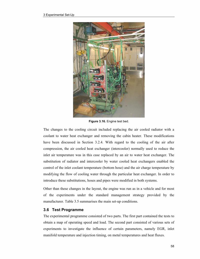
3 Experimental Set-Up
58
The changes to the cooling circuit included replacing the air cooled radiator with a
coolant to water heat exchanger and removing the cabin heater. These modifications
have been discussed in Section 3.2.4. With regard to the cooling of the air after
compression, the air cooled heat exchanger (intercooler) normally used to reduce the
inlet air temperature was in this case replaced by an air to water heat exchanger. The
substitution of radiator and intercooler by water cooled heat exchangers enabled the
control of the inlet coolant temperature (bottom hose) and the air charge temperature by
modifying the flow of cooling water through the particular heat exchanger. In order to
introduce these substitutions, hoses and pipes were modified in both systems.
Other than these changes in the layout, the engine was run as in a vehicle and for most
of the experiments under the standard management strategy provided by the
manufacturer. Table 3.5 summarises the main set-up conditions.
3.6 Test Programme
The experimental programme consisted of two parts. The first part contained the tests to
obtain a map of operating speed and load. The second part consisted of various sets of
experiments to investigate the influence of certain parameters, namely EGR, inlet
manifold temperature and injection timing, on metal temperatures and heat fluxes.
Figure 3.16. Engine test bed.

3 Experimental Set-Up
59
Cooling circuit set-up Standard thermostat (fully operating), radiator replaced by a water cooled heat exchanger
Pump control Full flow
Coolant inlet temperature Controlled at 87ºC ± 5ºC by adjusting the flow of cooling water through the heat exchanger
Coolant flow to oil cooler Standard (controlled by oil cooler thermostat)
Coolant flow to EGR cooler Standard (controlled by main thermostat)
Air charge cooling set-up Intercooler replaced by a water cooled heat exchanger
Air charge temperature Controlled at 60ºC ± 8ºC by adjusting the flow of cooling water through the heat exchanger
EGR flow Auto (controlled by ECU)
Injection timing Auto (controlled by ECU)
Table 3.5. Engine set-up conditions.
The experiments in the first part of the programme were carried out with the engine
running under the general set-up conditions summarised in Table 3.5. For the tests in the
second part of the programme additional settings were required. The air charge
temperature set point was varied during the experiments to explore the effect of
changing the inlet manifold temperature. In the case of variation of injection timing, it
was necessary to overwrite the standard ECU strategy, either to advance or retard the
injection.
The test programme also included repeating several of the experiments from the first
part of the program as well as some of the EGR experiments. These additional tests
were used to validate the results by comparing the raw temperature data taken under
nominally identical engine operating conditions on different days.
3.6.1 Map of Engine Speed and Torque
The initial phase of the test programme comprised the experiments to obtain a
comprehensive map of engine operating conditions over the entire range of speed and
load. The speed was increased from 1000 rev/min to 4500 rev/min at intervals of
500 rev/min. The torque was varied in steps of 10% of the maximum torque value for
the specific testing speed. The maximum torque at a given engine speed was defined by
the limiting torque curve (LTC) of the engine. The graph of limiting torque is included
in Appendix B.
At every test point, the engine was allowed to run until conditions were stable and then
temperature data were logged during a period of four and a half minutes using the

3 Experimental Set-Up
60
additional logging system described in Section 3.4.3. A time of four and a half minutes
was found to be sufficient to obtain data that adequately represented steady-state
operating conditions. The length of the logging time is discussed in Section 4.2.2.
Figure 3.17 illustrates the experimental sequence to obtain the required test points at
2500 rev/min. The example shown in the figure includes a warm-up period at
2000 rev/min previous to setting the engine speed to 2500 rev/min and the torque to
10% of the limiting torque at this speed (approximately 31 Nm), which represents the
first test point in the sequence.
0 1000 2000 3000 4000 5000 6000 7000 80000
500
1000
1500
2000
2500
3000
Speed (rev/m
in)
Time (s)0 1000 2000 3000 4000 5000 6000 7000 8000
-100
-50
0
50
100
150
200
250
300
350
400
Torque (Nm)
SpeedTorque
Figure 3.17. Test sequence at 2500 rev/min.
During the first part of the testing program, an experiment under motored conditions
was also undertaken at every testing speed. This experiment was completed at each
speed immediately after the test at 10% of the limiting torque. In this way the engine
was already warm before turning off the fuel supply and setting the dynamometer to
rotate the engine at the required speed. The motored test at 2500 rev/min is shown in
Figure 3.17. It can be noted that this is the only test condition at which the engine torque
is actually negative (approximately -46 Nm).
Since engine temperature decreased rapidly in the absence of combustion, no settling
time was allowed for the motored tests and the logging period was reduced to one
minute. However, the engine temperature still dropped considerably during the test. It
should be mentioned that the procedure to do the motored tests was not intended to be

3 Experimental Set-Up
61
particularly rigorous; the tests were only undertaken to have a rough idea of the power
required in this engine to do the pumping work, move the ancillary components and
overcome friction. A rigorous procedure to carry out motored tests can be found in
Stone (1999).
Table 3.6 shows the test points included in the map of engine speed and torque obtained
during the first part of the test program. The engine speed values shown in the table are
the set points for the experiments, whereas the engine torques are the actual measured
torques.
10% Motored 20% 30% 40% 50% 60% 70% 80% 90% 100%LTC
1000 14.9 -26.9 30.0 45.0 59.9 75.1 90.0 105.0 120.0 135.0 140.0
1500 27.1 -29.4 57.9 78.7 114.9 132.6 166.7 202.4 230.0 247.8 274.8
2000 31.1 -34.5 62.2 93.0 124.0 155.0 186.1 217.0 252.1 278.9 309.9
2500 31.0 -45.7 62.0 93.0 124.0 154.9 185.9 216.9 247.8 279.1 302.3
3000 28.2 -55.4 57.0 86.2 113.7 143.3 170.6 199.2 227.2 256.9 282.0
3500 26.0 -63.5 51.0 77.0 103.1 129.1 154.0 179.8 206.0 230.8 257.0
4000 23.0 -72.2 44.9 68.0 90.1 113.2 136.1 158.1 181.0 203.1 221.9
4500 17.9 -92.7 34.6 52.9 69.9 87.7 104.3 122.8 140.0 158.2 168.3
Averaged Torque (Nm)Speed
(rev/min)
Table 3.6. Map of engine speed and torque.
3.6.2 Variation of Parameters
The series of experiments to explore the influence of EGR, inlet manifold temperature
and injection timing on heat flux were carried out during the second part of the test
program. In the EGR investigation, tests were identified for those conditions where
significant EGR was observed during the first part of the program. These tests were then
repeated with the EGR valve closed (no EGR). The conditions for both sets of EGR
tests are shown in Table 3.7. The temperature measurements taken with no EGR could
then be compared with those obtained during the initial part of the test programme.
10% 20% 30% 40%LTC
1000 14.9 29.8 44.9 59.9
1500 31.0 51.8 87.5 116.4
2000 30.7 61.8 92.9 124.1
2500 30.9 93.0
Speed
(rev/min)
Averaged Torque (Nm)
Table 3.7. Test conditions for the EGR experiments.
The experiments to explore the effects of inlet manifold temperature and injection
timing on metal temperatures and heat fluxes were performed at two operating
conditions: limiting torque at 2000 rev/min and limiting torque at 4000 rev/min. The
first test condition corresponded to the maximum torque condition in the engine; the

3 Experimental Set-Up
62
second is close to the condition of maximum power, which occurs in this engine at
3800 rev/min.
The experiment of variation of inlet manifold temperature comprised a series of test
points for each operating condition. In order to obtain several test points the temperature
was gradually increased from about 30ºC to near 90ºC by increasing the temperature of
the air charge, which was controlled by modifying the flow of cooling water through the
heat exchanger used in place of the intercooler. The actual values of inlet manifold
temperature at which measurements were taken are shown in Table 3.8. The table also
shows how the maximum torque delivered by the engine decreased at temperatures
above 60ºC as a consequence of the lower air density.
Speed(rev/min)
33.9 34.2 40.0 48.4 54.5 62.9 72.4 88.5
310.0 309.9 309.7 310.0 309.9 310.0 303.5 282.6
45.6 44.6 43.9 49.6 58.2 64.6 73.8 87.2
226.0 226.0 225.9 225.9 225.8 225.2 219.6 161.2
2000
4000
Inlet Manifold Temp (°C)/Averaged Torque (Nm)
Table 3.8. Variation of inlet manifold temperature.
Similarly, the injection timing experiments were undertaken at maximum torque and
near maximum power. During these tests, the ECU standard injection set point or timing
demand given in degrees before top dead centre (ºBTDC) was overwritten by adding or
subtracting one degree each time to the previous set point. Starting at the standard
setting for each operating condition, the injection timing was first advanced up to a few
degrees and then retarded likewise.
The actual values of timing demand are shown in Table 3.9 with the standard setting
presented in red.
Test condition
100%LTC at 2000 rev/min 5.0 4.0 3.0 2.0 1.0 0.0 -1.0 -2.0 -3.0 -4.0 -5.0
100%LTC at 4000 rev/min 14.5 13.5 12.5 11.5 10.5 9.5 8.5
Timing Demand (°BTDC)
Table 3.9. Variation of injection timing.
Because cylinder pressure and exhaust temperature are very sensitive to fuel injection
timing, the degree of advancing or retarding was limited by maximum cylinder pressure
(168 bar) and maximum pre-turbine temperature (760°C) recommended by the
manufacturer. These variables were carefully monitored during the experiments.

63
4 Data Processing
4.1 Introduction
This chapter contains a discussion of the method used to process and validate the
experimental information. Also in this chapter, preliminary results of estimated surface
temperatures and heat fluxes are presented. The methodology used to process the data
focuses on an analysis of the variation of the controlled quantities, and is explained in
Section 4.2. This section also includes a description of the computer routines used in
processing the data. Section 4.3 contains the calculation procedures used to evaluate
thermal gradients in the metal, to estimate wall surface temperatures and heat fluxes,
and to predict heat transfer coefficients in the cylinder walls and cylinder head. The
validation of experimental data is discussed in Section 4.4. This section includes an
initial selection of experimental measurements based on an inspection of the
temperature data, a discussion of statistical parameters, evaluation of the coolant-side
heat transfer coefficient and an examination of the repeatability of experiments.
4.2 Methodology
4.2.1 Processing Criteria
The main consideration in processing the experimental data was to obtain average
values that adequately represented steady-state thermal operating conditions in the
engine. It has been discussed in Section 3.6.1 that at every test point, the engine was
allowed to achieve stable conditions before recording engine data. Naturally,
oscillations of the controlled variables about the set point occurred during the logging
period, and because some of these variables strongly affect operating temperatures in
the engine, the data processing was designed to take into account these oscillations.
4.2.2 Control Variables
In the discussion of the engine set-up (Section 3.5), it was mentioned that for most of
the experiments the engine ran under the control of the standard strategy provided by
the manufacturer. This meant that once speed and torque were set by the dynamometer
and controlled by the main computer system, the engine ECU managed the relevant
parameters (fuelling and timing) to meet the particular demand imposed by the
dynamometer. Thus, the governing ECU continuously adjusted these parameters in
accordance with the strategy in order to run the engine adequately at the required speed
and load. In this situation, the variations observed in the ECU parameters were in
general small and fast changes, provided that speed, torque and the other test cell
conditions were reasonably constant. This observation is illustrated in Figure 4.1, where

4 Data Processing
64
speed, torque, fuelling and injection timing are shown during an experiment at
3000 rev/min and 50% of the limiting torque (approximately 143 Nm). It should be
noted how small are the changes in the amount of fuel (less than 1 mg per stroke) and
injection timing (less than 0.1 degree of crank angle) during a test time of nearly 400
seconds. Also noteworthy in the figure are variations in engine speed and torque of less
than 1% during the same time.
3250 3300 3350 3400 3450 3500 3550 3600 36503001
3002
3003
Speed
(rev/m
in)
Time (s)
3250 3300 3350 3400 3450 3500 3550 3600 3650140
142
144
146
Torque
(Nm)
Time (s)
3250 3300 3350 3400 3450 3500 3550 3600 365026
27
28
29
Fuel
Demand
(mg/stroke)
Time (s)
3250 3300 3350 3400 3450 3500 3550 3600 36501
1.2
1.4
Tim
ing
Demand
(oBTDC)
Time (s)
Figure 4.1. Variation of speed, torque, fuelling and injection timing during a test at 3000 rev/min and 50% LTC (approximately 143 Nm).
Data recorded over a logging period of several seconds would have been sufficient to
obtain average values that allowed for the variations observed in the ECU parameters or
in speed and torque. However, longer logging times were necessary to take into
consideration the oscillations of the other significant variables controlled by the main
computer system. These variables were inlet coolant temperature (bottom hose
temperature) and air charge temperature.
The behaviour of speed and torque showed in Figure 4.1 was observed at most engine
running conditions. The variations found in these variables over the entire set of
experimental conditions were in the order of 5 rev/min and 10 Nm, which in the worse
cases represented around 1% of the running speed and 10% of the torque. This
demonstrated that both engine speed and torque were accurately controlled by the main
computer system during the experiments. Additional examples at various test conditions
are given in Figure 4.2. It can be seen in the figure that speed and torque changed
continuously by small quantities during the tests, but also displayed an overall trend to

4 Data Processing
65
oscillate about the set point. The amplitude of the speed fluctuations was generally
small, and the absolute value of the torque variations was only significant at load values
below 40% of the limiting torque. No particular trend was observed in the time period
of the fluctuations, either in speed or torque.
The other variables controlled by the main computer system, inlet coolant temperature
and air charge temperature, behaved differently from torque and speed during the
experiments. Coolant temperature and air temperature showed minor fluctuations about
their set points at all testing conditions, which were due to the characteristics of the
control system used in the test cell. In the example given in Figure 4.3, these variables
are shown along with speed and torque for the same running conditions as in Figure 4.1.
As mentioned in Section 3.2.4, the air cooled radiator in the cooling circuit was replaced
by a heat exchanger. The temperature of the coolant at the outlet (bottom hose) of the
radiator was controlled by adjusting the flow of cooling water through the heat
exchanger. Similarly, the temperature of the air charge compressed by the turbocharger
was kept at the required set point by modifying the flow of cooling water through the
heat exchanger that replaced the intercooler. In both cases a proportional, integral and
derivative (PID) control function was used by the computer system to adjust the
position of the flow control valve in response to variations in the temperature of the
working fluid with reference to the set point.
0 50 100 150 200 250 300 350 400 450998
999
1000
1001
1002
Speed
(rev/m
in)
Time (s)0 50 100 150 200 250 300 350 400 450
40
42
44
46
48
50
Torque
(Nm)
Speed
0 50 100 150 200 250 300 350 400 4501498
1499
1500
1501
1502
Speed
(rev/m
in)
Time (s)0 50 100 150 200 250 300 350 400 450
20
25
30
35
40
Torque
(Nm)
Torque
0 50 100 150 200 250 300 350 400 4503498
3499
3500
3501
3502
Speed
(rev/m
in)
Time (s)0 50 100 150 200 250 300 350 400 450
100
102
104
106
108
110
Torque
(Nm)
0 50 100 150 200 250 300 350 400 4503998
3999
4000
4001
4002
Speed
(rev/m
in)
Time (s)0 50 100 150 200 250 300 350 400 450
156
157
158
159
160
Torque
(Nm)
Figure 4.2. Variation of speed and torque at test conditions 1000 rev/min and 30% LTC, 1500 rev/min and 10% LTC, 3500 rev/min and 40% LTC, and 4000 rev/min and 70% LTC.

4 Data Processing
66
As indicated in Table 3.5 the control set points for inlet coolant temperature and air
charge temperature were 87ºC and 60ºC respectively. The coolant temperature set point
was kept the same for the entire experimental program, and the air temperature set point
was only modified during the tests of variation of inlet manifold temperature.
For most experiments the peak variation of the inlet coolant temperature about the set
point was of the order of 10ºC, while the air charge temperature fluctuations showed
corresponding variations of up to 16ºC. The amplitude of the oscillations of both
variables was not particularly sensitive either to speed or torque; naturally, the largest
amplitudes were observed at conditions of high load when more heat was rejected.
However, the time period of the oscillations could be dependant on both engine speed
and torque. Generally, as the engine produced more power, either by increasing the
speed or the load, the period of the oscillation of air charge temperature, and to some
extent that of coolant temperature, decreased. That is, as power increased more heat was
rejected to the coolant, and also the air charge temperature after compression became
higher as a result of the increased boost pressure. Accordingly, the temperature control
system responded more rapidly at higher heat rates. The effects of increasing speed and
torque on the control of inlet coolant and air charge temperatures are illustrated in
Figure 4.4 and Figure 4.5.
3250 3300 3350 3400 3450 3500 3550 3600 36503001
3002
3003
Speed
(rev/m
in)
Time (s)
3250 3300 3350 3400 3450 3500 3550 3600 3650140
142
144
146
Torque
(Nm)
Time (s)
3250 3300 3350 3400 3450 3500 3550 3600 365080
90
100
Inlet Coolant
Temperature
(°C)
Time (s)
3250 3300 3350 3400 3450 3500 3550 3600 365050
55
60
65
Air Charge
Temperature
(°C)
Time (s)
Figure 4.3. Variation of speed, torque, bottom hose temperature and air charge temperature during a test at 3000 rev/min and 50% LTC (approximately 143 Nm).

4 Data Processing
67
Evident from Figure 4.4 is the reduction in the time period of the oscillation of both
temperatures as the engine speed increases. The effect of increasing torque, however,
was important on the fluctuations of the air charge temperature, but not on the
oscillations of the coolant temperature, as shown in Figure 4.5.
4100 4150 4200 4250 4300 4350 4400 4450 4500 4550 460080
85
90
95
Inlet Coolant
Temperature
(°C)
Time (s)
1500 rev/min, 166 Nm
3700 3750 3800 3850 3900 3950 4000 4050 4100 4150 420080
85
90
95Inlet Coolant
Temperature
(°C)
Time (s)
2500 rev/min, 155 Nm
4200 4250 4300 4350 4400 4450 4500 4550 4600 4650 470080
85
90
95
Inlet Coolant
Temperature
(°C)
Time (s)
3500 rev/min, 154 Nm
4600 4650 4700 4750 4800 4850 4900 4950 5000 505080
85
90
95
Inlet Coolant
Temperature
(°C)
Time (s)
4000 rev/min, 158 Nm
(a)
4100 4150 4200 4250 4300 4350 4400 4450 4500 4550 460040
50
60
70
Air C
harge
Temperature
(°C)
Time (s)
1500 rev/min, 166 Nm
3700 3750 3800 3850 3900 3950 4000 4050 4100 4150 420040
50
60
70
Air Charge
Temperature
(°C)
Time (s)
2500 rev/min, 155 Nm
4200 4250 4300 4350 4400 4450 4500 4550 4600 4650 470040
50
60
70
Air Charge
Temperature
(°C)
Time (s)
3500 rev/min, 154 Nm
4600 4650 4700 4750 4800 4850 4900 4950 5000 505040
50
60
70
Air C
harge
Temperature
(°C)
Time (s)
4000 rev/min, 158 Nm
(b)
Figure 4.4. Effect of increasing speed on the control of inlet coolant temperature (a) and air charge temperature (b).

4 Data Processing
68
The small effect of increasing torque on the coolant temperature is mainly because at
constant speed the coolant flow through the engine remains the same and the change in
temperature differences between wall and coolant are relatively small. It may also be
noticed in the figures that the oscillations of the inlet coolant temperature had in general
1600 1650 1700 1750 1800 1850 1900 1950 2000 2050 210080
85
90
95
Inlet Coolant
Temperature
(°C)
Time (s)
26 Nm
2850 2900 2950 3000 3050 3100 3150 3200 3250 330080
85
90
95Inlet Coolant
Temperature
(°C)
Time (s)
77 Nm
4700 4750 4800 4850 4900 4950 5000 5050 5100 515080
85
90
95
Inlet Coolant
Temperature
(°C)
Time (s)
180 Nm
5600 5650 5700 5750 5800 5850 5900 5950 6000 605080
85
90
95
Inlet Coolant
Temperature
(°C)
Time (s)
231 Nm
(a)
1600 1650 1700 1750 1800 1850 1900 1950 2000 2050 210040
50
60
70
Air Charge
Temperature
(°C)
Time (s)
26 Nm
2850 2900 2950 3000 3050 3100 3150 3200 3250 330040
50
60
70
Air C
harge
Temperature
(°C)
Time (s)
77 Nm
4700 4750 4800 4850 4900 4950 5000 5050 5100 515040
50
60
70
Air Charge
Temperature
(°C)
Time (s)
180 Nm
5600 5650 5700 5750 5800 5850 5900 5950 6000 605040
50
60
70
Air Charge
Temperature
(°C)
Time (s)
231 Nm
(b)
Figure 4.5. Effect of increasing torque on the control of inlet coolant temperature (a) and air charge temperature (b), at an engine speed of 3500 rev/min.

4 Data Processing
69
a longer time period than the air charge temperature fluctuation, which is due to the
lower thermal inertia of the air and the different amounts of heat being rejected by these
fluids. It is also observed that only at low speed and low torque conditions, when no
significant boost pressure was demanded, the time period of the temperature
fluctuations of the air charge was found to be longer than the period of the oscillations
in coolant temperature. In some of these experiments at low power the air charge
temperature did not even reach the set point.
The effect of the observed variations in air charge temperature and inlet coolant
temperature on the measured temperatures in the engine block and cylinder head is
illustrated in Figure 4.6. These results were obtained at 4000 rev/min and 70% of the
limiting torque (approximately 158 Nm), and are representative of the general trend
observed in the measured metal temperatures at all experimental conditions.
The example shown in the figure clearly indicates that metal temperatures in the engine
block and cylinder head followed the trend of the inlet coolant temperature. The time
period of the oscillations of the measured temperatures is almost identical to that of the
coolant temperature fluctuations. However, the effects of the time period of the air
charge temperature oscillations on the period of the steady-state metal temperature
fluctuations are not that evident. It may be possible that small variations of the
4750 4800 4850 4900 4950 5000 505080
85
90
95
Inlet Coolant
Temperature
(°C)
Time (s)
4750 4800 4850 4900 4950 5000 505040
50
60
70
Air Charge
Temperature
(°C)
Time (s)
4750 4800 4850 4900 4950 5000 5050110
115
120
Temperature at
Location A2C
(°C)
Time (s)
4750 4800 4850 4900 4950 5000 5050120
125
130
Temperature at
Location C1D
(°C)
Time (s)
Figure 4.6. Effect of variations of inlet coolant and air charge temperatures on metal measured temperatures in the block (location A2C) and cylinder head (location C1D), at 4000 rev/min and 70% LTC (approximately 158 Nm).

4 Data Processing
70
temperature of the air charge (approximately 5°C in the example shown) have little
influence on the average temperature of the metal, although these variations affect the
instantaneous magnitude of metal temperatures.
The implications of variations of air charge temperature and coolant temperature in the
process of heat transfer in engines are well documented in the literature (Heywood,
1988 and Taylor, 1985). The coolant temperature for instance is known to strongly
influence the operating temperature of the metal components. It is also known that gas
temperature is affected by the inlet manifold temperature, which depends on the
temperature of the air charge and EGR. Thus, the temperature of the air charge
indirectly affects the temperature of the metal, because the heat flow from combustion
gases to the surrounding walls partly depends on the temperature of the inlet gases.
The period of the oscillations of inlet coolant temperature was in some experiments
more than four minutes, in particular at low speed and low torque. Because of these
observations, and once it had been demonstrated that measured temperatures in the
metal changed in accordance to the inlet coolant temperature, it was decided to set the
logging time for each test point to four and half minutes. In this way, experimental data
were logged over at least one entire oscillation of the main variables. Thus measured
temperatures and other quantities could be averaged over the time period of one
complete cycle of the coolant temperature about the set point. The data obtained by
following this procedure certainly included the effect of variation of the significant
parameters.
It is worth mentioning that temperature results were not significantly different from
average values obtained over the entire logging time. However, the procedure improved
the quality of the experimental data (reduced dispersion), and provided confidence in
the steady-state nature of the results.
4.2.3 Data Processing Routines
Several automated routines were developed in order to access and process the
experimental data, and to perform the calculations necessary to obtain thermal
gradients, surface temperatures, heat fluxes and heat transfer coefficients; and also to
present the results from the investigation. The purpose and a general description of these
routines are presented in this section; the actual routine codes are listed in Appendix D.
In Section 3.4.3 it was mentioned that the main data acquisition system (Cadet produced
by CP Engineering Systems) continuously saved the measured variables into an internal

4 Data Processing
71
file (trace file). The user could log data averaged over a specified time period, which in
this case was four and half minutes, into a second file (log file). Trace files can be
accessed by using the computer programme MatLab produced by The MathWorks, and
the software MatTrace, which is also provided by CP Engineering Systems. Log files
are generated by Cadet in a spreadsheet format that can be accessed with Microsoft
Excel. Log files were only used to verify overall running conditions in a particular
experiment. Trace files were the source of test bed data used for all processing purposes.
It should be noted that these data did not include metal temperatures measured to
evaluate thermal gradients.
The first routine, built in MatLab, was designed to access the trace file from a particular
experiment and create a graph of engine speed and torque versus time for the sequence
of torque conditions tested at a given engine speed. The graph was then used to identify
the specific time periods during which data were logged at the required operating
conditions, as shown in Figure 4.7. Usually, a complete testing sequence, as described
in Section 3.6.1, was logged into a single trace file. The example showed in Figure 4.7
used the data from the trace file saved during the experiments at 4000 rev/min.
In Figure 4.7, every pair of squared markers indicates the start and end of a test point.
The box associated to each marker displays the log time (x value) and the engine torque
(y value) for that particular point. For instance, the first marker in the graph (x: 1424,
0 1000 2000 3000 4000 5000 6000 7000 80000
500
1000
1500
2000
2500
3000
3500
4000
4500
Speed (rev/m
in)
Time (s)0 1000 2000 3000 4000 5000 6000 7000 8000
-100
-50
0
50
100
150
200
250
X: 1420
Y: 24.87
X: 2210
Y: -73.3
X: 1932
Y: 23.5
X: 1950
Y: -73.12
X: 2215
Y: 46.47
X: 2694
Y: 45.17
X: 5979
Y: 203.4
X: 6000
Y: 222.4
X: 6428
Y: 223.1
X: 5515
Y: 203.2
X: 5006
Y: 158.7
X: 4610
Y: 158.1
X: 4116
Y: 137
X: 4110
Y: 113.2
X: 5485
Y: 181.8
X: 5045
Y: 180.6
X: 4568
Y: 136.2
X: 3662
Y: 113.2
X: 3186
Y: 67.28
X: 3643
Y: 89.85
X: 2749
Y: 68.97
Torque (Nm)
X: 3200
Y: 91.15
SpeedTorque
Figure 4.7. Test sequence at 4000 rev/min.

4 Data Processing
72
y: 23.5) indicates the beginning of the first test point at 4000 rev/min (at this speed, 10%
of the limiting torque curve was approximately 23.52 Nm).
Once the starting and ending times of the logging period of every test point were found,
a second routine, also built in MatLab, used these times to find the data of each test
point within the trace file of the experiments taken at a particular engine speed, and to
produce graphs of the controlled variables (speed, torque, inlet coolant temperature and
air charge temperature) versus time at every testing condition. These are the graphs used
in the analysis of variations of the control variables discussed in Section 4.2.2. The
graphs were also used to find the time period of a complete oscillation of the inlet
coolant temperature, which was necessary to obtain average values representative of
every steady-state condition. This is illustrated in Figure 4.8; the graphs in this example
were produced with data from the fourth test point (starting at x: 2749, y: 68.97) of the
experiments at 4000 rev/min, which are showed in Figure 4.7.
Following the identification of the oscillation period of inlet coolant temperature for all
test points, another MatLab routine was used to access the trace files within the time
limits of the specific time periods for a given speed. These selected data were averaged
to produce a matrix of single values of every relevant variable measured in the test bed
for all load conditions at every engine speed. The routine also produced matrices of
statistical parameters (minimum and maximum values, and standard deviation) and
2700 2750 2800 2850 2900 2950 3000 3050 3100 3150 32003999
4000
4001
Speed
(rev/m
in)
Time (s)
2700 2750 2800 2850 2900 2950 3000 3050 3100 3150 320066
68
70
Torque
(Nm)
Time (s)
2700 2750 2800 2850 2900 2950 3000 3050 3100 3150 320080
90
100
X: 2915
Y: 91.14
X: 2981
Y: 91.05
Inlet Coolant
Temperature
(°C)
Time (s)
2700 2750 2800 2850 2900 2950 3000 3050 3100 3150 320050
55
60
65
Air C
harge
Temperature
(°C)
Time (s)
Figure 4.8. Test point at 4000 rev/min and 40% LTC (approximately 68 Nm).

4 Data Processing
73
matrices containing the logging times and periods used to average the data.
Subsequently, the matrices were stored in a MatLab work space, one for every testing
speed. Table 4.1 contains the matrix of average values for 4000 rev/min; notice that
only selected variables are shown.
The temperature measurements taken in the engine block and cylinder head as part of
the thermal survey were logged into data loggers and then transferred to a second
computer using the software DeLogger. The data loggers worked simultaneously with
the main data acquisition system. This has been explained in Section 3.4.3. The
programme DeLogger was configured to produce data files that could be accessed using
Microsoft Excel. Four of these files, one from each data logger, were created for every
sequence of torque conditions tested at a particular engine speed.
The temperature data were processed using Microsoft Visual Basic routines recorded in
Microsoft Excel (macros). The first routine used the time periods of the oscillations of
inlet coolant temperature previously determined with MatLab, to select data for every
torque condition within the required time period. The routine processed one temperature
file at a time and generated a new Excel file, in which the temperature data were
organised by torque condition in different spreadsheets. By using this routine, four files
of temperature data selected by torque were created for every engine speed.
Once the temperature data were prepared for a particular engine speed, a series of
routines were used to merge the four data files into a single file, to label the temperature
sets, and finally, to average the data for each test point. The routines also obtained the
minimum and maximum value, and standard deviation of each series of temperatures
measurements.
The resulting file had one spreadsheet per torque condition, each of them containing the
temperatures measured within the corresponding time period by all the thermocouples
installed in the engine block and cylinder head. In the same file, two spreadsheets of
average temperature values were created, one for the engine block and the other for the
cylinder head. The temperature sets were labelled in accordance with the thermocouple
identification method, as explained in Section 3.2.2, and organised in the spreadsheets
of average values by location of the set of thermocouples in the engine block and
cylinder head.

4 Data Processing
74
Cylinder
Head
Temp
(°C)
96.869
101.76
102.33
103.19
104.21
105.07
106.12
107.27
108.55
109.19
110.57
Air
Density
(kg/m
3)
1.5222
1.9159
1.7331
1.6531
1.7406
1.7661
1.9115
2.0413
2.1607
2.233
2.2694
Tim
ing
Demand
(°BTDC)
5.7171
5.72
6.4241
7.9018
9.2285
9.9584
10.36
10.841
11.535
11.505
11.464
Mass
Air
Flow
(kg/hr)
280.64
364.3
334.22
320.11
335.54
340.46
367.6
394.23
418.01
431.34
438.1
Fuel
Demand
(mg/st)
0
11.473
13.266
16.021
19.791
23.717
28.738
33.97
38.995
43.7
48.012
Inlet
Manifold
Pressure
(kPa gauge)
49.214
86.604
69.141
61.922
69.998
72.482
87.007
99.874
111.73
119.53
121.79
Air
Mass
Flow
(kg/hr)
308.63
405.08
370.04
355.35
373.32
378.75
409.81
435.83
460.93
476.33
484.43
Engine
Outlet
Coolant
Temp (°C)
92.368
93.633
93.861
93.969
94.018
94.296
94.378
94.458
94.448
94.508
94.42
Engine
Inlet
Coolant
Temp (°C
)
90.641
91.011
91.153
91.053
90.904
91.009
90.903
90.765
90.561
90.363
89.958
Coolant
Engine
Flow
(l/m
in)
0
9.1979
10.866
16.509
25.881
38.487
47.641
56.648
68.754
84.015
98.889
Post-
Intercooler
Temp
(°C)
58.86
56.822
57.513
57.617
57.186
57.088
57.882
58.163
58.324
59.475
60.05
Pre-
Turbine
Temp
(°C)
165.82
303.34
332.97
384.99
426.27
482.81
518.76
556.92
599.71
655.74
713.69
Inlet
Manifold
Temp
(°C)
58.517
56.503
56.845
57.072
56.568
56.499
57.092
57.488
57.742
58.785
59.2
Bottom
Hose
Temp
(°C)
86.952
86.988
87.084
86.96
86.76
87.084
87.007
86.977
86.977
87.041
87.074
Avg
Engine
Speed
(rev/m
in)
3999.7
3999.7
3999.8
3999.8
3999.8
3999.8
3999.7
3999.8
3999.8
3999.9
3999.9
Avg
Engine
Torque
(Nm)
-72.21
23.003
44.866
67.958
90.087
113.19
136.08
158.1
180.99
203.08
221.89
Table 4.1. Test bed average data at 4000 rev/m
in.

4 Data Processing
75
Table 4.2 contains part of the spreadsheet of average temperature values measured in
the engine block at 4000 rev/min. The data are organised in order of ascending torque,
the top line corresponds to motored conditions and the next ten lines to 10% increments
(10% to 100%) of the limiting torque curve at 4000 rev/min. In this example only the
values measured at locations A are shown. Similarly, the spreadsheet of average
temperatures measured in the cylinder head for the same experiment is shown in
Table 4.3.
The data from these spreadsheets were then added to the MatLab work space previously
created for every testing speed. In this way, the entire processed experimental data were
available in MatLab for further analysis.
4.3 Computation of Temperature Gradients, Wall Surface Temperatures, Heat Fluxes and Heat Transfer Coefficients
The instrumentation of the engine with sets of fixed thermocouples at key locations in
the engine block and cylinder head has been explained in Section 3.2.2. The
thermocouples of every set at all locations were arranged to allow the calculation of
steady-state temperature gradients in one direction. In its simplest form the temperature
gradient in one direction, ∆T/∆x, can be found from two temperature values T1 and T2,
measured by thermocouples located apart a certain distance ∆x, by using the following
equation:
21
21
xx
TT
x
T
−
−=
∆∆
(4.1)
This is the equation to obtain the one-dimensional temperature gradient in a flat wall,
which was applied to estimate the gradient in the direction of the cylinder axis in the
cylinder head, where only sets of two thermocouples were used at all locations. The
temperature gradient can then be used to find the surface temperature of the cylinder
head on the gas-side and coolant-side by linear extrapolation, in accordance with the
equation:
11
21
21 )( Txxxx
TTTx +−
−
−= (4.2)
In the cylinder walls, however, the heat transfer process is represented by a cylindrical
system with heat flowing in the radial direction. In this system the radial temperature
distribution is given by the following equation (Incropera and DeWitt, 1990):
11
21
21 )/ln()/ln(
Trrrr
TTTr +
−= (4.3)

4 Data Processing
76
A7L
105.15
109.34
109.90
111.60
112.44
113.94
116.31
117.55
119.00
118.71
120.77
A7R
106.77
111.56
112.11
114.20
115.23
117.09
119.71
121.12
122.97
123.00
125.75
A7C
107.24
112.33
112.93
115.01
116.15
118.12
120.86
122.48
124.44
124.56
127.54
A6L
100.61
104.44
104.66
106.30
106.66
107.96
109.91
110.71
112.10
112.00
114.03
A6R
103.08
107.80
108.31
110.62
111.16
112.97
115.24
116.30
118.18
118.41
121.07
A6C
104.40
110.04
110.60
113.16
113.95
116.22
118.95
120.46
122.96
123.66
127.17
A5L
97.25
99.88
100.07
101.36
101.55
102.52
103.89
104.23
105.03
104.88
106.35
A5R
101.37
105.64
106.37
108.74
109.33
111.15
113.17
113.93
115.76
116.14
119.12
A5C
102.76
107.81
108.83
111.54
112.51
114.90
117.40
118.54
120.87
121.71
125.53
A4L
95.92
97.66
97.74
98.57
98.50
98.93
99.82
100.00
100.46
100.15
101.04
A4R
101.27
104.66
105.21
107.01
107.65
108.89
110.69
111.50
113.00
113.57
115.95
A4C
102.35
106.27
106.99
108.87
109.77
111.29
113.34
114.47
116.28
117.18
120.01
A3L
98.26
100.87
101.23
101.98
102.39
103.21
104.75
105.24
106.22
106.06
107.62
A3R
100.95
104.31
105.00
106.28
107.11
108.36
110.28
110.91
112.53
112.80
115.07
A3C
101.48
105.23
106.02
107.22
108.17
109.60
111.74
112.63
114.37
114.73
117.22
A2L
101.01
105.23
105.80
106.85
107.70
109.05
111.24
112.18
113.79
114.62
117.24
A2R
101.86
106.46
107.14
108.45
109.45
111.01
113.41
114.35
116.28
117.46
120.27
A2C
102.51
107.46
108.30
109.61
110.81
112.56
115.11
116.28
118.46
119.82
123.08
A1L
103.21
109.42
109.58
110.94
111.79
113.38
115.89
117.48
119.35
121.29
124.34
A1R
105.21
113.04
113.38
115.18
116.49
118.82
121.93
124.23
126.94
130.16
134.45
A1C
107.14
116.15
116.61
118.62
120.18
122.91
126.45
129.23
132.47
136.56
141.84
Torque
(Nm)
-72.21
23.003
44.866
67.958
90.087
113.19
136.08
158.1
180.99
203.08
221.89
Table 4.2. Selected average temperature (ºC
) measured in the engine block at 4000 rpm

4 Data Processing
77
H2S
110.40
125.12
127.13
131.44
135.83
141.58
147.65
152.68
158.08
162.89
169.90
H1D
114.06
132.05
134.48
139.77
145.55
152.69
160.18
166.53
173.49
179.85
188.69
G2S
109.74
123.46
125.19
129.12
132.97
138.13
143.84
148.40
153.28
157.31
163.79
G1D
114.01
131.11
133.15
137.85
142.88
149.33
156.39
162.17
168.38
173.51
181.12
F2S
104.02
111.87
112.92
115.30
117.02
119.47
122.71
125.07
127.37
128.95
132.48
F1D
106.51
116.48
117.92
120.91
123.42
126.81
130.93
134.19
137.32
139.92
144.56
E2S
105.25
114.66
115.96
118.79
121.13
124.29
128.09
131.07
133.88
136.17
140.06
E1D
110.24
123.94
125.83
129.87
133.85
138.82
144.41
149.13
153.69
157.77
163.54
D2S
109.53
118.84
119.54
122.28
124.77
127.58
131.09
133.70
136.38
137.45
139.96
D1D
114.34
127.21
128.22
132.00
135.75
139.87
144.78
148.71
152.74
154.93
158.40
C2S
106.40
114.43
115.01
117.19
119.03
121.46
124.44
126.49
128.54
130.03
133.75
C1D
107.23
116.34
117.03
119.56
121.78
124.72
128.23
130.72
133.28
135.36
139.66
B2S
109.43
120.34
121.29
124.30
127.27
131.00
135.23
138.52
142.16
144.75
149.07
B1D
111.80
124.97
126.13
129.77
133.53
138.18
143.34
147.56
152.17
155.79
161.16
A2S
111.31
123.72
124.82
128.10
131.56
135.75
140.47
144.30
148.28
151.08
155.80
A1D
115.38
131.08
132.44
136.46
140.92
146.24
152.13
157.07
162.13
166.06
171.84
Torque
(Nm)
-72.21
23.003
44.866
67.958
90.087
113.19
136.08
158.1
180.99
203.08
221.89
Table 4.3. Average temperature (ºC
) measured in the cylinder head at 4000 rpm

4 Data Processing
78
Equation 4.3 corresponds to a logarithmic function that can be approximated to the line
that best fits the temperature measurements by applying the method of least squares. In
the engine block, arrays of three thermocouples were generally used to measure
temperature; hence the line generated by least squares is based on three discrete
temperature values. This is schematically illustrated in Figure 4.9.
The deduction of the equations to calculate the gradient and the independent term
(intercept with the ordinate axis) of a straight line by least squares can be found in most
books of experimental methods. Although, in this application the curve generated is not
a straight line, the equations can be modified to fit the logarithmic temperature
distribution (Equation 4.3). By plotting T against ln r the result is again a straight line.
The equations showed below were adapted from Holman (1994).
brrmT Br += )/ln( (4.4)
2321
23
22
21
321321332211
)lnln(ln])(ln)(ln)[(ln3
))(lnln(ln)lnlnln(3
rrrrrr
TTTrrrrTrTrTm
++−++
++++−++= (4.5)
−++−++
++++=
2
321
2
3
2
2
2
1
2
3
2
2
2
1321
)lnln(ln])(ln)(ln)[(ln3
})]/[ln()]/[ln()]/){[ln((
rrrrrr
rrrrrrTTTb BBB
2
321
2
3
2
2
2
1
321332211
)lnln(ln])(ln)(ln)[(ln3
)]/ln()/ln()/)][ln(/ln()/ln()/ln{[
rrrrrr
rrrrrrrrTrrTrrT BBBBBB
++−++
++++ (4.6)
Once the gradient m and the independent term b are determined, Equation 4.4 can be
used to estimate the metal temperature at any point in the cylinder wall along the line
Figure 4.9. Schematic representation of the one-dimensional heat flux and temperature distribution in the cylinder walls.
Combustion chamber
Cooling gallery
Cylinder wall
2 mm 1.5 mm 1.5 mm 2 mm
TwcTwg T1 T2 T3
(T2 ,r2)
T (K)
Twg
Twc
Tg Tc
43 r1 r2 r3 50 r (mm)
rq&rq&
(T3 ,r3)
(T1 ,r1)
rq&
Combustion chamber
Cooling gallery
Cylinder wall
2 mm 1.5 mm 1.5 mm 2 mm
TwcTwg T1 T2 T3
(T2 ,r2)
T (K)
Twg
Twc
Tg Tc
43 r1 r2 r3 50 r (mm)
rq&rq&
(T3 ,r3)
(T1 ,r1)
rq&

4 Data Processing
79
obtained by least squares. In this system, the temperature on the surface of the cylinder
wall in contact with the gases, Twg, is the temperature obtained for a radius of 43 mm,
which is the radius of the cylinder bore rB. Similarly, the temperature on the surface on
the coolant-side of the wall, Twc, is the temperature for a radius of 50 mm. The thickness
of the cylinder wall was generally taken as 7 mm, although at some locations the wall
was found to be up to 2 mm thinner (see Section 3.2.2.1). These variations have no
effect on the estimated gas-side wall surface temperature since the thermocouple holes
were drilled with reference to the gas face, but they were taken into account in the
estimation of the coolant-side wall surface temperature.
The one-dimensional temperature distribution can then be used to calculate the
corresponding heat flux through the cylinder head, xq& , or in the case of the cylinder
walls, the heat flux normal to a particular surface of radius r, rq& . The equations are
given by Fourier’s law of heat conduction:
x
Tkqx ∆∆
−=& (4.7)
r
mkqr −=& (4.8)
In the cylinder head, Equation 4.7 represents the local heat per unit area through the
flame deck in the direction of the cylinder axis. In the engine block, Equation 4.8 gives
the heat per unit area normal to the cylinder wall in the radial direction at one particular
location. It should be noticed that, in a radial system the conduction heat transfer rate
through any circular boundary is constant, but the heat flux normal to a particular
surface depends on the radius of the surface r. In Equation 4.8 m is the gradient given
by Equation 4.5. In both equations the sign indicates that the heat flows in the direction
of decreasing temperature, and is usually ignored in the calculations. The constant k,
represents the thermal conductivity of the cast iron or the aluminium alloy, which were
the metals used to make the engine block and cylinder head respectively. The thermal
conductivities used in the calculations were 45 W/m K for cast iron and 195 W/m K for
the aluminium alloy (AlSi10Mg). The conductivity of cast iron within the operating
temperature range of the engine block (300-450 K) does not vary much (Rohsenow et
al., 1998); the value used was estimated for a temperature around 400 K. The
conductivity of the aluminium alloy is based on measurements taken at the National
Physical Laboratory (2000).

4 Data Processing
80
In compliance with the first law of thermodynamics, the conductive heat flux at the gas
surface in the situation depicted in Figure 4.9 must be equal to the heat flux arising from
the combustion chamber. Similarly, the conductive heat flux at the coolant-side of the
wall must be equal to the convective heat flux between the wall surface and the coolant.
According to Newton’s law of cooling, the equations for the convective heat fluxes are:
)( wgggg TThq −=& (4.9)
)( cwccc TThq −=& (4.10)
Subsequently, it is possible to estimate the local time-averaged convective heat transfer
coefficient on the gas-side, hg, and on the coolant-side, hc of the combustion chamber
walls, providing that estimates of the mean gas temperature, Tg, and the mean coolant
temperature, Tc can be determined. The heat transfer on the gas-side is particularly
complicated compared to the coolant-side, since Tg and consequently hg change
significantly during the engine cycle. The method to estimate the temperature of the gas
is presented in Chapter 6 as part of the evaluation of existing correlations to predict
instantaneous convective heat transfer coefficients. The calculation of the coolant-side
heat transfer coefficient is discussed in Section 4.4.3; the temperature of the coolant
used in these calculations is taken as the mean value of the temperatures measured at the
inlet and outlet of the engine. The measurement of coolant temperatures was discussed
in Section 3.2.4.
It is worth mentioning that the one-dimensional approach used to estimate steady-state
temperatures and heat fluxes discussed in this section is particularly suitable to the heat
transfer process in the cylinder walls of the engine, where the dominant temperature
gradients occur in the radial direction. This assumption has been verified with published
data, for instance Woschni (1979), and also has been observed in results obtained in this
investigation. Therefore, at any particular location in the cylinder walls the one-
dimensional heat flux predicted by this method can be approximated to the total heat
flux. In the cylinder head, however, the heat transfer situation is highly three-
dimensional due to its complex geometry; significant thermal gradients exist in all
directions, and consequently the local heat flux obtained under this approach should be
interpreted as the axial component of the total heat flux.
The equations to obtain thermal gradients and estimate wall surface temperatures and
heat fluxes were programmed in MatLab; the codes of the calculation routines are listed
in Appendix D.

4 Data Processing
81
4.4 Data Validation
The objective of this section is to examine critically the measured temperature data and
hence to discard inconsistent or unreliable data in the light of average temperatures
obtained at all locations in the engine block and cylinder head. Also, to look at the
statistical dispersion of the experimental measurements; this includes presenting results
of the standard deviation of measured temperatures and control variables. The results
used in the examination were obtained from the experiments at 2500 rev/min and are
representative of the trends observed at all other conditions. The section concludes with
calculations of the coolant-side heat transfer coefficient and considerations of
repeatability.
4.4.1 Inspection of Temperature Data
Examination of the experimental data is initially concentrated on the temperatures
measured in the engine block. The average temperature obtained at 2500 rev/min for all
load conditions in the walls of the cylinders are shown in Figures 4.10 to 4.20.
In the figures, a set of graphs is shown for every array of thermocouples installed in the
engine block. For example, there are four sets of graphs in Figure 4.10 (locations A1 to
A4) and three sets of graphs in Figure 4.11 (locations A5 to A7), four sets in
Figure 4.12 (locations B1 to B4), and only two sets in Figure 4.13 (locations C1 and
C2). The graphs are identified with the name of the array and its position with reference
to the top deck (see Figures 3.2 and 3.3, and Table 3.1 for the exact location of all arrays
in the engine block). In every location there are eleven sets of measurements that
correspond to the torque conditions given in fractions of the limiting torque. The actual
values of torque are shown in Table 3.6.
In the ideal situation, the temperature readings taken at a single location in the cylinder
walls using three thermocouples, when plotted against the radius would lie on the curve
of the function described by Equation 4.3, which has the subtle concave shape
illustrated in Figure 4.9. However, in addition to the fact that heat transfer in the
cylinder wall is not strictly a one-dimensional process, the actual temperature
distribution provided by the measurements was affected by the accuracy of the
instruments and the positions of the tips of the thermocouples. The position of each tip
is defined by the precision of drilling the hole in the metal and the installation of the
thermocouple. Because of these factors a dispersion of temperature values was
expected, provided that the thermocouples were properly calibrated and the installation
was completed satisfactorily.

4 Data Processing
82
43 43.5 44 44.5 45 45.5 46 46.5 47 47.5 48 48.5 49 49.5 5090
100
110
120
130
140
150
160
Measured Temperature (°C
)Radius (mm)
Location A1 (10 mm from top deck)
Motored
10% LTC
20% LTC
30% LTC
40% LTC
50% LTC
60% LTC
70% LTC
80% LTC
90% LTC
100% LTC
43 43.5 44 44.5 45 45.5 46 46.5 47 47.5 48 48.5 49 49.5 5090
100
110
120
130
140
150
160
Measured Temperature (°C
)
Radius (mm)
Location A2 (25 mm from top deck)
Motored
10% LTC
20% LTC
30% LTC
40% LTC
50% LTC
60% LTC
70% LTC
80% LTC
90% LTC
100% LTC
43 43.5 44 44.5 45 45.5 46 46.5 47 47.5 48 48.5 49 49.5 5090
100
110
120
130
140
150
160
Measured Temperature (°C
)
Radius (mm)
Location A3 (40 mm from top deck)
Motored
10% LTC
20% LTC
30% LTC
40% LTC
50% LTC
60% LTC
70% LTC
80% LTC
90% LTC
100% LTC
43 43.5 44 44.5 45 45.5 46 46.5 47 47.5 48 48.5 49 49.5 5090
100
110
120
130
140
150
160
Measured Temperature (°C
)
Radius (mm)
Location A4 (55 mm from top deck)
Motored
10% LTC
20% LTC
30% LTC
40% LTC
50% LTC
60% LTC
70% LTC
80% LTC
90% LTC
100% LTC
Figure 4.10. Average measured temperature at locations A1 to A4 on the exhaust-side of cylinder two, for all torque values tested at 2500 rev/min.

4 Data Processing
83
43 43.5 44 44.5 45 45.5 46 46.5 47 47.5 48 48.5 49 49.5 5090
100
110
120
130
140
150
160
Measured Temperature (°C
)Radius (mm)
Location A5 (70 mm from top deck)
Motored
10% LTC
20% LTC
30% LTC
40% LTC
50% LTC
60% LTC
70% LTC
80% LTC
90% LTC
100% LTC
43 43.5 44 44.5 45 45.5 46 46.5 47 47.5 48 48.5 49 49.5 5090
100
110
120
130
140
150
160
Measured Temperature (°C
)
Radius (mm)
Location A6 (85 mm from top deck)
Motored
10% LTC
20% LTC
30% LTC
40% LTC
50% LTC
60% LTC
70% LTC
80% LTC
90% LTC
100% LTC
43 43.5 44 44.5 45 45.5 46 46.5 47 47.5 48 48.5 49 49.5 5090
100
110
120
130
140
150
160
Measured Temperature (°C
)
Radius (mm)
Location A7 (100 mm from top deck)
Motored
10% LTC
20% LTC
30% LTC
40% LTC
50% LTC
60% LTC
70% LTC
80% LTC
90% LTC
100% LTC
Figure 4.11. Average measured temperature at locations A5 to A7 on the exhaust-side of cylinder two, for all torque values tested at 2500 rev/min.
The average temperatures observed at locations A1, A2, A3, A6 and A7 (Figures 4.10
and 4.11), are good examples of this situation. Also, the results obtained at locations B1,
B2 and B4 (Figure 4.12), at C1 and C2 (Figure 4.13), at D1 and D2 (Figure 4.14), at F2
and F4 (Figure 4.16), at G2 and G3 (Figure 4.18), and at I1 and J1 (Figure 4.20)
revealed a sensible temperature distribution.

4 Data Processing
84
43 43.5 44 44.5 45 45.5 46 46.5 47 47.5 48 48.5 49 49.5 5090
100
110
120
130
140
150
160
Measured Temperature (°C
)Radius (mm)
Location B1 (10 mm from top deck)
Motored
10% LTC
20% LTC
30% LTC
40% LTC
50% LTC
60% LTC
70% LTC
80% LTC
90% LTC
100% LTC
43 43.5 44 44.5 45 45.5 46 46.5 47 47.5 48 48.5 49 49.5 5090
100
110
120
130
140
150
160
Measured Temperature (°C
)
Radius (mm)
Location B2 (25 mm from top deck)
Motored
10% LTC
20% LTC
30% LTC
40% LTC
50% LTC
60% LTC
70% LTC
80% LTC
90% LTC
100% LTC
43 43.5 44 44.5 45 45.5 46 46.5 47 47.5 48 48.5 49 49.5 5090
100
110
120
130
140
150
160
Measured Temperature (°C
)
Radius (mm)
Location B3 (40 mm from top deck)
Motored
10% LTC
20% LTC
30% LTC
40% LTC
50% LTC
60% LTC
70% LTC
80% LTC
90% LTC
100% LTC
43 43.5 44 44.5 45 45.5 46 46.5 47 47.5 48 48.5 49 49.5 5090
100
110
120
130
140
150
160
Measured Temperature (°C
)
Radius (mm)
Location B4 (55 mm from top deck)
Motored
10% LTC
20% LTC
30% LTC
40% LTC
50% LTC
60% LTC
70% LTC
80% LTC
90% LTC
100% LTC
Figure 4.12. Average measured temperature at locations B1 to B4 on the exhaust-side of cylinder two, for all torque values tested at 2500 rev/min.

4 Data Processing
85
43 43.5 44 44.5 45 45.5 46 46.5 47 47.5 48 48.5 49 49.5 5090
100
110
120
130
140
150
160
Measured Temperature (°C
)Radius (mm)
Location C1 (10 mm from top deck)
Motored
10% LTC
20% LTC
30% LTC
40% LTC
50% LTC
60% LTC
70% LTC
80% LTC
90% LTC
100% LTC
43 43.5 44 44.5 45 45.5 46 46.5 47 47.5 48 48.5 49 49.5 5090
100
110
120
130
140
150
160
Measured Temperature (°C
)
Radius (mm)
Location C2 (25 mm from top deck)
Motored
10% LTC
20% LTC
30% LTC
40% LTC
50% LTC
60% LTC
70% LTC
80% LTC
90% LTC
100% LTC
Figure 4.13. Average measured temperature at locations C1 and C2 on the exhaust-side of cylinder two, for all torque values tested at 2500 rev/min.
There was also the possibility of coolant infiltrating the holes due to defective sealing.
In this case the thermocouples would measure the temperature of the coolant heated
inside the hole instead of the metal temperature. Consequently, these measurements
would have to be considered unreliable and excluded from further calculations, given
that it was not practically possible to fix this problem. The left and right thermocouples
of every array were expected to be the most susceptible to coolant infiltration since their
tips were closer to the coolant-side surface of the cylinder wall and hence less epoxy
resin was used to fill the relatively shorter annular space between the hole and the
thermocouple.
The results at locations A4 (Figure 4.10) and A5 (Figure 4.11), at B3 (Figure 4.12), at
E2 (Figure 4.15), and also at G4 (Figure 4.18), illustrate the situation where coolant
might have passed through the sealant of the left thermocouple of the arrays. In these
cases the temperatures measured at a radius of 48 mm seem to be low compared to the
corresponding measurements from other arrays in the same location, or at an equivalent
location in other cylinders; for instance, E2 can be compared to A2, C2 and D2.

4 Data Processing
86
43 43.5 44 44.5 45 45.5 46 46.5 47 47.5 48 48.5 49 49.5 5090
100
110
120
130
140
150
160
Measured Temperature (°C
)Radius (mm)
Location D1 (10 mm from top deck)
Motored
10% LTC
20% LTC
30% LTC
40% LTC
50% LTC
60% LTC
70% LTC
80% LTC
90% LTC
100% LTC
43 43.5 44 44.5 45 45.5 46 46.5 47 47.5 48 48.5 49 49.5 5090
100
110
120
130
140
150
160
Measured Temperature (°C
)
Radius (mm)
Location D2 (25 mm from top deck)
Motored
10% LTC
20% LTC
30% LTC
40% LTC
50% LTC
60% LTC
70% LTC
80% LTC
90% LTC
100% LTC
Figure 4.14. Average measured temperature at locations D1 and D2 on the exhaust-side of cylinder three, for all torque values tested at 2500 rev/min.
43 43.5 44 44.5 45 45.5 46 46.5 47 47.5 48 48.5 49 49.5 5090
100
110
120
130
140
150
160
Measured Temperature (°C
)
Radius (mm)
Location E2 (25 mm from top deck)
Motored
10% LTC
20% LTC
30% LTC
40% LTC
50% LTC
60% LTC
70% LTC
80% LTC
90% LTC
100% LTC
Figure 4.15. Average measured temperature at location E2 on the exhaust-side of cylinder four, for all torque values tested at 2500 rev/min.
The measurements obtained at locations F1, F3, F5, F6 and F7 (Figures 4.16 and 4.17),
and at G1 (Figure 4.18), revealed unrealistic metal temperatures at a radius of 46.5 mm.
The fact that the temperature measured with the right thermocouple of these sets (at
46.5 mm) is lower than the temperature at 48 mm (left thermocouple) for various torque
conditions, can be explained by infiltration of coolant in the holes of those
thermocouples.

4 Data Processing
87
43 43.5 44 44.5 45 45.5 46 46.5 47 47.5 48 48.5 49 49.5 5090
100
110
120
130
140
150
160
Measured Temperature (°C
)Radius (mm)
Location F1 (10 mm from top deck)
Motored
10% LTC
20% LTC
30% LTC
40% LTC
50% LTC
60% LTC
70% LTC
80% LTC
90% LTC
100% LTC
43 43.5 44 44.5 45 45.5 46 46.5 47 47.5 48 48.5 49 49.5 5090
100
110
120
130
140
150
160
Measured Temperature (°C
)
Radius (mm)
Location F2 (25 mm from top deck)
Motored
10% LTC
20% LTC
30% LTC
40% LTC
50% LTC
60% LTC
70% LTC
80% LTC
90% LTC
100% LTC
43 43.5 44 44.5 45 45.5 46 46.5 47 47.5 48 48.5 49 49.5 5090
100
110
120
130
140
150
160
Measured Temperature (°C
)
Radius (mm)
Location F3 (40 mm from top deck)
Motored
10% LTC
20% LTC
30% LTC
40% LTC
50% LTC
60% LTC
70% LTC
80% LTC
90% LTC
100% LTC
43 43.5 44 44.5 45 45.5 46 46.5 47 47.5 48 48.5 49 49.5 5090
100
110
120
130
140
150
160
Measured Temperature (°C
)
Radius (mm)
Location F4 (55 mm from top deck)
Motored
10% LTC
20% LTC
30% LTC
40% LTC
50% LTC
60% LTC
70% LTC
80% LTC
90% LTC
100% LTC
Figure 4.16. Average measured temperature at locations F1 to F4 on the inlet-side of cylinder two, for all torque values tested at 2500 rev/min.

4 Data Processing
88
43 43.5 44 44.5 45 45.5 46 46.5 47 47.5 48 48.5 49 49.5 5090
100
110
120
130
140
150
160
Measured Temperature (°C
)Radius (mm)
Location F5 (70 mm from top deck)
Motored
10% LTC
20% LTC
30% LTC
40% LTC
50% LTC
60% LTC
70% LTC
80% LTC
90% LTC
100% LTC
43 43.5 44 44.5 45 45.5 46 46.5 47 47.5 48 48.5 49 49.5 5090
100
110
120
130
140
150
160
Measured Temperature (°C
)
Radius (mm)
Location F6 (85 mm from top deck)
Motored
10% LTC
20% LTC
30% LTC
40% LTC
50% LTC
60% LTC
70% LTC
80% LTC
90% LTC
100% LTC
43 43.5 44 44.5 45 45.5 46 46.5 47 47.5 48 48.5 49 49.5 5090
100
110
120
130
140
150
160
Measured Temperature (°C
)
Radius (mm)
Location F7 (100 mm from top deck)
Motored
10% LTC
20% LTC
30% LTC
40% LTC
50% LTC
60% LTC
70% LTC
80% LTC
90% LTC
100% LTC
Figure 4.17. Average measured temperature at locations F5 to F7 on the inlet-side of cylinder two, for all torque values tested at 2500 rev/min.
It should be noticed that in some locations (F1, F3, F5, F6 and G1) at high engine loads
(above 50% of the limiting torque) the local temperature of the metal at 46.5 mm is
sufficiently high to heat the amount of coolant inside the holes up to a value larger than
the metal temperature at a radius of 48 mm. Even boiling of stagnant coolant might
occur since metal temperatures are in many cases above the boiling point. That is why at
high engine torques the measurements appear reasonable.

4 Data Processing
89
43 43.5 44 44.5 45 45.5 46 46.5 47 47.5 48 48.5 49 49.5 5090
100
110
120
130
140
150
160
Measured Temperature (°C
)Radius (mm)
Location G1 (10 mm from top deck)
Motored
10% LTC
20% LTC
30% LTC
40% LTC
50% LTC
60% LTC
70% LTC
80% LTC
90% LTC
100% LTC
43 43.5 44 44.5 45 45.5 46 46.5 47 47.5 48 48.5 49 49.5 5090
100
110
120
130
140
150
160
Measured Temperature (°C
)
Radius (mm)
Location G2 (25 mm from top deck)
Motored
10% LTC
20% LTC
30% LTC
40% LTC
50% LTC
60% LTC
70% LTC
80% LTC
90% LTC
100% LTC
43 43.5 44 44.5 45 45.5 46 46.5 47 47.5 48 48.5 49 49.5 5090
100
110
120
130
140
150
160
Measured Temperature (°C
)
Radius (mm)
Location G3 (40 mm from top deck)
Motored
10% LTC
20% LTC
30% LTC
40% LTC
50% LTC
60% LTC
70% LTC
80% LTC
90% LTC
100% LTC
43 43.5 44 44.5 45 45.5 46 46.5 47 47.5 48 48.5 49 49.5 5090
100
110
120
130
140
150
160
Measured Temperature (°C
)
Radius (mm)
Location G4 (55 mm from top deck)
Motored
10% LTC
20% LTC
30% LTC
40% LTC
50% LTC
60% LTC
70% LTC
80% LTC
90% LTC
100% LTC
Figure 4.18. Average measured temperature at locations G1 to G4 on the inlet-side of cylinder two, for all torque values tested at 2500 rev/min.

4 Data Processing
90
43 43.5 44 44.5 45 45.5 46 46.5 47 47.5 48 48.5 49 49.5 5090
100
110
120
130
140
150
160
Measured Temperature (°C
)Radius (mm)
Location H2 (25 mm from top deck)
Motored
10% LTC
20% LTC
30% LTC
40% LTC
50% LTC
60% LTC
70% LTC
80% LTC
90% LTC
100% LTC
43 43.5 44 44.5 45 45.5 46 46.5 47 47.5 48 48.5 49 49.5 5090
100
110
120
130
140
150
160
Measured Temperature (°C
)
Radius (mm)
Location H3 (40 mm from top deck)
Motored
10% LTC
20% LTC
30% LTC
40% LTC
50% LTC
60% LTC
70% LTC
80% LTC
90% LTC
100% LTC
43 43.5 44 44.5 45 45.5 46 46.5 47 47.5 48 48.5 49 49.5 5090
100
110
120
130
140
150
160
Measured Temperature (°C
)
Radius (mm)
Location H4 (55 mm from top deck)
Motored
10% LTC
20% LTC
30% LTC
40% LTC
50% LTC
60% LTC
70% LTC
80% LTC
90% LTC
100% LTC
Figure 4.19. Average measured temperature at locations H2 to H4 (sets of two thermocouples on the rear of cylinder four), for all torque values tested at 2500 rev/min.
It can also be assumed that when a significant amount of coolant is entering the holes,
the measured temperatures would be closer to that of the flowing coolant (87°C ± 5°C;
see Table 3.5) than to the temperature of the metal, which might explain the trends
observed at locations F6 and F7 (Figure 4.17).
In those locations where one of the three temperature measurements is considered
unrealistic or unreliable, the gradient can be obtained from the remaining two
thermocouples of the arrays; providing that the other two measurements are adequate.

4 Data Processing
91
For instance, at location A4 the gradient can be determined from the thermocouples at
45 mm and 46.5 mm, and at location F3 from the thermocouples at 45 mm and 48 mm.
43 43.5 44 44.5 45 45.5 46 46.5 47 47.5 48 48.5 49 49.5 5090
100
110
120
130
140
150
160
Measured Temperature (°C
)
Radius (mm)
Location I1 (10 mm from top deck)
Motored
10% LTC
20% LTC
30% LTC
40% LTC
50% LTC
60% LTC
70% LTC
80% LTC
90% LTC
100% LTC
43 43.5 44 44.5 45 45.5 46 46.5 47 47.5 48 48.5 49 49.5 5090
100
110
120
130
140
150
160
Measured Temperature (°C
)
Radius (mm)
Location J1 (10 mm from top deck)
Motored
10% LTC
20% LTC
30% LTC
40% LTC
50% LTC
60% LTC
70% LTC
80% LTC
90% LTC
100% LTC
Figure 4.20. Average measured temperature at locations I1 and J1 on the rear-side of cylinder four), for all torque values tested at 2500 rev/min.
A similar situation existed at all locations except at F1 (Figure 4.16), where the
thermocouple at a radius of 45 mm (centre thermocouple) failed before testing and only
two remained in the array, one of which (right thermocouple at 46.5 mm) provided
unreliable measurements. Consequently, location F1 was excluded from further
calculations since is it not possible to estimate the thermal gradient from a single
temperature reading.
It should also be mentioned that the predicted surface temperature on the coolant-side of
the wall in any case should be higher than the estimated coolant temperature in the
engine block. This condition was verified at all locations excluding H3 and H4
(Figure 4.19), where the temperature in the wall predicted by extrapolation for a radius
of 48.5 mm was even lower than the temperature of the coolant entering the block. This
unlikely situation is believed to be caused by the same sealing problem already
described, which explains the relatively low metal temperatures measured at these
locations. It has been mentioned in Section 3.2.2.1 that the rear part of the wall of

4 Data Processing
92
cylinder four was significantly thinner than 7 mm, which compromised the installation
of the thermocouples. For these reasons, the arrays H3 and H4 were also discarded from
further processing at this stage.
To summarise the inspection of the temperature data measured in the engine block, at
all locations the observed trend was consistent with increasing torque; the measured
temperatures in all cases rose when the load was increased. Also, the lines defined by
measurements for different torques never cross each other, which indicate that the
thermocouples adequately responded to the increasing thermal load. However, the
installation method was not entirely successful in the block, since several thermocouples
failed to provide reliable measurements.
In the cylinder head, inspection of the experimental data revealed no evident problems
with any thermocouple. This is demonstrated by the cylinder head results obtained from
experiments at 2500 rev/min and all load conditions, which are shown in Figures 4.21
to 4.24. Each of these figures shows the temperature measurements taken at 2 mm
and 7 mm from the gas-side surface with arrays of thermocouples situated in one of the
four valve bridges; specifically temperatures measured at points along a series of radial
lines as indicated by locations A to H in Figure 3.7 and Table 3.2.
Figure 4.21, for example, contains three sets of graphs, one for each set of
thermocouples installed in one of the bridges between an exhaust valve and an inlet
valve. The graphs are identified with the name of the array and its position with
reference to the radius of the cylinder. There are eleven sets of measurements in every
location that correspond to the torque conditions given in fractions of the limiting
torque. The two measurements taken at a particular location are joined with a line,
whose slope indicates the temperature gradient in the direction of the cylinder axis.
Similarly to the measurements taken in the engine block, the temperatures measured in
the cylinder head were consistent with the increasing thermal load, and the
thermocouples adequately responded to changes in torque. At all locations, the slope of
the lines increased as the engine torque was raised.
The procedure to install the thermocouples in the engine worked better in the cylinder
head, as no doubtful results were observed among the measurements taken with the
sixteen thermocouples used in the head. This can be attributed to the fact that the flame
deck was thicker than the cylinder walls, which allowed the thermocouples to be

4 Data Processing
93
installed further away from the coolant, in deeper holes where more epoxy resin could
be used to seal the annular spaces between the holes and the thermocouples.
1 2 3 4 5 6 7 8 9 10 1190
100
110
120
130
140
150
160
170
180
190
Measured Temperature (°C
)
Distance from gas-side surface (mm)
Location A (radius = 15.0 mm)
Motored
10% LTC
20% LTC
30% LTC
40% LTC
50% LTC
60% LTC
70% LTC
80% LTC
90% LTC
100% LTC
1 2 3 4 5 6 7 8 9 10 1190
100
110
120
130
140
150
160
170
180
190
Measured Temperature (°C
)
Distance from gas-side surface (mm)
Location B (radius = 22.5 mm)
Motored
10% LTC
20% LTC
30% LTC
40% LTC
50% LTC
60% LTC
70% LTC
80% LTC
90% LTC
100% LTC
1 2 3 4 5 6 7 8 9 10 1190
100
110
120
130
140
150
160
170
180
190
Measured Temperature (°C
)
Distance from gas-side surface (mm)
Location C (radius = 34.5 mm)
Motored
10% LTC
20% LTC
30% LTC
40% LTC
50% LTC
60% LTC
70% LTC
80% LTC
90% LTC
100% LTC
Figure 4.21. Average measured temperature at locations A, B and C (exhaust-inlet valve bridge) in the cylinder head for all torque values tested at 2500 rev/min.

4 Data Processing
94
1 2 3 4 5 6 7 8 9 10 1190
100
110
120
130
140
150
160
170
180
190
Measured Temperature (°C
)
Distance from gas-side surface (mm)
Location D (radius = 22.5 mm)
Motored
10% LTC
20% LTC
30% LTC
40% LTC
50% LTC
60% LTC
70% LTC
80% LTC
90% LTC
100% LTC
Figure 4.22. Average measured temperature at location D (inlet valve bridge) in the cylinder head for all torque values tested at 2500 rev/min.
1 2 3 4 5 6 7 8 9 10 1190
100
110
120
130
140
150
160
170
180
190
Measured Temperature (°C
)
Distance from gas-side surface (mm)
Location E (radius = 22.5 mm)
Motored
10% LTC
20% LTC
30% LTC
40% LTC
50% LTC
60% LTC
70% LTC
80% LTC
90% LTC
100% LTC
1 2 3 4 5 6 7 8 9 10 1190
100
110
120
130
140
150
160
170
180
190
Measured Temperature (°C
)
Distance from gas-side surface (mm)
Location F (radius = 33.3 mm)
Motored
10% LTC
20% LTC
30% LTC
40% LTC
50% LTC
60% LTC
70% LTC
80% LTC
90% LTC
100% LTC
Figure 4.23. Average measured temperature at location E and F (inlet-exhaust valve bridge) in the cylinder head for all torque values tested at 2500 rev/min.

4 Data Processing
95
1 2 3 4 5 6 7 8 9 10 1190
100
110
120
130
140
150
160
170
180
190
Measured Temperature (°C
)Distance from gas-side surface (mm)
Location G (radius = 15.0 mm)
Motored
10% LTC
20% LTC
30% LTC
40% LTC
50% LTC
60% LTC
70% LTC
80% LTC
90% LTC
100% LTC
1 2 3 4 5 6 7 8 9 10 1190
100
110
120
130
140
150
160
170
180
190
Measured Temperature (°C
)
Distance from gas-side surface (mm)
Location H (radius = 15.0 mm)
Motored
10% LTC
20% LTC
30% LTC
40% LTC
50% LTC
60% LTC
70% LTC
80% LTC
90% LTC
100% LTC
Figure 4.24. Average measured temperature at location G and H (exhaust valve bridge) in the cylinder head for all torque values tested at 2500 rev/min.
4.4.2 Statistical Parameters
The standard deviation of the control variables and the temperature measurements is
shown in Figures 4.25 to 4.28. The general trends observed during the investigation are
illustrated with results from the experiments at 2500 rev/min.
Mot 10 20 30 40 50 60 70 80 90 100 0
0.5
1.0
1.5
2.0
2.5
3.0
3.5
4.0
4.5
5.0
5.5
6.0
Standard Deviation
Torque Condition (% LTC)
Speed (rev/min)
Torque (Nm)
Inlet Coolant Temp (°C)
Air Charge Temp (°C)
Figure 4.25. Standard deviation of controlled variables for all torque values tested at 2500 rev/min.

4 Data Processing
96
A1CA1R A1L A2CA2R A2L A3CA3R A3L 0
0.2
0.4
0.6
0.8
1.0
1.2
1.4
1.6
Standard Deviation (°C
)Thermocouple
Motored
10% LTC
20% LTC
30% LTC
40% LTC
50% LTC
60% LTC
70% LTC
80% LTC
90% LTC
100% LTC
A4CA4RA5CA5RA6CA6R A6L A7CA7R A7L 0
0.2
0.4
0.6
0.8
1.0
1.2
1.4
1.6
Standard Deviation (°C
)
Thermocouple
Motored
10% LTC
20% LTC
30% LTC
40% LTC
50% LTC
60% LTC
70% LTC
80% LTC
90% LTC
100% LTC
B1CB1R B1L B2CB2R B2L B3CB3R 0
0.2
0.4
0.6
0.8
1.0
1.2
1.4
1.6
Standard Deviation (°C
)
Thermocouple
Motored
10% LTC
20% LTC
30% LTC
40% LTC
50% LTC
60% LTC
70% LTC
80% LTC
90% LTC
100% LTC
B4CB4R B4L C1CC1RC1L C2CC2RC2L 0
0.2
0.4
0.6
0.8
1.0
1.2
1.4
1.6
Standard Deviation (°C
)
Thermocouple
Motored
10% LTC
20% LTC
30% LTC
40% LTC
50% LTC
60% LTC
70% LTC
80% LTC
90% LTC
100% LTC
Figure 4.26. Standard deviation of temperature measurements in the engine block (locations A, B and C) for all torque values tested at 2500 rev/min.

4 Data Processing
97
D1CD1R D1LD2CD2RD2L E2CE2R F2C F2R F2L 0
0.2
0.4
0.6
0.8
1.0
1.2
1.4
1.6
Standard Deviation (°C
)Thermocouple
Motored
10% LTC
20% LTC
30% LTC
40% LTC
50% LTC
60% LTC
70% LTC
80% LTC
90% LTC
100% LTC
F3C F3L F4C F4R F4L F5C F5L F6C F6L F7C F7L 0
0.2
0.4
0.6
0.8
1.0
1.2
1.4
1.6
Standard Deviation (°C
)
Thermocouple
Motored
10% LTC
20% LTC
30% LTC
40% LTC
50% LTC
60% LTC
70% LTC
80% LTC
90% LTC
100% LTC
G1CG1LG2CG2RG2LG3CG3RG3LG4CG4RG4L 0
0.2
0.4
0.6
0.8
1.0
1.2
1.4
1.6
1.8
Standard Deviation (°C
)
Thermocouple
Motored
10% LTC
20% LTC
30% LTC
40% LTC
50% LTC
60% LTC
70% LTC
80% LTC
90% LTC
100% LTC
H2CH2R I1C I1R I1L J1C J1R J1L 0
0.5
1.0
1.5
2.0
2.5
3.0
3.5
Standard D
eviation (°C
)
Thermocouple
Motored
10% LTC
20% LTC
30% LTC
40% LTC
50% LTC
60% LTC
70% LTC
80% LTC
90% LTC
100% LTC
Figure 4.27. Standard deviation of temperature measurements in the engine block (locations D, E, F, G, H, I and J) for all torque values tested at 2500 rev/min.

4 Data Processing
98
The standard deviation of each quantity is plotted against the torque condition expressed
as a percentage of the limiting torque at 2500 rev/min. The actual values of torque are
shown in Table 3.6; the set points for the inlet coolant temperature and air charge
temperature were respectively at 87ºC and 60ºC. The average temperatures measured by
each thermocouple for all torque values tested at 2500 rev/min are detailed in
Sections 4.4.1.
The standard deviations observed in the controlled variables (Figure 4.25) support the
results previously discussed in Section 4.2.2; the largest deviation occurred in the air
charge temperature at high torque. With regard to the temperatures measured in the
engine block (Figures 4.26 and 4.27) and in the cylinder head (Figure 4.28), it is
believed that the results confirm the steady-state nature of the temperature data.
Standard deviations of less than 2°C are in general observed, with the exception of the
measurements taken on the rear of cylinder four (thermocouples installed at locations H,
I and J), where deviations at high torque were off the usual trend. This means that the
average metal temperature at a test point was within ±2°C of the measured temperature
in more than 72% of the cases at any instant during the logging period.
A1D A2S B1D B2S C1D C2S D1D D2S 0
0.2
0.4
0.6
0.8
1.0
1.2
1.4
Standard Deviation (°C
)
Thermocouple
Motored
10% LTC
20% LTC
30% LTC
40% LTC
50% LTC
60% LTC
70% LTC
80% LTC
90% LTC
100% LTC
E1D E2S F1D F2S G1D G2S H1D H2S 0
0.2
0.4
0.6
0.8
1.0
1.2
1.4
Standard Deviation (°C
)
Thermocouple
Motored
10% LTC
20% LTC
30% LTC
40% LTC
50% LTC
60% LTC
70% LTC
80% LTC
90% LTC
100% LTC
Figure 4.28. Standard deviation of temperature measurements in the cylinder head for all torque values tested at 2500 rev/min.

4 Data Processing
99
The standard deviation of the temperature measurements taken in the cylinder head
(Figure 4.28) was generally lower than in the engine block. In the head, the average
metal temperature measured at all locations for a given test point was within ±1.25°C of
the measured temperature at any instant during the logging period.
4.4.3 Evaluation of the Coolant-Side Heat Transfer Coefficient
The convective heat transfer coefficient on the coolant-side of the cylinder wall
evaluated at a particular location for a constant engine speed should only increase
gradually with increasing load. This is a consequence of the relationship between Nu,
Re and Pr in forced convection (Equation 2.11) when no significant changes occur in
most fluid properties, which in liquids are primarily a function of the fluid temperature.
Unlike the conditions inside the cylinder, this is the usual case in the cooling galleries of
the engine; particularly in the block, given that the temperature of the coolant increases
little as the load increases, and the rise in temperature on the surface of the wall was less
than 20°C at all engine speeds when the load condition was changed from motored to
100% of the limiting torque. However, Robinson et al. (2007) have determined that
viscosity has a strong dependence on temperature, which is shown in Figure 4.29. This
figure illustrates the sensitivity of various fluid properties to temperature for a 50 to 50
mixture by volume of ethylene glycol antifreeze and distilled water. The properties are
given as a percentage of their value at 90°C. Its is evident from the figure that only
viscosity is particularly sensitive to temperature; and it can be noticed that an increase in
the coolant temperature from 90°C to 100°C reduces the viscosity by as much as 20%.
60 70 80 90 100 110 120 130 1400
20
40
60
80
100
120
140
160
180
Property value
compared to 90°C
(%)
Temperature (°C)
Density
Specific Heat Capacity
Thermal Conductivity
Dynamic Viscosity
Figure 4.29. Variation of physical properties with temperature of a 50-50 mixture of water and antifreeze. Adapted from Robinson et al. (2007).

4 Data Processing
100
In this situation, the heat transfer coefficient for a particular location in the engine
depends mainly on Re; that is to say on the fluid viscosity since the other coolant
properties are virtually constant, the characteristic length is fixed and the velocity of the
fluid flow should be constant if the engine speed is constant. Also, predicted
coefficients based on measurements taken at various points of the same location (e.g.
location A) should reveal a similar trend since the geometry of the cooling gallery for
those points is similar and so is the flow velocity profile.
However, there is the possibility of the temperature of the coolant increasing
significantly and even of local nucleate boiling as a result of stagnant or re-circulating
coolant (Robinson et al., 1999; Campbell et al., 1995; Sorrel, 1989), in which case a
large rise in the heat transfer coefficient could potentially be observed. Boiling in
particular is more likely to happen at conditions of maximum power or maximum
torque, when the highest thermal loads occur in the engine.
Figure 4.30 illustrates the heat transfer coefficient estimated from the measurements
taken at location A in the engine block by using the relevant equations presented in
Section 4.3, plotted against torque.
Mot 10 20 30 40 50 60 70 80 90 100 0
2000
4000
6000
8000
10000
12000
14000
Heat Transfer Coefficient
(W/m
2K)
Torque Condition (%LTC)
A1 (10 mm)
A2 (25 mm)
A3 (40 mm)
A4 (55 mm)
A5 (70 mm)
A6 (85 mm)
A7 (100 mm)
Figure 4.30. Convective heat transfer coefficient on the coolant-side evaluated at location A (7 sets of thermocouples on the exhaust-side of cylinder two) at 2500 rev/min.
The graphs show an increase in the coefficients with increasing torque and are a similar
shape, as expected from arrays of thermocouples within the same location. The
considerable variation of the heat transfer coefficient with increasing torque at each
location demonstrates the effect of a decreasing viscosity as a result of an increasing
film temperature; consequently, Re increases and so does Nu.

4 Data Processing
101
Significant differences among the actual values of the coefficient at the various points
on the wall for a given torque condition are also observed in Figure 4.30. This can be
explained by the facts that the flow regime in the cooling gallery is not necessarily
identical at all seven measuring points and film temperature varies along the wall.
It is worth mentioning that the predicted coefficients shown in Figure 4.30 agree well
with published experimental and simulation data (Robinson et al., 2003; Robinson,
2001; Sorrel, 1989). Despite the above, careful scrutiny of the data showed that
convective heat transfer coefficient on the coolant-side of the cylinder walls revealed
inconsistent trends at several locations. As a result, the left thermocouple of array B2
was discarded; and also measurements taken with the sets of thermocouples B3, F2, F4,
G2 and H2 had to be excluded from further calculations.
In the cylinder head, evaluation of the corresponding heat transfer coefficients
demonstrated the consistency of the measurements. Figure 4.31 shows the coefficient
predicted from measurements taken with the arrays A, B and C installed in the same
radial direction.
Mot 10 20 30 40 50 60 70 80 90 100 0
2000
4000
6000
8000
10000
Heat Transfer Coefficient
(W/m
2K)
Torque Condition (%LTC)
A (r=15.0 mm)
B (r=22.5 mm)
C (r=34.5 mm)
Figure 4.31. Convective heat transfer coefficient on the coolant-side of the cylinder head at locations A, B and C (exhaust-inlet valve bridge) at 2500 rev/min.
Although the flow regime in the cooling galleries of the head is more complex than in
the block, and therefore flow conditions are expected to be considerably different
between the locations where temperature was measured, the coefficients show a
consistent trend and the predicted values are of the same order of magnitude as in the
cylinder walls.

4 Data Processing
102
4.4.4 Repeatability
As mentioned in Section 3.6, several experiments from the test program were repeated
with the purpose of validating the temperature measurements by comparing the
temperature data from these additional tests with the data obtained during the original
experiments. The tests were carried out under nominally identical engine operating
conditions but on different days. The comparisons were made at various combinations
of engine speed and torque. In Figure 4.32 four examples are given from results of
measurements taken in the engine block.
A1C A1R A1L A2C A2R A2L A3C A3R A3L A4C A4R A5C A5R A6C A6R A6L A7C A7R A7L B1C B1R B1L C1CC1R C1L100
110
120
130
140
150Speed = 1500 rev/min, Torque = 90% LTC
Temperature (°C
)
Thermocouple
Original Repeat
A1C A1R A1L A2C A2R A2L A3C A3R A3L A4C A4R A5C A5R A6C A6R A6L A7C A7R A7L B1C B1R B1L C1CC1R C1L100
110
120
130
140
150Speed = 2000 rev/min, Torque = 100% LTC
Temperature (°C
)
Thermocouple
Original Repeat
A1C A1R A1L A2C A2R A2L A3C A3R A3L A4C A4R A5C A5R A6C A6R A6L A7C A7R A7L B1C B1R B1L C1CC1R C1L100
105
110
115
120
125Speed = 4000 rev/min, Torque = 30% LTC
Temperature (°C
)
Thermocouple
Original Repeat
A1C A1R A1L A2C A2R A2L A3C A3R A3L A4C A4R A5C A5R A6C A6R A6L A7C A7R A7L B1C B1R B1L C1CC1R C1L100
105
110
115
120
125Speed = 4500 rev/min, Torque = 10% LTC
Temperature (°C
)
Thermocouple
Original Repeat
Figure 4.32. Comparison of temperature data obtained in the engine block from experiments at various combinations of speed and torque.

4 Data Processing
103
The graphs show the temperatures measured during the original and repeated
experiments for a number of the thermocouples installed in the walls of the cylinder that
provided adequate measurements. Similarly, Figure 4.33 compares the measurements
obtained at all locations in the cylinder head.
A1D A2S B1D B2S C1D C2S D1D D2S E1D E2S F1D F2S G1D G2S H1D H2S130
140
150
160
170
180
190Speed = 1500 rev/min, Torque = 90% LTC
Temperature (°C
)
Thermocouple
Original Repeat
A1D A2S B1D B2S C1D C2S D1D D2S E1D E2S F1D F2S G1D G2S H1D H2S130
140
150
160
170
180
190Speed = 2000 rev/min, Torque = 100% LTC
Temperature (°C
)
Thermocouple
Original Repeat
A1D A2S B1D B2S C1D C2S D1D D2S E1D E2S F1D F2S G1D G2S H1D H2S110
120
130
140
150Speed = 4000 rev/min, Torque = 30% LTC
Temperature (°C
)
Thermocouple
Original Repeat
A1D A2S B1D B2S C1D C2S D1D D2S E1D E2S F1D F2S G1D G2S H1D H2S110
120
130
140
150Speed = 4500 rev/min, Torque = 10% LTC
Temperature (°C
)
Thermocouple
Original Repeat
Figure 4.33. Comparison of temperature data obtained in the cylinder head from experiments at various combinations of speed and torque.
The examples shown in Figures 4.32 and 4.33 demonstrate that in general both
experiments agree well. Temperature trends are almost identical and the relative change
calculated as the difference between the two temperatures divided by the original value,

4 Data Processing
104
was for most thermocouples less than 5°C. The difference between both sets of results
can be explained by small changes of significant variables (i.e. inlet coolant temperature
and fuelling) from test to test. These results provided confidence not only in the
consistency of the measurements, but also in the entire experimental procedure to
collect the steady-state metal temperatures.
Finally, it should be noted that as a result of the criteria followed to validate the data,
several measurements taken in the engine block had to be excluded from further
analysis (e.g. B3, F1, F2, F4, G2, H2, H3 and H4). However, sufficient dependable data
were obtained in the cylinders of the engine. In summary, measurements taken with 80
out of 109 thermocouples installed in the block and cylinder head were validated. The
predicted heat fluxes and gas-side surface temperatures presented in the next chapter are
based on these measurements.

105
5 Experimental Results
5.1 Introduction
In this chapter, steady-state results of wall surface temperature and heat flux on the gas-
side of the combustion chamber are discussed. This includes results obtained during the
first part of the experimental programme (map of engine speed and torque), as well as
results from the experiments of variation of parameters, which illustrate the influence of
EGR, inlet manifold temperature and injection timing on the surface temperature and
heat flux on the gas-side of the cylinder walls and cylinder head. The chapter also
contains an analysis of the uncertainty in the estimation of the predicted quantities.
The results from the map of engine speed and torque are organized in two separate
sections: cylinder head and cylinder bores. In each section the estimated surface
temperatures and heat fluxes from the experiments at 2000 rev/min and 4000 rev/min
are presented. Preliminary results at these conditions have already been published by the
author (Finol and Robinson, 2006b).
Within the considerable amount of experimental data produced during this research, the
results at 2000 rev/min and 4000 rev/min have been chosen to illustrate the major
findings because maximum torque occurs at 2000 rev/min, and the test point at 100% of
the limiting torque at 4000 rev/min is close to the condition of maximum power. Thus,
these experiments include the operating conditions at which the highest thermal loads
occur in the engine. They also feature the general tendencies observed in surface
temperature and heat flux among the whole set of experiments. In addition, the
modelling work presented in Chapters 6 and 7 was developed for the condition near
maximum power, mainly because of the availability of piston temperature data.
5.2 Cylinder Bores
The results presented in this section were obtained at locations A, B, C, D, F and G,
where at least two arrays of thermocouples were used (see Figures 3.2 and 3.3, and
Table 3.1). The sets of thermocouples A, B, F and G provide a good resolution of
temperatures and heat fluxes in cylinder two, whereas the arrays C and D respectively
installed in cylinders 1 and 3 are useful to compare results at equivalent locations in
different cylinders. The discussion centres on the distribution of surface temperature and
heat flux as a function of axial position in the cylinder wall, but some comments are
also given on the cylinder to cylinder variation of the predicted quantities and about
circumferential temperature differences between locations in the same cylinder.

5 Experimental Results
106
5.2.1 Surface Temperature
The estimated wall surface temperatures on the gas-side of the cylinders are shown in
Figures 5.1 and 5.2 for experiments at 2000 rev/min, and Figures 5.3 and 5.4 for the
tests at 4000 rev/min.
0 10 20 30 40 50 60 70 80 90 100 11090
100
110
120
130
140
150
160
170
Wall Surface Temperature (°C
)
Distance from top deck (mm)
Locations A1 to A7
Motored
10% LTC
20% LTC
30% LTC
40% LTC
50% LTC
60% LTC
70% LTC
80% LTC
90% LTC
100% LTC
0 10 20 30 40 50 60 70 80 90 100 11090
100
110
120
130
140
150
160
170
Wall Surface Temperature (°C
)
Distance from top deck (mm)
Locations B1, B2 and B4
Motored
10% LTC
20% LTC
30% LTC
40% LTC
50% LTC
60% LTC
70% LTC
80% LTC
90% LTC
100% LTC
0 10 20 30 40 50 60 70 80 90 100 11090
100
110
120
130
140
150
160
170
Wall Surface Temperature (°C
)
Distance from top deck (mm)
Locations C1 and C2
Motored
10% LTC
20% LTC
30% LTC
40% LTC
50% LTC
60% LTC
70% LTC
80% LTC
90% LTC
100% LTC
Figure 5.1. Predicted wall surface temperature at selected locations A, B and C in the engine block at 2000 rev/min and all torque conditions.

5 Experimental Results
107
0 10 20 30 40 50 60 70 80 90 100 11090
100
110
120
130
140
150
160
170
Wall Surface Temperature (°C
)
Distance from top deck (mm)
Locations D1 and D2
Motored
10% LTC
20% LTC
30% LTC
40% LTC
50% LTC
60% LTC
70% LTC
80% LTC
90% LTC
100% LTC
0 10 20 30 40 50 60 70 80 90 100 11090
100
110
120
130
140
150
160
170
Wall Surface Temperature (°C
)
Distance from top deck (mm)
Locations F3, F5, F6 and F7
Motored
10% LTC
20% LTC
30% LTC
40% LTC
50% LTC
60% LTC
70% LTC
80% LTC
90% LTC
100% LTC
0 10 20 30 40 50 60 70 80 90 100 11090
100
110
120
130
140
150
160
170
Wall Surface Temperature (°C
)
Distance from top deck (mm)
Locations G1, G3 and G4
Motored
10% LTC
20% LTC
30% LTC
40% LTC
50% LTC
60% LTC
70% LTC
80% LTC
90% LTC
100% LTC
Figure 5.2. Predicted wall surface temperature at selected locations D, F and G in the engine block at 2000 rev/min and all torque conditions.
In Figures 5.1 to 5.4, a set of eleven graphs of temperature plotted against distance from
the top deck is given for each of the selected locations; with every graph representing a
particular load condition. The dots on the curves correspond to the surface temperature
values derived from the actual measurements (Equation 4.4) at the indicated distances

5 Experimental Results
108
from the top deck; the dotted lines were obtained by cubic interpolation using the
routine provided in MatLab.
0 10 20 30 40 50 60 70 80 90 100 11090
100
110
120
130
140
150
160
170
Wall Surface Temperature (°C
)
Distance from top deck (mm)
Locations A1 to A7
Motored10% LTC20% LTC30% LTC40% LTC50% LTC60% LTC70% LTC80% LTC90% LTC100% LTC
0 10 20 30 40 50 60 70 80 90 100 11090
100
110
120
130
140
150
160
170
Wall Surface Temperature (°C
)
Distance from top deck (mm)
Locations B1, B2 and B4
Motored
10% LTC
20% LTC
30% LTC
40% LTC
50% LTC
60% LTC
70% LTC
80% LTC
90% LTC
100% LTC
0 10 20 30 40 50 60 70 80 90 100 11090
100
110
120
130
140
150
160
170
Wall Surface Temperature (°C
)
Distance from top deck (mm)
Locations C1 and C2
Motored
10% LTC
20% LTC
30% LTC
40% LTC
50% LTC
60% LTC
70% LTC
80% LTC
90% LTC
100% LTC
Figure 5.3. Predicted wall surface temperature at selected locations A, B and C in the engine block at 4000 rev/min and all torque conditions.

5 Experimental Results
109
0 10 20 30 40 50 60 70 80 90 100 11090
100
110
120
130
140
150
160
170
Wall Surface Temperature (°C
)
Distance from top deck (mm)
Locations D1 and D2
Motored
10% LTC
20% LTC
30% LTC
40% LTC
50% LTC
60% LTC
70% LTC
80% LTC
90% LTC
100% LTC
0 10 20 30 40 50 60 70 80 90 100 11090
100
110
120
130
140
150
160
170
Wall Surface Temperature (°C
)
Distance from top deck (mm)
Locations F3, F5, F6 and F7
Motored10% LTC20% LTC30% LTC40% LTC50% LTC60% LTC70% LTC80% LTC90% LTC100% LTC
0 10 20 30 40 50 60 70 80 90 100 11090
100
110
120
130
140
150
160
170
Wall Surface Temperature (°C
)
Distance from top deck (mm)
Locations G1, G3 and G4
Motored
10% LTC
20% LTC
30% LTC
40% LTC
50% LTC
60% LTC
70% LTC
80% LTC
90% LTC
100% LTC
Figure 5.4. Predicted wall surface temperature at selected locations D, F and G in the engine block at 4000 rev/min and all torque conditions.
Figures 5.1 to 5.4 show temperature values that agree well with results found in the
existing literature (Watson and Janota, 1982; Taylor, 1985; Heywood, 1988; Stone,
1999). They also reveal a realistic trend in surface temperature as a function of engine
load for a given engine speed, since rising temperatures are observed as the torque

5 Experimental Results
110
increases. The temperature on the surface of the bore is likely to rise when additional
torque is delivered by the engine since more fuel is required to meet the increasing load
demand; thus, more energy is available in the combustion chamber.
The axial variation of surface temperature in the cylinder bore shows an initial drop at
the top of the cylinder, which is observed at most locations. Then, as illustrated by the
graphs for locations A and F, temperatures tend to rise from about the middle of the
stroke (40 to 50 mm) before decreasing towards or after the end of the stroke. This trend
is more noticeable at 4000 rev/min. At the end of the stroke the top of the piston is
located at 86 mm below TDC.
The initial drop in temperature is consistent with the expected gas temperature, which is
known to decrease considerably after combustion as the gas pressure reduces when the
piston moves down from TDC in the expansion stroke; and also to increase toward the
end of the compression stroke and beginning of combustion. The predicted surface
temperatures are based on steady-state measurements averaged over many engine
cycles. The effect of gas compression can be seen in the graphs at motored conditions
(bottom blue line), where temperature is normally higher at the top of the bore even
though no fuel is burnt.
Interestingly, temperature values were higher at 2000 rev/min only at the top section of
the bore, which can be explained by the fact that maximum torque and consequently
higher in-cylinder pressures occur at 2000 rev/min; thus greater gas temperatures can be
expected. In addition, coolant velocity at 2000 rev/min is significantly lower than at
4000 rev/min. However, on the middle and bottom sections of the bore, higher
temperatures are observed at 4000 rev/min, which suggests that the effect of friction on
the distribution of temperature on this part of the bore is more important than the effect
of in-cylinder pressure. Also at high speed, there is less time for the temperature of the
piston and rings to decrease after combustion, which indicates that conduction from the
piston and rings near the bottom of the bore might increase with speed.
No important variation of surface temperature from cylinder to cylinder was found as
illustrated by the results at locations A, C and D (Figures 5.1 and 5.3). The two arrays of
thermocouples installed on the exhaust side of cylinders 1 and 3 (locations C and D)
correspond to the arrays at 10 mm and 25 mm of location A in cylinder two. The fact
that temperatures agree well demonstrated the similarity of steady-state conditions in
the cylinders of the engine.

5 Experimental Results
111
With regard to differences in surface temperature predicted from corresponding arrays
located in different circumferential directions in the same cylinder, the temperature at
10 mm in location B was consistently lower than the temperature at 10 mm in
location A. It is thought that this difference was related to the circumferential position
of the holes in the fuel injector. While one of the six holes in the injector was almost
aligned with location A, location B laid in between two holes. Perhaps, the higher
surface temperature observed in A is associated to a high local gas temperature in the
vicinities of the fuel jet, where initial combustion might be more intense due to the rich
fuel-air mixture. As the flame front advances and the piston moves downward,
combustion becomes more homogeneous which might explain why the discrepancy
disappears further down the bore.
5.2.2 Heat Flux
The discussion in this section concentrates on the results obtained at location A, where
measurements provided a good axial resolution of heat flux over the bore of cylinder
two. The one-dimensional heat flux predicted on the surface of the gas-side of the wall
at this location is shown in Figure 5.5 for 2000 rev/min and Figure 5.6 for 4000 rev/min.
As in the plots of surface temperature, in both figures a set of eleven graphs of heat flux
are plotted against distance from the top deck and each graph represents one of the
eleven torque conditions tested. The dots on the curves correspond to the values of the
estimated heat fluxes and the lines joining them were obtained by cubic interpolation in
MatLab. In each case the heat flux was computed by using the relevant equations given
in Section 4.3.
0 10 20 30 40 50 60 70 80 90 100 1100
50
100
150
200
250
300
Heat Flux (kW/m
2)
Distance from top deck (mm)
Motored
10% LTC
20% LTC
30% LTC
40% LTC
50% LTC
60% LTC
70% LTC
80% LTC
90% LTC
100% LTC
Figure 5.5. Predicted heat flux at locations A at 2000 rev/min and all torque conditions.

5 Experimental Results
112
0 10 20 30 40 50 60 70 80 90 100 1100
50
100
150
200
250
300
Heat Flux (kW/m
2)
Distance from top deck (mm)
Motored
10% LTC
20% LTC
30% LTC
40% LTC
50% LTC
60% LTC
70% LTC
80% LTC
90% LTC
100% LTC
Figure 5.6. Predicted heat flux at locations A at 4000 rev/min and all torque conditions.
In common with the predictions of surface temperature, the heat flux at a given engine
speed consistently increased as engine torque was increased. The heat flux also
increased with engine speed over the length of the cylinder bore; for a given torque the
heat flux was in general lower at 2000 rev/min than at 4000 rev/min. This should be the
case since the amount of heat transferred to the walls averaged over similar time periods
at a given torque is higher at 4000 rev/min than at 2000 rev/min.
The graphs also show that regardless of the operating condition, the distribution of heat
flux along the bore reveals an initial reduction followed by two significant rises, one
around 40 mm and the other in the second half of the stroke.
For the same reasons given in the discussion of wall surface temperature, the heat flux
was expected to be the highest at the top of the bore. The thermocouples of the top set
were very close to the top deck, which is a closed deck in this engine, and at the end of
the cooling gallery where conduction through the metal would be expected to provide
less cooling than further down the bore. Also the complex geometry departs from a one
dimensional situation, and therefore prediction at this point might not account for total
heat flux through the cylinder surface.
In the bottom part of the bore, the rise in heat flux compared to that observed in wall
surface temperature (see location A in Figures 5.1 and 5.3) is more noticeable at both
engine speeds and for all load conditions. This suggests that the combined effects of
friction and conduction from the piston skirt and rings through the oil film, and
convection to a lesser extent, is more important in determining the heat flux than the
surface temperature as the piston moves downward. In particular, friction seems to have
an important effect on heat flux, which is noticeable under motored conditions. In the

5 Experimental Results
113
absence of combustion gases the heat flux graphs show peaks around 40 mm and 85
mm, while in the surface temperature graphs only a moderate rise in temperature is
observed.
The fact that the temperature of the gases decreases considerably after combustion and
could even be lower than metal temperatures during the gas exchange process suggests
that conductive and frictional heat become important in the rest of the cycle. Therefore,
it is postulated that the combined effect of heat conduction through the piston skirt and
rings and heat generated by friction is the reason for the heat flux increments found in
the middle and bottom parts of the bore; and also, for the rise in temperature observed
after 40 mm from top deck at locations A and F. The objective of the model developed
in Chapter 7 is to demonstrate this postulate.
Friction has been previously identified as an important source of heat while measuring
heat flux in cylinder walls. For instance the results obtained by Woschni (1979) on a
supercharged diesel engine, discussed in Chapter 2 (Figure 2.11), revealed an important
rise in heat flux at some distance from TDC, and also a subtle increment in the bottom
half of the bore. However, the results did not show any rise in the wall temperature as
observed in this investigation. It should also be mentioned that the heat flux values
reported by Woschni (1979) are similar to those shown in Figures 5.5 and 5.6.
An important outcome of Section 5.2 is that the results of wall surface temperature and
heat flux discussed provide the basis for the heat transfer model presented in Chapter 7.
Also, it should be mentioned that the predicted quantities as showed in Figures 5.1
to 5.6 differ slightly from the initial results presented by the author (Finol and
Robinson, 2006b). The discrepancy resulted from further analysis of the experimental
data that lead to a different final selection of temperature measurements used to predict
wall surface temperature and heat flux.
5.3 Cylinder Head
In this section wall surface temperatures and heat fluxes on the gas-side of the cylinder
head are presented. The results include temperatures and heat fluxes derived from the
measurements taken at all locations in the flame deck of cylinder two. In order to
demonstrate the circumferential and radial variation of temperature and heat flux the
predicted quantities are grouped in sets of results for every valve bridge. The actual
position of the arrays of thermocouples in the cylinder head is given in Table 3.2 and
shown in Figure 3.7 (Section 3.2.2.2).
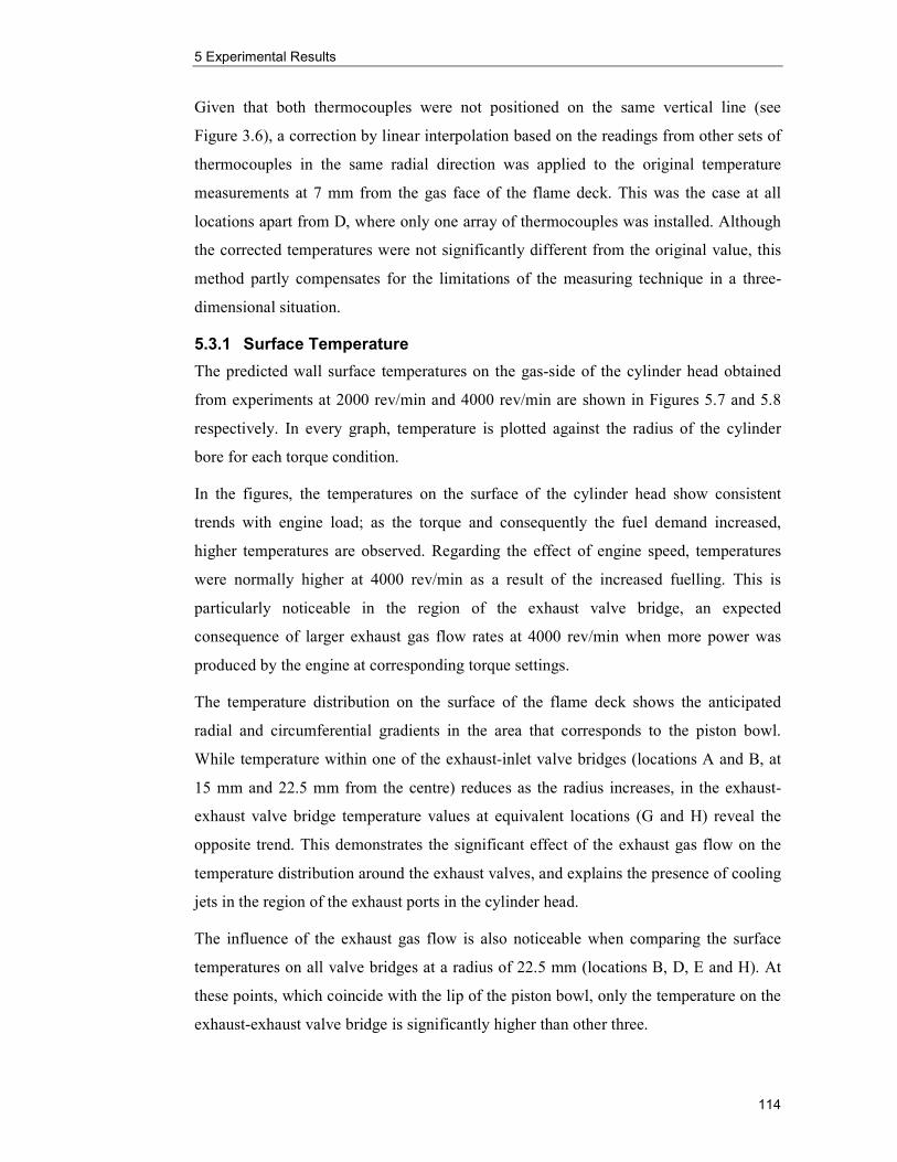
5 Experimental Results
114
Given that both thermocouples were not positioned on the same vertical line (see
Figure 3.6), a correction by linear interpolation based on the readings from other sets of
thermocouples in the same radial direction was applied to the original temperature
measurements at 7 mm from the gas face of the flame deck. This was the case at all
locations apart from D, where only one array of thermocouples was installed. Although
the corrected temperatures were not significantly different from the original value, this
method partly compensates for the limitations of the measuring technique in a three-
dimensional situation.
5.3.1 Surface Temperature
The predicted wall surface temperatures on the gas-side of the cylinder head obtained
from experiments at 2000 rev/min and 4000 rev/min are shown in Figures 5.7 and 5.8
respectively. In every graph, temperature is plotted against the radius of the cylinder
bore for each torque condition.
In the figures, the temperatures on the surface of the cylinder head show consistent
trends with engine load; as the torque and consequently the fuel demand increased,
higher temperatures are observed. Regarding the effect of engine speed, temperatures
were normally higher at 4000 rev/min as a result of the increased fuelling. This is
particularly noticeable in the region of the exhaust valve bridge, an expected
consequence of larger exhaust gas flow rates at 4000 rev/min when more power was
produced by the engine at corresponding torque settings.
The temperature distribution on the surface of the flame deck shows the anticipated
radial and circumferential gradients in the area that corresponds to the piston bowl.
While temperature within one of the exhaust-inlet valve bridges (locations A and B, at
15 mm and 22.5 mm from the centre) reduces as the radius increases, in the exhaust-
exhaust valve bridge temperature values at equivalent locations (G and H) reveal the
opposite trend. This demonstrates the significant effect of the exhaust gas flow on the
temperature distribution around the exhaust valves, and explains the presence of cooling
jets in the region of the exhaust ports in the cylinder head.
The influence of the exhaust gas flow is also noticeable when comparing the surface
temperatures on all valve bridges at a radius of 22.5 mm (locations B, D, E and H). At
these points, which coincide with the lip of the piston bowl, only the temperature on the
exhaust-exhaust valve bridge is significantly higher than other three.

5 Experimental Results
115
0 5 10 15 20 25 30 35 40 4590
100
110
120
130
140
150
160
170
180
190
200
Wall Surface T
empera
ture
(°C
)
Radius (mm)
Exhaust-Inlet Valve Bridge (Locations A, B and C)
Motored
10% LTC
20% LTC
30% LTC
40% LTC
50% LTC
60% LTC
70% LTC
80% LTC
90% LTC
100% LTC
0 5 10 15 20 25 30 35 40 4590
100
110
120
130
140
150
160
170
180
190
200
Wall Surface T
empera
ture
(°C
)
Radius (mm)
Inlet-Inlet Valve Bridge (Location D)
Motored
10% LTC
20% LTC
30% LTC
40% LTC
50% LTC
60% LTC
70% LTC
80% LTC
90% LTC
100% LTC
0 5 10 15 20 25 30 35 40 4590
100
110
120
130
140
150
160
170
180
190
200
Wall Surface T
empera
ture
(°C
)
Radius (mm)
Inlet-Exhaust Valve Bridge (Locations E and F)
Motored
10% LTC
20% LTC
30% LTC
40% LTC
50% LTC
60% LTC
70% LTC
80% LTC
90% LTC
100% LTC
0 5 10 15 20 25 30 35 40 4590
100
110
120
130
140
150
160
170
180
190
200
Wall Surface Temperature (°C
)
Radius (mm)
Exhaust-Exhaust Valve Bridge (Locations G and H)
Motored
10% LTC
20% LTC
30% LTC
40% LTC
50% LTC
60% LTC
70% LTC
80% LTC
90% LTC
100% LTC
Figure 5.7. Predicted wall surface temperature in the cylinder head at 2000 rev/min and all torque conditions.

5 Experimental Results
116
0 5 10 15 20 25 30 35 40 4590
100
110
120
130
140
150
160
170
180
190
200
Wall Surface Temperature
(°C
)
Radius (mm)
Exhaust-Inlet Valve Bridge (Locations A, B and C)
Motored
10% LTC
20% LTC
30% LTC
40% LTC
50% LTC
60% LTC
70% LTC
80% LTC
90% LTC
100% LTC
0 5 10 15 20 25 30 35 40 4590
100
110
120
130
140
150
160
170
180
190
200
Wall Surface T
empera
ture
(°C
)
Radius (mm)
Inlet-Inlet Valve Bridge (Location D)
Motored
10% LTC
20% LTC
30% LTC
40% LTC
50% LTC
60% LTC
70% LTC
80% LTC
90% LTC
100% LTC
0 5 10 15 20 25 30 35 40 4590
100
110
120
130
140
150
160
170
180
190
200
Wall Surface Temperature (°C
)
Radius (mm)
Inlet-Exhaust Valve Bridge (Locations E and F)
Motored
10% LTC
20% LTC
30% LTC
40% LTC
50% LTC
60% LTC
70% LTC
80% LTC
90% LTC
100% LTC
0 5 10 15 20 25 30 35 40 4590
100
110
120
130
140
150
160
170
180
190
200
Wall Surface Tempera
ture (°C
)
Radius (mm)
Exhaust-Exhaust Valve Bridge (Locations G and H)
Motored
10% LTC
20% LTC
30% LTC
40% LTC
50% LTC
60% LTC
70% LTC
80% LTC
90% LTC
100% LTC
Figure 5.8. Predicted wall surface temperature in the cylinder head at 4000 rev/min and all torque conditions.

5 Experimental Results
117
Outside the region corresponding to the piston bowl, the predicted temperatures on two
of the valve bridges (locations C and F) are similar for a given speed. However,
temperatures in C are slightly lower than at F, perhaps because of better coolant access
to the cooling galleries around C.
5.3.2 Heat Flux
The estimated axial heat flux on the gas face of the cylinder head is illustrated in
Figure 5.9 for test conditions at 2000 rev/min and Figure 5.10 for conditions at
4000 rev/min. Similarly to the temperature graphs, in both figures the heat flux
estimated for all locations is plotted versus cylinder radius for the range of engine loads
tested at each particular speed.
In Section 4.3, it was said that the heat flux predicted in the surface of the head could
only be interpreted as the axial component of the total heat flux. However, it can be
verified by inspection of the temperature data measured in the head (see Figures 4.21 to
4.24) that thermal gradients in the axial direction were significantly larger than in the
other directions. Therefore, the axial component of the heat flux represents the main
part of the total heat flux, so the results are useful in understanding the distribution of
heat flux in the cylinder head. These are the heat fluxes used in Chapter 6 to modify
some of the existing correlations.
In terms of engine load and speed, the heat flux results show similar trends to the
predicted wall surface temperature; heat fluxes consistently increase with engine torque
and are larger at 4000 rev/min than at 2000 rev/min. The distribution of heat flux on the
surface of the flame deck is also similar to the distribution of temperature; however, the
maximum value of the axial heat flux was observed at location E and not at location H
where maximum temperatures were observed. Maximum temperature does not
necessarily occur where the heat flux is highest since it also depends on the cooling
conditions (Heywood, 1988).
5.4 Uncertainty Analysis
The uncertainty in the prediction of wall surface temperature and heat flux on the gas-
side of the combustion chamber is discussed in this section. The discussion concentrates
on the results obtained at locations in the walls of cylinder two (Section 5.2). The
examples given of the estimated uncertainty in these quantities are for the experiment at
4000 rev/min and 100% of the limiting torque.

5 Experimental Results
118
0 5 10 15 20 25 30 35 40 450
100
200
300
400
500
600
700
800
900
Heat Flux (kW
/m2)
Radius (mm)
Exhaust-Inlet Valve Bridge (Locations A, B and C)
Motored
10% LTC
20% LTC
30% LTC
40% LTC
50% LTC
60% LTC
70% LTC
80% LTC
90% LTC
100% LTC
0 5 10 15 20 25 30 35 40 450
100
200
300
400
500
600
700
800
900
Heat Flux (kW
/m2)
Radius (mm)
Inlet-Inlet Valve Bridge (Location D)
Motored
10% LTC
20% LTC
30% LTC
40% LTC
50% LTC
60% LTC
70% LTC
80% LTC
90% LTC
100% LTC
0 5 10 15 20 25 30 35 40 450
100
200
300
400
500
600
700
800
900
Heat Flux (kW
/m2)
Radius (mm)
Inlet-Exhaust Valve Bridge (Locations E and F)
Motored
10% LTC
20% LTC
30% LTC
40% LTC
50% LTC
60% LTC
70% LTC
80% LTC
90% LTC
100% LTC
0 5 10 15 20 25 30 35 40 450
100
200
300
400
500
600
700
800
900
Heat Flux (kW
/m2)
Radius (mm)
Exhaust-Exhaust Valve Bridge (Locations G and H)
Motored
10% LTC
20% LTC
30% LTC
40% LTC
50% LTC
60% LTC
70% LTC
80% LTC
90% LTC
100% LTC
Figure 5.9. Predicted heat flux in the cylinder head at 2000 rev/min and all torque conditions.

5 Experimental Results
119
0 5 10 15 20 25 30 35 40 450
100
200
300
400
500
600
700
800
900
Heat Flux (kW
/m2)
Radius (mm)
Exhaust-Inlet Valve Bridge (Locations A, B and C)
Motored
10% LTC
20% LTC
30% LTC
40% LTC
50% LTC
60% LTC
70% LTC
80% LTC
90% LTC
100% LTC
0 5 10 15 20 25 30 35 40 450
100
200
300
400
500
600
700
800
900
Heat Flux (kW
/m2)
Radius (mm)
Inlet-Inlet Valve Bridge (Location D)
Motored
10% LTC
20% LTC
30% LTC
40% LTC
50% LTC
60% LTC
70% LTC
80% LTC
90% LTC
100% LTC
0 5 10 15 20 25 30 35 40 450
100
200
300
400
500
600
700
800
900
Heat Flux (kW
/m2)
Radius (mm)
Inlet-Exhaust Valve Bridge (Locations E and F)
Motored
10% LTC
20% LTC
30% LTC
40% LTC
50% LTC
60% LTC
70% LTC
80% LTC
90% LTC
100% LTC
0 5 10 15 20 25 30 35 40 450
100
200
300
400
500
600
700
800
900
Heat Flux (kW
/m2)
Radius (mm)
Exhaust-Exhaust Valve Bridge (Locations G and H)
Motored
10% LTC
20% LTC
30% LTC
40% LTC
50% LTC
60% LTC
70% LTC
80% LTC
90% LTC
100% LTC
Figure 5.10. Predicted heat flux in the cylinder head at 4000 rev/min and all torque conditions.

5 Experimental Results
120
The calculation of uncertainty in surface temperature and heat flux followed the method
described in Holman (1994). In this method, the uncertainty wR of a quantity R, which is
a direct result derived from independent variables x1, x2, x3,…, xn, is given as a function
of the uncertainties w1, w2, w3,…,wn of the independent variables according to the
equation:
22
3
3
2
2
2
2
1
1
2 ...
∂∂
++
∂∂
+
∂∂
+
∂∂
= n
n
R wx
Rw
x
Rw
x
Rw
x
Rw (5.1)
This equation written for the temperature on the surface of the gas face of the cylinder
walls Twg (Equation 4.4), gives the uncertainty wgTw in the determination of Twg:
+
∂
∂+
∂
∂+
∂
∂= 2
2
3
2
2
2
1
2
T
wgwgwg
T wT
T
T
T
T
Tw
wg
2
2
2
3
2
2
2
1
∂
∂+
∂
∂+
∂
∂+
∂
∂Br
B
wg
r
wgwgwgw
r
Tw
r
T
r
T
r
T (5.2)
In Equation 5.2, the uncertainty in the measured temperatures wT is defined by
calibration of the thermocouples as provided by the manufacturer and shown in
Appendix A (±0.5°C); the uncertainty in the radius of the cylinder Br
w is the machining
tolerance (±0.005 mm) of the cylinders specified in the engine drawings; and the
uncertainty in the position of the tip of the thermocouples wr have been assumed as
±0.25 mm. This value was considered sufficiently large to account for the tolerance in
drilling the holes, any imprecision in the installation of the thermocouples and the
unknown uncertainty of the actual position of the thermocouple junction. The partial
derivatives in Equation 5.2 were obtained by differentiation of Equation 4.4; the details
are given in Appendix E.
Figure 5.11 shows the uncertainty in the prediction of wall surface temperature at
locations in cylinder two. The relative contribution to the total uncertainty of the terms
in the right hand side of Equation 5.2 is also shown. The figure demonstrates (top
graph) that the uncertainty of the estimated temperature on the surface of the cylinder
wall is less than 3°C in most cases and never higher than 3.4°C.
The bottom graph of Figure 5.11 shows that at most locations the largest uncertainty in
the predicted surface temperatures is the uncertainty in the position of the
thermocouples, followed by the uncertainty in the temperature readings. It also shows
that the effect of the uncertainty in the cylinder radius is negligible. As explained by
Holman (1994), because the uncertainty predicted by Equation 5.1 is a function of the

5 Experimental Results
121
squares of the uncertainties in the independent variables, if the uncertainty in one
variable is significantly larger than the uncertainty in the other variables, then the largest
uncertainty outweighs the others. This is the case in the uncertainty of surface
temperature wgTw given by Equation 5.2, where wT and wr are two orders of magnitude
larger thanBr
w .
A1 A2 A3 A4 A5 A6 A7 B1 B2 B4 C1 C2 D1 D2 F3 F5 F6 F7 G1 G3 G40
1
2
3
4
Temperature
Uncertainty
(°C)
Location
A1 A2 A3 A4 A5 A6 A7 B1 B2 B4 C1 C2 D1 D2 F3 F5 F6 F7 G1 G3 G40
20
40
60
80
100
Relative Fraction
of Uncertainty
(%)
Location
Temperatures Thermocouple position Cylinder radius
Figure 5.11. Uncertainty in the predicted surface temperature at selected locations in the engine block, at 4000 rev/min and 100% LTC.
In Figure 5.12, uncertainty bars are plotted along with the surface temperature profile
predicted at location A in the bore of cylinder two.
0 10 20 30 40 50 60 70 80 90 100 110120
125
130
135
140
145
150
155
160
Wall Surface Temperature (°C
)
Distance from top deck (mm) Figure 5.12. Uncertainty in the predicted surface temperature at location A in the engine block, at 4000 rev/min and 100% LTC.

5 Experimental Results
122
Figure 5.12 shows that the observed trend in surface temperature as described in Section
5.2.1, and in particular its rise around the middle of the stroke, is beyond the limits of
the predicted uncertainty.
Equation 5.1 can also be applied to the heat flux (Equation 4.8) to find the uncertainty
Brqw&
involved in the prediction of the heat flux in the cylinder bore:
+
∂
∂+
∂
∂+
∂
∂= 2
2
3
2
2
2
1
2
T
rrr
q wT
q
T
q
T
qw BBB
Br
&&&
&
22
2
2
3
2
2
2
1
∂
∂+
∂
∂+
∂
∂+
∂
∂+
∂
∂k
r
r
B
r
r
rrrw
k
qw
r
qw
r
q
r
q
r
qB
B
BBBB&&&&&
(5.3)
In addition to the uncertainties in the temperatures, the position of the thermocouples
and the radius of the bore (wT, wr and Br
w respectively), already discussed in
conjunction with the surface temperature, the uncertainty in the heat fluxBr
qw&
also
depends on the uncertainty of the thermal conductivity wk since the heat flux is a
function of the thermal conductivity of the metal. The uncertainty in the determination
of the thermal conductivity of a metal is estimated at 4% (National Physical Laboratory,
2000), which represents ±1.8 W/m K in the case of cast iron.
In Figure 5.13 the uncertainty in the predicted heat flux is shown for selected locations
in cylinder two. The uncertainty is presented in kW/m2 and as a percentage of the
estimated heat flux. As in Figure 5.11, the relative contribution to the total uncertainty
of the terms in the right hand side of Equation 5.3 is also illustrated.
The figure shows uncertainties relatively larger than in surface temperature. As a
percentage, the uncertainty represents from 10% to 20% of the heat flux predicted at
most locations. Only at location G4, where the predicted heat flux was comparatively
low, the uncertainty exceeds 30% of the predicted value.
The bottom graph of Figure 5.13 illustrates the additional contribution of the uncertainty
in the thermal conductivity wk. As in the case of surface temperature, the uncertainty in
the position of the thermocouples and the uncertainty in the experimental measurements
are the dominant causes of uncertainty; and the effect of the uncertainty in the cylinder
radius was insignificant.

5 Experimental Results
123
A1 A2 A3 A4 A5 A6 A7 B1 B2 B4 C1 C2 D1 D2 F3 F5 F6 F7 G1 G3 G40
102030405060
Heat Flux
Uncertainty
(kW/m
2)
Location
A1 A2 A3 A4 A5 A6 A7 B1 B2 B4 C1 C2 D1 D2 F3 F5 F6 F7 G1 G3 G40
102030405060
Heat Flux
Uncertainty
(%)
Location
A1 A2 A3 A4 A5 A6 A7 B1 B2 B4 C1 C2 D1 D2 F3 F5 F6 F7 G1 G3 G40
20
40
60
80
100
Relative Fraction
of Uncertainty
(%)
Location
Temperatures Thermocouple position Cylinder radius Thermal conductivity
Figure 5.13. Uncertainty in the predicted heat flux at selected locations in the engine block, at 4000 rev/min and 100% LTC.
In Figure 5.14 uncertainty bars are plotted on the heat flux distribution predicted at
location A in the bore of cylinder two.
0 10 20 30 40 50 60 70 80 90 100 1100
50
100
150
200
250
300
350
Heat Flux (kW/m
2)
Distance from top deck (mm) Figure 5.14. Uncertainty in the predicted heat flux at location A in the engine block, at 4000 rev/min and 100% LTC.
The figure shows that in the case of heat flux the predicted values at some locations are
within the limits of uncertainty at other locations. However, the main features in the
distribution of heat flux, which are a heat flux reduction to a minimum value in the top
section of the bore, and an increase in the heat rate around the middle and second half of
the bore length, are still observed after consideration of heat flux variation between the
limits of uncertainty at those locations.

5 Experimental Results
124
5.5 Influence of Variation of Parameters on Surface Temperature and Heat Flux
The results presented in this section are from the experiments to explore the effect of
EGR, inlet manifold temperature and injection timing on steady-state wall surface
temperature and heat flux. These experiments were carried out during the second part of
the testing program as described in Section 3.6.2. The findings from these tests are
explained using mainly the temperatures and heat fluxes predicted at location A in the
wall of cylinder two.
5.5.1 Exhaust Gas Recirculation (EGR) Effect
The results given in Figures 5.15 and 5.16 compare temperatures and heat fluxes with
EGR on and off at some of the conditions shown in Table 3.7. These examples were
obtained from tests at 1500 rev/min at the load conditions where EGR is used in the
engine as part of the strategy to control the generation of NOx. These results were
chosen after examination of the engine data revealed that only during the tests
at 1500 rev/min were other important variables (in particular timing, pilot fuel injection
and main fuelling) not modified by the ECU as a result of disabling EGR in the engine.
In other words, these results were chosen for their ability to show the sole effect of EGR
on surface temperatures and heat fluxes.
The recirculation of exhaust gases into the cylinder decreases the rate of emission of
NOx by diluting the unburned gas mixture and consequently the peak flame temperature
during combustion (Heywood, 1988). The dilution effect, which is a consequence of
displacing some of the inlet charge oxygen with exhaust gas, reduces the NOx level at
the expense of higher particulates and hydrocarbons emissions. The engine power
output and fuel economy also deteriorate (Ladommatos et al., 1996a). There is also a
small effect of dissociated CO2 in the reduction of NOx. CO2 is a main constituent of
EGR and has a higher heat absorbing capacity than oxygen (Ladommatos et al., 1996b).
As a result of EGR the average gas temperature decreases, and surface temperatures as
well as the rate of heat transfer from combustion gases should decrease accordingly.
However, in steady-state operating conditions EGR seems to have no substantial
influence on surface temperatures (Figure 5.15) and only a marginal effect on heat
fluxes (Figure 5.16). In general, the heat fluxes under EGR conditions in cylinder two
are, as expected, slightly smaller than the values with no EGR. This trend is more
noticeable in the bottom part of the bore.

5 Experimental Results
125
0 10 20 30 40 50 60 70 80 90 100 11095
100
105
110
115
120
Torque = 10% LTCEGR Temp = 129.9°C
Wall Surface Temperature (°C
)Distance from top deck (mm)
EGR = 25.8%
EGR off
0 10 20 30 40 50 60 70 80 90 100 11095
100
105
110
115
120
Torque = 20% LTCEGR Temp = 125.4°C
Wall Surface Temperature (°C
)
Distance from top deck (mm)
EGR = 13.7%
EGR off
0 10 20 30 40 50 60 70 80 90 100 11095
100
105
110
115
120
Torque = 30% LTCEGR Temp = 118.6°C
Wall Surface Temperature (°C
)
Distance from top deck (mm)
EGR = 8.0%
EGR off
0 10 20 30 40 50 60 70 80 90 100 11095
100
105
110
115
120
Torque = 40% LTCEGR Temp = 119.7°C
Wall Surface Temperature (°C
)
Distance from top deck (mm)
EGR = 5.3%
EGR off
Figure 5.15. Effect of EGR on predicted wall surface temperature at location A in the engine block at 1500 rev/min.

5 Experimental Results
126
0 10 20 30 40 50 60 70 80 90 100 1100
10
20
30
40
50
60
70
80
90
Torque = 10% LTCEGR Temp = 129.9°C
Heat flux (kW/m
2)
Distance from top deck (mm)
EGR = 25.8%
EGR off
0 10 20 30 40 50 60 70 80 90 100 1100
10
20
30
40
50
60
70
80
90
Torque = 20% LTCEGR Temp = 125.4°C
Heat flux (kW/m
2)
Distance from top deck (mm)
EGR = 13.7%
EGR off
0 10 20 30 40 50 60 70 80 90 100 1100
10
20
30
40
50
60
70
80
90
Torque = 30% LTCEGR Temp = 118.6°C
Heat flux (kW/m
2)
Distance from top deck (mm)
EGR = 8.0%
EGR off
0 10 20 30 40 50 60 70 80 90 100 1100
10
20
30
40
50
60
70
80
90
Torque = 40% LTCEGR Temp = 119.7°C
Heat flux (kW/m
2)
Distance from top deck (mm)
EGR = 5.3%
EGR off
Figure 5.16. Effect of EGR on predicted heat flux at location A in the engine block at 1500 rev/min.

5 Experimental Results
127
5.5.2 Inlet Manifold Temperature Effect
Two sets of experiments were completed to investigate the effect of variation of inlet
manifold temperature on steady-state surface temperature and heat flux. Measurements
were taken at 100% of the limiting torque at engine speeds of 2000 rev/min and
4000 rev/min, which respectively represent the conditions of maximum torque and
nearly maximum power. The actual torque and inlet manifold temperatures are shown in
Table 3.8.
Figure 5.17 shows results of surface temperature against inlet manifold temperature at
location A in cylinder two. In the same way, Figure 5.18 illustrates the estimated heat
flux at the same location. The legend in both figures indicates the vertical distance from
TDC to the points where predictions were made.
30 35 40 45 50 55 60 65 70 75 80 85 90110
120
130
140
150
160
170
Wall Surface
Temperature (°C
)
Inlet Manifold Temperature (°C)
Speed = 2000 rev/min, Torque = 100% LTC
Distancefrom TDC
10 mm
25 mm
40 mm
55 mm
70 mm
85 mm
100 mm
30 35 40 45 50 55 60 65 70 75 80 85 90110
120
130
140
150
160
170
Wall Surface
Temperature (°C
)
Inlet Manifold Temperature (°C)
Speed = 4000 rev/min, Torque = 100% LTC
Distancefrom TDC
10 mm
25 mm
40 mm
55 mm
70 mm
85 mm
100 mm
Figure 5.17. Effect of inlet manifold temperature on predicted wall surface temperature at location A in the engine block.

5 Experimental Results
128
30 35 40 45 50 55 60 65 70 75 80 85 9050
100
150
200
250
300
350
Heat Flux (kW/m
2)
Inlet Manifold Temperature (°C)
Speed = 2000 rev/min, Torque = 100% LTC
Distancefrom TDC
10 mm
25 mm
40 mm
55 mm
70 mm
85 mm
100 mm
30 35 40 45 50 55 60 65 70 75 80 85 9050
100
150
200
250
300
350
Heat Flux (kW/m
2)
Inlet Manifold Temperature (°C)
Speed = 4000 rev/min, Torque = 100% LTC
Distancefrom TDC
10 mm
25 mm
40 mm
55 mm
70 mm
85 mm
100 mm
Figure 5.18. Effect of inlet manifold temperature on predicted heat flux at location A in the engine block.
The figures show that a variation from approximately 32°C to 73°C at 2000 rev/min and
from 44°C to 74°C at 4000 rev/min, have little impact on the steady-state temperature
(less than 5°C) and only a moderate effect on the heat flux (about 30 kW/m2).
Inspection of the engine data revealed that engine torque and consequently power
remained approximately constant over these temperature swings. However, control
variables were continuously adjusted by the ECU to compensate for the reduction in the
actual amount of air entering the engine. The engine data also showed that torque and
hence power reduced significantly for intake air temperatures above 75°C. The
reduction in power at inlet manifold temperatures higher than 75°C had an evident
effect on surface temperatures and heat fluxes; this is more noticeable at 4000 rev/min.

5 Experimental Results
129
5.5.3 Injection Timing Effect
The investigation of the influence of timing on surface temperature and heat flux was
also carried out at conditions of maximum torque (100% LTC at 2000 rev/min) and near
maximum power (100% LTC at 4000 rev/min). The degrees of advancing or retarding
the start of fuel injection at these conditions have been given in at Table 3.9.
In Figure 5.19, the predicted surface temperature at location A in cylinder two is plotted
against timing demand (°BTDC) for 2000 rev/min and 4000 rev/min. Similarly, in
Figure 5.20, the heat flux is shown at the same location. The legend of both figures
gives the vertical distance from TDC to the points where predictions were obtained. The
ECU variable timing demand indicates the start of injection.
-5 -4 -3 -2 -1 0 Std 1 2 3 4 5 110
120
130
140
150
160
170
Wall Surface
Temperature (°C
)
Timing Demand (°BTDC)
Speed = 2000 rev/min, Torque = 100% LTC
Distancefrom TDC
10 mm
25 mm
40 mm
55 mm
70 mm
85 mm
100 mm
8.5 9.5 10.5 11.5 Std 12.5 13.5 14.5 110
120
130
140
150
160
170
Wall Surface
Temperature (°C
)
Timing Demand (°BTDC)
Speed = 4000 rev/min, Torque = 100% LTC
Distancefrom TDC
10 mm
25 mm
40 mm
55 mm
70 mm
85 mm
100 mm
Figure 5.19. Effect of injection timing on predicted wall surface temperature at location A in the engine block.
A tendency in surface temperature to decrease as the injection of fuel is advanced is
observed at the top of the cylinder bore (10 mm from TDC) under both testing
conditions (Figure 5.19). This trend is also noticeable in the heat flux (Figure 5.20).

5 Experimental Results
130
At 2000 rev/min the predicted quantities at 10 mm from TDC decrease from their
highest value obtained when injection is the most retarded, to a relatively low value
around the standard ECU injection setting (0°BTDC). Further advance of the injection
after the standard timing seems to have no significant effect on steady-state surface
temperature or heat flux.
At 4000 rev/min the standard timing demand in the engine is advanced to 11.5°BTDC,
and it is not possible to operate the engine with retarded injection without exceeding the
recommended pre-turbine temperature. At this speed the surface temperature as well as
heat flux at 10 mm from TDC decreases as fuel injection is advanced from 8.5°BTDC
to 12.5°BTDC. Thereafter, no significant changes occur in temperature or heat flux.
-5 -4 -3 -2 -1 0 Std 1 2 3 4 5 50
100
150
200
250
300
350
Heat Flux (kW/m
2)
Timing Demand (°BTDC)
Speed = 2000 rev/min, Torque = 100% LTC
Distancefrom TDC
10 mm
25 mm
40 mm
55 mm
70 mm
85 mm
100 mm
8.5 9.5 10.5 11.5 Std 12.5 13.5 14.5 50
100
150
200
250
300
350
Heat Flux (kW/m
2)
Timing Demand (°BTDC)
Speed = 4000 rev/min, Torque = 100% LTC
Distancefrom TDC
10 mm
25 mm
40 mm
55 mm
70 mm
85 mm
100 mm
Figure 5.20. Effect of injection timing on predicted heat flux at location A in the engine block.
The fact that the effect of variation in injection timing on the predicted steady-state
quantities is only observed at 10 mm from TDC, confirms that at the top of the cylinder

5 Experimental Results
131
heat transferred by convection from combustion gases is more important than further
down the bore. As a result of delaying the injection of fuel and consequently the start of
combustion, the average temperature of the gases during the period of time when the top
of the bore is exposed to combustion, is higher than when combustion starts earlier.
Figure 5.21 relates to 2000 rev/min and 100% LTC. It shows that in the flame deck of
the cylinder head, which is continuously exposed to in-cylinder gases, steady-state
temperatures and heat fluxes are less affected by the timing of injection. This was
expected since no matter whether combustion occurs a few degrees earlier or later in the
cycle, the average rate of heat transferred to the cylinder head over a large number of
cycles is virtually the same providing that fuel and other relevant variables remain
reasonably constant. This is in contrast to the top of the cylinder, where the motion of
the piston exposes a bore area which is variable with time.
-5 -4 -3 -2 -1 0 Std 1 2 3 4 5 130
140
150
160
170
180
Wall Surface
Temperature (°C
)
Timing Demand (°BTDC)
Radius
15 mm
22.5 mm
34.5 mm
-5 -4 -3 -2 -1 0 Std 1 2 3 4 5 0
100
200
300
400
500
600
Heat Flux (kW/m
2)
Timing Demand (°BTDC)
Radius
15 mm
22.5 mm
34.5 mm
Figure 5.21. Effect of injection timing on predicted wall surface temperature and heat flux at locations A, B and C in the cylinder head, at 2000 rev/min and 100% LTC.
The results presented in Section 5.5 suggest that variations in the inlet manifold
temperature and particularly in the timing of injection have a significant effect on
steady-state surface temperatures and heat fluxes. At an engine speed of 2000 rev/min,
increments of more than 10°C in the surface temperature and in excess of 50kW/m2 in
the heat flux were observed at the top section of the bore when the start of injection was
retarded by 5°. Similar results were obtained at 4000 rev/min.

132
6 Evaluation of Heat Transfer Correlations
6.1 Introduction
In this chapter, a comparison of instantaneous spatially-averaged heat transfer
coefficients given by several of the correlations discussed in Section 2.3.2 is presented.
Also, a new correlation is proposed based on the evaluation of the existing correlations
and the data obtained from the experiments undertaken during this investigation.
The equations proposed by Eichelberg (Equation 2.9), Annand (Equation 2.13),
Woschni (Equation 2.16), Sitkei and Ramanaiah (Equation 2.17), Hohenberg (Equation
2.19) and Han et al. (Equation 2.21) are evaluated using analytical data and
experimental measurements obtained during tests at 4000 rev/min and various engine
loads including 100% of the limiting torque. This test point is of particular interest since
it corresponds to operating conditions near to maximum power, at which the highest
heat transfer rates take place in the engine.
The equations chosen for this analysis were all derived from experiments in actual
engines and were selected on the basis of availability of the relevant data to allow their
evaluation. For this reason, in the cases of the correlations proposed by Annand and
Sitkei and Ramanaiah, the radiative part of the coefficient was calculated using the
steady-state mean cylinder head temperature obtained from the experiments.
The description of the necessary data to evaluate the correlations is presented in the
second section of this chapter. Among the data required are in-cylinder pressure, mean
piston speed, the geometry of the cylinder and combustion chamber, gas temperature
and the gas properties of density, viscosity, thermal conductivity and ratio of specific
heats. Particular attention is given to the analytical method used to obtain the mean
temperature of the gas, which required determination of the mass of gas in the cylinder
during the entire cycle. With regard to gas properties, air was used as the working fluid
and its viscosity, thermal conductivity and ratio of specific heats were calculated as
functions of the gas temperature.
In the third section of this chapter the results from the evaluation of the correlations are
presented. Considerable variability was found among the predicted coefficients, either
on a crank angle basis or averaged over the engine cycle. Although the results
confirmed previous observations, the coefficients predicted by the selected equations
were generally higher than those reported in the literature (Stone, 1999). The difference
was attributed to the use in this case of data from a more powerful engine.

6 Evaluation of Heat Transfer Correlations
133
A modified correlation to predict the gas-side heat transfer coefficient in diesel engines
is presented in the final section of this chapter. The equation originated from
comparisons of the cycle-averaged values predicted by the existing correlations against
a steady-state heat transfer coefficient obtained from the experiments in the test engine.
The equation is a simple relationship between Nu and Re calibrated to predict the
spatially-averaged instantaneous heat transfer coefficient in the test engine.
6.2 Data Requirements
Evaluation of the correlations required specific data depending on the particular
equation. In general, the necessary data include the in-cylinder pressure (under firing
and motored conditions), the geometry of the cylinder and combustion chamber
(cylinder bore, swept volume, instantaneous surface and volume), the gas properties
(density, viscosity, thermal conductivity and ratio of specific heats), mean piston speed,
and the mean temperature of the gas as function of crank angle. Table 6.1 summarises
the data requirements to evaluate each of the selected equations.
Correlation Independent Variables
Eichelberg Vp, Tg, p
Annand B, kg, Re(B, ρg, µg, Vp)
Woschni B, Vp, Tg, p, pm, pr, Vs, Vr, Tr
Sitkei and Ramanaiah Vp, Tg, p, de(V, A)
Hohenberg Vp, Tg, p, V
Han, Chung, Kwon, and Lee B, Vp, Tg, p, V, γ (Cp, R)
Table 6.1. Data requirements for the selected correlations.
In Sections 6.2.1 to 6.2.4, the different data used to evaluate the correlations are
illustrated and the analytical method to determine the mean temperature of the gas
throughout the engine cycle is explained.
6.2.1 Cylinder Gas Pressure
The in-cylinder pressure was measured during the experiments at every test condition
with the engine firing, and also while motoring the engine with the fuel injection
disabled. The procedure has been explained in Section 3.3.1. Figure 6.1 shows the
pressure trace as a function of crank angle at 4000 rev/min measured at 40% and 100%
of the limiting torque, and under motored conditions.

6 Evaluation of Heat Transfer Correlations
134
TDC 60 120 BDC 240 300 TDC 420 480 BDC 600 660 TDC0
20
40
60
80
100
120
140
160
180
Crank Angle (°)
Pressure (bar)
EVC IVC EVO IVO
Firing (100% LTC)
Firing (40% LTC)
Motored
Figure 6.1. Cylinder pressure measurements at 4000 rev/min.
The pressure traces shown in the figure have been processed using a Matlab filtering
function, which removes noise from the raw pressure signal with little effect on the
actual magnitude and without causing any phase distortion (zero-phase digital filtering).
The gas pressure measured in the cylinder was invariably filtered with this method
before being used in the calculations. The crank angles when inlet valves and exhaust
valves open and close (IVO, IVC, EVO, EVC) have been indicated in the figure; also
shown in the figure are the instants when the piston reaches top or bottom dead centre
(TDC, BDC). This is a useful practice to illustrate changes in a particular variable
within the context of the relevant events occurring during the cycle, and it has been used
to present most results in this chapter.
The cylinder pressure is a common variable among all the correlations except for the
equation proposed by Annand. It appears in the heat transfer coefficient as a result of
expressing the gas density as a function of pressure and temperature and, in the case of
correlations given by Woschni and by Han et al., it is also part of the definition of the
turbulent cylinder gas velocity used as the characteristic velocity. In Woschni’s equation
the motored pressure and the pressure when inlet valves close (taken as a reference
pressure), are also factors of the characteristic velocity during combustion and
expansion.
6.2.2 Mean Piston Speed and Combustion Chamber Geometry
The mean piston speed is the distance travelled by the piston in one revolution divided
by the time required to complete one revolution at a particular engine rotational speed.
The following equation adapted from Heywood (1988) gives the mean piston speed for
a four-stroke engine:

6 Evaluation of Heat Transfer Correlations
135
60
2LnV p = (6.1)
By using this equation the mean piston speed in the test engine at 4000 rev/min was
found to be 11.47 m/s.
In most heat transfer coefficient equations the velocity of the gas is assumed to be a
function of the mean piston speed, which is normally used as the characteristic velocity
in the definition of the gas-side Re. In the equations of Woschni, Hohenberg and Han et
al., the mean piston speed is the main factor used to determine the characteristic
velocity. In each of these cases the author suggested that the mean piston speed was not
by itself adequate to represent the turbulent velocity of the gas, in particular during the
combustion and expansion strokes.
The cylinder bore is commonly used as the characteristic length of the combustion
chamber in the calculation of the gas-side Re and the heat transfer coefficient. However,
in the equation proposed by Sitkei and Ramanaiah the reference length was replaced by
a function of the instantaneous surface and volume of the combustion chamber and, in
the equation proposed by Hohenberg by a function of the instantaneous volume. The
instantaneous surface and volume of the combustion chamber for the engine used in the
investigation are illustrated as functions of the crank angle in Figure 6.2.
TDC 60 120 BDC 240 300 TDC100
120
140
160
180
200
220
240
260
280
300
320
340
360
Crank Angle (°)
Combustion C
hamber Area (cm2)
TDC 60 120 BDC 240 300 TDC0
50
100
150
200
250
300
350
400
450
500
550
Crank Angle (°)
Cylinder Volume (cm3)
Figure 6.2. Instantaneous area of the combustion chamber and cylinder volume.
The quantities shown in the figure were computed using the geometric data of the
engine, illustrated in Table 3.3, and the relevant equations as given by Heywood (1988).
In the calculation of the instantaneous surface of the combustion chamber shown in
Figure 6.2, the area of the piston has been assumed as the area of a flat-topped piston,
which is approximately equal to the surface of the cylinder head.

6 Evaluation of Heat Transfer Correlations
136
The swept volume or maximum instantaneous cylinder volume and the volume of the
combustion chamber when the inlet valves close (used as a reference volume) are also
necessary to evaluate Woschni’s equation.
6.2.3 Gas Properties
The properties of air as functions of temperature were used as gas properties in the
calculations. The thermal conductivity, dynamic viscosity and density of the gas were
only necessary to evaluate Annand’s correlation. However, the ratio of specific heats
was necessary for the determination of the gas temperature (Section 6.2.4), and also to
evaluate the equation by Han et al. The specific heat ratio was calculated using the gas
constant of air and the specific heat at constant pressure. The thermal conductivity,
dynamic viscosity and specific heat at constant pressure of air were obtained for the
given temperature at every crank angle by interpolation between tabulated values
(Incropera and DeWitt, 1990). These values are shown in Table 6.2.
Temperature Specific Heat at
Constant Pressure Dynamic Viscosity
Thermal Conductivity
K J/kgK Ns/m2 x10
6 W/mK x10
3
300 1007 18.46 26.30 350 1009 20.82 30.00 400 1014 23.01 33.80 450 1021 25.07 37.30 500 1030 27.01 40.70 550 1040 28.84 43.90 600 1051 30.58 46.90 650 1063 32.25 49.90 700 1075 33.88 52.40 750 1087 35.46 54.90 800 1099 36.98 57.30 850 1110 38.43 59.60 900 1121 39.81 62.00 950 1131 41.13 64.30 1000 1141 42.44 66.70 1100 1159 44.90 71.50 1200 1175 47.30 76.30 1300 1189 49.60 82.00 1400 1207 53.00 91.00 1500 1230 55.70 100.00 1600 1248 58.40 106.00 1700 1267 61.10 113.00 1800 1286 63.70 120.00 1900 1307 66.30 128.00 2000 1337 68.90 137.00 2100 1372 71.50 147.00 2200 1417 74.00 160.00 2300 1478 76.60 175.00 2400 1558 79.20 196.00 2500 1665 81.80 222.00
Table 6.2. Specific heat at constant pressure, dynamic viscosity and thermal conductivity of air at atmospheric pressure. Adapted from Incropera and DeWitt (1990).

6 Evaluation of Heat Transfer Correlations
137
The density of the gas was calculated at every crank angle from the instantaneous mass
and volume in the combustion chamber. The results are shown in Figure 6.3 for test
conditions 4000 rev/min and 100% of the limiting torque. The determination of the
instantaneous mass in the cylinder is explained in Section 6.2.4.
TDC 60 120 BDC 240 300 TDC 420 480 BDC 600 660 TDC0
5
10
15
20
25
30
35
40
Crank Angle (°)
Gas D
ensity (kg/m
3)
EVC IVC EVO IVO
Figure 6.3. Instantaneous density in the combustion chamber at 4000 rev/min and 100% LTC.
6.2.4 Mean Gas Temperature
The mean temperature of the gas as a function of crank angle was essential to evaluate
all correlations. Temperature is used directly in most equations and is also necessary to
calculate the properties of the gas. The temperature trace illustrated in Figure 6.4
represents an approximate spatially-averaged instantaneous temperature of the gas in the
combustion chamber at every crank angle. It was obtained by an analytical method
based on the actual cylinder pressure and fundamental equations of thermodynamics.
TDC 60 120 BDC 240 300 TDC 420 480 BDC 600 660 TDC300
500
700
900
1100
1300
1500
1700
1900
2100
2300
2500
Crank Angle (°)
Temperature (K)
EVC IVC EVO IVO
Figure 6.4. Gas temperature obtained at 4000 rev/min and 100% LTC.

6 Evaluation of Heat Transfer Correlations
138
In order to estimate the temperature of the gas, the engine cycle was divided in the
following parts: from IVC to EVO (compression, combustion and expansion), from
IVO to IVC (intake), and from EVO to EVC (exhaust). The sections of the cycle are
given in the order of the sequence followed in the calculation routine, which is included
in Appendix D.
In the first part of the cycle (from IVC to EVO), the temperature was determined by the
equation of state for a perfect gas. In the equation, the intake mass was used until fuel
was injected; at this crank angle the mass of fuel was added instantaneously to the
intake mass and then used for the remaining of this part of the cycle until EVO. The
intake mass of air was calculated from the mass flow rate measured during the tests. The
mass of fuel and injection crank angle are two of the variables given by the ECU.
The gas exchange process was modelled as isentropic with values of specific heats
which change with temperature. The isentropic equation used between consecutive
crank angle steps was:
γγ 1
1
2
1
2
−
=
p
p
T
T (6.2)
Because the specific heat γ depends on temperature, an iterative routine was used to
determine gas temperature and the specific heat ratio simultaneously. In the intake part
of the gas exchange process the temperature given by the isentropic relationship at IVC
should equal the temperature previously obtained at this crank angle by using the gas
law. For this reason, the isentropic relationship was used in a reverse manner, starting at
IVC and finishing at IVO. In the exhaust part of the gas exchange process the
temperature was already known at EVO, so the calculation began at this crank angle and
ended at EVC.
The sole application of the isentropic equation for the gas exchange process would lead
to inconsistent results during the valve overlap period. Temperature would be
unrealistically low if it was taken as calculated during the intake of the cycle, or
excessively high if it was assumed as the temperature found from the exhaust
calculations. In the actual process, the temperature during the overlap period mainly
depends on the energy content of the mass fractions of the exiting combustion gases and
the new air charge entering the cylinder. In the model, the temperature was obtained as
the weighted average based on the relative mass fractions of the remaining gas in the
cylinder and the entering air, and their respective temperatures. Therefore, in order to

6 Evaluation of Heat Transfer Correlations
139
obtain a reasonable instantaneous temperature of the gas for this part of the cycle, it was
necessary to determine the mass in the cylinder during the gas exchange process.
The instantaneous mass during the gas exchange process at every crank angle step can
be found by integrating the mass flow rate through the valves over the time period
corresponding to the crank angle step. The mass flow rate through the inlet and exhaust
valves is approximately given by the equations for compressible flow through a flow
restriction (Heywood, 1988):
( )
2/11
1
/1
1
2/1
0
0 11
2
−
−
=
−
γγ
γ
γγ
p
p
p
p
RT
PACm TTrd& (6.3)
( )( )12
1
2/1
2/1
0
0
1
2 −
+
+
=γγ
γγ
RT
PACm rd& if the flow is choked, i.e.,
1
1 1
2 −
−
≤
γγ
γγ
p
pT (6.4)
In addition to the stagnation conditions upstream of the restriction (T0, P0) and the static
pressure immediately after the restriction (PT), this procedure requires knowledge of the
valve discharge coefficient (Cd) and an area of reference (Ar) for the flow between valve
and port. In the calculations, the geometric minimum flow area was used as the
reference area. The minimum flow area depends on the valve-lift and the geometry of
the valves and ports. As explained by Heywood (1988), there are three different stages
of flow area development depending on the valve lift. For low and medium valve lift,
the minimum flow area is a frustum of a right circular cone; and when the lift is large
enough or the valve is fully opened, the minimum flow area is the annular space formed
between the port and the valve stem. The calculation details and equations for the
minimum flow area can be found in Heywood (1988). These equations were
incorporated into the Matlab routine given in Appendix D. The discharge coefficient
and valve lift for inlet and exhaust valves as a function of crank angle, and the
geometric data of the valves, have been provided by the engine manufacturer and are
given in Appendix B. The valve-lift and corresponding flow area of inlet and exhaust
valves are shown in Figure 6.5.
In the calculations of the mass flow through the intake valves, the stagnation pressure
and temperature upstream of the restriction were taken as the static pressure and
temperature in the inlet manifold (the unknown instantaneous flow velocity was
assumed to be zero), and the instantaneous cylinder pressure was used as the pressure
just downstream of the restriction. The pressure and temperature in the inlet manifold
were measured and assumed to be constant over the entire cycle. Similarly, in the

6 Evaluation of Heat Transfer Correlations
140
calculations of the exhaust flow rate the static pressure and temperature in the cylinder
were used as the stagnation conditions upstream of the restriction, and the steady-state
exhaust manifold pressure, also measured during the tests, was taken as the pressure
immediately after the restriction.
TDC 60 120 BDC 240 300 TDC 420 480 BDC 600 660 TDC0
1
2
3
4
5
6
7
8
9
10
Crank Angle (°)
Valve Lift (m
m)
EVC IVC EVO IVO
Intake
Exhaust
TDC 60 120 BDC 240 300 TDC 420 480 BDC 600 660 TDC0
0.5
1.0
1.5
2.0
2.5
3.0
3.5
4.0
4.5
Crank Angle (°)
Flow Area (cm2)
EVC IVC EVO IVO
Intake
Exhaust
Figure 6.5. Valve-lift timing diagram and flow area for inlet and exhaust valves.
The results from the mass flow calculations through the inlet and exhaust valves are
shown in Figure 6.6, and the predicted mass in the cylinder during the cycle is
illustrated in Figure 6.7.
The calculations of the mass flow through the valves were constrained by two
conditions. Firstly, the total mass entering the cylinder during one cycle should equal
the total intake air mass obtained from measurements of the mass flow rate of air and
the fraction of EGR, which is negligible at 4000 rev/min. Secondly, the total exhaust
mass should not exceed the total gas mass in the cylinder, which is the intake mass plus
the mass of fuel. On a cycle basis, the total exhaust mass could be slightly less than the

6 Evaluation of Heat Transfer Correlations
141
total gas mass to allow for some residual gas to remain in the cylinder. In order to
satisfy these conditions the model was calibrated by minor adjustments of the reference
areas (see Matlab routine in Appendix D).
TDC 60 120 BDC 240 300 TDC 420 480 BDC 600 660 TDC-20
0
20
40
60
80
100
120
140
160
180
200
220
Crank Angle (°)
Mass Flow (g/s)
EVC IVC EVO IVO
Intake
Exhaust
Figure 6.6. Mass flow through valves at 4000 rev/min and 100% LTC.
TDC 60 120 BDC 240 300 TDC 420 480 BDC 600 660 TDC0
0.1
0.2
0.3
0.4
0.5
0.6
0.7
0.8
0.9
1.0
1.1
Crank Angle (°)
Cylinder Mass (g)
EVC IVC EVO IVO
Fuel injection
(11.5°BTDC)
Figure 6.7. Mass of gas in the cylinder predicted at 4000 rev/min and 100% LTC.
Several assumptions had to be made in order to obtain the mean temperature of the gas
on a crank angle basis. It is likely that the main deficiency in the model was to ignore
the heat transfer effects during the cycle, which in general tended to over-predict the gas
temperature. This is recognised as not strictly rigorous, but the model provided a
reasonable estimate of the gas temperature which was sufficient to compare the various
correlations on a similar basis.
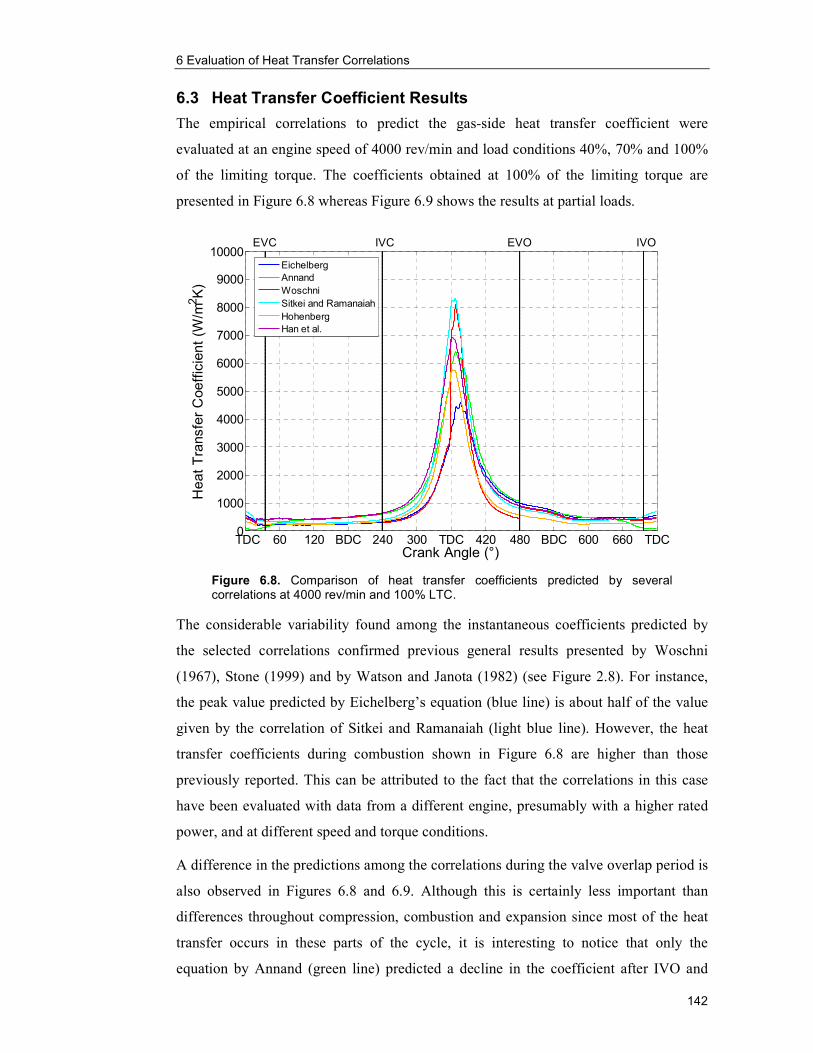
6 Evaluation of Heat Transfer Correlations
142
6.3 Heat Transfer Coefficient Results
The empirical correlations to predict the gas-side heat transfer coefficient were
evaluated at an engine speed of 4000 rev/min and load conditions 40%, 70% and 100%
of the limiting torque. The coefficients obtained at 100% of the limiting torque are
presented in Figure 6.8 whereas Figure 6.9 shows the results at partial loads.
TDC 60 120 BDC 240 300 TDC 420 480 BDC 600 660 TDC0
1000
2000
3000
4000
5000
6000
7000
8000
9000
10000
Crank Angle (°)
Heat Transfer Coefficient (W
/m2K)
EVC IVC EVO IVO
Eichelberg
Annand
Woschni
Sitkei and Ramanaiah
Hohenberg
Han et al.
Figure 6.8. Comparison of heat transfer coefficients predicted by several correlations at 4000 rev/min and 100% LTC.
The considerable variability found among the instantaneous coefficients predicted by
the selected correlations confirmed previous general results presented by Woschni
(1967), Stone (1999) and by Watson and Janota (1982) (see Figure 2.8). For instance,
the peak value predicted by Eichelberg’s equation (blue line) is about half of the value
given by the correlation of Sitkei and Ramanaiah (light blue line). However, the heat
transfer coefficients during combustion shown in Figure 6.8 are higher than those
previously reported. This can be attributed to the fact that the correlations in this case
have been evaluated with data from a different engine, presumably with a higher rated
power, and at different speed and torque conditions.
A difference in the predictions among the correlations during the valve overlap period is
also observed in Figures 6.8 and 6.9. Although this is certainly less important than
differences throughout compression, combustion and expansion since most of the heat
transfer occurs in these parts of the cycle, it is interesting to notice that only the
equation by Annand (green line) predicted a decline in the coefficient after IVO and

6 Evaluation of Heat Transfer Correlations
143
before EVC. The decline is considered to be more consistent with the instantaneous
density in the cylinder, particularly when only a residual mass being cooled by a new air
charge exists in the cylinder.
TDC 60 120 BDC 240 300 TDC 420 480 BDC 600 660 TDC0
1000
2000
3000
4000
5000
6000
7000
8000
9000
10000
Crank Angle (°)
Heat Transfer Coefficient (W
/m2K)
EVC IVC EVO IVO
Eichelberg
Annand
Woschni
Sitkei and Ramanaiah
Hohenberg
Han et al.
TDC 60 120 BDC 240 300 TDC 420 480 BDC 600 660 TDC0
1000
2000
3000
4000
5000
6000
7000
8000
9000
10000
Crank Angle (°)
Heat Transfer Coefficient (W
/m2K)
EVC IVC EVO IVO
Eichelberg
Annand
Woschni
Sitkei and Ramanaiah
Hohenberg
Han et al.
Figure 6.9. Comparison of heat transfer coefficients predicted by several correlations at 4000 rev/min and 70% LTC (top) and 40% LTC (bottom).
In relation to Figure 2.8, a different relative position of the curves by Annand (green
line) and Woschni (red line) near top dead centre was observed in Figure 6.8. In the test
engine, at 4000 rev/min and 100% of the limiting torque, Woschni’s correlation
predicted a peak coefficient larger than the one given by Annand’s equation, whereas

6 Evaluation of Heat Transfer Correlations
144
Figure 2.8 shows the reverse. It is not possible to offer an explanation for this
observation without further information from Watson and Janota (1982).
The results at partial load (Figure 6.9) show less variability between peak values and,
except for the correlations of Annand and Woschni, the relative position of the curves is
consistent with the results at 100% of the limiting torque. At 40% of the limiting torque,
the peak coefficient given by the equation of Woschni is less than the value predicted by
the correlations of Annand. Although this agrees with previously reported results, it
does not correspond with the observations at higher loads at 4000 rev/min. Possibly, the
influence of the turbulent gas velocity as defined by Woschni becomes more important
as the engine torque increases.
It should be mentioned that in the evaluation of Annand’s correlation an average scaling
factor (parameter a in Equation 2.13) was used in order to keep the heat transfer
coefficient during the gas exchange process within the range of the other predictions. In
addition, the radiative part of the heat transfer coefficient in this equation was estimated
using a steady-state spatially-averaged temperature on the cylinder head surface.
However, the contribution of the radiative part was found to have little effect on the
total heat transfer coefficient predicted by this equation, and even less in the values
obtained with the correlation of Sitkei and Ramanaiah.
Within the range of results presented in Figures 6.8 and 6.9, the correlation by Woschni
seems to underestimate the heat transfer coefficient during compression and expansion
and overestimate the coefficient during the gas exchange process in the test engine with
respect to the other equations. During most of the intake stroke the coefficients
predicted by this equation were the highest along with those obtained with the
correlation of Han et al. (purple line). Also, throughout the exhaust process the
predictions were among the highest values. In contrast, during compression and
expansion the estimates given by Woschni’s equation were the lowest. In addition, this
correlation seems to over-predict the heat transfer coefficient during combustion at full
load.
The observations discussed above agree with comments given by Hohenberg (1979) on
the suitability of Woschni’s equation to predict the heat transfer coefficient in high-
speed diesel engines. Incidentally, Hohenberg’s correlation (yellow line) appears to be
more consistent over the entire cycle in Figures 6.8 and 6.9. However, predictions made
with this equation during most part of expansion and exhaust, are smaller than those
obtained with the other formulae. Also throughout combustion, only the equation by

6 Evaluation of Heat Transfer Correlations
145
Eichelberg (developed in large low-speed engines) gave lower values than those from
Hohenberg’s equation.
In may be noted in Figures 6.8 and 6.9, that the curves of the equations by Eichelberg,
Sitkei and Ramanaiah, Hohenberg and Han et al., do not show the discontinuities
observed at some points in the cycle (IVC, EVO), particularly in the case of Woschni’s
equation, but also in the curve of Annand’s correlation. This has been previously
observed by Schubert et al. (2005), and is a consequence of the different constants
suggested by Annand and Woschni to be used in the equations for the various parts of
the cycle.
In Figure 6.10, the heat transfer coefficients predicted by the empirical formulae,
averaged over the cycle, are compared against the experimental steady-state coefficient
obtained in the cylinder head of the test engine for the selected operating conditions.
0 100 200 300 400 500 600 700 800 900 100011001200
1
2
3
4
5
6
Cycle-Averaged
Heat Transfer Coefficient (W/m2K)
Eichelberg
Annand
Woschni
Sitkei andRamanaiah
Hohenberg
Han et al.
Experimental steady-stateheat transfer coefficient
100% LTC
0 100 200 300 400 500 600 700 800 900 100011001200
1
2
3
4
5
6
Cycle-Averaged
Heat Transfer Coefficient (W/m2K)
Eichelberg
Annand
Woschni
Sitkei andRamanaiah
Hohenberg
Han et al.
Experimental steady-stateheat transfer coefficient
70% LTC
0 100 200 300 400 500 600 700 800 900 100011001200
1
2
3
4
5
6
Cycle-Averaged
Heat Transfer Coefficient (W/m2K)
Eichelberg
Annand
Woschni
Sitkei andRamanaiah
Hohenberg
Han et al.
Experimental steady-stateheat transfer coefficient
40% LTC
Figure 6.10. Cycle-averaged heat transfer coefficients compared with the experimental steady-state coefficient obtained in the cylinder head at 4000 rev/min.

6 Evaluation of Heat Transfer Correlations
146
Interestingly, all correlations evaluated made inconsistent predictions of the
experimental steady-state heat transfer coefficient indicated by a solid vertical line in
the graphs of Figure 6.10. While the equations by Eichelberg, Woschni and Hohenberg
underestimate the mean coefficient over the cycle at all operating conditions
investigated, the average coefficients predicted by the formulae of Annand, Sitkei and
Ramanaiah, and Han et al. over-predict the steady-state value at high load, but appear to
gradually approach the experimental coefficient as the engine torque reduces, and
eventually at some partial load condition, the correlations might begin to underestimate
the cycle-averaged value.
In Figure 6.10, it is also notable that the almost fixed relative differences between the
mean predicted heat transfer coefficients vary little with load. Invariably, the equations
by Han et al. and by Hohenberg gave respectively the highest and lowest cycle-averaged
values, with the other predicted mean coefficients scattered in between, including those
obtained with correlations that separately account for radiation (Annand and Sitkei and
Ramanaiah). This demonstrates that with the appropriate selection of relevant
parameters (characteristic length and velocity, and gas properties) it is possible to
include the radiative heat transfer contribution within the convective term in a lumped
form.
The correlations proposed by Hohenberg and by Han et al. are both of the convective
type; they do not have an explicit term for radiation, but differ substantially in the
definition of the characteristic length and the gas reference velocity. This is the main
reason for the large difference in the instantaneous values (Figures 6.8 and 6.9) and
consequently on the cycle-averaged values (over 300 W/m2K at full load).
In terms of the difference between each of the cycle-averaged predicted coefficients and
the experimental value, the correlation by Hohenberg was the most consistent over the
operating conditions investigated, but also gave the largest discrepancies (over 25% at
partial load). This was unexpected since this correlation was developed from
measurements in a high-speed diesel engine. However, the consistency in the observed
difference at several engine loads made this equation suitable for modification to
replicate the experimental steady-state values obtained in the test engine. Only in the
case of the correlation by Hohenberg, can this be done by the sole application of a
single scaling factor, for example to match the steady-state coefficient at 4000 rev/min
and 100% of the limiting torque, without causing a significant distortion in the

6 Evaluation of Heat Transfer Correlations
147
instantaneous predictions, in particular at other operating conditions. This is illustrated
in Figure 6.11.
TDC 60 120 BDC 240 300 TDC 420 480 BDC 600 660 TDC0
1000
2000
3000
4000
5000
6000
7000
8000
9000
10000
Crank Angle (°)
Heat Transfer Coefficient (W
/m2K)
EVC IVC EVO IVO
Eichelberg modified
Annand modified
Woschni modified
Sitkei and Ramanaiah modified
Hohenberg modified
Han et al. modified
TDC 60 120 BDC 240 300 TDC 420 480 BDC 600 660 TDC0
1000
2000
3000
4000
5000
6000
7000
8000
9000
10000
Crank Angle (°)
Heat Transfer Coefficient (W
/m2K)
EVC IVC EVO IVO
Eichelberg modified
Annand modified
Woschni modified
Sitkei and Ramanaiah modified
Hohenberg modified
Han et al. modified
Figure 6.11. Comparison of heat transfer coefficients predicted by the modified correlations at 4000 rev/min and 100% (top) and 40% LTC (bottom). The correlations were adjusted to equal the experimental steady-state coefficient at 100% LTC.
Figure 6.11 shows the heat transfer coefficients predicted by the modified (scaled)
correlations to match the experimental steady-state coefficient at 100% of the limiting
torque curve. The scaled correlations were used to estimate the coefficients at 100% and

6 Evaluation of Heat Transfer Correlations
148
40% of the limiting torque. By comparing the top graph in this figure with Figure 6.8, it
can be noticed that except for the correlations by Hohenberg and by Han et al., the
predictions made with the other modified equations have fallen beyond the range of the
original instantaneous values at some part of the cycle, for example the modified
Woschni correlation is 12% higher at its peak than the original Woschni equation.
At 40% of the limiting torque, bottom graph of Figure 6.11, only the curves of the
correlations of Eichelberg, Woschni and Hohenberg show a consistent relative position
compared with the top graph in Figure 6.11. This is because the difference between the
cycle-averaged coefficient obtained with the other equations and the experimental
coefficient varied significantly from 100% to 40% of the limiting torque (see Figure
6.10). Consequently, a different scaling factor would be required for each operating
condition.
The application of a scaling factor as a method of adjusting predictions to match actual
measurements is a common practice used in developing empirical correlations. For
instance, Annand (1963), suggested that factor a in his equation varies depending on the
air charge motion; and more recently Chang et al. (2004) included a specific scaling
factor to account for different engine geometries in their correlation to predict the heat
transfer in an experimental gasoline homogeneous charge compression ignition engine
(see Section 2.3.2). Accordingly, it would be expected that for a given engine operating
at a particular speed, the scaling factor should be fairly constant. However, this was
only observed in the case of Hohenberg’s equation.
It worth mentioning that the experimental coefficients indicated in Figure 6.10, are
average values calculated by Newton’s law of cooling (Equation 4.9), and using the
mean temperature of the gas given in Section 6.2.4, and the heat fluxes and surface
temperatures derived from the temperature measurements taken at location A, C, D and
H in the cylinder head (see Figure 3.7 and Section 5.3). The coefficients obtained in this
way took into account what the author considered the most representative temperatures
observed in the cylinder head and they appear, as observed in Figure 6.10, to respond
adequately to changes in engine power and consequently in the heat transfer rate.
In addition, the average heat flux used to calculate the steady-state heat transfer
coefficient at 4000 rev/min and 100% of the limiting torque, which is a test condition
near maximum power, has been validated with results from a heat balance performed on
the engine. The heat flux was used to estimate the heat transferred to the coolant in the
cylinder head and then added to the results of a similar calculation in the engine block.

6 Evaluation of Heat Transfer Correlations
149
The estimated heat lost from the engine block and cylinder head (29.2 kW)
corresponded well with the value obtained from the measured heat balance (30.8 kW).
Additionally, the estimated heat rejection to the coolant agreed well with data obtained
from the manufacturer and also, with typical values from heat balances at maximum
power in other diesel engines (see Heywood, 1998). At partial load, however, the
average heat fluxes used to estimate the experimental steady-state coefficient tended to
overestimate the heat transferred to the coolant in the engine block and cylinder head.
6.4 Proposal for a Modified Heat Transfer Correlation
Based on the analysis of the selected instantaneous heat transfer equations, and the
subsequent comparison of cycle-averaged coefficient with experimental steady-state
results, a modified empirical correlation is proposed. This correlation is also a
fundamental forced convection relationship for gases (Equation 2.12) that considers a
characteristic velocity proportional to the mean piston speed to represent the turbulent
gas velocity in the combustion chamber. The correlation can be written as:
b
g
gg
g
BU
B
kah
=
µ
ρ (6.5)
In Equation 6.5, a and b are constants and the velocity U is a function of the mean
piston speed Vp and is defined as:
pcVU = (6.6)
where c is a constant.
After substitution of Equation 6.6 into Equation 6.5, the proposed equation to estimate
the instantaneous gas-side heat transfer coefficient is given as:
b
b
g
pg
gg
cVkaBh
= −
µ
ρ1 (6.7)
As in most correlations, the constant a in Equations 6.5 and 6.7 is a scaling factor,
which is believed to depend on engine type, but also on the particular operating
condition. A value of 0.0947 was found appropriate to match the cycle-averaged heat
transfer coefficient predicted by Equation 6.7 with the experimental steady-state
coefficient obtained in the test engine at the condition near maximum power
(4000 rev/min and 100% of the limiting torque). The same value under-predicted the
experimental coefficient at 70% and 40% of the limiting torque although by less than
10%. The exponent b is 0.8; this value was taken from the equations by Woschni (1963)

6 Evaluation of Heat Transfer Correlations
150
and by Hohenberg (1979), who found that it was sufficiently large to include any
radiative heat transfer in a single convective term. Finally, a constant c (Equation 6.6)
equal to 1.5 was found to be adequate to estimate the cycle-averaged coefficient at the
various load conditions investigated at an engine speed of 4000 rev/min.
The results obtained with the proposed equation are compared with the instantaneous
heat transfer coefficients predicted by the other correlations in Figure 6.12 (full load)
and Figure 6.13 (partial load). At both load conditions, Equation 6.7 (black dashed line
in the figures) was evaluated using the set of constants given in the previous paragraphs.
The correlation by Hohenberg, modified to match the steady-state experimental
coefficient at 100% of the limiting torque (as in Figure 6.11), is also shown in the
figures (yellow dotted line).
It is evident from the figures that Equation 6.7 shows consistent trends in the various
parts of the cycle at the load conditions investigated. The coefficient predicted by this
equation during combustion is near the average of the other estimates, and throughout
expansion blends in well with them. The coefficient predicted by the proposed equation
is among the highest during intake and compression, and in the valve overlap period the
equation, like Annand’s correlation (green line), is consistent with the instantaneous
density in the cylinder.
These results demonstrate that the definition of the characteristic velocity (Equation 6.6)
is appropriate to describe the instantaneous heat transfer coefficient in the test engine by
using a single set of parameters throughout the cycle. It is recognised that the
instantaneous coefficient predicted by an equation calibrated on the basis of steady-state
values is possibly too high during intake and compression, and slightly low during
combustion. However, comparison with the other correlations revealed a consistent
trend within the range of the other predictions at all stages in the engine cycle.
In relation to the correlation by Hohenberg, the scaled equation shows some
improvements during combustion and particularly during expansion. It has been
mentioned that prediction made with the original Hohenberg equation were among the
lowest in these parts of the cycle. However, the peak value is now among the highest as
a consequence of multiplying the instantaneous coefficient by a scaling factor.

6 Evaluation of Heat Transfer Correlations
151
Figure 6.12. Comparison of heat transfer coefficients predicted by the proposed equation and the other selected
correlations at 4000 rev/m
in and 100% LTC.

6 Evaluation of Heat Transfer Correlations
152
TDC 60 120 BDC 240 300 TDC 420 480 BDC 600 660 TDC0
1000
2000
3000
4000
5000
6000
7000
8000
9000
10000
Crank Angle (°)
Heat Transfer Coefficient (W
/m2K)
EVC IVC EVO IVO
Eichelberg
Annand
Woschni
Sitkei and Ramanaiah
Hohenberg
Han et al.
Hohenberg modified
Proposed (Equation 6.7)
TDC 60 120 BDC 240 300 TDC 420 480 BDC 600 660 TDC0
1000
2000
3000
4000
5000
6000
7000
8000
9000
10000
Crank Angle (°)
Heat Transfer Coefficient (W
/m2K)
EVC IVC EVO IVO
Eichelberg
Annand
Woschni
Sitkei and Ramanaiah
Hohenberg
Han et al.
Hohenberg modified
Proposed (Equation 6.7)
Figure 6.13. Comparison of heat transfer coefficients predicted by the proposed equation and the other selected correlations at 4000 rev/min and 70% LTC (top) and 40% LTC (bottom).

6 Evaluation of Heat Transfer Correlations
153
6.5 Summary
In this chapter, several equations to predict the spatially-averaged gas-side
instantaneous heat transfer coefficient were evaluated under similar conditions using
experimental and analytical data derived from measurements in the test engine. The
coefficients predicted by the selected equations averaged over the cycle were compared
with the steady-state experimental coefficients at various operating conditions,
including maximum power. Significant variation was observed among the various
predicted coefficients and subsequently a new correlation to estimate the gas-side
instantaneous heat transfer coefficient has been proposed. The parameters a and b of the
new correlation were obtained on the basis of experimental data at three operating
conditions including maximum power (4000 rev/min and 100% of the limiting torque),
which is particularly important since the highest heat rates in the engine occur at this
condition. Other operating conditions at different speeds were explored, but because of
uncertainties found in the necessary experimental data the analysis was based on
measurements from experiments at 4000 rev/min.
Finally, it was shown by comparison with results from the existing equations that the
new correlation adequately predicted the instantaneous coefficient throughout the
operating cycle of a high-speed diesel engine. Additionally, the corresponding cycle-
averaged heat transfer coefficient was within 10% of the experimental value for the
operating conditions considered in the analysis.

154
7 Model from First Principles to Estimate the Heat Flux in the Cylinder Bore
7.1 Introduction
This chapter considers the modelling work undertaken to explain by prediction the heat
flux results obtained in the cylinder bore. Specifically, a heat transfer model developed
to predict the axial distribution of heat flux observed in cylinder two of the engine is
illustrated in this chapter. The experimental heat flux results were derived from
temperature measurements at location A in the engine block and have been presented in
Chapter 5 (See Figures 5.1 to 5.4). In developing the model, first principles of
dynamics, heat transfer and tribology were applied, and data provided by the engine and
piston manufacturers were used in addition to the experimental measurements at
4000 rev/min and 100% of the limiting torque.
The model considers the various forms in which heat is transferred from combustion
gases to the wall of the cylinders; namely convection and radiation between the gases
and the wall surface, and conduction from piston rings and skirt through the oil film.
The model also includes the frictional heat generation by rings and the skirt as a result
of the piston movement.
The heat transferred directly from the working fluid to the chamber walls has been
discussed in Chapter 6. In the model, the heat flux distribution in the cylinder bore due
to the convective and radiative contributions is estimated over the length of the stroke
using the correlation proposed in Section 6.4 (Equation 6.7). The results from these
calculations are illustrated in Section 7.2.
Determination of the heat transferred by conduction through the lubricating oil requires
knowledge of the oil film thicknesses between the piston rings and the cylinder wall and
between the skirt and the cylinder wall. The thickness of the oil films is a function of the
oil properties, the piston velocity and particularly of the forces acting on the rings and
skirt. These forces are evaluated as part of the analysis of a simple model of the piston-
cylinder assembly in Section 7.3. Prediction of the oil film thicknesses is illustrated
within the discussion of conductive heat transfer through the lubricant oil in Section 7.4.
The friction forces between the cylinder wall and the rings and skirt are also obtained
from the analysis of the piston-cylinder assembly presented in Section 7.3, combined
with the tribological properties of the oil films described above. These forces are used in
Section 7.5, to estimate the heat generated by friction between the cylinder wall surface

7 Model from First Principles to Estimate the Heat Flux in the Cylinder Bore
155
and the piston rings and skirt. Details of the calculation and results are given in that
section.
In the final part of this chapter, the various heat contributions obtained in the preceding
sections are added together to obtain the distribution of the total heat flux on the surface
of the cylinder wall over the piston stroke. The results presented in this section show
that the heat flux predicted by the model at an engine speed of 4000 rev/min and engine
load of 100% of the limiting torque on the thrust side of the bore was generally of the
same order of magnitude as the heat flux estimated from experimental measurements.
7.2 Heat Transfer from Combustion Gases to the Cylinder Bore
The steady-state distribution of convective and radiative heat flux over the length of the
stroke at location A in the cylinder bore, estimated at 4000 rev/min and 100% of the
limiting torque, is illustrated in Figure 7.1. This heat flux is the result of the heat
directly transferred from the working fluid to the wall of the cylinder. The values
indicated by dots were obtained by evaluating Newton’s law of cooling (Equation 4.9)
using the heat transfer coefficient given by the correlation proposed in Section 6.4
(Equation 6.7), the estimated temperature of the gas (Section 6.2.4) and the predicted
wall surface temperatures at location A (Figure 5.2).
0 10 20 30 40 50 60 70 80 90 100 1100
10
20
30
40
50
60
70
80
90
100
Heat Flux (kW/m
2)
Distance from top deck (mm) Figure 7.1. Heat flux from the cylinder gases estimated at location A in the cylinder wall, at 4000 rev/min and 100% LTC.
In order to estimate the steady-state heat flux at various distances from the top deck, the
heat transfer coefficient and gas temperature were averaged over the period of time that
a given section of the cylinder wall containing a particular set of thermocouples was
exposed to the cylinder gases. For example, the section of the wall containing the top set
of thermocouples was in contact with the gases while the instantaneous height of the
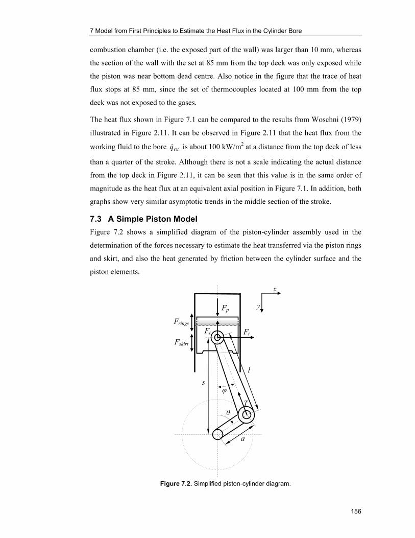
7 Model from First Principles to Estimate the Heat Flux in the Cylinder Bore
156
combustion chamber (i.e. the exposed part of the wall) was larger than 10 mm, whereas
the section of the wall with the set at 85 mm from the top deck was only exposed while
the piston was near bottom dead centre. Also notice in the figure that the trace of heat
flux stops at 85 mm, since the set of thermocouples located at 100 mm from the top
deck was not exposed to the gases.
The heat flux shown in Figure 7.1 can be compared to the results from Woschni (1979)
illustrated in Figure 2.11. It can be observed in Figure 2.11 that the heat flux from the
working fluid to the bore GLq& is about 100 kW/m2 at a distance from the top deck of less
than a quarter of the stroke. Although there is not a scale indicating the actual distance
from the top deck in Figure 2.11, it can be seen that this value is in the same order of
magnitude as the heat flux at an equivalent axial position in Figure 7.1. In addition, both
graphs show very similar asymptotic trends in the middle section of the stroke.
7.3 A Simple Piston Model
Figure 7.2 shows a simplified diagram of the piston-cylinder assembly used in the
determination of the forces necessary to estimate the heat transferred via the piston rings
and skirt, and also the heat generated by friction between the cylinder surface and the
piston elements.
Figure 7.2. Simplified piston-cylinder diagram.
l
s
a
θ
ϕ
Fi
Fp
T
Frings
Fskirt
y
x
Ft

7 Model from First Principles to Estimate the Heat Flux in the Cylinder Bore
157
In this simple analysis a system with only two degrees of freedom is considered. The
piston is assumed to move along the bore parallel to the cylinder axis and impacts
between the piston and the bore will be assumed due to a simple translation of the whole
piston, although in practice it tilts significantly under the influence of a frictional torque
at the piston pin and the rotational inertia of the piston. The forces taken into account in
the model are the gas pressure force Fp, the inertia force in the vertical direction Fi, the
tension force in the connecting rod T, the side thrust Ft, and the friction forces acting on
the rings Frings and skirt Fskirt (upwards when the piston is moving downwards and
downwards when the piston is moving upwards).
The piston diameter is reduced in the region of the rings, so the rings tend to remain in
contact with the bore and they slide into or out of the ring grooves on the thrust and
non-thrust sides. There is thus another friction force not shown in the diagram, which
exists in the ring grooves and is significant when the combustion chamber pressure is
high. In order to avoid an excessively complex analysis of the piston movement, the
friction force in the ring grooves, the frictional and inertia forces about the piston pin
axis and the inertia force in the horizontal direction were omitted. However, evidence
will be presented (Section 7.3.2) to show that these omissions did not significantly
affect the dynamics of the piston assembly, in particular the timing of its lateral
translation across the cylinder bore.
7.3.1 Piston Velocity and Acceleration
Knowledge of the velocity of the piston is necessary for the calculation of the friction
forces, and the acceleration multiplied by the piston mass gives the inertia force on the
piston. Details of these calculations are given in Section 7.3.2, whereas in this section,
the equations for piston velocity and acceleration, and results at 4000 rev/min are
presented.
The piston velocity as a function of crank angle is given by the following equation
adapted from Heywood (1988):
( )
−+==
2/122 sin
cos1sin
2 θ
θθ
π
RV
dt
dss p& (7.1)
In Equation 7.1, Vp represents the mean piston speed (see Section 6.2.2) and R is the
ratio of the connecting rod length l to the crank radius a (see Figure 7.2).
The velocity of the piston in the test engine obtained at 4000 rev/min is shown in
Figure 7.3 for an engine revolution.

7 Model from First Principles to Estimate the Heat Flux in the Cylinder Bore
158
TDC 30 60 90 120 150 BDC 210 240 270 300 330 TDC-20
-15
-10
-5
0
5
10
15
20
Crank Angle (°)
Piston Velocity (m/s)
Figure 7.3. Piston velocity at 4000 rev/min.
Differentiation of the equation for the piston velocity (Equation 7.1) gives the
instantaneous piston acceleration:
( )
−
++==
2/322
422
2
2
sin
sin2coscos
60 θ
θθθ
π
R
RnV
dt
sds
p&& (7.2)
In this equation, additionally to the variables Vp and R previously described, n
represents the rotational speed of the engine in rev/min.
Figure 7.4 illustrates the acceleration of the piston for one crankshaft revolution at an
engine rotational speed of 4000 rev/min.
TDC 30 60 90 120 150 BDC 210 240 270 300 330 TDC-6000
-4000
-2000
0
2000
4000
6000
8000
10000
Crank Angle (°)
Piston Acceleration (m/s2)
Figure 7.4. Piston acceleration at 4000 rev/min.

7 Model from First Principles to Estimate the Heat Flux in the Cylinder Bore
159
7.3.2 Determination of Forces
With reference to the piston model shown in Figure 7.2, the balance of forces acting on
the piston in the x and y directions gives the relevant equations. Resolving horizontally:
ϕsinTFt = (7.3)
Resolving vertically:
( ) ϕcosTFFFF skirtringsip =+− m (7.4)
Combining Equations 7.3 and 7.4 by replacing the force in the connecting rod T from
Equation 7.3 into Equation 7.4, the expression for the side thrust Ft is obtained as
follows:
( )[ ] ϕtanskirtringsipt FFFFF +−= m (7.5)
In Equation 7.5, the tangent of the angle ϕ is a function of the crank angle θ given by:
( ) 2/122 sin
sintan
θ
θϕ
−=
R (7.6)
The first term on the right hand side of Equation 7.5, the force caused by the gas
pressure Fp, can be simply found as the area of the piston times the gas pressure, that is:
pd
Fp
p4
2π= (7.7)
The actual diameter of the piston dp, was provided by the piston manufacturer and is
given in Appendix F, which includes the available piston related data. The
corresponding gas pressure force on the piston during the engine cycle is shown in
Figure 7.5.
The second term on the right hand side, the inertia force of the piston Fi, is given by:
smF pi&&= (7.8)
In this equation, the acceleration of the piston s&& is given by Equation 7.2 and mp is
defined as the equivalent mass of the piston or reciprocating mass, which includes in
addition to the mass of the piston and rings, the mass of the gudgeon pin and the
fraction of the mass of the connecting rod assumed to be concentrated on the piston end.
This latter mass was found experimentally for the connecting rod of the test engine (see
Appendix F), following the procedure explained by Stone (1998) which is used in
engine balance calculations.

7 Model from First Principles to Estimate the Heat Flux in the Cylinder Bore
160
TDC 60 120 BDC 240 300 TDC 420 480 BDC 600 660 TDC0
10
20
30
40
50
60
70
80
90
100
Crank Angle (°)
Gas Pressure Force (kN)
Figure 7.5. Piston gas pressure force at 4000 rev/min and 100% LTC.
The inertia force on the piston during one crankshaft revolution at 4000 rev/min is
shown in Figure 7.6.
TDC 30 60 90 120 150 BDC 210 240 270 300 330 TDC-8
-6
-4
-2
0
2
4
6
8
10
12
Crank Angle (°)
Inertia Force (kN)
Figure 7. 6. Piston inertia force at 4000 rev/min.
The friction force acting on the rings Frings is the result of the summation of the
individual friction forces acting on the two compression rings and on the oil control ring
according to:
ororsrsrfrfrrings WfWfWfF ++= (7.9)
In Equation 7.9, f represents the friction coefficient for the ring and W the load in the
direction normal to the cylinder wall. The subscripts fr, sr and or refer to first or top
compression ring, second compression ring and oil control ring respectively.
The load on a particular ring is a function of the gas pressure acting on the inner face of
the ring (which lies parallel to the cylinder wall), the area of this face, and the inherent

7 Model from First Principles to Estimate the Heat Flux in the Cylinder Bore
161
spring or elastic force in the ring acting normal to the cylinder wall. The latter may be
measured as the tangential force necessary to close the ring gap. The load on a ring is
also a function of the friction force in the ring grooves, which has been omitted in the
analysis. The tangential force and dimensions for all rings were provided by the piston
manufacturer (see Appendix F). The load Wfr on the top compression ring for instance,
is given by:
tfrfrfrfrfr FLBpW += (7.10)
In this equation, pfr and Ftfr are respectively the gas pressure and the inherent spring
force, Bfr is the axial length of the ring and Lfr is the circumferential length (internal in
this case).
In the model, the gas pressure acting on the top compression ring all over the cycle was
assumed to be equal to the in-cylinder pressure measured during the experiments. The
pressure on the second ring was taken as the gas pressure between the compression
rings (inter-ring pressure): both of these were clearly overestimates on account of the
pressure loss in the combustion gas in passing over the top and second piston lands
respectively. The inter-ring pressure was deduced analytically on the basis of the gas
pressure measured in the cylinder and experimental and theoretical results of cylinder
pressure and inter-ring pressure presented by Parker et al. (1990), Mierbach et al.
(1995), Taylor and Evans (2004), Richardson (1996), Akalin and Newaz (2001) and Liu
et al. (1998). The pressure behind the oil control ring was considered to be negligible, so
the load acting on the oil control ring was just equal to the inherent spring force of this
ring as provided by the manufacturer. The cylinder gas pressure measured at
4000 rev/min and 100% of the limiting torque and the predicted gas pressure between
the rings at these conditions are shown in Figure 7.7.
Similarly to the friction force on the rings, the friction force acting on the skirt Fskirt can
be expressed as:
skirtskirtskirt WfF = (7.11)
where the load on the skirt Wskirt is equal to the side thrust Ft.
The friction coefficient for rings and skirt in Equations 7.9 and 7.11, can be obtained
from the theory of hydrodynamic lubrication (Cameron, 1966) considering each of the
rings and the skirt as a finite rectangular tilting pad acting against the cylinder wall as a
thrust bearing. Stone (1998) demonstrates that the lubrication regime of the piston skirt
is fully hydrodynamic; however, the piston rings may work in mixed lubrication

7 Model from First Principles to Estimate the Heat Flux in the Cylinder Bore
162
conditions at the end of the strokes when the piston velocity reduces to zero. This is
shown in the Stribeck diagram of Figure 7.8.
TDC 60 120 BDC 240 300 TDC 420 480 BDC 600 660 TDC0
20
40
60
80
100
120
140
160
180
Crank Angle (°)
Gas Pressure (bar)
Cylinder
Inter-ring
Figure 7.7. Measured cylinder gas pressure and the predicted inter-ring gas pressure at 4000 rev/min and 100% LTC.
Figure 7.8. Engine lubrication regimes on the Stribeck diagram. Adapted from Stone (1998).
Cameron (1966) gives the following basic equation for the friction coefficient of a
rectangular pad of area L times B, where L is the length of the pad at right angles to the
direction of motion and B is the length in the direction of motion.
=f Y
2/1
/
LW
Uµ (7.12)
Coefficient of Friction
Sommerfeld Number x 104
LW
Uµ
0.001 0.01 0.1 1.0 10
0.001
0.01
0.1
Valve Train
Engine Bearings
Piston Skirt
Piston Rings
Thin Film Thick Film
Boundary Mixed Hydrodynamic

7 Model from First Principles to Estimate the Heat Flux in the Cylinder Bore
163
In Equation 7.12, Y is the coefficient of the friction factor, which depends on the
aspect ratio L/B and the inclination of the pad. However, the sensitivity of Y to
inclination is not great, so the model may be applied to the current situation in which a
detailed knowledge of skirt and ring inclination is absent (see Cameron, 1966). The
inclination of a tilting pad is represented by its inclination ratio K, which is defined as
shown in Figure 7.9. Additionally in Equation 7.12, µ is the dynamic viscosity of the
lubricating oil, U is the sliding velocity and W is the applied load. The variables µ, U, W
and the length L are combined to form the Sommerfeld number (see Figure 7.8). In
Equation 7.12, the exponent of this dimensionless group is 0.5; however, Richardson
(2000) reported that the exponent can be varied from 0.33 to 0.66.
Figure 7.9. Schematic of the piston rings or skirt as a rectangular tilting pad thrust bearing. Adapted from Cameron (1966) and Heywood (1988).
In order to apply Equation 7.12 to piston rings and skirt, the sliding velocity U can be
replaced by the piston velocity s& , and W by the specific load on each ring (Wfr, Wsr,
Wor) or the skirt (Ft). The length L of all rings is the same and equal to the
circumferential length of the bore, whereas the length L of the contact area of the skirt
was determined by observation of the skirt of the engine pistons. The length B of rings
and skirt is given in Appendix F. For the ratios L/B of rings and skirt, Cameron (1966)
gives approximate friction factors Y of 1.938 and 2.86 respectively for an inclination
ratio K of 1. Finally, the dynamic viscosity µ of the lubricating oil used in the test
engine was provided by the oil manufacturer (see viscosity-temperature chart in
Appendix F). Its value in the following equations depends on the average temperature
between the cylinder wall and the particular ring and between the wall and the skirt.
2/1
938.1
=
fr
ringsfr
frW
Lsf
&µ,
2/1
938.1
=
sr
ringssr
srW
Lsf
&µ,
2/1
938.1
=
oc
ringsoc
ocW
Lsf
&µ(7.13)
2/1
86.2
=
t
skirtskirt
skirtF
Lsf
&µ (7.14)
Bearing (cylinder wall)
Rectangular pad (rings or skirt)
U h0
h1
B
Oil film
Inclination ratio:
10
1 −=h
hK
W

7 Model from First Principles to Estimate the Heat Flux in the Cylinder Bore
164
By replacing Equation 7.13 into Equation 7.9 and rearranging, the following expression
is obtained for the frictional force of the rings:
( ) ( ) ( ) ( )[ ]2/12/12/12/1938.1 orocsrsrfrfrringsrings WWWLsF µµµ ++= & (7.15)
Figure 7.10 illustrates the estimated friction coefficient for the rings at each crank angle
(Equation 7.13). Figure 7.11 shows the frictional force acting on each ring and the total
friction force on the ring pack during the engine cycle as given by Equation 7.15. Notice
in Figure 7.10 that the range of friction coefficient values corresponds well with the
Stribeck diagram of Figure 7.8.
TDC 60 120 BDC 240 300 TDC 420 480 BDC 600 660 TDC0
0.01
0.02
0.03
0.04
0.05
0.06
0.07
0.08
Crank Angle (°)
Coefficient of Friction
First ring
Second ring
Oil control ring
Figure 7.10. Predicted friction coefficient for the piston rings during the engine
cycle (expansion stroke starts at 360°) at 4000 rev/min and 100% LTC.
TDC 60 120 BDC 240 300 TDC 420 480 BDC 600 660 TDC-40
-30
-20
-10
0
10
20
30
40
Crank Angle (°)
Friction Force (N)
First ring
Second ring
Oil control ring
Ring pack
Figure 7.11. Predicted friction force on piston rings at 4000 rev/min and 100% LTC.

7 Model from First Principles to Estimate the Heat Flux in the Cylinder Bore
165
In relation to the frictional forces, the results presented in Figure 7.11 were found to be
within the normal order of magnitude of friction forces occurring in the ring pack of
internal combustion engines (see Hoshi et al., 1989; Parker et al., 1990; and Akalin and
Newaz, 2001).
Similarly to the determination of the frictional force of the rings, substitution of
Equation 7.14 into Equation 7.11 gives the friction force acting on the skirt.
( ) 2/186.2 tskirtskirtskirt FLsF &µ= (7.16)
Since the friction force on the skirt is a function of the side thrust Ft, substitution of
Equation 7.16 into Equation 7.5 results in the following quadratic expression:
021
2 =++ CFCF tt (7.17)
The coefficients C1 and C2 in Equation 7.17 are given by:
( ) ϕµϕ 2
1 tan18.8tan2 skirtskirtringspi LsFFFC &−±−= (7.18)
( ) ϕ22
2 tanringspi FFFC ±−= (7.19)
The solution of Equation 7.17 for the expansion stroke gives the side thrust when the
frictional forces are the highest. Interestingly, these results were almost identical to the
side thrust obtained directly from Equation 7.5 without consideration of the frictional
forces. The maximum difference during the expansion stroke was less than 0.3%. This
demonstrated the small influence of friction on the value of the side thrust and on the
lateral translation of the piston across the cylinder bore. For this reason the side thrust
was calculated for the rest of the cycle using Equation 7.5 with no frictional forces. A
more rigorous approach would have required the solution of the equations of the piston
motion for a system with three degrees of freedom (see, for instance, Balakrishnan and
Rahnejat, 2005 and Livanos and Kyrtatos, 2006), which was considered to be beyond
the scope of the research.
Figure 7.12 shows the side thrust as a function of crank angle at 4000 rev/min and 100%
of the limiting torque. The results illustrate the lateral translation of the piston between
thrust side (positive values) and non-thrust side (negative values) during the cycle. The
crank angles at which the piston moves from one side to the other agree well with
measurements taken by Laws et al. (1973), Parker et al. (1985) and more recently by
Taylor and Evans (2004).

7 Model from First Principles to Estimate the Heat Flux in the Cylinder Bore
166
TDC 60 120 BDC 240 300 TDC 420 480 BDC 600 660 TDC-3
-2
-1
0
1
2
3
4
5
6
7
Crank Angle (°)
Side Thrust (kN)
Figure 7.12. Predicted side thrust at 4000 rev/min and 100% LTC.
The friction force on the skirt was then obtained from Equation 7.16 using the side
thrust previously found; the results are demonstrated in Figure 7.13.
TDC 60 120 BDC 240 300 TDC 420 480 BDC 600 660 TDC-12
-10
-8
-6
-4
-2
0
2
4
6
8
Crank Angle (°)
Friction Force (N)
Thrust side
Non-thrust side
Figure 7.13. Predicted skirt friction force at 4000 rev/min and 100% LTC.
The estimated frictional force on the skirt was compared with results from simulations
performed by the piston manufacturer. It was found that the friction force values from
this simple model were in the same order of magnitude of the results provided by the
manufacturer (Federal Mogul, 2005).
7.4 Conductive Heat Transfer
This section describes the calculation of the heat transferred by conduction between the
piston rings and the cylinder wall and between the skirt and the wall. In the modelling
of this process of heat transfer, it was assumed that heat passes entirely through the
lubricating oil film from the piston rings and from the skirt to the cylinder wall in
accordance to Fourier’s law of heat conduction in the radial direction.

7 Model from First Principles to Estimate the Heat Flux in the Cylinder Bore
167
Parker et al. (1985) contains a thorough and careful analysis of the heat flow between
pads on a piston skirt and the cylinder wall. Plots of the thermal contours in the oil film
occupying the space were almost entirely parallel to the cylinder wall, showing that heat
transfer occurred by thermal conduction rather than by any significant convection. Since
the oil films are very thin their heat capacity is small and one-dimensional conduction is
established quickly.
Fourier’s law of heat conduction in one dimension for the heat transfer process between
piston rings and cylinder wall and between piston skirt and the wall can be written as
follows:
0h
TTk
A
wp
o
b
p
−−==
&
& (7.20)
In Equation 7.20, pq& refers to the one-dimensional heat flow Q& per unit of the bore
area Ab covered by the particular piston ring or the skirt (considering only its contact
area) over the distance travelled by the piston in a crank angle step. Thus, pq& represents
the instantaneous heat flux taking place between any of the piston rings or the skirt and
the cylinder wall during a crank angle step. In addition, ko is the thermal conductivity of
the lubricating oil, Tp is the temperature of each piston ring or the skirt, Tw is the steady-
state temperature of the cylinder wall and h0 is the minimum oil film thickness.
The constant conductivity value ko used in the calculations was suggested by the oil
manufacturer and is given in Appendix F. The temperature distribution of the piston at
maximum power obtained from simulations performed by the piston manufacturer is
also given in Appendix F. The temperature of the rings was estimated on the basis of
this distribution and results of measurements of piston ring temperature by Parker et al.
(1975). The piston temperatures provided by the manufacturer were also used to
calculate the average temperature for the contact area of the skirt. In the model, the
temperature of the piston rings and skirt were assumed constant during the entire cycle.
Finally, the temperatures of the cylinder wall used in the model were the steady-state
surface temperatures obtained from measurements at locations A in the engine block at
4000 rev/min and 100% of the limiting torque (see Figure 5.2). These measurements
were taken on the exhaust side of the engine, which coincides with the thrust side of the
cylinders. At 4000 rev/min and 100% of the limiting torque the engine was operating
close to the condition of maximum power, so the temperature of the cylinder wall and
the temperature of the piston rings and skirt used in the model refer to conditions close
to maximum power.

7 Model from First Principles to Estimate the Heat Flux in the Cylinder Bore
168
7.4.1 Deduction of the Oil Film Thickness
The thickness of the oil film between the rings and the cylinder wall and between the
skirt and the wall was determined on the basis of the hydrodynamic lubrication concept
applied to piston rings and skirt, which has been discussed in the previous section.
Cameron (1966) gives the following equation for the minimum oil film thickness h0
between a rectangular pad of area L times B and a plane surface (refer to Figure 7.9):
( )2/1
2/1*
0/
6
=LW
UWBh
µ (7.21)
In Equation 7.21, the lengths of the rectangular pad B and L, and the variables µ, U and
W have been previously described (see Equation 7.12). The remaining factor in
Equation 7.21, 6W*, is defined by Cameron (1966) as the non-dimensional load, which
is a function of the inclination ratio K (see Figure 7.9) and depends also on the aspect
ratio L/B of the pad. Based on data presented by Cameron (1966), the non-dimensional
loads 6W* for the ratio L/B of the compression rings, the oil control ring and the skirt
are respectively 0.1353, 0.1447 and 0.05979. These are average values considering
inclination ratios K of 0.5, 1 and 2. The corresponding average values for (6W*)1/2
are
0.3672, 0.3800 and 0.2441 respectively.
Equation 7.21 can now be written for the piston rings and for the skirt using the
appropriate dimensions L and B, and by substitution of the sliding velocity U by the
piston velocity s& , the load factor 6W* by its respective values, and W by the particular
loads found in the previous section, Wfr, Wsr, Wor for the rings and the side thrust Ft for
the skirt. Similarly to Equations 7.13 and 7.14, it is necessary to indicate in the
following equations that the dynamic viscosity µ of the lubricating oil is a function of
the average temperature between the cylinder wall and the particular ring and between
the wall and the skirt.
2/1
3672.0
=
fr
ringsfr
frfrW
LsBh
&µ,
2/1
3672.0
=
sr
ringssr
srsrW
LsBh
&µ,
2/1
3800.0
=
oc
ringsoc
ococW
LsBh
&µ (7.22)
2/1
2441.0
=
t
skirtskirtskirtskirt
F
LsBh
&µ (7.23)

7 Model from First Principles to Estimate the Heat Flux in the Cylinder Bore
169
Equations 7.22 and 7.23 were then used to calculate the oil film thickness at every crank
angle during an engine cycle for the piston rings and piston skirt. Figure 7.14 shows the
results obtained for the piston rings and Figure 7.15 illustrates the oil film thicknesses
for the skirt on the thrust and non-thrust sides of the cylinder bore.
TDC 60 120 BDC 240 300 TDC 420 480 BDC 600 660 TDC0
2
4
6
8
10
12
14
Crank Angle (°)
Oil Film
Thickness ( µm)
First ring
Second ring
Oil control ring
Figure 7.14. Predicted oil film thickness between piston rings and cylinder wall
during the engine cycle (expansion stroke starts at 360°) at 4000 rev/min and 100% LTC.
In Figure 7.14, the calculated oil film thicknesses for the first compression ring shows a
peak of 3.7 µm (microns) during the power stroke and a maximum of 10.5 µm in the
cycle. This is in very good agreement with detailed calculations in Allen et al. (1975),
and also with analytical results in Shimada et al. (2004). The former was verified by
experiments. Additionally, the oil film thickness for every ring shown in Figure 7.14
was found to correspond well with predicted results from Parker et al. (1990) for a
three-ring piston running in a gasoline engine at 5000 rev/min.
TDC 60 120 BDC 240 300 TDC 420 480 BDC 600 660 TDC0
10
20
30
40
50
60
70
80
Crank Angle (°)
Oil Film
Thickness ( µm)
Thrust side
Non-thrust side
Figure 7.15. Predicted oil film thickness between piston skirt and cylinder wall at 4000 rev/min and 100% LTC.

7 Model from First Principles to Estimate the Heat Flux in the Cylinder Bore
170
In Figure 7.15, the minimum oil film thickness between the piston skirt and the cylinder
wall is observed during the power stroke on the thrust side of the bore, which is in good
agreement with analytical results by Balakrishnan and Rahnejat (2005). Moreover, the
calculated thickness of the oil film over most of the cycle is within the magnitude of the
nominal piston skirt to cylinder radial clearance (30 µm). However, the results also
illustrate the limitation of the model to predict a realistic thickness of the oil film when
the side thrust is near zero or zero. It may be noted that at about 70° and 655° a very
small lateral reaction (see Figure 7.12) led to unrealistic values in accordance to
Equation 7.23. For this reason at these crank angles the film thickness was arbitrarily
limited to half of the nominal clearance between the piston skirt and the cylinder bore.
Also at top and bottom dead centres, singular solutions of Equation 7.23 were omitted
from further calculations. In practice the thickness of the oil film at crank angles
corresponding to small values of side thrust would be limited by the rate at which the oil
film could change and perhaps by the amount of oil available. If squeeze lubrication had
been included in the model this would have been readily apparent.
7.4.2 Heat Conduction from the Piston Rings
The conductive heat flux between the piston rings and the cylinder wall through the oil
film obtained from Equation 7.20 is presented in this section. During one increment or
step of crank angle heat flows from the piston ring into a section of wall of axial
distance equal to the axial thickness of the piston ring plus the distance travelled by the
ring during one crank angle interval. In this way, for a small crank angle increment, a
given point on the wall receives a thermal flux over many crank angle intervals for
every passage of each piston ring. The evaluation of Equation 7.20 was performed using
crank angle steps of 0.1°. As a check other crank angle steps such as 1° were also
examined. The effect of changing the crank angle interval in this way on the predicted
heat flux was just to change the resolution of the results, but not their shape or
magnitude.
Figure 7.16 illustrates the calculated heat flux occurring between each piston ring and
the wall on the thrust side of the cylinder bore at 4000 rev/min and 100% of the limiting
torque. The heat flux is presented as a function of the distance from the top deck and is
plotted over the axial length of the wall at which temperature measurements where
taken at location A in cylinder two of the in engine. As described in Section 3.2.2.1, at
this location seven sets of thermocouples were used. The top set was located at 10 mm
from the top deck, the bottom set at 100 mm and the intermediate sets were at 25, 40,
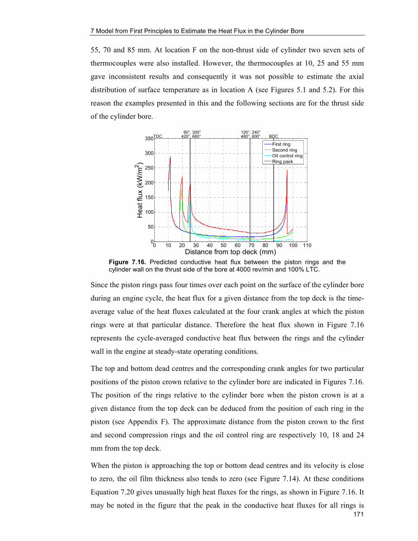
7 Model from First Principles to Estimate the Heat Flux in the Cylinder Bore
171
55, 70 and 85 mm. At location F on the non-thrust side of cylinder two seven sets of
thermocouples were also installed. However, the thermocouples at 10, 25 and 55 mm
gave inconsistent results and consequently it was not possible to estimate the axial
distribution of surface temperature as in location A (see Figures 5.1 and 5.2). For this
reason the examples presented in this and the following sections are for the thrust side
of the cylinder bore.
0 10 20 30 40 50 60 70 80 90 100 1100
50
100
150
200
250
300
350Heat flux (kW/m
2)
Distance from top deck (mm)
TDC 60°, 300°420°, 660°
120°, 240°480°, 600° BDC
First ring
Second ring
Oil control ring
Ring pack
Figure 7.16. Predicted conductive heat flux between the piston rings and the cylinder wall on the thrust side of the bore at 4000 rev/min and 100% LTC.
Since the piston rings pass four times over each point on the surface of the cylinder bore
during an engine cycle, the heat flux for a given distance from the top deck is the time-
average value of the heat fluxes calculated at the four crank angles at which the piston
rings were at that particular distance. Therefore the heat flux shown in Figure 7.16
represents the cycle-averaged conductive heat flux between the rings and the cylinder
wall in the engine at steady-state operating conditions.
The top and bottom dead centres and the corresponding crank angles for two particular
positions of the piston crown relative to the cylinder bore are indicated in Figures 7.16.
The position of the rings relative to the cylinder bore when the piston crown is at a
given distance from the top deck can be deduced from the position of each ring in the
piston (see Appendix F). The approximate distance from the piston crown to the first
and second compression rings and the oil control ring are respectively 10, 18 and 24
mm from the top deck.
When the piston is approaching the top or bottom dead centres and its velocity is close
to zero, the oil film thickness also tends to zero (see Figure 7.14). At these conditions
Equation 7.20 gives unusually high heat fluxes for the rings, as shown in Figure 7.16. It
may be noted in the figure that the peak in the conductive heat fluxes for all rings is

7 Model from First Principles to Estimate the Heat Flux in the Cylinder Bore
172
when the piston is at top dead centre and also for the first compression ring when the
piston is at bottom dead centre. The heat flux for the second compression ring and the
oil control ring at bottom dead centre are not shown in the figure since these rings were
beyond 100 mm from the top deck when the piston was at the bottom of the stroke.
Because normal hydrodynamic lubrication cannot exist at very low piston velocities, the
model produced unrealistically high values of heat flux when the piston was near the top
and bottom dead centres. However, when the piston velocity is near zero the forces
acting radially inwards on each piston ring can still provide lubrication by the squeeze
mechanism. In this regime the viscosity of the lubricant limits its rate of escape and so
tends to maintain the oil film thickness. Some mixed or boundary lubrication may
occur, though the low rate of wear achieved by piston rings suggests that this is
minimal. For these reasons, the peak values observed in Figure 7.16 may have been
overestimated by assuming normal hydrodynamic conditions.
7.4.3 Heat Conduction from the Piston Skirt
Similarly to the heat transferred by conduction between the piston rings and the cylinder
wall, the instantaneous conductive heat flux between the piston skirt and the wall
through the oil film was calculated using Equation 7.20. The instantaneous results were
then averaged over the engine cycle and integrated over the wall sections in contact with
the skirt during every increment of crank angle. The heat flux obtained in this way for
the thrust side of the cylinder bore is shown in Figure 7.17.
0 10 20 30 40 50 60 70 80 90 100 1100
20
40
60
80
100
120
Distance from top deck (mm)
Heat flux (kW/m
2)
TDC 60°, 300°420°, 660°
120°, 240°480°, 600° BDC
Figure 7.17. Predicted conductive heat flux between the piston skirt and the cylinder wall on the thrust side of the bore at 4000 rev/min and 100% LTC.
It may be seen in the figure that there is no contribution of heat from the skirt to the
cylinder wall above 27 mm from the top deck. This is because the top of the skirt is
approximately at this distance from the piston crown. As in the case of the piston rings,

7 Model from First Principles to Estimate the Heat Flux in the Cylinder Bore
173
no results are shown beyond 100 mm in Figure 7.17 (since no temperature
measurements where taken below this point).
In order to understand the shape of the heat flux between the piston skirt and the wall, it
is necessary to consider the lateral translation of the piston across the cylinder bore (see
Figure 7.12). The heat flux curve starts at 27 mm from the top deck, peaks at about 75
mm, and then declines rapidly before rising moderately towards 100 mm. It can be
verified that the sections on the thrust side of the cylinder wall where the heat flux from
the skirt increases and reaches the maximum correspond with the crank angles at which
the lateral force on the thrust side is the largest, so the oil film thickness is thinner and
the heat conduction increases in accordance to Equation 7.20. For example, it may be
observed in Figure 7.12 that the largest side-thrusts occur at the beginning of the
expansion stroke, specifically between 360° and 420°. During this part of the cycle the
centre of the skirt travels from 51 mm to 77 mm below the top deck. This is the region
in which a rapid increase in the conductive heat flux is observed in Figure 7.17. For the
rest of the cycle the side-thrust is significantly smaller, the oil film is correspondingly
thicker (with increased thermal resistance) and consequently, the heat conduction
through the oil film is less than in the expansion stroke.
7.5 Heat Generation by Friction
The instantaneous heat generation per unit time due to the friction force acting on the
particular ring or on the skirt, is given by the product of the force and the piston
velocity. The velocity of the piston and the friction forces for the rings and the skirt
have been calculated as a function of crank angle in Sections 7.3.1 and 7.3.2
respectively (see Figures 7.11 and 7.13). Accordingly, the friction heat generation can
be obtained from the equation:
sFQ ff&& = (7.24)
In this equation, fQ& is the rate of heat generated by friction between the piston rings
and the cylinder wall or between the piston skirt and the wall. The variable Ff represents
the friction force on each piston ring or the friction force on the skirt.
In order to obtain the heat flux received by the cylinder wall due to friction, the
instantaneous heat generated during one crank angle interval was divided by the area of
the corresponding section of the cylinder wall over which heat was generated within
that crank angle interval. Hence:

7 Model from First Principles to Estimate the Heat Flux in the Cylinder Bore
174
b
f
b
f
fA
sF
A
&&
& == (7.25)
The cycle-averaged friction heat flux was then calculated using the same method
applied to obtain the average heat flux by conduction through the oil film explained in
Section 7.4.
It should be mentioned, that not all of the heat that passes from the piston assembly into
the general engine oil circulation is transferred to the cylinder wall. The heat is partly
conveyed by the oil and afterwards is mainly taken from the oil by the coolant in the oil
cooler. The heat rejection to the coolant in the oil cooler also includes the heat removed
by the oil from the piston cooling galleries and under crown, and heat from other
sources in the engine (crankshaft, valvetrain, turbocharger, etc). This heat could be
calculated from the temperature and coolant flow measurements taken on the oil cooler
(see Section 3.2.4). However, it would have been difficult to accurately estimate the
fraction of heat due to friction from the piston pack. Additionally, the flow of oil past
the ring pack and piston skirt is very small in comparison with the other oil flows.
Therefore, it was reasonable to assume that all of this heat passed into the cylinder wall.
7.5.1 Piston Rings
Figure 7.18 illustrates the average heat frictional flux generated by the piston rings
during the engine cycle. Similarly to the graphs of heat flux by conduction from the
piston rings (Figure 7.16), the heat flux from every ring and the total heat flux from the
ring pack are given as a function of the distance from the top deck. Also, results are
only given for the axial length of the bore where temperature measurements were taken
on the thrust side of the cylinder wall.
The figure reveals the significant influence of the gas pressure on the frictional heat flux
generated by the compression rings. The heat fluxes reach their maximum values within
a short distance from their position at top dead centre (first ring at 15 mm and second
ring at 30 mm approximately). It can be verified that over this distance from the top
deck the piston was within the first 60° of its expansion stroke or within the last 60° of
the compression stroke. Although the piston velocity is relatively low at the start and
end of the strokes, these are the crank angles when the gas pressure and consequently
the friction force on the compression rings was highest (see Figure 7.11). This is also
the region where the heat generated by friction on the first compression ring is larger
than that on the second compression ring, which is in accordance with the

7 Model from First Principles to Estimate the Heat Flux in the Cylinder Bore
175
corresponding friction forces. It may be noted in Figure 7.11 that only at the beginning
of expansion and in the second half of compression is the force on the first compression
ring considerably larger than on the second compression ring.
0 10 20 30 40 50 60 70 80 90 100 1100
2
4
6
8
10
12
14
Distance from top deck (mm)
Heat flux (kW/m
2)
TDC 60°, 300°420°, 660°
120°, 240°480°, 600° BDC
First ring
Second ring
Oil control ring
Ring pack
Figure 7.18. Predicted heat flux due to friction between piston rings and the cylinder wall at 4000 rev/min and 100% LTC.
The heat flux due to friction from the oil control ring shows a moderate increase with
piston velocity. It may be noted in Figure 7.18 that once the piston has moved away
from the top dead centre and its velocity has increased sufficiently, the oil control ring
curve is fairly constant. In the model, the friction force acting on the oil control ring is
not dependant on the gas pressure; it is mainly a function of the inherent spring force
(constant over the cycle), the oil viscosity and the piston velocity. As shown in
Figure 7.11, the friction force on the oil control ring is less than on the compression
rings. Accordingly, the rate of heat generation is also smaller in the oil control ring than
in the other rings. However, the frictional heat per unit area received by the wall from
the oil control ring is actually larger than the heat flux from the compression rings, since
the oil control ring has a smaller contact area.
7.5.2 Piston Skirt
The average frictional heat flux generated by the piston skirt on the thrust side of the
cylinder wall is shown in Figure 7.19. As before, in this case the heat flux results are
presented as a function of the distance from the top deck, only for the axial length of the
bore where temperature measurements were taken.
Similarly to the conductive heat flux from the skirt (Figure 7.17), the frictional heat flux
increases from 27 mm and reaches its maximum near 75 mm from the top deck.
However, after this point it does not decline sharply as the conductive heat flux did;

7 Model from First Principles to Estimate the Heat Flux in the Cylinder Bore
176
instead, the frictional heat flux caused by the skirt shows only a modest decrease
between 75 mm and 100 mm from the top deck.
0 10 20 30 40 50 60 70 80 90 100 1100
2
4
6
8
10
12
14
Distance from top deck (mm)
Heat flux (kW/m
2)
TDC 60°, 300°420°, 660°
120°, 240°480°, 600° BDC
Figure 7.19. Predicted heat flux due to friction between the piston skirt and the thrust side of the cylinder wall at 4000 rev/min and 100% LTC.
Interestingly, the frictional heat flux increases at almost a constant rate between 30 mm
and 75 mm from the top deck. This can be explained by the combined effects of
variations in the friction force acting on the skirt and the bore area traversed by the
piston in each crank angle interval during the cycle. As shown in Figure 7.13, between
360° and approximately 390° the friction force on the thrust side of the bore increases
rapidly, but so does the piston velocity (Figure 7.3). Because of the rising piston
velocity, the area travelled by the skirt in each crank angle interval also increases. As a
result, the ratio of heat generated by friction to the bore area (i.e. the heat flux received
by the wall) during this part of the cycle increases by the same amount at each crank
angle interval. After 390°, the friction force acting on the skirt and the piston velocity
change in such a way that the heat flux received by the bore continues to rise at the
same rate. Additionally, the region on the bore corresponding to crank angles 360° to
430° receives the heat flux generated at the end of the exhaust stroke (between 650° and
720°) when the piston was again on the thrust side of the bore.
At 80 mm from top deck the heat flux reaches a maximum and levels off. After this
point it eventually begins to decline, but only moderately because of the additional heat
flux due to the friction force acting on the skirt during the second half of the intake
stroke (as shown in Figure 7.13, between 70° and 180°).

7 Model from First Principles to Estimate the Heat Flux in the Cylinder Bore
177
7.6 Results and Discussion
In the final section of this chapter, the axial heat flux distribution derived from
temperature measurements taken on the thrust side of the cylinder bore (Chapter 5) is
compared with the total predicted heat flux. The total heat flux comprises the heat
transferred directly from the combustion gases to the cylinder wall, the heat conducted
from the piston to the wall via the oil film and the heat generated by friction.
The heat transferred by convection and radiation from the combustion gases to the
cylinder wall has been presented in Section 7.2 and was obtained using the correlation
proposed in Chapter 6 to calculate the heat transfer coefficient. The heat transferred by
conduction through the oil film consists of the heat from the piston rings and the heat
from the piston skirt. These quantities and the heat generated by friction between the
rings and the cylinder wall and between the skirt and the wall were calculated using the
piston model developed in this chapter as discussed in Sections 7.3 to 7.5. The model
has been programmed into a Matlab routine included in Appendix D.
Figure 7.20 compares the total experimental heat flux with the total predicted heat flux
(dotted black line) on the thrust side of the cylinder bore at 4000 rev/min and 100% of
the limiting torque. The heat fluxes are given as a function of the distance from the top
deck. The experimental heat flux at the locations where temperature measurements were
taken in the wall of cylinder two (location A) are indicated by square markers. These
heat flux values and the corresponding interpolated curve have been previously shown
in Figure 5.6.
The curve of the total predicted heat flux shown in Figure 7.20 was obtained by addition
of the various contributions of heat previously calculated. In this way, the first curve at
the bottom of the graph (blue line) corresponds to the conductive heat flux from the
piston rings. The second curve (green line) was obtained by adding the heat generated
by friction from the piston rings to the first curve. The third curve (magenta line) also
includes the heat conduction from the piston skirt. The fourth curve (cyan line)
represents the heat flux due to conduction and friction from piston rings and piston skirt.
And finally, the heat transferred directly from the combustion gases was added to the
preceding curve to obtain the curve for the total predicted heat flux.
The comparison of the experimental and calculated heat fluxes, demonstrates that the
model is able to predict a heat flux distribution in the axial direction of the cylinder of
the same order of magnitude as the experimental values.

7 Model from First Principles to Estimate the Heat Flux in the Cylinder Bore
178
Figure 7.20. Comparison betw
een the total heat flux predicted by the m
odel (conduction and friction) plus the heat flux from
combustion gases w
ith the experimentally derived heat flux for the thrust side of the bore at 4000 rev/m
in and 100% LTC.

7 Model from First Principles to Estimate the Heat Flux in the Cylinder Bore
179
Although good agreement between experimental values and the predicted heat flux is
only observed at two locations in the cylinder bore, the model adequately predicts the
trend in the heat flux to increase in the mid of the bore and also the larger heat fluxes at
both ends of the stroke.
In Figure 7.20 the relative importance of the various sources of heat is also illustrated. It
may be observed that the heat flux due to friction is much less than that due to
conduction. In the rings for instance, the frictional heat flux represents no more than
20% of the conductive heat flux at any point on the wall, and less than 5% of the total
experimental heat flux. In the piston skirt, the heat flux due to friction is an entire order
of magnitude less that the conductive heat flux and no more than 5% of the total at the
end of the stroke.
The piston and piston ring temperatures used in the model were either obtained from
simulations performed by the piston manufacturer or interpolated from predictions or
measurements (Section 7.4.1). It is therefore evident that they would have been
influenced to some extend by the frictional heating that occurs in the oil films.
However, both the wall temperatures on the one hand and the piston skirt and ring
temperatures on the other would be raised by such heating. Thus by taking the
difference between these temperatures, the effect of this frictional heat flux on the flux
assumed to be conductive has been minimised. This is the justification for including the
frictional heating as well as the conductive heating in Figure 7.20. However, it is
evident (from comparison of the blue and green curves and from comparison of the
magenta and cyan curves) that exclusion of the frictional heating would not have
significantly altered the explanation for the observed axial distribution of heat flux in
the cylinder wall.
The significance of heat conduction from the piston rings and from the skirt was
precisely the conclusion of Parker et al. (1985), where it was found that conduction
through the oil film was the main mechanism of heat transfer from the piston to the
cylinder bore. As shown in Figure 7.20, this conclusion applies well in the middle and
at the end of the stroke. In this region, the cycle-averaged temperature of the gas is
much lower than at the beginning of the stroke, and consequently the heat transferred
directly from the cylinder gases to the wall mainly by convection is less important. In
addition, the time of exposure to such gases at a given point on the wall decreases with
progression down the bore.

7 Model from First Principles to Estimate the Heat Flux in the Cylinder Bore
180
Careful study of Figure 7.20 shows that in the process of heat transfer from the
combustion gases to the cylinder wall, convection and radiation of heat have their
greatest influence on the total heat flux in the top section of the cylinder bore and also
provide a significant contribution (approximately 25%) over the rest of the stroke
length. However, the distribution of heat flux in the middle and bottom parts of the
stroke demonstrates that the main mechanism of heat transfer is conduction from the
piston. In this mechanism, the piston acts as a heat sink and then transmits heat by
conduction through its skirt and rings. Because it travels most slowly near the dead
centres, heat flux peaks from the rings and the skirt are produced when the piston is near
the top and bottom dead centres. This explanation summarises the major findings
obtained from the application of the piston model developed in this chapter and the
predicted distribution of convective heat flux as a function of axial position in the
cylinder wall.
7.7 Concluding Remarks
The limitations of the model in predicting the heat conduction from the rings when the
piston velocity is close to zero (near the top and bottom dead centres) have been
explained in Section 7.4.2. In practice, axial conduction down the bore would average
out the peaks shown for ring conduction at both ends of the stroke. If a mid line through
the peaks were drawn, agreement between experimental and calculated heat fluxes
would be better. This has been done using a smoothing technique available in Matlab
and the results are shown in Figure 7.21. The figure also shows the uncertainty in the
experimental heat flux obtained from the analysis conducted in Section 5.4 and
presented in Figure 5.12.
0 10 20 30 40 50 60 70 80 90 100 1100
50
100
150
200
250
300
350
400
Heat flux (kW/m
2)
Distance from top deck (mm)
TDC BDC
Total predicted heat flux
Experimental heat flux
Figure 7.21. Comparison between the total heat flux predicted by the model plus the heat flux from combustion gases with the experimental heat flux for the thrust side of the bore at 4000 rev/min and 100% LTC.

7 Model from First Principles to Estimate the Heat Flux in the Cylinder Bore
181
It may be observed in Figure 7.21 that once the peaks in the predicted heat flux near the
top and bottom of the measured section in the bore are smoothed out, as they would be
to some extent by axial conduction, the predicted total heat flux only falls outside the
band constituted by the measured heat flux and its uncertainty by about 50 kW/m2 over
the central part of the bore section.
The uncertainty of the predicted heat flux is difficult to quantify. However, the principal
sources of uncertainty are probably the estimated piston and ring temperatures and the
contact conditions of the skirt to wall and ring to wall contacts. The piston temperature
quoted by the manufacturer would be the subject of detailed predictive analysis verified
by measurements and so is unlikely to have significant error. Likewise the measured
pressure data fed into the model.
With regard to the skirt to wall contact conditions, the inclinations were not accurately
known, but the data quoted by Cameron (1966) shows them to be relatively insensitive.
The skirt contact area was assumed to be constant and independent of the transverse
load. In practice, the area and position of the skirt to wall contact varies with crank
angle; indeed this information is produced by finite element analysis conducted by the
piston manufacturer. The ring to wall contact conditions can also be refined by detailed
analysis. The ring to wall inclinations and profiles are discussed at length in Parker et al.
(1975) and Allen et al. (1975).
These considerations suggest two methods of quantifying and reducing errors in the
predicted conductive and frictional heat fluxes. Firstly, repeating the exercise for a
number of different engines; making just a few spot temperature measurements to
evaluate the heat flux and then compare against predictions. Secondly, in conjunction
with the piston manufacturer, feeding in the skirt and ring contact areas and inclinations
as a function of crank angle to refine the conditions under which conductive and
frictional heat fluxes occur. These suggestions, as well as the inclusion in the model of
axial heat conduction in the cylinder wall, are highly appropriate areas for further work.
In the meantime, a very simple analysis derived from first principles, relying only on
measured pressure and limited temperature data, has accounted for the increase in heat
flux in the lower section of the bore. Given confirmation from parallel studies in other
engines, this may well provide a useful method of determining the axial variation in
heat flux through the cylinder wall at the scoping stage of future engine designs.

182
8 Conclusions and Further Work
In the course of this research work, an experimental investigation to study operating
temperatures and heat fluxes in the cylinder walls and cylinder head of a modern diesel
engine was completed. The study relied on a significant amount of data, which included
measurements of metal thermal gradients at many locations in the cylinder walls and
cylinder head of the test engine under a wide range of operating conditions, and also on
instantaneous measurements of the cylinder gas pressure at each test point. The analysis
of the experimental data and the application of fundamental concepts of heat transfer
lead to the proposal of a revised correlation to predict the direct heat transfer from
combustion gases to the containing chamber walls. Additionally, a model was
developed from first principles to estimate the heat conducted via the piston to the walls
by the piston rings and skirt, and the heat generated by friction. The development of
these methods represents the realization of the main objectives of this research.
This investigation was undertaken on the premise that the existing methodology to
predict the heat transferred from combustion gases to the cylinder walls in diesel
engines was outdated. In Chapter 6, some of the empirical correlations to calculate the
gas-side heat transfer coefficient, including the well known equations of Annand (1963)
and Woschni (1967), were evaluated on a comparative basis using data from a current
production diesel engine. Results from this evaluation confirmed the significant
variation previously observed among the coefficients given by these equations.
Furthermore, comparisons of these coefficients with an experimentally derived cycle-
averaged coefficient showed that some of the correlations under-predicted the
experimental value and others over-predicted it; also in most cases the trends were not
consistent with variations in engine load. As a result, a new correlation was proposed to
estimate the gas-side heat transfer coefficient. It was shown that the new correlation
predicted the cycle-averaged coefficient within 10% of the experimental value at a
range of operating conditions, including maximum power. The correlation also
predicted the correct trend with engine load and adequately estimated the instantaneous
coefficient throughout the engine cycle. However, it is suggested that extensive analysis
of the experimental data should be pursued in the future to further validate the proposed
correlation.
The new correlation has been used to calculate the heat directly transferred from the
gases to the cylinder bore within the model presented in Chapter 7. This model, which
also considers conduction from the piston rings and skirt through the oil film between

8 Conclusions and Further Work
183
these components and the cylinder wall, and heat generated by friction, has been
developed to estimate the axial variation of the total radial heat flux in the walls of the
cylinder bore. The predicted heat fluxes showed similar trends to those observed in the
experimental values. However, good agreement between calculated and measured heat
fluxes was limited to the top of the bore. The general conclusion drawn from these
predictions and the experimental results is that heat directly transferred to the cylinder
wall (mainly by convection) greatly affects the total heat flux in the top section of the
cylinder bore and provides approximately a quarter of the total heat flux over the length
of the stroke. It was also concluded that the heat flux in the middle and bottom parts of
the bore is controlled by heat conduction through the piston skirt and rings, and that the
contribution of frictional heating to the total heat flux is one order of magnitude less
than the other heat fluxes.
Some areas of further work to improve the piston model have already been identified in
Section 7.7. Additionally, it is believed that the model could be extended to a piston-
cylinder arrangement with three degrees of freedom where the piston, as in reality,
rotates around its pin as it moves up and down the bore. In this further developed model,
it might also be possible to consider squeeze film lubrication and the variation of shape
and size of the piston skirt contact area throughout the cycle. These are areas of future
work that would require additional experimental or simulation data. These data will also
provide opportunities for further validation of the model, which has been severely
constrained by the availability of piston temperature data at conditions other than
maximum power.
A few comments should be made about the data on which the developed models relied
and the experimental methods used to measure these data. The selection of
measurements that were chosen by the described validation process was found to be
consistent throughout the range of engine operating conditions. In terms of engine load
and speed, measured temperatures consistently increased with increasing torque and
were generally larger at higher speeds. The standard deviation of the temperature
measurements was generally less than 2°C, so the average metal temperatures
representing steady-state conditions were in most cases within ±2°C of the measured
temperature at any instant during the testing periods. This small deviation demonstrated
the reliability of the experimental measurements.
With regard to the experimental method, sufficient data were gathered by using fixed
sets of thermocouples at multiple locations in the engine. Although the technique was

8 Conclusions and Further Work
184
laborious in practice, it was economical and fairly reliable (about 70% of thermocouples
installed in the engine block and all of the thermocouples fitted in the cylinder head
provided consistent measurements). Probably its main disadvantage was the
impossibility of replacing faulty thermocouples once they were installed, which was a
consequence of the need to limit the intrusiveness of the method.
In relation to the experiments of variation of parameters, some interesting results were
obtained. Particularly, the significant effect of the start of injection on steady-state
temperatures and heat fluxes. However, these results should be observed with discretion
since it was difficult to isolate the effect of changing one particular parameter in the test
engine. This is because the strategy built into the ECU of modern engines is
programmed to compensate for any abnormality detected in one variable by shifting
other control parameters in order to keep the engine performing normally.
Finally, it is worth mentioning that this investigation has produced a large set of high
quality data which has been supplied to other research projects and could be further
exploited. In particular, thermal modelling methods using finite element analysis would
be a productive area for exploring three-dimensional heat transfer processes using data
from this study for the definition of boundary conditions and validation.

185
References
Akalin, O. and Newaz G. M. Piston Ring-Bore Friction Modelling in Mixed
Lubrication Regime: Part I-Analytical Results. Transactions of the ASME, Journal of
Tribology, Vol. 123, pp. 211-218, 2001.
Alcock, J. R., Robson, J. V. B. and Mash C. Distribution of Heat Flow in High Duty
Internal Combustion Engines. CIMAC 1957.
Allen, D. G., Dudley, B. R., Middleton, V. and Parker, D. A. Prediction of Piston
Ring-Cylinder Bore Oil Film Thickness in Two Particular Engines and Correlation with
Experimental Evidence. C73/75, pp. 107-124, IMechE, 1975.
Annand, W. J. D. Heat Transfer in the Cylinders of Reciprocating Internal Combustion
Engines. Proc. Instn. Mech. Engrs, Vol. 177, No. 36, pp. 973-990, 1963.
Annand, W. J. D. and Ma, T. H. Instantaneous Heat Transfer Rates to the Cylinder
Head Surface of a Small Compression-Ignition Engine. Proc. Instn. Mech. Engrs, Vol.
185, No. 72/71, pp. 976-987, 1970-71.
Annand, W. J. D. Heat Transfer in the Cylinder and Porting, in Horlock J. H. and
Winterbone, D. E. (Editors), The Thermodynamics and Gas Dynamics of Internal
Combustion Engines, Vol. II. Oxford University Press, 1986.
Balakrishnan, S. and Rahnejat, H. Isothermal Transient Analysis of Piston Skirt-to-
Cylinder Wall Contacts under Combined Axial, Lateral and Tilting Motion. Journal of
Physics D: Applied Physics, Vol. 38, pp. 787-799, 2005.
Borman, G. and Nishiwaki, K. A Review of Internal Combustion Engine Heat. Prog.
Energy Combust. Sci., Vol. 13, pp. 1-46, 1987.
Campbell, N.A.F., Charlton, S.J. and Wong L. Designing towards Nucleate Boiling
in Combustion Engines. Vehicle Thermal Management Systems (VTMS 2),
C496/092/95, pp. 587-595, IMechE, 1995.
Cameron, A. The Principles of Lubrication. Longmans Green and Co. Ltd., 1966.
Chang, J., Güralp, O., Filipi, Z., Assanis, D., Kuo, T., Najt, P. and Rask, R. New
Heat Transfer Correlation for an HCCI Engine Derived from Measurements of
Instantaneous Surface Heat Flux. Society of Automotive Engineers, Paper No. 2004-01-
2996, 2004.
Dent, J. C. and Suliaman, S. J. Convective and Radiative Heat Transfer in a High
Swirl Direct Injection Diesel Engine. Society of Automotive Engineers, Paper No.
770407, SAE Transactions, Vol. 86, 1977.
Eichelberg, G. Some Investigations on Old Combustion-Engine Problems.
Engineering, Vol. 148, Parts I and II, pp. 463-466, 547-550, 1939.
Federal Mogul. Piston Secondary Motion Analysis on Ford Puma 2.0l 130PS Engine
08662A201. June, 2005.
Ferguson, C. R. Internal Combustion Engines, Applied Thermosciences. John Wiley &
Sons, Inc., 1986.
Finol, C. A. Effect of Vibration on Heat Transfer in a Simulated Engine Cooling
Passage. Dissertation Submitted for the Degree of MSc in Automotive Engineering.
Department of Mechanical Engineering. University of Bath, October, 1999.
Finol, C. A. and Damia, Juan A. Extension of the Program “CONDUCT” to Solve
Three-dimensional Problems of Conduction Heat Transfer. I Venezuelan International
Congress of Numerical Methods in Engineering and Applied Sciences. Maracaibo,
Venezuela. October, 1993.

References
186
Finol, C. A. and Robinson, K. Thermal Modelling of Modern Engines: A Review of
Empirical Correlations to Estimate the In-cylinder Heat Transfer Coefficient. Proc.
Instn. Mech. Engrs, Part D: Journal of Automobile Engineering, Vol. 220, No. 12, pp.
1765-1781, 2006.
Finol, C. A. and Robinson, K. Thermal Profile of a Modern Passenger Car Diesel
Engine. Society of Automotive Engineers, Paper No. 2006-01-3409, 2006.
French, C. C. J. Taking the Heat Off the Highly Boosted Diesel. Society of Automotive
Engineers, Paper No. 690463, 1969.
Han, B. S., Chung, Y. J., Kwon, Y. J. and Lee, S. Empirical Formula for
Instantaneous Heat Transfer Coefficient in Spark Ignition Engines. Society of
Automotive Engineers, Paper No. 972995, SAE Special Publications, Vol. 1306, pp.
219-226, 1997.
Hart, J. S., Stryker, P. C. and Ciaravino, J. Multi-point Temperature Probe for
Measuring Combustion Chamber Heat Fluxes and Surface Temperatures. Vehicle
Thermal Management Systems (VTMS 4), C543/033/99, pp. 375-384, IMechE, 1999.
Heywood, J. B. Internal Combustion Engine Fundamental. McGraw-Hill International
Editions, 1988.
Hohenberg, G. F. Advance Approaches for Heat Transfer calculation. Society of
Automotive Engineers, Paper No. 790825, SAE Transactions, Vol. 88, 1979.
Holman, J. P. Experimental Methods for Engineers, Sixth Edition. McGraw-Hill, Inc.,
1994.
Hoshi, B., Baba, Y. and Fuhurama, S. A Study of Piston Friction Force in an Internal
Combustion Engine. Tribology Transactions, Vol. 32, 4, pp. 453-460, 1989.
Incropera, F. P. and DeWitt, D. P. Introduction to Heat Transfer, Second Edition.
John Wiley & Sons Inc., 1990.
Knight, B. E. The Problem of Predicting Heat Transfer in Diesel Engines. Proc. Instn.
Mech. Engrs, Vol. 179, Part 3C, pp. 93-106, 1964-65.
Ladommatos, N., Abdelhalim, S. M., Zhao, H. and Hu, Z. The Dilution, Chemical,
and Thermal Effects of Exhaust Gas Recirculation on Diesel Engine Emissions – Part 1:
Effect of Reducing Inlet Charge Oxygen. Society of Automotive Engineers, Paper No.
961165, 1996.
Ladommatos, N., Abdelhalim, S. M., Zhao, H. and Hu, Z. The Dilution, Chemical,
and Thermal Effects of Exhaust Gas Recirculation on Diesel Engine Emissions – Part 2:
Effects of Carbon Dioxide. Society of Automotive Engineers, Paper No. 961167, 1996.
Laws A. M., Parker, D. A. and Turner, B. Piston Movement in the Diesel Engine.
Proceedings 10th International Congress on Combustion Engines (CIMAC). Paper No
33, 809-833. Washington DC, 1973.
LeFeuvre, T., Myers, P. S. and Uyehara, O. A. Experimental Instantaneous Heat
Fluxes in a Diesel Engine and Their Correlation. Society of Automotive Engineers,
Paper No. 690464, SAE Transactions, Vol. 78, 1969.
Liu, K., Xie, Y. B. and Gui, C. L. Two-Dimensional Lubrication Study of the Piston
Ring Pack Proc. Instn. Mech. Engrs, Part J: Journal of Engineering Tribology. Vol.
212, pp. 215-220, 1998.
Livanos, G. and Kyrtatos, N. A Model of the Friction Losses in Diesel Engines.
Society of Automotive Engineers, Paper No. 2006-01-0888, SAE Technical Paper
Series, 2006.
Mierbach, A., Hildyard, M. L., Parker, D. A. and Xu, H. Piston Ring Performance
Modelling. T&N Technical Symposium. Paper 15, 1995.

References
187
National Physical Laboratory. Thermal Conductivity of an Aluminium Alloy. Test
Report. Reference: PP11/N00/004. October, 2000.
Oude Nijeweme, D. J., Kok, J. B. W., Stone, C. R. and Wyszynski, L. Unsteady In-
cylinder Heat Transfer in a Spark Ignition Engine: Experiments and Modelling. Proc.
Instn. Mech. Engrs. Part D: Journal of. Automobile Engineering, Vol. 215, pp. 747-
760, 2001.
Owen, N. J., Robinson, K. and Jackson, N. S. Quality Assurance for Combustion
Chamber Thermal Boundary Conditions – A Combined Experimental and Analytical
Approach. Society of Automotive Engineers, Paper No. 931139, 1993.
Parker, D. A., McC Ettles, C. M. and Richmond, J. W. The AEconoguide Low
Friction Feature – Analysis and Further Running Experience. C70/85, pp. 51-65,
IMechE, 1985.
Parker, D. A., Ruddy, B. L. and Harland, C. R. Application of Predictive Techniques
to Ring Pack Design. T&N Technical Symposium, Paper 24, 1990.
Parker, D. A., Stafford, J. V., Kendrick, M. and Graham, N. A. Experimental
Measurements of the Quantities Necessary to Predict Piston Ring-Cylinder Bore Oil
Film Thickness, and of the Oil Film Thickness Itself, in Two Particular Engines.
C71/75, pp. 79-98, IMechE, 1975.
Patankar S. V. Computation of Conduction and Duct Flow Heat Transfer. Innovative
Research, Inc. Maple Grove, MN, USA, 1991.
Richardson, D. E. Comparison of Measured and Theoretical Inter-Ring Gas Pressure
on a Disel Engine. Society of Automotive Engineers, Paper No. 961909, 1996.
Richardson, D. E. Review of Power Cylinder Friction for Diesel Engines. Transactions
of the ASME, Journal of Engineering for Gas Turbines and Power, Vol. 122, pp. 506-
519, 2000.
Robinson, K. IC Engine Coolant Heat Transfer Studies. PhD Thesis. University of
Bath, 2001.
Robinson, K., Campbell, N.A.F., Hawley, J.G. and Tilley, D.G. A Review of
Precision Engine Cooling. Society of Automotive Engineers, Paper No. 1999-01-0578,
1999.
Robinson, K., Hawley, J.G., Hammond, G.P. and Owen, N.J. Convective Coolant
Heat Transfer in Internal Combustion Engines. Proc. Instn. Mech. Engrs, Part D:
Journal of. Automobile Engineering, Vol. 217, pp. 133-146, 2003.
Robinson, K., Wilson, M., Leathard, M.J. and Hawley, J.G. Computational
Modelling of Convective Heat Transfer in a Simulated Engine Cooling Gallery. Proc.
Instn. Mech. Engrs, Part D: Journal of. Automobile Engineering, Vol. 221, pp. 1147-
1157, 2007.
Rohsenow, W.M., Hartnett, J.P. and Cho, Y.I. Handbook of Heat Transfer, Third
Edition. McGraw-Hill, 1998.
Schubert, C., Wimmer, A. and Chmela, F. Advance Heat Transfer Model for CI
Engines. Society of Automotive Engineers, Paper No. 2005-01-0696, 2005.
Shayler, P. J., Chick, J. P. and Ma, T. Correlation of Engine Heat Transfer for Heat
Rejection and Warm-Up Modelling. Society of Automotive Engineers, Paper No.
971851, SAE Transactions, Vol. 106, 1997.
Shimada, A., Harigaya, Y., Suzuki, M. and Takiguchi, M. An Analysis of Oil Film
Temperature, Oil Film Thickness and Heat Transfer on a Piston Ring of Internal
Combustion Engine: The Effect of Local Lubricant Viscosity. Society of Automotive
Engineers, Paper No. 2004-32-0024, 2004.

References
188
Sihling, K. and Woschni, G. Experimental Investigation of the Instantaneous Heat
Transfer in the Cylinder of a High Speed Diesel Engine. Society of Automotive
Engineers, Paper No.790833, SAE Special Publications, Vol. 79, pp. 95-103, 1979.
Sitkei, G. and Ramanaiah. G. V. A Rational Approach for Calculation of Heat
Transfer in Diesel Engines. Society of Automotive Engineers, Paper No.720027, 1972.
Sorrel, A.J. Spark Ignition Engine Performance During Warm-up. PhD Thesis. Brunel
University, 1989.
Stone, R. Introduction to Internal Combustion Engines, Third Edition. Macmillan Press
Ltd., 1999.
Taylor, C. F. The Internal-Combustion Engine in Theory and Practice, Vol. 1, Second
Edition, Revised. The MIT Press, 1985.
Taylor, C. F. and Toong, T.-Y. Heat Transfer in Internal-Combustion Engines.
American Society of Mechanical Engineers, Paper No. 57-HT-17, 1957.
Taylor, R. I. and Evans, P. G. In-Situ Piston Measurements. Proc. Instn. Mech. Engrs,
Part J: Journal of Engineering Tribology, Vol. 218, pp. 185-200, 2004.
Watson, N. and Janota, M. S. Turbocharging the Internal Combustion Engine.
Macmillan Education Ltd., 1982.
Woschni, G. A Universally Applicable Equation for the Instantaneous Heat Transfer
Coefficient in the Internal Combustion Engine. Society of Automotive Engineers, Paper
No. 670931, SAE Transactions, Vol. 76, 1967.
Woschni, G. Prediction of Thermal Loading of Supercharged Diesel Engine. Society of
Automotive Engineers, Paper No.790821, SAE Special Publications, Vol. 79, pp. 33-41,
1979.