Abstract. Heat input measurement during the welding process is a highly complex task, primar-ily because the welding arc is a non-uniform heat source. To solve this problem, various analyticaland numerical approaches have been proposed. They can be divided into two categories, the directand the inverse problems of heat transfer. The problem is considered direct when all the boundaryconditions are given for the outside surface of the domain. In an inverse problem, informationconcerning one or more boundary conditions is unknown. Thus, an inverse problem requires theknowledge of temperature at a fixed point inside the domain, in order to provide the temperatureprofile at the surface. Here, a methodology is proposed to calculate the heat flux delivered to theworkpiece during the welding process. The inverse-problem technique is based on the conjugatedgradient method with an adjoint problem. The proposed model is based on three-dimensionalheat transfer with spatial and temporal heat source variation. To assess the proposed technique,different welding conditions were used in the gas ^ tungsten-arc welding process. The arc heat inputwas estimated by temperature measurement at the surface at the rear of the weld, with tenthermocouples equally spaced along the middle line of the plate.

1 IntroductionOne of the most widely used welding processes is the gas ^ tungsten-arc (GTA) process,used for welding of stainless steels and non-ferrous materials. In this process, a tungstenelectrode is shielded by a flow of inert gas such as argon (generally used), helium, or amixture of the two. The intensity of the heat flux and the temperature gradients in theworkpiece are extremely important for the study of the welding process. The analysis ofthermal behaviour of the physical phenomena that take place in the process is crucialfor evaluating, for example the width and depth of weld penetration, changes of the micro-structure in the base metal and the residual stresses produced by the welding process.

Not all the electrical power necessary for producing the arc (calculated from thevoltage and current) is absorbed by the workpiece. The difference is due to heat losses tothe atmosphere by convection or radiation during the process and by the Joule effectin the electrode. The inverse heat conduction problem represents an alternative way ofarriving at the heat flux that enters the workpiece. This procedure is justified by thedifficulties in carrying out measurements in the thermally affected zone in the weldarea. The inverse technique can be used to derive the heat flux to the weld face of theworkpiece by temperature measurement at the face opposite to the weld bead.

Inverse heat conduction problems have been used recently in the studies of weldingprocesses. Katz and Rubinsky (1984) used a finite-element method with one-dimensionaltreatment, while Hsu et al (1986), also using the finite-element method, proposed a two-dimensional model. Here, the temperatures measured by thermocouple sensors in thesolid region are used to calculate the position of the solid ^ liquid interface andthe temperature field in the solid region of the workpiece. For this, a Newton ^Raphson

Heat flux determination in the gas ^ tungsten-arc weldingprocess by using a three-dimensional model in inverseheat conduction problem

High Temperatures ^ High Pressures, 2003/2004, volume 35/36, pages 117 ^ 126

Sandro M M Lima e Silva, Louriel O Vilarinho, Americo Scotti, Tiong H Ong,Gilmar Guimara¬ esHeat and Mass Transfer and Fluid Dynamics Laboratory, and Laboratory for Welding ProcessDevelopment, School of Mechanical Engineering, Federal University of Uberlaª ndia, Campus SantaMoª nica, Uberlaª ndia, MG, Brazil; email: metrevel@mecanica.ufu.brPresented at the 16th European Conference on Thermophysical Properties, Imperial College, London,England, 1 ^ 4 September 2002

DOI:10.1068/htjr086

interpolation is used, with the assumption of a stationary welding process. Gonc° alveset al (2002) used a quasi-stationary analytic model (Rosenthal 1935) to derive the directproblem equation and applied the simulated annealing method to obtain the heat fluxinput. It should be noted, however, that in the quasi-steady two-dimensional model theinfluence of heat diffusion through the plate thickness is neglected and the moving heatsource is considered constant during the whole welding process. Although these consid-erations are justified by practical results in GTA welding of thin plates, they represent alimitation for other processes when welding thicker plates.

In this work, we are determining the heat flux and the temperature field during aGTA process using a three-dimensional transient thermal model. An inverse techniquebased on the conjugated gradient optimisation method with an adjoint equation is used.The temperature is measured at the face at the rear of the weld. The moving heat sourceis taken as boundary condition with time and position dependence. The welded plate is asample of austenitic stainless steel AISI 304 fitted with ten thermocouples at the oppositeface of the plate. The use of the measured temperatures together with the inverse techniqueallows us to obtain the heat flux to the front surface of the plate and consequently therate of heating necessary for welding, in addition to the temperature field in the plate.

2 Theoretical fundamentals2.1 The direct problemThe thermal problem in GTA welding can be represented by figure 1. The temperaturefield can be obtained through the solution of the heat diffusion equation, consideringas thermal excitation a heat source moving in direction y with the remaining surfacessubject to convective heat losses.

The thermal model is obtained by numerical solution of the transient three-dimensionalheat diffusion equation considering as constant the thermal properties of the plate initiallyat temperature T0 . The equation can then be written down as

q2T�x, y, z, t�qx 2

� q2T�x, y, z, t�qy 2

� q2T�x, y, z, t�qz 2

� 1

aqT�x, y, z, t�

qt(1)

in the region R (0 5x 5 a, 0 5y5b, 05z5 c) at t4 0, with the boundary conditions:

ÿk qT�0, y, z, t�qx

� q�y, z, t� at S1 �y0 4 y 4 y1 , z0 4 z 4 z1 � , (2)

ÿk qT�0, y, z, t�qx

� h3 �T1 ÿ T�0, y, z, t�� at S2 �y, z 2 S j�y , z� 2 S= 1 � , (3)

Welding speed

Unknown heat flux, q �y; z; t�

z y

x

h6 , T1

h3 , T1

h2 , T1

h6 , T1

h5 , T1

h4 , T1

b

a

c

y0

yh

zhz0

Figure 1. Three-dimensional thermalwelding problem.

118 S M M Lima e Silva, L O Vilarinho, A Scotti, T H Ong, G Guimara¬ es

ÿk qT�a, y, z, t�qx

� h5 �T�a, y, z, t� ÿ T1 � , (4)

ÿk qT�x, 0, z, t�qy

� h6 �T1 ÿ T�x, 0, z, t�� , (5)

ÿk qT�x, b, z, t�qy

� h2 �T�x, b, z, t� ÿ T1 � , (6)

ÿk qT�x, y, 0, t�qz

� h4 �T1 ÿ T�x, y, 0, t�� , (7)

ÿk qT�x, y, c, t�qz

� h1 �T�x, y, c, t� ÿ T1 � , (8)

and the initial condition

T�x, y, z, 0� � T0 . (9)

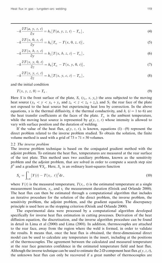
Here S is the front surface of the plate, S1 (zh , x, yh ) the area subjected to the movingheat source (y0 5 y 5 y0 � yh and z0 5 z 5 z0 � zh ), and S2 the rear face of the platenot exposed to the heat source but experiencing heat loss by convection. In the aboveequations, a is the thermal diffusivity, k the thermal conductivity, and hi (i � 1 to 6) arethe heat transfer coefficients at the faces of the plate. T1 is the ambient temperature,while the moving heat source is represented by q(y, z, t) whose intensity is allowed tovary with surface position and the duration of welding.

If the value of the heat flux, q(y, z, t), is known, equations (1) ^ (9) represent thedirect problem related to the inverse problem studied. To obtain the solution, the finitevolume method is used with a grid of 73671650 volumes.

2.2 The inverse problemThe inverse problem technique is based on the conjugated gradient method with theadjoint problem. To estimate the heat flux, temperatures are measured at the rear surfaceof the test plate. This method uses two auxiliary problems, known as the sensitivityproblem and the adjoint problem, that are solved in order to compute a search step sizeb k and a gradient HSq . Here, Sq is an ordinary least-squares function

Sq �� tf

t�0�Y�t� ÿ T�xi ; t��2dt , (10)

where Y�t� is the measured temperature, T(xi , t) is the estimated temperature at a singlemeasurement location, xi , and tf the measurement duration (Ozisik and Orlande 2000).The heat flux can then be estimated through a computational algorithm that includesan iterative procedure for the solution of the direct problem, the inverse problem, thesensitivity problem, the adjoint problem, and the gradient equation. The discrepancyprinciple is used here as the stopping criterion (Ozisik and Orlande 2000).

The experimental data were processed by a computational algorithm developedspecifically for inverse heat flux estimation in cutting processes. Derivation of the heatdiffusion equation, the discretisation, and the inverse algorithm procedure can be foundin detail in Lima et al (2000) and Lima (2001). In addition, thermocouples are attachedto the rear face, away from the region where the weld is formed, in order to validatethe results. It means that, once the heat flux is obtained, the three-dimensional directmodel can be used to calculate any temperature in the insert, including at the positionsof the thermocouples. The agreement between the calculated and measured temperatureat the rear face generates confidence in the estimated temperature field and heat flux.Although the inverse technique can be used to estimate the 2-D component heat flux q(y, z, t),the unknown heat flux can only be recovered if a great number of thermocouples are

Heat flux in gas ^ tungsten-arc welding 119

used in the y and z directions. In this work, keeping in mind that the behaviour of theGTA torch has little spatial change and the main interest is in its average value,q(y, z, t) is assumed a priori as a q(y, t) heat flux. This means that the heat fluxobtained here represents an average over the bead width (constant in z direction) as infigure 1. The bead width is obtained for each experiment individually. This procedure isdiscussed in the next section.

3 Experimental procedureFigure 2 represents the welding rig used in the experimental procedure. The GTA torch,representing a point heat source, moves at a specific speed along a straight path, withthe use of a totally automated X ^ Y coordinate table. To avoid test-plate dimension

Shieldinggas

Voltage and Coordinatedcurrent acquisition table control

Power

supp

ly

Welding plate

Coordinatedtable

Thermocouples

Multimeter

HP7500

0Multimeter

control

Figure 2. Schematic representation of the experimental rig.

GTA torch

Test plate

To powersupply

Ground cable

Support

To DASFigure 3. Schematic diagram showingthe test-plate support.

120 S M M Lima e Silva, L O Vilarinho, A Scotti, T H Ong, G Guimara¬ es

interference, the test plate was held suspended in air by four pointed cylindrical bars, sothat only very small contact area existed (figure 3).

Figure 4 shows how the ten type K thermocouples were located at the rear side ofthe test plate, ie at the face opposite to the bead (heat source). They were equally spacedfrom each other (16.7 mm), while the first was 25 mm from the test-plate edge.

Capacitor discharge was used to fix the ten type K thermocouples to the rear platesurface. The plate was of AISI 304 steel with dimensions of 200 mm650 mm64 mm.A detailed description of the procedure can be found in Vilarinho (2001). Collectionand storage of the data from the thermocouples was done with a microcomputer-baseddata-acquisition system (HP 75000 B E1326B), DAS for short. The DAS, under a soft-ware control, sampled (multiplexed) each thermocouple signal at intervals of 0.38 s(totaling 1028 points for each thermocouple).

A set of experiments with different welding conditions, such as current (40, 70, and100 A), arc length (2, 3, and 4 mm), gas (Ar and Ar� 25% He) and electrode angle(308, 608, and 708) was carried out. The electrode used was AWS EWTh-2, tungstendoped with 2% of thorium.

In order to reduce the number of experiments whilst keeping the results reliable,a statistical planning method Taguchi (Robust Project) with L9 matrix was used.

4 Analysis of resultsNine experiments were performed. The experimental conditions are listed in table 1.Four factors at three levels [electrode angle, length of the arc (LA), current, and shieldinggas] were used to obtain the optimal experimental matrix.

The width of the weld for each experimental condition was recorded with an imageanalyser, Neophot 21. The weld width determination is shown in figure 5 for the testA01 (sample 01). Figure 6 presents the voltage signs and current during the weldingprocess for this test.

The values of the thermal properties of AISI 304 (considered constant) were obtainedfrom the literature (Incropera and DeWitt 1996): thermal conductivity was taken as equalto 14.9 W mKÿ1 and thermal diffusivity as equal to 3:95610ÿ6 m2 sÿ1. The coefficient of

2525

50

25 16.7 16.7 16.7 16.7 16.7 16.7 16.7 16.7 16.7 25

1 2 3 4 5 6 7 8 9 10

Figure 4.Thermocouple positions in test plate, at the rear of the weld (all dimensions are in millimetres).

Table 1. Test conditions.

Test Electrode angle=8 Arc length=mm Current=A Shielding gas Bead width=mm

A01 30 2 40 Ar 2A02 30 3 70 Ar� 25% He 3A03 30 4 100 Ar� 25% He 4A04 60 2 70 Ar� 25% He 3A05 60 3 100 Ar 4A06 60 4 40 Ar� 25% He 2A07 90 2 100 Ar� 25% He 4A08 90 3 40 Ar� 25% He 2A09 90 4 70 Ar 3

Heat flux in gas ^ tungsten-arc welding 121

heat transfer by convection was also taken as constant and equal to 15 W mÿ2 Kÿ1 forall the surfaces. It should be noted that this value represents an average value obtainedfrom empirical correlation (Incropera and DeWitt 1996) for specific geometry and thetemperature.

A mesh of 73671650 volumes in the respective directions of y, z, and x has beenconstructed so as to coincide with the position of each thermocouple and its respectivecontrol volume. Figure 7 shows the measured temperatures at the rear surface of thetest plate A02 (sample 02). The time for all tests (table 1) was about 25 s. In figure 7 onlythe first 149 points are shown.

Figure 8 shows the heat input rate estimated at the surface calculated from theexperimental temperatures shown in figure 7. The estimated heat input rate for the mostsevere welding condition (test A03) is shown in figure 9.

It is seen in figure 7 that, although the maximum temperatures fluctuate around anaverage temperature, the dispersion is significant. This dispersion at the rear side isresponsible for a deviation in the estimated power of the order of 35 W (test A03).An investigation of this behaviour can indicate, in the future, procedures for optimisingwelding processes and obtaining more stable effective power.

(a) (b)

Dark-etchingregion

Bead width

Weld pool

2 mm

Figure 5.Weld bead: (a) measured dimensions, (b) view from above.

100

80

60

40

20

0

Current=A

15

10

5

0

Voltage=V

2000 2010 2020 2030 2040 2050 2000 2010 2020 2030 2040 2050Time=ms Time=ms

Figure 6.Welding voltage and current.

Thermocouple400

350

300

250

200

150

100

50

0

Exp

erim

entaltempe

rature=8C

1 3 5 7 9

2 4 6 8 10

0 10 20 30 40 50 60Time=s

Figure 7. Temperature evolution at the surfaceat the rear of the weldötest A02.

122 S M M Lima e Silva, L O Vilarinho, A Scotti, T H Ong, G Guimara¬ es

Figure 10 shows the heat flux field at the welding face in test A03, at the instants of7.98 s, 10.64 s, 14.06 s, and 17.86 s. One can see the effect of the speed of the movingsource as well as the stability of the estimated heat flux. One can also see the symmetryeffect related to the direction of the moving source.

The behaviour of the estimated components of the heat flux can be better seen infigure 11 for four specific positions, those of thermocouples 2, 4, 7, and 9. The effect ofthe heat source moving in the y direction can also be noticed.

The comparison between the estimated and experimental temperatures at threepositions for the severe welding condition is shown in figure 12. There is a reasonableagreement of the experimental and estimated temperatures with deviations of 9%, 3.3%,and 4.4% of the maximum values. Several factors can be responsible for these smalldiscrepancies, for example, the assumptions of constant values for the thermal propertiesand the assumed coefficient of heat transfer by convection in the theoretical model.

800

700

600

500

400

300

200

100

0Estim

ated

heat

inpu

trate=W

0 10 20 30 40 50 60Time=s

Figure 9. Estimated heat input rate in severeconditions (test A03).

600

500

400

300

200

100

0

Estim

ated

heat

inpu

trate=W

0 10 20 30 40 50 60Time=s

Figure 8. Estimated heat input rate in test A02.

30

27

24

21

30

27

24

21

z=mm

z=mm

50 100 150 200 50 100 150 200y=mm y=mm

(a) (b)

(c) (d)

Heat flux=W mÿ2

9597966

8958101

8318237

7678372

7038508

6398644

5758779

5118915

4479051

3839186

3199322

2559457

1919593

1279729

639864

Figure 10. Heat flux field in welding at the following instants: (a) 7.98 s, (b) 10.64 s, (c) 14.06 s,and (d) 17.86 s.

Heat flux in gas ^ tungsten-arc welding 123

Besides, effects such as phase change and heat losses by radiation have not been takeninto account. A theoretical model that takes account of all these aspects is beingdeveloped.

All the same, the results obtained here are promising. They show that the experimentalmethodology is adequate and that it is necessary to optimise the thermal model.

It is also seen that the use of a discrete model (space and time) for the moving heatsource is appropriate in analysing a thermal phenomenon. This represents, in fact,an advance over the three-dimensional model of Rosenthal which is based on a quasi-stationary state and constant heat source. An a priori assumption of constant powerdoes not allow a real investigation of the effective power delivered to the plate.

12

10

8

6

4

2

0

ÿ2ÿ4

12

10

8

6

4

2

0

ÿ2ÿ4

Heatflux=10ÿ

6W

mÿ2

Heatflu

x=10ÿ6

Wmÿ2

0 10 20 30 40 50 60 0 10 20 30 40 50 60Time=s Time=s

(a) position 2 (b) position 4

(c) position 7 (d) position 9

Figure 11. Estimated heat flux at four different thermocouple positions.

450

400

350

300

250

200

150

100

50

0

T=8C

Thermocouple

2 5 8

experimentalmodel

0 10 20 30 40 50 60Time=s

Figure 12. Comparison of calculated and measuredtemperatures at the surface of the rear of the weld forthermocouples 2, 5, and 8.

124 S M M Lima e Silva, L O Vilarinho, A Scotti, T H Ong, G Guimara¬ es

5 Statistical planning methodThe statistical planning method, Taguchi, was made through a L9 matrix in order to reducethe number of experiments. The method uses the average heat input rate for each experi-mental condition (table 1). This average heating rate is used to obtain the thermal efficiency

Z � q

VI, (12)

where V is the voltage, I is the current, and q the average heat input rate or effectivepower. Table 2 shows for each test, the average voltage and current, Vm and Im respec-tively, the calculated total power, Pt , the estimated heat input rate, q, and the calculatedthermal efficiency, Z.

With the thermal efficiency, Z, for each test (table 2), the larger-the-better functionof the Robust Planning of Taguchi was used to analyse the results. In the analysis, thevariable z was defined to relate thermal efficiency through the following equation

z � 8:6859 ln Zÿ 3610ÿ6 . (13)

Figure 13 shows the variation of z for the four factors studied. It can be seen thatmaximum efficiency should be obtained when the electrode angle is 308, the arc lengthis 2 mm, the current is 40 A, and the gas used is Ar� 25% He. This combination wasthen executed in test A10. The results obtained are presented in table 3. It is seen thatthe efficiency found in test A10, of 86.2%, is very close to the maximum thermalefficiency, 86.9%, obtained in previous tests (table 2). This procedure eliminates the needfor a larger number of experiments.

Table 2. Heat input rate and thermal efficiency for each test.

Test Electrode Arc length Shielding Im =A Vm =V Total q (average heat Z=%angle=8 /mm gas power=W input rate)=W

A01 30 2 Ar 41 8.2 336 280 83.4A02 30 3 Ar� 25% He 71 9.8 696 516 74.2A03 30 4 Ar� 25% He 102 10.8 1102 766 69.5A04 60 2 Ar� 25% He 71 9.0 639 486 76.1A05 60 3 Ar 101 9.6 970 573 59.1A06 60 4 Ar� 25% He 40 10.6 424 291 68.6A07 90 2 Ar� 25% He 101 8.5 859 572 66.6A08 90 3 Ar� 25% He 41 10.4 426 371 86.9A09 90 4 Ar 71 9.7 689 496 72.0

38.0

37.8

37.6

37.4

37.2

37.0

36.8

36.6

36.4

36.2

36.0

z

30 60 90 2 3 4 40 70 100 Ar Ar� 25%HeElectrode Arc length Current=A Shieldingangle=8 =mm gas

Figure 13. Statistical Taguchi results.

Heat flux in gas ^ tungsten-arc welding 125

6 ConclusionsThe use of the inverse heat conduction problem techniques to determine temperaturefields, heat input rate, and thermal efficiency in the GTA welding process is presented.The heat rate at the weld surface has been estimated by using the conjugated gradientmethod with the adjoint equation. The experimental technique is seen to be adequate inspite of not accounting for the effects of phase change and heat losses by radiation. It isseen that the values found for the thermal efficiency indicate the potential of the methodas an alternative to techniques based on calorimeters.

Acknowledgements.We would like to thank Fapemig and CNPq Government Agencies for financialsupport of this work. The technical support of Frederico R S Lima was invaluable.

ReferencesGonc° alves V C, Scotti A, Guimara¬ es G, 2002 ` Simulated annealing inverse technique applied in

welding: A theoretical and experimental approach'', paper presented at the 4th InternationalConference on Inverse Problems in Engineering, Angra dos Reis, Rio de Janeiro, Brazil

Hsu Y, Rubnski B, Mahin K, 1986 `An inverse finite element method for the analysis of stationaryarc welding process''ASME Journal of Heat Transfer 108 734 ^ 741

Incropera F P, De Witt D P, 1996 Fundamentals of Heat and Mass Transfer 4th edition (New York:John Wiley)

Katz M, Rubinsky B, 1984 `An inverse finite element technique to determine the change of inter-face location in one-dimensional melting problem'' Numerical Heat Transfer 7 269 ^ 283

Lima F R S, Machado A, Guimara¬ es G, Guths S, 2000 ` Numerical and experimental simulationfor heat flux and cutting temperature estimation using three-dimensional inverse heat con-duction technique'' Inverse Problems in Engineering 553 ^ 577

Lima F R S, 2001 Three-dimensional Modeling of Inverse Heat Conduction Problems: Applicationin Machining Problems PhD thesis, Federal University of Uberlaª ndia, Uberlaª ndia, MG, Brazil(in Portuguese)

Ozisik M N, Orlande H R B, 2000 Inverse Heat Transfer: Fundamentals and Applications (NewYork:Taylor and Francis)

Rosenthal D, 1935 ` Eè tude theorique du regime thermique pendant la soudure a© l'arc'', Congre© sNational des Sciences, Comptes Rendus Bruxelles, Volume 2, page 1277

Vilarinho L O, 2001 Assessment of Shielding Gases by Means of Numerical and ExperimentalTechniques Qualification Examination, La prosolda no.10/2001, Federal University ofUberlaª ndia, Uberlaª ndia, MG (in Portuguese)

ß 2003 a Pion publication

Table 3. Results of test A10.

Test Electrode Arc length Shielding Im =A Vm =V Ptotal =W q (average heat Z=%angle=8 /mm gas input rate)=W

A10 30 2 Ar� 25% He 41 9.2 375 323 86.2

126 S M M Lima e Silva, L O Vilarinho, A Scotti, T H Ong, G Guimara¬ es