H.Asano dissertation - Brookhaven National Laboratory
172
Nuclear modification of electron yields from charm and bottom hadrons in Au+Au collisions at √ s NN = 200 GeV Hidemitsu Asano Depertment of Physics, Kyoto University A dissertation submitted in partial fulfillment of the requirements for the degree of Doctor of Science Janually, 2015
-
Upload
khangminh22 -
Category
Documents
-
view
3 -
download
0
Transcript of H.Asano dissertation - Brookhaven National Laboratory

Nuclear modification of electron yieldsfrom charm and bottom hadrons in
Au+Au collisions at √sNN
= 200 GeV
Hidemitsu Asano
Depertment of Physics, Kyoto University
A dissertation submitted in partial fulfillment of therequirements for the degree of Doctor of Science
Janually, 2015

Contents
List of Figures iv
List of Tables ix
Acronyms and Abbreviations x
Nomenclatures xi
Abstract i
1 Overview 1
2 Quark Gluon Plasma and Heavy Ion Collision 42.1 Quark Gluon Plasma . . . . . . . . . . . . . . . . . . . . . . . 42.2 High energy Heavy Ion Collision experiment . . . . . . . . . . 7
2.2.1 Nuclear stopping power . . . . . . . . . . . . . . . . . . 72.2.2 Picture of space-time evolution . . . . . . . . . . . . . 82.2.3 Collision Geometry . . . . . . . . . . . . . . . . . . . . 112.2.4 Nuclear Modification Factor: RAA . . . . . . . . . . . . 14
2.3 States of created matter at RHIC . . . . . . . . . . . . . . . . 142.3.1 Jet quenching and energy loss . . . . . . . . . . . . . . 142.3.2 Collectivity of the QGP . . . . . . . . . . . . . . . . . 192.3.3 Temperature of the created matter . . . . . . . . . . . 21
3 Heavy quark as a probe of the QGP 243.1 Heavy flavor hadron production . . . . . . . . . . . . . . . . . 253.2 Decay of charm and bottom hadrons . . . . . . . . . . . . . . 283.3 Heavy flavor hadron measurement in RHIC and the LHC . . . 31
3.3.1 Overview of heavy flavor measurement . . . . . . . . . 313.3.2 Single electron measurements at PHENIX . . . . . . . 313.3.3 Electron-hadron correlation . . . . . . . . . . . . . . . 353.3.4 Direct reconstruction measurement . . . . . . . . . . . 36
i

3.3.5 Non-prompt J/ψ measurement . . . . . . . . . . . . . 373.3.6 Separating charm and bottom . . . . . . . . . . . . . . 39
3.4 Energy loss of heavy quark in the QGP . . . . . . . . . . . . . 393.4.1 Dead Cone effect . . . . . . . . . . . . . . . . . . . . . 393.4.2 Recent theoritical development . . . . . . . . . . . . . 40
3.5 Motivation of separating charm and bottom . . . . . . . . . . 43
4 Experiment 454.1 Relativistic Heavy Ion Collider (RHIC) . . . . . . . . . . . . . 454.2 PHENIX experiment . . . . . . . . . . . . . . . . . . . . . . . 48
4.2.1 Detector Overview . . . . . . . . . . . . . . . . . . . . 484.2.2 Beam-Beam Counter and trigger . . . . . . . . . . . . 504.2.3 Central arms . . . . . . . . . . . . . . . . . . . . . . . 514.2.4 Drift Chamber . . . . . . . . . . . . . . . . . . . . . . 514.2.5 Pad Chamber . . . . . . . . . . . . . . . . . . . . . . . 524.2.6 Ring Imaging Čherenkov Detector . . . . . . . . . . . . 544.2.7 Electromagnetic Calorimeter . . . . . . . . . . . . . . . 56
4.3 Data Acquisition . . . . . . . . . . . . . . . . . . . . . . . . . 584.4 Silicon Vertex Tracker Upgrade . . . . . . . . . . . . . . . . . 60
5 Analysis 675.1 Overview . . . . . . . . . . . . . . . . . . . . . . . . . . . . . . 675.2 Track reconstruction in Central arms . . . . . . . . . . . . . . 685.3 Electron identification . . . . . . . . . . . . . . . . . . . . . . 685.4 Event reconstruction in VTX . . . . . . . . . . . . . . . . . . 71
5.4.1 VTX alignment . . . . . . . . . . . . . . . . . . . . . . 715.4.2 VTX hit reconstruction . . . . . . . . . . . . . . . . . . 715.4.3 The primary vertex reconstruction . . . . . . . . . . . 725.4.4 Association of a central arm track with VTX . . . . . . 72
5.5 Event selection . . . . . . . . . . . . . . . . . . . . . . . . . . 765.5.1 z-vertex selection . . . . . . . . . . . . . . . . . . . . . 765.5.2 Data quality assurance . . . . . . . . . . . . . . . . . . 76
5.6 DCA measurement with the VTX . . . . . . . . . . . . . . . . 785.6.1 DCAT and DCAL . . . . . . . . . . . . . . . . . . . . . 785.6.2 DCA distribution of hadron tracks . . . . . . . . . . . 78
5.7 Electron DCA distribution and Background Components . . . 825.7.1 Overview . . . . . . . . . . . . . . . . . . . . . . . . . 825.7.2 Mis-identified hadron . . . . . . . . . . . . . . . . . . . 825.7.3 High-multiplicity background . . . . . . . . . . . . . . 835.7.4 Photonic electrons and conversion veto cut . . . . . . . 865.7.5 Ke3 . . . . . . . . . . . . . . . . . . . . . . . . . . . . . 93
ii

5.7.6 Quarkonia . . . . . . . . . . . . . . . . . . . . . . . . . 935.8 Normalization of electron background components . . . . . . . 945.9 Unfolding . . . . . . . . . . . . . . . . . . . . . . . . . . . . . 97
5.9.1 Overwiew . . . . . . . . . . . . . . . . . . . . . . . . . 975.9.2 Unfolding method . . . . . . . . . . . . . . . . . . . . . 985.9.3 Modeling the likelihood function . . . . . . . . . . . . . 995.9.4 Decay model and matrix normalization . . . . . . . . . 1005.9.5 Regularization/prior . . . . . . . . . . . . . . . . . . . 1055.9.6 Parent charm and bottom hadron yield and their sta-
tistical uncertainty . . . . . . . . . . . . . . . . . . . . 1065.10 Systematic uncertainties . . . . . . . . . . . . . . . . . . . . . 108
6 Results 1126.1 Invariant yield of charm and bottom hadron . . . . . . . . . . 1126.2 Bottom electron fraction . . . . . . . . . . . . . . . . . . . . . 1136.3 RAA of charm electrons and bottom electrons . . . . . . . . . 114
7 Discussion 1187.1 Re-folded comparisons to data . . . . . . . . . . . . . . . . . . 1187.2 Comparison with STAR D0 yield measurement . . . . . . . . . 1227.3 Comparison with theoretical models . . . . . . . . . . . . . . . 124
8 Conclusion 128
Acknowledgements 130
Appendix A Detailed Normalization of electron background com-ponents 132A.1 Photonic electrons simulation . . . . . . . . . . . . . . . . . . 132A.2 Fraction of nonphotonic electrons FNP . . . . . . . . . . . . . 137A.3 Normalization of Dalitz and conversion components . . . . . . 140A.4 Normalization of Ke3 and quarkonia components . . . . . . . . 142
Appendix B Coordinate offset and coordinate offset calibration143
Bibliography 145
iii

List of Figures
2.1 Summary of measurements of αs as a function of the momen-tum transfer Q. . . . . . . . . . . . . . . . . . . . . . . . . . . 5
2.2 Lattice QCD results from Hot QCD collaboration [1] . . . . . 62.3 The net-proton (number of protons − number of anti-protons)
rapidity distribution at AGS, SPS and RHIC measured byBRAHMS. . . . . . . . . . . . . . . . . . . . . . . . . . . . . 8
2.4 Time evolution of heavy ion collision from initial nucleus-nucleus collision to hadronic freeze out . . . . . . . . . . . . . 8
2.5 Parton distribution function times Bjorken-x as a function ofBjorken-x obtained in NNLO NNPDF2.3 global analysis [2, 3] 9
2.6 Energy density as a function of the number of participants Np
from PHENIX data [4]. . . . . . . . . . . . . . . . . . . . . . . 102.7 pT spectrum of inclusive charged hadrons and explanation
from fragmentation and recombination process. . . . . . . . . 112.8 Geometry of a collision between nucleus A and B. . . . . . . . 132.9 An illustrated example of the relationship of the impact pa-
rameter (b), Npart, overlap area of colliding nucleus, the mul-tiplicity distribution and centrality taken from [5]. . . . . . . . 15
2.10 Number of participants (Npart) and Number of binary colli-sions (Ncoll) for Au+Au and Cu+Cu collisions from GlauberMonte Carlo calculation [5]. . . . . . . . . . . . . . . . . . . . 16
2.11 Nuclear modification factor, RAA, for π0 in central (0-10%)and peripheral (80-92%) Au+Au collisions and minimum-biasd+Au collisions at mid-rapidity. . . . . . . . . . . . . . . . . . 18
2.12 Illustration of the collision geometry in a non-central heavyion collision. . . . . . . . . . . . . . . . . . . . . . . . . . . . . 19
2.13 Illustration of pressure gradient originated from spatial asym-metry of reaction zone. . . . . . . . . . . . . . . . . . . . . . 20
2.14 STAR measurement of v2 with hydrodynamical predictions forminimum bias Au+Au at √s
NN= 200 GeV from [6] . . . . . . 21
iv

2.15 Invariant cross section (p+p) and invariant yield (Au+Au) ofdirect photons as a function of pT . . . . . . . . . . . . . . . . 22
2.16 Electron pair mass distribution for p+p and Au+Au (Mini-mum Bias). . . . . . . . . . . . . . . . . . . . . . . . . . . . . 23
3.1 Schematic view of time evolution of heavy quarks. . . . . . . 243.2 Charm and bottom quark production cross section as a func-
tion of center of mass energy in p+p or p̄+ p collisions. . . . . 273.3 Electron from heavy flavor yield (0.8 < pT < 4.0 GeV/c ) mea-
sured in Au+Au collision at √sNN
= 200 GeV scaled by thenumber of binary collisions (Ncoll). The yield in p+p collisionsis also shown. . . . . . . . . . . . . . . . . . . . . . . . . . . . 28
3.4 PHENIX measurement of RAA and v2 of electron from heavyflavor from 2004/2005 data. . . . . . . . . . . . . . . . . . . . 33
3.5 The nuclear modification factors for heavy flavor electron atmidrapidity in central d+Au, Cu+Cu, and Au+Au collisionsat √s
NN= 200 GeV with PHENIX. . . . . . . . . . . . . . . 35
3.6 The azimuthal angle between heavy flavor electrons and hadronsmeasured with STAR in p+p collisions and relative contribu-tions of bottom decays to the total yield of electrons fromheavy flavor hadron decays as functions of the electron pT . . . 37
3.7 Centrality dependence of the D0 pT differential invariant yieldwith STAR in Au+Au collisions. . . . . . . . . . . . . . . . . 38
3.8 The ratio of gluon spectra off charm and light quarks for trans-verse quark momenta p⊥ = 10 GeV/c and p⊥ = 100 GeV/cin QGP matter from Ref.[7]. . . . . . . . . . . . . . . . . . . 40
3.9 The differential cross section per nucleon pair of charm andbottom quarks calculated to NLO in QCD compared to singleelectron distributions calculated with the fragmentation anddecay scheme of Ref.[8]. . . . . . . . . . . . . . . . . . . . . . 43
4.1 Au ion pass through three accelerators (Tandem Van de Graaff,AGS Booster, and AGS) and four charge-stripping stations toprepare the fully stripped Au ions for injection to the RHICring [9]. . . . . . . . . . . . . . . . . . . . . . . . . . . . . . . 46
4.2 A schematic view of the PHENIX detector configuration forthe 2011 run. . . . . . . . . . . . . . . . . . . . . . . . . . . . 48
4.3 PHENIX global coordinate system. . . . . . . . . . . . . . . . 494.4 A picture of Beam-Beam counters . . . . . . . . . . . . . . . . 504.5 A schematic view of Drift Chameber . . . . . . . . . . . . . . 52
v

4.6 The layout of DCH wire position within one sector and in-side the anode plane and top view of the DCH stereo wireorientations. . . . . . . . . . . . . . . . . . . . . . . . . . . . . 53
4.7 The pad and pixel geometry in the pad chamber. . . . . . . . 544.8 A cutaway view of one arm of the RICH detector [10]. . . . . . 554.9 Top view of the RICH in the PHENIX east arm [11]. . . . . . 554.10 Schematic view of a Pb-scintillator (PbCc) module . . . . . . 564.11 Schematic view of a Pb-glass (PbGl) module . . . . . . . . . . 574.12 A schematic diagram of the PHENIX Data Acquisition system. 584.13 A picture of the VTX detector and a schematic view fo the
VTX detector . . . . . . . . . . . . . . . . . . . . . . . . . . . 604.14 schematic view of a pixel sensor . . . . . . . . . . . . . . . . . 624.15 A schematic of the circuitry within one pixel cell in the AL-
ICE1LHCb sensor-readout chip. . . . . . . . . . . . . . . . . . 634.16 A picture of a pixel ladder and schematic view of a pixel ladder 634.17 A picture of a stripixel detector and Schematic view of a stripixel 644.18 X strips and U strips . . . . . . . . . . . . . . . . . . . . . . . 644.19 Conceptual schematic of a single SVX4 channel circuit. . . . . 65
5.1 Charged particle momentum vector reconstruction using DCHhit information [12]. . . . . . . . . . . . . . . . . . . . . . . . . 69
5.2 Matching variable between the reconstructed track momentum(p) and the energy measured in the EMCal (E): dep = (E/p−µE/p). . . . . . . . . . . . . . . . . . . . . . . . . . . . . . . . 70
5.3 The distributions for the difference in the primary vertex cal-culated from by the East and West VTX barrels (East - West)in x, y and z-axis . . . . . . . . . . . . . . . . . . . . . . . . . 73
5.4 An illustration of a tracking with the VTX in x-y plane. . . . 755.5 An illustration of a tracking with the VTX in r-z plane. . . . 755.6 Illustration of the definition of DCAT ≡ L - R in the transverse
plane. . . . . . . . . . . . . . . . . . . . . . . . . . . . . . . . 795.7 Distance of closest approach distributions for all VTX-associated
tracks in Au+Au at √sNN
= 200 GeV collisions . . . . . . . . 805.8 The DCAT resolution as a function of pT for all tracks in MB
events . . . . . . . . . . . . . . . . . . . . . . . . . . . . . . . 815.9 Simulated primary electron DCAT and DCAL distribution be-
fore and after embedding in real Au+Au data. . . . . . . . . . 855.10 Distribution of correlated hits near electron tracks for 1 <
pT < 2 GeV. . . . . . . . . . . . . . . . . . . . . . . . . . . . 885.11 charge x ∆φ vs pT for B0(top-left), B1(top-right), B2(bottom-
left), B3(bottom-right). . . . . . . . . . . . . . . . . . . . . . 89
vi

5.12 The survival rate as a function of electron pT (peT ) for electronsfrom photon conversion, Dalitz decay of π0, η, electron fromdirect photon and heavy flavor decay electrons. . . . . . . . . 92
5.13 DCAT distributions for electrons in MB Au+Au at√sNN
= 200 GeVthat pass the reconstruction and conversion veto cut in theindicated five electron-pT selections. Also shown are the nor-malized contributions for the various background componentsdetailed in Section 5.7. . . . . . . . . . . . . . . . . . . . . . 96
5.14 The decay matrix encoding the probability for charmed hadronsdecaying to electrons within |η| < 0.35 as a function of bothelectron pT (peT ) and charm hadron pT (pcT ) and an exampledecay matrix. . . . . . . . . . . . . . . . . . . . . . . . . . . . 103
5.15 The probability for (a) charm and (b) bottom hadrons in agiven range of hadron pT (pcT and pbT for charm and bottomhadrons respectively) to decay to electrons at mid-rapidity asa function of electron pT (peT ). . . . . . . . . . . . . . . . . . 104
5.16 The joint probability distributions for the vector of hadronyields, θ, showing the 2-D correlations between parameters.The diagonal plots show the marginalized probability distri-butions for each hadron pT bin. . . . . . . . . . . . . . . . . . 107
5.17 The relative contributions from the different components tothe uncertainty on the fraction of electrons from bottom hadrondecays as a function of pT . . . . . . . . . . . . . . . . . . . . 110
6.1 Charm (hc) and bottom (hb) hadron invariant yield as a func-tion of pT , integrated over all rapidities. . . . . . . . . . . . . 113
6.2 The fraction of heavy flavor electrons from bottom hadrondecays as a function of pT from this work and from fonllp+p calculations [8]. . . . . . . . . . . . . . . . . . . . . . . . 114
6.3 bottom electron fraction as a function of pT compared to mea-surements in p+p collisions at
√s= 200 GeV from PHENIX [13]
and STAR [14]. Also shown are the central values for fonll[8] for p+p collisions at √s
NN= 200 GeV. . . . . . . . . . . . 115
6.4 (a) The RAA for c→ e, b→ e and combined heavy flavor [11]as a function of peT . (b) The ratio Rb→e
AA /Rc→eAA as a function of
peT . . . . . . . . . . . . . . . . . . . . . . . . . . . . . . . . . 117
7.1 The heavy flavor electron invariant yield as a function of pTfrom measured data [11] compared to electrons from the re-folded charm and bottom hadron yields. . . . . . . . . . . . . 120
vii

7.2 The DCAT distribution for measured electrons compared tothe decomposed DCAT distributions for background compo-nents, electrons from charm decays, and electrons from bottomdecays. . . . . . . . . . . . . . . . . . . . . . . . . . . . . . . 121
7.3 The invariant yield of D0 mesons as a function of pT for |y| < 1inferred from the unfolded yield of charm hadrons integratedover all rapidity compared to measurements from STAR [15]. 123
7.4 Bottom electron fraction as a function of pT compared to aseries of model predictions detailed in the text. . . . . . . . . . 124
A.1 Electrons’ vertex position in radial direction in π0 simulationbefore the application of conversion veto. . . . . . . . . . . . 134
A.2 The ratio of conversion electrons to electrons from Dalitz decayfrom π0 simulation as a function of reconstructed electron pT . 135
A.3 Diagram of Dalitz decay of η meson. . . . . . . . . . . . . . . 137A.4 The fraction of π0, η, and direct photon Dalitz decay electrons
in all Dalitz electrons as a function of electron pT (peT ). . . . . 139A.5 The fraction of nonphotonic electrons to inclusive electrons as
a function of electron pT (peT ). . . . . . . . . . . . . . . . . . 140A.6 The fraction of π0, η, and direct photon electrons in all pho-
tonic electrons as a function of electron pT (peT ). . . . . . . . 141
B.1 (Left) the vtx local coordinate system for the WEST VTX andthe EAST VTX. (Right) the schematic view when the VTXis retracted. . . . . . . . . . . . . . . . . . . . . . . . . . . . 143
B.2 Parameters of DC hit information and beam center positionin the DCH coordinate system. . . . . . . . . . . . . . . . . . 144
viii

List of Tables
3.1 Decay modes, Branching ratios (B.R.), decay momentum∗ (p)and life times for main charm hadrons from PDG [3]. Chargeconjugates are abbreviated. . . . . . . . . . . . . . . . . . . . 29
3.2 The same as table 3.1 but for bottom hadrons from PDG [3].Charge conjugates are abbreviated. . . . . . . . . . . . . . . . 30
4.1 Summary of data sets with collision species, collision energy,and integrated luminosity delivered to PHENIX. . . . . . . . 47
4.3 A summary of the VTX detector. For each layer (B0 to B3),the detector type, read out chip, the central radius (r), ladderlength (l), sensor thickness (t), sensor active area (∆φ×∆z),the number of sensors per ladder (NS), the number of lad-ders (NL), pixel/strip size in φ (∆φ) and z (∆z), the numberof read-out channels (Nch), and the average radiation lengthincluding the support and on-board electronics (X0) are given. 61
4.4 Occupancy of the each VTX layer for central Au+Au collisionsat 200 GeV . . . . . . . . . . . . . . . . . . . . . . . . . . . . 66
7.1 The log likelihood values (LL) summed over each DCAT dis-tribution and for the comparison to the heavy flavor electroninvariant yield. . . . . . . . . . . . . . . . . . . . . . . . . . . 119
ix

Acronyms and Abbreviations
Acronyms and abbreviations used in this dissertation:
AGS Alternating Gradient Synchrotron.
ALICE A Large Ion Collider Experiment (at the LHC).BBC Beam-Beam Counters (subsystem of PHENIX).
BNL Brookhaven National Laboratory.
BRAHMS Broad RAnge Hadron Magnetic Spectrometers (experiment atRHIC).
CMS Compact Muon Solenoid (experiment at the LHC).DCA Distance of Closest Approach.
DCH Drift Chamber (subsystem of PHENIX).EMCal Electromagnetic Calorimeter (subsystem of PHENIX).LHC Large Hadron Collider.
LHCb Large Hadron Collider beauty experiment.MB Minimum Bias.PC Pad Chamber (subsystem of PHENIX).
PDF Parton Distribution Function.
PHENIX Pioneering High Energy Nuclear Interaction eXperiment (at RHIC).
pQCD pertavative Quantum Chromodynamics.QCD Quantum Chromodynamics.
QGP Quark Gluon Plasma.RHIC Relativistic Heavy Ion Collider.
RICH Ring Image Čherenkov Detector (subsystem of PHENIX).SPS Super Proton Synchrotron (CERN).
STAR Solenoidal Tracker at RHIC (experiment).VTX Silicon Vertex Tracker (subsystem of PHENIX).
x
Nomenclatures
Nomenclatures used in this dissertation:
Ncoll Number of binary collisions.
Npart Number of participants.
NN Nucleon-Nucleon (collision).
pT transverse momentum.√s
NNCenter of energy per nucleon pair.
Tc psudocritical temperature.
DCAL DCA along the beam axis.
DCAT DCA in transverse plane.
xi
Abstract
This dissertation details the measurement of electrons from semileptonicdecay of charm and bottom hadrons from Au+Au collisions at √s
NN= 200
GeV by using the PHENIX detector in the relativistic heavy ion collider(RHIC).
Heavy quarks (charm or bottom) are one of suitable probes of a QuarkGluon Plasma (QGP). Due to their large masses, the production process ofheavy quarks is restricted to initial nucleon-nucleon collisions. Thus, heavyquarks carry information about the entire time-evolution of the medium.
We previously measured the yields of electrons from semileptonic decaysof charm and bottom hadrons inclusively in Au+Au collisions at √s
NN= 200
GeV. It indicated substantial modification in the momentum distribution ofthe parent heavy quarks due to the QGP created in these collisions. However,at that time, PHENIX was not able to distinguish electrons from charm andbottom hadrons independently. In order to understand these medium effectsin more detail, the separation of electrons from charm and bottom hadronsare aimed to reveal the mass dependence of energy loss in the medium.
For the first time, by using the Silicon Vertex Tracker (VTX) installedin PHENIX to measure precision displaced tracking, we have succeeded inseparating the electrons from charm and bottom hadrons in Au+Au collisionsat √s
NN= 200 GeV in the transverse momentum (pT ) from 1 GeV/c to 8
GeV/c at midrapidity region (|η| < 0.35). The invariant yield of charmand bottom hadrons as a function of pT were calculated. Based on thisseparation, the fraction of the electrons from bottom hadrons were obtained.Further, by using that for p+p collision, the nuclear modification factor RAA
was extracted both for charm and bottom electrons.We have observed that bottom electron is suppressed for higher pT region
(pT > 4 GeV/c ) in Au+Au collisions compared to p+p collisions for the firsttime in RHIC energy. While the magnitude of suppression is smaller thanthat of charm in the region of 3 < pT < 4 GeV/c , it is similar for higher pTregion within systematic uncertainty.

Chapter 1
Overview
According to the lattice Quantum Chromodynamics (QCD) calculations [16,17], quarks and gluons are deconfined at the high temperature above ∼ 150MeV. To date, it is well established that heavy Ion collisions at the Relativis-tic Heavy Ion Collider (RHIC) and the Large Hadron Collider (LHC) createa new state of matter -QGP- that is described as an equilibrated system withinitial temperature in excess of 340 – 420 MeV [18–22].
This QGP follows hydrodynamical flow behavior with extremely smalldissipation, characterized by the shear viscosity to entropy density ratio η/sand is thus termed a near-perfect fluid [18, 23–25].
However, these recently established knowledge of QGP still raises newquestions about the property of QGP and how QCD works in this environ-ment.
Heavy flavor hadron (D,B) measurement has several advantages to lighthadrons (π,K...etc.) to investigate the property of the QGP because of theirspecific production mechanism. The heavy quarks (Q = c, b) are mainly pro-duced via hard scatterings at the initial nucleon-nucleon collisions, becausethe large momentum transfer is needed to produce heavy quarks [26]. Thisheavy quarks are clean probes which experience the entire time-evolution ofthe QGP as they pass through it.
The PHENIX collaboration has measured transverse momentum distri-bution of electrons1 from semileptonic decay of charm and bottom hadronsproduced in Au+Au collisions and observed it is significantly modified com-pared with p+p collisions from the year 2004/2005 data at RHIC. This resultwas unexpected, because in the perturbative QCD based calculation, par-ton energy loss in the QGP is believed to be dominated by gluon radiativeenergy loss [27], which was predicted much smaller for heavy quarks than
1 Here and throughout this dissertation, “electrons” is used to refer to both electronsand positrons.
1

Section CHAPTER 1. OVERVIEW
that for light partons [7]. In the past measurements before the year 2010,the PHENIX was not able to distinguish electrons from charm and bottomhadrons independently in Au+Au collisions.
In order to separate the contribution from charm and bottom, the PHENIXcollaboration has developed the silicon vertex tracker (VTX) [28] and in-stalled it covering at midrapidity region in 2010. The VTX was designedto give precise tracking reconstructions of the distance of closest approach(DCA) to the collision vertex. This enables the separation of electrons fromsemi-leptonic decay of charm and bottom hadrons statistically in Au+Aucollisions, because the decay kinematics and life time of charm (cτD0 = 123µm, cτD± = 312 µm) and bottom (cτB0= 455 µm, cτB± = 491 µm ) hadronsare different [3].
In the result, the suppression of electrons from bottom hadrons is observedfor higher pT region (pT > 4 GeV/c ) in Au+Au collisions compared to p+pcollisions for the first time in RHIC energy. It strongly implies bottom quarkssuffer energy loss in the QGP medium. The magnitude of suppression issmaller than that of charm in the region of 3 < pT < 4 GeV/c and similarfor higher pT region within systematic uncertainty. The new analysis methodusing the VTX detector was established and the same method can be appliedfor high statistics data taken in 2014/2015.
This dissertation details the first measurement of electrons from semilep-tonic charm and bottom hadron decays from Au+ Au collisions at √s
NN=
200 GeV in year 2011 using the VTX detector. The organization of this dis-sertation is as follows: In Chapter 2, physics backgrounds of the QGP andheavy ion collisions are reviewed.
In Chapter 3, heavy quark as a probe of the QGP and past measurementsat RHIC and the LHC are reviewed. In the measurements at RHIC, charmand bottom contribution was not separated. The motivation of charm/bottomseparation are also explained in this chapter.
In Chapter 4, the accelerator RHIC, the relevant PHENIX apparatus inyear 2011 and the VTX detector which was installed in the end of year 2010are introduced.
In Chapter 5, the analysis method to separate the contribution of elec-trons from charm and bottom using PHENIX central arms and the VTX areexplained. After that, the unfolding procedure using electron DCA distribu-tions and pT spectra are explained.
In Chapter 6, results of invariant yield of charm and bottom hadron,bottom electron fraction, and nuclear modification factor of charm electronsand bottom electrons in Au+Au collisions are shown.
Chapter 7 is for dicussions about these results. The consistency checkwith previously published results of invariant yield of heavy flavor electrons
2

Section CHAPTER 1. OVERVIEW
and STAR D0 measurement shown. After that, comparison of thereticalmodels are shown.
The conclusion of this measurement are described in Chapter 8.
Major ContributionsThe major part of this dissertaion is based on the published paper “Sin-
gle electron yields from semileptonic charm and bottom hadron decays inAu+Au collisions at √s
NN= 200 GeV by A. Adare et al.” [29]. The major
contributions of the author as a PHENIX collaborator are listed as follows:
• Construction, quality assurance and maintenance of pixel detectors (in-ner two layers of the VTX detector).
• Development of online monitoring system of pixel detectors.
• Commissioning and operation of the VTX detector during 2011 - 2014.
• Calibration of VTX sensors alignment.
• Establish the analysis method of electron DCA distributions using VTXdetector.
• Publication of the paper “Single electron yields from semileptonic charmand bottom hadron decays in Au+Au collisions at √s
NN= 200 GeV”
[29] with paper preparation group in PHENIX.
3

Chapter 2
Quark Gluon Plasma and HeavyIon Collision
This chapter is dedicated to giving a brief introduction to the QuarkGluon Plasma (QGP) and the high enegy heavy ion collision. In section2.1, the current understanding of QGP based on Quantum Chromodynamics(QCD) is reviewed. In section 2.2, the basic picture of space-time evolutionof the matter created in heavy ion collisions is described. After that thegeometry of collisions, which is important to understand the experimentalresults are explained. In the last section 2.3, the states of created matter inRHIC is explained from three important experimental results; jet quenching,strong collectivity, and temperature.
2.1 Quark Gluon PlasmaHigh energy Heavy Ion Collision experiments aim to create and investi-
gate the property of a high temperature matter which consists of deconfinedquarks and gluons. The new state of deconfined quarks and gluons is calleda QGP. QGP is expected based on the “Asymptotic freedom” property ofQCD. Asymptotic freedom was discovered in early 1970s by Gross, Wilczekand Politzer [30–32], and means that the QCD coupling constant αs de-creases with increasing the momentum transfer Q, as shown in Figure 2.1.The discovery of asymptotic freedom arises the expectation; asymptonic free-dom makes interaction at very short distances (or high momenta) arbitrarilyweak, so that if the temperature or net baryon density is high enough, atransition should occur from normal nuclear matter, where quarks and glu-ons are confined in hadrons, to the new state of matter where the quarks andgluons are deconfined [33, 34].
4

Section CHAPTER 2. QUARK GLUON PLASMA AND HEAVY IONCOLLISION
QCD αs(Mz) = 0.1185 ± 0.0006
Z pole fit
0.1
0.2
0.3
αs (Q)
1 10 100Q [GeV]
Heavy Quarkonia (NLO)
e+e– jets & shapes (res. NNLO)
DIS jets (NLO)
Sept. 2013
Lattice QCD (NNLO)
(N3LO)
τ decays (N3LO)
1000
pp –> jets (NLO)(–)
Figure 2.1: Summary of measurements of αs as a function of the momentumtransfer Q from PDG2014 [3]. Also shown in bottom is the αs value whenQ2 = Mz (Mz is Z boson’s mass, NLO: next-to-leading order; NNLO: next-to-next-to leading order; res.NNLO: NNLO matched with resummed next-to-leading logs; N3LO: next-to-NNLO).
Lattice QCD calculations predict that the transition from a low tempera-ture hadronic phase to a QGP phase should occur at a temperature of ∼ 150MeV for zero net baryon density. In early expectations, this transition couldbe first−order phase transition between normal nuclear matter and QGPphase. The QCD transition at finite-temperature and low baryon chemicalpotentials (µb) is, however, not a real phase transition, but a rapid crossover,meaning that it involves a rapid and smooth change, as opposed to a disconti-nuity, as the temperature is varied [35]. µb at RHIC (∼ 45 MeV [36]) is muchsmaller than typical hadron mass. Even though there is no well-defined sep-aration of phases because of the crossover behavior of the transition, recentlattice QCD results by Budapest-Wuppertal collaboration [37] and HotQCDcollaboration [1], for example, show that thermodynamic properties (pres-sure, energy density, and entropy density) really change rapidly around thecrossover region. Figure 2.2 shows the lattice QCD results on pressure, en-ergy density, and entropy density normalized by 1/T 4 by HotQCD Collabo-ration [1].
Instead of genuine critical temperature at which phase transition occurs,“pseudocritical temperature” is used to depict the phase diagram of QCD.
5

Section CHAPTER 2. QUARK GLUON PLASMA AND HEAVY IONCOLLISION
While there are several definitions of pseudocritical temperature Tc, an ex-ample of the pseudocritical temperature Tc= 154 ± 9 MeV is shown as avertical band in the Figure 2.2. This Tc is defined for chiral phase transition,at which up, down and strange quarks rapidly acquire their physical masses,taking chiral symmetry as order parameter [17]. There is another way todefine the Tc, for example, as the inflection point of ε/T 4 and (ε − 3p)/T 4,where p is the pressure and ε is energy density [16].
Figure 2.2: Lattice QCD results from Hot QCD collaboration [1]. The figureshows pressure, energy density, and entropy density normalized by 1/T 4 as afunction of the temperature. The dark lines show the prediction of the hadronresonance gas (HRG) model. The horizontal line at 95π2/60 corresponds tothe ideal gas limit for the energy density and the vertical band marks thecrossover region, Tc = 154± 9 MeV (see also texts) .
While deconfinement and chiral phase transition have not been directlyobserved in RHIC and the LHC experiments, there have been several exper-imental results which strongly indicate the creation of QGP. Three impor-tant observations which are understood as evidence of QGP found in Au+Aucollisions at RHIC, jet quenching, strong collectivity, and temperature arediscussed in section 2.3. An overview of the evidence for the creation of quark-gluon matter at RHIC can be found in those summary papers [18, 19, 38, 39]from four experiments at RHIC.
6

Section CHAPTER 2. QUARK GLUON PLASMA AND HEAVY IONCOLLISION
2.2 High energy Heavy Ion Collision experi-ment
2.2.1 Nuclear stopping power
In order to create a QGP state in heavy ion collisions, sufficient energymust be released from the two colliding nuclei into the QGP. The kineticenergy that is removed from the nuclei depends on the amount of stoppingpower between the colliding nuclei.
The stopping power can be estimated from the rapidity loss experiencedby the baryons in the colliding nuclei. The rapidity, y, of a particle is definedas:
y =1
2lnE + pzE − pz
,
where E and pz are energy and z component of momentum, respectively.The average rapidity loss, δy, is defined as the difference,δy = yp − 〈y〉
between the incoming beam rapidity yp and the average rapidity after thecollision which is expressed as [39].
〈y〉 =
∫ yp
0
ydN
dydy
/∫ yp
0
dN
dydy
Here dN/dy denotes the number of net-baryons (number of baryons minusnumber of antibaryons) per unit rapidity.
Figure 2.3 shows the measurement of net protons (number of protons −number of anti-protons) rapidity distribution at AGS (√s
NN= 5 GeV Au+Au),
SPS (√sNN
= 17 GeV Pb+Pb) and RHIC (√sNN
= 200 GeV Au+Au)data [40]. One can assume the rapidity distribution of net neutrons, netΛs, net Σs are similar with net protons. Thus the net proton distributionsrepresents the net baryon distributions.
The distributions yield a strong beam energy dependence as shown inFigure 2.3. At RHIC (red points), the distribution is almost flat up to y ∼ 3.It means incident nucleons do not lose all their kinetic energy and baryonchemical potential (µb) at RHIC (µb ∼ 25 [39] – 45 MeV [36]) is quite smallerthan AGS and SPS at midrapidity. In analogy to optics, it is often said thata nucleus becomes transparent in high energy collisions.
The average rapidity loss measured by BRAHMS is δy = 2.0± 0.1. Theenergy loss per participant nucleon is estimated to be ∼ 70 GeV from therapidity loss and transverse momentum spectra of baryons [40]. Thus, thetotal kinetic energy loss of two incoming nuclei at RHIC is estimated to be∼ 28 TeV (70 GeV× 2× 197) in most central 197Au +197 Au collision.
7

Section CHAPTER 2. QUARK GLUON PLASMA AND HEAVY IONCOLLISION
Figure 2.3: The net-proton (number of proton − number of anti-proton)rapidity distribution at AGS (green, Au+Au at √s
NN= 5 GeV), SPS (blue,
Pb+Pb at√sNN
= 17 GeV), and RHIC measured by BRAHMS (red, Au+Auat √s
NN= 200 GeV) [40]. The data are most central collisions (0-5 %
centrality. See subsection 2.2.3 for the definition of centrality). yp denotesbeam rapidity.
2.2.2 Picture of space-time evolution
The kinetic energy removed from two incoming nuclei is converted intoother degree of freedom. This subsection overviews the basic space-timepicture from initial collisions in partonic levels to freeze out in hadronicphase originated from the kinetic energies released in heavy ion collisions.Figure 2.4 is a simplified sketch of this sequence.
time
Au Au QGP mixed phase hadronic phase thermalization
hadronization hadronization
collision
Figure 2.4: Time evolution of heavy ion collision from initial nucleus-nucleuscollision to hadronic freeze out
In high energy heavy ion collisions, two incoming nuclei are Lorentz-contracted along the collision axis. Figure 2.5 shows the parton distributionfunctions (PDF), which describe the initial distribution of quarks and gluons
8

Section CHAPTER 2. QUARK GLUON PLASMA AND HEAVY IONCOLLISION
x
310
210
110 1
0
0.1
0.2
0.3
0.4
0.5
0.6
0.7
0.8
0.9
1
g/10
vu
vd
d
c
s
u
NNPDF2.3 (NNLO)
)2
=10 GeV2µxf(x,
x
310
210
110 1
0
0.1
0.2
0.3
0.4
0.5
0.6
0.7
0.8
0.9
1
g/10
vu
vd
d
u
s
c
b
)2
GeV4
=102µxf(x,
Figure 2.5: Parton distribution function times Bjorken-x as a function ofBjorken-x obtained in NNLO NNPDF2.3 global analysis [2, 3]
in colliding two protons as a function of Bjorken-x. 1 Bjorken-x is the fractionof the nucleon’s momentum carried by the struck parton:
x =Q2
2p · q.
Here q is the transfer of four-momentum. p is the four-momentum of anucleon, and Q2 = −q2. As shown in Figure 2.5, there are a lot of smallBjorken-x gluons. Most of the produced hadrons at RHIC and LHC atmidrapidity region are originated from those gluons.
At the initial nucleon-nucleon (NN) collision, scattering of these partonstake place. After that, those partons suffer multiple elastic and inelasticscattering generating a lot of softer partons. They are supposed to be inthe local thermal equilibrium within the time scale τ ∼ 1 fm/c = 1/ΛQCD.This process is called thermalization of partons and the typical time scale forthe system to relax to the local equilibrium distribution is called relaxationtime. As will be discussed in 2.3.2, the assumption of rapid realization of
1The PDF for free protons are known to be modified for protons bound in nucleus [41].Such effects which are not due to the production of a QGP are termed initial state effects.
9

Section CHAPTER 2. QUARK GLUON PLASMA AND HEAVY IONCOLLISION
local thermal equilibrium (∼0.6 – 1 fm/c) works well to describe azimuthalanisotropy (v2) of produced hadrons at RHIC in hydrodynamical model.
Phenomenologically, the energy density after the initial NN collision canbe roughly estimated through Bjorken’s formula [42]
εBj(τ) =1
cτA⊥
dETdy
,
where τ =√t2 − z2 is the proper time, and A⊥ is nuclei transverse overlap
area. ET is a sum of transverse energies of all particles emitted in an event.dETdy
is the transverse energy per unit rapidity.Figure 2.6 shows the PHENIX data on εBjτ as a function of number of
participants Np at three collision energy [4]. If τ is around 1 fm/c, energy
0 100 200 300
2
4
200 GeV130 GeV19.6 GeV
pN
/c]
2 [
Ge
V/f
mτ
Bj
∈
Figure 2.6: Energy density as a function of the number of participants Np
from PHENIX data [4].
densities at √sNN
=130 and 200 GeV are above 1 GeV/c /fm3 except forvery peripheral collision. According to the lattice QCD calculation (Fig-ure 2.2), the energy density around the pseudocritical temperature TC is∼ 0.3 GeV/fm3. The PHENIX data indicate energy density to be realized atRHIC is high enough to create a QGP.
As the QGP system expands, the energy density and temperature de-crease. When the temperature gets smaller than Tc, quarks are confinedand color neutral hadrons are produced. The cooling down process is called“freeze out”. It is expected to happen gradually, in the later stage of colli-sion, so that confined phase and deconfined phase are mixed (mixed phase),as illustrated in Figure 2.4,.
The hadronization process is explained by fragmentation and recombi-nation of partons [43]. As shown in Figure 2.7, transverse momentum pT
10

Section CHAPTER 2. QUARK GLUON PLASMA AND HEAVY IONCOLLISION
spectrum above 6 GeV/c is dominated by fragmentation, which can be fitby a power law function as it is characteristic in pQCD at large transversemomentum. The region below 4 GeV/c is dominated by so-called recombi-nation (coalecense) process.
Figure 2.7: pT spectrum of inclusivce charged hadrons and theoretical ex-planation from [43]. Top: inclusive charged hadron pT spectrum in centralAu+Au collisions at √s
NN= 200 GeV from PHENIX data [44]. Bottom:
ratio of proton to π+ as a function of pT .
In the recombination picture, three quarks or a quark-antiquark pairwhich are close enough in a phase space can form a baryon or meson, respec-tively. The pT spectrum of hadron generated from recombination falls offfaster than fragmentation with increasing pT . Eventually, the total amountof hadrons are fixed after the hadronization process. After that, producedhadrons are allowed to free-stream and particle spectra at this moment areseen by the detector.
2.2.3 Collision Geometry
The geometry of the collision must be taken into account in the analysisand interpretation of the experimental data. The impact parameter (b in
11

Section CHAPTER 2. QUARK GLUON PLASMA AND HEAVY IONCOLLISION
Figure 2.8) can be changed from 0 to the transverse nuclear size. The space-time evolution of collision may be different in central and peripheral collisions.In the centre-of-mass frame, owing to Lorentz contraction in the longitudinaldirection, the two nuclei can be seen as two thin disks of transverse size2RA ' 2A1/3fm. Some relevant quantities which characterize the collisiongeometry are listed below:
1. Npart: The number of participant nucleons involved in a heavy ioncollision. This is the total number of protons and neutrons which takepart in the collision.
2. Ncoll: The total number of binary collisions (NN collisions).
3. centrality: The value to quantify the overlap of two colliding nuclei.As illustrated in Figure 2.9, centrality takes a range from 0% to 100%as the impact parameter ranges b=0 to b = RA + RB. 0% centralitymeans the most central collision. When collisions are not selected bycentrality, it is called minimum bias (MB) collision (or event).
The geometrical quantities listed above (Npart,Ncoll, centrality) are usuallyestimated by a probabilistic model generally called “Glauber model” [5, 45,46].
The Glauber Model
In Glauber model, a collision of nucleus A and nucleus B is treated asthe multiple independent nucleon-nucleon interactions. The nucleons travelon straight-line trajectories and do not change their trajectories after thecollisions at all. This approximation works well since the crossing time ofAu+Au is 0.12 fm/c at √s
NN= 200 GeV and the nucleon can move to
transverse direction 0.12 fm at maximum. This is much smaller than theradius of nucleon (∼ 0.8 fm). The simplest version of the Monte Carloapproach, a nucleon-nucleon collision takes place if the nucleons’ distance, din the plane orthogonal to the beam axis satisfies
d ≤√σNNin /π,
where σNNin is the total inelastic nucleon-nucleon cross section in vacuum. AtRHIC, it is assumed σNNin = 42 mb at 200 GeV which is extracted from fitsto the total and elastic cross section of other experiments [3]. Secondaryparticle production and possible excitation of nucleons are not considered inthis model.
12
Section CHAPTER 2. QUARK GLUON PLASMA AND HEAVY IONCOLLISION
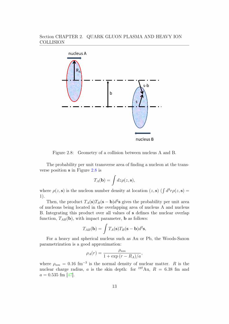
Figure 2.8: Geometry of a collision between nucleus A and B.
The probability per unit transverse area of finding a nucleon at the trans-verse position s in Figure 2.8 is
TA(b) =
∫dzρ(z, s),
where ρ(z, s) is the nucleon number density at location (z, s) (∫d3rρ(z, s) =
1).Then, the product TA(s)TB(s− b)d2s gives the probability per unit area
of nucleons being located in the overlapping area of nucleus A and nucleusB. Integrating this product over all values of s defines the nuclear overlapfunction, TAB(b), with impact parameter, b as follows:
TAB(b) =
∫TA(s)TB(s− b)d2s,
For a heavy and spherical nucleus such as Au or Pb, the Woods-Saxonparametrization is a good approximation:
ρA(r) =ρnm
1 + exp (r −RA)/a,
where ρnm = 0.16 fm−3 is the normal density of nuclear matter. R is thenuclear charge radius, a is the skin depth: for 197Au, R = 6.38 fm anda = 0.535 fm [47].
13

Section CHAPTER 2. QUARK GLUON PLASMA AND HEAVY IONCOLLISION
The number of participants (Npart), and the number of binary nucleon-nucleon collisions, (Ncoll), in the Glauber model are expressed as follows,
Npart(b) =∫d2s TA(s) (1− exp (−σinNNTB(s))) (2.1)
+∫d2s TB(s− b) (1− exp (−σinNNTA(s))) ,
Ncoll(b) =∫d2s σinNNTA(s)TB(s− b) (2.2)
= σinNNTAB(b).
Figure 2.10 shows the number of binary nucleon-nucleon collisions (Ncoll)and the number of participants (Npart) in Au+Au collisions as function ofimpact parameter.
2.2.4 Nuclear Modification Factor: RAA
Once the number of binary collisions (Ncoll) is obtained from Glaubermodel, experimental observables in Au+Au can be compared with those inp+p as baseline, by using nuclear modification factor RAA, which is definedas
RAA(pT , y; b) =d2NAA/dydpT
Ncoll × d2Npp/dydpT.
The numerator represents the observed hadron (or photon, lepton) spectrafor species X in nucleus-nucleus collision, and the denominator representsthe corresponding spectra produced in proton-proton collision scaled withthe number of binary collisions (Ncoll). Since hard scattering, QCD processwhich involves large momentum transfer, is point-like with distance scale1/pT ≤ 0.1 fm, the cross section p(d)+A or A+B collisions, compared top+p, is proportional to the relative number of possible point-like encounters.This binary-scaling property in Au+Au collisions is seen in high-pT directphoton spectra (subsection 2.3.3) and total yield of charm (section 3.1).
2.3 States of created matter at RHIC
2.3.1 Jet quenching and energy loss
At RHIC, high pT particles (pT ≥ 5 GeV/c ) are produced from hardcollision processes. In this subsection, parton production and its energy loss
14

Section CHAPTER 2. QUARK GLUON PLASMA AND HEAVY IONCOLLISION
Figure 2.9: An illustrated example of the relationship of the impact param-eter (b), Npart, overlap area of colliding nucleus, the multiplicity distributionand centrality taken from [5].
15

Section CHAPTER 2. QUARK GLUON PLASMA AND HEAVY IONCOLLISION
Figure 2.10: Number of participants (Npart) and Number of binary colli-sions (Ncoll) for Au+Au and Cu+Cu collisions from Glauber Monte Carlocalculation [5]. The lines represent the mean values.
in the medium in nucleon-nucleon collision is reviewed. After that, so-calledjet quenching discovered in Au+Au collision at RHIC is also discussed.
The definition of jet is ambiguous. Here the most commonly used defini-tion for hadron-hadron collision is introduced [48, 49]: a jet is a concentrationof transverse energy ET in a cone of radius R, where
R =√
(∆η)2 + (∆φ)2.
Here φ is the azimuthal angle and η is the pseudorapidity variable:
η = − ln tan(θ/2).
In the two-dimensional η, φ plane, curves of constant R are circles around theaxis of the jet. Jet production in hadronic collisions is a hard QCD process.An elastic parton scattering (2→ 2) or inelastic parton scattering (2→ 2 +X) of two partons from each of the colliding nuclei results in the productionof two or more high-pT partons in the final state. The jet observable cannot be the residue of a single parton because of color conservation, energymomentum conservation, and quantum-mechanical interference [50].
One of major discoveries that established the formation of dense partonicmatter at RHIC is the strong suppression of high-pT particles in central
16

Section CHAPTER 2. QUARK GLUON PLASMA AND HEAVY IONCOLLISION
Au+Au collisions [44, 51]. This phenomena is called “jet quenching”, whichis originally suggested by Bjorken in 1980’s [52].
Figure 2.11 shows the nuclear modification factor (RAA) for π0 in cen-tral (0-10%) and peripheral (80-92%) Au+Au collisions and minimum-biasd+Au collisions at mid-rapidity. The suppression provides direct evidencethat Au+Au collisions at RHIC have produced matter at extreme densities,greater than ten times the energy density of normal nuclear matter [18, 53].The RdA measurement in Figure 2.11 provides a test of the possible con-tribution of initial state nuclear effects to the observed suppression aboveand demonstrates that there is no significant initial state effect of nuclearparton distributions compared to the Au+Au RAA with pT > 2 GeV/c atmid-rapidity. Thus, the suppression of high pT hadrons in Au+Au collisionsis interpreted as final state effect of the produced dense medium. The datasuggest a small enhancement in d+Au collisions, consistent with expectationsdue to the Cronin effect [54]. The Cronin effect is expected to come from themultiple scattering of the incident partons while passing through the nucleusbefore the collision, which smears the axis of the hard scattering relative tothe axis of the incident beam, leading to the enhancement in mid-rapidityregion [55, 56].
The suppression of the high pT hadrons (RAA < 1) from the fragmen-tation of a parton is due to energy loss in the created matter in the reac-tion. The energy loss of a particle in a medium, ∆E, provides importantinformation on its properties. In general, ∆E depends both on the particlecharacteristics (energy E or transverse momentum pT and mass m) and onthe plasma properties (temperature T , particle-medium interaction couplingα, and path-length of the matter L). The recent theoretical developmentsare reviewed in [49, 57]
The total energy loss ∆E of a particle traversing a plasma with temper-ature T is the sum of collisional and radiative loss : ∆E = ∆Ecoll + ∆EradCollisional energy loss is the energy loss process through elastic scatter-ing inside a QGP of temperature [52, 58]. This was thought to domi-nate at low particle momentum. Radiative energy loss happens throughthe bremsstrahlung of gluons. This loss is believed to dominate at highermomentum.
Compared to the radiative energy loss, collisions energy loss was usuallyconsidered to be small for light flavor (leading) partons, especially when theenergy of the jet is sufficiently high. However in recent realistic calculationof nuclear modification factor RAA at RHIC and LHC energies, collisionalenergy loss may give non-negligible contribution [59–61].
17

Section CHAPTER 2. QUARK GLUON PLASMA AND HEAVY IONCOLLISION
0
0.2
0.4
0.6
0.8
1
1.2
1.4
1.6
0 2 4 6 8 10
Au-Au, Cent
Au-Au, Periph
d-Au, min-bias
pT (GeV/c)
RA
A
Figure 2.11: Nuclear modification factor, RAA, for π0 in central (0-10%) andperipheral (80-92%) Au+Au collisions and minimum-bias d+Au collisions atmid-rapidity. The shaded boxes on the left show the systematic errors forthe Au+Au RAA values resulting from overall normalization of spectra anduncertainties in the nuclear overlap function TAB. The shaded box on theright shows the same systematics error for the d+Au points. Reprinted from[18] with permission from Elsevier.
18

Section CHAPTER 2. QUARK GLUON PLASMA AND HEAVY IONCOLLISION
2.3.2 Collectivity of the QGP
In addition to the discovery of jet quenching, RHIC experiments foundone more important observable related to the collectivity of created matter.The collectivity is described by hydrodynamics and called “flow”.
In Au+Au non-central collision, the reaction zone of nucleus-nucleus col-lision is elliptic around the beam axis as illustrated in Figure 2.12. If themean free path among the produced particles is much larger than the typicalsize of the system, the azimuthal distribution of particles does not depend onazimuthal angle on average due to the symmetry of the production process.On the other hand, if the mean free path is very small compared to the sizeof reaction zone, hydrodynamics can be applied to describe the space-timeevolution of the system. In the absence of viscosity, initial multiple scatter-ing of partons should transform the initial state spatial asymmetry (ellipticshape) into asymmetry in momentum space [62], because the pressure gradi-ent in x-axis is larger than y-axis as illustrated in Figure 2.13. This is called“elliptic flow”, which is quantitatively characterized by v2 variable defined inthe following paragraph.
Figure 2.12: Illustration of the collision geometry in a non-central heavy ioncollision. Left figure illustrates reaction zone in the transverse plane. Rightfigure illustrates reaction plane of the collision.
The method of analyzing flow is summarize in Ref. [63]. The azimuthaldistribution of the associate particles with respect to reaction plane can beexpanded into a Fourier series :
19

Section CHAPTER 2. QUARK GLUON PLASMA AND HEAVY IONCOLLISION
Figure 2.13: Illustration of pressure gradient originated from spatial asym-metry of reaction zone.
dN
dφ=N
2π[1 + 2v1 cos(φ) + 2v2 cos(2φ) + · · ·],
vn =
∫dφ cos(nφ)dN
dφ∫dφdN
dφ
= 〈cos(nφ)〉,
where φ is the azimuthal angle of momentum and vn are the Fourier coefficientof n-th harmonics. Because of the symmetry around the y-axis in Figure 2.12,the sine terms vanish in this expansion.
At RHIC, STAR discovered large v2 of inclusive charged hadrons fromthe first RHIC run [64]. A lot of observables, particle dependence of v2, v2with different collision system, and v1, v3, · · · has been also measured afterthat. At low pT , below around 2 GeV/c , the measurements of v2 is well fitby hydrodynamical calculations which assume equilibrium established earlyin the collision (∼ 0.6 – 1 fm/c) and small viscosity over entropy density(for example, η/s ∼ 0.16 from Ref. [6]). It is often termed a near-perfectfluid [18, 23–25].
20

Section CHAPTER 2. QUARK GLUON PLASMA AND HEAVY IONCOLLISION
0 1 2 3 4p
T [GeV]
0
5
10
15
20
25
v2
(per
cent)
idealη/s=0.03
η/s=0.08
η/s=0.16
STAR
Figure 2.14: STAR measurement of v2 with hydrodynamical predictions forminimum bias Au+Au at √s
NN= 200 GeV from [6]
2.3.3 Temperature of the created matter
“Direct photons” stands for the photons which emerge directly from aparton collision. In this subsection, the direct photon measurements arereviewed.
They do not suffer medium effect and carry information about the circum-stances of their production [65]. The direct photon is called electromagneticprobe of QGP, as they interact only weakly (α = 1/137 � αs) and theirmean free path is larger than the typical system size (∼ 10 fm). Thermalradiation from the QGP phase is predicted to be the dominant source ofdirect photons with 1 < pT < 3 GeV/c in Au+Au collisions at RHIC [66].The measurement of direct photons at low pT will allow the determinationof the initial temperature of the matter.
As shown in Figure 2.15, PHENIX observed the enhancement of directphoton yield in Au+Au collision compared with p+p collision in the low pT(< 3GeV/c ) region [20]. The results were compared with several hydrody-namical models of thermal radiation from QGP at RHIC energies. The mod-els assuming the formation of QGP with initial temperature ranging Tinit ∼300 – 600 MeV at times τ ∼ 0.6–0.15 fm/c are in qualitative agreement withthe data [20, 67–70]. It it well above Tc predicted by lattice QCD.
The main background photon source is hadron decay, such as π0 → γγ.Their contribution to the photon spectrum is large and subtraction of the de-cay background from inclusive photon spectrum was a very challenging task.In the data analysis of PHENIX results in Figure 2.15, “internal conversion”method which measure the virtual photons , instead of real photon is used to
21

Section CHAPTER 2. QUARK GLUON PLASMA AND HEAVY IONCOLLISION
Figure 2.15: Invariant cross section (p+p) and invariant yield (Au+Au) ofdirect photons as a function of pT from [20]. The filled points are from virtualphoton measurements and open points are from real photon measurements.The three curves on the p+p data represents NLO pQCD calculations, andthe dashed curves show a modified power-law fit to the p+p data, scaled byTAA. The dashed (black) curves are exponential plus the TAA scaled p+pfit. The dotted (red) curve near the 0 – 20 % centrality data is a theorycalculation [66].
separate direct photons from decay background in the low pT region (filledpoints). In general, any source of high energy photons can also emit virtualphotons, which convert to low mass e+e− pairs. For example, gluon Comptonscattering (q+ g → q+ γ) has an associated process that produces low masse+e− pairs through internal conversion (q + g → q + γ∗ → q + e+e−).
The mass distribution of the e+e− from pseudo scalar meson decay (π0, η →γγ) follows the Knoll-Wada formula [71].
1
Nγ
dN
dMee
=2α
3π
√1− 4m2
e
M2ee
(1 +2m2
e
M2ee
)1
Mee
(1− M2ee
M2)3|F (M2
ee)|2, (2.3)
Here Mee is the mass of the electron pair; me is the mass of electron; M is
22

Section CHAPTER 2. QUARK GLUON PLASMA AND HEAVY IONCOLLISION
the mass of the parent meson; and F (M2ee) is a hadronic form factor. The
formula above is normalized as decay rate per photon, and therefore it differsfrom the total Dalitz decay rate by a factor of 2 for π0,η since these mesonsdecay into two photons. In the hadron decay, Mee does not exceed parenthadron mass M , so the part (1 − M2
ee
M2 )3 in the above formula becomes 0 if(Mee →M).
On the other hand, there is no parent hadron for direct photon, there is nophase space limitation above in Mee from direct photon. Then, if e+e− pairyield with large Mee is measured as shown in Figure 2.16, the contributionfrom hadron decay is strongly suppressed. Since 80% of the hadronic photonsare from π0 decays, the signal to background (S/B) ratio for the direct photonsignal improves by a factor of five for Mee > Mπ0 = 135 MeV/c2 in PHENIXmeasurement [20].
Figure 2.16: Electron pair mass distribution for p+p and Au+Au (MinimumBias) taken from [20] The pT ranges are shown in the legend. The solid curvesrepresent an estimate of hadronic sources; the dashed curves represent theuncertainty in the estimate.
23

Chapter 3
Heavy quark as a probe of theQGP
time
pre-equilibrium
- initial NN collisions
b c c c c
c c
b ~0.02 fm/c
~0.08 fm/c
Au Au
~0.3-1fm/c
b c c c
c
c
c b
u
u
u
u
u
d
d
d
d
d
s
d ~5 fm/c
QGP phase
-gluon radiation
- recombination (or resonance) - fragmentation - dissociation
s
~ 120 μm/c -decay
e X ν
~ 460 μm/c
e X ν
- formation of QQ pair
- elastic scattering
π-
p π+
Hadronic phase
Figure 3.1: Schematic view of time evolution of heavy quarks.
As discussed in the previous chapter, it is well established that the QGPis created in RHIC and the LHC above Tc. Heavy quarks (charm or bottom)
24

Section CHAPTER 3. HEAVY QUARK AS A PROBE OF THE QGP
is the suitable probe of the QGP created in high energy heavy ion collisions.Heavy quarks (Q), including charm (c) and bottom (b) quarks, may exist
either as bare quarks inside the QGP, or as bound states of QQ̄ when themedium temperature is still above Tc but not too high [72]. The formerstate is called as “open” heavy quark and the latter as heavy quarkonium(charmonium or bottomonuim). Bound states of heavy and light quarks(Qq̄, Q̄q,Qqq...) such as D,B,Λc are also named “open” heavy flavor hadrons.
In this dissertation, the dynamics of open heavy flavor in heavy-ion col-lisions is concentrated. While, study of heavy quarkonium is also importantto investigate property of the QGP, it is out of scope of this dissertation.
The most important property of heavy quarks is their large masses (mc ≈1.3 GeV, mb ≈ 4.7 GeV [3]) which are much larger than ΛQCD ≈ 200 MeVand the QGP temperature T ≈ 300 – 600 MeV at RHIC. The heavy quarks(Q = c, b) are mainly produced via hard scatterings at the initial nucleon-nucleon collisions, because the large momentum transfer is needed to produceheavy quarks [26]. The production of charm (bottom) quark pairs takes placeat timescale 1/(2mQ) ∼ 0.08 (0.02) fm/c.
After the heavy quark production, it is expected that the total number ofheavy quarks stays constant because mc,mb � Tc and they are not destroyedby the strong interaction. This is experimentally confirmed within uncer-tainties [11, 73, 74]. Thus, heavy quarks carry information about the entiretime-evolution and transport properties of the QGP or the pre-equilibriumphase before the formation of the QGP as illustrated in Figure 3.1.
On the other hand, light quarks can be generated during the evolution ofthe medium and even from the mixed phase by low momentum gluon fusion.Light hadron measurements are less sensitive to the energy loss mechanismand transport properties of the early stage of the QGP phase.
3.1 Heavy flavor hadron productionHeavy flavor hadron production in nucleon-nucleon collisions is described
by pQCD calculations. For heavy flavor hadrons, pQCD approach is war-ranted for all momenta since their large quark mass introduces large Q2 evenat zero momentum. This is specific contrast to gluon and light quark jetswhich can be treated by pQCD only at high pT .
The experimental results and theoretical calculations of their cross sectionare useful as a base line of heavy quark energy loss in Heavy ion collisions(the denominator of RAA). Heavy flavor hadron production (D,B · ··) innucleon-nucleon collisions is described by the QCD factorization approach.This calculation is performed by a convolution of three terms: the parton
25

Section CHAPTER 3. HEAVY QUARK AS A PROBE OF THE QGP
distribution function of nucleon 1 and nucleon 2 (fN11 , fN2
2 , respectively),the hard parton scattering cross section dσ̂f1f2→fX , and the fragmentationfunction (Dh
f ).
dσN1N2→hX =∑f1,f2,f
∫dx1dx2dzf
N11 (x1, µ
2FI)f
N22 (x2, µ
2FI)× (3.1)
dσ̂f1f2→fX(x1p1, x2p2, ph/z, µFI , µFF , µR)×Dhf (z, µ2
FF )
Here,
• The fragmentation function Dhf (z, µ2
FF ) describes the probability thatthe outgoing parton fragments into the observed hadron h with frac-tional momentum z = ph/pf , µFF is the factorization scale of frag-mentation function.
• dσ̂f1f2→fX(x1p1, x2p2, ph/z, µFI , µFF , µR) is perturbative partonic crosssection computable up to a given order in αs. µR is the renormalizationscale, and µFI is the factorization scales of parton distribution function.
The production cross section of charm hadrons at RHIC(√sNN
= 200GeV, p+p) [75, 76], at Tevatron (√s
NN= 1.96 TeV, p+p̄) [77–79] and at the
LHC (√sNN
= 2.76 TeV and 7 TeV, p+p) [80–82] are found to be larger thansuch calculations (NLO MNR calculation [83] and Fixed Order plus Next-to-Leading Logarithms (fonll) calculation [8, 84]), which is still compatiblewith the theoretical uncertainties as shown in Figure 3.2 [82].
The production cross section of bottom hadrons at RHIC(√sNN
= 200GeV, p+p) [13, 14], at Tevatron (√s
NN= 1.96 TeV, p+p̄) [85–87], UA1 (√s
NN
= 630 GeV, p+p̄) [88] and at the LHC (√sNN
= 2.76 TeV and 7 TeV, p+p)[89–91] are well described by fonll [84].
Most dominant charm and bottom production process is gluon fusiong+ g → Q+ Q̄ (Q = c, b) and flavor excitation g+ g → Q+ Q̄+ g [92]. Thisis a result of the large fraction of gluons in parton distribution function asshown in Figure 2.5.
In RHIC, measurement in p+p collision at √sNN
= 200 GeV, the totalcharm-anticharm quark cross section is 551± 57 (stat.)± 195 (sys.) µb [11].Almost 99% of produced charm quarks and bottoms quarks are known toform open heavy flavor hadrons. The total cross section of J/ψ is 4.0 ±0.6(stat.)±0.6(syst.)±0.4(abs.) µb [93]. The total bottom-antibottom quarkcross section is 3.2+1.2+1.4
−1.1−1.3 µb [13].In Au+Au collisions, medium effects, such as energy loss of charm or
bottom in the QGP, can only influence the momentum distribution of charm
26

Section CHAPTER 3. HEAVY QUARK AS A PROBE OF THE QGP
Figure 3.2: Heavy quark production cross section in p+p or p̄+ p collisionsas a function of center of mass energy in p+p or p̄ + p collisions. (Top)charm production cross section from [82]. (Bottom) Inclusive bottom pro-duction cross section per rapidity unit measured at mid-rapidity along withthe comparison to FONLL calculations from [91].
27

Section CHAPTER 3. HEAVY QUARK AS A PROBE OF THE QGP
or bottom, and the number of heavy quarks produced by binary nucleon-nucleon collision are conserved [11, 73, 74]. Namely,∫ ∫
RAA(Q)dpTdy = 1
The thermal production of heavy quarks, are believed to be very small atRHIC energy, because their mass (mc ≈ 1.3 GeV, mb ≈ 4.7 GeV [3]) is muchlarger than ΛQCD ≈ 200 MeV and the QGP temperature T ≈ 300 – 600MeV.
Figure 3.3 shows the centrality dependence of the yield of electron fromheavy flavor as well as the yield in p+p [74]. Those results show that thecentrality dependence of charm quark production is consistent with Ncoll
scaling. The Ncoll dependence of the yield was fit to Nα
coll and found α =
0.938±0.075(stat.)±0.018(sys.), showing that the total yield of charm-decayelectrons is consistent with binary scaling.
Figure 3.3: Electron from heavy flavor yield (0.8 < pT < 4.0 GeV/c )measured in Au+Au collision at √s
NN= 200 GeV scaled by the number of
binary collisions (Ncoll) from [74]. The yield in p+p collisions is also shown.
3.2 Decay of charm and bottom hadronsOpen heavy flavor hadrons can be measured by the direct reconstruction
(invariant mass reconstruction) or part of their decay products. Some im-portant decay channels of the relevant hadrons for identify open heavy flavorhadrons in measurements are summarized in Table 3.1 and 3.2.
28

Section CHAPTER 3. HEAVY QUARK AS A PROBE OF THE QGP
As will be discussed in the section 3.3, PHENIX has been measured elec-trons from semi-leptonic decay of charm and bottom hadrons (heavy flavorelectron). The advantage of semi-leptonic decay is relatively large branchingratio of heavy flavor hadrons ( ∼ 10%). The contribution from electrons fromlight neutral mesons and photon conversion are not negligible, but they canbe subtracted by cocktail method and isolation cuts (they will be introducedin chapter 5.
Table 3.1: Decay modes, Branching ratios (B.R.), decay momentum∗ (p)and life times for main charm hadrons from PDG [3]. Charge conjugates areabbreviated.
Particle Decay mode B.R. (%) p (MeV/c) cτ (µm)D+ e+ anything 16.07 ± 0.30 311.8
µ+ anything 17.6 ± 3.2e+K
0νe 8.83 ± 0.22 869
e+K∗0νe 3.68 ± 0.10 722
K−π+π+ 9.13 ± 0.19 846D0 e+ anything 6.49 ± 0.11 122.9
µ+ anything 6.7 ± 0.6e+K−νe 3.55 ± 0.04 867e+K∗−νe 2.16 ± 0.16 719K−π+ 3.88 ± 0.05 861
D+s e+ anything 6.5 ± 0.4 149.9
e+ηνe 2.67 ± 0.29 908e+φνe 2.49 ± 0.14 720φπ+ 4.5 ± 0.4 712
D∗+ D0π+ 67.5 ± 0.5 39 (2.1± 0.5) ×10−6
Λ+c e+ anything 4.6 ± 1.7 59.9
e+Λνe 2.1 ± 0.6 871pK−π+ 5.0 ± 1.3 823
∗ For a 2 body decay, p is the momentum of each decay product in the restframe of the decaying particle. For a 3 or more body decay, p is the largestmomentum any of the products can have in this rest frame.
29

Section CHAPTER 3. HEAVY QUARK AS A PROBE OF THE QGP
Table 3.2: The same as table 3.1 but for bottom hadrons from PDG [3].Charge conjugates are abbreviated.Particle Decay mode B.R. (%) p (MeV/c) cτ (µm)B+ e+νeX 10.8 ± 0.4 492.0
l+D0νl 2.26 ± 0.11 2310
l+D∗0νl 5.70 ± 0.19 2258
J/ψK+ 0.1016 ± 0.0033 1683B0 e+νeX 10.1 ± 0.4 455.4
l+D−νl 2.18 ± 0.12 2309l+D∗−νl 4.95 ± 0.11 2257J/ψK0
s 0.0437 ± 0.0016 1683B0s l+νX 9.5 ± 2.7 449
J/ψφ 0.109 +0.28−0.23 1588
Λ0b l−νlΛ
+c anythinag 9.8 ± 2.3 427l−νlΛ
+c 6.5 +3.2
−2.5 2345l−νlΛ
+c π
+π− 5.6 ± 3.1 2335
∗ For a 2 body decay, p is the momentum of each decay product in the restframe of the decaying particle. For a 3 or more body decay, p is the largestmomentum any of the products can have in this rest frame.
30
Section CHAPTER 3. HEAVY QUARK AS A PROBE OF THE QGP
3.3 Heavy flavor hadron measurement in RHICand the LHC
3.3.1 Overview of heavy flavor measurement
Measurement of heavy flavor hadrons is much more difficult than lighthadrons because their production cross section is small. Various methods ofheavy flavor detections are so far applied in RHIC and the LHC as follows,
• Single electron (or muon) measurement (from admixture of charm andbottom).
• electron-hadron correlation to separate charm and bottom (only avail-able in p+p).
• Invariant mass measurements for charm hadron and bottom hadron.(Direct reconstruction method)
• Non-prompt J/ψ (B → J/ψX) measurement.
• Displaced single electron (or muon) track to separate charm and bottomcontribution.
While heavy flavor measurements in heavy ion collisions are useful to in-vestigate the property of the QGP, reference measurements in p+p collisionsare also important from two points of view. First, these data provide an ex-perimental reference for corresponding measurements in heavy ion collisions.Such a reference is necessary for the denominator of RAA. Second, these dataprovide an important testing ground for pQCD calculations which, due tothe large masses of the charm and bottom quarks, should be able to predictopen heavy flavor observables even at low pT [11].
In following subsections, the previous single electron measurements atPHENIX are emphasized as it is the first observation of suppression of heavyquarks. The other recent measurements in RHIC and the LHC are alsoreviewed after that. In the end of this section, the new method to separatecharm and bottom contribution Au+Au collisions, which is the main goal ofthis dissertation, is briefly introduced.
3.3.2 Single electron measurements at PHENIX
method
Both charm and bottom mesons (D,B) have relatively large branchingratios (∼ 10%) to single electrons or single muons. Thus the single elec-
31

Section CHAPTER 3. HEAVY QUARK AS A PROBE OF THE QGP
tron measurement has an advantage to other methods in terms of statistic.A disadvantage is that kinematics of parent heavy flavor hadron is smearedthrough the decay, thus it is rather insensitive to the heavy quark momentum.The other disadvantage is that it cannot distinguish between the contribu-tions from the charm and bottom hadrons without additional information.
The inclusive single electron spectra consist primarily of four components:
1. electrons from open heavy flavor decays,
2. photonic background from Dalitz decays of light neutral mesons (forexample, π0 → e+e−γ and photon conversions in the material,
3. nonphotonic background from K → eπν (Ke3) and dielectron decaysof light vector mesons, and
4. heavy quarkonia (J/ψ,Υ) and Drell-Yan background processes.
The dominant source of electron is charm hadrons in total as the bottomproduction cross section is small. However due to the large Q-value forbottom decays, electrons from bottom hadrons can have an excess at highpT region. According to the fonll calculation [8], at about pT = 4 GeV/cthe contributions from charm and bottom decays are in the same level, andtowards higher pT , bottom decays become the dominant source of electrons.
Of the three background sources, the “photonic” background is the largest.To extract the heavy flavor electron signal, the various background contribu-tions listed above have to be subtracted from the inclusive electron spectra.So-called “cocktail subtraction” method (pT > 1.6 GeV/c ) and “convertersubtraction” method (0.3 < pT < 1.6 GeV/c ) are used for this measure-ment.
A cocktail of electron spectra from background sources is estimated byusing a Monte Carlo simulation of hadron decays and then subtracted fromthe inclusive electron spectra. The PHENIX measurements of the relevantelectron sources are precise enough to constrain the background within asystematic uncertainty better than 15% for all pT [11].
The yields of photonic and nonphotonic electrons are obtained by mea-suring the difference between inclusive electron yields with and without aphoton converter of precisely known thickness: a brass sheet of 1.680% radi-ation length (X0).
results and interpretations in Au+Au and p+p collisions
After subtraction of various background, PHENIX first observed the sup-pression of electrons from heavy flavor in Au+Au collision from year 2004
32

Section CHAPTER 3. HEAVY QUARK AS A PROBE OF THE QGP
data (RUN4), comparing with p+p collision from year 2005 data (RUN5)[11]. Figure 3.4 shows the PHENIX measurement of RAA (and v2) of elec-trons from open heavy flavor in the 2004/2005 data in 0-10% central andminimum bias collisions, and corresponding π0 data [11, 94].
AA
R
0.2
0.4
0.6
0.8
1
1.2
1.4
1.6
1.8
= 200 GeVNN
sAu+Au @
0-10% central(a)
Moore &
Teaney (III)T)π3/(2
T)π12/(2
van Hees et al. (II)
Armesto et al. (I)
[GeV/c]T
p0 1 2 3 4 5 6 7 8 9
HF
2v
0
0.05
0.1
0.15
0.2
(b)
minimum bias
AA R0π
> 2 GeV/cT
, p2 v0π
HF2 v±, eAA R±e
PH ENIX
Figure 3.4: PHENIX measurement of RAA and v2 of electron from heavy fla-vor from 2004/2005 data [11]. Top panel shows RAA of heavy flavor electronsin 0-10% central collisions compared with π0 data. Bottom panel shows theelliptic flow parameter v2 of heavy flavor electrons in minimum bias collisionscompared with π0’s v2.
While at low pT the suppression is smaller than that of π0, RAA of elec-trons from open heavy flavor approaches the π0 value for pT ≥ 4 GeV/c . Inthis pT region, the contribution of electrons from bottom hadrons was naivelyexpected to be large due to their large Q-value. In the 2004 Au+Au collisiondata, PHENIX did not have capability to separate charm and bottom.
Although the charm and bottom contributions are not separated in thismeasurement, this suppression of heavy flavor electrons was unexpected be-
33

Section CHAPTER 3. HEAVY QUARK AS A PROBE OF THE QGP
cause the radiative loss of heavy quarks were thought to be small due tothe dead cone effect, (see subsection 3.4.1), and collisional energy loss wasbelieved to be negligible at high pT .
Those data indicate strong coupling of heavy quarks to the medium.Figure 3.4 shows a quantitative comparison of model calculations. CurveI [95] shows radiative energy loss calculation with the BDMPS formalism[96]. Curves II [97] and III [98] show a calculation which considers elasticscattering mediated by the excitation of D or B meson like resonant states inthe medium. In those calculation, heavy quark is put into a thermal mediumand Langevin-based transport model are applied for the heavy quark motionin the QGP. Ref. [97] shows that the bottom contributions can dominateabove pT ∼ 3.5 GeV/c and it reduces both suppression and elliptic flow,which was not confirmed in this PHENIX measurement.
Initial state effect
The nuclear modification factor RAA is also expected to contain effectscome from normal nuclear matter. The presence of the normal nuclear mattercan change the kinematic distributions of the observables compared to p+pwithout the QGP ever being formed. This effect is generally referred to as“initial state effect”.
Figure 3.5 shows the nuclear modification factors for heavy flavor electronat midrapidity in central d+Au, Cu+Cu, and Au+Au collisions at √s
NN
= 200 GeV [99]. The d+Au data show the enhancement relative to p+pcollisions between 1 < pT < 5 GeV/c .
Such an enhancement is termed “Cronin effect” [54] as explained in sub-section 2.3.1 and expected to moderate the large suppression of heavy flavorelectron in Au+Au collisions at √s
NN= 200 GeV, but this is not fully un-
derstood.In the d+Au collision, it is expected that there is no QGP effect and thus
it is good control experiment to evaluate cold nuclear matter effect. Thisassumption is, however, challenged by phenomena recently found in p+Pb(LHC) and d+Au (RHIC) collisions (for example, “ridge”), which may comefrom hydrodynamics or gluon saturation [100–105] .
34

Section CHAPTER 3. HEAVY QUARK AS A PROBE OF THE QGP
[GeV/c]T
p0 2 4 6 8 10
AA
R
0
0.5
1
1.5
2d+AuCu+CuAu+Au
0-20%0-10%0-10%
9.9%±Global error:
Figure 3.5: The nuclear modification factors for heavy flavor electron atmidrapidity (η < 0.35) in central d+Au, Cu+Cu, and Au+Au collisionsat √s
NN= 200 GeV with PHENIX [99]. The boxes around 1 are global
uncertainties, which include the Ncoll scaling error. The global error given inthe legend is from the p+p yield.
3.3.3 Electron-hadron correlation
In p+p collision, there is an alternative approach to access bottom hadrons.Both PHENIX and STAR developed bottom and charm hadron separationtechniques based on electron-hadron correlation measurement, utilizing thedifference of decay property between charm and bottom hadrons. Due tothe fact that the combinatorial background in electron-hadron correlationmeasurements increases dramatically with particle multiplicity, this methodcan not be used in heavy ion collisions.
In the PHENIX, the separation of the relative contributions from charmand bottom decays was carried out based on the decay channel D/D̄ →e± +K∓X [13]. A correlation of the invariant mass distribution is observedfor unlike charge-sign electron-hadron pairs (e±K∓) below the D-meson mass,because of the charge correlation in D-meson decays.
In the STAR, the relative contribution from B decays to heavy flavorelectron yields was measured using the azimuthal correlations between heavyflavor electrons and charged hadrons, and between heavy flavor electrons andD0 mesons [14].
Figure 3.6 shows the distribution of the azimuthal angle between heavyflavor electrons and hadrons for two electron pT ranges. The distributionis normalized to the number of heavy flavor electrons. The shapes of these
35

Section CHAPTER 3. HEAVY QUARK AS A PROBE OF THE QGP
distributions are different because the decay kinematics of the charm andbottom hadron decays are different (some of them are shown in table 3.1and table 3.2). Figure 3.6 also shows the template distributions made bypythia simulation [106] reflecting the expected shapes of the electron-hadronazimuthal distributions from charm hadrons and bottom hadrons.
The contribution of bottom decays relative to the sum of charm andbottom decays was obtained from a fit to the azimuthal angle distributionsusing a linear combination of the charm and bottom templates with therelative normalization as a fit parameter. In this way, charm contributionand bottom contribution can be separated statistically.
STAR also performed an independent measurement using electron - D0
correlation, where D0 is identified by the invariant mass reconstruction of Kand π. In this measurement, the azimuthal angle distribution in the away-side(φ ∼ π) are dominated by charm hadrons due to the back-to-back correla-tion of cc̄ jets. Again, template distributions obtained by pythia simulationwere used to statistically separate charm and bottom. MC@NLO [107] sim-ulation, which is a Monte Carlo event generator with Next-to-Leading-Ordercalculations of rates for QCD processes, is used for the fitting in this analysisthe average value with the result from the pythia simulation for the finalvalue.
The observed away-side correlation signal in the electron-D0 azimuthalangle distribution was attributed to prompt charm hadron pair production(∼ 75%) and bottom hadron decays (∼ 25%), while the near side correlationsignal was mainly due to bottom hadron decays (B → Deµ ).
The contributions of bottom decays to the total electron spectrum fromheavy-flavor hadron decays obtained with these two methods are comparedin the right panel of Figure 3.6 as functions of the electron pT . The STARapparatus has larger acceptance compared to PHENIX, which is a clear ad-vantage for such multi-particle measurements.
3.3.4 Direct reconstruction measurement
This method uses hadronic decays of heavy flavor hadron by detecting alldecay products to observe invariant mass peaks. This measurement requireswide acceptance of detectors and good capability of particle identification aswell as high statistic data. STAR has measured D0 mesons via a hadronicdecay channel D0 → K− + π+ [15] in Au+Au collisions at √s
NN= 200
GeV. STAR also measured D0 and D∗+ via D0 → K− + π+ and D∗+ →D0π+ → K−π+π+ [108] in p+p. By comparing them, they reported thenuclear modification for D0 meson (i.e. RAA < 1) in the central collisionswhile no suppression was seen in peripheral collisions (Figure 3.7).
36

Section CHAPTER 3. HEAVY QUARK AS A PROBE OF THE QGP
Figure 3.6: (Left) The azimuthal angle between heavy flavor electrons andhadrons measured with STAR in p+p collisions is compared to charm andbottom decay templates obtained with pythia simulations for two electronpT ranges. (Right) Relative contributions of bottom decays to the total yieldof electrons from heavy flavor hadron decays as functions of the electron pTare compared to predictions from fonll pQCD calculations [8]. Both figuresare from [14].
In STAR, Time Projection Chamber (TPC) [109] is the main tracking de-tector, covering the full azimuthal angle at pseudorapidity η ≤ 1. It measuresthe charged-particle momenta and provides particle-identification (PID) ca-pability via the ionization energy loss (dE/dx) in the TPC gas, allowing sep-aration between charged kaons and pions up to momentum p ∼ 0.6 GeV/c .In addition to that, Time Of Flight detector (TOF) [110] gives good pionsand kaons separation up to pT = 1.6 GeV/c .
In Pb+Pb and p+p collision at the LHC at √sNN
= 2.76 TeV, ALICEreports similar modification via D+ → K−π+π+, D0 → K−π+ and D∗+ →D0π+ (and their anti-particle) [111, 112].
This direct reconstruction method also could be applied for B meson.However, since the mean multiplicity of the final state in B meson decayis larger than D meson decay, it is rather difficult compared to D mesonreconstruction. So far, Large Hadron Collider beauty experiment (LHCb)measured B+ → J/ψK+ with J/ψ → µ+µ− in p+p at √s
NN= 7 TeV [113].
The CMS has the preliminary result of measurement via B+ → J/ψK+,B0 → J/ψK∗(892) and Bs → J/ψφ, with J/ψ → µ+µ− in p+p and p+Pbcollisions at √s
NN= 5.02 TeV. [114].
3.3.5 Non-prompt J/ψ measurement
An alternative approach for bottom hadron production is the measure-ment of J/ψ emitted from displaced decay of bottom hadron vertices, uti-
37

Section CHAPTER 3. HEAVY QUARK AS A PROBE OF THE QGP
Figure 3.7: Centrality dependence of the D0 pT differential invariant yieldwith STAR in Au+Au collisions (solid symbols) [15]. The curves are number-of-binary-collision-scaled Levy functions from fitting to the p+p result (opencircles) [108]. The arrow denotes the upper limit with a 90% confidence levelof the last data point for 10%-40% collisions. The systematic uncertaintiesare shown as square brackets.
lizing relatively large life time (see table 3.2). Those J/ψ s are called “non-prompt J/ψ ”. This measurement requires high resolution vertex detector toprecisely separate primary and secondary vertices.
The Compact Muon Solenoid (experiment at the LHC) (CMS) measurednon-prompt J/ψ via the reconstruction of secondary µ+µ− vertices in Pb+Pband in p+p collision at√s
NN= 2.76 TeV and observed RAA ∼ 0.4 [115].This
is the first measurement which disentangled the charm and bottom produc-tion in Pb+Pb collision at the LHC. After that, CMS further improved theiranalysis and reconstructed b-jet [116]. Experimentally, the jet associatedwith a b hadron is commonly referred to a “b jet”, although the b quark isnot guaranteed to be the leading parton of the jet. By reconstructing a jettotal energy, it is more sensitive to the parton energy loss compared withmeasurement of fragmented J/ψ. The b-jet RAA is found to be ∼ 0.4 in themost central collisions and it is qualitatively consistent with that of inclusivejets above pT jet ∼ 100 GeV/c [117].
38

Section CHAPTER 3. HEAVY QUARK AS A PROBE OF THE QGP
3.3.6 Separating charm and bottom
The single electron measurement reviewed in subsection 3.3.2 has an ad-vantage in terms of statistics in the limited acceptance of detectors comparedwith direct reconstruction method, however the relative charm and bottomcontribution are unclear.
Since the large difference of lifetime of charm hadrons and bottom hadrons(see section 3.2) are useful to separate charm and bottom contribution in thesingle electron measurement, the PHENIX Collaboration proposed displacedtrack measurement to separate charm and bottom contribution from singleelectron data and has developed Silicon Vertex Tracker (VTX).
The Silicon Vertex Tracker (VTX) was installed in the RHIC-PHENIXdetector in the end of year 2010. The VTX was designed to give precisetracking reconstructions of the distance of closest approach (DCA) to thecollision vertex in order to distinguish prompt particles from in-flight decays.In this way, electrons from semi-leptonic decay of heavy flavor hadrons areable to be statistically separated. The detail of this method is described inchapter 5.
3.4 Energy loss of heavy quark in the QGPIn this subsection, the energy loss mechanism and the early theoretical
prediction for charm and bottom quarks before the experimental results fromthe year 2004 PHENIX data [11] are reviewed. After that, the recent theorydevelopment motivated by the PHENIX results are also explained.
Before the measurement of single electron from PHENIX [11] (see sub-section 3.3.2), the energy loss of fast partons in-medium was expected to bedominated by gluon bremsstrahlung (radiative energy loss) [118]. Radiativeloss of heavy quark in-medium was thought to be much smaller than lightpartons due to the “Dead cone effect” [7].
3.4.1 Dead Cone effect
Gluon bremsstrahlung from a heavy quark is suppressed from that of lightpartons at angles smaller than the ratio of the quark mass M to its energyE, due to kinematics constraints.
The double differential distribution of gluons of transverse momentum k⊥and energy ω radiated by a heavy quark ω dPrad,HQ
dωdk2⊥is expressed as,
ωdPrad,HQdωdk2⊥
=αsCFπ
k2⊥(k2⊥ + ω2θ20)
2,
39

Section CHAPTER 3. HEAVY QUARK AS A PROBE OF THE QGP
whereθ0 ≡
M
E=
1
γ,
αs is the strong coupling constant and CF is the Casimir factor and for thequark case here N2
c−12Nc
= 4/3. In the small angle approximation (k⊥ ∼ ωθ), itdiffers from the bremsstrahlung spectrum from the light partons ω dPrad,0
dωdk2⊥by
the factorωdPrad,HQdωdk2⊥
≈ ωdPrad,0dωdk2⊥
· (1 +θ20θ2
)−2
This formula means that gluon radiation at small angles with respect tothe quark momentum vector is reduced by (1 +
θ20θ2
)−2. This effect, termed“dead cone effect” [7] is larger for bottom than for charm; Thus, RAA
π <RAA
c < RAAb was expected against the PHENIX single electron measurement
[11].
0.2 0.4 0.6 0.8 1x
0.2
0.4
0.6
0.8
1
Ratio
Figure 3.8: The ratio of gluon spectra off charm and light quarks for trans-verse quark momenta p⊥ = 10 GeV (solid line) and p⊥ = 100 GeV (dashed)in QGP matter (the path length L = 5 fm), x = ω/p⊥, from Ref. [7].
3.4.2 Recent theoritical development
Along with dead cone effect, which suppress the radiative loss of heavyquarks in the QGP medium, there are a number of theoretical developments.In this subsection, some of them are briefly introduced. Both collisionalenergy loss and radiative energy loss have been reconsidered.
The propagation of heavy quark in the QGP has been often treated withinthe framework of Fokker-Planck equation [98, 119–123]. For slowly moving
40

Section CHAPTER 3. HEAVY QUARK AS A PROBE OF THE QGP
heavy quarks in the QGP, the dominant interaction is elastic scattering andat high momentum, radiative energy loss (gluon bremsstrahlung) is believedto eventually become the dominant energy loss mechanism. It is currentlynot known at which pT this transition occurs [120].
Transport Models
Brownian motion of heavy quarks can be considered for the collisional en-ergy loss. The typical momentum transfer from a thermal medium to a heavyquark is small compared to the heavy quark thermal momentum pth. Non-relativistically, the typical kinetic energy of heavy quarks with temperatureT
p2th/2mQ ' 3kBT/2, (3.2)
where kB is Boltzman constant. Then,
p2th ' 3mQkBT. (3.3)
This is much larger than the typical momentum transfer from the mediumof light partons, Q2 ∼ (kBT )2. This allows a Brownian Motion approach(Fokker-Plank equation) for heavy quarks as follows,
∂
∂tfQ(t,p) = γ
∂
∂pi[pifQ(t,p)] +D∆pfQ(t,p) . (3.4)
Here, fQ is the phase-space distirbution of a heavy quark and the γ is the drag(or friction) coefficient, which determines the relaxation rate of the averagemomentum to its equilibrium value: < p >= p0 exp (−γt).
The spatial diffusion constant D, characterising the dynamics of heavynon-relativistic particles (mass M and momentum p) traversing the plasma,is connected, via the Einstein relations
D = T/(MηD) = 2T 2/κ (3.5)
to the momentum diffusion coefficient κ - the average momentum gained bythe particle per unit time. The smaller values of D yield a stronger coupling.
Recent several calculations of Ref.[124–127] provide the prediction ofcharm and bottom fraction as a function of pT using the Langevin-type ap-proach, but the treatment of coupling between heavy quark and medium aredifferent in their models.
41

Section CHAPTER 3. HEAVY QUARK AS A PROBE OF THE QGP
T-matrix approach
Several lattice QCD calculations have found indications that hadronicresonances (or bound state) of heavy quarks survive up to ∼ 2TC or morehigher temperature [72, 128, 129]. Refs. [124, 130] assume that heavy-lightquark (Qq̄ or Q̄q) resonance (D or B meson) persist as hadron in the QGPand include this effect in the collisional energy loss. The formation of thoseresonance state is non-pertavative process. To solve this, a Brueckner-typein-medium T-matrix approach for heavy-light quark scattering in the QGPhas been applied in Ref. [124].In this calculation, it is assumed that theeffective in-medium potential can be extracted from lattice QCD calculationsof the color-singlet free energy and two different calculation are used for this[131, 132]. Both of them are suppressed in high pT in T-matrix calculationsthan in pQCD calculation [97].
DGLV theory
Recent calculations of radiative energy loss via gluon emission is describedin [133, 134], using the Djordjevic, Gyulassy, Vogt, and Wicks (DGLV) the-ory, which is extended from GLV reaction-operator method for light-partonradiative energy loss in the QGP [135].
This model assumes an effectively static medium and the medium effectin this approach is characterized by two parameters: the gluon density ρ(τ)of the scattering centers (or the mean free path λg of the radiated gluon) andthe Debye screening mass µD which is introduced to regulate the infraredbehavior of single scattering cross section.
Figure 3.9 shows the c and b quark distributions at midrapidity beforefragmentation as well as decay electron (c→ e and b→ e) distribution fromRef. [133]. Note in this calculation, only the energy loss by medium-inducedgluon radiation is taken into account.
Those results depends on the gluon density dNgdy
, which comes from theassumption: the medium is uniformly and cylindrically expanding, i.e ρ(τ) ≈dNgdyτπR2 with R = 6 fm in central collisions.In Figure 3.9. the electron decay distributions, c→ e and b→ e, are seen
to cross each other at pT ∼ 5.5 GeV/c when dNgdy
= 0 (no suppression), thecrossing point is reduced to pT ∼ 3GeV/c for dNg
dy= 3500.
42

Section CHAPTER 3. HEAVY QUARK AS A PROBE OF THE QGP
2 4 6 8 10 12 14 16
pT (GeV)
10−5
10−4
10−3
10−2
10−1
100
101
dσ
/dy
dp
T
(µ
b/G
eV
)
c 0
c 1000
c 3500
b 0
b 1000
b 3500
b → e
b
c
c → e
Figure 3.9: The differential cross section (per nucleon pair) of charm (upperblue) and bottom (upper red) quarks calculated to NLO in QCD [8] comparedto single electron distributions calculated with the fragmentation and decayscheme of Ref.[8]. The solid, dotted and long dashed curves show the effectof DGLV heavy quark quenching with initial rapidity densities of dNg/dy =0, 1000, and 3500, respectively. This figure is taken from [133].
3.5 Motivation of separating charm and bot-tom
As reviewed previous sections, heavy quarks (charm or bottom) are suit-able probes to charactarize the property of the QGP. Although electrons fromheavy flavor from the admixture of charm and bottom and D meson havebeen measured in RHIC and those data indicate that heavy quarks stronglyinteract with the medium, the energy loss mechanism of heavy quarks is stillunclear.
The collisional and radiative energy loss can not be distiguished directlyin experiments. However, since the different models predict different energyloss for charm and bottom quarks due to their large mass difference (mc ≈1.3 GeV, mb ≈ 4.7 GeV [3]), the charm and bottom separation in singleelectron spectrum plays an important role to discriminate those models orlimit their model parameters which characterize the property of the QGP,for example, gluon density in DGLV theory or diffusion constant of heavyquarks in the Langevin-type approach.
43
Section CHAPTER 3. HEAVY QUARK AS A PROBE OF THE QGP
As described in section 3.3.6, the large difference of lifetime of charmhadrons (cτD0 = 123 µm, cτD± = 312 µm) and bottom hadrons (cτB0= 455µm, cτB± = 491 µm) are useful to separate charm and bottom contributionin the single electron measurement. This feature brings us to develop theSilicon Vertex Tracker (VTX) which enables precision displaced tracking witha resolution < 100 µm and install it in PHENIX.
44

Chapter 4
Experiment
The data analyzed in this dissertation are Au+Au collisions at √sNN
=200 GeV collected at the RHIC with the PHENIX detector at BrookhavenNational Laboratory (BNL) in the year 2011. In this chapter the acceleratorcomplex (section 4.1) and the details of the PHENIX detector (section 4.2)and its Data acquisition (DAQ) (section 4.3) are explained. After that, thedetail of new VTX detector are described (section 4.4).
4.1 Relativistic Heavy Ion Collider (RHIC)The Relativistic Heavy Ion Collider (RHIC) is a superconducting hadron
collider located at Brookhaven National Lab (BNL) in Upton, New York.In the RHIC, the Heavy Ion collision(Au+Au,d+Au,U+U,Cu+Au..etc.) aswell as polarized p+p collision experiment has been performed from the year2000 [136]. Collisions are delivered to 6 interaction regions spread aroundthe ring, four of which are occupied by the experiments PHENIX, STAR,PHOBOS, and BRAHMS. The PHOBOS and BRAHMS detectors completeddata taking in 2006 and PHENIX and STAR are currently taking data atRHIC.
Table 4.1 shows the nuclear species,energies and integrated luminositythat RHIC delivered from 2000 to 2014. The analysis in this dissertationuses the data from Au+Au collisions at √s
NN= 200 GeV in data taking in
year 2011 (RUN11).The layout of the facility is shown in Figure 4.1. The accelerator complex
consists from Tandem Van de Graaff, Booster Synchrotron (BS), AlternatingGradient Synchrotron (AGS) and the RHIC.
The Au ions with negative charge (Au−) originate from a pulsed sputterion source and are delivered to the Tandem Van de Graaff. The Au ions
45

Section CHAPTER 4. EXPERIMENT
Figure 4.1: Au ion pass through three accelerators (Tandem Van de Graaff,AGS Booster, and AGS) and four charge-stripping stations to prepare thefully stripped Au ions for injection to the RHIC ring [9].
are partially stripped of their atomic electrons with a foil located inside theTandem’s high voltage terminal, and accelerated up to ∼ 1 MeV/nucleon.After further stripping at the exit of the Tandem and charge selection bybending magnets, beams of Au ions with a charge state of Au+32 are deliveredto the Booster Synchrotron and accelerated to 95 MeV/nucleon. The ionsare stripped again at the exit from the Booster to reach a charge state ofAu+72 and injected to the AGS, where the Au ions are accelerated furtherto 10.8 GeV/nucleon, which is the require injection energy for the RHIC.Au ions, injected into the AGS in 24 bunches, are debunched and then re-bunched to four bunches at the injection front porch prior to acceleration.These four bunches are ejected at the top energy, one bunch at a time, andtransferred to RHIC through the AGS-to-RHIC Beam Transfer Line. Thefinal k-shell electrons are removed at the exit from the AGS and Au ions arefully stripped to a charge state of Au+79.
The RHIC ring consists of two quasi-circular concentric rings on a com-mon horizontal plane, one (“Blue Ring”) for clockwise and the other (“Yel-low Ring”) for counter-clockwise beams. The rings are oriented so that thecounter-rotating beams intersect with one another at six locations along their
46

Section CHAPTER 4. EXPERIMENT
3.8 km circumference with equal distance from one to the next, and collidehead-on at intersections where detectors are located.
Table 4.1: Summary of data sets with collision species, collision energy, andintegrated luminosity delivered to PHENIX.
RHIC run beam collision energy integrated(year) species √
sNN
luminosity1 (2000) Au+Au 130 GeV 7 µb−1
2 (2001/2) Au+Au 200 GeV 93 µb−1
p+p 200 GeV 0.35 pb−1
3 (2002/3) d+Au 200 GeV 24.2 nb−1
p+p 200 GeV 2.0 pb−1
4 (2003/4) Au+Au 200 GeV 1260 µb−1
p+p 200 GeV 3.0 pb−1
5 (2005) Cu+Cu 200 GeV 15.2 nb−1
p+p 200 GeV 12.6 pb−1
6 (2006) p+p 200 GeV 43.6 pb−1
7 (2007) Au+Au 200 GeV 3270 µb−1
8 (2008) d+Au 200 GeV 238 nb−1
p+p 200 GeV 19.2 pb−1
9 (2009) p+p 500 GeV 57.8 pb−1
p+p 200 GeV 60.7 pb−1
10 (2010) Au+Au 200 GeV 5.01 nb−1
11 (2011) p+p 500 GeV 89.9 pb−1
Au+Au 200 GeV 4.97 nb−1
12 (2012) p+p 200 GeV 37.9 pb−1
p+p 510 GeV 133 pb−1
U+U 200 GeV 368 µb−1
Cu+Au 200 GeV 13.5 nb−1
13 (2013) p+p 510 GeV 543 pb−1
14 (2014) Au+Au 200 GeV 23.1 nb−1
14 (2014) 3He+Au 200 GeV 72.3 nb−1
15 (2015) p+p 200 GeV 196.7 pb−1
p+Au 200 GeV 0.63 pb−1
p+Al 200 GeV 2.37 pb−1
∗ Low energy runs are omitted in this table.
47

Section CHAPTER 4. EXPERIMENT
4.2 PHENIX experimentThe PHENIX experiment is the one of the large experiments being held
at RHIC. In this section, the overview of PHENIX and relevant detectorsused for this measurement are described.
4.2.1 Detector Overview
The PHENIX detector shown in Figure 4.2 was designed with precisioncharged particle reconstruction combined with excellent lepton identifica-tion [137].
West
South Side View
Beam View
PHENIX Detector2011
North
East
MuTr
MuID
RPC3
MuID
RPC3
MPC
BBC
VTX
PbSc PbSc
PbSc PbSc
PbSc PbGl
PbSc PbGl
TOF-E
PC1 PC1
PC3PC2
Central Magnet
CentralMagnet
North M
uon MagnetSouth Muon Magnet
TECPC3
BBC
VTX
MPC
BB
RICH RICH
DC DC
ZDC NorthZDC South
Aerogel
TOF-W 7.9 m = 26 ft
10.9 m = 36 ft
18.5 m = 60 ft
Figure 4.2: A schematic view of the PHENIX detector configuration for the2011 run. Top figure is from beam stream at z = 0 and bottom figure is fromthe perpendicular to the beam stream.
48
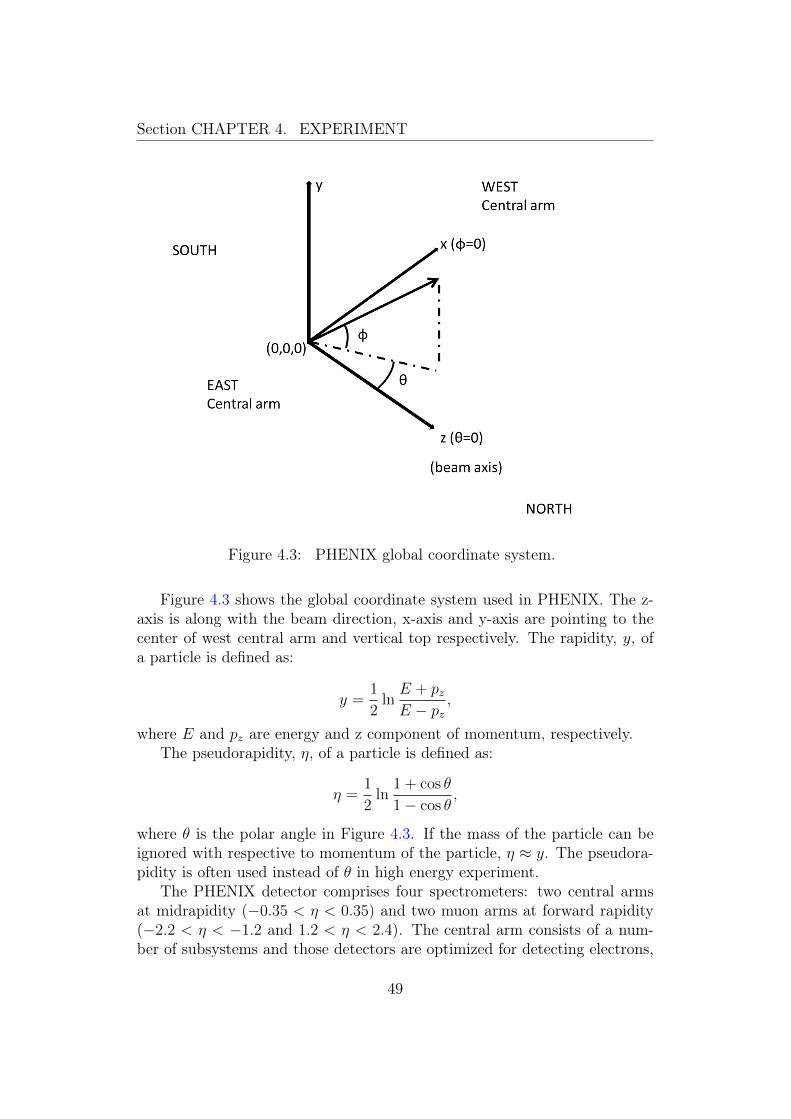
Section CHAPTER 4. EXPERIMENT
Figure 4.3: PHENIX global coordinate system.
Figure 4.3 shows the global coordinate system used in PHENIX. The z-axis is along with the beam direction, x-axis and y-axis are pointing to thecenter of west central arm and vertical top respectively. The rapidity, y, ofa particle is defined as:
y =1
2lnE + pzE − pz
,
where E and pz are energy and z component of momentum, respectively.The pseudorapidity, η, of a particle is defined as:
η =1
2ln
1 + cos θ
1− cos θ,
where θ is the polar angle in Figure 4.3. If the mass of the particle can beignored with respective to momentum of the particle, η ≈ y. The pseudora-pidity is often used instead of θ in high energy experiment.
The PHENIX detector comprises four spectrometers: two central armsat midrapidity (−0.35 < η < 0.35) and two muon arms at forward rapidity(−2.2 < η < −1.2 and 1.2 < η < 2.4). The central arm consists of a num-ber of subsystems and those detectors are optimized for detecting electrons,
49

Section CHAPTER 4. EXPERIMENT
hadrons and photons. A schematic view of the each subsystems is shown inFigure 4.2. In December 2010, the VTX was installed near the collision pointas shown in Figure 4.2, which enables micro-vertexing capabilities.
4.2.2 Beam-Beam Counter and trigger
Figure 4.4: (Left) A picture of Beam-Beam counters module comprising 64Čerenkov counters. (Right) A picture of quartz radiator and PMT.
The beam-beam counters (BBC) covering pseudorapidity 3.0 < |η| < 3.9and full azimuth are located at± 1.44 meters along the beam axis and relativeto the nominal beam-beam collision point. Each of the BBCs comprises 64Čerenkov counters as shown in Figure 4.4.
Based on the coincidence of the BBCs, Au+Au collisions are selected viaan online Minimum Bias (MB) trigger, which requires at least two counterson each side of the BBC to be fired.
The MB sample covers 96±3% of the total inelastic Au+Au cross sectionwith a |z-vertex| < 10 cm cut as determined by comparison with MonteCarlo Glauber models [5, 138] in 2011. The BBCs also provide a measureof the collision position along the beam axis (z-vertex) determined by thetime-of-flight difference between hits in the two sets of BBC counters. Thesystematics shift of z-vertex position of BBC with respect to the central arm(∼ 5 cm) was observed during the 2011 run and it was adjust by z-vertexprovided from VTX. The z-vertex resolution of the BBC is approximatelyσz = 0.6 cm in central Au+Au collisions.
During 2011, the pre-scale factor which prevails events of |z−vertex| < 12cm was set in the trigger algorithm to increase the number of events withinthe VTX acceptance. ∼ 85% of all Au+Au collisions within that selectionwere recorded by the PHENIX high-bandwidth data acquisition system.
50

Section CHAPTER 4. EXPERIMENT
4.2.3 Central arms
Electrons (e+ and e−) are reconstructed using two central spectrometerarms as shown in Fig. 4.2, each of which covers the pseudorapidity range|η| < 0.35 and with azimuthal angle ∆φ = π/2. The detector configurationof the central arms is the same as in previous PHENIX Collaboration heavyflavor electron publications [11, 94], but there was no He bags in 2011.
The transverse momentum of each charged particle is determined by itsbending radius in the magnetic field of central magnet system [139]. Themagnet consists of an outer and inner coil inside a steel yolk, generating ansymmetric axial magnetic field parallel to the beam axis. The field strength,B, is 0.9 Tesla around the beam pipe and gradually decrease along the radialposition. The field integral
∫B · dl is 1.15 (Tesla · m) at φ = 90◦.
The central arms are easily moveable to allow access to detector compo-nents for commissioning and maintenance.
Charged particle tracks are reconstructed outside of an axial magneticfield using layers of drift chamber (DCH) and multi-wire proportional padchambers (PC). The momentum resolution is σp/p ' 0.7% ⊕ 0.9% p (GeV).
Electron identification is performed by hits in a ring imaging Čerenkovdetector (RICH) and a confirming energy deposit in an electromagneticcalorimeter (EMCal).
4.2.4 Drift Chamber
The Drift Chambers (DCH) are main tracking detectors in central arms.DCHs are placed at the front of both the East and the West arms with aradius of 2.0 to 2.4 m far from the beam axis in a residual magnetic fieldwith a maximum of 0.06 Tesla[10]. Each DCH has a cylindrical shape with|z| ≤ 90 cm and π/2 azimuthal angle (φ) coverage as shown in Figure 4.5.There are 6 types of wire modules stacked radially in each sector. They arecalled X1, U1, V1, X2, U2 and V2. Each module contains 4 sense planesand 4 cathode planes forming wire cells with a 2 - 2.5 cm drift space in theφ direction. The X1 and X2 wire cells run in parallel to the beam axis tomeasure particle trajectories in r - φ. The U and V wires are tilted withabout 6◦ rotation with respect to the X wires, and measure the z-coordinateof the track.
Each of the X- and U,V-stereo cells contain 12 and 4 anode (sense) wires,respectively. As a result, there are 40 drift cells in the DCH located atdifferent radii. The layout of wires within one DCH sector is shown in Figure4.6. The stereo wires start in a sector on one side and end in a neighboringsector on the other side of the DCH.
51

Section CHAPTER 4. EXPERIMENT
Figure 4.5: A schematic view of Drift Chameber
To reduce the single wire occupancy, the wires are electrically isolatedinto two halves at the center of the DCH (z = 0) using kapton of 100 µmthickness. Therefore, the DCH system has 6400 sense wire (40/2 wires/cell *80 cells/side * 2 sides/arm * 2 arms = 6400 wires). The DCH operates witha mixture of 50% Ar, 50% ethane gas and small fraction of alcohol.
4.2.5 Pad Chamber
The Pad Chambers (PC) provide the hit information in z-direction andthis is used with DCH hit information to reduce track ambiguities in highmultiplicity environment. The PCs consist of three individual layers of multi-wire proportional chambers [10].
As shown in Figure 4.2, the first inner layer of the PC (PC1) are placedbetween the DCH and the RICH in both the East and the West arms. Thesecond layer (PC2) is located behind the RICH in the West arm only. The
52

Section CHAPTER 4. EXPERIMENT
Figure 4.6: (Left) The layout of DCH wire position within one sector andinside the anode plane. (Right) Top view of the DCH stereo wire orientations.
third layer (PC3) is mounted in front of the EMCal The installed radii ofthese three PC layers correspond to 248, 419 and 490 cm from the beampipe, respectively.
Each PC contains a single plane of wires inside a gas volume bounded bytwo cathode planes. One cathode is finely segmented into an array of pixels.The charge induced on a number of pixels when a charged particle starts anavalanche on an anode wire, is read out through specially designed readoutelectronics.
A special pad design was invented to archive a high pixel granularity andsmall readout channels. Figure 4.7 (left) shows the pixel configuration ofa pad. The nine by nine interleaved pixels are grouped together to formsingle readout channel. Each cell recognizes a valid hit and contains threepixels which are connected to different but neighboring pads shown in Figure4.7 (right). So, the hit information can be broken down to the cell level byidentifying the triplets of the pads. The cell size is 8.4 mm for the PC1 andPC2 , and is twice for the PC3, since the PC3 is twice far from the beampipe compared to the PC1. The spacial resolutions of the PC1 and PC3 inz direction is ± 1.7 mm and ±3.6 mm, respectively.
53

Section CHAPTER 4. EXPERIMENT
Figure 4.7: The pad and pixel geometry in the pad chamber. A cell definedby three pixels is at the center of the right picture.
4.2.6 Ring Imaging Čherenkov Detector
The Ring Imaging Čerenkov detector (RICH) [10, 140] is a gas Čerenkovdetector and is a primary device for identifying electrons among the very largenumber of charged hadrons (O(1000) times larger than electrons). The RICHis placed behind the PC1 in both the East and the West arms. Figure 4.8shows a cutaway view of the RICH. The RICH consists of a 40 m3 gas vesselwith an entrance and exit windows of the aluminized Kapton, 48 compositemirror panels, forming two intersecting spherical mirrors and two arrays of80(φ) × 16(z) photo multiplier tubes (PMT). A PMT array is placed behindthe central magnet so that particles from the collision do not directly hitthe PMT array as shown in Figure 4.9. The PMTs are equipped with 2inch diameter Winston cones and have magnetic shields that allow themto operate at up to 100 Gauss. The spherical mirror reflects the Čerenkovphotons emitted from an electron and focuses on the PMT array forming aring-shaped pattern. The diameter of the Čerenkov ring which correspondsthe emission angle of the Čerenkov photon. The vessel is filled with CO2 gasat 1 atm as Čerenkov radiator. This corresponds to Čerenkov threshold of4.65 GeV/c for pion and produces an average of 12 photons per ring for acompletely relativistic particle. The diameter of CO2 gas is about 11.8 cm.
54

Section CHAPTER 4. EXPERIMENT
Figure 4.8: A cutaway view of one arm of the RICH detector [10].
Figure 4.9: Top view of the RICH in the PHENIX east arm [11].
55
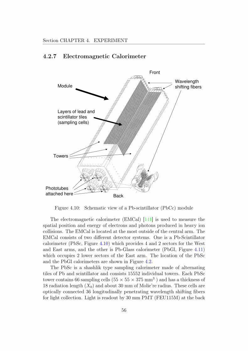
Section CHAPTER 4. EXPERIMENT
4.2.7 Electromagnetic Calorimeter
Wavelength
shifting fibersModule
Towers
Layers of lead and
scintillator tiles
(sampling cells)
Front
Back
Phototubes
attached here
Figure 4.10: Schematic view of a Pb-scintillator (PbCc) module
The electromagnetic calorimeter (EMCal) [141] is used to measure thespatial position and energy of electrons and photons produced in heavy ioncollisions. The EMCal is located at the most outside of the central arm. TheEMCal consists of two different detector systems. One is a Pb-Scintillatorcalorimeter (PbSc, Figure 4.10) which provides 4 and 2 sectors for the Westand East arms, and the other is Pb-Glass calorimeter (PbGl, Figure 4.11)which occupies 2 lower sectors of the East arm. The location of the PbScand the PbGl calorimeters are shown in Figure 4.2.
The PbSc is a shashlik type sampling calorimeter made of alternatingtiles of Pb and scintillator and consists 15552 individual towers. Each PbSctower contains 66 sampling cells (55 × 55 × 375 mm3 ) and has a thickness of18 radiation length (X0) and about 30 mm of Molie’re radius. These cells areoptically connected 36 longitudinally penetrating wavelength shifting fibersfor light collection. Light is readout by 30 mm PMT (FEU115M) at the back
56

Section CHAPTER 4. EXPERIMENT
Figure 4.11: Schematic view of a Pb-glass (PbGl) module
of the towers. A single basic structure is called as a module which consistsof 4 towers. On the other hand, the PbGl is Cerenkov calorimeter whichconsists of 9216 lead glass modules with PMT readout (FEU84). Each PbGlmodule is 40 ×40× 400mm3 and has 14.4 X0 and 36 mm of Molie’re radius.The PbGl has been used previously in CERNWA98 experiment [142]. Figure4.10 shows an unit array of the PbGl modules. The EMCal has an importantrole in particle identification using the informations of measured energy, timeand shower shape of electromagnetic cascade. The energy resolutions of thePbSc and the PbGl are obtained using electron and positron beam at a testexperiment for the PbSc and the PbGl respectively:
σEE Pbsc
=8.1%√E (GeV)
⊕ 2.1%
σEE PbGl
=5.9%√E (GeV)
⊕ 0.8%
57

Section CHAPTER 4. EXPERIMENT
4.3 Data Acquisition
RHIC clocks
20MB/s
250TB/yr
~350000 ch
ATM Switch
MTM
SEB
DCMFEM
Linux Farm
~600 CPU's
Online
Monitoring
ZD
C S
outh
ZD
C N
orth
A S
ubsyst
em
(e.g
. Eas
t DC
)
Data packets
over fiber
Clock, Trigger,
Mode bits
over fiber
Sh
ield W
all
a few
miles la
ter
DCB
PartitionerData Packets
Dat
a Pac
kets
over
NEV
IS T
oken
passing
Bus
over Parallel
FIFO Interface
GTM
GL1
L1
Bu
sy
Bu
sy
Trigger
tape
storage
1.2PB
Clock
Interaction regionCountingroom
RHIC
Computing
Facility
GL1 Global Level 1 Trigger
GTM Granual Timing Module
MTM Master Timing Module
DCB Data Collection Board
DCM Data Collection Module
FEM Front End Module
SEB Sub Event Buffer
ATP Assembly Trigger Processor
Missing:
• ARCNET Serial Interface to FEMs
• High and Low Voltage Control and
associated control systems
• Alarm system
'trigger' is a placeholder
for a much more complex
'Local Level 1' trigger system
SEBSEBSEB
ATP
End
User
Figure 4.12: A schematic diagram of the PHENIX Data Acquisition system.
The number of tracks passed through the detector varies from only a fewtracks in p+p to several hundred tracks in central Au+Au collisions. Theexpected interaction rate also varies from a few kHz from central Au+Auto approximately 500 kHz for p+p collisions. To handle a variety of eventsize and rate seamlessly, the PHENIX Data Acquisition system (DAQ) [143]consists of the detector front ends equipped with the pipelined and dead-timeless features and higher level trigger systems. Figure 4.12 shows a gen-eral schematic diagram of the PHENIX DAQ. The RHIC delivers the 9.4MHz fundamental clock which corresponds to 106 ns of time interval be-tween beam crossings. All of PHENIX Front End Electronics modules aresynchronized to the RHIC clock. Signals produced in the various subsystemsare processed by Front End Modules (FEMs) that converts the detector ana-log signals into digital data. The FEM for each subsystem is placed in thePHENIX Intersection Region (IR). A FEM module can buffer the data towait for the Level-1 trigger LVL1 decisions and to wait for digitization andreadout of triggered event. The RHIC clock is received by the Master TimingModule (module). The MTM distributes the master clock by fanning out theRHIC clock, where the internal phase locked loop is used to minimize theclock jitter. The master clock is transmitted to the FEM via the Granual
58

Section CHAPTER 4. EXPERIMENT
Timing Module (GTM). Thus, all the FEM’s are processed in a single clock.The GTM is prepared for a unit of detector elements. In addition, the GTMsend the control commands (mode bits) and trigger decisions. The purposeof the Level-1 trigger (LVL1) is to select interesting events and provide eventrejection for the limited DAQ rate. The Global Level-1 (GL1) system gen-erates the LVL1 decision based on logical combinations of the Local Level-1(LL1) decisions. The LL1 is generated by individual trigger detector. TheGL1 can treat totally 128 bits of the LL1 inputs to make the LVL1 decision.Once the LVL1 decision is generated, the decision signal is sent to the FEMvia the GTM, then the data buffered in the FEM are transfered to the DataCollection Module (DCM) located at the PHENIX Counting House. TheFEM, GTM and DCM are connected via a fiber optic cable to eliminate alarge number of noise, cross-talk and grounding problems. At the maximumLVL1 trigger rate, the whole FEM’s send over 100 Gbytes of data per second.The DCM is designed to receive this large amount of data. After receivingthe data, the DCM performs the zero suppression, error checking and dataformatting to generate data packets. The zero suppression is to compress thedata by comparing the preset threshold. In addition, the DCM provides abusy signal which are returned to the GL1 to hold off further triggers. Manyparallel streams of the data packets from the DCMs are sent to the eventbuilder (EVB). The EVB performs the final stage of event assembly.In theEVB, the streams of the data packets from the DCMs are first received andbuffered in a set of the Sub Event Buffers (SEB). These data are transferedon request to a set of Assembly/Trigger Processors (ATP) via AsynchronousTransfer Mode switch (ATM). The final events assembled in the ATPs aretransmitted to the PHENIX Online Control System (ONCS) for logging andmonitoring processes. The format of the final event is called “PHENIX RawData Format (PRDF)”. The raw data are sent to High Performance Stor-age System (HPSS) at RHIC Computing Facility (RCF) and converted tophysical quantities for analysis.
59

Section CHAPTER 4. EXPERIMENT
4.4 Silicon Vertex Tracker UpgradeSilicon Vertex Tracker (Silicon Vertex Tracker (subsystem of PHENIX)
(VTX)) is used for pricise collision vertex (primary vertex) in 3 dimensionalspace as well as displaced track measurement. The detail of VTX detectoris described in this section.
Figure 4.13: (Left) A picture of the one side of the VTX detector. (Right)A schematic view of the VTX detector from beam steam with the individualladders shown.
The (VTX) (Figure 4.13 (left) was installed near the collision point asshown in Figure 4.2 in December 2010. In addition, a new beryllium beampipe with 2.16 cm inner diameter and 760 µm nominal thickness (0.24 % radi-ation length (X0)) was installed to reduce conversion electrons and multiple-scattering before the VTX detector.
The VTX detector [28, 144, 145] consists of four cylindrical layers ofsilicon detectors as shown in Figure 4.13 (right). The detector is separatedinto west and east arms, each with nominal acceptance ∆φ ≈ 0.8π centeredon the acceptance of the outer PHENIX central arm spectrometers. Thedetector covers pseudorapidity |η| < 1.2 for collisions taking place at z = 0.The VTX can precisely measure the vertex position of a collision within|z| < 10 cm range of the center of the VTX. The main characteristics of theVTX detector are summarized in Table 4.3.
The two inner layers, referred to as B0 and B1, of the VTX detector com-prise silicon pixel detectors [146]. B0 (B1) comprises 10 (20) pixel ladders(Figure 4.16) with a central radial position of 2.6 (5.1) cm. The silicon pixel
60

Section CHAPTER 4. EXPERIMENT
Table 4.3: A summary of the VTX detector. For each layer (B0 to B3),the detector type, read out chip, the central radius (r), ladder length (l),sensor thickness (t), sensor active area (∆φ × ∆z), the number of sensorsper ladder (NS), the number of ladders (NL), pixel/strip size in φ (∆φ) andz (∆z), the number of read-out channels (Nch), and the average radiationlength including the support and on-board electronics (X0) are given.Layer B0 B1 B2 B3read out chip ALICE1LHCb ALICE1LHCb SVX4 SVX4
type pixel pixel stripixel stripixelr (cm) 2.6 5.1 11.8 16.7
sensor area l (cm) 22.8 22.8 31.8 38.2t (µ m) 200 200 625 625∆φ (cm) 1.28 1.28 3.07 3.07∆z (cm) 5.56 5.56 6.00 6.00NS 4 4 5 6NL 10 20 16 24
pixel/strip size ∆φ (cm) 50 50 80 80∆z (cm) 425 (625) 425 (625) 3× 10⁴ 3× 10⁴
Nch 1.3× 10⁶ 2.6× 10⁶ 1.2× 10⁵ 2.2× 105
X0 (%) 1.3 1.3 5.2 5.2
technology is based on the ALICE1LHCb sensor-readout chip [147], whichwas developed at CERN. Each ladder is electrically divided into two inde-pendent half-ladders. Each ladder comprises four sensor modules mountedon a mechanical support made from carbon-fiber composite.
As shown in Figure 4.14, each sensor module comprises a silicon pixelsensor with a pixel size of 50 µm(φ) × 425 µm(z). In the region between twochips, the pixel sensor cells are elongated in z (625 µm instead of 425 µm)to eliminate the dead area between chips. The silicon sensors are producedas p-in-n structures on 200 µm thick silicon. One pixel readout chip reads256 (φ)× 32 (z)= 8192 pixels and covers approximately 1.3 cm (∆φ)× 1.4cm (∆z) of the active area of the sensor. The number of pixels in total is8192 (pixels/chip) × 4 (chips/sensor) × 4 (sensors/ladder) × 30 (ladders) =3932160. The position resolution is σφ = 14.4 µm in the azimuthal directionand σz = 123 µm in the z direction. The typical operation bias voltage is30 V.
Each pixel is interconnected with four pixel readout chips by bump-bonding technique, which connect electrical structures with small balls ofsolder. Figure 4.15 shows the schematic of the circuitry within one pixel
61

Section CHAPTER 4. EXPERIMENT
Figure 4.14: schematic view of a pixel sensor
cell in the ALICE1LHCb chip. Each readout chip has 32 × 256 amplifier-discriminators for individual channel and the binary output of the discrim-inator is delayed with a programmable delay and stored for readout by thedownstream data acquisition system (DAQ). When the readout is issued,the data is transferred to Silicon Pixel Interface Read-Out (SPIRO) modulethrough the readout bus mounted on the sensor module (Figure 4.16 (bot-tom)). The readout bus is manufactured using flexible printed circuit (FPC)board technology [148]. The bus consists of four 3µ m copper signal layersand two 50 µm aluminum power layers (power and ground). The structuralmaterial for the bus is Polyimide. SPIRO module provides all service volt-ages, timing and control signal, reads out the data from pixel ladder andtransfer it to the front end module (FEM) via optical cable.
62

Section CHAPTER 4. EXPERIMENT
Figure 4.15: A schematic of the circuitry within one pixel cell in the AL-ICE1LHCb sensor-readout chip. Reprinted from [147] with permission fromElsevier.
Figure 4.16: (Top) A picture of a pixel ladder. (Bottom) Schematic view ofa pixel ladder.
63

Section CHAPTER 4. EXPERIMENT
The two outer layers of the VTX detector, referred to as B2 and B3, areconstructed using silicon stripixel sensors, as detailed in Ref. [149, 150]. TheB2 (B3) layer comprises 16 (24) silicon stripixel ladders at a central radialdistance of 11.8 (16.7) cm. The stripixel sensor is a novel silicon sensor,and is a single-sided, N-type, DC-coupled, two-dimensional (2-D) sensitivedetector. One sensor has an active area of approximately 30 mm × 60 mm,which is divided into two independent sectors of 30 mm × 30 mm. Eachsector is divided into 384 × 30 pixels. Each pixel has an effective size of80 µm (φ) × 1000 µm (z), leading to a position resolution of σφ=23 µm inazimuthal direction.
Figure 4.17: (Left) A picture of a stripixel detector. (Right) Schematic viewof a stripixel with two independent interleaved a-pixel (blue) and b-pixel (red)[151].
Figure 4.18: (Left) X strips formed by a-pixels. (Right) U strips formed byb-pixels. These figures are from [151].
As shown in Figure 4.17, a pixel comprises two spiral shape implants(a-pixel and b-pixel) interleaved such that the charge deposited by ionizing
64

Section CHAPTER 4. EXPERIMENT
particles are registered by both implants. There are 30 a-pixel implants alongthe beam direction, connected to form a 30 mm long X-strip, and 30 b-pixelimplants are connected with a stereo angle of 80 mrad to form a U-strip.X-strip and U-strip are visualized in Figure 4.18. When a charged particlehits a pixel, both the X- and the U-strip sharing the pixel register a hit.Thus the hit pixel is determined as the intersection of the two strips. Thisdesign allows to simplify fabrication process for both the sensor and readoutcompared with that for the double-sided strip sensor.
Figure 4.19: Conceptual schematic of a single SVX4 channel circuit [152].c©2004 IEEE.
The stripixel sensor is read out with the SVX4 chip developed by a FNAL-LBNL Collaboration [153]. The stripixel sensor and each SVX4 channel areDC-coupled. It contains 128 parallel charge integration channels, a 128 ×46-cell analog latency pipeline capable of buffering up to 4 samples, andWilkinson type 8 bit analog to digital converters (ADCs). ADCs informationare used as weighting factor of hit information for clustering (subsection 5.4.2)as well as dE/dx measurement. Figure 4.19 shows the conceptual schematicof a single SVX4 channel circuit.
The total number of channels in stripixel layers is 128 (channels/chip) ×12 (chips/sensor) × (5 (sensors/ladder) × 16 (ladders/B2 layer) + 6 (sen-sors/ladder) × 24 (ladders/B3 layer) = 344064. The typical operation biasvoltage is 200 V.
65

Section CHAPTER 4. EXPERIMENT
The detector occupancy for the central Au+Au at 200 GeV is studied byusing geant3 [154] model of the VTX detector and the HIJING [155] eventgenerator. The result of the simulation is summarized in the Table 4.4.
Table 4.4: Occupancy of the each VTX layer for central Au+Au collisionsat 200 GeV
Layer OccupancyB0 0.53%B1 0.16%B2 4.5% (X strip) 4.7% (U strip)B3 2.5% (X strip) 2.7% (U strip)
66

Chapter 5
Analysis
5.1 OverviewThe purpose of the analysis is to separate the electrons from charm hadron
decays and those from bottom hadron decays. The life time of B mesons(cτB0= 455 µm, cτB± = 491 µm [3]) is substantially longer than that of Dmesons (cτD0 = 123 µm, cτD± = 312 µm) and the decay kinematics aredifferent. This means that the distribution of values for the distance ofclosest approach (DCA) of the track to the collision vertex (primary vertex)for electrons from bottom decays will be broader than that of electrons fromcharm decays. Thus c→ e, b→ e can be separated via precise measurementof the DCA distribution and pT distribution. There are other sources ofelectrons, namely Dalitz decays of π0 and η, direct virtual photon, photonconversions in the material, Ke3 decays, and J/ψ → e+e− decays. With theexception of electrons from Ke3 decays, these background components haveDCA distributions narrower than those from charm decay electrons. Thesebackground components are subtracted before the charm/bottom separation.
In the first step of the analysis, good events where the collision vertex iswithin the acceptance of the VTX detector are selected, and its function isnormal (section 5.5). Then electron tracks are reconstructed in the PHENIXcentral arms (section 5.4.4). They are then associated with hits in the VTXdetector and their DCA is measured (section 5.6). At this point, the DCAdistribution of inclusive electrons has contributions from heavy flavor elec-trons (b→ e and c→ e) and several background components.
The next step is to determine the DCA shape and normalization of allbackground components (section 5.7). They include mis-identified hadrons,background electrons with large DCA caused by high-multiplicity effects,photonic electrons (Dalitz decay electrons, photon conversions), and elec-
67

Section CHAPTER 5. ANALYSIS
trons from Ke3 and quarkonia decays. The shapes of the DCA distributionsof the various background electrons are determined via data driven methodsor Monte Carlo simulation (DCA cocktail method). Then the normalizationof those background electron components in the data is determined (sec-tion 5.8).
Because the amount of the VTX detector material is substantial (13% ofone radiation length) the largest source of background electrons is photonconversion within the VTX. This background is suppressed by a conversionveto cut (section 5.7.4)
Once the shape and the normalization of all background components aredetermined and subtracted, the DCA distribution of heavy flavor decay elec-trons can be described as a sum of b → e and c → e DCA distributions.The heavy flavor DCA distribution is decomposed by an unfolding method(section 5.9).
5.2 Track reconstruction in Central armsCharged particle tracks are reconstructed using the outer central arm
detectors, DCH and PC [94]. The DCH has six types of wire modules stackedradially, named X1, U1, V1, X2, U2, and V2 (see subsection 4.2.4). The Xwires run parallel to the beam axis in order to measure the φ-coordinateof the track and the U and V wires have stereo angles varying from 5.4 to6.0 degrees. Tracks are required to have hits in both the X1 and X2 sectionsalong with uniquely associated hits in the U or V stereo wires and at least onematching PC hit, to reduce mis-reconstructed tracks. The track momentumvector is determined assuming the particle originated at the Au+Au collisionvertex as reconstructed by the BBC. The incident angle of the incoming trackat a reference radius within the DCH, α, is a measure of the momentum vectorand charge of the particle, as shown in Figure 5.1.
5.3 Electron identificationElectron candidates are selected by matching tracks with hits in the RICH
and energy clusters in the EMCal. The details on the electron selection cutsare given in Ref. [11]. In this analysis we select electron candidates within1.0 < pT < 5.0 GeV/c , and we briefly describe the cuts in the RICH andEMCal below.
Čerenkov photons from an electron track produce a ring-shaped cluster inthe RICH. At least three associated PMT hits are required in the RICH and
68

Section CHAPTER 5. ANALYSIS
Figure 5.1: Charged particle momentum vector reconstruction using DCHhit information [12].
a ring-shape cut is applied. The center of the ring is required to be within5 cm of the track projection. The probability that the associated clusterin the EMCal comes from an electromagnetic shower is calculated based onthe shower shape. Based on that probability, tracks are selected in a waythat maintains high efficiency for electrons while rejecting hadrons. Further,the energy (E) in the EMCal is required to match the track determinedmomentum (p). This match is calculated as dep = (E/p−µE/p)/σE/p, whereµE/p and σE/p are the mean and standard deviation respectively of a Gaussianfit to the E/p distribution, determined as a function of momentum as shownin Figure 5.2. A cut of dep > −2 is used to further reject hadrons that havean E/p ratio < 1, because they do not deposit their full energy in the EMCal.
In high-multiplicity Au+Au events there is a significant probability fora random association between the track and hits in the RICH and EMCal.This mis-identified hadron probability is estimated as follows. The z < 0and z > 0 sides of the RICH have their hits swapped in software, and thetracks are re-associated with RICH hits. Because the two longitudinal sidesof the RICH are identical, this gives a good estimate of the random hadronbackground in the electron sample.
69

Section CHAPTER 5. ANALYSIS
The distribution of electron candidates at pT = 1.0 – 5.0 GeV/c for thenormalized EMCal energy to track momentum ratio, dep defined above, isshown in Figure 5.2. There is a large peak near zero from true electrons asexpected and a clear low-side tail from mis-identified hadron. Also shownis the result of the above swap method. The difference between the data(black) and the “swap” distribution (red) is explained as contributions fromoff-vertex electrons caused by conversions from the outer layer of the VTXand weak decay of kaon. In the final accounting for all contributions to theidentified-electron DCA distribution, we utilize this swap method to statisti-cally estimate the contribution of mis-identified hadron in each pT selectionas detailed in Section 5.7.2.
)σdep (-4 -3 -2 -1 0 1 2 3 4
coun
ts
0
5000
10000
15000
20000
25000
30000
35000
40000
45000
< 1.5 GeV/cT
dep 1.0 < p < 1.5 GeV/cT
dep 1.0 < p
)σdep (-4 -3 -2 -1 0 1 2 3 4
coun
ts
0
1000
2000
3000
4000
5000
6000
7000
8000
9000
< 2.0 GeV/cT
dep 1.5 < p < 2.0 GeV/cT
dep 1.5 < p
)σdep (-4 -3 -2 -1 0 1 2 3 4
coun
ts
0
200
400
600
800
1000
1200
1400
1600
1800
2000
< 2.5 GeV/cT
dep 2.0 < p < 2.5 GeV/cT
dep 2.0 < p
)σdep (-4 -3 -2 -1 0 1 2 3 4
coun
ts
0
100
200
300
400
500
< 3.0 GeV/cT
dep 2.5 < p < 3.0 GeV/cT
dep 2.5 < p
)σdep (-4 -3 -2 -1 0 1 2 3 4
coun
ts
0
50
100
150
200
250
300
< 4.0 GeV/cT
dep 3.0 < p < 4.0 GeV/cT
dep 3.0 < p
)σdep (-4 -3 -2 -1 0 1 2 3 4
coun
ts
0
10
20
30
40
50
60
< 5.0 GeV/cT
dep 4.0 < p < 5.0 GeV/cT
dep 4.0 < p
Figure 5.2: Matching variable between the reconstructed track momentum(p) and the energy measured in the EMCal (E): dep = (E/p − µE/p)/σE/pin 5 pT bins. The black distribution is for identified electrons , the reddistribution is the estimated contribution from mis-identified electrons viathe RICH swap-method, and the green distribution is for electrons after thesubtraction of mis-identified electrons.
70

Section CHAPTER 5. ANALYSIS
5.4 Event reconstruction in VTX
5.4.1 VTX alignment
In order to achieve good DCA resolution to separate b → e and c → e,alignment of the detector ladders to high precision is required. The detectoralignment is accomplished via an iterative procedure of matching outer cen-tral arm tracks from the DCH and PC to the VTX hits. (See appendix Bfor more detail.) The procedure is convergent for the position of each ladder.The alignment was repeated each time the detector was repositioned follow-ing a service access. The final alignment contribution to the DCA resolutionin both φ and z is a few tens of microns.
5.4.2 VTX hit reconstruction
For layers B0 and B1, clusters of hit pixels are formed by connectingcontiguous hit pixels by a recursive clustering algorithm. An average clustersize is 2.6 (6.7) pixels for the pixel (stripixel). The center of the cluster in thelocal 2-D coordinate system of the sensor is calculated as the hit position.
For B2 and B3 layers, 2D hit points on the sensor are reconstructed fromthe X-view and the U-view. Hit lines in the X-view (U-view) are formed byclustering contiguous hit X-strips (U-strips) weighted by deposited charges,and then 2D hit points are formed as the intersections of all hit lines in X-and U- views. When one hit line in U-view crosses more than two hit linesin X-view, ghost hits can be formed, because which crossing point is thetrue hit is ambiguous. These ghost hits increase the number of reconstructed2D hits approximately by 50% (30%) in B2 (B3) in central Au+Au colli-sions. The ghost hit rate was studied using a full geant simulation with theHIJING [155] generator as input. However, because the occupancy of thedetector at the reconstructed 2D hit point level is low, less than 0.1%, theseghost hits do not cause any significant issue in the analysis.
The positions of all 2-D hits in the VTX are then transferred into theglobal PHENIX 3-D coordinate system. Correction of the sensor position andorientation, determined by the alignment procedure described in the previoussection, is applied in the coordinate transformation. The resulting 3-D hitpositions in the global coordinate system are then used in the subsequentanalysis.
71

Section CHAPTER 5. ANALYSIS
5.4.3 The primary vertex reconstruction
With the VTX hit information alone, charged particle tracks can be re-constructed only with modest momentum resolution δp/p ≈ 10% due to thelimited magnetic field integrated over the VTX volume and the multiplescattering within the VTX. These tracks can be utilized to determine thecollision vertex in three-dimensions (z0 along the beam axis, and x0,y0 in thetransverse plane) for each Au+Au event under the safe assumption that themajority of particles originate at the collision vertex. This vertex position iscalled the primary vertex position.
The position resolution of the primary vertex for each direction dependson the sensor pixel and strip sizes, the precision of the detector alignment,and the number of particles used for the primary vertex calculation and theirmomentum in each event. The primary vertex resolution is evaluated fromthe difference in the primary vertex calculated from by the EAST and WESTVTX barrels. The distributions for the EAST - WEST difference in x, y andz-axis is shown in Figure 5.3. The width of the distributions of the East -West difference is larger than the resolution of the primary vertex calculatedusing the full VTX by roughly a factor of 2. A factor of 1/
√2 comes from the
assumption the multiplicity of East/West VTX is half of full VTX, anotherfactor of 1/
√2 comes from the error propagation of East-West. Namely,
σ(East) = σ(West) =1√2σ(full VTX),
σ(East - West) =√σ(East)2 + σ(West)2 = 2× σ(full VTX)
For Minimum Bias (MB) Au+Au collisions, the resolution values are σx =96 µm, σy = 43 µm, and σz = 75 µm. The worse resolution in x compared toy is due to the orientation of the two VTX arms. For comparison, the beamprofile in the transverse plane is σlumi
x ≈ σlumiy ≈ 90 µm in the 2011 Au+Au
run.
5.4.4 Association of a central arm track with VTX
Each central arm track is projected from the DCH through the magneticfield to the VTX detector. Hits in VTX are then associated with the trackusing a recursive windowing algorithm as follows.
The association starts from layer B3. VTX hits in that layer that arewithin a certain (∆φ×∆z) window around the track projection are searched.If hits are found in this window, the track is connected to each of the foundhits, and then projected inward to the next layer. In this case the search
72

Section CHAPTER 5. ANALYSIS
Westvertex - X
EastvertexX
-0.3 -0.2 -0.1 0 0.1 0.2 0.30
500
1000
1500
2000
2500m]µ = 192.5 [fitσm]µ = 96.2 [resσ
Westvertex - Y
EastvertexY
-0.3 -0.2 -0.1 0 0.1 0.2 0.30
1000
2000
3000
4000
5000
6000
m]µ = 85.3 [fitσm]µ = 42.6 [resσ
Westvertex - Z
EastvertexZ
-0.3 -0.2 -0.1 0 0.1 0.2 0.30
500
1000
1500
2000
2500
3000m]µ = 150.2 [fitσm]µ = 75.1 [resσ
Figure 5.3: The distributions for the difference in the primary vertex cal-culated from by the East and West VTX barrels (East - West) in x, y andz-axis
window in the next layer is decreased, because there is much less uncertaintyin projection to the next layer. If no hit is found, the layer is skipped, and thetrack is projected inward to the next layer, keeping the size of the projectionwindow. This process continues until the track reaches layer B0, and a chainof VTX hits that can be associated with the track is formed. The windowsizes are momentum dependent and determined from a full geant3 [154]simulation of the detector so that the inefficiency of track reconstruction dueto the window size is negligible.
After all possible chains of VTX hits that can be associated with a givencentral arm track are found by the recursive algorithm, a track model fit(multi-helices) is performed for each of these possible chains as shown inFigure 5.4 and Figure 5.5 and the χ2 of the fit, χ2
vtx, is calculated. The effectof multiple scattering in each VTX layer is taken into account in calculationof χ2
vtx This best chain and its track model are called a VTX-associated track.Note that at most one VTX-associated track is formed from each central armtrack.
The detail of the calculation of χ2vtx is as follows:
χ2vtx =
n−1∑i=0
(∆φ2
i
σ2φ,i
+∆z2iσ2z,i
)
+n−2∑i=1
(∆θ2xy,iσ2θxy ,i
+∆θ2rz,iσ2θrz ,i
)+
∆θ2xy,n−1σ2θxy ,n−1 + σ2
phi0
+∆θ2rz,n−1
σ2θrz ,n−1 + σ2
the0
where
73

Section CHAPTER 5. ANALYSIS
• ∆φi (∆zi): the difference of the hit position and the projected positionof hit in azimuthal (z) direction.
• ∆θxy,i (∆θrz,i): the angle difference of the incoming and the outgoinghelices in x-y (r-z) plane.
All the indices, i, correspond to indices of the associated hits. The countingbegins from the innermost hit, i.e. 1st ((n − 1)-th) hit is the innermost(outermost) hit. σφ,i and σz,i are resolution of each pixel: σφ,0(σφ,1) = 14 µmand σz,0(σz,1) = 123 µm, σφ,2(σφ,3) = 23 µm and σz,2(σz,3) = 289 µm. σθxy ,iand σθrz ,i is the root mean square of the Gaussian approximation of themultiple scattering angle divided by
√2. The radiation length of each layer
is averaged and corrected by a path length in modules of each track. σphi0and σthe0 correspond to the resolution of the azimuthal and polar angles of atrack outside of the VTX, respectively. σphi0 is calculated to be 1 mrad fromthe position resolutions of X1 and X2 of the DCH and the distance betweenX1 and X2 plane. σthe0 is calculated to be 7 mrad from the resolution ofz coordinate measured by the PC1 and BBC [156]. The primary vertexposition is not used for the χ2
vtx calculation to avoid any bias on the longlived particle.
In this analysis we require that VTX-associated tracks have associatedhits in at least the first three layers, i.e. B0, B1, and B2. An additional trackrequirement is χ2
vtx/NDF < 2 for pT < 2 GeV/c and χ2vtx/NDF < 3 for pT
> 2 GeV/c , where NDF is the number of degrees of freedom in the track fit,namely
NDF = 2 ·Nhit − 2,
where Nhit is the number of associated hits on the VTX.
74

Section CHAPTER 5. ANALYSIS
Figure 5.4: An illustration of a tracking with the VTX in x-y plane.
Figure 5.5: An illustration of a tracking with the VTX in r-z plane.
75

Section CHAPTER 5. ANALYSIS
5.5 Event selectionThe data set presented in this analysis is from Au+Au collisions at√sNN
= 200 GeV recorded in 2011 after the commissioning of the VTX de-tector. As detailed earlier, the MB Au+Au data sample was recorded usingthe BBC trigger sampling 96± 3% of the inelastic Au+Au cross section. Anumber of offline cuts were applied for optimizing the detector acceptanceuniformity and data quality as described below. After all cuts, a data sampleof 2.4×10⁹ Au+Au events was analyzed.
5.5.1 z-vertex selection
The acceptance of the PHENIX central arm spectrometers covers colli-sions with z-vertex within ± 30 cm of the nominal interaction point. TheVTX detector is more restricted in |z| acceptance, as the B0 and B1 layerscover only |z| < 11.4 cm. Thus the BBC trigger selected only events withinthe narrower vertex range of |zBBC| < 12 cm. In the offline reconstruction,the tracks reconstructed from VTX information alone are used to reconstructthe Au+Au collision vertex with resolution σz = 75 µm. All Au+Au eventsin the analysis are required to have a z-vertex within±10 cm as reconstructedby the VTX.
5.5.2 Data quality assurance
Due to a number of detector commissioning issues in this first data takingperiod for the VTX, the data quality varies substantially. Therefore we dividethe entire 2011 Au+Au data taking period into four periods. The acceptanceof the detector changes significantly between these periods.
In addition, several cuts are applied to ensure the quality and the stabilityof the data. Applying electron identification cuts described in section 5.3,the electron to hadron ratios were checked for each run, a continuous datataking period typically lasting of order one hour, and three runs out of 547with ratios outside of 5σ from the mean were discarded. The B2 and B3stripixel layers had an issue in stability of read-out electronics where someof the sensor modules would drop out, resulting in a reduced acceptancewithin a given run. Additional instabilities also existed in the B0 and B1pixel layers. Detailed channel by channel maps characterizing dead, hot, andunstable channels were generated for all layers within a given run. Thesemaps were used to mask dead, hot, and unstable channels from the analysis,as well as to define the fiducial area of the VTX in simulations.
76

Section CHAPTER 5. ANALYSIS
During this first year of data taking, the instability of the read-out elec-tronics discussed above caused significant run-to-run variations in the accep-tance and efficiency of the detector. It is therefore not possible to reliablycalculate the absolute acceptance and efficiency correction while maintaininga large fraction of the total data set statistics. Instead, we report on therelative yields of charm and bottom to total heavy flavor. The DCA distri-butions have been checked consistent between running periods and are notimpacted by the changing acceptance. Thus we can measure the shape ofthe DCA distribution using the entire data set. In the following, we use theshape of the measured DCA distribution only to separate b → e and c → ecomponents.
77

Section CHAPTER 5. ANALYSIS
5.6 DCA measurement with the VTXCharged particle tracks reconstructed in the central arms must be associ-
ated with VTX hits in order to calculate their DCA. Three-dimensional (3-D)hit positions in the 4 layers of VTX are reconstructed. For each collision,the primary vertex is reconstructed by the VTX. Then central arm tracksare associated with hits in the VTX, and VTX-associated tracks are formed.Finally, the DCA between the primary vertex and the VTX-associated tracksare measured.
5.6.1 DCAT and DCAL
Using the primary vertex position determined above, the DCA of a trackis calculated separately in the transverse plane (DCAT ) and along the beamaxis (DCAL). Because by design the DCAT has a better resolution thanDCAL, we first find DCAT with a track model of a circle trajectory assumingthe uniform magnetic field over the VTX. We define DCAT as
DCAT ≡ L−R, (5.1)
where L is the distance from the collision vertex to the center of the circledefining the particle trajectory, and R is the radius of the circle as shownin Figure 5.6. DCAL is the distance between the z-coordinate of the pointDCAT found and z-coordinate of the primary vertex. As explained in thesubsection 5.4.4, we always require a hit in layer B0. The projection is alwaysstarted from the hit position in B0.
It is notable that DCAT has a sign in this definition. The distinctionbetween positive and negative values of DCAT—whether the trajectory isbending towards or away from the primary vertex—is useful since certainbackground contributions have asymmetric distributions in positive and neg-ative DCAT , as discussed in section 5.7. For electrons, the positive sideof DCAT distribution has less background contribution. There is no suchpositive/negative asymmetry in DCAL.
5.6.2 DCA distribution of hadron tracks
For each VTX-associated track, the DCA is calculated separately in theradial and longitudinal direction (DCAT and DCAL) from the track modeland the primary vertex position. Shown in Figure 5.7 is the resulting DCAT
and DCAL distributions for all VTX-associated tracks with pT = 1.0 –5.0 GeV/c . Since the vast majority of charged tracks are hadrons originatingat the primary vertex, we observe a large peak around DCAT , DCAL = 0
78

Section CHAPTER 5. ANALYSIS
Primary vertex
magnetic field
B0
Figure 5.6: Illustration of the definition of DCAT ≡ L - R in the transverseplane.
that is well fit to a Gaussian distribution where the σ represents the DCAT ,DCAL resolution. A selection of |DCAL | < 0.1 cm is applied to reducebackground. These DCA distributions are in integer-value counts and arenot corrected for acceptance and efficiency. There are broad tails for |DCAT
| > 0.03 cm. Monte Carlo simulation shows that the main source of the broadtails is the decay of long lived light hadrons such as Λ and K0
S.The DCAT resolution as a function of the track pT is extracted using a
Gaussian fit to the peak and is shown in Figure 5.8. The DCAT resolutionis approximately 75 µm for the 1.0 – 1.5 GeV/c bin and decreases withincreasing pT as the effect of multiple scattering becomes smaller for higherpT . The DCAT resolution becomes less than 60 µm for pT > 4 GeV/c , whereit is limited by the position resolution of the primary vertex.
79

Section CHAPTER 5. ANALYSIS
(cm)T
DCA0.15− 0.1− 0.05− 0 0.05 0.1 0.15
410
510
610
710
< 1.5T
All Tracks MB : 1.0 < p < 1.5T
All Tracks MB : 1.0 < p
(cm)T
DCA0.15− 0.1− 0.05− 0 0.05 0.1 0.15
310
410
510
610
710
< 2.0T
All Tracks MB : 1.5 < p < 2.0T
All Tracks MB : 1.5 < p
(cm)T
DCA0.15− 0.1− 0.05− 0 0.05 0.1 0.15
310
410
510
610
< 2.5T
All Tracks MB : 2.0 < p < 2.5T
All Tracks MB : 2.0 < p
(cm)T
DCA0.15− 0.1− 0.05− 0 0.05 0.1 0.15
210
310
410
510
610
< 3.0T
All Tracks MB : 2.5 < p < 3.0T
All Tracks MB : 2.5 < p
(cm)T
DCA0.15− 0.1− 0.05− 0 0.05 0.1 0.15
210
310
410
510
< 4.0T
All Tracks MB : 3.0 < p < 4.0T
All Tracks MB : 3.0 < p
(cm)T
DCA0.15− 0.1− 0.05− 0 0.05 0.1 0.15
10
210
310
410
510
< 5.0T
All Tracks MB : 4.0 < p < 5.0T
All Tracks MB : 4.0 < p
(cm)L
DCA0.15− 0.1− 0.05− 0 0.05 0.1 0.15
410
510
610
710
< 1.5T
: 1.0 < pT
All Tracks MB p < 1.5T
: 1.0 < pT
All Tracks MB p
(cm)L
DCA0.15− 0.1− 0.05− 0 0.05 0.1 0.15
410
510
610
< 2.0T
: 1.5 < pT
All Tracks MB p < 2.0T
: 1.5 < pT
All Tracks MB p
(cm)L
DCA0.15− 0.1− 0.05− 0 0.05 0.1 0.15
310
410
510
610
< 2.5T
: 2.0 < pT
All Tracks MB p < 2.5T
: 2.0 < pT
All Tracks MB p
(cm)L
DCA0.15− 0.1− 0.05− 0 0.05 0.1 0.15
210
310
410
510
< 3.0T
: 2.5 < pT
All Tracks MB p < 3.0T
: 2.5 < pT
All Tracks MB p
(cm)L
DCA0.15− 0.1− 0.05− 0 0.05 0.1 0.15
210
310
410
510
< 4.0T
: 3.0 < pT
All Tracks MB p < 4.0T
: 3.0 < pT
All Tracks MB p
(cm)L
DCA0.15− 0.1− 0.05− 0 0.05 0.1 0.15
10
210
310
410
< 5.0T
: 4.0 < pT
All Tracks MB p < 5.0T
: 4.0 < pT
All Tracks MB p
Figure 5.7: (Top 6 figures) Distance of closest approach distributions fortransverse plane (DCAT ) and (Bottom 6 figures) along the beam axis (DCAL)for all VTX-associated tracks in minimum bias Au+Au at √s
NN= 200 GeV
in the range 1.0 < pT < 5.0GeV/c .
80

Section CHAPTER 5. ANALYSIS
[GeV/c]T
p1 1.5 2 2.5 3 3.5 4 4.5
m]
µ [σ T
DC
A
30
40
50
60
70
80
90
Figure 5.8: The DCAT resolution as a function of pT for all tracks in MBevents
81
Section CHAPTER 5. ANALYSIS
5.7 Electron DCA distribution and BackgroundComponents
5.7.1 Overview
The sample of candidate electron tracks that pass all the analysis cutsdescribed above contains contributions from a number of sources other thanthe desired electrons from semi-leptonic decays of charm and bottom hadrons.In order to extract the heavy flavor contributions, all background componentsmust be fully accounted for and their DCAT shapes as a function of pTincorporated. These background components are listed in the order presentedbelow.
1. Misidentified hadrons
2. High-multiplicity background
3. Photonic electrons
4. Kaon decay electrons
5. Heavy-quarkonia decay electrons
As described in this and the following subsection, all background com-ponents are constrained by PHENIX measurements in Au+Au and are fullysimulated through a geant3 description of the detector. This method is sim-ilar to the cocktail method of background subtraction used in the previousanalysis of inclusive heavy flavor electrons [11].
Next, we describe these background sources and their DCA distributions.The first two components are caused by detector and multiplicity effects.DCA distributions and normalization of these two components are deter-mined by data driven methods, as detailed in this section. The last threecomponents are background electrons that are not the result of semi-leptonicdecays of heavy flavor hadrons. Their DCA distributions are determined byMonte Carlo simulation, and their normalization is determined by a boot-strap method described in section 5.8. Of those background electrons, pho-tonic electrons are the dominant contribution. We developed a conversionveto cut to suppress this background (5.7.4).
5.7.2 Mis-identified hadron
As detailed in the discussion on electron identification, there is a nonzerocontribution from mis-identified electrons. This contribution is modeled via
82

Section CHAPTER 5. ANALYSIS
the RICH swap-method described in Section 5.3. From this swap method, weobtain the probability that a charged hadron is mis-identified as an electronas a function of pT . This probability is then applied to the DCA distributionof charged hadrons to obtain the DCA distribution of mis-identified hadrons.
The resulting DCAT distribution is shown in each panel of Figure 5.13.Note that this component is properly normalized automatically. For eachpT bin, the DCA distribution of mis-identified prompt hadrons has a nar-row Gaussian peak at DCAT = 0. The broad tails for large |DCAT | aremainly caused by decays of Λ and K0
S. In all pT bins the magnitude of thisbackground is no more than 10% of the data for all DCAT
5.7.3 High-multiplicity background
Due to the high multiplicity in Au+Au collisions, an electron candidatetrack in the central arms can be associated with random VTX hits. Suchrandom associations can cause a background that has a very broad DCAT
distribution. Although the total yield of this background is only ' 0.1% ofthe data, its contribution is significant at large DCAT where we separateb→ e and c→ e.
To evaluate the effect of event multiplicity on the reconstruction per-formance, we embed simulated single electrons—i.e. the response of thePHENIX detector to single electrons that is obtained from a geant3 simulation—into data events containing VTX detector hits from real Au+Au collisions.The events are then processed through the standard reconstruction softwareto evaluate the reconstruction performance in MB Au+Au collisions.
The reconstructed DCAT and DCAL for embedded primary electrons inMB Au+Au collisions is shown in Fig. 5.9. Here the histograms, labeled as“Single Electrons", show the reconstructed DCAT and DCAL distributionsof primary electrons before embedding. The DCAT distribution comprisesa narrow Gaussian with no large DCAT tail and the DCAL distributioncomprises a similar, but slightly broader, Gaussian with no large tail. Theblue filled triangles show the DCAT and DCAL distributions after embed-ding. The DCAT and DCAL distributions comprise a Gaussian peaked atDCAT (DCAL) ∼ 0 which is consistent with the distribution before embed-ding. This demonstrates that the DCA resolution of the VTX is not affectedby the high multiplicity environment. However, the embedded distributionshave broad tails at large |DCAT | and |DCAL|.
As shown in Figure 5.9(b), tracks with |DCAL| > 0.13 cm are dominatedby random associations, as they are not present in the “Single Electron”sample. We therefore use the DCAT distribution for tracks with large |DCAL|as an estimate of this random high-multiplicity background. We choose the
83

Section CHAPTER 5. ANALYSIS
region 0.13 < |DCAL| cm < 0.18 to represent this background, and restrictour signal to |DCAL| < 0.1 cm. The DCAT distribution of tracks with0.13 < |DCAL| cm < 0.18 must be normalized in order to be used as anestimate of the high-multiplicity background for tracks within |DCAL| <0.1 cm. This normalization is determined by matching the integrated yieldof embedded primary electrons in each |DCAL| region for 0.08 < DCAT cm <0.2, as shown in the inlay of Figure 5.9(b). The region 0.08 < DCAT cm <0.2 is dominated by random associations, as shown in Fig. 5.9(a), and istherefore safe to use for determining the normalization. The normalizationof the high-multiplicity background is determined to be 2.89 ± 0.29. Thered filled circles in Fig. 5.9(a) show the embedded DCAT distribution withlarge DCAL (0.13 < |DCAL| cm < 0.18). This distribution agrees withthe embedded DCAT distribution (blue filled triangles in Fig. 5.9) for largeDCAT . This demonstrates that the tails for large DCAT are well normalizedby the distribution of electrons with large DCAL. However, there is a smallexcess in the region 0.05 < |DCAT | cm < 0.10 that is not accounted for bythe distribution with large DCAL. We address this excess in the systematicuncertainties, as described in section. 5.10, where it is found to have only asmall effect on the extraction of b→ e and c→ e.
In each panel of Figure 5.13 the high-multiplicity background is shown asa red line. It is determined from the DCAT distribution of the data within0.13 < |DCAL| cm < 0.18, as described above. The number of electron tracksin the large DCAL region is small. We therefore fit the resulting DCAT datain each pT bin with a smooth function to obtain the shape of the red curvesshown in Figure 5.13. A second order polynomial is used in the lowest pT bin,where there are enough statistics to constrain it. The higher pT bins are fitwith a constant value. All curves are multiplied by the same normalizationfactor, determined from embedded simulations as described above.
84

Section CHAPTER 5. ANALYSIS
[cm]TDCA-0.15 -0.1 -0.05 0 0.05 0.1 0.15
Yie
ld [a
.u.]
-210
-110
1
10
210
310
<2.5T
eSingle Electrons 2.0<p
| < 0.1 cmL
Embedded: |DCA
| < 0.18 cmL
Embedded: 0.13 < |DCA
(a)
| [cm]L
|DCA0 0.05 0.1 0.15 0.2 0.25 0.3 0.35 0.4 0.45
Yie
ld [a
.u.]
-110
1
10
210
310
410
<2.5T
eSingle Electrons 2.0<p
Embedded
(b)
| [cm]L
|DCA0 0.05 0.1 0.15 0.2 0.25 0.3 0.35
1
10
< 0.2T0.08 < DCA
Figure 5.9: Simulated primary electron (a) DCAT and (b) DCAL distribu-tion before and after embedding in real Au+Au data.
85

Section CHAPTER 5. ANALYSIS
5.7.4 Photonic electrons and conversion veto cut
Photon conversions and Dalitz decays of light neutral mesons (π0 and η)are the largest electron background. We refer to this background as photonicelectron background as it is produced by external or internal conversion ofphotons.
The PHENIX Collaboration has previously published the yields of π0 andη mesons in Au+Au collisions at √s
NN= 200 GeV [157, 158]. In addition
to the electrons from Dalitz decays of these mesons, the decay photons mayconvert to an e+e− pair in the detector material in the beam pipe or eachlayer of the VTX. The PHENIX Collaboration has also published the yieldsof direct photons in Au+Au collisions at √s
NN= 200 GeV [20, 69], that can
also be a source for conversions.In principle with these measured yields, combined with simple decay kine-
matics and a detailed geant3 description of the detector material and re-construction algorithm, one could fully account for these photonic electroncontributions as a function of DCAT and pT . However, systematic uncer-tainties on the measured yields for the π0, η, and direct photons would thendominate the uncertainty of the heavy flavor electron extraction. Therefore,we utilize the VTX detector itself to help reject these contributions in acontrolled manner.
We require that at least the first three layers of the VTX have hits asso-ciated with the electron track. Conversions in B1 and subsequent layers arerejected by the requirement of a B0 hit, leaving only conversions in B0 andthe beam pipe. The requirement of B1 and B2 hits enables us to impose aconversion veto cut, described below, that suppresses conversions from thebeam pipe and B0.
The conversion veto cut rejects tracks with another VTX hit within acertain window in ∆φ and ∆z around hits associated with a VTX-associatedtrack. Photons that convert to an e+e− pair in the beam pipe will leave twonearby hits in the first layer (B0) and/or subsequent layers of the VTX, andthus be rejected by the conversion veto cut. Similarly, conversions in B0 willresult in two nearby hits in the second layer (B1) and/or subsequent outerlayers. The same is true for e+e− from a Dalitz decay, though with a largerseparation due to a larger opening angle of the pair.
Figure 5.10 shows distribution of charge×∆φ of hits in each layer relativeto the electron track, where charge is the sign of charge of the track. Thered histogram shows the data in MB Au+Au collisions. If the track at theorigin is not an electron, we have a flat distribution due to random hits in thedetector. These random hits have been subtracted in Figure 5.10 by usingthe distribution for hadron tracks. The transverse momentum of the electron
86

Section CHAPTER 5. ANALYSIS
track is in the interval 1 < pT < 2 GeV/c .As mentioned above, these correlated hits around electron tracks are
caused by the partner e+ or e− of Dalitz decays or photon conversions. Theleft-right asymmetry of the distribution is caused by the fact that the partnere± track is separated from the electron track by the magnetic field and thedirection of the separation is determined by the charge of the electron track.In the distribution of charge × ∆φ, the partner track is bent towards thepositive direction.
The black histogram in Figure 5.10 shows the distribution from MonteCarlo simulations. In the simulation, the response of the PHENIX detectorto single π0s is modeled by geant3, and the resulting hits in the VTX andthe central arms are then reconstructed by the same reconstruction code asthe data. The correlated hits in the simulation are caused by the Dalitz decayof π0 and photon conversion in the material of the beam pipe and the VTXitself. The simulation reproduces the data well for charge×∆φ > 0. There isa difference between the data and the simulation for charge×∆φ < 0. Thisis caused by a subtle interplay between the conversions and high multiplicityeffects. The difference disappears for peripheral collisions. Similar correlatedhits are observed in B1 to B3 layers in the data and they are also wellexplained by the simulation.
We define a “window” of the conversion veto cut around an electron trackin each layer B0 to B3 and require that there is no hit other than the hitassociated with the electron track in the window. Since a photonic electron(Dalitz and conversion) tends to have a correlated hit in the window, as onecan see in Figure 5.10, this conversion veto cut rejects photonic background.A larger window size can reject photonic background more effectively, butthis can also reduce the efficiency for the heavy flavor electron signal dueto random hits in the window. The window for the conversion veto cut isa compromise in terms of the rejection factor on photonic backgrounds andefficiency for heavy flavor electrons. We optimized the size of the window ofthe conversion veto cut based on a geant3 simulation.
The pink hatched area shown in Figure 5.11 shows the window of theconversion veto cut in each layer. The window size is asymmetric sincecorrelated hits are mainly in the positive side of charge×∆φ. The windowsize is reduced for higher electron pT since the distribution of correlated hitsbecomes narrower for higher pT .
87

Section CHAPTER 5. ANALYSIS
[rad]φ∆ × charge-0.06 -0.04 -0.02 0 0.02 0.04 0.06
coun
t
210
310
410
510 (data)±e(sim)±Photonic e
at B0φ∆ × charge
[rad]φ∆ × charge-0.06 -0.04 -0.02 0 0.02 0.04 0.06
coun
t
210
310
410
510 (data)±e(sim)±Photonic e
at B1φ∆ × charge
[rad]φ∆ × charge-0.06 -0.04 -0.02 0 0.02 0.04 0.06
coun
t
210
310
410
510(data)±e
(sim)±Photonic e
at B2φ∆ × charge
[rad]φ∆ × charge-0.06 -0.04 -0.02 0 0.02 0.04 0.06
coun
t
210
310
410
510 (data)±e(sim)±Photonic e
at B3φ∆ × charge
Figure 5.10: Distribution of correlated hits near electron tracks for 1 <pT < 2 GeV.Distribution of correlated hits in B0 (top-left), B1 (top-right), B2 (bottom-left), B3(bottom-right) near electron tracks for 1 < pT < 2 GeV. The redpoints are from Au+Au data and the black points are from Monte Carlosimulation.
88

Section CHAPTER 5. ANALYSIS
[GeV/c]T
p0 0.5 1 1.5 2 2.5 3 3.5 4 4.5 5
[rad
]φ∆ ×
chrg
-0.06
-0.04
-0.02
0
0.02
0.04
0.06
1
10
210
310
)T
vs pφ∆ × chrgVeto residual B0 (
(b)
[GeV/c]T
p0 0.5 1 1.5 2 2.5 3 3.5 4 4.5 5
[rad
]φ∆ ×
chra
ge
-0.1
-0.05
0
0.05
0.1
1
10
210
310
410
)T
vs pφ∆ × chargeVeto residual B1 (
(b)
[GeV/c]T
p0 0.5 1 1.5 2 2.5 3 3.5 4 4.5 5
[rad
]φ∆ ×
chra
ge
-0.1
-0.05
0
0.05
0.1
1
10
210
310
)T
vs pφ∆ × chargeVeto residual B2 (
(b)
[GeV/c]T
p0 0.5 1 1.5 2 2.5 3 3.5 4 4.5 5
[rad
]φ∆ ×
chra
ge
-0.1
-0.05
0
0.05
0.1
1
10
210
310
)T
vs pφ∆ × chargeVeto residual B3 (
(b)
Figure 5.11: charge×∆φ vs pT for B0(top-left), B1(top-right), B2(bottom-left), B3(bottom-right). The conversion veto window is the pink hatchedarea.
89

Section CHAPTER 5. ANALYSIS
Figure 5.12 shows the survival fraction of the conversion veto cut forelectrons from photon conversions and Dalitz decays as a function of elec-tron pT from a geant3 simulation of the detector with hits run throughthe reconstruction software. The survival probability for conversions is lessthan 30% at pT = 1 GeV and decreases further at higher pT . The survivalprobability for Dalitz decays is higher since a Dalitz decay partner is morelikely to fall outside of the window of the conversion veto cut due to thelarger opening angle. Also shown in Figure 5.12 is the survival fraction ofelectrons from heavy flavor decays which pass the conversion veto cut (SHF).As expected, their efficiency for passing the conversion veto cut is quite highand pT independent.
The efficiencies shown in Figure 5.12 are calculated without the Au+Auhigh-multiplicity that may randomly provide a hit satisfying the conversionveto cut. Since these are random coincidences, they are a common reductionfor all sources including the desired signal — heavy flavor electrons. Thiscommon reduction factor, δrandom, is measured from the reduction of thehadron track yield by the conversion veto cut to be' 35% at pT = 1 GeV to'25% at pT = 5 GeV for MB Au+Au collisions. Note that when we determinethe DCAT distribution of the various background components using a fullgeant3 simulation we apply the same conversion veto cuts.
The DCAT distributions from photonic background processes that sur-vive the conversion veto cut are shown in Figure 5.13. The means of theDCAT distributions from Dalitz decays and conversions are shifted to nega-tive DCAT values due to the mis-reconstruction of the momentum caused bythe assumption that the tracks originate at the primary vertex, as explainedin the next paragraph. The shift is largest at the lowest pT bin and decreaseswith increasing pT .
For Dalitz electrons, the shift is due to the energy loss via induced radi-ation (bremsstrahlung). The total radiation length of the VTX is approxi-mately 13% as shown in Table 4.3. Thus a Dalitz electron coming from theprimary vertex loses approximately 1− e−0.13 ≈ 12% of its energy on averagewhen it passes through the VTX. The momentum measured by the DC isclose to the one after the energy loss due to the reconstruction algorithm.Since the momentum determined by the DC is used when projecting inwardfrom the hit in B0 to the primary vertex and in calculation of DCAT , this re-sults in a slight shift in the DCAT distribution. This effect is fully accountedfor in the DCAT template of Dalitz electrons since it is generated throughthe full geant3 and reconstruction simulation.
In the case of conversions, the effect is even larger, as one can clearly seein Figure 5.13. While a photon goes straight from the primary vertex to thebeam pipe or B0 layer where it converts, DCAT is calculated assuming that
90

Section CHAPTER 5. ANALYSIS
the electron track is bent by the magnetic field. Thus the DCAT distributionis shifted by the difference of the actual straight line trajectory and thecalculated bent trajectory. Again, this is fully accounted for with the fullgeant3 simulation. The effect is verified by selecting conversion electronswith a reversed conversion veto cut.
91

Section CHAPTER 5. ANALYSIS
[GeV/c]eT
p0 1 2 3 4 5 6 7S
urvi
val r
ate
afte
r th
e co
nver
sion
vet
o cu
t
0
0.2
0.4
0.6
0.8
1
c+bγ ee→ 0π
γ ee→ η
ee→ γdirect conversions
Figure 5.12: The survival rate as a function of electron pT (peT ) for electronsfrom photon conversion (black), Dalitz decay of π0 (red), η (green), electronsfrom direct photon (blue) and heavy flavor decay electrons (dark orange).
92

Section CHAPTER 5. ANALYSIS
5.7.5 Ke3
The background from Ke3 decays (K0S, K± → eνπ) contributes electrons
over a broad range of DCAT due to the long lifetime of the kaons. Bothcontributions are determined using pythia and a full geant3 simulation,taking into account the exact track reconstruction, electron identificationcuts, and conversion veto cut. The resulting DCAT distribution for thesekaon decays is shown in Figure 5.13. As expected, though the overall yield issmall, this contributes at large DCAT in the lower pT bins and is negligibleat higher pT .
5.7.6 Quarkonia
Quarkonia (J/ψ and Υ) decay into electron pairs. Due to the short life-time, these decays contribute to electrons emanating from the primary vertex.The J/ψ yields in Au+Au collisions at√s
NN= 200 GeV have been measured
by the PHENIX Collaboration [159]. The detailed modeling of these contri-butions out to high pT is detailed in Ref. [11]. While these measurementsinclude a small fraction of B → J/ψ decays, all J/ψ’s are considered promptwhen modeling the DCAT distribution. The J/ψ contribution is shown inFigure 5.13, and is quite small and peaked about DCAT = 0 as expected.Thus, the systematic uncertainty from the quarkonium yields in Au+Au col-lisions is negligible in all electron DCAT pT bins.
93
Section CHAPTER 5. ANALYSIS
5.8 Normalization of electron background com-ponents
If the detector performance were stable, we could convert the DCAT
distributions from counts into absolutely normalized yields. Then one couldstraightforwardly subtract the similarly absolutely normalized backgroundcontributions described above—with the normalization constrained by thepreviously published PHENIX yields for π0 [157], η [160], etc. However,due to detector instability during the 2011 run, such absolute normalizationof background contributions can have a large systematic uncertainty. Thuswe bootstrap the relative normalization of these background contributionsutilizing our published Au+Au results [11] from data taken in 2004.
The idea of the method is the following. PHENIX measured the invariantyield of open heavy flavor decay electrons from the 2004 dataset. In this 2004analysis we first measured inclusive electrons (i.e. the sum of backgroundelectrons and heavy flavor electrons). We then determined and subtracted thebackground electron components from the inclusive electron yields to obtainthe heavy flavor contribution. Thus the ratio of the background componentsto the heavy flavor contribution were determined and published in [11]. Weuse these ratios to determine the normalization of background components inthe 2011 data, as described in the next paragraph. Some backgrounds havethe same ratio to signal regardless of the year the data was collected, whileothers will differ due to the additional detector material added by the VTX.
The invariant yield in Au+Au collisions at √sNN
= 200 GeV of heavyflavor electrons and background electrons from Dalitz decays is a physicalobservable independent of the year the data was taken. Thus we can use theratio of heavy flavor/Dalitz that is determined in the 2004 analysis in the 2011data. On the other hand, the invariant yield of conversion electrons dependson the detector material present and is thus different in the 2011 data takingperiod with the VTX installed compared with the 2004 data. We accountfor this difference by calculating the fraction of nonphotonic electrons in the2011 data. A detailed description of the normalization procedure is given inAppendix A.
With this bootstrapped normalization completed, the correctly normal-ized background components are shown for all five pT bins vs DCAT in Fig-ure. 5.13. Note that the normalization of mis-identified hadron and randombackground is determined from the data as explained in sections 5.7.2 and5.7.3, respectively. The electron yield beyond the sum of these backgroundcomponents is from the combination of charm and bottom heavy flavor elec-trons.
94

Section CHAPTER 5. ANALYSIS
While the DCAT distributions in Figure 5.13 are plotted within |DCAT | <0.15 cm, only a |DCAT | < 0.1 cm is used in the analysis to extract thecharm and bottom yield described later. At large DCAT , the distributionis dominated by high-multiplicity background (subsection 5.7.3) and there-fore provides little constraint in the extraction of the charm and bottomcontributions.
95

Section CHAPTER 5. ANALYSIS
[cm]TDCA-0.15 -0.1 -0.05 0 0.05 0.1 0.15
coun
t
-110
1
10
210
310
410
< 2.0 [GeV/c]eT
1.5 < p
(a)=200 GeVNNsAu+Au MB PHENIX 2011
[cm]TDCA-0.15 -0.1 -0.05 0 0.05 0.1 0.15
coun
t
-110
1
10
210
310
< 2.5 [GeV/c]eT
2.0 < p
(b)=200 GeVNNsAu+Au MB PHENIX 2011
[cm]TDCA-0.15 -0.1 -0.05 0 0.05 0.1 0.15
coun
t
-110
1
10
210
310
< 3.0 [GeV/c]eT
2.5 < p
(c)=200 GeVNNsAu+Au MB PHENIX 2011
[cm]TDCA-0.15 -0.1 -0.05 0 0.05 0.1 0.15
coun
t
-110
1
10
210
< 4.0 [GeV/c]eT
3.0 < p
(d)=200 GeVNNsAu+Au MB PHENIX 2011
[cm]TDCA-0.15 -0.1 -0.05 0 0.05 0.1 0.15
coun
t
-110
1
10
210
< 5.0 [GeV/c]eT
4.0 < p
(e)=200 GeVNNsAu+Au MB PHENIX 2011 Data
Mis-identified hadron
Random
Dalitz
Conversion
Ke3
ψJ/
Figure 5.13: DCAT distributions for electrons in MB Au+Au at√sNN
= 200 GeV that pass the reconstruction and conversion veto cut inthe indicated five electron-pT selections. Also shown are the normalized con-tributions for the various background components detailed in Section 5.7.
96

Section CHAPTER 5. ANALYSIS
5.9 Unfolding
5.9.1 Overwiew
After we obtain the DCAT distributions as a function of electron pT andthe various background components, we proceed to extract the remainingcharm and bottom components. If one knew the shape of the parent charmand bottom hadron pT and rapidity distributions, one could calculate inadvance the DCAT shape for electrons from each heavy flavor via a model ofthe decay kinematics. Since the decay lengths of charm and bottom hadronsare significantly different, they will yield different DCAT distributions. Inthis case, one could simultaneously fit the DCAT distribution for each pTbin with all background components fixed across pT bins, and extract theone free parameter: the ratio of charm to bottom contributions. However,the pT distribution of charm hadrons is known to be significantly modifiedin Au+Au collisions — see for example Ref. [15]. For bottom hadrons thisis also likely to be the case. Therefore one does not know a priori the heavyflavor DCAT distribution since it depends on the parent pT distribution. Forexample, a B meson with momentum = 0 has a daughter electron with DCA= 0 no matter what the electron momentum happens to be.
Since the DCAT distributions for all electron pT result from the sameparent charm and bottom hadron pT spectrum, one can perform a simulta-neous fit to all the electron pT and DCAT data in order to find the mostlikely heavy flavor parent hadron pT distributions. The estimation of a setof most likely model parameters using a simultaneous fit to data is oftenreferred to as unfolding. Statistical inference techniques are often employedto solve such problems; see for example the extraction of reconstructed jetcross sections [161].
The DCAT distributions are in counts and have not been corrected forthe pT -dependent reconstruction efficiency in Au+Au collisions, and thereforehold no yield information. To further constrain the extraction of the charmand bottom components, we include the total heavy flavor electron invariantyield as measured by PHENIX [11] in Au+Au collisions at √s
NN= 200 GeV
with 2004 data set. This measurement is more accurate than currently avail-able with the 2011 data set, where the VTX acceptance changes with time.
The unfolding procedure, using a particular sampling method (describedin Section 5.9.2), chooses a set of trial charm and bottom parent hadronyields. The trial set of yields is multiplied by a decay matrix (describedin Section 5.9.4), which encodes the probability for a hadron in a given pTinterval to decay to an electron at mid-rapidity as a function of electronpT and DCAT . The resulting distributions of electron pT and DCAT are
97

Section CHAPTER 5. ANALYSIS
compared with the measured data using a likelihood function (described inSection 5.9.3). In order to dampen discontinuities and oscillatory behavior,a penalty upon the likelihood (described in Section 5.9.5) is added to enforcesmoothness in the resulting hadron pT distributions (regularization).
5.9.2 Unfolding method
Here we apply Bayesian inference techniques to the unfolding problem.A detailed introduction to these techniques is given in Ref. [162]. Bayesianunfolding techniques provides a joint probability density over the full set ofmodel parameters. In this analysis, the vector of model parameters, θ, is thevector of parent charm and bottom hadron yields binned in pT .
Given a vector of measured data, x, and our vector of model parameters,θ, we use Bayes’ theorem
p(θ|x) =P (x|θ)π(θ)
P (x), (5.2)
to compute the posterior probability density p(θ|x) from the likelihood P (x|θ)and prior information π(θ). The function P (x|θ), quantifies the likelihoodof observing the data given a vector of model parameters. In frequentiststatistics, the P (x|θ) is often used alone to determine the best set of modelparameters. Bayesian inference, on the other hand, allows for the inclusion ofthe analyzer’s a priori knowledge about the model parameters, as encodedin π(θ). The implementation of π(θ) used in this analysis is discussed inSection 5.9.5. The denominator P (x) serves as an overall normalization ofthe combined likelihood P (x|θ)π(θ) such that p(θ|x) can be interpreted asa probability density. In this analysis, p(θ|x) gives the probability for a setof charm and bottom hadron yields,
θ = (θc;θb), (5.3)
given the values of the measured electron data points x. Since we are onlyinterested in the parameters which maximize p(θ|x), we can dispense withthe calculation of P (x), as it serves only as an overall normalization.
Here θ comprises 17 bins of both charm and bottom hadron pT , yieldinga 34-dimensional space which must be sampled from in order to evaluatep(θ|x). To accomplish this we employ a Markov Chain Monte Carlo (MCMC)algorithm to draw samples of θ in proportion to p(θ|x). This makes accuratesampling of multidimensional distributions far more efficient than uniformsampling. In implementation, it is in fact the right hand side of Eq. 5.2 thatis sampled. The MCMC variant used here is an affine-invariant ensemble
98

Section CHAPTER 5. ANALYSIS
sampler described in Ref. [163] and implemented as described in Ref. [164].It is well suited to distributions that are highly anisotropic such as spectrawhich often vary over many orders of magnitude.
5.9.3 Modeling the likelihood function
This analysis is based on 21 data points of total heavy flavor electroninvariant yield, Ydata, in the range 1.0 – 9.0 GeV/c from the 2004 dataset [11], and five electron DCAT distributions Ddata
j , where j indexes eachelectron pT interval within the range 1.5 – 5.0 GeV/c from the 2011 dataset. Therefore,
x = (Ydata,Ddata0 ,Ddata
1 ,Ddata2 ,Ddata
3 ,Ddata4 ) (5.4)
in Eq. 5.2.Our ultimate goal is to accurately approximate the posterior distribution
over the parent hadron invariant yields θ by sampling from it. For each trialset of hadron yields, the prediction in electron pT , Y(θ), and DCAT , Dj(θ),is calculated by
Y(θ) = M(Y)θc + M(Y)θb (5.5)
Dj(θ) = M(D)j θc + M
(D)j θb, (5.6)
where M(Y) and M(D)j are decay matrices discussed in Section 5.9.4. We
then evaluate the likelihood between the prediction and each measurementin the data sets Ydata and {Ddata
j }4j=0. As is customary, the logarithm of thelikelihood function is used in practice. The combined log likelihood for thedata is explicitly
lnP (x|θ) = lnP (Ydata|Y(θ)) +5∑j=1
lnP (Ddataj |Dj(θ)). (5.7)
The Ydata dataset is assigned statistical uncertainties that are assumed tobe normally distributed and uncorrelated. Thus, the likelihood lnP (Ydata|Y(θ))is modeled as a multivariate Gaussian with diagonal covariance. The system-atic uncertainties on the Ydata dataset and their effect on the unfolding resultare discussed in Sec. 5.10.
The DCAT data sets, in contrast, each comprise a histogrammed dis-tribution of integer-valued entries, and the likelihood lnP (Ddata
j |Dj(θ)) isthus more appropriately described by a multivariate Poisson distribution.However, the likelihood calculation for the DCAT data sets requires three
99
Section CHAPTER 5. ANALYSIS
additional considerations. First, there are significant background contribu-tions from a variety of sources, as discussed in section 5.7. Secondly, detectoracceptance and efficiency effects are not explicitly accounted for in the DCAT
distributions. This implies that the total measured yield of signal electronsin each DCAT histogram is below what was actually produced, and conse-quently the measured Ddata
j distributions do not match the predictions innormalization. Lastly, because of the high number of counts in the regionnear DCAT = 0, this region will dominate the likelihood and be very sensitiveto systematic uncertainties in the DCAT shape there, even though the mainsource of discrimination between charm and bottom electrons is at largerDCAT .
To deal with the first issue, the relatively normalized background de-scribed in Sec. 5.7 is added to each prediction of the DCAT distribution forsummed electrons from charm and bottom hadrons so that the shape andrelative normalization of the background component of the measurement isaccounted for.
To handle the second, each prediction plus the background is scaled toexactly match the normalization of Ddata
j . In this way, only the shape of theprediction is a constraining factor.
To deal with the third, a 5% uncertainty is added in quadrature to the sta-tistical uncertainty when the number of counts in a given DCAT bin is greaterthan a reasonable threshold (which we set at 100 counts). This accounts forthe systematic uncertainty in the detailed DCAT shape by effectively de-weighting the importance of the region DCAT ≈ 0 while maintaining theoverall electron yield normalization (as opposed to removing the data en-tirely). This additional uncertainty also necessitates changing the modelingof lnP (Ddata
j |Dj(θ)) from a Poisson to a Gaussian distribution. We havechecked that varying both the additional uncertainty and the threshold atwhich it is added has little effect on the results.
5.9.4 Decay model and matrix normalization
The pythia-6 [106] generator with heavy flavor production process in-cluded, via the parameter MSEL=4(5), is used to generate parent charm(bottom) hadrons and their decays to electrons. Electrons within |η| < 0.35decayed from the ground state charm hadrons (D±, D0, Ds, and Λc) orbottom hadrons (B±, B0, Bs, and Λb) are used to create a decay matrix be-tween hadron pT (phT , representing charm hadron pT , pcT , or bottom hadronpT , pbT ) and electron pT (peT ) and DCAT . Here we treat the feed down decayB → D → e as a bottom hadron decay and exclude it from charm hadrondecays.
100

Section CHAPTER 5. ANALYSIS
The probability for a charm or bottom hadron at a given phT to decay to anelectron at a given peT and DCAT is encoded in the multidimensional matricesM(Y) and M
(D)j . An example decay matrix for charmed hadrons is shown in
Figure 5.14. Note that the marginal probabilities do not integrate to unity inthese matrices. This is because the decay probabilities are normalized to thenumber of hadrons that are generated at all momenta, in all directions, andover all decay channels. The probability distribution for a hadron integratedover all rapidities and decay channels within a given phT range to decay to anelectron at |y| < 0.35 with a given peT (integrated over DCAT ) is shown inFig. 5.15 for an example set of phT bins.
In principle, this decay matrix introduces a model dependence to theresult. In the creation of the decay matrix we are integrating over all hadronrapidities as well as combining a number of hadron species and their decaykinematics to electrons. This involves two assumptions. The first is thatthe rapidity distributions of the hadrons are unmodified. BRAHMS foundthat the pion and proton RAA did not depend strongly on rapidity up toy ≈ 3 [165], justifying the assumption. This assumption will further lead usto quote charm and bottom hadron yields as a function of pT integrated overall rapidity. The second assumption is that all ground state charm hadronsexperience the same modification as a function of pcT . While different thanthe charm suppression, all bottom hadrons are assumed to experience thesame modification.
An enhancement in the baryon to meson production ratios in both non-strange and strange hadrons has been measured at RHIC [166], which maycarry over into the heavy quark sector, invalidating the second assumption.While there are some models [167] that attempt to incorporate this anoma-lous enhancement into the charm hadrons to help explain the measured heavyflavor electron RAA, there are few measurements to help constrain this pro-posed enhancement. Following Ref. [168], we have tested the effect of thisassumption by applying the observed baryon/meson enhancement to boththe Λc/D and Λb/B ratios. As in Ref. [168], we assume that the modifica-tion asymptotically approaches 1 for hadron pT > 8 GeV/c. We find thatincluding the enhancement gives a lower charm hadron yield at high-pT anda larger bottom hadron yield at high-pT , but the modifications are within thesystematic uncertainties discussed in Section 5.10 and shown in Figure 6.1.We also find a larger bottom electron fraction, which is again within thesystematic uncertainties shown in Figure 6.2. While we have not used otherparticle generators to create alternate decay matrices, we find that the D0
andD± meson pT and rapidity distributions from pythia are similar to thosegiven by Fixed Order + Next-to-Leading Log (fonll) calculations [8]. We
101

Section CHAPTER 5. ANALYSIS
have not included any systematic uncertainty due to this model dependencein the final result.
102

Section CHAPTER 5. ANALYSIS
0 5 10 15 20pc
T [GeV/c]
1
2
3
4
5
6
7
8
9
pe T
[GeV
/c]
(a)
10-8
10-7
10-6
10-5
10-4
10-3
0 5 10 15 20pc
T [GeV/c]
0.20
0.15
0.10
0.05
0.00
0.05
0.10
0.15
0.20
e±
DC
AT
[cm
]
1.5<peT [GeV/c]<2.0(b)
10-8
10-7
10-6
10-5
10-4
Figure 5.14: (a) The decay matrix, M(Y), encoding the probability forcharmed hadrons decaying to electrons within |η| < 0.35 as a function ofboth electron pT (peT ) and charm hadron pT (pcT ). (b) An example decaymatrix, M
(D)j , encoding the probability for charmed hadrons decaying to
electrons within |η| < 0.35 and 1.5 < peT [ GeV/c] < 2.0 as a function of bothelectron DCAT and charm hadron pT (pcT ). In both cases the color intensityrepresents the probability of decay in the given bin.
103

Section CHAPTER 5. ANALYSIS
0.000
0.005
0.010
0.015
P(c→
e)
(a) 0.5 < pcT < 1.0
2.5 < pcT < 3.0
4.0 < pcT < 4.5
7.0 < pcT < 8.0
12.0 < pcT < 15.0
1 2 3 4 5 6 7 8 9pe
T [GeV/c]
0.000
0.005
0.010
0.015
P(b→
e)
(b) 0.5 < pbT < 1.0
2.5 < pbT < 3.0
4.0 < pbT < 4.5
7.0 < pbT < 8.0
12.0 < pbT < 15.0
Figure 5.15: The probability for (a) charm and (b) bottom hadrons in a givenrange of hadron pT (pcT and pbT for charm and bottom hadrons respectively)to decay to electrons at mid-rapidity as a function of electron pT (peT ).
104

Section CHAPTER 5. ANALYSIS
5.9.5 Regularization/prior
To penalize discontinuities in the unfolded distributions of charm andbottom hadrons, we include a regularization term to the right hand side ofequation 5.7. In this analysis we included a squared-exponential function
lnπ(θ) = −α2(|LRc|2 + |LRb|2
)(5.8)
where Rc and Rb are ratios of the charm and bottom components of theparent hadron pT vector to the corresponding 17 components of the prior,θprior, and L is a 17-by-17 second-order finite-difference matrix of the form
L =17
2
−1 11 −2 1
1 −2 1. . . . . . . . .
. . . . . . . . .1 −2 1
1 −2 11 −1
. (5.9)
Thus the addition of this term encodes the assumption that departuresfrom θprior should be smooth by penalizing total curvature as measured bythe second derivative.
Here, α is a regularization parameter set to α = 1.0 in this analysis.We determine α by repeating the unfolding procedure, scanning over α andchoosing the value of α which maximizes the resulting sum of Eq. 5.7 and− (|LRc|2 + |LRb|2) (Eq. 5.8 dropping α2). In this way we can directly com-pare log likelihood values for unfolding results with different α values. Weinclude variations on α in the systematic uncertainty as described in sec-tion 5.10.
We set θprior to pythia charm and bottom hadron pT distributions scaledby a modified blast wave calculation [123] which asymptotically approachesRAA values of 0.2(0.3) for D(B) mesons at high-pT . We have tested the sensi-tivity of the result to θprior by alternatively using unmodified pythia charmand bottom hadron pT distributions. We find that the result is sensitive tothe choice of θprior dominantly in the lowest charm hadron pT bins, wherethere is minimal constraint from the data. We have included this sensitivityin the systematic uncertainty as discussed in section 5.10.
105

Section CHAPTER 5. ANALYSIS
5.9.6 Parent charm and bottom hadron yield and theirstatistical uncertainty
The outcome of the sampling process is a distribution of θ vectors, whichis 34-dimensional in this case. In principle, the distribution of θ vectors con-tains the full probability, including correlations between the different param-eters. The 2-D correlations are shown in Figure 5.16. While it is difficult todistinguish fine details in the 34×34-dimensional grid of correlation plots, wecan see a few gross features. A circular contour in the 2-D panels representsno correlation between the corresponding hadron pT bins. An oval shapewith a positive slope indicates a positive correlation between correspondingbins, and an oval shape with a negative slope represents an anti-correlationbetween corresponding bins. A large positive correlation is seen for adjacentbins for high-pT charm hadrons and low-pT bottom hadrons. This is a con-sequence of the regularization, which requires a smooth pT distribution, andis stronger at the higher and lower pT regions where there is less constraintfrom the data. We also see that, while there is little correlation between themajority of nonadjacent pT bins, there does seem to be a region of negativecorrelation between the mid to high pT charm hadrons and the low to mid pTbottom hadrons. Charm and bottom hadrons in these regions contribute de-cay electrons in the same pT region, and appear to compensate for each otherto some extent. An example of this is shown between 3.5 < pcT GeV < 4.0and 2.5 < pbT GeV < 3.0 in Figure 5.16(b)-(d).
To summarize p(θ|x), we take the mean of the marginalized posteriordistributions (the diagonal plots in Figure 5.16) for each hadron pT bin asthe most likely values, and the 16th and 84th quantiles to represent the ±1σuncertainty in those values due to the statistical uncertainty in the datamodified by the regularization constraint.
106

Section CHAPTER 5. ANALYSIS
3.0e-03 7.0e-03yield
2.5<pbT <3.0
(d)
1.8e-02 3.2e-02yield
3.5<pcT <4.0
(b)
1.8e-02 3.2e-023.5<pc
T <4.0
3.0e-03
7.0e-03
2.5<
pb T<
3.0
(c)
pcT pb
T
pcT
pbT
Figure 5.16: The joint probability distributions for the vector of hadronyields, θ, showing the 2-D correlations between parameters. The diagonalplots show the marginalized probability distributions for each hadron pT bin(i.e. the 1-dimensional projection over all other parameters). Along the Y-axis the plots are organized from top to bottom as the 17 charm hadron pT(pcT ) bins from low to high pcT followed by the 17 bottom hadron pT (pbT )bins from low to high pbT . The X-axis is organized similarly from left toright. The pcT and pbT binning follows that shown in Figure 6.1. The regionof green plots shows the charm hadron yields and the correlations betweencharm hadron yields. The region of blue plots shows the bottom hadronyields and correlations between bottom hadron yields. The region of orangeplots shows the correlations between charm and bottom hadron yields. Sub-panels (b)-(d) show a set of example distributions. (b) The 1-D probabilitydistribution of charm hadron yield in 3.5 < pcT GeV < 4.0. (d) The 1-Dprobability distribution of bottom hadron yield in 2.5 < pbT GeV < 3.0. (c)The correlation between (b) and (d).107

Section CHAPTER 5. ANALYSIS
5.10 Systematic uncertaintiesWhen performing the unfolding procedure, only the statistical uncertain-
ties on the electron DCAT and pT spectra are included. In this section wedescribe how we consider the systematic uncertainties on both the measureddata and the unfolding procedure. We take the following uncertainties intoaccount as uncorrelated uncertainties:
1. Systematic uncertainty in the heavy flavor electron pT invariant yield
2. Uncertainty in the high-multiplicity background
3. Uncertainty in the fraction of nonphotonic electrons (FNP)
4. Uncertainty in Ke3 normalization
5. Regularization parameter α
6. Uncertainty in the form of θprior
The uncertainty in FNP (See section A.2), and Ke3 are propagated to theunfolded hadron yields by varying each independently by ±1σ, and perform-ing the unfolding procedure with the modified background template. Thedifference between the resulting hadron yields and the central values is takenas the systematic uncertainty. The same procedure is used to determine theuncertainty in the result due to the regularization parameter, which is var-ied by +0.60
−0.25 based on where the summed likelihood from both the data andregularization drops by 1 from the maximum value.
The uncertainty in the high-multiplicity background includes two com-ponents. The first is the uncertainty on the normalization of the high-multiplicity background DCAT distribution, as determined in section 5.7.3and shown in Figure 5.13. This is propagated to the unfolded hadron yieldsby varying the normalization by ±1σ and performing the unfolding procedurewith the modified background template, as with the FNP and Ke3 uncertain-ties. The second component addresses the small excess in the embeddedprimary electron distribution observed in Figure 5.9 and not accounted forby using the DCAT distribution for large DCAL. We parametrize the excess,which is more than two orders of magnitude below the peak, and apply it tothe background components, re-performing the unfolding procedure to findits effect on the hadron yield. Both effects combined are small relative to thedominant uncertainties.
Incorporating the pT correlated systematic uncertainty on the heavy fla-vor electron invariant yield is more difficult. Ideally one would include a full
108

Section CHAPTER 5. ANALYSIS
covariance matrix encoding the pT correlations into the unfolding procedure.In practice, the methodology employed in [11] does not provide a convenientdescription of the pT correlations needed to shape the covariance matrix.Instead we take a conservative approach by considering the cases which webelieve represent the maximum pT correlations. We modify the heavy flavorelectron invariant yield by either tilting or kinking the spectrum about agiven point. Tilting simply pivots the spectra about the given point so that,for instance, the first point goes up by a fraction of the systematic uncer-tainty while the last point goes down by the same fraction of its systematicuncertainty, with a linear interpolation in between. Kinking simply folds thespectra about the given point so that that the spectrum is deformed in theform of a V. We implement the following modifications and re-perform theunfolding procedure:
1. Tilt the spectra about pT = 1.8 GeV by ±1σ of the systematic uncer-tainty.
2. Tilt the spectra about pT = 5 GeV by ±1σ of the systematic uncer-tainty.
3. Kink the spectra about pT = 1.8 GeV by ±1σ of the systematic uncer-tainty.
4. Kink the spectra about pT = 5 GeV by ±1σ of the systematic uncer-tainty.
The pT points about which the spectra were modified were motivated bythe points in pT at which analysis methods and details changed, as discussedin [11]. We then take the RMS of the resulting deviations on the hadronyield from the central value as the propagated systematic uncertainty due tothe systematic uncertainty on the heavy flavor electron invariant yield.
The effect of our choice of θprior on the charm and bottom hadron yieldsis taken into account by varying θprior, as discussed in Section 5.9.5. Thedifferences between each case and the central value are added in quadratureto account for the bias introduced by θprior.
The uncertainties on the unfolded hadron yields due to the six compo-nents described above and the uncertainty determined from the posteriorprobability distributions are added in quadrature to give the uncertaintyshown in Figure 6.1.
Due to the correlations between charm and bottom yields, the relativecontributions from the different uncertainties depend on the variable being
109

Section CHAPTER 5. ANALYSIS
1 2 3 4 5 6 7 8 9
0.40.20.00.20.40.60.8 (a)Unfold Uncertainty
Spectra Systematic Uncertainty
1 2 3 4 5 6 7 8 9
0.40.20.00.20.40.60.8
Frac
tiona
l Unc
erta
inty (b)High-mult. Bkg. Uncertainty
FNP UncertaintyKe3 Uncertainty
1 2 3 4 5 6 7 8 9pe
T [GeV/c]
0.40.20.00.20.40.60.8 (c)α Uncertainty
θprior Uncertainty
Figure 5.17: The relative contributions from the different components tothe uncertainty on the fraction of electrons from bottom hadron decays as afunction of pT .The relative contributions from the different components to the uncertaintyon the fraction of electrons from bottom hadron decays as a function of pT .The shaded red band in each panel is the total uncertainty.
plotted. To give some intuition for this, we have plotted the relative contribu-tions from the different uncertainties to the fraction of electrons from bottom
110

Section CHAPTER 5. ANALYSIS
hadron decays as a function of pT (discussed in Section 6.1) in Figure 5.17.One can see that the dominant uncertainties come from the statistical uncer-tainty on the DCAT and heavy flavor electron invariant yield, the systematicuncertainty on the heavy flavor electron invariant yield, and FNP.
111

Chapter 6
Results
6.1 Invariant yield of charm and bottom hadronThe final result of the invariant yields of charm and bottom hadrons
12πpT
dNdpT is obtained. The unfolded results for MB (0%–96%) Au+Au colli-
sions at √sNN
= 200 GeV are shown in Figure 6.1. The unfolding procedureapplied simultaneously to the heavy flavor electron invariant yield as a func-tion of pT (shown in Figure 7.1) and the five electron DCAT distributions(shown in Figure 7.2). It is integrated over all rapidity, as a function of pT .As a reminder, the integration over all rapidity was carried out by assumingthe rapidity distribution within pythia is accurate and that it is unmod-ified in Au+Au, as detailed in section 5.9.4. The central point representsthe most likely value and the shaded band represents the 1σ limits on thecombination of the uncertainty in the unfolding procedure and the system-atic uncertainties on the data, as described in section 5.10. The uncertaintyband represents point-to-point correlated uncertainties.
The uncertainties on the hadron invariant yields shown in Figure 6.1 growrapidly for charm and bottom hadrons with pT > 6 GeV/c . This is dueto the lack of DCAT information for peT > 5 GeV/c . Above peT > 5GeV/c , the unfolding is constrained by the heavy flavor electron invariantyield only. This provides an important constraint on the shape of the hadronpT distributions, but the DCAT distributions provide the dominant source ofdiscriminating power between the charm and bottom. However, due to thedecay kinematics, even high pT (> 6GeV/c ) hadrons contribute electrons inthe range 1.5 < peT < 5.0 GeV/c . We find that charm(bottom) hadronsin the range 7 < phT < 20 GeV/c contribute 18.2% (0.3%) of the totalelectron yield in the region 1.5 < peT < 5.0 GeV/c . This explains the largeruncertainties in the bottom hadron yield compared to the charm hadron yield
112

Section CHAPTER 6. RESULTS
at high phT .
0 5 10 15pc
T [GeV/c]
10-9
10-8
10-7
10-6
10-5
10-4
10-3
10-2
10-1
100
1/2π
pT
dN/d
pT [(
GeV
/c)−
2]
Au+Au MB √
sNN =200 GeVPHENIX Run 4 + Run 11
(a)
0 5 10 15pb
T [GeV/c]
(b)
Unfolded charmUnfolded bottom
Figure 6.1: Unfolded (a) charm and (b) bottom hadron invariant yield asa function of pT , integrated over all rapidities, as constrained by electronyield vs DCAT in 5 pT bins and previously published heavy flavor electroninvariant yield vs pT [11].
6.2 Bottom electron fractionThe fraction of bottom electrons from heavy flavor hadrons decay:
FAuAu =N(b→ e)
N(b→ e) +N(c→ e)
is computed by the obtained charm and bottom hadron yields shown in Fig-ure 6.1 to get the invariant yield of electrons from charm and bottom decaysat midrapidity (|y| < 0.35). Here the electrons from bottom hadron decaysinclude the cascade decay b→ c→ e. The resulting bottom electron fractionis shown as a function of pT in Figure 6.2. The central values integrated overthe pT range of each DCAT distribution are also quoted in Figure 7.2. Asin the hadron yields, the band represents the 1σ limits of the point-to-pointcorrelated uncertainties.
113

Section CHAPTER 6. RESULTS
1 2 3 4 5 6 7 8 9pe
T [GeV/c]
0.0
0.2
0.4
0.6
0.8
1.0
1.2b→
e/(b→
e+
c→e)
|y|<0.35Au+Au MB
√sNN =200 GeV
PHENIX Run 4 + Run 11
FONLLUnfold Result
Figure 6.2: The fraction of heavy flavor electrons from bottom hadron decaysas a function of pT from this work and from fonll p+p calculations [8].
Also shown in Figure 6.2 is the bottom electron fraction predictions fromfonll [8] (pQCD calculation of expected charm and bottom yields in p+pcollisions) at √s
NN= 200 GeV. We find that the bottom electron fraction
is encompassed by the fonll calculation uncertainties. The shape of theresulting bottom electron fraction shows a steeper rise in the region 2.0 <pT < 4.0 GeV/c with a possible peak in the distribution compared to thecentral value of fonll calculation.
6.3 RAA of charm electrons and bottom elec-trons
The fraction of electrons from bottom hadron decays has been previ-ously measured in p+p collisions at √s
NN= 200 GeV by both PHENIX [13]
and STAR [14]. These measurements were made through electron-hadron orelectron-D meson correlation methods as reviewed in subsection 3.3.3. Theseare very different analyses than the one presented here, and have their ownmodel dependencies. In Figure 6.3 we compare the bottom electron frac-
114

Section CHAPTER 6. RESULTS
1 2 3 4 5 6 7 8 9pe
T [GeV/c]
0.0
0.2
0.4
0.6
0.8
1.0
1.2b→
e/(b→
e+
c→e)
|y|<0.35Au+Au MB
√sNN =200 GeV
PHENIX Run 4 + Run 11
FONLLUnfold ResultSTAR e-h correlation in p+p
STAR e-D0 correlation in p+p
PHENIX e-h correlation in p+p
Figure 6.3: bottom electron fraction as a function of pT compared to measure-ments in p+p collisions at
√s = 200 GeV from PHENIX [13] and STAR [14].
Also shown are the central values for fonll [8] for p+p collisions at √sNN
= 200 GeV.
tion between our Au+Au result and the electron-hadron correlation mea-surements in p+p. For pT > 4 GeV/c , we find agreement between Au+Auand p+p within the large uncertainties of both measurements. This impliesthat electrons from bottom hadron decays are similarly suppressed to thosefrom charm, because the total heavy flavor electron are known to be stronglysuppressed in Au+Au collisions from the previous PHENIX measurement[11]. For reference, included in Figure 6.3 is the central value of fonll cal-culation which, within the large uncertainties, is consistent with the p+pmeasurements.
With the additional constraints on the bottom electron fraction in p+pfrom the correlation measurements and the measured nuclear modification ofheavy flavor electrons, we can calculate the nuclear modification of electronsfrom charm and bottom hadron decays separately. The nuclear modifica-tions, Rc→e
AA and Rb→eAA , for charm and bottom hadron decays respectively are
calculated using
115

Section CHAPTER 6. RESULTS
Rc→eAA = (1−FAuAu)
(1−Fpp) RHFAA (6.1)
Rb→eAA = FAuAu
FppRHFAA, (6.2)
where FAuAu and Fpp are the fractions of heavy flavor electrons from bottomhadron decays in Au+Au and p+p respectively and RHF
AA is the nuclear mod-ification of heavy flavor electrons (combined charm and bottom). Ratherthan combining all measurements for the bottom electron fraction in p+p,which introduces a further extraction uncertainty, we have chosen to calcu-late Rc→e
AA and Rb→eAA using only the six STAR electron-hadron Fpp values.
When performing the calculation we determine the full probability distri-butions assuming Gaussian uncertainties on FAuAu, Fpp and RHF
AA. As whendetermining the charm and bottom hadron yields, we take the median of thedistribution as the central value, and the 16% and 84% of the distributionas the lower and upper 1σ uncertainties. The resulting values are shown inFigure 6.4(a). We find that the electrons from bottom hadron decays are lesssuppressed than electrons from charm hadron decays for 3 < pT < 4 GeV/c .To further clarify this statement, we calculate the ratio of Rb→e
AA /Rc→eAA , shown
in Figure 6.4(b). In this ratio, the uncertainty on RHFAA cancels. Here again
we calculate the full probability distributions and use the same procedure asabove to determine the central values and uncertainties. We find that theprobability distributions for Rb→e
AA /Rc→eAA are highly nonGaussian, which leads
to the large asymmetric uncertainty band shown in Figure 6.4(b). It is clearfrom the ratio that b→ e is less suppressed than c→ e at the 1σ level up topT ∼ 4 GeV.
116

Section CHAPTER 6. RESULTS
0.2
0.4
0.6
0.8
1.0
1.2
1.4
1.6R
AA
(a) c→e
b→e
(c+b)→ePhys. Rev. C 84, 044905 (2011)
1 2 3 4 5 6 7 8 9pe
T [GeV/c]0.0
0.5
1.0
1.5
2.0
2.5
3.0
3.5
Rb→
eA
A/R
c→
eA
A
|y|<0.35Au+Au MB
√sNN =200 GeV
PHENIX Run 4 + Run 11
Au+Au from Unfoldp+p from e-h correlations
Phys.Rev.Lett. 105 (2010)
(b)
Figure 6.4: (a) The RAA for c → e, b → e and combined heavy flavor [11]as a function of peT . The c → e and b → e RAA is calculated using Eq. 6.1-6.2 where FAuAu uses the unfolded result determined in this work and Fppdetermined from STAR e− h correlations [14]. (b) The ratio Rb→e
AA /Rc→eAA as
a function of peT .
117
Chapter 7
Discussion
7.1 Re-folded comparisons to dataThe vector of most likely hadron yields obtained the unfolding procedure
in section 5.9, with uncertainties can be multiplied by the decay matrix tocheck the consistency of the result with the measured data (here referredto as re-folding). Figure 7.1 shows the measured heavy flavor electron in-variant yield in Au+Au collisions [11] compared with the re-folded electronspectra from charm and bottom hadrons. We find good agreement betweenthe measured data and the electron spectrum from the re-folded charm andbottom hadron yields. Figure 7.2 shows the comparison in electron DCAT
space for each bin in electron pT . Shown in each panel is the measured DCAT
distribution for electrons, the sum of the background contributions discussedin section 5.7, the DCAT distribution of electrons from charm hadron de-cays, and the DCAT distribution of electrons from bottom hadron decays.Note that the sum of the background contributions is fixed in the unfoldingprocedure, and only the relative contribution of charm and bottom electronswithin |DCAT | < 0.1 cm, as well as their DCAT shape, vary. For convenience,the region of the DCAT distribution considered in the unfolding procedureis also shown, as discussed in Section 5.6.2. The sum of the backgroundcontributions, charm, and bottom electrons is shown for a direct comparisonwith the data.
The summed log likelihood values for each of the DCAT distributions andthe electron invariant yield are given in Table 7.1. To aid in the interpre-tation of the likelihood values, we use a Monte-Carlo method to calculatethe expected likelihood from statistical fluctuations around the re-folded re-sult. We draw samples from the re-folded result based on the data statisticsand calculate the distribution of resulting likelihood values. The number
118

Section CHAPTER 7. DISCUSSION
Table 7.1: The log likelihood values (LL) summed over each DCAT distri-bution and for the comparison to the heavy flavor electron invariant yield.Also quoted is the number of data points (Np) and the deviation from the loglikelihood value expected from statistical fluctuations (∆LL), as discussed inthe text, for each comparison.
Data set Np LL ∆LL [σ]e DCAT 1.5 < peT < 2.0 50 -195.5 -3.8e DCAT 2.0 < peT < 2.5 50 -156.5 -2.9e DCAT 2.5 < peT < 3.0 50 -115.8 -0.6e DCAT 3.0 < peT < 4.0 50 -104.1 -1.8e DCAT 4.0 < peT < 5.0 50 -53.2 0.0
e Inv. Yield. 1.0 < peT < 9.0 21 -45.9 -3.5Total Sum 271 -673.8
of standard deviations from the expected value is also shown in Table 7.1.We find that the log likelihood values are large compared to expectationsin the heavy flavor electron invariant yield as well as the lowest two DCAT
pT bins. We note that the likelihood values do not incorporate the system-atic uncertainties on the data, which are handled separately as described inSection 5.10. In particular the statistical uncertainties on the heavy flavorelectron invariant yield are much smaller than the systematics at low-pT ,making the likelihood value not surprising. We find reasonable agreementwithin uncertainties between the remaining DCAT pT bins.
119

Section CHAPTER 7. DISCUSSION
1 2 3 4 5 6 7 8 9
10-10
10-9
10-8
10-7
10-6
10-5
10-4
10-3
10-21
2πp
T
d2
Ndp
Tdy [
(GeV
/c)−
2]
|y|<0.35Au+Au MB
√sNN =200 GeV
PHENIX Run 4 + Run 11
c→e+b→e
c→e
b→e
Phys. Rev. C 84, 044905 (2011)
1 2 3 4 5 6 7 8 9pe
T [GeV/c]
0.00.51.01.52.02.5
Dat
a / R
e-fo
ld
Figure 7.1: The heavy flavor electron invariant yield as a function of pTfrom measured data [11] compared to electrons from the re-folded charm andbottom hadron yields. The boxes represent the point-to-point correlated un-certainties on the measured heavy flavor electron invariant yield, while theerror bars on the points represent the point-to-point uncorrelated uncertain-ties. The label “PHENIX Run 4 + Run 11” on this and all subsequent plotsindicates that the unfolding result uses the heavy flavor electron invariantyield as a function of pT from data taken in 2004 (Run 4) combined withDCAT measurements from data taken in 2011 (Run 11).
120

Section CHAPTER 7. DISCUSSION
0.15 0.10 0.05 0.00 0.05 0.10 0.15
100
101
102
103
104co
unts
1.5-2.0 GeV/cb/(b+c)=0.115
Au+Au MB√sNN =200 GeV
PHENIXRun 4 + Run 11
(a)
0.15 0.10 0.05 0.00 0.05 0.10 0.15DCAT [cm]
0.51.01.52.02.5
Dat
a / R
e-fo
ld
0.15 0.10 0.05 0.00 0.05 0.10 0.15
100
101
102
103
coun
ts
2.0-2.5 GeV/cb/(b+c)=0.264
Au+Au MB√sNN =200 GeV
PHENIXRun 4 + Run 11
(b)
0.15 0.10 0.05 0.00 0.05 0.10 0.15DCAT [cm]
0.51.01.52.02.5
Dat
a / R
e-fo
ld
0.15 0.10 0.05 0.00 0.05 0.10 0.15
100
101
102
103
coun
ts
2.5-3.0 GeV/cb/(b+c)=0.427
Au+Au MB√sNN =200 GeV
PHENIXRun 4 + Run 11
(c)
0.15 0.10 0.05 0.00 0.05 0.10 0.15DCAT [cm]
0.51.01.52.02.5
Dat
a / R
e-fo
ld
0.15 0.10 0.05 0.00 0.05 0.10 0.15
100
101
102
103co
unts
3.0-4.0 GeV/cb/(b+c)=0.520
Au+Au MB√sNN =200 GeV
PHENIXRun 4 + Run 11
(d)
0.15 0.10 0.05 0.00 0.05 0.10 0.15DCAT [cm]
0.51.01.52.02.5
Dat
a / R
e-fo
ld
0.15 0.10 0.05 0.00 0.05 0.10 0.15
100
101
102
coun
ts
4.0-5.0 GeV/cb/(b+c)=0.488
Au+Au MB√sNN =200 GeV
PHENIXRun 4 + Run 11
(e)
0.15 0.10 0.05 0.00 0.05 0.10 0.15DCAT [cm]
0.51.01.52.02.5
Dat
a / R
e-fo
ld
DataTotal BackgroundUnfolded charmUnfolded bottomBackground + charm + bottom
Figure 7.2: The DCAT distribution for measured electrons compared to thedecomposed DCAT distributions for background components, electrons fromcharm decays, and electrons from bottom decays. The sum of the backgroundcomponents, electrons from charm and bottom decays is shown as the redcurve for direct comparison to the data. The gray band indicates the regionin DCAT considered in the unfolding procedure. Also quoted in the figure isthe bottom electron fraction for |DCAT | < 0.1 cm integrated over the givenpT range. 121

Section CHAPTER 7. DISCUSSION
7.2 Comparison with STAR D0 yield measure-ment
The yield ofD0 mesons over |y| < 1 as a function of pT has been previouslypublished in Au+Au collisions at √s
NN=200 GeV by STAR [15]. In order
to compare our unfolded charm hadron results over all rapidity to the STARmeasurement, we used pythia to calculate the fraction of D0 mesons within|y| < 1 compared to charm hadrons over all rapidity. Since the measurementby STAR is over a narrower centrality region (0%–80% vs 0%-96%), we scalethe STAR result by the ratio of the Ncoll values. This comparison is shownin Figure 7.3. For added clarity, we have fit the STAR measurement with aLevy function modified by a blast wave calculation given by
f(pT ) = p0
(1− (1− p1)pT
p2
)1/(1−p1)
(7.1)
×(
1.3√
2πp24G(pT , p3, p4) +p5
1 + e−pT+3
),
whereG(pT , p3, p4) is a standard Gaussian function, and pi are the parametersof the fit. The ratio of the data to the fit is shown in the bottom panel ofFigure 7.3. We find that, within uncertainties, the D0 yield derived from ourdata agrees with that measured by STAR over the complementary pT range.The our D0 yield hints at a different trend than the STAR data for pT > 5GeV/c .
122

Section CHAPTER 7. DISCUSSION
0 1 2 3 4 5 6 7
10-6
10-5
10-4
10-3
10-2
10-1
100
1/2π
pT×
d2
N/d
pT
dy
[(GeV
/c)−
2]
D0 |y|<1Au+Au at
√sNN =200 GeV
(a) PHENIX Run 4 + Run 11 MBSTAR 0-80% × 257.8
291.9
Levy fit × modified blast wave
0 1 2 3 4 5 6 7pT [GeV/c]
0.00.51.01.52.02.5
Dat
a/fit
(b)
Figure 7.3: The invariant yield of D0 mesons as a function of pT for |y| < 1inferred from the unfolded yield of charm hadrons integrated over all rapiditycompared to measurements from STAR [15]. See the text for details on thecalculation of the D0 yield inferred from the unfolded result. To match thecentrality intervals, the STAR result has been scaled by the ratio of Ncoll
values. The bottom panel shows the ratio of the data to a fit of the STARD0 yield.
123

Section CHAPTER 7. DISCUSSION
7.3 Comparison with theoretical modelsThere are a number of theoretical calculations in the literature for the
interaction of charm and bottom quarks with the QGP. Many of these mod-els predicted the nuclear modification factor RAA for electrons from charmdecays and, RAA for electrons from bottom decays, separately, based on dif-ferent energy loss models to explain the RAA. Models plotted in Figure7.4(a) calculate radiative energy loss, while other models plotted in Figure7.4(b),(c),(d) take into account only collisional energy loss.
For consistency, we have assumed the fonll [8] yields for electrons fromcharm (bottom) decays calculated for p+p at √s
NN=200 GeV and then
scaled them by the heavy-ion model results for the RAA of electrons fromcharm (bottom).
1 2 3 4 5 6 7 8 9pe
T [GeV/c]
0.0
0.2
0.4
0.6
0.8
1.0
1.2
b→
e/(b→
e+
c→e)
(a)
|y|<0.35Au+Au MB
√sNN =200 GeV
PHENIX Run 4 + Run 11
FONLLDjordjevic et al. dN/dy=1000 (0-10%)Djordjevic et al. dN/dy=3500 (0-10%)Djordjevic et al. (0-10%)Unfold Result
1 2 3 4 5 6 7 8 9pe
T [GeV/c]
0.0
0.2
0.4
0.6
0.8
1.0
1.2
b→
e/(b→
e+
c→e)
(b)
|y|<0.35Au+Au MB
√sNN =200 GeV
PHENIX Run 4 + Run 11
FONLLD(2 π T)=30, van Hees et al. (0-10%)D(2 π T)=6, van Hees et al. (0-10%)D(2 π T)=4, van Hees et al. (0-10%)Unfold Result
1 2 3 4 5 6 7 8 9pe
T [GeV/c]
0.0
0.2
0.4
0.6
0.8
1.0
1.2
b→
e/(b→
e+
c→e)
(c)
|y|<0.35Au+Au MB
√sNN =200 GeV
PHENIX Run 4 + Run 11
FONLLAlberico et al.D(2 π T)=6, Cao et al.D(2 π T)=1.5, Cao et al.Unfold Result
1 2 3 4 5 6 7 8 9pe
T [GeV/c]
0.0
0.2
0.4
0.6
0.8
1.0
1.2
b→
e/(b→
e+
c→e)
(d)
|y|<0.35Au+Au MB
√sNN =200 GeV
PHENIX Run 4 + Run 11
FONLLHe et al. Au+AuHe et al. p+p
Unfold Result
Figure 7.4: Bottom electron fraction as a function of pT compared to aseries of model predictions detailed in the text.
Figure 7.4(a) compares the bottom electron fraction from one class of
124
Section CHAPTER 7. DISCUSSION
calculations modeling only energy loss of these heavy quarks in medium. Inan early pQCD calculation by Djordjevic, Gyulassy, Vogt, and Wicks [133],the authors assume an effectively static medium and apply the DGLV theoryof radiative energy loss. They find that even for extreme opacities withgluon rapidity densities dNg/dy up to 3500, the bottom quark decay electronsdominate at high-pT and that limits the single electron RAA to the range 0.5 –0.6 for pT > 5 GeV/c . Although this result is known to be higher than theprevious PHENIX measured heavy flavor electron RAA [11], we show theb → e/(b → e + c → e) predictions for gluon rapidity densities of 1000 and3500 in Figure 7.4(a). We do note that the calculations are for 0%–10%central collisions compared to the MB data, although the calculations spana factor of 3.5 range in the gluon density. We find that the calculations withtwo gluon rapidity densities dNg/dy are in good agreement with our resultsfor pT < 4 GeV/c , but are slightly above and outside the uncertainty bandon our result at higher pT .
More recent calculations which extend the theory in the previous para-graph [134] also shown in Figure 7.4(a) as a light blue line, gives a similarvalue to their previous result, but is only published for pT > 5 GeV/c . Thisupdated model assumes a dynamical medium with the average temperatureT = 221 MeV (as extracted by PHENIX direct photon measurement [20]), in-cluding the collisional energy loss [134, 169] and initial state effects [170, 171],result in a heavy flavor electron high pT RAA closer to 0.3 and in reasonableagreement with the previous PHENIX published results [11].
Figure 7.4(b) compares the bottom electron fraction from a calculationfor collisional energy loss using a T-matrix approach which take into ac-count heavy quark-light quark resonace states in the QGP by van Hees,Mannarelli, Greco, and Rapp [124]. For 0% – 10% central Au+Au colli-sions, they provided us with different results by changing the coupling ofthe heavy-quark to the medium. The coupling is encapsulated in the diffu-sion parameter D, where smaller values yield a stronger coupling. Shown inFigure 7.4(b) are three results corresponding to three values of the param-eter D(2πT ) = 4, 6, 30. The largest D(2πT ) value (30), corresponding tothe weakest coupling, agrees well with the p+p reference fonll result. Thesuccessively stronger couplings push the bottom fraction contribution higherand higher. We find that the calculations with D(2πT ) = 4, 6 are in goodagreement with our result for pT < 4 GeV/c , but begin to deviate largely at5 GeV/c where the calculation stops.
Figure 7.4(c) compares the bottom electron fraction from another classof calculations which employ a combination of Langevin, or transport typemodeling of heavy-quarks, in the bulk QGP with energy loss mechanisms thatdominate at higher pT . In Ref. [126], Alberico et al. employed a Langevin
125

Section CHAPTER 7. DISCUSSION
calculation in the background of an expanding deconfined medium describedby ideal and viscous hydrodynamics, while the interaction of the heavy quarkswith the QGP is treated within a weakly coupled framework. It is notablethat this calculation has a very strong suppression of charm decay electronssuch that bottom contributions dominate even at modest pT ≥ 2 GeV/c . Thecalculations are consistent with the data for pT < 4 GeV and over-predictthe bottom contribution for higher pT values.
Figure 7.4(c) also compares the bottom electron fraction from anothervariant of the Langevin calculation by Cao et al. [125]. For this calculation,we show two results corresponding to two different input valuesD(2πT ) = 1.5and 6. For the lower parameter, again stronger heavy-quark to mediumcoupling, there is a sharp rise in the bottom contribution which then flattensout. This feature is due to the increased collisional energy loss, which has alarger effect on the charm quarks, coupled with the strong radial flow effectsenabling the heavier bottom quarks to dominate even at pT ∼ 2GeV/c .These calculations used an impact parameter of b = 6.5 fm, which shouldroughly correspond to MB collisions. We find that the calculation using thelarger value of D(2πT ) = 6.0 is in reasonable agreement with the data acrossthe calculated pT range.
Lastly, Figure 7.4(d) shows a more recent calculation by He et al. em-ploying a T-matrix approach similar to that shown in Figure 7.4(b), but witha number of updates [127]. In this model, (1) nonperturbative heavy quarkscattering off light quarks is treated by the a updated T-marices [172], (2)the medium evolution model has been changed to an updated ideal hydro-dynamical model calculation which used the equation of state derived fromlattice QCD and tuned initial conditions that sucssessfully reproduced allπ,K, p as well as multistrange hadrons observables [173] and, (3) in hadronicphase, the diffusion of D and B mesons is continued with transport coeffi-cients calculated from elastic scattering amplitudes off light hadrons [174]. Inthis case the authors provided a calculation of the bottom electron fractionin both p+p and Au+Au at √s
NN=200 GeV [175], and we therefore do not
calculate the bottom fraction using fonll as a baseline. The calculation isperformed for the 20%–40% centrality bin, which the authors find well rep-resents MB. We find that the calculation under-predicts the bottom fractionfor pT < 3 GeV/c , although it is worth noting that the calculation in p+pis also below the fonll curve across the full pT range. Above pT ∼ 3 thecalculation is in agreement with the measurement. It is also worth notingthat, of the models presented here, this is the only one that shows in Au+Aua slight decrease in the bottom fraction at high pT .
Since these models decribed above predict different bottom fraction atpT > 4 GeV/c , it is important to reduce the uncertainty of the bottom frac-
126

Section CHAPTER 7. DISCUSSION
tion in higher pT region for future measurement. The T-matrix approach[124] and transport approaches [125, 126] also predict the elliptic flow pa-rameter v2 of electron from charm and bottom separately, depending on thecoupling between heavy quark and QGP medium. Thus, the measurementof v2 for electron from charm and bottom will provide further constraints onthese models.
There are numerous other calculations in the literature [176–178] thatrequire mapping charm and bottom hadrons to electrons at midrapidity tomake direct data comparisons. We look forward to soon being able to testthese calculations with analysis of new PHENIX data sets. We also lookforward to being able to test those calculations in the form of RAA.
127

Chapter 8
Conclusion
We have succeeded in measuring the electrons from charm and bottomhadrons decay separately as a function of pT from Au+Au data taken at√sNN
= 200 GeV in 2011 with the enhanced vertexing capabilities providedby the VTX detector. In conjunction with previous PHENIX results for theheavy flavor electron invariant yield as a function of pT [11], we performedan unfolding procedure to infer the parent charm and bottom hadron yieldsas a function of pT . We have found that this procedure yields consistentagreement between the heavy flavor electron invariant yield and the newlymeasured electron DCAT distributions. It was also confirmed that the ex-tractedD0 yield vs pT is in good agreement with that measured by STAR [15]over the complimentary pT region. Without a proper p+p baseline extractedfrom a similar analysis it is difficult to make any quantitative statementsabout the charm or bottom hadron modification within the uncetainties onthe current measurement.
We compared the extracted bottom electron fraction to measurementsin p+p collisions and have found agreement between Au+Au and p+p forpT > 4 GeV/c within the large uncertainties on both measurements. Sincethe total heavy flavor electron are known to be strongly suppressed in Au+Aucollisions from the previous measurement, the agreement between Au+Auand p+p strongly implies that electrons from charm and bottom hadrondecays are suppressed.
Using the bottom fraction in Au+Au collisions obtained from presentanalysis and that in p+p collisions measured by STAR [14], we calculatedthe nuclear modification for electrons from charm and bottom hadron decays.We have observed that bottom electron is suppressed for higher pT region(pT > 4 GeV/c ) in Au+Au collisions compared to p+p collisions for the firsttime in RHIC energy. It strongly implies bottom quarks suffer energy loss inthe matter created in Au+Au collisions at RHIC.
128

Section CHAPTER 8. CONCLUSION
The magnitude of suppression is smaller than that of charm in the regionof 3 < pT < 4 GeV/c and similar for higher pT region within systematicuncertainty.
We further compared the bottom electron fraction to a variety of theoret-ical model calculations employing various energy loss mechanisms; radiativeenergy loss, Langevin transport, and T-matrix approaches. We have foundthat the extracted bottom electron fraction agrees with a number of modelswithin the relatively large uncertainties, while it provides new constraints onsome model parameters.
Since these models predict different bottom fraction at pT > 4 GeV/c ,it is important to reduce the uncertainty of the bottom fraction in higher pTregion for future measurement. It is also important to measure the ellipticflow parameter v2 of electrons from charm and bottom hadron decay, becauseit would be sensitive to the coupling of the heavy quark to the QGP medium.
We note that a significantly larger statistics data set of Au+Au collisionsat √s
NN= 200 GeV was collected in 2014 with an improved performance of
the VTX detector. The 2014 Au+Au data coupled with the p+p data takenin 2015 should be important measurements of the nuclear modification of thecharm and bottom electrons in Au+Au collisions.
129

Acknowledgements
Many people provided substantial assistance and encouraged toward thecompletion of this work. First of all, I would like to thank my supervisorProf. T. Nagae, and my deputy supervisor Lecturer T. Murakami in Ky-oto University for their careful supports and suggestions to complete thisdissertation.
I would like to acknowledge the Radiation Laboratory (Rad. Lab.) atRIKEN and RIKEN BNL Research Center (RBRC) for the research activityas well as financial supports. I would like to thank Dr. H. En’yo, who is thechief scientist of the Rad. Lab., for strongly encouraging me to complete thisentire work. I also would like to thank Dr. Y. Akiba, who is the group leaderof the experimental group of RBRC and the project manager of silicon vertextracker upgrade. His essential comments and management of the project werecrucial for this work.
I would like to acknowledge all the collaborators of the PHENIX experi-ment. I was really happy to work together with such an excellent collabora-tion.
I am deeply obliged to those who were involved in the R&D, production,construction and operation of the VTX detector : Dr. R. Akimoto, Dr. N.Apadula, Dr. S. Boose, Dr. K. Boyle, Dr. C.-H. Chen, Dr. L. Ding, Dr. A.Dion, Dr. A. Enokizono, Dr. K. Fujiwara, Dr. S. Gal, Dr. T. Hachiya, Mr.J. Kanaya, Dr. J. Koster, Dr. M. Kurosawa, Dr. B. Lewis, Dr. M. Lenz,Dr. A. Manion, Dr. E. Mannel, Dr. M. McCumber, Prof. R. Nouicer, Prof.C. Ogilvie, Dr. R. Pak, Prof. C. Pancake, Dr. R.P. Pisani, Dr. H. Sako,Dr. S. Sato, Dr. M. Sekimoto, Mr. A. Shaver, Dr. M. Shimomura, Dr. M.Stepanov, Dr. A. Taketani, and Dr. S. Taneja.
I would like to thank the PHENIX computing team: Prof. S. Bathe,Dr. A. Datta, Dr. A. Franz, Dr. C. Pinkenburg and Dr. J. Seele, for theirmanagement of calibrations of subsystems and the data production.
I would like to thank those involved in the development of VTX softwareand the VTX analysis: Dr. A. Adare, Dr. Y. Akiba, Dr. R. Akimoto, Prof.S. Bathe, Mr. J. Bryslawskyj, Dr. C.-H. Chen, Dr. L. Ding, Dr. A. Dion,
130

Section CHAPTER 8. CONCLUSION
Dr. M. Kurosawa Dr. T. Hachiya, Mr. T. Koblesky, Dr. A. Lebedev, Dr.D. McGlinchey, Dr. M. McCumber, Prof. J. Nagle, Prof. R. Nouicer, Mr.T. Rinn, Prof. M. Rosati, Mr. A. Shaver, , Dr. M. Shimomura , and Dr.M. Wysocki. A lot of discussions with them, their ideas and suggestions arevital for this work.
I would like to thank all of my friends met in the BNL.Lastly, , I would like to express my gratitudes to my family for their
continuous supports and encouragements.
131

Appendix A
Detailed Normalization ofelectron background components
This appendix details the calculation of the normalizations for the back-ground components:
• Photonic electrons
• Kaon decay electrons
• Heavy quarkonia decay electrons
using the bootstrap method described in Section 5.8. We first determine thefraction of nonphotonic electrons, FNP. We then calculate the normalizationof Dalitz and conversion components followed by the normalization of Ke3
and quarkonia components.
A.1 Photonic electrons simulationπ0 simulation
The ratio of conversion electrons to electrons from Dalitz decay of π0 inyear 2011 data (R2011
CD (π0)) is determined by GEANT3 simulation. Since B0hits are always required in tracking, conversion electrons come from beampipe and B0 as shown in Figure A.1. π0 particles are simulated flat in pT atfirst and weighted with a published spectra [157] to account for momentumsmearing effects from the finite momentum resolution of the drift chamberand radiative loss of electrons in the material.
As shown in the Figure A.2, the R2011CD (π0) is 1.10 and flat from 1 to 10
GeV/c . In 2004 data [11], R2011CD (π0) is 0.4 [179] and a systematic error of 10%
132

Section APPENDIX A. DETAILED NORMALIZATION OF ELECTRONBACKGROUND COMPONENTS
is conservatively assigned to account for the fact that the actual thickness ofthe Be beam pipe as well as the thickness of the contributing layer of air (infront of the He bag) are not precisely known.
We assign a systematic error of 10% to the R2011CD (π0) in 2011 data as well,
since the actual radiation length of the new Be beam pipe and B0 layer arenot precisely known.
133

Section APPENDIX A. DETAILED NORMALIZATION OF ELECTRONBACKGROUND COMPONENTS
Cover page
Figure A.1: Electrons’ vertex position in radial direction in π0 simulationbefore the application of conversion veto. All track cuts described in Chapter5 are applied.
134

Section APPENDIX A. DETAILED NORMALIZATION OF ELECTRONBACKGROUND COMPONENTS
[GeV/c]e
Tp
0 1 2 3 4 5 6 7 8 9 10
)0 π(
CD
R
0
0.2
0.4
0.6
0.8
1
1.2
) in 2011 data0π(CDR ) in 2011 data0π(CDR
Figure A.2: The ratio of conversion electrons to electrons from Dalitz decayfrom π0 simulation as a function of reconstructed electron’s pT . The red lineis the result of a fit to constant.
135

Section APPENDIX A. DETAILED NORMALIZATION OF ELECTRONBACKGROUND COMPONENTS
η simulation
As we observed in π0 simulation, the ratio of conversion electrons toelectrons from Dalitz decay is pT independent and not sensitive to the slopeof spectra. That ratio of η in 2011 data (R2011
CD (η)) is obtained by just scalingR2011CD (π0), using theoretical relative branching ratios [180] rather than using
the experimental values which have large uncertainty.
R2011CD (η) = R2011
CD (π0) ∗
BR(η → 2γ)
BR(π0 → 2γ)
BR(η → e+, e−, γ)
BR(π0 → e+, e−, γ)
= R2011CD (π0) ∗ 0.0119
0.0162
= 0.809 (A.1)
We assigned a systematic uncertainty of 10% to the RCD(η) as well.
Direct photon simulation
There are two kind of photonic electrons contributions from direct pho-tons.
• conversion electrons from real direct photons (external conversion)
• electrons from direct virtual photon (internal conversion)
The relation between these two contributions is the same as for Dalitz de-cay of light neutral mesons. In both cases, we deal with a source emittingphotons that can be either real (π0(η) → γγ or direct photon) or virtual(π0(η)→ γe+e− or direct virtual photon). The contribution from real directphotons are derived from geant3 simulation using the measured direct pho-ton spectra published by PHENIX [20, 70]. The evaluation of contributionfrom direct virtual photon are more complicated, because there is no directway to simulate it in geant3 simulation. For the estimation of the electroncontribution from direct virtual photon, we choose to use the Dalitz decayof η shown in Figure A.3 as a representative case, because the phase spacefor the electron pair emission is similar up to 5 GeV/c [181, 182]. The pTweight is applied to the virtual photon emitted from the parent η shown inFigure A.3 to match the direct photon spectra [20, 70].
136

Section APPENDIX A. DETAILED NORMALIZATION OF ELECTRONBACKGROUND COMPONENTS
ηγ∗
γ
e+
e−
Figure A.3: Diagram of Dalitz decay of η meson.
The ratio of conversion electrons to Dalitz electrons for direct photon(γdir) is
R2011CD (γdir) = R2011
CD (η)/2.0 (A.2)= 0.404
The factor 2 comes from the fact that π0 and η decays into 2 photons.
A.2 Fraction of nonphotonic electrons FNP
We first determine FNP, the fraction of nonphotonic electrons to inclusiveelectrons after the application of all analysis cuts, including the conversionveto cut. Note that nonphotonic electrons include contributions from heavyflavor semi-leptonic decays, quarkonia decays, and kaon decays. Photonicelectrons are from π0 and η Dalitz decays and photon conversions.
FNP in the 2011 data can be determined using the published 2004 re-sult [11] as follows. Let YNP be the yield of nonphotonic electrons and YDalitzthe yield of electrons from Dalitz decays. Note that both YNP and YDalitz areindependent of the year of data taking. In the PHENIX 2004 Au+Au datarun, the ratio of the nonphotonic electron yield to the photonic electron yield(R2004
NP ) was measured. The relation of YNP and YDalitz is as follows:
YNP = R2004NP (1 +R2004
CD )× YDalitz, (A.3)
where R2004CD represents the ratio of conversion electron yield to Dalitz electron
yield in the 2004 PHENIX detector. It is calculated as
R2004CD =
∑i=π0,η,γdir
R2004CD (i) · rDalitz(i). (A.4)
137

Section APPENDIX A. DETAILED NORMALIZATION OF ELECTRONBACKGROUND COMPONENTS
Here R2004CD (i) is the ratio of conversion electrons to electrons from Dalitz
decays in the 2004 PHENIX detector calculated by a full geant3 simulation.The factors
• rDalitz(π0)
• rDalitz(η)
• rDalitz(γdir)
are the fractional contributions of π0, η, and direct photon contribution tothe total Dalitz decays, respectively1. We only consider the contributions ofπ0, η, and γdir (direct photon) since the sum of other contributions is small(5% or less). Thus they are normalized such that∑
i
rDalitz(i) = 1. (A.5)
Figure A.4 shows rDalitz for π0, η, and direct photon as a function oftransverse momentum of the electrons for MB Au+Au collisions at 200 GeV.The ratios are calculated from the invariant yield of π0 [157], η [158], anddirect photons [20, 69].
In the 2011 data set the observed electron yields from conversion andDalitz decays are modified by the electron survival probability after the con-version veto cut is applied. The yield of photonic electrons which pass theconversion veto (Y 2011
P ) is
Y 2011P = R2011
PD × YDalitz, (A.6)
R2011PD =
∑i=π0,η,γ
(SD(i) + SC ·R2011
CD (i))rDalitz(i), (A.7)
where SC is the survival probability of conversion electrons, SD(π0), SD(η), SD(γdir)are survival probabilities of Dalitz decay electrons from π0, η, and directphotons, respectively, as shown in Fig. 5.12. R2011
CD (i) (i = π0, η, γdir)is theratio of conversion electrons to Dalitz electrons for particle i in the 2011PHENIX detector after the addition of the VTX and the replacement of thebeam pipe. It is determined to be R2011
CD (π0) = 1.10 , R2011CD (η) = 0.809 and
R2011CD (γdir) = 0.404 as described in the previous section.The fraction of nonphotonic electrons to inclusive electrons can then be
calculated as1 Here we include internal conversion of direct photon in Dalitz decays. Note that the
Dalitz decay of π0 (η) is caused by internal conversion of one of two decay photons inπ0(η)→ γγ.
138

Section APPENDIX A. DETAILED NORMALIZATION OF ELECTRONBACKGROUND COMPONENTS
[GeV/c]eT
p0 0.5 1 1.5 2 2.5 3 3.5 4 4.5 5
(fra
ctio
n of
ele
ctro
ns fr
om D
alitz
dec
ay)
Dal
itzr
0
0.1
0.2
0.3
0.4
0.5
0.6
0.7
0.8
0.9
1 = 200 GeVNNsAu+Au MB
γ-e+ e→ 0π γ-e+ e→ η
-e+ e→ γDirect
Figure A.4: The fraction of π0, η, and direct photon Dalitz decay electronsin all Dalitz electrons as a function of electron pT (peT ).
FNP =YNP
YNP + Y 2011P
(A.8)
=R2004
NP (1 +R2004CD )
R2004NP (1 +R2004
CD ) +R2011PD
(A.9)
The resulting FNP as a function of peT and the calculated systematic un-certainties due to the uncertainties on the input yields is shown in Fig. A.5.With FNP in hand, we obtain the number of photonic electrons, N e
P , and thenumber of nonphotonic electrons, N e
NP as
N eP = Ne(1− FNP) (A.10)
N eNP = NeFNP, (A.11)
whereN e is the number of electrons with conversion veto after the subtractionof the hadronic contamination and random background.
139

Section APPENDIX A. DETAILED NORMALIZATION OF ELECTRONBACKGROUND COMPONENTS
[GeV/c]eT
p0 0.5 1 1.5 2 2.5 3 3.5 4 4.5 5
NP
F
0
0.1
0.2
0.3
0.4
0.5
0.6
0.7
0.8
0.9
1 = 200 GeVNNsAu+Au MB
PHENIX 2011
Figure A.5: The fraction of nonphotonic electrons to inclusive electrons asa function of electron pT (peT ).
A.3 Normalization of Dalitz and conversion com-ponents
In the previous section we obtained N eP , the number of photonic electrons
in the data after the conversion veto cut. There are two components in thephotonic electrons (N e
P ).
1. Electrons from Dalitz decays (π0 + η + γdir)
2. Electrons from conversions in the beam pipe and B0
In the next step, we determine the normalization of Dalitz and conversionsseparately. This is needed since the shape of DCAT distribution of Dalitzand conversions are different.
After application of the conversion veto cut, we have
N eC(i) = SCR
2011CD (i)(1− δrandom)εAYDalitz, (A.12)
N eD(i) = SD(i)(1− δrandom)εAYDalitz, (A.13)
(i = π0, η, γdir) (A.14)
140

Section APPENDIX A. DETAILED NORMALIZATION OF ELECTRONBACKGROUND COMPONENTS
[GeV/c]eT
p0 0.5 1 1.5 2 2.5 3 3.5 4 4.5 5
frac
tion
of p
hoto
nic
elec
tron
s
0
0.1
0.2
0.3
0.4
0.5
0.6
0.7
0.8
0.9
1Au+Au MB
= 200 GeVNNsPHENIX 2011
0πη
γDirect
Figure A.6: The fraction of π0, η, and direct photon electrons in all photonicelectrons as a function of electron pT (peT ).
where N eC(i) and N e
D(i) are the number of electrons from conversions andDalitz from particle i after the conversion veto cut, respectively; δrandom isthe common reduction factor of tracks due to random hits in the windowsof the conversion veto cut; and εA is the efficiency and acceptance withoutthe conversion veto cut. Since the number of photonic electron is N e
P (i) =N eD(i) +N e
C(i), the fraction of conversions and Dalitz decays in the photonicelectrons are
N eC(i)
N eP (i)
=SCRCD(i)
SD(i) + SCR2011CD (i)
, (A.15)
N eD(i)
N eP (i)
=SD(i)
SD(i) + SCR2011CD (i)
, (A.16)
The fraction of electrons from conversions (N eC/N
eP ) and Dalitz (N e
D/NeP )
is the average of these fractions, thus:
N eC = N e
P
∑i=π0,η,γdir
rph(i)SCR
2011CD (i)
SD(i) + SCR2011CD (i)
(A.17)
N eD = N e
P
∑i=π0,η,γdir
rph(i)SD(i)
SD(i) + SCR2011CD (i)
, (A.18)
141

Section APPENDIX A. DETAILED NORMALIZATION OF ELECTRONBACKGROUND COMPONENTS
where rph(i), (i = π0, η, γdir) is the relative contribution of electrons from(conversion + Dalitz decay) for particle i after application of conversion vetocut. Figure A.6 shows rph(i) (i = π0, η, γdir) as a function of peT .
The conversion contributions are nearly the same for π0, η and γdir, andeffectively cancel when calculating the ratio. Therefore, rph (Figure A.6) isalmost identical with rDalitz (Figure A.4).
A.4 Normalization of Ke3 and quarkonia com-ponents
The ratio of electrons from kaons to all nonphotonic electrons before theapplication of the conversion veto cut, δK , is calculated from the ratio of thenonphotonic electron yield to the electron yield from kaons [11]. Comparedto Ref. [11], we find that ∼ 50% of electrons from kaon decays are removedby DCAT and DCAL cuts as well as the method used to subtract randombackground, which contains some real electrons from kaon decays.
The ratio of electrons from J/ψ decays to all nonphotonic electrons beforethe application of the conversion veto cut, δJ/ψ, is taken from Ref. [11]. Thesurvival rate for electrons from J/ψ decays , SJ/ψ, is taken to be unity, whilethe survival rate for Ke3 decays, SK , is taken to be the same value as that forelectrons from charm and bottom decays (namely, SHF). See Section 5.7.4for details.
After application of conversion veto cut, the normalizations of these twononphotonic electron components are described by
N eJ/ψ = N e
NPδJ/ψSJ/ψ
δJ/ψSJ/ψ+δKSK+(1−δJ/ψ−δK)SHF(A.19)
N eK = N e
NPδKSK
δJ/ψSJ/ψ+δKSK+(1−δJ/ψ−δK)SHF(A.20)
The number of each DCA component satisfies this sum rule
Ne = N eNP +N e
P (A.21)= N e
c +N eb +N e
K +N eJ/ψ +N e
D +N eC (A.22)
142

Appendix B
Coordinate offset and coordinateoffset calibration
The VTX WEST barrel and the VTX EAST barrel are mechanicallyindependent modules and the relative position between the center of VTX-West coordinate system (O(VTX WEST)) and VTX-East coordinate system(O(VTX EAST)) can be moved on the extension rail (Figure B.1, right) inthe PHENIX experimental hall.
Figure B.1: (Left) the vtx local coordinate system for the WEST VTX andthe EAST VTX. (Right) the schematic view when the VTX is retracted.
There are 3 coordinate systems in the PHENIX central arm; VTX-East,VTX-West and DCH coordinate system. For the association of a centralarm track with VTX described in Section 5.4.4, we need to match those 3coordinate systems. The west and east half barrels of VTX and DCH in
143

Section APPENDIX B. COORDINATE OFFSET AND COORDINATEOFFSET CALIBRATION
the east and west arms are mechanically separated and the relative positionsare shifted in the PHENIX apparatus. Each time after we open up theapparatus to access to the detectors, we need to calibrate relative positionsof the detectors. The offset calibration is done in the zero magnetic fieldrun, assuming the beam center position is stable during the run. The beamcenter position is used to connect those 3 different coordinate system.
Figure B.2: Parameters of DC hit information and beam center position inthe DCH coordinate system.
Figure B.2 shows a DCH geometry and beam center position. The beamcenter position in the x and y direction, dx and dy, are related to dα and φas follows,
sin dα =−dx sinφ+ dy cosφ
R.
Here dx, dy << R is assumed, where R (220 cm) is the middle radius of X1and X2 plane in DCH.
The beam center position in the VTX-West and VTX-East coordinatesystem can be also obtained by the center of primary vertex distributionwhich is calculated by VTX half-barrel.
144

Bibliography
[1] A. Bazavov et al. Equation of state in ( 2+1 )-flavor QCD. Phys. Rev.D, 90(9):094503, 2014.
[2] Richard D. Ball et al. Parton distributions with LHC data. Nucl.Phys., B867:244–289, 2013.
[3] K. A. Olive et al. Rev. of Particle Phys. Chin. Phys. C, 38:090001,2014.
[4] S. S. Adler et al. Systematic studies of the centrality and sqrt(sNN)dependence of the dE(T)/deta and d (N(ch) / deta in heavy ion colli-sions at mid-rapidity. Phys. Rev., C71:034908, 2005. [Erratum: Phys.Rev.C71,049901(2005)].
[5] M. L. Miller, K. Reygers, S. J. Sanders, and P. Steinberg. Glaubermodeling in high energy nuclear collisions. Ann. Rev. Nucl. Part. Sci.,57:205, 2007.
[6] Paul Romatschke and Ulrike Romatschke. Viscosity Information fromRelativistic Nuclear Collisions: How Perfect is the Fluid Observed atRHIC? Phys. Rev. Lett., 99:172301, 2007.
[7] Y. L. Dokshitzer and D. E. Kharzeev. Heavy quark colorimetry of QCDmatter. Phys. Lett. B, 519:199, 2001.
[8] M. Cacciari, P. Nason, and R. Vogt. QCD predictions for charm andbottom production at RHIC. Phys. Rev. Lett., 95:122001, 2005.
[9] M. Harrison, T. Ludlam, and S. Ozaki. RHIC project overview. Nucl.Instrum. Meth., A499:235–244, 2003.
[10] M. Aizawa et al. PHENIX central arm particle ID detectors. Nucl.Instrum. Meth., A499:508–520, 2003.
145

Section BIBLIOGRAPHY
[11] A. Adare et al. Heavy Quark Production in p+p and Energy Loss andFlow of Heavy Quarks in Au+Au Collisions at
√sNN=200 GeV. Phys.
Rev. C, 84:044905, 2011.
[12] J. T. Mitchell et al. Event reconstruction in the PHENIX central armspectrometers. Nucl. Instrum. Meth., A482:491–512, 2002.
[13] A. Adare et al. Measurement of Bottom versus Charm as a Functionof Transverse Momentum with Electron-Hadron Correlations in p+pCollisions at
√s = 200 GeV. Phys. Rev. Lett., 103:082002, 2009.
[14] M. M. Aggarwal et al. Measurement of the Bottom contribution tononphotonic electron production in p + p collisions at
√s=200 GeV.
Phys. Rev. Lett., 105:202301, 2010.
[15] L. Adamczyk et al. Observation of D0 Meson Nuclear Modifica-tions in Au+Au Collisions at
√sNN=200 GeV. Phys. Rev. Lett.,
113(14):142301, 2014.
[16] Szabolcs Borsanyi, Zoltan Fodor, Christian Hoelbling, Sandor D Katz,Stefan Krieg, Claudia Ratti, and Kalman K. Szabo. Is there still any Tcmystery in lattice QCD? Results with physical masses in the continuumlimit III. JHEP, 09:073, 2010.
[17] A. Bazavov et al. The chiral and deconfinement aspects of the QCDtransition. Phys. Rev., D85:054503, 2012.
[18] K. Adcox et al. Formation of dense partonic matter in relativisticnucleus-nucleus collisions at RHIC: Experimental evaluation by thePHENIX Collaboration. Nucl. Phys. A, 757:184, 2005.
[19] J. Adams et al. Experimental and theoretical challenges in the searchfor the quark gluon plasma: The STAR Collaboration’s critical assess-ment of the evidence from RHIC collisions. Nucl. Phys. A, 757:102,2005.
[20] A. Adare et al. Enhanced production of direct photons in Au+Au col-lisions at
√sNN=200 GeV and implications for the initial temperature.
Phys. Rev. Lett., 104:132301, 2010.
[21] P. Romatschke. New Developments in Relativistic Viscous Hydrody-namics. Int. J. Mod. Phys. E, 19:1, 2010.
[22] U. Heinz and R. Snellings. Collective flow and viscosity in relativisticheavy-ion collisions. Ann. Rev. Nucl. Part. Sci., 63:123, 2013.
146

Section BIBLIOGRAPHY
[23] P. K. Kovtun, Dan T. Son, and A. O. Starinets. Viscosity in stronglyinteracting quantum field theories from black hole physics. Phys. Rev.Lett., 94:111601, 2005.
[24] M. Gyulassy and L. McLerran. New forms of QCD matter discoveredat RHIC. Nucl. Phys. A, 750:30, 2005.
[25] U. W. Heinz. RHIC serves the perfect fluid: Hydrodynamic flow of theQGP. In Proceedings, Workshop on Extreme QCD, page 3 (2005).
[26] Peter Levai, Berndt Muller, and Xin-Nian Wang. Open charm pro-duction in an equilibrating parton plasma. Phys. Rev., C51:3326–3335,1995.
[27] R. Baier, Yuri L. Dokshitzer, Alfred H. Mueller, S. Peigne, andD. Schiff. Radiative energy loss of high-energy quarks and gluons in afinite volume quark - gluon plasma. Nucl. Phys., B483:291–320, 1997.
[28] M. Baker et al. Proposal for a Silicon Vertex Tracker (VTX) for thePHENIX Experiment. BNL internal report 72204.
[29] A. Adare et al. Single electron yields from semileptonic charm andbottom hadron decays in Au+Au collisions at
√sNN = 200 GeV. Phys.
Rev., C93(3):034904, 2016. arXiv:1509.04662.
[30] David J. Gross and Frank Wilczek. Ultraviolet Behavior of NonabelianGauge Theories. Phys. Rev. Lett., 30:1343–1346, 1973.
[31] D. J. Gross and Frank Wilczek. Asymptotically Free Gauge Theories.1. Phys. Rev., D8:3633–3652, 1973.
[32] H. David Politzer. Reliable Perturbative Results for Strong Interac-tions? Phys. Rev. Lett., 30:1346–1349, 1973.
[33] Joseph I. Kapusta. Quantum Chromodynamics at High Temperature.Nucl. Phys., B148:461–498, 1979.
[34] John C. Collins and M. J. Perry. Superdense Matter: Neutrons OrAsymptotically Free Quarks? Phys. Rev. Lett., 34:1353, 1975.
[35] Y. Aoki, G. Endrodi, Z. Fodor, S. D. Katz, and K. K. Szabo. The Orderof the quantum chromodynamics transition predicted by the standardmodel of particle physics. Nature, 443:675–678, 2006.
147

Section BIBLIOGRAPHY
[36] Nu Xu and Masashi Kaneta. Hadron freezeout conditions in high-energy nuclear collisions. Nucl. Phys., A698:306–313, 2002.
[37] Szabocls Borsanyi, Zoltan Fodor, Christian Hoelbling, Sandor D. Katz,Stefan Krieg, and Kalman K. Szabo. Full result for the QCD equationof state with 2+1 flavors. Phys. Lett., B730:99–104, 2014.
[38] B. B. Back et al. The PHOBOS perspective on discoveries at RHIC.Nucl. Phys., A757:28–101, 2005.
[39] I. Arsene et al. Quark gluon plasma and color glass condensate atRHIC? The Perspective from the BRAHMS experiment. Nucl. Phys.,A757:1–27, 2005.
[40] I. G. Bearden et al. Nuclear stopping in Au + Au collisions ats(NN)**(1/2) = 200-GeV. Phys. Rev. Lett., 93:102301, 2004.
[41] J. J. Aubert et al. The ratio of the nucleon structure functions F2n foriron and deuterium. Phys. Lett., B123:275, 1983.
[42] J. D. Bjorken. Highly Relativistic Nucleus-Nucleus Collisions: TheCentral Rapidity Region. Phys. Rev., D27:140–151, 1983.
[43] R. J. Fries, Berndt Muller, C. Nonaka, and S. A. Bass. Hadronizationin heavy ion collisions: Recombination and fragmentation of partons.Phys. Rev. Lett., 90:202303, 2003.
[44] S. S. Adler et al. High pT charged hadron suppression in Au + Aucollisions at
√sNN = 200 GeV. Phys. Rev., C69:034910, 2004.
[45] R. J. Glauber and G. Matthiae. High-energy scattering of protons bynuclei. Nucl. Phys., B21:135–157, 1970.
[46] K. Yagi, T. Hatsuda, and Y. Miake. Quark-gluon plasma: From bigbang to little bang. Camb. Monogr. Part. Phys. Nucl. Phys. Cosmol.,23:1–446, 2005.
[47] R. Anni, G. Co, and P. Pellegrino. Nuclear charge density distributionsfrom elastic electron scattering data. Nucl. Phys., A584:35–59, 1995.
[48] R. Keith Ellis, W. James Stirling, and B. R. Webber. QCD and colliderphysics. Camb. Monogr. Part. Phys. Nucl. Phys. Cosmol., 8:1–435,1996.
148

Section BIBLIOGRAPHY
[49] David d’Enterria. Jet quenching. Landolt-Bornstein, 23:471, 2010.arXiv:0902.2011.
[50] Stephen D. Ellis, Zoltan Kunszt, and Davison E. Soper. The One JetInclusive Cross-section at Order α−s3 Quarks and Gluons. Phys. Rev.Lett., 64:2121, 1990.
[51] K. Adcox et al. Suppression of hadrons with large transverse momen-tum in central Au+Au collisions at
√sNN = 130-GeV. Phys. Rev. Lett.,
88:022301, 2002.
[52] J. D. Bjorken. Energy Loss of Energetic Partons in Quark - GluonPlasma: Possible Extinction of High p(t) Jets in Hadron - HadronCollisions. 1982.
[53] Enke Wang and Xin-Nian Wang. Jet Tomography of Hot and ColdNuclear Matter. Phys. Rev. Lett., 89:162301, 2002.
[54] J. W. Cronin, Henry J. Frisch, M. J. Shochet, J. P. Boymond, R. Mer-mod, P. A. Piroue, and Richard L. Sumner. Production of Hadronswith Large Transverse Momentum at 200-GeV, 300-GeV, and 400-GeV.Phys. Rev., D11:3105, 1975.
[55] A. Krzywicki, J. Engels, B. Petersson, and U. Sukhatme. Does a Nu-cleus Act Like a Gluon Filter? Phys. Lett., B85:407, 1979.
[56] M. Lev and B. Petersson. Nuclear Effects at Large Transverse Momen-tum in a QCD Parton Model. Z. Phys., C21:155, 1983.
[57] Alberto Accardi et al. Hard probes in heavy ion collisions at the LHC:Jet physics. 2004. arXiv:0310274.
[58] Eric Braaten and Markus H. Thoma. Energy loss of a heavy quark inthe quark - gluon plasma. Phys. Rev., D44:2625–2630, 1991.
[59] Simon Wicks, William Horowitz, Magdalena Djordjevic, and MiklosGyulassy. Elastic, inelastic, and path length fluctuations in jet tomog-raphy. Nucl. Phys., A784:426–442, 2007.
[60] Guang-You Qin, Jorg Ruppert, Charles Gale, Sangyong Jeon, Guy D.Moore, and Munshi G. Mustafa. Radiative and collisional jet energyloss in the quark-gluon plasma at RHIC. Phys. Rev. Lett., 100:072301,2008.
149
Section BIBLIOGRAPHY
[61] Guang-You Qin and Xin-Nian Wang. Jet quenching in high-energyheavy-ion collisions. 2015. arXiv:1511.00790.
[62] Jean-Yves Ollitrault. Anisotropy as a signature of transverse collectiveflow. Phys. Rev., D46:229–245, 1992.
[63] Arthur M. Poskanzer and S. A. Voloshin. Methods for analyzinganisotropic flow in relativistic nuclear collisions. Phys. Rev., C58:1671–1678, 1998.
[64] K. H. Ackermann et al. Elliptic flow in Au + Au collisions at(S(NN))**(1/2) = 130 GeV. Phys. Rev. Lett., 86:402–407, 2001.
[65] E. L. Feinberg. Direct Production of Photons and Dileptons in Ther-modynamical Models of Multiple Hadron Production. Nuovo Cim.,A34:391, 1976.
[66] Simon Turbide, Ralf Rapp, and Charles Gale. Hadronic production ofthermal photons. Phys. Rev., C69:014903, 2004.
[67] S. S. Adler et al. Centrality dependence of direct photon productionin s(NN)**(1/ 2) = 200-GeV Au + Au collisions. Phys. Rev. Lett.,94:232301, 2005.
[68] A. Adare et al. Centrality dependence of low-momentum direct-photonproduction in Au+Au collisions at √s
NN= 200 GeV. Phys. Rev.,
C91(6):064904, 2015.
[69] S. Afanasiev et al. Measurement of Direct Photons in Au+Au Collisionsat√sNN=200 GeV. Phys. Rev. Lett., 109:152302, 2012.
[70] A. Adare et al. Detailed measurement of the e+e− pair continuum inp + p and Au+Au collisions at
√sNN = 200 GeV and implications for
direct photon production. Phys. Rev., C81:034911, 2010.
[71] Norman M. Kroll and Walter Wada. Internal pair production as-sociated with the emission of high-energy gamma rays. Phys. Rev.,98:1355–1359, Jun 1955.
[72] M. Asakawa and T. Hatsuda. J / psi and eta(c) in the deconfinedplasma from lattice QCD. Phys. Rev. Lett., 92:012001, 2004.
[73] K. Adcox et al. Measurement of single electrons and implications forcharm production in Au+Au collisions at
√s(NN) = 130 GeV. Phys.
Rev. Lett., 88:192303, 2002.
150

Section BIBLIOGRAPHY
[74] S. S. Adler et al. Centrality dependence of charm production from singleelectrons measurement in Au + Au collisions at
√sNN = 200 GeV.
Phys. Rev. Lett., 94:082301, 2005.
[75] A. Adare et al. Measurement of high-p(T) single electrons from heavy-flavor decays in p+p collisions at s**(1/2) = 200-GeV. Phys. Rev. Lett.,97:252002, 2006.
[76] B. I. Abelev et al. Transverse momentum and centrality dependenceof high-pT non-photonic electron suppression in Au+Au collisions at√sNN = 200GeV. Phys. Rev. Lett., 98:192301, 2007. [Erratum: Phys.
Rev. Lett.106,159902(2011)].
[77] D. Acosta et al. Measurement of prompt charm meson production crosssections in pp̄ collisions at
√s = 1.96 TeV. Phys. Rev. Lett., 91:241804,
2003.
[78] Matteo Cacciari and Paolo Nason. Charm cross-sections for the Teva-tron Run II. JHEP, 09:006, 2003.
[79] B. A. Kniehl, G. Kramer, I. Schienbein, and H. Spiesberger. Reconcil-ing open charm production at the Fermilab Tevatron with QCD. Phys.Rev. Lett., 96:012001, 2006.
[80] R Aaij et al. Prompt charm production in pp collisions at sqrt(s)=7TeV. Nucl. Phys., B871:1–20, 2013.
[81] Georges Aad et al. Measurement of D∗+/− meson production in jetsfrom pp collisions at sqrt(s) = 7 TeV with the ATLAS detector. Phys.Rev., D85:052005, 2012.
[82] Betty Abelev et al. Measurement of charm production at central ra-pidity in proton-proton collisions at
√s = 2.76 TeV. JHEP, 07:191,
2012.
[83] Michelangelo L. Mangano, Paolo Nason, and Giovanni Ridolfi. Heavyquark correlations in hadron collisions at next-to-leading order. Nucl.Phys., B373:295–345, 1992.
[84] Matteo Cacciari, Stefano Frixione, Nicolas Houdeau, Michelangelo L.Mangano, Paolo Nason, and Giovanni Ridolfi. Theoretical predictionsfor charm and bottom production at the LHC. JHEP, 10:137, 2012.
151

Section BIBLIOGRAPHY
[85] D. Acosta et al. Measurement of the J/ψ meson and b−hadron pro-duction cross sections in pp̄ collisions at
√s = 1960 GeV. Phys. Rev.,
D71:032001, 2005.
[86] M. Cacciari, S. Frixione, M. L. Mangano, P. Nason, and G. Ridolfi.QCD analysis of first b cross-section data at 1.96-TeV. JHEP, 07:033,2004.
[87] Bernd A. Kniehl, Gustav Kramer, Ingo Schienbein, and Hubert Spies-berger. Finite-mass effects on inclusive B meson hadroproduction.Phys. Rev., D77:014011, 2008.
[88] C. Albajar et al. Beauty production at the CERN p anti-p collider. Phys. Lett., B256:121–128, 1991. [Erratum: Phys.Lett.B262,497(1991)].
[89] R. Aaij et al. Measurement of σ(pp → bb̄X) at√s = 7 TeV in the
forward region. Phys. Lett., B694:209–216, 2011.
[90] Vardan Khachatryan et al. Prompt and non-prompt J/ψ productionin pp collisions at
√s = 7 TeV. Eur. Phys. J., C71:1575, 2011.
[91] Betty Bezverkhny Abelev et al. Beauty production in pp collisionsat√s = 2.76 TeV measured via semi-electronic decays. Phys. Lett.,
B738:97–108, 2014.
[92] E. Norrbin and T. Sjostrand. Production and hadronization of heavyquarks. Eur. Phys. J., C17:137–161, 2000.
[93] S. S. Adler et al. J/ψ production from proton proton collisions at√s
= 200-GeV. Phys. Rev. Lett., 92:051802, 2004.
[94] A. Adare et al. Energy Loss and Flow of Heavy Quarks in Au+AuCollisions at
√sNN = 200 GeV. Phys. Rev. Lett., 98:172301, 2007.
[95] Nestor Armesto, Matteo Cacciari, Andrea Dainese, Carlos A. Salgado,and Urs Achim Wiedemann. How sensitive are high-p(T) electron spec-tra at RHIC to heavy quark energy loss? Phys. Lett., B637:362–366,2006.
[96] R. Baier, Yuri L. Dokshitzer, Alfred H. Mueller, S. Peigne, andD. Schiff. Radiative energy loss and p(T) broadening of high-energypartons in nuclei. Nucl. Phys., B484:265–282, 1997.
152

Section BIBLIOGRAPHY
[97] Hendrik van Hees, Vincenzo Greco, and Ralf Rapp. Heavy-quarkprobes of the quark-gluon plasma at RHIC. Phys. Rev., C73:034913,2006.
[98] G. D. Moore and D. Teaney. How much do heavy quarks thermalize ina heavy ion collision? Phys. Rev. C, 71:064904, 2005.
[99] A. Adare et al. System-size dependence of open-heavy-flavor produc-tion in nucleus-nucleus collisions at
√sNN=200 GeV. Phys. Rev. C,
90(3):034903, 2014.
[100] A. Adare et al. Quadrupole Anisotropy in Dihadron Azimuthal Cor-relations in Central d+Au Collisions at
√sNN=200 GeV. Phys. Rev.
Lett., 111(21):212301, 2013.
[101] Serguei Chatrchyan et al. Observation of long-range near-side an-gular correlations in proton-lead collisions at the LHC. Phys. Lett.,B718:795–814, 2013.
[102] Leonardo Milano. Long-range angular correlations at the LHC withALICE. Nucl. Phys., A931:1017–1021, 2014.
[103] Kevin Dusling and Raju Venugopalan. Azimuthal collimation of longrange rapidity correlations by strong color fields in high multiplicityhadron-hadron collisions. Phys. Rev. Lett., 108:262001, 2012.
[104] Kevin Dusling and Raju Venugopalan. Explanation of systematics ofCMS p+Pb high multiplicity di-hadron data at
√sNN = 5.02 TeV.
Phys. Rev., D87(5):054014, 2013.
[105] Kevin Dusling and Raju Venugopalan. Comparison of the color glasscondensate to dihadron correlations in proton-proton and proton-nucleus collisions. Phys. Rev., D87(9):094034, 2013.
[106] T. Sjostrand, S. Mrenna, and P. Z. Skands. PYTHIA 6.4 Phys. andManual. J. High Energy Phys. 05 (2006) 026.
[107] Andre Mischke. A New correlation method to identify and sepa-rate charm and bottom production processes at RHIC. Phys. Lett.,B671:361–365, 2009.
[108] L. Adamczyk et al. Measurements of D0 and D∗ Production in p + pCollisions at
√s = 200 GeV. Phys. Rev., D86:072013, 2012.
153

Section BIBLIOGRAPHY
[109] M. Anderson et al. The Star time projection chamber: A Unique toolfor studying high multiplicity events at RHIC. Nucl. Instrum. Meth.,A499:659–678, 2003.
[110] Joachim Schambach. Proposed STAR time of flight readout electronicsand DAQ. eConf, C0303241:MOGT006, 2003.
[111] B. B. Abelev et al. Azimuthal anisotropy of D meson production inPb-Pb collisions at
√sNN=2.76 TeV. Phys. Rev. C, 90(3):034904, 2014.
[112] B. Abelev et al. Suppression of high transverse momentum D mesonsin central Pb-Pb collisions at
√sNN=2.76 TeV. J. High Energy Phys.
09 (2012) 112.
[113] R. Aaij et al. Measurement of the B± production cross-section in ppcollisions at
√s = 7 TeV. JHEP, 04:093, 2012.
[114] Vardan Khachatryan et al. Study of B Meson Production in pPb Col-lisions at
√sNN = = 5.02 TeV. 2015. CMS-HIN-14-004, CERN-PH-
EP-2015-209.
[115] S. Chatrchyan et al. Suppression of nonprompt J/ψ, prompt J/ψ, andY(1S) in PbPb collisions at
√sNN=2.76 TeV. J. High Energy Phys. 05
(2012) 063.
[116] S. Chatrchyan et al. Evidence of b-Jet Quenching in PbPb Collisionsat√sNN=2.76 TeV. Phys. Rev. Lett., 113(13):132301, 2014. [Erratum:
Phys. Rev. Lett. 115, 029903 (2015)].
[117] Georges Aad et al. Measurement of the jet radius and transverse mo-mentum dependence of inclusive jet suppression in lead-lead collisionsat√sNN= 2.76 TeV with the ATLAS detector. Phys. Lett., B719:220–
241, 2013.
[118] R. Baier, Yuri L. Dokshitzer, S. Peigne, and D. Schiff. Induced gluonradiation in a QCD medium. Phys. Lett., B345:277–286, 1995.
[119] S. Cao, G.-Y. Qin, and S. A. Bass. Heavy-quark dynamics andhadronization in ultrarelativistic heavy-ion collisions: Collisional ver-sus radiative energy loss. Phys. Rev. C, 88(4):044907, 2013.
[120] Ralf Rapp and Hendrik van Hees. Heavy Quarks in the Quark-GluonPlasma. In R. C. Hwa, X.-N. Wang (Ed.) Quark Gluon Plasma 4,World Scientific, 111 (2010), 2009. arXiv:0903.1096.
154
Section BIBLIOGRAPHY
[121] H. van Hees, M. Mannarelli, V. Greco, and R. Rapp. Nonperturbativeheavy-quark diffusion in the quark-gluon plasma. Phys. Rev. Lett.,100:192301, 2008.
[122] P. B. Gossiaux, J. Aichelin, T. Gousset, and V. Guiho. Competitionof Heavy Quark Radiative and Collisional Energy Loss in DeconfinedMatter. J. Phys. G, 37:094019, 2010.
[123] A. M. Adare, M. P. McCumber, James L. Nagle, and P. Romatschke.Examination whether heavy quarks carry information on the early-timecoupling of the quark-gluon plasma. Phys. Rev. C, 90(2):024911, 2014.
[124] H. van Hees, M. Mannarelli, V. Greco, and R. Rapp. T-matrix ap-proach to heavy quark diffusion in the QGP. Eur. Phys. J. C, 61:799,2009.
[125] S. Cao, G.-Y. Qin, and S. A. Bass. Model and parameter dependenceof heavy quark energy loss in a hot and dense medium. J. Phys. G,40:085103, 2013.
[126] W. M. Alberico, A. Beraudo, A. De Pace, A. Molinari, M. Monteno,M. Nardi, and F. Prino. Heavy-flavour spectra in high energy nucleus-nucleus collisions. Eur. Phys. J. C, 71:1666, 2011.
[127] M. He, R. J. Fries, and R. Rapp. Heavy Flavor at the Large HadronCollider in a Strong Coupling Approach. Phys. Lett. B, 735:445, 2014.
[128] Gert Aarts, Chris Allton, Mehmet Bugrahan Oktay, Mike Peardon,and Jon-Ivar Skullerud. Charmonium at high temperature in two-flavorQCD. Phys. Rev., D76:094513, 2007.
[129] Swagato Mukherjee, Peter Petreczky, and Sayantan Sharma. CharmDegrees of Freedom in Quark Gluon Plasma. 2015. arXiv:1509.08887.
[130] Azfar Adil and Ivan Vitev. Collisional dissociation of heavy mesons indense QCD matter. Phys.Lett., B649:139–146, 2007.
[131] O. Kaczmarek, F. Karsch, P. Petreczky, and F. Zantow. Heavy quarkfree energies, potentials and the renormalized Polyakov loop. Nucl.Phys. Proc. Suppl., 129:560–562, 2004. [,560(2003)].
[132] Olaf Kaczmarek, Shinji Ejiri, Frithjof Karsch, Edwin Laermann, andFelix Zantow. Heavy quark free energies and the renormalized Polyakovloop in full QCD. Prog. Theor. Phys. Suppl., 153:287–294, 2004.
155
Section BIBLIOGRAPHY
[133] M. Djordjevic, M. Gyulassy, R. Vogt, and S. Wicks. Influence of bottomquark jet quenching on single electron tomography of Au + Au. Phys.Lett. B, 632:81, 2006.
[134] M. Djordjevic and M. Djordjevic. Heavy flavor puzzle from data mea-sured at the BNL Relativistic Heavy Ion Collider: Analysis of theunderlying effects. Phys. Rev. C, 90(3):034910, 2014.
[135] Magdalena Djordjevic and Miklos Gyulassy. Heavy quark radiativeenergy loss in QCD matter. Nucl. Phys., A733:265–298, 2004.
[136] Satoshi Ozaki and Thomas Roser. Relativistic Heavy Ion Collider, itsconstruction and upgrade. PTEP, 2015(3):03A102, 2015.
[137] K. Adcox et al. PHENIX detector overview. Nucl. Instrum. MethodsPhys. Res., Sec. A, 499:469, 2003.
[138] Mingxiu Sun J.T. Mitchell, Mike Dai. PHENIX Analysis Note 1076 -Centrality Calibration for the Run-11 200 GeV Au+Au Dataset .
[139] S. H. Aronson et al. PHENIX magnet system. Nucl. Instrum. Meth.,A499:480–488, 2003.
[140] Y. Akiba et al. Ring imaging Cherenkov detector of PHENIX experi-ment at RHIC. Nucl. Instrum. Meth., A433:143–148, 1999.
[141] L. Aphecetche et al. PHENIX calorimeter. Nucl. Instrum. Meth.,A499:521–536, 2003.
[142] M. M. Aggarwal et al. Centrality dependence of neutral pion pro-duction in 158-A-GeV Pb-208 + Pb-208 collisions. Phys. Rev. Lett.,81:4087–4091, 1998. [Erratum: Phys. Rev. Lett.84,578(2000)].
[143] Stephen Scott Adler et al. PHENIX on-line systems. Nucl. Instrum.Meth., A499:560–592, 2003.
[144] Rachid Nouicer. Probing Hot and Dense Matter with Charm and Bot-tom Measurements with PHENIX VTX Tracker. Nucl. Phys. A, 904-905:647c, 2013.
[145] M. Kurosawa. Higher harmonics flow measurement of charged hadronsand electrons in wide kinematic range with PHENIX VTX tracker.Nucl. Phys. A, 904-905:397c, 2013.
156

Section BIBLIOGRAPHY
[146] R. Ichimiya et al. Status and overview of development of the SiliconPixel Detector for the PHENIX experiment at the BNL RHIC. J. Inst.,4:P05001, 2009. and references therein.
[147] W. Snoeys et al. Pixel readout chips in deep submicron CMOS forALICE and LHCb tolerant to 10-Mrad and beyond. In Developmentand application of semiconductor tracking detectors. Proceedings, 4thInternational Symposium, Hiroshima, Japan, March 22-25, 2000, vol-ume 466, page 366, 2001.
[148] Y. Onuki et al. Assembly procedure for the silicon pixel ladder forPHENIX silicon vertex tracker. Nucl. Instrum. Meth., A606:395–403,2009.
[149] Z. Li et al. Novel silicon stripixel detector for PHENIX upgrade. Nucl.Instrum. Methods Phys. Res., Sec. A, 518:300, 2004.
[150] R. Nouicer et al. Status and Performance of New Silicon StripixelDetector for the PHENIX Experiment at RHIC: Beta Source, Cosmic-rays, and Proton Beam at 120 GeV. J. Inst., 4:P04011, 2009. andreferences therein.
[151] Rachid Nouicer. PHENIX Upgrade: Novel Stripixel Detector for HeavyQuark Detection and Proton Spin Structure Measurements at RHICEnergies. 2007. [Nucl. Instrum. Meth.B261,1067(2007)].
[152] B. Krieger et al. SVX4: A New Deep-Submicron Readout IC for theTevatron Collider at Fermilab. IEEE Trans. Nucl. Sci., 51:1968–1973,2004.
[153] M. Garcia-Sciveres et al. The SVX4 integrated circuit. Nucl. Instrum.Methods Phys. Res., Sec. A, 511:171, 2003.
[154] GEANT 3.2.1 Manual (CERN, Geneva, 1993).
[155] X.-N. Wang and M. Gyulassy. HIJING: A Monte Carlo model formultiple jet production in pp, pA and AA collisions. Phys. Rev. D,44:3501, 1991.
[156] Rhohji Akimoto. Measurement of Charms and Bottoms with Semi-Leptonic Decay Modes p+p Collisions at √s
NN= 200 GeV. PhD thesis,
University of Tokyo, 2014.
157

Section BIBLIOGRAPHY
[157] A. Adare et al. Suppression pattern of neutral pions at high transversemomentum in Au + Au collisions at
√sNN = 200 GeV and constraints
on medium transport coefficients. Phys. Rev. Lett., 101:232301, 2008.
[158] A. Adare et al. Transverse momentum dependence of meson suppres-sion η suppression in Au+Au collisions at
√sNN = 200 GeV. Phys.
Rev. C, 82:011902, 2010.
[159] A. Adare et al. J/ψ Production vs Centrality, Transverse Momentum,and Rapidity in Au+Au Collisions at
√sNN=200 GeV. Phys. Rev.
Lett., 98:232301, 2007.
[160] S. S. Adler et al. Common suppression pattern of eta and pi0 mesonsat high transverse momentum in Au+Au collisions at S(NN)**(1/2) =200-GeV. Phys. Rev. Lett., 96:202301, 2006.
[161] G. Cowan. A survey of unfolding methods for particle physics. Conf.Proc. C, 0203181:248, 2002.
[162] G. Choudalakis. Fully Bayesian Unfolding. arXiv:1201.4612.
[163] Goodman, J. and Weare, J. Ensemble samplers with affine invariance.Comm. App. Math. Comp. Sci., 5:65, 2010.
[164] D. Foreman-Mackey, D. W. Hogg, D. Lang, and J. Goodman. emcee:The MCMC Hammer. Publ. Astron. Soc. Pac., 125:306, 2013.
[165] P. Staszel. Recent results from the BRAHMS experiment. Nucl. Phys.A, 774:77, 2006.
[166] B. I. Abelev et al. Identified baryon and meson distributions at largetransverse momenta from Au+Au collisions at
√sNN = 200 GeV. Phys.
Rev. Lett., 97:152301, 2006.
[167] G. Martinez-Garcia, S. Gadrat, and P. Crochet. Consequences of aLambda(c)/D enhancement effect on the nonphotonic electron nuclearmodification factor in central heavy ion collisions at RHIC energy.Phys. Lett. B, 663:55, 2008. [Erratum: Phys. Lett. B 666, 533 (2008)].
[168] P. R. Sorensen and X. Dong. Suppression of nonphotonic electrons fromenhancement of charm baryons in heavy ion collisions. Phys. Rev. C,74:024902, 2006.
[169] Magdalena Djordjevic. Collisional energy loss in a finite size QCDmatter. Phys. Rev., C74:064907, 2006.
158

Section BIBLIOGRAPHY
[170] Rishi Sharma, Ivan Vitev, and Ben-Wei Zhang. Light-cone wave func-tion approach to open heavy flavor dynamics in QCD matter. Phys.Rev., C80:054902, 2009.
[171] Zhong-Bo Kang, Ivan Vitev, and Hongxi Xing. Nuclear modificationof high transverse momentum particle production in p+A collisions atRHIC and LHC. Phys. Lett., B718:482–487, 2012.
[172] Kyle Huggins and Ralf Rapp. A T-Matrix Calculation for in-MediumHeavy-Quark Gluon Scattering. Nucl. Phys., A896:24–45, 2012.
[173] Min He, Rainer J. Fries, and Ralf Rapp. Ideal Hydrodynamics forBulk and Multistrange Hadrons in
√sNN=200AGeV Au-Au Collisions.
Phys. Rev., C85:044911, 2012.
[174] Min He, Rainer J. Fries, and Ralf Rapp. Thermal Relaxation of Charmin Hadronic Matter. Phys. Lett., B701:445–450, 2011.
[175] Min He. private communication.
[176] I. Vitev, A. Adil, and H. van Hees. Novel heavy flavor suppressionmechanisms in the QGP. J. Phys. G, 34:S769, 2007.
[177] W. A. Horowitz. Fluctuating heavy quark energy loss in a stronglycoupled quark-gluon plasma. Phys. Rev. D, 91(8):085019, 2015.
[178] W. A. Horowitz. Shock Treatment: Heavy Quark Energy Loss in aNovel AdS/CFT Geometry. Nucl. Phys. A, 830:773C, 2009.
[179] Y.Akiba et al. PHENIX Analysis Note 415 - Non-photonic electronsfrom Au+Au collisions at
√sNN = 200 GeV (Run-4) .
[180] F.W. Busser, L. Camilleri, L. Di Lella, B.G. Pope, A.M. Smith, et al.A Measurement of Single Electrons, electron Pairs, and AssociatedPhenomena, in Proton Proton Collisions at the CERN ISR. Nucl.Phys.,B113:189, 1976.
[181] Alan Dion. Energy Loss and Flow of Heavy Quarks in Au+Au Colli-sions at √s
NN= 200 GeV. PhD thesis, Stony Brook University, May
2007.
[182] Fukutaro Kajihara. Measurement of Single Electrons from Semi-Leptonic Decay of Heavy Quarks in Au+Au Collisions at √s
NN= 200
GeV. PhD thesis, University of Tokyo, 2007.
159