Harmonic Balance, Melnikov Method andNonlinear Oscillators Under Resonant Perturbation

Michele Bonnin1∗ †

1Politecnico di Torino, Torino, Italy

SUMMARY

The Subharmonic Melnikov’s method is a classical tool for the analysis of subharmonic orbitsin weakly perturbed nonlinear oscillators, but its application requires the availability of an an-alytical expression for the periodic trajectories of the unperturbed system. On the other hand,spectral techniques, like the Harmonic Balance, have been widely applied tothe analysis and de-sign of nonlinear oscillators. In this manuscript we show that bifurcations of subharmonic orbitsin perturbed systems can be easily detected computing the Melnikov’s integralover the HarmonicBalance approximation of the unperturbed orbits. The proposed method significantly extend theapplicability of the Melnikov’s method since the orbits of any nonlinear oscillatorcan be easilydetected by the Harmonic Balance technique, and the integrability of the unperturbed equationsis not required anymore. As examples, several case studies are presented, the results obtained areconfirmed by extensive numerical experiments.

1. I

Nonlinear oscillators subject to periodic perturbations and coupled nonlinear oscillatorsare enduring problems in the classical theory of synchronization. While the full range ofdynamical behavior, including chaos, is exhibited by thesetypes of dynamical systems,periodic orbits are perhaps of primary importance from the point of view of applications.

If the single unperturbed oscillator is not structurally stable, a weak perturbation candrastically change the phase portrait. In the case of aggregates of structurally stable oscil-lators, an appropriate perturbation can introduce mutual entrainment or synchronizationin the network, and this phenomenon is believed to play a major role in self organizationin nature. The importance of synchronization in the self organization lies in the fact thatwhat looks like a single process on a macroscopic level oftenturns out to be a collectiveoscillation resulting from the mutual synchronization among the tremendous number ofthe constituent oscillators [1].

It is thus of primary importance to understand how synchronization is achieved underthe effect of perturbations or due to the presence of couplings. In these cases, control

∗Correspondence to: Michele Bonnin, Politecnico di Torino,Corso Duca degli Abruzzi, 24, I-10129Torino, Italy, Tel.+390115644199, Fax.+390115644099

†e-mail: michele.bonnin@polito.it

2 M B

parameters can be the amplitude and frequency of the external forcing or the couplingstrength. The problem is simplified if the amplitude of the external input or the strengthof the connections are assumed to be small. This allow to employ perturbative techniquesas the classical Melnikov’s method [2], based on the idea to make use of the computablesolutions of the unperturbed system to determine the solutions of the perturbed one.

The critical point is the required availability of an analytic expression for the unper-turbed solutions. Unfortunately, the periodic trajectories of almost all non trivial oscil-lators can only be determined through numerical integrations. Consequently, Melnikov’smethod has been mainly applied to integrable systems [3–6].

On the other hand, spectral techniques, like the Harmonic Balance, have been widelyused to study periodic solutions of nonlinear systems [9–12]. The idea is to expand theperiodic solution and the vector field in Fourier series and to equate the coefficients of thesame order harmonics. A system of nonlinear ordinary differential equations is then trans-formed in a systems of nonlinear algebraic equations whose unknowns are the amplitudeand the period of the harmonics.

In this manuscript nonlinear oscillators under the effect of weak perturbation are in-vestigated. As a main contribution, we show that the Melnikov’s integrals can be accu-rately evaluated over the analytical expression of the periodic orbit obtained through theHarmonic Balance technique. The proposed approach, permitsto investigate both limitcycles bifurcating from continuous family of periodic orbits in non hyperbolic oscillatorssubject to external forcing, and frequency entrainment in hyperbolic oscillators driven byresonant excitations.

The paper is organized as follows. In Section 2 the Harmonic Balance approach isoutlined, under the assumption that the dynamical system isdescribed by a system ofdifferential equations. In Section 3 the Melnikov’s method for subharmonic orbits isillustrated in details. Non hyperbolic oscillators drivenby an autonomous perturbationare analyzed in subsection 3.1, and the stability analysis of the bifurcating limit cycle isstudied in subsection 3.2. The case of a non hyperbolic oscillator under the effect of anon autonomous periodic perturbation is analyzed in subsection 3.3. Subsection 3.4 isdevoted to the analysis of dynamical systems whose free oscillation is a limit cycle. InSection 4 some key examples are presented. In section 5 conclusions are drawn.

2. H B T

We consider a system of nonlinear ordinary differential equations (ODE’s), of the form

x(t) = f(

x(t), µ)

, (1)

wherex ∈ Rn, f : Rn 7→ Rn is a nonlinear vector field, andµ ∈ Rm is a vector of realparameters. We assume that there exists a set of parameters values for which system (1)admits aT periodic orbitγ(t) = γ(t+T) described by a regular curveγ(t) ⊂ Rn. Thereforeγ(t) can be developed in Fourier series, giving

γ(t) =+∞∑

k=−∞

Γk ei kω t (2)

whereΓk is the vector of the complex valued Fourier coefficients andω = 2π/T.

N O U R P 3

For computational purposes, the Fourier series has to be truncated to a suitable numberof harmonics, high enough to accurately represent the solution γ(t), thereby obtaining

γ(t) =N∑

k=−N

Γk ei kω t. (3)

The coefficientsΓk and the angular frequencyω identify the T periodic function ˆγ(t),which is not, in general, a solution of (1). However, the higher the numberN of harmonicsin (3), the smaller the error made approximating the exact solution γ(t) with the truncatedFourier series ˆγ(t). In other words ˆγ(t) approachesγ(t) asN tends to infinity.

It is well known that any function of aT periodic argument is itselfT periodic, hencealso the vector field can be expanded in Fourier series

f(

γ(t), µ)

=

N∑

k=−N

Fk ei kω t, (4)

where the vector of the Fourier coefficients can be determined as

Fk =12π

∫ π

−π

f

N∑

m=−N

Γmei mω t, µ

e−i kω td(ω t). (5)

Such integrals can in all cases be evaluated numerically, but in many cases they can beexpressed in a closed analytical form [12].

By substituting equation (4) and the derivative of (3) in (1),we obtain the followingequation

N∑

k=−N

i kωΓk ei kω t=

N∑

k=−N

Fk ei kω t. (6)

Due to the orthogonality of the base functions, equation (6)implies that the coefficientsof the same order harmonics are equal, that is

i kωΓk − Fk = 0. (7)

System (7) will be referred to as the Harmonic Balance system.Two main situation mightbe encountered. If the nonlinear system (1) is autonomous (i.e f (x(t)) does not dependexplicitly on time) the period of the solution is unknown. Therefore system (7) has 2N+1equations and 2N + 2 unknowns, the 2N + 1 spectral coefficientsΓk andω. Take intoaccount thatΓkei kωt

= Γkei( kωt+φk) whereΓk = Γkei φk. Since we are interested in steadystate behaviors, one of the initial phasesφk is irrelevant and can be set to any desiredvalue. As a consequence one of the associated coefficients, for example Im{Γ1}, can beimposed to be null and the equation Im{Γ1} = 0 is added to system (7).

The second important case is the one in which the vector field is non-autonomous andcontains a periodic forcing term (f (x(t), t) = f (x(t), t + Tǫ)). In this situation the periodicsolutions of the forced nonlinear system (1) are expected tohave either the same periodof the forcing term (harmonic solutions,T = Tǫ) or be resonant with the perturbations(mT = n Tε with m, n ∈ Z). A m : 1 resonance with the external forcing is calledsubharmonic of orderm and the periodic solutions are calledsubharmonics. A 1 : nresonance is calledultraharmonicand am : n resonance is calledultrasubharmonic. The

4 M B

angular frequency is now determined to beω = mn ωε =

mn

2πTε

and the unknowns in system(7) are simply the 2N + 1 spectral coefficients.

In both cases the system of differential equations (1) is reduced to a system of non-linear algebraic equation (7) involving the aforementioned unknowns and which can beefficiently solved exploiting standard numerical techniques.

Once the harmonic balance system is solved, equation (3) gives the analytical, eventhough approximated, expression of the periodic trajectory. Any point (γ0 ∈ γ(t)) belong-ing to the orbit can be written as

γ0 =

N∑

k=−N

Γk ei kω t0 (8)

and the associated flow leaving fromγ0 is

ϕ(t, γ0) =N∑

k=−N

Γk ei kω (t0+t)=

N∑

k=−N

Γ0k ei kω t. (9)

3. M’ M S O

Melnikov’s method represents one of the few cases in which global information on spe-cific systems can be obtained analytically. The original Melnikov’s method [2], is appliedto homoclinic orbits passing through a hyperbolic saddle point. It defines an integralfunction which measure the first variation of the separationbetween the perturbed sta-ble and unstable manifolds of the hyperbolic saddle point [4, 6–8, 13]. The subharmonicMelnikov’s method, on the contrary, introduces an integralfunction which measure thedistance between two consecutive intersections of a perturbed orbit and a suitable crosssection. If there exist a cross section and a perturbed orbitsuch that the distance is zero,the two intersections coincide and the perturbed orbit is periodic. The prospecting of a pe-riodic orbit is therefore reduced to the research of a zero ofthe integral function [5,14,15].

The integral function, usually called Melnikov’s integral, yields a formal way for eval-uating the distance, provided that an explicit expression of the unperturbed periodic tra-jectory is known.

Recently some significant improvements have been developed for the classical sub-harmonic Melnikov’s method [16, 17]. These enhancements allow to investigate eitherlimit cycles which bifurcate from continuous family of periodic orbits or weakly per-turbed limit cycle oscillators. However, in both cases the integrability of the unperturbedsystem is still required.

In the remaining of this section, we recall classical results and recent developmentsconcerning the subharmonic Melnikov’s method. Before proceed to main results, weintroduce some fundamental concepts on the integration of both homogeneous and in-homogeneous variational equations of planar autonomous differential equations along agiven trajectory. We consider a smooth plane vector fieldf : R2 7→ R2, f = ( f1, f2)⊤ withflow ϕ(t, x) (i.e. ϕ(t, x) = f (ϕ(t, x))), and the orthogonal vector fieldf ⊥ = (− f2, f1)⊤. Thesolutions can be expressed in terms of geometric quantitieswhich involve the divergence

N O U R P 5

∇ · f , the curl∇ ∧ f = ∂ f2∂x −

∂ f1∂y and the curvature

K =def f (x) ∧ f (x)‖ f (x)‖3

. (10)

Theorem 1 (Diliberto’s Theorem [16,18]) Supposeϕ(t, x) is the flow of the differentialequation

x(t) = f(

x(t))

(11)

and consider a point x0 ∈ R2. If f (x0) , 0, then the fundamental matrix solutionΦ(t)satisfyingdet(Φ(0)) = 1, of the variational equation

y(t) = D f (ϕ(t, x0)) y(t) (12)

with D f is the jacobian matrix of f , is such that

Φ(t) f (x0) = f (ϕ(t, x0)) (13)

Φ(t) f ⊥(x0) = α(t) f (ϕ(t, x0)) + β(t) f ⊥ (ϕ(t, x0)) (14)

where

α(t) =def

∫ t

0

{

2K ‖ f(

ϕ(s, x0))

‖ − ∇ ∧ f(

ϕ(s, x0))

}

β(s) ds (15)

β(t) =def ‖ f (x0)‖2

‖ f (ϕ(t, x0)) ‖2e∫ t0 ∇· f (ϕ(s,x0))ds. (16)

For the proof of the theorem the reader is referred to [16,18]Diliberto’s theorem contains all the information about thesolutions of the linear varia-

tional equation along the trajectories of the plane vector field f . The next lemma gives anexplicit formula for the solution of the inhomogeneous linear variational equation alonga trajectory off .

Lemma 2 (Variational Lemma [16]) Let f : R2 7→ R2 and g : R2 7→ R2 denote smoothvector fields. Consider x0 ∈ R

2 and letϕ(t, x) denotes the flow of f . If f(x0) , 0 then thesolution of the initial value problem

z(t) = D f (ϕ(t, x0)) z(t) + g (ϕ(t, x0))

z(0) = 0,(17)

is

z(t) = [N(t, x0) + α(t)M(t, x0)] f (ϕ(t, x0)) +[

β(t)M(t, x0)]

f ⊥ (ϕ(t, x0)) . (18)

where

M(t, x0) =def

∫ t

0

f (ϕ(s, x0)) ∧ g (ϕ(s, x0))‖ f (ϕ(s, x0)) ‖2 β(s)

ds, (19)

N(t, x0) =def

∫ t

0

1‖ f (ϕ(s, x0))‖2

{

〈 f(

ϕ(s, x0))

,g(

ϕ(s, x0))

〉 −α(s)β(s)

f(

ϕ(s, x0))

∧ g(

ϕ(s, x0))

}

ds,

(20)whileα andβ are defined as in the statement of Diliberto’s theorem.

6 M B

Once again the interested reader can found a proof of the lemma in [16].Having these results at disposal it is possible to investigate the existence of periodic

orbits in the perturbed system, which bifurcate from a continuous family of periodic orbitsof the unperturbed one. We make one basic assumption about the unperturbed system, inparticular we assume that it possesses a period annulus, i.e. a one-parameter family ofperiodic orbitsγα(t), α ∈ (α1, α2) with periodT(γα(t)) > 0.

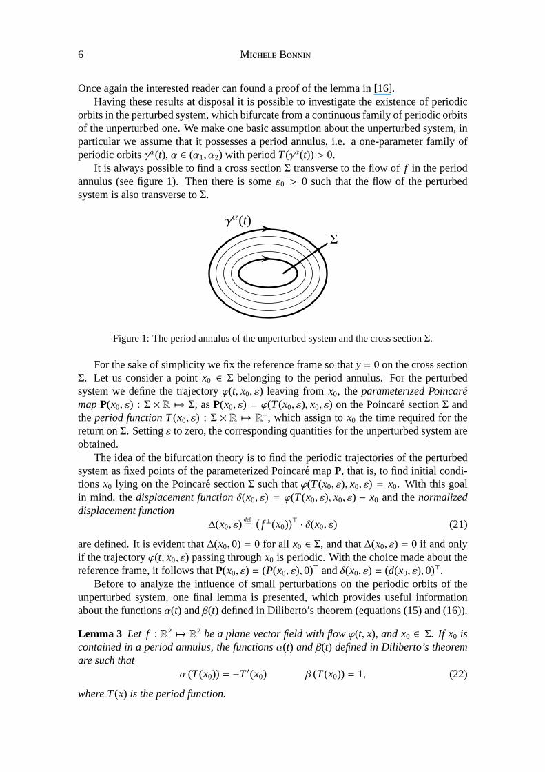
It is always possible to find a cross sectionΣ transverse to the flow off in the periodannulus (see figure 1). Then there is someε0 > 0 such that the flow of the perturbedsystem is also transverse toΣ.

γα(t)

Σ

Figure 1: The period annulus of the unperturbed system and the cross sectionΣ.

For the sake of simplicity we fix the reference frame so thaty = 0 on the cross sectionΣ. Let us consider a pointx0 ∈ Σ belonging to the period annulus. For the perturbedsystem we define the trajectoryϕ(t, x0, ε) leaving fromx0, the parameterized PoincaremapP(x0, ε) : Σ × R 7→ Σ, asP(x0, ε) = ϕ(T(x0, ε), x0, ε) on the Poincare sectionΣ andtheperiod function T(x0, ε) : Σ × R 7→ R+, which assign tox0 the time required for thereturn onΣ. Settingε to zero, the corresponding quantities for the unperturbed system areobtained.

The idea of the bifurcation theory is to find the periodic trajectories of the perturbedsystem as fixed points of the parameterized Poincare mapP, that is, to find initial condi-tions x0 lying on the Poincare sectionΣ such thatϕ(T(x0, ε), x0, ε) = x0. With this goalin mind, thedisplacement functionδ(x0, ε) = ϕ(T(x0, ε), x0, ε) − x0 and thenormalizeddisplacement function

∆(x0, ε) =def (

f ⊥(x0))⊤· δ(x0, ε) (21)

are defined. It is evident that∆(x0,0) = 0 for all x0 ∈ Σ, and that∆(x0, ε) = 0 if and onlyif the trajectoryϕ(t, x0, ε) passing throughx0 is periodic. With the choice made about thereference frame, it follows thatP(x0, ε) = (P(x0, ε),0)⊤ andδ(x0, ε) = (d(x0, ε),0)⊤.

Before to analyze the influence of small perturbations on the periodic orbits of theunperturbed system, one final lemma is presented, which provides useful informationabout the functionsα(t) andβ(t) defined in Diliberto’s theorem (equations (15) and (16)).

Lemma 3 Let f : R2 7→ R2 be a plane vector field with flowϕ(t, x), and x0 ∈ Σ. If x0 iscontained in a period annulus, the functionsα(t) andβ(t) defined in Diliberto’s theoremare such that

α (T(x0)) = −T′(x0) β (T(x0)) = 1, (22)

where T(x) is the period function.

N O U R P 7

Proof By hypothesisϕ(t, x) is the flow of f = ( f1, f2)⊤, let ψ(t, x) be the flow of theorthogonal fieldf ⊥ = (− f2, f1)⊤, thus

ϕ(t, x) = f (ϕ(t, x)) (23)

ψ(t, x) = f ⊥ (ψ(t, x)) . (24)

Consider a pointx(s) = ψ(s, x0) on the trajectory of the orthogonal vector field, and stillbelonging to the period annulus. AbbreviateT(s) = T(ψ(s, x0)) and consider that, sinceψ(s, x0) lies in the period annulus, the following equation holds

ϕ (T(s), ψ(s, x0)) − ψ(s, x0) = 0.

A differentiation with respect tos yields

ϕ (T(s), ψ(s, x0)) T′(s) + Dϕ (T(s), ψ(s, x0)) ψ(s, x0) − ψ(s, x0) = 0 (25)

and taking into account equations (23) and (24) we obtain

f[

ϕ (T(s), ψ(s, x0))]

T′(s) + Dϕ (T(s), ψ(s, x0)) f ⊥ (ψ(s, x0)) − f ⊥ (ψ(s, x0)) = 0.

An evaluation ats= 0, remembering thatψ(0, x0) = x0 (which impliesT(0) = T(ψ(0, x0)) =T(x0)) gives

f (ϕ (T(x0), x0)) T′(x0) + Dϕ (T(x0), x0)) f ⊥(x0) − f ⊥(x0) = 0. (26)

Applying Diliberto’s theorem the required formulas can be obtained. We begin by ob-serving that bothDϕ(t, x0) f ⊥(x0) andα(t) f (ϕ(t, x0)) + β(t) f ⊥ (ϕ(t, x0)) are solutions ofthe initial value problem (12) with initial conditiony(0) = f ⊥(x0), thus

Dϕ(t, x0) f ⊥(x0) = α(t) f (ϕ(t, x0)) + β(t) f ⊥ (ϕ(t, x0)) . (27)

Substituting equation (27) evaluated att = T(x0) into (26) we derive the following equa-tion

f (ϕ(T(x0), x0)) T′(x0) + α(T(x0)) f (ϕ(T(x0), x0)) + β(T(x0)) f ⊥(x0) − f ⊥(x0) = 0. (28)

By hypothesisx0 belongs to the period annulus, thereforeϕ(T(x0), x0) = x0, and consid-ering thatf and f ⊥ are orthogonal, equation (28) holds if and only if

α(T(x0)) = −T′(x0) and β(T(x0)) = 1.

which prove the thesis of the lemma.¤

3.1. Autonomous Perturbations

We now consider the case of a nonlinear dynamical systems with an autonomous pertur-bation

x = f (x) + εg(x), (29)

and denote byϕ(t, x, ε) the associated flow

ϕ(t, x, ε) = f (ϕ(t, x, ε)) + ε g (ϕ(t, x, ε)) . (30)

The following theorem [16,17] provides a mean to identify periodic trajectories in a periodannulus of the unperturbed system from which limit cycles emerge.

8 M B

Theorem 4 (Andronov-Poincare) Suppose forε = 0 system (29) has a period annulus.If the integral function

M(x0) =∫ T(x0,0)

0e−∫ t0 ∇· f (ϕ(s,x0)) dsf

(

ϕ(t, x0))

∧ g(

ϕ(t, x0))

dt (31)

has a simple zero at x0, that isM(x0) = 0 and∂M(x0)/∂x , 0, then, for small value ofε, there is a limit cycleϕ (t, x0, ε) of the perturbed system (29) passing throughΣ at x0,emerging from the periodic orbitϕ(t, x0) = ϕ(t, x0,0) of the unperturbed system.

Proof By differentiating both the normalized displacement function andthe displacementfunction with respect toε we have

∂∆(x0, ε)∂ ε

=(

f ⊥(x0))⊤·∂δ(x0,0)∂ ε

, (32)

∂δ(x0, ε)∂ ε

= ϕ(T(x0, ε), x0, ε)∂T(x0, ε)∂ ε

+∂

∂ εϕ(T(x0, ε), x0, ε).

The latter, evaluated atε = 0, gives

∂δ(x0,0)∂ ε

= ϕ(T(x0,0), x0,0)∂T(x0,0)∂ ε

+∂

∂ εϕ(T(x0,0), x0,0). (33)

We now consider thatϕ(t, x0,0) is a periodic trajectory of the unperturbed system, hencethe following equations hold

ϕ(t, x0,0) = f (ϕ(t, x0,0)) (34)

ϕ (T(x0,0), x0,0) = x0. (35)

By introducing equations (34) and (35) in equation (33) we obtain

∂δ(x0,0)∂ ε

= f (x0)∂T(x0,0)∂ ε

+∂

∂ εϕ(T(x0,0), x0,0), (36)

and consequently, equation (32) becomes

∂∆(x0,0)∂ ε

=(

f ⊥(x0))⊤·∂

∂ εϕ(T(x0,0), x0,0). (37)

To find the proper expression of∂ϕ/∂ ε we consider thatϕ(t, x0, ε) is a trajectory of theperturbed system leaving fromx0

ϕ(t, x0, ε) = f (ϕ(t, x0, ε)) + εg(

ϕ(t, x0, ε))

ϕ(0, x0, ε) = x0.

A differentiation with respect toε and an evaluation atε = 0 yield the variational initialvalue problem

ddt

(

∂ϕ(t, x0,0)∂ ε

)

= D f (ϕ(t, x0,0))∂ϕ(t, x0,0)∂ ε

+ g (ϕ(t, x0,0))

∂ϕ(0, x0,0)∂ε

= 0,

(38)

N O U R P 9

which is of the same kind of (17), hence the solution is given by the Variational Lemma(equation (18)). Inserting such solution in equation (37) we have

∂∆(x0,0)∂ ε

= β(T(x0))M(T, x0) ‖ f (ϕ(T, x0))‖2.

Keeping into account thatϕ(t, x0,0) = ϕ(t, x0) and the second one of (22) it can be inferredthat

∂∆(x0,0)∂ ε

=

∫ T(x0,0)

0e−∫ t0 ∇· f (ϕ(s,x0))dsf

(

ϕ(t, x0))

∧ g(

ϕ(t, x0))

dt. (39)

Sincex0 belongs to the period annulus∆(x0,0) = 0. If there exist an ¯ε > 0 and a con-tinuous functionh : (−ε, ε) 7→ Σ such that∆(h(ε), ε) = 0, then for eachε ∈ (−ε, ε) thereis a periodic trajectoryϕ(t,h(ε), ε) of the perturbed vector field passing through the pointh(ε).We take the Taylor expansion of∆(x0, ε) in the neighborhood ofε = 0

∆(x0, ε) = ∆(x0,0)+ ε∂∆(x0,0)∂ ε

+ O(ε2).

and observe that, as a consequence of (39), the hypothesis ofthe theorem can be recast as

∂∆(x0,0)∂ε

= 0 and∂2∆(x0,0)∂ε ∂x

, 0,

therefore the implicit function theorem ensures the existence of the required functionh(ε).¤

Integral (31) is often referred to as theMelnikov’s integraland is the basic measureof the distance betweenx0 and the first iteration of the Poincare map for the perturbedsystem. For every initial conditionx0 the associated periodT(x0) is uniquely determined.Since the integral is evaluated over the periodT(x0), the dependency on time in (31) isnot written explicitly.Remark If the unperturbed vector field is hamiltonian,∇ · f = 0 and the Melnikov’sintegral simply reduces to

M(x0) =∫ T(x0,0)

0f(

ϕ(t, x0))

∧ g(

ϕ(t, x0))

dt.

Remark The proposed approach is not unique. Here a cross sectionΣ is fixed, and theMelnikov’s integral is evaluated as the initial conditionx0 ∈ Σ is varied. This approachis preferred here in view of the joint application of the Melnikov’s method and the Har-monic Balance technique, since any initial condition can be written asx0 =

∑Nk=−N Γ

0k and

the associated flow is given byϕ(t, x0) =∑N

k=−N Γ0ke

i kω t. Another approach is to keepfixed x0 and evaluate the Melnikov’s integral on a cross section which moves along theunperturbed trajectory, however the two approaches are completely equivalent.

3.2. Stability of Subharmonic Orbits

The natural context to study stability and bifurcations of periodic orbits is the Poincaremap. Thus it is not surprising that Melnikov’s method, with its close relation to Poincaremap permits a simple approach to such problem.

10 M B

If the perturbative vector fields is time dependent and periodic, to investigate the sta-bility properties of the emerging limit cycles a symplectictransformation to action anglecoordinates has to be performed, but such transformation requires the unperturbed vectorfield to be hamiltonian.

Conversely, if the forcing vector field is autonomous, the stability analysis is muchsimpler. The following theorem provides information aboutthe stability of the limit cycleemerging from a period annulus:

Theorem 5 Suppose system (29) has, forε = 0, a period annulus containing a pointx0 ∈ Σ from which a limit cycle of the perturbed system emerges, and consider the function

ζ(x0,0) = ε

{

∇ · f (x0)∂T(x0,0)∂ε

+

∫ T(x0,0)

0

[

∇ · g(

ϕ(t, x0))

+d

dε∇ · f(

ϕ(t, x0))

]

dt

}

.

(40)If ζ(x0,0) < 0, then the limit cycle is asymptotically stable, while ifζ(x0,0) > 0 then thelimit cycle is asymptotically unstable.

Proof Sinceδ(x,0) = 0 for all x in the period annulus, the scalar displacementd(x,0) isalso null. The Taylor expansion of the scalar displacementd(x, ε) in the neighborhood of(x,0) has the form

d(x, ε) = ε∂d(x,0)∂ ε

+ O(ε2), (41)

and a differentiation with respect tox gives

∂d(x, ε)∂x

= ε∂2d(x,0)∂ε ∂x

+ O(ε2). (42)

By hypothesis the limit cycle of the perturbed system (29) passes throughx0, henced(x0, ε) = 0. Equation (42) implies that, for sufficiently small values ofε, d(x, ε) crossesthe valueδ(x0, ε) = 0 asx passes throughx0, with positive or negative slope depending onthe signs ofε and of the mixed partial derivative. We consider the case of negative slope,first

ε∂2d(x,0)∂ε ∂x

< 0 ⇒∂d(x, ε)∂x

< 0.

We take an initial conditionx ∈ Σ such thatx−x0 < 0, which impliesd(x, ε) = P(x, ε)−x >0, andP(x, ε)− x0 < 0 (otherwise the trajectories would intersect, see figure 2), it follows

P(x, ε) − x0 − (x− x0) > 0 ⇒ x− x0 < P(x, ε) − x0 < 0.

If we consider nowP(x, ε) as the new initial condition and we iterate the process, we seethat the sequence of points of the intersections withΣ converges towardsx0.

We consider now the second possible situation, that isx − x0 > 0, which impliesδ(x, ε) = P(x, ε) − x < 0 andP(x, ε) − x0 > 0. It gives

P(x, ε) − x0 − (x− x0) < 0 ⇒ 0 < P(x, ε) − x0 < x− x0,

and again the sequence of intersections with the Poicare section converges towardsx0.Therefore, ifζ(x0,0) < 0, the limit cycleϕ(t, x0, ε) passing throughx0 is stable. By thesame argument the limit cycle is unstable ifζ(x0,0) > 0.

N O U R P 11

−80 −60 −40 −20 0 20 40 60 80−40

−30

−20

−10

0

10

20

30

40

Σx

x0

P(x)

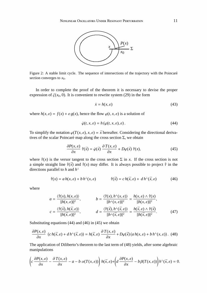
Figure 2: A stable limit cycle. The sequence of intersections of the trajectorywith the Poincaresection converges tox0.

In order to complete the proof of the theorem it is necessary to devise the properexpression ofζ(x0,0). It is convenient to rewrite system (29) in the form

x = h(x, ε) (43)

whereh(x, ε) = f (x) + εg(x), hence the flowϕ(t, x, ε) is a solution of

ϕ(t, x, ε) = h (ϕ(t, x, ε), ε) . (44)

To simplify the notationϕ(T(x, ε), x, ε) = x hereafter. Considering the directional deriva-tives of the scalar Poincare map along the cross sectionΣ, we obtain

∂P(x, ε)∂x

τ(x) = ϕ(x)∂T(x, ε)∂x

+ Dϕ(x) τ(x), (45)

whereτ(x) is the versor tangent to the cross sectionΣ in x. If the cross section is nota simple straight line ˆτ(x) and τ(x) may differ. It is always possible to project ˆτ in thedirections parallel toh andh⊥

τ(x) = a h(x, ε) + b h⊥(x, ε) τ(x) = c h(x, ε) + d h⊥(x, ε) (46)

where

a =〈τ(x),h(x, ε)〉‖h(x, ε)‖2

, b =〈τ(x),h⊥(x, ε)〉‖h⊥(x, ε)‖2

=h(x, ε) ∧ τ(x)‖h(x, ε)‖2

,

c =〈τ(x),h(x, ε)〉‖h(x, ε)‖2

, d =〈τ(x),h⊥(x, ε)〉‖h⊥(x, ε)‖2

=h(x, ε) ∧ τ(x)‖h(x, ε)‖2

. (47)

Substituting equations (44) and (46) in (45) we obtain

∂P(x, ε)∂x

(

c h(x, ε) + d h⊥(x, ε))

= h(x, ε)∂T(x, ε)∂x

+Dϕ(x)(

a h(x, ε) + b h⊥(x, ε))

. (48)

The application of Diliberto’s theorem to the last term of (48) yields, after some algebraicmanipulations

(

c∂P(x, ε)∂x

−∂T(x, ε)∂x

− a− b α(T(x, ε))

)

h(x, ε)+

(

d∂P(x, ε)∂x

− bβ(T(x, ε))

)

h⊥(x, ε) = 0.

12 M B

Taking into account equation (16) and the orthogonality of the vector fields we have

∂P(x, ε)∂x

=h(x, ε) ∧ τ(x)h(x, ε) ∧ τ(x)

exp

(∫ T(x,ε)

0∇ · h(ϕ(t, x, ε), ε) dt

)

. (49)

To evaluate the derivative of (49) with respect toε at ε = 0, we consider that ¯x =ϕ(T(x,0), x,0) = x. Therefore the first factor is equal to one and its derivative

∂

∂ε

h(x, ε) ∧ τ(x)h(x, ε) ∧ τ(x)

=

(

∂h(x, ε)∂ε

∧ τ(x)

)

(h(x, ε) ∧ τ(x)) − (h(x, ε) ∧ τ(x))

(

∂h(x, ε)∂ε

∧ τ(x)

)

(h(x, ε) ∧ τ(x))2

(50)is null. For the second factor we take into account that

∂

∂ε

∫ T(x,ε)

0∇ · h (ϕ(t, x, ε), ε) dt = ∇ · h (ϕ(T(x, ε), x, ε), ε)

∂T(x, ε)∂ε

+

∫ T(x,ε)

0

ddε∇ · h (ϕ(t, x, ε), ε) dt, (51)

and sinceh(x, ε) = f (x) + εg(x), the following equation holds

ddε∇ · h (ϕ(t, x, ε), ε) =

ddε∇ · f (ϕ(t, x, ε)) + ∇ · g(ϕ(t, x, ε)) + ε

ddε∇ · g(ϕ(t, x, ε)). (52)

Taking into account equations (51), (52), and the considerations made about (50), a dif-ferentiation of equation (49) with respect toε and an evaluation at (x, ε) = (x0,0) yields

∂2P(x0,0)∂x∂ε

= ∇ · f (x0)∂T(x0,0)∂ε

+

∫ T(x0,0)

0∇ ·g(

ϕ(t, x0))

dt+∫ T(x0,0)

0

ddε∇ · f(

ϕ(t, x0))

dt.

whereϕ(t, x0) = ϕ(t, x0,0). Keeping in mind that

∂2P(x0,0)∂ε ∂x

=∂2d(x0,0)∂ε ∂x

the thesis of the theorem follows.¤

Remark In general, stability of periodic orbits is determined computing Floquet’s mul-tipliers. Recently some authors [19] have proved that Floquet’s multipliers can be accu-rately computed by exploiting numerical algorithms described in [20] evaluated over theHarmonic Balance solutions. However that approach is not reliable for weakly perturbednon hyperbolic oscillators. In fact, in this case at least two Floquet’s multipliers lie on theunit circle, and since their moduli depend continuously on perturbative terms, under theeffect of a weak perturbation their value remains very close to the unity. Therefore, it isdifficult to discriminate between the variation due to the perturbations and the numericalinaccuracies.

Remark If the unperturbed system is hamiltonian∇ · f = 0, the functionζ(x0,0) reducesto

ζ(x0,0) = ε∫ T(x0,0)

0∇ · g(

ϕ(t, x0))

dt. (53)

It is worth noting that the stability of the bifurcating limit cycles depends not only on theperturbationg(x) and its strengthε, but also on the unperturbed system, since the forcingvector field is evaluated over the free oscillation.

N O U R P 13

3.3. Non Autonomous Perturbations

This section is devoted to study the system

x = f (x) + εg(x, t) (54)

where bothf (x) andg(x, t) are smooth functions,g is aT periodic function and forε = 0system (54) has a period annulus. Since the perturbed systemis expected to exhibit peri-odic trajectories resonant with the perturbation, it is natural to search for the persistenceof periodic orbits of the unperturbed system passing through x0, whose periodT(x0) iscommensurable with the periodT of the forcing term, that is

m T = n T(x0) m,n ∈ Z.

It is possible to find periodic trajectories of the perturbedsystem finding conditions onthe functionsf andg such that, for small values ofε , 0, fixed points of the parametrizedPoincare map remain. We consider the time derivative of the displacement function

Dδ(x, ε) x = ϕ(mT, x, ε) − x = f (ϕ(mT, x, ε)) − f (x)

Sinceϕ(mT, x,0) = x, an evaluation atε = 0 gives,

Dδ(x,0) f (x) = 0, (55)

thereforeDδ(x,0) is singular and the implicit function theorem cannot be applied directly.However, different kinds of reduction can be made depending on the degeneracy of theperiod annulus. The most degenerate condition is the case ofan isochronous annulus, forwhich the period function is constant, i.e.T′(x) = 0, for all x belonging to the annulus.

Theorem 6 Suppose system (54) has, forε = 0 an isochronous period annulus. If thereare two positive integers m and n such that the unperturbed system has a mT/n periodictrajectory passing through x0 and the functions

M(x0) =∫ mT

n

0e−∫ t0 ∇· f (ϕ(s,x0)) dsf

(

ϕ(t, x0))

∧ g(

ϕ(t, x0))

dt (56)

and

N(x0) =∫ mT

n

0

1‖ f(

ϕ(t, x0))

‖2

{

〈 f(

ϕ(t, x0))

, g(

ϕ(t, x0), t)

〉 −α(t)β(t)

f(

ϕ(t, x0))

∧ g(

ϕ(t, x0), t)

}

dt,

(57)have both a simple zero at x0 ∈ Σ, then the periodic orbit of the unperturbed systempersists for small values ofε.

Proof For the sake of simplicity we focus on a subharmonic orbit of the unperturbedsystem passing throughx ∈ Σ which is inm : 1 resonance with the external forcing. Wemake use of the Taylor expansion of the displacement function in a neighborhood ofε = 0

δ(x, ε) = ε∂δ(x,0)∂ε

+ O(ε2) = ε∂

∂ εϕ(mT, x,0)+ O(ε2). (58)

14 M B

It was shown in section 3.1 that∂ϕ/∂ε is a solution of the inhomogeneous linear varia-tional equation (17), hence, according to (18), it can be written as

∂

∂ εϕ(mT, x,0) = [N(x) + α(mT)M(x)] f (ϕ(mT, x,0))+

[

β(mT)M(x)]

f ⊥ (ϕ(mT, x,0))

(59)As a consequence of (22),α(mT) = −m T′(x) = 0 since the period annulus is isochronous,andβ(mT) = 1. Thus

∂

∂ εϕ(mT, x,0) = N(x) f (x) +M(x) f ⊥(x)

Introducing such expression in (58), the following equation is obtained

δ(x, ε) = ε(

N(x) f (x) +M(x) f ⊥(x) + O(ε))

.

Hence the implicit function theorem can be applied to determine when there is an implicitsolution of the equationδ(x, ε) = 0 at some point (x0,0). ¤

Before to consider the case of a regular period annulus, we introduce some preliminaryconsiderations. It is possible to split the displacement function into its tangent and radialprojections

δ(x, ε) = σ(x, ε) f (x) + ρ(x, ε) f ⊥(x) (60)

where

σ(x, ε) =〈δ(x, ε), f (x)〉‖ f (x)‖2

ρ(x, ε) =〈δ(x, ε), f ⊥(x)〉‖ f (x)‖2

.

In what follows, we need the directional derivatives ofσ(x, ε) andρ(x, ε), thus we recallthat

Dδ(x,0) = D[

ϕ(T, x,0)− x]

= Dϕ(T, x,0)− I , (61)

and applying Diliberto’s theorem we obtain

Dδ(x,0) f ⊥(x) = α(T) f (x) + β(T) f ⊥(x) − f ⊥(x) (62)

Dδ(x,0) f (x) = 0. (63)

Now we can compute the derivative ofσ(x, ε) in the directionf ⊥(x) and f (x) at (x, ε) =(x,0), we obtain

Dσ(x,0) f ⊥(x) =〈D δ(x,0) f ⊥(x), f (x)〉

‖ f (x)‖2+〈δ(x,0), D f (x) f ⊥(x)〉

‖ f (x)‖2= α(T) (64)

Dσ(x,0) f (x) =〈D δ(x,0) f (x), f (x)〉

‖ f (x)‖2+〈δ(x,0), D f (x) f (x)〉

‖ f (x)‖2= 0, (65)

where (62) and (63) were used, and sinceδ(x,0) = 0. In a similar way it is possible toprove that

D ρ(x,0) f ⊥(x) = β(T) − 1 (66)

D ρ(x,0) f (x) = 0. (67)

We can now introdue the theorem dealing with a regular periodannulus, that is whenT′(x) , 0. Even in this situation the implicit function theorem cannot be applied directly,since equation (55) still holds, then a Lyapunov-Schmidt reduction is applied.

N O U R P 15

Theorem 7 Suppose system (54) has, forε = 0 a regular period annulus. If there are twopositive integers m and n such that the unperturbed system has a mT/n periodic trajectorypassing through x0 and the function

M(x0) =∫ mT

n

0e−∫ t0 ∇· f(

ϕ(s,x0))

dsf(

ϕ(t, x0))

∧ g(

ϕ(t, x0), t)

dt (68)

has a simple zero at x0 ∈ Σ, i.e.M(x0) = 0 and∂M(x0)/∂x , 0, then the periodic orbitof the unperturbed system persists for small values ofε.

Proof Using equation (64) and the first of (22), we haveDσ(x,0) f ⊥(x) = −mT′(x) whichis different from zero because the annulus is regular. Applying theimplicit function the-orem to the functionσ(x,0), it is possible to define a smooth manifoldS such thatσvanishes onS. In addition, for anyx ∈ ϕ(t, x,0) equation (65) implies thatS is transverseto the sectionΣ andϕ(t, x,0) ⊂ S.

Now we focus on the restriction of the radial projectionρ to S. Equations (66) and(67) imply thatDρ(x,0) = 0. On the other hand, as a consequence of (58) and (59) wehave

∂δ(x,0)∂ ε

= [N(x) + α(mT)] f (x) + β(mT)M(x) f ⊥(x). (69)

while differentiation of (60) with respect toε and an evaluation atε = 0 yield

∂δ(x,0)∂ ε

=∂σ(x,0)∂ ε

f (x) +∂ρ(x,0)∂ ε

f ⊥(x). (70)

Comparing the last two equations and taking into account the second of (22) we infer

∂ρ(x,0)∂ ε

=M(x).

The hypothesesM(x0) = 0 and∂M(x0)/∂x , 0 imply∂ρ(x0,0)/∂ε = 0 and∂2ρ(x0,0)/∂ε∂x ,0. Therefore there is an ¯ε > 0 and a smooth functionh : (−ε, ε) 7→ R

2 such thatρ(h(ε), ε) ≡ 0, as a consequence

ρ(h(ε), ε) = σ(h(ε), ε) = 0

andδ(h(ε), ε) = 0, which proves the statement of the theorem.¤One more result, due to Chowet al. [21], is worth noting. This result is related to

system possessing a homoclinic orbit to a hyperbolic saddlepoint as the separatrix ofregions filled with periodic orbits. It implies that a countable sequence of subharmonicsaddle-node bifurcations of periodic orbits converges to ahomoclinic bifurcation (see[14,15] for details).

Theorem 8 Suppose forε = 0 system (54) has a homoclinic orbit q0(t) to a hyperbolicsaddle point p0. Assume the interior of q0(t) ∪ p0 is filled with a continuous family ofperiodic orbits qα(t) whose period tends monotonically to infinity as the periodic orbitsapproach the homoclinic orbit. Let

Mm(x) =∫ mT

0e−∫ t0 ∇· f(

qα(s))

dsf(

qα(t))

∧ g(

qα(t), t)

dt (71)

16 M B

be the Melnikov’s integral associated to the mT periodic orbit. Then

limm→+∞

Mm(x) =M(x)

where

M(x) =∫

+∞

−∞

e−∫ t0 ∇· f(

q0(s))

dsf(

q0(t))

∧ g(

q0(t), t)

dt

is the Melnikov’s integral whose simple zeroes are associated to homoclinic bifurcations.

3.4. Limit Cycle Oscillators

This section is devoted to the analysis of oscillators whosefree oscillation is a limit cycle,i.e. the unperturbed system is structurally stable. When we consider the forced oscillatoron the manifoldR2 × S1, the three dimensional system has forε = 0, an hyperbolic toruscorresponding to the limit cycle. The flow on the torus will beperiodic or quasi periodicdepending on wether or not some resonant condition is satisfied. In either case, the orbitcorresponding to the limit cycle will no longer be structurally stable, the stability of thelimit cycle being transferred to the torus. The existence offrequency entrained oscillationsin a limit cycle oscillator driven by a resonant forcing termis described by the followingtheorem

Theorem 9 (Limit cycle subharmonic bifurcation theorem [16]) Let us consider the dy-namical system

x(t) = f(

x(t))

+ εg(

x(t), t)

and suppose that it admits a limit cycleϕ(t, x0) whose period is resonant with the periodof the external forcing g

(

x(t), t)

= g(

x(t+T), t+T)

. If x0 is a simple zero of the bifurcationfunction

B(x0) =[

1− β(T)]

N(x0) + α(T)M(x0), (72)

namely,B(x0) = 0 and ∂B(x0)/∂x , 0 then the perturbed system has a limit cycleϕ(t, x0, ε) passing through x0.

Proof With the projections ofσ andρ defined in equations (64)-(67) we have two possi-bilities. If β(T) , 1 we can apply the implicit function theorem to the radial projection.Conversely, ifα(T) , 0 the implicit function theorem can be applied to the tangentpro-jection, in both cases we can define a smooth functionh : (−ε, ε) 7→ R2 such that eitherρ(h(ε), ε) = 0 orσ(h(ε), ε) = 0. Now we need to identify the bifurcation function. Let usconsider the Taylor expansion ofσ andρ in the neighborhood ofε = 0

σ(h(ε), ε) = σ(h(0),0)+ εdσ(h(0),0)

dε+ O(ε2) (73)

ρ(h(ε), ε) = ρ(h(0),0)+ εdρ(h(0),0)

dε+ O(ε2), (74)

where

dσ(h(0),0)dε

=∂σ(h(0),0)∂ε

+ Dσ(h(0),0)∂h(0)∂ε

(75)

dρ(h(0),0)dε

=∂ρ(h(0),0)∂ε

+ Dρ(h(0),0)∂h(0)∂ε, (76)

N O U R P 17

and comparing (69) and (70) we have

∂σ(h(0),0)∂ε

= N(h(0))+ α(T)M(h(0))∂ρ(h(0),0)∂ε

= β(T)M(h(0)). (77)

Sinceh(0) ∈ Σ, we can express the vector field∂h(ε)/∂ε as a linear combination off andf ⊥

∂h(0)∂ε= a f(h(0))+ b f⊥(h(0))

and taking into account (64)-(67)

Dσ(h(0),0)∂h(0)∂ε

= bα(T) (78)

Dρ(h(0),0)∂h(0)∂ε

= b(

β(T) − 1)

. (79)

Thus

dσ(h(0),0)dε

= bα(T) +N(h(0))+ α(T)M(h(0)) (80)

dρ(h(0),0)dε

= b[

β(T) − 1]

+ β(T)M(h(0)). (81)

For the case in whichβ(T) , 1 we consider equation (81), which implies

b =β(T)M((h(0))

1− β(T)

which substituted in (80) yields

dσ(h(0),0)dε

=

[

1− β(T)]

N(h(0))+ α(T)M(h(0))1− β(T)

The case in whichα(T) , 0 is similar, (80) implies

b = −N(h(0))+ α(T)M(h(0))

α(T)

which substituted in (81) gives

dρ(h(0),0)dε

=

[

1− β(T)]

N(h(0))+ α(T)M(h(0))α(T)

as required.¤

4. A

In the previous section we shoved that the Melnikov technique provides a mean to deter-mine conditions such that periodic trajectories survive under the effect of an external forc-ing. It was shown how the problem can be reformulated in termsof zeroes of an integral

18 M B

function evaluated over the periodic solution of the unperturbed system. Thus, an analyticexpression of the free oscillation must be available. Unfortunately, as stated in the intro-duction, trajectories of almost all non trivial oscillators can be only determined throughnumerical integration. Even for integrable systems, trajectories are often expressed interms of special functions, making the integral equations often unsolvable. In some cases,the problem can be solved recurring to the method of the residues, while in other cases itis necessary to consider some approximation of the functionto be integrated [5,14,15].

In this section we show that the Melnikov’s integrals can be accurately evaluated overthe Harmonic Balance approximation of the unperturbed system. The proposed approachpresents two main advantages, the Harmonic Balance technique yields the analytical ap-proximations of the periodic trajectory of any nonlinear oscillator. Hence, the integrabilityof the unperturbed system is not required anymore, and the applicability of the Melnikov’smethod is considerably extended. Moreover, the unperturbed trajectory is always approx-imated by a truncated Fourier series, and as a consequence the Melnikov’s integrals oftenresult quite simple to solve making use of the orthogonalityof the base functions.

4.1. Hamiltonian system with an autonomous perturbation

As a first application of the proposed technique, we considerthe following dynamicalsystem

x = y

y = x− x3+ ε(α y− β x2y).

(82)

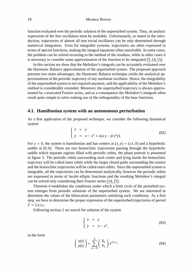
For ε = 0, the system is hamiltonian and has centers at (x, y) = (±1,0) and a hyperbolicsaddle at (0,0). There are two homoclinic trajectories passing through the hyperbolicsaddle which separate regions filled with periodic orbits, the phase portrait is presentedin figure 3. The periodic orbits surrounding each center and lying inside the homoclinictrajectory will be called inner orbits while the larger closed paths surrounding the centersand the homoclinic trajectories will be called outer orbits. Since the unperturbed system isintegrable, all the trajectories can be determined analytically, however the periodic orbitsare expressed in terms of Jacobi elliptic functions and the resulting Melnikov’s integralcan be solved only considering their Fourier series [14,15].

Theorem 4 establishes the conditions under which a limit cycle of the perturbed sys-tem emerges from periodic solutions of the unperturbed system. We are interested indetermine the values of the bifurcation parameters satisfying such conditions. As a firststep, we have to determine the proper expression of the unperturbed trajectories of periodT = 2π/ω.

Following section 2 we search for solution of the system

x = y

y = x− x3,(83)

in the form(

x(t)y(t)

)

=

N∑

k=−N

(

Xk

Yk

)

ei kω t. (84)

N O U R P 19

−2 −1.5 −1 −0.5 0 0.5 1 1.5 2−1

−0.8

−0.6

−0.4

−0.2

0

0.2

0.4

0.6

0.8

1

Figure 3: The phase portrait of the unperturbed Duffing oscillator obtained through the HarmonicBalance technique.

The nonlinear term is expressed as follow

x3=

N∑

k=−N

Fk ei kω t, (85)

where

Fk =12π

∫ π

−π

N∑

h=−N

Xh ei hω t

3

e−i kω t d(ωt).

Such integral can be expressed in a closed analytical form, in terms of the coefficientsXk

only.By substituting (84) and (85) in (83), computing the proper derivatives and equating

the coefficients of the same order harmonics we obtain

i kωXk − Yk = 0(

k2ω2+ 1)

Xk − Fk = 0.(86)

System (86) can be efficiently solved exploiting standard numerical algorithms,giving thecoefficients of the Harmonic Balance approximation of the free oscillation.

According to theorem 4, a limit cycles emerges from a periodic orbit of periodT =2π/ω, passing throughγ0 =

∑Nk=−N Γk ei kωt0, if the Melnikov’s integral has a simple zero,

namely if

M(γ0) =∫ T(γ0)

0f(

ϕ(t, γ0))

∧ g(

ϕ(t, γ0))

dt =∫ T(γ0)

0y(t)(

α y(t) − β x2(t) y(t))

dt = 0.

(87)Thus, for everyt0 ∈ (0,T], the Harmonic Balance coefficients describing the flowϕ(t, γ0)can be computed asΓ0

k = Γk ei kω t0. By introducing in (87) such coefficients we have

M(γ0) = α I (γ0) − β J(γ0) = 0

20 M B

where

I (γ0) =∫ T(γ0)

0

N∑

k=−N

Y0k ei kω t

2

dt (88)

J(γ0) =∫ T(γ0)

0

N∑

k=−N

X0k ei kω t

2

N∑

k=−N

Y0k ei kω t

2

dt. (89)

The two integrals can be analytically computed for any number of harmonics, and theyonly involve summations of the Harmonic Balance coefficients. Thus a limit cycle ariseswhen

α

β=

J(γ0)I (γ0)

. (90)

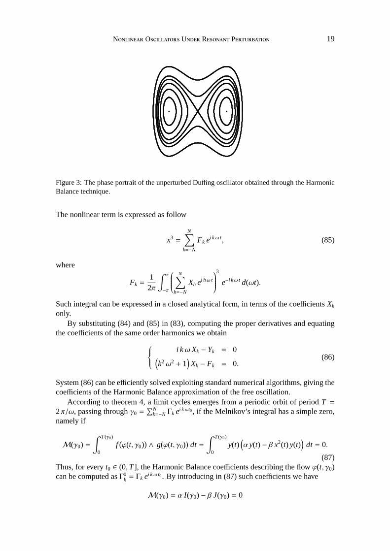
In figure 4 the values of the ratioα/β at which a limit cycle arise, are depicted as afunction of the frequency. Forα/β < 0.75 the perturbed system has not periodic solution.At α/β = 0.75, an outer limit cycle arise from the unperturbed orbit of frequencyω = 0.6through a saddle node bifurcation, and is the unique periodic solution for 0.75 < α/β <0.8. For α/β = 0.8 two limit cycles, one surrounding each center, have birth troughsaddle-node bifurcations, thus forα/β > 0.8 there is a limit cycle surrounding each centerand a large limit cycle enclosing all three equilibria.

0 0.5 1 1.50.5

0.75

1.0

1.25

1.5

ω

αβ

Figure 4: Bifurcation curves for the hamiltonian system with an autonomous perturbation as afunction of the frequency. (Solid line) Birth of a limit cycle from an outer periodic orbit. (Dashedline) Birth of a limit cycle from an inner periodic orbit.

In the present example, asω→ 0, i.e.T → +∞, both the inner and the outer periodicorbits of the unperturbed system approaches the homoclinictrajectory. Consequently, thevalues of the ratioα/β at which limit cycles arise, converge at the value (α/β = 0.8 here)at which a homoclinic tangency occurs, as stated by theorem 8. The convergence of thebifurcation curves forω→ 0 is evident in figure 4.

According to theorem 5, the stability of the bifurcating limit cycles can be determinedevaluating the sign of equation (53) on the unperturbed periodic solutionϕ(t, x0), thus weconsider

ε

∫ T(γ0)

0

(

α − β x2(t))

dt = ε∫ T(γ0)

0

{

α − β

N∑

k=−N

X0k ei kω t

2}

dt =2πεω

α − β

N∑

k=−N

∣

∣

∣X0k

∣

∣

∣

2

.

(91)

N O U R P 21

By substituting in equation (91) the Harmonic Balance coefficients we obtain that theinner limit cycles are asymptotically unstable, while the outer limit cycle is asymptoticallystable. The values at which limit cycles have birth and theirstability are confirmed bynumerical integration of the state equations.

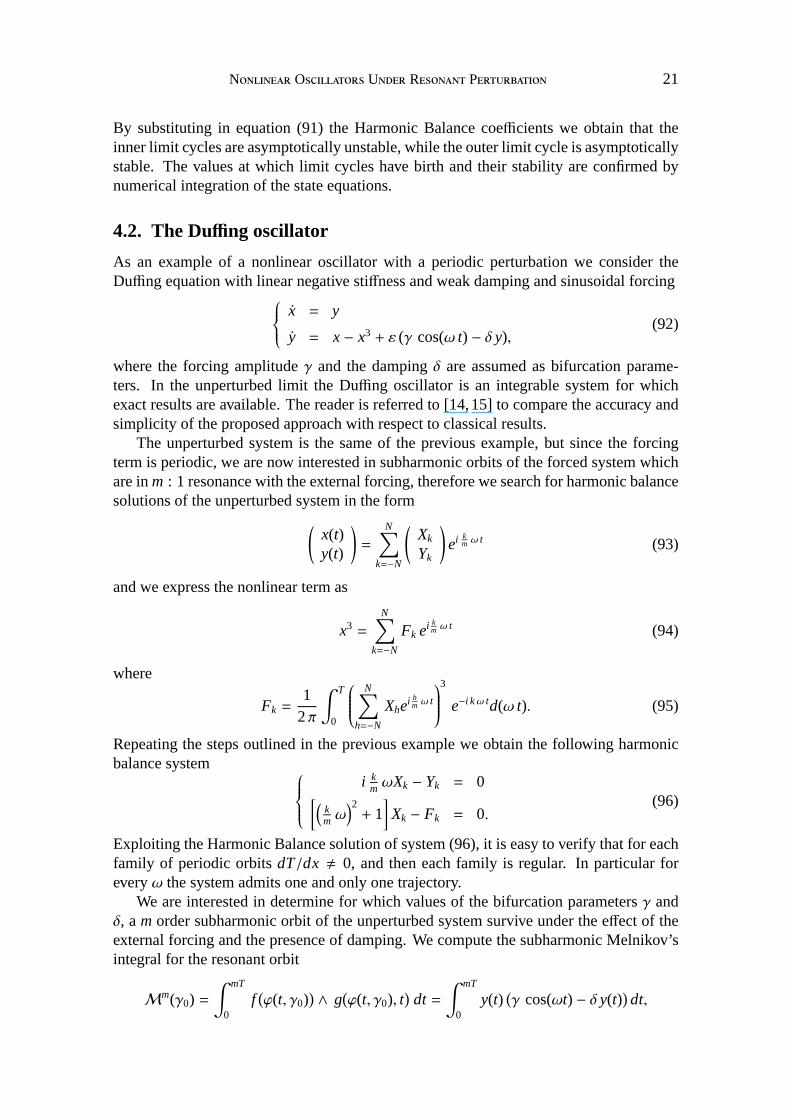
4.2. The Duffing oscillator

As an example of a nonlinear oscillator with a periodic perturbation we consider theDuffing equation with linear negative stiffness and weak damping and sinusoidal forcing

x = y

y = x− x3+ ε (γ cos(ω t) − δ y),

(92)

where the forcing amplitudeγ and the dampingδ are assumed as bifurcation parame-ters. In the unperturbed limit the Duffing oscillator is an integrable system for whichexact results are available. The reader is referred to [14,15] to compare the accuracy andsimplicity of the proposed approach with respect to classical results.

The unperturbed system is the same of the previous example, but since the forcingterm is periodic, we are now interested in subharmonic orbits of the forced system whichare inm : 1 resonance with the external forcing, therefore we searchfor harmonic balancesolutions of the unperturbed system in the form

(

x(t)y(t)

)

=

N∑

k=−N

(

Xk

Yk

)

ei km ω t (93)

and we express the nonlinear term as

x3=

N∑

k=−N

Fk ei km ω t (94)

where

Fk =1

2π

∫ T

0

N∑

h=−N

Xhei h

m ω t

3

e−i kω td(ω t). (95)

Repeating the steps outlined in the previous example we obtain the following harmonicbalance system

i kmωXk − Yk = 0

[

(

kmω)2+ 1]

Xk − Fk = 0.(96)

Exploiting the Harmonic Balance solution of system (96), it is easy to verify that for eachfamily of periodic orbitsdT/dx , 0, and then each family is regular. In particular foreveryω the system admits one and only one trajectory.

We are interested in determine for which values of the bifurcation parametersγ andδ, am order subharmonic orbit of the unperturbed system survive under the effect of theexternal forcing and the presence of damping. We compute thesubharmonic Melnikov’sintegral for the resonant orbit

Mm(γ0) =∫ mT

0f(

ϕ(t, γ0))

∧ g(

ϕ(t, γ0), t)

dt =∫ mT

0y(t)(

γ cos(ωt) − δ y(t))

dt,

22 M B

wherey(t) is determined introducing in (93) the Harmonic Balance coefficients obtainedsolving system (96). Thus

Mm(γ0) =γ

2

∫ mT

0

N∑

k=−N

(

Y0k ei k

m ω t) (

ei ωt+ e−i ωt

)

dt− δ∫ mT

0

N∑

k=−N

Y0k ei k

m ωt

2

dt

and solving the integral we obtain

Mm(γ0) =2πω

γ Re{Y0m} − δ

N∑

k=−N

∣

∣

∣Y0k

∣

∣

∣

2

. (97)

According to theorem 7, am-order subharmonic orbit with periodmT/ω, appears in theperturbed system when

γ

δ=

1Re{Y0

m}

N∑

k=−N

∣

∣

∣Y0k

∣

∣

∣

2. (98)

The bifurcation curves corresponding to the birth of a subharmonic of orderm in theperturbed system are easily determined by substituting in equation (98) the HarmonicBalance coefficients of the corresponding unperturbedmT-periodic orbit. Since the ratioγ/δ is a constant, the bifurcation curves are straight lines. Some of such curves are out-lined in figure 5, whereSm refers to an inner orbit whileSm refers to an outer orbit. Itis readily seen that, as predicted by theorem 8, the bifurcation curves accumulate on thecurveS0 associate to the homoclinic tangency.

0 0.05 0.10

0.05

0.1

δ

γS1S2S3S4S0S5S3

S1

Figure 5: Bifurcation curves for the subharmonics of the Duffing oscillator.Sm: m-order subhar-monic orbit inside the homoclinic trajectories;Sm: outer orbit. Note the rapid convergence ofSm

andSm to the homoclinic tangencyS0.

4.3. Coupled Van der Pol Oscillators

As a last application of the proposed technique, we considertwo coupled Van der Poloscillators running in resonance

u = vv = −u+ δ(1− u2)vx = τyy = τ

(

−x+ δ(1− x2) y)

+ εu.

(99)

N O U R P 23

Here the system (x(t), y(t))⊤ is view as the perturbed system subject to a periodic resonantexternal input provided by (u(t), v(t))⊤, τ ∈ Z is the resonance factor. The perturbationadmits the Harmonic Balance description

(

u(t)v(t)

)

=

N∑

k=−N

(

Uk

Vk

)

ei kω t

which leads to the Harmonic Balance system

{

i kωUk − Vk = 0(

k2ω2+ i k δω − 1

)

Uk − δGk = 0

where

Gk =12π

∫ π

−π

N∑

m=−N

Umei mω t

2

N∑

n=−N

Vnei nω t

e−i kω td(ωt).

The unperturbed system has a stable limit cycle whose Harmonic Balance descriptionis obtained solving

{

i kωXk − τYk = 0(

k2ω2

τ+ i k δ τω − τ

)

Xk − τ δ Fk = 0

where

Fk =12π

∫ π

−π

N∑

m=−N

Xmei mω t

2

N∑

n=−N

Ynei nω t

e−i kω td(ω t).

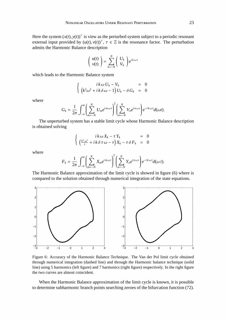
The Harmonic Balance approximation of the limit cycle is showed in figure (6) where iscompared to the solution obtained through numerical integration of the state equations.

−3 −2 −1 0 1 2 3−3

−2

−1

0

1

2

3

−3 −2 −1 0 1 2 3−3

−2

−1

0

1

2

3

Figure 6: Accuracy of the Harmonic Balance Technique. The Van der Pol limit cycle obtainedthrough numerical integration (dashed line) and through the Harmonic balance technique (solidline) using 5 harmonics (left figure) and 7 harmonics (right figure) respectively. In the right figurethe two curves are almost coincident.

When the Harmonic Balance approximation of the limit cycle is known, it is possibleto determine subharmonic branch points searching zeroes ofthe bifurcation function (72).

24 M B

Computing the terms appearing in (72) we obtain

β(t) =y2

0 +[

δ(

1− x20

)

y0 − x0

]2

y2 +[

δ(

1− x2)

y− x]2

exp

(∫ t

0τ δ(

1− x2)

ds

)

α(t) = −2τ∫ t

0

{x2+ y2+ δ x3 y+ δ x y

(

2y2 − 1)

y2 +[

δ(

1− x2)

y− x]2

−[

δx y+ 1]

}

β(s) ds

M(γ0) =1

τ

{

y20 +[

δ(

1− x20

)

y0 − x0

]2}

∫ t

0y u e−

∫ s0 τ δ(1−x2)dr ds

N(γ0) =1τ

∫ t

0

u

y2 +[

δ(

1− x2)

y− x]2

{

δ(

1− x2)

y− x−α(s)β(s)

y

}

ds

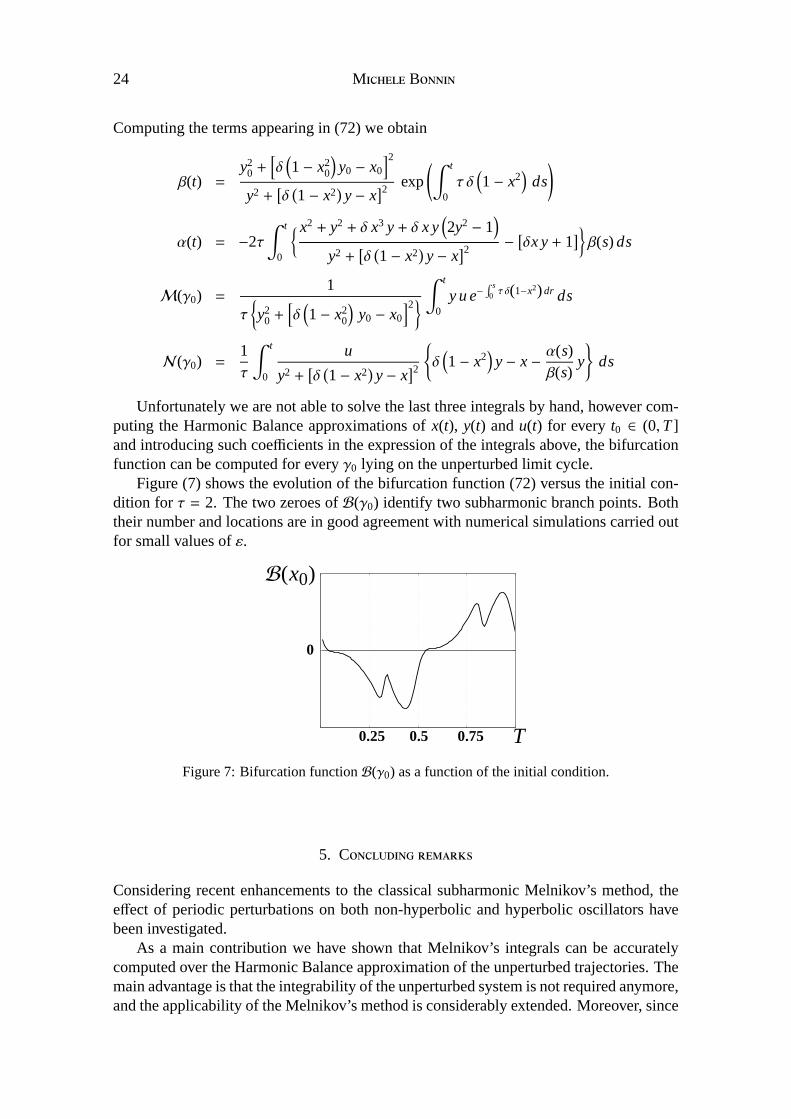
Unfortunately we are not able to solve the last three integrals by hand, however com-puting the Harmonic Balance approximations ofx(t), y(t) andu(t) for every t0 ∈ (0,T]and introducing such coefficients in the expression of the integrals above, the bifurcationfunction can be computed for everyγ0 lying on the unperturbed limit cycle.

Figure (7) shows the evolution of the bifurcation function (72) versus the initial con-dition for τ = 2. The two zeroes ofB(γ0) identify two subharmonic branch points. Boththeir number and locations are in good agreement with numerical simulations carried outfor small values ofε.

T

B(x0)

0.25 0.5 0.75

0

Figure 7: Bifurcation functionB(γ0) as a function of the initial condition.

5. C

Considering recent enhancements to the classical subharmonic Melnikov’s method, theeffect of periodic perturbations on both non-hyperbolic and hyperbolic oscillators havebeen investigated.

As a main contribution we have shown that Melnikov’s integrals can be accuratelycomputed over the Harmonic Balance approximation of the unperturbed trajectories. Themain advantage is that the integrability of the unperturbedsystem is not required anymore,and the applicability of the Melnikov’s method is considerably extended. Moreover, since

N O U R P 25

the unperturbed trajectories are expressed as truncated Fourier series, the Melnikov’s in-tegrals results rather simple to solve.

The joint application of the Harmonic Balance technique and the Melnikov’s method,has allowed to investigate the emergence of periodic orbitsfrom period annulus undereither autonomous or non-autonomous perturbations. We have shown how, in the formercase, the stability of the bifurcating limit cycle can be analytically determined.

In the case of limit cycle oscillators, we have shown the possibility to determine thenumber and locations of subharmonic branch points, i.e. intersections between the per-turbed and the unperturbed orbits.

A

This research was partially supported by theMinistero dell’Istruzione, dell’Universita edella Ricerca, under the FIRB project no. RBAU01LRKJ.

REFERENCES

[1] Kuramoto Y.Chemical Oscillations, Waves and Turbulence. Springer: New York, 1984.

[2] Melnikov V. K. On the stability of the center for time periodic perturbation.Transactions of theMoscow Mathematical Society1963;12:1–56.

[3] Greenspan B.D, Holmes P.J. Repeated resonances and homoclinic bifurcations in a periodically forcedfamily of oscillators.SIAM Journal of Mathematical Analysis1984;16(5):69–97.

[4] Gundler J. The existence of homoclinic orbits and the method of Melnikov for systems inRn. SIAMJournal of Mathematical Analysis1985;16(5):907–931

[5] Yagasaki K. The Melnikov theory for subharmonics and their bifurcations in forcd oscillators.SIAMJournal of Applied Mathematics1996;56(6):1720–1765.

[6] Yagasaki K. Periodic and homoclinic motions in forced, coupled oscillators.Nonlinear Dynamics1999;20:319–359.

[7] Jianxin Xu, Rui Yan, Weinian Zhang An alghorithm for Melnikov functions and application to achaotic rotor.SIAM Journal on Scientific Computation2005;26(5):1525–1546

[8] Zhengdong Du, Weinian Zhang Melnikov method for homoclinic bifurcation in nonlinear impactoscillators.Computational Mathematics Applications2005;50:445–458

[9] Mees A. I.Dynamics of Feedback Systems. John Wiley: New York, 1981

[10] Ushida A, Adachi T, Chua L. O. Steady-state analysis of nonlinear systems.IEEE Transactions onCircuits and Systems-I1992;39:649–661.

[11] Piccardi C. Bifurcations of limit cycles in periodically forced nonlinear systems.IEEE Transactionson Circuits and Systems-I1994;41(4):315–320.

[12] Moiola J. L, Chen G.Hopf Bifurcation Analysis-A Frequency Domain Approach. World Scientific:Singapore, 1996.

[13] Salam F. M. A, Mardsen J. E, Varaiya P. P. Chaos and Arnolddiffusion in dynamical systems.IEEETransactions on Circuits and Systems1983;30(9):697–708.

[14] Guckenheimer J, Holmes P.Nonlinear Oscillations, Dynamical Systems and Bifurcations of VectorFields. Springer: New York, 1982.

26 M B

[15] Wiggins S.Introduction to Nonlinear Dynamical Systems and Chaos. Springer: New York, 1990.

[16] Chicone C. Bifurcations of Nonlinear Oscillations andFrequency Entrainment Near Resonance.SIAMJournal of Mathematical Analysis1992;23(6):1577–1608.

[17] Chicone C. Lyapunov-Schmidt Reduction and Melnikov Integrals for Bifurcation of Periodic Solu-tions in Coupled Oscillators.Journal of Differential Equations1994;112(2):407–447.

[18] Diliberto S. P. On systems of ordinary differential equations. InContributions to the Theory of Non-linear Oscillations. Annals of Mathematical Studies20; Princeton University Press, 1950.

[19] Gilli M, Corinto F, Checco P. Periodic oscillations andbifurcations in cellular nonlinear networksIEEE Transactions on Circuits and Systems-I2004;51:948–962.

[20] Farkas M.Periodic Motions. Springer: New York, 1994.

[21] Chow S. N, Hale J. K, Mallet-Paret J. An example of bifurcation to homoclinic orbits.Journal ofDifferential Equations1980;57:351–373.