Hardware/Software Codesign of Embedded Systems ... - DiVA

“thesis” — 2015/8/12 — 12:54 — page i — #1

Linköping Studies in Science and Technology

Dissertations. No. 1680

Hardware/Software Codesign ofEmbedded Systems with

Reconfigurable and HeterogeneousPlatforms

by

Adrian Alin Lifa

Department of Computer and Information ScienceLinköping University

SE-581 83 Linköping, Sweden

Linköping 2015

“thesis” — 2015/8/12 — 12:54 — page ii — #2

Copyright c© 2015 Adrian Alin Lifa

ISBN 978-91-7519-040-2ISSN 0345–7524

Printed by LiU Tryck 2015

URL: http://urn.kb.se/resolve?urn=urn:nbn:se:liu:diva-117637

“thesis” — 2015/8/12 — 12:54 — page iii — #3

To my family

“thesis” — 2015/8/12 — 12:54 — page iv — #4

“thesis” — 2015/8/12 — 12:54 — page v — #5

!"#$%&#

Modern applications running on today’s embedded systems have veryhigh requirements. Most often, these requirements have many dimen-

sions: the applications need high performance as well as flexibility, energy-efficiency as well as real-time properties, fault tolerance as well as low cost.In order to meet these demands, the industry is adopting architectures thatare more and more heterogeneous and that have reconfiguration capabili-ties. Unfortunately, this adds to the complexity of designing streamlinedapplications that can leverage the advantages of such architectures.

In this context, it is very important to have appropriate tools and de-sign methodologies for the optimization of such systems. This thesis ad-dresses the topic of hardware/software codesign and optimization of adap-tive real-time systems implemented on reconfigurable and heterogeneousplatforms. We focus on performance enhancement for dynamically reconfig-urable FPGA-based systems, energy minimization in multi-mode real-timesystems implemented on heterogeneous platforms, and codesign techniquesfor fault-tolerant systems.

The solutions proposed in this thesis have been validated by extensiveexperiments, ranging from computer simulations to proof of concept imple-mentations on real-life platforms. The results have confirmed the importanceof the addressed aspects and the applicability of our techniques for designoptimization of modern embedded systems.

v

“thesis” — 2015/8/12 — 12:54 — page vi — #6

vi

“thesis” — 2015/8/12 — 12:54 — page vii — #7

!"#$%&'()(*+,-"$./

0-11-*2-))*.*/

Idag är inbyggda system vanligt förekommande och deras antal fortsätteratt öka. De används inom en mängd olika domäner, t.ex. hemelektronik,

fordonsindustri, flygelektronik, medicin, etc., och de hittas nästan överalltomkring oss: från våra telefoner, bärbara datorer och tvättmaskiner till vårabilar. De applikationer som körs på dessa system har flera olika ökande krav:högprestanda, energieffektivitet, flexibilitet, feltolerans, realtidsegenskaper,och naturligtvis låg kostnad. För att kunna uppfylla dessa krav har industrinanammat arkitekturer som är mer och mer heterogena och som har omkon-figureringsmöjligheter. Olyckligtvis ökar detta komplexiteten när man skautforma effektiva inbyggda system. I detta sammanhang blir det av ytterstabetydelse att utveckla effektiva optimeringsmetoder och verktyg.

Dagens applikationer består av en blandning av mjukvarukomponentersom har mycket olika energi- och prestandaegenskaper beroende på vilkahårdvaruenheter där de körs på, vilket gör dem lämpliga för heterogenaplattformar. En heterogen plattform består av olika typer av hårdvaruen-heter, var och en med sina egenskaper, som riktar sig till vissa tillämpn-ingsområden. Under det senaste decenniet har utvecklingen av rekonfig-urerbara hårdvarutekniker accelererat, vilket bidrar till den ökande pop-ulariteten för fältprogrammerbara grindmatriser (FPGA). Idag, ger hård-varutillverkare stöd för partiell dynamisk omkonfigurering; detta innebäratt delar av en FPGA kan konfigureras vid run-time, medan andra de-lar förblir fullt fungerande. Dessa tekniska framsteg har uppenbara förde-lar, men kan också göra arbetet med att utforma inbyggda system merkomplext. Forskarvärlden har ansvar för att utveckla effektiva verktyg ochföreslå konstruktionsmetoder och tekniker som gör det möjligt för designersatt utveckla högpresterande, energieffektiva och säkra inbyggda system somi slutändan kommer att kunna förbättra vår vardag.

Bidragen i denna avhandling består av en mängd verktyg och konstruk-tionsmetoder för adaptiva system som gör det möjligt för designers att an-

vii

“thesis” — 2015/8/12 — 12:54 — page viii — #8

vända de tillgängliga begränsade resurserna så effektivt som möjligt för attnå de mål som ålagts. Vi fokuserar på prestandaförbättringar för dynamisktomkonfigurerbara system, energiminimering i multi-mode realtidssystem förheterogena plattformar och codesigntekniker för feltoleranta system.

“thesis” — 2015/8/12 — 12:54 — page ix — #9

!"#$%&'()'*'#+,

It was a long journey, but it was the best part of my life so far. And whatmade it the best were the people.

First and foremost I want to thank my advisers, Petru Eles and ZeboPeng. They complement each other perfectly, in a charming way, and theymade me not only a better researcher, but most importantly a better person.

Petru became my friend, he is one of the most intelligent, passionate andcaring persons I know, one that I look up to with admiration and respect,and that will be a role model for the rest of my life. From the first emailwe exchanged (when I applied for the position in ESLAB), to the momentI finalized this thesis, he was constantly supportive and making sure I gavethe best out of me. For everything, I am thankful.

Zebo was the best lab leader I could have ever wished for. Besideshis valuable research-related support, he was also the one to encourage meto take the position on the SaS board, which was a positive experience.Furthermore, he was the one to organize the numerous badminton sessionsthat made our weeks more relaxing and more productive. Thank you Zebo.

The administrative staff at IDA was simply impeccable. Anne Moe wasthe most helpful, patient and supportive coordinator of graduate studies wecould have had. Inger Norén was always available and made things happen.Inger Emanuelsson and Marie Johansson took care of the administrativeissues with professionalism. Mariam Kamkar, our head of department, madesure that IDA is a great place to conduct research at.

My deepest appreciation to Eva Pelayo Danils and Åsa Kärrman, whomade our life painless by solving administrative issues at the blink of an eye.

I also take the opportunity to thank Nahid Shahmehri, for showing in-terest in my work and well-being. She has my respect and my appreciation.

The people I met in ESLAB and IDA during my PhD years had a pos-itive influence on me, and I want to collectively thank all of them for that.From the serious discussions up to the crazy lunch topics, the foosball, thebadminton, everything made my time here enjoyable and helped me grow.

ix

“thesis” — 2015/8/12 — 12:54 — page x — #10

Sergiu was the one who took care of me in the beginning, gave me valu-able advice and showed me his friendship. Slava, with his unique and con-tagious way of being, made my transition to the PhD life smooth. Dimitarwas a good friend, and an awesome (fanatic, like me) squash partner. Breetaconstantly reminded me how important it is to keep my childish side. Bycontrast, Nima taught me that sometimes it is important to be serious, andFarrokh taught me patience and persistence. Ivan was my confident in Rus-sian matters, and one whose discipline I admired and envied. Arian was agood friend, one who listened and comforted me when I needed it, and onewhose company I will always enjoy.

My thanks to Erik, for proofreading my “populärvetenskaplig samman-fattning” and to Urban, for helping me with my job search.

Special thanks go to Soheil, for being a good friend, for his valuablesupport in my job search process, and for proofreading my Swedish texts.

With Bogdan I have shared all the ups and downs, and it was greatto have his friendship. Besides the countless interesting discussions on allpossible topics, and all the funny jokes, he was also the one who introducedme to chess, and I am thankful for all that. I will also remember his favoritequote: “Everything will be ok in the end. If it’s not ok, it’s not the end.”

I want to thank Amir, another good friend, for making me a betterperson. I will miss all the intense discussions, all the late night dinners, allthe jokes we shared, all the amazing biking and canoeing trips we made.

Adi crossed my path only recently; but the time I knew him was sufficientto befriend him and to think that he is cool enough.

Then there are my two good office neighbors: Ke and Unmesh. Theywere the ones I would turn to first, when times got harder. They were goodfriends, providing both research-related support, and personal one.

I would like to thank Sarah, for proofreading my “populärvetenskapligsammanfattning”, and for teaching me to always question everything.

I thank Iulia, for encouraging me to come to ESLAB in the first place,and for her constant and unconditional support during our years together.

To all my friends, wherever in the world they are, goes my love and mymost sincere thanks, for all the energy they voluntarily donated to me.

My sister. I thank her for loving me like nobody else, and for knowinghow to always make me feel smart, no matter how stubborn I was. Confi-dence is very important when doing a PhD, and she gave me that.

Last but not least, my family. I could not thank them enough for alwaysproviding me everything that I needed, for the sacrifices they made forme, for their altruistic desire to see me happy and for their unlimited andunconditional love. I love you back!

Adrian Alin Lifa

Linköping15 Sep. 2015

“thesis” — 2015/8/12 — 12:54 — page xi — #11

!"#$"#%

1 Introduction 1

1.1 Motivation . . . . . . . . . . . . . . . . . . . . . . . . . . . . 11.1.1 Performance Enhancement and Flexibility . . . . . . . 21.1.2 Multi-Mode Behavior and Energy Minimization . . . . 21.1.3 Fault Tolerance and Error Detection Optimization . . 3

1.2 Summary of Contributions . . . . . . . . . . . . . . . . . . . . 41.3 List of Publications . . . . . . . . . . . . . . . . . . . . . . . . 51.4 Thesis Overview . . . . . . . . . . . . . . . . . . . . . . . . . 6

2 Background and Related Work 7

2.1 Field Programmable Gate Arrays . . . . . . . . . . . . . . . . 72.1.1 Partial Dynamic Reconfiguration . . . . . . . . . . . . 72.1.2 Static and Hybrid Configuration Prefetching . . . . . 82.1.3 Dynamic Configuration Prefetching . . . . . . . . . . . 10

2.2 Heterogeneous Architectures . . . . . . . . . . . . . . . . . . . 112.2.1 Multiprocessor Systems . . . . . . . . . . . . . . . . . 112.2.2 Real-Time Computing on GPUs . . . . . . . . . . . . 12

2.3 Fault-Tolerant and Multi-Mode Systems . . . . . . . . . . . . 132.3.1 Fault-Tolerant Safety-Critical Applications . . . . . . 13

2.3.1.1 Fault-Tolerant Scheduling . . . . . . . . . . . 142.3.1.2 Error Detection . . . . . . . . . . . . . . . . 14

2.3.2 Multi-Mode Behavior . . . . . . . . . . . . . . . . . . 15

3 FPGA Configuration Prefetching 17

3.1 System Model . . . . . . . . . . . . . . . . . . . . . . . . . . . 183.1.1 Hardware Platform . . . . . . . . . . . . . . . . . . . . 18

3.1.1.1 Reconfigurable Slots . . . . . . . . . . . . . . 203.1.1.2 Custom Reconfiguration Controller . . . . . 213.1.1.3 Piecewise Linear Predictor . . . . . . . . . . 22

3.1.2 Middleware and Reconfiguration API . . . . . . . . . 23

xi

“thesis” — 2015/8/12 — 12:54 — page xii — #12

xii CONTENTS

3.1.2.1 Partial Reconfiguration . . . . . . . . . . . . 233.1.2.2 Reconfigurable Slots . . . . . . . . . . . . . . 233.1.2.3 Piecewise Linear Predictor . . . . . . . . . . 23

3.1.3 Application Model . . . . . . . . . . . . . . . . . . . . 243.2 Static FPGA Configuration Prefetching . . . . . . . . . . . . 25

3.2.1 Problem Formulation . . . . . . . . . . . . . . . . . . 253.2.2 Motivational Example . . . . . . . . . . . . . . . . . . 253.2.3 Speculative Prefetching . . . . . . . . . . . . . . . . . 28

3.2.3.1 Prefetch Priority Function . . . . . . . . . . 303.2.3.2 Expected Execution Time Gain . . . . . . . 313.2.3.3 Execution Time Distribution . . . . . . . . . 34

3.2.4 Experimental Evaluation . . . . . . . . . . . . . . . . 383.2.4.1 Monte Carlo Simulator . . . . . . . . . . . . 383.2.4.2 Simulation Results . . . . . . . . . . . . . . . 393.2.4.3 Case Study – GSM Encoder . . . . . . . . . 423.2.4.4 Case Study – Floating Point Benchmark . . 44

3.3 Dynamic FPGA Configuration Prefetching . . . . . . . . . . . 463.3.1 Problem Formulation . . . . . . . . . . . . . . . . . . 463.3.2 Motivational Example . . . . . . . . . . . . . . . . . . 463.3.3 Dynamic Prefetching . . . . . . . . . . . . . . . . . . . 49

3.3.3.1 The Piecewise Linear Predictor . . . . . . . . 493.3.3.2 Expected Execution Time Gain . . . . . . . 533.3.3.3 Prefetch Priority Function . . . . . . . . . . 553.3.3.4 Run-Time Strategy . . . . . . . . . . . . . . 57

3.3.4 Hardware Organization of the Predictor . . . . . . . . 593.3.5 Experimental Evaluation . . . . . . . . . . . . . . . . 61

3.3.5.1 Proof of Concept . . . . . . . . . . . . . . . . 613.3.5.2 Performance Improvement . . . . . . . . . . 67

3.4 Summary . . . . . . . . . . . . . . . . . . . . . . . . . . . . . 69

4 Multi-Mode Systems 71

4.1 System Model . . . . . . . . . . . . . . . . . . . . . . . . . . . 724.1.1 Architecture Model . . . . . . . . . . . . . . . . . . . . 724.1.2 Application Model . . . . . . . . . . . . . . . . . . . . 724.1.3 Resource Management . . . . . . . . . . . . . . . . . . 734.1.4 Scheduling . . . . . . . . . . . . . . . . . . . . . . . . 74

4.2 Problem Formulation . . . . . . . . . . . . . . . . . . . . . . . 754.3 Motivational Example . . . . . . . . . . . . . . . . . . . . . . 754.4 Optimization for One Mode . . . . . . . . . . . . . . . . . . . 81

4.4.1 ILP Formulation . . . . . . . . . . . . . . . . . . . . . 814.4.2 Fast Heuristic . . . . . . . . . . . . . . . . . . . . . . . 83

4.5 Multi-Mode Optimization . . . . . . . . . . . . . . . . . . . . 864.5.1 Caching of Solutions . . . . . . . . . . . . . . . . . . . 874.5.2 Estimating the Mode Duration . . . . . . . . . . . . . 874.5.3 Run-Time Policies . . . . . . . . . . . . . . . . . . . . 87

xii

“thesis” — 2015/8/12 — 12:54 — page xiii — #13

CONTENTS xiii

4.5.3.1 Heuristic + ILP . . . . . . . . . . . . . . . . 884.5.3.2 Heuristic-Only . . . . . . . . . . . . . . . . . 88

4.6 Experimental Evaluation . . . . . . . . . . . . . . . . . . . . . 884.6.1 Real-Life Measurements . . . . . . . . . . . . . . . . . 884.6.2 Simulation Results . . . . . . . . . . . . . . . . . . . . 90

4.6.2.1 Energy Consumption . . . . . . . . . . . . . 914.6.2.2 Rejection Rate . . . . . . . . . . . . . . . . . 92

4.7 Summary . . . . . . . . . . . . . . . . . . . . . . . . . . . . . 92

5 Fault-Tolerant Systems 93

5.1 Preliminaries: Error Detection Technique . . . . . . . . . . . 935.2 Real-Time Distributed Embedded Systems . . . . . . . . . . . 96

5.2.1 Optimization Framework . . . . . . . . . . . . . . . . 965.2.2 System Model . . . . . . . . . . . . . . . . . . . . . . . 975.2.3 Problem Formulation . . . . . . . . . . . . . . . . . . 985.2.4 Motivational Examples . . . . . . . . . . . . . . . . . . 995.2.5 Static FPGA Reconfiguration . . . . . . . . . . . . . . 102

5.2.5.1 Tabu Search Moves . . . . . . . . . . . . . . 1035.2.5.2 Neighborhood Restriction . . . . . . . . . . . 1055.2.5.3 Move Selection . . . . . . . . . . . . . . . . . 1065.2.5.4 Diversification . . . . . . . . . . . . . . . . . 107

5.2.6 Partial Dynamic Reconfiguration . . . . . . . . . . . . 1075.2.6.1 Revised System Model . . . . . . . . . . . . 1085.2.6.2 Revised Problem Formulation . . . . . . . . 1085.2.6.3 Revised Scheduler . . . . . . . . . . . . . . . 1085.2.6.4 Anti-fragmentation Policy . . . . . . . . . . . 1095.2.6.5 Illustrative Example . . . . . . . . . . . . . . 1115.2.6.6 Tunning the Scheduler . . . . . . . . . . . . . 112

5.2.7 Experimental Evaluation . . . . . . . . . . . . . . . . 1135.2.7.1 Static FPGA Reconfiguration . . . . . . . . . 1145.2.7.2 Partial Dynamic Reconfiguration . . . . . . . 1165.2.7.3 Case Study – Adaptive Cruise Controller . . 119

5.3 Average Execution Time Minimization . . . . . . . . . . . . . 1215.3.1 Basic Concepts . . . . . . . . . . . . . . . . . . . . . . 1225.3.2 System Model . . . . . . . . . . . . . . . . . . . . . . . 1245.3.3 Problem Formulation . . . . . . . . . . . . . . . . . . 1245.3.4 Motivational Example . . . . . . . . . . . . . . . . . . 1255.3.5 Speculative Reconfiguration . . . . . . . . . . . . . . . 128

5.3.5.1 Reconfiguration Schedule Generation . . . . 1285.3.5.2 FPGA Area Management . . . . . . . . . . . 132

5.3.6 Experimental Evaluation . . . . . . . . . . . . . . . . 1335.3.6.1 Experimental Results . . . . . . . . . . . . . 1345.3.6.2 Case Study – GSM Encoder . . . . . . . . . 135

5.4 Summary . . . . . . . . . . . . . . . . . . . . . . . . . . . . . 137

xiii

“thesis” — 2015/8/12 — 12:54 — page xiv — #14

xiv CONTENTS

6 Conclusions and Future Work 139

6.1 Conclusions . . . . . . . . . . . . . . . . . . . . . . . . . . . . 1396.1.1 FPGA Configuration Prefetching . . . . . . . . . . . . 1396.1.2 Multi-Mode Systems . . . . . . . . . . . . . . . . . . . 1406.1.3 Fault-Tolerant Systems . . . . . . . . . . . . . . . . . 140

6.2 Future Work . . . . . . . . . . . . . . . . . . . . . . . . . . . 141

xiv

“thesis” — 2015/8/12 — 12:54 — page xv — #15

!"# $% &!'()*"

3.1 A general architecture model for partial dynamic reconfigu-ration of FPGAs . . . . . . . . . . . . . . . . . . . . . . . . . 19

3.2 The internal architecture of the reconfigurable slot RS2 . . . 213.3 The custom reconfiguration controller . . . . . . . . . . . . . 223.4 Motivational example for static FPGA configuration prefetching 263.5 Computing the gain probability distribution step by step . . . 333.6 Forward control dependence tree . . . . . . . . . . . . . . . . 343.7 Comparison with state-of-the-art [S+10] for the synthetic bench-

marks . . . . . . . . . . . . . . . . . . . . . . . . . . . . . . . 413.8 Control flow graphs for the case studies . . . . . . . . . . . . 433.9 Comparison with state-of-the-art [S+10] for the GSM encoder

case study . . . . . . . . . . . . . . . . . . . . . . . . . . . . . 443.10 Comparison with state-of-the-art [S+10] for the floating point

benchmark case study . . . . . . . . . . . . . . . . . . . . . . 453.11 Motivational example for dynamic FPGA configuration prefetch-

ing . . . . . . . . . . . . . . . . . . . . . . . . . . . . . . . . . 473.12 The 3D weight array (Ω) of the predictor . . . . . . . . . . . 503.13 The internal architecture of the predictor . . . . . . . . . . . 593.14 The hardware organization of the predictor . . . . . . . . . . 603.15 The hardware implementation of corner detection . . . . . . . 633.16 Average execution time reduction for SUSAN . . . . . . . . . 653.17 Performance improvement for the simulation experiments . . 68

4.1 A heterogeneous architecture model for multi-mode systems . 724.2 Motivational example for on-the-fly energy minimization for

multi-mode real-time systems . . . . . . . . . . . . . . . . . . 774.3 Experimental evaluation for the simulation experiments . . . 91

5.1 Code fragment with error detectors . . . . . . . . . . . . . . . 945.2 Optimization framework overview . . . . . . . . . . . . . . . . 97

xv

“thesis” — 2015/8/12 — 12:54 — page xvi — #16

xvi LIST OF FIGURES

5.3 System model for fault-tolerant distributed embedded systems 975.4 Motivational examples for the optimization of error detection

implementation . . . . . . . . . . . . . . . . . . . . . . . . . . 1005.5 Architecture and application for motivational example 2 . . . 1015.6 Swap move example for Tabu Search . . . . . . . . . . . . . . 1045.7 Restricting the neighborhood for Tabu Search . . . . . . . . . 1055.8 Architecture and application example for neighborhood re-

striction . . . . . . . . . . . . . . . . . . . . . . . . . . . . . . 1055.9 Using the fragmentation metric to place modules on the FPGA

according to the anti-fragmentation policy . . . . . . . . . . . 1105.10 Modified scheduler for systems with partial dynamic recon-

figuration capabilities . . . . . . . . . . . . . . . . . . . . . . 1115.11 The ranges for the random generation of EDI overheads . . . 1135.12 Experiments’ space . . . . . . . . . . . . . . . . . . . . . . . . 1145.13 Comparison with theoretical optimum for statically reconfig-

urable FPGAs . . . . . . . . . . . . . . . . . . . . . . . . . . 1155.14 Impact of varying the hardware fraction for statically recon-

figurable FPGAs . . . . . . . . . . . . . . . . . . . . . . . . . 1165.15 Impact of varying the number of tasks/processor for statically

reconfigurable FPGAs . . . . . . . . . . . . . . . . . . . . . . 1175.16 Impact of varying the hardware fraction for partially dynam-

ically reconfigurable FPGAs . . . . . . . . . . . . . . . . . . . 1185.17 Impact of varying the number of tasks/processor for partially

dynamically reconfigurable FPGAs . . . . . . . . . . . . . . . 1195.18 Average running times for the optimization heuristics . . . . . 1195.19 Task graph for the adaptive cruise controller case study . . . 1205.20 Results for the adaptive cruise controller case study . . . . . 1205.21 Motivational example for speculative reconfiguration of error

detection components . . . . . . . . . . . . . . . . . . . . . . 1255.22 Performance improvement . . . . . . . . . . . . . . . . . . . . 1345.23 Reconfiguration schedule table size . . . . . . . . . . . . . . . 1355.24 Results for the GSM encoder case study . . . . . . . . . . . . 137

xvi

“thesis” — 2015/8/12 — 12:54 — page xvii — #17

!"# $% &'()*"

3.1 Resource utilization for the partial dynamic reconfigurationframework . . . . . . . . . . . . . . . . . . . . . . . . . . . . . 20

3.2 Hardware candidates’ characteristics . . . . . . . . . . . . . . 48

4.1 Task parameters for the motivational example . . . . . . . . . 764.2 Board measurements – CPU and GPU . . . . . . . . . . . . . 894.3 Board measurements – FPGA . . . . . . . . . . . . . . . . . . 90

5.1 Worst-case execution times and error detection overheads forthe motivational example . . . . . . . . . . . . . . . . . . . . 99

5.2 Task characteristics for the illustrative example . . . . . . . . 1125.3 Time and area overheads for the adaptive cruise controller

case study . . . . . . . . . . . . . . . . . . . . . . . . . . . . . 1215.4 Error detection overheads for the motivational example . . . 1265.5 Conditional reconfiguration schedule tables for the motiva-

tional example . . . . . . . . . . . . . . . . . . . . . . . . . . 1275.6 Time and area overheads of checkers for the GSM encoder

case study . . . . . . . . . . . . . . . . . . . . . . . . . . . . . 136

xvii

“thesis” — 2015/8/12 — 12:54 — page xviii — #18

xviii LIST OF TABLES

xviii

“thesis” — 2015/8/12 — 12:54 — page xix — #19

!"# $% &''()*!+#!$,"

ACC Adaptive Cruise ControllerASIC Application-Specific Integrated CircuitAXI Advanced eXtensible InterfaceBB Branch and BoundBRAM Block Random Access MemoryCDG Control Dependence GraphCE Checking ExpressionCFG Control Flow GraphCLB Configurable Logic BlockCP Critical PathCPU Central Processing UnitDDR Double Data RateDMA Direct Memory AccessECFG Extended Control Flow GraphEDI Error Detection ImplementationEDT Error Detection TechniqueEST Earliest Start TimeFCC Fragmentation Contribution of a CellFCDG Forward Control Dependence GraphFCDT Forward Control Dependence TreeFF Flip-FlopFOD Fetch-On-DemandFPGA Field Programmable Gate ArrayGPU Graphics Processing UnitHW HardWareILP Integer Linear ProgramLUT Look-Up TablePCP Partial Critical PathPDR Partial Dynamic ReconfigurationPI Performance Improvement

xix

“thesis” — 2015/8/12 — 12:54 — page xx — #20

xx LIST OF ABBREVIATIONS

pmf probability mass functionSUSAN Smallest Univalue Segment Assimilating NucleusSW SoftWareTF Total FragmentationUSAN Univalue Segment Assimilating NucleusWCET Worst-Case Execution TimeWCP Waiting (tasks on) Critical PathWCSL Worst-Case Schedule LengthWCTT Worst-Case Transmission Time2D 2-Dimensional3D 3-Dimensional

xx

“thesis” — 2015/8/12 — 12:54 — page 1 — #21

1

Chapter 1

!"#$%&'"($!

The topic of this thesis is hardware/software codesign and optimiza-tion of adaptive real-time systems implemented on reconfigurable and

heterogeneous platforms. The main contributions include performance op-timizations for dynamically reconfigurable FPGA-based systems, codesignmethodologies for fault-tolerant systems that leverage the advantages of theaforementioned platform, and optimization algorithms for the minimizationof energy consumption in multi-mode real-time systems implemented onheterogeneous platforms composed of CPUs, GPUs and FPGAs. In thischapter we shall introduce and motivate these research topics, as well as theexisting challenges. Last we shall summarize the contribution of this thesisand outline its organization.

1.1 Motivation

Today’s embedded systems have ever increasing requirements in many dif-ferent dimensions: high performance, flexibility, energy-efficiency, real-timeproperties, fault tolerance, and, of course, low cost [Mar10], [Kop11]. Fur-thermore, the applications running on these systems have a high level ofcomplexity, often exhibiting dynamic and non-stationary behavior, or hav-ing multi-mode characteristics [SSC03]. In this context, the use of reconfig-urable and heterogeneous architectures attempts to address these stringentrequirements [PTW10]. However, in order to leverage the advantages of sucharchitectures, careful optimization is needed. The contribution of this thesisis a set of optimization tools and design methodologies for adaptive real-timesystems that enable the designer to use the available limited resources asefficiently as possible in order to achieve the goals imposed.

1

“thesis” — 2015/8/12 — 12:54 — page 2 — #22

1

2 CHAPTER 1. INTRODUCTION

1.1.1 Performance Enhancement and Flexibility

The development of reconfigurable hardware technologies, as well as theadvances made in the area of design methodologies and tools, have con-tributed to the increasing popularity of dynamically reconfigurable hardwareplatforms [PTW10], like field programmable gate arrays (FPGAs) [Koc13].Beside the obvious advantages compared to application specific integratedcircuits (ASICs), like field reprogrammability and faster time-to-market,FPGAs also present the potential to implement fast and efficient systems,with high performance gains over equivalent software applications.

Many modern systems that require both hardware acceleration and highflexibility are suitable for FPGA implementation. Today, manufacturersprovide support for partial dynamic reconfiguration (PDR) [Koc13], i.e.parts of the FPGA may be reconfigured at run-time, while other partsremain fully functional [Xil12]. This extra flexibility comes with one ma-jor drawback: the time overhead to perform partial dynamic reconfigura-tion. One technique that addresses this problem is configuration prefetching,which tries to preload future configurations and overlap as much as possibleof the reconfiguration overhead with useful computations.

Chapter 3 presents our contributions to static and dynamic FPGA con-figuration prefetching1, together with a complete framework for partial dy-namic reconfiguration of FPGAs.

1.1.2 Multi-Mode Behavior and Energy Minimization

Many modern applications exhibit a multi-mode behavior, their computa-tional requirements varying over time: certain tasks are active during acertain period of time, determining the load during that period and defininga mode. The application enters a new mode if the set of active tasks changes.For systems with dynamic and non-stationary behavior, the information re-garding mode changes, or even the modes themselves, are usually unavailableat design-time. Thus, on-line optimization algorithms coupled with adap-tive platforms are necessary to ensure energy-efficiency while meeting thereal-time constraints.

In many of today’s embedded systems, the typical workloads consist ofa mix of tasks which have very different performance and power consump-tion characteristics depending on the processing element to which they aremapped, which makes them suitable for heterogeneous architectures. Plat-forms composed of CPUs, GPUs and FPGAs are becoming more and morewidespread, partly due to the energy, performance and flexibility require-ments of modern applications. The industry is making strong efforts tofacilitate the adoption of heterogeneous architectures by streamlining theprocess of designing and programming applications for them [Fou15].

1Configuration compression and caching [Li02] are complementary techniques thatcan be used in conjunction with our approaches.

2

“thesis” — 2015/8/12 — 12:54 — page 3 — #23

1

1.1. MOTIVATION 3

Heterogeneous architectures have the advantage that each type of pro-cessing element provides substantial improvement (in terms of energy con-sumption, performance, flexibility, etc.) within its target domain [CLS+08].GPUs have been shown to be efficient, e.g., for medical imaging [MLH+12],network packet processing [SGO+09], molecular dynamics [ALT08] and, ofcourse, graphics (multimedia), image processing and other massively par-allel applications. While the suitability of GPUs for throughput-orientedapplications is accepted, their use in a real-time context is an open researchissue. There are strong motivations for utilizing GPUs in real-time sys-tems [EA11], [KLRI11]; their use can increase the performance orders ofmagnitude (thus, possibly improving system responsiveness, important inreal-time systems), at a fraction of the power needed by traditional CPUs.FPGAs have been shown to be suitable for data mining [BP05], bioinfor-matics [HJL+07], query acceleration for databases [BBZT14], digital sig-nal processing [ASG13], [BGG13], pattern matching and image processing[SBHT13], [dRGLH06], etc. Furthermore, as mentioned in Section 1.1.1,most FPGA manufacturers provide support for partial dynamic reconfigura-tion [Xil12]. This flexibility is highly beneficial in the context of multi-modesystems [WAST12], [WRZT13].

Chapter 4 presents our contribution to the optimization of multi-modereal-time systems implemented on heterogeneous platforms.

1.1.3 Fault Tolerance and Error Detection Optimiza-tion

Safety-critical applications must function correctly even in the presence offaults. Such faults might be transient, intermittent or permanent. Modernelectronic systems are experiencing an increase in the rate of transient andintermittent faults [Con03], [MBT04], [HMA+01]. From the fault tolerancepoint of view, transient and intermittent faults manifest themselves verysimilarly: they have a short duration and then disappear without causingpermanent damage. Thus, we will further refer to both types as transientfaults2.

Error detection is crucial for meeting the required reliability of the sys-tem. Unfortunately, it is also a major source of time overhead. To reducethis overhead, the error detection mechanisms could be implemented in hard-ware, but this increases the overall cost. Because error detection incurs highoverheads, optimizing it early in the design phase of a system can result ina big gain. The advantages of partial dynamic reconfiguration of FPGAs,discussed in Section 1.1.1, can be used to optimize error detection such thatthe system’s cost is kept at a minimum while the real-time constraints aremet.

Chapter 5 presents our contributions to the optimization of error detec-tion implementation for fault-tolerant systems.

2Permanent faults are not addressed in this thesis.

3

“thesis” — 2015/8/12 — 12:54 — page 4 — #24

1


1.2 Summary of Contributions

This thesis addresses the area of system-level design optimization and code-sign of adaptive real-time embedded systems implemented on reconfigurableand heterogeneous platforms. The main contributions can be divided intothree major parts which are treated in Chapters 3-5, respectively.

In Chapter 3 we start by introducing a reconfigurable framework forperformance enhancement using partial dynamic reconfiguration of FPGAs[LEP15a]. We propose a hardware implementation based on commercialtools, together with a comprehensive API that enables designers to in-tegrate their applications into our framework with minimal effort. Themain challenge for dynamically reconfigurable systems is their high recon-figuration overhead. In order to address this issue we propose two con-figuration prefetching approaches. The first approach (static) schedulesprefetches speculatively at design-time and simultaneously performs hard-ware/software partitioning in order to minimize the expected execution timeof an application [LEP12b], [LEP12c]. The second approach targets appli-cations that exhibit a dynamic and non-stationary phase behavior. Theoptimization technique dynamically schedules prefetches at run-time basedon a piecewise linear predictor [LEP13]. Our methods achieve high degreesof adaptability and answer the performance requirements of cost-constrainedsystems.

In Chapter 4 we address the problem of energy efficiency in the contextof multi-mode real-time systems implemented on heterogeneous platformscomposed of CPUs, GPUs and FPGAs [LEP15b]. We consider applicationsthat change their computational requirements over time and have tight tim-ing constraints; thus, intelligent on-line resource management is essential.We propose a resource manager that implements run-time policies to decideon-the-fly task admission and the mapping of active tasks to resources, suchthat the energy consumption of the system is minimized and all deadlinesare met.

In Chapter 5 we present system-level optimizations for error detectionimplementation in the context of fault-tolerant real-time distributed embed-ded systems used for safety-critical applications. We address the problemfrom two angles: inter-task and intra-task optimization. In the first case,we propose hardware/software codesign techniques that leverage the advan-tages of partial dynamic reconfiguration of FPGAs in order to minimizethe global worst-case schedule length of an application, while meeting theimposed hardware cost constraints and tolerating multiple transient faults[LEPI10]. In the latter case, we propose a technique to minimize the aver-age execution time of a program by speculatively prefetching on the FPGAthose error detection components that will provide the highest performanceimprovement [LEP11].

4

“thesis” — 2015/8/12 — 12:54 — page 5 — #25

1

1.3. LIST OF PUBLICATIONS 5

1.3 List of Publications

Parts of this thesis have been presented in the following publications:

• Adrian Lifa, Petru Eles, Zebo Peng and Viacheslav Izosimov. “Hard-ware/Software Optimization of Error Detection Implementation forReal-Time Embedded Systems.” International Conference on Hard-ware/Software Codesign and System Synthesis (CODES+ISSS 2010),part of the Embedded Systems Week, Scottsdale, AZ, USA, October24-29, 2010 [LEPI10].

• Adrian Lifa, Petru Eles and Zebo Peng. “Performance Optimization ofError Detection Based on Speculative Reconfiguration.” 48th DesignAutomation Conference (DAC 2011), San Diego, CA, USA, June 5-10,2011 [LEP11].

• Adrian Lifa, Petru Eles and Zebo Peng. “Minimization of AverageExecution Time Based on Speculative FPGA Configuration Prefetch.”International Conference on ReConFigurable Computing and FPGAs(ReConFig 2012), Cancun, Mexico, December 5-7, 2012 [LEP12b].

• Adrian Lifa, Petru Eles and Zebo Peng. “Dynamic ConfigurationPrefetching Based on Piecewise Linear Prediction.” Design, Automa-tion & Test in Europe (DATE 2013), Grenoble, France, March 18-22,2013 [LEP13].

• Adrian Lifa, Petru Eles and Zebo Peng. “A Reconfigurable Frame-work for Performance Enhancement with Dynamic FPGA Configura-tion Prefetching.” Accepted for publication in the IEEE Transactionson Computer-Aided Design of Integrated Circuits and Systems Jour-nal, 2015 [LEP15a].

• Adrian Lifa, Petru Eles and Zebo Peng. “On-the-fly Energy Mini-mization for Multi-Mode Real-Time Systems on Heterogeneous Plat-forms.” IEEE Symposium on Embedded Systems for Real-time Multi-media (ESTIMedia 2015), part of the Embedded Systems Week, Ams-terdam, The Netherlands, October 4-9, 2015 [LEP15b].

The following publications are not included in this thesis but are directlyrelated to the field of reconfigurable real-time embedded systems:

• Adrian Lifa, Petru Eles and Zebo Peng. “Context-Aware Specula-tive Prefetch for Soft Real-Time Applications.” International Confer-ence on Embedded and Real-Time Computing Systems and Applica-tions (RTCSA 2012), Seoul, Korea, August 19-22, 2012 [LEP12a].

• Ke Jiang, Adrian Lifa, Petru Eles, Zebo Peng and Wei Jiang. “Energy-Aware Design of Secure Multi-Mode Real-Time Embedded Systems

5

“thesis” — 2015/8/12 — 12:54 — page 6 — #26

1


with FPGA Co-Processors.” 21st International Conference on Real-Time Networks and Systems (RTNS 2013), Sophia Antipolis, France,October 16-18, 2013 [JLE+13].

1.4 Thesis Overview

This thesis is organized in six chapters. In Chapter 2 we discuss relatedresearch results in the area of real-time embedded systems implemented onreconfigurable and heterogeneous platforms. We shall present the currentproblems and challenges, highlighting the contributions of this thesis relatedto the state-of-the-art in the development and optimization of adaptive em-bedded systems.

In Chapter 3 we present a reconfigurable framework for performanceenhancement using partial dynamic reconfiguration of FPGAs. We proposetwo design optimizations for FPGA configuration prefetching: one static,that prepares prefetches at design-time, and another one dynamic, thatadaptively decides the prefetches at run-time, suitable for applications withdynamic and non-stationary behavior.

In Chapter 4 we address the problem of energy minimization for multi-mode real-time systems implemented on heterogeneous platforms composedof CPUs, GPUs and FPGAs. We propose an on-the-fly optimization thatperforms resource management such that the platform is used in an energy-efficient manner while the timing constraints are met.

In Chapter 5 we focus on fault-tolerant real-time distributed embeddedsystems used for safety-critical applications. We propose design approachesthat leverage the advantages of partial dynamic reconfiguration of FPGAsin order to optimize the error detection implementation for cost- and time-constrained systems.

In Chapter 6 we conclude this thesis and we outline several directionsof future research that build on the contribution presented here.

6

“thesis” — 2015/8/12 — 12:54 — page 7 — #27

2

Chapter 2

!"#$%&'() !() *+,!-+) .&%#

The purpose of this chapter is to review the research efforts made in thearea of hardware/software codesign and optimization of adaptive real-

time systems implemented on reconfigurable and heterogeneous platforms.Section 2.1 covers the background and state-of-the-art related to partialdynamic reconfiguration of FPGAs and algorithms for static, hybrid anddynamic configuration prefetching. Section 2.2 presents the related work,advantages and challenges in the area of heterogeneous systems composedof CPUs, GPUs and FPGAs. Finally, Section 2.3 presents the necessarybackground and the related work concerning the topics of fault-tolerant andmulti-mode real-time applications, respectively.

2.1 Field Programmable Gate Arrays

In recent years, dynamically reconfigurable hardware platforms [PTW10],especially those based on field programmable gate arrays (FPGAs), havebeen employed for a large class of applications because of their advantages:field reprogrammability, flexibility, faster time-to-market, and the potentialto deliver high performance gains over equivalent software implementations.

2.1.1 Partial Dynamic Reconfiguration

Many modern applications that require both hardware acceleration and highflexibility are suitable for FPGA implementation. Today, manufacturersprovide support for partial dynamic reconfiguration (PDR) [Koc13], whichmeans that parts of the FPGA may be reconfigured at run-time, while otherparts remain fully functional [Xil12].

There has been a lot of work related to dynamically reconfigurable sys-tems [PTW10]. Especially relevant for this thesis are those approaches thatmake use of self-reconfiguring FPGA platforms [Koc13]. To the best of ourknowledge, one of the first references to self-reconfiguration using an FPGA

7

“thesis” — 2015/8/12 — 12:54 — page 8 — #28

2

8 CHAPTER 2. BACKGROUND AND RELATED WORK

device was presented in [ML99]. The authors describe in detail the designand physical implementation of the architecture, engineered on a Xilinxcustom development platform, XC6216, one of the first FPGA families withpartial dynamic reconfiguration (PDR) support.

Virtex-II and Virtex-II Pro were the successor families with PDR sup-port, that included improved features, which are now present in most mod-ern FPGAs. One example is the internal configuration access port (ICAP),which is a functional configuration interface accessible from inside the FPGA.In [BJRK+03], the authors present a platform in which the FPGA is recon-figuring itself through the ICAP under the control of an embedded CPU(Xilinx MicroBlaze). This implementation requires no external circuitry tocontrol the reconfiguration process.

Since then, several other self-reconfiguring platforms have been proposed.For example, the authors of [LKLJ09] investigate the performance of fivedifferent ICAP reconfiguration controllers. They all use the (now obsolete)Processor Local Bus (PLB). Another PLB design is presented in [DML11].Its main focus is on reducing the reconfiguration time overhead, by us-ing techniques such as ICAP overclocking or bitstream compression. Theauthors of [BPPC12] present a reconfiguration controller that supports dy-namic frequency scaling in order to satisfy different power constraints.

Despite the advantages of PDR, one major barrier in its wide adoption inindustrial applications seems to be the lack of mature high-level design toolsand methodologies [TK11]; the few available ones are often cumbersometo use. Given this state of facts, in Chapter 3 we propose an IP-basedarchitecture, together with an API, that is easy to deploy using the state-of-the-art, commercially available design suite from Xilinx1. The frameworkhides away all the details related to PDR and lets the designer focus onapplication development.

The extra flexibility offered by PDR comes with another major drawback:the potentially high time overhead to perform partial reconfiguration. Onetechnique that addresses this problem is configuration prefetching, whichtries to preload future configurations and overlap as much as possible of thereconfiguration overhead with useful computations.

2.1.2 Static and Hybrid Configuration Prefetching

The literature contains a multitude of papers that approach, from differentangles, the problem of partitioning and scheduling applications on reconfig-urable architectures. Many of these works leverage the advantages of staticFPGA configuration prefetching. The authors of [CRR+09] proposed a par-titioning algorithm, as well as an ILP formulation and a heuristic approachto scheduling of task graphs. In [BBD05] the authors present an exact and aheuristic algorithm that simultaneously partitions and schedules task graphs

1Note that the framework is general and can be implemented on any FPGA architec-ture that supports partial dynamic reconfiguration (e.g. [Alt12]).

8

“thesis” — 2015/8/12 — 12:54 — page 9 — #29

2

2.1. FIELD PROGRAMMABLE GATE ARRAYS 9

on FPGAs. A similar problem is addressed in [CRM14], where the authorspresent an approach to manage reconfigurations while ensuring that the tem-poral constraints of hard real-time applications are met. The work presentedin [CBR+14] introduces a mapper-scheduler for temporal constrained dataflow diagrams that aims at reducing the reconfiguration overhead, using asfew hardware resources as possible, while meeting the application deadline.Most of these works have the disadvantage that they do not consider thecontrol flow. For a large class of applications, by ignoring the control flow,many prefetch opportunities are missed.

To our knowledge, the works most closely related to our own, presentedin Section 3.2, are [S+10], [LH02] and [PBV05]. Panainte et al. proposedboth an intra-procedural [PBV05] and an inter-procedural [PBV06] staticprefetch scheduling algorithm that minimizes the number of executed FPGAreconfigurations taking into account FPGA area placement conflicts. In or-der to compute the locations in the control flow graph of an applicationwhere hardware reconfigurations can be anticipated, they first determinethe regions of the graph not shared between any two conflicting hardwaremodules, and then insert prefetches at the beginning of each such region.This approach is too conservative and a more aggressive speculation couldhide more reconfiguration overhead. Also, profiling information (such asbranch probabilities and execution time distributions) could be used to pri-oritize between two non-conflicting modules.

Li et al. continued the pioneering work of Hauck [Hau98] in configurationprefetching. They compute the probabilities to reach any hardware module,based on profiling information [LH02]. This algorithm can be applied onlyafter all the loops in the control flow graph of the application are identifiedand collapsed into dummy nodes. Then, the hardware modules are rankedat each basic block according to these probabilities and prefetches are is-sued. The main limitations of this work are that it removes all loops (whichleads to loss of path information) and that it uses only probabilities to guideprefetch insertion (without taking into account execution time distributions,for example). Also, this approach was developed for FPGAs with reloca-tion and defragmentation, and it does not account for placement conflictsbetween modules.

To our knowledge, the state-of-the-art in static configuration prefetchingfor partially reconfigurable FPGAs is the work of Sim et al. [S+10]. The au-thors present an algorithm that minimizes the reconfiguration overhead foran application, taking into account FPGA area placement conflicts. Usingprofiling information, the approach tries to predict the execution of hard-ware modules by computing ‘placement-aware’ probabilities (PAPs). Theyrepresent the probabilities to reach a hardware module from a certain basicblock without encountering any conflicting hardware module on the way.These probabilities are then used in order to generate prefetch queues tobe inserted by the compiler in the control flow graph of the application.The main limitation of this work is that it uses only the ‘placement-aware’

9

“thesis” — 2015/8/12 — 12:54 — page 10 — #30

2


probabilities to guide prefetch insertion. As we will show in Section 3.2,it is possible to generate better prefetches (and, thus, further reduce theexecution time of the application) if we also take into account the executiontime distributions, correlated with the reconfiguration time of each hardwaremodule.

The authors of [MSP+12], [R+05] and [RCG+08] present hybrid heuris-tics that identify a set of possible application configurations at design-timeand then, at run-time, a resource manager chooses among them. In [Li02],the author also proposes a hybrid prefetch heuristic that performs part orall of the scheduling computations at run-time and also requires additionalhardware. Although these approaches provide more flexibility than staticones, they are still limited by the fact that they rely on off-line information.For example, in the case of applications with highly non-stationary behaviorit might be impossible to get accurate and complete profiling information.In such cases, a dynamic technique is more suitable.

2.1.3 Dynamic Configuration Prefetching

Several run-time resource managers for reconfigurable architectures havebeen developed. The authors of [JTY+99] describe a dynamically reconfig-urable system that can support multiple applications running concurrentlyand implement a strategy to preload FPGA configurations in order to re-duce the execution time. The authors of [HHSC10] propose a schedulingalgorithm that can cope with dynamically relocating tasks from software tohardware, or vice versa. The authors of [PSA10] propose reconfigurationstrategies for minimizing the number of reconfigurations.

In [HV09], the authors continue their work from [HV08], and propose anon-line algorithm that manages coprocessor loading by maintaining an ag-gregate gain table for all hardware candidates. For each run of a candidate,the performance gain resulted from a hardware execution over a softwareone is added to the corresponding entry in the table. When a coprocessor isconsidered for reconfiguration, the algorithm only loads it when the aggre-gate gain exceeds the reconfiguration overhead. One limitation of this workis that it does not perform prefetching, i.e it does not overlap the reconfig-uration overhead with useful computations. Another difference between allthe works discussed so far and ours, presented in Section 3.3, is that noneof the above papers explicitly consider the control flow in their applicationmodel. Furthermore, they also ignore correlations.

The authors of [LH02] propose a dynamic prefetch heuristic that rep-resents hardware modules as the vertices in a Markov graph. Transitionsare updated based on the modules executed at run-time. Then, a weightedprobability in which recent accesses are given higher weight is used as a met-ric for candidate selection and prefetch order. The main limitations of thiswork are that it uses only the weighted probabilities for issuing prefetches(ignoring other factors as, e.g., the execution time gain resulting from differ-

10

“thesis” — 2015/8/12 — 12:54 — page 11 — #31

2

2.2. HETEROGENEOUS ARCHITECTURES 11

ent prefetch decisions), and that it uses a history of length 1 (i.e. it predictsonly the next module to be executed based on the current module, conse-quently completely ignoring branch correlations). As we will show in Section3.3, it is possible to obtain significant improvements by taking into accountthe branch history and capturing correlations, as well as by estimating theexecution time gains associated with different prefetches.

2.2 Heterogeneous Architectures

Much work has been done in the area of heterogeneous systems. In somedomains, using FPGAs (and their partial dynamic reconfiguration capabili-ties) alongside CPUs in order to accelerate tasks or increase energy efficiencyis frequent practice (e.g. [SBH14], [PTW10]). However, the increasing useof GPUs for general processing tasks has determined researchers to look intoheterogeneous architectures that consist of CPUs together with FPGA andGPU accelerators [NOS13], [CMHM10].

2.2.1 Multiprocessor Systems

The authors of [TL10] present Axel, a heterogeneous computer cluster, inwhich CPUs, FPGAs and GPUs run collaboratively. The architecture is de-scribed, together with a Map-Reduce framework to be used for implement-ing distributed applications. In [LHK09], the authors propose an adaptivemapping technique that automatically maps computations to processing ele-ments on a CPU+GPU machine. They build performance models per CPUand accelerator, then use these models at run-time to balance the work-load across processing elements and, thus, minimize the execution time. In[BBG13] the authors propose a workload balancing scheme for the executionof loops on heterogeneous multiprocessor systems composed of CPUs+GPUsor CPUs+FPGAs. Their algorithm dynamically learns the computationalpower of each processing element and then maps the workload accordingly.The authors of [BLBY11] present a machine learning algorithm to performdynamic task scheduling and load balancing. In [HLS11], the authors presentan utilization balancing approach to scheduling of functionally heteroge-neous systems.

In [PRP+15] the authors present a design flow for customizing OpenCLapplications in order to maximize their performance on heterogeneous plat-forms with multiple accelerators. They take into account device-specificconstraints in a task tuning phase and, after that, they improve the task-level parallelism in a mapping phase. For the validation, the authors haveused two heterogeneous platforms, one composed of CPU+GPU, and an-other one composed of four quad-core CPUs. In [ZSJ10] the authors presenta Pareto efficient optimization approach that optimizes buffer requirementsand hardware/software implementation cost for streaming applications on

11

“thesis” — 2015/8/12 — 12:54 — page 12 — #32

2


a CPU+FPGA platform. Neither one of the above mentioned articles con-siders energy minimization as an objective, and neither one of them targetsreal-time computations.

The authors of [KFP+15] address the problem of scheduling dynamically-arriving tasks in a high performance heterogeneous computing system that isenergy-constrained. They propose energy-aware resource allocation heuris-tics whose goal is to maximize the total utility of the system based on eachtask’s completion time. This problem is different from the one that weaddress in Chapter 4, since we consider tasks with hard deadlines. Further-more, we target multi-mode systems implemented on heterogeneous plat-forms with CPUs, GPUs and FPGAs.

Mapping optimizations for many-core systems are extensively addressedin the existing literature, targeting different application domains (see, e.g.[JPT+10], [hKYS+12], [QP13a]). The authors of [JLK+14] present a hy-brid approach that performs compile-time scheduling and then chooses be-tween the stored schedules at run-time. In [QP13b], the authors presenta scenario-based task mapping algorithm for MPSoCs, based on staticallyderived mappings. The authors of [SBR+12] present a scenario-based de-sign flow for mapping streaming applications on many-core systems. In[DSB+13], a DVFS technique for scenario-aware dataflow graphs is pro-posed, which assures timing guarantees while minimizing the energy con-sumption. The main limitation of these works is that they assume that thescenarios (analogue to our modes from Chapter 4) are known at design-time. There exist applications for which the scenarios are unknown, or theirnumber is exponential. In such cases, adaptive on-the-fly optimizations areneeded.

2.2.2 Real-Time Computing on GPUs

While GPUs have been traditionally used for graphics and throughput-oriented applications, in recent years the idea of using GPUs to performreal-time processing has been proposed [EA11], [EA12]. In [EA11], theauthors explore possible applications for GPUs in real-time systems, sum-marizing the challenges and limitations, and discussing possible solutionsto address them. In [EA12], the same authors present two analysis meth-ods that permit the integration of GPUs in soft real-time multiprocessorsystems. They follow up their work in [EWA13], where they propose andanalyze GPUSync, a highly configurable real-time GPU management frame-work.

The authors of [VMS14] present a method that allows real-time appli-cations to run in multi-GPU systems, by efficiently using the communi-cation infrastructure and, at the same time, maintaining execution timepredictability. They rely on executing batch operations from multiple com-mand streams that can run in parallel. The authors of [MLH+12] investi-gate resource management and scheduling techniques for medical imaging

12

“thesis” — 2015/8/12 — 12:54 — page 13 — #33

2

2.3. FAULT-TOLERANT AND MULTI-MODE SYSTEMS 13

applications that employ GPU accelerators. The work proposes a schedulercapable to utilize multiple GPUs in order to minimize the response timeof multiple applications with soft real-time requirements. Both works men-tioned above do not address multi-mode systems and do not take energyminimization into consideration.

The recent work presented in [MBH+14] proposes an approach to schedul-ing hard real-time jobs from data parallel streams, such that the energy con-sumption of a GPU-based heterogeneous system is minimized. The authorsdeveloped a heuristic to generate a static cyclic schedule and to map jobsto computation resources. Although this work addresses the problem of en-ergy minimization for real-time systems, its limitations lie in the simplifiedapplication model, and the fact that the approach is not designed to adaptto changing run-time conditions.

2.3 Fault-Tolerant and Multi-Mode Embed-ded Systems

This section will discuss the background and previous work related to twoimportant topics in the embedded and real-time systems community: thefirst topic is that of fault-tolerant systems (which must function correctlyeven in the presence of faults), while the second topic addresses multi-modesystems (whose computational requirements vary over time).

2.3.1 Fault-Tolerant Safety-Critical Applications

Modern electronic systems are experiencing an increase in the rate of tran-sient and intermittent faults. This happens because of several reasons,like smaller transistor sizes, higher operational frequencies, lower voltages[Con03], [MBT04], [HMA+01]. From the point of view of the fault toler-ance techniques, transient and intermittent faults manifest themselves verysimilarly: they have a short duration and then disappear without causingpermanent damage. Thus, we will further refer to both types as transientfaults.

The topic of fault-tolerant systems has been addressed extensively inthe literature, from many different angles: starting with general design op-timization methods [IPEP05], [GGPM11], [SPM10], continuing with opti-mizations of control systems [SBE+12], [MEP05], and ending with consider-ations related to fault-tolerant communications [TBEP10], [TBEP11]. Theconsiderable amount of research in this area highlights the importance ofthe topic.

13

“thesis” — 2015/8/12 — 12:54 — page 14 — #34

2


2.3.1.1 Fault-Tolerant Scheduling

In this section we limit the discussion to transient faults2. One line ofprevious work mainly focused on optimizing different fault tolerance tech-niques, while considering error detection as a black box: [KHM03], [IPEP05],[IPEP06], [IPEP08], [IPP+09]. In [KHM03], the authors present an ap-proach to construct fault-tolerant schedules with sufficient slack to accom-modate recovery and re-execution of at most one faulty task in a systemperiod. In [IPEP05], a design optimization approach is presented that de-cides both the mapping of tasks to processors and the assignment of fault-tolerant policies (re-execution or replication) to processes. In [IPEP06], amore advanced scheduling algorithm is proposed, that makes use of thefault-occurrence information to reduce the overhead due to fault tolerance.In [IPP+09] a design optimization approach is presented, which combineshardware and software fault tolerance techniques, in order to achieve therequired levels of reliability with low system costs. All the approaches dis-cussed so far consider error detection as a black box. Thus, no optimizationis done in order to reduce the overhead (or cost) of the error detection tech-niques.

2.3.1.2 Error Detection

Error detection is crucial for meeting the required reliability of the system.Unfortunately, it is also a major source of time overhead. To reduce thisoverhead, the error detection mechanisms could be implemented in hard-ware, but this increases the overall cost. Because error detection incurs highoverheads, optimizing it early in the design phase of a system can result ina big gain.

An important body of previous work refers to various error detectiontechniques, both software-based and hardware-based: [BGFM06], [BMR+08],[HLD+09], [RCV+05], [PKI11]. In [BGFM06], the authors present two low-cost soft error protection techniques implemented in hardware. The first oneuses a cache of live register values to protect the register file. The secondtechnique augments a subset of flip-flops in the processor core with time-delayed shadow latches for fault detection. This is a pure hardware-onlytechnique, and thus does not allow any trade-off between area and timeoverhead. In [BMR+08], the authors develop a solution that uses both soft-ware and hardware approaches to achieve high fault coverage in generic IPprocessors. The software part consists of instruction replication and selfchecking block signatures. Partial hardware replication is applied on top,considering a subset of processor registers. In [HLD+09], a technique to du-plicate instructions at compile time for error detection in VLIW datapathsis presented. The need of comparison instructions is eliminated by usinga hardware enhancement for result verification. In [RCV+05], the authorspresent SWIFT (software implemented fault tolerance), inserting redundant

2Permanent faults are not addressed in this thesis.

14

“thesis” — 2015/8/12 — 12:54 — page 15 — #35

2

2.3. FAULT-TOLERANT AND MULTI-MODE SYSTEMS 15

code to recompute all register values and using validation instructions be-fore control-flow and memory operations. The paper also presents CRAFT(compiler-assisted fault tolerance), which is a hybrid hardware/softwaretechnique, that extends SWIFT with microarchitectural enhancements (anaugmented store buffer that commits entries to memory only after they arevalidated, and a load value queue that achieves redundant load execution).

Recently, the concept of application-aware reliability has been intro-duced as an alternative to traditional one-size-fits-all approaches (like manyof those presented above). Application-aware techniques [PKI11] use theknowledge about the application’s characteristics to create customized so-lutions. Recent research has proved that it is possible to obtain high errorcoverage, with low percentage of benign errors detected, at reasonable costand performance overheads [PKI11]. As a result, in Chapter 5 we will fo-cus our attention on this technique and present approaches to optimize itshardware/software implementation.

2.3.2 Multi-Mode Behavior

Another important topic, addressed by this thesis in Chapter 4, is that ofmulti-mode applications; in this section we will present the background andprevious work related to it.

Many modern applications exhibit a multi-mode behavior, their compu-tational requirements varying over time: certain tasks are active during acertain period of time, determining the load during that period and defin-ing a mode. A new mode is entered by the application if the set of ac-tive tasks changes. For systems with dynamic and non-stationary behavior[SSC03], [SBSH12], the information regarding mode changes, or even themodes themselves, are usually unavailable at design-time. Such applica-tions are too dynamic to be implemented as fixed designs; instead, it is veryimportant to have adaptive hardware platforms and flexible on-line opti-mization algorithms that can ensure that the application’s constraints aremet.

The authors of [WAST12] address the problem of modeling and dynam-ically placing, at run-time, multi-mode streaming applications on FPGA-based platforms. This allows for resource sharing between tasks which runmutually exclusive in different modes. The paper does not address energyminimization or real-time applications.

The authors of [SEPC09] address the synthesis of multi-mode embeddedcontrol systems. Since a control system can switch at run-time betweenalternative functional modes, the approach tries to exploit the availableresources in each particular mode in order to optimize its control perfor-mance. The authors of [WPQ+12] propose a formal visual modeling frame-work which can be used to specify and analyze periodic control systems thatexhibit a multi-mode behavior. Both these works are particular to controlsystems.

15

“thesis” — 2015/8/12 — 12:54 — page 16 — #36

2


In [JLE+13] the authors follow up their work from [JEP13] and presenta design framework that maximizes the security protection of a multi-modereal-time system in an energy-efficient manner, while meeting all the dead-lines. The approach pre-computes off-line solutions for a subset of all thepossible functional modes of the system. At run-time, if the solution for acertain mode has been pre-computed it will be applied; otherwise, a solu-tion is derived from the existing ones. The limitation of this work is thatfor systems with dynamic and non-stationary behavior the information re-garding the modes is, in most cases, unavailable at design-time. Thus, it isimpossible to prepare solutions off-line.

The authors of [SAHE05] present a co-synthesis methodology that takesinto account mode execution probabilities in order to statically decide theimplementation of a multi-mode application such that the energy consump-tion is minimized and the timing constraints are satisfied. While takinginto account mode execution probabilities is useful, this information is notalways available (e.g. for applications with non-stationary behavior) andbetter results could be obtained with run-time management of resources.

16

“thesis” — 2015/8/12 — 12:54 — page 17 — #37

3

Chapter 3

!"#$"%&'(! )'*&'(!%!'+ ,&-!.

$' / 01 2$'#345"&+3$'

"!#!+(*3'4

In recent years, FPGA-based reconfigurable computing systems havegained popularity because they promise to satisfy the simultaneous needs

of high performance and flexibility [PTW10]. Modern FPGAs provide sup-port for partial dynamic reconfiguration [Xil12], which means that parts ofthe device may be reconfigured at run-time, while the other parts remainfully functional. This feature offers high flexibility, but does not come with-out challenges: one major impediment is the high reconfiguration overhead.Configuration prefetching is one method to reduce this penalty by overlap-ping FPGA reconfigurations with useful computations.

Despite the potential advantages of partial dynamic reconfiguration ofFPGAs [Koc13], the challenges faced by designers trying to set-up a func-tioning system are still significant, mainly because of the still immaturedesign tools and limited device drivers [TK11]. In this chapter we first de-scribe a complete framework, based on Xilinx’s commercial design suite,that enables an application designer to leverage the advantages of partialdynamic reconfiguration with minimal effort. Our IP-based architecture,together with the comprehensive API, can be employed to accelerate anapplication by dynamically scheduling hardware prefetches. Based on thisframework, we further propose two approaches to configuration prefetchingfor performance enhancement:

1. The first one is a speculative approach that schedules prefetches atdesign-time and simultaneously performs hardware/software partition-ing, in order to minimize the expected execution time of an application.Our method prefetches and executes in hardware those configurationsthat provide the highest performance improvement. The algorithmtakes into consideration profiling information (such as branch proba-

17

“thesis” — 2015/8/12 — 12:54 — page 18 — #38

3

18 CHAPTER 3. FPGA CONFIGURATION PREFETCHING

bilities and execution time distributions), correlated with the applica-tion characteristics.

2. The second approach addresses modern applications that exhibit a dy-namic and non-stationary behavior, with certain characteristics in onephase of their execution, which change as the application enters newphases, in a manner unpredictable at design-time. In order to meetthe demands of such applications, it is important to have adaptive andself-reconfiguring hardware platforms, coupled with intelligent on-lineoptimization algorithms, that together can adjust to the run-time re-quirements. Thus, we propose an optimization technique that mini-mizes the expected execution time of an application by dynamicallyscheduling hardware prefetches based on a piecewise linear predictorthat captures correlations and predicts the hardware modules that willbe reached.

The remainder of this chapter is organized as follows. Section 3.1 in-troduces our framework for partial dynamic reconfiguration of FPGAs, de-tailing the hardware platform together with the middleware and API, anddiscussing the application model assumed in this chapter. Our approachesto static and dynamic FPGA configuration prefetching are presented in Sec-tions 3.2 and 3.3, respectively. The contribution of the chapter is summa-rized in Section 3.4.

3.1 System Model

3.1.1 Hardware Platform

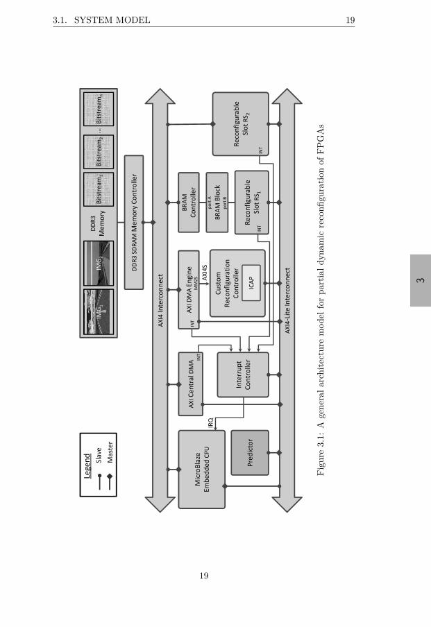
Many dynamically reconfigurable systems are implemented using FPGAplatforms [PTW10]. One common architecture choice is to partition theFPGA into a static region, and a partially dynamically reconfigurable (PDR)region (used as a coprocessor for hardware acceleration) [Koc13]. A hostCPU resides in the static region, together with a reconfiguration controllerand other hardware modules that need not change at run-time. In the PDRregion, the application hardware modules can be dynamically loaded at run-time [SBB+06]. The host CPU executes the software part of the applicationand is also responsible for initiating the reconfiguration of the PDR regionof the FPGA. The reconfiguration controller will configure this region byloading the bitstreams from the memory, upon CPU requests. While onereconfiguration is going on, the execution of the other (non-overlapping)modules on the FPGA is not affected.

Figure 3.1 presents our overall architecture, which is described next.The entire framework has been implemented and tested on a ML605 boardfrom Xilinx1, featuring an XC6VLX240T Virtex6 FPGA, which was one of

1Note that the framework is general and can be implemented on any FPGA architec-ture that supports partial dynamic reconfiguration (e.g. [Alt12]).

18

“thesis” — 2015/8/12 — 12:54 — page 19 — #39

3

3.1. SYSTEM MODEL 19

!

"

#$

%&

'

()

*'

!

!

(

#$

*(

%

&

+

,

-,

!

'

(

#$

#$

Fig

ure

3.1:

Age

nera

lar

chit

ectu

rem

odel

for

part

ial

dyna

mic

reco

nfigu

rati

onof

FP

GA

s

19

“thesis” — 2015/8/12 — 12:54 — page 20 — #40

3


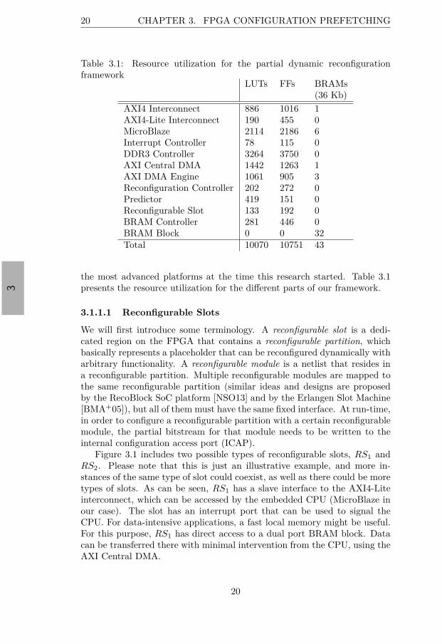
Table 3.1: Resource utilization for the partial dynamic reconfigurationframework

LUTs FFs BRAMs(36 Kb)

AXI4 Interconnect 886 1016 1AXI4-Lite Interconnect 190 455 0MicroBlaze 2114 2186 6Interrupt Controller 78 115 0DDR3 Controller 3264 3750 0AXI Central DMA 1442 1263 1AXI DMA Engine 1061 905 3Reconfiguration Controller 202 272 0Predictor 419 151 0Reconfigurable Slot 133 192 0BRAM Controller 281 446 0BRAM Block 0 0 32Total 10070 10751 43

the most advanced platforms at the time this research started. Table 3.1presents the resource utilization for the different parts of our framework.

3.1.1.1 Reconfigurable Slots

We will first introduce some terminology. A reconfigurable slot is a dedi-cated region on the FPGA that contains a reconfigurable partition, whichbasically represents a placeholder that can be reconfigured dynamically witharbitrary functionality. A reconfigurable module is a netlist that resides ina reconfigurable partition. Multiple reconfigurable modules are mapped tothe same reconfigurable partition (similar ideas and designs are proposedby the RecoBlock SoC platform [NSO13] and by the Erlangen Slot Machine[BMA+05]), but all of them must have the same fixed interface. At run-time,in order to configure a reconfigurable partition with a certain reconfigurablemodule, the partial bitstream for that module needs to be written to theinternal configuration access port (ICAP).

Figure 3.1 includes two possible types of reconfigurable slots, RS1 andRS2. Please note that this is just an illustrative example, and more in-stances of the same type of slot could coexist, as well as there could be moretypes of slots. As can be seen, RS1 has a slave interface to the AXI4-Liteinterconnect, which can be accessed by the embedded CPU (MicroBlaze inour case). The slot has an interrupt port that can be used to signal theCPU. For data-intensive applications, a fast local memory might be useful.For this purpose, RS1 has direct access to a dual port BRAM block. Datacan be transferred there with minimal intervention from the CPU, using theAXI Central DMA.

20

“thesis” — 2015/8/12 — 12:54 — page 21 — #41

3


! "

#

Figure 3.2: The internal architecture of the reconfigurable slot RS2

Reconfigurable slot RS2 differs from RS1 by not having access to a sharedBRAM block but, instead, benefiting from a master interface to the AXI4interconnect. Figure 3.2 presents the internal organization of such a reconfig-urable slot. The slot is connected to the AXI4 and AXI4-Lite interconnectsthrough the corresponding AXI IP Interfaces (IPIF), master and slave, whichsimplify the implementation of the user logic (the reconfigurable partition).Of course, other types of interfaces could also be implemented, dependingon the application needs.

The main advantage of such a design is the generality of the recon-figurable slots. The designer needs to implement only the logic which isparticular to the actual application (user logic in Figure 3.2). Note thatonly this area (the reconfigurable partition) will be partially reconfiguredat run-time, and everything else is static logic that will remain unchanged.An enable signal can be used to isolate the user logic until it is completelyreconfigured, and all output signals should be registered on the static side.The local reset should be asserted in the user logic after reconfiguration hascompleted to ensure a known valid initial state.

3.1.1.2 Custom Reconfiguration Controller

All the bitstreams are stored in the DDR3 memory (Bitstream1 to Bitstreamn

in Figure 3.1). When a reconfiguration is requested, the bitstream is trans-ferred to the ICAP using DMA burst transfers. Thus, the CPU (MicroBlaze)is almost completely out of the loop. After setting up the DMA transfer,MicroBlaze can perform useful computations in parallel with the reconfigu-ration. We have implemented a custom reconfiguration controller, which isdescribed below.

In Figure 3.1 the AXI DMA Engine streams the bitstream data throughthe Xilinx AXI4-Stream (AXI4S) interface (a high throughput point-to-point connection) to our reconfiguration controller, which forwards it to theICAP. Similar solutions have been proposed in the literature (e.g. [LKLJ09],

21

“thesis” — 2015/8/12 — 12:54 — page 22 — #42

3


!

!

!"

#

$

%&

!"

!

'

Figure 3.3: The custom reconfiguration controller

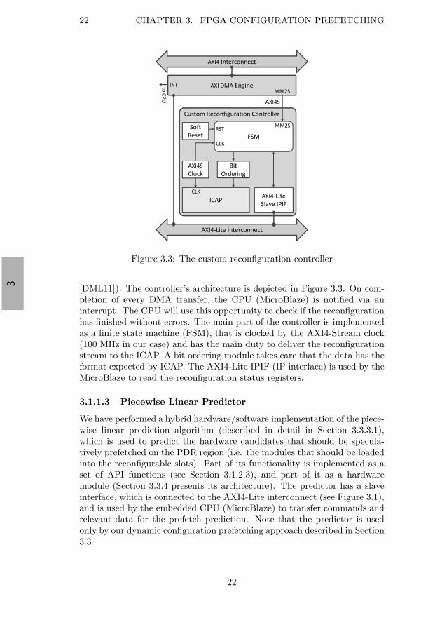
[DML11]). The controller’s architecture is depicted in Figure 3.3. On com-pletion of every DMA transfer, the CPU (MicroBlaze) is notified via aninterrupt. The CPU will use this opportunity to check if the reconfigurationhas finished without errors. The main part of the controller is implementedas a finite state machine (FSM), that is clocked by the AXI4-Stream clock(100 MHz in our case) and has the main duty to deliver the reconfigurationstream to the ICAP. A bit ordering module takes care that the data has theformat expected by ICAP. The AXI4-Lite IPIF (IP interface) is used by theMicroBlaze to read the reconfiguration status registers.

3.1.1.3 Piecewise Linear Predictor

We have performed a hybrid hardware/software implementation of the piece-wise linear prediction algorithm (described in detail in Section 3.3.3.1),which is used to predict the hardware candidates that should be specula-tively prefetched on the PDR region (i.e. the modules that should be loadedinto the reconfigurable slots). Part of its functionality is implemented as aset of API functions (see Section 3.1.2.3), and part of it as a hardwaremodule (Section 3.3.4 presents its architecture). The predictor has a slaveinterface, which is connected to the AXI4-Lite interconnect (see Figure 3.1),and is used by the embedded CPU (MicroBlaze) to transfer commands andrelevant data for the prefetch prediction. Note that the predictor is usedonly by our dynamic configuration prefetching approach described in Section3.3.

22

“thesis” — 2015/8/12 — 12:54 — page 23 — #43

3


3.1.2 Middleware and Reconfiguration API

Our extensive API can be divided into several sets of utility functions, asdescribed below.

3.1.2.1 Partial Reconfiguration

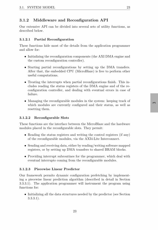
These functions hide most of the details from the application programmerand allow for:

• Initializing the reconfiguration components (the AXI DMA engine andthe custom reconfiguration controller).

• Starting partial reconfigurations by setting up the DMA transfers.After that, the embedded CPU (MicroBlaze) is free to perform otheruseful computations.

• Treating the interrupts when partial reconfigurations finish. This in-cludes reading the status registers of the DMA engine and of the re-configuration controller, and dealing with eventual errors in case offailure.

• Managing the reconfigurable modules in the system: keeping track ofwhich modules are currently configured and their status, as well asresetting them.

3.1.2.2 Reconfigurable Slots

These functions are the interface between the MicroBlaze and the hardwaremodules placed in the reconfigurable slots. They permit:

• Reading the status registers and writing the control registers (if any)of the reconfigurable modules, via the AXI4-Lite Interconnect.

• Sending and receiving data, either by reading/writing software mappedregisters, or by setting up DMA transfers to shared BRAM blocks.

• Providing interrupt subroutines for the programmer, which deal witheventual interrupts coming from the reconfigurable modules.

3.1.2.3 Piecewise Linear Predictor

Our framework permits dynamic configuration prefetching by implement-ing a piecewise linear prediction algorithm (described in detail in Section3.3.3.1). The application programmer will instrument the program usingfunctions for:

• Initializing all the data structures needed by the predictor (see Section3.3.3.1).

23

“thesis” — 2015/8/12 — 12:54 — page 24 — #44

3


• Updating all the predictor data, e.g. execution frequencies for hard-ware modules, timestamps, the weights and all the branch historiesused by the predictor.

• Performing the actual prediction, whose result will determine the mod-ules to be prefetched.

3.1.3 Application Model

The main goal of our approaches (presented in Sections 3.2 and 3.3 respec-tively) is to minimize the expected execution time of a sequential programexecuted on the hardware platform described above. We model the appli-cation as a control flow graph G(N , E), where nodes in N correspond tocomputational tasks (either basic blocks, or hardware modules), and edgesin E model the flow of control within the application (G captures all poten-tial execution paths). We distinguish several types of nodes: root and sink,correspond to the entry and the exit of the program; control nodes representconditional instructions in the program; loop header nodes represent the en-try points of loops, and they are the target of a back edge (i.e. an edge thatpoints to a block that has already been met during a depth-first traversal ofthe graph). All the other nodes in N are either regular basic blocks (thatwill be executed only in software), or hardware modules (described below).

We denote with H ⊆ N the set of tasks (also referred to as modules) con-sidered for hardware implementation. We assume that all modules in H haveboth a hardware and a corresponding software implementation. Since some-times it might be impossible to hide enough of the reconfiguration overheadfor all candidates in H, our techniques decide which are the most profitablemodules to perform prefetches for (at a certain point in the application).Thus, for some candidates, it might be better to execute the module insoftware, instead of performing a prefetch too close to its location (becausewaiting for the reconfiguration to finish and then executing the module onthe FPGA is slower than executing it in software).

Note that there exist many established methodologies (e.g. [SHTT13],[BPCF13], [NSO+12], [BSY+10], [LCD+00]) to perform the hardware/softwarepartitioning step (i.e. determine the set H automatically), that will decidewhich are the hardware candidates to be (potentially) implemented on theFPGA. Alternatively, this decision can be taken by the designer, who hasin-depth knowledge about the application domain. Intuitively, the hard-ware candidates in H will represent those parts of the application whichare computationally intensive, and at the same time amenable for FPGAacceleration. Please note that it is not necessary that all candidate modulesfrom H will end up on the FPGA. Given a particular choice for H, ourtechniques will try to use the limited hardware resources as efficiently aspossible in order to maximize the performance of the application.

At run-time, once a candidate m ∈ H is reached, there are two possibil-ities:

24

“thesis” — 2015/8/12 — 12:54 — page 25 — #45

3

3.2. STATIC FPGA CONFIGURATION PREFETCHING 25

1. m is already fully loaded in a reconfigurable slot on the FPGA, andthus it will be used and executed there;

2. m is not fully loaded. Then, we face two scenarios:

(a) if starting/continuing the reconfiguration of m, waiting for it tofinish, and then executing the module on FPGA results in anearlier finishing time than the software execution, then the appli-cation will do so;

(b) otherwise, m will be executed in software.

For each hardware candidate m ∈ H, we assume that we know its soft-ware execution time, sw : H → R

+, its hardware execution time (includingany additional communication overhead between the CPU and the reconfig-urable partition hosting m), hw : H → R

+, and the time to reconfigure mon the FPGA, rec : H → R

+.

3.2 Static FPGA Configuration Prefetching

In this section we will present our contribution to static configuration prefetch-ing. We use profiling information (e.g. the function prob : E → [0, 1] rep-resents the probability of each edge in the control flow graph to be taken,and for each loop header n, iter_probn : N → [0, 1] represents the probabil-ity mass function of the discrete distribution of loop iterations) to decide atdesign-time what prefetches to apply in order to obtain the best performanceimprovement for the application.

3.2.1 Problem Formulation

Given an application (as described in Section 3.1.3) intended to run on thereconfigurable architecture described in Section 3.1.1, our goal is to deter-mine, at each node n ∈ N , the candidate modules to be prefetched (storedin loadQ(n)) by the middleware described in Section 3.1.2 such that the ex-pected execution time of the application is minimized. This will implicitlyalso determine the hardware/software partitioning of the candidate modulesfrom H.

3.2.2 Motivational Example

Let us consider the control flow graph (CFG) in Figure 3.4a, where candidatehardware modules are represented with squares, and software nodes withcircles. The discrete probability distribution for the iterations of the loopa − b, the software and hardware execution times for the nodes, as well asthe edge probabilities, are illustrated on the graph. The reconfigurationtimes are: rec(M1) = 37, rec(M2) = 20, rec(M3) = 46. We also consider

25

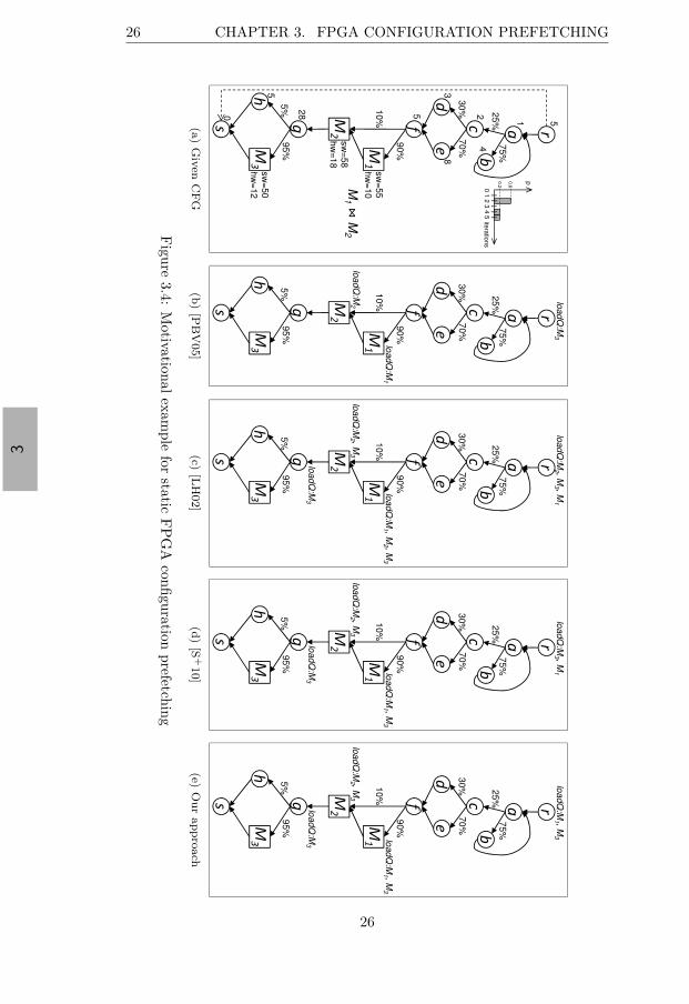
“thesis” — 2015/8/12 — 12:54 — page 26 — #46

3


25%

75%

30%

70%

90%

10%

p

itera

tions

0 1

2 3

4 5

0.6

0.2

5

5

3

hw

=10

1

42

8

sw

=55

hw

=18

sw

=58

M1

M2

95%

5% 2

8

5

0

hw

=12

sw

=50

(a)

Giv

enC

FG

25%

75%

30%

70%

90%

10%

loadQ

:M1

loadQ

:M3

loadQ

:M2

95%

5%(b

)[P

BV

05]

25%

75%

30%

70%

90%

10%

loadQ

:M2 , M

3 , M1

loadQ

:M1 , M

2 , M3

loadQ

:M2 , M

3

95%

5%

loadQ

:M3

(c)[L

H02]

25%

75%

30%

70%

90%

10%

loadQ

:M3 , M

1loadQ

:M1 , M

3

loadQ

:M2 , M

3

95%

5%

loadQ

:M3

(d)

[S+

10]

25%

75%

30%

70%

90%

10%

loadQ

:M1 , M

3loadQ

:M1 , M

3

loadQ

:M2 , M

3

95%

5%

loadQ

:M3

(e)O

ur

ap

pro

ach

Figure

3.4:M

otivationalexam

plefor

staticF

PG

Aconfiguration

prefetching

26

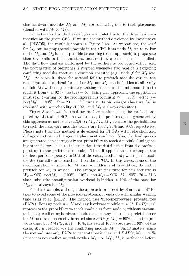
“thesis” — 2015/8/12 — 12:54 — page 27 — #47

3


that hardware modules M1 and M2 are conflicting due to their placement(denoted with M1 ⊲⊳ M2).

Let us try to schedule the configuration prefetches for the three hardwaremodules on the given CFG. If we use the method developed by Panainte etal. [PBV05], the result is shown in Figure 3.4b. As we can see, the loadfor M3 can be propagated upwards in the CFG from node M3 up to r. Fornodes M1 and M2 it is not possible (according to this approach) to propagatetheir load calls to their ancestors, because they are in placement conflict.The data-flow analysis performed by the authors is too conservative, andthe propagation of prefetches is stopped whenever two load calls targetingconflicting modules meet at a common ancestor (e.g. node f for M1 andM2). As a result, since the method fails to prefetch modules earlier, thereconfiguration overhead for neither M1, nor M2, can be hidden at all. Onlymodule M3 will not generate any waiting time, since the minimum time toreach it from r is 92 > rec(M3) = 46. Using this approach, the applicationmust stall (waiting for the reconfigurations to finish) W1 = 90% · rec(M1) +rec(M2) = 90% · 37 + 20 = 53.3 time units on average (because M1 isexecuted with a probability of 90%, and M2 is always executed).

Figure 3.4c shows the resulting prefetches after using the method pro-posed by Li et al. [LH02]. As we can see, the prefetch queue generated bythis approach at node r is loadQ(r) : M2, M3, M1, because the probabilitiesto reach the hardware modules from r are 100%, 95% and 90% respectively.Please note that this method is developed for FPGAs with relocation anddefragmentation and it ignores placement conflicts. Also, the load queuesare generated considering only the probability to reach a module (and ignor-ing other factors, such as the execution time distribution from the prefetchpoint up to the prefetched module). Thus, if applied to our example, themethod performs poorly: in 90% of the cases, module M1 will replace mod-ule M2 (initially prefetched at r) on the FPGA. In this cases, none of thereconfiguration overhead for M1 can be hidden, and in addition, the initialprefetch for M2 is wasted. The average waiting time for this scenario isW2 = 90% · rec(M1) + (100% − 10%) · rec(M2) = 90% · 37 + 90% · 20 = 51.3time units (the reconfiguration overhead is hidden in 10% of the cases forM2, and always for M3).

For this example, although the approach proposed by Sim et al. [S+10]tries to avoid some of the previous problems, it ends up with similar waitingtime as Li et al. [LH02]. The method uses ‘placement-aware’ probabilities(PAPs). For any node n ∈ N and any hardware module m ∈ H, PAP (n, m)represents the probability to reach module m from node n, without encoun-tering any conflicting hardware module on the way. Thus, the prefetch orderfor M1 and M2 is correctly inverted since PAP (r, M1) = 90%, as in the pre-vious case, but PAP (r, M2) = 10%, instead of 100% (because in 90% of thecases, M2 is reached via the conflicting module M1). Unfortunately, sincethe method uses only PAPs to generate prefetches, and PAP (r, M3) = 95%(since it is not conflicting with neither M1, nor M2), M3 is prefetched before

27

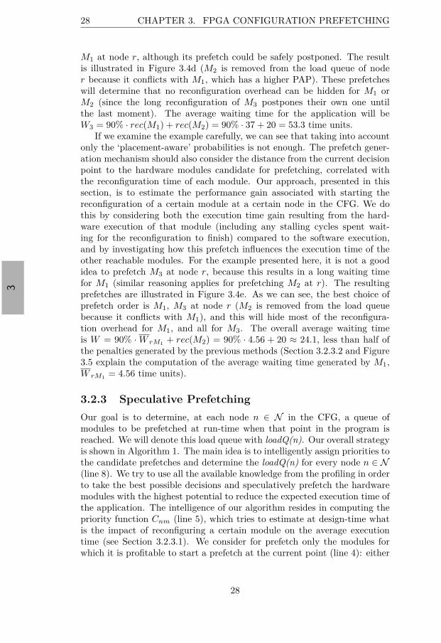
“thesis” — 2015/8/12 — 12:54 — page 28 — #48

3


M1 at node r, although its prefetch could be safely postponed. The resultis illustrated in Figure 3.4d (M2 is removed from the load queue of noder because it conflicts with M1, which has a higher PAP). These prefetcheswill determine that no reconfiguration overhead can be hidden for M1 orM2 (since the long reconfiguration of M3 postpones their own one untilthe last moment). The average waiting time for the application will beW3 = 90% · rec(M1) + rec(M2) = 90% · 37 + 20 = 53.3 time units.

If we examine the example carefully, we can see that taking into accountonly the ‘placement-aware’ probabilities is not enough. The prefetch gener-ation mechanism should also consider the distance from the current decisionpoint to the hardware modules candidate for prefetching, correlated withthe reconfiguration time of each module. Our approach, presented in thissection, is to estimate the performance gain associated with starting thereconfiguration of a certain module at a certain node in the CFG. We dothis by considering both the execution time gain resulting from the hard-ware execution of that module (including any stalling cycles spent wait-ing for the reconfiguration to finish) compared to the software execution,and by investigating how this prefetch influences the execution time of theother reachable modules. For the example presented here, it is not a goodidea to prefetch M3 at node r, because this results in a long waiting timefor M1 (similar reasoning applies for prefetching M2 at r). The resultingprefetches are illustrated in Figure 3.4e. As we can see, the best choice ofprefetch order is M1, M3 at node r (M2 is removed from the load queuebecause it conflicts with M1), and this will hide most of the reconfigura-tion overhead for M1, and all for M3. The overall average waiting timeis W = 90% · W rM1

+ rec(M2) = 90% · 4.56 + 20 ≈ 24.1, less than half ofthe penalties generated by the previous methods (Section 3.2.3.2 and Figure3.5 explain the computation of the average waiting time generated by M1,W rM1

= 4.56 time units).

3.2.3 Speculative Prefetching

Our goal is to determine, at each node n ∈ N in the CFG, a queue ofmodules to be prefetched at run-time when that point in the program isreached. We will denote this load queue with loadQ(n). Our overall strategyis shown in Algorithm 1. The main idea is to intelligently assign priorities tothe candidate prefetches and determine the loadQ(n) for every node n ∈ N(line 8). We try to use all the available knowledge from the profiling in orderto take the best possible decisions and speculatively prefetch the hardwaremodules with the highest potential to reduce the expected execution time ofthe application. The intelligence of our algorithm resides in computing thepriority function Cnm (line 5), which tries to estimate at design-time whatis the impact of reconfiguring a certain module on the average executiontime (see Section 3.2.3.1). We consider for prefetch only the modules forwhich it is profitable to start a prefetch at the current point (line 4): either

28

“thesis” — 2015/8/12 — 12:54 — page 29 — #49

3


Algorithm 1 Generating the prefetch queuesInput: N , H, PAP (n, m), profiling informationOutput: loadQ(n) = prefetches to apply at node n

1: procedure GeneratePrefetchQ

2: for all n ∈ N do

3: for all m ∈ H|PAP (n, m) Ó= 0 do

4: if Gnm > 0 ∨ m in loop then

5: compute priority function Cnm

6: end if

7: end for

8: loadQ(n) ← modules in decreasing order of Cnm

9: remove all lower priority modules that have area conflicts withhigher priority modules in loadQ(n)

10: end for

11: eliminate redundant prefetches12: end procedure

the average execution time gain Gnm (over the software execution of thecandidate) obtained if its reconfiguration starts at this node is greater than 0,or the module is inside a loop. In the latter case, even if the reconfigurationis not finished in the first few loop iterations and we execute the modulein software, we will gain from executing the module in hardware in futureloop iterations. Since in most of the cases the software execution time of amodule has the same order of magnitude as the reconfiguration overhead forthe module, the reconfiguration will be finished after the first loop iteration.More exactly, while the module in discussion is executed in software inthe first loop iteration, its hardware version is being reconfigured on theFPGA. As a result, in the next loop iterations the module will be executedin hardware.

The next step is to sort the prefetch candidates in decreasing order oftheir priority function (line 8), and in case of equality we give higher priorityto modules placed in loops. After the loadQ(n) has been generated for a noden, we remove all the lower priority modules that have area conflicts with thehigher priority modules in the queue (line 9). Once all the queues have beengenerated, we eliminate redundant prefetches (all consecutive candidates ata child node that are a starting sub-sequence at all its parents in the CFG),as in [LH02] or [S+10].

The actual hardware module to be prefetched will be determined at run-time (by the middleware, using the reconfiguration API), since it depends onthe run-time conditions. If the module with the highest priority (the headof loadQ(n)) is not yet loaded and is not being currently reconfigured, it willbe loaded at that particular node n. If the head of loadQ(n) is already onFPGA, the module with the next priority that is not yet on the FPGA willbe loaded, but only in case the reconfiguration controller is idle. Finally, if

29

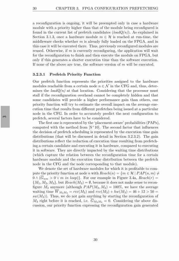
“thesis” — 2015/8/12 — 12:54 — page 30 — #50

3


a reconfiguration is ongoing, it will be preempted only in case a hardwaremodule with a priority higher than that of the module being reconfigured isfound in the current list of prefetch candidates (loadQ(n)). As explained inSection 3.1.3, once a hardware module m ∈ H is reached at run-time, themiddleware checks whether m is already fully loaded on the FPGA, and inthis case it will be executed there. Thus, previously reconfigured modules arereused. Otherwise, if m is currently reconfiguring, the application will waitfor the reconfiguration to finish and then execute the module on FPGA, butonly if this generates a shorter execution time than the software execution.If none of the above are true, the software version of m will be executed.

3.2.3.1 Prefetch Priority Function

Our prefetch function represents the priorities assigned to the hardwaremodules reachable from a certain node n ∈ N in the CFG and, thus, deter-mines the loadQ(n) at that location. Considering that the processor muststall if the reconfiguration overhead cannot be completely hidden and thatsome candidates will provide a higher performance gain than others, ourpriority function will try to estimate the overall impact on the average exe-cution time that results from different prefetches being issued at a particularnode in the CFG. In order to accurately predict the next configuration toprefetch, several factors have to be considered.

The first one is represented by the ‘placement-aware’ probabilities (PAPs),computed with the method from [S+10]. The second factor that influencesthe decision of prefetch scheduling is represented by the execution time gaindistributions (that will be discussed in detail in Section 3.2.3.2). The gaindistributions reflect the reduction of execution time resulting from prefetch-ing a certain candidate and executing it in hardware, compared to executingit in software. They are directly impacted by the waiting time distributions(which capture the relation between the reconfiguration time for a certainhardware module and the execution time distribution between the prefetchnode in the CFG and the node corresponding to that module).

We denote the set of hardware modules for which it is profitable to com-pute the priority function at node n with Reach(n) = m ∈ H | PAP (n, m) Ó=0 ∧ (Gnm > 0 ∨ m in loop). For our example in Figure 3.4a, Reach(r) =M1, M2, M3, but Reach(M3) = ∅, because it does not make sense to recon-figure M3 anymore (although PAP (M3, M3) = 100%, we have the averagewaiting time W M3M3

= rec(M3) and rec(M3) + hw(M3) = 46 + 12 > 50 =sw(M3)). Thus, we do not gain anything by starting the reconfiguration ofM3 right before it is reached, i.e. GM3M3

= 0. Considering the above dis-cussion, our priority function expressing the reconfiguration gain generated

30

“thesis” — 2015/8/12 — 12:54 — page 31 — #51

3


by prefetching module m ∈ Reach(n) at node n is defined as:

Cnm = PAP (n, m) · Gnm

+∑

k∈MutEx(m)

PAP (n, k) · Gsk

+∑

k Ó∈MutEx(m)

PAP (n, k) · Gk

nm

(3.1)

In the above equation, Gnm denotes the average execution time gain gen-erated by prefetching module m at node n (see Section 3.2.3.2), MutEx(m)denotes the set of hardware modules that are executed mutually exclusivewith m, the index s in Gsk represents the node where the paths leading fromn to m and k split, and G

k

nm represents the expected gain generated by k,given that its reconfiguration is started immediately after the one for m.

The first term of the priority function represents the contribution (interms of average execution time gain) of the candidate module m. Thesecond term tries to capture the impact that the reconfiguration of m willproduce on other modules that are executed mutually exclusive with it. Inthis case, the earliest time we can start the reconfiguration of module k,which is competing with m for the reconfiguration controller, is at nodes, where the paths reaching m and k split. The third term captures theimpact on the execution time of modules that are not mutually exclusivewith m (and might be executed after m). The intuition behind the thirdterm is the following: if from node n we can reach both module m and k (i.e.they are not mutually exclusive), then we want to see what is the impact ofreconfiguring m first, and only then k.

In Figure 3.4a, modules M1, M2 and M3 are not mutually exclusive2.Let us calculate the priority function for the three hardware modules fromFigure 3.4a at node r (considering their areas proportional with their re-configuration time). CrM1

= 90% · 40.4 + 0 + 10% · 36.9 + 95% · 38 ≈76.1. Note that MutEx(M1) = ∅, PAP (r, M1) = 90%, PAP (r, M2) =10%, PAP (r, M3) = 95%, GrM1

= 40.4, GrM2= 36.9, GrM3

= 38. Simi-larly we compute CrM2

= 10% · 40 + 90% · 22.5 + 95% · 38 ≈ 60.3 andCrM3

= 95% · 38 + 90% · 1.7 + 10% · 30.9 ≈ 40.7 (the computation of ex-ecution time gains is discussed in Section 3.2.3.2). As we can see, sinceCrM1

> CrM2> CrM3

, the correct loadQ(r) = M1, M3 is generated at noder. Note that M2 is removed from loadQ(r) because it is in placement conflictwith M1, which is the head of the queue (see line 9 in Algorithm 1).

3.2.3.2 Expected Execution Time Gain

Let us consider a node n ∈ N from the CFG and a hardware module m ∈ H,reachable from n. Given that the reconfiguration of module m starts at

2Two mutually exclusive nodes are, for example, d and e in Figure 3.4a, and the pathsreaching them split at c.

31

“thesis” — 2015/8/12 — 12:54 — page 32 — #52

3


node n, we define the average execution time gain Gnm as the expectedexecution time that is saved by executing m in hardware (including anystalling cycles when the application is waiting for the reconfiguration of mto be completed), compared to the software execution of m. In order tocompute it, we start with the distance (in time) from n to m. Let Xnm

be the random variable associated with this distance. The waiting time isgiven by the random variable:

Wnm = max(0, rec(m) − Xnm) (3.2)

Note that the waiting time cannot be negative (if a module is already presenton FPGA when we reach it, it does not matter how long ago its reconfigu-ration finished). The execution time gain is given by the distribution of therandom variable:

Gnm = max(0, sw(m) − (Wnm + hw(m))) (3.3)

In case the software execution time of a candidate is shorter than waiting forits reconfiguration to finish and executing it in hardware, then the modulewill be executed in software by the middleware, and the gain is zero. Ifwe denote the probability mass function (pmf) of Gnm with gnm, then theaverage gain Gnm will be computed as:

Gnm =

∞∑

x=0

(x · gnm(x)

)(3.4)

The discussion is illustrated graphically in Figure 3.5, considering thenodes n = r and m = M1 from Figure 3.4a. The probability mass function(pmf) for XrM1

(distance in time from r to M1) is represented in Figure3.5a and the pmf for the waiting time WrM1

in Figure 3.5b. Note that thenegative part of the distribution (depicted with dotted line) generates nowaiting time. In Figure 3.5c we add the hardware execution time to thepotential waiting time incurred. Finally, Figure 3.5d represents the discreteprobability distribution of the gain GrM1

. The resulting average gain isGrM1

= 34 · 18% + 39 · 42% + 44 · 6% + 45 · 34% = 40.44 time units.Before presenting our algorithm for computing the gain distribution and

the average gain, let us first introduce a few concepts. Given a control flowgraph Gcf (Ncf , Ecf ), we introduce the following definitions [ALSU06]:

Definition 3.1 A node n ∈ Ncf is post-dominated by a node m ∈ Ncf inthe control flow graph Gcf if every directed path from n to sink (excludingn) contains m.

Definition 3.2 Given a control flow graph Gcf , a node m ∈ Ncf is controldependent upon a node n ∈ Ncf via a control flow edge e ∈ Ecf if thefollowing two hold:

32

“thesis” — 2015/8/12 — 12:54 — page 33 — #53

3


p[%

]

0

26

31

36

41

46

6

tim

e u

nits

14

18

20

42

rec(M

1)=

37

(a)

Xr

M1

p[%

]

-9 -

4

1

6

11

6

tim

e u

nits

14

18

20

42

34

(b)

Wr

M1

p[%

]

1

6 1

1

16

21

6

tim

e u

nits

14

18

20

42

34

hw

(M1)

sw

(M1)=

55

(c)

Wr

M1

+h

w(M

1)

34

p[%

]

0

34

39

44

6

tim

e u

nits

14

18

20

42

(d)

Gr

M1

Fig

ure

3.5:

Com

puti

ngth

ega

inpr

obab

ility

dist

ribu

tion

step

byst

ep

33

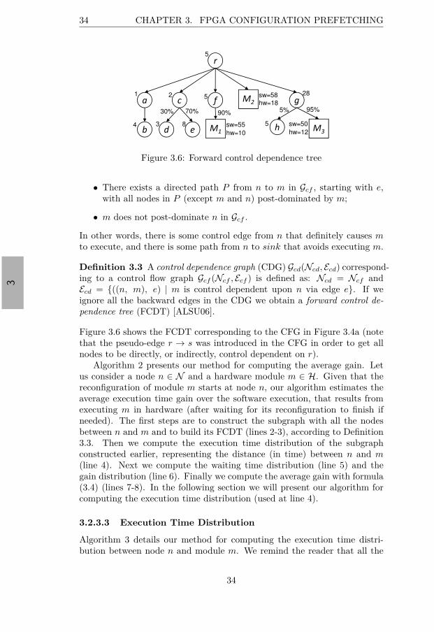
“thesis” — 2015/8/12 — 12:54 — page 34 — #54

3


30% 70% 90%95%5%

5

528

3 5

hw=10

1

4

2

8 sw=55

hw=18

sw=58

hw=12

sw=50

Figure 3.6: Forward control dependence tree

• There exists a directed path P from n to m in Gcf , starting with e,with all nodes in P (except m and n) post-dominated by m;

• m does not post-dominate n in Gcf .

In other words, there is some control edge from n that definitely causes mto execute, and there is some path from n to sink that avoids executing m.

Definition 3.3 A control dependence graph (CDG) Gcd(Ncd, Ecd) correspond-ing to a control flow graph Gcf (Ncf , Ecf ) is defined as: Ncd = Ncf andEcd = ((n, m), e) | m is control dependent upon n via edge e. If weignore all the backward edges in the CDG we obtain a forward control de-pendence tree (FCDT) [ALSU06].

Figure 3.6 shows the FCDT corresponding to the CFG in Figure 3.4a (notethat the pseudo-edge r → s was introduced in the CFG in order to get allnodes to be directly, or indirectly, control dependent on r).

Algorithm 2 presents our method for computing the average gain. Letus consider a node n ∈ N and a hardware module m ∈ H. Given that thereconfiguration of module m starts at node n, our algorithm estimates theaverage execution time gain over the software execution, that results fromexecuting m in hardware (after waiting for its reconfiguration to finish ifneeded). The first steps are to construct the subgraph with all the nodesbetween n and m and to build its FCDT (lines 2-3), according to Definition3.3. Then we compute the execution time distribution of the subgraphconstructed earlier, representing the distance (in time) between n and m(line 4). Next we compute the waiting time distribution (line 5) and thegain distribution (line 6). Finally we compute the average gain with formula(3.4) (lines 7-8). In the following section we will present our algorithm forcomputing the execution time distribution (used at line 4).

3.2.3.3 Execution Time Distribution

Algorithm 3 details our method for computing the execution time distri-bution between node n and module m. We remind the reader that all the

34

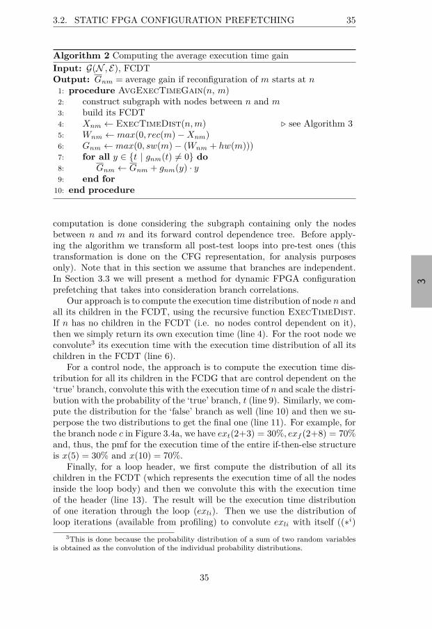
“thesis” — 2015/8/12 — 12:54 — page 35 — #55

3


Algorithm 2 Computing the average execution time gainInput: G(N , E), FCDTOutput: Gnm = average gain if reconfiguration of m starts at n

1: procedure AvgExecTimeGain(n, m)2: construct subgraph with nodes between n and m3: build its FCDT4: Xnm ← ExecTimeDist(n, m) ⊲ see Algorithm 35: Wnm ← max(0, rec(m) − Xnm)6: Gnm ← max(0, sw(m) − (Wnm + hw(m)))7: for all y ∈ t | gnm(t) Ó= 0 do

8: Gnm ← Gnm + gnm(y) · y9: end for

10: end procedure

computation is done considering the subgraph containing only the nodesbetween n and m and its forward control dependence tree. Before apply-ing the algorithm we transform all post-test loops into pre-test ones (thistransformation is done on the CFG representation, for analysis purposesonly). Note that in this section we assume that branches are independent.In Section 3.3 we will present a method for dynamic FPGA configurationprefetching that takes into consideration branch correlations.

Our approach is to compute the execution time distribution of node n andall its children in the FCDT, using the recursive function ExecTimeDist.If n has no children in the FCDT (i.e. no nodes control dependent on it),then we simply return its own execution time (line 4). For the root node weconvolute3 its execution time with the execution time distribution of all itschildren in the FCDT (line 6).

For a control node, the approach is to compute the execution time dis-tribution for all its children in the FCDG that are control dependent on the‘true’ branch, convolute this with the execution time of n and scale the distri-bution with the probability of the ‘true’ branch, t (line 9). Similarly, we com-pute the distribution for the ‘false’ branch as well (line 10) and then we su-perpose the two distributions to get the final one (line 11). For example, forthe branch node c in Figure 3.4a, we have ext(2+3) = 30%, exf (2+8) = 70%and, thus, the pmf for the execution time of the entire if-then-else structureis x(5) = 30% and x(10) = 70%.

Finally, for a loop header, we first compute the distribution of all itschildren in the FCDT (which represents the execution time of all the nodesinside the loop body) and then we convolute this with the execution timeof the header (line 13). The result will be the execution time distributionof one iteration through the loop (exli). Then we use the distribution ofloop iterations (available from profiling) to convolute exli with itself ((∗i)

3This is done because the probability distribution of a sum of two random variablesis obtained as the convolution of the individual probability distributions.

35

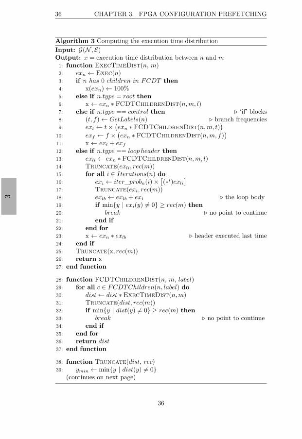
“thesis” — 2015/8/12 — 12:54 — page 36 — #56

3


Algorithm 3 Computing the execution time distributionInput: G(N , E)Output: x = execution time distribution between n and m

1: function ExecTimeDist(n, m)2: exn ← Exec(n)3: if n has 0 children in FCDT then

4: x(exn) ← 100%5: else if n.type = root then

6: x ← exn ∗ FCDTChildrenDist(n, m, l)7: else if n.type == control then ⊲ ‘if’ blocks8: (t, f) ← GetLabels(n) ⊲ branch frequencies9: ext ← t ×

(exn ∗ FCDTChildrenDist(n, m, t)

)

10: exf ← f ×(exn ∗ FCDTChildrenDist(n, m, f)

)

11: x ← ext + exf

12: else if n.type == loop header then

13: exli ← exn ∗ FCDTChildrenDist(n, m, l)14: Truncate(exli, rec(m))15: for all i ∈ Iterations(n) do

16: exi ← iter_probn(i) ×[(∗i)exli

]

17: Truncate(exi, rec(m))18: exlb ← exlb + exi ⊲ the loop body19: if miny | exi(y) Ó= 0 ≥ rec(m) then

20: break ⊲ no point to continue21: end if

22: end for

23: x ← exn ∗ exlb ⊲ header executed last time24: end if

25: Truncate(x, rec(m))26: return x27: end function

28: function FCDTChildrenDist(n, m, label)29: for all c ∈ FCDTChildren(n, label) do

30: dist ← dist ∗ ExecTimeDist(n, m)31: Truncate(dist, rec(m))32: if miny | dist(y) Ó= 0 ≥ rec(m) then

33: break ⊲ no point to continue34: end if

35: end for

36: return dist37: end function

38: function Truncate(dist, rec)39: ymin ← miny | dist(y) Ó= 0

(continues on next page)

36

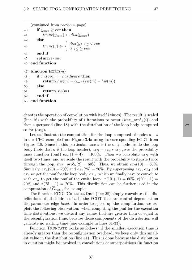
“thesis” — 2015/8/12 — 12:54 — page 37 — #57

3


(continued from previous page)40: if ymin ≥ rec then

41: trunc(ymin) ← dist(ymin)42: else

43: trunc(y) ←

dist(y) : y < rec0 : y ≥ rec

44: end if

45: return trunc46: end function

47: function Exec(m)48: if m.type == hardware then

49: return hw(m) + αm · (sw(m) − hw(m))50: else

51: return sw(m)52: end if

53: end function

denotes the operation of convolution with itself i times). The result is scaled(line 16) with the probability of i iterations to occur (iter_probn(i)) andthen superposed (line 18) with the distribution of the loop body computedso far (exlb).

Let us illustrate the computation for the loop composed of nodes a − bin our CFG example from Figure 3.4a using its corresponding FCDT fromFigure 3.6. Since in this particular case b is the only node inside the loopbody (note that a is the loop header), exli = exa ∗ exb gives the probabilitymass function (pmf) exli(1 + 4) = 100%. Then we convolute exli withitself two times, and we scale the result with the probability to iterate twicethrough the loop, iter_proba(2) = 60%. Thus, we obtain ex2(10) = 60%.Similarly, ex4(20) = 20% and ex5(25) = 20%. By superposing ex2, ex4 andex5 we get the pmf for the loop body, exlb, which we finally have to convolutewith exa to get the pmf of the entire loop: x(10 + 1) = 60%, x(20 + 1) =20% and x(25 + 1) = 20%. This distribution can be further used in thecomputation of GrM1

, for example.The function FCDTChildrenDist (line 28) simply convolutes the dis-

tributions of all children of n in the FCDT that are control dependent onthe parameter edge label. In order to speed-up the computation, we ex-ploit the following observation: when computing the pmf for the executiontime distributions, we discard any values that are greater than or equal tothe reconfiguration time, because those components of the distribution willgenerate no waiting time (one example in lines 31-33).

Function Truncate works as follows: if the smallest execution time isalready greater than the reconfiguration overhead, we keep only this small-est value in the distribution (line 41). This is done because the distributionin question might be involved in convolutions or superpositions (in function

37

“thesis” — 2015/8/12 — 12:54 — page 38 — #58

3


ExecTimeDist), and keeping only this minimal value is enough for com-puting the part of the execution time distribution of interest (that mightgenerate waiting time). Otherwise, we simply truncate the distribution atrec (line 43).

One observation related to the computation of the execution time of anode m ∈ N (function Exec in Algorithm 3, line 47) is that, if m is ahardware candidate (m ∈ H) we need to approximate its execution time,since the prefetches for it might be yet undecided and, thus, it is not knownif the module will be executed in software or on the FPGA. In order toestimate the execution time, we make use of a coefficient αm ∈ [0, 1]. Theexecution time for a hardware module m will be computed as (line 49):exec(m) = hw(m) + αm · (sw(m) − hw(m)). Our experiments have proventhat good results are obtained by setting the value of αm, for each hardwaremodule, to the ratio between its own hardware area and the total area neededfor all modules in H: αm = area(m)∑

k∈Harea(k)

. The intuition behind using αm is

the following: the smaller the area of a module, the faster it is to reconfigureit and the easier it is to accommodate it on the FPGA. As a result, we canexpect that module to be executed in hardware often. For modules with bigarea, it will be harder to accommodate them on the FPGA. Thus, they willbe executed sometimes in software too.

3.2.4 Experimental Evaluation

3.2.4.1 Monte Carlo Simulator

Sampling

In order to evaluate the quality of our prefetch solutions we have usedan in-house developed Monte Carlo simulator that produces the executiontime distribution of an application considering the architectural assumptionsdescribed in Section 3.1.1 and 3.1.2. Each simulation generates a tracethrough the control flow graph, starting at the root node, and ending at thesink node (and we record the length of these traces). Whenever a branchnode is encountered, we perform a Bernoulli draw (based on the probabilitiesof the outgoing edges) to decide if the branch is taken or not. At loop headernodes we perform random sampling from the discrete distribution of loopiterations (iter_probn) to decide how many times to loop. Note that, asmentioned earlier, we consider branches independent. In Section 3.3 we willaddress the case when branches are correlated and will present a dynamicFPGA configuration prefetching method that will take advantage of this.

Accuracy Analysis

We stop the Monte Carlo simulation once we reach a satisfactory ac-curacy for the mean of the execution time distribution. We describe thedesired accuracy in the following way: “The mean of the output distribution

38

“thesis” — 2015/8/12 — 12:54 — page 39 — #59

3


should be accurate to within ±ǫ with confidence κ”. The accuracy can bearbitrarily precise at the expense of longer simulation times. We will nextpresent an analysis based on confidence intervals [HWC14], to determine thenumber of samples to run in order to achieve the required accuracy.

Let us assume that µ is the actual mean of the true output distributionand µ is the estimate mean computed by the Monte Carlo simulation. Sinceeach simulation result is an independent sample from the same distribu-tion, using the Central Limit Theorem we have that the distribution of theestimate of the true mean is (asymptotically) given by:

µ = Normal

(µ,

σ√N

)

where σ is the true standard deviation of the output execution time distri-bution and N represents the number of samples. The above equation canbe rewritten as follows:

µ = Normal

(µ,

σ√N

)

By considering the required accuracy for our mean estimate and per-forming a transformation to the standard Normal distribution (i.e. withmean 0 and standard deviation 1), we can obtain the following relationship[HWC14]:

ǫ =σ√N

Φ−1

(1 + κ

2

)

where the function Φ−1(•) is the inverse of the standard Normal cumulativedistribution function. By rearranging the terms and considering that wewant to achieve at least this accuracy we obtain the minimum value for thenumber of samples N :

N >

(σ · Φ−1

(1+κ

2

)

ǫ

)2

Please note that we do not know the true standard deviation σ, but forour purpose we can estimate it by taking the standard deviation of the firstfew samples (e.g. the first 40).

3.2.4.2 Simulation Results

In order to evaluate the effectiveness of our algorithm we first performedexperiments on synthetic examples. We generated two sets of control flowgraphs: Set1 contains 20 CFGs with ∼100 nodes on average (between 67and 126) and Set2 contains 20 CFGs with ∼200 nodes on average (between142 and 268).

The software execution time for each node was randomly generated inthe range of 10 to 100 time units. A fraction of all the nodes (between

39

“thesis” — 2015/8/12 — 12:54 — page 40 — #60

3


15% and 25%) were then chosen to become hardware candidates, and theirsoftware execution time was generated β times larger than their hardwareexecution time. The coefficient β was chosen from the uniform distributionon the interval [3, 7], in order to model the variability of hardware speedupsover software. We also generated the size of the hardware modules, whichin turn determined their reconfiguration time.

The size of the PDR region available for placement of hardware modulesfor each application was varied as follows: we summed up the areas of allthose hardware nodes for which our heuristic performed at least one prefetch:max_hw =

∑m∈H area(m). Then we generated problem instances by

considering the size of the available reconfigurable region corresponding todifferent fractions of max_hw: 15%, 25%, 35%, 45%, and 55%. As a result,we obtained a total of 2×20×5 = 200 experimental settings. All experimentswere run on a PC with CPU frequency 2.83 GHz, 8 GB of RAM, and runningWindows Vista.

For each experimental setting, we first generated a placement for all thehardware modules, which determined the area conflict relationship betweenthem. Then, for each application we inserted the configuration prefetchesin the control flow graph. Finally, we have evaluated the result using thesimulator described in Section 3.2.4.1 that produces the average executiontime of the application considering the architectural assumptions describedin Section 3.1.1 and 3.1.2. We have determined the result with an accuracyof ±1% with confidence 99%.

As a baseline we have considered the average execution time of the appli-cation (denoted as baseline) in case all the hardware candidates are placedon FPGA from the beginning and, thus, no prefetch is necessary. Pleasenote that this is an absolute lower bound on the execution time; this idealvalue might be unachievable even by the optimal static prefetch, because itmight happen that it is impossible to hide all the reconfiguration overheadfor a particular application.

First of all we were interested to see how our approach compares to thecurrent state-of-the-art [S+10]. Thus, we have simulated each applicationusing the prefetch queues generated by our approach and those generatedby [S+10]. Let us denote the average execution times obtained with exG forour approach, and exP AP for [S+10]. Then we computed the performanceloss over the baseline for our approach, PLG = exG−baseline

baseline; similarly we

calculate PLP AP . Figures 3.7a and 3.7c show the results obtained (averagedover all CFGs in Set1 and in Set2). As can be seen, for all FPGA sizes, ourapproach achieves better results compared to [S+10]: for Set1, the perfor-mance loss over ideal is between 10% and 11.5% for our method, while for[S+10] it is between 15.5% and 20% (Figure 3.7a). In other words, we arebetween 27% and 42.6% closer to the ideal baseline than [S+10]. For Set2,we also manage to get from 28% to 41% closer to the ideal baseline than[S+10] (Figure 3.7c).

One other metric suited to evaluate prefetch policies is the total time

40

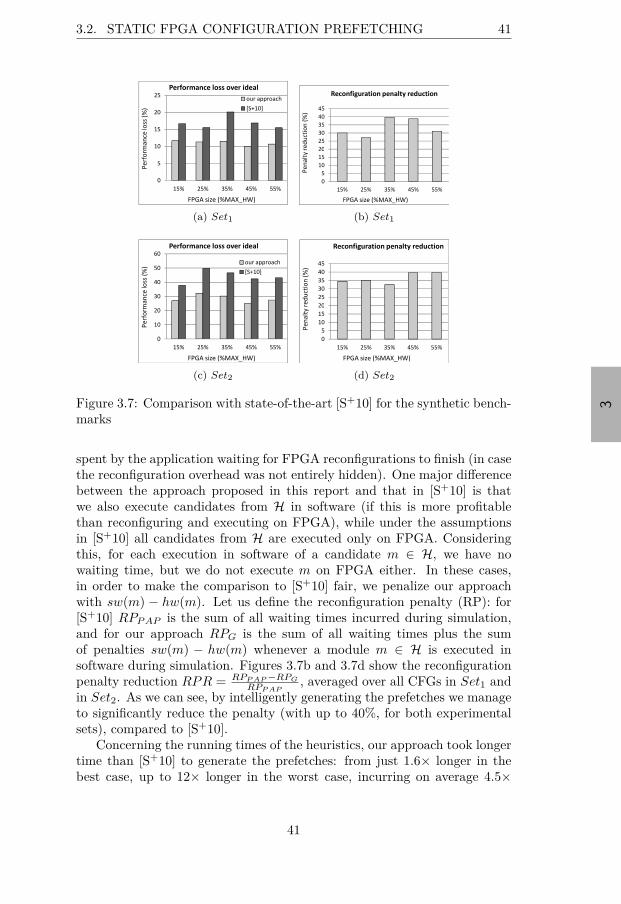
“thesis” — 2015/8/12 — 12:54 — page 41 — #61

3


S+10

!"#$

(a) Set1

!

(b) Set1

S+10

!"#$%

(c) Set2

!

(d) Set2

Figure 3.7: Comparison with state-of-the-art [S+10] for the synthetic bench-marks

spent by the application waiting for FPGA reconfigurations to finish (in casethe reconfiguration overhead was not entirely hidden). One major differencebetween the approach proposed in this report and that in [S+10] is thatwe also execute candidates from H in software (if this is more profitablethan reconfiguring and executing on FPGA), while under the assumptionsin [S+10] all candidates from H are executed only on FPGA. Consideringthis, for each execution in software of a candidate m ∈ H, we have nowaiting time, but we do not execute m on FPGA either. In these cases,in order to make the comparison to [S+10] fair, we penalize our approachwith sw(m) − hw(m). Let us define the reconfiguration penalty (RP): for[S+10] RPP AP is the sum of all waiting times incurred during simulation,and for our approach RPG is the sum of all waiting times plus the sumof penalties sw(m) − hw(m) whenever a module m ∈ H is executed insoftware during simulation. Figures 3.7b and 3.7d show the reconfigurationpenalty reduction RPR = RPP AP −RPG

RPP AP, averaged over all CFGs in Set1 and

in Set2. As we can see, by intelligently generating the prefetches we manageto significantly reduce the penalty (with up to 40%, for both experimentalsets), compared to [S+10].

Concerning the running times of the heuristics, our approach took longertime than [S+10] to generate the prefetches: from just 1.6× longer in thebest case, up to 12× longer in the worst case, incurring on average 4.5×

41

“thesis” — 2015/8/12 — 12:54 — page 42 — #62

3


more optimization time. For example, for the 15% FPGA fraction, for thebiggest CFG in Set2 (with 268 nodes), the running time of our approachwas 3832 seconds, compared to 813 seconds for [S+10]; for CFGs with asmaller size and a less complex structure we generated a solution in as lowas 6 seconds (vs 2 seconds for [S+10]).

3.2.4.3 Case Study – GSM Encoder

We also tested our approach on a GSM encoder, which implements the Euro-pean GSM 06.10 provisional standard for full-rate speech transcoding. Thisapplication can be decomposed into 10 functions executed in a sequentialorder: Init, GetAudioInput, Preprocess, LPC_Analysis, ShortTermAnaly-sisFilter, LongTermPredictor, RPE_Encoding, Add, Encode, Output. Theexecution times were derived using the MPARM cycle accurate simulator,considering an ARM processor with an operational frequency of 60 MHz.We have identified through profiling the most computation intensive partsof the application, and then these parts were synthesized as hardware mod-ules for an XC6VLX240T Virtex6 device, using the Xilinx ISE design suite.The resulting overall CFG of the application contains 30 nodes. The re-configuration times were estimated considering a 100 MHz configurationclock frequency and the ICAP 32-bit width configuration interface (see ourreconfiguration controller described in Section 3.1.1.2).

The CFG for the GSM Encoder, as well as the profiling information, wasgenerated using the LLVM suite [LA04] as follows: l lvm-gcc was first usedto generate LLVM bytecode from the C files. The opt tool was then usedto instrument the bytecode with edge and basic block profiling instructions.The bytecode was next run using l li, and then the execution profile wasgenerated using l lvm-prof. Finally, opt-analyze was used to print the CFGsto .dot files. Profiling was run considering several audio files (.au) as input.

Figure 3.8a shows the detailed control flow graph (CFG) for our GSMencoder case study. Nodes are labeled with their ID, their execution time(for example, for node with id = 1, the execution time is 10 time units)and their type: root, sink, control nodes, loop header nodes, basic nodesand hardware candidates (denoted with HW and represented with shadedboxes). We have used two scenarios: one considering 5 nodes as hardwarecandidates (namely modules with IDs 6, 9, 12, 15 and 22), and anotherscenario considering 9 nodes as hardware candidates (depicted in Figure3.8a).

We have used the same methodology as for the synthetic examples andcompared the results using the same metrics defined above in Section 3.2.4.2,i.e. performance loss over ideal and reconfiguration penalty reduction (pre-sented in Figure 3.9). As can be seen, for the scenario with 5 candidatemodules, the performance loss over ideal is between 10.5% and 14.8% forour approach, while for [S+10] it is between 25.5% and 32.9% (Figure 3.9a).Thus, we were from 50% up to 65% closer to the ideal baseline than [S+10].The reconfiguration penalty reduction obtained is as high as 58.9% (Figure

42

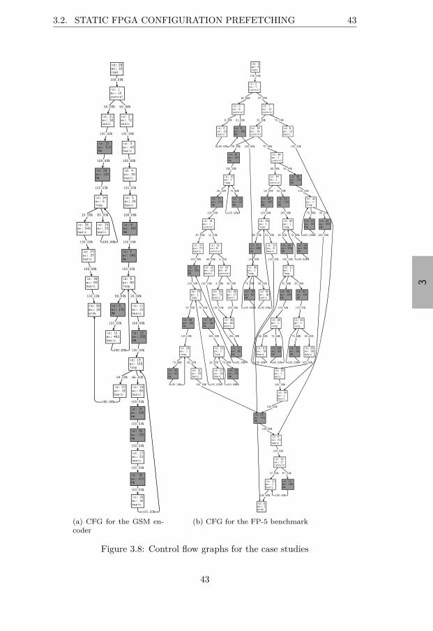
“thesis” — 2015/8/12 — 12:54 — page 43 — #63

3


(a) CFG for the GSM en-coder

(b) CFG for the FP-5 benchmark

Figure 3.8: Control flow graphs for the case studies

43

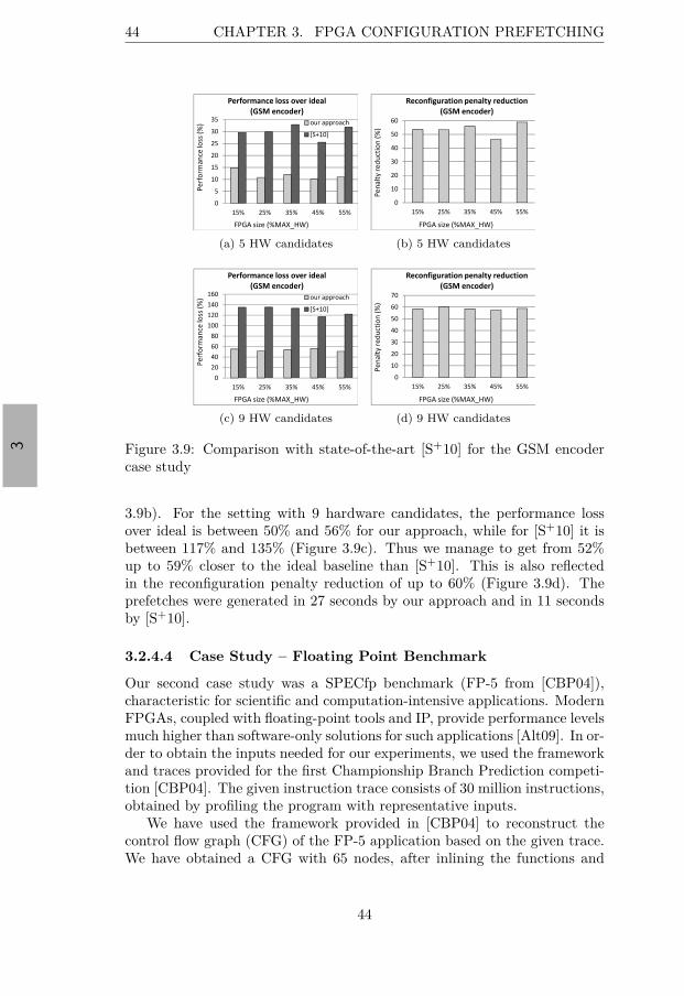
“thesis” — 2015/8/12 — 12:54 — page 44 — #64

3


S+10

!"#$

(a) 5 HW candidates

!"

(b) 5 HW candidates

S+10

!"#$%&

(c) 9 HW candidates

!"#

(d) 9 HW candidates

Figure 3.9: Comparison with state-of-the-art [S+10] for the GSM encodercase study

3.9b). For the setting with 9 hardware candidates, the performance lossover ideal is between 50% and 56% for our approach, while for [S+10] it isbetween 117% and 135% (Figure 3.9c). Thus we manage to get from 52%up to 59% closer to the ideal baseline than [S+10]. This is also reflectedin the reconfiguration penalty reduction of up to 60% (Figure 3.9d). Theprefetches were generated in 27 seconds by our approach and in 11 secondsby [S+10].

3.2.4.4 Case Study – Floating Point Benchmark

Our second case study was a SPECfp benchmark (FP-5 from [CBP04]),characteristic for scientific and computation-intensive applications. ModernFPGAs, coupled with floating-point tools and IP, provide performance levelsmuch higher than software-only solutions for such applications [Alt09]. In or-der to obtain the inputs needed for our experiments, we used the frameworkand traces provided for the first Championship Branch Prediction competi-tion [CBP04]. The given instruction trace consists of 30 million instructions,obtained by profiling the program with representative inputs.

We have used the framework provided in [CBP04] to reconstruct thecontrol flow graph (CFG) of the FP-5 application based on the given trace.We have obtained a CFG with 65 nodes, after inlining the functions and

44

“thesis” — 2015/8/12 — 12:54 — page 45 — #65

3


S+10

!"#$%&

(a) 9 HW candidates

!

(b) 9 HW candidates

S+10

!"#$

(c) 25 HW candidates

!

(d) 25 HW candidates

Figure 3.10: Comparison with state-of-the-art [S+10] for the floating pointbenchmark case study

pruning all control flow edges with a probability lower than 10−5. Then weused the traces to identify the parts of the CFG that have a high executiontime (mainly loops).

Figure 3.8b shows the detailed control flow graph (CFG) for our sec-ond case study: the floating point benchmark from SPECfp. Nodes arerepresented as discussed in Section 3.2.4.3. The software execution timesfor the basic blocks were obtained by considering the following cycles perinstruction (CPI) values for each instruction: for calls, returns and floatingpoint instructions CPI = 3, for load, store and branch instructions CPI =2, and for other instructions CPI = 1. Similar to the previous experimentalsections, we considered the hardware execution time β times smaller thanthe software one, where β was chosen from the uniform distribution on theinterval [3, 7].

We have used two scenarios: one considering as hardware candidates thetop 9 nodes with the highest software execution times (namely modules withIDs 5, 11, 17, 21, 22, 32, 42, 45 and 56), and another scenario consideringthe top 25 nodes (depicted in Figure 3.8b). Following the same methodologyas described in Section 3.2.4.2, we compared our approach with [S+10]. Theresults are presented in Figure 3.10. For example, for the scenario with 9candidate modules, the performance loss over ideal is between 77% and 90%for our approach, while for [S+10] it is between 107% and 118% (Figure

45

“thesis” — 2015/8/12 — 12:54 — page 46 — #66

3


3.10a). Thus, we are from 20% up to 28% closer to the ideal baseline than[S+10]. The reconfiguration penalty reduction is as high as 28% (Figure3.10b). For the setting with 25 hardware candidates the reconfigurationpenalty reduction increases, up to 31.1% (Figure 3.10d). As we can see, forboth case studies our approach produces significant improvements comparedto the state-of-the-art. The prefetches for FP-5 were generated in 53 secondsby our approach and in 32 seconds by [S+10].

3.3 Dynamic FPGA Configuration Prefetch-ing

As we have shown above, static configuration prefetching algorithms cansignificantly improve the performance of an application. Unfortunately, theysuffer from one important limitation: in case of non-stationary behavior theyare unable to adapt since the prefetch schedule is fixed based on averageprofiling information. In such cases a dynamic configuration prefetchingtechnique is desirable, as the one that we will present in this chapter.

We assume that the application exhibits a non-stationary branch be-havior. More exactly, we consider that the application passes through anunpredictable number of stationary phases [SSC03]. Branch probabilitiesand correlations are stable in one phase and then change to another stablephase, in a manner unpredictable at design-time. This model can be appliedto a large class of applications [SBSH12].


Given an application (as described in Section 3.1.3) intended to run onthe reconfigurable architecture described in Section 3.1.1, our goal is todetermine dynamically, at run-time, at each node m ∈ H, the prefetchesto be issued such that the expected execution time of the application isminimized.


Figure 3.11 illustrates two of the stationary phases, each one with a differentbranch behavior, among those exhibited by an application. Hardware can-didates are represented with squares (i.e. H = M0, M1, M2, M3, M4),and software-only nodes with circles (i.e. B0, B1, B2, B3, n0, n1, n2, n3,n4, n5, n6). For each phase, the edge probabilities of interest are illus-trated on the graph, and they remain unchanged for that phase. We repre-sent branch correlations with different line patterns: in phase 1, conditionalbranch B0 is positively correlated with B2 and B1 is positively correlatedwith B3; in phase 2, B0 and B2, as well as B1 and B3, become negativelycorrelated and the probabilities of B0 and B2 also change, from 50%-50%

46

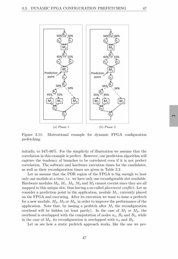
“thesis” — 2015/8/12 — 12:54 — page 47 — #67

3

3.3. DYNAMIC FPGA CONFIGURATION PREFETCHING 47

(a) Phase 1

(b) Phase 2

Figure 3.11: Motivational example for dynamic FPGA configurationprefetching

initially, to 34%-66%. For the simplicity of illustration we assume that thecorrelation in this example is perfect. However, our prediction algorithm willcapture the tendency of branches to be correlated even if it is not perfectcorrelation. The software and hardware execution times for the candidates,as well as their reconfiguration times are given in Table 3.2.

Let us assume that the PDR region of the FPGA is big enough to hostonly one module at a time, i.e. we have only one reconfigurable slot available.Hardware modules M0, M1, M2, M3 and M4 cannot coexist since they are allmapped to this unique slot, thus having a so-called placement conflict. Let usconsider a prediction point in the application, module M1, currently placedon the FPGA and executing. After its execution we want to issue a prefetchfor a new module, M2, M3 or M4, in order to improve the performance of theapplication. Note that, by issuing a prefetch after M1 the reconfigurationoverhead will be hidden (at least partly). In the case of M2 or M3, theoverhead is overlapped with the computation of nodes n4, B2 and B3, whilein the case of M4, its reconfiguration is overlapped with n4 and B2.

Let us see how a static prefetch approach works, like the one we pre-

47

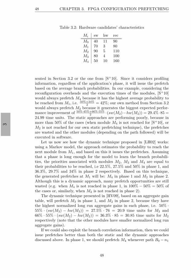
“thesis” — 2015/8/12 — 12:54 — page 48 — #68

3


Table 3.2: Hardware candidates’ characteristics

Mi sw hw rec

M0 40 11 90M1 70 3 80M2 90 5 110M3 80 4 100M4 50 10 160

sented in Section 3.2 or the one from [S+10]. Since it considers profilinginformation, regardless of the application’s phase, it will issue the prefetchbased on the average branch probabilities. In our example, considering thereconfiguration overheads and the execution times of the modules, [S+10]would always prefetch M4 because it has the highest average probability tobe reached from M1, i.e. 50%+34%

2 = 42%; our own method from Section 3.2would always prefetch M2 because it generates the biggest expected perfor-mance improvement of 50%·45%+66%·55%

2 ·(sw(M2)−hw(M2)) = 29.4% ·85 =24.99 time units. The static approaches are performing poorly, because inmore than 50% of the cases (when module M4 is not reached for [S+10], orM2 is not reached for our own static prefetching technique), the prefetchesare wasted and the other modules (depending on the path followed) will beexecuted in software.

Let us now see how the dynamic technique proposed in [LH02] works:using a Markov model, the approach estimates the probability to reach thenext module from M1, and based on this it issues the prefetches. Assumingthat a phase is long enough for the model to learn the branch probabili-ties, the priorities associated with modules M2, M3 and M4 are equal totheir probabilities to be reached, i.e 22.5%, 27.5% and 50% in phase 1, and36.3%, 29.7% and 34% in phase 2 respectively. Based on this technique,the generated prefetches at M1 will be: M4 in phase 1 and M2 in phase 2.Although this is a dynamic approach, many prefetch opportunities are stillwasted (e.g. when M4 is not reached in phase 1, in 100% − 50% = 50% ofthe cases or, similarly, when M2 is not reached in phase 2).

The dynamic technique presented in [HV09], based on an aggregate gaintable, will prefetch M3 in phase 1, and M2 in phase 2, because they havethe highest normalized long run aggregate gains in each phase, i.e. 50% ·55% · (sw(M3) − hw(M3)) = 27.5% · 76 = 20.9 time units for M3 and66% · 55% · (sw(M2) − hw(M2)) = 36.3% · 85 = 30.85 time units for M2

respectively (note that the other modules have smaller normalized long runaggregate gains).

If we could also exploit the branch correlation information, then we couldissue prefetches better than both the static and the dynamic approachesdiscussed above. In phase 1, we should prefetch M4 whenever path B0 − n1

48

“thesis” — 2015/8/12 — 12:54 — page 49 — #69

3


is followed (because of the positive correlation of B0 with B2), M2 wheneverpath B0 − n0 : B1 − n2 is followed and M3 whenever path B0 − n0 : B1 − n3

is followed (for similar considerations). Similar reasoning can be used forphase 2.

The big limitation of static prefetching is its lack of robustness andflexibility: the prefetches are fixed based on average profiling informationand they cannot adapt to the run-time conditions. For our example, thestatic approaches always prefetch M4, which is a very restrictive decision.Although the dynamic approaches provide extra flexibility, they still missprefetch opportunities. One limitation exhibited by [LH02] and [HV09] isthat the approaches rely only on the hardware modules’ history and do notexploit the path information (like branch outcomes together with their cor-relations). As a result, for [LH02] and [HV09], the prefetch opportunitiesare wasted in more than 50% of the cases. We will present an approach thattries to overcome the mentioned limitations.

3.3.3 Dynamic Prefetching

We next describe a piecewise linear prediction algorithm used for FPGAconfiguration prefetching and its hardware organization. The main idea isto assign priorities to all the hardware candidates and then issue prefetchesbased on them, at certain points in the application (a natural choice for theprefetch points is after the execution of a candidate m ∈ H).

3.3.3.1 The Piecewise Linear Predictor

The concept of piecewise linear prediction was successfully applied in thecontext of branch prediction [Jim05] and it is based on the idea to use thehistory of a branch in order to predict its outcome (taken or not taken).We extend the concept for the case of FPGA configuration prefetching. Weassociate one piecewise linear predictor with each hardware candidate andtry to capture the correlation between a certain branch history leading to acertain prediction point, and a candidate being reached in the future. Thebranch history for a prefetch point m ∈ H is represented by the dynamic se-quence of conditional branches (program path) leading to m. The predictorkeeps track of the positive or negative correlation of the outcome of everybranch in the history with the predicted hardware candidate being reachedor not.

The output of a predictor (associated with a hardware candidate) isa single number, obtained by aggregating the correlations of all branchesin the current history, using a linear function (Predict in Algorithm 4).This function induces a hyperplane in the space of all outcomes for thecurrent branch history, used to estimate what is the likelihood to reach thehardware candidate in discussion. We interpret the output y of the predictoras the probability to reach the candidate, since the distance of y from thehyperplane (on the positive side) is proportional to the degree of certainty

49

“thesis” — 2015/8/12 — 12:54 — page 50 — #70

3


M4 0 1

B0

B1

B2

B3

M3 0 1

B1 w11 w12

B2 w21 w22

B3 w31 w32

B4 w w

M2 0 1

B1 w11 w12

B2 w21 w22

B3 w31 w32

M1 0 1

B1 w11 w12

B2 w21 w22

M0 0 1

B0

0

000

01

This dimension in the 3D array

represents the position on which a

particular branch occurs in the

branch address history register A.

For example, if at some point in

time, A = [B2 B3], when making a

prediction for M0 the prediction

function (described in the nextB4 w41 w42B3 w31 w32

B4 w41 w42

21 22

B3 w31 w32

B4 w41 w42

B1

B2

B3

00

0

10

0

20

0

30

01

0

11

0

21

0

31

function (described in the next

section) would use the entries

.20

(because B2

is on position 0

in A) and31

(because B3

is on

position 1 in A) from the 3D array.

0

0

Figure 3.12: The 3D weight array (Ω) of the predictor

that the candidate will be reached. Considering that there are many pathsleading to a prediction point m ∈ H, there are also many linear functionsused for prediction. Together, they form a piecewise linear surface thatseparates the paths for which the hardware candidate will be reached in thefuture, from those paths for which it will not be reached.

Data Structures

The predictor uses the following data structures:

• A – the branch address history register. At run-time, when a condi-tional branch is executed, its address is shifted into the first positionof this register.

• H – the branch outcome history register, containing the taken ornot taken outcomes for branches. As for the address register, theoutcomes are shifted into the first position. Together, A and H char-acterize the path history.

• h – the length4 of both the history registers A and H.

• HW – the hardware history register, containing the last q hardwarecandidates reached.

• q – the length4 of the hardware history register HW .

• Ω – a 3D array of weights (shown in Figure 3.12 for the example fromFigure 3.11, with five hardware candidates, M0 to M4). The indexesare: the ID of a hardware candidate, the ID of a branch and its position(index) in the path history. We can view Ω as a collection of matrices,one for each hardware candidate. The entries in Ω keep track of the

4The values of h and q reflect the trade-off between the space budget available for thepredictor and its accuracy. We obtained good experimental results for relatively smallvalues: h ∈ [4, 16] and q ∈ [2, 8].

50

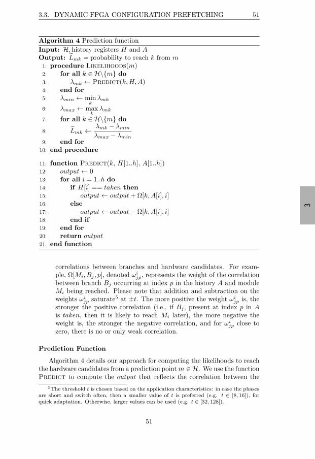
“thesis” — 2015/8/12 — 12:54 — page 51 — #71

3


Algorithm 4 Prediction functionInput: H, history registers H and AOutput: Lmk = probability to reach k from m

1: procedure Likelihoods(m)2: for all k ∈ H\m do

3: λmk ← Predict(k, H, A)4: end for

5: λmin ← mink

λmk

6: λmax ← maxk

λmk

7: for all k ∈ H\m do

8: Lmk ← λmk − λmin

λmax − λmin9: end for

10: end procedure

11: function Predict(k, H[1..h], A[1..h])12: output ← 013: for all i = 1..h do

14: if H[i] == taken then

15: output ← output + Ω[k, A[i], i]16: else

17: output ← output − Ω[k, A[i], i]18: end if

19: end for

20: return output21: end function

correlations between branches and hardware candidates. For exam-ple, Ω[Mi, Bj , p], denoted ωi

jp, represents the weight of the correlationbetween branch Bj occurring at index p in the history A and moduleMi being reached. Please note that addition and subtraction on theweights ωi

jp saturate5 at ±t. The more positive the weight ωijp is, the

stronger the positive correlation (i.e., if Bj , present at index p in Ais taken, then it is likely to reach Mi later), the more negative theweight is, the stronger the negative correlation, and for ωi

jp close tozero, there is no or only weak correlation.

Prediction Function

Algorithm 4 details our approach for computing the likelihoods to reachthe hardware candidates from a prediction point m ∈ H. We use the functionPredict to compute the output that reflects the correlation between the

5The threshold t is chosen based on the application characteristics: in case the phasesare short and switch often, then a smaller value of t is preferred (e.g. t ∈ [8, 16]), forquick adaptation. Otherwise, larger values can be used (e.g. t ∈ [32, 128]).

51

“thesis” — 2015/8/12 — 12:54 — page 52 — #72

3


branch history leading to module m and candidate k being reached in thefuture. For all the entries in the current history (line 13), if the branch onposition i was taken then we add to the output the weight Ω[k, A[i], i] (line15); otherwise we subtract it (line 17). Once the outputs were calculatedfor all candidates (lines 2-4), we normalize the results (line 8). The resultLmk ∈ [0, 1] represents the estimated likelihood to reach hardware candidatek from prefetch point m, and will be used in computing the prefetch priorityfunction (see Section 3.3.3.3). Consider the example in Figure 3.11, withA = [B0 B1] and H = [taken taken] at prediction point M1. Then, inphase 1, the estimated probability to reach M2 is LM1M2

= 100% and theprobabilities to reach M3 or M4 are LM1M3

= LM1M4= 0. This is because

the predictor weights are ω200 = ω2

11 = +t and ω300 = ω3

11 = ω400 = ω4

11 = −t(where t is the saturation threshold).

Lazy Update Function

After making a prediction, we need to train the predictor based on thereal outcome (i.e. which modules were actually reached). Since this infor-mation becomes available only later, we opted for a lazy update: we save thecontext (history registers A and H) based on which the current predictionis made, and we update the predictor as late as possible, i.e. only when thesame prediction point is reached again, and before making a new prediction.The next q candidates that will be reached after the prediction point areaccumulated in the hardware history register HW .

Algorithm 5 presents our lazy update. It takes as parameters the modulem where the update is done, the saved branch outcome register (Hm

S ), thesaved branch address register (Am

S ) and the saved hardware history register(HW m

R ), containing the first q hardware modules executed after the predic-tion point m. The path information was saved when the last prediction wasmade at m, and the register HW was saved when the qth module after mwas reached and m was evicted from the HW register. For all history posi-tions (line 2), for all the q modules reached after m (line 3), we update thecorresponding weights in Ω (saturating at ±t), depending on the outcomeof the branch on position i: if the branch was taken, then we increment thecorresponding weight (line 5); otherwise we decrement it (line 7). For all themodules not reached after m we do the opposite: decrement the weights inΩ for taken branches, and increment them for not taken ones (lines 10-16).

Next, we save the current path that has led to m (lines 18-19). Then wepop the qth hardware module (top) from the history register HW (line 20)and we push the current module m on the first position of HW , but onlyif m is not already there (line 21). If m is executed in a loop, we want toavoid having repetitions in the HW history register; instead of pushing m,we only update its timestamp, used for computing the potential executiontime gain (see Section 3.3.3.2). Finally we save the hardware history registercontaining the q modules executed after top (line 24).

52

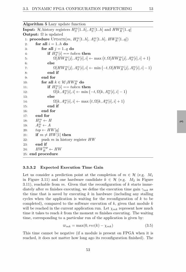
“thesis” — 2015/8/12 — 12:54 — page 53 — #73

3


Algorithm 5 Lazy update functionInput: H, history registers Hm

S [1..h], AmS [1..h] and HW m

R [1..q]Output: Ω is updated

1: procedure Update(m, HmS [1..h], Am

S [1..h], HW mR [1..q])

2: for all i = 1..h do

3: for all j = 1..q do

4: if HmS [i] == taken then

5: Ω[HW mR [j], Am

S [i], i] ← max(t, Ω[HW m

R [j], AmS [i], i] + 1

)

6: else

7: Ω[HW mR [j], Am

S [i], i] ← min(−t, Ω[HW m

R [j], AmS [i], i] − 1

)

8: end if

9: end for

10: for all k ∈ H\HW mR do

11: if HmS [i] == taken then

12: Ω[k, AmS [i], i] ← min

(−t, Ω[k, Am

S [i], i] − 1)

13: else

14: Ω[k, AmS [i], i] ← max

(t, Ω[k, Am

S [i], i] + 1)

15: end if

16: end for

17: end for

18: HmS ← H

19: AmS ← A

20: top ← HW [q]21: if m Ó= HW [1] then

22: push m in history register HW23: end if

24: HW topR ← HW

25: end procedure

3.3.3.2 Expected Execution Time Gain

Let us consider a prediction point at the completion of m ∈ H (e.g. M1

in Figure 3.11) and one hardware candidate k ∈ H (e.g. M2 in Figure3.11), reachable from m. Given that the reconfiguration of k starts imme-diately after m finishes executing, we define the execution time gain γmk asthe time that is saved by executing k in hardware (including any stallingcycles when the application is waiting for the reconfiguration of k to becompleted), compared to the software execution of k, given that module kwill be reached in the current application run. Let χmk represent how muchtime it takes to reach k from the moment m finishes executing. The waitingtime, corresponding to a particular run of the application is given by:

mk = max(0, rec(k) − χmk) (3.5)

This time cannot be negative (if a module is present on FPGA when it isreached, it does not matter how long ago its reconfiguration finished). The

53

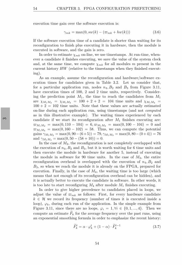
“thesis” — 2015/8/12 — 12:54 — page 54 — #74

3


execution time gain over the software execution is:

γmk = max(0, sw(k) − (mk + hw(k))) (3.6)

If the software execution time of a candidate is shorter than waiting for itsreconfiguration to finish plus executing it in hardware, then the module isexecuted in software, and the gain is zero.

In order to estimate χmk on-line, we use timestamps. At run-time, when-ever a candidate k finishes executing, we save the value of the system clockand, at the same time, we compute χmk for all modules m present in thecurrent history HW (relative to the timestamps when they finished execut-ing).

As an example, assume the reconfiguration and hardware/software ex-ecution times for candidates given in Table 3.2. Let us consider that,for a particular application run, nodes n4, B2 and B3 from Figure 3.11,have execution times of 100, 2 and 2 time units, respectively. Consider-ing the prediction point M1, the time to reach the candidates from M1

are χM1M2= χM1M3

= 100 + 2 + 2 = 104 time units and χM1M4=

100 + 2 = 102 time units. Note that these values are actually estimatedon-line during each application run, using timestamps (and not computedas in this illustrative example). The waiting times experienced by eachcandidate if we start its reconfiguration after M1 finishes executing are:M1M2

= max(0, 110 − 104) = 6, M1M3= max(0, 100 − 104) = 0 and

M1M4= max(0, 160 − 102) = 58. Thus, we can compute the potential

gains γM1M2= max(0, 90− (6+5)) = 79, γM1M3

= max(0, 80− (0+4)) = 76and γM1M4

= max(0, 50 − (58 + 10)) = 0.In the case of M2, the reconfiguration is not completely overlapped with

the execution of n4, B2 and B3, but it is worth waiting for 6 time units andthen execute the module in hardware for another 5, instead of executingthe module in software for 90 time units. In the case of M3, the entirereconfiguration overhead is overlapped with the execution of n4, B2 andB3, so when we reach the module it is already on the FPGA, prepared forexecution. Finally, in the case of M4, the waiting time is too large (whichmeans that not enough of its reconfiguration overhead can be hidden), andit is actually better to execute the candidate in software. In other words, itis too late to start reconfiguring M4 after module M1 finishes executing.

In order to give higher precedence to candidates placed in loops, weadjust the value of mk as follows: First, for every hardware candidatek ∈ H we record its frequency (number of times it is executed inside aloop), ϕk, during each run of the application. In the simple example fromFigure 3.11, since there are no loops, ϕi = 1, ∀i ∈ 0, 1, ..., 4. Then wecompute an estimate Fk for the average frequency over the past runs, usingan exponential smoothing formula in order to emphasize the recent history:

F tk = α · ϕt

k + (1 − α) · F t−1k (3.7)

54

“thesis” — 2015/8/12 — 12:54 — page 55 — #75

3


In equation 3.7, F tk represents the estimate at time t of the expected fre-

quency for module k, F t−1k represents the previous estimate, ϕt

k representsk’s frequency in the current application run and α is the smoothing param-eter. Given Fk, we adjust the waiting time ˜ mk = mk

Fk

, and consequently

the adjusted gain is:

γmk = max(0, sw(k) − ( ˜ mk + hw(k))) (3.8)

This adjustment is done because, for modules in loops, even if the recon-figuration is not finished in the first few loop iterations and we execute themodule in software first, we will gain from executing the module in hardwarein future loop iterations. Note that for the simple illustrative example fromFigure 3.11, since ϕi = 1, ∀i ∈ 0, 1, ..., 4, we have γmk = γmk, ∀m, k ∈ H.

We are interested to estimate the potential performance gain γmk overseveral application runs. We denote this estimate Gmk, and we use anexponential smoothing formula (similar to equation 3.7) to compute it, em-phasizing recent history:

Gtmk = α · γt

mk + (1 − α) · Gt−1mk (3.9)

In equation 3.9, Gtmk represents the estimate at time t of the potential gain

obtained if we start reconfiguring module k immediately after m finishes ex-ecuting, Gt−1

mk represents the previous estimate, γtmk represents the adjusted

gain computed considering the current application run and α is the smooth-ing parameter. The speed at which older observations are dampened is afunction of α, which can be adjusted to reflect the application characteris-tics: if the stationary phases are short, then α should be larger (for quickdampening and fast adaptation); if the phases are long, then α should besmaller.

3.3.3.3 Prefetch Priority Function

At each node m ∈ H we assign priorities to all the hardware candidatesin Km = k ∈ H|Lmk > 0, thus deciding a prefetch order for all thecandidates reachable from m with nonzero likelihood (the computation ofLmk is described in Algorithm 4). Our priority function estimates the overallimpact on the average execution time that results from different prefetchesbeing issued after module m finishes executing. Three factors are considered:

1. The estimated likelihood Lmk to reach a candidate k ∈ Km from m,obtained from the piecewise linear prediction algorithm (see Section3.3.3.1);

2. The estimated performance gain Gmk resulting if k is prefetched at m(see Section 3.3.3.2);

55

“thesis” — 2015/8/12 — 12:54 — page 56 — #76

3


3. The estimated frequencies for candidates, Fk (see equation 3.7), usedto give higher precedence to modules executed many times inside aloop:

Γmk = Lmk(1 + log2 Fk)Gmk +

+∑

h∈Km\k

Lmh(1 + log2 Fh)Gkh(3.10)

The first term in equation 3.10 represents the contribution (in terms of ex-ecution time gain) of module k: the larger the probability to reach it fromm (Lmk), the higher its estimated frequency (Fk) and the bigger the perfor-mance gain (Gmk) it generates if its reconfiguration is started immediatelyafter m finishes executing, the better. Note that the potential executiontime gain of module k (Gmk) is weighted with the estimated probability toreach it (Lmk) in the current application run. The second term capturesthe impact that k’s reconfiguration will produce on other modules compet-ing with it for the reconfiguration controller. For all these other reachablemodules (h ∈ Km\k), we look at the gain (Gkh) obtained if we will re-configure them only after k has finished executing. If for example, k andh are mutually exclusive, then Gkh = 0. Otherwise, if Gkh Ó= 0, it meansthat we can afford to start the reconfiguration of h after k and, thus, byreconfiguring k first we still have potential gain generated by h.

Let us compare Γmk from equation 3.10 (used for dynamic configura-tion prefetching) with Cnm from equation 3.1 (used for static configurationprefetching). Lmk is the analogue of PAP (n, m) and reflects the probabil-ity to reach the hardware module in discussion from the current predictionpoint. Gmk is the analogue of Gnm and represents the execution time gaingenerated by the hardware module in discussion if we prefetch it at thecurrent prediction point. Note that the frequency with which module k isexecuted, Fk, is taken into consideration in the case of dynamic configu-ration prefetching, as a way to improve over the priority function used forstatic configuration prefetching. Another difference between the two prior-ity functions is that, in the case of dynamic prefetching (equation 3.10), itdoes not make sense to discriminate the modules that are mutually exclusivewith the one in discussion. This is because in the dynamic prefetching casewe only issue prefetches after hardware candidates, not after every node inthe control flow graph (as in the static prefetching case). To summarize, thefirst term in equation 3.10 is analogue to the first term in equation 3.1, andthe second term in 3.10 is analogue to the second and third terms in 3.1.

Let us consider the example from Figure 3.11, and the prediction pointimmediately after M0 finishes executing. In this case, we have 4 reachablecandidates, M1 to M4, and we want to start the reconfiguration of one ofthem. Assume the reconfiguration and execution times for candidates givenin Table 3.2; nodes B1, n2 and n3 have execution times of 2, 100 and 100time units, respectively. For these values, the time to reach M1 from M0 is

56

“thesis” — 2015/8/12 — 12:54 — page 57 — #77

3


χM0M1= 2+100 = 102 time units, the waiting time experienced by M1 if we

start its reconfiguration immediately after M0 finishes executing is M0M1=

max(0, 80 − 102) = 0 and the gain γM0M1= max(0, 70 − (0 + 3)) = 67 time

units. The potential gains for M2, M3 and M4, as computed in Section3.3.3.2, are γM1M2

= 79, γM1M3= 76 and γM1M4

= 0 (similarly, we cancompute all the other needed gains, γM0M2

= 85, γM0M3= 76, γM0M4

= 40and γM2M1

= γM2M3= γM2M4

= γM3M1= γM3M2

= γM3M4= γM4M1

=γM4M2

= γM4M3= 0).

Let us now consider phase 1 from Figure 3.11a, and assume that B0

was taken, i.e. n0 was executed. Under these assumptions, we have thefollowing probabilities to reach the four hardware candidates: LM0M1

=

100%, LM0M2= 45%, LM0M3

= 55% and LM0M4= 0. The priority functions

for the four candidates will be: ΓM0M1= 100% · 1 · 67 + 45% · 1 · 79 + 55% · 1 ·

76+0 ·1 ·0 = 144.35, ΓM0M2= 45% ·1 ·85+100% ·1 ·0+55% ·1 ·0+0 ·1 ·0 =

38.25, ΓM0M3= 55% · 1 · 76 + 100% · 1 · 0 + 45% · 1 · 0 + 0 · 1 · 0 = 41.8 and

ΓM0M4= 0 · 1 · 40 + 100% · 1 · 0 + 45% · 1 · 0 + 55% · 1 · 0 = 0 time units.

Thus, we can see that the highest execution time gain is obtained if we startreconfiguring M1 after M0, because once M1 will finish executing, we canreplace it with one of the other candidates, and we gain by executing bothM1 and the other module in hardware. In contrast, reconfiguring M2 orM3 after M0 will make sure that their gain is obtained, but it will preventobtaining any gain from the execution of M1, which will be in software.

3.3.3.4 Run-Time Strategy

Algorithm 6 presents our overall run-time strategy for configuration prefetch-ing. Once a module m ∈ H is reached, we increment its frequency counter(line 2) that will be used later to update the frequency estimates with equa-tion 3.7. Next we perform the update of the piecewise linear predictor (line3). We use the path history (registers Hm

S and AmS ) saved when the last

prediction was made at m, and the q candidates reached after m, saved inHW m

R . After the update, we save the current path history (to be used atthe next update), as described in Algorithm 5. Next we compute the likeli-hoods to reach other candidates from m (line 4), as illustrated in Algorithm4. Then, for all candidates reachable with nonzero likelihood (line 5), wecompute the priority Γmk (line 6) with equation 3.10. Once all Γmk havebeen computed, we find the candidate from Km = k ∈ H|Lmk > 0 withthe highest priority (line 7), giving precedence to modules placed in loopsin case of equality. If the top candidate found is already fully configuredon the FPGA, it will be reused and there is no need to reconfigure it. Inthis case, we find the candidate with the next highest priority that does nothave a placement conflict (i.e. it is not mapped to the same reconfigurableslot) with the higher priority module (because we do not want to replace it

57

“thesis” — 2015/8/12 — 12:54 — page 58 — #78

3


Algorithm 6 Overall run-time strategy for prefetching1:candidate m is reached2: increment frequency counter ϕm

3: Update(m, HmS , Am

S , HW mR ) ⊲ Update

the predictor using the path history saved when the last prediction wasmade, and then save the current path history

4: Likelihoods(m) ⊲ Compute Lmk

5: Km ← k ∈ H|Lmk > 0 ⊲ Compute the set of candidates reachablefrom m with nonzero likelihood

6: compute priority function Γmk, ∀k ∈ Km, based on the current estimatesfor likelihoods (Lmk), frequencies (Fk) and performance gains (Gmk),using equation 3.10

7: pick the module with the highest priority Γmk that is not yet placed onthe FPGA

8: stop (pause) any ongoing reconfiguration9: start reconfiguring top candidate

The part above executes in parallel with the one below

10: if m fully loaded on FPGA then

11: execute m on FPGA12: else if remaining reconfiguration+hw(m) < sw(m) then

13: continue reconfiguration and execute m on FPGA14: else

15: execute m in SW16: end if

17: save timestamp of m⊲ Compute estimated gains based on m’s finishing time

18: for all k ∈ HW do ⊲ Candidates reached before m19: compute performance gain Gkm with equation 3.9, using the times-

tamps of k and m to get χkm, ˜ km and γkm 20: end for

on the FPGA). Finally, we pause6 any ongoing reconfiguration (line 8) andwe start prefetching the top candidate (line 9) identified (line 7).

The execution of the predictor update and the mechanism of generatingthe prefetches (described above) take place in parallel with the execution ofm. This observation, coupled with the facts that our algorithm has a worst-case complexity of O(|H| log |H|) and that part of it runs as a dedicatedhardware module (see Section 3.3.4), makes the on-line approach feasible.The execution of m is done in hardware or in software, depending on the run-time conditions: if m is already loaded then it can be executed on the FPGA(lines 10-11); if reconfiguring m and then executing it on the FPGA results

6Note that, if not overwritten, these modules might have their reconfiguration resumedlater.

58

“thesis” — 2015/8/12 — 12:54 — page 59 — #79

3


±

±

!"#$

%

&

%

&

!"#$

%

&

'

"

0

00

0

10

0

20

0

30

0

01

0

11

0

21

0

31

(a) Function PREDICT

±

±

0

00

0

10

0

20

0

30

0

01

0

11

0

21

0

31

±1±1

±1±1

±

(b) Function UPDATE

Figure 3.13: The internal architecture of the predictor

in a shorter delay than its software execution, then it is worth to wait for thereconfiguration to finish and then execute the module on the FPGA (lines12-13); if none of the above holds, then the candidate is executed in software(lines 14-15). Once the execution of m finishes, we save its timestamp andthen we compute the estimated performance gains Gkm for all the modulescurrently recorded in the hardware history register HW (lines 17-19). Afterthis, the execution of the application continues as normal.

3.3.4 Hardware Organization of the Predictor

This section will discuss the hardware organization of a HW/SW prototypeimplementation of the predictor described above, on a Xilinx ML605 board.Note that the part specific to the Xilinx architecture is minimal, referring

59

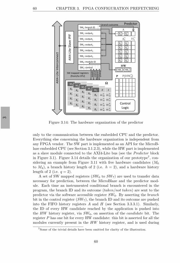
“thesis” — 2015/8/12 — 12:54 — page 60 — #80

3


!

"!

#"

#

$

%

&

Bx

By

Bx By

Bx By

Bx By

Bx By

Bx By

HWx HWy

'()*+,

*

0

00

0

10

0

20

0

30

0

01

0

11

0

21

0

31

Figure 3.14: The hardware organization of the predictor

only to the communication between the embedded CPU and the predictor.Everything else concerning the hardware organization is independent fromany FPGA vendor. The SW part is implemented as an API for the MicroB-laze embedded CPU (see Section 3.1.2.3), while the HW part is implementedas a slave module connected to the AXI4-Lite bus (see the Predictor blockin Figure 3.1). Figure 3.14 details the organization of our prototype7, con-sidering an example from Figure 3.11 with five hardware candidates (M0

to M4), a branch history length of 2 (i.e. h = 2), and a hardware historylength of 2 (i.e. q = 2).

A set of SW mapped registers (SW0 to SW7) are used to transfer datanecessary for prediction, between the MicroBlaze and the predictor mod-ule. Each time an instrumented conditional branch is encountered in theprogram, the branch ID and its outcome (taken/not taken) are sent to thepredictor via the software accessible register SW0. By asserting the branchbit in the control register (SW7), the branch ID and its outcome are pushedinto the FIFO history registers A and H (see Section 3.3.3.1). Similarly,the ID of every HW candidate reached by the application is pushed intothe HW history register, via SW6, on assertion of the candidate bit. Theregister P has one bit for every HW candidate: this bit is asserted for all themodules currently present in the HW history register, and is used during

7Some of the trivial details have been omitted for clarity of the illustration.

60

“thesis” — 2015/8/12 — 12:54 — page 61 — #81

3


the update of the predictor. Instead of explicitly saving all the IDs of thehardware modules reached after a prediction point, we save the register P .The Control Logic block takes care of generating the internal control signals.

The architecture presented here implements the functions Predict (fromAlgorithm 4) and Update (from Algorithm 5). For clarity, we will describethem separately, although they work with the same data structures (samecolors/shades are used in Figures 3.14, 3.13a and 3.13b to illustrate therelations between the three schematics). Figure 3.13a presents the internalorganization of the prediction function (exemplified for candidate M0). Notethat the address history register A currently contains the IDs of 2 branches,Bx and By. Each one of these is used to index into a table containing theweights (Ω), which are added or subtracted (depending on the content ofthe branch outcome history register H) to compute the prediction outputfor M0. Similarly, all the outputs are computed for all the hardware candi-dates, using the corresponding weights from Ω. The results are written tothe software accessible registers (SW1 to SW5), from where the MicroBlazecan read them.

Figure 3.13b illustrates the update functionality. Before proceeding, letus mention that, each time an update is made (after reaching a hardwarecandidate m), the registers A, H and P are saved in Am

S , HmS and P [HW top

R ](where top is the module at the top of the HW history register). Thesesaved values are used when we perform the lazy update (see Algorithm 5).Returning to Figure 3.13b, note that the weights in Ω are incremented fortaken branches, and decremented for not taken ones, if the correspondingmodule was reached (as indicated by P [HW m

R ]), and vice versa for notreached modules (note that we encode taken/not taken branches, as well asreached/not reached modules with ±1). As mentioned above, the controlsignals are generated by the Control Logic block in Figure 3.14, and, forclarity, are not depicted.

Given the hardware implementation of the predictor, all the updates toΩ, as well as the prediction, can be made in parallel, thus reducing the timeoverhead incurred, especially for big designs. This comes at the cost of asmall area overhead (see Table 3.1), which is justifiable given the perfor-mance improvement obtained in return.


3.3.5.1 Proof of Concept

We have implemented the entire framework described in Section 3.1.1 on aXilinx ML605 board, featuring an XC6VLX240T Virtex6 FPGA8. In orderto demonstrate the efficiency and practicality of the piecewise linear predic-tor we used a case study application: the SUSAN image processing [SB97].This algorithm was developed for recognizing corners and edges in MRIs of

8Note, however, that the framework could be instantiated on any other FPGA archi-tecture that supports PDR (e.g. [Alt12])

61

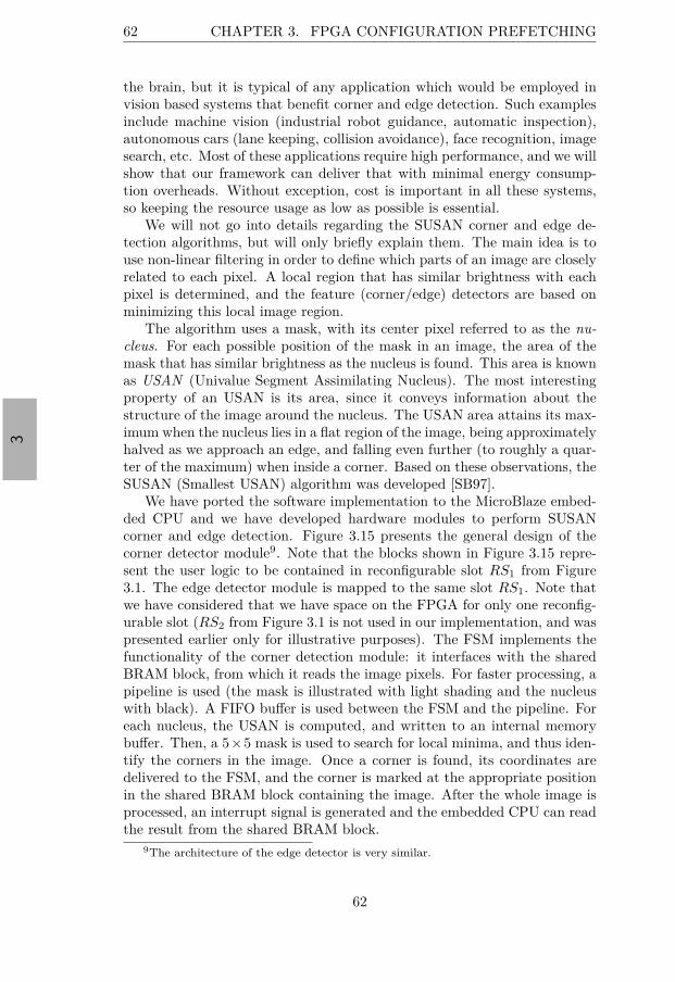
“thesis” — 2015/8/12 — 12:54 — page 62 — #82

3


the brain, but it is typical of any application which would be employed invision based systems that benefit corner and edge detection. Such examplesinclude machine vision (industrial robot guidance, automatic inspection),autonomous cars (lane keeping, collision avoidance), face recognition, imagesearch, etc. Most of these applications require high performance, and we willshow that our framework can deliver that with minimal energy consump-tion overheads. Without exception, cost is important in all these systems,so keeping the resource usage as low as possible is essential.

We will not go into details regarding the SUSAN corner and edge de-tection algorithms, but will only briefly explain them. The main idea is touse non-linear filtering in order to define which parts of an image are closelyrelated to each pixel. A local region that has similar brightness with eachpixel is determined, and the feature (corner/edge) detectors are based onminimizing this local image region.

The algorithm uses a mask, with its center pixel referred to as the nu-cleus. For each possible position of the mask in an image, the area of themask that has similar brightness as the nucleus is found. This area is knownas USAN (Univalue Segment Assimilating Nucleus). The most interestingproperty of an USAN is its area, since it conveys information about thestructure of the image around the nucleus. The USAN area attains its max-imum when the nucleus lies in a flat region of the image, being approximatelyhalved as we approach an edge, and falling even further (to roughly a quar-ter of the maximum) when inside a corner. Based on these observations, theSUSAN (Smallest USAN) algorithm was developed [SB97].

We have ported the software implementation to the MicroBlaze embed-ded CPU and we have developed hardware modules to perform SUSANcorner and edge detection. Figure 3.15 presents the general design of thecorner detector module9. Note that the blocks shown in Figure 3.15 repre-sent the user logic to be contained in reconfigurable slot RS1 from Figure3.1. The edge detector module is mapped to the same slot RS1. Note thatwe have considered that we have space on the FPGA for only one reconfig-urable slot (RS2 from Figure 3.1 is not used in our implementation, and waspresented earlier only for illustrative purposes). The FSM implements thefunctionality of the corner detection module: it interfaces with the sharedBRAM block, from which it reads the image pixels. For faster processing, apipeline is used (the mask is illustrated with light shading and the nucleuswith black). A FIFO buffer is used between the FSM and the pipeline. Foreach nucleus, the USAN is computed, and written to an internal memorybuffer. Then, a 5×5 mask is used to search for local minima, and thus iden-tify the corners in the image. Once a corner is found, its coordinates aredelivered to the FSM, and the corner is marked at the appropriate positionin the shared BRAM block containing the image. After the whole image isprocessed, an interrupt signal is generated and the embedded CPU can readthe result from the shared BRAM block.

9The architecture of the edge detector is very similar.

62

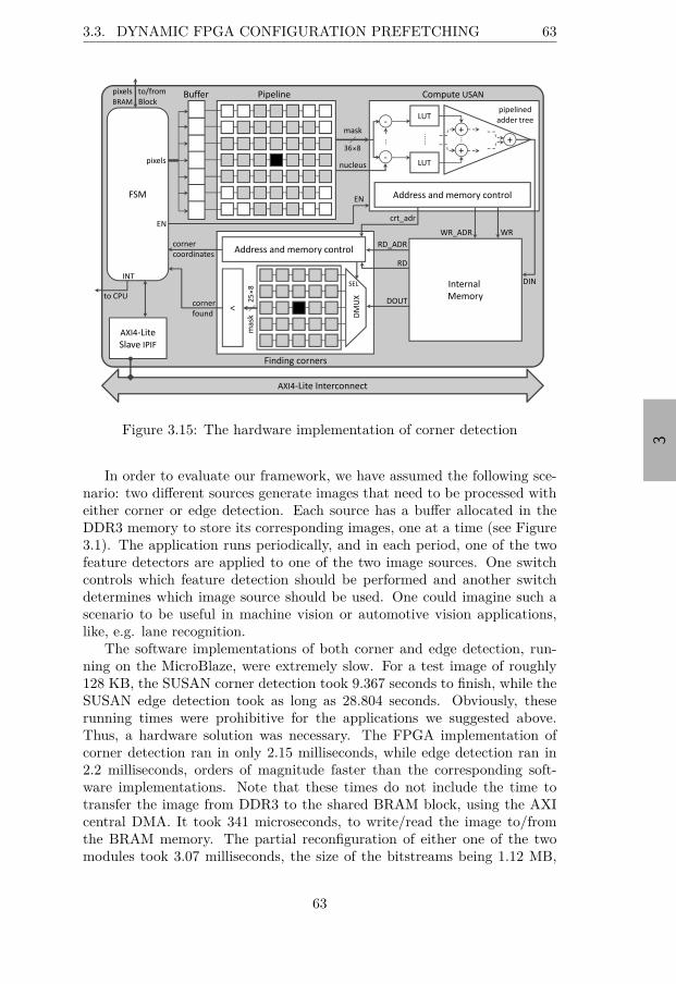
“thesis” — 2015/8/12 — 12:54 — page 63 — #83

3


!×"

#

## #

$

%

%&

'

(

(

)

$*'*'+,'

,(

+

,-

',+,'

',

,.

$

/0×"

.(1

2((

.(1(

3

Figure 3.15: The hardware implementation of corner detection

In order to evaluate our framework, we have assumed the following sce-nario: two different sources generate images that need to be processed witheither corner or edge detection. Each source has a buffer allocated in theDDR3 memory to store its corresponding images, one at a time (see Figure3.1). The application runs periodically, and in each period, one of the twofeature detectors are applied to one of the two image sources. One switchcontrols which feature detection should be performed and another switchdetermines which image source should be used. One could imagine such ascenario to be useful in machine vision or automotive vision applications,like, e.g. lane recognition.

The software implementations of both corner and edge detection, run-ning on the MicroBlaze, were extremely slow. For a test image of roughly128 KB, the SUSAN corner detection took 9.367 seconds to finish, while theSUSAN edge detection took as long as 28.804 seconds. Obviously, theserunning times were prohibitive for the applications we suggested above.Thus, a hardware solution was necessary. The FPGA implementation ofcorner detection ran in only 2.15 milliseconds, while edge detection ran in2.2 milliseconds, orders of magnitude faster than the corresponding soft-ware implementations. Note that these times do not include the time totransfer the image from DDR3 to the shared BRAM block, using the AXIcentral DMA. It took 341 microseconds, to write/read the image to/fromthe BRAM memory. The partial reconfiguration of either one of the twomodules took 3.07 milliseconds, the size of the bitstreams being 1.12 MB,

63

“thesis” — 2015/8/12 — 12:54 — page 64 — #84

3


and the effective throughput of our custom reconfiguration controller withDMA reaching 375 MB/s.

We have experimented with two different phases, characterized by dif-ferent correlations: in phase 1, images from source 1 require edge detectionwhile those from source 2 require corner detection, and vice versa in phase 2.Given this, we considered a number of scenarios, varying the phase length,as well as the frequency at which images were generated by the two sourceswithin a phase. All these parameters determined the interleaving of perform-ing edge detection or corner detection, as well as the long term probabilitiesto perform one or the other.

We have considered four scenarios:

1. Phase length 100 iterations, and the two image sources produce imageswith the same frequency (i.e. we always alternate between corner andedge detection);

2. Phase length 100 iterations, but the second image source producesimages with half the frequency of the first;

3. Phase length 20 iterations, and the two image sources produce imageswith the same frequency;

4. Phase length 20 iterations, and the second image source produces im-ages with half the frequency of the first.

We compared our approach with two alternative approaches:

1. The straightforward fetch-on-demand (FOD) technique. In this case,no reconfiguration overhead is hidden, since the hardware modules arereconfigured only on demand, when they need to run, but are notalready on the FPGA.

2. The static configuration prefetching approach presented in Section 3.2.In this case, the hardware modules are prefetched based on probabili-ties obtained via profiling10.

We have run 1000 iterations of the application, and we have measured howlong one iteration takes on average.

Figure 3.16 presents the improvements that we obtained for the differentscenarios: given that the average execution time of one iteration of theprogram is denoted with AV G, we computed the improvement producedby the prediction (P) approach over FOD as IP

F OD = AV GF OD−AV GP

AV GF ODand

over the static (S) prefetching (Section 3.2) as IPS = AV GS−AV GP

AV GS. Note

10Note that this information can be obtained for the simple scenarios we have assumed,but in more complex cases it might be impossible to obtain such profiling information, orit might be inaccurate. Furthermore, the profiling information is average, and the statictechnique completely ignores the phase behavior. Thus, in many cases, the prefetchesgenerated for the average behavior might be completely irrelevant for certain phases.

64

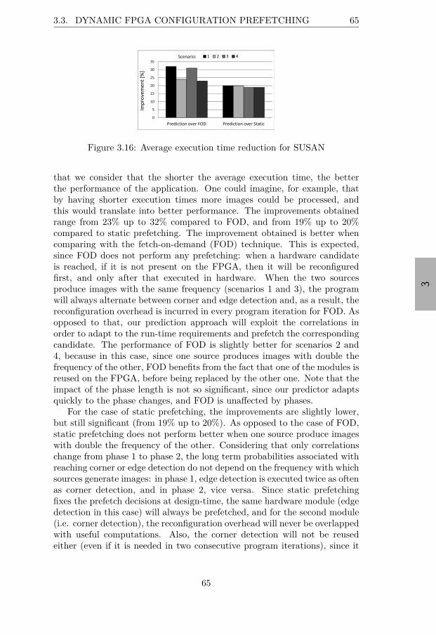
“thesis” — 2015/8/12 — 12:54 — page 65 — #85

3


Figure 3.16: Average execution time reduction for SUSAN

that we consider that the shorter the average execution time, the betterthe performance of the application. One could imagine, for example, thatby having shorter execution times more images could be processed, andthis would translate into better performance. The improvements obtainedrange from 23% up to 32% compared to FOD, and from 19% up to 20%compared to static prefetching. The improvement obtained is better whencomparing with the fetch-on-demand (FOD) technique. This is expected,since FOD does not perform any prefetching: when a hardware candidateis reached, if it is not present on the FPGA, then it will be reconfiguredfirst, and only after that executed in hardware. When the two sourcesproduce images with the same frequency (scenarios 1 and 3), the programwill always alternate between corner and edge detection and, as a result, thereconfiguration overhead is incurred in every program iteration for FOD. Asopposed to that, our prediction approach will exploit the correlations inorder to adapt to the run-time requirements and prefetch the correspondingcandidate. The performance of FOD is slightly better for scenarios 2 and4, because in this case, since one source produces images with double thefrequency of the other, FOD benefits from the fact that one of the modules isreused on the FPGA, before being replaced by the other one. Note that theimpact of the phase length is not so significant, since our predictor adaptsquickly to the phase changes, and FOD is unaffected by phases.

For the case of static prefetching, the improvements are slightly lower,but still significant (from 19% up to 20%). As opposed to the case of FOD,static prefetching does not perform better when one source produce imageswith double the frequency of the other. Considering that only correlationschange from phase 1 to phase 2, the long term probabilities associated withreaching corner or edge detection do not depend on the frequency with whichsources generate images: in phase 1, edge detection is executed twice as oftenas corner detection, and in phase 2, vice versa. Since static prefetchingfixes the prefetch decisions at design-time, the same hardware module (edgedetection in this case) will always be prefetched, and for the second module(i.e. corner detection), the reconfiguration overhead will never be overlappedwith useful computations. Also, the corner detection will not be reusedeither (even if it is needed in two consecutive program iterations), since it

65

“thesis” — 2015/8/12 — 12:54 — page 66 — #86

3


will always be overwritten by the prefetch of the edge detection module. Asin the case of FOD, the effect of phase length is marginal.

Energy measurements

We have also evaluated the energy consumption of our predictor framework,implemented on the Xilinx ML605 board. We have used a shunt resistor(R = 100mΩ) in series with the voltage source of the FPGA (VCC = 12V)in order to measure the current drawn by the board (I). The voltage dropon the shunt resistor (U) was amplified (10×) and monitored using thePicoScope USB oscilloscope. The current drawn by the board is I = U

R=

UoscV10×0.1Ω = UoscA, where Uosc is the value measured by the oscilloscope.Thus, by integrating the oscilloscope traces on a time interval ∆t = [t0, t1]and then multiplying with the supply voltage VCC = 12V we obtained theenergy consumption of the board in the interval ∆t.

We have run 1000 iterations of the image processing application for sce-nario 1) from above, we have measured the energy consumption, and thencomputed the average energy consumed by the application in one iteration.We have considered three implementations of the image processing applica-tion:

1. SW-only: both corner and edge detection were run as software sub-routines;

2. static-HW: both corner and edge detection were implemented as mod-ules on the FPGA, each one with its dedicated area (i.e. no partialdynamic reconfiguration was used);

3. with prediction: the hardware modules for corner and edge detectionwere mapped to the same area on the FPGA, and our predictor wasused to prefetch the modules using partial dynamic reconfiguration.

For the SW-only implementation, since the execution time of the imageprocessing application was very big (as reported above, 9.367s for cornerdetection and 28.804s for edge detection), the average energy consump-tion was also high: ESW-only = 304.60J. For the static-HW implementa-tion, which is orders of magnitude faster (2.49ms for corner detection and2.54ms for edge detection), the average energy consumption amounts toEstatic-HW = 89.59mJ. Finally, when running the predictor, we obtain anaverage energy consumption of Epred = 98.64mJ. This represents an in-crease of as little as 10.1% over the static-HW implementation, but onlyhalf the FPGA area was needed for the implementation of the image pro-cessing application, and the average execution time with the predictor wasonly 10% bigger than the static-HW execution time.

Note that the resource usage of the framework itself is equal in the caseof FOD and static prefetching. Our technique needs the “Predictor” module(depicted in Figure 3.1), so an overhead of 419 LUTs and 151 FFs is incurred

66

“thesis” — 2015/8/12 — 12:54 — page 67 — #87

3


(as little as 4% out of the total framework LUTs, and 1.5% out of thetotal framework FFs; see Table 3.1). We consider this small area overheadjustified, given the improvements obtained. The measurements show thatby using our prediction framework we can obtain good performance (shortexecution times) with limited hardware area and with only a minor energyconsumption overhead.

3.3.5.2 Performance Improvement

We have also performed simulation experiments with generated examples,in order to evaluate how the piecewise linear predictor behaves comparedto other prefetching approaches. We generated 2 sets containing 25 con-trol flow graphs each: Set1 with small graphs (between 48 and 166 nodes,∼100 on average), and Set2 with bigger graphs (between 209 and 830 nodes,∼350 on average). The software execution time for each node was randomlygenerated in the range of 50 to 1000 time units. Between 15% and 40%of the nodes were selected as hardware candidates (those with the highestsoftware execution times), and their hardware execution time was generatedβ times smaller than their software one (the coefficient β models the hard-ware speedups). We considered two possible situations: in the first one, βwas chosen from the uniform distribution on [103, 3 · 103] (fast hardware:applications exhibiting high hardware acceleration), in order to reflect theresults obtained from our board measurements (see Section 3.3.5.1); in thesecond situation, we generated much lower speedups, from the uniform dis-tribution on [3, 7] (slow hardware: applications exhibiting lower hardwareacceleration), similar to the assumptions from Section 3.2.4.2 and [S+10].We also generated the size of the candidates in concordance with our real-life implementation of the SUSAN image processing algorithm. The re-configuration time for the modules was determined based on their size,considering the average throughput of our DMA reconfiguration controller(375 MB/s). The placement was decided using existing techniques (like[HMZB12] or [BHS+13]) that minimize the number of placement conflicts.We generated problem instances where the size of the reconfigurable regionis a fraction (15% or 25%) of the total area required by all candidates,max_hw =

∑m∈H area(m).

All experiments were run on a PC with CPU frequency 2.83 GHz, 8 GBof RAM, and running Windows Vista. For each application we have evalu-ated different prefetch techniques using an in-house Monte Carlo simulator(based on the one described in Section 3.2.4.1) that considers the archi-tectural assumptions described in Section 3.1.1. Recall that in the case ofstatic prefetching (see Section 3.2) we ignored correlations between branches.Thus, we had to modify the simulator such that, for control nodes, correla-tions between two or more branches were captured through joint probabilitytables. In such a case, whenever we performed a draw from the marginalBernoulli distribution for a branch, we computed the conditional probabil-ities for all the branches correlated with it, based on the joint probability

67

“thesis” — 2015/8/12 — 12:54 — page 68 — #88

3


!" !" !" !"

(a) Fast hardware

!" !" !" !"

(b) Slow hardware

Figure 3.17: Performance improvement for the simulation experiments

table. Later in the simulation, when the correlated branches were reached,we did not sample their marginal distribution, but instead we sampled theirconditional distribution based on the outcome of the first branch. We havedetermined the results with an accuracy of ±1% with confidence 99%.

We were interested to see how our approach compares to the currentstate-of-the-art, both in static (Section 3.2) and dynamic prefetching [LH02],[HV09]. Thus, we simulated each application using the prefetch queuesgenerated by our approach and those generated by the static prefetchingtechnique presented in Section 3.2, [LH02] and [HV09]. The parameters forour predictor (see Section 3.3.3.1) were chosen, depending on the applicationsize, from the following ranges: α = [0.4, 0.6], q = [2, 8], h ∈ [4, 16].

The appropriate metric to evaluate prefetch policies is the total timespent executing the hardware candidates, plus the time waiting for recon-figurations to finish (in case the reconfiguration overhead was not entirelyoverlapped with useful computations). If this value is small, it means thatthe prefetch policy had accurate predictions (many candidates were exe-cuted in hardware), and the prefetch was done early enough to have shortwaiting times. We do not include comparisons with the SW-only and static-HW implementations: As our case study suggested, the SW-only version ofan application has prohibitive execution times and can only be worse thanany prefetching technique; The static-HW version corresponds to an idealand unrealistic scenario, when we have unlimited resources (i.e. enough HWarea to place all the application modules at the same time on the FPGA).

We denote the average time spent executing hardware candidates, pluswaiting for reconfigurations to finish, with EXP for our dynamic approach,with EXS for the static approach from Section 3.2, with EXM for the dy-namic Markov approach [LH02] and with EXA for the dynamic aggregategains approach [HV09]. We compute the performance improvement of ourapproach over the static, PIP

S = EXS−EXP

EXS; similarly we calculate PIP

M

and PIPA , the improvements of our approach over [LH02] and [HV09], re-

spectively.Figures 3.17a and 3.17b show the results obtained (averaged over all

graphs in Set1 and Set2) for the scenarios with fast and slow hardware, re-

68

“thesis” — 2015/8/12 — 12:54 — page 69 — #89

3

3.4. SUMMARY 69

spectively. The improvements obtained for fast hardware are slightly higherthan those obtained for slower hardware. It is important to note that thebaseline approaches also benefit from faster hardware. The improvementsover the static approach (presented in Section 3.2) are higher because staticprefetch lacks flexibility. The improvements over both dynamic approaches([LH02], [HV09]) are also significant, ranging from 15% up to 30% on averagefor fast hardware and from 14% up to 29% on average for slow hardware.

3.4 Summary

This chapter proposed a complete framework for partial dynamic recon-figuration of FPGAs, together with optimization approaches to configura-tion prefetching for performance enhancement. We first presented a staticprefetching algorithm. Based on profiling information, and taking into ac-count the placement of hardware modules on the FPGA, we statically sched-ule the appropriate prefetches (and implicitly perform HW/SW partitioningof the candidate hardware modules) such that the expected execution timeof the application is minimized. For applications with inaccurate or unavail-able profiling information, and for those that exhibit non-stationary behav-ior, it is important to have a mechanism that adapts to changes. Thus,we proposed an approach for dynamic prefetching of FPGA configurations,with the goal to minimize the expected execution time of an application.We used a piecewise linear predictor, coupled with an on-line mechanism,based on timestamps, in order to generate prefetches at run-time. The effi-ciency and practicality of our FPGA configuration prefetching platform wasdemonstrated with a proof of concept implementation of a real-life appli-cation (the SUSAN image processing algorithm [SB97]), complemented byextensive simulations.

69

“thesis” — 2015/8/12 — 12:54 — page 70 — #90

3


70

“thesis” — 2015/8/12 — 12:54 — page 71 — #91

4

Chapter 4

!"#$%"&'( )!%*+( ,-!-.-/0#-1!

&1* ,2'#-",13% 4%0'"5-.% 6(7#%.7

Modern heterogeneous architectures bring together multiple general-purpose CPUs and multiple GPUs and FPGAs, in an attempt to

answer the performance, energy-efficiency and flexibility requirements oftoday’s complex applications [Fou15]. However, in order to leverage theadvantages of such architectures, careful optimization is essential. Real-time multi-mode systems are a good model for a wide range of applica-tions that dynamically change their computational requirements over time[SSC03], [SBSH12]. In this context, intelligent on-line resource managementis needed, such that the heterogeneous resources are used in an energy-efficient manner, while meeting the real-time constraints. In this chapterwe propose a resource manager that implements run-time policies to de-cide on-the-fly task admission and the mapping of active tasks to resources,such that the energy consumption of the system is minimized and all taskdeadlines are met.

The remainder of this chapter is organized as follows. The system modelassumed and the statement of the problem addressed are presented in Sec-tions 4.1 and 4.2, respectively. Section 4.3 describes the challenges we arefacing by means of a motivational example. Details of the design optimiza-tion approach for one mode and the integrated multi-mode optimization forenergy minimization, respectively, are described in Sections 4.4 and 4.5. Wepresent the experimental validation of the proposed approaches in Section4.6, which includes both real-life measurements and simulation results. Thecontribution of the chapter is summarized in Section 4.7.

71

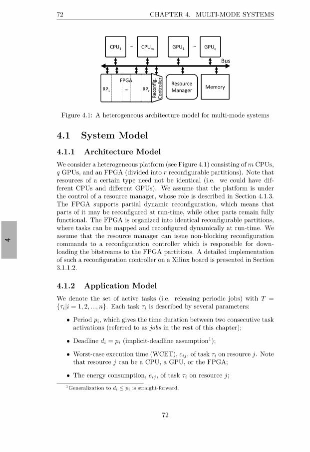
“thesis” — 2015/8/12 — 12:54 — page 72 — #92

4

72 CHAPTER 4. MULTI-MODE SYSTEMS

Figure 4.1: A heterogeneous architecture model for multi-mode systems

4.1 System Model

4.1.1 Architecture Model

We consider a heterogeneous platform (see Figure 4.1) consisting of m CPUs,q GPUs, and an FPGA (divided into r reconfigurable partitions). Note thatresources of a certain type need not be identical (i.e. we could have dif-ferent CPUs and different GPUs). We assume that the platform is underthe control of a resource manager, whose role is described in Section 4.1.3.The FPGA supports partial dynamic reconfiguration, which means thatparts of it may be reconfigured at run-time, while other parts remain fullyfunctional. The FPGA is organized into identical reconfigurable partitions,where tasks can be mapped and reconfigured dynamically at run-time. Weassume that the resource manager can issue non-blocking reconfigurationcommands to a reconfiguration controller which is responsible for down-loading the bitstreams to the FPGA partitions. A detailed implementationof such a reconfiguration controller on a Xilinx board is presented in Section3.1.1.2.

4.1.2 Application Model

We denote the set of active tasks (i.e. releasing periodic jobs) with T =τi|i = 1, 2, ..., n. Each task τi is described by several parameters:

• Period pi, which gives the time duration between two consecutive taskactivations (referred to as jobs in the rest of this chapter);

• Deadline di = pi (implicit-deadline assumption1);

• Worst-case execution time (WCET), cij , of task τi on resource j. Notethat resource j can be a CPU, a GPU, or the FPGA;

• The energy consumption, eij , of task τi on resource j;

1Generalization to di ≤ pi is straight-forward.

72

“thesis” — 2015/8/12 — 12:54 — page 73 — #93

4


• The time overhead cri and the energy overhead er

i of reconfiguring taskτi on the FPGA;

• Given the above parameters, we can compute for every task τi itsmaximal utilization on every resource: uij =

cij

pi.

We assume that all tasks from the active task set have implementationsfor at least one computational resource2. The executable code for the CPUs,the kernel implementations for the GPUs, and the bitstreams specifying theFPGA implementations are all stored in a memory to which the resourcemanager has access. We denote with map(τi) = j the fact that task τi ismapped to resource j.

Let us next define a mode: we characterize a functional mode o by thecomposition of the active task set To containing the tasks that are currentlyreleasing periodic jobs. For the duration of a certain mode, To does notchange. When an existing task leaves the system (i.e. stops releasing jobs),or a new task enters the system, we say that a transition to a new modehas occurred. Every such transition (if allowed by the resource managerdescribed in Section 4.1.3) has to take place within a specified set-up time,tset. This time is used to perform the mapping optimization and enforceany remapping decisions, including FPGA reconfigurations and loading ofthe tasks’ software into memory.

4.1.3 Resource Management

The entire system is under the control of a resource manager, whose mainresponsibility is to decide at run-time task admission and the mapping oftasks to resources such that the energy consumption is minimized whileall the deadlines are met. We consider that the manager is running ona dedicated resource, and it could be implemented either in software orin hardware. The manager needs to know the task parameters mentionedin Section 4.1.2 and to be aware of the current mode (i.e. which is thecurrently active task set). Thus, any task that is currently active but wantsto leave the system (i.e. stop releasing jobs) must notify the manager of this.Also, any new task that wants to become active in the system (i.e. wantsto start releasing jobs) must first register with the resource manager (i.e.communicate its task parameters), and wait for permission to become active.In case the manager cannot find a mapping for the new task such that alldeadlines will be satisfied, then the new task will not be granted permissionto activate. This situation might occur in two cases: either the system wouldbecome overloaded if the new task is accepted (thus, no feasible mappingexists), or a feasible mapping exists, but the manager is unable to find

2Of course, the more implementations a task has the better the optimization op-portunities. However, it is not needed that tasks have implementations for all processingelements; if no implementation is available for task τi on resource j then the correspondingmapping option is ignored by setting cij = eij = ∞.

73

“thesis” — 2015/8/12 — 12:54 — page 74 — #94

4


it. Section 4.6.2.2 evaluates our proposed run-time policies (presented inSection 4.5.3) from this point of view. The resource manager performsadmission management by deciding if a new task can enter the system ornot (i.e. deciding if transition to a new mode is allowed or not), dependingon the current load. Moreover, if admission is granted, a task mapping is alsodecided. In Section 4.5.3 we propose several run-time policies to performthese decisions.

4.1.4 Scheduling

One approach to multiprocessor scheduling is partitioning, which means thattasks are assigned to resources and then each resource schedules its assignedtasks using a uniprocessor scheduling algorithm. We have to address thescheduling problem for each of the three types of processing elements (CPUs,GPUs, FPGA) assumed in our architecture.

Let us first note that for the FPGA, there is no scheduling problem,because each FPGA partition can be seen as a dedicated processor, runningone single task. Thus, we need to make sure that at any moment in timethere are no more than r tasks mapped to the FPGA (because we have rreconfigurable partitions):

∑

imap(τi)=j

1 ≤ r, j = FPGA index (4.1)

Note that, in order to ensure the feasibility of mapping a certain task to theFPGA, we also need to make sure that its execution time is shorter than itsdeadline:

cij ≤ di, ∀τi ∈ T : map(τi) = j, j = FPGA index (4.2)

As opposed to the FPGA, the situation is different for the CPUs andthe GPUs, as we will explain next. We will apply the Earliest DeadlineFirst (EDF) scheduling policy for the tasks mapped to the CPUs. One ofthe advantages of EDF is that there exists a simple necessary and sufficientcondition which ensures that all task deadlines are met [But04]:

∑

imap(τi)=j

cij

pi

≤ 1, ∀CPU j (4.3)

As far as the GPUs are concerned, execution of tasks is non-preemptive.Thus, we chose to schedule the tasks mapped to the GPUs using uniprocessorFIFO scheduling. The schedulability conditions in this case are:

∑

imap(τi)=j

cij

pi

≤ 1, ∀GPU j (4.4)

74

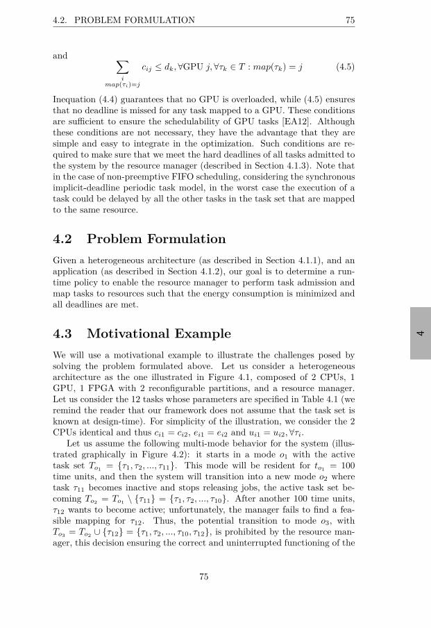
“thesis” — 2015/8/12 — 12:54 — page 75 — #95

4

4.2. PROBLEM FORMULATION 75

and ∑

imap(τi)=j

cij ≤ dk, ∀GPU j, ∀τk ∈ T : map(τk) = j (4.5)

Inequation (4.4) guarantees that no GPU is overloaded, while (4.5) ensuresthat no deadline is missed for any task mapped to a GPU. These conditionsare sufficient to ensure the schedulability of GPU tasks [EA12]. Althoughthese conditions are not necessary, they have the advantage that they aresimple and easy to integrate in the optimization. Such conditions are re-quired to make sure that we meet the hard deadlines of all tasks admitted tothe system by the resource manager (described in Section 4.1.3). Note thatin the case of non-preemptive FIFO scheduling, considering the synchronousimplicit-deadline periodic task model, in the worst case the execution of atask could be delayed by all the other tasks in the task set that are mappedto the same resource.

4.2 Problem Formulation

Given a heterogeneous architecture (as described in Section 4.1.1), and anapplication (as described in Section 4.1.2), our goal is to determine a run-time policy to enable the resource manager to perform task admission andmap tasks to resources such that the energy consumption is minimized andall deadlines are met.

4.3 Motivational Example

We will use a motivational example to illustrate the challenges posed bysolving the problem formulated above. Let us consider a heterogeneousarchitecture as the one illustrated in Figure 4.1, composed of 2 CPUs, 1GPU, 1 FPGA with 2 reconfigurable partitions, and a resource manager.Let us consider the 12 tasks whose parameters are specified in Table 4.1 (weremind the reader that our framework does not assume that the task set isknown at design-time). For simplicity of the illustration, we consider the 2CPUs identical and thus ci1 = ci2, ei1 = ei2 and ui1 = ui2, ∀τi.

Let us assume the following multi-mode behavior for the system (illus-trated graphically in Figure 4.2): it starts in a mode o1 with the activetask set To1

= τ1, τ2, ..., τ11. This mode will be resident for to1= 100

time units, and then the system will transition into a new mode o2 wheretask τ11 becomes inactive and stops releasing jobs, the active task set be-coming To2

= To1\ τ11 = τ1, τ2, ..., τ10. After another 100 time units,

τ12 wants to become active; unfortunately, the manager fails to find a fea-sible mapping for τ12. Thus, the potential transition to mode o3, withTo3

= To2∪ τ12 = τ1, τ2, ..., τ10, τ12, is prohibited by the resource man-

ager, this decision ensuring the correct and uninterrupted functioning of the

75

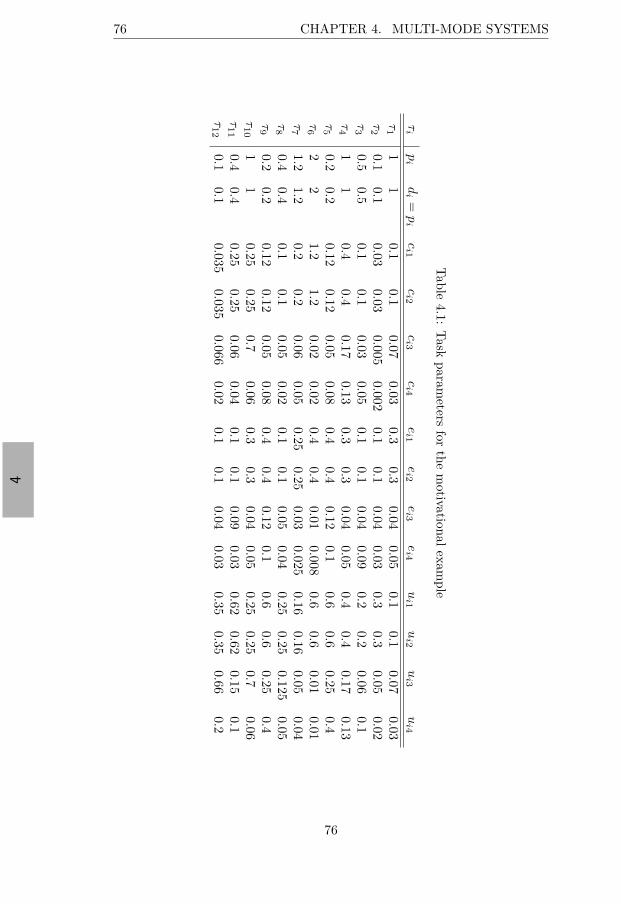
“thesis” — 2015/8/12 — 12:54 — page 76 — #96

4


Table

4.1:T

askparam

etersfor

them

otivationalexam

ple

τi

pi

di

=p

ic

i1c

i2c

i3c

i4e

i1e

i2e

i3e

i4u

i1u

i2u

i3u

i4

τ1

11

0.10.1

0.070.03

0.30.3

0.040.05

0.10.1

0.070.03

τ2

0.10.1

0.030.03

0.0050.002

0.10.1

0.040.03

0.30.3

0.050.02

τ3

0.50.5

0.10.1

0.030.05

0.10.1

0.040.09

0.20.2

0.060.1

τ4

11

0.40.4

0.170.13

0.30.3

0.040.05

0.40.4

0.170.13

τ5

0.20.2

0.120.12

0.050.08

0.40.4

0.120.1

0.60.6

0.250.4

τ6

22

1.21.2

0.020.02

0.40.4

0.010.008

0.60.6

0.010.01

τ7

1.21.2

0.20.2

0.060.05

0.250.25

0.030.025

0.160.16

0.050.04

τ8

0.40.4

0.10.1

0.050.02

0.10.1

0.050.04

0.250.25

0.1250.05

τ9

0.20.2

0.120.12

0.050.08

0.40.4

0.120.1

0.60.6

0.250.4

τ1

01

10.25

0.250.7

0.060.3

0.30.04

0.050.25

0.250.7

0.06τ

11

0.40.4

0.250.25

0.060.04

0.10.1

0.090.03

0.620.62

0.150.1

τ1

20.1

0.10.035

0.0350.066

0.020.1

0.10.04

0.030.35

0.350.66

0.2

76

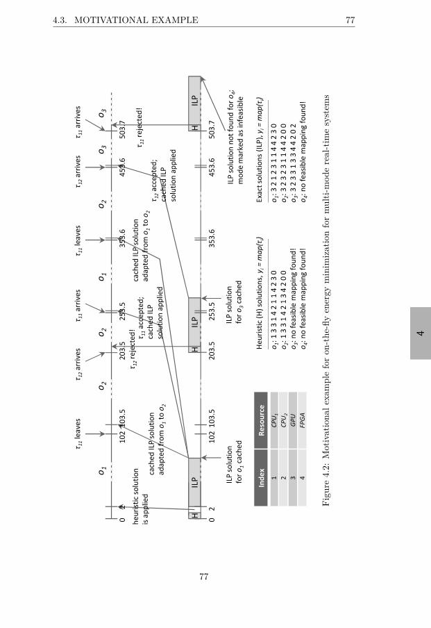
“thesis” — 2015/8/12 — 12:54 — page 77 — #97

4

4.3. MOTIVATIONAL EXAMPLE 77

!

"

##$

%"$

"$

$#$%&

'$(

%"$

#$)

"$

##$

#$)

"$

##$

'$(

%$%)

&$&

*$%+

"$

$#$%&

%+&

##,%$(

%+&

##,%$(

%+&

##,%$(

Fig

ure

4.2:

Mot

ivat

iona

lex

ampl

efo

ron

-the

-fly

ener

gym

inim

izat

ion

for

mul

ti-m

ode

real

-tim

esy

stem

s

77

“thesis” — 2015/8/12 — 12:54 — page 78 — #98

4


current mode o2. Assume that mode o2 stays resident for 50 more timeunits (thus, to2

= 150) and then the system performs a transition back tothe initial mode o1. Further, the events and transitions illustrated in Figure4.2 happen, and they are discussed below.

Our goal is to minimize the energy consumption of the system during itslifetime, while ensuring that all the active tasks’ deadlines are met. Recallthat any mode transition has to take place withing a set-up time, whichin this example we consider to be at most tset = 5 time units. Also, notethat we handle task arrivals and departures one at a time. In Figure 4.2 wepresent a timeline to illustrate the above multi-mode scenario. At t = 0 thesystem starts and all the tasks from the set To1

register their parameters withthe resource manager and express their intent to become active and startreleasing jobs. The manager has to decide if the task set To1

is schedulable onthe given architecture and what is the best mapping of tasks to processingelements that will generate the minimum energy consumption. Since theset-up time is only 5 time units, the manager cannot afford to wait for theresult of an exact optimization (which would take longer). Instead, a fastheuristic solution is found and enforced. The mapping vector yi = map(τi)obtained with our heuristic presented in Section 4.4.2 is specified in Figure4.2; note that a schedulable solution is found and no task is rejected. Thesolution is obtained and applied (i.e. FPGA reconfigured and processingelements initialized) in 2 time units.

Thus, at time t = 2 the system starts running in mode o1, with alltasks active and releasing jobs. According to the obtained mapping, tasksτ1, τ7 and τ11 will be assigned to CPU1, τ2 and τ10 to CPU2, τ3, τ4, τ6 andτ8 to the GPU , and τ5 and τ9 to the FPGA. Although this mapping issuboptimal we cannot do better at this moment. However, we could runan exact optimization for this mode, cache the result and apply it nexttime when the mode is visited. We solve our ILP presented in Section4.4.1 in parallel with the execution of mode o1. The optimization takes 20time units, after which the result is cached. At time 102, task τ11 becomesinactive, thus freeing some computational resources. Since we do not havea solution cached for this mode yet, we are now faced with several options:

1. Run the fast remapping heuristic. However, since the difference com-pared to the previous mode is only that task τ11 became inactive,we cannot expect a significantly improved solution. If we look at theheuristic solutions for modes o1 and o2 in Figure 4.2, we can see thatthe mapping for tasks τ1 to τ10 is identical. Instead of wasting time andenergy to re-run the heuristic, we would better just keep the mappingfrom the previous mode o1. In this case, the system would functionwithout interruption. However, we can do better as we discuss next.

2. Another viable option is to use the exact solution (cached) from modeo1 for all tasks except τ11 which is not active anymore. As can beseen from Figure 4.2, tasks τ1 to τ10 have identical mapping in modes

78

“thesis” — 2015/8/12 — 12:54 — page 79 — #99

4

4.3. MOTIVATIONAL EXAMPLE 79

o1 and o2 for the ILP too. Thus, we will use a set-up time of 1.5time units to replace the heuristic mapping from o1 with the mappingadapted for o2 from the cached ILP solution for o1 (which turns outto be optimal for all the tasks active in o2).

Let us next discuss the time step t = 203.5, when task τ12 wants tobecome active attempting to switch the system to mode o3. In this case,the resource manager is again faced with several options, in order to decidewhere to map τ12:

1. The most straight-forward solution would be to map τ12 to a processingelement that still has enough free capacity to accommodate τ12 andthat is the most energy efficient for it. Unfortunately, there is nosingle resource with enough computational capacity to accommodateτ12 (and this is often the case in situations where the system load ishigh). Thus, we need a better approach.

2. A second option is to run the fast mapping heuristic, and if this resultsin a feasible solution, enforce it. Otherwise, reject task τ12. In ourexample it happens that the heuristic does not find a feasible solutionfor mapping the task set To3

even though one exists (see the ILPsolution in Figure 4.2). As a result, τ12 is rejected at 204.5.

In order to mitigate the problem above, we resort to caching: if a cachedsolution for mode o3 existed, it would not be needed to re-run any optimiza-tion. With this in mind, we run the ILP in parallel with the execution ofthe system, and cache the result. A feasible solution that permits the acti-vation of τ12 exists and at a future instantiation of mode o3 we will be ableto accommodate it. In the scenario we discussed above, mode o2 continuesits execution until t = 253.5, and then task τ11 becomes active again andthe system transitions back to mode o1 with To1

= τ1, τ2, ..., τ11. Notethat this time we already have an optimal solution for o1 (cached from itsprevious instantiation) and we can apply it directly in a very short set-uptime of 0.1 time units.

The system goes next through the following mode transitions: o1 → o2

(τ11 leaving the system at 353.6); no cached solution exists for o2, but theILP solution for o1 was cached at 22. Thus, the resource manager canadapt this mapping (as it did the first time when o2 was entered, at 103.5).Next we encounter o2 → o3 (τ12 arriving at 453.6 and being allowed to ac-tivate at 353.7); the instantiation of mode o3 is now possible as opposedto the first time (when τ12 arrived at 203.5), because an optimal solutionfor o3 was cached at 224.5. At time t = 503.7, when τ11 arrives, the sys-tem will try to perform the transition o3 → o4, to the new mode o4 withTo4

= τ1, τ2, ..., τ12. This situation is not schedulable (see Figure 4.2, nofeasible mapping found for o4), so the resource manager will not allow τ11

to activate. It is important to note that we consider a very simple scenarioin this example, only to illustrate some of the challenges. New tasks might

79

“thesis” — 2015/8/12 — 12:54 — page 80 — #100

4


appear and generate new modes. We need not know which tasks will run inthe system at design-time, the only requirement is that they register withthe resource manager when they want to become active.

So far we did not mention the energy consumption of the system. Let usconsider the time horizon up to 553.7 time units. We have simulated the sce-nario described above (applying heuristic solutions together with ILP onesas described), and we obtained a total energy consumption of E = 268 J;this value includes the energy overheads for running the heuristic and theILP, as well as the overheads of reconfiguring the FPGA partitions. Forcomparison purposes, we have simulated a golden run of the system, withthe same mode changes, but every time we assumed that we have the ILP so-lution already cached. For the golden run we did not consider any overheadsfor running the optimization, but only those for reconfiguring the FPGA,and we obtained an energy consumption of Egold = 209 J. The describedapproach is only 28% away from the golden run. Note that the golden runis impossible to achieve in practice, and the fact that we considered only arestricted time horizon. Depending on the multi-mode behavior of the sys-tem, the cached solutions might be reused multiple times in the future, thusobtaining low energy consumption without re-running the optimizations.

Let us note that we have discussed three ways to obtain the mapping fora new mode:

1. Optimal, by running the ILP from Section 4.4.1;

2. Heuristic:

(a) by running the algorithm from Section 4.4.2;

(b) by adapting the exact cached solution of a previous mode.

Let us summarize the run-time behavior of the resource manager. When-ever a mode change occurs, the following actions are taken:

1. If a cached (thus optimal) solution for the new mode exists, it is en-forced;

2. Otherwise, if a cached solution for a super-mode (i.e. a mode whosetask set is a superset of the current active task set) exists, it is adaptedto the current mode by ignoring all the tasks that are not active (likewe did in the example from Figure 4.2 at time steps 103.5 and 353.6when for mode o2 we adapted the optimal solution generated for modeo1);

3. If none of the above is successful, then the fast heuristic (see Section4.4.2) is run. If a feasible mapping is found, it is enforced; otherwise,the new task is not allowed to activate and the system remains in theprevious mode;

4. Once a decision regarding the new mode has been taken, in parallelwith the system’s execution the resource manager will run the ILP;

80

“thesis” — 2015/8/12 — 12:54 — page 81 — #101

4

4.4. OPTIMIZATION FOR ONE MODE 81

(a) If the ILP returns a feasible solution, it is cached for future use(e.g. the ILP solution for o1 is used 3 times in Figure 4.2);

(b) Otherwise, the mode is marked as infeasible (e.g. mode o4 inFigure 4.2).

Since running the ILP is a time and energy consuming process, we wouldlike to do this as rarely as possible. We try to achieve this by using caching.For example, let us look at time step 253.5 in Figure 4.2: when τ11 arrivesthe ILP is running, in an attempt to find a feasible solution for mode o3

(for which the heuristic was unable to obtain a schedulable mapping). If asolution for o1 would not be cached, at 253.5 the resource manager wouldneed to interrupt the ILP and run the heuristic for the new mode instead.Note also that, the longer the residence time of a mode the more pay-off weget from having an optimal solution prepared for it.

The solutions generated by the fast heuristic are not cached, because wewant to store as many exact (ILP) solutions as possible in the limited cachespace. Due to the low overhead of running the heuristic, we can afford to dothis. Note that, since the cache for storing solutions is limited, a replacementpolicy is needed (this is discussed in Section 4.5.1). In the following sectionswe will propose solutions to the challenges identified above.

4.4 Optimization for One Mode

4.4.1 ILP Formulation

We will first formulate an integer linear program to solve the problem ofmapping the active tasks in mode o, i.e. To, to the available resources inour heterogeneous architecture. In what follows, we will use the followingconventions:

• CPUs are indexed from 1 to m;

• GPUs are indexed from m + 1 to m + q;

• The FPGA has index m + q + 1;

• Recall that the FPGA has r reconfigurable partitions;

• Size of the task set in the current mode is n;

• The mapping variables are denoted with xij , where:

xij =

1 if task τi is mapped to resource j;0 otherwise

Let us assume that the length (residence time duration) of a certainmode o is to time units. A particular task τi ∈ To (with period pi) that is

active during mode o would release⌈

to

pi

⌉jobs3. We are interested in min-

3We assume that jobs are immediately ready at the beginning of a mode.

81

“thesis” — 2015/8/12 — 12:54 — page 82 — #102

4


imizing the total energy consumption of the system during mode o, which

is expressed as∑n

i=1

∑m+q+1j=1 xij

⌈to

pi

⌉eij . Since we assume that mode du-

rations are significantly longer than task periods (i.e. to ≫ pi, ∀τi ∈ To), we

can approximate the number of job releases for each task with⌈

to

pi

⌉≈ to

pi.

As a result, we can factor out the mode duration to, obtaining the followingILP formulation:

minimizexij

n∑

i=1

m+q+1∑

j=1

xij

eij

pi

subject ton∑

i=1

xijuij ≤ 1, j = 1, 2, ..., m (4.6)

n∑

i=1

xijuij ≤ 1, j = m + 1, m + 2, ..., m + q (4.7)

if xkj = 1 :n∑

i=1

xijcij ≤ dk, j = m + 1, m + 2, ..., m + q (4.8)

n∑

i=1

xij ≤ r, j = m + q + 1 (4.9)

xijcij ≤ di, j = m + q + 1 (4.10)m+q+1∑

j=1

xij = 1, i = 1, 2, ..., n (4.11)

Constraints (4.6) model the necessary and sufficient conditions for EDFscheduling (if neither one of the CPUs are overloaded, then the tasks meettheir deadlines). The next two constraints capture the schedulability con-ditions for the GPUs. Constraints (4.7) ensure that no GPU is overloaded.Constraints (4.8) correspond to schedulability conditions (4.5) and requirefurther clarifications. As can be seen, the variable xkj controls whether thelinear relationship takes effect or not; in other words, if task τk is mapped toGPU j, only then we need to check whether the task will meet its deadlineunder non-preemptive FIFO scheduling on GPU j. One standard way todeal with such constraints is to use the so-called big-M formulation4:

n∑

i=1

xijcij ≤ xkjdk + (1 − xkj)M (4.12)

where M is sufficiently large (one option is to set M =∑

τi∈To

maxj=m+1,...,m+q

cij).

4Note that, already starting with CPLEX 10, indicator constraints have been intro-duced as an alternative to big-M formulations, in order to avoid numerical instability incases when M is too large [IBM09].

82

“thesis” — 2015/8/12 — 12:54 — page 83 — #103

4


Constraint (4.9) models the FPGA area restriction; recall that the FPGAis divided into r identical reconfigurable partitions, thus at most r tasks canbe mapped to the FPGA at a time. Constraint (4.10) simply states thatany FPGA task should finish before its deadline (each one of the r FPGApartitions could be considered a dedicated processing element for the taskmapped to it). Finally, constraints (4.11), also referred to as the couplingconstraints, enforce that each task is mapped to one and only one resource.

Please note that the constraint matrix has block-angular structure; if wedelete the coupling constraints we are left with one block for each resource.As a result, Dantzig-Wolfe decomposition can be applied to improve thetractability of large-scale linear programs of this type. The original problemis reformulated into a master program and several subprograms (one for eachblock in the constraint matrix: in our case, m + q + 1, as many resourceswe have). A solution to a sub-problem represents a column in the masterproblem, which then enforces that the coupling constraints are satisfied.This particular structure of the constraint matrix makes it possible to solvethe problem in reasonable time.

4.4.2 Fast Heuristic

Although the ILP formulation can be solved in reasonable time, it is stilltoo expensive to apply at run-time for every mode change. Thus, we needa heuristic that provides high quality results and has affordable executiontimes to apply. We decided to extend the polynomial-time algorithm de-scribed in Chapter 7.4 from [MT90]. Note that this heuristic solves thegeneralized assignment problem, and our formulation contains the extrascheduling constraints (4.8) and (4.10).

Algorithm 7 describes our optimization approach. Lines 2-19 performthe initialization of the algorithm. Note that yi = map(τi) is the mappingvector, specifying for each task τi the index j of the resource where it ismapped; in case no feasible mapping is found for particular tasks, theiryi will be zero. These tasks will not be allowed to become active by theresource manager. Let fij be a measure of the “desirability” of assigningtask τi to resource j (the smaller the fij the better). For the CPUs andthe GPUs, we consider fij =

eij

pi, ∀j ∈ 1, 2, ..., m + q (line 8). However,

in the case of the FPGA, reconfiguring a new task incurs a reconfigurationenergy overhead. As a result, we would like to discourage task migrations(unless the expected energy reduction is greater than the reconfigurationoverhead), or in other words it might be desirable to keep tasks that arealready on the FPGA from a previous mode. Thus, for the FPGA we definefij =

eij

pi+

eri

t, j = m + q + 1 if a task is not already on the FPGA from a

previous mode (line 14), where t is the predicted mode length. Otherwise,we keep fij =

eij

pi, j = m + q + 1 (line 12).

We iteratively consider all the tasks that were not yet mapped to any re-source (line 20), and determine the task τi∗ that has the maximum difference

83

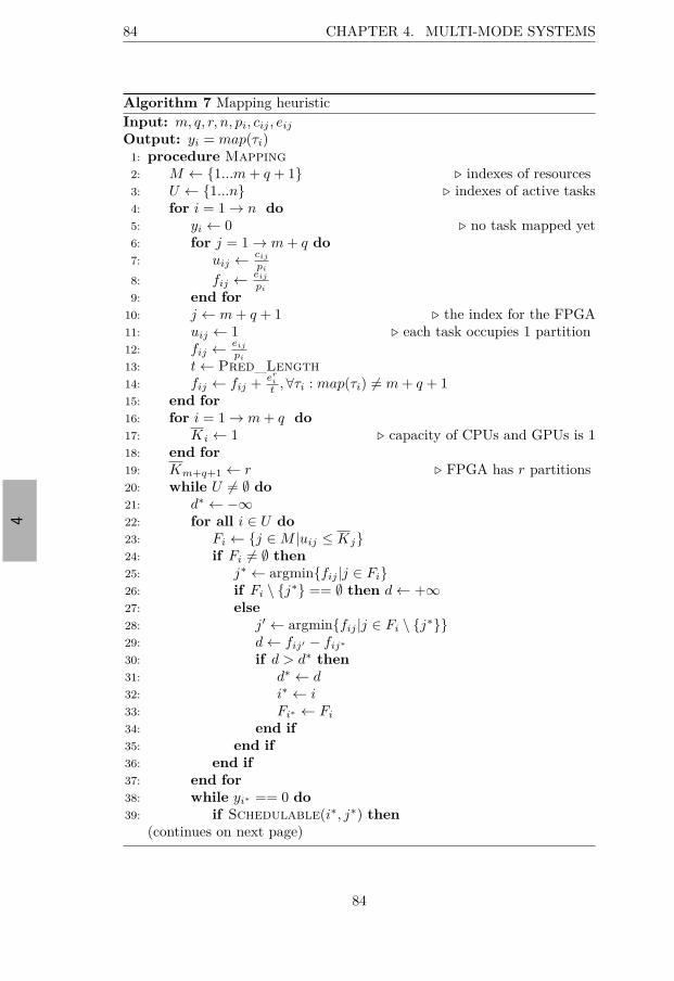
“thesis” — 2015/8/12 — 12:54 — page 84 — #104

4


Algorithm 7 Mapping heuristicInput: m, q, r, n, pi, cij , eij

Output: yi = map(τi)1: procedure Mapping

2: M ← 1...m + q + 1 ⊲ indexes of resources3: U ← 1...n ⊲ indexes of active tasks4: for i = 1 → n do

5: yi ← 0 ⊲ no task mapped yet6: for j = 1 → m + q do

7: uij ← cij

pi

8: fij ← eij

pi

9: end for

10: j ← m + q + 1 ⊲ the index for the FPGA11: uij ← 1 ⊲ each task occupies 1 partition12: fij ← eij

pi

13: t ← Pred_Length

14: fij ← fij +er

i

t, ∀τi : map(τi) Ó= m + q + 1

15: end for

16: for i = 1 → m + q do

17: Ki ← 1 ⊲ capacity of CPUs and GPUs is 118: end for

19: Km+q+1 ← r ⊲ FPGA has r partitions20: while U Ó= ∅ do

21: d∗ ← −∞22: for all i ∈ U do

23: Fi ← j ∈ M |uij ≤ Kj24: if Fi Ó= ∅ then

25: j∗ ← argminfij |j ∈ Fi26: if Fi \ j∗ == ∅ then d ← +∞27: else

28: j′ ← argminfij |j ∈ Fi \ j∗29: d ← fij′ − fij∗

30: if d > d∗ then

31: d∗ ← d32: i∗ ← i33: Fi∗ ← Fi

34: end if

35: end if

36: end if

37: end for

38: while yi∗ == 0 do

39: if Schedulable(i∗, j∗) then


84

“thesis” — 2015/8/12 — 12:54 — page 85 — #105

4


(continued from previous page)40: yi∗ ← j∗

41: Kj∗ ← Kj∗ − ui∗j∗

42: U ← U \ i∗43: else ⊲ τi∗ can’t be scheduled on resource j∗

44: Fi∗ ← Fi∗ \ j∗45: if Fi∗ == ∅ then ⊲ no more resources46: break47: else ⊲ pick next best resource48: j∗ ← argminfi∗j |j ∈ Fi∗49: end if

50: end if

51: end while

52: end while

53: end procedure

between the smallest and the second smallest fi∗j , j = 1, 2, ..., m+q+1 (lines22-37). Intuitively, we want to find that task which, if it is not mapped onits most desirable resource, will generate the biggest penalty in terms of en-ergy consumption. Once task τi∗ was identified, we need to decide where tomap it (considering the schedulability constraints). We try to map the taskto resource j∗ for which fi∗j∗ is minimum (lines 39-42). If the schedulingconstraint for resource j∗ is violated (considering the tasks mapped to it sofar), we try to map τi∗ to the resource j∗ for which fi∗j∗ is the next smallest(lines 43-50). We continue until we manage to map τi∗ to a resource (fulfill-ing the scheduling constraints), or until all resources have been consideredand no feasible mapping for τi∗ has been found (line 46). In the latter casetask τi∗ will not be allowed to become active (i.e. release jobs). Thus, forcertain modes, the resource manager will decide not to admit certain newtasks in order to guarantee the timing constraints of all the other tasks. InSection 4.6 we will evaluate how well our heuristic performs from this pointof view, i.e. how many tasks are rejected compared to the ideal case.

The function Schedulable presented in Algorithm 8 checks the schedu-lability conditions. In particular, given a certain partial mapping specifiedby map(τk), the function tries to see if it is possible to map task τi toresource j without violating any of the constraints. There are three cases:

1. If resource j is a CPU, then we only need to check the necessary andsufficient condition specified by inequation (4.3), which ensures thatthe processor is not overloaded. This is done in line 3.

2. If resource j is a GPU, then we first need to check that the GPU isnot overloaded (line 9), corresponding to inequation (4.4). On top ofthis, we need to make sure that by mapping task τi to GPU j, thedeadlines of all the tasks mapped to the same GPU are still met (lines

85

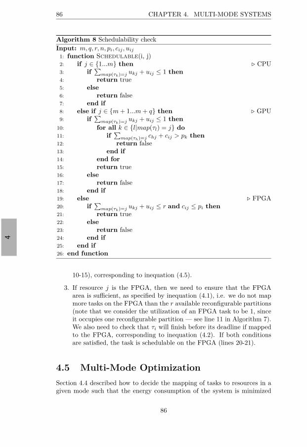
“thesis” — 2015/8/12 — 12:54 — page 86 — #106

4


Algorithm 8 Schedulability checkInput: m, q, r, n, pi, cij , uij

1: function Schedulable(i, j)2: if j ∈ 1...m then ⊲ CPU3: if

∑map(τk)=j ukj + uij ≤ 1 then

4: return true5: else

6: return false7: end if

8: else if j ∈ m + 1...m + q then ⊲ GPU9: if

∑map(τk)=j ukj + uij ≤ 1 then

10: for all k ∈ l|map(τl) = j do

11: if∑

map(τh)=j chj + cij > pk then


14: end for



19: else ⊲ FPGA20: if

∑map(τk)=j ukj + uij ≤ r and cij ≤ pi then



25: end if

26: end function

10-15), corresponding to inequation (4.5).

3. If resource j is the FPGA, then we need to ensure that the FPGAarea is sufficient, as specified by inequation (4.1), i.e. we do not mapmore tasks on the FPGA than the r available reconfigurable partitions(note that we consider the utilization of an FPGA task to be 1, sinceit occupies one reconfigurable partition — see line 11 in Algorithm 7).We also need to check that τi will finish before its deadline if mappedto the FPGA, corresponding to inequation (4.2). If both conditionsare satisfied, the task is schedulable on the FPGA (lines 20-21).

4.5 Multi-Mode Optimization

Section 4.4 described how to decide the mapping of tasks to resources in agiven mode such that the energy consumption of the system is minimized

86

“thesis” — 2015/8/12 — 12:54 — page 87 — #107

4

4.5. MULTI-MODE OPTIMIZATION 87

and all timing constraints are satisfied. However, our ultimate goal is tominimize the energy consumption of the system during its lifetime. Next wepresent the run-time strategy to achieve our goal.

4.5.1 Caching of Solutions

Since finding the solution for a particular mode is a time- and energy-consuming optimization, we try to minimize the number of times the map-ping algorithm is run. As a result, we decided to apply caching of solutions.Every time the solution for a particular mode is obtained, it is saved in acache. If the same mode5 is visited again later, a mapping solution might re-side in the cache and the resource manager could immediately use it. Whenthe cache is full, we use the least frequently used replacement policy tochoose the solution that will be replaced.

In case no cached solution for the current mode exists, we return thesolution (if present in the cache) for the most recently used super-mode(whose task set is a superset of the current active task set). If the differencebetween the size of this superset and the size of the current mode’s task setis smaller than a threshold6 tr, then we adapt the solution to the currentmode by ignoring the tasks that are not anymore active.

4.5.2 Estimating the Mode Duration

As we discussed previously, it is desirable to estimate how long a certainmode will be resident (referred to as the residence time). We use this infor-mation to compute the desirability factors fij for the heuristic (see line 14in Algorithm 7).

We use timestamps to estimate the residence time to of a mode o at run-time. We assume that the residence time of a mode is similar to its residencetimes in the recent past. Let to denote the current measured residence timeof mode o. We update the estimate to for the average residence time overthe past mode occurrences using an exponential smoothing formula in orderto emphasize the recent history:

to = αto + (1 − α)to (4.13)

This is the value returned by the function Pred_Length on line 13 fromAlgorithm 7.

4.5.3 Run-Time Policies

We describe next two possible run-time policies for the resource manager.

5Recall that a mode is defined by the active task set.6We obtained good experimental results for tr ∈ [3, 5].

87

“thesis” — 2015/8/12 — 12:54 — page 88 — #108

4


4.5.3.1 Heuristic + ILP

In case it is feasible to run the ILP on the platform assumed7, then thefollowing procedure can be applied. At the beginning of every new mode,the cache is checked. If a solution for the current mode is found, then it isapplied. Otherwise, if there exists in the cache a solution for a super-mode(whose task set size differs from the current mode’s task set size within athreshold tr), then that solution is adapted to the current mode (as ex-plained in Section 4.5.1). If no solution is found in the cache, the fast map-ping heuristic is applied first. If a feasible solution is obtained, the modestarts running as soon as the mapping is enforced (during the set-up time).Otherwise, it means that some tasks could not be mapped such that all thedeadlines are met; those tasks will not receive permission to activate fromthe resource manager. Once the heuristic is done, the manager will startrunning the ILP. The exact solution, if found, will be cached and used later,the next time the mode activates. If the ILP fails to find a solution it meansthat the mode is not feasible and it will be marked as such. In case a newmode arrives before the ILP has finished and we need to run the mappingoptimization for the new mode, the execution of the ILP is interrupted.

4.5.3.2 Heuristic-Only

If it is impossible to run the ILP on-the-fly, then we propose to always usethe heuristic to decide the mapping of tasks to resources. Of course, cachingcan still be applied to save the energy consumption overhead of re-runningthe heuristic. As we will show in the experimental evaluation, good resultsare still obtained and the number of rejected tasks stays within reasonablelimits.

4.6 Experimental Evaluation

We performed simulation experiments in order to evaluate how our poli-cies for on-line resource management behave. First of all, we performedmeasurements on real platforms (with an actual CPU, GPU, and FPGA).Based on the results obtained for execution time and energy consumption,we generated experimental settings whose parameters had similar ranges.

4.6.1 Real-Life Measurements

We selected the Samsung Exynos Dual Arndale platform (popular in theindustry) running at 5 volts. The board contains two Cortex A15 CPU coresrunning at 1.7 GHz and a Mali T604 GPU with 4 cores running at 533 MHz.We selected 6 applications: convolution, Rijndael (AES), pattern matching,

7Note that it is not necessary to run the ILP on the platform itself. Since the ILP isrun only seldom, one might imagine that this optimization happens in the cloud.

88

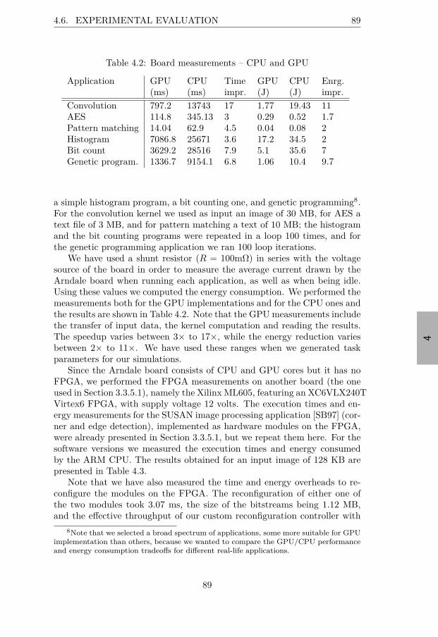
“thesis” — 2015/8/12 — 12:54 — page 89 — #109

4

4.6. EXPERIMENTAL EVALUATION 89

Table 4.2: Board measurements – CPU and GPU

Application GPU CPU Time GPU CPU Enrg.(ms) (ms) impr. (J) (J) impr.

Convolution 797.2 13743 17 1.77 19.43 11AES 114.8 345.13 3 0.29 0.52 1.7Pattern matching 14.04 62.9 4.5 0.04 0.08 2Histogram 7086.8 25671 3.6 17.2 34.5 2Bit count 3629.2 28516 7.9 5.1 35.6 7Genetic program. 1336.7 9154.1 6.8 1.06 10.4 9.7

a simple histogram program, a bit counting one, and genetic programming8.For the convolution kernel we used as input an image of 30 MB, for AES atext file of 3 MB, and for pattern matching a text of 10 MB; the histogramand the bit counting programs were repeated in a loop 100 times, and forthe genetic programming application we ran 100 loop iterations.

We have used a shunt resistor (R = 100mΩ) in series with the voltagesource of the board in order to measure the average current drawn by theArndale board when running each application, as well as when being idle.Using these values we computed the energy consumption. We performed themeasurements both for the GPU implementations and for the CPU ones andthe results are shown in Table 4.2. Note that the GPU measurements includethe transfer of input data, the kernel computation and reading the results.The speedup varies between 3× to 17×, while the energy reduction variesbetween 2× to 11×. We have used these ranges when we generated taskparameters for our simulations.

Since the Arndale board consists of CPU and GPU cores but it has noFPGA, we performed the FPGA measurements on another board (the oneused in Section 3.3.5.1), namely the Xilinx ML605, featuring an XC6VLX240TVirtex6 FPGA, with supply voltage 12 volts. The execution times and en-ergy measurements for the SUSAN image processing application [SB97] (cor-ner and edge detection), implemented as hardware modules on the FPGA,were already presented in Section 3.3.5.1, but we repeat them here. For thesoftware versions we measured the execution times and energy consumedby the ARM CPU. The results obtained for an input image of 128 KB arepresented in Table 4.3.

Note that we have also measured the time and energy overheads to re-configure the modules on the FPGA. The reconfiguration of either one ofthe two modules took 3.07 ms, the size of the bitstreams being 1.12 MB,and the effective throughput of our custom reconfiguration controller with

8Note that we selected a broad spectrum of applications, some more suitable for GPUimplementation than others, because we wanted to compare the GPU/CPU performanceand energy consumption tradeoffs for different real-life applications.

89

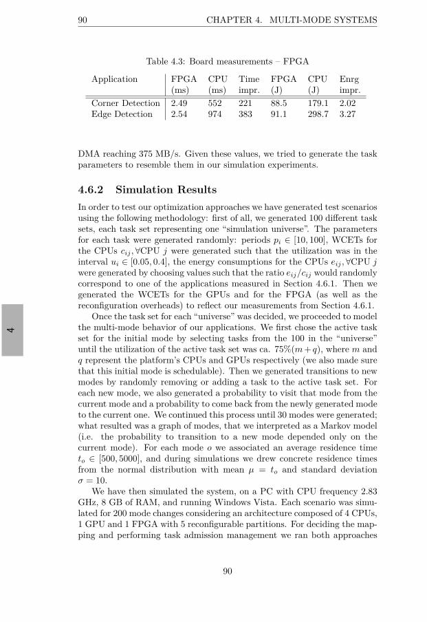
“thesis” — 2015/8/12 — 12:54 — page 90 — #110

4


Table 4.3: Board measurements – FPGA

Application FPGA CPU Time FPGA CPU Enrg(ms) (ms) impr. (J) (J) impr.

Corner Detection 2.49 552 221 88.5 179.1 2.02Edge Detection 2.54 974 383 91.1 298.7 3.27

DMA reaching 375 MB/s. Given these values, we tried to generate the taskparameters to resemble them in our simulation experiments.

4.6.2 Simulation Results

In order to test our optimization approaches we have generated test scenariosusing the following methodology: first of all, we generated 100 different tasksets, each task set representing one “simulation universe”. The parametersfor each task were generated randomly: periods pi ∈ [10, 100], WCETs forthe CPUs cij , ∀CPU j were generated such that the utilization was in theinterval ui ∈ [0.05, 0.4], the energy consumptions for the CPUs eij , ∀CPU jwere generated by choosing values such that the ratio eij/cij would randomlycorrespond to one of the applications measured in Section 4.6.1. Then wegenerated the WCETs for the GPUs and for the FPGA (as well as thereconfiguration overheads) to reflect our measurements from Section 4.6.1.

Once the task set for each “universe” was decided, we proceeded to modelthe multi-mode behavior of our applications. We first chose the active taskset for the initial mode by selecting tasks from the 100 in the “universe”until the utilization of the active task set was ca. 75%(m + q), where m andq represent the platform’s CPUs and GPUs respectively (we also made surethat this initial mode is schedulable). Then we generated transitions to newmodes by randomly removing or adding a task to the active task set. Foreach new mode, we also generated a probability to visit that mode from thecurrent mode and a probability to come back from the newly generated modeto the current one. We continued this process until 30 modes were generated;what resulted was a graph of modes, that we interpreted as a Markov model(i.e. the probability to transition to a new mode depended only on thecurrent mode). For each mode o we associated an average residence timeto ∈ [500, 5000], and during simulations we drew concrete residence timesfrom the normal distribution with mean µ = to and standard deviationσ = 10.

We have then simulated the system, on a PC with CPU frequency 2.83GHz, 8 GB of RAM, and running Windows Vista. Each scenario was simu-lated for 200 mode changes considering an architecture composed of 4 CPUs,1 GPU and 1 FPGA with 5 reconfigurable partitions. For deciding the map-ping and performing task admission management we ran both approaches

90

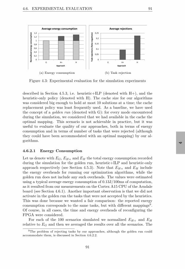
“thesis” — 2015/8/12 — 12:54 — page 91 — #111

4

4.6. EXPERIMENTAL EVALUATION 91

(a) Energy consumption

(b) Task rejection

Figure 4.3: Experimental evaluation for the simulation experiments

described in Section 4.5.3, i.e. heuristic+ILP (denoted with H+), and theheuristic-only policy (denoted with H). The cache size for our algorithmswas considered big enough to hold at most 10 solutions at a time; the cachereplacement policy was least frequently used. As a baseline, we have usedthe concept of a golden run (denoted with G): for every mode encounteredduring the simulation, we considered that we had available in the cache theoptimal mapping. This scenario is not achievable in practice, but it wasuseful to evaluate the quality of our approaches, both in terms of energyconsumption and in terms of number of tasks that were rejected (althoughthey could have been accommodated with an optimal mapping) by our al-gorithms.

4.6.2.1 Energy Consumption

Let us denote with EG, EH+ and EH the total energy consumption recordedduring the simulation for the golden run, heuristic+ILP and heuristic-onlyapproach respectively (see Section 4.5.3). Note that EH+ and EH includethe energy overheads for running our optimization algorithms, while thegolden run does not include any such overheads. The values were estimatedusing a typical average energy consumption of 0.13J/100ms of computation,as it resulted from our measurements on the Cortex A15 CPU of the Arndaleboard (see Section 4.6.1). Another important observation is that we did notactivate in the golden run the tasks that were not accepted by the heuristics.This was done because we wanted a fair comparison: the reported energyconsumption corresponds to the same tasks, but with different mappings9.Of course, in all cases, the time and energy overheads of reconfiguring theFPGA were considered.

For each of the 100 scenarios simulated we normalized EH+ and EH

relative to EG and then we averaged the results over all the scenarios. The

9The problem of rejecting tasks by our approaches, although the golden run couldaccommodate them, is discussed in Section 4.6.2.2.

91

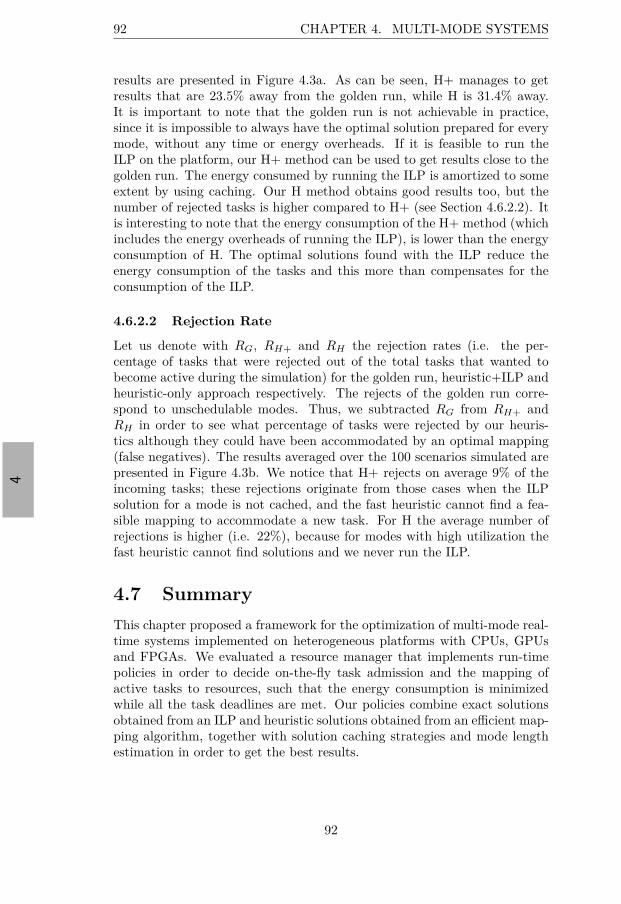
“thesis” — 2015/8/12 — 12:54 — page 92 — #112

4


results are presented in Figure 4.3a. As can be seen, H+ manages to getresults that are 23.5% away from the golden run, while H is 31.4% away.It is important to note that the golden run is not achievable in practice,since it is impossible to always have the optimal solution prepared for everymode, without any time or energy overheads. If it is feasible to run theILP on the platform, our H+ method can be used to get results close to thegolden run. The energy consumed by running the ILP is amortized to someextent by using caching. Our H method obtains good results too, but thenumber of rejected tasks is higher compared to H+ (see Section 4.6.2.2). Itis interesting to note that the energy consumption of the H+ method (whichincludes the energy overheads of running the ILP), is lower than the energyconsumption of H. The optimal solutions found with the ILP reduce theenergy consumption of the tasks and this more than compensates for theconsumption of the ILP.

4.6.2.2 Rejection Rate

Let us denote with RG, RH+ and RH the rejection rates (i.e. the per-centage of tasks that were rejected out of the total tasks that wanted tobecome active during the simulation) for the golden run, heuristic+ILP andheuristic-only approach respectively. The rejects of the golden run corre-spond to unschedulable modes. Thus, we subtracted RG from RH+ andRH in order to see what percentage of tasks were rejected by our heuris-tics although they could have been accommodated by an optimal mapping(false negatives). The results averaged over the 100 scenarios simulated arepresented in Figure 4.3b. We notice that H+ rejects on average 9% of theincoming tasks; these rejections originate from those cases when the ILPsolution for a mode is not cached, and the fast heuristic cannot find a fea-sible mapping to accommodate a new task. For H the average number ofrejections is higher (i.e. 22%), because for modes with high utilization thefast heuristic cannot find solutions and we never run the ILP.

4.7 Summary

This chapter proposed a framework for the optimization of multi-mode real-time systems implemented on heterogeneous platforms with CPUs, GPUsand FPGAs. We evaluated a resource manager that implements run-timepolicies in order to decide on-the-fly task admission and the mapping ofactive tasks to resources, such that the energy consumption is minimizedwhile all the task deadlines are met. Our policies combine exact solutionsobtained from an ILP and heuristic solutions obtained from an efficient map-ping algorithm, together with solution caching strategies and mode lengthestimation in order to get the best results.

92

“thesis” — 2015/8/12 — 12:54 — page 93 — #113

5

Chapter 5

!"#$!"%&'()*$!"% +,*-.-/!*-(0

() 1""(" 2%*%3*-(0 4.,5%.%0*!*-(0

Safety-critical systems need to function correctly even in the presenceof faults. To provide resiliency against transient faults, efficient error de-

tection and recovery techniques have to be employed. Unfortunately, thesemechanisms incur high penalties, either from the cost perspective, or fromthe performance point of view. Since both cost and performance are impor-tant issues for today’s embedded systems, this chapter presents system-levelapproaches to optimize the hardware/software implementation of error de-tection in the context of fault-tolerant real-time embedded systems.

The remainder of this chapter is organized as follows. We start bypresenting in Section 5.1 the preliminaries related to the error detectiontechniques assumed in our work. Section 5.2 presents two approaches tominimize the global worst-case schedule length of a distributed application,while meeting the imposed hardware cost constraints and tolerating mul-tiple transient faults. Both statically reconfigurable FPGAs and partiallydynamically reconfigurable FPGAs are considered. Section 5.3 discusses anapproach to minimize the average execution time of an application by op-timizing the hardware/software implementation of error detection. Finally,Section 5.4 summarizes the contributions of this chapter.

5.1 Preliminaries: Error Detection Technique

We next present the application-aware error detection technique that weuse in this chapter. The idea of this technique ([PKI11], [LCP+09]) is toidentify, based on specific metrics [PKI05], critical variables in a program. Acritical variable is defined as “a program variable exhibiting high sensitivityto random data errors” [PKI11]. The backward program slice for each acycliccontrol path is extracted for the identified critical variables. The backwardprogram slice is defined as “the set of all program statements/instructions

93

“thesis” — 2015/8/12 — 12:54 — page 94 — #114

5

94 CHAPTER 5. FAULT-TOLERANT SYSTEMS

y = read_int();

p = y;

r = -y;

s = y mod 3;

t = s*y;

if (s == 0)

u = p - r;

v = y + t;

u = 2*p + r;

v = y - t;

x = s*y + u - v;

path = 1; path = 2;

if (path == 1)

x' = y'; x' = 2*s'*y';

use x;

if (x == x')

flag error and

recover!

then

then

else

else

then else

Figure 5.1: Code fragment with error detectors

that can affect the value of the variable at a program location” [PKI11].Each slice is optimized at compile time, resulting in a series of checkingexpressions. Since the backward program slices run across basic blocks,the optimizations performed cannot be done by regular compilers. Theslices do not contain any conditional statements (they consist of straight-linecode); thus, aggressive optimization is possible. The checking expressionsare inserted in the original code before the use of a critical variable. Finally,the original program is instrumented with instructions to keep track of thecontrol paths followed at run-time and with checking instructions to choosethe corresponding checking expression and, then, compare the results.

We present an example of how this error detection technique works. Weuse the C program in Figure 5.1 (adapted from [PKI11]). The original pro-gram code is presented on the left (no shading), the checking code added ispresented on the right (light shading) and the path tracking instrumentationis shown with dark shading. Assuming that x is a critical variable, it needsto be checked before its use.

We identify two paths in the program slice of x, corresponding to thetwo branches. To compute the corresponding backward program slices, westart with the instruction computing the critical variable (x) and traversethe program backward, placing in each slice the instructions that can affectthe value of x. The resulting slices are:

• for the first path (if s = 0):

y = read_int();

94

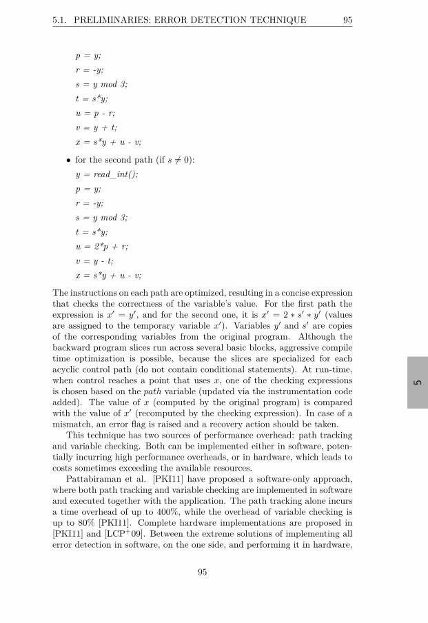
“thesis” — 2015/8/12 — 12:54 — page 95 — #115

5

5.1. PRELIMINARIES: ERROR DETECTION TECHNIQUE 95

p = y;

r = -y;

s = y mod 3;

t = s*y;

u = p - r;

v = y + t;

x = s*y + u - v;

• for the second path (if s Ó= 0):

y = read_int();

p = y;

r = -y;

s = y mod 3;

t = s*y;

u = 2*p + r;

v = y - t;

x = s*y + u - v;

The instructions on each path are optimized, resulting in a concise expressionthat checks the correctness of the variable’s value. For the first path theexpression is x′ = y′, and for the second one, it is x′ = 2 ∗ s′ ∗ y′ (valuesare assigned to the temporary variable x′). Variables y′ and s′ are copiesof the corresponding variables from the original program. Although thebackward program slices run across several basic blocks, aggressive compiletime optimization is possible, because the slices are specialized for eachacyclic control path (do not contain conditional statements). At run-time,when control reaches a point that uses x, one of the checking expressionsis chosen based on the path variable (updated via the instrumentation codeadded). The value of x (computed by the original program) is comparedwith the value of x′ (recomputed by the checking expression). In case of amismatch, an error flag is raised and a recovery action should be taken.

This technique has two sources of performance overhead: path trackingand variable checking. Both can be implemented either in software, poten-tially incurring high performance overheads, or in hardware, which leads tocosts sometimes exceeding the available resources.

Pattabiraman et al. [PKI11] have proposed a software-only approach,where both path tracking and variable checking are implemented in softwareand executed together with the application. The path tracking alone incursa time overhead of up to 400%, while the overhead of variable checking isup to 80% [PKI11]. Complete hardware implementations are proposed in[PKI11] and [LCP+09]. Between the extreme solutions of implementing allerror detection in software, on the one side, and performing it in hardware,

95

“thesis” — 2015/8/12 — 12:54 — page 96 — #116

5


on the other side, there is a wide range of alternatives characterized by theimplementation decision taken for each task in the application. This decisiondepends on various factors: time criticality, amount and cost of availablehardware resources and their nature (FPGAs with static or partial dynamicreconfiguration). We focus on efficiently implementing error detection in thecontext mentioned above.

The error detection technique described above detects any transient er-rors that corrupt the architectural state, provided that they corrupt one ormore variables in the backward slice of a critical variable. To achieve maxi-mal error coverage, we assume that some complementary, generic error de-tection techniques (like a watchdog processor and/or error-correcting codes)are used in conjunction with the application-aware one. Hardware redun-dancy techniques might also be used to deal with the remaining, not covered,faults [BMR+08]. We concentrate on the optimization of the application-aware error detection component.

5.2 Real-Time Distributed Embedded Systems

In this section we focus on the hardware/software implementation of theapplication-aware error detection components for a safety-critical applica-tion implemented on a distributed embedded platform. We present ap-proaches to the optimization of error detection implementation in a system-level design context, minimizing the global worst-case schedule length, whilemeeting the imposed hardware cost constraints.

Our fault model assumes that a maximum number k of transient faultscan affect the system during one period. To provide resiliency against thesefaults re-execution is used. Once a fault is detected, the initial state is re-stored and the task is re-executed. We will use the scheduling techniquepresented in [IPEP06], which considers error detection as a black box. Theauthors proposed to generate fault-tolerant schedules for hard real-time sys-tems such that multiple transient faults are tolerated. The algorithm pro-duces, as output, schedule tables that capture alternative execution scenar-ios corresponding to possible fault occurrences. Among all fault scenarios,one corresponds to the worst-case schedule length (WCSL). We are inter-ested in minimizing this WCSL by accelerating error detection in reconfig-urable hardware, so that we meet the time and cost constraints imposed.

5.2.1 Optimization Framework

Figure 5.2 illustrates our framework. The applications, available as C code,are represented as a set of task graphs. The code is processed throughthe error detection instrumentation framework [LCP+09], which outputsthe initial code with the embedded error detectors, as well as VHDL codeneeded to synthesize error detector modules on FPGA.

96

“thesis” — 2015/8/12 — 12:54 — page 97 — #117

5

5.2. REAL-TIME DISTRIBUTED EMBEDDED SYSTEMS 97

C code

Error detection

instrumentation and

overheads estimation

Process

graphs

Optimization of

error detection

implementation

Fault-tolerant

schedule

synthesis

Overheads

Mapping

WC

SL

(c

ost

fu

nct

ion)

HW Archi-

tecture

Figure 5.2: Optimization framework overview

P4

P1

P2

m24

P3 i)

(a)

N1

comm. ctrl.

N2

comm. ctrl.

FPGA1 FPGA2

Bus

ii)

Memory

(b)

Figure 5.3: System model for fault-tolerant distributed embedded systems

This information, together with the system architecture and the mappingof tasks to computation nodes, is used by the optimization tool to find aclose to optimal error detection implementation (EDI). The cost function isthe WCSL generated by the fault-tolerant schedule synthesis tool [IPEP06].

5.2.2 System Model

We consider a set of real-time applications Ai, modeled as directed acyclicgraphs Gi(Vi, Ei), executed with period Ti. The graphs Gi are merged intoa single graph G(V, E), having the period T equal with the least commonmultiple of all Ti. Each vertex Pj ∈ V represents a task, and each edge ejk ∈E indicates that Pj ’s output is Pk’s input. Tasks are non-preemptable andall data dependencies have to be satisfied before a task can start executing.

We assume a distributed architecture composed of computation nodes,connected to a bus (see Figure 5.3b). The task mapping to these nodes isgiven (illustrated with shading in Figure 5.3a). The bus is assumed to befault-tolerant (we use a protocol such as TTP [KB03]). Each node consistsof a central processing unit, a communication controller, a memory subsys-tem, and a reconfigurable device (FPGA). Since SRAM-based FPGAs aresusceptible to single event upsets [WJR+03], we assume that suitable miti-gation techniques are employed (e.g. [LCR03], [NOS14]) in order to provide

97

“thesis” — 2015/8/12 — 12:54 — page 98 — #118

5


sufficient reliability of the hardware used for error detection.For each task we consider three alternative error detection implementa-

tions (EDIs):

1. SW-only, when the checking code (light shading in Figure 5.1) andthe path tracking instrumentation (dark shading in Figure 5.1) areimplemented in software and interleaved with application code.

2. mixed-HW/SW, when the path tracking is moved to hardware anddone concurrently with the application’s execution, while the check-ing expressions remain in software, interleaved with the initial code.This is a reasonable refinement, since the path tracking’s overhead issignificant.

3. HW-only, which further reduces the time overhead by also moving theexecution of the checking expressions to hardware.

For each task Pi and each of the three possible EDIs, we know the worst-case execution time WCET

i [WEE+08], the corresponding HW area hi ,

and reconfiguration time ρi needed to implement error detection ( ∈ SW-

only, mixed-HW/SW, HW-only).For all messages sent over the bus, their worst-case transmission time

WCTTij is given. This transmission is modeled as a communication taskinserted on the edge Pi → Pj (see m24 in Figure 5.3a). For tasks mappedon the same node, the communication time is considered to be part of thetask’s WCET and is not modeled explicitly.


Input

• A set of applications Ai modeled together as a task graph G(V, E) (seeSection 5.2.2).

• The WCETs for each alternative EDI of every task Pi ∈ V, given byW : V × H → Z

+, where H = SW-only, mixed-HW/SW, HW-only.

• The hardware costs for each alternative EDI of every task Pi ∈ V, givenby C : V×H → Z

+×Z+, i.e. we know the size (hi = rowsi×columnsi)

of the rectangle needed on FPGA1.

• The reconfiguration time (ρi) for each alternative EDI of every taskPi ∈ V, given by R : V × H → Z

+.

• The worst-case transmission time (WCTTij) for each message mij ,from Pi to Pj .

1Function C covers both 1D and 2D reconfiguration scenarios. Note also that, beingmore generic, these assumptions cover the ones used in the previous chapters.

98

“thesis” — 2015/8/12 — 12:54 — page 99 — #119

5


Table 5.1: Worst-case execution times and error detection overheads for themotivational example

Pi W CET Ui

Error Detection Implementation (EDI)SW-only mixed-HW/SW HW-only

W CETi hi ρi W CETi hi ρi W CETi hi ρi

P1 60 240 0 0 100 15 20 80 40 45P2 50 140 0 0 80 15 20 60 40 45P3 40 150 0 0 60 10 15 50 30 35P4 30 100 0 0 60 15 20 40 40 45

• The parameter k, denoting the number of transient faults to be tol-erated during one period, T . This k is used for the generation offault-tolerant schedules with the synthesis tool presented in [IPEP06].

• The set of computation nodes N connected by a bus B on which theapplication is implemented. For each Nj ∈ N , the available hardwarearea (HWj = rowsj × columnsj) which we can use to implement theerror detection is known.

• The mapping of tasks to computation nodes, given by M : V → N .

Output

• An EDI assignment S : V → H, such that k transient faults aretolerated and the worst-case schedule length (WCSL) is minimal, whilethe hardware cost constraints are met.

5.2.4 Motivational Examples

Figure 5.3a presents an application with four tasks, P1 − P4, mapped on anarchitecture with two computation nodes, N1 and N2, connected by a bus(Figure 5.3b). Tasks P1 and P2 are mapped on N1, while P3 and P4 aremapped on N2. The WCET of tasks for each of the three alternative EDIsare listed in Table 5.1. The WCET of the un-instrumented task (WCET U

i )is also given in Table 5.1, only to emphasize the error detection time over-heads. For example, the error detection overhead incurred by the SW-onlyEDI for P1 is 240 - 60 = 180 time units. The HW area (hi) and the re-configuration times (ρi) incurred by each EDI2, are also presented in Table5.1. The WCTT of messages is 20 time units. The recovery overhead for alltasks is 10 time units. Our application has to tolerate k = 1 fault within itsperiod.

2For simplicity we consider the 1D case here, but note that the model supports 2Dplacement and FPGA reconfiguration.

99

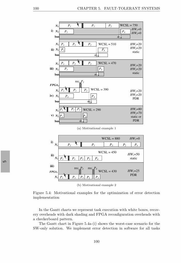
“thesis” — 2015/8/12 — 12:54 — page 100 — #120

5


N1

N2

bus

N1

N2

bus

N1

N2

bus

N1

N2

bus

N1

N2

bus

i)

ii)

iii)

iv)

v)

P1 P1 P2

P3 P4

P1 P2 P2

P1 P2 P2

P1 P1 P2

P1 P1 P2

P3 P4

P4

P4

P3 P4

m24

m24

m24

m24

m24

WCSL = 470

WCSL = 510

WCSL = 390

WCSL = 290

WCSL = 750

HW1=0

HW2=0

HW1=20

HW2=20

static

HW1=20

HW2=20

static

HW1=20

HW2=20

PDR

HW1=80

HW2=70

static or

PDR

P3

P3

rec. P2

FPGA1

(a) Motivational example 1

P1 P1 P2 P4

WCSL = 880 HW1=0

N1

i)

WCSL = 450 HW1=50

static N1

ii)

WCSL = 430 HW1=25

PDR N1

iii)

P1 P1 P2 P3 P4

P1 P1 P2 P3 P4

rec. P2 rec. P4

P3

FPGA1

(b) Motivational example 2

Figure 5.4: Motivational examples for the optimization of error detectionimplementation

In the Gantt charts we represent task execution with white boxes, recov-ery overheads with dark shading and FPGA reconfiguration overheads witha checkerboard pattern.

The Gantt chart in Figure 5.4a-(i) shows the worst-case scenario for theSW-only solution. We implement error detection in software for all tasks

100

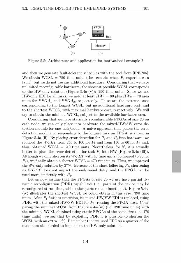
“thesis” — 2015/8/12 — 12:54 — page 101 — #121

5


P1

P2

P4

P3 iii)

(a)

iv)

Bus

N1

comm. ctrl.

FPGA1

Memory

(b)

Figure 5.5: Architecture and application for motivational example 2

and then we generate fault-tolerant schedules with the tool from [IPEP06].We obtain WCSL = 750 time units (the scenario when P1 experiences afault), but we do not use any additional hardware. Considering that we haveunlimited reconfigurable hardware, the shortest possible WCSL correspondsto the HW-only solution (Figure 5.4a-(v)): 290 time units. Since we useHW-only EDI for all tasks, we need at least HW1 = 80 plus HW2 = 70 areaunits for FPGA1 and FPGA2, respectively. These are the extreme casescorresponding to the longest WCSL, but no additional hardware cost, andto the shortest WCSL, with maximal hardware cost, respectively. We willtry to obtain the minimal WCSL, subject to the available hardware area.

Considering that we have statically reconfigurable FPGAs of size 20 oneach node, we can only place into hardware the mixed-HW/SW error de-tection module for one task/node. A naive approach that places the errordetection module corresponding to the longest task on FPGA, is shown inFigure 5.4a-(ii). By placing error detection for P1 and P3 into hardware, wereduced the WCET from 240 to 100 for P1 and from 150 to 60 for P3 and,thus, obtained WCSL = 510 time units. Nevertheless, for N2 it is actuallybetter to place the error detection for task P4 into HW (Figure 5.4a-(iii)).Although we only shorten its WCET with 40 time units (compared to 90 forP3), we finally obtain a shorter WCSL = 470 time units. Thus, we improvedthe SW-only solution by 37%. Because of the slack following P3, shorteningits WCET does not impact the end-to-end delay, and the FPGA can beused more efficiently with P4.

Let us now assume that the FPGAs of size 20 we use have partial dy-namic reconfiguration (PDR) capabilities (i.e. parts of the device may bereconfigured at run-time, while other parts remain functional). Figure 5.4a-(iv) illustrates the shortest WCSL we could obtain in this case: 390 timeunits. After P1 finishes execution, its mixed-HW/SW EDI is replaced, usingPDR, with the mixed-HW/SW EDI for P2, reusing the FPGA area. Com-paring the minimal WCSL from Figure 5.4a-(iv) (i.e. 390 time units) withthe minimal WCSL obtained using static FPGAs of the same size (i.e. 470time units), we see that by exploiting PDR it is possible to shorten theWCSL with an extra 17%. Remember that we used FPGAs a quarter of themaximum size needed to implement the HW-only solution.

101

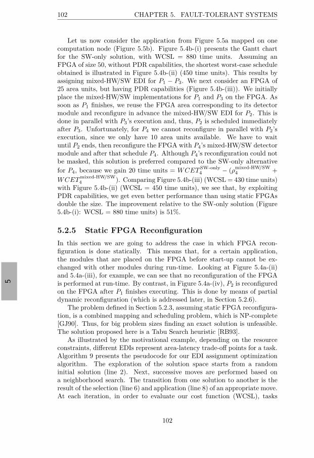
“thesis” — 2015/8/12 — 12:54 — page 102 — #122

5


Let us now consider the application from Figure 5.5a mapped on onecomputation node (Figure 5.5b). Figure 5.4b-(i) presents the Gantt chartfor the SW-only solution, with WCSL = 880 time units. Assuming anFPGA of size 50, without PDR capabilities, the shortest worst-case scheduleobtained is illustrated in Figure 5.4b-(ii) (450 time units). This results byassigning mixed-HW/SW EDI for P1 − P3. We next consider an FPGA of25 area units, but having PDR capabilities (Figure 5.4b-(iii)). We initiallyplace the mixed-HW/SW implementations for P1 and P3 on the FPGA. Assoon as P1 finishes, we reuse the FPGA area corresponding to its detectormodule and reconfigure in advance the mixed-HW/SW EDI for P2. This isdone in parallel with P3’s execution and, thus, P2 is scheduled immediatelyafter P3. Unfortunately, for P4 we cannot reconfigure in parallel with P2’sexecution, since we only have 10 area units available. We have to waituntil P2 ends, then reconfigure the FPGA with P4’s mixed-HW/SW detectormodule and after that schedule P4. Although P4’s reconfiguration could notbe masked, this solution is preferred compared to the SW-only alternativefor P4, because we gain 20 time units = WCET SW-only

4 − (ρmixed-HW/SW4 +

WCETmixed-HW/SW4 ). Comparing Figure 5.4b-(iii) (WCSL = 430 time units)

with Figure 5.4b-(ii) (WCSL = 450 time units), we see that, by exploitingPDR capabilities, we get even better performance than using static FPGAsdouble the size. The improvement relative to the SW-only solution (Figure5.4b-(i): WCSL = 880 time units) is 51%.

5.2.5 Static FPGA Reconfiguration

In this section we are going to address the case in which FPGA recon-figuration is done statically. This means that, for a certain application,the modules that are placed on the FPGA before start-up cannot be ex-changed with other modules during run-time. Looking at Figure 5.4a-(ii)and 5.4a-(iii), for example, we can see that no reconfiguration of the FPGAis performed at run-time. By contrast, in Figure 5.4a-(iv), P2 is reconfiguredon the FPGA after P1 finishes executing. This is done by means of partialdynamic reconfiguration (which is addressed later, in Section 5.2.6).

The problem defined in Section 5.2.3, assuming static FPGA reconfigura-tion, is a combined mapping and scheduling problem, which is NP-complete[GJ90]. Thus, for big problem sizes finding an exact solution is unfeasible.The solution proposed here is a Tabu Search heuristic [RB93].

As illustrated by the motivational example, depending on the resourceconstraints, different EDIs represent area-latency trade-off points for a task.Algorithm 9 presents the pseudocode for our EDI assignment optimizationalgorithm. The exploration of the solution space starts from a randominitial solution (line 2). Next, successive moves are performed based ona neighborhood search. The transition from one solution to another is theresult of the selection (line 6) and application (line 8) of an appropriate move.At each iteration, in order to evaluate our cost function (WCSL), tasks

102

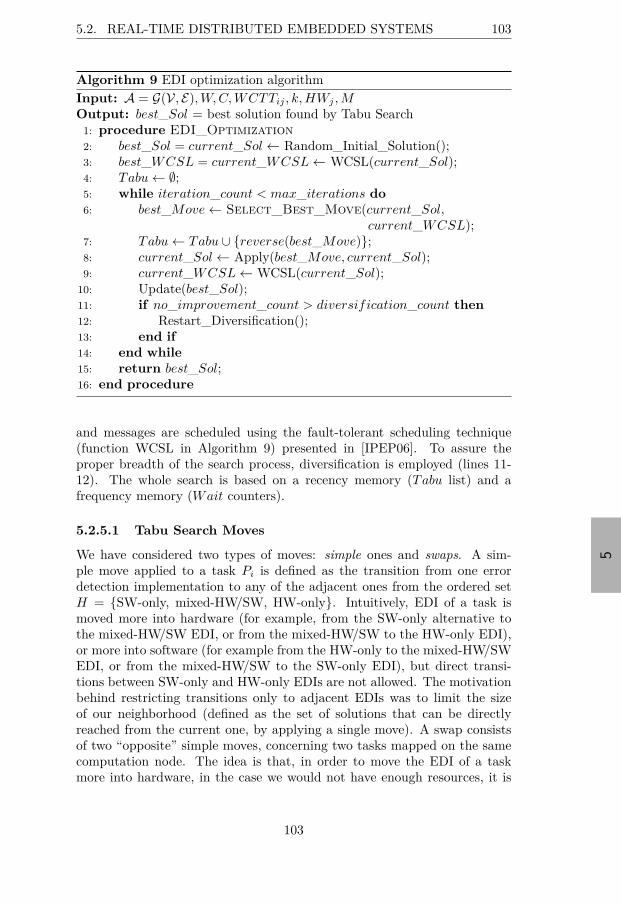
“thesis” — 2015/8/12 — 12:54 — page 103 — #123

5


Algorithm 9 EDI optimization algorithmInput: A = G(V, E), W, C, WCTTij , k, HWj , MOutput: best_Sol = best solution found by Tabu Search

1: procedure EDI_Optimization

2: best_Sol = current_Sol ← Random_Initial_Solution();3: best_WCSL = current_WCSL ← WCSL(current_Sol);4: Tabu ← ∅;5: while iteration_count < max_iterations do

6: best_Move ← Select_Best_Move(current_Sol,current_WCSL);

7: Tabu ← Tabu ∪ reverse(best_Move);8: current_Sol ← Apply(best_Move, current_Sol);9: current_WCSL ← WCSL(current_Sol);

10: Update(best_Sol);11: if no_improvement_count > diversification_count then

12: Restart_Diversification();13: end if

14: end while

15: return best_Sol;16: end procedure

and messages are scheduled using the fault-tolerant scheduling technique(function WCSL in Algorithm 9) presented in [IPEP06]. To assure theproper breadth of the search process, diversification is employed (lines 11-12). The whole search is based on a recency memory (Tabu list) and afrequency memory (Wait counters).

5.2.5.1 Tabu Search Moves

We have considered two types of moves: simple ones and swaps. A sim-ple move applied to a task Pi is defined as the transition from one errordetection implementation to any of the adjacent ones from the ordered setH = SW-only, mixed-HW/SW, HW-only. Intuitively, EDI of a task ismoved more into hardware (for example, from the SW-only alternative tothe mixed-HW/SW EDI, or from the mixed-HW/SW to the HW-only EDI),or more into software (for example from the HW-only to the mixed-HW/SWEDI, or from the mixed-HW/SW to the SW-only EDI), but direct transi-tions between SW-only and HW-only EDIs are not allowed. The motivationbehind restricting transitions only to adjacent EDIs was to limit the sizeof our neighborhood (defined as the set of solutions that can be directlyreached from the current one, by applying a single move). A swap consistsof two “opposite” simple moves, concerning two tasks mapped on the samecomputation node. The idea is that, in order to move the EDI of a taskmore into hardware, in the case we would not have enough resources, it is

103

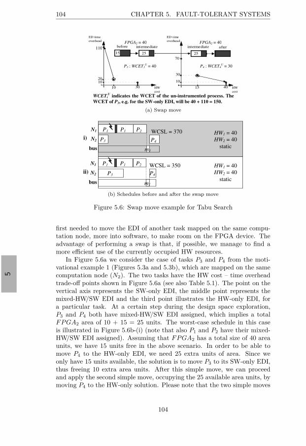
“thesis” — 2015/8/12 — 12:54 — page 104 — #124

5


WCETi

U indicates the WCET of the un-instrumented process. The

WCET of P3, e.g. for the SW-only EDI, will be 40 + 110 = 150.

120

ED time

overhead

HW

cost

2010

10 30

P3: WCETU

= 40

70

ED time

overhead

HW

cost

30

10

15 40

P4: WCETU

= 30

15 25

before intermediate

FPGA

25

intermediate after

FPGA

110

FPGA2 = 40 FPGA2 = 40

P3 : WCET3U = 40 P4 : WCET4

U = 30

(a) Swap move

N1

N2

bus

i)

N1

N2

bus

ii)

WCSL = 370 HW1 = 40

HW2 = 40

static

P1 P1 P2

P3

m1

P4

WCSL = 350 HW1 = 40

HW2 = 40

static

P1 P1 P2

m1

P4 P3

(b) Schedules before and after the swap move

Figure 5.6: Swap move example for Tabu Search

first needed to move the EDI of another task mapped on the same compu-tation node, more into software, to make room on the FPGA device. Theadvantage of performing a swap is that, if possible, we manage to find amore efficient use of the currently occupied HW resources.

In Figure 5.6a we consider the case of tasks P3 and P4 from the moti-vational example 1 (Figures 5.3a and 5.3b), which are mapped on the samecomputation node (N2). The two tasks have the HW cost – time overheadtrade-off points shown in Figure 5.6a (see also Table 5.1). The point on thevertical axis represents the SW-only EDI, the middle point represents themixed-HW/SW EDI and the third point illustrates the HW-only EDI, fora particular task. At a certain step during the design space exploration,P3 and P4 both have mixed-HW/SW EDI assigned, which implies a totalFPGA2 area of 10 + 15 = 25 units. The worst-case schedule in this caseis illustrated in Figure 5.6b-(i) (note that also P1 and P2 have their mixed-HW/SW EDI assigned). Assuming that FPGA2 has a total size of 40 areaunits, we have 15 units free in the above scenario. In order to be able tomove P4 to the HW-only EDI, we need 25 extra units of area. Since weonly have 15 units available, the solution is to move P3 to its SW-only EDI,thus freeing 10 extra area units. After this simple move, we can proceedand apply the second simple move, occupying the 25 available area units, bymoving P4 to the HW-only solution. Please note that the two simple moves

104

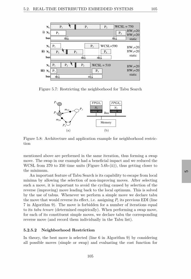
“thesis” — 2015/8/12 — 12:54 — page 105 — #125

5


N1

N2

bus

ii)

N1

N2

bus

iii)

P1 P1 P2

P4

m24

WCSL = 750

m32

N1

N2

bus

i) HW1=20

HW2=20

static

P1 P2 P2

P3 P4

m32 m24

WCSL = 510 HW1=20

HW2=20

static

P1 P2

P3 P3 P4

m32 m24

WCSL=590 HW1=20

HW2=20

static

P3

Figure 5.7: Restricting the neighborhood for Tabu Search

P4

P1

P2

m24

P3 m32

(a)

N1

comm. ctrl.

N2

comm. ctrl.

FPGA1 FPGA2

Bus

ii)

Memory

(b)

Figure 5.8: Architecture and application example for neighborhood restric-tion

mentioned above are performed in the same iteration, thus forming a swapmove. The swap in our example had a beneficial impact and we reduced theWCSL from 370 to 350 time units (Figure 5.6b-(ii)), thus getting closer tothe minimum.

An important feature of Tabu Search is its capability to escape from localminima by allowing the selection of non-improving moves. After selectingsuch a move, it is important to avoid the cycling caused by selection of thereverse (improving) move leading back to the local optimum. This is solvedby the use of tabus. Whenever we perform a simple move we declare tabuthe move that would reverse its effect, i.e. assigning Pi its previous EDI (line7 in Algorithm 9). The move is forbidden for a number of iterations equalto its tabu tenure (determined empirically). When performing a swap move,for each of its constituent simple moves, we declare tabu the correspondingreverse move (and record them individually in the Tabu list).

5.2.5.2 Neighborhood Restriction

In theory, the best move is selected (line 6 in Algorithm 9) by consideringall possible moves (simple or swap) and evaluating the cost function for

105

“thesis” — 2015/8/12 — 12:54 — page 106 — #126

5


Algorithm 10 Hierarchical neighborhood explorationInput: A = G(V, E), W, C, WCTTij , k, HWj , MOutput: trial_Move = best move found according to Section 5.2.5.3

1: function Select_Best_Move(current_Sol, current_WCSL)2: CP ← Select_CP_Tasks(current_Sol);3: trial_Move ← Try_Simple_Moves_into_HW(CP );4: if trial_Move exists then

5: return trial_Move;6: else

7: trial_Move ← Try_Swap_Moves(CP );8: trial_Sol ← Apply(trial_Move, current_Sol);9: trial_WCSL ← WCSL(trial_Sol);

10: if trial_WCSL < current_WCSL then

11: return trial_Move;12: else

13: WCP ← p ∈ CP | Wait(p) > waiting_count;14: trial_Move ← Diversifying_Non-improving_Moves(WCP );

15: return trial_Move;16: end if

17: end if

18: end function

each one. This, however, is inefficient from the computational point ofview. Therefore, in each iteration, the selection of the best move is done byexploring only a subset of the possible moves, namely the ones affecting thetasks on the critical path (CP) of the worst-case schedule for the currentsolution. In Figure 5.7 we consider the application from Figure 5.8a mappedon the architecture in Figure 5.8b, with static FPGAs of size 20. We showhow we move from the SW-only solution (Figure 5.7-(i): WCSL = 750) to thesolution in Figure 5.7-(iii) (WCSL = 510), passing through two consecutiveiterations. At each iteration, only the tasks on the CP (illustrated withdotted rectangles) are considered for new EDI assignment. From (i) to (ii),the best possible choice is to move P1 to its mixed-HW/SW EDI. As a result,the CP changes (as can be seen from Figure 5.7-(ii)) and, thus, in the nextiteration P3 will also be considered (while P1 is now excluded). The bestchoice is to move P3 to its mixed-HW/SW EDI. The result is shown in Figure5.7-(iii) (WCSL = 510).

5.2.5.3 Move Selection

Algorithm 10 presents our approach to selecting the best move in each it-eration (line 6, Algorithm 9). As explained earlier, we first determine theset of tasks on the critical path (CP) of the current solution (line 2). Next,based on this set, we proceed and search for the best move in a hierarchical

106

“thesis” — 2015/8/12 — 12:54 — page 107 — #127

5


manner (in order to reduce the number of evaluations of the cost function,done in each iteration). We first explore the simple moves into HW (line 3).If at least one such move exists and it is not tabu, then we select the movethat generates the best improvement and we stop further exploring the restof candidate moves (lines 4-5). Otherwise, we try to improve the currentWCSL by searching for the best swap move (line 7). If we get closer to aminimum (line 10), we accept the move (line 11). Otherwise, we diversifythe search (lines 13-15).

5.2.5.4 Diversification

In order to assure the proper breadth of the search process, we decided to em-ploy a continuous diversification strategy (lines 13-15, Algorithm 10), com-plemented by a restart diversification strategy (lines 11-12, Algorithm 9).The continuous diversification uses an intermediate-term frequency memory(Wait counters), where we record how many iterations a task has waitedsince the last time it was involved in a move. The Wait counters are resetwhenever a new minimal solution is reached. Whenever we need to escapelocal minimum points, the Wait memory is used to selectively filter candi-date moves (and generate the set WCP – line 13 in Algorithm 10). So, ifthe waiting counter of a task is greater than a threshold (waiting_count),we consider that the task has waited a long time and should be selectedfor diversification (it is included in WCP ). Our neighborhood explorationcontinues by selecting the non-improving move (simple or swap) that leadsto the solution with the lowest cost, giving priority to diversifying moves(line 14 in Algorithm 10).

We complemented our continuous diversification strategy with a restartdiversification. Whenever we do not get any improvement of the best knownsolution for more than a certain number, diversification_count, of itera-tions, we restart the search process (lines 11-12 in Algorithm 9). The searchis restarted from a state corresponding to an EDI assignment to tasks thathas not been visited, or has been visited rarely, during the previous searches.

The search process is stopped after a specified maximum number of it-erations (line 5 in Algorithm 9). This value (max_iterations), as wellas the counters used for diversification purposes (i.e. waiting_count anddiversification_count), and the length of the tabu list, were determinedempirically for each application size.

5.2.6 Partial Dynamic Reconfiguration

PDR enables the reuse of FPGA area corresponding to error detector mod-ules of tasks that finished executing. Task execution is overlapped withreconfiguration of other detector modules, in order to mask the reconfig-uration overhead. We reconfigure the detector modules on the FPGA asthey are needed, at run-time. In this way we accelerate error detection in

107

“thesis” — 2015/8/12 — 12:54 — page 108 — #128

5


hardware, while, at the same time, keeping system costs within reasonablelimits.

5.2.6.1 Revised System Model

We model our PDR FPGA as a matrix of configurable logic blocks (CLBs).Each EDI occupies a rectangular area of this matrix. The model allows2D or 1D placement and reconfiguration. The execution of an EDI canproceed in parallel with the reconfiguration of another EDI, but only onereconfiguration may be done at a time (i.e. we assume a single reconfigu-ration controller). If it is not possible to completely overlap reconfigurationwith useful computations, then task execution is scheduled as soon as thereconfiguration of its EDI ends. Figure 5.4b-(iii) illustrates this: for P2 theentire reconfiguration overhead was masked; Because of limited resources,this was not possible for P4, which had to wait for the reconfiguration of itsEDI module to finish.

5.2.6.2 Revised Problem Formulation

Under PDR assumptions, our problem formulation (Section 5.2.3) becomesmore complex. Besides generating the EDI assignment to tasks (S : V → H)we also need to generate a placement and a schedule for EDI reconfigurationson FPGA. For all tasks with error detection in HW (mixed-HW/SW or HW-only), we find the function:

R : p ∈ V | S(p) Ó= SW-only → Z+

which specifies the reconfiguration start time for the EDI modules, and theplacement function:

P : p ∈ V | S(p) Ó= SW-only → Z+ × Z

+

which specifies the position of the upper left corner of each EDI module onthe FPGA.

5.2.6.3 Revised Scheduler

We simultaneously schedule tasks on the processor and place their corre-sponding EDIs on the FPGA: once a task is selected for scheduling fromthe list of ready tasks, its EDI is placed onto the FPGA, as soon as enoughspace is available for it. Thus, the generated static schedules are correct byconstruction.

In order to take into account the issues presented above, we extendedthe fault-tolerant schedule synthesis tool from [IPEP06] (used in Section5.2.5). This tool is based on a list scheduling approach that uses a modi-fied partial critical path (PCP ) priority function [EDPP00] to decide theorder of task execution. Since this priority function does not capture the

108

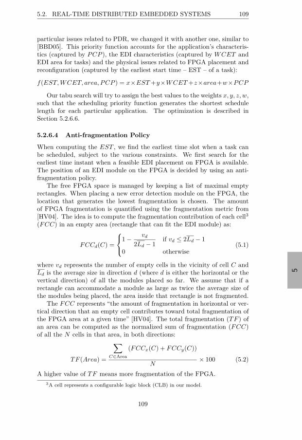
“thesis” — 2015/8/12 — 12:54 — page 109 — #129

5


particular issues related to PDR, we changed it with another one, similar to[BBD05]. This priority function accounts for the application’s characteris-tics (captured by PCP ), the EDI characteristics (captured by WCET andEDI area for tasks) and the physical issues related to FPGA placement andreconfiguration (captured by the earliest start time – EST – of a task):

f(EST, WCET, area, PCP ) = x×EST +y×WCET +z×area+w×PCP

Our tabu search will try to assign the best values to the weights x, y, z, w,such that the scheduling priority function generates the shortest schedulelength for each particular application. The optimization is described inSection 5.2.6.6.

5.2.6.4 Anti-fragmentation Policy

When computing the EST , we find the earliest time slot when a task canbe scheduled, subject to the various constraints. We first search for theearliest time instant when a feasible EDI placement on FPGA is available.The position of an EDI module on the FPGA is decided by using an anti-fragmentation policy.

The free FPGA space is managed by keeping a list of maximal emptyrectangles. When placing a new error detection module on the FPGA, thelocation that generates the lowest fragmentation is chosen. The amountof FPGA fragmentation is quantified using the fragmentation metric from[HV04]. The idea is to compute the fragmentation contribution of each cell3

(FCC) in an empty area (rectangle that can fit the EDI module) as:

FCCd(C) =

1 − vd

2Ld − 1if vd ≤ 2Ld − 1

0 otherwise(5.1)

where vd represents the number of empty cells in the vicinity of cell C andLd is the average size in direction d (where d is either the horizontal or thevertical direction) of all the modules placed so far. We assume that if arectangle can accommodate a module as large as twice the average size ofthe modules being placed, the area inside that rectangle is not fragmented.

The FCC represents “the amount of fragmentation in horizontal or ver-tical direction that an empty cell contributes toward total fragmentation ofthe FPGA area at a given time” [HV04]. The total fragmentation (TF ) ofan area can be computed as the normalized sum of fragmentation (FCC)of all the N cells in that area, in both directions:

TF (Area) =

∑

C∈Area

(FCCx(C) + FCCy(C))

N× 100 (5.2)

A higher value of TF means more fragmentation of the FPGA.3A cell represents a configurable logic block (CLB) in our model.

109

“thesis” — 2015/8/12 — 12:54 — page 110 — #130

5


M1

R2

R1

M2

(a)

M3

M2

(b)

M2

(c)

Figure 5.9: Using the fragmentation metric to place modules on the FPGAaccording to the anti-fragmentation policy

Whenever we choose a location for an error detection module, we calcu-late the TF of all maximal empty rectangles large enough to fit that module.We choose the rectangle with the highest TF , leaving less fragmented areason the FPGA for placement of future modules. Once a rectangle is chosenfor placement, we compute the TF of the remaining empty area when themodule is placed in each of the four corners of the rectangle. We choose thelocation that generates the lowest TF , to keep the remaining FPGA area asless fragmented as possible.

Figure 5.9 exemplifies the fragmentation metric, assuming 2D placementof modules on the FPGA. Let us assume that at one point in time EDImodule M1 is placed on the FPGA and we need to decide a location formodule M2. We identify two maximal empty rectangles on the FPGA, R1

and R2 (Figure 5.9a). Applying equations 5.1 and 5.2 to compute the TFfor R1 and R2 we obtain TF (R1) = 0.92 and TF (R2) = 0.95. Thus, wechoose R2 for placing M2. Figures 5.9b and 5.9c show the two possiblelocation of M2 within R2. For the first case TF (FPGA) = 0.67, while forthe second case TF (FPGA) = 1.20. So we choose the first location for M2.Assuming that the next module to be placed is M3, we observe that it canbe accommodated in Figure 5.9b, but not in Figure 5.9c, because of thefragmentation.

After finding a location for the EDI module, its reconfiguration can bescheduled immediately if the reconfiguration controller is available. Other-wise, it has to wait until the controller becomes free. Once the reconfigura-tion component (corresponding to the EDI of a task) is scheduled, we checkif the task could be scheduled immediately after that, subject to dependencyconstraints.

110

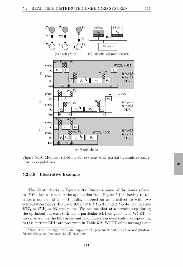
“thesis” — 2015/8/12 — 12:54 — page 111 — #131

5


P1

P4 P5 P3

P6 P2

m2 m3

m1

(a) Task graph

N1

comm. ctrl.

N2

comm. ctrl.

FPGA1 FPGA2

Bus

ii)

Memory

(b) Distributed architecture

N1

N2

bus

i) HW1=25

HW2=25

PDR

FPGA2

FPGA1

N1

N2

bus

HW1=25

HW2=25

PDR

FPGA2

FPGA1

N1

N2

bus

HW1=25

HW2=25

PDR

FPGA2

FPGA1

iii)

ii)

WCSL = 525

WCSL = 475

WCSL = 360

P1 P2

P4 P3 P4 P5

P6

rec. P2

rec. P4

m1 m2 m3

rec. P5

rec. P6

P1 P2

P3 P4 P4 P5

P6

m3 m1 m2

rec. P4 rec. P5

rec. P1 rec. P6

P1 P2

P3 P4 P4 P5

P6

m3 m1 m2

rec. P4

rec. P1 rec. P6

(c) Gantt charts

Figure 5.10: Modified scheduler for systems with partial dynamic reconfig-uration capabilities

5.2.6.5 Illustrative Example

The Gantt charts in Figure 5.10c illustrate some of the issues relatedto PDR. Let us consider the application from Figure 5.10a, having to tol-erate a number of k = 1 faults, mapped on an architecture with twocomputation nodes (Figure 5.10b), with FPGA1 and FPGA2 having sizesHW1 = HW2 = 25 area units. We assume that at a certain step duringthe optimization, each task has a particular EDI assigned. The WCETs oftasks, as well as the EDI areas and reconfiguration overheads correspondingto this current EDI4 are presented in Table 5.2. WCTT of all messages and

4Note that, although our model supports 2D placement and FPGA reconfiguration,for simplicity we illustrate the 1D case here.

111

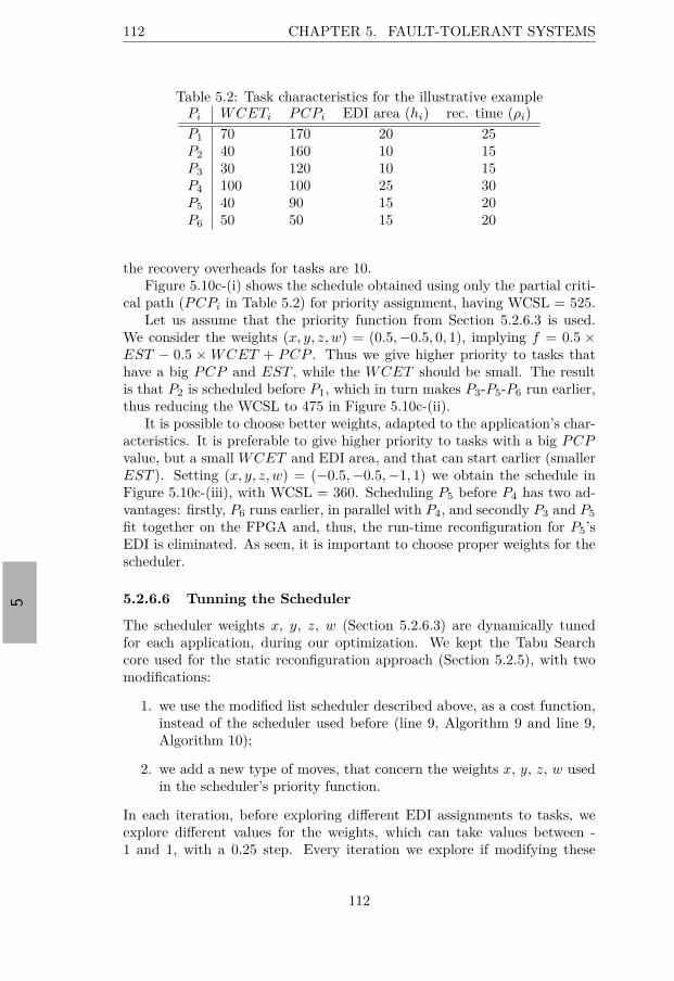
“thesis” — 2015/8/12 — 12:54 — page 112 — #132

5


Table 5.2: Task characteristics for the illustrative examplePi WCETi PCPi EDI area (hi) rec. time (ρi)

P1 70 170 20 25P2 40 160 10 15P3 30 120 10 15P4 100 100 25 30P5 40 90 15 20P6 50 50 15 20

the recovery overheads for tasks are 10.Figure 5.10c-(i) shows the schedule obtained using only the partial criti-

cal path (PCPi in Table 5.2) for priority assignment, having WCSL = 525.Let us assume that the priority function from Section 5.2.6.3 is used.

We consider the weights (x, y, z, w) = (0.5, −0.5, 0, 1), implying f = 0.5 ×EST − 0.5 × WCET + PCP . Thus we give higher priority to tasks thathave a big PCP and EST , while the WCET should be small. The resultis that P2 is scheduled before P1, which in turn makes P3-P5-P6 run earlier,thus reducing the WCSL to 475 in Figure 5.10c-(ii).

It is possible to choose better weights, adapted to the application’s char-acteristics. It is preferable to give higher priority to tasks with a big PCPvalue, but a small WCET and EDI area, and that can start earlier (smallerEST ). Setting (x, y, z, w) = (−0.5, −0.5, −1, 1) we obtain the schedule inFigure 5.10c-(iii), with WCSL = 360. Scheduling P5 before P4 has two ad-vantages: firstly, P6 runs earlier, in parallel with P4, and secondly P3 and P5

fit together on the FPGA and, thus, the run-time reconfiguration for P5’sEDI is eliminated. As seen, it is important to choose proper weights for thescheduler.

5.2.6.6 Tunning the Scheduler

The scheduler weights x, y, z, w (Section 5.2.6.3) are dynamically tunedfor each application, during our optimization. We kept the Tabu Searchcore used for the static reconfiguration approach (Section 5.2.5), with twomodifications:

1. we use the modified list scheduler described above, as a cost function,instead of the scheduler used before (line 9, Algorithm 9 and line 9,Algorithm 10);

2. we add a new type of moves, that concern the weights x, y, z, w usedin the scheduler’s priority function.

In each iteration, before exploring different EDI assignments to tasks, weexplore different values for the weights, which can take values between -1 and 1, with a 0.25 step. Every iteration we explore if modifying these

112

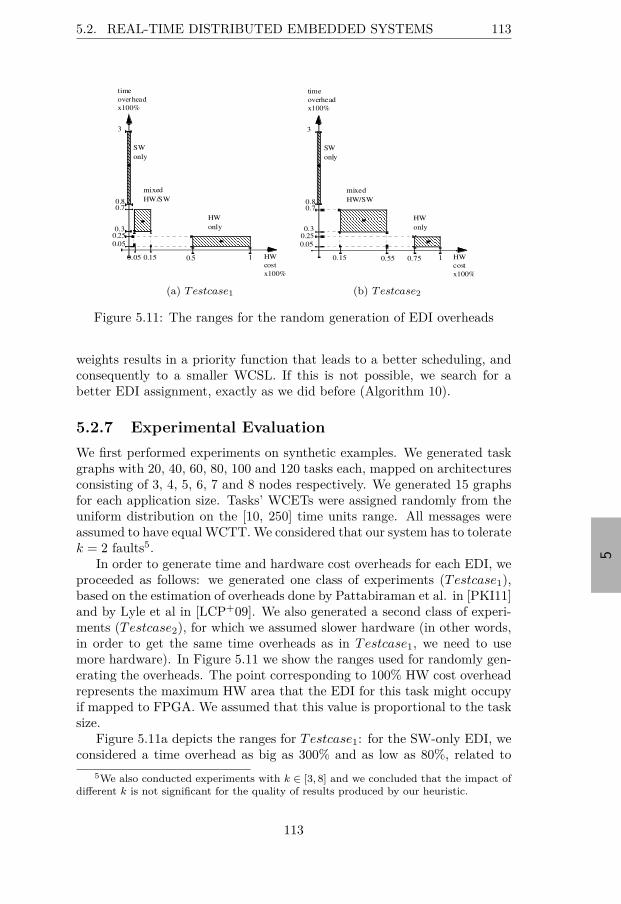
“thesis” — 2015/8/12 — 12:54 — page 113 — #133

5


time

overhead

x100%

HW

cost

x100%

10.50.150.05

3

0.8

0.250.3

0.7

0.05

time

overhead

x100%

3

0.8

0.250.3

0.7

0.05

SW

only

HW

only

mixed

HW/SW

a)

(a) T estcase1

HW

cost

x100%

time

overhead

x100%

HW

cost

x100%

10.550.15 0.75

3

0.8

0.250.3

0.7

0.05

SW

only

HW

only

mixed

HW/SW

b)

(b) T estcase2

Figure 5.11: The ranges for the random generation of EDI overheads

weights results in a priority function that leads to a better scheduling, andconsequently to a smaller WCSL. If this is not possible, we search for abetter EDI assignment, exactly as we did before (Algorithm 10).


We first performed experiments on synthetic examples. We generated taskgraphs with 20, 40, 60, 80, 100 and 120 tasks each, mapped on architecturesconsisting of 3, 4, 5, 6, 7 and 8 nodes respectively. We generated 15 graphsfor each application size. Tasks’ WCETs were assigned randomly from theuniform distribution on the [10, 250] time units range. All messages wereassumed to have equal WCTT. We considered that our system has to toleratek = 2 faults5.

In order to generate time and hardware cost overheads for each EDI, weproceeded as follows: we generated one class of experiments (Testcase1),based on the estimation of overheads done by Pattabiraman et al. in [PKI11]and by Lyle et al in [LCP+09]. We also generated a second class of experi-ments (Testcase2), for which we assumed slower hardware (in other words,in order to get the same time overheads as in Testcase1, we need to usemore hardware). In Figure 5.11 we show the ranges used for randomly gen-erating the overheads. The point corresponding to 100% HW cost overheadrepresents the maximum HW area that the EDI for this task might occupyif mapped to FPGA. We assumed that this value is proportional to the tasksize.

Figure 5.11a depicts the ranges for Testcase1: for the SW-only EDI, weconsidered a time overhead as big as 300% and as low as 80%, related to

5We also conducted experiments with k ∈ [3, 8] and we concluded that the impact ofdifferent k is not significant for the quality of results produced by our heuristic.

113

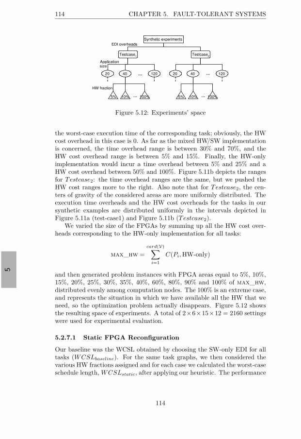
“thesis” — 2015/8/12 — 12:54 — page 114 — #134

5


Testcase1 Testcase

2

Synthetic experiments

20 2012040 120 40

5% 10% 100% 5% 10% 100%

Application size

HW fraction

……

……

EDI overheads

Figure 5.12: Experiments’ space

the worst-case execution time of the corresponding task; obviously, the HWcost overhead in this case is 0. As far as the mixed HW/SW implementationis concerned, the time overhead range is between 30% and 70%, and theHW cost overhead range is between 5% and 15%. Finally, the HW-onlyimplementation would incur a time overhead between 5% and 25% and aHW cost overhead between 50% and 100%. Figure 5.11b depicts the rangesfor Testcase2: the time overhead ranges are the same, but we pushed theHW cost ranges more to the right. Also note that for Testcase2, the cen-ters of gravity of the considered areas are more uniformly distributed. Theexecution time overheads and the HW cost overheads for the tasks in oursynthetic examples are distributed uniformly in the intervals depicted inFigure 5.11a (test-case1) and Figure 5.11b (Testcase2).

We varied the size of the FPGAs by summing up all the HW cost over-heads corresponding to the HW-only implementation for all tasks:

max_hw =

card(V)∑

i=1

C(Pi, HW-only)

and then generated problem instances with FPGA areas equal to 5%, 10%,15%, 20%, 25%, 30%, 35%, 40%, 60%, 80%, 90% and 100% of max_hw,distributed evenly among computation nodes. The 100% is an extreme case,and represents the situation in which we have available all the HW that weneed, so the optimization problem actually disappears. Figure 5.12 showsthe resulting space of experiments. A total of 2×6×15×12 = 2160 settingswere used for experimental evaluation.

5.2.7.1 Static FPGA Reconfiguration

Our baseline was the WCSL obtained by choosing the SW-only EDI for alltasks (WCSLbaseline). For the same task graphs, we then considered thevarious HW fractions assigned and for each case we calculated the worst-caseschedule length, WCSLstatic, after applying our heuristic. The performance

114

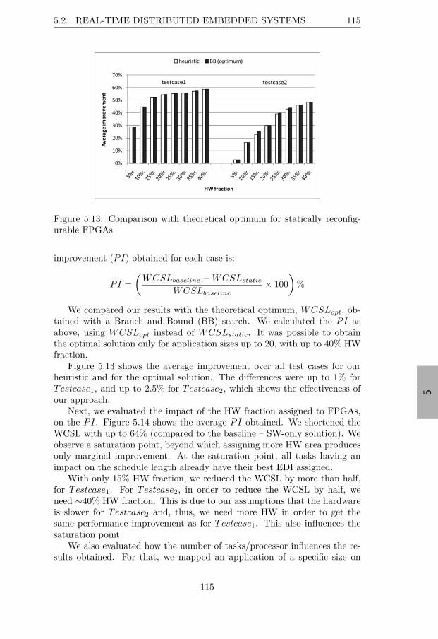
“thesis” — 2015/8/12 — 12:54 — page 115 — #135

5


Figure 5.13: Comparison with theoretical optimum for statically reconfig-urable FPGAs

improvement (PI) obtained for each case is:

PI =

(WCSLbaseline − WCSLstatic

WCSLbaseline

× 100

)%

We compared our results with the theoretical optimum, WCSLopt, ob-tained with a Branch and Bound (BB) search. We calculated the PI asabove, using WCSLopt instead of WCSLstatic. It was possible to obtainthe optimal solution only for application sizes up to 20, with up to 40% HWfraction.

Figure 5.13 shows the average improvement over all test cases for ourheuristic and for the optimal solution. The differences were up to 1% forTestcase1, and up to 2.5% for Testcase2, which shows the effectiveness ofour approach.

Next, we evaluated the impact of the HW fraction assigned to FPGAs,on the PI. Figure 5.14 shows the average PI obtained. We shortened theWCSL with up to 64% (compared to the baseline – SW-only solution). Weobserve a saturation point, beyond which assigning more HW area producesonly marginal improvement. At the saturation point, all tasks having animpact on the schedule length already have their best EDI assigned.

With only 15% HW fraction, we reduced the WCSL by more than half,for Testcase1. For Testcase2, in order to reduce the WCSL by half, weneed ∼40% HW fraction. This is due to our assumptions that the hardwareis slower for Testcase2 and, thus, we need more HW in order to get thesame performance improvement as for Testcase1. This also influences thesaturation point.

We also evaluated how the number of tasks/processor influences the re-sults obtained. For that, we mapped an application of a specific size on

115

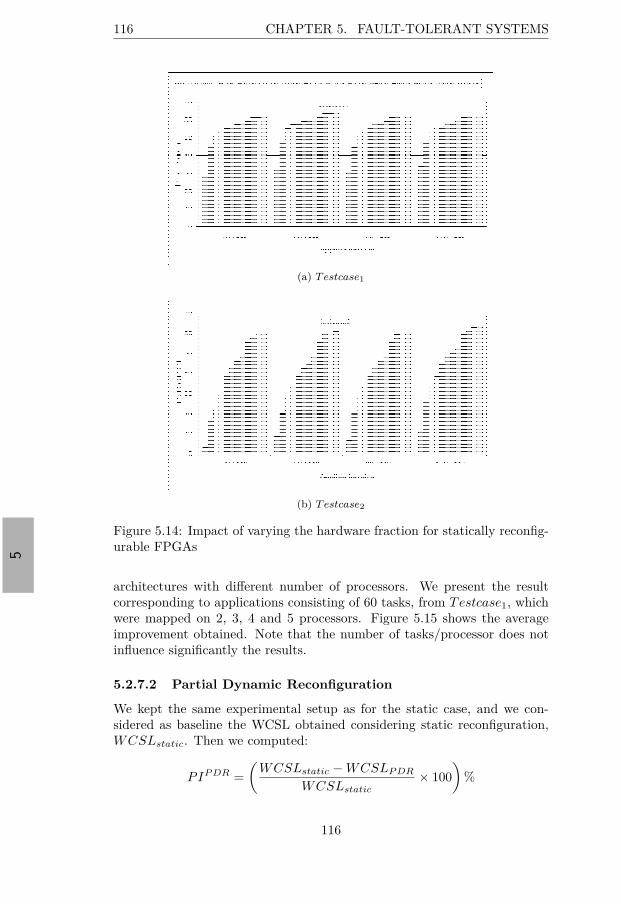
“thesis” — 2015/8/12 — 12:54 — page 116 — #136

5


(a) T estcase1

(b) T estcase2

Figure 5.14: Impact of varying the hardware fraction for statically reconfig-urable FPGAs

architectures with different number of processors. We present the resultcorresponding to applications consisting of 60 tasks, from Testcase1, whichwere mapped on 2, 3, 4 and 5 processors. Figure 5.15 shows the averageimprovement obtained. Note that the number of tasks/processor does notinfluence significantly the results.

5.2.7.2 Partial Dynamic Reconfiguration

We kept the same experimental setup as for the static case, and we con-sidered as baseline the WCSL obtained considering static reconfiguration,WCSLstatic. Then we computed:

PIP DR =

(WCSLstatic − WCSLP DR

WCSLstatic

× 100

)%

116

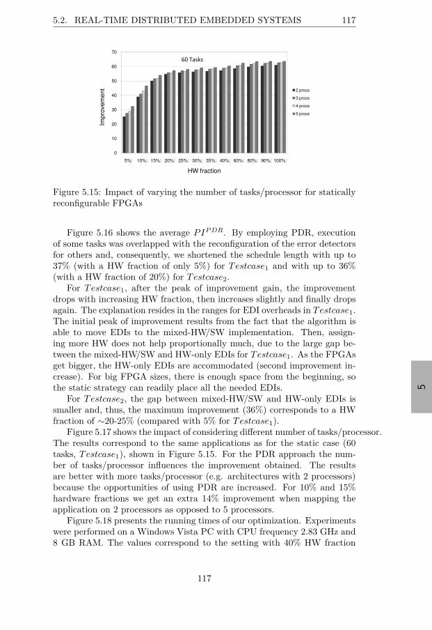
“thesis” — 2015/8/12 — 12:54 — page 117 — #137

5


30

40

50

60

70

Impro

vem

ent 2 procs

3 procs

4 procs

5 procs

0

10

20

30

40

50

60

70

5%: 10%: 15%: 20%: 25%: 30%: 35%: 40%: 60%: 80%: 90%: 100%:

Impro

vem

ent

HW fraction

2 procs

3 procs

4 procs

5 procs

Figure 5.15: Impact of varying the number of tasks/processor for staticallyreconfigurable FPGAs

Figure 5.16 shows the average PIP DR. By employing PDR, executionof some tasks was overlapped with the reconfiguration of the error detectorsfor others and, consequently, we shortened the schedule length with up to37% (with a HW fraction of only 5%) for Testcase1 and with up to 36%(with a HW fraction of 20%) for Testcase2.

For Testcase1, after the peak of improvement gain, the improvementdrops with increasing HW fraction, then increases slightly and finally dropsagain. The explanation resides in the ranges for EDI overheads in Testcase1.The initial peak of improvement results from the fact that the algorithm isable to move EDIs to the mixed-HW/SW implementation. Then, assign-ing more HW does not help proportionally much, due to the large gap be-tween the mixed-HW/SW and HW-only EDIs for Testcase1. As the FPGAsget bigger, the HW-only EDIs are accommodated (second improvement in-crease). For big FPGA sizes, there is enough space from the beginning, sothe static strategy can readily place all the needed EDIs.

For Testcase2, the gap between mixed-HW/SW and HW-only EDIs issmaller and, thus, the maximum improvement (36%) corresponds to a HWfraction of ∼20-25% (compared with 5% for Testcase1).

Figure 5.17 shows the impact of considering different number of tasks/processor.The results correspond to the same applications as for the static case (60tasks, Testcase1), shown in Figure 5.15. For the PDR approach the num-ber of tasks/processor influences the improvement obtained. The resultsare better with more tasks/processor (e.g. architectures with 2 processors)because the opportunities of using PDR are increased. For 10% and 15%hardware fractions we get an extra 14% improvement when mapping theapplication on 2 processors as opposed to 5 processors.

Figure 5.18 presents the running times of our optimization. Experimentswere performed on a Windows Vista PC with CPU frequency 2.83 GHz and8 GB RAM. The values correspond to the setting with 40% HW fraction

117

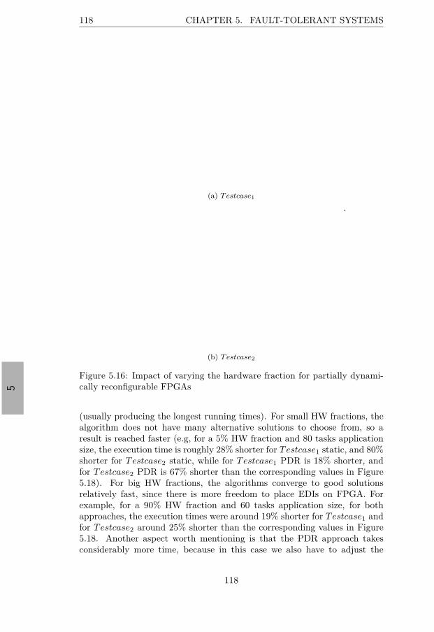
“thesis” — 2015/8/12 — 12:54 — page 118 — #138

5


(a) T estcase1

(b) T estcase2

Figure 5.16: Impact of varying the hardware fraction for partially dynami-cally reconfigurable FPGAs

(usually producing the longest running times). For small HW fractions, thealgorithm does not have many alternative solutions to choose from, so aresult is reached faster (e.g, for a 5% HW fraction and 80 tasks applicationsize, the execution time is roughly 28% shorter for Testcase1 static, and 80%shorter for Testcase2 static, while for Testcase1 PDR is 18% shorter, andfor Testcase2 PDR is 67% shorter than the corresponding values in Figure5.18). For big HW fractions, the algorithms converge to good solutionsrelatively fast, since there is more freedom to place EDIs on FPGA. Forexample, for a 90% HW fraction and 60 tasks application size, for bothapproaches, the execution times were around 19% shorter for Testcase1 andfor Testcase2 around 25% shorter than the corresponding values in Figure5.18. Another aspect worth mentioning is that the PDR approach takesconsiderably more time, because in this case we also have to adjust the

118

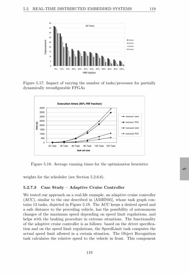
“thesis” — 2015/8/12 — 12:54 — page 119 — #139

5


15

20

25

30

35

40

45

Impro

vem

en

t 2 procs

3 procs

4 procs

5 procs

0

5

10

15

20

25

30

35

40

45

5%: 10%: 15%: 20%: 25%: 30%: 35%: 40%: 60%: 80%: 90%: 100%:

Impro

vem

en

t

HW fraction

2 procs

3 procs

4 procs

5 procs

Figure 5.17: Impact of varying the number of tasks/processor for partiallydynamically reconfigurable FPGAs

1500

2000

2500

3000

3500

4000

tim

e [

s]

Execution times (40% HW fraction)

testcase1 static

testcase1 PDR

testcase2 static

0

500

1000

1500

2000

2500

3000

3500

4000

20 Task 40 Task 60 Task 80 Task 100 Task 120 Task

tim

e [

s]

task set size

Execution times (40% HW fraction)

testcase1 static

testcase1 PDR

testcase2 static

testcase2 PDR

Figure 5.18: Average running times for the optimization heuristics

weights for the scheduler (see Section 5.2.6.6).

5.2.7.3 Case Study – Adaptive Cruise Controller

We tested our approach on a real-life example, an adaptive cruise controller(ACC), similar to the one described in [AMHN05], whose task graph con-tains 13 tasks, depicted in Figure 5.19. The ACC keeps a desired speed anda safe distance to the preceding vehicle, has the possibility of autonomouschanges of the maximum speed depending on speed limit regulations, andhelps with the braking procedure in extreme situations. The functionalityof the adaptive cruise controller is as follows: based on the driver specifica-tion and on the speed limit regulations, the SpeedLimit task computes theactual speed limit allowed in a certain situation. The Object Recognitiontask calculates the relative speed to the vehicle in front. This component

119

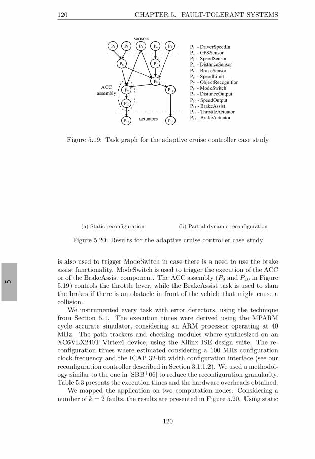
“thesis” — 2015/8/12 — 12:54 — page 120 — #140

5


P1 - DriverSpeedIn

P2 - GPSSensor

P3 - SpeedSensor

P4 - DistanceSensor

P5 - BrakeSensor

P6 - SpeedLimit

P7 - ObjectRecognition

P8 - ModeSwitch

P9 - DistanceOutput

P10 - SpeedOutput

P11 - BrakeAssist

P12 - ThrottleActuator

P13 - BrakeActuator

P1 P3 P4 P5 P2

P6

P9

P7

P8

P11

P12

P10

P13 actuators

sensors

ACC

assembly

Figure 5.19: Task graph for the adaptive cruise controller case study

(a) Static reconfiguration

(b) Partial dynamic reconfiguration

Figure 5.20: Results for the adaptive cruise controller case study

is also used to trigger ModeSwitch in case there is a need to use the brakeassist functionality. ModeSwitch is used to trigger the execution of the ACCor of the BrakeAssist component. The ACC assembly (P9 and P10 in Figure5.19) controls the throttle lever, while the BrakeAssist task is used to slamthe brakes if there is an obstacle in front of the vehicle that might cause acollision.

We instrumented every task with error detectors, using the techniquefrom Section 5.1. The execution times were derived using the MPARMcycle accurate simulator, considering an ARM processor operating at 40MHz. The path trackers and checking modules where synthesized on anXC6VLX240T Virtex6 device, using the Xilinx ISE design suite. The re-configuration times where estimated considering a 100 MHz configurationclock frequency and the ICAP 32-bit width configuration interface (see ourreconfiguration controller described in Section 3.1.1.2). We used a methodol-ogy similar to the one in [SBB+06] to reduce the reconfiguration granularity.Table 5.3 presents the execution times and the hardware overheads obtained.

We mapped the application on two computation nodes. Considering anumber of k = 2 faults, the results are presented in Figure 5.20. Using static

120

“thesis” — 2015/8/12 — 12:54 — page 121 — #141

5

5.3. AVERAGE EXECUTION TIME MINIMIZATION 121

Table 5.3: Time and area overheads for the adaptive cruise controller casestudy

Pi

Error Detection Implementation (EDI)SW-only mixed-HW/SW HW-onlyW CETi W CETi hi ρi W CETi hi ρi

(µs) (µs) (slices) (µs) (µs) (slices) (µs)

P1 8.12 6.02 2 1.23 4.9 15 9.23P2 8.12 6.02 2 1.23 4.9 15 9.23P3 8.12 6.02 2 1.23 4.9 15 9.23P4 8.17 6.07 2 1.23 4.95 15 9.23P5 7.32 5.4 2 1.23 4.27 13 8P6 8.37 6.27 2 1.23 4.92 13 8P7 10.35 7.87 2 1.23 6.75 42 25.83P8 12.17 9.6 3 1.85 8.45 15 9.23P9 46.22 33.7 11 6.77 27.25 43 26.45P10 20.3 14.45 4 2.46 11.57 28 17.22P11 37.27 29.47 7 4.31 21.7 52 31.99P12 8.12 6.02 2 1.23 4.9 15 9.23P13 8.12 6.02 2 1.23 4.9 15 9.23

reconfiguration, we obtained up to 47% reduction in schedule length (overthe SW-only implementation) with as little as 35% HW fraction. AssumingPDR, we got an extra reduction. The best result is obtained for 20% HWfraction, where the static reconfiguration approach achieves 42% improve-ment (over the SW-only implementation), while the PDR approach achievesan extra 9% improvement (over the static approach).

5.3 Average Execution Time Minimization

The previous section handled the matter of safety critical applications, con-sidering strict worst-case scenarios, where deadlines have to be satisfied evenin case of faults. However, for a large class of applications faults have tobe handled, but what is important is the average execution time. Faultsappear only seldom, and their handling does not affect the average. Whatis important is to minimize the impact of the error detection on the averageperformance. In order to achieve this, a more refined model is needed (com-pared to Section 5.2), that captures data and control dependencies. Theprevious section addressed the performance optimization problem at a tasklevel. Using such a task-level coarse granularity is not appropriate for manyapplications, e.g. those that consist of a single sequential task. In what fol-lows, instead of considering the tasks as black boxes, we will analyze theirinternal structure and properties.

Note that in this section, similar to Section 3.3, we consider correlations.

121

“thesis” — 2015/8/12 — 12:54 — page 122 — #142

5


However, there are some differences: first of all, the optimization presentedin this section is done off-line, as opposed to the technique presented in Sec-tion 3.3, which is dynamic and performed on-line. Another difference is thatin this section we consider the correlations in an implicit manner, i.e. wewill take into account the correlation between a certain program path beingfollowed and the corresponding checking expression being reached. There-fore, the output of our optimization will be a conditional reconfigurationschedule table.

The rest of this section presents an approach to minimize the averageexecution time of a program by optimizing the hardware/software imple-mentation of error detection. We leverage the advantages of partial dynamicreconfiguration of FPGAs in order to speculatively place in hardware thoseerror detection components that will provide the highest reduction of exe-cution time. Our optimization algorithm uses frequency information from acounter-based execution profile of the program. Starting from a control flowgraph representation, we build the interval structure and the control depen-dence graph, which we then use to guide our error detection optimizationalgorithm.

5.3.1 Basic Concepts

Before presenting our optimization approach, let us introduce some defini-tions that will help the reader better understand the rest of this section.Note that the model used in the following is similar to the one used inSection 3.2. Thus, some definitions will be repeated, for the sake of thepresentation flow.

Definition 5.1 A control flow graph (CFG) of a program is a directed graphGcf (Ncf , Ecf ), where each node in Ncf corresponds to a straight-line se-quence of operations and the set of edges Ecf corresponds to the possibleflow of control within the program. Gcf captures potential execution pathsand contains two distinguished nodes, root and sink, corresponding to theentry and the exit of the program.

Definition 5.2 A node n ∈ Ncf is post-dominated by a node m ∈ Ncf inthe control flow graph Gcf if every directed path from n to sink (excludingn) contains m.

Definition 5.3 Given a control flow graph Gcf , a node m ∈ Ncf is controldependent upon a node n ∈ Ncf via a control flow edge e ∈ Ecf if the nextconditions hold:

• There exists a directed path P from n to m in Gcf , starting with e,with all nodes in P (except m and n) post-dominated by m;

• m does not post-dominate n in Gcf .

122

“thesis” — 2015/8/12 — 12:54 — page 123 — #143

5


In other words, there is some control edge from n that definitely causes mto execute, and there is some path from n to sink that avoids executing m.

Definition 5.4 A control dependence graph (CDG) Gcd(Ncd, Ecd) correspond-ing to a control flow graph Gcf (Ncf , Ecf ) is defined as: Ncd = Ncf andEcd = ((n, m), e) | m is control dependent upon n via edge e. A forwardcontrol dependence graph (FCDG) is obtained by ignoring all back edges inthe CDG [ALSU06].

Definition 5.5 An interval I(h) in a control flow graph Gcf (Ncf , Ecf ), withheader node h ∈ Ncf , is a strongly connected region of Gcf that contains hand has the following properties:

• I(h) can be entered only through its header node h;

• all nodes in I(h) can be reached from h along a path contained in I(h);

• h can be reached from any node in I(h) along a path contained inI(h).

The interval structure represents the looping constructs of a program.

Definition 5.6 An extended control flow graph (ECFG) is obtained by aug-menting the initial control flow graph with a pseudo control flow edge (root,sink) and with explicit interval entry and exit nodes as follows:

• for each interval I(h), a preheader node, ph, is added and all intervalentries are redirected to ph (i.e. every edge (n, h), with n not in I(h)is replaced with the edge (n, ph) and an unconditional edge (ph, h) isadded);

• a postexit node, pe, is added and every edge (n, m) with n in I(h) andm not in I(h) is replaced by edges (n, pe) and (pe, m);

• a pseudo control flow edge (ph, pe) is added.

The pseudo control flow edges provide a convenient structure to the controldependence graph (causing all nodes in an interval to be directly or indirectlycontrol dependent on the preheader node).

Definition 5.7 Given an edge (n, m) ∈ Efcd in the forward control depen-dence graph (FCDG) Gfcd(Nfcd, Efcd), the execution frequency of the edge[Sar89] is defined as follows:

• if n is a preheader and m is a header, freq(n, m) ≥ 0 is the averageloop frequency for interval I(m);

• otherwise, 0 ≤ freq(n, m) ≤ 1 is the branch probability.

123

“thesis” — 2015/8/12 — 12:54 — page 124 — #144

5


Let us exemplify these concepts on the control flow graph from Figure5.21. Node a is post-dominated by nodes e and h, but not by node b, forexample (that is because there exists the path from node a to the sink sgoing through node d, that excludes node b). Nodes b and d are controldependent upon node a via edges a − b and a − d, respectively. Note thatthe addition of the pseudo control flow edge r − s transforms the initialCFG into an extended control flow graph (ECFG), and causes all nodes tobe control dependent on r.

5.3.2 System Model

We consider a structured [ALSU06] program, modeled as a control flow graphGcf (Ncf , Ecf ). The program runs on an architecture composed of a centralprocessing unit, a memory subsystem and a reconfigurable device (FPGA).As in the previous section, we assume that suitable mitigation techniques areemployed (e.g. [LCR03], [NOS14]) in order to provide sufficient reliabilityof the hardware used for error detection.

We model our FPGA, supporting partial dynamic reconfiguration, asa rectangular matrix of configurable logic blocks (CLBs). Each checkeroccupies a contiguous rectangular area of this matrix. The model allowsmodules of any rectangular shape and size. The execution of a checker canproceed in parallel with the reconfiguration of another checker, but only onereconfiguration may be done at a certain time.


Input

• A structured program modeled as a CFG Gcf (Ncf , Ecf ).

• Each node n ∈ Ncf has a corresponding execution time, given bytime : Ncf → Z

+.

• Each edge has associated the probability to be taken, given by prob :Ecf → [0; 1].

We assume that this information is obtained by profiling the program andit is given.

• The set of checkers (checking expressions), CE, corresponding to theprogram is also given. Each checker c ∈ CE has associated the follow-ing:

1. The node where it will be executed, given by host : CE → Ncf .

2. The acyclic path for which the checker has been derived (denotedwith path(c) = sequence of edges that lead to host(c) in the CFG).

3. The execution time (sw : CE → Z+) if implemented in software.

124

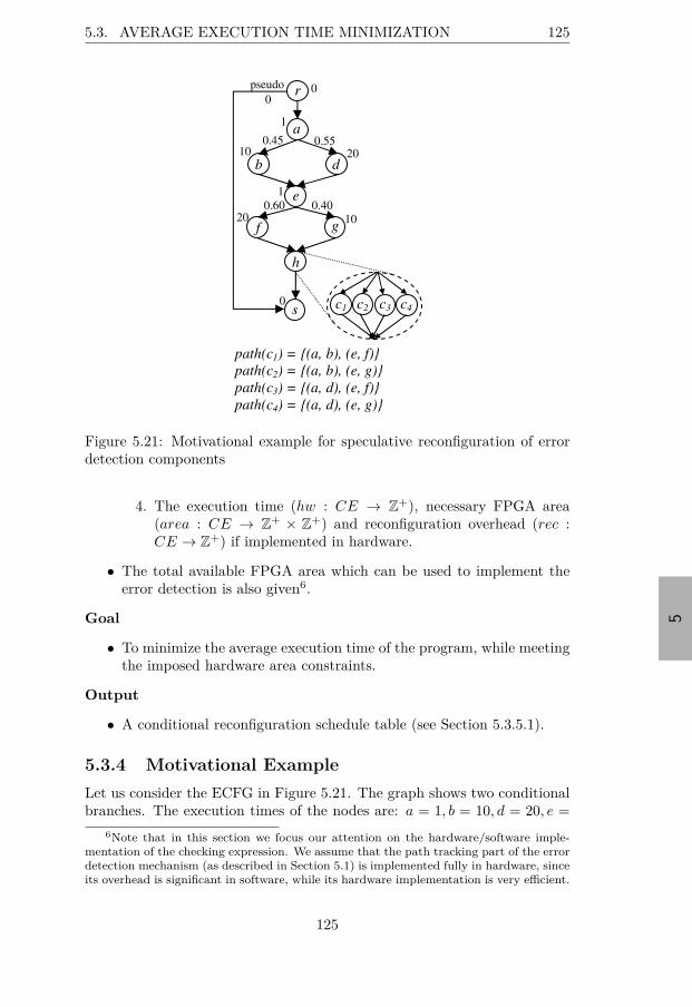
“thesis” — 2015/8/12 — 12:54 — page 125 — #145

5


path(c1) = (a, b), (e, f)

path(c2) = (a, b), (e, g)

path(c3) = (a, d), (e, f)

path(c4) = (a, d), (e, g)

r

a

b

e

g f

h

s

0.55

0.40 0.60

0

d

c1 c2 c3 c4

pseudo

0.45

1

10

1

20 10

20

0

0

Figure 5.21: Motivational example for speculative reconfiguration of errordetection components

4. The execution time (hw : CE → Z+), necessary FPGA area

(area : CE → Z+ × Z

+) and reconfiguration overhead (rec :CE → Z

+) if implemented in hardware.

• The total available FPGA area which can be used to implement theerror detection is also given6.

Goal

• To minimize the average execution time of the program, while meetingthe imposed hardware area constraints.

Output

• A conditional reconfiguration schedule table (see Section 5.3.5.1).


Let us consider the ECFG in Figure 5.21. The graph shows two conditionalbranches. The execution times of the nodes are: a = 1, b = 10, d = 20, e =

6Note that in this section we focus our attention on the hardware/software imple-mentation of the checking expression. We assume that the path tracking part of the errordetection mechanism (as described in Section 5.1) is implemented fully in hardware, sinceits overhead is significant in software, while its hardware implementation is very efficient.

125

“thesis” — 2015/8/12 — 12:54 — page 126 — #146

5


Table 5.4: Error detection overheads for the motivational example

ci

SW HWtime time area reconfig.

overhead overhead units time

c1 22 4 25 25c2 18 3 10 10c3 15 2 20 20c4 29 3 40 40

1, f = 20, g = 10, while the root(r) and sink(s) have execution time zero.The conditional edges have their associated probabilities presented on thegraph.

Let us assume that inside node h we have a critical variable that needsto be checked and, by applying the technique described in Section 5.1 wederived four checkers for it: c1 to c4. Each of them corresponds to a differentacyclic control path in the ECFG, as shown in Figure 5.21. In Table 5.4 wepresent the time overheads incurred by the software implementation of eachchecker, as well as the overheads, area and reconfiguration time incurredby the hardware implementation. Since node h is composed of the fourcheckers, its execution time depends on the actual path followed at run-time, which will determine which of the four, mutually exclusive, checkerswill get executed.

For the given example, if we assume that all the checkers are implementedin software, the resulting average execution time of the ECFG is 54.01 timeunits. On the other hand, if we assume that we have enough FPGA area sothat we can place all the checkers in hardware from the beginning (i.e. 95area units), the average execution time will be 36.44 time units.

Let us now consider an FPGA supporting partial dynamic reconfigura-tion and having an area of only 40 units. For the reconfiguration decisionon each of the outgoing edges of node a, one intuitive solution would be thefollowing: if edge (a, b) is followed, we would start reconfiguring the checkerthat has the highest probability to be reached on this branch (i.e. c1). Atrun-time, when we reach the second conditional node, if the edge (e, f) isfollowed, then our previous speculation was right, and the reconfigurationof c1 will have been finished by the time we reach it; otherwise, if the edge(e, g) is taken, then we can drop the reconfiguration of c1 (because we willnot execute it for sure) and we can start the reconfiguration of c2. Let usnow consider the situation when edge (a, d) is followed. Applying the samestrategy as above, we would start reconfiguring c3 (because its probabilityis 60% compared to 40% for c4). In this case, when we reach node e, if theprediction was right, we will have c3 on FPGA by the time we reach it. Butif the prediction was wrong, it is not profitable to reconfigure c4 (on edge(e, g)) because reconfiguring it and then executing it in hardware would take40 + 3 = 43 time units (note that node g is executed in parallel with the re-

126

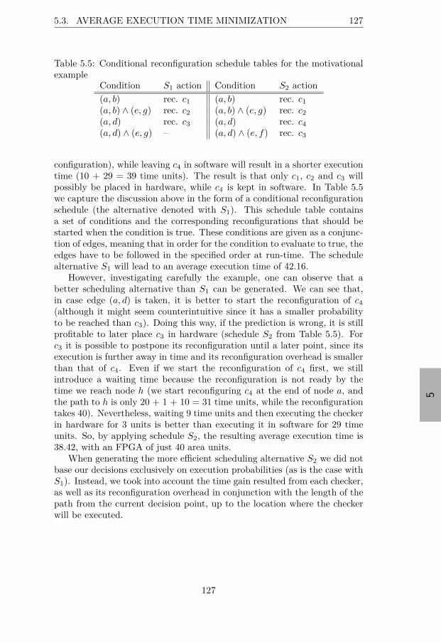
“thesis” — 2015/8/12 — 12:54 — page 127 — #147

5


Table 5.5: Conditional reconfiguration schedule tables for the motivationalexample

Condition S1 action Condition S2 action

(a, b) rec. c1 (a, b) rec. c1

(a, b) ∧ (e, g) rec. c2 (a, b) ∧ (e, g) rec. c2

(a, d) rec. c3 (a, d) rec. c4

(a, d) ∧ (e, g) – (a, d) ∧ (e, f) rec. c3

configuration), while leaving c4 in software will result in a shorter executiontime (10 + 29 = 39 time units). The result is that only c1, c2 and c3 willpossibly be placed in hardware, while c4 is kept in software. In Table 5.5we capture the discussion above in the form of a conditional reconfigurationschedule (the alternative denoted with S1). This schedule table containsa set of conditions and the corresponding reconfigurations that should bestarted when the condition is true. These conditions are given as a conjunc-tion of edges, meaning that in order for the condition to evaluate to true, theedges have to be followed in the specified order at run-time. The schedulealternative S1 will lead to an average execution time of 42.16.

However, investigating carefully the example, one can observe that abetter scheduling alternative than S1 can be generated. We can see that,in case edge (a, d) is taken, it is better to start the reconfiguration of c4

(although it might seem counterintuitive since it has a smaller probabilityto be reached than c3). Doing this way, if the prediction is wrong, it is stillprofitable to later place c3 in hardware (schedule S2 from Table 5.5). Forc3 it is possible to postpone its reconfiguration until a later point, since itsexecution is further away in time and its reconfiguration overhead is smallerthan that of c4. Even if we start the reconfiguration of c4 first, we stillintroduce a waiting time because the reconfiguration is not ready by thetime we reach node h (we start reconfiguring c4 at the end of node a, andthe path to h is only 20 + 1 + 10 = 31 time units, while the reconfigurationtakes 40). Nevertheless, waiting 9 time units and then executing the checkerin hardware for 3 units is better than executing it in software for 29 timeunits. So, by applying schedule S2, the resulting average execution time is38.42, with an FPGA of just 40 area units.

When generating the more efficient scheduling alternative S2 we did notbase our decisions exclusively on execution probabilities (as is the case withS1). Instead, we took into account the time gain resulted from each checker,as well as its reconfiguration overhead in conjunction with the length of thepath from the current decision point, up to the location where the checkerwill be executed.

127

“thesis” — 2015/8/12 — 12:54 — page 128 — #148

5


5.3.5 Speculative Reconfiguration

We propose a constructive algorithm to solve the problem defined in Section5.3.3. The idea is to use the knowledge regarding already taken branches,in order to take the best possible decision for the future and speculativelyreconfigure on FPGA the checkers with the highest potential to provide aperformance improvement.

Since for each checker c ∈ CE we have the corresponding acyclic pathspecified as a sequence of instrumented branches (edges from the CFG), wedefine the reach probability, given by reach_prob : Ncf × CE → [0; 1]. Thevalue reach_prob(n, c) represents the probability that the checker’s path isfollowed at run-time, given that node n ∈ path(c) is reached and all thenodes on path(c) up to n were visited. This is computed as the product ofthe probabilities of the edges in the checker’s path, from n up to host(c).If n is not on path(c), then the reach probability will be zero. Consideringthe example from Figure 5.21, e.g. reach_prob(a, c1) = 0.45 × 0.60 = 0.27,reach_prob(b, c1) = 0.60 and reach_prob(d, c1) = 0.

For each checker c ∈ CE we also define its time gain as the differencebetween its time overhead when implemented in SW versus in HW (gain :CE → Z

+, gain(c) = sw(c) − hw(c)). Finally, we denote with iterations(c)the average frequency of the loop inside which c is executed. If c is not insidea loop, iterations(c) = 1. We will use this value to give higher priority tocheckers that get executed inside loops.

We also assign a weight to each checker c ∈ CE:

weight(n, c) =reach_prob(n, c) · iterations(c) · gain(c)

area(c)(5.3)

This weight represents the average time gain per area unit correspondingto c. As we traverse the CFG of the program, the weights of some checkersmight become zero (when certain paths are followed, i.e. reach_prob be-comes zero), while the weight of other checkers will increase (as we approachtheir host on a certain path).

5.3.5.1 Reconfiguration Schedule Generation

The pseudocode of our reconfiguration schedule generation algorithm is pre-sented in Algorithm 11. Considering the CFG received as an input, we firstdetermine its interval structure (line 2), then we build the ECFG (line 3)according to Definition 5.6, and the FCDG (line 4) according to Definition5.4.

The next step is to traverse the ECFG and build the reconfigurationschedule (line 5). Once the schedule is generated all the checkers have beenassigned an implementation (in hardware or in software), on any path thatmight get executed at run-time. Thus we can estimate the average executiontime of the given CFG (line 6).

128

“thesis” — 2015/8/12 — 12:54 — page 129 — #149

5


Algorithm 11 Speculative optimization algorithm1: procedure Build_Reconfiguration_Schedule(CFG)2: determine interval structure of CFG3: build ECFG4: build FCDG

⊲ traverse ECFG and build reconfiguration schedules5: Build_Schedule(root, TRUE)6: compute average execution time of CFG7: end procedure

8: procedure Build_Schedule(n, cond)9: for all edge e = (n, m) do

10: if (e not back edge or loop exit edge) or (e not visited) then

11: mark e as visited12: if e is a back edge or a loop exit edge then

13: cond ← TRUE ⊲ reset context14: end if

15: new_cond ← cond ∧ e16: for all checker cinCE do

17: compute reach_prob(m, c)18: compute weight(m, c)19: compute path_length(n, c)20: end for

21: build ACE(e)22: if reconfiguration controller available and ACE(e) Ó= ∅ then

23: Schedule_New_Reconfigurations(e, new_cond)24: end if

25: Build_Schedule(m, new_cond)26: end if

27: end for

28: end procedure

29: procedure Schedule_New_Reconfigurations(e = (n, m), cond)30: sort ACE(e) in descending order by weight31: repeat

32: pick and remove c ∈ ACE(e) with highest weight33: if c already configured on FPGA but inactive then

34: activate c at its current location35: else

36: loc ← Choose_FPGA_Location(c)37: mark start of reconfiguration for c, at loc, on new_cond38: for all checkers c′ ∈ ACE(e) do

39: recompute path_length(n, c′)40: end for

41: end if


129

“thesis” — 2015/8/12 — 12:54 — page 130 — #150

5


(continued from previous page)42: until end of reconfiguration ≥ end of m’s execution43: end procedure

44: function Choose_FPGA_Location(c)45: if there is enough free contiguous space on FPGA then

46: return empty rectangle with lowest fragmentation metric47: else

48: choose the least recently used inactive modules to be replaced49: return this location50: end if

51: end function

The actual HW/SW optimization is performed in the recursive procedureBuild_Schedule. The ECFG is traversed such that each back edge andeach loop exit edge is processed exactly once (line 10). In order to be able tohandle the complexity, whenever a back or loop exit edge is taken, we resetthe current context (lines 12-13). This means that in each loop iterationwe take the same reconfiguration decisions, regardless of what happened inprevious loop iterations. The same applies to loop exit: decisions after aloop are independent of what happened inside or before the loop. This guar-antees that the conditional reconfiguration schedule table that we generateis complete (i.e. we tried to take the best possible decision for any path thatmight be followed at run-time).

The generated schedule table contains a set of conditions and the cor-responding reconfigurations to be performed when a condition is activatedat run-time. Considering the example in Figure 5.21 a condition and itscorresponding action is:

(a, b) ∧ (e, g): reconfiguration of c2

At run-time, a condition is activated only if the particular path specifiedby its constituent edges is followed. At each control node n ∈ Necf inthe ECFG we take a different reconfiguration decision on every outgoingedge (line 9). We will next describe the decision process for one such edge,e = (n, m) ∈ Eecf . First, the new condition is constructed (line 15). Thiscondition corresponds to a conjunction of all the taken edges so far, and thecurrent edge, e.

As we process a control edge e = (n, m) ∈ Eecf in the ECFG, we computethe reach_prob(m, c) and the weight(m, c) of all checkers in CE (lines 17-18). These values will obviously be different from the previously computedones, reach_prob(n, c) and weight(n, c). To be more exact they will increaseas we approach host(c).

We also compute the path length corresponding to each checker (denotedwith path_length(n, c)). This represents the length (in time) of the paththat leads from the current node n to host(c) in the CFG. Please note that

130

“thesis” — 2015/8/12 — 12:54 — page 131 — #151

5


all the checkers active along that path will have assigned an implementation(either SW or HW) for the current traversal of the ECFG, so we can compute(line 19) the length of the path (from the current node up to the location ofthe checker):

path_length(n, c) =

=∑

m∈path(c),m successor of n

time(m) +∑

k∈CE,k Ó=c,host(k)=m,

k active

overhead(k)

(5.4)

where

overhead(k) =

sw(k), if k is implemented in software

wait(k) + hw(k), otherwise

andwait(k) = eventual waiting time introduced due to the fact that

reconfiguration is not finished when the checker is reached.We denote with ACE(e) the set of currently active checking expressions

(checkers) if edge e is taken in the ECFG, i.e.:

ACE(e) =c ∈ CE|e ∈ path(c)∧area(c) fits in currently available FPGA area ∧rec(c) + hw(c) < path_length(n, c) + sw(c)∧path from m to host(c) does not contain any back edge

(5.5)

We discard all the checkers for which we do not currently have enoughcontiguous FPGA area available for a feasible placement, as well as the onesfor which it is actually more profitable (at this point) to leave them in soft-ware (because they are too close to the current location and reconfiguringand executing the checker in hardware would actually take longer time thanexecuting it in software). We also do not start reconfigurations for check-ers over a back edge, because we reset the context on back edges; thus, ifa reconfiguration would be running, it would be stopped, and this mightpossibly lead to a wasteful use of the reconfiguration controller.

The next step after building ACE(e) (line 21) is to check if the recon-figuration controller is available, in order to schedule new reconfigurations(line 22). We distinguish three cases:

1. The reconfiguration controller is free. In this case we can simply pro-ceed and use it.

2. The reconfiguration controller is busy, but it is currently reconfiguringa checker that is not reachable anymore from the current point (we

131

“thesis” — 2015/8/12 — 12:54 — page 132 — #152

5


previously started a speculative reconfiguration and we were wrong).In this case we can drop the current reconfiguration, mark the FPGAspace corresponding to the unreachable checker as free and use thereconfiguration controller.

3. The reconfiguration controller is busy configuring a checker that isstill reachable from the current point. In this case we leave the re-configuration running and schedule new reconfigurations only in casethe current reconfiguration will finish before the next basic block willfinish. Otherwise, we can take a better decision later, on the outgoingedges of the next basic block.

In case ACE(e) Ó= ∅ we start new reconfigurations (line 23) by calling theprocedure Schedule_New_Reconfigurations (described in Algorithm11). Otherwise, we do not take any reconfiguration action. Then we continuetraversing the ECFG (line 25).

5.3.5.2 FPGA Area Management

When we start a new reconfiguration, we choose a subset of checkers fromACE(e) so that they fit on the currently available FPGA area, trying tomaximize their total weight (lines 32-39 in Algorithm 11).

Let us next describe how the FPGA space is managed. After a checkeris placed on the FPGA, the corresponding module is marked as active andthat space is kept occupied until the checker gets executed. After this point,the module is marked as inactive but it is not physically removed from theFPGA. Instead, if the same checker is needed later (e.g. in a loop), and it hasnot been overwritten yet, we simply mark it as active and no reconfigurationis needed, since the module is already on the FPGA (lines 33-34). In case themodule is not currently loaded on the FPGA we need to choose an FPGAlocation and reconfigure it. We distinguish two cases:

1. We cannot find enough contiguous space on the FPGA, so we need topick one inactive module to be replaced. This is done using the leastrecently used policy (line 48);

2. There is enough contiguous free FPGA space, so we need to pick alocation (line 46).

The free space is managed by using the anti-fragmentation policy describedin Section 5.2.6.4.

After deciding on a free location, we mark the reconfigurations in theschedule table as active on the previously built condition (line 37). Westop as soon as the sum of reconfiguration times for the selected subset ofcheckers exceeds the execution time of the next basic block (line 42). Forall the other checkers we can take a better decision later, on the outgoingedges of the next basic block.

132

“thesis” — 2015/8/12 — 12:54 — page 133 — #153

5



In order to evaluate our algorithm we first performed experiments on syn-thetic examples. We randomly generated control flow graphs with 100 and300 nodes (15 CFGs for each application size). The execution time of eachnode was randomly generated in the range of 10 to 250 time units. We theninstrumented each CFG with checkers (35 and 75 checkers for CFGs with100 and 300 nodes, respectively). For each checker, we generated an execu-tion time corresponding to its software implementation, as well as executiontime, area and reconfiguration overhead corresponding to its hardware im-plementation. The ranges used were based on the overheads reported in[LCP+09] for this error detection technique.

The size of the FPGA available for placement of error detection moduleswas varied as follows: we sum up all the hardware areas for all checkers ofa certain application:

Max_HW =

card(CE)∑

i=1

area(ci) (5.6)

Then we generated problem instances by considering the size of theFPGA corresponding to different fractions of Max_HW: 3%, 5%, 10%,15%, 20%, 25%, 40%, 60%, 80% and 100%. As a result, we obtained a totalof 3 × 15 × 10 = 450 experimental settings. All experiments were run on aPC with CPU frequency 2.83 GHz, 8 GB of RAM, and running WindowsVista.

We compared the results generated by our optimization algorithm (OPT)with a straight-forward implementation (SF), which statically places in hard-ware those expressions that are used most frequently and give the best gainover a software implementation, until the whole FPGA is occupied. Moduleplacement is done as discussed in Section 5.3.5.2, according to the fragmen-tation metric (FCC) described in Section 5.2.6.4.

In order to compute our baseline, we considered that all checkers areimplemented in hardware (for a particular CFG) and then calculated the ex-ecution time of the application (EXHW-only). We also calculated EXSW-only

considering that all checkers are implemented in software. For the sameCFGs, we then considered the various hardware fractions assigned and foreach resulting FPGA size we computed the execution time after applying ouroptimization, EXOP T , and after applying the straight-forward approach,EXSF . In order to estimate the average execution time corresponding to aCFG (line 6 in Algorithm 11), we used the methodology described in [Sar89],adapted to take into account reconfiguration of checkers.

For a particular result, EX, we define the normalized distance to theHW-only solution as:

D(EX) =

(EX − EXHW-only

EXSW-only − EXHW-only× 100

)% (5.7)

133

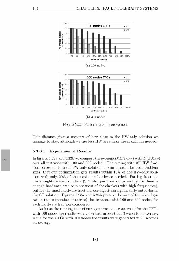
“thesis” — 2015/8/12 — 12:54 — page 134 — #154

5


(a) 100 nodes

(b) 300 nodes

Figure 5.22: Performance improvement

This distance gives a measure of how close to the HW-only solution wemanage to stay, although we use less HW area than the maximum needed.

5.3.6.1 Experimental Results

In figures 5.22a and 5.22b we compare the average D(EXOP T ) with D(EXSF )over all testcases with 100 and 300 nodes . The setting with 0% HW frac-tion corresponds to the SW-only solution. It can be seen, for both problemsizes, that our optimization gets results within 18% of the HW-only solu-tion with only 20% of the maximum hardware needed. For big fractionsthe straight-forward solution (SF) also performs quite well (since there isenough hardware area to place most of the checkers with high frequencies),but for the small hardware fractions our algorithm significantly outperformsthe SF solution. Figures 5.23a and 5.23b present the size of the reconfigu-ration tables (number of entries), for testcases with 100 and 300 nodes, foreach hardware fraction considered.

As far as the running time of our optimization is concerned, for the CFGswith 100 nodes the results were generated in less than 3 seconds on average,while for the CFGs with 100 nodes the results were generated in 93 secondson average.

134

“thesis” — 2015/8/12 — 12:54 — page 135 — #155

5


(a) 100 nodes

(b) 300 nodes

Figure 5.23: Reconfiguration schedule table size

5.3.6.2 Case Study – GSM Encoder

We also tested our approach on a real-life example, a GSM encoder, whichimplements the European GSM 06.10 provisional standard for full-rate speechtranscoding. This application can be decomposed into 10 tasks executedin a sequential order: Init, GetAudioInput, Preprocess, LPC_Analysis,ShortTermAnalysisFilter, LongTermPredictor, RPE_Encoding, Add, En-code, and Output. We instrumented the whole application with 56 check-ers, corresponding to the 19 most critical variables, according to the tech-nique described in Section 5.1. The execution times were derived usingthe MPARM cycle accurate simulator, considering an ARM processor withan operational frequency of 60 MHz. The checking modules were synthe-sized for an XC6VLX240T Virtex6 device, using the Xilinx ISE design suite.The reconfiguration times were estimated considering a 100 MHz configu-ration clock frequency and the ICAP 32-bit width configuration interface(see our reconfiguration controller described in Section 3.1.1.2). We used amethodology similar to the one presented in [SBB+06] in order to reducethe reconfiguration granularity.

The gain, area and reconfiguration overheads for each checker are givenin Table 5.6. The CFGs for each task, as well as the profiling information wasgenerated using the LLVM suite [LA04] as follows: l lvm-gcc was first usedto generate LLVM bytecode from the C files. The opt tool was then usedto instrument the bytecode with edge and basic block profiling instructions.The bytecode was next run using l li, and then the execution profile was

135

“thesis” — 2015/8/12 — 12:54 — page 136 — #156

5


Table 5.6: Time and area overheads of checkers for the GSM encoder casestudy

cigain area reconfig.

cigain area reconfig.

(µs) (slices) time (µs) (µs) (slices) time (µs)

c1 0.8 6 3.69 c29 0.7 16 9.84c2 0.71 8 4.92 c30 0.66 13 7.995c3 0.725 7 4.305 c31 0.515 9 5.535c4 0.59 2 1.23 c32 1 18 11.07c5 0.88 3 1.845 c33 1.02 22 13.53c6 0.45 2 1.23 c34 0.795 17 10.455c7 0.675 6 3.69 c35 0.82 18 11.07c8 0.665 6 3.69 c36 0.78 16 9.84c9 0.82 4 2.46 c37 0.6 19 11.685c10 1.005 9 5.535 c38 0.625 21 12.915c11 0.46 6 3.69 c39 0.9 32 19.68c12 0.67 7 4.305 c40 1.35 45 27.675c13 0.625 11 6.765 c41 1.34 40 24.6c14 0.7 13 7.995 c42 1.01 30 18.45c15 0.73 15 9.225 c43 1.02 40 24.6c16 0.67 10 6.15 c44 1 35 21.525c17 1.1 15 9.225 c45 1.01 26 15.99c18 0.905 15 9.225 c46 1.05 32 19.68c19 0.91 12 7.38 c47 1.4 34 20.91c20 0.915 13 7.995 c48 1.45 33 20.295c21 0.7 14 8.61 c49 1.605 37 22.755c22 0.62 12 7.38 c50 1.56 37 22.755c23 0.58 10 6.15 c51 0.5 10 6.15c24 1.01 16 9.84 c52 0.79 16 9.84c25 0.705 12 7.38 c53 0.78 14 8.61c26 0.735 12 7.38 c54 0.7 16 9.84c27 0.5 14 8.61 c55 0.715 18 11.07c28 0.96 9 5.535 c56 0.8 22 13.53

generated using l lvm-prof. Finally, opt-analyze was used to print the CFGsto .dot files. We ran the profiling considering several audio files (.au) asinput. The results of this step revealed that many checkers (35 out of the56) were placed in loops and executed on average as much as 375354 times,which suggests that it is important to place them in HW.

Using the information generated we ran our optimization algorithm. Theresults obtained are shown in Figure 5.24a. It can be seen that the resultsfollow trends similar to those for the synthetic experiments. Our optimiza-tion generated results within 27% of the HW-only solution with just 15%hardware fraction. Also note that for hardware fractions between 15% and40%, the solution generated by our algorithm (OPT) was roughly 2.5 times

136

“thesis” — 2015/8/12 — 12:54 — page 137 — #157

5

5.4. SUMMARY 137

(a) Performance improvement

(b) Reconfiguration schedule table size

Figure 5.24: Results for the GSM encoder case study

closer to the HW-only solution than that generated by the straight-forwardalgorithm (SF). Finally, Figure 5.24b shows the sizes for the reconfigurationtables.

5.4 Summary

This chapter proposed techniques to optimize the hardware/software imple-mentation of error detection mechanisms. First we developed system-leveloptimization algorithms that perform HW/SW codesign in order to mini-mize the global worst-case schedule length of a safety-critical application,while meeting the imposed hardware cost constraints and tolerating mul-tiple transient faults. Both statically reconfigurable FPGAs and partiallydynamically reconfigurable FPGAs have been considered. In the second partof this chapter we presented an algorithm for performance optimization oferror detection based on speculative reconfiguration. We minimize the av-erage execution time of a program by using partially reconfigurable FPGAsto place in hardware only those error detection components that provide thehighest performance improvement.

137

“thesis” — 2015/8/12 — 12:54 — page 138 — #158

5


138

“thesis” — 2015/8/12 — 12:54 — page 139 — #159

6

Chapter 6

!"#$%&'!"& (") *%+%,- .!,/

In this chapter we shall summarize the research contributions of this thesisand discuss possible directions of future work.

6.1 Conclusions

In order to meet the stringent demands of modern applications and keepcosts within reasonable limits, today’s engineers are faced with difficult de-sign optimization problems. Often, they deal with multi-objective optimiza-tions, having to deliver solutions that provide high performance as well asflexibility, energy-efficiency as well as real-time features, fault tolerance aswell as low cost. The use of reconfigurable and heterogeneous architecturesis one approach to deal with these demanding requirements. However, inorder to leverage the advantages of such platforms and deliver efficient so-lutions, the engineers and designers of modern embedded systems need tohave available tools and methodologies. It is the responsibility of the re-search community to develop these tools and to explore the advantages andpossible uses of new technologies.

In this thesis we have presented several approaches to the hardware/softwarecodesign and optimization of adaptive real-time systems implemented on re-configurable and heterogeneous platforms. We have addressed topics thatare of interest to the industry: performance enhancement using static anddynamic FPGA configuration prefetching (Chapter 3), energy optimizationfor multi-mode real-time systems implemented on platforms composed ofCPUs, GPUs and FPGAs (Chapter 4), and hardware/software codesign offault-tolerant safety-critical systems (Chapter 5).

6.1.1 FPGA Configuration Prefetching

In Chapter 3 we proposed a complete framework for partial dynamic recon-figuration of FPGAs, together with optimization algorithms for static and

139

“thesis” — 2015/8/12 — 12:54 — page 140 — #160

6

140 CHAPTER 6. CONCLUSIONS AND FUTURE WORK

dynamic FPGA configuration prefetching. The framework is modular andpermits rapid integration of user applications with minimal effort from thedesigner. We proposed an IP-based architecture, together with a compre-hensive API, that hides the low-level details from the programmer and canbe used to accelerate applications using partial dynamic reconfiguration ofFPGAs.

Based on this framework, we next proposed two algorithms for FPGAconfiguration prefetching:

1. The first one schedules prefetches at design-time and simultaneouslyperforms hardware/software partitioning in order to minimize the ex-pected execution time of an application. The algorithm performs spec-ulative FPGA configuration prefetching based on profiling informationin order to reduce the reconfiguration penalty by overlapping FPGAreconfigurations with useful computations.

2. The second algorithm targets applications that exhibit a dynamic andnon-stationary behavior. In such cases we can not obtain accurateprofiling information, so we need approaches that are able to adaptto the run-time conditions. Our technique uses a piecewise linearpredictor that captures correlations in order to launch prefetches forthose hardware modules that will provide the highest performanceimprovements.

The framework and our optimization approaches have been tested usingextensive simulations and a proof of concept implementation on a platformfrom Xilinx.

6.1.2 Multi-Mode Systems

In Chapter 4 we addressed the problem of energy optimization for multi-mode real-time systems. We characterize a functional mode by the compo-sition of the active task set (containing the tasks that are currently releasingperiodic jobs). In order to meet the real-time requirements of such dynamicsystems and keep a low energy consumption, we propose intelligent on-lineresource management algorithms. The resource manager implements run-time policies to decide on-the-fly task admission and the mapping of activetasks to the available resources in a heterogeneous platform composed ofCPUs, GPUs and FPGAs. The experimental validation, including bothreal-life measurements and simulations, has showed the practicality and ef-ficiency of our approach.

6.1.3 Fault-Tolerant Systems

In Chapter 5 we addressed the problem of optimizing the error detectionimplementation for fault-tolerant safety-critical systems. In order to provideresiliency against transient faults, error detection has to be employed, but

140

“thesis” — 2015/8/12 — 12:54 — page 141 — #161

6

6.2. FUTURE WORK 141

this incurs high performance and cost overheads. In order to deal with thisissue, we proposed two optimization strategies:

1. The first one targets real-time applications running on a distributedembedded architecture and addresses the problem at a task level. Wedecide on the hardware/software implementation of the error detectionmechanisms for each task in order to minimize the global worst-caseschedule length of the whole application, while meeting the imposedhardware cost constraints and tolerating multiple faults.

2. The second algorithm presents a method to minimize the average exe-cution time of an application composed of a single sequential task. Byanalyzing the internal structure and properties of the application, andby using the advantages of partial dynamic reconfiguration of FPGAs,we speculatively place in hardware those error detection componentsthat will result in a minimal performance overhead.

Both optimization approaches have been tested using extensive experi-ments, including real-life case studies.

6.2 Future Work

The entire work presented in this thesis constitutes a solid basis that has abig potential for future extensions, improvements and applications. In thissection we will mention some specific points that can be addressed:

• For a large class of applications, optimizing the worst-case behavioris not important, while optimizing for the average is not enough. In-stead, statistical guarantees are desirable, like, e.g., optimizing theα-percentile. An interesting direction of future work would be to ex-tend our configuration prefetching strategies presented in Chapter 3for such a case.

• In Chapter 3 we presented configuration prefetching algorithms tominimize the FPGA reconfiguration penalties. Other techniques thataddress the same problem are configuration compression and caching.Since they are complementary to the approaches we presented, it wouldbe interesting to investigate holistic solutions that combine the threemethods to obtain the best results.

• In the context of multi-mode systems, introducing soft real-time tasksinto the model would be very interesting. There exist many applicationareas in which hard real-time tasks coexist with soft real-time ones,or with tasks that only have certain quality of service demands (butno strict deadlines). Extending the optimizations presented in Chap-ter 4 to account for such scenarios would be an important researchcontribution.

141

“thesis” — 2015/8/12 — 12:54 — page 142 — #162

6

142 CHAPTER 6. CONCLUSIONS AND FUTURE WORK

• The faults that affect a system might be transient, intermittent orpermanent. In Chapter 5 we addressed only the case of transient andintermittent faults. An interesting area of future work would be toconsider permanent faults and use the capabilities of partial dynamicreconfiguration of FPGAs to optimize for such scenarios.

• In the context of fault-tolerant systems, we have performed optimiza-tion of the error detection implementation. One possible directionof future work is to combine this technique with the prefetching ap-proaches presented in Chapter 3, in order to optimize both the errordetection mechanisms and the original application.

142

“thesis” — 2015/8/4 — 23:59 — page 143 — #163

!"#!$%&'()*

[ALSU06] Alfred V. Aho, Monica S. Lam, Ravi Sethi, and Jeffrey D. Ull-man. Compilers: Principles, Techniques, and Tools. AddisonWesley, 2006.

[ALT08] Joshua A. Anderson, Chris D. Lorenz, and A. Travesset. Gen-eral purpose molecular dynamics simulations fully implementedon graphics processing units. Journal of Computational Physics,227(10):5342 – 5359, 2008.

[Alt09] Altera. Taking advantage of advances in FPGA floating-pointIP cores - white paper 01116. 2009.

[Alt12] Altera. Using the Stratix V reconfiguration controller to per-form dynamic reconfiguration - application note an-664-1.0.2012.

[AMHN05] M. Akerholm, A. Moller, H. Hansson, and M. Nolin. Towardsa dependable component technology for embedded system ap-plications. 10th IEEE Intl. Workshop on Object-Oriented Real-Time Dependable Systems, pages 320–328, 2005.

[ASG13] A. Ashrafi, Antonio G. M. Strollo, and O. Gustafsson. Hard-ware implementation of digital signal processing algorithms. J.Electrical and Computer Engineering, 2013:782575:1–782575:2,2013.

[BBD05] S. Banerjee, E. Bozorgzadeh, and N. Dutt. Physically-awareHW-SW partitioning for reconfigurable architectures with par-tial dynamic reconfiguration. 42nd Design Automation Confer-ence, pages 335–340, 2005.

[BBG13] Mehmet E. Belviranli, Laxmi N. Bhuyan, and R. Gupta. Adynamic self-scheduling scheme for heterogeneous multiproces-

143

“thesis” — 2015/8/4 — 23:59 — page 144 — #164

144 BIBLIOGRAPHY

sor architectures. ACM Trans. Archit. Code Optim., 9(4):57:1–57:20, January 2013.

[BBZT14] A. Becher, F. Bauer, D. Ziener, and J. Teich. Energy-awareSQL query acceleration through FPGA-based dynamic partialreconfiguration. 24th International Conference on Field Pro-grammable Logic and Applications (FPL), pages 1–8, 2014.

[BGFM06] Jason A. Blome, S. Gupta, S. Feng, and S. Mahlke. Cost-efficient soft error protection for embedded microprocessors.Intl. Conf. on Compilers, Architecture and Synthesis for Em-bedded Systems, pages 421–431, 2006.

[BGG13] P.P. Boopal, M. Garrido, and O. Gustafsson. A recon-figurable FFT architecture for variable-length and multi-streaming OFDM standards. IEEE International Symposiumon Circuits and Systems (ISCAS), pages 2066–2070, 2013.

[BHS+13] Rana M. Bilal, R. Hafiz, M. Shafique, S. Shoaib, A. Munawar,and J. Henkel. Isomer: integrated selection, partitioning, andplacement methodology for reconfigurable architectures. In-ternational Conference on Computer-Aided Design (ICCAD),pages 755–762, 2013.

[BJRK+03] B. Blodget, P. James-Roxby, E. Keller, S. McMillan, andP. Sundararajan. A self-reconfiguring platform. Proceedingsof Field Programmable Logic and Applications, pages 565–574,2003.

[BLBY11] M. Bogdanski, P.R. Lewis, T. Becker, and Xin Yao. Improvingscheduling techniques in heterogeneous systems with dynamic,on-line optimisations. International Conference on Complex,Intelligent and Software Intensive Systems (CISIS), pages 496–501, 2011.

[BMA+05] C. Bobda, M. Majer, A. Ahmadinia, T. Haller, A. Linarth,and J. Teich. The Erlangen slot machine: a highly flexibleFPGA-based reconfigurable platform. 13th Annual IEEE Sym-posium on Field-Programmable Custom Computing Machines,pages 319–320, 2005.

[BMR+08] C. Bolchini, A. Miele, M. Rebaudengo, F. Salice, D. Sciuto,L. Sterpone, and M. Violante. Software and hardware tech-niques for SEU detection in IP processors. J. Electron. Test.,24(1-3):35–44, 2008.

[BP05] Z.K. Baker and V.K. Prasanna. Efficient hardware data miningwith the apriori algorithm on FPGAs. 13th Annual IEEE Sym-posium on Field-Programmable Custom Computing Machines,pages 3–12, 2005.

144

“thesis” — 2015/8/4 — 23:59 — page 145 — #165

BIBLIOGRAPHY 145

[BPCF13] J. Bispo, N. Paulino, J.M.P. Cardoso, and J.C. Ferreira.Transparent trace-based binary acceleration for reconfigurableHW/SW systems. IEEE Transactions on Industrial Informat-ics, 9(3):1625–1634, 2013.

[BPPC12] R. Bonamy, H.-M. Pham, S. Pillement, and D. Chillet. UPaRC– ultra-fast power-aware reconfiguration controller. Design, Au-tomation & Test in Europe (DATE), pages 1373–1378, 2012.

[BSY+10] K. Bertels, V.M. Sima, Y. Yankova, G. Kuzmanov, W. Luk,José Gabriel F. Coutinho, F. Ferrandi, C. Pilato, M. Lattuada,D. Sciuto, and A. Michelotti. HArtes: Hardware-softwarecodesign for heterogeneous multicore platforms. IEEE Micro,30(5):88–97, 2010.

[But04] Giorgio C. Buttazzo. Hard Real-time Computing Systems: Pre-dictable Scheduling Algorithms And Applications (Real-TimeSystems Series). Springer-Verlag TELOS, Santa Clara, CA,USA, 2004.

[CBP04] The 1st championship branch prediction competi-tion. Journal of Instruction-Level Parallelism, 2004.http://www.jilp.org/cbp.

[CBR+14] Juan A. Clemente, I. Beretta, V. Rana, D. Atienza Alonso,and D. Sciuto. A mapping-scheduling algorithm for hardwareacceleration on reconfigurable platforms. ACM Transactionson Reconfigurable Technology and Systems (TRETS), 1(1):1–27, 2014.

[CLS+08] S. Che, Jie Li, J.W. Sheaffer, K. Skadron, and J. Lach. Acceler-ating compute-intensive applications with GPUs and FPGAs.Symposium on Application Specific Processors, pages 101–107,2008.

[CMHM10] E.S. Chung, P.A. Milder, J.C. Hoe, and Ken Mai. Single-chipheterogeneous computing: Does the future include custom logic,FPGAs, and GPGPUs? 43rd Annual IEEE/ACM Interna-tional Symposium on Microarchitecture (MICRO), pages 225–236, 2010.

[Con03] C. Constantinescu. Trends and challenges in VLSI circuit reli-ability. IEEE Micro, 23(4):14–19, 2003.

[CRM14] Juan A. Clemente, J. Resano, and D. Mozos. An approach tomanage reconfigurations and reduce area cost in hard real-timereconfigurable systems. ACM Trans. Embed. Comput. Syst.,13(4):90:1–90:24, 2014.

145

“thesis” — 2015/8/4 — 23:59 — page 146 — #166

146 BIBLIOGRAPHY

[CRR+09] R. Cordone, F. Redaelli, M. A. Redaelli, M. D. Santambro-gio, and D. Sciuto. Partitioning and scheduling of task graphson partially dynamically reconfigurable FPGAs. IEEE Trans-actions on Computer-Aided Design of Integrated Circuits andSystems, 28(5):662–675, 2009.

[DML11] F. Duhem, F. Muller, and P. Lorenzini. FaRM: Fast recon-figuration manager for reducing reconfiguration time overheadon FPGA. Andreas Koch, Ram Krishnamurthy, John McAl-lister, Roger Woods, and Tarek A. El-Ghazawi, editors, ARC,volume 6578 of Lecture Notes in Computer Science, pages 253–260. Springer, 2011.

[dRGLH06] B. de Ruijsscher, G.N. Gaydadjiev, J. Lichtenauer, and E. Hen-driks. FPGA accelerator for real-time skin segmentation.IEEE/ACM/IFIP Workshop on Embedded Systems for RealTime Multimedia, pages 93–97, 2006.

[DSB+13] M. Damavandpeyma, S. Stuijk, T. Basten, M. Geilen, andH. Corporaal. Throughput-constrained DVFS for scenario-aware dataflow graphs. IEEE 19th Real-Time and EmbeddedTechnology and Applications Symposium (RTAS), pages 175–184, 2013.

[EA11] G.A. Elliott and J.H. Anderson. Real-world constraints ofGPUs in real-time systems. IEEE 17th International Confer-ence on Embedded and Real-Time Computing Systems and Ap-plications (RTCSA), volume 2, pages 48–54, 2011.

[EA12] G.A. Elliott and J.H. Anderson. Globally scheduled real-timemultiprocessor systems with GPUs. Real-Time Syst., 48(1):34–74, 2012.

[EDPP00] P. Eles, A. Doboli, P. Pop, and Z. Peng. Scheduling with busaccess optimization for distributed embedded systems. IEEETransactions on Very Large Scale Integration (VLSI) Systems,8(5):472–491, 2000.

[EWA13] G.A. Elliott, B.C. Ward, and J.H. Anderson. GPUSync: Aframework for real-time GPU management. IEEE 34th Real-Time Systems Symposium (RTSS), pages 33–44, 2013.

[Fou15] HSA Foundation. Harmonizing the industry around heteroge-neous computing. 2015. http://www.hsafoundation.com/.

[GGPM11] Junhe Gan, F. Gruian, P. Pop, and J. Madsen. En-ergy/reliability trade-offs in fault-tolerant event-triggered dis-tributed embedded systems. 16th Asia and South Pacific DesignAutomation Conference (ASP-DAC), pages 731–736, 2011.

146

“thesis” — 2015/8/4 — 23:59 — page 147 — #167

BIBLIOGRAPHY 147

[GJ90] Michael R. Garey and David S. Johnson. Computers and In-tractability; A Guide to the Theory of NP-Completeness. W. H.Freeman & Co, New York, NY, USA, 1990.

[Hau98] Scott Hauck. Configuration prefetch for single context reconfig-urable coprocessors. Intl. Symp. on Field Programmable GateArrays, 1998.

[HHSC10] P.-A. Hsiung, C.-H. Huang, J.-S. Shen, and C.-C. Chiang.Scheduling and placement of hardware/software real-time re-locatable tasks in dynamically partially reconfigurable systems.ACM Trans. Reconfigurable Technol. Syst., 4(1):9:1–9:32, 2010.

[HJL+07] B. Harris, A.C. Jacob, J.M. Lancaster, J. Buhler, and R.D.Chamberlain. A banded Smith-Waterman FPGA acceleratorfor Mercury BLASTP. International Conference on Field Pro-grammable Logic and Applications, pages 765–769, 2007.

[hKYS+12] S.-H. Kang, H. Yang, L. Schor, I. Bacivarov, Soonhoi Ha, andL. Thiele. Multi-objective mapping optimization via problemdecomposition for many-core systems. IEEE 10th Symposiumon Embedded Systems for Real-time Multimedia (ESTIMedia),pages 28–37, 2012.

[HLD+09] Jie Hu, Feihui Li, V. Degalahal, M. Kandemir, N. Vijaykrish-nan, and Mary J. Irwin. Compiler-assisted soft error detectionunder performance and energy constraints in embedded sys-tems. ACM Trans. Embed. Comput. Syst., 2009., 8(4):1–30,2009.

[HLS11] Y. He, Jie Liu, and Hongyang Sun. Scheduling functionallyheterogeneous systems with utilization balancing. IEEE Inter-national Parallel Distributed Processing Symposium (IPDPS),pages 1187–1198, 2011.

[HMA+01] S. Hareland, J. Maiz, M. Alavi, K. Mistry, S. Walsta, andChanghong Dai. Impact of CMOS process scaling and SOIon the soft error rates of logic processes. Symposium on VLSITechnology. Digest of Technical Papers, pages 73–74, 2001.

[HMZB12] Ruining He, Yuchun Ma, K. Zhao, and J. Bian. ISBA: An inde-pendent set-based algorithm for automated partial reconfigura-tion module generation. International Conference on ComputerAided Design, 2012.

[HV04] M Handa and R Vemuri. Area fragmentation in reconfigurableoperating systems. Intl. Conf. on Engineering of ReconfigurableSystems and Algorithms, 2004.

147

“thesis” — 2015/8/4 — 23:59 — page 148 — #168

148 BIBLIOGRAPHY

[HV08] C. Huang and F. Vahid. Dynamic coprocessor management forFPGA-enhanced compute platforms. Proceedings of the inter-national conference on compilers, architectures and synthesisfor embedded systems, pages 71–78, New York, NY, USA, 2008.

[HV09] C. Huang and F. Vahid. Transmuting coprocessors: Dynamicloading of FPGA coprocessors. Design Automation Conference,pages 848 –851, 2009.

[HWC14] M. Hollander, Douglas A. Wolfe, and E. Chicke, editors. Non-parametric Statistical Methods, 3rd Edition. Wiley, 2014.

[IBM09] IBM. IBM ILOG CPLEX v12.1 - user’s manual for CPLEX.2009.

[IPEP05] V. Izosimov, P. Pop, P. Eles, and Z. Peng. Design optimiza-tion of time- and cost-constrained fault-tolerant distributed em-bedded systems. Design, Automation & Test in Europe, pages864–869, 2005.

[IPEP06] V. Izosimov, P. Pop, P. Eles, and Z. Peng. Synthesis of fault-tolerant schedules with transparency/performance trade-offs fordistributed embedded systems. Design, Automation & Test inEurope, pages 1–6, 2006.

[IPEP08] V. Izosimov, P. Pop, P. Eles, and Z. Peng. Scheduling offault-tolerant embedded systems with soft and hard timing con-straints. Design, Automation & Test in Europe, pages 915–920,2008.

[IPP+09] V. Izosimov, I. Polian, P. Pop, P. Eles, and Z. Peng. Analy-sis and optimization of fault-tolerant embedded systems withhardened processors. Design, Automation & Test in Europe,pages 682–687, 2009.

[JEP13] Ke Jiang, P. Eles, and Z. Peng. Optimization of secure em-bedded systems with dynamic task sets. Design, Automation &Test in Europe, pages 1765–1770, 2013.

[Jim05] D.A. Jimenez. Piecewise linear branch prediction. 32nd In-ternational Symposium on Computer Architecture, pages 382 –393, 2005.

[JLE+13] Ke Jiang, A. Lifa, P. Eles, Z. Peng, and Wei Jiang. Energy-aware design of secure multi-mode real-time embedded systemswith FPGA co-processors. Proceedings of the 21st InternationalConference on Real-Time Networks and Systems, pages 109–118, New York, NY, USA, 2013.

148

“thesis” — 2015/8/4 — 23:59 — page 149 — #169

BIBLIOGRAPHY 149

[JLK+14] H. Jung, C. Lee, S.-H. Kang, Sungchan Kim, Hyunok Oh, andSoonhoi Ha. Dynamic behavior specification and dynamic map-ping for real-time embedded systems: HOPES approach. ACMTrans. Embed. Comput. Syst., 13(4s):135:1–135:26, 2014.

[JPT+10] Zai Jian Jia, A.D. Pimentel, M. Thompson, T. Bautista, andA. Nunez. NASA: A generic infrastructure for system-level MP-SoC design space exploration. 8th IEEE Workshop on EmbeddedSystems for Real-Time Multimedia (ESTIMedia), pages 41–50,2010.

[JTY+99] J. S. N. Jean, K. Tomko, V. Yavagal, J. Shah, and R. Cook. Dy-namic reconfiguration to support concurrent applications. IEEETransactions on Computers, 48(6), 1999.

[KB03] H. Kopetz and G. Bauer. The time-triggered architecture. Pro-ceedings of the IEEE, 91(1):112–126, 2003.

[KFP+15] B. Khemka, R. Friese, S. Pasricha, Anthony A. Maciejewski,Howard J. Siegel, Gregory A. Koenig, S. Powers, M. Hilton,R. Rambharos, and S. Poole. Utility maximizing dynamic re-source management in an oversubscribed energy-constrainedheterogeneous computing system. Sustainable Computing: In-formatics and Systems, 5(0):14 – 30, 2015.

[KHM03] N. Kandasamy, J. P. Hayes, and B. T. Murray. Transparentrecovery from intermittent faults in time-triggered distributedsystems. IEEE Transactions on Computers, 52(2):113–125,2003.

[KLRI11] S. Kato, K. Lakshmanan, R. Rajkumar, and Y. Ishikawa.TimeGraph: GPU scheduling for real-time multi-tasking en-vironments. Proceedings of the 2011 USENIX Conference onUSENIX Annual Technical Conference, pages 2–2, Berkeley,CA, USA, 2011.

[Koc13] Dirk Koch. Partial Reconfiguration on FPGAs - Architectures,Tools and Applications, volume 153 of Lecture Notes in Electri-cal Engineering. Springer, 2013.

[Kop11] Hermann Kopetz. Real-Time Systems: Design Principles forDistributed Embedded Applications. Springer Publishing Com-pany, Incorporated, 2nd edition, 2011.

[LA04] C. Lattner and V. Adve. LLVM: A compilation frameworkfor lifelong program analysis & transformation. Intl. Symp. onCode Generation and Optimization, 2004.

149

“thesis” — 2015/8/4 — 23:59 — page 150 — #170

150 BIBLIOGRAPHY

[LCD+00] Yanbing Li, T. Callahan, E. Darnell, Randolph E. Harr,U. Kurkure, and J. Stockwood. Hardware-software co-design ofembedded reconfigurable architectures. 37th Design Automa-tion Conference, pages 507–512, 2000.

[LCP+09] G. Lyle, S. Chen, K. Pattabiraman, Z. Kalbarczyk, andR. Iyer. An end-to-end approach for the automatic derivationof application-aware error detectors. IEEE/IFIP Intl. Conf. onDependable Systems & Networks, pages 584–589, 2009.

[LCR03] F. Lima, L. Carro, and R. Reis. Designing fault tolerant sys-tems into SRAM-based FPGAs. 40th Design Automation Con-ference, pages 650–655, 2003.

[LEP11] A. Lifa, P. Eles, and Z. Peng. Performance optimization oferror detection based on speculative reconfiguration. DesignAutomation Conference (DAC), pages 369–374, 2011.

[LEP12a] A. Lifa, P. Eles, and Z. Peng. Context-aware speculativeprefetch for soft real-time applications. IEEE 18th InternationalConference on Embedded and Real-Time Computing Systemsand Applications (RTCSA), pages 174–183, 2012.

[LEP12b] A. Lifa, P. Eles, and Z. Peng. Minimization of average executiontime based on speculative FPGA configuration prefetch. Inter-national Conference on Reconfigurable Computing and FPGAs(ReConFig), 2012.

[LEP12c] A. Lifa, P. Eles, and Z. Peng. Execution time minimiza-tion based on hardware/software partitioning and speculativeprefetch. Technical Report 2012:11, Linköping University, Soft-ware and Systems, 2012.

[LEP13] A. Lifa, P. Eles, and Z. Peng. Dynamic configuration prefetch-ing based on piecewise linear prediction. Design, Automation& Test in Europe (DATE), pages 815–820, 2013.

[LEP15a] A. Lifa, P. Eles, and Z. Peng. A reconfigurable framework forperformance enhancement with dynamic FPGA configurationprefetching. IEEE Transactions on Computer-Aided Design ofIntegrated Circuits and Systems, 2015.

[LEP15b] A. Lifa, P. Eles, and Z. Peng. On-the-fly energy minimizationfor multi-mode real-time systems on heterogeneous platforms.IEEE Symp. on Embedded Systems for Real-time Multimedia(ESTIMedia), 2015.

[LEPI10] A. Lifa, P. Eles, Z. Peng, and V. Izosimov. Hardware/softwareoptimization of error detection implementation for real-time

150

“thesis” — 2015/8/4 — 23:59 — page 151 — #171

BIBLIOGRAPHY 151

embedded systems. Intl. Conf. on Hardware/Software Code-sign and System Synthesis, pages 40–50, 2010.

[LH02] Zhiyuan Li and Scott Hauck. Configuration prefetching tech-niques for partial reconfigurable coprocessor with relocation anddefragmentation. Intl. Symp. on Field Programmable Gate Ar-rays, 2002.

[LHK09] Chi-Keung Luk, S. Hong, and Hyesoon Kim. Qilin: Exploit-ing parallelism on heterogeneous multiprocessors with adaptivemapping. Proceedings of the 42Nd Annual IEEE/ACM Inter-national Symposium on Microarchitecture, MICRO 42, pages45–55, New York, NY, USA, 2009.

[Li02] Zhiyuan Li. Configuration management techniques for recon-figurable computing, 2002. PhD thesis, Northwestern Univ.,Evanston, IL.

[LKLJ09] Ming Liu, W. Kuehn, Zhonghai Lu, and A. Jantsch. Run-timepartial reconfiguration speed investigation and architectural de-sign space exploration. International Conference on Field Pro-grammable Logic and Applications, pages 498–502, 2009.

[Mar10] Peter Marwedel. Embedded System Design: Embedded SystemsFoundations of Cyber-Physical Systems. Springer PublishingCompany, Incorporated, 2nd edition, 2010.

[MBH+14] A. Maghazeh, U.D. Bordoloi, A. Horga, P. Eles, and Z. Peng.Saving energy without defying deadlines on mobile GPU-basedheterogeneous systems. International Conference on Hard-ware/Software Codesign and System Synthesis, pages 8:1–8:10,New York, NY, USA, 2014.

[MBT04] A. Maheshwari, W. Burleson, and R. Tessier. Trading off tran-sient fault tolerance and power consumption in deep submicron(DSM) VLSI circuits. IEEE Transactions on Very Large ScaleIntegration (VLSI) Systems,, 12(3):299–311, 2004.

[MEP05] S. Manolache, P. Eles, and Z. Peng. Fault and energy-awarecommunication mapping with guaranteed latency for applica-tions implemented on NoC. Design Automation Conference,pages 266–269, 2005.

[ML99] G. McGregor and P. Lysaght. Self controlling dynamic recon-figuration: A case study. Field Programmable Logic and Appli-cations, pages 144–154. Springer, 1999.

[MLH+12] R. Membarth, J.-H. Lupp, F. Hannig, J. Teich, M. Körner, andW. Eckert. Dynamic task-scheduling and resource management

151

“thesis” — 2015/8/4 — 23:59 — page 152 — #172

152 BIBLIOGRAPHY

for GPU accelerators in medical imaging. 25th InternationalConference on Architecture of Computing Systems, pages 147–159, 2012.

[MSP+12] G. Mariani, V. Sima, G. Palermo, V. Zaccaria, C. Silvano, andK. Bertels. Using multi-objective design space exploration toenable run-time resource management for reconfigurable archi-tectures. Design, Automation & Test in Europe, pages 1379–1384, 2012.

[MT90] Silvano Martello and Paolo Toth. Knapsack Problems: Algo-rithms and Computer Implementations. John Wiley & Sons,Inc., New York, NY, USA, 1990.

[NOS13] B. Navas, J. Oberg, and I. Sander. Towards the generic re-configurable accelerator: Algorithm development, core design,and performance analysis. International Conference on Recon-figurable Computing and FPGAs (ReConFig), pages 1–6, 2013.

[NOS14] B. Navas, J. Oberg, and I. Sander. On providing scalable self-healing adaptive fault-tolerance to RTR SoCs. InternationalConference on ReConFigurable Computing and FPGAs (Re-ConFig), pages 1–6, 2014.

[NSO+12] R. Nane, Vlad M. Sima, B. Olivier, R. Meeuws, Y. Yankova, andK. Bertels. DWARV 2.0: A CoSy-based C-to-VHDL hardwarecompiler. International Conference on Field-programmableLogic and Applications (FPL), pages 619–622, 2012.

[NSO13] B. Navas, I. Sander, and J. Öberg. The RecoBlock SoC plat-form: A flexible array of reusable run-time-reconfigurable IP-blocks. Design, Automation & Test in Europe, pages 833–838,2013.

[PBV05] Elena M. Panainte, K. Bertels, and S. Vassiliadis. Instructionscheduling for dynamic hardware configurations. Design, Au-tomation & Test in Europe, 2005.

[PBV06] Elena M. Panainte, K. Bertels, and S. Vassiliadis. Interprocedu-ral compiler optimization for partial run-time reconfiguration.The Journal of VLSI Signal Processing, 43(2), 2006.

[PKI05] K. Pattabiraman, Z. Kalbarczyk, and R. K. Iyer. Application-based metrics for strategic placement of detectors. 11th PacificRim Intl. Symp. on Dependable Computing, 2005.

[PKI11] K. Pattabiraman, Z. Kalbarczyk, and R. Iyer. Automatedderivation of application-aware error detectors using static anal-ysis: The trusted Illiac approach. IEEE Transactions on De-pendable and Secure Computing, 8(1):44–57, 2011.

152

“thesis” — 2015/8/4 — 23:59 — page 153 — #173

BIBLIOGRAPHY 153

[PRP+15] E. Paone, F. Robino, G. Palermo, V. Zaccaria, I. Sander, andC. Silvano. Customization of OpenCL applications for efficienttask mapping under heterogeneous platform constraints. De-sign, Automation & Test in Europe, pages 736–741, 2015.

[PSA10] T. Pionteck, S. Sammann, and C. Albrecht. Optimizing runtimereconfiguration decisions. IEEE/IFIP 8th International Confer-ence on Embedded and Ubiquitous Computing (EUC), pages 39–46, 2010.

[PTW10] Marco Platzner, JÃ14 rgen Teich, and Norbert Wehn, editors.

Dynamically Reconfigurable Systems. Springer, 2010.

[QP13a] Wei Quan and A.D. Pimentel. An iterative multi-applicationmapping algorithm for heterogeneous MPSoCs. IEEE 11thSymposium on Embedded Systems for Real-time Multimedia(ESTIMedia), pages 115–124, 2013.

[QP13b] Wei Quan and A.D. Pimentel. A scenario-based run-time taskmapping algorithm for MPSoCs. Design Automation Confer-ence (DAC), pages 1–6, 2013.

[R+05] J. Resano, D. Mozos, and F. Catthoor. A hybrid prefetchscheduling heuristic to minimize at run-time the reconfigura-tion overhead of dynamically reconfigurable hardware. Design,Automation & Test in Europe, 2005.

[RB93] Colin R. Reeves and John E. Beasley. Modern Heuristic Tech-niques For Combinatorial Problems. John Wiley & Sons, Inc,New York, NY, USA, 1993.

[RCG+08] J. Resano, Juan A. Clemente, C. Gonzalez, D. Mozos, andF. Catthoor. Efficiently scheduling runtime reconfigurations.ACM Trans. Des. Autom. Electron. Syst., 13(4):58:1–58:12,2008.

[RCV+05] George A. Reis, J. Chang, N. Vachharajani, R. Rangan, David I.August, and Shubhendu S. Mukherjee. Software-controlled faulttolerance. ACM Trans. Archit. Code Optim., 2005., 2(4):366–396, 2005.

[S+10] Joon E. Sim, W.-F. Wong, G. Walla, T. Ziermann, and J. Te-ich. Interprocedural placement-aware configuration prefetchingfor FPGA-based systems. IEEE Symp. on Field-ProgrammableCustom Computing Machines, 2010.

[SAHE05] M.T. Schmitz, B.M. Al-Hashimi, and P. Eles. Cosynthesisof energy-efficient multimode embedded systems with consid-eration of mode-execution probabilities. IEEE Transactions

153

“thesis” — 2015/8/4 — 23:59 — page 154 — #174

154 BIBLIOGRAPHY

on Computer-Aided Design of Integrated Circuits and Systems,24(2):153–169, 2005.

[Sar89] V. Sarkar. Determining average program execution times andtheir variance. Proceedings of the ACM SIGPLAN Conferenceon Programming Language Design and Implementation, pages298–312, New York, NY, USA, 1989.

[SB97] Stephen M. Smith and J. Michael Brady. SUSAN — a newapproach to low level image processing. International Journalof Computer Vision, 23(1):45–78, 1997.

[SBB+06] P. Sedcole, B. Blodget, T. Becker, J. Anderson, and P. Lysaght.Modular dynamic reconfiguration in Virtex FPGAs. IEE Pro-ceedings - Computers and Digital Techniques, 153(3):157 – 164,2006.

[SBE+12] S. Samii, U.D. Bordoloi, P. Eles, Z. Peng, and A. Cervin.Control-quality optimization for distributed embedded systemswith adaptive fault tolerance. 24th Euromicro Conference onReal-Time Systems (ECRTS), pages 68–77, 2012.

[SBH14] M. Shafique, L. Bauer, and J. Henkel. Adaptive energy manage-ment for dynamically reconfigurable processors. IEEE Trans-actions on Computer-Aided Design of Integrated Circuits andSystems, 33(1):50–63, 2014.

[SBHT13] M. Schmid, M. Blocherer, F. Hannig, and J. Teich. Real-timerange image preprocessing on FPGAs. International Conferenceon Reconfigurable Computing and FPGAs (ReConFig), pages1–8, 2013.

[SBR+12] L. Schor, I. Bacivarov, D. Rai, H. Yang, S.-H. Kang, andL. Thiele. Scenario-based design flow for mapping streaming ap-plications onto on-chip many-core systems. 15th InternationalConference on Compilers, Architecture, and Synthesis for Em-bedded Systems, pages 71–80, 2012.

[SBSH12] A. Sembrant, D. Black-Schaffer, and E. Hagersten. Phase be-havior in serial and parallel applications. IEEE InternationalSymposium on Workload Characterization (IISWC), pages 47–58, 2012.

[SEPC09] S. Samii, P. Eles, Z. Peng, and A. Cervin. Quality-driven syn-thesis of embedded multi-mode control systems. Design Au-tomation Conference, pages 864–869, 2009.

154

“thesis” — 2015/8/4 — 23:59 — page 155 — #175

BIBLIOGRAPHY 155

[SGO+09] R. Smith, N. Goyal, J. Ormont, K. Sankaralingam, and C. Es-tan. Evaluating GPUs for network packet signature match-ing. IEEE International Symposium on Performance Analysisof Systems and Software, pages 175–184, 2009.

[SHTT13] M. Schmid, F. Hannig, A. Tanase, and J. Teich. High-level syn-thesis revised - generation of FPGA accelerators from a domain-specific language using the polyhedron model. InternationalConference on Parallel Computing, pages 497–506, 2013.

[SPM10] P.K. Saraswat, P. Pop, and J. Madsen. Task mapping and band-width reservation for mixed hard/soft fault-tolerant embeddedsystems. Real-Time and Embedded Technology and ApplicationsSymposium (RTAS), pages 89–98, 2010.

[SSC03] T. Sherwood, S. Sair, and B. Calder. Phase tracking and predic-tion. Proceedings of the 30th annual international symposiumon Computer architecture (ISCA), pages 336–349, New York,NY, USA, 2003.

[TBEP10] B. Tanasa, U.D. Bordoloi, P. Eles, and Z. Peng. Scheduling forfault-tolerant communication on the static segment of Flexray.Real-Time Systems Symposium (RTSS), pages 385–394, 2010.

[TBEP11] B. Tanasa, U.D. Bordoloi, P. Eles, and Z. Peng. Reliability-aware frame packing for the static segment of Flexray. Inter-national Conference on Embedded Software (EMSOFT), pages175–184, 2011.

[TK11] Jim Torresen and Dirk Koch. Can run-time reconfigurable hard-ware be more accessible? Intl. Conf. on Engineering of Recon-figurable Systems & Algorithms, 2011.

[TL10] Kuen H. Tsoi and Wayne Luk. Axel: A heterogeneous clus-ter with FPGAs and GPUs. 18th Annual ACM/SIGDA In-ternational Symposium on Field Programmable Gate Arrays(FPGA), pages 115–124, New York, NY, USA, 2010.

[VMS14] U. Verner, A. Mendelson, and A. Schuster. Batch method forefficient resource sharing in real-time multi-GPU systems. 15thInternational Conference on Distributed Computing and Net-working, pages 347–362, 2014.

[WAST12] S. Wildermann, J. Angermeier, E. Sibirko, and J. Teich. Plac-ing multimode streaming applications on dynamically partiallyreconfigurable architectures. Int. J. Reconfig. Comp., 2012.

[WEE+08] R. Wilhelm, J. Engblom, A. Ermedahl, N. Holsti, S. Thesing,D. Whalley, G. Bernat, C. Ferdinand, R. Heckmann, T. Mitra,

155

“thesis” — 2015/8/4 — 23:59 — page 156 — #176

156 BIBLIOGRAPHY

F. Mueller, I. Puaut, P. Puschner, J. Staschulat, and P. Sten-strom. The worst-case execution-time problem — overview ofmethods and survey of tools. ACM Trans. Embed. Comput.Syst., 2008., 7(3):1–53, 2008.

[WJR+03] M. Wirthlin, E. Johnson, N. Rollins, M. Caffrey, and P. Gra-ham. The reliability of FPGA circuit designs in the presenceof radiation induced configuration upsets. 11th IEEE Symp. onField-Programmable Custom Computing Machines, pages 133–142, 2003.

[WPQ+12] Z. Wang, Geguang Pu, Shengchao Qin, Jianwen Li, Kim G.Larsen, J. Madsen, Bin Gu, and Jifeng He. MDM: A mode di-agram modeling framework for periodic control systems. Com-puting Research Repository (CoRR), 2012.

[WRZT13] S. Wildermann, F. Reimann, D. Ziener, and J. Teich. Symbolicsystem-level design methodology for multi-mode reconfigurablesystems. Design Autom. for Emb. Sys., 17(2):343–375, 2013.

[Xil12] Xilinx. Partial reconfiguration user guide ug702. 2012.

[ZSJ10] Jun Zhu, I. Sander, and A. Jantsch. Pareto efficient design forreconfigurable streaming applications on CPU/FPGAs. Design,Automation & Test in Europe (DATE), pages 1035–1040, 2010.

156

Department of Computer and Information Science

Linköpings universitet

Dissertations


Linköping Studies in Arts and ScienceLinköping Studies in Statistics

Linköpings Studies in Information Science


No 14 Anders Haraldsson: A Program Manipulation

System Based on Partial Evaluation, 1977, ISBN 91-

7372-144-1.

No 17 Bengt M agnhagen: Probability Based Verification of

Time Margins in Digital Designs, 1977, ISBN 91-7372-

157-3.

No 18 M ats Cedwall: Semantisk analys av process-

beskrivningar i naturligt språk, 1977, ISBN 91- 7372-

168-9.

No 22 Jaak Urmi: A Machine Independent LISP Compiler

and its Implications for Ideal Hardware, 1978, ISBN

91-7372-188-3.

No 33 Tore Risch: Compilation of Multiple File Queries in

a Meta-Database System 1978, ISBN 91- 7372-232-4.

No 51 Erland Jungert: Synthesizing Database Structures

from a User Oriented Data Model, 1980, ISBN 91-

7372-387-8.

No 54 Sture Hägglund: Contributions to the Development

of Methods and Tools for Interactive Design of

Applications Software, 1980, ISBN 91-7372-404-1.

No 55 Pär Emanuelson: Performance Enhancement in a

Well-Structured Pattern Matcher through Partial

Evaluation, 1980, ISBN 91-7372-403-3.

No 58 Bengt Johnsson, Bertil Andersson: The Human-

Computer Interface in Commercial Systems, 1981,

ISBN 91-7372-414-9.

No 69 H. Jan Komorowski: A Specification of an Abstract

Prolog Machine and its Application to Partial

Evaluation, 1981, ISBN 91-7372-479-3.

No 71 René Reboh: Knowledge Engineering Techniques

and Tools for Expert Systems, 1981, ISBN 91-7372-

489-0.

No 77 Östen Oskarsson: Mechanisms of Modifiability in

large Software Systems, 1982, ISBN 91- 7372-527-7.

No 94 Hans Lunell: Code Generator Writing Systems, 1983,

ISBN 91-7372-652-4.

No 97 Andrzej Lingas: Advances in Minimum Weight

Triangulation, 1983, ISBN 91-7372-660-5.

No 109 Peter Fritzson: Towards a Distributed Programming

Environment based on Incremental Compilation,

1984, ISBN 91-7372-801-2.

No 111 Erik Tengvald: The Design of Expert Planning

Systems. An Experimental Operations Planning

System for Turning, 1984, ISBN 91-7372- 805-5.

No 155 Christos Levcopoulos: Heuristics for Minimum

Decompositions of Polygons, 1987, ISBN 91-7870-

133-3.

No 165 James W. Goodwin: A Theory and System for Non-

Monotonic Reasoning, 1987, ISBN 91-7870-183-X.

No 170 Zebo Peng: A Formal Methodology for Automated

Synthesis of VLSI Systems, 1987, ISBN 91-7870-225-9.

No 174 Johan Fagerström: A Paradigm and System for

Design of Distributed Systems, 1988, ISBN 91-7870-

301-8.

No 192 Dimiter Driankov: Towards a Many Valued Logic of

Quantified Belief, 1988, ISBN 91-7870-374-3.

No 213 Lin Padgham: Non-Monotonic Inheritance for an

Object Oriented Knowledge Base, 1989, ISBN 91-

7870-485-5.

No 214 Tony Larsson: A Formal Hardware Description and

Verification Method, 1989, ISBN 91-7870-517-7.

No 221 M ichael Reinfrank: Fundamentals and Logical

Foundations of Truth Maintenance, 1989, ISBN 91-

7870-546-0.

No 239 Jonas Löwgren: Knowledge-Based Design Support

and Discourse Management in User Interface

Management Systems, 1991, ISBN 91-7870-720-X.

No 244 Henrik Eriksson: Meta-Tool Support for Knowledge

Acquisition, 1991, ISBN 91-7870-746-3.

No 252 Peter Eklund: An Epistemic Approach to Interactive

Design in Multiple Inheritance Hierarchies, 1991,

ISBN 91-7870-784-6.

No 258 Patrick Doherty: NML3 - A Non-Monotonic

Formalism with Explicit Defaults, 1991, ISBN 91-

7870-816-8.

No 260 Nahid Shahmehri: Generalized Algorithmic

Debugging, 1991, ISBN 91-7870-828-1.

No 264 Nils Dahlbäck: Representation of Discourse-

Cognitive and Computational Aspects, 1992, ISBN

91-7870-850-8.

No 265 Ulf Nilsson: Abstract Interpretations and Abstract

Machines: Contributions to a Methodology for the

Implementation of Logic Programs, 1992, ISBN 91-

7870-858-3.

No 270 Ralph Rönnquist: Theory and Practice of Tense-

bound Object References, 1992, ISBN 91-7870-873-7.

No 273 Björn Fjellborg: Pipeline Extraction for VLSI Data

Path Synthesis, 1992, ISBN 91-7870-880-X.

No 276 Staffan Bonnier: A Formal Basis for Horn Clause

Logic w ith External Polymorphic Functions, 1992,

ISBN 91-7870-896-6.

No 277 Kristian Sandahl: Developing Knowledge Manage-

ment Systems with an Active Expert Methodology,

1992, ISBN 91-7870-897-4.

No 281 Christer Bäckström: Computational Complexity of

Reasoning about Plans, 1992, ISBN 91-7870-979-2.

No 292 M ats Wirén: Studies in Incremental Natural

Language Analysis, 1992, ISBN 91-7871-027-8.

No 297 M ariam Kamkar: Interprocedural Dynamic Slicing

w ith Applications to Debugging and Testing, 1993,

ISBN 91-7871-065-0.

No 302 Tingting Zhang: A Study in Diagnosis Using

Classification and Defaults, 1993, ISBN 91-7871-078-2

No 312 Arne Jönsson: Dialogue Management for Natural

Language Interfaces - An Empirical Approach, 1993,

ISBN 91-7871-110-X.

No 338 Simin Nadjm-Tehrani: Reactive Systems in Physical

Environments: Compositional Modelling and Frame-

work for Verification, 1994, ISBN 91-7871-237-8.

No 371 Bengt Savén: Business Models for Decision Support

and Learning. A Study of Discrete-Event

Manufacturing Simulation at Asea/ ABB 1968-1993,

1995, ISBN 91-7871-494-X.

No 375 Ulf Söderman: Conceptual Modelling of Mode

Switching Physical Systems, 1995, ISBN 91-7871-516-

4.

No 383 Andreas Kågedal: Exploiting Groundness in Logic

Programs, 1995, ISBN 91-7871-538-5.

No 396 George Fodor: Ontological Control, Description,

Identification and Recovery from Problematic

Control Situations, 1995, ISBN 91-7871-603-9.

No 413 M ikael Pettersson: Compiling Natural Semantics,

1995, ISBN 91-7871-641-1.

No 414 Xinli Gu: RT Level Testability Improvement by

Testability Analysis and Transformations, 1996, ISBN

91-7871-654-3.

No 416 Hua Shu: Distributed Default Reasoning, 1996, ISBN

91-7871-665-9.

No 429 Jaime Villegas: Simulation Supported Industrial

Training from an Organisational Learning

Perspective - Development and Evaluation of the

SSIT Method, 1996, ISBN 91-7871-700-0.

No 431 Peter Jonsson: Studies in Action Planning:

Algorithms and Complexity, 1996, ISBN 91-7871-704-

3.

No 437 Johan Boye: Directional Types in Logic

Programming, 1996, ISBN 91-7871-725-6.

No 439 Cecilia Sjöberg: Activities, Voices and Arenas:

Participatory Design in Practice, 1996, ISBN 91-7871-

728-0.

No 448 Patrick Lambrix: Part-Whole Reasoning in

Description Logics, 1996, ISBN 91-7871-820-1.

No 452 Kjell Orsborn: On Extensible and Object-Relational

Database Technology for Finite Element Analysis

Applications, 1996, ISBN 91-7871-827-9.

No 459 Olof Johansson: Development Environments for

Complex Product Models, 1996, ISBN 91-7871-855-4.

No 461 Lena Strömbäck: User-Defined Constructions in

Unification-Based Formalisms, 1997, ISBN 91-7871-

857-0.

No 462 Lars Degerstedt: Tabulation-based Logic Program-

ming: A Multi-Level View of Query Answering,

1996, ISBN 91-7871-858-9.

No 475 Fredrik Nilsson: Strategi och ekonomisk styrning -

En studie av hur ekonomiska styrsystem utformas

och används efter företagsförvärv, 1997, ISBN 91-

7871-914-3.

No 480 M ikael Lindvall: An Empirical Study of Require-

ments-Driven Impact Analysis in Object-Oriented

Software Evolution, 1997, ISBN 91-7871-927-5.

No 485 Göran Forslund: Opinion-Based Systems: The Coop-

erative Perspective on Knowledge-Based Decision

Support, 1997, ISBN 91-7871-938-0.

No 494 M artin Sköld: Active Database Management

Systems for Monitoring and Control, 1997, ISBN 91-

7219-002-7.

No 495 Hans Olsén: Automatic Verification of Petri Nets in

a CLP framework, 1997, ISBN 91-7219-011-6.

No 498 Thomas Drakengren: Algorithms and Complexity

for Temporal and Spatial Formalisms, 1997, ISBN 91-

7219-019-1.

No 502 Jakob Axelsson: Analysis and Synthesis of Heteroge-

neous Real-Time Systems, 1997, ISBN 91-7219-035-3.

No 503 Johan Ringström: Compiler Generation for Data-

Parallel Programming Languages from Two-Level

Semantics Specifications, 1997, ISBN 91-7219-045-0.

No 512 Anna M oberg: Närhet och distans - Studier av kom-

munikationsmönster i satellitkontor och flexibla

kontor, 1997, ISBN 91-7219-119-8.

No 520 M ikael Ronström: Design and Modelling of a

Parallel Data Server for Telecom Applications, 1998,

ISBN 91-7219-169-4.

No 522 Niclas Ohlsson: Towards Effective Fault Prevention

- An Empirical Study in Software Engineering, 1998,

ISBN 91-7219-176-7.

No 526 Joachim Karlsson: A Systematic Approach for

Prioritizing Software Requirements, 1998, ISBN 91-

7219-184-8.

No 530 Henrik Nilsson: Declarative Debugging for Lazy

Functional Languages, 1998, ISBN 91-7219-197-x.

No 555 Jonas Hallberg: Timing Issues in High-Level Synthe-

sis, 1998, ISBN 91-7219-369-7.

No 561 Ling Lin: Management of 1-D Sequence Data - From

Discrete to Continuous, 1999, ISBN 91-7219-402-2.

No 563 Eva L Ragnemalm: Student Modelling based on Col-

laborative Dialogue with a Learning Companion,

1999, ISBN 91-7219-412-X.

No 567 Jörgen Lindström: Does Distance matter? On geo-

graphical dispersion in organisations, 1999, ISBN 91-

7219-439-1.

No 582 Vanja Josifovski: Design, Implementation and

Evaluation of a Distributed Mediator System for

Data Integration, 1999, ISBN 91-7219-482-0.

No 589 Rita Kovordányi: Modeling and Simulating

Inhibitory Mechanisms in Mental Image

Reinterpretation - Towards Cooperative Human-

Computer Creativity, 1999, ISBN 91-7219-506-1.

No 592 M ikael Ericsson: Supporting the Use of Design

Knowledge - An Assessment of Commenting

Agents, 1999, ISBN 91-7219-532-0.

No 593 Lars Karlsson: Actions, Interactions and Narratives,

1999, ISBN 91-7219-534-7.

No 594 C. G. M ikael Johansson: Social and Organizational

Aspects of Requirements Engineering Methods - A

practice-oriented approach, 1999, ISBN 91-7219-541-

X.

No 595 Jörgen Hansson: Value-Driven Multi-Class Overload

Management in Real-Time Database Systems, 1999,

ISBN 91-7219-542-8.

No 596 Niklas Hallberg: Incorporating User Values in the

Design of Information Systems and Services in the

Public Sector: A Methods Approach, 1999, ISBN 91-

7219-543-6.

No 597 Vivian Vimarlund: An Economic Perspective on the

Analysis of Impacts of Information Technology:

From Case Studies in Health-Care towards General

Models and Theories, 1999, ISBN 91-7219-544-4.

No 598 Johan Jenvald: Methods and Tools in Computer-

Supported Taskforce Training, 1999, ISBN 91-7219-

547-9.

No 607 M agnus M erkel: Understanding and enhancing

translation by parallel text processing, 1999, ISBN 91-

7219-614-9.

No 611 Silvia Coradeschi: Anchoring symbols to sensory

data, 1999, ISBN 91-7219-623-8.

No 613 M an Lin: Analysis and Synthesis of Reactive

Systems: A Generic Layered Architecture

Perspective, 1999, ISBN 91-7219-630-0.

No 618 Jimmy Tjäder: Systemimplementering i praktiken -

En studie av logiker i fyra projekt, 1999, ISBN 91-

7219-657-2.

No 627 Vadim Engelson: Tools for Design, Interactive

Simulation, and Visualization of Object-Oriented

Models in Scientific Computing, 2000, ISBN 91-7219-

709-9.

No 637 Esa Falkenroth: Database Technology for Control

and Simulation, 2000, ISBN 91-7219-766-8.

No 639 Per-Arne Persson: Bringing Power and Knowledge

Together: Information Systems Design for Autonomy

and Control in Command Work, 2000, ISBN 91-7219-

796-X.

No 660 Erik Larsson: An Integrated System-Level Design for

Testability Methodology, 2000, ISBN 91-7219-890-7.

No 688 M arcus Bjäreland: Model-based Execution

Monitoring, 2001, ISBN 91-7373-016-5.

No 689 Joakim Gustafsson: Extending Temporal Action

Logic, 2001, ISBN 91-7373-017-3.

No 720 Carl-Johan Petri: Organizational Information Provi-

sion - Managing Mandatory and Discretionary Use

of Information Technology, 2001, ISBN-91-7373-126-

9.

No 724 Paul Scerri: Designing Agents for Systems with Ad-

justable Autonomy, 2001, ISBN 91 7373 207 9.

No 725 Tim Heyer: Semantic Inspection of Software

Artifacts: From Theory to Practice, 2001, ISBN 91

7373 208 7.

No 726 Pär Carlshamre: A Usability Perspective on Require-

ments Engineering - From Methodology to Product

Development, 2001, ISBN 91 7373 212 5.

No 732 Juha Takkinen: From Information Management to

Task Management in Electronic Mail, 2002, ISBN 91

7373 258 3.

No 745 Johan Åberg: Live Help Systems: An Approach to

Intelligent Help for Web Information Systems, 2002,

ISBN 91-7373-311-3.

No 746 Rego Granlund: Monitoring Distributed Teamwork

Training, 2002, ISBN 91-7373-312-1.

No 757 Henrik André-Jönsson: Indexing Strategies for Time

Series Data, 2002, ISBN 917373-346-6.

No 747 Anneli Hagdahl: Development of IT-supported

Interorganisational Collaboration - A Case Study in

the Swedish Public Sector, 2002, ISBN 91-7373-314-8.

No 749 Sofie Pilemalm: Information Technology for Non-

Profit Organisations - Extended Participatory Design

of an Information System for Trade Union Shop

Stewards, 2002, ISBN 91-7373-318-0.

No 765 Stefan Holmlid: Adapting users: Towards a theory

of use quality, 2002, ISBN 91-7373-397-0.

No 771 M agnus M orin: Multimedia Representations of Dis-

tributed Tactical Operations, 2002, ISBN 91-7373-421-

7.

No 772 Pawel Pietrzak: A Type-Based Framework for Locat-

ing Errors in Constraint Logic Programs, 2002, ISBN

91-7373-422-5.

No 758 Erik Berglund: Library Communication Among Pro-

grammers Worldwide, 2002, ISBN 91-7373-349-0.

No 774 Choong-ho Yi: Modelling Object-Oriented Dynamic

Systems Using a Logic-Based Framework, 2002, ISBN

91-7373-424-1.

No 779 M athias Broxvall: A Study in the Computational

Complexity of Temporal Reasoning, 2002, ISBN 91-

7373-440-3.

No 793 Asmus Pandikow: A Generic Principle for Enabling

Interoperability of Structured and Object-Oriented

Analysis and Design Tools, 2002, ISBN 91-7373-479-9.

No 785 Lars Hult: Publika Informationstjänster. En studie av

den Internetbaserade encyklopedins bruksegenska-

per, 2003, ISBN 91-7373-461-6.

No 800 Lars Taxén: A Framework for the Coordination of

Complex Systems´ Development, 2003, ISBN 91-

7373-604-X

No 808 Klas Gäre: Tre perspektiv på förväntningar och

förändringar i samband med införande av

informationssystem, 2003, ISBN 91-7373-618-X.

No 821 M ikael Kindborg: Concurrent Comics -

programming of social agents by children, 2003,

ISBN 91-7373-651-1.

No 823 Christina Ölvingson: On Development of

Information Systems with GIS Functionality in

Public Health Informatics: A Requirements

Engineering Approach, 2003, ISBN 91-7373-656-2.

No 828 Tobias Ritzau: Memory Efficient Hard Real-Time

Garbage Collection, 2003, ISBN 91-7373-666-X.

No 833 Paul Pop: Analysis and Synthesis of

Communication-Intensive Heterogeneous Real-Time

Systems, 2003, ISBN 91-7373-683-X.

No 852 Johan M oe: Observing the Dynamic Behaviour of

Large Distributed Systems to Improve Development

and Testing --- An Empirical Study in Software

Engineering, 2003, ISBN 91-7373-779-8.

No 867 Erik Herzog: An Approach to Systems Engineering

Tool Data Representation and Exchange, 2004, ISBN

91-7373-929-4.

No 872 Aseel Berglund: Augmenting the Remote Control:

Studies in Complex Information Navigation for

Digital TV, 2004, ISBN 91-7373-940-5.

No 869 Jo Skåmedal: Telecommuting’s Implications on

Travel and Travel Patterns, 2004, ISBN 91-7373-935-9.

No 870 Linda Askenäs: The Roles of IT - Studies of

Organising when Implementing and Using

Enterprise Systems, 2004, ISBN 91-7373-936-7.

No 874 Annika Flycht-Eriksson: Design and Use of Ontolo-

gies in Information-Providing Dialogue Systems,

2004, ISBN 91-7373-947-2.

No 873 Peter Bunus: Debugging Techniques for Equation-

Based Languages, 2004, ISBN 91-7373-941-3.

No 876 Jonas M ellin: Resource-Predictable and Efficient

Monitoring of Events, 2004, ISBN 91-7373-956-1.

No 883 M agnus Bång: Computing at the Speed of Paper:

Ubiquitous Computing Environments for Healthcare

Professionals, 2004, ISBN 91-7373-971-5

No 882 Robert Eklund: Disfluency in Swedish human-

human and human-machine travel booking di-

alogues, 2004, ISBN 91-7373-966-9.

No 887 Anders Lindström: English and other Foreign

Linguistic Elements in Spoken Swedish. Studies of

Productive Processes and their Modelling using

Finite-State Tools, 2004, ISBN 91-7373-981-2.

No 889 Zhiping Wang: Capacity-Constrained Production-in-

ventory systems - Modelling and Analysis in both a

traditional and an e-business context, 2004, ISBN 91-

85295-08-6.

No 893 Pernilla Qvarfordt: Eyes on Multimodal Interaction,

2004, ISBN 91-85295-30-2.

No 910 M agnus Kald: In the Borderland between Strategy

and Management Control - Theoretical Framework

and Empirical Evidence, 2004, ISBN 91-85295-82-5.

No 918 Jonas Lundberg: Shaping Electronic News: Genre

Perspectives on Interaction Design, 2004, ISBN 91-

85297-14-3.

No 900 M attias Arvola: Shades of use: The dynamics of

interaction design for sociable use, 2004, ISBN 91-

85295-42-6.

No 920 Luis Alejandro Cortés: Verification and Scheduling

Techniques for Real-Time Embedded Systems, 2004,

ISBN 91-85297-21-6.

No 929 Diana Szentivanyi: Performance Studies of Fault-

Tolerant Middleware, 2005, ISBN 91-85297-58-5.

No 933 M ikael Cäker: Management Accounting as

Constructing and Opposing Customer Focus: Three

Case Studies on Management Accounting and

Customer Relations, 2005, ISBN 91-85297-64-X.

No 937 Jonas Kvarnström: TALplanner and Other

Extensions to Temporal Action Logic, 2005, ISBN 91-

85297-75-5.

No 938 Bourhane Kadmiry: Fuzzy Gain-Scheduled Visual

Servoing for Unmanned Helicopter, 2005, ISBN 91-

85297-76-3.

No 945 Gert Jervan: Hybrid Built-In Self-Test and Test

Generation Techniques for Digital Systems, 2005,

ISBN: 91-85297-97-6.

No 946 Anders Arpteg: Intelligent Semi-Structured Informa-

tion Extraction, 2005, ISBN 91-85297-98-4.

No 947 Ola Angelsmark: Constructing Algorithms for Con-

straint Satisfaction and Related Problems - Methods

and Applications, 2005, ISBN 91-85297-99-2.

No 963 Calin Curescu: Utility-based Optimisation of

Resource Allocation for Wireless Networks, 2005,

ISBN 91-85457-07-8.

No 972 Björn Johansson: Joint Control in Dynamic

Situations, 2005, ISBN 91-85457-31-0.

No 974 Dan Lawesson: An Approach to Diagnosability

Analysis for Interacting Finite State Systems, 2005,

ISBN 91-85457-39-6.

No 979 Claudiu Duma: Security and Trust Mechanisms for

Groups in Distributed Services, 2005, ISBN 91-85457-

54-X.

No 983 Sorin M anolache: Analysis and Optimisation of

Real-Time Systems with Stochastic Behaviour, 2005,

ISBN 91-85457-60-4.

No 986 Yuxiao Zhao: Standards-Based Application

Integration for Business-to-Business

Communications, 2005, ISBN 91-85457-66-3.

No 1004 Patrik Haslum: Admissible Heuristics for

Automated Planning, 2006, ISBN 91-85497-28-2.

No 1005 Aleksandra Tešanovic: Developing Reusable and

Reconfigurable Real-Time Software using Aspects

and Components, 2006, ISBN 91-85497-29-0.

No 1008 David Dinka: Role, Identity and Work: Extending

the design and development agenda, 2006, ISBN 91-

85497-42-8.

No 1009 Iakov Nakhimovski: Contributions to the Modeling

and Simulation of Mechanical Systems with Detailed

Contact Analysis, 2006, ISBN 91-85497-43-X.

No 1013 Wilhelm Dahllöf: Exact Algorithms for Exact

Satisfiability Problems, 2006, ISBN 91-85523-97-6.

No 1016 Levon Saldamli: PDEModelica - A High-Level Lan-

guage for Modeling w ith Partial Differential Equa-

tions, 2006, ISBN 91-85523-84-4.

No 1017 Daniel Karlsson: Verification of Component-based

Embedded System Designs, 2006, ISBN 91-85523-79-8

No 1018 Ioan Chisalita: Communication and Networking

Techniques for Traffic Safety Systems, 2006, ISBN 91-

85523-77-1.

No 1019 Tarja Susi: The Puzzle of Social Activity - The

Significance of Tools in Cognition and Cooperation,

2006, ISBN 91-85523-71-2.

No 1021 Andrzej Bednarski: Integrated Optimal Code Gener-

ation for Digital Signal Processors, 2006, ISBN 91-

85523-69-0.

No 1022 Peter Aronsson: Automatic Parallelization of Equa-

tion-Based Simulation Programs, 2006, ISBN 91-

85523-68-2.

No 1030 Robert Nilsson: A Mutation-based Framework for

Automated Testing of Timeliness, 2006, ISBN 91-

85523-35-6.

No 1034 Jon Edvardsson: Techniques for Automatic

Generation of Tests from Programs and

Specifications, 2006, ISBN 91-85523-31-3.

No 1035 Vaida Jakoniene: Integration of Biological Data,

2006, ISBN 91-85523-28-3.

No 1045 Genevieve Gorrell: Generalized Hebbian

Algorithms for Dimensionality Reduction in Natural

Language Processing, 2006, ISBN 91-85643-88-2.

No 1051 Yu-Hsing Huang: Having a New Pair of Glasses -

Applying Systemic Accident Models on Road Safety,

2006, ISBN 91-85643-64-5.

No 1054 Åsa Hedenskog: Perceive those things which cannot

be seen - A Cognitive Systems Engineering

perspective on requirements management, 2006,

ISBN 91-85643-57-2.

No 1061 Cécile Åberg: An Evaluation Platform for Semantic

Web Technology, 2007, ISBN 91-85643-31-9.

No 1073 M ats Grindal: Handling Combinatorial Explosion in

Software Testing, 2007, ISBN 978-91-85715-74-9.

No 1075 Almut Herzog: Usable Security Policies for Runtime

Environments, 2007, ISBN 978-91-85715-65-7.

No 1079 M agnus Wahlström: Algorithms, measures, and

upper bounds for Satisfiability and related problems,

2007, ISBN 978-91-85715-55-8.

No 1083 Jesper Andersson: Dynamic Software Architectures,

2007, ISBN 978-91-85715-46-6.

No 1086 Ulf Johansson: Obtaining Accurate and Compre-

hensible Data Mining Models - An Evolutionary

Approach, 2007, ISBN 978-91-85715-34-3.

No 1089 Traian Pop: Analysis and Optimisation of

Distributed Embedded Systems with Heterogeneous

Scheduling Policies, 2007, ISBN 978-91-85715-27-5.

No 1091 Gustav Nordh: Complexity Dichotomies for CSP-

related Problems, 2007, ISBN 978-91-85715-20-6.

No 1106 Per Ola Kristensson: Discrete and Continuous Shape

Writing for Text Entry and Control, 2007, ISBN 978-

91-85831-77-7.

No 1110 He Tan: Aligning Biomedical Ontologies, 2007, ISBN

978-91-85831-56-2.

No 1112 Jessica Lindblom: Minding the body - Interacting so-

cially through embodied action, 2007, ISBN 978-91-

85831-48-7.

No 1113 Pontus Wärnestål: Dialogue Behavior Management

in Conversational Recommender Systems, 2007,

ISBN 978-91-85831-47-0.

No 1120 Thomas Gustafsson: Management of Real-Time

Data Consistency and Transient Overloads in

Embedded Systems, 2007, ISBN 978-91-85831-33-3.

No 1127 Alexandru Andrei: Energy Efficient and Predictable

Design of Real-time Embedded Systems, 2007, ISBN

978-91-85831-06-7.

No 1139 Per Wikberg: Eliciting Knowledge from Experts in

Modeling of Complex Systems: Managing Variation

and Interactions, 2007, ISBN 978-91-85895-66-3.

No 1143 M ehdi Amirijoo: QoS Control of Real-Time Data

Services under Uncertain Workload, 2007, ISBN 978-

91-85895-49-6.

No 1150 Sanny Syberfeldt: Optimistic Replication w ith For-

ward Conflict Resolution in Distributed Real-Time

Databases, 2007, ISBN 978-91-85895-27-4.

No 1155 Beatrice Alenljung: Envisioning a Future Decision

Support System for Requirements Engineering - A

Holistic and Human-centred Perspective, 2008, ISBN

978-91-85895-11-3.

No 1156 Artur Wilk: Types for XML with Application to

Xcerpt, 2008, ISBN 978-91-85895-08-3.

No 1183 Adrian Pop: Integrated Model-Driven Development

Environments for Equation-Based Object-Oriented

Languages, 2008, ISBN 978-91-7393-895-2.

No 1185 Jörgen Skågeby: Gifting Technologies -

Ethnographic Studies of End-users and Social Media

Sharing, 2008, ISBN 978-91-7393-892-1.

No 1187 Imad-Eldin Ali Abugessaisa: Analytical tools and

information-sharing methods supporting road safety

organizations, 2008, ISBN 978-91-7393-887-7.

No 1204 H. Joe Steinhauer: A Representation Scheme for De-

scription and Reconstruction of Object

Configurations Based on Qualitative Relations, 2008,

ISBN 978-91-7393-823-5.

No 1222 Anders Larsson: Test Optimization for Core-based

System-on-Chip, 2008, ISBN 978-91-7393-768-9.

No 1238 Andreas Borg: Processes and Models for Capacity

Requirements in Telecommunication Systems, 2009,

ISBN 978-91-7393-700-9.

No 1240 Fredrik Heintz: DyKnow: A Stream-Based Know-

ledge Processing Middleware Framework, 2009,

ISBN 978-91-7393-696-5.

No 1241 Birgitta Lindström: Testability of Dynamic Real-

Time Systems, 2009, ISBN 978-91-7393-695-8.

No 1244 Eva Blomqvist: Semi-automatic Ontology Construc-

tion based on Patterns, 2009, ISBN 978-91-7393-683-5.

No 1249 Rogier Woltjer: Functional Modeling of Constraint

Management in Aviation Safety and Command and

Control, 2009, ISBN 978-91-7393-659-0.

No 1260 Gianpaolo Conte: Vision-Based Localization and

Guidance for Unmanned Aerial Vehicles, 2009, ISBN

978-91-7393-603-3.

No 1262 AnnM arie Ericsson: Enabling Tool Support for For-

mal Analysis of ECA Rules, 2009, ISBN 978-91-7393-

598-2.

No 1266 Jiri Trnka: Exploring Tactical Command and

Control: A Role-Playing Simulation Approach, 2009,

ISBN 978-91-7393-571-5.

No 1268 Bahlol Rahimi: Supporting Collaborative Work

through ICT - How End-users Think of and Adopt

Integrated Health Information Systems, 2009, ISBN

978-91-7393-550-0.

No 1274 Fredrik Kuivinen: Algorithms and Hardness Results

for Some Valued CSPs, 2009, ISBN 978-91-7393-525-8.

No 1281 Gunnar M athiason: Virtual Full Replication for

Scalable Distributed Real-Time Databases, 2009,

ISBN 978-91-7393-503-6.

No 1290 Viacheslav Izosimov: Scheduling and Optimization

of Fault-Tolerant Distributed Embedded Systems,

2009, ISBN 978-91-7393-482-4.

No 1294 Johan Thapper: Aspects of a Constraint

Optimisation Problem, 2010, ISBN 978-91-7393-464-0.

No 1306 Susanna Nilsson: Augmentation in the Wild: User

Centered Development and Evaluation of

Augmented Reality Applications, 2010, ISBN 978-91-

7393-416-9.

No 1313 Christer Thörn: On the Quality of Feature Models,

2010, ISBN 978-91-7393-394-0.

No 1321 Zhiyuan He: Temperature Aware and Defect-

Probability Driven Test Scheduling for System-on-

Chip, 2010, ISBN 978-91-7393-378-0.

No 1333 David Broman: Meta-Languages and Semantics for

Equation-Based Modeling and Simulation, 2010,

ISBN 978-91-7393-335-3.

No 1337 Alexander Siemers: Contributions to Modelling and

Visualisation of Multibody Systems Simulations w ith

Detailed Contact Analysis, 2010, ISBN 978-91-7393-

317-9.

No 1354 M ikael Asplund: Disconnected Discoveries:

Availability Studies in Partitioned Networks, 2010,

ISBN 978-91-7393-278-3.

No 1359 Jana Rambusch: Mind Games Extended:

Understanding Gameplay as Situated Activity, 2010,

ISBN 978-91-7393-252-3.

No 1373 Sonia Sangari: Head Movement Correlates to Focus

Assignment in Swedish,2011,ISBN 978-91-7393-154-0.

No 1374 Jan-Erik Källhammer: Using False Alarms when

Developing Automotive Active Safety Systems, 2011,

ISBN 978-91-7393-153-3.

No 1375 M attias Eriksson: Integrated Code Generation, 2011,

ISBN 978-91-7393-147-2.

No 1381 Ola Leifler: Affordances and Constraints of

Intelligent Decision Support for Military Command

and Control --- Three Case Studies of Support

Systems, 2011, ISBN 978-91-7393-133-5.

No 1386 Soheil Samii: Quality-Driven Synthesis and

Optimization of Embedded Control Systems, 2011,

ISBN 978-91-7393-102-1.

No 1419 Erik Kuiper: Geographic Routing in Intermittently-

connected Mobile Ad Hoc Networks: Algorithms

and Performance Models, 2012, ISBN 978-91-7519-

981-8.

No 1451 Sara Stymne: Text Harmonization Strategies for

Phrase-Based Statistical Machine Translation, 2012,

ISBN 978-91-7519-887-3.

No 1455 Alberto M ontebelli: Modeling the Role of Energy

Management in Embodied Cognition, 2012, ISBN

978-91-7519-882-8.

No 1465 M ohammad Saifullah: Biologically-Based Interactive

Neural Network Models for Visual A ttention and

Object Recognition, 2012, ISBN 978-91-7519-838-5.

No 1490 Tomas Bengtsson: Testing and Logic Optimization

Techniques for Systems on Chip, 2012, ISBN 978-91-

7519-742-5.

No 1481 David Byers: Improving Software Security by

Preventing Known Vulnerabilities, 2012, ISBN 978-

91-7519-784-5.

No 1496 Tommy Färnqvist: Exploiting Structure in CSP-

related Problems, 2013, ISBN 978-91-7519-711-1.

No 1503 John Wilander: Contributions to Specification,

Implementation, and Execution of Secure Software,

2013, ISBN 978-91-7519-681-7.

No 1506 M agnus Ingmarsson: Creating and Enabling the

Useful Service Discovery Experience, 2013, ISBN 978-

91-7519-662-6.

No 1547 Wladimir Schamai: Model-Based Verification of

Dynamic System Behavior against Requirements:

Method, Language, and Tool, 2013, ISBN 978-91-

7519-505-6.

No 1551 Henrik Svensson: Simulations, 2013, ISBN 978-91-

7519-491-2.

No 1559 Sergiu Rafiliu: Stability of Adaptive Distributed

Real-Time Systems with Dynamic Resource

Management, 2013, ISBN 978-91-7519-471-4.

No 1581 Usman Dastgeer: Performance-aware Component

Composition for GPU-based Systems, 2014, ISBN

978-91-7519-383-0.

No 1602 Cai Li: Reinforcement Learning of Locomotion based

on Central Pattern Generators, 2014, ISBN 978-91-

7519-313-7.

No 1652 Roland Samlaus: An Integrated Development

Environment w ith Enhanced Domain-Specific

Interactive Model Validation, 2015, ISBN 978-91-

7519-090-7.

No 1663 Hannes Uppman: On Some Combinatorial

Optimization Problems: Algorithms and Complexity,

2015, ISBN 978-91-7519-072-3.

No 1664 M artin Sjölund: Tools and Methods for Analysis,

Debugging, and Performance Improvement of

Equation-Based Models, 2015, ISBN 978-91-7519-071-6.

No 1666 Kristian Stavåker: Contributions to Simulation of

Modelica Models on Data-Parallel Multi-Core

Architectures, 2015, ISBN 978-91-7519-068-6.

No 1680 Adrian Lifa: Hardware/ Software Codesign of

Embedded Systems with Reconfigurable and

Heterogeneous Platforms, 2015, ISBN 978-91-7519-040-

2.

No 1685 Bogdan Tanasa: Timing Analysis of Distributed

Embedded Systems with Stochastic Workload and

Reliability Constraints, 2015, ISBN 978-91-7519-022-8.

Linköping Studies in Arts and Science

No 504 Ing-M arie Jonsson: Social and Emotional

Characteristics of Speech-based In-Vehicle

Information Systems: Impact on Atti tude and

Driving Behaviour, 2009, ISBN 978-91-7393-478-7.

No 586 Fabian Segelström: Stakeholder Engagement for

Service Design: How service designers identify and

communicate insights, 2013, ISBN 978-91-7519-554-4.

No 618 Johan Blomkvist: Representing Future Situations of

Service: Prototyping in Service Design, 2014, ISBN

978-91-7519-343-4.

No 620 M arcus M ast: Human-Robot Interaction for Semi-

Autonomous Assistive Robots, 2014, ISBN 978-91-

7519-319-9.

Linköping Studies in Statistics

No 9 Davood Shahsavani: Computer Experiments De-

signed to Explore and Approximate Complex Deter-

ministic Models, 2008, ISBN 978-91-7393-976-8.

No 10 Karl Wahlin: Roadmap for Trend Detection and As-

sessment of Data Quality, 2008, ISBN 978-91-7393-

792-4.

No 11 Oleg Sysoev: Monotonic regression for large

multivariate datasets, 2010, ISBN 978-91-7393-412-1.

No 13 Agné Burauskaite-Harju: Characterizing Temporal

Change and Inter-Site Correlations in Daily and Sub-

daily Precipitation Extremes, 2011, ISBN 978-91-7393-

110-6.

Linköping Studies in Information Science

No 1 Karin Axelsson: Metodisk systemstrukturering- att

skapa samstämmighet mellan informationssystem-

arkitektur och verksamhet, 1998. ISBN-9172-19-296-8.

No 2 Stefan Cronholm: Metodverktyg och användbarhet -

en studie av datorstödd metodbaserad

systemutveckling, 1998, ISBN-9172-19-299-2.

No 3 Anders Avdic: Användare och utvecklare - om

anveckling med kalkylprogram, 1999. ISBN-91-7219-

606-8.

No 4 Owen Eriksson: Kommunikationskvalitet hos infor-

mationssystem och affärsprocesser, 2000, ISBN 91-

7219-811-7.

No 5 M ikael Lind: Från system till process - kriterier för

processbestämning vid verksamhetsanalys, 2001,

ISBN 91-7373-067-X.

No 6 Ulf M elin: Koordination och informationssystem i

företag och nätverk, 2002, ISBN 91-7373-278-8.

No 7 Pär J. Ågerfalk: Information Systems Actability - Un-

derstanding Information Technology as a Tool for

Business Action and Communication, 2003, ISBN 91-

7373-628-7.

No 8 Ulf Seigerroth: Att förstå och förändra system-

utvecklingsverksamheter - en taxonomi för

metautveckling, 2003, ISBN91-7373-736-4.

No 9 Karin Hedström: Spår av datoriseringens värden ---

Effekter av IT i äldreomsorg, 2004, ISBN 91-7373-963-

4.

No 10 Ewa Braf: Knowledge Demanded for Action -

Studies on Knowledge Mediation in Organisations,

2004, ISBN 91-85295-47-7.

No 11 Fredrik Karlsson: Method Configuration method

and computerized tool support, 2005, ISBN 91-85297-

48-8.

No 12 M alin Nordström: Styrbar systemförvaltning - Att

organisera systemförvaltningsverksamhet med hjälp

av effektiva förvaltningsobjekt, 2005, ISBN 91-85297-

60-7.

No 13 Stefan Holgersson: Yrke: POLIS - Yrkeskunskap,

motivation, IT-system och andra förutsättningar för

polisarbete, 2005, ISBN 91-85299-43-X.

No 14 Benneth Christiansson, M arie-Therese Christiansson: Mötet mellan process och komponent

- mot ett ramverk för en verksamhetsnära

kravspecifikation vid anskaffning av komponent-

baserade informationssystem, 2006, ISBN 91-85643-

22-X.

Hardware/Software Codesign of Embedded Systems ... - DiVA

Documents

Transcript of Hardware/Software Codesign of Embedded Systems ... - DiVA