handbook of thermal analysis and calorimetry - Pyrotechnics

PRINCIPLES AND PRACTICE

H A N D B O O K OF THERMAL ANALYSIS A N D CALORIMETRY

SERIES EDITOR

PATRICK K. G A L L A G H E R

D E P A R T M E N T O F C H E M I S T R Y

O H I O S T A T E U N I V E R S I T Y

U S A

ELSEVIER A M S T E R D A M - B O S T O N - L O N D O N - N E W YORK - O X F O R D - PARIS

SAN D I E G O - SAN F R A N C I S C O - S I N G A P O R E - S Y D N E Y - T O K Y O

H A N D B O O K OF THERMAL ANALYSIS A N D CALORIMETRY

VOLUME 1

PRINCIPLES A N D PRACTICE

EDITED BY

MICHAEL E. B R O W N

D E P A R T M E N T O F C H E M I S T R Y

R H O D E S U N I V E R S I T Y

G R A H A M S T O W N 6140

S O U T H A F R I C A

ELSEVIER AMSTERDAM - BOSTON - L O N D O N - NEW Y O R K - OXFORD - PARIS

SAN D I E G O - SAN FRANCISCO - S I N G A P O R E - SYDNEY- TOKYO

ELSEVIER SCIENCE B.V. Sara Burgerhartstraat 25 P.O. Box 211, 1000 AE Amsterdam, The Netherlands

�9 1998 Elsevier Science B.V. All rights reserved.

This work is protected under copyright by Elsevier Science, and the following terms and conditions apply to its use:

Photocopying Single photocopies of single chapters may be made for personal use as allowed by national copyright laws. Permission of the Publisher and payment of a fee is required for all other photocopying, including multiple or systematic copying, copying for advertising or promotional purposes, resale, and all forms of document delivery. Special rates are available for educational institutions that wish to make photocopies for non-profit educational classroom use.

Permissions may be sought directly from Elsevier's Science & Technology Rights Department in Oxford, UK: phone: (+44) 1865 843830, fax: (+44) 1865 853333, e-mail: [email protected]. You may also complete your request on-line via the Elsevier Science homepage (http://www.elsevier.com), by selecting 'Customer Support' and then 'Obtaining Permissions'.

In the USA, users may clear permissions and make payments through the Copyright Clearance Center, Inc., 222 Rosewood Drive, Danvers, MA 01923, USA; phone: (+1) (978) 7508400, fax: (+1) (978) 7504744, and in the UK through the Copyright Licensing Agency Rapid Clearance Service (CLARCS), 90 Tottenham Court Road, London W lP 0LP, UK; phone: (+44) 207 631 5555; fax: (+44) 207 631 5500. Other countries may have a local reprographic rights agency for payments.

Derivative Works Tables of contents may be reproduced for internal circulation, but permission of Elsevier Science is required for external resale or distribution of such material. Permission of the Publisher is required for all other derivative works, including compilations and translations.

Electronic Storage or Usage Permission of the Publisher is required to store or use electronically any material contained in this work, including any chapter or part of a chapter.

Except as outlined above, no part of this work may be reproduced, stored in a retrieval system or transmitted in any form or by any means, electronic, mechanical, photocopying, recording or otherwise, without prior written permission of the Publisher. Address permissions requests to: Elsevier's Science & Technology Rights Department, at the phone, fax and e-mail addresses noted above.

Notice No responsibility is assumed by the Publisher for any injury and/or damage to persons or property as a matter of products liability, negligence or otherwise, or from any use or operation of any methods, products, instructions or ideas contained in the material herein. Because of rapid advances in the medical sciences, in particular, independent verification of diagnoses and drug dosages should be made.

First edition 1998 Second impression 2003

Library of Congress Cataloging in Publication Data

Handbook of thermal a n a l y s l s and c a l o r i m e t r y / [ s e r l e s e d i t o r , P a t r l c k K. Gallagher].

p. Cm. Inc ludes b i b l i o g r a p h i c a l r e fe rences and index. Contents: v. 1. P r i n c i p l e s and p r a c t l c e / ed l ted by Mlchael E.

Brown ISBN 0-444-82085-X (v. 1) 1. Thermal a n a l y s i s - - H a n d b o o k s , manuals, e tc . 2. C a ] o r i m e t r y -

-Handbooks, manuals, e tc . I . Ga l l aghe r , P a t r l c k K. ( P a t r l c k K e n t ) , 1931- OD117.T4H36 1998 5 4 3 ' . 0 8 6 - - d c 2 1 98-31~74

CIP ISBN: 0-444-82085-X

The paper used in this publication meets the requirements of ANSI/NISO Z39.48-1992 (Permanence of Paper). Printed in The Netherlands.

FOREWORD

The applications and interest in thermal analysis and calorimetry have grown enormously during the last half of the 20th century. The renaissance in these methods has been fueled by several influences. Certainly the revolution in insmmaentation brought on by the computer and automation has been a key factor. Our imaginations and outlooks have also expanded to recognize the tremendous versatility of these techniques. They have long been used to characterize materials, decompositions, and transitions. We now appreciate the fact that these techniques have greatly expanded their utility to studying many processes such as catalysis, hazards evaluation, etc. or to measuring important physical properties quickly, conveniently, and with markedly improved accuracy over that in the past.

Consequently, thermal analysis and calorimetry have grown in stature and more scientists and engineers have become, at least part time, practitioners. It is very desirable that these people new to the field can have a source of information describing the basic principles and current state of the art. Examples of the current applications of these methods are also essential to spur recognition of the potential for future uses. The application of these methods is highly interdisciplinary and any adequate description must encompass a range of topics well beyond the interests and capabilities of any single investigator. To this end, we have produced a convenient four volume compendium of such information (a handbook) prepared by recognized experts in various aspects of the topic.

Volume 1 describes the basic background information common to the broad subject in general. Thermodynamic and kinetic principles are discussed along with the instrumentation and methodology associated with thermoanalytical and calorimetric techniques. The purpose is to collect the discussion of these general principles and minimize redundancies in the subsequent volumes that are concerned with the applications of these principles and methods. More unique methods which pertain to specific processes or materials are covered in later volumes.

The three subsequent volumes primarily describe applications and are divided based on general categories of materials. Volume 2 concerns the wide range of inorganic materials, e.g., chemicals, ceramics, metals, etc. It covers the synthesis, characterization, and reactivity of such materials. Similarly, Volume 3 pertains to polymers and describes applications to these materials in an appropriate manner. Lastly the many important biological applications are described in Volume 4.

vi

Each of these four volumes has an Editor, who has been active in the field for many years and is an established expert in the material covered by that specific volume. This team of Editors has chosen authors with great care in an effort to produce a readable informative handbook on this broad topic. The chapters are not intended to be a comprehensive review of the specific subject. The intent is that they enable the reader to glean the essence of the subject and form the basis for further critical reading or actual involvement in the topic. Our goal is to spur your imaginations to recognize the potential application of these methods to your specific goals and efforts. In addition we hope to anticipate and answer your questions, to guide you in the selection of appropriate techniques, and to help you to perform them in a proper and meaningful manner.

P.K. G A L L A G H E R Series Editor

vii

PREFACE TO VOLUME 1

This volume contains fourteen chapters on the principles and techniques of thermal analysis and calorimetry, contributed by individuals and teams of authors. Production of the volume has been slow - the original plans were made during the ESTAC conference in Grado, Italy, almost four years ago - but it is hoped that the final result will be judged worthy of the effort spent on coaxing the contributors to live up to their initial enthusiasm. I am especially grateful to those contributors who came to the rescue at an advanced stage after some of the original authors had withdrawn for various reasons. To those model authors who worked entirely to schedule and then had to wait for a long time for their work to appear, my sincere apologies.

Throughout this project Ms Swan Go of Elsevier has been a wonderful source of encouragement and support, always available to sort out the many problems that arose.

I am also grateful to Dr Richard Kemp, author of Chapter 14 of this volume and Editor of his own Volume 4, for his encouragement by e-mail, combined with exchanges of cricket test scores, which cleared severe bouts of editorial depression on many occasions. To my wife and colleagues at Rhodes University who had to endure this long obsession of mine, my appreciation of your tolerance.

To all contributors and to the Series Editor, Professor Pat Gallagher, many thanks for your part in reaching this stage. May Volume 1 be only the start of a series which will enhance the use and understanding of Thermal Analysis and Calorimetry.

M I C H A E L E. B R O W N Volume Editor

This Page Intentionally Left Blank

ix

CONTENTS

Foreword - P.K. Gallagher . . . . . . . . . . . . . . . . . . . . . . . . . . . . . . . . . . . . . . . v

Preface- M.E. Brown . . . . . . . . . . . . . . . . . . . . . . . . . . . . . . . . . . . . . . . . . . . vii Contributors . . . . . . . . . . . . . . . . . . . . . . . . . . . . . . . . . . . . . . . . . . . . . . . . . xxix

CHAPTER 1. DEFINITIONS, NOMENCLATURE, TERMS AND LITERATURE (W. Hemminger and S.M. Sarge)

~

1.1 1.2 1.3 1.4 1.5 1.6 1.7 1.8

INTRODUCTION . . . . . . . . . . . . . . . . . . . . . . . . . . . . . . . . . . . . . . . . . 1 Basic considerations . . . . . . . . . . . . . . . . . . . . . . . . . . . . . . . . . . . . . . . . 1 Definition ranges and limits of thermal analysis . . . . . . . . . . . . . . . . . . 2 General aspects related to classification principles . . . . . . . . . . . . . . . . 3 Features common to all methods of thermal analysis . . . . . . . . . . . . . . 3 The temperature scale . . . . . . . . . . . . . . . . . . . . . . . . . . . . . . . . . . . . . . 5 Definitions related to calibration . . . . . . . . . . . . . . . . . . . . . . . . . . . . . . 5 Traceability and quality assurance . . . . . . . . . . . . . . . . . . . . . . . . . . . . . 6 Are thermoanalytical methods analytical methods? . . . . . . . . . . . . . . . 7

.

2.1 2.2 2.3

2.4

T H E R M A L ANALYSIS AND C A L O R I M E T R Y - DEFINITIONS, CLASSIFICATIONS AND N O M E N C L A T U R E . . . . . . . . . . . . . . . . . 7 General . . . . . . . . . . . . . . . . . . . . . . . . . . . . . . . . . . . . . . . . . . . . . . . . . . 7 Definition of thermal analysis and calorimetry . . . . . . . . . . . . . . . . . . . 8 Classification principles for thermal analysis and calorimetry . . . . . . . 9 2.3.1 Terms describing modes of operation and special techniques . 10 Classification, names and definitions of thermoanalyt ica l methods . . 12 2.4.1 Heating or cooling curve analysis . . . . . . . . . . . . . . . . . . . . . . . 12 2.4.2 Differential thermal analysis (DTA) . . . . . . . . . . . . . . . . . . . . . 12 2.4.3 Differential scanning calorimetry (DSC) . . . . . . . . . . . . . . . . . 16

Heat flux differential scanning calorimeters Power compensating differential scanning calorimeters Measured curves and peak directions in DTA and DSC

2.4.4 Thermogravimetric analysis (TGA), thermogravimetry (TG) . . 20 2.4.5 Thermomechanical analysis (TMA) . . . . . . . . . . . . . . . . . . . . . 21

Static force thermomechanical analysis (sf-STMA) Thermodilatometry

2.5

,

3.1 3.2

3.3 3.4

o

4.1

Dynamic force thermomechanical analysis (df-DTMA) Modulated force thermomechanical analysis (mf-TMA)

2.4.6 Thermomanometric analysis . . . . . . . . . . . . . . . . . . . . . . . 24 2.4.7 Thermoelectrical analysis . . . . . . . . . . . . . . . . . . . . . . . . . 24

Thermally stimulated current analysis Alternating current thermoelectrical analysis Dielectric thermal analysis (DETA)

2.4.8 Thermomagnetic analysis . . . . . . . . . . . . . . . . . . . . . . . . 24 2.4.9 Thermooptical analysis (TOA) . . . . . . . . . . . . . . . . . . . . 25

Thermoluminescence analysis Thermophotometric analysis Thermospectrometric analysis Thermorefractometric analysis Thermomicroscopic analysis

2.4.10 Thermoacoustic analysis (TAA) . . . . . . . . . . . . . . . . . . . 25 Thermally stimulated sound analysis

2.4.11 Thermally stimulated exchanged gas analysis (EGA) .. 26 Thermally stimulated exchanged gas detection Emanation thermal analysis (ETA)

2.4.12 Thermodiffractometric analysis (TDA) . . . . . . . . . . . . . . 26 Classification, names and definitions of calorimetric techniques . . . . 27 2.5.1 Classification system . . . . . . . . . . . . . . . . . . . . . . . . . . . . 27 2.5.2 Examples . . . . . . . . . . . . . . . . . . . . . . . . . . . . . . . . . . . . . 28

Heat compensating calorimeters Heat accumulating calorimeters Heat exchanging calorimeters

CHARACTERIZATION OF MEASURING INSTRUMENTS . . . . . 31 General specifications of the measuring instrument . . . . . . . . . . . . . . 31 Performance characteristics of the measuring system . . . . . . . . . . . . . 32 3.2.1 Noise . . . . . . . . . . . . . . . . . . . . . . . . . . . . . . . . . . . . . . . . 32 3.2.2 Repeatability . . . . . . . . . . . . . . . . . . . . . . . . . . . . . . . . . . 33 3.2.3 Linearity . . . . . . . . . . . . . . . . . . . . . . . . . . . . . . . . . . . . . . 34 3.2.4 Time constant . . . . . . . . . . . . . . . . . . . . . . . . . . . . . . . . . 34 3.2.5 Sensitivity . . . . . . . . . . . . . . . . . . . . . . . . . . . . . . . . . . . . 35 Instrument checklist . . . . . . . . . . . . . . . . . . . . . . . . . . . . . . . . . . . . . . . 35 Assessment of evaluation programs . . . . . . . . . . . . . . . . . . . . . . . . . . 36

CHARACTERIZATION OF MEASURED CURVES AND VALUES 36 Terms to describe the curve . . . . . . . . . . . . . . . . . . . . . . . . . . . . . . . . . 37

xi

Sections of the measured curve Terms for the evaluation of the measured curves Characteristic quantities determined with the aid of the measured curve

.

5.1 5.2

5.3 5.4

CHARACTERIZATION, INTERPRETATION AND PRESEN- TATION OF RESULTS . . . . . . . . . . . . . . . . . . . . . . . . . . . . . . . . . . . . 41 Characterization of results . . . . . . . . . . . . . . . . . . . . . . . . . . . . . . . . . . 41 Interpretation of results . . . . . . . . . . . . . . . . . . . . . . . . . . . . . . . . . . . . 41 Presentation of measured values, curves and results . . . . . . . . . . . . . . 42 Terms, symbols and units . . . . . . . . . . . . . . . . . . . . . . . . . . . . . . . . . . . 44

.

6.1 6.2 6.3 6.4 6.5 6.6

LITERATURE ON THERMAL ANALYSIS AND C A L O R I M E T R Y

Textbooks . . . . . . . . . . . . . . . . . . . . . . . . . . . . . . . . . . . . . . . . . . . . . . . 50 Reviews or chapters in books . . . . . . . . . . . . . . . . . . . . . . . . . . . . . . . 53 Conference proceedings . . . . . . . . . . . . . . . . . . . . . . . . . . . . . . . . . . . . 54 Journals . . . . . . . . . . . . . . . . . . . . . . . . . . . . . . . . . . . . . . . . . . . . . . . . . 58 Standards . . . . . . . . . . . . . . . . . . . . . . . . . . . . . . . . . . . . . . . . . . . . . . . 60 Literature on the history of thermal analysis and calorimetry . . . . . . 70

Acknowledgement . . . . . . . . . . . . . . . . . . . . . . . . . . . . . . . . . . . . . . . . . . . . . 72 References . . . . . . . . . . . . . . . . . . . . . . . . . . . . . . . . . . . . . . . . . . . . . . . . . . . . 72

CHAPTER 2 (P.J. van Ekeren) THERMODYNAMIC B A C K G R O U N D TO THERMAL ANALYSIS AND CALORIMETRY

1. INTRODUCTION 75

2. THERMODYNAMIC SYSTEMS AND THE CONCEPT OF TEMPERATURE

2.1. Thermodynamic systems 2.2. The concept of temperature 2.3. Measurement of temperature, temperature scales 2.4. The International Temperature Scale of 1990 (ITS-90) 2.5. Temperature on a microscopic scale

76 76 77 79 81 81

3. THE FIRST LAW OF THERMODYNAMICS 3.1. Change of the state of a system by heat flow B.2. Change of the state of a system by performing work

82 82 83

xii

3.3. The first law of thermodynamics; internal energy 3.4. Processes at constant volume 3.5. Processes at constant pressure. The enthalpy 3.6. The heat capacity

85 89 89 90

4. THE SECOND AND THE THIRD LAWS OF THERMODYNAMICS 91 4.1. Negative formulation of the second law 91 4.2. Positive formulation of the second law; the entropy 92 4.3. The third law of thermodynamics 94

5. THE HELMHOLTZ ENERGY AND THE GIBBS ENERGY 95

6. EQUILIBRIUM CONDITIONS 98

7. OPEN SYSTEMS 103

8. SYSTEMS CONSISTING OF A PURE SUBSTANCE 8.1. Stability of phases 8.2. Equilibrium between two phases; the Clapeyron equation 8.3. Phase transitions; the order of a phase transition 8.4. The glassy state and the glass transition

106 106 110 113 116

9. MIXTURES AND PHASE DIAGRAMS 119 9.1. Thermodynamic properties of mixtures 119 9.2. Mixtures ofideal gases 123 9.3. Ideal mixtures 125 9.4. Real mixtures 126 9.5. Partial molar quantities; activity and the activity coefficient 129 9.6. Phase diagrams 130

9.6.1. Region of demixing 131 9.6.2. Equilibria between two mixed states 133 9.6.3. Equilibria between an unmixed solid and a mixed liquid state 135 9.6.4. Thermodynamic phase diagram analysis 136

10. CHEMICAL REACTIONS 136 10.1. Gibbs energy of reaction; entropy of reaction and enthalpy of reaction 136 10.2. Formation from the elements 139 10.3. Combustion 140 10.4. Chemical equilibrium 142

References 144-145

CHAPTER 3 (A.K.Galwey and M.E. Brown) KINETIC BACKGROUND TO THERMAL ANALYSIS AND CALORIMETRY

1. INTRODUCTION 1.1. Fundamentals 1.2. The kinetics of homogeneous reactions 1.3. The kinetics of heterogeneous reactions 1.4. Review of literature on the kinetics of heterogeneous reactions

2. KINETIC MODELS FOR SOLID-STATE REACTIONS 2.1. Rate control 2.2. Nucleation 2.3. Growth of nuclei 2.4. Diffusion processes in reactions of solids 2.5. The reaction interface 2.6. Kinetics of nucleation 2.7. Kinetics of nucleation and growth 2.8. Contracting geometry models 2.9. Models based on autocatalysis 2.10.Diffusion models 2.11 .Contributions from both diffusion and geometric controls 2.12.Models based on an order of reaction 2.13.Isothermal yield-time curves 2.14.Particle size effects 2.15.Other factors influencing kinetic behaviour

~ THE MOST IMPORTANT RATE EQUATIONS USED IN KINETIC ANALYSES OF SOLID STATE REACTIONS

4. KINETIC ANALYSIS OF ISOTHERMAL EXPERIMENTS 4.1. Introduction 4.2. Definition of tr 4.3. Data for kinetic analysis 4.4. Methods of kinetic analysis of isothermal data 4.5. Testing the linearity of plots of g(tr) against time 4.6. Reduced-time scales and plots of ec against reduced-time 4.7. The use of differential methods in kinetic analysis 4.8. Confirmation of kinetic interpretation

xiii

147 147 148 148 150

150 150 152 152 153 155 157 160 161 162 163 164 165 166 167 168

172

172 172 174 175 175 177 177 178 178

xiv

5. THE INFLUENCE OF TEMPERATURE ON REACTION RATE 5.1. Overview 5.2. Determination of the Arrhenius parameters, A and E, 5.3. The significance of the Arrhenius parameters, A and E, 5.4. Activation within the reaction interface 5.5. The compensation effect

179 179 179 180 181 184

6. KINETIC ANALYSIS OF NON-ISOTHERMAL EXPERIMENTS 6.1. Literature 6.2. Introduction 6.3. The "inverse kinetic problem (IKP)" 6.4. Experimental approaches 6.5. The shapes of theoretical thermal analysis curves 6.6. Classification of methods of NIK analysis 6.7. Isoconversional methods 6.8. Plots of a~ against reduced temperature 6.9. A selection of derivative (or differential) methods (first derivatives)

185 185 185 186 189 190 191 195 195 196

6.10. A selection of derivative (or differential) methods (second derivatives) 197 6.11. Shape index 6.12. A selection of integral methods 6.13. Comparison of derivative (or differential) and integral methods 6.14. Non-linear regression methods 6.15. Complex reactions 6.16. Prediction of kinetic behaviour 6.17. Kinetics standards 6.18. Comments 6.19. Conclusion

199 200 201 202 203 205 206 206 208

7. KINETIC ASPECTS OF NON-SCANNING CALORIMETRY 7.1. Introduction 7.2. Kinetic analysis

7.2.1. Basic assumptions 7.2.2. Conduction calorimetry 7.2.3. Flow calorimetry

7.3. Selected examples of thermokinetic studies

209 209 209 209 210 211 212

8. PUBLICATION OF KINETIC RESULTS 8.1. Publication 8.2. Introduction

214 214 214

8.3. Experimental 8.3.1. Materials 8.3.2. Equipment and methods

8.4. Results 8.4.1. Reaction stoichiometry 8.4.2. Kinetic analysis

8.5. Discussion

References

CHAPTER 4 (P.K. Gallagher) THERMOGRAVIMETRY AND THERMOMAGNETOMETRY

1. INTRODUCTION 1.1. Purpose and scope 1.2. Brief historical description

2. MEASUREMENT OF MASS 2.1. Mechanical scales and balances 2.2. Modem electrobalances 2.3. Resonance based methods 2.4. Influence of an external magnetic field (Thermomagnetometry)

3. DESIGN AND CONTROL OF THE THERMOBALANCE 3.1. Providing and controlling the heat

3.1.1. Types of furnaces 3.1.2. Temperature measurement and control 3.1.3. Sources of error related to temperature

3.2. Control of the atmosphere 3.2.1. Isolation and protection from reactive gases 3.2.2. Total pressure 3.2.3. Sources of error related to the atmosphere

3.3. Sample considerations

4. DATA COLLECTION AND PRESENTATION 4.1. Modes of presenting the experimental results 4.2. Analog and digital data acquisition 4.3. Automation

XV

214 214 214 215 215 215 216

216-224

225 225 226

227 227 228 233 236

237 237 237 242 249 254 257 257 259 260

263 263 263 266

xvi

5. CALIBRATION 267 5.1. Mass 267 5.2. Temperature 269

References 274-277

CHAPTER 5 (P. J. Haines, M. Reading and F. W. Wilbum) DIFFERENTIAL THERMAL ANALYSIS AND DIFFERENTIAL SCANNING CALORIMETRY

1. INTRODUCTION AND HISTORICAL BACKGROUND 279

2. DEFINITIONS AND DISTINCTIONS 2.1. Differential Thermal Analysis (DTA) 2.2. Differential Scanning Calorimetry (DSC)

2.2.1. Heat-flux DSC 2.2.2. Power compensation DSC

2.3. Modulated Temperature DSC (MTDSC) 2.4. Self-Referencing DSC (SRDSC) 2.5. Single DTA (SDTA) 2.6. Other terms relating to DTA and DSC

2.6.1. Derivative DSC

284 285 285 286 286 286 286 286 287 287

3. THEORY OF DTA AND DSC 3.1. The use of heat transfer equations 3.2. The use of reaction equations 3.3. Combined approach 3.4. The effects of design

3.4.1. Thermocouples within the samples 3.4.2. Thermocouples beneath the sample pans 3.4.3. Power compensationDSC 3.4.4. High temperature apparatus

3.5. Construction of the baseline

288 289 292 293 294 294 295 296 296 298

3.6. Application of theory to consideration of the factors affecting DTA and DSC 299 3.6.1. Effect of atmosphere 299 3.6.2. Sample size 299

xvii

4. INSTRUMENTATION 4.1. The sensors

4.1.1. Thermocouple cold junctions 4.1.2. The choice of sensor

4.2. Sensor assemblies 4.3. Reference materials. 4.4. Crucibles and sample holders 4.5. Assessment of sensor assemblies 4.6. Heating and cooling

4.6.1. Heating 4.6.2. Cooling

4.7. Programming and control of fiamace temperature 4.8. Atmosphere control 4.9. High pressure DSC (HPDSC) 4.10.Photocalorimetry and DSC 4.11 .Thermomicroscopy and Photovisual DSC 4.12.Simultaneous DSC and X-ray measurement 4.13.Adaptations to measure thermal and electrical properties

4.13.1. Thermal conductivity and diffusivity 4.13.2. Emissivity 4.13.3. Electrical conductance

4.14.Other modifications

5. MODULATED TEMPERATURE DIFFERENTIAL SCANNING CALORIMETRY (MTDSC)

5.1. Theory 5.2 Irreversible processes 5.3. The glass transition 5.4. Melting 5.5. Alternative theoretical approaches 5.6. Alternative modulation functions and methods of analysis 5.7. Benefits of MTDSC and future prospects

6. OPERATIONS AND SAMPLING 6.1. Calibration and standardization

6.1.1. Experimental runs of suitable, well-established samples 6.1.2. Temperature calibration 6.1.3. Calibration for energy or power 6.1.3.A. Calibration using reference materials

299 300 301 301 303 308 308 311 311 311 312 313 314 315 315 315 316 317 317 319 319 320

321 322 327 327 330 332 333 333

334 334 334 336 338 338

xviii

6.1.3.B. Specific heat capacity calibration 6.1.3.C. Electrical calibration

6.2. Sampling 6.2.1. Crystalline solid samples 6.2.2. Powdered solid samples 6.2.3. Voluminous powders and fibres 6.2.4. Thin film solid samples 6.2.5. Liquids and solutions 6.2.6. Pastes and viscous liquids 6.2.7. Volatile liquids

6.3. Autosamplmg and Robotics

7. GENERAL INTERPRETATION AND CONCLUSIONS 7.1. Baselines and peak shapes 7.2. Effects of sample parameters 7.3. Effects of instrumental parameters 7.4. Hazards of operation

7.4.1. Hazards due to samples 7.4.2. Hazards due to apparatus factors

7.5. Errors 7.6. Furore trends 7.7. Acknowledgements

References

340 341 342 342 343 343 343 343 344 344 344

345 345 347 348 348 348 349 351 352 354

355-361

CHAPTER 6 (R. E. Wetton) THERMOMECHANICAL METHODS

1. INTRODUCTION 2. STATIC METHODS 2.1. Thermodilatometry 2.2. Thermomechanical analysis (TMA) - instrumentation 2.3. Dynamic and load effects in TMA 2.4. Applications of TMA

3. DYNAMIC MECHANICAL THERMAL ANALYSIS (DMTA) 3.1. Dynamic moduli and loss tangent 3.2. Relaxation times - effect of measurement frequency 3.3. Effects of temperature - multiple relaxations 3.4. Activation energy/WLF procedures

363 363 363 366 369 371

373 373 376 378 379

xix

3.5. Experimental techniques - torsion pendulum 3.6. Experimental techniques - forced vibration (DMTA) 3.7. Clamping errors and optimising sample geometry 3.8. DMTA data for metals and ceramics 3.9. DMTA data for homopolymers 3.10.Polymer blends and composites 3.11 .Comparison of DMTA loss peaks with DSC

4. CONCLUSION

References

382 384 387 389 391 394 397

398

398-399

CHAPTER 7 (Sue Ann Bidstrup Allen) DIELECTRIC TECHNIQUES

1. INTRODUCTION

2. D~LECTRIC RESPONSE 2.1. Microscopic mechanisms

2.1.1. Unrelaxed permittivity 2.1.2. Contribution of static dipole orientation 2.1.3. Models for relaxed permittivity 2.1.4. Ionic conduction 2.1.5. Electrode polarization

3. TEMPERATURE DEPENDENCE

4. EFFECT OF MOISTURE CONTENT

5. INSTRUMENTATION 5.1. Parallel plate 5.2. Interdigitated electrodes 5.3. Capacitance and impedance measurement equipment

NOMENCLATURE

401

401 404 404 404 408 411 412

413

416

416 416 419 420

421

References 422

XX

CHAPTER 8 (M. Reading) CONTROLLED RATE THERMAL ANALYSIS AND RELATED TECHNIQUES

1. INTRODUCTION 423

2. HISTORICAL DEVELOPMENT 423

3. DIFFERENT PROPERTIES AND MODES USED FOR SCTA 428

4. NOMENCLATURE 429

5. THE ADVANTAGES OF SCTA 430

6. KINETIC ASPECTS 434

7. PROSPECTS FOR THE FUTURE 439

8. CONCLUSIONS 440

References 441-443

CHAPTER 9 (V. Balek and M.E. Brown) LESS-COMMON TECHNIQUES

1. INTRODUCTION 445

2. EMANATION THERMAL ANALYSIS (ETA) 2.1. Definition and basic principles 2.2. Sample preparation for ETA

2.2.1 Diffusion technique 2.2.2. Physical vapour deposition (PVD) 2.2.3. Implantation of accelerated ions of inert gases 2.2.4. Inert gases produced from nuclear reactions 2.2.5. Introduction of parent nuclides

2.3. Mechanisms of trapping and release of the inert gases from solids 2.4. Measurement of inert gas release 2.5. Potential applications of ETA

445 445 445 446 446 446 446 446 447 451 452

xxi

2.6. Examples of applications of ETA 2.6.1. Diagnostics of the defect state 2.6.2. Assessment of active (non-equilibrium) state of thermally

decomposed powders 2.6.3. Changes in surface and morphology of solids 2.6.4. Structure transformations

453 453

453 455 456

2.6.5. Dehydration and thermal decomposition of salts and hydroxides 457 2.6.6. Solid-gas reactions 457 2.6.7. Solid-liquid reactions 457 2.6.8. Solid-solid reactions 458

3. THERMOSONIMETRY 3.1. Introduction 3.2. Apparatus for TS 3.3. Interpretation 3.4. Applications of thermosonimetry

460 460 460 461 463

4. THERMOACOUSTIMETRY 4.1. Introduction 4.2. Apparatus for Thermoacoustimetry 4.3 Applications ofthermoacoustimetry

465 465 465 467

5. MISCELLANEOUS References

469 469-471

CHAPTER 10 (H.G. Wiedemann and S. Felder-Casagranda) THERMOMICROSCOPY

1. HISTORICAL INTRODUCTION 473

2. GENERAL EQUIPMENT AND ACCESSORIES 2.1. The microscope 2.2. Hot stage and sample holder

474 474 475

3. EXPERIMENTAL METHODS 478 3.1. Simple thermomicroscopy 478 3.2. Thermoptometry 479 3.3. Thermomicroscopy with simultaneous differential scanning calorimetry 480

xxii

4. EXAMPLES OF APPLICATIONS 4.1. Inorganic compounds

4.1.1. Hydration and dehydration of gypsum 4.1.2. Nucleation characteristics of decompositions 4.1.3. Phase diagrams 4.1.4. Structure selective reactions

4.2. Organic materials 4.2.1. Detection of polymorphism 4.2.2. Glass transition 4.2.3. Crystallization behaviour of explosives 4.2.4. Phase transition and melting of substituted PET 4.2.5. Investigation of pharmaceuticals 4.2.6. Phase determination of liquid crystals

5. CONCLUSIONS

6. ACKNOWLEDGEMENTS

References

481 481 481 482 484 484 485 485 486 488 489 490 491

494

494

494-496

CHAPTER 11 (J. van Humbeeck) SIMULTANEOUS MEASUREMENTS

1. INTRODUCTION

2. SIMULTANEOUS THERMO GRAVIMETRY-DIFFERENTIAL SCANNING CALORIMETRY TG-DSC (DTA)

2.1. Calibration 2.2. Technical aspects of TG-DTA (DSC) equipment

~ SIMULTANEOUS THERMOMECHANICAL ANALYSIS- DIFFERENTIAL THERMAL ANALYSIS (TMA-DTA)

~ SIMULTANEOUS DIFFERENTIAL SCANNING CALORIMETRY- THERMOPTOMETRY (DSC-TOA)

o SIMULTANEOUS DYNAMIC MECHANICAL ANALYSIS- DIELECTRIC THERMAL ANALYSIS (DMA-DETA)

497

498 498 499

503

505

506

xxiii

6. OTHER TECHNIQUES

ACKNOWLEDGEMENTS

References

507

507

507-508

CHAPTER 12 (J. Mullens) EGA- EVOLVED GAS ANALYSIS

1. INTRODUCTION 509

2. COUPLING TG-MS 2.1. The technique 2.2. Applications and examples of TG-MS experiments

2.2.1. Contamination and stability of the YBa2Cu307. x superconductor 2.2.2. The decomposition of calcium oxalate in argon and in oxygen

509 509 511 511 513

2.2.3. The investigation of a waste mixture of cellulose-copper sulphate 514 2.2.4. Other examples of the combination of TG-MS 516

3. COUPLING TG-FTIR 3.1. The technique 3.2. Applications and examples of TG-FTIR experiments

3.2.1. Thermal decomposition of Cu2(OH)3NO3 3.2.2. Synthesis of poly(2,5 thienylene vinylene) 3.2.3. Oxidation of polyethylene 3.2.4. Other examples of the combination of TG-FTIR

518 518 520 520 523 523 525

4. THE USE OF ANALYTICAL TECHNIQUES BY ON-LINE AND OFF-LINE COMBINATION WITH THERMAL ANALYSIS

4.1. The technique 4.2. Applications and examples of the use of analytical techniques by

on-line and off-line combination with thermal analysis 4.2.1 The oxidative degradation of polystyrene studied by the

combination of on-line TG-FTIR with off-line (using tenax and TD) TG-GC-MS

4.2.2. Successive collection and identification of intermediate products during thermal analysis; the uptake of oxygen by the high T~ superconductor YBa2Cu30 x

526 526

527

527

531

xxiv

4.2.3. The characterization of sulphur functional groups in fossil fuels, rubber and clay by coupling TPR (temperature programmed reduction) and potentiometry

4.2.4. The use of AAS, XRD, SEM, DSC, TG-MS and TG-FTIR in the preparation and thermal decomposition of the acid salt of strontium oxalate

4.2.5. The use of copper oxalate for checking the inert working conditions of thermal equipment

4.2.6. Other examples of the use of analytical techniques by on-line and off-line combination with thermal analysis

533

536

539

540

References 541-546

CHAPTER 13 (M.J. Richardson and E.L. Charsley) CALIBRATION AND STANDARDISATION IN DSC

1. INTRODUCTION

2. TEMPERATURE CALIBRATION 2.1. Dynamic temperatures 2.2. Thermodynamic temperatures 2.3. Thermal lag and calibration in cooling

3. CALORIMETRIC CALIBRATION 3.1. Enthalpy calibration 3.2. Specific heat calibration 3.3. Comparisons between enthalpy and specific heat capacity calibrations

4. REFERENCE MATERIALS 4.1. General requirements 4.2. Experimental procedures 4.3. Certified reference materials (CRM) 4.4. Other reference materials 4.5. International Confederation for Thermal Analysis and Calorimetry

(ICTAC) reference materials 4.6. Other potential calibrants 4.7. Materials for special applications

4.7.1. Cooling and modulated temperature DSC 4.7.2. The glass transition

547

548 548 551 553

556 556 558 560

561 561 562 563 566

566 569 570 570 570

XXV

4.8. Specific heat capacity (heat flow rate) calibrants

5. CONCLUDING REMARKS

References

572

573

573-575

CHAPTER 14 (R.B. Kemp) NONSCANNING CALORIMETRY

1. INTRODUCTION

2. DEFINITIONS AND EXPLANATIONS 2.1. Direct and indirect calorimetry 2.2. Calorimeter size 2.3. Adiabatic and isothermal jacket calorimeters 2.4. Principle of heat measurement

2.4.1. Heat accumulation calorimeters 2.4.2. Heat compensation calorimeters 2.4.3. Heat conduction calorimeters 2.4.4. Peltier effect

2.5. Single and twin calorimeters 2.6. Closed and open calorimeters 2.7. Batch and flow calorimeters 2.8. Chemical kinetics

3. SYSTEMATIC ERRORS 3.1. Mechanical effects 3.2. Evaporation and condensation 3.3. Gaseous reaction components 3.4. Adsorption 3.5. Ionization reactions and other side reactions 3.6. Incomplete mixing 3.7. Slow reactions 3.8. Changes of instrument design

4. TEST AND CALIBRATION PROCEDURES

5. CALORIMETRY SCIENCES CORPORATION AND RELATED CALORIMETERS

5.1. Introduction

577

579 579 579 580 580 581 581 581 584 584 585 585 586

586 587 587 588 589 590 590 590 591

591

595 595

xxvi

5.2. Instruments 5.2.1. CSC Model 4400 Macrovolume, Isoperibol, Heat Conduction

Calorimeter 5.2.2. CSC Model 4100 Differential Scanning Calorimeter 5.2.3. CSC Model 5100 Differential Scanning Calorimeter 5.2.4. CSC Model 4300 Macrovolume Solution Calorimeter 5.2.5. CSC Model 4200 ITC Microvolume Solution Calorimeter 5.2.6. CSC Model 7500 High Pressure Flow Calorimeter

6. SCERES CALORIMETERS 6.1. Introduction 6.2. Calorimeter Heads

6.2.1. B-400 6.2.2. B-900 6.2.3. B-900S 6.2.4. B-600 6.2.5. HT-100 6.2.6. BLD-350 6.2.7. B- 1000 6.2.8. TNL-400 6.2.9. TL-1000 6.2.10. VL-8 6.2.11. VL-400

6.3. Electronic control and data processing 6.4. Accessories

7. SETARAM CALORIMETERS 7.1. History 7.2. The Tian-Calvet design

7.2.1. The heat conduction principle 7.2.2. Differential principle

7.3. The family of modem Calvet calorimeters 7.3.1. The classical Calvet microcalorimeter 7.3.2. The mixing calorimeter 7.3.3. The low temperature calorimeter 7.3.4. The high temperature calorimeter 7.3.5. The high sensitivity calorimeter 7.3.6. The multi-detector calorimeter 7.3.7. The mini Calvet calorimeter

596

596 597 600 602 604 606

609 609 610 610 612 612 613 613 613 613 614 614 615 616 616 616

618 618 618 618 618 619 619 622 623 623 627 627 629

7.4. Accessories 7.4.1. Controller 7.4.2. Vessels for different applications

8. THERMOMETRIC CALORIMETERS 8.1. Introduction

8.2. Early LKB calorimeters 8.2.1. The LKB 8700 precision calorimetric system 8.2.2. The LKB 10700 microcalorimetric system

8.3. The present line of thermometric calorimeters 8.3.1. The basic TAM units 8.3.2. Twin microcalorimeters 8.3.3. Permanently-installed flow vessels

8.4. Microcalorimetric insertion vessels 8.4.1. Closed ampoules 8.4.2. Titration/perfusion vessels

8.5. A note about calibration of microcalorimeters 8.6. Key specification data for the Thermometric Microcalorimeters 8.7. The Precision Solution Calorimeter 2225

9. SOME OTHER COMMERCIALIZED DESIGNS 9.1. Introduction 9.2. MicroCal calorimeters 9.3. BRIC calorimeters 9.4. ESCO calorimeters 9.5. Mettler-Toledo calorimeters

10. COMBUSTION CALORIMETERS 10.1 .Introduction 10.2.Compliance with standard test methods 10.3.Classification of combustion calorimeters

10.3.1. Isoperibol calorimeters 10.3.2. Adiabatic calorimeters 10.3.3. Automatic combustion calorimeters

10.4.Commercially-available bombs 10.5.Commercially-available combustion calorimeters

10.5.1. Parr calorimeters 10.5.2. IKA calorimeters

xxvii

630 630 631

634 634

635 635 635 636 637 638 639 641 641 643 648 648

650

652 652 652 655 656 656

657 657 657 658 659 659 659 659 661 661 663

xxviii

10.5.3. Digital Data Systems CP500 calorimeter 10.5.4. C3 Analysentechnik calorimeters 10.5.5. Leco AC-350 calorimeter 10.5.6. Morat Automatic MK200 calorimeter

10.6.Commercial microbomb calorimeters 10.6.1. Calvet microcalorimeter 10.6.2. Phillipson microbomb calorimeter

10.7.Conclusions

665 665 666 666 666 668 668 669

ACKNOWLEDGMENTS 669

References 670-675

INDEX 677

xxix

CONTRIBUTORS

Balek, V. Nuclear Research Institute, CZ-25068 Rez, Czech Republic

Bidstrup Allen, S. Department of Chemical Engineering, Georgia Institute of Technology, Atlanta, GA 30332-0100, U.S.A.

Brown, M.E. Chemistry Department, Rhodes Grahamstown, 6140 South Africa

University,

Charsley, E.L. Centre for Thermal Studies, School of Applied Science, University of Huddersfield, Huddersfield HD1 3DH, U.K.

Gallagher, P.K. Department of Chemistry, Ohio State University, 120 West 18th Avenue, Columbus, OH 43210-1173, U.S.A.

Galwey, A.K. 18 Viewfort Park, Dunmurry, Belfast BT17 9JY, Northern Ireland

Haines, P.J. 38 Oakland Avenue, Weyboume, Famham, Surrey GU9 9DX, U.K.

Hemminger, W. Physikalisch-Technisch Bundesanstalt, Bundesallee 100, Postfach 3345, D-38023 Braunschweig, Germany

Kemp, R.B. Institute of Biological Sciences, University of Wales, Aberystwyth, SY23 3AN, Wales

Mullens, J. Chemistry Department, Limburgs Centrum, B-3590 Diepenbeek, Belgium

Universitaire

Reading, M. Thermal Methods Centre, Department of Chemistry, University of Surrey, Guildford, Surrey GU2 5XH, U.K.

XXX

Richardson, M.J. Polymer Research Centre, School of Physical Sciences, University of Surrey, Guildford, Surrey GU2 5XH, U.K.

Sarge, S.M. Physikalisch-Technisch Bundesanstalt, Bundesallee 100, Postfach 3345, D-38023 Braunschweig, Germany

van Ekeren, P.J. Thermodynamisch Centrum, Universiteit Utrecht, Padualaan 8, 3584 CH Utrecht, Netherlands

van Humbeeck, J. Departement MTM, K.U. Leuven, De Croylaan 2, B- 3001 Leuven, Belgium

Wetton, R.E. Wetton Associates, 23 Nanhill Drive, Woodhouse Eaves, Leicestershire, LE 12 8TL, U.K.

Wiedemann, H.G. Mettler Toledo GmbH, CH-8603 Schwerzenbach, Switzerland

Wilburn, F.W. 26 Roe Lane, Southport, PR9 9DX, U.K.

Handbook of Thermal Analysis and Calorimetry. Vol. 1: Principles and Practice. M.E. Brown, editor. �9 1998 Elsevier Science B.V. All rights reserved.

Chapter 1

DEFINITIONS, NOMENCLATURE, TERMS AND LITERATURE

W. Hemminger and S.M. Sarge

Physikalisch-Technische Bundesanstalt Bundesallee 100 D-38116 Braunschweig, Germany

1. INTRODUCTION

This introductory chapter of the Handbook of Thermal Analysis and Calorime- try will present the tools for the exchange of unequivocal, clear information in these fields.

Communication free from misunderstandings is possible only if the meaning and contents of the terms used have been defined and generally accepted. Pre- requisite for this is the definition of methods of thermal analysis and calorimetry, which leads to a nomenclature describing the methods and the instruments. In addition, measuring systems must be clearly characterized on the basis of suitable performance criteria, and it must finally be possible to describe characteristic measurement results by means of suitable terms. It is therefore the primary objective of this chapter to present a vocabulary applicable to both thermal analysis and calorimetry. In addition, reference will briefly be made to important literature in these fields.

1.1. Basic considerations The terms thermal analysis (TA) and calorimetry denote a variety of measur-

ing methods, which involve a change in the temperature of the sample to be investigated.

These methods include the measurement of the time dependence of the sample temperature, when the sample follows a temperature-time variation imposed on it.

Many thermoanalytical instruments and calorimeters can also be used for isothermal measuring methods. Methods allowing the experiment to be

conducted under isothermal conditions therefore also belong to the field of thermal analysis and calorimetry.

Which are the physical quantities measured by methods of thermal analysis and calorimetry?

The quantities concerned are either changes in variables of state of the sample (temperature, mass, volume, etc.) which are used to determine process or material properties (e.g. heat of transition, heat capacity, thermal expansivity, etc.) or changes in the sample's material properties (chemical composition, interatomic forces, crystalline structure, etc.). These changes take place at varying or constant sample temperature. If these processes are connected with the generation/consumption of heat, one also speaks of thermal events as the events underlying the measurement (even if the generated/consumed heat itself is not measured).

In modem measuring instruments, many of these changes in the variables of state and material properties are picked up by specific sensors and transformed into electric signals (indirect measuring methods). To obtain quantitative information about these changes, the true value of the quantity sought must be assigned to this signal through calibration.

Direct measuring methods, by which the quantity to be measured is directly related to the SI base units (International System of Units (SI): The coherent system of units adopted and recommended by the General Conference on Weights and Measures (CPGM)) are not commonly used. It would be a direct measurement if, for example, the thermal expansion of a sample was measured with a line scale or if the change in the sample mass was determined by means of a beam scale and weights.

1.2. Definition ranges and limits of thermal analysis In connection with the definition of thermal analysis and the description of

thermoanalytical methods, the problem arises of how to delimit thermoanalytical techniques from the large number of other well-established measuring techniques. The definition of thermal analysis used to date (cf. section 2.2.) has been made in such general terms and it is so comprehensive that almost all measurements of physical and chemical quantities can be included (measurements of viscosity, density, concentration, hardness, electrical resistance, emittance, thermal conductivity, for example) in which the quantity to be measured is influenced by the temperature.

This conflict between the high degree of comprehensiveness claimed by thermal analysis and the fact that almost all of the long-established measuring techniques are independent can be solved only by pragmatic agreement. It is expedient and useful to define those methods as thermoanalytical methods for which

perfected instrmnents are commercially available (the so-called classical thermoanalytical methods, e.g. thermogravimetry (TG), differential thermal analysis (DTA)) and those methods in which the forced change of the sample temperature is of primary importance, even if conventional physical quantities are measured. Such a pragmatic delimitation is, of course, neither conclusive nor sharp.

1.3. General aspects related to classification principles It is the aim of a system of definitions, and of the nomenclature resulting from

it for the field of thermal analysis and calorimetry, to clearly describe and denote �9 metrological principles and �9 characteristic measured quantities. The use of the recommended terms reflects a classification system, and it will

be ensured in this way that a certain term always fitmishes the same information. The system of definitions should have a hierarchical structure, from the general to the particular. In many cases, basic definitions (e.g. that of thermal analysis, cf. section 2.2.) are by no means necessarily given on the basis of scientific or metrological arguments; they are defined taking historical facts and/or their suitability into consideration.

Measuring techniques (and, therefore, measuring instruments as well) must be sorted on the basis of suitable criteria, i.e. classification characteristics must be fotmd which allow measuring techniques and measuring instruments to be assigned to groups which can be described in uniform terms. These groups in turn must be hierarchically structured as far as this is necessary. This means that primary, secondary etc. classification characteristics must be fotmd. Here, too, nothing has been defined in advance on the part of science; differing primary criteria are possible and are in fact used.

Calorimeters are an example of this. Many measuring instruments applying different measuring principles come trader this generic term. Several classification systems have been proposed, none of them has so far become generally accepted (cf. section 2.5.1.).

1.4. Features common to all methods of thermal analysis Thermoanalytical methods are usually not equilibrium methods. In general, the

change in the sample temperature does not take place so slowly that there is thermal equilibrium both between the sample and its surroundings and inside the sample.

The fact that, in dynamic operatio n , there is no thermal equilibrium between the sample and the surroundings can be taken into account by the determination of the thermal lag. In addition, it should be borne in mind that the sample temperature is usually not homogeneous and that the Conditions become very

complex as soon as the sample generates or consumes heat and/or changes its mass, its volume, its composition or its structure. Thermoanalytical methods usually finnish integral measurement results, i.e. data which are non-specific as regards the sample volume; the values concerned are mean values. In general, it cannot be found out where a reaction/transition begins or how quickly a certain crystallite grows in a structure.

Thermoanalytical methods may be specific for certain reactions/transitions, for example thermogravimetry for reactions involving a gaseous component, or magneto-gravimetric methods for magnetic transitions of solids.

The results obtained by thermoanalytical and calorimetric methods can depend both on operational parameters (heating rate, atmosphere, pressure, etc.) and on sample parameters (mass, geometrical shape, structure, etc.). Interpretations should not be based on a single method. It is convenient to use simultaneous techniques (cf. section 2.3.1.) or several thermoanalytical methods and in addition, if possible, investigational methods of another kind (electrochemical, wet- chemical, spectroscopic, etc.).

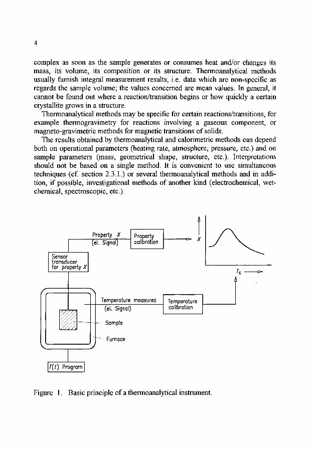
Sensor transducer for property X

Property X (el. Signal)

Property calibration X

"5

C

Y Temperature measured

(el. Signal)

Sample

- ~ Furnace %,

Temperature calibration

IT(t) Program I

Figure 1. Basic principle of a thermoanalytical instrument.

The design of thermoanalytical instruments is usually such that the sample to be investigated is in an environment whose temperature can be varied in a defined way (of. Figure 1). It depends on the conditions of heat transfer between sample and environment, in which way the sample temperature follows the temperature of the environment. In general, the precise determination of the sample temperature is not a trivial matter and must be made through temperature calibration.

Calorimeters exist in a large variety of designs and the principles of measurement applied differ. A feature common to all calorimeters is that they are instrtunents to measure heat and/or heat flow rates.

1.5. The temperature scale The temperature scale valid on the international level from 01.01.1990 is the

International Temperature Scale of 1990 (ITS-90) [1]. It superseded the Inter- national Practical Temperature Scale of 1968 (IPTS-68) [2] valid until that date. The ITS-90 is realized by a number of fixed points, by means of standard instruments and on the basis of prescriptions for the interpolation between the temperature fixed points. The fixed points are realized by transition temperatures (freezing or melting temperatures) and by triple points of suitable pure substances. Platinum resistance thermometers are used as interpolating standard instruments in the temperature range from 13.8033 K to 961.78 ~ Above 961.78 ~ (the freezing point of silver), radiation thermometers (spectral pyrometers) are used.

There are differences between the ITS-90 and the temperature scales valid before, which may be of significance in certain cases (comparison with data in the literature). The temperature t90 = 20.000 ~ (ITS-90), for example, corresponds to the temperature t68 = 20.005 ~ (IPTS-68), that is to say, there is a difference of 5 mK between the two scales. The different temperature scales and the conversion of one scale to the other are described in [1 - 4].

(In thermal analysis, thermocouples are normally used for temperature measurement. In rare cases, resistance thermometers or semiconductor sensors are used. These temperature sensors are usually calibrated in situ with the aid of reference materials (cf. section 1.6.)).

1.6. Definitions related to calibration Calibration means [5]: "The set of operations that establish, under specified

conditions, the relationship between values of a quantity indicated by a measuring instrument or measuring system, or values represented by a material measure or a reference material, and the corresponding values realised by standards.

Notes: (1)

(2)

The result of a calibration permits either the assignment of values of measurands* to the indications or the determination of corrections with respect to indications. A calibration may also determine other metrological properties such as the effect of influence quantities."

A standard can be represented by a (certified) reference material (cf. below), but also by a material measure (e.g. weight), a measuring instrument (e.g. micrometer) or a measuring system (e.g. current-carrying electrical resistor).

A reference material (RM) is a "Material or substance one or more of whose property values are sufficiently homogeneous and well established to be used for the calibration of an apparatus, the assessment of a measurement method, or for assigning values to materials." [5]

A certified reference material (CRM) is a "Reference material, accompanied by a certificate, one or more of whose property values are certified by a procedure which establishes traceability to an accurate realization of the trait in which the property values are expressed, and for which each certified value is accompanied by an uncertainty at a stated level of confidence." [5]

Certified reference materials guarantee traceability (cf. below) of the measurement results, i.e. their link-up with international standards and thus ultimately with the SI base units.

Reference materials are used �9 to calibrate instruments; �9 to back up measuring procedures; �9 to ensure the traceability of the measurement results and thus to determine

the uncertainty of measurement.

1.7. Traceability and quality assurance The definition of traceability is as follows [:5]: "Property of the result of a

measurement or the value of a standard whereby it can be related to stated references, usually national or international standards, through an unbroken chain of comparisons all having stated uncertainties."

Ensuring the traceability of a measurement result is an essential requirement of all standards for quality assurance to achieve the comparability of the measurement results and to allow the uncertainty of measurement to be determined. Traceability means that each single measurement result is made part of a global, hierarchically structured metrology system with the national institutes of

particular quantity subject to measuremem

metrology at its top. The totality of efforts made to obtain reliable measurement results is referred to as quality assurance and covers a comprehensive concept intended to ensure the metrological reliability and apparentness in the determination of the measurement results [6].

1.8. Are thermoanalytical methods analytical methods? The classical meaning of the term analysis is: dissolution, separation, break-up

into constituent elements. A typical example is the chemical analysis of a substance, whose purpose is to find out the substance's composition of components (which are to be defined) in proportions in terms of quantity, which are to be determined.

If the term analysis in its classical sense is understood only as the determination of the material composition of a sample or the change in this composition, gravimetric techniques in conjunction with molecule- or element- specific (also isotope-specific) detection methods are best suited for this purpose (e.g. the simultaneous method thermogravimetry with evolved gas analysis, where it is possible to realize the gas analysis by various methods). However, if analysis is understood in a more comprehensive sense as the qualitative or quantitative determination of a physical quantity in conjunction with an appraising presentation of both the measuring method and the measured values, possibly supplemented by the processing and interpretation of the measured values within the framework of a model concept, thermoanalytical methods can definitely be referred to as analytical.

The following physical quantities may be determined: temperature, heat flow rate, change of length, change of mass, change of concentration, and others. Analysis thus means more than measurement which describes only a single step of the analysis, namely the correct determination of the numerical value of the physical quantity or it's changes.

In this sense, calorimetry also is an analytical method, because the values of quantities which are determined (heat flow rate, heat) are directly related to changes in variables of state or material properties and serve as their explanation and description.

2. T H E R M A L ANALYSIS AND C A L O R I M E T R Y - DEFINITIONS, CLASSIFICATIONS AND NOMENCLATURE

2.1. General To begin with, the concepts thermal analysis and calorimetry will be defined

(sections 2.2., 2.5.). Then the different methods (and measuring techniques) will be sorted and defined with the aid of classification criteria (sections

2.3.,2.4.,2.5.1.). Quantities will then be proposed which will allow the performance of the measuring system of individual instruments to be described (section 3.). In addition, characteristic quantities measured by thermal analysis and calorimetry will be defined, which are used to express measurement results (section 4.). Finally, terms, symbols and units used in conjunction with thermal analysis and calorimetry will be presented according to the recommendations of the International Union of Pure and Applied Chemistry (IUPAC) [8] (section 5.4.).

An important basis of definitions and nomenclature in the field of thermal analysis is the work of the Nomenclature Committee of the International Con- federation for Thermal Analysis and Calorimetry (ICTAC) [7].

The definitions given here are not identical with the present ICTAC recommendations (see below) but are based on a more developed structure.

2.2. Definition of thermal analysis and calorimetry Definitions of "thermal analysis" and of "calorimetry" are formulated in the

following paragraph, taking the limitations referred to in section 1.2. into consideration:

Thermal Analysis (TA) means the analysis of a change in a sample property, which is related to an imposed temperature alteration.

Calorimetry means the measurement of heat. In contrast to this, the present definition of thermal analysis formulated by the

International Confederation for Thermal Analysis and Calorimetry (ICTAC) reads as follows [9]:

Thermal Analysis (TA): A group of techniques in which a property of the sample is monitored against time or temperature while the temperature of the sample, in a specified atmosphere, is programmed.

The differences between the definitions given here and the ICTAC definition of thermal analysis call for an explanation:

A definition of calorimetry is added. But, two separate definitions of thermal analysis and calorimetry are suggested. No uniform definition of thermal analysis and calorimetry has so far been accepted.

Analysis means more than monitoring, namely the whole experimental process and the evaluation procedure of the measured data.

The gist of thermal analysis is the measurement of the change of a property which is due to an alteration of the sample temperature. Only this combination/sequence gives the basis, reason and justification to define a special field of measuring techniques and to combine many different methods into "thermal analysis".

By property of the sample is meant thermodynamic properties (temperature, heat, enthalpy, mass, volume, etc.), material properties (hardness, Young's modulus, susceptibility, etc.), chemical composition or structure. In thermal analysis and calorimetry, a signal is measured which is a measure of the change of the property. Only after calibration of the instrtmaent does the measuring signal finnish a quantitative information about the change of the property. In most cases this change - and not a property of the sample itself- is monitored and may be used to determine the actual physical property of the sample. Example: The electrical signal of a displacement transducer is calibrated by means of a certified reference material to display the change of the sample length, together with other information this change is used to calculate the coefficient of thermal expansion of the sample material.

Temperature alteration means any sequence of temperatures with respect to time which may either be predetermined (temperature-programmed) or sample- controlled. Sample-controlled temperature alteration means that a feedback signal from the sample controls the temperature to which the sample is subjected.

Temperature alteration includes: �9 stepwise change from one constant temperature to another (this includes the

isothermal mode of operation) �9 linear rate of change of the temperature (constant heating or cooling rate) �9 modulation of a constant or a linearly changing temperature with constant

frequency and amplitude �9 free (uncontrolled) heating or cooling Any combination and sequence of these modes of operation is possible. Isothermal techniques belong to thermal analysis if at least one alteration from

a specific temperature (even ambient temperature) to another takes place. I.e. only measurements at ambient temperature do not belong to thermal analysis.

The qualification that the sample must be in a specified atmosphere is of no significance for the general defmition. A specified atmosphere is an operational parameter which must be taken into consideration in the individual case (as must the use of suitable crucible material).

2.3. Classification principles for thermal analysis and calorimetry It is expedient to first develop a classification system that can be applied to the

methods of thermal analysis and calorimetry. This will create an order structure in which both established and new measuring techniques can be incorporated. The change of the sample property, which is to be investigated, will be the primary classification criterion. Additional classification criteria will be required for some of the thermoanalytical methods listed in Table 1.

10

For some of the thermoanalytical methods, a sub-classification will be made according to the stress to which the sample is subjected, or according to the special kind of monitoring used to make the respective quantity accessible to the measurement (Table 2).

The classification of the calorimeters makes fundamental considerations necessary. These will be given in a separate section (cf. section 2.5.).

Individual methods will be defined and described in detail in section 2.4.

2.3.1. Terms descr!bing modes of operation and special methods Static mode of operation means any quantity acting on the sample is constant

with time. Dynamic mode of operation means any alteration with time of any quantity

acting on the sample. The alteration may be predetermined (programmed) or controlled by the sample.

(Modulated mode of operation is a special variant of the dynamic mode of operation in which the alteration of a quantity acting on the sample is characterized by frequency and amplitude. The modulated quantity has to be specified.)

The definition of the dynamic mode provides an additional distinguishing criterion which includes predetermined and sample-controlled programs of any quantity acting upon the sample (temperature and others).

Differential methods of measurement are applied both in the classical methods of thermal analysis (DTA, DSC) and in some calorimeters. The measuring methods concerned compare the quantity to be measured simultaneously with a quantity of the same kind, under identical experimental conditions. The value of this quantity is known and deviates only slightly from that of the quantity to be measured, the difference between the two values being the object of the measurement. The properties of both the sample and the reference sample thus enter into the measured signal.

The advantages of the differential methods of measurement are the following: �9 The differential signal can be highly amplified and reproduces irregularities

in the development of the sample property with high sensitivity as the high basic signal - which is of no interest- is suppressed.

�9 Disturbances acting on the differential measuring system from the outside (e.g. temperature variations in the surroundings) compensate one another, to a first approximation, as they affect both individual measuring systems (almost) to the same extent.

Simultaneous methods of measurement mean the application of two or more techniques to a single sample at the same time. Abbreviations of the techniques should be connected by a hyphen.

11

Table 1

Primary classification scheme of thermoanalytical and calorimetric methods

Property under study Method Abbreviation (Remarks) Temperature Heating/Cooling Curve

Analysm

Temperature Differential Thermal DTA difference Analysis

Heat Calorimetry

Mass

Dimension/ mechanical properties

Pressure

Electrical properties

Magnetic properties

Optical properties

Acoustic properties

Chemical composition/ crystalline structure/ microstructure

Differential Scanning Calorimetry

Thermogravimetric Analysis Thermogravimetry

Thermomechanical Analysis

Thermomanometric Analysis

Thermoelectrical Analysis

Thermomagnetic Analysis

Thermooptical Analysis

Thermoacoustic Analysis

(Needs an extensive sub- classification system because of the variety and variability of calorimetric techniques)

DSC

TGA

TG

TMA (See sub-classification)

TEA (See sub-classification)

TOA (See sub-classification)

TAA (See sub-classification)

(See sub-classification)

12

Derivative means determining the rate of change of a property of the sample (the first derivative with respect to time).

The designation micro (micro-calorimeter, micro-DTA, etc.) should be avoided because it is not clear whether the term "micro" is related to the sample size (mass, volume), the size of the instrument, or the value of the measured signal (which could be amplified) or quantity.

The term photo is used in Connection with differential scanning calorimetry (photo-DSC). It refers to the possibility of an in situ irradiation of the sample, in which case the kind of radiation may differ. It characterizes a special technical feature of the instrmnent, the irradiation of the sample serving in general to initiate a sample reaction. As optical influencing of the sample is not restricted to DSC and no characteristic quantities of the radiation used are measured, the term "photo thermoanalytieal technique" is misleading and superfluous.

Special fields of use, or operating conditions of instnnnents, are often indicated very broadly (and are no classification criteria), e.g. high temperature (HT), low temperature (LT), high pressure (HP, above ambient).

2.4. Classification, names and definitions of thermoanalytical methods This section gives definitions of the most important thermoanalytical methods.

Reference is made to basically different pattems or measuring principles of the instruments concemed. If necessary, directions are given as regards the presentation of the measured curve.

2.4.1. Heating or cooling curve analysis A technique in which the change of the temperature of the sample is analysed

while the sample is subjected to a temperature alteration (heated or cooled). (Cf. Figure 2).

2.4.2. Differential thermal analysis (DTA) A technique in which the change of the difference in temperature between the

sample and a reference sample is analysed while they are subjected to a temperature alteration.

Two different designs exist: �9 measuring systems with free standing crucibles (of. Figure 3); �9 block measuring systems (of. Figure 4).

13

Table 2

Secondary classification scheme of methods of thermal analysis

Property trader study Secondary classification criteria/distinguishing features

Method, Abbreviation (Remarks)

Dimension/mechanical properties

Electrical properties

Magnetic properties

Optical properties

With or without any kind of force acting on sample

Static force

Special case: Negligible force

Dynamic force

Special case: Modulated force

With or without any kind of electric field

Without superimposed electric field

Alternating electric field (dynamic mode)

With or without any kind of magnetic field

Intensity of radiation emitted

Intensity of total radiation reflected or transmitted

Generic term: Thermomechanical Analysis, TMA

Static Force Thermomechanical Analysis, sf-TMA

Thermodilatometry

Dynamic Force Thermomechanical Analysis, df-TMA

Modulated Force Thermomechanical Analysis, mf-TMA

Generic term: Thermoelectrical Analysis, TEA

Thermally Stimulated Current Analysis, TSCA

Generic term: Alternating Current Thermo- electrical Analysis, ac-TEA

Special case: Dielectric Thermal Analysis, DETA

Generic term: Thermomagnetic Analysis (Various techniques to measure susceptibility, permeability etc.)

Generic term: Thermooptical Analysis, TOA

Thermoluminescence Analysis

Thermophotometric Analysis

14

Continuation Table 2

Property under study Secondary classification criteria/distinguishing features

Method, Abbreviation (Remarks)

Acoustic properties

Chemical composition/ crystalline structure/ microstructure

Intensity of radiation of specific wavelength(s)

The refractive index is measured

The sample is observed by means of a microscope

Acoustic waves are monitored atter having passed through the sample

Acoustic waves emitted by the sample are monitored

Analysing the change in chemical composition and/or in the crystalline structure and/or in the microstructure of the sample

Special case: Use of diffraction technique

Special cases: Investigation of the gas exchanged with the sample

Determination of the composition and/or amount of gas

Monitoring of the amount only

Determination of the composition (and the amount)

Special case: Release of trapped radioactive gas from the sample is monitored

Thermospectrometric Analysis

Thermorefractometric Analysis

Thermomicroscopic Analysis

Generic term: Thermoacoustic Analysis, TAA

Thermally Stimulated Sound Analysis

Various techniques (optical, nuclear, X-ray, electrical, etc.)

Thermodiffractometric Analysis, TDA

Generic term: Thermally Stimulated Exchanged Gas Analysis, EGA

Various techniques

Thermally Stimulated Exchanged Gas Detection

Thermally Stimulated Exchanged Gas Determination (e.g. by gas chromatography, mass spectrometry etc.)

Emanation Thermal Analysis, ETA

15

f r

/

---~ Sample

J ~ Furnace

I I ' It<,> Program m--

o rs o I .

rs

f t~.

Figure 2. Device to determine the heating or cooling curve.

, /i/' i i' J n A T t -

A&. f s Crucibles J

- - - - Sample

~ Reference sample

" "-~ Furnace

J ~ - - - ' ~ T. ~ Thermocouples

* Ars. c

Figure 3. DTA measuring system with free standing crucibles. The crucibles are contacted by thermocouples to measure ATsR and the reference temperature TR.

16

Somplel ; /

\

Thermocouples J A

r

I I I

\

/ j Ars.

~ - - Sample cavities

Reference sample Furnace block

f# T R I~>"

Jr(t) Progrom J Figure 4. DTA block measuring system. The temperature sensors are located inside the specimens.

2.4.3. Differential scanning calorimetry (DSC) A technique in which the change of the difference in the heat flow rate to the

sample and to a reference sample is analysed while they are subjected to a temperature alteration.

Note �9 The difference between DTA and DSC is the assignment of a heat flow rate difference (by calibration) to an originally measured temperature difference. To allow this assignment to be carried out, the instruments' design must be such that they are capable of being calibrated.

Two designs of DSC are available, whose measuring systems differ: �9 heat flux DSC with two modifications (disk-type and cylinder-type measur-

ing system); �9 power compensating DSC.

Heat f lux differential scanning calorimeters In a heat flux DSC, the temperature difference between sample and reference

sample is recorded as a direct measure of the difference in the heat flow rates to

Sample

the sample and the reference sample. The heat flow rate difference is assigned by calorimetric calibration.

Two different types of instnmaents are available: �9 disk-type D S C (cf. Figure 5); �9 cylinder-type D S C (cf. Figure 6).

S R

IT(t) Program]

Reference sample l Furnace I~~AC'sR

17

t , T S ....

Figure 5. Disk-type DSC.

In the disk-type DSC, the crucibles with the specimens are positioned on a disk (made of metal, ceramics or the like). The temperature difference ATsR between the specimens is measured with temperature sensors integrated in the disk or contacting the disk surface.

In a cylinder-type DSC, the (block-type) finaaace is provided with two (or more) cylindrical cavities. They take up hollow cylinders whose bottoms are closed (cells) and in which the specimens are placed directly or in suitable crucibles. Thermopiles or thermoelectrical semi-conducting sensors are arranged between the hollow cylinders and the furnace, which measure the temperature difference between hollow cylinder and fiamace (integral measurement). A differential connection of the thermopiles furnishes the temperature difference between the two hollow cylinders, which is registered as the temperature difference ATsr~ between sample and reference sample. Variants of the design: The two hollow cylinders are arranged side by side in the furnace and are directly connected through one or several thermopiles. There are also other DSC

18

designs whose construction features are between those of disk-type and cylinder- type DSC.

Reference semple Sample cell cell . . . .

~ 1 ~ ~ Thermopiles

,ru , I , , , ~u~ocK) Ar

i t r [ T'(t) Program i ~ , , . ~ f ,T s t:,..

Figure 6. Cylinder-type DSC.

Power compensating differential scanning c a l o r i m e t e r s

In a power compensating DSC, the specimens are arranged in two separate small furnaces each of which is provided with a heating unit and a temperature sensor (cf. Figure 7). During the measurement, the temperature difference between the two furnaces is maintained at a minimum with the aid of a control loop that appropriately adapts the heating powers P. A proportional-controller is used for this purpose so that there is always a residual temperature difference between the two specimens (offset). When there is thermal symmetry in the measuring system, the residual temperature difference is proportional to the difference between the heating powers fed to sample and reference sample. If the resulting temperature difference is due to differences in the heat capacity between sample and reference sample, or to exothermic/endothermic transformations in the sample, the heating power additionally required to keep this temperature difference as small as possible (which would reach the same value as with the heat flux DSC if there was no compensation heating) is proportional to the difference A q~sR between the heat flow rates supplied to sample and reference sample (Aq~sR = ACp. fl), or proportional to the heat flow rate of transition A q)trs.

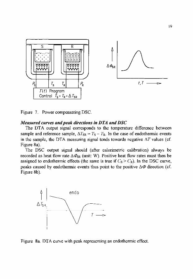
19

, S ,

I

'jj T(t) ProgFam Control Ts = TR + A TSR

l Ad~SR

t , T t=~

Figure 7. Power compensating DSC.

M e a s u r e d c u r v e s and peak directions in DTA and DSC The DTA output signal corresponds to the temperature difference between

sample and reference sample, ATsR = Ts - TR. In the case of endothermic events in the sample, the DTA measuring signal tends towards negative AT values (cf. Figure 8a).

The DSC output signal should (after calorimetric calibration) always be recorded as heat flow rate A q~SR (unit: W). Positive heat flow rates must then be assigned to endothermic effects (the same is true if Cs > CR). In the DSC curve, peaks caused by endothermic events thus point to the positive Aq~ direction (cf. Figure 8b).

ATSR

endo

Figure 8a. DTA curve with peak representing an endothermic effect.

20

t

Figure 8b. DSC curve with peak representing an endothermic effect.

2.4. 4. Thermogravimetric analysis (TGA), thermogravimetry (TG) A technique in which the change in the sample mass is analysed while the

sample is subjected to a temperature alteration. (Cf. Figure 9).

I r(t) Program I

f-

I I - J /

r

Furnace Sample

Thermocouple

Balance (ms] ' I

ms

T f

Figure 9. Basic set-up of a thermobalance.

21

A differentiation between thermobalances can be made on the basis of the arrangement of the sample in relation to the weighing system: below the load receptor (vertical), above the load receptor (vertical), horizontal.

2.4.5. Thermomechanical analysis (TMA) Techniques in which the change of a dimension or a mechanical property of

the sample is analysed while the sample is subjected to a temperature alteration.

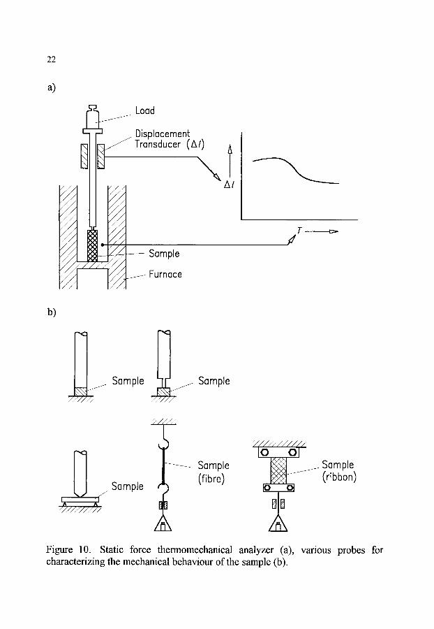
Special techniques: Static force thermomechanical analysis (sf-TMA): Techniques in which a

static force acts on the sample.

Note: To investigate the behaviour of substances under stresses similar to those occurring in practice, samples of suitable shape are subjected to static stress. Compressive, tensile, flexural or torsional stress may be concerned, even complex states of stress are simulated. Depending on the kind of stress to which the sample is to be exposed, suitable sample holding devices and force applying mechanisms are used. (Cf. Figure 10).

Special case: Th e rm odi lato m e try :

sample. Techniques in which a negligible force acts on the

Note: The instrument is a dilatometer. The classical instrument for the determination of the coefficient of thermal expansion is the push-rod dilatometer. (Cf. Figure 11). Via the push-rod, the variation of the length of the rod-shaped sample is transmitted to a displacement transducer (electromagnetic, capacitive, optical, mechanical) which gives an electrical signal proportional to the change in length. The arrangement of the sample in the furnace must be such that there is only low friction.

Dynamic force thermomechanical analysis (df-TMA): Techniques in which a dynamic force acts on the sample and the change of a dimension is analysed.

Special case: Modulated force thermomechanical analysis (mf-TMA): Techniques in which

a modulated force acts on the sample and the change of a mechanical property is analysed. (Cf. Figure 12).

22

a)

Y./ / V// , . .

V//

///

/// v//

V//

V//

V//

J// /// ///

/ / /

/ / /

/ / / I / / ,

j•-• Load L.] Displacement ~]1 ~'"'mransducer (AI)

Sample / /

Furnace

T ~.-

b)

Sample ////,.'> V///,..~

Sample

J I "1 A A z/////////

Sample

//////

Sample (fibre)

Sample (ribbon)

Figure 10. Static force thermomechanical analyzer (a), characterizing the mechanical behaviour of the sample (b).

various probes for

23

A / Signal

Displacement/ \ transducer / Furnace

Push rod Jr(t) Program J

f Siqnal t

" ~ At /,

~ Sam

Sample Bearings

m,. T t:>

pie support

Figure 11. Push-rod dilatometer.

f

E'I 2L C0il

l ffl

- O

0

E

L

Sample (plate) 1

Furnace

IT(t) Program J

7-, Z/

l t-- Grl

(1)

1:3 r

Figure 12. Modulated force thermomechanical analyzer.

24

Note: For the sake of the new systematic approach, the former terms for thermomechanical analysis and its various techniques had to be re- defined: Thermomechanical Analysis ~ Static Force TMA Dynamic Load TMA ~ Dynamic Force TMA Thermodilatometry ~ Thermodilatometry Dynamic Mechanical Analysis (also named Dynamic Mechanical Spectrometry) ~ Modulated Force TMA

2.4. 6. Thermomanometric analysis Techniques in which the change of the pressure exerted by the sample is

analysed while the sample is subjected to a temperature alteration.

2.4. 7. Thermoelectrical analysis Techniques in which the change of an electrical property of the sample is


Special techniques: Thermally stimulated current analysis: Analysis of the thermally stimulated

sample current without the sample being exposed to an electric field after the sample has been exposed to a static electric field.

Alternating current thermoelectrical analysis: Analysis of the thermally stimulated sample current while the sample is exposed to an alternating electric field.

Special case: Dielectric thermal analysis (DETA): The dielectric properties of the sample

are measured by exposing the sample to an alternating electric field.

Note: Thermoelectrical analysis includes measurements with and without any kind of electric field. (That means, dielectric thermal analysis is a special case of alternating current thermoelectrical analysis.) Analogous statements are valid with respect to thermomagnetic analysis.

2.4.8. Thermomagnetic analysis Techniques in which the change of a magnetic property of the sample is


25

2.4.9. Thermooptical analysis (TOA) Techniques in which the change of an optical property of the sample is


Note" The generic term of thermooptical analysis covers the recording of light emitted by thermal excitation, the recording of light reflected or transmitted, or the investigation of the refractive index, or the observation of the sample by means of a microscope.

Special techniques" Thermoluminescence analysis: The intensity of radiation emitted by the

sample is analysed.

Thermophotometric analysis: The transmitted by the sample is analysed.

intensity of radiation reflected or

Thermospectrometric analysis" Radiation of specific wavelength(s) reflected, transmitted or scattered by the sample is analysed.

Thermorefractometric analysis: The (spectral) refractive index is measured.

Thermomicroscopic analysis" The sample is observed by means of a microscope and the changes in the appearance of the sample are monitored.

Note 1: The instrument used is a thermomicroscope, usually consisting of a hot stage and a microscope, often equipped with a camera or video recorder.

Note 2: The visual appearance of the sample's surface or interior may be monitored simply by observing the reflected or transmitted light by means of the eye and describing what happens. According to the methods used, for example, in solid-state physics, the observation can be performed by any kind of camera that registers the image, for example electronically, which makes an evaluation possible (surface pattern analysis).

2.4.10. Thermoacoustic analysis (TAA) A technique in which the change of imposed acoustic waves after passage

through the sample is analysed while the sample is subjected to a temperature alteration.

26

Thermally stimulated sound analysis: A technique in which the sound emitted by the sample is analysed while the sample is subjected to a temperature alteration.

2.4.11. Thermally stimulated exchanged gas analysis (EGA) Techniques to investigate the gas exchanged with the sample while the sample

is subjected to a temperature alteration.

Special techniques: Thermally stimulated exchanged gas detection: Techniques in which the

amount of gas is analysed.

Thermally stimulated exchanged gas determination: Techniques in which the composition (and amount) of gas is (are) measured.

Emanation thermal analysis (ETA): Techniques in which the amount of the thermally stimulated release of trapped radioactive gas (emanation) from the sample is analysed.

Note 1: Thermally stimulated exchanged gas analysis means the determination of the composition and/or amount of gas exchanged with the sample. Here the composition/amount of the gas is measured, which means that a corresponding change of the sample composition and/or mass occurs.

Note 2: Various kinds of analytical techniques are used for thermally stimulated exchanged gas detection and for thermally stimulated exchanged gas determination.

2.4.12. Thermodiffractometric analysis (TDA) Techniques in which the change of a structural property of the sample is

analysed by means of diffraction techniques while the sample is subjected to a temperature alteration.

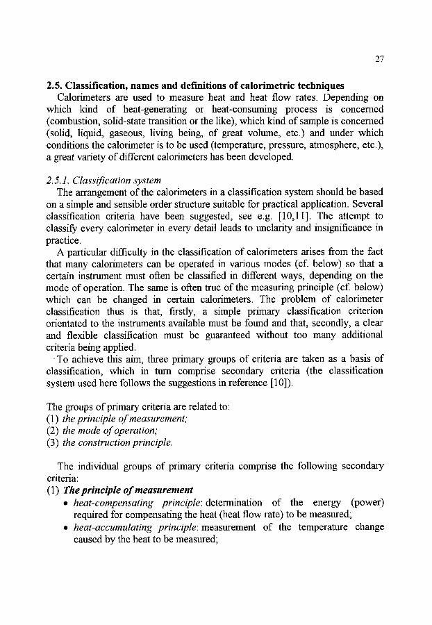
27

2.5. Classification, names and definitions of calorimetric techniques Calorimeters are used to measure heat and heat flow rates. Depending on

which kind of heat-generating or heat-consuming process is concerned (combustion, solid-state transition or the like), which kind of sample is concerned (solid, liquid, gaseous, living being, of great volume, etc.) and under which conditions the calorimeter is to be used (temperature, pressure, atmosphere, etc.), a great variety of different calorimeters has been developed.

2.5.1. Classification system The arrangement of the calorimeters in a classification system should be based

on a simple and sensible order structure suitable for practical application. Several classification criteria have been suggested, see e.g. [10,11]. The attempt to classify every calorimeter in every detail leads to unclarity and insignificance in practice.

A particular difficulty in the classification of calorimeters arises from the fact that many calorimeters can be operated in various modes (of. below) so that a certain instrument must often be classified in different ways, depending on the mode of operation. The same is often true of the measuring principle (cf. below) which can be changed in certain calorimeters. The problem of calorimeter classification thus is that, firstly, a simple primary classification criterion orientated to the instruments available must be found and that, secondly, a clear and flexible classification must be guaranteed without too many additional criteria being applied.

To achieve this aim, three primary groups of criteria are taken as a basis of classification, which in turn comprise secondary criteria (the classification system used here follows the suggestions in reference [10]).

The groups of primary criteria are related to: (1) the principle of measurement; (2) the mode of operation; (3) the construction principle.

The individual groups of primary criteria comprise the following secondary criteria: (1) The principle of measurement

�9 heat-compensating principle:determination of the energy (power) required for compensating the heat (heat flow rate) to be measured;

�9 heat-accumulating principle: measurement of the temperature change caused by the heat to be measured;

28

�9 heat-exchanging principle: measurement of the temperature difference between sample and surroundings caused by the heat (heat flow rate) to be measured.

(2) The mode o f operation (temperature conditions) �9 static: isothermal;

isoperibol~); adiabatic2);

�9 dynamic: scanning of surroundings; isoperibol scanning3); adiabatic scanning.

(3) The constructionprinciple �9 single measuring system; �9 twin or differential measuring system.

Most of the calorimeters can be classified by means of these criteria. Not all secondary criteria from the three groups can be combined. As the heat to be measured (first) appears as a heat flow to be exchanged, there are always temperature gradients in calorimetric measuring systems so that, for example, an ideally isothermal state cannot be established. In addition, temperature differences always occur between sample and environment so that there are undesired heat leaks which must be taken into consideration as a correction, i.e. there are no ideal adiabatic operating conditions. In the following a few examples show the suitability of the classification system.

2.5.2. Examples Heat compensating calorimeters

The effect of the heat to be measured is compensated, either passively by the phase transition of a suitable calorimeter substance (e.g. ice), or with the aid of an active control system which compensates a temperature change in the sample or the sample container through electrical heating/cooling or other suitable heat sources/sinks. The compensation energy is to be determined, for example, from the mass of the transformed calorimeter substance or from the electrical heating/cooling energy. Advantages of the compensation method are that the measurement is carried out under quasi-isothermal conditions and heat leaks thus remain unchanged to a first approximation. Possible instruments:

~) isoperibol refers to constant temperature surroundings with the temperature of the measuring system possibly differing from this.

2) adiabatic refers to a prevention of the heat exchange between measuring system (sample) and surroundings. 3) isoperibol scanning refers to the scanning of the measuring system (sample) in surroundings at constant

temperature.

29

�9 Ice calorimeter Principle of measurement: heat compensation (passive, by latent heat); mode of operation: isothermal; construction principle: single measuring system. At 0 ~ a heat exchange between sample and calorimeter substance (ice) takes place; the mass of the transformed ice is determined. From this and from the known heat of transition, the heat emitted by the sample is determined.

�9 Adiabatic scanning calorimeter Principle of measurement: heat compensation (active, by electronic control); mode of operation: adiabatic scanning; construction principle: single measuring system. A known electric heating power is fed into the sample. Heat losses into the surroundings are minimized by matching the environmental temperature. The sample's heat capacity may be obtained from the heating power and the heating rate. Heats of transition are determined from the time integral of the heating power. During a first-order transition, the calorimeter's behaviour is quasi-isothermal.

�9 Power compensating D S C Principle of measurement: heat compensation (active, by electronic control); mode of operation: isoperibol scanning; construction principle: twin measuring system. The temperature of the surroundings remains constant (isoperibol). The twin measuring system is heated; each specimen has its own heater and temperature sensor. The temperature difference between is maintained at a minimum by increasing or decreasing the sample heating. The difference in heating power is related to the sample heat flow rate to be measured.

Heat accumulat ing calorimeters The effect (e.g. an increase in temperature) of the heat to be measured is not

minimized by any compensation, but leads to a temperature change in the sample and the calorimeter substance with which the sample is thermally connected. This temperature change is the quantity to be measured. It is proportional to the amount of heat exchanged between the sample and the calorimeter substance. Possible instruments:

�9 Drop calorimeter Principle of measurement: heat accumulation (measurement of the resulting temperature change); mode of operation: isoperibol; construction principle: single measuring system.

30

The sample is dropped into the calorimeter that consists of a calorimeter substance (e.g. water, metal) which is thermally insulated from the isoperibol surrotmdings (thermostat, fitmace). The temperature change in the calorimeter substance is measured. Calibration is performed by means of electrical heating. Heat leaks between the calorimeter substance and the surroundings must be taken into consideration as a correction.

�9 Adiabatic bomb calorimeter Principle of measurement: heat accumulation; mode of operation: adiabatic; construction principle: single measuring system. The combustion bomb (a metallic, pressure-tight vessel) shows an increase in temperature after ignition of the sample. The temperature of the surroundings (thermostat) is continously matched to the bomb temperature by means of an electrical control system. The increase in temperature is the measured signal; a correction (as with the drop calorimeter) is not necessary.

�9 Flow calorimeter Principle of measurement: heat accumulation; mode of operation: isoperibol; construction principle: single measuring system (twin design also feasible). In a gas calorimeter which serves to measure the heat of combustion of fuel gases, the heat to be measured is transferred to a flowing liquid (e.g. water) or gas (e.g. air). The temperature increase in the flowing medium is the measured signal. Other types of flow calorimeters are used to measure heats of reaction, for example by mixing two liquids in a reaction tube. The temperature difference between the liquids flowing in and the reaction product flowing out is the measured signal.

Heat-exchanging calorimeters In heat-exchanging calorimeters, a defined exchange of heat takes place

between the sample (sample container/crucible/support) and the surroundings. The amount of the flowing heat, the heat flow rate, is determined on the basis of the temperature difference along a "thermal resistance" between sample and surroundings. Registration of the dependence of the heat flow rate on time allows kinetic investigations to be carried out. Possible instrument:

�9 Hea t f l ux differential scanning calorimeter (heat f lux DSC) Principle of measurement: heat exchange; mode of operation: scanning of surroundings; construction principle: twin measuring system (disk-type or cylinder-type). Two containers/supports with sample and reference sample are provided with temperature sensors which measure the temperature difference

31

between the specimens. This temperature difference is proportional to the difference in the heat flow rates flowing from the surroundings (fimaace) to both specimens. Due to the twin construction, a direct measurement of the temperature difference between sample and surroundings is not necessary; the main heat flow must not be registered, only the differential one.

3. CHARACTERIZATION OF MEASURING INSTRUMENTS

The requirements to be met by the measuring instrument follow from the kind of problem to be investigated. To be able to judge whether a thermoanalytical instrument or a calorimeter is suitable for the task in question, the instrument must be clearly characterized.

The following can be used for characterization: �9 the general specifications of the measuring instrument; �9 the performance characteristics of the measuring system. All specifications and characteristic data given in the following account thus

serve to select the best instrument from among those offered by various manufacturers. Prior to purchasing an instrument, all necessary information should be obtained from the manufacturer.

3.1. General specifications of the measuring instrument A comprehensive general description of the measuring instrument should

specify: �9 Type of measuring instrument (thermobalance, dilatometer, etc.). In

addition, closer details of the design (DTA: block system or free-standing crucibles; TG: weighing system above or below the load receptor; DSC: of the heat flux or power compensating type, etc.).

�9 Temperature range. �9 Atmosphere (which gases, vacuum, pressure). �9 Range of heating and cooling rates, temperature-time programs.

The following information may serve to characterize the measuring instrument with a view to the sample to be investigated and the effect of the measuring system on the sample:

�9 kind of sample (solid, liquid, gaseous); �9 suitable sample volume; �9 suitable sample mass; �9 possible sample dimensions and shapes; �9 mass changes that can be registered (TG);

32

�9 static forces acting on the sample (STMA); �9 frequency, amplitude of stress to which the sample is exposed.

If the instrument is designed for simultaneous measurements, the kind of measurement is indicated, e.g.:

�9 DTA / TG; �9 DSC / thermomicroscopy; �9 TG / EGA.

Distinguishing features of the design are, for example: �9 The sample can be irradiated (of. section 2.3.1.). �9 The instrument is suitable for sample controlled rate mode of operation (cf.

section 2.3.1 .). �9 The (linear) heating or cooling rate can be superimposed with temperature

oscillations ((temperature-) modulated scanning) (of. section 2.3.1 .). �9 Different modes of operation are possible (e.g. adiabatic or isoperibol). �9 The first time derivative of the signal is also registered (derivative signal). �9 There are special possibilities of monitoring the sample in situ (optical,

acoustic). �9 There are possibilities of manipulating the sample (mechanically: addition or

removal of substance). �9 A calibration device is installed.

3.2. Performance characteristics of the measuring system A quantitative characterization of a measuring system can be made on the

basis of the following performance criteria (not all performance criteria are significant or can be determined for every thermoanalytical instrument or calorimeter). The performance criteria are evaluated from the measured curve.

3.2.1. Noise The registration of the measurement curves over a period of approx. 1 min

furnishes the mean variation of the measured signal, indicated in the units of the measured signal (e.g. TG: lag; DSC: gW).

Characteristic quantity: Noise as a function of the heating/cooling rate, the temperature, the sample mass etc. (Zero line (for definition, cf. section 4.1.) noise: without specimens, without crucibles). Important in practice is the signal- to-noise ratio as a measure of signals still detectable.

33

The noise thus allows the smallest detectable measured signal to be estimated (threshold value: approx. 2 to 5 times the noise). It is often expedient to indicate the noise related to the sample mass or the useful sample volume.

The noise can be indicated as: �9 peak-to-peak noise (pp), i.e. the maximum variation of the measured signal; �9 peak noise (p), i.e. the maximum deviation of the measured signal from the

mean value; �9 root-mean-square noise (RMS), i.e. the root of the mean value of the

squared instantaneous deviations of the signal from the mean value.

3.2.2. Repeatability The repeatability reflects the degree of agreement between many measure-

ments of the same kind carried out with the same measuring instrument. The repeatability is a very important quality criterion. Reasons for changes in the behaviour during successive measurements may be:

�9 disturbances, changes due to the removal of the sample and its re-introduction;

�9 changes in the environmental temperature, the atmospheric pressure, the flow velocity of the purge gas etc. (statistical causes).

If the intervals between measurements of the same kind are larger, long-term changes (drift) can become visible the causes of which may be:

�9 ageing of components, adhesives; �9 contamination, adsorption. The measure of repeatability is the repeatability error. It is determined by

comparing many successive measurements; it depends on operational and sample parameters.

Examples: The repeatability scatter of the zero line is determined by measuring several zero lines over the whole temperature range at medium scanning rate and superimposing the curves. The range of deviation from the mean zero line yields the repeatability scatter (absolute value or in %). The repeatability of the peak area, characteristic temperatures (e.g. extrapolated onset temperature), mass loss, etc. can be evaluated in analogy.

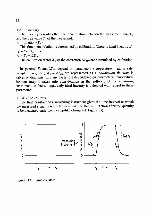
34

3.2.3. Linearity The linearity describes the fimctional relation between the measured signal Ym

and the true value Yt~ of the measurand: Ytr = fimction (Ym)

This functional relation is determined by calibration. There is ideal linearity if: Y t r = K Y " Ym o r

Ytr--Ym+AYcorr The calibration factor Kv or the correction AYr are determined by calibration.

In general, Ky and AYoo,, depend on parameters (temperature, heating rate, sample mass, etc.). Ky or AY~orr are represented as a calibration function in tables or diagrams. In many cases, the dependence on parameters (temperature, heating rate) is taken into consideration in the software of the measuring insmmaent so that an apparently ideal linearity is indicated with regard to these parameters.

3.2.4. Time constant The time constant of a measuring instrument gives the time interval at which

the measured signal reaches the new value to the e-th fraction after the quantity to be measured underwent a step-like change (cf. Figure 13).

c -

0 3

c - ~

t o time

measuring.~ instrument~

_ _

1/e ~ -1

0

0 0

t o time t 1

Figure 13. Time constant.

35

The time constant is a measure of the inertia of a measuring system, i.e. it describes how well variations of the quantity to be measured with time can be determined (time resolution). Knowledge of the time constant of the measuring system is important for all deconvolution (desmearing) methods. (Deconvolution: reconstruction of the original sample signal which, due to the inertia of the transmitting measuring system, was registered as a time-delayed and distorted measured signal.)

3.2.5. Sensitivity The sensitivity gives the relation between the change of the measured signal

AYm and the change of the measured quantity AX that creates the signal: Sensitivity = AYm/AX

The sensitivity is given as a number and a ratio of units, for example: �9 DSC sensitivity in gV/mW; �9 TG sensitivity in g V/mg.

In most cases, the signal is given as an electrical voltage (which, by calibration, is linked to the sample property to be measured).

The sensitivity may be increased by electronic amplification. The highest reasonable degree of amplification is limited by the noise of the measuring system that is also amplified.

3.3. Instrument checklist On the basis of the general criteria describing a thermoanalytical instrument or

a calorimeter and the special performance characteristics of the measuring system, the user may compile a checklist which may include additional problem- specific quantities. Such a list can be used to compare different instruments. It may be submitted to the insmunent manufacturers to be filled in by them, and it then documents the performance of a certain instnnnent.

Example of an instrument checklist

Manufacturer: Instrument category: Type, pattern: Temperature range: Sample volume/mass/dimensions: Detection range of sample property changes: Method/place of temperature measurement: Atmosphere: Heating/cooling rates:

36

Special design features: Method of calibration: Zero line scatter: Signal noise: Repeatability error of characteristic measured quantities: Total uncertainty of temperature assignment: Total uncertainty of sample property (change): Time constant (with sample): Additional information on the measuring system:

3.4. Assessment of evaluation programs Values obtained by thermal analysis and calorimetry are often used to

calculate characteristic quantities (temperatures, peak areas, etc.) using evaluation programs, and from them to determine problem-specific results (purity, characteristic kinetic factors, etc.). The user of such evaluation programs must know on which physical or chemical laws the program is based and which the boundary conditions are (scope of applicability).

To estimate the overall uncertainty and to optimize the reliability of the calculated results, the uncertainties caused by the algorithm (calculation procedure) itself must be taken into consideration. Only then a decision can be taken as to whether a certain evaluation program is suited to calculate the required data and which uncertainties result from the evaluation. In some cases it is possible to evaluate a measurement using various alternatives of a specific program, for example, calculation of the peak area using different baselines. The comparison of the results obtained is useful for the estimate of uncertainties.

It is also useful (and advisable prior to the purchase of an instrument) to investigate a sample using the instruments and programs of various manufacturers. Marked differences in the results should be a reason for analyzing more precisely the underlying evaluation concepts and models.

4. CHARACTERIZATION OF MEASURED CURVES AND VALUES

The results of thermoanalytical and calorimetric measurements are in general represented as a measured curve (avoid the term thermogram). A (measured) curve shows the property, or change of property, of a sample depending on temperature or time in a graphic presentation. A number of terms are used to describe the measured curve; these will be defined below.

Characteristic quantities can be determined from the measured curve, which describe the sample behaviour and are of importance for the evaluation of the measurement and the interpretation of the measurement results.

37

4.1. T e r m s to descr ibe the curve The terms defined in the following paragraphs describe characteristic points or

sections of a measured curve (cf. Figures 14a and 14b). The determination of some of these points or sections is often the aim of the thermoanalytical or calorimetric experiment; some of them are, however, used in the calculation of derived quantities.

�9 M e a s u r e d curve: Continuous graphical representation of the measured values as a function of time or temperature.

�9 Ze ro line: Measured curve of the empty measuring instrument (either without specimens and without crucibles or without specimens, with the crucibles empty).

�9 S a m p l e m e a s u r e m e n t curve: Measured curve of the measuring instrument with sample crucible and sample.

Note: The following subscripts are used: 0 for zero line, S for sample, R for reference sample, SR for differential curve with sample and reference sample.

S e c t i o n s o f t h e m e a s u r e d c u r v e

�9 Peak: Section of a measured curve comprising ascending slope, maximum and descending slope, or descending slope, minimum and ascending slope, within a specific time or temperature interval, due to a reaction or transition in the sample.

�9 Step: Section of a measured curve comprising ascending slope and point of inflection, or descending slope and point of inflection within a specific time or temperature interval, due to a reaction or transition in the sample.

�9 P la teau: Section of a measured curve with constant or almost constant measured signal within a specific time or temperature interval.

�9 Base l ine : Section of a measured curve outside a peak or a step without underlaying reaction or transition in the sample.

�9 I s o t h e r m a l basel ine: Section of a measured curve in which the set temperature of the furnace is kept constant and no reaction or transition takes place in the sample.

�9 In i t ia l base l ine: Section of a measured curve before a peak or step, in which a reaction or transition has not yet taken place.

38

�9 Final baseline: Section of a measured curve beyond a peak or step in which a further reaction or transition in the sample does not take place.

�9 Isothermal initial baseline: Section of a measured curve in which the set temperature of the fumace is kept constant and no reaction or transition takes place in the sample before the dynamic phase of the temperature program begins.

�9 Isothermal f inal baseline: Section of a measured curve in which the set temperature of the fitmace is kept constant and no reaction or transition takes place in the sample after the dynamic phase of the temperature program came to an end.

Note 1: For an analogous characterization of the zero line, the terms "isothermal zero line", "isothermal initial zero line" and "isothermal final zero line" are used.

Note 2: The following additional subscripts are used: "bl" for baseline, "iso" for isothermal, "ini" for initial, "fin" for final.

Terms for the evaluation of the measured curves �9 Interpolated baseline: Curve interpolated in the region of a peak and

connecting the initial baseline and the final baseline as if no reaction or transition had taken place in the sample.

�9 Interpolated isothermal baseline: Curve interpolated in the dynamic phase and connecting the isothermal initial baseline with the isothermal final baseline as if no dynamic temperature program had been executed.

�9 Extrapolated mitial baseline: Initial baseline extrapolated in the region of a peak or step as if no reaction or transition had taken place in the sample.

�9 Extrapolated f inal baseline: Final baseline extrapolated in the region of a peak or step as if no reaction or transition had taken place in the sample.

Note 1: For an analogous characterization of the zero line, the term "interpolated isothermal zero line" is used.

Note 2: The following additional indices are used: "i" for interpolated, "e" for extrapolated.

39

Characteristic quantities determined with the aid of the measured curve �9 Peak height: Maximum of the amount of the difference between peak

and interpolated baseline. �9 Peak area: Area bounded by peak and interpolated baseline between

the initial and the final point of the peak (tini and tnn). �9 Step height: Maximum of the amount of the difference between ex-

trapolated initial baseline and extrapolated final baseline at the step midpoint temperature (cf. below).

�9 Ini t ialpeak/s tep temperature Ti,i: Temperature of the first detectable deviation of the measured curve in the region of a peak or a step from the extrapolated initial baseline.

�9 Final peak/step temperature Tfin: Temperature of the last detectable deviation of the measured curve in the region of a peak or a step from the extrapolated final baseline.

�9 Extrapolatedpeak/s tep onset temperature Te: Temperature of intersection of the extrapolated initial baseline and the tangent or fitted line through the linear section of the descending (ascending) peak/step slope.

�9 Extrapolatedpeak/s tep completion temperature Tc: Temperature of intersection of the extrapolated final baseline and the tangent or fitted line through the linear section of the ascending (descending) peak/step slope.

�9 Peak extremum temperature Tp: Temperature at which the maximum of the amount of the difference between peak and interpolated baseline is reached.

�9 Step midpoint temperature T~/2: Temperature at which, in the region of a step, the difference between extrapolated initial baseline and measured curve is equal to the difference between measured curve and extrapolated final baseline.

Note 1: For differentiation, two subscripts must be added if necessary: "p" for peak, "s" for step, e.g. Tini,p, Te,s.

Note 2: To characterize the glass temperature for polymer materials, the different temperatures characterizing the step are used: Tini,s, T~,s, T1/2, Tc,s or Ttin,s.

Note 3: Analogous definitions are also possible to describe characteristic times t of the measured curve (cf. Figure 14a). The designation of the quantity measured corresponding to these temperatures/times (e.g. heat flow rate o~ with DSC, change of mass Am with TG) by means of the indices stated is also possible.

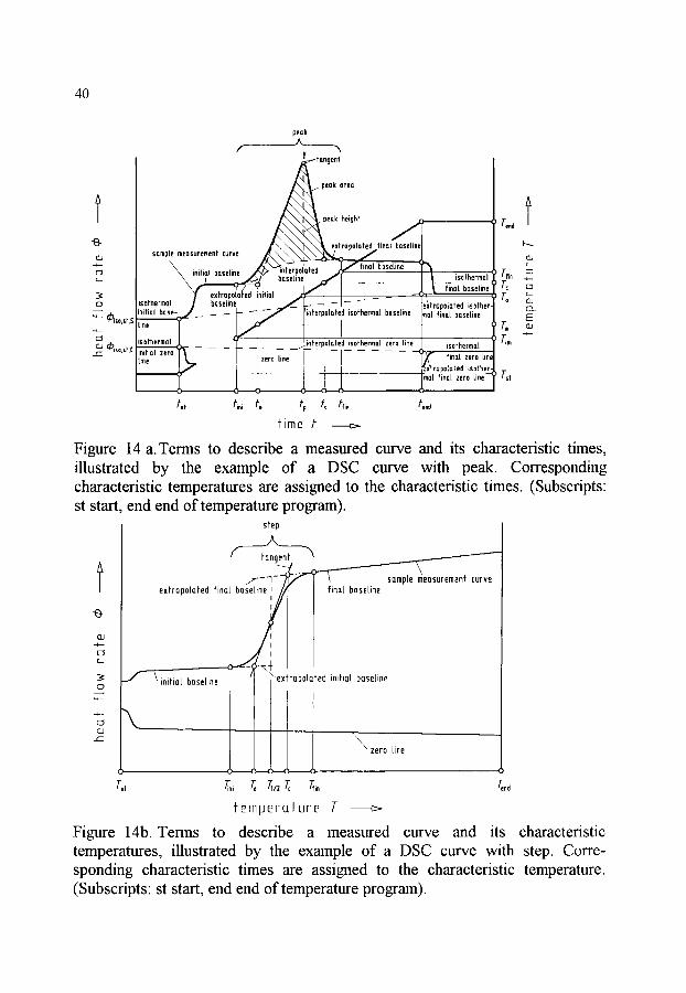
40

peak

/ ~ t a n g e n t

"(~ l \ ~ l ~ \ l k extrQpatoted finol baseline I-~ samp[e meosuremen! curve , ~ ~ ' ~ . ' ~ _ ~ q , ~ / r

c_C~ ~ , n ; ~ , b a s e l i ~ b ' ~ finolis~ 7"c Tfin ~CI : I extropolofed inifiol J f I t . . . . c_

l isothermol i bosetine I L ,--. ~ J-- - - ~fropoloted isother. Tp oJ .__., I::1_ o linifiol b o s e - J _ _ . - p " - I " - 7 - 'inferpolol'ed isofherlnul hoseline tool fin.l boseline F:::

I~ I isothermol ~ __ ~ ~ jnferpolnfed isofh . . . . I . . . . line isel'hermul Tini ~iso sl. 0 itnitiot zero ~ - - [- - - I - - - " - - ' +

= " + i + ++o,+n+ ine zero line ~:x'fropototed isofher-

�9 ' ~ /st tool fmol zero line

tsf tini te tp tc /'fin fend

t ime t

Figure 14 a.Zerms to describe a measured curve and its characteristic times, illustrated by the example of a DSC curve with peak. Corresponding characteristic temperatures are assigned to the characteristic times. (Subscripts: st start, end end of temperature program).

step

('~ tangent ~ l / - - " l ~ a s u r e m e n t cur ve

extrapotofed finnl

--4---- CJ f-.-

�9 - " f ~ i ~ i n ilia[ bnseline o ...._.,

+ \ D r--

]"sf ~ni re TI/;P ~ ~in Tend

femperofure 7- Figure 14b. Terms to describe a measured curve and its characteristic temperatures, illustrated by the example of a DSC curve with step. Corre- sponding characteristic times are assigned to the characteristic temperature. (Subscripts" st start, end end of temperature program).

41

5. CHARACTERIZATION, INTERPRETATION AND PRESENTATION OF RESULTS

5.1. Characterization of results Prior to making use of measured values obtained in thermoanalytical or

calorimetric investigations, the values must be verified as being reliable. A basis for this are the characteristic data describing the quality of the measuring system (repeatability, noise, etc., cf. section 3.2.).

Terms describing the quality of results are: The accuracy which describes how well the result approximates the true value

of a quantity. The accuracy is determined by random and systematic errors. Systematic errors may comprise known and unknown components. Known systematic errors are taken into consideration in the measurement results as corrections. The uncertainty of the corrections, unknown systematic errors and random errors must be estimated. An estimate of random errors is the standard deviation.

The total uncertainty of measurement indicates a range of values in which the true value of the quantity to be determined lies with high probability (see textbooks of statistics). Accuracy and total uncertainty are not identical with the repeatability or the reproducibility. (Reproducibility describes the degree of agreement between the values measured using one sample but different instruments in the same or in different laboratories. A measure of the reproducibility is the deviation of the result obtained by a particular instrument from the total mean value. The determination of the reproducibility is a means of detecting systematic errors.)

5.2. Interpretation of results Every interpretation is based on the results of thermoanalytical or calorimetric

investigations, including their total uncertainty. To back up an interpretation, it is advisable:

�9 to use additional (simultaneous) measuring techniques, �9 to check the agreement with thermodynamic laws, �9 to carry out measurements of reference samples with known properties, �9 to analyze the measuring principle and possible influences of operational

and sample parameters.

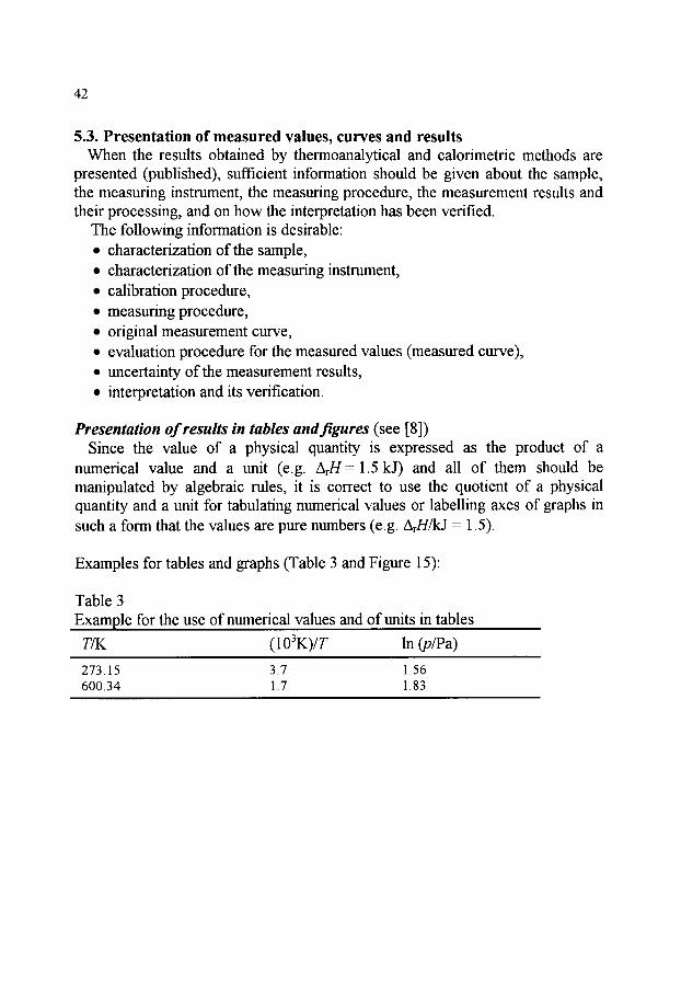
42

5.3. Presentation of measured values, curves and results When the results obtained by thermoanalytical and calorimetric methods are

presented (published), sufficient information should be given about the sample, the measuring instrument, the measuring procedure, the measurement results and their processing, and on how the interpretation has been verified.

The following information is desirable: �9 characterization of the sample, �9 characterization of the measuring instrtnnent, �9 calibration procedure, �9 measuring procedure, �9 original measurement curve, �9 evaluation procedure for the measured values (measured curve), �9 uncertainty of the measurement results, �9 interpretation and its verification.

Presentation of results in tables and figures (see [8]) Since the value of a physical quantity is expressed as the product of a

numerical value and a unit (e.g. ArH = 1.5 kJ) and all of them should be manipulated by algebraic rules, it is correct to use the quotient of a physical quantity and a unit for tabulating numerical values or labelling axes of graphs in such a form that the values are pure numbers (e.g. A r H / k J = 1.5).

Examples for tables and graphs (Table 3 and Figure 15):

Table 3 Example for the use of numerical values and of traits in tables

T/K (103K)/T In (p/Pa)

273.15 3.7 1.56 600.34 1.7 1.83

43

I 6

4 Od

2

0 q

- DTA

O0 !

400 T/K I >

I

50O

E

<::]

10 DSC

I

10 I I I

20 30 O/~

4O I

5O

I O

-1 E3"I

~-2 <~

_ TO

-~ l --10

r -

o

- - 2 0

<::] t I I

0 :30 60 90 120 f /min ~-

Figure 15. Examples for labelling the axes of figures.

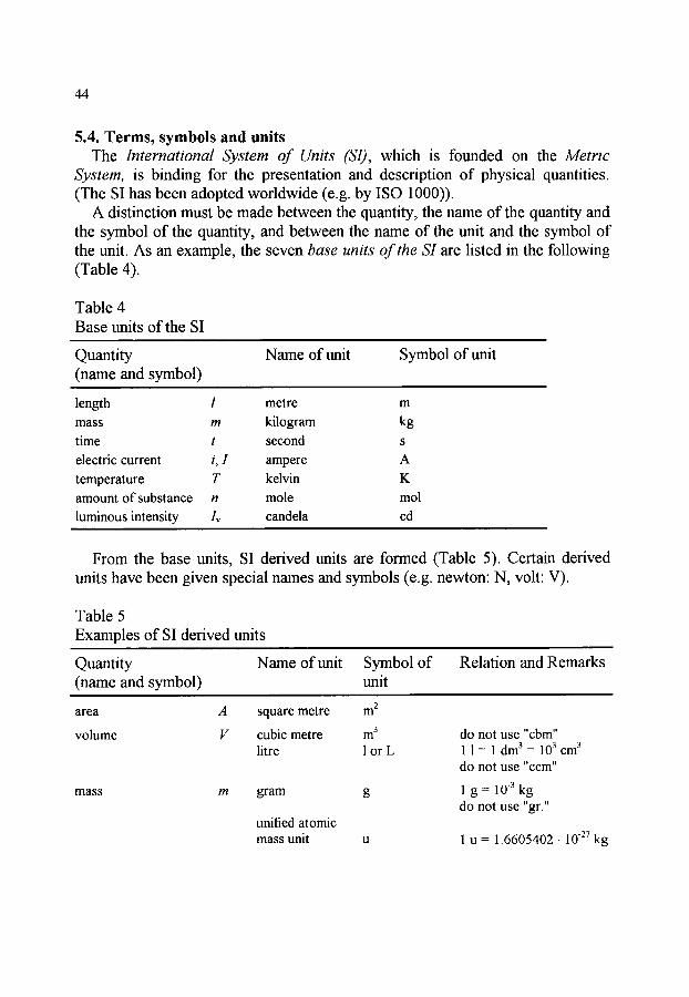
44

5.4. Terms , symbols and units The International System of Units ($1), which is founded on the Metric

System, is binding for the presentation and description of physical quantities. (The SI has been adopted worldwide (e.g. by ISO 1000)).

A distinction must be made between the quantity, the name of the quantity and the symbol of the quantity, and between the name of the unit and the symbol of the unit. As an example, the seven base units of the $1 are listed in the following (Table 4).

Table 4 Base traits of the SI

Quantity Name of unit Symbol of unit (name and symbol)

length 1 metre m mass m kilogram kg time t second s electric current i, 1 ampere A temperature T kelvin K amount of substance n mole mol luminous intensity Iv candela cd

From the base units, SI derived units are formed (Table 5). Certain derived units have been given special names and symbols (e.g. newton: N, volt: V).

Table 5 Examples of SI derived units

Quantity Name of unit (name and symbol)

area A square metre

volume V cubic metre litre

mass m gram

unified atomic mass unit

Symbol of unit

m 2

m 3 lorL

Relation and Remarks

do not use "cbm" 11 = l d m 3=10 3cm 3 do not use "ccm"

1 g = 10 -3 kg do not use "gr."

1 u = 1.6605402 �9 10 -27 kg

C o n t i n u a t i o n T a b l e 5

E x a m p l e s o f SI d e r i v e d uni t s

45

Q u a n t i t y

( n a m e a n d s y m b o l )

N a m e o f uni t S y m b o l o f

uni t

R e l a t i o n a n d R e m a r k s

time

v,f F

p,P

frequency

force

pressure

dynamic viscosity r/

kinematic viscosity 7"

energy E } work W heat Q

heat capacity C

power g } heat flow rate

heat flux Jq

thermal conductivity

heat transfer coefficient h

voltage (difference) U

electric resistance R

resistivity p

electric conductance G

conductivity K, cr

celsius temperature 0, t

minute min 1 min = 60 s hour h 1 h = 3600 s day d 1 d = 86400 s

hertz Hz 1 Hz = 1 s 1

newton N 1 N = 1 kg m s -2

pascal Pa 1 P a - 1 N m 2 bar bar 1 bar = 105 Pa

pascal second Pa s 1 Pa s = 1 N s m -2

m 2 s -1

joule J 1 J = 1 N m electronvolt eV 1 eV = 1.60218 �9 10 19 J

J K 1 1 J K 1 = 1 m 2 kg s 2 K 1

watt W 1 W- - 1 J s -1

W m -2

W m 1 K 1

W rn -2 K -1

volt V 1 V = 1 W A 1

ohm ~ 1 ~ = 1 V A -1

O m

siemens S 1 S = 1 ~ -1= 1 A V 1

S m -I

degree Celsius ~

T h e r e is a n u m b e r o f un i t s w h i c h s h o u l d n o t b e u s e d a n y m o r e in sc ien t i f i c a n d

t e c h n i c a l l i t e r a tu re ( T a b l e 6).

46

Tab le 6 E x a m p l e s o f units not to be used any m o r e in scientif ic and technica l repor ts

N a m e Symbol Rela t ion i

inch in 1 in = 2 .54 .10 z m

dyne dyn 1 dyn = 10 .5 N

pond p 1 p = 9.80665 N

millimetre of mercury mm Hg 1 mm Hg = 133.322 Pa

standard atmosphere atm 1 arm = 1.01325 bar

technical atmosphere at 1 at = 0.980665 bar

Torr Torr 1 Torr = 1.333224 mbar

pounds per square inch psi 1 psi - 6895 Pa

poise P 1 P = 0.1 Pa s

stokes St 1 St = 10 .4 m 2 s ~

erg erg 1 erg = 10Tj

calorie, international table calrr 1 calrr = 4.1868 J

calorie, thermochemical calth 1 calth = 4.184 J

The International Union of Pure and Applied Chemistry (IUPAC) r e c o m m e n d s a n u m b e r o f Quant i t ies , Uni t s and Symbols in Phys ica l Chemis t ry

[8], w h i c h are l is ted b e l o w for the quant i t ies mos t f requent ly used in thermal

analys is and ca lo r imet ry (Table 7).

Tab le 7 R e c o m m e n d e d quanti t ies , units and symbol s ( reference [8])

N a m e Symbol Def in i t ion SI unit

molar mass M MB - m (applied to entities B) n B

relative atomic mass Ar A r - ma (atomic weight) mu

molar volume V (applied to entities B) Vm Vm B =

' / 7 B

mass fraction m~ (applied to component j) w wj- Zm,

mole fraction nB (applied to entities B) x, y XB- ~ n A

kg mol 1

m 3 mo1-1

47

Continuation Table 7 Recommended quantities, units and symbols (reference [8])

solubility s

molality (applied to entities B, solvent A)

heat q, Q

heat flow rate

n B m, b mB =

mA

heat flux Jq

internal energy U enthalpy H thermodynamic temperature T Celsius temperature O, t entropy S Helmholtz energy A Gibbs energy G

heat capacity at constant Cp pressure

heat capacity at constant volume

Cv

chemical potential p

equilibrium constant

rate of conversion

fraction reacted order of reaction activation energy (Arrhenius) pre-exponential factor

partial molar quantity X

K

6t

H

Ea, EA

XB

rate of change of quantity X (flow) X

flux of a quantity X Jx

dO d t o~ J~ = ~ (A Area)

T,p,nj~B

~=d~ d t

�9 d X X =

dt

T,p, nj~B

Jx -~"

mol m -3

mol kg 1

W

W m 2

J J K ~ C j K -1

J J

j K -1

j K "1

J mol 1

mol s -1

J mol 1

(m 3 mol-1) n-1 S -1

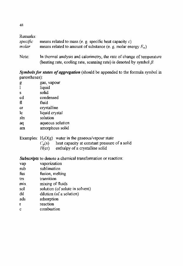
48

Remarks: specific molar

means related to mass (e. g. specific heat capacity c) means related to amount of substance (e. g. molar energy Em)

Note: In thermal analysis and calorimetry, the rate of change of temperature (heating rate, cooling rate, scanning rate) is denoted by symbol/3.

Symbols for states of aggregation (should be appended to the formula symbol in parentheses): g gas, vapour 1 liquid s solid cd condensed fl fluid cr crystalline lc liquid crystal sin solution aq aqueous solution am amorphous solid

Examples: H20(g) water in the gaseous/vapour state Cp(s) heat capacity at constant pressure of a solid H(cr) enthalpy of a crystalline solid

Subscripts to denote a chemical transformation or reaction: vap vaporization sub sublimation fus fusion, melting trs transition mix mixing of fluids sol solution (of solute in solvent) dil dilution (of a solution) ads adsorption r reaction c combustion

49

Superscripts: o , o standard , pure substance oo infinite dilution id ideal E excess quantity

Symbol for change in an extensive thermodynamic quantity: A Examples: nvapH-- H(g) - H(1) AfusHm molar enthalpy of fusion ArS ~ standard reaction entropy

Subscripts used in thermal analysis and calorimetry If related to an object: capital letters (e.g. ms, mass of the sample S; TR,

temperature of the reference sample R). If related to a phenomenon: lower case (e.g. Tg, glass transition temperature). If related to a specific point in time or temperature: lower case (e.g. T~,

extrapolated peak onset temperature).

6. LITERATURE ON THERMAL ANALYSIS AND CALORIMETRY

The literature dealing with thermoanalytical and calorimetric topics is, of course, very extensive and faceted, as these techniques are applied in the most diverse fields. Focal points of application of thermal analysis are the fields of chemistry, safety engineering, material technology and solid state physics; calorimetry is applied in addition in biology, pharmacy and food technology. Papers whose main topic is not only the technical development of the instruments used but which describe also their practical use can be found in the joumals relevant to the respective special field of application.

Four scientific joumals concentrate on the publication of original papers from the fields of thermal analysis, calorimetry and thermodynamics.

A survey of the present state of the measuring techniques and their application is given in conference proceedings which are published as digests on the occasion of scientific conferences held on a larger scale. Articles giving an overview of partial fields of thermal analysis and calorimetry are published as review papers in joumals or as single chapters in compilations. The fundamental measuring techniques applied in thermal analysis and calorimetry have been described in detail in some monographs.

50

6.1. Textbooks The selection presented in the following is essentially restricted to books

published after 1980. The main topic of these books is the measuring technique, not its application to certain classes of substances.

M.E. Brown: Introduction to Thermal Analysis: Techniques and Ap- plications, Chapman and Hall, New York, 1988, 211 pp.

A. Cezairliyan (Ed.): CINDAS Data Series on Materials Properties. Vol. 1-2. Specific Heat of Solids, Hemisphere, New York, 1988, 484 pp.

E.L. Charsley, S.B. Warrington (Eds.): Thermal Analysis: Techniques and Applications, Royal Society of Chemistry, Cambridge, 1992, 296 pp.

J.W. Dodd, K.H. Tonge: Thermal Methods: Analytical Chemistry by Open Learning, Wiley, Chichester, 1987, 337 pp.

P.J. Haines: Thermal Methods of Analysis: Principles, Applications and Problems, Blackie Academic and Professional, London, 1995, 286 pp.

K. Heide: Dynamische thermische Analysenmethoden, Deutscher Verlag far Grundstoffindustrie, Leipzig, 2nd Ed., 1982, 311 pp.

W.F. Hemminger, H.K. Cammenga: Methoden der Thermischen Analyse, Springer, Berlin, 1989, 299 pp.

W. Hemminger, G. H0hne: Calorimetry- Fundamentals and Practice, Verlag Chemie, Weinheim, 1984, 310 pp.

G. HOhne, W. Hemminger, H.-J. Flammersheim: Differential Scanning Calorime- try - An Introduction for Practitioners, Springer, Berlin, 1996, 222 pp.

51

C.G. Hyde, M.W. Jones: Gas Calorimetry. The Determination of the Calorific Value of Gaseous Fuels, Ernest Benn, London, 1960, 456 pp.

B. LeNeindre, B. Vodar (Eds.): Experimental Thermodynamics. Vol. 2. Calorimetry of Non-Reacting Fluids, Butterworths, London, 1975, 1318 pp.

K.D. Magli6, A. Cezairliyan, V.E. Peletzky (Eds.): Compendium of Thermo- physical Property Measurement Methods. Vol. 1: Survey of Measurement Techniques, Plenum, New York, 1984, 789 pp. Vol. 2: Recommended Measurement Techniques and Practices, Plenum, New York, 1992, 643 pp.

J.P. McCullough, D.W. Scott (Eds.): Experimental Thermodynamics. Vol. 1. Calorimetry of Non-reacting Systems, Butterworths, London, 1968, 606 pp.

M.I. Pope, M.D. Judd: Differential Thermal Analysis: A Guide to the Tech- nique and its Applications, Heyden, London, 1977, 197 pp.

S. Sunner, M. MS, nsson (Eds.): Experimental Chemical Thermodynamics. Vol. 1. Combustion Calorimetry, Pergamon, Oxford, 1979, 428 pp.

W.W. Wendlandt: Thermal Analysis, Wiley, New York, 3rd Ed., 1986, 814 pp.

B. Wunderlich: Thermal Analysis, Academic Press, Boston, 1990, 450 pp.

The books listed below deal with thermal analysis and calorimetry from the angle of special technical fields:

52

V. Balek, J. Tolgessy: Emanation Thermal Analysis and other Radiometric Emanation Methods, (Wilson and Wilson's Comprehensive Analytical Chemis- try. Vol. 12. Thermal Analysis. Part C), Elsevier, Amsterdam, 1984, 303 pp.

F.X. Eder: Arbeitsmethoden der Thermodynamik. Band 2. Thermische und kalorische Stoffeigenschaften, Springer, Berlin, 1983, 524 pp.

J.L. Ford, P. Timmins: Pharmaceutical Thermal Analysis: Applications, E. Horwood, Chichester, 1989, 313 pp.

Techniques and

V.R. Harwalkar, C.-Y. Ma (Eds.): Thermal Analysis of Foods, Elsevier, London, 1990, 362 pp.

F. Hatakeyama, F. X. Quinn: Thermal Analysis: Fundamentals and Applications to Polymer Science, Wiley, Chichester, 1994, 158 pp.

N.D. Jespersen (Ed.): Biochemical and Clinical Applications of Thermometric and Thermal Analysis, (Wilson and Wilson's Comprehensive Analytical Chem- istry. Vol. 12. Thermal Analysis. Part B), Elsevier, Amsterdam, 1982, 245 pp.

C.J. Keattch, D. Dollimore: An Introduction to Thermogravimetry, Heyden, London, 2nd Ed., 1975, 164 pp.

O. Kubaschewski, C. B. Alcock, P. J. Spencer: Materials Thermochemistry, Pergamon, Oxford, 6th Ed., 1993, 363 pp.

L. Kubic~ir: Pulse Method of Measuring Basic Thermophysical Pa- rameters, (Wilson and Wilson's Comprehensive Analytical Chemis- try. Vol. 12. Thermal Analysis. Part E), Elsevier, Amsterdam, 1990, 341 pp.

53

V.B.F. Mathot (Ed.) Calorimetry and Thermal Analysis of Polymers, Carl Hanser, Mtinchen, 1994, 369 pp.

R.Sh. Mikhail, E. Robens: Microstructure and Thermal Analysis of Solid Sur- faces, Wiley, Chichester, 1983, 496 pp.

F. Paulik: Special Trends in Thermal Analysis, Wiley, Chichester, 1995, 459 pp.

J. Paulik, F. Paulik: Simultaneous Thermoanalytical Examinations by Means of the Derivatograph, (Wilson and Wilson's Comprehensive Analytical Chem- istry. Vol. 12. Thermal Analysis. Part A), Elsevier, Amsterdam, 1981,277 pp.

v

J. Sest~k Thermophysical Properties of Solids: Their Measurements and Theoretical Thermal Analysis, (Wilson and Wilson's Comprehensive Analytical Chem- istry. Vol. 12. Thermal Analysis. Part D), Elsevier, Amsterdam, 1984, 440 pp.

W. Smykatz-Kloss, S.St.J. Wame (Eds.)" Thermal Analysis in the Geosciences, Springer, Berlin 1991, 379 pp.

R.F. Speyer: Thermal Analysis of Materials, Marcel Dekker, New York, 1994, 285 pp.

E.A. Turi (Ed.): Thermal Characterization of Polymeric Materials, Academic Press, New York, 2nd Ed., 1996

G. Widmann, R. Riesen: Thermal Analysis. Terms, Methods, Applications, Htithig, Heidelberg, 1986, 131 pp.

6.2. Reviews or chapters in books J. Boerio-Goates, J.E. Callanan: Differential Thermal Methods.

in: B.W. Rossiter, R.C. Baetzold (Eds.): Physical Methods of Chemistry. Vol. 6. Determination of Thermodynamic Properties, Wiley, New York, 2nd Ed., 1992, Chapter 8, pp. 621 - 717.

54

J.L. Oscarson, R.M. Izatt: Calorimetry. in: B.W. Rossiter, R.C. Baetzold (Eds.): ibidem, Chapter 7, pp. 573 - 620.

S.M. Sarge: Kalorische ZustandsgrOBen. in: V. Kose, S. Wagner (Eds.): F. Kohlrausch. Praktische Physik, Band 1, B.G. Teubner, Stuttgart, 24th Ed., 1996, Chapter 3.3, pp. 411 - 440.

H.-G. Wiedemann, G. Bayer: Trends and Applications of Thermogravimetry. in: F.L. Boschke, (Ed.): Topics in Current Chemistry. Vol. 77: Inorganic and Physical Chemistry, Springer, Berlin, 1978, pp. 67 - 140.

6.3. Conference proceedings Conference proceedings of national and international meetings are sometimes

published as monographs, sometimes as special issues of certain journals.

Proceedings of the International Conference on Thermal Analysis (and Calorimetry), ICTA/ICTA C:

J.P. Redfern (Ed.): Thermal Analysis 1965" Proceedings of the First International Conference on Thermal Analysis, Aberdeen, United Kingdom, 06.-09.09.1965. Macmillan, London, 1965, 293 pp.

R.F. Schwenker, P.D. Garn (Eds.): Thermal Analysis. Proceedings of the Second International Conference on Thermal Analysis, Worcester, USA, 18.-23.08.1968. Vol. 1" Instrumentation, Organic Materials, and Polymers, Vol. 2: Inorganic Materials and Physical Chemistry, Academic Press, New York, 1969.

H.-G. Wiedemann (Ed.): Thermal Analysis' Proceedings of the Third Interna- tional Conference on Thermal Analysis, Davos, Switzerland, 23.- 28.08.1971. Vol. 1" Advances in Instrumentation, Vol. 2" Inorganic Chemistry,

55

Vol. 3: Organic and Macromolecular Earth Sciences,

Birkh~user, Basel, 1972.

Chemistry, Ceramics,

I. Buzas(Ed.): Thermal Analysis: Proceedings of the Fourth International Conference on Thermal Analysis, Budapest, Hungary, 08.- 13.07.1974. Vol. 1: Theory, Inorganic Chemistry, Vol. 2: Organic and Macromolecular Chemistry. Earth Sciences, Vol. 3: Applied Sciences. Methodics and Instrumentation, Akademiai Kiado, Budapest, 1975.

H. Chihara(Ed.): Thermal Analysis: Proceedings of the Fifth International Conference on Thermal Analysis, Kyoto, Japan, 01 .-06.08.1977. Heyden, London, 1977, 575 pp.

H.-G. Wiedemann (Ed.): Thermal Analysis: Proceedings of the Sixth Interna- tional Conference on Thermal Analysis, Bayreuth, Federal Re- public of Germany, 06.-12.07.1980. Vol. 1: Theory, Instrumentation, Applied Sciences, Industrial

Applications, Birkhguser, Basel, 1980, 612 pp.

W. Hemminger (Ed.): Thermal Analysis: Proceedings of the Sixth International Conference on Thermal Analysis, Bayreuth, Federal Republic of Germany, 06.-12.07.1980. Vol. 2: Inorganic Chemistry/Metallurgy, Earth Sciences, Orga-

nic Chemistry/Polymers, Biological Sciences/Medicine/ Pharmacy,

Birkh~user, Basel, 1980, 590 pp.

B. Miller(Ed.): Thermal Analysis: Proceedings of the Seventh International Conference on Thermal Analysis, Kingston, Canada, 22.- 27.08.1982.2 Volumes. Wiley, Chichester, 1982, 1530 pp.

A. Blazek (Ed.): Thermal Analysis. Proceedings of the Eighth International Conference on Thermal Analysis, Bratislava, Czechoslovakia, 19.-23.08.1985.

56

Vol. 1: Thermochim. Acta, 92 ( 1 9 8 5 ) , 1 - 845 , Vol. 2: Thermochim. Acta, 93 (1985), 1 - 777.

V. Balek, J. Sest~ik (Eds.) Thermal Analysis Highlights Thermochim. Acta, 110 (1986), 1 - 563.

1985 (8th ICTA),

S. Yariv (Ed.): Thermal Analysis. Proceedings Conference on Thermal Analysis, 25.08.1988. Part A: Thermochim. Acta, 133 (1988), Part B: Thermochim. Acta, 134 (1988), Part C: Thermochim. Acta, 135 (1988).

of the Ninth International Jerusalem, Israel, 21.-

S. Yariv (Ed.): Thermal Analysis Highlights 1988 (9th ICTA), Thermochim. Acta 148, (1988), 1 - 554.

S. Yariv (Ed.): ICTA 9 Plenary Lectures, Pure Appl. Chem. 61, (1989), 1323- 1360.

D.J. Morgan: Proceedings of the Tenth International Conference on Thermal Analysis, Hatfield, United Kingdom, 24.-28.08.1992. Vol. I: Earth Sciences, Cements, Glasses, Ceramics, Fuels,

Metallurgical Systems, Superconductors, J. Thermal Anal. 40, (1993), 1 - 386.

VollI: Pharmaceutical and Organic Compounds, Polymers, Biological and Biochemical Materials, J. Thermal Anal. 40, (1993), 387 - 869.

Vol. III: Instrumentation, Inorganic Compounds, Catalysis, The- ory and Kinetics, Standardization Workshop, Education Workshop, Awards J. Thermal Anal. 40, (1993), 871 - 1486.

Proceedings of the European Symposium o n

Calorimetry); ES TA/ES TA C: Thermal Analysis (and

D. Dollimore (Ed.): Proceedings of the First European Symposium on Thermal Analysis, Salford, United Kingdom, 20.-24.09.1976. Heyden, London, 1976, 458 pp.

57

D. Dollimore(Ed.):Proceedings of the Second European Symposium on Thermal Analysis, Aberdeen, United Kingdom, 01 .-04.09.1981. Heyden, London, 1981, 617 pp.

E. Marti, H.R. Oswald (Eds.): Proceedings of the Third European Symposium on Thermal Analysis and Calorimetry, Interlaken, Switzerland, 09.- 15.09.1984. Thermochim. Acta, 85 (1985), 1 - 533.

D. Schultze (Ed.): Proceedings of the Fourth European Symposium on Thermal Analysis and Calorimetry, Jena, German Democratic Republic, 24.-28.08.1987. J. Thermal Anal., 33 (1988).

R. Castanat, E. Karmazsin (Eds.): Proceedings of the Fifth European Symposium on Thermal Analysis and Calorimetry, Nice, France, 25.- 30.08.1991. Vol. 1: J. Thermal Anal., 38 (1992), 1 - 253, Vol. 2: J. Thermal Anal., 38 (1992), 255 - 530, Vol. 3: J. Thermal Anal., 38 (1992), 531 - 1025.

I Kikic, a. Ces~ro (Eds.): Recent Advances in Thermal Analysis and Calorimetry. A Selection of Papers presented at the 6th European Symposium on Thermal Analysis and Calorimetry, Grado, Italy, 11.- 16.09.1994. Thermochim. Acta, 269/270 (1995), 884 pp.

A. Cesgro, G. Della Gatta (Eds.): Invited and Selected Lecutres presented at the 6th European Symposium on Thermal Analysis and Calorimetry, Grado, Italy, 11 .- 16.09.1994. Pure and Appl. Chem., 67 (1995), 1789 - 1890.

Conferences of the International Union of Pure and Applied Chemistry, IUPAC, on Chemical Thermodynamics:

12th International Conference on Chemical Thermodynamics, London, United Kingdom, 06.-10.09.1982. Pure and Appl. Chem., 55 (1983), 417 - 551.

58

International Conference on Chemical Thermodynamics, Hamilton, Ontario, Canada, 13.-17.08.1984. Pure and Appl. Chem., 57 (1985), 1 - 103.

9th International Conference on Chemical Thermodynamics, Lisbon, Portugal, 14.-18.07.1986. Pure and Appl. Chem., 59 (1987), 1 - 100.

10th International Conference on Chemical Czechoslovakia, 29.08.-02.09.1988. Pure and Appl. Chem., 61 (1989), 979 - 1132.

Thermodynamics, Prague,

1 l th International Conference on Chemical Thermodynamics, Como, Italy, 26.- 31.08.1990. Pure and Appl. Chem., 63 (1991), 1313 - 1526.

12th International Conference on Chemical Thermodynamics, Snowbird, Utah, USA, 16.-21.08.1992. Pure and Appl. Chem., 65 (1993), 873 - 1008.

13th International Conference on Chemical Thermodynamics, Clemond-Ferrand, France, 17.-22.07.1994. Pure and Appl. Chem., 67 (1995), 859- 1030.

6.4. Journals Several journals publish original papers from the fields Thermal Analysis,

Calorimetry and Experimental Thermodynamics. �9 Thermochimica Acta (Elsevier, Amsterdam) �9 Journal of Thermal Analysis (Wiley, Chichester und Akad6miai Kiad6,

Budapest) �9 Journal of Chemical Thermodynamics (Academic Press, New York) �9 Netsuosokutei (= Calorimetry and Thermal Analysis) (Nikon Netsuosokutei

Gakkai, Tokyo-to) In "Thermal Analysis Abstracts" (Wiley, Chichester) Vol. 1 (1972)- Vol. 17

(1988) and in the subsequent editions, Vol. 18 (1989) - Vol. 20 (1991) entitled "Thermal Analysis Reviews and Abstracts", original papers from the field of thermal analysis were excerpted from a variety of journals and indexed.

At two-year intervals, the journal "Analytical Chemistry" publishes reviews including detailed references.

59

The journals "Review of Scientific Instruments" and "Journal of Physics E: Scientific Instruments" publish papers which describe new developments in the insmnnent sector.

The "International Journal of Thermophysics" publishes, among other things, papers dealing with calorimetry, at higher temperatures in particular.

The "Journal of Thermal Analysis" and "Thermochimica Acta" publish special issues which are either dedicated to certain persons who made important contributions to thermal analysis or calorimetry, or which concentrate on one particular topic:

W.W. Wendlandt, V. Satava, J. Sest~ak (Eds.) The Processes by Thermal Analysis, Yhermochim. Acta, 7(5) (1973), 222 pp.

Study of Heterogeneous

R.C. Mackenzie: A History of Thermal Analysis, Thermochim. Acta, 73(3) (1984), 124 pp.

W.W. Wendlandt (Ed.): Aspects of Calorimetry and Thermal Analysis, Thermochim. Acta, 100(1) (1986), 342 pp.

P.K. Gallagher, T. Ozawa, J. Sest~k (Eds.): High-Temperature Superconductors, Thermochim. Acta, 174 (1991 ), 324 pp.

I. Lamprecht, W. Hemminger, G.W.H. HOhne (Eds.): Calorimetry in the Bio- logical Sciences, Thermochim. Acta, 193 (1991 ), 452 pp.

v

J. Sest~k (Ed.)" Reaction Kinetics by Thermal Analysis, Thermochim. Acta, 203(1/2) (1992), 562 pp.

Th. Grewer, J. Steinbach (Eds.): Safety Techniques, Thermochim. Acta, 225(2) (1993), 174 pp.

V.B.F. Mathot (Ed.): Thermal Analysis and Calorimetry in Polymer Physics, Thermochim. Acta, 238(1/2) (1994), 472 pp.

A. Schiraldi (Ed.): Applications of Calorimetry and Thermal Analysis to Food Systems and Processes, Thermochim. Acta, 246(2) (1994), 187 pp.

60

Yu.K. Godovsky, G.W.H. H6hne (Eds.): Deformation Calorimetry of Polymers, Thermochim. Acta, 247(1) (1994), 128 pp.

B. Cantor, K. O'Reilly, J. Hider (Eds.): Thermal Analysis of Advanced Materials, J. Thermal Anal., 42(4) (1994), 643 - 838.

J. Sest~tk, B. Step~ek (Eds.) Thermodynamic Applications in Material Science, J. Thermal Anal., 43(2) (1995), 371- 544.

J.L. Ford (Ed.): Pharmaceuticals and Thermal Analysis, Thermochim. Acta, 248 (1995), 360 pp.

A.A.F. Kettrup (Ed.): Thermal Analysis Applied to Environmental Problems, Thermochim. Acta, 263 (1995), 163 pp.

M. Sorai, J. Sest~k (Eds.)" Transition Phenomena in Condensed Matter, Thermochim. Acta, 266 (1995), 407 pp.

R.N. Landau (Ed.): Reaction Calorimetry, Thermochim. Acta, 289(2) (1996), 378 pp.

6.5. Standards In the following, standards of different national and international standardi-

zation bodies relevant to thermal analysis and calorimetry (mainly combustion calorimetry) are listed (as of 31.12.1996):

American Standards ASTM C 351 (1992): Test method for mean specific heat of thermal insulation ASTM D 240 (1992): Test method for heat of combustion of liquid hydrocarbon fuels by bomb calorimetry ASTM D 1519 (1995): Test method for rubber chemicals - melting range ASTM D 1826 (1994): Test method for calorific (heating) value of gases in natural gas range by continuous recording calorimeter ASTM D 1989 (1995): Test method for gross calorific value of coal and coke by microprocessor controlled isoperibol calorimeters ASTM D 2015 (1995): Test method for gross calorific value of coal and coke by the adiabatic bomb calorimeter ASTM D 2382 (1988): Test method for heat of combustion of hydrocarbon fuels by bomb calorimeter (high-precision method) ASTM D 2766 (1995): Test method for specific heats of liquids and solids

61

ASTM D 3286 (1991): Test method for gross calorific value of coal and coke by the isoperibol bomb calorimeter ASTM D 3386 (1994): Test method for coefficient of linear thermal expansion of electrical insulating materials ASTM D 3417 (1983 (rev. 1988)): Test method for heats of fusion and crystallization of polymers by thermal analysis ASTM D 3418 (1982 (rev. 1988)): Test method for transition temperatures of polymers by thermal analysis ASTM D 3850 (1994): Test method for rapid thermal degradation of solid electrical insulating materials by thermogravimetric method (TGA) ASTM D 3895 (1995): Test method for oxidative-induction time of polyolefins by differential scanning calorimetry ASTM D 3947 (1992): Test method for specific heat of aircraft turbine lubricants by thermal analysis ASTM D 4065 (1992): Determining and reporting dynamic mechanical properties of plastics ASTM D 4092 (1990): Terminology relating to dynamic mechanical measurements on plastics ASTM D 4419 (1990 (rev. 1995)): Test method for measurement of transition temperatures of petroleum waxes by differential scanning calorimetry (DSC) ASTM D 4535 (1985): Test method for thermal expansion of rock using a dilatometer ASTMD 4565 (1994): Physical and environmental performance properties of insulations and jackets for telecommunication wire and cable ASTM D 4591 (1993): Temperatures and heats of transition of fluoropolymers by DSC ASTM D 4611 (1986): Test method for specific heat of rock and soil ASTM D 4809 (1995): Test method for heats of combustion of liquid hydrocarbon fuels by bomb calorimetry (precision method) ASTM D 4816 (1994): Test method for specific heat of aircraft turbine fuels by thermal analysis ASTM D 5028 (1990): Test method for curing properties of pultrusion resins by thermal analysis ASTM D 5468 (1995): Standard test method for gross calorific and ash value of waste materials ASTM D 5483 (1995): Test method for oxidation induction time of lubricating greases by pressure differential scanning calorimetry ASTM D 5865 (1995): Test method for gross calorific value of coal and coke ASTM D 5885 (1995): Test method for oxidation induction time of polyolefin geosynthetics by high-pressure differential scanning calorimetry

62

ASTM E 228 (1995): Linear thermal expansion of solid materials with a vitreous silica dilatometer ASTM E 289 (1995): Linear thermal expansion of rigid solids with interferometry ASTM E 422 (1983 (rev. 1994)): Test method for measuring heat flux using a water-cooled calorimeter ASTM E 472 (1986 (rev. 1991)): Reporting thermoanalytical data ASTM E 473 (1994): Terminology relating to thermal analysis ASTM E 476 (1987 (rev. 1993)): Standard test method for thermal instability of confined condensed phase systems (confinement test) ASTM E 487 (1979 (rev. 1992)): Test method for constant-temperature stability of chemical materials ASTM E 537 (1986 (rev. 1992)): Test method for assessing the thermal stability of chemicals by methods of differential thermal analysis ASTM E 698 (1979 (rev. 1993)): Test method for Arrhenius kinetic constants for thermally unstable materials ASTM E 711 (1987 (rev. 1992)) Test method for gross calorific value of refuse- derived fuel by the bomb calorimeter ASTM E 793 (1995): Test method for heats of fusion and crystallization by differential scanning calorimetry ASTM E 794 (1995): Test method for melting and crystallization temperatures by thermal analysis ASTM E 831 (1993): Test method for linear thermal expansion of solid materials by thermomechanical analysis ASTM E 914 (1983 (rev. 1993)): Standard practice for evaluating temperature scale for thermogravimetry (withdrawn) ASTM E 928 (1985 (rev. 1989)): Test method for mol percent impurity by differential scanning calorimetry ASTM E 967 (1992): Standard practice for temperature calibration of differential scanning calorimeters and differential thermal analyzers ASTM E 968 (1983 (rev. 1993)): Standard practice for heat flow calibration of differential scanning calorimeters ASTM E 1131 (1993): Test method for compositional analysis by thermogravimetry ASTM E 1142 (1983): Terminology relating to thermophysical properties ASTM E 1231 (1996): Calculation of hazard potential figures-of-merit for thermally unstable materials ASTME 1269 (1995): Test method for determining specific heat capacity by differential scanning calorimetry

63

ASTM E 1354 (1994): Test method for heat and visible smoke release rates for materials and products using an oxygen consumption calorimeter ASTM E 1356 (1991): Test method for glass transition temperatures by differential scanning calorimetry or differential thermal analysis ASTM E 1363 (1995): Temperature calibration of thermomechanical analyzers ASTM E 1545 (1995): Standard test method for glass transition temperatures by thermomechanical analysis ASTME 1559 (1993): Contamination outgassing characteristics of spacecraft materials ASTM E 1582 (1993): Standard practice for calibration of temperature scale for thermogravimetry ASTM E 1640 (1994): Test method for assignment of the glass transition temperature by dynamic mechanical analysis ASTM E 1641 (1994): Test method for decomposition kinetics by thermogravimetry

British Standards BS 2000-12 (1993): Methods of test for petroleum and its products. Determina- tion of specific energy BS 3804-1 (1964): Methods for the determination of the calorific values of fuel gases. Non-recording methods (obsolescent) BS 4550-3 (1978): Methods of testing cement. Physical tests. Test for heat of hydration BS 4791 (1985): Specification for calorimeter bombs BS 7420 (1991): Guide for determination of calorific values of solid, liquid and gaseous fuels (including definitions)

German Standards DIN 1164-8 (1978): Portland-, iron portland-, blast-fumace-, and trass cement; determination of the heat of hydration with the solution calorimeter DIN 3761-15 (1984): Rotary shaft lip type seals for automobils; test; determination of cold resistant of elastomers; differential-thermoanalysis DIN 50456-1 (1991): Testing of materials for semiconductor technology; method for the characterisation of moulding compounds for electronic components; determination of the thermo-mechanical dilatation of epoxy resin moulding compounds DIN 51004 (1994): Thermal analysis (TA). Determination of melting temperatures of crystalline materials by differential thermal analysis (DTA) DIN 51005 (1993): Thermal analysis (TA). Terms DIN 51006 (1990): Thermal analysis (TA). Principles of thermogravimetry

64

DIN 51007 (1994): Thermal analysis (TA). Differential thermal analysis (DTA). Principles DIN 51045-1 (1989): Determination of the thermal expansion of solids. Basic rules DIN 51045-2 (1976): Determination of the change of length of solids by thermal effect. Testing of fired fine ceramic material DIN 51045-3 (1976): Determination of the change of length of solids by thermal effect. Testing of non-fired fine ceramic material DIN 51045-4 (1976): Determination of the change of length of solids by thermal effect. Testing of fired ordinary ceramic material DIN 51045-5 (1976): Determination of the change of length of solids by thermal effect. Testing of non-fired ordinary ceramic material DIN 51900-1 (1989): Testing of solid and liquid fuels. Determination of gross calorific value by the bomb calorimeter and calculation of net calorific value. Principles, apparatus and methods DIN 51900-2 (1977): Testing of solid and liquid fuels. Determination of gross calorific value by the bomb calorimeter and calculation of net calorific value. Method with the isothermal water jacket DIN 51900-3 (1977): Testing of solid and liquid fuels. Determination of gross calorific value by the bomb calorimeter and calculation of net calorific value. Method with the adiabatic jacket DIN 53545 (1990): Determination of low-temperature behaviour of elastomers. Principles and test methods DIN 53765 (1994): Testing of plastics and elastomeres. Thermal analysis. DSC- method DIN-E 65467 (1989): Aerospace. Testing of organic polymeric materials with and without reinforcement. DSC method

European Standards EN 725-3 (1994): Advanced technical ceramics. Methods of test for ceramic powders. Determination of the oxygen content of non-oxides by thermal extrac- tion with a carrier gas prEN 728 (1992): Plastics piping and ducting systems. Polyolefin pipes and fittings. Determination of the induction time ENV 820-1 (1993): Advanced technical ceramics. Monolithic ceramics. Thermo- mechanical properties. Part 1: Determination of flexural strength at elevated temperatures ENV ,820-2 (1992): Advanced technical ceramics. Monolithic ceramics. Thermo- mechanical properties. Part 2: Determination of selfloaded deformation

65

ENV 820-3 (1993): Advanced technical ceramics. Monolithic ceramics. Thermo- mechanical properties. Part 3: Determination of resistance to thermal shock by water quenching EN 821-1 (1995): Advanced technical ceramics. Monolithic ceramics. Thermo- physical properties. Part 1: Determination of thermal expansion prEN 821-2 (1992): Advanced technical ceramics. Monolithic ceramics. Thermo- physical properties. Part 2: Determination of thermal diffusivity ENV 821-3 (1993): Advanced technical ceramics. Monolithic ceramics. Thermo- physical properties. Part 3: Determination of specific heat capacity ENVl159-1(1993): Advanced technical ceramics. Ceramic composites. Thermophysical properties. Part 1: Determination of thermal expansion ENVl159-2(1993): Advanced technical ceramics. Ceramic composites. Thermophysical properties. Part 2: Determination of thermal diffusivity ENV 1159-3y(1995): Advanced technical ceramics. Ceramic composites. Thermophysical properties. Part 3: Determination of specific heat capacity prEN 1878 (1995): Products and systems for the protection and repair of concrete structures. Test methods. Reactive functions related to epoxy resins. Thermogravimetry of polymers. Temperature scanning method prEN 3877 (1993): Aerospace series. Test methods for braze alloys. Determina- tion of solidus and liquidus temperatures by differential thermal analysis prEN 6032 (1995): Aerospace series. Fibre reinforced plastics. Test method; determination of the glass transition temperature prEN 6039 (1995): Aerospace series. Fibre reinforced plastics. Test method; determination of the exothermic reaction during curing of prepreg material prEN6041 (1995): Aerospace series. Non-metallic materials. Test method; analysis of non-metallic materials (uncured) by differential scanning calorimetry (DSC) prEN 6064 (1995): Aerospace series. Non-metallic materials. Test method; analysis of non-metallic materials (cured) for the determination of the extent of cure by differential scanning calorimetry (DSC) EN 61043 (1993): Determination of heats and temperatures of melting and crystallization of electrical insulating materials by differential scanning calorimetry

Standards by the International Electrotechnical Commission IEC 1006 (1991): Methods of test for determination of the glass transition temperature of electrical insulating materials IEC/TR 1026 (1991): Guidelines for application of analytical test methods for thermal endurance testing of electrical insulation materials

66

IEC/TR 1074 (1991): Method of test for the determination of heats and temperatures of melting and crystallization of electrical insulating materials by differential scanning calorimetry

Standards by the International Standards Organization ISO 472 (1988): Plastics. Vocabulary ISO 745 (1976): Sodium carbonate for industrial use. Determination of loss mass and of non-volatile matter at 250 ~ ISO 1716 (1973): Building materials. Determination of calorific potential ISO 1928 (1995): Solid mineral fuels. Determination of gross calorific value by the calorimeter bomb method, and calculation of net calorific value ISO 3146 (1985): Plastics. Determination of melting behaviour (melting temperature or melting range) of semi-crystalline polymers ISO 7111 (1987): Plastics. Thermogravimetry of polymers. Temperature scanning method ISO/DIS 7215 (1993): Iron ores. Determination of relative reducibility ISO/DIS 9831 (1991): Animal feeding stuffs. Determination of gross calorific value. Calorimeter bomb method ISO 9924-1 (1993): Rubber and rubber products. Determination of composition of vulcanizates and uncured compotmds by thermogravimetry. Part 1: Butadiene, ethylene-propylene copolymer and terpolymer, isobutene-isoprene, isoprene and styrene-butadiene rubbers ISO/DIS 11357-1 (1994): Plastics. Differential scanning calorimetry (DSC). Part 1. General principles ISO/DIS 11357-2 (1996): Plastics. Differential scanning calorimetry (DSC). Part 2. Determination of glass transition temperature ISO/DIS 11357-3 (1996): Plastics. Differential scanning calorimetry (DSC). Part 3. Determination of temperature and enthalpy of melting and crystallization ISO/DIS 11358 (1994): Plastics. Thermogravimetry (TG) of polymers. General principles ISO/CD 11359-1 (1996): Plastics. Thermomechanical analysis (TMA). Part 1. General principles ISO/CD 11359-2 (1996): Plastics. Thermomechanical analysis (TMA). Part 2. Determination of coefficient of linear thermal expansion and glass transition temperature ISO/CD 11359-3 (1996): Plastics. Thermomechanical analysis (TMA). Part 3. Determination of penetration temperature ISO 11409 (1993): Plastics. Phenolic resins. Determination of heats and temperatures of reaction by differential scanning calorimetry

67

Japanese Standards JIS H 7101 (1989): Method for determining the transformation temperatures of shape memory alloys JIS H 7151 (1991): Method of determining the crystallization temperatures of amorphous metals JIS K 0129 (1994): General rules for thermal analysis JIS K 2279 (1993): Crude petroleum and petroleum products. Determination and estimation of heat of combustion JIS K 7120 (1987): Testing methods of plastics by thermogravimetry JIS K 7121 (1987): Testing methods for transition temperatures of plastics JIS K 7122 (1987): Testing methods for heat of transitions of plastics JIS K 7123 (1987): Testing methods for specific heat capacity of plastics JIS K 7196 (1991): Testing method for softening temperature of thermoplastic film and sheeting by thermomechanical analysis JIS K 7197 (1991): Testing method for linear thermal expansion coefficient of plastics by thermomechanical analysis JIS R 1618 (1994): Measuring method of thermal expansion of fine ceramics by thermomechanical analysis

French Standards NF C26-306 (1994): Guidelines for application of analytical test methods for thermal endurance testing of electrical insulating materials NFL17-451 (1988): Aerospace. Fabrics pre-impregnated with thermosetting resin. Differential scanning calorimetry. Test method NF M03-005 (1990): Solid fuels. Determination of gross calorific value and calculation of net calorific value NFM07-030 (1965) Liquid fuels. Determination of gross calorific value of petroleum products NF P15-436 (1988): Binders. Measuring the hydration heat of cements by means of semi-adiabatic calorimetry (Langavant method). NF T01-021 (1974): Thermal analysis. Vocabulary. Reporting data NF T30-603 (1978): Paints. Fillers for interior use. Differential thermal analysis NF T45-114 (1989): Raw materials for the rubber industry. Determination of the rubber bound with carbon black NF T46-047 (1986): Vulcanized or non-vulcanized rubber. Detennination of the centesimale composition of mixtures through thermogravimetry NF T51-223 (1985): Plastics. Semi-crystalline materials. Determination of the conventional melting temperature by thermal analysis NFT51-507-1 (1991): Plastic. Differential enthalpy analysis. Part 1. General principles

68

NF T51-507-2 (1991): Plastic. Differential enthalpy analysis. Part 2. Determina- tion of the conventional glass transition temperature NF T51-507-3 (1991): Plastic. Differential enthalpy analysis. Part 3. Determina- tion of the conventional temperatures and of the fusion and crystallization enthalpies NF T54-075 (1986): Plastics. Polyethylene pipes and fittings. Determination of thermal stability by thermal analysis. Isothermal method NF T70-313 (1995): Energetic materials for defense. Physical-chemical analysis and properties. Coefficient of linear thermal expansion by direct measurement

These standards are available through the respective standardization bodies:

Association fran~aise de normalisation (AFNOR) Tour Europe F-92049 Paris La D6fense Cedex France Telephone: +33 1 42 91 55 55 Telefax: +33 1 42 91 56 56 Telex: 61 19 74 afnor f Telegrams: afnor courbevoie Internet: www.afnor.fr

American Society for Testing and Materials (ASTM) 100 Barr Harbor Drive West Conshohocken, PA 19428-2959 United States of America Telephone: +1 61 08 32 95 00 Tel. (Sales): +1 61 08 32 95 85 Telefax: +1 61 08 32 95 55 Intemet: [email protected]

British Standards Institution (BSI) 389 Chiswick High Road GB-London W4 4AL Great Britain Telephone: +44 18 19 96 90 00 Telefax: +44 18 19 96 74 00 Intemet: [email protected] X.400: c=gb; a=gold400; p=bsi; o=bsi; s=surname; g=first name

69

European Committee for Standardization (CEN) 2 Rue de Brederode, Bte 5 B-1000 Brussels Belgium Telephone: +32 5 19 68 11 Telefax: +32 5 19 68 19

DIN Deutsches lnstitut fiir Normung (DIN) Burggrafenstrage 6 D-10787 Berlin Germany Telephone: +49 30 26 01 0 Telefax: +49 30 26 01 12 31 Telex: 18 42 73 din d Telegrams: deutschnormen berlin Internet: [email protected] X.400: c=de; a=d400; p=din; s=postmaster

International Electrotechnical Commission (IEC) 3, Rue de Varemb6 Case Postale 131 CH-1211 Geneva 20 Switzerland Telephone: +41 22 9 19 02 11 Telefax: +41 22 9 19 03 01 Telex: 41 41 21 IEC CH Telegrams: inelission geneve Intemet: www.iec.ch

International Standards Organization (ISO) 1, Rue de V aremb6 Case Postale 56 CH- 1211 Geneva 20 Switzerland Telephone: +41 22 7 49 01 11 Telefax: +41 22 7 33 34 30 Telex: 41 22 05 ISO CH Telegrams: isoorganiz Intemet: [email protected] X400: c=ch; a=400mt; P=iso; o=isocs; s=central

70

Japanese Industrial Standards Committee (JISC) c/o Standards Department Ministry of International Trade and Industry 1-3-1, Kasumigaseki, Chiyoda-ku Tokyo 100 Japan Telephone: +81 3 35 01 20 96 Telefax: +81 3 35 80 86 37

6.6. Literature on the history of thermal analysis and calorimetry Development of the DTA instrument into a quantitative heat flow differential calorimeter: S.L. Boersma: A Theory of Differential Thermal Analysis and New Methods of Measurement and Interpretation, J. Am. Ceram. Soc., 38 (1955), 281 - 284.

Determination of kinetic parameters from DTA curves: H.J. Borchardt, F. Daniels: The Application of Differemial Thermal Analysis to the Study of Reaction Kinetics, J. Am. Chem. Soc., 79 (1959), 41 - 46.

Description of an adiabatic precision calorimeter: H. Moser: Messung der wahren spezifischen Wiirme von Silber, Nickel, 13- Messing, Quarzkristall und Quarzglas zwischen +50 und 700 ~ C nach einer verfeinerten Methode, Phys. Z., 37 (1936), 737 - 753.

Description of an isothermal precision calorimeter: W. Nernst, F. Koref, F.A. Lindemann: Untersuchungen tiber die spezifische Wal-rne bei tiefen Temperaturen. I, Sitzungsber. Akad. Wiss. Berlin, 1 (1910), 247 - 261.

Description of a power-compensated differential calorimeter: M. J. O'Neill: The Analysis of a Temperature-Controlled Scanning Calorimeter, Anal. Chem., 36 (1964), 1238- 1245.

71

Description of a modem type of thermobalance: H. Peters, H.-G. Wiedemann: Eine vielseitig verwendbare Thermowaage hoher Genauigkeit, Z. Anorg. Allg. Chemic, 298 (1959), 202 - 211.

A selection of historical works in the fields of thermal analysis and calorimetry, including "milestones", is given in the following (both as books, sections of books and as papers in journals).

G.T. Armstrong: The Calorimeter and its Influence on the Develop- ment of Chemistry, J. Chem. Educ., 41 (1964), 297 - 307.

C. Duval: Inorganic Thermogravimetric Analysis, 2nd Ed., Elsevier, Amsterdam, 1963.

W. Hemminger, G. HOhne: Calorimetry - Fundamentals and Practice, Verlag Chemic, Weinheim, 1984.

C.J. Keattch, D. Dollimore: An Introduction to Thermogravimetry, 2nd Ed., Heyden, London, 1975, pp. 1 - 11.

C.J. Keattch: The History and Development of Thermogravimetry, Ph.D. Thesis, University of Salford, United King- dom, 1977.

S. Kopperl, J. Parascandola: The Development of the Adiabatic Calorimeter, J. Chem. Educ., 48 (1971), 237 - 242.

H.G. Langer: Early Developments of EGA by Mass Spectrometry, Thermochim. Acta, 100 (1986), 187 - 202.

R.C. Mackenzie: A History of Thermal Analysis, Thermochim. Acta, 73 (1984), 251 - 367.

L. Mtdard, H. Tachoire: Histoire de la thermochimie, Prtlude h la thermo- dynamique chimique, Publications de l'Universit6 de Provence, France, 1994.

72

J.L. Oscarson, R.M. Izatt, J.J. Christensen: Some Reflections on Changes in the Field of Solution Calorimetry Over the Past Twenty- Five-Years, Thermochim. Acta, 100 (1986), 271 - 282.

F. Paulik, J. Paulik: Thermoanalytical Examination Under thermal-Quasi-Isobaric Conditions, Thermochim. Acta,. 100 (1986), 23 - 59.

Quasi-Iso-

H.J. Seifert, G. Thiel: Thermal Analysis for Generating Phase Diagrams of Systems Alkali Metal Chloride/Divalent Metal Chloride, Thermochim. Acta, 100 (1986), 81 - 107.

W.W. Wendlandt: The Development of Thermal Analysis Instrumen- tation 1955- 1985, Thermochim. Acta, 100 (1986), 1 - 22.

W.W. Wendlandt, L.W. Collings (Eds.): Benchmark Papers in Analytical Chemistry, Vol. 2. Thermal Analysis, Dowden, Ross and Hutchinson, Stroudsburg, Pennsylvania, 1976.

Acknowledgement We are indebted to a number of colleagues - in particular members of the ICTAC Nomenclature Committee - for valuable contributions.

References 1. H. Preston-Thomas: The International Temperature Scale of 1990 (ITS-90),

Metrologia, 27 (1990), 3 - 10, 107 2. The International Practical Temperature Scale of 1968. Amended Edition of

1975, Metrologia, 12 (1976), 7 - 17 3. Supplementary Information for the International Temperature Scale of 1990,

Bureau International des Poids et Mesures, Pavilion de Breteuil, 92312 S~vres C6dex, France, 1990 R.L. Rusby, R.P. Hudson and M. Durieux: Revised Values for (t90 - t68) from 630 ~ to 1064 ~ Metrologia, 31 (1994), 149 - 153

5. DIN Deutsches Institut ftir Normung e. V. (Ed.): International Vocabulary of Basic and General Terms in Metrology, 2nd Ed., Beuth Verlag, Berlin, 1994

.

73

10.

11.

6. International Organization for Standardization: ISO 9000 to 9004 7. R.C. Mackenzie: Nomenclature in Thermal Analysis, in: Treatise on

Analytical Chemistry (P.J. Elving, Ed.), Part 1, Vol. 12, Wiley, New York, 1983, pp. 1 - 16

8. International Union of Pure and Applied Chemistry, Physical Chemistry Division: Quantities, Units and Symbols in Physical Chemistry, 2nd Ed. (I. Mills, T. Cvita~, K. Homann, N. Kallay, K. Kuchitsu, Eds.), Blackwell, Oxford, 1993

9. International Confederation for Thermal Analysis: For Better Thermal Analysis and Calorimetry, 3rd Ed. (J.O. Hill, Ed.), 1991 W. Hemminger, G. H0hne: Calorimetry- Fundamentals and Practice, Verlag Chemie, Weinheim, 1984, pp. 5 - 19 J. Rouquerol, W. Zielenkiewicz: Suggested Practice for Classification of Calorimeters, Thermochim. Acta, 109 (1986), 121 - 137

Handbook of Thermal Analysis and Calorimetry. Vol. 1: Principles and Practice. M.E. Brown, editor. �9 1998 Elsevier Science B.V. All rights reserved. 75

Chapter 2

T H E R M O D Y N A M I C B A C K G R O U N D TO T H E R M A L ANALYSIS AND C A L O R I M E T R Y

P.J. van E k e r e n

Utrecht University, Debye Institute, Chemical Thermodynamics Group, Padualaan 8, NL-3584 CH Utrecht, The Netherlands.

1. INTRODUCTION

Thermal Analysis is a series of techniques where physical properties of a material are measured as a function of time, while the material is subjected to a temperature programme. The physical properties are thus also measured as a function of temperature. In all calorimetric techniques the property that is measured is heat (see Chapter 1, section 2.2). Thermodynamics (from the Greek words "thermos", heat, and "dunamis", power) is the branch of science that deals with relations between different physical properties in which temperature and heat play an important role. In fact, the concept of temperature is defined in thermodynamics.

It is therefore obvious that persons working with thermal analysis techniques or calorimetry should have a thorough command of thermodynamics. The necessary thermodynamic background will be presented in this chapter.

In thermodynamics (sometimes also called classical thermodynamics or equilibrium thermodynamics) macroscopic systems are considered. This implies that the laws of thermodynamics may only be applied to systems which are sufficiently large. Furthermore, this implies that it is, in principle, not necessary to have knowledge of the microscopic structure of the systems under investigation.

It is an empirical fact that a macroscopic system, which is left alone for a sufficiently long period of time, will reach a state in which the system does not

76

change with time any more. This state is usually called the equilibrium state. Equilibrium states can be described by a number of macroscopic quantities, e.g. volume, pressure and temperature. Equilibrium states are clearly distinguished from non-equilibrium states. In thermodynamics the quantity time does not play a role. A process is described as a change from one (equilibrium) state to another.

Macroscopic quantities, which describe the state of a system, may be classified in two groups. Extensive quantities are quantities which are proportional to the extent of the system. This implies that, if a system is separated into two subsystems, which both have states identical to the original system, the sum of the values of the extensive quantities of the two subsystems is equal to the value of the extensive quantity of the original system. Examples of extensive quantities are volume and mass. On the other hand, intensive quantities do not depend on the extent of the system, i.e. separation of a system into two subsystems has no effect on the values of the intensive quantities. Examples of intensive quantities are pressure, density, and chemical composition.

The difference between extensive and intensive quantities may also be looked upon as follows. For measurement of the value of an extensive quantity, the total system has to be considered. An intensive quantity can be determined at a certain position inside the system; the value for an intensive quantity does not necessarily need to be the same at all locations inside the system. As an example consider a system which consists of an amount of water together with some ice cubes. It is clear that the intensive quantity density is different for positions corresponding to the ice or to the water.

Closely related to (classical or equilibrium) thermodynamics are statistical thermodynamics, irreversible thermodynamics and kinetics. In statistical thermodynamics, the link between the macroscopic thermodynamic quantities and the molecular structure of the material is the subject of investigation. Irreversible thermodynamics describes systems that are not in equilibrium states and therefore the quantity time does play an important role. Kinetics gives us another way to describe processes as a function of time (see Chapter 3).

0 THERMODYNAMIC SYSTEMS AND THE CONCEPT OF TEMPERATURE

2.1. Thermodynamic systems In thermodynamics, the part of the universe that is under investigation is called

the system. This system is clearly distinguished from the rest of the

77

universe, the surroundings. The system is separated from its surroundings by a wall (the wall may be real or imaginary). Depending on the properties of the wall three types of systems are defined: - open system: the wall between the system and the surroundings allows

exchange of matter as well as heat; - closed system: matter can not pass the wall between the system and the

surroundings, exchange of heat between the system and the surroundings is possible (normally, if the word 'system' is used without any indication, a closed system is meant);

- isolated system: the wall completely isolates the system from its surroundings, i.e. no matter and no heat can be exchanged between the system and the surroundings. In Thermal Analysis and Calorimetry we are usually interested in properties

of materials. Therefore, the system is usually chosen as a certain amount of the material that is under investigation. Such a material may consist of a pure chemical component or of a mixture of two or more components.

It is well known that a pure component can exist in different states of aggregation: solid, liquid and gas. These states of aggregation are sometimes also called phases, but, to be more precise, a phase must be defined as: a phase consists of all parts of the system that have identical intensive properties. If a system consists of a single phase, the system is called a homogeneous system. A system consisting of two or more phases is called a heterogeneous ~ystem. In heterogeneous systems, two different phases are separated from each other by an interface. Normally there is only one gaseous (or vapour) phase, but there may be several liquid and solid phases. A system consisting of a mixture of water and oil, for example, consists of two liquid phases. One phase consists of water with a small amount of oil dissolved, the other phase consists of oil with a small amount of water dissolved. More than one solid phase is also possible, even for pure component systems. If, for example, an amount of the salt cesium chloride is heated, at a temperature of 743 K a phase transition from one solid phase to another solid phase may be observed (the difference between the two solid phases is the crystal structure). At the transition temperature (743 K) the two phases may coexist together (heterogeneous equilibrium).

2.2. The concept of temperature If two different systems, which are both in internal equilibrium, are brought

in thermal contact which each other (i.e. heat exchange between the two systems is possible), then, in general, the states of both systems will change. After some time the states of both systems do not change any more. Then the systems are in thermal equilibrium with each other. Now consider three

78

systems, indicated with the letters A, B and C. Suppose that system A is in thermal contact with system B and, at the same time, system B is in thermal contact with system C. After sufficient time, system A will be in thermal equilibrium with system B and system B will be in thermal equilibrium with system C (see Figure 1). If system A is brought in thermal contact with system C, then no change of the states of the systems A and C is observed, i.e. systems A and C are also in thermal equilibrium with each other. This important observation is referred to as the zeroth law of thermodynamics.

It may therefore be stated that all systems, which are in thermal equilibrium with a well-defined reference system, have in common that they are in thermal equilibrium with one another. The physical quantity that is equal for all systems in thermal equilibrium is called temperature.

: : : : : : : : r ( ( ( ( ( ( (

System B

,./' /

System A System C >-i.>>>>>:

. / / 1 1 1 / / .

U////..~

.///////•

N

Figure 1. The zeroth law of thermodynamics. System A is in thermal contact with system B and after sufficient time thermal equilibrium is reached. System B is also in thermal contact and in thermal equilibrium with system C. Then system A is also in thermal equilibrium with system C, although these two systems are not in thermal contact. The physical quantity that is equal for all three systems is called temperature.

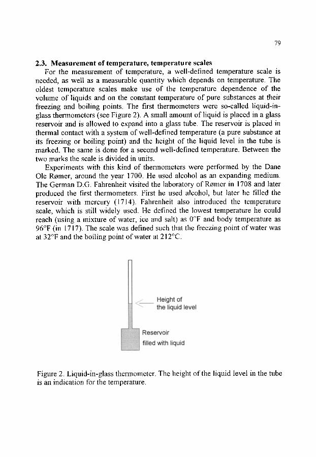
79

2.3. Measurement of temperature, temperature scales For the measurement of temperature, a well-defined temperature scale is

needed, as well as a measurable quantity which depends on temperature. The oldest temperature scales make use of the temperature dependence of the volume of liquids and on the constant temperature of pure ~ substances at their freezing and boiling points. The first thermometers were so-called liquid-in- glass thermometers (see Figure 2). A small amount of liquid is placed in a glass reservoir and is allowed to expand into a glass tube. The reservoir is placed in thermal contact with a system of well-defined temperature (a pure substance at its freezing or boiling point) and the height of the liquid level in the tube is marked. The same is done for a second well-defined temperature. Between the two marks the scale is divided in units.

Experiments with this kind of thermometers were performed by the Dane Ole Romer, around the year 1700. He used alcohol as an expanding medium. The German D.G. Fahrenheit visited the laboratory of Remer in 1708 and later produced the first thermometers. First he used alcohol, but later he filled the reservoir with mercury (1714). Fahrenheit also introduced the temperature scale, which is still widely used. He defined the lowest temperature he could reach (using a mixture of water, ice and salt) as 0~ and body temperature as 96~ (in 1717). The scale was defined such that the freezing point of water was at 32~ and the boiling point of water at 212~

i

~~ Reservoir filled with liquid

Height of the liquid level

Figure 2. Liquid-in-glass thermometer. The height of the liquid level in the tube is an indication for the temperature.

80

A second temperature scale, which is also widely used, is the scale of Anders Celsius. The freezing point of water was defined as 0~ and the boiling point of water as 100~ (in fact Celsius defined the temperature scale in 1742 the other way around: 100~ at the freezing point and 0~ at the boiling point of water; the scale which is now known as the Celsius scale was introduced by his successor Martin Stromer in 1749).

A very important temperature scale is the ideal gas temperature scale or absolute temperature scale. This scale is based on the properties of a very diluted gas. From the work of Boyle (in 1660) it was known that, for an amount of diluted gas at a certain temperature, the product of the pressure and the volume is constant. Gay Lussac (1778 - 1850) found that, for diluted gases at constant volume, the pressure linearly depends on the temperature and, at constant pressure, the volume depends linearly on temperature. Combination of these observations with Boyle's law leads to the law of Boyle-Guy Lussac:

p v = c (1 + a t) (1)

where p is the pressure and V the volume of the gas, t the temperature expressed in degrees Celsius, and C and a are constants. It appears that the constant C depends on the amount of gas. The constant a appears to be equal to 1/273.15. This implies that at a temperature of t = -273.15~ the product p V equals zero. Lower temperatures are impossible, because then either the pressure or the volume should be negative. This implies that an absolute temperature scale may be defined (the unit of this scale is Kelvin, abbreviated as K). The zero point of this scale (the absolute zero) equals-273.15~ Because the absolute zero is set by nature, only one fixed point needs to be chosen (for the other temperature scales two points had to be chosen). In order to have a temperature difference of 100 K between the boiling point and the freezing point of water, the freezing point of water was defined as T = 273.15 K. With this definition of the absolute temperature scale (or ideal gas temperature scale) the law of Boyle-Guy Lussac can be rewritten as:

p V = n R T (2)

This equation is called the ideal gas law. In the equation p is the pressure (expressed in Pa) and V the volume of the gas (expressed in m3), n is the amount of gas (expressed in moles), T is the absolute temperature and R is the so-called gas constant (= 8.31451 J K -~ mol-~).

81

In the second half of the 19 th century, the thermodynamic temperature scale was introduced by W. Thomson (Lord Kelvin). This temperature scale, which can be proven to be identical to the ideal gas temperature, is discussed in section 4.

2.4. The International Temperature Scale of 1990 (ITS-90) The thermodynamic temperature, with symbol T and unit Kelvin (K) is a

fundamental physical quantity. In practice, however, this scale is difficult to realise. The absolute or ideal-gas temperature scale, which is identical to the thermodynamic temperature scale, is also difficult to realise, since real gases may behave differently from an ideal gas. For this reason, in practice we work with a temperature scale that is defined by agreement (in the International Committee of Weights and Measures) on a number of fixed points and on the basis of prescriptions for interpolation between these points. The latest scale, which was agreed on, is the International Temperature Scale of 1990 (ITS-90). The numerical value of the ITS-90 temperature is a very close approximation to the value of the thermodynamic temperature. Since this temperature scale is also treated in Chapter 1, section 1.5, it will not be discussed further here.

2.5. Temperature on a microscopic scale The quantity temperature, which is a macroscopic quantity, was discussed in

the previous sections. Of course, there must be a "bridge" between the macroscopic thermodynamic property temperature and some molecular property. Although, as pointed out in section 1, knowledge of the microscopic structure of the system is not necessary for treatment of thermodynamics, it may help in understanding the theory.

The "perfect gas" is a microscopic model for a very diluted gas. In the model there is no interaction between the molecules. Collisions between molecules and between a molecule and the wall are assumed to be completely elastic. Each molecule moves in a random direction with a certain speed; thus, the kinetic energy can be calculated. Using a function that describes the distribution of molecular speeds, the total kinetic energy of the gas and, from collisions of the molecules with the wall, the pressure that the gas exerts on the wall can be calculated. This leads to a relation between pressure, volume and the total kinetic energy. Comparison with the ideal gas law, equation (2), leads to the conclusion that the macroscopic quantity temperature, for a perfect gas, is related to the total kinetic energy of the gas system.

For other systems, the temperature appears to be related to the "thermal movement" of the molecules of the system. For further reading the reader is referred to the book of Berry, Rice and Ross [2].

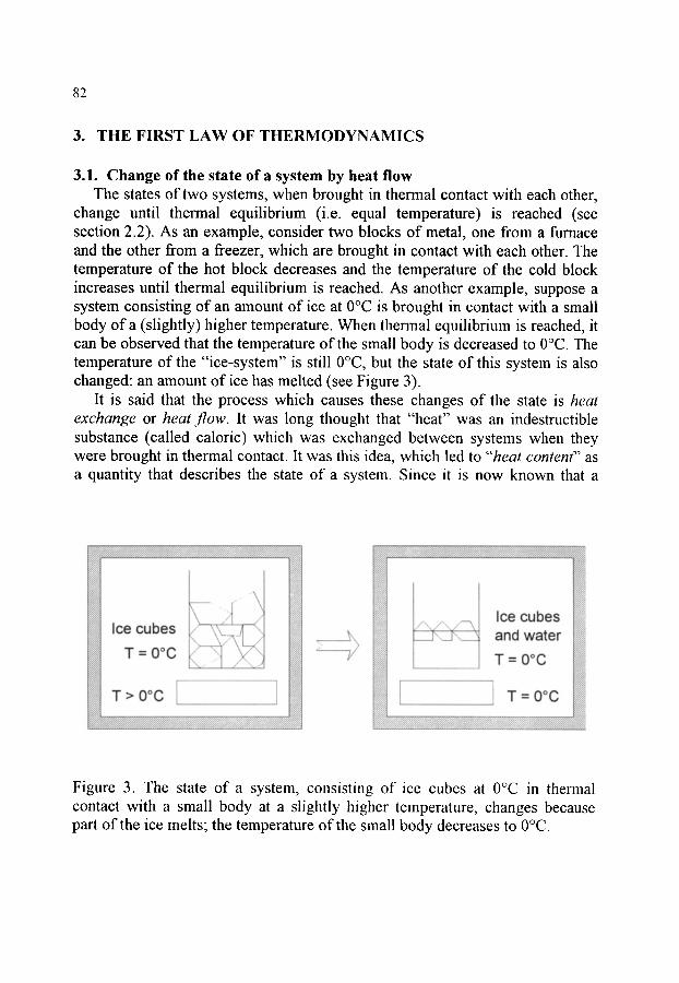
82

3. THE FIRST LAW OF THERMODYNAMICS

3.1. Change of the state of a system by heat flow The states of two systems, when brought in thermal contact with each other,

change until thermal equilibrium (i.e. equal temperature) is reached (see section 2.2). As an example, consider two blocks of metal, one from a furnace and the other from a freezer, which are brought in contact with each other. The temperature of the hot block decreases and the temperature of the cold block increases until thermal equilibrium is reached. As another example, suppose a system consisting of an amount of ice at 0~ is brought in contact with a small body of a (slightly) higher temperature. When thermal equilibrium is reached, it can be observed that the temperature of the small body is decreased to 0~ The temperature of the "ice-system" is still 0~ but the state of this system is also changed: an amount of ice has melted (see Figure 3).

It is said that the process which causes these changes of the state is heat exchange or heat.flow. It was long thought that "heat" was an indestructible substance (called caloric) which was exchanged between systems when they were brought in thermal contact. It was this idea, which led to "'heat content" as a quantity that describes the state of a system. Since it is now known that a

7 ?-///~

- / 1 / ~

Ice cubes T = 0 o c

, \ ( ,)

T > 0 ~

~////, ...... V...;///.

r / 1 / J .

v i l l i

7"//A

~///.&

>-/llz ~i/iI , / / / / ~

.. \

~ l l / I / ~ z

. l /Z. : , , 7 . . . 7

:.,,,,,;,,:: , ,

;:. ,/, ,, 7;2 !

, N I . ?,;'//, ~ Ice cubes ~j t -T -J ' .... q and water ~ , T = 0 C 7/ : ' , "

F-~/ /2

r . . . . . . . . . . . . . . . . . . . . , ~ / ~

L T = 0 ~ . . . . . . . . . . . . . . . . . . . . J

Figure 3. The state of a system, consisting of ice cubes at 0~ in thermal contact with a small body at a slightly higher temperature, changes because part of the ice melts; the temperature of the small body decreases to 0~

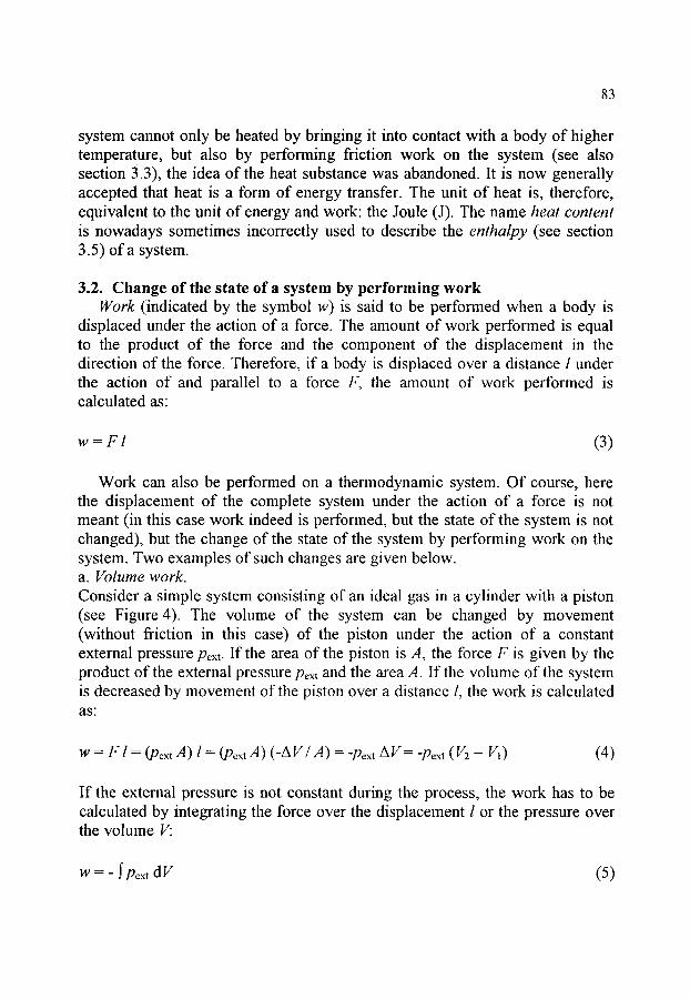
83

system cannot only be heated by bringing it into contact with a body of higher temperature, but also by performing friction work on the system (see also section 3.3), the idea of the heat substance was abandoned. It is now generally accepted that heat is a form of energy transfer. The unit of heat is, therefore, equivalent to the unit of energy and work: the Joule (J). The name heat content is nowadays sometimes incorrectly used to describe the enthalpy (see section 3.5) of a system.

3.2. Change of the state of a system by performing work Work (indicated by the symbol w) is said to be performed when a body is

displaced under the action of a force. The amount of work performed is equal to the product of the force and the component of the displacement in the direction of the force. Therefore, if a body is displaced over a distance l under the action of and parallel to a force F, the amount of work performed is calculated as:

w = F l (3)

Work can also be performed on a thermodynamic system. Of course, here the displacement of the complete system under the action of a force is not meant (in this case work indeed is performed, but the state of the system is not changed), but the change of the state of the system by performing work on the system. Two examples of such changes are given below. a. Volume work. Consider a simple system consisting of an ideal gas in a cylinder with a piston (see Figure 4). The volume of the system can be changed by movement (without friction in this case) of the piston under the action of a constant external pressure Pext. If the area of the piston is A, the force F is given by the product of the external pressure Pext and the area A. If the volume of the system is decreased by movement of the piston over a distance l, the work is calculated a s :

w = F l = (Pext A) l = (Pext A) (-AV/A) = -Pext AV= -Pe• (V2 - V~) (4)

If the external pressure is not constant during the process, the work has to be calculated by integrating the force over the displacement l or the pressure over the volume V:

w = - j'Pext dV (5)

84

~///////~ Pext . . . . . . . . . . .

" l / l / I / I l I A " / ' / / / / / / / / J

"./.44/d44/././,. ~//////./A . . . . . . . . . . .

"////////.4~ ~/,(/././/4

" / / ' / / / / / / / , 4

V T

y / x / H / / / / , > > > > > > > > > > ~

. . . . . . . . . . .

. . . . . . . . . . .

~/ / / / / / /~

........... N N

Pext N

P2 V2 T2N

Figure 4. Performance of volume work on a system by an external pressure Pext. Under influence of this pressure the piston is moved over a distance l.

If, during the process, the difference between the external pressure pext and the internal pressure p is constantly infinitesimal (such a process is called a reversible process), then the work may be calculated by substituting the internal pressure p for the external pressure Pext in equation (5):

w = - j'p d V (6)

b. Electrical work. Consider a system consisting of a rechargeable battery. On charging the battery, (electrical) work is performed on the system. The amount of work can be calculated by integrating the potential difference E over the amount of charge e that is transferred:

w = ~E de (7)

It is obvious that the state of the system changes by performing this work on the system: after charging, the battery can be used to feed electrical tools, which before charging was not possible.

85

In the rest of this chapter, it is assumed that only volume work is performed by or on systems, unless otherwise stated.

3.3. The first law of thermodynamics; internal energy In sections 3.1 and 3.2 it was shown that the state of a system can be

changed by adding heat to the system and/or by performing work on the system. It was recognised that, in some cases, the same change of the state of a system could be reached by only adding heat to the system or by only performing work on the system. As an example, consider an amount of liquid at an initial temperature. This system may be heated to a slightly higher temperature by adding a certain amount of heat. However, by placing a paddle wheel in the liquid, isolating the system, and performing work to rotate the wheel, it is also possible to heat the system to the same final temperature. In fact, using this kind of experiments, the mechanical equivalent of heat was measured by Joule in 1840. The amount of heat added was directly proportional to the amount of work performed. It was this observation, which demonstrated that heat and work can be expressed in the same unit.

Experience shows that, for each (closed) system that is brought from a certain initial state A to a final state B, independent of the route which is followed during the process, the sum of the amount of heat added to the system and the amount of work performed on the system is constant. This statement is referred to as the first law of thermodynamics. It is schematically demonstrated in Figure 5.

It is now obvious that there must be a function which depends on the state of the system. If the state of the system changes, then the value of this function changes by an amount which is equal to the sum of the heat applied to the system and the work performed on the system. Since we know that heat and work are forms of energy transfer, this function may be called the internal energy (expressed by the symbol U) of the system. For a change of the state of a system from A to B (as in Figure 5) the first law can be expressed as:

AU = U(state B ) - U(state A) = q + w (s)

From equation (8) it can be seen that only energy differences can be determined by measuring the heat and the work for a certain process. Although it is possible to speak of the energy of a system in a certain state, it is not possible to determine this energy without agreeing on a particular reference point at which the energy is defined. In chemical thermodynamics the reference point of energy is defined as follows: the energy of chemical elements (in their

86

State A

Route I ~ ~ / / ~-///,

/

Route II ~-///,

"\\ R o u t e III ~ S t a t e B

Y//A

Route I: Heat: q(I); Work: w(I) Route I1: Heat: q(ll); Work: w(ll) Route II1: Heat: q(lll); Work: w(ll l)

{q(1) + w(1)} : {q(ll) + w(ll)}: {q(lll) + w(lll)}: = {U(state B) - U(state A) = A U

Figure 5. Change of the state of a closed system from A to B through different process routes. For all processes the sum of the heat applied to the system and the work performed on the system is equal (first law of thermodynamics). This sum equals the difference of the internal energy of the system between states A and B.

most stable form) at a temperature of 298.15 K and a pressure of 1 bar (or sometimes 1 atmosphere) is set to zero.

The energy function depends on the state of a system; therefore, the internal energy (and all other thermodynamic functions depending on the state of the system) is called a state function. Contrary to this, it is clear that the quantities heat and work have nothing to do with the state of a system: heat and work are quantities which are related to processes. Contrary to the energy difference function, which is also related to a process, the quantities heat and work not only depend on the initial and final state of the system, but also on the process route which is chosen.

That work and heat depend on the chosen process route may be demonstrated as follows. A system consisting of an amount of gas at temperature T~, pressure Pl and volume Vl is brought to a state with

87

temperature T~, pressure P2 and volume V2 using two different reversible processes (see Figure 6). The first process route consists of two sub-processes: first the temperature is increased from T~ to T~ at constant pressure p~ (during this sub-process the volume increases from V~ to V2) and then decreased, but now at constant volume V2, from T2 to T~ (during this sub-process the pressure decreases from pl to P2). During the second sub-process no (volume) work is performed because the volume is constant; therefore the work that is performed on the system during the total process is equal to the work performed on the system during the first sub-process and can be calculated using equation (6):

p~ n

P2

\ \ \ \ \ \

'\ \ \ \ \ \ ' \ \ "\

\ \ \ \ \, \

,\ \ \ , :: i \ i

\ " \ , ~ i \ \ :: "--. i

\ ' \ :: "--,~i ............................ . . . . . . . . . . . . . . . . . . . . . . . . . . . . . . . . . . . . . . . . . . . . . . . . . . . . . . . . . . . . . . . . . . . . . . . . . . . . . .

--...

V o l u m e

V 1 V 2

Figure 6. An amount of an ideal gas is brought from an initial state characterised by pressure pl, volume //1, and temperature T~ to a final state characterised by pressure p2, volume V2, and temperature Tl using two different process routes. The first process route consists of two sub-processes: the first at constant pressure, the second at constant volume. The second process route also consists of two sub-processes: the first at constant volume and the second at constant pressure. The work for both process routes is different (see text).

88

w(process 1) = -P l (V2 - VI) (9)

The second process is chosen such that first the gas is cooled at constant volume V1 from temperature Tl to /'3 (during this sub-process the pressure decreases from pl to p2) and then, at constant pressure p2, the volume is increased from Vl to V2 (during this sub-process the temperature increases from T3 to T1). The work performed on the system during the complete second process is equal to the work performed on the system during the second sub- process (because during the first sub-process the volume is constant) and, again, can be calculated using equation (6):

w(process 2) = -P2 (V2- Vl) (10)

Because pl is not equal to P2, it is obvious that the amount of work performed on the system during the first process is different from the amount of work performed during the second process. Because, for both processes, the initial and the final state of the system are equal, the change of the internal energy AU is equal for both processes. So the heat exchange during the two processes must also differ.

Often, it is convenient to look at infinitesimal changes of the state of a system. For example, the infinitesimal change the change of the internal energy of the system is given by the differential of the internal energy, indicated by dU. Because the amount of heat added to, and the amount of work performed on, a system depend on the process route chosen (i.e. heat and work are not a function of the state of the system), it is inappropriate to write these quantities as differentials; therefore no different indication is given for infinitesimal amounts of heat or work. Whether an infinitesimal amount of heat or work is meant or an actual amount will always be clear from the other parts of the equation. For an infinitesimal change of the state of a system the first law of thermodynamics may be stated as:

dU=q+w ( l l )

If no other forms of work but volume work are allowed, the infinitesimal amount of work performed on the system is calculated as:

w = - p dV (12)

89

3.4. Processes at constant volume For processes at constant volume, from equation (6) or (12) it is clear that no

work is performed on (or by) the system. This implies that, from equation (8) or (11), the change of the internal energy of the system is equal to the amount of heat added to the system:

(AU)v = q or (dU)v = q (13)

This observation is very important, because, for all processes at constant volume, the heat q that is exchanged with the surroundings and which can be measured using a calorimeter, is related to the change of the internal energy of the system and is thus independent of the process route. Based on this observation is the bomb of Berthelot (1827 - 1907), which may be used to measure, e.g. "heats of combustion". The bomb is a steel vessel of constant volume, in which a sample of known mass of a substance and an excess of oxygen gas can be placed. The substance is ignited and the amount of heat exchanged is measured. Using this method, the heat of combustion of the substance may be measured together with the heats of combustion of the constituent elements. From the chemical composition of the substance, the energy difference between the substance and the elements can be calculated.

3.5. Processes at constant pressure. The enthalpy It is very useful that for processes at constant volume the measured

exchange of heat is equal to the change of the internal energy. However, in practice, many processes occur at constant pressure (e.g. atmospheric pressure). It is obvious that for such processes the work performed on (or by) the system is not necessarily equal to zero, so the amount of heat exchanged cannot be related directly to the change of the internal energy. For this reason, it is very convenient to define a new quantity that is closely related to the internal energy. This quantity is called enthalpy (indicated by H) and is defined as the sum of the internal energy and the product of pressure and volume:

H - U+p V (14)

It is obvious that the enthalpy, like the internal energy, is a state function. For an infinitesimal change of the state of a system, the infinitesimal change of the enthalpy is given by:

d H = d ( U + p V) = dU+ d(p V)= d U + p dV+ Vdp (15)

90

Combination of the first law (equation (11)) with equation (12) for volume work leads to:

d H = ( q - p d V) + p d V + V dp = q + V dp (16)

For processes at constant pressure, the heat which is exchanged with the surroundings is equal to the change of the enthalpy of the system:

(dH)p = q or (zLq)p = q (17)

This implies that, for processes at constant pressure too, measured heats can be directly related to a state function (the enthalpy) and are therefore independent of the process route. For this reason the enthalpy is sometimes, incorrectly, called heat content.

3.6. The heat capacity The heat capacity (indicated by the symbol C) is a very important quantity

in engineering and materials science. The heat capacity of a system is defined as the (infinitesimal) amount of heat divided by the (infinitesimal) temperature increase that is the result of the adding this amount of heat to the system:

C - q (18) dT

Because the amount of heat, which must be added to accomplish a certain change of the state of the system, depends on the process route that is followed, the heat capacity also depends on the process route. For processes at constant volume the heat capacity at constant volume (indicated by (;v) may be defined by combining equations (18) and (13):

OU (19) C v = v

This implies the heat capacity at constant volume is the partial derivative of the internal energy to the temperature.

For processes at constant pressure, combination of equations (18) and (17) leads to the following definition of the heat capacity at constant pressure (indicated by Cp):

91

Cp - (20) p

which implies that the heat capacity at constant pressure is the partial derivative of the enthalpy with respect to the temperature.

If the heat capacities are known, the change of the energy or the enthalpy of a system on heating (or cooling) may be calculated as:

T2 (AU)v = U(V, T 2 ) - U ( V , T1) = ~CvdT

T, (21)

(AH)p t .

= H(p , T2 ) - H(p , TI) = . | C p d T v,

(22)

4. THE SECOND AND THE THIRD LAWS OF THERMODYNAMICS

4.1. Negative formulation of the second law The second law of thermodynamics was developed during the investigations

of Sadi Carnot (1796 - 1832) and dates from before the first law. For didactic purposes, however, the first law is usually treated first.

The experience that leads to the second law is the following. In section 3.3, it was demonstrated that a system, consisting of an amount of water in which a paddle wheel is placed, may be heated by performing work on the paddle wheel (i.e. on the system). Suppose work is performed on the paddle wheel, but the system is kept at constant temperature. This can only be accomplished by a flow of heat from the system to the surroundings. The observation is in accordance with the first law: if the state of the system does not change (the temperature is constant), the internal energy of the system is constant and, from equation (8), it is found that the amount of heat which flows from the system to the surroundings is equal to the amount of work performed on the system. This implies that the work performed on the system is converted into heat that is supplied by the system to the surroundings.

The opposite process, i.e. a flow of heat from the surroundings to the system and performance of work by the ~ystem on the paddle wheel, however, has never been observed, although this process is not in conflict with the first law.

92

These kinds of observations have resulted in the second law of thermodynamics which may be stated as follows: It is not possible that, as the only result of a process, an amount of heat that .flows from the surroundings to the system is converted into work, which is performed by the system.

Stated in this form, the second law cannot be applied conveniently to practical problems. Therefore, another formulation, or a usable quantity, has to be derived, which will be demonstrated in the following section.

4.2. Positive formulation of the second law; the entropy The amount of heat, which is exchanged with the surroundings, depends not

only on the initial and final state of the system, but also on the process route which is followed. For reversible processes, however, it may be demonstrated that the reduced hea t - that is the (infinitesimal) amount of heat exchanged divided by the absolute thermodynamic temperature at which this heat exchange takes place - does not depend on the process route, i.e.:

reversible route t reversible route 2

This statement, in fact, is the positive formulation of the second law and is here regarded as a postulate that is confirmed by all its consequences. The temperature that is used in the expression is the absolute thermodynamic temperature, which was introduced by W. Thomson (Lord Kelvin) in 1846. This temperature scale is independent of the special nature of any system. It is possible to prove that the absolute thermodynamic temperature scale is equivalent to the ideal gas temperature scale. This exercise is, however, outside the scope of this Work.

Because the reduced heat is, for reversible processes, independent of the process route chosen, a new state function may be defined. This state function is called the entropy (indicated by S, and first introduced by Clausius in 1865):

= s'ate : (24)

or, for infinitesimal changes:

93

The entropy change of a system, which undergoes a process, may thus only be determined by measuring the (reduced) heat and applying equation (24) if the process is reversible. If the process is irreversible, because entropy is a state function, it is possible to imagine a different, reversible route between the initial and the final state and to use equation (24) to calculate the entropy difference.

As a first example, consider a system that is heated at constant pressure from temperature T~ to temperature T2. The entropy change AS associated with this process may be calculated using equation (24) as follows:

(AS)p = S(p , T 2 ) - S(p , Tl)= = P dT (26) r, r, T

As a second example, one mole of ice (i.e. 18 grams) is considered, which melts (reversibly) at 273.15 K (0~ At the end of the melting process we have one mole of water at 273.15 K. The entropy change for this melting process

(Als S) may be calculated as follows, again with use of equation (24):

A~sS(T = 273.15 K) = S(water, T = 273.15 K ) - S(ice, T = 273.15 K) =

qre____&v = ~A _- ~6000 = 22 J K "l T T 273.15

(27)

where A is the latent heat for the transition from ice to water at the melting point (A = 6000 J mol-~). Phase transitions are treated further in sections 8.1, 8.2, and 8.3.

Although the definition of entropy as given in this section is sufficient for the treatment of classical thermodynamics, the molecular interpretation of entropy will be discussed briefly. For the molecules of a system the location, the speed of translation, the speed of rotation, the energy of vibration, etc., constantly change. The molecular state of a system at a certain time is determined by the values of all these quantities for each molecule at that time. A thermodynamic state, characterised by the macroscopic quantities energy, volume, etc., consists of an enormous number of molecular "configurations"

94

through which the system passes in time. There appears to be a relation between the thermodynamic quantity entropy and the number of molecular configurations W which are possible for the system at a given energy and volume. According to Boltzmann (1872) this relation is:

S = k In W (28)

where k is Boltzmann's constant (k = R / NA = 1.380658 x 10 .23 J K -~', NA = 6.0221367 x 1023 mol -~ is Avogadro's constant, the number of molecules in one mole).

This implies that a system with a large number of possible molecular configurations (i.e. a disordered system) has a larger entropy than a system with fewer possible molecular configurations (i.e. a more ordered system). From this observation it is clear that the entropy of water is larger than the entropy of ice (both at the melting point T - 273.15 K).

4.3. The third law of thermodynamics The third law of thermodynamics, like the other laws, is a postulate that is

confirmed by its consequences. The observations, which led to the statement of the postulate, will not be discussed here.

Nernst stated that the entropy change for each chemical or physical transition between condensed phases, at temperatures very close to the absolute zero, is equal to zero:

lim AS = 0 (29) T---~0

This statement is also referred to as the Nernst heat theorem. The statement of Nernst was simplified by Planck. He stated that not only the entropy change for processes but also the actual entropy of each condensed substance equals zero if the temperature approaches absolute zero. This statement explicitly excludes mixtures. The following statement makes the explicit exclusion of mixtures unnecessary:for each ,wstem in equilibrium, the entropy equals zero when the temperature approaches the absolute zero. This statement is referred to as the third law of thermodynamics.

lim S(system in equilibriu m) = 0 (30) T---~0

95

An important consequence of the third law is that for chemical materials (elements as well as compounds) the absolute entropy (i.e. independent of a certain reference state) may be defined. The absolute entropy of a substance can now be determined calorimetrically by measuring the heat capacity of the substance over the entire temperature range from the absolute zero up to the desired temperature, together with the latent heats of phase transitions, which occur in this temperature range. Using equations (26) and (27) the absolute entropy may be calculated as:

I A o Cp II r~ Cp dT+ + dT (31) S(T = 6))=

T Ttr T T=0 Ttr

where it is assumed that only one phase transition (at T = T t r from phase I to phase II) is observed in the temperature interval from 0 to |

$. THE H E L M H O L T Z ENERGY AND THE GIBBS ENERGY

For reversible processes the heat exchange with the surroundings is given by equation (25), which, now that the entropy has been introduced, may be stated as:

qrev = T dS (32)

Using this equation for the reversible heat and equation (12) for the reversible volume work, the first law for reversible processes may be rewritten as:

dU= r d S - p dV (33)

In section 3.5 the state function enthalpy was introduced. Inserting equation (32) in equation (16) leads to the following equation for the (infinitesimal) enthalpy change for a reversible process:

dH= r d S + Vdp (34)

Because entropy is a state function and because temperature is one of the quantities that describe the state of a system, the product of temperature and entropy (i.e. T,V) is also a state function. This implies that, by subtraction of the

96

product T S from the state functions energy and enthalpy, two new state functions may be defined. These functions are the Helmholtz energy (indicated by A; sometimes also called free energy) and the Gibbs energy (indicated by G; sometimes also called free enthalpy), respectively:

A = T s (35)

G - H - T S - U + p V - T S (36)

Using these definitions, infinitesimal changes of the Helmholtz energy and the Gibbs energy are given by:

dA = dU - d(T ~V) = -S d T - p dV (37)

dG : d H - d(T S) = -S dT + V dp (38)

Mathematically, for a function Z of the variables X and Y, the following differential equation may be stated:

d Z= dX+ dY (39) Y X

In this equation (OZ/OX)r is the partial derivative of Z to X (at constant Y). Because Z is a function of X and Y (which implies that for specific values of X and Y there is only one value of Z), this differential equation is called a total differential or an exact differential. Characteristic of a total differential is the so-called cross-differential identity:

(40)

The cross-differential identity implies that the result of taking the derivative of function Z first with respect to the variable X and then with respect to the variable Y gives exactly the same result as first taking the derivative of Z with respect to Y and then with respect to X.

Equation (33) is thus the total differential of the internal energy as a function of entropy and volume, equation (34) is the total differential of the enthalpy as

97

a function of entropy and pressure, equation (37) is the total differential of Helmholtz energy as a function of temperature and volume, and equation (38) is the total differential of Gibbs energy as a function of temperature and pressure. From comparisons of equations (33), (34), (37), and (38) with equation (39) (where Z is replaced by U, H, A, or G, respectively) the following equalities may be identified:

V p

p ~ ~ ...-

S T (42)

S T

V p

It can be demonstrated that all thermodynamic quantities can be calculated if only one of the following functions is known: �9 the energy as a function of entropy and volume; �9 the enthalpy as a function of entropy and pressure,; �9 the Helmholtz energy as a function of temperature and volume; �9 the Gibbs energy as a function of temperature and pressure. Therefore, these functions are called characteristic functions.

Application of the cross-differential identity to the total differentials of energy, enthalpy, Hehnholtz energy and Gibbs energy (equations (33), (34), (37), and (38)) leads to the following equations:

S V

98

/o l 46) S p

T V

T p

These equations are very important, especially the last two, because they show that the dependence of entropy on volume and pressure, which is experimentally not very accessible, is equal to the dependence of pressure or volume on temperature!

As an example of the applicability of these equations, the entropy change AS for an ideal gas, which expands, in a reversible process at constant temperature, from volume V~ to volume V2, may be calculated as:

As = ~, k o v ) ~ (49)

Substitution of the differential quotient using equation (47), together with the ideal gas law (equation (2)), results in:

A s = ~ d r = ! , - - d = (50)

6. EQUILIBRIUM CONDITIONS

To find a condition, which must be fulfilled for a system in equilibrium, a completely isolated system is considered. Suppose that an irreversible, spontaneous process brings this system from state A to state B. Because the system is isolated, interaction with the surroundings is not allowed, i.e. no heat

99

is exchanged with the surroundings and no work is performed on or by the system:

qirr = 0 a n d Wir r -- 0 (51)

Now imagine that the system is brought back from state B to state A by a reversible route. During this reversible process the system exchanges heat with the surroundings and work is performed on or by the system:

qrev r 0 and Wrev ~: 0 (52)

The irreversible process and the reversible process together form a cycle (i.e. a process to a final state that is equal to the initial state); see Figure 7. The heat exchanged and the work performed during the cycle are given by:

~ ~ J S J ' f ~ I rl

52222

,~,~ State A r , ~ ~ ~ ~ a

Irreversible route Reversible route: Cycle:

rreversible route "(system isolated)'\j

/ \ , .,/

Reversible rouie

route: Heat: qirr = 0 Heat: qrev Heat: qcycle

First law: q cycle + Wcycle - 0

Second law: q cycle < 0

State B

Work: w irr = 0 Work : w rev

Work: w cycle

Figure 7. An irreversible process brings a completely isolated system from state A to state B. Via a reversible route, during which interaction with the surroundings is allowed, the system is transferred back to the initial state A. From the first law, for the cycle, the sum of the heat and the work equals zero. From the second law, heat must flow from the system to the surroundings.

100

qcycle = q~ + qrev = qr~v (53)

Wcycle = Wirr + Wrev - Wrev (54)

For the cycle, the energy change is equal to zero, because the initial and the final state are equal. Therefore, according to the first law (equation (8)):

( m U ) c y c l e -- qcycle -4- Wcycl e = qr~v + Wrev -- 0 (55)

From the (negative formulation of the) second law, which states that it is not possible that, as the only result of a process, an amount of heat is absorbed by a system and completely transformed into work (see section 4.1), heat must be transferred during the cycle from the system to the surroundings, i.e.:

qcycle < 0 (56)

Then also:

qrev < 0 (57)

Using the positive formulation of the second law, equation (24), the entropy change during the reversible process from state B to state A may be calculated as~

/~'rev-- S(state A) - S(state B) = < 0 (58)

Because for the cycle:

AScycle -- (/~q]irr)U,V q" / ~ ' r e v - - 0 (59)

during the irreversible process in the completely isolated system the entropy must increase:

(l~k~'irr)L:,V > 0 (60)

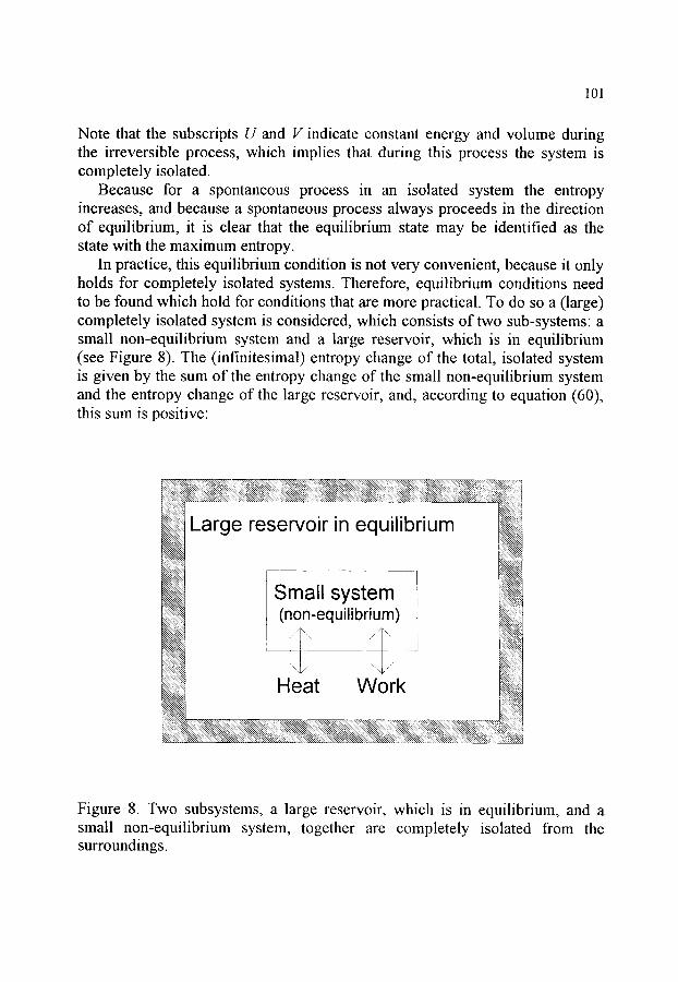
101

Note that the subscripts U and V indicate constant energy and volume during the irreversible process, which implies that during this process the system is completely isolated.

Because for a spontaneous process in an isolated system the entropy increases, and because a spontaneous process always proceeds in the direction of equilibrium, it is clear that the equilibrium state may be identified as the state with the maximum entropy.

In practice, this equilibrium condition is not very convenient, because it only holds for completely isolated systems. Therefore, equilibrium conditions need to be found which hold for conditions that are more practical. To do so a (large) completely isolated system is considered, which consists of two sub-systems: a small non-equilibrium system and a large reservoir, which is in equilibrium (see Figure 8). The (infinitesimal) entropy change of the total, isolated system is given by the sum of the entropy change of the small non-equilibrium system and the entropy change of the large reservoir, and, according to equation (60), this sum is positive:

,,xx.\\\\\\-~ ~%.\\\'-,~ * \ \ \ \ \ \ ~ . ' x \ \ \ \ \ \ \ ~

i . . . . . . . . . . . ' x \ \ \ \ \ \ \ ~

,\\\\\\ 'x. '..~ . . . . . . . . . .

. . . . . . . . .

Large reservoir in equilibrium

Small system (non-equilibrium)

/ - \ /~//

Heat Work

. . . . . . . . ...q

~ \ \ \ \ \ % , - q

. \ \ \ \ \ \ - , ,-~

~N

Figure 8. Two subsystems, a large reservoir, which is in equilibrium, and a small non-equilibrium system, together are completely isolated from the surroundings.

102

(dSt)u,v = + dSr > 0 (61)

The subscripts s, r, and t indicate quantities for the small system, the large reservoir, and the total system, respectively. In the following it is assumed that the temperature of the small non-equilibrium system, Ts, is equal to the temperature of the large reservoir, Tr, and that these temperatures are constant during the process. Because the large reservoir is considered to be in equilibrium, the entropy change of the reservoir is given by rewriting equation (33):

= ~ + dV r (62)

Because the total system is completely isolated, the total volume is constant and the total internal energy is constant too:

dVt= dVs + dV~= O dV~ = - dVs (63)

d U t = d U s + d ~ h = 0 => dUr=-dUs (64)

Now two different cases are investigated. 1. During the (irreversible) process in the small system, the volume of this

system is constant, i.e. dVs = 0. Then, according to equation (63), the volume of the reservoir is also constant: d V~=0. Inserting this, together with equations (62) and (63), in equation (61) leads to:

ckS' s dUs > 0 => dUs- T~ ckg's < 0 (65) Ys

Because for the small system constant temperature and constant volume were assumed, this may be rewritten as:

[d (U- T S)]V,T "( 0 or (dA)v.:r < 0 (66)

This implies that, for an irreversible process (in a non-isolated system) at constant temperature and volume, the Helmholtz energy decreases. The

103

equilibrium state may be identified as the state for which the Helmholtz energy has the lowest value.

2. Now, during the irreversible process in the small system, the pressure in the small system is assumed to be constant and equal to the pressure in the reservoir: ps = Pr = constant. Inserting this, together with equations (62), (63), and (64) into equation (61) leads to:

dUs

rs kJsJ

Because, for the small system, constant temperature and constant pressure were assumed, equation (67) may be rewritten as:

[d (U- T S + p V)]p,r < 0 or (dG)p,r < 0 (68)

which implies that, for an irreversible process (in a non-isolated system) at constant temperature and pressure, the Gibbs energy decreases. The equilibrium state may be identified as the state for which the Gibbs energy has the lowest value.

7. OPEN SYSTEMS

Up to this section closed systems have been considered, i.e. systems for which there is no exchange of matter with the surroundings. Systems for which the amount of matter in the system is not constant are called open systems. These systems are treated in this section.

Suppose that a system contains a number of chemical components (in one homogeneous phase). It is clear that the state of this system depends on the amount of each of these components present in this system. The amount of substance (indicated by n) is expressed in the unit mole. If each component is given a number, then the amount of component number i is indicated by ni.

This implies that the thermodynamic state functions must be treated as functions that depend on the amount of each component present in the system. For an (infinitesimal) change of the internal energy of a closed system equation (33) was derived, and it was demonstrated that this expression is the total differential of the energy as a function of entropy and volume. For an open

104

system, besides being a function of entropy and volume, the energy must be treated as a function of the amounts of each of the components present. Mathematically the total differential of the energy is then written as:

d U = OU dS + dV+ V ,ni S,gli " S , V , t ' / j ~ i

dn i (69)

The partial derivatives of the energy with respect to the amount of substance are called thermodynamic potentials (indicated by pi):

(70)

Therefore, the analogue of equation (33) for an open system may be written as:

dU = T ckS' - p dV+ Z pi dni (71)

Likewise, the open system analogues of equations (34), (37) and (38) for the changes of the enthalpy, Helmholtz energy, and Gibbs energy, respectively, may be written as:

dH = T &~ + V dp + E p ~ dn ~ (72)

dA = -S d T - p dV+ E pi dni (73)

d G= -S dT + V dp + Z pi dni (74)

From equation (74) the thermodynamic potential may be identified as:

Ill = l t~~H i l p,T,nj~, (75)

The partial derivative of a quantity with respect to the amount of substance, if performed at constant pressure and temperature, is called a partial molar quantity; therefore, the thermodynamic potentials may also be called partial

105

molar Gibbs energies. Using the cross-differential identity, equation (40), on equation (74), for the temperature and pressure dependence of the thermodynamic potential, the following is found"

OTjp ,n ' - T,p,nj~i = - -S i (76)

019 )T, , i r,p,nj,, = v i (77)

where Si and V i are the partial molar entropy and the partial molar volume of component i, respectively. These partial molar quantities are functions of pressure, temperature and composition of the system. Using these equations the total differential of the thermodynamic potential as a function of temperature and pressure, at constant composition, may be written as:

dpi = - s i dT+ V i d p (78)

Let us now investigate how the thermodynamic potential of an ideal gas depends on pressure. Suppose that the gas consists of only one component, and that the gas is compressed at a constant temperature from p = p O = 1 bar to a final pressure o fp = pf. The change of the thermodynamic potential of the gas for this process, Ap, can be calculated using equation (77), together with the ideal gas law, equation (2):

Ap(T) =/.fiT, p = p f ) - p ( T , p = pO= l b a r ) =

= OCt dp= ~ dp= d p = R T l n T r,p po~. P J

('79)

Thermodynamic properties, which are valid for a standard pressure p = pO, where pO is a unit pressure (usually chosen as "atmospheric" pressure: pO = 1 bar = 105 Pa or pO= 1 atm = 101325 Pa), are indicated with a superscript "o" (or sometimes "o") and are called s tandard thermodynamic properties; therefore, we may define the standard thermodynamic potential as:

/2o(7) - p = pO) ( 8 0 )

106

Combining the last two equations results in:

(81)

In this equation, as indicated above, the standard pressure pO is the pressure for which the standard thermodynamic potential po is valid. Because p~ is usually chosen as a unit pressure, equation (81) is often, incorrectly, written as:

p ( T , p = p f ) = / . t~ + R T ln(pf ) (82)

Combination of the definition of the Gibbs energy, equation (36), and equation (75) leads to the relation between the thermodynamic potential, on the one hand, and partial molar enthalpy (indicated by hi) and partial molar entropy (indicated by si), on the other hand:

Pi(P, T, nj) = hi(p, T, nj) - T si(p, T, nj) (83)

8. SYSTEMS CONSISTING OF A PURE SUBSTANCE

8.1. Stability ofphases In this section, a system consisting of an amount of a single chemical

substance is considered. Depending on the temperature and the pressure, this substance can exist in several phases.

First, a simple substance is considered which can exist in three phases: solid, liquid, and gas. A phase transition, for example melting (i.e. a transition from solid to liquid), may be considered thermodynamically as removal of a certain amount (dn s~ of the solid phase and simultaneous addition of an amount (at,/liq) of liquid phase. If the thermodynamic potentials of the substance in the solid and in the liquid phases are given by p* sol and/~* liq, respectively (note that quantities for a pure component are indicated by a superscript "*"), then the (infinitesimal) change of the Gibbs energy of the system is, according to equation (74), given by:

,L/* sol d/'/sol ,/1" liq d/q liq (dG)p,r = + (84)

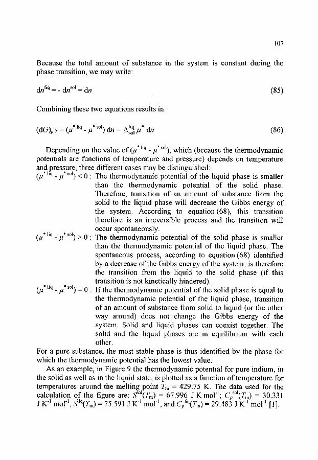
107

Because the total amount of substance in the system is constant during the phase transition, we may write:

d/,/liq = - d/ ' /s~ dF/ ( 8 5 )

Combining these two equations results in:

(dG)p,r = (j/* liq ]/* sol) dfl = A liq * - sol/2 dn (86 )

Depending on the value of (/~* liq . H* sol), which (because the thermodynamic potentials are functions of temperature and pressure) depends on temperature and pressure, three different cases may be distinguished: (fl* hq _ fl* sol) ( 0 " The thermodynamic potential of the liquid phase is smaller

than the thermodynamic potential of the solid phase. Therefore, transition of an amount of substance from the solid to the liquid phase will decrease the Gibbs energy of the system. According to equation(68), this transition therefore is an irreversible process and the transition will occur spontaneously.

(fl, l i q . fl* sol)> 0" The thermodynamic potential of the solid phase is smaller than the thermodynamic potential of the liquid phase. The spontaneous process, according to equation (68) identified by a decrease of the Gibbs energy of the system, is therefore the transition from the liquid to the solid phase (if this transition is not kinetically hindered).

(fl* liq _ fl* sol) = 0 " If the thermodynamic potential of the solid phase is equal to the thermodynamic potential of the liquid phase, transition of an amount of substance from solid to liquid (or the other way around) does not change the Gibbs energy of the system. Solid and liquid phases can coexist together. The solid and the liquid phases are in equilibrium with each other.

For a pure substance, the most stable phase is thus identified by the phase for which the thermodynamic potential has the lowest value.

As an example, in Figure 9 the thermodynamic potential for pure indium, in the solid as well as in the liquid state, is plotted as a function of temperature for temperatures around the melting point Tm - 429.75 K. The data used for the calculation of the figure are s~~ 67.996 J K moll; CpS~ = 30.331 J K -1 mol-1, sliq(Tm) - 75.591 J K -1 nlo1-1 a n d Cpliq(Tm) -- 29.483 J K -1 mo1-1 [1]

o

108

|

m

0 E

v

-1

-2

--...

solicl J \ . -<..~ ~.<

~..~....

t I

- - .~

l iquid J

m - m

400 410 420 430 440 450

T / K

Figure 9. Standard thermodynamic potential of pure indium in the liquid state (dashed curve) and in the solid state (solid curve) around the melting point Tm = 429.75 K. The melting point is indicated by the vertical dashed line, and corresponds to the intersection of the two curves. The state for which the thermodynamic potential has the lowest value is the most stable state. The scale is chosen such, that the thermodynamic potential of indium at Tm is equal to zero.

Because the thermodynamic potentials are functions of pressure and temperature, it is possible to indicate regions of stability for different phases of a pure substance in a graph of pressure versus temperature. In general, a graph in which regions of stability of different phases are indicated is called a phase diagram. The phase diagram for a pure substance is called a unary phase diagram. The curves in such a graph, which separate the regions of stability for different phases, are called the two-phase equilibrium curves, and indicate the circumstances for which there is equilibrium between the two phases.

Figure 10 represents the unary phase diagram for the organic substance benzoic acid (data taken from de Kruif and Blok [8]). The point where the three two-phase equilibrium curves intersect is called the triple point: solid, liquid

109

and gas are in mutual equilibrium with each other. The solid-liquid two-phase equilibrium line usually has a slope that is close to vertical (the slope may be calculated using the Clapeyron equation, see section 8.2). The liquid-gas two- phase equilibrium line may be followed to higher temperatures and pressures. This line ends at a point, called the critical point, at which the difference between gas and liquid vanishes because the densities of gas and liquid become equal (gases are more compressible than liquids). The critical point is not indicated in Figure 10.

The expression "'stable phase" means a phase which is stable with respect to other phases. The transition from one of the other phases to the stable phase causes a decrease of the Gibbs energy of the system, and thus indicates (the direction of) a spontaneous process. Such a transition, however, does not necessarily have to occur: it may be kinetically hindered. Therefore, a phase may also appear to be stable outside its stability region in the phase diagram.

5000

4000 I

3000 I a_ Solid

2000 -

1000 -

0 375

. /

I l l - ~ j

I

Liquid l

/ /

/ /

/ / - /

/ /

"~ Gas . J

385 395 405 415 425

T / K

Figure 10. The unary phase diagram for benzoic acid shows the stability regions of the solid, liquid, and gas phases in the pressure-temperature plane, together with the two-phase equilibrium curves.

110

As an example, consider graphite and diamond, two (solid) phases of the element carbon, which both exist under normal circumstances (at atmospheric pressure and room temperature). Under these circumstances, the thermodynamic potential of graphite is lower than the thermodynamic potential of diamond, and therefore graphite is stable with respect to diamond. Diamond, however, is a very stable material and will (fortunately) not transform spontaneously into graphite! A phase which exists outside the region where it has a lower thermodynamic potential than other phases (outside its stability region) is called a metastable phase. A metastable phase may spontaneously transform into a (more) stable phase, but the reverse process will never occur!

As a second example, an amount of water is considered. If the water is cooled, at 0~ the water-ice two-phase curve is reached. At lower temperatures, ice is stable with respect to water. In practice water may be undercooled many degrees below its freezing point. The undercooled liquid is also a metastable phase.

8.2. Equilibrium between two phases; the Clapeyron equation In the following it is supposed that, for a pure substance, two phases, say

phase ~ and phase [3, are in equilibrium with each other if the pressure is Pe and the temperature is T~ (i.e. the point (pe, T~) is an element of the two-phase equilibrium curve). This implies, as shown in the previous section, that, for this pressure and temperature, the thermodynamic potentials of these phases are equal:

]A" ~ Te) = ,L/" 13(pe, Te) --~ A~gt(Pe,T e)= 0 (87)

Now suppose that the temperature and the pressure are changed (infinitesimally) such that the equilibrium between the two phases is retained. This implies that the pressure and temperature are changed such that we move along the two-phase equilibrium curve (i.e. the point (pe+dp, T~+dT) is also an element of the two-phase equilibrium curve). Because of this change of the pressure and the temperature, the thermodynamic potentials also change. The change of the thermodynamic potentials may be calculated using equation (78). If the equilibrium is retained in the new situation, then the thermodynamic potentials must be equal to each other again, which implies that the change of the thermodynamic potential of phase ot must be equal to the change of the thermodynamic potential of phase 13:

cz = V* ot = -S* V* f5 d/~* dcz *f~ ---) -s *~ dT+ dp I~ dT+ dp (88)

111

This equation can be rewritten as:

- A~s*dT + Aav dp = 0 (89)

where the quantities A~s* and A~v* are the molar entropy of transition and the molar volume of transition, respectively. This leads to the temperature dependence of the pressure along the two-phase equilibrium curve:

dp _ A~s (90)

- ~ eq.curve -- A~ v----------~

This equation is known as the Clapeyron equation. Inserting equation (83), for phase ct as well as for phase 13, into equation

(87) leads to:

A~h* (Pe,Te) - TeA~s* (Pe,Te) = O ~ A~s*(Pe,Te)= A~h*(Pe,T e)

Ve (91)

Together with equation (90), this equation leads to another form of the Clapeyron equation:

dp) _ A~h* (92)

eq. curve TeA~v

This form of the Clapeyron equation is convenient because the quantity A~h*,

the enthalpy of transition (from phase ot to phase 13), can be measured using calorimetric techniques.

For equilibria between a condensed phase (solid or liquid) and a vapour phase, the Clapeyron equation can be simplified by making some assumptions. Generally, the molar volume of a substance in the vapour phase is much larger than the molar volume of the same substance in the condensed phase. Then the difference in molar volume may be approximated as the molar volume of the vapour phase (i.e. the molar volume of the condensed phase is neglected):

A vap a,* = v*vap _ v*cond ~ V*vap cond (93)

112

If it is assumed that the vapour phase behaves as an ideal gas, then the molar volume follows from the ideal gas law, equation (2):

v,Va p _ - _V _- RT (94) n p

Inserting the last two equations into the Clapeyron equation, equation (92), leads to:

(_d_~] * Avap h* dp Avap h dp ~ c o n d " = cond' ' _.~ =

eq. curve T --~.

dT (95)

which may also be written as

(;) d{ln(p)} = - ~cona d (96) R

These two very useful equations are equivalent and are called the Clausius- Clapeyron equation. The equation indicates that the slope of the equilibrium curve, if plotted as the logarithm of the equilibrium pressure versus the reciprocal temperature, is given by the negative value of the enthalpy of vaporisation or sublimation divided by the gas constant. The enthalpy of vaporisation (for equilibrium between a liquid and a vapour phase), or the enthalpy of sublimation (for equilibrium between a solid and a vapour phase) depends on temperature, but the temperature derivative is relatively small. Therefore, the enthalpy of vaporisation, or the enthalpy of sublimation, may be considered as constant, if the temperature range is not very large. Equation (96) can then be easily integrated, which leads to a third form of the Clausius- Clapeyron equation:

= - cond" 1 1 (97) ~PlIJ R r 2 T 1

In this equation (p~,T~) and (p2,T2) are two points on the solid-vapour equilibrium line, or on the liquid-vapour equilibrium line. If equilibrium vapour

113

pressures are available as a function of temperature, these equations may be used to evaluate the enthalpy of vaporisation or sublimation. If, on the other hand, the enthalpy of vaporisation or sublimation is available together with one point of the condensed phase - vapour phase equilibrium line, then other points of the equilibrium line may be calculated.

8.3. Phase transitions; the order of a phase transition In section 8.1 it was demonstrated that, for two phases which are in

equilibrium with each other, the thermodynamic potentials of both phases are equal. In section 8.2 the Clapeyron equation, equation (90), was derived. It was assumed that the molar entropy of transition and the molar volume of transition were not equal to zero. This is true for phase transitions between states of aggregation and also for many other phase transitions. There are, however, many phase transitions known for which the molar entropy of transition and the molar volume of transition are equal to zero.

Ehrenfest classified phase transition into orders. Phase transitions for which the molar entropy of transition and the molar volume of transition are not equal to zero are called phase transitions of the first order. It may be recalled that the (molar) entropy is the first derivative of the (molar) Gibbs energy (or thermodynamic potential) with respect to temperature. The (molar) volume is the first derivative of the (molar) Gibbs energy (or thermodynamic potential) with respect to pressure. So a first-order phase transition can be defined as a phase transition for which the first (partial) derivatives of the Gibbs energy difference function with respect to pressure and temperature are not equal to zero:

First-order phase transition:

= - A ~ s * . 0 aT

p

= A~v* ~0 ap r

(98)

First-order phase transitions can be investigated using dilatometry, because the molar volume changes on transition. Calorimetry is also an excellent tool to investigate first-order phase transitions, because the molar entropy changes on transition, which implies that the molar enthalpy changes too, and therefore a heat of transition (also called the latent heat of transition) can be measured.

114

Phase transitions for which the molar entropy of transition and the molar volume of transition are equal to zero, are called phase transitions of a higher order. For a second-order phase transition, according to Ehrenfest, the second derivatives of the Gibbs energy difference function with respect to temperature and/or pressure are not equal to zero:

Second-order phase transition:

A~s =0 ;

p

OP2 r

OpOT p,r

A~v* =0

I*l OA~s

O7" p

@ T

= -z-~ ~ 0

p

a Cp* ~ ~ 0

(99)

Thus, for a second-order phase transition, there is no entropy of transition (and thus also no enthalpy of transition) and no volume change on transition. The heat capacity, the thermal expansion and the compressibility, however, do change for a second-order phase transition. Many so-called order-disorder transitions (e.g. the transitions from ferromagnetic to paramagnetic at the Curie temperature, which are observed for iron and nickel) are examples of second- order phase transitions. For these transitions, the curve of the heat capacity versus temperature often shows a peak at the transition temperature. Because of the similarity of the shape of this peak with the letter ~, (lambda), these transitions are also called )~-transitions.

In Figure 11 the difference between first-order and second-order phase transitions is demonstrated using schematic graphs of thermodynalnic potential, enthalpy, and heat capacity versus temperature.

In general, for an n th order phase transition the n th derivatives of the Gibbs energy difference function with respect to pressure and temperature are not equal to zero, while all lower derivatives of the Gibbs energy difference function are equal to zero.

115

" n

-!- -I-

r

1

. ~ _ - - l j ~ _ J

c" / . ~ J

i

-r T

0 r

J _ t i - - -

_j1._j_.1-"J

/ ,

-I- T

Figure 11. Schematic graphs of thermodynamic potential, enthalpy, and heat capacity versus temperature around a phase transition. The transition temperature is indicated by the dotted vertical line. Left-hand graphs: first- order phase transition; right-hand graphs: second-order phase transition.

116

8.4. The glassy state and the glass transition Materials that form glasses are widely investigated using calorimetric

techniques or thermal analysis. For this reason, some thermodynamic aspects of the glassy state are discussed in this section. More detail may be found in references [6, 9].

On a molecular scale, the glassy state (also called the vitreous state) may be seen as a "frozen" liquid. Many liquids may be undercooled, i.e. they may be cooled below their thermodynamic melting point. In these cases, a metastable liquid is formed. If the metastable liquid is cooled further, usually at a certain degree of undercooling, crystallisation starts and the stable or a metastable crystalline (solid) state is formed. In some cases, however, even at (very) high degrees of undercooling, crystallisation is kinetically hindered. Because the viscosity of the (metastable) liquid increases on cooling, the molecular mobility may become too slow to allow formation of the molecular conformation characteristic of the undercooled liquid. This results in a glassy state, which is a state in which the (molecular) conformation is frozen and is typical of a higher temperature liquid. From a mechanical point of view (e.g. the hardness), however, the glassy state is characterised as a solid. The process of glass formation is called vitrification. It is clear from the above that the glassy state is not an equilibrium state!

The temperature at which an undercooled liquid transforms from the liquid- like state to the glassy state is called the glass transition temperature, indicated by the symbol Tg. The glass transition temperature depends on the rate of cooling. If a material is cooled very slowly, a lower glass transition temperature will be observed than for a quenched material. This is unlike transitions between thermodynamically stable phases (either first- or higher-order phase transitions), which were discussed in the previous section. For these transitions, the transition temperature is fixed by thermodynamic properties alone, independent of kinetic parameters.

If, during cooling of a glass forming material, the volume is recorded as a function of temperature, the slope of the volume versus temperature curve is different above and below the glass transition temperature. This implies that the thermal expansion coefficient for the glass differs from that of the undercooled liquid. At the glass transition temperature, however, the volume of the glass is equal to the volume of the undercooled liquid. This is also found for a second- order phase transition. In fact, the similarity between the glass transition and a second-order phase transition goes much further. All the criteria given in equation (99) for a second-order phase transition also hold for the glass transition. The glass transition therefore is a pseudo second-order transition. It is not a real second-order transition, because the glassy state is not a

117

thermodynamic equilibrium state. The value of the glass transition temperature is not defined by thermodynamics alone, but also depends on kinetic parameters (rate of cooling).

After the glass has formed, the glass transition temperature may be defined thermodynamically as the temperature for which the volume, the entropy and the enthalpy of the glass phase is equivalent to that of the undercooled liquid. Usually the formation of a glass from an undercooled liquid (or vice versa) does not take place at a specific temperature but over a temperature range, which, in some cases, may be quite large. The glass transition temperature has to be found by extrapolating volume, entropy or enthalpy versus temperature curves from the glass range and from the undercooled liquid range to find the crossing point.

Glass transitions are often investigated using calorimetric or thermal analysis techniques. This usually results in heat capacity data as a function of temperature. Around the glass transition temperature the heat capacity curve shows a discontinuity. A typical example of a heat capacity versus temperature curve for glycerol is given in Figure 12.

300 i i

25O

- - 200 o IE

'7, ,,z 150

~ . 100 o

50

i .1

j j / IT : g

i 1

150 200

iTm

i i i

100 250 300 350

T / K

Figure 12. Heat capacity of glycerol as a function of temperature for the liquid and for the glassy state (solid curve) and for the crystalline state (dashed curve). The glass transition temperature (Tg) and the melting point (Tm) are indicated by vertical dashed lines.

118

n

. /

j J

i . / / / , . / "

/ / / /

T g

. C

IT i o

/ 1

Figure 13. Schematic graphs of heat capacity and enthalpy as a function of temperature for a glass transition. The glass transition temperature may be found by extrapolating the enthalpy of the glassy state and the enthalpy of the undercooled liquid state into the glass transition region to find the crossing point.

If the glass transition is observed over a wide temperature range, it is difficult to determine the glass transition temperature, as defined above, from a heat capacity versus temperature curve. Often the heat capacity data of the glass and of the undercooled liquid are extrapolated into the glass transition region. The temperature at which the experimental heat capacity curve equals the mean value of the two extrapolated curves is indicated as the glass transition temperature. In other cases, the glass transition temperature is indicated as the temperature of the point of inflection of the experimental heat

119

capacity curve. It should be obvious that both methods do not necessarily result in the glass transition temperature as defined in this section! To find the glass transition temperature as defined in this section (i.e. as a pseudo second-order phase transition temperature) it is therefore best to convert (by integration) the heat capacity versus temperature curve into an enthalpy versus temperature curve. The temperature at which the enthalpy of the glass equals the enthalpy of the undercooled liquid (see Figure 13) is then found by extrapolation.

9. MIXTURES AND PHASE DIAGRAMS

9.1. Thermodynamic properties of mixtures An important property of a mixture is its composition. The composition of a

mixture, which consists of N different components, may be indicated by the amount of each component (e.g. the number of moles r/i) which is present in the mixture. In most cases it is convenient to use composition variables which are independent of the extent of the system, e.g. the mole fractions of each component, indicated by the symbol xi. The mole fraction of component i is defined as the amount of component i present in the mixture, divided by the total amount of substance present:

ni Xiz N

~ n i i=l

(loo)

It is obvious that, of these N mole fractions, (N-1) are independent, because the sum over all N mole fractions must equal 1.

If, at a fixed pressure and temperature, one or more components are added to the system (i.e. the composition is changed), the change in Gibbs energy is given by equation (74):

N (dG) p,T = Z (101)

i=l

The thermodynamic potentials (or partial molar Gibbs energies) fli in this equation are functions of pressure, temperature and composition. Similar equations hold for the change of the other thermodynamic extensive properties (notice that this equation is just the mathematical total differential equation); e.g. for the change of the volume:

120

N

(dV) p,T = ~ vidrti (102) i = l

The partial molar volumes ~'i are also functions of pressure, temperature and composition.

In an imaginary experiment, amounts of each component are added to the mixture in such a way that the composition of the mixture does not change. This implies that, during this imaginary experiment, the partial molar volumes are constant, and therefore integration results in:

N

V ( p , T , n , ) = ~)-'v~n~ (103) i=l

This result is obvious, since it surely is expected that if the volume of a mixture equals V, then the volume of another system, which has the same composition as the first system but contains the double amount of each component, equals 2V, i.e. the volume of a system is directly proportional to the total amount of substance, as long as the composition is fixed.

Because volume is a thermodynamic state function, this equation is valid in general (because it is irrelevant which process route was followed to arrive at the final composition). The same holds for other (extensive) thermodynamic state functions. The Gibbs energy, for instance, is given by:

N

G(p,T,n~) = Z~u~n~ (104) i=l

Because the extent of the system is usually not of interest, the thermodynamic properties are quoted per mole of mixture. The molar volume (Vm) and the molar Gibbs energy (Gin) are given by"

N

Vm(P,T, xi) = V ( p ' T ' n i ) = ~ v i x i (105) N

i=l

i=l

N

Gm(P,T , xi) = G ( p ' T ' n i ) = ~~ Pixi (106) N

i=l ~--'n i i=l

121

and the (infinitesimal) changes of the molar volume and of the molar Gibbs energy are given by:

N (dVm) p,T = ~ vidxi (107)

i=l

N (dGm)p, T = ~--',ttidx i (108)

i=l

Discussion here is restricted to b i n a r y m i x t u r e s , i.e. mixtures consisting of two components. There is only one independent mole fraction x for these mixtures, defined here as the mole fraction of the second component. The mole fraction of the first component is then (l-x). Thus for a binary mixture the molar volume and the (infinitesimal) change of the molar volume are give by:

Vm(p, T,x) - (l-x) vl + x v2 - vl + x (v2 - vl) (109)

(dVm)p,r = (v2 - vi) dx (llO)

From these two equations the procedures to find the partial molar volumes from the integral molar volume can be found by elimination of (v2 - vl):

v l ( P , T , x ) = V m ( P , T , x ) - x OX p,T

(111)

v 2 ( P , T , x ) = g m ( P , T , x ) + (1- x ) r avon \ . . . . . Ox )p,r

(112)

Differentiation of these equations with respect to x results in:

=

0 X ) --X 0X 2 (113)

122

OX .~ O%A 2 (114)

and combination of these two equations leads to the well-known equation of Gibbs-Duhem, which gives the relation between the change of the partial molar volumes (at constant pressure and temperature) if the composition is slightly changed:

0V 2 ) 1 - x

Analogous equations hold for other thermodynamic functions and their partial molar quantities, such as Gibbs energy, entropy and enthalpy. As an example, the relation between the (integral) molar Gibbs energy and the partial molar Gibbs energies (the thermodynamic potentials) is represented in Figure 14.

I . , . t I 1

, ~/~I- Q)

co

.o

E

o.o 0.2 0.4 0.6 o.8 ~.o m o l e f r a c t i o n

Figure 14. The relation between the integral molar Gibbs energy and the partial molar Gibbs energies (thermodynamic potentials) for a binary mixture.

123

9.2. Mixtures of ideal gases In this section a mixture of ideal gases is considered which itself is an ideal

gas. Because, from a molecular point of view, an ideal gas is defined as a phase in which molecules do not interact with each other, in an ideal gas mixture the components behave as if each component occupies the volume of the system without the presence of the other components.

This implies that all quantities of an ideal gas mixture can be seen as the superposition of the contributions of each component. The partial pressure Pi of component i in an ideal gas mixture is the pressure which would be observed if only this component were present in the system and, thus, in the total volume. If the amount of component i is given by n~, the partial pressure Pi can be calculated using the ideal gas law (equation (2)):

Pi V= ni R T (116)

The total pressure is given by the sum, over all components, of each partial pressure:

N P=~-'~Pi (117)

i=l

From these two equations and from the definition of the mole fraction, equation (100), the partial pressure of a component is equal to the total pressure multiplied by the mole fraction of the component in the mixture:

pi=pxi (118)

Let us now consider the (molar) energy of an ideal gas mixture consisting of two components at a certain temperature T. The total pressure is p, the mole fraction of the second component is x and the partial pressures of the first and the second component are pl and P2, respectively. The partial molar energies of the first and the second component in the mixture are ul(pl, T) and u2(p2,T), respectively. The molar energy is equal to the sum of the contributions of both components (analogous to equation (109) for the molar volume), i.e.:

Um(p,T,x) = ( l - x ) Ul(P1, T ) q- x b/2(P2, T ) (119)

124

For an ideal gas, the energy depends only on temperature, and is thus independent of pressure. Furthermore, in an ideal gas mixture each component behaves as if it is the only component in the system. Therefore, equation (119) may be rewritten as:

Um (T,x) = (l-x) ul*(T) + x u2*(T) (120)

For the molar Gibbs energy, the contributions of the components are the partial molar Gibbs energies or thermodynamic potentials. The thermodynamic potential of the first component in the mixture (pressure p, temperature T, and mole fraction of the second component x) is equivalent to the thermodynamic potential of this component without presence of the second component (i.e. as a pure component at pressure pt and temperature T). With use of equation (81) this results in:

"(p, l.tl(P, T,x) = l.tl I T) = pl~ + R T ln(p,/p ~ (121)

For the thermodynamic potential of the second component an equivalent equation may be stated. The molar Gibbs energy of the mixture is given by the sum of the contributions of the two components (analogous to equation (109) for the molar volume):

Gm(p, T,x) = (l-x) Ill(p, T,x) + x ,u2(p, T,x) (122)

Substitution of equation (121) and the equivalent equation for the thermodynamic potential of the second component into this equation results in:

Gm(p,T,x) = (l-x) pl~ + x p2~ +

+ (l-x) R T ln(pt/p ~ + x R T ln(p2/p ~ (123)

By substituting for the partial pressure the product of the total pressure and the mole fraction, equation (1 18), this equation may be rewritten as:

Gm(p,T,x) = ( l -x) {~l~ + R Tln(p/p~ x {~//2~ + R Tln(p/p~ +

+ R T { (l-x) ln(1-x) + x ln(x) } (124)

125

which is equivalent to the well-known general form:

Gm(p,T,x) = (l-x)/~l'(p, T) + X/~2*(p, T) + R T {(l-x) ln(1-x) + x ln(x)} (125)

In this equation, the first term represents the Gibbs energy of (l-x) moles of the pure first component at pressure p and temperature T. The second term represents the Gibbs energy of x moles of the pure second component at the same pressure and temperature. This implies that the third term represents the difference between the Gibbs energy of components in a mixed state and the same components in an unmixed state; therefore this term represents the (molar) Gibbs energy of mixing (AmixGm) for an ideal gas mixture.

9.3. Ideal mixtures In general, a mixture -whether in the gaseous, in the liquid or in the solid

state- is called an ideal mixture if the molar Gibbs energy of the mixture may be described by equation (125), i.e. if the mixing behaviour of the mixture is equivalent to the mixing behaviour of an ideal gas mixture. This implies that for an ideal mixture the Gibbs energy of mixing is represented by:

AmixGmid(T,Y) : R T { (1 -X) ln(1 -X) + X ln(X) } (126)

Using this equation, other thermodynamic mixing properties for ideal mixtures can be evaluated. The (molar) volume change on mixing can be found as the partial derivative of the (molar) Gibbs energy of mixing with respect to pressure (analogous to equation (43)). Because, for an ideal mixture, the Gibbs energy of mixing does not depend on pressure (as can be seen from equation (126)), the volume also does not change on mixing:

lop T,x

The (molar) entropy of mixing for an ideal mixture is evaluated as the partial derivative of the (molar) Gibbs energy of mixing with respect to temperature (analogous to equation (44)), and is not equal to zero:

126

AmixSm id (T,x)=-[ gg(AmixGmid0T (T,x))) p ,x

= -R{(1 - x) ln(1 - x) + x ln(x)}

(128)

Because, from the definition of Gibbs energy (equation (36)):

AmixGmid( T, x) -- AmixHmid( T, x) - T AmixSmid( T, x) (129)

the (molar) enthalpy of mixing of an ideal mixture follows from combining the previous two equations with equation (126), and appears to be equal to zero"

AmixHmid( T, x) = 0 (130)

9.4. Real mixtures For a real mixture, the (molar) Gibbs energy is usually described as the sum

of the (molar) Gibbs energy of an ideal mixture and a term that gives the deviation from ideal mixing behaviour. The property, which represents the deviation from ideal mixing behaviour, is called the (molar) excess Gibbs energy (indicated by the symbol GmE). The excess Gibbs energy may be a function of pressure, temperature and composition. Therefore, the molar Gibbs energy of a real mixture is represented by the following equation:

Gin(p, T,x) = Gmid(p, T,x) + GmE(p, T,x) (131)

Substitution of equation (125) for the molar Gibbs energy of the ideal mixture gives"

Gm(p,T,x) -- (l-x)/~l'(p, T) + X ~2"(p, T) +

+ R T {(l-x) In(l-x) + x In(x)} + GmE(p, T,x) (132)

The first two terms of this equation represent the contributions of the pure components (i.e. the Gibbs energy of the unmixed state). The third term represents the molar Gibbs energy of mixing for an ideal mixture and the fourth term represents the deviation from ideal mixing behaviour. Plots of the Gibbs energy versus composition for the unmixed state, for an ideal mixture and for a real mixture are given in Figure 15, together with a plot of the excess Gibbs

127

energy versus composition. The molar Gibbs energy of mixing for a real mixture is represented by"

AmixGm(p, r ,x) = AmixGmid(T,x) + GmE(p, T ,x )=

= R T {(l-x) ln(1-x) + x ln(x)} + GmE(p, T,x) (133)

If the molar Gibbs energy of mixing is known, the molar volume change on mixing, the molar entropy of mixing, and the molar enthalpy of mixing may be calculated using the same procedures as in section 9.3"

X v

(a) (b)

L I I 1

\ \

0.0 1 l I 1'

0.2 0.4 0.6 0.8 1.0

X

X v

r~

! ! . . . . ! 1

I ' I I I

0.0 0.2 0.4 0.6 0.8 1.0

X

Figure 15. (a) The Gibbs energy at fixed temperature and pressure is given as a function of mole fraction for three cases: the unmixed situation (mechanical mixture), the hypothetical ideal mixture and the real mixture. (b) The excess Gibbs energy, which is the difference between the Gibbs energy of the real mixture and the Gibbs energy of the ideal mixture, as a function of mole fraction.

128

P T,x

=IO(AlnixGInid(T,x)+GInE(p,T,x))!

Op TX

= O+(OGmE(p'T'x) I ~P T,x

= VmE (p, T, x)

(134)

mix m T, T, / : OT p,x

p,x

=-R{(1- x)ln(l-x) + x In(x)}-Ic3GmE(p'T'x)IOT p,x

= - R { ( 1 - x ) l n ( l - x )+ x In(x)} + S,n E ( p , T , x )

(135)

Amixmm(P, T,x) --- A,ni,,Gm(p, T,x) + T AmixSm(p, T,x) --

= R T {(l-x) In(l-x) + x In(x) + GmE(p, T, XE) ' + + T [-R {(l-x) In(l-x) + x ln(x)} + Sin (p, T,x)] =

= GmE(p, T,x) + T sinE(p, T,x) =

---- HmE(p, T,x)

(136)

From equations (134) and (136), it may be seen that the volume change on mixing is equal to the excess volume, and the enthalpy of mixing is equal to the excess enthalpy, respectively. This last observation is especially interesting, because, if the mixing process is performed at constant pressure, the enthalpy

129

of mixing (and thus also the excess enthalpy) is equal to the heat of mixing (see equation (17)). This means that the excess enthalpy can be measured using calorimetric techniques. The heat of mixing for many liquid mixtures can be measured directly. For solid mixtures indirect methods must be used; for example, the heat of solution of the mixture can be measured and compared to the heat of solution of the pure components.

9.5. Partial molar quantities; activity and activity coefficient In sections 9.3 and 9.4, we focussed on the integral molar thermodynamic

properties, in particular the molar Gibbs energy. In this section we will focus on partial molar quantities, in particular the thermodynamic potentials, and introduce the properties "activity" and "activity coefficient".

The procedure to find the partial molar quantities from the integral molar quantity was presented in section 9.1. The thermodynamic potential can be found using equations that are analogous to equations (111) and (112):

fll (P, T, x ) - G m (p, T, x)-x[~--~- ! p,T (137)

OGm i /~2 (P, T, x) = G m (p, T, x) + (1 - x) O x p,T (138)

For an ideal binary mixture, the Gibbs energy is given by equation (125); therefore, the thermodynamic potentials for an ideal mixture are given by:

id * lu 1 ( p , T , x ) = ju I ( p , T ) + RTln(1 - x) (139)

id * lu 2 ( p , T , x ) = ju 2 ( p , T ) + R T l n ( x ) (140 t

For real binary mixtures, the same procedure is used on equation (132) to find the thermodynamic potentials:

T x)= I (141)

130

PE(p'T'x)= PE*(P'T)+ RTln(x)+tGmE(p,T,x)+(I_x)~ " Ox )p,r (142)

In these equations, the terms in braces are the excess thermodynamic potentials plE(p.T,x) and ktEE(p,T,x), respectively. Here, too, the excess properties are terms that must be added to the equations valid for ideal mixtures to account for non-ideal mixing behaviour.

In some cases, especially if diluted solutions are considered, it is convenient to use equations for the thermodynamic potentials that resemble the equations for the ideal mixture. Non-ideal mixing behaviour is accounted for by introducing the activity (represented by the symbol a) of a component. The thermodynamic potentials of the components in a real mixture are given by the following equations:

id * , t l i (p,T,x)= i l l i (p,W)+ RTln(ai) (143)

In general, the activity is a function of pressure, temperature and composition. Usually the activity of a component is considered to be equal to the mole fraction of that component in the mixture multiplied by a factor which is called the activity coefficient (represented by the symbol D of that component:

ai(p, T,x) = xi f ( p , T,x) (144)

The activity coefficients are also functions of pressure, temperature and composition.

The relation between activity coefficient and excess thermodynamic potential follows from substitution of equation (144) in equation (143) and comparing the result with equation (141 ) or equation (142):

,L/iE(p, T,x) = R TIn {~(p, T,x) } (145)

9.6. Phase diagrams Phase diagrams are plots, which represent regions of stability of different

phases. They are very important for materials research. Because phase diagrams are often determined experimentally using calorimetric or thermal analysis techniques, a section on phase diagrams may not be omitted in this chapter. In this section, we will restrict ourselves to binary systems (i.e.

131

systems consisting of two components). Phase diagrams for systems consisting of only one component (unary systems) were discussed in section 8.1.

9. 6.1. Region of demixing Real mixtures were discussed in section 9.4. The Gibbs energy of a real

mixture is described by equation (132). For ideal mixtures (i.e. mixtures for which Gm E = 0) a plot of the molar Gibbs energy versus composition results in a curve that is convex over the entire composition range. For positive deviations from ideal mixing behaviour (i.e. Gm = > 0), it is possible that the curve of the molar Gibbs energy versus composition is not convex over the entire composition range. An example is given in Figure 16 (a). In this graph, for a certain temperature T = O (and a certain pressure) the molar Gibbs energy is plotted as a function of composition. For compositions X' < x < Y', the Gibbs energy will be lower if the system separates into two phases, one of composition x = X' and the other of composition x = Y'. This phenomenon is called demixing. Because the Gibbs energy of the demixed system is lower than the Gibbs energy of the mixed system, the demixed system is thermodynamically stable. At another temperature, different values for X' and for Y' will be found. In a temperature versus composition graph, a curve is drawn through the data points (T,X') and (T,Y'). This curve is called the binodal. The area, which is enclosed by the binodal, is called the region of demixing or the miscibility gap. A typical region of demixing is plotted in Figure 16 (b). In this case, the mutual miscibility of the components increases with increasing temperature, resulting in a maximum of the binodal. This maximum is called the critical point and the corresponding temperature is called the critical temperature. There are, however, also regions of demixing known where the mutual miscibility of the components decreases with increasing temperature. These regions of demixing have a minimum in the binodal and therefore a lower critical point. Closed regions of demixing have a lower as well as an upper critical point, which implies that a homogeneous mixture upon cooling may demix into two phases and may remix again upon further cooling.

Referring to the Figure 16 (a), at temperature T = t9, the equilibrium compositions are x - X ' and x - Y'. For over-all compositions between these two values (X' <i x .~: Y') the Gibbs energy of the mixed phase is given by the curve drawn. The Gibbs energy of the system, which is demixed into two phases of compositions x -- X' and x -- Y', is represented by the dashed curve. The dashed curve is the tangent to the Gibbs energy curve, i.e. the drawn curve, at x = X' as well as at x = Y'. The dashed curve is therefore called the common tangent. Because the tangent to a Gibbs energy curve intersects the Gibbs

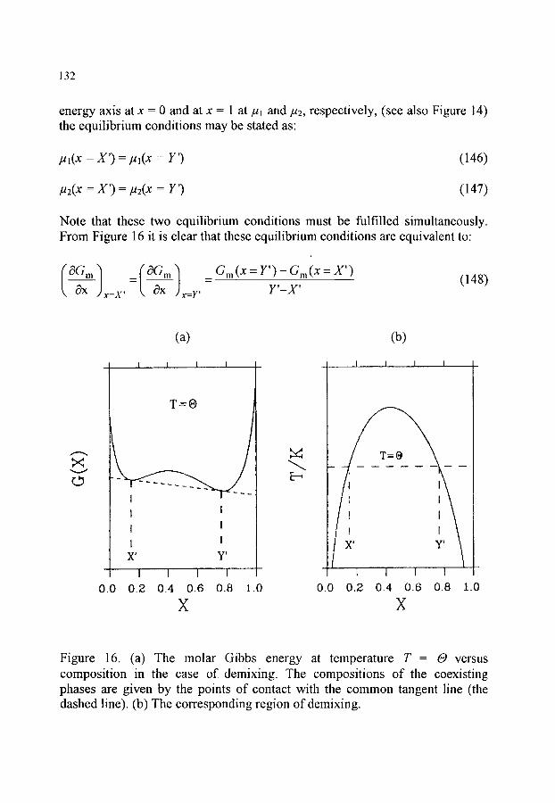
132

energy axis at x = 0 and at x = 1 at ~ 1 and/~2, respectively, (see also Figure 14) the equilibrium conditions may be stated as"

/~l(x = X') = ktl(x = Y') (146)

m ( x - x ' ) = = r ' ) (147)

Note that these two equilibrium conditions must be fulfilled simultaneously. From Figure 16 it is clear that these equilibrium conditions are equivalent to"

Ox x=x' o~ x=Y' Y ' - X '

(a) (b)

._L. I 1 I

T - - O

I I

I I ! I

X' Y'

I -I . . . . | - 1 ....

0 .0 0 .2 0 .4 0 .6 0 .8 1.0

X

E-,

_1 1 I l

X 0 y i

1 1 I I 0 .0 0 .2 0 .4 0 .6 0.8 1.0

X

Figure 16. (a) The molar Gibbs energy at temperature T = O versus composition in the case of demixing. The compositions of the coexisting phases are given by the points of contact with the common tangent line (the dashed line). (b) The corresponding region of demixing.

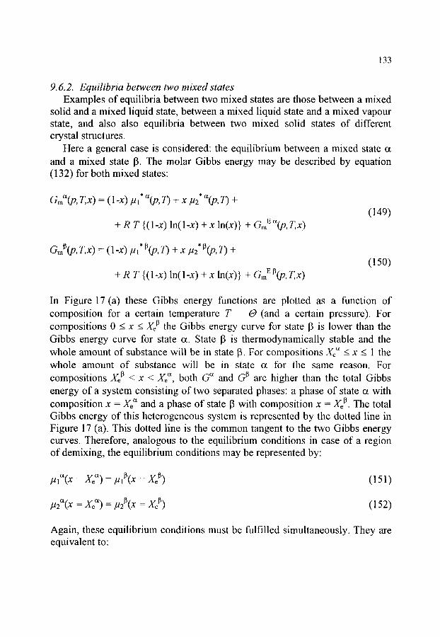
133

9.6.2. Equilibria between two mixed states Examples of equilibria between two mixed states are those between a mixed

solid and a mixed liquid state, between a mixed liquid state and a mixed vapour state, and also also equilibria between two mixed solid states of different crystal structures.

Here a general case is considered: the equilibrium between a mixed state ot and a mixed state 13. The molar Gibbs energy may be described by equation (132) for both mixed states:

Gm~ r ,x) -- (l-x)/../1 Or(p, T) q- x ]./2 Or(p, T) -I-

+ R T { (l-x) In(l-x) + x In(x) } + Gm E Or(p, T,x) (149)

Gm~(p,T,x) = ( l -x) ~,,* ~(p, 73 + x m* ~(p, 73 +

+ R T {(l-x) In(l-x) + x In(x)} +Gm E I~(p, T,x) (15o)

In Figure 17 (a) these Gibbs energy functions are plotted as a function of composition for a certain temperature T - O (and a certain pressure). For compositions 0 < x < Xe I~ the Gibbs energy curve for state 13 is lower than the Gibbs energy curve for state or. State 13 is thermodynamically stable and the whole amount of substance will be in state 13. For compositions X~'* _< x < 1 the whole amount of substance will be in state ot for the same reason. For compositions Xe ~ < x < X~ ~, both G ~ and G ~ are higher than the total Gibbs energy of a system consisting of two separated phases: a phase of state ot with composition x = Xe'* and a phase of state 13 with composition x = Xe ~. The total Gibbs energy of this heterogeneous system is represented by the dotted line in Figure 17 (a). This dotted line is the common tangent to the two Gibbs energy curves. Therefore, analogous to the equilibrium conditions in case of a region of demixing, the equilibrium conditions may be represented by:

l~(X = Xe ~ ) = ~, ,~(X --- Xe ~) ( 151 )

. 2~ (x = x~ ~) = m~(x = Xe ~) (152)

Again, these equilibrium conditions must be fulfilled simultaneously. They are equivalent to:

134

x = X . ~ x = X . a X e a -- e

(153)

Of course, a different temperature will result in different equilibrium compositions. In a graph of temperature versus composition (see Figure 17 (b)) the complete set of (T, X~ ~, X~ I~) data triplets represents the two-phase region. If c~ and 13 are solid and liquid, respectively, then the curves through the points (T, X~ ~~ and (T, Xr liq) are called the solidus and the liquidus, respectively. The area which is enclosed by the solidus and the liquidus is called the solid-liquid two- phase region.

(a) (b)

r~

I I . . . . t ! I

. - ~ J I a -" X~ X e

I I ! i

0 . 0 0 .2 0 .4 0 .6 0 .8 1.0

X

! I I I . . . . . . �9 . . . . 1_

I I

I

-! i I I

0 .0 0 .2 0 .4 0 .6 0.8 1.0

X

Figure 17. (a) The curves of the molar Gibbs energy at temperature T = O versus composition for two mixed states a and 13. The compositions of the coexisting phases are the points of contact of these curves with the common tangent line (the dashed line). (b) The corresponding a-13 two-phase region.

135

9. 6.3. Equilibria between an unmixed solid and a mixed liquid state The equilibrium between an unmixed solid (i.e. a pure component in the

solid state) and a mixed liquid state is a limiting case of the solid-liquid two- phase region. The Gibbs energies of the solids are given by points lying on the Gibbs-energy axes (i.e. on the vertical lines at x = 0 and x = 1). For compositions 0 < x < 1 the Gibbs energy of the solid state does not exist (or is extremely high). An example of this situation is given in Figure 18 (a). The equilibrium conditions are stated in conformity with equations (151) and (152):

* s O l ( T = = = ') ]A1 - 19) ,L/lliq(T O, X X (154)

,//2* sOl(T -- 19) -- ,L/21iq(T -- 19, X = Y ') (1 5 5)

O

(a) (b)

... I I ,,I I

T=|

/

i, +,

0.0 ] I . . . . . . I . . . . . I

0.2 0 .4 0.6 0 .8 X

. . . ! ! I _ _ I

T=O

I 1 I ...... I I 1

1 . 0 0 . 0 0 . 2 0 . 4 0 . 6 0 . 8 1.0

X

Figure 18. (a) The molar Gibbs energy at a temperature T = O for a liquid mixture, together with the molar Gibbs energies of the two solid pure components (o). Because the components do not mix in the solid state, there is no Gibbs energy curve for solid mixtures. (b) The corresponding eutectic phase diagram.

136

Note that these equilibrium conditions now do not have to be fulfilled simultaneously.

The phase diagram, which corresponds to this situation, is plotted in Figure 18 (b). This type of phase diagram is called a eutectic phase diagram. The point where the two liquidi intersect is called the eutectic point.

9. 6. 4. Thermodynamic phase diagram analysis In sections 9.6.1, 9.6.2, and 9.6.3, it was demonstrated how (binary) phase

diagrams depend on thermodynamic properties. The stated equilibrium conditions may be used to calculate phase diagrams if the thermodynamic properties of the pure components and the thermodynamic mixing properties are known. The reverse process, however, is also possible: derivation of thermodynamic mixing properties from a known (experimentally determined) phase diagram. This process is called thermodynamic phase diagram analysis.

Thermodynamic phase diagram analysis is a fitting procedure, which makes use of thermodynamic (excess) functions. The parameters to be adjusted in the fitting procedure are coefficients of these functions.

The result of thermodynamic phase diagram analysis, i.e. the mathematical representation of the thermodynamic excess functions, corresponds to a calculated phase diagram which is thermodynamically consistent and which reproduces the experimental phase diagram well. Therefore, thermodynamic phase diagram analysis is also a method of reliably fitting experimental phase diagram data, as well as a means of testing the internal consistency of these data. Finally, thermodynamic phase diagram analysis is the first step in estimating ternary and higher-order phase diagrams from binary data.

Although the subject of thermodynamic phase diagram analysis will not be treated further in this chapter, researchers using calorimetric and/or thermal analysis techniques to determine phase diagrams experimentally are strongly urged to support their experimental results with calculations. Too often experimental results are published which are thermodynamically inconsistent! For more information on this subject, see reference [10].

10. CHEMICAL REACTIONS

10.1. Gibbs energy of reaction; entropy of reaction and enthalpy of reaction

A chemical reaction is a process during which the molecular structure of one or more components (these components are called the reactants) change; the new components which are formed are called the products. Chemical bonds in

137

the reactants are broken and formed in the products. Chemical reactions are described using stoichiometric equations, e.g.:

N2(g) + 3 H2(g) --) 2 NH3(g) (156)

implies that one mole of nitrogen gas reacts with 3 moles of hydrogen gas to form 2 moles of ammonia gas. In principle, depending on the temperature and partial pressures, reaction in the opposite direction is also possible:

2 NH3(g) "-) N2(g)+ 3 H2(g) (157)

For a particular temperature, the partial pressures may be chosen such, that ammonia is neither formed nor dissociated. In this case, the system is at equilibrium:

N2(g) + 3 H2(g) ~ 2 NH3(g) (158)

As was demonstrated previously (see section 6), a spontaneous (irreversible) process at constant pressure and temperature is characterised by a decrease of the Gibbs energy of the system. Therefore, to find out whether components can react spontaneously, the change of the Gibbs energy caused by the chemical reaction must be determined. Consider a chemical reaction between reactants A and B to form products C and D:

IVAIA + IVBIB ~ v c C + VDD (159)

Note that the coefficients vA and VB are placed within absolute signs. This is because the coefficients VA and VB (i.e.. the coefficients of the reactants) are defined as negative values while the coefficients Vc and VD (i.e. the coefficients of the products) are defined as positive values. The extent of the reaction, indicated by the symbol ~:, is defined as a numerical value between 0 and 1; if ~:= 0, only reactants are present in the system. If ~:= 1, only products are present in the system. An infinitesimal change of the extent of the reaction d~ results in a decrease in the amount of reactants (the amounts of A and B decrease with dnA = VA d~ and dnB = VB d~, respectively) in the system and an increase in the amount of products (the amounts of C and D increase with dnc = Vc d~: and dnD= VD d~:, respectively).

138

Because the Gibbs energy is a state function, the change of the Gibbs energy caused by this change of the extent of the reaction is equal to the change of the Gibbs energy which would be observed if dnA and dnB moles of A and B were reversibly removed from the system, while dnc and dnD moles of C and D were reversibly added to the system. Thus the change of the Gibbs energy for a chemical reaction at constant pressure and temperature is, according to Equation (74), given by:

(dG)p,T = ,UA dnA + l.tB dns + ~ dnc + t2D dllD (160)

or:

(dG)p,T = (VA/.tA + vB ,t~ + Vc ,uc + VD t.tD) d~, (161)

In more general terms, this equation may be written as:

(dG)p,r = (~i (vipi)}d~ (162)

where the summation is over all the reactants and products involved in the reaction. An equilibrium state is reached if the Gibbs energy is at its lowest value, i.e. when:

f r:_'~[O@| =0 ~ ~ ( v ~ p ~ ) = O (163) \ o ~ j p ,T i

For simplicity, the summation over the thermodynamic potentials multiplied by the stoichiometric coefficients, is often identified as the Gibbs energy of reaction, indicated by the symbol ArG:

ArG - Z (v~/2~ ) (164) i

In principle, since (at constant pressure and temperature) the Gibbs energy tends towards a minimum value, the reaction will proceed to the right-hand side of the stoichiometric equation if the Gibbs energy of reaction is negative, and to the left-hand side if positive.

139

The temperature dependence of the Gibbs energy of reaction, which is the entropy of reaction, can be found using equation (76):

p = aT = ~ Vi~, 0T Jp

P

= --ZViSi = - A r S (165) i

The enthalpy of reaction follows from the combination of equations (83), (164), and (165):

A r H = X (v ih i )= X {vi (fli + Tsi )} : ArG + TArS i i

(166)

The enthalpy of reaction is an important quantity, because, for processes at constam pressure, it is equal to the heat of reaction, which is accessible experimemally using calorimetric techniques.

Two types of chemical reactions are very important for tabulating thermodynamic data: reactions in which compounds are formed from the most stable forms of chemical elemems, and reactions in which compounds react with oxygen to form stable oxides.

10.2. Formation from the elements The Gibbs energy of reaction and the enthalpy of reaction for a reaction in

which a chemical compound (the product) is formed from the corresponding chemical elements (in their most stable form) are called the Gibbs energy of formation (indicated by the symbol AfG) and the enthalpy of formation (indicated by the symbol At-H), respectively. These thermodynamic quantities are given for many substances in the thermodynamic tables. If, for each reactant and product of a certain reaction, the Gibbs energy of formation and/or the enthalpy of formation is known, then the Gibbs energy of reaction and/or the enthalpy of reaction may be calculated using an imaginary cycle, by applying the fact that Gibbs energy and enthalpy are state functions.

As an example, the dissociation of magnesium carbonate into magnesium oxide and carbon dioxide is considered together with the formation reactions in the following cycle:

140

MgCO3(s) ") MgO(s) + CO2(g)

-,,, J/ / (167)

(Mg(s) + C(s, graphite) + 1% O2(g))

For the total cycle, i.e. dissociation of MgCO3 into MgO and CO2, followed by dissociation of MgO and CO2 into the stable form of the chemical elements (i.e. the opposite of formation from the elements), and finally formation of MgCO3 from these elements, the change of the enthalpy and the change of the Gibbs energy is equal to zero. Therefore, the enthalpy and Gibbs energy of the dissociation of MgCO3 into MgO and CO2 are equal to:

ArH = At-H(MgO) + At-H(CO2)- At-H(MgCO3) (168)

ArG = AtG(MgO) + AtG(CO2)- AtG(MgCO3) (169)

If tables of Gibbs energies of formation are not available, tabulated absolute entropies can be used to calculate the entropy of reaction. Together with the enthalpy of reaction, calculated using the enthalpies of formation, the Gibbs energy of reaction can then be calculated.

10.3. Combustion. For organic compounds especially, enthalpies of combustion can often be

found in thermodynamic tables. The enthalpy of combustion is the enthalpy change for a reaction with excess oxygen to form the most stable oxides. Using the enthalpies of combustion of each of the substances involved in a reaction, found from thermodynamic tables, the enthalpy of reaction can be calculated using an imaginary cycle. Together with the absolute entropies, which may be used to obtain the entropy of reaction, again the Gibbs energy of reaction can be obtained.

As an example, consider the gas phase reaction between methanol and carbon monoxide to acetic acid at a temperature of 500 K:

CH3OH (g, T=500 K) + CO (g, T=500 K) ---) CH3COOH (g, T=500 K) (170)

Suppose that the enthalpy of reaction is needed. In the thermodynamic tables, the properties given in the following table were found. The quantities tabulated

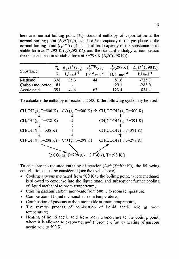
141

here are: normal boiling point (Tb), standard enthalpy of vaporisation at the normal boiling point (AvH~ standard heat capacity of the gas phase at the normal boiling point (cp ~ v~P(Tb)), standard heat capacity of the substance in its stable form at T=298 K (cp~ K)), and the standard enthalpy of combustion for the substance in its stable form at T=298 K (z~H~ K)).

ovaP(Tb) o (298 K) AcH ~ (298 K) T b Avm~ (Tb) Cp r Substance

K kJ moll J K q tool q J K l mol -j kJ mol l

Methanol 338 35.3 44 81.6 -725.7 Carbon monoxide 81 - 29.1 -283.0 Acetic acid 391 44.4 67 123.4 -874.4

To calculate the enthalpy of reaction at 500 K the following cycle may be used:

CH3OH (g, T=500 K) +CO (g, T=500 K) --) CH3COOH (g, T=500 K) 1, ,L ~t

CH3OH (g, T=338 K) ,I, CH3COOH (g, T=391 K) ,I, ,~ ~t

CH3OH (1, T=338 K) ,I, CH3COOH (1, T-391 K) ,[, 1, T

CH3OH (1, T=298 K) + CO (g, T=298 K) CH3COOH (1, T=298 K)

x, j [2 CO2 (g, T=298 K) + 2 H20 (1, T=298 K)I

To calculate the required enthalpy of reaction (ArH~ K)), the following contributions must be considered (see the cycle above): �9 Cooling gaseous methanol from 500 K to the boiling point, where methanol

is allowed to condense into the liquid state, and subsequent further cooling of liquid methanol to room temperature;

�9 Cooling gaseous carbon monoxide from 500 K to room temperature; �9 Combustion of liquid methanol at room temperature; �9 Combustion of gaseous carbon monoxide at room temperature; �9 The reverse process of combustion of liquid acetic acid at room

temperature; �9 Heating of liquid acetic acid from room temperature to the boiling point,

where it is allowed to evaporate, and subsequent further heating of gaseous acetic acid to 500 K.

142

The reaction enthalpy, therefore, is calculated as the sum of all these contributions, i.e.:

ArH~ K) = Cp~ vap(cH3OH) {Tb(CH3OH)- 500 / + - AvH~ + + cp~ { 298 - Tb(CH3OH) } + + A~H~ + + Cp~ {298 -- 500 } + A~H~ + - AcH~ + + cp~ {Tb(CH3COOH) - 298} + + AvH~ + + Cp ~ vaP(CH3COOH) { 500 - Tb(CH3COOH) }

(171)

The result of this calculation is: A~H~ K)=-122.7 kJ mol -l.

10.4. Chemical equilibrium The Gibbs energy of reaction is defined in equation (164). If the reaction

involves mixtures (either solid, liquid or gaseous) and/or pure gases, then the thermodynamic potentials in equation (164) are functions of the compositions of the mixtures (see for example equation (142)) and/or of the partial pressures of the gases (see for example equation (81). Because, during progress of the reaction, the compositions of the mixtures and/or the partial pressures may change, the Gibbs energy of reaction may also change. An equilibrium state is reached if the Gibbs energy of reaction equals zero (see equation (163)).

This criterion may be used, for example, for calculations of decomposition equilibria, which are often observed in thermogravimetric experiments. The Gibbs energy of reaction for the decomposition of calcium carbonate:

CaCO3 --) CaO + CO2 (172)

is defined as:

ArG = p(CaO) + p(CO2) -/~(CaCO3) (173)

The components, calcium carbonate (calcite) and calcium oxide, are both in the solid state. These two components, however, do not form a mixed solid phase. The thermodynamic potentials of these components may therefore be marked with an asterisk, indicating that these are properties for pure components. The

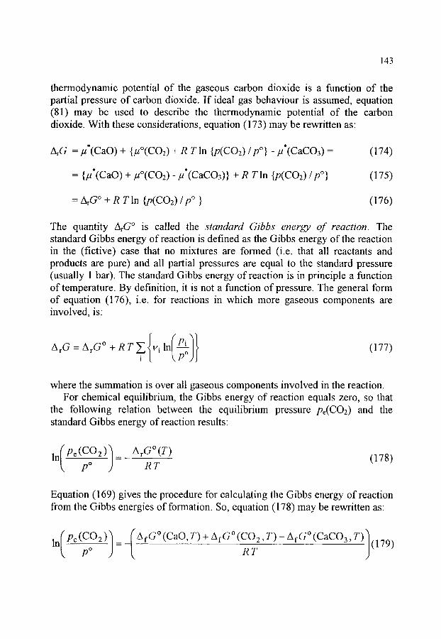
143

thermodynamic potential of the gaseous carbon dioxide is a function of the partial pressure of carbon dioxide. If ideal gas behaviour is assumed, equation (81) may be used to describe the thermodynamic potential of the carbon dioxide. With these considerations, equation (173) may be rewritten as:

ArG = ~'(CaO) + {/~~ + R T In {p(CO2) / p~ -/~*(CaCO3) = (174)

= {p*(CaO) + p~ - p*(CaCO3) } + R TIn {p(CO2) / pO } (175)

= &G ~ + R TIn {p(CO2) /pO } (176)

The quantity ArG ~ is called the standard Gibbs energy of reaction. The standard Gibbs energy of reaction is defined as the Gibbs energy of the reaction in the (fictive) case that no mixtures are formed (i.e. that all reactants and products are pure) and all partial pressures are equal to the standard pressure (usually 1 bar). The standard Gibbs energy of reaction is in principle a function of temperature. By definition, it is not a function of pressure. The general form of equation (176), i.e. for reactions in which more gaseous components are involved, is:

(177)

where the summation is over all gaseous components involved in the reaction. For chemical equilibrium, the Gibbs energy of reaction equals zero, so that

the following relation between the equilibrium pressure pe(CO2) and the standard Gibbs energy of reaction results:

ln( pe (CO2)1 = - pO ArGO RT(T) (178)

Equation (169) gives the procedure for calculating the Gibbs energy of reaction from the Gibbs energies of formation. So, equation (178) may be rewritten as"

/ i/: ( ~ / In Pe (CO__ 2) _ A f G ~ (CaO, T) + AfG ~ ( C O 2 , T) - Af 3, (179) pO RT

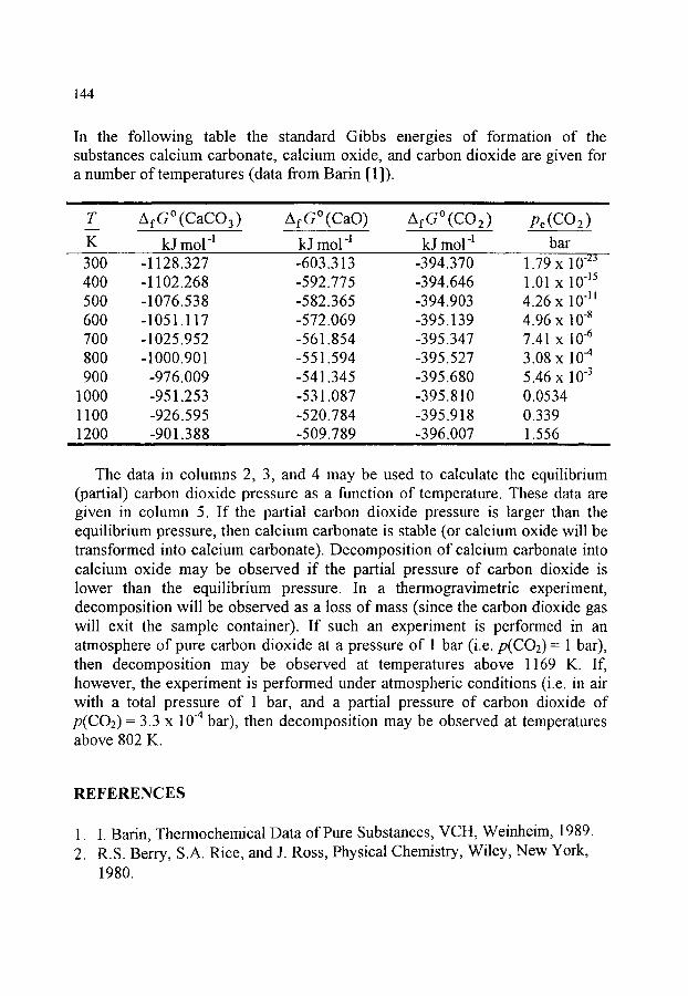
144

In the following table the standard Gibbs energies of formation of the substances calcium carbonate, calcium oxide, and carbon dioxide are given for a number of temperatures (data from Barin [ 1 ]).

T AfG~ (CaCO3) AfG~ AfG~ Pe(CO2)

K kJ mol "l kJ mol "l kJ mol "l bar 300 -1128.327 -603.313 -394.370 1.79 X 10 -23

400 -1102.268 -592.775 -394.646 1.01 x 10 -15 500 -1076.538 -582.365 -394.903 4.26 x 10 l l 600 -1051.117 -572.069 -395.139 4.96 x 10 -8 700 -1025.952 -561.854 -395.347 7.41 x 10 -6 800 -1000.901 -551.594 -395.527 3.08 x 10 -4 900 -976.009 -541.345 -395.680 5.46 x 10 -3

1000 -951.253 -531.087 -395.810 0.0534 1100 -926.595 -520.784 -395.918 0.339 1200 -901.388 -509.789 -396.007 1.556

i i i i i

The data in columns 2, 3, and 4 may be used to calculate the equilibrium (partial) carbon dioxide pressure as a function of temperature. These data are given in column 5. If the partial carbon dioxide pressure is larger than the equilibrium pressure, then calcium carbonate is stable (or calcium oxide will be transformed into calcium carbonate). Decomposition of calcium carbonate into calcium oxide may be observed if the partial pressure of carbon dioxide is lower than the equilibrium pressure. In a thermogravimetric experiment, decomposition will be observed as a loss of mass (since the carbon dioxide gas will exit the sample container). If such an experiment is performed in an atmosphere of pure carbon dioxide at a pressure of 1 bar (i.e. p(CO2)= 1 bar), then decomposition may be observed at temperatures above 1169 K. If, however, the experiment is performed under atmospheric conditions (i.e. in air with a total pressure of 1 bar, and a partial pressure of carbon dioxide of p (CO2)- 3.3 x 10 .4 bar), then decomposition may be observed at temperatures above 802 K.

REFERENCES

1. I. Barin, Thermochemical Data of Pure Substances, VCH, Weinheim, 1989. 2. R.S. Berry, S.A. Rice, and J. Ross, Physical Chemistry, Wiley, New York,

1980.

145

3. J.M. Bijvoet, A.F. Peerdeman, A. Schuijff and E.H. Wiebenga, Korte Inleiding tot de Chemische Thermodynamica, 4th edition, Wolters- Noordhoff, Groningen, 1979. (Dutch Language)

4. P.J. van Ekeren, Phase Diagrams and Thermodynamic Properties of Binary Common-Ion Alkali Halide Systems, Thesis, Utrecht University, 1989.

5. E.A. Guggenheim, Thermodynamics; An Advanced Treatment for Chemists and Physicists, 5th edition, North-Holland, Amsterdam, 1967. I. Gutzow and J. Schmelzer, The Vitreous State: thermodynamics, structure, rheology and crystallization, Springer, Berlin, 1995. I.M. Klotz and R.M. Rosenberg, Chemical Thermodynamics; Basic Theory and Methods, 5th edition, Wiley, New York, 1994. C.G. de Kruif and J.G. Blok, J. Chem. Thermodyn., 14 (1982) 201. S.V. Nemilow, Thermodynamic and Kinetic Aspects of the Vitreous State, CRC Press, Boca Raton, 1995.

10. H.A.J. Oonk, Phase Theory; The Thermodynamics of Heterogeneous Equilibria, Elsevier, Amsterdam, 1981.

11. A. Shavit and C. Gutfinger, Thermodynamics; from concepts to applications, Prentice Hall, London, 1995.

12. M.W. Zemansky, Heat and Thermodynamics, 3rd edition, McGraw-Hill, New York, 1951.

,

~

~

9.


Chapter 3

KINETIC BACKGROUND TO THERMAL ANALYSIS AND CALORIMETRY

Andrew K. Galwey" and Michael E. Brown b

"School of Chemistry, Queen's University of Belfast, Northern Ireland

bChemistry Department, Rhodes University, Grahamstown, South Africa

1. INTRODUCTION

1.1. Fundamentals Two principal objectives are common to the vast majority of kinetic studies of

chemical reactions. One of these is the determination of the rate equation that satisfactorily describes the extent of conversion of reactant(s) or formation of product(s) with time as reaction proceeds, usually, but not necessarily, at constant temperature. Experimental data are compared with values predicted from a range of theoretical kinetic expressions to determine which rate equation describes the experimental measurements most precisely. The form of this kinetic expression enables inferences to be made concerning the reaction mechanism, i.e. the detailed sequence of chemical steps (including possibly a very slow and hence rate- detenmnmg step) through which reactants are converted into products. The second purpose of kinetic analysis is to determine the influence of temperature on the rate of reaction. The parameter(s) m the rate equation which are most affected by temperature are the rate constant(s) (or rate coefficient(s)). This temperature dependence is usually expressed quantitatively by the Arrhenius equation:

k = A exp (-E./RT) (or k = A T ~ exp (-E./RT)) (1)

Values of the Arrhenius parameters (E. and A) are accepted as providing measures of the magnitude of the energy barrier to reaction (the activation energy, Ea) and the frequency of occurence of the situation that may lead to product formation (the frequency factor, A). The theoretical significance of the Arrhenius parameters will be considered ~ e r below. In addition, these parameters provide a convenient and widely-used method for the concise reporting of kinetic data, for the comparison of

148

reactivities of different systems, and for use (with suitable precautions) in estimating reactivities or stabilities at temperatures outside the interval of the experimental measurements.

The essential foundation of any kinetic study is a series of measurements of the extent of reaction as fimctions of both time and temperature. The total amounts of reactant and/or of product (or of any parameter quantitatively related to these) present at time t are used as measures of the extent of reaction, or fractional reaction (e c). Alternatively, the rate of change of tr, (dtr/dt), may be measured together with the reaction temperature, T. The definition of tr in terms of a measurable parameter requires knowledge of the reaction stoichiometry including consideration of the contributions from any concurrent or consecutive rate processes.

Isothermal conditions are widely used for kinetic studies in which rates of the reaction of interest are measured at several different constant temperatures to obtain the Arrhenius parameters. In the field of thermal analysis, much attention has been directed towards the problem of obtaining kinetic information from programmed temperature, dynamic or non-isothermal experiments. These experiments usually revolve measurement of some quantity (e.g., mass, heat evolved, etc.), which can be related directly to the fractional reaction t~, at a series of different, usually constant, heating rates (fl = dT/dt).

1.2. The kinetics of homogeneous reactions The kinetics of homogeneous reactions are conventionally determined from

measurements of changes of concentration of one (or more) reactant or product with time, at constant temperature. Rate equations are usually of the form:

Rate = k(T) f(concentrations of reactants and/or products)... (T constant).

1.3. The kinetics of heterogeneous reactions Heterogeneous reactions differ from homogeneous reactions in that the chemically

identical constituents of the reactant may possess different reactivities depending upon their location within the sample and the history of each sample preparation. For many reactions involving solids, chemical changes occur preferentially at crystal surfaces, or the regions of direct contact between reactant and product phases (the reaction interface). Each chemical change occurring within this zone of locally enhanced reactivity, where reactant constituents are situated close to the product solid, increases the amount of product phase present. Incorporation of this reacted material into the residual (product) phase results in advance of the reactant-product interface into unreacted material. Interface advance, through reaction within a thin reactive contact zone, may result in small displacements of participating species (together with diffusive loss of gaseous products) but these do not migrate with the

149

region of active chemical change. The probability that a particular constituent of the reactant will undergo reaction is significantly enhanced when it is reached by an advancing reactant-product interface. The reactivities of the transitory species comprising such interfaces are regarded in the theory as remaining constant from the time of initial establishment until final termination when no further reactant remains available at a crystal boundary, or by mutual anihilation on coalesence.

Reaction interfaces are created by the nucleation process and each advances thereafter by growth into the reactant material composing the crystal in which it is located. Nucleation usually occurs on crystal faces and is believed to involve sites of damage or imperfections associated with locally enhanced reactivity. Because interface reactivity remains constant, the rate of linear advance or growth is constant throughout its lifetime. The rate of product formation within a reacting solid in reactions of this type is thus directly proportional to the total area of the reactant- product interface and rate equations may be derived from quantitative consideration of their changing three-dimensional geometry during advance of the interface.

The general theory of chemical kinetics of reactions of solids is based largely on observations for decompositions of selected individual crystalline compounds, reactions which provide the simplest models of such rate processes. In many decompositions the reactant-product interface is regarded as a very thin layer within which the chemical change is completed. Structures and properties of interfaces are discussed below. Other mechanisms of chemical change have been recognized. For example, the kinetics of some dehydrations of crystalline hydrates have been shown to be controlled by the rate of outward diffusion of water from within a crystal structure that undergoes relatively minor modification during this change. Here the reaction zone effectively grows in thickness during the outward migration and loss of water (or other chemical change). Interactions of a solid with a second reactant (gas, liquid or solid) frequently results in the formation of solid products generated at reactant surfaces. These may constitute a barrier layer that opposes, or even completely prevents, its own continued formation. The rates of reactions of this type are usually controlled by the (diminishing) rate of diffusion of constituents of one or both reactants across the barrier layer of product. Other factors that may influence the rates at which solids react, but have no counterparts in homogeneous reactions, are melting, sintering and the specific effects of intracrystalline impurities, including nonstoichiometry and imperfections, both local and extended,.

Unlike homogeneous reactions, concentration terms are usually of less significance in the kinetic analysis of rate processes involving solids. Within the volume of reactant crystals, concentrations are everywhere the same, whereas beyond these boundaries the amotmts of the species tmdergoing the chemical change of interest are everywhere zero. The disposition of material in a diffusion controlled reaction is inhomogeneous in that there are spatial variations of concentration. Thus the

150

reactivities of components of a solid differ with position and with time in the sense that the probability of reaction is significantly increased when that component is located within the zone of influence of an advancing interface. Kinetic analyses thus require consideration of the systematically changing disposition of the active interface and also, possible influences or controls exerted by rates of diffusion of reactant or product species.

The word mechanism is used rather ambiguously in the literature concerned with the kinetics of solid state reactions. Some authors use this term to describe the fit of a rate equation to their data. A preferable term might be the kinetic model. Others use the word in the more conventional way (as in homogeneous kinetics) to describe the sequence of chemical steps through which reactants are transformed into products. The latter definition is used here to emphasize the chemical basis for solid state reactions, which is often neglected in favour of mathematical analyses directed towards determining the kinetic model.

1.4. Review of literature on the kinetics of heterogeneous reactions Jacobs and Tompkins [1 ] gave the first systematic presentation of the theory of

application of rate equations to solid state decompositions. In the same volume, Garner [2] discussed the chemical characteristics of this type of reaction. Young [3] presented the formal theory, together with historical reviews of progress in understanding the behaviour of the thermal decompositions of selected solids. Delmon [4] extended the analysis of kinetics by consideration of a variety of geometric aspects of rate control. Barret [5] was concerned with the theory of interface advance processes and also discussed reaction rates where there is diffusion control. Brown et al. [6] reviewed the kinetic features of decompositions of, and interactions between, inorganic solids. The most general recent review of the subject is by Sestfik [7]. Other books which provide relevant background material on the properties of solids are by Budnikov and Ginstling [8], Schmalzried [9] and West [10]

2. KINETIC MODELS FOR SOLID-STATE REACTIONS

2.1. Rate control The following factors may exert dominant controls on reactions of solids and have

to be considered in the formulation of rate equations. (i) The chemical reaction: one or more bond redistribution steps that usually occur at a reaction interface. This is the chemical control of reactivity. (ii) Reaction geometry: systematic variations in the total area of the reaction interface, due to the changing geometry of disposition of that interface as reaction proceeds, exert an important influence on kinetic behaviour. (iii) Diffusion: the rate of transport of participants to or from an interface

151

as reaction proceeds influences the rate of product formation in many reactions. More than one of these factors, together with others that are mentioned later, may exert significant, but independent and different, influences on the kinetic behaviour.

The kinetic characteristics of the rate controlling step in a solid decomposition can be measured directly only when all subsequent rate processes are rapid. This condition is fulfilled in most irreversible reactions. In reversible decompositions, the escape of product gases must be unimpeded, otherwise there is the possibility that a gaseous product may interact with the intranuclear solid product through, or past, which it must diffuse during escape. Beruto and Searcy [l 1 ] have demonstrated unambiguously the importance of eliminating contributions from the reverse process in an outstanding fundamental kinetic study of CaCO3 dissociation. Other investigations, mainly concerned with the evolution of water from crystalline hydrates, have shown that dehydration rates vary with the prevailing pressure of HzO product, as shown in Figure 1. This kinetic pattern is usually referred to as Smith - Topley behaviour [reference 6, p. 125 ff].

Discussion of the formulation of kinetic equations below is preceded by consideration of the processes that control the rates of solid state reactions : nucleation, interface advance (growth) and diffusion. Reaction models based on chain mechanisms [6] are regarded as being of historical interest only and are not included.

P, L _ _

! & | i |

Water vapour pressure (arbitrary units)

Figure 1. Schematic representation of the Smith- Topley effect ( reference 6, p. 125 if). The variation in rate of a reversible reaction (usually dehydration of a crystalline hydrate) with prevailing pressure of the volatile product (water vapour).

152

2.2. Nucleation Nucleation can be defined as "the initial establishment of a new and discrete product

particle within the solid reactant" [12]. Two types of chemical change may be involved: (i) the chemical transformation of one or more constituents (e.g., ions or molecules) of the reactant into the constituents of the product; and (ii) recrystallization of reacted material to the lattice structure of the product phase. The result of nucleation, perhaps requiring several steps, is the generation of the active reactant-product interface at which reaction occurs preferentially during its subsequent advance into unchanged reactant as the nucleus grows.

Recent studies of dehydration reactions have shown that superficial changes across reactant surfaces, identified with water loss, precede the appearance of growth nuclei. Nucleation occurs, therefore, within this modified boundary layer and, in some hydrates, a rapid onset of nucleation can follow exposure of partially dehydrated material to water vapour [13].

Identification of the chemical changes that contribute to nucleation is a matter of considerable experimental difficulty. The sites of locally enhanced reactivity at which nucleation occurs are changed beyond recognition by the formation of the product particle. Characterization of these changes presents a considerable challenge to the laboratory techniques available, particularly for a site embedded within a larger crystal, the boundary layer of which may have already undergone chemical or structural modifications [ 13].

Because reactions are often initiated at only a relatively small number of nucleation sites [ 12] it is concluded that these possess significantly enhanced local reactivity. The first stage in their development may involve changes within the reactant phase to generate an incipient nucleus. Proceeding from this precursor to the germ nucleus may require an investment of energy. This is regarded as the difficult step and perhaps includes recrystallization of reacted material to generate the product phase. Thereafter, the interface of the growth nucleus that appears advances by preferred chemical change at the reactant-product contact. The relative ease of nucleation exerts an important influence on the kinetics of the overall reaction. When the nucleation step occurs infrequently, sometimes ascribed to a large activation energy, a sigmoid yield-time curve is observed. In contrast, if nucleation is rapid, all surfaces of the reactant are rapidly converted to product early in the reaction and the interface so formed advances inwards. Yield-time curves are then predominantly or entirely deceleratory.

2.3. Growth of nuclei Nuclei can be identified under the microscope because of the textural changes that

accompany reaction. Decomposition is often accompanied by material loss, together with the appearance of cracks because the residual products do not fully occupy the

153

volume of the former reactant material. Recrystallization yields small particles with crystallite textures that scatter light and the opaque intranuclear (product) material is recognizable. The advancing boundary surface of each nucleus is the reaction interface.

A characteristic feature of the kinetics of most solid decompositions is that rates o f interface advance are constant [1,2,6]. This is expressed by:

Or/dr) : leo(t- to)

where r is a linear dimension of the nucleus at time t and k6 is the rate constant for growth of a nucleus formed at time to, after the commencement of reaction.

Rates of growth of small nuclei (often at the lower limits of microscopic detection) may be different from those subsequently attained. Low rates of initial growth have been ascribed to the instability of very small nuclei, but instances of relatively more rapid early growth of small nuclei are also known [13]. However, it is generally agreed that, after initial deviations, all nuclei within a particular reactant sample grow at the same rate.

Growth of nuclei in three dimensions (2 = 3, where 2 is the number of dimensions term for use in kinetic analysis) means that the interface expands outwards at an equal (constant) rate in all directions, generating hemispheres of product and an increasing area of active reactant/product contact. Such unrestricted freedom of expansion is not always possible, however, and nucleus growth may be effectively confmed to two dimensions (/ /= 2) in reactants possessing a layer structure, or where the solid is in the form of thin crystals [14]. Two-dimensional growth may also arise when many closely-spaced nuclei are generated in the form of linear arrays. These grow initially in three dimensions which, however, soon leads to coalesence between neighbours and generation of a cylindrical reaction zone where the increase in diameter with time fits the square law (,~ = 3 ~ ,~ = 2). This pattern ofbehaviour has been proposed for nickel oxalate decomposition [ 15]. Growth in a single dimension (2 = 1) may occur where severe restrictions on nucleus development are imposed by the crystal structure or the sample morphology, for example in reactions of fibre-like crystals.

2.4. Diffusion processes in reactions of solids Diffusion processes participate in many types of chemical changes involving solids.

Two important reaction models, in which diffusion is a dominant kinetic control, are given here as examples. These are (i) decompositions of solids in which the rate is controlled by the diffusive escape of a volatile product, and (ii) reactions between solids where a solid product is formed between the reactants, so that progress is maintained by transport across the barrier layer. As with other reactions of solids, consideration must be given to the changing boundary geometry of the participating

154

barrier layers (which are the reaction interfaces) and appropriate terms must be incorporated in the overall rate equation.

In the decompositions of some particularly stable crystalline materials, the reactant structure does not tmdergo recrystallization or disintegration, although there may be modification of lattice parameters following the loss of a small stable molecule, such a s H20 or NH3, from the reactant phase. Such molecules diffuse outwards between structural components that are sufficiently stable to smMve unmodified. Reaction rates are controlled by Fick's laws, ease of movement being determined by the dimensions of the intracrystalline channels. This factor in the rate process is often expressed by a t v2 tenn. Theoretical aspects of the subject have been discussed by Okhotnikov et al. [ 16-20]. Transport is a dominant control in a structure that is not reorganized directly as a result of the chemical change.

Reactions of this type are often characterized by anisotropy of interface advance in layered structures where migrations are exclusively in the interlayer planes. Examples of diffusion controlled reactions have been reported for the dehydrations of some crystalline hydrates, including CaSO4.2H20 [17,21 ] and CaHPO4.2H20 [22].

The interaction of a solid with a second reactant (gas, liquid or solid) to form a solid product can result in the generation of a barrier layer that opposes its own further formation. Such opposition increases in direct proportion to the thickness of the material interposed between reactants. At low temperatures, a thin layer of product of atomic dimensions may be sufficient to suppress reaction completely. At higher temperatures, the product may become permeable to reactant species so that reaction continues. Reactions at the interfaces are often relatively rapid, so that the diffusion process controls the overall rate of reaction. The theory of such rate processes is presented by Grimley [23] and Szekely et al. [24] for gas-solid reactions and by Welch [25], Schmalzried [9] and by Brown et al. [6] for solid-solid reactions. In reactions of this type, the rate diminishes with increasing thickness of the product layer and diffusion control results in a t 1/2 dependence on the rate of linear advance. Rate equations require terms expressing the contributions from both diffusion control and the geometric changes resulting from interface advance. It is usually the cations that are mobile within the bamer layer because these are smaller than the anions that maintain the immobile crystal structure within which the chemical changes occur. A complication that may arise in kinetic studies is that two or more crystalline products may be generated and rate is controlled by diffusion across both these contiguous phases, represented schematically by:

AX/BX ~ AX/ABX2/BX ~ AX/A2BX3/ABX2/BX

where A and B represent the migrating cations and X is the immobile (larger) anion. Diffusion coefficients of A and B in the phases ABX 2 and A2BX 3 may be different

155

and due allowance for their individual contributions must be incorporated into the kinetic analysis of such systems.

2.5. The reaction interface Recent work has shown that interface structures in several reactions are more

complex than the very thin (perhaps monomolecular) layer that has been implicitly assumed in solid state kinetics. In some dehydrations, water is lost from a zone extending appreciably in front of the crystal transformation discontinuity with which the interface is often identified [26]. This dehydration layer retains a modified reactant structure during this initial loss until transformation into the product phase, perhaps with completed water elimination. Thus the interface is identified as a composite structure, composed of at least two different layers. This model has been developed from examinations, using diffraction methods, of the structures within a sequence of small volumes extending across the interfaces developed during the dehydrations of CuSO4.5H20 and LiESO4.H20 [26].

If the thickness of a composite interface is small compared with crystal size, it may be acceptable to apply kinetic equations based on simple geometric models. However, if the pre-interface zone, within which there is perceptible reaction, is of appreciable thickness, several different types of kinetic behaviour are possible. While these possibilities have apparently not been fully explored, two different reaction models have been described. In the first model, reaction is shown [16] to be controlled by the diffusive loss of a structural component (migration of HEO in dehydration) to a surface where it is volatilized. Within nuclei, the product phase promotes recrystallization of the partially dehydrated material (seed crystals), thus opening channels and enabling diffusive loss to continue. In regions where the product phase is not present, diffusive losses are restricted in extent. Nuclei must be present for the reaction to continue to completion. This mechanism has been proposed to explain the dehydration of d LiKC4H406.H20 where the rate of interface advance is controlled by a diffusion process [16]. The second model requires that the chemical change proceeds virtually to completion in the reactant with minimal rearrangement of lattice constituents and is then followed by a separate recrystallization step to the final product structure. The overall rate of product formation cannot, therefore, be correlated with models based on an observed nucleation and growth process which represents only the ordering of already reacted material. Behaviour of this type has been proposed to account for kinetic observations in the dehydrations of Ca(OH)2 [27] and, in certain circumstances, NiSO4.6H20 [28] and possibly in alums [29].

During some decompositions (topotactic reactions), certain features of the crystal symmetry of the reactant are maintained in the structure of the crystalline product and this uniformity of product orientation is maintained throughout the total chemical

156

change [30,31 ]. The relative positions of at least some of the reactant components thus undergo only minor displacements during such chemical changes. Behaviour of this type has been observed in many diffusion controlled processes, including the dehydrations of clays and of talc [32]. Other examples include the dehydration of Mg(OH)2 [33], the decomposition of CrO2 to Cr203 [34], and isomerization of complex cobalt salts, including [Co(NH3)5(SCN)]C12, [35,36] and many other crystalline reactants. Identification of the features that are preserved undisturbed across a reaction interface provides invaluable stereochemical evidence concerning the nature of changes that are possible within the reaction zone.

Galwey [37] has discussed the role of interfaces in reactions of solids and classified behaviour on the basis of the physico-chemical changes occurring within these active zones. A brief description of each class of nucleus distinguished is given below. Functional nuclei: The solid product catalyzes the essential chemical changes occurring at the reactant-product interface, e.g. the decompositions of silver malonate and of nickel squarate. Flux-filigree nuclei: Reaction ahead of the advancing recrystallization interface yields a finely-divided product crystalline phase, for example the dehydration of lithium sulphate monohydrate [38]. Fluid-flux nuclei: Structures in which a proportion of a volatile product is retained temporarily in condensed or adsorbed form and which promotes the difficult phase change from crystalline reactant to crystalline product, e.g. the dehydrations of alums [13] and the reaction of potassium bromide with chlorine ( ~ KC1 + V2 Br2). Fusion nuclei: Reactions may proceed more rapidly when the stabilizing intracrystalline forces are relaxed on melting to yield a fluid phase, in which there is also greater stereochemical freedom for chemical changes to take place. The molten zone may be localized and temporary. Examples include the decompositions of ammonium dichromate, ammonium perchlorate and copper (II) malonate. Fictive nuclei: In some rate processes no residual phase is formed, for example, during sublimation of a solid. In other systems there can be a physical change only, for example, the evaporation of water physically immobilized in a coherent matrix, as in the dehydration of lignite [39] where there is no chemical reaction.

Constituents of solids are confined and stabilized by attractive interactions with neighbours and hence their ability to adopt the spatial disposition that corresponds to the minimum energy barrier to chemical change is diminished. These conditions are changed locally within any reaction interface where melting occurs and reactivity may be enhanced [40]. Conditions which may be associated with the onset of melt formation include: (i) accumulation of a condensable product in large amounts, for example during low temperature dehydrations in a confined reactant volume; (ii) where there is a molten intermediate or a product capable of eutectic formation with

157

the reactant; or (iii) when the melting point of reactant, product or intermediate is exceeded.

When melting is localized (perhaps within a thin interface layer), the overall kinetics of such rate processes may resemble the behaviour of an interface-controlled reaction in a solid. If reactant melting is comprehensive, the kinetic behaviour can be expected to be that of a homogeneous reaction. The kinetics of reactions involving restricted melting is a subject that merits fiLrther theoretical and experimental investigation.

Identification of the textures, structures and properties of the active interface, including the occurrence or absence of melting, are essential contributions towards the determination of the mechanism of any solid state reaction. Such evidence may enable the bond redistribution steps that control the overall rate of chemical change to be identified and the factors which determine the increased reactivity within this zone to be recognized.

2.6. Kinetics of nucleation If nucleation is assumed to occur randomly at No identical potential nucleation sites

distributed across the faces of the reactant crystals, the rate of nucleation can be expressed as a first-order rate process :

dN/dt = k N (N O - N)

where N growth nuclei are present at time t and k N is the rate constant for nucleation. Integration with (N=0, t=0) leads to:

N = No[l- exp(- k N t)]

and differentiation again gives the exponential law o f nucleation:

dN/dt = ky N O exp(- ky t)

When ky is large, nucleation is virtually instantaneous, N = No, and no further nuclei are generated during the subsequent reaction. When ky is small, the rate of nucleation is approximately constant because the number of sites, (No- N), undergoes little change. This is known as the linear law o f nucleation:

N = k y N o t

A different approach was provided by Bagdassarian [41 ] and developed by Allnatt and Jacobs [42]. It was assumed that several distinct steps are required to generate

158

a growth nucleus. This results in an acceleratory nucleation process known as the p o w e r law o f nucleat ion"

dN/d t = C r l t ~- 1

The above results are summarized in Table 1 and schematic representations of the variations of N with time are shown in Figure 2. The significance of the term, r/, in these rate equations is explained below.

Table 1 Nucleation rate laws for solid state decompositions

Rate law Nucleation rate Number of nuclei r/value used dN/d t = present at time t in rate equation

N =

Exponential k N (N O - N) N O [1- exp(- k N t)] 1 kN No exp(- kN t)

Linear ky No kN No t 1

Instantaneous oo No 0

Power C r/t ~- ~ C t ~ > 1 (usually 2 or 3)

Branching kN No exp(k2 t) (k N N o/k2)[exp(k 2 t) - 1]

No = initial total number of potential nucleation sites; N = number of growth nuclei present at time t; (dN/dt) = rate of nucleation, k N = nucleation rate constant; kB - branching rate constant; gr =tennination rate constant: k2 = kB - kT. C is a constant.

N

N o

N

| | II |

t t (a) Exponential (b) Linear

No

N N

(c) Instantaneous

I ' " I I I I | '

t t (d) Power

_ _ _ _ _ _ L _ . " | n n I

159

Figure 2. Idealized representations of the variations with time of numbers of growth nuclei (N) present at time, t, for four of the different nucleation rate equations given in Table 1.

Kinetics of nucleation may be studied by microscopic examinations of surfaces from which numbers of growth nuclei/unit area (N) are counted after known reaction times. Photographs of the surface may be taken at appropriate intervals and used to obtain the quantitative information. The nucleation law is sometimes inferred from the overall kinetic behaviour. Precise fits to rate laws (including nucleation) require large numbers of accurate observations to enable reliable statistical analyses of the data to be made and it is frequently difficult to obtain sufficient numbers of reliable (N,t) values. The trends in Table 1 cover, to an acceptable approximation, all types of behaviour that can realistically be expected [ 13]. These relationships provide a

160

sufficient foundation for kinetic analyses where the nucleation step, although the essential precursor to all subsequent changes, contributes only a single term to the overall composite kinetic expression.

2.7. Kinetics of nucleation and growth Three main constraints on nucleus growth restrict the amount of product formed.

These are coalesence of nuclei, ingestion of sites potentially capable of generating nuclei, and crystal boundaries. (i) Coalesence describes the loss of active interface which occurs when the reactive zones of two (or more) growing nuclei meet. This is sometimes described (incorrectly) as "overlap of nuclei" through reference to the shapes that would have developed in the absence of interference to growth. (ii) Ingestion refers to the elimination of a nucleation site, at which a fitrther nucleus would have developed, by the growth of an existing nucleus. (iii) Growth cannot continue beyond a crystal boundary, this sets limits on the development of nuclei formed near reactant particle edges. Sizes and shapes of crystallites influence kinetic behaviour in ways that are discussed further below.

The simplest kinetic expression based on the model of interface advance is the power law. Assuming the unrestricted and constant rate of interface advance at all surfaces of N instantaneously formed growth nuclei in three dimensions, the total volume of product, V, in the N hemispherical product assemblages after time t (radii = k o t) will be V = (2~N/3)(k~ t) 3. The exponent is determined by the number of dimensions in which growth proceeds. If nucleation continues during reaction, the acceleratory character is increased by the value of r] given in Table 1. The power law (model Pn) is more generally expressed a ,l/~ = kt, where n = r] + ~ (representing the nucleation law and the number of dimensions in which nuclei grow). This acceleratory equation can be applicable only to the early stages of reaction when the assumption of unrestricted nucleus growth is acceptable. Subsequently, overlap between neighbouring nuclei reduces the acceleratory contribution leading to the deceleratory behaviour characteristic of the later stages of reaction shown in Figure 3. Hemispherical nuclei, indicative of equal rates of growth in all directions, are found for example in the decomposition of barium azide [43] and in the dehydration of chrome alum [13]. Other reactions develop nuclei of different shapes characteristic of preferred advance in certain crystallographic directions as in the dehydration of CuSO4.5H20 [44].

In interface advance reactions, the total volume of product at time t, V(t), is given by the volume summation to include all individuals of the set of growth nuclei. Due allowance must be made for the different starting times at which each participating nucleus (linear dimension, r(t, tj)) begins to grow. In principle this may be expressed as an integration for any combination of a rate equation for nucleation (Table 1) together with a rate equation for growth �9

161

~(t) -- Oro~t [t, f t r(t,t)] ~ [dN/dtl,=tj dt (2)

where a is a shape factor for the growth nuclei. V(t) may be related to the fractional extent of reaction at time t, tr = V(t)/Vf. The final volume, Vf, corresponds to completion of reaction. Definitions and methods of measurement of tr are described in Section 4.2.

In principle, equation (2) may be integrated for any combination of rate laws for nucleation and growth to give a rate expression of the form g(~ = kt. In practice, this cannot be performed generally because there is no functional relationship between the nucleation and the growth terms. Simplifications are possible for a number of behaviour patterns. Avrami [45] introduced the concept of an extended value of tr', based on the assumption that randomly distributed nuclei grow in the absence of the constraints of overlap and site ingestion, tr and tr' may be related by

dor dt~' (1 - tr)

which satisfies the requirements that when tr = 0, (dtr/d0 = (dtr '/dO and when tr = 1, (dtr/dt) = 0, but (dtr '/dO is finite. Hence

f (1- /~,)-1 da~- f da~' and t r ' = - ln(1 - tr)

Power law equations of the form oc'= k" ( t - to)" can thus be modified to:

- ln (1 - tr) = k" ( t - to)" or [- ln (1- l~)] 1/n = k (t- to) (3)

Again n = 1? + 2, is based on the nucleation rate law (r/) and number of dimensions in which nuclei grow (2). This equation (model An) is of considerable importance in kinetic studies of decompositions of solids and is associated with the names of several workers in the field, including Avrarni, Erofeev, Johnson, Kohlmogorov, Mampel and Mehl, but is most commonly referred to as the Avrami-Erofeev equation (or the JMAEK equation). Derivations of these (and other) rate equations are given in [1-81.

2.8. Contract ing geometry models Contracting geometry models are based on an initial rapid (instantaneous) dense

nucleation across all, or some specific, crystal faces. Close spacing of nuclei results in the rapid (low a) generation of a coherent reaction zone that advances inwards at a constant rate (k~) in the absence of diffusion effects (considered below in Section

162

2.11). This topic has been discussed for a variety of crystal shapes by Delmon [4], see also [1, 6].

The progress of reaction, rapidly initiated on all surfaces of a cube edge, a, and advancing inwards at equal rates is described by :

a'-- [a 3- (a- 2k~ t) 3]/a 3 or 1- (1 - tr) v3 = (2ko/a)t (4)

This is referred to as the contracting volume (cube or sphere) equation (model R3) and is the simplest example of a more general family of expressions [46-48]. Consideration has been given to the effects of different rates of interface advance in different directions, allowances for angles between the crystal faces, and the variations in shapes and dimensions of crystals of reactant [49,50].

In equation (4), n = ,~ = 3 and the equation can be made more general as

1 -(1 - oOV"=kt

where n is the number of dimensions in which the interface advances. When n = 2, the equation is known as the contracting area (disc, cylinder or rectangle) equation (model R2). When n = 1, the equation becomes t r= kt, i.e., the reaction proceeds at a constant rate, which is the zero-order equation (model F0).

2.9. Models based on autocatalysis The rate equations considered under this heading were originally formulated on the

concept of "nucleus branching" (Table 1), analogous to homogeneous chain reactions. Occurrence of "branching", without restriction on multiplicative development or allowance for termination, would lead to an exponential dependence of a~ on t: a = k exp (k B/), where k B is the rate coefficient for nucleus branching. Acceleratory behaviour cannot be maintained indefinitely in any real reaction and allowance for termination can be made by including a term kT(a0, so that:

dN/dt = kNN o + N[k B - kT(tr)]

where (tr) expresses a dependence upon a~. When k N is large, all available sites (No) are rapidly exhausted. When kN is very small,

N[k B - kT(tr)] >> k N No, and dN/dt = N[k B - kT(a')]

If it is assumed that the rate of reaction (da~/dt) is proportional to the number of participating nuclei (N), integration of this expression requires knowledge of the relationship between kB, kT(a ) and a. Prout and Tompkins [51] considered the

163

particular case of sigmoid a-time curves, with the point of inflection at tr = 0.50. This leads to:

d oc/ d t = k B a ' (1 - a')

which on integration gives:

ln[a~/(1 - a0] = kBt + c (5)

which is often referred to as the Prout-Tompkins equation (model B 1) or, sometimes, the Aust in-Ricket t equation [52]. The sigmoid form of the a-time curve expressed by equation (5) is similar in shape to those derived from the Avrami-Erofeev equation (model An) (Section 2.7 above). Distinguishing the fit of data to these alternative kinetic expressions is discussed below.

Equation (5) requires an additional term to represent the initiation of the nucleation that subsequently undergoes branching, to enable such reactions to start. If k~ varies inversely with time (i.e., there is a decrease in the effectiveness of branching as reaction proceeds) it follows that [53]:

In [a~/(1 - 6c)] -- kB In t + c

The energy chain theory on which this model was based is now regarded as unacceptable because energy quanta released from reaction are expected to be dispersed as thermal energy and not specifically transferred to potential reactant species.

Product generation at branching nuclei promotes particle disintegration, exposing more surface on which decomposition proceeds. This model was clearly and graphically described by Prout and Tompkins [51]. However, observational support for this model could not be obtained in an examination of the reaction zone in KMnO4 crystals [54]. Autocatalytic behaviour has also been ascribed [55] to the accelerated reaction proceeding in an increasing volume of melt.

2.10. Diffusion models Reactions which require the transport of reactants to or products from the site of

chemical change may be controlled by a diffusion process if the essential migrations are slower than the subsequent chemical steps. (Where the chemical step is slow, interface chemistry controls the overall reaction rate as described above). Diffusion processes can be rate controlling in the decompositions of a limited range of solids for which the reactant structure is maintained across the reaction zone [ 16-20]. Much more generally important are the oxidation of metals (gas + solid reactions) and

164

reactions between solids (solid + solid reactions) where progress is controlled by the diffusion of one or more participating species across the barrier product layer [5- 10,23,251.

The simplest rate equation, which applies when the reaction zone has a constant area and the rate of product formation decreases in direct proportion to the thickness of the product barrier layer, is:

a,= (k D 0 '/2 (6)

known as the parabol ic law (model D1) [5-10,23,25]. Variations in behaviour become important when diffusion in or across the barrier

layer is inhomogeneous as a consequence of cracking or due to the development of more than a single layer of product. Such behaviour may sometimes be satisfactorily represented by the alternative empirical rate equations:

ot = k I In (kEt + k3) (the logarithmic law)

ot= k l t + k 2 (the linear law)

2.11. Contributions from both diffusion and geometric controls For a diffusion-limited reaction proceeding in spherical particles (radius r) the rate

expression is obtained by' combining the parabolic expression (6) with the contracting volume equation (4, n = 3) to give

[1- (1- a01/3] 2 = kt/r z (7)

usually referred to as the Jander equation (model D3) [56]. If allowance is made for differences in the molar volumes of reactant and of product (ratio, z -~) then Carter [57] and Valensi [58] showed that

[1 + (z- 1)~] 2/3 + (2'- 1)(1- i~') 2/3 = Z + 2(1- z)kt/r z (8)

When z = 1, equation (8) reduces to the Gmstl ing-Brounshtein equation [59] (model D4):

1- 2a~/3 - (1- tr) 2/3 = kt/r z

If the rate of reaction with diffusion control is also proportional to the amount of reactant present based on the contracting sphere model, then:

165

[(1- 0s -1/3- 1 ]2 = kt/r 2

The Dunwald-Wagner equation [60], based on Fick's second law of diffusion into or out of a sphere of radius r, is:

ln[6/x2(1 - a0] = xZDt / r 2

where D is the diffusion coefficient of the migrating species. The rate equation for diffusion-controlled reaction in two dimensions (the D2

model), e.g., of a cylindrical particle, radius r, is [61] :

( 1 - tr) I n ( l - er) + er = k 1 t / r 2

Incorporation of a diffusion term in nucleation and growth reaction models has been proposed by Hulbert [62]. Interface advance is assumed to obey the parabolic law and is proportional to (Dr) 1/2, but the nucleation step is uninhibited. The overall rate expressions have the same form as the Avrami-Erofeev equation (3):

- ln(1- er) - (kt) m

but the exponent m = q + A/2.

2.12. Models based on an order of reaction Rate equations based on reaction order are very widely used in thermal analysis and

discussions of their validity must always be considered in the context of the objectives of each study. First-order behaviour (model F1) is closely similar to the contracting volume equation (4) [63], except in the final stages of reaction when tr approaches 1.00. In measurements of reactivity, or in comparisons of properties of similar substances, the first-order expression can sometimes be used as a convenient empirical measurement of rate. The assumption of first-order behaviour is often made in the kinetic analyses of programmed temperature experiments (Section 6). The software supplied with many commercial instrmnents often assumes order-based equations for kinetic analysis of data, but other equations more obviously applicable to solids, such as those given here, are not tested.

Solid state reactions sometimes exhibit first-order kinetics, this is one form of the Avrami-Erofeev equation (n = 1) (so that model A1 is identical with model F1). Such kinetic behaviour may be observed in decompositions of fine powders if particle nucleation occurs on a random basis and growth does not advance beyond the individual crystallite nucleated.

Homogeneous reactions studied by thermal methods can correctly be analyzed by

166

equations in which rate depends on concentration terms. Such systems include solids that have melted, vitreous materials, polymers, solutions etc. Recent studies show that progressive melting during reaction results in acceleratory behaviour [55,64,65]. Comprehensive melting before dehydration was observed to result in an approximately constant rate of water evolution [66,67].

2.13. Isothermal yield-t ime curves The most characteristic and commonly observed shapes of e-time and (dtr/dt)- time

curves found for decompositions of solids are schematically represented in the composite diagrams in Figure 3. Different segments of the most general curve are delimited by the axes A to E.

.C: CD.

0

CD

CC

1

A B i l

A B C D E F

C

J I I i

"~ ' 1 - " - I " 1 ' i - -

D Z F

I " I " I I " '

T i m e

E

D B C A

Figure 3. Diagrammatic representations of various typical shapes of isothermal a~- time and (dtr/dt) - time curves observed for the decompositions of solids. The alternative sets of axes A - E represent the different types of behaviour that are discussed in the text.

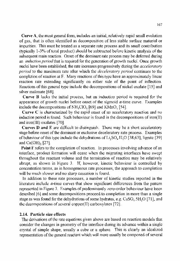
167

Curve A, the most general form, includes an initial, relatively rapid small evolution of gas, that is often identified as decomposition of less stable surface material or impurities. This must be treated as a separate rate process and its small contribution (typically 1-3% of total product) should be subtracted before kinetic analysis of the subsequent main reaction. Onset of the dominant rate process may be deferred during an induction period that is required for the generation of growth nuclei. Once growth nuclei have been established, the rate increases progressively during the acceleratory period to the maximum rate after which the deceleratory period continues to the completion of reaction at F. Many reactions of this type have an approximately linear reaction rate extending significantly on either side of the point of inflection. Reactions of this general type include the decompositions of nickel oxalate [15] and silver malonate [68].

Curve B lacks the initial process, but an induction period is required for the appearance of growth nuclei before onset of the sigmoid t~-time curve. Examples include the decompositions ofNHaC104 [69] and KMnO4 [54].

Curve C is characterized by the rapid onset of an acceleratory reaction and no induction period is found. Such behaviour is found in the decompositions of iron(II) and iron(III) oxalates [70].

Curves D and E are difficult to distinguish. There may be a short acceleratory stage before onset of the dominant or exclusive deceleratory rate process. Examples ofbehaviour of this type include the dehydrations of LizSO4.H20 [38,63], lignite [39] and Ca(OH)2 [27].

Point F refers to the completion of reaction. In processes involving advance of an interface, product formation will cease when the migrating interfaces have swept throughout the reactant volume and the termination of reaction may be relatively abrupt, as shown in Figure 3. If, however, kinetic behaviour is controlled by concentration terms, as in homogeneous rate processes, the approach to completion will be much slower and no sharp cessation is found.

In addition to these rate processes, a number of kinetic studies reported in the literature include e-time curves that show significant differences from the pattern represented in Figure 3. Examples of predominantly zero-order behaviour have been described [6] and some decompositions proceed to completion in more than a single stage as was found for the dehydrations of some hydrates, e.g. CuSOa.5H20 [71], and the decompositions of several copper(II) carboxylates [72].

2.14. Particle size effects The derivations of the rate equations given above are based on reaction models that

consider the changes in geometry of the interface during its advance within a single crystal of simple shape, usually a cube or a sphere. This is clearly an idealized representation of the general reactant which will more usually be composed of several

168

crystals and, for powders, very many crystallites having a range of sizes and shapes. Attempts have been made to allow for the influence of particle-size distributions on kinetic behaviour [73-77], but most usually it is assumed (perhaps implicitly) that all reactant particles behave similarly. Allowances for size effects, which are difficult to quantify, are most often based on numerical integration across an assumed or measured distribution of particle dimensions [78,79].

For those reactions in which a layer of product is rapidly established across all or certain surfaces and rate is controlled by inward advance of the interface, equation (7), the kinetic relationships can be calculated by geometric methods from particle- size distributions and shapes. The kinetic behaviour during nucleation and growth processes is more difficult to predict. Here the dominant controlling factor is whether or not the advancing interface can progress from one nucleated particle to a neighbouring unreacted crystallite which it touches.

2.15. Other factors influencing kinetic behaviour Kinetic observations may thus be interpreted [1-10] through consideration of

geometric factors (including particle shapes and sizes), chemical controls (bond redistribution steps) and diffusion. In real reacting systems, additional contributions which may arise include phase transitions (particularly melting), particle-size effects (discussed above), abrasion or other damage to crystal surfaces [2,11], surface impurities and irradiation. The kinetics of reactions involving the intervention of either temporary or extensive melt formation may be different from the characteristics of the same decompositions proceeding exclusively in the solid state [65-67].

The local environment can also participate in the reaction being studied. Metal containers can interact with some reactants by catalyzing the chemical change of interest, or promoting interactions between volatilized products. Gases present in the atmosphere, or remaining from a precursor step, may combine with reactant or product. A precursor step, e.g. dehydration, may also influence the reactant particle size and thus control kinetic behaviour during subsequent steps.

The molar volume of the solid product of decomposition is usually smaller than that of the reactant crystal from which it was formed and so cannot exactly fill the space previously occupied by reactant. The particles of dense nickel metal cannot fill the decomposed zones in nickel formate [80] and may be mobile across the surfaces. The active contact area may be small in comparison with the nucleus surface.

Strain may result in disintegration of reactant crystallites (e.g. KM.nO 4 disrupts vigorously during decomposition) so that changes of shapes and sizes of the active contact area may occur during the progress of a reaction. These changes can be studied by measurements of surface area at known values of tr. Interpretation may, however, be difficult because the area determined is the aggregate of both reactant and product boundary faces and may not include the interface.

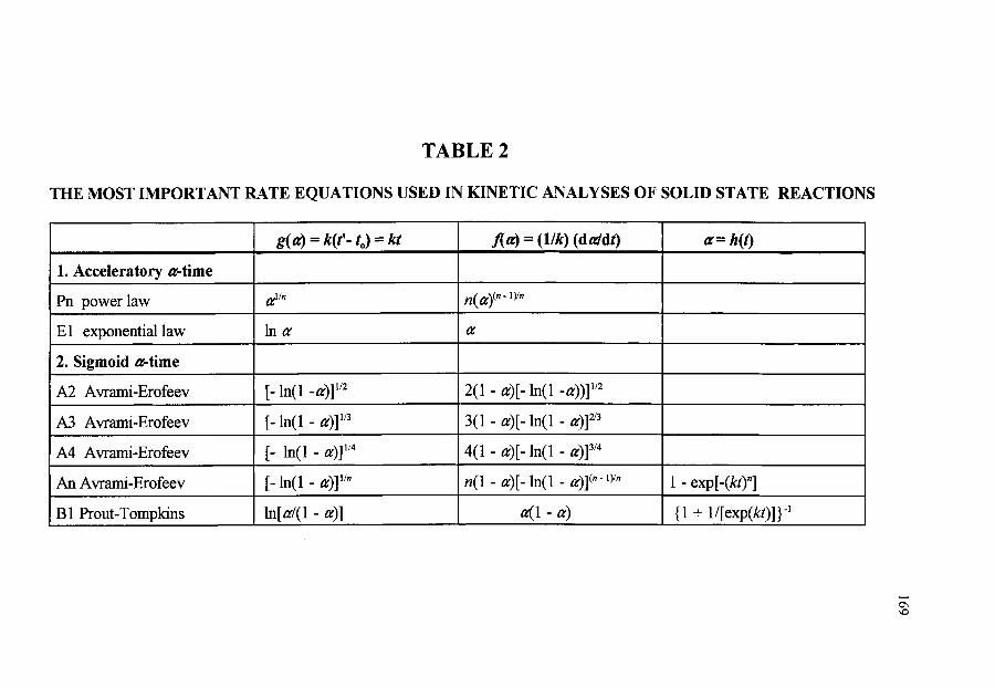
TABLE 2

g( a) = k(t’- to) = kt

1. Acceieratory a-time

Pn powerlaw

El exponential law lna

2. Sigmoid a-time

A2 Avrami-Erofeev [- ln( 1 - 4 1 1 ’ 2

[- ln(i - 4 y 3

[- ln(1 - a)yn

A3 Avrami-Erofeev

A4 Avrami-Erofeev

An Avrami-Erofeev

[- ln(i - 4 y 4

THE MOST IMPORTANT RATE EQUATIONS USED IN KINETIC ANALYSES OF SOLID STATE REACTIONS

f(a) = (lk) (daldt)

n( a)(” - 1PJ

a

2(1 - a)[- ln(1 -a))]”’

3(i - a)[- ln(i - 4 1 2 3

n(1 - a)[- ln(1 - a)](*-lYn

4( 1 - a)[- In( 1 -

_ _ _ _ ~

B1 Rout-Tompkins ln[a/(l - a)] 4 1 - 4

a= h(t)

1 - exp[-(kt)”]

{ 1 + l/[exp(kt)]}-’

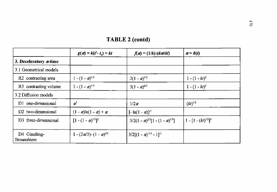
TABLE 2 (contd)

g(a) = k( t - to) = kt

3. Deceleratory a-time

3.1 Geometrical models

Aa) = (l/k) ( d d d t ) a = h(t)

~~

R2 contracting area

1 - (1 - ay3 R3 contracting volume

3.2 Diffusion models

3(1 - 1 - (1 - k t ) 3

~

D 1 one-dimensional

D2 two-dimensional

D3 three-dimensional

D4 Ginstling- B r o un s h t e in

I 1

1 - (2d3)- (1 - I 3/2[(1 - - 11-l

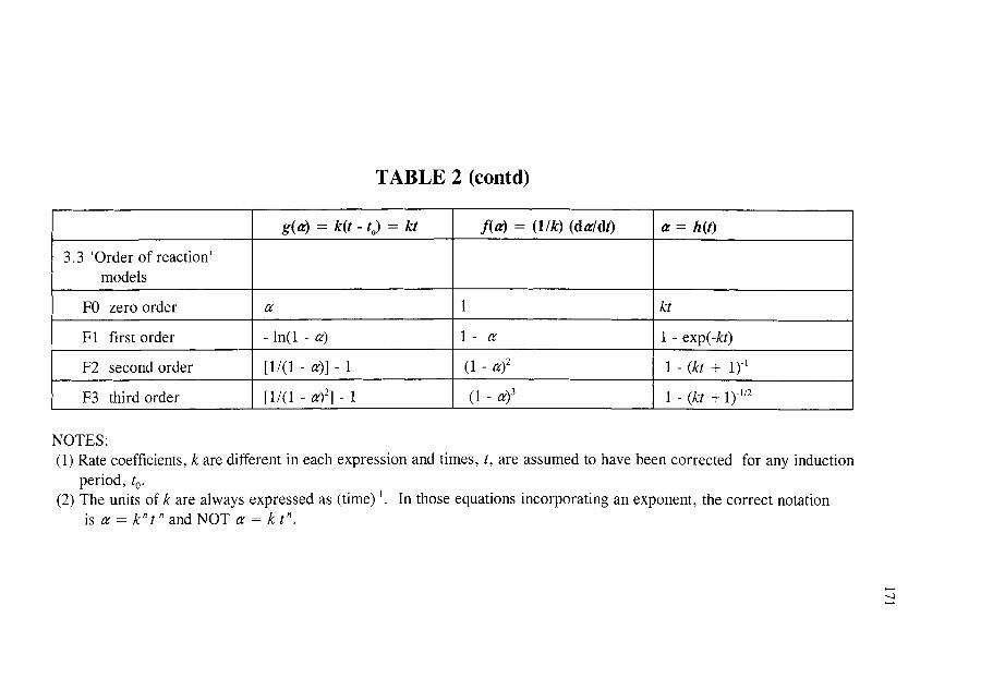
TABLE 2 (contd)

g(@ = k(t - to) = kt

3.3 'Order of reaction' models

FO zero order a

F1 first order - ln(1 - a)

F2 second order [ l / ( l - a)] - 1

F3 third order [ l / ( l - a)2] - 1

f(a) = (l/k) (da /d t ) a = h(t)

1 kt

1 - a 1 - exp(-kt)

(1 - a)* 1 - (kt + 1)-'

(1 - a)3 1 - (kt + 1)-"2

NOTES : (1) Rate coefficients, k are different in each expression and times, t, are assumed to have been corrected for any induction

(2) The units of k are always expressed as (time).'. In those equations incorporating an exponent, the correct notation period, to.

is a = k" t and NOT a = k t".

172

The reversibility of many endothermic reactions, e.g. dehydrations [29] and dissociations of carbonates [11 ], is an important kinetic control. Sintering or recrystallization of a solid product can result in changes of pore structure which can limit the rates of escape of volatile product in reversible reactions. Self-heating or self-cooling can introduce fitrther uncertainties into kinetic investigations.

3. THE MOST IMPORTANT RATE EQUATIONS USED IN KINETIC ANALYSES OF SOLID STATE REACTIONS

The rate equations that have found most general application in solid state kinetics are summarized in Table 2 and the corresponding isothermal tr-time curves are illustrated in Figure 4. These expressions are grouped according to the shape of the isothermal tr-time curves as acceleratory, sigmoid or deceleratory. The deceleratory group is fitrther sub-divided according to the dominant controlling factor assumed in the derivation as geometrical, diffusion or reaction order.

General rate equations have been proposed [81-83] to cover those listed in Table 2. Either or both are often referred to as the Sestdtk - Berggren equation:

dtr/dt = k r - e0 n

doddt = k ~m(l_ tr)" [-ln(1- tr)] p (9)

Sest~ [84] has suggested the term "'accommodation coefficient" for any additional terms, other than (1 - tr) ~ ,which are needed to modify equations based on reaction order (RO) for application to heterogeneous systems. (See also Koga [85]).

4. KINETIC ANALYSIS OF ISOTHERMAL EXPERIMENTS

4.1. Introduction Isothermal kinetic analysis requires the measurement of a set of (a, t) values for the

reaction selected for investigation at a known, constant temperature (7). These data are then tested for accuracy of fit to the equations listed in Table 2 to identify which expression represents most precisely the systematic changes of tr with time. From an observed satisfactory agreement, it may be concluded that the model used in deriving the equation so identified may portray the way in which the reactant/product interface develops geometrically during the reaction. Such interpretations may be supported by microscopic examination. For many (but not all) solid state reactions the expression giving the best fit to the a-time data is often independent of temperature, while the magnitudes of the rate constants increase with temperature.

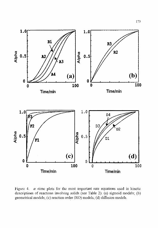
173

1.0

m

o. 0.5 ,=,m

<

,

B1

Z~ ~L3

) 0

1.0 ......

<

O I I I a

100 0 100 Time/rain Time/min

1.0

" 0 5 Q. <

// i

F1

(c) 0 100

1.0

~0 5

0 0 i00

Time/rain Time/rain

Figure 4 ec-time plots for the most important rate equations used in kinetic descriptions of reactions involving solids (see Table 2): (a) sigmoid models; (b) geometrical models; (c) reaction order (RO) models; (d) diffusion models.

174

4.2. Definit ion of ar The fractional reaction tr, by definition, changes progressively from reactants (tr

= 0.00) to products (1.00). Techniques for measuring tr that have found wide application include determinations of the changes of pressure of a gaseous product evolved during reaction in a constant volume system, changes in reactant mass, evolved gas analyses, chemical and/or X-ray diffraction measurements on partly reacted material, determination of heat evolved, etc. The parameter measured must be quantitatively and unambiguously related to the extent of the reaction of interest and be independent of contributions from any other process occurring. In practice, these requirements are usually met by establishing accurately the reaction stoichiometry, including any systematic variations in product yield with tr. Kinetic analyses increase in difficulty and decrease in reliability if data contain contributions from more than one rate process. During stepwise chemical changes the stoichiometry and kinetics of each individual stage must be analyzed separately. For example, an initial reaction (sometimes ascribed to breakdown of surface or other defective material, or desorption of solvent, etc.) may occur and be completed before onset of the main reaction.

If a reaction yields one or more gaseous products (and the evolved gas composition is constant), tr values can be calculated from the mass loss up to time t, m o - mt, related to the overall mass loss corresponding to completion of reaction, m o - me, by tr= (mo - mt)/ (mo - mr). Analogous expressions are applicable to measurements using other techniques.

Accurate determination of the final product yield is very important, particularly in distinguishing between the fit of data to alternative kinetic expressions" e.g. the contracting volume (R3)model (where the rate process ceases when the advancing interface reaches the particle centre) and the first-order (F1) model (where the rate continually diminishes) [63]. Sufficient time must be allowed for the reaction to reach completion. Hastening this process by increasing the temperature may change the product distribution and/or initiate a subsequent reaction. The total product yield measured should be compared with that expected from reaction stoichiometry. For example, Bircumshaw and Newman [75] recognized the range of different products evolved from the decomposition of NHaC10 4 and demonstrated that the yield of permanent gases (N 2 + 02), on which the kinetic measurements were based, was almost directly proportional to the mass of salt decomposed.

For reversible reactions, product yields may be misleading because reaction is progressing towards an equilibrium rather than to completion. In the decomposition of calcite, for example, the yield of CO2 does not necessarily measure the extent of the forward reaction (CaCO 3 ~ CaO + CO2) at the reaction interface if CO2 reacts with CaO elsewhere in the product mass (CaO + CO2 ~ CaCO3). Apparent product yields for this relatively simple reaction may thus represent the difference between

175

opposing processes: the dominant change of interest with, under certain conditions, a significant contribution from the reverse process. Rate data for the dissociation alone can sometimes be obtained using suitable experimental conditions to suppress the reverse step [11 ].

The products detected from any particular decomposition may be those formed in the primary breakdown step or those which result from secondary reactions. Either is acceptable for ~ measurements in kinetic studies, provided that the gas yield from unit mass of salt reacted does not change as reaction proceeds. Reports of kinetic studies do not always include exhaustive stoichiometric investigations. Identification of primary products can be useful in establishing the chemistry of the breakdown step. With increasing complexity of the reactant, the range of possible secondary processes involving volatile materials increases. Post-decomposition reactions can be catalyzed by available surfaces, such as those of the metal containers used in thermoanalytical equipment.

4.3. Data for kinetic analysis Data to be used for kinetic analysis must be accurate and reproducible, and refer

to an identified rate process. While no clear criteria have been agreed as to what constitutes reproducible behaviour, the variations in o-time values between similar experiments can be determined and reported. Experiments using different reactant masses may reveal the extents and influences of self-heating (-cooling), reverse and secondary reactions, all of which are expected to increase with the amount of solid reacting. Kinetic characteristics may be markedly changed by reactant damage or pretreatment (e.g., pre-irradiation, surface abrasion, ageing, grinding, pelleting, annealing etc.). Comparisons of reactivities of untreated and treated reactant samples may provide information that can be used in the formulation of a reaction mechanism.

Data for isothermal kinetic analyses thus consist of sets of values : vc, t; (da'/dt), t; (dvddt), a, etc., that may be interconverted. The temperature (and accuracy limits of all data) for each experiment are also recorded. Some experimental techniques may yield relatively noisy sets of or, t ; (dvc/dt), t (etc.) values and some smoothing of data may be necessary. Apparently smooth traces obtained using other techniques may contain an unknown contribution from instrumental damping.

4.4. Methods of kinetic analysis of isothermal data The initial objective in kinetic analysis is to identify which, if any, of the rate

equations in Table 2 provides the most acceptable description of each experimental (~t) data set. In deciding what constitutes an "acceptable description", at least three aspects of the problem must be considered. (i) The accuracy of the mathematical fit of the experimental values to the relationship between ec and t, (dec/d0 and t, or

176

(da~/dt) and tr, expressed by the equations listed in Table 2. (ii) The range of a~ across which the acceptable fit extends. It is acceptable that two different equations may apply across successive a ranges, but it is essential to demonstrate first that a single rate expression does not represent the overall rate process. (iii) Evidence in support of the reaction model identified as applicable must be sought through complementary experimental techniques, including optical and electron microscopy, X-ray diffraction measurements, spectroscopy etc.

The most important methods that have been used in the kinetic analysis of data from isothermal experiments include the following. (i) Examination of the linearity of plots of g(tr) (from Table 2) against time. (ii) Comparison of plots of a~ against reduced-time with curves calculated from the rate equations in Table 2. (Dimensionless reduced-time values, try, are obtained by scaling the measured time values, t, appropriately to give a common point on all curves, usually t0.5 = 1.0 at a~ = 0.5, with allowance for any induction period, so that trod = t/to.5). (iii) Comparison of plots of measured (dtr,/dt) values against reduced-time or a~ with curves given by the rate equations in Table 2. (iv) Examination of the linearity of plots of measured (dtr/dt) values against J(tr) (from Table 2). This may give better discrimination amongst kinetic models than method (i) above [86]. These methods are described in greater detail below.

The decision as to which of the available rate equations provides the most acceptable description of a given set of data requires consideration of the following: (i) the a~-time ranges over which the different reaction models can be most clearly distinguished [87], and (ii) the effects of experimental errors, including random scatter in the measured values of a~, which may reduce distinguishability.

There is no general agreement on the range of a~ over which a perceived fit can be regarded as acceptable. Carter [57] has stated that conformity between measured and theoretical values should extend across virtually the complete reaction, 0.00 < a~ < 1.00. In contrast, many literature reports describe the applicability of different rate equations during comparatively limited a~ ranges and, hence, a sequence of models is proposed to apply during different stages of reaction. The value of such interpretations is increased if the changes in behaviour can be supported by complementary evidence such as microscopic observations. Ses t~ [84] has, however, pointed out some of the dangers of attempting to correlate the results of the averaged measurements produced by thermoanalytical methods with microscopic detail for a very limited fraction of the sample, such as the surface, which may even be susceptible to damage during the investigation, e.g., by the electron beam in an electron microscope.

177

4.5. Testing the linearity of plots of g(~ against time This method is particularly suitable for preliminary testing [86]. The deviation

from linearity of g( tr)-time plots can be used to identify which equations merit more detailed consideration. The decision as to which kinetic expression provides the best fit is frequently a compromise between the maximum tr range applicable and the deviations at the limits. Such deviations may be a result of contributions from an initial reaction or errors in final yield measurement. Standard statistical criteria can be used to measure linearity across any defined tr range. These include :the correlation coefficient, r , the standard error of the slope of the regression line, s b ; or the standard error of the estimate of g(a 0 from t, Sxy, used to quantify the deviation of a set of experimental points from the calculated regression line. The inadequacies of r as an indication of fit have been pointed out [6-8]. The use of s b is to be preferred in that its value is dependent on the range of t used in the analysis.

The use of a single parameter to express the deviation of data from the least- squares line does not reveal whether such deviations are systematic or approximately random. The magnitudes and directions of the differences between data and theoretical equations can, however, be useful in identifying the most appropriate rate expression and plots of residuals, (g(tr)EXPTL - g(tr)PREDICTED), against time have been recommended [6,86]. Once a satisfactory fit has been obtained, identifying the applicable rate equation, g ( t r ) = k ( t - to), the value of k, at that recorded temperature, and its standard error can be determined from the slope of the plot.

For those rate expressions containing exponents, n , e . g . the Avrami-Erofeev equations (equation (3) and Table 2), An, plots of In[- ln(1 - tr)] against ln(t - to) should provide the most direct method for the determination of the value of n. Such plots are, however, notoriously insensitive and an error in to can significantly influence the apparent value of n. Fractional values of n have been reported [88].

4.6. Reduced-time scales and plots of ~ against reduced-time Measured time values are corrected by subtraction of to, the induction period to

onset of the main reaction (also including the time required to heat the reactant to temperature, T ). Experimental time values, ( t - to), can then be scaled by the reduced-time factor, tr~ d = ( t - to ) / ( to . 5 - to ) , where to. 5 is the time at which t r - 0.50 and k(t0. 5 - to) = 1.0.

Plots of measured values of tr against trod , for all experiments including those at different isothermal temperatures, should then all fall on a single curve. This composite curve can be compared with the calculated curve for each rate equation (reaction model) (see Figure 4) from Table 2. Such calculated curves are expressed in the form, tr = k(tr~d) and deviations (trTnEO R - trEXPTL) for each point can be determined. Comparisons of the magnitudes, and variations with tr, of these

178

differences are then used to identify the rate equation giving the most acceptable kinetic fit to the data and its range of applicability.

Any systematic change in the shape of the a~-time curve with temperature can be identified during preparation of the composite curve. The magnitude of (tr~d) 1 is proportional to the rate coefficient at temperature T, so that the reciprocals of the time scaling factors can be used as quantitative measures of k to calculate the activation energy, without the necessity for identifying the kinetic model [89].

The reference value of tr is not always selected at 0.50 because this often corresponds to the region of maximum rate and, hence, this choice introduces error into the determination of to. 5. When there is an initial reaction, or tmcertainty in the length of the induction period, it may be appropriate to use two common points for the scaling, for example [90] tr~ d = 0.00 at a = 0.20 and trod = 1.00 at tr= 0.90. Other aspects of analysis by the reduced-time method have been discussed by Jones et al. [91].

4.7. The use of derivative (differential) methods in kinetic analysis Values of daf/dt may be measured or calculated with sufficient accuracy to use

derivative methods in kinetic analyses. Some experimental techniques, e.g., DSC and DTA, provide an output signal that is directly proportional to reaction rate.

Derivative methods of kinetic analysis include plots of daf/dt against af [4], or of daf/dt against t~e d [92]. Experimental values can be compared directly with those calculated (Figure 4) for each rate equation (Table 2). A third derivative method involves testing the linearity of plots of experimentally measured rate dtr/dt values against the derivat ive functions of the rate equations, ta r ) in Table 2 [86]. This method of kinetic analysis can provide better distinguishability amongst the available kinetic expressions, particularly for the sigmoid group of equations (A2 to A4 in Table 2) and is promising for the geometric processes (R2 and R3 in Table 2).

4.8. Confirmation of kinetic interpretation The conclusion that the kinetic behaviour, g(tr) = kt, or dtr/dt = kf(a') , observed for

the reaction of interest, results from a particular geometric pattern of advance of an interface should, if possible, be confirmed by independent evidence, because geometric interpretations are often ambiguous [6]. For example, the fit of a set of (~t) values to equation A3 (Table 2) can result either from instantaneous nucleation followed by three-dimensional growth (r /= 0, A - 3 so that n - 3) or from linear nucleation accompanied by two-dimensional growth (q = 1, A - 2 and again n -- 3). The most direct method for confirming geometric deductions is by microscopic observation of the textural changes related to interface development in a sequence of partially-decomposed reactant samples.

179

5. THE INFLUENCE OF TEMPERATURE ON REACTION RATE

5.1. Overview Temperature exerts a strong controlling influence over the rates of most chemical

reactions. This influence is expressed quantitatively through the magnitude of the rate coefficient, k, which is assumed to be separable from other variables :

Rate = dtr/dt = k ( T ) C f ~ ( ~ ) ..... f.(X) (10)

where C is a constant and f~(a~) is the dependence on extent of reaction, discussed above. Examples of changes in the kinetic model f~(tr) with temperature are relatively rare [7 5] and the effect of temperature on reaction rate is usually studied on the assumption that the influences of all other contributions remain constant.

Experimentally measured rate coefficients for rate processes of very many types, including both homogeneous and heterogeneous chemical reactions (and related phenomena) have been shown to fit one or other form of the Arrhenius equation (1).

Laidler [93] has given a very clear discussion of the reasons for preferring this expression over possible alternatives. Linear relationships between In k and T, or In k and In T may be found because T, 1/T and In T are approximately linearly related over the usual relatively limited temperature interval used in most kinetic studies. Functions including additional constants such as:

I n k = a + b T 1 + cln T+ d T

are dismissed by Laidler [93] as "theoretically sterile" because their constants do not provide deeper understanding of the mechanisms of chemical reactions. Moreover, the accuracy of most experimental kinetic data is insufficient to confirm, or to exclude, a fit to such alternative functions. Thus the Arrhenius equation (1) is almost exclusively used as the functional relationship between k and T.

Irrespective of any physical and theoretical importance to be attached to the parameters A and E,, their magnitudes represent an important established method of reporting and comparing kinetic data.

5.2. Determination of the Arrhenius parameters, A and E~ The data from isothermal experiments are analysed, as described above, to yield

a set of values of k, at each temperature T~. These values are usually presented in the form of a plot of In k~ against 1/T, (referred to as an Arrhenius plot). Linear regression (with suitable weighting for the In function) yields values for (Ea/R) and In A, together with their standard errors.

180

The linearity of the Arrhenius plots should be examined to identify any curvature or discontinuities in shape. The temperatures at which any such discontinuities occur may be significant in interpreting the behaviour of the reactant. There is also always the possibility that rate coefficients may be compound terms including contributions from different rate processes such as nucleation and growth. The dimensions of k, and hence of A, should be (time)-

5.3. The significance of the Arrhenius parameters, A and E~ Arrhenius parameters, A and Ea, calculated for reactions of solids are usually

described in terms synonymous with those used in the collision theory of gaseous reactions. The activation energy is frequently regarded as the threshold or energy barrier that must be overcome to permit the occurrence of the bond redistribution steps that are essential for the transformation of reactants into products. The frequency factor, the pre-exponential term, A, is a measure of the frequency of occurrence of the reaction situation and is regarded as including the vibration frequency in the reaction coordinate. The alternative reaction dynamics representation [94] regards the activation energy as the difference between the overall average energy for all molecules concerned and the energy of those undergoing reaction. The energy difference from the threshold value may be significant, particularly for low energy reactions.

The theoretical foundations of Arrhenius behaviour are well established and accepted for homogeneous rate processes. The direct application of this model to reactions of solids has been questioned [6,95-98]. Garn [97], in particular, has emphasized that the distribution of energy amongst the immobilized constituents of a crystalline solid cannot be expressed by the Maxwell-Boltzmann function that assumes a free exchange of energy between particles in the homogeneous system. He believes that decompositions of solids involve no discrete activated state. The observed wide variations of calculated activation energies for these reactions give support to this conclusion. Energy within a solid is rapidly transferred between neighbourmg constituents so that no substantial difference from the average, which is the essential feature of any activation model, can be acquired. Bertrand et al. [98] identify E, as a composite term that includes contributions from several reaction controls such as deviations from equilibrium and thermal gradients.

The earliest detailed theoretical description of an activated reaction occurring at an advancing interface was provided by Polanyi and Wigner [99]. The rate of reaction at the interface was assumed to be controlled by the vibration frequency in the reaction co-ordinate, v, and the energy barrier to chemical change is the calculated activation energy. The critical energy for reaction can be derived through three degrees of freedom, introducing the term (2E a/RT) into the pre-exponential

181

tenn. Thus, i f Xo is the incremental linear distance of movement of the interface for trait reaction, the rate of interface advance (dx/dt) is:

dx/dt = (2 vE~/RT) x o exp (-E~/RT) (11)

The magnitude of the vibrational frequency at the surface of the reactant crystal, or at the reaction interface, is expected to be of the order of 1013 s l. Many values of A reported in the literature are comparable with this theoretical value [100], but there is a significant spread on either side. The term 'abnormal' has been used to describe reactions not consistent with the predictions from equation (11).

Young [3], examining the thermodynamic foundations of the activation process, expressed the Polanyi-Wigner equation, for an irreversible reaction, as:

dx/dt = (kBT/h) x o exp (ASC/R) exp (-AI-I~/RT)

(where kB is the Boltzmann constant). The values of A calculated for the so-called 'abnormal' reactions gave magnitudes of AS r between 200 and 500 J K -~ mol -~. Other theoretical discussions of the magnitudes of Arrhenius parameters measured for solid state reactions have been given by Shannon [101 ] and by Cordes [102].

5.4. Activation within the reaction interface The Polanyi-Wigner approach to reaction rates of solids (equation (11)) is based

on an idealized interface composed of an array of reactant species possessing identical reactivities. For many reactions this representation is probably unrealistic. Local variations ofreactivities are to be expected within the heterogeneous zone of reactant-product contact (discussed in detail above) for any particular solid. Preferred reaction at the interface has often been ascribed either to the strain associated with the region of contact between different crystal structures or/and the catalytic activity of a product surface. Intermediates, perhaps in very small total amounts, may also be present and participate in the chemical changes. Reactions within this zone, involving species that are either immobilized or possess limited translational freedom, may proceed by mechanisms which differ from those applicable to interactions between freely moving participants. Localized, neighbouring reactant structures (an enhanced 'cage' effect) may participate in processes oftri- (or even higher) molecularity or in linked sequences of consecutive reactions (immobilized chains).

Galwey and Brown [103] have suggested that the activation step may proceed through changes in occupancy of energy levels at the active reactant surfaces or interfaces that constitute the zone of chemical change. The interface levels in this proposed reaction model bear a formal similarity to the impurity levels portrayed in

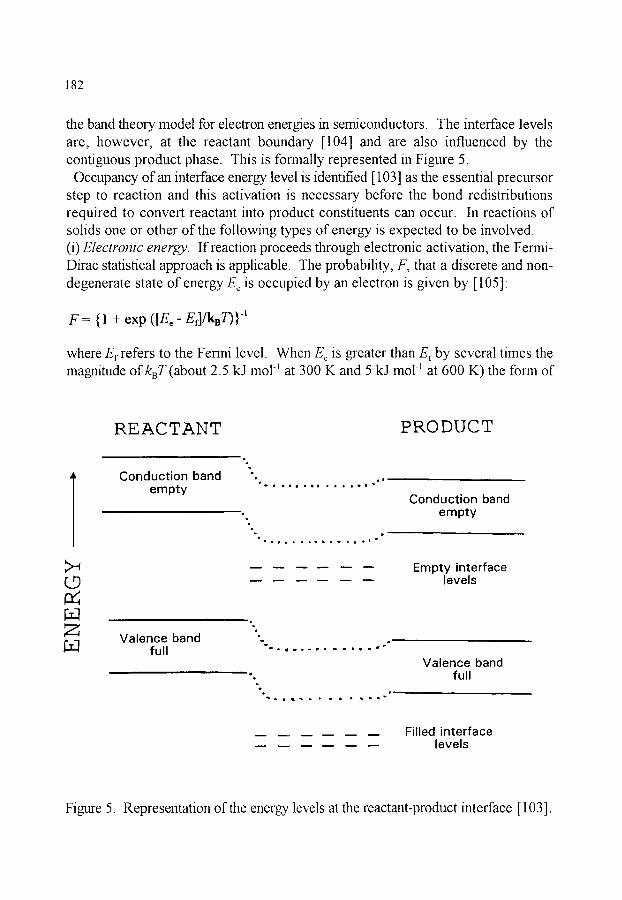
182

the band theory model for electron energies in semiconductors. The interface levels are, however, at the reactant boundary [104] and are also influenced by the contiguous product phase. This is forlnally represented in Figure 5.

Occupancy of an interface energy level is identified [103] as the essential precursor step to reaction and this activation is necessary before the bond redistributions required to convert reactant into product constituents can occur. In reactions of solids one or other of the following types of energy is expected to be involved. (i) Electronic energy. If reaction proceeds through electronic activation, the Fermi- Dirac statistical approach is applicable. The probability, F, that a discrete and non- degenerate state of energy Ee is occupied by an electron is given by [105]:

F : {1 + exp ([Eo- Er]/kBT)}-'

where Er refers to the Fermi level. When E e is greater than Er by several times the magnitude of kBT (about 2.5 kJ mol -~ at 300 K and 5 kJ mol ~ at 600 K) the form of

t0

Z

REACTANT

% q,

Conduction band " �9 , iI

I I i D i �9 I I I ii �9 i I I I empty

g �9 lJ 0 o D q u U m �9 qP Ii Q �9 I m

m . . . . .

Valence band m.,. a , . , , . F i ,, ,, 0 e . ~ full

PRODUCT

Conduction band empty

Empty interface levels

Valence band full

. - - - m m m m m

. . . . . . m u m ~ . . . . ~

Filled interface levels

Figure 5. Representation of the energy levels at the reactant-product interface [103].

183

this equation approximates to that of the Maxwell-Boltzmann equation (although it is derived from a different energy distribution). For these conditions:

F ~ exp (-[E~ - Ef]/kBT).

(ii) Vibrational energy. Product formation may result from vibration in the reaction co-ordinate, a model that has been assumed in the mechanistic discussions of many solid-state reactions, particularly dehydrations [2,6,106]. Vibrational freedom is expected to be greater at a reaction interface than for reactant constituents within more perfect regions of the crystal. If it is assumed that phonons within the solid reactant are mobile [107] and that their migration into all bonds of the material comprising the crystal boundary is unrestricted, then the energy distribution function, n(w), in this zone can be expressed by Bose-Einstein statistics as:

n(w) = {exp(ha~/2n kBT)-I }-1

where to is the angular frequency of the lattice mode. At larger energies, when h w >> 2nkBT, the function decreases exponentially, this expression again approximates to the Maxwell-Boltzmann relation [108] :

n(co) ~ exp (- h~o/2n kBT)

The energy distributions for the most energetic quanta, significantly above the Fermi level, are thus expressed for electrons (through Fermi-Dirac statistics) and for phonons (through Bose-Einstein statistics) by a function that approximates closely to that given by Maxwell-Boltzmann statistics. From consideration of activation energy requirements that are large compared with kBT, the distributions of either electronic or thermal vibrational energy can thus be expressed to a good approximation by a function that is analogous to that given by the Maxwell- Boltzmann treatment. This provides a theoretical explanation for the fit of k , T data for reactions of solids to the Arrhenius equation [103]. The frequency factor, A, represents the frequency of occurrence of the reaction situation/(unit area of interface) and includes the vibration frequency in the reaction coordinate.

Other influences may be incorporated into equation (10) [97], such as the partial pressures of gases involved, heat transfer, etc., through additional terms that are assumed to be separable from all other dependencies. If such terms are assumed to be constant, they may be implicitly incorporated into the frequency factor, A.

The structure of the reaction zone will influence the band theory representation of interface levels, Figure 5. If the overall reaction is accompanied by little structural reorganization, as, for example, in topotactic processes [30,31 ], the band structure

184

may be only slightly modified, but interface levels associated with the species undergoing bond redistributions may be created. Interfaces in reactions involving greater structural reorganization may incorporate more mobile species. The above model portrays the interface energy level as a feature of the solid, associated with an active zone, that participates in the controlling step of a solid state reaction. If, however, the chemical change occurs within a melt, even if the melting is localised between solid reactant and solid product, this is a homogeneous reaction and the Arrhenius parameters have their customary interpretation.

5.5. The compensation effect The literature contains many reports of the fit of calculated Arrhenius parameters

for the decompositions of solids to the compensation equation [6,109]:

lnA = aE, + b (12)

where a and b are constants. This pattern of behaviour is described as compensation because, in a set of data exhibiting this trend, the decrease in reaction rate expected to result from an increase in activation energy, E,, is offset by an increase in the magnitude of In A. This is also known as the isokinetic effect because, for the set of (A, E,) values that fit equation (12), there exists a temperature, Ix, at which all rate coefficients are equal. For many reactions, the value of TK is at, or within, the temperature ranges of the kinetic measurements exhibiting the compensation behaviour.

Two classes of phenomena have been given the label "compensation effect". (i) A series of closely related, but not identical, reactions for which the Arrhenius parameters, determined by similar experimental procedures, conform to equation (12). (ii) A series of closely related, but not identical, experiments on a single chemical reaction, where the differences in the experimental conditions, including the physical state and history of the solid reactant, may result in a relationship of the form of equation (12) between the apparent Arrhenius parameters.

Although many theoretical explanations for compensation behaviour have been proposed, none has received general acceptance. Aspects of the appearance of compensation phenomena in thermoanalytical data have been recently reviewed by Koga [109].

185

6. KINETIC ANALYSIS OF NON-ISOTHERMAL EXPERIMENTS

6.1. Literature The literature concerned with non-isothermal kinetics (NIK) is extensive. A scan

of Chemical Abstracts covering the interval from January 1967 to May 1995 showed that there were 10 675 papers which referred to "thermal analysis", and 2292 papers dealing with "nonisothermal kinetics", 63 of which were classified as general reviews. Not all of the non-isothermal kinetic papers refer directly to thermoanalytical measurements, but they are of potential relevance. 208 papers referred to "programmed temperature". The literature is thus vast and the account given here must be selective. Several special issues of Thermochimica Acta provide excellent reviews of the development of the "state of the art" [7 (1973) 447-504; 110 (1987) 87-158; 203 (1992) 1-526]. The Special Issue honoring Professor J.H. Flylm [203 (1992) 1-526] includes a philosophical introduction by Sestak and Sestfikov~i. Reports of the workshops of the ICTAC Kinetics Committee have appeared in Thermochimica Acta [110 (1987) 101; 148 (1989) 45; 256 (1995) 477]. Sestfik [110] has discussed the early development of the literature on NIK and also provided [111] a useful glossary of kinetic terminology. Carr and Galwey [112] have reviewed some aspects of the literature on NIK in the wider context of the literature on decomposition of solids.

6.2. Introduction As in isothermal kinetic studies, the analysis of NIK data is directed towards

identifying the rate equation (Table 2) and Arrhenius parameters which most satisfactorily describe the observations. In a typical NIK experiment the temperature of the environment of the reactant sample is systematically changed according to some defined programme (usually, but not necessarily, a linear increase of T with time). The value of all kinetic conclusions ultimately depends on the accuracy of the original measurements of a, t and T (or terms from which these can be derived, (da~/d0 or (dec/dT), etc.). It is important that a is defined for an identified stoichiometric reaction. Changes in kinetic characteristics during the course of a non-isothermal experiment are probably more easily overlooked than in a series of isothermal experiments. Possible changes include variations in the magnitudes ofA, E, and the form of the kinetic expression, g(a~) orf(ec). There may also be changes with temperature of the reaction stoichiometry, the product yields and the secondary reactions between products. The relative contributions from reversible, concurrent and consecutive reactions will also generally vary considerably with temperature.

Amongst the very strong criticisms of NIK are those of Boldyreva [113] who states that the only argument in favour of NIK studies is their rapidity compared with

186

isothermal studies. In certain technological situations, e.g. processes carried out under non-isothermal conditions, the rapidity with which the information is obtained and the similarities between laboratory and process conditions "may compensate for the absence of a physical meaning". She also criticizes the use of the NIK approach for the determination of kinetic parameters and reaction mechanisms in the absence of more direct studies.

Maciejewski [114], in a characteristically provocative article, questions the usefulness of kinetic data for solid state reactions, under the title "Somewhere between fiction and reality". He rightly warns of the dangers of regarding measured kinetic parameters as being characteristic of the compound being studied, without reference to the experimental conditions used.

Isothermal and non-isothermal methods provide complementary routes to a common objective, the determination of the kinetic parameters for a selected reaction. Isothermal studies represent one limit of the numerous possibilities for temperature changes which can, in principle, be employed in non-isothermal studies. Both approaches have their advantages and their disadvantages and attempts to downplay or ignore the importance of either approach are unproductive.

In 1979, J. Sestak, who has made many important contributions to both the philosophy and the practice of NIK studies, published [110] a series of thought- provoking questions on the subject and many of these queries remain unresolved.

Many papers on NIK include kinetic analyses using rate equations based on concentration dependence of reaction rate (Table 2, F0 to F3). These are analogous to homogeneous reaction behaviour and, if a solid state reaction is believed to occur, the fit of data to the geometric models should be tested. Conclusions should be confirmed by use of suitable complementary techniques, such as microscopy, whenever possible.

Non-isothermal measurements may enable steps in a sequence of of chemical processes to be distinguished in what might otherwise be regarded as a single reaction.

6.3. The "inverse kinetic problem (IKP)" The usual starting point for kinetic analysis of non-isothermal data is:

dtr/dT - (dtr/dt).(dt/dT) = (dtr/dt).(1/fl) (13)

where t = (dT/dt), is the heating rate. Even this step has aroused continuing debate [ 115-117]. Kris and Sestfik [ 118] have pointed out that both a~ and T may vary with position in the sample and that heat and mass transport effects are seldom taken into consideration, even in DTA where the real temperature deviation from the programmed temperature is recorded [119].

187

It is almost invariably assumed that the Arrhenius equation is applicable [103] to the rate processes being studied, so that equation (13) may be expanded to:

dtr/dT= (1/fl).(dtr/dt) = (A/fl) exp(-E~/RT)f(tr) (14)

wheref(t 0 is a kinetic expression (see Table 2). A central problem of NIK is the integration of the right-hand side of equation (14). Separating the variables leads to:

dtr/J( tr) = (A/fl) exp(-E a/RT) dT

Integrating between the limits, a~ = 0 at T = T O and a~ = a~ at T = T

o.~ ~ ~oc))-' dtr = rol r (A/fl) exp(-E~/RT) dT

g(ec) = To.~ r (A/fl) exp(-E~/RT) d T = oJ "r (A/fl) exp(-Ea/RT) dT (15)

(because of T~ (A/fl) exp(-E~ /RT) dT = 0).

Kris and Ses t~ [118] emphasize that the above separation of the variables a~ and T is not justified when significant self-heating or self-cooling occurs.

For any reaction under investigation, experimental measurements, obtained at a known heating rate, fl, are converted (see section 4.2) to values of a~ and/or doddt at temperatures T.

Militk~ and Sestfik [120] have expressed the "inverse kinetic problem" (IKP) as the necessity to determine up to six unknown constants, b l, b2, b3, dl , d2 and d3 in the expression

dtr/dt = bl T b2 exp(-b3/RT) tr d~ (1- tr)d2 [-ln(1 - tr)] d3 (16)

Often the analysis uses the rate equations familiar from homogeneous kinetics, in that dl and d3 are taken to be zero, so that f(a 0 is assumed to be (1 - a~)" and n (= d2), the apparent "reaction order" (RO), becomes the unknown. The simpler form of the Arrhenius equation, i.e. b2 = 0, is generally used because a temperature dependent term in the pre-exponential factor [121,122] only adds a ft~her adjustable parameter. When d3 is zero, J(a 0 = a~ d~ (1 - a~) d2, is known as the Sestfik-Berggren (SB) equation (9) (see section 3), or if d l = d2 -- 1, as the Prout- Tompkins or Austin-Rickett equation (see section 2.9).

It is also usually assumed that a single rate expression, f(a 0 or g(a0, applies over a wide range of ar values (ideally 0 < a~ < 1.0) and that the values of the Arrhenius

188

parameters, A and E,, are constant over at least that o~ range. If the rate expression and/or the Arrhenius parameters vary with a~, i.e. the reaction mechanism changes (see section 6.15 below), the kinetic analysis becomes very much more complicated and hence the results of such analyses become less reliable and less useful. By allowing for such variations, one is effectively adding further adjustable parameters to the analysis and Churchill [123] has warned against such practices. Budrugeac and Segal [124] have, for example, used the assumption that E, may be a function of a~ of the form:

Ea=Eo + E 1 ln(1-a~)

where E0 and E~ are constants, together with the assumption of a compensation relationship between E, and A (section 5.5). This effectively introduces four more adjustable parameters.

Whether rate measurements from a single experiment extending across a range of temperatures are, in principle, capable of providing a complete kinetic analysis (the form off(a) or g(a0 and the magnitudes of E, and A) has been debated. Agrawal [125] discussed some of the problems of the uniqueness of the derived parameters. Problems occur whenever attempts are made to determine more than two parameters from a single curve. Use of kinetic expressions containing multiple a terms also leads to non-unique kinetic parameters, as does the existence of an apparent compensation effect (section 5.5). Criado et al. [126] have shown that the same TG curve can be generated using three different kinetic models with different Arrhenius parameters.

Vyazovkin and Lesnikovich have provided two interesting reviews [127,128] of methods and principles for the solution of the IKP (which also serve as a very useful entry to the Russian literature). They emphasize that all inverse problems have ambiguous solutions. The ambiguity may arise from attempts to determine too many unknown constants from limited data, or appear when a set of experimental data can be alternatively described by different formal models and kinetic constants.

Some workers choose to describe their experimental results in terms of partial application of various models over different regions of time or temperature and others prefer approximate agreement with a single model (or very limited number of models) over as wide a range of a~ as possible, allowing for deviations from ideality arising from factors such as variations in particle size and shape. The ideal analysis uses as few adjustable parameters as possible.

Segal [117] has suggested a classification of NIK methods based on the extent of the (a~, t, T) interval which is subjected to analysis. Three methods are distinguished: (i) integration over all (a~, t, 7) values; (ii) integration over small intervals of (a, t, 7); and (iii) the use of point values of (~ t, T) data.

189

M~ilek [129] has given an excellent account of the correlation between kinetic parameters and the kinetic models from which they are derived. As a consequence of the correlation between E~ and A (the so-called "compensation effect" (section 5.5)) a TA curve can be described by a kinetic model and an associated apparent E~ value, instead of the true model and true E~ value, where:

(E~)~pp = F. (E~) ~

and the multiplying factor, F, is characteristic of the true kinetic model. Values of such factors are given.

6.4. Experimental approaches The most common experimental approach is to maintain the heating rate, fl, at a

suitable constant value, as is done in most commercial instruments, but other programmes have been employed [130-132]. Reading et al. [133] have developed a technique referred to as constant rate thermal analysis (CRTA) in which the the sample is heated in such a way that reaction takes place at constant rate (see Chapter 8), and Ortega et al. [134] have extended this idea to control the temperature so that the reaction proceeds at a constantly increasing rate (acceleration).

A temperature-jump or step-wise programme has also been suggested [135,136] in which, during a single experiment, the temperature is rapidly changed ("jumped") from one value to another and the rates at the two (or more) temperatures are measured and used to calculate Arrhenius parameters for that particular tr value. This method assumes that a does not change significantly during the time taken to measure the two rate values.

Modulated temperature DSC [137-141] (see Chapter 5), in which the programmed temperature follows small regular oscillations, is a promising technique for distinguishing reversible and irreversible contributions to the thermal behaviour of samples and kinetic applications are awaited.

Agrawal [125] points out some of the practical problems of non-isothermal kinetic experiments, particularly temperature calibration in TG where the difference between the measured and the correct sample temperature may be large. He recommends a temperature range of at least 70 K for the estimation of Arrhenius parameters. Biader Ceipidor et al. [142] have provided an interesting series of papers dealing with simulation of TG and DSC/DTA curves with allowance for heat transfer and other experimental parameters.

In spite of the division of experimental approaches into isothermal and non- isothermal methods of kinetic analysis, Criado et al. [126] have pointed out that the alternative types of experimental conditions all represent approximations to the true

190

sample temperature. Garn [143 ] has warned that factors such as heat transfer from the fin-nace to the sample, complicated by self-cooling or self-heating of the sample during reaction, and the influence of evolved product gases trapped in the vicinity of the sample on the rates of reversible reactions, all make increased contributions under non-isothermal conditions. Other difficulties encotmtered during kinetic analysis of the results of isothermal experiments, such as the fitting of data across as wide a range of a~ as possible and distinguishing amongst kinetic expressions with similar forms, are also magnified under programmed temperature conditions. Whatever the temperature programme, kinetic studies can benefit from supporting analytical [144] and microscopic [145,146] evidence concerning reaction stoichiometry, phase transitions and textural changes.

6.5. The shapes of theoretical thermal analysis curves The shapes of the theoretical isothermal ~, t curves for the various kinetic models

listed in Table 2 are illustrated in Figure 4. Distinguishing amongst these models, even under isothermal conditions [86,87], is often difficult. Under non-isothermal, i.e. linear programmed temperature, conditions, the shapes of these curves are considerably altered and theoretical ~, T curves for various models are illustrated in Figures 6(a), (b) and (c). (These curves were constructed using the Doyle approximation [147] for the temperature integral, p(x), see Table 3 below.) The models based on apparent order of reaction, n, (also including fractional values) i.e. F1, F2, F3, R2 and R3, Figure 6(b), are difficult to distinguish at low values of ~. Distinguishability improves for higher orders at higher values of ~. The diffusion models, D 1, D2, D3 and D4, give generally lower onset temperatures and flatter curves (i.e., extended temperature intervals) (Figure 6(c)) than the nth-order group, while the Avrami-Erofeev (JMAEK) models, An, (Figure 6(a)) have higher onset temperatures and steeper curves. Figures 7(a), (b) and (c) show the derivative curves corresponding to the integral curves given in Figure 6.

For a fixed model, e.g. R3, the influences of the other variables, the heating rate t , the pro-exponential factor, A, and the activation energy, E,, are shown in Figures 8, 9 and 10, respectively. Elder [148] has provided similar curves and Zsak6 [149] has shown similar influences for the first-order (F 1) model. Although the F 1 model is not a very realistic representation, it is often assumed to apply as an approximation. Figure 8 shows the regular effect on the theoretical R3 curve of doubling the heating rate in the range fl = 1 to 16 K min-~. Decreasing the pre- exponential factor by factors of ten in the range A = 1017 to i 0 ~3 s -1 also affects mainly the onset temperature and the acceleratory portion of the curves, Figure 9, with the remaining segments being almost parallel. Very similar behaviour is observed for curves in which the activation energy increases in steps of 5 kJ mol ~ as shown in Figure 10.

191

The overall shape of the thermal analysis curve (a, T) is thus mainly determined by the kinetic model, while the position of this curve on the temperature axis is controlled by the values of E~, A and, to a lesser extent, the heating rate ft.

6.6. Classification of methods of NIK analysis Methods used for the analysis of non-isothermal kinetic data can be classified as

derivative (ICTAC preferred term), also referred to as differential methods, based on the use of equation (14), or integral methods, based on the use of equation (15). Vyazovkin and Lesnikovich [127] criticized this conventional classification because it refers to the type of experimental data used. They suggested instead a classification based on the method of calculation of the kinetic parameters, which involves either "discrimination ", i.e. identification of the kinetic modelf(t~) or g(a 0, or a "non-discriminatory" method. Methods involving discrimination can be ft~her sub-divided into methods of "analysis ", where a single model is sought to describe the experimental data, or methods of "synthesis", where several models are combined to give a better description of the data. A further sub-classification could be based on the manipulation of the kinetic expressions into forms suitable for testing the quality of the fit by methods of linear regression or, less commonly, non- linear regression.

The three (or more) unknown features of reaction, A, E~ and the form off(a) or g(a 0, can only be estimated from a single dynamic (i.e. a, T) experiment if assumptions are made about the form of the rate expression. It is often assumed, without appropriate justification, that the reaction of interest can be regarded as a first-order (F1) process (f(a~) = (1 - t~) and g(t~) = - ln(1 - a~)). There has also been extensive discussion [150,151 ] of the applicability under non-isothermal conditions of the JM K equation (see section 2.7), which is based on a model that includes contributions from the distinct processes of nucleation and of product growth which may have very different temperature dependences.

It is more usual to calculate kinetic parameters from two or more otherwise identical dynamic experiments at different heating rates, although methods have been suggested for combining information from dynamic and isothermal experiments. Experiments at different heating rates can result in different temperature gradients in the samples which unless corrected for may lead to erroneous kinetic conclusions.

192

- q r -

___J

- r -

3 [ . . 0

0 . 5

O

1 . O

0 . 5

O

(a)

A 2

3 0 0 3 1 5 T / K

R 3

(b)

2 8 0 3 2 0 T / K

A3

A4

330

F3

360

- - r -

____!

1 . O

0 . 5

O

(C) D4

D 1

D 2

2 5 0 2 9 0 3 3 0

T / K

Figure 6. Theoretical a~, temperature curves for various kinetic models. Heating rate, f l= 1~0 K min-~; A = 1.9 x 10 ~s min -~ and E, = 100 kJ mol -~. (a) the Avrami-Erofeev (JMAEK) models, An, (b) models based on apparent order of reaction, n, and contracting geometry

i.e. F1, F2, F3, R2 and R3, (c) diffusion models, D 1, D2, D3 and D4. Note the different temperature intervals across which the expressions apply.

193

0 .18

0.09

0

0.08

0.04

O

(a) A.

3 0 0

A 3

315 330 T / K

(b) ~~ R 3

260 310

-I- / I<

F1

F2

360

0.06

0.03

O

(c) /

D 2

D 3

2 5 0 2 9 0 3 3 0

T / K Figure 7. Theoretical doddt, temperature curves for various kinetic models. Heating rate, r = 1.0 K min~; A = 1.9 x 10 ~5 min ~ and E~ = 100 kJ mol -~. (a) the Avrami-Erofeev (JMAEK) models, An, (b) models based on apparent order of reaction, n, and contracting geometry

i.e. F1, F2, F3, R2 and R3, (c) diffusion models, D1, D2, D3 and D4.

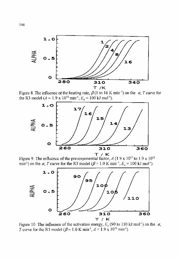
194

i.o I

zIZ 1:2_

0..5 16

0 �9 i i I i

280 310 340

-I- / K Figure 8. The influence of the heating rate, fl (1 to 16 K min-1) o n the a~, T curve for the R3 model (A = 1.9 x 10 ~5 minl ; E~ = 100 kJ mola).

2 . . 0

. - 17 16

" 15 14 <~ -r- " 0..5 - --J 13 <~

oF 260 310 360

T / K Figure 9 The influence of the pre-exponential factor, A (I 9 x ] 0 ~7 to 19 x 10 ~3 min -~) on the a~, T curve for the R3 model (f l= 1.0 K min ~, E~ = 100 kJ mol~).

- 1 " -

.__1 <1:

1 ~

0 . . 5

0

m .

2 6 0 |

3 1 0 3 6 0

T / K Figure 10. The influence of the activation energy, E~ (90 to 110 kJ mol ~) on the a~, T curve for the R3 model (fl = 1.0 K min -~, A = 1.9 x 1015 minl).

195

6.7. Isoconversional methods When more than one set of experimental results is available, the unknown form of

the conversion functionfl a~) or g(tr) may be eliminated by comparing measurements made at a common value of a under the two sets of different conditions. These isoconversional methods are thus "model independent" or "non-discriminating" techniques for determining the Arrhenius parameters [89]. These methods have been recently actively promoted by Vyazovkin and Lesnikovich [127,128].

To avoid discarding potentially significant information, the parameters obtained from isoconversional methods may be used with the original data to determine the kinetic model, which Sestfik [110] regards as the major goal of kinetic studies, although this is often not done.

Isoconversional methods [128] rely on the general equation:

ln(da/dT)fl = ln(A/f(a')) - Ea/RT

The numerical values of E~ and of the combination (A/f(a0) can be determined unambiguously, but the value of A depends upon the model chosen, t a0. The relationship between A and f(a~) is a "complementary description" [128]. The treatment also assumes that the modelf(a 0 remains the same over the whole range of ec. A main advantage of isoconversional methods is identified [128] as being the calculation of consistent activation energies which are in good agreement with values from isothermal experiments. A disadvantage is that the value of A cannot be determined without knowledge of the model f(a~).

6.8. Plots of ar against reduced temperature By analogy with the use of plots of a against reduced time in isothermal kinetic

analysis, described in section 4.6, Meindl et al. [152] have suggested plots of ec against reduced temperature. Vyazovkin et al. [153] have compared these isothermal and non-isothermal methods. The shapes of plots of a~ against reduced temperature are less sensitive to the form of the kinetic model than are plots of a~ against reduced time. The isothermal and non-isothermal curves are not related, as has been suggested [154], simply by the heating rate, fl = dT/dt, but the times, t, corresponding to an isothermal curve at T = Ti~ o are obtained from measurements of tr and T at heating rate t , by use of the relationship:

t = A 0I r exp(-E,/RT) dT / [flAis o exp(- Ei~ o/RTiso) ]

or the quantity, t*, proportional to the time, where:

t*= of r exp(-E~/RT) dT

196

6.9. A selection of derivative (or differential) methods (first derivatives) These are methods based on equation (14), which can be written in a variety of

forms, for example:

In [(dtr/dT)/f(tr)] = ln(A/f l ) - (Ea/R)(1 /T) = y (17)

ff assumptions are made about the form offltr), then the slope and intercept of a plot of y against (l/T) may be used to determine the values of E, and A, respectively. Vfirhegyi [155] has pointed out that the sensitivity of the left-hand side of equation (17) is inversely proportional to dtr/dt. Thus, tmless appropriate weighting factors are used, the derived kinetic parameters will be extremely sensitive to the data at the onset and the end of the thermal analysis curve and have decreased sensitivity in the vicinity of the maximum dtr/dt, where most of the reaction proceeds.

If several sets of data are available, e.g. a series of thermal analyses at different heating rates, fl~, various different mathematical procedures may be applied. Friedman's method [156] is to plot ln(da~/dt)~ against 1/Ti, at the same value of tr i at different heating rates fli (or different isothermal reaction temperatures, Ti). The parallel lines obtained have slopes = -E~/R and different intercepts = ln[A f(tr)i ]. A value for A is obtained by extrapolation of a plot of the intercept against ~ to ~ = 0. Carroll and Manche [157] in a procedure otherwise identical with Friedman's above, suggested plotting ln[fl (dtr/dT)] against 1/T. A fiLrther variation on this approach, suggested by Flynn [158], was to plot T i In (dtr/dt)i against T i for the same value of ~ at different heating rates fli. The lines obtained have a common intercept- -E~/R, but different slopes = ln[A J(tr)i ].

The widely used Freeman and Carroll [159] method assumes f( tr) = (1 - tr) ~ and considers incremental differences in (dtr/dT), (1 - tr) and (l/T) which leads to the expression:

Aln(dtr/dT) = n Aln(1- t r ) - (E~/R) A(1/T)

This expression can be used to determine the value of E~ by plotting either:

[Aln(dtr/dT)/Aln(1 - tr)] against [A(1/T)/Aln(1 - tr)]

o r

[Aln(dtr/dT)/A(1/T)] against [Aln(1- tr)/A(1/T)]

Sestfik et al. [160] have discussed some improvements to this method, including the extension to other rate equations (Table 2). Criado et al. [161] have

197

demonstrated that the Freeman and Carroll treatment does not allow an nth order kinetic equation to be distinguished successfully from other kinetic models. This was confirmed by Jerez [162] who pointed out the large errors involved in the regression procedure, and suggested a modification in the method used to calculate E~ and n involving the use of the point at which the rate is a maximum and the centre of gravity of the cluster of experimental points.

Van Dooren and Muller [163] have examined the effects of sample mass, particle size and heating rate on the determination of n, E~ and A from DSC data using the Freeman and Carroll procedure. Plots using points from the complete DSC peaks were curved, so different sections of the DSC peak were considered separately. Different values of the kinetic parameters were obtained for the different sections of the peak and these values also varied with sample mass, particle size and heating rate.

6.10. A selection of derivative (or differential) methods (second derivatives) Several approaches involve use of the second derivative of equation (14), or the

version withf(u) = (1 - try, with respect to temperature [149,160] or with respect to a [149], in spite of the problems of obtaining accurate values of second derivatives. Differentiation of:

dtr/dT = (K/J) exp(-E~ IRD (1- 0J') n (18)

gives:

d 2 a:/dT 2 = (da:/dT)[(E~/RT2) - n(dtf fdT)/(1- aO]

and, because this derivative must be zero at the inflexion point of a TG curve or the maximum of a DSC peak, it follows that:

g a/(RT2maO - - (da'/dT)m~x (n/(1- trm~,,)) (19)

from which E~ may be calculated if n is known and Tm~x, (da'/dT)m~x and trm~x have been measured [164].

Combining equations (18) and (19) gives:

(A/fl) exp(-E]RTm.x) n(1- ~maJ n-l "-- Ea/RTmax 2

Because (1 -/~'mD is a constant for a given value of n, the Kissinger [165] method of obtaining a value for E~ is to plot ln(fl/TZmJ against 1/Tm~x for a series of experiments at different heating rates, fli. The slope of such a plot is -Ea/R. Augis

198

and Bennett [166] have modified the Kissinger treatment for use with the Avrami - Erofeev (or JMAEK) model (An, Table 2), which applies to many solid-state reactions. They plot ln(fl/(Tm~x - To)) against 1/Tm~ x where T O is the initial temperature at the start of the heating programme, instead of ln(fl/TEmax) against 1/Tm~ x. Elder [148] has generalized the Kissinger treatment to make it applicable to the full range of kinetic models. The generalized equation is:

ln(fl/Tm,Z +:) = ln(AR/E,) + In L - ga/RTma x

where m is the temperature exponent of the preexponential term in the modified Arrhenius equation (often taken as zero) and L = - fl%~x)/(1 + mRTm~x/E~). This correction term was found to be relatively small, but helps in distinguishing between similar models. Llopiz et al. [167] have derived correction terms for the usual range of kinetic models. The values of E, obtained were not very sensitive to the incorrect choice of model [ 148].

Although originally developed as an integral method, the Ozawa treatment [168] is also applicable to derivative curves and is similar to the Kissinger method. In the Ozawa method ln(fl) is plotted against 1/Tm,x and the slope of this plot is again -E~/R. Van Dooren and Muller [163] found that both sample mass and particle size could influence the calculated magnitudes of the apparent kinetic parameters determined from DSC experiments using the methods of Kissinger and of Ozawa. The two methods gave similar values for E~ with a slightly lower precision for the Kissinger method. It was suggested [163] that temperatures at tr = 0.5 (half conversion) should be used in place of Tm,x. The application of this approach has been reviewed by Tanaka [169].

The Borchardt and Daniels method [170,171], originally developed for DTA studies of homogeneous liquid-phase reactions, involves calculating the rate coefficient, k, from the expression [172]:

k = [(JSV/mo)"-' (C dAT/dt + JAT)] / [(J(S- s ) - CAT]"

where Vis the volume of the sample, m o the initial amount of sample in moles, S is the total DTA peak area, and s is the partial area up to the time t at which the peak height AT and the slope dAT/dt are measured. J is the heat transfer coefficient and C is the total heat capacity of the sample and the holder. Because of the problems of obtaining values of J and C, the assumptions are made [ 171 ] that n = 1 and that C(dAT/dt) and CAT are small compared with the terms to which they are added (or from which they are subtracted). It follows that:

k= t T/(S-s)

199

For DSC the equivalent form would be"

k = (dH/d t ) / (S - s)

where H is the enthalpy, so that (dH/dt) is the DSC signal. The values of k obtained are then used in a conventional Arrhenius plot. Shishkin [173] has discussed the similarities between the Borchardt and Daniels and the Kissinger approaches.

There have been discussions [110,172] of the reliability of kinetic information obtained from DTA where the sample temperature may deviate significantly from the programmed temperature. Hugo et al., [174] have discussed the corrections required to the baseline and for the time lag inherent in the kinetic analysis of DSC data.

Another method based on a second derivative is that of Flynn and Wall [175]. Equation (16) is rearranged (with b2 = d l = d3 = 0) as:

TE(dtr/dT) = (AT2/fl) exp(-E a/RT) (1- a')"

and differentiated with respect to a~, to give:

d[T 2 (dtr/dT)]/dtr = ( E . / R ) + 2 T + [n/(1 - g)] [dtr/d(1/T)]

At low values of tr, the last term on the fight-hand side is negligible and even 2T << E~/R. By use of finite differences instead of the derivative

A[T (da /d73] /aa = +

where Ta, o was the average temperature over the interval. The value of E~ was then calculated from the slope of a plot of A[T2(dtr/dT)] against Aoc for the early stages of the reaction only.

6.11. Shape index M~ilek [176] expanded the earlier suggestions of Kissinger [165] on the use of a

"shape index" (S) in kinetic analyses of thermoanalytical (TA) curves. S is defined (Figure 11) as the absolute ratio of the slopes of the tangents to the derivative TA peak at the inflection points on the rising and falling regions of the curve, i.e.,

S = (d 2tr/dt 2)i = 1 / ( d 2 ~r/dt 2)i = 2

The value of S and the temperatures 7'1 and T 2 at the inflection points are readily determined. Calculation of the value of S expected for a theoretical rate equation

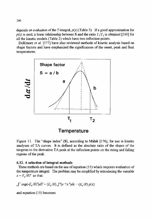
200

depends on evaluation of the T integral, p(x ) (Table 3). If a good approximation for p(x) is used, a linear relationship between S and the ratio T]/T 2 is obtained [160] for all the kinetic models (Table 2) which have two inflection points.

Dollimore et al. [177] have also reviewed methods of kinetic analysis based on shape factors and have emphasized the significances of the onset, peak and final temperatures.

Shape factor / I

i I

S =

4 I i l

i

I

III

T 1 T 2

Temperature Figure 11. The "shape index" (S), according to M~ilek [176], for use in kinetic analyses of TA curves. S is defined as the absolute ratio of the slopes of the tangents to the derivative TA peak at the inflection points on the rising and falling regions of the peak.

6.12. A selection of integral methods These methods are based on the use of equation (15) which requires evaluation of

the temperature integral. The problem may be simplified by introducing the variable x = E ~ / R T so that:

ol r exp(-E./RT)dT = (E. /R) xI'(e -X/x 2)dx = (E. /R) p(x)

and equation (15) becomes"

201

g( eO : (A& /Rfl ) p(x) (20)

Criado et al. [178] have surveyed the 'integral' methods of NIK developed from the 1951 paper of Van Krevelen et al. [179]. Zsak6 [149] has suggested sub- classification of integral methods on the basis of the means of evaluation of the temperature integral in equation (20). The three main approaches are: (i) use of numerical values of p(x); (ii) use of series approximations for p(x); and (iii) use of approximations to obtain an expression which can be integrated.

Tables of values of the integral p(x ) have been provided [180, 181]. Much attention has been directed towards finding suitable approximations for the above temperature integrals [149, 160, 182-184]. Gorbachev [185] and Sest~k [110,186] have suggested that there is little value in trying to find more accurate approximations considering the experimental uncertainties in the original ~, T data. Representative examples of the series suggested for approximating p(x ) are given in Table 3 (see also references [187,188]).

Table 3: Some approximations for the temperature integral, p(x), with x = E a / R T

p(x):(eVx 2) ~ 1-(2 T/x)+(3 !/x2)-(4 !/x3)+ .... +(-1)"((n+ 1)!/xg+...

p(x):(e-X/x(x+ l )) ~ 1-(1/(x+2))+(2/(x+2)(x+3))- (4/(x+2)(x+3)(x+4))+

p(x) ~ eV((x-d)(x-2)) with d = 16/(x 2- 4x + 84)

[149]

[189]

[190]

p(x) ~ e"C/(x(x2+4x) 1/2) [191 ]

Doyle's approximation (for x > 20) is logl0p(x) " -2.315 - 0.4567x [147]

6.13. Comparison of derivative (or differential) and integral methods The use of derivative methods avoids the need for approximations to the

temperature integral (discussed above). Measurements are also not subject to cumulative errors and the often poorly-defined boundary conditions for integration do not appear in the calculation [175]. Numerical differentiation of integral measurements normally produces data which require smoothing before further analysis. Derivative methods may be more sensitive in determining the kinetic model [178], but the smoothing required may lead to distortion [189].

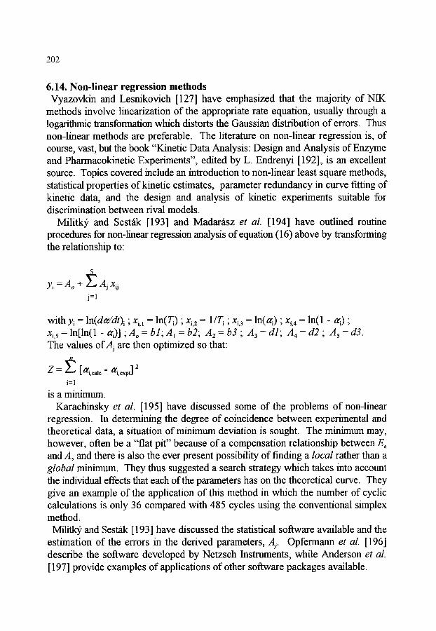
202

6.14. Non-linear regression methods Vyazovkin and Lesnikovich [127] have emphasized that the majority of NIK

methods involve linearization of the appropriate rate equation, usually through a logarithmic transformation which distorts the Gaussian distribution of errors. Thus non-linear methods are preferable. The literature on non-linear regression is, of course, vast, but the book "Kinetic Data Analysis: Design and Analysis of Enzyme and Pharmacokinetic Experiments", edited by L. Endrenyi [192], is an excellent source. Topics covered include an introduction to non-linear least square methods, statistical properties of kinetic estimates, parameter redundancy in curve fitting of kinetic data, and the design and analysis of kinetic experiments suitable for discrimination between rival models.

Militk~, and Sestfik [193] and Madar/lsz et al. [194] have outlined routine procedures for non-linear regression analysis of equation (16) above by transforming the relationship to:

y, = A o + ~ Aj x~j j=l

with Yi = ln(d~dt)~ ; xi, ~ : ln(T 3 ; xi. 2 : 1/T~ ; xi, 3 = ln(~) ; xi, 4 = ln(1 - ~) ; xi, 5 = ln[ln(1 - ~)] ,A o = bl ; AI = b2; A 2 = b3 ; A 3 = d l ; A4 = d2 ; A5 = d3. The values of Aj are then optimized so that:

Z : ~ [~i,o~lo- ai,oxpt] 2

i=l

is a minimum. Karachinsky et al. [195] have discussed some of the problems of non-linear

regression. In determining the degree of coincidence between experimental and theoretical data, a situation of minimum deviation is sought. The minimum may, however, often be a "fiat pit" because of a compensation relationship between E a and A, and there is also the ever present possibility of finding a local rather than a global minimum. They thus suggested a search strategy which takes into account the individual effects that each of the parameters has on the theoretical curve. They give an example of the application of this method in which the number of cyclic calculations is only 36 compared with 485 cycles using the conventional simplex method.

Militl~ and Sest~ [193] have discussed the statistical software available and the estimation of the errors in the derived parameters, Aj. Opfermann et al. [196] describe the software developed by Netzsch Instruments, while Anderson et al.

[197] provide examples of applications of other software packages available.

203

6.15. Complex reactions In spite of the already daunting difficulties described above, some attention has

been given to the NIK analysis of complex reactions (i.e., reversible, concurrent and consecutive reactions). A useful guide to the possible occurrence of complex reactions [198] is a lack of correspondence between DSC and DTG results which indicates that the rate of change of enthalpy is not directly proportional to the rate of mass loss. Experiments at different heating rates also show up complexities. Another indication is a dependence of the value obtained for E~ upon the extent of reaction, tr [ 199].

The occurrence of complex reactions is detected in isothermal studies by Arrhenius plots that are curved or give two linear regions [199]. The shapes of plots of against reduced time also vary systematically with temperature.

Elder [200] has modelled several multiple reaction schemes, including mutually independent concurrent first-order reactions, competitive first-order reactions, mutually independent n-th order reactions, and mutually independent Avrami- Erofeev models with n = 2 or 3. The aim was to identify criteria that could be used in recognizing the occurrence of multiple reactions. The criteria suggested were: (i) the apparent order of reaction, n, varies with the method of calculation; and (ii) the kinetic parameters, A and E~, vary with the extent of reaction, or.

Vyazovkin and Lesnikovich [199] proposed that the type of complex process encountered in non-isothermal experiments could be identified by analysis of the shape of the curve of the dependence of the apparent value of Ea on a, found by isoconversional methods. Concurrent competitive reactions are characterized by an increasing dependence of Ea on a, but detailed shapes are dependent on the ratios of the contributing rates. A decreasing dependence of E~ on a:, was found for intermediate reversible processes [199]. Their flowchart is shown in Figure 12.

Reversible reactions. Many solid-gas reactions are reversible, e.g., dehydration of crystal hydrates, so that rate equations for such processes should include terms for the rate of the reverse reaction. If the rates of the forward and reverse reactions are comparable, the general set of models (Table 2) will not be applicable. The usual advice [11] is to study reversible reactions under conditions as far removed from equilibrium as possible. Use of low pressures or of high flow rates of carrier gas are not always successful. Sinev [201] has illustrated this with calculations for the decomposition of calcium carbonate which show that the rate of the reverse reaction is comparable with that of the forward reaction even when small sample masses (10 rag) and high flow rates (200 c m 3 s "1) of inert gas are used.

Vaganova et al. [202] describe a method for the determination of kinetic parameters for reversible reactions of first-, second- and mixed-orders, using both isothermal and non-isothermal DSC and TG.

204

E a increases with alpha

YES

Dependence of E a on alpha

E a decreases with alpha

! concave

parallel reversible reactions stage

NO ]

single stage process

c o n v e x

J change in rate

determining step

Figure 12. The characteristic shapes of the curves of the dependence of the apparent E, on tr, for complex processes, found by isoconversional methods. (Based on reference [199], Figure 4.)

Consecutive reactions. Marcu and Segal [203] considered two consecutive reactions of the reaction order (RO) type. The TA curves were particularly influenced by the E, values (which determine the onset temperatures of the reactions). Differences of > 10 kJ mol -~ between E, values of the two processes led to their total separation. Different values for the pre-exponential factor, A, could compensate for this effect. The value of the reaction order also influenced separation. Thus, at low a~ the kinetic parameters are approximately those of the first reaction step. Comparison of an expected TA curve, constructed using these parameters, with the experimental curve may be used to provide an indication of the complexity of the overall reaction.

Concurrent reactions. Separation of the contributions to complex reactions is most easily achieved when the activation energies of the individual reactions are considerably different. Reactions with low E, values dominate the kinetics at low temperatures and slow heating rates, while those with high E~ values dominate at high temperatures and high heating rates. At the isokinetic temperature the rates of

205

the participating reactions are equal. Contributions from individual reactions with similar E~ values are not separable by changing the heating rate and deconvolution has to be attempted by mathematical methods [204]. Many such methods proposed in the literature are restricted to RO models. Criado et al. [204] proceed on the basis of summing the individual contributions. The overall reacted fraction tr is defined as:

t~'-- ~ Wi ~ i

where w i is the fraction of the total mass loss due to contributing reaction i (with Arrhenius parameters, A~ and (Ea) i ). A method is then presented which uses non- linear optimization combined with a version of the Kissinger method to deconvolute up to 15 contributing processes.

Ozawa and Kanari [205] have also discussed the kinetic analysis of competitive reactions for which measurements of the extents of conversion and rates of production of individual products are required. Suitable data could be obtained by combining evolved gas analysis with TG or DSC. Reaction complicated by diffusion. Vyazovkin [206] has treated such a system as

consecutive reactions involving the formation of a surface layer followed by diffusion through that layer.

Vaganova et al. [202] have proposed a mathematically complicated method for obtaining the kinetic parameters of two-stage (concurrent or consecutive) reactions, tinder isothermal or non-isothermal conditions, without separation of the individual stages.

6.16. Prediction of kinetic behaviour One of the practical aims of kinetic studies is to enable predictions to be made of

kinetic behaviour under conditions other than those used in the original experimental measurements [207]. The reliability of predictions depends upon the values of the kinetic parameters, E,, A and f ( ~ (or g(~), not varying with T and also the precision with which these values are known [208]. The relative error in the time, At~t, calculated from:

t= g(~/[A exp(- E,/RTo) l

is given by:

IA I- + laA/AI + IA /RT01

206

Vyazovkin and Linert [208] have described some of the implications of attempting to predict kinetic behaviour when the kinetic model g(tr) orJ(tr) has been incorrectly chosen, and when the reactions are complex.

Flynn [209] has reviewed the prediction of service lifetimes of polymeric materials, at lower temperatures, from decomposition parameters obtained at relatively high temperatures. Reasons for the failure of predictions are discussed. These include extrapolation beyond temperatures at which phase changes (and accompanying changes of physical properties) occur.

6.17. Kinetics standards During an ICTAC Kinetics Workshop [210], Gallagher listed the major

requirements for a reaction to be usable as a kinetics standard for comparison of reliability in rate measurements. These are: (i) an irreversible reaction taking place in a single stage, with (ii) a low value of the enthalpy of reaction, to minimize self- heating or self-cooling effects; (iii) the temperature range required for reaction to proceed at a slow, but measurable rate should not be too low, so as to avoid large temperature calibration errors; (iv) there should be no reaction of the sample with the surrounding atmosphere; (v) no dependence of reaction on the method of sample preparation, pretreatment or particle size and distribution; and (vi) the changes to be measured to follow the course of reaction, e.g., mass, amounts of evolved gases, enthalpy change, should be large, to permit the use of small samples. Some of these requirements are not compatible with each other, so compromises are necessary.

On the above criteria, the use of the dehydration of lithium sulphate monohydrate as a kinetic standard was ruled out [210], because: (i) the reaction is reversible at low temperatures, and (ii) is moderately endothermic; (iii) the reaction takes place at temperatures below 370 K and TG instnnnents are difficult to calibrate accurately in this range; (iv) rates of reaction are very dependent upon particle-size and prehistory; (v) overall dehydration involves several rate processes, e.g., chemical reaction, diffusion, recrystallization, and the rate-determining step may not remain the same during the course of experiments; and (vi) the overall rate of dehydration is influenced by the presence of water vapour in the surrounding atmosphere.

6.18. Comments Arguments about the relative value of non-isothermal and isothermal methods of

kinetic analysis are generally unproductive. The results of some kinetic studies using non-isothermal techniques are in good agreement with those obtained for the same system using isothermal methods. By contrast, other systems are reported as giving kinetic results which are very dependent on the technique used. Thus the complementary use of the two approaches can be valuable in revealing potential

207

sources of difference, such as those discussed above. Both techniques can provide valuable insights into the processes occurring, provided that the experimenter is critically aware of the shortcomings and limitations of each approach. Vyazovkin and Lesnikovich [127] point out that the kinetic parameters calculated from isothermal data are not very dependent upon the kinetic model chosen, while the opposite is true for non-isothermal methods. They suggest that this is a reason for detenninmg the Arrhenius parameters from isothermal measurements and the kinetic model from non-isothermal measurements.

The reported lack of agreement amongst kinetic parameters calculated from the same set of experimental data using different methods of mathematical analysis [6,83] is disturbing. Some of the commercially available programs for kinetic analysis do not even specify the algorithms on which they are based, while other packages use kinetic expressions restricted to the reaction order (RO) type.

Vyazovkin and Lesnikovich [127] emphasize the need for careful statistical testing of the significance of the calculated parameters. Such tests may, at least, decrease the number of kinetic models which need to be considered. They specifically warn against the practice of forcing the model to be of the reaction order (RO) type where the value ofn may not possess physical significance. Coincidence of the parameters calculated by alternative methods confirms only the equivalence of the methods of calculation and not the validity of the parameters obtained.

One of the arguments against the use of"discrimination" methods [127] is that the set of models from which the 'best model' is to be chosen is too limited. Hence one of the set is going to be the 'best model' even if the set does not contain the true model. The formal models in the accepted set (e.g., Table 2) are too simple to account for all the features of real processes. Modification of the models, however, results in an increased number of adjustable parameters. Vyazovkin and Lesnikovich [211] have discussed the possible solving of the IKP using methods based on generalized descriptions, (or "synthesis" rather than "analysis"). These methods are based upon the premise that different aspects of the real process may be best described by a synthesis of individual features of competing ideal models. Such a generalized description is the Sest~tk - Berggren equation (9) which, depending on the exponents, may represent the usual set of models (Table 2). The number of parameters which can be determined depends upon the experimental data [124,200]. Usually a maximum of two of the three exponents can be determined. Wyandt and Flanagan [212] describe the use of the Sestb.k - Berggren equation (9) in a non-isothermal kinetic method suggested by Zimmerman [213]. No assumptions are made about the mechanism of the solid-state process being investigated. Values for m, n and p are calculated directly from the data. Once these values are known, the most likely mechanistic model can be selected.

208

Generalized descriptions include restriction to one class of model (e.g., reaction order or Avrami - Erofeev), i.e. using only one of the terms in the above equation, but placing no restriction on the value of the exponent. Also suggested are linear combinations of several formal models. Vyazovkin and Lesnikovich [128] have shown that the Avrami - Erofeev model is equivalent to linear combinations of some of the other formal models and hence may serve as a generalized description. Generalized descriptions may also include approximating functions, such as polynomials, splines, etc., but the number of adjustable parameters becomes unwieldy and the parameters lose both their independence and their physical significance.

6.19. Conclus ion Nman's general summary [214] of his observations of the dehydration (I) and the

decomposition (II) stages of the reactions of hydrated calcium oxalate:

I II

CaC204 .2H20 ~ CaC204 ~ C a C O 3

is a worthy conclusion to this section. "There is an everlasting controversy between isothermal and non-isothermal and between mechanistic and non- mechanistic approaches. At least in our study, we do not find any reason for condemning one in preference to the other; each has its own merits and drawbacks. The mechanism of a thermal decomposition reaction cannot be assigned unequivocally from the mathematical curve fitting of the TG data alone, whereas the isothermal mass-loss data give a better insight into the reaction mechanism. As far as the values of the kinetic parameters are concerned, there is no significant difference between isothermal and non-isothermal methods or between mechanistic and non-mechanistic approaches, in the sense that they show the same degree of fluctuation or trend, as the case may be. Thus, for the purpose of calculating the kinetic constants, the non-isothermal method has the advantage of greater simplicity. However, one has to ascertain the influence of procedural factors on the kinetic parameters before making any conclusion regarding the kinetics and mechanism of a solid state thermal decomposition reaction. Finally, it may be possible to superimpose the effects of the individual procedural factors, in order to predict the kinetic parameters for any set of experimental parameters."

209

7. KINETIC ASPECTS OF NON-SCANNING CALORIMETRY

7.1. Introduction Most calorimetric studies are tmdertaken (Chapter 14) for either thermodynamic

or general analytical purposes, but investigations of the kinetics of processes accompanied by evolution or absorption of heat (and this includes virtually all chemical reactions, phase transitions, dissolutions, etc.) are of great importance. An introduction to such studies is given in the book by Hemminger and HOhne [215]. According to Liu et al. [216] and to Zielenkiewicz [217], the first investigation of reaction kinetics by calorimetry was by Duclaux [218] in 1908.

Different types of calorimetry require different methods of kinetic analysis. Kinetic analyses of the results of differential scanning calorimetry (DSC) follow the procedures described for non-isothermal methods in section 6 above. The various types of non-scanning calorimetric methods are described in Chapters 1 and 14. Such methods can be classified broadly according to whether they are carried out adiabatically or isothermally. An ideal adiabatic calorimeter has no heat exchange between the measuring vessel and the surrotmdings, and the heat produced or absorbed causes a temperature difference in the system, AT, so that processes studied by adiabatic calorimetry are non-isothermal, although this temperature change is often ignored in kinetic studies. To minimise this temperature change, the amount of heat leaving the calorimeter may be increased through use of a good thermal conductor between the calorimeter and a constant-temperature shield. The heat flow rate through this conductor is used as a measure of the process occurring in a heat conduction calorimeter.

A calorimeter is described as a batch calorimeter if the reactants are initially isolated in separate sections of a vessel and later mixed. Titration calorimetry involves stepwise addition of one component using motorized burettes and syringes, linked to a batch vessel. Inflow-mixing calorimeters, separate streams of reactants are combined in a mixing chamber. The flow may be continuous, for slow reactions, or stopped, for faster processes. Both batch and flow calorimeters can be operated under either adiabatic or isothermal conditions. Care is required in distinguishing spurious heats, especially of mixing, from those associated with the reaction of interest.

7.2. Kinetic analysis 7.2.1. Basic assumptions

The determination of kinetic parameters from calorimetric experiments is based upon the assumption that during the reaction the measured response of the sensor of the calorimeter is proportional to the rate of the process and, hence, that the course of the process can be followed from curves of this response against time.

210

Hemminger and HOhne [215] have illustrated the idealized types of response curves obtained using different types of calorimeters. For processes which proceed slowly, relative to the time constant of the calorimeter, kinetic measurements are taken directly from the measured curve and analyses are generally based on those well-documented in homogeneous kinetics for batch and for flow processes. Rate equations are often based upon the assumption of a simple reaction order (RO) model, so that the order, the activation energy and the frequency factor of the process are the parameters to be determined. For fast processes, where the heat is released within time intervals of the same order of magnitude as the time constant of the calorimeter, the measured curve has to be suitably corrected (see below) before accurate kinetic parameters can be determined.

7. 2.2. Conduc t ion ca lor ime t ry

Zielenkiewicz and Margas [219] have described the complex mathematical models used to reconstruct the input function (the heat flow rate, �9 = dQ/dt) from the measured output function ( the measured temperature difference, U, at time t). They note that very similar reconstructions result even if considerably different mathematical approaches are used. A comparison of four different numerical methods based on state fimction theory, Fourier transform analysis, dynamic optimization and simple differentiation, has been reported [220]. Adamowicz [221] proposed a ~rther numerical method based on spectral resolution into rectangular pulses.

Hemminger and HOhne [215], Randzio and Suurkuusk [222], and Gronlund [223] have also provided useful discussions of the interpretation and correction of calorimetric response curves. The heat flow rate in the vessel of a batch calorimeter is made up of contributions from the heat generated or absorbed during reaction and the heat being exchanged with the surroundings. If measurements are made relative to a reference vessel, so that "accidental" effects are compensated for, an equation of the form:

q~ = dQ/dt = er [ U + r (dU/dt)] (21)

known as the Tian equation (or the Tian-Calvet equation) (see Chapter 14, section 2.4.3) applies, where U is the measured temperature difference at time t, er is a instrument constant (W K -~) and r is the time constant of the calorimeter. For a non-homogeneous calorimetric vessel, second (or higher) time derivatives of U may be included [222]. Equation (21) may be written in various forms, e.g.,

= dQ/d t = C [(1/r) U + (dU/dt)]

211

where C is the heat capacity, or:

�9 = dQ/dt = (1/R~) U + C (dU/dt) (22)

where R~ is the thermal resistance (K W l ) . The time constant, r, of the calorimeter vessel may be determined [222] by using

a very short but large power input to the calibration heater and measuring the temperature difference as a function of time. A plot of In U against t over the cooling section of the response curve will be linear with slope =- 1/r. An alternative approach [222] is to use a frequency response procedure, where a sinusoidal power (W) signal is introduced in the calibration heater. The resulting temperature response curve is also sinusoidal and the time constant can be determined from measurements of the damping and the phase shifts at least two frequencies.

7.2.3. Flow calorimetry Beezer and Tyrrell [224] have dealt with the relationship between the heat flow

rate and the kinetic parameters for zero- and first-order reactions in flow microcalorimeters. If two reactants with concentrations c~ and c~ are mixed at flow rates F~ and F2, respectively, they are diluted by factors Fj/(F~ + F2) (j = 1 and 2) as they enter the vessel [224]. If the heats of dilution are AHD1 and AHD2 for reagents 1 and 2, respectively, then the heat flow rate due to dilution is:

- (F 1 C~ AHD1 + F 2 c~ AHD2 )

A "base line" for reference is usually established by mixing the reagent which is in excess with solvent, using identical flow rates. The total heat output rate, dQ/dt, is then measured relative to this base line.

For a reaction which is first-order in reagent 2 and zero-order in reagent 1, the rate of formation of product, in a given volume element at time t after the volume element entered the vessel, is k~ c2, where k~ is an apparent first-order rate coefficient and c 2 is the concentration of reagent 2. If the mixing is fast compared with the residence time, r, then:

k 1 c 2 -- [k 1 F 2 c~ --}- F2) ] exp(- kit)

The average reaction rate in the vessel, -dc/dt, is found by integrating over the residence time in the vessel and multiplying by the volume of the vessel, V.

212

Because:

r = V/(F +

- dc/dt = R 2 c~ [1 - exp(- k~ r)]

The experimental average heat flow rate, dQ/dt, is then:

dQ/dt = - F 2 c~ {AHD2 + AH~[1 - exp(- k~ r)]}

where AH r is the enthalpy of reaction. If the reaction is very fast and reagent 1 is present in excess:

dQ/dt = - F 2 c~ (AH~ + AHD2 )

AHD2 is generally small in comparison with AH~. Flow calorimetric studies can thus provide kinetic information if k~ values are of the order of 1/r. The average concentration of component 2, c 2, in the vessel while flow continues is:

c 2 = { F 2 c~ / [k,(F, + F2)r]} [1- exp(- k~ r)]

For a "stopped flow" experiment, this concentration will decrease exponentially with time:

dQ/dt = - F 2 c~ AH~[1 - exp(- k 1 g-)]exp(- kit )

The rate coefficient, k~, can be obtained by plotting the logarithm of the heat flow rate against the time elapsed since the flow ceased. Second-order reactions, when treated in a similar manner, give more complex relationships.

7.3 Selected examples of thermoldnefic studies Liu et al. [225] used an approach based on equation (22) to calculate the rate

coefficient for a first-order reaction in a batch heat conduction calorimeter. Integration of equation (22) gives:

Q - (1/R~) s + C U

and:

Qoo = (1/R~,) S

213

where Q is the heat produced up to time t, s is the area under the curve up to time t, Q~ is the total heat effect and S is the total area trader the curve. The extent of reaction, a~, is measured by Q / Q=. For a first-order reaction:

U : S [k~ k,/(k~- k,)][exp(- k l0 - exp(- kth t)]

where k 1 is the first-order rate coefficient and k~ = (R~ C)-1 = r -1 is the cooling constant of the calorimeter. The shape of the calorimetric response curve thus depends upon the relative values of k 1 and kth (see Figure 1 of reference [225]). Defining the characteristic time, t~, of the first-order reaction as the time from the start of the experiment to the peak maximum, and the dimensionless parameter, y = kth / kl, gives:

t n + 1 - t n : At = In Lv / (k~- k,)] (23)

The heights of the curve, U1, U2 and U3, at times, t~, t 2 = 2q, and t 3 = 3tl, respectively, are then measured. Writing m = U3 / U1 and n = U2 / U~, they showed that:

rn = (1 + y +)7) y2yl(1-y) and n = (1 + y) yy/(1-y>

According to equation (23):

At k~,= t, kth = y l n D ' / ( y - 1)l

The time constant of the calorimeter is r= 1/k~ and is determined from calibration, so the value of the dimensionless parameter [226,227], y, can be determined from comparison of At and r.

In further papers, Liu et al. have extended their approach to the study of the kinetics of higher-order reactions [228], and of reversible [216] and consecutive [229,230] reactions, using fairly standard methods of kinetic analysis to determine the rate coefficients and equilibrium constants.

Hansen et al. [231,232] have used calorimetric measurements of isothermal induction periods to determine the kinetic parameters of materials which tmdergo autocatalytic decomposition. The results of such studies were applied to the determination of shelf-lives of pharmaceuticals. Willson et al. [233] have discussed the prediction of shelf-lives in more general terms.

Kinetic studies of some reactions of biochemical interest have been reviewed by Spink and Wads6 [234]. Results obtained using calorimetry are in good agreement with those obtained using other techniques (e.g., spectrophotometry).

214

8. PUBLICATION OF KINETIC RESULTS

8.1. Publication In this Chapter, the theory and many of the pitfalls likely to be encountered in the

measurement and analysis of kinetic data have been discussed. The final important stage of any useful research programme is the publication of kinetic results for the information (and scrutiny) of the scientific community. Many publications in the existing literature do not provide adequate information for assessment of the value of the contribution being made. In an attempt to rectify these omissions in future publications, the following guidelines have been compiled under the traditional sub- headings of a typical scientific paper.

8.2. Introduction Reasons for undertaking the research reported should be explained. The relevant

literature, especially work by other authors, should be appropriately cited and briefly reviewed, so that the work is set in a context enabling it to be understood without extensive preliminary reading of earlier references.

8.3. Experimental 8.3.1. Materials

Each reactant should be described as completely and unambiguously as possible. The supplier and, if possible, the method of preparation or manufacture should be specified. Both structures and compositions may have to be reported for mineral reactants, because samples obtained from different sources may be inhomogeneous and different phases may have similar chemical compositions. Polymer samples also need careful specification. Analytical results should be given (with limits of accuracy), including purity and the nature and concentrations of any impurities or other inert constituents specifically sought, and any structural information. Particle sizes and distributions should also be reported. The particle size of the reactant may change before the reaction of interest is studied. For example, the loss of water of crystallization from a hydrate may be followed by recrystallization before decomposition. Reactant pretreatments before study (ageing, cold working, crushing, pelleting, recrystallization, irradiation, etc.) should be described in full.

8.3.2. Equipment and methods Full details of the conditions prevailing within the reaction vessel should be

recorded. These include heating rates, method of data acquisition and storage, together with information about the base-line of the instnnnent. The dimensions, geometry and material of the reactant container should be specified, and the possibility of its catalytic activity should be kept in mind. The pressures, flow rates

215

and purities of all gases present in or admitted to the reaction environment should be reported.

The particular advantages and possible shortcomings of the experimental methods selected for the investigation should be discussed, with particular reference to their relevance to the rate process being studied. Simultaneous measurements of several parameters yield data of increased reliability, particularly for more complicated reactions.

The reliability of mechanistic interpretations of kinetic observations can be substantially increased by appropriate confirmatory studies. Microscopic observations often provide direct evidence of reaction geometry and also of the participation of melting [37,40]. The positive identification of intermediates has obvious value in supporting a proposed chemical mechanism.

8.4. Results 8. 4.1. Reaction stoichiometry

The identifies and amounts of all products are needed to provide a quantitative description of the chemical change taking place. Product yields must be correlated accurately with the experimental parameter used to measure the extent of reaction, a (e.g., mass loss, yield of a particular gas, heat evolved, etc.). Analysis of the residual solid product may be necessary to identify the phases produced, together with their proportions, and to confirm that reaction has gone to completion. The participation and roles of active intermediate compotmds should be determined. Estimated errors in all measured compositions should also be reported.

Any changes in the relative yields of products during the course of reaction with a, with temperature, or with any other variable such as gaseous oxygen or water vapour present, should be determined. The influence of precursor reactions, such as initial dehydration, on reactant structure and composition (e.g. the possibility of hydrolysis), must be investigated. The relevance of all other changes that may accompany reactions, such as recrystallization, sintering, sublimation, melting, eutectic formation, to kinetic behaviour and on any reaction mechanism proposed should also be considered.

8.4.2. Kinetic analysis The reproducibility of the data measured for kinetic analysis should be specified.

Publication of the raw data has also been recommended [178]. It is also important to specify in detail the rate process being studied and the definition of a~. Accounts of the test of fit of data to the kinetic expressions being used should record the methods used, criteria for acceptability of fit, and the range of fit of the equations considered. (Such information is often not clearly specified in commercially available software packages). Reasons for accepting that a particular reaction

216

model satisfactorily expresses the observations should be stated. The need to list yet again tables of the now well-known models and kinetic equations should be carefully assessed. Rate coefficients reported should include estimates of their accuracy (determined

by standard statistical methods), the range of ~ across which the fit is regarded as acceptable, and the temperature conditions during reaction [6]. Variations of these parameters with reactant temperature, reactant mass, etc., should also be mentioned. Errors arising from systematic deviations must be distinguished from the uncertainty in random scatter of values. Values of Arrhenius parameters, E~ and A, should also include their standard errors. The number of significant figures used to report numerical values (+ errors) must be realistic.

Further indications of the reliability of a kinetic analysis may be obtained by comparison of isothermal kinetic measurements with those obtained from programmed temperature experiments.

8.5. Discussion Discussions should include appraisal of the extent to which the work has fulfilled

the expectations set out in the Introduction. Interpretation of all results must be considered in the context of all relevant work, including citation of related studies by other workers. Advances should be explained and discussed realistically and directions for possible future advances should be indicated.

REFERENCES

1. P.W.M. Jacobs and F.C. Tompkins, in W.E. Garner (ed), Chemistry of the Solid State, Butterworth, London, 1955, Ch. 7.

2. W.E. Garner, in W.E. Garner (ed), Chemistry of the Solid State, Butterworth, London, 1955, Chs. 8 and 9.

3. D.A. Young, Decomposition of Solids, Pergamon, Oxford, 1966. 4. B. Delmon, Introduction a la Cinttique Htttrogtne, Technip, Paris, 1969. 5. P. Barret, Cinttique Htttrogtne, Gauthier-Villars, Paris, 1973. 6. M.E. Brown, D. Dollimore and A.K. Galwey, Comprehensive Chemical

Kinetics, Vol. 22, Elsevier, Amsterdam, 1980. 7. J. Sest~ik, Thermophysical Properties of Solids, Comprehensive Analytical

Chemistry, Vol. XIID, Elsevier, Amsterdam, 1984. 8. P.P. Budnikov and A.M. Ginstling, Principles of Solid State Chemistry

(translated by K.Shaw), MacLaren, London, 1968. 9. H. Schmalzried, Solid State Reactions, 2nd edn, Verlag Chemie, Weinheim,

1981; Chemical Kinetics of Solids, VCH, Weinheim, 1995. 10. A.R. West, Solid State Chemistry, John Wiley, Chichester, 1984.

217

11. D. Beruto and A.W. Searcy, J. Chem. Soc., Faraday Trans.I, 70 (1974) 2145. 12. A.K. Galwey and G.M. Laverty, Solid State Ionics, 38 (1990) 155. 13. A.K. Galwey, R. Spinicci and G.G.T. Guarini, Proc. R. Soc. London, A378

(1981)477. 14. A.K. Galwey, D.M. Jamieson and M.E. Brown, J. Phys. Chem., 78 (1974)

2664. 15. D.A. Dominey, H. Morley and D.A. Young, Trans. Faraday Soc., 61 (1965)

1246. 16. A.K. Galwey, G.M. Laverty, N.A. Baranov and V.B. Okhomikov, Phil.

Trans. R. Soc. London, A347 (1994) 139, 157. 17. V.B. Okhotnikov, S.E. Petrov, B.I. Yakobson and N.Z. Lyakhov, React.

Solids, 2 (1987) 359. 18. V.B. Okhomikov and I.P. Babicheva, React. Kinet. Catal. Lett., 37 (1988)

417. 19. V.B. Okhomikov, I.P. Babicheva, A.V. Musicantov and T.N. Aleksandrova,

React. Solids, 7 (1989) 273. 20. V.B. Okhotnikov, N.A. Simakova and B.I. Kidyarov, React. Kinet. Catal.

Lett., 39 (1989) 345. 21. M.C. Ball and L.S. Norwood, J. Chem. Soc. A, (1969) 1633; (1970) 1476. 22. M.C. Ball and M.J. Casson, J. Chem. Soc., Dalton Trans., (1973) 34. 23. T.B. Grimley, in W.E. Garner (ed), Chemistry of the Solid State,

Butterworth, London, 1955, Ch. 14. 24. J. Szekely, J.W. Evans and H.Y. Solm, Solid-Gas Reactions, Academic

Press, New York, 1976. 25. A.J.E. Welch, in W.E. Garner (ed), Chemistry of the Solid State,

Butterworth, London, 1955, Ch. 12. 26. V.V. Boldyrev, Y.A. Gapanov, N.Z. Lyakhov, A.A. Politov, B.P. Tolochko,

T.P. Shakhtslmeider and M.A. Sheromov, Nucl. Inst. Method. Phys. Res., A261 (1987) 192.

27. A.K. Galwey and G.M. Laverty, Thermochim. Acta, 228 (1993) 359. 28. G.G.T. Guarini, J. Thermal Anal., 41 (1994) 287. 29. A.K. Galwey and G.G.T. Guarini, Proc. R. Soc. London, A441 (1993) 313. 30. H.R. Oswald, Thermal Analysis, Proc. 6th Internat. Conf., Birkh~iuser, Basel,

(1980), p.1. 31. V.V. Boldyrev, React. Solids, 8 (1990) 231. 32. J.D. Daw, P.S. Nicholson and J.D. Embury, J. Amer. Ceram. Soc., 55

(1972) 149. 33. M. Kim, V. Dahmen and A. Searcy, J. Amer. Ceram. Soc., 70 (1987) 146. 34. R.D. Shannon, J. Amer. Ceram. Soc., 50 (1967) 56. 35. M.R. Snow and R. Boomsma, Acta Crystallogr., Sect. B, 28 (1972) 1908.

218

36. M.R. Snow and R.J. Thomas, Austr. J. Chem., 27 (1974) 1391. 37. A.K. Galwey, Thermochim. Acta, 96 (1985) 259; React. Solids, 8 (1990)

211. 38. A.K. Galwey, N. Koga and H. Tanaka, J. Chem. Soc., Faraday Trans. I, 86

(1990) 531. 39. M.E. Brady, M.G. Burner and A.K. Galwey, J. Chem. Soc., Faraday Trans.

I, 86 (1990) 1573. 40. A.K. Galwey, J. Thermal Anal., 41 (1994) 267. 41. C. Bagdassarian, Acta Physicochem. URSS, 20 (1945) 441. 42. A.R. Allnatt and P.W.M. Jacobs, Canad. J. Chem., 46 (1968) 111. 43. A. Wischin, Proc. R. Soc. London, A172 (1939) 314. 44. N.F.H. Bright and W.E. Garner, J. Chem. Sot., (1934) 1872. 45. M. Avrami, J. Phys. Chem., 7 (1939) 1103; 8 (1940) 212; 9 (1941) 177. 46. J. Hurne and J. Colvin, Proc. R. Soc. London, A125 (1929) 635. 47. W.D. Spencer and B. Topley, J. Chem. Soc., (1929) 2633. 48. S.J. Gregg and R.I. Razouk, J. Chem. Soc., (1949) 536. 49. R.C. Eckhardt and T.B. Flanagan, Trans. Faraday Soc., 60 (1964) 1289. 50. P.M. Fichte and T.B. Flanagan, Trans. Faraday Soc., 67 (1971) 1467. 51. E.G. Prout and F.C. Tompkins, Trans. Faraday Soc., 40 (1944) 488. 52. J.B. Austin and R.L. Rickett, Trans. AIME, 135 (1939) 396. 53. E.G. Prout and F.C. Tompkins, Trans. Faraday Soc., 42 (1946) 468. 54. M.E. Brown, A.K. Galwey, M.A. Mohamed and H. Tanaka, Thermochim.

Acta, 235 (1994) 255. 55. N.J. Carr and A.K. Galwey, Proc. R. Soc. London, A404 (1986) 101. 56. W. Jander, Z. Anorg. Allg. Chem., 163 (1927) 1; Angew. Chem., 41 (1928)

79. 57. R.E. Carter, J. Chem. Phys., 35 (1961) 1137, 2010. 58. G. Valensi, C.R. Acad. Sci. Ser. C, 202 (1936) 309; J. Chem. Phys., 47

(1950) 489. 59. A.M. Ginstling and B.I. Brounshtein, Zh. Prikl. Khim., 23 (1950) 1327. 60. B. Serin and R.T. Ellickson, J. Chem. Phys., 9 (1941) 742. 61. J.B. Holt, J.B. Cutler and M.E. Wadsworth, J. Amer. Ceram. Sot., 45 (1962)

133. 62. S.F. Hulbert, J. Br. Ceram. Soc., 6 (1969) 11. 63. M.E. Brown, A.K. Galwey and A. Li Wan Po, Thermochim. Acta, 203

(1992) 221; 220 (1993) 131. 64. A.K. Galwey and G.M. Laverty, Proc. R. Soc. London, A440 (1993) 77. 65. A.K. Galwey, L. P0ppl and S. Rajam, J. Chem. Soc., Faraday Trans. I, 79

(1983)2143.

219

66. S.D. Bhattamisra, G.M. Laverty, N.A. Baranov, V.B. Okhotnikov and A.K. Galwey, Phil.Trans. R. Soc. London, A341 (1992) 479.

67. A.K. Galwey, G.M. Laverty, V.B. Okhotnikov and J. O~eill, J. Thermal Anal., 38 (1992) 421.

68. A.K. Galwey and M.A. Mohamed, J. Chem. Soe., Faraday Trans. I, 81 (1985) 2503.

69. A.K. Galwey and P.W.M. Jacobs, Proc. R. Soc. London, A254 (1960) 455. 70. A.K. Galwey and M.A. Mohamed, Thermochim. Acta, 213 (1993) 269, 279. 71. W.L. Ng, C.C. Ho and S.K. Ng, J. Inorg. Nucl. Chem., 34 (1978) 459. 72. A.K. Galwey and M.A. Mohamed, Thermoehim. Acta, 239 (1994) 211. 73. W.E. Garner and A.J. Gomm, J. Chem. Soe., (1931) 2123. 74. S. Miyagi, J. Japn. Ceram. Sot., 59 (1951) 132. 75. L.L. Bircumshaw and B.H. Newman, Proc. R. Soc. London, A227 (1954)

115, 228. 76. H. Sasaki, J. Amer. Ceram. Sot., 47 (1964) 512. 77. P.G. Fox, J. Solid State Chem., 2 (1970) 491. 78. R.W. Hutchinson, S. Kleinberg and F.P. Stein, J. Phys. Chem., 77 (1973)

870. 79. H.G. McIlvried and F.E. Massoth, Ind. Eng. Chem. Fundam., 12 (1973) 225. 80. M.E. Brown, B. Delmon, A.K. Galwey and M.J. McGinn, J. Chim. Phys., 75

(1978) 147. 81. W-L. Ng, Aust. J. Chem., 28 (1975) 1169. 82. J. Sestb.k and G. Berggren, Thermoehim. Acta, 3 (1971) 1. 83. J. M~lek and J.M. Criado, Thermoehim.Acta, 175 (1991) 305. 84. J. Sest~k, J. Thermal Anal., 36 (1990) 1997. 85. N. Koga, Thermochim.Acta, 258 (1995) 145. 86. A.K. Galwey and M.E. Brown, Thermochim. Acta, 269/270 (1995) 1. 87. M.E. Brown and A.K. Galwey, Thermochim.Acta, 29 (1979) 129. 88. H. Tanaka and N. Koga, Thermochim.Acta, 173 (1990) 53. 89. M.E. Brown and A.K. Galwey, Anal.Chem., 61 (1989) 1136. 90. B.R. Wheeler and A.K. Galwey, J.Chem.Soc., Faraday Trans.I, 70 (1974)

661. 91. L.F. Jones, D. Dollimore and T. Nicklin, Thermoehim. Acta, 13 (1975) 240. 92. M. Selvaratnam and P.D. Gam, J.Amer.Ceram.Soc., 59 (1976) 376. 93. K.J. Laidler, J. Chem. Ed., 61 (1984) 494. 94. M.Menzinger and R. Wolfgang, Angew. Chem., 8 (1969) 438. 95. H.C. Anderson, Thermal Analysis, Proc. 2nd Toronto Symp., Toronto,

Chem.Inst. Canada, 1967, p.37. 96. J.P. Redfem, in R.C. Mackenzie (ed), Differential Thermal Analysis, Vol. 1,

Academic Press, New York, 1970, p.123.

220

97. P.D. Garn, J. Thermal Anal., 7 (1975) 475; 10 (1976) 99; 13 (1978) 581; Thermoehim. Aeta, 135 (1988)71; 160 (1990) 135.

98. G. Bertrand, M. Lallemant and G. Watelle, J. Thermal Anal., 13 (1978) 525.

99. M. Polanyi and E. Wigner, Z. Phys. Chem. Abst. A, 139 (1928) 439. 100. A.K. Galwey, Thermoehim. Aeta, 242 (1994) 259. 101. R.D. Shannon, Trans. Faraday Sot., 60 (1964) 1902. 102. H.F. Cordes, J. Phys.Chem., 72 (1968) 2185. 103. A.K. Galwey and M.E. Brown, Proe. R. Soe. London, A450 (1995) 501. 104. J.Cunningham, Comprehensive Chemical Kinetics, Vol. 19, Elsevier,

Amsterdam, 1984, Ch.3, p.294,305. 105. G.G. Roberts, in G.M. Burnett, A.M. North and J.N. Sherwood (eds),

Transfer and Storage of Energy by Molecules, Vol.4, The Solid State, Wiley, London, 1974, p.153-155.

106. B. Topley and J. Hume, Proe. R. Soe. London, A120 (1928) 211. 107. J.R. Hook and H.E. Hall, Solid State Physics, 2nd edn., Wiley,

Chichester, 1991, Ch.2. 108. R.J. Elliott and A.F. Gibson, Introduction to Solid State Physics and its

Applications, MacMillan, London, 1974, p.43. 109. N. Koga, Thermoehim. Aeta, 244 (1994) 1. 110. J. Sest~.k, J. Thermal Anal., 16 (1979) 503. 111. J. Sest~, Thermoehim. Aeta, 110 (1987) 109. 112. N.J. Carr and A.K. Galwey, Thermoehim.Acta, 79 (1984) 323. 113. E.V. Boldyreva, Thermochim. Acta, 110 (1987) 107. 114. M. Maciejewski, J. Thermal Anal., 38 (1992) 51; 33 (1988) 1269. 115. J.R. MacCallum, Thermoehim. Aeta, 53 (1982) 375. 116. J. Sest~k, Thermochim. Acta, 83 (1985) 391. 117. E. Segal, Thermochim. Aeta, 148 (1989) 127. 118. J. Kris and J. Sest~k, Thermochim. Acta, 110 (1987) 87. 119. M.W. Beck and M.E. Brown, J. Chem. Sot., Faraday Trans.,

87 (1991) 711. 120. J. Militk~, and J. Sest~.k, Thermochim. Acta, 203 (1992) 31. 121. A.A. Zuru, R. Whitehead and D.L. Griffiths, Thermochim. Acta,

164 (1990) 285. 122. D. Dollimore, G.A. Gamlen and T.J. Taylor, Thermochim. Acta,

54 (1982) 181. 123. S.W. Churchill, The Interpretation and Use of Rate Data: The Rate

Concept, McGraw-Hill, New York, 1974, p. 317-319. 124. P. Budrugeae and E. Segal, Thermochim. Acta, 260 (1995) 75. 125. R.K. Agrawal, Thermochim. Acta, 203 (1992) 93.

221

126. J.M. Criado, A. Ortega and F. Gotor, Thermochim. Acta, 157 (1990) 171. 127. S.V. Vyazovkin and A.I. Lesnikovich, J. Thermal Anal., 35 (1989) 2169. 128. S.V. Vyazovkin and A.I. Lesnikovich, J. Thermal Anal., 36 (1990) 599. 129. J. M~ilek, Thermochim. Acta, 200 (1992) 257. 130. G. Vfirhegyi, Thermochim. Acta, 57 (1982) 247. 131. C. Popescu and E. Segal, J. Thermal Anal., 24 (1982) 309. 132. J.M. Criado and A. Ortega, Thermochim. Acta, 103 (1986) 317. 133. M. Reading, D. Dollimore, J. Rouquerol and F. Rouquerol, J. Thermal

Anal., 29 (1984) 775. 134. A. Ortega, L.A. P6rez-Maqueda and J.M. Criado, Thermochim. Acta, 239

(1994) 171; J. Thermal Anal., 42 (1994) 551. 135. O. Toil Sorensen, Thermochim. Acta, 50 (1981) 163. 136. J.H. Flylm and B. Dickens, Thermochim. Acta, 15 (1976) 1. 137. M. Reading, A. Luget and R. Wilson, Thermochim. Acta, 238 (1994) 295;

M. Reading, Thermochim. Acta, 292 (1997) 179. 138. M. Reading, D. Elliott and V. Hill, J. Thermal Anal., 40 (1993) 949; P.S.

Gill, S.R. Sauerbrtmn and M. Reading, J. Thermal Anal., 40 (1993) 931. 139. J.E.K. Schawe, Thermochim. Acta, 271 (1996) 127. 140. R. Riesen, G. Widmann and R. Trotmann, Thermochim. Acta,

272 (1996) 27. 141. B. Wunderlich, Y. Yinn and A. Boller, Thermochim. Acta, 238 (1994) 277. 142. U. Biader Ceipidor, R. Bucci, V. Carunchio and A.D. Magi, 158 (1990)

125; 161 (1990) 37; 199 (1992) 77, 85; 231 (1994) 287. 143. P.D. Garn, Crit. Rev. Anal. Chem., 3 (1972) 65. 144. V. Berbenni, A. Marini, G. Bruni and T. Zerlia, Thermochim. Acta, 258

(1995) 125. 145. Z. Bashir and N. Khan, Thermochim. Acta, 276 (1996) 145. 146. N. Koga and H. Tanaka, J. Phys. Chem., 98 (1994) 10521. 147. C. D. Doyle, J. Appl. Polym. Sci., 6 (1962) 639. 148. J. P. Elder, J. Thermal Anal., 30 (1985) 657; in P.S. Gill and Ji F. Johnson

(eds), Analytical Calorimetry, Vol. 5,Plenum, New York, 1984, p.269. 149. J. Zsak6, in Z.D. Zivkovic (ed), Thermal Analysis, University of Beograd,

Bor, Yugoslavia, 1984, p. 167. 150. D.W. Henderson, J. Thermal Anal., 15 (1979) 325. 151. J.W. Graydon, S.J. Thorpe and D.W. Kirk, J. Non-crystalline Solids, 175

(1994) 31. 152. J Meindl, I.V. Arkhangelskii and N.A. Chernova, J. Thermal Anal., 20

(1981) 39. 153. S.V. Vyazovkin, A.I. Lesnikovich and V.I. Goryachko, Thermochim. Acta,

177 (1991) 259.

222

154. N.S. Felix and B.S. Girgis, J. Thermal Anal., 35 (1989) 743. 155. G. V~hegyi, Thermochim. Acta, 110 (1987) 95. 156. H. Friedman, J. Polym. Sci., 50 (1965) 183. 157. B. Carroll and E.P. Manche, Thermochim. Acta, 3 (1972) 449. 158. J.H. Flynn, J. Thermal Anal., 37 (1991) 293. 159. E.S. Freeman and B. Carroll, J. Phys. Chem., 62 (1958) 394; 73 (1969) 751. 160. J. Sest~, V. Satava and W.W. Wendlandt, Thermochim. Acta,

7 (1973) 333. 161. J.M. Criado, D. Dollimore and G. R. Heal, Thermochim. Acta,

54 (1982) 159. 162. A. Jerez, J. Thermal Anal., 26 (1983) 315. 163. A.A. Van Dooren and B.W. Muller, Thermochim. Acta, 65 (1983)

257,269. 164. R.M. Fuoss, O. Sayler and H.S. Wilson, J. Polym. Sci., 2 (1964) 3147. 165. H. E. Kissinger, J. Res. Nat. Bur. Stand., 57 (1956) 217; Anal. Chem., 29

(1957) 1702. 166. J. A. Augis and J. E. Bennett, J. Thermal Anal., 13 (1978) 283. 167. J. Llopiz, M.M. Romero, A. Jerez and Y. Laureiro, Thermochim. Acta,

256 (1995) 205. 168. T. Ozawa, Bull. Chem. Soc. Japan, 38 (1965) 1881; J. Thermal Anal., 2

(1970) 301. 169. H. Tanaka, Thermochim. Acta, 267 (1995) 29. 170. H. J. Borchardt and F. Daniels, J. Amer. Chem. Soc., 79 (1957) 41. 171. R. L. Reed, L. Weber and B. S. Gottfried, Ind. Eng. Chem. Fundam.,

4(1965) 38. 172. E. Koch and B. Stikerieg, Thermochim. Acta, 17 (1976) 1. 173. Y. L. Shishkin, J. Thermal Anal., 30 (1985) 557. 174. P. Hugo, S. Wagner and T. Gnewikow, Thermochim. Acta, 225 (1993)

143,153. 175. J. H. Flynn and L. A. Wall, J. Res. Nat. Bur. Stand., 70A (1966) 487. 176. J. M~lek, Thermochim. Acta, 222 (1993) 105. 177. D. Dollimore, T.A. Evans, Y.F. Lee, G.P. Pee and F.W. Wilburn,

Thermochim. Acta, 196 (1992) 255. 178. J.M. Criado, J. M~lek and J. Sest~ik, Thermochim. Acta, 175 (1991) 299. 179. D. W. Van Krevelen, C. Van Heerden and F. J. Huntjens, Fuel,

30(1951)253. 180. C.D. Doyle, J. Appl. Polym. Sci., 5 (1961) 285. 181. J. Zsak6, J. Phys. Chem., 72 (1968) 2406. 182. J. Blazejowski, Thermochim. Acta, 48 (1981) 125. 183. A. J. Kassman, Thermochim. Acta, 84 (1985) 89.

223

184. R. Quanin and Y. Su, J. Thermal Anal., 44 (1995) 1147. 185. V. M. Gorbachev, J. Thermal Anal., 25 (1982) 603. 186. J. Sest~tk, Thermochim. Acta, 3 (1971) 150. 187. J. Zsak6, J. Thermal Anal., 34 (1988) 1489. 188. E. Urbanovici and E. Segal, Thermochim. Acta, 168 (1990) 71. 189. J.H. Flyrm, J. Thermal Anal., 37 (1991) 293. 190. C. D. Doyle, Nature, London, 207 (1965) 290. 191. J. Zsak6, J. Thermal Anal., 8 (1975) 593. 192. L. Endrenyi (ed), Kinetic Data Analysis: Design and Analysis of

Enzyme and Pharmacokinetic Experiments, Plenum, New York, 1981. 193. J. Militk37 and J. Sest~k, Thermochim. Acta, 203 (1992) 31. 194. J. Madar~isz, G. Pokol and S. G~I, J. Thermal Anal., 42 (1994) 559. 195. S.V. Karachinsky, O. Yu. Peshkova, V.V. Dragalov and A.L. Chimishkyan,

J. Thermal Anal., 34 (1988) 761. 196. J. Opfermann, F. Giblin, J. Mayer and E. Kaiserberger, Amer. Lab.,

(Feb. 1995) 34. 197. H.L. Anderson, A. Kemmler and R. Strey, Thermochim. Acta,

271 (1996) 23. 198. R.K. Agrawal, Thermochim. Acta, 203 (1992) 111. 199. S.V. Vyazovkin and A.I. Lesnikovich, Thermochim. Acta, 165 (1990) 273. 200. J.P. Elder, J. Thermal Anal., 29 (1984) 1327; 34 (1988) 1467; 35 (1989)

1965; 36 (1990) 1077. 201. M. Yu. Sinev, J. Thermal Anal., 34 (1988) 221. 202. N.I. Vaganova, V.I. Rozenband and V.V. Barzykin, J. Thermal Anal.,

34 (1988) 71. 203. V. Marcu and E. Segal, Thermochim. Acta, 35 (1980) 43. 204. J.M. Criado, M. Gonz~lez, A. Ortega and C. Real, J. Thermal Anal.,

34 (1988) 1387. 205. T. Ozawa and K. Kanari, Thermochim. Acta, 234 (1994) 41. 206. S.V. Vyazovkin, Thermochim. Acta, 223 (1993) 201. 207. S.V. Vyazovkin and A.I. Lesnikovich, Thermochim. Acta, 182 (1991) 133. 208. S.V. Vyazovkin and W. Linert, Anal. Chim. Acta, 295 (1994) 101. 209. J.H. Flynn, J. Thermal Anal., 44 (1995) 499. 210. M.E. Brown, R.M. Flynn and J.H. Flylm, Thermochim. Acta,

256 (1995) 477. 211. S.V. Vyazovkin and A.I. Lesnikovich, Thermochim. Acta, 122 (1987)413. 212. C.M. Wyandt and D.R. Flanagan, Thermochim. Acta, 197 (1992) 239. 213. J. Zimmerman, MS Thesis, Illinois State University, Normal, Illinois,

USA, 1983. 214. K.N. Ninan, J. Thermal Anal., 35 (1989) 1267.

224

215. W. Hemminger and G.W.H. HOhne, Calorimetry, Verlag Chemic, Weinheim, 1984, p. 125.

216. Jing-Song Liu, Xian-Cheng Zeng, An-Ming Tian and Yu Deng, Thermochim. Acta, 219 (1993) 43.

217. W. Zielenkiewicz, J. Thermal Anal., 29 (1984) 179. 218. J. Duclaux, C. R. Acad. Sci., 146 (1908) 4701. 219. W. Zielenkiewicz and E. Margas, J. Thermal Anal., 32 (1987) 173. 220. E. Cesari, P.C. Gravelle, J. Gutenbaum, J. Hatt, J. Naval-cO, J.L. Petit, R.

Point, V. Torra, E. Utzig and W. Zielenkiewicz, J. Thermal Anal., 20 (1981)47.

221. L. Adamowicz, J. Thermal Anal., 22 (1981) 199. 222. S.L. Randzio and J. Suurkuusk, in A.E. Beezer (ed), Biological

Microcalorimetry, Academic Press, London, 1980, p.311. 223. F. Gronlund, J. Chem. Thermodynamics, 22 (1990) 563. 224. A.E. Beezer and H.J.V. Tyrrell, Sci. Tools, 19 (1972) 13. 225. Jing-Song Liu, Xiancheng Zeng, An-Ming Tian and Yu Deng,

Thermochim. Acta, 231 (1994) 39. 226. Yu Deng, Xiancheng Zeng and Yuanqing Chan, Thermochim. Acta, 169

(1990) 223. 227. Yu Deng, Ziming Qing and Xiaoping Wu, Thermochim. Acta,

123(1988)213. 228. Jing-Song Liu, Xiancheng Zeng, Yu Deng and An-Ming Tian,

Thermochim. Acta, 236 (1994) 113. 229. Jing-Song Liu, Xiancheng Zeng, Yu Deng and An-Ming Tian, J. Thermal

Anal., 44 (1995) 617. 230. Jing-Song Liu, Xiancheng Zeng, An-Ming Tian and Yu Deng, Thermochim.

Acta, 273 (1996) 53. 231. L.D. Hansen, D.J. Eatough, E.A. Lewis, R.G. Bergstrom, D. DeGrafl-

Johnson and K. Cassidy-Thompson, Canad. J. Chem., 68 (1990) 2111. 232. L.D. Hansen, E.A. Lewis, D.J. Eatough, R.G. Bergstrom and D. DeGraft-

Johnson, Pharm. Res., 6 (1989) 20. 233. R.J. Willson, A.E. Beezer, J.C. Mitchell and W. Loh, J. Phys. Chem., 99

(1995) 7108. 234. C. Spink and I. Wads0, in D. Glick (ed), Methods of Biochemical

Analysis, Vol. 23, Wiley, New York, 1976, p. 1.


Chapter 4

THERMOGRAVIMETRY AND THERMOMAGNETOMETRY

Patrick K. Gallagher

Departments of Chemistry and Materials Science and Engineering, The Ohio State University, Columbus, Ohio 43210, U.S.A.

1. INTRODUCTION

1.1. Purpose and scope The mass of an object or material has been an important property since the

beginnings of time. It is the major method for quantifying the amount of a material and, consequently, techniques have developed to enable its measurement with relatively high accuracy on a routine basis. Such instruments are not only scientific apparatus, but also tools of commerce and capable of a wide range of measurement e.g., a postal scale, the grocer's scale, or the tax collector's scale at the wayside truck station. Thermogravimetry (TG) or thermogravimetric analysis (TGA) is merely an extension of this fundamental measurement as one's study deviates from room temperature or extends into time.

The technique has been defined earlier in Chapter 1 concerning nomenclature and related topics. Both TG and TGA are used extensively and interchangeably in the literature to describe the measurement of mass as a function of temperature and/or time. This chapter will primarily use the term and symbol, thermogravimetry and TG.

The closely related technique of thermomagnetometry (TM) is described also. In TM the apparent mass is measured while the sample resides in a magnetic field gradient. Hence, this apparent mass will include the affects of any potential magnetic attraction or repulsion upon the sample, as well as any changes in mass. Strictly speaking, such effects include the much weaker diamagnetic and paramagnetic interactions. In practice, however, only the stronger interactions with ferro- and ferrimagnetic materials are concerned. These latter effects involve long range cooperative alignments of the unpaired spins in a magnetic field. Thus, the use of typical Gouy or Faraday balances to measure magnetic moments as a

226

function of temperature is not considered as being TM. Occasionally TM enables one to follow reactions or processes that do not have any actual change in mass associated with them, but only a change in apparent mass.

This chapter will describe in some detail: (1) the particular instrumentation and modifications utilized, (2) potential sources of error, and (3) the general methodology associated with both TG and TM. Applications will be used occasionally as examples of a particular aspect under discussion, however, a general description of the prolific applications of these methods will be given in the companion volumes of this Handbook which are intended specifically to describe the applications of thermal methods in each area of chemistry and materials science.

One of the very important advances in the field of thermal analysis has been the tendency towards using multiple techniques simultaneously on the same sample in the same thermal and atmospheric environment. Seldom is a single thermoanalytical technique adequate to describe the reaction or process under study completely. Hence, such combined techniques not only save time but also lead to a better understanding of the event. One of these simultaneous techniques is often TG or TM. Occasional reference will be made to such approaches in this chapter, but the details of the general topic are deferred to Chapter 11, specifically devoted to such multiple methods.

Another related area concerns evolved gas analysis (EGA) or evolved gas detection (EGD). EGA identifies the products and is either qualitative or quantitative in operation. EGD is directly analogous to TG in nature, since the specific nature of the gaseous products is not determined, only their presence. These methods are the direct complement of TG in that they measure the same loss of mass but in a different manner, i.e., analysis of the volatiles. Conversely, for gas- solid reactions, e.g., oxidation or adsorption, one can correlate the gain in mass with the gases consumed. The important complementary aspect is that EGA will identify the compounds lost or gamed whereas TG only indicates an amount (mass). Once the chemical nature of the products(s) is determined, however, the mass loss or gain may be a more quantitative or convenient measure of the amount. The details of EGA and EGD are described in Chapter 12.

1.2. Brief historical description Having defined the general scope of this chapter, it is time to briefly consider the

origins of TG. Certainly, the components have been around for many centuries. Fire undoubtedly preceded the balance, however, the latter has existed since at least 3800 B.C [1]. Pictures of fire and a balance share the walls of ancient mastabas or tombs in Egypt. Courtship between them began in the Middle Ages at the goldsmiths and other predecessors of the modem metallurgists [2]. The formal wedding, however, did not occur until Honda combined them in the

227

"thermobalance" early in the twentieth century [3]. The subsequent early TG work in Japan has been reviewed by Saito [4]. A thermobalance implies that the sample is in a controlled thermal environment, but it should not be inferred that the balance exists in this same environment. The balance or mass sensing component is virtually always at ambient temperature or at a controlled temperature very near to that.

Much of the impetus for the early work came from establishing the "gravimetric factor" for quantitative chemical analysis via precipitation, filtration, and subsequent firing to a constant weight [5]. Many early high temperature isothermal studies were performed to follow the oxidation or corrosion of materials, most notably metals. A wide range of thermobalances exists, from quartz spring scales by Gulbransen [6] to modifications of more traditional balances, such as by Chevenard [7]. These corrosion studies and the thermobalances used are described by Evans [8] and references therein.

Although the Chevenard balance became available commercially, most investigators continued to modify the currently available conventional analytical balances [9] and semi-micro balances [10]. One of the most famous of these was the derivatograph by Erdey et al. [11 ]. It became the leading instrument in Eastern Europe for the remainder of the century. Commercial traditional thermobalances beyond the Chevenard and Derivatograph were developed in the 1960s by the Ainsworth and the Mettler corporations. It remained, however, for the invention of the electrobalance by Cahn and Schultz [12] to usher in the modem era of thermogravimetric equipment. Other manufacturers have rapidly followed with their versions of the electrobalance to establish the current state of the art.

2. M E A S U R E M E N T OF MASS

2.1. Mechanical scales and balances Prior to actually considering the instrumentation, recall the distinction between

mass and weight. Mass is the intrinsic property of the material that reflects the number of atoms and their respective masses comprising the sample. Weight, on the other hand, is the effective force of gravitational attraction on the mass and consequently, will vary with the location on the Earth's surface. In space one may be weightless, but never massless. The term weighing is acceptable when one is making a comparison with standard masses using some technique at the same location. The particular technique or method to be utilized reflects an appropriate compromise between many factors, such as sensitivity, range of mass and mass change, environmental or experimental conditions, cost, convenience, etc.

The distinction between a scale and balance has blurred and largely disappeared over the years. The extension of a quartz spring represents one of the most often used scales for determining mass. The effective use of this by Gulbranson [6] to

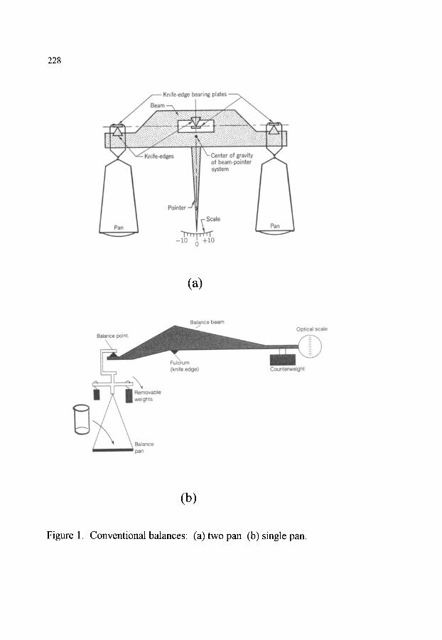
228

(a)

(b)

Figure 1. Conventional balances (a) two pan (b) single pan.

229

study oxidation was mentioned earlier. In this instance the weight of the object pulls on a coiled helical fiber of fused quartz. The extension is generally measured by following the movement of a fixed point on the fiber using a telescopic cathetometer. This requires a clear view of that moving point on the fiber so that position is usually distant from the sample and outside the furnace. The extension is, of course, calibrated using standard weights. The source and nature of such standard weights are described later in the section on calibration.

Mechanical balances have progressed over the years from the traditional two pan balance to the more modem single pan versions. Figure 1 indicates the functioning and differences between the two. The two pan balance in Figure 1 (a) generally has equal length beams that pivot around the fulcrum. The vertical displacement is frequently amplified using an optical lever. The null position is generally established with both pans empty. Subsequently, the weight on the sample pan is matched by an adjustable weight in the tare pan to restore the null deflection. At this point the two weights are considered equal. The weights on the tare side that are summed to give the sample weight should have been calibrated to sufficient accuracy.

The more modem single pan balance is depicted in Figure 1 (b). A counterweight is constructed for the tare side; generally in the form of a dashpot that also serves as a dampening device. The calibrated weights are suspended on the sample beam from the same point as the sample pan or holder. The full set of these weights exactly counterbalances the tare side to provide the null point in the absence of a sample. Again this null point is often detected on an optical scale. In order to preserve the null point when a sample is placed on the pan or holder, an equal weight must be removed by lifting an appropriate amount of the calibrated set of weights. The final one or more decimal places are typically measured on the optical scale where the deflection has been previously calibrated in terms of mass.

2.2. Modern electrobalances The electrobalance, however, provides the foundation for most contemporary

thermobalances. Again single pan and dual pan versions exist. The original version by Cahn [12] is depicted in Figure 2(a), while a later version capable of handling larger masses is shown in Figure 2(b). A taut band ribbon suspension, that is directly connected to an electrical torque motor having a wide linear range of torque versus electrical current, is used in place of the fulcrum. Sufficient weights are placed on the tare pan to reach a weight which must be within the linear range of the torque motor. The null position is determined by a lamp, mask, and photocell arrangement. This exact position is established and maintained through control of the current to the motor. As long as the change in weight occurs within the linear range of the torque motor, the restoring current is directly proportional to the weight,

230

and the direction of current flow indicates whether it represents a loss or gain in sample weight. A particular advantage of the electrobalance is that the electrical current can be directly translated into a voltage that is read directly by a digital voltmeter and is thus readily compatible with electronic data acquisition systems.

The capacity of the balance is directly related to the strength of the beam, ribbon suspension, and torque motor. The beam of the microbalance in Figure 2(a) is aluminum tubing and has two suspension points for the sample holder. The most sensitive position near the end has a capacity of approximately one gram. The suspension point closer to the middle has twice the capacity, but half the sensitivity. The much more robust version shown in Figure 2(b) has stronger components and a capacity of about 100 grams. Both versions, however, have a comparable sensitivity approaching 0.1 gg at room temperature in a static atmosphere.

i CONTROLS CIRCUITS INDICATORS

photo-

LED [~ flag

balance beam ~

'A' loop

sample

I

,are t loop

'B' loop

is torque suspension of beam and coil motor and torque assembly

motor coil connection

Figure 2. Electrobalances (a) Cahn original model.

231

Figure 2.(continued). Electrobalances (b) high capacity model.

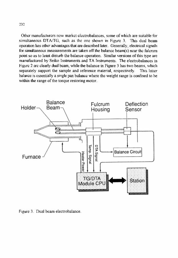
232

Other manufacturers now market electrobalances, some of which are suitable for simultaneous DTA/TG, such as the one shown in Figure 3. This dual beam operation has other advantages that are described later. Generally, electrical signals for simultaneous measurements are taken off the balance beam(s) near the fulcrum point so as to least disturb the balance operation. Similar versions of this type are manufactured by Seiko Instntments and TA Instruments. The electrobalances in Figure 2 are clearly dual beam, while the balance in Figure 3 has two beams, which separately support the sample and reference material, respectively. This latter balance is essentially a single pan balance where the weight range is confined to be within the range of the torque restoring motor.

Balance Fulcrum Deflection Holder-~ Beam-~ Housing Sensor

Furnace t,

i .... ~L I

$ ~.. ~'-----'IBal ance Circuit

. . ! . i!i!i!iiiii!

================================================= Li.i. ;;j

Figure 3. Dual beam electrobalance.

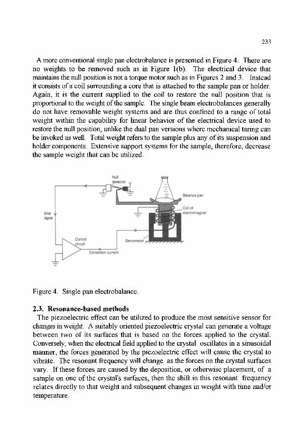
233

A more conventional single pan electrobalance is presented in Figure 4. There are no weights to be removed such as in Figure l(b). The electrical device that maintains the null position is not a torque motor such as in Figures 2 and 3. Instead it consists of a coil surrounding a core that is attached to the sample pan or holder. Again, it is the current supplied to the coil to restore the null position that is proportional to the weight of the sample. The single beam electrobalances generally do not have removable weight systems and are thus confined to a range of total weight within the capability for linear behavior of the electrical device used to restore the null position, unlike the dual pan versions where mechanical taring can be invoked as well. Total weight refers to the sample plus any of its suspension and holder components. Extensive support systems for the sample, therefore, decrease the sample weight that can be utilized.

Figure 4. Single pan electrobalance.

2.3. Resonance-based methods The piezoelectric effect can be utilized to produce the most sensitive sensor for

changes in weight. A suitably oriented piezoelectric crystal can generate a voltage between two of its surfaces that is based on the forces applied to the crystal. Conversely, when the electrical field applied to the crystal oscillates in a sinusoidal manner, the forces generated by the piezoelectric effect will cause the crystal to vibrate. The resonant frequency will change as the forces on the crystal surfaces vary. If these forces are caused by the deposition, or otherwise placemem, of a sample on one of the crystal's surfaces, then the shift in this resonant frequency relates directly to that weight and subsequent changes in weight with time and/or temperature.

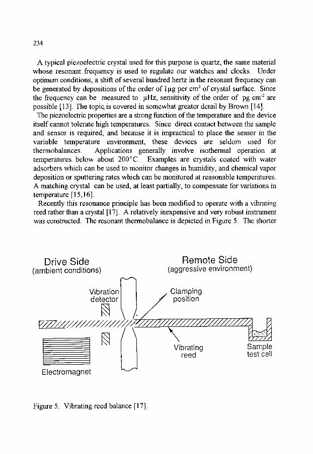
234

A typical piezoelectric crystal used for this purpose is quartz, the same material whose resonant frequency is used to regulate our watches and clocks. Under optimum conditions, a shift of several hundred hertz in the resonant frequency can be generated by depositions of the order of 1 gg per cm 2 of crystal surface. Since the frequency can be measured to gHz, sensitivity of the order of pg cm -2 are possible [13]. The topic, is covered in somewhat greater detail by Brown [14].

The piezoelectric properties are a strong function of the temperature and the device itself cannot tolerate high temperatures. Since direct contact between the sample and sensor is required, and because it is impractical to place the sensor in the variable temperature environment, these devices are seldom used for thermobalances. Applications generally involve isothermal operation at temperatures below about 200~ Examples are crystals coated with water ads0rbers which can be used to monitor changes in humidity, and chemical vapor deposition or sputtering rates which can be monitored at reasonable temperatures. A matching crystal can be used, at least partially, to compensate for variations in temperature [ 15,16].

Recently this resonance principle has been modified to operate with a vibrating reed rather than a crystal [17]. A relatively inexpensive and very robust instrument was constructed. The resonant thermobalance is depicted in Figure 5. The shorter

Drive Side (ambient conditions)

Remote Side (aggressive environment)

Vibration det~tor

Clamping position

Electromagnet

Vibrating reed

Sample test cell

Figure 5. Vibrating reed balance [ 17].

235

external section of a stiff elastic reed is clamped. The longer section extends into the temperature controlled environment and supports the sample. The reed is vibrated and the frequency varies with the load at the sample position. A calibration curve indicated a linear relationship of frequency versus weight having a slope of 3.847 Hz g -1. The uncertainty w a s 10 "2 Hz so that the sensitivity of this initial version was only about 3 mg. Besides the sturdiness and simplicity, however, other advantages accrue because of the constant vibration of the sample, which facilitates mass transport and mixing within the sample.

The electrodynamic balance has been adapted to do a wide range of thermoanalytical measurements. The history and characteristics for such a balance are described by Davis [18]. Figure 6 shows the schematics of such a balance [19]. The basic principle involves the electrostatic suspension of a small sample, an aerosol droplet or fine particle, by means of the shaped electrodes and a toroid surrounding the sample. The mass is related to the de potential required to maintain the sample suspended in the same position Vdr as a function of time, temperature, or composition of the ambient gas. The specific relationship is m - qCV~r where m is the sample mass, q is the particle charge, g is the gravitational constant, C and Z0 are constants related to the geometry of the system.

~ IT 1

L__.

LASER BEAM .... y

Figure 6. Schematic of an electrodynamic balance [19].

236

The sample is heated by a laser to create a TG system. Simultaneous FTIR-EGA has been achieved [20]. Adaptations also exist for magnetic measurements [21] and particle sizing [22]. As the quest for sensitive methods to use with minute samples advances these devices may see more use in the future.

2.4. Influence of an external magnetic field (Thermomagnetometry) The presence of a magnetic field gradient at the site of the sample may alter the

apparent weight (not mass) by virtue of the additional force superimposed on the gravitational field. For diamagnetic materials and even paramagnetic samples these changes are not likely to be noticed during conventional TG, because they are so small compared to the normal weight of the sample. For ferro- and ferrimagnetic materials, however, these forces can be very great, depending upon the strength of the magnetic field gradient at the sample position. The force may even be strong enough to completely levitate or remove the sample, when the direction of the magnetic field gradient is in the upward direction.

Stray magnetic fields, therefore, represent potential sources of error and are discussed later. There are, however, several areas of research where the magnetic effects can be deliberately utilized, through TM, to gain useful information that would not be obtained by conventional TG. Some aspects of this will be mentioned under the appropriate sections later in this chapter and in the subsequent volumes dealing with applications. A recent tutorial review and the references therein describe TM and some of its applications [23].

The strength of the magnetic field used for TM depends on the purpose of the measurement. If the object is to determine the magnetic transition temperature, Tc, then the magnetic field need not be greater than that necessary to detect the effect on the apparent weight. In fact a stronger field may be undesirable [24]. However, when the intent is to determine the formation of magnetic intermediates or final products during the course of a reaction, then the sensitivity of detection obviously increases with the strength of the magnetic field gradient at the sample position. This strength depends not only on the strength of the magnet, but also on the physical arrangement and proximity of the sample and magnet. Consequently, the size of the fiunace and its arrangement in relation to the fitmace become important. A large furnace surrounding the sample will preclude bringing the magnet close to the sample and necessitate the use of a stronger magnet.

The strength of the magnetic field, however, cannot be increased indefinitely without raising concern for the possible effects of the resulting field on the accuracy of the balance. Such aspects have been considered when studying the possible influence of an external magnetic field on the rates of chemical reactions [25 - 27]. Alternative methods, e.g., evolved gas analysis (EGA), to follow the rate of a reaction in very strong magnetic fields may become advisable.

237

3. DESIGN AND CONTROL OF THE THERMOBALANCE

In this major portion of the chapter the considerations involved in the construction and operation of a thermobalance are discussed in some detail. The fundamental difference that distinguishes a thermobalance from a conventional balance is the ability to fimction in a manner that allows the sample to be simultaneously weighed and heated or cooled in a controlled manner. In addition, this has to be accomplished whilst maintaining the desired atmosphere and pressure. The topic is subdivided into three sections involving the factors associated with temperature, atmosphere, and the sample.

3.1. Providing and controlling the heat Controlling the temperature of the sample is the most difficult and critical aspect

of thermogravimetry. The three primary aspects are: (1) the means of exchanging heat with the sample; (2) the method of determining the temperature at the critical point, the sample; and, finally, (3) the link between these previous two considerations, i.e., the mode of feedback and control of the temperature.

3.1.1. Types of furnaces The controlled exchange of heat between the sample and its surroundings, in

conjunction with the heat capacity and enthalpic events associated with the sample, determine the sample's temperature during the course of the TG experiment. Manipulation of the temperature of the sample's surroundings is the principal means of controlling the temperature of the sample. The transfer between the surroundings and the sample must not interfere with the measurement of the sample's mass. Consequently, the thermal transport is via conduction by the intervening atmosphere, or direct radiation through that atmosphere.

Cooling the sample in a controlled manner is generally more difficult, particularly at rapid rates. This is usually done by surrounding the entire region with a low temperature environment, such as a Dewar flask of refrigerant, and counteracting the appropriate amount of cooling by supplying energy from a supplemental heater. Alternatively, the flowing atmosphere may be maintained at a low temperature and the temperature of the sample is again controlled by the supply of heat from the surroundings. The heating processes controlling the temperature of the surroundings are basically of two types.

Convective (Resistive): A furnace or oven is constructed which partially surrounds the sample container in a reasonably symmetrical fashion. The furnace is of necessity substantially larger then the sample. In most instances the furnace surrounds a tube containing the sample and through which the controlled atmosphere

238

flows. Figure 7 shows the most common spatial arrangements of the fitmace and sample. Clearly this is detelmmed by the nature of the link between the balance and sample. The hangdown arrangement allows for a non-riNd suspension link between the balance and sample. The other two relationships require a rigid link. The respective advantages and disadvantages of each configuration are discussed in the section on errors, 3.1.3.

Furnace Programmer Controller

//////~I "I Balance

Temp.

Temp.

Mass

Temp. l

Data Acquisition

H i H -.. ,.-_ Temperature Sensing .,, IS! Possible Sample and - " "- and Furnace Power I~1 Furnace Positions

Figure 7. Typical arrangement of furnace, balance, and sample holder.

Figure 8 shows an exception to the above arrangements. The furnace is located inside the atmospheric protection tube. This allows for a much smaller tin, ace, with less demand for power, that is more capable of rapid heating and cooling by virtue of its diminished size and closer proximity to the sample. It is, however, subject to direct exposure to both the flowing atmosphere and the volatile products of any decomposition. In addition, the small size puts greater constraints on the sample size and the positions of the sample and the temperature sensor.

Convectively heated furnaces have resistive elements that are carefully coupled with their support to raise the temperature of the surface of the fimaace that is exposed to the sample and its environment. The mode of thermal transport is

239

Figure 8. The Perkin-Elmer micro-furnace.

determined by the temperature of this surface and both the transparency and thermal conductivity of the intervening medium. At temperatures below about 800~ thermal transport is predominantly determined by conduction through the external atmosphere, the atmosphere containment tube, the internal atmosphere, the sample holder, and finally the sample itself. The flow and convective patterns within the gas phase are important For this reason baffles play a significant role in providing uniform heating of the sample and its holder. At higher temperatures thermal conduction through radiative mechanisms becomes significant and ultimately dominant.

Typical resistive elements are listed in Table 1 along with their limitations. Flexible materials may be wrapped, in the form of wire or tape, directly on the atmosphere containment tube. It is more common, however, to wind the elements on a separate fimaace tube, surrounding the atmosphere control tube, to allow for easy independent removal of either component. The inflexible materials are formed as rods, SiC, or hairpin shaped, MoSi2, heating elements. These are arranged symmetrically around the atmosphere control tube and the independent elements are interconnected electrically.

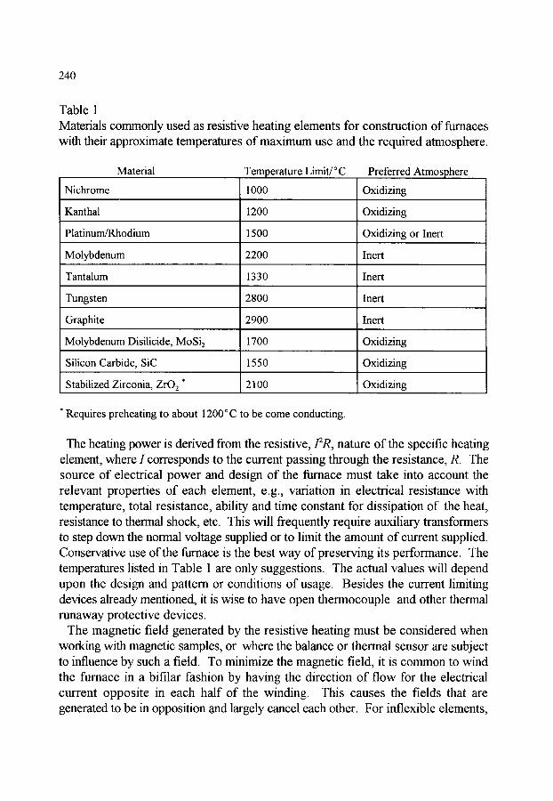
240

Table 1 Materials commonly used as resistive heating elements for construction of furnaces with their approximate temperatures of maximum use and the required atmosphere.

Material

Nichrome

Kanthal

Platinum/Rhodium

Molybdenum

Tantalum

Tungsten

Graphite

Molybdenum Disilicide, M o S i 2

Silicon Carbide, SiC

Stabilized Zirconia, ZrO2*

Temperature Limit/~ C Preferred Atmosphere

1000

1200

1500

2200

1330

2800

2900

1700

1550

2100

Oxidizing

Oxidizing

Oxidizing or Inert

Inert

Inert

Inert

Inert

Oxidizing

Oxidizing

Oxidizing

* Requires preheating to about 1200 ~ to be come conducting.

The heating power is derived from the resistive,/2R, nature of the specific heating element, where I corresponds to the current passing through the resistance, R. The source of electrical power and design of the tin-ace must take into account the relevant properties of each element, e.g., variation in electrical resistance with temperature, total resistance, ability and time constant for dissipation of the heat, resistance to thermal shock, etc. This will frequently require auxiliary transformers to step down the normal voltage supplied or to limit the amount of current supplied. Conservative use of the fiu~ace is the best way of preserving its performance. The temperatures listed in Table 1 are only suggestions. The actual values will depend upon the design and pattern or conditions of usage. Besides the current limiting devices already mentioned, it is wise to have open thermocouple and other thermal runaway protective devices.

The magnetic field generated by the resistive heating must be considered when working with magnetic samples, or where the balance or thermal sensor are subject to influence by such a field. To minimize the magnetic field, it is common to wind the furnace in a bifilar fashion by having the direction of flow for the electrical current opposite in each half of the winding. This causes the fields that are generated to be in opposition and largely cancel each other. For inflexible elements,

241

the hairpin curve ofMoSi 2 elements or an alternation in direction of electrical flow for SiC rods helps to minimize the magnetic field.

Precise control of the sample's temperature requires that the fiamace, controller, sensor, and system geometry be carefully matched and optimized. This cannot be attained over a wide temperature range using a single furnace. Manufacturers market a variety of fiamaces and control systems to combine with their balance and sample suspension systems in a modular form, facilitating ready imerchange. Typical arrangements are: (1) a Nichrome or Kanthal based fiamace in conjunction with fused silica refractories for operation up to 1000~ and (2) a platinum/rhodium or MoSi 2 based furnace combined with alumina refractories for operation to 1500-1700~ Special lower or higher temperature systems are available on a more limited basis.

Radiative (IR heating): One of the major limitations to conventionally heated fiamaces is the inability to heat rapidly. This drawback arises from the power and time required to raise the temperature of the relatively massive furnace. The refractories and heating elements may also not be able to cope with the rapid changes in thermal expansion and mismatches in components may arise. Heating of the sample and its comainer by focused infrared emission has recemly been introduced by at least one manufacturer, Ulvac Sinku-Riko. Speyer [28] has adapted this method of heating to thermodilatometry in order to take advantage of the rapid response time for studies of controlled rate simering. Obviously, the same advantage would apply for controlled rate thermogravimetry, see below, and studies of the kinetics of rapid pyrolysis or other fast reactions. Simulating the problems associated with rocket engines or the re-entry of space vehicles are potential examples.

Halogen lamps or infrared heaters can be carefully focused in a symmetrical manner on the sample or its container. The thermal transport is virtually instantaneous. The absolute heat flux depends, however, upon the transparency of the optical path and the absorbency of the sample or its container. Figure 9 indicates some of the forms that such furnaces may take. Reflectors are generally gold-coated surfaces that may be shaped elliptically or parabolically. The focus may be a point, a line, or a surface which should be centered on the sample or its holder. Clearly the intervening gas comammem tube, usually fused quartz, must be highly transparem to the radiation in order to avoid dissipation of the heat within the outside tube.

If the sample evolves infrared absorbing gases upon heating, the heat flux reaching the sample during that time will be altered. Should the products condense on the cooler surface of the fused quartz tube, then they will continue to absorb the radiation and probably darken further with time. Changes in emissivity of the

242

heater, sample, or sample holder with time or temperature will also alter the effective heating rate. Measurement of the sample's temperature may be more difficult in this type of furnace, particularly since it is more likely to involve faster heating rates. Such systems offer major advantages regarding the potential response time of a relatively clean system, but other factors may preclude their use in particular situations.

TYPES AND MAXIMUM ATTAINABLE TEMPERATURE OF RADIANT HEATING

Parabolic reflector RHi-P Tubular focusing Tubular focusing Planar focusing

. . . . . .

1300~ 1300~ 1200~ 1500~ . . . . . . . . . . . . .

--~--~ :+; K---JD- �9

Elliptical reflector RHL-E Tubular focusing Tubular focusing Linear focusing

=

1300oC . . . .

i

. . . . . . .

Figure 9. Examples of image heating.

3.1.2. Temperature measurement and control The specific goal of each investigation determines the relative importance of

temperature measurement and control. Measurements designed to determine the constant mass of a gravimetric precipitate, corresponding to a particular stoichiometry, are generally unconcerned about the exact temperature and the heating rate. The emphasis is on the mass. Kinetic and calorimetric measurements, however, usually demand constant well-defined heating rates and an accurate knowledge of the sample temperature, as well as its mass as a fimction of time. Designing a furnace system to respond rapidly to the desired commands, yet to be immune to gyrations caused by unintended instabilities is most demanding. Wendlandt [29] has pointed out that the change in the derivative (~ rain -1) with time is a more sensitive indicator of a stable temperature program.

Sensors and their placement: There are several types of sensors for the measurement of temperature based on changes of a specific property with temperature, e.g., electrical conductivity (metallic resistance thermometers and semiconducting thermistors), volume expansion (Hg in glass), pressure of a confined gas (He thermometer), black-body radiation laws (optical pyrometers), and the Seebeck Effect (various thermocouples). The International Temperature Scale, ITS-

243

90, is based upon the use of gas thermometers at the lowest range of temperature, platinum resistance thermometers at intermediate temperatures, and optical pyrometry at the highest temperatures [30]

The vast majority of thermobalances, however, use thermocouples. Older instruments, predating the modem PC, provided readings of the thermocouple output in ~tV. which then had to be converted to temperatures based on standard tables. With the advent of digital data acquisition, it became more practical to use the curve fitting equations themselves rather than the derived tables. These equations generally are of the form of fifth- to fifteenth-order polynomial expansions. Chebyshev expansions are used for the most demanding requirements, such as for the construction of the lookup tables. Details are discussed in Chapter 6 and Appendices V and VI of Quinn [30]

The use of the Seebeck Effect depends on one of the two junctions comprising the thermocouple being at a fixed and defined temperature. Traditionally this was 0 ~ established by an ice bath. Modem measurement techniques involve an isothermal block as part of the measuring circuit and it is easiest to maintain the temperature of this block at slightly above the anticipated room temperature. This necessitates adjustments to the temperature versus voltage curves used to convert the signal into temperature.

Table 2 lists some of the most common thermocouples used in TG, along with the applicable temperature range and appropriate atmosphere. It must be noted that these recommended ranges and atmospheres are dependent upon several parameters and are only approximately based on average conditions. When more than one thermocouple is possible for a particular application, such factors as stability, sensitivity (~tV/~ and cost enter into the decision. If stability is dependent upon contact with the sample, its container, or the atmosphere, it is customary to protect the thermocouple by enclosing it in a inert sheath. The response time is lengthened by the increased thermal resistance. The response time and lifetime of the thermocouple are strongly influenced by the diameter of the wire. Larger diameters add to the mechanical strength and lifetime, but also add to the thermal losses and heat capacity of the sensing system and thereby decrease the sensitivity and increase the response time.

Should one base control of the furnace on the temperature at the sample point or at the heating element? The latter will give better stability and control of the thermal environment. The response to changes in the power supplied will be quicker and thus such factors as overshooting the control point will be reduced. The downside, however, is that the events within the immediate environment of the sample, such as changes in enthalpy and heat capacity during reactions, or changes in thermal conductivity occurring within the atmosphere, are essentially ignored.

244

Table 2 Common types ofthermocouples used in thermogravimetry and their recommended conditions for usage [24]

T, ~e

E

K

R

Description Temperature Range/~ Atmosphere

Cu / Cu-Ni -250 to 850 air, inert

Ni-Cr / Cu-Ni

Fe / Cu-Ni

Ni-Cr / Ni-A1

Pt / Pt- 10%Rh

Pt / Pt-13%Rh

W / W-26%Re

-250 to 800

0 to 760

-270 to 1260

0 to 1600

0 to 1600

0 to 2700

inert

air, inert

air, inert

air, inert

air, inert

inert, reducing

The exact temperature of the sample is seldom attainable. Direct contact between the sensor and the sample will disturb or interfere with the measurement of mass. An indirect measurement of temperature, such as by optical means, will measure the temperature of only that portion of the sample or its holder on which the optics are focused. The temperature at the moving reacting interface is unavailable by the present state of the art and represents one of the major limitations to the study of heterogeneous kinetics.

A logical and frequent compromise is to use separate sensors for control of the heating profile and measurement of the sample temperature, while recognizing the limitations of the latter. Figure 10 shows some of the common placements of the sensor, in these cases a thermocouple, for the measurement of the sample's temperature. Insmmaents specifically designed for simultaneous TG/DTA will often have more direct contact with the sample holder, such as in Figure 10(c). Other schemes will position the sample immediately above (Figure 10(b) or below (Figure 10(a)) the sample pan. Should the sample ignite, a sensor directly above the open portion of the container is more likely to detect and be influenced by the combustion and heated gases.

Increasing the size of the uniformly heated zone eases the conditions on placing the temperature sensor. In some cases, such as the small furnace depicted in Figure 8, the placements of both the sample and the thermocouple are more critical. It is tempting to adjust the thermocouple directly underneath the sample pan to the closest possible position without touching the pan, as in Figure 10(a). Thermal expansion of both the sample suspension system and the thermocouple, however, will quickly lead to contact problems as the system is heated. Under such circumstances it is more prudent to bend the thermocouple off the vertical axis and

245

around the side of the pan. Other considerations are the shielding effects that impede radiative transport, or the cooling effect of a flowing atmosphere and hence its flow pattern. A thermocouple on the upstream or downstream side of the sample, its holder, or a baffle will sense different temperatures.

/ ' \

(a) /

(b)

! I

(c) Figure 10. Examples of thermocouple placement relative to the sample position.

Conventional control of temperature: Typical control of temperature for a thermobalance is based on comparison of the temperature of a sensor with a predetermined time-temperature profile. Power is then supplied to the furnace in such a manner as to maintain a minimum difference between the sensor and the control setting. One of the major options concerns the choice of sensor. Types and locations have been discussed in the previous section. By far the most common choice is a thermocouple. The concern at this stage is whether to use the same thermocouple that is used to record the sample temperature for control, or whether to introduce a second thermocouple in a more advantageous position or environment. There should be some form of protection circuit present to prevent thermal runaway of the furnace in the event of a sensor malfunction. The most common technique is when a break in the thermocouple circuit is detected, the temperature reading is set to the maximum temperature. The consequence of this is to reduce the power to the furnace.

Generally the thermocouple position that is best suited to measuring the sample temperature is too isolated from the heating elements to provide the smoothest temperature control. Consequently, a second thermocouple is inserted at a central location very near the furnace winding. The response time is thereby markedly reduced and the controller has a better opportunity to maintain the desired temperature programme. The difference between the furnace temperature and the immediate sample environment may, however, be significant. This offset has to be compensated for through the calibration procedure.

246

The predominant temperature programme involves the use of simple linear heating or cooling ramps. Altematively, isothermal programmes are used to ascertain changes as a function of time. Frequently, the temperature programme has some complexity and involves a mixture of linear and isothermal segments. The general nomenclature is that a temperature controller provides simple isothermal control of temperature and a programmer controller allows for the variation of temperature with time. Programmers are available over a range of flexibility, some are capable of a relatively few steps in the temperature programme while others offer potentially many variations.

The controller continually determines the difference between the desired and measured values of temperature. That difference is amplified and a proportional signal is applied to the power supply of the furnace. It may be in the form of a simple dc voltage, however, this has the disadvantage that if that circuit should become open, an undefined potential exists and the fiamace will be uncontrolled. Generally a 4 to 20 mA signal is used for control purposes, because an open circuit clearly results in a zero current reading and power is shut off to the fimaace.

The control signal is used to bias the p-n junctions of the silicon controlled rectifier, SCR, in such a manner that the low signal of 4 mA represents virtually no current to the furnace and the high signal of 20 mA represents full power to the furnace. This electrical power may not be of the optimum voltage to operate the specific furnace. Consequently, it is frequently modified to the proper current and voltage relationship, through the use of a power transformer, prior to application to the fimaace resistive elements or lamps. A more detailed explanation of this process is given in the book by Speyer [31]

Simple "on - off" application of power to the furnace is insufficient to achieve the desired degree of control for thermoanalytical techniques. This results in too great a variation in the programmed temperature or heating/cooling rates for proper control or measurement of the chemical and physical processes under investigation. Particular problems involve cycling temperatures, over or undershoot of the desired isothermal temperature, a very slow approach to the control temperature, etc.

These problems can be minimized by careful manipulation of the control functions (referred to as proportional integral derivative or PID). These functions are adjustable in most modem sophisticated, temperature control equipment. They may require manual tuning or may be automatically adjusted by the computer that controls the overall system. The ideal settings will change over a wide range of temperature and heating/cooling rates and generally some form of compromise is used to arrive at the optimum values for each system. PID control is extremely important in most feedback control loops. Instructions for proper tuning of the system can generally be obtained from the manufacturer of the control equipment, or from various other tutorial sources [31 - 33]

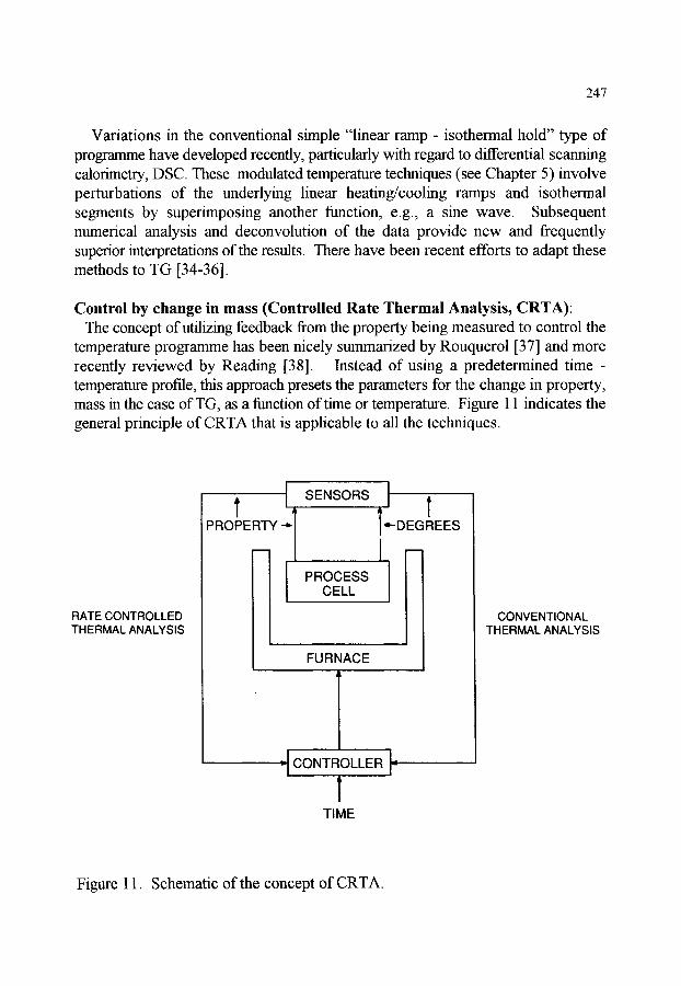
247

Variations in the conventional simple "linear ramp - isothermal hold" type of programme have developed recently, particularly with regard to differential scanning calorimetry, DSC. These modulated temperature techniques (see Chapter 5) involve perturbations of the underlying linear heating/cooling ramps and isothermal segments by superimposing another function, e.g., a sine wave. Subsequent numerical analysis and deconvolution of the data provide new and frequently superior interpretations of the results. There have been recent efforts to adapt these methods to TG [34-36].

Control by change in mass (Controlled Rate Thermal Analysis, CRTA): The concept of utilizing feedback from the property being measured to control the

temperature programme has been nicely summarized by Rouquerol [37] and more recently reviewed by Reading [38]. Instead of using a predetermined time - temperature profile, this approach presets the parameters for the change in property, mass in the case of TG, as a fimction of time or temperature. Figure 11 indicates the general principle of CRTA that is applicable to all the techniques.

RATE CONTROLLED THERMAL ANALYSIS

t I PROPERTY "']

SENSORS

PROCESS CELL

FURNACE

I ; ] '~"DEGREES

_1 L 7 CONTROLLER, ..,I-

T TIME

CONVENTIONAL THERMAL ANALYSIS

Figure 11. Schematic of the concept of CRTA.

248

The nature of the feedback loop can assume at least three forms. The first is to simply to prescribe a rate of mass loss in some form, e.g., mg min -1 or % h -~, and use the difference between the observed rate of loss versus the programmed rate of loss as the input signal to the furnace programmer/controller. This could be for multiple segments, i.e, several iso-rate steps as a function of time. When the rate of mass loss is below the prescribed rate, more current is supplied to the fimaace. Clearly this would have to be reversed, if the process was one of mass gain, such as oxidation of a metal. The PID values of the control circuit must be revised to reflect the change in the control parameter.

An excellent example of this mode of operation is its use to determine temperature programmes for the binder burnout of critical ceramic parts [39]. Rates of 0.01 to 0.001 mg min -1 were found to be appropriate. Figure 12 shows the results at the 0.001 mg min -~ rate of loss. Three regions of temperature are indicated, corresponding to the burnoff of three different components of the organic binder lubricant formulation. Another excellent example is the work of Paulik and Paulik concerning the decomposition of calcium carbonate [40]. This accentuates the effect of the technique, because the reaction is readily reversible and dependent on mass transport as well as thermal transport.

3 0 ' 2 2 0

2 9

~ 2 8

27

/ I

!

, / ,/

J / ' / '

S S ~

!

2 0 0

1 8 0 .~

1 6 0 "~

1 4 0 ~

1 2 0

2 6 ' ' ' ' ' ' 1 0 0 0 1 0 0 0 2 0 0 0 3 0 0 0

T i m e / m i n

Figure 12. Example of CRTA, TG of the binder burnout from a layered green multilayer ceramic. Mass loss at a rate of 0.001 mg min -1 [39].

249

The second mode is to set a limit for the lower rate of mass loss, typically 0.08% of the maximum rate of loss at a normal linear heating rate. Below this threshold a prescribed, generally fast, rate of linear heating is applied until the rate of mass loss exceeds the preset upper rate of mass loss. The value of this threshold is generally about 100 times the lower threshold. When this rate of loss is achieved, the temperature is held constant until the rate of loss decreases to the lower limit, at which point the cycle repeats. This step-wise isothermal mode has been advocated by Sichina [41] and is commercially available.

The third method is very closely related to the previous technique. The difference is that the upper threshold does not invoke isothermal behavior but rather a marked reduction in the heating rate. It is known as high resolution, Hi-Res, TG [42]. The changes in heating or cooling rates are controlled by manipulating two numerical parameters referred to as resolution and sensitivity. An example is shown in Figure 13 using CuSO4o5H20 [42]. Clearly the steps associated with the loss of the waters of hydration are much better resolved through use of the CRTA approach. The relative elapsed time for the two approaches will vary depending upon the settings selected.

Barnes has compared the methods and supported the claims of enhanced resolution over conventional TG using any of the three modifications [43]. Resolution in conventional, linearly heated, TG can be significantly enhanced by mixing isothermal hold periods into the temperature programme based on previous experience with the material. In a quality control laboratory, where routine measurements are performed on similar samples, this simple approach may be quite satisfactory, however, the CRTA approach is self-adapting and hence flexible in its application. Whichever approach is adopted for CRTA, it is advisable to be aware of the algorithms and criteria used, and to examine the resulting temperature-time profile in order to better understand what has occurred [44].

3.1.3. Sources o f error related to temperature Accurately defining the sample temperature during a dynamic thermogravimetric

experiment is a non-trivial task [45]. The techniques used to calibrate and thus minimize these consequences are described in Section 5. The sources of error may be grouped into three principal areas. Sensor: As was discussed earlier, the overwhelming choice of a temperature sensor for TG is the thermocouple. Thermocouples are not the method of choice for the most accurate determination of temperature in any range. They are, however, the most practical devices for TG at other than the very highest temperatures, where optical pyrometry may be the most practical as well as the preferred method.

250

1 0 0 -

9 0 -

8 0 -

7 0 - o~ r" C)') (1)

60 -

100-

9 0 -

8 0 -

7 0 -

STANDARD TGA @ 5~

/

__/

6 0 - ~ ' " , , 0 50 100 150

T / ~

! I I

HIGH RESOLUTION TGA RES 4.31SEN 8.0 @ 5~

I

200 250

Figure 13. Hi-Res TG of CuSO4"5H20 [42].

300

_ C O

o< c

,, , . , .

- C I- r-

251

Errors related to the use of thermocouples may be considered in three general areas: their placement, their composition, and the measuring circuitry. The placement has been discussed above, because it relates to aspects of temperature control. Placement is also clearly a factor in assigning the sample temperature to that of the thermocouple temperature. The thermocouple junction should be placed in the position most likely to have the same temperature as the sample, but which will not interfere with the operation of the balance or system. Positions in a different atmosphere or flow pattern are clearly suspect, as would be positions far removed from the sample. The predominant mode of thermal transport must be carefully considered. Consequently, convection patterns, emissivity, etc. play a major role in this placement decision. The thermal transport properties of the protective sheath around the thermocouple become important in terms of both the resistance of the thermal path and thermal conductivity away from the junction down the sheath. The thermal conductivity of the atmosphere, particularly if it is flowing, can also play a significant role [46].

The initial accuracy of the thermocouple depends on its conformance to the alloy composition and the potential presence of strains in the materials. Strains tend to anneal away during the first few cycles. If the construction of the complete thermocouple system, i.e., thermocouple, sheath, insulation, etc., is incorrect, however, strains may actually develop during use.

The long term stability of the thermocouple depends largely on maintaining its composition. Diffusion, both solid state or vapor phase, will tend to make the two alloys more similar and thus reduce the sensitivity, particularly at the upper temperatures of use. Reaction with any of the materials that the thermocouple contacts, such as fitrnace refractories, sample or sample holder, its own sheath or insulation, and any reactive atmosphere, will alter the characteristics of the thermocouple or even break the electrical path. The metals undergo grain growth at the elevated temperatures and this can ultimately lead to loss of mechanical strength and brittleness. The lifetimes of most thermocouples are increased by using a larger gauge thermocouple wire. This is more practical for the control thermocouple.

The errors induced by the measuring circuitry are generally minor in nature, but do limit the ultimate noise limit that can be attained. If there is significant electrical pickup by the thermocouple from the changes in the fitmace current, then some form of electrical shielding is required. Electrically grounding the sheath of the junction will usually reduce the observed electrical fluctuations. Drifts in the temperature of the isothermal block, or in the stability of the amplifiers, can become factors, but these forms of error are generally not significant with modem equipment.

252

Rate of heating: The errors in the observed sample temperature with heating or cooling rate are associated with the thermal lag between the sensor and the sample. They can take any form, in that the thermocouple may be in a relative position that will receive either greater or less thermal flux than the sample. Consequently the lag can be in either direction. The factors in this type of error are similar to those discussed in the previous section related to the placement of the sensor and the relative thermal transport properties of the sensor and the sample configurations. It is impossible to completely alleviate such errors and they increase with increasing heating rates. Departure from the programmed heating and cooling rates may be related to inappropriate PID values, or simple inability of the furnace to keep up with programmed rate. These effects are very sensitive to the design factors of the system and may vary substantially from one instrument to another.

In selecting an example of the dependence on heating rate, it is important to choose a system that does not involve factors other than the simple heating rate. Such potential factors are discussed in following sections. Figure 14 is a good choice in that it indicates the variation in a simple magnetic transition with heating rate [24]. The small fiamace depicted in Figure 8 was used, where the temperature gradients are steep and the location of the thermocouple therefore critical. Determination of the disappearance of the magnetic attraction based on the differential signal, DTM, is slightly more sensitive. Clearly there is a pronounced dependence of the result upon the heating rate. A simple linear extrapolation to zero heating rate shows excellent agreement between the results based on either heating or cooling. The extrapolated result, however, is far from the accepted value and indicates the need for temperature calibration.

The melting point of lead was measured simultaneously with the TM measurements shown in Figure 14 and it required the same correction after extrapolation to zero heating rate. The dependence of the observed melting temperature, however, was nonlinear and indicates that each process and instrument will exhibit unique behavior. Heat of reaction: It is impossible to compensate completely for the effect of the enthalpy of reaction or change in heat capacity at the reacting interface. The temperature sensor never detects the true temperature at the exact time and place of the reaction. It is always necessary to contend with a significant time lag and temperature offset [47]. A typical enthalpy of reaction will absorb or provide energy sufficient to lower or raise the temperature of the mixture of reactants and products 1000 ~ or more [48]. Besides the actual enthalpy of the reaction, there are likely to be subsequent reaction interfaces sweeping through the sample as the initially formed products undergo strain relief, crystallization, particle size growth, etc. There may even be oscillatory reactions taking place at the surface of the sample due to catalytic reactions [49,50].

253

350 TG

O 340 O v

o I-- D 330

LU n" Z3 03 350 < uJ

340

I , . I ,,. I

DTG

330 L I ! , ! .... I

0 10 20 30 40

RATE (~ min Figure 14. Observed values of T~ for nickel as a function of both heating and cooling rates based on both TM and DTA. (O) heating, (F1) cooling [24]

The progress of the reaction also alters the thermal and mass transport properties of the system, which further complicates the correlation between the temperature sensor and the temperature of the relevant portion of the sample. Since sensors are unable to track the temperature at the reacting interface, it is essential that the experimentalist be aware of problem. Performing measurements with different sample sizes and at different heating rates will reveal the extent of the problem in the specific experimental system under investigation. Slower heating rates and smaller samples will minimize the discrepancy between the measured and actual temperature. Consideration can be given to extrapolation to zero sample mass, and heating or cooling rate, in order to obtain a value more closely approaching the "true intrinsic" temperature of the reaction or process.

254

3.2. Control of the atmosphere Most effects investigated by TG or TM are dependent on the atmosphere to which

the sample is subjected. Consequemly, it is vital to control the nature and flow of the atmosphere. Besides the affect of the atmosphere upon the process and temperature of the measuremem, care must taken that it also does not damage or disturb the balance mechanism and the heating elements.

The use of helium, nitrogen, or argon as an inert or purge gas is based on several considerations. Among these are cost, availability, purity, density, and thermal conductivity. The first two criteria are self explanatory. Initial purity is one aspect, but so is the ability to filrther clean, particularly deoxygenate, the gas stream. Noble gases are particularly desirable in this respect because they can be passed over titanium turnings or powder at an elevated temperature to remove oxygen, most oxygen containing molecules, and even nitrogen, very effectively. Density is a consideration for a purge gas because it is desirable to have it assist in minimizing back-streaming. If the balance is above the furnace and sample, then denser argon is preferable to helium, but the reverse holds for the opposite configuration of balance and furnace [51]. The effects of thermal conductivity on the thermal transport have been noted earlier.

Various devices are available to measure and/or control the flow rate of the desired atmosphere. Least expensive for measuring the flow rate are the conventional float and tube, a simple liquid bubble tower, or a soap film bubble tower. The former device requires additional compensation to account for the density of the specific gas, but is suitable for faster rates. A range of floats and tubes are available to cover a very wide range in flow rates. The latter two devices measure volume directly and require simultaneous measurement of time to convert to rate. Many of the mstmmem manufactures provide valves to switch gas streams at preset times, enabling simple programming, such as changing from an inert to oxidizing environmem at a specified temperature in a controlled pyrolysis reaction.

Control of the flow rate may simply rely on a pressure regulator and an assumed unchanging drop in pressure along the transmission line. Added stability can be obtained by using diffusion disks of porous metal, glass, or ceramic to further control the drop in pressure from the source tank. Disks are available to deliver prescribed rates of flow per unit of pressure at the source. When accurate control or more complex programming is required, mass flow controllers are particularly versatile and convenient. With suitable calibration, these devices are capable of maintaining the desired rate of flow and controlled mixing of gases indefinitely. They are relatively expensive, require calibration and maintenance, and must be matched to the gas and rate desired.

255

Frequently it is advisable to analyze either the entering gas stream or, more often, the exit gas. The latter is EGA or EGD and is covered in Chapter 12. There are other occasions, however, when it is necessary to verify the composition of the incoming gas, e.g., mixed gases to establish a particular oxygen comem, or the exhaust gas to check for leaks in the system. If such analyses are performed simultaneously with the TG measurement, then consideration must be given to possible alterations in the flow rate or total pressure of the system and their effect on the mass and temperature measuremems.

It is desirable to preheat the gas stream close to the sample temperature prior to contact. The most common way is to pass the gas over baffles as it is introduced to the hot zone. Alternatively, the gas can be passed through the hot zone or over the heating elemems before being exposed to the sample. A common technique is to pass the gas through a small tube that exits at the closed end of the larger sample tube so that the flow pattern brings the preheated gas back over the sample, exiting at the same end of the tube as it entered.

Percolating the atmosphere directly through a powdered sample represents the ultimate way of sweeping any volatile products away and preveming a reverse reaction. Arranging the apparatus in such a manner severely complicates the sample suspension system. It has been recently achieved in a below the balance sample configuration [52]. The resulting forces from the gas stream, however, oppose the gravitational force and lower the observed weight, even during periods of no mass loss. This change in weight has been used to study both the fluidization forces operating within a tapered fluidized bed and the hysteresis in these forces as the fluid velocity is raised and then lowered.

There are occasions when information is needed concerning the decomposition of a substance in its own gaseous products. Such conditions may more closely simulate the actual situation occurring under normal process conditions. Several sample holders have been devised to establish the desired "self generated atmosphere". Figure 15 depicts three of these [53]. In each case a restricted path is provided for the gases escaping from the small sample volume. Because the sample volume is quite limited, it quickly fills with the product gases which displace the original atmosphere. Figure 16 indicates the dramatic effect that this build up of decomposition products can have on the observed temperature for readily reversible processes, such as many decompositions of carbonates or hydrates. The thermodynamic equilibrium constant for such decomposition reactions is established by the activities of these gaseous decomposition products.

256

Lid Type 2

l c r n

(b)

:~ i ' i o ,

(a) (c)

Lid Type 1

Crucible

nple �9 amic Rod ;rmoelement

Figure 15. Several sample holders designed to produce a self generated atmosphere [54-56].

CaCO_a " - 0 -

c- . . m .

.,.., 20-

CaO 40-

W t7 \ \ \ X \ \ \ \ \ \ \ \ ,, \

\ \ \ \ \ X \ \ k \ \ \ \ \ \ \ \ \ \ \ \ \ \ \ \

\ \ \ \ \

\ \ \k \ \ k \ \ \~5 \~6 ,, ,, ',<--7 \~8

\ \ \ \ \ \ \ \

\ \ \ \

! If ! !

600 800 1000

TI~

Figure 16. TG curves for the thermal decomposition of calcium carbonate, measured in different sample holders [40].

257

3.2.1. Isolation and protection from reactive gases: The most common way of protecting the balance from reaction with an incoming reactant gas stream, or any of the volatile product species, is to pass an inert purge gas through the balance chamber. This purge gas can be mixed with reactant gases downstream from the balance chamber but prior to passing through the sample compartment. Clearly the gas interacting with the sample is the sum of the two gas streams. The purge flow exiting the balance chamber, plus suitable baffling, will prevent the back diffusion of products into the balance compartment. If only an inert gas is desired, then there need be no mixing of the second gas with the purge gas.

Significant quantities of normally liquid or solid species can be incorporated into the reactive gas stream, provided that the substances introduced have the necessary vapor or sublimation pressures. Passing the carrier gas of the reactant gas stream through the liquid, or over the solid, at the appropriate temperature and at a suitable rate can lead to a saturated gas stream for that temperature. It is necessary then to maintain that temperature, or higher, in the transfer lines to the sample. It is also 'essential that the purge gas stream should dilute the reactant gas stream sufficiently to compensate for any resultant cooling effect, to avoid condensation at the mixing jtmcture.

There are times when mixing the purge and reactant gases may provide inadequate protection, or be otherwise incompatible with the experimental study. In cases where the gas is extremely corrosive, e.g., halogens, acids, or bases, it may be unwise to rely on the protection of a purge gas whose flow may become interrupted or exhausted.

Figure 17 depicts a magnetic suspension approach that serves to totally isolate the balance from the reaction chamber [57]. Netzsch currently markets a similar configuration referred to as a "Thermo Suspension System". A review on this general topic is available [58].

3.2.2. Total pressure: Although most work has been performed at atmospheric pressure, there is an extensive data base of results obtained at other pressures, particularly reduced pressures. The proceedings of the frequent conferences on vacuum microbalance techniques provide a comprehensive description of the special techniques required to work at sub-ambient pressures. Most modem thermobalances are packaged as msmmaents capable of working at 10 .5 or 10 .6 torr. Knudsen cells have been developed for measurements of vapour pressure and are frequently operated at reduced pressures.

Besides the requirement of a leak-free system, it is necessary to greatly reduce the outgassing of the components in the system. Careful consideration must be given to preserving the viability of the system by controlling the backfilling and storage

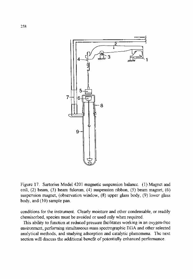
258

2

4

,- 5 t ' I

8

9

Figure 17. Sartorius Model 4201 magnetic suspension balance. (1) Magnet and coil, (2) beam, (3) beam fulcrum, (4) suspension ribbon, (5) beam magnet: (6) suspension magnet, (observation window, (8) upper glass body, (9) lower glass body, and (10) sample pan.

conditions for the instnmaent. Clearly moisture and other condensable, or readily chemisorbed, species must be avoided or used only when required.

This ability to function at reduced pressure facilitates working in an oxygen-free environment, performing simultaneous mass spectrographic EGA and other selected analytical methods, and studying adsorption and catalytic phenomena. The next section will discuss the additional benefit of potentially enhanced performance.

259

There has been a surge in interest associated with higher pressures. The major interests have been in the areas of catalysis, nonstoichiometry and its resulting defects, combustion processes, phase transformations and structures at elevated pressures, and the never-ending quest for new electronic and optical materials. This has led to perhaps a dozen manufacturers providing a range of insmunents designed to work at pressures as high as 100 atm and temperatures up to 1600 ~ Custom made equipment has been developed to work at pressures as high as 3000 atm at ambient temperature [59].

Clearly, the specific operational limits depend upon the atmosphere used and the design and materials of construction. Oxidizing gases such as oxygen and halogens are of particular concern. The specifications for an instrument would be dramatically decreased for use with such gases. Besides the hazards of uncontrolled combustion or explosion, virtually every task is more difficult. The greatly increased thermal conductivity of the gaseous medium at high pressures makes control of Ahe~temperatt~e over a significant sample space more difficult and increases the power necessary to achieve elevated temperatures.

The high pressure containment vessel is generally made of stainless steel, Monel, Inconel, or other alloys with suitable strength and corrosion resistance. The vessel may be cooled to retain its strength as the sample compartment is heated. Therefore, internal fiLrnaces are required to achieve temperatures higher than a few hundred ~ Each manufacturer establishes specifications unique to their design. Costs of the systems cover a wide range, determined largely by the specifications.

The highest operating parameters are achieved through clever procedures in which the active gas is contained within a thin-walled particularly inert inner vessel. This is surrotmded by a relatively cool inert gas at a pressure matching that on the sample side. Thus the external pressure vessel sees only a cooled inert gas, and the relatively fragile inner vessel is preserved by equalized pressures on both sides. The inner vessel must contend with a much higher temperatures, but can be made of fused quartz or ceramic. Only the internal furnace, the sample support system and the sample itself are exposed to the highest temperature in the reactive gas environment.

3.2.3. Sources of error related to the atmosphere: The most obvious source of error involving the atmosphere concems the effects of buoyancy. A cm -3 of air weighs about 120 ~tg at room temperature and pressure. For hydrogen the mass is less than 9 ~tg and for carbon dioxide 196 lag. Consequently, the most accurate work requires consideration of these differences. There are interludes of changing buoyancy during the evolution of volatile products. These variations are, however, generally short lived and are minor perttn'bations on the buoyancy effects due to the purge gas.

260

Changes in gas density with temperature can be approximated using Charles' Law. Hence, the change in buoyancy, when the temperature of air increases from 25 ~ to 1000 o C, results in an apparent weight gain for a solid sample of about 100 ~tg cm -3. The gain would be much less in hydrogen, but more in carbon dioxide. Careful studies of such topics as oxygen stoichiometry, where changes of the order of one part in 105 are monitored, require corrections for buoyancy.

Corrections due to buoyancy decrease with decreasing pressure and essentially vanish under vacuum conditions. However, they are greatly exacerbated by working at elevated pressures. The ideal gas laws provide only approximate corrections at higher temperatures and pressures.

Aerodynamic forces buffet the sample and its suspension system, superimposing both a random noise and a variable offset on the apparent mass. These forces arise from several sources. There are the Brownian motions of the atoms comprising the atmosphere; convection currents set up by the heating or cooling of the surroundings, and disturbances arising from the flow pattems of the purge and reacting gas streams. All of these effects are influenced by the kinetic energy of the gaseous molecules, total pressure, baffling, and flow pattern established by the configuration of the system. Minimization of these factors involve compromises in the flow conditions and aerodynamic noise for mass and thermal transport reasons depending upon the specific purpose of the experiment.

Figure 7 indicates three major configurations for a thermobalance. The direction of gas flow is from the balance to the sample and thus varies for each arrangement. A horizontal gas flow tends to provide the minimum of aerodynamic disturbance and higher flow rates can be tolerated. Preheating the gases will cause minimal currents related to convection. Some experimental arrangements aim the flow directly onto the sample, while others use baffles to shield the sample from such direct gaseous impact. The conditions and position of any mixing of the reactive gas and purge gas streams are an added factor. Each instrument and the requirements of the particular experiment will dictate the extent of the problem. Figure 18 illustrates two common modes of mixing. Configuration (b) is an example of pre-heating the reactive gas stream.

3.3. Sample considerations The nature of the sample and the goal of the experiment dictate the sample size.

Particular consideration must be given to the homogeneity of the sample. This aspect is overlooked surprisingly often in the drive towards smaller samples. A representative sample is a fundamental prerequisite for any analysis. Alternatively a large number of smaller non-representative samples may be analyzed to yield an average value and an indication of the degree of homogeneity. Care should be exercised in the selection of these smaller samples to assure that the accumulation

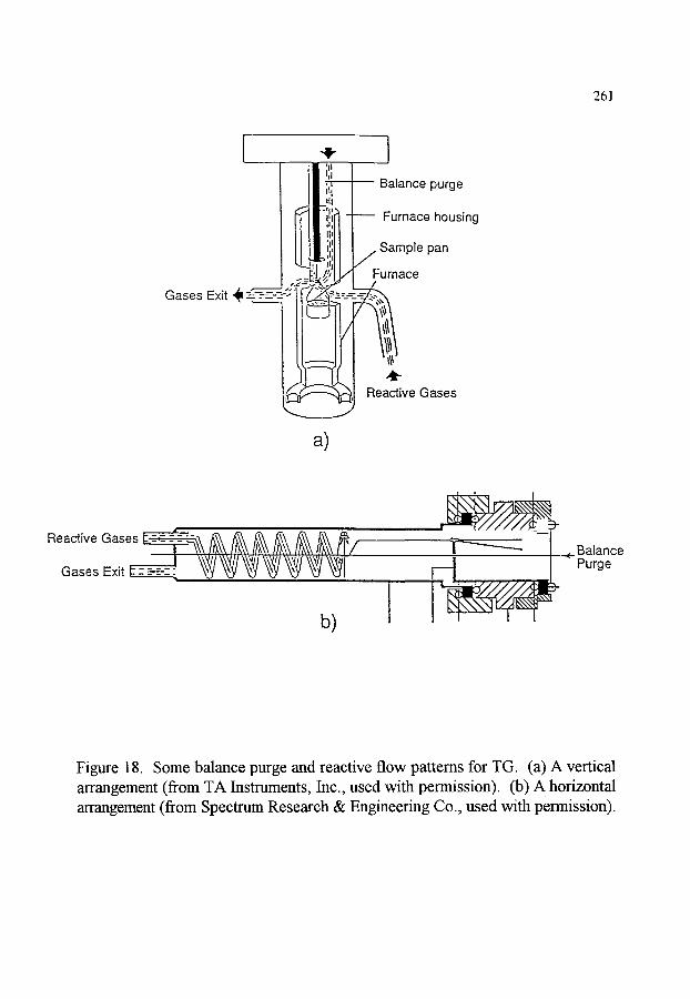
261

Gases Exit -~ ---'----

"IP

I ~II 1 i,i I 'II |

]" z'ill

�9 ~ ~ ' ! /

a)

-1 Balance purge

Furnace housing

Sample pan Furnace

Reactive Gases

Reactive Gases [::-~--"-I ~-~_ . .~ /~ ~. ~ / ~ _ ~ / ~ / : . . . . . . . . . .

GasesExit[ ::--=e---:! ~ ~ ~ ~ ~ ~ ' ~1 ,

b)

--- Balance -< Purge

I

Figure 18. Some balance purge and reactive flow patterns for TG. (a) A vertical arrangement (from TA Instruments, Inc., used with permission). (b) A horizontal arrangement (from Spectrum Research & Engineering Co., used with permission).

262

is representative. Statistical sampling methods have been developed for quality control or certification procedures.

High-capacity balances are available for larger samples. Soils, ores, coals, biological specimens, and other naturally occurring substances are particularly heterogeneous. The use of the higher capacity balance is not, however, restricted to such needs alone. Occasionally, the shape of the specimen requires a larger sample volume, such as oxidation studies of metal coupons or adsorption studies of very porous monoliths. In addition, obtaining accurate data, e.g., one part in 105, is made easier through the use of more massive samples.

Generally the sample is placed in an open pan suspended in a suitable harness from the balance beam. When an interaction with the gaseous environment is a factor, however, exposure of the sample's surface to the gas stream must be considered. The previous discussion concerning "self generated atmospheres" and sample holders is relevant. Figure 16 illustrates potential effects of sample exposure. The four most important cases concern: (1) reversible reactions, (2) reactions in which the volatiles produced will react further with the gas stream in an exothermic manner, (3) studies of chemisorption or physisorption, and (4) those reactions where the supply of an active component in the gas stream may be restricted (deliberate or otherwise).

In Figure 16 the decomposition of C a C O 3 is an example of a reversible reaction. The decomposition or otherwise volatilization of organic matter into an oxidizing gas stream exemplifies the second category. The highly exothermic nature of the subsequent combustion frequently heats the sample well beyond the desired or indicated temperature at that point. Chemisorption might involve acidic or basic sites on a catalyst, while an example of physisorption would be the use of nitrogen for studies of surface area and porosity. An example of the fourth category is the oxidation of a metal in a predominantly inert carrier gas.

Static electricity can produce charging on the sample and surrotmding surfaces. This effect induces errors in the measurement of the mass and proves frustrating when the sample swings to cling to the chamber wall. This problem is worst in dry atmospheres and on glass surfaces when the electrical conductivity is poor. Remedies generally involve discharging the static via a conducting film or mesh on the surface of the chamber, or inducing ionization in the gas phase through electrical discharge or weak alpha emission.

Other sample considerations include the creeping of liquid samples or the decrepitation of solids. The wetting of the sample container by the sample upon melting can lead to the sample flowing out of the container and reacting with less corrosion resistant parts of the sample suspension. It can also lead to sticking of the parts when the melt solidifies during cooling. The decrepitation induced in some solids by outgassing or mechanical strain relief may actually cause the sample to pop

263

out of its comainer and be lost. This manifests itself through overly abrupt weight losses and can be alleviated through the use of a cover. If atmospheric interaction is needed, then the cover may be a mesh of suitable size to prevent the loss of sample.

4. DATA C O L L E C T I O N AND PRESENTATION

4.1. Modes of presenting the experimental results Results from TG experiments can be presented in a variety of graphical ways. The

most common versions are mass or mass percent as the abscissa and temperature or time as the ordinate, see Figures 13 and 16. Weight or mass percent has the advantage that it normalizes the axis so that related plots can be easily placed and compared on the same set of axes. If time has been used as the abscissa, then a second curve of temperature versus time may be plotted. This complicates the direct comparison of temperatures at specific events during the change in mass, but provides a direct indication of the temperature programme used. It is particularly desirable for controlled rate or dynamic temperature thermogravimetric studies.

Plotting the rate of mass change as a function of time or temperature (Derivative Thermogravimetry, DTG) is commonly used to detect more subtle effects, or to establish kinetic parameters. The points of inflection in the TG curve associated with completions of steps in a series of reactions, or changes in the mechanism during a reaction, are more obvious and identifiable as maxima or minima in DTG. It is also easier to compare the shape or overlap of DTG curves with other differential measurements such as DTA, DSC, or EGA. Plots of the derivative are also useful in TM for similar reasons. The derivative of noise is increased noise, so frequently some form of noise suppression or smoothing is needed. These aspects pertaining to software and data acquisition are discussed in subsequent sections.

Examples of DTG curves are presented in Figures 19 and 20 for the decomposition of physical and coprecipitated mixtures of magnesium and ferrous oxalate dihydrates, respectively [60]. These curves not only indicate the clear separation or degree of overlap for the different steps in the decomposition of these materials, but also reveal the effects of an oxidizing versus an inert atmosphere, and coprecipitation as opposed to simple physical mixtures.

4.2. Analog and digital data acquisition Progress in this aspect has been enormous and has greatly stimulated the growth

of new instruments and applications. The conversion from analog to digital data handling and processing is virtually complete in modem instrumentation and has revolutionized the convenience and ease of everyday operation. Entirely analog

264

o.o / -

~o.so ~i "~ -1.0

-1.5 -2.0 Physical Mixtures -2.5 In Air

~(~-3.0 1:1 Mg:Fe 1:2 Mg:Fe . . . . .

n -3.5 1:4 Mg :Fe - - -

-4.0

-4.5 , , o o ~000 200.0 3c;00 400.0 500.0 660.0 700.0 800.0

Temperature (~ (a)

5 . 0 - 0 . 0 -

"E" -5.o ~ .~ -10.0

-~5.o -20.0 -25.0

(~ -30.0 IC1 -35.0

-40.0 -45.0

0.0

i i . . . . . . . . .

[ ~ \ ) ~ ~ F p h ysical Mixtu re s ~~il ~.~ inArgon

1:1 Mg:Fe 1:2 Mg:Fe - 1:4 Mg:Fe

I I I I

100.0 200.0 300.0 400.0 500.0 600.0 700.0 800.0

T e m p e r a t u r e (~

(b)

Figure 19. DTG curves for the thermal decomposition of physical mixtures of magnesium and ferrous oxalate dihydrates having the indicated ratios at 5 ~ min -~. (a) in flowing air. (b) in flowing argon [60].

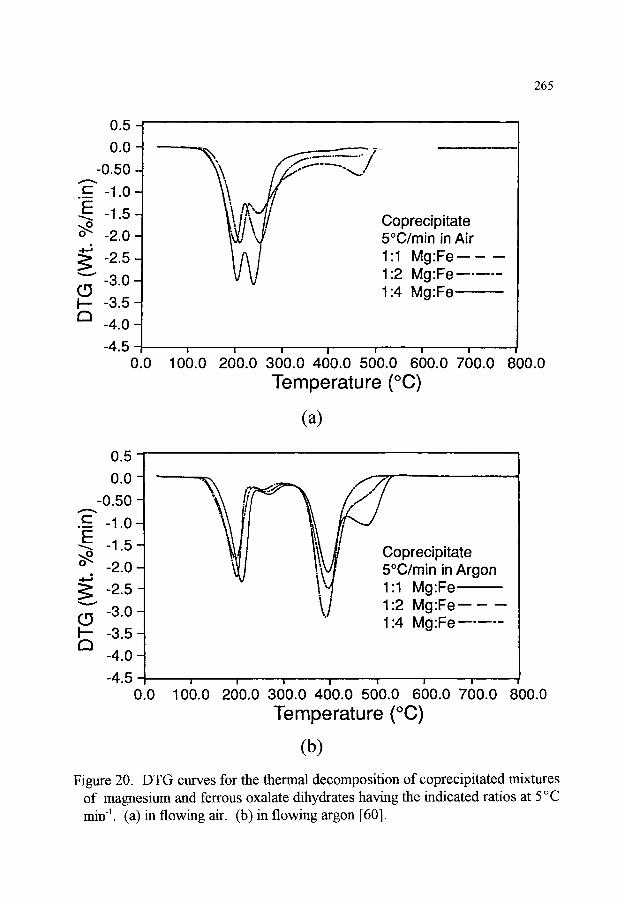
265

0 , 5 -

0 . 0 -

~ 0 . 5 0 ._E -1.0

-1.5

~ -2.0

-2.5

~ -3.0 (5 I-- -3.5 -

-4.0 -

-4.5 - 0.0

;~ ~ / ........

Coprecipi tate 5~ in Air 1:1 M g : F e - - - - - 1:2 Mg:Fe . . . . . 1:4 M g : F e ~

' ' ; ' ' ; 6 100.0 200.0 3 0.0 400.0 500.0 6 0.0 7 0.0 Temperature (~

800.0

(a)

0 , 5 -

0 . 0 -

-0.50 -

~E_ -1.0 - E o~ Coprecip i tate

5~ in Argon i " 1"1 Mg 'Fe \ j 1:2 M g : F e - - - - -

1:4 Mg:Fe . . . . . (.9 I-- r'~

-1.5 -

-2.0 -

-2.5 -

-3.0 -

-3.5 -

-4.0 -

-4.5 - 0.0

i I / I I i i

100.0 200.0 300.0 400.0 500.0 600.0 700.0 800.0 Temperature (~

(b) Figure 20. DTG curves for the thermal decomposition of coprecipitated mixtures

of magnesium and ferrous oxalate dihydrates having the indicated ratios at 5 ~ min ~. (a) in flowing air. (b) in flowing argon [60].

266

based instrmnems still continue in daily use, however, particularly when fimds for updates are limited. Some simple analog computers also remain in use, e.g., differentiators and integrators, however, such devices are much slower, less flexible, and generally inferior to the modem digital techniques. One should keep in mind that differentiation amplifies noise, while integration and averaging reduce the noise.

The output device of choice for analog data has been the chart recorder. The archival storage of such results has been a major problem in terms of space, convenience, and permanence. The errors associated with chart slippage, ink bleeding or fading, paper shrinkage or expansion, etc., are unique to this format of data storage. The problems associated with electronics, e.g., drift, amplification, noise, etc., are common to both analog and digital data collection. They are, however, exacerbated for most analog recording since the equipment is generally older. Factors related to maximum readability or sensitivity require that the analog output range be maintained at a constant high amplification and offsets be applied to keep the actual signal within that range. An early example of such an apparatus involved limit switches on the ends of the recorder travel to trigger the change in tare weight of the balance [61 ]. Wendlandt has discussed the interesting early stages of the evolution from analog to digital processing [62].

The ability to collect, analyze, and store data in a digital fashion has markedly enhanced and expanded our research capacity. A greater control and flexibility is achieved through digital data acquisition. The increased versatility is particularly evident in the timing aspects. Several formats for controlling the number and quality of the data points are available. Some easily programmable options are outline in Table 3. If the designer has provided the flexibility in the software, then the operator will select the mode and methodology. It is more likely, though, that the decisions will have been made by the manufacturer.

The size and format of the resulting data files affect their storage and portability. The proliferation of commercial software emphasizes the need for portability from one program to another. The manufacturer's software package that accompanies the instrument will perform most of the common functions. The operator, however, may not be aware of the underlying algorithms and assumptions. The experimentalist can do little to control the mode or parameters of data acquisition, but the data can be transported via removable storage media or a network to third- party software, or other computers, when desired. A very competitive market has arisen for such general software packages, or even those tailored specifically to kinetics and thermoanalytical systems.

It is imperative that investigators impose their experience and judgement on the computed results. Incorrect input data can not be salvaged by the computer nor can all of the numbers in the long string of computer output be considered significant.

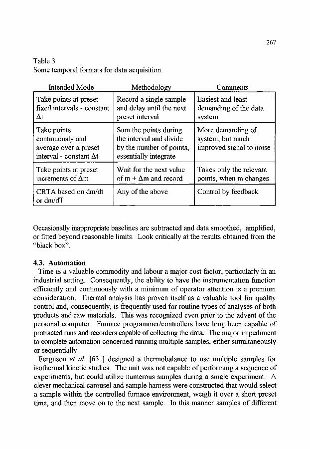
Table 3 Some temporal formats for data acquisition.

Intended Mode Methodology Comments

267

Take points at preset fixed intervals - constant At

Take points continuously and average over a preset interval - constant At

Take points at preset increments of Am

CRTA based on dm/dt or dm/dT

Record a single sample and delay until the next preset interval

Sum the points during the interval and divide by the number of points, essentially integrate

Wait for the next value of m + Am and record

Any of the above

Easiest and least demanding of the data system

More demanding of system, but much improved signal to noise

Takes only the relevant points, when m changes

Control by feedback

Occasionally inappropriate baselines are subtracted and data smoothed, amplified, or fitted beyond reasonable limits. Look critically at the results obtained from the "black box".

4.3. Automation Time is a valuable commodity and labour a major cost factor, particularly in an

industrial setting. Consequently, the ability to have the instrumentation function efficiently and continuously with a minimum of operator attention is a premium consideration. Thermal analysis has proven itself as a valuable tool for quality control and, consequently, is frequently used for routine types of analyses of both products and raw materials. This was recognized even prior to the advent of the personal computer. Furnace programmer/controllers have long been capable of protracted rtms and recorders capable of collecting the data. The major impediment to complete automation concerned running multiple samples, either simultaneously or sequentially.

Ferguson et al. [63 ] designed a thermobalance to use multiple samples for isothermal kinetic studies. The unit was not capable of performing a sequence of experiments, but could utilize numerous samples during a single experiment. A clever mechanical carousel and sample harness were constructed that would select a sample within the controlled fiamace environment, weigh it over a short preset time, and then move on to the next sample. In this manner samples of different

268

materials could be studied almost simultaneously and under identical conditions. This provided a slightly offset series of data points as a function of time for each sample, rather than a continuous scan of a single sample. An instrument is available commercially, the LECO Model TGA-500, that operates in a similar fashion. It can operate one or two fiamace systems simultaneously and have as many as 19 specimens per fiamace.

Most manufacturers of modem thermoanalytical instruments have carefully integrated robotics into their systems to enable long periods of tmattended operation for their various modules. Figure 21 depicts several of these commercial TG modules. Again a carousel of identical sample holders is utilized to supply the samples, in this case one per experiment. The samples are run sequentially and experimental conditions can be programmed for each sample individually, or collectively for the entire set. Data are collected continuously as though the operator were there changing samples and establishing the temperature programme and gas switching.

5. CALIBRATION

Previous sections of this chapter have stressed the importance of carefully calibrating the specific instrument in use under the particular experimental conditions employed. This can only be ignored when the exact temperature is relatively tmimportant or when an accurate change in mass is not required. Either of these may be the case for rapid surveys and other essentially qualitative experiments.

Most studies, however, demand more accurate data. Consideration must be given to the distinction between precision (reproducibility) and accuracy (the true value). Precision depends upon the instrumentation, homogeneity of the sample, and the ability to provide an identical experimental environment. Good precision is essential for accuracy, however, it is no guarantee of accuracy because of potential systematic errors. Systematic errors arise from generally constant offsets in the experimental measurements, rather than the random fluctuations that determine precision. Elimination of these systematic errors is the intent of calibration. The critical measurements for TG are mass, temperature, and time. The accuracy of time is seldom a factor and is considered outside the scope of this chapter.

5.1. Mass The standard for mass is unique in that it does not depend upon the value of a

physical constant but rather on the one kilogram weight in a laboratory in S6vres, France. The physical constant becomes involved through the conversion of mass to weight which is dependent upon the local gravitational force. Consequently

269

(a)

(b)

Figure 21. Examples of automated thermobalances. (a) TA Instruments, Inc. (b) Seiko Instruments, Inc.

270

standard masses are needed to calibrate weighing procedures at differem altitudes and latitudes. Such changes are quite small, however, the assumptions and instabilities attributable to the balance mechanism and associated electronics may not be insignificant. Vibration and aerodynamic disturbances give rise to obvious random noise in the. resulting curve.

Calibration masses in a wide range of sizes and several classes of accuracy may be obtained from the national standards organizations, e.g., NIST in the United States, or commercial suppliers such as Rice Lake Weighing Systems, Rice Lake, WI 54868. The most accurate standard is class M, which is basically retained at the standards organization for certification of lower classes. Type S masses are highly accurate for the more demanding efforts and type S-1 is of similar high quality construction, but with relaxed tolerances. For example, a 100 mg Class S mass has a tolerance of +0.025 mg or 250 ppm, while a class S-1 mass has a tolerance of twice that. ASTM procedure E617 describes establishing the linear response of the mass sensor over its useful range.

These certified masses can be used to establish accurately the calibrated mass at room temperature. At other temperatures, changes in buoyancy and aerodynamic forces resulting from changing temperature, as previously discussed, will disturb the calibration. A dual system, where both a tare and sample side are treated the same with respect to temperature and atmospheric conditions, will alleviate much of the problem. There are few such instruments in operation, however, and subtraction of a blank run under essentially identical conditions is the next best alternative.

Two other significant sources of error are, fommately, generally not applicable. At very high temperature it may be necessary to account for the rate of change in the mass of the sample suspension system, e.g., vaporization of platinum in oxygen, above about 1300~ The second possible source of error is the effect of stray magnetic fields on magnetic samples. If the resistive fitmace element is not wound in a bifilar fashion, application of electrical current to the winding will induce a substantial gradient in the magnetic field at the sample position. Consequently, if one is working with magnetic samples, it is essential that a suitable fiu-nace be used. Even with properly wound tin, aces, care must be taken when working with strongly magnetic materials [64].

5.2. Tempera ture The discussion in the earlier section on errors in temperature clearly indicates the

need for careful calibration of temperature at the sample position in TG. Early attempts at calibration involved the use of materials optimistically hoped to have well established decomposition temperatures. Variability in the results due to slight compositional or morphological differences among samples of nominally the same compound is of concern. If the reaction is at all reversible, then mass transport

271

factors will induce shifts in the temperature. Similarly, evolution or adsorption of heat due to changes in enthalpy will alter the apparen t temperature of the decomposition.

Because the melting points of selected pure metals define the International Temperature Scale [30] in the region of interest, efforts are made to trace the calibration procedure back to these temperatures. Recently Brown et al. [65] have proposed some organometallic materials as standards based on the onset of their explosive decomposition. The abrupt onset temperatures can be determined by the sharp exotherms in their DTA or DSC curves. These DTA or DSC instruments would have had prior calibration using standards based on the melting points of appropriate pure metals. Instruments capable of simultaneous TG/DTA can, of course, be calibrated using their DTA capability.

The two currently most accepted calibration techniques for simple TG involve the "fusible link" or the "magnetic standard". The fusible link method has been pioneered by McGhie et al. [66,67]. A thin wire of the pure metal is suspended from the sample support system, in a position very close to that of the normal sample. As the temperature is raised through the melting point, the link melts and drops from its support. Depending on the specific arrangement used, the weight will either be lost and produce an abrupt loss in weight, or it will fall onto the sample pan causing a momentary detectable disturbance in the mass signal. Either of these effects yields a sharp transition at a known temperature that can readily correlated with the "apparent" temperature determined by the conventional sensor.

The approach based on magnetic standards uses pure metals or alloys that have sharp well-defined values of the Curie temperature, T c. This method was initially proposed for use with the small furnace developed by the Perkin-Elmer Co. [68]. The marked reduction in the size of the uniform heating zone made careful calibration imperative. The method was quickly adopted by investigators using that instrument and adapted for early digital data processing [69]. The calibration is a TM measurement, where the extrapolated end point of the magnetic effect is equated to To. Figure 22 shows one of the early applications, indicating that either the conventional TM or DTM traces could be used. Because the DTM curve is somewhat more sensitive to changes, a slightly higher temperature is measured for the extrapolated end point. Hence, a consistent policy should be adopted.

One of the advantages of the magnetic scheme is indicated in Figure 22, where multiple magnetic samples can be conveniently measured in a single experiment. The magnetic materials used in these early studies were those supplied by the Perkin-Elmer Co. Within a decade, however, the Committee for Standardization of ICTA (now ICTAC) had certified five materials and marketed them through NBS (now NIST) [70]. Unfortunately, the results of the certification did not indicate the high degree of precision normally associated with standard materials.

2 7 2

7 . 6 9 9

7.040

6 . 3 8 0

5.72t

5.061

0.(

~)~ MLUMEL ~3"C (165"C)

�9 NICKEL 354*C (354"C)

PERKALLOY �9 596"C 1592"C1

ZRON 780"C 1780"C1

8 HISAT-50 t000"C (t002"C) ee "

I I I I I I I , I t 1.79 3.57 5.35 7.13

VOLTS

.

t . 6 0

c E

E

1.20

0 . 8 0 - -

0 . 4 0

" 0 . l I ~ 1 t I I 1 I 2 0 0 4 0 0 6 0 0 8 0 0 t 0 0 0

Figure 22. TM and DTM curves for several magnetic materials. The calibration is achieved by equating the sensor voltages at the extrapolated end points for each transition with the established values of T c in parentheses [69].

Table 4 Suggested magnetic materials for use as temperature standards in TG. [50]

273

Material Recommended Tr176 Source [endpoint]

Monel 65 Perkin-Elmer a Alumel 163 Perkin-Elmer Permanorm 3 266.3 + 6.6 ICTAC-NIST Nickel 354 Perkin-Elmer

354.4 + 5.4 ICTAC-NIST Numetal 393 Perkin-Elmer a

386.2 • 7.4 ICTAC-NIST Nicroseal 438 Perkin Elmer a Permanorm 5 458.8 + 7.6 ICTAC-NIST Perkalloy 596 Perkin-Elmer Trafoperm 753.8 i 10.2 ICTAC-NIST Iron 780 Perkm-Elmer Hisat-50 1000 Perkin-Elmer

a NO longer supplied.

Table 4 presents a summary of these materials along with those supplied by Perkin-Elmer. Nickel gave the best result, but even that standard deviation of 5.4 ~ is inappropriate for a reference standard.

The advent of excellent commercially available simultaneous TG/DTA (TM/DTA) instruments, however, has presented an oppommity to re-evaluate this approach to calibration [71-73]. An appropriate pair of pure metals, whose melting points bracket the magnetic transition, are placed in the sample pan alongside the magnetic material. The measured melting points are used to construct a correction curve for the observed temperatures and a linear interpolation yields the suitable correction factor to be applied to the observed T c. Figure 23 presents the results for such an experiment using nickel. Lead and zinc were used as the melting point standards. In this instrument the magnetic attraction is upward and the sample apparently weighs less below Tc. The extrapolations to the onsets for melting and to the end points for Tc are indicated. In Figure 23 there is also an indication of the second- order magnetic transition, however, it is not always evident, nor is the proper extrapolation obvious. The main interest in the TM curve, however, is for use with instruments incapable of simultaneous TG/DTA measurements.

274

270 - 4.5 . . . . 94 .5 .' .' �9

92 .5

90.5

88 .5 ~ .

86 .5 TG

D T G 84 .5

-70 - -2 .5 , = = J I = = 82 .5 250 3 0 0 350 400 450

185 - 2 .75

t,-

.~ lOO > 1 t-..

D 121

15 -0 .75

T / ~ (Heating)

Figure 23. Simultaneous TM/DTA curves for nickel, lead, and zinc at 10 ~ min ~ in flowing nitrogen [71 ].

Early measurements [71 ] suggested that a precision (standard deviation) of +0.2 ~ was attainable with pure nickel. Because primary standards are used, the accuracy is comparable. In addition, the observed values of Tc are essentially independent of heating rate, because the correction procedure accounts for the variation due to temperature lag. Subsequent measurements using alloys have had larger standard deviations, but are still much superior to those reported in Table 4. [72,73]. A certification program is in progress to use cobalt- and nickel-based alloys to provide a series of standards in the temperature range of 160 to 1130~ [74].

275

R E F E R E N C E S

o

.

.

4.

.

.

7. 8.

.

10. 11.

12. 13. 14.

15.

16.

17.

18. 19.

20.

21.

22.

23.

R. Viweeg, Progress in Vacuum Microbalance Techniques, Vol. 1, (Eds Th. Gast and E. Robens), Heyden & Son, London, 1972, p. 1. F. Szabadvary, History of Analytical Chemistry, Pergamon, Oxford, 1966, p.16. K. Honda, Sci. Rep. Tohoku Univ., 4 (1915) 97. H. Saito, Thermobalance Analysis, Technical Books Pub. Co., Tokyo, 1962. C. Duval, Inorganic Thermogravimetric Analysis, 2nd Ed., Elsevier, Amsterdam, 1963. E.A. Gulbranson, Rev. Sci. Instrum., 15 (1944) 201. P. Ch6venard, X. Wach6, R.de laTullayne, M6taux, 18 (1943) 121. U.R. Evans, The Corrosion and Oxidation of Metals: Principles and Practical Applications, St. Martin's Press, New York, 1960, p.782. P.D. Garn, C.R. Geith, and S. DeBalla, Rev. Sci. Instrum., 33 (1962) 293. P.K. Gallagher and F. Schrey, J. Am. Ceram. Soc., 46 (1963) 567. L. Erdey, F. Paulik, and J. Paulik, Acta. Chim. Acad. Sci. Htmgr., 10(1956) 61. L. Cahn and H. Schultz, Anal. Chem., 35 (1963) 1729. A.F. Plant, Ind. Res., 13 (1971) 36. M.E. Brown, Introduction to Thermal Analysis, Chapman and Hall, London, 1988, Chap.3. F. Boersma and F.J. Van Empel, Progress in Vacuum Microbalance Techniques, Vol. 3, (Eds Th. Gast and E. Robens), Heyden & Son, London, 1975, p.9. A. Coetzee, L.R. Nassimbeni and K. Achlitner, Thermochim. Acta, 298 (1997) 81. H. Mahgerefteh., H. Khoory and A. Khodaverdian, Thermochim. Acta, 237 (1994) 175. E. J. Davis, Aerosol Sci. Tech., 2 (1983) 121. G. Sageev, R.C. Flagan, J.H. Seinfeld and S. Arnold, J. Colloid Interface. Sci., 113 (1986) 421. G.S. Grader, S. Arnold, R.C. Flagan and J.H. Seinfeld, J. Chem. Phys., 86 (1987) 5897. G.S. Grader, A.F. Hebard and R. H. Eick, Appl. Phys. Lett., 53 (1988) 2238. G. Sageev, J.H. Seinfeld and R.C. Flagan, Rev. Sci. Instrum., 57 (1986) 933. P.K. Gallagher, J. Thermal Anal., 49 (1997) 33.

276

24. 25.

26.

27.

28.

29. 30. 31.

32. 33.

34. 35.

36. 37. 38.

39. 40. 41. 42.

43.

44. 45.

46.

47.

48.

P.K. Gallagher and E.M. Gyorgy, Thermochim. Acta, 109 (1986) 193. P.K. Gallagher, E.M. Gyorgy, F. Schrey and F. Hellman, Thermochim. Acta, 121 (1987) 231. P.K. Gallagher, E.M. Gyorgy and W.R. Jones, J. Chem. Phys., 75 (1981) 3847. M.W. Rowe, P.K. Gallagher and E.M. Gyorgy, J. Chem. Phys., 79 (1983) 3534. G. Agarwal, R.F. Speyer and W.S. Hackenberger, J. Mater. Res., 11 (1996) 671. W.W. Wendlandt, Thermochim. Acta, 12 (1975) 109. T.J. Quinn, Temperature, Academic Press, New York, 1990. R.F. Speyer, Thermal Analysis of Materials, Marcel Dekker, Inc., New York, 1993, Chap.2. Expertune, Inc., http://www.expertune.com/tut.html, 1996. C.D.H. Williams, http://newton.ex.ac.uk/teaching/ CDHW/Feedback/index.html, 1996. D. Chen and D. Dollimore, Thermochim. Acta, 272 (1996) 75. R.L. Blame, Proc. 25th NATAS Conf., (Ed. R.J. Morgan), NATAS c/o The Complete Conference, Sacramento, CA, 1997, p.485. R.L. Blaine and B.K. Hahn, J. Thermal Anal., in press. J. Rouquerol, Thermochim. Acta, 144 (1989) 209. M. Reading, Thermal Analysis - Techniques and Applications, (Eds E.L. Charsley and S.B. Warrington), Royal Society of Chemistry, Cambridge, U. K., 1992, p. 126. A. Dwivedi and R.F. Speyer, Thermochim. Acta, 247 (1994) 431. F. Paulik and J. Paulik, Thermochim. Acta, 100 (1986) 23. W.J. Sichina, Am. Lab. (Fairfield, CT), 25 (1993) 45. P.S. Gill, S.R. Sauerbrunn and B.S. Crowe, J. Thermal Anal., 38 (1992) 255. P.A. Barnes, G.M.B. Parkes and E.L. Charsley, Anal. Chem., 66 (1994) 2226. J.K. Arthur and J.P. Redfern, J. Thermal Anal., 38 (1992) 1645. R.P. Tye, A. Maesomo and T. Masuda, Thermochim. Acta, 243 (1994) 971. K.M. Caldwell, P.K. Gallagher and D.W. Johnson, Jr., Thermochim. Acta, 18 (1977) 15. P.A. John, F. Hoornaert, M. Makkee and J.A. Moulijn, Thermochim. Acta, 287 (1996) 261. P.K. Gallagher and D.W. Johnson, Jr., Thermochim. Acta, 6 (1973) 67.

277

49.

50. 51.

52. 53.

54. 55. 56.

57.

58. 59. 60. 61. 62.

63.

64. 65.

66. 67.

68.

69. 70.

71.

P.K. Gallagher, D.W. Johnson, Jr. and E.M. Vogel, Catalysis in Organic Synthesis, (Eds P. A. Rylander and H. Greenstreet), Academic Press, New York, 1976, p. 113. U.S. Ozkan, M.K. Kumthekar and G. Karakas, J. Catal., 171 (1997) 67. J. Czamecki and D. Thumin, Proc. 17th NATAS Conf., (Ed. C.M. Earnest), NATAS c/o The Complete Conference, Sacramento, CA, 1988, p.93. Y. Chen, R. Wu and S. Mori, Chem. Eng. J. (Lausanne), 68 (1997) 7. P.K. Gallagher, Thermal Characterization of Polymeric Materials, (Ed. E. Turi), 2nd Edn, Academic Press, New York, 1997, Chap. 1. P.D. Garn and J. Kessler, Anal. Chem., 32 (1960) 1563. A.E. Newkirk, Thermochim. Acta, 2 (1971) 1. J. Paulik and F. Paulik,Thermal Analysis, (Ed. H. G. Wiedemann), Vol. 1,

Birkha~user, Basel, 1971, p.489. B. Schubart and E. Knothe, Progress in Vacuum Microbalance Techniques, (Eds Th. Gast and E. Robens), Vol. 1, Heyden & Son, London, 1972, p.207. H. Sabrowski and H.G. Deckert, Chem. Eng. Tech., 50 (1978) 217. W. Pahnke and T. Gast, Thermochim. Acta, 223 (1994) 127. R.G. Rupard and P.K. Gallagher, Thermochim. Acta, 272 (1996) 11. P.K. Gallagher and F. Schrey, J. Am. Ceram. Sot., 46 (1963) 567. W.W. Wendlandt, Thermal Analysis, 3rd Edn, Wiley & Sons, New York, 1986, Chap.12. J.M. Ferguson, P.M. Livesey and D. Mortimer, Progress in Vacuum Microbalance Techniques, Vol. 1, (Eds Th. Gast and E. Robens), Heyden & Son, London, 1972, p.87. P.K. Gallagher and E.M. Gyorgy, Thermochim. Acta, 31 (1979) 380. M.E. Brown, T.T. Bhengu and D.K. Sanyal, Thermochim. Acta, 242 (1994) 141. A.R. McGhie, Thermochim. Acta, 55 (1983) 987. A.R. McGhie, J. Chiu, P.G. Fair and R.L. Blaine, Thermochim. Acta, 67 (1983) 241. S.D. Norem, M.J. O'Neill and A.P. Gray, Thermochim. Acta, 1 (1970) 29. P.K. Gallagher and F. Schrey, Thermochim. Acta, 1 (1970) 465. P.D. Gam, O. Menis and H.G. Wiedemann, Thermal Analysis, (Ed. H.G. Wiedemann), Vol. 1, Birkh/aeuser, Basel, 1980, p.201. P.K. Gallagher, Z. Zhong, E.L. Charsley, S.A. Mikhail, M. Todoki, K. Tanaguchi and R.L. Blaine, J. Thermal Anal., 40 (1993) 1423.

278

72.

73. 74.

B.J. Weddle, S.A. Robbins and P.K. Gallagher, Pure Appl. Chem., 67 (1995) 1843. E.M. Gundlach and P.K. Gallagher, J. Thermal Anal., 49 (1997) 1013. P.K. Gallagher, B.J. Weddle, E.M. Gundlach, K. Norton, C. Hickle, E. Lee and D. Owens, J. Thermal Anal., to be published.

Handbook of Thermal Analysis and Calorimetry. Vol. 1" Principles and Practice. M.E. Brown, editor. �9 1998 Elsevier Science B.V. All rights reserved. 279

Chapter 5

DIFFERENTIAL THERMAL ANALYSIS AND DIFFERENTIAL SCANNING CALORIMETRY

P. J. Haines a, M. Reading b and F. W. Wilburn c

a. 38 Oakland Avenue, Farnham, GU9 9DX, England b. IPTME, Loughborough University, Loughborough, LE11 3TU, England c. 26 Roe Lane, Southport, PR9 9DX, England

1. INTRODUCTION AND HISTORICAL BACKGROUND

The observation of changes m materials during heating provided the foundation of experimental chemistry and technology. The skills of the metal worker and the makers of pottery relied on their choice of materials but also on using the correct heating regime. The knowledge gained from innumerable trials allowed the manufacture of metals, of pottery and of glass to be improved and more fully documented. [1,2] This early empirical thermal work has been surveyed by Mackenzie [3,4].

The thermometers of the Florentine school of the 17th century were limited to lower temperatures, and it is the work of Fahrenheit in 1713 in devising a temperature scale which was universally acceptable which should be regarded as the "onset date" for thermal analysis since "thermometry forms the basis for thermal analysis" [5]. Martine [6,7] in 1739 was the first to demonstrate the benefits of differential thermometry by comparing the heating rates of equal volumes of mercury and of water "placed close to one another before a great fire so that the heat should equally set upon them". The observation that the mercury heated more quickly than the water, and that, in a cooling experiment the mercury cooled more quickly is perhaps the first illustration of the potential for comparing heat capacities by differential thermal analysis.

Higher temperature pyrometers often used the expansion of metals but the Wedgwood pyrometer consisted of a ceramic body cut to exact size after firing at dull red heat. This clay piece was inserted into the furnace, cooled and the

280

shrinkage measured in a calibrated V-notch device. Temperatures up to the melting point of iron (1540 ~ could now be measured, but it was not appreciated that the shrinkage was not uniform as a function of temperature and therefore the higher temperatures were greatly overestimated [8].

The experimental investigation of the electrical potential difference generated when junctions of dissimilar metals are at different temperatures was first performed by Seebeck in 182119]. This is the thermoelectric effect, and the sensor is the thermocouple, possibly the most important component for differential thermal analytical equipment and furnace control since it is possible to produce reliable, robust, reproducible thermocouples which have well established temperature-thermoelectric e.m.f relationships coveting a very large temperature range. Le Chatelier [10] established the viability of thermocouples to measure temperature and is often credited with making the first programme of thermoanalytical investigations when he determined directly the rate of change of temperature of the sample, (d7 s/dt), for water, sulphur, selenium and gold and for a range of clay minerals. [ 11,12]. The work of Le Chatelier and his co- workers is described most fully in [4] which also illustrates the apparatus used.

The change in the electrical resistance of metals with temperature was described by Siemens [13] and the relationship between temperature and resistance has been measured most carefully. Thermistors and other semiconductor devices have also been used as temperature sensors, although over a limited, low temperature range. Pyrometers and infrared non-contact thermocouples are most useful at high temperatures up to 3600 ~

Le Chatelier [ 10] showed that the physical and chemical events which occurred as a material was heated could be recorded by measuring the temperature of the sample as a function of time. A great improvement in this technique was provided by Roberts-Austen in 1899 [14a]. As Chemist to the Royal Mint in London, he constructed a device to give a continuous record of the output of a platinum/platinum-rhodium thermocouple, which allowed the first published automatically recorded continuous cooling curves. Later, with his assistant Stansfield, he improved the sensitivity of the instrument by measuring the temperature difference ATSR where:

a V S R -- ( T s - 7'R ) (1)

between a sample S and a suitable reference material R placed side-by-side in the same thermal environment and he published the first DTA curve [ 14b] which showed, with remarkable sensitivity, the transitions of iron during cooling [5, Figure 5]. The development and applications of temperature-time and of

281

differential temperature-time curves were reviewed by Burgess [ 15] in 1908 and the construction, control and quantitative theories of that time are discussed very fully in references [5 ] and [ 12].

The thermochemical nature of the events occurring during the heating or cooling regime was recognisable from Le Chatelier's temperature-time experiments. For example in the heating of the clay halloysite, a "feeble" endotherm was marked by the decrease in the rise of temperature with time between 150 and 200 ~ a second endotherm showed at 700 ~ and an exotherm followed at 1000 ~ represented by a greater rise in temperature versus time.

This suggests that it may be possible to relate thermometric and differential thermometric measurements to the determination of heats of transition and of reaction. Joule [ 16,17] was the first to employ a "twin calorimeter" principle in 1845, comparing the sample calorimeter with a reference calorimeter as nearly the same as possible. Since Joule also made many investigations of the heating effects of electrical current, he might be said to have been the "grandfather" of DSC.

Clearly, a properly calibrated thermocouple will indicate the temperature at which a thermal event occurs. Burgess [15] recognised that there was also a relationship between the DTA peak area and the enthalpy change involved in the thermal event. Workers were perhaps slow to realize that factors such as sample mass, heating rate, thermocouple position and atmosphere all had marked effects on the measured DTA era-re. Mackenzie comments [5] that "From the literature up to 1939, one gets the impression that authors were generally aware of the quantitative potentialities of DTA, even if they did not specifically say so". The assessment of the composition of mixtures [18] was a semi-quantitative application of DTA.

Berg and Anosov [19] were the first to propose from a general theory that

m A H - K ; r A T dt

t i

(2)

where a mass m having a specific enthalpy change M-/gives a peak whose area is the value of the integral between the start time t~. and the end time tf K is a constant. Speil [20] and Kerr and Kulp [21 ] also derived relationships between the peak area and the enthalpy change and drew attention to the effects of the thermal properties of the sample and to the assumptions which were made in the theories. Vold [22] proposed a more advanced general theory and Boersma [23] provided a theoretical basis for heat-flux DSC. The development of these

282

theories is discussed more fully in Section 3 of this chapter. In the application of theory to explain how the reaction kinetics of thermal

events may change the characteristics of a DTA peak, the work of Kissinger [24] and of Borchardt and Daniels [25] was very important, although the latter workers originally referred to the very specific conditions for stirred solutions, unusual in DTA experiments. Mackenzie [5] comments that "the literature bristles with theories and is so confused that it is best left for a future historian...".

Early experiments were carried out by Le Chatelier using the apparatus devised by Saladin for recording the differential temperature photographically [12,26,27] and Russian workers made extensive use of the Kurnakov Pyrometer [28]. The simplest instrumentation used for DTA is an apparatus where the sample and reference are held in tubes or holes in a block, and thermocouples are inserted directly into the sample and reference [29-31 ]. The block is heated by a wire- wound furnace surrounding the block, and the heating rate of the furnace is controlled by a simple programmer. Variations such as placing the samples in crucibles mounted on separate ceramic stems and surrounded by air or other gas were also used. Boersma [23] showed that if better quantitative performance is to be obtained from a DTA system, then the effects of the sample properties, such as its volume, shrinkage and conductivity, and of thermocouple interference by heat conduction and of any loss of material must be eliminated. To do this he suggested "leading the heat of reaction outside the sample through a special piece of material on which the temperature difference can be measured. The peak area then is solely dependent on the produced heat of reaction and on the calibration of the msmunent which no longer contains the sample properties". These design principles were employed by many workers in constructing their "Boersma DTA" systems.

The use of DTA for estimating calorimetric quantities was very dependent on the proper control, calibration and operation of an instrument designed for quantitative work. A cell described as a "quantitative DTA cell following the Boersma principles" might have a calibration coefficient which alters by a factor of more than three over the range -100 to +700 ~

This changed completely when Watson, O'Neill, Justin and Brenner [32] described in 1964 a "Differential Scanning Calorimeter for Quantitative Differential Thermal Analysis". The earliest work of this type was by Sykes [33], Kumanin [34], Eyraud [35] and Clarebrough et al. [36]. Eyraud referred to his technique as "differential enthalpic analysis" and he measured the differential power as a function of temperature. Clarebrough, Hargreaves, Mitchell and West [36] describe an apparatus for measuring stored energy of a deformed specimen by using two small heating elements, one located inside the

283

specimen, the other reside an annealed sample of equal mass. During heating the samples are kept at the same temperature and surrounded by a shield continuously adjusted to this temperature. The stored energy is calculated from measurements of the difference in power supplied to the specimens by a differential wattmeter. The commercial Differential Scanning Calorimeter described by Watson et al. [32] and analysed theoretically by O'Neill in the next paper [37] has separate sample and reference holders, each with its own platinum resistance temperature sensor and heater closely embedded in the holders. The average temperature is controlled by the programmer, which then adjusts the power fed to the sample and reference heaters. A differential temperature control loop senses any difference between the sample and reference and supplies differential power to correct this, with due regard to the direction and magnitude needed. The signal from this part of the instrument provides directly the ordinate signal as differential power, AP, against the programmed temperature T.

The advantages of this new concept, later to be distinguished as "power compensation DSC", was that any calibration factor used was a constant electrical factor and that it did not Change with sample, sample mass, heating rate or with temperature.

An analysis of the principles of the use of thermal analysers as calorimeters was put forward by Blaine [38]. He notes that the primary transducer is in all cases a temperature sensor and that these sensors should be located external to the sample for better calorimetric performance. The distinction then arises between insmmaents which use the temperature difference to drive a servo system and those which derive thermal data directly from the measured temperature difference. He suggests that, if the instrument has an output proportional to the heat flow (i.e. power) then it may be called a DSC. He states that "It is a desirable, but not a necessary condition for a DSC instrument to have a constant calorimetric sensitivity. Later in the same paper he comments that "results from instruments of the temperature servo type and instruments of the differential temperature type are indistinguishable from each other". Any calorimetric instrument of the differential temperature type is now referred to as "heat flux DSC" and the term "quantitative DTA" is redundant.

A most useful compilation of information on the history, theories and applications of DTA, was published by Smothers and Chiang in 1958 [12] together with a very considerable collection of reference material to that date. Two landmark volumes on DTA, edited by Mackenzie [39] appeared in the early 1970s. They cover the background, theory, apparatus and the applications to a very wide range of materials.

284

The adaptability of both DTA and DSC allows simultaneous measurements to be made and this has been exploited widely and will be discussed in Section 4 and in Chapter 11. Since measurements of heat flow, from whatever cause, may be made, these techniques can study heat capacity, thermal conductivity, diffusivity and emissivity, heats of transition, reaction or mixing as well as reaction kinetics and mechanisms. However, this very wide-ranging collection of thermal events may sometimes occur together so that we are unsure whether the peak is due to reaction, transition, changes in the thermal characteristics or in the instrumental behaviour. By combining the DTA or DSC with a complementary technique, such as TG or hot stage microscopy, many overlapping stages may be resolved and interpreted. But the simultaneous occurrence of two thermal events, such as a change in heat capacity and a reaction, may be difficult to separate analytically.

There is need for additional instrumental methods which will respond in different ways to specific thermal changes. A new approach to these calorimetric investigations was provided by the invention of temperature modulated DSC. Reading, Elliot and Hill [40] showed that by modulating the temperature ramp with a sinusoidal tipple the amount of information that can be obtained can be increased. Related, though distinct, techniques have been developed and these new expansions of DSC are discussed in Section 5 of this chapter.

From the simplest DTA to the most recent, most sophisticated DSC, improvements may be made by linking to a computer. The control of the temperature programme, the smoothing of experimental data and the calculation of differentials of curves, or integrals of peaks are all best carried out using a modem computer. It must be stressed that, in reporting or assessing thermal analysis data, the nature of the computer data collection and processing must be considered. Dunn [41] suggests that "it would be most useful for the raw data to be viewed and then a personal decision made about the degree of any smoothing routine applied" The calibration, filtering, signal sampling, A/D conversion and baseline treatment ought all to be critically reviewed and reported.

2. DEFINITIONS AND DISTINCTIONS

It is necessary to have a consistent, sensitive definition of each technique, so that we may draw critical distinctions between results obtained in different ways. The Societies and organisations using DTA and DSC have made various recommendations concerning these definitions and the reporting of work carried out using thermal analysis techniques, including DTA and DSC. The reports of

285

the International Confederation for Thermal Analysis and Calorimetry (ICTAC, formerly ICTA), may be taken as the basis for definitions [42,43].

2.1. Differential Thermal Analysis (DTA) A technique in which the difference in temperature between the sample and a

reference sample (ATsR) is monitored against time while the samples are exposed to a temperature programme.

The instrument is a differential thermal analyser and the record is the differential thermal or DTA curve. The temperature difference (AT) should be plotted on the ordinate with endothermic reactions downwards and t or T increasing from left to fight.

The first recommendations [44] clarified the terminology to be used, such as the sample, reference material, block and differential thermocouple. It is stated that "in DTA it must be remembered that, although the ordinate is conventionally labelled AT the output from the thermocouple will in most instances vary with temperature and the measurement recorded is normally the e.m.f, output, E, i.e. the conversion factor, b in the equation

aT bE (3)

is not constant since b -- f(T), and that a similar situation occurs with other sensor systems".

There should be clear distinction between different instrumental conditions and experimental regimes. The ICTAC recommendations [41] specify that the nature, history and size of the sample, the geometry of the system, and sample holder, the temperature programme used, the gaseous atmosphere and flow rate, and the type, sensitivity and placement of the sensors, as well as the design of the sample holder should ideally be given. It has already been pointed out that the methods of data collection and processing also need to be described carefully.

2.2. Differential Scanning Calorimetry (DSC) A technique in which the difference in heat flow rate (or power) to the sample

and to the reference sample is monitored against time while the samples are exposed to a temperature programme.

The instrument is a differential scanning calorimeter and may be one of two types, heat-flux DSC or power compensation DSC, depending on the method of measurement used.

286

2.2.1. Heat-fluxDSC In a heat-flux DSC instrtunent, the temperature difference between sample and

reference is recorded, after suitable calorimetric calibration, as a direct measure of the difference in heat flow rate or the difference in power.

2.2.2. Power compensation DSC In a power compensation DSC instrument the difference in power supplied

to the sample and to the reference, to keep their temperatures as nearly the same as possible, is measured directly.

The power difference in units of watts (AP) should be plotted as ordinate. Since endothermic reactions require a positive input of power into the sample, the DSC convention demands that endothermic peaks should be plotted upwards, and t or T increasing from left to fight. However, the DTA convention (endotherms downwards) is quite often used, and it is recommended that the ordinate axis be labelled with the endothermic (or exothermic) direction.

2.3. Modulated Temperature DSC (MTDSC) {45] To keep the definition in line with the previous ICTAC definitions, it is

suggested that the following be used: A technique in which the difference in heat flow rate (or power) to the sample

and to the reference sample is monitored as a function of time while the sample is subjected to a modulated temperature programme.

The instrument is generally a modified conventional DSC of either of the types described above, but could be described as a modulated temperature differential scanning calorimeter. The recommendations for reporting DSC experiments apply equally to MTDSC and it is additionally necessary to report the type and frequency of the modulation used, and the mathematical technique used to deconvolute the results. This will be discussed in detail in Section 5 of this chapter.

2.4. Self-Referencing DSC (SRDSC) 1461 A technique in which the difference in heat flow rate between the sample and

the furnace is monitored against time or temperature while the sample is subjected to a temperature programme. Multiple radially symmetrical reference thermocouples provide an averaged integral reference.

2.5. Single DTA (SDTA) [47] A technique in which the sample temperature is measured and the reference

temperature calculated using a mathematical model, so that a differential

287

temperature may be derived and monitored against time while the sample is subjected to a temperature programme.

2.6. Other terms relating to DTA and DSC Such terms as "photo DSC" and "pressure DSC (PDSC)" are self explanatory,

and are discussed further in Section 4 of this chapter, but it may be worth commeming on the use (or misuse) of the term "high sensitivity DSC (HSDSC)".

By definition, the sensitivity is the change in the instrument response for unit variation in the quantity being determined, although it can be related to the detection limit, that is, the minimum detectable quantity. For DTA, this would be either the value of A T per watt of power, or the thermocouple e.m.f, per unit power, AE/P, e.g. 5 BV (mW) -1. For DSC it maybe related to the minimum detectable power AP in watts. Thus several manufacturers quote their DSC sensitivity as 10 BW. An instrument of high sensitivity may be able to detect a very small signal from a transition of low energy, or from a very small sample, but if this requires a very large sample, perhaps the correct term should be a "large volume DSC". Mitchell [48] commented in 1961 that "increased sensitivity is not without attendant difficulties" and he drew attention to instrumental and operating factors which might cause spurious effects which could be confused with changes due to the sample. Even with modem mstrumems, high sensitivity may produce noisy curves which are then subjected to computer smoothing so that some effects may be blurred.

2.6.1. Derivative DSC. Derivative DSC has been used to distinguish between transitions, for example

between a heat capacity change and an endothermic peak [49]. The primary curve is the derivative with respect to time (or temperature) of the original DSC curve and is generally computed electronically.

The first derivative curve of a glass transition gives a peak whose area is proportional to the value of A Cp. Peak temperatures of the first derivative can be used as a measure of changes in Tg or for the comparison of the effects of additives. The second derivative curve gives the onset of a DSC peak as the maximum of the first peak. The number of peak minima may be equated to the number of components in a blend. Higher derivatives may also be useful. Derivative DTA has also been used [50].

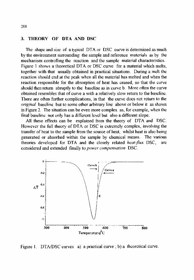
288

3. THEORY OF DTA AND DSC

The shape and size of a typical DTA or DSC curve is determined as much by the environment surrounding the sample and reference materials as by the mechanism controlling the reaction and the sample material characteristics. Figure 1 shows a theoretical DTA or DSC curve for a material which melts, together with that usually obtained in practical situations. During a melt the reaction should end at the peak when all the material has melted and when the reaction responsible for the absorption of heat has ceased, so that the curve should then return abruptly to the baseline as in curve b. More often the curve obtained resembles that of curve a with a relatively slow return to the baseline. There are often further complications, in that the curve does not return to the original baseline but to some other arbitrary line above or below it as shown in Figure 2. The situation can be even more complex as, for example, when the final baseline not only has a different level but also a different slope.

All these effects can be explained from the theory of DTA and DSC. However the full theory of DTA or DSC is extremely complex, involving the transfer of heat to the sample from the source of heat, whilst heat is also being generated or absorbed within the sample by chemical means. The various theories developed for DTA and the closely related heat-flux DSC, are considered and extended finally to power compensation DSC.

AT

CUrV'b l / ~" u r v e 11

-02

-0.4

-0.6

-0~

300 . . . . . . . 40o . . . . . . . 500 . . . . . . . 600 . . . . . . . 7o0 . . . . . . . 8oo

Tempe e/'C ratur

Figure 1. DTA/DSC curves a) a practical curve ; b) a theoretical curve.

289

0.4-

AT

0 _ r

-0.5

-1

- 1 . 4 - . . . . . . . . . . . . . . . . . . . . . . - . . . . . . . . . . . . . . . . . . . . . . . . . . , . . . . . . . . . . . . . . .

3 0 0 400 500 600 700

Temperature~C

Figure 2. The temperature difference curve measured by thermocouples the material when a change in thermal conductivity occurs.

within

3.1. The use of heat transfer equations Theories of DTA can usually be placed into one of two types. In the first type,

heat transfer equations such as the thermal analogue of Ohm's Law:

d q / d t = ( T v - Ts) /RSF (4)

are used to simulate heat flow into the test materials. Here d q / d t is the heat flow in J s -1 between points F and S which have temperatures T v and T s , and between which the thermal resistance is RSF K s J-1. The papers of Void [22], Borchardt and Daniels [25], Gray [51] and others follow this line of reasoning. The integration of this equation contains a ' time constant ', that is, the temperature T s does not immediately follow T F but is delayed by a time t which depends on RSF.

Heat transfer equations of this form were used by Vold [22] to develop equations whereby the heat of reaction involved in a particular DTA peak could be calculated. According to this theory, when a reaction that is producing a peak ceases, then the form of the differential temperature return to the baseline is exponential. This is clearly seen in Figure 1. Void defined the 'active area' under the peak as that from the commencement to that point where the curve form is exponential. The point at which this occurs can be determined if a plot of the

290

logarithm of that part of the curve between the peak and its return to the baseline is plotted against time. When the curve is exponential the logarithm plot is linear. Void showed that if the slope of the linear part is A then the heat H absorbed by the reaction is related by:

H = A. 'active area' (5)

Unfortunately many reactions, unlike melts, do not cease at the peak of the DTA curve and so the extent of the exponential part of the curve is small or in some cases may not exist at all. The reaction then only ceases at or near the baseline. In such a situation it is well nigh impossible to obtain a reliable value for A making it difficult to calculate the heat of the reaction. Equation 4 has a similar form to the equation for the charge of a capacitor through a resistor :

d q / d t : ( V m - V c ) / R (6)

where the voltages V m and V c are analogous to temperatures, and dq /d t , the rate of charging is analogous to heat flow rate and R, the electrical resistance between m and c is analogous to thermal resistance. Now:

dq/dt : C . d V c / d t (7)

where C is the electrical capacity, analogous to the heat capacity. As a result of this analogy there have been many theories [52-55] using resistor-capacitor networks to simulate actual DTA apparatus. These analogues showed that the difference temperature baseline of a DTA or a heat flux DSC curve would only be zero if both sample and reference physical properties were identical and remained so throughout the whole experiment. Otherwise the baseline would be non-zero and the offset would be proportional to the heating rate. If the test properties varied with temperature then the baseline would be sloped relative to zero temperature difference. Often the greatest changes in physical properties occur when reactions are producing a DTA peak, so that this causes the baseline level to be different before and after a reaction. If a property changes with temperature in a different manner before a peak to that after the peak, then the slope of the baseline can be different on either side of a peak. This baseline shift during a reaction makes for difficulties in peak area measurement. The practice of joining a straight line across the 'ends' of the peak often leads to area values which are too large. Later a method of area measurement will be outlined which reduces such errors.

291

In a generalised theory of Dynamic Thermal Measurement, Gray [51] suggested that the following equation represented the instantaneous rate of heat generation by the sample:

R (dh/dt) = (T s - 7R) + R (C s - CR) (dT/dt) + R C s ( d(7' s - 7 R ) / dt ) (8)

where R is the thermal resistance from heat source to sample in Ks j-l; (dh/dt) is the rate of heat generation by the sample; Ts, T R are the sample and reference temperatures, respectively; Cs, C R are the sample and reference heat capacities, respectively, and

(dT/dt) is the rate of temperature rise of the reference material which should be the controlled heating rate of the experiment.

The first term on the right hand side of equation (8) is the differential temperature and is continuously recorded. In the steady state, and if dh/dt is zero, the third term is also zero (baseline constant) so that the first term is equal and opposite to the second term. This second term represents the baseline displacement. The third term is the slope of the curve at any point multiplied by a constant RC s (assuming C s is constant). This is the thermal constant mentioned earlier and used by Vold [22] in her theory. If it is assumed that RC s is known, the magnitude of the third term can be determined graphically. The displacement from the baseline at any time is proportional to the reaction rate at that time and the fraction of the area generated up to that time is the fraction of the material which has reacted by that time. RC s should be as small as possible, a feature considered later [56] as then the mstnunent will more accurately record the thermal behaviour of the test material. Gray only modelled melting, pointing out, in a similar manner to Vold that, when all melting has ceased then the A T curve returns to the baseline exponentially. Gray suggests that the total area under a given peak, including the exponential return to the baseline, is representative of the heat involved. Gray showed that two transitions A and B of the same magnitude will only be resolved if they are separated by a temperature difference (T A -TB) given by:

(T A -TB) = (0.693 RC s + 1/2 tmax) (dT R/dt ) (9)

where tma x is the time taken from the commencement to the peak of the curve and (dT/dt) is the heating rate.

More recently, Hongtu and Laye [57] used the theories of Gray [51] and of Boersma [23] to assess the quantitative performance of a thermal analyzer

292

constructed so that the thermocouples were situated beneath the sample holders. They found that the calibration was affected as to whether the holders were made of metal or quartz. This is to be expected from theory, for the ability to use such an apparatus quantitatively depends on there being a controlled resistance pathway between the source of heat and the test materials. This pathway will be different for different holder materials because these will form, together with the resistance of the intervening space between heat source and holder, a different

resistance pathway for different holder materials. Results obtained from electrical analogue circuits which use resistors and capacitors only, have the limitation that reaction kinetics cannot be introduced into the equations produced.

Some years ago, Wilbum et al. [58] used an analogue computer to assess the effect of holder design on the distortion introduced into a typical reaction peak. In this work it was possible to include some limited forms of the reaction equation. This enabled more realistic DTA curves to be produced which could be directly compared to curves of rates of reaction versus temperature given by the reaction equation alone. Hence indications of distortion due to holder design could be estimated.

Borchardt and Daniels [25] developed heat transfer equations for a system consisting of test tubes containing liquid reactants within a stirred, heated liquid. In this situation the transfer of heat to the test materials would be rapid, a situation which is not usual when studying solid materials. Their theory is only valid if the following conditions are met:

1. The temperature in the holders must be uniform. While this might be true for liquids, it is certainly not the case for solids.

2. Heat transfer must be by conduction only. 3. The heat transfer coefficient must be the same for both holders. 4. The heat capacity of the test materials must be the same.

These conditions are relatively easy to achieve for liquids, due to the rapid transfer of heat within the system, but much more difficult to achieve for solids, so that for such materials, this theory is of little use.

3.2. The use of reaction equations The second approach towards the understanding of DTA and DSC curves

considers the problem in a different manner, using reaction equations such as those given by Brown [59] and Keattch and Dollimore [60]. These equations are manipulated to develop various relationships between the difference in

293

temperature A T and the sample temperature at a specific time. Coats and Redfem [61 ] manipulated reaction equations to show that various relationships exist between the peak temperature and the heating rate from which it is possible to derive activation energies and 'orders of reaction'. Kissinger [62] showed that peak shape was related to the reaction order and by making certain measurements on the shape of a DTA curve it was possible to calculate n, the 'order of reaction'.

n -- 1.26 S 1/2 (10)

where S is the "shape index", that is the value of the ratio of the slopes of the tangents at the two inflection points of the peak. He also developed an equation relating the temperature of the maximum of a DTA peak, Tp with the heating rate fl:

d (In ,Y / Tp 2 ) / d (1/Tp) - (E a/R ) (1 l)

so that a plot of ( In ,8 / Tp 2 ) against (1 / lp ) is linear and of slope - E a/R. In cases in which only reaction equations are manipulated, no account is taken

of heat transfer, a factor which has recently been found to be important in peak shape [56]. This work showed that poor transfer of heat from heat source to test material can distort the shape of TG curves, so producing distortion of the DTG curve. As the DTA and DTG curves of a given material in which mass is lost, are usually similar and linked in shape, the DTA curve will also be distorted and thus lead to erroneous values of reaction order if the shape factor as defined by Kissinger is used.

3.3. Combined approach In an effort to combine the two different approaches, Melling et al. [63] and

later Wilbum et al. [64,65] used a mathematical finite difference approach in which they were able to combine both heat transfer and reaction equations. The technique uses an iterative method by which the temperatures of thin annuli of a cylindrical test material and holder are calculated repeatedly as the outer annulus is increased in temperature at a known rate. It is assumed that the temperature along any radial surface parallel to the central axis of the cylinder is uniform. A number of outer annuli represent the holder whilst the inner ones represent the sample material. A second set of annuli are similarly subdivided into holder and reference material. Heat is also generated within the inner annuli of the test material according to any one of the reaction equations referred to above [59,60]

294

and values of density, specific heat and thermal conductivity can be assigned to the holder, test and reference materials. Thus it is possible to calculate the temperature at any point in the system and thus the temperature difference between similar positions within the sample and reference materials as well as that between the sample holder and the reference holder. The process is very time consuming and necessitates the use of a computer to generate the temperature profiles throughout the system. By computing the 'ideal' DTA curve using the reaction equation alone and comparing this with that obtained using the finite difference scheme, they were able to show the effect the properties of the holder and testmaterials on a typical DTA peak. Their work substantiated the earlier work found when analogue networks had been used, but went further in describing how holder properties could affect the transfer of heat during a reaction. In so doing they were able to show that such properties could also affect peak shapes and peak temperatures adversely.

In the finite difference scheme, it was possible to use values of physical properties of the test materials which were different both before and after a reaction and these properties could also be varied with temperature.

Similarly, the properties of the holder could be varied, also showing their effect on a typical DTA curve. This work produced many important formulae connecting both holder and test material properties with the generation of DTA and heat flux DSC curves.

3.4. The effects of design 3.4.1. 7hermocouples within the samples

In many of the older DTA apparatuses, the measurement thermocouples, which were more massive than those used today, were buffed in the centre of the test materials. There were many reasons for these arrangements, the main one being the lack of means whereby the small microvolt difference signals from the thermocouples could be satisfactorily amplified. For such designs, the baseline temperature difference A 7" for cylindrical samples of radius r is given by equation (12):

AT - - ( ~ r 2/4)(pRCR/kR) - ([~ CS/kS)] (12)

where fl is the heating rate in K/s, r is the sample (and reference) radius;

Ps, 9R are the densities of the sample and reference; Cs, c R are the specific heat capacities of the sample and reference; k s, k R are the thermal conductivities of sample and reference materials.

295

Obviously only when the factor in the square bracket of equation (12) is zero will there be no offset of the baseline. A change in any of the physical properties of the sample or reference dtLring a reaction will affect the offset of the baseline. As r is reduced the offset is less, thus the offset effect is reduced for small samples, but, of course, so is the temperature difference due to any transition or reaction. Similar equations may be derived for other cell geometries.

One difficulty found with small samples occurs in the preparation of mixtures of a number of components, such that a very small sample may not be representative of the bulk material, particularly if the bulk sample contains a mixture of various grain sized materials. This should always be considered when using these techniques.

If any one of the physical properties of the test sample changes during the generation of a DTA peak (but the properties of the reference material remain constant) then the filfite difference theory showed that the change in offset of the baseline was related to the change of physical properties by the relationship:

AOffset = fl ( A g A c r 2 / 4 A k ) (13)

where Ax represents the change in the property x, ( x - 9, c or k) and the other symbols retain their previous meav.ing. Thus a change in any one of the physical properties during the generation of a DTA peak will cause a shift of the baseline.

3.4.2. Thermocouples beneath the sample pans Boersma [23] was one of the first to show that a DTA in which the temperature

measurement is made beneath the holders was truly calorimetric. When the temperature measuring devices are situated beneath the pans containing the test materials, as in heatf lux DSC, then a baseline shift only occurs from a change in the specific heat of sample and reference materials, assuming that the sample mass does not change. A change in the other physical properties, namely density and thermal conductivity of the test materials has no effect on the level of the baseline. For a cylindrical container and sample of unit length, the baseline shift is given by the expression:

Baseline shift = fl m A c s [ In ( r H /r s ) ] / 2 k H (14)

where fl is the rate of heating in K s-l; m is the mass of the sample per unit length;

A c s is the change in the specific heat capacity of the sample; r, r s are the radii of the holder and sample, respectively, and

296

k H is the thermal conductivity of the holder. Thus, so long as the mass remains unchanged by the reaction, the baseline shift is due only to a sample specific heat capacity change. The comments outlined earlier concerning an exponential return to the baseline, together with those concerning area measurement, still apply. However, it is possible to measure the change of specific heat capacity with this design, as the offset is defined as the difference in baselines before and after a peak when dynamic equilibrium is established. In this situation it can be shown that the area of a DTA or heat-flux DSC peak, where the sample is in a circular pan, is given by

Ar ea - H m [ l n ( r H s / r s ) ] ( R s s / 2 ) (15)

where A is the peak area in K s; H is the heat per unit mass; m is the mass of the sample;

rHS, r s are the radii of heat source and sample, respectively, and Rss is the thermal resistance from heat source to sample in K s j-1.

3.4.3. Power compensation DSC In power compensation DSC, the sample and reference holders are insulated

from each other and have their own individual sensors and heaters. The electrical circuitry operates to maintain the holders at the same temperature, within the electrical sensitivity of the circuitry, by varying the power supplied to the heater in each of the holders. [66]. The thermal energy absorbed by the sample per unit time is exactly compensated by the differential electrical power A P supplied to the heaters. The baseline will be given by:

AP = dAq/dt = fl (C s - C R ) (16)

and the peak area gives A H, the heat of reaction, directly.

3.4. 4. High temperature apparatus Above about 700~ heat transfer by radiation, which is always present but

increases with temperature becomes more significant. Theories of DTA and DSC are generally based on heat transfer by conduction and assume that radiation is insignificant. Thus the majority of the present theories are only valid for lower temperatures. At high temperatures (up to 1500 ~ it is usual to employ the heat flux DSC design with thermocouples beneath the holders and this also avoids contamination of the thermocouples at such high temperatures.

297

-0.5i

~T o

-0.5

-1 v ~ ) ! �9 ' - " ! " ' " ~ ' ' ' y ' , . ~ , ~ y . , �9 i , ' , , i' , �9 , i - �9 , - ! , e , I " , " ' r ~ ! , , ~ i , , ~ ] - , , , , - v-.-q,

3~I 400

/

500 600

Temperature/~

700

Figure 3. The temperature difference measured by thermocouples between the pan and the test materials when a change of specific heat of the sample occurs.

AT

-0.5

Y

300 400 500 600 500 TemperatureJ~

Figure 4. The temperature difference measured by thermocouples between the pan and test materials when a change of thermal conductivity or density of the sample occurs.

298

3 . 5 . C o n s t r u c t i o n o f t h e b a s e l i n e

The construction of the baseline across a peak presents considerable problems unless the baselines preceding and following the peak are collinear. In cases where the sample properties change, especially the heat capacity, the baselines may be at very different ordinate values and may have different slopes. Joining the extrapolated onset to the extrapolated end of the peak by a straight line will not give the correct peak area. A sigmoidal baseline may be computed from the peak itself or other constructions may be done.

Figure 5 suggests a baseline construction in the situation where the baseline before and that after the peak are at different levels [67]. This construction does not give the absolute area but the approximation is considerably closer than drawing a straight line across the ends of the peak.

0 , 5 -

0.0

AT -

-0.5

-1.0 -

I 300 400

B D

C

I I ' "1

500 600 700 Temperature]~

Figure 5. Area measurement with baseline shift. Curved area ACDFA- area AEBDFA + area CBDC - area ACEA. As area CBDC ~area ACEA then ACDFA~ AEBDFA. This provides an easily constructed area which is more accurate than that produced by a straight baseline joining A to D. The curved line ACD is not easily constructed.

299

3.6. Application of theory to consideration of the factors affecting DTA and DSC

3.6.1: Effect of atmosphere Atmosphere plays an important part in the generation of a DTA or DSC curve,

particularly when the reacting sample emits gas. If such gas is not swept away, this produces a back pressure on the reaction and can, in some cases [68] alter the course of the reaction. Whether a gas is evolved or not, it is a wise arrangement to have a flowing gas over the system at all times to ensure that conditions are as uniform as possible in all experiments. If the sample and reference materials are contained in crucibles in a gaseous space and the temperature is measured below the crucibles, the area of the peak will depend on the thermal conductivity of the gaseous space as shown by equation (14). Changing the atmosphere from nitrogen to helium will alter the response of the sensor system.

3.6.2. Sample size The effect of sample size has been referred to above and the use of very large

samples is not recommended. One exception is When bulk samples consisting of many different grain sized materials are studied. In this case it is not easy to obtain a representative small sample, but the heat transfer problems associated with larger samples may be more representative of the commercial process and may therefore be justified.

4. INSTRUMENTATION

Modem DTA and DSC insmnnents have been surveyed in recent texts [69,70] and the earlier instruments discussed in the historical references of section 1. The major components of any DTA or DSC instrument are shown in Figure 6. Some are common to most thermal analysis instruments, and the comments made in other chapters concerning the construction of furnaces, of control of temperature and of atmosphere, and of collecting and processing data should be noted in connection with DTA and DSC.

The parts of the system may be listed as; a. the DTA or DSC sensors plus their crucibles and signal amplifier; b. the furnace, its temperature sensor and any cooling and atmosphere

facilities;

300

c. the programmer or computer controller and d. the recorder, plotter or data processor.

Furnace

Sample

Sensor

Atmosphere Control

s .

+

N + A

Sensor Amplifier

Progrmnmer or Computer

I Cooling Control

Data Recorder or Computer

Figure 6. Schematic of a DTA or DSC apparatus. ( A represents the differential signal: A T for DTA, AP for DSC)

4.1. The s e n s o r s

The temperature sensors most often used in thermal instrumentation are thermocouples and platinum resistance thermometers. Table 1 shows an approx imate comparison of their characteristics. For a pair of thermocouples with the cold junction at 0 ~ and the other junction at a Celsius temperature, O, the relationship between the emf and temperature requires a polynomial equation of 9th order for the highest accuracy [71 ], but it may be expressed approximately by a cubic equation:

MER + a 0 + 1/2 b 0 2 + 1/3 c 0 3 (17)

and:

MQR - dE/d0 -=: a ~ b0 ~- c0 2 (is)

301

where mER is the thermocouple e.m.f, in the direction from M to R, and MQR is the derivative with respect to temperature and is called the "thermoelectric power".

For a resistance thermometer, an equation may be written relating the ratio of the resistance at a higher temperature 0 to that at 0 ~ Ro/R o to the temperature [72]:

Ro/R o - 1 + ~ 0 + [3 0 2 + It 0 3 (0 -100) (19)

while for a semiconductive resistor, or thermistor having a negative temperature coefficient, the approximate relationship is [73]:

In (Ro/Ro)-- {Eg/2k }(1 / (0+273) - 1/273 ) (20)

where Eg is the energy gap for the semiconductor; k is the Boltzmann constant,

and the other symbols have their previous significance. In all cases, particular thermometric sensors must be calibrated, either using the

well-defined fixed points of the International Temperature Scale, or the NIST- ICTAC reference standards [71,74].

The sensitivity of the thermocouple sensors is represented by their thermometric power, Q, that is the rate of change of e.m.f with respect to temperature. In Table 1 (a) Q is quoted approximately for temperatures around 200 ~ It can be seen from the table that a Type K sensor is over four times more sensitive at this temperature than a Type R sensor and this may allow a more sensitive sensor assembly to be made. It should also be noted that the thermocouple output may change with time due to chemical attack, physical change and diffusion across the interface.

4.1.1. Thermocouple cold junctions The factors given above relate to a cold junction held at 0 ~ but an equivalent

circuit for cold junction compensation is sometimes used. This may involve keeping a thermocouple at a suitably low temperature using Peltier cooling, or using a block maintained at a higher, constant temperature, for example 50.0 + 0.1 ~ or an electronic compensation circuit.

4.1.2. The choice of sensor The choice of a temperature sensor depends on the needs of the experimenter.

The resistance to chemical attack, the temperature range and the mechanical stability must be considered in addition to the thermometric sensitivity.

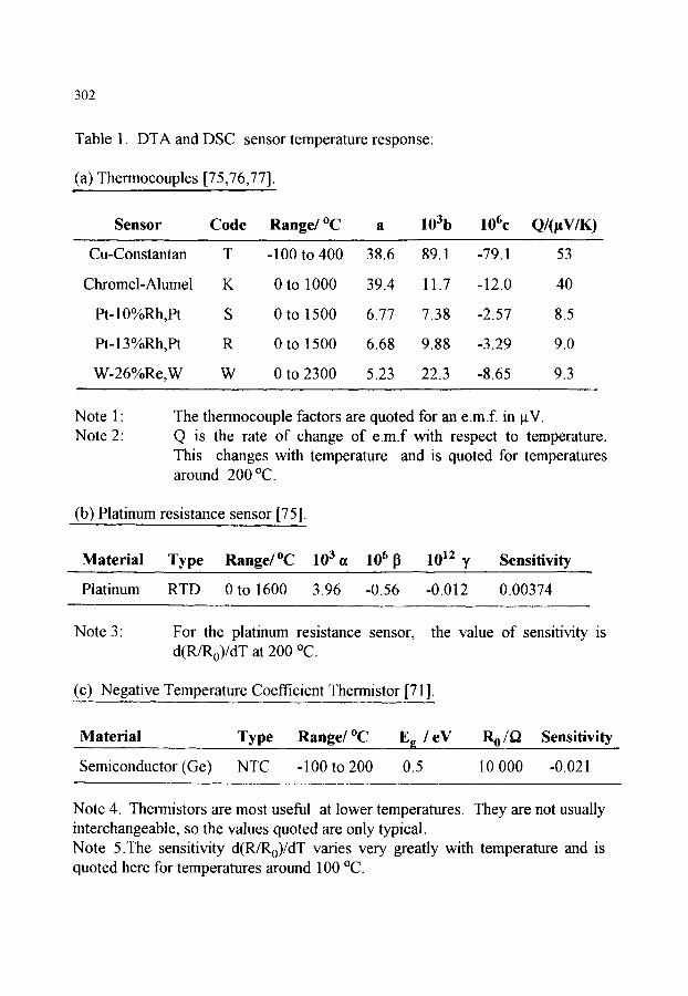
302

Table 1. DTA and DSC sensor temperature response:

(a) Thermocouples [75,76,77].

Sensor Code Range/~ a 103b 106c Q/(~tV/K)

Cu-Constantan T -100 to 400 38.6 89.1 -79.1 53

Chromel-Alumel K 0 to 1000 39.4 11.7 -12.0 40

Pt-10%Rh,Pt S 0 to 1500 6.77 7.38 -2.57 8.5

Pt-13%Rh,Pt R 0 to 1500 6.68 9.88 -3.29 9.0

W-26%Re,W W 0 to 2300 5.23 22.3 -8.65 9.3

Note 1: Note 2:

The thermocouple factors are quoted for an e.m.f, in laV. Q is the rate of change of e.m.f with respect to temperature. This changes with temperature and is quoted for temperatures around 200 ~

(b) Platinum resistance sensor [75].

Material Type Range/~ 10 3 a 106 [~ 1012 3( Sensitivity

Platinum RTD 0 to 1600 3.96 -0.56 -0.012 0.00374

Note 3: For the platinum resistance sensor, d(R/R0)/dT at 200 ~

the value of sensitivity is

(c) Negative Temperature Coefficient Thermistor [71].

Material Type Range/~ Ea / eV Ro/f] Sensitivity . . . . . . . .

NTC - 100 to 200 0.5 10 000 -0.021 Semiconductor (Ge)

Note 4. Thermistors are most useful at lower temperatures. They are not usually interchangeable, so the values quoted are only typical. Note 5.The sensitivity d(R/R0)/dT varies very greatly with temperature and is quoted here for temperatures around 100 ~

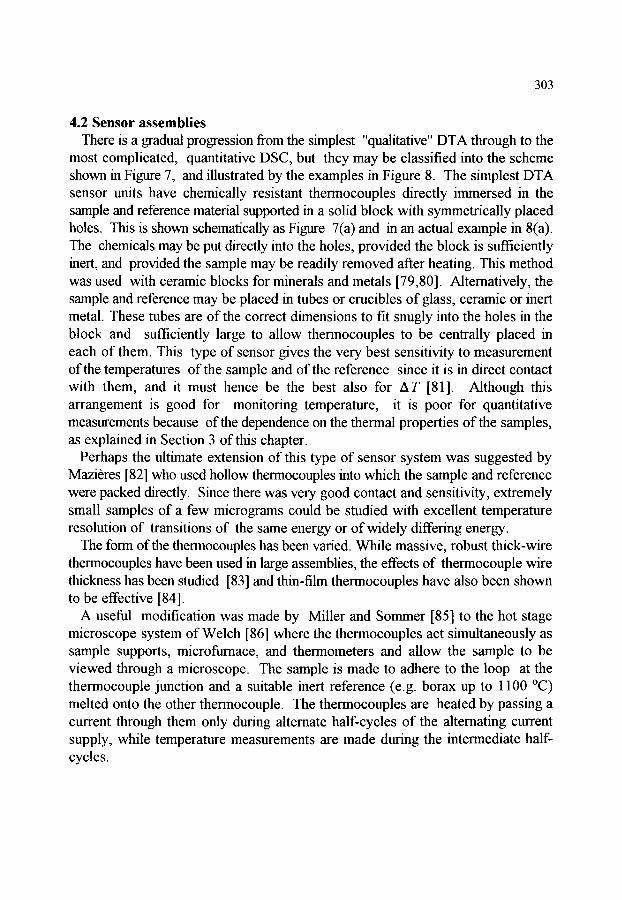
303

4.2 Sensor assemblies There is a gradual progression from the simplest "qualitative" DTA through to the

most complicated, quantitative DSC, but they may be classified into the scheme shown in Figure 7, and illustrated by the examples in Figure 8. The simplest DTA sensor units have chemically resistant thermocouples directly immersed in the sample and reference material supported in a solid block with symmetrically placed holes. This is shown schematically as Figure 7(a) and in an actual example in 8(a). The chemicals may be put directly into the holes, provided the block is sufficiently inert, and provided the sample may be readily removed after heating. This method was used with ceramic blocks for minerals and metals [79,80]. Alternatively, the sample and reference may be placed in tubes or crucibles of glass, ceramic or inert metal. These tubes are of the correct dimensions to fit snugly into the holes in the block and sufficiently large to allow thermocouples to be centrally placed in each of them. This type of sensor gives the very best sensitivity to measurement of the temperatures of the sample and of the reference since it is in direct contact with them, and it must hence be the best also for AT [81]. Although this arrangement is good for monitoring temperature, it is poor for quantitative measurements because of the dependence on the thermal properties of the samples, as explained in Section 3 of this chapter.

Perhaps the ultimate extension of this type of sensor system was suggested by Mazi6res [82] who used hollow thermocouples into which the sample and reference were packed directly. Since there was very good contact and sensitivity, extremely small samples of a few micrograms could be studied with excellent temperature resolution of transitions of the same energy or of widely differing energy.

The form of the thermocouples has been varied. While massive, robust thick-wire thermocouples have been used in large assemblies, the effects of thermocouple wire thickness has been studied [83] and thin-film thermocouples have also been shown to be effective [84].

A useful modification was made by Miller and Sommer [85] to the hot stage microscope system of Welch [86] where the thermocouples act simultaneously as sample supports, microfumace, and thermometers and allow the sample to be viewed through a microscope. The sample is made to adhere to the loop at the thermocouple junction and a suitable inert reference (e.g. borax up to 1100 ~ melted onto the other thermocouple. The thermocouples are heated by passing a current through them only during alternate half-cycles of the alternating current supply, while temperature measurements are made during the intermediate half- cycles.

304

,r

I

r, Cj

IVi IVI all,

I~II.A ! b

I M A A

C.

do

eo

l i i f.

V

-I !'-

Figure 7. The DTA-DSC series, based on [78].

a: Qualitative DTA b: Quantitative DTA c: "Boersma" DTA or heat-flux DSC d: Heat flux DSC with thermopile. e: Calvet-principle DSC f: Power compensation DSC.

Sample holder or crucible

Thermocouple

Heat link

Thermopile

Temperature sensor: TC or RTD

Heater

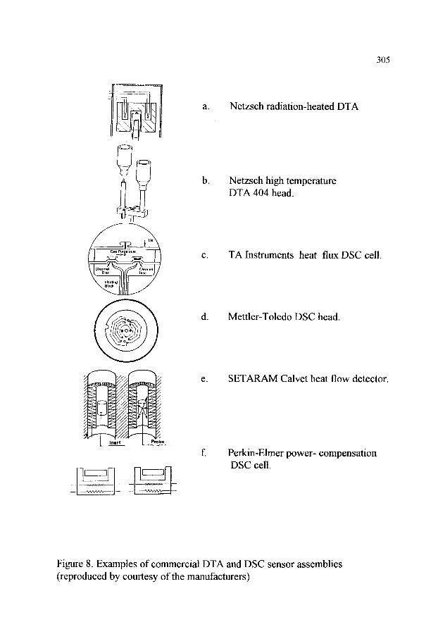
305

/

Inert Probe

a.

b.

C.

do

e.

Netzsch radiation-heated DTA

Netzsch high temperature DTA 404 head.

TA Instruments heat flux DSC cell.

Mettler-Toledo DSC head.

SETAR~dM Calvet heat flow detector.

Perkin-Elmer power- compensation DSC cell.

Figure 8. Examples of commercial DTA and DSC sensor assemblies (reproduced by courtesy of the manufacturers)

306

The use of infrared pyrometric sensors for TA work at very high temperatures, up to 2200 ~ has been demonstrated [87]. The differential signal is generated between one IR sensor measuring the black-body cavity (BBC) radiation centred at a wavelength ~'0, and a second sensor focused on the sample enclosed within the cavity. The laws of radiation [88] show that the temperatures are given by:

1 _ 1 _ _ k O ( l n [ e s ] )

T B T s C 2 (21)

where

Vs C2 c S

is the temperature of the BBC, is the temperature of the sample, is the second radiation constant and is the emissivity of the sample.

Since emissivity is a thermochemical property of the material, it will alter in magnitude as the sample goes through a phase change. The melting of rare earth aluminates around 2000 ~ has been studied with this apparatus, referred to as "optical differential thermal analysis" or ODTA [89].

Wilburn [66] has shown that the optimum arrangement of sensors and holders for quantitative work consists of separate metal containers enclosed in an air space and sitting on the thermocouple junctions. This is represented in Figure 7(b) and exemplified in Figure 8(b). Boersma [23] proposed the introduction of a controlled heat leak between sample and reference holders which gave the basis for heat-flux DSC, represented in Figure 7(c) and exemplified in Figure 8(c). This type of head has been adapted to make measurements simultaneously on two samples [90]. The heat flux DSC is a passive system.

The use of several thermocouple junctions (or a thermopile) to measure the temperature difference between sample and reference will give a larger signal and is indicated in Figure 7(d) and these have been designed for both cylinder-type systems [91] and disk-type systems [92]. A disk version is shown in Figure 8(d).

A rather different principle applies for the system shown in Figures 7(e) and 8(e). The sample and reference are located in a calorimetric block which surrounds the experimental zone and which consists of a large number of thermocouples connected as a thermopile detector as in the Tian-Calvet calorimeter [93,94]. The thermopiles have a high thermal conductivity and sensitivity and measure heat exchanged between the furnace and the sample cell.

The power-compensation DSC is shown in Figures 7(f) and 8(f). The sample and reference have their own independent sensors and heaters and any temperature

307

difference sensed between them is fed into a control circuit which determines the power to be supplied to the sample and reference. Although this system does monitor a temperature difference, it is the difference in electrical power which provides the analytical signal. The sensors may be either platinum resistors or thermocouples [29,95]. The power-compensation DSC is an active system, since there is a continuous and automatic sensing of the error signal and thence adjustment of the power to the heaters.

One disadvantage of the power-compensation system is that it is most effective over the temperature range -170 ~ to 730 ~ The development of higher temperature DSC instruments has therefore concentrated on the heat flux design.

The use of two sample cells is avoided in the novel design of self- referencing DSC shown in Figure 9 [46]. The heat is transferred between the furnace and the sample via a flat plate. The plate has a central sample location whose temperature is monitored by a thermocouple. Another four thermocouples are radially positioned around the sample to provide an averaged temperature signal or "averaged integral reference" from which the differential signal may be derived. This signal is directly proportional to the heating rate and the heat capacity of the sample and should show improved baseline reproducibility since there is less instrumental thermal asynunetry. Faster heating rates than with conventional DSC are possible and the proportionality of the signal to heating ramp rate allows conversion of calibration between different rates.

Figure 9. Self-referencing DSC [46]

308

Discussion of simultaneous TG-DTA and TG-DSC is concentrated in Chapter 11, but it is, perhaps worth noting that a "Single DTA or SDTA" curve may be obtained from the measured temperature of a single cell in a TG experiment through a calculation of the reference temperature using a mathematical model [47].

4.3. Reference materials. The techniques of DTA and DSC measure a difference in sensor signal between

a sample and a reference material. While the sample may be practically any chemical from a mineral, through polymeric, to biological material, the reference should be inert over the temperature range studied, unreactive to the crucible or thermocouple and, preferably, similar in thermal properties to the sample.

The reference materials most frequently used in DTA of minerals and inorganics are ~-alumina, AI203 (which must be heated to around 1500 ~ to remove adsorbed water), titania, TiO2, or carborundum, SiC. These have thermal conductivities in the range 3 to 40 W m -1 K -I in the temperature range up to 1000 ~ In order to make the sample and reference more similar, the sample may be diluted with the reference, although this will decrease the sample signal. Care must be taken that no reaction takes place between sample and reference diluent.

For organic and polymer samples which have rather lower thermal conductivities, silicone oil and dioctyl phthalate with thermal conductivities between 0.1 and 0.2 W m -I K -1 may be used as reference materials. Occasionally the pure solvent may be used as reference for samples in Solution [59,96].

Since the DSC signal should be independent of the thermal properties of the samples, it may be possible to use an empty pan as reference and this is often done with both types of DSC.

4.4. Crucibles and sample holders Although in early apparatus the sample and reference were put directly into wells

in the DTA block, it is more usual to put the samples into an inert holder which is then placed into the sensor assembly. The crucibles may either be open or closed, or with controlled leakage to the atmosphere. The main classes are shown in Table 2. There are also many types of specialist crucibles available. For example, it may be important for a gaseous reactant to flow through the sample and this has been achieved [97]. Crucibles of particular special materials have been made. Some crucible designs are shown in Figure 10.

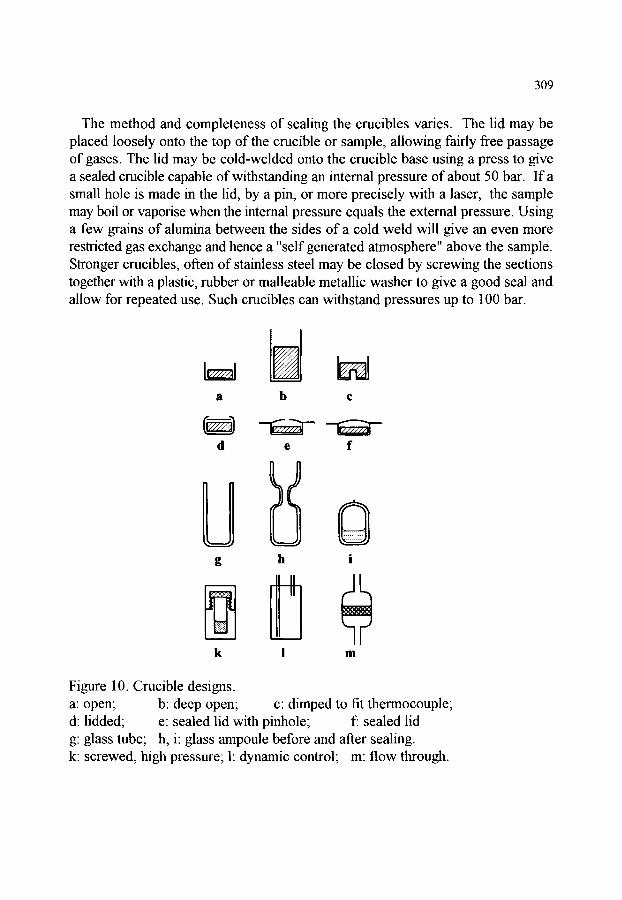
309

The method and completeness of sealing the crucibles varies. The lid may be placed loosely onto the top of the crucible or sample, allowing fairly free passage of gases. The lid may be cold-welded onto the crucible base using a press to give a sealed crucible capable of withstanding an internal pressure of about 50 bar. If a small hole is made in the lid, by a pin, or more precisely with a laser, the sample may boil or vaporise when the internal pressure equals the external pressure. Using a few grains of alumina between the sides of a cold weld will give an even more restricted gas exchange and hence a "self generated atmosphere" above the sample. Stronger crucibles, often of stainless steel may be closed by screwing the sections together with a plastic, rubber or malleable metallic washer to give a good seal and allow for repeated use. Such crucibles can withstand pressures up to 100 bar.

b

d e

g h

II II

II1'' k !

W c

--UwHHL -

G

!111

Figure 10. Crucible designs. a: open; b: deep open; c: dimped to fit thermocouple; d: lidded; e: sealed lid with pinhole; f: sealed lid g: glass tube; h, i: glass ampoule before and after sealing. k: screwed, high pressure; 1: dynamic control; m: flow through.

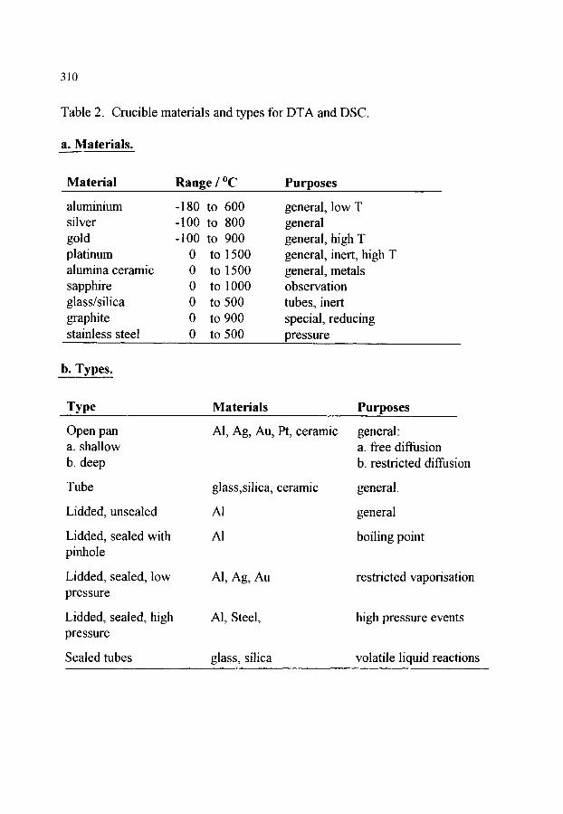
310

Table 2. Crucible materials and types for DTA and DSC.

a. Materials.

Material Range / ~ Purposes

aluminium -180 to 600 silver -100 to 800 gold -100 to 900 platinum 0 to 1500 alumina ceramic 0 to 1500 sapphire 0 to 1000 glass/silica 0 to 500 graphite 0 to 900 stainless steel 0 to 500

general, low T general general, high T general, inert, high T general, metals observation tubes, inert special, reducing pressure

b. Types.

Type Materials Purposes

Open pan a. shallow b. deep

Tube

Lidded, unsealed

Lidded, sealed with pinhole

Lidded, sealed, low pressure

Lidded, sealed, high pressure

Sealed tubes

A1, Ag, Au, Pt, ceramic

glass,silica, ceramic

AI

AI

A1, Ag, Au

AI, Steel,

glass, silica

general: a. free diffusion b. restricted diffusion

general.

general

boiling point

restricted vaporisation

high pressure events

volatile liquid reactions

311

For samples which might react with metallic crucibles, it is possible, though awkward, to seal the sample in a glass ampoule. It is convenient to inject the sample, liquid or solid into a glass vessel with a narrowed neck which may then be sealed to from the ampoule. Sealed sample containers for high pressure work have a higher mass than usual, and results should be compared with calibrations nm under the same conditions and preferably at lower heating rates.

4.5. Assessment of sensor assemblies Assessment of the quality of the sensor assemblies requires both calibration and

testing. A good system should show a reproducible baseline with minimal noise, drift and slope. The sensitivity of the assembly might be tested by using a small sample, or by diluting the sample with reference, or by using a sample with a small change at transition, for example the ct-[3 quartz transition at 573 ~

The resolution of the assembly, that is its ability to distinguish between two thermal events occuring at similar temperatures may be tested too. For low temperatures, the two transitions of dotriacontane (C32H66) at 63 and 68 ~ should be well resolved. For higher temperatures, the resolution of the quartz peak at 573 ~ from the potassium sulphate transition at 584 ~ is a good test.

The calibration of DTA and DSC insmanents will be discussed briefly in Section 6 of this chapter and more fully in Chapter 13.

4.6. Heating and cooling 4.6.1. Heating

The temperature of the fiamaee, whether a block or tube, is measured by sensors of the same type as those used for the sample temperature, i.e. by thermocouples or resistance sensors. The significance of temperature control has been discussed by Tye et al. [98].

Graphite furnaces for high temperatures are maintained in an inert atmosphere and heated directly by passing a current through the electrically conducting graphite. At temperatures below about 1700 ~ an alumina lining tube may be inserted to allow controlled atmospheres which might attack the graphite [99].

The Perkin-Elmer power compensation DSC has separate electrical heaters for the sample and for the reference in their pans which are placed in inert metal holders within a metal shield.

The use of larger, separate furnaces for sample and for reference is also employed in some Tian-Calvet systems, particularly for simultaneous TG-DSC.

312

Other types of heating are sometimes useful. The Ulvac-/Sinku-Rico infrared gold image furnace uses one or more tungsten-halogen lamps with highly reflective, water cooled gold surface mirrors. The response of this system is fast, and it is compact and allows observation of the sample [ 100,101 ]. A radiation heated block system, using a 100 W halogen lamp, has been described as being very suitable for vacuum work and for high heating and cooling rates [70]. Heating by microwaves [102] has also been used, although the absorption coefficient for microwaves varies considerably with material and with temperature, causing some complications.

4.6.2. Cooling If the behaviour of the sample is only studied under conditions of rising

temperature, much useful information may be lost. The phase behaviour of some organics, e.g. liquid crystals, may involve metastable states only found during cooling. Glass transition phenomena are very dependent on both heating and cooling rates. It is important that any DTA or DSC instrument should be capable of controlled cooling as well.

The cooling may be enhanced by fitting a fan to blow air over the assembly. This is only suitable down to about 40 ~ Various cooling systems have been used to allow DTA or DSC measurements at temperatures below ambient. Early examples were reviewed by Redfem [ 103]. A very simple expedient is to enclose the whole fiamace and sensor unit within a refrigerated space. This is probably only useful for temperatures down to -20 ~ or so.

Circulating a coolant around the casing of the furnace has several advantages. It may be incorporated in the control system to give better low temperature control, or it may be used to bring the temperature of the tin-ace down more rapidly to attain a quicker turn-round of samples. With special design it may also keep sensitive parts of the apparatus at safe temperatures.

Peltier cooling of the circulating liquid may also be employed. Passing a current through the thermocouple in one direction will produce a heating effect, whereas reversing the current will cool the junction. This allows controlled cooling of the fluid to about-20 ~ [104]. The same principle has been used to allow faster equilibration of samples after insertion.

A simple and effective way of cooling is to attach a Dewar flask to the thermally conducting enclosure of the furnace and sensor unit and then to cool this by filling with liquid nitrogen for temperatures to -190 ~ or with acetone/solid CO 2 down to about -70 ~ A similar system uses a massive cold finger thermally connected to the sensor enclosure and immersed in a large capacity cooling bath situated below the analyzer and containing liquid nitrogen or other refrigerant. A typical system is shown in Figure 11.

313

Computer '~" Controller ] L

lye

[ Liquid I L Nitrogen ]

Dry Box

DSC Unit

Dry N2

A ~ . ~ - - Heater

Figure 11. DSC assembly with cooling system.

A more elaborate method is to attach a container of liquid nitrogen to the assembly via a coolant comroller. By means of a pressure gauge and a heater attached to a controller, a pressure of around 0.5 atm is maintained in the container. Cold gas is fed into a heat exchanger fitted over the DTA or DSC furnace and will allow cooling to -170 ~

A refrigeration unit built into the instrument may be useful for continuous operations m the range from -70 ~ to about 350 ~ Circulation of a coolant fluid through the cooling arrangement of the analyser gives very good control of the heating and cooling programmes I105]. One cautionary note should be mentioned. Condensation of ice onto the cell or the outlet pipe must be avoided. The system should be purged with a dry gas stream and often a small heater is fitted to the apparatus to prevent ice forming.

4.7. Programming and control of furnace temperature An essential requirement for good DTA and DSC experiments is that the

temperature shall be controlled as precisely as possible. The regulation of the set temperature for isothermal work must be very good, while a wide range of heating rates should be available and well controlled. Modem msmnnents offer heating rates between 0.1 and 100 K min -1, while specially designed systems can provide much higher rates up to 500 K min -1. Cooling is more difficult especially below

314

ambient, but cooling rates of -10 to -20 K min -1 are often available. Computer control of the programming and of the cooling facilities is most useful.

Much of what has already been said concerning programming for thermogravimetry in Chapter 4 also applies here. The earliest control was by the manual adjustment of the electrical supply to the furnace. This was later adapted for mechanical control, for example the manipulation of a resistance or transformer control by a clockwork mechanism. Neither method gave proper control of the heating, nor were they usuable for a variety of different heating rates. Electromechanical control followed, using a variety of control devices. In one system, the furnace temperature was measured by a thermocouple and fed to a meter. A cam cut into an appropriate spiral pattern was turned electrically to operate a "make and break" switch. If the programme temperature was below that required, the switch was opened and, if above, the switch was closed. This type of on/off control tends to give over- or undershoot of the required temperature. It is better to employ some form of PID control [106]. This gives control through:

�9 Proportional action depending on the difference between the measured and programmed temperatures;

�9 Integral control depending on the integrated value of the difference and �9 Derivative control depending on the rate of change of the difference.

This type of control better regulates the temperature of the fumace to follow the programme required. Electronic programmers and computer control allow very sophisticated programmed temperature regimes to be set. A rapid heat to a set temperature, followed by an isothermal equilibration, followed by a slow temperature ramp to high temperature and a controlled cool to ambient are easy to incorporate into computerised temperature control [98].

4.8. Atmosphere control The atmosphere surrounding the sample will affect the thermal analysis curve

obtained. Most DTA and DSC instruments have facilities for establishing an atmosphere of a chosen gas around the sensor assembly. The thermal conductivity of the gases used will affect the response of the sensors as discussed in Section 3. The use of inert gases such as nitrogen, argon or helium, and reactive gases, particularly air and oxygen, is possible with most instruments. Flow rates are generally in the region of 10 to 100 cm 3 min -1. Some systems allow operation under reduced gas pressure, or permit specific mixing of gases. Rapid switch-over from inert to oxidative atmosphere (or the reverse) is also important for some experiments, such as oxidative stability tests.

315

4.9. High pressure DSC (HPDSC) If studies at high pressure are required, two different techniques may be used.

Either the high pressure cells described above may be employed, although this means that the sample is subject to its own "self-generated" pressure of gas, or else the emire system may be modified to withstand higher pressures up to 7 MPa (1000 psig), sometimes by enclosing in a high pressure casing, usually of stainless steel. As with any high pressure apparatus, care should be taken when operating at

elevated pressures. Increased pressure operation is useful to raise the temperature of vaporisation of a material, or to increase the reaction rate. For example, accelerated oxidation tests may be carried out using oxygen under high pressure [108,109]. Vacuum operation is also possible with specially designed systems. Pressure-resistant enclosures will allow the DSC to be used in a vacuum as low as 1 Pa (~0.0075 torr) The dependence of reaction kinetics upon pressure may be studied, as well as vapour pressure variation with temperature using, sealed crucibles with precise "pinholes" in the lid [110].

4.10. Photocalorimetry and DSC Polymerisation and other reactions may be initiated by ultraviolet light and this

is made use of in disciplines such as electronics, coatings technology and dental materials. DSC equipment has been adapted to allow UV illumination of the sample [110] and instruments have been specially designed to provide photocalorimetric measurements with standard DSC cells [ 111,112]. The UV illumination is provided by a mercury or xenon discharge lamp, whose intensity is kept constant by a feedback control. Wavelengths are selected using a filter or monochromator and passed, via a shutter and heat absorbing filter, through a quartz window into the DSC cell.

4.11. Thermomicroscopy and Photovisual DSC The observation of the changes which occur during heating of samples in a DSC

adds considerably to the diagnostic power of a thermal analysis experiment. The technique of thermomicroscopy is discussed more fully in Chapter 10, but it is worthwhile noting here some of the simple adaptations which allow direct observation. Some DSC models, such as the early Perkin-Elmer DSC 1B, had a transparent window in the head cover. This allowed direct observation of samples, provided they were not covered with lids. Haines and Skinner [113] adapted this to use a low power stereomicroscope to observe the sample and record changes in the light reflected ~from it, as shown in Figure 12. A more comprehensive microscope-DSC system is described by Wiedemann [114], (see also Chapter 10), permitting simultaneous DSC-thermomicroscopy with videorecording of the

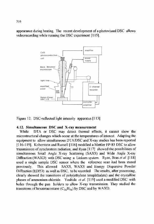
316

appearance during heating. The recent development of a photovisual DSC allows videorecording while running the DSC experiment [ 115].

Figure 12. DSC-reflected light intensity apparatus [ 1 13]

4.12. Simultaneous DSC and X-ray measurement While DTA or DSC may detect thermal effects, it cannot show the

microstructural changes which occur at the temperatures of interest. Adapting the equipment to allow simultaneous DTA/DSC and X-ray studies has been reported [116-119]. Koberstein and Russell [116] modified a Mettler FP-85 DSC to allow transmission of synchrotron radiation, and Ryan [ 117] showed the possibilities of simultaneous Small Angle X-ray Scattering (SAXS) and Wide Angle X-ray Diffraction (WAXD) with DSC using a Linkam system. Ryan, Bras et al .[118] used a single sample DSC sensor where the reference scan had been stored previously. This allowed SAXS, WAXS and Energy Dispersive Powder Diffraction (EDPD) as well as DSC, to be recorded. The results, after processing, clearly showed the transitions of poly(ethylene terephthalate) and the crystalline phases of ammonium chloride. Yoshida et al. [119] used a modified DSC with holes through the pan holders to allow X-ray transmission. They studied the transitions of hexatriacontane (C36H74) by DSC and by WAXD.

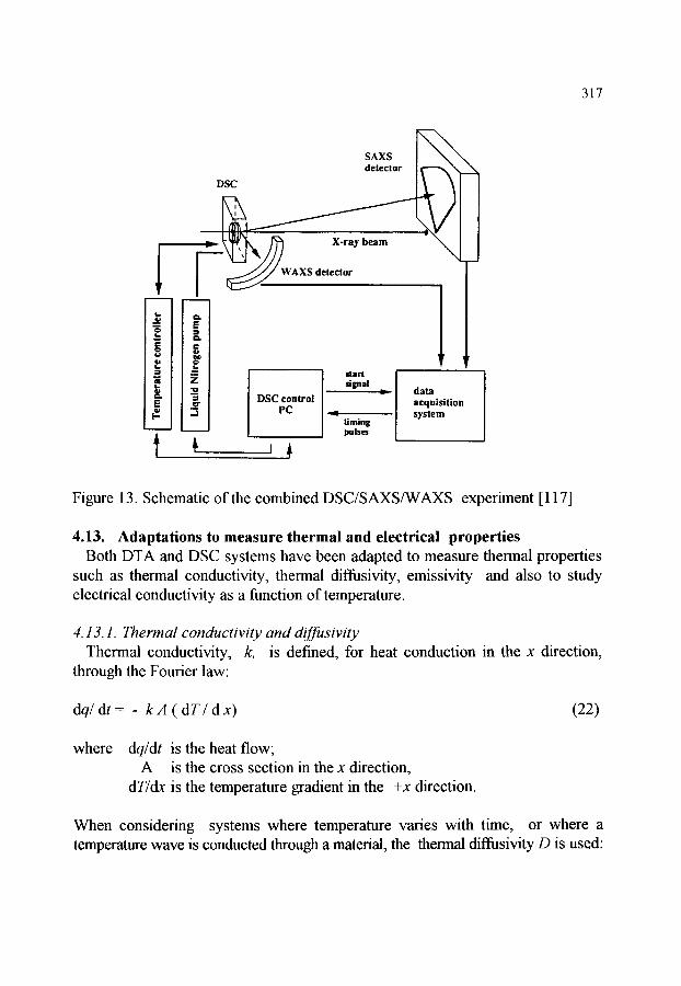
317

1 g~

z g~

~ ~ / f ~ X-ray beam

AXS detector

DSC control PC

start signal

timing pulses

data acquisition system

Figure 13. Schematic of the combined DSC/SAXS/WAXS experiment [ 117]

4.13. Adaptations to measure thermal and electrical properties Both DTA and DSC systems have been adapted to measure thermal properties

such as thermal conductivity, thermal diffusivity, emissivity and also to study electrical conductivity as a function of temperature.

4.13.1. Thermal conductivity and diffusivity Thermal conductivity, k, is defined, for heat conduction in the x direction,

through the Fourier law:

dq/ dt= - kA ( dT/ dx) (22)

where dq/dt is the heat flow; A is the cross section in the x direction,

dT/dx is the temperature gradient in the +x direction.

When considering systems where temperature varies with time, or where a temperature wave is conducted through a material, the thermal diffusivity D is used:

318

D - k / p c (23)

where P is the sample density, and c is the specific heat capacity.

For thermal conduction along a cylinder heated at one end :

D (d 2 T / d x 2) = dT / dt (24)

The heat flow occul-mg along the axis of a cylindrical sample depends on its area, the temperature gradient and the thermal conductivity. Brennan et al. [120] and later Ladbury, Currell et al. [121 ] placed a metallic heat sink above the sensors and used thermocouples to measure the temperature at the top of the specimen, while the temperature of the base of the sample was given by the DSC holder temperature. After equilibration, the DSC holder temperature was raised by A T, about 5 K, which produced an increased power signal A q at equilibrium, and hence the thermal conductivity was given by:

k-: ( A q l ) / ( A AT) (25)

They obtained reasonable results for conductivities from 0.1 to 0.75 W m -1K -1. A similar system was described by Chiu and Fair [122] where a glass standard

was used to calibrate the system. Flynn and Levin [123], using a power compensation DSC, measured the slope

of the leading edge of the melting peak for a high purity specimen, such as indium, depends on the heating rate fl and the thermal resistance factor R, so that:

Slope ~ fl / R (26)

If a sample of thermal conductivity k, area A and thickness l is placed between the pan and the indium sample, using a suitable fluid such as silicone oil to achieve good thermal contact, then the value of R will alter to R' and

k~- I / ( A ( R ' - R ) (27)

Even allowing for corrections, agreement was poor, probably due to contact changes. Hakvoort and van Reijen [124] used the similar technique with a heat flux DSC.

319

With Modulated Temperature DSC, (see Section 5 of this chapter), it is possible to obtain good thermal conductivity data directly from the apparent heat capacity, and the sample area, density and heat capacity plus the period of the signal modulation. After correction for heat losses due to purge gas, good results are obtained for the range 0.1 to 1 W m -l K l [125].

Modifications to a Stanton-Redcrofl DTA 673 were made to determine the thermal diffusivity of materials, particularly pyrotechnics [126,127]. Thermocouples from the DTA were embedded in the samples, one near the edge, one in the centre. Reproducible results were obtained for materials with diffusivities between 1.0 x 10 -7and 3 .5x10 -7 m 2s -1.

4.13.2. Emissivity For heat transfer by radiation, the ideal radiator is a black body and the radiant

power emitted is ~BB watts and varies with the fourth power of temperature:

(I)BB -- A O T 4 (28)

where A is the surface area radiating, and o is the Stefan's Law constant, 5.67 x 10 -8 W m -2 K-4

For a non-black body of the same area and at the same temperature, the emissivity r is defined by:

= e ~BB (29)

Rogers and Morris [128] showed that the baselines of early power-compensation DSC curves were greatly affected by changes in emissivity, although this can be avoided by placing matched covers over both sample and reference. The apparatus was modified so that a constant temperature cover was placed over both sample and reference. Measurement of the deflections on the power axis relate to the emissivity differences between sample and reference. A simplified procedure was later reported [ 129] and mstatmental improvements have eliminated some emissivity effects.

4.13.3. Electrical conductance The conduction of electricity through a material is similar in many ways to the

conduction of heat and the thermal and electrical versions of Ohm's Law have already been mentioned. For electrical conduction in the x direction :

320

I - - G/V o r (30)

I -- - e r A ( V / x ) (31)

where 1 G (l

A (V/x)

is the current in amps, is the conductance in f~ -I is the electrical conductivity in ~--)-I m-1 is the cross sectional area of the conductor in m 2 and is the potential gradient in V m -1.

An early adaptation of the Du Pont 960 DTA [ 130] by the insertion of electrodes of rod or foil demonstrated the changes in electrical conduction corresponding to phase changes and decompositions. Carroll and Mangravite [131] adapted a Perkin- Elmer DSC 1B by fixing electrodes to contact the edge of the aluminium sample pan and centre of the top of the sample. Currents of l0 8 to 10 "15 A were measured with a supply voltage of 500 V. Provided there was good electrical contact, secured by screwing down the contacts after resolidifying the sample from the melt, good agreement was observed between the response of the DSC and the changes in electrical conductance for polymers such as poly(vinyl acetate) and poly(ethylene terephthalate).

4.14. Other modifications The adaptability of the DTA and DSC apparatus has allowed many possibilities

for making simultaneous or alternative measurements. The enthalpies of vaporization of volatile liquids and solids from sample cells with pin holes in their lids have been estimated by using high pressure DSC cells [111,132], although reasonable results were obtained for sublimation enthalpies when aluminium powder was used to ensure minimal thermal gradients [133].

An interesting use of a conventional power-compensation DSC as a simple isothermal calorimeter for measuring heats of mixing was demonstrated by Mita e t

al. [134] A microsyringe mounted above the sample cell was used to deliver known amounts into a sample cell through a pm hole in the lid. Correction for heating and the effects of vaporization gave reasonable results for benzene-ethanol and for pyridine-ethanoic acid. The system could also be used for vaporization studies.

Analysis of the products of decomposition is dealt with in other chapters, but it is possible to perform both evolved gas detection and analysis by removing products for chemical, chromatographic or physical analysis. The cell may even be mounted in an infrared spectrometer so that the products remaining in the cell can be analysed by reflectance IR [ 13 5].

321

A special DTA unit is described by Bollin [ 136] for use on the Martian space programme. Charsley et al. [137] modified the arrangement of a DTA in order to monitor the ignition temperature of pyrotechnic samples. Many other modifications and adaptations have been made to DTA and DSC systems and some will be described in later sections devoted to particular applications.

5. MODULATED T E M P E R A T U R E DIFFERENTIAL SCANNING C A L O R I M E T R Y (MTDSC)

Modulated Temperature Differential Scanning Calorimetry is a technique in which the conventional heating programme is modulated by some form of perturbation. The resultant heat flow signal is then analysed, using an appropriate mathematical procedure, to deconvolute the response to the perturbation from the response to the underlying heating programme. It was first proposed by Reading and co-workers [40,45,138-143] who used a heat flux calorimeter subjected to a sinusoidal modulation. For the mathematical analysis they employed a combination of an averaging procedure to obtain the underlying response and a Fourier transform analysis to measure the amplitude of the response to the temperature modulation. Other types of modulation are possible, as well as many alternative methods of mathematical analysis and some are discussed here.

" 0

o �9

~L" -10

a -20

A

0.7

g 3.~ o.s S

�9 I - - -,0.3

dTIdt n J=: 2 . 0

o" o.1 ,'r

1.o -o.~

- 0 . 3

100 206 3O0

Temperature I "C

Figure 14. Schematic of the MTDSC programme for quenched PET

322

5.1. Theory The simplest starting point for a general expression for describing the origin of the

different type of contributions to the heat flow can be expressed as follows:

dq / dt = Cp,t (dT"/dt) + f (t, T) (32)

where dq/dt Cp,t

f(t,

is the heat flow into the sample, is the heat capacity of the sample due to its rapid molecular motions,(vibrational, rotational and translational) and is the heat flow arising as a consequence of a kinetically hindered event.

There will be many forms of fit, 7) and they will differ with different types of transition and different kinetic laws. The intention here is to provide a general overview and so specific examples of this function will not be discussed. The reader is referred to the literature where some have already been treated in detail [148, 149].

It is appropriate to define the nomenclature and to describe what constitutes a reversing quantity. The heat capacity, Cp, t would normally be considered constant over some narrow interval of time and temperature. Thus, equation (32) assumes that, at any time and temperature, there is a process that provides a contribution to the heat flow that is proportional to and synchronous with the heating rate. This response is effectively instantaneous given the time scale of the measurement. Generally this is a reversible process, however the term reversing is preferred, to distinguish it from processes such as melting and crystallisation. These are reversible processes in the sense that with large temperature cycles they can be reversed. Reversing in this context means that, at the time and temperature that the measurement is being made, the process is reversible. Conversely, fit, T) represents the contribution to the heat flow that, at the time and temperature the measurement is made, is either irreversible, or in some way kinetically hindered. It should be noted that Cp, t is an inherently time dependent quantity. A molecular motion that is frozen cannot contribute to the heat capacity. Whether it is considered frozen will sometimes depend on the time scale of the measurement. The clearest example of this is a glass transition in a polymer, where the change in heat capacity as a function of temperature depends on the frequency at which the observation is made. This is true of DMA, DETA and MTDSC.

323

In MTDSC, the sample is subjected to a modulated heating programme, for example:

T= T O + fit + B sin (~ot) (33)

where To P B 60

is the starting temperature, is the heating rate, is the amplitude of the modulation and is its angular frequency.

When we combine equations (32) and (33) we obtain [40,139, 140-143]:

dq / d t - fl Cp, t + F( l, ~) ..... the total or underlying signal (34)

+ cob Cp, t c o s (6or) + D s in (60 0 ... t h e cyclic signal (35)

where F(t, T) is the average of f(t, 7) over the interval of at least one modulation and D is the amplitude of the kinetically hindered response to the temperature modulation.

Both %, t and D will be slowly varying functions of time and temperature but can be considered effectively constant over the duration of a single modulation, fit, 7) can also give rise to a cosine contribution. However, most kinetically hindered responses can be modelled, at least approximately, by an Arrhenius type expression. When this is the case, the cosine response of f(t, T) dan be made insignificantly small by ensuring that there are many cycles over the course of the transition [148]. MTDSC normally requires that the frequency of modulation and the underlying heating rate be adjusted to ensure that this criterion is met [148]. Not to do so would usually invalidate the use Of this technique. Consequently, in most cases, except for melting as discussed below, it can be assumed that the cosine response derives from the reversing heat capacity. Another assumption is that the amplitude of the temperature modulation is sufficiently small for the kinetic response to be considered linear. This will normally be true when the modulation is of the order of a degree or less.

Inspection of equations (34) and (35) clearly implies that the cyclic signal will have an amplitude and a phase shift determined by cOBCp, t and D. The relationships between these quantities are given by:

C c = AHF / AHR (36)

324

where Cc AHF AHR

is the cyclic heat capacity, (= complex heat capacity, see below) is the amplitude of the heat flow modulation and is the amplitude of the heating rate modulation.

Cp, t - C C c o s ( 6 ) / 6 o B (37)

D = C c sin (6) (38)

where 8 is the phase shift. Consequently there are three basic signals derived from a MTDSC experiment

[1391: �9 the average or underlying signal, that is equivalent to a conventional DSC; �9 the in-phase cyclic component, from which Cp, t can be calculated and �9 the out-of-phase signal, D.

Reading and co-workers, when they first introduced MTDSC, observed that D was often so small that it could be neglected, thus Cc~Cp, t and this quantity could be calculated without the use of the phase lag [40,45,138-143]. They also proposed that it was useful to calculate a fourth signal, called the non-reversing signal. It is explained above how C p,t can be calculated using the amplitude of the cyclic signal and the phase lag (or in many cases the phase lag can be neglected). This can then be multiplied by fl to calculate the reversing contribution to the underlying heat flow. By subtracting this from the underlying signal, a value is obtained for the contribution derived from F(t, 7), i.e. the non-reversing heat flow is given by:

Non-reversing heat flow = Underlying heat flow - fl.Cp, t (39)

= F(t, 7 ' ) (40)

In this way, the reversing contribution can be separated from the non-reversing contribution., This simple analysis has been applied many times to many transitions [40,45,138-143], principally for polymer systems, and found to work well when the non-reversing process is the loss of a volatile material, a cold crystallisation or a chemical reaction. The situation is somewhat more complex when considering glass transitions, but the non-reversing signal can still be interpreted in a meaningful and useful way [149] as discussed below. This analysis is not strictly valid when dealing with melting, but useful information can be gained from the non-reversing signal, nevertheless. This is also discussed in more detail below.

325

The time scale dependence of Cp, t can be explicitly expressed as

dq / dt = Cp,[3 + F(t, T) + B coC p, to COS (60t) + D sin (cot) (41)

where Cp,13 is the reversing heat capacity assigned to the underlying signal and Cp,,o is the reversing heat capacity at the frequency 60.

Generally Cp,13 and Cp,~ will be the same except in the region of a glass transition. It should be noted that Cp,,o is the reversible component (at the time and temperature the measurement is made) that is synchronous with dT/dt at the frequency of the modulation and is thus by definition the reversing heat capacity at this frequency. The value of Cp,[~ during the glass transition must be inferred from Cp,~o and some frequency- heating rate equivalence. This is dealt with in more details in the section on the glass transition.

In the above example, only reversing quantities are expressed as heat capacities. This approach can also be applied to the out-of-phase signal, by treating it as if it were a heat capacity. Thus, the out-of-phase cyclic component is given by [139]:

Out-of-phase (or kinetic) heat f l o w - ft . D ~cob (42)

where D/coB is an apparent heat capacity.

It is sometimes convenient to express the cyclic signal as a complex quantity, by analogy with DMA and DETA:

C c = C * - C ' - iC" (43)

and thence

C * 2 = C ' 2 + C " 2 (44)

where C* C I

C "

is the complex heat capacity, is the real part and is the imaginary part.

The analogy with DMA and DETA should, however, be treated with caution. In these techniques, mechanical work or electrical energy is lost from the sample as heat. In MTDSC, during an endothermic process, such as a glass transition, energy is not lost, yet there will be a measurable C "component. For this reason, it should not be referred to as a loss signal. The term kinetic heat capacity is to be preferred.

326

The relationships between the two approaches are then:

Cp,~o = C' = reversing (or in-phase ) heat capacity (45)

D ~cob = C" = kinetic (or out-of-phase ) heat capacity (46)

Therefore, equations (34) and (35) can be expressed as

dq /dt = fl Cp, b + F (t,T) + coB[C' cos (cot) + C"sin (wt) ] (47)

This can be taken a step further:

dq/dt = ,6 (Cp, b + CE) + coB[C' cos (tot) + C"sin (wt) ] (48)

where C E = F(t, 7)/fl and can be referred to as the non-reversing, or excess heat capacity [149]. The signals can equally well be expressed as apparent heat capacities, or heat flows, where each apparent heat capacity is multiplied by the underlying heating rate [139]. While expressing these different contributions to the measured heat flow in terms of heat capacities is sometimes convenient, only quantities Cp, p and Cp,,o are true heat capacities in the normal use of this term. The others should be referred to as apparent heat capacities.

2 l Rever$in, e pp

KlneUc Cp___,..j = 0 U

Non-reversing Cp _~) _

Total Cp

- 4 �9

D 100 200

Temperature I~ 300

Figure 15. Separation of the component parts of the MTDSC signal for a run on quenched PET.

327

The methodology and theoretical background for the calibration are given in [139, 141,145, 156]. In summary, the underlying signal is equivalent to a conventional DSC and is calibrated in the same way. The cyclic signal is calibrated using heat capacity standards, such as sapphire, while the phase lag can be corrected for instrumental effects using a simple baseline subtraction technique [139, 148]

5.2 Irreversible processes For irreversible processes like chemical reactions, it can be shown that [ 148]"

D - B r ' (49)

where r" is the derivative of the rate of production of heat from the chemical reaction with respect to temperature. For most polymer samples, the contribution to the heat flow from the reversing heat capacity is usually a significant part of the total, (of the order of a tenth or more). When this so and when it is ensured that there are many modulations over the course of the reaction, D is often small and can be neglected when compared to ~oBC p,t, thus, as mentioned above

c c cp,+ (50)

Therefore, Co, + can be calculated without the use of the phase angle [40,45,138-143]. In these cases, whether the phase angle is used or the approximation in equation (50) is made, generally Cp,+ = Cp,[~, which is the frequency independent heat capacity of the sample. The non-reversing signal is then a measure of the enthalpy of the chemical reaction or other non-reversing process. Similar results apply to crystallisation [148] and loss of volatiles. In Figure 15, during the cold recrystallisation, the peak does not appear in the reversing signal but it does in the non-reversing heat capacity, while the kinetic signal is negative, as predicted by this analysis for this exothermic non-reversing processes.

5.3. The glass transition In Figure 16 typical MTDSC results for the glass transition of quenched and

annealed polystyrene are given. Figure 16a gives the total signal, while b gives the reversing, c the non-reversing and d the kinetic signals. The sample was quenched and then annealed up to 45 minutes and a range of intermediate times. The total signal shows the typical progressively increasing annealing peak, see Figure 16a.

2.2 1 annealed for 45 minutes

/I a 2 9 7 a 1.8 0 m - 1.6

1.4

1 3 1 I . .- 90 loo 110 120 130 140

Temperature I r C )

0.6 annealed for 45 minutes

6 h 0.4 Y n u

7

.- P 0.2

t E

z o z

0 . 2 ' 90 100 110 120

Temperature /('C)

w h, W

quenched -; 1.8

1.2 ' Temperature /('C)

0.15

0.05 90 im 110

Temperature I(%)

Figure 16. Typical MTDSC results for the glass transition of quenched and annealed polystyrene. a: total signal; b: reversing signal; c: non-reversing signal; d: kinetic signal.

329

The reversing signal, in contrast, is influenced only slightly by annealing, Figure 16b. Thus the non-reversing signal, Figure 16c, increases monotonically with increasing annealing. The kinetic "heat capacity" is largely unaffected by annealing as shown in Figure 16d.

A simple model for the glass transition can be used where there is a reversing heat capacity component that derives from the rapid motions of covalent bond vibrations etc. that are unaffected by the glass transition: these are denoted by Cpg. There is then a motion associated with the glass transition which has a relaxation time z that is a function of temperature and enthalpy following the model proposed by Hutchinson and co-workers [ 152] viz:

dh/dt = (TA C o - h) /z (T, h) - f (h, 7) (51)

where A C o h

is the difference in heat capacity between the glass and liquid, is the enthalpy of the sample relative to that for the glass, is the relaxation time of the motion associated with the glass transition.

It can be shown that [149];

dq/dt = flCpg + fa(H, bt) ......... the total or underlying signal (52)

+ B 60[(Cpg - falfa2/(ro 2 + fal2)) cos 60t + ((.Ofa2/(ro 2 + fal2)) sin cot]

............ the cyclic signal (53)

where H Cpg fa,

and fa2

is the average value of h, is the heat capacity of the glass, = a fa (h, T)/O h = c3 fa (h, 7)/0 V

We can identify

C = Bro2fa2/((o 2 + fal2)) (54)

Cp,co - C / - C p g - falfa2/(60 2 + fal 2) (55)

C / / = 60 fa2/(60 2 + fal 2) _ C / B 6) (56)

330

where C' and C" are the real and imaginary parts of the complex heat capacity. B coC' is, by defimtion, the reversing heat flow at the frequency co, whereas flCpg provides a reversing contribution to the underlying signal at any heating rate.

The Tg measured by Cp,~o is a function of frequency [143]. The dependence of .Tg on cooling rate, as measured by conventional DSC, and therefore the total signal m MTDSC, is well known [147]. It is, therefore, possible to propose some form of cooling rate - frequency equivalence for the reversing signal, thus Cp,13 = f(fl,Cp,,,). The simplest approach to this equivalency is to identify the frequency which gives rise to the same fictive temperature as a given cooling rate. Alternatively, duplicating the exact shape of the cooling curve would require a distribution of frequencies as a function of devitrification. Thus a given cooling rate can be said to be equivalent to a distribution of frequencies [143, 149] (which will also give the same fictive temperature).

There are then two equivalent ways of viewing a cooling experiment; either there are two effective cooling rates, the real one and the one equivalent to w, or two effective frequencies, co and the frequency equivalent to p. The cooling rate/3 will always be slower than that equivalent to co and the equivalent frequency for/3 will always be lower than co. Whichever perspective is taken, this means there will be a peak in the non-reversing signal on cooling because of the frequency/cooling rate differences.

It has been observed that, for a given frequency, C p,,o is largely independent of cooling/heating rate [138] (up to a limit that ensures there are many modulations over the transition). In Figure 16b it can be seen that the reversing signal is only slightly affected by annealing. In contrast, the total signal is affected not only by the value of/3 [147] but also by ageing as Figure 16a shows. As a consequence of this the reversing signal provides an approximately invariant baseline. Thus the non-reversing signal, shown in Figure 16c, is approximately linearly related to the enthalpy loss on annealing, with an offset arising from the effective frequency differences of the underlying and Cp,,o measurements. In reality the reversing signal is somewhat changed by extensive annealing, however it remains a small fraction of the total enthalpy measured in the non-reversing signal. Whether the simple frequency-cooling rate equivalence based on a fictive temperature described above is used, or some other relationship is invoked or simply equations (34-35) are used, to avoid such arguments, is largely a matter of convention.

5.4. Melting When considering melting, it is necessary to make an addition to the simple

starting equation:

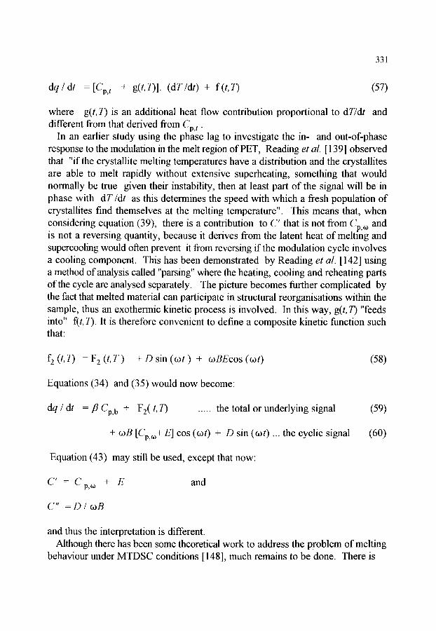
331

dq / dt = [Cp, t + g(t, T)]. (dT/dt) + f (t, 7) (57)

where g(t, T) is an additional heat flow contribution proportional to dT/dt and different from that derived from Cp, t .

In an earlier study using the phase lag to investigate the in- and out-of-phase response to the modulation in the melt region of PET, Reading et al. [139] observed that "if the crystallite melting temperatures have a distribution and the crystallites are able to melt rapidly without extensive superheating, something that would normally be true given their instability, then at least part of the signal will be in phase with d T/dt as this determines the speed with which a flesh population of crystallites find themselves at the melting temperature". This means that, when considering equation (39), there is a contribution to C' that is not from Cp, o and is not a reversing quantity, because it derives from the latent heat of melting and supercooling would often prevent it from reversing if the modulation cycle involves a cooling component. This has been demonstrated by Reading et al. [142] using a method of analysis called "parsing" where the heating, cooling and reheating parts of the cycle are analysed separately. The picture becomes ft~her complicated by the fact that melted material can participate in structural reorganisations within the sample, thus an exothermic kinetic process is involved. In this way, g(t, 7) "feeds into" f(t, T). It is therefore convenient to define a composite kinetic function such that:

f2 (t,T) = F 2 ( t , T ) + D sin (cot) + ~oBEcos (~ot) (58)

Equations (34) and (35) would now become:

dq / dt - fl Cp, b + F2( t, T) ..... the total or underlying signal (59)

+ coB [Cp,~o+ E] cos (cot) + D sin (cot) ... the cyclic signal (60)

Equation (43) may still be used, except that now:

C' = C + E and p,to

C" = D / coB

and thus the interpretation is differem. Although there has been some theoretical work to address the problem of melting

behaviour under MTDSC conditions [ 148], much remains to be done. There is

332

also evidence that temperature gradients strongly affect the results obtained in the melt region. This aspect of sample behaviour needs to be addressed before a quantitative analysis of MTDSC results in the melt region can be undertaken.

Because the in-phase cyclic heat capacity (C) no longer depends solely on C p, co

the calculation of the non-reversing signal given by equations (39) and (40) is no longer valid. However, the structural rearrangements that can occur during melting involve exothermic processes. Thus, it has been observed that, during the lower heating rate part of the cycle, exotherms occur that are balanced against endotherms in the higher heating rate period, this can be seen in Figure 15 over the melt region. This occurs as the dynamic exchange of material between the melt and the crystalline phases oscillates back and forth. The result of this is that the C" appears very large. Thus the reversing signal does also and consequently the non-reversing signal appears exothermic as can be seen in Figure 15 over the temperature range where rearrangement is occurring. While this does not mean that there is a large net exotherm, it does indicate the presence of an exothermic process during the cycle. Because conventional DSC often shows very little when this kind of reorganisation is taking place (see the total signal in Figure 15) this characteristic behaviour of the non-reversing signal is a useful indication that it is occurring.

5.5. Alternative theoretical approaches The approach described above is that developed by Reading and co-workers

[40,45,138-143] and can be called the kinetic approach to MTDSC theory. The response of the sample is divided into a rapidly reversing response that arises from molecular motions and a kinetically hindered response that is non-instantaneous and, therefore, must be governed by some kinetic expression. These kinetics can be generally be described by the Arrhenius equation, or by the related equations that model the kinetics of the glass transition. It also allows that a distribution of metastable crystallites can provide an instantaneous response through rapid melting [ 148]. This is not classified as reversing because supercooling during negative heating rates can give rise to a highly asymmetric signal [ 142].

An alternative theoretical approach has been proposed by Schawe [ 144] who has advocated the use of linear response theory to formulate an approach that is based on irreversible thermodynamics. In his initial exposition [144a] he erroneously criticised the approach of Reading and co-workers for its failure to take account of the phase lag and its inability to deal with time dependent phenomena such as glass transitions. The refutation of these criticisms can be found in [139, 148, 149] and above. However, his theoretical approach presents an interesting alternative view. Schawe identified C ' as a storage component arising from molecular motions (in effect the same as the definition of Cp, co given by Reading et al.) while C " is

333

identified as a "loss" component arising from entropy changes within the sample. Whether this is a fundamentally different analysis or equivalent to Reading's remains controversial.

5.6. Alternative modulation functions and methods of analysis Some workers and manufacturers (Perkin-Elmer and Mettler Toledo [155]) have

preferred a square wave or a sawtooth modulation. In some cases they have proceeded with a Fourier transform analysis and taken the first Fourier coefficient (Perkin-Elmer). This then gives equivalent results to the use of a sine wave with a FT analysis. One possible advantage of these more angular perturbations is that they could provide a response over many frequencies by use of a Fourier transform but this has yet to be realised.

An altemative is to use a square wave (Mettler Toledo) and ensure that the steady state is regained, and only then take points over this portion of the isothermal plateau. If an isothermal plateau is used as part of the modulation then, because dT/dt is zero, the signal during this portion must be a non-reversing contribution. The difference between the maxima and the minima generated by the modulation, i.e. the amplitude, gives a measure of the reversing signal. An alternative is to use equal positive and negative heating rates, with a longer duration being given to the positive or negative portions in order to provide a net heating or cooling rate. From equation (34), the sum of the maxima and minima in the heat flow produced by this modulation, provides a measure of the non-reversing component (where F(t, T) is assumed not to change during the modulation). Again the difference between them is a measure of the reversing signal. The disadvantage of these approaches is that there is only one point per modulation obtained using only part of the data with the intervening data being lost. This severely compromises accuracy and resolution.

5.7. Benefits of MTDSC and future prospects MTDSC offers advantages when looking at the glass transition because separating

reversing processes, such as glass transitions, from non-reversing processes such as relaxation cndotherms, or cure reactions, makes it is easier to identify the Tg in complex systems where there are many transitions. Baseline curvature on the cyclic signal is generally very low, thus making it easier to distinguish between baseline effects and real transitions. The signal-to- noise ratio of the cyclic measurement of heat capacity is generally greater, because all drift or noise at frequencies other than that of the modulation is ignored by the Fourier transform analysis. Resolution can be very high because very low underlying heating rates can be used. Because of these benefits, it is often useful to take the derivative of C' with respect to temperature. Glass transitions then appear as peaks and are more easily identified

334

and quantitative measurements are more easily made. There are not many techniques available to the polymer scientist that can deal in such a quantitative manner with systems that comprise many phases and interphases [ 152-4].

MTDSC is still a very young technique and the extant literature is still inadequate. However, a great deal of work is being carried out and will soon be published. The prospects for the future seem bright both in term of applications and more sophisticated methods of temperature programming and data analysis, such as multiplexing [ 142].

6. OPERATIONS AND SAMPLING

6.1. Calibration and standardization The general topics of standardization and calibration will be discussed more fully

in Chapter 13, but it is important to state the criteria which are to be satisfied for the best operation of any DTA or DSC equipment.

Before any equipment can be useful to its operator, it must be checked for reliability and calibrated for accuracy. If an apparatus has been constructed for the laboratory, or if alternative instruments from various manufacturers are to be compared, the user must consider what criteria will best demonstrate the qualities required in the instrument.

�9 Does the apparatus suit the samples to be run? �9 Does the apparatus respond well to changes to be detected or measured? �9 Does the apparatus give results for temperatures and thermal properties

which are accurate with respect to good literature values?

The testing and calibration of any DTA or DSC equipment might therefore be divided into three stages of increasing quantitative accuracy:

6.1.1. Experimental runs of suitable, well-established samples This is often done to illustrate the capabilities of equipment. For example, just as

an infrared spectrometrist will recognise the IR spectrum of polystyrene, since it is used to check instruments, so the user of DTA or DSC will probably recognise the curve for poly-(ethylene terephthalate), (PET) quenched from the melt shown

335

as Figure 17, or the curves for copper sulphate pentahydrate or calcium oxalate monohydrate, because these have been used many times to demonstrate the response to thermal events, the temperature range and the sample and data handling facilities.

The temperatures for the PET curve are not suitable for temperature calibration, but should normally lie within the range 75 to 85 ~ for the glass transition, 130 to 180 ~ for the cold crystallisation and 230 to 270 ~ for the melting.

An experienced user working in a particular field will choose an appropriate sample to try. For example, if the determination of purity is a major priority of the laboratory, a Certified Reference Material consisting of phenacetin doped with a small percentage (0 to 5%) ofp- aminobenzoic acid is available [74,157]. Certified polymer samples are available for users specialising in polymeric materials.

The sensitivity of the instrument may be tested using samples which are either small, dilute or which undergo small thermal changes. The resolution of the equipment could be tested with samples having two transitions separated by a small temperature interval.

EXO

AP

50

Cold Crystallisation

Glass Transition

u | �9 �9 | �9

100 150 200

Temperature PC

Melting

250

Figure 17. DSC of PET quenched from the melt.

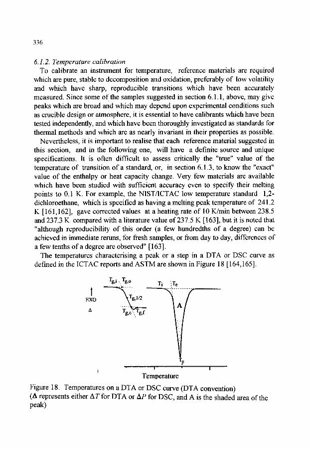
336

6.1.2. Temperature calibration To calibrate an instrument for temperature, reference materials are required

which are pure, stable to decomposition and oxidation, preferably of low volatility and which have sharp, reproducible transitions which have been accurately measured. Since some of the samples suggested in section 6.1.1, above, may give peaks which are broad and which may depend upon experimental conditions such as crucible design or atmosphere, it is essential to have calibrants which have been tested independently, and which have been thoroughly investigated as standards for thermal methods and which are as nearly invariant in their properties as possible.

Nevertheless, it is important to realise that each reference material suggested in this section, and in the following one, will have a definite source and unique specifications. It is often difficult to assess critically the "true" value of the temperature of transition of a standard, or, in section 6.1.3, to know the "exact" value of the enthalpy or heat capacity change. Very few materials are available which have been studied with sufficient accuracy even to specify their melting points to 0.1 K. For example, the NIST/ICTAC low temperature standard 1,2- dichloroethane, which is specified as having a melting peak temperature of 241.2 K [ 161,162], gave corrected values at a heating rate of 10 K/min between 238.5 and 237.3 K compared with a literature value of 237.5 K [163], but it is noted that "although reproducibility of this order (a few hundredths of a degree) can be achieved in immediate reruns, for fresh samples, or from day to day, differences of a few tenths of a degree are observed" [ 163].

The temperatures characterising a peak or a step in a DTA or DSC curve as defined in the ICTAC reports and ASTM are shown in Figure 18 [ 164,165].

I EXO

Tg'i" Tg'~ Ti !Te -~- .... . -~ . . . . . . . . . . .

Tgl/2 ' /

g,c g,f

�9 | �9

Temperature

Figure 18. Temperatures on a DTA or DSC curve (DTA convention) (A represents either A T for DTA or AP for DSC, and A is the shaded area of the peak)

337

Table 3 gives a few of the established temperature standards, the literature values and the transitions to which the temperatures correspond. Not all of these are ICTAC standards, but some, such as the melting point of water, are very well established and others, for example the melting temperatures of zinc, silver and gold are accepted as fixed points of the IPTS temperature scale. Difficulties exist with calibrations at very low temperatures and at very high temperatures. These matters are addressed in Chapter 13.

It is necessary to perform temperature calibration for at least two points bracketing the temperatures of interest of the samples to be examined. The calibration procedure should follow a well tried regime. For example [161 ], for each calibration material the operator should:

�9 load 5 to 15 mg into a clean sample holder and load into the instrument and purge with nitrogen;

�9 allow it to equilibrate at a temperature about 30 ~ below the transition temperature;

�9 heat it through its transition at 10 ~ (or another suitable rate); �9 measure the extrapolated onset and peak temperatures from the resultant

curve; �9 record and report the mean values from duplicate specimens

Table 3. Materials for temperature calibration.

Material Transition T / ~ Reference

water mp 0.00 162, 164

polystyrene glass transition 105 163

indium mp 157 (156.6)

zinc mp 419.5

157,(162)

157

aluminium mp 660 162

silver mp 961.9 164

gold mp 1064.2 164

Note: mp - melting point.

338

If a two-point calibration is used, the relationship between the observed temperature (To) and the actual sample temperature (T) may be assumed to be a linear one:

T = ( T o x S ) + I (61)

where S is the slope and I the intercept of the line of T against T o. Thus, for two standards, represented by suffices 1 and 2:

S --(T 1- T2)/(Tol- To2 ) (62)

I -:-l(Wol x T2)- ao2X 71)//(wOl- ~102 ) (63)

For a one-point calibration, the intercept (or correction) only may be determined:

I - (T 1 - 7Ol ) (64)

For three-point or multipoint calibrations, the statistical fit of the data to a plot of T against T O must be established mathematically. For the early power compensated DSC units, the calibration correction followed a curve approximating to a parabola [66].

6.1.3. Cal ibrat ionJor energy or power

For any calorimetric measurement it is necessary to perform a calorimetric calibration run under conditions as close as possible to those of the sample experimental run. This applies equally well to classical calorimetry as to DSC, in any of its forms. Since an extended discussion of calibration will be given in Chapter 13, it is not intended to give extensive descriptions of the theoretical basis here, but to give a few examples of the practices which may be used. There are three chief methods which may be employed:

A. Calibration using transition enthalpies of known reference materials. B. Calibration using specific heat capacity. C. Direct electrical calibration.

6.1.3.A. Calibration using reference materials Reference materials are available for which the enthalpies of transition or melting

are well established. Provided that they obey the criteria outlined above of purity, stability and "credibility" (i.e, accurately measured enthalpy changes), then they may

339

be used in the same sample cell and under the same experimental conditions as the unknown samples which the operator wishes to measure. Table 4 shows some of the materials which have been used, with approximate values of their enthalpy of fusion, beating in mind that each sample should be individually certified. Thus, a particular sample of indium may have an enthalpy of fusion of 28.7 J g-1.

As noted for temperature calibration, an approved regime similar to that outlined above should be followed, with the additional step that the sample mass must be known accurately and the area A of the endothermic melting peak measured according to the constructions described in Section 3 and shown in Figure 18.

Having equilibrated the sample and then scanned through the melting or transition, the sample should then be cooled and reweighed to be sure that no loss has occurred. A calibration coefficient, K, may then be calculated for the specific temperature of transition of the sample used.

Table 4. Reference materials for energy calibration [75,157,162]

Material Fusion Temperature/o C Afu s H / J g

mercury

benzoic acid

-38.9 11.5

123 148

indium 156.6 28.5

tin 231.9 60.2

zinc 419.5 107.5

aluminium 660.3 395

K = ( A H . m ) / ( A ) (65)

where -2 K will have units of J cm -1 AH is the enthalpy change in J g

m is the mass of calibrant in g and A is the peak area in cm 2.

Alternative units may be used. For example, if the area is multiplied by the recorder time scale B in cm s -1 and by the ordinate heat flow sensitivity S in mW cm -1, then a dimensionless calibration constant 8is obtained:

340

8 - ( A H . m ) / ( A B S ) (66)

An extensive calibration of the Du Pont 1090 DSC 910 cell was carried out by Eysel and Breuer [165]. They showed that, while the value of K obtained as above may be temperature dependent and would need to be linearized and set constant electronically, the ratio of the reference value of the enthalpy of transition to the measured value was essentially constant:

A H R e f / A H m = 1.046 + 0.3% (67)

The variation of the measured values with heating rate, weighing error, sample mass and nature of sample is discussed.

6.1.3.B. Specific heat capacity calibration Since the ordinate deflection of a DSC depends upon the heat capacity of the

sample, it is possible to calibrate the instrument for heat flow by measuring the ordinate deflection, or for energy by measuring the area between the curve obtained with a sample of well-known heat capacity and the "no-sample" baseline, rtm over the same temperature range, as shown in Figure 19.

EXO

�9

|

|

!

start v

Displacement

i �9

Temperature Finish T

Figure 19. Heat capacity calibration

The material most often used for this purpose is sapphire ( ~- A1203) for which the values of Cp have been measured with high accuracy between -180 and + 1400 ~ [166]. In the range 0 ~ to 300 ~ the specific heat capacity is given fairly accurately by:

341

Cp (sapphire)/J K-1 g-1

=1.4571 - 3.355 x 10 -5 x (T/K) - 200.17 / ( T/K) (68)

The sequence of operations recommended for calibration by this method is;

�9 Condition the sapphire by heating in the instrtunent to at least 10 ~ above the maximum temperature of interest. Cool the sample in a desiccator.

�9 Record the "no-sample" baseline using the empty sample pan and lid and heating them at 10 ~ min -1 throughout the temperature range of interest.

�9 After cooling, introduce the sapphire sample of accurately known mass into the sample pan, and replace the lid. Repeat the heating programme under the same conditions as for the baseline above and record the sample DSC curve.

�9 Measure the difference in heat flow signal between the sample and baseline and the total area between the curves.

For a calibration at a particular temperature, T, if the calibration factor at another temperature, for example for indium at 157 ~ is known, we may compare the deflections:

K T = K ( C T D ) / ( C D T) (69)

where C is the heat capacity of sapphire and D the difference in recorded heat flow signal, and the subscript T refers to the new temperature, while the values at 157 ~ are unsubscripted. The area between the curves will give a calibration constant averaged over the temperature range.

Both the above methods have been shown to give good agreement with the calibration coefficients determined with standard reference materials [167] and also to vary little with sample mass or scan rate.

6.1.3. C. Electrical calibration

It is possible to arrange that the sample cell contains a small electrical heater of known resistance R ohms, or that a special calibration vessel containing such a resistor is available. If a current I amps is passed through this resistor for a time t seconds, the energy E joules supplied is:

E = I 2 R t = VI t = Pt (70)

where V is the voltage and P the electrical power used.

342

Heating for different times with the same current and resistance values is sometimes employed. If a large temperature change is caused by heating, the change in resistance with temperature must be allowed for in the calculations. The electrical energy supplied will increase the temperature of the sample cell and its contents and produce a peak in the recorded DSC curve. By equating the heat flow deflection with the power, or the area of this peak with the electrical energy supplied, a calibration constant may be found. This method generally requires a

3 rather large sample cell of volume about 1 cm

6.2. Sampling The purpose of proper sampling practice and proper choice of sample cell and

conditions is clearly to obtain the best possible results for the particular experiment. These results should be accurate and reproducible measurements of temperatures,

of enthalpy and heat capacity for DSC experiments, and reproducible kinetic behaviour and interaction for samples which react. Good thermal contact and hence low thermal resistance between the sensor and the sample in its pan is essential. Anything which affects the contact must be considered when preparing the sample.

The samples which have been studied by DTA and DSC cover almost the entire range of natural materials, biological and organic materials, minerals and inorganic chemicals, plus the very large number of synthetic materials and composites. These have very different physical characteristics, from extremely hard, impervious ceramics, through organic powders, metals, waxes, to liquids with a range of viscosities. Many require a special regimen and protocol to produce accurate, reproducible thermal analysis results, and all these cannot be dealt with here. A selection of fairly standard methods is given, with cautions where materials need special treatment. In all experiments, the empty sample pan to be used should be weighed and the prepared sample and pan also weighed. Use of clean tweezers or spatula for discs, a vibrating spatula for powders and a micropipette for liquids is usual. It is also important that the cells and sensor should be as clean as possible.

6.2.1. Crystalline solid samples With some samples, their crystalline nature is an important characteristic.

Excessive grinding may destroy the crystallinity or allow reaction to take place. For example, grinding of copper sulphate pentahydrate may cause formation of the basic sulphate. More spectacularly, grinding of explosive mixtures can produce violent reaction! For such samples, two techniques may be used. Either, the sample may be ground gently, and possibly at a lowered temperature, or the sample may be deposited in the sample pan as a concentrated solution as described for liquids under 6.2.5, and the solvent then evaporated. This is only possible if the solvent

343

may be removed readily and completely at a temperature lower than those to be used in the experiment.

6.2.2. Powdered solid samples Many samples are received as fine powders, for example many organics,

inorganic pigments, complexes and fillers. These can be loaded directly into the pan, with the usual precautions. Since fine powders make good contact with the pans and generally pack more evenly, they are recommended for good DSC results. If grinding does not adversely affect a bulk sample, for example, many minerals and stable organics, then the sample may be carefully ground, with obvious care against contamination. Investigation of the effects of particle size can be undertaken by separating the powdered sample through a sequence of meshed sieves.

Some soil polymers and rubbers, at temperatures above their glass transition, are most difficult to grind. However, after cooling in liquid nitrogen, they may become brittle and may be ground more easily. This may introduce moisture into the sample. Another technique borrowed from infrared spectrometry is to abrade the sample with a file or emery paper to produce a coarse powder.

6.2.3. Voluminous powders and fibres Powders of low density, flocks and fibres are difficult to retain within the sample

pan prior to sealing. Two techniques may be used to contain them. They may be placed in the centre of a small piece of thin foil of the same metal as the crucible, e.g. aluminium or platinum. This is then folded over them to contain the sample into smaller bulk. This capsule is then loaded into the pan and flattened before sealing. Another method is to use a washer or inner lid to retain the sample before lidding.

6.2.4. Thin film solid samples If the sample may be produced as a thin film, for example, a metal or alloy, a

polymer, woven fabric, composite or natural product, then a circular disc of radius just less than that of the sample pan may be punched out using a sharp punch (e.g. a cork borer) and loaded into the crucible. In the process of punching out, the disc may become uneven, and it is best if it can be flattened in the pan with a suitable tool to give the best contact between sample and pan. This is the method used for calibration with metals like indium.

6.2.5. Liquids and solutions Small samples of involatile liquids may be introduced into the prepared sample

pan from a calibrated syringe, micropipette or dropper. Care must be taken that liquid does not spread onto the edges due to surface tension. If a liquid mixture is

344

to be studied, mixing before loading into the pan is probably better, since droplets may stay separated within the pan for some time. One method of retaining liquids on the base of the pan is to use a small disc of glass fibre.

6.2.6. Pastes and viscous liquids These are some of the more difficult samples due to their high viscosity. A thin

paste or mull may be loaded as a liquid, but a thick paste may have to be placed into the cell with a spatula and then flattened against the bottom of the pan using a rod with a flat end. Viscous biological liquids, such as starch suspensions, may be treated this way, as may samples of semi-solid materials like soft waxes and tars. Some melts have a very low surface tension and will spread excessively. For these, tall sided crucibles are better.

6.2.7. Volatile liquids These should be nm in sealed pans or sealed glass capillaries [168] and, for good

contact the surrounding space should be filled with conducting material.

6.3. Autosampling and Robotics In modern laboratories, there is a demand for rapid, routine analysis plus

unattended operation and calculation of results. Thus, for many analytical techniques, prepared samples may be selected, treated and analysed and the answers recorded on a computerised database. This applies equally well to DSC equipment.

A typical system includes a motorised carousel or tray with up to 50 samples, a robotic arm with an attachment suitable to pick up, transport and release DSC pans of the particular type used for this sequence, and a computer system capable of controlling the movements of the carousel, robot and of opening and closing the DSC assembly to allow placement and removal of the pans and of adjusting the conditions to those pre-selected for each sample. To avoid contamination, the whole assembly is protected by a cover and the components placed as close as possible to each other. This is shown in Figure 20. Samples are prepared and their masses and am conditions entered into the computer against their numbered location on the carousel. These data are stored as a named data file. When the loading process is complete, the analysis sequence is started.

For each sample, the DSC head cover is opened, the appropriate sample pan selected and loaded with precision into the sensor assembly. The DSC head cover is closed and the run conditions established, with such limits as the user has placed into the data file. The DSC analysis is performed and data are automatically stored in their computer file.

345

On completion of the experimental work, the cover is opened after suitably adjusting the instrumental conditions, the finished sample removed and the system prepared for the next one. The stored results are then analysed according to the rules to give the results for whatever the user has selected. The report may give peak onset temperatures, peak enthalpies, glass transitions, kinetics or heat capacity. A hard copy report will be available, or the data may be transmitted on- line to other workplaces.

Sample Chalnger AI~

Sample Tray

DSC Unit

. . . .

Computerised Control Unit

Lid Control

J Unit

Figure 20. Robotic sampling system.

7. GENERAL INTERPRETATION AND CONCLUSIONS Drawing the various sections of this chapter together requires comment on the

correct operational procedure and warnings on the problems which will be encountered with incorrect techniques. The interpretation is largely to be considered in chapters relating to applications, but comments on the effects of the many sample and instrumental variables are necessary. The opportunity has been taken to review, as far as possible, likely future trends, both as they affect instrumental development and also novel applications and operation.

7.1 Baselines and peak shapes The shape of a DTA or DSC peak will depend on all the sample and apparatus

conditions which are involved. As shown in Section 3 of this Chapter, the

346

chemical and physical nature of the sample, its thermal properties and packing will govern the heat transfer. The way in which the sample is located in the crucible and the degree of contact it makes are important. The heating rate, atmosphere composition and flow and the instrumental response factors are all contributory to the ultimate result.

If we consider two examples to illustrate the problems, the simplest case is when a small sample of pure material undergoes a single phase transition with no change of mass, e.g. melting. If the heat capacity of the sample before and after the transition is almost the same, then the baseline should be a straight line connecting the baseline before the peak for the melting endotherm, with the baseline after the peak. The peak should show a straight leading edge and an exponential tail.

A second example might be a change controlled by the reaction kinetic behaviour of the sample:

A(s) = B(s) + C(g)

Here, the shape will depend upon the kinetic mechanism which applies and, to a much lesser extent, on the instrumental factors. The work of Kissinger gives a relationship between the peak shape and the reaction order [62]. At the end of the reaction, the signal will again decay exponentially. If the heat capacity of the reactant (A) and that of the residual product (B) are different, the baseline should show a gradual change governed by the proportions of reactant

Cp = ( l - a ) Cp, A + ( a) Cp,B (71)

where Cp is the specific heat capacity and a is the fraction reacted. This will give a baseline which follows the progress of the reaction and is generally sigmoid in shape.

In general, for symmetrical peaks with minimal change in baseline, little difference is observed whichever baseline is used. For symmetrical peaks with a change in baseline, a sigmoid construction works well, as do the Wilburn method [67] and the polyline method. For overlapping peaks, it is very difficult to decide on the optimum baseline unless the peaks may be resolved and their shapes or kinetics established separately. Attempts to analyse complex peaks as the sum of Gaussian peaks, or first-order peaks, or melting peaks are, at best, trial-and-error methods. Experimental methods of resolving overlapping peaks include the use of smaller samples, or of a slower heating rate, or of a different atmosphere.

For isothermal kinetic studies, such as polymer cure [169], it is beneficial to re- mn the sample after reaction to establish the initial transient and the final baseline,

347

and also to show whether the reaction was, indeed, complete.

7.2. Effects of sample parameters Since the primary object of a DTA or DSC experiment is to discover evidence

concerning the thermal behaviour of the analytical sample, it is most important that any effects which the sample may have upon the results are carefully considered. In TG, while the actual mass losses and the temperatures at which they occur are sample dependent, the subtler changes detected by DTA are even more likely to be altered by small differences in sample nature or sampling procedure.

The provenance and history of the sample is important. Mineral specimens may have different chemical natures or impurities. The thermal history, morphology and crystallinity of polymer samples can differ widely, despite the samples having indistinguishable chemical compositions. The method of sampling and the subsequent storage of the sample should be documented. Samples of high alumina cement concrete, needed for testing to determine their degree of conversion by DTA, should be obtained by a clearly prescribed method involving slow drilling to avoid heating and then treated and stored under defined conditions [ 170].

The grinding, particle size and packing of the sample into the crucible will affect the DTA traces quite markedly. Grinding has a complex effect, since the initial reduction of particle size will increase the total surface area of the sample and change the rates of any surface reaction or transition. Further grinding may actually destroy crystal structure and reduce the size of the transition peak obtained. Grinding of metals will strain harden them. Particle size distribution should be considered when investigating the kinetic behaviour of systems. The packing of samples into crucibles and the geometry of the crucible used will alter the heat transfer and gas diffusion characteristics at the gas-solid interface. If any reaction is diffusion controlled, for example metal oxidation, the access of the reactant gas to the solid surface, and the diffusion of any product gas away will be much altered between a thin layer of sample spread on a wide crucible, and a thick layer packed into a deep crucible. [68] The effects of a diluent, such as calcined alumina, are similarly complex. The DTA curves of siderite, FeCO 3 in air [171] with 60% alumina shows an endotherm for the decomposition to FeO, followed by an exotherm for the oxidation of FeO to Fe203.. With higher percentages of diluent, the carbon dioxide escapes and, at 74% alumina, the two peaks largely cancel.

The mass of sample must affect the signal produced by any thermal event. While an average mass for general purposes with modem apparatus is around 10 mg, there may be a need to use much more, for example in the case of a thin surface coating on a powder, or very much less, for example in the study of explosive reactions. The detection limit for observing a signal depends on the material and

348

the matrix. While the melting peak of an organic chemical, such as cholesterol or a triglyceride, may often be measured with a few micrograms of pure material, detection in a mixture with inert filler requires about 1 mg. Calibration parameters may only hold over a limited range of mass.

7.3. Effects of instrumental parameters The most significant parameter in any DTA or DSC run is the heating rate.

Theoretical considerations show that the peak area expressed as the integral with respect to time is a constant for the same sample melted at different rates. [ 172]. Since the peak is higher at high heating rates, it would seem to be useful to use as high a heating rate as possible. However, high heating rates increase the uncertainty due to thermal lag and actually increase the range of many transition peaks. The user must judge whether it is more important to keep the experiment at conditions as close to equilibrium as possible, when the lowest available heating rate should be used, or whether obtaining comparative results as quickly as possible is the priority, in which case high heating rates may be selected. For heat capacity measurements, the ordinate deflection, Ay, is proportional to both the heat capacity and the heating rate, so there is often a need to use a fairly high heating rate.

The atmosphere above and in contact with the sample is another primary factor affecting the DTA or DSC curve. With the transitions of inert materials, such as the melting of unreactive metals and salts, the effects of the atmosphere will be due to its thermal properties. If the sample interacts in any way, either by vaporising, reacting, adsorbing or absorbing the gas, or by catalysing reactions involving the gas, then the chemical nature, pressure and flow rate of the gaseous atmosphere will strongly affect the thermal analysis curves.

7.4. Hazards of operation For continued successful operation of a sensitive DTA or DSC, as well as for the

avoidance of expensive repairs and replacements, the user must place limits on the range of samples and conditions employed. In talking to instrument manufacturers, a need is recognised for both adequate instruction in apparatus use from acknowledged practitioners, for example at thermal analysis workshops organised by the national TA groups and for the establishment of well-documented standard methods such as the ASTM procedures. The list below is drawn from experience over many years and from manufacturers' reports.

7. 4.1. Hazards due to samples The amount of sample should be chosen with care. Too much can damage

crucibles and sensors by spillage or expansion, too little may not give any detectable

349

signal for events. Running an experiment with the sample placed directly on the sensors can chemically damage them severely, and this should never be done without exceptional reason or unless the apparatus is designed with robust, inert sensors.

Samples which produce gaseous products, or which have a very high vapour pressure at the temperatures studied, may cause problems. Although a normal sealed crucible will withstand pressures slightly above one atmosphere, too high a pressure can cause bursting or rupture of the seal. Use of high pressure apparatus may be necessary for these samples.

The loading of the sample, and of the sample pan into the apparatus must be done carefully. Spillage of sample onto sensors or furnace can be damaging and dangerous. Lidding of the samples to prevent spills and evaporation or contamination from outside materials is recommended. If the sample pan is to be sealed, any sample present on the surfaces forming the seal may prevent proper contact and give poor results. For samples which react with atmospheric moisture, special precautions for loading are needed, and samples, pans and tools may have to be kept in a dry box.

The production of corrosive or toxic products from the thermal degradation of any sample must be considered. For example, heating of poly(vinyl chloride) produces HC1 gas, and of poly(acrylonitrile) produces HCN. Even inorganic hydrates giving off water may cause problems, and some biological samples may attack aluminium crucibles.

Experience may not always help to distinguish between "real", "spurious" and "mstrumentar' effects. For small samples, there may appear to be an endothermic drift, followed by an exothermic peak, followed by further drift. This could be due to insmnnental effects, or a slow endothermic change or baseline shift, followed by an exothermic reaction. Alternatively, there may be a larger endotherm, followed by a return to baseline, followed by another endotherm. Changing the run conditions or the sample size may resolve this, or it may be necessary to use another technique simultaneously. The appearance of a "melting endotherm" superimposed on a glass transition is a real effect due to the use of a heating rate greater than the previous cooling rate [ 173].

7.4.2. Hazards due to apparatus factors The calibration of the apparatus for temperature, and if necessary, for power,

should be carried out frequently, especially after cleaning the sensor assembly or rtmning it under exceptionally difficult conditions.The interval between calibrations clearly depends on the regime in use, but for any new sample type or set of

350

conditions, re-calibration should be considered. Unless a recent calibration has been done, results cannot be relied upon.

A blank run is often a useful guide to the performance of the instrument and to any likely hazards. A run with the same material as sample and as reference can show whether there is a baseline drift due to mis-alignment of the sensor head, imbalance of the sensors (e.g. due to contamination) or through some other cause. When the difference between runs is important, as in the determination of specific heat capacity, the sample pans should be heated through the temperature range required before the main runs are done.

The crucible location must be matched and reproducible. Deformed or damaged crucibles may give erroneous spikes, sometimes due to sudden expansion, and poor contact will encourage drit~ of the baseline. Movement of crucibles with respect to the sensors will also cause problems.

The temperature range must be suitable to the apparatus, samples and crucibles to be used. Exceeding the melting point of an aluminium crucible by running above 660 ~ can ruin the sensor assembly. Allowing thermal runaway can heat a furnace above safe limits. Cut-out units should generally prevent this.

The reactivity of the apparatus must be considered. Crucibles which react with sample or atmosphere above a certain temperature must not be used. Occasionally unusual materials will attack the most durable of crucibles, for example, certain high-temperature conducting polymers may attack platinum. Oxidation of crucibles or sensors must be avoided.

The icing and condensation which may occur when operating below room temperature present two hazards. First, the presence of ice may alter the results obtained, for example, an ice peak may appear around 0 ~ or the water may absorb into the sample and subsequently vaporise, altering transitions and the baseline. Secondly, the gas flow may become restricted due to ice and pressure build-up may occur. The use of dried purge gas is important here.

The transients which often happen at the start and end of a run must not be mistaken for thermal events due to the sample. As a general rule, a run should be started at least 30 K below any expected thermal event and finished about 30 K after the event, unless this involves unacceptable decompositions or vaporisation. The transients may be minimised by adjusting the heat capacity of the reference pan using extra material. For a DSC with aluminium pans and lids, addition of a few more lids to the reference side may give a better balance to the sample and reduce the start-up hook [ 173]. Transients may also occur if the thermal resistance between pan and holder is different for the sample and the reference.

351

The smoothmg of a DTA or DSC run using the computer software must be done with caution! Although experience will show whether an event (e.g. a sharp spike) is to be expected with a particular sample, it is sometimes an indication of a real event. A very uneven trace is sometimes obtained for a reaction where gases are evolved. The heating of silver oxide to produce silver metal gave a most irregular trace as did the dehydration of hydrated magnesium nitrate.[172]

7.5. Errors It would be impossible, and invidious, to discuss the entire range of errors which

may occur before, during and after a DTA or DSC experiment. Certainly the problems outline above as "Hazards" can all contribute to the production of results which are not worthy of the technique or of the instrument used. In a recent text, [174] the present authors suggested the acronym SCRAM: to summarise the factors likely to affect a thermal analysis run:

S: Thesample. The collection, storage, preparation and nature of the sample are all factors which can change a DTA or DSC run. While one laboratory may wish to study the sample in its form "as received", another may take great care in preparing the same sample in a particular way. The results from the two samples are often quite different.

C: The crucible. (or sample holder). It has been made clear above that there are a large variety of sample holder materials and designs. Errors can arise if the crucible is of the wrong material, shape or size.

R: The rate of heating If thermodynamic equilibrium is desired, for example in phase equilibria studies, the slowest heating rate should be used. Very rapid heating rates can give errors because of the thermal lag, or because different kinetic effects apply. Tin(II) formate shows two endotherms at high heating rate, but only one at lower rates. This has been shown to be due to decomposition with superimposed melting. Enough original material remains to melt when heated rapidly, but most has decomposed before the melting point during slow heating [175]. Again, examination by other techniques helps to avoid any errors.

352

A: The atmosphere. The wrong choice of atmosphere, or comparison of results from two runs in different atmospheres, or at different flow rates, can lead to error. As noted above, moist gases may give spurious effects. High flow rates can remove volatiles by transpiration, so that the peaks due to, for example, desolvation occur at lower temperatures. Reactive atmospheres must be treated with caution. In high temperature studies of the composition of filled polymers, changing to an oxidising atmosphere too early can cause ignition.

M: The mass. Errors arising from inaccurate weighing are readily avoided. Precautions should be taken to ensure that what is weighed is what is studied, that is that spillage or evaporation have not occurred. Using the wrong amount of sample may cause errors. Re-weighing after a run is also a good idea.

Additionally, account should be taken of the possibility of errors during data collection or processing. Too few data points collected in the region of interest will give unreliable integration or analysis. Data collected over too narrow a range may prevent accurate measurement or baseline construction.

Willcocks [176] has pointed out that "the same type of mstnunents, connected via identical computer systems, may give output temperature differentials of 10 ~ even though the precision is quoted as + 0.1 ~ For the majority of thermal analysts, a DSC instrument, set up according to the manufacturers' specification, would produce precise, accurate and reproducible data. This is largely true for heating, but ... is not always true when cooling". He suggests that reproducible "cooling standards" might combat this.

7.6. Future trends In looking forward to future developments, we need to consider the historical

trends, the present state of the art and the perceived future needs for thermal methods. In the first section of this chapter, the development of DTA from an empirical, qualitative method using equipment constructed in-house, through to a reliable analytical technique with numerous commercial instruments capable of reproducible, accurate quantitative measurements and with a firm theoretical base for both DTA and DSC has been shown.

The second half of the 20th century might be known to future analysts as the Age

353

of the Computer. Many thermal analysts working in 1960 would have produced their results on a chart recorder. The time-consuming manual measurements, corrections and calculations needed for data analysis extended the experiment by many hours. By the 1980s, links to computers were becoming easier and the newer generation of analysts were more familiar with their use and the possibilities they gave for time saving and more rigorous calculations. Going into a laboratory in the 1990s, the overwhelming impression is that every instrument has its attendant computer, and in larger laboratories, these are linked into networks and LIMS. Because of the improvement in instnnnentation, and, through computer control and data handling, in the ease of use and of obtaining results, there has been an increase in interest in thermal analysis, calorimetry and in making thermal and other analytical measurements simultaneously.

In reviewing the present usage of DTA and DSC, the contributions to the recent 10th ICTAC meeting at Hatfield in 1992 may be one guide. 20% of the published papers relate to polymers, 13% to inorganics, 12% each to pharmaceuticals and instrumentation, with the remainder coveting everything from archaeology to zeolites. About 28% of the papers relate to DTA, DSC or associated and simultaneous methods and there was a considerable upsurge of interest with the presentations on modulated temperature DSC.

Mathot, in a lecture at a meeting celebrating 30 years of the Thermal Methods Group of the United Kingdom [177] discussed "Thermal Analysis and Calorimetry: Is familiarity breeding contempt?". His predictions for the year 2000 include a hope that measurements will be standardised to DIN, ASTM, etc., and that research and development will be supported by DSC and other thermal methods. In order that this shall happen, he suggests that

" producers and centres of expertise should combine to develop methods and equipment. For DSC, some suggestions are as follows:

Improve existing equipment: �9 Increase the throughput per DSC, with several measuring cells and sample

exchangers. �9 Develop cheaper and more robust measuring cells. �9 Incorporate empty pan correction for imbalance as standard. �9 Improve DSC stability to enable unattended operation. �9 Make quantitative measurement of heat changes routine.

Develop new equipment: �9 Modulated temperature DSC should be widely available and more understood.

354

�9 Multiffequency calorimetry should be developed. �9 Baselines should be determined continuously. �9 Higher cooling and heating rates; higher pressure systems should all be available. �9 Reaction calorimetry should be expanded, with all its possibilities. �9 There should be flexible reaction conditions for process and safety research. �9 Miniaturization of sensors should be investigated. �9 DSC should be combined with microscopy, including scanning probe microscopy. �9 Thermal methods should be used as coupled, simultaneous techniques with a

wide variety of analytical methods.

For the encouragement of future users of DSC and DTA, it is important both that the education process should include exposure to good, modem equipment and knowledgeable instruction by practitioners skilled in the use of DSC, DTA and other methods, and also that the executives and management directing the testing, quality control and research and development shall be made aware of these methods."

Perhaps modem trends in integrating instruments with computers and in reducing their size, while maintaining their robust structure and making them, as foolproof as possible, may be what is desirable on the exterior. Inside the "black box" we might expect that there will be developments of new techniques extending the use of DSC and DTA and improving their performance and range.

7.7. Acknowledgements The authors gratefully acknowledge the help and cooperation of many people,

particularly the representatives of the major manufacturers who gave their time in discussions, their advice on instrumental developments and their collaboration in devising the figures. We also acknowledge our debt to Dr. Robert Mackenzie for his help and for many valuable discussions.

355

REFERENCES. 1 G. Agricola, De Re Metallica, Froben, Basel,1556. 2. A. Neri, De Arte Vitraria, Florence, 1640. 3. R.C. Mackenzie, Thermochim. Acta, 73 (1984) 251. 4. R.C. Mackenzie, Thermochim. Acta, 73 (1984) 307. 5. R.C. Mackenzie, Thermochim. Acta, 148 (1989) 57. 6. R.C. Mackenzie, J.Thermal Anal., 35 (1989) 1823. 7. G. Martine, Essays on the Construction and Graduation of Thermometers

and on the Heating and Cooling of Bodies,1738-40,A.Donaldson, Edinburgh, 1772.

8. J.Wedgwood, Phil. Trans.R.Soc.(London), 74 (1784) 358; 76 (1786) 390. 9. T. Seebeck,Ann. Phys. Chem., 6 (1826) 130, 253. 10. H. Le Chatelier, C.R. Acad. Sci., Paris, 104 (1887) 1443;

Bull. Soc. Fr. Mineral. Cristallog., 10 (1887) 204. 11. M. I. Pope and M. D. Judd, Differential Thermal Analysis, Heyden,

London, 1977. 12. W. J. Smothers and Y. Chiang, Handbook of Differential Thermal

Analysis, Chemical Publishing Co., New York, 2nd Edn, 1966. 13. C. W. Siemens, Proc. R. Soc.(London), 19 (1871) 443. 14. W. C. Roberts-Austen, Proc. Inst. Mech. Eng.,(a) (1891),543; (b)

(1899),35. 15. G. K. Burgess, Bull. Bur. Stan., Washington, 4 (1908) 180. 16. J .P. Joule, Scientific Papers of J. P. Joule, Physical Society of London,

1884, 1887. 17. J. P. McCullough and D. W. Scott, Experimental Thermodynamics, Vol.

1, p. 437, Butterworth, London, 1968. 18. J. Orcel, Cong. Int. Miner. Metal., Geol. Appl.,7 Sess.,Paris,1935,

Geol.1 (1936) 359. 19. L. G. Berg and V. A. Anosov, Zh. Obsch. Khim., 12 (1942) 31. 20. S. Speil, L. H. Berkelhamer, J. A. Pask and B. Davies, Tech. Pap. U.S.

Bur. Mines, 664, (1945). 21. P. F. Kerr and J. L. Kulp, Am. Mineral., 33 (1948) 387. 22. M. J. Vold, Anal. Chem., 21 (1949) 683. 23. S. L. Boersma, J. Am. Ceram. Sot., 38 (1955) 281. 24. H. E. Kissinger, J. Res. Natl.Bur. Stand., 57 (1956) 217. 25. H.J. Borchardt and F. Daniels, J. Amer. Chem. Sot., 79 (1957) 41.

H.J. Borchardt, J. Inorg. Nucl. Chem., 12 (1960) 252 26. E. Saladin, Iron & Steel Metallurgy and Metallography, 7 (1904) 237. 27. H. Le Chatelier, Rev. mrt., 1 (1904) 134.

356

28. N. S. Kumakov, Z. anorg. Chem., 42 (1904) 184. 29. R. C. Mackenzie (Ed.), Differential Thermal Analysis of Clays,

Mineralogical Society, London, 1957. 30. R. A. Schultz, Clay Minerals Bull., 5 (1963) 279. 31. C. Geacintov, R. S. Schotland and R. B. Miles,

J. Polym. Sci., C, 6 (1963) 197. 32. E.S.Watson, M.J.O'Neill, J.Justin and N.Brenner, Anal. Chem.,36 (1964)

1233. 33. C. Sykes, Proc. R. Soc. (London), 148 (1935)422. 34. K. G. Kumanin, Zh. Prikl. Khim., 20 (1947) 1242. 35. C. Eyraud, C.R. Acad. Sci, Paris, 240 (1955) 862. 36. L.M.Clarebrough, M. E. Hargreaves, D. Mitchell and G.W.West,

Proc. R. Soc.(London), A215 (1952) 507. 37. M. O'Neill, Anal. Chem., 36 (1964) 1238. 38. R. L. Blaine, A Genetic Definition of Differential Scanning Calorimetry,

Du Pont Instruments, 1978. 39. R. C. Mackenzie, Ed., Differential Thermal Analysis, 2 Volumes,

Academic Press, London, 1970,1972. 40. M. Reading, D. Elliott and V. L. Hill, J. Thermal Anal., 40 (1993) 949. 41. J. G. Dunn, J. Thermal Anal., 40 (1993) 1431. 42. R.C. Mackenzie, Thermochim. Acta, 46 (1981) 333. 43. R.C. Mackenzie, Treatise on Analytical Chemistry, (P J Elving, Ed.),

Wiley, New York,1983, Part I, Vol. 12, p. 1. 44. R. C. Mackenzie,Talanta, 16 (1969) 1227; 19 (1972) 1079. 45. P. S. Gill, S. R. Sauerbrunn and M. Reading,

J. Thermal Anal., 40 (1993) 931. 46. P. Nicholas and J. N. Hay, NATAS Notes, 25 (1995) 4. 47. Mettler TGA850 Brochure, Mettler-Toledo, Switzerland, 1995 48. B. D. Mitchell, Clay Minerals Bulletin, 4 (1961) 246. 49. J. S. Mayer, Pittsburgh Conference, Paper #731, (1986). 50. A. Marotta, S. Saiello and A. Buri,Thermal Analysis ,(B.Miller, Ed.),

Proc. 7th ICTA,Wiley, Chichester, (1982), 85. 51. A. P. Gray, Perkin-Elmer Thermal Analysis Study #1,Perkin Elmer,1972.

Analytical Calorimetry, Vol. 1, (R.S.Porter, J.F. Johnson, Eds.), Plenum, New York, 1968, p. 209.

52. D. M. Speros and R. L. Woodhouse, J.Phys. Chem., 67 (1963) 2164. 53. D. J. David, Anal. Chem., 36, (1964) 2162. 54. W. Hemminger, Calorimetry and Thermal Analysis of Polymers,

(V. B. Mathot, Ed.), Hanser, Munich, 1994, Ch. 2.

357

55. P. Pacor, Anal. Chim. Acta., 37 (1967) 200. 56. J. H. Sharp and F. W. Wilburn, J.Thermal Anal., 41 (1994) 483. 57. F. Hongtu and P. G. Laye, Thermochim. Acta, 153 (1989) 311. 58. F. W. Wilburn, J. R. Hesford and J. R. Flower,

Anal. Chem., 40 (1968) 777. 59. M. E. Brown, Introduction to Thermal Analysis, Chapman & Hall,

London, 1988. 60. C.J. Keattch and D. Dollimore, Introduction to Thermogravimetry, 2nd

Edn., Heyden, London, 1975. 61. A. W. Coats and J. P. Redfem, Nature, 201 (1964) 68. 62. H. E. Kissinger, Anal. Chem., 29 (1957) 1702. 63. R. Melling, F. W. Wilbum and R. M. McIntosh,

Anal. Chem., 41 (1969) 1275. 64. F.W.Wilburn,D.Dollimore and J.S. Crighton,

Thermochim.Acta., 181 (1991) 173. 65. F.W.Wilburn,D.Dollimore and J.S. Crighton,

Thermochim. Acta, 181 (1991) 191. 66. J. L. McNaughton and C.T. Mortimer, Differential Scanning Calorimetry,

IRS Physical Chemistry Series, Vol. 10, Butterworths, London and Perkin- Elmer Ltd., 1975.

67. F.W.Wilbum, R. M. McIntosh and A.Turnock, Trans. Brit. Ceram. Soc., 73 (1974), 117.

68. F.W.Wilburn and J.H. Sharp, J.Thermal Anal.,40 (1993)133. 69. W. W. Wendlandt, Thermal Analysis, 3rd Edn, J. Wiley, New York,1986. 70. R. F. Speyer,Thermal Analysis of Materials, M. Dekker, New York,1994. 71. T. J. Quinn, Temperature, 2nd Edn, Academic Press, London, 1990. 72. J. R. Leigh, Temperature Measurement and Control,Control Engineering

Series 33, P. Peregrinus for IEE, London, 1988. 73. H. van Vlack, Elements of Material Science, 5th Edn, Addison-Wesley,

Reading, 1987, p. 318. 74. J. O. Hill, For Better Thermal Analysis and Calorimetry III, ICTA,1991. 75. G. W. C. Kaye and T. H. Laby, Tables of Physical and Chemical

Constants, 16th Edn, Longmans, London, 1995. 76. B. F. Billing, Thermocouples: their Instrumentation, Selection and Use,

IEE Monograph, 64/1, London, 1964. 77. J. C. Lachman and J. A. McGurty, Temperature: Its Measurement and

Control in Science and Industry, (C. M. Herzfeld, Ed.), Volume 3, Part 2 Chapter 11, Reinhold, New York, 1962, p. 185.

78. R. C. Mackenzie, Anal. Proc., (1980) 217.

358

79. T. Daniels, Thermal Analysis, Kogan Page, London, 1973. 80. R. C. Mackenzie, Nature, 174 (1954) 688. 81. T. Ozawa, Bull. Chem. Soc. Japan, 39 (1966) 2071. 82. C. Mazi6res, Anal. Chem., 36 (1964) 602. 83. D. A. Vassallo and J. L. Harden,Anal. Chem., 34 (1962) 132. 84. W.H.King, A.F. Findeis and C. T. Camilli, Analytical Calorimetry,

Vol.1, (R.S.Porter,J.F. Johnson, Eds.), Plenum, New York,1968, p. 261. 85 . . . . . . . . . . . and G. Sommer, J. Sci. Inst.,43 (1966) 293. 86. J. H. Welch, J. Sci. Inst., 31 (1954) 458. 87. G.N. Rupert, Rev. Sci. Inst., 36 (1965) 1629. 88. W.R. Barron,The Infrared Temperature Handbook, Omega Engineering,

Stamford, 1995. 89. J. L. Caslavsky, Thermochim. Acta, 134 (1988) 371,377. 90. R.C. Johnson and V. Ivansons,Analytical Calorimetry, Vol. 5,

(J F Johnson, P S Gill, Eds.), Plenum, New York, 1984, p. 133. 91. J. L. Petit, L. Sicard and L. Eyraud, C.R. Hebd. Seances Acad. Sci.,

252 (1961) 1740. 92. G. van der Plaats and T. Kehl, Thermochim. Acta, 166 (1990) 331. 93. E. Calvet and H. Prat, Recent Progress in Microcalorimetry,

Pergamon Press, New York, 1983. 94. P. Le Parlouer and J. Mercier, J. AFCAT., Orsay, (1977) 2. 95. Rigaku TG-DSC Brochure, Rigaku Denki Co, Tokyo, Japan 96. E.M. Barrall and L. B. Rogers, Anal. Chem., 34 (1962) 1106. 97. R.L. Stone, Anal. Chem., 32 (1960) 1582. 98. R.P. Tye, R. L. Gardner and A. Maesono,

J. Thermal Anal., 40 (1993) 1009. 99. P. Le Parlouer, Rev. Sci. Hautes Temper. Refract.,Fr.,28 (1992-1993) 101. 100. A. Maesono, M.Ichihasi, K. Takaoka and A. Kishi, Thermal Analysis,

Proc. 6th ICTA, Birkhauser, Basel, 1 (1980) 195. 101. Ulvac Sinku-Riko, Inc, Infrared Gold Image Furnace, Brochure

Ulvac Sinku-Riko, Yokohama, Japan 102. E. Karmazin,R.Barhoumi and P.Satre, Thermochim. Acta, 85 (1985) 291. 103. J. P. Redfem, Differential Thermal Analysis, ( R. C. Mackenzie, Ed.),

Vol. 2, Academic Press, London, 1972, Chap. 30. 104. SETARAM, Calvet Microcalorimeter Brochure, SETARAM, Lyon. 105. T. Hatakeyama and F. X. Quinn, Thermal Analysis: Fundamentals and

Applications to Polymer Science, Wiley, Chichester, 1994, p. 36. 106. G. F. Franklin, J. D. Powell and M. L. Workman, Digital Control of

Dynamic Systems (2nd Edn.), Addison-Wesley, London, 1990,p. 222.

359

107. H. G. Wiedemann andA. Boller, Int. Lab., 22 (1992) 14. 108. L. C. Thomas, Int. Lab., 17 (1987) 30. 109. B. Cassel and M. P. DiVito, Int. Lab., 24 (1994) 19. 110. F. R. Wright and G. W. Hicks, Polym. Eng. Sci., 18 (1978) 378. 111. G. R.Tryson and A.R.Schultz, J. Polym. Sci., Polym. Phys. Ed.,

17 (1979), 2059. 112. K. A. Hodd and N. Menon, Proc. 2nd ESTA, Aberdeen, Heyden,

London,1981, p. 259. 113. P. J. Haines and G. A. Skinner, Thermochim. Acta, 59 (1982) 343. 114. H. G. Wiedemann, J. Thermal Anal., 40 (1993) 1031. 115. Shimadzu, Photovisual DSC 50V Brochure, 1995 116. J.T. Koberstein and T. P. Russell, Macromolecules, 19 (1992) 714. 117. A. J. Ryan, J. Thermal Anal., 40 (1993) 887. 118. W. Bras, G.E. Derbyshire, A. Devine, S. M. Clark, J. Komanschek,

A. J. Ryan and J. Cooke, J. Appl. Cryst., 28 (1995) 26. 119. H. Yoshida, R. Kinoshita and Y. Teramoto,

Thermochim. Acta, 264 ( 1995) 173. 120. W.P.Brennan, B.Miller and J. C. Whitwell,

J. Appl. Polym. Sci., 12 (1968) 1800. 121. J.E.S. Ladbury, B. R. Currell, J. R. Horder, J. R. Parsonage, and E.A.

Vidgeon, Thermochim. Acta, 169 (1990) 39. 122. J. Chiu and P. G. Fair, Thermochim. Acta, 34 (1979) 267. 123. J. H. Flynn and D. M. Levin, Thermochim. Acta, 126 (1988) 93. 124. G. Hakvoort, L. L. van Reijen and A. J. Aartsen, Thermochim. Acta,

93 (1985) 317. 125. S.M.Marcus and R.L.Blaine, T A Instruments Applications Note

TA-086, 1993. 126. T. Boddington, P. G. Laye, J. Tipping, E.L. Charsley and M. R. Ottaway,

Proc. 2nd ESTA, Heyden, London, 1981,p. 34. 127. T. Boddington and P. G. Laye, Thermochim. Acta, 115 (1987) 345. 128. R. N. Rogers and E. D. Morris, Anal. Chem., 38 (1966) 410. 129. L. W. Ortiz and R. N. Rogers, Thermochim. Acta, 3 (1972) 383. 130. J. Chiu, Anal. Chem., 39 (1967) 861. 131. R. W. Carroll and R. V. Mangravite, Thermal Analysis, Proc. 2nd ICTA,

Vol. 1, (R. F. Schwenker, P. D. Garn, Eds.), Academic Press, London,1969, p. 189.

132. G. P. Morie, J. A. Powers and C. A .Glover, Thermochim. Acta, 3 (1972) 259.

133. G. Beech and R. M.Lintonbon, Thermochim. Acta, 2 (1971) 86.

360

134. I. Mita, I. Imai and H. Kambe, Thermochim. Acta, 2 (1971) 337. 135. D.J.Johnson, D.A .Compton and P.L .Canale,

Thermochim. Acta, 195 (1992) 5. 136. E. M. Bollin, Thermal Analysis, Proc. 2nd ICTA, Vol. 1,

(R. F. Schwenker, P. D. Garn, Eds.),Academic Press, London, 1969, p.255.

137. E. L. Charsley, C. T. Cox, M. R. Ottaway, T. J. Barton and J. M. Jenkins, Thermochim. Acta, 52 (1982) 321.

138. J. C. Seferis, I. M. Salin, P. S. Gill and M. Reading, Proc.Acad. Greece, 67 (1992) 311.

139. M.Reading, D. Elliott and V. L. Hill, Proc. 21 st North American Thermal Analysis Society Conference, (1992) 145.

140. M.Reading, Trends Polym. Sci., 1 (1993) 248. 141. M.Reading, A. Luget and R. Wilson, Thermochim. Acta, 238 (1994) 295. 142. M.Reading, R.Wilson and H.M.Pollock, Proc. 23rd North American

Thermal Analysis Society Conference, (1994) 2. 143. M.Reading, K. J. Jones and R. Wilson, Netsu Sokutie, 22 (1995) 83. 144. J. E. K. Schawe, Thermochim. Acta, (a) 260 (1995) 1;

(b) 261 (1995) 183. 145. B. Wunderlich, Personal communication. 146. Y. Jin, A. Boiler and B. Wunderlich, Proc. 22nd North American Thermal

Analysis Society Conference, (1993) 59. 147. B. Wunderlich, Thermal Analysis, Academic Press, Boston, 1990. 148. A. A. Lacey, C. Nikolopoulos and M. Reading, J. Thermal Anal., in press. 149. A. A. Lacey, C. Nikolopoulos, H. M.Pollock, M. Reading, K. Jones,

and I. Kinshott, Thermochim. Acta, in press. 150. A. Boiler, Y. Jin and B. Wunderlich, J. Thermal Anal., 42 (1994) 277. 151. Y. Jin, A. Boiler and B. Wunderlich, Proc. 22nd North American

Thermal Analysis Society Conference, (1993) 59. 152. M. Song, A. Hammiche, H. M.Pollock, D. J. Hourston and M. Reading,

Polymer, 36 (1995) 3313. 153. M. Song, D. J. Hourston, M. Reading, A. Hammiche and H. M. Pollock,

Polymer, 37 (1996) 243. 154. D. J. Hourston, M. Song, H. M. Pollock and A. Hammiche, Proc. 24th

North American Thermal Analysis Symposium (NATAS) (1995) 109. 155. B. Schenker and F. Stager, Thermochim. Acta, in press. 156. B. Wunderlich, Y. Jin and A. Boller, Thermochim. Acta, 238 (1994) 277. 157. LGC Office of Reference Materials, Catalogue, LGC Teddington,1995,

p. 67.

361

158. E. L. Charsley, J. P. Davies, E. G10ggler, N. Hawkins, G.W. H6hne, T. Lever, K. Peters, M. J. Richardson, I. Rothemund and A. Stegmayer, J. Thermal Anal., 40 (1993) 1405.

159. G. Lombardi, For Better Thermal Analysis, ICTA, Rome, 1977, p. 22. 160. ASTM D3418-82: Standard Test Methods for Transition Temperatures of

Polymers by Thermal Analysis. ASTM, Philadelphia, 1982. 161. ASTM E967-83: Temperature Calibration of DSC and DTA,

ASTM, Philadelphia, 14.02, 1992, p. 658 162. T A Instruments, Thermal Applications Note TN11, 1994. 163. a). E. Kaisersberger and H. M6hler, DSC of Polymeric Materials, Netzsch

Annual for Science and Industry, Vol. 1, Netzsch, Selb, 1991, p. 31. b). E. L. Charsley, J. Thermal Anal., 40 (1993) 1399.

164. International Temperature Scale,ITS-90, 1990. 165. W. Eysel and K. H. Breuer, Thermochim. Acta., 57 (1982) 317. 166. G.T. Furukawa, T. B. Douglas, R. E. McCloskey and D. C. Ginnings,

J. Res. Nat. Bur. Stand., 57 (1956) 67. 167. W.P. Brennan and A. P. Gray, Paper at Pittsburgh Conference, 1973. 168. G.R.Taylor, G.E.Dunn and W.B. Easterbrook, Anal. Chim. Acta,

53(1971)452. 169. J.M. Barton, Polymer, 33 (1992) 1177. 170. Recommendations for the Testing of High Alumina Cement Concrete

Samples by Thermoanalytical Methods, TMG, London, 1975. 171. R.A. Rowland and E. C. Jonas, Am. Mineral., 34 (1949) 550. 172. E.L.Charsley and S. B. Warrington (Eds.,), Thermal Analysis-

Techniques and Applications, RSC, Cambridge, 1992. 173. L .C.Thomas, Interpreting Unexpected Events and Transitions in DSC

Results, T A Instruments Applications Note TA039, 1994. 174. P.J. Haines, Thermal Methods of Analysis, Blackie, Glasgow, 1995, p. 18. 175. J. Fenerty, P. G. Humphries and J. Pearce,

Thermochim. Acta, 61 (1983) 319 176. P.H. Willcocks and I.D.Luscombe,

J. Thermal Anal., 40 (1993) 1451. 177. V.B.F. Mathot, Lecture at 30th Anniversary Meeting of the Thermal

Methods Group, UK, York, 1995.


Chapter 6

T H E R M O M E C H A N I C A L METHODS

R. E. Wetton

Innovation Centre, Jubilee Drive, Loughborough, UK

1. INTRODUCTION

Thermomechanical methods share the common ground of a mechanical parameter being measured as temperature is scanned. They are usually restricted to solids and, in the simplest case, length change with temperature can be followed and, after calibration, the expansion coefficient deduced. This is usually termed Thermodilatometry. If the expansion of a solid is hindered by application of a load, then a combination of expansion effects and modulus changes are observed. This is termed Thermomechanical Analysis (TMA) and modulus changes give rise to the main features on the recorded curves. More exact information, solely on modulus values and their transitions, is provided by impressing a small sinusoidal stress onto a sample with well defined geometry and calculating the modulus from the amplitude of the resultant strata. This technique has been termed Dynamic Mechanical Thermal Analysis (DMTA or DMA), although the recommended nomenclature of the International Confederation for Thermal Analysis and Calorimetry (ICTAC) is Dynamic Thermomechanical Analysis (DTMA) (see Chapter 1). A survey of Chemical Abstracts shows that the overwhelming majority of publications use the former term and hence it used in this Chapter.

DMTA has the advantage of monitoring the loss tangent peaks with high resolution. Figure 1 shows the schematic behaviour of a glassy solid (e.g. high molecular weight poly(styrene)) investigated by these three main methods.

2. STATIC METHODS

2.1. Thermodilatometry Classical dilatometry involves immersing the sample in a fluid (historically

mercury) and measuring expansion accurately by restricting the fluid in a capillary, much like mercury in a glass thermometer. Such methods are not normally classed as thermal analysis and attention here will focus on dilatometry by length

364

(D >--

- I -

Z L~ __J

E #

L {OiLa~ometry)

A L/TMA) I I

Tg[ !

A

TEMPERATURE Figure 1. Thermal curves of a glassy solid (A) dilatometry, (B) TMA and (C) 1 Hz DMTA

measurement, bearing in mind that the volume expansion coefficient is 3 x the linear expansion coefficient (a:) for an isotropic material. Insmunentation for length change measurement is usually TMA equipment (see section 2.2) modified or designed to measure under zero load conditions. Such a system is suitable for truly solid materials but will fail to measure right through a melting transition (Tm) and may fail to measure through a glass transition Tg, depending on the nature of the material above Tg. A cross-linked rubber is an amorphous solid above Tg and will still allow accurate expansion measurements. Conversely a sucrose/water glass will be a high viscosity liquid above Tg and not be amenable to length measurement. Various types of transitions can be established by dilatometry and are illustrated in Figure 2.

The most interesting applications of thermodilatometry lie in quantifying the anisotropy of materials. Anisotropy arises in the following situations: (i) drawn fibres (uniaxial); (ii) drawn or blown film (biaxial); (iii) fibre composites (usually biaxial); (iv) single crystals (generally triaxial), (v) liquid crystal displays; (vi) some metallic glasses. The expansion coefficients can usually be measured along the three principal axes. Porter et al. [1] reported good correlation between the birefringence measurement of the orientation distribution of drawn poly(styrene) with the value obtained from thermal expansion coefficients measured parallel and perpendicular to the orientation direction. The volume expansion coefficient for amorphous polymers usually differs little between isotropic and anisotropic conditions. This leads to

(~L/err (2- 1)/3 (1)

where 2 is the draw ratio.

365

\

\ \ \

\ \

~---~~c I

, IITg Tm

TEMPERATURE

Figure 2. Schematic of measurement regions where thermodilatometric accuracy is useful. These encompass Tg and solid/solid first-order transitions. Accurate length measurements are difficult in the hatched region.

In some anisotropic solids, the expansion coefficient in one of the principal axes can be found to be negative. This is the case for single crystal calcite. The length change measurements shown in Figure 3 give, after instrument corrections,

160

,,, 180

< rw ,,, 200 r~

u.. i i - -

220

1601

~8o-' Start Length:

8mm 200.

220 ~

s ,,s L/MICRONS

h: 2"6253mm

/ 0;s ~;0 ~.? /x L / MICRONS

Figure 3. Thermal expansion of calcite in perpendicular directions, along the c and a axes. Measurements were performed on a Mettler TA 3000 system. [2]

366

a(c axis) = 25.5 x 10 -6 K -1 mad a(a-axis) = - 6.1 x 10 -6 K -1 in good agreement with X-ray measurements. The phenomenon of negative expansion in this case is due to rotation of the CO3 groups out of their plane, with consequent reduction of the steric interaction.

2.2. Thermomechanical analysis (TMA)- instrumentation Insmanentation is arranged such that a predetermined load is applied to the

sample, almost invariably through a quartz rod. A typical arrangement is shown in Figure 4. Quartz has the advantage of possessing a small coefficient of thermal expansion and its low heat conductivity allows the transducer, usually a linear variable displacement transducer (LVDT), to be spaced away from heat sources.

6 6 / /

I IAMPLIFIER l I, ~i---~ RECORDE

WATER OUT

WATE R IN GAS IN ~I GAS OUT

Figure 4. Schematic of TMA Instrument (Rheometric Scientific). Features shown are 1 sample thermocouple, 2 quartz rod/probe, 3 LVDT core, 4 counterweight, 5 frictionless balance, 6 load platform. UTP is the Universal Temperature Programmer.

367

In this Rheometric Scientific instnunent, the load platform is actually a balance arm arrangement, allowing the quartz rod and probe assembly weight to be counterbalanced. This is ideal, not only for TMA, but also for producing the low force requirements for thermal dilatometry. Most displacement transducers drift significantly if their ambient temperature changes. Figure 4 shows water circulation below the transducer to obviate the heat-rise problem. Some of the manufacturers invert the quartz rod by using a stirrup assembly which allows the displacement transducer to operate below the temperature enclosure. The area around the sample can usually be both heated (electrically) and cooled (cold nitrogen gas) and the sample temperature (sensed by a thermocouple) has to be subject to programmer control. Heating rates up to 20~ can be employed, but a large thermal mass makes slower rates preferable.

Calibration of the instrument with a solid of known expansion coefficient is vital if sensible values of AL (corrected) are to be obtained from AL (measured). The reason for this is that expansion of the inswament support assembly is otten comparable, or greater than that of the relatively small sample. Calibration with a standard must be performed at the same heating rate as is used in the sample experiment, because more of the support structures will have time to change temperature at slow heating rates than at fast rates. It is also preferable to use calibration samples whose thickness ranges span that of the sample. A simple linear interpolation is usually sufficient to give the apparent expansion coefficient for the standard of the same initial thickness as the sample. If the experimentalist observes the foregoing, then

a (true) - Inst. Correction = a (obs) (2)

and the Instnunent Correction obtained from the standard sample experiment is applied to the required sample data.

The most usual calibration standards are made by machining aluminium cubes. The linear expansion coefficient of aluminium is 25 x 10 -6 K -~ compared to 0.6 x 10 -6 K -1 for quartz and 9 x 10 -6 K -1 for platinum. It is worth noting that linear expansion coefficients for glassy polymers are in the region of 70 x 10 -6 K 1 and for elastomers in the region of 200 x 10 -6 K 1.

More modem TMA instnunentation allows the load to be applied as a controlled voltage to a linear drive system ("motor"). This can be in the form of a speaker magnet/coil assembly, or an eddy current drive. Perkin-Elmer and Mettler are amongst manufacturers offering this electrical load control. Its advantages are:

a) The load can be applied by computer control, with little inertial shock and without operator intervention.

368

b)

c)

The load can be changed as required during the experiment, i.e. reduced if the sample softens dramatically. Feedback control could be used to keep the deformation constant by varying the stress.

This last technique is an under-utilised measurement technique for films and fibres (see section 2.4). Disadvantages are:

1)

2)

Force measurements need calibration and with the problem of temperature drift will not be as consistently accurate as with applied weights. Significant increase in manufacturing complexity and costs.

The choice of probe type determines the actual modulus/expansion property being measured. Figure 5 illustrates the most useful attachments.

Force l

Ht i I 1 t t i I 4 i r -

Compression

Force Force Force / Force

!." . ' .: .: ! ' . ' ~ - ' ; : . : ; . ' ; L ' : " : , : - , : |

, , , , , , , . , , . . , , , , . , 9 , , , , ,

Penetration Hemi-sphericat Tension Ftexure Indenfor

Formulae for modulus E for above modes

E = F /A Empirical E = 3(1-v2)F E = F/A E = FL 3

A L / H 4 R 1/2 AL 3/2 A L / H 2 A L C H ~

where AL is the vertical probe displacement, F is the force applied over cross section area A, H is sample height, L is sample length (bending beam), C is sample breadth, v is Poisson's ratio. R is the hemispherical radius.

Figure 5. TMA modes and respective modulus formulae.

The formulae in Figure 5 are for loading conditions at constant temperature. If temperature is being scanned, AL must be corrected for sample and instrument expansion if a modulus value is to be obtained. In practice this is difficult, so the DMTA technique is preferred. It should be noted that any indentor with a smaller area than the sample gives an empirical result unless a hemispherical tip is

369

employed. The Hertzian [3] approximation is given in this case for H>>AL. If this is not the case, reference should be made to Finkin [4].

In order to achieve zero load for dilatometry, manufacturers adopt various strategies. Perkin-Elmer provide buoyancy from a dense liquid, Netzsch support rind samples horizontally on frietionless supports, etc. The most accurate method is to work horizontally using optical interferometry between light reflected from each end of the sample. AL is measured routinely to 0.01 gm accuracy and more recent tuned laser techniques are decreasing this to nanometers [5]. Reflective end surfaces limit the optical method to about 700~ whereas high temperatm'e TMA insmmaents can reach 2000~

2.3. Dynamic and load effects in TMA Except for dilatometfic measurements, the primary application of TMA is in the

detection of changes in the modulus of a material at major transitions, such as melting or glass transitions. The material thus becomes fluid, or at least viscoelastic, above the transition, wlfich leads to major complications in interpreting the curves. The material will flow more under higher loads. This is illustrated schematically in Figure 6 for a penetrometer probe being used to detect a glass transition of a polymer.

<~

Z o <~ re"

w Z

A

TEMPERATURE

Figure 6. Probe penetration (AL) as temperature is scanned upwards through Tg for an amorphous polymer. Load increases A through C.

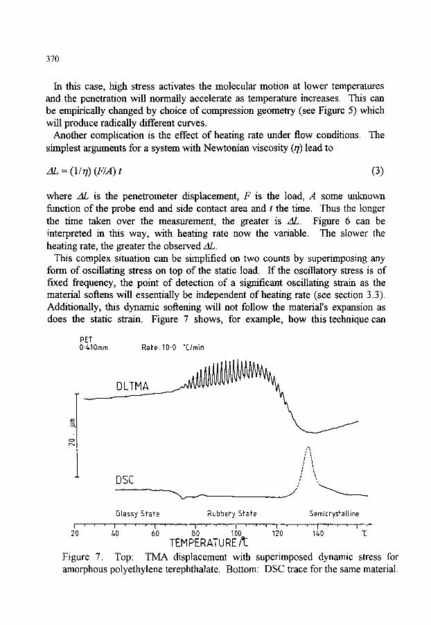
1 =

o

In this case, high stress activates the molecular motion at lower temperatures and the penetration will normally accelerate as temperature increases. This can be empirically changed by choice of compression geometry (see Figure 5) which will produce radically different curves.

Another complication is the effect of heating rate under flow conditions. The simplest arguments for a system with Newtonian viscosity (r/) lead to

,4/, = (l/r/) (F/A) t (3)

where AL is the penetrometer displacement, F is the load, A some unknown function of the probe end and side contact area and t the time. Thus the longer the time taken over the measurement, the greater is AL. Figure 6 can be interpreted in this way, with heating rate now the variable. The slower the heating rate, the greater the observed AL.

This complex situation can be simplified on two counts by superimposing any form of oseiUating stress on top of the static load. If the oscillatory stress is of fixed frequency, the point of detection of a significant oscillating strain as the material softens will essentially be independent of heating rate (see section 3.3). Additionally, this dynamic softening will not follow the material's expansion as does the static strain. Figure 7 shows, for example, how this technique can

DLTMA - ~ . ~ -

PET O.Z, lOmm Rate 10"0 "C/rain

370

I , I t

i \ DSC ;

Glassy Sfafe Rubbery Slate Semicrystattine I ' " ' I ' ' ' I " ' ' I ' ' ' I ' ' ' I ' ' ' l ' ' ' l e -

20 &0 60 80 100 120 I/+0 32 TEMPERATURE/t_

Figure 7. Top TMA displacement with superimposed dynamic stress for amorphous polyethylene terephthalate. Bottom: DSC trace for the same material.

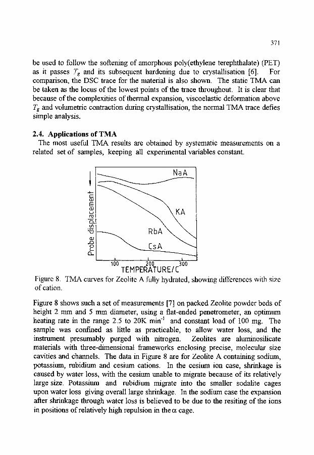
371

be used to follow the sottening of amorphous poly(ethylene terephthalate) (PET) as it passes 7g and its subsequent hardening due to crystallisation [6]. For comparison, the DSC trace for the material is also shown. The static TMA can be taken as the locus of the lowest points of the trace throughout. It is clear that because of the complexities of thermal expansion, viscoelastic deformation above Tg and volumetric contraction during crystallisation, the normal TMA trace defies simple analysis.

2.4. Applications of TMA The most useful TMA results are obtained by systematic measurements on a

related set of samples, keeping all experimental variables constant.

. , . . . , ,

L . ,

r k

NaA

KA

I I I 100 200 300

TEHPERATURE/C Figure 8. TMA curves for Zeolite A fully hydrated, showing differences with size of cation.

Figttre 8 shows such a set of measurements [7] on packed Zeolite powder beds of height 2 mm and 5 mm diameter, using a flat-ended penetrometer, an optimum heating rate in the range 2.5 to 20K rain -~ and constant load of 100 mg. The sample was confined as little as practicable, to allow water loss, and the insmmaent presumably purged with nitrogen. Zeolites are aluminosilicate materials with three-dimensional frameworks enclosing precise, molecular size cavities and channels. The data in Figure 8 are for Zeolite A containing sodium, potassium, rubidium and cesium cations. In the cesium ion case, shrinkage is caused by water loss, with the cesium unable to migrate because of its relatively large size. Potassium and rubidium migrate into the smaller sodalite cages upon water loss giving overall large shrinkage. In the sodium case the expansion ~ e r shrinkage through water loss is believed to be due to the resiting of the ions in positions of relatively high repulsion in the ct cage.

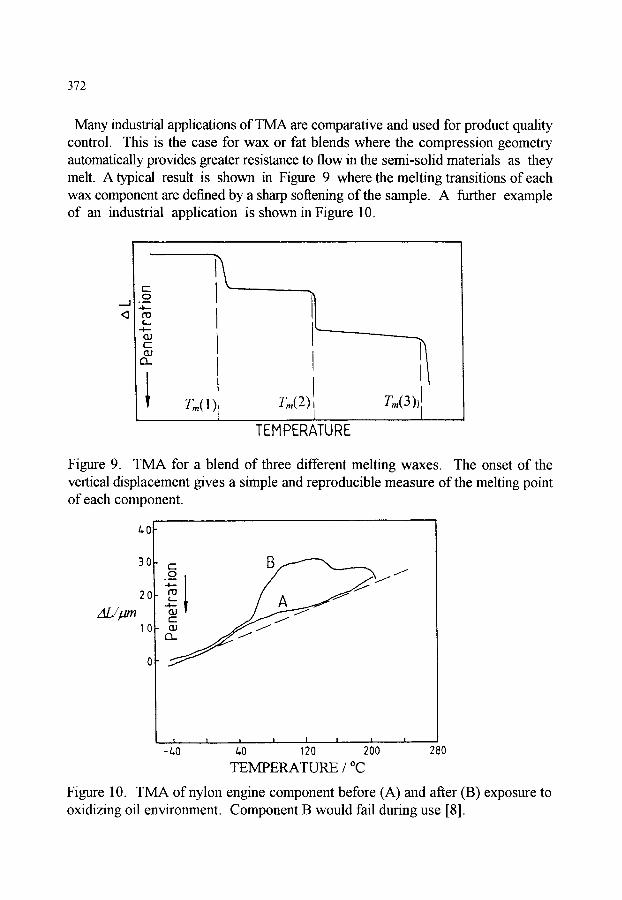
372

Many industrial applications of TMA are comparative and used for product quality control. This is the case for wax or fat blends where the compression geometry automatically provides greater resistance to flow in the semi-solid materials as they melt. A typical result is shown in Figure 9 where the melting transitions of each wax component are defined by a sharp softening of the sample. A further example of an industrial application is shown in Figure 10.

AL//.zm

C

-4--

t...

" I r

(33

I Tin(2)

TEMPERATURE

Tm(3) l I

Figure 9. TMA for a blend of three different melting waxes. The onset of the vertical displacement gives a simple and reproducible measure of the melting point of each component.

t~0

30

20 t._

10

! 1 /~ I I I 1 J

'~0 0 120 200 2~ TEMPERATURE / ~

Figure 10. TMA of nylon engine component before (A) and after (B) exposure to oxidizing oil environment. Component B would fail during use [8].

373

TMA with a square-ended displacement probe is used to assess the degradation in mechanical properties of a nylon component exposed to hot engine oil. Component B will be close to failure in service. The changes which are assessed as a combination of elevated Tg and reduced crystallinity, are due to oxidative changes to the nylon and a decrease in the equilibrium level of water.

TMA ms~mentation fitted with an electro-mechanical loading system can be used to perform a variety of experiments. An important variation which applies to all oriented polymer films and fibres, and to some metallic glasses, is to measure the thermal stress curves for a sample held at constant length. Figure 11 shows data [9] for a series of poly(ester)yams with different degrees of frozen-in orientation (as defined by the material's birefiingence). The higher the initial sample orientation, the more complex the thermal profile. For the highest birefringence sample (A r / - 0.05) there are three discrete relaxations, which allow the frozen-in strain to translate to an active stress. This would appear to be an under-utilized technique.

I 6O

(._

20

. ,

/ \, ,~ .... ".. X__~C ]: \ , ,/ : / / \ \"" " ~ . - ~

~176 ~ %

A \ '. a" Lx--~ "'', I , \ 5o ~oo ~5o 200

TEMPERATURE/'C 2 iO

Figure 11. Thermal stress curves of spun, Poly(ester) yarn and drawn fibres. (A) least oriented, (C) most oriented. Length is held constant during the scan.

3. DYNAMIC MECHANICAL T H E R M A L ANALYSIS (DMTA) (Note ICTAC nomenclature is Dynamic Thermomechanical Analysis, DTMA)

3.1. Dynamic moduli and loss tangent It may seem that the DMTA method has been derived by refining the static TMA

experiment, but this is actually not so The DMTA method has its origins in

3 7 4

the physics of modulus measurements for solids and their frequency and temperature dependence (relaxation studies). The principal moduli of solids are the rigidity or shear modulus (G), Young's modulus (E) and bulk modulus (B).These differ by virtue of the direction in which stress is applied to the solid. Figure 12 only defines G and E because the DMTA techniques are currently only used to measure these and the tensile modulus (identical to E for isotropic materials). Bulk modulus measurements have high combined errors and are not routine for DMTA measurements.

F

l _ / A r e a A _ _

C

~C

I -.-4 OI

I I I I I I

1 I .,.d I el !

I t I I/ ! II

I

E = F/A ~C/C 15 = F/A e

Figure 12. Definition of the shear modulus (G) and Young's (E) modulus. Note 0 is in radians.

In order to impose a time scale on the measurement, DMTA techniques impress a small sinusoidaUy varying stress (or strain) on a sample of appropriate geometry and transduce the strain (or stress). The technique is sometimes referred to as Dynamic Mechanical Analysis (DMA) because it is not necessary to scan temperature to measure the dynamic modulus.

The time dependent stress resulting from an imposed sinusoidal strain is shown in Figure 13. For a completely elastic material the stress is in-phase with the strain, and for a purely viscous material the stress leads the strain by 90 ~ (i.e. it is out-of-phase). Most solid metals are predominantly elastic at room temperature, but show a significant viscoelastic (anelastic) behaviour in certain temperature regions. Polymers are somewhat viscoelastic over normal working temperature

ess

375

-..F~ ,..,/~ sr~,~~ ,,..,/7~

7',, '\ / I', \ '", I / ~', :" ". I' ",

Out-of-phase stress In-phase stress

Figure 13. Sinusoidally varying stress and strain in a dynamic mechanical experiment. Construction shows definition of E'= C / B and E" = D / B

ranges but may be extremely so in the region above Tg. The simple definitions of the different moduli, given in Figure 12 are now complicated by a phase relationship between stress and strain, i.e. the moduli are complex quantities. It is convenient to resolve the viscoelastic response into an in-phase, elastic, component defining a storage modulus (G' or E') and an out-of-phase viscous component defining a loss modulus (G" or E"). The lower curves of Figure 13 show the stress response resolved into these in-phase and out-of-phase components with respect to the imposed strata.

The storage and loss moduli are now defined by:

Storage modulus = in-phase stress amplitude strain amplitude

= C / B (4)

Loss modulus = out-of-ph~e stress amplimd.e = D / B (5) strain amplitude

These relationships can be summarised in an Argand diagram, with the total response governed by the complex modulus (E*, G*), as shown in Figure 14.

376

MECHANICAL MOBULUS

G "

_ . _ _ . _

G'

Figure 14. Argand diagram showing the relation between dynamic moduli.

The phase angle (lag of strain behind stress) is also clearly defined in the Argand diagram and a convenient dimensionless parameter is the 'loss tangent' (tan 6)"

Tan c~ = G"/G' (in shear) or E"/E' (in bending) (6)

Tan 8 is the ratio of energy lost to energy stored per deformation cycle and, as shown in section 3.2, provides the best indicator for transitions in atomic/molecular mobility in thermal scanning measurements.

All the theory and measurement of dynamic moduli assume that the material is 'linear viscoelastic'. Simplistically stated, this means for example that doubling the stress doubles the strain response without change in the G"/G' ratio (i.e. tan c~). It is generally assumed that all materials approximate to linear behaviour at small strains, but in some cases these have to be as low as 0.1%.

3.2. Relaxat ion t imes - effect of m e a s u r e m e n t frequency

Atomic and molecular motions in solids are thermally activated. In metals these processes are typically due to motion of grain boundaries and crystal dislocations and an excellent stmunary is to be found in Zener's book [10]. In polymers the main chains and side groups exhibit various degrees of motional freedom at different temperatures and the effect of frequency was clearly shown by Alexandrov and Lazurkin in 1940 [ 11 ].

A material can be held at an appropriate temperature such that a motional process is occurring at a convenient time scale (fraction of a second). If the impressed frequency is swept over a wide range (say five decades) then the modulus will change from a high unrelaxed value (G U or E v ) at high frequency,

377

to a relaxed value (GR or ER ) at low frequency. If the motional transition being measured is the glass transition (Tg) process for an amorphous polymer, then the unrelaxed value approximates to the glassy modulus (109 Pa) and the relaxed value to a rubbery modulus (10 6 Pa). The response of the system is largely elastic in both the unrelaxed, glassy state and the relaxed, rubbery state. In the interval between these states the molecular motion is occtming with a similar time scale to the impressed stress, giving a region of high irreversibility and energy dissipation. Both tan 6 and the loss component of modulus pass through a maximum as shown in Figure 15. The loss peak positions differ and any work

1.0 1.0

0 "9 0.9

0.8 t Q ~.s 0.8

0-7 / ' F N ~ ~-0.7

0.~ I ~ 0 . 6

o-5 ~.o o.s~

bo. I / I \ \ -G" I o iOo I I-O.

, ', , -~ -3 -2 fmax -I 0 1

Log f I Hz Figure 15. O', G" and tan d~ plotted against log f for a single relaxation time model with Gc,/GR = 10 and ry = 10 s.

should systematically use either tan 6 or G" loss peak maxima. The loss peaks can be used to measure an average relaxation time ( r ) for the process. Iff,,a~ is the frequency at which tan 6 peaks then

r = 1/2Zfm= (7)

If mathematical transformations are to be performed on the data, fm,~ needs to be defined from the G" maximum. This defines a different average to the tan 6 maximum from the distribution of relaxation times present. For practical purposes, tan 6 maxima are sharper and no error is incurred if r is defined in a systematic way.

378

3.3. Effects of temperature- multiple relaxations All motional processes studied by DMTA are thermally activated, i.e. whether

or not they occur in a given set of measurements depends on the activation energy (Ea) for the process, compared to the thermal energy (RT) available to cause activation. Thus, to a first approximation, r will vary according to the Arrhenius equation where A is a constant independent of temperature.

r =A exp (E . /RT) (8)

This shows that condition is then

r can be swept by changing temperature. The loss peak

2 n f = 1 / r at T,,,a.,~ (9)

In the context of thermal analysis this is the usual way of observing loss peaks. Temperature is ramped up, usually at a fairly slow rate (1 to 5~ and the temperatures are observed for maximum loss location at constant impressed frequency, say 1Hz.

Figure 16 illustrates the main features observed during a DMTA scan of a

t . t J

o _..I

t-- t l j

txa

- 100 0 * 100 + 200

Temperature / ~

Figure 16. Schematic multiple loss peaks in a semi-crystalline polymer as temperature is scanned upwards at constant frequency.

379

semi-crystalline polymer. Relaxations can occur in both crystalline and amorphous regions and 'a' and 'c' subscripts are used to denote the origin. Relaxations in the amorphous phase are usually the overwhelming events until the melting region is reached. Relaxations in the amorphous phase are labelled with the Greek alphabet (a,/3~, L, ~ , etc.) with decreasing temperature of occurrence. Crystalline-phase relaxations, if observed, are labelled similarly but with the subscript 'c'. This procedure ensures that the Tg process is always a and subsequent glassy state relaxations are/3 ~, etc. Relaxations above Tg in the crystalline phase are usually given the symbols a'~ a"~ etc. in order of increasing temperature because they are all believed to be due to the melting process. This nomenclature is still awaiting IUPAC approval. The alternative is to follow the early terminology of Schmieder and Wolf [12] and label loss peaks in order of decreasing temperature irrespective of their origin.

3.4. Activation energy/WLF (Williams, Landel and Ferry [13]) procedures Equation (8) shows that if the measurement frequency is increased, the loss peak

will occur at a higher temperature, where the relaxation time has decreased to a smaller value. This is an inherent feature of relaxation processes occurring in materials which are not changing structure with temperature. Figure 17 shows

] 1 | i '1 ! i ,

~a

A / / r- / . = I / / /

cn / --~'~-'~

- 3 , I I I I I !

100 2~0 Temperafure / K

300

Figure 17. Plots of tan c~ in the y- relaxation region of DGEBA/DDM epoxy 0.01 Hz (curve A) 0.1 Hz (curve B) and 1.0 Hz (curve C) [14].

380

the change in glassy state ( fl, and F, ) loss peak position with frequency for a common cross-linked epoxy. This is based on the diglycidyl ether of bisphenol A (DGEBA) extended with 4, 4'-diaminodiphenylmethane (DDM). These small magnitude relaxations are both sub-Tg, the a, peak occurring at 453 K/1 Hz. The ~,~ peak displacement with frequency yields an activation energy of 54 kJ mol -~ and is interpreted as local in-chain motion. The fl, process is interpreted as due to pendent molecule motion of unreacted species.

Taking logarithms of equation (8) gives

log r = - log A + E, / 2.303 RZma x

and using equation (9) gives

log f = const - E~ / 2.303 RTm~ x (10)

which predicts that a plot of log (measurement frequency) versus reciprocal of the relaxation peak maximum (in K) will be linear with slope - E, / 2.3R. It is found that relaxations in metals follow the Arrhenius rule with activation energies typically 200 kJ mol -~ . Relaxations in polymers occurring below Tg also conform to the Arrhenius rule with activation energies in the range 40 to 200 kJ mol -~ . The data of Figure 17 give 54 kJ mo1-1 as the activation energy for the g, process.

The major relaxation processes (a , ) occurring in the temperature region above Tg for polymers and inorganic glasses show Arrhenius behaviour at high

temperature, but show critical behaviour as Tg is approached, i.e. E, becomes increasingly large as Tg is approached.

A more satisfactory description of the temperature dependence of the a, process was devised by Williams, Landel and Ferry [13] and their relation is commonly referred to as the WLF equation. It is assumed that a change of temperature shifts dynamic moduli and loss tangent curves along the log (frequency) axis without change of shape. The shift factor is given by the WLF equation

log a T : C~ (T 1 - To)/[C 2 + (T 1 -To) ] (11)

which relates the shift along the log frequency axis between data measured at a reference temperature T o and higher temperature T~. The WLF equation, if used with care, can generate 'master curves' which extend data at the reference temperature to a far wider frequency range than that available experimentally.

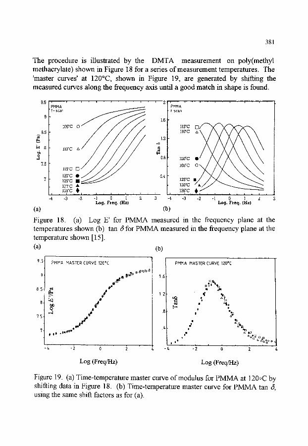
381

The procedure is illustrated by the DMTA measurement on poly(methyl methacrylate) shown in Figure 18 for a series of measurement temperatures. The 'master curves' at 120~ shown in Figure 19, are generated by shiftmg the measured curves along the frequency axis until a good match in shape is found.

�9 | �9 ! i i ! i

9.5 . . . . . . . . 2 'PMMA PMMA f - scan f scan

+~ ++ +++i .~ 8.5 / llO'C

8 n0"c ,, ..~ ~"0.8 !20"C

7.5 1050C O 1]s'c []

12o'c �9 0.4 125"C mm 125"C 139"C �9 130"C A , , , , 135"C ~ l 135"C +;/,

! . 1 , - . 1. . . �9 t �9 . 1 ' �9 . . L i I i I , |

Log. Freq. (Hz) Log. Freq . (Hz)

(a) (b)

Figure 18. (a) Log E' for PMMA measured in the frequency plane at the temperatures shown (b) tan O for PMMA measured in the frequency plane at the temperature shown [ 15].

Ca) (b)

9.5

8.5

7.5

PMMA MASTER CURVE 120~

O .j

. je I 00 .,.oantr~m

.._% n ~,o'o d

IB

PHMA MASTER CURVE 120"C

0

0 1 1

o" 0

am

~ 0 t

I I o . ~ a+

"- e,,~o o

Log (Freq/Hz) Log (Freq/Hz)

Figure 19. Ca) Time-temperature master curve of modulus for PMMA at 120oC by shifting data in Figure 18. (b) Time-temperature master curve for PMMA tan 8, using the same shift factors as for Ca).

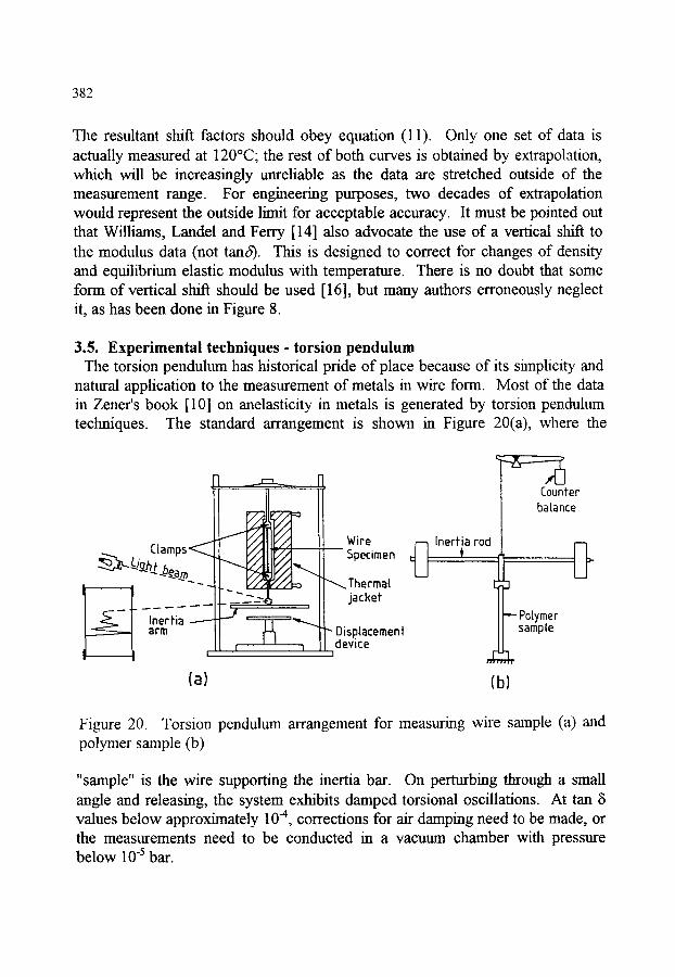
382

The resultant shift factors should obey equation (11). Only one set of data is actually measured at 120~ the rest of both curves is obtained by extrapolation, which will be increasingly unreliable as the data are stretched outside of the measurement range. For engineering purposes, two decades of extrapolation would represent the outside limit for acceptable accuracy. It must be pointed out that Williams, Landel and Ferry [14] also advocate the use of a vertical shift to the modulus data (not tan6). This is designed to correct for changes of density and equilibrium elastic modulus with temperature. There is no doubt that some form of vertical shift should be used [16], but many authors erroneously neglect it, as has been done in Figure 8.

3.5. Experimental techniques- torsion pendulum The torsion pendulum has historical pride of place because of its simplicity and

natural application to the measurement of metals in wire form. Most of the data in Zener's book [10] on anelasticity in metals is generated by torsion pendulum techniques. The standard arrangement is shown in Figure 20(a), where the

n ~ N

~Wire Clamps~.___21 ~ Specimen ~L"ig'h-t"bea"m- . V__z~ If'-.. Thermat

"- _'...-.--. I I jacker -Inertia ~_~f___l~ ' --~r~--- ~ , , ' Disp. [acemen{ �9 ~ d e v l r . e

o

(a) (b)

Figure 20. Torsion pendulum arrangement for measuring wire sample (a) and polymer sample (b)

"sample" is the wire supporting the inertia bar. On perturbing through a small angle and releasing, the system exhibits damped torsional oscillations. At tan 6 values below approximately 10 -4, corrections for air damping need to be made, or the measurements need to be conducted in a vacuum chamber with pressure below 10 -5 bar.

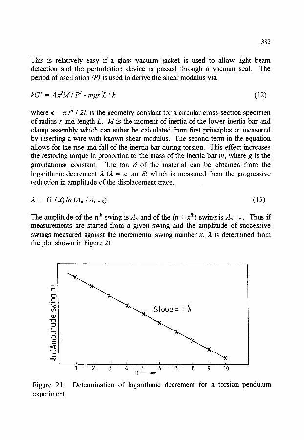
383

This is relatively easy if a glass vacuum jacket is used to allow light beam detection and the perturbation device is passed through a vacuum seal. The period of oscillation (P) is used to derive the shear modulus via

kG' = 4 ~ M / p2 _ m gr2L / k (12)

where k = ~r r 4 / 2L is the geometry constant for a circular cross-section specimen of radius r and length L. M is the moment of inertia of the lower hlertia bar and clamp assembly which can either be calculated from first principles or measured by inserting a wire with known shear modulus. The second term in the equation allows for the rise and fall of the inertia bar during torsion. This effect increases the restoring torque in proportion to the mass of the inertia bar m, where g is the gravitational constant. The tan d of the material can be obtained from the logarithmic decrement 2 (2 = rc tan 6) which is measured from the progressive reduction in amplitude of the displacement trace.

= (1 i x ) In (An/An+x) (13) . .

The amplitude of the n th swing is A~ and of the (n + x th) swing is A~ + ~. Thus if measurements are started from a given swing and the amplitude of successive swings measured against the incremental swing number x, )l, is determined from the plot shown in Figure 21.

r -

E7~

t,O

(13 "ID

- 4 - - ~

_ _ . _ _ ,

E

t--- " v '

- .... ; ; § b 4 0

Figure 21. experiment.

Determination of logarithmic decrement for a torsion pendulum

384

Torsion pendulum measurements were used extensively in the early investigation of polymers, particularly by Schmieder and Wolf [12] and by Heijboer et al [17]. With polymers it is necessary to place the specimen effectively in series with a wire support which carries the weight of the inertia bar and prevents continuous sample creep. This arrangement is shown schematically in Figure 20(b) without the oven necessary for thermal scanning. Polymers and ceramics are more conveniently measured as bar samples with the geometry constant k in equation [12] now having the value shown in Table 1.

Torsion pendulum measurements versus temperature are fairly laborious because the time taken for a measurement is a few minutes. It is thus common practice to raise the temperature stepwise rather than to scan continuously. Torsion pendulum measurements are impracticable for samples with tan J higher than 0.5 mad are thus very suited to metals, but not to measurements of polymers in their Tg region.

3.6. Experimental techniques- forced vibration (DMTA) The natural frequency techniques, such as the torsion pendulum, and resonant

frequency techniques, such as the vibrating reed, have largely been supplanted by forced vibration measurements, below the resonant frequency, in commercial instruments. The first successful commercial mstnmaent, the "Rheovibron", was actually a forced vibration mstnnnent, but suffered from weak clamping and only a single mode of deformation- tension.

The standard for modem instrumentation now adopted by all the major manufacturers, TA Instnnnents, Rheometric Scientific, Perkin-Elmer, Netzsch, etc., is to follow the methodology implied by the definitions in equations (4) and (5). In many mstnnnents linear air bearings are also employed to support the drive assembly. This minimizes mstnmaental friction and defines the mechanics precisely. An electromagnetic drive is used to apply the force which is usually transduced independently by an in-line strain-gauge transducer. The motion of the sample is measured by an LVDT, eddy current or similar non-contacting displacement transducer. Both the stress and strain transducers need calibration by some absolute method based on mass and micrometer measurement, or some instrumentation traceable to these standards.

The practice of direct stress and strain measurement is easily seen in Figure 22, showing the original Polymer Laboratories Mk I measuring head. In this case the drive system is supported on springs giving linear motion. This is equivalent to an air bearing, except that the spring contributes a small elastic stiffness which must be subtracted from the measured elastic stiffness to give the sample value.

3 8 5

. Vibrator] f ~ Displace me nt I

T ran' uc~ I l ~ J l / / ~ ~ ] ) ~ ~ _ Temperature I / Sample

II J h - L . I I ~ J L Liquid I itrogenl _ ~~~, ] E)rive/e Sha/ft Clamps~, I

Figure 22. Schematic diagram of the PL-DMTA head used in the bending mode.

This technique works well for high sfiffiaess samples and less well for very soft samples. The additional spring stiffness is useful, however, in keeping the resonant frequency high enough to have a good available measurement range. Most modem msmmaents achieve 0.01 Hz (or lower) to about 100 Hz. The limit on the low frequency side is the time taken to perform a measurement, as a complete cycle is needed. On the high frequency side, besides msmnnent resonance, there is the fundamental problem of wave propagation along a sample at frequencies greater than about 1 kHz for softer materials. For a driven vibrating system the equation of motion is

m 3c+ k E* x = Fo exp (i co t ) (14)

where m is the mass of the system, x its displacemem at time t and Fo the peak force, kE* is the complex sample restoring force which is interpreted m terms of the sum of storage and loss moduli as defined in equations (4) and (5). The observed phase angle (60) of such a system (lag of strain behind stress) is given by

tan 60 = k E" / k E' - m ~ ) (1 5)

and tan rio only equals tan fi for the material if m co 2 is small, i.e. the measurement is made well below resonance, or if the inertia is corrected for at high frequencies.

386

Measurement at a fixed frequency of 1 Hz has become standard practice because measurement times are of the order of 1 second and also normally well below resonance. The importance of short measurement times is crucial for high thermal scanning rates. If a measurement is being performed at 0.1 Hz the measurement time is at least 10 seconds. At a scanning rate of 6 K min -a the temperature will have changed one degree during measurement!

Low thermal scanning rates are to be preferred in DMTA measurements because of the normally high sample and clamp mass compared to a technique such as DSC. The sample temperature will lag significantly behind that sensed by the temperature probe near the sample if rates above 4 K rain -~ are employed. Despite this, high scanning rates can be employed if comparative data only are required and measurements are made with samples of similar dimensions.

Clamping in DMTA instnmaents can be optimised by using different fixtures. The possible range of deformation geometries is shown in Figure 23. All these

~ @ Fixed Plate

~ Sample

Dnve Plate

COMPRESSION

Drive Clamp I

Fixed Clamp

CANTILEVER BEND

SHEAR

L--) ~ ~ ' c~

3 POINT BEND

TENSILE

�9 Angular Oscilation.

Sample ~

~ ~ Fixed Clamp

TORSION

Figure 23. Deformation modes possible in DMTA measurements.

geometries are simply achieved from a linear drive action, apart from torsion which strictly needs a rheometer type of measuring head, but even this can be approximated by a lever ann arrangement. The choice of clamping geometry depends on the type of modulus required (E or G) and the form of the sample.

387

Fibres and films are best measured in tension. Solid samples, cut fxom sheet, are best measured in bending and very soft samples, such as gels, measured in compression. Three point bending is only useful for very rigid samples which do not creep, e.g. ceramics, metals and polymer composites. Table 1 gives the geometry constants (k) for the modes of deformation indicated and not shown in Figure 5.

Table 1 Complex Geometry Constants

Geometry Geometry Constant (k)

Single rectangular cantilever, both ends clamped BH 3 / L 3

Single rectangular cantilever, one end clamped BH 3 / 4L 3 Double cantilever, both ends clamped, centre driven 2BH 3 / L 3

Single cantilever rod, both ends clamped 3 ~ r 4 / L 3

Single cantilever rod, one end clamped 3 ~r 4 / 4L 3 Double cantilever rod, both ends clamped, centre driven 6r~r 4 / L 3

Torsion of rod xr 4 / 2L Torsion of rectangular bar BH 3 (1 - 0.63 H/B)/3L

B is sample breadth, H its thickness, L its length (length each side for double cantilever) and r the radius for rods.

3.7. Clamping errors and optimising sample geometry Surprisingly, the errors in DMTA measurements are highest in the absolute

modulus values not in tan 6. The reason for this is that tan 6 is either obtained as a direct measurement or as the sfiffiaess ratio kE" / kE'. The major errors are in the geometry constant k and these cancel. The errors in k however apply directly to the E' and E" values. The errors normally arise from end effects in clamping the short samples employed in DMTA measurements. Taking an extreme case of a sample of 2 mm thickness (H) and 10 mm length (L) in single cantilever bending. The geometry constant is given by

k = B (H/L) 3 / [1 + 2.9 (H/L) 2] (16)

388

Even ignoring the approximate shear correction in the denominator which becomes ~ t y , a 0.5 mm error in L is a 5% error on L but because of the cubic term it translates to a 15% error in E' and E". Clamping errors of this magnitude are common with stiff samples, because the clamping line cannot be defined precisely just from elastic pressure from the clamps. The situation improves with sorer solids, but the implication is that the error changes with temperature for materials such as polymers which exhibit large modulus changes.

The fundamental clamping problem occurs in bending and tension because only the surface of the sample is immobilised by normal detachable clamping arrangements. Figure 24 illustrates the problem. The central portions of the

~ ~ Effec five sampte cramping line

,i" ~ ~ ~ x , ~ ~ ~ Sample

tamp .\"',J.'l '~m

Mefat brock

Sampte l ~frue

Figure 24. Origin of end corrections. Figure 25. Butt-jointed sample.

sample can move undemeath the clamps even with the sample surface completely constrained. The problem gives particularly high errors in bending geometry because the erroneous length (L + OZ) is cubed (equation 16 above). In tensile deformation (L + 6L) occurs only to the first power and usually thinner samples are used, making the problem less severe. The end correction 6L can be measured at a given temperature, as can the absolute modulus, by proceeding as follows in bending:

1/3 1/3 L m~a~/E A p p - - (L ~t~ + 6L) / E r,~ (18)

where LM~ is the measured length between clamps and EAp p the modulus calculated using this length value. To obtain the true modulus Evrur and 6 L, plot LM~ / EApp 1/3 versus LM~. This gives a straight line with slope (1 / Eyrue 1/3) and intercept 6L. One experimental method of removing the end correction problem,

389

for samples with modulus values of 109pa and below, is to butt joint the sample to a metal block (aluminium) and then to clamp the block as shown in Figure 25. The sample must be cut with precisely square ends and only a thin layer of high temperature rigid adhesive use&

All measuring insmanents have a dynamic measurement range. This needs to be four decades to accommodate stiffness changes in polymers. This range can only be optimised by matching it to the stiffness window of the insmmaent. For example, no commercial insmnnent is able to measure even a 3 mm square cross- section bar of steel say 10 mm long in tension, because the sample in this geometry will be as stiff as the measuring head. The geometry constant in tension is given by k = A / L and the sample stiffness (kE') with E' = 3 x 1011 Pa gives a stiffness of 2.7 x 105 Nm -~. The same sample could however be measured in bending because this is a much softer geometry. The same steel sample, clamped at one end and free (knife edge) at the vibrating end ( k - B/~ / 4L3), gives kE' a value of 6 x 103 Pa m -~. This will be just in the measuring range for stiff insmmaents.

At the other end of the scale, soft materials must be measured with a stiff geometry. A soft gel of modulus 104 Pa can produce a stiff sample by using either compression or shear with a thin sample of large area. In both cases k - A / L and, if the cross section is optimised to say a square cm and L is 1 mm the overall stiffness (kE') has a value of unity, four decades lower than the bending steel case and thus still in the measuring range of a good instrument.

3.8. DMTA data for metals and ceramics Materials scientists working with rigid materials were quick to apply torsion

pendulum and other suitable techniques such as the damping of acoustic waves. They have however been slow to rediscover modem insmanentation, which now has the resolution in tand required for these low damping materials. Examples chosen here still refer to relatively old torsion pendulum results.

The pioneering work by K~. established the effect of grain boundary slip in metals and particularly the effect of crystal grain size. Figure 26 shows his [18] torsion pendulum data for aluminium which were obtained at 0.67 Hz at room temperature, with frequency drifting higher in proportion to E 1/2 as temperature is lowered. The modulus data are expressed as a fraction of the lowest temperature value, in order to avoid the geometry constant errors referred to in section 3.7.

390

0"10

0 '09

0 "08

0"07

0 "06

0"05

c 0.0l,. m

0 0 3

0"02

0 "01

t~50 t,00 350 300 250 200 150 100 , i ! ! | ! |

TEMPERATURE/'[ "-

=

=

1 i i i I I | _L L i i i_ .

'3 1./. 1.5 1.6 1"7 1'8 1.9 2"0 2"1 2"2 2"3 2.t. 2'-5 2"6 2"7 103 [lIT(K)]

--1-0 : : : 7

- 0 . 9 t .~

t.D - 0 . 8

-0"7

~

Figure 26. Effect of grain size on tan 6 and G' for aluminimn plotted against 1/T. Average grain diameter: O, 0.02 cm.; X, 0.04 cm. (After K~.)

The data are plotted versus 1/T(K) and it should be noted that the tan 8 peak does not change in magnitude with grain size, but does change in temperature location when measured at the same frequency.

The PL-DMTA has been used to measure metals [19]. Figure 27 gives 1 Hz data obtained in single cantilever bending for steel. The sharpness of the loss

0.2

0.15

0.1

0.05

I t: = 3 H z ' 1 r 20 "C IHIN

I I ! I I t [ !. I 1 [ , t I 100 200 300 tOO 500 600 700

TEMPE-IL4,TURE /~ I

11.t,

11.3

11.2

- 11.1

B00

Figure 27. PL-DMTA data of steel through the martensitic transition.

r~ O

391

process is due to the mechanism occtm'ing at the first-order martensitic transition from a bee to fee crystal structure. The relaxation is strong in carbon steels but weak in stainless steels which are predominantly formed with fee structure. The transition is irreversible with simple heat cycles and a rerun of the same sample will show a weaker loss peak.

Inorganic glasses and ceramics have also largely been studied by the torsion pendulum method. The major damping peaks occur above the Tg, as with the aa peak in polymers, but with glasses the system becomes fairly fluid above Tg, necessitating sample support, with a metal braid for example [20]. Inorganic glasses exhibit multiple loss peaks due to ionic diffusion processes. Figure 28

LJ (I,I

0-008

0-006

c:n o O'OOa ..,g

0.002

A Soda-silica / ~ glass / ~ _

freq. -,, O- 2 Hz

I �9 , |

-1()0 0 100 Temperafure/C

Figure 28. Loss peaks in different silica glasses.

I I

200 300

shows torsion pendulum data [21] for two different glasses. The purer the material in general, the smaller the loss peaks. Systematic studies show that the low temperature loss peak is due to hopping of alkali metal ions, whilst the higher temperature peak is believed to be due to motion of non-bridging oxygens. As with polymer glassy state relaxations, peaks are broad, signifying that the ions are moving in a wide diversity of local environments.

3.9. DMTA data for homopolymers DMTA measurements in most polymers cause difficulty because of the wide

modulus variation which can occur with temperature. The modulus of glassy state polymers is always about 10 9 Pa and that of elastomers about 10 6 Pa. The

392

variation between different materials at the glassy stage is not large and differs mainly by virtue of the occurrence of secondary (fla, %a ) molecular motions. The variations in modulus in the elastomerie range are much greater because filler (carbon black, silica etc.) can be added to increase the modulus and the cross-link density can be varied. Modulus levels for elastomers can thus vary by a factor of about 30 on the upward side of 106 Pa. The modulus values can be depressed by a fiuther decade by addition of plasticizer (compatible small mobile molecules). Thus an extreme case is provided by plasticized PVC shown in Figure 29. Tan 6 magnitudes vary with the logarithmic modulus step and the tan6 magnitude of 3.5

1 0 . 5 -

1 0 . 0 -

9 . 5 -

9 . 0 -

8 . 5 -

8.0-

7 . 5 -

7 . 0 -

6 . 5 -

6 . 0 -

5.5-

5 . 0

4 . 5

4 . 0

- 9 0

MODIFIED PVC PL-DMTA

I

I to 13.

4.4 D CADES L9 O J (.9 _z Q Z "" ~ I

I 1 I I I I I I I -O0 - 7 0 -60 -50 -40 -30 -20 - t 0 0

f 51.0 5

0

- 3 . 5

-3 .0

-2 .5

-2 .0

1.5

t .0

- .5

- 0 . 0

T E M P E R A T U R E (~

Figure 29. DMTA data for plasticized PVC.

is thus exceptionally high. More normally for the glass transition it approaches 2. In the above PVC measurement extreme care was taken to optimise the sample stiffness range to the instrument's measurement window.

One of the prime advantages of the DMTA technique is its wide range of sensitivity. Reference to Figure 17 shows secondary loss peaks in an epoxy resin of magnitude 0.03 in tan 6. However, good insmunentation will resolve down to 10 -4 in tan 6, which leads to the 1000 range in sensitivity claimed for DMTA insmunentation. It must be remembered that DSC measurements are unable to detect any specific heat changes due to secondary loss processes.

393

Conversely, the DMTA method can only detect melting transitions via the step change in modulus due to a structure change and any relaxation processes which arise from the crystal disruption process. Thus tan 6 peaks are not necessarily expected in the melting range. However, they are observed in some common polymers. Figure 30 shows data for two different poly(ethylenes) (PE) through

1-0

'-0

O.5-

cxc~

I L

0 -I00 0 I00

TEMPERATURE/~Z

Figure 30. Transitions in high density (HDPE) and low density (LDPE) poly(ethylenes) measured by DMTA at 1 Hz.

the melting range. This behaviour is still not unambiguously explained. The final melting temperature for high density PE is approximately 140~ and the tan peak (a~ ') is related to interaction of the mechanical stress with the crystal melting process. As such it is expected to be non-linear. The peaks in both types of PE at above 60~ (a~ ") are due to chain translation through the crystal lattice. The peak ( aa ) at -20~ in low density PE is the Tg process for the amorphous phase of branched chains. The peak at-120~ is attributed to motion of small - CH2- chain segments and may well be the rig process for this chain structure.

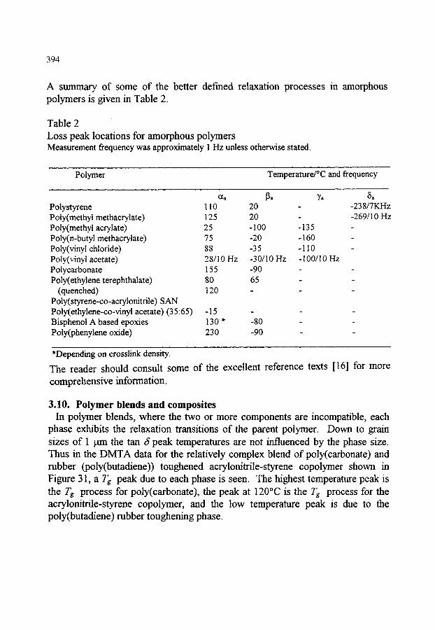
394

A summary of some of the better defined relaxation processes in amorphous polymers is given in Table 2.

Table 2 Loss peak locations for amorphous polymers Measurement frequency was approximately 1 Hz unless otherwise stated.

Polymer Temperature/~ and frequency

Polystyrene Poly(methyl methacrylate) Poly(methyl acrylate) Poly(n-butyl methacrylate) Poly(vinyl chloride) Poly(vinyl acetate) Polycarbonate Poly(ethylene terephthalate)

(quenched) Poly(styrene-co-acrylonitrile) SAN Poly(ethylene-co-vinyl acetate) (35:65) Bisphenol A based epoxies Poly(phenylene oxide)

~, 13. "/, 5, 110 20 - -238/7KHz | 25 20 - -269/10 Hz 25 -100 -135 - 75 -20 - 160 - 88 -35 -110 - 28/10 Hz -30/10 Hz -100/10 Hz 155 -90 - - 8O 65 - - 120 - - -

-15 - - - 130 * -80 - - 230 -90 - -

*Depending on crosslink density.

The reader should consult some of the excellent reference texts [16] for more

comprehensive information.

3 . 1 0 . P o l y m e r b l e n d s a n d c o m p o s i t e s

In polymer blends, where the two or more components are incompatible, each phase exhibits the relaxation transitions of the parent polymer. Down to grain sizes of 1 pm the tan 6 peak temperatures are not influenced by the phase size. Thus in the D M T A data for the relatively complex blend of poly(carbonate) and rubber (poly(butadiene)) toughened acrylonitrile-styrene copolymer shown in Figure 31, a Tg peak due to each phase is seen. The highest temperature peak is the Tg process for poly(carbonate), the peak at 120~ is the Tg process for the acrylonitrile-styrene copolymer, and the low temperature peak is due to the poly(butadiene) rubber toughening phase.

395

LOCi E' (Pa

8.5

7.5

6.5

I ! . ! 100 150

. 9.5

L05 Tan 6

;-,.Z.o I-Io, RATE = t, C lminl]

I 0

-0.~

-0.B

-1.2

1.6

- 100 -50 0 50 TEHP (degC)

200

Figure 31. Incompatible blend of poly(carbonate) with ABS. Each polymer phase exhibits its own a. transition.

Tan 6 PL- DMTA PSMA/PEP[ BLENDS f =IHz

wl'. % PI3HA R=5~

0 20 30 40 50 60 70 80 100 0.025

f

0.0125 ~~/

_ F _ - : 3 - ~ , _ _ _ , , - - . : . ~ . . . . . . . . . . . - ~ . ~ = - - - - " ' " / - . _ __ _ .

[ ' - . . . . . . . - - - 2 - - . . . . . . . . . . -40 0 40 100

Temp (~ }

Figure 32. DMTA curves for a series of compatible polymer blends of poly(glycidyl methacrylate) with poly(epichlorohydrin) [22].

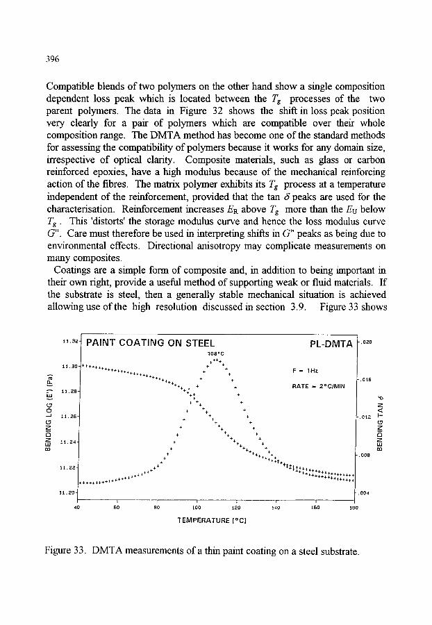
396

Compatible blends of two polymers on the other hand show a single composition dependent loss peak which is located between the Tg processes of the two parent polymers. The data in Figure 32 shows the shift in loss peak position very clearly for a pair of polymers which are compatible over their whole composition range. The DMTA method has become one of the standard methods for assessing the compatibility of polymers because it works for any domain size, irrespective of optical clarity. Composite materials, such as glass or carbon reinforced epoxies, have a high modulus because of the mechanical reinforcing action of the fibres. The matrix polymer exhibits its Tg process at a temperature independent of the reinforcement, provided that the tan d peaks are used for the characterisation. Reinforcement increases ER above Tg more than the Eu below Tg. This 'distorts' the storage modulus curve and hence the loss modulus curve G". Care must therefore be used in interpreting shifts in G" peaks as being due to environmental effects. Directional anisotropy may complicate measurements on many composites.

Coatings are a simple form of composite and, in addition to being important in their own right, provide a useful method of supporting weak or fluid materials. If the substrate is steel, then a generally stable mechanical situation is achieved allowing use of the high resolution discussed in section 3.9. Figure 33 shows

1 1 . 3 2

1 1 . 3 0 " ..-,.

,.,.,. " " 1 1 . 2 8 - h,

0 ._,/

Z D Z UJ m

1 1 . 2 6

1 1 . 2 4 '

1 1 . 2 2 ]

1 1 . 2 0 ]

40

PAINT COATING ON STEEL PL-DMTA 1 0 8 * C

.I .+++§

+ + + + + + + + 4 . + + + . 1 - "1- 4- 4, F = 1 H z +4-+§ + 4, 4-+§247 4, 4-

+++4-+4- . + + R A T E = 2 ~ 4"4"4-.t- 4-

4- § 4, 4-

4. + 4, 4-

4, 4, 4-

4, 4- 4, +

4- +4- 4- § 4-4- 4"

§ 4- 4- 4-4. .I-

4- 4"+4,.i . 4". I. 4- .I-4,4, 4-

+ -=- .t. + "t"

,,4, **§ " -r+++4.~_~__ 4- 4 ++-+'1"4"+ " 4"4-4-4-++++++

.i. 4,4,4,4,4,4,4,4.4,4,§ 4-4. " "r'r § 4- + 4..I..F 4.4 § § 4- 4- 4-

I I i I I I 60 80 100 120 140 t 6 0 180

TEMPERATURE (~

�9 0 2 0

. 0 1 6

Z <

. 0 1 2 I--

Z a

Z Lid rr~

� 9

0 0 4

Figure 33. DMTA measurements of a thin paint coating on a steel substrate.

397

data for a paint film on steel. The location of the tan 6 loss peak will faithfidly reflect the maximum due to the polymer in the free state as the underlying modulus and damping changes are small. Thicknesses down to 1 gm and below can be measured [23].

Clamping in these situations should be right through the coating onto the steel. If this is not so, an erroneous damping peak may be observed after the sample softens because of slip (sample shear) between the substrate and the clamp. Similar erroneous peaks can be generated between the braid in torsional braid measurements.

3.11. Comparison of DMTA loss peaks with DSC A source of confusion arises when determining Tg temperatures by differem

techniques. In DSC, a specific heat step is detected and it is sometimes inferred incorrectly that this is a 'static' measurement. In this case the rate of sca~ming determines the time scale imposed on the molecular motion in the sample. If the molecular motion follows an Arrhenius rule, then the observed Tg will decrease with log (scanning rate). DSC sensitivity decreases with scanning rate rendering measurements at very slow scanning rates impossible. It is common practice to extrapolate to 'zero heating rate' in a linear plot as is shown in Figure 34 for PVC.

- 3 - 2 -1 D 1 2

2.700

(DMTA) xloj.~s ~ Tg(~ 9~ (OSC)

-85

Z.85

"/5

-~176 I ~ _ _ 3s_.c _Tg

t ..... ~ . . . . t _ I, �9 0 5 10 15 20

HEATINI3 RATE (OSC)(~

Figure 34. DSC Tg location for PVC plotted versus thermal scanning rate compared to DMTA loss peak location plotted against log / (independent of scanning rates).

398

As discussed above, the zero rate Tg is only a constructional convenience. On the same figure, DMTA data is shown as a fimction of log f (independent of scanning rate at the low rates used). This shows that the limiting DSC measurement of Tg agrees in location approximately with a DMTA measurement of 10 .3 Hz, whereas DSC at 10 K min -~ agrees with approximately the 10 -~ Hz peak position.

4. CONCLUSION

The TMA method is a useful comparative tool and can be particularly valuable in detenninmg linear expansion coefficients for anisotropic materials. Care is needed in interpreting data when effects of modulus change, creep and time scale are imposed on expansion.

The DMTA technique is useful over a very wide range of materials for assessing transitions in molecular mobility. It is less useful for investigating melting phenomena. Its high sensitivity allows all motional transitions to be detected and provides Tg information for extremely thin coatings on rigid substrates. It is the method of choice for studying polymer blends.

REFERENCES

1. Lu-Hui Wang, C.L. Choy and R.S. Porter, Thermal Analysis, Vol.2 (Ed. 13. Miller), Wiley-Heyden, 1982, p964.

2. H.G. Wiedemann and G. Widermann, Thermal Analysis, Vol.2 (Ed. B. Miller), Wiley-Heyden, 1982, p 1497.

3. S. Timoshenko and J.N. Goodier, Theory of Elasticity, 2nd Edition, McGraw- Hill, New York, 1951, p372.

4. E.F. Finkin, Wear, 19 (1972) 277. 5. Personal Communication, Renishaw plc, UK. 6. G. Widman, First Intl. Conf. on Thermal Characterization of Polymers, Univ.

of Bradford, UK, 1990. 7. A. Dyer, Anal. Proc., (1981) 447. 8. A.T. Riga, G.H. Patterson and W.R. Pistillo, Proc. 21st NATAS Conf.,

Atlanta, 1992, p635. 9. G.D. Ogilvie, Anal. Proc., (1981) 426. 10. C. Zener, Elasticity and Anelasticity of Metals, Univ. Chicago Press, 1948. 11. A.P. Alexandrov and J.S. Lazurkin, Acta Phys. Chem. USSR, 12 (1940) 647. 12. K. Schmieder and K. Wolf, Kolloid Z., 127 (1952) 65. 13. M.L. Williams, R.F. Landel and J.D. Ferry, J. Am. Chem. Soc. 71 (1955)

3701. 14. G. Mikolajczak, J.Y. Cavaille and G.P. Johari, Polymer, 28 (1987) 2023.

399

15. R.E. Wetton, Polymer Characterization, (Ed. B. J. Hunt and M. I. James), Chapman and Hall, London, 1993, p204.

16. N.G. McCrmn, B.E. Read and G. Williams, Anelastic and Dielectric Effects in Polymeric Solids, Dover Publications, New York, 1991.

17. J. Heijboer, P. Dekking and A.J. Staverman, Proc. 2nd Intl. Congr. Rheology, Academic Press, New York, 1954, p123.

18. T. S. K~, Phys. Rev., 71 (1947) 533. 19. J.W.E. Gearing, J.S. Fisher, R.E. Wetton, J.C. Duncan and A.M.J. Blow,

Proc. 17th NATAS Conf, Florida, 1988, p407. 20. J.K. Gillham, Developments in Polymer Characterization - 3, (Ed. J. V.

Dawkins), Applied Science, London, 1982, p 159. 21. D.G. Holloway, The Physical Properties of Glasses, Wykeham, London,

1973, p142. 22. R.E. Wetton, Polymer Characterization, (Ed. B.J. Hunt and M.I. James),

Chapman and Hall, London, 1993, p200. 23. R.E. Wetton, M.R. Morton and A.M. Rowe, American Laboratory, (Jan.

1986), 10.


Chapter 7

DIELECTRIC TECHNIQUES

Sue Ann Bidstrup Allen

School of Chemical Engineering Georgia Institute of Technology Atlanta, GA 30332-0100 U.S.A.

1. INTRODUCTION

Dielectric analysis measures changes in the properties of a material as it is subjected to a periodic electric field. In dielectric thermal analysis (DETA) the sample is also subjected to a temperature programme (see Chapter 1). Electrical properties of polymers (i.e. complex dielectric constant, permittivity, loss factor and conductivity) are directly obtained using dielectric analysis. In addition, the a~- transition (the glass transition temperature, Tg) and secondary transitions can be inferred from DETA data. Dielectric response is also related to the number and strength of molecular dipoles, and may be used to study molecular relaxations in a polymeric system. Dielectric information has also been correlated with the extent of cure and rheological changes during polymerization.

This chapter is an introduction to the DETA measurement methods used to study polymeric systems. The basic principles behind dielectric analysis are reviewed. The chapter begins with a background discussion of the behavior of materials in electric fields. The next portion focuses on models which have been used to correlate dielectric property measurements with the number of dipoles, the strength of the dipole moment and molecular relaxations in the system. In addition, the effects of frequency, temperature and moisture on the measured dielectric properties are covered. Finally, instrumentation for measurement of dielectric properties is discussed. In particular, the advantages and disadvantages of different electrode geometries are summarized.

2. DIELECTRIC RESPONSE

The measurement and characterization of the response of a material to an applied electric field is called dielectric analysis. The material is placed between two conducting electrodes, a smusoidal voltage is applied across the electrodes, and the current response is measured. On a molecular level, the response is simply a

402

displacement of charged units in the material. If the charged units are dipoles, they will orient in the direction of the electric field as shown in Figure 1. If the charged units are mobile (i.e. free electrons or ions), then conduction will take place as shown in Figure 2.

Random Motion Dipole Orientation

Q Q Q Q Q Q Q Q Q Q Q Q

Figure 1. Response of dipoles to an applied electric field.

Random Motion

@ | O

@ O@

Ion Conduction

Figure 2. Response of charged particles to an applied electric field.

Usually, both kinds of charges are present in a polymer sample in varying amounts. Important characteristic material properties (e.g. complex dielectric constant, relative permittivity and ion conductivity) can be extracted from a dielectric measurement, as derived below.

403

The applied voltage E, is related to the current response, J through the complex dielectric constant of the material, e-*

J = i a) e* e 0 E (1)

where i = (-1)~ a~ is the measurement frequency and e 0 is the permittivity of flee space (equal to 8.85 x 10 -14 F cm-~).

The complex dielectric constant can be separated into its real and imaginary parts:

e , (co) = e (~o) - l e"(~o) (2)

where e' (a0 is the relative permittivity and e"(a)) is the relative loss factor. The ratio e"(~o)/g(a~) is known as the loss tangent, tan~. Both the relative permittivity and the relative loss factor are functions of the measurement frequency, the temperature and the structure of the material. Because of their importance as characteristic properties of a material, the permittivity and loss factor are discussed further below.

The relative permittivity, g(a~) is a measure of the electrical polarization of a material in the presence of an electric field. It is composed of the unrelaxed permittivity e u and a term associated with dipole alignment ed,(a 0.

g(w) = e u + ed'(~o ) (3)

The unrelaxed permittivity corresponds to electronic and atomic polarizations and is independent of frequency at low frequencies. Therefore, considering e u as a baseline permittivity, ed'(a~ ) is the additional, frequency dependent, permittivity due to dipole polarization or orientation.

The relative loss factor, e"(co), is a measure of the energy required for molecular motion in the presence of an electric field. It consists of energy losses due to the orientation of molecular dipoles ed"(a~ ), and energy losses due to the conduction of ionic species ec"(a~):

e"(~o) = ed"(~o) + e~"(co) (4)

Based on DeBye's model [1] of dipolar behavior (see section 2.1.2) ed"(Co ) is a complex function of relaxation time and measurement frequency. The energy loss due to the conduction of ions, eo"(a)), is simply inversely proportion to frequency

e'(~o) = cd"(~o) + a/~o Co (5)

404

where ~is the ionic conductivity. The dielectric loss factor is dominated by energy losses due to ion conduction when e"(co) exhibits a linear dependency with 1/a~. Hence, the ionic conductivity can be easily extracted from the dielectric loss in this frequency regime [2].

2.1. Microscopic mechanisms The relative permittivity, g(co) is a measure of the electrical polarization of a

material in the presence of an electric field. Depending on the frequency of the electrical field, electronic, atomic, orientational and interracial polarization may result, which contribute to the capacitive nature of the material and hence, e'(a0. Electronic polarization is a slight displacement of electrons with respect to the positively charged nucleus. Atomic polarization is the relative displacement of atoms in a polar covalent bond. Orientational polarization is due to the force exerted on permanent dipole moments by an electric field, which orients the dipole in the direction of the field. Interfacial polarization results from the accumulation of free charge (e.g. ions) at the electrodes, when charge is transported through the bulk of the material at a rate faster than it can be discharged. In this section, the effects of these different types of polarization on dielectric properties are examined. In addition the effect of molecular relaxations and the concentration and strength of static dipoles on the electrical properties is discussed.

2.1.1. Unrelaxed permittivity In the presence of an electric field, electron clouds and atoms in polar covalent

bonds may be slightly shifted, inducing a slight polarization that is aligned with the electric field. This acts to store energy and contributes to the capacitive nature of the material. The response times of the electronic and atomic shifts are extremely fast so that, at normal dielectric measurement frequencies, this effect is always present. These induced dipoles are responsible for nonpolar or symmetrically polar polymers having permittivities of 2 or greater. The permittivity due to these induced dipoles is known as the unrelaxed or infinite frequency permittivity (eu). At the frequency range typically found in dielectric experiments (10 -3 to 108 Hz), induced dipoles react so quickly to an electric field that e u is frequency independent.

2.1.2. Contribution of static dipole orientation Static dipoles consist of inherently polar moieties (not induced by the electric field)

within the polymer. The static dipoles, if sufficiently mobile, may rotate in an electric field, thus also storing energy and contributing to the capacitive nature of the polymer. Because the dipoles are rigidly attached to relative large molecules in a viscous medium, the orientation process requires a characteristic time, called the dipole relaxation time and denoted by r d.

405

Debye [1] developed a model for the relative permittivity and loss factor of spherical polar molecules relaxing in a viscous medium, based on the assumption of a single relaxation time r o for all molecules. The resulting Debye expression for the relative permittivity and loss factor are:

# = C u + (C r - Cu)/[1 + (60 rd) 2] (6)

# '= (c r - Cu)6O Zd/[1 + (60 Zd) 2] (7)

where

a~ = 2n x measurement frequency r a = dipole relaxation time e r = relaxed dielectric constant or low frequency dielectric constant

(relative permittivity due to induced plus static dipoles) e u = unrelaxed dielectric constant or high-frequency dielectric constant

(relative permittivity due to induced dipoles only)

The Debye equations were developed for a non-conducting material. conductivity makes an additional contribution to the relative loss factor:

Ionic

e"= (a/co e0) + (er - eu) O rd/[1 + rd) (8)

where a = bulk ionic conductivity; and e 0 = permittivity of free space The dependence of the permittivity and loss factor on the product 6or d, as expressed

by the Debye equations, is shown in Figure 3. At low frequencies, or when the relaxation time is small, the dipoles are free to orient. The permittivity approaches the relaxed permittivity and the loss factor approaches zero. At high frequencies or when the relaxation time is large, the dipoles are unable to orient. As a result, the permittivity approaches the unrelaxed permittivity and the loss factor approaches zero. At frequencies and relaxation times such that the product a~r~ is close to one, the permittivity decreases from e r to e u with increasing frequency or relaxation time. Correspondingly, the loss factor increases to a maximum when the product a~r d = 1. As a result of the viscous drag as the dipole rotates through the surrounding medium, there can be a significant phase lag between the maximum applied field and the maximum dipole deflection. The energy lost due to this phase lag reaches a peak as co approaches 1/r d. At higher frequencies the dipole hardly moves and so little energy is lost, while at lower frequencies the dipole can keep up with the changing field more easily and, again, less energy is expended.

406

.,,.~ ;>

E r

E r + E u

2

E u -

0.01

I I I

I I I 0 . 1 1 1 0

C01; d

100

% o

o

0.01 0.1 liO 1

E - s r u

0)1; d

)0

Figure 3. Debye single relaxation model for dipole orientation

407

The Debye model serves as a very useful template upon which dielectric data can be analyzed and interpreted. However, it should be noted that equations are a form of the ideal Debye equation for a single relaxation time model [1]. In reality, polymers often contain more than one type of dipole and each of these has a distribution of relaxation times, causing some differences between calculated and observed results. As the relaxation time widens and becomes skewed the loss peak might not occur at car d - 1. There has been much work at refining the model to account for distributed relaxation time systems [3-7]. Cole and Cole [4] found that, for most materials, the locus of experimental data fell inside this semicircle. They observed that the locus often formed the arc of a circle having a center below the e" = 0 axis and proposed that the data could be described empirically by a modified Debye Equation:

e = eu + (er - eu)/[ 1 + (ico Z-d)~ ] (9)

where fl is known as the distribution parameter and ranges from 0 to 1 (the lower the fl parameter, the broader the dipole relaxation time distribution). This empirical function implicitly defines a functional form of the distribution of relaxation times, which is symmetrical and centered about the value r d.

Davidson and Cole [5] proposed an alternate empirical function to describe dielectric relaxations. In this function, the complex dielectric constant is expressed a s :

e = e. + (e r - eu)/[1 +ico rd]/~ (10)

where the distribution of relaxation time is one-sided (i.e. there are no relaxation times below the value z-d). The maximum loss for this case occurs at:

COma x T d = tan [x/2(fl+ 1)] (11)

A third empirical relaxation function was proposed by Williams and Watts [6,7]. This function also gives rise to a skewed arc diagram, and describes a large number of relaxations in polymers and glasses. The Williams-Watts function is derived by assuming that the time decay of the polarization is expressed by the exponential function:

P(t) = exp ( - t~ rd) fl (12)

408

The distribution parameter, ,6, ranges from 0 to 1, and the expression reduces to the Debye single relaxation time case for fl = 1. Lindsey and Patterson [8] have presented a detailed comparison of the Davidson-Cole and Williams-Watts functions. While originally developed as an empirical model, there have been attempts to explain the success of this function using models for relaxation times based on diffusion [9,10].

2.1.3. Models for relaxed permlttivity Permanent dipoles contribute to the overall polarization of the system. At low

frequencies in the absence of electrode polarization, e reaches a maximum value known as the relaxed permittivity e r. The relaxed permittivity depends on the number and moments of the permanent dipoles. The unrelaxed permittivity is obtained at high frequencies, where dipole orientation is absent. The difference b e t w e e n E r and e u is known as the permittivity increment and is related to the number and moments of permanent dipoles in the system. In this section, a historical development of theories relating e r and e u is presented.

The simplest theory was developed for a material composed of nonpolar, noninteracting molecules. If this material is place in an electric field E, atomic and electronic polarizations cause a dipole moment m to be induced by atomic and electronic polarizations. The dipole moment is directly proportional to the electric field and the proportionality constant is the deformation polarizability t~ e [1 ]:

m = a~eE (13)

The deformation polarizability is related to the frequency independent e (i.e. e u in materials containing dipoles) and can be obtained from the Clausius-Mossotti relation:

(e - 1)/(e + 2) = NecJ 3e0 (14)

where N is the number of dipoles per unit volume and e 0 is the permittivity of free space.

Debye [1] developed a relationship for the orientation polarizability of permanent dipoles a~ by developing an expression for the permittivity of polar gases composed of molecules having a dipole moment/~o:

= t%2/3kBT (15)

where k~ is the Boltzmann constant and T is temperature. This expression assumes the distribution of orientations follows Boltzmann's law. Debye's expression for

409

relaxed permittivity for polar gases is obtained by combining the expression for orientation polarization and for deformation polarization with the Clausius-Mosotti relationship:

(e r - 1)/(e r + 2 )= (N/3e0)[a e + ,Uo2/kBT] (16)

It should be noted that the Debye expression does not take into account interactions between neighbouring molecules, such as would typically be present in liquids or polymers. However, this expression has been successfully applied to dipolar gases at low pressures and to dilute solutions of polar molecules in nonpolar solvents.

An expression was developed by Onsager [11] for the relaxed permittivity of liquids. By considering the total field acting on the dipole to be the vector sum of the reaction field due to the dipole and the externally applied field, the following expression was obtained:

(e r - e u )(2 e r + eu)/er(e u + 2) 2 = NCzo2/9 e0 kBT (17)

In this expression, Onsager assumed that a molecules is a polarizable point dipole at the center of a spherical cavity in a homogeneous material having a dielectric

constant, er, equivalent to the macroscopic dielectric constant. Again, this expression did not include interactions between neighbouring molecules, and therefore cannot be used to describe materials with strong intermolecular interactions. However, the Onsager expression has been used with moderate success to calculate dipole moments of simple polar molecules, via permittivity measurements in the liquid state.

Kirkwood [12] attempted to account for the interactions between neighbouring dipoles. Unlike Onsager's assumption of a spherical cavity, this approach assumed the sphere to be filled with interacting dipoles. The interactions between neighbouring molecules were treated using statistical mechanics and the deformation polarization was empirically added:

(e~- 1)(2c~ + 1)/9e r = (4r~N/3)[a~ e + gcz2/3kBT] (18)

In this expression, g is the correlation factor that quantifies the interactions of a reference dipole with neighbouring dipoles. For a dipole with z equivalent nearest neighbours, the correlation factor is

g = 1 + z cos y (19)

where ?' is the angle between the dipole and one of its nearest neighbours.

410

Kirkwood's expression predicts the dielectric constant of water and simple alcohols within 20%. However, objections were raised to the theory since the expression does not reduce to the Onsager model for the case of no interactions (g= 1).

Frohlich improved on the Kirkwood model by properly including the deformation polarization in the derivation. Like Onsager, he used the concept of two fields acting on a dipole: the reaction field due to the dipole and the external field. Additionally, he used the Clausius-Mossotti formula as an expression for the deformation polarizabilty. The resulting expression is:

#

(e r - e, )(2 e~ + eu)/3 e~ = N m m / 3 e o kBT (20)

where m is the moment of a reference dipole unit in a particular configuration and m * is the average moment of the sphere when the reference dipole is fixed in that particular configuration. In small molecules and isolated macromolecules, m is the dipole moment of the material. However, in entangled macromolecules, the dipole moment of the repeat unit should be used.

For small molecules, m --/.t. The moment m can be related to the dipole moment of a molecules in a vacuum,/~o, by the relation

= (eu + 2)/3#o (21)

This leads to Frohlich's modification of the Kirkwood expression [13]"

(er- eu )(2 e r + eu)/er(e,., + 2)2 = N g ,Uo2/9 e o kB T (22)

where N is the number of molecules per unit volume,/% is the dipole moment of a molecule of the material in the gaseous phase, and g is the correlation factor for interaction between molecules:

No g = 1 + )-I, cos y,j (23)

i=j

where ?~j is the angle between dipole units i andj. The correlation factor is summed over the total number of molecules in the sphere (No). This equation does reduce to the Onsager expression in the case where there is no dipole interaction (g = 1).

The application of Frohlich theory to polymers is described in McCrum et al. [3]. For a high molecular weight polymer, the effect of differences between end groups and the polymer backbone repeat units can be neglected. This leads to:

(e,.- e u )(2 e r + eu)/<(eu + 2) 2 = Nr gr/ao 2/9 e0 kuT (24)

411

where N~ is the number of monomer repeat units per unit volume,/~o now equals the dipole moment of the monomer repeat unit, if it were to exist in the gaseous phase, and gr equals the interaction parameter for a repeat unit in a polymer molecule. There are two ways to express gr for a polymer with a degree of polymerization equaling n. For isolated macromolecules (i.e. a dilute solution of distinct, monodisperse polymer molecules), the interaction parameter is given by:

n n n

gr = 1 + ( 1 / n ) ~ ~ cos F,j ~ 1 + )-I, cos Es (25) i j j=2

where F0 is the angle between dipole units i and j (where i ~ j). The simplified expression results when all the repeat units are equivalent. For a system of entangled macromolecules:

n n

gr = 1 + ~ COS Es + ~H COS Es (26) j = 2 j = l

I cos F0 is the average of the cosine of the angle between a reference unit i and a unit

j within the same polymer chain. This term corresponds to intra-chain interactions. I1

cos ~j is the average of the cosine of the angle made between a reference unit i and a unitj which does not belong to the polymer chain that contains reference unit i. The treatment of these systems often assumes that the intermolecular correlation term, II, is zero, and that only a few of the dipoles adjacent to a given dipole are correlated. The correlation factor can then be calculated based on a model for the polymer structure, including bond angles and energy barriers for rotation.

2 .1 .4 . I o n i c c o n d u c t i o n

Ionic conduction is the result of current flow due to the motion of mobile ions within the material under test. Consider a polymer system containing i species of ions. If an electric field E is applied to the system, the ith species of ion will acquire an average drift velocity, v;. Assuming a linear relationship between the drift velocity and the applied electric field:

v i = u i E (27)

where the proportionality constant u~ is called the mobility of the ion. If each species of ions i has a concentration N~ and a charge magnitude q~, the ionic conductivity of the polymer system can be expressed as

a = ~ q; N, u~ (28) i

412

The relation between the mobility of the ion and the properties of the resin can be qualitatively examined using Stokes' law for the drift of a spherical object in a viscous medium. The mobility of a sphere of radius r~ embedded in a medium of viscosity r/and subjected to a force q~E is:

u,. = q , / 6~ r/r, (29)

It should be noted that Stokes' law does not directly apply to the mobility of ions in polymer systems, because the motion of an object as small as an ion is dependent on the microviscosity (individual chain segment motions), not the macroviscosity (concerted chain segment motions) of the medium. Hence, during polymerization of thermoset systems, the bulk viscosity becomes infinite because of the formation of a macroscopic molecular network. However, the resistivity (inverse of conductivity) remains finite because the polymer segments comparable in size to the ions are still mobile. Well before gelation, the resistivity and viscosity are tightly correlated because both the viscosity and ion mobility have similar dependencies on polymer segment mobility.

It is often assumed that ionic conduction is insignificant due to low mobile ion concentrations. However, it has been demonstrated that concentrations well below 1 ppm are sufficient to cause significant ionic conduction levels [2,14]. From the Debye model, it is seen that ionic conduction contributes only to the loss factor and does not affect the permittivity (as long as electrode polarization is negligible). It is very common to observe large loss factors in polymers when the temperature is above the glass transition, due to the ionic conduction contribution to the loss factor.

2.1.5. Electrodepolarization Electrode polarization is not due to the polymer under test alone, but is the result

of the resin in combination with the electrodes used to introduce the electric field. Electrode polarization occurs when ionic conduction is extremely high, causing ions to collect at the polymer/electrode interface during one-half cycle of the oscillating electric field cycle. As ions build up at the electrode in a thin boundary layer and do not exchange their charges, a large capacitance is formed (not unlike an electrolytic capacitor). This has the effect of artificially decreasing the measured values of high loss factors and increasing the measured values of permittivity. The extent to which the actual and measured values of permittivity differ depends on the sample inhomogeneity, as measured by the thickness of the charge layer relative to the interelectrode distance.

In a Cole-Cole plot or arc diagram [3,4], electrode polarization appears much like a semicircular dipole transition. However, the measured permittivities attained through electrode polarization are usually high (>100), thus making electrode polarization easy to identify. In addition, electrode polarization peaks vary with electrode separation, whereas dipole polarization peaks are independent of electrode separation. Corrections can be made to the loss factor for electrode polarization

413

influence if the e r value is known [15]. A detailed derivation of the electrode polarization influence is given by Day et al. [16].

3. TEMPERATURE DEPENDENCE

Both permittivity and loss factor depend on the measurement temperature. From the measure of the temperature dependence of the oscillator strength, important information regarding intramolecular interactions can be obtained. According to the Kirkwood-Frohlich equation (equation (22)), the temperature dependence of the oscillator strength of the dielectric transition is determined by the temperature dependence of e u and e r , the dipole moment,/~, and the reduction factor, g. According to the Clausius-Mosotti equation (equation (14)), e u is independent of temperature. The temperature dependence of e r, in the case of freely rotating dipoles is given by equation (16). The dipole moment depends on temperature only if the configuration of the molecule is changed. The interaction factor g is temperature dependent because it is a measure of intramolecular interactions. Therefore, the temperature dependence of the oscillator strength can be summarized by the following equation:

eu- = c g(7) ,,o(7)/T (30)

where the factor C is independent, or just slightly dependent on the temperature. It can be seen, from equation (30), that, when the molecular configuration and the

mtramolecular interactions are not changed, the oscillator strength should decrease with increasing temperature. This is generally observed in dilute solution or in the molten state. The oscillator strength of polymers is more generally increased by increasing temperature, indicating that the dependence is mainly governed by changes in the intramolecular interactions.

Assuming a single relaxation approximation of Debye:

e" = (c r - Cu)a) rd/[1 + (60 rd) 21 (7)

the temperature dependence of the dielectric loss can be expressed using Eyring's general theory of rate processes for the temperature dependence of the distribution time:

r a (7) = r o exp(Ea/kB7) (31)

where E~ is the activation energy of the transition. This function exhibits a maximum at temperature T m

v 4 (Tm) = r o exp(EJ k BTm) = 1 / a) (32)

414

where ~o is the fixed angular frequency of the measurement.

Hence, exp (x)

e"(7) = eu) (33) 1 + exp (2x)

where x = (Ea / kB) ( T ~- Tm-~). Both the dipole relaxation time and ionic conductivity are related to the glass

transition temperature (Tg) of the polymer [2, 3, 17]. As a material is heated through the glass transition temperature, static dipoles gain mobility and start to oscillate in the electric field. This generally causes an increase in permittivity with a corresponding loss factor peak. At the lower temperature side of the glass transition, dipoles will only be able to respond to low frequency excitation since they do not have the higher mobility associated with higher temperatures. The frequency dispersion observed in the dielectric measurement is very analogous to that observed for mechanical measurements. It has generally been observed that low-frequency dipole peaks (less than 1 Hz) correspond well with other thermal analysis measurements of Tg. Materials containing static dipoles that gain mobility during the glass transition will usually exhibit permittivity changes and dipole loss peaks. However, materials with no static dipoles or non Tg active static dipoles will obviously exhibit little dipolar influence through the glass transition.

Charged ions also gain mobility as a material is heated through the glass transition and will start to contribute to conductive losses above the glass transition. The contribution of ion conductive loss to the measured loss factor can be enormous and can often overshadow small dipole loss contributions.

For this review Shell Epoxy Resin EPON 825 (diglycidyl ether of bisphenol A) is selected to illustrate the relationship between the dielectric properties and the glass transition temperature. The temperature dependencies of the permittivity and loss factor for EPON 825 at frequencies ranging from 1 to 10000 Hz are shown in Figures 4 and 5. The glass transition temperature of this polymer is reported to be -20 ~ measured at a temperature ramp of 15 ~ using a differential scanning calorimeter.

At temperatures well below rig, the permittivity at all frequencies has a value of 4 (the unrelaxed permittivity) and the loss factor is below 0.1. As the temperature approaches Tg, the dipoles gain sufficient mobility to contribute to the permittivity, with evidence of this mobility increase occurring first at the lowest frequency. With a fin/her increase in temperature, the permittivity for a given frequency levels off at the relaxed permittivity, which then decreases due to increasing temperature, and then abruptly increases again as a result of electrode polarization. At each

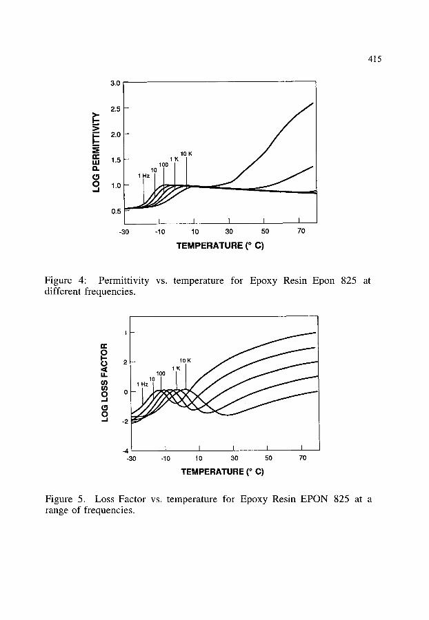
4 1 5

3.0

2.5

E 2.0

=.. n~l 1.5

1.0

0.5

10

1K 10K 100 I ]

I I I, I ! I -30 -10 10 30 50 70

TEMPERATURE (o C)

Figure 4" Permittivity vs. temperature for Epoxy Resin Epon 825 at different frequencies.

I.

re O I-- 0 2 ,r 14. r

O 0 ,-I

O ,,..I -2

100

1OK 1 K I

-4 I I I I I I -30 -10 10 30 50 70

T E M P E R A T U R E (o C)

Figure 5. Loss Factor vs. temperature for Epoxy Resin EPON 825 at a range of frequencies.

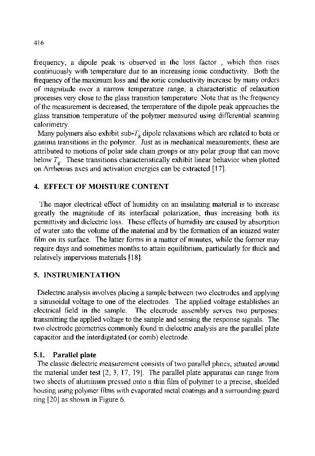
416

frequency, a dipole peak is observed in the loss factor , which then rises continuously with temperature due to an increasing ionic conductivity. Both the frequency of the maximum loss and the ionic conductivity increase by many orders of magnitude over a narrow temperature range, a characteristic of relaxation processes very close to the glass transition temperature. Note that as the frequency of the measurement is decreased, the temperature of the dipole peak approaches the glass transition temperature of the polymer measured using differential scanning calorimetry.

Many polymers also exhibit sub-Tg dipole relaxations which are related to beta or gamma transitions in the polymer. Just as in mechanical measurements, these are attributed to motions of polar side chain groups or any polar group that can move below Tg. These transitions characteristically exhibit linear behavior when plotted on Arrhenius axes and activation energies can be extracted [17].

4. EFFECT OF MOISTURE CONTENT

The major electrical effect of humidity on an insulating material is to increase greatly the magnitude of its interfacial polarization, thus increasing both its permittivity and dielectric loss. These effects of humidity are caused by absorption of water into the volume of the material and by the formation of an ionized water film on its surface. The latter forms in a matter of minutes, while the former may require days and sometimes months to attain equilibrium, particularly for thick and relatively impervious materials [18].

5. INSTRUMENTATION

Dielectric analysis revolves placing a sample between two electrodes and applying a sinusoidal voltage to one of the electrodes. The applied voltage establishes an electrical field in the sample. The electrode assembly serves two purposes: transmitting the applied voltage to the sample and sensing the response signals. The two electrode geometries commonly found in dielectric analysis are the parallel plate capacitor and the interdigitated (or comb) electrode.

5.1. Parallel plate The classic dielectric measurement consists of two parallel plates, situated around

the material under test [2, 3, 17, 19]. The parallel plate apparatus can range from two sheets of aluminum pressed onto a thin film of polymer to a precise, shielded housing using polymer films with evaporated metal coatings and a surrounding guard ring [20] as shown in Figure 6.

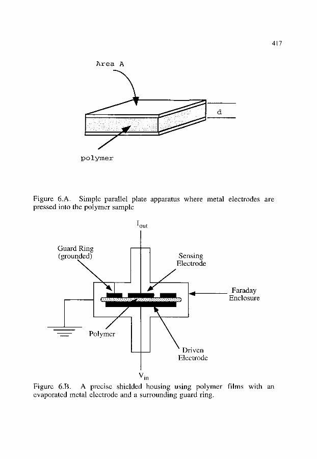
417

Area A

polymer

Figure 6.A. Simple parallel plate apparatus where metal electrodes are pressed into the polymer sample

Iout

Guard Ring (grounded) Sensing

Electrode

Polymer

�9 Driven Electrode

Faraday Enclosure

Vin Figure 6.B. A precise shielded housing using polymer films with an evaporated metal electrode and a surrounding guard ring.

418

One plate is excited with a sinusoidal electrical potential at frequencies ranging (in general ) from 1 mHz to 1 MHz, and the resulting sinusoidal current passing from the second electrode to ground is monitored. To achieve accurate results, the following requirements are necessary:

1. Controlled plate areas and separation distance 2. Good contact (evaporated metal on polymer surface may be used) 3. A grounded guard ring to leak off surface conduction 4. A well shielded cell and cables

A rounded guard ring is an important element in making the best dielectric measurements with a parallel plate. The guard ring prevents surface leakage of current from the driven electrode to the sensing electrode. Any current flowing from the driven electrode to the grounded guard ring is drained into the ground connector. Since the sensing electrode is used a ground potential (a virtual ground), it is at the same potential of the guard ring; consequently, no current flows between them. The guard ring also minimizes flinging at the edge of the sensing electrode.

Normally, the plate spacing is designed to be much less than the plate size, which minimizes the effect of flinging fields. The dielectric properties may then be easily calculated [2, 3, 17, 19] based on the amplitude and phase of the measured current, and the area and separation of the plates:

(S' = C p d / A eo (34)

e" = d /Rp A 61 60 (35)

where Cp d A Rp 6)

= equivalent parallel capacitance = separation between parallel plates = area of a single plate = equivalent parallel resistance - angular frequency of the applied voltage

Combining these equations yields the loss tangent,

tan c~= e ' / e " (36)

Therefore, for a parallel plate structure containing a homogeneous medium and having no interface effects, the loss tangent of the medium is independent of plate spacing and area. However, tan c~ is not an ideal quantity to measure since e' and e" are independent functions of dipoles, conductivity and polarization. Nevertheless, it is often measured since it is independent of the plate separation d. The plate separation can vary during the experiment as a result of application of temperature

419

and measurement. For example, during polymerization reactions, matrix resins typically go through significant dimensional changes either due to temperature, to reaction-induced contraction or to applied pressure, and it has proved difficult to maintain the calibration of parallel plates in these cases.

The primary advantages of parallel plate electrodes are the ease with which measured data can be interpreted, and that they can be made form almost any conductor. The primary disadvantages are the need to control plate spacing and area if quantitative measures of either e' or c" are to be obtained and the instrmnental difficulties associated with making admittance measurement at frequencies below about 100 Hz [2].

5.2. Interdigitated electrodes An alternative to the parallel plate electrode involves the use two interdigitated

electrodes (Figure 7) on an insulating substrate. This design permits a one-sided, very local measurement of dielectric properties and is particularly well suited for thin films. For this sensor, metal electrodes of gold, copper or aluminum are fabricated on an insulating substrate using photopatteming. The substrate is typically a ceramic, a polymer composite or a silicon integrated circuit. The electrode sensor is used either by placing a small amount of material over the electrodes or by embedding the sensor in the test medium.

Figure 7.A. Top view of interdigitated electrodes.

Figure :7,B Cross-section:: of:interdigitated electrodes.

420

The advantages of comb electrodes lie in the reproducibility of the calibration (which pen~ts separation of e' and e") and in the ease with which they can be used in monitor properties in a variety of environments. The calibration depends on the electrode size and spacing and on the dielectric properties of the substrate, all of which can be made quite reproducible with photopatterning technology. Furthermore, the calibration is relatively insensitive to temperature or pressure changes, a major advantage compared with parallel plates. The major disadvantage of the interdigitated electrode is associated with sensor sensitivity. With mterdigitated electrodes, only a fringing field is measured. Consequently, the signal obtained for a given area of comb electrode as compared to a parallel plate is much smaller. Hence, their primary application is with materials where the loss factor is dominated by conductivity effects and where the conductivity is relatively high (> 10 -8 (ohm-cm) -1)

An important variation of the comb electrode is the microdielectric sensor [2, 21, 22, 23], which combines a comb electrode with a pair of field-effect transistors in a silicon integrated microcircuit, to achieve sensitivities comparable with parallel- plate electrodes, but retaining the reproducible calibration features of the mterdigitated electrode. The circuit is modified to integrate current flow over time enabling the sensor to function at frequencies as low as 0.001 Hz. Calibration difficulties are overcome by conducting a finite difference analysis modeling the electrode, the material sample, the oxide insulator, and the underlying silicon. The resulting calibration is fairly complex and resides in the equipment memory. In addition, since the electrodes are rigid and are manufactured with microelectronic precision, the calibration of the sensor is stable with respect to temperature and pressure variations.

5.3. Capacitance and impedance measurement equipment Whether using parallel plate or interdigitated electrodes, the basic measurement

involves determining the admittance between the electrodes under sinusoidal steady- state conditions. In the low and intermediate frequency range (20 Hz to 2 MHz), several types of bridges are commercially available. Above the MHz range, the resonance technique is typically used, although some types of transformer bridges can be used up to 108 Hz with high accuracy. The capacitance-variation method is one of the several resonance techniques providing high accuracy. Another very important technique for high frequency measurement is time domain reflectometry (TDR). The method utilizes the standing wave due to the reflected wave involves finding the impedance of electromagnetic waves in a loss-less transmission line terminated by a sample and a short circuit. The impedance in the loss-less section is transformed to the sample interface, and the dielectric properties of the sample are calculated.

421

NOMENCLATURE

A G d E & g

i J

m

N N, qi Rp ri T Tg bl i

z

B

G 6 , Et Gtl

Eo c d ' Ec" Ed" Cr c~ 7/

1) i

O rd

area of a single plate equivalent parallel capacitance separation between parallel plates complex voltage activation energy correlation factor that quantifies the interactions of a reference dipole with neighbouring dipoles (_1) ~ complex current Boltzmann's constant dipole moment number of dipoles per unit volume concentration of ith ion charge of ith ion equivalent parallel resistance radius of ith ion temperature glass transition temperature mobility of ith ion mmaber of equivalent nearest neighbour dipoles to a reference dipole distribution parameter in the Cole-Cole, Davidson-Cole and William- Watts expressions (equations 9 -12) polarizability of permanent dipoles deformation polarizability

complex dielectric constant relative permittivity relative, loss factor permlttlvaty of free space (equal to 8.85 x 10 -14 F/cm) permittivity associated with dipole alignment dielectric loss due to ionic conduction dielectric loss due to orientation of dipoles relaxed permittivity unrelaxed permittivity angle between the dipole and one of its nearest neighbours dipole moment average drift velocity ionic conductivity dipole relaxation time

tan c~ loss tangent to measurement frequency

422

REFERENCES

1. P. Debye, Polar Molecules, Chemical Catalog Co., New York (1929). 2. S.D. Senturia and N. F. Sheppard, Jr., "Dielectric Analysis of

Thermoset Cure", Advances in Polymer Science, 80 (1986) 1. 3. N.G. McCrum, B. E. Read, G. Williams, Anelastic and Dielectric

Effects in Polymeric Solids, Wiley and Sons, New York, 1967. 4. K.S. Cole and R. H. Cole, J. Chem. Phys., 9 (1941) 341. 5. D.W. Davidson and R. H. Cole, J. Chem. Phys., 18 (1950) 1417. 6. G. Williams and D. C. Watts, Trans. Faraday Soc., 66 (1970) 80. 7. G. William, D. C. Watts, S. B. Dev and A. M. North, Trans.

Faraday Soc., 67 (1971) 1323. 8. C . . . . . . . . . . and G. D. Patterson, J. Chem. Phys., 73 (1980) 3348. 9. E.W. Montroll and J. T. Bendler, J. Stat. Phys., 34 (1984) 129. 10. M.F. Shlesinger, J. Stat. Phys., 36 (1984) 639. 11. L. Onsager, J. Am. Chem. Soc., 58 (1936) 1486. 12. J.G. Kirkwood, J. Chem. Phys., 7 (1939) 911. 13. H. Frolich, Theory of Dielectrics: Dielectric Constant and Dielectric

Loss, Oxford University Press, Oxford, 1958. 14. A.R. Blythe, Electrical Properties of Polymers, Cambridge,

Cambridge University Press, Cambridge,1979. 15. D.R. Day, in Quantitative Nondestructive Evaluation, Plenum Press,

New York, Vol 5B (1986), 1037. 16. D.R. Day, T. J. Lewis, H. L. Lee and S. D. Senturia, J. Adhesion, 18

(1985) 73. 17. P. Hedvig, Dielectric Spectroscopy of Polymers, McGraw-Hill, New

York, 1977. 18. R.F. Field, J. Appl. Phys., 17 (1946) 318. 19. C.W. Reed, Dielectric Properties of Polymers, (Ed. F.E. Kraus),

Plenum Press, New York, 1972. 20. "Standard Test Method for A-C Loss Characteristics and Permittivity

(Dielectric Constant) of Solid Electrical Insulating Materials", ASTM Designation: D150-92.

21. N.F. Sheppard, D. R. Day, H. L. Lee and S. D. Senturia, Sensors and Actuators, 2 (1982) 263.

22. N.F. Sheppard, S. L. Garverick, D. R. Day and S. D. Senturia Proceedings of the 26th SAMPE Symposium, (1981) 65.

23. S.D. Senturia and S. L. Garverick, "Method and Apparatus for Microdielectrometry", U.S. Patent No.4,423,371


Chapter 8

CONTROLLED RATE THERMAL ANALYSIS AND RELATED TECHNIQUES

M. Reading

IPTME, Loughborough University, Loughborough, Leicestershire LEI 1 3TU

1. INTRODUCTION

Most thermal methods are based on subjecting a sample to a predetermined temperature programme, almost always either isothermal or linear, while measuring one or more of its properties. The temperature programme proceeds in the manner chosen by the experimenter regardless of any changes undergone by the sample. There are methods that have departed from this approach by allowing the measured sample response to influence the course of the temperature programme in some way. Several algorithms have been used to determine the changes in the temperature programme as a function of sample behaviour and a variety of different sample properties have been used as the input to the temperature controller. This has given rise to a number of different methods that are the subject of this chapter.

It is unforttmate that several different nomenclatures have evolved with no widely accepted genetic name coveting them all. This topic is briefly reviewed later in this chapter. The terms and abbreviations proposed by Reading [1 ], as described in the next section, together with the term Sample Controlled Thermal Analysis (SCTA) will be used here for all methods where the transformation tmdergone by the sample in some way influences the course of the temperature programme it experiences.

2. HISTORICAL DEVELOPMENT

The earliest example of the use of the use of a measured sample response being used as part of the temperature control system in a thermoanalytical method was developed by Smith in 1940 [2]. He used a differential thermal approach where one half of the thermocouple pair was placed next to the sample and the other on the opposite side of a material of known thermal resistance which formed the sample container. This whole assembly was then heated in a furnace. The control system

424

was designed to maintain the temperature differential across the thermocouple pair at a constant value.

If the thermal conductivity of the container material could be considered as constant over the operating range of the apparatus, this would mean that the rate of heat flow into the sample would be maintained constant. In reality the thermal conductivity changes with temperature so it would be more correct to say that the heat flow into or out of the sample followed a known function of temperature. Smith noted that [2], as a consequence of adopting this method, "the temperature gradients within the specimen and along the thermocouple are smaller and the arrests are sharper" ('arrests' in this context means peaks due to transformations). This form of analysis came to be known as Smith Thermal Analysis and has been used principally to study metal alloys.

In the early 1960s J. Rouquerol [3] on his own, and a team consisting of two brothers, F. Paulik and J. Paulik [4], independently of each other and without being aware of the work of Smith, developed methods that sought to hold at a constant value the rates of reactions that led to a mass loss or the evolution of a gas. The Pauliks based their apparatus on a thermogravimetric balance. They devised a control system that would heat a sample in such a way as to maintain the rate of mass loss at a constant value. This type of experiment often produced temperature traces that were almost isothermal during much of the reaction, hence the name quasi-isothermal [5]. The Pauliks proposed the abbreviation QTG for this method. They also designed a number of crucibles from which the escape of evolved gases to the outside atmosphere was restricted in such a way as to force the rapid generation within the crucible of an atmosphere consisting ahnost entirely of the evolved species at the ambient pressure [5]. When experiments were carried out under these conditions the Pauliks used the term quasi-isothermal, quasi-isobaric [5]. Rouquerol's approach [3] relied upon using a transducer to monitor the pressure of evolved gas in a continuously evacuated chamber. He designed a controller that heated the sample in such a way as to maintain the monitored pressure constant. Because the pressure is maintained constant, the rate at which the gas is pumped away remains constant, thus the rate of mass loss, when a single gas is evolved, is also constant. Subsequently he coupled this type of approach with vacuum thermogravimetry [6].

The similarity between the techniques proposed by the Pauliks and Rouquerol is immediately apparent. Both maintain the reaction rate constant, both control the pressure of the evolved species in the reaction environment. The differences lie simply in the means adopted to achieve these ends and the pressure regime they are best suited for. The similarities with Smith thermal analysis are also clear. For a decomposition reaction which evolves only one gas and where the thermal conductivity of the sample container in the Smith apparatus could be considered

425

constant over the temperature range of the reaction, all three approaches would lead to a constant reaction rate. The name controlled transformation rate thermal analysis has been proposed by Rouquerol [7] to describe this approach in which the heating programme is determined by the need to control the transformation rate in a predetermined way. The word transformation can be dropped when it is clear that the controlled parameter is not the heating rate but the rate of change of a measured property of the sample. The word constant can be substituted for controlled when this is case. The most frequently used abbreviation is CRTA (m this chapter the abbreviation CnRTA is used). Rouquerol has compared this general approach with conventional thermal analysis by use of the schematic diagrams shown in Figures 1 and 2 [7]. These figures are an excellent method of illustrating the basic philosophy of conventional and constant/controlled rate thermal methods. Rouquerol [7] has defined this method as "a general thermoanalytical method where a physical or chemical property, 'X', of a substance is modified, following a predetermined programme X = f(t), under the appropriate action of temperature".

Another technique that is similar to those described above has been proposed by Sorensen [8] called stepwise isothermal analysis. In this method an upper and lower limit is set for the reaction rate. When the rate falls below the minimum, the temperature is increased until it exceeds the maximum; then the temperature is held constant until the reaction rate again falls below the minimum. This method has been applied to thermogravimetry and to dilatometry. The emergence of the stepwise isothermal technique as a distinct method is interesting because it underlines the difference between the control scheme illustrated in Figure 2 and that illustrated in Figure 3 which more correctly describes the control mechanism required to implement the stepwise method.

One way of characterising the stepwise isothermal method is to say that it is 'badly controlled CnRTA' where the control system fails to provide the smooth continuous response required to maintain the reaction rate at a constant value. The distinction between the two techniques has become blurred and Sorensen himself has used the terms quasi-isothermal to describe his approach [8]. However, Sorensen clearly asserted that it was his intention to avoid the continuous change of constant (CnRTA) or controlled (CrRTA) rate thermal analysis because he believed there were disadvantages to this approach [8]. Paulik and Paulik [5] have also pointed to the differences between their approach and that advocated by Sorensen. As soon as this distinction is appreciated, it becomes clear that in the stepwise method the reaction rate is not a predetermined function of time. It is constrained by the temperature control algorithm, but it will have a complex and unpredictable development as a function of time. The implications of this became clear when another method was introduced by TA Instruments called dynamic rate TGA [9] in which the heating rate is linked to the rate of mass loss by a sigmoidal relationship.

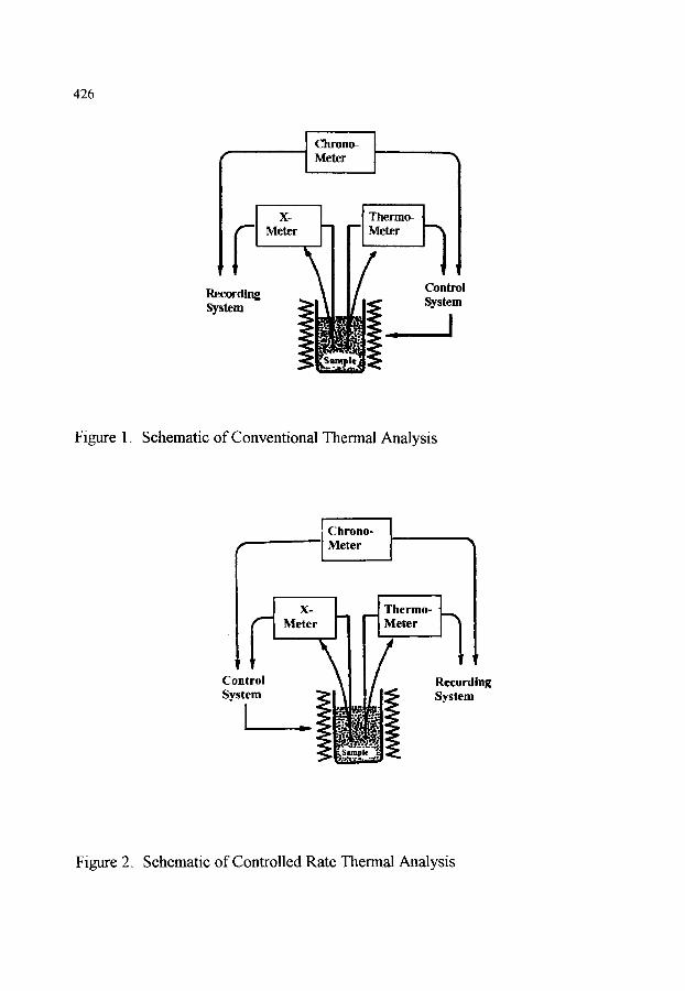
426

~ r ' " ""J 'j ' Chrono- Meter

Recording System

X- Meter

Thermo- Meter

Control System

I

Figure 1. Schematic of Conventional Thermal Analysis

Chrono- Meter

X. Meter

Thermo- Meter

Control

Sysiem Recording System

Figure 2. Schematic of Controlled Rate Thermal Analysis

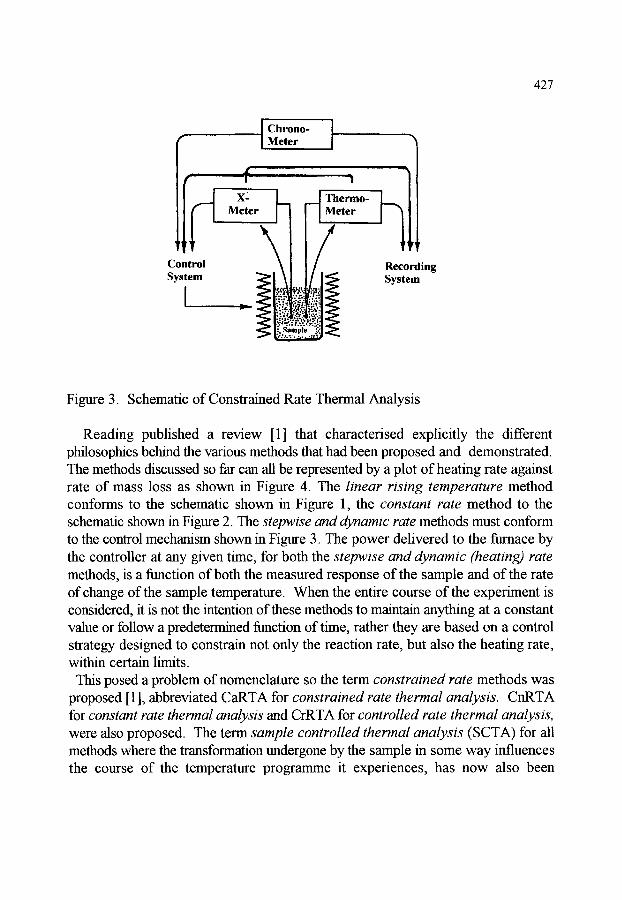
427

Chrono- Meter

.L

Jr- ~ l

X- Thq Meter Me

Control System

oO~r " ~

Thermo- Meter

Recording S y s t e m

Figure 3. Schematic of Constrained Rate Thermal Analysis

Reading published a review [1] that characterised explicitly the different philosophies behind the various methods that had been proposed and demonstrated. The methods discussed so far can all be represented by a plot of heating rate against rate of mass loss as shown in Figure 4. The linear rising temperature method conforms to the schematic shown in Figure 1, the constant rate method to the schematic shown in Figure 2. The stepwise and dynamic rate methods must conform to the control mechanism shown in Figure 3. The power delivered to the fi[mace by the controller at any given time, for both the stepwise and dynamic (heating) rate methods, is a function of both the measured response of the sample and of the rate of change of the sample temperature. When the entire course of the experiment is considered, it is not the intention of these methods to maintain anything at a constant value or follow a predetermined fimction of time, rather they are based on a control strategy designed to constrain not only the reaction rate, but also the heating rate, within certain limits.

This posed a problem of nomenclature so the term constrained rate methods was proposed [1 ], abbreviated CaRTA for constrained rate thermal analysis. CnRTA for constant rate thermal analysis and CrRTA for controlled rate thermal analysis, were also proposed. The term sample controlled thermal analysis (SCTA) for all methods where the transformation undergone by the sample in some way influences the course of the temperature programme it experiences, has now also been

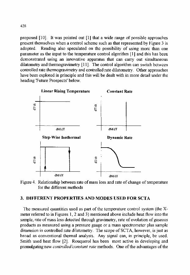
428

proposed [10]. It was pointed out [1 ] that a wide range of possible approaches present themselves when a control scheme such as that represented by Figure 3 is adopted. Reading also speculated on the possibility of using more than one parameter as the input to the temperature control algorithm [1] and this has been demonstrated using an innovative apparatus that can carry out simultaneous ditatometry and thermogravimetry [ 11 ]. The control algorithm can switch between controlled rate thermogravimetry and controlled rate dilatometry. Other approaches have been explored in principle and this will be dealt with in more detail under the heading 'Future Prospects' below.

Linear Rising Temperature Constant Rate

dM/dT dM/dT

Step-Wise Isothermal Dynamic Rate

dM/dT dM/dT

Figure 4. Relationship between rate of mass loss and rate of change of temperature for the different methods

3. DIFFERENT PROPERTIES AND MODES USED FOR SCTA

The measured quantities used as part of the temperature control system (the X- meter referred to in Figures 1, 2 and 3) mentioned above include heat flow into the sample, rate of mass loss detected through gravimetry, rate of evolution of gaseous products as measured using a pressure gauge or a mass spectrometer plus sample dimension in controlled rate dilatometry. The scope of SCTA, however, is just as broad as conventional thermal analysis. Any signal can, in principle, be used. Smith used heat flow [2]. Rouquerol has been most active in developing and promulgating new controlled~constant rate methods. One of the advantages of the

429

method he initially adopted, which consisted simply of a pumping system and a pressure transducer, is that this method can easily be coupled with other techniques. In early work It was coupled with a thermobalance [6] and also a microcalorimeter [12]. In a further development he and co-workers were the first to substitute a mass spectrometer for the pressure gauge [13,14] thus making possible the control of a single mass peak and therefore, under favourable conditions, the control of a single evolved species.

Stacey [15] developed the first CnRTA apparatus based on controlling the partial pressure of water using a dew point hygrometer. This was used in series with a katharometer so the information could be gained about the rate of evolution of other species. This apparatus was used to study thermal decomposition and catalyst activation by using reactive (hydrogen containing) atmospheres. The first CnRTA apparatus based on the use of infrared detectors was developed by Reading [16,17]. This instnm~ent had the advantage that it enabled the control of the rate of evolution of any infrared-active gas, rather than just water, while simultaneously monitoring the evolution of another. It was also developed for the study of catalyst preparation and reactivity [ 17]. Subsequently Criado et al. duplicated this approach [ 18]. Other applications of CnRTA, where a reaction between the vector gas and the sample is the process being controlled, include those of Real et al. [ 19], who used an oxygen detector, and Barnes et al. [20]. These latter workers have developed a versatile apparatus which can use a hygrometer, katharometer or mass spectrometer as the detector, as well as being able to employ a variety of controlled and constrained rate methods [21 ]. The use of CnRTA to study interactions between solids and liquids by thermal desorption has been reviewed by Staszczuk [22]. The use of the thermal desorption of pre-adsorbed water to characterise microporosity has been explored by Torralvo et al. [23]. Dilatometry has been used by itself and, as mentioned above, combined with thermogravimetry [ 11 ]. The first results for constrained rate Dynamic Mechanical Analysis have been presented by Reading [1 ]. Ortega et al.

have developed the first CrRTA apparatus where the rate of the reaction is changed linearly with titne [24-26]. This can have advantages for discrimination between different reaction mechanisms.

In summary, it can be seen that a diverse range of thermal methods has been adapted for use with SCTA methods. A number of manufacturers now offer SCTA approaches for their thermobalances and these approaches should find increasing general application.

4. NOMENCLATURE

Given the currently confused and confusing state of nomenclature in this area it is appropriate to offer some observations on this topic. A very useful review is given

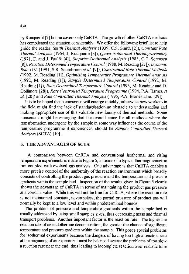
430

by Rouquerol [7] but he covers only CnRTA. The growth of other CaRTA methods has complicated the situation considerably. We offer the following brief list to help guide the reader: Smith Thermal Analysis (1939, C.S. Smith [2]), Constant Rate Thermal Analysis (1964, J. Rouquerol [3]), Quasi-isothermal Thermogravimetry (1971, F. and J. Paulik [4]), Stepwise Isothermal Analysis (1983, O.T. Sorensen [8]), Reaction Determined Temperature Control (1988, M. Reading [27]), Dynamic Rate TGA (1991, S.R. Sauerbrunn et al. [9]), Constrained Rate Thermal Methods (1992, M. Reading [ 1 ]), Optimising Temperature Programme Thermal Analysis (1992, M. Reading [1 ]), Sample Determined Temperature Control (1992, M. Reading [1 ]), Rate Determined Temperature Control (1993, M. Reading and D. Dollimore [28]), Rate Controlled Temperature Programme (1994, P.A. Barnes et al. [20]) and Rate Controlled Thermal Analysis (1995, P.A. Barnes et al. [29]).

It is to be hoped that a consensus will emerge quickly, otherwise new workers in the field might find the lack of standardisation an obstacle to understanding and making appropriate use of this valuable new family of thermal methods. Some consensus might be emerging that the overall name for all methods where the transformation undergone by the sample in some way influences the course of the temperature programme it experiences, should be Sample Controlled Thermal Analysis (SCTA) [10].

5. THE ADVANTAGES OF SCTA

A comparison between CnRTA and conventional isothermal and rising temperature experiments is made in Figure 5, in terms of a typical thermogravimetric run coupled with evolved gas analysis. One advantage is that CnRTA enables a more precise control of the tmiformity of the reaction environment which broadly consists of controlling the product gas pressure and the temperature and pressure gradients within the sample bed. Inspection of the results given in Figure 5 clearly shows the advantage of CnRTA in terms of maintaining the product gas pressure at a constant value. While this will not be true for CaRTA, where the reaction rate is not maintained constant, nevertheless, the partial pressure of product gas will normally be kept to a low level and within predetermined bounds.

The problem of pressure and temperature gradients within the sample bed is usually addressed by using small samples sizes, thus decreasing mass and thermal transport problems. Another important factor is the reaction rate. The higher the reaction rate of an endothermic decomposition, the greater the chance of significant temperature and pressure gradients within the sample. This poses special problems for isothermal experiments because the dangers of having too high a reaction rate at the beginning of an experiment must be balanced against the problems of too slow a reaction rate near the end, thus leading to incomplete reaction over realistic time

431

scales. Linear rising temperature experiments pose a similar problem. With this type of experiment, the rate goes through a maximum near the midpoint of a reaction step. Adjusting the heating rate to limit this maximum can also give rise to tmrealistically long experiments. Once a rate is chosen that is sufficiently low to avoid excessive temperature gradients, CnRTA ensures that the experiment will take the minimum possible time compatible with obtaining undistorted results. Thus CnRTA and other forms of SCTA are eminently practical approaches.

Isothermal Temp. CnRTA Ramp

Temp.

Mass

t

Partial Pressure

0 0 0 Time

Figure 5. Course of temperature, mass and partial pressure of product gas as a function of time for different methods

Because SCTA, and in particular CnRTA, enable much better control of the sample environment, making it possible for uniform conditions to exist throughout the sample bed, it is a very good preparative method for porous or finely divided solids that are prepared by thermal decomposition. Rouquerol [30] has illustrated the profound effect product gas pressure can have on the surface area of the decomposition products of gibbsite. Changing the pressure above the sample from 0.0002 to 5 Torr changed the surface area of the product by about two orders of magnitude at any point in the decomposition. While this was already known in general terms, Rouquerol's work illustrates well how CnRTA can be used to exert a much greater degree of control over the reaction environment and consequently over the properties of the decomposition product. Stacey revealed a similar effect with his experiments on the preparation of catalysts [31 ]. He found that changing

432

the partial pressure of water from 658 to 2150 Pa when decomposing zinc hydroxide had a significant affect on the surface area, pore size and mean crystallite size of the product. Barnes et al. also confirmed the benefits of CnRTA for catalyst preparation [20]. Criado and coworkers have made observations on the effect of preparation conditions under CnRTA conditions on the products of mixed oxalate decompositions in terms of particle size, crystal state and dielectric properties [32,33].

For the same reasons cited above, CnRTA and other forms of SCTA avoid artefacts that stem from having a non-uniform sample environment, such as artificial broadening of the temperature interval over which a reaction occurs, and is consequently also to be preferred for measuring kinetic parameters. This is discussed in more detail below.

A common feature of heterogeneous decomposition reactions is that the reaction rate can be controlled by the rate of diffusion of the gaseous product from the reaction interface because it finds its access to the external environment restricted by the intervening layer of already reacted material. Whether the diffusion step is the rate limiting one will generally depend upon the rate of gas evolution. Stacey has pointed out [15] that by controlling reaction rate using CnRTA it is possible to move progressively from a diffusion controlled regime to one where the interface geometry is the governing factor.

Another advantage of CnRTA and other types of SCTA is that they often improve resolution for an experiment of a given duration [5, 9, 29]. Using a linear temperature ramp, there is a gradual increase in the reaction rate as the reaction starts and then a gradual decrease as it finishes. In contrast, the start of a reaction under CnRTA is often marked by an abrupt change from a steeply rising temperature to an almost isothermal plateau (this depends upon the reaction mechanism, but such behaviour is frequently encountered, see reference [5]). The end of the reaction is similarly well delineated because the temperature rises exponentially. Furthermore, by decreasing the heating rate as the reaction rate accelerates, the temperature window within which the decomposition occurs is narrowed. For both of these reasons, the ability of CnRTA to resolve the different steps clearly in multi-step processes generally appears much better than is possible using conventional methods for a similar, total elapsed time for the experiment. Whether this improvement in resolution is genuine has been questioned by Criado [34] after making comparisons based on mathematical simulations. In reality this point has not been studied systematically and merits more attention. However, inspection of the available literature does seem to support the assertion that resolution is improved.

433

In summary, it can be seen that CaRTA, and m particular CnRTA, provide a number of advantages. Because these methods enable a greater control over the reaction environment they provide: (i) results that are less liable to contain artefacts due to inhomogeneous reaction throughout the sample bed; (ii) the ability to pass from a diffusion controlled regime to one determined by the geometry of the reaction interface in a controlled manner; (iii) better kinetic data; and (iv) better defined preparative conditions for porous or finely divided solids. Because CaRTA and CnRTA allow reactions to occur in a much narrower temperature window and clearly delineate the beginning and end of a reaction, they generally provide: (v) better resolution for a given duration of experiment.

The above discussion has been principally concerned with constant rate thermal analysis, i.e. methods which follow the schematic given in Figure 2. In part this is because this method has been most often used to date, having been developed first. The maintenance of a constant rate also ensures that the partial pressure of product gas is more precisely controlled than the alternative CaRTA approaches. The question must then be asked: what are the reasons one might wish to depart from this and opt for control algorithms that are based on the schematic given in Figure 3 ? One possibility is that using CnRTA is difficult to achieve in practice for the high reaction rates which are desirable in industrial laboratories to achieve a fast throughput of samples. The dynamic rate method can offer a workable approach that significantly improves resolution while decreasing experimental time. While possible in principle, it is difficult, in this author's experience, in practice, to perform properly controlled CnRTA at speeds that would give results in a comparable time.

A more fundamental reason is that, for a given length of experiment, CnRTA may not be the best way ofmaximising resolution. If maximum resolution is the required outcome, then concerns about maintaining the evolved gas at a constant pressure are secondary (or irrelevant if the process being considered does not involve the evolution of a gas). If a two-stage reaction is considered, then, as Reading has pointed out [1 ], it might be that the maximum time, i.e. the slowest heating rate, should be spent during the transition from one stage to the other. This is opposite from what is normally encountered with CnRTA, where the heating rate usually decreases during a reaction and increases as it passes between one step and another. To implement an algorithm that slows down the heating rate between successive reaction steps requires that the rate of change of temperature be taken into account. Simply monitoring the sample response without the sample temperature could not produce the desired result. Such a system must conform to the schematic shown in Figure 3 and thus fall outside of the current definition of CnRTA, but within the proposed definition of CaRTA (hence Reading's proposal with regard to nomenclature [1 ]). Modem microprocessor-based controllers permit very complex

434

strategies to be adopted to achieve specific results for a given type of system. There is no absolute requirement that any single parameter be held at a constant value, especially in homogeneous systems.

We do not, as yet have a proper theory of how the question of maximising resolution should be approached. Some further comments on this topic will be made in the 'Future Prospects' section below.

6. KINETIC ASPECTS

The kinetics of solid state reactions, such as those to which CnRTA methods are usually applied, is a problematic field. An extensive review [35] has commented that "the kinetic parameters most frequently used to provide information about the (reaction) step identified as rate limiting are A and E~. Values for nominally the same chemical change often show significant deviations ". Because of the precise control that CnRTA offers over the reaction environment, this is the preferred technique for kinetic studies and offers a solution to the problems summarised in the above quotation. A particularly powerful means of measuring activation energies is the rate jump method. It is illustrated in Figure 6 for calcium carbonate. The reaction rate jumps between two preset values and the corresponding temperature jump is measured. Equation (1) gives the general expression used to describe solid state reactions:

dtr/dt = f(tr) A exp(- EJRT) (1)

where tr = fractional extent of conversion; f(tr)= some fimction of extent of conversion; A = the pre-exponential constant; E~ = the activation energy; R = the gas constant, and T = the absolute temperature.

A small interpolation is made and the values of the temperatures immediately before and after the rate jump are taken together with the two different rate values.

Assuming that dtr/dt o, dM/dt, where M is the sample mass, it can be shown from equation (1) that (see Figure 6):

E~ - - R T(1) T(2) ln[dM/dt(1) / dM/dt(2)]/[T(2)- T(1)] (2)

The advantage of this method is that E, is determined independently of any assumptions regarding the form of f(tr). The pressure remains precisely controlled both before and after the rate jump. In many respects this approach can be considered as the most reliable method of measuring activation energies provided that the interpolation procedure can be considered accurate. This should generally be true when the degree of advancement of the reaction is small during the course

435

d M / d t ( 2 ) ~ ,

Thermocouple Signal

..-"" Time

Figure 6. Illustration of the Rate Jump Method

of the rate jump and re-establishment of the control regime. Many methods require a series of experiments at different isothermal temperatures or at different ramp rates [28] and these may be influenced by sample to sample variations. Methods that use a single non-isothermal experiment have been shown to be unreliable [25,28,36]. The rate jump method overcomes all of these problems and offers advantages over the temperature jump equivalent, because (i) the partial pressure of product gas is controlled, and (ii) there is very little error in the interpolation of temperature, whereas the errors associated with interpolation of reaction rate can be large. There is also the advantage that apparent changes in Ea can be determined as a fimction of

Reading et al. [37] demonstrated that the rate jump method under high vacuum gave values for Ea that were insensitive to sample mass and rate jump ratio for calcium carbonate. This was followed by an equivalent study by Ortega et al. [38, 39] which demonstrated this was also tree for dolomite. This suggests that the value for E a measured by this method does characterise the fimdamental chemical reaction rather than experimental conditions that are dependent upon thermal and mass transport. It has, therefore, been demonstrated that the theoretical advantages of the rate jump method do translate into real practical benefits.

436

Reading et al. [36,37], from their own measurements and from a critical review of the literature, concluded that, although the rate jump method was the most reliable approach, it was possible to obtain the correct value for the activation energy for the thermal decomposition of calcium carbonate using isothermal and rising temperature experiments. Ortega et al. [38,39] concluded that this was not the case for dolomite. In reality the position that only CnRTA measurements can provide good values for kinetic parameters is not tenable. However, more comparative studies are required to resolve the question of what approaches should be used with conventional temperature programming methods for kinetic studies.

One factor that plays a crucial role in determining the values of the measured kinetic parameters is the pressure of product gas in the sample environment. Reading and co-workers [36] demonstrated, using theoretical arguments and data gathered from the literature, that high product gas pressures lead to artificially high values for Ea for reversible reactions. These workers also pointed out [1] how this was relevant to the work of Paulik and co-workers because the their quasi-isobaric methods inevitably lead to high product gas pressures and consequently cannot be used for kinetic measurements. Criado et al. [40], using the relationship derived by Reading and co-workers [36], later illustrated this point very clearly using numerical simulations. They demonstrated that the insensitivity of reaction rate to temperature under quasi-isothermal conditions was due to the mechanism presented in [36]. A consequence of this is that using high product gas pressures can improve separation between successive reaction steps.

A further advantage of the CnRTA method is the possibility of using the reduced temperature master plots for determining f(cr) [27]. The most commonly used kinetic expressions fall into three categories (see Chapter 3). The first includes models that assume the formation of sparse nuclei that grow, resulting in an accelerating reaction rate, then merge. These expressions are known as Avrami- Erofeev equations. The second assumes that the surface is rapidly covered with diffuse overlapping nuclei and then the reaction interface proceeds through the sample particle. These are known as order, or geometric expressions and are of the form

f(cr) = (1- or)"

where n is the order. The third category assumes diffusion to be the rate limiting process. The reduced temperature is calculated as follows. Taking T0.9 to be the temperature at a = 0.9 and T0.3 to be the temperature at or= 0.3, we may write:

(1/T~- 1/To.9) / (1/To.a- 1/To.9) = [In f(tr) - In f(0.9)] / [In f(0.3) - In f(0.9)]

437

so that

(a- T.) b / aT~ = [In f(tr) - q] / d

where a = T0.9, b = (T0.9 - T0.3) / T0.9 T0.3, q = In f(0.9) and d - [ln f(0.3) - In f(0.9)] are all constants. Thus, in a similar manner to the well-known reduced time plots (see Chapter 3), a series of reduced temperature master plots of f(a 0 - q/d against a~ can be drawn as illustrated in Figure 7. While it is not possible to distinguish between different order expressions using this method, it does provide a means of distinguishing between the different categories of mechanism more sensitively than conventional techniques [27]. If a reaction is found to follow an order expression, the exact order, n, can be established once the rate jump method has been used to determine the activation energy as detailed below. Criado has also proposed a series of'master plots' [41,42], but these require a knowledge of E~.

An alternative approach to analysing CnRTA results is to invoke the relationship

-ln[f(a0] = ln(A/C) - E , / R T

where C = a constant reaction rate. A plot of the left hand side of this equation against 1/T should give a straight line with a slope of- E , / R , thus enabling both Ea and f(a~) to be determined. For reaction order expressions the slope is - E , / R n where n is the order. Consequently, n can be determined if Ea is known (as from rate jump experiments, see above).

A possible approach could be to plot a range of fimctions and decide on the correct one by some test of linearity [43-48]. One obvious shortcoming is the inability of this method to distinguish between order expressions with different values of n. However, the problem is greater than this. Such an approach has been shown to be unreliable [36,49] because of experimental uncertainties and the possibility that the appropriate function is not amongst those tested for. The CrRTA method of Criado [24-26], where the reaction rate is increased linearly with time, offers a method of increasing discrimination. However, there would seem little point to pursuing these more elaborate approaches when the rate jump methods can be used to determine E~ and this then largely resolves any problem of discriminating between candidate conversion functions, f(a).

There remains a more fimdamental problem in identifying the 'true' f(a 0. A careful study by Reading et al. [36] on calcium carbonate failed to reveal a unique f(a0. It appeared to change with experimental conditions even when CnRTA was used. There has as yet been no similar follow-up study on other compounds. However, Rouquerol et al. [50] have shown that the f(a) for the dehydration of Li2SO4.H20 changes with water vapour pressure. Consequently, while there is good evidence

438

that we can determine a value for E~ that is independent of sample size and particle size and may therefore be considered to be the true activation energy, we have no similar body of evidence to say that we can determine a unique f(a~). Further work on this question is urgently required.

12]

0.6"

0.0

1.2.

~ 0.6 ~ .

~ 0.0

4.0

2.0

0.0

Diffusion Equations

0.2 0.6 1.0

Extent of Reaction

Figure 7. Reduced temperature plots for various conversion fimctions, f(a~).

439

In conclusion it should be noted that CnRTA offers significant advantages in studying decompositions of solids to form solid plus gas. The more widespread use of low pressure CnRTA could resolve many of the current problems in the field of the kinetics of solid state decompositions.

7. PROSPECTS FOR THE FUTURE

Figure 3 provides a very general schematic, and Figure 4 gives examples of only two, stepwise and dynamic rate, of a potentially infinite range of algorithms. The question is: what principles will guide the development of future approaches? We propose that one important line of development will be algoritbans that, when considering the rate of transformation, look at peak shape rather than peak height. The CaRTA and CnRTA methods considered above use one or two set values, or a smooth function of some measure of reaction rate, as the targets or threshold values in the control algorithm. An alternative approach is best illustrated by an example. During a conventional linear rising temperature programme the profile of an EGA experiment might well look, to a first approximation, like a Gaussian peak (as would the differential of a mass loss curve). This is illustrated in Figure 8, along with the first and second differentials. In the CaRTA or CrRTA approaches so far proposed, the temperature profile that would result from such a reaction would depend upon the height and the threshold values selected for the Ca/rRTA control algorithm. An alternative [51] would be to start the experiment using a preselected heating rate, then decrease it when the first and second differentials became positive and negative, respectively. The heating rate could be increased again, when the derivatives became negative and positive, respectively. (Following the proposal by Reading [ 1 ], an altemative would be to switch from a faster to a slower heating rate, then back to a faster heating rate in order to heat slowly between reaction steps). The important difference between this and current methods is that the response would then be the same, regardless of the peak height. It is the peak shape that is important.

This method is offered as a simple example of this new approach. Much more sophisticated methods are possible based on this peak shape concept. When improvements in resolution for short experimental times are what is being sought, this type of approach has advantages as it would avoid too long a time being spent on large peaks as a consequence of a threshold or target value being set too low or small peaks being missed because of a target or threshold value being set too high. Most decompositions do not have a Guassian response but equivalent approaches can be devised for skewed Gaussian and other functions.

440

P e a k

Hieght

First Derivative

- v e

Temperature

Second Derivative

+ v e I - v e I - v e I + v e

Figure 8. Illustration of a possible 'peak shape recognition' CaRTA algorithm.

8. CONCLUSIONS

There are a growing number of techniques where the temperature to which the sample is subjected is influenced in some way by the measured sample response. The earliest examples of this approach sought to keep the rate of any transformation that the sample undergoes at a constant or near constant rate. The advantages include improvements of resolution, better kinetic data and better control when preparing porous material by decomposition. Later approaches were more flexible and complex algorithms can be used mainly to improve resolution. It is encouraging that these techniques are becoming commercially available and there are more examples of these approaches being applied to a wider variety of thermal methods.

441

REFERENCES

1. M. Reading, Thermal Analysis - Techniques and Applications, Eds. E.L. Charsley and S.B. Warrington, Royal Society of Chemistry, Cambridge, 1992, Chapter 7.

2. C.S. Smith, Trans. Am. Inst. Min. Metal. Eng., 177 (1940) 236. 3. J. Rouquerol, Bull. Soc. Chim. Fr., (1964) 31. 4. a) L. Erdey, F. Paulik and J. Paulik, Hungarian Patent No. 152197, (1962).

b) J. Paulik and F. Paulik, Anal. Chim. Acta, 56 (1971) 328. 5. F. Paulik and J. Paulik, Thermochim. Acta, 100 (1986) 23. 6. J. Rouquerol, J. Thermal Anal., 2 (1970) 123. 7. J. Rouquerol, Thermochim. Acta, 144 (1989) 209. 8. O. Toft Sorensen, Thermochim. Acta, 50 (1981) 163. 9. S.R. Sauerbrtmn, P.S. Gill and B.S. Crowe, Proceedings of 5th ESTAC,

(1991) O-6. 10. P.A. Barnes, M. Reading and J. Rouquerol, in preparation. 11. M.E. Thomas, S.P. Terblanche, J.W. Stander, K. Gilbert, L.P. Nortman and

N.A. Stone, Proceedings of the International Ceramics Conference 94, International Ceramics Monographs, Eds. C.C. Sorell and A.J. Ruys, 1 (1994) 281.

12. M. Ganteaume and J. Rouquerol, J. Thermal Anal., 3 (1971) 413. 13. G. Thevand, F. Rouquerol and J. Rouquerol, Thermal Analysis, Ed. B.

Miller, John Wiley and Sons, New York, 1982, Vol.2, p1524. 14. J. Rouquerol, S. Bordere and F. Rouquerol, Thermochim. Acta, 203 (1992)

193. 15. M.H. Stacey, Anal. Proc., 22 (1985) 242. 16. M. Reading and J. Rouquerol, Thermochim. Acta, 85 (1985) 299. 17. M. Reading and D. Dollimore, Thermochim. Acta, 240 (1994) 117. 18. M.D. Alcala, C. Real and J.M. Criado, J. Thermal Anal., 38 (1992) 313. 19. C. Real, M.D. Alcala and J.M. Criado, J. Thermal Anal., 38 (1992) 797. 20. P.A. Barnes and G.M.B. Parkes, Proceedings of the 6th Int. Symp. on the

Scientific Bases for the Preparation of Catalysts, Louvain-la-Neuve, Ed. G. Poncelet et al., (1995) 859.

21. P.A. Barnes, G.M.B. Parkes and E.L. Charsley, Anal. Chem., 66 (1994) 2226.

22. P. Staszczuk, Thermochim. Acta, 247 (1994) 169. 23. M.J. Torralvo, Y. Grillet, F. Rouquerol and J. Rouquerol, J. Thermal

Anal., 41 (1994) 1529. 24. A. Ortega, L.A. Perez-Maqueda, J.M. Criado, Thermochim. Acta, 239

(1994) 171.

442

25.

26.

27. 28.

29.

30. 31.

32.

33.

34. 35.

36.

37.

38.

39.

40.

41.

42. 43.

44.

45. 46.

A. Ortega, L.A. Perez-Maqueda and J.M. Criado, J. Thermal Anal., 42 (1994) 551. A. Ortega, L. Perez-Maqueda and J.M. Criado, Thermochim. Acta, 254 (1995) 147. M. Reading, Thermochim. Acta, 135 (1988) 37. D. Dollimore and M. Reading, Treatise on Analytical Chemistry, Ed. J.D. Winefordner, 13 (1993) 1. P.A. Barnes, G.M.B. Parkes, D.R. Brown and E.L. Charsley, Thermochim. Acta, 269/270 (1995) 665. J. Rouquerol and M. Ganteaume, J. Thermal Anal., 11 (1977) 201. M.H. Stacey, Proceedings of the 2nd ESTA, Ed. D. Dollimore, Heyden, London, 1981, p408. J.M. Criado, J.F. Gotor, C. Real, F. Jimenez, S. Ramos, J. Del Cerro, Ferroelectrics, 115 (1991) 43. J.M. Criado, F.J. Gotor, A. Ortega and C. Real, Thermochim. Acta, 199 (1992) 235. J.M. Criado, A. Ortega, F.J. Gotor, Thermochim. Acta, 203 (1992) 187. D. Dollimore, M.E. Brown and A.K. Galwey, Reactions in the Solid State, Comprehensive Chemical Kinetics, Vol. 22, Elsevier, Amsterdam, 1980. M. Reading, D. Dollimore and R. Whitehead, J. Thermal Anal., 37 (1991) 2165. M. Reading, D. Dollimore, J. Rouquerol and F. Rouquerol, J. Thermal Anal., 29 (1984) 775. A. Ortega, S. Akhouatri, F. Rouquerol and J. Rouquerol, Thermochim. Acta, 163 (1990) 25. A. Ortega, S. Akhouayri, F. Rouquerol and J. Rouquerol, Thermochim. Acta, 235 (1994) 197. J.M. Criado, A. Ortega, J. Rouquerol and F. Rouquerol, Thermochim. Acta, 240 (1994) 247. J.M. Criado, L.A. Perez-Maqueda and A. Ortega, J. Thermal Anal., 41 (1994) 1535. J M Criado, J. Thermal Anal., 1 (1980) 145. J.M. Criado, F. Rouquerol and J. Rouquerol, Thermochim. Acta, 38 (1980) 117. J.M. Criado, F. Rouquerol and J. Rouquerol, Thermochim. Acta, 38 (1980) 109. J.M. Criado, Mater. Sci. Monogr., 6 (1980) 1096. J.M. Criado, Proceedings of the 6th ICTA, Ed. H.G. Wiedemann, Birkh~iuser, Basel, 1 (1980) 145.

443

47. F. Rouquerol, J. Rouquerol, G. Thevand and M. Triaca, Surf. Sci., 162 (1985) 239.

48. J.M. Criado, A. Ortega, J. Rouquerol and F. Rouquerol, Bol. Soc. Esp. Ceram. Vidrido, 26 (1987) 3.

49. A. Ortega, S. Akhouayri, F. Rouquerol and J. Rouquerol, Thermochim. Acta, 247 (1994) 321.

50. F. Rouquerol, Y. Laureiro, J. Rouquerol, Solid State Ionics, 63-65 (1993) 363.

51. M Reading, 6th European Symposium on Thermal Analysis and Calorimetry (1994) Italy, informal presentation during the CRTA workshop.


Chapter 9

LESS-COMMON TECHNIQUES

Vladimir Balek ~ and Michael E Brown b

"Nuclear Research Institute P,.e~ plc, 250 68 P,.e~, Czech Republic

bChemistry Department, Rhodes University, Grahamstown, 6140 South Africa

1. INTRODUCTION

Under the heading of "less-common techniques" come a variety of thermal methods, such as emanation thermal analysis (ETA), thermosonimetry, etc., which usually require rather specialised equipment which is often not commercially available. Because of this limitation, some applications of these techniques are illustrated in this chapter, to promote interest in their use.

2. EMANATION THERMAL ANALYSIS (ETA)

2.1. Definition and basic principles Emanation thermal analysis (ETA) [1] involves the monitoring of the release of

trapped inert (usually radioactive) gas from a sample, while the temperature of the sample, m a specified atmosphere, is programmed. The rate of release of inert gas is used as an indication of the changes taking place as the initially solid sample is heated. Gas release is controlled by physico-chemical processes in the solid, such as structural changes, interaction of the solid sample with the surrounding medium, and the establishment of chemical equilibrium in the solid.

ETA is, strictly speaking, not a method of analysis. The inert gas release is used for the characterization of the solid state. Both radioactive and nonradioactive (stable) inert gas isotopes can be used, although radioactive isotopes are more useful because they can be detected simply and with high sensitivity.

2.2. Sample preparation for ETA Most of the solids to be investigated by ETA do not naturally contain inert gas and

it is necessary to label them with a trace amount of the inert gas. Various techniques

446

can be used for the introduction of the inert gas atoms into the samples to be investigated [1,2].

2.2.1 Diffusion technique: This is based on the diffusion of the inert gas into solids at elevated temperatures and high pressures of the gas. The substance to be labelled and the inert gas (usually labelled with radioactive nuclides, e.g. 85Kr) are placed in a high-pressure vessel which is then closed and heated for several hours at a temperature of approximately 0.3 to 0.5 Tmo~t of the substance to be labelled, and finally quenched in liquid nitrogen. The amount of inert gas introduced into the sample depends upon the time, the temperature and the pressure, as given by diffusion theory.

2.2.2. Physical vapour deposition (PVD): The sample preparation is carried out in an inert gas (argon, krypton) atmosphere. The inert gas atoms are captured in the structure of the deposited substance. In this method, the thin films produced are automatically labelled by the inert gas, the release of which can be used for diagnostics of the film during its subsequent heating.

2.2.3. Implantation of accelerated ions of inert gases: The amount of inert gas introduced and its concentration profile depends on the energy of ion bombardment and the properties of the labelled matrix. Several techniques can be used for inert gas ion bombardment [1 ]. A defined ion beam can be produced using a magnetic separator. A versatile low-cost technique for sample labelling was invented by Jech [3] (see also reference [1]) in which the ionisation and acceleration of ions take place in a low-temperature plasma produced by a high-frequency discharge.

2.2. 4. Inert gases produced from nuclear reactions: The recoil energy of nuclear reactions which produce inert gases can be used for the implantation of gases into solid samples. Some of the nuclear reactions which have been used for the production of inert gas atoms and their introduction into solid samples are listed in Table 1.

2.2.5. Introduction ofparent nuclides: When carrying out longer duration and/or high-temperature measurements of surface and morphology changes, it is necessary to introduce parent nuclides of the inert gas, e.g. radon, as a relatively permanent source of the labelled gas. Trace amounts of thorium 228Th can be introduced into the sample by co-precipitation during the sample preparation from a solution or by adsorption on the surface of the sample. 22~ is formed by spontaneous alpha decay according to the scheme:

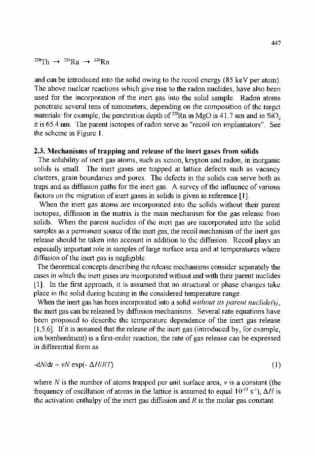
447

228Th - , 224Ra --~ 220Rn

and can be introduced into the solid owing to the recoil energy (85 keV per atom). The above nuclear reactions which give rise to the radon nuclides, have also been used for the incorporation of the inert gas into the solid sample. Radon atoms penetrate several tens of nanometers, depending on the composition of the target materials: for example, the penetration depth of 22~ in MgO is 41.7 nm and in SiO2 it is 65.4 nm. The parent isotopes of radon serve as "recoil ion implantators" See the scheme in Figure 1.

2.3. Mechanisms of trapping and release of the inert gases from solids The solubility of inert gas atoms, such as xenon, krypton and radon, in inorganic

solids is small. The inert gases are trapped at lattice defects such as vacancy clusters, grain boundaries and pores. The defects in the solids can serve both as traps and as diffusion paths for the inert gas. A survey of the influence of various factors on the migration of inert gases in solids is given in reference [1 ].

When the inert gas atoms are incorporated into the solids without their parent isotopes, diffusion in the matrix is the main mechanism for the gas release from solids. When the parent nuclides of the inert gas are incorporated into the solid samples as a permanent source of the inert gas, the recoil mechanism of the inert gas release should be taken into account in addition to the diffusion. Recoil plays an especially important role in samples of large surface area and at temperatures where diffusion of the inert gas is negligible.

The theoretical concepts describing the release mechanisms consider separately the cases in which the inert gases are incorporated without and with their parent nuclides [ 1]. In the first approach, it is assumed that no structural or phase changes take place in the solid during heating in the considered temperature range.

When the inert gas has been incorporated into a solid without its parent nuclide(s), the inert gas can be released by diffusion mechanisms. Several rate equations have been proposed to describe the temperature dependence of the inert gas release [1,5,6]. If it is assumed that the release of the inert gas (introduced by, for example, ion bombardment) is a first-order reaction, the rate of gas release can be expressed in differential form as

-dNIdt = vN exp(- AHIRT) (1)

where N is the number of atoms trapped per unit surface area, v is a constant (the frequency of oscillation of atoms in the lattice is assumed to equal 10 -13 s-I), AH is the activation enthalpy of the inert gas diffusion and R is the molar gas constant.

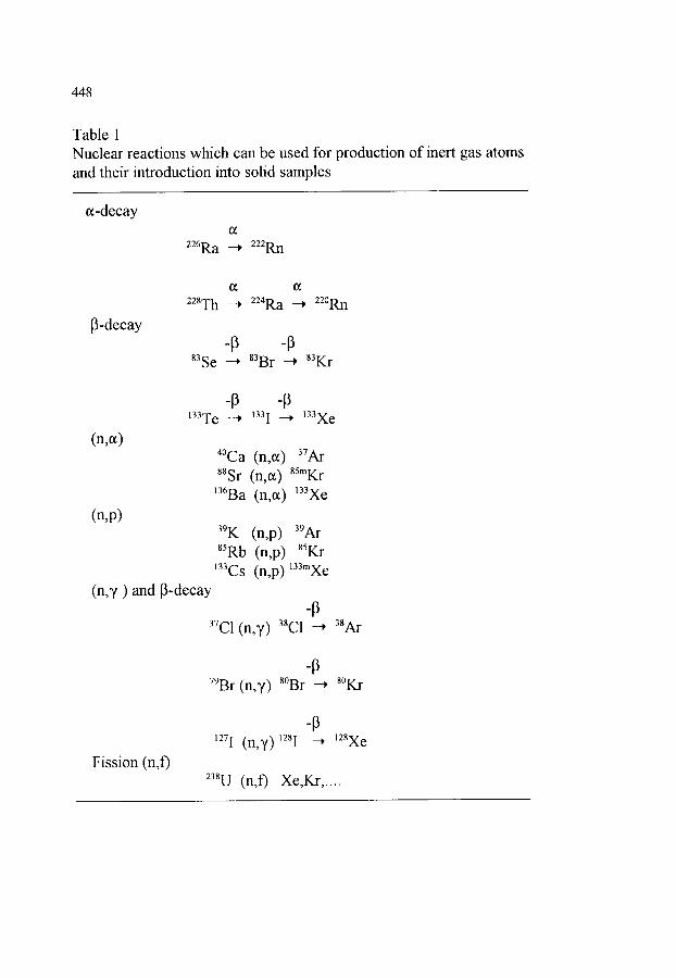
448

Table 1 Nuclear reactions which can be used for production of inert gas atoms and their introduction into solid samples

a-decay

226Ra --~ 222Rn

13-decay

228Th - , 224Ra --~ 220Rn

83Se --, 83Br --~ 83Kr

(n,a)

(n,p)

(n,y) and 13-decay

-13 -13 133Te ~ 1331 ~ 133Xe

4~ (n,a) 3TAr 88Sr (n,a) 85mK_l- 136Ba (n,a) 133Xe

39K (n,p) 39At SSRb (n,p) SSKr 133Cs (n,p)133mXe

37C1 (n,y) 3sc1 --~ 38Ar

-p 79Br (n,y) S~ ~ S~

Fission (n,f)

127I (n,y)12sI --~ 12SXe

238U (n,f) Xe,Kr,....

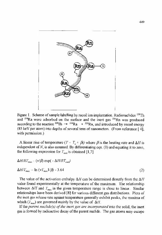
449

Figure 1. Scheme of sample labelling by recoil ion implantation. Radionuclides 228Th and 224Ra were adsorbed on the surface and the inert gas 22~ was produced according to the reaction 22STh ---* 224Ra -+ 22~ and introduced by recoil energy (85 keV per atom) into depths of several tens of nanometers. (From reference [ 4], with permission.)

A linear rise of temperature ( T - To + fit) where fl is the heating rate and AH is independent of N, is also assumed. By differentiating eqn. (1) and equating it to zero, the following expression for Tin, x is obtained [1,7]

AH/RTmax = (v/tO) exp(- AH/RTm, Q

Am/Tma x --In ( V T m a x l / t ~ ) - 3.64 (2)

The value of the activation enthalpy AH can be determined directly from the AH value found experimentally at the temperature of the maximum. The relationship between AH and Tin, x in the given temperature range is close to linear. Similar relationships have been derived [8] for various different gas distributions. Plots of the inert gas release rate against temperature generally exhibit peaks, the maxima of which (Tmax) are governed mainly by the value of AH.

If the parent nuclide(s) of the inert gas are incorporated into the solid, the inert gas is formed by radioactive decay of the parent nuclide. The gas atoms may escape

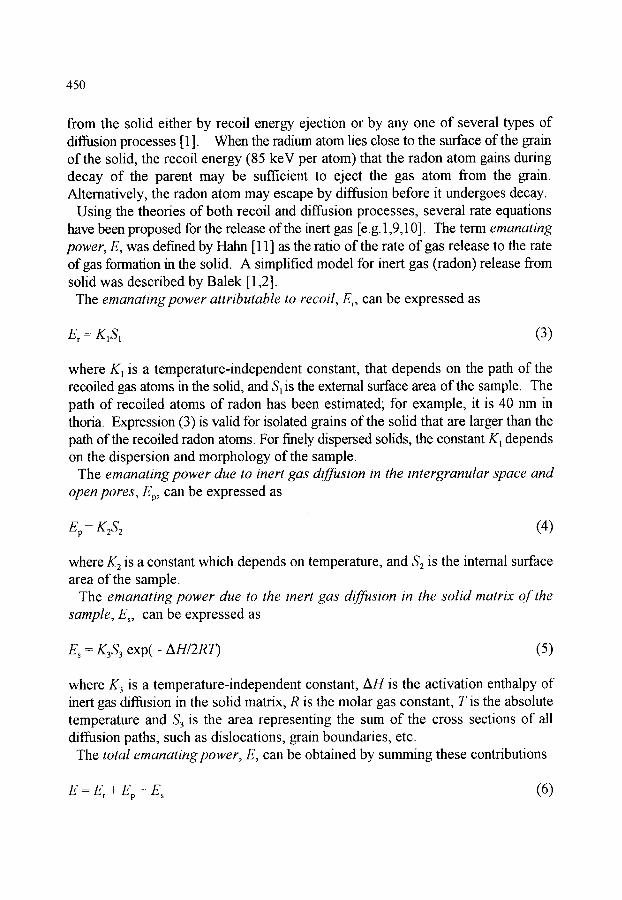
450

from the solid either by recoil energy ejection or by any one of several types of diffusion processes [1 ]. When the radium atom lies close to the surface of the grain of the solid, the recoil energy (85 keV per atom) that the radon atom gains during decay of the parent may be sufficient to eject the gas atom from the grain. Altematively, the radon atom may escape by diffusion before it undergoes decay.

Using the theories of both recoil and diffusion processes, several rate equations have been proposed for the release of the inert gas [e.g. 1,9,10]. The term emanating power, E, was defined by Hahn [11 ] as the ratio of the rate of gas release to the rate of gas formation in the solid. A simplified model for inert gas (radon) release from solid was described by Balek [1,2].

The emanating power attributable to recoil, Er, can be expressed as

E r -. K 1 S 1 (3)

where K~ is a temperature-independent constant, that depends on the path of the recoiled gas atoms in the solid, and S~ is the external surface area of the sample. The path of recoiled atoms of radon has been estimated; for example, it is 40 nm in thoria. Expression (3) is valid for isolated grains of the solid that are larger than the path of the recoiled radon atoms. For finely dispersed solids, the constant K1 depends on the dispersion and morphology of the sample.

The emanating power due to inert gas diffusion in the intergranular space and open pores, Ep, c a n be expressed as

Ep= Kz& (4)

where K 2 is a constant which depends on temperature, and $2 is the intemal surface area of the sample.

The emanating power due to the inert gas diffusion in the solid matrix o f the sample, E s, can be expressed as

Es = K3S3 exp(- AH/2RT) (5)

where K3 is a temperature-independent constant, AH is the activation enthalpy of inert gas diffusion in the solid matrix, R is the molar gas constant, T is the absolute temperature and $3 is the area representing the sum of the cross sections of all diffusion paths, such as dislocations, grain boundaries, etc.

The total emanating power, E, can be obtained by summing these contributions

E = E r + Ep + E s (6)

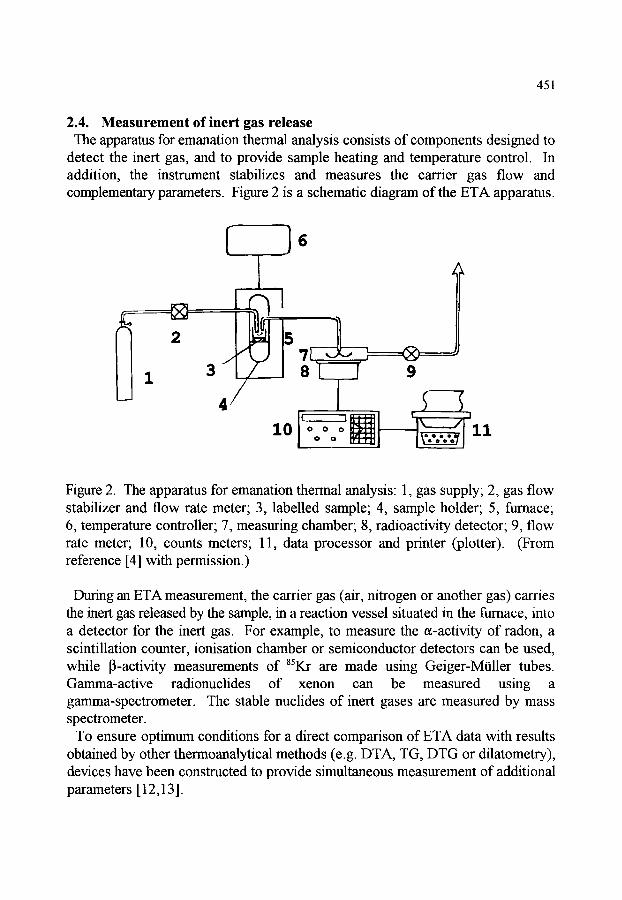
4 5 1

2.4. Measurement of inert gas release The apparatus for emanation thermal analysis consists of components designed to

detect the inert gas, and to provide sample heating and temperature control. In addition, the instrument stabilizes and measures the carrier gas flow and complementary parameters. Figure 2 is a schematic diagram of the ETA apparatus.

6

2 I [NI 15

10 ~ 1 7 6 1 7 6

___J 9 ;-U

E _1

Figure 2. The apparatus for emanation thermal analysis: 1, gas supply; 2, gas flow stabilizer and flow rate meter; 3, labelled sample; 4, sample holder; 5, fitmace; 6, temperature controller; 7, measuring chamber; 8, radioactivity detector; 9, flow rate meter; 10, counts meters; 11, data processor and printer (plotter). (From reference [4] with permission.)

During an ETA measurement, the carrier gas (air, nitrogen or another gas) carries the inert gas released by the sample, in a reaction vessel situated in the fitrnace, into a detector for the inert gas. For example, to measure the ~-activity of radon, a scintillation counter, ionisation chamber or semiconductor detectors can be used, while [3-activity measurements of 8SKr are made using Geiger-Mialler tubes. Gamma-active radionuclides of xenon can be measured using a gamma-spectrometer. The stable nuclides of inert gases are measured by mass spectrometer.

To ensure optimum conditions for a direct comparison of ETA data with results obtained by other thermoanalytical methods (e.g. DTA, TG, DTG or dilatometry), devices have been constructed to provide simultaneous measurement of additional parameters [ 12,13].

452

2.5. Potential applications of ETA The theoretical considerations summarized above indicate that emanation thermal

analysis can be applied to the investigation of processes taking place in solids or on their surfaces. Any process in a solid, or at a phase boundary, which leads to a change in either the surface and/or changes in the inert gas diffusivity (permeability) becomes observable from the ETA measurements. ETA has been used in the study of such solid state processes as aging of precipitates or gelatinous materials, recrystallisation, annealing of structure defects and changes in the defect state of both crystalline and non-crystalline solids, sintering, phase changes, surface and morphology changes accompanying thermal decomposition of solids, and chemical reactions in solids and on their surfaces, including solid-gas, solid-liquid and solid-solid interactions. Chemical reactions of practical importance for chemical technology, metallurgy and environmental technology, as well as the technology of building materials, have also been studied by means of ETA.

The kinetics of surface area changes, mechanisms of defect annealing, pore smtering and the kinetics of morphology changes in general can be evaluated from ETA results obtained under either isothermal or non-isothermal conditions.

In contrast to X-ray diffractometry, emanation thermal analysis makes it possible to investigate poorly crystalline or amorphous solids. In contrast to adsorption measurements for surface area determination, ETA permits a continuous investigation of the surface, even at elevated temperatures during heat treatment of solid samples, or their hydration under wet conditions, without the necessity of interrupting the heat treatment, or the hydration and cooling of the sample to liquid nitrogen temperatures. For this reason, ETA may reflect the nature of the surface at elevated temperatures more accurately than adsorption measurements.

In contrast to DTA and thermogravimetry, ETA makes it possible to investigate processes that are not accompanied by thermal effects or mass changes, such as sintering of powdered or gelatinous samples, which would also be difficult to investigate by means of dilatometry.

Moreover, by applying different radioactive labelling techniques of either the surface alone or the volume of solids, the processes taking place in the surface and in the bulk of the sample have been discerned by ETA. This is especially advantageous when studying the thermal behaviour of thin films or coatings on substrates. By labelling the thin film to a depth not exceeding its thickness, ETA gives information concerning the thin film alone, without the influence of the larger substrate. This is a further advantage of ETA over X-ray investigations, when the thin film represents a negligible part of the sample. When the interaction of the thin film with the substrate during heating is to be investigated, a deeper inert gas implantation has to be used.

453

The high sensitivity of ETA to the chemical interactions between a solid surface labelled with the radioactive inert gas and aggressive agents makes it possible to reveal the very beginning of corrosion reactions. The durability of materials towards aggressive liquids and gases, as well as the effectiveness of preserving coatings, can be tested by means of ETA.

The possibility of thin-film labelling by inert gases during physical deposition (PVD) or chemical vapour deposition (CVD) on a substrate can be applied for diagnostics of the thin layers, during their processing, thermal treatment and durability testing.

In addition, ETA measurements make it possible to obtain information about the diffusion parameters of the inert gas in the solid. The diffusion coefficient, D, and the activation enthalpy, AH, of the inert gas diffusion can be evaluated. The diffusion parameters of inert gases in inorganic and organic materials are important for characterization of the transport properties of materials. The determination of inert gas permeability in polymers is a possible way of testing the local structure and revealing irregularities in polymer membranes and composites.

2.6. Examples of applications of ETA 2. 6. l. Diagnostics of the defect state. Inert gas diffusion parameters evaluated from ETA measurements are an indication of the mobility of inert gases in the solids. Such information can be used to investigate the defect states in solids. Inert gas atoms incorporated into solids are situated on the natural and/or artificial defects produced, for example, by ion bombardment, neutron irradiation or mechanical treatment.

The release of the inert gases on heating the sample results from thermally stimulated processes, such as diffusion, annealing of defects, etc. The mobility of inert gas atoms in iomc crystals differs in various crystallographic directions, owing to the channelling effect. The mobility of the inert gases (indicated by the activation energy for diffusion) can be used as a parameter characterizing the defect state of an ionic crystal. Such movement may lead to the formation of the metamict phase (structure disrupted by the radioactive decay processes. The annealing of the metamict phase is indicated by a sharp ETA peak. The activation energy of inert gas release and of recrystallisation of the metamict phase can be evaluated from the peak temperature. A number of alkali metal halides, alkaline-earth metal halides and oxides, have been investigated by ETA [1,14-16].

2.6.2. Assessment of active (non-equilibrium) state of thermally decomposed powders. From the ETA curves measured during the cooling of heat-treated materials, the active state of the powders (the non-equilibrium defect state) can be assessed. The values of the activation enthalpy AH of radon diffusion in samples

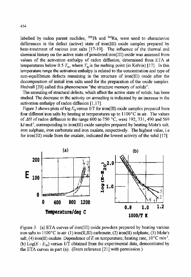
454

labelled by radon parent nuclides, 228Th and 224Ra, were used to characterize differences in the defect (active) state of iron(III) oxide samples prepared by heat-treatment of various iron salts [17-19]. The influence of the thermal and chemical history on the active state of powdered iron(III) oxide was assessed from values of the activation enthalpy of radon diffusion, determined from ETA at temperatures below 0.5 Tm, where Tm is the melting point (in Kelvin) [17]. In this temperature range the activation enthalpy is related to the concentration and type of non-equilibrium defects remaining in the structure of iron(III) oxide after the decomposition of initial iron salts used for the preparation of the oxide samples. Hedvall [20] called this phenomenon "the structure memory of solids".

The annealing of structural defects, which affect the active state of solids, has been studied. The decrease in the activity on annealing is indicated by an increase in the activation enthalpy of radon diffusion [1,17].

Figure 3 shows plots of log EDversus 1/T for iron(III) oxide samples prepared from four different iron salts by heating at temperatures up to 1100 ~ in air. The values of A l l of radon diffusion in the range 600 to 750 ~ were 192, 331,490 and 569 kJ mol l, corresponding to iron(III) oxide samples prepared by heating Mohr's salt, iron sulphate, iron carbonate and iron oxalate, respectively. The highest value, i.e for iron(III) oxide from the oxalate, indicated the lowest activity of the solid [17].

(a) (b)

200

E lOO . . . . / / /

2 / " ~ ~ .~ ~ I , ,

0 400 800 1200 Teeperature/deq C

^ 2 0 0 ~ N

M I

M

mlO 0 " ,.4

1

0.8

L

2

1.0 1.2 1000/ 1(

Figure 3. (a) ETA curves of iron(III) oxide powders prepared by heating various iron salts to 1100~ in air: (1) iron(II,III) carbonate; (2) iron(II) sulphate; (3) Mohr's salt; (4) iron(II) oxalate. Dependence of E on temperature; heating rate, 10 ~ min -1. (b) Log(E- E20 ) versus 1/T obtained from the experimental data, demonstrated by the ETA curves in part (a). (From reference [21] with permission.)

455

2. 6. 3. Changes m surface and morphology of solids. The changes taking place in the surface and morphology of powdered and gel solids have been investigated by means of ETA. It was shown during investigation of the sintering of finely dispersed Cu, NiO, MgO, Fe203, TiO2, alumina and other solids that ETA is a powerful tool for the study of sintering, especially in its initial stage [22-24]. Good agreement between the ETA data and those obtained by traditional adsorption measurements on finely dispersed solids was obtained later. Gel materials such as silica gel, urania, titania and other materials prepared by the so-called "sol-gel" technique, were investigated by ETA during their drying, recrystallization or sintering [25-28]. Differences in the behaviour of the urania xerogels caused by different concentrations of gelation additives, various means of drying, by ageing, etc., have been determined by ETA [26].

The kinetic par~eters for sintering of thorium oxide powder were determined from ETA experiments. Figure 4 shows the isothermal ETA curves for initial sintering of thorium oxide powder in the range 660 to 825 ~ [29].

60

20 i \ ~

,0

(a)

7O5

1

E = .- j / ,

1 I

20 Time/min

/

I I

40 60

i

t~ 0 ,-I

.5

I.C

0.5

(b)

~ . . 9L ~k

0.5 1.0 1.5 2.0

Iog(t/min)

Figure 4. ETA curves of thoria powder (from the oxalate) measured during isothermal heating in air at 705, 735, 780 and 825~ (a) E versus time. (b) Log(E - E20) versus log(time). (From reference [21] with permission.)

456

The results obtained could be described by the kinetic expression

log S~f~ = n log t + constant (7)

where n = 0.64 and S, ff is the surface area indicated by the radon diffusion in the respective temperature range.

ETA was also used for determination of densification temperatures of thin layers deposited on glass plates [30].

2.6. 4. Structure transformations. ETA has been used by a number of workers [29-31] to study the changes in structure taking place during heating and cooling of solids. During systematic investigations of nitrates, sulphates, and other salts it was shown that the temperature intervals of phase transitions of the first and second order (from the thermodynamic viewpoint) may be determined by ETA [1 ].

ETA has also been used for characterization of structural alterations in coals [34] and other minerals [35], e.g. differences in the thermal behaviour of calcite and aragonite, goethite and lepidocrocite, etc.) [36]. The high sensitivity of the method to changes in the surface layers of samples has been used to advantage in the characterization of altered (weathered) minerals.

The differences between the surface and volume stages of crystallization and melting were demonstrated on ETA curves, e.g. the crystallization and melting of glasses [37,38] in PbO-SiO2 and Ge-Se-Te systems.

In a study of processes for immobilization of nuclear waste by vitrification [39], ETA indicated interactions of vitrified nuclear waste with waters during samples leaching. Products of the early hydrolytic corrosion were also characterized by ETA.

2. 6. 5. Dehydration and thermal decomposition of salts and hydroxides. Numerous studies where ETA has been used to investigate the thermal decompositions of hydroxides, carbonates, oxalates, nitrates, sulphates, and other salts have been reported [21,40,41]. The existence of metastable phases formed during the decomposition of solids was revealed and the thermal stability of these phases was characterized by ETA. ETA has also been used for the assessment of the active stage of solids, prepared by the decomposition of various salts and hydroxides [32].

The use of ETA in the construction of phase diagrams for KC1-CaC12, CaO-Fe203, NaBeF3-NaPO3, NaBeFa-KPO 3 and pyrophosphoric acid-carbamide systems [42-44] should be mentioned. ETA may be used successfully for determining the phase diagrams of poorly crystalline or glass-like systems, where traditional methods do not provide satisfactory results.

457

2.6. 6. Solid-gas reactions. The kinetics of the reaction

NiO(s) + H2(g ) ~ Ni(s) + H20(g)

were investigated by means of ETA, using 222Rn for labelling of the NiO [45]. During heating of NiO in hydrogen, a peak appears on the ETA curve between 230 and 300~ A similar peak of water release was simultaneously recorded by a katharometer. ETA is especially useful for studying gas-solid reactions with industrial gases such as hydrocarbons, where the gaseous products of the reactions can hardly be detected.

The surface oxidation of metallic copper labelled by 85Kr was studied by Chleck and Cucchiara [46] and the reaction rate, reaction order, concentration and temperature dependence were determined. It was shown that oxidation during friction wear can be assessed by comparing 85Kr losses in air and in an inert atmosphere. Matzke [47] used ~33Xe release measurements to establish the temperature dependence of the growth of oxide layers on stainless steel, Ti, Ni, Cu and alpha-brass. 40 kV Xe ion bombardment was used for labelling the metals.

Catalytic reactions on ZrO2 arid MgO surfaces were investigated by means of ETA by Zhabrova et al. [48]. The catalytic reaction and the subsequent regeneration of the catalyst are accompanied by inert gas release. The reaction of hydrogen-oxygen mixtures on platinum foil labelled by 222Rn was studied by Jech [49]. ETA measurements carried out by Beckman and Teplyakov [50], in the course of various catalytic reactions on A1203, supported theoretical considerations about the selectivity of the active centres in the surface of the catalysts.

2.6.7. Solid-liquid reactions. The hydration reactions of tricalcium silicate, 3CaO.SiO2 and various cements [51,52] with water vapour present in air and also in the liquid phase were investigated by ETA. Figure 5 shows ETA results obtained during the hydration of Portland cement (PC-400) in water (w/c = 0.3) under isothermal conditions at 35, 45 and 65 ~ The reactivity of the cement towards water can be determined by ETA in the early stage of the interaction. Moreover, the changes of surface and morphology taking place in the hydration products of cement have also been investigated by this method [52].

For tricalcium silicate, the effects on hydration of activation of the solid by heating and subsequent cooling and by the presence of various additives were investigated [51]. For cement hydration [52], ETA results obtained at different temperatures were compared with consistometric and calorimetric measurements. ETA can used in the study of surface hydration where calorimetric and consistometric measurements were not sensitive enough. ETA also permits the investigation of changes in the microstructure of a cement paste, i.e., when the size of the micropores

458

is comparable to the size of radon atoms (d = 0.4 nm). Good agreement between ETA results and adsorption measurements was found. In general, ETA [52] is a method suitable for the characterization of the reactivity of cement under various technological conditions.

E

3

2

1

0 - j ~ ~ , ~ ~ . , ~ ~ ~ _

I0 I00

Time/min Figt, re 5. ETA curves of Portland cement-water suspension (w:c = 0.3) measured during isothermal heating at 35~ (curve 3), 45~ (curve 2) and 65~ (curve 1). (From reference [21 ] with permission).

ETA has been used for the study of solid-gas and solid-liquid reactions involved in corrosion. Radioactively labelled surfaces are sensitive to all chemical influences that cause changes in the surface. Many of the current methods used to evaluate anti-corrosive or protective agents are unreliable and may take several months to complete. ETA measurements make it possible to carry out such investigations relatively quickly and simply. Traces of corrosion of glasses, building materials and metals imperceptible to the human eye can be demonstrated [1,53,54] within a few minutes or hours. This method is suitable primarily for comparative measurements of various substances.

2.6.8. Solid-solid reactions. A number of reactions between solid powders, e.g. ZnO-Fe203 [55], BaCO3-TiO2, BaSO4-TiO2 [56], have been studied by means of ETA. A systematic study [55] of the ZnO-Fe203 system demonstrated that ETA can

459

be used advantageously for the investigation of the initial stage of the reaction, the bulk reaction and the formation of the structure of the ferrites. DTA, dilatometry and X-ray diffraction were not sensitive enough to detect the initial reaction stage. The high sensitivity of ETA towards reaction between powders permits the determination of the reactivities of the components of the reaction mixtures. The reactivities of iron(III) oxide samples with various chemical and thermal histories, determined by ETA [57], agreed well with the results of other experimental techniques.

ETA revealed differences m the reactivities of commercial iron(III) oxide samples pronounced as being identical by the producer when using surface area measurements [58]. The difference in the reactivities was checked by the ETA during heat treatments of reaction mixtures corresponding to the technological conditions of ferrite manufacture [21 ]. The ETA curves for two commercial samples of iron(III) oxide of the same surface area (2.6 m 2 g-l) are shown in Figure 6. ETA was recommended for industrial laboratory applications, because the information obtained on reactivity is more appropriate with respect to the solid-state reaction of ferrite production than surface area measurements by adsorption methods.

The main disadvantage of ETA is that preparation and handling of samples requires all the usual radiochemical facilities and precautions. The amounts used in samples are so small that evolved gas, after dilution with carrier, does not form a hazard. Inert gases are not incorporated biologically and the decay products are stable, so hazards are decreased.

E

3

2

0 , 0

/

(a)

/ / !

, {/ t ! I

| , J L !

400 800

T e m p e r a t u r e / d e g C

E

10 (b)

1200 0 1 2 3

Time/hours

Figure 6. ETA curves for ZnO + Fe203 (1:1) reaction mixtures. The ZnO was labelled with 228Th. For Fe203 the commercial samples: (1) 1360 WF and (2) 1360 Bayferrox were used. (a) Non-isothermal heating in air; heating rate, 5 ~ min -1. (b) Subsequent isothermal heating at 1350~ in N2 + 10% 02. (From reference [21] with permission).

460

3. THERMOSONIMETRY

3.1. Introduction Measurements of acoustic emission (AE) have been used for the monitoring of

many chemical processes, from the dilution of concentrated sulfuric acid to oscillating reactions [59,60]. When the sound waves emitted by a sample are monitored as a function of time or temperature, while the temperature of the sample in a specified atmosphere is programmed, the technique is usually referred to as thermosonimetry [61 ]. Although no abbreviation has been officially approved by ICTAC, the abbreviation TS is in general use.

Acoustic emission from a solid [62] results from processes within the solid which release elastic energy, e.g., movement of dislocations, generation and propagation of cracks, nucleation of new phases, relaxation processes and discontinuous changes in physical properties, e.g., at the glass transition temperature, a discontinuous change in free volume generates elastic waves which cause an acoustic effect. Frequencies range from audio to several MHz. The limit of detection of a burst of acoustic emission has been estimated [58] as about 1 fJ. Several of the processes mentioned above are not generally detectable by the more conventional thermal analysis techniques, on account of their low energy, and thus TS may be used, amongst other applications, to assess radiation damage, defect content and the degree of annealing of samples. It is also a sensitive technique for detecting the mechanical events associated with dehydration, decomposition, melting, etc.

3.2. Apparatus for TS The sounds are emitted as mechanical vibrations prior to and during thermal events

in the sample. This sonic activity in the sample is picked up and transmitted by means of a specially adapted stethoscope. The mechanical waves are converted to electrical signals by conventional piezoelectric transducers. The stethoscope is made of fused silica (up to 1000~ or ceramics or noble metals for higher temperatures. The sample is held in the sample head which acts as an acoustic transformer and is connected via a transmitting rod to a piezoelectric sensor, fixed on a heavy recoil foundation and a seismic mount to prevent interference from external noise. A schematic diagram of the apparatus [61,62] is shown in Figure 7.

The properties of the transducer may vary with temperature, so the waveguiding system is used to transmit the acoustic emissions from the heated sample to the transducer at ambient temperature. Contact surfaces must be well polished and thin films of silicone oil improve signal transfer. Direct insertion of a thermocouple in the sample can cause severe mechanical damping, so the thermocouple is usually placed as close as possible to the sample without actually touching it.

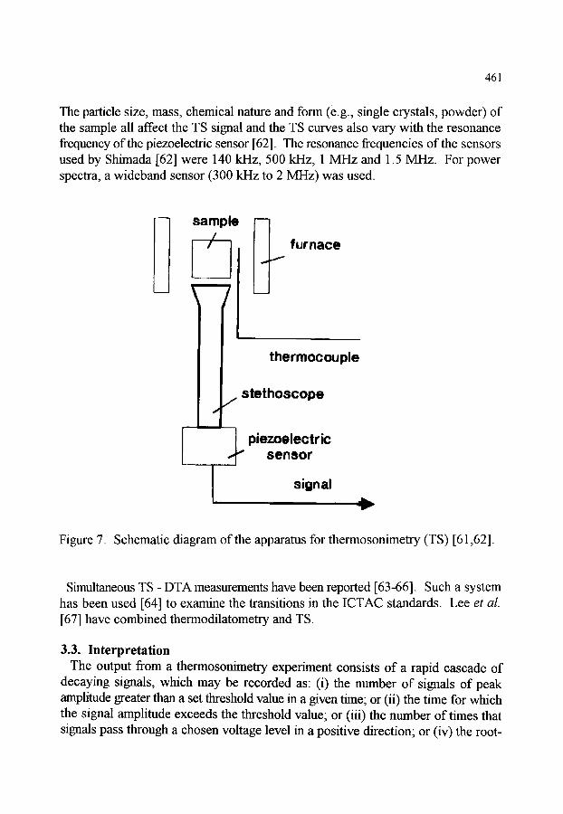
461

The particle size, mass, chemical nature and form (e.g., single crystals, powder) of the sample all affect the TS signal and the TS curves also vary with the resonance frequency of the piezoelectric sensor [62]. The resonance frequencies of the sensors used by Shimada [62] were 140 kHz, 500 kHz, 1 MHz and 1.5 MHz. For power spectra, a wideband sensor (300 kHz to 2 MHz) was used.

sample furnace

J

__ J

thermocouple

/ stethoscope

piezoelectric sensor

signal q ~

Figure 7. Schematic diagram of the apparatus for thermosonimetry (TS) [61,62].

Simultaneous TS - DTA measurements have been reported [63-66]. Such a system has been used [64] to examine the transitions in the ICTAC standards. Lee et al.

[67] have combined thermodilatometry and TS.

3.3. Interpretation The output from a thermosonimetry experiment consists of a rapid cascade of

decaying signals, which may be recorded as" (i) the number of signals of peak amplitude greater than a set threshold value in a given time; or (ii) the time for which the signal amplitude exceeds the threshold value; or (iii) the number of times that signals pass through a chosen voltage level in a positive direction; or (iv) the root-

462

mean-square amplitude level (energy); or (v) as a set of frequencies. The Nyquist theorem requires that the sampling frequency should be at least twice that of the maximum frequency component present in the signal. Because chemical acoustic emission usually occurs in bursts, continuous recording of high frequency data is usually replaced by data acquisition only when the signal exceeds a set threshold. Choice of this threshold relative to the background noise is discussed by Wade et

al. [68]. Frequency distributions of the TS signals are obtained [64] by timing the intervals

between the amplitude components of the decaying signal. The time intervals are converted into pulse heights which are fed to a multi-channel analyzer to give a display of the frequency distribution.

Wentzell and Wade [69] investigated (i) the reproducibility of power spectra from a given chemical system; (ii) the dependence of the spectra on the transducer used; and (iii) whether the information obtained in the spectra was sufficient to distinguish amongst the different processes which could be occurring. They found that reproducibility of spectra obtained with the same transducer was good, but that reproducibility between transducers was not as good. Transducer response remained reasonably constant over several months of use.

Relationships have been sought between the frequency distributions and the processes occumng in the sample. In the simplest case, frequency distributions can be used as 'fingerprints' of sample origin. Detailed interpretation is complex and empirical pattern recognition methods have been suggested [70,71 ]. Wentzell et al.

[70] evaluated possible descriptors obtained from AE signals for use in characterizing the processes giving rise to the signals. Descriptors were grouped into four categories: (i) those associated with the absolute magnitude of the signal; (ii) those related to the rate of decay of the signal; (iii) those measuring the central tendency of the power spectrum, and (iv) those characterizing the dispersion of the power spectrum. The conclusion reached [70] was that "acoustic emission will present a challenge to modem pattern reco~ition methods", and the subtlety of the information obtainable was emphasized.

Although interpretation of power spectra is complicated by distortion of the acoustic signal by instrumental factors, the main features of the spectra could be associated [69] with fundamental processes occurring in the systems examined, e.g., bubble release was associated with low frequencies and crystal fracture with high frequencies.

463

3.4. Applications of thermosonimetry TS results are usually combined with other thermoanalytical information to build

up a complete picture of the processes occtmSng in the sample during heating. An example of a combined TS - DTA curve for KCIO4 is shown in Figure 8 [63]. The curve of rate of acoustic emission (C) against temperature shows two regions of increased acoustic activity. Comparison of these TS results with the results obtained from DTA (curve A) identified the processes occurring at these temperature regions as a phase transition (orthorhombic to cubic) (200 to 340~ followed by melting accompanied by decomposition (560 to 660~ The onset of the lower temperature TS peak is well below the transition temperature (298~ indicating that mechanical changes occur in the sample particles prior to the transition. Solidification of the KC1 product of decomposition is detectable by TS but not on the DTA curve.

In a series of further papers, Shimada et al. [62,63,65,66] showed that the low temperature TS signals decreased with decreasing sample mass, which confirmed that acoustic emission was from the whole sample and not just from particles in contact with the sample holder. Resolution of the peaks in the higher temperature signal was better at low sample masses. The low temperatm'e peak decreased with particle size and was undetected below 75 ~tm diameter particles. Optical and scanning electron microscopy showed that the low temperature TS peak results from fracture of large particles and/or release of liquid from their surfaces. CsC104 behaves similarly, but TS curves for NaC104.H20 were complicated by dehydration in two steps (55 to 80 ~ and 155 to 200 ~ The DTA curve for KC103 [62(d)] shows melting at 340 to 380~ and two successive exotherms due to decomposition (540 to 610~ The TS curve shows four main peaks. The first two (360 to 480~ and 485 to 520~ arise from post-melting events, while the last two (530 to 570~ and 570 to 620~ correspond to the decomposition stages KC103 -~ KC104 ~ KC1. The first two TS peaks were shown by high temperature microscopy to be related to the formation and evolution of gas bubbles in the melt.

The phase transitions (t~ orthorhombic -, [3 trigonal 128~ [3 -, ~t trigonal on cooling 124~ occtming on heating and cooling powdered and single crystal samples of KNO3 were investigated [66] using simultaneous TS - DTA, supported by microscopy. The ~t phase has useful ferroelectric properties. The ~, -. t~ transition was affected by the temperature from which the samples were cooled. This observation was interpreted as resulting from annealing of defects formed by the t~ ~ [~ transition. The TS signals for the ~, ~ ct transition were stronger than for the ct - [~ or [3 - ~, transitions

Lee et al. [67] have used TS - dilatometry to study the phase II -- phase IIi transition of hexachloroethane in great detail. Results are shown in Figure 9. Agreement between integrated acoustic emission and the dilatometric plots is good. Emission was less intense during heating than during cooling, on account of

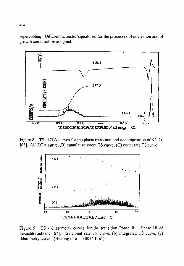
464

supercooling. Different acoustic 'signatures' for the processes of nucleation and of growth could not be assigned.

~,, ,r �9 m mm �9 �9

( A )

W3

oo. t, ]~

2 . 0 0 aoo 300 400 sOO

TEMPERATURE / de g C 6 0 0

Figure 8. TS - DTA curves for the phase transition and decomposition of KC104 [63]. (A) DTA curve, (B) cumulative count TS curve, (C) count rate TS curve.

| ] ,

(c) , J

�9 o ,

" l (a) ............. , :I,~L,,~,~ilL , ~ '''ll'~i'l'~j~I'J;~l~lilii'~illl~'(~'"!i~L. '~ ............

39 38 37 36 35

TEMPERATURE/deg C

Figure 9. TS -dilatometry curves for the transition Phase II -, Phase III of hexachloroethane [67]. (a) Count rate TS curve, (b) integrated TS curve, (c) dilatometry curve. (Heating rate = 0.0034 K s1).

465

4. THERMOACOUSTIMETRY

4.1. Introduction In thermoacoustimetry, the characteristics of imposed acoustic waves after passing

through a sample, are monitored, as a function of time or temperature, while the temperature of the sample, in a specified atmosphere, is programmed. No abbreviation has been officially approved by ICTAC, although the abbreviation TAA, for thermoacoustic analysis, has been used.

4.2. Apparatus for Thermoacoustimetry In the apparatus used by Mraz et al. [72], a pair of lithium niobate transducers are

in contact (under a constant pressure of about 300 kPa) with opposite faces of the sample (Figure 10). One transducer induces the incident acoustic signal and the other detects the transmitted signal. Thermal expansion of the sample during the heating programme is monitored continuously with a linear variable differential transformer (LVDT), so that changes in sample dimensions can be allowed for in the calculations. Arrangements are made for atmosphere control around the sample.

top cool in

b lock

top s u p p o r t [ ~ ~ , ,bar

1

3 p l s t o n - ~ L V D T

l Y top s tack ' ! - |

hea te r a l u m i n u m c o n t a c t . I J d r i v e r ~ - to pulse

si lver c r y s t a i ~ . . . . * g e n e r a t o r p la tes -ff - ~ ] s a m p l e -- ~ I tods . : . -~ ~ -. rece ive r

a m p # 1 ~- [ - - - - ~ - ~ J ~ . . ~ - - - ] - crysta l c e r a m i c .~_ ~ ~ . Taluminu m

a l u m i n u m I = } = ' ' c o n t a c t s p a c e r I b o t

insu la tor , cool ing b o t t o m b lock }'[ . ] t ' i b l ock [

_ b a s e p late

a l u m i n u m s p a c e r

b o t t o m s tack h e a t e r

Figure 10. Schematic apparatus for thermoacoustimetry [72].

466

The incident signal is generated by a pulse generator. The transmitted signal received by the second transducer is inverted and amplified and an attenuated version of the driving pulse is added to this output signal. This summation procedure enables detection of the first-arrival times of both the compressional (P) and shear (S) waves. The velocities of the P and S waves and hence the various elastic moduli are then computed at set temperature intervals, and the final result is a plot of velocity or modulus against tem~_grature. The instrument was calibrated with an aluminium standard forwhi-6h the P and S wave velocities were accurately known.

The apparatus described by Kasap and Mirchandan [73] (Figure 11) operates from room temperature to 350~ The sample is loaded between two identical glass rods, one of which is stationary and the other vertically movable. Transducers and thermocouples are attached to the rods and not the sample.

i , t r a n s m i t t e r -------i--_ I

t h e r m o c o u p l e

f ixed rod

r e c e i v e r ~ 1

m o v e a b l e rod

f u r n a c e |

I

I

I

I

1

I !

.signal h ._

Figure 11. Schematic apparatus for thermoacoustimetry [73].

467

Samples are in the form of sheets or pellets. Blank experiments are carried out with the two glass rods in contact. The ultrasonic transit time through the sample is obtained from the time delay between the through signal and the echo signal. The through signal travels the length of both rods plus the sample length. The echo signal travels the length of the top rod and back. allowance also has to be made for travel time through the coupling regions at the interfaces. Absolute determination of the ultrasonic velocity is usully unnecessary - only the variation with temperature. The use of the through and echo signals eliminates the influence of temperature variations in the glass rods.

The change in attenuation, Va, of the ultrasonic waves with temperature is obtained by measuring the peak-to-peak amplitude of the through signal, Vp_p(T), at temperature T and relating it to the value at a reference temperature, T o.

Va =- (1/Ls) In [Vp_p(T)/Vp.p(To)]

(where Ls is the path length through the sample). Kasap and Mirchandan [73] illustrated the operation of their system with curves of In [vT/V3oo] and of Va against T (where v x is the ultrasonic velocity at T) for various materials exhibiting glass transitions. The In [vT/V3oo] plots showed distinct changes in slope at Tg, while the Va plots showed peaks. The features of the thermoacoustic curves were clearly related to DSC and microhardness measurements.

Ravi Kumar et al. [74] have given a detailed description of the thermoacoustical parameters of polymers.

4.3 Applications of thermoacoustimetry Thermoacoustimetry has been used [72] to distinguish between grades of oil shales. Both the P and the S wave velocities decrease with increasing temperature and with

increasing organic content (Figure 12). Results are very reproducible. Changes in behaviour are related to loss of water and decomposition of some hydrocarbon fractions. Results of thermoacoustimetry and DTA experiments [75] have been combined to characterize synthetic fibres (Figure 13). The increases in signal occur firstly at the glass-transition temperatures and then prior to melting. Glass fibre shows no changes in this temperature range.

468

E

0 _J kU > UJ > <

3050

2050

1050

300

L.

L_

0 i00 200 300 400

T e m p e r a t u r e / d e g C

Figure 12. Thermoacoustimetry curves of different grades of oil shales [72]. (a) 24.9 gpt; (b) 26.2 gpt; (c) 37.7 gpt; (d) 67.6 gpt. (gpt = gals per ton).

z O I - -

o

O " - - " ,-r i i i u a ~

(I"3-- --F-- a_

20 ( (f) _+

_

(c)

(b)~j- - _ _ ~ ( a )

A A | A A i

0 i00 200 300

Temperature/deg C

Figure 13. Thermoacoustimetry curves of synthetic fibres [75]. (a) glass; (b) teflon; (c) fortrel polyester; (d) dacron polyester; (e) nylon 4; (f) nylon 6,6; (g) vylor; (h) nylon 6,10.

469

5. MISCELLANEOUS

Mandelis [76] has reviewed photothermal applications in the thermal analysis of solids. Thermal waves may be optically induced in solid samples by modulated irradiation. The thermal waves then interact with the sample before being detected by suitable sensors. Acoustic waves may be simultaneously induced and then detected. These photothermal techniques may also be used to study processes in fluids.

Photothernial techniques may be classified as synchronous (frequency domain), transient (time domain) and frequency multiplexed. Details of the theory and experimental techniques are given in the review [76]. Applications include accurate measurement of thermal transport properties such as thermal conductivity, difffusivity and effusivity and, indirectly, specific heat capacity. Use of these techniques can add significantly to the information obtainable from other thermal analysis techniques, particularly in determining the mechanisms of phase transitions.

REFERENCES

1. V. Balek and J. TOlgyessy, Emanation Thermal Analysis and other Radiometric Emanation Methods, in G. Svehla (ed), Wilson and Wilson's Comprehensive Analytical Chemistry, Part XIIC, Elsevier, Amsterdam, 1984. 2. V. Balek, Thermochim. Acta, 22 (1978) 1. 3. C. Jech, Nature, 178 (1956) 1343. 4. V. Balek, Thermochim. Acta, 192 (1991) 1. 5. G. Carter and J.S. Colligon, Ion Bombardment of Solids, Heinemann,

London, 1968. 6. M.D. Norgett and H.B. Lidiard, Philos. Mag. 18 (1968) 1193. 7. P.A. Redhead, Vacuum, 21 (1962) 203. 8. R. Kelly and Hj. Matzke, J. Nucl. Mater., 17 (1965) 197; 20 (1966) 175. 9. J. K ~ and V. Balek, Thermochim. Acta, 78 (1984) 377; 110 (1987) 245. 10. S. FlOgge and K.E. Zimens, Z. Phys. Chem.,Abt. B. 42 (1939) 179. 11. O. Hahn, J. Chem. Soc. Suppl., $259 (1949). 12. V. Balek, (~s. Patent No. 151172. 13. W.D. Emmerich and V. Balek, High Temp. High Press., 5 (1973) 67. 14. C. Jech and R. Kelly, Proc. Br. Ceram. Soc., 9 (1976) 359. 15. F.W. Felix and K. Meier, Phys. Status Solidi, 32 (1969) 139. 16. A.S. Ong and T.S. Elleman, J. Nucl. Mater., 42 (1972) 191. 17. V. Balek, J. Mater. Sci., 5 (1979) 166.

470

18. V. Balek, Farbe und Lack, 85 (1979) 252. 19. V. Balek, Z. Anorg. Allg. Chem., 380 (1971) 61. 20. J.A. Hedvall, Solid State Chemistry, Elsevier, 1969. 21. V. Balek, Thermochim. Acta 110 (1987) 221. 22. H. Schreiner and G. Glawitsch, Z. Metallkd., 25 (1954) 200. 23. P. Gourdier, P. Bussi~e and B. Imelik, C.R. Acad. Sci., Ser. C, 264 (1967)

1624. 24. C. Quet and P. Bussihre, C.R. Acad. Sci., Ser. C, 280 (1976) 859. 25. V. Balek, Sprechsaal, 116 (1983) 978. 26. V. Balek, M. Vobofil and V. Baran, Nucl. Technol., 50 (1980) 53. 27. V. Balek and I.N. Bekman, Thermochim. Acta 85 (1985) 15. 28. V. Balek, Z. M~ilek and H.J. Pentinghaus, J. Sol-Gel Sci. Technol., 2 (1994)

301. 29. V. Balek, J. Mat. Sci., 17 (1982) 1269. 30. V. Balek, J. Fusek, O. K/i~, M. Leskel~i, L. Niinist6, E. Nyk~,nen, J. Rautanen

and P. Soininen, J. Mater. Res., 9, (1994) 119. 31. K.B. Zaborenko and Ju.Z. Mochalova, Radiokhimiya, 10 (1968) 123. 32. R. Th~itner and K.B. Zaborenko, Radiokhimiya, 8 (1966) 482. 33. V. Balek and K.B. Zaborenko, Russ. J. Inorg. Chem., 14 (1969) 464. 34. V. Balek and A. de Kor~nyi, Fuel, 69 (1990) 1502. 35 W.D. Emmerich and V. Balek, High Temp.-High Pressures, 5 (1973) 67. 36. V. Balek and J. Subrt, J. Pure Appl. Chem. 67 (1995) 1839. 37. V. Balek and J. GOtz, in J. G6tz (Ed.), Proc. 11 th Int. Glass Congress, Prague,

1977, Vol. 3, p. 35. 38. S. Bordas, M. Clavaguera-Mora and V. Balek, Thermochim. Acta, 93 (1985)

283. 39. O. Vojt~ch, F. Pl~il, V. Kou~im and J. Stissmilch, J. Radioanal. Chem., 30

(1976) 583. 40. V. Balek and K.B. Zaborenko, Russ. J. Inorg. Chem., 14 (1969) 464. 41. V. Balek, J. Thermal Anal., 35 (1989) 405. 42. K.B. Zaborenko, V.P. Polyakov and J.G. Shoroshev, Radiokhimiya, 7 (1965)

324, 329. 43. M.E. Levina, B.S. Shershev and K.B. Zaborenko, Radiokhimiya, 7 (1965) 480. 44. A.I. Czeckhovskikh, D. Nietzold, K.B. Zaborenko and S.I. Volfkovich, Zh.

Neorg. Khim., 11 (1966) 1948. 45. C. Quet, P. Bussi~e and R. Fretty, C.R. Acad. Sci., Ser. C, 275 (1972) 1077. 46. D.J. Chleck and D. Cucchiara, J. Appl. Radiat. Isotop., 14 (1963) 599. 47. Hj. Matzke, J. Appl. Radiat. Isotop., 27 (1976) 27. 48. G.M. Zhabrova, S.Z. Roginskij and M.D. Shibanova, Kinet. Katal., 6 (1965)

1018.

471

49. C. Jech, Proc. 2nd Int. Congress on Catalysis, Editions Techniques, Paris, 1961, p. 2285.

50. I.N. Bekman and V.V. Teplyakov, Vestrl. Mosk. Univ., 1974. 51. V. Balek, Thermochim. Acta 72 (1984) 147. 52. V. Balek and J. Dohn~lek, J. Mater. Sci., 17 (1982) 2281. 53. V. Jesen/tk, J. T6lgyessy, P. Varga and B. Sile~, Silik~ty, 15 (1971) 65. 54. V. Balek and J. Dohn~lek, Proc. 3rd Int. Conf. on Durability of Building

Materials, Espoo, Finland, 1981, Vol. 3, p. 26. 55. V. Balek, J. Am. Ceram. Soc., 53 (1970) 540. 56. T. Ishii, Thermochim. Acta, 88 (1985) 277; 93 (1985) 469; 109 (1979) 252. 57. V. Balek, J. Appl. Chem. (London), 20 (1970) 73. 58. V. Balek, J. Therm. Anal., 12 (1977) 111. 59. D. Betteridge, M.T. Joslin and T. Lilley, Anal. Chem., 53 (1981) 1064. 60. R.M. Belchamber, D. Betteridge, M.P. Collins, T. Lilley and A.P. Wade, Anal.

Chem., 58 (1986) 1873. 61. K. Lonvik and co-workers, 4th ICTA (1975) Vol.3, p 1089; 6th ICTA (1980)

Vol.2, p313; 7th ICTA (1982) Vol.1, p306; J. Therm. Anal., 25 (1982) 109; Thermochim. Acta, 72 (1984)159,205; 110 (1987) 253; 214 (1993) 51.

62. S. Shimada,(a) Thermochim. Acta, 163 (1990) 313" (b) 196 (1992) 237; (c) 200 (1992) 317; (d) 255 (1995) 341; (e) J. Thermal Anal., 40 (1993) 1063.

63. S. Shimada and R. Furuichi, Bull. Chem. Soc. Jpn, 63 (1990) 2526; Thermochim. Acta, 163 (1990) 313.

64. G.M. Clark, 2nd ESTA (1981) p85; Thermochim. Acta, 27 (1978) 19. 65. S. Shimada, Y. Katsuda and R. Furuichi, Thermochim. Acta, 183 (1991)365;

184(1991)91. 66. S. Shimada, Y. Katsuda and M. Inagaki, J. Phys. Chem., 97 (1993) 8803. 67. O. Lee, Y. Koga and A.P. Wade, Talanta, 37 (1990) 861. 68. A.P. Wade, K.A. Soulsbury, P.Y.T. Chow and I.H. Brock, Anal. Chim. Acta,

246(1991)23. 69. P.D. Wentzell and A.P. Wade, Anal. Chem., 61 (1989) 2638. 70. P.D. WentzeU, O. Lee and A.P. Wade, J. Chemomet., 5 (1991) 389. 71. I.H. Brock, O. Lee, K.A. Soulsbury, P.D. Wentzell, D.B. Sibbald and A.P.

Wade, Chemomet. InteU. Lab. Syst., 12 (1992) 271. 72. T. Mraz, K. Rajeshwar and J. Dubow, Thermochim. Acta 38 (1980) 211. 73. S.O. Kasap and V. Mirchandan, Meas. Sci. Technol., 4 (1993) 1213. 74. M. Ravi Kumar, R.R. Reddy, T.V.R. Rao and B.K. Sharma, J. Appl. Polym.

Sci., 51 (1994) 1805. 75. P.K. Chatterjee, 4th ICTA, Vol. 3, p835. 76. A. Mandelis, J. Thermal Anal., 37 (1991) 1065.


Chapter 10

T H E R M O M I C R O S C O P Y

H.G. W i e d e m a n n a and S. Felder-Casagrande b

aMettler Toledo GmbH, CH-8603 Schwerzenbach, Switzerland

blnstitute of Inorganic Chemistry, University of Ztirich, Winterthurerstrasse 190, CH-8057 Ztirich, Switzerland

1. H I S T O R I C A L I N T R O D U C T I O N

The first investigations using a hot stage microscope were carried out and reported by Otto Lehmann more than one hundred years ago [1, 2]. He first used a simple device heated in an oil bath and later his "crystallisation microscope" developed. The focus of his research was physics and crystallography. In the course of the following decades he published a lot of facts and disclosures with the help of his equipment which, however, encountered little interest in the literature. Also the laboratory device called "the chemical microscope" was not used very often in chemical research. In 1931, as thermal microscopy was not popular yet, Kofler developed a series of several prototypes of their successful heat bench. These devices used by Kofler were simple in design and construction when compared with the models of Lehmann. In 1936 they started using a mercury thermometer. Kofler put great efforts into the further development and the improvement of his "Kofler hot stage". He tried also to show a broad scope of application for the new area of thermal microscopy [3].

Today we know this method as a thermoanalytical measurement specified by the DIN 51005 in which a sample is heated by an exact temperature rate and its behaviour is examined by a microscope. Thermomicroscopy is the most important method of investigation in the area of thermoptometry (ICTAC) (or thermo-optical analysis (TOA)) where the optical properties of substances are measured as a function of temperature. W. C. McCrone played a very method important role in the further development of thermal microscopy as a high precision measuring method and also in its popularization [4-6].

474

The information obtained from microscopic examination can be enhanced considerably by combination with the results of other investigations. Simultaneous registration of the measurements from different methods on a single process yields the most informative results [7-9].

Instrument combinations of light microscopy with other methods such as laser micro-emission spectroanalysis [ 10] , X-ray diffraction [ 11], electron microscopy [12], UV- and IR-spectroscopy [13,14], magnetic resonance [15] or differential thermal analysis are described in the literature [7,16,17].

The emphasis of this chapter is on the combinations of thermomicroscopy with differential scanning calorimetry (DSC), as well as with thermogravimetry (TG), and their applications. An arrangement that permits visual observation during conventional differential thermal analysis was described in 1960 by Hogan and Gordon [18], but the temperature range for effective use of the microscope was very limited. A modification of the hot-stage microscope, developed originally by Welch [19, 20], constructed by Mercer and Miller [21], permits continuous monitoring and recording of the cooling or heating curves of microscopic quantities of materials, which are supported and observable in the thermocouple controlled micro furnace. In this form, the apparatus has been applied to high temperature phase studies in oxide and mineral systems [16, 22, 23]. Great progress in the design of the measuring devices has been made from the first apparatus allowing simultaneous measurement, and the new instruments can be used in a much more universal manner [24, 25].

2. GENERAL EQUIPMENT AND ACCESSORIES

Thermomicroscopy allows the observation of morphological and structural changes as a function of temperature. Such changes are based on physical or chemical processes. The observation of the dependence of a characteristic parameter of a substance on temperature helps to identify and characterize the substance. For such an investigation a thermomicroscope, comprising a hot and/or cold stage, a sample holder, a light source, devices for optical recording and documentation and data and picture processing analysers is needed.

2.1. The microscope The objective lens is the most critical designed part of the microscope since it

must operate as near as practical to the hot stage to yield the highest resolution. It is thus imperative to protect it from any damaging effects of the heat from the stage. This may be achieved by physically separating the objective lens from the hot sample and by the introduction of an optical quality window in the stage shell. However, long working distances limit the resolving power of the objective

475

lens. Manufacturers of hot stages have often designed special lenses with optimized numerical aperture (N.A.) for the required working distance. The thickness and composition of the furnace window is also taken into consideration to minimize spherical aberration of the objective lens. These special objective lenses have N.A. values ranging from 0.45 to 0.60, giving useful magnifications from 450 to 600x [26].

2.2. Hot stage and sample holder After the invention of the hot stage microscope by Lehmann at the end of the

last century, many different models of hot and cold stages were developed. Some of the more important considerations in hot stage microscopy are given by Brenden, Newkirk and Bates [27], Lozinskii [28] and Smallman and Ashbee [29]. A large variety of instruments are reported in the general literature [30, 31 ], showing the broad field of application. Hot stages can be classified according to their temperature range and, in addition, according to their combinations with other methods.

Table 1

Type temperature with with different range DSC TG atmospheres

cold stage -50 ~ to 25~ _ _ + hot stage 25 ~ to 350~ + + +

25 ~ to 2700~ high temperature stage + - -

The cold stage, working generally between room temperature and -50~ and, in special cases down to -268~ is suitable for a number of applications in both the biomedical and the materials fields. The study of effects of low temperature on microorganisms and the study of the efficacy of cryogenic storage on donor organs are examples of studies in biology and medicine. In the materials sciences, the cold stage is useful for the study of low temperature phase transformations in metals and the evaluation of polymers below their glass transition temperatures. Cooling is commonly accomplished using liquefied gases such as liquid carbon dioxide (-78.5~ liquid nitrogen (-195.8~ liquid hydrogen (-252.9~ or liquid helium (-268.9~ An interesting method of cooling a sample in a cold stage makes use of thermoelectric or Peltier coolers. There are two difficulties. First the illumination can introduce an appreciable quantity of heat, therefore it is important to include an infrared or heat absorbing filter in the illumination system. The second problem is icing of the cold stage window and of the outer

476

objective lens. To minimize icing, the common solutions are: isolating the surfaces from humid air, for example with sections of a toy balloon, or flooding these areas with very dry gas such as the vapor from liquid nitrogen [26].

The hot stage can range in maximum temperature capability from slightly above ambient to as high as 2700~ The lower temperature devices are suitable for the study of living cultures and for the characterization of organic compounds (i.e. melting point, crystallinity, etc.). The higher temperature devices are used for dynamic examination of high temperature physical properties and kinetics of high temperature phase transformation of metals, ceramics and minerals [26]. The stage design for high-temperature microscopy has to consider that the intens radiation emitted by the specimen itself at maximum temperature. This must be overcompensated by high-intensity lamps and blue filters in order to obtain ima- ges of rich contrast [7]. Ideally the atmosphere in the hot stage should be optimized for the particular sample and the requirements of the study. It is necessary, however, to minimize heater-atmosphere reactions or to reduce heat transfer to the stage shell, i.e. with a vacuum. Vacuum heating chambers exist for chemical microscopy, where chemical reactions under various atmospheres can be observed. If a sublimation layer of the sample material hinders the focusing and observation, another part of the sample can be brought into position rotating by eccen- tric cover plates [32].

Figure 1. Cross section of the hot stage FP82 (Mettler-Toledo AG).

All models have one common requirement: the hot stage has to be as thin as possible in order to be placed between the objective and the microscope table. Figure 1 shows the standard model FP 82 with a medium temperature range. In this drawing the basic construction elements are the following: heating and/or cooling device (4, 5) which is placed on both sides of the sample cartier (6), in order to prevent any temperature gradient; a temperature sensor (3) with good

477

contact to the sample for the registration of the sample temperature, a heat protection filter (7) which shields the lens from the heat radiation. The inner parts around the light beam are encased in quartz or borosilicate glass and are cooled by a gas stream (8) produced of a blower (1).

A hot stage with the capability for simultaneous DSC measurement needs further identification of the construction. The sample holder is also heated from both sides. A Pt 100 sensor is placed in the lower heated plate as close to the sample as possible.

Flat furnace Reference pan DTA/DSC sensor Sample pan

Light

Figure 2. a) Hot stage FP84 with simultaneous DSC shown with open top entry, b) Cross section of the hot stage.

Two heat protection filters serve as heat shields toward the microscope in the upwards and downwards direction. The upper part of the hot stage with the upper heat plate can be lifted to allow access in the inside of the device (see Figure 2(a)). There are two pans as sample and reference holders lbr the simultaneous DSC heat flow measurement. The temperature difference is measured by a gold / nickel thermopile. For stable experimental conditions, the illumination of the sample during the experiment needs a stabilized poly- or monochromatic light source. The illumination acts as an additional heating source and therefore causes asymmetric heat distribution in the cell. This can be corrected lbr by subtracting a blank experiment from the measured curve.

The sample holder must be able to accommodate the sample if it melts during a thermoanalytical experiment. The sample must be visible from above and the light should pass through the pan from below. The pan must be compatible with the sample at higher temperatures. Sapphire glass proved to be the ideal holder material.

Different sample preparation techniques have proved to be useful for the various applications of thermomicroscopy-DTA. Open sapphire sample pans are used for non-volatile samples and covered sapphire pans for volatile samples. The technique is similar to the usual microscope sample preparation where pre-

478

melted samples are placed between parallel slides and cover glasses (a). A modification of this method encloses the substance between two sapphire disks (b). This preparation is only recommended for melts of substances with a high viscosity.

(a)

(c)

sapphire ~ , ~ ~---I disk crucible ........................ ~ ................

sample sample , sapphire (d) diskSapphire ..... ..... ~ ~-~%~ -~,%~. ,< , ,< }~ . . . . . . . . . . . . . . . . . balllid crucible crucible

Figure 3. Sample holders for different sample arrangement.

With covered sapphire pans (c) for volatile samples, unstrained samples can be observed through the cover disk, or the sample can first be evaporated (sublimed) and melted on the cover disk. For low-viscosity substances and liquid crystals, three sapphire balls act as spacers and help to maintain a uniform sample distribution and thickness during the measurement (d).

3. EXPERIMENTAL METHODS

3.1. Simple thermomicroscopy Historically seen, simple thermomicroscopy was the starting point for the fur-

ther development of the technique which is still in use today. Thermomicroscopy plays an important role in materials research, characterization of substances and also in quality assurance, either as a simple device or as the core of a combination with other equipment.

I photo I, Lv eo l

hot stage ~ proc, ;sso~s-]

puter)

J [!rinte~

Figure 4. Scheme of the instrumental setup of simple hot stage microscopy.

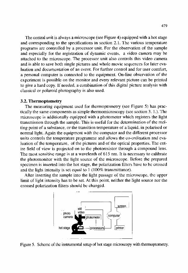
479

The central unit is always a microscope (see Figure 4) equipped with a hot stage and corresponding to the specifications in section 2.1. The various temperature programs are controlled by a processor unit. For the observation of the sample and especially for the registration of dynamic events, a video camera may be attached to the microscope. The processor unit also controls this video camera and is able to save both single pictures and whole movie sequences for later evaluation and documentation of an event. For further control and for user comfort, a personal computer is connected to the equipment. On-line observation of the experiment is possible on the monitor and every relevant picture can be printed to give a hard copy. If needed, a combination of this digital picture analysis with classical or polaroid photography is also used.

3.2. Thermoptometry The measuring equipment used for thermoptometry (see Figure 5) has prac-

tically the same components as simple thermomicroscopy (see section 3. 1.). The microscope is additionally equipped with a photometer which registers the light transmission through the sample. This is useful for the determination of the melting point of a substance, or the transition temperature of a liquid, in polarised or normal light. Again the equipment with the computer and the different processor units controls the temperature programme and allows the co-ordination and evaluation of the temperature, of the pictures and of the optical properties. The entire field of view is projected on to the photoresistor through a compound lens. The most sensitive range is at a wavelenth of 615 nm. It is necessary to calibrate the photomonitor with the light source of the microscope. Before the prepared specimen is inserted into the hot stage, the polarization filters have to be crossed and the light intensity is set equal to 1 (100% transmittance).

After inserting the sample into the light passage of the microscope, the upper limit of light intensity has to be set. At this point, neither the light source nor the crossed polarization filters should be changed.

hot stage ~ processors], __ nter

Figure 5. Scheme of the instrumental setup of hot stage microscopy with thermoptometry.

480

3.3. Thermomicroscopy with simultaneous differential scanning calorimetry

The optical results and morphological changes from thermomicroscopic measurements alone can sometimes not be completely interpreted. Additional specific investigations have their to be made. Simultaneous measurements also save on expensive samples and reduce analysis time. The precision of the interpretation of the various events which occur during the experiments also improves. On the other hand, results obtained from thermoanalytical measurements like TG or DSC are generally reproducible and quantitative, but they cannot always be correlated with the respective phase transitions or chemical reactions occurring in the substance. The combination of both methods in a simultaneous instrument allows cross checking of the interpretation. For example, effects which do not show any significant enthalpy change in DSC can often be detected with microscopy. On the other hand, thermomicroscopic investigation often require estimates of heats of transformation, fusion or crystallization. Almost the same set of measuring and controlling devices can be used as decribed in section 3.2. for thermoptometry.

0s, 't~ I hot p r~176 "

en

Figure 6. Scheme of the instrumental setup of hot stage microscopy with simultaneous differential scanning calorimetry.

The most important difference is the change of the hot stage for the unit explained in section 2.2, to allow for the measurement of the heat flow and simultaneously the optical observation of the events induced by the temperature change. Suitable processor units are able to measure and control the temperature, the light transmission and the change in heat flow. On-line observation of the morphological changes together with the corresponding data is possible on the multi screen monitor.

480a

3.4. Thermomicroscopy with simultaneous thermogravimetry Chemical reactions including gases can be studied by thermogravimetry (TG)

measuring the mass change of a sample with temperature. The simultaneous weighing and microscopic observation of the sample can correlate the morphological changes of the material with its mass decrease or increase during a decomposition of the sample or a reaction with the surrounding gas.

Figure 7. Scheme of the instrumental setup of hot stage microscopy with simultaneous thermogravimetry.

Figure 7 is a schematic drawing of a thermomicroscope with simultaneous thermogravimetry. The sample holder is attached to the balance by a capillary made of aluminium oxide and can be placed in the hot stage. The observation during the heating or cooling of the sample is done using a reflection light microscope which is equipped with a still video camera or a standard camera for the documentation of the changes of the sample. The setup shown can use various gas environments at flow rates up to 5 cm3/min. The temperature range is from 20 to approximately 370 ~ with heating rates of 0.1 to 10 ~ The sample mass can range from 0.1 to 20 mg, but the amount loaded depends on its density. The same peripheral equipment and computer as for the simultaneous thermomicroscopy-DSC method is used for processing, storage and documentation of the data.

481

4. EXAMPLES OF APPLICATIONS

4.1. Inorganic compounds 4.1.1. Hydration and dehydration of gypsum

The term "gypsum", is used for CaSO4 2 H20 which is a common mineral. There are four other phases in the CaSO4 / H20 system; semihydrate (CaSO4 0.5 H20) and anhydrite (CaSO4), which each have two forms with different crystallite size and structure. Each phase has special characteristics and applications. Exact knowledge of the phase components and impurities is of great engineering interest because, among other things, the phases and impurities influence the later material properties.

Hydration: The hydration proceeds according to the reaction equation

CaSO 4- 0.5 H20 + 1.5 H20 ---> CaSO4 2 H20

and can be divided into four steps. These steps were confirmed using thermoptometry and the accompanying heat of reaction can be measured using DSC. Distinguishing between the ~- and ~-semihydrate forms is possible by measuring isothermal DSC curves.

Dehydration: The dehydration of semihydrate to anhydrite takes place in the temperature range 90 to 180~ whereby a difference between the ~- and 13- semihydrates can be observed [33]. Many thermoanalytical studies deal with dehydration of the dihydrate, with the kinetics and the influencing parameters,

Figure 8. a) Micrographs (50x) taken during DSC measurements (o), showing nucleation at cracks.

E E

o

Temperature / ~ I

90 130 170

b) DSC curve measured during dehydration. The circles in the curve correspond to the micrographs.

482

such as water vapor partial pressure, nucleus size and distribution and type or origin of the dihydrate. Related to this are the intermediate and end products, the corresponding temperatures of formation and the resulting products. The simultaneous thermo-optical photographs accompanying DSC measurements (Fig. 8) show that nucleation in the dehydration of gypsum visibly begins after the start of separation of water. As can be expected, the first nuclei form preferably at a location where there is inhomogeneity, e.g., cracks. Under the test conditions selected (p(H20) = 30 mbar), dehydration proceeds immediately by a single step to y-anhydrite.

4.1.2. Nucleation characteristics of decompositions The formation and growth of nuclei during thermal decomposition investiga-

ted by thermomicroscopy permits the continuous observation of the various effects which determine the kinetics of decomposition. Of special importance are the rates of nuclei formation and growth in relation to the different crystallographic directions and the surface defects. Other important factors are the surrounding atmosphere, the formation of fissures and cracks due to diffusion of gaseous decomposition products, and the structural rearrangement.

graphite

natural diamond

O m

c l 3

E

Temperature / ~ I I I I

l i t _ _

N

I l l m

I I I I I I I I

1000 2000

Figure 9. SEM pictures of natural diamond, 500 x (a) before heating and after heating in high vacuum (10 .5 torr) (b); graphite nucleus on surface, 5000x; (c) and graphitization, fracture surfaces, 500x. The TG curves were recorded in high vacuum with a heating rate of 4 K min -I (d).

483

As an example, the nucleation processes in diamonds are presented. After heating diamonds above 1000~ at low pressure (10 -5 torr) a dulling of the surface is observed. At increasingly higher temperatures, the diamonds become gray (but are still translucent) and then, above 1600~ darken until they are black. This graphitization process obviously takes place at first only on the surface. When diamonds are heated to temperatures between 1650~ and 1800~ nuclei of graphite are formed on the surface. Figure 9(a) shows a scanning electron micrograph taken of diamond fragments before heating. Oriented graphite nuclei on diamond faces, which were formed after heating for 20 min at 1700~ can be seen in (b). The SEM picture (c) is taken of a diamond after heating at still higher temperatures, the spreading of the nuclei with simultaneous formation of cracks can be seen. This diamond sample then broke into small fragments which finally disintegrated to graphite powder. Figure 9(d) shows the TG curves which were recorded in high vacuum. On natural diamond, graphitization occurs in the region 1700~ 1900~ The mass changes during graphitization (1%) could be attributed to a partial vaporization of polyatomic carbon molecules, which takes place at these temperatures, together with a release of any gaseous inclusions [34].

Figure 10. a) Micrographs of the crystallization of 3 KNO3" 1 NaNO3.

E o

Temperature / ~ I I

260 240 200

b) DSC cooling curve. Sample mass" 24.44 mg; cooling rate: 2 K rain -~.

[ v

Temperature /~ 300 200

I I I I

1 I t

100

80

60 d z

40

20

c) Phase diagram of KNO3-NaNO 3.

484

4.1.3. Phase diagrams From the micro-thermoanalytical investigations by Kofler [43], the

KNO3/NaNO3-system is known to form a continuous series of solid solutions. A special characteristic of these solid solutions, however, is that periodic segregation phenomena occur during heating and cooling. In these experiments, mixtures of KNO3 and NaNO3 in 5 mole% steps were melted and the corresponding cooling curves were recorded afterwards with DTA. Simultaneously, the crystallization process was observed microscopically with a hot stage. As an example, Figure 10(b) shows the DSC cooling curve of a 3:1 mixture of KNO3 and NaNO3. The onset-point of the primary crystallization was determined as 257.5~ This is in good agreement with the microscopic observation that the nucleation of the first crystals occurs at 258~ (Figure 10(a)). The number of crystal nuclei increases down to about 248~ further cooling to 240~ results in pronounced crystal growth, with comlplete eutectic solidification at 216~ The liquidus curve and the eutectic line for the system KNO3-NaNO3, were determined from DSC curves. These results confirm that this system is indeed a simple eutectic system. It should be pointed out that it is relatively difficult, however, to determine the exact temperature of the eutectic onset points for mixtures with low concentrations (< 5 mole%) of KNO3 or NaNO3. A mixture of the nitrates in the eutectic proportion showed typical dendritic solidification after cooling to below 216~ The 13-a transformation of KNO3 is metastably frozen in at room temperature, independently of the temperature and the cooling rate. In the micrograph, the spontaneous transformation which may occur, afterwards becomes visible as nucleation [35]. (See also colour plate II, Figure 10.)

4.1.4. Structure selective reactions Oxidation of graphite: To investigate the detailed mechanism of the oxidation

of graphite a microbalance with a hot stage, light microscope and video equipment was constructed. With this instrumentation the course of oxidation of graphite flakes in air was monitored.The oxidation proceeds parallel to the layers, again indicating a mechanism governed by the structural features of the parent phase. The instrumentation allows the determination of the kinetics of the oxidation of isolated graphite flakes as follows: the temperature-dependent advancement of the "oxidation zone", i.e. the boundary prismatic, can be determined as a direction-dependent velocity. These data can be evaluated in terms of carbon atoms being oxidized along a given crystallographic direction as a function of time, temperature and atmosphere. Thus kinetic data are available which contain the information of the actual structural mechanism, i.e. the anisotropic reaction behaviour of graphite can be quantified [361.

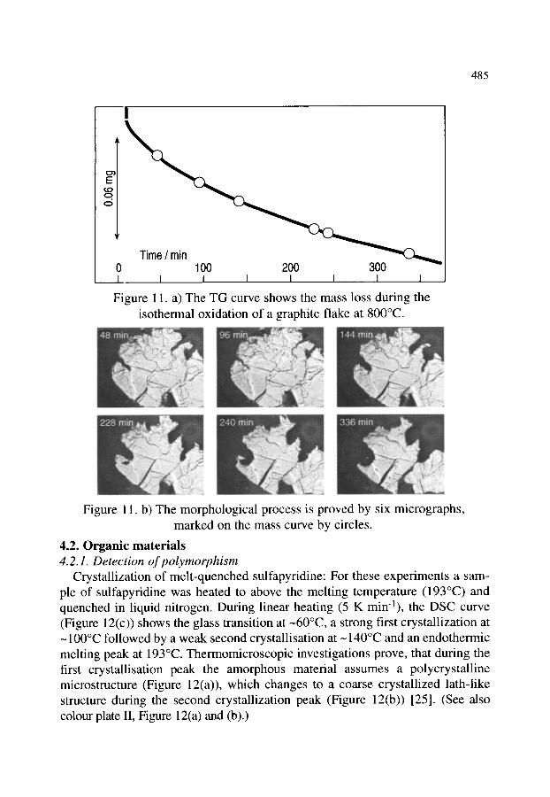
485

d I

Time / rain 0 100 200 300 I I I I I I I I

Figure 11. a) The TG curve shows the mass loss during the isothermal oxidation of a graphite flake at 800~

Figure 11. b) The morphological process is proved by six micrographs, marked on the mass curve by circles.

4.2. Organic materials 4.2.1. Detection of polymorphism

Crystallization of melt-quenched sulfapyridine: For these experiments a sample of sulfapyridine was heated to above the melting temperature (193~ and quenched in liquid nitrogen. During linear heating (5 K min-1), the DSC curve (Figure 12(c)) shows the glass transition at--60~ a strong first crystallization at ~ 100~ followed by a weak second crystallisation at--140~ and an endothermic melting peak at 193~ Thermomicroscopic investigations prove, that during the first crystallisation peak the amorphous material assumes a polycrystalline microstructure (Figure 12(a)), which changes to a coarse crystallized lath-like structure during the second crystallization peak (Figure 12(b)) [25]. (See also colour plate II, Figure 12(a) and (b).)

486

Figure 12 a) Micrograph of the polycrystalline microstructure after the first crystallization, b) The second crystallization within the first phase.

First crystallization

glass transition Second crystallization

n

I Temperature / ~ I I

50 100 150 200 c) DSC curve of melt-quenched sulfapyridine.

4.2.2. Glass transition The determination of the glass transition temperature, Tg, of polymers by DSC

and thermomechanical analysis (TMA) is sometimes problematic and rather sub- jective. The main reasons are the temperature gradients caused by the relatively high sample mass required for DSC and by limited heat transfer in TMA, respectively. A combination of DSC with thermoptometry or hot stage microscopy under polarized light can solve some of these problems. Thermoptometry is a nonsubjective method since the changes in birefringence and light transmittance during the glass transition, which are visible under the microscope, are measured with a photocell. As an example, poly(ethyleneterephthalate) is presented. During heating, the glass transition as well as the crystallization of PET were recorded by DSC. Simultaneous thermoptometry-DSC measurements of the

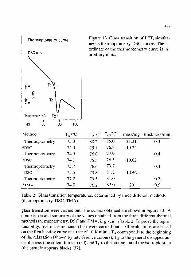
487

Thermoptometry curve

DSC curve

o

Temperature / ~ TC I I I I

40 60 80 100

Figure 13. Glass transition of PET, simultaneous thermoptometry-DSC curves. The ordinate of the thermoptometry curve is in arbitrary units.

Method T A/~ TB/~ Tc/~ mass/mg thickness/mm

~ Thermoptometry 75.3 80.2 85.0 21.21 0.3

2DSC 74.3 75.1 76.3 10.24

Yhermoptometry 74.9 76.0 77.9 0.4

3DSC 74.1 75.5 76.5 10.62


4DSC 75.5 79.8 81.2 10.46


5TMA 74.0 76.2 82.0 20 0.5

Table 2: Glass transition temperatures, determined by three different methods (thermoptometry, DSC, TMA).

glass transition were carried out. The curves obtained are shown in Figure 13. A comparison and summary of the values obtained from the three different thermal methods thermoptometry, DSC and TMA, is given in Table 2. To prove the reproducibility, five measurements (1-5) were carried out. All evaluations are based on the first heating curve at a rate of 10 K min -l. TA corresponds to the beginning of the relaxation (shown by interference colours), TB to the general disappearance of stress (the colour turns to red) and Tc to the attainment of the isotropic state (the sample appears black) [37].

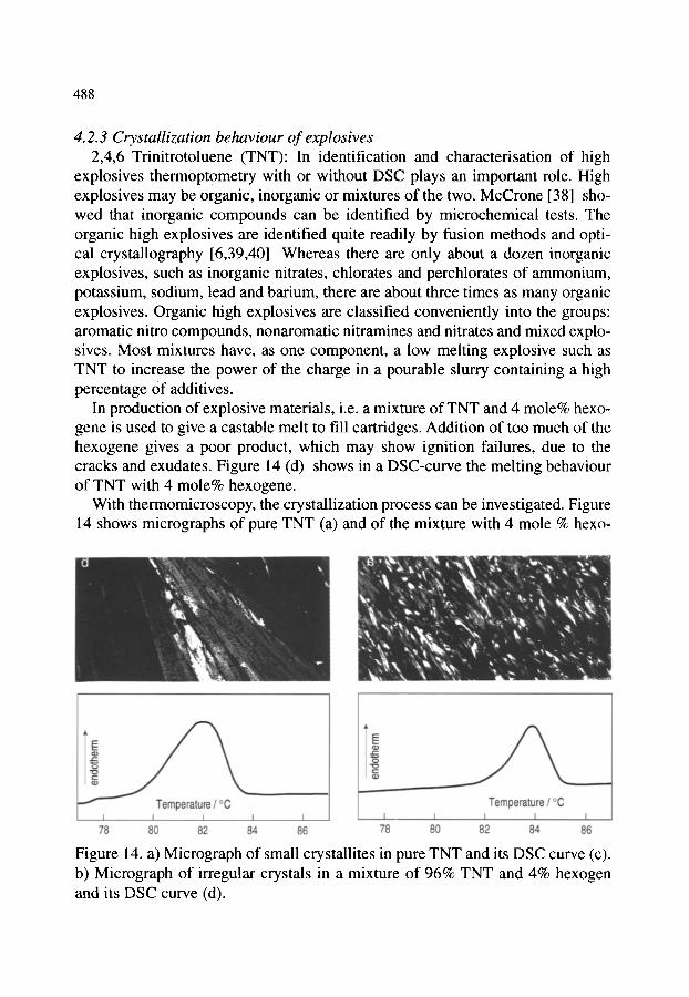
488

4.2.3 Crystallization behaviour of explosives 2,4,6 Trinitrotoluene (TNT): In identification and characterisation of high

explosives thermopt0metry with or without DSC plays an important role. High explosives may be organic, inorganic or mixtures of the two. McCrone [38] showed that inorganic compounds can be identified by microchemical tests. The organic high explosives are identified quite readily by fusion methods and optical crystallography [6,39,40] Whereas there are only about a dozen inorganic explosives, such as inorganic nitrates, chlorates and perchlorates of ammonium, potassium, sodium, lead and barium, there are about three times as many organic explosives. Organic high explosives are classified conveniently into the groups: aromatic nitro compounds, nonaromatic nitramines and nitrates and mixed explosives. Most mixtures have, as one component, a low melting explosive such as TNT to increase the power of the charge in a pourable slurry containing a high percentage Of additives.

In production of explosive materials, i.e. a mixture of TNT and 4 mole% hexogene is used to give a castable melt to fill cartridges. Addition of too much of the hexogene gives a poor product, which may show ignition failures, due to the cracks and exudates. Figure 14 (d) shows in a DSC-curve the melting behaviour of TNT with 4 mole% hexogene.

With thermomicroscopy, the crystallization process can be investigated. Figure 14 shows micrographs of pure TNT (a) and of the mixture with 4 mole % hexo-

Figure 14. a) Micrograph of small crystallites in pure TNT and its DSC curve (c). b) Micrograph of irregular crystals in a mixture of 96% TNT and 4% hexogen and its DSC curve (d).

489

gene (b) (see colour plate II, Figure 14 (a) and(b). A slow cooling rate (2 K min l) produced small r crystallites in pure TNT, whereas the mixture gives crystallites having fewer phase boundaries. Fast cooling (10 K min -1) changes the results and the mixture gives irregular crystal shapes and even a segregation [24].

4.2.4 Phase transition and melting of substituted PET The photographs (Figure 15 (a-c)) of single crystals of substituted PET, dime-

thyl 3,6-dichloro-2,5-dihydroxy-terephthalate, were taken on the hot stage of the microscope. Isothermal heating at 118.9~ the temperature of the beginning of the phase transition, leads to a colour change from yellow to white due to rotation of the molecules (see colour plate). This gives rise to cracks and fissures which can be seen in their growth state (118.9~ The melting point of this substituted PET (Figure 15(b)) is strongly decreased to about 180~ compared with 235~ for non-substituted PETE During cooling, the crystallization of the yellow modification starts at 164.6~ Slow cooling rates (0.1 K min -1) lead to the formation of a single crystal, whereas rapid cooling (10 K min -1) results in a polycrystalline aggregate due to supercooling [25].

100 150 200 I I Temperature / ~ I

phase transformation

E

fusion

Figure 15. Micrographs of substituted PET, during (a) the phase transition at 118~ (b) the melting process at 179.8~ and (c) the single crystal crystallization 164.6~ d) DSC curve of dimethyl-3,6-dichloro-2.5 dihydroxyterephthalate

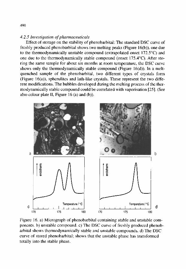
490

4.2.5 Investigation of pharmaceuticals Effect of storage on the stability of phenobarbital: The standard DSC curve of

freshly produced phenobarbital shows two melting peaks (Figure 16(b)), one due to the thermodynamically unstable compound (extrapolated onset 172.5~ and one due to the thermodynamically stable compound (onset 175.4~ After storing the same sample for about six months at room temperature, the DSC curve shows only the thermodynamically stable compound (Figure 16(d)). In a melt- quenched sample of the phenobarbital, two different types of crystals form (Figure t 6(a)), spherulites and lath-like crystals. These represent the two different modifications. The bubbles developed during the melting process of the thermodynamically stable compound could be correlated with vaporisation [25]. (See also colour plate II, Figure 16 (a) and (b)).

l f

Temperature / ~ I I I I I I I I I

170 175 180

Temperature / ~ I I I I I I I I I

170 175 180

Figure 16. a) Micrograph of phenobarbital containing stable and unstable components, b) unstable compound, c) The DSC curve of freshly produced phenobarbital shows thermodynamically stable and unstable compounds, d) The DSC curve of stored phenobarbital; shows that the unstable phase has transformed totally into the stable phase.

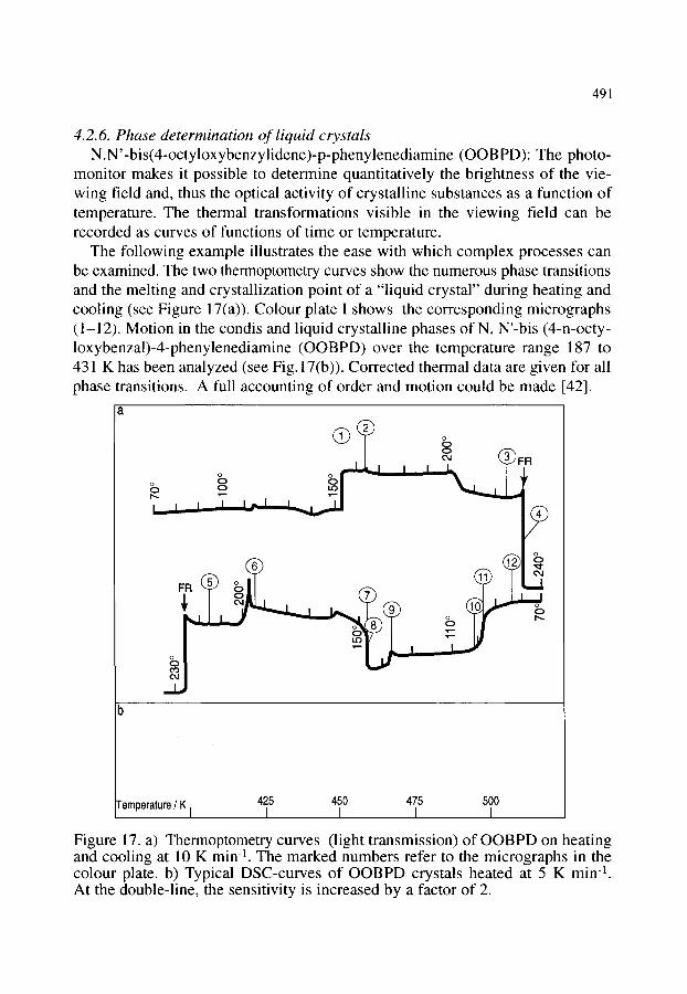
491

4.2.6. Phase determination of liquid crystals N.N'-bis(4-octyloxybenzylidene)-p-phenylenediamine (OOBPD): The photo-

monitor makes it possible to determine quantitatively the brightness of the viewing field and, thus the optical activity of crystalline substances as a function of temperature. The thermal transformations visible in the viewing field can be recorded as curves of functions of time or temperature.

The following example illustrates the ease with which complex processes can be examined. The two thermoptometry curves show the numerous phase transitions and the melting and crystallization point of a "liquid crystal" during heating and cooling (see Figure 17(a)). Colour plate I shows the corresponding micrographs (1-12). Motion in the condis and liquid crystalline phases of N, N'-bis (4-n-octy- loxybenzal)-4-phenylenediamine (OOBPD) over the temperature range 187 to 431 K has been analyzed (see Fig.17(b)). Corrected thermal data are given for all phase transitions. A full accounting of order and motion could be made [42].

- I I I R r o E, ~ I

o o m l

E,

o F R ~ o

425 450 475 500 Temperature / K I I I I I

Figure 17. a) Thermoptometry curves (light transmission) of OOBPD on heating and cooling at 10 K min -l. The marked numbers refer to the micrographs in the colour plate, b) Typical DSC-curves of OOBPD crystals heated at 5 K min -l. At the double-line, the sensitivity is increased by a factor of 2.

492

Colour Plate I

493

Colour Plate II

Figure 11. Figure 14. a) and b)

Figure 12. a) and b)

Figure 16. a) and b)

494

5. CONCLUSIONS

The addition of a heating or cooling stage to the polarizing microscope extends very considerably the application of this instrument, especially in the study of organic compounds. Hot stage microscopy has gained importance during the last few decades especially in combination with other physical measurements including thermal analysis.

On the other hand, the application of the hot stage microscope in inorganic chemistry micro-analysis, and its use in mineralogy is still somewhat limited. This is due to the nature of the high melting, frequently opaque materials. In this connection, combined hot stage microscopy-thermal analysis has proven to be very useful.

The identification of organic compounds is now a well-established technique in organic micro-analysis. The fusion methods consist in determining the different properties of a microscope preparation during heating, melting, cooling of the melt, after cooling to room temperature. The wide range of properties obtained can then be used in the identification of the compound. The information from such microscopic observations is, however, greatly increased by simultaneous TG and DSC measurements. In the present chapter the application of hot stage microscopy combined with TG or DSC is discussed for both inorganic and organic compounds.

6. ACKNOWLEDGEMENTS

The authors wish to express their gratitude and appreciation to Prof. Dr. G. Bayer, Institute for Nonmetallic Materials, ETH, Zurich, Switzerland

REFERENCES

1. O. Lehmann, Molekularphysik, Engelmann, Leipzig, 1888. 2. O. Lehmann, Das Kristallisationsmikroskop, Vieweg, Braunschweig, 1910. 3. L. Kofler and A. Kofler, Mikroskopische Methoden, Springer-Verlag,

Wien, 1954, Vol. 1. 4. W.C. McCrone, Fusion Methods in Chemical Microscopy, Wiley,

New York, 1957. 5. J.H. Kilbourn and W.C. McCrone, Microscope, 33 (1985) 73. 6. W.C. McCrone, J.H. Andreen and S.-M. Tsang, Microscope,

41 (1993) 161. 7. H.-H. Emons, H. Keune and H.-H. Seyfarth, Chemical Microscopy,

Elsevier Scientific Publishing Company, Amsterdam, 1982, Vol. 16.

495

~

9. 10. 11. 12.

13. 14. 15. 16. 17. 18. 19. 20. 21. 22. 23. 24. 25. 26.

27.

28.

29.

30.

31.

32.

33. 34. 35. 36. 37.

P.M. Cook, Anal. Chem., 64 (1992) 219R. P.M. Cooke, Anal. Chem., 66 (1994) 558R. S. Demirsoy, Zeiss-Mitt., 4 (1967) 254. G. Perinet, Bull. Soc. Fran~. Mineral. Cristallogr., 89 (1966) 325. G. Suwalski and H. Vollstfidt, Wiss. Ztschr. Humboldt-Universitfit Berlin, Math. Naturwiss. Reihe XVI, 5 (1967), 801-807. A. Hovnanian, Microscope, 14 (1964) 141. A. Wilke, Fortsch. Mineralog., 28 (1951) 84. E Brandstaetter, R. Mitsche and E Gabler, Radex-Rdsch., 2/4 (1967) 710. R.P. Miller and G.J. Sommer, J. Sci. Instr., 43 (1966) 293. H.J. Dichtl, E Jeglitsch, Radex-Rdsch., 3/4 (1967) 671. V.D. Hogan and S. Gordon, Anal. Chem., 32 (1960) 573. J.H.J. Welch, J. Sci. Instr., 31 (1954) 458. J.H.J. Welch, J. Sci. Instr., 38 (1961) 402. R.A. Mercer and R.P. Miller, J. Sci. Instr., 40 (1963) 352. R.A. Mercer and R.P. Miller, Nature, Lond., 202 (1964) 581. R.A. Mercer, and R.P. Miller, Mineralog. Mag., 35 (1965) 250. H.G. Wiedemann and G. Bayer, Thermochim. Acta., 85 (1985) 271. H.G. Wiedemann, J. Thermal Anal., 40 (1993) 1031. J.H. Richardson, Handbook for the Light Microscope, Noyes Publications, New Jersey, 1991. B.B. Brenden, H.W. Newkirk and J.L.J. Bates, J. Am. Cer. Soc., 43 (1960) 246. M.G. Lozinskii, High Temperature Metallography, Pergamon Press, New York, 1961. R.E. Smallman and H.B. Ashbee, Modern Metallography, Pergamon Press, New York, 1966. E.M. Chamot and C.W. Mason, Handbook of Chemical Microscopy, 3 ed., Wiley New York, 1958, Vol. 1. H.H. Emons, H. Keune and H.H. Seyfarth, Chemische Mikroskopie, VEB Deutscher Verlag fiJr Grundstoffindustrie, Leipzig, 1973. W.E Hemminger and H.K. Cammenga, Methoden der Thermischen Analyse, Springer-Verlag, Berlin, 1989. H.G. Wiedemann and M. R6ssler, Thermochim. Acta, 95 (1985) 145. H.G. Wiedemann and G. Bayer, Z. Anal. Chem., 276 (1975) 21. H.G. Wiedemann and G. Bayer, J. Thermal Anal., 30 (1985) 1273. H.G. Wiedemann and A. Reller, Thermochim. Acta, 271 (1996) 163. H.G. Wiedemann, G. Widmann and G. Bayer, Assignment of the Glass Transition, ASTM STP 1249, R.J. Seyler, Ed., American Society for Testing and Materials, Philadelphia, 1994.

496

38. 39. 40. 41.

42.

43.

W.C. McCrone, Microscope, 86 (1934) 107. T.J. Hope and J.H. Kilbourn, Microscope, 33 (1985) 1. J.H. Kilbourn and W.C. McCrone, Microscope, 33 (1985) 73. H.G. Wiedemann, J. Grebowicz and B. Wunderlich, Mol. Cryst. Liq. Cryst., 140 (1986) 219. J. Cheng, Y. Jin, G. Liang, B. Wunderlich and H.G. Wiedemann, Mol. Cryst. Liq. Cryst., 213 (1992) 237. A. Kofler, Mh. Chem., Bd. 86, 4 (1955) 648


Chapter 11

SIMULTANEOUS THERMAL ANALYSIS

J. Van Humbeeck

Dep. MTM-K.U.Leuven, W. de Croylaan 2, 3001 Leuven (Heverlee), Belgium

1. INTRODUCTION

Simultaneous thermal analysis, STA, is a standard term to indicate the simultaneous application of different types of (thermal analysis) techniques. Generally the word simultaneous has to be interpreted very strictly: on one and the same sample at the same time. This means that different types of sensors are (in-)directly connected to the same sample. This sample is further heated or cooled in a single furnace. It should thus be clear that we do not discuss results obtained from two different samples, even if they are heated or cooled in a single furnace at the same time. Simultaneous measurements must thus be distinguished from parallel measurements, where different samples are examined using different instruments.

There are many reasons for performing simultaneous thermal analysis:

1. Simultaneous measurements need much less time to perform all required measurements than when each of the recorded properties is measured separately.

2. Accurate correlation of the observed different events is assured. 3. Because of a synergetic effect in that the total amount of information about

the sample that is obtained is greater than the sum of the information obtained from the individual techniques [ 1 ].

4. The same sample (size, mass, surface, morphology, composition) is monitored by different techniques but under identical external factors (heating or cooling rate, gas-flow, gas-composition, type of furnace, ...). This can lead to a much more correct interpretation and correlation than for the results obtained by different techniques.

498

0

. The price of a STA-instrument is lower than the purchase of each thermal analysis instrument separately if all those instruments are necessary for use at similar intensity.

As a drawback, simultaneous thermal analysis instruments are generally more complicated, because different sensors have to be combined. This might lead to a reduction of sensitivity for one or more signals because of compromises in instrumental design. Compromises in measurement parameters can also lead to less clear signals. Regarding the combination of sensors, there is basically no limit. It is only restricted by the ingenuity of the investigator and, to some extent, by the technological state of the art of the different sensors and signal detectors. Complementary techniques might include all forms of physical, chemical and mechanical property measurements and all forms of spectroscopy, such as X-ray diffraction, mechanical spectroscopy, electron- and optical spectroscopy. It is not the purpose to discuss all of these potential combinations in this chapter. A very well-known coupled simultaneous measurement, TG-EGA (evolved gas analysis) is treated in Chapter 12. In this chapter we will deal mainly with combinations of classical thermal analysis techniques with less common, but for some research areas, successful techniques.

SIMULTANEOUS THERMOGRAVIMETRY-DIFFERENTIAL SCANNING CALORIMETRY TG-DSC (DTA)

2.1. Calibration The most common single sample simultaneous thermal analysis technique is the

combination of DSC (or DTA) and TG. A first important advantage of this combination is the possibility of temperature calibration by using the DSC (DTA) sensor (see also Chapter 13). Endo- or exothermic effects at invariant point transitions (i.e. melting, eutectic points, ...) can be much more accurately detected than weight changes, occurring at particular temperatures. According to ANSI/ASTM 1582-93 a TG can be calibrated by two methods: one method uses an indirect melting point measurement by dropping a part of the sample, causing a disruption of the weight. It is evident that the TG-fumace may need cleaning afterwards. The second method uses Curie point standards. A magnet placed at/or around the fiamace will not affect the magnetic sample above the Curie point of the sample, but causes a "balance disruption" when the sample passes through crossing the Curie point. Drawbacks of this method are: availability of (sometimes) complex materials, instability of the sample _due to oxidation (thermal history),....

499

Heating m a DSC is done primarily by conduction, while, due to the large size and construction of the TG-fumace, heating of the sample occurs by convection and radiation [2]. The sensitivity of the calibration constant to the heating rate will thus be more important for TG-DSC than for DSC alone.

Another important advantage is the fact that any endo- or exothermic flux can be directly related to the actual mass of the sample or the reacted fraction of the sample. Since both measurements are made on a single sample, a high accuracy of the heat exchange per unit mass (reacted, evaporated, sublimated, ...) can be obtained. Since the heat released is thus proportional to the transformed (reacted) volume fraction, the derivative of the sample mass dm/dt (derivative thermogravimetry) will have a similar appearance to the heat flux (DSC) or DTA signal. Of course, this is only valid for chemical reactions, where the mass change is responsible for the energetic effect. The conclusion is not valid for solid state transformations (without mass change) and meltmgs. The software available allows easy plotting of m, dm/dt as function of temperature. This makes detailed interpretation easier and more correct.

2.2. Technical aspects of TG-DTA (DSC) equipment Almost every supplier of TG and DSC equipment has STA available. Except

in case of power-compensated DSC, TG and DSC can be combined with relative ease. As mentioned earlier, the TG-DTA and TG-DSC cells are generally so conceived that they contain the sensor elements (thermocouples, heat-flux plate sensor) in the lever arm of the TG-balance at the position of the sample and reference, as illustrated in Figure 1.

Sample Cup/Sample Thermocouple Configuration

Figure 1. Schematic view of sample cup/sample. Thermocouple configuration for TG-DSC (TA Instruments).

500

The Setaram TG-DSC 111 is an exception (Figure 2). There is no mechanical contact of the sample pans with the detectors of the DSC tubes (Calvet principle). The whole concept is claimed to result in very accurate weighing. This instrument is promoted for measurement of vaporisation and sublimation enthalpies: the TG signal measures the mass that is evaporated and the DSC signal gives the corresponding heat of evaporation. For such an experiment, a Knudsen-type cell is used [3].

/ \

gas-tight enclosure

symmetrical microbalance

gas supply

suspensions

access pits

-sample" crucible

"reference" crucible

surrounding

heatflux transducers

calorimeter

gas flow

control output

Figure 2. Schematic view of the SETARAM TG-DSC 111 with two hanging arms, each arm surrounded by a heat flux sensor.

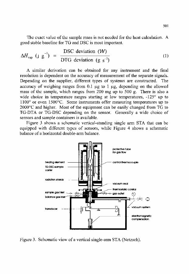
501

The exact value of the sample mass is not needed for the heat calculation. A good stable baseline for TG and DSC is most important.

-1) _ D S C devia t ion ( W ) ~vap (J g (1)

D T G devia t ion (g s -1)

A similar derivation can be obtained for any instrument and the final resolution is dependent on the accuracy of measurement of the separate signals. Depending on the supplier, different types of systems are constructed. The accuracy of weighing ranges from 0.1 ~tg to 1 ~tg, depending on the allowed mass of the sample, which ranges from 200 mg up to 500 g. There is also a wide choice in temperature ranges starting at low temperatures, -125 ~ up to 1100 ~ or even 1500~ Some instruments offer measuring temperatures up to 2000~ and higher. Most of the equipment can be easily changed from TG to TG-DTA or TG-DSC depending on the sensor. Generally a wide choice of sensors and sample containers is available.

Figure 3 shows a schematic vertical-standing single arm STA that can be equipped with different types of sensors, while Figure 4 shows a schematic balance of a horizontal double-arm balance.

he~ing element

TG-DSC-sompte corrler

rodlalton shields

K r n p ~ gas inlet

balance gas Inlet

tTansducer

- - protective tube for gas flow

conhd ~enT~cou~e

vacuum seal

l t~mostattc controt

vocuLrn S ~ T I

electTomagnetlc con3pE~sofloR

Figure 3. Schematic view of a vertical single-arm STA (Netzsch).

502

Figure 4. Schematic view (TA instruments).

of a horizontal double arm TG-DSC

The mode of construction is quite different, dependent on the company providing the equipment. As usual the best choice is a personal decision depending on the specific requirements for the samples, the economic situation of the purchaser and, in some cases, the wide variety of samples and users, i.e. universities require student-proof msmmaents. For discussion of the weighing principle (null-deflection balance or not, compensation for buoyancy effects, the influence of a "chimney- effect" depending on the gas-inlet), refer to Chapter 4 on TG.

Table I summarises the concept of some instruments as could be deduced from information brochures. This list is certainly not exhaustive.

503

Table 1

Company System TGA-DSC (DTA)

TA Instruments

Seiko

Mettler

B~hr

Rheometrics Scientific (former Stanton Redcroft)

Netzsch

Setaram I

Setaram II

Horizontal - two separate lever arms

Horizontal - two separate lever arms

Horizontal - a single arm - no reference sample (based on the SDTA principle)

Horizontal - a single arm with serial mounting of sample and reference

Vertical - a pending arm with parallel mounting of sample and reference

Vertical - a standing arm with parallel mounting of sample and reference

Vertical - a standing arm with parallel mounting of sample and reference

Vertical - two hanging separate arms with heat- sensors surrounding the reference and the sample separately

3. S I M U L T A N E O U S T H E R M O M E C H A N I C A L ANALYSIS- DIFFERENTIAL THERMAL ANALYSIS (TMA-DTA)

Although not difficult to construct, because there are no free moving or driven parts included, the combination of TMA-DTA is uncommon. Nevertheless, the same arguments as given in the introduction can be applied to this technique. The different methods of TMA (linear expansion, penetration, volume change measurements), allow collection of quite different types of information, such as weakening, melting, demixing, etc., but not all of those effects are accompanied by heat exchange. A combination with DTA or DSC could give simultaneous information for the same sample, measured in identical circumstances.

The combination of Dynamic TMA and DTA can also give interesting information on the dimensional changes and rigidity accompanying melting.

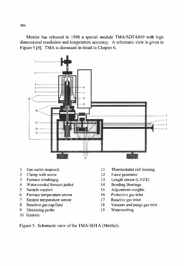
504

Mettler has released in 1998 a special module TMA/SDTA840 with high dimensional resolution and temperature accuracy. A schematic view is given in Figure 5 [4]. TMA is discussed in detail in Chapter 6.

1 Gas outlet stopcock 2 Clamp with screw 3 Furnace windingsg 4 Water-cooled furnace jacket 5 Sample support 6 Furnace temperature sensor 7 Sample temperature sensor 8 Reactive gas capillary 9 Measuring probe 10 Gaskets

11 Thermostated cell housing 12 Force generator 13 Length sensor (LVDT) 14 Bending Bearings 15 Adjustment weights 16 Protective gas inlet 17 Reactive gas inlet 18 Vacuum and purge gas inlet 19 Watercooling

Figure 5. Schematic view of the TMA-SDTA (Mettler).

505

4. SIMULTANEOUS DIFFERENTIAL SCANNING CALORIMETRY- THERMOPTOMETRY MEASUREMENT (DSC-TOA)

Heating stages for microscopes are available in a very wide temperature range (liquid nitrogen to 2000~ Visual inspection of the sample is thus possible as function of temperature. Information like colour change, decomposition, melting, polymorphism can be easily observed. In combination with a photomonitor, the light intensity of a reflected beam can yield information on the sample that is difficult to detect by other methods. This allows a certain quantification of the envisaged effects. This visual inspection can be combined with another quantitative measurement such as DSC or DTA (see also Chapter 10).

Mettler developed a special module that can operate in the temperature range - 60~ to 375~ based on a s-element thermopile DTA sensor deposited on a special glass disc. The sample is placed in a sapphire crucible in transmitted light (Figure 6).

CONVENTIONAL DSC

SYMMETRIC CELL

MICROSCOPY WITH DSC

A !

!

i K \ "k \ \ \ ' i :1 I ASYMMETRIC CELL

Figure 6. Conventional DSC and Thermomicroscopy- DSC [5] (Mettler).

In reference [5] a method is described for the purity determination of an eutectic mixture by DSC-TOA. The observation of the molten fraction as function of temperature is used as parameter for purity determination on a single sample, without the need for a pure reference sample. The method can be used in the area of dyes, liquid crystals, pharmaceuticals, fats and various organic compounds (more details are given in Chapter 10).

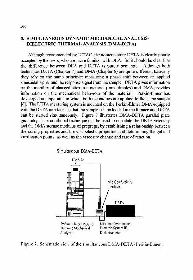
506

5. SIMULTANEOUS DYNAMIC MECHANICAL ANALYSIS- DIELECTRIC THERMAL ANALYSIS (DMA-DETA)

Although recommended by ICTAC, the nomenclature DETA is clearly poorly accepted by the users, who are more familiar with DEA. So it should be clear that the difference between DEA and DETA is purely semantic. Although both techniques DETA (Chapter 7) and DMA (Chapter 6) are quite different, basically they rely on the same principle: measuring a phase shift between an applied sinusoidal signal and the response signal from the sample. DETA gives information on the mobility of charged sites in a material (ions, dipoles) and DMA provides information on the mechanical behaviour of the material. Perkin-Elmer has developed an apparatus in which both techniques are applied to the same sample [6]. The DETA measuring system is mounted on the Perkin-Elmer DMA equipped with the DETA interface, so that the sample can be loaded m the fimaace and DETA can be started simultaneously. Figure 7 illustrates DMA-DETA parallel plate geometry. The combined technique can be used to correlate the DETA viscosity and the DMA storage modulus of prepregs, by establishing a relationship between the curing properties and the viscoelastic properties and determining the gel and vitrification points, as well as the viscosity change and rate of reaction.

Simultaneous DMA-DETA

DMA 7e

Mid Conductivity Interface

g . . ~

Perkin- Elmer DMA 7e Dynamic Mechanical Analyzer

Micromet Instruments Eumetric System III Dielectrometer

Figure 7. Schematic view of the simultaneous DMA-DETA (Perkin-Elmer).

507

6. OTHER TECHNIQUES

In spite of important advantages, simultaneous thermal analysis remains less popular than single or parallel measurements. Nevertheless, the above examples of S TA have illustrated the potential of this methodology and the list of possible combinations is certainly not Complete. Indeed for specific materials, such as metals or ceramics, "home-built" equipment for simultaneous temperature- dependent measurements could reveal specific information. As such, the simultaneous measurement of thermal energy and acoustic emission produced by a solid-solid martensitic transformation in intermetallic Cu-based alloys has been applied to study the growth kinetics of martensite variants during cooling and heating [7] . The influence of fatigue on the constitution of thermoplastic vulcanisates for biomedical applications has been studied by combined DSC-SAXS- WAXS (Differential Scanning Calorimetry-Small and Wide Angle X-ray Scattering)[8].

The main questions or problems related to STA remain whether the results obtained are as accurate as in single experiments, and whether the resolution and sensitivity of each signal obtained in STA are the same as those in single TA mode. If resolution and sensitivity are not critical, the advantages of STA, as enumerated in the introduction, should be taken into account when selecting appropriate experiments.

ACKNOWLEDGEMENTS

The author thanks the representatives of all mentioned companies for providing documentation, literature and permission for publication related to their specific products for STA.

REFERENCES

1. M.E. Brown, Introduction to Thermal Analysis, Chapman and Hall, London, 1988, Chap.4.

2. J.P. Redfem, Polymer Intemational, 26 (1991) 51. 3. G. Della Gatta, L. Benoist, P. Le Parlouer, 22th NATAS Conference

Proceedings, Denver, September 1993. 4. Mettler, private communication. 5. Mettler Application Note No. 806, H.G. Wiedemann and R. Riesen, Purity

Determination by Simultaneous DSC-Thermomicroscopy. 6. Perkin-Elmer, Thermal Analysis Newsletter, PETAN-55.

508

7. C. Picomell, C. Segui, V. Torra, J. Hemaer, C. Lopez del Castellio, Thermochim. Acta, 91 (1985) 311.

8. J.A. Helsen, S.V.N. Jacques, Recent Research Developments in Polymer Science, 1 (1996) 19.


Chapter 12

EGA - EVOLVED GAS ANALYSIS

J. Mullens

Limburgs Universitair Centrum, Department SBG, B 3590 Diepenbeek, Belgium

1. I N T R O D U C T I O N

According to the ICTAC nomenclature (International Confederation for Thermal Analysis and Calorimetry) EGA (Evolved Gas Analysis) is a technique of determining the nature and amount of volatile product or products formed during thermal analysis [1]. This definition includes coupled techniques such as TG-MS (Thermogravimetry-Mass Spectrometry), TG-FTIR (Fourier Transform Infra Red)and also TPR (Temperature Programmed Reduction) and TPD (Temperature Programmed Desorption) coupled to a detection system, and all other techniques by which gases are released and detected either directly or indirectly by using a solvent or an adsorbent.

In this chapter attention will be focused on techniques which have become of significant importance during the past decade and which have resulted in an indispensable addition to TA (Thermal Analysis). Examples of coupled TG-MS and TG-FTIR will be described. Also recent developments of TPR will be given.

Many laboratories do not possess the indispensable interfaces and coupling software but they do possess the separate analytical techniques. With some creativeness TA can be combined- in an off-line way - with many kinds of analytical techniques such as GC (Gas Chromatography), MS, (FT)IR, IC (Ion Chromatography), potentiometry etc. These possibilities, as well as the on-line combinations, will be illustrated using real examples. By describing many real examples, the author will try to alert the reader to the opportunities of coupling the above mentioned techniques in the investigation of all kinds of materials.

2. COUPLING TG-MS

2.1. The technique Interfaces and software are available from manufacturers of TA and/or MS

equipment which enable the coupling of MS with TG. Some manufacturers of

510

MS equipment have extended their gamut with MS equipment that is dedicated to be coupled to TG equipment in a user friendly way.

A detailed description of MS is outside the scope of this work. We restrict discussion to that necessary to understand the application. MS is an extremely sensitive technique which even enables Xe in air (8 ppb for the 136 isotope) to be detected. The coupling between TG and MS requires a special interface due to the fact that TG normally operates at atmospheric pressure, whereas MS requires a vacuum of about 10 -6 mbar. The connection is realized by bringing into the MS only a small part of the gases leaving the TG via a heated ceramic (inert) capillary. He is mostly used as the carrier gas, but gases such as air or 02 can also be used.

The incoming gases are bombarded with electrons in the ionisation chamber. Gas molecules are fragmented into positive ions. These positive ions are separated (e.g. by quadrupole) on the basis of their mass/charge ratio. By measuring the ion current, one obtains a plot of intensity as a function of the mass/charge ratio as shown in Figure 1.

~D

"" 1s

o

I I , I,I,

1'0 1'5 20 2'5 3'0 3'5 40 4'5 50 5'5 6'0 65 7'0 7'5 80 Mass Scan 169 - Scan 59

Figure 1. MS" intensity as a function of mass/charge.

Figure 1 represents an instantaneous scan. As the scanning continues during the total TG experiment, one can (with appropriate software) join all instantaneous scans of each mass/charge ratio to obtain, for each ratio, the intensity as a function of time or temperature. In Figure 2 the results for the values 18 (H20+) , 28 (CO +) and 44 (CO2+), during the heating of CaC204 .H20 in oxygen, are given as an example.

511

~D +,,,a

E8

E9

El0

Ell

C••CO --___.___co J I c o / - " -q

00 15 00 00 30 00 00 45 00 01 0'0 00 01 1'5 00 01 30 00

2'6 1()0 2(}0 360 460 5()0 6()0 7170 8()0 9;0 992

Time/h m s

Temp/~

Figure 2. MS" intensities as a function of temperature and time.

If one has a library of spectra available one can compare experimental results of the fragments obtained with the library in order to identify the original gas before ionisation. This is not always easy, due to differences in total composition of the sample and in the experimental working conditions of the MS equipment. In general, there is no problem of identification of simple molecules. For example, when the resolution of the MS equipment is not high enough for the distinction between the values 28.013 (N2 +) and 28.011 (CO+), the assignment of the value 28 to N2 +, CO +, or C2H4 + can be determined from the kind of material. Another example" the detection of the values 40 and 20 (Ar 2+ since one measures the mass/charge value) when using Ar as the carrier gas is not a surprise. The identification of traces of NH3 + (17) in the presence of water is not always evident due to the fact that besides H20+(18) and the fragment O + (16), the fragment OH+ (17) is also present. MS detects all molecules, even those without dipole moment (permanent or during vibration), and is an extremely sensitive technique.

2.2. Appl icat ions and examples of TG-MS experiments

2.2.1. Contamination and stability of the YBa2Cu307-x superconductor [2] Ceramic superconductors can be prepared using an oxalate precursor [3, 4]

which can be transformed to the superconducting oxide by sintering and annealing. This transformation takes place through the carbonate which is very stable and decomposes at temperatures above 900~

512

Carbonate can be formed at the surface of the superconductor by the reaction with CO2 in air. TG-MS is very suited to the determination of the purity, for example the presence of residues of oxalate and carbonate.

The TG result recorded in Ar (50 ml min-1) at a heating rate of 20 K min-1 is plotted on a very sensitive scale in Figure 3. Figure 4 shows the release of CO up to about 700~ followed by the release of CO2.

1 0 1 ~ -----~--~ 0.6

100 0.4 .=

N 99 0.2 ~

98 0.0

97 - 0.2 0 5 10 15 20 25 30 35 40

Time/min Figure 3. TG of YBa2Cu307-x contaminated with oxalate and BaCO3 (in Ar).

10.0

9.0

8.0 C O 2 ~ ~ 7.0

"~ 6.0 water = E 1 5.0 /'

" 0 q~.~~ 4.0

3.0 .~

2.0 o~ ~ CO~, 1.0 ~ t 0.0 ygen

00 00 00 00 06 00 00 1'2 00 00 1'8 00 00 24 00 00 30 00 00 36 00 00 42 00 Time/h m s I I I i i i i i i i i

25 108 192 275 358 442 525 608 692 775 858 Temp/~ Figure 4. MS of YBa2Cu307-x contaminated with oxalate and BaCO3 (in Ar).

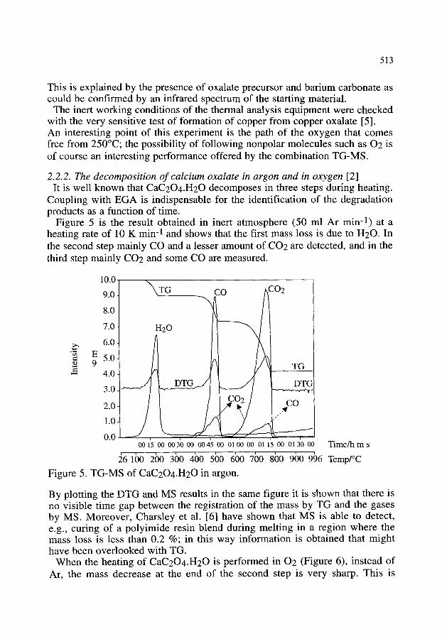
513

This is explained by the presence of oxalate precursor and barium carbonate as could be confirmed by an infrared spectrum of the starting material.

The inert working conditions of the thermal analysis equipment were checked with the very sensitive test of formation of copper from copper oxalate [5]. An interesting point of this experiment is the path of the oxygen that comes free from 250~ the possibility of following nonpolar molecules such as 02 is of course an interesting performance offered by the combination TG-MS.

2.2.2. The decomposition of calcium oxalate in argon and in oxygen [2] It is well known that CaC204.H20 decomposes in three steps during heating.

Coupling with EGA is indispensable for the identification of the degradation products as a function of time.

Figure 5 is the result obtained in inert atmosphere (50 ml Ar min-1) at a heating rate of 10 K min-1 and shows that the first mass loss is due to H20. In the second step mainly CO and a lesser amount of CO2 are detected, and in the third step mainly CO2 and some CO are measured.

10.0 9.0 "X~TG CO CO2

8.0

7.0 H20

6.0

5.0 , TG

4.0

3.0

2.0

1.0

0.0 00 15 00 00 30 00 00 45 00 01 0'0 00 01 15 00 01 3'0 00 Time/h m s

}61bo 2bo 3bo 4bo 500 600 760 800 900 9~)6 Temp/~ Figure 5. TG-MS of CaC204.H20 in argon.

By plotting the DTG and MS results in the same figure it is shown that there is no visible time gap between the registration of the mass by TG and the gases by MS. Moreover, Charsley et al. [6] have shown that MS is able to detect, e.g., curing of a polyimide resin blend during melting in a region where the mass loss is less than 0.2 %; in this way information is obtained that might have been overlooked with TG.

When the heating of CaC204.H20 is performed in 02 (Figure 6), instead of Ar, the mass decrease at the end of the second step is very sharp. This is

514

attributed to the partial oxidation of CO to CO2, which accelerates the second step once it has started. This is the reason that, in Ar, the amount of CO2 is higher than that of CO, even in the second step. Detection of CO2 by MS is always accompanied by the detection of some of the CO formed by some fragmentation of CO2 in the ionisation chamber.

As mentioned before, FTIR has the advantage that this technique detects the gases as they are released. Some of the CO2 can also be formed in the TG by the disproportionation reaction of evolved CO to yield CO2 and carbon which is typical for oxalates [7, 8, 9].

El0

o , , . ~

Ell

i CO"q .... . . ? C02 ]

001'500 003'000 004500 010000 01 1500 013000

27 100 200 300 400 500 600 700 800 900 993

Figure 6. TG-MS of CaC204.H20 in oxygen.

Time/h m s

Temp/~

2.2.3. The investigation of a waste mixture of cellulose-copper sulphate [10] The decomposition temperature of compounds can be strongly influenced by

the presence of other compounds, which makes identification on the basis of degradation temperatures totally impossible. Figures 7 and 9 show the TG-MS result of pure copper sulphate pentahydrate in inert atmosphere (50 ml min -1 helium; 20 K min-1); some typical mass/charge ratios are given as a function of time and temperature.

It is well known that the formation of the anhydrous sulphate takes place between 75 and 300~ and that the formation of copper oxide starts between 400 (MS traces in figure 9) and 575~ (TG in Figure 7).

The identification of the degradation temperatures (Figures 8 and 10) of the two compounds in a 1/1 mass mixture is done by following typical degradation masses: cellulose is followed by the detection of 28 (CO +) and 44 (CO2 +) as a function of temperature, and for the degradation of copper sulphate

515

pentahydrate (Figure 9), ratios of 64 (SO2+), 48 (fragment SO +) and 32 (SO22+) are followed.

120 0.6

r ~ r ~

100-

80-

60-

40- c__

-0.4

-0.2

-0.0

20 . . . . . - 0.2 0 260 460 660 860 1000

Temperature/~

Figure 7. TG of pure CuSO4.5H20.

r,.) o

~D

120 1.2

100

80-

60-

40

20

-1.0

' 260 ' 460 ' 660 ' 860 Temperature/~

Figure 8. TG of a 1/1 mixture cellulose-CuSO4.5H20.

0.8 r,..) o

0.6 ~ ~"

0.4 ~ o,,,~

0.2

0.0

|

0 oob ~

When one compares this with pure copper sulphate pentahydrate, it is obvious that, in the mixture of copper sulphate pentahydrate and cellulose, the degradation of the copper sulphate takes place at a temperature that is about 200 degrees lower than in the pure sulphate. This example clearly shows that

516

mixing different compounds can very drastically change the thermal stability. In this mixture the effect is due to the reducing properties of the cellulose on the sulphate.

E8 18

E9 17

32 El0

N Ell

El2 64

El3

30 1()0 260 3()0 400 560 6()0 760

Figure 9. MS of pure CuSO4.5H20.

00 IJ6 00 00 1'2 00 00 1'8 00 00 2~4 00 00 3b 00 00 3'6 00 00 4'2 00 Time/h m s ' /

800 889 Temp/~

o~,~

tD

E9

El0

Ell

El2

El3

. . 2 ~

00 00 00 00 06 00 00 12 00 00 18 00 00 24 00 00 30 00 00 36 00 00 42 00 TimeB1 m s

20 100 2(30 300 400 500 6()0 700 800 8~/4 Figure 10. MS of a 1/1 mixture of cellulose-CuSO4.5H20.

Temp/~

2.2.4. Other examples of the combination TG-MS The application of mass spectrometry to the study of the thermal degradation

of tin dithiocarbamate complexes has recently been reviewed [11]. Thermal decomposition mechanisms of nickel thiourea chloride complexes are proposed

517

[ 12]. Methods of calibrating systems for CO and CO2 using calcium carbonate and calcium oxalate are described [13]. TG-MS is used to study organo soluble segmented rigid-rod polyamide films [14]. Sulphated zirconia catalysts are studied using TG-DTA-MS [15]. TG-MS of X-ray pure YBa2Cu30x has shown evolution of CO2 in addition to the known 02 liberation causing degradation of its superconducting properties due to the weakening of the intergrain coupling in the compound [16]. Studies on the thermal decomposition behaviour of homogeneously precipitated Zr2(SO4)(OH)6.6H20 using TG- DTA-MS are reported [ 17]. The mechanism and rate of sulphur release during coal combustion are studied using TG and MS [18]. TG has been combined with MS to verify moisture data for group Y meningococcal polysaccharide and freeze-dried antibody to hepatitis B surface antigen and to identify an impurity in a Haemophilus b polysaccharide [ 19].

Selected analytical problems encountered by the Research Division of the U.S. Customs Service and solved by combining TG and MS are reported i.e. the detection of a benzenoid containing compound in dry ink, the compositional analysis of styrene-butadiene rubber blends, the differentiation between the natural and chemically modified forms of guar gums and the determination of country of origin of coffee beans [20].

TG-MS is also used for the analysis of a coal sample and an oil shale [21 ], for the study of the decomposition of poly(ethylene-co-vinyl alcohol) [22], the study of a peroxide-cured EPDM rubber [23], the study of an electronic waste material from the automotive industry showing fragments of epoxy resin or bromine fragments [23], the thermal stability of the blend components in a blend of polypropylene and melamine resin [23], the degradation of ripidolite and polysilane [24], the thermal decomposition of the n-alkylamine t~- zirconium phosphate intercalates Zr(CnH2n+INH3PO4)x(HPO4)2-x.nH20 [25], the reaction between CaC03, A1203, Si02 and CaF2 [26], the influence of molybdenum trioxide on the degradation of polyvinyl chloride [27], the assessment of the catalitic activity of modified clays [27], the examination of brick clays [27], the degradation of calcium oxalate [28], strontium nitrate [28], ethylene-hexene copolymers [28], linear polyethylene [28] and poly(ethylene oxide) [28], the composition analysis of a coating spray [29], the compositional analysis of polyvinyl acetate [29] and the degradation of calcium acetate monohydrate [29]. Pyrolysis MS has been used for the chemometric classification of wines [30].

The combination TG-DTA-MS is used for the study of a partially cured phenol-formaldehyde resin [31], the investigation of the combustion of wool [31], the char combustion of a bituminous coal [32], the study of a polyimide resin [33] and the study of the relation of the thermal stability of anionic planar complexes (ML2)2-.xH20 and neutral trans-octahedral M(LH2)2X2 complexes (where M is Ni, Mn or Cu, X is C1, Br or I and LH2 is CH2(CONH2)2) with the metal-ligand bond strength and the crystal field stabilization theory [34]. As an application to Mars surface exploration,

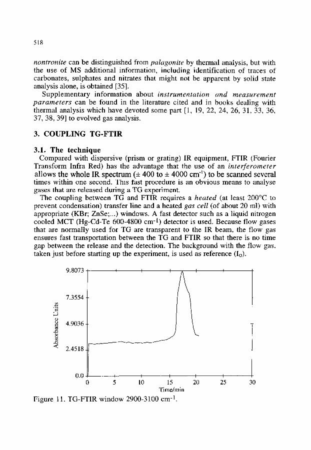
518

nontronite can be distinguished from palagonite by thermal analysis, but with the use of MS additional information, including identification of traces of carbonates, sulphates and nitrates that might not be apparent by solid state analysis alone, is obtained [35].

Supplementary information about instrumentation and measurement parameters can be found in the literature cited and in books dealing with thermal analysis which have devoted some part [1, 19, 22, 24, 26, 31, 33, 36, 37, 38, 39] to evolved gas analysis.

3. C O U P L I N G T G - F T I R

3 . 1 . T h e t e c h n i q u e Compared with dispersive (prism or grating) IR equipment, FTIR (Fourier

Transform Infra Red) has the advantage that the use of an interferometer allows the whole IR spectrum (• 400 to + 4000 cm ~) to be scanned several times within one second. This l'ast procedure is an obvious means to analyse gases that are released during a TG experiment.

The coupling between TG and FTIR requires a heated (at least 200~ to prevent condensation) transfer line and a heated gas cell (of about 20 ml) with appropriate (KBr; ZnSe;...) windows. A fast detector such as a liquid nitrogen cooled MCT (Hg-Cd-Te 600-4800 cm -1) detector is used. Because flow gases that are normally used for TG are transparent to the IR beam, the flow gas ensures fast transportation between the TG and FTIR so that there is no time gap between the release and the detection. The background with the flow gas, taken just before starting up the experiment, is used as reference (Io).

o , . , ~

�9

<

9.8073 i I i

7.3554

4.9036

J 2.4518

0.0 i i 10 15

Time/min

Figure 11. TG-FTIR window 2900-3100 cm -1

I I

\

I

20 I

25 30

519

Software gives complete and interesting information [40]. Besides the registration of the whole spectrum, one can also tune in on

several windows in order to follow specific bands as a function of time (or temperature) as illustrated in Figure 11 with the CH-window 2900-3100 cm -1. Also contour plots with different intensities are possible (Figure 12). The so-called stacked plot (Figure 13) is a three-dimensional plot with information about the kind (wavenumber) and the amount (absorbance units) of the released gases as a function of the temperature or time at which they are released.

The on-line combination TG-FTIR makes it possible to identify all molecules or bonds with an oscillating dipole. The fact that the registration is done on molecules in the gas phase offers a high degree of resolution, with a fine structure that is typical of gas phase IR spectra, as compared with those of liquids or solids.

tS. 5,~8

11,6976

W

~" 2 , 8 5 7 3 z

{_)

4 . 8 1 6 9

0. 1266

0 I = . . . . . . ,0

I)

1, ,ttl

I

3800 3500

Wavenumbers /cm -1

Figure 12. TG-FTIR contour plot.

350 CONTOUR-LINES A

0. 008 B

----- ~l,ot (] ----- 0.04 D

- 2 7 2 . 5 ~

-195 *C

. 1 1 7 . 5 ~

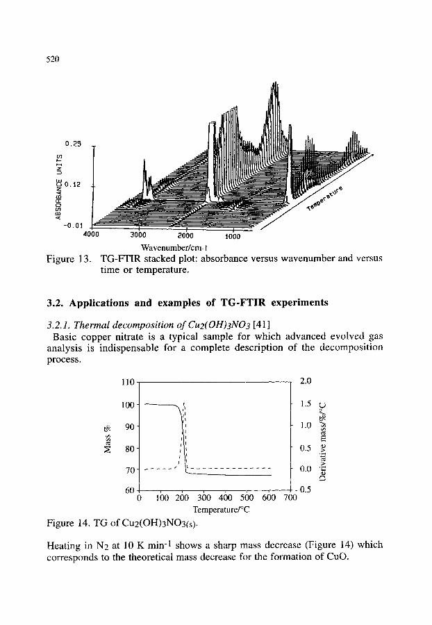
520

0.25

r l----

z

IL l ~ 0 . 1 2 Z

r r " O

-0.01 4000

Figure 13.

3ooo 2o0o iobo Wavenumber/cm- I

TG-FTIR stacked plot: absorbance versus wavenumber and versus time or temperature.

3.2. Applications and examples of TG-FTIR experiments

3.2.1. Thermal decomposition of Cu2(OH)3N03 [41 ] Basic copper nitrate is a typical sample for which advanced evolved gas

analysis is indispensable for a complete description of the decomposition process.

110 2.0

100

90

70

i I

i I I I I I

I I

I I

1.5 r,.) o

1.0 "~

0.5

0.0 = (D

60 , - 0.5 0 100 2()0 3()0 460 560 6()0 700

Temperature/~

Figure 14. TG of Cu2(OH)3NO3(s).

Heating in N2 at 10 K min-1 shows a sharp mass decrease (Figure 14) which corresponds to the theoretical mass decrease for the formation of CuO.

521

All the different gases are released at the same time with a maximum at about 241 ~ (stacked plot in Figure 15). Figure 16 shows the FTIR plot at 241 ~ By comparison of this plot With a plot of HNO3(g) (Figure 17), taken under the same conditions, it is demonstrated clearly that besides H20 (3800-3600 and 1600-1500 cm- 1) and NO2 (1318, 749 and strong absorption v 1' at 1612 cm- 1 in Figure 16) HNO3 is also liberated, of which only a part is dissociated.

Only by using TG-FTIR can a complete reaction scheme be found

Cu2(OH)3NO3(s) ..... > 2. CuO(s) + H20(g) + HNO3(g)

HNO3(g) <===> 0.5 H20(g)+ NO2(g) + 0.2502(g)

The decomposi t ion is not the same as for basic yttr ium nitrate Y2(OH)5(NO3). l .SH20, where the gases H20, NO2 and 02 are evolved in three steps between 200 and 600~ and where no HNO3 is detected [42].

0.45

�9 . . , . i

0.225 0

0.0 4(

. . . . . . . . . . . . . . . . . . . . . 396

. . . . . . . . . . ~ ............ 319 . . . . . . . . . . . . . . . . . . f t - ~ 286

~J~ . . . . . . . ~ ' 2 6 6 2 ,2

" ' ~ ~ - - .............. 1~ t l~J ~ ~'t tJ_ h,~, 241

. . . .

34 31

. . . . . * .. ! . . - ! - -

)00 3000 2000 1000 Wavenumber/cm -1

Figure 15. FTIR of Cu2(OH)3NO3(s).

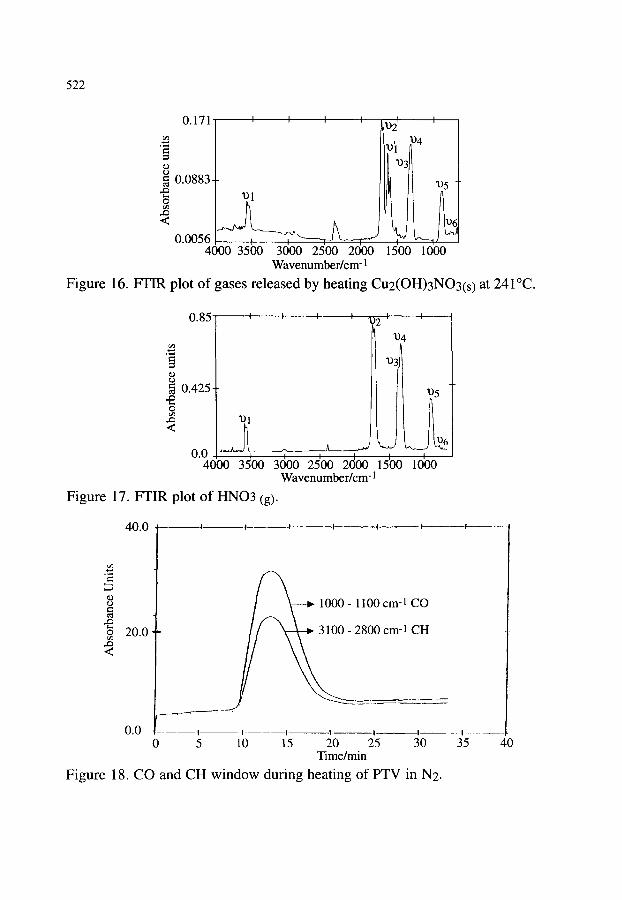
522

0.171

- , " ' 4

~ o.o883

<

0.00561 n 4000 3500

II

1) 3

3000 2500 2000 W avenum ber / cm -1

1

1)5

1 5 0 0 1 0 0 0

Figure 16. FTIR plot of gases released by heating Cu2(OH)3NO3(s) at 241 ~

0.85

= 0.425

o

I I I I I I

1)4

1)5

0.0 J I 0 0 0 0 4000 3500 3000 2500 2000 1500 1000

Wavenumber /cm- 1

Figure 17. FTIR plot of HNO3 (g).

40.0 - ~ - t . . . . . t . . . . . . ! . . . . . I - ! . . . . I l __.

r u 1 0 0 0 - 1100 cm-I CO

"~ 20.0 00 - 2800 cm-l CH

<

�9 _ . . .

0.0 , - - , - - - - - ~ . . . . t - , . . . . , . . . . . . , ............ 0 5 10 15 20 25 30 35 40

Time/min

Figure 18. CO and CH window during heating of PTV in N2.

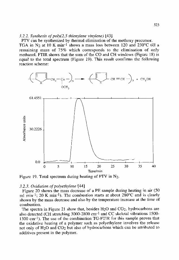
523

3.2.2. Synthesis of poly(2,5 thienylene vinylene) [43] PTV can be synthesized by thermal elimination of the methoxy precursor.

TGA in N2 at 10 K min-1 shows a mass loss between 120 and 230~ till a remaining mass of 75% which corresponds to the elimination of only methanol. FTIR shows that the sum of the CO and CH windows (Figure 18) is equal to the total spectrum (Figure 19). This result comfirms the following reaction scheme"

( Ls~CH2--~H% ~ ( < [~CH--CH ~)n OCH 3

+ CH 3OH

. , , , , ~

~D

,.Q

O

,.Q <

61.4551 I J I I I

30.2226

0.0 I I I I I ....

0 5 10 15 20 25 30 35 40 Time/min

Figure 19. Total spectrum during heating of PTV in N2.

3.2.3. Oxidation of polyethylene [44] Figure 20 shows the mass decrease of a PE sample during heating in air (50

ml min-1; 20 K min-1). The combustion starts at about 280~ and is clearly shown by the mass decrease and also by the temperature increase at the time of combustion.

The spectra in Figure 21 show that, besides H20 and CO2, hydrocarbons are also detected (CH stretching 3000-2800 cm -1 and CC skeletal vibrations 1500- 1300 cm -1). The use of the combination TG-FTIR for this sample proves that the oxidative heating of a polymer such as polyethylene involves the release not only of H20 and CO2 but also of hydrocarbons which can be attributed to additives present in the polymer.

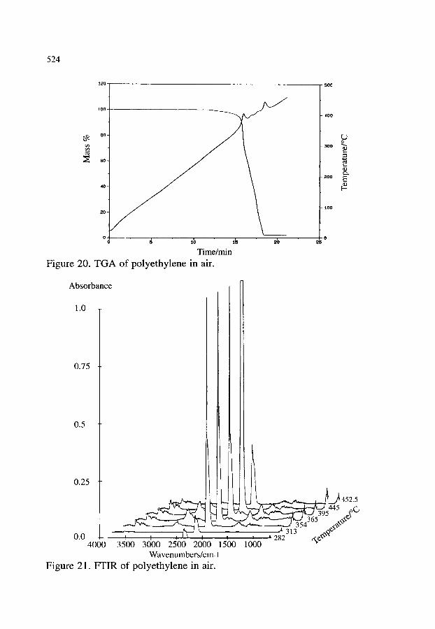
524

120

t o o ~

~ . 8 0 -

r~

6 0 -

40 ,

2 0 -

0 ' ' ' ~ - - " i o ~ go ti5 ~o Time/min

Figure 20. TGA of polyethylene in air.

- 500

400

300

200

t 0 0

~ 0 ~6

o

�9

y,

Absorbance

1.0

0.75

0.5

0.25

i ~ i ~ ~-'~452"5 5445 ~Q,, �9 365 ,,,,~,~

0.0 , , . . . . . . . . . . ~ ~ t 313 . . . . 282 4000 3500 3000 2500 2000 1500 1000

Wavenumbers/cm-1 Figure 21. FTIR of polyethylene in air.

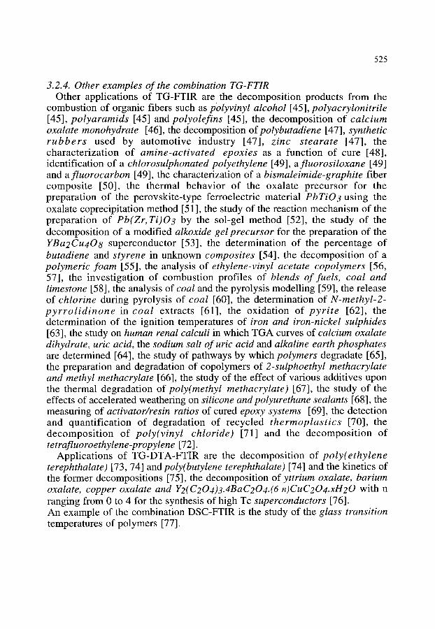
525

3.2.4. Other examples of the combination TG-FTIR Other applications of TG-FTIR are the decomposition products from the

combustion of organic fibers such as polyvinyl alcohol [45], polyacrylonitrile [45], polyaramids [45] and polyolefins [45], the decomposition of calcium oxalate monohydrate [46], the decomposition ofpolybutadiene [47], synthetic rubbers used by automotive industry [47], zinc stearate [47], the characterization of amine-activated epoxies as a function of cure [48], identification of a chlorosulphonated polyethylene [49], a fluorosiloxane [49] and a fluorocarbon [49], the characterization of a bismaleimide-graphite fiber composite [50], the thermal behavior of the oxalate precursor for the preparation of the perovskite-type ferroelectric material PbTi03 using the oxalate coprecipitation method [51 ], the study of the reaction mechanism of the preparation of Pb(Zr, Ti)03 by the sol-gel method [52], the study of the decomposition of a modified alkoxide gel precursor for the preparation of the YBa2Cu408 superconductor [53], the determination of the percentage of butadiene and styrene in unknown composites [54], the decomposition of a polymeric foam [55], the analysis of ethylene-vinyl acetate copolymers [56, 57], the investigation of combustion profiles of blends of fuels, coal and limestone [58], the analysis of coal and the pyrolysis modelling [59], the release of chlorine during pyrolysis of coal [60], the determination of N-methyl-2- pyrrolidinone in coal extracts [61], the oxidation of pyrite [62], the determination of the ignition temperatures of iron and iron-nickel sulphides [63], the study on human renal calculi in which TGA curves of calcium oxalate dihydrate, uric acid, the sodium salt of uric acid and alkaline earth phosphates are determined [64], the study of pathways by which polymers degradate [65], the preparation and degradation of copolymers of 2-sulphoethyl methacrylate and methyl methacrylate [66], the study of the effect of various additives upon the thermal degradation of poly(methyl methacrylate) [67], the study of the effects of accelerated weathering on silicone and polyurethane sealants [68], the measuring of activator~resin ratios of cured epoxy systems [69], the detection and quantification of degradation of recycled thermoplastics [70], the decomposition of poly(vinyl chloride) [71] and the decomposition of tetrafluoroethylene-propylene [72].

Applications of TG-DTA-FTIR are the decomposition of poly(ethylene terephthalate) [73, 74] and poly(butylene terephthalate) [74] and the kinetics of the former decompositions [75], the decomposition of yttrium oxalate, barium oxalate, copper oxalate and Y2(C204)3.4BaC204.(6-n)CuC204.xH20 with n ranging from 0 to 4 for the synthesis of high Tc superconductors [76]. An example of the combination DSC-FTIR is the study of the glass transition temperatures of polymers [77].

526

4. THE USE OF A N A LY TIC A L TECHNIQUES BY ON-LINE AND OFF-LINE C O M B I N A T I O N WITH T H E R M A L ANALYSIS

4.1. The technique For the identification of the gases evolved during combustion of polymers

that contain a variety of additives such as flame retardants, fillers, plasticizers, colouring matters, anti-oxidants, one can obtain complete information only by the combination of several techniques. TG can be used for the determination of the degradation profile (mass loss as a function of time or temperature). The evolved gases can be investigated by the on-line coupling with FTIR or/and MS as illustrated before. If one does not possess on-line coupling, one can collect the gases on an adsorbent (e.g. a tenax tube) or collect them successively in a series of solvents. After adsorption on a solid adsorbent and TD (thermal desorption), one can identify the gases by GC-MS (gas chromatography-mass spectrometry). Such a combination can be completed by investigating the solvents in which the gases are collected by analytical techniques such as ion chromatography, potentiometry, spectroscopic techniques etc. The investigation of the residue can also be a source of useful information. Additional important information can be obtained by isolating intermediate products from the pan as well as from the absorbent or/and the solvents in which the evolved gases are collected. A flow chart of possible combinations is given in Figure 21.

On-line coupling TA: TG

DTA DSC

Off-line coupling TA: TG

DTA DSC

> heated transfer line > FTIR MS

-> Adsorption on an adsorbent

Collection in a liquid

> TD: thermal desorption I

I

> I

(FT)IR (FT)Raman

(GC)MS Visible and UV spectroscopy

X-ray spectroscopy Ion chromatography

Atomic absorption spectroscopy Potentiometry, etc.

Figure 21. Flow chart of possible combinations of thermal analysis with other techniques.

5 2 7

4.2. Applications and examples of the use of analytical techniques by on-line and off-line combination with thermal analysis

4.2.1. The oxidative degradation qf polystyrene studied by the combination of on-line TG-FTIR with off-line (using tenax and TD) TG-GC-MS [78]

Figures 22 and 23 show the mass decrease of two polystyrene samples with different additives during heating in 50 ml min-1 air at 20 K min-1, being the maximum rate recommended (ASTM E698-79) for the study of thermally unstable materials. The oxidative degradation starts at about 300~ as shown by the mass decrease and the increased temperature.

120 500

100

80-

60-

40-

20-

_

- 2 0 ' I ' I ' I ' I

0 5 10 15 20 T i m e / m i n

Figure 22. TG of polystyrene sample 1. 120

- 400

L) - 3 0 0

- 200

-100

0 25

800

1 0 0

80

60 r/3

40

20

Y / /

/

J / /

/

( ' ~ ' l b ' ~'5 ' i o ' i 5 ' T i m e / m i n

Figure 23. TG of polystyrene sample 2.

600

400

200

L) o

< D

528

The evolved gases are analyzed by transmission FTIR using the on-line coupling between the TG and the FTIR, whereas the FTIR is used at a speed to acquire four complete spectra within 1 second at a spectral resolution of 8 cm-1. The stacked plots with the absorbance versus wavenumber and versus temperature or time are shown in Figures 24 and 25.

<D

O <

1.00.

0.75

0.50

0.25

. . . . .

40 10 35b0 3d00 2500 20:(30 15"00 1000 -275

CO2

I/ t %'%%~.~ ~ ~ ~ 5 ~ . . _ _ ~ . _ _ . . ~ 473 /

~ ~ ~ ~ ~ ' ~ 4 3 _ _ ~ _ _ 4 ~ + 8 428 ~ , ~ ' - -~ : " .~'4--~!-!--~363.5 / ~ ' -

t , _ , , ~ ~ O , r

Wavenumber/cm- 1 Figure 24. FTIR of polystyrene sample 1.

3.0

r ~

o , , - q

= 2.0 ~D

o 1.0 ,.Q < t. , , . . . ,.~- ~ . , . . . . - -

. . . . . . . .

o.o - - " ' " . . . . ~ ~00 .... ~..++~ 4000 3500 3000 2500 2000 1 1 Wavenumber/cm -1

Figure 25. FTIR of polystyrene sample 2.

~ ~ ~ . . ~ 22 (470) 0 (444)

15 (334) _ca ~ ' / 10 (225) \~,~ ~

0 5 ~ 5 (125) \ ~ ' ~ �9 (35) ~ ; ~ ~

529

The FTIR spectra of the evolved gases are recorded continuously as a function of temperature and time and can be plotted at different time intervals as illustrated by Figures 24 and 25. Assignment of the spectra: H20 (3600-3400 and 1650-1600 cm-1), CO2 (2360-2340 and 750 cm-1) and aromatic hydrocarbons (3040 and 1600-1580 cm-1).

The window spectrum for the aromatic hydrocarbons evolved by sample 2 is

I I I I I given in Figure 26.

9.8073

7.3554 o ~

~ 4.9036

o

< 2.4518

J J

0.0 I I I I

0 5 10 15 20 25 Time/min

Figure 26. FTIR window spectrum of CH 3100-2900 cm-1 (sample 2).

30

on-line .. ~ l FTIR ,ii

[ITEN Ax

! TD i ~l GC-~

.......... off. :.!L~e ................................ i

Figure 27. Flow chart of the combination of techniques.

In order to identify molecules, instead of specific bands of the aromatic hydrocarbons, one needs an additional separation and detection technique such as GC-MS. Therefore the gases coming out of the FTIR during the TG-FTIR experiment are collected on a tenax tube.

530

After the TG-FTIR experiment, the tenax tubes are thermally desorbed (TD) and transferred to a GC-MS apparatus,

8.7

RIC

benzene 563

| i ' i i I i | !

500 4:10

828

toluene

| xylene I 1066

L. Jj 1000 8:20

1134

styrene

! | | i | 1 i

1500 Scan 12:30 Time

Figure 28. GC-MS chromatogram of sample 1.

4.7

RIC

779

styrene --~ toluene - - >

' ' ' ' I w w , ~ I

500 1000 4:10 8:20

1130 m

12

Figure 29. GC-MS chromatogram of sample 2.

1318

~5 r

I

i

benzaldehyde

q l ~ methylstyrene

1500 12:30

Scan Time

A flow chart of the use of the techniques is given in Figure 27. TD parameters and GC-MS parameters are published elsewhere [78].

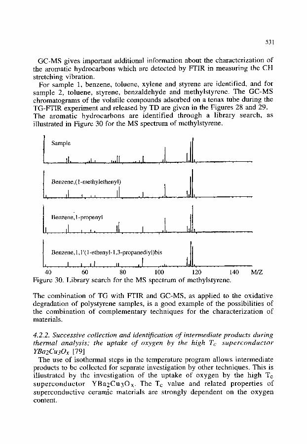
531

GC-MS gives important additional information about the characterization of the aromatic hydrocarbons which are detected by FTIR in measuring the CH stretching vibration.

For sample 1, benzene, toluene, xylene and styrene are identified, and for sample 2, toluene, styrene, benzaldehyde and methylstyrene. The GC-MS chromatograms of the volatile compounds adsorbed on a tenax tube during the TG-FTIR experiment and released by TD are given in the Figures 28 and 29. The aromatic hydrocarbons are identified through a library search, as illustrated in Figure 30 for the MS spectrum of methylstyrene.

Sample

Benzene,(1-methylethenyl)

�9 1! Benzene, 1-propenyl

Benzene, l,l'(1-ethenyl-l,3-propanediyl)bis ]1

, ............. I ,. ,I ...... ,, ..... ,.[ ..... ._,,, .... .... J,.. .... 40 60 80 100 120

Figure 30. Library search for the MS spectrum of methylstyrene. 140 M/Z

The combination of TG with FTIR and GC-MS, as applied to the oxidative degradation of polystyrene samples, is a good example of the possibilities of the combination of complementary techniques for the characterization of materials.

4.2.2. Successive collection and identification of intermediate products during thermal analysis; the uptake of oxygen by the high Tc superconductor YBa2Cu30x [79]

The use of isothermal steps in the temperature program allows intermediate products to be collected for separate investigation by other techniques. This is illustrated by the investigation of the uptake of oxygen by the high Tc superconductor YBa2Cu3Ox. The Tc value and related properties of superconductive ceramic materials are strongly dependent on the oxygen content.

532

In the first experiment (Figure 31) a pellet was heated up at 20 K min -1 to 920~ in 30 ml 02 min-1, kept at this temperature for 4 h, cooled down at 2 K min-1 to 475~ kept constant again for 4 h and cooled down to 25~ at 2 K min- 1.

102

1400

101

1200

100

1000

~ 99 ~ . . . . . . . . . . . . . . . - ,

98t/1 600 ' 7

"--" 97 - , . . . . . . . . . , ,

400 , '~

96 "',

200 v ",,,, 00 l;o 3;o 4;0 5;0 6;o 7;0 8;0 960 obo liOO

Time/min Figure 31. TG of YBa2Cu3Ox: mass versus time and temperature.

To obtain samples with different x-values, a table is constructed with small quartz bars and is mounted in the quartz tube of the TG analyzer so that the oxygen stream can reach uniformly each of the different samples of the same precursor pellets placed on that table. The pellets are placed in such a way that the temperature gradient between them is acceptable. The mass of one sample of the precursor is followed continuously during the whole 2000 min run in 30 ml 02 min-1. As can be seen from Figure 32, the following programme is carried out: heating to 920~ at 10~ min-1, isothermal period of 2 h, cooling at 2~ min -1, holding the temperature constant at 500~ 350~ 250~ 150~ and 50~ each for a period of 4 h. On heating (see Figures 31 and 32) there is a mass loss, on cooling there is an uptake of oxygen and during the isothermal periods there is no change in mass because, after a few minutes, the thermodynamic equil ibr ium O2(gas)- O2(solid) is reached. During each isothermal period a sample was taken from the quartz table and the oxygen level was measured by iodometric titration [80]. The following results were obtained T = 920~ x = 5.8; T = 500~ x =6.47; T = 350~ x - 6.7; T = 250~ x - 6.74; T =150~ x = 6.89; T - 50~ x - 6.9. The samples taken at 350~ 250~ 150~ and 50~ show the Meissner effect, proving that these samples are superconductive at the temperature of liquid nitrogen.

533

Using this combination of TG-potentiometry a better idea about the important reaction between oxygen and YBa2Cu3Ox is obtained.

102 . . . . . . , , , , . . . . . . . , , , , , , , ,

101

100

99

:~ 98

97

96

95

\r---',, I ~ " - - - F - - - ~ ~

X \ / [ k._~ ! ',,

I I ",

0.0 260 4 0 0 6 6 0 "800 1000 1200 Time/min

Figure 32. TG of YBa2Cu3Ox: mass versus time and temperature.

\ \

1 0 i I , I i �9 ,

1 0 1600 1800 2 0 0 0 2 2 0 0

1400

1200

1000 o r`-)

800

6 0 0

4 0 0 i !

I

2 0 0

4.2.3. The characterization of sulphur functional groups in fossil fuels, rubber and clay by coupling TPR (temperature programmed reduction) and potentiometry

Sulphur is present in fossil fuels, both in inorganic compounds (mainly pyrite) and in the organic matrix and is released during combustion in the form of SO2 and SO3. In this way sulphur contributes to acid rain. The same happens during heating and sintering of clays. Moreover, sulphur compounds produced during several processing periods can have a deleterious effect on construction materials and are highly toxic.

The ultimate fate of sulphur during processing is dependent on its form. In coal, for example, thiols and sulphides give labile sulphur compounds fairly readily during processing, whilst thiophenic products are more stable. A knowledge of the sulphur functional groups is therefore desirable and is an important parameter in selecting a coal or a clay for a particular process. There has been no convenient method available for determining the sulphur containing functional group distribution. Recently an interesting approach to the characterization of sulphur in materials such as coal [81, 82, 83], coal- derived pyrite [84] and clay [85] has been developed, namely temperature programmed reduction. This method is based on nonisothermal heating of the sulphur-containing compound at a fixed programming rate, in a reducing atmosphere, in order to form H2S. The procedure for TPR is the following: an amount of the sample, according to its sulphur content, is mixed in a quartz glass reactor vessel with a reducing

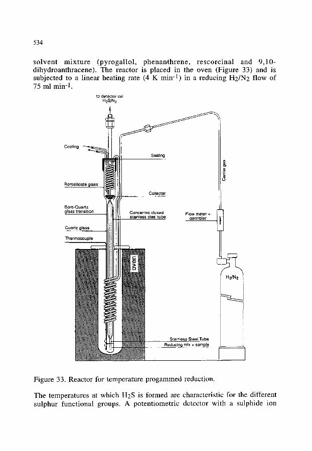
534

solvent mixture (pyrogallol, phenanthrene, rescorcinal and 9,10- dihydroanthracene). The reactor is placed in the oven (Figure 33) and is subjected to a linear heating rate (4 K min -1) in a reducing H2/N2 flow of 75 ml min- 1.

to detector eel H2S/N2

Cooling

Borosi[icate glass

Boro-Quartz glass transition

Quartz glass

Thermocouple

Sealing

Collector

Concentric closed Flow meter + stainless steel tube controler

Stainless Steel Tube Reducing mix § sample

Figure 33. Reactor for temperature progammed reduction.

The temperatures at which H2S is formed are characteristic for the different sulphur functional groups. A potentiometric detector with a sulphide ion

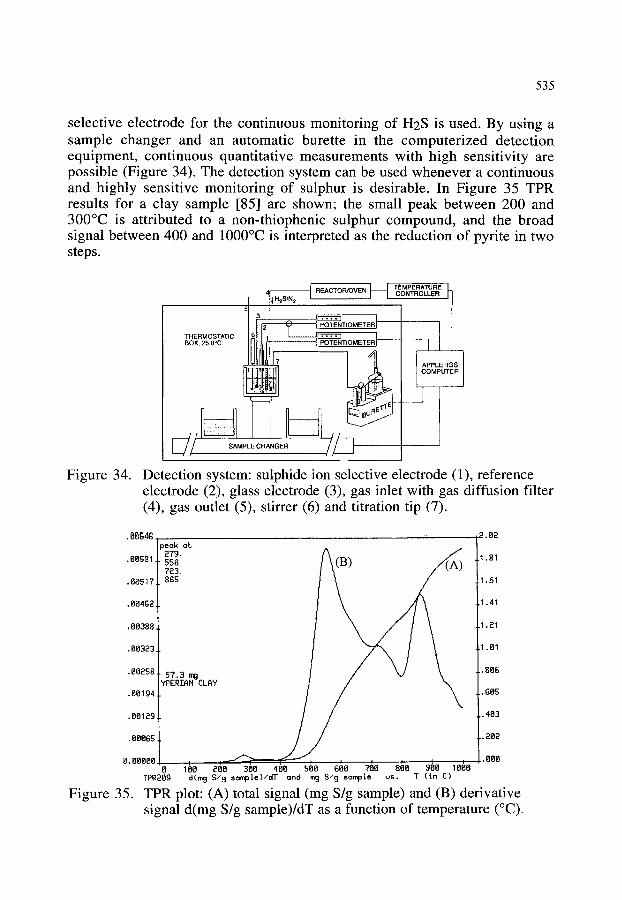
535

selective electrode for the continuous monitoring of H2S is used. By using a sample changer and an automatic burette in the computerized detection equipment, continuous quantitative measurements with high sensitivity are possible (Figure 34). The detection system can be used whenever a continuous and highly sensitive monitoring of sulphur is desirable. In Figure 35 TPR results for a clay sample [85] are shown; the small peak between 200 and 300~ is attributed to a non-thiophenic sulphur compound, and the broad signal between 400 and 1000~ is interpreted as the reduction of pyrite in two steps.

Figure 34.

I '~.~SIN= [ ,-,=,, . . . . ..,_.,r,. , I , - -

'~ l l r . . . . . . . . . '------------q, POTE{'~-;-;~qNTIOMETERI

[ ~ / SAMPLE CHANGER /, / j

REACTOR/OVEN H TEMPERATURE CONTROLLER

. I ....

Detection system: sulphide ion selective electrode (1), reference electrode (2), glass electrode (3), gas inlet with gas diffusion filter (4), gas outlet (5), stirrer (6) and titration tip (7).

I '3~n .88S81!

,80S17.

.OO4B2.

,00388

.00323

.00258

.80194

.00129

.OOOGS

0.80800

Figure 35.

/ 27g. / x 1 "

t s ? . 3 ~ i v \ PERIAN CLAY

TPR209 d(m 9 S/9 sample)/dT and m 9 S/9 sample us. T ( in C)

2.82

,1.81

.I ,61

.I .41

.1,21

.1.81

.. 806

..GO~;

,. 403

.. 202

�9 0 O O

TPR plot: (A) total signal (mg S/g sample) and (B) derivative signal d(mg S/g sample)/dT as a function of temperature (~

536

This method is also promising for the characterization of sulphur bridges in the analysis of vulcanized rubbers [86]. Direct methods include measurements of physical properties like swelling and stress-strain, specific degradation with chemical probes, or pyrolysis coupled with gas chromatography or mass spectrometry. TPR results in maximum H2S evolution at discrete temperatures which can be correlated to free sulphur and to the number and the type of crosslinks varying from monosulphidic to polysulphidic.

4.2.4. The use of AAS, XRD, SEM, DSC, TG-MS and TG-FTIR in the preparation and thermal decomposition of the acid salt of strontium oxalate [9]

Stront ium oxalate exists in two different forms" the neutral hydrate SrC204.xH20 and the acid hydrate SrC204.yH2C204.xH20. The stoichiometric acid hydrate SrC204.1 /2H2C204.H20 is prepared at a sufficiently low pH as described elsewhere [9]. The determination of Sr2+ in the precipitates was performed by AAS and the crystals were examined by XRD and SEM.

The acid salt decomposes in inert atmosphere (50 ml Ar min-1; 10 K min -1) in four well-defined steps between 145 and 1060~ as illustrated in Figure 36:

--0.5 100

90

80

rar 70--

0 400 500 600 o Temperature/C

50

40

, -',,

~ SrC204~ ~

"", .. s'G~176176176

s,qo,.o.43,,c,o,.~.2~o ",, ~ t : : : : : : : : : : : : : : : : : : : : /~1

s~o,.,t2~qo,.~o

1 O0 200 300 700 800 900

Figure 36. TG of SrC204.yH2C204.xH20 in Ar at 10 K min -1

-0.4

o -0.3

-0.2 .~ >

-0.1

0.0

1000 1100

145-210~ �9 SrC204.1/2H2C204.H20 . . . . . > SrC204.1/2H2C204 + H20

240-350~ SrC204.1/2H2C204 . . . . . > SRC204 + 1/2HCOOH + 1/2CO2 SrC204.1/2H2C204 . . . . . > SRC204 + 1/2H20 + 1/2CO + 1/2CO2

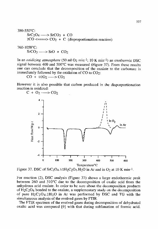
537

380,550~ SRC204 . . . . . > SrC03 + CO 2C0 <====> C02 + C (disproportionation reaction)

760-1058~ �9 SrCO3 . . . . . > SrO + CO2

In an oxidizing atmosphere (50 ml 02 min-1; 10 K min -1) an exothermic DSC signal between 400 and 500~ was measured (Figure 37). From these results one can conclude that the decomposition of the oxalate to the carbonate is immediately followed by the oxidation of CO to CO2:

CO + 1/202 . . . . . > CO2

However it is also possible that carbon produced in the disporportionation reaction is oxidized:

C + 02 . . . . . > CO2

4 - -

2 - -

"7,

o -

o

.,.a c~

~Z - 2 -

-4

i'l I 1

I I I |

I ! I !

t I i n O 2

t ~ / ' x i n A r

" x /

I I ~ ' i I I ' I I ' " ' I ' 1

100 200 300 400 500 600

Temperature/~ Figure 37. DSC of SrC204.1/2H2C204.H20 in Ar and in 02 at 10 K min-1

For reaction (2), DSC analysis (Figure 37) shows a large endothermic peak between 260 and 310~ due to the decomposition of oxalic acid from the anhydrous acid oxalate. In order to be sure about the decomposition products of H2C204 bonded to the oxalate, a supplementary study on the decomposition of pure H 2 C 2 0 4 . 2 H 2 0 in Ar was performed by DSC and TG with the simultaneous analysis of the evolved gases by FTIR.

The FTIR spectrum of the evolved gases during decomposition of dehydrated oxalic acid was compared [9] with that during sublimation of formic acid.

538

From this comparison it was concluded that H 2 C 2 0 4 decomposes with the release of CO2, H 2 0 and gaseous formic acid, confirming that reaction (2) takes place. The FTIR spectrum (Figure 38) of S r C 2 0 4 . 1 / 2 H 2 C 2 0 4 . H 2 0 also shows the release of CO, which proves that a second reaction takes place, namely the decomposit ion of H2C204 with the release of H 2 0 , CO and CO2 as given by reaction (3). At this temperature, the MS result in Figure 39 shows the simultaneous release of H 2 0 , CO and CO2, whilst H C O O H is detected as H 2 0 and CO due to fragmentation. This is a good example of the complementarity of MS and FTIR.

r 1000 oo o~ ~.~

~ . . . .

, 1 ~ . . . . .

4000 3750 3500 3250 3000 2750 2+00 2250 2 50 1 1150 1 0

Figure 38.

W a v e n u m b e r / c m -1

200 100

FTIR plot of gases released by heating SrC204.1/2H2C204.H20 in Ar at 10 K min-1.

1E-10

1E-II ~

IE-13 ~

IE-14

Figure 39.

' t / I

i I �9 i i # i + =

l �9 . l . l . s

, i + s �9

i + ' �9 + r

t l

�9 ~ r ~ c = 18:~0

�9 , - rig�9 = 28" CO #

i

t

!

-m/c = 44 : CO 2

' I ' I '+q ' I ' --I--' I ' I ' I ' I ' I ' I 0 100 200 300 400 500 600 700 800 900 1000 1100

o T e m p e r a t u r e / C

Mass spectrum of gases released by heating SrC204 .1 /2H2C204 .H20 in Ar at 10 K rain -1.

539

The mass loss from the third to the fourth plateau (Figure 36) for reaction (4) in Ar corresponds to the evolution of both CO and CO2, as shown with TG- FTIR (Figure 38) and TG-MS (Figure 39). Because at this stage the temperature is still below the carbonate decomposition temperature, the detection of CO2 must result from the CO disproportionation reaction (5), which explains the exothermic signal in the DSC experiment (Figure 37) between 500 and 550~ Finally, by means of the FTIR spectrum corresponding to the conversion of the carbonate into the oxide (reaction (6)), it is proven that only CO2 is evolved. The mass spectrometer monitors characteristic ion peaks at m / e - 44 and m/e = 28. The presence of the latter peak is consequently assigned to fragmentation of CO2.

The decomposition of SrC204.1/2H2C204.H20 is a good example to illustrate how one can obtain a full description of a reaction scheme by combination of DSC, TG-FTIR and TG-MS. As mentioned before, it also shows the complementarity of TG-FTIR and TG-MS.

4.2.5 The use of copper oxalate for checking the inert working conditions of thermal equipment [5]

All thermal analysis techniques require careful control of the gaseous atmosphere in which the experiment is carried out. As shown by several of the preceding examples, particularly at high temperatures, even very small amounts of oxygen can drastically influence the experiment, so that totally different results are obtained compared with those in a completely inert atmosphere.

110 . . . . . .

100

90

80

:~ 7o

60

50

40, ~ " -'260 0

31.873 mg CUC204 50 ml/min argon 10 dog/min

"460 " 660 8 6 0 ' " 1()00 r 1200 Temperamre/~

Figure 40. The decomposition of copper oxalate in a completely inert atmosphere.

540

Copper oxalate is well suited for checking the inert working conditions. In an inert atmosphere the decomposition goes to metallic copper (theoretical remaining mass 41.9%) as shown in Figure 40. In the presence of even very small amounts of oxygen there is a mass increase (Figure 41) between 300 and 600~ due to the oxidation of metallic copper to copper(II) oxide (theoretical remaining mass 52.5% if 100% CuO).

Z~

110

1 0 0 -

9 0 -

80-

70-

60-

50-

40

30.543 mg CUC204 50 ml/min argon 10 deg/rain

0 200 400 600 800 1000 1200 Temperature/~

Figure 41. The decomposition of copper oxalate in the presence of oxygen.

Oxidation of the copper will occur if the flow gas is not free from oxygen, or if air is admitted because all the removable parts do not fit correctly. It also happens that the equipment contains a dead volume that is not completely air free in spite of flushing with inert gas before starting the experiment. Some modification (e.g., an additional gas inlet) of the TA equipment may be necessary to obtain equipment that is able to work in a completely inert atmosphere. The decomposition of copper oxalate is such a sensitive reaction that it is well-suited for checking all kinds of TA equipment.

4.2.6. Other examples of the use of analytical techniques by on-line and off- line combination with thermal analysis

The kinetics of thermal and thermo-oxidative degradation and the characterization of the various degradation products of polystyrene alone [78, 87] and in the presence [87] of the retardant 4,4'-isopropylidene bis(2,6- dibromophenol) were investigated using thermal volatilisation analysis, FTIR and GC-MS. The phase transition behavior was measured by simultaneous DSC-X ray diffractometry [88, 89]. The off-line coupling of TG and GC-MS

541

was used for the determination of the degradation products of a latex and the on-line coupling TG-FTIR, together with the off-line use of FIA (flow injection analysis) and photometry (via successive sampling of the gases coming from the TGA in NaOH solutions), were used for the determination of the amount of evolved HCN during heating of an unknown waste product [90]. The oxidative degradation products of a flame retardant for polymers (HET- acid i.e. 1,4,5,6,7,7 hexachlorobicyclo[2.2.1]hept-5-en-2,3-dicarboxylic acid) were identified by the on-line combination of TG-FTIR and the off-line (using tenax and thermal desorption) combination TG-GC-MS [91]. The thermal behavior of flame retarded polyurethane foams has been investigated using on- line TG-MS and off-line (using XAD resin as adsorbent) TG-GC-MS [92]. With the same techniques, adhesives used in the automobile industry have been investigated [93]. The combination of GC with TG has been used for the determination of the composition of polymeric composites [94]. The determination of evolved water can also be done by the use of a piezoelectric detector [95]. Coupled pyrolysis-GC and FTIR have been used for the investigation of substructure components of various aquatic humic substances [96] and for the investigation of the thermal degradation mechanism of diphenyl alkyl allophanates and carbanilates as model compounds for cross- linking sites in polyurethane networks [97]. The thermal behavior and fire- retardant properties of polyester resins and the gases evolved have been studied by trapping at low temperature and pyrolysis-MS [98, 99]. TG-GC-MS on a coal sample, with implementation of on-column focused cryogenic trapping, has been used for the identification of compounds ranging from gases like sulphur dioxide to high-boiling alkanes and aromatics [100]. TG- GC-IR was used for the study of the decomposition of ethylene-vinylacetate copolymers [101], polyacrylamide [102], poly(ethylene-co-vinyl alcohol) [103] and other polymers [104] such as an acrylonitrile-butadiene-styrene product, polycarbonate optical components, poly(butylene terephthalate) and poly(alkyl methacrylate).

REFERENCES

~

,

,

.

.

W.W. Wendlandt, Thermal Analysis, 3rd Ed., Wiley, New York, 1986, p. 461. C. Walker, T. Levor, I. Groves, D. Pattyn, D. Roedolf, R. Carleer and J. Mullens, unpublished results. A. Vos, R. Carleer, J. Mullens, J. Yperman, J. Vanhees and L.C. Van Poucke, Eur. J. Solid State Inorg. Chem., 28 (1991) 657. J. Mullens, A. Vos, A. De Backer, D. Franco, J. Yperman and L.C. Van Poucke, J. Thermal Anal., 40 (1993) 303. J. Mullens, A. Vos, R. Carleer, J. Yperman and L.C. Van Poucke, Thermochim. Acta, 207 (1992) 337.

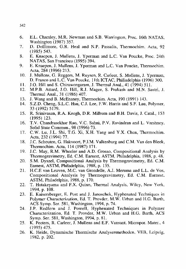
542

.

.

o

,

10.

11. 12.

13. 14.

15.

16.

17.

18.

19.

20.

21.

22.

23.

24.

25.

26.

E.L. Charsley, M.R. Newman and S.B. Warrington, Proc. 16th NATAS, Washington (1987) 357. D. Dollimore, G.R. Heal and N.P. Passalis, Thermochim. Acta, 92 (1985) 543. E. Knaepen, J. Mullens, J. Yperman and L.C. Van Poucke, Proc. 24th NATAS, San Francisco (1995) 394. E. Knaepen, J. Mullens, J. Yperman and L.C. Van Poucke, Thermochim. Acta, 284 (1996) 213. J. Mullens, G. Reggers, M. Ruysen, R. Carleer, S. Mullens, J. Yperman, D. Franco and L.C. Van Poucke, 1 l th ICTAC, Philiadelphia (1996) 300. J.O. Hill and S. Chirawongaram, J. Thermal Anal., 41 (1994) 511. M.P.B. Attard, J.O. Hill, R.J. Magee, S. Prakash and M.N. Sastri, J. Thermal Anal., 31 (1986) 407. J. Wang and B. McEnaney, Thermochim. Acta, 190 (1991) 143. S.Z.D. Cheng, S.L.C. Hsu, C.J. Lee, F.W. Harris and S.F. Lau, Polymer, 33 (1992) 5179. R. Srinivasan, R.A. Keogh, D.R. Milburn and B.H. Davis, J. Catal., 153 (1995) 123. T.V. Chandrasekhar Rao, V.C. Sahni, P.V. Ravindran and L. Varshney, Solid State Commun., 98 (1996) 73. C.W. Lu, J.L. Shi, T.G. Xi, X.H. Yang and Y.X. Chen, Thermochim. Acta, 232 (1994) 77. J.C. Schouten, G. Hakvoort, P.J.M. Valkenburg and C.M. Van den Bleek, Thermochim. Acta, 114 (1987) 171. J.C. May, R.M. Wheeler and A.D. Grosso, Compositional Analysis by Thermogravimetry, Ed. C.M. Earnest, ASTM, Philadelphia, 1988, p. 48. S.M. Dyszel, Compositional Analysis by Thermogravimetry, Ed. C.M. Earnest, ASTM, Philadelphia, 1988, p. 135. H.C.E van Leuven, M.C. van Grondelle, A.J. Meruma and L.L. de Vos, Compositional Analysis by Thermogravimetry, Ed. C.M. Earnest, ASTM, Philadelphia, 1988, p. 170. T. Hatakeyama and F.X. Quinn, Thermal Analysis, Wiley, New York, 1994, p. 108. E. Kaisersberger, E. Post and J. Janoschek, Hyphenated Techniques in Polymer Characterization, Ed. T. Provder, M.W. Urban and H.G. Barth, ACS Symp. Ser. 581, Washington, 1994, p. 74. J.P. Redfern and J. Powell, Hyphenated Techniques in Polymer Characterization, Ed. T. Provder, M.W. Urban and H.G. Barth, ACS Symp. Ser. 581, Washington, 1994, p. 81. K. Peeters, R. Carleer, J. Mullens and E.F. Vansant, Micropor. Mater., 4 (1995) 475. K. Heide, Dynamische Thermische Analysenmethoden, VEB, Leipzig, 1982, p. 202.

543

27.

28.

29. 30.

31.

32. 33.

34.

35.

36.

37.

38.

39.

40.

41.

42.

43. 44.

45.

46.

47.

E.L. Charsley, C. Walker and S.B. Warrington, J. Thermal Anal., 40 (1993) 983. E.L. Charsley, S.B. Warrington, G.K. Jones and A.R. Mc. Ghie, Am. Lab., Jan. 1990. J. Chiu and A.J. Beattie, Thermochim. Acta, 50 (1981) 49. L. Montanarella, M.R. Bassani and O. Breas, Rapid Commun. Mass Spectrom., 9 (1995) 1589. M. Wingfield, Calorimetry and Thermal Analysis of Polymers, Ed. V.B.F. Mathot, Hanser Publishers, Munich, 1993, p. 331. P. Burchill, D.G. Richards and S.B. Warrington, Fuel, 69 (1990) 950. S.B. Warrington, Thermal Analysis - Techniques and Applications, Ed. E.L. Charsley and S.B. Warrington, Royal Society of Chemistry, Cambridge, 1992, p. 103. S.H.J De Beukeleer, H.O. Desseyn, S.P. Perlepes and J. Mullens, Thermochim. Acta, 257 (1995) 149. J.L. Heidbrink, J.G. Li, W.P. Pan, J.L. Gooding, S. Aubuchon, J. Foreman and C.J. Lundgren, Thermochim. Acta, 284 (1996) 241. P.J. Haines, Thermal Methods of Analysis - Principles, Applications and Problems, Blackie, Glasgow, 1995, chapter 5. M.E. Brown, Introduction to Thermal Analysis - Techniques and Applications, Chapman and Hall, New York, 1988, chapter 10. F. Paulik, Special Trends in Thermal Analysis, Wiley, New York, 1995, chapter 8. P.K. Gallagher, Thermal Characterization of Polymeric Materials, Ed. E.A. Turi, Academic Press, London, 2nd Ed., 1997, chapter 1. J. Mullens, R. Carleer, G. Reggers, J. Yperman and L.C. Van Poucke, Proc. 19th NATAS, Boston (1990) 155. I. Schildermans, J. Mullens, B.J. Van der Veken, J. Yperman, D. Franco and L.C. Van Poucke, Thermochim. Acta, 224 (1993) 227. I. Schildermans, J. Mullens, J. Yperman, D. Franco and L.C. Van Poucke, Thermochim. Acta, 231 (1994) 185. W. Eevers, R. Carleer, J. Mullens and H. Geise, unpublished results. J. Mullens, R. Carleer, G. Reggers, J. Yperman, J. Vanhees and L.C. Van Poucke, Thermochim. Acta, 212 (1992) 219. J. Khorami, A. Lemieux, H. Menard and D. Nadeau, Compositional Analysis by Thermogravimetry, Ed. C.M. Earnest, ASTM, Philadelphia, 1988, p. 147. S.B. Warrington, Thermal Analysis - Techniques and Applications, Ed. E.L. Charsley and S.B. Warrington, Royal Society of Chemistry, Cambridge, 1992, p. 95. J.P. Redfern and J. Powell, Hyphenated Techniques in Polymer Characterization, Ed. T. Provder, M.W. Urban and H.G. Barth, ACS Symp. Ser. 581, Washington, 1994, p. 90.

544

48.

49.

50. 51.

52.

53.

54.

55. 56.

57. 58.

59.

60.

61. 62. 63. 64.

65.

66.

67.

68.

69.

70. 71.

D.J. Johnson, D.A.C. Compton, R.S. Cass and P.L. Canala, Thermochim. Acta, 230 (1993) 293. D.J. Mc.Ewen, W.R. Lee and S.J. Swarin, Thermochim. Acta, 86 (1985) 251. Q. Zhang, W.P. Pan and W.M. Lee, Thermochim. Acta, 226 (1993) 115. A. Vos, J. Mullens, J. Yperman, D. Franco and L.C. Van Poucke, Eur. J. Solid State Inorg. Chem., 30 (1993) 929. R. Nouwen, J. Mullens, D. Franco, J. Yperman and L.C. Van Poucke, Vibration. Spectr., 10 (1996) 291. M.K. Van Bael, J. Mullens, R. Nouwen, J. Yperman and L.C. Van Poucke, J. Thermal Anal., 48 (1997) 989. B. Bowley, E.J. Hutchinson, P. Gu, M. Zhang, W.P. Pan and C. Nguyen, Thermochim. Acta, 200 (1992) 309. D.R. Clark and K.J. Gray, Lab. Pract., 40 (1991) 77. M.B. Maurin, L.W. Dittert and A.A. Hussain, Thermochim. Acta, 186 (1991) 97. K.R. Williams, J. Chem Educ., 71(8) (1994) A195. T. Roth, M. Zhang, J.T. Riley and W.P. Pan, Proc. Conf. Int. Coal Test. Conf., (1992) 46. P.R. Solomon, M.A. Serlo, R.M. Carangelo, R. Bassilakis, Z.Z. Yu, S. Charpenay and J. Whelan, J. Anal. Appl. Pyrolysis, 19 (1991) 1. D. Shao, W.P. Pan and C.L. Chou, Prepr. Pap. - ACS. Div. Fuel Chem., 37 (1992) 108. M.F. Cai and R.B. Smart, Energy and Fuels, 7 (1993) 52. J.G. Dunn, W. Gong and D. Shi, Thermochim. Acta, 208 (1992) 293. J.G. Dunn and L.C. Mackey, J. Thermal Anal., 37 (1991) 2143. R. Materazzi, G. Curini, G. D'Ascenzo and A.D. Magri, Thermochim. Acta, 264 (1995) 75. M.L. Mittleman, D. Johnson and C.A. Wilkie, Trends Polym. Sci., 2 (1994) 391. S.L. Hurley, M.L. Mittleman and C.A. Wilkie, Polym. Degrad. Stab., 39 (1993) 345. C.A. Wilkie and M.L. Mittleman, Hyphenated Techniques in Polymer Characterization, Ed. T. Provder, M.W. Urban and H.G. Barth, ACS Symp. Ser. 581, Washington, 1994, p. 116. R.M. Paroli and A.H. Delgado, Hyphenated Techniques in Polymer Characterization, Ed. T. Provder, M.W. Urban and H.G. Barth, ACS Symp. Ser. 581, Washington, 1994, p. 129. D.J. Johnson, P.J. Stout, S.L. Hill and K. Krishnan, Hyphenated Techniques in Polymer Characterization, Ed. T. Provder, M.W. Urban and H.G. Barth, ACS Symp. Ser. 581, Washington, 1994, p. 149. J.W. Mason, Annu. 52nd Tech. Conf. Soc. Plast. Eng., 3 (1994) 2935. R.C. Wieboldt, G.E. Adams, S.R. Lowry and R.J. Rosenthal, Am. Lab., 20(1) (1988) 70.

545

72. 73.

74.

75.

76.

77. 78.

79.

80.

81.

82.

83.

84.

85.

86.

87.

88.

89.

90.

91.

92. 93.

94.

95.

H.G. Schild, J. Polym. Sci. Part A: Polym. Chem., 31 (1993) 1629. T. Hatakeyama and F.X. Quinn, Thermal Analysis, Wiley, New York, 1994, p. 109. R. Kinoshita, Y. Teramoto and H. Yoshida, J. Thermal Anal., 40 (1993) 605. R. Kinoshita, Y. Teramoto and H. Yoshida, Thermochim. Acta, 222 (1993) 45. A. Vos, J. Mullens, R. Carleer, J. Yperman, J. Vanhees and L.C. Van Poucke, Bull. Soc. Chim. Beiges, 101 (1992) 187. S.Y. Lin, C.M. Liao and R.C. Liang, Polym. J. (Tokyo), 27 (1995) 201. J. Mullens, R. Carleer, G. Reggers, M. Ruysen, J. Yperman and L.C. Van Poucke, Bull. Soc. Chim. Belg., 101 (1992) 267. K. Leroy, J. Mullens, J. Yperman, J. Vanhees and L.C.Van Poucke, Thermochim. Acta, 136 (1988) 343. J. Yperman. A. De Backer, A. Vos, D. Franco, J. Mullens and L.C. Van Poucke, Anal. Chim. Acta, 273 (1993) 511. B.B. Majchrowicz, J. Yperman, J. Mullens and L.C. Van Poucke, Anal. Chem., 63 (1991 ) 760. I.I. Maes, S.C. Mitchell, J. Yperman, D. Franco, S. Marinov, J. Mullens and L.C Van Poucke, Fuel, 75 (1996) 1286. G. Gryglewicz, P. Wilk, J. Yperman, D. Franco, I.I. Maes, J. Mullens and L.C. Van Poucke, Fuel, 75 (1996) 1499. I.I. Maes, J. Yperman, H. Van den Rul, D. Franco, J. Mullens, L.C. Van Poucke, G. Gryglewicz and P. Wilk, Energy and Fuels, 9 (1995) 950. J. Mullens, J. Yperman, R. Carleer, D. Franco, L.C. Van Poucke and J. Van der Biest, Applied Clay Science, 8 (1993) 91. S. Mullens, J. Yperman, D. Franco, J. Mullens and L.C. Van Poucke, J. Thermal Anal., in press (1997). I.C. McNeill, L.P. Razumovskii, V.M. Gol'dberg and G.E. Zaikov, Polym. Degrad. and Stabil., 45 (1994) 47. H. Yoshida, R. Kinoshita and Y. Teramoto, Thermochim. Acta, 264 (1994) 173. W. Bras, G.E. Derbyshire, A. Devine, S.M. Clark, J. Cooke, B.E. Komanschek and A.J. Ryan, J. Appl. Crystallogr., 28 (1995) 26. G. Reggers, M. Ruysen, R. Carleer and J. Mullens, Thermochim. Acta, 295 (1997) 107. J. Mullens, G. Reggers, M. Ruysen, R. Carleer, J. Yperman, D. Franco and L.C. Van Poucke, J. Thermal. Anal., 49 (1997) 1061. G. Matuschek, Thermochim. Acta, 263 (1995) 59. G. L6rinci, G. Matuschek, J. Fekete, I. Gebeftigi and A. Kettrup, Thermochim. Acta, 263 (1995) 73. E.J. Hutchison, B. Bowley, W.P. Pan and C. N guyen, Thermochim. Acta, 223 (1993) 259. J. Kristof, Talanta, 41 (1994) 1083.

546

96.

97. 98.

99.

100. 101.

102.

103.

104.

R. Kuckuk, W. Hill, P. Burba and A.N. Davies, Fresenius' J. Anal. Chem., 350 (1994) 528. N. Yoshitake and M. Furukawa, J. Anal. Appl. Pyrolysis, 33 (1995) 269. P.J. Haines, T.J. Lever and G.A. Skinner, Thermochim. Acta, 59 (1982) 331. G.A. Skinner, P.J. Haines and T.J. Lever, J. Appl. Polym. Sci., 29 (1984) 763. L.W. Whiting and P.W. Langvardt, Anal. Chem., 56 (1984) 1555. B.J. McGrattan, Hyphenated Techniques in Polymer Characterization, Ed. T. Provder, M.W. Urban and H.G. Barth, ACS Symp. Ser. 581, Washington, 1994, p. 103. J.D. Van Dyke and K.L. Kasperski, J. Polym. Sci. Part A: Polym. Chem., 31 (1993) 1807. T. Hatakeyama and F.X. Quinn, Thermal Analysis, Wiley, N.Y., 1994, p. 112. J.A.J. Jansen, Calorimetry and Thermal Analysis of Polymers, Ed. V.B.F. Mathot, Hanser Publishers, Munich, 1993, p. 336.


Chapter 13

CALIBRATION AND STANDARDISATION IN DSC

M.J. R i c h a r d s o n ~ and E .L . C h a r s l e y b

a Polymer Research Centre, School of Physical Sciences, University of Surrey, Guildford GU2 5XH, U.K.

b Centre for Thermal Studies, School of Applied Science, University of Huddersfield, Huddersfield HD1 3DH, U.K.

1. INTRODUCTION

Basic procedures for the calibration of differential scanning calorimeters were introduced in Chapter 5. These are discussed in more detail in the present chapter. Particular emphasis is placed on calibration schemes that lead to true thermodynamic properties, rather than arbitrary quantities that may not even be reproducible between two different types of instrument.

Current theories of DSC are inadequate for a complete description of the behaviour of a particular sample in a given instnunent. Differential scanning calorimeters must therefore be operated in a relative, rather than absolute, mode. Quantitative data can only be obtained after calibration, under conditions that approach those of the "unknown" as closely as possible, using materials with well-defined properties. Ideally, "well-defined" means that the relevant properties have been measured by at least two groups using different techniques - which should certainly not include DSC. In reality, these criteria must be relaxed to varying extents and these will be discussed later in the chapter.

At its most basic, the DSC signal is a differential temperature or power (ordinate) as a function of time or temperature (abscissa). The aim of any calibration procedure is to define the temperature scale for a given set of experimental conditions and to fix the ordinate so that it refers to known heat flow rates - either directly or, in combination with the abscissa, as an area that corresponds to a known quantity of heat, for example a heat of fusion. In fact the abscissa is more useful as a heat capacity rather than a heat flow rate and the calibration described in Section 3.2 is for the former- a true material property.

548

Before any calibration procedure, it is important to consider what use will be made of the DSC in day-to-day operation. In many cases quality control applications will be dominant. Here, it is important to ensure that a given "event" is reproducible in both temperature and magnitude. Just how these are measured is relatively unimportant (absolute accuracy is not required), but measurements must be consistent and well-defined. A combination of simple calibration procedures and standard conditions (sample size and geometry, type of crucible, gas flow rate, ambient temperature, heating rate - often, to save time, 10 or 20 K min ~) ensures that deviations from some accepted norm have real significance. As the need for precise data increases so must the sophistication of the calibration process. In the following, good general calibration practices will first be described followed by any modifications that lead to improved accuracy.

2. TEMPERATURE CALIBRATION

2.1. Dynamic temperatures The sensors in any DSC are relatively remote from the sample. Thus, even if the

sensor itself is reading correctly, the sample temperature may differ because of a thermal gradient between sensor and sample - even under isothermal conditions. Under scanning conditions the thermal gradient will change because of an additional "dynamic" thermal lag that is negative in heating and positive in cooling.

Calibration in cooling has been little discussed but is becoming of increasing importance as DSC is used to simulate the many material-forming processes that feature the solidification of a liquid phase. There are unique problems of calibration for the cooling mode because most phase changes need some degree of supercooling. This is poorly reproducible, not only from sample to sample but even for a given sample. For example, milligram quantities of tin, a useful and widely used calibrant in heating, may supercool some 60 K at 20 K min l but specific values vary by several degrees on simply recycling a given sample through the melting and solidification regions. The initial discussion, therefore, will concentrate on heating and procedures for cooling will be considered later (Section 2.3).

The temperature distribution in a loaded DSC cell is shown in Figure 1. In most scanning calorimeters heat arrives through the base of the sample and under dynamic conditions (and, in principle, static conditions also, see below) there will be an additional gradient through the sample itself. The sample temperature should therefore be characterised by some average value. In practice, the almost universally used "extrapolated onset" method (Figure 2) gives the temperature To when fusion starts - that is, at the sample face that is in contact with its container.

549

Sample , , . , Tc(~ T(av)

t A !:i:-.":.-:-~:-:!(~- B --i----:-"?:-:-! i'-: !!,

$ O r-.

u.l

L ~

Temperature

Figure 1. Temperatures in a loaded DSC Figure 2. Definition of the extrapolated cell. Calibration establishes To(.fl) or, onset temperature T~(~ at a heating rate through thermal lag, some average ft. temperature T(av). Interfaces P and Q are barriers to efficient heat transfer. A: DSC head, B: temperature sensor.

A conventional temperature calibration uses known transition (x = trs) and/or fusion (x = fus) temperatures (Tx) to construct a temperature correction (fiT) curve for various heating rates (,/5'):

6T(fl) = T~- T~(~ (1)

where the dependence of both 6T and To on fl is emphasised. Exactly how the correction is made is very much a fimction of the particular

instnmaent/software combination. Controls may be adjusted manually (to make 6T(fl) - 0 or to minimise it over a range of temperature) or the software may include an algorithm that, given Tx and To(fl), automatically corrects "observed" temperatures.

A full temperature calibration will use several reference materials to generate a calibration curve of the form of Figure 3. The number of points needed for such a curve will obviously depend on the overall shape and on the temperature range of interest. If the curve is roughly linear and/or only a short range is to be covered, it is reasonable to use ASTM Method E967 [1 ]. In this, the temperature that is to be determined is bracketed by just two calibrants and it is assumed that 6T for the tmknown sample can be linearly interpolated between values for these two materials. Full details are given in Chapter 5. The temperature correction software for most modem instruments will accept a "two-point" method but this is really the very minimum that is required. Even if the basic assumption of linearity is correct this should be checked by at least one additional point. If there is curvature - and this is probably inevitable if a large temperature range is to be covered- more points are

550

required and the sottware should be able to accommodate these. In some cases this is still not possible and the 6T against T~ curve must be approximated by a set of linear regions. Two such approximations are shown in Figure 3, which also shows the dangers of extrapolation outside the "linear" regions.

5~/b J

J

I ST(o) Temperature ]3

Figure 3. Temperature correction 6T(fl) Figure 4. fiT(B) (equation 1) as a function as a function of temperature. See text for of heating rate fl details.

Because of the finite path, and associated thermal resistance, between sample and sensor, a new temperature calibration is required for each fl and also whenever any other condition (e.g. type of sample pan, ambient and/or sample temperature, flow rate and nature of carrier gas) is changed. For many well-defined first order thermodynamic events, especially fusion, there is a linear relationship between To and/3. Figure 4 shows a typical example and indicates how the several parameters that characterise thermal lag are defined. For convenience, a given instrument is usually adjusted to make 6T~0 for some widely-used temperature range and [3 (e.g. 10 or 20 K min l) so that the indicated temperature is approximately correct. Once the slope tr is known equation (1) can be generalised to:

6v( = Tx- L(0)- ap (2)

(For most instnmaents tr lies between 0.05 and 0.15 minl). This procedure can obviously be carried out for a range of temperature standards and the results again incorporated in the temperature calibration software provided the latter has sufficient flexibility for this approach.

Any calibration should reproduce the conditions of subsequent usage as closely as possible. It is important to obtain a general impression of the effects of changes in experimental and machine parameters on calibration behaviour early in the lifetime of a particular msmmaent. This is especially relevant for one that will find a variety of applications because here there may need to be frequent changes in instrumental

551

conditions. With this background information, and an indication of the tmcertamties that can be tolerated, it is possible to make an informed judgement when additional calibration is needed. For example, for a power compensation DSC 6T is little influenced by a doubling of the gas flow rate, whereas a reduction of ambient temperature from 273 to 173 K increases 6Tby 4 K with obvious implications for the degree of control required.

The above procedures give the conventional dynamic temperature calibration 6T(fl). Derived temperatures are good to from 0.5 to 1 K or 3 to 4 K. The lower figures are valid for thin specimens at low fl, the higher values for irregular shapes and/or high ft. The temperature is always that at the point where the sample is in contact with the pan. It makes no allowance for thermal gradients within the sample itself, although some idea of these can be obtained by embedding indium in the two faces of a disc-shaped specimen and noting the delay in the response from the upper "sensor". The reproducibility on recycling a given sample in a DSC is generally much better than the above figures imply - a few hundredths of a degree even at high f l - but this must not be equated with accuracy. Simple repeat experiments using flesh samples will quickly establish realistic values for the overall performance of an instrttment.

Although it is often sufficient to know the temperature of an event to one or two degrees, this does not fully utilise the potential of modem instruments. As already indicated, temperatures can be controlled to within a few hundredths of a degree (as shown by the reproducibility of data on cycling an undisturbed sample) and this facility can be used to better define temperatures by an approach to equilibrium conditions. Procedures for this are discussed in the following section.

2.2. Thermodynamic temperatures The most obvious procedure is to use the wide range of heating rates to extrapolate

to fl = 0 and this is the method suggested by the German Society for Thermal Analysis (GEFTA) [2] for the determination of equilibrium melting temperatures. The method is summarised in Figure 4 and a very detailed description of the GEFTA procedure appears in [3]. The To against fl curve appears to be linear for most fusion events but there are certainly deviations for some solid/solid transitions. Non- linearity is very obvious at low values of fl and these rates must always be included where possible - there may be problems with a metastable structure that can transform on the time scale of a slow heating experiment. (It is, of course, always possible to select stable phases for calibration purposes but it is timely to emphasise that valuable information can often be obtained from DSC work on metastable phases).

An altemative to the GEFTA approach uses a direct determination of the apparent isothermal melting or transition temperature (Ti) [4]. This is achieved by a series of

552

stepwise temperature increments through the fusion region (Figure 5). The increment may be coarse (perhaps 5 K) for an initial scan to define the approximate value of T i corresponding to the known T x (a coarse step is useful if the DSC is some way out of calibration) or fine (0.1 K or even less) for the final definition of T i. This type of experiment is ideally suited to a chart recorder because a direct comparison of the several increments is readily available. It is important to allow sufficient time for the system to come to equilibrium between successive increments and this can take many minutes when within one or two tenths of T~ - for an increment of 0.1 K the rate of supply of energy to the sample is low and in the transition region the full heat of fusion is required. Much time can be saved by preliminary runs that deliberately exceed T i so that this can then be defined to lie between T 1 and 7'2, subsequent experiments progressively decrease the temperature interval between solid and liquid by a factor of two giving a rapid convergence on T.,.

The isothermal procedure gives a correction of the form

6ri= rx- (3)

and the temperature of any unknown event, similarly determined, can be read from a 6T~ against T i curve. Ideally, both GEFTA (6T(0)) and isothermal (6T~) procedures should give identical results for the same event and this is generally true for the small samples (of the order of one rag) that are used for temperature calibration. For those samples that are thick enough to develop a temperature gradient between top and bottom, the two procedures will differ with T(GEFTA) < T(isothermal). This is because the former gives the start of fusion and the latter the e n d - when the molten front reaches the upper surface of the sample and the final trace of order vanishes. Of course, any sample melts over a range of temperature but it is assumed that purity is such that this aspect is negligible compared with the thermal gradient within the sample. The last is a function of thermal conductivity and, as a general rule, it would be anticipated that metals give the minimum "sample" gradient. Metals are also favoured calibration materials because they are widely available in high purity (6N - 99.9999% - is routine) whereas it is rare to encounter commercial inorganics or organics that approach 4N purity. Fusion temperatures can be routinely defined to +0.1 K. For a given specimen it is possible to reproduce temperatures to htmdredths of a degree but this may be influenced by lateral temperature gradients in the DSC specimen holder [5]; in addition variable contact resistances from one sample to another make +0.1K a realistic limit to DSC determinations of equilibrium melting temperatures.

Both the GEFTA and isothermal approaches described imply that the DSC is being used as a sophisticated thermometer rather than a calorimeter. To some extent the two procedures are complementary. The fusion temperature of a metastable structure

553

can be determined using the GEFTA method by extrapolation from high rates to discourage transformation to a more stable phase at low t, this could occur on the lengthy time scale of a "stepwise" experiment. On the other hand, the GEFTA determination requires a well-defined value for To and the necessary construction may be obscured by previous behaviour, e.g. for the second of two closely-spaced events. Another use of the step method is to determine the liquidus temperature of a system showing eutectic behaviour. Here, the final melting temperature for a given composition is readily observed and it is a simple matter to construct phase diagrams in this way - even metastable states are accessible because these final traces of melting do not demand large enthalpy inputs and only short isothermal periods are needed.

As a general rule it seems that curves of the type shown in Figure 4 are linear for melting phenomena but specific rate effects for solid/solid transitions mean that each of these must be treated as a special case and individually investigated.

T~

m m ~A

-0.l - I 3 ]~k +0"1+02

A l I A V ~ Time Time B C

Figure 5. Isothermal temperature Figure 6. Definition of the area 8A used correction. The indicated fusion to calculate thermal lag. temperature is Ti. Temperature increments of 0.1 K, some premelting is shown at T i -0.1.

2.3. Thermal lag and calibration in cooling Any thermal gradient between the faces of a sample of fmite thickness naturally

increases with heating rate and sample mass. There is, therefore, a need for some average temperature to characterise conditions in a heat capacity experiment which requires large fl and/or mass to give an adequate signal-to-noise ratio. A reasonable measure of "thermal lag" may be obtained from the rate of rettwn to isothermal conditions at the end of a scanning experiment where the programed temperature is T~ [6]. In an ideal situation the retum would be instantaneous (AB, Figure 6) but in reality a finite time is needed and the area 8A (ABC, Figure 6) represents an "enthalpy lag" that is related to the thermal lag 8T by

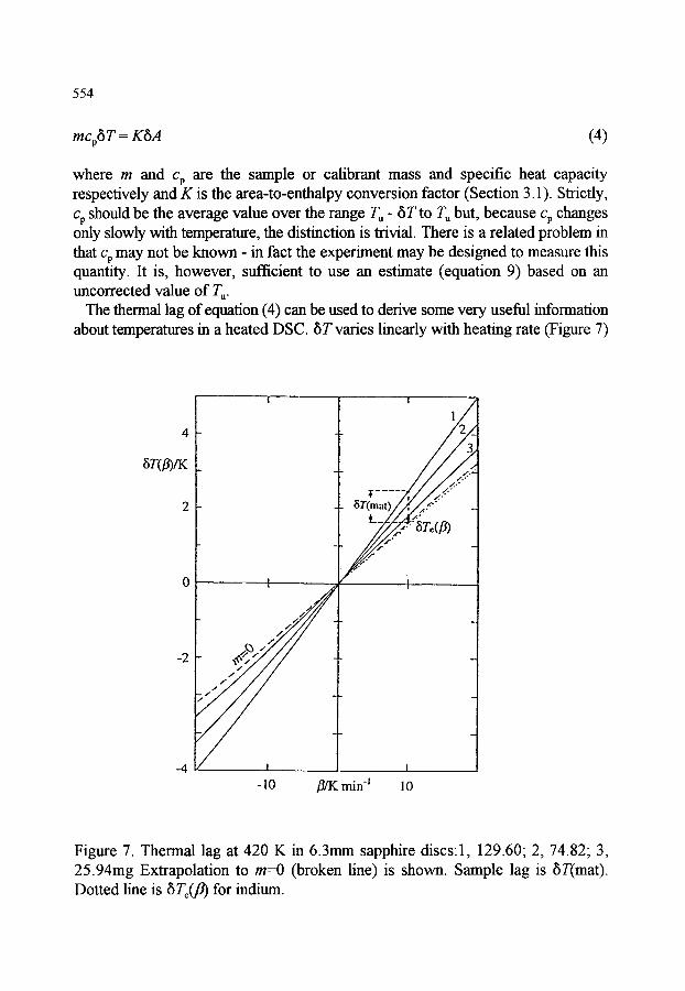
5 5 4

mcp6T= K6A (4)

where m and cp are the sample or calibrant mass and specific heat capacity respectively and K is the area-to-enthalpy conversion factor (Section 3.1). Strictly, Cp should be the average value over the range T, - 6T to Tu but, because Cp changes only slowly with temperature, the distinction is trivial. There is a related problem in that cp may not be known - in fact the experiment may be designed to measure this quantity. It is, however, sufficient to use an estimate (equation 9) based on an uncorrected value of T,.

The thermal lag of equation (4) can be used to derive some very useful information about temperatures in a heated DSC. 6T varies linearly with heating rate (Figure 7)

2 -

O ~ I ,,

. j -2r

/ f

- 1 0

i - l "

- _

I

. !

f l / K m i n "l 10

Figure 7. Thermal lag at 420 K in 6.3mm sapphire discs:l, 129.60; 2, 74.82; 3, 25.94mg Extrapolation to m=0 (broken line) is shown. Sample lag is 6T(mat). Dotted line is 6To(fl) for indium.

555

and also with sample mass (or thickness for constant diameter discs), extrapolation of the latter to zero mass (6 To) gives the temperature at the sample face in contact with the pan and this should equal To(fl) - T~(0) of equations (1) and (2). The equivalence of the two quantities is shown by results from sapphire discs at 420 K and indium at Tf~ (429.74 K) here both 6To(fl) and To(~ - To(0) equal 3.0 K for fl = 20 K min -~ [7]. The validity of the "thermal lag" approach is further confirmed when it is found that 6T O is a true insmmaent parameter - a constant for a given cell and pan configuration. For example, a variety of materials having very different thermal properties (and thus different total thermal lags) all extrapolate to a common value of 8 T O [8].

It is clear from Figure 7 that errors (the "material" thermal lag, the difference between 8T and 8To) of a few degrees in the average sample temperature are possible at commonly used heating rates - it should be emphasised that the examples of Figure 7 represent lower limits because the smooth faces give good sample/pan contact. They are a useful reminder that precision and accuracy are separate, distinct quantities and some thought is needed in discussing DSC temperatures. Although thermal lag may appear to throw doubt on the thermometric possibilities of DSC, in reality it is ideal for modem instruments with data treatment facilities and, of great importance, may be used for work in both cooling and heating.

Conventional DSC temperature calibrants cannot be used in cooling. All require some degree of supercooling but the extent cannot be certified because it varies from one sample to another. The problem is currently overcome by assuming that the To(fl) against fl curve is symmetrical so that To(fl) (Figure 4) can be extrapolated to fl < 0. Thermal lag experiments in cooling have confirmed this for two power compensation calorimeters [7,9] and symmetry would be expected for heat flux DSC. An important consequence is that reliable To(fl) values are available for fl < 0 so that potential calibrants can be evaluated with some confidence. As already mentioned, negligible supercooling is essential and the only possible candidates appear to be liquid crystal transitions [9-11] which are now being extensively investigated. There are some problems on the scale of a few tenths of a degree. Reported transition temperatures usually refer to some characteristic optical behaviour observed by hot-stage microscopy and it is not clear to what point on a DSC curve this corresponds. The latter has a finite width (a few tenths of a degree) and it would seem natural to take the peak, rather than onset, temperature. This is possible because liquid crystal transition enthalpies are generally so small that there is no significant perturbation of steady state heat flow conditions [12] in marked contrast with melting, for example, when To alone has significance. The low energies also mean that liquid crystals are very useful temperature calibrants for modulated temperature DSC (Section 4.7.1) because the system remains linear over a wide range of experimental conditions.

556

If a combination of isothermal (thermodynamic) temperature calibration plus thermal lag from individual runs is used there is really no need for specific calibrants for cooling. Unforttmately, this approach is not practicable with currently available software and there is, therefore, a demand for direct calibration in cooling.

3. C ALORI METRIC CALIBRATION

The use of a DSC as a calorimeter, rather than a thermometer, requires a knowledge of area-to-enthalpy or ordinate-to-specific heat calibration factors that are obtained from measurements on calibration materials with well-defined values for these properties. "Knowledge" must be emphasised because many parameters influence these important quantities and it is essential to be aware of those that are important for a given instrument. Best results are always obtained when "tmknown" and calibrant are run under exactly the same experimental conditions.

It is important to have a clear view of exactly what area or ordinate is relevant for a particular measurement. There is little point in precise experimental work if the conversion factor is nullified by the use of an incorrect area or ordinate. The problem is, of course, common to all quantitative DSC work and there may be instances where this type of error compensates for both calibrant and sample - but in other cases errors may reinforce each other.

Although only material calibrants are discussed in this section (so that final data can only be as good as the calibrant data) it should be mentioned that it is possible to calibrate cylinder-type calorimeters using built-in electrical heaters [13]. In principle these give an independent, absolute, calibration but in practice the problems of miniaturisation lead, in ttwn, to other difficulties and the technique has not found general application. It is, however, a very useful standard procedure for some Setaram calorimeters where the sample volume is larger than for conventional DSC.

3.1. Enthalpy calibration In principle, enthalpy calibration is a simple procedure. The area (A) corresponding

to a known enthalpy of fusion or transition (mAx h, where Ax h is the specific enthalpy of fusion or transition) is used to derive an area-to-enthalpy conversion factor (K) through KA = mAxh. Since K may be a function of temperature, two [14] or three calibrants should be used- even if the third only confirms (as with temperature, Section 2.1) the implied linearity of the calibration. Although simple in principle, insufficient attention is generally paid to a proper definition of the area A and this important point is further considered below.

The major fraction of even an impure material may melt over a temperature range of about a degree - and this is reduced to hundredths of a degree for 6N indium, for

557

example. By contrast, a DSC melting curve, even for a pure material, a p p e a r s to cover several degrees at conventional rates of 5 to 20 K min -1. This is an artefact caused by the finite time needed to transfer heat of fusion to the melting sample. The real behaviour can be observed at very low fl or by the step procedure shown in Figure 5. Steady state Cp conditions are perturbed at Tf~ s (or Ttrs) and the apparent enthalpy-temperature distribution is incorrect in such a region. The effect is magnified for large sample masses and/or high heating rates. Although it is possible to "desmear" [15] such signals to give more realistic curves this is not necessary for the calculation of Axh.

A heat of fusion or transition should always refer to a particular temperature - generally the corresponding Tfus or T~s. The usual baseline construction (AD, Figure 8) that joins points (at T1 and T2) before and after the event does n o t correspond to A• it defines a quantity that is generally meaningless in a thermodynamic sense. Axh is related to the overall enthalpy change (q) between T1 and T2 by

- h o ( r l ) = [ho(Tx)- ho(T1)] + , xh(rx) + - h (Tx)] q = I + A x h ( r x ) + I I

(5) (5a)

where subscripts 0 and h refer to the low and high temperature states, respectively, and I and II in equation (5a) are the terms in square brackets in equation (5). They are extrapolations to T x from low and high temperatures, respectively, and define the stepped baseline ABCD shown in Figure 8. For this case, when the change in Cp (Acp = BC) is positive, it is clear that the conventional baseline AD gives an apparent Axh greater than from the stepped baseline. Longer AD-type baselines are needed for larger samples and/or high heating rates so that there is an apparent dependence of Axh on these parameters. This is, however, merely an artefact of the method of data treatment. Although the positive A c v of Figure 8 is probably the commonest, many examples are known for which Acp is negative. An AD-type of baseline can therefore give Axh values that a p p e a r to increase or decrease with increase in m and/or/3. Baseline errors of this type are clearly minimised for low values of m and fl but there should be no need for this restriction, which implies that Axh and Cp should be measured in separate experiments. The extrapolations for I and II are trivial operations that could (and should) be easily incorporated into the rather sophisticated programs that are routine with most modem instruments.

The practical effects of ignoring the baseline demanded by equations (5) and (5a) depend on the magnitudes of A c v and Axh. When the former tends to zero the problem vanishes and this is (fommately) the case for that almost-universal calibrant, indium, and for most metals. Increases in c v of 10 to 20% are common at the melting points of many organic compotmds and this can give baseline errors of a few percent when Afu~h is about 100 J g-l, a typical organic melting enthalpy [7]. Naturally, when

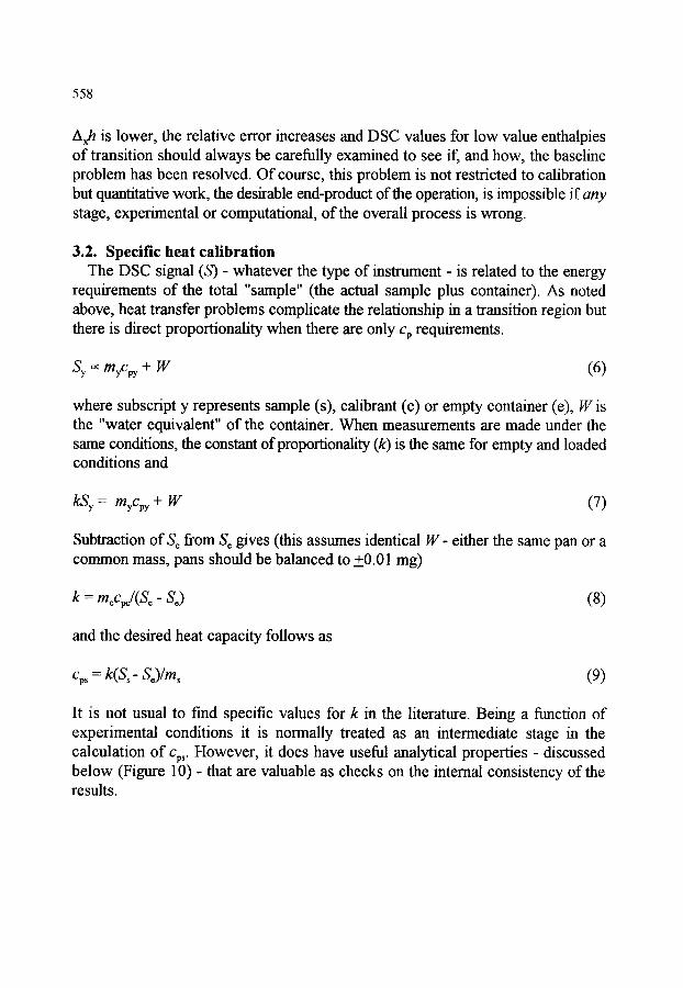
558

Ax h is lower, the relative error increases and DSC values for low value enthalpies of transition should always be carefully examined to see if, and how, the baseline problem has been resolved. Of course, this problem is not restricted to calibration but quantitative work, the desirable end-product of the operation, is impossible if a n y

stage, experimental or computational, of the overall process is wrong.

3.2. Specific heat calibration The DSC signal (S) - whatever the type of instrument - is related to the energy

requirements of the total "sample" (the actual sample plus container). As noted above, heat transfer problems complicate the relationship in a transition region but there is direct proportionality when there are only Cp requirements.

Sy cx myCpy + W (6)

where subscript y represents sample (s), calibrant (c) or empty container (e), W is the "water equivalent" of the container. When measurements are made trader the same conditions, the constant of proportionality (k) is the same for empty and loaded conditions and

kSy = myCpy + W (7)

Subtraction of S~ from S, gives (this assumes identical W- either the same pan or a common mass, pans should be balanced to +0.01 mg)

k = mr162 Sr (8)

and the desired heat capacity follows as

Cp~ = k ( S s - Se)/m~ (9)

It is not usual to find specific values for k in the literature. Being a function of experimental conditions it is normally treated as an intermediate stage in the calculation of %. However, it does have useful analytical properties - discussed below (Figure 10) - that are valuable as checks on the internal consistency of the results.

559

1, o

~ J

C D f--- / t !

A --3'13

T~ Tx ..

Temperature

$ o

Ixl

7", 7", I-~- . . . . . S C a l a . . . . ----~'

I/ i _Z-2<cr~

_ I ' - - - - - - - - - + . i _ T i m e

Figure 8. Schematic diagram to show Figure 9. The construction used to how a change m Cp influences Axh (much calculate the effective ordinate S~ - S~ exaggerated f or emphasis), when isothermal baselines do not

coincide.

Modem heat flux DSCs usually have an ordinate scale that is labelled as a "heat flow rate" with units of watts (or mW). In reality, this is an appropriately calibrated differential temperature that transforms the ordinate to a scale equivalent to the "differential power" of power compensation DSC. In either case, specific heat capacities then follow as ordinate/fl (with appropriate allowance for sample mass and use of a common time scale). In practice, because Cp work is one of the more demanding applications of DSC, it is dangerous to accept a factory calibration for some unstated experimental conditions. Specific heat capacities should always be determined by direct comparison of signals from the "unknown" and the calibrant run under the same conditions.

The main problem m DSC heat capacity work is to determine the "effective" signal Sr - So or S=- So of equations (8) or (9). Figure 9 shows a much exaggerated schematic demonstration of potential difficulties. Specific heat capacity measurements should be based on a sequence of isothermal (at TJscannmg/isothermal (at Tu) runs. Ideally, the isothermal baselines should be colinear and not displaced as shown. The latter is not a problem if displacement is the same for all rtms - empty, calibrant and sample. Inevitable errors m any experiment ensure that this requirement is rarely met so that some procedure is needed to deal with baseline imbalances. The general approach is to assume that the "isothermal" baselines (broken lines, Figure 9) are linear between the programed temperature limits and to measure Sy from this (for clarity, S~ in Figure 9 is shown

560

as a negative quantity). If the isothermal baseline is actually curved the assumption of linearity has no deleterious effects providing curvature is the same in all cases. This is where it is important to ensure that the container presents a reproducible heat transfer path throughout the sequence: pan only/pan+calibrant/pan+sample. Thus the base should always be flat and the surfaces should have reproducible emissivity. This is particularly important at high temperatures. It is very useful to record the isothermal baseline offsets iy(T~)-iy(T~) (Figure 9) for the required sequence of three runs in any Cp determination. Experience then shows what differences are acceptable for a particular set of conditions. It is valuable to combine these results with data for k (equation 7) because this should be a constant (if all circuits are correctly adjusted) or change steadily with temperature. For short runs k should not pass through a maximum or minimum - this behaviour implies baseline problems. These are minimised for shorter nms and, if there is doubt, it is always helpful to compare data from long and short rtms (Figure 10).

As mentioned above, the calibration factor may vary with instnunental conditions (sample and ambient temperature, heating/cooling rate, type and rate of gas flow) but these should affect the sample similarly, so that the final Cp should be independent of insmmaental conditions. If this can be demonstrated it is a powerful argument for the quantitative operation of a given instnunent [16].

3.3. Comparisons between enthalpy and specific heat capacity calibrations To observe any temperature dependence of the area-to-enthalpy conversion factor

it is essential to use several transition enthalpy standards. A single heat capacity standard covers a wide range of temperature and it could be argued that this should replace the more conventional "area" procedure. In fact both are needed, because Cp work is generally more demanding and time-consuming. In any case it is by no means clear how close there is to a one-to-one correspondence between the two techniques. There are theoretical reasons for some difference [13], but the effects are difficult to calculate because some of the parameters that are needed have wide uncertainties in their values. We have used the specific heat capacity of synthetic sapphire (Table 5) for calibration of materials showing phase changes or fusion and have been able to reproduce the heats of fusion of all the CRM of Table 1 and benzil (no others have yet been tried) of Table 2 to better than 1% using a power compensation calorimeter [17]. However, a difference of about 1% has also been reported using a similar instnunent [5] and a difference of several percent for a heat flux DSC [18]. It is well to be aware of this, particularly for "intermediate" areas that do not fall easily into a particular classification.

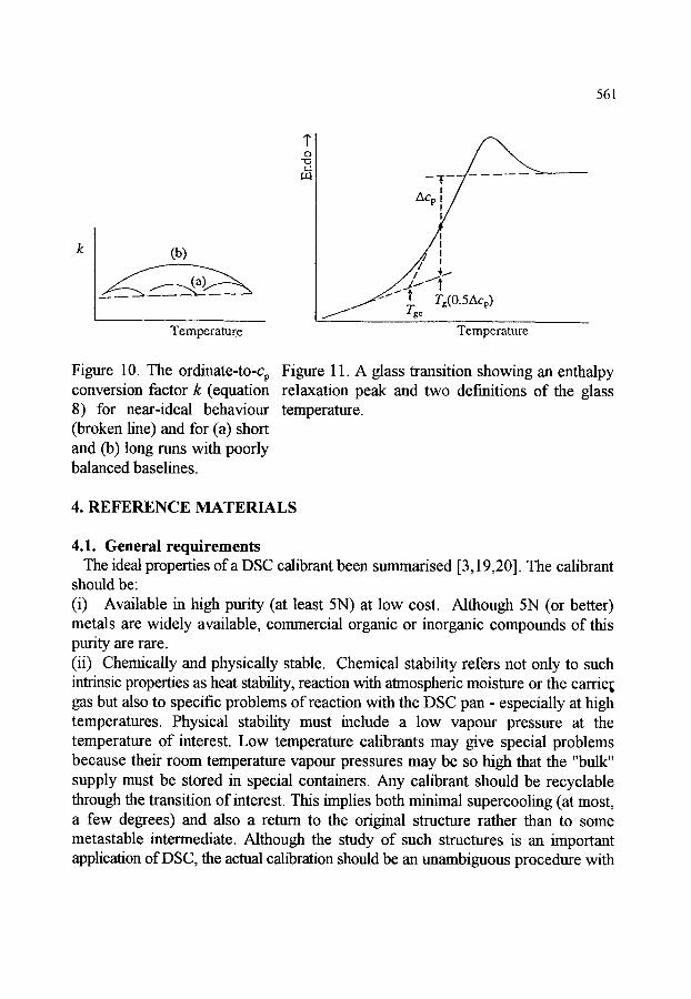
561

(b)

"1" o

Acpl i

,f dL / .x ' t--"f

Temperature Temperature

Figure 10. The ordinate-tO-Cp Figure 11. A glass transition showing an enthalpy conversion factor k (equation relaxation peak and two defmitions of the glass 8) for near-ideal behaviour temperature. (broken line) and for (a) short and (b) long rims with poorly balanced baselines.

4. REFERENCE MATERIALS

4.1. General requirements The ideal properties of a DSC calibrant been summarised [3,19,20]. The calibrant

should be: (i) Available in high purity (at least 5N) at low cost. Although 5N (or better) metals are widely available, commercial organic or inorganic compounds of this purity arc rare. (ii) Chemically and physically stable. Chemical stability refers not only to such intrinsic properties as heat stability, reaction with atmospheric moisture or the carrie[ gas but also to specific problems of reaction with the DSC pan - especially at high temperatures. Physical stability must include a low vapour pressure at the temperature of interest. Low temperature calibrants may give special problems because their room temperature vapour pressures may be so high that the "bulk" supply must be stored in special containers. Any calibrant should be recyclable through the transition of interest. This implies both minimal supercooling (at most, a few degrees) and also a return to the original structure rather than to some metastable intermediate. Although the study of such structures is an important application of DSC, the actual calibration should be an unambiguous procedure with

562

the minimum potential for operator error. In particular, there should be no need for any form of thermal treatment to restore the sample to its original state. (iii) Easy to handle and of low toxicity. No special sample preparation should be needed. Ideally, all would be powders or liquids so that the possibility of properties being influenced by pre-treatment (e.g. by excessive grinding of granular materials) is minimised. Alternative forms, such as sheet or discs, are acceptable if their preparation does not affect the properties of iv). (iv) Thermodynamically well defined. Both enthalpy and specific heat capacity data should be available. To minimise uncertainties in the final results, they should be known to an order of magnitude better than the DSC reproducibility (+1% for careful, but not excessively time-consuming, work). The thermodynamic data should have been obtained using an absolute technique such as adiabatic calorimetry. It is a bonus if the calibrant has more than one transition and it is obviously simpler to use the same material for both ordinate and abscissa calibration. Transition temperatures are fairly well defined for a wide range of diverse materials, although purity tends to be addressed in only a small fraction of reported data. By contrast, precise enthalpy and Cp measurements are rare and the desirable situation, whereby two independent groups report results for the same material, are even fewer (and, within this select body, agreement to a few tenths of one per cent is even rarer!). In fact, there is a growing anomaly because commercial pressures are causing the relative, but simple and rapid, technique of DSC to displace adiabatic calorimetry as the preferred tool for many investigations. As a result, it becomes increasingly difficult to find laboratories that can supply independent thermodynamic data for any type of material - especially when those that have suitable facilities may be more interested in relatively "exotic" compounds with properties that do not meet the criteria of (i) to (iii) above.

For any calibrant in common use some relaxation of one or more of the above conditions is required. In particular, it must be emphasised that enthalpies of fusion or transition are not generally known to better than +1%, let alone the desired +0.1%. Later sections will discuss the numerous materials that are currently available for the calibration of differential scanning calorimeters. Their thermodynamic properties are not all defined to similar standards and problem areas are noted, together with other deviations from (i) to (iv) above. First, however, it is appropriate to comment on the "best" procedures that should be used.

4.2. Experimental procedures As with any DSC experiment, it is essential to optimise thermal contact between

sample and pan and to relieve any strain reduced by sample preparation. For melting transitions this should always mean that the sample has been premelted to give a thin

563

layer sandwiched between the pan and its lid. A lid is essential for quantitative work for two quite different reasons: (i) In a set of experiments with samples of different emissivities, heat loss characteristics will be different for the several samples tmless there is a lid to ensure that the pan presents a constant emissivity package in the DSC cell. (ii) Surface tension effects may cause many materials, especially metals, to form spheres on melting. A closely fitting lid is needed to prevent this.

Only small samples are needed for calibration purposes - the minimum size is dictated by the need for sufficient signal to adequately define the heat of fusion or transition. Whenever there is any possibility of the vapour pressure exceeding a few tens of pascals samples should be run in sealed cells. Samples should always be reweighed at the end of a run and this is particularly important if there is any possibility of vapourisation. A wide range of pans is available from most manufacturers. Calibration runs should be made with all types over a wide range of temperatures - agreement at a single temperature may be an accidental crossover of two quite different curves. When an overall picture has been obtained, it is a simple matter to define what types of pan may be interchanged before recalibration is needed. It is often convenient to isolate a sample (including calibrants) from its pan (and lid) by sandwiching it between inert spacers. For example, aluminium and its alloys have been run to 1000 K between sapphire wafers in platinum pans. The calibration must obviously reflect the changed circumstances and it is a commonsense procedure to first melt the assembly outside the calorimeter to check the probity of the system- this should always be done if there is any doubt about sample/pan interaction. A full description of sample/pan compatibilities has been given [3].

4.3. Certified reference materials (CRM) CRM are available from some national laboratories, mainly the UK Laboratory of

the Government Chemist (LC~) [21] and the US National Institute of Standards and Technology (NIST) [22]. Measurements, traceable to national standards, have been made on the batch of material from which the CRM is formed and uncertainty limits are given. Measurements are of the highest metrological quality. Tables 1 and 2 show data for metallic and organic CRMs respectively. Where both Tf~ and Af~h are given, the values were determined by adiabatic calorimetry and the associated platinum resistance thermometry [23] (an exception is the NIST data for tin which are based on a method of mixtures and phase change calorimeter [24]). The Tfus-only data used the classical melting point techniques of time-temperature curves or thermostatted baths and effectively zero heating rates to observe the fmal traces of melting. The agreement between the paired measurements shown in Tables 1 and 2 gives a good impression of the consistency between the two techniques, the overall

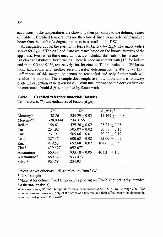
564

accuracies of the temperatures are shown by their proximity to the defining values of Table 1. Certified temperatures are therefore defined to an order of magnitude better than the tenth of a degree that is, at best, realistic for DSC.

As suggested above, the position is less satisfactory for Afus h. The uncertainties shown for Afush in Tables 1 and 2 are estimates based on the known features of the apparatus. Even when these uncertainties are included, the heats of fusion may not fall close to tabulated "best" values. There is good agreement with [ 13] for indium and fin, to 0.3 and 0.1%, respectively, but for zinc the Table 1 value falls 3% below most tabulations and another recent careful determination is 4% lower [25]. Differences of this magnitude cannot be reconciled and only further work will resolve the problem. The example does emphasise how important it is to always quote the calibration value taken for A~h. With this information the derived data can be corrected, should Axh be modified by future work.

Table 1. Certified reference materials (metals) Temperatures (T) and enthalpies of fusion (Afus h)

T/~ T/K Af~hl J g-1 Mercury* -38.86 234.29 + 0.03 11.469 + 0.008 Mercury *~ -38.8344 234.3156 Indium 156.61 429.76 + 0.02 28.71 + 0.08 Tin 231.92 505.07 + 0.02 60.55 + 0.13 Tin* 231.91 505.06 + 0.01 60.22 + 0.19 Lead 327.47 600.62 + 0.02 23.00 + 0.05 Zinc 419.53 692.68 + 0.02 108.6 + 0.5 Zinc *~ 419.527 692.677 Aluminium 660.33 933.48 + 0.05 401.3 + 1.6 Aluminium *~ 660.323 933.473 Silver *~ 961.78 1234.93

Unless shown otherwise, all samples are from LGC. * NIST sample Material for defining fixed temperatures (shown) on ITS-90 (not primarily intended

for thermal analysis) Where necessary, IPTS-68 temperatures have been corrected to ITS-90. In the range 200-1000 K corrections are, however, only of the order of a few mK and their effect cannot be detected in even the most precise DSC work.

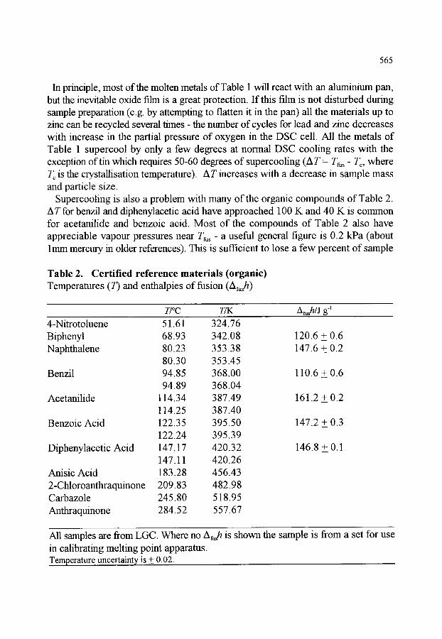
565

In principle, most of the molten metals of Table 1 will react with an aluminium pan, but the inevitable oxide film is a great protection. If this film is not disturbed during sample preparation (e.g. by attempting to flatten it in the pan) all the materials up to zinc can be recycled several times - the number of cycles for lead and zinc decreases with increase in the partial pressure of oxygen in the DSC cell. All the metals of Table 1 supercool by only a few degrees at normal DSC cooling rates with the exception of tin which requires 50-60 degrees of supercooling (AT = Tins- T~, where Tr is the crystallisation temperature). AT increases with a decrease in sample mass and particle size.

Supercooling is also a problem with many of the organic compounds of Table 2. AT for benzil and diphenylacetic acid have approached 100 K and 40 K is common for acetanilide and benzoic acid. Most of the compounds of Table 2 also have appreciable vapour pressures near Tins - a useful general figure is 0.2 kPa (about lmm mercury in older references). This is sufficient to lose a few percent of sample

Table 2. Certified reference materials (organic) Temperatures (7) and enthalpies of fusion (Af~sh)

T/~ T/K A~h/J g-1

4-Nitrotoluene 51.61 324.76 Biphenyl 68.93 342.08 Naphthalene 80.23 353.38

80.30 353.45 Benzil 94.85 368.00

94.89 368.04 Acetanilide 114.34 387.49

114.25 387.40 Benzoic Acid 122.35 395.50

122.24 395.39 Diphenylacetic Acid 147.17 420.32

147.11 420.26 Anisic Acid 183.28 456.43 2-Chloroanthraquinone 209.83 482.98 Carbazole 245.80 518.95 Anthraquinone 284.52 557.67

120.6 + 0.6 147.6 + 0.2

110.6+0.6

161.2 + 0.2

147.2 + 0.3

146.8 + 0.1

All samples are from LC~. Where no Afush is shown the sample is from a set for use in calibrating melting point apparatus. Temperature uncertainty is + 0.02.

566

from an unsealed pan- and even 1% loss is enough to invalidate a calibration or subsequent quantitative measurement. As a general procedure, organic compounds should always be rtm in sealed pans if Tfu~ is to be approached. This precaution is particularly relevant for naphthalene and benzoic acid. Even if precision measurements are not being attempted, it must always be remembered that the high vapour pressure material must go somewhere and the DSC head itself may be damaged. This caveat even applies to metals at relatively low temperatures: neither cadmium (also a potential health hazard) nor magnesium should be taken near their respective Tfu~ except in special sealed cells.

4.4. Other reference materials A comprehensive IUPAC publication [26] discusses potential reference materials

for the realisation of many physicochemical properties. Those for temperatures and enthalpies of phase changes and for specific heat capacities are of particular interest to thermal analysts. The reference is dated 1987 but there have not been many additions since then- the main systematic effort being the clarification of results for the lower melting metals (Table 1). It should be emphasised that, although tabulated "best" values may lack the certification generally demanded by the many accreditation bodies that guarantee good experimental practice, they often include data from diverse sources - and consistency among these always increases confidence in the final data. Of course, it is essential to compare materials of similar purity but, at the better than 4N level that should be aimed at for a calibrant, minor compositional differences have only a negligible effect on the measured Afush values.

Many of the materials of reference [26] have already been considered in Tables 1 and 2. Some additional compounds are shown in Table 3 which also contains other suggestions for substances to use at lower and elevated temperatures. The latter, especially, are subject to much wider uncertainties and some still lack reliable independent enthalpy data. Two compounds that appear in [26], but are not shown in Table 3, are ethylene carbonate and succinonitrile. These are used in the construction of triple-point cells (309.4643 and 331.2142 K respectively) but their long-term properties on storage in air (i.e. after opening an initially sealed container) are unclear and Afus h values are unknown. A useful alternative compound, phenyl salicylate, (Tfus-~314 K) is being investigated by LGC.

4.5. International Confederation for Thermal Analysis and Calorimetry (ICTAC) reference materials

Reference materials for the comparison of temperatures (only) have been available for many years from NIST acting on behalf of ICTAC (Table 4). They are high purity commercial compounds that mainly feature solid/solid transitions because many of the earlier designs of DTA could not accept liquids. Materials were

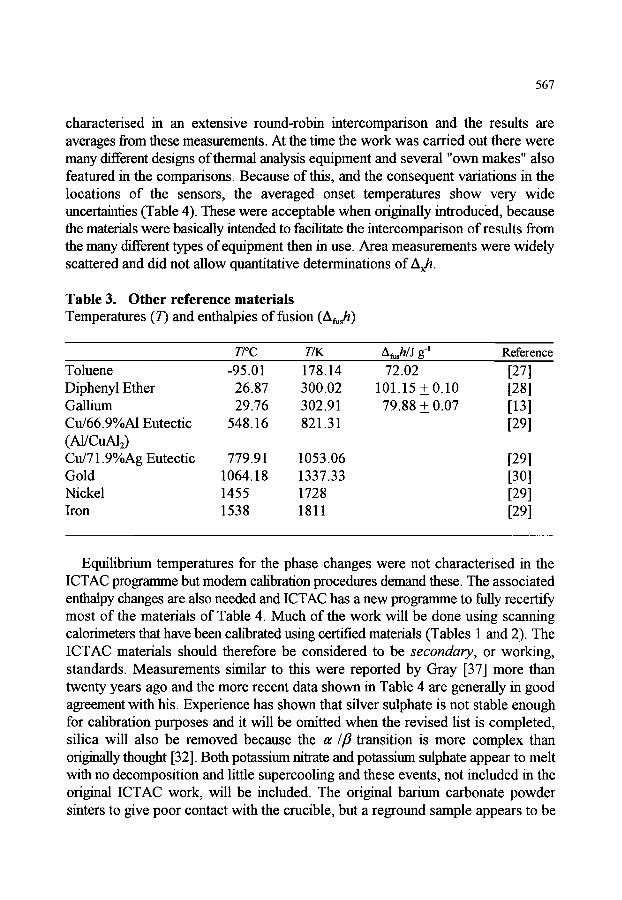
567

characterised in an extensive rotmd-robin intercomparison and the results are averages from these measurements. At the time the work was carried out there were many different designs of thermal analysis equipment and several "own makes" also featured in the comparisons. Because of this, and the consequent variations in the locations of the sensors, the averaged onset temperatures show very wide uncertainties (Table 4). These were acceptable when originally introduced, because the materials were basically intended to facilitate the intercomparison of results from the many different types of equipment then in use. Area measurements were widely scattered and did not allow quantitative determinations of Axh.

Table 3. Other reference materials Temperatures (T) and enthalpies of fusion (Afu~h)

T/~ T/K Af~hlJ g~ Reference Toluene -95.01 178.14 Diphenyl Ether 26.87 300.02 Gallium 29.76 302.91 Cu/66.9%A1 Eutectic 548.16 821.31 (A1/CuAI~) Cu/71.9%Ag Eutectie 779.91 1053.06 Gold 1064.18 1337.33 Nickel 1455 1728 Iron 1538 1811

72.02 [27] 101.15+_0.10 [28]

79.88+_0.07 [13] [29]

[29] [30] [29] [29]

Equilibrium temperatures for the phase changes were not characterised in the ICTAC programme but modem calibration procedures demand these. The associated enthalpy changes are also needed and ICTAC has a new programme to fully recertify most of the materials of Table 4. Much of the work will be done using scanning calorimeters that have been calibrated using certified materials (Tables 1 and 2). The ICTAC materials should therefore be considered to be secondary, or working, standards. Measurements similar to this were reported by Gray [37] more than twenty years ago and the more recent data shown in Table 4 are generally in good agreement with his. Experience has shown that silver sulphate is not stable enough for calibration purposes and it will be omitted when the revised list is completed, silica will also be removed because the af//3 transition is more complex than originally thought [32]. Both potassium nitrate and potassium sulphate appear to melt with no decomposition and little supercooling and these events, not included in the original ICTAC work, will be included. The original barium carbonate powder sinters to give poor contact with the crucible, but a reground sample appears to be

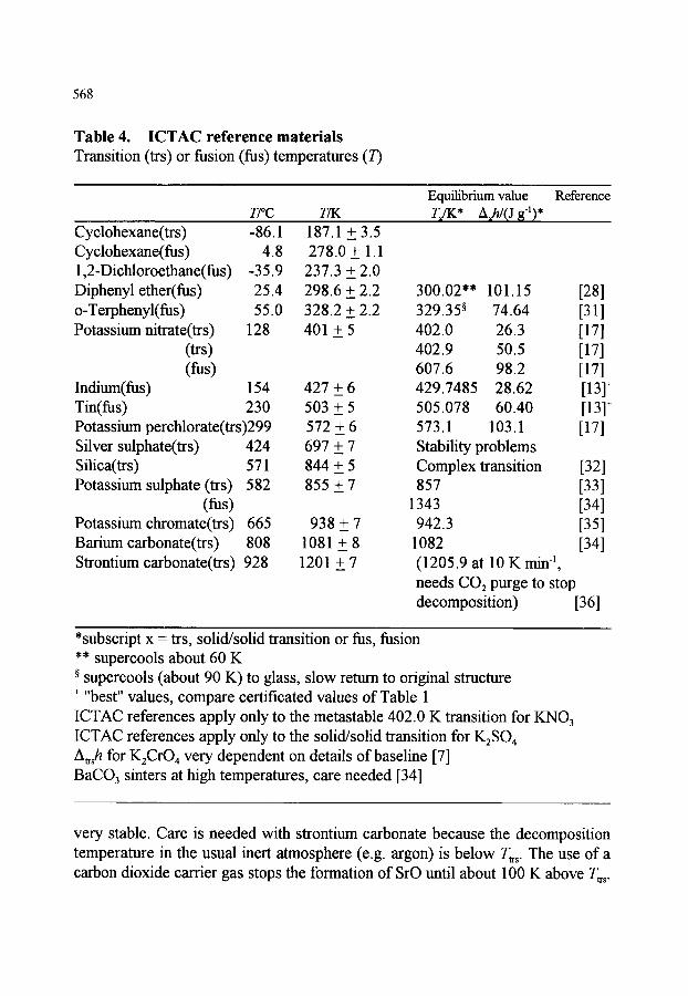
568

Table 4. ICTAC reference materials Transition (trs) or fusion (fus) temperatures (T)

T/~ T/K

Cyclohexane(trs) Cyclohexane(fus) 1,2-Dichloroethane(fus) Diphenyl ether(fus) o-Terphenyl(fus) Potassium nitrate(trs)

(trs) (fus)

Indium(fus) 154 Tin(fus) 230 Potassium perchlorate(trs)299 Silver sulphate(trs) 424 Silica(trs) 571 Potassium sulphate (trs) 582

fins) Potassium chromate(trs) 665

Barium carbonate(trs) 808 Strontium carbonate(trs) 928

-86.1 4.8

-35.9 25.4 55.0

128

187.1 + 3.5 278.0 + 1.1

237.3 + 2.0 298.6 + 2.2 328.2 + 2.2 401 +5

427 + 6 503 + 5 572 + 6 697 + 7 844 + 5 8 5 5 + 7

938 + 7 1081 + 8 1201 +7

Equilibrium value Ts/K* Ash/(J ~-1),

Reference

300.02** 101.15 [28] 329.35 ~ 74.64 [31] 402.0 26.3 [17] 402.9 50.5 [17] 607.6 98.2 [17] 429.7485 28.62 [13] + 505.078 60.40 [13] + 573.1 103.1 [17] Stability problems Complex transition [32] 857 [33]

1343 [34] 942.3 [35]

1082 [34] (1205.9 at 10 K min ~, needs CO2 purge to stop decomposition) [36]

*subscript x = trs, solid/solid transition or fus, fusion ** supercools about 60 K

supercools (about 90 K) to glass, slow return to original structure + "best" values, compare certificated values of Table 1 ICTAC references apply only to the metastable 402.0 K transition for KNO 3 ICTAC references apply only to the solid/solid transition for K2SO 4 A~h for K2CrO 4 very dependent on details of baseline [7] BaCO 3 sinters at high temperatures, care needed [34]

very stable. Care is needed with strontium carbonate because the decomposition temperature in the usual inert atmosphere (e.g. argon) is below T~. The use of a carbon dioxide carrier gas stops the formation of SrO tmtil about 100 K above T~.

569

ICTAC standards have been sold by NIST as sets covering (with some overlap) four ranges of temperature:

(i) Cyclohexane - o-terphenyl (ii) Potassium nitrate - silver sulphate

(iii) Potassium perchlorate - potassium chromate (iv) Quartz- strontium carbonate

but shortage of individual components means that whole sets go out of stock. To overcome this problem, future sales will be made on the basis of individual materials.

Other ICTAC standards are available for the calibration of thermogravimetric analysers (these are discussed in Chapter 4) and for the glass transition - see Section 4.7.2.

4.6. Other potential calibrants Eysel and Breuer [38] reviewed a large number of potential calibrants, among

which were various n-alkanes and other hydrocarbons. These are stable and calorimetricaUy well defined but the lower members (which are the most useful, as low temperature calibrants) are volatile at room temperature and need special containers for storage. There are alternative inorganic compounds that are free from this drawback - the widely used ammonium dihydrogen phosphate, for example, has a very reproducible low temperature (~ 148 K) and low energy (~5.5 J g-l) solid/solid transition that could be developed as a useful low temperature calibrant. An additional candidate is sodium nitrate, readily available in nearly 5N purity, which has both a polymorphic (549 K) and a melt (580 K) transition. Other simple inorganic salts such as potassium bromide and sodium chloride, whilst covering useful temperature ranges (Tfu~ ~ 1007 and 1074 K, respectively) have significant vapour pressures at these temperatures and need special crucibles. Several organic compounds have been suggested by Sabbah and coworkers [39]

and characterised, using a specially constructed digerential thermal analyser, for triple temperatures and the corresponding heats of fusion,

Mention should also be made of the range of organic melting point standards produced by the World Health Organisation (WHO) [40]. These have been characterised by a capillary melting method using a finite heating rate, so corrections are needed to obtain equilibrium values. Nevertheless the materials (azobenzene, vanillin, benzil, acetanilide, phenacetin, benzanilide, sulphanilamide, sulphapyridine, dicyandiamide, saccharin, caffeine, phenolphthalein) form a series with enough overlap with those of Table 2 to cover most temperatures over which organic materials are stable.

570

4.7. Materials for special applications 4. 7.1. Cooling and modulated temperature DSC

The problems of supercooling have been discussed earlier. The only materials that seem to be free of this problem on a practical DSC scale of+0.1 K are liquid crystals (lc) [10,11 ]. These are now widely available with some showing a complex series of lc/lc transitions. On the basis of "two (or more) for the price of one" transition it is natural to prefer multiple events to simple transitions from lc to isotropic liquid. It should, however, be emphasised that, although peak temperatures are well- defined, precise measurements of the associated enthalpy changes require at least ten degrees of undisturbed low and high temperature Cp curves [41] (closely spaced transitions are not acceptable for calibration purposes). It will be noted that peak, not onset, temperatures were mentioned above. Liquid crystal transitions take place over a finite temperature range and the most reproducible point is the peak. The peak temperature can be used for this type of transition because the energies involved are low and the signal reflects real material requirements - in contrast with a melting transition, for example, where heat transfer problems perturb the true shape of the curve and only the total enthalpy change is significant.

This aspect of liquid crystal behaviour makes them very useful materials for the special requirements of modulated DSC [12]. Here the low energies involved allow the sample to follow the oscillating temperature signal (albeit with a phase lag), but even here it is essential to confirm linearity for specific transitions. For example [12], in 4:4'n-octyloxy-cyanobiphenyl the smectic/nematic transition at 341 K is ideal for a wide range of modulation conditions, whereas the nematic/isotropic event at 354 K is more limited in its applications. At the present stage of its development, it is far from certain that optimum conditions for the calibration of modulated temperature DSC have been achieved, but there seems little doubt that increasing attention will be paid the properties of liquid crystals.

4. 7.2. The glass transition The glass transition temperature (T g) needs special attention because it is not a

well-defined thermodynamic event: the transition region can be shifted by suitable thermal or mechanical treatment of the sample. It is, however, still possible to formally define a Tg that is a valuable parameter for the characterisation of a material. The Tg region appears on a DSC curve as a fairly abrupt increase in Cp on going from the glass to the liquid or rubber. The Cp step may be accompanied by fine structure - a peak or trough - and this appears to complicate the location of" Tg " as some point on a DSC curve. Several definitions of Tg are used. The most common choice is either the onset or the point where half the change in Cp has been reached (Tgo or Tg(O.5Acp), respectively, Figure 11). These are useful characteristic temperatures although both depend on experimental conditions. Because of this

571

dependence, a "standard" glass is particularly useful to ensure the transferability of data from one user to another.

A suitable polystyrene glass has been available from ICTAC for more than twenty years as NIST Reference Material 754 (currently 8754). Measurements [17] show that this is extremely stable: for the as-received material (the form certified) Tgo has increased from 377.4 to 378.2 K (for fl= 20 K min -1) over a twenty year period (the certificate, again an average from many laboratories, gives 377.6 + 3.1 K). This small change is within the experimental reproducibility (+0.5 K) of the specific instrument that was used. However, that there are real changes is shown by an increase of about 50% in the peak height (the fine structure referred to above). This is a clear sign of the physical ageing that any glass experiences on storage. Our knowledge of this phenomenon has improved enormously in recent years - to a large extent this has been due to results from DSC work [42]. Physical ageing is significant for any glass that has a Tg up to perhaps 50 to 60 K above ambient. Polystyrene is therefore only slightly affected but, on the lengthy time scale discussed, there are changes that are reflected more in the increased peak height than in changes in Tg~. That RM 8754 has not undergone any parallel chemical change over the twenty years is shown by the unchanged (375.0 + 0.5) value of Tgo, and of the peak height, for the glass formed by cooling through the Tg region at 20 K min -~ with subsequent measurements made on heating at the same rate. In fact, it is probably better to certify a well-defined glass of this type, that can be formed in situ, rather than the "as received" state which may have had unknown storage conditions (e.g. close to heating pipes), leading to unusual physical ageing.

One of the improvements in the definition of Tg has been the use of the fictive temperature (T f) to characterise Tg. This has a thermodynamic basis in that it represents the point of intersection of enthalpy curves [43] for the glassy and liquid states. The enthalpy of a glass depends on the method of glass formation- a quenched glass has a higher enthalpy than a slowly cooled one - and Tf reflects this but it shows no dependence on heating rate. Most manufacturers now offer programs that give Tf and an additional advantage is that the same sample may be used for day-to-day repeat measurements. Unlike Tgo etc, Tf changes in a simple way with the conditions of glass formation. Thus it decreases as the extent of annealing increases - the reverse of the behaviour of the various other types of Tg which are, in fact, somewhat arbitrary quantities that combine material and instrumental effects. The advantage of using Tf is shown in the decrease in this quantity from 371.2 K in 1975 to a 1996 value of 369.9 K [ 17]. The glass formed by cooling at 20 K min ~ has an unchanged Tf of 375.0 K (the equality with Tg, is fortuitous and should not be used to ascribe any fundamental meaning to the latter). Work is now under way to recertify RM 8754 to incorporate data on Tf, in situ glasses, and results from modulated temperature DSC work. Modulated DSC has been extensively applied to

572

the glass transition region and standards will play an important role in the resolution of material and instrumental effects.

The glass transition is of increasing importance for a wide range of materials, from foods and pharmaceuticals to inorganics and metals. There are more common features than differences in the DSC responses of these, although sometimes there are complications due to the onset of crystallisation at the upper end of the transition region. It would clearly be helpful to have specific standards for these several types of glasses (even if only to cover the temperature range that is generally used in a particular laboratory). In their absence the existing polystyrene RM 8754 is a very helpful intermediate.

4.8. Specific heat capacity (heat flow rate) calibrants It is almost universal to use a-alumina (synthetic sapphire) for this type of

calibration. The material is available from NIST (RM 720) and several independent measurements suggest that Cp is known to within 0.1%. The GEFTA group [20] have given polynomials (Table 5) that accurately represent the heat capacity of sapphire (to 2250 K) and of oxygen-free high conductivity copper (to 320 K). The latter is useful at sub-ambient temperatures where the heat capacity of alumina changes rather rapidly with temperature. Another possible calibrant for lower temperatures is benzoic acid [44] but this should never be used much above ambient temperatures because of potential problems due to the rapid increase in vapour pressure.

Table 5. Fitting polynomials for specific heat capacity of calibrants

i a b c 0 3.63245x10 ~ -5.81126x10 -~ 1 -1.11472x10 -~ 8.25981x10 ~ 2 -5.38683x10 .06 -1.76767x10 .05 3 5.96137xl 0 .07 2.17663xl 0 .08 4 -4.92923x10 -~ -1.60541x10 1~ 5 1.83001x10 -~ 7.01732x10 -~5 6 -3.36754x10 -14 -1.67621x10 -~8 7 2.50251x10 -17 1.68486x10 -22

-1.63570x10 -~ 7.07745x10 ~

-3.78032x10 -~ 9.60753x10 -~

-9.36151x10 -~

Sapphire: Sapphire: Copper: 7 7 4

Cp = ~ a i~ Cp = ~ b i~ Cp -- ~ c i~i I=O i=o i=o

(valid 70-300 K) (valid 290-2250 K) (valid 100-320 K)

573

High quality synthetic sapphire is readily available and it is relatively cheap to produce discs that fit snugly into a variety of DSC pans. Of course, such fabricated parts are not certified but Cp is insensitive to impurities even at levels as high as 1% [17].

5. CONCLUDING REMARKS Calibration of differential scanning calorimeters is not a difficult procedure. A

range of materials is available for temperatures from about 250 to 700 K but the lower and (especially) upper temperature ranges are less well served. Calibration should be tailored to the demands of the operator. For comparative data, measurements (and associated calibrations) can be at any convenient rate using Te(fl) and Ah defined by some arbitrary but reproducible baseline. Such measurements will not necessarily agree with those made by another operator using a different type of instrument. Agreement only comes with more careful work that emphasises the thermodynamic nature of the underlying quantities that are to be determined. Careful calibration is essential for this type of work but, with this for a foundation, it is possible to characterise temperatures to +0.1 K and heat capacities and enthalpy changes to +1.0%.

REFERENCES

1. Standard Practice for Temperature Calibration of Differential Scanning Calorimeters and Differential Thermal Analyzers, American Society for Testing Materials, Standard E967.

2. G.W.H. HOhne, H.K. Cammenga, W. Eysel, E. Gmelin and W. Hemminger, Thermochim. Acta, 160 (1990) 1.

3. H.K. Cammenga, W. Eysel, E. Gmelin, W. Hemminger, G.W.H. HOhne and S.M. Sarge, Thermochim. Acta, 219 (1993) 333.

4. M.J. Richardson, Calorimetry and Thermal Analysis of Polymers, (Ed. V.B.F. Mathot), Hansel Munich, 1994, p. 100.

5. G.W.H. HOhne and E. G1Oggler, Thermochim. Acta, 151 (1989) 295. 6. M.J. Richardson and N.G. Savill, Thermochim. Acta, 12 (1975) 213. 7. M.J. Richardson, Thermochim. Acta, 300 (1997) 15. 8. M.J. Richardson and P. Burrington, J. Thermal Anal., 6 (1974) 345. 9. G.W.H. HOhne, J. Schawe and C. Schick, Thermochim. Acta, 221 (1993)

129. 10. J.D. Menczel and T.M. Leslie, J. Thermal Anal., 40 (1993) 957. 11. J.D. Menczel, J. Thermal Anal., 49 (1997) 193. 12. A. Hensel and C. Schick, Thermochim. Acta, 304/305 (1997) 229.

574

13. G.W.H. H6hne, W. Hemminger and H.-J. Flammersheim, Differential Scanning Calorimetry, Springer, Berlin, 1995, Chapter 4.

14. Standard Practice for Heat Flow Calibration of Differential Scanning Calorimeters, American Society for Testing Materials Standard E968.

15. J.E.K. Schawe and C. Schick, Thermochim. Acta, 187 (1993) 335. 16. M.J. Richardson, Compendium of Thermophysical Property Measurement

Methods, (Eds. K.D. Maglic, A. Cezairliyan and V.E. Peletsky), Plenum, New York, 1992, Vol. 2, Chapter 18.

17. M.J. Richardson unpublished data. 18. S.M. Sarge and H.K. Cammenga, Thermochim. Acta, 94 (1985) 17. 19. G.W.H. H6hne, J. Thermal Anal., 37 (1991) 1987. 20. S.M. Sarge, E. Gmelin, G.W.H. H0hne, H.K. Cammenga, W. Hemmmger

and W. Eysel, Thermochim. Acta, 247 (1994) 129. 21. Certified Reference Materials for Thermal Analysis, Office of Reference

Materials, Laboratory of the Government Chemist, Teddington, Middlesex, TW11 0LY, UK.

22. Standard Reference Materials Catalog, SRM Program, National Institute for Standards and Technology, Gaithersburg, MD 20899-0001, USA.

23. F. Gronvold, J. Chem. Thermodynamics, 25 (1993) 1133. 24. D.A. Ditmars, Compendium of Thermophysical Property Measurement

Methods, (Eds. K.D. Maglic, A. Cezairliyan and V.E. Peletsky), Plenum, New York, 1992, Vol 2, Chapter 15.

25. D.A. Ditmars, J. Chem. Thermodynamics, 22 (1990) 639. 26. Recommended Reference Materials for the Realization of Physicochemical

Properties, (Ed. K.N. Marsh), Blackwell, Oxford, 1987, Chapters 8, 9. 27. D.W. Scott, G.B. Guthrie, J.F. Messerly, S.S. Todd, I.A. Hossenlopp and

J.P. McCullough, J. Phys. Chem., 66 (1962) 911. 28. G.T. Furukawa, D.C. Ginnings, R.E. McKoskey and R.A. Nelson,

J. Res. Natl. Bur. Stand., 46 (1951) 195. 29. R.E. Bedford, G. Bonnier, H. Maas and F. Pavese, Metrologia, 20 (1984)

145. 30. R.L. Rusby, R.P. Hudson, M. Durieux, J.F. Schooley, P.P.M. Steur

and C.A. Swenson, Metrologia, 28 (1991) 9. 31. S.S. Chang and A.B. Bestul, J. Chem. Phys., 56 (1972) 503. 32. F. Gronvold, S. Stolen and S.R. Svendsen, Thermochim. Acta, 139 (1989)

225. 33. JANAF Tables, J. Phys. Chem. Ref. Data, 14 (Suppl. 1) 1985 1418. 34. E.L. Charsley, C.M. Earnest, P.K. Gallagher and M.J. Richardson,

J. Thermal Anal., 40 (1993) 1415.

575

35. E.L. Charsley, P.G. Laye and M.J. Richardson, Thermochim. Acta, 216(1993)331.

36. S.A. Robbins, R.G. Rupard, B.J. Weddle, T.R. Maull and P.K. Gallagher, Thermochim. Acta, 269/270 (1995) 43.

37. A. P. Gray, Proc. Proc. Fourth ICTA, Budapest, (Ed. I. Buz~is), Akad6miai Kiad6, Budapest, 1974, Vol. 3, p.991.

38. W. Eysel and K.-H. Breuer, Thermochim. Acta, 57 (1982) 317. 39. R. Sabbah and L. E1 Watik, J. Thermal Anal., 38 (1992) 855. 40. World Health Organisation Melting Point Reference Substances,

Promochem Ltd, PO Box 300, Herts AL7 1SS, UK. 41. M.J. Richardson, Thermochim. Acta, 229 (1993) 1. 42. J.M. Hutchinson, Progr. Colloid Polym. Sci., 87 (1992)69. 43. M.J. Richardson, Calorimetry and Thermal Analysis of Polymers,

(Ed. V. B. F. Mathot), Hanser, Mtmich, 1994, Chapter 6. 44. G.T. Funfl~awa, R.E, McKoskey and G.J. King, J. Res. Natl. Bur.

Stds., 47 (1951) 256.


Chapter 14

NONSCANNING CALORIMETRY

R. B. Kemp*

Institute of Biological Sciences, University of Wales, Aberystwyth, Penglais, Aberystwyth, SY23 3DA, Wales, United Kingdom.

When first asked to write a chapter on reaction calorimeters, I was hesitant because I have experience only of LKB/Thermometric heat conduction types. On contacting my friends, it turned out (perhaps not surprisingly) that most had "hands-on" knowledge of models from one manufacturing lineage alone. So, the idea was born of a multi-authored chapter capitalizing on the diverse experiences of "drivers" expert in handling instruments from particular manufacturers. The thought of a "string" of authors at the head of the chapter appealed to me, but then the scientists' singleness of mind intervened and there evolved the present concept of a series of "chapterlets" woven together and in- filled by this general factotum as defined, "a servant who manages all his masters' affairs".

1. IN TRO D U CTION

The original commission for this chapter was to write about reaction calorimeters, meaning instruments that measure the heat of reaction, more precisely, the enthalpy change of reaction, Arn m. However, most types of calorimeter which do not scan a range of temperatures during an experiment can also measure heats of other processes (solution, transfer, dilution, etc.) providing that suitable vessels are available so, the word "nonscanning" has been invoked to collect them. The intention then became to describe the range of techniques used under essentially isothermal conditions. Scanning is the prime subject of an earlier chapter but some instruments can be operated in either mode and thus deserve mention. Later on, it was realized that "combustion" fell between two chapters and is more appropriate to those who don't scan than to the ones who do! Thus, it is included here.

* Author of some and editor of all.

578

General scientific progress in earlier centuries was marked by the design and construction of (often magnificent) instruments fabricated with high precision tools and, in many cases, difficult to operate without considerable training, skill and, most importantly, patience. For measuring the quantities of heat, the earliest work was on latent heats and heat capacities by Black around 1760 and, of course, most people are aware of Lavoisier's ice calorimeter (1783) used for estimating the heat produced by a guinea pig. This phase of home-building continued well into this century (see Chapter 1 for the literature on history section 6.6) with calorimeters being built to individual specifications, usually in university workshops; and tested exhaustively at the bench. These requirements caused calorimetry to be limited essentially to a relatively small number of specialized thermodynamics laboratories with good workshop facilities. Excellent progress was made in a rather restricted field to obtain important and precise data for heat but, until relatively recently, the wider scientific community did not benefit from the major developments in calorimetric techniques. In the sixties, developments led to more sensitive instruments with much improved long-term stabilities, several new measurement functions and a high degree of automation [1]. Then came the commercialization of several different genera of instruments originally designed and built in specific laboratories. In order to sell instruments to relatively inexpert scientists, calorimeters were made user-friendly with the minimum of controls and the maximum of electronics; all this is greatly enhanced these days by "bolt-on" personal computers and dedicated software which allows fully analyzed numbers to be produced at the "touch of a button".

Improvements to electronics and greater precision in manufacturing has led to more sensitive instruments capable of measurements in the ~tW range hence microcalorimeters. At the same time, commercial accessibility has allowed scientists from many different disciplines to explore the potential of heat measurements as analytic and kinetic tools in the more biological disciplines, especially that of physiology. Such a "black box" approach is permissible providing that the operator applies appropriate corrections, but this necessity is not always obvious to the newcomer and thus will be addressed in this chapter (Sections 3 and 4). Since virtually all processes give rise to heat effects, it is important to be aware of, and eliminate, systematic errors and faulty interpretation.

Scientists new to calorimetry must firstly assess which of the many types available in the market place is most suitable for their particular problem. Such a choice also involves matching the geometry and materials of the measuring vessel to the nature of the sample and the required temperature which can be anywhere from virtually absolute zero to well in excess of 1000 ~ This chapter

579

is directed at enterprising scientists looking for "new" solutions to their problems rather than to "old hands" who may already know much that is written here ....... but who might enjoy a different slant to it!

2. DEFINITIONS AND EXPLANATIONS

The diversity in the origins and early development of calorimeters as custom- made, specialized instruments have often resulted in there being several different words and/or phrases for the same type of calorimeter or part of the instrument. It also seems as though the more crucial for accurate description the word should be, the greater the choice of words there is! Hemminger and Sarge in Chapter 1 (Section 2.5) have suggested a system of classification for calorimeters, but there is no general agreement that this is the most appropriate o n e .

2.1. Direct and Indirect Calorimetry There are two main methods of calorimetry [2]. The direct way involves the

measurement of heat loss or gain by a system, corrected for extraneous heat changes. Many of these latter have to be found by calculation. In indirect calorimetry, heat changes are calculated from non-calorimetric data and extrathermodynamic assumptions ultimately based on previous direct calorimetric measurements. Only the direct ones are of value in thermodynamics, indirect methods being employed mainly for living systems (see Volume 4).

2.2. Calorimeter Size Much use has been made of classical Greek in singularizing calorimeters by

size. At the small end, artificial distinction has been created by the prefix "micro" for instruments with a detection limit in the lower gW range [1]. In principle, these are little different to "ordinary" calorimeters and range in sample size from a few gL to m 3. Hemminger and Sarge (Chapter l, Section 2.3. l) argue against the use of the term "micro" because it is not clear to what it refers ~ size, scope or detection limit! One fears this plea runs against the tide, especially as microwatt instruments have distinct problems in operation not shared with their less sensitive sisters which have larger detection limits ~ see, for instance, systematic errors in section 3!

Calorimeters prefixed "macro" and "mega" may well be large in size, but that is subsidiary to the fact that they are designed to measure big amounts of heat and therefore do not require low detection limits. These prefixes frequently have been applied to biological processes from bench-scale microbial cultures

580

(macro) to industrial fermentations (mega). The bioreactor doubles as a calorimeter and, while detection is not a problem, securing the correct heat balance can cause difficulties, see References [3,4].

2.3. Adiabatic and Isothermal Jacket Calorimeters Calorimeters are often classified by the type of vessel(s) contained within

them (e.g. batch, titration or flow) or the process undertaken with the vessel (e.g. perfusion or mixing). Alternatively, or sometimes additionally, they are subdivided according to the description of the change in heat content (e.g. reaction, solution, etc.). However, there is a more fundamental division of most calorimeters according to the control of their surroundings and thus into adiabatic and isothermal jacket. Another term frequently used as an alternative to the latter phrase is isoperibol (sometimes isoperibolic).

By definition, an adiabatic calorimeter has no heat exchange between the measuring vessel and the surroundings. In an ideal instrument, the quantity, q (J) or rate, @ = d q / d t (W), of heat produced or absorbed (exothermic, +q and endothermic processes,-q) causes a temperature change in the system, AT,

A T - q / g a (1)

d T / d t = ~ / E a (2)

where g a is the proportionality ("calibration") constant. This must be determined experimentally but, in the ideal case, it is equal to the heat capacity of the vessel and its surroundings. A process studied by adiabatic calorimetry is of necessity anisothermal in nature. The temperature difference may be small enough to be neglected but, if not, it will be necessary to make a correction.

When the surroundings of the calorimetric measuring system are constant in temperature and pressure, the instrument is isothermal jacket in type. The vessel may be separated from the surrounding thermostatic bath by insulation, usually an air gap or a vacuum, but, since this can never be perfect, it is usually necessary to apply corrections.

2.4. Principle of Heat Measurement The principle of heat measurement allows instruments to be classified into a

maximum of three types (see Chapter 1, Section 2.5). Heat may be measured by recording (i) the temperature rise in a vessel of known heat capacity, (ii) the power of an electrical heater required exactly to compensate for the heat effect of interest, or (iii) the temperature difference across a path of known thermal conductivity. These three methods are embodied in instruments termed respectively heat accumulation, heat compensation and heat conduction

581

calorimeters. As is so often true in casual classification, there are several other alternative phrases for each of these types of measurement (see, for instance, Reference [5]).

When a heat accumulation calorimeter is used with constant surroundings, a correction must be made for heat exchange with those surroundings. This is normally done by applying Newton's Cooling Law in the form of the Regnault- Pfaundler relationship. Nevertheless, the principle of measurement is (leaky) temperature rise. Isothermal jacket instruments are relatively simple compared with adiabatic ones. They are excellent for fast processes but not for slow ones (>=1 h) where the heat exchange term becomes too great to allow accurate correction. Of course this problem can be avoided if there is no heat exchange, a solution considerably adding to the complexity and thereby the cost. The exact means to secure the absence of heat exchange depends on whether heat is produced or absorbed during the measured process.

2.4.1. Heat Accumulation Calorimeters For recording exothermic processes, an adiabatic "shield" can be introduced

into the air gap or vacuum between the measuring vessel and the thermostatic bath or block (see Figure 1). The shield usually consists of a thin-walled metal enclosure with a heater wire wound over its surface. This modification makes adiabatic-shield calorimeters very useful for measuring slow processes, or those far from ambient, e.g. scanning calorimeters. An alternative phrase for "heat accumulation" is "temperature rise".

2.4.2. Heat Compensation Calorimeters For endothermic processes, the difficulty of measuring "negative" heat can be

avoided by introducing electrical energy into the system to balance the heat absorbed in the process. Now the instrument is in isothermal operation and the endothermic power of the process is equal to that of the input of electrical power. "Power compensation" is an alternative phrase to "heat compensation".

2.4.3. Heat Conduction Calorimeters In this type of calorimeter, the heat released by a process is quantitatively

transferred from the measuring vessel to the surrounding heat sink (metal block see Figure 2) through a "thermopile wall" [5] in the transfer path. Thus, a

property proportional to the total heat flow rate is measured by the instrument. It is the temperature difference over the thermopile that gives the potential difference, U (not the thermodynamic internal energy) proportional to the heat flow rate from the vessel, q~v = dq/dt. At steady state this is identical with the

heat produced in the vessel, qJ (to distinguish it from the same symbol in

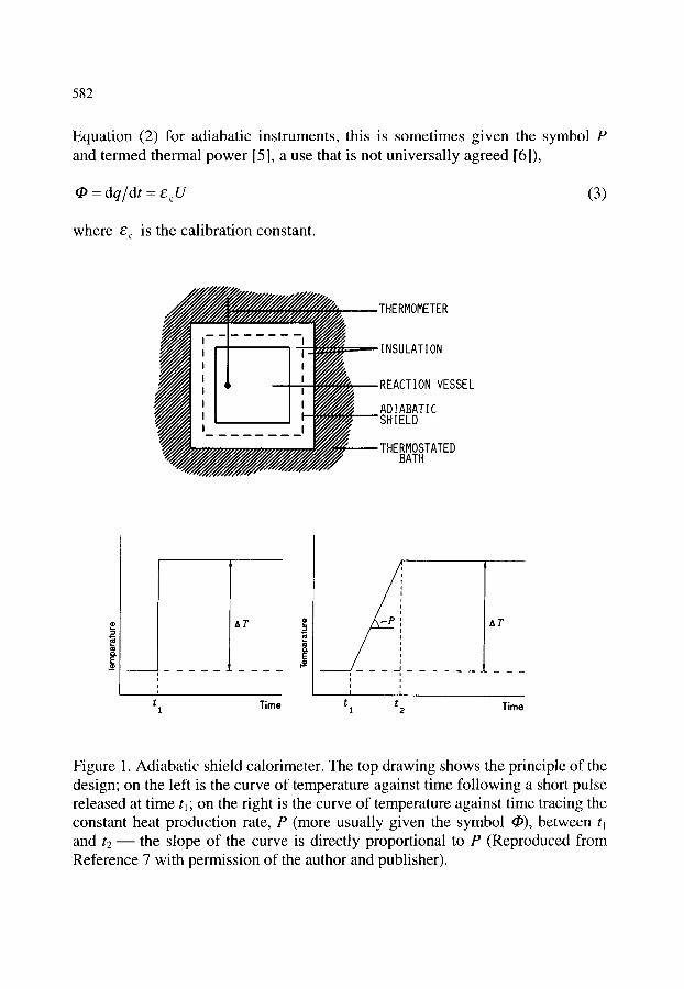
582

Equation (2) for adiabatic instruments, this is sometimes given the symbol P and termed thermal power [5], a use that is not universally agreed [6]),

(I) - d q / d t - e , : U (3)

where e c is the calibration constant.

THERMOMETER

a i REACTION VESSEL

SHIELD

THERMOSTATED BATH

AT

I

AT

t Time t t Time 1 1 2

Figure 1. Adiabatic shield calorimeter. The top drawing shows the principle of the design; on the left is the curve of temperature against time following a short pulse released at time tl; on the right is the curve of temperature against time tracing the constant heat production rate, P (more usually given the symbol q~), between t~ and t2 ~ the slope of the curve is directly proportional to P (Reproduced from Reference 7 with permission of the author and publisher).

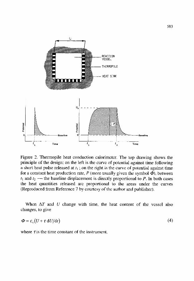
583

~////I//J//pJ~... ~--~/ REACT I ON VESSEL

THERMOP I LE

HEAT S INK

Baseline , Baseline i i ! i

t 1 Time t 1 t Time 2

Figure 2. Thermopile heat conduction calorimeter. The top drawing shows the principle of the design; on the left is the curve of potential against time following a short heat pulse released at t~ ; on the right is the curve of potential against time for a constant heat production rate, P (more usually given the symbol q~), between t~ and t2 the baseline displacement is directly proportional to P. In both cases the heat quantities released are proportional to the areas under the curves (Reproduced from Reference 7 by courtesy of the author and publisher).

When AT and U change with time, the heat content of the vessel also changes, to give

- e c ( U + "C d U / d t ) (4)

where ~: is the time constant of the instrument.

584

Equation 4 is usually named after Tian. In the ideal case, the time constant is defined by,

where C is the heat capacity of the vessel and K the thermal conductivity through the thermopile. It should be noted that there is an assumption in Equation (4) of no temperature gradients in the vessel [ 1,7]. If they occur, then Equations (3) and (4) should reflect the situation given by the simple expression,

q - e c f U dt (6)

provided that the thermopile potential at the initial and final integration times are the same (normally the baseline value, U = 0, see Reference [1 ]). Equations (3) and (6) are independent of the heat capacity of the reaction system and the vessel, unlike the corresponding equations for adiabatic calorimeters, Equations (1) and (2). Under non-steady-state conditions, the expression for heat produced in the vessel, Equation (3), depends on the time constant, Equation (5), and therefore on the heat capacity and heat conductivity of the measuring system.

2.4.4. Peltier Effect As has already been stated, a shield facilitates measurement of slow

exothermic processes by adiabatic calorimeters. Compensation for temperature changes in exothermic processes estimated in a heat compensation calorimeter is often by "pumping out" the heat with a thermoelectric cooler utilizing the Peltier effect [7]. A suitable thermopile (semiconducting Peltier-effect cooler) is positioned in the air gap or vacuum between the vessel and the thermostatic bath (see Figure 1). The cooling effect produced at each junction of the thermopile is proportional to the current through it. In practice, this effect is superimposed on the Joule heating effect produced throughout a heater. Alternatives to Peltier-effect cooling are (i) melting of a solid, (ii) vaporization of a liquid, or (iii) a flow of cooling liquid or gas (often used in whole body calorimetry).

2.5. Single and Twin Calorimeters Heat accumulation and heat compensation calorimeters are usually

constructed with single vessels [7-9]. The twin arrangement, first introduced by Joule in 1845, is often used with heat conduction calorimeters and is probably essential when high precision is required for determination of slow processes in

585

a microcalorimeter. The vessels are arranged as perfect twins with the detection units being in opposition to give a differential signal. Thus, extraneous disturbances are cancelled, giving long-term stability. It is also possible to allow a reaction to proceed in one vessel while running a control or blank in the second vessel.

As stated in Section 2.4, it is possible to balance the heat produced in the reaction vessel of twin calorimeters by evolution of electrical energy in the second (reference) vessel, thus keeping the temperature of the two vessels the same [9]. It is supposed that, in this way, disturbances are cancelled by active means. Compensation was carried one step further by Calvet & Prat [10] who used Joule heating or Peltier cooling in the reaction vessel according to the process ~ endothermic or exothermic ~ taking place, in order to achieve a stable zero reading and eliminate fluctuations arising from imperfections in the thermostatted jacket.

2.6. Closed and Open calorimeters In a closed reaction vessel, the volume is constant and consequently the

change in heat is a change in internal energy, AU = A H - p A V . In open calorimeters, the vessels are at atmospheric pressure ~ so the measurements are performed at constant pressure. The heat gains and losses recorded are changes in enthalpy.

2.7. Batch and Flow Calorimeters In many calorimeter experiments, the two or more components of the system

have to be brought into proximity to initiate a process. The means of initiation are diverse but the instrument is described as batch if the reactants are initially isolated in separate sections of a vessel [11,12]. Mixing is then by rotation of the heat-sink assembly containing a suitably-charged reference vessel, by breaking an ampoule, or by injecting a reactant or catalyst. Of course, in these cases all the reactants are mixed at once to give a single measurement. Stepwise addition of one component (discontinuous titration) has been achieved using motorized burettes and syringes linked to a batch vessel. The reactions usually are comparatively fast so the instruments tend to be basically adiabatic in type (see, for instance, Reference [13]). Similar design principles apply to continuous titration calorimetry [ 14].

Flow vessels have become more common in the thirty years since first commercial manufacture by LKB [15]. Flow-through vessels have been used mainly in studies of cell suspensions [16,17] and solid sorption reactions[7]. Flow-mixing vessels, on the other hand, are employed in experiments on enthalpies of dilution and reaction in chemical thermodynamics. The reaction

586

time must be short compared with the retention time of the liquid in the vessel but, despite this limitation, the method can have advantages over that of mixing in a batch vessel where there may be distillation effects and changes to the gas phase composition.

Data collection utilizing batch vessels tends to be quite slow owing to the relatively long equilibration period after introducing the samples. If the experimental system is appropriate, then stopped-flow and titration are considerably faster techniques.

2.8. Chemical Kinetics While it is true that most calorimetric studies are for either thermodynamic or

general analytical purposes, an increasing number of them are addressed to investigating chemical kinetics. The exact kinetic treatment for the data depends crucially on the basic type of calorimetric design used to obtain the results [9] and, conventionally, on the state of the reaction system. As an example of what can be done, the reader is referred to Beezer and Tyrrell [ 18] who developed a kinetic treatment of data from flow microcalorimeters of the heat conduction type. Dynamic correction of such data is now on a firm basis [19]. More recently, Hansen et al. [20] have given a detailed account of the determination of kinetic parameters from heat conduction calorimeters. The needs of such a method have been discussed further by Willson et al. [21 ] who advocate the use of an iterative procedure on the plot of heat flow versus heat output to determine the rate constant, order and change in enthalpy for the reaction. A second method of analysis was proposed as a means to determine the extent of reaction [21 ]. A comprehensive treatment of this subject is given in Chapter 3.

3. SYSTEMATIC ERRORS

Systematic errors are probably more prominent in calorimetric measurements than in most other types of measurement because the evolution and adsorption of heat accompanies most of the events in the preparation for and then the actual act of assessing the wanted value of heat change. This is not to minimize the importance of random errors but these, of course, can be handled by conventional statistics. The problem when assessing heat is that it has no "colour", no "spectrum" ~ heat from extraneous sources cannot be "filtered" out or, in many cases, even be identified as an event. Such changes in heat from chemical and physical processes can have very considerable values, "swamping" the measurement for which the experiment was designed in the first place. Of course, the risk of large spurious effects is greater in microcalorimetry than in studies where the quantity of heat involved in the

587

process is comparatively great [7,9]. In many cases, these errors are small enough to be neglected but sometimes they cause highly erroneous results which mislead the scientific community. As Wads6 frequently states [1,5,7,9], all calorimetrists should be aware of this possibility and be prepared to carry out the appropriate calibration procedures to cancel these errors. Nowadays, most manufacturers equip their instruments with electrical heaters and, in some cases, insertion heaters are available which allow greater accuracy. Some vessel designs, while necessary for experimental reasons, do not allow accurate electrical calibration. These must be calibrated by a chemical reaction. In fact, this is good practice even when it is not absolutely essential.

3.1. Mechanical Effects Agitation by stirring of liquid in the measuring vessel or by rotation of the

whole vessel generally will cause a heat of friction. The motors for modern stirring devices are sufficiently constant and their heat effects small enough to permit cancellation during calibration but a few rotations of the reaction vessels in a batch microcalorimeter, even of the differential type, gives frictional heat so large and irreproducible as to require correction.

In reaction calorimetry, it is common to initiate a process mechanically by, to give instances, breaking an ampoule or turning a valve, both of which may cause quite large heat effects (<50 mJ). If this is small compared with the enthalpy of reaction ~ as is true in "normal-scale" calorimetry ~ then it can be neglected, but this may not be true at the "micro" scale where the lack of reproducibility may even preclude experimentation.

Care must be taken to account for frictional effects in flow calorimetry. The heat effect of a flowing liquid increases rapidly with flow rate [ 15] and will be affected by changes in viscosity during measurement. This may occur, for instance, during a polymerization process [9] or when actively growing microbial or animal cells are pumped through the measuring vessel from a bioreactor, viscosity increasing with the density of cells in the suspension. Corrections can be made by obtaining a baseline for a non-reactive system which has viscosity similar to that found in "test" experiments conducted in the appropriate vessel. It is more difficult to apply corrections for changes in viscosity with time, but final non-reactive mixtures must be assessed by comparison with the initial state.

3.2. Evaporation and Condensation Water is present in many experiments ~ but it is important to realize that its

enthalpy of vaporization is very high, 43.9 kJ mol -~ at 25 ~ [9]. In the reaction calorimetry of some mixtures this would be of the same order as the heat

588

production. Clearly, no uncontrolled evaporation or condensation can be permitted in experiments. Leakage must be avoided, but the main problem is vaporization occurring within a batch calorimetric vessel which contains a gas phase. In many cases this phase is created in order to allow thorough mixing and, in this case, careful design of twin vessels can obviate errors. Nevertheless, it is crucial to recognize that, despite good technique for a given batch mixing, vessel distillation effects and changes in vapour-phase composition may distort the results to a serious extent (see discussion by Spink and Wads6, Reference [9]).The cooling effect of the heat of vaporization can be a particular problem for some of the most recent types of ampoule calorimeters manufactured by Thermometric in which it is possible to perfuse respiring biological or sorptive material and/or titrate (bio)chemical reactions [22]. Usually the vessel is filled but, if it is necessary to have a gaseous headspace, then it must be saturated with the aqueous phase prior to lowering the vessel to the first "equilibration" position.

Mixing experiments with a gas phase should never be contemplated if two aqueous solutions have large differences in molar composition in which the distillation effect may result in a significant temperature gradient within the vessel. It is also wrong to mix volatile organic compounds in a calorimeter vessel with a gas phase. Both types of experiment should be performed using a flow calorimeter with no vapour phase.

3.3. Gaseous reaction components In many reactions occurring in aqueous solution, a gas is evolved which is

saturated with water vapour. If the gas is allowed to leave the calorimetric reaction vessel, then there is considerable evaporation. This has been calculated to cause an endothermic enthalpy change of 2.68 kJ per mole of gas leaving the vessel at 37 ~ and 3.8 kJ mol -~ at 25 ~ The phenomenon can be quite a problem for accurate measurement and is paralleled by a similar effect when dry gas, for instance air, is pumped through an aqueous reactant. Initially, the gas must be saturated with water but, even so, it is difficult totally to eliminate vaporization or condensation even with a carefully designed vessel having a wet heat-exchange tube [9,22]. Particular strategies can be adopted if the gas-liquid experimental system demands it (see, for instance, Reference [23]). In at least one case, a calorimeter has been designed specifically to study the enthalpy of reaction between gaseous compounds and substances in solution, the volume of gas absorbed being measured simultaneously with a sensitive differential manometer [24].

If there is a change during an experiment in the amount of gas dissolved in solution, then consideration must be given to the enthalpy of solution of the gas.

589

Taking as an example a respiring biological system, the enthalpy change for oxygen dissolution in an aqueous medium is -15.9 kJ mol -~ at 25 ~ [9]. Quite clearly, experimental design is important to encompass this and any other spurious effects.

Experiments with mixed flows of liquid and gas pumped through the vessel of a flow calorimeter are much less susceptible to the problems described in this section.

3.4. Adsorption Interaction of substances with the vessel walls of calorimeters was not

considered a problem until technical advances allowed measurement in the ~tW range. Probably because the ratio of wall surface area to quantity of heat measured is high, heat effects due to adsorption and desorption of reagents at the vessel walls has become a problem in the choice of materials for the measuring compartments. It was quickly recognized that this is not just a difficulty caused by complex molecules (e.g. ring compounds) interacting with the walls of vessels fabricated from chemically active materials (for example, metals) but a phenomenon seen, for instance, in NaOH-HC1 neutralization experiments in glass vessels due to the adsorption of C1 ions [11]. Salt- adsorption also has been noted for even 18 carat gold vessels containing 0.5M KC1. As reported by Spink and Wads6 [9], this is a large exothermic effect of -6 mJ, but they also state that other reactions give enthalpy changes sufficiently great to preclude accurate measurement using batch vessels unless they are rigorously subjected to a washing procedure with the reaction medium. This is necessary not only with solutions containing ions but also with pure water. It is an unpredictable phenomenon in the sense that only some of the many highly interactive molecules show sorptive behaviour. It does not seem possible reliably to "back off" the interactions using the reference vessel of a twin system. Perhaps more disturbingly, some biologically active molecules bind to the walls without a heat effect but remain active against cells even after several washes, e.g. the plant glycoside ouabain which binds to 18 carat gold [5].

No adsorption phenomena are to be expected in continuous flow calorimetry because the sorption sites on the walls of the flow vessel are saturated with the reactive species at the beginning of the experiment [7]. There are no net effects from sorptive processes when the instrument is at steady state.

Calorimetric studies of living cells have been hampered by their tendency to stick to the walls of vessels [5]. Adhesion processes are hydrophilic in nature, however, and so suitable vessels can be designed to minimize this phenomenon. Flow calorimetry can present particular problems for cellular studies and

590

remedies include segmenting the stream of cells in suspension by mixing it with a flow of air saturated with culture medium [25].

3.5. Ionization Reactions and Other Side Reactions In thermodynamic experiments using calorimetry to determine the enthalpy

of a chemical reaction, it is usual to correct the results to give values for an idealized process [9]. This mainly requires additional experiments often combined with the application of previously known data. For example, in many cases the buffering medium is involved in the overall thermal process measured in the calorimeter because the reaction involves the uptake or release of protons or hydroxyl ions. Of course, the enthalpies of ionization vary considerably for different buffers and suitable adjustments must be made from appropriate published data. In reactions of biological macromolecules, the acid-base equilibria of the buffers are usually involved to a considerable degree. Moreover, the involvement of buffers may extend beyond this easily recognized phenomenon to that of direct interaction with complex molecules which have undergone steric changes in structure to reveal different binding sites, for instance in denaturation.

3.6. Incomplete Mixing In batch experiments where the whole vessel is rotated in the block, it is

usual to perform a second gyration after the reaction has taken place in order to determine possible friction effects [9]. Of course, this procedure would also reveal incomplete mixing by abnormal and variable changes in heat. As mentioned in Section 3.1, modern stirrers are very constant in action and are used to ensure complete mixing in single and multiple injection reaction calorimetry, as well as in studies of perfused biological material.

The systematic errors that occur in flow calorimetry are most common for mixing vessels [9]. A stirrer is not usually at the point of mixing, so the efficiency of the process depends on turbulence and may be quite low at the relatively slow flow rates recommended for this type of operation. Incomplete mixing is not revealed by the calorimetric signal because it will still be at an apparently normal steady state. Incomplete mixing is not usually a serious problem for mixing solutions of low viscosity, but often causes difficulties with solutions of high molarity or those that are otherwise of considerable viscosity [15]. In such cases trials should be conducted by varying concentration (mol dm -3) and flow rate of the components in the reaction mixture.

3.7. Slow Reactions Slow reactions are a source of possible systematic error in batch calorimeters

591

which are primarily of the isothermal jacket type (see Section 2.3). For continuous-flow experiments, however, it is important that either the process is complete before the liquid leaves the vessel or it is at steady state/zero order [9]. The difficulties are most acute when a flow-mixing vessel is used for slow reactions, because much of the heat could be produced after the reactants have left the measuring vessel. Trials should be conducted at different flow rates to give dissimilar retention times for the mixture of reactants. For slow reactions, the apparent heat of reaction will appear to vary with flow rate.

3.8. Changes of Instrument Design Scientists often make modifications to the different kinds of instruments used

in their research. In most cases it is obvious what effect those changes will have to their response. This is not necessarily the case for calorimeters because the relationship between the site at which the thermal event occurs and the point at which it is measured is complex and in many respects empirical in nature [9]. The position of a vessel in a calorimeter may involve compromise but the design will have been subjected to many test experiments and, within stated uncertainty limits, gives correct results. Even small changes made to a calorimeter for a certain experimental protocol, mean that a series of tests is required to determine their effect on the quantity of heat measured by the instrument. This should involve electrical [9] and chemical [7] calibrations (see below).

4. TEST AND C A L I B R A T I O N P R O C E D U R E S

The previous section illustrates many of the more common systematic errors in calorimetry. These arise because nearly all physical and chemical processes are accompanied by heat effects. While this enables the instruments to be used for general processes as well as for specific thermodynamic events, it also means that extreme care has to be exercised in testing and calibrating them [7,9]. The more sensitive the instrument the more care has to be taken with these procedures. However, even when a calorimeter is used analytically rather than thermodynamically, calibration always should be subject to regular checks [1].

With the exception of combustion calorimetry (see Section 10), all instruments nowadays are calibrated by an electrical procedure (Joule effect heating), often with an automated protocol supplied by the manufacturers. This is easily performed and is designed so that users incorporate such a test as a regular element in their methodological routine. It is always a convenient method with a sufficient accuracy to make it valid for even the most "micro" of

592

measurements. As intimated earlier, however, the electrical heater is not always in the most appropriate position. This may be due to the manufacturer not being rigorous or having to compromise for reasons of design. Alternatively, the user may have made modifications. In the last case, it is now possible to fabricate or, in certain instances, buy a suitable immersion heater for tests [7]. Otherwise, and in this case additionally, the wise calorimetrist will heed Wads6 and choose a suitable type of chemical calibration as an addition to the methodological routine. Such calibrations need only be occasional when the same vessel is in use but should always be done when there are changes. The greatest necessity for chemical calibration is in flow calorimetry where it is extremely difficult to position a heater so as accurately to reflect heat transfer from the bulk of the liquid in flow to the point of measurement. The difference in assessed heat production between an electrical heater positioned near a flow-through vessel and the enthalpy of reaction in a solution flowing through the vessel can be more than 20% [ 1 ].

Obviously, the chemical reaction chosen for calibrating a calorimeter depends upon the type of process under study. Neutralization reactions are often used in which a solution of a strong acid, most commonly HC1, is added to a solution of a strong base (NaOH) in excess, z ~ - - 5 5 . 7 9 5 kJ mol -~ at zero ionic strength [9]. Unfortunately, contamination with CO2 results in a reaction between the acid and bicarbonate ions which then gives an erroneous figure for the reaction. In the case of HCI + NaOH, the base should always be in large excess in the reaction vessel to avoid reaction of any carbonate present in the mixture. The calibration solutions must be prepared from CO2-free water and be protected from CO2 uptake. It should be noted that any strong acid plus strong base reaction may be used, for instance perchloric acid is sometimes preferable to HC1 because it avoids the large heat of dilution and corrosion problems sometimes encountered with HC1. An alternative is the protonation of a buffered solution of Tris, AH =-47 .50 kJ mol -I [11 ]. The reaction of Tris is also subject to error from CO2 contamination. Because carbonate is a stronger base than Tris, this error can only be avoided by using Tris in the buffer range.

Dissolution of propan-1-ol in water is a reliable calibration process [26]. The enthalpy of dissolution (kJ mol -~) to form an infinitely dilute solution is given by,

Aso I H m - a + b T + c T 2 (7)

where a = 123.76, b = 0.5528 and c = 5.762 x 10 -4. The inaccuracy of the results is _< _+0.03 kJ mol -~ for the temperature range 288 K to 348 K. For applications where this process produces "too much" heat, it may be more

593

convenient to use the dilution of aqueous propan-l-ol [26]. At 298.15 K the enthalpy of dilution of 1 mg aqueous 10% (w/v) propan-l-ol solution is (2.570 +0.015) kJ mo1-1, provided that the final concentration is <1.4 g m -3.

In reaction calorimetry, where the equilibration constant (K c) and enthalpy

change of the reaction (ArHm) a r e measured simultaneously by titration, the 2+

binding of Ba (aq) to 18-crown-6(1,4,7,10,13,16-hexaoxacyclooctadene) has

been proposed as a suitable system to use for calibration [26].

In the calorimetric vessel, the concentration of the crown ether is varied

between 1 mmol dm -3 and 10 mmol dm -3 and that of the Ba 2+ solution from

10mmol dm -3 to 100 mmol dm -3 [26]. At 298.15 K, the values derived

for the 1"1 binding process were: K c = (5900 + 200) mmol d m -3 ;

A r n m -" - ( 3 1 . 4 2 + -0.20) kJ mol -I , and heat capacity, ACp,m -- -126 kJ mol -I . There

was no sign of concentration dependence.

A suitable test process for solution calorimetry is the dilution of aqueous

sucrose solutions in the concentration range 15 to 25% (w/v) [26]. Those with a

sweet tooth know that such solutions are very viscous and thus difficult to mix

rapidly with water in, for instance, a flow vessel. On the other hand, this

difficulty can be turned to advantage as a process for evaluating mixing and

stirring efficiency. Enthalpy values are expressed by Equation (8) and the

values for constants A and B are given in Table 1,

AdilHm-A(mf-mi)-B(m2-m?) (8)

where m~ and mf are the initial and final molalities (mol kg -1) respectively, of

the sugar solution. If the constants A and B are replaced by the corresponding

temperature dependent functions, Equations (9) and (10) respectively, AdilHm

can be calculated at different temperatures (K),

A ( T ) - - 8 4 3 . 9 + 4.719T (9)

B ( T ) - -389 + 2 .47T- 45 x l 0 -3 T 2 (10)

These equations allow accurate predictions of A di I H m [7].

594

Table 1 Aqueous Sucrose Solutions. A and B are coefficients in Equation (8)

T / K A / J kg mo1-2 B~ J kg 2 mo1-3

293.15 539.3 28.94 298.15 563.2 29.50 303.15 586.6 29.62 310.15 619.6 29.66

From References [7,26,27]

As stated earlier, it is difficult accurately to calibrate flow-through vessels by electrical means. Wads6 and colleagues [1,7,26,28] have proposed that the hydrolysis of triacetin in imidazole-acetic acid buffers is a suitable test and calibration system to overcome this problem. Five different reaction mixtures have been described (see Table 2) that give heat production values, in the range of 5 to 100 laW g-'. At constant ambient temperature, these change only very slowly and, for low values (540 ~tW g-' ), almost linearly with time. Curves of heat production against time can be described by a quadratic equation:

�9 - a - b t + c t 2 (11)

where t is the time and a, b and c are constants, values for which at 25 and 37 ~ are given in Table 3. The accuracy of the heat production predicted by Equation (11) is less than 1% for at least 20 h. Decline in the heat produced is so slow that it is not necessary accurately to measure time. Temperature coefficients are, however, quite high, dclg/dT being 5 to 10% per degree. Storage be low-20 ~ slows the reaction to give only a small decrease (2% per month) in heat production.

There are several other well characterized processes useful for testing and/or calibrating calorimeters. Endothermic dilution of urea [29] has its uses and, for the addition of solids to liquids, KC1 into water (endothermic) [26] and solid Tris into HC1 (aq) (exothermic) can be used. Dissolution of oxygen in water is a good calibration system for experiments where a slightly soluble gas is dissolved in water [7]. A test system for dissolving a slightly soluble liquid in water is benzene [30]. Other chemical processes suitable for test purposes under certain conditions are given in References [5,7,9,26].

Radioactive probes give excellent calibration with little time spent on preparation (and none on washing up!), but strict rules on handling and use make it doubtful that they will be found in most laboratories!

Table 2 Composition of Triacetin Test Solutions.

595

Solution Buffer composition" Acetic acid (g) added to imidazole solution a

A 10.00 B 16.00 C 18.00 D 20.00 E 24.00

Test solution: Triacetin (g) added to 100 g buffer

10.000 5.000 3.600 3.600 3.600

aprepared by adding 27.23 g imidazole to 100 g water. Adapted from References [26,28].

Table 3 Triacetin Reaction Mixtures. Values for the constants in Equation (11)

Test solution T/K a~ gW g-~ 104b/gW g-~ s -~ 101~ / g W g - ' s -~

A 310.15 90.66 3.63 8.1 A 298.15 34.32 0.62 1.2 B 310.15 35.35 1.16 2.3 B 298.15 13.35 0.26 1.0 C 310.15 21.80 0.79 3.5 D 310.15 16.00 0.45 1.1 D 298.15 5.19 0.08 0.4 E 310.15 7.25 0.16 0.5

From References [26,28]

5. C A L O R I M E T R Y C A L O R I M E T E R S

SCIENCES C O R P O R A T I O N AND R E L A T E D

L. D. Hansen a, D. J. Russell b and E. A. Lewis ~'b

aDepartment of Chemistry and Biochemistry, Brigham Young University, Provo, UT 84602; bCalorimetry Sciences Corp., 515 E. 1860 S., Provo, UT 84606, USA.

5.1. Introduction One of the first commercially produced, precision calorimeters was

manufactured and first marketed in 1966 by Tronac, Inc., a Utah company based

596

on research and development work done at Brigham Young University. A competing company, Hart Scientific, was organized in 1978 by Roger Hart to manufacture and market precision temperature controllers, constant temperature baths, thermometers and calorimeters. Calorimetry Sciences Corporation (CSC) was formed as a subsidiary division of Hart Scientific in 1993.

CSC currently manufactures calorimeters using all three of the means for measuring heat; i.e. accumulation, compensation and conduction (for further details, see Section 2.4 and Chapter 1, Section 2.5). CSC markets both temperature scanning and isoperibol (constant environment) types of calorimeters with provisions for handling solids, liquids, and gases over a wide temperature range.

In addition to calorimeters for specialized applications, CSC markets six different types of calorimeters for general use: a) A differential, isoperibol, heat conduction calorimeter which, in addition to its

use as a thermal activity monitor, can be equipped with various reaction vessels for performing flow, flow sorption, batch and incremental titration measurements (CSC 4400).

b) A four-vessel, differential, heat conduction calorimeter that can be operated in either an isothermal or a scanning mode (CSC 4100).

c) A high-sensitivity, differential, temperature scanning calorimeter for measurement of the heat capacities of solutions (CSC 5100).

d) A series of macrovolume, isoperibol, solution calorimeters for measuring enthalpy changes of reactions in solution by batch, incremental titration or continuous titration (CSC 4300).

e) A differential, isoperibol, heat conduction calorimeter for incremental titration with sub-cm 3 volumes of solutions (CSC 4200).

f) An isoperibol, heat compensation, flow calorimeter primarily for measurement of heats of mixing of fluids (CSC 7500).

Each of these calorimeters is discussed in detail in the following sections.

5.2. Instruments

5.2.1. CSC Model 4400 Macrovolume, Isoperibol, Heat Conduction Calorimeter The Model 4400 Isothermal Microcalorimeter evolved from the Tronac model

350RA and Hart Scientific model 7708 differential, heat conduction calorimeters originally developed to make measurements on batteries of various types [31]. The CSC model 4400 isoperibol, heat conduction calorimeter (Figure 3) is manufactured with various size reaction chambers from a few cm 3 to 500 cm 3, the standard size being about 70 cm 3. The calorimetric measurement is made with bismuth telluride thermopiles with an upper temperature limit of 100 ~ in the standard unit, or 200 ~ in units with specially built thermopiles. The calorimeter

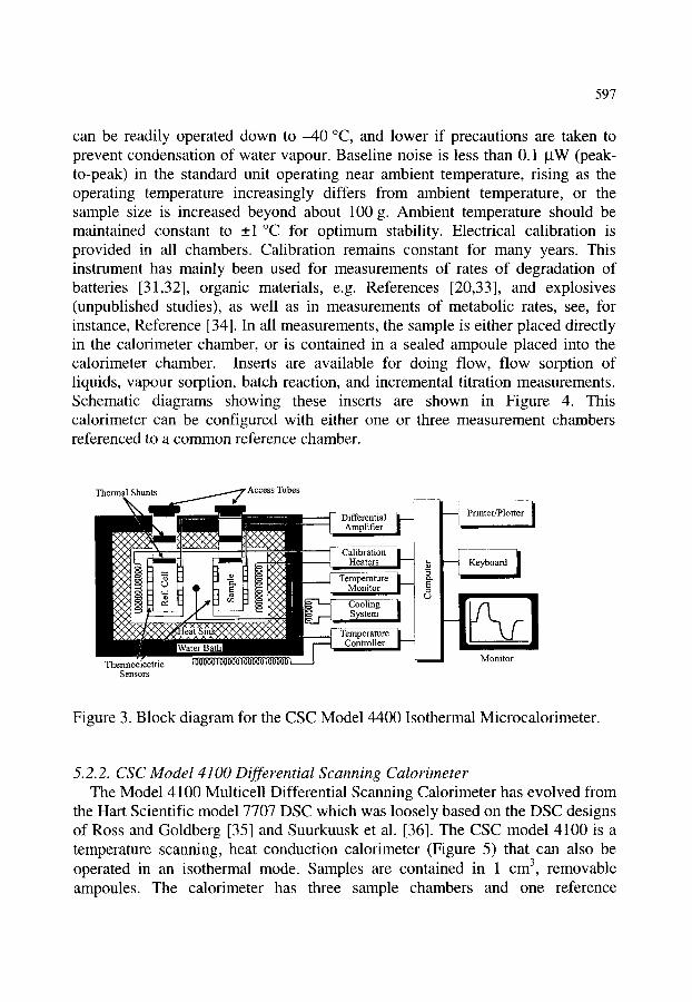
597

can be readily operated down to -40 ~ and lower if precautions are taken to prevent condensation of water vapour. Baseline noise is less than 0.1 laW (peak- to-peak) in the standard unit operating near ambient temperature, rising as the operating temperature increasingly differs from ambient temperature, or the sample size is increased beyond about 100 g. Ambient temperature should be maintained constant to _+1 ~ for optimum stability. Electrical calibration is provided in all chambers. Calibration remains constant for many years. This instrument has mainly been used for measurements of rates of degradation of batteries [31,32], organic materials, e.g. References [20,33], and explosives (unpublished studies), as well as in measurements of metabolic rates, see, for instance, Reference [34]. In all measurements, the sample is either placed directly in the calorimeter chamber, or is contained in a sealed ampoule placed into the calorimeter chamber. Inserts are available for doing flow, flow sorption of liquids, vapour sorption, batch reaction, and incremental titration measurements. Schematic diagrams showing these inserts are shown in Figure 4. This calorimeter can be configured with either one or three measurement chambers referenced to a common reference chamber.

Thermal Shunts ~ Access Tubes

Thermoelectric Sensors

D/~mff; rle~lt~al ~-~ b Printer/Plotter i

Calibration Heaters

Temperature Monitor Cooling System

Temperature Controller

Monitor

Figure 3. Block diagram for the CSC Model 4400 Isothermal Microcalorimeter.

5.2.2. CSC Model 4100 Differential Scanning Calorimeter The Model 4100 Multicell Differential Scanning Calorimeter has evolved from

the Hart Scientific model 7707 DSC which was loosely based on the DSC designs of Ross and Goldberg [35] and Suurkuusk et al. [36]. The CSC model 4100 is a temperature scanning, heat conduction calorimeter (Figure 5) that can also be operated in an isothermal mode. Samples are contained in 1 cm 3, removable ampoules. The calorimeter has three sample chambers and one reference

Inlet A ) + Outlel -. Inlet (B) +

Top Access Cover

Inlet Flow Heat

Pressure Transducer

Thermal

Thermal

3 Thermal

A B C D E

Figure 4. Accessory reaction vessels for the CSC 4400 Isothermal Microcalorimeter. Inserts shown are for: A, flow reaction; B, flow sorption; C, vapour sorption; D, batch reaction and incremental titration; and E, calorespirometry .

599

Sample & Reference Ampoule Holders

Sensors [ Cooling

f Temperature Monitor ]

Calibration | Heaters |

Scan Rate Controller

Adiabatic Shi Controller

Differential /.--.A Hi-ResA/D

. ~ _ . . .

S y s t e m ] Computer ]

" 0 . ~ .

Exhaust \ Vapour Saturated Gas

Dry Gas Inlet ~ " uid Temperature p i Controlled 11

Gas Exchange Insu~r ~ i

Ampoule Holder

Pressure Tubing

1

A

Capillary Tubing to Pressure

I Transducer

"

�9 C

Thermoelectric High Pressure Ampoule L ~ Sensor Ampoule

B C D

Figure 5. Block diagram for the CSC model 4100 Multicell Differential Scanning Calorimeter. Special purpose ampoules shown for use with the DSC are for: A, gas exchange; B, vapour sorption; C, high pressure; and D, calorespirometry.

600

chamber. Ampoules are commonly made from Hastelloy C which has good chemical resistance and is not reactive toward biological materials, but they can be constructed from many other materials including glass.

The instrument is controlled and data are collected and analyzed by means of an integrated computer that is fully compatible with IBM desk-top computers.

In the isothermal mode, the heat rate signal is stable to _+0.2 ~tW and reproducible to about +2 ~tW on removal and replacement of the ampoules. Reproducibility during scanning is similar. Consecutive scans done without removing the ampoules are reproducible to about _+1 ~tW. Noise and irreproducibility increase only slightly as the operating temperature is changed from ambient temperature, but the absolute uncertainty in heat rate increases rapidly. An external source of constant temperature, circulating fluid is required for operation. Baseline noise is dependent on the operating temperature relative to the room, the relative temperature of the circulating fluid, and the quality of temperature control of the fluid and the room.

The instrument can be operated from 110 to -40 ~ A high temperature version with an upper limit of 200 ~ is also available. Scan rates from about 1 ~ h -~ to 120 ~ h -~ are available. Scan rate is a quadratic function of temperature in this instrument, is derived from the data collected during a scan, is reproducible to about +0.1%, and is controlled in both up and down directions. Electrical calibration is provided in all chambers. The calibration constant is a quadratic function of temperature, stable for many years.

This instrument was designed primarily for the study of phase transitions in biological molecules and molecular assemblages such as proteins and lipid bilayers, but has found applications in studies of metabolic heat rates, e.g. References [37,38], degradation of materials, see Reference [39], rates of reaction, for instance Reference [40], and phase changes in polymers, organic materials, and inorganic materials. Heats of phase transitions are reproducible to about +1% or +20 mJ. In isothermal mode, the instrument has been used for measurements of metabolic heat rates of plant and animal tissues and cell cultures of various types, for instance, References [37,38,41 ], and of degradation rates of organic materials, e.g. References [39,40], and explosives (unpublished studies). Inserts for gas exchange over samples [42], for vapour sorption studies [43], and for measurements at pressures to 15 MPa are available, for example References [40,44], see Figure 5. The high pressure ampoules can also be used in scanning mode.

5.2.3 CSC Model 5100 Differential Scanning Calorimeter The model 5100 Nanowatt DSC has been described in a recent paper by

Privalov et al. [45] and is shown schematically in Figure 6. This instrument is an

601

isoperibol, heat compensation, differential, temperature-scanning calorimeter equipped with a fixed pair of gold capillary vessels and semiconductor sensors. The calorimeter block is heated and cooled by thermoelectric devices. A circulating cooling bath is not required. The instrument is operated by an IBM compatible, integrated computer that also provides for conversion of the results into thermodynamic parameters.

No organic materials are used in construction of the calorimeter, thus eliminating a source of baseline noise that has affected previous calorimeters. The scan rate can be set between 0.1 and 2 ~ min -~. The operating temperature range is 0 to 125 ~ The gold capillary vessels (nominal volume - 0.8 crn 3) minimize temperature gradients in the heated/cooled liquid sample and permit easy washing and reloading without air bubbles. These features are critical to the accuracy of difference heat capacity measurements and determination of the absolute value of the partial heat capacity of solute molecules. Measurements can be performed under excess constant pressure (up to 300 kPa) to prevent formation of gas bubbles and boiling of aqueous solutions above 100 ~

The noise level of the heating/cooling power difference between reference and sample is less than 40 nJ s -1 with a response half-time of 5 s. The reproducibility of the baseline, with and without refilling the capillary cells, is of the order of 0.5 gW, providing an accuracy in difference heat capacity determinations in the order of 40 mJ K -~ cm -3 at a heating rate of 60 K h -~ (0.02 K s-~).

Pressure Manostat Transducer - " - ~ 1 [

Heating & Cooling ,~ TEDs

Heat Sink

Platinum RTD Cell Heater

Adiabatic Shield

Capillary Sample and Reference Cells

Pressure Monito r ~ - -

Temperature Controller

Temperature Monitor

f Power Compensation

Controller

I Signal Amplifier

I Computer

'11 / Monitor

Figure 6. Block diagram for the CSC Model 5100 Nanowatt Differential Scanning Calorimeter.

602

5.2.4 CSC Model 4300 Macrovolume Solution Calorimeter The specially designed glass Dewars that made high-precision, continuous-

titration calorimetry possible were first developed at Brigham Young University [14]. These reaction vessels have a very low thermal mass, a well-defined boundary, a time constant of a fraction of a second, and very low heat loss rates. Calorimeters using such Dewars with volumes from 3 to 200 cm 3 were developed during the decade from about 1965 to 1975 [46]. The very low heat loss rates simplify and increase the accuracy of heat loss corrections. The stringent time constant requirement for continuous titration also led to the development of very stable bead-in-glass thermistor bridges for temperature measurement and to calibration heaters with rapid responses. Because the titrant must be injected at the temperature of the surroundings, very stable water baths were developed to control the temperature of the surroundings and titrant [47]. Highly efficient, low- mass stirrers were developed to minimize both power input and thermal noise from stirring. Because the specific enthalpy change cannot be known any better than the burette delivery rate, precision constant rate burettes were developed. New methods for analyzing the data produced by continuous titration were developed to make maximum use of the large amounts of data generated by this method [48,49].

Continuous titration calorimeters based on the developments at Brigham Young University have been marketed since the mid-1960s, first by Tronac (Model 450, Isoperibol Calorimeter) and most recently by Calorimetry Sciences Corp. (CSC Model 4300, Isoperibol Titration Calorimeter). These are the only commercially available calorimeters capable of high accuracy measurements with continuous titration. This calorimeter can also be operated in an incremental titration or batch mode. Batch addition of both liquids and solids is possible for measurements of enthalpy changes of dissolution and mixing (Figure 7).

The continuous-titration, heat-accumulation technique is capable of producing data precise to a few parts in 10 000 [50]. This type of calorimeter has primarily been used to study chemical systems with multiple, simultaneous reactions, e.g. proton ionization of polyprotic acids, metal ion complexation, and multiple site binding on proteins [51 ]. Methods have been developed and thoroughly tested for simultaneous determination of equilibrium constants and enthalpy changes for single and multiple reaction systems [49]. The complexity of data analysis for such systems has daunted many workers, but continuous titration can be shown to be the most efficient calorimetric method, both in quantity of materials required and in measurement time [52]. Both Tronac and CSC supply data analysis programs. Because of the very short time constant, this calorimeter is also useful for determination of kinetics of reactions with half-lives of seconds to minutes, e.g. Reference [53].

irrer Motor

603

21

I II

Burette Contrqller Stirrer | Controller |

I Ampoule [ , Breaker Calibration Heater

Bridge

I Computer

i I I

/

Ti an I Mta Titrant poule Ca~bration ~ ) ~., ~i!~eiiO n Line ~ ~ 1 ~ ~ Assembly r ,X Thermistor

T h e ~ L~llb(~~~/l, x r m i s t o r , [ [ 11, ~....[. Gliadows Stirrer~-- ~ ) I r ~ "

Stlrrer/./' ~ .Calaitberration Co anttero 1~//~2"~~ ~~1;~ Chntmar~

A B

Figure 7. Block diagram for the CSC model 4300 Isoperibol Solution Calorimeter. The glass Dewar reaction vessel is illustrated in detail A. The Tronac model 550 heat-compensation reaction vessel is shown in detail B.

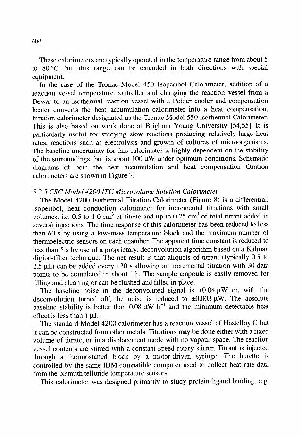
604

These calorimeters are typically operated in the temperature range from about 5 to 80 ~ but this range can be extended in both directions with special equipment.

In the case of the Tronac Model 450 Isoperibol Calorimeter, addition of a reaction vessel temperature controller and changing the reaction vessel from a Dewar to an isothermal reaction vessel with a Peltier cooler and compensation heater converts the heat accumulation calorimeter into a heat compensation, titration calorimeter designated as the Tronac Model 550 Isothermal Calorimeter. This is also based on work done at Brigham Young University [54,55]. It is particularly useful for studying slow reactions producing relatively large heat rates, reactions such as electrolysis and growth of cultures of microorganisms. The baseline uncertainty for this calorimeter is highly dependent on the stability of the surroundings, but is about 100 ktW under optimum conditions. Schematic diagrams of both the heat accumulation and heat compensation titration calorimeters are shown in Figure 7.

5.2.5 CSC Model 4200 ITC Microvolume Solution Calorimeter The Model 4200 Isothermal Titration Calorimeter (Figure 8) is a differential,

isoperibol, heat conduction calorimeter for incremental titrations with small volumes, i.e. 0.5 to 1.0 cm 3 of titrate and up to 0.25 cm 3 of total titrant added in several injections. The time response of this calorimeter has been reduced to less than 60 s by using a low-mass temperature block and the maximum number of thermoelectric sensors on each chamber. The apparent time constant is reduced to less than 5 s by use of a proprietary, deconvolution algorithm based on a Kalman digital-filter technique. The net result is that aliquots of titrant (typically 0.5 to 2.5 ktL) can be added every 120 s allowing an incremental titration with 30 data points to be completed in about 1 h. The sample ampoule is easily removed for filling and cleaning or can be flushed and filled in place.

The baseline noise in the deconvoluted signal is _+0.04 ktW or, with the deconvolution turned off, the noise is reduced to _+0.003 ktW. The absolute baseline stability is better than 0.08 ktW h -~ and the minimum detectable heat effect is less than 1 ktJ.

The standard Model 4200 calorimeter has a reaction vessel of Hastelloy C but it can be constructed from other metals. Titrations may be done either with a fixed volume of titrate, or in a displacement mode with no vapour space. The reaction vessel contents are stirred with a constant speed rotary stirrer. Titrant is injected through a thermostatted block by a motor-driven syringe. The burette is controlled by the same IBM-compatible computer used to collect heat rate data from the bismuth telluride temperature sensors.

This calorimeter was designed primarily to study protein-ligand binding, e.g.

605

aomduaoD

~ ~ 0~ r,.)

.....,

z

r.,O

o o r~

t"q

o

o6

606

Reference [56], but has also been used for measuring heats of mixing, adsorption, and dissolution, see Reference [57], metabolic heat rates, and kinetics of degradation of drugs. In fact, this instrument has approximately the same detection limit for degradation rates as larger volume heat conduction calorimeters previously used for degradation studies, but it requires far less material [58].

5.2.6 CSC Model 7500 High Pressure Flow Calorimeter The Model 7500 Isothermal Flow calorimeter is an isoperibol, heat

compensation, flow calorimeter (Figure 9) based on a design developed at Brigham Young University [59]. Tronac previously marketed a similar calorimeter. This instrument operates from 200 to -40 ~ at total flow rates from 0.004 to 0.2 cm 3 s -~ and with ratios of the two inlet flow streams from 0 to 1. Flow rates can be programmed to either vary continuously or in steps at fixed time intervals. Output is in the form of heat rate. Baseline noise is typically +50 gW. The upper limit of heat rate that can be measured is 1 W. Reagents are pumped either by reciprocating piston pumps similar to those used for high pressure liquid chromatography or by large syringe pumps. Measurements can be made at pressures up to 33 MPa. Flow tubing can be made from most metals including stainless steel, Hastelloy, tantalum, platinum and gold. High temperature versions have been constructed [60-62], but are not commercially available. This instrument has been used primarily for measurement of enthalpies of mixing of pure fluids [63], although some work has been done on electrolytes and reactions in solution.

Inlets

IIII Outlet

tier Cooler

Temperature S e n s o r ~ l ~ ~ ~ - ~ - - - - C o n t r o l S e n s O r H e a t Sink ~ ii

Heater

Flow Tube

~mtion Heater n~ Tee

Figure 9. Schematic diagram for the reaction vessel of the heat-compensation CSC 7500 High Pressure Isothermal Flow Calorimeter.

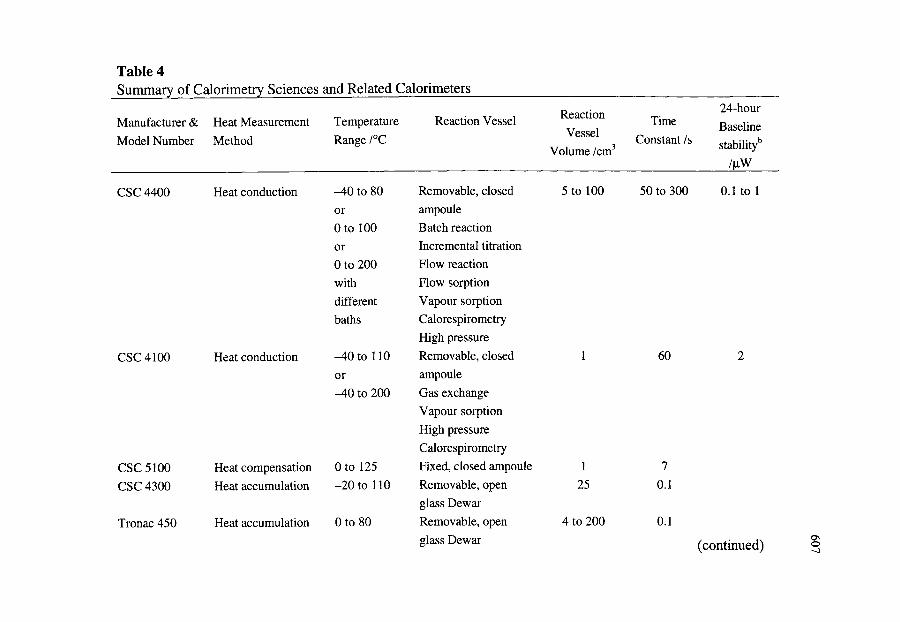
Table 4 Summary of Calorimetry Sciences and Related Calorimeters

24-hour Baseline Manufacturer & Heat Measurement Temperature Reaction Vessel

Model Number Method Range /"C Constant /s stabifityb Time Reaction

Volume /cm3

CSC 4400 Heat conduction

CSC 4100 Heat conduction

CSC 5100 Heat compensation CSC 4300 Heat accumulation

Tronac 450 Heat accumulation

-40 to 80 or 0 to 100 or 0 to 200 with

different baths

-40 to 110

or -40 to 200

0 to 125 -20 to 110

0 to 80

Removable, closed 5 to 100 50 to 300 0.1 to 1 ampoule Batch reaction Incremental titration Flow reaction Flow sorption Vapour sorption Calorespirometry High pressure Removable, closed ampoule Gas exchange Vapour sorption High pressure Calorespirometry

Removable, open 25 glass Dewar

glass Dewar

Fixed, closed ampoule 1

Removable, open 4 to 200

1 60 2

7 0.1

0.1 Q\ 0 4 (continued)

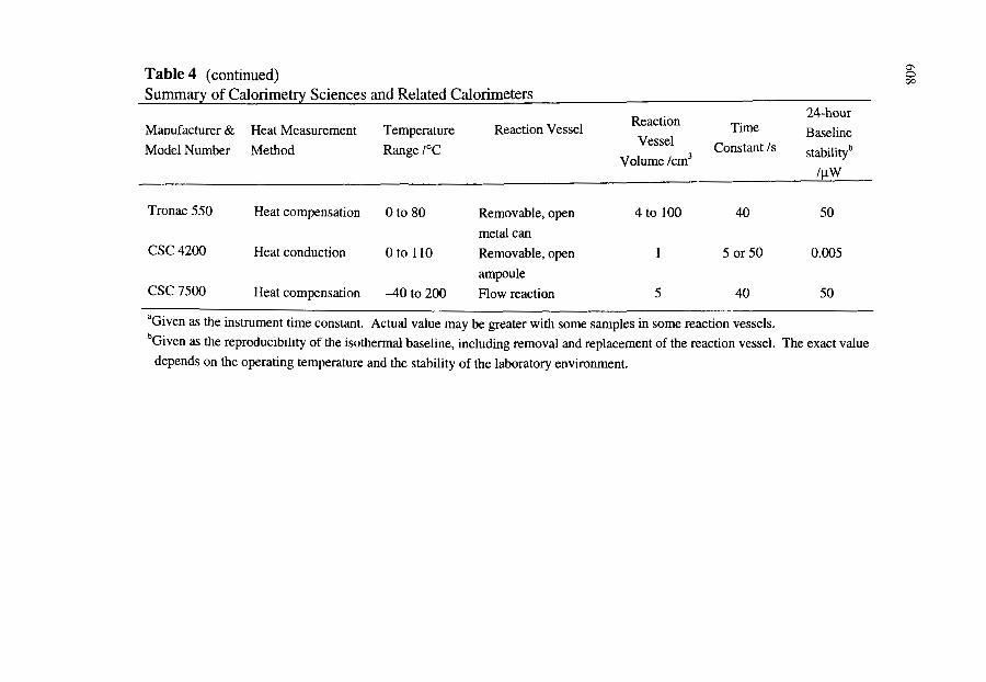
Q\ 0 Table 4 (continued) CQ

Summary of Calorimetry Sciences and Related Calorimeters

Manufacturer & Heat Measurement Temperature Reaction Vessel Model Number Method

24-hour Reaction Time Baseline

Range 1°C Constat / S stabifityb Volume /cm3

/pW

Tronac 550 Heat compensation 0 to 80 Removable, open 4 to 100 40 50

metal can

ampoule

CSC 4200 Heat conduction Oto 110 Removable, open 1 5 or 50 0.005

csc 7500 Heat compensation 4 0 to 200 Flow reaction 5 40 50

aGiven as the instrument time constant. Actual value may be greater with some samples in some reaction vessels. bGiven as the reproducibility of the isothermal baseline, including removal and replacement of the reaction vessel. The exact value

depends on the operating temperature and the stability of the laboratory environment,

609

6. SCERES CALORIMETERS

I. Lamprecht

Institut ftir Biophysik, Freie Universit~it Berlin, Thielallee, 63 D-14195 Berlin, Germany.

6.1. Introduction SCERES (Soci6t6 de Conception d'Etude et R6alisation; 16, rue de Chartres,

F-91400 Orsay, France) produces a line of calorimeters with working volumes between 0.2 cm 3 and 400 dm 3 with an open end for larger capacities. All instruments have some characteristics in common: i. a solid construction with heads made entirely of metal; a "head" in the DSC

and SCERES terminology is the separate measuring unit essentially without any thermal isolation (see Figures 10 and 11),

ii. a central structure with only two movable parts so that baseline drifts are limited and homogeneous temperature distributions guaranteed, a differential arrangement with a reaction and a reference vessel (twin system), heads always separated from the electronic control and data acquisition systems so that they can be placed easily in specific or highly protective environments, e.g. a cooling box or a very constant incubator, the same electronics are used for all calorimeters with control performed manually or by computer,

vi. heads can be purchased separately for individual instrumental designs and connection to other detection units like mass spectrometers or gas analysers;

vii. most of the calorimeters can be run in an isothermal or in a temperature scanning mode as in DSC,

viii.most heads cited in Table 5 use classical thermopiles as heat flow detectors, but the large instruments (last two in the list) have thermoresistors in a sensor-bridge.

Quite a number of vessels (often called "cells") of different form and different material are offered by SCERES depending upon the application. Glass, quartz, Kel.F, teflon, monel 300b, aluminium, Hastelloy, stainless steel 316L, copper and platinum are employed routinely for the construction. A more detailed description of their form and application is given under "Accessories" (Section 6.4).

Figure 10 shows schematically the basic design common to the heads from the B-400 to the TL-1000 given in Table 5. Two vessel compartments (left for the reaction vessel, right for the reference vessel) are connected via a thermopile of varying numbers of thermoelements. Beneath both compartments,

iii.

iv.

V.

610

thermoresistors are located which serve as both temperature probes and calibration heaters for the head. A Pt-100 resistor for the oven temperature is indicated at the right in Figure 10. The two sockets in the base of the calorimeter connect the thermopile, the two indicated thermoresistors, the oven heater and its temperature probe with the external recorder and the programme controller. This drawing shows a modification of the B-600 head equipped with vessels allowing the mixing of two liquids by a rocking mechanism.

Usually, the vessel volume is the main determining factor for the choice of a calorimeter, besides its detection limit. If only small amounts of substance are available, as often occurs with biochemical or medical samples, then comparably sized vessels are essential for successful investigations. On the other hand, inhomogeneous matter and crude material, or whole animals like insects or reptiles, require appropriately larger volumes. With increasing size the sensitivity of the instrument decreases, time constants increase and baseline drifts become more severe (see Table 5). In general, SCERES calorimeters are constructed for temperatures between -200 and 650 ~ with some exceptions up to 850 ~ Only the very large instruments have significantly reduced temperature ranges. Since most heads can be used in a DSC manner, a general standard detection limit is given in those terms as 0.02 mg indium (melting enthalpy around 0.6 mJ), which transforms to a heat flow of about 10 ~tW. The exact individual characteristics of the various heads are given in Table 5.

SCERES calorimeters are applied in many fields of science: agriculture, biochemistry, biology, biophysics, chemistry, environmental sciences, experimental medicine, metallurgy, physics, physical chemistry and in industries such as aerospace research, cement production, electrics and electronics, food production and distribution, nuclear applications, paper production and recycling, and refuse handling. Of course, this list is far from comprehensive, but gives an impression of the multitude of applications.

6.2 Calorimeter Heads

6. 2.1. B-400 The B-400 is the "fastest" head among the SCERES calorimeters with a very

small vessel volume of only 0.5 cm 3. With a high sensitivity of 60 laV mW -~ and a low detection limit of 1 laW, it is the smaller brother of the B-900. It is sold at an attractive price. It is intended for investigations of low-energy biological processes, for (bio)chemical tests and analyses and for research on medical incompatibility. Used as a DSC instrument in a reduced, but biochemically interesting temperature range from -190 to 200 ~ it has a practically linear baseline drift which thus allows an easy evaluation of truly calorimetric, not thermometric DSC curves.

611

Figure 10. Schematic cross section through a calorimeter head (B-600) equipped with two mixing vessels for a rocking mechanism: 1, upper flange; 2, springs; 3, cap; 4, mixing vessels with two different liquids A and B (reaction side) or with two equal liquids (reference side); 5, mercury drop as seal; 6, Pt-100 resistor as oven temperature probe; 7, thermistor as temperature probe for the vessel containers and for calibration purposes; 8, sockets connecting the head with the control system and with the data recorders; and 9, rocking mechanism of the head (By courtesy of SCERES).

612

6.2.2. B-900 The B-900 is a genuine calorimeter of great precision with 1.5 cm 3 vessels

and a high sensitivity of 110 gV mW -~ resulting from 110 thermocouples. Nevertheless, it is still competitive as a modern DSC instrument (Figure 11). It has a low background noise of 30 nW (directly at the thermopile) and operates at temperature scanning rates from 0.01 up to 15 ~ min -~. The signal half-time figure is 30 to 40 s. With its temperature range f r o m - 1 9 0 to 650 ~ it is suitable for all applications in physics and chemistry in a multifunctional manner: in an isothermal mode as the other calorimeters presented in this Chapter, in a scanning mode as a DSC (see the earlier Chapter) and with a stepwise temperature programme as used for the determination of specific heats.

6.2.3. B-900S The B-900S is a special version of the B-900 mentioned above with an

Figure 11. Calorimeter heads B-900 (smaller left one) and B-600 (larger right one) in front of the control system. Different vessels are placed inside the heads (By courtesy of SCERES).

613

extended temperature range (Table 5) and a significantly increased detection limit of 0.1 gW. As stated in this Table, the detection limit is defined as twice the background noise when all electrical units are connected. The B-900 is well suited for biological or biochemical reactions with small enthalpy changes.

6. 2.4. B-600 This medium sized calorimeter (Figure 11) with vessels of 25 cm 3, a

sensitivity around 50 gV mW -~ and a detection limit of 10 gW is again a multifunctional instrument. Although best suited for investigations in the isothermal mode, it allows for scanning rates of 2 ~ min -~ in a temperature range from -190 to 650 ~ It was conceived for use in agronomic, biological and medical research and can be easily converted into a high-sensitivity instrument by immersing it in a thermostat-controlled bath. A thermoresistor under each vessel compartment serves as a probe for measuring temperature, but is also applied as a heating resistor for calibration purposes. This allows for quick calibrations during, or just before, and immediately after an experiment.

Owing to its larger vessel volume of 25 cm 3, many different vessels are available for this head, among them mixing and injection devices, combustion microbombs (see also Section 10) and vessels for pressures up to 200 MPa. They will be discussed in more detail under "Accessories" in Section 6.4.

6.2.5. HT-IO0 The HT-100 calorimeter with its even larger vessels of 100 cm 3 has similar

applications to the B-600, but is especially valuable for studies of coarse material (like household refuse) or smaller animals. The sensitivity is slightly reduced compared with the B-600 (Table 5), but it does have an extended temperature range of up to 850 ~ Again many different vessels including mixing systems and combustion microbombs are offered for this head.

6.2.6. BLD-350 The BLD-350 head (Figure 12) with 25-cm 3 vessels is designed for

investigating the heat production rates of radioactive substances. To this end, both vessel compartments are separately armoured for radiation protection. With its high sensitivity of 45 gV mW -~ and a detection limit of 10 gW, it is well suited to be an absolute dosimeter in irradiation studies.

6.2.7. B-IO00 This fast "enthalpimeter" (Figure 12) with 0.2 cm 3 vessels is meant to be complementary to the B-400 head for educational purposes as well as for systematic measurements by students. With its low price and easy operation it is

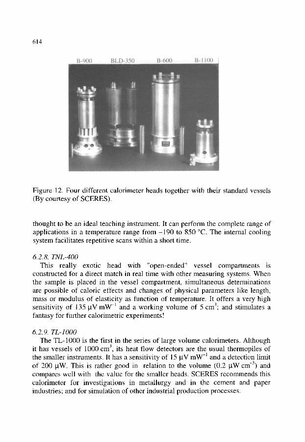
614

Figure 12. Four different calorimeter heads together with their standard vessels (By courtesy of SCERES).

thought to be an ideal teaching instrument. It can perform the complete range of applications in a temperature range f rom-190 to 850 ~ The internal cooling system facilitates repetitive scans within a short time.

6. 2.8. TNL-400 This really exotic head with "open-ended" vessel compartments is

constructed for a direct match in real time with other measuring systems. When the sample is placed in the vessel compartment, simultaneous determinations are possible of caloric effects and changes of physical parameters like length, mass or modulus of elasticity as function of temperature. It offers a very high sensitivity of 135 gV mW -~ and a working volume of 5 cm3; and stimulates a fantasy for further calorimetric experiments!

6.2.9. TL-IO00 The TL-1000 is the first in the series of large volume calorimeters. Although

it has vessels of 1000 cm 3, its heat flow detectors are the usual thermopiles of the smaller instruments. It has a sensitivity of 15 gV mW -1 and a detection limit of 200 gW. This is rather good in relation to the volume (0.2 gW cm -3) and compares well with the value for the smaller heads. SCERES recommends this calorimeter for investigations in metallurgy and in the cement and paper industries; and for simulation of other industrial production processes.

615

6.2.10. VL-8 The calorimeters VL-8 and VL-400 differ from the above mentioned

instruments in two important respects: (i) they use thermoresistors, fed by a bridge, as heat sensors instead of thermopiles, and (ii) they are constructed concentrically, with the reference vessel surrounding the reaction vessel and serving as its heat sink (Figure 13). Sensitivities and detection limits are given (Table 5) for the condition that the bridge has an applied potential of 5 V. VL-8 has a working volume of 8000 cm 3 and a sensitivity of 10 gV mW -1. It stands in a line of increasing volume with the heads B-600, HT-100 and TL-1000 and can be applied in the same investigations as those, but on a larger scale.

Figure 13. Schematic picture of the concentric construction of the large-volume calorimeter, VL-8 with the central reaction vessel ("cell"), the surrounding reference vessel and the oven (By courtesy of SCERES).

616

6.2.11. VL-400 The VL-400 is the largest calorimeter in the SCERES catalogue with a

volume of 400 dm 3 (400 L!). It is a repeat of the concentric construction type seen in the VL-8. The indicated detection limit of 10 mW (Table 5) transforms to a volume specific sensitivity of 0.025 gW cm -3 and compares with those of the small heads. The total outside volume of the calorimeter amounts to 1 m 3.

In earlier catalogues an instrument VL-200 with 200 dm 3 was indicated showing that SCERES constructs calorimeters as required by customers apparently without any limitation to the size.

6.3. Electronic Control and Data Processing All heads cited in Table 5 have a common external control system and the

same data processing. The control system (see Figure 11, left side behind the two calorimeter heads) works in either computer-controlled or manual modes. It determines the oven temperature and regulates the heating power of the oven. Isothermal conditions are possible, as well as scanning operations in up to 100 temperature/time segments for DSC investigations. Moreover, it produces the power for the two calibration heaters shown in Figure 10.

The data acquisition and programming system digitizes and records the temperatures of the oven and of the two vessel compartments, together with the heat flow signal of the thermopile. The original (raw) data are stored in a "results" file which cannot be modified by the user. They are kept intact and are always available for further treatment. Baseline drift corrections, curve smoothing and other manipulations are performed by the user so that no "black box behaviour" of the system impedes the interpretation of results.

6.4. Accessories Many vessels and instrumental accessories are available, mainly for the

medium sized calorimeters of 25 and 100 cm 3 (B-600 and HT-100). Liquid- liquid mixing vessels (CR1) for a rocking system are shown in Figure 10, and a similar set-up (CR2) is used for mixing a liquid with a solid. In both vessels, the two components are thermally equilibrated before the experiment and then mixed by a rotating movement of the head. Another device (coded as CME) allows the mixing of two separated liquids, or the stirring of suspensions with the movement of a glass-embedded metallic mass by means of an electromagnet just above the vessel. This arrangement avoids heat leaks by connections to the outside. An alternative is a rotating mechanical stirrer (CMM). A further mixing vessel for liquids and gases (CMHP) uses a concentric flow line for both components which are mixed at the bottom and leave the vessel via a counterflow heat exchanger along the walls of the calorimeter. Several injection

617

systems for liquids and gases are offered, systems with a syringe and external furnace (CIS2), the same with an extended tube for thermal equilibration (CIS3) and the already mentioned device, CMHP.

Microbombs (CMB) are available for B-600 and HT-100 heads and these are described in more detail in Section 10. Three different high pressure vessels for a maximum 1 MPa (10 bar; C10), 10 MPa (100 bar; C100) and 30 MPa (300 bar; C300) can be applied for both heads. When investigations are made at low temperatures, the whole calorimetric head can be placed in a special bucket, suitable for dry ice (SCG) or for liquid nitrogen (SNL), with automatic or manual filling.

This list is not complete but just gives an idea which experiments may be performed with the different heads and the various equipment produced by SCERES.

Table 5 Characteristics of the SCERES Calorimeter Heads

Calorimeter Temperature Vessel Sensitivity a Detection DimensionC'd

r ange /~ v o l u m e / c m 3 /laV mW -l limit b, c Q, H / m m

/---laW

B-400 - 1 9 0 ~ 2 0 0 0.5 60 1 60,120

B-900 - 1 9 0 ~ 6 5 0 1.5 110 5 60,220

B-900S - 1 9 0 - - 8 5 0 1.5 110 0.1 60,220

B-600 - 1 9 0 w 6 5 0 25 45 10 110,260

HT-100 - 1 9 0 m 8 5 0 100 35 20 180,260

BLD-350 - 6 0 ~ 4 5 0 25 45 10 170,260

B-1100 - 1 9 0 m 8 5 0 0.2 25 10 60,130

TNL-400 Specificaions 5 135 variable 50,140

TL-1000 - 6 0 m 1 5 0 1000 15 200 320,670

VL-8 - 6 0 m 1 5 0 8000 10(at5V) 200 (at5V) 250,500

VL-400 - 6 0 m 1 5 0 400 103 2(a t5V) 10mW l m 3

aDirect sensitivity at the thermopile socket.

bDetection limit is twice the background noise with all electrical equipment. A measurement

may be considered to be reliable at 10 times the detection limit.

CVL-8 and VL-400: Calorimeters with thermoresistor detector fed by a bridge, concentric

position of reference and experimental vessel.

d~ is the diameter and H is the height of the head.

618

7. SETARAM C A L O R I M E T E R S

B. Schaarschmidt

Institut ftir Biophysik, Freie Universit~it Berlin, Thielallee 63, D-14195 Berlin, Germany.

7.1. History Tian's calorimeter was a "single calorimeter" with only one measuring

system. It was built 7 m deep in the ground below a cellar to obtain a stable temperature for the surroundings. In the years 1922/1923 [64], Tian introduced electrical compensation of the thermal effect by means of the Peltier effect. His "microcalorimetric element" had two thermoelectric piles, one serving to measure the heat flow, and the other providing Peltier cooling. Thus the calorimeter could be operated in a nearly isothermal manner when the heat liberated was compensated by the cooling. Calvet's modifications in 1948 [65] consisted of arranging the ~ as far as possible identical ~ thermocouples in a highly regular array, and of using two measuring systems symmetrically placed in the same thermostat.

7.2. The Tian-Calvet Design

7. 2.1. The Heat conduction principle Tian was one of the first to use the advantages of this principle in

constructing calorimeters. So typically all Calvet instruments are still made as heat conduction calorimeters. Thermopiles of high thermal conductivity surround the experimental space within a large calorimeter block of high heat capacity (see Section 2.4.3). Because of the radial arrangement of the thermopiles, thermal changes in the space are integrated almost completely and the recorded heat signal is independent of the distribution of local temperatures.

7.2.2. Differential principle Calvet's great contribution was to constitute a twin calorimetric system from

two Tian microcalorimetric vessels. The Calvet calorimeter has two identical positions, one for the measuring vessel and the other for the reference vessel (twin construction, see Section 2.5), which are located symmetrically within the block. Providing that a careful balance between the heat capacities of both vessels has been established, then this siting compensates for irregular heat effects when the two are connected electrically in opposition.

619

7.3. The Family of Modern Calvet Calorimeters Following Tian-Calvet design, the French company DAM (later SETARAM)

in Lyon developed a modern type of heat conduction calorimeter, the Calvet microcalorimeter. In order to cover a broad field of applications, a series of variations of the standard type was designed which relates to differences in sample size, temperature range and sensitivity. Most of these instruments are constructed for an isothermal (in the strict sense of thermodynamics, isoperibol) operation, but also can be used for slow temperature scanning operations. The reverse also holds true for their DSC instruments. Though mainly constructed for operation in a temperature scanning mode, some of these, due to the Tian- Calvet principles for their heat detectors, can be used as highly sensitive, isothermal calorimeters (see Table 6).

7.3.1. The Classical Calvet Microcalorimeter The standard microcalorimeter (latest marque MS 80) is a typical thermopile

conduction instrument, by nature suited for studies of slow processes with small heat outputs. It is the most sensitive (detection threshold -~1 jaW) of the Calvet types and mainly it is used for isothermal operations in the temperature range from ambient to 200 ~ The technical lay-out of this calorimeter has not been changed essentially since the construction of the first prototype Calvet microcalorimeter in the fifties (Figures 14 and 15). The main feature of its design lies in the two symmetrically positioned measuring spaces for the measuring sample and the reference. They are located in the middle of a cylindrical aluminium block which sits between the bases of two truncated cones. A double differential arrangement (two measuring systems in the same calorimeter) is available as an option.

The envelope of this block contains a precision thermostat controlled by an exterior temperature regulator which maintains the set temperature to an accuracy of +0.001 ~ To achieve an equi-partition of lateral thermal disturbances from the outside, the thermostat is built up of several concentric shells in an alternating sequence of good and poorly conducting material. The outermost shell is surrounded by heating elements. The distribution of thermal disturbances is further improved by the conical caps of the calorimeter block which act as heat collimators in the vertical direction. The whole block is embedded within a large insulating container.

The sensitive part of the calorimeter is the conduction device which connects the outer wall of the small measuring chamber to the large isothermal metallic block. This device is composed of 496 thermocouples (platinum/platinum- rhodium) arranged in 16 sheets, each of 31 thermocouples. These sheets cover radially the measuring chamber in vertical arrays (Figure 16). Within each

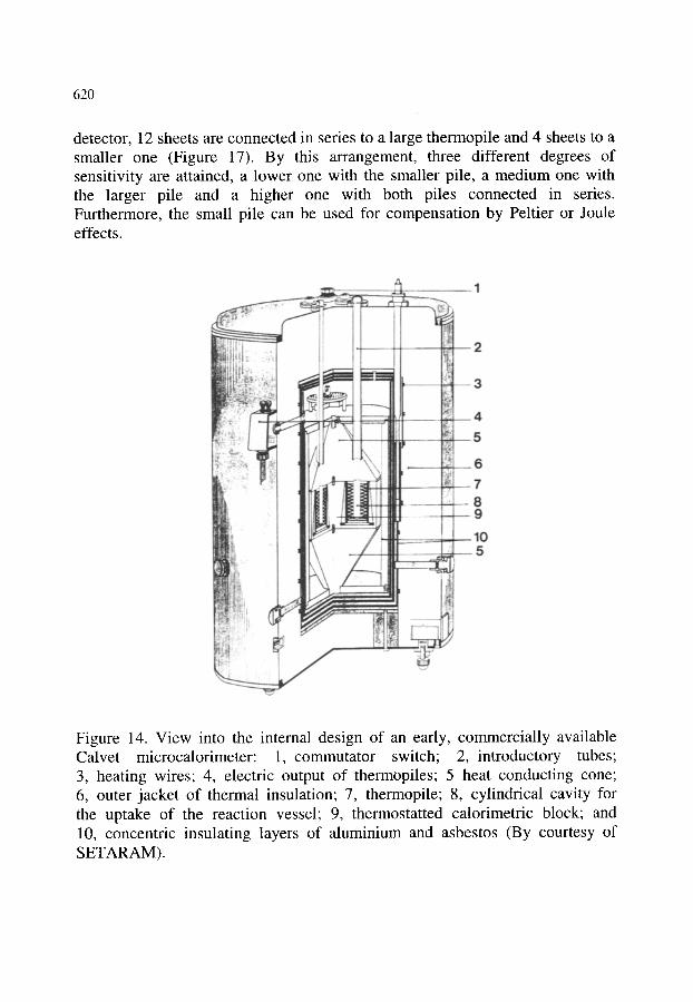
620

detector, 12 sheets are connected in series to a large thermopile and 4 sheets to a smaller one (Figure 17). By this arrangement, three different degrees of sensitivity are attained, a lower one with the smaller pile, a medium one with the larger pile and a higher one with both piles connected in series. Furthermore, the small pile can be used for compensation by Peltier or Joule effects.

Figure 14. View into the internal design of an early, commercially available Calvet microcalorimeter: 1, commutator switch; 2, introductory tubes; 3, heating wires; 4, electric output of thermopiles; 5 heat conducting cone; 6, outer jacket of thermal insulation; 7, thermopile; 8, cylindrical cavity for the uptake of the reaction vessel; 9, thermostatted calorimetric block; and 10, concentric insulating layers of aluminium and asbestos (By courtesy of SETARAM).

621

. ~

1 I

J

o , ii

~

~.~..,..,.,,,.

Figure 15. Vertical cross section of a Calvet calorimeter MS 80: 1, access tubes to the measuring chambers; 2, commutator and electric output of the thermopiles; 3, heating wires; 4, arrangement of the thermopiles; and 5, calorimetric block (By courtesy of SETARAM).

The measuring zone of the calorimeter is accessible from the top of the calorimeter through open shafts, allowing the reaction and the reference vessels to be introduced or removed from the outside. The vessels must have exactly the correct diameter and their height must not exceed that of the measuring zone. The open shafts are also used to connect the system under investigation to the outside by optical, electrical or mechanical devices.

To achieve the highest sensitivities, the calorimeter should be placed in a closed room with neither windows nor large thermal disturbances such as intermittent heaters or draughts. The ambient temperature should be 5 ~ below the experimental temperature. No other cooling device should be connected to

622

the calorimeter itself due to the risk of internal condensation which would totally disturb the operation.

,N

u

, i

I--

Figure 16. Vertical section of the heat conduction measuring zone showing the radial arrangement for the layers of thermocouples (By courtesy of SETARAM)

7.3.2. The Mixing Calorimeter The C 80 mixing calorimeter is a simplified model of the standard Calvet

type microcalorimeter It can be used either as an isothermal reaction calorimeter or as a DSC in the range from ambient temperature up to 300 ~ set by manual control or by programme. In order to have the facility of operating in both modes, the design featured a reduced reaction volume, a lower response time and a refined thermostat. By these changes, a robust versatile instrument with flexibility in operation and simplicity in handling was made, which is suitable for thermodynamic studies and laboratory analyses.

The technical lay-out shown in Figure 18 is very similar to that of the standard model (Figures 14 and 15). The main differences lie in an essentially

623

lighter calorimeter block, a blower fitted under the instrument for cooling the block during decreasing temperature scans and a removable lid on top of the calorimeter which gives direct access to the measuring chamber. A special buffer zone, directly above the block, serves as a thermal prestabilization area for the reaction vessel or for other additional devices (no.2 in Figure 18).

/

Y%

I, [ . . . . . . . . . . .

L ,tT I,I, ' r - - z_ - : l L ,,V L-,I,I

Figure 17. Horizontal section of the heat conduction measuring zone, the left side shows the arrangement of a small thermopile, the right side that of a large thermopile (By courtesy of SETARAM).

The whole instrument is fitted on a reversing mechanism (Figure 19) driven by an electric motor allowing either a simple intermittent reversal of the calorimeter by 180 ~ or an oscillating mixing. Depending on the type of experiment, different vessels for batch or flow mixing operations are available.

7.3.3. The Low Temperature Calorimeter The low temperature microcalorimeter BT 2.15 can be cooled by liquid

nitrogen, thus extending the working temperature from ambient t o - 1 9 6 ~ To function at low temperatures, protection is required against all condensable substances which would cause large thermal and electrical variations. Therefore the thermostatted calorimeter block is located inside a vacuum-tight, cylindrical chamber which is maintained under a controlled gaseous atmosphere to avoid any condensation at low temperatures. This container is immersed in a tank of

624

liquid nitrogen surrounded by a thicker shell of insulating material (Figure 20), which is a mineral powder kept under vacuum.

Figure 18. Cross section of the C80 mixing calorimeter: 1, removable lid; 2, thermal buffer zone; 3, heating elements; 4, thermopiles; 5, experimental area; 6, calorimetric block; 7, insulation layers; and 8, cooling circuit (By courtesy of SETARAM).

Depending on the temperature and the mode of operation (isothermal or temperature scan), the liquid nitrogen is either maintained at a constant level in the tank by an automatic gauge from an outside storage container or it is introduced continuously at a constant flow rate. After cooling the calorimeter, the nitrogen can be replaced by liquid helium in order to improve the heat transfer between the block and the enclosure. The access holes on top of the

625

instrument are closed by tight lids to exclude any atmospheric mixture. For very low temperature experiments, the top cover on the calorimeter is heated to prevent icing.

. .

i

I i i i i i I

ooo o i o ooo 0 i " 0

i

I _1

L /

Figure 19. Reversing mechanism of the C80 mixing calorimeter (By courtesy of SETARAM).

The BT 2.15 calorimeter can be used in all laboratories without special equipment. It can be mounted on a reversal fitting like the C 80 calorimeter. Many of the reaction vessels available for the standard calorimeter can also be used for the low temperature one. The fields of application for this calorimeter are the same as those of the standard one but, due to its low temperature range, it is also used for studies of freezing, crystallization and superconductivity.

7.3.4. The High Temperature Calorimeter The HT 1000 calorimeter is designed for operation in the range from ambient

temperature up to 1000 ~ The operating principle and the general appearance is nearly the same as for the standard model. Because of the high experimental temperatures, the outer protection shell is strengthened, and the heating elements of the furnace are more effective because they are made of Kanthal. In contrast to the standard model, the heaters are placed under the base of the calorimeter block and above the top cover to achieve a better homogeneity of temperature distribution (Figure 21). The whole furnace is thermally insulated by refractory elements embedded within a metal support. Isothermal operation

Figure 20. Cross section of the BT 2.15 low Figure 21. Cross section of the HT 1000 high temperature calorimeter: 1, vacuum connection; temperature calorimeter with: 1, access tubes; 2, control of the nitrogen level; 3, introductory tubes; 2, commutator and electric output of the calorimetric 4, vacuum tight container, calorimetric shell; 5 , liquid signal; 3, heat-flow detector; 4, calorimetric block; and nitrogen tank; 6, thermostat; 7, thermopiles; and 5 , furnace (By courtesy of SETARAM). 8, calorimetric block (By courtesy of SETARAM).

627

and temperature scanning is possible with the HT 1000 calorimeter. The reaction vessels available are either a simple batch type or a closed tube system. Both are made from aluminium oxide. A special mechanism to introduce the sample allows insertion of the experimental vessels and/or the addition of solid samples under a controlled atmosphere. The main application fields of the high temperature calorimeter are surface interactions between gases, liquids and solids, besides studies of mixing solutions, dilution processes, specific heats, and stability at elevated temperatures. The HT 1000 calorimeter can be installed anywhere but stabilization of the ambient temperature is necessary if a high sensitivity is required in experiments.

7.3.5. The High Sensitivity Calorimeter Though originally designed as a DSC bench instrument, the micro DSC

(latest type III) can be used as a multipurpose calorimeter in batch and flow mode for small samples (1 cm3). By applying semiconducting, resistance thermometers as the heat conduction detectors, the sensitivity is increased to about 90 ~V mW -1 which is nearly double that of the thermopile detectors in the Calvet calorimeters. The basic lay-out is similar to that of the standard Model MS 80, but with the further exception that the temperature is set by an internal liquid loop which flows around the calorimeter block. Thus the temperature range is extended down t o - 2 0 ~ when using water in the external cooling circuit. In order to avoid any disturbance from the outside, a long thermal buffer zone is housed above the measuring area. Furthermore the top of the block is surrounded by a pre-stabilizing ring (Figure 22), through which fluid reagents flow before entering the reaction vessel. Besides a liquid and gas tight batch vessel with removable lids (no.1 in Figure 22), flow vessels with two (nos. 2 and 3) or three tubes (no. 4) are available for flow-through or mixing experiments. Because of its high sensitivity and the small sample size required, this calorimeter is suitable for biochemical investigations, e.g. enzymatic reactions, binding of proteins and bacterial growth, and also for checking the stability of foodstuffs and pharmaceuticals, or the compatibility between materials.

7.3.6. The Multi-detector Calorimeter The multi-detector, high temperature calorimeter can be equipped with two

different measuring insets ("detectors") which may be used alternatively with the same basic instrument containing the furnace. The "DSC detector", with a crucible volume of 0.45 cm 3, is made from two identical ceramic chambers linked to each other by two conducting plates holding 20 thermocouples (Figure 23a). With this detector a rapid temperature scan up to 1600 ~ is possible. The

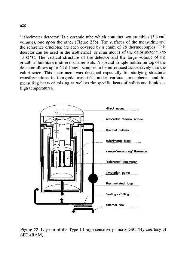
628

"calorimeter detector" is a ceramic tube which contains two crucibles (5.3 cm 3 volume), one upon the other (Figure 23b). The surfaces of the measuring and the reference crucibles are each covered by a chain of 28 thermocouples. This detector can be used in the isothermal or scan modes of the calorimeter up to 1500 ~ The vertical structure of the detector and the large volume of the crucibles facilitate routine measurements. A special sample holder on top of the detector allows up to 23 different samples to be introduced successively into the calorimeter. This instrument was designed especially for studying structural transformations in inorganic materials, under various atmospheres, and for measuring heats of mixing as well as the specific heats of solids and liquids at high temperatures.

direct acces

removable thermal screen

thermal buffers

calorimetric block

sample"measuring" fluxmeter

"reference" f l u x m e t e r

circulation p u m p

thermostated loop

. . . . . . . . . . h e a t i n g - cooling

4;' r j external flow

Figure 22. Lay-out of the Type III high sensitivity micro-DSC (By courtesy of SETARAM).

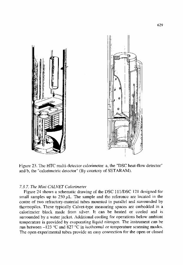
629

i .

Figure 23. The HTC multi-detector calorimeter: a, the "DSC heat-flow detector" and b, the "calorimetric detector" (By courtesy of SETARAM).

7.3.7. The Mini CALVET Calorimeter Figure 24 shows a schematic drawing of the DSC 111/DSC 121 designed for

small samples up to 250 jaL. The sample and the reference are located in the centre of two refractory-material tubes mounted in parallel and surrounded by thermopiles. These typically Calvet-type measuring spaces are embedded in a calorimeter block made from silver. It can be heated or cooled and is surrounded by a water jacket. Additional cooling for operations below ambient temperature is provided by evaporating liquid nitrogen. The instrument can be run between-123 ~ and 827 ~ in isothermal or temperature scanning modes. The open experimental tubes provide an easy connection for the open or closed

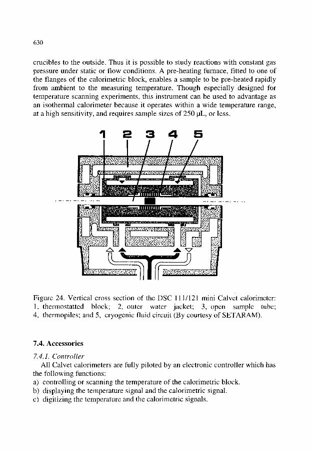
630

crucibles to the outside. Thus it is possible to study reactions with constant gas pressure under static or flow conditions. A pre-heating furnace, fitted to one of the flanges of the calorimetric block, enables a sample to be pre-heated rapidly f rom ambient to the measuring temperature. Though especially designed for temperature scanning experiments, this instrument can be used to advantage as an isothermal calorimeter because it operates within a wide temperature range, at a high sensitivity, and requires sample sizes of 250 IlL, or less.

1 2 3 4 5

, ! , 1 1 . . . . . . . . . . . i ~ ~ ~ , ~ @ ; , ~

1

U @

Figure 24. Vertical cross section of the DSC 11 1/121 mini Calvet calorimeter: 1, thermostatted block; 2, outer water jacket; 3, open sample tube; 4, thermopiles; and 5, cryogenic fluid circuit (By courtesy of SETARAM).

7.4. Accessories

7.4.1. Controller All Calvet calorimeters are fully piloted by an electronic controller which has

the following functions: a) controlling or scanning the temperature of the calorimetric block. b) displaying the temperature signal and the calorimetric signal. c) digitizing the temperature and the calorimetric signals.

631

d) transferring the temperature and the calorimetric signals to a microcomputer. e) operating the gas and vacuum circuits, if necessary. All signals can be stored, displayed and processed by dedicated software.

7. 4.2. Vessels for Different Applications The choice of calorimetric vessel depends closely on the type of experiment.

Though the operator is free to design and build the most appropriate device for the scientific requirement, it is often convenient to use one of the specially constructed vessels offered on the market. The following short selection of the most important vessels for the calorimeters suited for different sample volumes (100, 15 and 1 cm 3) may give an impression of the diversity of experiments which are possible with SETARAM calorimeters.

Standard batch vessel. This is a simple closed container which can be used for the investigation of fluids and solids when no physical contact between the sample and outside is required. The internal pressure must not exceed 500 kPa (5 bar) and the temperature must not rise above 220 ~ Auxiliary equipment for initiating reactions, mixing, stirring, illumination, etc. need to be led through a specially adjusted lid. The batch vessel is appropriate for physical, chemical and biological applications, because the heat change of anything that fits into it can be measured!

High pressure vessel. This has a greater wall thickness and a stronger top cover and is suitable for investigations under a static pressure of inert or active gases, or for compounds developing high vapour pressures during the reaction. The pressure limit is 10 MPa (100 bar) at temperatures up to 300 ~

Vacuum vessel. This can operate at either normal or high pressures and is similar to the standard vessel, but is connected to the outside by a tube in order to evacuate the vessel or to introduce a gas under either reduced or high pressures. A pressure transducer can be linked to the outlet. These vessels are used for studies of decomposition of materials and for processes of desorption, adsorption and polymerization, as well as for oxidation and reduction reactions and gas dependent biological reactions (anoxic, hypoxic and hyperoxic conditions).

Circulat ion vessel. This has two coaxial tubes for inlet and outlet to circulate a gas or a liquid over the sample (adsorption and binding processes) and/or to remove emitted fluids or vapours from the vessel. The incoming fluid is pre- thermostatted just before the calorimeter inlet. These vessels can also be used as

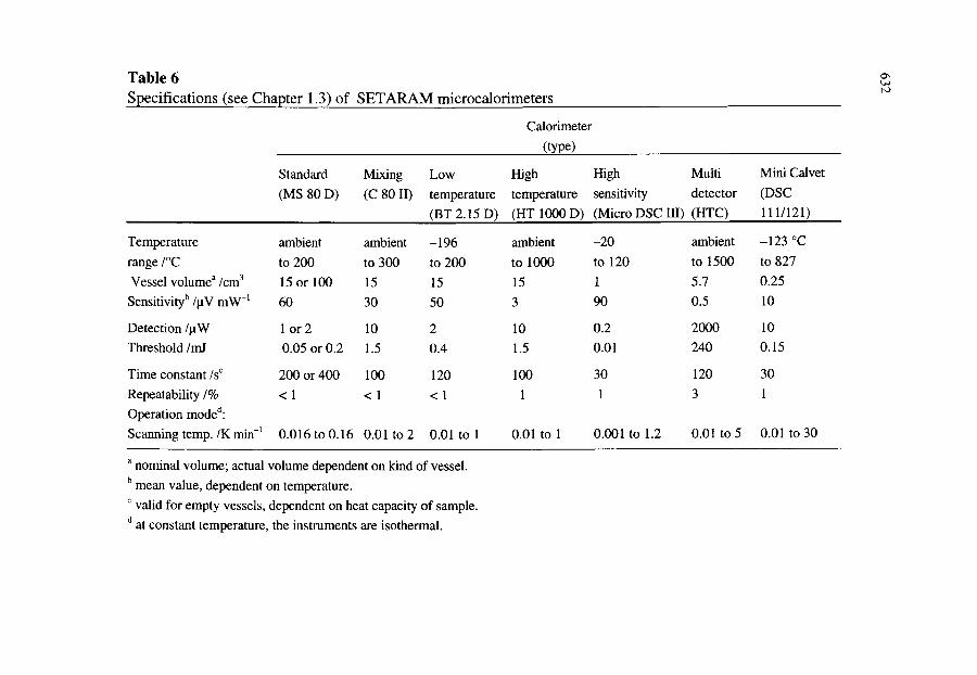
Table 6 Specifications (see Chapter 1.3) of SETARAM microcalorimeters

Calorimeter

(type)

Standard Mixing Low High High Multi Mini Calvet

(MS 80 D) (C 80 11) temperature temperature sensitivity detector (DSC

(BT 2.15 D) (HT lo00 D) (Micro DSC In) (HTC) 11 11121)

Temperature ambient ambient -196 ambient -20 ambient -123 "C

range /"C to 200 to 300 to 200 to 1000 to 120 to 1500 to 827

Vessel volumea /cm3 15 or 100 15 15 15 1 5.7 0.25

Sensitivityb /pV mW-' 60 30 50 3 90 0.5 10

Detection /pW 1 o r 2 10 2 10 0.2 2000 10 Threshold /mT 0.05 or 0.2 1.5 0.4 1.5 0.01 240 0.15

Time constant /sc 200or400 100 120 100 30 120 30

Operation moded: Scanning temp. /Kmin-' 0.016 to 0.16 0.01 to 2 0.01 to 1 0.01 to 1 0.001 to 1.2 0.01 to 5 0.01 to 30

Repeatability /% < 1 < 1 < 1 1 1 3 1

a nominal volume; actual volume dependent on kind of vessel. mean value, dependent on temperature. valid for empty vessels, dependent on heat capacity of sample. at constant temperature, the instruments are isothermal.

b

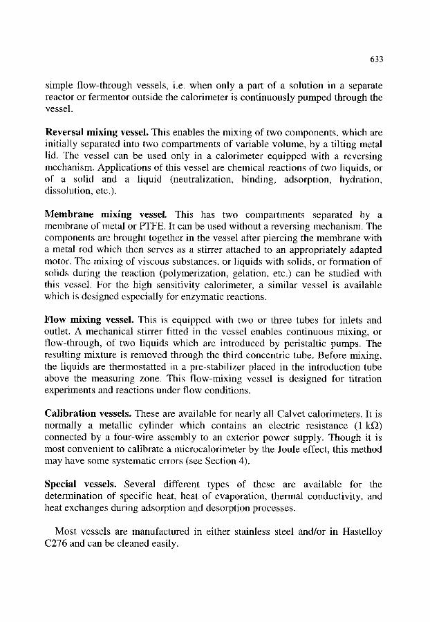
633

simple flow-through vessels, i.e. when only a part of a solution in a separate reactor or fermentor outside the calorimeter is continuously pumped through the vessel.

Reversal mixing vessel. This enables the mixing of two components, which are initially separated into two compartments of variable volume, by a tilting metal lid. The vessel can be used only in a calorimeter equipped with a reversing mechanism. Applications of this vessel are chemical reactions of two liquids, or of a solid and a liquid (neutralization, binding, adsorption, hydration, dissolution, etc.).

Membrane mixing vessel. This has two compartments separated by a membrane of metal or PTFE. It can be used without a reversing mechanism. The components are brought together in the vessel after piercing the membrane with a metal rod which then serves as a stirrer attached to an appropriately adapted motor. The mixing of viscous substances, or liquids with solids, or formation of solids during the reaction (polymerization, gelation, etc.) can be studied with this vessel. For the high sensitivity calorimeter, a similar vessel is available which is designed especially for enzymatic reactions.

Flow mixing vessel. This is equipped with two or three tubes for inlets and outlet. A mechanical stirrer fitted in the vessel enables continuous mixing, or flow-through, of two liquids which are introduced by peristaltic pumps. The resulting mixture is removed through the third concentric tube. Before mixing, the liquids are thermostatted in a pre-stabilizer placed in the introduction tube above the measuring zone. This flow-mixing vessel is designed for titration experiments and reactions under flow conditions.

Calibration vessels. These are available for nearly all Calvet calorimeters. It is normally a metallic cylinder which contains an electric resistance (1 kf~) connected by a four-wire assembly to an exterior power supply. Though it is most convenient to calibrate a microcalorimeter by the Joule effect, this method may have some systematic errors (see Section 4).

Special vessels. Several different types of these are available for the determination of specific heat, heat of evaporation, thermal conductivity, and heat exchanges during adsorption and desorption processes.

Most vessels are manufactured in either stainless steel and/or in Hastelloy C276 and can be cleaned easily.

634

Two great advantages of all Calvet calorimeters are that experimental vessels are removable between experiments and are accessible from the outside during experiments. These allow continuous or sporadic manipulations of the system under investigation by various appropriate devices at any time. These possibilities are of particular interest during experiments with biological materials which often exhibit a multitude of parallel and successive interdependent reactions. Examples of specially constructed devices are reported in the literature: electromechanical [66], electric stimulation [67], stirring [68,69], pressure application [70], perfusion system [71], irradiation with UV and visible light [72], optical density [72,73], endoscopy [74] and acoustic transducer [75].

8. THERMOMETRIC CALORIMETERS

Ingemar Wads6

Division of Thermochemistry, Chemical Center, Lund University, P.O. Box 124, S-221 00 Lund, Sweden.

8.1. Introduction The LKB Instrument Company started marketing its Precision Solution

Calorimeter (8700) in the mid-sixties and, after a few years, it introduced the Microcalorimetric System (10700). In the early eighties, that instrument system was succeeded by a multichannel microcalorimetric system (2277), initially called the B ioActivity Monitor or "BAM" but later changed in name to the Thermal Activity Monitor or "TAM". The LKB calorimeter line was taken over by Thermometric AB (Spjutv~igen 5 A, S-175 61 J~irf~illa, Sweden) when LKB in 1986 became part of the Pharmacia group. TAM and, to some extent, earlier LKB calorimeters were designed as modular instrument systems incorporating several calorimeters designed for different sample sizes and for different kinds of experiments. The TAM system still forms Thermometric's main product line, but it has been enlarged and several of its parts have been redesigned/updated resulting in new specifications for its key properties.

All microcalorimeters marketed by LKB and Thermometric are based on the (thermopile) heat conduction principle, i.e. heat evolved or absorbed in the reaction vessel is transferred to a surrounding heat sink through a thermopile (see Section 2.4.3). As for most other commercial microcalorimeters, the thermopile consists of semiconducting (Bi/Te) thermocouple plates ("Peltier- effect plates", primarily manufactured for use as thermoelectric coolers).

635

Up to the present time, most calorimeters produced and marketed by LKB- Thermometric have been based on original work carried out at the Division of Thermochemistry, Chemical Center, Lund University, Sweden. Several other university laboratories have also contributed to these developments. The design and properties of prototypes for the commercial instruments and novel experimental procedures have therefore been documented in considerable detail in scientific publications.

This chapter focuses on the design and the properties of the present TAM system. The early LKB calorimeters are still used in many laboratories and will be discussed briefly, like some of the still non-commercialized units from the Lund laboratory which fit into the TAM system.

8.2. Early LKB Calorimeters

8.2.1. The LKB 8700 Precision Calorimetric System The "8700-calorimeters" are a group of "semiadiabatic" (or "isoperibol")

calorimeters using the same thermostatic bath and electronic units. The main instrument is a general purpose reaction and dissolution "macro"-calorimeter [76], the basic development work for which is given in Reference [77]. Its standard calorimetric vessel is almost identical to the vessel of the new Thermometric 2225 Precision Solution Calorimeter described in Section 8.7. Its temperature sensor is a thermistor. The calorimetric vessel is contained in a metal can submerged in a thermostatted water bath, stability _+1• -3 K. Other units included in the 8700 system are a titration calorimeter [13,78], a vaporization calorimeter [79] and a closed-bomb calorimeter [80].

8.2.2. The LKB 10700 Microcalorimetric System The LKB 10700 microcalorimetric system includes a rotating "batch"

calorimeter [12], a flow calorimeter [15] and calorimeters for use with different insertion vessels, see References [81, 82]. All instruments were designed as twin calorimeters using one main heat sink which is surrounded by a thermostatted air bath. The twin calorimetric units form sandwich-like constructions with the calorimetric vessels in the centre surrounded by two thermocouple plates connected in series. On the outer side of the thermopile there are small aluminium blocks serving as thermal bridges to the heat sink.

The reaction vessels for the batch instrument [12] are designed as squared cans, each divided into two compartments by a partition wall. The compartments, volume 4 and 2 cm 3, respectively, are open and the contents of the vessel are thus in contact with the air space. The vessels are normally made from 18-carat gold or from glass. Mixing is achieved by rotation of the calorimeter block one turn and then back. This mixing technique (where

636

bubbles from the gas phase are important) is very efficient and, in some respects, preferable to injection/stirring techniques. Therefore, this instrument still is of interest in experiments with particularly difficult mixing problems (e.g. viscoussolutions, suspensions with heavy particles, sediments). However, users should be aware of the problem with two-compartment vessels joined by a gas phase, in particular the possible change of the gas phase composition following mixing of two volatile liquids [9,12,83]. Further, adsorption of reaction components (ions, proteins, etc.) on "clean" surfaces of the vessel can give significant systematic errors, if not taken into account [9,12,83].

It is quite time-consuming to work with the original type of batch calorimeter. Following developments in several laboratories, a later LKB model included micro syringes attached to the calorimetric block and the instrument could then be used as an automatic titration calorimeter [28].

The LKB flow calorimeter has a design which is analogous to that of the batch instrument. It is normally equipped with one flow mixing vessel and one flow-through vessel. Both vessels consist of flat spirals made from 24-carat gold tubes, inner diameter 1 mm. The spirals are positioned between two thin copper plates which are surrounded by the thermopile. The incoming liquid flow passes a heat exchanger, which is in close contact with the heat sink.

Several workers using the LKB flow calorimeter have enclosed the calorimetric block in a steel container and submerged it into a thermostatted water bath (as in the prototype design [15]), which usually leads to a more stable baseline. The same applies to the different versions of the LKB "ampoule microcalorimeter".

Among the non-commercial instruments connected with the LKB 10700- system may be mentioned an ampoule drop heat capacity calorimeter for solid and liquid samples (about 1 g) [84]. This instrument still appears to be the most accurate Cp calorimeter in use for the room temperature region.

8.3. The Present Line of Thermometric Calorimeters Soon after 1980, the Lund laboratory completed the design of a "4-channel"

twin microcalorimetric system [22] which subsequently was developed by LKB into a commercial instrument system called the 2277 B ioActivity Monitor ("BAM"). Corresponding with the change to a digital signal output, the name was altered to 2277 Thermal Activity Monitor or "TAM". This name has been kept by Thermometric despite the fact that the instrument system has been much expanded and updated since the old LKB days. The following discussion will focus on the design of the TAM and on the use and properties of its different parts. Data relating to quality specifications are valid for the products presently on the market. Major changes of properties have been made since the earlier versions were introduced and these are indicated in the proper place.

637

8.3.1. The Basic TAM Units The TAM instrument (Figure 25) consists of a thermostatted water bath (b),

electronic units (a) and up to four twin calorimeters (c). The calorimeters, identical or different, are operated independently of each other except for the use of a common thermostatted bath. The bath has a high temperature stability of l x l 0 -4 K over 24 h. It is of the overflow type. Water, or some other liquid, is circulated by use of a thermostatted centrifugal pump (e) positioned under the bath. The temperature is regulated by use of a thermistor (f) and a heater (d) placed in the inlet tube and the outlet tube of the bath, respectively. The bath is insulated by a thick layer of foamed polyurethane, giving a heat exchange coefficient of about 1 W K -~. Under standard conditions the bath can be used between 12 and 90 ~ The electronic units include a computer interface

- a

Figure 25. The Thermal Activity Monitor (TAM) showing: a, electronic units; b, thermostatted water bath; c, twin microcalorimeter; d, electrical heater; e, centrifugal pump; and f, inlet tube to the bath which has a thermistor in it (By courtesy of Thermometric, AB).

638

(Digitam 4.0 for Windows) and an amplifier for each calorimeter. A nanowatt amplifier was recently introduced to the system.

At present, four different twin microcalorimeters ("channels") are marketed and are used with a selection of cylindrical insertion vessels. In addition to these calorimeters, the TAM system now also includes a single vessel macrocalorimeter, the modern version of the LKB 8700 solution calorimeter.

8.3.2. Twin Microcalorimeters Figures 26 and 27 show schematically the four microcalorimetric channels.

Three of them (Figures 26, 27A and 27B) have an outer diameter of 75 mm and are used with insertion vessels with a sample volume of 2 to 4 cm 3 (diameter 14 mm). The larger calorimeter (Figure 27C) has an outer diameter of 95 mm and is used with 20 cm 3 vessels (diameter 27.5 mm). The general design of the calorimeters is shown in some detail for the "ampoule channel", Figure 26. A cylindrical stainless steel vessel (b) houses an aluminium block assembly serving as the heat sink. It consists of two main parts, the aluminium cylinders (d, i) enclosing the twin calorimetric units (e, f, g). Each of these units is made up of a "vessel holder" (e) which is in thermal contact with two thermocouple plates (f), connected in series. Heat flow from, or to, the calorimetric vessels is conducted through the vessel holders (e) (aluminium tubes, partly with a squared circumference), through the thermopiles (f) and to the aluminium cylinders (d, i), via the small aluminium blocks (g). The lower cylinder rests on a plastic insulated pin and the upper cylinder is joined by plastic tubes to the lid of the steel container (b) and to the heat exchange tubes (a). These tubes are in contact with the thermostatted water. A reaction vessel is introduced stepwise into its measurement position via two or more equilibration positions in the heat exchange tubes and in the entrance holes of the upper cylinder. Total equilibration time used for a 2 cm 3 vessel is typically 40 min.

The calorimeters shown in Figures 27A and 27B are equipped with permanently installed flow vessels. The calorimeter shown in Figure 27A has a flow-through vessel, and normally employs an empty vessel holder as reference, whereas the calorimeter in Figure 27B has a flow-through vessel with a flow- mixing vessel as reference, or vice versa. These flow vessels consist of 24 carat gold tubes (inner diameter 1 ram) which are wound in spiral grooves cut into the outside of the vessel holder. The incoming flows first pass through heat exchange coils positioned in the thermostatted bath and then through temperature equilibration tubes in contact with the calorimeter heat sink. Except for the gold tube flow lines, the two flow channels are the same as the ampoule channel (Figure 26) and the same insertion vessels (diameter 14 mm) can be used for all of them. The larger calorimeter shown in Figure 27C is similar in

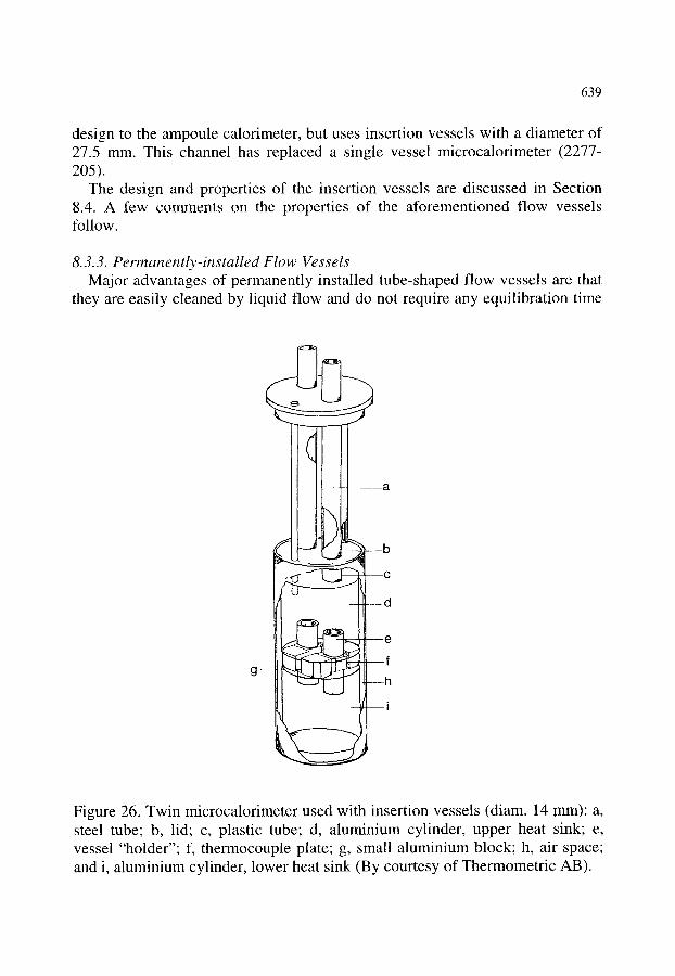
639

design to the ampoule calorimeter, but uses insertion vessels with a diameter of 27.5 mm. This channel has replaced a single vessel microcalorimeter (2277- 205).

The design and properties of the insertion vessels are discussed in Section 8.4. A few comments on the properties of the aforementioned flow vessels follow.

8.3.3. Permanently-installed Flow Vessels Major advantages of permanently installed tube-shaped flow vessels are that

they are easily cleaned by liquid flow and do not require any equilibration time

~ a

b

l -m i

Figure 26. Twin microcalorimeter used with insertion vessels (diam. 14 ram): a, steel tube; b, lid; c, plastic tube; d, aluminium cylinder, upper heat sink; e, vessel "holder"; f, thermocouple plate; g, small aluminium block; h, air space; and i, aluminium cylinder, lower heat sink (By courtesy of Thermometric AB).

640

in addition to the residence time in the heat exchange system. For example, it is possible to pass a liquid flow directly from refrigerator temperature to a flow vessel, kept at 37 ~ in less than 5 min (flow rate 20 cm 3 h-l). The main use of the flow-through vessel is for investigations of living cells (see comments below).

b

b--- c

A B C

Figure 27. Three TAM twin microcalorimeters. A, one equipped with a permanently installed flow-through vessel: a, heat exchange coil; and b, combined "vessel holder" (see e in Figure 26) and flow through vessel made from 24 carat gold. B, one possessing permanently installed flow-through and flow-mixing vessels: a, heat exchange coil; b, flow-through vessel; and c, flow mixing vessel. C, schematic picture of a twin microcalorimeter used with insertion vessels (diameter 27.5 mm). (By courtesy of Thermometric AB).

The mixing vessel is also used in studies of cell suspensions but, more importantly, in solution chemistry for mixing/reaction of two liquids. If a continuous flow is used, the reaction time must obviously be shorter than the residence time of the reaction mixture in the vessel. Applications include titration experiments where, usually, the concentration of the reagent in one

641

liquid stream is held constant, whereas the concentration of the other one is increased, stepwise or continuously. However, it is felt that for most experiments of that kind, e.g. ligand binding experiments, it is usually preferable to use the insertion titration vessel described below (Section 8.4.2).

Two problems with these flow vessels should be pointed out; first, in work with some types of living cells there is a risk that they will adhere to the flow line, including the calorimetric vessel, leading to significant systematic errors; see, for instance, References [83,84]. Secondly, a tube-shaped, flow-through vessel cannot be accurately calibrated with the electrical calibration heater; a chemical calibration must be performed ~ see Sections 3 and 4, as well as the discussions in References [1,7,9,26,83].

8.4. Microcalorimetric Insertion Vessels Thermometric markets several different insertion vessels which can be

separated into two groups: closed (static) ampoules and the more complex titration/perfusion vessels.

8.4.1. Closed Ampoules Closed ampoules of standard type include 2, 4 and 20 cm 3 vessels made from

acid proof steel (which can be rhodium plated) or 18 carat gold. Glass ampoules, volume 3, 4 and 20 cm 3 are often used as disposable vessels (e.g. in studies of hydration of cement and polymerization processes). The lids of the metal ampoules are sealed by use of thin O-rings which do not show any significant relaxation effect, see Reference [22]. The glass vessels are sealed with teflon-covered rubber discs by means of an aluminium cap crimped onto the glass rim.

The ampoule calorimeters (Figures 26, 27C), used with closed ampoules, are the most sensitive and the most stable of the Thermometric calorimeters, see Table 7. As may be expected, installation of gold tube flow vessels to some extent decreases these properties, see also Reference [22], as does the use of more complex insertion vessels.

Closed ampoules are mainly utilized to investigate slow processes for which no agitation is required and where it is not necessary to initiate the process in the reaction vessel. Typical examples of applications include stability and compatibility measurements of pharmaceutical compounds, explosives, batteries, foodstuffs and metabolic studies of living materials (see, however, the comments below). In ecology, where soil and sediments are studied, and in investigations of slow curing processes (cement, polymers), these simple vessels are often the preferred choice. Figure 28 shows results from long term baseline stability measurements using empty 4 cm 3 ampoules. Figure 29 shows

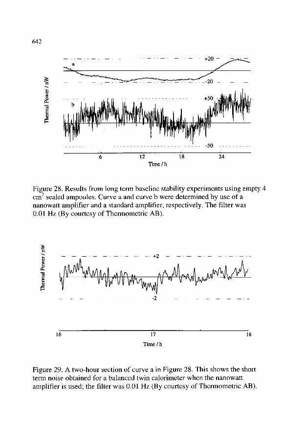
6 4 2

+ 2 0 - - ~ a

.......

20 . . . . . .

. . . . . . . . . . . . . . . . . . . . . . . . . . . . . . . . . . + ot

. . . . . . . . . . . . . . . . . . . . . . . . . . . . . . . . . . . . . . . . . 50 . . . . . . . . . . .

i2 18 24 T i m e / h

Figure 28. Results from long term baseline stability experiments using empty 4 cm 3 sealed ampoules. Curve a and curve b were determined by use of a nanowatt amplifier and a standard amplifier, respectively. The filter was 0.01 Hz (By courtesy of Thermometric AB).

,_. . . . . . . . . n-L . . . . . . . . . . . . . . .

O

, , , ,

~ r- " v ~ " V V ~ V ~ V ~~ v TM

. . . . . . . . . . . . . . . . . . . . . . . . . . . . . . . . . . .

16 17 18

T i m e / h

Figure 29. A two-hour section of curve a in Figure 28. This shows the short term noise obtained for a balanced twin calorimeter when the nanowatt amplifier is used; the filter was 0.01 Hz (By courtesy of Thermometric AB).

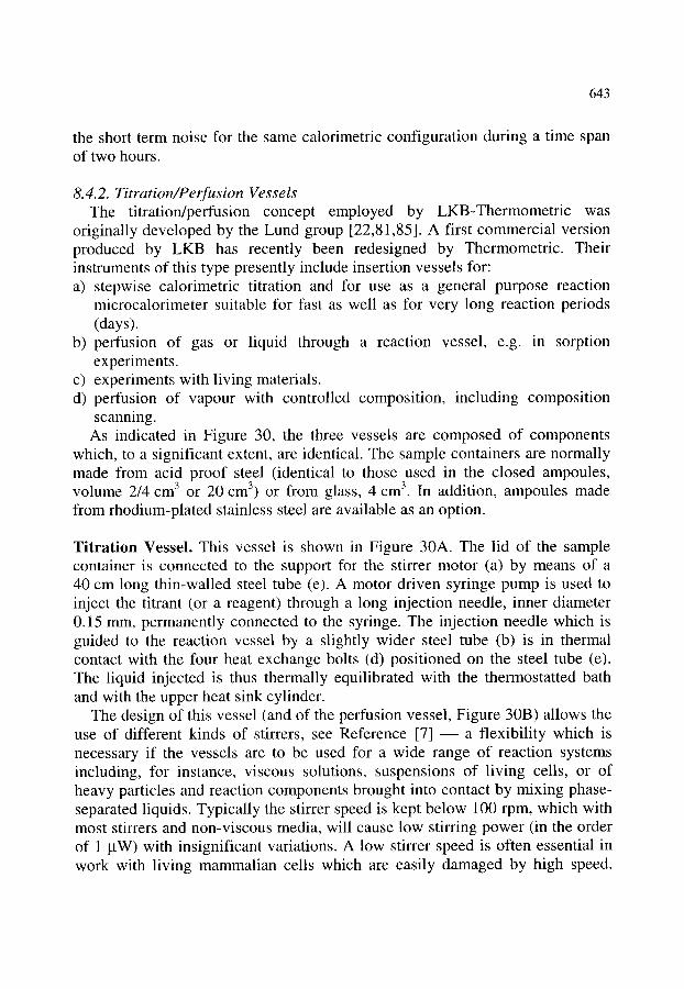
643

the short term noise for the same calorimetric configuration during a time span of two hours.

8.4.2. Titration/Perfusion Vessels The titration/perfusion concept employed by LKB-Thermometric was

originally developed by the Lund group [22,81,85]. A first commercial version produced by LKB has recently been redesigned by Thermometric. Their instruments of this type presently include insertion vessels for: a) stepwise calorimetric titration and for use as a general purpose reaction

microcalorimeter suitable for fast as well as for very long reaction periods (days).

b) perfusion of gas or liquid through a reaction vessel, e.g. in sorption experiments.

c) experiments with living materials. d) perfusion of vapour with controlled composition, including composition

scanning. As indicated in Figure 30, the three vessels are composed of components

which, to a significant extent, are identical. The sample containers are normally made from acid proof steel (identical to those used in the closed ampoules, volume 2/4 cm 3 or 20 cm 3) or from glass, 4 cm 3. In addition, ampoules made from rhodium-plated stainless steel are available as an option.

Titration Vessel. This vessel is shown in Figure 30A. The lid of the sample container is connected to the support for the stirrer motor (a) by means of a 40 cm long thin-walled steel tube (e). A motor driven syringe pump is used to inject the titrant (or a reagent) through a long injection needle, inner diameter 0.15 mm, permanently connected to the syringe. The injection needle which is guided to the reaction vessel by a slightly wider steel tube (b) is in thermal contact with the four heat exchange bolts (d) positioned on the steel tube (e). The liquid injected is thus thermally equilibrated with the thermostatted bath and with the upper heat sink cylinder.

The design of this vessel (and of the perfusion vessel, Figure 30B) allows the use of different kinds of stirrers, see Reference [7] ~ a flexibility which is necessary if the vessels are to be used for a wide range of reaction systems including, for instance, viscous solutions, suspensions of living cells, or of heavy particles and reaction components brought into contact by mixing phase- separated liquids. Typically the stirrer speed is kept below 100 rpm, which with most stirrers and non-viscous media, will cause low stirring power (in the order of 1 gW) with insignificant variations. A low stirrer speed is often essential in work with living mammalian cells which are easily damaged by high speed.

644

m

" b

c

i d

g

A B C

Figure 30. Titration - perfusion insertion vessels (14 or 20 mm diameter). A, Titration vessel; a, stirrer motor; b, steel tube (guide tube for injection needle); c, "flow divider"; d, heat exchange aluminium bolt; e, steel tube; f, sample container (2, 4 or 20 cm3); and g, "turbine" stirrer. B, Perfusion vessel. C, Vapour perfusion vessel ("RH cell"), h, gas flow switch valve; and i, vapour saturation cup. (By courtesy of Thermometric AB).

Even protein molecules may be destroyed if the vessel or the stirrer design requires a very high stirring rate.

A stepwise microcalorimetric titration may be conducted with a gas phase present or with the sample container completely f i l l e d - the "Gill technique" [86]. Typically 1 to 5 ~tL titrant is added in each step. The recommended injection technique employs the Thermometric syringe drive (Model 6120) and a Hamilton syringe permanently connected to a very thin needle which is introduced into the sample container by use of a thin guide tube (b) made from acid proof steel. It is possible to make additions with a precision in the order of 10 nL.

A stepwise calorimetric titration, which may lead to values for the equilibrium constant(s) and the enthalpy change(s) and thus also for entropy

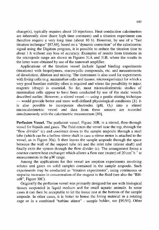
645

change(s), typically requires about 10 injections. Heat conduction calorimeters are inherently slow (have high time constants) and a titration experiment can therefore require a very long time (about 10 h). However, by use of a "fast titration technique" [87,88], based on a "dynamic correction" of the calorimetric signal using the Digitam program, it is possible to reduce the titration time to about 1 h without any loss of accuracy. Examples of results from titrations in the microjoule range are shown in Figures 31A and 31B, where the results in ' the latter were obtained by use of the nanowatt amplifier.

Applications of the titration vessel include ligand binding experiments (titrations) with biopolymers, macrocyclic compounds, etc. and measurements of dissolution, dilution and mixing. The instrument is also used for experiments with living cells (e.g. mammalian cells and tissues, microorganisms) for which a very good baseline stability often is required and where the possibility to inject reagents (drugs) is essential. So far, most microcalorimetric studies of mammalian cells appear to have been conducted by use of the static vessels described earlier. However, a stirred vessel ~ using a gentle stirring technique

would provide better and more well-defined physiological conditions [ 1]. It is also possible to incorporate electrodes (pH, O2) into a stirred microcalorimetric vessel and data from these sensors are recorded simultaneously with the calorimetric measurement [89].

Perfusion Vessel. The perfusion vessel, Figure 30B, is a stirred, flow-through vessel for liquids and gases. The fluid enters the vessel near the top, through the "flow divider" (c) and continues down to the sample ampoule through a steel tube (which can be a hollow stirrer shaft in case a stirrer motor is attached to the vessel, as in Figure 30a). It then leaves the sample ampoule through the space between the wall of the support tube (e) and the inlet tube (stirrer shaft) and finally exits the system through the flow divider (c). The arrangement forms a counter-current heat exchanger which allows a flow rate (water) of 20 cm 3 h -1 at measurements in the BW range.

Among the applications for this vessel are sorption experiments involving solutes and gases on solid samples contained in the sample ampoule. Such experiments may be conducted as "titration experiments", using continuous or stepwise increases in concentration of the reagent in the fluid (see also the "RH- cell", Figure 30C).

Originally the perfusion vessel was primarily designed for use with biological tissues suspended in liquid medium and for small aquatic animals. In some cases it can then be acceptable to let the tissue rest at the bottom of the sample ampoule. In other cases, it is better to house the living material in a rotating cage or in a combined "turbine stirrer" - sample holder, see [90,91]. Other

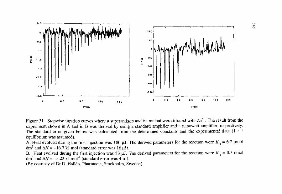
0.5 I

2 0 0

1 0 0

o +

- 1 0 0

2 \ n

- 2 0 0

- 3 0 0

-400

- 5 0 0

I .

0

-0.5

- 1

$ - 1 . 5 n

- 2

-2 .5

- 3

-3.5 ~

0 4 0 8 0 1 2 0 1 6 0

t h i n

I

0 2 0 4 0 6 0 8 0 1 0 0 1 2 0

tlm i n

2+ Figure 3 1. Stepwise titration curves where a superantigen and its mutant were titrated with Zn . The result from the experiment shown in A and in B was derived by using a standard amplifier and a nanowatt amplifier, respectively. The standard error given below was calculated from the determined constants and the experimental data (1 : 1 equilibrium was assumed). A, Heat evolved during the first injection was 180 pl. The derived parameters for the reaction were KD = 6.2 pmol dm3 and AH = -16.7 W mol (standard error was 16 pl). B. Heat evolved during the first injection was 33 pl. The derived parameters for the reaction were KD = 0.3 nmol dm3 and AH = -5.23 kJ mol-' (standard error was 4 pJ). (By courtesy of Dr D. HallCn, Pharmacia, Stockholm, Sweden).

647

biological uses of the perfusion vessel involve experiments with immobilized enzymes.

The Lund laboratory has designed a series of microcalorimetric dissolution vessels for use with gases [30], liquids [92], and solids [93,94] which are modular versions of the Thermometric gas/liquid perfusion vessel. A photocalorimetric system [95] can also be seen as a modular version of the titration-perfusion instrument. Light is introduced into a stirred sample ampoule by means of one or more optical cables. From the same light source another set of optical cables is brought into a dark vessel (a closed ampoule) of a second twin microcalorimeter. With this arrangement it is possible to record, continuously, the radiation power supplied to the photo reaction calorimeter, even if the intensity of the radiation from the light source varies with time.

Vapour Perfusion Vessel ("RH cell"). The idea behind the perfusion vessel shown in Figure 30C stems from original work conducted by Prof. A. Bakri, Universit6 Joseph Fourier, France. This vessel is designed for the perfusion of vapours with defined composition (in particular water vapour), or gas mixtures, over a solid sample contained in the sample ampoule. One difference from the perfusion vessel shown in Fig. 30B is that two of the heat exchange bolts (d) are substituted by vapour saturation cups (i) and that a gas flow switch valve (h) is positioned above the flow divider.

In a vapour sorption experiment, the saturation cups are charged with a vapour-forming substance, e.g. water. In the upper part of the sample ampoule, inert (dry) gas is mixed with a flow of vapour which is formed by letting another stream of inert gas pass the saturation cups. The vapour concentration (e.g. the RH-value; RH - relative humidity) in the upper part of the sample ampoule is determined by setting the flow switch valve which is controlled by the Digitam program. For instance, an RH-value can be kept constant at a predetermined concentration or the switching time can be changed to produce a stepwise or a continuous vapour concentration scan ("ramp"). This may be run upwards or downwards. It is also possible to use the flow switch valve to produce defined mixtures of two incoming gases with or without an active use of the saturation cups. The gas flow switch valve can also be mounted on the regular perfusion vessel shown in Figure 30B.

Presently, the main use of this perfusion vessel appears to be in the chemical industry (in particular the pharmaceutical industry) for investigations of water vapour sorption on powders. Results from such experiments can, for instance, lead to estimates of the extent of highly reactive (unstable) amorphous regions in a crystalline material [96]. Other applications of significant interest include

648

studies of corrosion processes and of biological systems, see the Perfusion Vessel in Section 8.4.2.

8.5. A Note about Calibration of Microcalorimeters Calorimeters produced by Thermometric are equipped with permanently

installed electrical calibration heaters. In order to reach a higher accuracy, some of the vessels can now also be calibrated by use of insertion heaters.

Systematic errors in electrical calibration of the type of microcalorimeters reviewed in this section are discussed in Section 4, but also see References [1,7,9,26,83]. In some cases and especially for modified vessels, it may be difficult to combine a certain experimental function/mechanical design with an accurate electrical calibration technique. In such cases, the operator must use chemical calibrations [ 1,7,26]. Some constructors of calorimeters, in particular microcalorimeters, appear to neglect the vital point of optimizing the calibration technique used with their instruments and, in general, to ignore significant risks of systematic errors in microcalorimetric measurements.

8.6. Key Specification Data for the Thermometric Microcalorimeters It is not a trivial task to report key data for a scientific instrument. Properties

of calorimeters described in scientific papers and in commercial brochures are often poorly defined and are determined under different non-standardized conditions. It is therefore frequently not possible to make a practically useful evaluation of a calorimeter, or a comparison between different instruments, even if extensive documentation is available.

However, it is believed that the data given in Table 7 are among the most important from a user's point of view. There follows some definitions and comments for the values given in this Table which were determined for balanced twin vessels (identical or similar vessels with the same time constants). The volume, V, is the nominal volume of the reaction vessel. The time constant, z, was taken as the time for the decline of the calorimetric signal to 36.8% of its value (following interruption of a steady state heating power). The baseline stability, Pb, is often of crucial importance in measurements of long duration, e.g. in experiments with living cells and in the evaluation of stabilities of technical materials and products. Baseline values were fitted to a straight line by a least squares method in order to obtain the drift (the slope) of the line over a period of 24 h and the standard deviation of the fit. Values given in Table 7 are twice the standard deviation from the ideal straight line with zero slope.

The "detection limit", Po or Qo, is the smallest deviation that can be distinguished from the baseline noise. Po, the deviation in thermal power, was

Table 7 Key Data for Thermometric M i c r o c a l o r i m e t e r s a .

Identification Calorimetric V / c m 3 "t"/s Pb /laW

number vessel Pd / nW

std nW

ampl ampl

649

P I / l a W R / %

-201 closed 4/2 200/300 0.1

ampoule

-202 flow through 0.6 100 0.5 (20 cm 3 h -l)

-204 flow mix 0.6 100 0.5 (20 cm 3 h -l)

-201+2250/2 perfusion 4/2 200/300 0.5 (20 cm 3 h -l)

-201+2255/7 "RH cell" 4/2 200/300 2.0 (100 cm 3 h- l)

2230 closed 20 200 0.2 b

ampoule

2230+2254 perfusion 20 150 0.5 (20 cm 3 h -j)

2230+2259 "RH cell" 20 150 2

(100 cm 3 h- l)

-201+2251/3 Titration 4/2 200/300 0.5

2230+2254 Titration 20 150 1

50 5

50 5

50 5

100 10

200 20

100 10

200 20

400 40

Qd (laJ)

std nW

ampl ampl

25 2

100 10

0.1 0.1

- 0.2

- 0.2

0.5 0.5

0.5 0.5

0.2 0.1

1 0.5

1 0 . 5

0.5

0.5

aInstrument parameters:

V = vessel volume

T = time constant

Pb = baseline stability over 24 h

Pd and Qd = detection limit

Pl = "loading reproducibility"

R = precision

std ampl = standard amplifier

nW ampl = nanowatt amplifier

Unless otherwise stated, the standard amplifier was used in the determinations.

bP b is about 0. ! if nanowatt amplifier is used.

650

determined by perturbing a steady state system with an extended electrical heat pulse. For a titration vessel, an energy quantity supplied by a short electrical heat pulse, Qd, is a more relevant measure of the "detection limit". These limits per unit of volume are of great importance, for instance in stability measurements. For heat conduction calorimeters, estimates of such values are obtained by division of Pa or Qa by V.

The "loading reproducibility", P~, is of crucial importance when values are determined for the thermal power in, for example, stability measurements and in experiments with living cellular systems. For most microcalorimeters, the baseline value will change significantly in connection with loading and/or insertion of a reaction vessel. P~ is usually the property which limits the precision/accuracy by which low thermal power values can be determined. It is of no particular importance in titration experiments where the actual baseline is established before making the first injection. The precision or repeatability, R, for a calorimeter can be determined and expressed in many different ways. Here R is reported as the variation (twice the standard deviation, expressed in per cent) of the value for the calorimetric signal when the vessel is heated electrically with a power of 100 gW. Note that the precision does not include possible systematic errors (which are included in corresponding values for the accuracy). The values listed in Table 7 were communicated by Drs J. Suurkuusk and A. Sch6n, Thermometric AB.

8.7. The Precision Solution Calorimeter 2225 As pointed out in the Introduction (Section 8.1.), the Thermometric Precision

Solution Calorimeter is a modern version of the classical LKB 8700 "macro" calorimeter. The calorimeter is a "semiadiabatic" ("isoperibol") reaction and dissolution calorimeter. The reaction vessel is practically identical with the vessel in the LKB instrument and its properties have thus been tested and evaluated in numerous investigations. The electronic system is entirely new and the experimental control, data acquisition, presentation and analysis of results are now computerized. The new instrument is designed to fit the precisely thermostatted Thermometric water bath and can thus be taken as part of the TAM instrument system. However, the electronic units and the computer program are different from those used with the microcalorimeters.

The 2225 calorimeter is shown in Fig. 32. The vessel (b), volume 100 cm 3, is made from Pyrex glass and is equipped with a temperature sensor (c, a thermistor) and an electrical calibration heater (e) which are in close thermal contact with the stirred reaction medium. In its centre is a combined stirrer and sample ampoule holder made from 18 carat gold. Glass ampoules (f), volume 1 cm 3, are cylindrical with very thin end walls which are broken when the stirrer

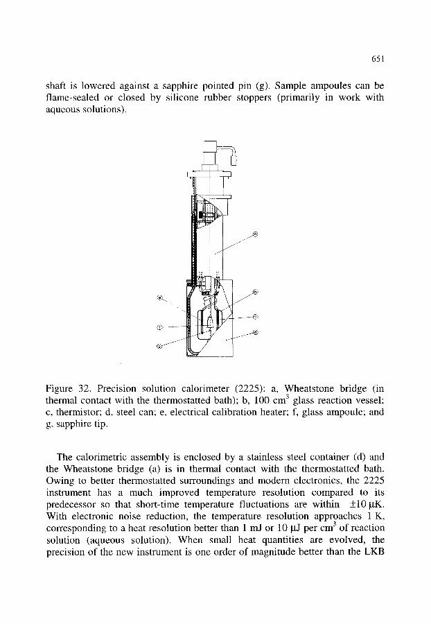
651

shaft is lowered against a sapphire pointed pin (g). Sample ampoules can be flame-sealed or closed by silicone rubber stoppers (primarily in work with aqueous solutions).

j . / f

Figure 32. Precision solution calorimeter (2225)" a, Wheatstone bridge (in thermal contact with the thermostatted bath); b, 100 cm 3 glass reaction vessel; c, thermistor; d, steel can; e, electrical calibration heater; f, glass ampoule; and g, sapphire tip.

The calorimetric assembly is enclosed by a stainless steel container (d) and the Wheatstone bridge (a) is in thermal contact with the thermostatted bath. Owing to better thermostatted surroundings and modern electronics, the 2225 instrument has a much improved temperature resolution compared to its predecessor so that short-time temperature fluctuations are within +_10 ~tK. With electronic noise reduction, the temperature resolution approaches 1 K, corresponding to a heat resolution better than 1 mJ or 10 ~tJ per cm 3 of reaction solution (aqueous solution). When small heat quantities are evolved, the precision of the new instrument is one order of magnitude better than the LKB

652

instrument. When rather large heat quantities for a fast process (about 100 J) are measured, the precision and accuracy of the Thermometric instrument are about the same as for a skillfully operated LKB instrument: precision about 0.02% and accuracy 0.05% (+2o).

The instrument is used in the area of classical solution thermodynamics, for instance in dissolution of pure compounds in water and in other solvents. Among applications of more practical interest one may note very precise dissolution measurements of solid pharmaceutical substances, giving information about possible polymorphism [97]. Wetting and swelling experiments of various technically important materials are other important areas in the applied field.

9. SOME OTHER COMMERCIALIZED DESIGNS

R.B. Kemp

Institute of Biological Sciences, University of Wales, Aberystwyth, Penglais, Aberystwyth, SY23 3DA, Wales, United Kingdom.

9.1. Introduction As stated in the general Introduction, in the early days calorimeters were

designed and built as specialist instruments. Individual designs are still quite common, more so than in many fields of physicochemistry and this penchant is in the search for greater accuracy and/or precision and/or the need to make novel vessels for investigating particular problems in scientific research. These "tender-loving-care" machines are too numerous to describe in a relatively short chapter and the reader is referred to References [5,7,9,10] for the necessary details. The following account is not exhaustive but pays attention to some important commercialized designs not covered elsewhere in the chapter.

9.2. MicroCal Calorimeters Of the commercial instruments not within the personal experience of the

present authors, those originating from Brandt's laboratory [98] and manufactured by MicroCal Inc., 22 Industrial Drive, Northampton, MD01060, USA, are significant types. One of their instruments is an adiabatic, titration microcalorimeter (Omega) with a very fast response time. This can be adjusted using a digital potentiometer, the fastest being 6 to 7 s half-time response. As can be seen in Figure 33, the two vessels are permanently mounted on either side of a semiconducting thermocouple plate containing 264 orientated crystals of bismuth telluride. This functions as a differential thermometer and not, as

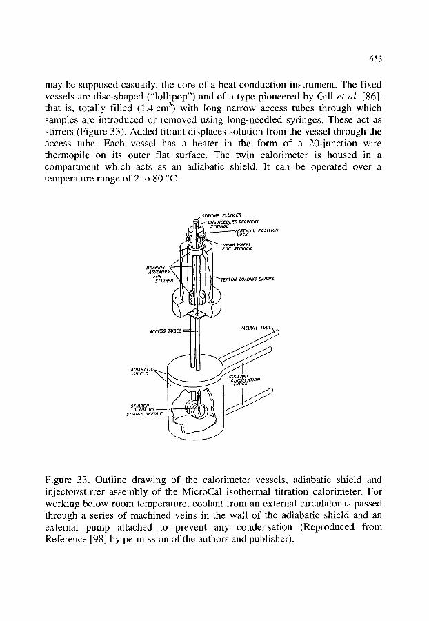
653

may be supposed casually, the core of a heat conduction instrument. The fixed vessels are disc-shaped ("lollipop") and of a type pioneered by Gill et al. [86], that is, totally filled (1.4 cm 3) with long narrow access tubes through which samples are introduced or removed using long-needled syringes. These act as stirrers (Figure 33). Added titrant displaces solution from the vessel through the access tube. Each vessel has a heater in the form of a 20-junction wire thermopile on its outer flat surface. The twin calorimeter is housed in a compartment which acts as an adiabatic shield. It can be operated over a temperature range of 2 to 80 ~

...g...SYR INGE PLUNGER ~=ii~.~LONG NEEDLED DELIVERY

�9 .~1 I '~ SYRINGE .~....| |'.~.~_._.---.-----~ERTICAL PO$1 rtotv (.~ ~1 IIJJJ- LOCK

A ~ J ~ " ~ ~ T/MINe WHEEL . ~ ~ FOR STIRRER

BEARING .r I I I ,,,..,.,E,,,,,..Y\ It I I.IIM I \ I

FOR . . . . x , , , I " I I I I I '~I ~ , [~|,| , |,'~TEFLON LOADING BARREL SI"IRRER r k l N I l ! I I I

ACCESS TUBES U

S,,ELD ~ ' b ' , ~,4%00LXNT _

TUBES

BLADE ON.------. - ~ SYRINGE NEEDL E

Figure 33. Outline drawing of the calorimeter vessels, adiabatic shield and injector/stirrer assembly of the MicroCal isothermal titration calorimeter. For working below room temperature, coolant from an external circulator is passed through a series of machined veins in the wall of the adiabatic shield and an external pump attached to prevent any condensation (Reproduced from Reference [98] by permission of the authors and publisher).

654

In the course of an experiment, a constant power (_<1 mW) is dissipated in the heater of the reference vessel. This activates a feedback circuit to drive the temperature difference back to zero. In the absence of a reaction in either of vessels, the feedback power is constant at the baseline value. An exothermic reaction in the sample vessel decreases feedback power, while an endothermic reaction increases it. So, Omega is a heat compensation instrument (see Chapter 1, Section 1.2.5 and this Chapter, Section 2.4). Values for the enthalpy of reaction are obtained by computer integration of the deflections from the baseline power value.

The authors [98] state that the best performance allows the equilibration time between injections for a fast chemical process to be only 90 s. To emphasize this point, a titration experiment with 10 direct data points (not the total capacity for points) may then be completed in less than 30 min, allowing 2 min between each injection. This makes the instrument a highly competitive isothermal titration calorimeter (to make a comparison, see Sections 5.2.5 and 8.4.2), especially as the time for equilibration after emptying, cleaning and refilling the vessels for the next experiment is also very short owing to the absence of a heat sink. The detection limit of the instrument (expressed as the minimum detectable heat quantity) is reported [31] to be 1.3 gJ. This is about the same as that claimed for a Freire's "home-built" calorimeter, having features in common with the Gill machine [86] ,which was also designed for titration measurements [99]. MicroCal's instrument is also very sensitive, having a volume-normalized sensitivity of 0.8 J cm 3. Commercially, it is similar in performance to CSC Model 4200 isothermal titration calorimeter (see Table 4), having a time constant of 13 s and a 24-h baseline stability of 0.02 gW.

"Ultrasensitive titration microcalorimetry", as MicroCal has styled it, is finding very considerable application these days, particularly in the field of biomolecular interactions (see Reference [100]). Within this area, the Omega isothermal titration instrument is making a great impact in studies of protein interactions with small ligands, such as the binding of carbohydrate to lectins [101] and of tyrosyl phosphopeptides to Src homology 2 (SH2) domains [102]. Many papers have also been published using it to investigate ~ (i) interactions of DNA (see, for instance, Reference [ 103]) and DNA to protein (reviewed in Reference [104]); (ii) lipid (for example, Reference [105]) and lipid to protein (see, e.g. Reference [106]) and, (iii) protein to protein (see Reference [107]). A particularly important aspect of the latter is antibody-antigen interactions and these are exemplified by two studies of monoclonal antibodies binding to cytochrome c [108,109]. Of course, antibodies can be directed against carbohydrates and the Omega microcalorimeter has been used to investigate, for instance, the binding of heparin to human antithrombin III [ 110]. These studies

655

of immunoglobulin interactions are further evidence of the role of titration microcalorimetry in elucidating the binding properties of biomolecules. The list of applications for the MicroCal instrument has been extended to receptor interactions, such as the serine receptor of bacterial chemotaxis [111], and to enzyme kinetics, for example the activity of cytochrome c oxidase [ 112]. It goes without saying that the uses of titration calorimeters are not exclusive to interactions and, among the other applications for the Omega instrument, are studies of protein folding, for instance salt-induced formation of the molten globule state of cytochrome c [ 113].

MicroCal also manufactures a high performance, heat compensation DSC (MC-II) with a temperature range of 0 to 115 ~ The reaction vessel is a fixed, closed 1-cm 3 ampoule. The time constant of the instrument is 13 s and it has a baseline stability of 2gW over 24 h. Its detection limit is comparable to that of the CSC Model 4100 (see Section 5.2.2). Both have the capability to detect changes in heat capacity of 40 gJ per ~ and a baseline repeatability of about 100 gJ per ~ at a scan rate of 1 ~ mm -~. The MicroCal DSC cannot be operated in an isothermal mode.

9.3. BRIC Calorimeters Lovrien and his group [114,115] have built several different types of heat

conduction differential calorimeter. These have been reviewed by Wads6 [5] and include batch and flow designs for solution, reaction, perfusion and titration calorimetry. They are characterized generically by the use of Peltier (thermoelectric) pumps to maintain a long-term stable baseline (0.5 to 1 gV) by transferring small pulses of heat to or from the ambient air outside and the aluminium shell around the central calorimetric units. These pumps provide a controlled environment inside the instruments without resort to massive heat sinks. This means that the time to equilibration after loading a batch vessel is quite fast, at about 15min [115]. In terms of sensitivity, the instrument detects 7 gW sample heat input per gV signal output in the range 5 to 50 mJ +5% for 5 cm 3 vessels. In a multichannel version, the calorimeter is made by Biotechnology Reactions Instruments and Chemicals Inc. (BRIC, successor to Microcalorimeters, Inc., St. Paul, Minnesota 55108, USA). The instruments have been promoted as integral parts of analytical methods to assay for carbon and for cell numbers in opaque samples containing microbial or animal cells [116]. Thus, it has proved possible to measure petroleum, hydrocarbons, sugars from cellulose hydrolysis and lignin-related phenols, as well as to estimate the number of cells in a medium containing a known amount of "metabolic" carbon.

656

9.4. E S C O Calorimeters Yamamura et al. [117] have designed a thermopile heat conduction

microcalorimeter essentially for use as a stopped-flow instrument in studies of the metabolism exhibited by human and animal cells, as well as by mitochondria. It has a detection limit of 0.5 ktW and a baseline drift of 1 ~W per 24 h at an ambient temperature of between 10 and 30 +3 ~ for that period. The gold flow vessel has a similar volume (0.6 cm 3) to that in the Thermometric equivalent (see Section 8.3.3), but the calorimeter has a water bath with a highly-stable, fixed temperature of 37 ~ It is available as the Thermoactive Cell Analyzer (Model 3000) from ESCO Ltd, Musashino-Shi, Tokyo 180, Japan.

9.5. Mettler-Toledo Calorimeters While most calorimetrists have been searching for ever lower detection limits

and greater sensitivity, a certain type of industrial chemist has been seeking to measure heat changes in reactions at bench (litre) scale, when the amount of heat produced by a chemical system (mW) is not a limitation to accurate measurement. Ciba-Geigy AG (Basle, Switzerland) developed an isothermal reaction calorimeter for determining the heat balance of chemical processes I118]. It was commercialized by Mettler-Toledo AG (Greifensee, Switzerland) as the Reaction Calorimeter, RC-1 and is now a widely used automatic laboratory reactor to study many different aspects of producing chemicals. Since the vessel is glass, qualitative observations can be made of a chemical process, while simultaneously thermal data can give, for instance, the reaction temperature and enthalpy; kinetic data on reaction rate; the heat transfer coefficient; and the specific heat of reaction mass. All this information is vital to the chemical engineer, particularly when contemplating the upscaling of a chemical process. Marison and von Stockar [119] adapted the instrument to study energetic processes in microbial systems.

The RC-1 "mega" calorimeter consists of a 2 dm 3 jacketed glass reaction vessel, through the jacket of which is pumped a silicone oil at a rate of 2 dm 3 s -~ [4]. The temperature of this circulating fluid is controlled by mixing warm and cool amounts of it at a computer-controlled, electronic valve. The temperature in the reactor is measured very accurately and the control algorithm adapts the oil temperature continuously so that the reactor temperature remains constant. The difference between the two temperatures is a measure of the heat flow rate transferred to the jacket and is used to determine that rate in an equation requiring knowledge of the heat transmission coefficient and effective heat transfer area [4].

657

10. COMBUSTION CALORIMETERS

I. Lamprecht

Institut ftir Biophysik, Freie Universit~it Berlin, Thielallee 63, D-14195 Berlin, Germany.

10.1. Introduction Combustion calorimeters have a broad industrial application nowadays, not

only in the traditional sectors of energy and fuel technology or explosives and heat powders, but also in industries concerned with cement and lime, combustible-wastes, disposals and recycling, and in various investigations concerning food or animal feed. Moreover, they remain important scientific instruments for basic (thermodynamic) research in the natural sciences. Most calorimeters require sample sizes of around 1 g, or combustion heats up to 30 kJ, but semimicro bombs for samples of 50 to 250 mg (-- 5 kJ) and also microbombs (10 to 50 mg) are on the market.

In recent years, the number of companies manufacturing combustion calorimeters has been reduced to only a few. J. Peters/Berlin (Germany) was taken over by Haake/Karlsruhe-Germany, and its combustion calorimeter, HC10, is now being sold by C3-Analysentechnik/Baldham (Germany) while the latter's own bomb calorimeter, CP 500, is no longer distributed by them. Gentry/Aiken (S.C. USA) only sells spare parts for their Phillipson microbomb calorimeter and Newham Electronics/London (UK) no longer exists. Besides commercial instruments, however, many home built combustion calorimeters are described in the literature [120-125].

10.2. Compliance with Standard Test Methods Most of the commercial combustion calorimeters are designed to meet the

international specifications given in the various national standards (ASTM, BS, DIN and ISO). Those which apply the procedure of Regnault and Pfaundler (DIN 51900) or the Dickinson formula (ASTM 3286) are listed below: a) ASTM D240-92 entitled Standard Test Method of Hydrocarbon Fuels by

Bomb Calorimeter. b) ASTM D 1989-92a: Standard Test Method for Gross Calorific Value of Coal

and Coke by Microprocessor Controlled Isoperibol Bomb Calorimeter. c) ASTM D3286-91: Standard Test Method for Gross Calorific Value of Coal

and Coke by the Isoperibol Bomb Calorimeter. d) ASTM D4809-90: Standard Test Method for Heat of Combustion of Liquid

Hydrocarbon Fuels by Bomb Calorimeter (Intermediate Precision Method).

658

e) ASTM D5468-93: Standard Test Method for Gross Calorific and Ash Value of Waste Materials.

f) ASTM E711-87: Standard Test Method for Gross Calorific Value of Refuse- Derived Fuel by the Bomb Calorimeter.

g) BS 1016 Part 5, 1977: Methods for Analysis and Testing of Coal and Coke, Part 5, Gross Calorific Value of Coal and Coke.

h) DIN 51 900: Determination of Calorific Values and Calculation of Heat Values with the Bomb Calorimeter. Procedure with Isothermal Jacket.

i) ISO 1928-1976 (E): Solid Mineral Fuels Determination of Gross Calorific Value by the Bomb Calorimeter Method, and Calculation of Net Calorific Value.

10.3. Classification of Combustion Calorimeters The calorimeters described in the preceding sections are designed for

multiple purposes with a main basic instrument and varying vessels ("cells") and accessories for the different applications. Combustion calorimeters are ~ in contrast aimed at only one goal, determination of the combustion heat of solid, liquid or gaseous matter. Moreover, such investigations are always destructive, while research with batch or flow calorimeters may be either destructive or non-destructive.

For a full description of a combustion calorimeter, three characteristics should be given: a) The thermal exchange between the calorimeter proper and the jacket allows a

distinction between adiabatic, isoperibol and heat conduction instruments (see Section 1.2.5 of Chapter 1 and Section 2.3 in this chapter).

b) The calorimeter proper may be designed as a "stirred-liquid calorimeter" or as an "aneroid calorimeter" which works without liquid (the Greek word "neros" means wet).

c) There is a subdivision into "bomb calorimeters" in which the combustion proceeds in a heavy-walled metal container under an oxidant pressure higher than ambient, and "flame calorimeters" in which a gaseous mixture of combustible matter and oxidant burns at atmospheric pressure after leaving a nozzle [ 126].

All the combustion calorimeters detailed below are of the bomb type, most of them isoperibol and "stirred-liquid" Electric calibration by means of the Joule effect is common to all manufactured calorimeters described earlier (Section 4) but none of the commercial combustion instruments uses this method. It is reserved for calorimeters home-built only in the best equipped laboratories [123]. The usual way of calibration is to burn a reference substance of well-

659

known combustion heat. In most cases, this is benzoic acid (certificate value: 26 434 J g-1 ).

10.3.1. Isoperibol Calorimeters In these instruments (Parr 1261, 1271, 1281; IKA C7000; LECO AC-350;

Morat MK-200), the bomb delivers the combustion heat to an exactly determined amount of water contained in a "bucket". Bomb and bucket together are surrounded by a water jacket, which is held at a constant temperature during the test. Temperatures in both the bucket and the jacket are continuously monitored to determine the heat leak of the system and to calculate the necessary corrections. An "equilibrium method" may be applied, whereby the run continues until all the heat produced in the bomb is dissipated to the bucket water and the system comes to its final equilibrium state. A quicker "Dynamic Operation Method" is to compare the momentary temperature profile with a known (standard) curve of the system, enabling the extrapolation of the final temperature to be made without loss of accuracy.

10.3.2. Adiabatic Calorimeters In these calorimeters (e.g. IKA C4000), the temperature difference between

the bucket water and the jacket is minimized to practically zero, thereby avoiding all heat losses. To this end, the temperature of the jacket liquid is regulated very rapidly to the same value as that of the bucket water by means of either an electric heater (Figure 34) or an electrolyte (mainly potassium hydroxide or sodium carbonate) as thermostatic liquid with a controlled electric current. In an adiabatic system, the difference between the initial and the final temperature multiplied by the calorimeter's heat capacity ("water value") gives the combustion heat.

10.3.3. Automatic Combustion Calorimeters The term "automatic" in connection with combustion calorimeters is used

with different meanings or different degrees of automation by the various companies. It should be checked carefully how much manual preparation is necessary for a run and if the cited time per test includes the sample preparation, or is just "machine" time.

10.4. Commercial ly-avai lable Bombs Bombs applied in combustion calorimeters are heavy-walled metal containers

with volumes of 300 to 500 cm 3 which allow for combustion heats up to 30 kJ per sample. In semimicro or microbomb calorimeters the size is reduced to 10 to

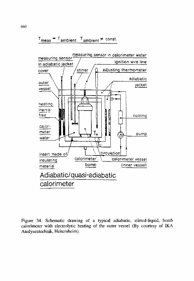
660

Tmeas -- Tambient Tambient "~ const.

mea._.__.ssu rincj senso__._.._sr f in adiabatic j a c k e t / . .

calori- i l l t , I ~ate: ~ F ' _ _

! / \

inse~ made of calorimeter \̀ , insulating

material bomb

measuring sensor in calorimeter water ignition wire line

adjusting thermometer

adiabatic jacket

co_o!in.s

pump

circulation calorimeter vessel

(inner vessel)

Adiabatic/quasi-adiabatic calorimeter

Figure 34. Schematic drawing of a typical adiabatic, stirred-liquid, bomb calorimeter with electrolytic heating of the outer vessel (By courtesy of IKA Analysentechnik, Heitersheim).

661

50 cm 3. They are filled with gaseous oxidants up to pressures of 3 to 4 MPa. Special bombs are available on request: a) chlorine resistant bombs are particularly necessary in disposal and waste

investigations. b) platinum lined bombs are used when a completely inert combustion chamber

is required for subsequent analytical determinations. c) high strength bombs are needed for combustion of explosives, fast-burning

propellants or other reactions of violent character.

10.5. Commercially-available Combustion Calorimeters

10.5.1. Parr Calorimeters The Parr Instrument Company (211 Fifty-Third Street, Moline, IL 61265,

USA) ~ nearly 100 years of experience in the field of calorimetry produces the largest family of combustion calorimeters from fully automatic isoperibol instruments to low-cost, plain jacket instruments.

System 1271. This isoperibol (stirred-liquid bomb) calorimeter is their flag- ship: a modular, fully automatic, microprocessor controlled system with a new bomb device in an inverted position. The head is at the bottom of the bomb cylinder which is firmly attached to the water bucket. The operator just loads the sample into the bomb head, attaches an auxiliary cotton thread fuse and closes the safety guard. All further classical steps of bomb calorimetry are performed automatically, controlled by a microprocessor: pneumatic sealing of the bomb, filling with oxygen, ignition of the sample, monitoring the temperature rise in the bucket water, exhausting the bomb, washing and collecting the combustion residues, opening of the bomb for the next test. Systems 1271 and 1281 operate with on-screen menu programming, and an expanded range of computational capabilities, direct connections to printer, computer and digital balance and an enlarged test memory.

The 340 cm 3 combustion bomb (No. 1131) is used with a greatly reduced amount of bucket water (400 cm 3 instead of the usual 2000 cm 3) so that temperature increases of 10 ~ during combustion are typical instead of just 3 ~ Temperature resolution is 0.0001 ~ and repeatability is 0.10%. Tests after ASTM, DIN or ISO can be performed within 6 min, so that a total of 80 tests per day is possible. By means of an Expansion Module, a second independent system can be operated by the already existing controller, doubling the number of tests per day.

System 1281. This isoperibol (stirred-liquid bomb) calorimeter is identical in its main features with System 1271 except for manual closing of the upright

662

standing bomb and the expansion to a dual system. This calorimeter is thus placed between the full automatic 1271 and the traditional semi-automatic 1261.

System 1261. The Model 1261 is a self-contained operating unit for routine and occasional calorific tests. It is a microprocessor controlled, isoperibol (stirred- liquid) bomb calorimeter with the same temperature resolution and repeatability as Models 1271 and 1281. In this semi-automate, the bucket must be removed from the calorimeter and refilled with water for each test. After this, the microprocessor takes over all steps of the programmed combustion and the data acquisition. Up to 10 samples can be burnt per hour.

A semimicro calorimeter is obtained by applying the Conversion Set 1266 to System 1261. The 342 cm 3 standard bomb (No. 1131) is replaced by a 22 cm 3 bomb (No. 1107) for samples between 25 and 200 mg (up to 5 kJ). This is specially interesting for studies in marine microbiology and ecology.

System 1351. This moderately priced, microprocessor controlled calorimeter is built in the same housing as System 1261 while the temperature controlled water-jacket system is exchanged for a static air jacket. Thus, it is to be considered as a static jacket (stirred-liquid bomb) calorimeter. The instrument should be used in rooms without air draught or fluctuations in the air temperature. A standard deviation of +0.2% can be obtained with benzoic acid as reference substance. All the other semi-automatic features and the oxygen bomb (No. 1108) are the same as in the System 1261.

System 1351. This low price unit with a static jacket is the improved model of a stirred-liquid bomb calorimeter produced for more than 80 years. It is called a "plain" jacket instrument because of its simple construction and is recommended for student laboratories. It houses the No. 1108 oxygen bomb for samples up to 30 kJ and enables 10 to 12 tests to be done per day. Before and after each run, heat leak measurements are taken and temperature corrections computed. Standard deviations with benzoic acid are better than +0.3%. The temperature readings are performed to +0.002 ~

System 1425. Parr's calorimeter range is completed by a compact and easily operated semimicro, static jacket (stirred-liquid bomb) calorimeter housed in a silvered glass Dewar as calorimetric vessel with 400 g water, surrounded by a stainless steel air can. The features are the same as in insert 1266 for the semi- automatic 1261" a 22 cm 3 oxygen bomb (No. 1107), samples between 25 and 200 mg (< 5 kJ). The precision depends upon the heat released, but at an output of 1.5 kJ, it is better than +0.4%.

663

10.5.2. IKA Calorimeters IKA Analyzing Technology (IKA Analysentechnik GmbH, Gril3heimer Weg

5, D-79423 Heitersheim, Germany) produces two oxygen combustion calorimeters with all the necessary accessories.

System C4000. This is a fourth generation adiabatic, stirred-liquid bomb calorimeter with the highest accuracy and reproducibility (Figure 34). Nearly 2000 of the third generation predecessor (C400) were sold in the last 10 years, for all the fields of application mentioned in the introduction (see Section 10.1). Designed according to the DIN 51 900 Standard and meeting all other international standards, it is controlled automatically by a PC, allows for pressures up to 23 MPa and uses platinum resistance thermometers with an accuracy of +_0.001 ~ The internal bucket is filled manually with 1800 cm 3 of water. The adiabatic heating system works with an electrolyte (1.5 g sodium carbonate in 1300 cm 3 water) and shows a drift no larger than 0.0012 ~ within 3 min, corresponding to DIN 51 900, part 3. Only two temperature values before and after each ignition are necessary to determine the combustion heat. The maximum standard deviation is less than 0.25%. The optimal sample size amounts to 1 g. A typical test takes about 15 min of calorimeter time, quick runs with reduced sensitivity are performed within 9 min.

This bomb calorimeter may be used under vacuum or with a special high pressure combustion container (C 49) of 25 c m 3 and an operating pressure of 210 MPa when investigating explosives or pyrotechnic material. The system C4000 may be expanded to a multiple calorimeter with up to eight instruments controlled by the main computer. Moreover, a microcalorimetric kit (C 55) is available for samples between 50 and 250 mg.

System C7000. The most recent member of the IKA family is an isoperibol, aneroid bomb calorimeter arranged in a "doppelt-trocken" (double aneroid) fashion in which the temperature course is determined directly within the calorimetric bomb. A series of 48 temperature sensors is equally distributed over the wall of the bomb (Figure 35) to determine its temperature every 6 s, sending the signals to the processor via contacts incorporated in the bottom of the chamber. This calorimeter thus allows measuring times to be, at best, less than 2 rain, but usually 2 to 5 min. The microprocessor controlled, fully automatic system meets the regulations of ISO 1928 for automatic calorimeters (and also those of ASTM, BS and DIN). It accepts samples of 0.05 to 1.5 g, relative to benzoic acid, with typical masses around 200 mg (corresponding to 1 to 40 kJ) at 3 MPa (maximum 4 MPa). The optimal standard deviation of 0.05

664

to 0.1% is obtained with runs of 7.5 min while, for test times less than 2.75 min, values of 0.5% are typical. Besides the combustion heat, the amounts of halogens and sulphur in the specimen can be determined. To this end, the combustion gases are released in a controlled manner through washing bottles where they are absorbed for further analysis by titration.

/ / 1 j

//

' ! ; -

0 2

j "~" , '~"~

t

i l l

\

Figure 35. Schematic drawing of an isoperibol aneroid bomb calorimeter of the "doppelt-trocken" type (C500, C7000): 1, the aneroid isolation; and 4, the temperature sensors in the double walled combustion bomb. The inner wall consists of a special steel (VA), the outer one of copper. Also shown are: 2, Fuse wire plus cotton thread; 3, sample; and 5, connection to the processor (By courtesy of IKA Analysentechnik, Heitersheim).

665

10.5.3. Digital Data Systems CP500 Calorimeter This is another isothermal aneroid bomb calorimeter with a construction

similar to the C7000 described above in Section 10.5.2. It is a "doppelt-trocken" system with typical sample sizes of 0.5 g, a sensitivity of up to 0.1 J g-l, and measuring times of a few minutes. Up to 16 bombs are automatically identified by the computer through contacts in the bottom of the bomb. The control unit is connected with a balance and a plotter via an interface. An external dry cooling station determines the internal bomb temperature and lowers it to ambient temperatures within 60 to 80 s. This bomb calorimeter is produced by Digital Data Systems DDS (P.O. Box 35872, Northcliff 2115, South Africa) and distributed by DDS, SELBY Scientific & Medical (32 Burnie Avenue, Lidcombe N.S.W. 2141, Australia) and, until 1995, by C3 Analysentechnik (Fuchsweg 50, D-85598 Baldham, Germany), which then discontinued it in favour of two (former) Haake combustion calorimeters.

10.5.4. C3 Analysentechnik Calorimeters This company (Fuchsweg 50, D-85598 Baldheim, Germany) now markets

two combustion calorimeters formerly made by Haake.

System HC10. This isoperibol (stirred-liquid bomb) calorimeter was designed to the regulations of DIN 51 900 Standard, but works in a simpler and more accurate way. The water bucket, automatically filled with 1800 cm 3 water, is fixed in the calorimeter while the bomb is removed for preparation and charging to 3 to 4 MPa. After inserting the bomb, the test further proceeds under microprocessor control with a temperature resolution of 0.00025 ~ and a reproducibility better than 0.05%. The heat leaks are determined and, after about 15 min, the mass specific combustion heat is shown or transduced to plotter and computer. The combustion gases are released and collected under control. The bomb is automatically cooled to the initial temperature in a separate solid state device.

System HC100. This is an isoperibol (aneroid bomb) calorimeter requiring no water at all, its outer jacket being kept constant at 28 ~ (+_0.0015 ~ by Peltier cooling and Joule heating. A copper alloy jacket for quick heat transfer is incorporated instead of the usual water bucket. A built-in precooling unit presets the bomb temperature to 25 ~ After charging the prepared bomb with oxygen, a fully automatic measuring sequence proceeds in four different selectable test times of 3, 8, 16 and 26 min. The slowest test gives a repeatability of 0.05%, while fast orientation runs of 3 min show values of 1%. The linearity of temperature reading is better than 0.0001 ~ Investigations are

666

supported by automatic barcode recognition of up to 14 bombs, on-line graphical and numerical display of important data and three interfaces for balance, printer and computer.

10.5.5. Leco AC-350 Calorimeter LECO Corporation (3000 Lakeview Ave, St. Joseph, MI 49085-2396, USA)

produces an automatic isoperibol (stirred-liquid bomb) calorimeter for nominal 1 g samples or specific combustion heats between 15 and 35 kJ g-~ at 3 MPa. It has a bucket water volume of 2000 cm 3 and a self-contained water supply volume of 15000 cm 3. The temperature resolution amounts to 0.0001 ~ the precision based on benzoic acid is better than 0.05%, the linearity 0.05% and the resolution 1 J g-l. One test takes 7 to 10 min and, in a predictive mode, 5 to 7 min. A 16 bit controller and interfaces for printer, PC and balance are included. As in the predecessor model AC-100, ignition is automatically performed when the equilibrium is reached. The temperature increase is followed to the final equilibrium, determined and transformed into mass specific combustion heats. Corrections for acid, or per cent nitrogen, for fuse wire, sulphur, moisture and spiking can be included in the automatic programme.

The instrument follows the regulations of the ASTM, DIN and ISO Standards.

10.5.6. Morat Automatic MK200 Calorimeter This isoperibol (stirred-liquid bomb) calorimeter is produced by Franz Morat

KG (D-79871 Eisenbach, Germany) conforming to the regulations of the ASTM, DIN and ISO Standards. It should be considered as being semi- automatic, since several steps of a test have to be performed manually. The bomb is firmly attached to the bucket (Figure 36), while a removable part contains the crucible support, the electrodes and the heat shield. The total water volume of the system amounts to 4800 cm 3. The calorimeter has a high temperature resolution of 0.00005 ~ and a reproducibility of _+20 J, which corresponds to a temperature difference of 0.002 ~ Combustion heats of up to 20 kJ, at high accuracy, and up to 40 kJ at usual tests are possible which are equivalent to about 1.5 g benzoic acid. Combustion gases are released in a controlled fashion for further analysis. The system can be connected to a printer and a computer and up to 3 runs per hour are possible.

10.6. Commercial Microbomb Calorimeters Besides the combustion calorimeters mentioned above, which typically use

masses of 1 g and follow the international standards, there are a few semimicro

667

"i! I �9 . +

I =

~ F / ~ ] - < ' -"

[1' i

- - 9 .

Figure 36. Design of an isoperibol, stirred-liquid bomb calorimeter: 1, the whole inner part with 2, the crucible and 3, the support is removable from 4, the bomb which rests firmly attached to 5, the bucket in the calorimeter. The jacket is warmed by 6, an electrical heater or cooled by 7 and 8, a water system (By courtesy of Franz Morat KG, Eisenbach).

668

or microbomb calorimeters for more modest requirements and smaller samples [127]. Two of them are designed according to the original Phillipson calorimeter [128]. The others are accessories to existing microcalorimeters of the heat flow type. The precision of these microbombs is significantly below that of the macrobombs.

10.6.1. Calvet Microcalorimeter Heat-flow aneroid bomb vessels of 58 cm 3 active volume are available for

Calvet microcalorimeters with 100 cm 3 vessels (e.g. type MS 70; SETARAM see Section 7.3.1), but not for the smaller instruments with 15 cm 3 vessels. Bomb vessels may be used at stable, constant temperatures, thus reducing temperature corrections considerably. Moreover, the oxygen pressure can be lowered to 0.1 MPa, or even ambient, owing to the low detection limit of the calorimeters (about 0.4 mJ or 15 lag benzoic acid). The small sizes also eliminate the need for pressure corrections. Samples below 1 mg should be avoided because of parasitic ignition energies and errors in weighing. As one can calculate maximum oxygen pressures in these bombs of 0.1 MPa per mg sample, pressures lower than 0.2 to 0.5 MPa are typical. The heat flow curve due to the combustion is registered until the signal returns to the initial base line. The area under the curve is proportional to the combustion heat. A much quicker way of evaluation is to use the maximum amplitude only, an approach which is correct to 0.5%. This system is described in detail with its advantages and drawbacks in References [ 129,130].

A similar microbomb system (ref. code CMB) is produced by SCERES for its calorimeter HT-100 (see Section 6.2.5) with 100 cm 3 vessels. This microbomb, with a mass of 300 g, a heat capacity of 125 J deg -~, an internal volume of 56 cm 3 and a direct thermopile sensitivity (HT-100 calorimeter) of 35 mV W -], takes samples of usually 10 mg (dry mass) and oxygen pressures up to 10 MPa.

10.6.2. Phillipson microbomb calorimeter In 1964, Phillipson [128] described an inexpensive, miniature aneroid, bomb

calorimeter for samples of 5 to 100 mg dry mass. The idea was to burn rare biological material in small quantities without the necessity to mix these with filler substances like benzoic acid, or Millipore membranes, as is done with the usual large commercial instruments. This easy-to-handle, non-adiabatic instrument consisted of a microbomb of approximately 270 g, a stand supporting the bomb and housing the heat flow meter of eight thermocouples, and a larger aluminium block as heat sink. Bomb and stand may be covered by a polished steel jacket as thermal shield. With benzoic acid as standard and oxygen pressures up to 3 MPa, the accuracy was about 1%. The sensitivity

669

amounted to 1.8 jaV per Joule of combustion heat. The precision with biological material was better than 2.5%.

This microbomb calorimeter was later manufactured in the USA by Gentry Instruments Inc. (1007 Owens St., Aiken S.C. 29801, USA) and in Great Britain in a modified version by Newham Electronics (209a Plashet Rd., London El3, Great Britain). Further details of the latter instrument are given in the paper of Basu and Sale [ 131 ].

The present author found out by chance that the bombs manufactured by Gentry, much smaller in volume (approximately 10cm 3) than those of SETARAM, but with the same diameter, exactly fit into the Calvet calorimeters. Thus, they can be used in this combination with greatly increased sensitivity.

10.7. Conclusions Only a few commercial combustion calorimeters on the market are in

compliance with the international standard test methods cited in Section 10.2. They are not designed for a special field of application, but for all topics mentioned in Section 10.1. A choice between the different instruments will depend mainly on: a) of course, whether the combustion heats determined have to meet the

international standards (Section 10.2) or are only approximate figures; b) the amount of material available for the tests; c) the number of samples that need to be burnt per day; d) the convenience required for the experiments; and, of course, e) the budget of the institution. Manufacturers should be asked for reference lists of customers and perhaps for literature about experiments performed with their own calorimeters in the field of interest.

If less accurate values are sufficient and small sample sizes prevail, as in biochemistry or (marine) ecology, one of the much cheaper microbomb calorimeters may be chosen for the determinations.

A C K N O W L E D G M E N T S

The quite challenging task of editing this work composed of sections from several different sources would have been impossible without my colleague, Dr Yue Guan, who is a computer "wizard". Messers David Jenkins and Antony Pugh of our Photographic Services Unit were "super" at transforming drawings of various quality into acceptable figures.

670

REFERENCES

o

2. 3.

o

5.

.

7.

.

9.

10.

11.

12. 13.

14.

15. 16.

17. 18. 19.

20.

21.

22. 23.

I. Wads6, Thermochim. Acta, 219 (1993) 1. E. Battley, Thermochim. Acta, 250 (1995) 337. U. von Stockar and I.W. Marison. Adv. Biochem. Eng. Biotechnol, 40 (1989) 93. U. von Stockar and I. Marison, Thermochim. Acta, 193 (1991) 215. I. Wads6, in A.M. James (Ed.), Thermal and Energetic Studies of Cellular Biological Systems, Wright, Bristol, 1987, p.34. E. Gnaiger, Pure Appl. Chem., 65 (1993) 1983. I. Wads/5, in K.N. Marsh and P.A.G. O'Hare (Eds.), Experimental Thermodynamics, Vol. IV, Solution Calorimetry, B lackwell, Oxford, 1994, p.267. R.L. Putnam and J. Boerio-Goates, J. Chem. Thermodyn., 25 (1993) 607. C. Spink and I. Wads6 in D. Glick (Ed.), Methods of Biochemical Analysis, Vol. 23, Wiley, New York, 1976, p.123. E. Calvet and H. Prat, in H.A. Skinner (Ed.), Recent Progress in Microcalorimetry, Macmillan, London, 1964, p.35. T.H. Benzinger and C. Kitzinger, in J.D. Hardy (Ed.), Temperature its Measurement and Control in Science and Industry, Vol. 3, Pt. 3, Reinhold, New York, 1963, p.53. I. Wads6, Acta Chem. Scand., 22 (1968) 927. I. Danielsson, B. Nelander, S. Sunner and I. Wads6, Acta Chem. Scand., 18 (1964) 995. J.J. Christensen, R.M. Izatt and L.D. Hansen, Rev. Sci. Instr., 36 (1965) 779. P. Monk and I. Wads6, Acta Chem. Scand., 22 (1968) 1842. I. Lamprecht, W. Hemminger and G.W.H. H6hne (Eds), Calorimetry in the Biological Sciences; Thermochim. Acta (special issue), 193 (1991). R.B. Kemp, Thermochim Acta, 219 (1993) 17. A.E. Beezer and H.J.V. Tyrrell, Sci. Tools, 19 (1972) 13. S.L. Randzio and J. Suurkuusk, in A.E. Beezer (Ed.), Biological Microcalorimetry, Academic Press, London, 1980, p.311. L.D. Hansen, E.A. Lewis, D.J. Eatough, R.G. Bergstrom and D. DeGraft- Johnson Pharm. Res., 6 (1989) 20. R.J. Willson, A.E. Beezer, J.C. Mitchell and W. Loh, J. Phys. Chem., 99 (1995) 7108. J. Suurkuusk and I. Wads6, Chem. Scripta, 20 (1982) 155. N. Langerman and J.M. Sturtevant, Biochemistry, 10 (1971) 2809.

671

24.

25. 26. 27.

28. 29. 30. 31. 32. 33.

34.

35. 36.

37.

38.

39.

40.

41.

42. 43.

44.

45.

46.

47.

S.A. Rudolph, S.O. Boylke, C.D. Dresden and S.J. Gill, Biochemistry, 11 (1972) 1098. L. Gustafsson, Thermochim. Acta, 193 (1991) 145. L.-E. Briggner and I. Wads6, J. Biochem. Biophys. Meth., 22 (1991) 101. F.T. Gucker, H.B. Pickard and R.W. Planck, J. Amer. Chem. Soc., 61 (1939) 459. A.-T. Chen and I. Wads6, J. Biochem. Biophys. Meth., 6 (1982) 297. F.T. Gucker and H.B. Pickard, J. Amer. Chem. Soc., 62 (1940) 1464 D. Hall6n and I. Wads6, J. Chem. Thermodyn., 21 (1989) 519. L.D. Hansen and R.M. Hart, J. Electrochem. Soc., 125 (1978) 842. L.D. Hansen and H. Frank, J. Electrochem. Soc., 134 (1987) 1. L.D. Hansen, D.J. Eatough, E.A. Lewis, R.G. Bergstrom, D. DeGraft- Johnson and K. Cassidy-Thompson, Can. J. Chem., 68 (1990) 2111. D.J. Russell, M.S. Thesis, Brigham Young University, Provo, UT, USA, 1994. P.D. Ross and R.N. Goldberg, Thermochim. Acta, 10 (1974) 143. R.J. Suurkuusk, B.R. Lentz, Y. Barenholz, R.L. Biltonen and T.E. Thompson, Biochemistry, 15 (1976) 1393. R.S. Criddle, R.W. Breidenbach and L.D. Hansen, Thermochim. Acta, 193 (1991) 67. L.D. Hansen, M.S. Hopkin, D.K. Taylor, T.S. Anekonda, D.R. Rank, Thermochim. Acta, 250 (1995) 215. A.J. Fontana, L. Howard, R.S. Criddle, L.D. Hansen and E. Wilhelmsen, J. Food Sci., 58 (1993) 1411. R.S. Criddle, R.W. Breidenbach, A.J. Fontana and L.D. Hansen, Thermochim. Acta, 216 (1993) 147. A.J. Fontana, L.D. Hansen, R.W. Breidenbach and R.S. Criddle, Thermochim. Acta, 172 (1990) 105. L.D. Hansen and R.S. Criddle, Thermochim. Acta, 154 (1989) 81. L.D. Hansen, J.W. Crawford, D.R. Keiser and R.W. Wood, Int. J. Pharm., (1996) in press, L.D. Hansen, M. Afzal, R.W. Breidenbach and R.S. Criddle, Planta, 195 (1994) 1. G. Privalov, V. Kavina, E. Freire, and P.L. Privalov, Anal. Biochem., (1995) in press. L.D. Hansen, T.E. Jensen, S. Mayne, D.J. Eatough, R.M. Izatt and J.J. Christensen, J. Chem. Thermodyn., 7 (1975) 919. L.D. Hansen and R.M. Hart, in P.J. Elving, (Ed.), Treatise on Analytical Chemistry, Part 1, vol. 12, 2nd ed., John Wiley & Sons, New York, 1983, p 135.

672

48.

49.

50. 51.

52. 53.

54.

55.

56.

57.

58. 59.

60. 61.

62.

63.

64. 65. 66. 67. 68. 69. 70.

71. 72.

L.D. Hansen, E.A. Lewis and D.J. Eatough, in K. Grime (Ed.), Analytical Solution Calorimetry, John Wiley & Sons, New York, 1985, pp 57-95. D.J. Eatough, E.A. Lewis and L.D. Hansen, in K. Grime (Ed.), Analytical Solution Calorimetry, John Wiley & Sons, New York, 1985, p 137. L.D. Hansen and E.A. Lewis, J. Chem. Thermodyn., 3 (1971) 35. L.D. Hansen, T.E. Jensen and D.J. Eatough, in A.E. Beezer (Ed.), Biological Microcalorimetry, Academic Press, New York, 1980, p 453. L.D. Hansen and D.J. Eatough, Thermochim. Acta, 70 (1983) 257. R.E. Tapscott, L.D. Hansen and E.A. Lewis, J. Inorg. Nucl. Chem., 37 (1975) 2517. J.J. Christensen, J.W. Gardner, D.J. Eatough, R.M. Izatt, P.J. Watts and R.M. Hart, Rev. Sci. Instr., 44 (1973) 481. D.J. Eatough, J.J. Christensen and R.M. Izatt, J. Chem. Thermodyn., 7 (1975) 417. A.L. Creagh, E. Ong, E. Jervis, D.G. Kilburn, and C.A. Haynes, (1995) submitted. S.M. Habermann and K.P. Murphy Nature: Structural Biology, (1996) in press. L.D. Hansen, Pharm. Technol. (1995) submitted. J.J. Christensen, L.D. Hansen, D.J. Eatough, R.M. Izatt and R.M. Hart, Rev. Sci. Instr., 47 (1976) 730. J.J. Christensen and R.M. Izatt, Thermochim. Acta, 73 (1984) 117. J.J. Christensen, P.R. Brown and R.M. Izatt, Thermochim. Acta, 99 (1986) 159. J.L. Oscarson, X. Chen, S.E. Gillespie and R.M. Izatt, Thermochim. Acta, 185 (1991) 51. J. Gmehling and T. Holderbaum, in D. Behrens and R. Eckermann (Eds.), Preface, in Heats of Mixing Data Collection, Chemistry Data Series, Vol. III, Part 4, DECHEMA, Frankfurt am Main., 1991, p. v. A. Tian, Bull. Soc. Chim. France Ser. 4, 33 (1923) 427. E. Calvet, C.R. Acad. Sci. (Paris) 226 (1948) 1702. P. Boivinet and B. Rybak, Life Sci. Part II, 8 (1969) 11. I. Lamprecht and F.R. Matuschka, Thermochim. Acta, 94 (1985) 161. P. Leydet, C.R. Acad Sci. (Paris), 262 (1966) 48. I. Lamprecht and C. Meggers, Z. Naturforsch. B24 (1969) 1205. I. Lamprecht and B. Schaarschmidt, Bull. Soc. Chim. France, 4 (1973) 1200. F. Baisch, Thermochim. Acta, 22 (1978) 303. B. Schaarschmidt and I. Lamprecht, Exper. 29 (1973) 505.

673

73.

74. 75. 76. 77. 78. 79. 80.

81. 82. 83.

84. 85.

86.

87.

88.

89. 90. 91. 92.

93. 94. 95. 96.

97. 98.

99. 100. 101.

B. Schaarschmidt, I. Lamprecht, T. Plesser and S.C. Mtiller, Thermochim. Acta, 105 (1986) 205. I. Lamprecht and W. Becker, Thermochim. Acta, 130 (1980) 87. P. Schultze-Motel and I. Lamprecht, J. Exp. Biol., 187 (1994) 315. S. Sunner and I. Wads6, Science Tools, 13 (1966) 1. S. Sunner and I. Wads6, Acta Chem. Scand., 13 (1959) 97. G. Olofsson, J. Phys. Chem., 89 (1985) 1473. I. Wads6, Acta Chem. Scand., 20 (1966) 536. G. Olofsson, S. Sunner, M. Efimov and J. Laynez, J. Chem. Thermodyn., 5 (1973) 199. K. Kuseno, B. Nelander and I. Wads6, Chem. Scripta, 1 (1971) 211. I. Wads6, Science Tools, 21 (1974) 18. I. Wads6 in E.A. Beezer (Ed.), Biological Microcalorimetry, Academic Press, London, 1980, p 247. J. Suurkuusk and I. Wads6, J. Chem. Thermodyn., 6 (1974) 667. M. G6rman Nordmark, J. Laynez, A. Sch6n, J. Suurkuusk and I. Wads6, J. Biochem. Biophys. Meth., 10 (1984) 187. I.R. McKinnon, L. Fall, A. Parody-Morreale and S. Gill, Anal. B iochem., 139 (1984) 134. M. Bastos, S. H~igg, P. L6nnbro and I. Wads6, J. Biochem. Biophys. Meth., 23 (1991) 255. P. B~ickman, M. Bastos, D. Halldn, P. L6nnbro and I. Wads6, J. Biochem. Biophys. Meth., 28 (1994) 85. P. B~ickman and I. Wads6, J. Biochem. Biophys. Meth., 23 (1991) 283. B. Fagher, M. Monti and I. Wads/3, Clinical Sci., 70 (1986) 63. P. L6nnbro and P. Hellstrand, J. Physiol., 440 (1991) 385. D. Hall6n, S.-O. Nilsson and I. Wads6, J. Chem. Thermodyn., 21 (1989) 529. S.-O. Nilsson and I. Wads6, J. Chem. Thermodyn., 18 (1986) 1125. D. Hall6n, E. Qvarnstr6m and I. Wads6, to be published. C. Teixeira and I. Wads6, J. Chem. Thermodyn., 22 (1990) 703. L.-E. Briggner, G. Buckton, K. Bystr6m and P. D'Arcy, Int. J. Pharm., 105 (1994) 125. S. Lindenbaum and S. E. McGraw, Pharm. Manuf., 2 (1985) 27. T. Wiseman, S. Williston, J.F. Brandts and L.-N. Lin, Anal. Biochem., 179 (1989) 131. E. Friere, O.L. Mayorga and M. Straume, Anal. Chem., 62 (1990) 950A. A. Cooper and C.M. Johnson, Methods Mol. Biol., 22 (1994) 137. M.C. Chervenak and E.J. Toone, Biochemistry, 34 (1995) 5685.

674

102. J.E. Ladbury, M.A. Lemmon, M. Zhou, J. Green, M.C. Botfield, and J. Schlessinger, Proc. Natl. Acad. Sci. USA, 92 (1995) 3199.

103. D. Rentzeperis, K. Alessi and L.A. Marky, Nucleic Acids Res., 21 (1993) 2683.

104. J.E. Ledbury, Current Biol., Structure, 3 (1995) 635. 105. R.M. Epand and R.F. Epand, B iophys. J., 66 (1994) 1450. 106. J. Seelig, R. Lehrmann and E. Terzi, Molec. Membr. Biol., 12 (1995) 51. 107. A. Cooper and K.E. McAuleyhecht, Phil. Trans. Roy. Soc. A, 345 (1993)

23 108. C.S. Raman, M.J. Allen and B.T. Nall, Biochemistry, 34 (1995) 5831. 109. K.P. Murthy, E.Freire and Y. Paterson, Proteins, 21 (1995) 83. 110. S. Delauder, F.P. Schwarz, J.C. Williams and D.H. Atha, Biochim.

Biophys. Acta, 1159 (1992) 141. 111. L.N. Lin, J.Y. Li, J.F. Brandts and R.M. Weiss, Biochemistry, 33 (1994)

6564. 112. P.E. Morin and E. Freire, Biochemistry, 30 (1991) 8494. 113. D. Hamada, S.I. Kidokoro, H. Fukada, K. Takahashi and Y Goto, Proc.

Natl. Acad. Sci. USA, 91 (1994) 10325. 114. P.C. Anderson and R. Lovrien, Anal. Biochem., 100 (1979) 77. 115. R.H. Hammerstedt and R.E. Lovrien, J. Exp. Zool., 228 (1983) 459. 116. I. Boe and R. Lovrien, B iotechnol. B ioeng., 35 (1990) 1. 117. M. Yamamura, H. Hayatsu and T. Miyamae, Biochem. Biophys.

Res.Commun., 140 (1986) 414. 118. W. Regenass, Thermochim. Acta, 20 (1977) 65. 119. I. Marison and U. von Stockar, Thermochim. Acta, 85 (1985) 493. 120. W.P. White, The Modern Calorimeter, The Chemical Catalog Company,

New York 1928. 121. D.C. Ginnings and E.D. West, in J.P. McCulloch and D.W. Scott (Eds.),

Experimental Thermodynamics, Vol. 1, Butterworths, London, 1968, Ch. 4.

122. J.P. McCullough and D.W. Scott (Eds.), Calorimetry of Non-Reacting Systems, Experimental Thermodynamics, Vol. 1, Butterworths, London, 1968.

123. S. Sunner and M. Mansson (Eds.), Combustion Calorimetry, Experimental Chemical Thermodynamics, Vol. 1, Pergamon Press, Oxford, 1979.

124. W. Hemminger and G. H6hne, Calorimetry ~ Fundamentals and Practice, Verlag Chemie, Weinheim, 1984.

125. M. Frenkel (Ed.), Thermochemistry and Equilibria of Organic Compounds, Verlag Chemie, Weinheim, 1993.

675

126. S. Sunner, in S. Sunner and M. Mansson (Eds.),Combustion Calorimetry, Pergamon Press, Oxford, 1979, p. 13.

127. M. Mansson, in S. Sunner and M. Mansson (Eds.), Miniaturization of Bomb Combustion Calorimetry, Pergamon Press, Oxford, 1979, p. 388.

128. J. Phillipson, Oikos, 15 (1964) 130. 129. E. Calvet and H. Prat, Recent Progress in Microcalorimetry (Ed. and

transl, by H.A. Skinner), Pergamon Press, Oxford, 1963. 130. M. Laffitte, in S. Sunner and M. Mansson (Eds.), Combustion

Calorimetry, Pergamon Press, Oxford, 1979, p. 395. 131. H.A. Basu and F.R. Sale, Thermochim. Acta, 10 (1974) 373.

ASTM - American Society for Testing Materials

BAM - Biological Activity Monitor

BS - British Standard

CSC - Calorimetry Sciences Corporation

DDS - Digital Data Systems

DIN - Deutsche Industrienorm

IKA- Janke und Kunkel Apparate

ISO - International Standard Organization

LECO - Laboratory Equipment Corporation

PTFE- Polytetrafluorethylene

SCERES - Soci~t6 de Conception d'Etude et R~alisation

SETARAM - Societ6 d'Etude d'Automatisation de R6gulation et D'Appareile de Mesures

TAM - Thermal Activity Monitor

INDEX

a (see fractional reaction) a-alumina (see sapphire) a-temperature curves 190,192 a-time curves 166,173,190 a-transition 401 A acceleratory period 167,169 accommodation coefficient 172 accuracy 41,555 acid-base equilibria 590 acoustic emission 460,462,463 acoustic transducer 634 activation energy (Ea) 147,177-184,188, 190,194,293,380,413,414,421,434,436 activation step 181 activity 129,130 activity coefficient 129,130 adiabatic bomb calorimeter 30,663 adiabatic calorimeter 209,562,563, 580,584,659,660 adiabatic conditions 209 adiabatic scanning calorimeter 29 adiabatic scanning mode 28,29 adiabatic shield calorimeter 581,582,653 adsorption 226 alloys 424 alums 155,160 American Society for Testing and Materials (ASTM) 60-63,68,270,348,353, 527,657,658 ammonium perchlorate 167,174 amorphous solids 452 amplification 266 ampoule calorimeter 636,639,641 analog data 263 aneroid calorimeter 658,663-665,668 anisotropic materials 364,365 annealing 330,452-454,460,463 aquatic animals 645 area (see peak area) Arrhenius equation 147,179-184,187, 198,332,378 Arrhenius parameters (Ea and A) 147, 179-184,187-189,207,434 ASTM (see American Society for Testing and Materials)

677

atmosphere control 168,254,299,314, 346,348,352,539,540 atmosphere, self-generating 255 Austin-Rickett equation 163,187 autocatalysis 162,213 automatic combustion calorimeter 659 automation 267 autosampling 344 Avogadro constant 94 Avrami-Erofeev equation 161,163,165,169, 177,178,190-193,198,208,438 B baffles 239 balance capacity 230 balance, electrodynamic 235 balance sensitivity 230 balance, vibrating reed 234 band theory 182,183 baseline 37,38,211,284,288,290,291, 295,298,311,319,341,345,346,573 baseline construction 557, 559 baseline errors 557 baseline, isothermal 560 batch calorimeter 209,210,585,590,631 batch vessel 585,631 benzoic acid 109,566,572,659,662, 663,666,668 beta-transitions 416 binodal curve 131 biological specimens 262 black body radiation 306,319 blank run 350 Boersma DTA (see also heat flux DSC) 281,282 Boltzmann constant 94,408 Boltzmann equation 94,408 bomb calorimeter (see calorimeter, closed bomb) Bose-Einstein statistics 183 Boyle's law 80 British standards 63,68 bubble release 462 buoyancy effects 259,502 C Cahn balance 228,230 calcium carbonate 144,174,248,

678

256,262,435-437 calcium hydroxide 155,167 calcium oxalate 208,513,514,517,525 calibrants 569 calibrant, ideal 561 calibration 2,5,32,268,311,334-342, 547-574,592,610,613 calibration, calorimetric 556 calibration, chemical 591 calibration coefficient 339 calibration curve 549 calibration, electrical 341,556,591, 597,641,650,651 calibration, enthalpy 556,560,562 calibration factors (see also conversion factors) 556,560 calibration, heat capacity 558,560,562,572 calibration, mass 268,270 calibration materials (see also reference materials and calibrants) 552,556 calibration procedures 562 calibration, temperature 269-273,548 calorespirometry 598, 599 calorimeter 3,9,27 calorimeter, adiabatic 562,580,584 calorimeter, adiabatic bomb 30 calorimeter, adiabatic shield 581,582,653 calorimeter, ampoule 636,639,641 calorimeter, aneroid 658,668 calorimeter, automatic combustion 659 calorimeter, batch 585,590,631 calorimeter, closed 585 calorimeter, closed bomb 635,658,661 calorimeter, combustion 591,613, 657,658,663 calorimeter, drop 29 calorimeter, flame 658 calorimeter, flow 585,635 calorimeter heads 614,617 calorimeter, heat accumulating 580,581 calorimeter, heat compensating 580,581 calorimeter, heat conduction 580,581, 583,650 calorimeter, ice 29,578 calorimeter, isoperibol 596,635,651, 663-667 calorimeter, isothermal jacket 320,580,630 calorimeter, open 585 calorimeter, reaction 577,593

calorimeter, semiadiabatic 635 calorimeter size 579 calorimeter, solution 602,638,651 calorimeter, stirred-liquid 658 calorimeter, temperature scanning 596 calorimeter, Tian-Calvet 306 calorimeter, titration 635,653 calorimeter, twin 28,584,585 calorimeter, vaporization 635 calorimetry 1,9,10,75,209,577 calorimetry, definition 1,7-9 Calorimetry Sciences Corporation 595,607,608 capacitance measurements 420 carbon chain motion 393 CaRTA (see constrained rate thermal analysis) catalytic reactions 259,429,431,432,457 cell cultures 600 cellulose 514 cement 457,458,641,657 ceramics 248,389,391 certified reference materials (see CRM) chain branching kinetics 163 characteristics of measured curves 39,40 chart recorder 266 chemical analysis, offline 526-533 chemical calibration 591 chemical equilibrium 142 chemical vapour deposition 453 chemisorption 262 Chevenard balance 227 circulation vessel 631 clamping (see DTMA) Clapeyron equation 109-112 classification principles 3,9,27 Clausius-Clapeyron equation 112 Clausius-Mosotti relationship 408,413 clays 156,517,533 closed systems 77,103 CrlRTA (see constant rate thermal analysis) coals 167,262,456,517,525,533 coatings 396,452,453,517 coffee beans 517 cold junction 243,301 cold stage 475 Cole-Cole function 407,412 comb electrode (see interdigitated electrode)

combustion 140,259,657 combustion calorimeters 591,613,663,664 combustion calorimetry 591,657,658, 663,664 compensation effect 184,188 complex reactions 203,204 composites 394,396,525 computer networks 353 concurrent reactions 204 condensation 350,588 conduction calorimetry 210 consecutive reactions 204,205,213 constant pressure processes 89 constant rate thermal analysis (CRTA or CnRTA) 189,425,427,429-433,438 constant volume processes 89 constrained rate thermal analysis (CaRTA) 427,430,432,433,438 contact resistance 552 contracting area 162,170 contracting geometry models 161,170, 192,193 contracting volume 162,164,170 controlled rate thermal analysis (CrRTA or CRTA) 241,247,423,425,426,429 controlled transformation rate thermal analysis 425 convective (resistive) heating 237 conversion factor (see also calibration factor) 554,556,560,561 conversion function, f(a) 169-172,438 cooling 237,313,314,330,548,553,555,556 cooling curve 12 coordination compounds 156,517 copper 572 copper nitrate (basic) 520-522 copper oxalate 539,540 copper sulphate pentahydrate 155,160, 167,250,514-516 correlation factor 409-411 corrosion 517,520,522 coupled techniques (see simultaneous techniques) creeping 262 critical point 109,131 critical temperature 131 CRM (certified reference materials) 6,563 CRM, metals 564 CRM, organic 565

679

CrRTA(see controlled rate thermal analysis) CRTA (see constant rate thermal analysis) crucibles 308-311,350,548 crystal defects 149,452-454,460 crystal fracture 462 crystal imperfections (see crystal defects) crystallization 486 Curie temperature 114,271,272 Curie temperature calibration 271,272 curve, characteristic points 37-40 cylinder-type DSC 17 D d a / d T - temperature curves 193 d a / d t - time curves 166 data acquisition 263,267 data processing 263,616 Davidson-Cole function 407,408 DeBye model of dipole behaviour 403,405- 407,413 deceleratory period 167,170 deconvolution 35,321,604 decrepitation 262 definitions 1,7, 8 deformation polarizability 410 dehydration 151,152,155,156,160,166,168, 215,456,460,463,481,482 demixing 131,132 demixing region 131 density 297 derivative 12,287 derivative kinetic methods 178,191, 196-199,201 derivative kinetic methods (second derivative) 197 derivative thermogravimetry (see DTG) Derivatograph 227 detection limit 648,650 diamagnetism 225,236 diamond 110,482,483 dielectric analysis 401-422 dielectric analysis, electrode geometry 416,417 dielectric analysis, instrumentation 416 dielectric analysis, nomenclature 421 dielectric constant 401 dielectric constant, complex 401 dielectric constant, relaxed 405

680

dielectric constant, unrelaxed 405 dielectric loss factor 401,403,413 dielectric loss factor, effect of moisture 416 dielectric loss factor, temperature dependence 413 dielectric loss tangent 403,423 dielectric response 401 dielectric techniques 401-422 dielectric thermal analysis (DETA) 24,325,401 differential enthalpic analysis (see also DSC) 282 differential methods (see also derivative methods) 10,28 differential principle 618 differential scanning calorimetry (see DSC) differential thermal analysis (see DTA) differential thermal analyzer 285 diffusion 149-151,153-156,161,163-165, 168,170,172,173,193,206,432,433,446, 447,450,453,454,456,482 diffusion coefficient 453 diffusion models 153,163,192,193,438 dilatometry 21,113,428,429,464 DIN (Deutsche Industrienorm) 63,64, 69,303 dipole moment 401,410,413,519 dipole orientation 404 dipole relaxation time 404,405 discriminatory kinetic methods 191,207 dissolution vessel 647 dolomite 435,436 "doppelt-trocken" (see double aneroid) double aneroid calorimeter 663,664 draw ratio 365 DSC 16-19,29,30,263,279,282, 284,288,299,397,597,600,629,630 DSC, calibration 334-342,547-575 DSC, Calvet principle 304 DSC, cylinder type 17,18,306 DSC, derivative 287 DSC, disk type 17,306 DSC, heat flux 16-18,30,281-288,296, 304,306,307,318,320 DSC, high pressure 287,315 DSC, high sensitivity 287 DSC, interpretation 345-352 DSC, modulated temperature (see modulated temperature DSC)

DSC, photo 287,315 DSC, power compensation 16,18,29, 283-288,296,304-307,318,320,551,555, 559,560 DSC, self referencing 286,307 DTA 10,12,15,253,263,279, 282-284,288,299 DTA, calibration 334-342 DTA, interpretation 345-352 DTA, optical 306 DTA, qualitative 304 DTA, quantitative 304 DTA, single 286,308 DTG 263-265,293 DTM 271,272 DTMA, clamping errors 387-389 DTMA, dynamic range 389 DTMA, geometric constants 387 DTMA, modes 386 DTMA, sensitivity 392 Dunwald-Wagner equation 165 Du Pont DSC 340 dynamic methods (see non-isothermal methods) dynamic mechanical analysis (DMA) 325,363,374,429 dynamic mechanical thermal analysis (DMTA) (see dynamic thermomechanical analysis (DTMA) dynamic rate TGA 425,427,430,433,438 dynamic thermomechanical analysis (DTMA) 21,363,373-398

E EGA (evolved/exchanged gas analysis) 26,226,255,263,320,430,509-540 EGD (evolved/exchanged gas detection) 26,226,255,320 elastomers 392, 517 electrical calibration 581,597,641,648,658 electrical conductivity 317,319 electrical heaters 587,592 electrical polarization 403,404 electrical work 84 electrobalance 228-236 electrobalance, high capacity 231 electrobalance, single pan 229,233 electrode geometries 401 electrode polarization 412

electrodes, comb 420 electrodes, interdigitated 419 electronic energy 182 electronic polarization 404 emanating power 450 emanation thermal analysis (ETA) 26, 445-459 emissivity 241,306,317,319,560 endoscopy 634 endothermic processes 19,654 energy dispersive powder diffraction (EDPD) 316 enthalpy 83,89,90,281,447,449 enthalpy change for ionization 590 enthalpy change for oxygen dissolution 589 enthalpy of combustion 140 enthalpy of dissolution 592 enthalpy of formation 139 enthalpy of fusion (melting) 564,565 enthalpy of mixing of fluids 126,320,606 enthalpy of reaction 136,139-142,593,654 enthalpy of sublimation 112,320 enthalpy of transition 111 enthalpy of vaporization 112,320,587,588 entropy 92 entropy, molecular interpretation 93 entropy of activation 181 entropy of mixing 125 entropy of reaction 139 enzyme reactions 627 equilibrium 76,99,142 equilibrium between mixed states 133-135 equilibrium, chemical 142 equilibrium constants 213 equilibrium, heterogeneous 77 equilibrium melting temperature 551 equilibrium, thermal 78 errors in DSC or DTA 351 ESCO calorimeters 656 ethylene carbonate 566 European standards 64,65 eutectic 484,553 eutectic formation 156,215 eutectic phase diagram 136 eutectic point 136 evaporation 588 evolved/exchanged gas analysis (see EGA) evolved/exchanged gas detection (see EGD)

681

evolved/exchanged gas determination 26 excess enthalpy 129 excess Gibbs energy 126 excess thermodynamic potential 130 exothermic processes 654 expansion coefficient, linear 364,365 expansion coefficient, volume 364,365 explosives 488 exponential law 157,169 extensive quantities 76 extent of reaction (see also fractional reaction, a) 137 extrapolated onset 548,549 F Faraday balance 225 feedback 9 Fermi-Dirac statistics 183 ferrimagnetism 225,236 ferroelectric materials 525 ferromagnetism 225,236 fibres 343,365,373,387 Fick's laws 154 fictive temperature 571 films 343,365,373,387 finite difference simulation 293,294 first law of thermodynamics 82,85 first-order kinetics 171,213 first-order phase transitions 113 flow calorimeter 30,211,585,586,588,638 flow-mixing calorimeters 209,585,623,638 flow rates 254,260 flow-through vessel 585,594,638,639 food 572,610,627,641,657 forced vibration 384 Fourier heat transfer law 317 Fourier transform 210,321,333 Fourier transform infrared spectroscopy (see FTIR) fractional reaction (a) 148,174,434 free energy (see Helmholtz energy) free enthalpy (see Gibbs energy) French standards 67,68 frequency factor (A) 147,181,190,194,434 frictional effects 587 Frohlich theory 410 FTIR (Fourier transform infrared spectroscopy) 509,518-520,52.9,540,541 FTIR, contour plots 519

682

FTIR, stacked plots 519,520 furnace 237-242,299,300,311 fusible-link temperature calibration 271 fusion (see melting) G gamma-transitions 416 gas chromatography (GC) 509 gas flow 260,261 gas flow rate 548 gas thermometry 80,242 Gay Lussac 80 GC-MS 526,529-531,540 GEFTA (see German Society for Thermal Analysis) geometrical models 170,173,178,432,433 German Society for Thermal Analysis (GEFTA) 551-553,572 Gibbs-Duhem equation 122 Gibbs energy 95,96,1.04 Gibbs energy, excess 126 Gibbs energy of formation 139 Gibbs energy of mixing 119-136 Gibbs energy of reaction 136-144 gibbsite 431 Ginstling-Brounshtein equation 164,170 glass, standard 571 glass transition 116-119,312,322-330,333, 364,369,377,392,393,414-416,486,487, 525,561,570,572 glass transition temperature, Tg, 116-119, 287,401,414-416,570 glasses 365,373,391,456,458 glassy state 116 glycerol 117 gold vessels 589 Gouy balance 225 graphite 110,485 growth of nuclei 149,151-153,155, 157-161,165,167,168,191 gypsum 481,482 I-I hazards of operation 348-351 heat 86 heat accumulating calorimeters 580,581 heat capacity 90,211,292,294,297, 322,325,326,338,340,547,580,593, 596,601,612,628,633,656 heat capacity, calibration 340,572 heat capacity, constant pressure 90,91

heat capacity, constant volume 90 heat capacity, kinetic 325,326 heat capacity, non-reversing 326 heat capacity, polynomials 572 heat capacity, reversing 325,326 heat capacity, specific 554,559 heat collimators 619 heat compensating calorimeters 27,28,580,581,601,603,604,655 heat conduction calorimeters 209,212,580,581,583,596,650,656 heat conduction principle 618,634 heat content 82,90 heat exchange 588 heat exchanging calorimeters 28,30 heat filter 477 heat flow 82,322,324,547,609,629 heat flow, non-reversing 324 heat flux DSC (see DSC, heat flux) heat of dilution 592 heat of fusion 557 heat of mixing of fluids 596 heat of reaction 252 heat of transition 557 heat of vaporization 588,633 heat sink 581 heat transfer 289,291-293,296,557,558,570 heat transfer coefficient 292 heaters, electrical 587,592 heaters, insertion 587 heating curve 12 heating elements 239,240 heating power 240 heating rate, fl 186,190,194,252, 293,346,348,351,370,548-550,554 Helmholtz energy 95,96,104 heterogeneous reactions 148,150 high pressure 315,320,606 high pressure vessel 631 high resolution (Hi-Res) TG 249,250 high temperature apparatus 296,306, 463,475,476,625 history of thermal analysis 70-72, 279-284,423-425 homogeneous reactions 148 hot stage 475-478 hot-stage microscopy (see thermomicroscopy) humidity (see moisture content)

hydration 481 hygrometer 429 I ice calorimeter 578 icing 350 ICTAC (see International Confederation for Thermal Analysis) ICTAC reference materials 566-569 IEC (see International Electrotechnical Commission) ignition temperature 322 impedance measurements 420 indirect calorimetry 579 indium 555,564 induction period 167,177,213 inert spacers 563 influence of temperature on reaction rate 179 infrared detector 429,518 infrared gas cell 518 infrared heating 241,242,312 infrared spectroscopy (see also FTIR) 320,509 insertion vessel 635 instantaneous nucleation 157-159 instrument checklist 35 instrument specifications 31 integral kinetic methods 191,200,201 intensive quantities 76 interdigitated electrode 419 interface 77 interface levels 181-184 interferometer 518 internal energy 85 International Confederation for Thermal Analysis and Calorimetry (ICTAC) 8,185, 271,273,285,301,509,571 International Electrotechnical Commission (IEC) 65,66,69 International Standards Organisation (ISO) 66,69 International System of Units (SI) 44,45 International Temperature Scale (1990) 5,81,242,301,337 International Union of Pure and Applied Chemistry (IUPAC) 8,46,57 interpretation of results 41 inverse kinetic problem (IKP) 186,187 ion chromatography (IC) 509,526

683

ion conductivity 402,411 ion implantation 449 ion mobility 412 ion selective electrodes 535 irreversible processes 99,103,327,377 irreversible thermodynamics 76,332 ISO (see International Standards Organisation) isoconversional kinetic methods (see also non-discriminatory kinetic methods) 195, 203,204 isokinetic effect 184 isolated system 77,98 isoperibo128,580 isoperibol calorimeter 596,601,603, 659,661,662,665-667 isoperibol mode 28 isoperibol scanning mode 28 isothermal conditions 9,148,174,209 isothermal jacket calorimeters 580,630 isothermal melting 551,552 isothermal mode 9,28 isothermal yield-time curves 166,173 IUPAC (International Union of Pure and Applied Chemistry) 566 J Jander equation 164 Japanese standards 67,70 JMAEK equation (see Avrami-Erofeev equation) Joule heating effect 584,591,620, 633,658,665 Journal of Thermal Analysis 58,59 K Kanthal 625 katharometer 429 kidney stones 525 kinetic analysis 147-216,433-440 kinetic behaviour, prediction of 205,206 kinetic method, Borchardt and Daniels 198 kinetic method, Carroll and Manche 196 kinetic method, Flynn 196 kinetic method, Flynn and Wall 199 kinetic method, Freeman and Carroll 196 kinetic method, Friedman 196 kinetic method, Kissinger 197,346 kinetic method, Ozawa 198 kinetic model 150,169-171,178,179, 189,191,195,201,206,207

684

kinetic standards 206 kinetics 76,147-216 Kirkwood expression 409 Kirkwood-Frohlich equation 410 Kofler hot stage 473 L laws of thermodynamics, first 82, 85 laws of thermodynamics, second 91,92 laws of thermodynamics, third 94 laws of thermodynamics, zeroth 78 LECO Corporation 268,666 less-common techniques 445 LGC (UK Laboratory of the Government Chemist) 563-565 linear law 157,164 linear response theory 332 linear variable differential transformer (LVDT) 366,384,465 linearity 34 liquid crystals 365,478,491,555,570 liquids 343,344 liquidus 134 liquidus temperature 553 literature of thermal analysis and calorimetry 27-31 literature, conference proceedings 54-58 literature, history 70-72 literature, journals 58,59 literature, journals (special issues) 59,60 literature, reviews 53,54 literature, textbooks 50-53 lithium potassium tartrate hydrate 155 lithium sulphate monohydrate 155,167, 206,437 living cells 640,641,643,655 LKB calorimeters 634,635 logarithmic law 164 loss tangent (see phase angle and also dielectric loss tangent) low temperature 352,623 M macroscopic systems 75 magnetic field 225,236,240,270,271 magnetic intermediates 236 magnetic products 236 magnetic standards 273 magnetic standard temperature calibration 271-274 magnetic suspension balance 258

magnetic transitions 114 martensitic transformation 390,507 mass and weight 227 mass calibration 268,270 mass spectrometry (MS) 429,509-511,609 Maxwell-Boltzmann statistics 180,183 measured curve 36-40 mechanical equivalent of heat 85 mechanism of reaction 150 melting 149,156,157,166,168,184,215, 262,291,324,330-332,337,346,393,454, 456,460,463,467,489,549,553 metabolic rates 597 metals 163,376,382,389,390,552, 563-565,572 metastable phases 456 Mettler TMA 367 Mettler-Toledo Thermomicroscopy-DSC 476,505 Mettler-Toledo TG-DSC 503 Mettler-Toledo TMA-SDTA 504 micro 12 microcalorimeter 429,578,668,669 microdielectric sensor 420 microporosity 429 microscopy 159,176,178,186,463 microwave heating 312 minerals 456,518 miscibility gap 131 mixed states, equilibria 133-135 mixtures, binary 121,129 mixtures, ideal 125,129 mixtures of ideal gases 123 mixtures, real 126,129 mixtures, thermodynamics of 119 mode, adiabatic 28,29,30 mode, adiabatic scanning 28,29 mode of operation 28 mode, isoperibol 28 mode, isoperibol scanning 28 mode, isothermal 9,28 modulated force thermomechanical analysis (mf-TMA) 21 modulated temperature DSC (MTDSC) 189,247,284,286,319,334,555,570,571 MTDSC, calibration 327 modulation 9,323,333 modulation amplitude 323 modulation frequency 323

modulus, bulk 374 modulus, complex 375,376 modulus, loss 375,376 modulus, shear 374,383 modulus, storage 375,376 modulus, tensile 374 modulus, Young's 374 modulus of elasticity 363,368,614 molar Gibbs energy 122,125 molar volume 121 mole fraction 119 moment of inertia 383 morphology 446,450,452,455,457 multiplexing 334 N naphthalene 566 Nernst heat theorem 94 neutralization 589 neutron irradiation 453 Netzsch DTA 305 Netzsch simultaneous thermal analyser 501,503 Netzsch TG 257 Netzsch TMA 369,384 Newton's law of cooling 581 nickel sulphate hexahydrate 155 NIST (US National Institute of Standards and Technology) 271,273,563,564,569, 571,572 noise 32,175,260,266,311 nomenclature 1,7,27,421,429,430,509 non-discriminatory kinetic methods 191 non-isothermal conditions 148,185,186, 189-191,195,203 non-isothermal kinetics (NIK) 185-208 NIK methods, classification 188,191 non-linear regression 191,202 nonscanning calorimetry 209,577 nonscanning calorimetry, kinetic aspects 209 non-stoichiometry 149 nuclear reactions 446-448 nucleation 149,151,152,155,157-161,163, 165,168,178,180,191,460,464,482,483 nucleation kinetics 157 nucleation rate laws 158 nucleus branching 162 nucleus classification 156 nucleus growth 149,151-153,155,

685

157-161,165,167,168,178,180,191,482 Nyquist theorem 462 O Ohm's law 319 oil shales 467,468,517 Onsager relation 409 open systems 77,103 optimising temperature programmed thermal analysis 430 order of a phase transition 113-115 order of reaction models 293 ores 262 oscillating DSC (see modulated temperature DSC) oscillator strength 413 oscillator strength, temperature dependence 413 oscillation 370 oxalates 264,265 oxidation 226,262,457 oxidation of graphite 485 P parabolic law 164,165 parallel measurements 497 parallel plate capacitor 418-420 paramagnetism 225,236 Parr Instrument Co.661,662 parsing 331 partial molar Gibbs energy 105,119,122 partial molar Helmholtz energy 104 partial molar quantities 104,105,129 partial molar volumes 121 particle size effects 167 peak 37 peak area 39,281,289-291,296,298,339 peak directions 19 peak height 39,439 peak resolution 346 peak shape 345,346,439,440 peak temperature 293 Peltier effect 312,584,618,620,634,635 Peltier pumps 604,655 perfect gas 81 performance characteristics 32 Perkin-Elmer DMA-DETA 505 Perkin-Elmer DSC 305,333 Perkin-Elmer magnetic standards 271,273 Perkin-Elmer micro-furnace 239,271 Perkin-Elmer TMA 367,369,384

686

permeability 452,453 permittivity 401 permittivity, effect of moisture 416 permittivity increment 408 permittivity, relative 403 permittivity, relaxed 408 permittivity, effect of temperature 413 permittivity, unrelaxed 403 pharmaceuticals 213,490,572,606, 627,641,645,652 phase 77 phase angle (6) 376,377,383,385,393 phase diagram (KNO3/NaNO3) 484 phase diagram analysis 136 phase diagrams 108,109,130,456 phase stability 106-113 phase transitions 106,113-115,456,463, 469,489,548,600,628 phase transitions, order of 113-115 phenyl salicylate 566 photo 12 photo-DSC 287,315,316 photometer 479 physical vapour deposition 446 physisorption 262 PID control 246,314 piezoelectric crystal 234 plateau 37 platinum resistance thermometers 5, 300-302,563 Polanyi-Wigner equation 180,181 polarizability, deformation 408 polarization, atomic 404 polarization, electrical 403 polarization, electronic 403 polarization, interracial 404 polarization, interracial, effect of moisture 416 polarization, orientational 404 polarizing filters 479 polymer blends 394-396 Polymer Labs DTMA 384,385 polymerization 315 polymers 373-376,391,401,410,414, 453,467,486,517,522-525,541,600,641 polymorphism 485,652 polysaccharides 517 polystyrene 527,540 polystyrene glass 571

potentiometry 509,526,533 potassium permanganate 163,167,168 powders 343,453,454,458,459,624 power compensation DSC (see DSC, power compensation) power law 158,160,161,169 precision 555 pre-exponential factor (see frequency factor) preparative method 431,433 presentation of results 41-43 pressure DSC (see DSC, high pressure) pretreatment (see also sample history) 175,206,562 programmed temperature experiments (see non-isothermal conditions) proportional integral derivative (see PID) protein-ligand binding 604 Prout-Tompkins equation 163,169,187 publication of kinetic results 214-216 purge gas 257 purity 552,561,566 pyrometers 5,242,279,280,306 pyrotechnics 319,321 Q quality assurance 6 quartz crystal balance 234 quartz spring 227 quasi-isobaric methods 424,436 quasi-isothermal methods 424,425,430,436 R radiation damage 460 radiative heating 239,241 radiation thermometers (see pyrometers) radioactive probes 594 radioactive substances 613 radionuclides 449,451 random errors 41 rate coefficient 147,162,178,179,198, 211-213 rate constant (see rate coefficient) rate controlled temperature programme 430 rate controlled thermal analysis 430 rate controlling step 150,151 rate determined temperature control 430 rate equations 147,150,154,158,160,164, 165,169-171,177,178,185,199,202 rate equations, table 169-171

rate jump 434,435,437 reactant-product interface 148,149, 152,156,182 reaction calorimeter 577,593 reaction determined temperature control 430 reaction geometry 150,172,215 reaction interface 148,150,153, 155,156,175,181,183 reaction mechanism 147,176,188,208,215 reaction order (RO) 165,171,172,192, 193,204,207,437,438 reactive gases 257 recoil 446-450 recrystallisation 452,453 reduced time 176,177,195,203 reduced temperature 195,436-438 reference materials (see also calibrants and calibration materials) 6,308,336-341, 547,549,561,567 reference materials, certified (see CRM) reference materials, ICTAC (see ICTAC reference materials) Regnault-Pfaundler relationship 581 relative loss factor 403 relative permittivity 402 relaxations (molecular) 379,393,401,416 relaxation times 376,377 repeatability 33 reproducibility 41,175,551,560, 562,573,650 residence time 211 residuals 177 resistance thermometry 242 resistive elements 240 resolution 311,432-434 resonance frequency 384 reversible decompositions 151 reversible processes 84,95,99,172,175,322 reversible reactions 203,213,262,436 reversing 322 reversing quantity 322 Rheometric Scientific TG-DSC 503 Rheometric Scientific TMA 366,367,384 robotics 344,345 rubbers (see also elastomers) 536 S sample 295,445-453,460-463,465-469 sample containers (see sample pans)

687

sample controlled thermal analysis (SCTA) 423,427-430 sample determined temperature control 430 sample history 347,351 sample holder 292,295,296,308,351 sample homogeneity 260 sample mass 347,352 sample pans 563,566 sample preparation 445,446,562 sample size 260,2999,348,548,563 sample temperature 244 sampling 342-345 sapphire discs 555,572,573 sapphire sample pans 477,478 Sartorius magnetic suspension balance 258 scanning electron microscopy (SEM) 482,483 SCERES (Soci6t6 de Conception d'Etude et R6alisation) 609,617 SCTA (see sample controlled thermal analysis) sealed sample containers (see sample pans) secondary reactions 175 second law of thermodynamics 91,92 second-order phase transitions 114 Seebeck effect 242 Seiko Instruments 232,269,503 self-cooling 172,187,190,206 self-generated atmosphere 255,256 self-heating 172,175,187,190 sensitivity 35,301,311 sensors 242,548 Sesthk-Berggren equation 172,187,207 Setaram calorimeters 618-632 Setaram DSC 305 Setaram TG-DSC 500,503 shape index 199,200,293 sigmoid models 169,173,192,193 simulation 189,293,294,432 simultaneous DMA-DETA 505 simultaneous DSC-SAXS-WAXS 507 simultaneous DSC-XP-d) 316,317,540 simultaneous measurements 10,32,226, 284,354,497-508 simultaneous TG-DSC 308,311,498,502 simultaneous TG-DTA 232,273,308, 498,503 simultaneous TG-FTIR 236,509,518-529 simultaneous TG-FTIR, applications

688

520-529 simultaneous TG-FTIR, interface 518 simultaneous TG-FTIR, instrumentation 518 simultaneous TG-MS 509-518 simultaneous TG-MS, applications 511-518 simultaneous TG-MS, interface 509,510 simultaneous TG-MS, instrumentation 518 simultaneous TM-DTA 273,274 simultaneous thermal analysis 497-508 simultaneous thermomicroscopy - DSC 315,477,480-485,488,490,494 simultaneous thermomicroscopy - DTA 477,484 simultaneous thermomicroscopy - TG 484,485,494 simultaneous thermomicroscopy - XRD 474 simultaneous thermoptometry - DSC 486,487,493,505 simultaneous TM-DTA 272,273 simultaneous TMA-DTA 503,504 sintering 241,452,453 small angle X-ray scattering (SAXS) 316,317 Smith thermal analysis 424,430 Smith-Topley effect 151 smoothing of data 175,284,351 soitware 266 sol, ware, kinetics 202 soils 262 solid-gas reactions 154,163 solid-solid reactions 154,164 solid-state reactions 150 solidus 134 solution calorimeter 602,638 specific heat capacity (see heat capacity, specific) spontaneous process 101 standardization 547-575 standardization organizations 68-70,569 standard materials 6,301,466 standard methods 60-68,657 standard pressure 106 standard thermodynamic properties 105,143 Stanton Redcroff (see Rheometric Scientific) state, equilibrium 76

state function 86 state, non-equilibrium 76 state, standard 105,143 static electricity 262 static force thermomechanical analysis (sf- TMA) 21 statistical criteria 177 statistical thermodynamics 76 step 37 stepwise isothermal analysis 249,427, 430,438 stethoscope 460 stirred-liquid calorimeter 658 stirrer 602, 616,643,645 Stoke's law 412 stopped flow 209,212 stress-strain relationships 374,375 strontium oxalate 536-539 sublimation 476 succinonitrile 566 superconductivity 625 superconductors 512,513,517,525,531-533 supercooling 548,555,561,565,570 surface area 447,450,452,456,459 surface tension effects 563 surroundings 77 symbols 44-49 synthetic fibres 467,468 systematic errors 41,586 system, thermodynamic 77 systems, closed 77 systems, heterogeneous 77 systems, homogeneous 77 systems, isolated 77 systems, macroscopic 75 systems, open 77 T TA Instruments DSC 305 TA Instruments TG 232,269 TA Instruments TG-DSC 502,503 TA Instruments TMA 384 tan ~ (see phase angle) temperature 5,77,78 temperature calibration 5, 270-274,301,498,548,549 temperature, completion 39,40 temperature control 242-247, 299,311,313,423,428 temperature controller 246

temperature programmer controller 246 temperature correction 549,550 temperature, fictive (see fictive temperature) temperature, influence on reaction rate 179 temperature integral (p(x)) 201 temperature-jump 189,435 temperature measurement 79,242 temperature, onset 39,40 temperature, peak 39,293 temperature programme 8,9,246,323,423 temperature programmed desorption (TPD) 509 temperature programmed reduction (TPR) 509,533,536 temperature rise 581 temperature scale 5,79,279,547 temperature scale, Celsius 80 temperature scale, Fahrenheit 79 temperature scale, Kelvin 80 temperature scanning calorimeter 596 temperature sensors 242,300-305 temperature sensors, placement 242-245 temperature sensors, sources of error 249 temperature, thermodynamic 551 temperature, transition 562 Tg (see glass-transition temperature) TG (see thermogravimetry) TGA (see thermogravimetric analysis) thermal analysis 1,2,426 thermal analysis curve (see curve) thermal analysis, definition 8 thermal conductivity 294,297,314, 317-319,469 thermal constant 291 thermal contact 562 thermal decomposition 149,452,456 thermal diffiasivity 317,322 thermal equilibrium 77 thermal events 2,284,460 thermal gradients 548,551,553 thermal lag 3,548,549,553-555 thermal power 582 thermal resistance 211,289,290, 296,318,350 thermally stimulated current analysis 24 thermistor (or thermoresistors) 242,280, 301,302,610,611,613,615,637,651 thermo-optical analysis (TOA) (see

689

thermoptometry) 473 thermoacoustimetry 25,465-468 thermoanalytical instrument 1,4 thermobalance 20,21,31,227,429 thermobalance, control 23 7 thermobalance, design 237 thermobalance, high capacity 262 thermobalance, resonance based 233 thermobalance, vibrating reed 234 Thermochimica Acta 58, 59 thermocouples 5,15,242-244,280, 294,295,300-306,466,619,622, 627,638,652 thermocouples, accuracy 251 thermocouples, composition 251 thermocouples, measuring circuitry 251 thermocouples, placement 251 thermocouples, polynomial expansion 243 thermocouples, response time 243 thermocouples, stability 251 thermodiffractometric analysis 26 thermodilatometry (TD) 21,241,363-366 thermodynamics 75-144 thermodynamic cycle 99,100 thermodynamic potentials 104,122,129 thermodynamic process 76 thermodynamic process, constant pressure 89 thermodynamic process, constant volume 89 thermodynamic process, reversible 84 thermodynamics of mixing 119-135 thermodynamics, laws of, first 82,85 thermodynamics, laws of, second 91,92 thermodynamics, laws of, third 94 thermodynamics, laws of, zeroth 77 thermodynamic standard conditions 105,106 thermodynamic state 76 thermodynamic state function 86 thermodynamic systems 77 thermoelectric cooler 584,601 thermoelectric effect 280 thermoelectrical analysis 24 thermogravimetric analysis (TGA) (see thermogravimetry) thermogravimetry (TG) 7,225-273,424 thermogravimetry, data 263 thermogravimetry, high pressure 259

690

thermogravimetry, high resolution 249 thermogravimetry, history 226,227 thermogravimetry, pressure range 257 thermoluminescence 25 thermomagnetometry (TM) 24,225, 236,253,263,271 thermomanometric analysis 24 thermomechanical analysis (see TMA) Thermometric AB 637,639,642,649 thermometry 79,242,279 thermomicroscopy 25,315,473,555 thermomicroscopy, applications 481 thermomicroscopy, equipment 474,478 thermomicroscopy, history 473 thermophotometric analysis 25 thermopile 17,304,306,583,584,596, 612,619-621,634 thermo optical analysis (TOA) (see also thermoptometry) 11,13,25,473 thermoptometry 473 thermoptometry, calibration 479 thermoptometry, equipment 479 thermorefractometric analysis 14,25 thermosonimetry (TS) 25,460-464 thermosonimetry- DTA 464 thermosonimetry- dilatometry 464 thermospectrometric analysis 25 thin films 446,452,460 third law of thermodynamics 94 third-order reaction 171 Tian-Calvet design 618 Tian-Calvet equation 210,584 Tian-Calvet principle 619 Tian equation (also Tian-Calvet equation) 210,584 time constant 34,210-213 time domain reflectometry (TDR) 420 tin 563,564

titration calorimeter 604,605,636,640, 644-646,652,653 titration calorimetry 209,597,602 titration/perfusion vessel 643 TM (see thermomagnetometry) TMA (thermomechanical analysis) 21,24, 363,487 TMA, calibration 367 TMA, modes 368 TMA, probes 368

topotactic reactions 155,183 torsion pendulum 382-384 traceability 6 transducer 460,462,465,466 transients 350 transition temperatures (see temperature, transition) triacetin 594,595 triple points 5,108 triple point cells 566 TS (see thermosonimetry) twin calorimeters 28,584,585,609,618 two-compartment vessel 636 two-point calibration 549 U UK Laboratory of the Government Chemist (see LGC) US National Institute of Standards and Technology (see NIST) units (SI) 2,44-47 UV illumination 315 V vacuum 315 vacuum vessel 631 vapour perfusion vessel 644,647 vapour pressure 315,566 vapour sorption 599,600 vessel, batch 585,631 vessel, calibration 633 vessel, circulation 631 vessel, dissolution 647 vessel, flow mixing 585,633,638 vessel, flow-through 585,638,639 vessel, high pressure 631 vessel, insertion 635,638 vessel, membrane mixing 633 vessel, mixing 611,616,638,640 vessel, perfusion 645,647 vessel, reaction 615,623 vessel, reversal mixing 633 vessel, titration/perfusion 643 vessel, two-compartment 636 vessel, vacuum 631 vessel, vapour perfusion 643 vibrational energy 183 video camera 479,480 viscoelasticity 374 viscosity 412 vitreous state (see glassy state)

691

volume work 83,86-88 vulcanisates 507 W water vapour 507 waxes 372 WHO (see World Health Organization) whole animals 610,613 wide angle X-ray diffraction (WAXD) 315,316 wide angle X-ray scattering (WAXS) 315,316 Williams, Landel and Ferry (WLF) equation 379,380,382 Williams-Watts function 407,408 wines 517 wool 517 work 83,86 work, volume 83,86-88 World Health Organization (WHO) standards 569 X X-ray diffraction (XRD) 176,316 Y yttrium nitrate (basic) 521 Young's modulus (see modulus, Young's) Z zero line 37 zero-order reaction 171 zeroth law of thermodynamics 77 zinc 564 zinc hydroxide 432 zinc stearate 525 zirconium salts 517

handbook of thermal analysis and calorimetry - Pyrotechnics

Documents

Transcript of handbook of thermal analysis and calorimetry - Pyrotechnics