
Handbook for seismic data acquisition in exploration
318
GEOPHYSICAL MONOGRAPH SERIES David V. Fitterman, Series Editor William H. Dragoset Jr., Volume Editor NUMBER 7 A HANDBOOK FOR SEISMIC DATA ACQUISITION IN EXPLORATION By Brian J. Evans SOCIETY OF EXPLORATION GEOPHYSICISTS
-
Upload
independent -
Category
Documents
-
view
4 -
download
0
Transcript of Handbook for seismic data acquisition in exploration

GEOPHYSICAL MONOGRAPH SERIES
David V. Fitterman, Series EditorWilliam H. Dragoset Jr., Volume Editor
NUMBER 7
A HANDBOOK FOR SEISMIC DATA ACQUISITION IN EXPLORATION
By Brian J. Evans
SOCIETY OF EXPLORATION GEOPHYSICISTS
Title page Page i Monday, February 7, 2005 2:32 PM
Downloaded 11 Nov 2011 to 198.3.68.20. Redistribution subject to SEG license or copyright; Terms of Use: http://segdl.org/

Downloaded 11 Nov 2011 to 198.3.68.20. Redistribution subject to SEG license or copyright; Terms of Use: http://segdl.org/

To my wife, Margaret, who not only typed for endless weekends to complete the earlier versions of this text but who waited at home for many months in anticipation of my returning from the field. The good thing about going
away is coming home again.
Title page Page iii Monday, February 7, 2005 2:32 PM
Downloaded 11 Nov 2011 to 198.3.68.20. Redistribution subject to SEG license or copyright; Terms of Use: http://segdl.org/

Title page Page iv Monday, February 7, 2005 2:32 PM
Downloaded 11 Nov 2011 to 198.3.68.20. Redistribution subject to SEG license or copyright; Terms of Use: http://segdl.org/

v
Contents
Preface................................................................................................ xi
1 Seismic Exploration...................................................................1
1.1 Introduction ........................................................................11.2 Seismic Data Acquisition ..................................................2
1.2.1 Historical Perspective ............................................21.2.2 Modern Data Acquisition......................................5
1.3 Seismic Wave Fundamentals..........................................121.3.1 Types of Elastic Waves ........................................13
1.4 The Common Midpoint Method....................................281.4.1 Source/Receiver Configuration and Fold ........311.4.2 Stacking Diagrams ...............................................34
1.5 Survey Design and Planning ..........................................381.5.1 Seismic Resolution ...............................................391.5.2 Survey Costs and Timing....................................401.5.3 Technical Considerations ....................................421.5.4 Special Considerations ........................................44
Exercise 1.1.................................................................................45Exercise 1.2.................................................................................46
2 Receiver Design and Characteristics ...................................47
2.1 Land Receiver Systems (Geophones and Cables)........482.1.1 Frequency Response and Damping...................492.1.2 Electrical Characteristics .....................................522.1.3 Physical Characteristics.......................................522.1.4 Special Geophones ...............................................552.1.5 Geophone Response Testing ..............................592.1.6 Cables.....................................................................61
2.2 Marine Receiver Systems (Hydrophones and
Title pageTOC Page v Monday, February 7, 2005 2:33 PM
Downloaded 11 Nov 2011 to 198.3.68.20. Redistribution subject to SEG license or copyright; Terms of Use: http://segdl.org/

vi
Streamers)..........................................................................642.2.1 Hydrophones ........................................................642.2.2 Streamers ...............................................................672.2.3 Depth Control .......................................................692.2.4 Streamer Depth Indicators..................................712.2.5 Streamer Heading ................................................712.2.6 Streamer Noise .....................................................71
2.3 Fundamentals of Array Design......................................732.3.1 Synthetic Record Analysis ..................................752.3.2 Receiver Array Design.........................................77
2.4 Symmetric and Asymmetric Recording........................932.5 Receiver Ghosting ............................................................94Exercise 2.1.................................................................................95Exercise 2.2.................................................................................95Exercise 2.3.................................................................................95Exercise 2.4.................................................................................97
3 Seismic Energy Sources..........................................................99
3.1 Source Array Design......................................................1013.2 Land energy sources .....................................................103
3.2.1 Land Explosives .................................................1043.2.2 Vibroseis ..............................................................1103.2.3 Other Land Energy Sources..............................126
3.3 Marine Energy Sources..................................................1323.3.1 Air Guns ..............................................................1343.3.2 Sparker.................................................................1363.3.3 Flexotir .................................................................1363.3.4 Maxipulse ............................................................1373.3.5 Detonating Cord.................................................1373.3.6 Gas Gun ...............................................................1373.3.7 Water Gun ...........................................................1383.3.8 Steam Gun ...........................................................1393.3.9 Flexichoc ..............................................................1413.3.10 Vibroseis ..............................................................141
3.4 Marine Air-Gun Arrays.................................................1413.4.1 Far-Field Testing.................................................145
Title pageTOC Page vi Monday, February 7, 2005 2:33 PM
Downloaded 11 Nov 2011 to 198.3.68.20. Redistribution subject to SEG license or copyright; Terms of Use: http://segdl.org/

vii
3.4.2 Shot Timing.........................................................1473.4.3 Relative Energy Source Levels .........................148
3.5 Source and Receiver Depth (Ghost Effect) .................1493.6 Determining Optimum Air-Gun Specifications ........155Exercise 3.1...............................................................................155Exercise 3.2...............................................................................156Exercise 3.3...............................................................................156Exercise 3.4...............................................................................157
4 Seismic Instrumentation ......................................................159
4.1 Introduction ....................................................................1594.2 Basic Concepts ................................................................160
4.2.1 Basic Components ..............................................1614.2.2 Instrument Noise and Sampling ......................163
4.3 Filtering............................................................................1654.4 Amplification ..................................................................1714.5 A/D Conversion.............................................................172
4.5.1 Converter Operation..........................................1744.6 Dynamic Range ..............................................................1754.7 Recording ........................................................................176
4.7.1 Formats ................................................................1764.7.2 Recording Channels...........................................179
4.8 Miscellaneous..................................................................1804.8.1 Telemetry.............................................................1804.8.2 Sign-Bit Recording .............................................1814.8.3 Field Computers .................................................183
Exercise 4.1...............................................................................184
5 Survey Positioning ................................................................187
5.1 Introduction ....................................................................1875.2 Maps and Projections.....................................................1895.3 Geodetic Datuming........................................................1925.4 Land Surveying ..............................................................1955.5 Satellite Surveying .........................................................198
5.5.1 Global Positioning System (GPS).....................2005.6 Radio Navigation ...........................................................201
Title pageTOC Page vii Monday, February 7, 2005 2:33 PM
Downloaded 11 Nov 2011 to 198.3.68.20. Redistribution subject to SEG license or copyright; Terms of Use: http://segdl.org/

viii
5.6.1 Phase Comparison .............................................2045.6.2 Range Measurement ..........................................2065.6.3 Other Radio Navigation Systems.....................209
5.7 Navigation Systems .......................................................2115.8 Navigation Planning for an Offshore Program
Using Radio Positioning Systems ................................2145.8.1 Distance ...............................................................2145.8.2 Accuracy ..............................................................2145.8.3 Timing..................................................................2155.8.4 Cost.......................................................................2155.8.5 Number of Vessels .............................................215
Exercise 5.1...............................................................................216Exercise 5.2...............................................................................217
6 Establishing Field Parameters.............................................221
6.1 Survey Planning .............................................................2216.2 Noise Analysis ................................................................222
6.2.1 Spread Types.......................................................2236.3 Experiments for Designing Parameters ......................226
6.3.1 Array Performance Analysis Using 2-D Frequency Transforms ....................................227
6.3.2 Crude
f-k
Plotting ...............................................2286.4 Dip Recording and Beaming Effect .............................2306.5 Parameter Optimizing ...................................................231
6.5.1 Receiver Frequency............................................2316.5.2 Energy Source Parameters ................................232
Exercise 6.1...............................................................................241
7 Three-Dimensional Surveying ...........................................243
7.1 Three-Dimensional Procedures....................................2437.2 Three-Dimensional Marine Surveying Method.........2497.3 Three-Dimensional Land Surveying Method ............2547.4 Other Marine Survey Methods.....................................258
7.4.1 Circular Shooting ...............................................2597.4.2 Two-Vessel Operations .....................................261
Title pageTOC Page viii Monday, February 7, 2005 2:33 PM
Downloaded 11 Nov 2011 to 198.3.68.20. Redistribution subject to SEG license or copyright; Terms of Use: http://segdl.org/

ix
7.4.3 Reconnaissance Surveying (3-D or 2.5-D Surveys).............................................................262
7.5 Three-Dimensional Survey Design..............................2627.5.1 Sampling..............................................................2637.5.2 CMP Binning.......................................................2637.5.3 Migration .............................................................265
Exercise 7.1...............................................................................268Exercise 7.2...............................................................................270
Appendices .....................................................................................273
Appendix A .............................................................................273The Decibel Scale............................................................273
Appendix B..............................................................................276Computing Array Responses .......................................276Exercise B.1......................................................................278Exercise B.2......................................................................278
Appendix C .............................................................................279Weighted Arrays ............................................................279
Appendix D .............................................................................282Fourier Analysis .............................................................282Exercise D-1.....................................................................288
Index.................................................................................................295
Title pageTOC Page ix Monday, February 7, 2005 2:33 PM
Downloaded 11 Nov 2011 to 198.3.68.20. Redistribution subject to SEG license or copyright; Terms of Use: http://segdl.org/

x
Title pageTOC Page x Monday, February 7, 2005 2:33 PM
Downloaded 11 Nov 2011 to 198.3.68.20. Redistribution subject to SEG license or copyright; Terms of Use: http://segdl.org/

xi
Preface
In 1983, like so many other geophysical consultants of the day and thepetroleum exploration industry in general, I experienced a downturn inexploration activity. In previous years, I had been an electronics engineer, awell-logging geologist/engineer, a seismic instrument engineer, a seismiccrew party manager and an operations manager, after which I had turned toconsulting. My “doodle-bugging” career in seismic exploration had beenevery young and agile person’s dream—getting lost in Mexican bandit coun-try, ducking bullets in Angola and the Philippines, playing soccer in Monte-video, cruising around Singapore in a rickshaw, visiting temples in Thailand,sitting with maidens in Senegal, dodging limpet mines in Vietnam, losingstreamers in the North Sea, being incredibly inebriated in the SpratleyIslands, getting stuck in the middle of the Kalahari Dessert, driving fast rentalcars along interminable freeways in the United States, experiencing negativegravity during plane flights over Alberta, being caught in a force-9 gale in theShetland Islands, losing all belongings after a “willy-willy” struck our campin Central Australia, depositing the grand piano (and pianist) in an upmarkethotel lobby in Singapore and, in the end, having enough money to buy a fastcar and a house on the same day.
I wanted to learn more about the seismic industry, which had treated meso well and which I loved so much. I had never had a formal lecture in seis-mic exploration, so like many others, I turned to the education industry tolearn more about seismic methods so I would be better prepared when theindustry picked up again. When I began studying exploration geophysics atthe West Australian Institute of Technology (WAIT) in Perth, I was surprisedto find there was no textbook that gave an up-to-date, in-depth treatment ofseismic data acquisition—the area of geophysics in which I had spent most ofmy professional life. There were many good broad textbooks available, butnone was an adequate lecture text. I realized quickly that I knew more aboutboth land and marine seismic operations than was presented in most of theavailable texts. I had worked within and offshore from most countries of theworld during the previous 11 years. The only countries I hadn’t worked inwere the then-communist countries. My initial duties at WAIT were to lecture
Preface Page xi Monday, February 7, 2005 2:32 PM
Downloaded 11 Nov 2011 to 198.3.68.20. Redistribution subject to SEG license or copyright; Terms of Use: http://segdl.org/

xii
(part time) in seismic data acquisition while I completed my course work. Buthow could I lecture without some form of text?
So, I assembled notes I had collected over the years and tried to put themin some order. I spent three months handwriting a text (there were no per-sonal computers in those days) which I then had printed at the WAIT press. Ifinally started teaching seismic data acquisition to students, and I still amdoing so. Meanwhile, new seismic methods and instruments were beingdeveloped, and I had to keep my notes up to date. I finally converted thehandwritten text to a typed (IBM golf-ball) version, for which I am eternallygrateful to my wife (since I could not type at the time). Each time I updatedmy version of seismic data acquisition methods and printed copies for mystudents, someone would prove another seismic method successful and I hadto modify the text. The evolution in computing technology and its applicationin seismic data acquisition has been so breathtakingly fast that I haven’t beenable to update the text at the same rate. Therefore, dear reader, I apologize ifthe text still doesn’t provide you with all the answers you are seeking, but Ithink it goes a long way toward explaining the fundamentals of our innova-tive science.
This book is written primarily for the novice—the person (such as me)who was qualified in another area (engineer, geologist, chemist, accountant,economist, etc.); it is pitched at students of exploration seismology who wantto know how and why in simple language. I use it as my main text for final-year geophysics honors students at Curtin University of Technology. It alsocan be used as a good basic text for teaching seismic methods.
The text concentrates on seismic data acquisition in hydrocarbon explora-tion. It is light on mathematical methods but heavy on why we do things.Consequently, it will be a useful reference book for all those workers on seis-mic crews the world over who wonder how we possibly could get a profilethrough the Earth by firing shots over it. (I am still constantly amazed at whatwe can do with seismic.) The text does not cover refraction, shear-wave orvertical seismic profiling exploration in any detail because other books do abetter job on those topics.
This book was written with Bill Dragoset’s editorship, for which I am eter-nally grateful. I thank Western Atlas for allowing Bill time to correct a lot ofmy written words. I also am indebted to a few others for its publication, suchas my industry colleagues from whom I have learned much, including myearly field associates at Geophysical Service Inc., those at Geoservice, Aqua-tronics, Shell Australia, and Horizon Exploration. My current associates atCurtin University, including Norm Uren, John McDonald and Milovan Uro-sevic, have individually taught me a lot, as well as my colleagues from theUniversity of Houston including Dan Ebrom, K. K. Sekharan, Bob Sheriff, andBarbara Murray, with whom I spent most of 1991.
Preface Page xii Monday, February 7, 2005 2:32 PM
Downloaded 11 Nov 2011 to 198.3.68.20. Redistribution subject to SEG license or copyright; Terms of Use: http://segdl.org/

xiii
As for me, I am a great believer in practicing what you preach. Conse-quently, I continue to run my experimental land crew from Curtin University,so if you ever need to talk to me on any aspect of seismic data acquisition, callme. I’m on e-mail—[email protected]—and I’ll do my best toanswer your questions. Oh yes, in return, perhaps you can update me withyour latest best practice, and between us we can keep this volume updated.
Happy doodle-bugging.
Brian EvansSenior Lecturer in Geophysics
Curtin University of TechnologyPerth, Australia
Preface Page xiii Monday, February 7, 2005 2:32 PM
Downloaded 11 Nov 2011 to 198.3.68.20. Redistribution subject to SEG license or copyright; Terms of Use: http://segdl.org/

Title page Page xiv Monday, February 7, 2005 2:32 PM
Downloaded 11 Nov 2011 to 198.3.68.20. Redistribution subject to SEG license or copyright; Terms of Use: http://segdl.org/

1
Chapter 1
Seismic Exploration
1.1 IntroductionThe science of seismology began with the study of naturally occurring
earthquakes. Seismologists at first were motivated by the desire to under-stand the destructive nature of large earthquakes. They soon learned, how-ever, that the seismic waves produced by an earthquake contained valuableinformation about the large-scale structure of the Earth’s interior.
Today, much of our understanding of the Earth’s mantle, crust, and core isbased on the analysis of the seismic waves produced by earthquakes. Thus,seismology became an important branch of geophysics, the physics of theEarth.
Seismologists and geologists also discovered that similar, but muchweaker, man-made seismic waves had a more practical use: They could probethe very shallow structure of the Earth to help locate its mineral, water, andhydrocarbon resources. Thus, the seismic exploration industry was born, andthe seismologists working in that industry came to be called exploration geo-physicists. Today seismic exploration encompasses more than just the searchfor resources. Seismic technology is used in the search for waste-disposalsites, in determining the stability of the ground under proposed industrialfacilities, and even in archaeological investigations. Nevertheless, sincehydrocarbon exploration is still the reason for the existence of the seismicexploration industry, the methods and terminology explained in this book arethose commonly used in the oil and natural gas exploration industry.
The underlying concept of seismic exploration is simple. Man-made seis-mic waves are just sound waves (also called acoustic waves) with frequenciestypically ranging from about 5 Hz to just over 100 Hz. (The lowest sound fre-quency audible to the human ear is about 30 Hz.) As these sound waves leavethe seismic source and travel downward into the Earth, they encounterchanges in the Earth’s geological layering, which cause echoes (or reflections)to travel upward to the surface. Electromechanical transducers (geophones or
Chapter 1 Page 1 Monday, February 7, 2005 2:27 PM
Downloaded 11 Nov 2011 to 198.3.68.20. Redistribution subject to SEG license or copyright; Terms of Use: http://segdl.org/

2 SEISMIC DATA ACQUISITION
hydrophones) detect the echoes arriving at the surface and convert them intoelectrical signals, which are then amplified, filtered, digitized, and recorded.The recorded seismic data usually undergo elaborate processing by digitalcomputers to produce images of the earth’s shallow structure. An experi-enced geologist or geophysicist can interpret those images to determine whattype of rocks they represent and whether those rocks might contain valuableresources.
Thus, seismic data acquisition, the subject of this book, is just one stage of amultistage process. The full process is known as seismic surveying. Such sur-veying involves four discrete stages: survey design and planning, data acqui-sition, data processing, and data interpretation. The success or failure of aseismic survey often is not determined until the final interpretation stage.Because resurveying can be prohibitively expensive, it is of immense impor-tance to ensure that all aspects of the survey are performed correctly the firsttime. This means that care in planning and acquiring data is extremely impor-tant. This book provides useful information for the first two stages of the sur-vey in the hope that it will help the geophysicist to acquire the best possibledata under each survey environment.
This chapter describes the fundamentals of seismic data acquisition so thatthe reader will gain the basic knowledge necessary to plan a sensible survey.To appreciate fully the various techniques for data acquisition, one must havea grasp of both the physics of seismic waves and the data-processing stepsused to create an image of the earth. Those two topics are reviewed in thischapter. The chapter concludes with an overview of survey design consider-ations.
1.2 Seismic Data AcquisitionIf the seismic exploration industry were to be described in one word, the
word would have to be “innovative.” In continually striving to improve theirimages of the Earth, exploration geophysicists always have been quick toadapt new technologies in electronics, computer processing, data recording,and transducer design to seismic surveying. Because of this innovative spirit,seismic exploration technology has evolved rapidly, especially during thepast 30 years. Today a well-rounded exploration geophysicist should have abasic knowledge of not only geology but also of physics, mathematics, elec-tronics, and computer science. Grasping mathematics at a high level was notrequired of the earliest seismologists.
1.2.1 Historical Perspective
The earliest known seismic instrument, called the seismoscope, was pro-duced in China about A.D. 100. A small ball bearing was wedged in the
Chapter 1 Page 2 Monday, February 7, 2005 2:27 PM
Downloaded 11 Nov 2011 to 198.3.68.20. Redistribution subject to SEG license or copyright; Terms of Use: http://segdl.org/

1. Seismic Exploration 3
mouth of each of six dragons mounted on the exterior of a vase (Figure 1). Anearthquake motion would cause a pendulum fastened to the base of the vaseto swing. The pendulum in turn would knock a ball from a dragon’s mouthinto a toad’s mouth to indicate the direction from which the tremor came.
In 1848 in France, Mallet began studying the Earth’s crust by using acous-tic waves. This science developed into what is now called earthquake seis-mology, solid earth, or crustal geophysics, which is still a broad area ofacademic research. In 1914 in Germany, Mintrop devised the first seismo-graph; it was used for locating enemy artillery during World War I. In 1917 inthe United States, Fessenden patented a method and apparatus for locatingore bodies.
The introduction of refraction methods for locating salt domes in the GulfCoast region of the United States began in 1920, and by 1923, a German seis-mic service company known as Seismos went international (to Mexico andTexas) using the refraction method to locate oil traps.
As the search for oil moved to deeper targets, the technique of usingreflected seismic waves, known as the seismic reflection method, became morepopular because it aided delineation of other structural features apart fromsimple salt domes. It is said that one of the few good things produced duringWorld War II was the technological advances made in seismology in thesearch for oil. Because Germany could not overcome the Allied forces holdingMiddle East oil supplies, it had to develop indigenous oil to sustain the wareffort. As a result, the Seismos company’s budget was increased. The results
Fig. 1. The seismoscope (after Sheriff).
Chapter 1 Page 3 Monday, February 7, 2005 2:27 PM
Downloaded 11 Nov 2011 to 198.3.68.20. Redistribution subject to SEG license or copyright; Terms of Use: http://segdl.org/

4 SEISMIC DATA ACQUISITION
included several technical innovations that furthered the development ofseismic data acquisition equipment and the interpretation of seismic data.
Beginning in the early 1930s seismic exploration activity in the UnitedStates surged for 20 years as related technology was being developed andrefined (Figure 2). For the next 20 years, seismic activity, as measured by theU.S. crew count, declined. During this period, however, the so-called digitalrevolution ushered in what some historians now are calling the InformationAge. This had a tremendous impact on the seismic exploration industry. Theability to record digitized seismic data on magnetic tape, then process thatdata in a computer, not only greatly improved the productivity of seismiccrews but also greatly improved the fidelity with which the processed dataimaged earth structure. Modern seismic data acquisition as we know it couldnot have evolved without the digital computer.
During the past 20 years, the degree of seismic exploration activity hasbecome related to the price of a barrel of oil, both in the United States(Figure 3) and worldwide. In 1990, US$2.195 billion was spent worldwide ingeophysical exploration activity (Goodfellow, 1991). More than 96% of this(US$2.110 billion) was spent on petroleum exploration.
Despite the recent decline in the seismic crew count, innovation has con-tinued. The late 1970s saw the development of the 3-D seismic survey, inwhich the data imaged not just a vertical cross-section of earth but an entirevolume of earth. The technology improved during the 1980s, leading to more
Fig. 2. U.S. seismic crew count (Goodfellow, 1991).
Chapter 1 Page 4 Monday, February 7, 2005 2:27 PM
Downloaded 11 Nov 2011 to 198.3.68.20. Redistribution subject to SEG license or copyright; Terms of Use: http://segdl.org/

1. Seismic Exploration 5
accurate and realistic imaging of earth. This was partly responsible for theincreased use of seismic data by the production arm of the oil industry.
1.2.2 Modern Data Acquisition
Because subsurface geologic structures containing hydrocarbons arefound beneath either land or sea, there is a land data-acquisition method anda marine data-acquisition method. The two methods have a common goal—imaging the earth. But because the environments differ so, each requiresunique technology and terminology.
In this section, simple examples of both methods are described in a presen-tation of the basic concepts of seismic data acquisition. Also, a hybrid of thetwo methods, called transition-zone recording, is described briefly.
Consider the simple land acquisition diagram shown in Figure 4. A seis-mic wave is generated by exploding an energy source near the surface tocause a shock wave to pass downward toward the underlying rock strata.Some of the shock wave’s energy is reflected from the rocks back to the sur-face. The geophones vibrate as the reflected seismic wave arrives, and eachgenerates an electrical signal. This signal is passed along cables to a recordingtruck, where it is digitized and recorded on magnetic tape or disk. Therecorded information is taken to a computer center for processing. The seis-mic recording technique often is referred to as seismic surveying, so thewords “recording” and “surveying” are interchangeable.
The positions at which the energy sources are detonated are called
shot-points.
The energy-receiving geophones—”phones” for short—are placed
Fig. 3. U.S. price per barrel (courtesy U.S. Bureau of Mines, API).
Chapter 1 Page 5 Monday, February 7, 2005 2:27 PM
Downloaded 11 Nov 2011 to 198.3.68.20. Redistribution subject to SEG license or copyright; Terms of Use: http://segdl.org/

6 SEISMIC DATA ACQUISITION
along a line at points known as stations. The geophones are electrically con-nected to the recording truck (known as a “doghouse” or “dog-box”) bycables. The recording truck engineer is referred to as the observer, and he and aline foreman organize the placement and retrieval of the geophones by per-sonnel called “juggies.
Each station’s location must be known, so a surveyor and assistants areused to survey the line prior to recording. The survey party places woodenpegs at the stations along this line. These pegs define the location of the seis-mic line or seismic section to be shot. Sometimes a drilling crew is required ifshot holes are needed. A party manager controls daily operations, and line-kilometers or line-miles of seismic profile are recorded daily by the seismicparty or crew.
A display of the received data is called a
shot record and usually consists ofwiggle traces, where each trace represents the electrical output signal from ageophone. Figure 5 shows a land shot record that has 96 such traces, with 48of them being on each side of the energy source. Such records are displayed asthey are recorded over a period of time, so while the horizontal axis of therecord shows the traces from 96 stations, the vertical axis is time. Reflectedenergy arrives in waves; some are labeled on the figure. The display is pro-duced by a seismic camera,
so called because in the early years of the seismictechnique, traces were recorded onto film that was developed in a darkroomand hung out to dry like normal photographs.
In this record, a seismic reflection event is seen at A around 600 ms at thetraces on the left; this event appears at about 450 ms near the center of the
Fig. 4. Seismic land survey using an explosive source.
Chapter 1 Page 6 Monday, February 7, 2005 2:27 PM
Downloaded 11 Nov 2011 to 198.3.68.20. Redistribution subject to SEG license or copyright; Terms of Use: http://segdl.org/

1. Seismic Exploration 7
Fig. 5. Land shot record.
Tim
e (s
)
1 96
STATIONS
Shot location
F
A
B
C
E
D
1.0
2.0
Chapter 1 Page 7 Monday, February 7, 2005 2:27 PM
Downloaded 11 Nov 2011 to 198.3.68.20. Redistribution subject to SEG license or copyright; Terms of Use: http://segdl.org/

8 SEISMIC DATA ACQUISITION
record. So, the reflected energy has arrived as a seismic wave that has passedacross the stations to the left of the shotpoint. Deeper reflection events areobserved to be arriving at B near 1450 ms and at C near 1900 ms on the lefthalf. There are also a number of events on the right half, although they do notstand out as clearly as those on the left. Several traces near the shot, at D, andalso one trace at E, are especially noisy. The event at F is the first energyarrival. That energy may be the result of a seismic wave traveling horizontallyfrom the source to the phones (a direct arrival) or energy that has refractedalong a shallow layer boundary in the earth (a refraction arrival).
Using the information in Figure 5, the velocity at which the direct-arrivingwave traveled may be computed. The distance from the shotpoint to any geo-phone is called that phone’s
offset
distance (hence, the distance from the shot-point to the nearest phone is the near-offset distance, while the distance fromthe shotpoint to the farthest phone is the far-offset distance). In Figure 5,therefore, the near-offset distance is the distance from the shotpoint location,midway between stations 48 and 49, to those stations (i.e., a half-station dis-tance); the far-offset distance is the distance from the shotpoint midwaybetween 48 and 49 to the farthest stations at 1 and 96 (i.e., 47.5 stationlengths). The time taken for the direct arrival F to travel from the source to thefar station 1 is 400 ms. To compute the arrival velocity for F, the distance trav-eled is divided by the time of travel. Therefore, if the distance between sta-tions (called the
station interval
) is 12.5 m, then the velocity of event F is (47.5 x12.5 m) / 0.4 s = 1484.4 m/s. This happens to be close to the velocity of soundthrough water, so we may assume that the direct wave probably traveledalong a water table (or through water-saturated soil) situated just beneath thesurface of the earth.
Thus, a shot record not only shows the presence (or in some cases theabsence) of various kinds of seismic events but also allows for determinationof the propagation velocity through the earth. The propagation velocity (orspeed of sound) in a rock layer is indicative of the type of rock. For linearevents such as F in Figure 5, the velocity is given simply by dividing the dis-tance traveled by the time of travel. Reflection events such as A have a morecomplicated relationship among velocity, time, and offset because their travelpaths (Figure 4) are not a straight line. As will be seen later, though, analysisof reflection events also yields information about the propagation velocity ofsound in the earth.
As with land acquisition, marine recording is performed by exploding anenergy source and recording reflected energy. Because the recording processtakes place offshore, a ship tows the energy source and phones behind it (Fig-ure 6). All members of the seismic crew are aboard the ship. The cable towedastern is a
streamer
containing the hydrophones. The ship’s position is typi-
Chapter 1 Page 8 Monday, February 7, 2005 2:27 PM
Downloaded 11 Nov 2011 to 198.3.68.20. Redistribution subject to SEG license or copyright; Terms of Use: http://segdl.org/

1. Seismic Exploration 9
cally monitored by radio navigation so that shots (or “pops”) can be fired atthe desired locations.
Just as with land records, marine shot records also are recorded and dis-played in time (Figure 7). Instead of traces showing stations versus time, theyare referred to as channels versus time. The shot records in Figure 7 have theship and energy-source position to the left of the streamer. Seismic eventssuch as A arrive first at channels on the left which are nearest to the source,then spread to the right in a curved manner. Event B is the direct arrival. Thearea of a marine shot record of greatest interest to the geophysicist is win-dowed on the right-hand record. A comparison of the land shot record (Fig-ure 5) with the marine records shows that the marine events appear morecontinuous across the record. Although some reflection events are visible onthe land record, most of that record is obscured by surface-generated noise.The marine record—being relatively noise free—is said to have a high signal-to-noise ratio, while the land record has a low signal-to-noise ratio. Reasonsfor this are discussed in greater detail in Chapter 3.
Consider again the land and marine acquisition schemes (Figures 4 and 6).After each land shot, the line of receivers may be moved along to anotherappropriate location and the shot fired again. This is the so-called roll-alongmethod of seismic recording, the parameters of the roll-along being governedby both the geology and how the data are to be processed. Alternatively, thegeophones may be left in place while the shot position is moved severaltimes. To record an extensive number of lines on land is clearly time consum-ing because of the need to reposition the geophones manually. In marine
Fig. 6. Marine recording technique.
Chapter 1 Page 9 Monday, February 7, 2005 2:27 PM
Downloaded 11 Nov 2011 to 198.3.68.20. Redistribution subject to SEG license or copyright; Terms of Use: http://segdl.org/

10 SEISMIC DATA ACQUISITION
acquisition, however, both the sources and receivers are very mobile. Typi-cally, only 10 seconds lapse between one shot and the next. Thus, on a per-kilometer basis, marine acquisition is much less costly than land acquisition.On the other hand, start-up costs for a marine crew are higher than those for aland crew because of the cost of the ship.
The operational difficulties faced by land and marine crews differ consid-erably. Marine crews are beset with the problems of keeping complex equip-ment performing well in the harsh ocean environment; land crews are more
Fig. 7. Marine shot records. (Courtesy of Allied Geophysical Laboratories, University of Houston.
Chapter 1 Page 10 Monday, February 7, 2005 2:27 PM
Downloaded 11 Nov 2011 to 198.3.68.20. Redistribution subject to SEG license or copyright; Terms of Use: http://segdl.org/

1. Seismic Exploration 11
likely to be hindered by cultural hazards such as the need to avoid disruptinga region’s agricultural activities. For these reasons, land and marine opera-tions often are considered as separate endeavors and the field personnelinvolved in one type of operation rarely move into the other. The case inwhich both land and marine operations are conducted together is known astransition-zone recording. Transition-zone recording takes place in the coast-line area where the land line is terminated by the sea and shallow sea depthsrestrict access by a standard marine seismic vessel. Following is a moredetailed contrast of the three survey types.
1.2.2.1 Land Data Acquisition
In land acquisition, a shot is fired (i.e., energy is transmitted) and reflec-tions are recorded at a number of fixed receiver stations. These geophone sta-tions are usually in-line although the shot source may not be. When the sourceis in-line with the receivers—at either end of the receiver line or positioned inthe middle of the receiver line—a two-dimensional (2-D) profile through theearth is produced. If the source moves around the receiver line causing reflec-tions to be received from points out of the plane of the in-line profile, then athree-dimensional (3-D) image is possible (the third dimension being dis-tance, orthogonal to the in-line receiver line). Land operations are relativelyslow compared with the 24-hour-per-day recording that takes place in marineseismic surveying. The majority of land survey effort is expended in movingthe line equipment along across farm fields or through populated communi-ties. Hence, operations often are conducted only during daylight.
1.2.2.2 Marine Data Acquisition
In a marine operation, a ship tows one or more energy sources astern par-allel with one or more towed seismic receiver lines. In this case, the receiverlines take the form of cables containing a number of hydrophones. The vesselmoves along and fires a shot, with reflections received by the streamers. If asingle streamer and a single source are used, a single seismic profile may berecorded in like manner to the land operation. If a number of parallel sourcesand/or streamers are towed at the same time, the result is a number of paral-lel lines recorded at the same time. If many closely spaced parallel lines arerecorded, a 3-D volume of data is recorded. More than one vessel may beemployed to acquire data. Marine operations usually are conducted on a 24-hour basis since there is no need to curtail operations in the dark.
1.2.2.3 Transition-Zone Recording
Because ships are limited by the water depth in which they safely can con-duct operations, and because land operations must terminate when the
Chapter 1 Page 11 Monday, February 7, 2005 2:27 PM
Downloaded 11 Nov 2011 to 198.3.68.20. Redistribution subject to SEG license or copyright; Terms of Use: http://segdl.org/

12 SEISMIC DATA ACQUISITION
source approaches the water’s edge, transition-zone recording techniquesmust be employed if a continuous seismic profile is required over the landand then into the sea. Geophones that can be placed on the seabed are usedwith both marine and land shots fired into them. As may be imagined, differ-ent types of coastline require different equipment; consequently, these opera-tions are often more labor intensive than either land or marine operations.They also can be the most expensive to record and process because of opera-tional and instrumentational complexities.
In transition-zone surveys, any number of shallow draft vessels areemployed and operations usually are conducted 12 hours daily. This bookwill concentrate on describing and contrasting land and marine operationsbecause, in most cases, transition-zone surveying is merely a mixture of thetwo.
Although the 1989 marine crew count (Figure 2) appears low comparedwith the total number of seismic crews, marine crews recorded three timesmore seismic data than land crews, as shown in Table 1:
1.3 Seismic Wave FundamentalsBefore seismic surveying methods are discussed further, the reader should
gain a basic understanding of seismic waves themselves. This section willequip the reader with a fundamental knowledge of the phenomena of wavepropagation. It reviews the various seismic wave types, describes how theypropagate and are affected by changes in geology, and discusses the ray-trac-ing concept. Energy-decay considerations then are reviewed. The seismicphenomena of reflection, refraction, transmission, and diffraction are dis-cussed. The section finishes with an explanation of the problem of seismicmultiples and a description of the so-called normal moveout (NMO) of eventsin a seismic shot record.
Table 1.1. 1989 crew count statistics.
Crew type Miles recordedAvg. cost per mile
(US$)
Land 241 265 3511
Marine 777 278 700
Transition zone 9700 1956
Chapter 1 Page 12 Monday, February 7, 2005 2:27 PM
Downloaded 11 Nov 2011 to 198.3.68.20. Redistribution subject to SEG license or copyright; Terms of Use: http://segdl.org/

1. Seismic Exploration 13
1.3.1 Types of Elastic Waves
To understand the phenomena of seismic wave transmission, consider anexplosive detonating in a shot hole (Figures 8 and 9). After the initial fractur-ing of the hole around the exploding energy point, further transmission ofenergy can be explained by assuming the Earth has the elastic properties of asolid. The Earth’s crust is considered as completely elastic (except in the
Fig. 8. Compressional wave transmission.
Fig. 9. Shear wave generation.
Chapter 1 Page 13 Monday, February 7, 2005 2:27 PM
Downloaded 11 Nov 2011 to 198.3.68.20. Redistribution subject to SEG license or copyright; Terms of Use: http://segdl.org/

14 SEISMIC DATA ACQUISITION
immediate vicinity of the shot), and hence the name given to this type ofacoustic wave transmission is elastic wave propagation. Several kinds of wavephenomena can occur in an elastic solid. They are classified according to howthe particles that make up the solid move as the wave travels through thematerial.
1.3.1.1 Compressional Waves (P-waves)
On firing an energy source, a compressional force causes an initial volumedecrease of the medium upon which the force acts. The elastic character ofrock then causes an immediate rebound or expansion, followed by a dilationforce. This response of the medium constitutes a primary compressional waveor P-wave. If we were able to put a finger against the rock in line with the P-wave arrival, our finger would move back and forth in the direction of wavepropagation, just like the particles that make up that rock. Particle motion in aP-wave is in the direction of wave propagation. The P-wave velocity is a func-tion of the rigidity and density of the medium. In dense rock, it can rangefrom 2500 to 7000 m/s, while in spongy sand, from 300 to 500 m/s.
In addition, on land the energy source (shot) generates an airwave knownas the air blast, which itself can set up an air-coupled wave, a secondary wave-front in the surface layer. This wave generally travels at about 350 m/s, aslower velocity than the compressional wave. The speed of the airwave,which depends mainly on temperature and humidity, varies from 300 to400 m/s.
1.3.1.2 Shear Waves (S-waves)
Shear strain occurs when a sideways force is exerted on a medium; a shearwave may be generated that travels perpendicularly to the direction of theapplied force. Particle motion of a shear wave is at right angles to the direc-tion of propagation. A shear wave’s velocity is a function of the resistance toshear stress of the material through which the wave is traveling and is oftenapproximately half of the material’s compressional wave velocity.
In liquids such as water, there is no shear wave possible because shearstress and strain cannot occur. Marine records generally appear to havehigher signal-to-noise ratios than land records. This is partly because inmarine recording, since shear waves are not generated in the water by thesource or received by the hydrophones, all arrivals are compressional waves.Shear waves are readily generated and received during land operations; landrecords often contain a mixture of compressional and shear waves as well asother types of waves.
With stratified rock in which there are fluid-filled cracks and inclusions,there is often a greater resistance to a shear force than in a homogenous rock,
Chapter 1 Page 14 Monday, February 7, 2005 2:27 PM
Downloaded 11 Nov 2011 to 198.3.68.20. Redistribution subject to SEG license or copyright; Terms of Use: http://segdl.org/

1. Seismic Exploration 15
as cracks limit the degree of shear particle movement. The result is that ashear velocity change may occur as a result of the layering and cracking.Compressional waves are not so readily affected by cracks. A comparison ofcompressional velocities with shear-wave velocities in such media thereforeconveys information about the nature of the rock. Obtaining such informationis the goal of the type of seismic surveying called shear-wave exploration.
1.3.1.3 Mode-Converted Waves
Each time a wave arrives at a boundary, a portion of the wave is reflectedand transmitted. Depending upon the elastic properties of the boundary, theP-wave or S-wave may convert to one or the other or to a proportion of each.Such converted waves sometimes degrade the signal-to-noise ratio. This deg-radation causes problems during data processing.
1.3.1.4 Surface Waves
On land, the weathering of surface rocks and the laying down of soft sedi-ment over the years causes a layer of semiconsolidated surface rock overlyingthe sedimentary section to be explored. This layer is known as the
weatheringlayer
or
low-velocity layer
(LVL). The latter term is used because of the lowvelocity of propagation of
P
-waves passing through the layer. The LVL alsoallows the transmission of surface waves along its air-earth boundary. Surfacewaves spread out from a disturbance like ripples seen when a stone isdropped into a pond.
Lord Rayleigh (1842-1919) developed the physics to explain surfacewaves; in his honor the surface wave is now commonly known as the
Rayleighwave.
Dobrin (1951) performed a series of trials to test Rayleigh’s theory. Hesuspended geophones down vertical boreholes and fired a number of explo-sive shots at the surface. His measurements of the relative amplitude anddirection of particle motion agreed with the theory that Rayleigh waves wereof low frequency, traveling horizontally with retrogressive elliptical motionand away from the energy source (shot), as shown in Figure 10.
Going deeper (i.e., down the bore), Dobrin found that the particle motionof the surface wave reduced in amplitude with increases in depth, eventuallyreversing in direction. This point was in the vicinity of the base of the weath-ering layer. Because the motion of the ground appears to roll, the wave iscommonly known as
ground roll.
Figure 11 indicates the Rayleigh wave’s elliptical ground-roll motion, andFigure 12 shows how surface waves appear on a shot record; several surface-wave modes can be seen (a and b). The clearly defined reflections at c and dare completely masked by the surface waves at the shorter offsets.
Chapter 1 Page 15 Monday, February 7, 2005 2:27 PM
Downloaded 11 Nov 2011 to 198.3.68.20. Redistribution subject to SEG license or copyright; Terms of Use: http://segdl.org/

16 SEISMIC DATA ACQUISITION
Such surface waves appear as coherent events on seismic reflectionrecords, where they are treated as unwanted noise. In some regions where theweathering layer is thick, ground roll completely masks useful reflected data.In such areas, the signal-to-noise ratio is therefore very poor and the resultantseismic section is often equally poor in defining a sequence of seismic reflec-tions. Offshore surveys often observe Rayleigh wave equivalents (Scholtewaves) as long-period, water-bottom, sinusoidal waves, known as bottom rollor mud roll. This tends to occur only in water depths of 10–20 m.
1.3.1.5 Love or Pseudo-Rayleigh Waves
The Love wave is a surface wave borne within the LVL, which has horizon-tal motion perpendicular to the direction of propagation with, theoretically,no vertical motion. Also known as the horizontal SH-wave, Q-wave, Lq-wave,or G-wave in crustal studies, such waves often propagate by multiple reflec-tion within the LVL, dependent upon the LVL material (Figure 11). If such
Fig. 10. Surface wave motion.
Fig. 11. Weathering layer wave motion.
Chapter 1 Page 16 Monday, February 7, 2005 2:27 PM
Downloaded 11 Nov 2011 to 198.3.68.20. Redistribution subject to SEG license or copyright; Terms of Use: http://segdl.org/

1. Seismic Exploration 17
waves undergo mode conversion, a number of noise trains appear across theseismic record, obscuring reflected energy content even further.
1.3.1.6 Direct and Head Waves
The expanding energy wavefront that moves along the air-surface inter-face outward from a shot commonly is observed as the direct wave and has thevelocity of the surface layer through which it travels. In the marine case, thedirect wave has been used to determine the speed of sound in water, which isaround 1500 m/s. Head waves are the portions of the initial wavefront that aretransmitted down to the base of the weathering layer or the water bottom andare refracted along the weathering base. They then return to the surface asrefracted energy or refractions. Sometimes the refracted velocity is higher thanthe velocity of propagation in the surface layer. In that case, refracted headwaves appear in the mid- to far-offset traces before arrival of the direct wave.
1.3.1.7 Guided Waves
When a layer of the Earth has an extreme density or velocity contrast atboth its upper and lower boundaries, a wave traveling along the layer may
Fig. 12. Shot record showing extreme ground roll obscuring reflection events.
Chapter 1 Page 17 Monday, February 7, 2005 2:27 PM
Downloaded 11 Nov 2011 to 198.3.68.20. Redistribution subject to SEG license or copyright; Terms of Use: http://segdl.org/

18 SEISMIC DATA ACQUISITION
undergo internal reflection (i.e., stay within the layer, reflecting from upperinterface to lower, back up again, and so on). Such waves are called guidedwaves and exhibit mainly vertical particle motion. They appear as short shin-gled waves, repeating on the shot record.
1.3.1.8 Ray Theory
Seismic waves created by an explosive source emanate outward from theshotpoint in a 3-D sense. If the spherically expanding 3-D wave is to beunderstood, a simple mechanism is needed to explain how the waveresponds on contact with geological discontinuities. Huygens’s principle iscommonly used to explain the response of the wave when a mathematicallyrigorous treatment is not necessary. Every point on an expanding wavefrontcan be considered as the source point of a secondary wavefront (Figure 13).The envelope of the secondary wavefronts produces the primary wavefrontafter a small time increment. The trajectory of a point moving outward isknown in optics as a ray, and hence in seismics as a raypath (Figure 14). Think-ing of waves in terms of raypaths allows the geophysicist to model the wavenumerically and visually more simply than if the full wavefront wereconsidered.
The mathematical explanation of the 3-D elastic wave may be found instandard textbooks, for example, Aki and Richards (1980), Pilant (1979), Ken-nett (1983), Bullen and Bolt (1987). The theoretical treatment for raypath mod-eling is given by Cerveny et al. (1977). Such modeling is also known as ray-trace modeling.
Hereafter, the raypath concept is used to explain what happens as a wave-front expands. For example, the wavefront energy gradually decays in ampli-tude as it passes through rock. The next section will discuss this amplitudedecay.
Fig. 13. Huygens’s principle.
Chapter 1 Page 18 Monday, February 7, 2005 2:27 PM
Downloaded 11 Nov 2011 to 198.3.68.20. Redistribution subject to SEG license or copyright; Terms of Use: http://segdl.org/

1. Seismic Exploration 19
1.3.1.9 Energy Decay
There are two types of amplitude decay, namely spreading loss and absorp-tion. As a seismic wave expands outward from a shot, the energy per unit areaof the wavefront is inversely proportional to the square of the distance fromthe shot because the total energy—which remains constant if absorption isignored—has to spread over an increasingly larger area (Figure 15). This phe-nomenon is called energy spreading loss. The amplitude of a wave is propor-tional to the square root of the energy per unit area. Thus, a wave’s amplitudeis inversely proportional to the distance traveled.
Fig. 14. Raypath trajectory.
Fig. 15. Spreading loss.
Chapter 1 Page 19 Monday, February 7, 2005 2:27 PM
Downloaded 11 Nov 2011 to 198.3.68.20. Redistribution subject to SEG license or copyright; Terms of Use: http://segdl.org/

20 SEISMIC DATA ACQUISITION
As a wavefront expands, the spreading loss per unit area is given by
(1)
where r1 and r2 are two radial distances from a shot (see Appendix A for anexplanation of decibel). A correction to recover this amplitude loss is appliedin data processing. Such processing algorithms are based on equation (1).
Amplitude loss also occurs as a wavefront passes through the rock, vibrat-ing the rock particles. The vibrating particles absorb energy as heat; this formof energy loss is called absorption. Amplitude loss because of absorption var-ies exponentially with distance, so that in amplitude terms
(2)
where A1 is the amplitude at distance r1, A2 is the amplitude at distance r2,and α is the absorption coefficient of the material.
(3)
Accounting for both types of losses, we have in amplitude terms
(4)
Assuming a typical value of α is 0.25 dB per wavelength λ, where r1 and r2are the radial distances from the shot, V is the velocity of sound through thematerial, f is the wavefront’s predominant frequency, and wavelength λ = V/f,then from equation (3),
(5)
Thus, for a fixed velocity, absorption loss is frequency and distance depen-dent. For a particular frequency and velocity, absorption loss may be greateror less than the spreading loss. At short radial distances from a shot (shallowdepth), the spreading loss is greater than the absorption loss because the loga-rithmic ratio in equation (1) is greater than the linear ratio in equation (5). Atgreater depth, the absorption loss tends to be greater than the spreading loss.
Amplitude Spreading Loss in dB 10r2
r1---- ,log=
A2 A1e α r2 r1–( )– .=
Absorption loss in dB 10 e α r2 r1–( )–log 4.3α r2 r1–( ).= =
A2 A1r1
r2----e α r2 r1–( )– .=
Absorption loss in dB1.1 f r2 r1–( )
V-------------------------------.=
Chapter 1 Page 20 Monday, February 7, 2005 2:27 PM
Downloaded 11 Nov 2011 to 198.3.68.20. Redistribution subject to SEG license or copyright; Terms of Use: http://segdl.org/

1. Seismic Exploration 21
According to equation (5), higher frequencies experience greater absorptionloss than do lower frequencies. The combined effect of both losses explainswhy deeper events in shot records generally have lower frequency content.
1.3.1.10 Reflections
Energy incident on a subsurface discontinuity is both transmitted andreflected. The amplitude and polarity of reflections depend on the acousticproperties of the material on both sides of the discontinuity (Figure 16). Con-sider the boundary between two layers of sonic velocities V1 and V2, and den-sities ρ1 and ρ2.
Acoustic impedance is the product of density and velocity. The relation-ship among incident amplitude Ai, reflected amplitude Ar, and reflection coef-ficient Rc is:
(6)
where
(7)
Equation (7) shows that Rc ranges from –1 to +1 and is negative when thesecond layer has lower acoustic impedance than the first layer. When a reflec-tion coefficient is negative, the polarity of the reflected wave is reversed from
Fig. 16. Ray at a boundary.
Ar RcAi,=
Rcρ2V2 ρ1V1–
ρ2V2 ρ1V1+--------------------------------.=
Chapter 1 Page 21 Monday, February 7, 2005 2:27 PM
Downloaded 11 Nov 2011 to 198.3.68.20. Redistribution subject to SEG license or copyright; Terms of Use: http://segdl.org/

22 SEISMIC DATA ACQUISITION
that of the incident wave. Where velocity is constant, a density contrast willcause a reflection, and vice versa. In other words, any abrupt change in acous-tic impedance causes a reflection to occur. Energy not reflected is transmitted.With a large Rc, less transmission occurs and, hence, signal-to-noise ratioreduces below such an interface. Ideally, geophysicists would prefer that theearth layering had small Rc’s increasing in size gradually with depth so as tocompensate for the spreading and absorption losses with increased depth.Exercise 1 at the end of this chapter provides the reader with some practice inusing equation (7).
When an impinging wave arrives at an interface, part of its energy isreflected back into the same medium. The incident angle i is then equal to thereflection angle as shown in Figure 17.
1.3.1.11 Snell’s Law
Snell’s Law describes how waves refract. Simply put, Snell’s Law statesthat the sine of the incident angle of a ray, sin i, divided by the initial mediumvelocity V1 equals the sine of the refracted angle of a ray, sin r, divided by thelower medium velocity V2 (Figure 17). That is,
(8)
Thus, when a wave encounters an abrupt change in elastic properties, partof the energy is reflected, and part of the energy is transmitted or refractedwith a change in the direction of propagation occurring at the interface.
i′
Fig. 17. Geometry for Snell’s Law.
i/V1sin r/V2.sin=
Chapter 1 Page 22 Monday, February 7, 2005 2:27 PM
Downloaded 11 Nov 2011 to 198.3.68.20. Redistribution subject to SEG license or copyright; Terms of Use: http://segdl.org/

1. Seismic Exploration 23
1.3.1.12 Refractions
When an impinging wave arrives at such an angle of incidence that energytravels horizontally along the interface at the velocity of the second medium,then critical reflection occurs. The incident angle, ic, at which critical reflectionoccurs can be found using Snell’s Law:
(9)
Figure 18 shows a typical raypath when angle i equals or exceeds ic. Thearrivals at x1, x2, etc. are refractions. Refraction data are useful for determin-ing the LVL depth, dip, and velocities. However, where complex LVL bodiesexist, the refraction method for the determination of weathering informationloses accuracy. In such cases, deep uphole surveys often are preferred.
1.3.1.13 Diffractions
Diffractions occur at sharp discontinuities, such as at the edge of a bed,fault, or geologic pillow. Consider a wavefront arrival at a point discontinuityas shown in Figure 19. When the wavefront arrives at the edge, a portion ofthe energy travels through into the higher velocity region, but much of it isreflected, as shown. The reflected wavefront arrives at the receiving elementsto give a curved event on the seismic record as shown in Figure 20.
In conventional in-line recording, diffractions may arrive from out of theplane of the seismic line’s profile. Such diffractions are considered noise andreduce the in-line signal-to-noise ratio. However, in 3-D recording, in whichspecialized data processing techniques are used (i.e., 3-D seismic migration),the diffractions are considered as useful scattered energy because the data-processing routines transfer the diffracted energy back to the point fromwhich it came, thereby enhancing the subsurface image. Hence, in 3-D sur-veying, out-of-the-plane diffracted events are considered part of the signal.
icsin V1/V2 90°sin V1/V2.= =
c c c
Fig. 18. Refraction raypaths.
Chapter 1 Page 23 Monday, February 7, 2005 2:27 PM
Downloaded 11 Nov 2011 to 198.3.68.20. Redistribution subject to SEG license or copyright; Terms of Use: http://segdl.org/

24 SEISMIC DATA ACQUISITION
1.3.1.14 Multiple Raypaths
Offshore seismic surveys often are affected by air-sea surface/water-bot-tom multiples and interbed (or “peg-leg”) multiples. The seabed multiples arecaused by high acoustic impedance contrasts between the air and sea, andbetween the sea and seabed, that reflect much of the incident energy. In par-ticular, the air-sea interface is completely reflective with a reflection coeffi-cient Rc of -1 (dimensionless units). This means a 180° phase change of thewavefront occurs at the surface (i.e., polarity reversal). A seabed reflectioncoefficient of 0.5 is not uncommon and is high compared to the normal Rcrange of 0.01 to 0.1 found in the subsurface. Interbed multiples can occur
wavefront
Fig. 19. Wave arrival and diffraction transmission
Fig. 20. Point diffraction and its seismic record.
Chapter 1 Page 24 Monday, February 7, 2005 2:27 PM
Downloaded 11 Nov 2011 to 198.3.68.20. Redistribution subject to SEG license or copyright; Terms of Use: http://segdl.org/

1. Seismic Exploration 25
when a portion of the incident wavefront energy becomes internally reflectedwithin a layer.
Figure 21 shows both water-bottom multiples and interbed multiples. Thefirst water-bottom multiple is reversed polarity because of its reflection off thesea surface. The second water-bottom multiple undergoes another reversal,which returns its polarity to that of the original wavefront. The interbed mul-tiple may or may not undergo such a phase reversal depending upon the signof the reflection coefficients at the top and bottom of the bed.
The time taken for an initial water-bottom reflection to be received at thestreamer is the two-way traveltime for the expanding wavefront to travelfrom the energy source down to the seabed and back up to the streamer. Thefirst water-bottom multiple has twice the zero-offset traveltime of the initialwater-bottom reflection. The nth water-bottom multiple has a traveltimeequal to n + 1 times that of the water-bottom reflection.
Often, distinguishing between multiples and true reflections is not easy.The problem with multiples is that they are an unwanted noise that have thesame appearance as normal reflections and have similar traveltimes. Forexample, in the marine shot record in Figure 7, the event at 700 ms is the sea-bed reflection, while the events at about 1.4 s and 2.1 s are probably seabedmultiples.
Ideally, such multiples are best removed in the field if possible. By carefulchoice of streamer and source depth, multiples sometimes can be attenuated.Alternatively, the source output power or streamer group spacing may be
Fig. 21. Multiple raypaths for a positive seabed reflection coefficient.
Chapter 1 Page 25 Monday, February 7, 2005 2:27 PM
Downloaded 11 Nov 2011 to 198.3.68.20. Redistribution subject to SEG license or copyright; Terms of Use: http://segdl.org/

26 SEISMIC DATA ACQUISITION
adjusted to reduce these effects. Whichever technique is used, field testingbecomes a requirement. Such testing requires the expertise of experiencedgeophysicists aboard the vessel and, of course, it costs time and money. Moreoften than not, multiple noise cannot be suppressed adequately by field tech-niques. In that case, the multiple noise becomes a problem at the data-pro-cessing stage of a seismic survey. There are several processing methods thatcan remove multiples. One example is the NMO correction, followed bystacking.
1.3.1.15 Normal Moveout (NMO)
Reflected events on a shot record do not appear as straight lines but ascurved lines (see Figure 7). This effect is called normal moveout (NMO). Asshown in Figure 22, because reflected wave b has a longer travel path thanreflected wave a, a horizontal bed appears on a record as a hyperbolic curve.The shape of the curve is a function of the velocity of sound in the Earth andthe depth and dip of the reflecting interface.
Consider the geometry of Figure 22, which shows two rays from the shot.Wave a travels down to point d and reflects up to arrive at a phone positioneda distance x away from the shot. Suppose two imaginary lines are constructedon the left part of Figure 22. One extends the line from point x to d below thereflecting interface, and the other extends vertically below the shotpoint.They meet at the so-called image point, I. The distance from the shot to d isthe same as the distance from the image point I to d. Hence, the distance trav-eled by wave a from the shotpoint to d and up to the phone is the same as thedistance from the image point I to the phone. Also, distance h (the depth tothe reflecting layer) is the same as the distance from that reflector to I. Hence,the distance from shot to image point is 2h.
By the construction of the image point lines, a Pythagorean triangle hasbeen drawn. In that triangle, of sides 2h vertically and x horizontally, thehypotenuse D may be computed
Fig. 22. Normal moveout.
Chapter 1 Page 26 Monday, February 7, 2005 2:27 PM
Downloaded 11 Nov 2011 to 198.3.68.20. Redistribution subject to SEG license or copyright; Terms of Use: http://segdl.org/

1. Seismic Exploration 27
(10)
or
(11)
If the reflection was received by a phone positioned at the shotpoint (x =0), the traveltime would be that for zero offset. This is known as the zero-offsettime. In Figure 22, the zero-offset reflection follows a vertical raypath from thesource to the reflecting layer and back up the same path to the receiver at theshotpoint location. The synthetic shot record of Figure 22 shows this event asoccurring at time t1. Hence,
(12)
or
(13)
where V is the average speed of sound in the earth.Substituting this expression for h in equation (11) yields
(14)
or
(15)
Defining tx as the traveltime for an event received from the reflecting layerfor a phone at offset x, gives
(16)
or
D 2h( )2 x2+ ,=
D 4h2 x2+ .=
t12hV------ ,=
ht1V
2--------- ,=
D t12V2 x2+=
DV---- t1
2 x2
V2------+ .=
tx t12 x2
V2------+ ,=
Chapter 1 Page 27 Monday, February 7, 2005 2:27 PM
Downloaded 11 Nov 2011 to 198.3.68.20. Redistribution subject to SEG license or copyright; Terms of Use: http://segdl.org/

28 SEISMIC DATA ACQUISITION
(17)
Equation (17) describes a hyperbolic shape geophysicists call the normalmoveout hyperbola, or simply NMO. It describes the relationship of thearrival time of a reflection event to the reflector’s depth (via t1), the source-to-phone offset, and the average speed of sound in the earth layers throughwhich the wavefront travels. Because tx represents the total traveltime for areflection—that is, the sum of time the wave travels downward and the timeit travels upward—tx is called the two-way traveltime.
During data processing NMO is removed from the data by shifting eachtrace sample upward by an amount δt = tx –t1. The quantity δt is called theNMO correction. Further discussion of NMO appears in Section 1.4.
1.3.1.16 Events on a Shot Record
The various types of seismic events that are observed on a shot record aresummarized in Figure 23. Note that the only useful event—the primary reflec-tion—must compete with all of the other wave types so far discussed. Theseother wave types commonly are referred to as coherent noise. Other forms ofnoise also are prevalent in day-to-day seismic recording; there are variousways to try to attenuate such noise, as listed in Figure 23.
Direct arrivals and ground-roll travel from the shotpoint horizontally.Thus, their arrival times across a receiver spread represent one-way time ratherthan the two-way traveltime associated with reflection events.
1.4 The Common Midpoint MethodThe common midpoint method of seismic surveying is universally accepted
as the optimum approach to obtaining an image of earth layers. When a shotis fired, the emanating wave has many rays that travel downward. When theincident wave is reflected from a horizontal boundary, the point of reflectionis midway between the source position (shotpoint) and the receiving-phoneposition. This point is called the midpoint. As shown in Figure 24, a reflectionpoint can be the midpoint for a whole family of source-receiver offsets. Thetraces in that family have one thing in common—the midpoint lies equidis-tant between their source and receiver positions. Hence, the group of traceshas a common midpoint, or CMP. If the CMP traces are corrected for NMO andthen summed, the resulting stack trace has an improved signal-to-noise ratio(compared to that of the individual recorded traces). This happens becauseeach trace in the stack contains the same signal (i.e., the reflection event) thatsums coherently, but the random noise doesn’t. A collection of traces having a
tx2 t1
2 x2
V2------ .+=
Chapter 1 Page 28 Monday, February 7, 2005 2:27 PM
Downloaded 11 Nov 2011 to 198.3.68.20. Redistribution subject to SEG license or copyright; Terms of Use: http://segdl.org/

1. Seismic Exploration 29
Typ
ical
vel
oci
ties
Ref
ract
ion
2000
m/s
Ref
lect
ion
3000
m/s
Sou
nd th
roug
h w
ater
150
0 m
/sG
roun
d ro
ll 50
0 m
/sA
ir bl
ast 3
50 m
/sD
irect
wav
e 80
0 m
/sM
ultip
le 3
000
m/s
She
ar w
ave
≈ 1/
2 P
-wav
e
TIM
Ese
c1.5
1.0
0.5
050
010
0015
00m
etre
s
Ref
ract
ion
Prim
ary
Dire
ctw
ave M
ultip
le
Air
wav
ere
flect
edre
frac
tion
Gro
und
roll
PR
OB
LEM
ATT
EN
UAT
ION
TE
CH
NIQ
UE
SG
eolo
gy
ind
uce
d
Gro
und
Rol
l
Mul
tiple
s
Diff
ract
ion
No
ise
Win
d
Inst
rum
ents
Pow
er li
ne
Alia
sing
Mov
ing
traf
fic
Mar
ine
No
ise
Cab
le je
rk
Wav
e bu
rsts
Cab
le c
ontr
olle
r
Sou
rce/
Rec
eive
r ar
rays
and
freq
uenc
y re
spon
seLo
w-c
ut fi
lters
inst
rum
ents
and
pho
ne r
espo
nse
Hig
h nu
mbe
r of
rec
eive
rs to
trac
e m
ix la
ter
CM
P s
tack
ing
Long
offs
et r
ecei
vers
, hig
h nu
mbe
r of
sta
tions
CM
P s
tack
ing,
dat
a pr
oces
sing
Dat
a P
roce
ssin
g
Bur
y ge
opho
nes,
geo
phon
e ar
rays
Hig
h ou
t filt
ers
on in
stru
men
tsH
igh
reso
nant
freq
uenc
y ph
ones
Hig
her
ener
gy s
ourc
e
Wel
l mai
ntai
ned
inst
rum
ents
Ade
quat
e sp
ares
Not
ch fi
lters
Rev
erse
coi
l geo
phon
esFr
eque
ncy
bala
ncin
g in
stru
men
tsU
se a
lum
inum
foil
to c
over
cab
les
Spa
tial-m
ove
stat
ions
clo
ser
toge
ther
Tem
pora
l-app
ly c
orre
ct h
igh
cut f
ilter
Sto
p m
ovem
ent d
urin
g re
cord
ing
Sig
n bi
t rec
ord
Incr
ease
sou
rce
pow
erV
ertic
ally
sta
ck
Leng
then
str
etch
sec
tions
at f
ront
and
tail-
buoy
Mov
e to
w p
oint
furt
her
aste
rn o
f ves
sel
Che
ck ta
il-bu
oy a
nd tr
ailin
g eq
uipm
ent d
epth
rea
ding
s
Sho
ot th
roug
h tr
ough
sM
ake
cabl
e de
eper
Impr
ove
cabl
e ba
llast
Wai
t for
cal
mer
wea
ther
Mov
e fr
om li
ve s
ectio
nsC
heck
for
stra
y flo
tsam
Fig.
23.
Si
mul
ated
se
ism
ic
reco
rd.
Chapter 1 Page 29 Monday, February 7, 2005 2:27 PM
Downloaded 11 Nov 2011 to 198.3.68.20. Redistribution subject to SEG license or copyright; Terms of Use: http://segdl.org/

30 SEISMIC DATA ACQUISITION
CMP is called a CMP gather. The number of traces in such a gather is called itsfold. As for a shot record, the NMO of reflection events in a CMP gatherincreases as the source-receiver offset increases.
Longer offset data can assist in the separation of multiples from reflectionevents because the moveout of longer offset reflections is less than themultiple moveout. A longer spread or cable length often improves the processof multiple suppression. This is explained in Figure 25, which shows a sche-matic example of two primary events and a multiple. At the small offsets, M2has a traveltime identical to that of P2, but at far offsets, the traveltimes differ.The difference in NMO occurs because the two events have different average
Fig. 24. A common midpoint gather of traces.
Fig. 25. Multiple reflections on records.
Chapter 1 Page 30 Monday, February 7, 2005 2:27 PM
Downloaded 11 Nov 2011 to 198.3.68.20. Redistribution subject to SEG license or copyright; Terms of Use: http://segdl.org/

1. Seismic Exploration 31
velocities. That is, M2 travels through only the upper layer with velocity V1while P2 travels through the upper layer with velocity V1 and the lower layerwith velocity V2. If V2 is greater than V1, then P2 has a greater average veloc-ity. Therefore, according to equation (11), P2 will have less moveout than M2.
In data processing, the NMO correction flattens primary P2 but leavesresidual curvature in M2 (Figure 26). When the traces are stacked, thereflected primary P2 is enhanced but the multiple M2 is attenuated. Thus,CMP stacking helps attenuate multiples.
After applying NMO corrections, all traces become pseudo zero-offsetrecorded traces. If the reflecting beds were flat and the speed of sound in theearth were uniform within beds, stacking the traces would provide an accept-able image of the earth’s layering. However, geologic horizons rarely are flatand of uniform sonic velocity. Therefore, the CMP method with simple NMOand stack is not perfect. Nonetheless, data-processing techniques such as dipmoveout (DMO) are available to account for the departure of the earth fromthe ideal case (Yilmaz, 1979).
1.4.1 Source/Receiver Configuration and Fold
The evolution of the CMP technique of surveying began in the 1950s. Seis-mic recording prior to the 1950s utilized a single explosive energy source, fir-ing into a few (six to 12) receivers. One shot would be taken at a shotpoint;then the entire system would be picked up and moved on to another location.Figure 27 shows two often-used survey patterns. One is a split-spread configu-ration with the energy source at the center of spread length X, and the other is
Fig. 26. Stacked trace after NMO correction.
δδδδt
2
Chapter 1 Page 31 Monday, February 7, 2005 2:27 PM
Downloaded 11 Nov 2011 to 198.3.68.20. Redistribution subject to SEG license or copyright; Terms of Use: http://segdl.org/

32 SEISMIC DATA ACQUISITION
an off-end spread with all of the receivers to one side of the SP. Subsurface cov-erage from S1 to S2 results from a single shotpoint. In noisy areas, ground rolland other noise often masks the reflecting events.
As a result, the signal-to-noise ratio during that era was often extremelylow. The technique to improve signal-to-noise ratio, known as the commondepth point or common midpoint (CMP) method, was devised and patentedin 1956, and publicized in 1962 (Mayne, 1962). With this method, one hasduplication of reflections from a single reflection point but with differenttravel paths. Figure 28 shows how CMP data can be collected by having ashotpoint interval of less than half the receiver spread distance.
Generally, the more traces that are stacked, the more enhanced the signal-to-noise ratio becomes because signal is additive while random noise is not.The fold of a CMP stack is, therefore, an important survey parameter. For par-ticular geologic conditions, an increase in fold above a certain amount maymake no noticeable improvement in data quality.
OFF END
Fig. 27. Recording spread configuration.
Chapter 1 Page 32 Monday, February 7, 2005 2:27 PM
Downloaded 11 Nov 2011 to 198.3.68.20. Redistribution subject to SEG license or copyright; Terms of Use: http://segdl.org/

1. Seismic Exploration 33
In a CMP survey:
(18)
The value of 1/2 is necessary because adjacent CMP points are separatedby one-half the receiver station interval. Equation (18) is valid for a shotpointinterval greater or equal to half the receiver station interval. If the shotpointinterval is less than a half station interval, the number of reflection pointsincreases but the fold of each of them remains the same as that when the shot-point interval is half the station interval.
Signal processing theory states that the signal-to-noise ratio improvementis proportional to the square root of the fold, if all noise is truly random. How-ever, noise is not always random in practice. Noise can be classified as eithercoherent (as in the case of a noise train) or incoherent (as in the case of ran-dom background noise). Attenuation of noise can be achieved by the follow-ing strategies:
Vertical stacking. The shot and receivers remain at the same points, whileseveral separate shots are fired sequentially and recorded. The records arethen added to improve signal; random noise that changes in time is attenu-ated. Coherent noise is not attenuated.
Horizontal stacking (expanded spread). Shot and receivers move away inopposite directions so that they maintain the same midpoints (for later stack-ing). For land surveys, this strategy has the added benefit of widening theground-roll-free zone in the records. The method may not be practical, how-ever, in areas having severe topographic changes.
CMP Stacking. Shot and receivers move but individual CMP traces aresummed/mixed to attenuate random noise and multiples.
If there is a great deal of random surface noise (such as in high-resolutionseismic surveying), the vertical stacking method is probably the best
Fig. 28. Duplication of reflection points.
FOLD 12--- No. of spread receiver stations receiver station interval
shotpoint interval--------------------------------------------------------------×⎝ ⎠
⎛ ⎞ .=
Chapter 1 Page 33 Monday, February 7, 2005 2:27 PM
Downloaded 11 Nov 2011 to 198.3.68.20. Redistribution subject to SEG license or copyright; Terms of Use: http://segdl.org/

34 SEISMIC DATA ACQUISITION
approach. If signal-to-noise ratio is poor because of a weak energy source (orpoor reflections), the horizontal or expanded spread method of stacking maybe preferred. However, if the energy source is adequate but random noise isstill prevalent, the CMP method is preferred.
Equation (18) provides a method of computing the theoretical fold at eachCMP location. In practice, the actual fold is often less than equation (18) pre-dicts because excessively noisy or dead traces are removed during data pro-cessing. The actual fold at each CMP location (after recording the data) canthen be determined by drawing (or having a computer draw) a stacking dia-gram or chart. This is a fundamental method of checking the fold of coverageof a seismic line.
1.4.2 Stacking Diagrams
Mayne (1962) is accepted as being the first person to propose the use of theCMP recording method to enhance subsurface coverage. To explain its appli-cation, he devised the stacking diagram or chart. His charting method will beused here. Such diagrams indicate the amount of fold at each CMP. In thefield, stacking diagrams help the geophysicist understand how coverage hasbeen affected by such problems as dead stations and obstacles, which cancause loss of fold.
Stacking diagrams are more important in 2-D land work than in marinework because land source/receiver configurations are variable, whereas themarine source/receiver configuration is always an off-end tow. In 3-D seismicwork, stacking diagrams become essential; because of the complexity of 3-Dsurveys, computer assistance is an essential ingredient in monitoringcoverage.
The ends of seismic lines are of particular interest because the CMP tech-nique causes a reduction in fold toward line ends (referred to as tails). The tailof a seismic line is referred to in marine work as the run-out because the shipmust record beyond the end of the desired full-fold line to achieve full fold atthat end. In land surveying, the source may continue away from the receiverstations or stop at the end of the receiver line. Either approach modifies thestacking diagram and fold. This is where the stacking diagram helps explainwhat happens to the coverage value.
There are two methods of drawing a stacking diagram. One method pro-duces CMP lines obliquely whereas the Mayne approach used here producesthem horizontally.
Figure 29 shows an example stacking diagram having 12 receiver stations.Here are the step-by-step rules for creating such a diagram:
Chapter 1 Page 34 Monday, February 7, 2005 2:27 PM
Downloaded 11 Nov 2011 to 198.3.68.20. Redistribution subject to SEG license or copyright; Terms of Use: http://segdl.org/

1. Seismic Exploration 35
1) Using a sheet of 1-cm-square or 1-inch-square graph paper, draw eachstation as a flag along a line at the top of the paper (a flag every centi-meter or half inch). Stations must be equidistant.
2) Label flags across the top of the paper; they mark the station positions.In Figure 29, they are labeled as shotpoint 1 (SP 1) onward.
3) Pretend a shot is fired at SP 1 and draw the first raypath down from SP1 to a convenient reflection point midway between SP 1 and the near-offset receiver position (station 3 in this example). Let the reflectionpoint be on the next square down (1 cm or a half inch down).
4) Draw the raypath from the reflection point back up to the near-offsetreceiver. Now draw the shotpoint raypaths from SP 1 down to reflec-tion points midway between SP 1 and the remaining receiver stations(4, 5, 6, and so on up to 14 in this example). Draw the horizontal line ofreflection coverage through all reflection points. This horizontal linenow represents the extent of single fold coverage.
5) Move along to the next shotpoint (SP 2 at station 2) and repeat theexercise to complete the next single-fold coverage line, which is posi-tioned beneath the first SP 1 coverage line completed in step (4).Continue this process for the other shotpoints. The stacking diagramis complete.
6) At any point, count the number of coverage lines that occur verticallyunder that point. This number is the subsurface fold at that point. Forexample, station 5 has a fold of 4. The value of fold may be annotatedon the stacking diagram where needed.
Fig. 29. A 12-trace stacking diagram (off-end).
Chapter 1 Page 35 Monday, February 7, 2005 2:27 PM
Downloaded 11 Nov 2011 to 198.3.68.20. Redistribution subject to SEG license or copyright; Terms of Use: http://segdl.org/

36 SEISMIC DATA ACQUISITION
The stacking diagram is useful proof of coverage at any point because, if adead trace exists along the line, a hole will occur in the coverage line for eachshot into that dead trace. Dead and unusable traces are not accounted for inequation (18), so the stacking diagram allows the geophysicist to determinequickly which stations have a loss of coverage and the degree of coverage(fold) at any subsurface point.
When the shotpoint interval is every station, the maximum fold is half thenumber of recorded traces, and hence 6 fold in Figure 29. Maximum fold maybe computed from equation (18). If the shotpoint interval is doubled (i.e.,every second station in Figure 29), the maximum coverage would be halved(i.e., 3), and so on.
Figure 30 shows a stacking diagram for a split-spread configuration, withthe fold value shown at each station location beneath the lines of coverage.Note that with split-spread recording, there is a diagonal gap running downthe center of the coverage lines, the width of which is dependent upon thesource to near-offset receiver distance. This gap is a loss of coverage caused
-
Fig. 30. A 24-trace stacking diagram (split-spread). Not all the traces at the left of the line are shown.
Chapter 1 Page 36 Monday, February 7, 2005 2:27 PM
Downloaded 11 Nov 2011 to 198.3.68.20. Redistribution subject to SEG license or copyright; Terms of Use: http://segdl.org/
1. Seismic Exploration 37
by using a two-station offset in this particular case. If a one-station offset hadbeen chosen, the gap would have been half the width. However, becauserecording equipment is limited to a set number of recording channels, reduc-ing the near-offset distance (to reduce the gap width) would require movingthe whole recording spread closer to the shotpoint. That would result in a lossof the longest offset station. Therefore, survey objectives must be reviewed todetermine if trading far offsets for near offsets is reasonable where the num-ber of recording channels available is limited.
Figures 29 and 30 show that at the ends of each seismic line (the tails), thefold reduces from the desired level to zero at the last receiver. To accomplishthis operationally in land surveying when using the split-spread recordingconfiguration, the first shot of a line is fired at the first receiver station at oneend of a split-spread. With the receivers static, the shots are then fired pro-gressively into the recording geophone receiver spread until the energysource arrives at the center of the split-spread. From then on, the shot andreceiver spread both advance (or roll along) with each shot. This methodallows the fold to build up in value to reach the desired amount at the centerof the first receiver spread before commencement of rolling along. (If, on theother hand, shooting had started at the center of the receiver spread, then cov-erage would begin halfway along the tail leg of the split-spread receiver line).Such a technique, known as rolling into or rolling through the tail spread, isused to build up the fold at the start of the line. The offset of Figure 30 is onestation split, meaning that the distance from source to near receiver on eachleg of the split-spread is one station interval.
At the start of a marine seismic line, where the streamer is towed astern,the location of the first shotpoint will become the first full-fold CMP position.The portion of the line prior to that CMP position, where fold graduallyincreases, is called the run-in to the line. If the same technique were adoptedat the start of a land seismic line, it would be considered as off-end recordingof the tail of the line. At the end of a land seismic line, the source may berolled through the stationary spread to obtain the maximum fold at a pointhalf a spread length from the end of line. If maximum fold is required to theend of a survey line, then the geophone stations must be put half a spreadlength past the end of the line to obtain this fold. For the same reason, amarine vessel will continue shooting for at least half a streamer length pastthe last station at which full fold is desired.
Today, hand-drawn stacking diagrams, such as Figure 30, are still some-times used on land crews. The technique shown here is a good learning tooland acts as a good check of any charts drawn on a field, quality-assurancecomputer. In the marine industry, stacking diagrams are constructed auto-matically by computer, especially in the 3-D survey case, in which coverageissues are more complicated. In marine recording, hand-drawn stacking dia-
Chapter 1 Page 37 Monday, February 7, 2005 2:27 PM
Downloaded 11 Nov 2011 to 198.3.68.20. Redistribution subject to SEG license or copyright; Terms of Use: http://segdl.org/

38 SEISMIC DATA ACQUISITION
grams are generally only used in special circumstances (such as in transitionzone or erratic coverage areas).
1.5 Survey Design and PlanningIf we take a vertical cut through a geologic section, the direction where the
geologic units are horizontal is known as the strike direction. A geologic sec-tion perpendicular to this direction is cut in the dip direction (see Figure 31).
The geology of beds is easier to understand if a 2-D profile through them ismade in the dip direction rather than in the strike direction. Also, data tend tobe of better quality in the dip direction. Hence, dip lines are more importantthan strike lines in 2-D recording. In 3-D surveying, the situation is somewhatdifferent (see Chapter 7). In 2-D recording, lines shot in any direction otherthan the dip direction can be confusing to interpret. Consequently, a generalidea of basin shape, orientation, or structure initially must be appreciated inorder to position lines correctly. In addition, advanced 2-D migration process-ing is more effective with dip lines and thus a knowledge of the steepest dipdirection is of extreme importance in line layout. In a new area to be mapped,seismic lines ideally should be recorded in both the dip and strike directions.The strike lines, in conjunction with the dip lines, help the interpreter form acoherent picture of an area’s geology.
Line spacing is determined by the type of survey and the nature of thestructure under examination. For reconnaissance work, large line spacing(50 km+) may give a regional picture, and in-fill lines with small spacing(500 m+) may be added later. If an interpreter cannot follow the geologic hori-zons from one line to the next during his interpretation of the data, the linesare too far apart. In 3-D surveying, the line spacing is required to be as little as25 m in many cases to provide as detailed a geologic image as possible. Apartfrom geologic considerations, survey planning cannot proceed until the logis-
Fig. 31. Dip and strike directions.
Chapter 1 Page 38 Monday, February 7, 2005 2:27 PM
Downloaded 11 Nov 2011 to 198.3.68.20. Redistribution subject to SEG license or copyright; Terms of Use: http://segdl.org/

1. Seismic Exploration 39
tical and economic constraints are understood. A geophysicist should have abroad understanding of the geologic target before a survey is planned anddesigned.
In planning a seismic survey, the geophysicist must keep the followingsurvey objectives in mind:
Primary: To obtain geophysical data that provide a representation of thesubsurface geology that is adequate to meet the interpretational goals.
Secondary: To acquire the maximum amount of data within budgetedfunds and time available.
For a particular prospect, a particular acquisition type may well be pre-ferred; for example, explosive sources using single geophone receiver stationsmay be preferred in marsh conditions. For large structures, wide line spacingusing a conventional energy source and low-resolution techniques may beadequate. For smaller structures, closer line and station spacing is required, aswell as selection of seismic acquisition parameters that will produce a higher-resolution seismic section.
1.5.1 Seismic Resolution
Structures more complex than the simple dipping structure in Figure 31are more demanding of the seismic technique. As the search for smallerhydrocarbon traps continues, improved seismic imaging of the subsurface isrequired. If geology could be viewed in section through a piece of frostedglass, the details observable would depend upon the thickness and clarity ofthe glass, as well as upon the complexity of the geology. So it is with seismicsurveying: The more refined the approach to gathering data, the better theobserved geologic image. In the field of optics, if an image is required to beclearer, the imaging equipment needs better resolving power. Seismic explora-tion has borrowed part of this term; the seismic explorer talks of increasingthe seismic resolution. Thus, more complex structures may require higher-reso-lution data. This includes both lateral and vertical resolution. High lateral res-olution demands close line and shot/receiver spacing (i.e., spatial sampling),whereas higher vertical resolution requires higher temporal sampling of thereceived data. Good field procedures will produce better signal-to-noise ratioand higher resolution.
1.5.1.1 Seismic Signal Bandwidth
The frequency content of the reflected seismic signal limits vertical resolu-tion. The wider the bandwidth and the higher the frequencies received, thegreater the resolution of the final stacked profile and the greater the definitionand imaging of geologic beds. If noise is constant in amplitude, then thegreater the reflection amplitude and signal-to-noise ratio, the more coherent
Chapter 1 Page 39 Monday, February 7, 2005 2:27 PM
Downloaded 11 Nov 2011 to 198.3.68.20. Redistribution subject to SEG license or copyright; Terms of Use: http://segdl.org/

40 SEISMIC DATA ACQUISITION
the final stack. Increased bandwidth also helps lithologic interpretations thatdepend on detailed knowledge of the amplitude and phase of reflectionevents. Therefore, it is important that the survey recording parameters do notcompromise the survey objectives by either temporally sampling the data toofar apart or band-limiting the received frequencies. The seismic signal mustbe recorded adequately if it is to be reproduced in the computer center at alater date.
1.5.1.2 Target Depth
The target depth is determined by the geologic objective. Acoustic imped-ance contrasts (i.e., a sonic velocity or density contrast) determine if the targetat a particular depth will be a good reflector. The following three issues areclosely tied to the depth and nature of the target reflectors:
1) The energy source must have adequate power at the desired frequen-cies to obtain the target reflections. If the source is too strong, thedynamic range of the recording instruments may be saturated, ruiningthe fidelity of the data. If the source is too weak, poor signal-to-noiseratio may result and the target will be imaged poorly.
2) There must be sufficient fold to maintain a target signal-to-noise ratioadequate for the geophysicist to make a correct interpretation.
3) The source/receiver geometry must have an adequately long offset tooptimize velocity calculations and multiple attenuation in order toresolve the target properly.
Often, survey parameters are optimized for the deepest target, sacrificingthe quality and resolution of shallower targets.
1.5.2 Survey Costs and Timing
Economic considerations are important. Without a survey budget, theexploration company cannot sign a contract for a survey to begin. The size ofthe survey budget often dictates the size of the survey. To make a profit, theservice company must work within the contracted price. Budget and surveysize are closely related. The geophysicist initially may know the minimumsurvey size required to adequately image the target, then request the surveycosting the least per kilometer from the contractor. An adequate workingbudget is required to perform the desired survey. A budget to record data inmill pond conditions is useless if the survey is to be recorded in the wintermonths of the North Sea; a blown budget can be expected before the surveystarts. Hence, costs may depend to a great extent on survey timing. The sur-vey budget also constrains the level of survey instrument technology to be
Chapter 1 Page 40 Monday, February 7, 2005 2:27 PM
Downloaded 11 Nov 2011 to 198.3.68.20. Redistribution subject to SEG license or copyright; Terms of Use: http://segdl.org/

1. Seismic Exploration 41
used. The lower the budget, the greater the limitation placed on the use ofhigh-cost equipment.
Land acquisition costs are generally higher per kilometer than the cost ofacquiring marine data. The cost of both land and marine acquisition is influ-enced by the mobilization/demobilization costs of the seismic crew to thesurvey area and the cost of the capital equipment. For large surveys, marineacquisition costs-per-kilometer tend to be lower because, once the vessel is inthe survey area, a larger amount of data can be recorded per day.
1.5.2.1 Survey Timing
In selecting when a survey starts, the planner should consider a number offactors:
1) The availability of equipment and personnel. Obviously, a survey can-not begin until the equipment and crew are in place.
2) The recording crew production rate can be a factor in determiningwhen a previous survey may be completed and the next survey starts.
3) If timing is flexible, survey work should be scheduled for goodweather periods. That is, with land recording, a dry season is pre-ferred to a wet season (equipment may become immovable andrecording may cease during heavy rainfall); in marine recording, it ispreferable to record data during calm seas because rough seas maycause safety problems and higher noise, which degrades the signal-to-noise ratio.
4) Permitting is required in all areas of an operation, including permits togain access to land, permits to store and fire explosives, and permits touse radios. Such permits may take a long time to obtain with land sur-veys but less time with marine because environmental problems areconsidered to be fewer in marine operations. Government agencies areoften involved in every step of the operation.
5) Visas for expatriate staff are often necessary since some countriesapply work limitations on certain visa types. Such restrictions must beallowed for during the planning stage.
6) A great deal of consideration to the terrain over which land recordingis to take place may be required in order to determine whether to usefour-wheel-drive vehicles, helicopters, or aircraft.
7) Marine operations always require resupply, and it is important toensure that the ship supplies are ready at the quay side when the shiparrives in port. Otherwise, delays can occur which may compoundsome of the problems discussed above.
Chapter 1 Page 41 Monday, February 7, 2005 2:27 PM
Downloaded 11 Nov 2011 to 198.3.68.20. Redistribution subject to SEG license or copyright; Terms of Use: http://segdl.org/

42 SEISMIC DATA ACQUISITION
1.5.3 Technical Considerations
Having established the logistical and economic framework in which a sur-vey will be conducted, it is necessary to determine the technical specificationsrequired by the seismic reflection technique. The following technical checklistis intended as a general review of what technical considerations are requiredprior to the commencement of operations. Later chapters cover these consid-erations in more detail as indicated in each subsection.
The best way to establish technical specifications is to perform tests in thefield. Unfortunately, time and cost to perform tests are often prohibitive; thus,technical specifications of previous seismic surveys in an area often are used.Prior to any survey, all previous acquisition parameters and results must bereviewed to see if a change in parameters might improve on previous work. Ifacquisition parameters are changed, a previous line should be reshot to provethat the newer parameters are an improvement over the previous parameters(assuming there is an adequate financial budget). The key elements of thetechnical specifications checklist are:
Cable length: Selection is based on a knowledge of moveout of reflections.This is discussed in Chapter 6 in a discussion of parameter optimizing.
Station spacing and minimum wavelength: There must be adequate spa-tial sampling. An erroneous interpretation may occur when the receiver sta-tions are so far apart that there is ambiguity in the angular orientation of anarriving wavefront. This is termed aliasing (just as anyone who has used afalse name has used an alias) because a false event may be interpreted. Thelimiting distance that stations must be spaced to avoid such an occurrence is afunction of the reflection velocity, frequency, and dip angle. Thus, stationspacing is chosen to avoid spatial aliasing. For further information, refer to aChapter 6 discussion on channel spacing.
Channel numbers: These are limited to the number of channels therecording equipment can handle. Generally, the greater the number of chan-nels, the shorter the station spacing which can be used in the field.
Geophone Array Design: If a line of single geophones experienced a verti-cal ground movement together, a lineup of events would appear on the seis-mic record. This lineup is called a coherent event. Because the geophones eachprovide a single output, any localized noise (such as wind) would generate anoutput only on the geophones affected. Such signal is considered incoherentbecause it does not produce a lineup of events on the seismic record. If thegeophones were connected to each other to form an array of geophones, thearray would provide an increased output to any vertical motion as a result ofall of the geophones adding their individual output together, whereas inco-herent wind noise output from any single geophone would be attenuated.
Chapter 1 Page 42 Monday, February 7, 2005 2:27 PM
Downloaded 11 Nov 2011 to 198.3.68.20. Redistribution subject to SEG license or copyright; Terms of Use: http://segdl.org/

1. Seismic Exploration 43
In the event that harmful coherent surface waves are received (which havevertical motion), the geophones within the array may be positioned so thathalf of the geophones record the surface wave’s peak amplitude displacementwhile the other half of the geophones record the surface-wave trough dis-placement. Therefore, with a knowledge of the surface-wave velocity andwavelength, arrays can be designed to suppress much of the coherent surface-wave vertical energy while maintaining output when receiving useful verti-cally arriving coherent reflections. Geophone array design is discussed inChapter 2.
Detector frequency: Geophones are tuned to give a peak voltage ampli-tude output over a desired frequency spectrum of ground motion. Becausegeophones respond to the velocity of the ground motion, they are known asvelocity phones. They can be tuned to commence their peak output at an initialground motion frequency value, from as low as 8 Hz to greater than 100 Hz.This is their “natural” or “resonant” frequency. Geophones display bothmechanical and electrical resonance; here, the resonance is the lowest electri-cal value observed. Because of excessive low-frequency ground-roll ampli-tude, it may be necessary to choose a higher natural frequency geophone,thereby reducing the possibility of the heavy surface-wave or ground-rollswamping reflected signals.
By contrast, the marine hydrophone is pressure sensitive and gives a flatoutput across a wide spectrum of frequencies. Further information onreceiver design is offered in Chapter 2.
Fold: Generally, greater fold leads to greater signal-to-noise ratio andhence more coherent reflections in the section, although this is not always so.There is, however, a minimum level of multiplicity necessary to produce anacceptable signal-to-noise ratio, and that is considered to be when reflectionevents are just sufficiently coherent to produce an interpretable stacked sec-tion. (This minimum level is commonly utilized in coal exploration wherefold is frequently as low as four to six, which produces an adequate seismicimage of the coal seams.)
Maximum fold for a given station spacing occurs when the shot interval isa half-station spacing. When the shot interval is shorter than the station spac-ing, this results in a reduction in the distance between CMP points along aline and does not change the maximum fold value a line can have (see the dis-cussion of stacking diagrams earlier in this chapter).
Line length: This must be longer than the required full-fold coveragelength in order that run-in and run-out tails may be recorded to generate therequired maximum fold at the end of line points. The geophysical survey planshould allow for full-fold coverage at the ends of lines after data processing(see Chapter 6). A good rule of thumb is to extend the ends of the line by alength equal to the depth of the deepest target.
Chapter 1 Page 43 Monday, February 7, 2005 2:27 PM
Downloaded 11 Nov 2011 to 198.3.68.20. Redistribution subject to SEG license or copyright; Terms of Use: http://segdl.org/

44 SEISMIC DATA ACQUISITION
Energy source: In land surveying, the source with the best signal-to-noiseratio is determined by field experiments. In marine acquisition, there are con-straints on the type and size of source that will be used. The geophysicistmust be aware of this during the planning stage. Some land sources offer theoption of varying energy source output by increasing charge or sweep rate,whereas some marine sources make a similar offer by varying source capacityor gas content (see Chapter 3).
1.5.4 Special Considerations
Because land and marine operations are very different, they each haveunique problems and survey aspects that need special consideration by thesurvey planner. These special topics are described briefly here.
1.5.4.1 Land Surveys
Positioning: This may depend on terrain and production rate. Jungle sur-veys may require theodolites and flat-plane lasers; in swamp conditions, sat-ellite navigation with beacons and Mini-Ranger equipment becomesnecessary.
Statics: Rough terrain, deep LVL, or karst tops may require uphole sur-veys as well as the use of special refraction crew techniques to obtain data forstatic corrections.
Noise problems: Traffic (environmental), power line, generator, air, andsurface (dynamite blowout) noise may be present to some degree. Specializedequipment may be needed to try to overcome these noise problems.
Crew numbers: A small, high-resolution party typically is comprised offour workers. A normal land crew would be comprised of 40, whereas anIndonesian jungle crew may use 100.
1.5.4.2 Marine Surveys
Positioning: Satellite navigation or offshore range equipment must beused. The choice of equipment depends upon the accuracy required and dis-tance off shore. Land-based ranging systems are used most often, but thismay change now that the Global Positioning System (GPS) satellites are fullyoperational. Round-the-clock GPS coverage still is not available in some partsof the world. Consequently, ranging systems still are commonly used in theseareas.
Vessel logistics: Generally, the vessel and crew logistics are described in asurvey bid. The length of time a vessel may stay at sea between port calls maybe an important consideration. It also may be possible to time share a vessel ifthe vessel is recording a survey for another company in an adjacent area.
Chapter 1 Page 44 Monday, February 7, 2005 2:27 PM
Downloaded 11 Nov 2011 to 198.3.68.20. Redistribution subject to SEG license or copyright; Terms of Use: http://segdl.org/

1. Seismic Exploration 45
Communications: The vessel is supplied with all the necessary communi-cation equipment installed. It may be necessary to review communications indifficult areas of operation.
Streamer cables: Most seismic ships can tow more than one streamer at atime. For 3-D surveys, costs, data quality, and target illumination are allaffected by the number of cables towed. Designers of 3-D surveys must beaware of the tradeoffs involved in selecting a streamer pattern. For 2-D and 3-D lines, the length and group interval of the streamer(s) are important. Also,special consideration must be given to the equipment needed to determinestreamer positions during a survey.
Energy source: The energy pulse signature of the source should be knownbefore a survey begins. If possible, perform a pulse test prior to survey startupto obtain the source signature for later processing. Alternatives are to use aprevious test result or to model the source signature numerically.
Exercise 1.1During and after drilling a well, a geophysical tool known as a sonde or
sonic tool may be run down the well to obtain sonic velocity informationabout the rock strata. The tool has a transmitter that sends a short sonic pulsethrough the rock to its receiver. Knowing the transmitter/receiver separationallows a computation of the rock layer or interval velocity. In a similar well-logging run with a density detection tool, relative rock densities are deter-mined. Knowledge of interval velocity and density allow a crude form of seis-mic modeling.
Figure 32 represents a well drilled through four dipping layers. R is thereflection coefficient at each boundary, and ρ and V represent sonic densityand velocity, respectively. Four interval velocities have been determined foreach of the four beds; a density log is also available. Values are provided inFigure 33. Draw the seismic model representing the well, in the form of a“stickogram,” with the reflection coefficient Rc being represented by a stickand having maximum deflection amplitude values of ±1. Ignore traveltimes.The stickogram would have positive or negative reflections at levels R1, R2,and R3, as indicated below.
Chapter 1 Page 45 Monday, February 7, 2005 2:27 PM
Downloaded 11 Nov 2011 to 198.3.68.20. Redistribution subject to SEG license or copyright; Terms of Use: http://segdl.org/

46 SEISMIC DATA ACQUISITION
Exercise 1.2Draw the stacking diagram for a 12-channel split-spread recording config-
uration, in which the station interval is 10 m, the shot interval is 10 m, and thenear-offset distance is one station. Draw the diagram for 10 shots in whichstation 6 is dead throughout the recording, and label the fold at the base of thediagram.
Fig. 32. A well drilled through four dipping layers.
Fig. 33. Values of four interval velocities.
Chapter 1 Page 46 Monday, February 7, 2005 2:27 PM
Downloaded 11 Nov 2011 to 198.3.68.20. Redistribution subject to SEG license or copyright; Terms of Use: http://segdl.org/

47
Chapter 2
Receiver Design and Characteristics
In geophysical exploration, seismic data are acquired by firing an energysource on or near the Earth’s surface and recording the energy reflected backto the surface from the geologic substrata. This chapter discusses the methodsby which the geophysicist detects reflected energy on land and offshore. Geo-phones are used by land explorers, and hydrophones are used in the marineexploration industry. The energy detected at the surface contains useful signalbut also unwanted noise.
This chapter explains the operation of the receiver phone, how it convertsacoustic energy into an electrical signal, and how this signal is passed alongcables to recording instruments. Because much of the useful reflected energyis weak compared with geologically generated coherent surface noise (seeChapter 1), the geophysicist often must attempt to enhance the signal leveland reduce the coherent noise level. We exploit the fact that the useful signalis arriving almost vertically when compared with the horizontally arrivingnoise. The signal is enhanced, when compared to the noise, by using manyreceivers in a geometric pattern that attenuates energy traveling horizontally.Such arrangements are known as arrays.
A complete discussion of array theory requires the reader to have a goodknowledge of mathematics; since that is not the intention of this book, themathematical treatise has been included as Appendix B. In contrast, this chap-ter describes a simple, practical approach to array design and noise attenua-tion that the reader can apply to real field problems with the aid of a simplecalculator. However, the reader should keep in mind that array theoryassumes that all geophones have identical coupling with the earth, that thephones are all positioned at the same elevation, and that there are no errors inhorizontal positioning. This is never so in practice, which means that actualfield arrays never reach the theoretically expected performance.
Chapter 2 Page 47 Monday, February 7, 2005 3:26 PM
Downloaded 11 Nov 2011 to 198.3.68.20. Redistribution subject to SEG license or copyright; Terms of Use: http://segdl.org/

48 SEISMIC DATA ACQUISITION
2.1 Land Receiver Systems (Geophones and Cables)Conventional geophones are based on Faraday’s Law of electromagnetic
induction. This law states that relative motion of a conductor through a mag-netic field induces an electromotive force (EMF) which causes a current toflow through the conductor if the conductor is an element of an electrical cir-cuit.
Figure 34 shows a cutaway view of a simple geophone and a simplifiedschematic sketch of the main parts of a geophone. The schematic is useful forunderstanding how the geophone works. The case that houses the geophoneelement is shown as being in rigid contact with the earth and a magnet. Theessential ingredients to make a geophone are a permanent magnet, a conduc-tor, and a spring, which positions the conductor in the magnetic field space.Schematically, the magnet is shown with north and south poles; the lines offorce pass between the two poles. The conductor is represented as a wirepassing between the poles; it is shown to be connected to an external electricalload by the resistor at each end of the conductor.
The conductor, in reality, is a length of copper wire wrapped into a cylin-drical coil shape. It is often referred to as the
coil
or
element.
This coil has mass,which dictates how much strength the springs must have to hold the coilbetween the magnet’s poles. Hence, the schematic shows this mass, sus-pended in space, as an addition to the electrical coil. Only the coil is affectedby the magnetic field, so only it is placed within the field.
If the earth moves upward, the magnet and case must follow because theyare in rigid contact with the earth. Initially the mass will try to remain in thesame place because of its inertia or move down with respect to the upward-moving magnet and frame. Then the spring will exert an upward force on themass, making it move upward. When the earth and case stop movingupward, the inertia of the mass causes it to continue upward until pulled to astop by the lower spring. Hence, the mass motion lags the case movement. Ifthe case is not moved back downward, the lower spring will pull the massdown until the upper spring stretches so far that it stops the downwardmotion; then the mass starts moving upward again. Thus, the initial motionof the case causes the mass to oscillate between the two springs. Since energyis constantly being dissipated through the springs and by the mass movementthrough air, the mass movement gradually decreases in amplitude. Physicistscall this behavior decaying
simple harmonic motion
(SHM).The conductor’s motion through the magnetic field, according to Fara-
day’s Law, causes an EMF to be induced that is proportional to the velocity ofthe earth’s motion. Hence, such a geophone is called a
velocity phone
because
Chapter 2 Page 48 Monday, February 7, 2005 3:26 PM
Downloaded 11 Nov 2011 to 198.3.68.20. Redistribution subject to SEG license or copyright; Terms of Use: http://segdl.org/

2. Receiver Design and Characteristics 49
its output is proportional to the velocity of the earth’s motion. Since the coiland magnet are always engineered as a single package within the geophonecase, this package is often referred to as the element.
2.1.1 Frequency Response and Damping
If the mass is displaced from its equilibrium position then set free, it willexperience SHM. This is called “undriven” SHM because no outside forces
Fig. 34. Geophones. (a) A geophone cutaway (courtesy of Mark Products). (b) A schematic diagram of a geophone.
(a)
(b)
Chapter 2 Page 49 Monday, February 7, 2005 3:26 PM
Downloaded 11 Nov 2011 to 198.3.68.20. Redistribution subject to SEG license or copyright; Terms of Use: http://segdl.org/

50 SEISMIC DATA ACQUISITION
are driving the motion. The output frequency and voltage of an undriven geo-phone are given by equations (19) and (20):
(19)
where fn is the natural or resonant frequency, K is the spring constant, and M isthe mass of the geophone; and
(20)
where E is the output voltage EMF, B is the magnetic field strength, L is thenumber of turns in the coil, V is the relative velocity of the coil with respect tothe magnet, and c is a component geometry factor set by the manufacturerafter laboratory testing of the geophone response (using coils of different areaand material).
When seismic reflections arrive at the Earth’s surface, the earth moves upand down at different velocities, causing the case of the geophone to move upand down. The geophone is then said to be “driven,” and the output is nolonger SHM. As the case moves, so the mass moves later in time, dependenton the strength of the spring constant. This time lag between the case motionand the mass motion is termed the “phase response” of the geophone. Therelationship between the coil velocity V and the ground velocity is given byequation (21):
(21)
where
D
is the vertical ground velocity, φ is the phase between the casemotion and the mass motion, and R is the damping constant.
Because of its electrical and mechanical characteristics, a geophoneresponds differently to different excitation frequencies. Ideally, a geophoneshould give an equal voltage amplitude output for equal coil displacementacross all frequencies. This is called a flat response across the frequency spec-trum. Since in practice the output of a geophone is not the same at all dis-placement frequencies, the geophone will distort the true shape of the soundwaves it detects. Also, an ideal phase response should be zero across all fre-quencies. This is extremely difficult to achieve in practice because of varia-tions in spring materials and mechanical coupling variations of the case withthe earth at different frequencies.
f n1
2π------ K
M----- ,=
E BLVc,=
V D φcosR
-----------------,=
Chapter 2 Page 50 Monday, February 7, 2005 3:26 PM
Downloaded 11 Nov 2011 to 198.3.68.20. Redistribution subject to SEG license or copyright; Terms of Use: http://segdl.org/

2. Receiver Design and Characteristics 51
Figure 35 shows the amplitude response of a typical geophone as a func-tion of output voltage damping. Clearly, using the natural response (23%damping) will incorrectly emphasize frequency content at the geophone’snatural frequency (14 Hz in this example). If a resistor is placed across thegeophone coil’s output, some energy will dissipate through the resistor andreduce the output. This is known as damping the coil’s output. The dampingresistor is also called the shunt resistor. The lower the resistance value used,the greater the amount of damping.
An undamped geophone has a limited amount of damping (23% in thiscase) because of the electrical resistance of the coil. The damping of the geo-phone is also affected by connecting that geophone to others and by theimpedance of the recording system. In today’s systems, the overall imped-ance is considered negligible.
If a geophone has no shunt resistor (shunt open implies an infinitely highresistance) and is tapped lightly, it will oscillate for some time. As the shuntresistor is decreased in value, the number of oscillations will decrease becausedamping increases until a point is finally reached where a tap will fail to pro-duce an oscillation. This is the point at which the geophone is critically
Fig. 35. Geophone response.
Chapter 2 Page 51 Monday, February 7, 2005 3:26 PM
Downloaded 11 Nov 2011 to 198.3.68.20. Redistribution subject to SEG license or copyright; Terms of Use: http://segdl.org/

52 SEISMIC DATA ACQUISITION
damped. The various curves shown in Figure 35 correspond to different val-ues of damping and are typical of a 14 Hz geophone.
The different values of damping are expressed as a percentage of criticaldamping. As the damping increases, the output peak in the frequencyresponse decreases in amplitude and moves toward higher frequencies. Thepeak disappears between 50% and 70% of critical damping, at which point theflattest frequency response is obtained. The value of the shunt resistor used isdetermined by laboratory tests to ensure that a geophone’s output is thedesired response characteristic required by the manufacturer.
Generally, geophones are manufactured to have a natural frequency in therange of 1–60 Hz, but most commonly 4–15 Hz geophones are used for oilexploration reflection work. For shallow reflection work, 100 Hz and 400 Hzgeophones are used sometimes, whereas 1–10 Hz geophones are used inrefraction work.
2.1.2 Electrical Characteristics
2.1.2.1 Sensitivity
Modern geophone construction ensures high sensitivity compared withthe maximum sensitivity of geophones of yesteryear. Geophones are availablewith a wide range of sensitivities. For example, at one end of the sensitivityscale, a Mark Products geophone can produce 0.1 V output for a 2.5 cm/s(1 inch/s) velocity, while another geophone can provide as much as 0.4 mVoutput for a tiny movement of 2.5 x 10⁻⁸ m/s (1 µ inch/s).
2.1.2.2 Tolerances
Geophones have typical tolerances as follows:
• Natural frequency within ±0.5 Hz of the manufacturer’s stated value• Natural frequency distortion with a maximum 20° tilt, ±0.1 Hz• Sensitivity within ±5% of the manufacturer’s stated value
To ensure tolerances are maintained, geophones should be checked inde-pendently at least once a month. This can be done on a shaker table or with anelectrical impulse from the recording instruments or separate instrumenta-tion. The simplest method to determine if a geophone is functioning at all is touse a voltmeter and manually shake or tap the geophone.
2.1.3 Physical Characteristics
Figure 36 shows different types of typical geophones and their cases. Ageophone couples with the ground through a spike screwed into its case.
Chapter 2 Page 52 Monday, February 7, 2005 3:26 PM
Downloaded 11 Nov 2011 to 198.3.68.20. Redistribution subject to SEG license or copyright; Terms of Use: http://segdl.org/

2. Receiver Design and Characteristics 53
Geophones intended for different applications have different case types. Theland case has wiring connections on each side for ease of handling and stabil-ity. The marsh case has top wiring connections and a slim vertical case fordeeper planting, with a broad spike for soft spongy material. The spike mustbe long enough for good coupling in hard ground but short enough to allowthe case body to touch the ground. Generally, it has been found that thelonger spike gives improved amplitude response. Flat bases are sometimesused over rocky terrain where it is too hard to put spikes in the ground, butsuch poor ground coupling usually produces inferior data quality.
A gimballed version of the geophone allows the element always to be ori-ented vertically. These geophones are used in bay and shallow marine areaswhere obstacles on the bottom prevent the case from sitting upright. Theyalso can be used in operations in snow-covered terrain.
Fig. 36. Geophone types.
Land case
Marsh case
3-inch spike
Extension2-inch spike
Tripod base Conical base
Chapter 2 Page 53 Monday, February 7, 2005 3:26 PM
Downloaded 11 Nov 2011 to 198.3.68.20. Redistribution subject to SEG license or copyright; Terms of Use: http://segdl.org/

54 SEISMIC DATA ACQUISITION
2.1.3.1 Reliability
Geophones do not give their specified output when they lie on their side,are open circuit, or have faulty circuitry. Faulty damping resistors can causesensitivity and phase distortion. Failure rates may be as high as 10% permonth, particularly with new geophones. Rugged use in harsh environmentsincreases wear and tear on mechanical moving parts that can affect a geo-phone’s output frequency and phase response.
2.1.3.2 Harmonic Distortion
Geophones have nonlinear characteristics because of imperfections in themechanical and electrical components. For example, the relative motion of thecoil through the magnetic field is not a perfectly straight line because of irreg-ular spring forces. Also, electrical distortion prevails during extreme or rapidcoil displacements. Geophones generally are manufactured to reduce suchdistortion. When quoting distortion levels, the supplier should indicate thegeophone driving frequency and velocity for the measurement and state thatthe value provided is for total harmonic distortion, not just a single harmonic.For example, one commercially available geophone has less than 0.1% totalharmonic distortion at resonant frequency with a velocity of 1.78 cm/s(0.7 inch/s) per second.
Manufacturers’s literature sometimes refers to “digital grade” geophones.Such a geophone is made for use with digital recording equipment for whichdistortion can be tested, whereas such tests could not be performed with theolder analog equipment that used lesser-tolerance geophones. Because theindustry uses only digital recording equipment today, the phrase is no longerrelevant.
2.1.3.3 Noise
In addition to external environmental noise sources (wind, traffic, vibra-tion), a geophone is sensitive to two kinds of internal noise: thermal noise as aresult of coil resistance, and Brownian particle movement within the casebody. Because of the nature of thermal and Brownian noise phenomena, thereis no easy solution for removing them. However, the internal signal-to-noiseratio caused by the coil’s movement within the geophone element is propor-tional to the square root of the coil’s mass. The element is therefore designedto minimize such noise.
Other background noise, known as electrical pickup, results from externalinfluences such as electromagnetic fields (power lines), Earth ground systems,cathodic protection of pipelines, thunderstorms, charged fences, shot blasters,and radios.
Chapter 2 Page 54 Monday, February 7, 2005 3:26 PM
Downloaded 11 Nov 2011 to 198.3.68.20. Redistribution subject to SEG license or copyright; Terms of Use: http://segdl.org/

2. Receiver Design and Characteristics 55
To attempt to reduce pickup, the geophone impedance is kept low byreducing shunt and coil resistance values and by modifying the magnetdesign accordingly. The plastic geophone body insulates the geophone to adegree. Dual coils have been tried (with limited success) to give isolationfrom electromagnetic fields such as power lines. With dual-coil geophones,two coils are physically arranged with opposing magnetic fields so that theiroverall field is zero, while their respective output is summed. Dual coil geo-phones are not used routinely because the industry found a better solution—phase-canceling balancing boxes—to the power-line noise problem. Such boxescancel the recorded power-line frequency by summing an input voltage ofopposite polarity to the power-line frequency at the input to the instruments.However, when power-line frequency is not stable, such balancing boxesbecome useless. (The author has observed frequencies as far off as 5–7 Hzfrom the expected power supply frequency, particularly where local farmgenerator sets are used.)
2.1.4 Special Geophones
A geophone will give an output only when it has undergone motion alongthe axis of its element. That is, the geophone will give an output when movedvertically; this output diminishes rapidly as the phone is tilted. A phone willnot give an output when motion is horizontal to it. A geophone on its sidewill not respond to vertical waves, if it responds at all. Thus, shear (S-wave)geophones are built for the purpose of recording horizontal particle motion. Alevel bubble aids horizontal placement, so planting of such geophones tendsto be slower since more care is exercised than with vertical geophones(Figure 37).
Manufacturers are upgrading their geophone designs continually. One
Fig. 37. Shear-wave geophone (courtesy Mark Products).
Chapter 2 Page 55 Monday, February 7, 2005 3:26 PM
Downloaded 11 Nov 2011 to 198.3.68.20. Redistribution subject to SEG license or copyright; Terms of Use: http://segdl.org/

56 SEISMIC DATA ACQUISITION
company offers a shear-wave geophone that is gimballed in a lubricatingfluid so it will perform well at tilt angles up to 30° (Figure 38). The companyalso offers a three-component geophone that uses a bubble level indication ofground positioning (Figure 39). Three-component geophones having ele-ments mounted at right angles may be used where both S- and P-waves are tobe recorded. In the field, such a geophone must have the bubble centered to
Fig. 38. Gimballed geophone (courtesy Litton Industries).
Fig. 39. Three-component geophone (courtesy Litton Industries).
Chapter 2 Page 56 Monday, February 7, 2005 3:26 PM
Downloaded 11 Nov 2011 to 198.3.68.20. Redistribution subject to SEG license or copyright; Terms of Use: http://segdl.org/

2. Receiver Design and Characteristics 57
ensure all three components are correctly aligned horizontally and vertically.Two companies offer a geophone in which the moving part is the magnet; thefixed part is the coil. One company claims its geophone allows 100% opera-tion irrespective of tilt, and hence the same geophone may be used for eitherS- or P-wave study.
2.1.4.1 Transition-Zone Phones
Transition zones are areas where the sea meets the land such as shallowwater coasts, beaches, shallow reefs, or river estuaries. Data acquisition isvery difficult in these areas. One approach adopted for recording data is theuse of thick-skinned cables (marine cables built using multiple cable skins),where thin-skinned cables would otherwise rip on rugged seabeds and reefs.For many years, these have been used (and still are in use) in shallow waterback-down operations. The cable is known as a bottom-tow cable, the operationbeing simply to tow the cable toward the desired shotpoint, and when cor-rectly positioned to back the towing vessel down (thereby allowing the cableto sink to the bottom) and then record the shot.
These thick-skinned cables are also used for inshore shallow-reef opera-tions, which is an acceptable practice where there is a fairly constant layer ofwater covering the cables, allowing the hydrophones to produce an output.However, such cables are often ripped by incessant wave action, causing therecording of poor data of low signal-to-noise ratio. Instead, we may use spe-cial geophones (similar to marsh phones) that are made with long spikes forinsertion into sand. Such phones are built to be moisture resistant so that theymay be used in beach or tidal flat areas where they are covered with a shallowwater column for a limited period of time (see Figure 40). Such phones are fre-
Fig. 40. Transition-zone recording.
Chapter 2 Page 57 Monday, February 7, 2005 3:26 PM
Downloaded 11 Nov 2011 to 198.3.68.20. Redistribution subject to SEG license or copyright; Terms of Use: http://segdl.org/

58 SEISMIC DATA ACQUISITION
quently submerged, but their cables may be difficult to handle physicallyunder surf conditions. To overcome this problem, phones have been madewhich have a radio transmitter that transmits the output back to the recordinginstruments (known as telemetry) from a whip antenna mounted on a buoybuilt to float (Figure 41). The geophone may then become the buoy’s anchorto the sand or seabed. Some form of alternative anchor is sometimes used toremove the strain from the geophone cables to prevent wear, tear, and vibra-tion on the phone cables. On tidal flats, when the tide regresses, the unit hous-ing the antenna falls on its side, and radio transmission may be affected.Therefore, this type of operation has its limitations.
Wave noise presents a serious problem when surf crashes onto eachphone; on beaches, geophones may be buried in the sand in an attempt toreduce such wave noise, but the noise from a pounding wave is almostimpossible to attenuate. Since waves have a variable wavelength and possessa largely vertical motion as they roll along the shoreline, noise cancellation bythe use of arrays (which will be discussed later in this chapter) is of little use.Even if the phones in Figure 40 were arranged in some form of array, thewaves would pound against the connecting cables, thereby vibrating the geo-phones to produce an output. Consequently, transition-zone data are often ofbetter quality during days when the sea is calm.
A geophone for use in areas where the water depth is less than 200 m mayhave a hydrophone built in alongside the geophone. These are known as dual-sensor phones (Barr et al., 1990) and may be built into a bottom-tow cable. The
Fig. 41. Shallow water buoys (courtesy Digiseis).
Chapter 2 Page 58 Monday, February 7, 2005 3:26 PM
Downloaded 11 Nov 2011 to 198.3.68.20. Redistribution subject to SEG license or copyright; Terms of Use: http://segdl.org/

2. Receiver Design and Characteristics 59
geophone is gimballed in one direction to allow it to maintain an uprightposition because the cable may settle on an uneven seabed. The relativeimpedances and mechanical responses of the two phone types are matched sothat frequency and phase differences are minimized. The benefit of such dual-sensor cables is that the two types of data can be combined so as to eliminatethe water column multiple or ghost, discussed in Section 2.5.
A geophone and a hydrophone are placed together on the sea floor andconnected to the recording system so that their responses to an upward-trav-eling sound wave are in phase. Because a geophone’s response is dependenton direction, but a hydrophone’s isn’t, downward-traveling sound wavesproduce two responses that differ by 180-degree phase. If these two phoneoutputs are properly scaled and then summed, all sea-air reflections are can-celed and, hence, water-column multiples are attenuated. This summationdoes not affect the upgoing arriving reflections since both types of phonesrespond to them with the same polarity output. Current research is focusingon using multicomponent geophones in ocean-bottom, dual-sensor acquisi-tion.
2.1.5 Geophone Response Testing
The response of a geophone can be determined either mechanically orelectrically (by an impulse method). Figure 42 indicates the mechanicalmethod, which uses a shaker table. A calibrated coil is used as the referencegeophone and is coupled mechanically to the test geophone. A resonatorvibrates both geophones vertically, and their electrical output may be dis-played on an oscilloscope as a Lissajous figure, as shown in Figure 43. If thegeophones are identical, a straight line at 45° will result. If the phones have
Fig. 42. The shaker table mechanical schematic.
Test geophone with cavityfor spike
Reference geophone
Vibrating element
Support leg
Chapter 2 Page 59 Monday, February 7, 2005 3:26 PM
Downloaded 11 Nov 2011 to 198.3.68.20. Redistribution subject to SEG license or copyright; Terms of Use: http://segdl.org/

60 SEISMIC DATA ACQUISITION
different amplitude responses, the slope of the line will change. If theyrespond at different frequencies, the line will expand into an ellipse.
The impulse method (Figure 44) is performed by providing an electricalspike into the geophone and by determining the resultant coil electricalamplitudes and crossover delay times as the geophone responds. Thereafter,the parameters of the geophone may be calculated. Clearly, the impulsemethod can test any geophone type, whereas the vertically vibrating shakertable is only useful for vertical geophones. (Horizontal shaker tables are usedrarely.) Although the impulse equipment is less bulky than a shaker table, themethod does require some analysis of the geophone output signal.
When a geophone is shaken, its coil motion produces an electrical signalacross its output terminals, as explained earlier in this chapter. If a geophonehas an electrical signal applied across those same terminals, the signal is saidto “drive” the coil, causing the coil to move in its case. When the driving sig-
Fig. 43. The shaker table electrical schematic.
Fig. 44. Geophone response to a step acceleration.
Chapter 2 Page 60 Monday, February 7, 2005 3:26 PM
Downloaded 11 Nov 2011 to 198.3.68.20. Redistribution subject to SEG license or copyright; Terms of Use: http://segdl.org/

2. Receiver Design and Characteristics 61
nal is in the form of a positive electrical spike, it causes the coil initially tomove upward. With no further signal applied, the coil will drop and continuemoving up and down, depending on its damping and electrical output char-acteristics. If the phone’s output is wired across an oscilloscope, the outputvoltage would appear as shown in Figure 44. Using this information, the geo-phone’s resonant frequency may be computed from equation (22). Such a testis normally performed in a laboratory (Aston, 1977).
Consider
(22)
where fn is the natural or resonant frequency, t1 is the time of the first zerocrossing, and d is the damping constant. The damping constant is a functionof the geophone voltage ratio, where r = Vn/V1 (see Figure 44).
Typically, n = 2, but sometimes V2 is difficult to measure. In that case r =V3/V1, and n = 3 may be a better choice for the voltage ratio.
Use
(23)
for coils with damping between 0.2 and 0.8 (dimensionless units) of criticaldamping. For coils with less than 0.2 of critical damping, V2 can always bemeasured, so
(24)
For a perfectly undamped system,
d = 0, and fn = . (25)
2.1.6 Cables
The connection of the geophone string to the recording cable is known asthe string takeout and the connector is the clip, whereas the recording cableconnection to the data-acquisition system is the cable takeout and the plug on
f n1
2t1 1 d2–( )-------------------------------,=
dloger–
n 1–( )π2 loge2r+
-----------------------------------------------,=
dloger–
π2 loge2r+
-----------------------------.=
12t1-------
Chapter 2 Page 61 Monday, February 7, 2005 3:26 PM
Downloaded 11 Nov 2011 to 198.3.68.20. Redistribution subject to SEG license or copyright; Terms of Use: http://segdl.org/

62 SEISMIC DATA ACQUISITION
the end of each cable is known as the cable head. These electrical takeouts aredesigned so that their connection clips mate in only one direction, thus pre-venting an accidental polarity-reversing connection. Geophones are con-nected to each other and to the main multiwire recording cable via a twin pairof wires (one pair is used as output to the cable while the other pair may beused for connecting phones in a serial/parallel configuration), which isreferred to as a geophone string. During transportation and storage, geophonestrings are attached with wire or nylon loops to a hasp or pin. Methods ofhandling multiple geophone strings are shown in Figure 45. The metal hasp iscarried by hand.
Types of cable takeout connectors are illustrated in Figure 46. Takeout clipscan be paralleled, as shown in Figure 47, to provide more geophones perrecording station.
Takeouts suffer from all the normal problems associated with electricalconductivity; that is, they can be shorted (by wires touching each other ormoisture causing shorting between wire pairs) or open circuited (by wires
Fig. 45. Carrying equipment.
Fig. 46. Cable connectors.
Chapter 2 Page 62 Monday, February 7, 2005 3:26 PM
Downloaded 11 Nov 2011 to 198.3.68.20. Redistribution subject to SEG license or copyright; Terms of Use: http://segdl.org/

2. Receiver Design and Characteristics 63
breaking as a result of rough handling). They also can experience electricalcrossfeed (as a result of moisture or poor wire insulation).
An ideal recording cable should have a small diameter, a low resistance, beof low cost, be reliable, be capable of handling a large number of channels, belightweight, be simple to repair in the field, and not suffer from normal elec-trical conductivity problems. Unfortunately, these features are not alwayscompatible and tradeoffs have to be accepted. Copper wire is often usedrather than an alloy because thin wire conductors reduce the cable bulk andmany alloys cannot take the same strain as copper. Cables are constructed invarious lengths dependent upon the manufacturer’s requirements of distancebetween and number of geophone takeouts.
Fiber-optic cables using multiplexing of signals achieve many of the idealobjectives mentioned above, but much fieldwork continues to be done withbulkier multipair-wire cables. Fiber optics provide minimal resistance, leak-age, pickup, and line losses. The problem with fiber-optic cables is that theydon’t easily lend themselves to field repair, as do normal wires that can be sol-dered. Also, since the electrical signal must be converted to light in the field,this means that light-converter equipment (powered by batteries) also mustbe distributed in the field with the geophones, which can add extra work andexpense to the survey.
Fig. 47. Parallel clips (courtesy Litton Industries).
Chapter 2 Page 63 Monday, February 7, 2005 3:26 PM
Downloaded 11 Nov 2011 to 198.3.68.20. Redistribution subject to SEG license or copyright; Terms of Use: http://segdl.org/

64 SEISMIC DATA ACQUISITION
2.2 Marine Receiver Systems (Hydrophones and Streamers)
Where geophones and cables are used as the receiving equipment on landrecording, so hydrophones and their cables (streamers) are used in water.Solid structure supports elastic wave propagation, but liquids support onlyacoustic propagation. This means that, in land recording, both compressionaland shear waves are received as a physical movement of the geophone. In themarine case, however, only a compressional wave can be transmitted throughthe water. The pressure changes caused by compressional waves are detectedby hydrophones.
2.2.1 Hydrophones
The hydrophone is an electro-acoustic transducer that converts a pressurepulse into an electrical signal by means of the piezoelectric effect. If mechani-cal stress is applied on two opposite faces of a piezoelectric crystal, then elec-trical charges appear on some other pair of faces. If such a crystal is placed inan environment experiencing changes in pressure, it will produce a voltageproportional to that pressure.
The piezoelectric crystals are sealed to prevent water ingress and henceelectrical leakage. Various styles of hydrophones are manufactured, but gen-erally the hydrophone consists of two crystals, each shaped in the form of a –2-mm-thick, 2-cm-diameter disc, housed in a thin alloy container. The hous-ing is about 4 cm long, 2 cm in diameter and is designed to allow the transferof the pressure field through the metal housing and apertures in its body. Thishousing is also the mechanical junction point for wires going to each crystaldisc.
The responses of a hydrophone crystal to acceleration due to unsteadystreamer towing and pressure due to seismic signals are explained with theaid of Figure 48. For simplicity of explanation, the crystals are shown withfront and side views and the direction of tow is right to left. During streamertow, the crystals’ two sides are parallel with the direction of tow and the phys-ical compression is therefore along their axis as shown in the upper front-view figure. This is schematically represented in the upper-side-view figure.Compressional waves arrive at approximately right angles to the direction oftow (or some component of compression will) as indicated in the lower-front-view figure. Such an arrival has the effect of physically compressing the crys-tals as shown by the dashed lines in the lower-side-view figure.
By summing their positive and negative electrical output as shown in Fig-ure 49, the output as a result of acceleration is canceled, whereas it is summedduring compression. Thus, the crystal pair performs as a single acceleration-
Chapter 2 Page 64 Monday, February 7, 2005 3:26 PM
Downloaded 11 Nov 2011 to 198.3.68.20. Redistribution subject to SEG license or copyright; Terms of Use: http://segdl.org/

2. Receiver Design and Characteristics 65
Fig. 48. Hydrophone response to acceleration and compressional waves.
Fig. 49. Hydrophone connections.
Chapter 2 Page 65 Monday, February 7, 2005 3:26 PM
Downloaded 11 Nov 2011 to 198.3.68.20. Redistribution subject to SEG license or copyright; Terms of Use: http://segdl.org/

66 SEISMIC DATA ACQUISITION
canceling hydrophone. The hydrophone is referred to as acceleration cancel-ing because it reduces tow acceleration noise while providing an output forcompressional arrivals. This helps to provide a signal-to-noise ratio whichmeets industry standards for streamer operation.
Most hydrophones fall into one of three categories: flat disc, separate disc,and ceramic. A single hydrophone’s sensitivity is typically in the range 25-48 µV per µbar (a bar being equal to 14.5 psi, which is approximately 1 atmo-sphere at sea level). Hydrophone pairs are summed in series to improve theirvoltage output response. This voltage is modified by a transformer, whichincreases the current into the recording instruments. The typical series-con-nected hydrophones shown schematically in Figure 50 give a transformedsensitivity of 5 µV per µbar, which is an acceptable value for the recordinginstruments. Such a set of hydrophones is built as an array of hydrophones. Itis also conventional to refer to the array as a group with any number of groupsup to about 240 making up the cable, or streamer. Streamers using up to 480groups have been used, but the more common figure in use is 240.
The pressure amplitude of a seismic wave is linearly proportional to itsfrequency. Since a hydrophone’s output is a function of that pressure, the out-put voltage varies with the frequency of the seismic wave. This is undesirablebecause output will therefore increase at higher frequencies and, just like thegeophone, we want a flat frequency response. A damping resistor is thereforeplaced across the array to flatten the response as shown in Figure 50.
Fig. 50. Equivalent circuit for a streamer group.
Chapter 2 Page 66 Monday, February 7, 2005 3:26 PM
Downloaded 11 Nov 2011 to 198.3.68.20. Redistribution subject to SEG license or copyright; Terms of Use: http://segdl.org/
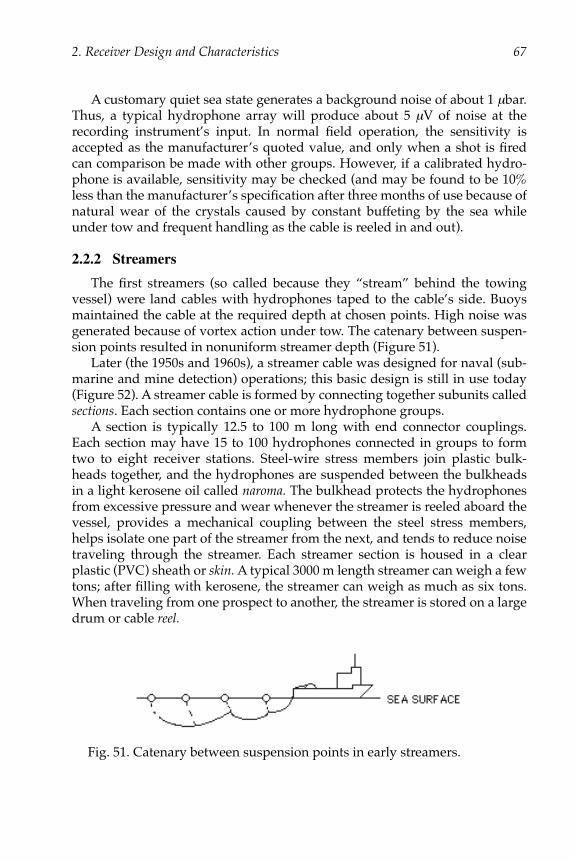
2. Receiver Design and Characteristics 67
A customary quiet sea state generates a background noise of about 1 µbar.Thus, a typical hydrophone array will produce about 5 µV of noise at therecording instrument’s input. In normal field operation, the sensitivity isaccepted as the manufacturer’s quoted value, and only when a shot is firedcan comparison be made with other groups. However, if a calibrated hydro-phone is available, sensitivity may be checked (and may be found to be 10%less than the manufacturer’s specification after three months of use because ofnatural wear of the crystals caused by constant buffeting by the sea whileunder tow and frequent handling as the cable is reeled in and out).
2.2.2 Streamers
The first streamers (so called because they “stream” behind the towingvessel) were land cables with hydrophones taped to the cable’s side. Buoysmaintained the cable at the required depth at chosen points. High noise wasgenerated because of vortex action under tow. The catenary between suspen-sion points resulted in nonuniform streamer depth (Figure 51).
Later (the 1950s and 1960s), a streamer cable was designed for naval (sub-marine and mine detection) operations; this basic design is still in use today(Figure 52). A streamer cable is formed by connecting together subunits calledsections. Each section contains one or more hydrophone groups.
A section is typically 12.5 to 100 m long with end connector couplings.Each section may have 15 to 100 hydrophones connected in groups to formtwo to eight receiver stations. Steel-wire stress members join plastic bulk-heads together, and the hydrophones are suspended between the bulkheadsin a light kerosene oil called naroma. The bulkhead protects the hydrophonesfrom excessive pressure and wear whenever the streamer is reeled aboard thevessel, provides a mechanical coupling between the steel stress members,helps isolate one part of the streamer from the next, and tends to reduce noisetraveling through the streamer. Each streamer section is housed in a clearplastic (PVC) sheath or skin. A typical 3000 m length streamer can weigh a fewtons; after filling with kerosene, the streamer can weigh as much as six tons.When traveling from one prospect to another, the streamer is stored on a largedrum or cable reel.
Fig. 51. Catenary between suspension points in early streamers.
Chapter 2 Page 67 Monday, February 7, 2005 3:26 PM
Downloaded 11 Nov 2011 to 198.3.68.20. Redistribution subject to SEG license or copyright; Terms of Use: http://segdl.org/

68 SEISMIC DATA ACQUISITION
Because kerosene is lighter than sea water, a streamer filled with enoughkerosene to counter its dead weight can be placed at a particular depth andwill remain there. This is known as neutral buoyancy. When filled with addi-tional kerosene, each section will become positively buoyant, which can be anadvantage if the cable is accidentally cut (causing it to float to the surface forretrieval). If sea salinity conditions change or an excessive amount of kero-sene is put into the streamer, strips of lead weight may be taped to the PVCskin to make the section neutrally buoyant again. However, such externalweights are undesirable because one positioned near a hydrophone may gen-erate excessive vibration noise. Ideally, the cable should be neutrally buoyantsuch that other mechanisms may guide the streamer to the required depthwithout buoyancy problems.
A typical streamer system is illustrated in Figure 53. The lead-in sectionhas a solid core rather than being filled with kerosene. A flexible metal sheathprovides protection against damage from vibration and rubbing where thelead-in contacts the ship’s stern pylons, back deck, and cable reel. The lead-inalso must be capable of withstanding high pressure from the energy sourcebecause it may come in contact with the energy source equipment during ves-sel turns.
Not every section in a streamer has to contain hydrophones. Sometimesdead sections are used to achieve desired group spacings. Such dead sectionscontain no hydrophones and are interspersed between the active or live sec-tions. Combinations of dead and live sections provide a great deal of flexibil-ity in designing optimum receiver arrays.
The principal purpose of the tail buoy is to provide a reference on the cableposition. This is important at the beginning of a line to ensure that the cable
Fig. 52. Marine streamer schematic.
Chapter 2 Page 68 Monday, February 7, 2005 3:26 PM
Downloaded 11 Nov 2011 to 198.3.68.20. Redistribution subject to SEG license or copyright; Terms of Use: http://segdl.org/

2. Receiver Design and Characteristics 69
has straightened out after any pre-line ship maneuvers. During shooting, itmay also help indicate cable drift as a result of crosscurrents. The tail buoyhas a radar reflector and may have a strobe light mounted on it. A bearing onthe buoy can be obtained on the ship’s radar or, with less precision, byobserving the buoy through binoculars. Rough seas can make it difficult tolocate the buoy because of its limited size and height. In some cases, a low-power radio beacon is mounted on the buoy. Automatic direction finding(ADF) equipment on the vessel may be used to give a continuous bearing tothe radio beacon. The tail buoy serves as a marker for ships passing asternand also aids in retrieving the cable if it is cut.
One or more stretch sections are installed behind the lead-in to attenuatecable noise caused by the vibration and jerk from the ship. The stretch sectionhas a vinyl jacket and often contains kerosene. Rope is used in the stretch sec-tions in place of the wire stress members to give a stretch capacity of up to50% of the relaxed length. Any section that is stretched more than 20% shouldbe tested before further use.
2.2.3 Depth Control
The depth of the streamer is controlled by attaching winged devices calledbirds to the cable. On passive birds, the wings (sometimes called “divingplanes”) are controlled by spring tension preadjusted to make the bird fly atthe target depth, typically about 11 m. When the cable reaches the targetdepth, the water force on the wings will be balanced by the spring tension. Ifthe cable should drop to a lower depth, the angle of the wings will be
Fig. 53. Marine towed configuration.
Chapter 2 Page 69 Monday, February 7, 2005 3:26 PM
Downloaded 11 Nov 2011 to 198.3.68.20. Redistribution subject to SEG license or copyright; Terms of Use: http://segdl.org/

70 SEISMIC DATA ACQUISITION
reduced, causing the cable to return to the target depth. Conversely, adecrease in cable depth produces a greater angle of the wings, causing thebird to seek a deeper level. This type of system also is affected by vesselspeed. By varying the speed of the vessel, say between 4.8 knots and 5.2knots, some overall adjustment of depth is possible without retrieving thecable to reset the spring tension. However, this also can be a disadvantage if itdictates a vessel speed that is unacceptable for reasons such as noise, cablestability, or desired production speed.
A better system of control is with birds containing active control elements(Figure 54). The wings are attached to a water-piston, tension-spring mecha-nism that causes the assembly to seek a depth to which the spring tension hasbeen programmed. The desired depth is controlled individually by a com-mand transmitter (also shown in Figure 54) in the ship’s instrument room.The observer sets the depth on the controlling computer, which then trans-mits a pulse along the streamer. The bird recognizes the depth code commandand automatically adjusts the wings to the required tilt. The birds are pow-ered by rechargeable batteries to provide system operation for a number ofweeks.
Remote depth control has the following advantages:
1) The cable does not have to be reeled in to change the depth settings.(This convenience is the biggest advantage).
2) The cable can be submerged to a safe depth if a vessel should attemptto cross it.
Fig. 54. Active depth controller “bird” (courtesy Syntron, Inc.).
Chapter 2 Page 70 Monday, February 7, 2005 3:26 PM
Downloaded 11 Nov 2011 to 198.3.68.20. Redistribution subject to SEG license or copyright; Terms of Use: http://segdl.org/

2. Receiver Design and Characteristics 71
3) It can be raised to the surface to avoid reefs or shoals.4) Lines crossing from deep water into shallow water can be shot at opti-
mum cable depth (but with inherent change in the receiver ghosteffect).
2.2.4 Streamer Depth Indicators
The streamer depth as well as lateral position can be monitored from theinstrument room using remote sensors. The depth is usually measured at anumber of locations along the cable. The sensor placed in the streamer is acoil whose electrical inductance changes as a function of pressure. The coil isconnected through a pair of wires along the streamer to the depth indicatorsystem in the instrument room. With a calibration of depth to pressure to coilinductance, the visual readout provides a continuous indication of cabledepth with an accuracy of ±5%. The depth sensors or depth sections usually areplaced at the same point as the depth control birds to monitor cable depth andbird performance. This is probably satisfactory with a well-ballasted cable butcould be deceptive if the cable is not neutrally buoyant.
2.2.5 Streamer Heading
Streamer compasses can be placed in or on the cable to detect heading.With 1° accuracy, 10 or more are often used to detect cable drift (i.e.,feathering) off line. Ships have computer systems that continuously log thecompass data and process them to produce an on-board plan view of thestreamer position with respect to the preplotted desired line to be shot. Thisallows the crew to adhere to streamer feathering specifications as well asallow the computation and storage of common midpoint (CMP) locationsneeded during 3-D surveying (see Chapter 7).
2.2.6 Streamer Noise
Good design of acceleration-canceling hydrophones has limited much ofthe noise to the extent that in a calm-sea state, signal-to-noise ratio frequentlyis better in marine data than in land data. Noise is also generated by vesselmechanical vibration, cable strumming, and the vortex action of wateraround the cable. All such actions result in forces that cause unwanted noise.In the 1940s and 1950s, it was customary to stop the boat dead to minimizethese noise sources during recording operations. A continuous tow cable wasthen designed to suppress such acceleration noise by combining the hydro-phones as explained earlier.
The following noise types can occur in a modern cable when cables aretowed through water:
Chapter 2 Page 71 Monday, February 7, 2005 3:26 PM
Downloaded 11 Nov 2011 to 198.3.68.20. Redistribution subject to SEG license or copyright; Terms of Use: http://segdl.org/

72 SEISMIC DATA ACQUISITION
1) Depth controller noise—Water flow turbulence along the streamer andover the birds may be reduced if birds are placed away from livehydrophones. Such turbulence also can generate extreme noise whenbirds are diving hard.
2) Poor-ballast noise—If a streamer is poorly ballasted, the birds will tilttheir wings to greater angles trying to pull the streamer up or down tothe desired depth. As a result, local turbulence is generated which pro-duces bird noise on the streamer.
3) Rough sea state noise—Sea swell causes up-welling and down-draftingof volumes of sea water. This turbulence often generates a short-wave-length vertical pressure wavefield causing individual live sections toraise up or drop down depending on the direction of the surface swell.When individual live sections are moved relative to adjacent live sec-tions, high-amplitude noise bursts are observed. In rough seas, as arule of thumb, a maximum depth of turbulence which causes unac-ceptable streamer noise bursts occurs at half a wavelength of the swellbeneath the swell trough (Figure 55). Such noise bursts can be over-come by trough shooting (Figure 56). During trough shooting (a tech-nique often used in the North Sea where the weather window islimited), the troughs drop the whole cable down, and it is lifted up
Fig. 55. Rough sea turbulence.
Fig. 56. Trough shooting.
Chapter 2 Page 72 Monday, February 7, 2005 3:26 PM
Downloaded 11 Nov 2011 to 198.3.68.20. Redistribution subject to SEG license or copyright; Terms of Use: http://segdl.org/

2. Receiver Design and Characteristics 73
equally when the next wave peak arrives. Consequently, if lines can beshot at right angles to the sea swell direction, production can continuewith acceptable noise limits. One problem associated with this type ofrecording is that individual shots are recorded with the streamer atdifferent depths to the seabed, which may deteriorate stack quality. Itis therefore not recommended but is often the only alternative torecording no data at all. Also, in shallow-water areas where streamerdepth must be reduced, surf and waves breaking at the sea surface cancontribute significantly to background coherent noise. This is a con-stant problem with shallow water and transition-zone recording,about which nothing can be done.
4) Ship propeller noise—Propeller noise may travel horizontally throughthe water column and be recorded by the cable. Alternatively, if a shal-low hard seabed exists, a propeller beat frequency can be set up by thepressure wave from the propeller being reflected back to the surfaceby the reflective seabed. This noise can be attenuated during data pro-cessing by trace mixing and stacking. Seismic vessels either have a sin-gle propeller (in which the speed is adjusted by the blade pitch) ortwin propellers (in which the speed is adjusted by changing bladerotation velocity). If the vessel has twin propellers, the individual pro-peller speeds may be adjusted so that the beat frequency is reduced.With a single-propeller ship, changing the pitch may not resolve theproblem and, as a last resort, the vessel may have to be changed.
2.3 Fundamentals of Array DesignNoise is a major problem experienced in seismic recording. If noise has a
consistent, repeatable form, we should be able to recognize it and, hence,attempt to attenuate it. Once recognized, repeatable noise can be canceledusing arrays of phones. First we must understand the types of noise withwhich we have to deal.
As was seen in Chapter 1, ground roll (a Rayleigh or surface wave) is aform of noise that occurs when the weathering layer is excited by a shot beingfired. Because ground roll has particle motion that is circular to elliptical, thenoise has a vertical component that shakes the phones vertically as the noisetravels along the surface. On a shot record, ground roll appears as lines ofcoherent noise overriding the data; that is, the ground roll has a recognizablepattern from one trace to the next. In Figure 12, coherent noise appears on theseismic shot record as event a, masking the reflected event c at the shorter off-sets. Noise that does not occur in repeatable patterns is called incoherent orrandom noise; area D in Figure 5 shows an example. Random noise can be
Chapter 2 Page 73 Monday, February 7, 2005 3:26 PM
Downloaded 11 Nov 2011 to 198.3.68.20. Redistribution subject to SEG license or copyright; Terms of Use: http://segdl.org/

74 SEISMIC DATA ACQUISITION
removed by stacking, so usually the greatest concern in the field is how toremove coherent noise from the field records.
Noise attenuation in the field is preferable because the high amplitude ofcoherent noise may not allow low-amplitude reflection signals to be seen.Coherent noise is continuous across the seismic record. Random noise doesnot have this property but may be simply observed on the seismic record asoccasional high-amplitude noise bursts. Halfway between these is pseudo-random noise in which receivers are spaced so far apart that the coherentnoise train does not appear linear across the record.
Random noise may be attenuated simply by spacing the elements of areceiver array far enough apart to ensure no correlation between the noisedetected on those elements. For example, a gust of wind may affect two geo-phones similarly if they are positioned close to each other, but the effectbecomes random if they are spaced so far apart that only one of the geo-phones is affected. When elements are spaced far enough apart for such atten-uation, the noise reduction factor is n1/2, where n is the number of geophones.Therefore element spacing is a factor to be considered.
For coherent noise attenuation, size, spacing, weighting, and orientation ofthe array also must be considered. With ground roll, noise trains travel hori-zontally from the shot with distinct velocity, wavelength, and frequency char-acteristics. As ground roll travels along a horizontal surface, the particlemotion is roughly elliptical in the vertical plane containing the direction ofpropagation. As a consequence, ground roll vibrates geophone elements ver-tically. The geophones can be arranged so that their summed signal will can-cel the vertical component of the horizontally traveling noise trains whileadding the vertical component of the reflections.
Consider a simple horizontal wave (Figure 57), with two receivers closetogether. As the horizontal wave moves past the two receivers, provided theyare spaced a half wavelength apart, their total vertical output will sum to
Fig. 57. Horizontal and vertical waves.
Chapter 2 Page 74 Monday, February 7, 2005 3:26 PM
Downloaded 11 Nov 2011 to 198.3.68.20. Redistribution subject to SEG license or copyright; Terms of Use: http://segdl.org/

2. Receiver Design and Characteristics 75
zero. However, the arrival of a vertically reflected wave will cause an additiveoutput from both geophones since the wavefront is in phase at the receiverarray. This is how we can attenuate or suppress the horizontal wave whileenhancing the useful vertical signal wave.
In shallow-water areas, an equivalent ground-roll type wave exists thatcorrectly is called the Scholte wave. This is referred to in the industry as bot-tom roll or mud roll, which the geophysicist should expect when designingshallow-water marine surveys. Here, we will use land-noise problems toillustrate the concept of receiver array design. These concepts apply equallywell to land and marine source array design.
2.3.1 Synthetic Record Analysis
A synthetic record is a record numerically constructed from a model of theearth, as opposed to a field shot record, which is a measurement of the earth’sresponse to a shot. We will analyze a simple synthetic record to illustrate theconcepts of noise attenuation. Consider the schematic shot record ofFigure 58. This involves a simplified five-channel (or “station”) land record.The shot has been fired 25 m from the nearest geophone, with all geophonesspaced 25 m apart. Events A and B are seen at each geophone station. Event Atakes a shorter time to cross the stations, whereas event B takes longer.
Fig. 58. Schematic shot record.
Chapter 2 Page 75 Monday, February 7, 2005 3:26 PM
Downloaded 11 Nov 2011 to 198.3.68.20. Redistribution subject to SEG license or copyright; Terms of Use: http://segdl.org/

76 SEISMIC DATA ACQUISITION
Obviously, A must be a wave moving faster than B. Note also that wave Btakes longer than wave A to complete one full cycle. The length of one cycle ofa wave is called its periodic time, T, and is inversely proportional to a wave’sdominant frequency. That is,
(26)
The relationship between velocity (V), wavelength (λ), and frequency (f) ofa wave, is given by
(27)
The velocity of a sound wave is a vector quantity that cannot be measuredunambiguously by a single line of receivers. For example, if a wave pulseappears simultaneously at all geophones in a linear spread, then we couldinterpret that as either 1) a wave traveling perpendicularly to the spread (withunknown speed), or 2) a wave traveling parallel to the spread (with an infi-nite speed). To apply the above equation to ground roll, V is interpreted as theapparent horizontal velocity. The true velocity can be determined only if thewave’s direction of propagation is known.
In the record in Figure 58, we can determine the ground roll’s apparentvelocity simply by working out how fast the same point (say a peak) on thewavefront moves past the detectors (25 meters apart). The periodic time T isdetermined by finding the time between two adjacent trace peaks of the samearrival, and the dominant frequency can then be calculated. Hence, sincewavelength λ = V/f, the ground-roll wavelength may be computed. Let usnow show in detail how the above ideas can be used to design a simple, two-element array that will attenuate event B in Figure 58.
1) Select a group of traces that has a representative sample of the wave tobe attenuated. Take any two adjacent peaks or troughs of the wavewhere the wave has similar character (or shape) to that on the nextadjacent trace. For example, the largest amplitude wave on the secondtrace (at 50 m offset) has troughs at about 0.22 and 0.31 s. The time dif-ference is therefore 0.09 s, and since f = 1/T, the dominant frequency isabout 11 Hz.
2) The strong, low-frequency (11 Hz), high-amplitude wave going acrossthe synthetic record is now inspected to find its apparent velocity. Thepeak of the low-frequency wave appears on trace 1 at t1, which is atabout 0.17 s (at 25 m offset from the shot) and on trace 2 at t2, at about0.26 s (at 50 m offset from the shot). So, the wave has traveled 50 m –
f 1T--- .=
V fλ.=
Chapter 2 Page 76 Monday, February 7, 2005 3:26 PM
Downloaded 11 Nov 2011 to 198.3.68.20. Redistribution subject to SEG license or copyright; Terms of Use: http://segdl.org/

2. Receiver Design and Characteristics 77
25 m = 25 m in 0.26 s – 0.17 s = 0.09 s. That is, the wave has moved atan apparent velocity of 25 m per 0.09 s or 278 m/s.
3) The wavelength is V/f or 278/11 = 25 m.4) Any wave is best canceled by adding the maximum positive values to
the maximum negative values; for a perfect sinusoidal wave, theresult is zero. So, to position two geophones to cancel such a wave,they must be a half wavelength apart. In this case, the geophones mustbe 25/2 apart or about 12 m apart.
In actual field data, ground roll is comprised of many wavelengths and,furthermore, its composition may change from point to point along a line. Forthis reason, many elements are used in the array instead of just two. Somearrays may even be spread in a 2-D pattern to eliminate broadside noise aswell as in-line noise.
The ground roll’s bandwidth, as a rule of thumb, is considered to extendfrom 0.5 to 1.5 times the dominant frequency calculated. Hence, ground rollwith a dominant frequency of 20 Hz often has a bandwidth of 10–30 Hz,while a dominant frequency of 30 Hz has a bandwidth of 15–45 Hz.
2.3.2 Receiver Array Design
As the previous example showed, receivers may be positioned to cancelparticular waves. So far, the use of just two receivers has been considered.One way to expand this number is to space the geophones equally along aline. This pattern of phones is called a uniform or linear array. Variations ofthis, such as weighting of the array, are possible.
Before considering array design, it should be understood that, in practice,field arrays do not have ideal characteristics. Arrays may fail to perform opti-mum attenuation of ground roll because of
1) Erratic element spacing because of terrain or poor placement (land)2) Elevation variation (land) or cable depth variation (marine)3) Arrival time variations because of weathering thickness variations4) Detector sensitivity and coupling variations5) Change in surface-wave characteristics because of changes in weather-
ing-layer lithology parameters
However, even if arrays reduce coherent noise only marginally, their use isstill an important step because a minor reduction in ground roll is an increasein data quality and an improvement in signal-to-noise ratio.
2.3.2.1 The Uniform Array
Because sound waves can approach an array of receivers from any direc-
Chapter 2 Page 77 Monday, February 7, 2005 3:26 PM
Downloaded 11 Nov 2011 to 198.3.68.20. Redistribution subject to SEG license or copyright; Terms of Use: http://segdl.org/

78 SEISMIC DATA ACQUISITION
tion, characterizing an array’s response is, in general, a 3-D problem. Here,however, we will consider only a much simpler, 1-D problem. The full 3-Dtheory is described in Appendix B.
Suppose a set of geophones are laid out in a straight line on the surfaceand we are interested in how that array responds to a sound wave that travelshorizontally and parallel to the array. A convenient way to characterize such awave is by its horizontal wavenumber, k, which is the reciprocal of the wave’swavelength. Thus, we have the following relationships:
(28)
Note that k = 0 implies that the wavelength is infinite. This can occur eitherbecause a wave’s velocity is infinite or because the wave’s frequency is zero.
Before explaining how to calculate an array response for the simple 1-Dproblem, it is worth noting that the method can have some uses even forsound waves propagating in two dimensions. Figure 59 shows some waveswhose raypaths lie in the vertical plane below the 1-D linear array. Clearly, thepropagation of such waves has two components, one vertical and one hori-zontal. The 1-D array response method applies to the horizontal component.Often geophysicists speak of the horizontal component by using the word“apparent.” Thus, the apparent velocity or apparent wavelength of a sound waverefers to the velocity and wavelength of the horizontal component. A wavethat travels vertically has a zero horizontal wavenumber and an infiniteapparent horizontal velocity. This is just another way of saying that a verticalwavefront is detected simultaneously by all the surface geophones.
Figure 60 shows the response R of a five-element horizontal linear arrayhaving uniform element spacing d. The figure shows cancellation of waves ofsix different wavelengths, ranging from λ = infinity to λ = 0.8. Numbers onthe right show the product of phone spacing d with wavenumber k, assuminga phone spacing of unit value 1. If a wavelength λ is infinitely long (k = 0), allphones observe equal amplitude and the total output response R is 5. If the
λ 1/k V/ f .= =
Fig. 59. Wavefront raypaths arrive at points along line.
Chapter 2 Page 78 Monday, February 7, 2005 3:26 PM
Downloaded 11 Nov 2011 to 198.3.68.20. Redistribution subject to SEG license or copyright; Terms of Use: http://segdl.org/

2. Receiver Design and Characteristics 79
wavelength is 4 units, the response is –1, and so on. A graph of the responsesin Figure 60, using a linear output response scale R versus a linear wavenum-ber k scale for unit geophone separation d, is shown in Figure 61.
Fig. 60. Geophone array response.
Fig. 61. Response/k curve.
Chapter 2 Page 79 Monday, February 7, 2005 3:26 PM
Downloaded 11 Nov 2011 to 198.3.68.20. Redistribution subject to SEG license or copyright; Terms of Use: http://segdl.org/

80 SEISMIC DATA ACQUISITION
If we continue shortening the wavelength, a point is reached where thewavelength is exactly one phone spacing. The response from this point on isidentical to that observed over the 0.0–1.0 wavenumber range. We havereached the alias or fold-over point, where even shorter wavelengths canappear as the longer wavelengths (see “Digital Sampling,” Chapter 4). Thisunwanted situation means the array has passed the point where it can pro-vide maximum wavelength attenuation. In Figure 61, this occurs in the regionof k = 1.0, and hence wavenumber values in excess of 1 just repeat theresponse of the array.
For the theoretical approach to the computation of array response, refer toAppendix B. From that theory, and using the decibel form of notation,
(29)
where d is the element spacing and N is the number of elements. The ampli-tude response of a six-geophone array with 5-m phone spacing is shown inFigure 62.
Attenuation is maximum at five notch points occurring at 1/Nd, 2/Nd,.....(1–N)/Nd. The first alias peak, at wavenumber 1/d, has no attenuation. A fea-ture of a uniform array’s attenuation characteristics is that the attenuationlobes form a curve or “envelope” of attenuation, where the amplitude of thearray response at the envelope base is 1/N, or 20 log 1/N (dB scale).
Amplitude response (dB) 20 log πdkN( )sinN πdk( )sin---------------------------,=
Fig. 62. Array response for six geophones 5 m apart to horizontally traveling waves.
Chapter 2 Page 80 Monday, February 7, 2005 3:26 PM
Downloaded 11 Nov 2011 to 198.3.68.20. Redistribution subject to SEG license or copyright; Terms of Use: http://segdl.org/

2. Receiver Design and Characteristics 81
Because of the 1/N factor, overall attenuation increases as array lengthincreases, or, viewed alternatively, as the number of phones increases. Thecenter of the lobe envelope is at wavenumber 1/2d. Thus, overall array lengthideally should be at least twice the longest wavelength to be attenuated.
A very long array has good attenuation of horizontal noise, but it alsoattenuates high-frequency reflections. Shallow reflections, which have under-gone a minimum of absorption attenuation because of their short travel-pathlength, arrive at shallowest incident angle θ. Because of the small incidentangle, shallow reflections can have a significant component of motion in thehorizontal direction (see Figure 63) and are therefore affected by array attenu-ation. In comparison, deep reflections undergo greater absorption attenuationbecause of their longer travel-path length, but deeper reflections arrive atsteeper incident angles and are not as affected by array attenuation. Conse-quently, shallow, high-frequency reflections may be attenuated by an array toa greater degree than the deeper, low-frequency reflections.
This is therefore a good reason to maintain a short array length, whichmust be designed for the retention of the target (shallow or deep) reflection.The use of field arrays always entails a compromise. Long arrays can achievebetter noise attenuation than short arrays, but at the expense of partial attenu-ation of the desired signal.
2.3.2.2 The Weighted Array
Coherent noise trains often consist of a number of different wavelengthnoise trains that gradually separate with distance along the receiver line, asthey are traveling at different velocities. The shot record of Figure 3 shows agood example of this phenomenon, which is referred to as a dispersive wavebecause the initial fundamental ground-roll wave at short offset separates outinto packages of energy or waves. That is, the noise disperses into separatewavetrains or higher-order-mode waves. If a number of different noise
Fig. 63. Shallow and deep raypaths.
Chapter 2 Page 81 Monday, February 7, 2005 3:26 PM
Downloaded 11 Nov 2011 to 198.3.68.20. Redistribution subject to SEG license or copyright; Terms of Use: http://segdl.org/

82 SEISMIC DATA ACQUISITION
wavetrains, each having different values of k, are to be attenuated, it would beuseful to have an array that could be designed to attenuate those specific val-ues of k. The weighted array provides this option.
The problem of designing weighted arrays and computing their responsecan be approached by thinking of weighted arrays as composites of simplerunweighted subarrays. Consider the geophone array depicted below inwhich small circles represent phones as if the array were laid out on theground and the two phones at the center of the four-phone array show thatthe array is weighted at the center by a factor of 2:
This figure is schematic, representing a weighted array, and is not how thearray is laid out on the ground (imagine the center phone gives an outputtwice the amplitude of the other phones, so we represent it by two phones).The array therefore has a weighting of (1,2,1), where the number of phones ateach receiver point is represented by the numbers in parenthesis. This array isjust the same as the composite of two simpler unweighted identical subarraysdepicted below.
For a linear unweighted array, the maximum ground-roll cancelationoccurs when λ = 2d. Thus, in this simple case, we can consider the weightedarray as a single linear subarray repeated again after lining up first and lastphones. The response of the resulting weighted array can then be obtained byconvolving the response of the simple basic subarray with a repeat factor rep-resenting the number of times the original basic subarray has been repeated.
The mathematical process of convolution is shown diagramatically below,where the weighted array on the left (1,2,1) is the same as the two subarrayson the right (1,1,0) and (0,1,1), where the “0” shows no phone present in thatposition, and the “1” indicates that there is a phone present in that position.As above, circles represent phones.
o
o
oo d d
o d oFirst subarray
o d o
Second subarray
Chapter 2 Page 82 Monday, February 7, 2005 3:26 PM
Downloaded 11 Nov 2011 to 198.3.68.20. Redistribution subject to SEG license or copyright; Terms of Use: http://segdl.org/

2. Receiver Design and Characteristics 83
1st 2nd 3rd Postitiono o o o o
o o o1 2 1 1 2 1
In the equivalent array on the right, the first two-phone subarray has onephone in the first position and one phone in the second position. Hence, thatsubarray is represented by (1,1). The second subarray is identical but has beenshifted along one position. This shift is the repeat factor, which can be repre-sented by (1,1), where the first “1” shows us that basic subarray started in thefirst position (denoted by 1) and the array then moved to the second position(denoted by 1). So, the repeat factor (1,1) shows that the basic subarray movedone position. Note that (1,1) is the same as (1,1,0), since the 0 only shows thateither there is no third geophone (where it represents a geophone array) orthe basic array is not repeated (where it represents the repeat factor).
Convolving the basic array with the repeat factor produces the same rep-resentation as the weighted array (which was 1,2,1). A convolution is per-formed by reversing the order of the first numbers and shifting them acrossthe second number series while multiplying. We use a star (*) to represent thisprocess of convolution. In our example, we have to show that the convolutionof (1, 1) * (1, 1) = (1,2,1).
For example, arrange the two arrays by reversing the first array numbers(where we represent 1,1 by 1,1,0) to become (0,1,1) and write the two arrays intwo columns. The numbers at positions A and B will be the first to bemultiplied.
1) Now multiply 1 at A by 1 at B by placing the 1 at A underneath posi-tion B (arrowed) and position the resulting value of 1 at C.
First (reversed) array Second array
0, 1, 1 1, 1, 0A B
0, 1, 1 1, 1, 01
1C
A B
Chapter 2 Page 83 Monday, February 7, 2005 3:26 PM
Downloaded 11 Nov 2011 to 198.3.68.20. Redistribution subject to SEG license or copyright; Terms of Use: http://segdl.org/

84 SEISMIC DATA ACQUISITION
2) Now we shift the first array numbers along and multiply again. To dothis, we put the last two numbers of the first array under the first twonumbers of the second array and multiply them so that the result canbe written down in position D.
3) Do the next shift of the first array, multiply with the second array, andput the result at position E.
4) Perform the next shift of the first array and multiply again, putting theresult at F. Note that the last 1 of the first array is not written down (atG) because there is nothing to multiply it by.
0, 1, 1 1, 1, 01, 1
11 1 D
A B
0, 1, 1 1, 1, 00, 1, 1
11 10, 1, 0 E
1, 1, 00, 1 G
1
1 1
0 1 0
0 0 F
0, 1, 1
Chapter 2 Page 84 Monday, February 7, 2005 3:26 PM
Downloaded 11 Nov 2011 to 198.3.68.20. Redistribution subject to SEG license or copyright; Terms of Use: http://segdl.org/

2. Receiver Design and Characteristics 85
5) The final shift puts 0 under 0 at the G location so the multiplicationcontributes nothing to the exercise. Finally then, we add up the rowsof numbers to produce a resultant answer for the convolution of thetwo arrays. The result is shown in the left column as 1,2,1.
This is known as the convolution table and is the final result of the convolu-tion of the subarray and its repeat factor. Thus, the convolution of subarray(1,1) with repeat factor (1,1) gives the array (1,2,1). So far, we have convolvedtwo very simple uniform arrays to obtain the response of a simple weightedarray. Here is a slightly more complicated example.
Consider the weighted array (1,2,2,1), which appears below using our ear-lier notation.
o o o o o o
This pattern is a simple three-element uniform subarray that appearstwice. As in the previous example, the repeat factor is (1,1). Thus, theweighted array response is given by (1,1,1) convolved with (1,1).
The first 1 in the repeat factor represents the first subarray, while the sec-ond 1 represents the number of times that subarray has been repeated at thesecond position. Thus, the repeat factor establishes the position of the secondidentical array with respect to the first.
Proceeding as explained above, the convolution table is as shown below.
1, 1, 00, 1
1
1 1
0 1 0
0 0
121
{finalresult
sum
0, 1, 1
1
1 1
1 1
11
2
21
Sum
Chapter 2 Page 85 Monday, February 7, 2005 3:26 PM
Downloaded 11 Nov 2011 to 198.3.68.20. Redistribution subject to SEG license or copyright; Terms of Use: http://segdl.org/

86 SEISMIC DATA ACQUISITION
Thus, (1,1,1) * (1,1) = (1,2,2,1). This procedure works with any number ofsubarrays, provided the repeating subarrays are identical.
We now have a simple mathematical tool that allows us to determine theresponse of complex weighted arrays. The response of any complex arrange-ment of identical simple arrays can be described as a convolution of the sim-ple array pattern with a repeat factor. The amplitude response formula (1) ofAppendix B is then applied so that lobe and notch values can be computedfor the array and its repeat factor on the same graph, then summed. Theresulting response of the simple array plus its repeat factor is the totalresponse of the complex array. The simplicity of this treatment allows thefield hand to compute response curves rapidly by hand, without field com-puters.
(Remember that summing two negative dB values produces a larger nega-tive dB value. When we refer to the attenuation of waves, a 0 dB value is awave’s peak value, and attenuation of a wave reduces values. So, reducingvalues from a peak in dB terms is the same as subtracting dB numbers tobecome more negative. Further attenuation of a wave increases the –dB value.For example, –20 dB plus –10 dB produces an attenuation of –30 dB.)
An array pattern that repeats after two shifts rather than one can beaccommodated using the repeat factor (1,0,1), where the zero shows that theshift did not stop at the second point but continued on.
o o o oo o o o
(1, 1, 1, 1) * (1, 0, 1) = (1,1,2,2,1,1)
A uniform array with equal phone spacing but consisting of odd numberswhich are some function of the full station length also can be accommodated.Consider a nine-phone array in this pattern where the station length is, say, 8/3 units. Each phone may be 1/3 units apart, so that it looks as shown below.
This can be considered as the basic array along the top line which wouldbe (1,0,0,1,0,0,1) convolved with the repeat factor (1,1,1) where the distanceapart d = 1/3. It also will appear as a nine-element array to waves traveling
1 1 1/ / /3 3 3
0
0
0
0
0
0
0
0
0
Chapter 2 Page 86 Monday, February 7, 2005 3:26 PM
Downloaded 11 Nov 2011 to 198.3.68.20. Redistribution subject to SEG license or copyright; Terms of Use: http://segdl.org/

2. Receiver Design and Characteristics 87
from left to right because the array is unweighted and phones are of equalseparation distance (1/3 between phones).
Therefore, the response will be identical to a nine-element uniform array.
2.3.2.3 The ‘Superposition’ Pitfall
One mistake to avoid is attempting to compute the response of a compli-cated array by summing the responses of simpler arrays. This is inherentlyincorrect because it does not account for the change in phase as a result of thehorizontal wave arrival. The phase change is accounted for correctly in theconvolution method repeat factor.
For example, consider a simple array of two phones with in-line separa-tion d. This would look as follows.
oo
The incorrect approach would say this is a single phone array------ oand added to this is the other single phone array----------------------- o.
Since the response of a single element is flat, the sum of the two single-ele-ment responses is also flat. Obviously, this is an incorrect result, which illus-trates the pitfall of just summing responses.
Land geophone arrays frequently use weighted patterns. An alternativeapproach is to position phones (and hence stations) very close together in lin-ear-array form and record a very large number of stations. This allows arrayweighting to be performed in the processing center by mixing data recordedby the closely spaced stations. However, the choice is not always whichapproach is better for signal-to-noise ratio improvement but which approachis more economical.
The convolution approach also may be used for computing the response ofan areal 2-D pattern.
Occasionally, another type of array is used, called the cosine or Chebychevarray. This type of array has weighting like a cosine curve peaking at the cen-ter, the response of which can be computed by the convolution theory. Arraysalso can be simulated in a computer to produce a desired response. For exam-ple, if a number of very short linear arrays are used in the field (on land, geo-phones may be placed close together; in marine recording, short streamergroups may be used), we can sum them to produce a single longer array (thisis referred to as mixing the receiver stations) which will cancel long-wave-
1 1 1/ / /3 3 3
0 0 0 0 0 0 0 0 0
Chapter 2 Page 87 Monday, February 7, 2005 3:26 PM
Downloaded 11 Nov 2011 to 198.3.68.20. Redistribution subject to SEG license or copyright; Terms of Use: http://segdl.org/

88 SEISMIC DATA ACQUISITION
length ground roll. This initial computer processing step may be performed inthe field or in the processing center. If a known array response is thereforerequired, receiver station mixing can be a useful step, provided the receiverinterval is short enough to allow it.
Another array approach, called the stack array, is an extension of the appli-cation of data processing to remove ground roll. Developed by Anstey(1986a), it basically builds long arrays using a particular source/receivergeometry to remove ground roll by the stacking process. An acquisitiongeometry known as symmetric sampling (see later this chapter) adds to this byusing a source array, which helps increase attenuation of ground roll. Thesewill now be discussed in detail.
2.3.2.4 The Stack Array
As discussed in Chapter 1, the signal-to-noise ratio is improved by stack-ing the data. For some years, many geophysicists often preferred to lay outuniform geophone arrays and simulate weighted arrays by trace mixing indi-vidual receiver station data in the processing center to remove ground roll.Their reasoning was that this approach was often less expensive and cumber-some than laying weighted geophone arrays, and frequently appeared to dojust as good a job. Anstey (1986a) was the first to explain the obvious. If geo-phones are equally spaced along the full length of each station, and the sta-tion interval is short enough for correct subsurface sampling, then the tracesin a CMP gather are distributed evenly and continuously across the gather. Bythe application of NMO and subsequent stacking of these traces in data pro-cessing, the ground roll observed on shot records is canceled. Ansteyexplained the logic behind what had been practiced in the processing centerfor years and called this the stack-array technique. He also went on to suggestrecording configurations that would help the stack array to further suppressground roll.
Ground roll is a function of space and time. The wave moves along thesurface (and across the geophone arrays) horizontally and down the traces intime. Using the synthetic time-space (t-x) shot record of Figure 64, imagine aseries of panels of seismic traces with the ground roll or noise cone passingdiagonally across the record. In the top diagram of Figure 64, the seismic tracepanels are separated by the six straight lines with the last synthetic trace dis-playing the ground roll as it might normally be seen on the record. The geo-phone groups producing these panels have a linear array with equally spacedgeophones covering the whole spread of stations along the line.
The bottom diagram of Figure 64 shows a series of individual traces thatwill be resorted to make up panels of CMP traces. The ground roll passesacross the individual traces, and if the appropriate traces had NMO correc-
Chapter 2 Page 88 Monday, February 7, 2005 3:26 PM
Downloaded 11 Nov 2011 to 198.3.68.20. Redistribution subject to SEG license or copyright; Terms of Use: http://segdl.org/

2. Receiver Design and Characteristics 89
tions and then were added together or stacked to produce one CMP trace, theresult would be the same as having a longer geophone array to cancel theground roll wavelength, as we did earlier using linear geophone arrays. Thisis stacking in its simplest form. The result is cancelation of ground roll to adegree dependent on the ground-roll complexity. This is displayed syntheti-cally for each panel in Figure 65.
Anstey pointed out that particular arrays used in the field would assist thebreakup of ground roll in a CMP gather and called the use of these arrayswith stacking the stack-array criterion. Array geometries could be determinedprior to the commencement of a survey, so that there would be no need toperform noise tests. Anstey described a number of source-receiver configura-
Fig. 64. Synthetic record.
Chapter 2 Page 89 Monday, February 7, 2005 3:26 PM
Downloaded 11 Nov 2011 to 198.3.68.20. Redistribution subject to SEG license or copyright; Terms of Use: http://segdl.org/

90 SEISMIC DATA ACQUISITION
tions that would satisfy the stack-array criterion. If trace mixing is employedin data processing, then the field layouts would be as shown in Figure 66. Thetrace mixing allows stations to be shorter, as the mix doubles the effectivelength of the station. One problem with such mixing is that the high frequen-cies at steep reflection dips are destroyed (Anstey, 1986b).
In Figure 66, the flags indicate the centerpoint of the receiver stations. Theblack dot indicates the shot location. Where the spread is split-spread, the
Fig. 65. Stacked trace ground roll cancellation in a CMP gather.
Fig. 66. Stack-array configurations.
Chapter 2 Page 90 Monday, February 7, 2005 3:26 PM
Downloaded 11 Nov 2011 to 198.3.68.20. Redistribution subject to SEG license or copyright; Terms of Use: http://segdl.org/

2. Receiver Design and Characteristics 91
shot location is shown in its correct location for continuous coverage. Wherethe spread is off end, the shot is shown at each end to emphasize an off-endconfiguration, but shot locations are still at the value stated in the sourceinterval column where distances are in meters. The split-spread configuration(Type 3) with the shot at the station is not recommended.
The stack-array criterion therefore requires an even, continuous, uniformsuccession of phones across the CMP gather, so that:
1) In marine operations using an off-end spread, the group length mustbe equal to the group interval, and the source interval must be half thegroup interval.
2) In land operations, split-spread recording ideally should be used inwhich the station length is equal to the station interval, the sourceinterval equal to the station interval, and the shot is between the sta-tions.
For split-spread recording, shooting between the stations is preferredbecause this provides more continuous array coverage and hence a betterchance of ground-roll suppression.
The common-shot CMP stacking diagrams described in Chapter 1 canexplain how ground roll can be attenuated. Two alternative ways to representstacking diagrams are shown in Figure 67.
Both diagrams represent six adjacent shots into a split-spread array. Onthe right, the CMP coverage is shown in the customary manner with mid-points shown horizontally. The gap is the split-spread configuration gap. Onthe left, the midpoints are diagonal with one half of the spread above the lineand the other half below the line. The fold is four at the chosen CMP. Therequirement for continuous receiver coverage is shown for both methods inFigure 68.
Fig. 67. Stacking diagram styles.
Chapter 2 Page 91 Monday, February 7, 2005 3:26 PM
Downloaded 11 Nov 2011 to 198.3.68.20. Redistribution subject to SEG license or copyright; Terms of Use: http://segdl.org/

92 SEISMIC DATA ACQUISITION
Anstey uses the method on the left to demonstrate continuous coverage, inwhich the bottom half coverage lines (e.g., lines 1 and 2) must fit like a combinto the top half to produce continuous coverage. Alternatively, with themethod on the right, the stacking diagram left half must show lines of cover-age that fit into and between the lines of the right half (a line of coverage isneeded where the dotted line is shown) to provide continuous coverage.
An alternative approach to understanding the benefits of shootingbetween the stations is to consider near-offset travel paths. The signal-to-noise ratio in CMP data is increased if different raypaths are stacked to makethe CMP trace. Using split-spread geometry with the shot fired at the receiverstation, and looking at the near-offset traces with the conventional method ofdrawing stacking diagrams (the one on the left in Figure 68), we can draw theraypaths as the spread rolls along the line. In Figure 69, the raypaths from SP1are shown as expected. When SP2 is fired, the raypath to the right of SP1 isduplicated by the raypath to the left of SP2. Instead of the CMP between SP1
Fig. 68. Stack-array coverage.
Fig. 69. Split-spread shot on station.
Chapter 2 Page 92 Monday, February 7, 2005 3:26 PM
Downloaded 11 Nov 2011 to 198.3.68.20. Redistribution subject to SEG license or copyright; Terms of Use: http://segdl.org/

2. Receiver Design and Characteristics 93
and SP2 being two horizontally stacked traces, it becomes two verticallystacked traces (i.e., instead of two-fold, it is two times single fold).
If the shot is fired between the receiver stations, SP2 has different ray-paths, allowing correct CMP stacking, as shown in Figure 70. Consequently,the simple rule is that when shooting off-end, fire the shot at and between thestations, whereas when recording split-spread, fire the shot between the sta-tions.
2.4 Symmetric and Asymmetric RecordingIn symmetric recording, both source arrays (like vibrator arrays) and
receiver arrays are used. In asymmetric recording, the source is a point source(such as a single-charge explosive) and the receiver has an array. In updip ordowndip recording, symmetric recording is preferred because this will avoidthe static effects caused by using only a receiver array (Vermeer, 1991). Forexample, in Figure 71, an updip shot from a single energy source into areceiver has the reflections arriving nearly vertically and at similar times.However, the single shot downdip has the reflectors arriving at an acuteangle, and at different times. The result is a different stack for the updip ver-sus downdip recording. If split-spread recording is used, then the dippingevents from updip recording will not stack in well with those from the down-dip recording and reflections may not image well.
By comparison, the use of symmetric arrays provides similar travel paths(though not identical since there are normally more receivers than sources),and hence Figure 71 makes the point that we always should use symmetric
Fig. 70. Firing between the stations.
Chapter 2 Page 93 Monday, February 7, 2005 3:26 PM
Downloaded 11 Nov 2011 to 198.3.68.20. Redistribution subject to SEG license or copyright; Terms of Use: http://segdl.org/

94 SEISMIC DATA ACQUISITION
arrays where possible. The choice of the array parameters is dependent onnoise tests performed in the area of operations.
2.5 Receiver GhostingWhen reflected seismic waves travel vertically upward toward the
receiver array, some of the energy can become trapped within the weatheringlayer by rebounding off the air-ground interface (and air-sea interface inwater), internally reflecting down at different transmission angles. Suchwaves again may reflect upward from the weathering base, causing what isknown as a reverberation. Such a reverberating wave is unwanted and is con-sidered as a ghost of the earlier-arriving wave. Techniques to attenuate suchwaves in the field are discussed later in Section 3.5. (With land receivers, thereis little that can be done to attenuate such waves apart from changing thesource depth). Marine techniques using dual sensors were discussed inSection 2.1.4.
Fig. 71. Symmetric and asymmetric recording.
Chapter 2 Page 94 Monday, February 7, 2005 3:26 PM
Downloaded 11 Nov 2011 to 198.3.68.20. Redistribution subject to SEG license or copyright; Terms of Use: http://segdl.org/

2. Receiver Design and Characteristics 95
Exercise 2.1Find the wavelengths of the three waves indicated in Figure 72. Trace
spacing (geophone interval) is 5 m. Seventy-two traces have been recorded inthree groups of 24 traces.
Exercise 2.2On a graph of attenuation (0–40 dB) versus wave number (0–0.2), sketch
the response of a six-element array with 5-m uniform spacing.
a) Note notch points, lobes, and first alias peak.b) Calculate attenuation at the lobes.c) Calculate maximum lobe envelope value.d) What is the effect of reducing the interval to 3 m?
Formulae, Response (dB) = 20 log
k = , ..... (notches)
= , .... (peaks of lobes)
(Answers: Lobes are at 0.0495, 0.0825, 0.115, 0.149. Notches are at 0.033,0.066, 0.099, 0.132, 0.165. Attenuation is 12.55, 15.26, 15.26, 12.55. Maximumlobe envelope value is 15.56 dB.)
Exercise 2.3Show that a weighted array (1,2,3,3,2,1) can be modeled as three uniform
subarrays (1,1,1,1) with a repeat factor of (1,1,1).The response of such an array is shown in Exercise 2.4.
SinπdkNNSinπdk-----------------------
1Nd-------- 2
Nd--------
1.5Nd-------- 2.5
Nd--------
Chapter 2 Page 95 Monday, February 7, 2005 3:26 PM
Downloaded 11 Nov 2011 to 198.3.68.20. Redistribution subject to SEG license or copyright; Terms of Use: http://segdl.org/

96 SEISMIC DATA ACQUISITION
Fig. 72. Wavelength measurement.
TIM
E -
sec
on
ds
0
.5
1.0
1.5
2.0
λ =
λ =
λ =
Chapter 2 Page 96 Monday, February 7, 2005 3:26 PM
Downloaded 11 Nov 2011 to 198.3.68.20. Redistribution subject to SEG license or copyright; Terms of Use: http://segdl.org/

2. Receiver Design and Characteristics 97
Exercise 2.4Determine the geophone separation for an array with weighting (1, 2, 3, 3,
2, 1) for the response curve shown in Figure 73.
Fig. 73. Response curve.
Chapter 2 Page 97 Monday, February 7, 2005 3:26 PM
Downloaded 11 Nov 2011 to 198.3.68.20. Redistribution subject to SEG license or copyright; Terms of Use: http://segdl.org/

Chapter 2 Page 98 Monday, February 7, 2005 3:26 PM
Downloaded 11 Nov 2011 to 198.3.68.20. Redistribution subject to SEG license or copyright; Terms of Use: http://segdl.org/

99
Chapter 3
Seismic Energy Sources
For many years a single explosive charge was the most often used sourceof seismic energy. A single charge is an impulsive point source; that is, all of itsenergy is generated at one time in one location. For small charges, the amountof seismic energy produced per shot can be increased simply by increasingthe charge size. However, as years of experimentation have shown, there arediminishing returns of seismic energy as large charges are made even larger.Single impulsive point sources cannot efficiently produce the amount of seis-mic energy needed to image deeper targets well. Three strategies evolved forovercoming the limitations of an impulsive point source: (1) distribute thesource energy in space, (2) distribute the source energy in time, and (3) dis-tribute the source energy in space and time.
A source can be distributed in space by dividing the single large chargeinto smaller point charges and firing them together in spatial patterns. Theresulting source array produces more seismic energy than does its single-charge counterpart. As an additional benefit, the array pattern can bedesigned to reduce noise problems, just as can be done with a receiver array(see Chapter 2). Primacord is an example of a spatially distributed explosivesource.
There are two ways a source can be distributed in time. In the discretemethod, a single massive charge is replaced by many small charges that arefired sequentially from a single shotpoint. The resulting data records arestacked to simulate the shot of a single large charge. The land Thumper (Geo-source Inc. trade name) is a source of this type; its charge is created by drop-ping a heavy weight on the ground. In the continuous method, the sourcecreates a relatively low-amplitude signal that may last 30 seconds or more.Data are recorded for the entire duration of the shot and then processed in aspecial fashion to make them look as if they had been shot by an impulsivesource. The vibrator is a source of this type. Often several vibrators are usedsimultaneously by arranging them in an array pattern and synchronizing
Chapter 3 Page 99 Monday, February 7, 2005 4:00 PM
Downloaded 11 Nov 2011 to 198.3.68.20. Redistribution subject to SEG license or copyright; Terms of Use: http://segdl.org/

100 SEISMIC DATA ACQUISITION
their signals in time. Thus, a vibrator source can be distributed in both timeand space.
Seismic energy sources usually are compared to one another in terms oftheir strength or energy level because these parameters determine how well thesound from a given source will illuminate a given target. For land sourcesstrength is stated as energy in megajoules, whereas for marine sources it isquoted in terms of the pressure in bars at a distance 1 m from the source. Thetable below shows the relative strengths for a selection of source types.
Of the sources mentioned, only the gas gun is not in common use. A oncepopular source, the gas gun has characteristics inferior to those of the air gun,which replaced it in the early 1980s. The explosive sources are often restrictedin use by environmental considerations. On land, explosives are not toleratednear population centers; offshore, explosives may damage reefs and kill fish.The air gun is by far the most popular marine energy source. The reasons forthis are that its pulse is predictable and controllable, it has little impact onmarine life, and it uses compressed air, a readily available substance.
The Society of Exploration Geophysicists (SEG) frequently publishesresults of questionnaires sent to exploration companies. Such a survey con-ducted in 1990 showed that dynamite was the most commonly used landenergy source. This result surprised many in the industry who thought
Table 3.1. Comparison of relative energy levels for various impulsive and vibratory sources.
Energy(MJ)
Pressure(bar)
Impulse typeDynamite 1 kg 5.0 6.0
Thumper 3000 kg (3 tons)(1 drop @ 3 m)30 drops
0.08
2.6
land only
land only
Air gun 1639 cm3, 138 bar 1.5 2.0
Gas gun Single gun 1.3 1.5
Water gun 245.85 cm3, 144.9 bar marine only 1.0
Vibrator typeVibrator 56 HP, 14 s
209 HP, 14 s0.62.2
land vibratorland vibrator
Mini-Sosie 1 impact1000 impacts
0.0001350.135
land onlyland only
Chapter 3 Page 100 Monday, February 7, 2005 4:00 PM
Downloaded 11 Nov 2011 to 198.3.68.20. Redistribution subject to SEG license or copyright; Terms of Use: http://segdl.org/

3. Seismic Energy Sources 101
vibroseis to be the most commonly used. However, the survey showed thatthe extremely high use of explosives in Africa outweighed the use of vibratorson a worldwide basis.
No equivalent statistics are available for marine sources, but by far themost used source is compressed air (sleeve and shuttle air guns).
The recording of acceptable-quality data is the most important consider-ation when choosing an energy source. Generally, an energy source is inade-quate if the desired reflections are not observed on the recorded shot records.Usually this happens when the output of the source is too weak to penetrateto the target reflectors. Occasionally, a source is too strong. For example, alarge air-gun array in shallow water with a hard bottom could create water-bottom multiples strong enough to exceed the dynamic range of the recordinginstruments (see Chapter 4). Once this occurs, any underlying signal is lostfor good. Sometimes a source performing poorly can be improved by adjust-ing some of its operational parameters. For example, one can alter the charac-teristics of an air-gun array by changing the depth of the guns in the water, orone can tune up a vibrator array by selecting a more appropriate sweep func-tion.
This chapter aims to give the geophysicist the information required tomake sensible decisions concerning the selection, operation, and quality con-trol of seismic sources. After a short section on source array design, landsources and then marine sources are described in detail. Some seldom-usedsources are mentioned only briefly so that the most popular sources (i.e., airguns, vibrators, and dynamite) can be covered in depth.
3.1 Source Array DesignThe theory of receiver array design applies equally well to source array
design. Source arrays may be used to increase output energy level, cancelground roll, and beam energy directionally. They provide the ability to
Table 3.2. Land Energy Sources in Use, 1989 (Goodfellow, 1990).
%
Dynamite 51.18
Vibrator 46.82
Air gun 1.40
Gas gun 0.01
Thumper 0.17
Other 0.42
Chapter 3 Page 101 Monday, February 7, 2005 4:00 PM
Downloaded 11 Nov 2011 to 198.3.68.20. Redistribution subject to SEG license or copyright; Terms of Use: http://segdl.org/

102 SEISMIC DATA ACQUISITION
improve the spectral characteristics of the outgoing energy if a concentrationof energy in a particular bandwidth is desirable. This is one of the main rea-sons for the use of a source array.
Explosives, vibroseis, Dinoseis (Arco trade name), air guns, and Thumpershave been used in “patterns” or arrays. When using three or more sources inan array configuration, the resulting record is the received energy from a shotby that array. As the array moves along the line, individual records may bestored for later summing to produce an equivalent output as if the sourcearray were longer or weighted.
On land, each source vehicle typically travels in a straight line with vehi-cles in either an areal formation or a linear formation. A staggered lineup mayproduce a weighted array. However, land source arrays tend to be more effec-tive when relatively flat surface terrain conditions are encountered because,where difficult terrain is encountered, array formations often are disruptedduring source movement around obstacles. This is one reason geophysicistssometimes prefer that arrays be simulated in the processing center rather thanimplemented in the field. Keeping source arrays simple also helps make fieldoperations efficient.
When using both source and receiver arrays, each array response may bedetermined separately. The combined array response can be found by multi-plication of the individual responses in the wavenumber domain. Figures 74,75, and 76 show an example of a receiver array response, a source arrayresponse, and a combined array response for a horizontally traveling wave ofdifferent wave numbers. Note that the combined array response has betterrejection of the horizontal wave than does either of the individual responses.
Fig. 74. Receiver response.
Chapter 3 Page 102 Monday, February 7, 2005 4:00 PM
Downloaded 11 Nov 2011 to 198.3.68.20. Redistribution subject to SEG license or copyright; Terms of Use: http://segdl.org/

3. Seismic Energy Sources 103
3.2 Land energy sourcesThe choice of energy source is critical in land data acquisition because res-
olution and signal-to-noise quality often are limited by the source characteris-tics. A geophysicist should select a source based on the following five criteria:
Fig. 75. Source response.
Fig. 76. Combined response.
Chapter 3 Page 103 Monday, February 7, 2005 4:00 PM
Downloaded 11 Nov 2011 to 198.3.68.20. Redistribution subject to SEG license or copyright; Terms of Use: http://segdl.org/

104 SEISMIC DATA ACQUISITION
1) Penetration to the required depth—Knowing what the explorationobjectives are, the geophysicist should select a source that has ade-quate energy to illuminate the target horizons. Past experience canhelp here. If a five-element vibrator array produced good data in anarea, one should hesitate to use, say, just a single vibrator in that area.
2) Bandwidth for the required resolution—If high-resolution reflectionsare required to delineate subtle geological features such as a strati-graphic trap, the source must transmit a broad range of frequencies,both high and low. For very shallow targets, a detonator may possessadequate energy and frequency bandwidth. For the deeper reflections,the longer travel path to a deep reflector requires the selection of asource that has enough energy at the higher frequencies to maintain abroad reflection bandwidth.
3)
Signal-to-noise characteristics—
Different areas have different noiseproblems. They may dictate the source selection. For example, areashaving severe ground roll may require the use of source arrays toattack that problem. Also, the signal level created by a source can bearea dependent. A vibrator running in an area of loose, dry sand mayproduce a weak signal because of poor coupling of the vibrator pad tothe earth.
4)
Environment—
When working in populated areas, there are specialsafety requirements to which geophysicists must adhere. When vibra-tors are used in and around small towns, the survey lines may bediverted away from the town center to avoid causing traffic conges-tion or damage to buildings, flora, or fauna. Local authorities may notallow the use or transportation of dynamite in or near towns, and geo-physicists must adapt to such regulations. In rural areas, any damagedone to farm fields by vibrators or drilling rigs always must berepaired.
5) Availability and cost—The time of arrival of a crew can be extremelyimportant. In such regions as the Arctic Sea and the North Sea, crewshave to move into operation quickly to take advantage of favorableweather when it occurs. In land operations, there is no point in wait-ing months for special dynamite permits to be issued when vibratorcrews may be available immediately, though at greater cost.
3.2.1 Land Explosives
Dynamite was the only source used until 1953, when the weight-droppingThumper technique was introduced. Since that time, other land energysources (vibroseis, air guns) have been introduced and have met with successin many areas of the world. Generally, dynamite produces more energy and a
Chapter 3 Page 104 Monday, February 7, 2005 4:00 PM
Downloaded 11 Nov 2011 to 198.3.68.20. Redistribution subject to SEG license or copyright; Terms of Use: http://segdl.org/

3. Seismic Energy Sources 105
broader bandwidth than any other source. In-line or pattern charges (holes)have been useful in high-noise arid areas of Texas and North Africa. Largeareal arrays consisting of holes that are 4.5 to 9 m (15 to 30 ft) deep and loadedwith ammonium nitrate have been used with success. Dynamite, however,has some serious drawbacks that have led to the increasing popularity ofalternative sources. Among those drawbacks are handling safety, high hole-drilling costs, logistical problems, hole blowout generating significant noise,and special crew requirements.
Most often, explosive land sources are detonated in drilled holes calledshot holes. Figure 77 shows a drilling rig drilling the shot hole. The shot hole isloaded with an explosive charge, and the hole is back-filled with earth to stopexplosive energy from escaping up the hole to cause a blowout
and loss ofenergy when the charge is detonated. (Alternatively, in holes that collapsebefore the explosive can be loaded, the shot hole may be filled with foam andwater to keep the shot hole walls firm for loading explosives.) The recordingcrew shooter comes along later, wires the explosive leads to an encoderknown as a
shooting box or a blaster box,
and prepares the encoder to fire thecharge by radio command from the instrument truck.
Compared to other land sources, explosives in shot holes have severaladvantages: easy portability to remote areas, high energy output, broad band-width, and simplified weathering corrections (since the shot is below the low-velocity layer).
Gelatine dynamite, nitrocarbonitrate (NCN), and ammonium nitrate arethree types of land explosives commonly loaded down a shot hole.
Gelatine is a mixture of nitroglycerine, gelatin, and inert material. Themixture may vary in content depending on the charge strength required. The
Fig. 77. The shot hole.
Chapter 3 Page 105 Monday, February 7, 2005 4:00 PM
Downloaded 11 Nov 2011 to 198.3.68.20. Redistribution subject to SEG license or copyright; Terms of Use: http://segdl.org/

106 SEISMIC DATA ACQUISITION
speed by which it explodes (i.e., the detonation velocity) is 6,500 m/s. Thesource creates a steep wavefront giving a broad-band, high-resolution pulse.Gelatine is not stable in storage for any length of time because the nitroglyc-erin separates.
NCN is more popular than Gelatine because it is less dangerous and lessexpensive. It is easier to transport; it is a class C explosive. A primer is used toset off NCN because of the NCN’s low volatility. The primer may be l0 g ofexplosive with a velocity of 8000 m/s.
Ammonium nitrate granules are mixed with diesel fuel and poured intothe shot hole and a primer is placed on top. This nitrate type has been usedoften in desert regions, where it is more economical to obtain supplies of suchlow-velocity explosives (it is a by-product of manure) than of high-velocityexplosives.
The Gelatine and NCN types of seismic explosives generally are packed inplastic or cardboard tubes about 5 cm in diameter. The charge sizes vary from0.5 to 5 kg per tube. The tubes often are designed to screw into each other foreasy connection and lowering down the shot hole.
Detonators are used to initiate an explosion. A detonator is usually a smallmetal cylinder about 0.6 cm in diameter and 4 cm long. It contains a resistancewire embedded in powder. When a current passes through the wire, it heatsup and ignites the powder, typically within 1 ms of the current application. Ahigh-voltage
blaster decoder
(Figure 78) detonates the detonator or
cap
. Theblaster charges a capacitor to a high voltage via batteries or a generator. Thecapacitor is discharged through the cap by radio command from the record-ing instrument encoder so that time reference zero is the instant the current ispassed to the cap.
Detonators may be connected either in series or in parallel. When in series,all caps can be checked to ensure that they are electrically connected correctly.This is performed by placing a specially constructed detonator testing meter
Fig. 78. Blaster box (courtesy Input/Output Inc.).
Chapter 3 Page 106 Monday, February 7, 2005 4:00 PM
Downloaded 11 Nov 2011 to 198.3.68.20. Redistribution subject to SEG license or copyright; Terms of Use: http://segdl.org/

3. Seismic Energy Sources 107
across the ends of the series circuit. If a resistance less than infinity isobserved (less than 2000 ohms in most cases), the detonators are wired cor-rectly. A reading of infinite resistance means there is an open circuit and thecharges will not fire (i.e., misfire). In a parallel circuit, an open circuit in thewiring or resistance element of any one of the detonators will not be observedreadily because the total resistance being measured across a large number ofcaps will not change much if one of the parallel circuits is open. Hence, aseries connection circuit often is preferred. However, there are reliabilityproblems with a series connection; a break in the connection results in none ofthe caps firing. In the series case, either all caps fire or none fire, whereas inthe parallel case, there is uncertainty about which caps may have fired.
Special techniques may be used to direct energy from the shot. Shapedcharges (Figure 79) are used to break the rock during well-perforation opera-tions (i.e., in order to release hydrocarbons from the formation) or during off-shore trench-digging operations (prior to laying seabed pipelines). There hasbeen some experimentation with shaped charges to examine their seismicbeaming effect, but such experiments have shown little focusing of the energyany farther than a few meters away (Evans and Uren, 1985). Delay fuses andacoustic detonators are used in mine rock-blasting operations. Such detona-tors also have been tried in seismic exploration but are not used because theirdetonation velocities are low (around 3000 m/s) and the instant of detonationis unpredictable. However, mine quarry blasts have been used as a source indeep crustal refraction work where basin basement velocity information hasbeen required.
Fig. 79. Shaped charge.
Chapter 3 Page 107 Monday, February 7, 2005 4:00 PM
Downloaded 11 Nov 2011 to 198.3.68.20. Redistribution subject to SEG license or copyright; Terms of Use: http://segdl.org/

108 SEISMIC DATA ACQUISITION
In marsh areas, dynamite can be inserted into the soft ground using a toolcalled a planting pole. In other areas, shot holes have to be drilled. This may beaccomplished by mud or air-circulation rotary drills, auger drills, or portableflush drills.
Dynamite does not necessarily require drilled holes. Primacord, an explo-sive in rope-like form, is sold under various trade names including primacord(Ensign Bickford Co. trade name) and Flexicord and Geoflex (Imperial Chem-ical Industries trade names). The cord varies in diameter from 0.5 cm to 1 cm.Primacord produces a broad-band, high-energy pulse and is packaged toallow easy ploughing to a meter underground. A detonator is taped to oneend of the cord so the cord can be ignited (Figure 80). The cord can be sup-plied in weights of 10 to 40 g/m, depending on the firepower required. Gen-erally, the seismic signal-to-noise ratio is influenced by the length of thedetonated cord rather than the weight of it. It is apparent that the longer thecord length, the greater the signal-to-noise ratio, especially over areas con-taining high-velocity, near-surface layers, such as basalts (Evans, 1982). Theproblem with having long primacord explosives (in excess of 100 m) per shotis that, at a velocity of 7000 m/s, 100 m takes 14 ms to explode along itslength. This causes the wavefront to expand slowly (see Figure 80), resultingin the wavefront energy output reducing from an energy spike to a broadpulse.
With a split-spread configuration, the detonator can be placed at the cordcenter so that the effects of the finite explosion time are symmetric on eachside of the spread. If the dip is unknown, a center detonator with a split-spread configuration will ensure at least one spread is updip. The cord is bur-ied with a plough (Figure 81) to a depth of at least 1 m in order to reduce airblast.
An alternative explosive energy source is the Betsy (Mapco Inc. trade-mark) for use on high-resolution surveys. A 21-mm shotgun pellet is firedinto the ground vertically to produce a relatively weak, broad-band pulse.Small spatial patterns can be built from Betsy guns as shown in Figure 82.
Fig. 80. Detonating cord.
Chapter 3 Page 108 Monday, February 7, 2005 4:00 PM
Downloaded 11 Nov 2011 to 198.3.68.20. Redistribution subject to SEG license or copyright; Terms of Use: http://segdl.org/

3. Seismic Energy Sources 109
Fig. 81. Primacord plow.
Fig. 82. Betsy three-gun carrier (courtesy Mapco Inc.).
Chapter 3 Page 109 Monday, February 7, 2005 4:00 PM
Downloaded 11 Nov 2011 to 198.3.68.20. Redistribution subject to SEG license or copyright; Terms of Use: http://segdl.org/

110 SEISMIC DATA ACQUISITION
Generally, a Betsy gun is effective for penetrating to a depth corresponding toabout 0.5 s of traveltime.
3.2.2 Vibroseis
The original vibroseis technique was tested by Conoco in 1966 using a vehi-cle known as a vibrator. (The term “Vibroseis” is no longer a Conoco trade-mark.) The vibrator is a mechanical device mounted on a truck. Several trucksmay be positioned along a line to make a source array. Vibrator trucks are nor-mally as large as garbage trucks and weigh as much as 50 tons. They have theability to move along public roads and sometimes have individual-wheeldrive so they can be driven almost anywhere that can take their weight. Thevibroseis technique is popular because the cost of operating vibrators is lessthan the cost of most alternative powerful energy sources. Only the GasExploder or “gas-gun” costs less, but its power is less than that generated bythe vibrator.
The vibroseis concept is that if a signal containing a known set of frequen-cies is transmitted into the earth, the received signal at the surface, afterextraction of the transmitted signal, will produce a signal that is the earth’sreflection series. To transmit a signal containing a known set of frequenciesinto the ground, a steel plate is vibrated on the ground at known frequencies.This plate is the base plate. The vibrator truck is driven like a normal motorvehicle to the shotpoint, or vibrator point (VP) in this case, where the base plateis lowered to the ground. After the base plate completes its vibrating and theVP recording is completed, the base plate is lifted up and the vibrator truckdriven to the next VP. This completes a single VP cycle, equivalent to anexplosive shotpoint.
The base plate of a vibrator is driven by a continuous, variable-frequency,sinusoidal-like signal. At any particular time, the signal has an instantaneousfrequency that lies within the seismic bandwidth. The driving signal is calleda
sweep
because of the way in which the variable frequency sweeps throughthe seismic bandwidth. When the frequency range is swept from low to highfrequencies, it is called an
upsweep
. A
downsweep
is a sweep from high to lowfrequencies.
To move the base plate at the desired frequencies, a driving force isrequired. The driving force is a heavy mass called the
reaction mass,
which isapplied to the plate by hydraulic pistons. The movement of the hydraulic pis-tons is controlled by a
sweep generator.
The total hydraulic system, the reactionmass, and the base plate are mounted on the vibrator truck.
To ensure that the signal actually being transmitted into the ground is thedesired sweep signal, a sensor like a geophone is mounted on the base plate.This sensor produces an electrical output signal that can be compared with
Chapter 3 Page 110 Monday, February 7, 2005 4:00 PM
Downloaded 11 Nov 2011 to 198.3.68.20. Redistribution subject to SEG license or copyright; Terms of Use: http://segdl.org/

3. Seismic Energy Sources 111
the desired sweep signal. This electrical feedback loop keeps the transmittedsignal the same as the sweep signal.
The method of recovering the reflection series from the signal received bythe geophones is known as the correlation process (see Section 3.2.2.1). Thesweep signal is often called the sweep, reference, or pilot trace. Once recordingcommences, a pilot trace is stored in the recording truck’s electronic correlatorunit. The received signal is stored in a memory unit, then correlated with thepilot trace. The output of this correlation process, known as the correlatedtrace, is saved on magnetic tape. A series of these traces, one from each geo-phone station, is a correlated field record, similar to a dynamite shot record.
In the field, the vibrator sweeps for a chosen period of time, known as thesweep time. The memory records the geophone output for the sweep time plusthe time required to produce the desired record length. This additional time iscalled the listen time. An example of an upsweep and its recording cycle isshown in Figure 83.
3.2.2.1 Sweep Correlation
Figure 83 shows a reflected signal from three geological boundaries, eachreflecting the complete sweep signal at a given time delay. Note that prior tocorrelation the signal at the detected surface does not readily indicate eventarrival times. Two or more sweeps may be summed to build up the energylevel and attenuate random noise. The summed signal is then crosscorrelatedwith the sweep signal. If a reflection event is present, a symmetrical wavelet isproduced at a point in the correlated trace corresponding to the arrival time ofthat event.
Crosscorrelation of two series can be accomplished by reversing one ofthem in time and then convolving (see Chapter 2). For example, series (1, 3, 0,
Fig. 83. Vibroseis sweep correlation (courtesy Conoco Inc.).
Sweep signal
Reflection A
Reflection B
Reflection C
Memorized trace
Correlated trace
Zero Time A B
C
Geology stickogram
Chapter 3 Page 111 Monday, February 7, 2005 4:00 PM
Downloaded 11 Nov 2011 to 198.3.68.20. Redistribution subject to SEG license or copyright; Terms of Use: http://segdl.org/

112 SEISMIC DATA ACQUISITION
–2) crosscorrelated with (–1, 2, 2) produces an output (2, 8, 5, –7, –4, 2), whichis the convolution of (1, 3, 0, –2) with (2, 2, –1). Thus, the correlated trace inFigure 83 is produced by crosscorrelation of the detected trace with the sweepsignal. Note how the wavelets in the correlated trace occur at times corre-sponding to the presence of the three reflections in the geology trace. If thesweep signal is correlated with itself (autocorrelation), a wavelet centered attime zero results.
In the field, the recording process is as follows:
1) Commence recording in memory and sweep for 8 s (for example), fol-lowed by another sweep (as many times as required).
2) Continue recording data in memory for as long as the final section isrequired (say 6 s) after sweeping ceases. The time from completion ofsweeping to the end of recording is the listen time (Figure 84).
3) Vibrators move up to the next vibrator point as the correlation processtakes place, and the final record is dumped from memory onto mag-netic tape.
The vibrator sweep is governed by an electronic sweep generator. Thesweep signal is transmitted to the hydraulic piston that moves the base plate.The output wavefront from the base plate is a function of the couplingbetween the plate and the elastic earth and, hence, a knowledge of the outputwave form is of extreme interest for correlation purposes. Furthermore, vibra-tors are mechanical instruments subject to normal mechanical failure. Errorsin sweep input to the earth must be monitored at all times so that they can becorrected immediately.
Fig. 84. Correlation process.
RECORD
Sweep signal Listen time
Uncorrelated trace
t = 14 sect = 8 sec
vib stop
Correlated tracet = 0
vib start
Chapter 3 Page 112 Monday, February 7, 2005 4:00 PM
Downloaded 11 Nov 2011 to 198.3.68.20. Redistribution subject to SEG license or copyright; Terms of Use: http://segdl.org/

3. Seismic Energy Sources 113
Because the output energy of a vibrator is spread over time compared withthe spontaneous explosive effect of dynamite, vibrators can be used in popu-lated areas (provided windows are well sealed since the vibrator energy maycause glass to vibrate and fracture).
Figure 85 shows a schematic of a vibrator system. The base plate is typi-cally 20–25% of the reaction mass. The hydraulic piston causes the base plateto move relative to the mass. The vehicle’s weight keeps the base plate cou-pled to the ground and, when the pistons move, the reaction mass motion istransmitted through the ground. The resulting ground motion depends onthe driving frequency and the coupling with the earth. The base-plate massattenuates continuous high-frequency motion. The flexible couplings preventany high-amplitude low frequencies from being transmitted to the truck,which otherwise would shake it apart. Figure 86 shows a vibrator sweepingwith its rear wheels off the ground to apply maximum weight to the baseplate.
3.2.2.2 Sweep Control
One of the major problems with the vibrator or any other swept-frequencyenergy source is a lack of knowledge of the waveform transmitted into theearth. The pilot trace is what we would like to have transmitted because thatis what is fed to the reaction mass. However, because of vagaries of the plate/earth coupling, the outgoing sweep frequency signature is never the samefrom one VP to the next.
Because the output beneath the vibrator base plate is not the same as thepilot trace driving the hydraulics, it is necessary to monitor the output fre-quencies and correct the driving electronics to try to maintain output as close
Fig. 85. Schematic of a typical vibrator sweeping in the field.
Chapter 3 Page 113 Monday, February 7, 2005 4:00 PM
Downloaded 11 Nov 2011 to 198.3.68.20. Redistribution subject to SEG license or copyright; Terms of Use: http://segdl.org/

114 SEISMIC DATA ACQUISITION
to the pilot trace as possible. If the output is different from the pilot, the corre-lation process may fail and poor records could result. The correction tech-nique involves tracking the changing phase of the sweep and pilotfrequencies and making the output phase as close to the pilot phase as possi-ble. This is known as phase locking, and the feedback comparator is called aphase lock loop circuit.
It is not possible to use a geophone to measure the base-plate motionbecause a geophone produces an electrical output proportional to velocity.Instead, since the base-plate motion is accelerating across a range of frequen-cies, we need a device that can give an output proportional to an accelerationmovement. The instrument is an accelerometer and gives a raw output some90° out of phase with the pilot signal. This is allowed for during correlation.
While sweeping across a range of frequencies, if the hydraulic drive makesthe reaction mass move a greater distance than normal during selected fre-quencies, then there is an increase in the amount of ground force exerted bythe vibrator base plate at those frequencies. This is known as changing thedrive level. The more usual method of frequency control is to maintain a con-stant drive level and adjust the amount of time the sweep allocates to differ-ent frequencies.
An advantage gained by changing the drive level is that at desirable fre-quencies more energy may be imparted into the ground to enhance therecorded data at those chosen frequencies. However, this again is accompa-nied by changes in output sweep phase (Martin and Jack, 1990) and, conse-quently, it is hard to determine exactly what the true output sweep looks like,even with an accelerometer mounted on the base plate. One solution is tobury an accelerometer underneath the base plate and record its output
Fig. 86. Vibrator sweeping with its rear wheels off the ground.
Chapter 3 Page 114 Monday, February 7, 2005 4:00 PM
Downloaded 11 Nov 2011 to 198.3.68.20. Redistribution subject to SEG license or copyright; Terms of Use: http://segdl.org/

3. Seismic Energy Sources 115
instead of that of the base-plate accelerometer. However, this is not feasible ina production sense, so we have to accept the base-plate accelerometer as thebest indication of output motion.
3.2.2.3 Sweep Design
The sweep frequency range is designed to obtain the highest reflection sig-nal-to-noise ratio and data quality/character. The vibroseis sweep is pro-grammed to transmit a broad range of frequencies. Shallow reflectors requirea broad bandwidth containing high frequencies. Deeper reflectors do not, ingeneral, return higher frequencies because of the absorption properties of theearth. One solution to higher-frequency absorption is to concentrate sweepfrequencies in the higher end of the spectrum. Initial parameter testing is nec-essary to observe the results. Often, such tests show that the effort is notrewarded with the result desired and the effort expended is not consideredworthwhile. Hence, the inclusion of less high-frequency energy is often thecase in sweeps designed for deeper targets, compared with vibrator sweepsdesigned for shallow horizon reflections.
An upsweep with a constant sweep rate (in Hz/s) is known as a linearsweep in time. The frequency spectrum of data recorded with a linear sweepnormally has most of its energy in the lower frequencies, generally as a resultof poor base-plate coupling and attenuation of the high frequencies. As analternative choice, a nonlinear sweep may make the received frequency con-tent more equal across the spectrum. A nonlinear sweep may be logarithmic(spending more time at lower or upper frequencies). Other sweep types(time-squared and amplitude-tapered) are possible, but generally the linearor logarithmic sweeps are accepted as the most useful. Linear sweeps providean equal time spent at all frequencies, useful when ground roll is not anextreme problem. Logarithmic sweeps allow more time to be spent at thehigher end of the frequency spectrum, enabling the enhancement of high-fre-quency reflected energy while requiring that less time be spent generatinglow-frequency ground roll.
The sweep type is selected for the area of operation. The propagatingwavelet after correlation is zero-phase. The greatest resolution wavelet resultsfrom the broadest sweep range. Figure 87 shows how the correlated waveletdepends on sweep parameters. To the seismic interpreter, high-amplitudeside lobes (the negative troughs on either side of the central positive peak) areunwanted because they make horizons difficult to interpret. Ideally, a large-amplitude, high-frequency peak is preferred because it offers improved reso-lution and thin bed definition. A short-duration, high-amplitude spike withlow-amplitude side lobes is the seismic interpreter’s preference. Having asbroad a bandwidth as possible is preferred to varying the center frequency. In
Chapter 3 Page 115 Monday, February 7, 2005 4:00 PM
Downloaded 11 Nov 2011 to 198.3.68.20. Redistribution subject to SEG license or copyright; Terms of Use: http://segdl.org/

116 SEISMIC DATA ACQUISITION
Fig.
87.
Ban
dw
idth
, fre
quen
cy, a
nd ta
per.
Chapter 3 Page 116 Monday, February 7, 2005 4:00 PM
Downloaded 11 Nov 2011 to 198.3.68.20. Redistribution subject to SEG license or copyright; Terms of Use: http://segdl.org/

3. Seismic Energy Sources 117
Figure 87, a 60 Hz bandwidth sweep is shown with center frequencies of 45and 70 Hz. The wavelet has a narrower time duration at the 70 Hz center fre-quency, but the lower 45 Hz center frequency wavelet does not introduce del-eterious side lobes while the higher-center frequency does. Thus,interpretation is easier if the bandwidth is wide enough to avoid the introduc-tion of excessive side lobes. The center frequency should be chosen at a valuewhere the most useful frequencies for interpretation are received. Figure 87also shows how sweep tapering affects the received wavelet.
The design of operational sweep-frequency parameters can depend onmany factors, both geophysical and operational. For example, higher fre-quency sweeping may not increase the bandwidth of the received signalbecause the higher frequencies may be absorbed by the earth anyway. Above100 Hz, the vibrator often is difficult to synchronize, so the range often is lim-ited in practice to below 100 Hz. Vibrators built recently can have operatingranges as broad as 5–250 Hz. Although lower frequencies are not absorbed asreadily as high frequencies, low-frequency sweep generation below 20 Hzalso can cause operational problems, such as an increase in vibrator hydraulicline failures. Consequently, when designing sweep-frequency parameters,one should understand the limitations of frequency transmission as a result ofabsorption as well as the operational impediments involved in sweeping thedesired range. Once again, compromises are often reached to ensure accept-able signal-to-noise ratio results while retaining efficient operations.
Ideally, the vibrator force should be as large as possible, the sweep rangewide, and the sweep length long in order to impart the maximum amount ofbroad-band energy into the earth. Thus, signal-to-noise ratio improves asforce, sweep length, and bandwidth increase. As was discussed in Chapter 1,the signal-to-noise improvement in the stacked section is approximately asquare-root relationship to the increase in fold. In vibroseis, a rule of thumb isthat the signal-to-noise improvement is approximately in square-root propor-tion to the increase in force, sweep length, and bandwidth. That is,
(30)
where F = force, L = sweep length, and W = sweep bandwidth.The noise referred to here is the noise generated by the force. Signal tends
to increase at a different rate than noise during increasing force so that the sig-nal-to-noise ratio does not remain constant by changing the force alone. If thepredominant noise is environmental background noise, then equation (30) isnot a reasonable approximation. Doubling sweep length theoretically has thesame effect as doubling bandwidth on signal-to-noise improvement. Thus,
SignalNoise---------------- Improvement α FLW ,
Chapter 3 Page 117 Monday, February 7, 2005 4:00 PM
Downloaded 11 Nov 2011 to 198.3.68.20. Redistribution subject to SEG license or copyright; Terms of Use: http://segdl.org/

118 SEISMIC DATA ACQUISITION
since bandwidth may be limited, longer sweeps or a greater number ofrecordings may compensate. Two 8-s sweeps are equivalent to one 16-s sweepin signal-to-noise improvement, but in practice, the delay between twosweeps makes one sweep preferable.
3.2.2.4 Side-Lobe Noise
As shown to in Figure 87, a square frequency spectrum producesunwanted side lobes in the autocorrelation wavelet. These can be reduced bytapering the spectrum. If the sweep amplitude spectrum is tapered off at fre-quencies at both ends of a sweep, the result is to reduce side lobes, but thisalso reduces energy. A compromise is to taper the sweep from 0.0–0.3 s or 0.0–0.5 s on each end to reduce side-lobe energy while maintaining the majority ofthe desirable energy and frequency content.
Cunningham (1979) proposed side-lobe reduction by use of a pseudo-ran-dom coded signal, impressed on the transient vibrator sweep, that wouldallow full power on the vibrator sweep without tapering. However, thisapproach does not appear to have been adopted by the industry.
Alternatively, attenuation of side lobes can be attained by varying thesweep-frequency range between successive sweeps (known as Varisweep). Ifa vibrator sweeps across six different frequency ranges and bandwidths, thecorrelated signal will have different side-lobe wavelengths. These then couldbe summed to produce a correlated signal containing little side-lobe energy,as shown in Figure 88.
Therefore, in practice, instead of all vibrators having the same sweep fre-quency range, vibrators may be programmed to sweep different spectra atdifferent vibrator points (VPs), as shown in Figure 89. This sometimes isreferred to as
frequency modeling
the data.Here, three vibrators are shown schematically as they move from right to
left with vibrator 1 in the lead. The programmed frequencies of each vibratorat each VP are shown.
Here, the vibroseis array is not only weighted in position but in frequencyas well. It is possible with some vibrators to achieve an equivalent frequencyweighting by changing the ground force as a function of frequency, ratherthan by changing the sweep frequency range. Summation of records buildsthe peak and attenuates the lobes as shown in Figure 88. Crosscorrelation isperformed before summing.
The Varisweep sweep can be up or down, linear or exponential (the lattercausing frequency spectrum shift and, thus, side-lobe attenuation). If the low-frequency spectra of the sweeps is concentrated at the outer edges of thearray, there is the potential for horizontally generated ground roll cancellationas the sweeps are summed after crosscorrelation. Hence, it may be preferable
Chapter 3 Page 118 Monday, February 7, 2005 4:00 PM
Downloaded 11 Nov 2011 to 198.3.68.20. Redistribution subject to SEG license or copyright; Terms of Use: http://segdl.org/

3. Seismic Energy Sources 119
to program the swept-frequency range so that the lower frequencies areswept at the ends of the vibrator array and the higher frequencies are spreadacross the array’s center. In practice, a reduction in low-frequency ground rollcan result from sweeping the lower frequencies at the ends of the array. Thiscan cause the frequency spectrum to become squarer than it is when large-amplitude ground roll has been generated by low-frequency sweeping at thecenter of the array. An example of this is Figure 90, which shows the spectrumof an actual field record after vibrator frequency modeling was used to pro-duce a relatively flat peak of power across a frequency range of 14–38 Hz.
Fig. 88. Varisweep (courtesy GeoSystems).
10-60 11-64 12-72 13-84 13-92 12-94 11-96 10-100
10-60 11-64 12-72 13-84 13-92 12-94 11-96 10-100
* * * * * * * * * *VP
VIB 1
VIB 2
VIB 3
10-60 11-64 12-72 13-84 13-92 12-94 11-96 10-100
Fig. 89. Vibrator frequency modeling.
Chapter 3 Page 119 Monday, February 7, 2005 4:00 PM
Downloaded 11 Nov 2011 to 198.3.68.20. Redistribution subject to SEG license or copyright; Terms of Use: http://segdl.org/

120 SEISMIC DATA ACQUISITION
3.2.2.5 Vibrator Harmonic Ghosts
If the vibrator base plate is poorly coupled to the earth (i.e., when sweep-ing high frequencies over inelastic ground or vibrating over hard rock), ittemporarily might lose contact for parts of the sweep. The loss of contact cancause base-plate warping at particular sweep frequencies, which can causesecondary waves to be transmitted. These are called harmonics of the originalsweep frequencies. As a result, the outgoing vibrator sweep transmittedthrough the earth is not the same as the pilot sweep and, hence, the crosscor-relation process does not work correctly. Such false waves are known as har-monic ghosts, which appear on recorded data.
There have been two methods proposed for the elimination of harmonics:(1) using upsweeps of the desired sweep time and frequency, and (2) phaseshifting the sweep frequency during recording.
Using Upsweeps
With a downsweep, the sweep (i.e., the pilot trace) crosscorrelates at a pos-itive time shift, producing a harmonic ghost at positive record time. Figure 91is a good example of a downsweep and the resulting harmonic ghosts (andside lobes). The two-way traveltime of a harmonic ghost is given by
Fig. 90. Power spectrum of recorded data after frequency modeling (courtesy GeoSystems).
Nor
mal
ized
Pow
er
1.0
0 50 Hz
Chapter 3 Page 120 Monday, February 7, 2005 4:00 PM
Downloaded 11 Nov 2011 to 198.3.68.20. Redistribution subject to SEG license or copyright; Terms of Use: http://segdl.org/

3. Seismic Energy Sources 121
(31)
where L = sweep length, f1 = lowest sweep frequency, and f2 = highest sweepfrequency.
For a 12-s downsweep from 60–15 Hz, an initial ghost begins at 4 s, andfurther ghosts may appear at later times. Ghosts have the same moveout asother arrivals, but the time of their appearance on the record can be changedby changing the sweep length and/or by reducing the sweep bandwidth.
With an upsweep, the crosscorrelation process causes the harmonic ghostto appear at a negative correlation shift, hence at a negative two-way travel-time. Therefore, by recording upsweeps, these harmonic ghosts correlatebefore zero time and so do not appear on the record.
Fig. 91. Downsweep harmonic ghosts.
TL f 1
f 2 f 1–-----------------,=
Chapter 3 Page 121 Monday, February 7, 2005 4:00 PM
Downloaded 11 Nov 2011 to 198.3.68.20. Redistribution subject to SEG license or copyright; Terms of Use: http://segdl.org/

122 SEISMIC DATA ACQUISITION
Phase Shifting the Sweep Frequency
The phase-shift approach (Rietsch, 1981) aims to reduce the amplitude ofthe first harmonic of the sweep frequency because that harmonic is usuallylarger than the others. The method works by recording a number of consecu-tive sweeps with different phases at each sweep location and then summingtheir results to produce a harmonic-free radiated signal.
For example, in Figure 92a, an input downsweep trace is shown with itsfirst harmonic, which is twice the input sweep frequency. The radiated signalfrom the bottom of the base plate is shown beneath them. It is the sum of thesweep and its first harmonic.
In Figure 92b, the same radiated sweep signal (but the full length) isshown as trace 1, where the harmonics cause extreme deterioration in theradiated signal. Traces 2, 3, and 4 are the same trace shifted 90°, 180°, and270°, respectively. Trace 5 is the difference between 1 and 3, showing a reduc-tion in harmonic noise. Trace 6 is the difference between 2 and 4. Trace 7 istrace 5 shifted by 90° and summed with trace 6 to give greater attenuation ofthe harmonic noise. This process, which requires electronic modifications tothe sweep generator, can attenuate the harmonics from a vibrator.
Of the two approaches to harmonic elimination, the upsweep method isthe most popular. Even when vibrator sweep generators have been modified
Fig. 92. (a) Input sweep signal and its first harmonic. (b) Results of shifting and summing individual sweeps.
Input sweep
First harmonic
Radiated signal
1
2
3
4
5
6
7
Input sweep
90°
180°
270°
(1-3)(2-4)
5 shifted 90° + 6
(a)
(b)
Chapter 3 Page 122 Monday, February 7, 2005 4:00 PM
Downloaded 11 Nov 2011 to 198.3.68.20. Redistribution subject to SEG license or copyright; Terms of Use: http://segdl.org/
3. Seismic Energy Sources 123
to incorporate sweep phase shifting, the vibrator crew tends to recordupsweeps just to ensure there are no ghosts generated on records.
Summary of Vibrator Problems and Possible Solutions
Here is a summary of vibrator problems and possible solutions:
1) A long sweep may cause additional vibration to equipment, therebycausing faster deterioration of equipment. Long sweeps can reduceside lobes and improve resolution and signal-to-noise ratio. However,this is at the expense of reduced operational speed, which may not befinancially acceptable. A decision must be made on whether to acceptreduced signal-to-noise ratio or to improve this ratio, but at a price.
2) A broad bandwidth is required for the best seismic resolution possi-ble. A frequency range should be selected to maintain ground roll at aminimum level.
3) Downsweeps are easier to control than upsweeps at low frequency.This is because the reaction mass displacement is inversely propor-tional to the drive frequency and it is easier to start with low displace-ment and increase accordingly. However, downsweeps can generateharmonic ghosts, which are only eliminated by special modification tosweep generator electronics, or using upsweeps instead. Sweep lengthshould be adjusted to remove harmonic ghosts.
4) Often any improvement in signal-to-noise ratio is proportional to theincrease in the number of sweeps per VP. The signal-to-noise ratio canbe improved by increasing the effort expended, a function of force,sweep length, and bandwidth.
3.2.2.7 Starting a Vibroseis Crew
This section outlines the basic techniques for determining the field param-eters that would optimize a vibroseis exploration crew’s recording efficiencyand data quality in an area where no previous recording has been performed.The parameters that need to be determined and the techniques used to deter-mine them are not necessarily unique to the vibroseis system of exploration.They all have a direct or analogous counterpart in any source method used inCMP reflection work. The parameters that need to be determined are:
1) Coverage of receiver group and source2) Minimum and maximum offsets (split spread or off-end)3) Receiver group interval4) Number of geophones per group5) Number of sweeps per source point and number of vibrators to be
used
Chapter 3 Page 123 Monday, February 7, 2005 4:00 PM
Downloaded 11 Nov 2011 to 198.3.68.20. Redistribution subject to SEG license or copyright; Terms of Use: http://segdl.org/

124 SEISMIC DATA ACQUISITION
6) Spectrum of the sweep7) Length of the sweep8) Source point interval9) Amount of CMP fold
Coverage of receiver group and source—The configuration of the sourcepattern and geophone coverage, irrespective of the number of sweeps givenper source point or the number of geophones in a receiver array, is an initialrequirement. Often, the distances over which the source and geophonegroups are spread are made equal to help attenuate the horizontally travelingRaleigh waves, air waves, and other surface waves. Generally, in areas wherein-line coverage is used, the length of the source and geophone group is setequal to one wavelength of the highest velocity surface wave that is to beattenuated. If the frequency of the surface wave is not known, a good rule ofthumb for determining this wavelength is to divide the velocity of the waveby 10. The best way to obtain the velocity is to record a noise test or a noisespread.
Minimum and maximum offsets—The minimum and maximum offsetsof the geophone spread need to be determined, as does whether the setupshould be an off-end or split spread (see Chapter 2).
Receiver group interval—The group interval must be determined. This isthe distance between the center of one group and the center of the next adja-cent group. This parameter is related to the choice of offsets, the number ofrecording channels available, and possible cable limitations (see Chapter 2). Itis also a function of the steepest dip expected in the area, the maximum fre-quency expected, and the target reflector velocity.
Number of geophones per group—The number of geophones per groupusually has an upper limit because of the number physically available to thecrew (see Chapter 2). This number always should be sufficient to handlealmost every case in which a crew finds itself operating.
Number of sweeps per source point and number of vibrators—The num-ber of vibrators, the number of geophones, and the number of channels avail-able on the recording instruments affect the spatial sampling. The number ofsweeps per source point and how the data are processed later affect the sig-nal-to-noise ratio of the data. The number of vibrators available is usuallyfixed, but the only limitation on the number of sweeps is the time required torecord each source point or profile.
Spectrum of the sweep—The spectrum of the sweep must be determinedso that most of the vibrator time is spent generating useful frequencies ratherthan frequencies that are not reflected or lost in noise. In the case ofVarisweep, after vibrating a series of different frequency sweeps, the datamay be summed. A computer capable of performing a Fourier transform pro-
Chapter 3 Page 124 Monday, February 7, 2005 4:00 PM
Downloaded 11 Nov 2011 to 198.3.68.20. Redistribution subject to SEG license or copyright; Terms of Use: http://segdl.org/

3. Seismic Energy Sources 125
duces the resultant spectra, and the aim then is to enhance the amplitudes ofreflection frequencies. The resulting combinations of sweeps should showthat target reflections are enhanced. A bandwidth of at least two octaves ispreferred in field data, though that may be impractical in deeper reflecteddata.
Length of sweep—The preferred sweep length is usually a function of theharmonic ghosting that may be encountered. This is a consideration whendealing with downsweeps. The computation for the ghost time is given byequation (31). For example, according to that equation, a 54–6 Hz downsweeplasting 16 s has a ghost time of 2 s. If some target reflections are expected tooccur later than the 2-s ghost time plus the first arrival time, the sweepparameters must be changed to get a longer ghost time. In general, the twoparameters that affect the ghost time the most are the length of the sweep andthe low-end frequency of the sweep. In a situation in which the possible ghostis too shallow, the low-frequency end of the sweep should be raised or thelength of the sweep increased. Because the low-frequency end of a sweep maybe selected for other reasons (see the spectrum of the sweep paragraphabove), in most cases we may be reluctant to raise it. Therefore, the bestparameter to change to get a later ghost time is the length of the sweep. This isone reason the sweep lengths, particularly in areas where the low frequenciesare of interest, become fairly long, in the neighborhood of 13–18 s. Considereight sweeps of 20-s duration, each with a 5-s listen time. This would take 8 x(20 + 5) = 200 s per vibrator point. However, 16 sweeps of 10-s duration withthe same listen time would take 16 x (10 + 5) = 240 s. Hence, longer sweeps areclearly more efficient; this is a further reason for preferring longer sweeps.
Source point interval—The source point (vibrator point or VP) interval isnormally a function of the receiver station interval. When using more thanone vibrator in line, the VP is considered to be at the center of the vibratorarray. Noise spread tests determine the distance vibrators must be apart tominimize ground roll; the shortest vibrator array length is bumper-to-bumper. The source interval is dependent on the signal-to-noise ratio and theamount of coverage required to enhance signal-to-noise ratios. Also, see thediscussions on field coverage in Chapter 2.
Amount of CMP fold—The CMP fold is determined before the field workbegins. If the survey is in an area that has been recorded successfully withvibroseis previously, it is useful to decimate the fold (by reprocessing theexisting data) to observe if a reduction in fold still can give an acceptable seis-mic section. If a reduction can be tolerated, then the acceptable level of foldwill determine the source interval. If the survey is in an area where littlevibroseis has been recorded previously, then one practice often adopted is tostart recording with a CMP fold of half the number of available recordinginstrument receiver channels. If data quality is poor, then all channels are
Chapter 3 Page 125 Monday, February 7, 2005 4:00 PM
Downloaded 11 Nov 2011 to 198.3.68.20. Redistribution subject to SEG license or copyright; Terms of Use: http://segdl.org/

126 SEISMIC DATA ACQUISITION
used. However, if data appear acceptable after the stack has displayed good-quality reflections, then further fold reduction may be made.
3.2.3 Other Land Energy Sources
3.2.3.1 Thumper
The Thumper or “weight dropper” is a popular source in desert areas (Fig-ure 93). It was introduced by McCallum in 1953 and used widely in SaudiArabia and central Australia. It generates a high level of horizontally travel-ing surface waves and, relative to other impulsive sources (such as explo-sives), is of low energy level. Typically, the weight is a two-ton steel block,dropped from a height of 3 m (10 ft). The records from multiple drops aresummed. Summing multiple drops is successful provided the weight doesnot bounce, causing secondary waves to occur and be summed. Weights fre-quently bounce, depending on the terrain upon which they are dropped; thisis a shortcoming of the technique. The chains hanging down around theThumper weight are a safety measure meant to prevent field hands fromwalking underneath the weight during operations.
In early Thumper surveys, large geophone groups or patches were usedwith two Thumpers, one at short offsets and the other one at long offsets(Figure 94). The geophone patches were designed to reduce ground roll. Thepatches were often geophone arrays arranged in a star-like pattern, with thetakeout at the center. The Thumpers worked at different offsets because thelimited number of stations that could be connected to the recording instru-ments meant that coverage had to be improved by more weight drops,
Fig. 93. Thumper weight-drop vehicle (courtesy Geosource Inc.).
Chapter 3 Page 126 Monday, February 7, 2005 4:00 PM
Downloaded 11 Nov 2011 to 198.3.68.20. Redistribution subject to SEG license or copyright; Terms of Use: http://segdl.org/

3. Seismic Energy Sources 127
increasing the number of source points. By weight dropping on each side of apatch, additional traces could be added to produce longer offset split-spreadrecords, with the spread becoming symmetric when all the individual tracesare summed to produce one record.
By comparison with yesteryear, today’s operations have many more chan-nels available, so that when two Thumpers are used, one drops while theother moves up. A record is produced every 10 s during good operationalperiods when all equipment functions correctly. Figure 95 indicates how oneor more Thumpers are arranged on line to record as a source array. Movingalong diagonally side by side, they each drop at the dashed points shown, thedashes representing individual drop points per Thumper spread. The indi-vidual records are summed to produce Drop 1, Drop 2, etc., so that in this fig-ure, Drop 3 centered at station 3 is also duplicated by segments of Drops 2and 4. This acquisition scheme usually produces good reflection coherenceand some ground roll noise attenuation.
Thumpers rarely are triggered to drop at the same time because the dis-tance from the weight-release point to ground level can vary with the terrainover which the Thumpers work. If they were to drop in unison, the weights
Fig. 94. Offset recording with two Thumpers (plan view).
STN1 STN2 STN3 STN4 STN5
Thumper 1
Thumper 2
Thumper 3
Thumper 4
Thumper 5
Fig. 95. Thumper array recording.
Chapter 3 Page 127 Monday, February 7, 2005 4:00 PM
Downloaded 11 Nov 2011 to 198.3.68.20. Redistribution subject to SEG license or copyright; Terms of Use: http://segdl.org/

128 SEISMIC DATA ACQUISITION
hitting the ground would have to arrive only milliseconds apart to avoid lossof high-frequency content in the total outgoing signature.
3.2.3.2 Dinoseis
Sinclair introduced the Dinoseis technique in 1962. The method uses theexplosion of a propane-oxygen mix in an enclosed chamber to blast a mov-able bottom plate against the earth. Prior to detonation, the heavy chambersits on the ground. Upon explosion, the chamber flies upward and is caughtby a mechanism to avoid it dropping back to the ground to produce a second-ary impact. Unlike with the Thumper, three or four Dinoseis units can be firedsimultaneously (Figure 96). The advantage of the Dinoseis is found in resup-ply. Bottles of propane and oxygen used by the Dinoseis are generally readilyavailable worldwide. However, the Dinoseis signal was weak relative to thatof vibroseis, which has taken most of the work that was available for Dinoseisoperations.
3.2.3.3 Air Gun
One version of the land air gun consists of a steel bell filled with water andsealed at the bottom by a diaphragm that rests on a base plate. An air gun ismounted within the bell and filled with air to 138 bar (2000 psi). When the airgun is fired, the air bursts into the water, causing expansion of the diaphragmwhich transmits the pressure wave to the base plate. In reaction, the bell isdriven upward clear of the base plate and is caught 50.8 cm (20 inches) abovethe base plate. It is then slowly lowered back into position for the next shot.As with vibroseis, a number of units (three or more) may be fired simulta-neously. An output from base-plate-mounted sensors is transmitted back to
Fig. 96. Propane–oxygen gas gun (courtesy Teledyne).
Chapter 3 Page 128 Monday, February 7, 2005 4:00 PM
Downloaded 11 Nov 2011 to 198.3.68.20. Redistribution subject to SEG license or copyright; Terms of Use: http://segdl.org/

3. Seismic Energy Sources 129
the recording truck to give a firing time signal (Figure 97). For country use,the air gun may be mounted on the back of a tractor.
Alternatively, a specialized air gun may be made to operate within anauger drill, which may be drilled into soft ground (see Figure 98). A shot withsuch an air gun has a minimum air blast. Auger air guns have been used inmarsh type areas where other forms of energy source have had operationalproblems. Care must be taken to ensure there is no invasion of mud into theair chambers.
3.2.3.4 Mini-Sosie
The Mini-Sosie (Figure 99) uses a multiple-impact, pedestrian-controlledrammer and is equivalent to a mini-vibroseis (requiring correlation and sum-ming). Similar rammers can be seen on building sites for ramming the earthin preparation for load-bearing construction.
The Mini-Sosie ground force is little more than the sum of the rammerweights as they vibrate up and down impacting on the ground. A sensormounted on the base plate (or “shoe”) records each impact, which is con-trolled by the speed of a two-stroke engine piston. The sensor output is storedin sign-bit format (see Chapter 4). At the end of recording, a crosscorrelationwith the sign-bit-recorded data produces the seismogram.
The Mini-Sosie suffers from occasional poor coupling like the vibrator, buttwo or three rammers may be linked for use. This provides better signal out-put and a limited potential for random noise attenuation, since the Mini-Sosieis essentially a random signal generator. The rammer is walked from one sta-tion to the next. Two rammers are often used side by side to increase reflectionsignal levels.
Mini-Sosie is used as a high-resolution, shallow seismic energy source inmineral, groundwater, coal-mining exploration surveys and engineeringstudies.
3.2.3.5 Hydrapulse
A Hydrapulse (Figure 100) is a rammer that uses hydraulics to maintainits ground force (rather than the simple weight dependency of the Mini-Sosie). Its output energy is higher than that of the Mini-Sosie, but it has lowerrepetition rates. Source arrays of two or three tractor-mounted machines maybe used where terrain access is difficult for other sources (such as in jungles orforests).
Chapter 3 Page 129 Monday, February 7, 2005 4:00 PM
Downloaded 11 Nov 2011 to 198.3.68.20. Redistribution subject to SEG license or copyright; Terms of Use: http://segdl.org/

130 SEISMIC DATA ACQUISITION
Fig. 97. Air gun (courtesy Bolg Associates).
Chapter 3 Page 130 Monday, February 7, 2005 4:00 PM
Downloaded 11 Nov 2011 to 198.3.68.20. Redistribution subject to SEG license or copyright; Terms of Use: http://segdl.org/

3. Seismic Energy Sources 131
Fig. 98. Dual-auger air guns.
Fig. 99. Mini-Sosie (courtesy CGG).
Chapter 3 Page 131 Monday, February 7, 2005 4:00 PM
Downloaded 11 Nov 2011 to 198.3.68.20. Redistribution subject to SEG license or copyright; Terms of Use: http://segdl.org/

132 SEISMIC DATA ACQUISITION
3.3 Marine Energy SourcesAs with the land energy source, desirable characteristics for a marine
energy source are: (1) maximum-output signal-to-noise ratio, (2) high-outputenergy, (3) high resolution, (4) minimum disturbance of the environment, (5)low capital and maintenance cost, (6) convenience of resupply, and (7) reli-ability. In water, the available energy sources for use can be classified asexplosive, implosive, and vibrator types.
When an explosive source (such as dynamite) detonates in water, theexplosion causes a gas bubble to form. The outgoing exploding wavefrontprovides the pulse of energy needed for the seismic survey reflections tooccur, but the bubble formed by the remaining gases becomes a significantproblem as a generator of secondary wavefronts, which are considered coher-ent noise. The bubble expands until its gas pressure is less than the hydro-static pressure of the water head around it. The bubble then begins tocollapse, compressed by the hydrostatic pressure. Bubble compression contin-ues until the pressure reaches a level almost as great as the pressure createdduring the initial explosion. The bubble again expands and collapses, produc-ing another outgoing wavefront. This can continue for several cycles. Theoscillating bubble slowly rises in the water because of the differential water-head pressure between its top and bottom. As Figure 101 shows, the rate atwhich the bubble rises depends on its radius. The result of this oscillatingbubble is that each recorded reflection event is represented by a wholesequence of pulses—a primary followed by many bubble pulses. As the bubblepulses make interpretation of a seismic section difficult, they are considered aform of noise.
Fig. 100. Hydrapulse (courtesy C.M.I. Corporation).
Chapter 3 Page 132 Monday, February 7, 2005 4:00 PM
Downloaded 11 Nov 2011 to 198.3.68.20. Redistribution subject to SEG license or copyright; Terms of Use: http://segdl.org/

3. Seismic Energy Sources 133
The shape of the pressure signal created by a marine source is called itssignature. Figure 101 shows a generic signature for an explosive marinesource. The initial positive peak is the explosive pulse. This is followed by atrough that is the reflection of the initial pulse from the sea surface. Followingthis is the bubble-generated noise train. The useful signal is measured byevaluating the peak-to-trough amplitude, whereas the harmful noise trainmaximum peak-to-trough amplitude is evaluated as the noise or “bubble”level. The performance of an energy source is rated by the source signaturepulse-to-bubble ratio and the pressure output 1 m away from the source upondetonation. The pulse-to-bubble ratio is an indication of how close the signa-ture is to that of an ideal pulse, and the pressure output is evaluated in bar-meters. Because the pulse-to-bubble ratio is an initial indicator of purity of thesource signal, it is therefore desirable to attain as high a ratio as possible.
Fig. 101. Bubble radius and position in time after shot (after Kramer et al., 1968), and a simplified schematic of its pressure signature.
Chapter 3 Page 133 Monday, February 7, 2005 4:00 PM
Downloaded 11 Nov 2011 to 198.3.68.20. Redistribution subject to SEG license or copyright; Terms of Use: http://segdl.org/

134 SEISMIC DATA ACQUISITION
The source signature can be affected by depth of detonation and other fac-tors in the source design. Source signature testing and evaluation is discussedin detail later in this chapter.
The bubble problem affects all types of marine explosive energy sources.Approaches to resolving this problem include the use of implosive energysources in which the outgoing wavefront is generated by the collapse of a cav-ity in the water and the marine vibrator that sweeps rather than generates apulse of energy. Vibrator sources are seldom used in marine surveying,whereas impulsive energy sources such as air guns are used most commonly.
3.3.1 Air Guns
Air guns are the most common type of marine impulsive energy source.There are two main types of air guns—shuttle guns and sleeve guns.
3.3.1.1 The Shuttle Gun
The principle of the air gun is that a high-energy pulse occurs by the sud-den release of a volume of high-pressure air. Consider Figure 102, whichshows a section through a shuttle gun. The gun has two air chambers with acentrally mounted piston or shuttle. The shuttle moves between both cham-bers; a hole through its center allows the passage of air from the upper cham-ber to the lower chamber. High-pressure air (138–345 bar, 2,000–5,000 psi) is
Fig. 102. Firing shuttle gun (courtesy Bold Associates).
SOLENOIDVALVE
Air-Pipe
TRIGGERINGPISTON
FIRINGPISTON
PORTShuttle
HIGH PRESSUREAIR
HIGH PRESSUREAIR
HIGH PRESSUREAIR
Chapter 3 Page 134 Monday, February 7, 2005 4:00 PM
Downloaded 11 Nov 2011 to 198.3.68.20. Redistribution subject to SEG license or copyright; Terms of Use: http://segdl.org/

3. Seismic Energy Sources 135
supplied to the upper chamber; this flows through the shuttle to fill the lowerchamber with air.
A solenoid is positioned at the top of the upper chamber to control air tothe air pipe, a thin pipe that leads from the upper high-pressure chamberthrough the gun casing to the bottom of the shuttle’s upper flange. The sole-noid is connected by an electrical line to the seismic vessel. The air gun is sup-plied by air (via air hoses or “lines”) from air compressors aboard the seismicvessel. To release the high-pressure air into the water through holes in the air-gun assembly, an electrical impulse to the solenoid allows a short pulse of airto escape along the air pipe.
When the air pulse arrives underneath the shuttle flange, an imbalance ofair pressure to either side of the flange dislodges the shuttle to move it up andslightly farther into the upper chamber. As this occurs, air is released from thebottom firing piston end of the shuttle, which has been blocking the flow ofair from the lower chamber. The air then bursts out of the lower chamberthrough port holes in the assembly casing (Figure 102). After most of the air isexhausted, the high-pressure air feeding to the top chamber forces the shuttleback down to seat above the lower chamber, thereby filling both chambers. Atthis point the gun is ready for the next shot.
The air-gun energy is a function of the pressure and the volume of the airstored in the air chambers. Shuttle-gun volumes typically range from 164–4920 cm3 (10–300 in3); air-pressure levels commonly used in the industryrange from 34.5–345 bar (500–5000 psi).
3.3.1.2 The Sleeve Gun
An alternative gun type is the sleeve gun, in which there are fewer parts(and, hence, fewer equivalent maintenance requirements). The sleeve gunallows air to escape in the form of an air annulus rather than via the four portsof the shuttle gun (Figure 103). Both measurements and theory indicate thatthe amplitude of the initial pressure pulse produced by an air gun is propor-tional to the square root of the gun’s port area. Since the outlet annulus area ofa sleeve gun is significantly larger than the port area used by a shuttle gun ofsimilar volume, a sleeve gun produces a more powerful source signature.Nevertheless, the signatures of a sleeve gun and a shuttle gun (of the samevolume) have the same spectral shape. Hence, the two guns have equivalentfrequency bandwidths.
Individual guns may be chained to each other so that they no longer func-tion as individual source points but as arrays or strings towed behind theseismic ship. Guns also may be arranged in rigid groups or subarrays, eitherfor towing astern of the ship or from arms extending outward from either sideof the ship.
Chapter 3 Page 135 Monday, February 7, 2005 4:00 PM
Downloaded 11 Nov 2011 to 198.3.68.20. Redistribution subject to SEG license or copyright; Terms of Use: http://segdl.org/

136 SEISMIC DATA ACQUISITION
3.3.2 Sparker
The sparker generates a pressure pulse by the discharge of a high electriccurrent between electrodes in the water. The electrical energy is stored onboard in capacitor banks. The discharge generates heat in the water, therebyvaporizing it and creating a steam bubble like a dynamite explosion.
3.3.3 Flexotir
The Flexotir (CCG trade name) source creates a pressure pulse by detonat-ing a 56.7-g (2-ounce) explosive charge in a cage, which is a cast-iron perfo-rated spherical shell with a diameter of 0.6 m (2 ft). The charge is pumpeddown a hose to the cage and fired with a delayed detonator. After detonation,the cage dissipates the bubble, which helps to reduce gas bubble oscillations(Figure 104). The cage cannot be used in shallow water because the Flexotircage may become entangled in seabed objects and break away from the hose.
Fig. 103. Shuttle and sleeve gun firing schematics.
Shuttle gun Sleeve gun
Air releaseAir annulus
releasethroughfour ports
Fig. 104. Flexotir.
Charge loading breech
Hose
Spherical cage
Chapter 3 Page 136 Monday, February 7, 2005 4:00 PM
Downloaded 11 Nov 2011 to 198.3.68.20. Redistribution subject to SEG license or copyright; Terms of Use: http://segdl.org/

3. Seismic Energy Sources 137
3.3.4 Maxipulse
Maxipulse (Western Atlas Inc. trade name) utilizes a special cartridge (thesize of a soft drink can) containing 200 g of NCN and a delay detonator (cap)that protrudes from the top of the can. Water is used to flush the can down ahose trailing behind the seismic ship. One end of the hose is mounted on thestern of the ship, and the other end of the hose trails at about 10 m below thesea surface. At the deep end of the hose is a rotating wheel or “shoe.” Whenthe cap end of the can strikes the wheel, the cap detonates after a 1-s delay.This delay allows the can to move away from the hose so that the explosiondoes not damage the hose. The explosive has a large bubble pulse, so the sig-nature for each shot must be recorded for later debubble processing. This isdone by positioning a pressure detector (hydrophone) on the hose end. Thefirst bubble pulse is often higher in amplitude than the initial pulse from theexplosion.
3.3.5 Detonating Cord
A detonating cord (otherwise known as primacord or Geoflex as discussedpreviously in this chapter) is thin plastic tubing filled with explosive, which issupplied in coiled drums. It often is used where the water depth is too shal-low to allow standard seismic vessel operations. A detonator is taped to oneend of the tube as in land operations. The cord is placed in the water fromsmall boats, wired to a normal blaster unit, and radio-fired remotely. A deto-nating cord has a minimal bubble because the rope-like cord floats justbeneath the sea surface. Detonating cords have been used in environmentallysensitive areas with good results seismically and environmentally.
3.3.6 Gas Gun
The gas gun source, otherwise known as Aquapulse (Western Geophysicaltrade name), generates a pressure pulse by detonation of a propane–oxygenmixture (Figure 105). A flexible rubber “boot” is filled with the mixture. Whenignited by a car spark plug, the mixture explodes and causes the boot toexpand rapidly. The ballooning of the boot causes the initial pulse, followedby secondary oscillations as the boot returns to its original shape. These oscil-lations are reduced compared to those resulting from uncontained explosions.The exhaust gases are vented to the water surface. The more the boot is worn,the worse the secondary oscillations become. The output energy is consideredpoor compared with that from other sources, but this source produces accept-able results in some areas, and propane–oxygen bottles are relatively cheap.One benefit has been the reduction in multiples—observed in some areas ofIndonesia and northwest Australia—compared to those that result from other
Chapter 3 Page 137 Monday, February 7, 2005 4:00 PM
Downloaded 11 Nov 2011 to 198.3.68.20. Redistribution subject to SEG license or copyright; Terms of Use: http://segdl.org/

138 SEISMIC DATA ACQUISITION
sources. This reduction may be a result of the spectral content of the gas gunsignature, which is not as broad-band as that of an air gun. Usually four gunsare fixed in tandem.
3.3.7 Water Gun
The water gun uses a shuttle driven by compressed air to move waterthrough a chamber (Figure 106). When the shuttle is at rest, it is held in posi-tion by compressed air. A firing signal opens a solenoid valve, causing a rapidincrease in air pressure on one side of the shuttle, which immediatelyresponds by moving down the water chamber. This causes a high-velocitywater plug to eject through four ports. A momentary void forms in the waterbehind the jets. Implosion of the void then occurs, causing a single energypulse output. The water guns are operated at about 138 bar (2000 psi), similarto air guns. Their energy levels are comparable to those of air guns. Unlike theair gun, a water gun has no oscillating air bubble. However, it does have sev-eral disadvantages. As with the Vaporchoc steam gun described below, thesignature has an undesirable precursor peak. Furthermore, the implosion tim-ing depends on gun depth. If the water guns are fired at variable depth, thenarray-gun, firing-time synchronization becomes a problem.
Fig. 105. Oxygen–propane gas gun system.
Chapter 3 Page 138 Monday, February 7, 2005 4:00 PM
Downloaded 11 Nov 2011 to 198.3.68.20. Redistribution subject to SEG license or copyright; Terms of Use: http://segdl.org/

3. Seismic Energy Sources 139
3.3.8 Steam Gun
The steam gun (otherwise known as the Vaporchoc, Figure 107) was devel-oped by CGG and is one of the impulsive energy source types used in marineexploration. A volume of superheated steam is injected under pressure intothe water. This generates a pressure pulse like that produced by an air gunwhen it fires. As the steam bubble expands, its pressure decreases until it isbelow the hydrostatic pressure. Implosion then occurs according to Ray-leigh’s law,
(32)
where t = implosion time (s), Ro = maximum bubble radius (cm), W = waterdensity (g/cm3), and Po = hydrostatic pressure (bars).
The implosion causes a second shock wave, with the pressure reachingthousands of bars. This wavefront is the main outgoing pulse for seismicreflections. The source signature consists of two unequal amplitude pulsepeaks, 1 and A, separated by bubble period T (Figure 108).
Ideally, the most desirable marine source signature has a high spike-shaped pulse and no coherent noise caused by bubble oscillations. The Vapor-
Fig. 106. Water gun.
SOLENOID VALVE
SHUTTLE
PORTHOLES
STOP
FIRING CHAMBER
AIR PRESSURE
ARMED FIRED
t 0.91RoWPo----- ,=
Chapter 3 Page 139 Monday, February 7, 2005 4:00 PM
Downloaded 11 Nov 2011 to 198.3.68.20. Redistribution subject to SEG license or copyright; Terms of Use: http://segdl.org/

140 SEISMIC DATA ACQUISITION
choc offers a close approximation to this by providing a high-energy levelpulse and no bubble. A signature minima occurs at frequencies 1/2T, 3/2T, 5/2T, etc. The greatest energy transfer occurs at frequencies 1/T, 2/T, 3/T, etc.
During survey operations, a steam boiler and super heater produce threetons of steam per hour, supplying 197 000 cm3 (12 000 in3) at 69 bar (1000 psi)every eight seconds. Steam is fed down a supply line to a tank or “gun” in thewater. A steam-triggered valve has outlet jets controlling the steam injectioninto the water. Up to eight individual outlet jets may be employed, and twoguns are used (one being spare). The steam temperature is 320–400°C. Theimplosion peak amplitude is independent of temperature but proportional tosteam pressure supplied. Thus, if greater output peak amplitude is required,the steam pressure is increased, which upon supply to the tank increases out-put jet volume and, hence, steam bubble size. When the system is operated atmaximum pressure, considerable maintenance is required. That is one of thesystem’s disadvantages.
The bubble period T is related to steam pressure as follows:
(33)
where K = system constant and p = steam pressure.The signature amplitude can be adjusted some 12 dB by changing pres-
sure. As with the water gun, the implosion period T depends on gun depth in
Fig. 107. Vaporchoc schematic (courtesy CGG).
Fig. 108. Vaporchoc firing schematic.
T Kp 5/6– ,=
Chapter 3 Page 140 Monday, February 7, 2005 4:00 PM
Downloaded 11 Nov 2011 to 198.3.68.20. Redistribution subject to SEG license or copyright; Terms of Use: http://segdl.org/

3. Seismic Energy Sources 141
the water. In practice, pressure peak A varies in inverse proportion to the jetexit length. The initial peak can be reduced by decreasing the steam jet length,but this then reduces output energy.
3.3.9 Flexichoc
The Flexichoc source is a chamber consisting of two steel plates joiningfour expanding sides. The plates initially are separated by compressed air andlocked into a fixed position. The air is evacuated and, shortly afterward, aport is opened rapidly, causing an inrush of water and implosion with no sub-sequent bubble. Compressed air is then injected into the chamber and theplates locked into position, followed by evacuation before the next shot. Flex-ichoc was developed by CGG and is rarely used today.
3.3.10 Vibroseis
Two versions of marine vibroseis initially were tested during the late 1980sby Geco-Prakla and Western Geophysical. The vibrators were mounted on asled towed behind the recording vessel. Vibrators also could be towed inarrays at 5–7 m depth, and some comparisons with air-gun arrays showedvery similar reflection–signal strength and frequency content. The vibratorsran with a continuous sweep (typically 10 s), with no listen time betweensweeps, but were correlating as the vessel sailed along the seismic line. Whilecomparisons were reasonable when compared with air guns, marine vibra-tors had to be designed so as to avoid cavitation, which could cause radiatedsignal deterioration and potential correlation failure.
The marine vibrator may have an application in offset vertical seismic pro-filing. The Geco parent company, Schlumberger, investigated this approach.
3.4 Marine Air-Gun ArraysIndividual air guns have a signature that is a function of their air volume,
pressure, and operational depth (Figure 109). During the conception of theair-gun array in the early 1960s, only two or three guns with a total volume of9830–14 700 cm3 (600–900 in3) at 82.8 bar (1200 psi) were used. Arrays cur-rently use 15 to 100 guns with a total capacity ranging from 23 800–147 000 cm3 (1450–9000 in3). Typical air pressure is 138 bar (2000 psi). Experi-mental arrays have had a total air volume as high as 197 000cm3 (12 000 in3).
Since a fixed air pressure and gun depth are operationally desirable, airvolume and the total number of guns employed are the variables of an air-gun array. The use of many air guns in the form of an array provides anincrease in outgoing energy and also provides a means of reducing the ampli-
Chapter 3 Page 141 Monday, February 7, 2005 4:00 PM
Downloaded 11 Nov 2011 to 198.3.68.20. Redistribution subject to SEG license or copyright; Terms of Use: http://segdl.org/

142 SEISMIC DATA ACQUISITION
Fig. 109. Typical air-gun signatures.
Bubble periodas a function ofpressure
gun pressure 500 psig gun pressure 1000 psig
gun pressure 2000 psig gun pressure 2500 psig
standard 600B Air Gunchamber volume 20 cu in.
standard 1900B Air Gunchamber volume 120 cu in.
standard 1500C Air Gunchamber volume 300 cu in.
standard 800CAir Gunchamber volume 2000 cu in.
Bubble periodas a function ofdepth
gun depth 1 ft gun depth 5ft
gun depth 10 ft gun depth 20 ft
Bubble periodas a function ofvolume
Chapter 3 Page 142 Monday, February 7, 2005 4:00 PM
Downloaded 11 Nov 2011 to 198.3.68.20. Redistribution subject to SEG license or copyright; Terms of Use: http://segdl.org/

3. Seismic Energy Sources 143
tude of secondary bubble pulses. When air guns of different volumes are cho-sen so as to optimize the array’s primary-to-bubble ratio, the array is said tobe tuned. When two or more air guns in close proximity are fired as a cluster(replacing individual large guns), the bubbles may coalesce into one, increas-ing the primary-to-bubble ratio when compared to an individual gun. Forexample, a two-gun cluster can have a larger initial pulse amplitude and alower bubble amplitude than a single gun of the same volume as the cluster.Better tuning is possible using so called cluster guns. Individual groups ofguns may be arranged in subarrays so that, on firing, all gun signatures areadded as shown in Figure 110.
When an air gun receives a firing pulse, its mechanical components beginto move against each other at different speeds (friction causes a time delay atthe start of movement, known as stiction friction in mechanical engineering).Consequently, the actual firing time of individual guns tends to vary. Repeat-ability of timing is critical since all guns must fire in synchronization to pro-duce the signature of a correctly tuned array. A fairly wide industry standardadopted in the past has been to ensure that no guns fire more than 2 ms before
Fig. 110. Five guns summed to improve pulse-to-bubble ratio.
Chapter 3 Page 143 Monday, February 7, 2005 4:00 PM
Downloaded 11 Nov 2011 to 198.3.68.20. Redistribution subject to SEG license or copyright; Terms of Use: http://segdl.org/

144 SEISMIC DATA ACQUISITION
or 2 ms after the array’s average firing time. Guns failing this criterion areconsidered defective. This can happen because of normal wear and tear ofelectrical and mechanical parts. All guns are monitored independently bysensors on each gun body that detect shuttle movement. These transmit apulse to the monitoring equipment on the vessel. Hence, any firing-timedelays required to synchronize the guns may be executed aboard the vesselwithout retrieving the guns. Such movement sensors also detect any malfunc-tion or misfires by the guns.
With the aid of computer programs, arrays can be designed for ideal sum-mation of pulses using subarrays of guns towed in various configurations.Guns may be towed in two strings (just like geophone arrays) behind the seis-mic vessel (Figure 111) or in individual subarrays from booms spread outacross the stern of the vessel. An alternative to towing from a boom is the useof paravanes, which are submerged tubes with onboard steering mechanisms.The paravane has the advantage of remote steering control from the ship sothat the positions of individual subarrays with respect to each other and the
Fig. 111. Gun-array tow con gurations.
WIDE-TOW SUBARRAYS
PARALLEL TOWED STRINGS
Gun string
Streamer
Streamer
Chapter 3 Page 144 Monday, February 7, 2005 4:00 PM
Downloaded 11 Nov 2011 to 198.3.68.20. Redistribution subject to SEG license or copyright; Terms of Use: http://segdl.org/

3. Seismic Energy Sources 145
vessel may be changed as required; the use of booms alone restricts this capa-bility. Some vessels may use a mixture of booms and paravanes.
Subarrays of guns spread broadly across the line to be recorded are termedwide-tow arrays. When all of the guns are fired at the same time, the cross-linearray response cancels some side-scattered energy (which is reflected orrefracted from surfaces out of the plane of the line being surveyed) or back-scattered energy (that energy being reflected/refracted back toward thestreamer). Such wide-tow arrays should be used only where side- and back-scattered energy exists. They should not be used in areas where the geologyhas dipping horizons across the line direction, reflections of which may becanceled by the wide-tow array response. Such back-scattered noise may bestacked out during conventional CMP stacking (Lynn and Larner, 1989). Theindustry has tried a variety of long, wide, and different geometry arrays.Clearly, the shorter the array width, the less scattered the noise attenuation,but the less attenuation of steeply dipping reflections.
One additional advantage of using wide-tow subarrays is the ability torecord more than one seismic line at any time. It is possible to fire individualsubarrays alternately to record two or more separate midpoint lines per shiptraverse. These configurations are discussed in Chapter 7.
3.4.1 Far-Field Testing
The performance of an energy source such as an air-gun array is of majorimportance in data acquisition. This is monitored by executing a far-field sig-nature test, which provides:
1) Peak-to-peak (p-p) amplitude of the primary energy pulse measuredin bar-meters (bar-m), equivalent to the outgoing pressure wavefront1 m from the source
2) Pulse-to-bubble ratio defined as the ratio of primary-pulse peak-to-peak amplitude to bubble peak-peak amplitude after the signature’sthird zero crossing (Figure 110)
3) The optimum air-gun array design, including how an array performswhen individual guns fail to fire
The performance of an air-gun array may be measured in the field by posi-tioning a single hydrophone directly below the array. This has been done bytowing a depressor from a ship’s anchor cable and trailing a hydrophonefrom the depressor as shown in Figure 112. This is known as a far-field signa-ture test. The opposite of this type of test is a near-field signature test, in whicheach gun’s signature is observed close to each gun (hydrophone strapped to agun-tow chain). To be in the far field, the hydrophone has to be far enoughfrom the source array so that all source-to-hydrophone raypaths differ by no
Chapter 3 Page 145 Monday, February 7, 2005 4:00 PM
Downloaded 11 Nov 2011 to 198.3.68.20. Redistribution subject to SEG license or copyright; Terms of Use: http://segdl.org/

146 SEISMIC DATA ACQUISITION
more than about one recording sample interval. Consequently, the hydro-phone should be located at least 300 m below the array. Furthermore, the sea-bed must be at least 200 m below the far-field phone to prevent contaminationof the measurement by sea-floor reflections. In practice, this may be hard toachieve because the water depth may not approach 500 m for many hundredsof nautical miles offshore (meaning the seismic ship must travel for days toarrive at an acceptable depth). Consequently, compromises must be made.Far-field tests have been performed in 200 m of water. In such cases, thehydrophone may be as close as 50 m from the nearest gun in the array. Resultsfrom such tests are extremely questionable.
A problem associated with towing a depressor beneath the gun array isthat if the results are to be representative of the far-field signature, the cali-brated hydrophone ideally should be maintained directly beneath the array.This is a difficult exercise to perform operationally because the ship mustmove continually forward at normal recording speed, and any crosscurrentsthat cause the hydrophone to drift away must be countered by the ship steer-ing a course at an appropriate speed into the currents. This may require theship to travel at very slow speeds (not at the normal recording speed of about5 knots).
Signatures also have been measured using sonobuoy telemetry systems,which allow the vessel to move at normal recording speed without the prob-lems of towing a depressor and hydrophone, as shown in Figure 113.
The advantage of telemetry transmission is that sonobuoy hydrophonesare less noisy compared to towed hydrophones. Also, when the hydrophoneis towed, the vessel speed must be maintained at a low level to keep thehydrophone at depth. This can cause gun depth variation and, thus, changesin the array’s signature. However, the sonobuoy method has the disadvan-
Fig. 112. Far-field signature (“pulse”) test.
Chapter 3 Page 146 Monday, February 7, 2005 4:00 PM
Downloaded 11 Nov 2011 to 198.3.68.20. Redistribution subject to SEG license or copyright; Terms of Use: http://segdl.org/

3. Seismic Energy Sources 147
tage that the source-to-hydrophone geometry is not fixed and, hence, everyrecorded shot may appear different because of array directionality.
The hydrophone output is recorded onboard the seismic vessel in the formof a voltage waveform that represents the source signature. The hydrophonesensitivity must be known (typical sensitivity is 0.1–2 V per bar) accuratelyprior to the test. (In the United States, hydrophone calibration can be verifiedat the U.S. Navy research laboratory in Orlando, Florida.) The one-way dis-tance of the source from the receiver is obtained from the one-way traveltime(difference in time between firing of the guns and arrival reception) by multi-plying this value by the local velocity of sound through water.
The computation of the signature wavefield amplitude is then
(34)
where P = outgoing pressure in bar-meters (pressure at a distance of 1 m fromsource), V = peak-to-peak volts measured, D = one-way distance, and S =hydrophone sensitivity.
3.4.2 Shot Timing
Multielement sources should fire at precisely the same time. To compen-sate for inherent mechanical delays, firing times are adjusted electrically. Nor-mally, each gun has a movement sensor built within or adjacent to the gun’s
Radio transmission
Radio t
Radio transmission
Direct seismic wave
Antenna
Fig. 113. Sonobuoy far-field recording technique.
Hydrophoneweight
Sonobuoy
Gun array
Radio transmission
P VDS
--------- ,=
Chapter 3 Page 147 Monday, February 7, 2005 4:00 PM
Downloaded 11 Nov 2011 to 198.3.68.20. Redistribution subject to SEG license or copyright; Terms of Use: http://segdl.org/

148 SEISMIC DATA ACQUISITION
chamber. The sensor produces an electrical signal at the instant of firing. Thetiming for each gun is then observed by an onboard computer, and the electri-cal firing time of each gun is adjusted so that all guns fire within a predeter-mined interval. On older gun controllers, the firing time for each gun wasadjusted manually on the run-in to the start of each line so that all gunswould fire at the same time when the line recording began. With firing con-trolled by computers, the use of a staggered firing command has been investi-gated with the aim of simulating beaming effects of the energy source. Thismethod has not yielded outstanding results.
Individual gun-firing times may be displayed either on paper or on video.The advantage of hard copy is that it can be kept for record and quality con-trol (QC) purposes.
3.4.3 Relative Energy Source Levels
It is difficult to compare relative energy source levels and pulse-to-bubbleratios because they are dependent to a great extent on both the source depthand the recording technique. However, while only being approximate invalue, these figures provide some insight as a comparison:
Figure 114 shows the Rayleigh-Willis diagram relating bubble period topotential energy for a number of sources, expressed in logarithmic scales.Small energy sources (such as a detonator denoted as “det.”) have low energybut relatively high frequency when compared to larger sparker units. Thelarger energy sources usually have the greater bubble periods. Sources withlonger bubble periods tend to have lower bubble amplitudes. Note that indi-vidual air guns fall midway between sparkers and explosives. No recentwork has been performed to update this diagram using water guns or differ-ent air-gun arrays.
Table 3.3. Relative energy source levels.
Bar meters Primary-to-bubble ratio
Aqua pulse-4 Gas guns 12 4:1
Maxipulse 10 0.9:1
20 air guns (27 044 cm3 138 bar) 35 8:1
40 air guns (65 560 cm3 138 bar) 75 >10:1
Vaporchoc 6 3:1
Chapter 3 Page 148 Monday, February 7, 2005 4:00 PM
Downloaded 11 Nov 2011 to 198.3.68.20. Redistribution subject to SEG license or copyright; Terms of Use: http://segdl.org/
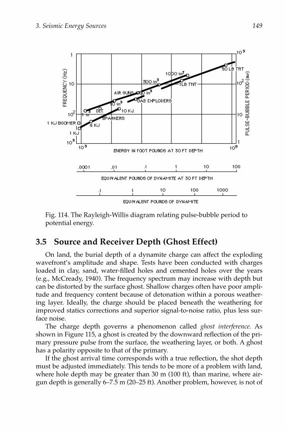
3. Seismic Energy Sources 149
3.5 Source and Receiver Depth (Ghost Effect)On land, the burial depth of a dynamite charge can affect the exploding
wavefront’s amplitude and shape. Tests have been conducted with chargesloaded in clay, sand, water-filled holes and cemented holes over the years(e.g., McCready, 1940). The frequency spectrum may increase with depth butcan be distorted by the surface ghost. Shallow charges often have poor ampli-tude and frequency content because of detonation within a porous weather-ing layer. Ideally, the charge should be placed beneath the weathering forimproved statics corrections and superior signal-to-noise ratio, plus less sur-face noise.
The charge depth governs a phenomenon called ghost interference. Asshown in Figure 115, a ghost is created by the downward reflection of the pri-mary pressure pulse from the surface, the weathering layer, or both. A ghosthas a polarity opposite to that of the primary.
If the ghost arrival time corresponds with a true reflection, the shot depthmust be adjusted immediately. This tends to be more of a problem with land,where hole depth may be greater than 30 m (100 ft), than marine, where air-gun depth is generally 6–7.5 m (20–25 ft). Another problem, however, is not of
Fig. 114. The Rayleigh-Willis diagram relating pulse-bubble period to potential energy.
Chapter 3 Page 149 Monday, February 7, 2005 4:00 PM
Downloaded 11 Nov 2011 to 198.3.68.20. Redistribution subject to SEG license or copyright; Terms of Use: http://segdl.org/

150 SEISMIC DATA ACQUISITION
the ghost interfering with a reflected event but the ghost actually causingnotching of the frequency spectrum.
In Figure 116, the solid line represents a direct downgoing wave and thedashed line represents the wave reflected from the surface. The physics ofsinusoidal wave propagation states that when two waves have the samewavelength, destructive interference (cancellation) occurs when they arriveexactly 180° out of phase. Because the reflection coefficient at the surface isnegative, the downgoing reflected wave experiences a 180° phase shift rela-tive to the direct wave. However, the reflected wave experiences a furtherphase shift because of the additional distance, 2d, that it travels relative to thedirect wave. If destructive interference is to occur, that distance must be anintegral number of wavelengths. That is, destructive interference occurs when2d = nλ, where n = 0,1,2,.... Since λ = V/f, the notch frequencies where destruc-tive interference is experienced are given by
(35)
For example, if V = 1500 m/s and d = 6m, then source ghost-notch fre-quencies are at 0, 125, 250,... Hz. Figure 117 shows field examples of the signa-ture of an air-gun array as the array changes depth. PTP refers to the peak-to-peak strength, and the PBR refers to the primary-to-bubble ratio.
Figures 118 and 119 display normalized versions of the normalized ampli-tude spectra for source and receiver arrays as a function of source andreceiver depths. Figure 118 maintains the source array constant at 5 m and
Fig. 115. Ghost generation.
f nV2d-------- , n 0 1 2 … ., , ,= =
Chapter 3 Page 150 Monday, February 7, 2005 4:00 PM
Downloaded 11 Nov 2011 to 198.3.68.20. Redistribution subject to SEG license or copyright; Terms of Use: http://segdl.org/

3. Seismic Energy Sources 151
changes the streamer depth from 5 to 15 m, while Figure 119 repeats the exer-cise but with the source array at 10 m. These examples show how streamerdepth can affect the location of notches in the spectra and how important it isto maintain a constant source and receiver depth.
The ghost notches are not of infinite depth because of noise in the recordedsignatures and their finite length. In particular, the signature truncation pro-duces a finite DC component (at 0 Hz). This has the effect of making the ghostnotch that actually occurred at f = 0 appear instead at about f = 3 Hz.
Ideally, a streamer should be towed at a depth designed to minimize theimpact of the receiver ghosts on the spectrum of the seismic data. At depths ofless than about 6 m, the ghost notch at f = 0 begins to seriously attenuate thelow end of the seismic spectrum. At depths of 15 m or more, the first nonzeroghost notch affects the higher end of the spectrum. A 10-m streamer depth is areasonable compromise that has become something of a de facto standard forstreamer surveys.
For land work, the ghost becomes a real problem if good-quality recordingrequires the shot to be placed beneath a thick weathering layer. Ghost notch-
Fig. 116. Surface ghosting and sinusoidal wave cancellation.
Chapter 3 Page 151 Monday, February 7, 2005 4:00 PM
Downloaded 11 Nov 2011 to 198.3.68.20. Redistribution subject to SEG license or copyright; Terms of Use: http://segdl.org/

152 SEISMIC DATA ACQUISITION
ing can then occur as a result of reflections from beneath the weathering andfrom the surface.
Fig. 117. Air-gun array signatures for a varying depth of source (after Dragoset, 1990).
Gun-depth(m)
PTPStrength PBR
20 b
ar –
m
80 ms
Chapter 3 Page 152 Monday, February 7, 2005 4:00 PM
Downloaded 11 Nov 2011 to 198.3.68.20. Redistribution subject to SEG license or copyright; Terms of Use: http://segdl.org/

3. Seismic Energy Sources 153
Fig. 118. Array response, source at 5 m, receiver depth variable (courtesy Geco-Prakla).
Signature and normalized amplitude spectrum(a) with array at 5 m depth and streamer at 5 m,(b) with array at 5 m and streamer at 10 m,and (c) with array at 5 m and streamer at 15 m
FREQUENCY (HZ)
FREQUENCY (HZ)
(c)
(b)
(a)
FREQUENCY (HZ)
AIRGUN ARRAY DEPTH 5 MSTREAMER DEPTH 5 M
AIRGUN ARRAY DEPTH 5 MSTREAMER DEPTH 10 M
AIRGUN ARRAY DEPTH 5 MSTREAMER DEPTH 15 M
PRESSURE PULSE
PRESSURE PULSE
PRESSURE PULSE
TIME (MS)NORMALIZED AMPLITUDE SPECTRUM
NORMALIZED AMPLITUDE SPECTRUM
NORMALIZED AMPLITUDE SPECTRUM
TIME (MS)
TIME (MS)
BA
R-M
BA
R-M
BA
R-M
40
20
0
-20-40
40
20
0
-20-40
40
20
0
-20-40
0 100 200 300
0 100 200 300
0 100 200 300
0 25 50 75 100 125 150
0 25 50 75 100 125 150
0 25 50 75 100 125 150
Chapter 3 Page 153 Monday, February 7, 2005 4:00 PM
Downloaded 11 Nov 2011 to 198.3.68.20. Redistribution subject to SEG license or copyright; Terms of Use: http://segdl.org/

154 SEISMIC DATA ACQUISITION
Fig. 119. Array response, source at 10 m, receiver depth variable (courtesy Geco-Prakla).
Signalization and normalized amplitude spectrum (a) with array at 10 m depth and streamer at 5 m depth, (b) with array at 10 m depth, and (c) with array at 10 m depth and streamer at 15 m depth.
PRESSURE PULSE
PRESSURE PULSE
PRESSURE PULSE
AIRGUN ARRAY DEPTH 10 MSTREAMER DEPTH 5 M
0 100 200 300
40
20
0
–20
–40
40
20
0
–20
–40
40
20
0
–20
–40
0 100 200 300
0 100 200 300
AIRGUN ARRAY DEPTH 10 MSTREAMER DEPTH 10 M
AIRGUN ARRAY DEPTH 10 MSTREAMER DEPTH 15 M
TIME (MS)
TIME (MS)
TIME (MS)
NORMALIZED AMPLITUDE SPECTRUM
NORMALIZED AMPLITUDE SPECTRUM
NORMALIZED AMPLITUDE SPECTRUM
0 25 50 75 100 125 150
0 25 50 100 125 15075
0 25 50 100 125 15075
FREQUENCY (HZ)
FREQUENCY (HZ)
FREQUENCY (HZ)
BA
R-M
BA
R-M
BA
R-M
(a)
(b)
(c)
Chapter 3 Page 154 Monday, February 7, 2005 4:00 PM
Downloaded 11 Nov 2011 to 198.3.68.20. Redistribution subject to SEG license or copyright; Terms of Use: http://segdl.org/

3. Seismic Energy Sources 155
3.6 Determining Optimum Air-Gun SpecificationsAlthough the seismic industry typically uses signature time-domain char-
acteristics to characterize air-gun arrays, this is an inadequate approach todetermining array performance. Because time-domain characteristics can bemodified by filtering, time-domain specifications (i.e., peak-to-peak andpulse-to-bubble ratios) are only valid when accompanied by a description ofhow the air-gun signature was filtered. An array signature recorded with a 2-ms sample rate (125 Hz antialias) cannot be compared in the time domainwith another recorded with 1-ms sample rate (250–375 Hz antialias). Theshorter sample interval recording will exhibit greater peak values because ithas twice the bandwidth. Instead, amplitude spectra are preferred for com-parison purposes: Any false impressions caused by sampling will be evidenton the amplitude spectra. Amplitude spectra should be referenced to a fixedminimum pressure. Energy-source researchers use micropascals (µPa), equiv-alent to 10-11 bars.
The total number of guns provides the greatest influence on outputenergy, not the pressure or the total array capacity. Two guns having a totalvolume of 1639 cm3 (100 in3) will give a greater output than a single 3280-cm3
(200-in3) gun. This is because the signal output strength is proportional to thecube root of each gun’s volume. For example, if the two guns are each 819 cm3
(50 in3), their net strength is proportional to 2(50)1/3 while the strength of thesingle gun is proportional to (100)1/3. The ratio of the strength of the two gunsto that of the single gun is 2(50/100)1/3, which is approximately 1.6. An excel-lent treatise is offered on the subject by Dragoset (1990). For those who needto check gun specifications before the start of a survey, this is mandatory read-ing.
Exercise 3.1Select the energy-source parameters for a vibrator survey with the follow-
ing objectives in mind:• Target depth—3000 m• Velocity at target—3000 m/s• Optimum resolution desired, using a sweep length of 16 seconds
Consider Figure 120 while solving the following problems:
1) Using the signal-and-noise spectra, select the preferred sweep fre-quency range to minimize the generation of ground roll but maximizethe reflected signal. In your selection, compromises will have to bemade.
Chapter 3 Page 155 Monday, February 7, 2005 4:00 PM
Downloaded 11 Nov 2011 to 198.3.68.20. Redistribution subject to SEG license or copyright; Terms of Use: http://segdl.org/

156 SEISMIC DATA ACQUISITION
2) If a downsweep were used, what time would the correlation noiseoccur on the record? Would this interfere with the target reflection?
3) Field tests have shown that a single vibrator record has an S/N of 2 to1 at the target depth when a sweep of 8-s length and 20 to 60 Hz isused. What combination of sweep length and sweeps per VP wouldgive a 4-to-1 improvement in signal-to-noise ratio?
4) If 10 s are needed for the moveup between sweep points, how longwill it take one vibrator to record one VP? Assume a 6-s listen time, abasic sweep of 8 s, and an S/N improvement of 4.
Exercise 3.2The direct energy wave and its ghost provide a two-point filter operator
and hence discriminate against certain frequencies (see Figure 121). Sketchthe frequency response for the two source depths and decide which depthgives the broadest frequency range with the minimum number of notches inthe seismic bandwidth.
Exercise 3.3In a real situation, a marine survey is being conducted with a 2-ms sample
rate and the hi-cut filter is 125 Hz. Sea state has deteriorated and, in order tomaintain a noise-free cable, the vessel must reduce speed to 4 knots and divethe cable to 13.7 m (45 ft). Unfortunately, the front end of the air-gun arraysdips to 13.7 m (45 ft) and the back end is maintained at 10.6 m (35 ft) by buoys.Sketch the source frequency response. Assuming the cable is now noise free,would this be adequate justification to continue recording? If not, why not?What would be the effect on the frequency response if the source were main-tained at 7.6 m (25 ft) but the receiver (streamer) were put at 15.2 m (50 ft)?
Fig. 120. Signal-and-noise characteristics from a previous dynamite survey.
Chapter 3 Page 156 Monday, February 7, 2005 4:00 PM
Downloaded 11 Nov 2011 to 198.3.68.20. Redistribution subject to SEG license or copyright; Terms of Use: http://segdl.org/

3. Seismic Energy Sources 157
Exercise 3.4The following data were provided by a crew as part of the results of a
pulse test:
• Velocity of sound through the water = 1500 m/s• Amount of hydrophone cable reeled out = 250 m• Gun depth = 6 m• First arrival traveltime = 10 msWhat can be said of the location of the hydrophone?
Fig. 121. Sketch the frequency response.
AIR
WATER
SHOTGHOST
TIME FREQUENCY Hz
FREQUENCY Hz
SOURCE DEPTH=7.5 MPrimary
Time
0.01 sec
Ghost AM
PL
ITU
DE
AM
PL
ITU
DE
SOURCE DEPTH=15 M
Primary
Time
Ghost
0.02 sec
0 20 40 60 80 100
0 20 40 60 80 100
+
-
+
-
d
Where t 27.5 m
1500 m/s-------------------------=
Chapter 3 Page 157 Monday, February 7, 2005 4:00 PM
Downloaded 11 Nov 2011 to 198.3.68.20. Redistribution subject to SEG license or copyright; Terms of Use: http://segdl.org/

159
Chapter 4
Seismic Instrumentation
4.1 IntroductionSo far, the complexities of the seismic source and receiver have been dis-
cussed. Once a seismic signal is transmitted and received, it must be recorded.The different types of signals discussed in this chapter are defined as follows:
1) Source signal—The pressure field created by the seismic source.2) Reflectivity signal—The earth's reflection sequence convolved with the
source wavelet.3) Seismic signal—Everything received as a result of the source firing. The
seismic signal includes the reflectivity signal as well as ground roll,refractions, diffractions, sideswipe, channel waves, etc.
4) Received signal—The electrical output of the receiver group. This is theseismic signal plus all environmental noise.
5) Recorded signal—The data, that is the instrument-filtered signal plusany additive instrument noise, which go on tape.
The information contained in a signal can be characterized by three quan-tities: signal-to-noise ratio, bandwidth, and duration. Signal-to-noise ratio canhave different meanings depending on the circumstances. For example, dif-fractions from out of the reflection plane are noise on 2-D data but are part ofthe signal in 3-D surveys. In seismic exploration, the recorded signal band-width is usually 0–250 Hz or lower. Often, data are processed in a narrowerband, say 5–80 Hz, even though they may be recorded in a broader band. Theduration of recorded signals depends on the nature of the source and targetdepth. Impulsive sources, such as land dynamite or marine air guns, create asource signal with a duration of a few tenths or hundredths of a millisecond.On the other hand, the duration of an uncorrelated vibrator source signal maybe 10 s or longer.
A reflection is a physical event caused by a change in the acoustic imped-ance of the earth. In a recorded signal, that event is represented by a wavelet
Chapter 4 Page 159 Monday, February 7, 2005 4:27 PM
Downloaded 11 Nov 2011 to 198.3.68.20. Redistribution subject to SEG license or copyright; Terms of Use: http://segdl.org/

160 SEISMIC DATA ACQUISITION
that has two components—the earth filter and the acquisition wavelet. Thewavelet can be described in the time domain or, alternatively, in the frequencydomain. The Fourier transform can be used to move from one representationto the other. If a wavelet has a short extent in time and appears like a spike, itis likely to be composed of a broad band of frequencies, each separate fre-quency having its own phase value. The amplitude and phase of a waveletcontains all the spectral information of a wavelet. These spectra are called thefrequency-domain representation of the wavelet, whereas the wavelet in time isconsidered to be in the time domain. For a brief explanation of the frequencydomain, the reader may refer to the Appendix.
4.2 Basic ConceptsWhen seismic recording first began in the 1920s the recording systems
consisted of heavy, metal-cased geophones connected by wire cables to arecording truck. The geophones were analog sensors that transmitted analogsignals to analog instruments inside the truck. Each incoming analog signalwas connected to its own analog amplifier, after which the signal wasrecorded on a rotating photographic drum (similar to the equipment still usedtoday at many seismic observatories). Drums were replaced by analog mag-netic tape recorders (like the reel-to-reel tape recorders sometimes used byradio stations) during the late 1950s, but these often failed to operate well. Inthe early 1960s they were replaced by digital tape recorders, each of whichhad an analog-to-digital converter at the input to the tape drive. The individ-ual analog amplifiers also were unreliable, and by the late 1960s, they werebeing replaced in recording devices by a single multiplexed analog amplifier.This single digital amplifier allowed the incoming analog signal from all geo-phones to be recorded digitally.
The amplifier required a multiplexer switch to synchronize the switchingof geophone lines to the amplifier at the correct time. In the late 1970s distrib-uted systems were introduced that performed amplification, filtering, digiti-zation, and multiplexing at or near the receiver stations. GeoSystems andOpseis were two early market leaders. By the mid-1980s distributed systemswere in wide use throughout the industry.
In land recording using a nondistributed system, an analog seismic signaltravels from the geophones along electrical conductors (the cable) to a roll-along switch in the recording truck (or “doghouse” or “dog-box”), afterwhich it is converted to a digital signal and recorded on tape or disk. In con-trast, in a distributed system, the seismic signal passes from the geophonestring directly into an amplifier and/or A/D converter, after which it travelsin digital form along a cable to the recording truck. Because digital transmis-sion of multiplexed data uses many fewer cables than analog transmission,
Chapter 4 Page 160 Monday, February 7, 2005 4:27 PM
Downloaded 11 Nov 2011 to 198.3.68.20. Redistribution subject to SEG license or copyright; Terms of Use: http://segdl.org/

4. Seismic Instrumentation 161
layout of the large receiver spreads often used for 3-D acquisition becameconsiderably simpler.
4.2.1 Basic Components
The basic components of the land recording system are reviewed next,using the generic schematic shown in Figure 122. This review is general, sinceeach actual recording system has unique aspects that can be understood bestby studying the manufacturer's documentation. The discussion also appliesto distributed systems if one imagines that the main amplifier, gain controller,and A/D converter are positioned before the multiplexer.
The components are as follows:
Fig. 122. Nondistributed land recording system schematic.
Chapter 4 Page 161 Monday, February 7, 2005 4:27 PM
Downloaded 11 Nov 2011 to 198.3.68.20. Redistribution subject to SEG license or copyright; Terms of Use: http://segdl.org/

162 SEISMIC DATA ACQUISITION
Roll-along switch—Used in land surveying and located in the recordingtruck, it allows the observer to record a selected subset of the geophones con-nected to the recording truck. The roll-along switch minimizes the need tomove the recording truck. The switch has many input seismic channels andoutputs the seismic data to the recording system. In marine streamer record-ing, a roll-along switch is unnecessary because every hydrophone group isrecorded continually by a dedicated instrument channel.
Preamplifier—This is a fixed gain amplifier that raises the incoming seis-mic signal above the background instrument noise level. The preamplifier haslow noise, high input impedance and low distortion. Its input impedance isequal to or greater than the cable impedance to the furthest station so that nosignal amplitude is lost because of mismatching of impedances. The amplifiermust be completely linear over its operating range.
Multiplexer—This is an electronic switch that time shares data from multi-ple channels. It changes multiple parallel inputs to a serial output ready foramplification, digitizing, and recording. The multiplexer cycles through all ofthe inputs during each digital sampling interval.
Main amplifier—This amplifier receives all analog signals input to it andpasses them on to the A/D converter with an amount of gain determined bythe gain controller.
A/D converter—Analog signals are converted to digital signals with thisdevice. It allows the analog stream of data to be recorded in digital form. Thereceived incoming signal must be filtered to prevent aliasing prior to conver-sion to a digital form. This is discussed in more detail below.
Gain controller—The received signal includes reflections, refractions,ground roll, and environmental noise, all of which may have amplitudesvarying in a range from microvolts to volts. A fixed form of amplificationwith only a relatively small number of data bits (such as 14) cannot handlethat range without some clipping at the most significant bit end of the con-verter. Instead, a variable or automatic gain control (AGC) level is determinedfor application by the main amplifier in the feedback loop with the A/D con-verter to reduce or amplify incoming signal to keep signal levels within thedesired converter range. The controller sets the amount of gain while theamplifier applies it to the incoming signal. The AGC level set at each sampleis recorded on tape as part of the gain word.
Formatter—
Next, the formatter puts the data stream (in the form of volt-age and gain levels) into a binary code for writing onto magnetic tape. Inaddition, instrument operational commands are distributed by the formatterto all the other components, making the formatter the “brain” of the recordingoperation.
Chapter 4 Page 162 Monday, February 7, 2005 4:27 PM
Downloaded 11 Nov 2011 to 198.3.68.20. Redistribution subject to SEG license or copyright; Terms of Use: http://segdl.org/

4. Seismic Instrumentation 163
Tape drive—Data finally are recorded on tape in digital form, ready to bepassed on to the processing center for further processing. Magnetic tape maybe replaced by floppy disks, depending upon the system in use.
4.2.2 Instrument Noise and Sampling
A major component of all seismic recording instruments, which is notshown in Figure 122, is the recording filter system. The received seismic sig-nal must undergo frequency filtering prior to the recording process to ensurethat it can be reproduced later in the data processing center with no confusionof its frequency content (known as aliasing). Recording-system filters also areused to remove unwanted noise. The issues of noise and aliasing must befully understood before a discussion of instrument filtering is possible.
4.2.2.1 Instrument Noise
Several types of electronic noise can occur in recording instruments.Coherent repetitive signals (50, 60, or 100 Hz) are caused by electrical interfer-ence or
crossfeed
between the instruments and nearby power supplies orcables. Such noise can be attenuated by shielding or rerouting cables. Modernelectronic instruments can suffer from several types of incoherent noise thatare inherent in the nature of the components. For example,
Johnson noise (orthermal noise) is caused by the randomness of conducting electrons, whereasshot noise is caused by the discreteness of charge carriers within semiconduc-tors. Quantization noise is another type of incoherent noise that is caused bythe finite width of the voltage level represented by the least significant bit in adigitized signal. Instrument designers strive to minimize these kinds of noisethrough various design strategies.
If the instrument noise is outside the desired seismic signal spectrum, ana-log or digital filtering may remove it. If the noise is coherent and of a fre-quency similar to the seismic signal, then it is difficult to remove without alsoremoving some seismic signal. Incoherent spiking transients may be removedby special data processing techniques performed in the processing center.
4.2.2.2 Sampling
As stated earlier, analog signals must be sampled correctly when digitiz-ing. The seismic signal is sampled at discrete time intervals called the sampleintervals, which can vary from 0.25 ms to 8 ms depending on the instrumentsin use (industry often uses the term “sample rate” to mean sample interval).The smaller the sample interval, the larger the potential frequency range thatcan be recorded. The choice of sample rate is dependent on the seismic objec-tives and the required bandwidth. As was explained in Chapter 2, to digitizean analog signal properly, it must be sampled at least twice per cycle of the
Chapter 4 Page 163 Monday, February 7, 2005 4:27 PM
Downloaded 11 Nov 2011 to 198.3.68.20. Redistribution subject to SEG license or copyright; Terms of Use: http://segdl.org/

164 SEISMIC DATA ACQUISITION
highest frequency present in the signal. This is called the Nyquist criterion. Fora given sample interval, the highest frequency that satisfies this criterion iscalled the Nyquist frequency. Frequencies above the Nyquist frequency aresampled incorrectly and are said to be aliased.
Consider Figure 123, in which an 80 Hz sinusoidal wave has been sampledat an interval of 4 ms. The wave's amplitude values are shown, relative to apeak value of 1, and the sample times are shown at 4 ms, 8 ms, 12 ms, and soon. If a 170-Hz wave is sampled now at the same interval, as shown by thesecond wave, we can see that the values are exactly the same as for the 80-Hzwave, so sampling and reconstructing a 170-Hz wave at a 4-ms sample ratewill produce an 80-Hz wave. Hence, a 170-Hz wave is an alias of an 80-Hzwave. This example shows that a 4-ms sample interval is too low to sample a170-Hz wave adequately. Taking the example to its extremes, if we sample a
Fig. 123. Digital sampling.
Chapter 4 Page 164 Monday, February 7, 2005 4:27 PM
Downloaded 11 Nov 2011 to 198.3.68.20. Redistribution subject to SEG license or copyright; Terms of Use: http://segdl.org/

4. Seismic Instrumentation 165
250-Hz wave (the frequency for a period of 4 ms), a constant output value willresult (called a dc bias).
Since aliasing commences at the Nyquist frequency, and the Nyquist fre-quency is half the sampling frequency, for 4-ms sampling, all frequenciesabove 125 Hz are aliased. For 2-ms sampling, aliasing starts at 250 Hz; for 1-ms sampling, aliasing starts at 500 Hz. One major role of filters in seismicinstruments is to remove frequencies that will be aliased if they are presentwhen the signal is digitally sampled.
Figure 124 shows a method to work out the value of an alias at a particularsample interval. First, triangles are constructed to each side of the Nyquistfrequency. Then a horizontal line is drawn across the figure. Aliased frequen-cies at the intersection of the line with the second triangle will appear, whensampled, to be the frequency at the intersection of the line with the first trian-gle. For example, with a 4-ms sampling interval, analog frequencies of 170 Hzand 330 Hz will be represented as 80 Hz after digitization.
4.3 FilteringFigure 125a shows an amplitude response plot (see Appendix) of an ideal-
ized seismic instrument filter. The graph is plotted in logarithmic form, withthe peak signal amplitude at a value of 0 dB. The frequency range over whichsignal is allowed to pass in such a filter is known as the passband, and a filterwhich has such a passband is called a band-pass filter. The frequency rangeover which a filter attenuates signal is called the reject area or reject zone.
Fig. 124. Frequency aliasing at 4 ms.
Chapter 4 Page 165 Monday, February 7, 2005 4:27 PM
Downloaded 11 Nov 2011 to 198.3.68.20. Redistribution subject to SEG license or copyright; Terms of Use: http://segdl.org/

166 SEISMIC DATA ACQUISITION
The passband of the filter of Figure 125 is conventionally defined as thefrequency interval between –3 dB points (70% amplitude, known as the half-power point). The filter slope is measured in dB/octave, an octave being the fre-quency range from a starting frequency to twice that frequency (e.g., 10–20 Hz, 15–30 Hz).
All passband filters cause some amount of amplitude and phase distortionof the true signal. To minimize this distortion and still ensure the filter oper-
(a)
(b)
Fig. 125. (a) Idealized frequency response of a filter. (b) Actual frequency response of a 3–125-Hz filter.
Chapter 4 Page 166 Monday, February 7, 2005 4:27 PM
Downloaded 11 Nov 2011 to 198.3.68.20. Redistribution subject to SEG license or copyright; Terms of Use: http://segdl.org/

4. Seismic Instrumentation 167
ates adequately, it is necessary to use a gentle gradient of the filter slope at thelow frequency end (e.g., about 12–26 dB/octave). The slope gradient at thehigher frequency end of the spectrum can be 70 dB/octave or more withoutcausing undue high-frequency distortion. The high-end filter is known as thehi-cut filter (because it cuts out higher frequencies) or antialias filter (because itguards against aliasing), whereas the low-end filter is known as the lo-cut fil-ter.
In Figure 125a, if filter points f1 and f2 were an octave apart, then the slopewould be 15 dB per octave. The passband is between half-power points f2 andf3. In practice, analog filters respond with rounded corners, as shown in Fig-ure 125b. We say that the filter response rolls on at the lo-cut end and rolls off atthe hi-cut end of the passband.
In recording or data processing documentation, a filter's frequency rangeoften is expressed solely in frequency terms starting at its lowest operationalpoint, followed by the passband values, and finishing at an end-frequencyvalue. The values for Figure 125b would be 3/12/125/220 Hz (where theeffective lowest and highest frequencies to be passed by the filter would begreater than 50 dB down). An alternative approach is the filter-value/slopenotation, which expresses the filter in terms of lo-cut/slope followed by thehi-cut/slope value. For example, a lo-cut filter reaching the half-power pointat 12 Hz, having a slope of 26 dB/octave from its start up to that point, will bedocumented as 12/26; a hi-cut filter with a half-power point at 125 Hz andthereafter with a slope of 70 dB/octave will be documented as 125/70. Thisfilter then is written as 12/26/125/70. Documentation must state the filtervalues clearly in order to avoid confusion during data processing. When thelo-cut filter is switched off so that no low frequencies are attenuated, the lo-cut filter is said to be “OUT.” Such a filter is sometimes referred to as either aband-stop filter or a low-pass filter.
The hi-cut filter in a recording instrument is designed to attenuate aliasedfrequencies so that they will not distort the received signal after it has beendigitized. As shown in Figure 126, a given degree of attenuation at the onsetof aliasing (125 Hz in this example) can be obtained by dissimilar filterparameters. The 64/12 filter achieves about the same attenuation at 125 Hz asdoes the 90/70 filter. Beyond 125 Hz, the steeper filter has better rejection.Whether that is important depends on the amplitude of the aliased frequen-cies in the received signal. Steeper antialias hi-cut filters usually are preferred,however, because they provide a wider recorded signal bandwidth and,hence, potentially better seismic resolution.
Analog hi-cut filters are typically only effective with slopes up to about70 dB/octave. Steeper slopes are possible, but such filters have undesirableripples (known as Gibbs’s effect) in their time-domain responses. The intro-
Chapter 4 Page 167 Monday, February 7, 2005 4:27 PM
Downloaded 11 Nov 2011 to 198.3.68.20. Redistribution subject to SEG license or copyright; Terms of Use: http://segdl.org/

168 SEISMIC DATA ACQUISITION
duction of state-of-the-art, 24-bit systems using digital filters has allowedsteep slopes of as much as 200 dB/octave to be used, moving the high-cut endof the spectrum close to the Nyquist frequency.
Just as the hi-cut filter value and slope can be changed to alter the upperend of the signal spectrum, so the lo-cut filter value and slope can be changedas desired. It was common practice for many years to use the lo-cut filter toattenuate low-frequency noise when it became a problem. For example, whenstrong ground roll was observed on land shot records, one approach toremoving it was to increase the lo-cut filter value to a point where it attenu-ated the coherent wavetrains. This approach also has worked in marinerecording, where strong streamer strumming (commonly referred to as“streamer jerk”) as a result of the vessel or tail buoy moving through roughsea can cause a high-amplitude coherent noise train along the streamer.
More recently, the application of such lo-cut filtering has been discour-aged. Increasing the low-frequency cutoff point reduces the recording band-width and may cause a loss of useful signal in addition to noise attenuation.Such coherent noise may not have stable characteristics throughout a survey;the reduction in recording bandwidth then becomes unjustified. In addition,different filters and instruments have different phase characteristics so that ifdifferent recording filters and instruments are used for a period of years overa survey area, it may become difficult to tie in different vintages of stackeddata. Consequently, once a band-pass filter value has been set for an area dur-ing an initial survey, ideally that filter should be maintained thereafter during
Fig. 126. Use of different filter slopes.
Chapter 4 Page 168 Monday, February 7, 2005 4:27 PM
Downloaded 11 Nov 2011 to 198.3.68.20. Redistribution subject to SEG license or copyright; Terms of Use: http://segdl.org/

4. Seismic Instrumentation 169
subsequent surveys, in spite of any low-frequency noise problems. Because oftheir wide dynamic range (see Section 4.6), modern systems can afford to sim-ply record any low-frequency noise and let it be dealt with during data pro-cessing.
In land seismic surveying, when power lines are crossing above the seis-mic cable, the cable conductors may pick up electrical noise at the power-linefrequency. Such electrical pickup often can be so high in amplitude that itcompletely masks the useful seismic signal. One way to avoid this problem isto use a recording filter to reject the power-line frequency. A filter designed toremove a single frequency is known as a notch filter. The notch may be at 50 or60 Hz, depending on the local power-line frequency.
A notch filter can have an undesirable phase response. Using the notationof frequency-value/slope, Figure 127 shows the filter response of a DFS-Vrecording instrument using a sample rate of 2 ms and having 12/26/124/70Hz filters (where the passband is 12 to 124 Hz). Such spectra are obtained byFourier analysis of the instrument impulse response. That is, an electricalspike is input into the recording system, recorded, and then transformed intothe frequency domain. The amplitude response in this case indicates that a 60-Hz notch filter is in use. The phase spectrum shows the instrument responsewith and without the 60-Hz notch filter. Clearly, the use of the notch filtermakes a major change to the filter response, causing a phase reversal (i.e.,180° phase change) at frequencies of about 60 Hz.
Figure 127 also shows how a notch filter changes the time-domain repre-sentation of an instrument impulse response. Clearly, use of a notch filter in arecording system makes its impulse response less desirable from an inter-preter's viewpoint. Another problem with a notch filter is that it not onlyremoves the noise at the notch frequency but also the signal at that frequency.Consequently, the use of such a notch filter in recording instruments is dis-couraged; other field approaches (such as applying an input signal to theaffected channels of exactly the same frequency and reversed phase as thepower line) can resolve the problem of power-line pickup in the field.
Figure 128 shows the temporal impulse response of a DFS-V instrumentusing different filters and how the response would appear after transformingeach filter to its zero-phase equivalent (ZPE). The ripples after the initial spikeshow the effect of the notch filter. Note how the ZPE wavelet has more ripplesas the filter passband reduces. This is not a desirable effect because when seis-mic data are stacked to produce a seismic section, such ripples can sum toproduce either a ringing wavelet or a lower stack frequency content, therebyreducing horizon resolution.
If the optimum response for a recording instrument is a spike, then thebest response in Figure 128 is the OUT-124 Hz option, which most closely
Chapter 4 Page 169 Monday, February 7, 2005 4:27 PM
Downloaded 11 Nov 2011 to 198.3.68.20. Redistribution subject to SEG license or copyright; Terms of Use: http://segdl.org/

170 SEISMIC DATA ACQUISITION
resembles an input spike. This is logical because, of these filters, the OUT-124Hz filter applies the least amount of filtering. By comparison, the 60-Hz notchfilter causes ringing and phase shifts, as explained earlier. Often such ringingand phase shifts are removed from the seismic data by an inverse filteringoperation called designature. This helps in making the seismic sections easierto interpret.
Fig. 127. Amplitude and phase response of a DFS-V instrument, with and without a notch filter.
Chapter 4 Page 170 Monday, February 7, 2005 4:27 PM
Downloaded 11 Nov 2011 to 198.3.68.20. Redistribution subject to SEG license or copyright; Terms of Use: http://segdl.org/

4. Seismic Instrumentation 171
4.4 AmplificationReceived seismic signals have a wide dynamic range; that is, at times the
signals are quite large, whereas at other times the signals are very small. Onthe other hand, recording devices, whether analog or digital, have limiteddynamic ranges. When a recording device is presented with a signal outsideof its dynamic range, that signal cannot be recorded faithfully. Signals that aretoo small are not recorded at all, and those that are too large are distorted or“clipped.” Seismic recording systems contain an amplifier, the role of which isto match the amplitude of the received signal to the dynamic range of the
Fig. 128. DFS-V instrument impulse response using different filters.
Chapter 4 Page 171 Monday, February 7, 2005 4:27 PM
Downloaded 11 Nov 2011 to 198.3.68.20. Redistribution subject to SEG license or copyright; Terms of Use: http://segdl.org/

172 SEISMIC DATA ACQUISITION
recording device so that the signal can be recorded faithfully. This amplitudematching is called gain control.
In seismic recording instruments, gain control can be either constant or“fixed,” dynamic or “ranging,” or a combination of both. In a constant gainsystem, the amplification is set to a fixed amount so that the highest ampli-tude of interest in the received signal is recorded without being clipped. Theamount of fixed gain can be determined by performing and analyzing gain-constant test shots at the start of a survey. In a fixed-gain system, small signalsare lost if their voltage level falls below the recordable threshold. For exam-ple, if an A/D converter (see next section) represents each digital sample by12 bits and the largest signal is amplified to the point that it is represented byall 12 bits being “on,” then the smallest recordable signal is represented byjust one bit being on. Such a system has a recordable dynamic range of 72 dBbecause each bit represents a factor of 2, or 6 dB.
The limitations of fixed-gain amplification can be overcome through theuse of gain ranging. In a gain-ranging system, the amplification factorchanges on a sample-by-sample basis so that the amplified signal falls withinthe dynamic range of the A/D converter. The gain for each sample must berecorded so that true amplitude levels can be recovered when the data areprocessed. The so-called instantaneous floating point (IFP) systems introducedin the 1960s used a 14-bit data word and a 4-bit gain word, for a total dynamicrange of about 108 dB. Because of this increased dynamic range, IFP systemswere adopted industry-wide soon after their introduction.
In the 1990s A/D converters became available that had 24 bits of dynamicrange. In these systems, gain ranging is unnecessary, so, once again, fixed-gain amplification is in vogue.
4.5 A/D ConversionThe conversion process is performed by the analog-to-digital converter.
The A/D converter samples the input seismic analog data amplitude at dis-crete points in time and represents each sample by a digital word. The greaterthe number of bits in each digital word, the greater the range of amplitudethat can be converted without distortion. If a recording instrument has 14 bits,it can convert signal up to a value of 214 or 16 384. Therefore, 14 bits plus asign bit can represent an amplitude from –16 384 to +16 384.
The smallest signal that can be converted is that signal value representedby the least significant bit (lsb) of the converter. The dynamic range in theabove example is then 16 384 to 1 or 84 dB (see Appendix A for this relation-ship). In practice, the absolute converter range is slightly less since the ampli-fier has an ambient background noise value which is converted into a value in
Chapter 4 Page 172 Monday, February 7, 2005 4:27 PM
Downloaded 11 Nov 2011 to 198.3.68.20. Redistribution subject to SEG license or copyright; Terms of Use: http://segdl.org/

4. Seismic Instrumentation 173
bits. For example, in some IFP amplifiers, the lsb is used up by converting theinstrument noise alone, reducing the total system dynamic range by 6 dB.
An amplifier has ambient noise, whereas a converter does not. If it werepossible to increase the number of bits that could be converted, then thedynamic-gain amplifier could be replaced by a fixed-gain amplifier (in theform of the GC mentioned earlier), thus reducing amplifier noise. A 24-bitconverter expands the dynamic range to a theoretical value of 138 dB. Instru-ment manufacturers have introduced this innovation into their recording sys-tems, which because of internal system noise have a practical dynamic of114 dB. The main land manufacturers are Input/Output Inc. and OYO Inc.Input/Output has a 24-bit system widely used in the marine surveyingindustry, and Syntron Inc. also is marketing similar systems.
These systems can have advantages over the previous dynamic gain-rang-ing systems, apart from the ability to reduce amplifier noise. For example, amajor advantage of the Input/Output system is that the antialias filter is digi-tal rather than analog. Consequently, the antialias filter is zero-phase, so itdoes not change the phase of the recorded signal. Digital filtering also allowsa broadening of the passband spectrum up to 3/4 Nyquist frequency with asteeper 200-dB/octave filter slope, rather than the 1/2 Nyquist frequency and70 dB/octave slope required by the analog filters (see earlier in this chapter).Most 24-bit systems have such filters after digitization so that different filterscan be used without affecting the input data. If filters are not available toattenuate ground roll prior to A/D conversion on a system (they were avail-able with the previous AGC systems), then this would be a drawback of suchsystems. A schematic of one type of A/D converter is shown in Figure 129.The output of the A/D converter is a digital representation of a voltage sam-ple, known as the seismic word. When written on magnetic tape, a seismicword represents a single seismic sample—one voltage value. A seismic wordhas three parts—a data word (often referred to mathematically as the
man-tissa
), a gain word (referred to as the
exponent
or
characteristic
), and a sign bit.A data word is the basic value that has been converted, whereas the gainword represents the amount of gain to be applied to the data word to restoreit to its true analog value.
In practice, the signal is connected to a sample and hold circuit for approx-imately 1
µ
s. This charges a capacitor to a voltage which remains and is usedfor comparison for 30
µ
s with a series of fixed-ladder voltages. When theappropriate voltage comparison is made, this value is supplied at the nextsample time. The voltage is on a binary scale. If the voltage level has attaineda maximum value, the AGC is requested to step down 12 dB on the next sam-ple. If a minimum converter value has been reached, the AGC steps up 12 dB.This range of gain is known as the
gain window.
The output is then sent withall logical commands to the formatter, which puts the bits into a format for
Chapter 4 Page 173 Monday, February 7, 2005 4:27 PM
Downloaded 11 Nov 2011 to 198.3.68.20. Redistribution subject to SEG license or copyright; Terms of Use: http://segdl.org/

174 SEISMIC DATA ACQUISITION
writing magnetically on tape. A full gain of 84 dB may be stepped up or downin one sample.
In the decimal number system, 10 is the base number. All numbers can berepresented as a function of 10. For example, a decimal system data word thathas a value of one thousand is represented by 1000. In the binary system, 2 isthe base number, where a data word is represented by a series of powers of 2.A binary data word which has a value of 1 is then represented by 20; a dataword with a value of 2 is represented by 21; 22 represents 4; 23 represents 8,and so on. So, if a data word has the values 20 + 21 + 22, it represents a value of1 + 2 + 4 = 7. If the gain word has a value of 21, the data word value of 7should be multiplied by 2 to produce the true value of 14. To take this exam-ple to its conclusion, a true value of +14 will have a seismic word consisting ofa gain word of 21, followed by a data word of 20 + 21 + 22, and a positive signbit.
4.5.1 Converter Operation
In Figure 129, consider what happens when a seismic voltage samplearrives at the converter. A value of voltage is already resident on the first unitwith which it comes into contact—the comparator unit. The two values of volt-
Fig. 129. Analog-to-digital converter schematic and gain word.
Chapter 4 Page 174 Monday, February 7, 2005 4:27 PM
Downloaded 11 Nov 2011 to 198.3.68.20. Redistribution subject to SEG license or copyright; Terms of Use: http://segdl.org/

4. Seismic Instrumentation 175
age are compared, and if they are the same, the register outputs a signal to thelogic circuitry to record a binary word containing a number of data bits and asign bit representing the comparator voltage. A gain value of 1 (or 20) in thegain word would be used to maintain the same data value to be written tomagnetic tape. When the next sample arrives at the comparator—let usassume it is a quarter of the previous sample value—then the comparator willinform the register that it has a lower voltage, and the register informs thevoltage divider that it must reduce its value. The divider reduces by one bit(i.e., divides the reference voltage Vref by 4), and this value is then input to thecomparator, and the gain word becomes 22 (i.e., 12 dB). The two inputs at thecomparator are now the same again and the new binary word representation(consisting of a data word and a gain word 22) of the voltage sample is writ-ten to tape. Any mantissa bit up to 213 may be stepped in one sample, whichis 84 dB as discussed previously.
The lowest sample amount that can be converted is typically 0.25 µV, sothat an A/D converter with a total of 120 dB dynamic range would be able todigitize signal in a range from 0.25 µV to 0.262144 V (i.e., 220). Allowing forthe sign bit, the most significant bit represents ± 0.262144 V.
4.6 Dynamic RangeInstrument dynamic range (DR) is the ratio of the largest storable signal
on the system to the smallest background noise. The storable signal is theamount of signal amplitude that can be digitized and recorded on a medium(such as magnetic tape) and subsequently recovered in the processing centerwithout distortion. DR is influenced by the instrument system noise as aresult of the chosen gain constant value and the number of converter bitsavailable to represent the analog signal in a digital form. To explain this con-cept, we will use, as an example, a recording system having both fixed anddynamic gain control.
The total instrument gain is the amount of fixed gain available (the GC) inthe instrument plus the amount of variable gain which can be applied by theamplifier to record the signal without distortion. This variable amplifier gainis applied to the signal in steps of 6 or 12 dB. All incoming signals have theinitial fixed GC gain applied to them (which may have a maximum value of30 dB), followed by an amount of variable amplifier gain, depending on theamount of gain required to correctly record the signals. The variable amplifiergain normally can apply a maximum amount of 90 dB to the smallest signals.Therefore, the total amount of gain possible is the fixed GC plus the variable90 dB, or 120 dB.
In the gain schematic of Figure 130, if the system noise level is 120 dB lessthan the signal that can be recorded without applying any gain, and the
Chapter 4 Page 175 Monday, February 7, 2005 4:27 PM
Downloaded 11 Nov 2011 to 198.3.68.20. Redistribution subject to SEG license or copyright; Terms of Use: http://segdl.org/

176 SEISMIC DATA ACQUISITION
GC plus the amplifier gain is 90 dB, then the remaining DR available will beonly 30 dB. Conversely, if the GC is set at 24 dB, then the DR available will be120 – 24 = 96 dB above the system noise. The maximum amount of gainavailable in any instrument is limited by the number of analog-to-digitalconversion bits available in the instrument converter. We ideally would likean infinite DR in the recording instruments, but this is not necessarily usefulsince eventually low-level signals become completely lost in instrumentnoise.
4.7 Recording
4.7.1 Formats
Because seismic data may not be processed by the same company thatrecorded them, data must be recorded in a standard field format that can beread by any processing center. For this reason, the Society of Exploration Geo-physicists (SEG) established a series of standard tape formats for the explora-tion industry (SEG, 1980). As a result, data in the past have been recorded in
Fig. 130. System dynamic range as a function of gain.
GAIN INCREASE
SIGNALLEVEL
dB
–90
–120
–180
Full Gain
Total System
Dynamic
Range
Zone
30 dB
0
RangeIdeal
Gain Steps
System Noise Level
Non-recordable
Amplifier
Chapter 4 Page 176 Monday, February 7, 2005 4:27 PM
Downloaded 11 Nov 2011 to 198.3.68.20. Redistribution subject to SEG license or copyright; Terms of Use: http://segdl.org/

4. Seismic Instrumentation 177
SEG B, C, or D formats on magnetic tape. Generally in seismic recording, dataare written in the SEG D format, be the tape in nine-track, DAT, cartridge orExabyte form. This is usually transcribed in the processing center to theSEG Y format—the industry standard format which all processing centers canread.
The field formats differ in the number of channels that can be recordedand the amount of space available to record peripheral data (such as filter set-tings). Such space is called header space, so that peripheral data in a header areoften called header information. Before the early 1970s, recording systems usedup to 21-track tape (1-inch width). Today, nine-track tape is the most com-mon. Use of cassette-type cartridge tape is prevalent in marine recording. TheSEG D format is shown as an example in Figure 131.
Data bits on magnetic tape are written and read by the so-called write headand read head, respectively. As a quality-control check to ensure proper datarecording, the read-after-write head reads the data immediately after they arerecorded. The tape drive (or tape transport) read head is connected to a play-back unit, which allows an immediate replay of data. This unit also may beconnected to an oscilloscope, a video display terminal, or a camera unit; theseallow a visual check of recorded shot data.
The seismic camera is a wiggle-trace plotter, which plots the wiggle traceson paper as a camera monitor record. Alternatively, an electrostatic plotter (e.g.,Versatec) or a thermal plotter (e.g., OYO) may perform this duty. The cameramonitor received its name historically; in the early days of seismic recording,the only form of record of the wiggle traces (before the invention of the mag-netic tape drive) was a photographic camera. A voltage output representing aseismic trace from the recording unit was fed to a galvanometer, from whichwas suspended a mirror. As the voltage moved positive, then negative, themirror rotated. A light beam reflecting off the mirror was thus deflectedacross a piece of photographic paper, and this represented the seismic trace.In those days, seismic crews also had a darkroom alongside the recordingroom.
Dual tape drives are used in surveys when high data production ratesleave insufficient time to rewind and replace a full tape reel between shots.Where cartridge tape drives are used, a number of cartridge drives may oper-ate at any one time, depending on how many data channels are beingrecorded. Tape speed is quoted in inches per second (ips) and may be checkedby an oscilloscope, a hand gauge, or an LED display. Tape speed should notvary more than ±2%, although data have been recovered from tapes recordedwith a tape speed error as high as 15%. Loss of tape-speed timing synchroni-zation is the most common cause of unreadable tapes.
The volume of data on a tape depends on the tape's bit-packing density. A6250-bits-per-inch (bpi) density system will pack nearly four times the data as
Chapter 4 Page 177 Monday, February 7, 2005 4:27 PM
Downloaded 11 Nov 2011 to 198.3.68.20. Redistribution subject to SEG license or copyright; Terms of Use: http://segdl.org/

178 SEISMIC DATA ACQUISITION
Fig. 131. SEG D tape format.
Chapter 4 Page 178 Monday, February 7, 2005 4:27 PM
Downloaded 11 Nov 2011 to 198.3.68.20. Redistribution subject to SEG license or copyright; Terms of Use: http://segdl.org/

4. Seismic Instrumentation 179
a system that records at a 1600-bpi packing density. The packing density ofmagnetic tape is given by
(36)
Cartridge tapes can record data at 32 000 bpi, which is a substantialincrease in data per unit area compared with the older systems, whichrecorded data at 800, 1200, 1600, and 3200 bpi. Cartridge tapes that havehigher packing densities are expected in the near future.
4.7.2 Recording Channels
Recording instruments such as the System Two (Input/Output Inc. tradename) can record as many as 4000 channels of data in SEG D format at6250 bpi. In marine recording, especially 3-D recording, data often arerecorded from three or more seismic streamers, each of 240 channels, at onetime. Hence, it is realistic to record with at least 720 channels in marine sur-veys, although single- and double-streamer operations (240 and 480 channels,respectively) are more common in conventional marine 2-D recording. Landsurveying often is performed using 120 to 240 channels. Sometimes, anincrease in the number of channels can cause limitations elsewhere within therecording instruments. For example, a set of instruments may be capable ofrecording 240 channels at a 2-ms sample rate, but to record 480 channels, asample interval of 4 ms is required. Here, there is the question of which ismore important, the maximum number of channels that may be used (therebypossibly increasing the fold) or the faster 2-ms sample rate (thereby doublingthe recording frequency range).
Often, by using more equipment, more channels can be recorded. The eco-nomics of equipment availability then becomes an important part of the limi-tations compromise. In today's complicated 3-D surveys, firm conclusionsregarding the optimum number of channels are difficult to reach. That is whythe industry has such a proliferation of survey designs.
The Geocor IV, marketed by GeoSystems, was the leader in channel expan-sion technology in the early 1980s. It could record 1024 channels when otherinstruments could record only 120 channels. It did this by the use of sign-bitrecording, as opposed to full-word recording (see later). Two advantages ofthis system were that it could perform real-time vibrator correlation and fastFourier transforms. However, the increasing sophistication of electronics hascaught up with this system; today real-time vibrator correlation and transfor-mations can be performed on full-word instruments recording a high numberof channels.
Packing density BPI Data rateTape speed------------------------------.=
Chapter 4 Page 179 Monday, February 7, 2005 4:27 PM
Downloaded 11 Nov 2011 to 198.3.68.20. Redistribution subject to SEG license or copyright; Terms of Use: http://segdl.org/

180 SEISMIC DATA ACQUISITION
Manufacturers such as GUS, Sercel, and Input/Output market distributedsystems that utilize twin-wire coaxial cable or fiber-optic cable, connected toindividual remote seismic data-acquisition units. Each station acquisition unitcan take as many as six stations of geophones, and their output is transmittedin serial format to the recording truck (Figure 132). It is a simple and fast oper-ation to lay a coaxial or fiber-optic cable down on the ground and plug into itan acquisition unit that receives, amplifies, samples, and multiplexes six sta-tions of data. Such field units simplify field work while allowing the use of agreater number of recording channels.
4.8 Miscellaneous
4.8.1 Telemetry
Telemetry is the act of transmitting signals from remote locations to a cen-tral receiving point, either by cable (coaxial or fiber optics) or by radio. Eachremote acquisition unit typically consists of a preamplifier (fixed or variablegain), a converter for digitization, and a data transmitter. In the case of cabletransmission, data are sent in packets from one remote unit to another, cas-cading into a stream, so that a large number of remote stations eventuallymay feed data to a single receiver in the recording truck. With radio opera-tion, the recording truck has individual receivers which demodulate the radiosignals before recording them on tape or disk.
Because radio telemetry systems rely on radio transmission of the seismicsignals, they may perform poorly in mountainous terrain due to a loss inradio signal strength. However, radio telemetry has been successfully used in
Fig. 132. Distributed systems using land line or telemetry.
Chapter 4 Page 180 Monday, February 7, 2005 4:27 PM
Downloaded 11 Nov 2011 to 198.3.68.20. Redistribution subject to SEG license or copyright; Terms of Use: http://segdl.org/

4. Seismic Instrumentation 181
remote areas over shallow water, on mud and tidal flats, and in swamps andjungles.
The advantages of telemetry over conventional land systems are:
1) Digital conversion at each station allows an increase in the number ofrecording channels that may be used.
2) It is sometimes faster to lay out and pick up the receiver spreadbecause individual personnel can pick up the receiver units ratherthan wait for a cable truck.
3) The ability to position remote receiver units anywhere allows moreflexibility in multiline receiver spread geometry.
4) Because there are no lengthy cable pairs running to a recording truck,there are no power-line noise pickup problems. Power-line pickupdoes not occur with fiber optic cables, either.
5) Data parity checks can be performed before transmission and afterreception to ensure that data have been transmitted and recorded cor-rectly.
6) Individual stations and remote units can be transported by helicopterfaster than other types of cables.
7) Telemetry units can avoid cable-laying obstacles such as rivers, rail-ways, and highways.
Apart from the poor radio transmission, another problem with the use ofany remote systems is that they obtain their power from batteries that requirefrequent recharging. Solar panels can charge unit batteries during the day, butsuch energy is dependent on the sun shining, so the batteries still must bechecked frequently to ensure no failures occur.
Texaco was an original user of telemetry transmission in the 1960s. Aqua-tronics developed Teleseis, a system that replaces cables with a radio link, inthe 1970s. A telemetry leader in the 1980s was Applied Automation's Opseissystem, which scanned more than 1000 channels at 2 ms. The system used acassette recorder at each station to record data to tape after each shot had beenfired. The tapes were retrieved from each acquisition unit at the end of eachday.
Where the survey area is flat with few obstacles to recording operations,most crews tend to use the coaxial or fiber optic cable approach. However,where there are ravines or hazards to the smooth flow of operations, radiotelemetry often is preferred, weather permitting.
4.8.2 Sign-Bit Recording
Sign-bit recording came into use in the early 1980s. This technique, origi-nally devised by NASA as a method of enhancing low signal-to-noise ratio
Chapter 4 Page 181 Monday, February 7, 2005 4:27 PM
Downloaded 11 Nov 2011 to 198.3.68.20. Redistribution subject to SEG license or copyright; Terms of Use: http://segdl.org/

182 SEISMIC DATA ACQUISITION
transmissions from a Venus space probe, uses vertical stacking of successiverecords to enhance the signal-to-noise. This method later was applied torecording seismic traces with great success.
Vertical stacking to enhance the signal works well, provided the noiseamplitude level is equal to or less than that of the signal. But if the noise isrecorded in random bursts with an amplitude value much higher than thesignal, it will take many stacks of records to reduce the noise bursts to the sig-nal level. This problem is overcome if all values of signal and noise are limitedto plus or minus 1. In this case, strong or weak signals have a value of ±1 andare always enhanced by the vertical stacking process. By comparison, large-amplitude random noise bursts are limited to ±1, so that stacking furthershots reduces the noise level.
A system that records a value of +1 or –1 for any positive or negative sig-nal is known as a sign-bit recording system, since it only need record the sign ofthe amplitude, the value itself always being 1. A value of zero is not recorded,and the converter only needs to know whether the signal is positive or nega-tive.
Figure 133 shows how sign-bit recording can be equivalent to an 18-bitrecording of a seismic trace. Random noise causes the zero crossing of theinput trace to shift from record to record; after 16 stacks (sums), the sign-bitrecording is almost identical to the conventional 18-bit recording. This onlyworks if there is random noise. If the noise level is too low, then additionalnoise must be generated (this is very easy when recording a land seismic linebecause line vehicles are constantly moving along the receiver line). Sign-bitrecording therefore works well under high-noise conditions, in which qualityis improved by recording many apparently poor-quality (low signal-to-noise-ratio) records.
Where high-amplitude random noise bursts occur and the signal-to-noiseratio is less than 1:1, the sign-bit technique is effective. This may prove benefi-cial, for example, when working in populated areas having random traffic-generating noise or when working in seismically poor areas of weak reflec-tions and occasional sideswipe.
The sign-bit technique is marketed by GeoSystems Corporation (which,although it has become insolvent in the United States, still is active elsewhere)as its petroleum survey Geocor instruments, and by Sercel as its Mini-Sosiehigh-resolution shallow survey instruments. The Mini-Sosie, rather than pro-ducing a programmed sweep, uses a random sweep, but apart from thataspect, its recording system is similar in operation to the Geocor system. TheMini-Sosie generates its own random noise bursts as the rammers are manu-ally pushed along the seismic line. Geocor and Mini-Sosie are the only sign-bit systems currently used by the industry.
Chapter 4 Page 182 Monday, February 7, 2005 4:27 PM
Downloaded 11 Nov 2011 to 198.3.68.20. Redistribution subject to SEG license or copyright; Terms of Use: http://segdl.org/

4. Seismic Instrumentation 183
4.8.3 Field Computers
Computers in the field can provide powerful support for various aspectsof the recording operation. A vibroseis uncorrelated field record is uninter-pretable, so this computation always has been performed in the field. Earlyfield data processing computers were based on the DEC PDP-11 machine.However, the large size of such machines restricted their common use until
Fig. 133. Simulation of the sign-bit recording technique. (a) Seismic trace recorded with a full-word (18-bit) instrument. (b) Data recorded with sign bit only. (c) Second recording and sum by a full-word instrument. (d) Sign-bit data after two sums. (e) The conventional full-word record after summing 16 times. (f) The sign-bit equivalent after 16 sums. In the sign-bit case, additional random noise is added to the trace prior to summation.
(a)
(b)
(c)
(d)
(e)
(f)
Chapter 4 Page 183 Monday, February 7, 2005 4:27 PM
Downloaded 11 Nov 2011 to 198.3.68.20. Redistribution subject to SEG license or copyright; Terms of Use: http://segdl.org/

184 SEISMIC DATA ACQUISITION
the advent of the IBM personal computer (PC). The PC reduced the cost ofprocessing but was frequently too slow or had inadequate software to per-form much more than the simplest of input/output functions. UNIX-basedworkstations were then developed to be more powerful than the PCs. Today,many field crews have data processing workstations to provide quick-lookand general data processing support during field acquisition.
Interactive field computers are considered necessary during land crewstartup when test lines and source tests need to be evaluated. Processing costsand time at the computer center can be saved using a field computer systemthat can demultiplex field records. Three-dimensional data acquisition, bothland and marine, would be almost impossible today without some form offield computing—even if it were only to locate the position of common mid-points during the recording operations—to ensure that the fold of coverage isadequate and within specified tolerances.
Field computers have blossomed on marine vessels during the upsurge in3-D data recording. When four streamers are collecting data from four sourcearrays, the amount of positioning information for recording increases sub-stantially. Networked workstations are becoming the norm for recording andprocessing the navigation sensor data in near real time. For example, astreamer's depth, feathering angle, and x,y location can be updated every sec-ond using ship-monitoring computers. The collected data also can beinspected to ensure that the quality of recording is acceptable.
Many recording systems have computers able to perform on-line phonetests and analyses as well as cable tests prior to each shot. This is useful inchecking receiver integrity before recording commences. A number of instru-ments are able to perform limited signal processing as a quick-look data pro-cessing package. The advantage of having a system that can do some form offield processing is that interpretation of field stacks may identify interestingformations that could be further delineated by a modified program. Onequick-look approach in marine 3-D recording is to bin short offset traces in alow fold 3-D volume, which may be rapidly processed and provide an earlyindication of data quality as well as profiles and time slices through the 3-Dvolume.
Exercise 4.11) If two seismic lines (which tie at their respective centers) were
recorded by different source, receivers, and instruments, what testswould be needed on the field-acquisition system to ensure that thedata phase ties in data processing would be made correctly?
Chapter 4 Page 184 Monday, February 7, 2005 4:27 PM
Downloaded 11 Nov 2011 to 198.3.68.20. Redistribution subject to SEG license or copyright; Terms of Use: http://segdl.org/

4. Seismic Instrumentation 185
2) (a) Surface waves take up a substantial amount of the dynamic rangeof floating-point recording instrumentation. Why should this be lessof a problem when using 24-bit instrumentation?(b) If the least significant bit of a 96 dB dynamic range system repre-sents 0.25 µV, and a peak reflection of 1 mV is detected at the receiversaccompanied by a surface wave valued at 2 V peak, would thedynamic range be adequate to record the reflection?
Chapter 4 Page 185 Monday, February 7, 2005 4:27 PM
Downloaded 11 Nov 2011 to 198.3.68.20. Redistribution subject to SEG license or copyright; Terms of Use: http://segdl.org/

Chapter 4 Page 186 Monday, February 7, 2005 4:27 PM
Downloaded 11 Nov 2011 to 198.3.68.20. Redistribution subject to SEG license or copyright; Terms of Use: http://segdl.org/

187
Chapter 5
Survey Positioning
5.1 IntroductionAccurate positioning of a seismic line is as crucial as having the best possi-
ble data quality. Positioning is important for three reasons: (1) many data pro-cessing steps require accurate relative source and receiver positions; (2) tyingseveral seismic lines together requires knowledge of where they are relativeto one another; and (3) when drilling sites are selected from seismic data theyhave to be referenced back to an actual location on the Earth’s surface. Ofthese reasons, perhaps the last is most important: No exploration companywants to spend millions of dollars drilling, only to miss the target because theseismic data were mispositioned.
Accurate positioning is not a trivial task, especially for marine surveys.Once a seismic vessel has sailed along an intended line, no permanent evi-dence remains behind to show where the ship actually sailed. Furthermore, atsea, intended shot and receiver positions cannot be identified by markersprior to shooting. Finally, during shooting, both the ship and the trailingequipment are somewhat at the mercy of the wind, currents, and wave action;the position of the shots and receivers cannot, therefore, be controlled accu-rately. For these reasons, positioning in marine surveys is a so-called real-timeactivity; that is, position measurements have to be made, recorded, and pro-cessed as a line is shot.
For land seismic surveys, positioning does not have the real-time urgencythat it does in marine surveys. The shot and receiver positions can be markedon the ground either before or during the shooting of a line. Likewise, accu-rate marker positions can be measured leisurely at any time. Furthermore,land surveys have the luxury of being referenced to
permanent markers,
loca-tions that are unlikely ever to be moved. Nevertheless, accurate land position-ing is not simple. Survey terrains are not flat, so land positioning mustinclude accurate elevation measurements, a dimension that is not so crucialfor marine surveys. In swamps, heavily forested regions, and mountainous
Chapter 5 Page 187 Monday, February 7, 2005 4:58 PM
Downloaded 11 Nov 2011 to 198.3.68.20. Redistribution subject to SEG license or copyright; Terms of Use: http://segdl.org/

188 SEISMIC DATA ACQUISITION
areas, accessibility and line-of-sight problems can make land positioning diffi-cult.
Geophysicists refer to locating a seismic line on land as surveying the linebecause the positioning technology is based on traditional land-surveyingmethods. The hydrographer or marine surveyor employed in the marineindustry to locate lines refers to the same task as positioning. There are otherdistinct differences between land and marine surveying. For example, in landsurveying, distances along seismic lines have been measured for many yearsusing theodolite and compass instruments, whereas in marine positioning,the position of the seismic ship is determined by radio navigation equipment,which requires radio towers to be erected along the shoreline as well asaboard ship.
While these differences have distinguished land from marine surveying inthe past, the introduction of GPS satellite positioning systems over the pastfew years has meant a unifying of positioning methods using a common tech-nology. Today, 3-D survey coordinates can be computed on a small computeras the surveyor walks along the seismic line on land or as the ship cruisesalong the seismic line offshore. In a few areas of the world, full 24-hour cover-age by GPS satellite is not yet available; consequently, the time-tested use oftheodolite on land or radio positioning offshore is still prevalent.
Even with satellite control of location, land surveys should be tied into atleast one permanent point that has accurately known coordinates. A perma-nent point, known as a survey
benchmark,
provides a fixed reference for futureline and well placement. On regional land surveys with large grids, bench-marks can be located at the ends of each seismic line so that any tie-in errorscan be checked. A steel stake (often referred to as a
star picket
) or pipe set inconcrete alongside some clearly visible landmark makes a good benchmark.Existing structures such as buildings in populated areas or large trees inremote areas also can be used as survey benchmarks. However, because suchstructures are not really permanent, a wise surveyor will establish severalalternative benchmarks as backups.
In marine surveying, the use of accurate electronic positioning equipmentis important because no trace of a survey can be found after a line is shot.Large hydrographic and geophysical research projects typically use naviga-tion instruments with only kilometer accuracy. In contrast, hydrocarbonexploration requires precise positioning to meter accuracy, if possible,because of the limited size of potential oil traps. Consequently, highly accu-rate radio instruments are used in offshore seismic work. Streamer receiversand sources have transponders (or
pingers
) positioned along their length thattransmit and receive signals between each other, from which the relativesource and receiver positions can be computed. Cable compasses mountedalong the streamer’s length measure streamer orientation, data which
Chapter 5 Page 188 Monday, February 7, 2005 4:58 PM
Downloaded 11 Nov 2011 to 198.3.68.20. Redistribution subject to SEG license or copyright; Terms of Use: http://segdl.org/

5. Survey Positioning 189
improve the accuracy of receiver position calculations. Tail buoys often havesatellite receivers and transmitters on them, which provide a continuousupdate of their location with respect to the streamer and towing ship. In sur-veys in which two ships are used, they are linked by radio, satellite, or acous-tics in a network so that the location of all of the equipment is knownprecisely at any point in time.
Even though survey positioning usually is done by experts in the use ofthe positioning hardware and software, all data-acquisition geophysicistsshould understand the fundamentals of this activity. This is especially true for3-D acquisition, in which the complexity of a survey, the large number of shotand receiver stations, and the need for precise positioning make surveying acrucial and costly part of operation. Viable 3-D surveys cannot be designedwithout an appreciation of the types and limitations of positioning equipmentand an understanding of surveying fundamentals such as spheroidal coordi-nates, datum corrections, mapping projections, and so on. This chapter willexplain the fundamentals of seismic surveying; the more advanced 3-D topicsare discussed in Chapter 7.
5.2 Maps and ProjectionsSeismic surveys usually are planned, processed, and interpreted as if the
surface of the Earth were flat. In reality, of course, data acquisition takes placeon the irregularly shaped surface of the Earth. To convert survey positioncoordinates from one type of reference frame to the other can involve one ormore complicated mathematical transformations. Further complicating mat-ters is the fact that there is not a universally used set of reference frames.There is a universally recognized coordinate frame representing the Earth’ssurface called WGS-72, but individual countries and regions tend to preferlocal reference frames, mostly for the convenience of having compatibilitywith historically significant surveys of their areas. Confusion over the usageof different reference frames can spell geophysical disaster. For example, a rigonce positioned in the South China Sea using WGS-72 coordinates missed itsdrilling target by some 500 m because it was not known that the target posi-tion was based on a seismic survey that had coordinates given in a local refer-ence frame. This section of Chapter 5 and the next section aim to prevent suchblunders by introducing the reader to the various types of reference framesused in survey positioning and explaining how they are related to oneanother.
The Earth’s nearly spherical surface is called the geoid. A mathematicalapproximation of the geoid is called a spheroid. The surface of a sphere or aspheroid can be represented (i.e., mapped) as a flat surface in many ways—called projections. All of them introduce distortion into the map. Most projec-
Chapter 5 Page 189 Monday, February 7, 2005 4:58 PM
Downloaded 11 Nov 2011 to 198.3.68.20. Redistribution subject to SEG license or copyright; Terms of Use: http://segdl.org/

190 SEISMIC DATA ACQUISITION
tions attempt to minimize distortion of a particular type or of a particularregion at the expense of increasing distortion elsewhere. Although projectionsare actually mathematical formulae that explicitly describe how a point on aspheroid is placed onto a flat map, they can be understood easily in terms ofvisual projections. The most common projection types are conical and cylin-drical. A conical projection is obtained by mapping the Earth’s spheroid to thesurface of a cone. The vertex angle θ is chosen to cause the cone to intersectthe sphere at two latitudes (Figure 134). This produces a flat map with lowdistortion in the middle latitudes. Such a map will have similar distances atthe middle latitudes in the east-west direction to the spheroidal distances.However, conical projections do have significant distortion within 30° of thepoles and the equator.
A cylindrical projection known as the transverse mercator, the type of mapmost people are familiar with, also has low distortion in the middle latitudes.The Universal Transverse Mercator (UTM) system is widely used by theexploration community. The UTM system divides the Earth into 60 verticalstrips or zones, each being 6° wide (Figure 134). The zones are centered at lon-gitudes 3,9,15,..., 357°. These longitudes are called the central meridians (CM)of the zones. The UTM coordinates of a position are called its northing andeasting. By convention, the central meridian of a zone has an easting of500 000 m. The easting increases for points east of the CM and decreases for
Fig. 134. Different projection types.
Chapter 5 Page 190 Monday, February 7, 2005 4:58 PM
Downloaded 11 Nov 2011 to 198.3.68.20. Redistribution subject to SEG license or copyright; Terms of Use: http://segdl.org/

5. Survey Positioning 191
points west of the CM (Figure 135). In the northern hemisphere, the equator isassigned a northing value of 0 m. Northing values increase as one movesnorth of the equator. In the southern hemisphere, the equator is assigned anorthing value of 10 000 000 m. As one moves south of the equator, the north-ing values decrease.
The northings and eastings of a point can be computed in any number ofTM projections. For example, point A in Figure 135 could have northings andeastings expressed in reference to either UTM zone 1 or UTM zone 2. Point Aalso could have northings and eastings expressed, say, in a TM projectionwith a central meridian passing through point A. In that case, the easting ofpoint A would be 500 000 m exactly. To compare or work with the northingsand eastings of two points, they must have a common projection choice. Sup-pose, for example, that in Figure 135 one has the northing and easting of pointB for UTM zone 1 and of point A for UTM zone 2. To compute, say, the dis-tance between the two points, one must either convert both points into lati-tudes and longitudes or convert one point from one projection to the other.That is, one could find the latitude and longitude of point A and then com-pute its northing and easting for UTM zone 1. The exploration geophysicistalways must be aware that northings and eastings are meaningless unless oneknows with which projection they were computed.
Figure 136 shows the various types of projections used for surveying andmapping, and provides an indication of how often they are used and theirdegree of complexity. The geophysicist tends to deal mainly with TM andUTM projections.
Fig. 135. Intersection between zones.
Chapter 5 Page 191 Monday, February 7, 2005 4:58 PM
Downloaded 11 Nov 2011 to 198.3.68.20. Redistribution subject to SEG license or copyright; Terms of Use: http://segdl.org/

192 SEISMIC DATA ACQUISITION
5.3 Geodetic DatumingA spheroid is an oblate ellipsoid of revolution that best fits the form of the
area to be surveyed. To describe a spheroid’s shape, we refer to the spheroidin terms of its radius of axes. There are two orthogonal directions whichdetermine the shape of an ellipse, known as the semi-major axis, A, and thesemi-minor axis, B (Figure 137). A geoid is the best fit surface, which fits theaverage topography of a local area of the earth to be surveyed and may becentered near but not at sea level for that area. A geoid tends to be perpendic-ular to the Earth’s gravitational field at all points along its length. The topog-raphy may vary either side of this local geoid, which may not be far in
Projection Type Conformal GridsArc to chord calculation
Used for surveying
Used for charts
Mercator Yes Not often used Simple On small scales only
Yes
Transverse Mer-cator
Yes Universal T.M.
Simple Yes No
Conical ortho-morphic
Yes Many with 1 or 2 parallels
Not simple Yes A few
Skew ortho-morphic
Yes Malaysia Simple Yes No
Stereographic Yes Polarstereographic
Not simple Yes No
Gnomonic No Not used No arc to chord
No Yes
Cassian No Very Many Difficult Not recommended
Fig. 136. Projections used for surveying and mapping (after Admiralty Manual of Hydrographic Surveying, 1965).
Mercator Yes Not often used Simple On small
Stereographic Yes Polar
Gnomonic No Not used No arc to
Cassian No Very Many Difficult Not recommended
Chapter 5 Page 192 Monday, February 7, 2005 4:58 PM
Downloaded 11 Nov 2011 to 198.3.68.20. Redistribution subject to SEG license or copyright; Terms of Use: http://segdl.org/

5. Survey Positioning 193
elevation from the spheroid. Satellites are referenced to a geoidal datum level,not to sea level.
Figure 137 is a schematic figure of the Earth’s geodetic surface relation-ships, which may be determined from a model of the Earth’s gravity field.With a knowledge of the geoidal height and a spheroid’s axis values, one candetermine the differences between a local geoid and spheroid; typical valuesare shown in Figure 138 for the most common spheroids. The shifts are usedto translate the satellite position figures into the local coordinates. This isimportant when working over large land or sea areas where the Earth’s cur-vature becomes a factor in the survey line positioning accuracy.
The difference between spheroid and geoid depends on the selection ofthe semi-major A and the semi-minor B axes. In the early surveying daysbefore satellite positioning, there was no need to tie continents togetherbecause all surveying was local. Hence, surveyors chose a spheroid to fit localareas. For example, the Everest spheroid has values of A and B to obtain a bestfit of the Indian continent to the spheroid produced by those values.
Land surveying uses a best-fit geodetic datum for the area being surveyed.The geodetic datum is defined by the following parameters:
1) A semi-major axis (A)
2) A semi-minor axis (B), or alternatively, flattening (f) where f =
Fig. 137. Geodetic surface relationships.
A B–A
--------------
Chapter 5 Page 193 Monday, February 7, 2005 4:58 PM
Downloaded 11 Nov 2011 to 198.3.68.20. Redistribution subject to SEG license or copyright; Terms of Use: http://segdl.org/

194 SEISMIC DATA ACQUISITION
Fig.
138
. Tra
nsfo
rmat
ion
cons
tant
s be
twee
n ge
odet
ic s
yste
ms
(aft
er S
tans
del
l, 19
78).
Chapter 5 Page 194 Monday, February 7, 2005 4:58 PM
Downloaded 11 Nov 2011 to 198.3.68.20. Redistribution subject to SEG license or copyright; Terms of Use: http://segdl.org/

5. Survey Positioning 195
3) a latitude and longitude for a point of origin.
A change in any value of (1), (2), or (3) alters the computed values of hori-zontal and vertical distance along the datum. Hence, there is no conformity inposition, distance, or azimuth of surveys which have physical points in com-mon but are based on quite different geodetic data. When comparing loca-tions in two such surveys, a mathematical correction called datum shifting isnecessary. Datum-shift values often are provided for an area referenced to acentral position. Although such shifts are correct for that central position, theyare only approximate for any other location. Large areas may require achange to this shift when working some distance from the central position.
For example, satellite receivers in Australia produce positions in the Aus-tralian National Spheroid (ANS). These positions (ideally) should be com-pared with the WGS-72 computation for the area in which the position wascomputed before the ANS coordinates are accepted as being correct. If the sat-ellite receiver had been used with some other spheroid system prior to mobi-lization to Australia, it still could be computing the Australian position usingthe previous spheroidal shift. A vertical error of 4 m and horizontal error of 10m, could be made. Consequently, before any surveying is performed for aseismic survey, one must ensure that the coordinate system and shift valuesare correct. Otherwise, gross errors may occur that will affect the final posi-tioning of the lines and of subsequent drilling rigs.
5.4 Land SurveyingBenchmarks are generally located with varying degrees of accuracy. Sur-
vey benchmarks can be categorized as first order, second order, or third order.First-order markers, which are positioned by government agencies, are gener-ally of millimeter accuracy and appear in different forms in different coun-tries. For example, in Europe, first-order markers are often a plaque cementedinto the ground or a well-known point in a public building, whereas in Aus-tralia they may be large steel triangles resident on the top of a hill. Seismicsurvey benchmarks are often second order, which is of less than 1 m accuracy,and may be recognized as pickets or spikes along a seismic line. (Metaldescription tags should be attached to pickets rather than paint markings,which wear with age.) Third-order accuracy, which is greater than a meter, isnot acceptable for seismic surveying.
In seismic land surveying, accuracies are often less demanding than thoserequired for geodetic and engineering surveys. The amount of positionalerror acceptable in a seismic survey depends on how the data will be usedand the bandwidth of the data. For example, larger source and receiver posi-tional errors may be acceptable in a 2-D survey than those acceptable in a 3-Dsurvey. In general, positional errors are acceptable as long as they do not
Chapter 5 Page 195 Monday, February 7, 2005 4:58 PM
Downloaded 11 Nov 2011 to 198.3.68.20. Redistribution subject to SEG license or copyright; Terms of Use: http://segdl.org/

196 SEISMIC DATA ACQUISITION
affect the quality of the final product of the survey. In the past, surveys wereconducted by traversing from a known benchmark using a survey instrument(theodolite), a rod, and a chain (measuring tape). As a result, short horizontalerrors of 1% (10 m per km) often were considered acceptable, while longerrors of 0.1% (60 m in 50 km) also were accepted if the survey lines were partof a reconnaissance survey rather than a detailed in-fill survey.
Today, laser distance measurement units (DMUs) with LED displaysobtain accuracies better than 0.01% on all line-of-sight ranges up to around 5km. In hot desert conditions, heat may cause laser refraction to occur (similarto the generation of a mirage), which can cause inaccuracies in laser distancereadings. Under such conditions, line locations should be surveyed duringthe cooler hours of the morning.
Before commencing a survey, part of the line location planning exercise isto determine the degree of positioning accuracy required and if local bench-marks have that accuracy. If the benchmarks do not have the desired accu-racy, then at least two benchmarks that do must be established in the area tobe surveyed. The line drawn between these two benchmarks is called a base-line,
with chosen points along the baseline being considered as newly estab-lished benchmarks of the required accuracy. Distances from these baselinepoints to stations on seismic lines may then be determined. A baseline pro-vides the surveyor with secondary benchmarks from which the seismic linesmay be referenced, and therefore more flexibility for surveying the seismiclines.
Alternatively, if three benchmarks are located in an area, their three con-necting baselines provide three sets of secondary benchmark locations. Sincethree points form a triangle, this is sometimes referred to as constructing a tri-angulation network
of benchmarks across the length and breadth of an area.For example, in Figure 139, point P on a seismic line is to be surveyed. It islocated within a triangle of stations A, B, and C. Distances from P to the three
Fig. 139. Triangular network.
Chapter 5 Page 196 Monday, February 7, 2005 4:58 PM
Downloaded 11 Nov 2011 to 198.3.68.20. Redistribution subject to SEG license or copyright; Terms of Use: http://segdl.org/

5. Survey Positioning 197
benchmark stations or to chosen points along the baselines can be measured,and an accurate location of point P therefore can be obtained. It is more com-mon to use the three benchmark stations as the primary survey benchmarksthan to use the secondary baselines.
When measuring distances from seismic lines to two benchmark stations(known as tying in), the accuracy is limited by the accuracy of the each of thetwo benchmarks. Tying in with a triangulation network improves the accu-racy, with three sets of distance data for comparison and checking.
Vertical elevation values can be obtained from station to station by view-ing a stadia rod from the DMU and computing the elevation value. SomeDMUs compute elevation automatically when the appropriate information issupplied to them. The true value of elevation above sea level is not critical,but a relative value from station to station is needed for computation of eleva-tion statics corrections. A 0.5 m elevation difference can cause a l-ms arrival-time difference from one station to the next, which if unnoticed can cause aloss of subtle geologic features in the stack of the seismic data. Elevation accu-racy can be checked with a loop closure map (Figure 140).
The map is produced by calculating and annotating elevation changesbetween all line intersections. Arrows may be placed between intersectionpoints in the direction of decreasing elevation; sometimes a rotating arrow isused within each loop to indicate the direction of a total sum of elevationchanges. If there are no elevation errors, summing the elevation changesaround any closed loop gives zero. Nonzero sums are caused by measure-ment errors or computational errors. An unjustified change in any one branch
Traverse to end of line and back
Loops
Fig. 140. Loop closure map.
Chapter 5 Page 197 Monday, February 7, 2005 4:58 PM
Downloaded 11 Nov 2011 to 198.3.68.20. Redistribution subject to SEG license or copyright; Terms of Use: http://segdl.org/

198 SEISMIC DATA ACQUISITION
will cause a change in all associated loops; this can be used as a quality con-trol scheme for the surveyor. On lines on which loops do not close, a doublerun—a traverse to the end of a line and back—is used. Double runs are shownat the left of Figure 140. A difference in total distance between the run to theend of the line and back will indicate an error in distance measurement thatmust be corrected.
5.5 Satellite SurveyingWhile land surveying has been performed for many years using theodo-
lite, rod, and chain, new technologies in surveying have evolved in recentyears. Navies around the world have used satellite systems to position theirships; in the early 1970s such systems became sufficiently accurate to use inthe offshore seismic business. Magnavox Inc. was a leading commercialretailer of satellite receiver systems that allowed seismic ships to obtain theirpositional information independent of shore-based systems.
Magnavox receivers were able to use the TRANSIT satellite system, whichwas operated by the U.S. Navy. Basically, six satellites are in polar orbit 1075km above the Earth, each one circling the globe every 107 minutes(Figure 141). The satellites form a cage within which the Earth rotates, carry-
Fig. 141. The TRANSIT satellite system.
Chapter 5 Page 198 Monday, February 7, 2005 4:58 PM
Downloaded 11 Nov 2011 to 198.3.68.20. Redistribution subject to SEG license or copyright; Terms of Use: http://segdl.org/

5. Survey Positioning 199
ing us past each orbit in turn. When a satellite passes overhead, a pass is saidto occur during which a fixed position, also called a fix, is measured. Theaverage time interval between each satellite pass is from 10 to 110 minutes,depending on the latitude of the receiver. Polar latitudes have the shortestintervals between fixes. Each satellite transmits two carrier signals, 150 MHzand 400 MHz. Every two minutes, each satellite transmits a message suffi-cient for a receiver to determine the receiver’s location at that time.
To obtain the receiver’s position relative to the satellite, the Doppler shift—a function of the observer’s position and the satellite motion—is measured. Afrequency shift is measured which is a result of satellite movement toward thereceiver, i.e., more cycles per second received than transmitted in a giventime. For each wavelength the satellite moves closer, one more cycle isreceived. As the satellite moves toward the ship, the received wavelengthfrom the satellite appears to compress so that its apparent frequency increasesin value (like an ambulance siren increasing in pitch as the ambulance travelstoward an observer). When the satellite passes the ship, the received wave-length appears to stretch, causing the apparent frequency to reduce in value(like an ambulance siren pitch decreasing as an ambulance travels away).Thus, a
Doppler count
is a measurement of a change in satellite apparent fre-quency, and that apparent frequency depends on the receiver’s location. Bymaking many Doppler counts, the receiver’s location can be computed accu-rately. About 20 counts, taking 10 to 18 minutes, provides a positioning accu-racy of about 200 m.
All satellite receptions are subject to errors in transmission (such as thosecaused by atmospheric changes or equipment failure). To eliminate receptionerrors, dual receivers may be used in the
translocation mode,
in which onereceiver is placed permanently on a benchmark (first order) while the otherreceiver is located at the position whose coordinates are desired. Any errorfound between the benchmark receiver’s computed position and the truebenchmark position can be used to correct the position computed by the otherreceiver.
TRANSIT receivers have been used to establish geophysical and naviga-tion-station locations, but their low-order accuracy limits the positioningaccuracy of any subsequent seismic survey. TRANSIT satellite receivers areused on seismic survey vessels, but because a single fix is accurate to withinonly 200 m, they are too inaccurate to provide total control of survey location.Consequently, when the U.S. military began to establish a far more accuratesystem in space, known as the Global Positioning System, the industry wasquick to adopt it.
Chapter 5 Page 199 Monday, February 7, 2005 4:58 PM
Downloaded 11 Nov 2011 to 198.3.68.20. Redistribution subject to SEG license or copyright; Terms of Use: http://segdl.org/

200 SEISMIC DATA ACQUISITION
5.5.1 Global Positioning System (GPS)
The NAVSTAR (Navigation System with Time and Ranging) Global Posi-tioning System (GPS) was conceived in 1973 when the U.S. armed servicesagreed to cooperate in the development of a highly accurate, space-based,military satellite navigation system orbiting just under 19 000 km above theEarth twice a day. The system was designed to provide instantaneous posi-tioning for navigation purposes 24 hours a day.
The system consists of three segments: (1) a space segment comprised ofsatellites that transmit coded radio signals, (2) a ground-based control seg-ment to monitor the position and health of the satellites, and (3) the user-equipment segment. When fully operational, the GPS system will have 18 sat-ellites in orbit, with three spare satellites available for use if required. Thiswill ensure that four to seven satellites will be visible from any point on Earthat all times.
Each GPS satellite transmits a unique signal on two L-band frequencies.The satellite signal consists of the L-band carrier wave modulated with a pre-cision or P code, which can provide positioning accuracy to better than 20 m.The P code can be encrypted for military use only. A less precise clear acquisi-tion
or C/A code provides accuracy to better than 100 m. This code is avail-able for public use. The primary function of the P and C/A codes is to permitthe signal transit time from the satellite to the receiver to be determined. Thenavigation message contains information on the satellite’s instantaneousposition and on the other satellite positions to enable the receiver to computethe other satellite times of appearance over the receiver. The transit time of asatellite, when multiplied by the velocity of light, gives the range from thesatellite to the receiver. By receiving up to four satellites, the user can solvefour equations with four unknowns: the 3-D position components of thereceiver and the receiver clock error.
The GPS system can be used in both the
point-position mode
and the trans-location or
differential-operation mode.
Because of orbital and timing errors, thepoint-position mode has an accuracy of 5 to 10 m, which is not adequate forland survey purposes. Point-position mode is used mostly for offshore navi-gation purposes. As with the TRANSIT satellite system, much higher accura-cies can be obtained from observations made simultaneously at two groundreceivers. In the differential mode, a number of the dominant errors will causenearly equal shifts in the estimated positions of both receivers so those errorscan be removed. This can provide accuracies of 5 m or better, with a separa-tion between the two receivers of up to 500 km. If the two receivers are sta-tionary for 30 minutes, their positions can be determined with an accuracy of5 mm plus 1 mm per kilometer of separation.
Chapter 5 Page 200 Monday, February 7, 2005 4:58 PM
Downloaded 11 Nov 2011 to 198.3.68.20. Redistribution subject to SEG license or copyright; Terms of Use: http://segdl.org/

5. Survey Positioning 201
The GPS system is a vast improvement over the TRANSIT Doppler systembecause it gives faster and more accurate results. Presently, the receiversavailable are becoming less expensive and bulky than the first-generationreceivers. One example of the miniaturization of the receiver is the MagellanNAV 1000, which can be held in the hand, as shown in Figure 142. In general,a single GPS satellite fix will give a position no better than 30 m. A minimumof three satellites are required to compute a 2-D position, and four arerequired for 3-D (which includes altitude) positioning in latitude/longitudeor UTM. Once the first fix is computed, updates can occur approximatelyevery three seconds.
The GPS system is commonly used offshore for 2-D and 3-D surveyingand rig positioning. It is also used in land surveying where immediate resultsof surveys may be plotted out at the end of a day’s work. Both Germany andthe Commonwealth of Independent States also have navigation satellitesorbiting in space. If the U.S. military decides to commence encoding transmis-sions from the GPS system, we can expect to use German and Russian satel-lites instead as our positioning and navigation system. An alternative tosatellite navigation is the shore-based radio-controlled system, discussednext.
5.6 Radio NavigationAll radio navigation systems are based on a simple principle: The distance
covered by a radio transmission between two points can be measured by mul-tiplying the transmission speed (the speed of light—299 792.458 km/s) by thetransmission traveltime. In practice, however, there are several complications.Because radio waves reflect and refract in the atmosphere, a transmissionpath may not be equivalent to the direct path (i.e., the straight line) betweenthe transmission points (Figure 143).
Furthermore, changes in atmospheric conditions can change the transmis-sion path from one hour to the next. Sometimes radio waves may follow sev-eral transmission paths between two points; the path with the shortesttraveltime may not be the signal received most strongly. This multipathingeffect is known as sky-wave disturbance or tropospheric scatter and can cause thenavigation system to be unacceptably inaccurate.
The basic principle of radio navigation can be used in two fundamentalways. In one scheme, known as phase comparison, the radio receiver detectsphase differences among synchronized continuous signals broadcast by twoor more shore-based stations. In some phase-comparison systems, a transmit-ter at the receiver location transmits a continuous signal that is rebroadcast bythe shore-based stations. The receiver then detects the phase differencesbetween the transmitted signal and the rebroadcast signals. In the other
Chapter 5 Page 201 Monday, February 7, 2005 4:58 PM
Downloaded 11 Nov 2011 to 198.3.68.20. Redistribution subject to SEG license or copyright; Terms of Use: http://segdl.org/

202 SEISMIC DATA ACQUISITION
Fig. 142. Hand-held Magellan NAV 1000 GPS receiver.
Chapter 5 Page 202 Monday, February 7, 2005 4:58 PM
Downloaded 11 Nov 2011 to 198.3.68.20. Redistribution subject to SEG license or copyright; Terms of Use: http://segdl.org/

5. Survey Positioning 203
scheme, known as range measurement, the ship’s radio unit transmits a codedmessage to the shore-based stations, which then rebroadcast it. Because thesignal in this system is not continuous, the radio receiver can measure directlythe round-trip traveltimes—and, hence, the distances—from the ship to theshore stations. By contrast, in phase-comparison systems, only phase differen-tials are detected. That information has to be integrated (a process called lanecounting) before it can be used to determine the ship’s position.
If the distance to a single station is known, all that tells us is that the ship issomewhere on the circumference of a circle of known radius from the station.When the distances from a ship to two stations are known, the ship must belocated at one of the places where the two circles associated with the distancesand stations intersect (Figure 144). Usually, the ambiguity can be resolved byknowing the approximate ship position and picking the circle intersectionclosest to that position. Thus, with both radio navigation types, the location of
Fig. 143. Line-of-sight and tropospheric transmission.
Fig. 144. Two-station fix positioning.
Chapter 5 Page 203 Monday, February 7, 2005 4:58 PM
Downloaded 11 Nov 2011 to 198.3.68.20. Redistribution subject to SEG license or copyright; Terms of Use: http://segdl.org/

204 SEISMIC DATA ACQUISITION
a ship is determined by finding the distance from the ship to at least two sta-tions; this is known as a position fix. Additional stations provide redundantdata and, hence, greater accuracy of a fix position. In the situation where theship is near the line connecting the two stations, a third distance measure-ment is required to resolve the intersection ambiguity. Circular lines are usedto represent lines of equal distance to each station. These are referred to aslines of position (LOPs). The minimum number of stations that can be used fora fix is two (Figure 144), whereas a third station would allow a three-way fix ona location.
5.6.1 Phase Comparison
There are two kinds of navigation based on phase comparison: hyperbolicand circular. Of these, hyperbolic navigation is used most often. With thehyperbolic network system, only the shore-based stations transmit a signal tothe mobile receiver. Continuous, uninterrupted analog signals are receivedaboard the survey ship from two shore-based transmitters. The separate sig-nals are synchronized so that the ship’s mobile receiver can determine theirphase difference. Knowing the phase difference constrains the location of thereceiver to lie along a hyperbolic LOP (Figure 145). If a second pair of shorestations are received and a further phase comparison made, a second LOP canbe obtained. The receiver is located where the two LOPs intersect. Normally,only three shore stations are used unless the survey extends out of the rangeof one station, in which case a fourth would be necessary.
Fig. 145. Hyperbolic lines of position.
Chapter 5 Page 204 Monday, February 7, 2005 4:58 PM
Downloaded 11 Nov 2011 to 198.3.68.20. Redistribution subject to SEG license or copyright; Terms of Use: http://segdl.org/

5. Survey Positioning 205
A measured phase difference is ambiguous by +360n° or −360n°, wheren = 1,2,.... Thus, determining the phase difference between two broadcast sig-nals actually constrains the ship to be along one of many possible hyperbolicLOPs. This ambiguity is resolved by locking the phase of the receiver at apoint of reference having a known, unambiguous phase value. Often, this isaccomplished by steering the ship alongside a marker buoy located at aknown phase.
Once receivers have been referenced, a ship may move away from the ref-erence point and the receiver shows the phase changing according to the dis-tance and direction traveled. When the phases pass through 360°, a lane hasbeen traversed. The number of times this happens is called the lane count.Typically, lanes are about 92 m wide. The phase difference (Figure 146) isreferred to as the fractional lane count. The phase comparison receiver there-fore is constantly monitoring the phase of the received signal and determin-ing the LOP. If a signal weakens and the receiver loses lock on the phase, thereceiver may skip a cycle, thereby adding or subtracting a whole lane. Thus,phase measuring requires continual position checks to keep track of the cor-rect lane count.
When a seismic ship uses two shore stations, the ship is limited to the twosets of lanes. This form of operation has been typical of the North Sea surveysprior to the introduction of accurate satellite surveying. Typically, the stationswould be located on the coast of one country (such as Britain) and the surveyship would then work off that coast. Alternatively, if a third station wereadded (which could be located on the Hook of Holland, for example), the sur-vey ship would have LOPs from all three stations and improved navigationalaccuracy. If one station failed for some reason, the other two stations still
Fig. 146. Lane count phase difference.
Chapter 5 Page 205 Monday, February 7, 2005 4:58 PM
Downloaded 11 Nov 2011 to 198.3.68.20. Redistribution subject to SEG license or copyright; Terms of Use: http://segdl.org/

206 SEISMIC DATA ACQUISITION
could be used. Phase-comparison systems are useful for long-range work off-shore (up to 1000 km) and can offer an accuracy of better than 20 m.
Phase-comparison systems use tall shore-based transmission towers withelectrical wires spread across the tower site, making the tower and ground theactive radio transmitter. By comparison, range-measurement systems operatewith smaller towers where only their antennae are the transmitters (so theymay be operated offshore or on land).
Characteristics of the phase-comparison system are:
1) Unlimited number of users with hyperbolic networks.2) Transmission distances of up to 400 km can be attained during day-
time.3) Long-range accuracy (theoretically 0.01 lane on the baseline).4) The mobile unit must be calibrated at a known reference point to
establish the lane count.5) Shore stations are located at or near the shoreline to minimize trans-
mission losses over land areas.6) Transmitters operate in the medium frequency band of 1500 to
3000 kHz at long wavelengths, using whip antennae.7) Circular networks can be obtained when an atomic clock standard is
used as a frequency reference.
5.6.2 Range Measurement
These systems (known as range-range systems) use two or more shore-based stations (sometimes referred to as “beacons”). The ship-based transmit-ter/receiver unit transmits a coded message that is received by a shore-basedstation and then retransmitted to the ship’s unit. The ship’s mobile receivercomputes the two-way traveltime and, therefore, distance or “range” to theshore station. At least three stations are needed to provide a position fix withthe minimum accuracy required for seismic surveying.
The range-range equipment may allow the use of coded pulses so that upto 30 stations may be addressed at any one time, and as many as five mobileunits may be used. Provided pulses are correctly synchronized, all mobileunits may operate at the same time. This allows a number of ships to work inthe same area simultaneously using the same base-station network.
The range-range system is capable of line-of-sight or just-over-the-horizonwork and may provide a positioning accuracy of 1 to 30 m. However, range-measurement equipment operates on higher frequencies than the phase-com-parison systems and rarely achieves distances of 300 km offshore. The range-range system is less expensive than the phase-comparison system because ref-erence locations are unnecessary and larger towers are not a requirement. Afurther bonus of the range-measurement system is that the ship does not have
Chapter 5 Page 206 Monday, February 7, 2005 4:58 PM
Downloaded 11 Nov 2011 to 198.3.68.20. Redistribution subject to SEG license or copyright; Terms of Use: http://segdl.org/

5. Survey Positioning 207
to take time to sail back to a reference point as a phase-comparison ship musteach time the phase has been lost.
Characteristics of range-measurement systems are:
1) Mobile units transmit signals to each shore beacon, which respondswith a similar transmission back to the mobile unit. The distance isdetermined by the two-way traveltime. The range is usually limited toa line-of-sight distance.
2) Accuracy of 3 m at 10 km and 50 m at 200 km is possible.3) Transmitters operate in the UHF/SHF frequency bands at 400–
6000 MHz at short wavelengths using Yagi-type, high-gain directionalantennae.
4) High-gain directional antennae can be employed for improved perfor-mance or a reduction in power.
5) Pulse correlation methods can provide improved signal-to-noise char-acteristics.
6) Circular lines of position provide simple position computations.
When a range from a ship to each of two stations is known, it is possible tocalculate the receiver location, which will be either side of the direct linebetween the two stations (known as the baseline). In Figure 147, two island-based stations, A and B, are transmitting to a ship. When only two ranges aremeasured, the receiver position is constrained to be in two possible locations,corresponding to the two points at which the circular lines of position inter-sect (Figure 147). Addition of a third range to station C resolves thisambiguity (Figure 148).
For the best accuracy of positioning using three stations, the survey pro-gram should lie within an area that subtends an angle of 30° to 150° to every
Fig. 147. A two-way fix of a position.
Chapter 5 Page 207 Monday, February 7, 2005 4:58 PM
Downloaded 11 Nov 2011 to 198.3.68.20. Redistribution subject to SEG license or copyright; Terms of Use: http://segdl.org/

208 SEISMIC DATA ACQUISITION
pair of the three stations (often referred to as an area of good angle), as shownin Figure 149.
To construct a good angle area from two stations, put a compass point onstation 1 (Figure 149) and draw an arc from station 2 to both sides of theirbaseline. Now put the point on station 2 and draw the arcs from station 1either side of the baseline to intersect at locations A and B. With the point onintersection B, draw the right-hand part of a circle from station 1 to station 2.The lines drawn from any point on this circle to stations 1 and 2 subtend anangle of 30° (known as the Euclidian rule). Now put the compass point on theother intersection point (on the other side of the baseline) at A and draw anarc from station 1 to station 2. The lines drawn from any point on this arc tostations 1 and 2 subtend 150°. The shaded area between the 30° intersection
Fig. 148. A three-way fix of a position.
Fig. 149. Angle-of-cut construction for range-measurement systems.
Chapter 5 Page 208 Monday, February 7, 2005 4:58 PM
Downloaded 11 Nov 2011 to 198.3.68.20. Redistribution subject to SEG license or copyright; Terms of Use: http://segdl.org/

5. Survey Positioning 209
and the 150° intersection is called good angle because the ship positioning hasthe required accuracy for offshore seismic survey work. Any position outsideof this area (unshaded area outside of the circle) is considered bad angle and oftoo low an accuracy level of positioning for seismic operations.
With the line-of-sight range systems (i.e., within 100 km), the range maxi-mum is estimated from
(37)
where R = range in km, h1 = antenna height above sea level in m, h2 = mobileantenna height above sea level in m, and K = an empirical factor in units ofmeters1/2. For example, if h1 = 9 m, h2 = 100 m, then R = 13 km with K = 1. Kvaries with different navigation equipment from 1 to 2.5, and depends uponthe transmitter power, the operational frequency, and the atmospheric propa-gation conditions in which the equipment is being used. Being empirical,such factors are only approximate and are generally determined by the opera-tor after tests in an area of operation.
5.6.3 Other Radio Navigation Systems
Although GPS is very popular, a number of other navigation systems areoften in use. A brief description of such systems follows, with briefer notes onsome of the systems popular in the past but now archaic.
Syledis—Manufactured by Sercel of Nantes, France, Syledis operates ineither hyperbolic or range-range mode with virtually unlimited mobile users.It has a narrow (1 MHz) operating bandwidth and a good low-noise signal.Operating frequencies range from 420 MHz to 450 MHz. The range of Syledisis approximately 130 km without booster amplifiers and up to 250 km withpower boosters and directional antennae. Accuracy and repeatability valuesof a few meters are possible at the maximum range. When Syledis is usedwith linear amplifier boosters to increase its maximum range, there may be aloss of accuracy. Base stations do not have to be manned, and the system isvery portable. Syledis is one of the best medium-range radio-positioning sys-tems available.
Maxiran—This is a range-range system using a mobile unit designed tooperate with three base stations. The system is multiuser and can operatewith up to six mobile stations at one time. The maximum operating range isdependent upon the equipment configuration used and the prevailing atmo-spheric conditions. Ranges of up to 340 km are possible with high-gain direc-tional antennae and linear amplifier boosters. The operating bandwidth of6 MHz can make this system difficult to license near populated areas.
R K h1 K h2+( ) 103× ,=
Chapter 5 Page 209 Monday, February 7, 2005 4:58 PM
Downloaded 11 Nov 2011 to 198.3.68.20. Redistribution subject to SEG license or copyright; Terms of Use: http://segdl.org/

210 SEISMIC DATA ACQUISITION
Mini-Ranger—This is a time-interrogation system developed by Motorolafor short-range, high-accuracy applications. The operating range of the sys-tem is limited to line-of-sight distances because of the very high operating fre-quency of 5.4 GHz. The mobile unit transmits at 100 W and the shore-basedbeacons at 13 W. Dual-channel reception permits continuous display of dis-tances to two base stations.
Trisponder—The Trisponder, built by Del Norte Technology of Euless,Texas, is similar to the Mini-Ranger. The principle differences are that it hashigher operating frequency, better resolution, and 10 W mobile transmitterpower.
Argo—Argo is a phase-comparison system. The name was derived fromAutomatic Ranging Grid Overlay system and was first introduced by CubicWestern Data Corporation of San Diego in 1971. Argo operates with up tofour base stations in either the circular or hyperbolic modes, or a combinationof both. Typical operational ranges are 750 km during daylight hours and400 km at night. Accuracy is quoted as 0.05 lanes with lane widths between75 and 94 m. Frequency range is from 1.6 to 2.0 MHz. As with all medium-fre-quency systems, sky-wave interference is a problem.
Decca Hi-Fix—Decca Hi-Fix is a phase-comparison system derived fromthe fact that a series of up to six stations (known as a “chain”) can use thesame single-frequency signal. Each station sends the transmission signal for ashort period of time according to the timing sequence controlled by the mas-ter station. The sequential signal train has a repetition rate of 1 Hz. The geo-metric configuration can be either hyperbolic or circular or in combination.The lane width varies from 30 m at the highest frequency to 94 m at the lowestfrequency.
Decca Mainchain—This is the original hyperbolic system developed inthe early 1940s as a phase-comparison system with three base stations (onemaster and two slaves).
Pulse/8—This system was developed by Decca. The pulse repetition ratevaries from 20 to 100 ms for identification purposes between chains. Pulse/8can be used as a hyperbolic or circular system. The system derived its namefrom the eight pulse codes that are transmitted.
Loran—The name was the acronym for Long Range Navigation, a systemwhich determined location by measuring the difference in arrival of pulse sig-nals from a number of fixed transmitters. Loran “C” operated at a frequencyof 100 kHz with a ground-wave coverage of 1600 km over land and 2500 kmover water. The base stations operated synchronously, and the network gridwas hyperbolic. An atomic clock was used on the mobile unit for circular net-work operations.
Nano-Nav was a phase-comparison system operating in the 1.5 to 2 MHzfrequency band. Accuracy/repeatability was quoted as 0.01 lane width with
Chapter 5 Page 210 Monday, February 7, 2005 4:58 PM
Downloaded 11 Nov 2011 to 198.3.68.20. Redistribution subject to SEG license or copyright; Terms of Use: http://segdl.org/

5. Survey Positioning 211
lanes of 180 m on the baseline. Maximum range was 650 km during daylighthours and 450 km at night.
Raydist—This was a phase-comparison system that provided a circularnetwork using two base stations, and it used a cesium frequency standard.The mobile unit contained a transmitter that sent the synchronizing signal tothe base stations.
XR-Shoran—The extended-range Shoran system was a range-range sys-tem using three base stations, limited to ranges of less than 150 statute miles.XR-Shoran operated in the 230 MHz to 450 MHz range with an accuracy andrepeatability of approximately 25 m under good conditions. The solid stateversion of this became Maxiran.
5.7 Navigation SystemsDuring marine seismic survey operations, the recording and processing of
navigation data is handled by a computer. The numerous sensors monitoringthe vessel’s location and trailing equipment, together with the computer,form the navigation system. For example, if GPS is the primary operationalnavigation system, the secondary system may be Syledis supplying data tothe computer, with peripheral equipment such as streamer compasses, acous-tic equipment, the ship’s gyrocompass, attitude sensors, and Doppler sonarproviding other positioning data. The navigation system integrates all of thisinformation to produce real-time estimates of the ship’s position as well as thesource and receiver positions.
Having these real-time estimates, the navigation system computer con-trols the ship’s speed, its direction, and the shot firing time so that the actualseismic positioning data match, as well as possible, the intended, or “preplot-ted,” acquisition program. Computer-generated preplots can contain a vari-ety of useful information, either in graphical form or in tabular form. Usuallypreplots show at least the beginning and ending shotpoint coordinates foreach planned line in an acquisition program. Sometimes every shotpoint posi-tion is plotted or listed. If shore-based radio stations are tabulated, the preplotoften lists the intended ranges between each station and each planned shotposition (in Table 5.1, for example, ranges are shown for stations A, B, C, andD). That information lets the navigation system operator know when a stationwill become unusable because of excessive range from the station to the seis-mic vessel.
Before the advent of computers, navigation of a vessel toward the seismicline was performed using preplots alone, which resulted in inefficiencies andlost time steering a vessel into position to begin a line. Today, steering is basedon information provided by computer monitor screens that visually indicatethe vessel’s actual position and desired position.
Chapter 5 Page 211 Monday, February 7, 2005 4:58 PM
Downloaded 11 Nov 2011 to 198.3.68.20. Redistribution subject to SEG license or copyright; Terms of Use: http://segdl.org/

212 SEISMIC DATA ACQUISITION
Below is a summary of calculations performed by the navigation com-puter:
1) Determine vessel’s x,y coordinates or latitude and longitude. Bearingand distance to an aiming point such as the beginning of the seismicline, or the next shotpoint
2) Distance and velocity of vessel and seismic cable along course3) Distance and velocity of vessel and seismic cable off course4) Shotpoint number and firing control sequencing5) Ship’s track, cable, and source tracks6) Positions of sources, receivers, and common midpoints7) Position fixes and error probability8) Coordinate conversions (x,y to latitude, longitude)9) Datum conversions10) Calculation of preplots onboard11) Amount of coverage or fold along line, and CMP bin location points in
3-D recording
Integrated navigation systems have evolved continuously as computerhardware has advanced and new navigation system devices have been devel-oped. When the TRANSIT satellite system first became available for commer-cial use, the geophysical industry rushed to it as a panacea for worldwide, 24-hour-a-day tracking with 50-m accuracy. It was learned quickly that long timeintervals between satellite passes and a lack of accurate knowledge of theship’s velocity made the satellite system by itself almost useless for seismicnavigation. Satellite navigation became useful only after the addition of manyadditional sensors on board the vessel and a computer to combine all avail-able data into an integrated system.
When satellite positioning (TRANSIT, not GPS) is the only navigation sys-tem and shore-based stations are not available, a gap between satellite fixes
Table 5.1. Seismic line preplot.
SYSTEM NAME SYLEDIS STATIONS
PT NO.LATITUDENORTHING
LONGITUDEEASTING
A (km) B (km) C (km) D (km)
17 2 07 48.58 N 665239
018 24 34.74 E 533863
41.744 36.224 55.740 68.643
25 2 07 53.37 N 665387
018 24 40.61 E 533863
41.562 36.033 55.619 68.561
33 2 07 58.16 N 665536
018 24 46 48 E 534131
41.379 35.842 55.498 68.480
Chapter 5 Page 212 Monday, February 7, 2005 4:58 PM
Downloaded 11 Nov 2011 to 198.3.68.20. Redistribution subject to SEG license or copyright; Terms of Use: http://segdl.org/

5. Survey Positioning 213
requires the additional sensors to provide data to help compute the vessel’slocation (known as dead reckoning). Parameters that help to determine a ship’sdead-reckoned position include the vessel’s pitch, roll, yaw, and relativevelocity between fixes. An accurate bearing (track) and velocity of the ship isthus required between each fix. To achieve this objective, the peripheral sen-sors installed on the vessel (the satellite receiver, sonar, inclinometer, veloci-meter, gyrocompass, shore-based radio systems, rubidium frequencystandard, and inertial guidance system) provide the data, which are inte-grated by the navigation computer system.
A ship’s velocity is continually computed by the navigation computer byaveraging the ship’s position data over time. Alternatively, a sonar transceivermay be positioned on the ship’s hull, providing a measure of the ship’s veloc-ity in two dimensions relative to the water bottom. The sonar system utilizesthe principle of a Doppler frequency shift where the returned sonar signal isshifted up or down in frequency depending on the ship’s motion. An incli-nometer is used to sense the ship’s deviation from a level position to correctthe sonar measurement. Sonar data are notoriously inaccurate when the seaswell causes turbulence (as a result of aeration around the transceiver head).Sonar bottom tracking fails in water depths greater than 200 m. Because ofthese problems, sonar is used only as backup data to the primary systems.The velocity of sound propagation in water varies as a function of tempera-ture and salinity, and so a velocimeter is usually incorporated in the inte-grated navigation system.
Streamer compass sensors provide orientation of the streamers withrespect to some reference azimuth. Transponders mounted on the streamer, aswell as on guns and tail buoys, provide further positioning information tolocate the sources and receivers. In the case of 3-D surveys, tail buoys mayeven have GPS receivers mounted on their reflective mast. The ship-basedgyrocompass provides the azimuth information for heading and navigationcalculations. Gyro sensor data are also used to refine data provided by theacoustic systems used to locate the sources and streamers. Since the gyro sen-sors (like the sonar) are mounted on the hull, corrections for hull orientationbecome important.
Numerous errors can exist in the sensors used to measure the ship’s veloc-ity. The performance of an integrated satellite navigation system can beimproved by coupling in shore-based radio positioning data. Navigation dataare supplied continuously even if one or all sensors are out of order. The com-puters use a priority order to select sensor data. An abstract representation ofthe ship’s position, attitude, and motion is maintained within the navigationcomputer. The data from each sensor type update that model in a way thatautomatically adjusts for the importance of the data relative to that from othersensors.
Chapter 5 Page 213 Monday, February 7, 2005 4:58 PM
Downloaded 11 Nov 2011 to 198.3.68.20. Redistribution subject to SEG license or copyright; Terms of Use: http://segdl.org/

214 SEISMIC DATA ACQUISITION
Integration of all data provides much redundancy. Thus, a typical opera-tion can afford the luxury of a few malfunctioning sensors, and perhaps evena temporary loss of an entire subsystem. This integration is also very impor-tant for quality control. By comparing redundant data, the navigation systemcan pinpoint sensors that are misbehaving and automatically exclude themfrom the position calculations.
5.8 Navigation Planning for an Offshore Program UsingRadio Positioning Systems
Planning an offshore program begins with a number of fundamental con-siderations:
1) The distance of the seismic program from shore. This will determinethe required range for any radio navigation equipment.
2) The degree of positioning accuracy required3) The survey time and duration (and hence the equipment availability)4) Cost considerations5) The number of vessels to be used (normally one)6) The survey-area water depth
Let us examine the decision-making process with regard to each of theseconsiderations:
5.8.1 Distance
If the majority of lines are short range (less than 100 km) from shore, thenshort range-range equipment may be considered. If the seismic program isgreater than 100 km or less than 150 km from shore, medium range-rangeequipment with possible amplification may be necessary. If ranges are greaterthan 150 km offshore, longer range-range equipment using phase-comparisontechniques may be necessary.
If offshore platforms are near the program area, a navigation system canbe established by installing base stations on them. However, a considerationand constraint when using platforms is whether they provide good-anglenavigation from three platforms for the survey area.
5.8.2 Accuracy
Accuracy depends on the precision and propagation errors (travel pathand velocity) and the distance over which the signal is to be transmitted to theshore. Today the most favored range-range system for accuracy would be theSyledis system, which can provide submeter positioning accuracy on ranges
Chapter 5 Page 214 Monday, February 7, 2005 4:58 PM
Downloaded 11 Nov 2011 to 198.3.68.20. Redistribution subject to SEG license or copyright; Terms of Use: http://segdl.org/

5. Survey Positioning 215
up to 70 km. At longer ranges, booster amplifiers sometimes are required.These reduce the Syledis accuracy to less than 5 m.
5.8.3 Timing
Navigation contractors may not have equipment available immediately inan area of operation, and it may become necessary to hire it from overseas. Ifnavigation equipment is not readily available, it may become necessary toconduct a survey using GPS alone, and tolerate any breaks in satellite recep-tion. If base stations require satellite fixing or simple survey checking beforeuse, a few weeks of notice may be required to mobilize and set up one ormore GPS receivers.
5.8.4 Cost
Generally, the navigation cost is only 10–15% of the total survey cost, sosystem accuracy is the important criterion. If you have found two contractorsoffering the same system, you may discover one contractor may own his andoffer it cheaper than the other (who hires it). If there is a choice of range-rangesystems of similar accuracy, then the relative age or usage of the equipmentmay become a factor. (If the equipment is old, a supply of electronic sparesmay be a problem.) In such cases, the higher cost of more recently manufac-tured equipment may be worthwhile. Also, when using a “term” rate (a dayor monthly rental rate), vessel standby time as a result of navigation down-time may be chargeable to the exploration company (the cost of a seismic ves-sel shutdown may be $40 000 or more per 24-hour period). Therefore, havinga standby mobile unit and at least one spare set of station transmitter/receiver equipment (for example, a spare Syledis shore-based transponderunit) makes sense because standby rates for navigation equipment arecheaper than a seismic vessel’s standby rate.
5.8.5 Number of Vessels
If two or more companies intend to conduct survey operations about thesame time, it is cheaper to request a single contractor to perform the surveywork as a total survey package for the two companies. Cost sharing of thesame equipment can reduce mobilization/demobilization costs for separatesurvey crews. Most shore navigation systems allow the use of many vessels atthe same time. Where there are vessels using the same navigation chain (forexample, a supply boat may be moving a rig while a seismic survey is inprogress), the cost of setting up the navigation chain can be shared.
Items that should be included in a shore-based positioning system’smobile and base units are listed below.
Chapter 5 Page 215 Monday, February 7, 2005 4:58 PM
Downloaded 11 Nov 2011 to 198.3.68.20. Redistribution subject to SEG license or copyright; Terms of Use: http://segdl.org/

216 SEISMIC DATA ACQUISITION
Mobile Unit
1 range indicator unit for each seismic vessel1 spare indicator for each vessel1 whip antenna for low-frequency systems2 rotating beam antennae for each UHF unitBatteries and/or gasoline power units, antennae masts as required1 navigation computer with video monitors and magnetic-tape
recording ability1 line printer for each system1 radio transceiver for communications with shore1 complete set of spare parts for all of the above
Base Units
1 base station beacon for each shore location1 spare beacon for every two locations1 whip antenna for each low-frequency station1 or more directional antennae for each UHF stationBatteries and/or gasoline power suppliesAntenna masts as required1 or more vehicles as required1 radio transceiver for communication with mobile1 complete set of spare parts for all of the aboveLocal guards and helpers if needed
Exercise 5.1Figure 150 is a land surveyor’s loop closure map in which the elevation
differences along portions of seismic lines are shown and errors in loop clo-sure are shown in the center of each arrowed loop. Double-run elevation dif-ferences are also shown with a value for each run. Answer the followingquestions:
1) How many surveying errors greater than 1.0 m are shown on the loopclosure map?
2) Are the loop–closure values shown consistent with the elevationchanges?
3) Can any adjustments be made in the elevation changes to improve theloop closure values?
Chapter 5 Page 216 Monday, February 7, 2005 4:58 PM
Downloaded 11 Nov 2011 to 198.3.68.20. Redistribution subject to SEG license or copyright; Terms of Use: http://segdl.org/

5. Survey Positioning 217
Exercise 5.2(Show your map, station choice, and lines of cut.)Plan a navigation network to cover the seismic program shown on the
base map (Figure 151).
1) Select base stations to provide coverage over the prospect area, takinginto consideration range capabilities of the equipment. Intersectingangles of the grid should be between 30° and 150°. A minimum ofthree stations placed at any chosen points on the coast is necessary.
2) Select the navigation system(s) to be used, indicating the total amountof equipment, personnel, and their cost structure for a survey to lastone month.
Note:We are fortunate that another survey has been run on an adjacent per-mit, using Argo and Syledis. Thus, Argo demobilization costs have tobe considered (using three stations), and Syledis has been quoted ashaving no mobilization/demobilization costs. Consider the prospectis in the western Pacific, so for Maxiran use there is a mobilization/demobilization cost because that system is currently stored in Sin-gapore.
Fig. 150. Loop-closure map.
Chapter 5 Page 217 Monday, February 7, 2005 4:58 PM
Downloaded 11 Nov 2011 to 198.3.68.20. Redistribution subject to SEG license or copyright; Terms of Use: http://segdl.org/

218 SEISMIC DATA ACQUISITION
Fig. 151. Seismic program displayed on base map.
Chapter 5 Page 218 Monday, February 7, 2005 4:58 PM
Downloaded 11 Nov 2011 to 198.3.68.20. Redistribution subject to SEG license or copyright; Terms of Use: http://segdl.org/

5. Survey Positioning 219
Maxiran maximum range is 250 km. Accuracy less than 20 m. Argomaximum range is 1000 km. Accuracy less than 25 m. Syledis withoutbooster amplifiers range maximum at 130 km, accuracy approxi-mately 5 m. Syledis with booster amplifiers range maximum at 180km, accuracy approximately 15 m.GPS satellite navigation may be used at any time, but its accuracy isquestionable when there are few passes. Where signal is lost, however,the Doppler sonar bottom track may be used to a maximum depth of350 m. The area of greatest interest for surveying and drilling is withinthe shore to a 300-m contour. There is no cost for the use of sonar.
3) Having established the best navigation chain for your survey:a) Does your selection remain best if the survey has had weather
problems and takes one week longer than expected?b) Suppose that after the first 30 days equipment cost rates drop by
30%. Is the selection you made still the best, if the survey contin-ues for an extra week?
Equipment Available Rental/Day
MaxiranIndicator with 20 kW amplifier, navigation computer, track
plotter, and antenna (mobile)Base station unit, 20 kW amp, power supplies, and antennaMobilization/demobilization ex. Singapore
$400
$100@ $400
ArgoThree-range indicator, track plotters, and antennaBase station unit, power supplies, and antennaDemobilization only (since previous client paid the
mobilization)
$380$150@ $2000
SyledisThree-range mobile, complete with power supplies,
navigation computer, and antennaBeacon with battery, charger, and antenna (directional)Optional booster amp, 1 per beacon (more expensive than
beacon since beacon is owned, whereas boosters must be hired for a minimum of 30-day period)
$350
$80
$100
PersonnelMobile operation (minimum of two required)Shore based engineer (minimum of one required)
$200$180
Chapter 5 Page 219 Monday, February 7, 2005 4:58 PM
Downloaded 11 Nov 2011 to 198.3.68.20. Redistribution subject to SEG license or copyright; Terms of Use: http://segdl.org/

Title page Page 220 Monday, February 7, 2005 2:32 PM
Downloaded 11 Nov 2011 to 198.3.68.20. Redistribution subject to SEG license or copyright; Terms of Use: http://segdl.org/

221
Chapter 6
Establishing Field Parameters
Before a survey begins in a new area, there should be a review of the localgeology, past seismic surveys and well-log data, and seismic interpretationobjectives. A knowledge of such data allows forward planning of the geo-physical operations to ensure objectives are met. The local geology will pro-vide information on geologic parameters that will affect the survey, such asthe target depth, geologic features of interest, the maximum dip to beexpected, and the level of resolution needed to image the target adequately.Past seismic survey data can act as a guide for the success of proposed geo-physical parameters. For example, if one proposes to use a source at least asstrong as that used in earlier work, and the earlier source successfully illumi-nated the target, then the proposed source also should succeed. Past surveydata also can show where problems existed and how they were overcome andif economical data-quality improvements are feasible. Once the geophysicalparameters have been established for a survey, they must not be changedwithout contractor approval from the client company. This chapter discusseshow to determine the field parameters needed to meet the goal of recordingthe highest quality 2-D field data. The special requirements of 3-D surveys areconsidered in Chapter 7.
6.1 Survey PlanningChapter 1 provided a general discussion of survey planning. In that dis-
cussion, target depth, seismic resolution, budget, and timing were featuredbecause these are the areas of most interest to the field geophysicist. Once thetarget depth and features have been identified, the planner should decidewhat spatial and temporal resolutions are needed to illuminate the targets.The ability to image and resolve subtle geological structures puts a funda-mental requirement on a minimum signal-to-noise ratio and the seismic sig-nal bandwidth, which must be addressed prior to the field operation.
Chapter 6 Page 221 Monday, February 7, 2005 5:04 PM
Downloaded 11 Nov 2011 to 198.3.68.20. Redistribution subject to SEG license or copyright; Terms of Use: http://segdl.org/

222 SEISMIC DATA ACQUISITION
Thereafter, surveys must be performed within the allowed budget and withina time frame acceptable to both client and contractor.
The resolution requirements determine the maximum allowed line spac-ing and shot spacing and the necessary recording bandwidth. The plannershould select a source that provides sufficient energy throughout the record-ing bandwidth.
Orientation of lines and line spacing depend on the structure size to beinterpreted. Targets must be crossed at least once (ideally with at least oneline over the structure in the dip direction). If the strike and dip directions areunknown, a uniform grid is used. For such a grid, an estimate may be madeof the total survey size. One simple approach to determine the size of a sur-vey is to make an estimate based on the area to be mapped, such as
(38)
One approach to establishing the line separation in 2-D surveys is to deter-mine initially the minimum size reservoir a petroleum engineer considerseconomical to produce. This will establish the areal extent of a field. Considerthe producing field as circular so that a minimum-sized target of knownradius is determined. At least three lines are required to delineate the twosides and the center of the target so the line spacing must be no more than thetarget radius, while tie-lines can be two times this line spacing.
If the targets are elongated (such as fault-bound sand traps), then the linesof most use for interpretation purposes are those perpendicular to the direc-tion of maximum target length. These are referred to as the
dip lines
becausethey will run parallel to the geology of maximum dip. In this case, the maxi-mum line separation would be half of the target length in the longest (elon-gated) direction.
Higher temporal resolution improves bed definition and detection of low-relief structural and stratigraphic changes. Because this may require a morecostly source effort (for example, longer vibrator sweeps at higher frequen-cies), the cost-to-benefit ratio must be examined. High resolution may not bepossible where high signal attenuation and absorption occur. Areas of steepgeologic dip require higher spatial resolution and, therefore, closer receiverstation spacing.
6.2 Noise AnalysisInterpretation accuracy is often limited by the seismic signal-to-noise ratio
and signal bandwidth. At the start of a survey, a noise spread should be per-
Total line km Area 1dip line separation------------------------------------------------- 1
strike line separation-------------------------------------------------------+⎝ ⎠
⎛ ⎞ .=
Chapter 6 Page 222 Monday, February 7, 2005 5:04 PM
Downloaded 11 Nov 2011 to 198.3.68.20. Redistribution subject to SEG license or copyright; Terms of Use: http://segdl.org/

6. Establishing Field Parameters 223
formed to measure the level of noise (be it surface wave, general geologicbackground, or sideswipe noise). If the noise is severe enough to hinder sur-vey objectives, the geophysicist must decide how to handle the noise prob-lem. One approach is to ignore noise problems in the field and to assume thatvarious data processing steps (such as CMP stacking and the stack arrayexplained in Chapter 2, and f-k filtering explained later in this chapter) subse-quently will remove the problem of high noise levels. If the dynamic rangebetween the amplitude of the noise and that of the underlying seismic signalexceeds the dynamic range of the recording instruments, the signal will not berecorded and the data processing methods have nothing to recover. Further-more, prestack processing methods designed to operate on signal may be hin-dered by the noise. In such situations, it is best to select survey parameters toattenuate noise prior to recording in the field, but only if that can be donewithout compromising other aspects of the survey.
The most common methods of reducing noise in the field are frequency fil-tering in the recording instruments and wavelength filtering through use ofdirectional source and receiver arrays. The wavelength data needed to opti-mize array parameters may be measured by performing noise-spread tests.
These tests are described below. For each kind of spread, the offset betweengeophones and the source should extend from zero to the maximum offsetthat will be used in production recording. The receiver interval used during anoise test must be short enough to avoid
spatial aliasing
of the short-wave-length noise. Conventionally, it is set at 5 to 10 m; that is, all phones arebunched at 5-to-10-m intervals.
6.2.1 Spread Types
There are four methods of noise analysis: the normal spread, the transposedspread, the double-ended spread, and the expanded spread. All of the methods,except for the expanded spread method are used commonly by the industryprior to conventional land CMP recording. The expanded spread is used mostfrequently offshore by research agencies wishing to record deep crustal datausing two vessels.
Normal spread—After laying out the geophone spread, a shot is firedfrom one end and the data recorded. The receiver spread is then picked upand moved to a new location one spread length away. Another shot is thenfired from the same location as the first shot, after which the receiver spread ispicked up again and the whole recording process repeated. The individualshot records are placed side by side, and continuous noise trains and reflec-tions may be analyzed across the combined shot record. On the combinedrecord, reflection events occur after refraction arrivals, followed by theground-roll noise. This method is not popular because of the time required to
Chapter 6 Page 223 Monday, February 7, 2005 5:04 PM
Downloaded 11 Nov 2011 to 198.3.68.20. Redistribution subject to SEG license or copyright; Terms of Use: http://segdl.org/

224 SEISMIC DATA ACQUISITION
move the receiver spread. However, it is ideally the best method for noiseanalysis, especially if the number of receiver recording channels is limited.
Transposed spread—The spread remains fixed in one location and theshot moves away from the receiver spread one spread length after each shot isfired. This method is more popular than the normal spread because it is easierto move the source than the receivers. A problem with this method is that ashot static difference misaligns noise and reflection traces when the individ-ual shot records are placed side by side. However, the transposed noisespread is still the most popular type of noise analysis. It is often called a walk-away noise test because the shot or vibrator literally walks away from thereceiver spread during the recording operation.
3) Double-ended spread—The transposed spread is repeated, but in thiscase, the shot is fired from each end of the spread, providing twice as muchinformation and data than does a single-ended noise spread. It can be used toexamine how noise would appear on split-spread records, or to examine theweathering effect on refracted arrivals, and it gives an early indication of thepresence of dipping horizons.
4) Expanded spread—The expanded spread is often performed by usingtwo vessels shooting in the opposite direction from each other. They caneither move away from a starting point or they can move in opposite direc-tions toward, then past, and away from each other. For example, inFigure 152, a vessel at shot “a” may be moving toward another vessel whichis towing a streamer at spread “A” toward the first vessel. The next shot isfired a spread length closer, with the spread at “B,” thereby duplicating CMPswhile measuring surface noise from different offsets. Shots are moved along,continuing to fire, while the receiver spread is moved continuously in theopposite direction. Since the vessels can move long distances apart, the
Fig. 152. Expanded noise test.
Chapter 6 Page 224 Monday, February 7, 2005 5:04 PM
Downloaded 11 Nov 2011 to 198.3.68.20. Redistribution subject to SEG license or copyright; Terms of Use: http://segdl.org/

6. Establishing Field Parameters 225
spread is called expanded. Such a recording method allows a signal-and-noiseanalysis, as well as limited CMP coverage over a length of the Earth’s crust.
Noise created by shots can be classified as in-line or broadside. While mostin-line noise is a result of ground roll within the weathering layer, broadsidewavetrains can occur when source energy reflects into the receivers from sub-surface features that lie outside of the vertical plane defined by the line direc-tion. Such features include shallow carbonate or silcrete pillows within theweathering layer and fault planes that run parallel to the line. If such broad-side wavetrains (commonly referred to as sideswipe) are suspected, a cross-spread noise test in a “T” or “L” shape can confirm their presence.
If a wavetrain is a reflection from a steeply dipping event in the profile ofthe noise spread, it is desirable to retain it. If it is sideswipe, then it is desirableto attenuate it for 2-D surveys but retain it for 3-D surveys. When a “T” or “L”spread is recorded, sideswipe may appear as conventional linear noise on thereceivers which are in-line with it. If the wavetrain appears to have curvedmoveout on the main in-line spread but is flat on the other spread arm, it maybe a deep, steeply dipping reflection and should not be attenuated.
In years past, 2-D areal geophone arrays were used to attenuate broadsidenoise in the field. The linear array theory that is described in Chapter 2applies to 2-D arrays, except that the apparent noise wavelengths to be atten-uated arrive from different directions. In an attempt to attenuate noise fromdirections other than those along the line of receivers, experiments have beenconducted using arrays spread over an area (known as areal arrays). Geo-phones may be laid along the seismic line direction and off-the-line direction.The
star array
and the
herringbone array,
as shown in Figure 153, are two com-mon areal arrays.
The use of such arrays is limited, not only because of the increase in effortand cost required to lay geophones in an areal array but also because, once aparticular lateral reflection event has been physically passed, it no longer pre-sents a problem. Today broadside events that pass diagonally across the seis-mic record may be attenuated in the processing center using an f-k filter.
The noise-spread record indicates the energy level of received reflectedsignals and noise interference. The apparent wavelength of noise is used todetermine the array’s geophone separation in an attempt to attenuate thenoise from whichever direction the noise may arrive. The theory for this formof attenuation was discussed in Chapter 2. Since a shot record may showmany noise trains of different wavelengths, one solution is to use weightedarrays, which also are discussed in Chapter 2. However, areal receiver arrayshave built-in weighting because of their 2-D layout, since the geophones areat unequal separations when viewed at different azimuths. Consequently,designing an areal array is more complex than designing a linear array.
Chapter 6 Page 225 Monday, February 7, 2005 5:04 PM
Downloaded 11 Nov 2011 to 198.3.68.20. Redistribution subject to SEG license or copyright; Terms of Use: http://segdl.org/

226 SEISMIC DATA ACQUISITION
Once the station spacing and receiver array configuration are determined,noise spreads may be repeated to determine the optimum source configura-tion, which may also be either linear or weighted.
6.3 Experiments for Designing ParametersNoise spreads allow an estimation to be made of the optimum source and
receiver array parameters, the relative signal strength of reflections, any vari-ations in signal and noise frequencies with a change in offset, and the coher-ency of events. As discussed in previous chapters, arrays help attenuatecoherent as well as random noise. Whether a particular noise appears as ran-dom or coherent to the elements of an array depends on the spatial coherencelength of the noise and the element spacing. If array elements are spacedapart by an amount that exceeds the spatial coherence length of the noise,
then summing
N
of those elements reduces the noise by . However, ifthe element spacing is less than the spatial coherence length of the noise, thensumming attenuates the noise by a lesser amount. Noise-spread tests withclosely spaced receivers provide a way to determine the spatial coherence ofthe noise. Such data can help one judge the benefits to be gained by adjusting
Fig. 153. Star and herringbone areal arrays.
1/ N
Chapter 6 Page 226 Monday, February 7, 2005 5:04 PM
Downloaded 11 Nov 2011 to 198.3.68.20. Redistribution subject to SEG license or copyright; Terms of Use: http://segdl.org/

6. Establishing Field Parameters 227
the spacing between elements in an array. With the use of field computers, theperformance of specific arrays may be examined in the field, and the arraysmodified to improve their performance.
6.3.1 Array Performance Analysis Using 2-D Frequency Transforms
Figure 154 is a schematic plot of frequency f versus wavenumber k, dis-playing where signal-and-noise wavetrains typically may lie in the f-kdomain. The f-k plot is a 2-D Fourier transform of a seismic record, plottingdata in a frequency versus wavenumber domain. Beneath the f-k plot is anarray response plot showing amplitude response versus wavenumber k (asused in Chapter 2). The k axis is the same for both f-k and array-responseplots.
Fig. 154. Array response in the f-k and k domains.
Chapter 6 Page 227 Monday, February 7, 2005 5:04 PM
Downloaded 11 Nov 2011 to 198.3.68.20. Redistribution subject to SEG license or copyright; Terms of Use: http://segdl.org/

228 SEISMIC DATA ACQUISITION
The separation of the signal-and-noise wavetrains on the f-k plot is a resultof a difference in apparent velocity. The schematic contoured regions of the f-kplot indicate that the signal strength is greater at the center of the contours. Byarranging the two plots one above the other, the relationships of the twodomains may be compared for the same k number values. For example, thearray response plot shows that, with the correct receiver-array choice, noisetrains may be rejected while most of the signal may be retained. This form ofanalysis is useful in determining array design in the field. When appropriate,computing facilities are not available, an approximate f-k plot can be per-formed by hand, just as can an array response. The following section willexplain this approach in detail.
6.3.2 Crude f-k Plotting
A seismic field array can be considered equivalent to an f-k filter. This canbe shown by a simple exercise with a synthetic field record. Suppose that thegeophone spacing that will attenuate the ground-roll noise train in Figure 155is to be determined. The synthetic field record shows a shallow reflection andthe unwanted ground roll noise train arriving later with a lower velocity. Thef-k plot for the record is sketched, and a simple two-geophone array may bedesigned to attenuate the ground roll as follows:
1) The center frequency of each arrival’s wavelet is computed from thewavetrain’s periodic time, as is normal practice (see Section 2.3.1). Inthis example, the center frequency for the reflection is f = 1/t = 1/0.033 = 30 Hz. For the noise train, f = 1/0.07 = 14 Hz.
2) Using each arrival’s moveout, each arrival’s velocity V and wavenum-ber k is determined (k = f/V).For the reflection, V = distance/time = 100 m/0.01 s =10,000 m/s. Hence, k = 30/10,000 = 0.003 m-1.For the noise train, V = 100/0.035 = 2857 m/s. Hence, k = 14/2,857=0.005 m-1. This is the value at which maximum attenuation will bedesired.
3) The two events’ values are plotted on the f-k plot, with a rule-of-thumb range of frequency being 0.5 and 1.5 times the center frequencycomputed from step 1 above (i.e., a wavelet with a center frequency of60 Hz has an approximate range of 30–90 Hz). A line is drawn throughthe origin representing each wave, and contours are drawn spanningthe approximate frequency range.
4) The spacing for two geophones now may be determined so that anotch in the f-k plot attenuates the noise while the array passes the sig-nal. Consider that a maximum signal passband has a 100% response,
Chapter 6 Page 228 Monday, February 7, 2005 5:04 PM
Downloaded 11 Nov 2011 to 198.3.68.20. Redistribution subject to SEG license or copyright; Terms of Use: http://segdl.org/

6. Establishing Field Parameters 229
Fig. 155. An example of f-k plotting.
Chapter 6 Page 229 Monday, February 7, 2005 5:04 PM
Downloaded 11 Nov 2011 to 198.3.68.20. Redistribution subject to SEG license or copyright; Terms of Use: http://segdl.org/

230 SEISMIC DATA ACQUISITION
whereas the maximum attenuation is at a response of 0%. With twophones, a single notch occurs at k = 1/nd, i.e., 1/2d. In this case, thedesired distance d = 1/2k = 1(2 x 0.005) = 100 m.
5) From the array-response curve, it can be seen that this simple arraywill pass 70% of the reflection at the center frequency while attenuat-ing most of the noise. This provides a good reason to make theresponse curve passband steeper by the use of more phones withappropriate spacing and/or weighting.
6.4 Dip Recording and Beaming EffectMost reflection events are not traveling vertically when they reach a geo-
phone array. An array attenuates random and any coherent horizontal noisethat coincides with the linear axis of the array, as well as the horizontal com-ponents of reflections which do not arrive vertically and which coincide withthe linear axis of the array. The degree of attenuation is dependent on a reflec-tion’s apparent wavelength and the array dimensions (see Section 2.5).Apparent wavelength depends on the depth and dip of a reflector, the source-receiver offset, and the velocity structure between the reflector and the sur-face (the last because of ray bending at each reflecting layer).
Based on the theory of reciprocity (i.e., the interchangeability of receiverand source arrays), source arrays can be tuned to beam their energy in a pre-ferred direction, just as geophone arrays can enhance data received from apreferred direction. This is useful when we wish to concentrate energytoward a direction that will best illuminate a desired target. For example,source arrays wide in the cross-line direction have been used in an attempt toreduce out-of-the-plane reflections (i.e., sideswipe), whereas in marine sur-veying, the surface ghost provides a significant beaming effect in the verticaldirection.
Arnold (1977) examined energy source beaming with vibrator arrays, andin 1982, the author of this book compared the beaming effect of explosive cordwith that of dynamite shot holes drilled in an array. Arnold found that energybeaming was partially successful but was limited by the complexity of thegeology being profiled; the author of this book found that the longer the cord,the greater the reflected signal (irrespective of explosive weight per unitlength), and that the cord was superior in beaming to the shot-hole pattern. Ifexplosive cord is detonated from one end, the wavefront is tilted because ofthe finite detonation velocity of the explosive cord (about 7000 m/s). (Withpattern-style shot holes, shots may be placed at varying depths to tilt thewavefront in a desired direction, or an electric detonator delay circuit cancause staggering of the individual shots in order to tilt the wavefront, asshown in Figure 80.)
Chapter 6 Page 230 Monday, February 7, 2005 5:04 PM
Downloaded 11 Nov 2011 to 198.3.68.20. Redistribution subject to SEG license or copyright; Terms of Use: http://segdl.org/

6. Establishing Field Parameters 231
Small charges also have been used for energy beaming. The technique is toload a single drill hole with a series of separate small charges, one on top ofthe other, separated by a meter of soil. An explosive cord taped to each chargeis detonated by a single cap at the top of the hole; as the cord explodes (at arate of 7000 m/s), each charge is ignited in turn. Theoretically, provided thespacing of the charges is correct, the downgoing energy should be increasedas it travels past each exploding charge. Tests with small charges in this con-figuration have met with varying degrees of success; while there may be anear-field beaming effect, the concentration of energy in the near field doesnot travel to the far field, probably because of absorption and sphericalspreading effects.
A short receiver array is preferred for shallow reflections because thereflected energy from those targets tends to have a large moveout over a shortdistance (a wide range of horizontal component of their wavenumber). Toavoid attenuating this wide angle energy, a short array is needed. Energyfrom deep reflectors usually arrives almost vertically at the surface, display-ing little moveout on shot records. A long array can attenuate noise withoutaffecting the signal from deep reflectors.
Because of the effect of long arrays on signal from shallow horizons, theseismic industry has trended toward the use of short arrays in the field inrecent years. This trend was made possible by the advent of wide dynamic-range recording systems capable of handling 200 or more channels. Some-times shorter arrays are combined into longer arrays to reduce the volume ofa prestack data set. The combination is done either by a field computer or in adata processing center. Usually, NMO timing corrections are applied prior tosuch trace summing based on nominal moveout velocities of the region.These corrections prevent the energy reflected from shallow horizons frombeing attenuated by the summation.
6.5 Parameter Optimizing
6.5.1 Receiver Frequency
Sometimes the amplitude of low-frequency ground roll is high enough tosaturate the output of the geophones. When that happens, one can switch togeophones that are either less sensitive or that have a natural frequency cutoff(see Chapter 2) above the frequency of the ground roll. Either solution maycompromise the ability of the geophones to detect low-amplitude, low-fre-quency reflection signal. Performing and analyzing noise tests with differentgeophone types can help a geophysicist to select the geophone parametersthat are most appropriate in a given area.
Chapter 6 Page 231 Monday, February 7, 2005 5:04 PM
Downloaded 11 Nov 2011 to 198.3.68.20. Redistribution subject to SEG license or copyright; Terms of Use: http://segdl.org/

232 SEISMIC DATA ACQUISITION
Shallow, high-resolution seismic surveys can have a particular problemwith high-amplitude, shot-generated noise because of the short shot-to-receiver offset distance. Instead of increasing the natural frequency of the geo-phones in an attempt to attenuate this problem, an alternative approach is touse a low-cut filter in the range of 200–300 Hz, with a 24 dB-per-octave roll off(Steeples, 1992). This assumes that the reflected energy is of sufficiently highamplitude and frequency content that reflections also are not attenuated.
6.5.2 Energy Source Parameters
In land and marine surveying, the most important source parameters toconsider are bandwidth and power. The source must produce sufficientenergy over a sufficient frequency range to allow reflections from the targethorizons to be detected and resolved. Sometimes the noise producing orattenuating characteristics of a source are important. For example, if in a par-ticular region only frequencies of less than 35 Hz penetrate to the target, thenone may not want to use a source rich in higher frequencies because all thatwill do is contribute to shot-generated noise. Other source characteristics thatcan be important are wavelet shape, costs, reliability, environmental impact,and logistics.
The bandwidth and power of a marine air-gun source are governed by thenumber of guns in the array, the size of the guns, and their deployment depth.Typically, an air-gun array is built up of modular subarrays of six to eightguns. Since such subarrays are carefully designed to optimize power andbandwidth, it is usually best to select marine source parameters in terms ofsubarrays. For example, the strength of a three-subarray source can be dou-bled by adding three more subarrays (assuming the ship’s air compressorcapacity is not a limiting factor). As has been discussed in Chapter 3, thebandwidth of an air-gun source is controlled mainly by the depth of the airgun. A typical depth is 6 to 7 m, which puts the first nonzero frequency ghostnotch at about 125 Hz. Shallower guns have more high frequencies in theirsignature but fewer low frequencies (because of the zero-frequency ghostnotch). Deeper guns can be used to enhance lower frequencies while sacrific-ing the high ones. In general, the first nonzero frequency notch should be keptabove the top end of the data processing bandwidth. Air-gun parametersother than depth and the number of subarrays fired are adjusted rarely once abasic subarray design has been chosen.
With land dynamite, however, there are many variables that require atten-tion and site-specific optimization. For example, when using an explosiveenergy source, the frequency spectrum is related to the charge size. Generally,smaller charges produce sharper pulses and higher frequency content (seeFigure 156).
Chapter 6 Page 232 Monday, February 7, 2005 5:04 PM
Downloaded 11 Nov 2011 to 198.3.68.20. Redistribution subject to SEG license or copyright; Terms of Use: http://segdl.org/

6. Establishing Field Parameters 233
A pattern of smaller charges produces much higher amplitudes andhigher frequencies than does an equivalent single large charge. (This is truebecause of the one-third power law, just as in the case of air guns.) For exam-ple, in Figure 156, two of the small charges produce an amplitude equal tothat of the one large charge but use only one-quarter the amount of explosivematerial.
Figure 157 shows six shot records using different charge sizes at three dif-ferent offsets from a receiver line which had star, square, and in-line receiverarrays. The records have been displayed using the same fixed gain. One one-quarter-pound and eight one-quarter-pound charges of explosive were firedat an offset of 134 m (440 ft) from the receiver line. Both the star and squarearrays canceled little of the coherent noise but provided a lineup of reflectionswhich were weakest using the in-line array. This comparison showed thatthere was an increase in signal-and-noise energy as a result of increasing thecharge size by eight times at the short offsets.
Fig. 156. Pulse duration and amplitude are proportional to the cube-root of the charge size.
Chapter 6 Page 233 Monday, February 7, 2005 5:04 PM
Downloaded 11 Nov 2011 to 198.3.68.20. Redistribution subject to SEG license or copyright; Terms of Use: http://segdl.org/

234 SEISMIC DATA ACQUISITION
The source-to-receiver offset distance was then increased to 335 m (1100 ft)and a one-pound charge compared with the eight one-quarter-pound charges.The reflected signal strength was of greater amplitude and coherency, usingthe small charges (amounting to 0.9 kg or 2 lb), than the single charge (of 0.45kg or 1 lb), as may be expected. At an offset of 671 m (2200 ft), a two-poundcharge was compared with the eight one-quarter-pound charges (equalcharge weight) and the small charges continued to be marginally superior tothe single charge. The conclusion which may be drawn is that, in this case, anumber of small charges are preferred at all offsets to a single larger charge,even though the signal-to-noise ratio may remain fairly constant.
When data have been recorded using an explosive source, a signal-to-noise ratio of 1:1 is acceptable for deep penetration, whereas 10:1 is preferredfor high-resolution recording. This ratio can be found by comparing fixed gainamplitude playbacks of target reflections with noise records for which a shotwas not fired. The noise records must be typical of the area and must not berecordings that were especially quiet.
6.5.2.1 Source and Receiver Depth
The depth at which a source is fired affects the frequency content of signal,noise, multiples (ghosts), and statics (if any). As mentioned in the previoussection and Chapter 3, air-gun-array depth is extremely important since gun
Fig. 157. Results of changing charge size, offset, and array design (after McDonald et al., 1981).
Chapter 6 Page 234 Monday, February 7, 2005 5:04 PM
Downloaded 11 Nov 2011 to 198.3.68.20. Redistribution subject to SEG license or copyright; Terms of Use: http://segdl.org/

6. Establishing Field Parameters 235
arrays must be positioned to minimize ghost interference with the recordedreflections. Marine streamers also should be placed at an appropriate depth toavoid surface ghost problems. An accepted mean for streamer operation hasbeen 10 m, which is sufficiently shallow to keep ghost notches above the seis-mic bandwidth but sufficiently deep to avoid the increased noise suffered byshallow streamers. Streamers may be raised during recording operations toavoid a shallow seabed; this is acceptable since it moves the ghost notch tohigher frequencies. However, the prevailing sea state then becomes an issuesince sea turbulence can cause a rapid increase in streamer noise level. A longswell at a low sea state (say, 3) can cause more turbulence noise on streamersthan a short swell at a medium sea state (of about 5). When sea state-inducednoise exceeds noise specifications, a crew must shut down unless the clientgives permission to continue. Streamers also may be lowered to avoidseaborne traffic. In both cases, the streamer noise level must be monitored incase it moves outside of noise specifications.
In land recording, receiver depth is not an issue, whereas source depth isonly an issue with explosive sources. Ideally, charge holes should be beneaththe LVL to minimize noise and high-frequency energy loss and to improvecoupling. Ghost reflections, whether resulting from peg-leg reflections at thesurface or within the weathering layer, tend not to be a problem on most landsurveys. Since they occur at variable times (because of topography changes orvariable shot depth), the CMP stacking process often cancels them. If ghostsare a problem, and if the LVL has a constant velocity, then the explosive depthmay be adjusted. However, in practice, the LVL velocity is likely to vary alongthe line, so changing the source depth rarely resolves the problem of ghosts.
6.5.2.2 Recording Cable Geometry
When seismic energy arrives at reflecting layers at incident angles greaterthan the critical angle, it refracts rather than reflects (Figure 158). Conse-quently, if offsets are too large, the recorded seismic energy will be refractionsrather than reflections. Although refraction data do have uses, in reflection
Fig. 158. The near offset must be short enough to record reflections rather than refractions for the shallowest events desired.
Chapter 6 Page 235 Monday, February 7, 2005 5:04 PM
Downloaded 11 Nov 2011 to 198.3.68.20. Redistribution subject to SEG license or copyright; Terms of Use: http://segdl.org/

236 SEISMIC DATA ACQUISITION
surveys, the far offsets should be small enough so that the target horizons aredetected as reflections rather than as refractions. Conversely, if offsets are tooshort, the normal moveout correction may become too small for accuratevelocity analysis and optimum multiple attenuation. Hence, it is important todetermine both maximum and minimum near and far offsets for recordinggood-quality data.
The desired receiver cable length is a function of the depth of the horizonto be imaged. As a rule, the industry makes the far-offset receivers about thesame distance from the source as the horizon is beneath the source. The nearoffset tends to be determined by the amount of noise that is generated by thesource. A more rigorous determination of the desired near- and far-offset dis-tances is based on the expression for NMO, as follows:
The far-offset distance is determined by both the critical angle and theamount of NMO stretch allowed on the reflections expected on the far-offsettraces. NMO corrections applied to those traces will stretch the reflectionevents upward, causing a reduction in frequency content. Consequently, adecision has to be made regarding how much stretch (i.e., frequency reduc-tion) is tolerable for an acceptable stack. The greatest stretch occurs on the far-offset traces of the shallowest reflections. Since the far offsets are most impor-tant for velocity analysis, then the maximum far-offset distance is mainly afunction of the maximum NMO stretch on the shallowest reflections of inter-est. If the NMO correction δt stretches the data on the far trace an equal orgreater time value than the period of that reflection’s dominant frequency,then that stretched data will be unusable. This, therefore, sets the criterion fordetermining the far-offset distance. From the NMO equation (17) inChapter 1, consider that the NMO correction
(39)
so
(40)
where x = the far offset distance, tx = two-way traveltime of the horizon con-taining the maximum stretch at the farthest offset, t1 = two-way traveltime ofthe horizon containing the maximum stretch at zero offset, and v = the aver-age velocity to that horizon of interest.
Stretching is quantified as
δt tx t1,–=
δt x2
v2----- t1
2+ t1,–=
Chapter 6 Page 236 Monday, February 7, 2005 5:04 PM
Downloaded 11 Nov 2011 to 198.3.68.20. Redistribution subject to SEG license or copyright; Terms of Use: http://segdl.org/

6. Establishing Field Parameters 237
(41)
where f is the dominant frequency, and δf is the change in frequency (Yilmaz,1987). In estimating the dominant reflection frequency f, estimate on the lowside. A stretch of the far-offset traces greater than 50% would distort thereflected data after stacking (i.e., if δf/f is greater or equal to 0.5). Conse-quently such data are muted out before the stacking process. This maximumstretch allows us to set the maximum far offset.
For example, if the maximum NMO correction δt is 50% of a deep reflec-tion’s zero-offset two-way traveltime, then δt = 0.5 t1. That is,
(42)
so
(43)
or
(44)
Thus,
(45)
The near-offset distance should be short enough to record reflectionsrather than refractions from shallow events (Figure 158). Generally,
(46)
where = maximum near-offset distance, V1 = interval velocity above ashallow target, V2 = interval velocity below a shallow target, and Zn = thedepth of a shallow target.
δff
-----δtt1----- ,=
0.5 t1x2
v2----- t1
2+ t1,–=
1.52 t12 x2
v2----- t1
2,+=
x2 1.25 t12 v2.=
xmax 1.25 t1 v, where xmax the maximum far offset.= =
x′maxZnV1
V22 V1
2–( )-----------------------------,=
x′max
Chapter 6 Page 237 Monday, February 7, 2005 5:04 PM
Downloaded 11 Nov 2011 to 198.3.68.20. Redistribution subject to SEG license or copyright; Terms of Use: http://segdl.org/

238 SEISMIC DATA ACQUISITION
The minimum near-offset distance should be long enough to ensure thatthe shot-generated noise level is acceptable. During marine surveys, cablejerk, air-gun bubbles, water turbulence, and ship-propeller noise can causeexcessive near-trace noise. With land work, the shortest offset tends to be onestation length (about 25 m). In marine operations, it tends to be the distance tothe farthest gun from the towing vessel (60–120 m); otherwise, the nearreceiver would be saturated by gun tow and/or bubble noise.
6.5.2.3 Station Spacing
Receiver stations should be close enough together to avoid the possibilityof spatial aliasing. If spatial aliasing occurs on shot records, some transforms(such as f-k) repeat the aliasing in f-k space, so they are no help in reducingcoherent noise levels. Spatial aliasing occurs when sampling is inadequate forthe frequencies and apparent dips present in the data. For example, spatialaliasing can cause misinterpretation of dipping events (Figure 159). Pickingthe correct dipping event is just guesswork because the data are aliased.
Fig. 159. Stacked section trace aliasing. The addition of a trace at station 6 would define the dip direction.
Chapter 6 Page 238 Monday, February 7, 2005 5:04 PM
Downloaded 11 Nov 2011 to 198.3.68.20. Redistribution subject to SEG license or copyright; Terms of Use: http://segdl.org/

6. Establishing Field Parameters 239
In Figure 159, a series of seven CMP traces are shown and trace 6 is miss-ing (indicated with an arrow). Where beds dip and the receiver station dis-tance is too large, spatial aliasing will occur. The missing trace is needed toensure the correct interpretation because the wavelets on traces 5 and 7 aregreater than a half wavelength apart (the interpretation could be that the bedis faulted rather than being continuous). This problem also can occur on shotrecords. To avoid it, the station interval is set with regard to the desired fre-quency bandwidth and the steepest apparent dip to be expected. For exam-ple, frequencies on the order of 70 Hz require shorter receiver spacing thanthat needed for 30 Hz data.
The most important parameter is the apparent dip at the receivers. Whilethis depends somewhat on geologic dip, it is more a function of offset andraypaths (for example, at far offsets, a water-bottom reflection can be aliasedeven if the geological dip is zero). Spatial aliasing also depends on frequencybandwidth of the data. Consider what happens on a shot record when awavefront from a single dipping bed arrives at two receivers A and B(Figure 160).
Receiver stations A and B are δx apart and the waves arriving at A and Bare a half wavelength apart. Aliasing begins when the upgoing receivedwaves are received at A, a half wavelength later than at B, and continues if thewaves are farther apart. The additional half wavelength that the reflectiontravels to A is called δz, where δz = λ/2 (a half wavelength).
Fig. 160. Dip recording.
Chapter 6 Page 239 Monday, February 7, 2005 5:04 PM
Downloaded 11 Nov 2011 to 198.3.68.20. Redistribution subject to SEG license or copyright; Terms of Use: http://segdl.org/

240 SEISMIC DATA ACQUISITION
Now,
(47)
hence
(48)
where v is the medium velocity. If stations were separated by this value of δxor more, then events of velocity v, dip angle θ, and frequency f are spatiallyaliased. On a shot record in which dip is present and a reflection’s moveoutincreases with offset, the receiver-station spacing should be based on thesteepest wavefront arrival dip observed on all stations. To overcome the spa-tial aliasing problem, we often put receiver stations one-half of the δx distanceapart.
That is,
(49)
where v = average velocity of the shallowest target horizon, f = highest fre-quency expected, and θ = maximum dip angle.
If there are large elevation changes, high frequencies may be attenuatedbecause of differences in arrival times at each geophone. The δx should thenbe short enough to allow as small a difference as possible in arrival timesfrom one station to the next.
6.5.2.4 Recording Limitations
The amount of fold is a function of the number of recorded channels andthe station-interval/shot-interval ratio (see Chapter 1). Since the station inter-val is established by the degree of dip and the velocity expected in the area(see above), and the number of channels is limited by the recording instru-ments, then the fold is determined by the SP interval (Chapter 1). The maxi-mum fold occurs when the shotpoint interval equals half the station interval.
In marine recording, the fold can be limited by the vessel speed, the recordlength, and how frequently the source can be fired (the source cycle time). Forexample, in subsalt recording where record lengths are longer than normal(around 8–10 s), the cycle time may be as long as 8 s, and if the shotpointinterval is 25 m, then the maximum vessel speed will be 25 m/8 s = 3.1 m/s =
θsin δzδx------=
δx λ2 sin θ----------------- v
2 f sin θ---------------------= =
δx v4 f sin θ---------------------=
Chapter 6 Page 240 Monday, February 7, 2005 5:04 PM
Downloaded 11 Nov 2011 to 198.3.68.20. Redistribution subject to SEG license or copyright; Terms of Use: http://segdl.org/

6. Establishing Field Parameters 241
6 knots. In shorter record length operations (such as 6 s), the maximum vesselspeed is higher. However, because streamer noise increases as vessel speedincreases, the normal operational speed is 4.5 to 5 knots.
The vessel speed often has a bearing on contractors’ cost per kilometerbecause the faster a survey can be shot, the greater the profit that can bemade. There is also a minimum vessel speed. A speed of 4 knots or less maycause the vessel (and hence cable) to move erratically (especially underwindy conditions), and this may cause source and receiver trailing equipmentproblems.
Exercise 6.1Plan a seismic field program to evaluate a permit block of 70 km x 70 km.
Seismic data have not been previously recorded on the block, but area geol-ogy indicates a favorable prospect of low-relief anticlinal folds with minorfaulting. The long fold axes are north-south. The minimum structure consid-ered economically viable to develop has a radius of 2 km; maximum dip is15°. Table 6.1 shows a sand/shale sequence in an adjacent permit.
The shallow horizon will be useful in static corrections. A noise spreadgave a prestack signal-to-noise ratio of 0.5:1 at the target depth, but 3:1 isneeded for processing. The target frequency is in the range of 15–40 Hz. Holeblowout was avoided if the near-trace offset was no less than 75 m. Table 6.2shows the crews available.
Table 6.1. A sand/shale sequence.
AGE Depth (m) Vav (m/s) TWT (s) Vi (m/s)
Recent 300 2000 0.333 2000
Eocene 3000 3000 2.222 3140
Cretaceous 5000 3300 3.000 4137
Table 6.2. Crews available.
Source Channels 24-fold km/month 48-fold km/month
A) Dynamite 96 $300 /km 270 $330 /km 210
B) Vibrator 96 $270 /km 300 $280 /km 230
C) Dynamite 192 $325 /km 180 $355 /km 160
Chapter 6 Page 241 Monday, February 7, 2005 5:04 PM
Downloaded 11 Nov 2011 to 198.3.68.20. Redistribution subject to SEG license or copyright; Terms of Use: http://segdl.org/

242 SEISMIC DATA ACQUISITION
1) Determine the spacing and orientation of a 2-D line grid to cover thearea.
2) What CDP fold is required to give a signal-to-noise ratio of 3:1 at thetarget depth after CDP stack?
3) Determine the best cable geometry: (a) far-channel offset distance toobtain NMO calculations at the Cretaceous and full fold at the Eocene;(b) near-channel offset distance to avoid shot noise but record theRecent-age reflection; (c) maximum channel spacing that will avoidspatial aliasing; (d) minimum number of channels.
4) Compute complete survey length in kilometers.5) Select a crew from A, B, and C. (a) How long will each take to com-
plete the survey? (b) Determine survey cost for each crew. (c) Deter-mine the shotpoint interval.
6) Briefly note other factors that may influence your choice of the mosteconomical crew. Discuss in general terms crew availability, timing ofthe survey, budget, government, and the potential to cost-share.
Chapter 6 Page 242 Monday, February 7, 2005 5:04 PM
Downloaded 11 Nov 2011 to 198.3.68.20. Redistribution subject to SEG license or copyright; Terms of Use: http://segdl.org/

243
Chapter 7
Three-Dimensional Surveying
7.1 Three-Dimensional Procedures
The goal of seismic data acquisition and processing is to provide a realisticimage of the subsurface structure of the Earth. Since that structure is three-dimensional, one might suspect that 2-D data acquisition and processing canbe inadequate. That is indeed the case: 2-D seismic data can provide amisleading image of the earth’s subsurface, even for the simplest 3-Dstructures. Figure 161, for example, shows a reflector that has a dip directionperpendicular to the shooting direction of a 2-D seismic line. When the dataare processed, the cross dip causes two problems in the image. First, the partof the reflector being imaged is not the part that actually lies vertically under
Fig. 161. The line of profile being recorded over a dipping reflector plane. The reflection from point A appears at point B beneath the 2-D line.
Chapter 7 Page 243 Monday, February 7, 2005 5:12 PM
Downloaded 11 Nov 2011 to 198.3.68.20. Redistribution subject to SEG license or copyright; Terms of Use: http://segdl.org/

244 SEISMIC DATA ACQUISITION
the 2-D line, as an interpreter unaware of the cross dip would assume.Second, the reflector’s depth is incorrect. Both of these problems occurbecause the actual reflection points do not lie in the vertical plane below theline.
The solution to these problems is to record 3-D seismic data and to processthem using 3-D rather than 2-D imaging algorithms. In 3-D acquisition, thedata are collected over a 2-D surface area instead of along 1-D lines. After 3-Dprocessing, reflection events appear as 2-D surfaces rather than as 1-D events.A dipping, reflecting plane such as that in Figure 161 is then correctly imaged.
French (1974) illustrated the benefits of 3-D versus 2-D seismic methods ina classical modeling study performed at Gulf Research Laboratories. One ofFrench’s models (unpublished) had a normal fault at the base of the first layerplus a channel and a ridge between the middle and bottom layers (similar toFigure 162). A synthetic seismic profile running at a 45
°
diagonal across themodel was studied.
The synthetic 2-D time section of the diagonal profile is shown inFigure 163a. The reflection from the interface between the upper and middlelayers is apparent from 0.5 to 0.8 s. The fault is undefined, but a strong diffrac-tion from the top of the fault is apparent, curving downward toward andoverlapping with the upper layer on the left. Because the 2-D line was
Fig. 162. A model French used to illustrate the effect of data.
Chapter 7 Page 244 Monday, February 7, 2005 5:12 PM
Downloaded 11 Nov 2011 to 198.3.68.20. Redistribution subject to SEG license or copyright; Terms of Use: http://segdl.org/

7. Three-Dimensional Surveying 245
Fig. 163. (a) Time section from a 2-D line run at 45° across the model of Figure 162. (b) A 2-D migrated line. (c) A 3-D migrated line (after French, 1974).
Chapter 7 Page 245 Monday, February 7, 2005 5:12 PM
Downloaded 11 Nov 2011 to 198.3.68.20. Redistribution subject to SEG license or copyright; Terms of Use: http://segdl.org/

246 SEISMIC DATA ACQUISITION
“recorded” diagonally across the fault, the diffraction pattern is partially outof the plane of the profile. The channel to the left in the model appears as twocurved diffractions. These are caused by reflections from both sides of thechannel. The ridge is marginally better defined than the channel, though itsrepresentation is much broader than the true ridge width. The diffractionsfrom the flanks of the ridge are as strong as those from the channel, curvingdownward toward the bottom of the section.
Figure 163b shows the section after 2-D migration processing (see Section7.5 for a discussion of diffractions and migration). The fault is of shorterwidth, and the channel is becoming imaged in a V shape. The ridge is alsonarrower, and for all three shapes, the diffractions are shorter in length. Thisis because the migration process shortens the diffractions by collapsing themto their point of origin. The diffraction data that remain on the section arethose data that arrived from the off-line direction. These data cannot bemigrated by 2-D processing.
Figure 163c shows the section after 3-D migration processing. Data havebeen acquired in the off-line direction, migrated into the in-line direction, andthen migrated along the line of profile. The fault, the channel, and the ridgeare now positioned correctly and are imaged better. Diffraction patterns stillexist as a result of either the migration processing not being perfect or por-tions of the diffractions arriving from directions other than that of themigrated off-line direction.
Historically, 2-D surveys were the main method for imaging geology.More expensive 3-D surveys were used only when detailed geologic informa-tion was needed during reservoir development. However, the ability to cor-rectly image a 3-D target using 3-D rather than 2-D acquisition and processingtechniques, as shown above, is a powerful argument for recording 3-D datafrom the outset. In well-developed areas such as the United States, this argu-ment has been accepted. Three-dimensional techniques generally are adoptedfrom the outset because the cost of a single 3-D survey that images the geol-ogy properly is less than that of a series of 2-D surveys performed over aperiod of time (Nestvold, 1992).
Three-dimensional seismic data, properly recorded and processed, repre-sents a 3-D image of the subsurface geology, sometimes referred to as a “vol-ume of the Earth.” Using such data, an interpreter can (with computer aid)reconstruct 2-D profiles along any direction or azimuth
.
Figures 164 and 165show this concept in isometric and plan views. In a 3-D data volume, thetraces contributing to the stack at each CMP location or
bin
can have both dif-ferent offsets and different azimuths (see Section 7.5). Three-dimensional pro-cessing steps account for this so that each bin stacks properly. If a desired 2-Dprofile does not intersect bin centers, then trace interpolation can provide anevenly sampled profile.
Chapter 7 Page 246 Monday, February 7, 2005 5:12 PM
Downloaded 11 Nov 2011 to 198.3.68.20. Redistribution subject to SEG license or copyright; Terms of Use: http://segdl.org/

7. Three-Dimensional Surveying 247
Two-dimensional profiles selected from a 3-D data volume do not have tobe vertically oriented planes but can be oriented in any direction. One popu-lar interpretation tool is the
time slice,
a horizontally oriented 2-D profile. Thiskind of profile gets its name from the vertical axis of a 3-D volume, which isoften time. The name indicates that the profile cuts across the data volume ata constant time.
Fig. 164. Three-dimensional recording in which a single shot is fired into many receivers, located at all azimuths. The reflection raypaths occur at all azimuths, dependent on the location of the receivers.
Fig. 165. Plan view of different azimuth 2-D profiles that can be obtained from a 3-D volume.
Chapter 7 Page 247 Monday, February 7, 2005 5:12 PM
Downloaded 11 Nov 2011 to 198.3.68.20. Redistribution subject to SEG license or copyright; Terms of Use: http://segdl.org/

248 SEISMIC DATA ACQUISITION
The interpretational power of time slices is shown in Figure 166, whichdepicts a
listric fault
(a fault that flattens as it increases in depth) as it “tracks”across four time slices. As time increases, the fault boundary moves north-ward as indicated by the arrows. At 2 s, most of the fault boundary is nolonger within the 3-D data volume. Time slice interpretation often is done oncomputer workstations where the ability to rapidly scan through a sequenceof slices helps the interpreter visualize the 3-D character of a reservoir.
Fig. 166. Time slice interpretation.
Chapter 7 Page 248 Monday, February 7, 2005 5:12 PM
Downloaded 11 Nov 2011 to 198.3.68.20. Redistribution subject to SEG license or copyright; Terms of Use: http://segdl.org/

7. Three-Dimensional Surveying 249
As was discussed in Chapter 1, the cost of acquiring 2-D seismic data perkilometer offshore is less than the cost of acquiring that same data on land.This statement equally holds true for 3-D surveying. However, the techniquesof acquiring 3-D data differ for land and marine surveying. A ship tows oneor more seismic cables behind it, and this configuration cannot be changedeasily, apart from the potential to use two vessels at the same time. The landconfiguration, by contrast, can be much more versatile. Since reflected seismicwaves arrive at the surface from all azimuths, it is beneficial to record seismicdata at all azimuths. The land seismic technique can accomplish this, but thestandard marine technique cannot. The two approaches will now be dis-cussed, beginning with marine 3-D, the simpler of the two.
7.2 Three-Dimensional Marine Surveying Method
In marine 3-D seismic surveys, the geometrical constraints imposed byusing a towed streamer allow only a few types of survey designs to be practi-cal. Most 3-D marine surveys recorded with towed streamers are designed asa sequence of closely spaced (say 50–150 m) parallel 2-D lines. (One alterna-tive, circle shooting, is described in Section 7.4. Marine 3-D recording usingbottom cables also is described in that section.) The parallel 2-D lines provideareal CMP coverage that, after processing, gives a 3-D image of the subsur-face. Except for the tight line spacing, this type of marine 3-D acquisition issimilar to 2-D acquisition. The sequence of 2-D lines can be shot in severalways; Figure 167 shows one such pattern, in which the shooting directionreverses every line. Other
sail lines
patterns are possible. Generally, a marinecrew selects a pattern that minimizes the time spent moving from the end ofone line to the start of the next.
Fig. 167. Marine 3-D recording technique.
Chapter 7 Page 249 Monday, February 7, 2005 5:12 PM
Downloaded 11 Nov 2011 to 198.3.68.20. Redistribution subject to SEG license or copyright; Terms of Use: http://segdl.org/

250 SEISMIC DATA ACQUISITION
During the early days of recording marine 3-D surveys, data wererecorded using a single vessel, a single streamer, and several air-gun stringsacting as a single energy source. This meant that each traverse of the surveyarea by the sail line produced one line of subsurface coverage. A typical early(1970s) survey had parallel lines about 10 km long, spaced some 50 m apart. Ifthe seismic vessel towed the streamer at 5 knots, then each line would takejust over one hour to shoot. Because the vessel turning time between lineswas also about an hour, on such surveys the vessel was productive for onlyhalf the time. Consequently, contractor service companies preferred to bid forseismic surveys on a time rate or daily rate, rather than on a kilometer (“turn-key”) basis. Many early surveys were recorded and processed by the samecontractor because a convenient “package” cost for acquisition plus process-ing could reduce the overall cost to the client exploration company.
Because the cost of 3-D marine acquisition was so high, during the 1980snew ideas were considered to increase the speed of data acquisition, therebylowering costs. One idea was to record data using two well-coordinated shipssailing side-by-side, each towing a streamer and an air-gun array. The sourceswere fired in an alternating sequence, while data were recorded by bothstreamers for every shot. In this fashion, three seismic lines were collected forthe price of two. That is, each ship recorded a standard line plus a line cover-ing CMPs halfway between the two vessels. This acquisition configurationalso allowed subsurface coverage to be obtained under obstructions such asproducing platforms (see Section 7.4).
Economics is the driving force behind the technological advances in 3-Dmarine acquisition. The company with crews that can collect the most qualitydata at the lowest cost will get the most business. If a ship tows two cablesrather than one, its production rate almost doubles, with a much lower per-centage increase in costs. Consequently, during the late 1980s, contractorsstarted to tow a number of streamers and sources from a single vessel toincrease productivity. With two sources in the water, it was possible to firethem separately and record data separately on the two streamers. The shippower to tow two such streamers would render the conventional seismic ves-sel (which was often little more than a modified rig supply tender) as inade-quately powered. Furthermore, towing two streamers (known as
dual-streamer
operations) and air-gun arrays required wider back-deck space andgreater air compressor power.
The result was the commissioning of so-called “super ships” by contrac-tors such as Western Geophysical and Geco-Prakla. An example of a ship tow-ing three streamers and two gun arrays is shown in Figure 168. If gun array 1fires first, then the vessel would record data from CMP line 1 at streamer 1,CMP line 2 at streamer 2, and CMP line 3 at streamer 3. When gun array 2fires, data of CMP line 2 are recorded at streamer 1, CMP line 3 at streamer 2,
Chapter 7 Page 250 Monday, February 7, 2005 5:12 PM
Downloaded 11 Nov 2011 to 198.3.68.20. Redistribution subject to SEG license or copyright; Terms of Use: http://segdl.org/

7. Three-Dimensional Surveying 251
and CMP line 4 at streamer 3. By firing the two-gun arrays alternatively every25 m (i.e., individually every 50 m), four CMP lines may be recorded by thetwo-gun, three-streamer configuration shown here. Alternatively, by chang-ing the cross-line offsets of the sources or streamers, it is possible to record sixCMP lines at once.
To position streamers and sources outboard of the vessel and separatefrom each other, two approaches are used. One approach is to tow the trailingequipment from booms swung out from the vessel’s sides. The otherapproach is to tow equipment from paravanes (or “baravanes”—a Hallibur-ton trade name). A paravane is a steel chamber, shaped like a cigar; thathouses remotely controlled fins (controlled from the vessel) and other mecha-nisms to allow it to move sideways and dive to a required depth, if necessary.Paravanes also may house transponders for navigational positioning.
With such super ships, more data could be recorded in one day than hadbeen dreamed of only 15 years previously. For example, with a singlestreamer and a single source, a vessel shooting a continuous line 24 hours perday could not record more than 200 km. Allowing for mechanical and othertechnical failures, the record for such 2-D work—some 180 km in 24 hours—was held by a vessel recording in the Arctic Ocean in 1987. A multistreamersconfiguration using four streamers changed the book of records to 1200 km ina 24-hour period in 1992. This record lasted only 18 months, after which newrecords were set by super ships that could tow as many as six to eight cables.
Fig. 168. A multisource/streamer con guration.
Chapter 7 Page 251 Monday, February 7, 2005 5:12 PM
Downloaded 11 Nov 2011 to 198.3.68.20. Redistribution subject to SEG license or copyright; Terms of Use: http://segdl.org/

252 SEISMIC DATA ACQUISITION
A recently launched ship has been built to tow as many as 12 cables. The eco-nomic incentives to increase productivity probably never will disappear. Con-sequently, further technological advances that lower the cost per unit of 3-Dcoverage are likely.
Whether a seismic ship is towing a single streamer and source or manystreamers and sources, the positions of the towed systems are affected bywinds and currents. Figure 169 shows a phenomenon called
streamer feather-ing,
which occurs when there is a current having a component in the cross-line direction. Feathering introduces a cross-line component to CMP posi-tions. During data processing the location of each trace’s CMP must beknown so it can be assigned to the correct stack bin. Because of feathering, theactual subsurface coverage obtained by one traverse of a survey area is sel-dom the same as the planned coverage. Thus, accurate source and receiverpositioning data must be recorded and processed during data acquisition toensure that the actual subsurface coverage meets the survey coverage specifi-cations.
When only a single streamer and source were towed, the positioningequipment and processing systems were quite modest. Typically, a streamerwould contain four to 10 compasses whose data would be integrated toreconstruct the streamer shape. The tail-end position of the streamer was
Fig. 169. Streamer drift can cause midpoints to be located off-line.
Chapter 7 Page 252 Monday, February 7, 2005 5:12 PM
Downloaded 11 Nov 2011 to 198.3.68.20. Redistribution subject to SEG license or copyright; Terms of Use: http://segdl.org/

7. Three-Dimensional Surveying 253
Fig. 170. The use of multiple streamers and sources requires cross-communication transponders.
Chapter 7 Page 253 Monday, February 7, 2005 5:12 PM
Downloaded 11 Nov 2011 to 198.3.68.20. Redistribution subject to SEG license or copyright; Terms of Use: http://segdl.org/

254 SEISMIC DATA ACQUISITION
monitored by the ship’s radar. The front section of the streamer and thesource were located using acoustic triangulation measurements. Some crewsused
tow sensors
to measure the angle at which the streamer left the ship. Allof these data were processed in real time to provide a continuous monitoringof subsurface coverage.
With the advent of ships towing several streamers and sources, the posi-tioning systems became more elaborate. Figure 170 shows an example. Typi-cally, the near-offset receiver and source positions are determined by a systemof transponder pingers and receivers. Each such pair provides an acousticrange measurement of the distance separating the pair. Many such measure-ments can be combined to determine accurate positions, just like in the range-range ship-navigation systems described in Chapter 5. Acoustic systems areoften also deployed at the tail end of the towed streamers and sometimes at amiddle offset. GPS receivers and laser range finders may be positioned onstreamer tail buoys and other buoys to provide additional positional data. Allof the data together make up a so-called
positional network.
The network dataare inverted in real time by powerful workstation-class computers to provideaccurate positions for all of the sources, receivers, and midpoints. A CMP cov-erage map is maintained by the computer so that any coverage shortcomingscan be seen and subsequently fixed by shooting
in-fill lines.
Although requiredpositional accuracy is dependent on CMP bin size, current industry practice isto aim always for average positional errors of 5 m or less.
In some areas, such as the North Sea, changing and unpredictable windsand currents cause the initial CMP coverage to have many holes. Sometimesas much as 30% of data acquisition time is spent shooting in-fill lines to cor-rect coverage deficiencies. Survey budgets should allow for such contingen-cies in areas where they are likely to occur.
7.3 Three-Dimensional Land Surveying Method
In 3-D land recording, there are a number of source/receiver configura-tions that may be used. Ideally, we wish to produce a gather of data contain-ing all azimuths when feasible (because if the raypath azimuths are from alldirections, then the data are truly three-dimensional). To do this properly, thesource/receiver lines may be positioned at right angles to each other, asshown in Figure 171. This configuration is commonly known as the
crossed-array approach,
in which the source is fired along the source line toward thereceiver line as a broadside shot, eventually crossing the receiver line in split-spread manner, then continues firing as it moves away from the receiverspread. The shot records commence with the reflected waves arriving broad-side, becoming progressively hyperbolic until in the split-spread configura-tion, when they appear like normal split-spread shot records before becoming
Chapter 7 Page 254 Monday, February 7, 2005 5:12 PM
Downloaded 11 Nov 2011 to 198.3.68.20. Redistribution subject to SEG license or copyright; Terms of Use: http://segdl.org/

7. Three-Dimensional Surveying 255
more broadside as the source moves away from the receiver line again. TheCMP lines are shown for each shot in Figure 171, where a full crossed-arrayrecording spread produces a set of single-fold traces with a total areal size onefourth that of the crossed-array area.
The benefit of using the crossed-array approach is that all azimuths arerecorded, which is the ideal situation for 3-D acquisition. However, such ben-efits are often outweighed by the realities of ground roll and geologic dip.Ground roll is prevalent in land seismic recording and masks useful data asdiscussed in Chapter 2. It can be removed by the use of source and receiverarrays (Chapter 2), by the “stack-array” technique, or by the use of
f-k
pro-cessing techniques (Chapter 6). All of these methods of ground-roll reductionrely on the fact that the ground roll has a relatively constant apparent wave-length and/or velocity of propagation.
When the crossed-array source/receiver configuration is used, the groundroll not only changes apparent wavelength but also velocity as the sourcechanges azimuth with respect to the receiver line. Rapid changes in apparentwavelength or velocity often render transforms such as
f-k
unusable. The useof source/receiver arrays also fails unless the arrays are three-dimensionaland spread out on the ground in star shapes or other such patterns (Sheriff,1991a). In practice, such arrays are not used because the short station dis-tances make the arrays cumbersome (and therefore time consuming andexpensive) to handle. It is preferred to leave array forming or other ground-
Fig. 171. Crossed-array configuration.
Chapter 7 Page 255 Monday, February 7, 2005 5:12 PM
Downloaded 11 Nov 2011 to 198.3.68.20. Redistribution subject to SEG license or copyright; Terms of Use: http://segdl.org/
256 SEISMIC DATA ACQUISITION
roll cancellation transforms to the processing center. Consequently, with thecrossed-array technique for recording 3-D data, there is no conventionalmethod for removing ground roll in the field or in the processing center.
However, the crossed-array approach does have a further benefit. Sincesource lines run orthogonally across the center of the receiver lines, it can easeaccess problems in areas of country where there are rectangular cross-tracks,such as farms with ploughed paddocks. Low-fold data can be recorded undersuch conditions when access problems exist. This approach to recording low-fold 3-D data has been termed the
lofold3d
technique by Allied GeophysicalLaboratories (University of Houston), which pioneered the approach in themid-1980s. This was prior to the publication of the results using the techniqueby Allen and Howell (1990), who termed the technique “poor man’s 3-D.”
To build up fold in the lofold3d technique, data are recorded over onearea, then the receiver line is moved along half a receiver line and the nextsource line is shot across the center of the next receiver line, as shown in Fig-ure 172. As each receiver line is crossed, two-fold data are built up by theoverlapping bins. After completing the desired strip of two-fold data (withsingle fold at the ends), the receiver line may move up a half source-linelength and the operation repeated. This produces three-fold coverage, consid-ered as low by any standard. However, provided the receiver stations areclosely spaced along what tracks are available, different sized CMP bins may
1 1
11
1 1
11
1
1
1
1
1 1
1
11
1
1
1
1
2
2
2 2
2 2
2
2
2
2
2 2
22
3 3 3
11
Fig. 172. Building fold with the crossed array.
Chapter 7 Page 256 Monday, February 7, 2005 5:12 PM
Downloaded 11 Nov 2011 to 198.3.68.20. Redistribution subject to SEG license or copyright; Terms of Use: http://segdl.org/

7. Three-Dimensional Surveying 257
now be mixed so that if four bins close together (each of four-fold data) aremixed, they will produce a 16-fold bin. This would be typical of the level offold in a land 3-D survey, the fold never attaining the high level of fold preva-lent in marine surveying.
Another source/receiver line configuration is
swath recording,
which usesparallel receiver lines and allows the source to move up and down the lineclose to the receivers as shown in Figure 173. CMPs are again located halfwaybetween each source shotpoint and each receiver station.
In Figure 173, 12 receiver stations (open circles) are positioned along eachparallel receiver line so that if a 120-channel recording system were used,there would be 10 receiver lines. Seven receiver lines are shown. If they wereall active, they all would receive a number of different azimuth data. How-ever, in this case, since the parallel receiver lines are closely spaced comparedwith their length (making the cable layout more like a strip than a square), themajority of offsets are biased toward a minimum (in-line) azimuth with mostof the data being recorded in-line rather than broadside, as it is with thecrossed-array approach. Therefore, with this approach, noise-canceling arraysoperate better, and even 2-D DMO processing has been used successfully asopposed to the more expensive 3-D DMO processing (Lansley, 1992).
Swath recording is the most popular form of recording 3-D data, but itrequires virtually unlimited source and receiver access to the area to be sur-
Fig. 173. Swath recording.
Chapter 7 Page 257 Monday, February 7, 2005 5:12 PM
Downloaded 11 Nov 2011 to 198.3.68.20. Redistribution subject to SEG license or copyright; Terms of Use: http://segdl.org/

258 SEISMIC DATA ACQUISITION
veyed. There must be easy access for the energy source along each side ofeach receiver line. Vibrators are the preferred energy source for this form ofsurveying.
In farming areas, it is difficult for seismic survey crews to gain entry towork (either because the farmer demands a cash payment for entry orbecause there are cultivated farmlands within the region to be surveyed).Many farming areas are located on one-mile rectangular grids, with publicaccess no closer than along the outskirts of the rectangular grid. The only wayseismic data can be recorded over such areas is by undershooting them. Thisis
framework
(or “seisloop”) recording and is performed by placing the geo-phone stations along two of the rectangle’s parallel sides and using the othertwo sides as source lines, as shown in Figure 174. After recording the datawith this configuration, the source/receiver perimeter lines may be swapped.If the recording system has a high recording-channel capacity, it may be possi-ble to completely encompass the area to be surveyed with receiver stationsand run the source around the perimeter. Either way, the fold of coverage isnot as high as that using swath or crossed-array techniques.
7.4 Other Marine Survey Methods
When performing transition-zone surveys where the water is extremelyshallow, hydrophones can be attached to buoys and placed on the seabed.Alternatively, ocean-bottom cables that are not buoyant may be laid on the
Fig. 174. Framework 3-D recording.
Chapter 7 Page 258 Monday, February 7, 2005 5:12 PM
Downloaded 11 Nov 2011 to 198.3.68.20. Redistribution subject to SEG license or copyright; Terms of Use: http://segdl.org/

7. Three-Dimensional Surveying 259
seabed. Both of these methods allow a source vessel to run along the receiverlines (as in the land-swath recording technique shown in Figure 173), oracross the receiver lines (as in the crossed-array land recording techniqueshown in Figure 171). In the early years of recording marine data, modifiedland cables were deployed on the seabed, the action often being referred to asback-down operations because it required the recording vessel to take thecable to a location, drop the cable to the seabed, and then back down the ves-sel when retrieving it. The shot could be fired either by the recording vessel ora separate shooting vessel.
7.4.1 Circular Shooting
The point was raised earlier that line-change time reduces the efficiency ofmarine 3-D operations. French, while employed at Grant Tensor, proposedthat instead of shooting along straight lines to collect the required CMP cover-age, data could be recorded in a circular manner (which was thereafterreferred to as
circular shooting
), thereby reducing the line-change time to zero.Figure 175 is an example of how an area may be recorded using circle shoot-ing. Note that the bins are filled with different azimuth data (which some con-sider better for imaging 3-D geology than the conventional linear approach).
Fig. 175. One possible circular shooting sail line.
Chapter 7 Page 259 Monday, February 7, 2005 5:12 PM
Downloaded 11 Nov 2011 to 198.3.68.20. Redistribution subject to SEG license or copyright; Terms of Use: http://segdl.org/

260 SEISMIC DATA ACQUISITION
However, a simple sketch of the approach shows that a much greater foldoccurs at the outer edges of the volume than at the inner points. Since theextra fold does not generally provide any significant information, the timespent recording them is an inefficient period, analogous to line-change time.Alternatively, the ship can sail a spiral pattern, thereby avoiding the recordingof redundant traces. The problem this causes is that a greater noise is evidenton front-end groups than is normal. Onboard navigation systems must beclosely monitored, not just to ensure correctly filled bins but also to ensurethat the streamer(s) do not come in close proximity to the shooting vessel.(Such a dangerous situation can happen rapidly if the current directionchanges dramatically.) The postprocessing of these navigational data is morecomplex than that for the normal linear configuration of recording 3-D, andthe exploration company must weigh the advantage of a reduction in sail-time costs compared with an increase in navigation processing costs.
One area where the circular seismic method has been acclaimed is shoot-ing around a salt dome. With such structures, recording a seismic line overthe top of the dome can be a waste of time since the important oil and gastraps lay on the flanks of the dome. Consequently, circular seismic surveyinghas been successful in recording data around a dome in a circular manner.The circular sail-line grid may be followed by a few sail lines crossing them totie in the data from the circular lines. This is to ensure that the navigationaland seismic data have been recorded correctly and tie well. Any mis-ties(such as events that do not arrive at the same two-way time on the seismicsection) alert the processor to either seismic or navigational problems. Thedata are binned in the conventional 3-D manner, and azimuths are muchmore variable than those for a linear survey. The survey, consisting of circularand straight 2-D lines, is shown schematically in Figure 176.
Fig. 176. CMP seismic lines over and around a domed
Chapter 7 Page 260 Monday, February 7, 2005 5:12 PM
Downloaded 11 Nov 2011 to 198.3.68.20. Redistribution subject to SEG license or copyright; Terms of Use: http://segdl.org/

7. Three-Dimensional Surveying 261
The series of circular lines complete an annular grid of lines around domestructures, and the line separation is dependent upon the geology to beimaged, as is normal practice. All of the conventional 3-D navigation technol-ogy is required here, so the survey cost is similar to that of a normal 3-D sur-vey, with the exception that there are very few line tails.
7.4.2 Two-Vessel Operations
Many marine 3-D surveys are shot in mature producing areas where per-manent structures such as production platforms make it impossible to getuniform CMP coverage with a standard survey. Figure 177 shows one solu-tion to this problem: two-vessel acquisition. Seismic vessel A may be only asource boat, whereas vessel B tows only a streamer. As they sail on oppositesides of the obstruction, CMP coverage is obtained under the obstruction.Alternatively (as discussed in Section 7.2), both ships can have sources andstreamers so that three lines of coverage are obtained at once. In either config-uration, the source firing times and recording start times must be synchro-nized between the two vessels. This is accomplished by a continuous radiolink between the ships.
Before recording such data, it must be ensured that feathering will notcause the streamer to stray near platform chains or buoy chains (which encir-cle the platform). Therefore, a current meter is often positioned near the plat-form or rig to provide information on the local current direction. (Althoughthe seismic crew monitors current by checking streamer position, many pro-
Fig. 177. Two vessels undershooting a platform.
Chapter 7 Page 261 Monday, February 7, 2005 5:12 PM
Downloaded 11 Nov 2011 to 198.3.68.20. Redistribution subject to SEG license or copyright; Terms of Use: http://segdl.org/

262 SEISMIC DATA ACQUISITION
duction companies still prefer to monitor the current status directly using acurrent meter, since this also can provide other useful local information.) Acurrent meter is basically a paddle wheel that turns to the direction of maxi-mum current (like a weather vane) and transmits both current intensity andits predominant direction, via radio, to the seismic vessel. In the event thatcurrents pose a problem, either the ships move off to work elsewhere or theyconfigure their towing direction to ensure the cable feather is away from thechains.
7.4.3 Reconnaissance Surveying (3-D or 2.5-D Surveys)
Reconnaissance 3-D surveys are not full comprehensive 3-D surveys andare, therefore, often sarcastically referred to as “2.5-D surveys.” Such surveyslower the cost of full 3-D data acquisition and processing by recording everysecond or third line of a conventional 3-D survey. Lines between the recordeddata are interpolated in the processing center. While such surveying isacceptable in areas of simple geology, it will often miss fine featured geologysuch as faulting. In zones of complex faulted geology, a reconnaissancesurvey is unacceptable and leads only to erroneous interpretation.Consequently, such “recon 3-D” surveys are generally frowned upon by theindustry and often are viewed as penny-pinching because the overall cost offield development is much larger than the cost difference between a true 3-Dsurvey and a recon 3-D.
7.5 Three-Dimensional Survey Design
Because of their greater complexity and cost, 3-D surveys are more diffi-cult to design than 2-D surveys. The primary goal of 3-D survey design is toensure that field acquisition parameters and processing parameters producean interpretable image of the exploration target. An important secondarygoal, however, is to minimize the acquisition and processing costs of the sur-vey. Unfortunately, these two goals are usually at odds with one another. Tosatisfy both of them, a survey designer must consider not only the purely geo-physical issues but also issues such as crew logistics, survey-area accessibility,weather, personnel costs, time sharing with other crews, and so on. All ofthese complications make an exhaustive treatise on 3-D survey design beyondthe scope of this book. Instead, this section concentrates on only the geophys-ical parameters that affect the processed image. A more in-depth study of 3-Dsurvey design is given by Stone (1994).
Design of a 3-D survey begins by specifying the depth and areal extent ofthe target image and the largest dip among events that will contribute to thefinal image. The maximum dip is an important geophysical parameter for tworeasons. First, it governs the spatial sampling of a survey. That is, sources,
Chapter 7 Page 262 Monday, February 7, 2005 5:12 PM
Downloaded 11 Nov 2011 to 198.3.68.20. Redistribution subject to SEG license or copyright; Terms of Use: http://segdl.org/

7. Three-Dimensional Surveying 263
receivers, and CMPs must be spaced so that spatial aliasing is not a problemin the steep-dip events. Second, steeply dipping events from within the targetarea can produce their reflected energy at the Earth’s surface in regionsbeyond the target edges. If such energy is not recorded, then migration pro-cessing cannot refocus that energy back into the target image. Thus, theamount of dip in an area ultimately determines the physical size of a surveyneeded to image the area.
7.5.1 Sampling
An adequate spatial sampling is necessary for the dips and frequenciesexpected; otherwise, spatial aliasing will occur. Temporal aliasing also willoccur if inadequate temporal sampling is performed. Depending on the geol-ogy to be imaged three-dimensionally, a typical 3-D survey has CMP linesanywhere from 25 m apart in marine recording to 100 m apart in land record-ing. Spatial sampling is now a 2-D rather than a 1-D issue.
As explained in Chapter 6, in practice, spatial aliasing is avoided by mak-ing the receiver separation
∆
x
, either or . For example,using
∆
x
= , and if
V
= 3000 m/s,
f
= 20 Hz, sin
θ
= 0.5, then
∆
x
should be less than 75 m. This applies for in-line receivers as well as cross-linereceivers, and so determines the 3-D line-separation distance. Thus, we ide-ally prefer
∆
L
less than , where
∆
L
is the line spacing. In comput-ing
∆
x
, the survey designer should use for
f
the highest nonspatially aliasedfrequency desired. For a review of temporal sampling, see Chapters 2 and 4. Ifa target horizon has
V
= 3000 m/s,
θ
= 10
°
maximum, and a frequency of 60Hz, then the line spacing,
(50)
If
θ
= 15
°
, then
∆
L
= 50 m; or if
θ
= 5
°
, then
∆
L
= 143 m. A line spacing of50 m is considered fairly detailed for a marine 3-D survey, while a linespacing of 143 m would be similar to that adopted by marine reconnaissance3-D surveying. By contrast, the larger line separation would be typical of land3-D. The reason for this difference is that a land survey costs more than amarine survey, and so line spacing, in practice, can become more a question ofeconomics than obtaining the best-sampled 3-D data.
7.5.2 CMP Binning
A
CMP bin
is the name for an area that will provide a collection of seismictraces to be stacked in 3-D data processing. Bin sizes generally are determined
V/3 f sin θ V/4 f sin θV/4 f sin θ
V/4 f sin θ
∆L 30004 60 sin 10°×----------------------------------- 72 m.= =
Chapter 7 Page 263 Monday, February 7, 2005 5:12 PM
Downloaded 11 Nov 2011 to 198.3.68.20. Redistribution subject to SEG license or copyright; Terms of Use: http://segdl.org/

264 SEISMIC DATA ACQUISITION
by the signal-to-noise ratio and the CMP spacing. Since the CMP (and lineseparation) spacing is decided by a knowledge of the dip, frequency, andvelocity values, then the reflection signal-to-noise ratio and resolution (bothhorizontal and vertical) become the most important factors in determiningbin size.
The signal-to-noise ratio in marine surveying is generally of a relativelyhigh value because data are collected with a high fold of coverage, similar tothat of 2-D surveys. However, in land 3-D recording, establishing the mini-mum signal-to-noise ratio and resolution becomes a problem because, often,land recording does not have high coverage and dense spatial sampling.Thus, ways of enhancing the signal-to-noise ratio after the data acquisitionare necessary.
A common practice is a processing step that takes the desired traces fromadjacent bins by changing the bin size. This method is called “dynamic” or“elastic” binning, as opposed to “static” binning (where bin sizes have beenset by the CMP and line spacing). For example, if the signal-to-noise ratio isnot as good as is expected in the strike direction, it is feasible to take pairs ofbins in the strike direction and stack the traces as elongated bins (one binwidth in the dip direction, two bin widths in the strike direction). While thismay improve the signal-to-noise ratio and reflector continuity in the strikedirection, the final stacked section may deteriorate since this process takesdata from two adjacent CMP lines. Dip moveout processing goes some waytoward resolving this issue. Nevertheless, such elastic binning is treated withcaution and is commonly performed to overcome minor coverage imperfec-tions, where spatial resolution and reflector frequency content allow such bin-ning.
Each bin ideally should have a minimum fold amount, a range of offsets,and a range of azimuths. While the minimum fold amount is not a problemfor marine surveying, it can become a problem with land 3-D where recordingover or through surface obstacles or rough terrain can be difficult. Having afull range of offsets can become a major problem for both land and marine3-D. In land 3-D, recording a complete range of offsets may be difficultbecause of the same problems as those limiting the fold amount. In marinesurveying, streamer feathering may cause erratic offset binning as the longer-offset trace data stray into adjacent bins.
A full range of azimuths is the most difficult to bin successfully in marine3-D because the recording configuration in marine seismic is mainly off-end.This is not the case in land operations, where a full range of azimuths is possi-ble, as the source can move around the receiver cable to all desirable azi-muths. Figure 178 is a typical azimuth-versus-range quality check diagramthat is often constructed before a land seismic survey.
Chapter 7 Page 264 Monday, February 7, 2005 5:12 PM
Downloaded 11 Nov 2011 to 198.3.68.20. Redistribution subject to SEG license or copyright; Terms of Use: http://segdl.org/

7. Three-Dimensional Surveying 265
In Figure 178a, the azimuth range is broad over a group of near-,medium-, and far-offset distances for a single CMP bin. This is consideredideal. However, the situation often exists, as shown in Figure 178b, where theoffset groups have erratic azimuths. Such an azimuth/offset range is notdesirable in land surveying, and decisions must be made to either improvethe azimuth range or find an alternative solution (such as elastic binning).
Generally, such diagrams are not used before recording a marine 3-D sur-vey because of the minimum range of azimuths possible (in marine 3-D, inwhich the near groups are closest and almost parallel with the gun arrayscompared with the almost in-line far groups, the largest azimuth is that fromthe source to the near offset group). Seabed and transition-zone 3-D surveys,in which the receiver cable is placed on the seabed or shore and the seismicvessel runs around the stationary cable, are the closest that the marine surveyever comes to recording a large range of azimuths.
7.5.3 Migration
A major step in 3-D survey design is deciding the extent of surface cover-age needed to obtain a desired subsurface image. When geologic layering isflat, reflection points lie at the CMP point, midway between the seismicsource and the receiver. When geologic layering is not flat, reflection pointsno longer coincide with the CMP. This can be visualized easily using the geo-metric construction of a reflector’s “source image point.” To explain this geo-metrically, we can consider the reflecting plane to be like a mirror so that wecan draw lines to an image on the other side of the mirror. The line from amirror’s image to the receiver results in the reflection point being directly
Fig. 178. Azimuth versus offset diagrams.
Chapter 7 Page 265 Monday, February 7, 2005 5:12 PM
Downloaded 11 Nov 2011 to 198.3.68.20. Redistribution subject to SEG license or copyright; Terms of Use: http://segdl.org/

266 SEISMIC DATA ACQUISITION
between the midpoint between source and receiver. With seismic rays, thestraight line to the receiver from the image point shows the travel path of theseismic ray from source to reflection point, to receiver, as shown inFigure 179a.
If geologic dip of an angle “
θ
” is now introduced, the reflection pointmoves updip as shown in Figure 179b and is no longer beneath the midpointbetween source and receiver. To return these data to the correct midpoint, weperform a processing technique called “migration.” Migration is “an inver-sion operation involving rearrangement of seismic information elements sothat reflections and diffractions are plotted at their true locations” (Sheriff,1991b). Migration takes the data caused by diffractions (see Chapter 1) andreturns them to the CMP from which they emanated. This is known as “col-lapsing the diffractions” and is a major processing step usually applied to theseismic section after stacking. Event movement by migration must be allowedfor when establishing the size of a 3-D survey needed to image a particularreflection area.
When planning a survey to generate a seismic volume consisting of CMPtraces, two issues are important. First, there must be additional coverage atthe edges of the 3-D volume to ensure that the target image has full-fold cov-
Fig. 179. (a) Raypath with flat reflector. (b) Raypath moving updip. (c) Aperture A, the additional distance to be recorded to provide data for migration processing.
I
I
(a) (b)
(c)
Reflectionpoint
Source ReceiverCMP ReceiverCMPSource
Reflection pointmoved updip
θ
A
Z
θ
Chapter 7 Page 266 Monday, February 7, 2005 5:12 PM
Downloaded 11 Nov 2011 to 198.3.68.20. Redistribution subject to SEG license or copyright; Terms of Use: http://segdl.org/

7. Three-Dimensional Surveying 267
erage across the area intended to be mapped. Second, there must be addi-tional coverage because of the behavior of migration processing. At the end ofseismic lines, therefore, a tail end of data (half the streamer length) is recordedto obtain a stacked full-fold coverage at the desired last full-fold CMP. Wealso must record additional lines for migration processing where necessary.
Because reflection points move when dip is present, we must record a dis-tance A, called the migration aperture, past the end of the line.
In Figure 179c, the reflection point has moved updip as a result of dipangle θ. In the right-angle triangle constructed in Figure 179c with sides A,depth Z, and acute angle θ,
(51)
That is, the aperture
(52)
Consequently, each CMP seismic line must be increased at each end by theaperture length to allow for migration processing along the line. This extralength must be accounted for in the data-acquisition budget. Because thereare two apertures (one at each end of a line), the total amount to be added to aline sometimes is referred to as the aperture and the half at each end as the half-aperture. Whatever terminology is used, the most important point is that anaperture exists at each end of a line, which must be added for migration pro-cessing. This is as applicable to 2-D recording as it is to 3-D.
If deep steeply dipping reflections are to be imaged and correctlymigrated, the aperture can add a substantial length to each line. Geologic dipis three-dimensional, which requires 3-D migration processing. This meansthat an aperture is required all around the seismic program area, like a win-dow frame as shown in Figure 180.
The aperture width can be different in different directions. For example, inthe dip direction, the aperture will be wider than in the strike direction. InFigure 180, the aperture A in the dip direction will be greater in size than theaperture a in the strike direction because the dip direction has a greater valuefor θ.
In most seismic surveys, the major lines of interpretational interest are inthe dip direction (see Chapter 1), and, therefore, most seismic lines recordedin a parallel direction in a 3-D survey are recorded in the dip direction. Wherethere are large velocity contrasts across the shallow section of faults, it hasbecome a practice to record 3-D surveys in the strike direction, which avoids
θtanAZ---- .=
A Z θtan .=
Chapter 7 Page 267 Monday, February 7, 2005 5:12 PM
Downloaded 11 Nov 2011 to 198.3.68.20. Redistribution subject to SEG license or copyright; Terms of Use: http://segdl.org/

268 SEISMIC DATA ACQUISITION
the possibility of 3-D data processing stacking-in false back faults (Evanset. al, 1995). Since 3-D surveys require an aperture around the outside of theprogram area, not only must the dip lines be increased in length to allow forthe dip direction aperture but more lines must be added in the strike aperture.
Exercise 7.11) For the 28-trace swath example shown in a plan view in Figure 181,
the shotpoint locations are marked as “x” and receiver stations by tri-angles labeled R1, R2, etc. This configuration is possible during nor-mal land 3-D operations or marine bottom-cable 3-D operations.Firing SP1 and SP2 into receiver line 1 generates the single-fold CMPlines as shown schematically on the right (like a stacking diagram onits side), and this continues for eight shots. Indicate where the shotsare located on the figure to produce the CMP lines shown, and deter-mine what the maximum in-line fold would be if only source line 1were fired into receiver line 2.
2) In-line and cross-line fold accumulates when such shots are fired inswath manner, into the full 28 stations. In-line fold increases as shotsare recorded along a line as in 1) above, but cross-line fold accumu-lates as a number of source lines are fired into the same receiverspread. Source line 2 would commence after SP8 when the source
Fig. 180. The 3-D aperture window fr
Chapter 7 Page 268 Monday, February 7, 2005 5:12 PM
Downloaded 11 Nov 2011 to 198.3.68.20. Redistribution subject to SEG license or copyright; Terms of Use: http://segdl.org/

7. Three-Dimensional Surveying 269
Fig. 181. A 28-trace swath example shown in a plan view.
Chapter 7 Page 269 Monday, February 7, 2005 5:12 PM
Downloaded 11 Nov 2011 to 198.3.68.20. Redistribution subject to SEG license or copyright; Terms of Use: http://segdl.org/

270 SEISMIC DATA ACQUISITION
moves to the next line (as shown by the arrow). Determine for this 28-station receiver spread the maximum cross-line fold, after the sourceshoots along all four receiver lines.
3) The maximum fold for this recording configuration is the product ofthe in-line and cross-line fold. Determine the maximum fold.
Exercise 7.2Plan a 3-D marine seismic survey to cover the prospect area shown on the
contour map (Figure 182), using the conventional towed streamer CMPrecording technique. The desired frequency spectrum for reflections from thetarget horizon (top of the contoured structure) is 15 to 40 Hz. Average velocityat the target is 3000 m/s.
1) Determine the maximum dip considering the major features.2) What should the line orientation be?3) What digital sample rate should be used to avoid temporal aliasing?
What channel spacing should be used to avoid spatial aliasing in thedip direction? What line spacing should be used to avoid spatial alias-ing in the strike direction?
4) If a 2400 m streamer cable is used, what is the tail-spread distancerequired to obtain full-fold CMP over the end of each line marked onthe base map?
5) For accurate data processing, calculate the aperture distance A thatmust be recorded at the end of each line. This will be in addition to thetail spread calculated in 4) above.
6) Calculate the total number of line kilometers required for the survey,taking into consideration the basic line coverage needed to map theprospect, plus the tail spread, plus the aperture window.
7) A 60-fold CMP program is planned to obtain the desired multipleattenuation and S/N enhancement. Two crews are available for thesurvey. Select a crew and calculate the survey cost. What will the shot-point spacing be to obtain 60-fold coverage?
8) What (in words) is the result of making the maximum dip angle 5°compared with the value found in 1) above?
Table 7.1. Crew for a 60 CMP program.
Crew Energy Source Streamer Channels $/km
A Air Gun 2350 m 120 450
B Explosive 3000 m 240 500
Chapter 7 Page 270 Monday, February 7, 2005 5:12 PM
Downloaded 11 Nov 2011 to 198.3.68.20. Redistribution subject to SEG license or copyright; Terms of Use: http://segdl.org/

Fig. 182. A contour map.
Chapter 7 Page 271 Monday, February 7, 2005 5:12 PM
Downloaded 11 Nov 2011 to 198.3.68.20. Redistribution subject to SEG license or copyright; Terms of Use: http://segdl.org/

Chapter 7 Page 272 Monday, February 7, 2005 5:12 PM
Downloaded 11 Nov 2011 to 198.3.68.20. Redistribution subject to SEG license or copyright; Terms of Use: http://segdl.org/

291
References
Aki, K., and Richards, P. G., 1980, Quantitative seismology—Theory andmethods, Vol. 1: Freeman.
Allen, J., and Howell, J., 1987, Using “Poor man’s 3-D” to identify distributarychannel sands in the Wilcox formation, Lavaca County, Texas: The Lead-ing Edge, 6, No. 10, 8-15.
Anstey, N. A., 1986a, Whatever happened to ground roll?: The Leading Edge,5, No. 3, 40-46.
Anstey, N. A., 1986b, A reply by Nigel Anstey: The Leading Edge, 5, No. 12,19-21.
Arnold, M. E., 1977, Beam forming with vibrator surveys: Geophysics, 42,1321-1338.
Aston, M. W., 1977, Theory and practice of geophone calibration in-situ usinga modified step method: IEEE Transactions on Geosciences and RemoteSensing, 15, No. 4, 208-214.
Bullen, K. E., and Bolt, B. A., 1987, An introduction to the theory of seismol-ogy: Cambridge Univ. Press.
Barr, F. J., Wright, R. M., Sanders, J. I., and Obkirchner, S. E., 1990, A dual-sen-sor, bottom-cable 3-D survey in the Gulf of Mexico: 60th Ann. Internat.Mtg., Soc. Expl. Geophys. Expanded Abstracts, 855-858.
Cerverny, V., Molotkov, I. A., and Psencik, I., 1977, Ray method in seismology:Univerzita Karlova.
Cunningham, A. B., 1979, Some alternate vibrator signals: Geophysics, 44,1901-1921.
Dobrin, M. B., Simon, R. F., and Lawrence, P. L., 1951, Rayleigh waves fromsmall explosions: Trans. Am. Geophys. Union, 32, 822-832.
Dragoset, W. H., 1990, Air-gun array specs: A tutorial: The Leading Edge, 9,No. 1, 24-32.
Evans, B. J., Oke, B., Urosevic, M., and Chakraborty, K., 1995, A comparison ofphysical model with field data over the Oliver field, Vulcan Graben: APEAJournal, 24, 26-43.
References Page 291 Monday, February 7, 2005 5:19 PM
Downloaded 11 Nov 2011 to 198.3.68.20. Redistribution subject to SEG license or copyright; Terms of Use: http://segdl.org/
292 SEISMIC DATA ACQUISITION
Evans, B. J., and Uren, N. F., 1985, The seismic performance of shapedcharges: Minerals and Energy Research Institute of Western Australia,Report on Project 66.
French, W. S., 1974, Two-dimensional and three-dimensional migration ofmodel-experiment reflection profiles: Geophysics, 39, 265-277.
Goodfellow, K., 1990, Special Report: Geophysical Activity in 1990: The Lead-ing Edge, 9, No. 11, 49-72.
Goodfellow, K., 1991, Special Report: Geophysical Activity in 1990: The Lead-ing Edge, 10, No. 11, 45-72.
Hydrographer of the Navy, 1965, Admiralty manual of hydrographic survey-ing, Vol. 1.
Kennett, B. L. N., 1983, Seismic wave propagation in stratified media: Cam-bridge Univ. Press.
Kramer, F. S., Peterson, R. A., and Walter, W. C., Eds., 1968, Seismic energysources 1968 handbook: Bendix United Geophysical Corp.
Lansley, M., 1992, Personal communication.Lynn, W., and Larner, K., 1989, Effectiveness of wide marine seismic source
arrays: Geophys. Prosp., 37, 181-207.Martin, J. E., and Jack, I. G., 1990, The behavior of a seismic vibrator using dif-
ferent phase control methods and drive levels: First Break, 8, 404-414.Mayne, W. H., 1962, Common reflection point horizontal data stacking tech-
niques: Geophysics, 27, 927-938.McCready, H. J., 1940, Shot-hole characteristics in reflection seismology: Geo-
physics, 5, 373-381.McDonald, J. A., Gardner, G. H. F., and Kotcher, J. S., 1981, Areal seismic
methods for determining the extent of acoustic discontinuities: Geophys-ics, 46, 2-16.
Nestvold, E. O., 1992, 3-D seismic: Is the promise fulfilled?: The LeadingEdge, 11, No. 6, 12-21.
Pilant, W. L., 1979, Elastic waves in the earth: Elsevier.Rietsch, E., 1981, Reduction of harmonic distortion in vibratory source
records: Geophys. Prosp., 2, 178-188.Sheriff, R. E., 1991a, Arrays, Fig. A-15, Encyclopedic dictionary of exploration
geophysics: Soc. of Expl. Geophys.Sheriff, R. E., 1991b, Encyclopedic dictionary of exploration geophysics: Soc.
of Expl. Geophys.Society of Exploration Geophysicists Technical Standards Committee, 1980,
Digital tape standards: Soc. of Expl. Geophys.Stansdell, N. A, 1978, The transit satellite navigation system: Magnavox pub-
lication, California.Steeples, D, 1992, High resolution seismic surveying short course notes: Soc.
of Expl. Geophys.
References Page 292 Monday, February 7, 2005 5:19 PM
Downloaded 11 Nov 2011 to 198.3.68.20. Redistribution subject to SEG license or copyright; Terms of Use: http://segdl.org/

References 293
Stone, D. G., 1994, Designing seismic surveys in two and three dimensions:Soc. of Expl. Geophys.
Vermeer, G. J. O., 1991, Symmetric sampling: The Leading Edge, 10, No. 11,21-29.
Yilmaz, O., 1987, Seismic data processing: Soc. of Expl. Geophys.
References Page 293 Monday, February 7, 2005 5:19 PM
Downloaded 11 Nov 2011 to 198.3.68.20. Redistribution subject to SEG license or copyright; Terms of Use: http://segdl.org/

References Page 294 Monday, February 7, 2005 5:19 PM
Downloaded 11 Nov 2011 to 198.3.68.20. Redistribution subject to SEG license or copyright; Terms of Use: http://segdl.org/

273
Appendices
Appendix A
The Decibel Scale
The decibel (dB) scale is a method of comparing quantities, such as twosignals, based on the logarithm of their power ratio.
By definition, the decibel level of signal #1 relative to that of signal #2 isgiven by
(A.1)
where the Ps represent power. Since power is amplitude squared, the defini-tion also can be given in terms of an amplitude ratio:
(A.2)
Two signals always differ by the same number of decibels whether theyare described in terms of power or amplitude, because
(A.3)
Many parameters in geophysics vary over a wide range. For example, thevoltage output from a geophone may be 100 000 times larger for a shallowreflection than for a deep reflection. Geophysicists prefer a logarithmic scaleto a linear scale for calculations and display of such parameters. Also, we areusually more interested in the relative value of a parameter rather than theabsolute value (how large it is at one time relative to another time).
10P1
P2------ ,log
10A1
2
A22
-------log 20A1
A2------ .log=
10P1
P2------log 20
A1
A2------ .log=
Appendices Page 273 Monday, February 7, 2005 5:16 PM
Downloaded 11 Nov 2011 to 198.3.68.20. Redistribution subject to SEG license or copyright; Terms of Use: http://segdl.org/

274 SEISMIC DATA ACQUISITION
Because of its logarithmic nature, the decibel scale provides a method toexpress conveniently large ranges of values. For example, a factor of 2between two signal amplitudes is about 6 dB because 20 log10 2 = 20 (0.301) ≈
6. Two signals that differ in amplitude by 215 are 90 dB apart (20 log10 215 =15(20)(0.301) ≈ 90). The following table shows some further equivalencesbetween powers of 2 and decibel values.
This table shows that when a value becomes large on a linear scale it is notso large using the dB scale. Thus, we can plot values of seismic signal andnoise that differ by 90 dB more easily with the dB scale than with the linearscale. This scale is frequently used in many disciplines of geophysics andengineering.
To reiterate, if x and y are expressed in amplitude units, and x = 2y, thenthey differ by 6 dB. This is so because
(A.4)
If power is computed, then
Table A.1. Further equivalences between powers of 2 and decibel values.
4 = 22 = 2 x 6dB = 12dB
8 = 23 = 3 x 6dB = 18dB
16 = 24 = 4 x 6dB = 24dB
32 = 25 = 30dB
64 = 26 = 36dB
128 = 27 = 42dB
256 = 28 = 48dB
512 = 29 = 54dB
1024 = 210 = 60dB
2048 = 211 = 66dB
4096 = 212 = 72dB
8182 = 213 = 78dB
16 264 = 214 = 84dB
32 728 = 215 = 90dB
65 456 = 216 = 96dB
130 912 = 217 = 102dB
20 xy---log 20 2y
y------log 20 2log 6.= = =
Appendices Page 274 Monday, February 7, 2005 5:16 PM
Downloaded 11 Nov 2011 to 198.3.68.20. Redistribution subject to SEG license or copyright; Terms of Use: http://segdl.org/

Appendices 275
. (A.5)
The calculation gives 6 dB, since
. (A.6)
Px x2= and Py y2=
10Px
Py------log 10 x2
y2-----log 10 4y2
4y2--------log= =
Appendices Page 275 Monday, February 7, 2005 5:16 PM
Downloaded 11 Nov 2011 to 198.3.68.20. Redistribution subject to SEG license or copyright; Terms of Use: http://segdl.org/

276 SEISMIC DATA ACQUISITION
Appendix B
Computing Array Responses
Consider a linear array of N receivers at constant spacing d where, by con-vention, the center of the array is represented by a flag.
.............. o o o o o ..............
← d → V →
A wave with an in-line horizontal velocity V will arrive at each phone inturn at time intervals
(B.1)
The Z-transform is a method used to represent a time series in either thetime or frequency domain (Sheriff, 1991b). It is used now to solve the transferfunction of an array.
The mathematical transfer function parameter for an odd number ofreceivers of an array is
(B.2)
where Z is the general progression transfer function parameter and the centerreceiver is at Z0.
Note that the sum to N terms of a geometric progression is
(B.3)
Let a = 1 and r = Z–1. Therefore,
(B.4)
∆t dV---- d
fλ------= = (from V fλ) .=
A Z( ) Z N 1–( )– /2 … Z 1– Z0 Z+1 … Z N 1–( )/2+ + + + + +=
= Z N 1–( )/2 1 Z 1– Z 2– … Z N 1–( )–+ + + +[ ]
SN a 1 rN–1 r–
---------------⎝ ⎠⎛ ⎞ for a ar ar2 … .+ + +=
A Z( ) Z N 1–( )/2 1 Z 1–( )N–1 Z 1–( )–
--------------------------.⋅=
Appendices Page 276 Monday, February 7, 2005 5:16 PM
Downloaded 11 Nov 2011 to 198.3.68.20. Redistribution subject to SEG license or copyright; Terms of Use: http://segdl.org/

Appendices 277
The frequency response is found from the Z transfer function by letting
(B.5)
or
(B.6)
Hence,
(B.7)
Now,
(B.8)
Hence,
. (B.9)
Thus,
(B.10)
Because the amplitude value may vary widely, it is convenient to normal-ize peak amplitude values to unity by dividing by the number of phones.When normalized, we write
(B.11)
Z ei2πf∆t=
Z ei2πd/λ.=
A Z( ) eiπd N 1–( )/λ 1 e i2πNd/λ––1 e i2πd/λ––
-------------------------------.⋅=
1 e i2θ–– e iθ– eiθ e iθ––( ) e iθ– 2i θ.sin= =
A ei2πd/λ( ) eiπd N 1–( )/λ e iπNd/λ– 2i πNd/λ( )sin⋅e iπd/λ– 2i πd/λ( )sin⋅
--------------------------------------------------------------⋅=
πNd/λ( )sinπd/λ( )sin
--------------------------------=
amplitude response A ei2πd/λ( ) πNd/λ( )sinπd/λ( )sin
-------------------------------- .= =
1N---- πNd/λ( )sin
πd/λ( )sin--------------------------------⋅ .
Appendices Page 277 Monday, February 7, 2005 5:16 PM
Downloaded 11 Nov 2011 to 198.3.68.20. Redistribution subject to SEG license or copyright; Terms of Use: http://segdl.org/

278 SEISMIC DATA ACQUISITION
The phase response (B.12)
In this case the phase response is zero because the geophone spread issymmetrical. In the general case of a non-symmetrical spread, the phase willdepend upon the geophone spacing.
Exercise B.1Derive the general case for a linear array with an even number of
elements.
Exercise B.2
Determine the expression for the phase response if Z0 is the left side ele-ment, and discuss the effect on the phase response when t = 0 is moved tosome other arbitrary reference point.
Arg A ei2πd/λ( )[ ]=
Arg πNd/λ( )sinπd/λ( )sin
-------------------------------- 0= =
Appendices Page 278 Monday, February 7, 2005 5:16 PM
Downloaded 11 Nov 2011 to 198.3.68.20. Redistribution subject to SEG license or copyright; Terms of Use: http://segdl.org/

Appendices 279
Appendix C
Weighted Arrays
When a weighted geophone array is used, the transfer function changes.For example, consider a weighted array with geophones of weighting 1,2,1:
oo o
o← d → ← d →
(C.1)
where the central 2 phones weight the array at the center. This is representedin the transfer function as a doubling of the central term of Z0 to 2Z0.
The Fourier transform (FT) of these data takes them from the time domaininto the frequency domain, where the transfer function is represented interms of amplitude A and phase θ.
The frequency response is then:
(C.2)
Increasing the weighting further,
o o o o oo o o
o
The expression becomes
(C.3)
For convenience, since wavenumber k is the reciprocal of wavelength λ,
z = e-i2πk∆x.
A z( ) Z 1– 2Z0 Z+1,+ +=
A ei2πd/λ( ) 2 e+i2πd/λ e-i2πd/λ.+ +=
A z( ) Z-2 2Z-1 3 2Z Z2.+ + + +=
Appendices Page 279 Monday, February 7, 2005 5:16 PM
Downloaded 11 Nov 2011 to 198.3.68.20. Redistribution subject to SEG license or copyright; Terms of Use: http://segdl.org/

280 SEISMIC DATA ACQUISITION
Then, the Fourier transform = e+i2πk(2∆x) + 2e+i2πk(∆x) + 3 + 2e+i2πk(∆x) + e-i2πk(2∆x), where (∆x) and (2∆x) are the offset distances to the receivers fromthe center.
Here is an example for irregularly spaced arrays:
(C.4)
where
(C.5)
All imaginary parts cancel, leaving real cosine terms only.Unequally spaced phones are easily accommodated by modifying ∆t, so
that all times are multiples of a common unit.An example of where the spacing of each term in the array is d/2:
(C.6)
where
o 6m o 6m 2.5m 2.5m 6m o 6m o
o o o o o o o
-14.5 -8.5 -2.5 0 2.5 8.5 14.5
FT 2e+i2πk 14.5( ) 2e+i2πk 8.5( ) e+i2πk 2.5( ) 1 e-i2πk 2.5( )+ + + +=
+ 2e-i2πk 8.5( ) 2e-i2πk 14.5( ),+
θj 2πkxi when x is a negative distance from the take-out,=
= 2 θ jcos 2i θ j … 2 θ j 2i θ j.sin–cos+ +sin+
3d d 3d o . . o o . . o
A z( ) Z-7 0 0 0 0 0 Z-1 0 Z+1 0 0 0 0 0 Z+7+ + + + + + + + + + + + + +=
Appendices Page 280 Monday, February 7, 2005 5:16 PM
Downloaded 11 Nov 2011 to 198.3.68.20. Redistribution subject to SEG license or copyright; Terms of Use: http://segdl.org/

Appendices 281
(C.7)
and
(C.8)
∆t d2V-------=
f∆t d2λ------ .=
Appendices Page 281 Monday, February 7, 2005 5:16 PM
Downloaded 11 Nov 2011 to 198.3.68.20. Redistribution subject to SEG license or copyright; Terms of Use: http://segdl.org/

282 SEISMIC DATA ACQUISITION
Appendix D
Fourier Analysis
Fourier (1786-1830) theory states that a nonperiodic time function (e.g., aseismic trace) may be treated as the sum of a series of harmonic waves, eachhaving a specific amplitude, frequency, and phase. The Fourier transform is amathematical procedure that decomposes a signal into its harmonics. Theharmonic representation of a signal is called its frequency-domain representa-tion. The inverse Fourier transform applied to the frequency-domain repre-sentation of a signal, such as a seismic trace, converts the signal into the timedomain. The three parameters which uniquely characterize a harmonic waveare:
Amplitude—The maximum excursion from a zero value. In Figure D-1,the amplitude of waves A, B, and C are 10, 10, and 5 units, respectively. For aseismic trace, or any other signal, amplitude may be expressed in terms ofvoltage.
Frequency—The number of times per second a wave repeats itself, whichis the same as the number of positive amplitude peaks that occur per second.This may be expressed as the number of cycles per second or as hertz (Hz). Wealso call the time from one positive peak to the next (or from one negativepeak to the next) the periodic time.
(D.1)
where F is the frequency and T is the periodic time.Since wave A in Figure D-1 displays two cycles in 0.1 s, then its frequency
is 20 cycles per second or 20 Hz. Wave A's period is therefore 1/20 s. The fre-quencies of waves B and C are both 10 Hz, with periods of 1/10 s.
Phase—The difference expressed in angular measure between a referencepoint in time and a chosen point on a wave. For example, in Figure D-1, a cho-sen point on a peak on wave C must move 0.025 s to the left to make the pointappear at zero time. That is, if zero time is the reference point for peaks onwave C, then wave C lags the zero reference point by 0.025 s. This is known ashaving negative phase. One full cycle of a wave corresponds to a phase of 360°.Since the period of wave C is 0.1 s, its phase lag is (0.025/0.1) x 360°, or 90°.
The Fourier transforms in Figure D-2 show:
1) An infinite range of frequencies will be produced from a spike in thetime domain.
F 1T--- ,=
Appendices Page 282 Monday, February 7, 2005 5:16 PM
Downloaded 11 Nov 2011 to 198.3.68.20. Redistribution subject to SEG license or copyright; Terms of Use: http://segdl.org/

Appendices 283
Figure Amplitude Frequency Phase-Radians Phase-Degrees
A 10 20 Hz 0 0
B 10 10 Hz
C 5 10 Hz
0.051/10-------------± 2π× π±=
0.051/10------------- 360×± 180±=
0.0251/10-------------– 2π× 0.5π–= 0.025
1/10------------- 360×– 90–=
Fig. D-1. Amplitude, frequency, and phase.
Appendices Page 283 Monday, February 7, 2005 5:16 PM
Downloaded 11 Nov 2011 to 198.3.68.20. Redistribution subject to SEG license or copyright; Terms of Use: http://segdl.org/

284 SEISMIC DATA ACQUISITION
2) A single frequency in the frequency domain is the result of an infi-nitely long wave in the time domain.
3) An impulse of two opposite sign spikes in the time domain is a filterwith notches at l/∆t.
4) Two positive spikes in the time domain produce notches at 1/2∆t, 3/2∆t, and so on in the frequency domain.
5) A block time function has low frequency with a central peak at DCand side lobes that decay. A closely spaced geophone array is a filterwith this shape.
Fig. D-2. Fourier transforms.
Appendices Page 284 Monday, February 7, 2005 5:16 PM
Downloaded 11 Nov 2011 to 198.3.68.20. Redistribution subject to SEG license or copyright; Terms of Use: http://segdl.org/

Appendices 285
6) A block frequency-domain filter has a (sin x/x) time-domain impulseresponse.
7) A comb wave shape in time is a comb shape in frequency. Shortentooth spacing in one domain and it spreads in the other.
8) A bell-shaped wave which tapers to zero at each side of the center ofthe bell in the time domain produces a similar frequency-domainshape.
Phase Response and Types of Phase
The Fourier transform decomposes a wave into its phase and amplitudecontent at different frequencies. A phase spectrum can be displayed graphi-cally by plotting phase versus frequency. Often, for convenience, a wrap-around display is used in which 360° is subtracted from the true phase anytime it exceeds 180° (see Figure D-3).
Seismic wavelets can have different types of phase. We can separate wave-lets into five categories of phase, which are called linear-, minimum-, maxi-mum-, mixed-, and zero-phase. These are described in Figures D-4 throughD-8 as follows:
The phase spectrum in a seismic wavelet depends on:
1) Source character2) Receiver response3) Earth's characteristics4) Recording instrument impulse response5) Data processing parameters
Fig. D-3. Graphic displays of phase versus frequency.
Appendices Page 285 Monday, February 7, 2005 5:16 PM
Downloaded 11 Nov 2011 to 198.3.68.20. Redistribution subject to SEG license or copyright; Terms of Use: http://segdl.org/

286 SEISMIC DATA ACQUISITION
Fig. D-4. Linear-phase—The phase of each harmonic is defined by a constant times the harmonic frequency. The phase spectrum is a straight line passing through the phase origin.
Fig. D-5. Minimum-phase—A function which concentrates energy in the time domain close to zero without having energy present before time zero. The phase value is low at all frequencies.
Fig. D-6. Maximum-phase—Energy concentrated as far from time zero as possible (that is, at the end of the wavelet) produces a maximum value of phase at all frequencies (shown here as wrapping around).
Appendices Page 286 Monday, February 7, 2005 5:16 PM
Downloaded 11 Nov 2011 to 198.3.68.20. Redistribution subject to SEG license or copyright; Terms of Use: http://segdl.org/

Appendices 287
The dynamite source is minimum-phase since all energy is exploded ondetonation (this is sometimes referred to as being front-end loaded in energy).Air guns are very close to minimum-phase for the same reason but have aslightly broader energy spread in time and frequency (see Chapter 3).Vibroseis signals are zero-phase after crosscorrelation with the sweep signal.The source ghost (the reflection of the air-Earth interface) which travels downand behind the source wavelet tends to minimum-phase while energyabsorption by the Earth causes the phase to lose its minimum-phase value.
When the source, receiver, and instrument phase relationships are known,we can alter their character by computer processing to help our interpreta-tion. Ideally, the interpreter needs a wavelet centered at the horizon of interestto him. For convenience, a wavelet having no phase (i.e., zero-phase)response is used, and so we convert all reflected events to a zero-phase wave-let wherever possible. A zero-phase wavelet is centered at zero time and sym-metric, as shown in Figure D-8.
Fig. D-7. Mixed-phase—Any other function of phase not covered above.
Fig. D-8. Zero-phase wavelet.Fig. D-8. Zero-phase wavelet.Fig. D-8. Zero-phase wavelet.Fig. D-8. Zero-phase wavelet.
Appendices Page 287 Monday, February 7, 2005 5:16 PM
Downloaded 11 Nov 2011 to 198.3.68.20. Redistribution subject to SEG license or copyright; Terms of Use: http://segdl.org/

288 SEISMIC DATA ACQUISITION
Exercise D-1For the following waves, compute the frequencies and note how, when
they are summed to produce the wavelets at the bottom of the two figures, thewavelet shape changes.
At the point where the waves coincide to become in-phase (as in Figure D-9), they may sum coherently to produce a short-period wave. Figure D-10shows that many more frequencies are required to be summed together toproduce a narrower wavelet.
These figures help explain how bandwidth affects resolution. A narrow-frequency wavelet would not detect thin beds or small faults, whereas abroad-band wavelet consisting of many frequencies (as in Figure D-10) maycarry information of subtle geologic (facies) changes.
The received signal may have a poor quality waveform, but the recordinginstruments must reproduce this faithfully. Any reduction in recordable band-width would reduce the useful frequency content available for data process-ing. The greater the bandwidth of frequencies which have been put into theground, the greater the chances of recording broad-band reflection energy.Hence, the energy source should produce a broad-band source signal.
Appendices Page 288 Monday, February 7, 2005 5:16 PM
Downloaded 11 Nov 2011 to 198.3.68.20. Redistribution subject to SEG license or copyright; Terms of Use: http://segdl.org/

Appendices 289
Fig. D-9. A short-period wavelet is produced at a point where waves are in-phase.
TIME (seconds)
Appendices Page 289 Monday, February 7, 2005 5:16 PM
Downloaded 11 Nov 2011 to 198.3.68.20. Redistribution subject to SEG license or copyright; Terms of Use: http://segdl.org/

290 SEISMIC DATA ACQUISITION
Fig. D-10. More frequencies are required to produce a narrower wavelet.
TIME (seconds)
Appendices Page 290 Monday, February 7, 2005 5:16 PM
Downloaded 11 Nov 2011 to 198.3.68.20. Redistribution subject to SEG license or copyright; Terms of Use: http://segdl.org/

295
—AAA—
A/D converters. See analog-to-digi-tal converters
absorption 19–22, 115, 117, 222, 231,287
absorption attenuation 81acceleration 60, 64–65
acceleration cancelling 64–66, 71acceleration noise 66, 71accelerometer 114–115
accuracy 5, 23, 44, 71, 187–189, 193,195–201, 204–215, 219, 222,236, 252–253, 270
acoustic detonators 107acoustic energy 47acoustic impedance 21–22, 24, 40, 159acoustic propagation 64acoustic systems 213, 253acoustic waves 1, 3, 14ADF. See automatic direction find-
ingAGC. See automatic gain controlair blast 14, 29, 108, 129air guns 100–104, 128–131, 134–136,
138, 141–150, 155–157, 159,232–234, 238, 250–251, 265,270, 287
shuttle guns 101, 134–136sleeve guns 101, 134–136
air hoses 135air-coupled waves 14aircraft 41aliasing 29, 42, 162–167, 223, 238–242,
263, 270ammonium nitrate 105–106amplification 2, 160–162, 171–176,
180, 209, 214–215, 219amplitude decay 18–21amplitude response 51, 53, 60, 80, 86,
165, 169, 227amplitude spectrum 118, 150, 153–
155amplitude-tapered sweep 115analog-to-digital converters 160–162,
172–175angle
bad angle 209good angle 208–209, 214incident angle 22–23, 81, 235
antialiasing 155, 167aperture 64, 266–270Argo 210, 217–219attitude 211, 213autocorrelation 112, 118automatic direction finding 69automatic gain control 162axis values 192–193azimuths 195, 213, 225, 246–249, 253–
257, 259–260, 264–265
—BBB—back deck 68back faults 268back-down operations 57, 259balancing boxes 55band-pass filters 165, 168
Index
Title pageIX Page 295 Monday, February 7, 2005 5:55 PM
Downloaded 11 Nov 2011 to 198.3.68.20. Redistribution subject to SEG license or copyright; Terms of Use: http://segdl.org/

296 SEISMIC DATA ACQUISITION
band-stop filters 167bandwidth 39–40, 77, 102, 104–105,
110, 115–118, 121, 123, 125,155, 159, 163, 167–168, 195,209, 221–222, 232, 235, 288
baravanes 251base maps 217–218, 270base plates 128baselines 196–197, 207–208, 211beacons 44, 69, 206–207, 210, 216, 219beams 101, 177
beaming effect 107, 148, 230–231bearing 69, 212–213benchmarks 188, 195–199
first order 195, 199Betsy 108–110binary 162, 173–175bins 184, 212, 246, 253, 256–265birds 69–72blasters 54, 106, 137
blaster boxes 105blaster decoders 106
blowouts 44, 105, 241booms 144–145, 251boreholes 15bottom-tow cables 57–58broadside noise 77, 225broadside shots 253–257Brownian particle movement 54bubbles 132–143, 145, 148, 150, 155,
238bubble pulses 132, 137, 143
budget 39–42, 221–222budgets 253, 267buoys 58, 67–69, 71, 156, 168, 189,
205, 213, 253, 258, 261
—CCC—C/A code. See clear acquisition codecable 5–6, 8, 11, 29, 30, 42, 45, 47–48,
57–73, 77, 124, 156, 160–163,169, 180–181, 184, 188, 212,
235–238, 249–252, 257–259,262, 264–265
cable strumming 71camera 6, 177camera monitor record 177capacitors 106, 136, 173caps 106–107, 137, 231catenary 67central meridians 190–191chains
measurement 196, 198series of stations 210, 215, 219
charge 44, 64, 93, 99, 105–107, 136,163, 173, 231
circular shooting 259–261clear acquisition code 200clips 61–63cluster guns 143CMP. See common midpoint methodcoherent events 16, 42–43, 163, 168coherent noise 16, 28, 33, 47, 73–74,
77, 81, 132, 139, 163, 168, 226,230, 233, 238
common midpoint method 28–38, 43,71, 88–93, 123–125, 145, 212,223–225, 235, 239, 246, 249–270
communications 45comparators 114, 174–175compasses 71, 188, 208, 211, 213, 252compressed air 100–101, 138, 141computers 2, 4–5, 34, 37, 40, 70–71,
86–88, 124, 144, 148, 183–184,211–213, 227, 231, 248, 253,287
conductors 48, 63, 160, 169connectors 61–62, 67convolution 82–87, 111–112
convolution tables 85coordinates 188–190, 193, 211cords 108, 137correlated traces 111–112
Title pageIX Page 296 Monday, February 7, 2005 5:55 PM
Downloaded 11 Nov 2011 to 198.3.68.20. Redistribution subject to SEG license or copyright; Terms of Use: http://segdl.org/

Index 297
correlation process 111–114, 118, 129,141
coupling 47, 50, 53, 67, 77, 104, 112–113, 115, 129, 213, 235
coverage 32, 34–38, 43–44, 90–92,123–127, 188, 210, 212, 217,225, 249–270
crews 4–12, 41, 44, 104–105, 123–124,177, 184, 215, 235, 241–242,249, 258, 261–262
critical damping 51–52, 61critical reflection 23cross dip 243–244crosscorrelation 111–112, 118–121,
129, 287crosscurrents 69, 146crossed-array approach 253–259crossfeed 63, 163cross-line fold 268–270crust 1, 3, 13–14, 16, 107, 223, 225current meters 261–262curves 26, 52, 80–87
hyperbolic 26cycles 76, 110–111, 132, 199, 282
cycle time 240
—DDD—
damping 49–54, 61data
data word 172–175data bits 162, 175, 177data quality 32, 45, 115, 123, 125–126,
184datum shifting 195dc bias 164–165dead reckoning 212–213dead sections 68dead traces 34, 36decibel scale 273–275delay fuses 107density 14, 17–18, 21–22, 40, 45, 139depth sections 71
destructive interference 150detonation 5–6, 13, 104–108, 128,
132–137detonation cords 230–231detonators 104, 106–108, 136–137
differential-operation mode 200diffractions 12, 23–24, 159, 244–246,
266digital grade 54digital sampling 80, 162, 164Dinoseis 102, 128dip direction 38, 222, 238, 264, 267–
268dip moveout 31, 264direct arrival 8–9, 28distance measurement units 196distortion 52, 54, 162, 166–167, 175,
189–190DMU. See distance measurement
unitsdoghouses 6, 160domain 155, 160, 167–169, 227–228,
276, 279, 282–286Doppler count 199Doppler shift 199, 213double run 198downdip 93drive 49–50, 60drive level 114dual sensors 58, 94dual-streamer operations 250dynamic binning 264dynamic range 40, 101, 169, 171, 175–
176, 223, 231dynamite 44, 100–101, 104–105, 108,
111, 113, 132, 149, 156, 159,230, 232, 241, 287
—EEE—
earthquakes 1–3easting 190–191, 212elastic binning 264–265
Title pageIX Page 297 Monday, February 7, 2005 5:55 PM
Downloaded 11 Nov 2011 to 198.3.68.20. Redistribution subject to SEG license or copyright; Terms of Use: http://segdl.org/

298 SEISMIC DATA ACQUISITION
elastic wave propagation 64electromotive force 48electrostatic plotters 177elevation 47, 77, 197, 240
measurement 187, 197ellipses 60, 192encoders 105–106envelope 18, 80–81, 95Euclidian rule 208expanded spread 33–34, 223–224explosives 6, 13, 15, 18, 31, 39, 41, 93,
99–110, 113, 126, 132–137,148, 230–235
—FFF—
far field 145, 231Faraday’s Law 48faults 222, 225, 239, 241, 244–248, 262,
267–268, 288feathering 71, 252, 261, 264feedback 111, 114, 162fiber optics 63, 180–181field techniques 26filters 29, 156, 162–173, 177, 225, 228,
284–285hi-cut 156, 167lo-cut 167–168
fins 251fix 199, 199–210fixed position 199f-k filtering 223–229, 255flexible couplings 113Flexichoc 141Flexicord 108Flexotir 136flush drills 108fold 30–37, 43, 91–93, 124–126, 179,
184, 212, 240–242, 255–270fold-over point 80force 14, 48, 54, 69, 110, 114, 117–118,
123, 129ground force 114, 118, 129
formatters 162, 174Fourier analysis 169, 282–290Fourier transforms 124–125, 160, 179,
227, 279, 280, 282–285four-wheel drive 41French 244–245, 259frequency domain 160, 169, 276, 279,
284frequency modeling 118–120
—GGG—gain constant 175gain control 161–162, 172, 175gain window 173gap 36–37, 91Gas Exploders 110gas guns 100–101, 128, 137–138, 148Gelatine 105–106Geoflex 108, 137geoids 189, 192–193geophones 1–12, 15, 29, 37, 39, 42–43,
47–66, 74–89, 111, 114, 123–126, 160, 180, 223–232, 258,273, 278–279
dual-coil 55geophone response 50–51, 59–60gimballed 53, 56, 59groups 123–124, 126, 159, 260
ghosts 59, 94, 149–151, 230, 232, 234–235, 287
ghost interference 149, 234–235harmonic 120–125
Gibbs’s effect 167Global Positioning System 44, 199–
201GPS. See Global Positioning Systemgrids 188, 192, 210, 217, 222, 258, 260–
261ground roll 15–17, 29, 32, 73–77, 87–
91guided waves 17–18gyrocompasses 211, 213
Title pageIX Page 298 Monday, February 7, 2005 5:55 PM
Downloaded 11 Nov 2011 to 198.3.68.20. Redistribution subject to SEG license or copyright; Terms of Use: http://segdl.org/

Index 299
—HHH—half aperture 267half-power points 166–167harmonic distortion 54hasps 62head waves 17helicopters 41, 181herringbone arrays 225–226Hi-Fix 210higher-order mode 81horizontal stacking 33Huygens’s principle 18Hydrapulse 129, 132hydraulics 110, 112–114, 117, 129hydrocarbons 1, 5, 39, 107, 188hydrographer 188hydrophones 8, 11, 14, 43, 57–59, 64–
72, 137, 145–147, 162, 258
—III—IFP. See instantaneous floating pointimage point 26, 265–266impulsive point source 99inclinometer 213inertial guidance system 213in-fill lines 196, 253in-line fold 11, 268instantaneous floating point 172instantaneous frequency 110instrument noise 159, 162–163, 173,
176insulation 63interbed multiples 24–25interface 17–26, 94, 244, 287interference 163, 210, 225interpretation 2–4, 38–42, 117, 132,
184, 221–222, 239, 247–248,267, 287
—JJJ—jerk 29, 69, 168Johnson noise 163
juggies 6
—KKK—kerosene 67–69
—LLL—
land surveying 6, 11, 33–34, 37, 41,44, 162, 179, 187–188, 193–201, 216, 235, 253–258, 263,265
lanes 203, 205–206, 210–211lane counting 203, 205
latitude 190–191, 195, 199–201layering 1, 15, 22, 31, 265lead weight 68lead-in 68–69leakage 63–64line of sight 188, 196, 203, 206–210linear sweep 115linear unweighted array 82lines of position 204, 207Lissajous figures 59listen time 111–112, 125live sections 29, 68, 72lobes 80, 115–123, 284lofold 3d 256longitude 190–195, 201, 212loops 111, 114, 162, 197LOP. See lines of positionloran 210low-velocity layers 15, 105
—MMM—
magnetic tape 4–5, 111–112, 160–163,173–177
mainchain 210mantissa 173, 175mantle 1maps 189–192, 197, 216–218, 253,
270–271marine records 8–9, 14marine surveying 44, 75, 134, 156,
Title pageIX Page 299 Monday, February 7, 2005 5:55 PM
Downloaded 11 Nov 2011 to 198.3.68.20. Redistribution subject to SEG license or copyright; Terms of Use: http://segdl.org/

300 SEISMIC DATA ACQUISITION
173, 179, 187–188, 230, 232,238, 249–253, 258–262
marsh phones 57mass 48–50, 54, 110, 113–114, 123Maxipulse 137, 148Maxiran 209, 211, 217, 219migration 23, 38, 246Mini-Ranger 44, 210Mini-Sosie 100, 129, 131, 182misfiring 107, 144mixing 33, 73, 87–90mobilization/demobilization 41,
215, 217, 219mode conversion 17modeling 18, 45, 118–120, 244–246most significant bit 162, 175moveout 12, 26–31, 121, 225, 228, 231,
236, 240, 264multiples 30–33, 59, 101, 137, 234multiplexers 160–162multiplexing 63, 160, 180multistreamers 251
—NNN—Nano-Nav 210–211natural frequency 43, 51–52, 231–232navigation systems 200–219, 260–261NAVSTAR satellite systems 200near field 231networked workstations 184neutral buoyancy 68nitrocarbonitrate 105NMO. See normal moveoutnoise 9, 81noise cones 88noise spread 124–125, 222–225, 241noise trains 17, 33, 74, 81, 133, 168,
223, 225, 228normal moveout 12, 26–31, 88, 231,
236–237, 242NMO correction 88
northing 190–191, 212
notch 80, 86, 95, 150–151, 228–235,284
notch filters 169–170Nyquist frequency 164–165, 168
—OOO—observers 6, 162octaves 125, 166–168, 232off-end shooting 31–37, 91–93, 123–
124offsets
far offsets 30, 37, 236–239near offsets 37, 235–236, 265small offsets 30
1-D 78, 244, 263open circuit 54, 62oscilloscopes 59, 61, 177out-of-the-plane reflections 230output signals 6, 60, 110overlapping bins 256
—PPP—
P code 200paravanes 144–145, 251party 6, 44
party manager 6passband 165–167, 169, 228–230patches 126–127peak 43, 52, 73, 76, 80, 86, 95, 115,
118–119, 133, 138–141, 164–165, 185, 277, 282, 284
peak-to-peak amplitude 145, 147,150, 155
peg-leg multiples 24, 235pegs 6pendulums 3penetration 104, 234periodic time 76, 228, 282permanent markers 187permitting 41, 104phase
phase comparison 201, 204–205
Title pageIX Page 300 Monday, February 7, 2005 5:55 PM
Downloaded 11 Nov 2011 to 198.3.68.20. Redistribution subject to SEG license or copyright; Terms of Use: http://segdl.org/

Index 301
phase difference 59, 201, 204–205phase lock loop circuit 114phase locking 114phase response 50, 54, 169–170,
278, 285phase shift 120–123, 150, 170
pickets 188, 195pickup 54–55, 63, 169, 181piezoelectric crystals 64pilot traces 111, 113, 120pingers 188, 253pins 62planting 53, 55, 108plotters 177, 219pops 8–9positional networks 253positioning 44, 47, 56, 184, 187–219,
251–253power lines 29, 44, 54–55, 169preamplifiers 162, 180preplots 211–212pressure signature 133primacord 99, 108–109, 137primary-to-bubble ratio 148primary-to-pulse ratio 143projections 189–192propagation velocity 8, 15, 17, 255propane–oxygen mixture 128, 137propellers 73, 238pulse 45, 64, 70pulse tests 146, 157Pulse/8 210pulses 100, 106, 108, 132–149, 153–
155, 206–207, 232–233PVC 67–68P-waves 14–15, 56–57
—QQQ—quantization noise 163quick-look 184
—RRR—
radio beacons 69radio navigation 8–9, 188, 201–211,
214rammers 129, 182range measurement 201–203, 253ranging 172–173ranging systems 44ray theory 18–19Raydist 211Rayleigh waves 15–16, 73reaction mass 110, 113, 114read-after-write heads 177real time 184, 253receiver arrays 29, 68, 74–93, 99–102,
124, 223–226, 231, 233, 255receiver stations 11, 34–35, 39, 42, 67,
87, 90, 93, 160, 189, 238–240,256–258
recon 3-D 262reconnaissance 38, 196, 262–263recorded signal 159, 167, 173recording
channels 37, 42, 124, 179–181, 224equipment 54instruments 163trucks 5–6, 111, 129, 160, 162,
180–181reels 67–68reference points 205–207reflection coefficients 21–25, 45, 150refraction 17refraction arrivals 8, 223refractions 3, 12, 23, 29, 52, 107, 159,
162, 235–237register 175reject area 165reliability 54, 107, 132, 232repeat factor 82–87resistance 14, 51, 54–55, 63, 106–107resistors 48, 51–54, 66resolution 33, 39–40, 44, 103–108, 123,
Title pageIX Page 301 Monday, February 7, 2005 5:55 PM
Downloaded 11 Nov 2011 to 198.3.68.20. Redistribution subject to SEG license or copyright; Terms of Use: http://segdl.org/

302 SEISMIC DATA ACQUISITION
129, 132, 167–169, 182, 210,221–222, 232, 234, 264, 288
resolving power 39resonators 59reverberation 94rigidity 14ringing 169–170roll along 9, 37roll into 37roll through 37rotary drills 108
—SSS—S/N improvement. See signal-to-
noise improvementsail lines 249–250, 259–260sample intervals 145–146, 155, 163–
165sample rates 155–156, 163–164, 169,
179, 270sampling 39–42, 88, 124, 155, 163–
165, 238, 262–264sand 14, 57–58, 104, 149, 222, 241satellite positioning systems 44, 188–
189, 193–195, 198–201, 212–213, 215, 219
scattered energy 23, 145Scholte waves 16, 75seabeds 12, 24–25, 57–59, 73, 107, 136,
146, 235, 258–259, 265SEG digital tape standards 176–177seisloop 258seismic lines 6, 23, 34, 37–38, 141, 145,
182, 187–188, 195–197, 211–212, 225, 243, 250, 260, 267
seismic sections 6, 16, 39, 125, 132,169–170, 260, 266
seismograms 129seismology 1, 3Seismos 3seismoscope 2–3semi-major axis 192–193
semi-minor axis 192–193sensitivity 52, 54, 66–67, 77, 147sensors 58–59, 71, 94, 110, 128–129,
144, 147–148, 160, 211–214,253
shaker tables 52, 59–60shaped charges 107shear strain 14shear stress 14shear waves 13–15, 64SHM. See simple harmonic motionshots 5–46, 57, 67, 73–76, 90–93, 99–
108, 128–129, 133, 135–137,141, 147–157, 163, 172, 181–183, 187–189, 211, 222–225,232–241, 247–261, 268
shot holes 6, 13, 105–108, 230shot records 6–12, 15–18, 21, 25–
30, 73–75, 81, 88, 101,111, 168, 223–225, 231–233, 238–240
shotpoint position 211shotpoints 5–8, 18, 26–28, 31–37,
57, 99, 110, 211–212, 240,268–270
shunts 51–52, 55shuttles 134–135, 138, 144side lobes 115–123, 284sideswipe 159, 182, 223, 225sign bits 29, 172–175, 183signal-to-noise improvement 77, 87,
117–118signal-to-noise ratio 9, 14–16, 22–23,
28, 32–34, 39–44, 54, 57, 66,71, 92, 103–104, 108, 115, 117,123–125, 132, 149, 181–182,221–222, 234, 264
simple harmonic motion 48–50skins 57sky-wave disturbances 201sky-wave interference 210slope 60, 166–169, 173
Title pageIX Page 302 Monday, February 7, 2005 5:55 PM
Downloaded 11 Nov 2011 to 198.3.68.20. Redistribution subject to SEG license or copyright; Terms of Use: http://segdl.org/

Index 303
Snell’s Law 22–23sonar 211, 213, 219sonobuoy 146–147source arrays 75, 88, 93, 99, 101–102,
104, 110, 127, 129, 145, 150–151, 184, 230
source image point 265source signature 45, 133–135, 139,
147sparkers 136, 148spatial aliasing 42, 223, 238–242, 270spatial sampling 39, 42, 124, 262–264spheroids 189–195spikes 60–61, 108, 115, 139, 160, 169,
195, 282–284split spread 123–124spreading loss 19–22spring tension 69–70stack arrays 88, 223stacked sections 43, 117, 238, 264stacking diagrams 34–38, 43, 91–92,
268standby 215star arrays 225–226, 233star pickets 188static binning 264station intervals 8, 33, 36–37, 88, 91,
239–240station spacing 39, 42–43, 222, 226,
238–240steam guns 138–141stickograms 45, 111streamers 8–11, 25, 37, 45, 64–73, 87,
145, 151–154, 162, 168, 179,184, 188–189, 211, 213, 224,235, 241, 249–253, 260–261,264
groups 25, 45, 66–68, 87–88, 91,162
strike 38, 222, 264, 267–270strings 61–62, 135, 144, 160, 250subarrays 82–86, 135, 143–145, 232
subsurface 5, 21–24, 32–36, 39, 88,225, 243, 249–253, 265
summing 55, 64, 86–87, 102, 118, 122,126, 129, 183, 197, 226, 231
super ships 250–251superposition 87suppression 30, 91surface waves 15–16, 43, 73, 124, 126,
185, 222survey party. See partysurvey planning 38–45, 221–222,
266–267swath 257–259, 268–269S-waves 14–15, 55sweep 101sweeps 110–125, 134, 141, 182, 222
downsweeps 110, 120–125sweep control 113–115sweep design 115–118sweep generators 110, 112sweep length 117, 121, 123, 125sweep rate 44sweep time 111, 120upsweeps 110–111, 115, 120
Syledis 209–215symmetric recording 93–94, 127, 278symmetric sampling 88synchronization 117, 144, 160, 201,
204, 206, 261synthetic seismic 244
—TTT—tags 195tail ends 252, 267tails 34, 37, 43, 261takeouts 61–63, 126tape drives 160, 163, 177tape transports 177targets 40, 69–70, 99–104, 155–156,
221–222, 230–242, 262–263telemetry 58, 146, 180–181terminals 60
Title pageIX Page 303 Monday, February 7, 2005 5:55 PM
Downloaded 11 Nov 2011 to 198.3.68.20. Redistribution subject to SEG license or copyright; Terms of Use: http://segdl.org/

304 SEISMIC DATA ACQUISITION
terrain 41, 44, 53, 77, 102, 126–127,129, 180, 187, 264
theodolites 44, 188, 196, 198third order 1953-D 4, 11, 18, 23, 34, 37–38, 45, 78,
159–161, 179, 184, 188–189,195, 200–201, 212–213, 221,225, 243–271
three-way fix 204, 208Thumpers 99–104, 126–128tilt 52, 55–57, 70, 72time domain 155, 160, 167, 169, 279,
282–286time interrogation 210time slice 184, 247–248time squared 115timing 40–41, 143, 147–148, 215, 221,
242tolerances 52–54tow sensors 253traces 6–9, 17, 28–36, 73, 76, 88–95,
120, 122, 127, 177, 182–184,224, 231, 236–241, 246, 252,255, 260, 263–269, 282
tracks 212–213, 219, 256transducers 1–2, 64TRANSIT 198–201, 212transition zones 5, 11–12, 38, 57–58,
73, 258, 265translocation 199–200transmission 12–15, 22, 24, 94, 117,
146, 160, 180–182, 199–210transponders 188, 213, 215, 251–254travel paths 8, 26, 32, 92–94, 104, 214,
266traveltime 25–30, 45, 201–203traversing 196triangulation 196–197, 253Trisponder 210tuning 43, 101, 143, 230turnkey 25024-bit systems 167–168, 172–173, 185
2-D 11, 34, 38, 45, 77, 87, 159, 179, 195,201, 221, 225, 227–228, 243–271
two-vessel operations 261–262two-way traveltime 25, 28, 120–121,
206–207, 236, 237tying in 187, 197
—UUU—
UHF/SHF 207Universal Transverse Mercator 190–
192, 201UNIX 184updip 93, 108, 266–267uphole 23, 44UTM. See Universal Transverse Mer-
cator
—VVV—
Vaporchoc 138–140, 148Varisweep 118–119, 124velocimeter 213velocity 8, 14–17, 20–23, 26, 31, 40,
42–43, 45, 48, 50, 52, 54, 73–78, 105–108, 114, 124, 138,147, 200, 212–214, 228–230,235–237, 240, 255, 264, 267,276
velocity phones 43vertical stacking 33, 182vessels 11–12, 26, 37, 41, 44–45, 57,
67–73, 135, 137, 141–147, 168,184, 187, 199, 211–216, 223–224, 238, 240–241, 249–251,259–262
vibrator points 110, 112, 118, 125vibrators 99–104, 110–129, 132, 134,
141, 159, 179, 222, 224, 230,241, 258
vibroseis 100–104, 110–111, 115, 117–118, 123, 125, 128–129, 141,183, 287
Title pageIX Page 304 Monday, February 7, 2005 5:55 PM
Downloaded 11 Nov 2011 to 198.3.68.20. Redistribution subject to SEG license or copyright; Terms of Use: http://segdl.org/

Index 305
vortex 67, 71VP. See vibrator points
—WWW—water columns 57, 59, 73water guns 100, 138–141, 148water tables 8water-bottom roll 16, 75wave propagation 12–28, 64, 150wavefronts 14, 17–20, 23–25, 28, 42,
75–76, 78, 106, 108, 112, 132,134, 139, 145, 149, 230
wavelengths 20, 42–43, 58, 72, 74, 76–81, 87–89, 95–96, 118, 124,150, 199, 206–207, 223, 225,230, 239, 255, 279
wavenumbers 78–81, 102, 227–228,231, 279
wavetrains 81–82, 168, 225–228
weathering 15–17, 23, 73, 77, 94, 105,149, 151–152, 224–225, 235
weight droppers 126–128weighted arrays 81–88, 95, 102, 225,
279–281well logging 45wide-tow arrays 145wiggle traces 6, 177wings 69–70, 72word 162, 172–175
full word 179, 183gain word 172–175
—XXX—
XR-Shoran 211
—ZZZ—
zero offset 25, 27, 31, 236–237zero-phase 115, 169, 173, 285–287
Title pageIX Page 305 Monday, February 7, 2005 5:55 PM
Downloaded 11 Nov 2011 to 198.3.68.20. Redistribution subject to SEG license or copyright; Terms of Use: http://segdl.org/