Habitat suitability for terrestrial orchids in a tropical forest: best sites for survival differ...

Ecology, 96(3), 2015, pp. 693–704� 2015 by the Ecological Society of America

Terrestrial orchids in a tropical forest: best sites for abundancediffer from those for reproduction

MELISSA WHITMAN1,3

AND JAMES D. ACKERMAN2

1University of Nebraska–Lincoln, School of Biological Sciences, 348 Manter, Lincoln, Nebraska 68588-0118 USA2University of Puerto Rico, Department of Biology and Center for Applied Tropical Ecology and Conservation, P.O. Box 23360,

San Juan, Puerto Rico 00931-3360 USA

Abstract. Suitable habitat for a species is often modeled by linking its distributionpatterns with landscape characteristics. However, modeling the relationship between fitnessand landscape characteristics is less common. In this study we take a novel approach towardsspecies distribution modeling (SDM) by investigating factors important not only for speciesoccurrence, but also abundance and physical size, as well as fitness measures. We used theNeotropical terrestrial orchid Prescottia stachyodes as our focal species, and compiledgeospatial information on habitat and neighboring plants for use in a two-part conditionalSDM that accounted for zero inflation and reduced spatial autocorrelation bias. First, wemodeled orchid occurrence, and then within suitable sites we contrasted habitat characteristicsimportant for orchid abundance as compared to plant size. We then tested possible fitnessimplications, informed by analyses of allometric scaling of reproductive effort and laminaarea, as well as size–density relationships in areas of P. stachyodes co-occurrence. Wedetermined that orchid presence was based on a combination of biotic and abiotic factors(indicator species, diffuse solar radiation). Within these sites, P. stachyodes abundance washigher on flat terrain, with fine, moderately well-drained soil, and areas without other nativeorchids, whereas plant size was greater in less rocky areas. In turn, plant size determinedreproductive effort, with floral display height proportionate to lamina area (morephotosynthates); however, allometric scaling of flower quantity suggests a higher energy costfor production, or maintenance, of flowers. Overall, habitat factors most important forabundance differed from those for size (and thus reproductive effort), suggesting that sitesoptimal for either recruitment or survival may not be the primary source of seeds. For plotswith multiple P. stachyodes plants, size–density relationships differed depending on the sizeclass examined, which may reflect context-dependent population dynamics. Thus, ecologicalresolution provided by SDM can be enhanced by incorporating abundance and fitnessmeasures.

Key words: local distribution; Luquillo Forest, Puerto Rico; Orchidaceae; Prescottia stachyodes;reproductive effort; size–density; source–sink; species distribution modeling; tropical wet forest; two-partconditional model; vegetative trait allometry; zero inflation.

INTRODUCTION

A central goal in ecology is to understand the

underlying mechanisms that determine where a species

is found (Brown et al. 1995, Brotons et al. 2004,

Cunningham and Lindenmayer 2005, McCormick and

Jacquemyn 2014) and how this relates to fitness (Mroz

and Kosiba 2011, Lasky et al. 2014). Species distribution

modeling (SDM) can provide valuable insights on the

environmental characteristics underlying where a species

is located (Franklin 2009, Peterson et al. 2011). These

models are important for conservation of rare species

(Brown et al. 1995, Cunningham and Lindenmayer

2005, Potts and Elith 2006), control of invasive species

(Latimer et al. 2009), or estimates of ecosystem recovery

after disturbance (Thompson et al. 2002, Comita et al.

2009, Lasky et al. 2014). One shortcoming of SDMs is

that they rarely incorporate metrics of fitness or test

principles of ecological theory; however, there is

growing incentive to develop more mechanistic SDMs

that incorporate eco-physiological knowledge (Kearney

and Porter 2009, Douma et al. 2012), population

dynamics or biotic interactions (Guisan and Thuiller

2005), or trait-mediated patterns of survival (Lasky et

al. 2014).

In the sensu stricto definition of the term, SDMs are

based on both species presence and absence (Brotons et

al. 2004, Peterson et al. 2011), with relaxed interpreta-

tion using presence-only data. Other metrics, such as

abundance (i.e., count data or density), can also be

incorporated. However, relying on abundance data

exclusively can be misleading, especially if high values

are indicative of dispersal limitation rather than habitat

Manuscript received 16 January 2014; revised 11 August2014; accepted 14 August 2014. Corresponding Editor: M.Uriarte.

3 E-mail: [email protected]

693

optimum (Condit et al. 2000). Using a combination of

both presence–absence and abundance data within

SDMs can help to distinguish between sites suitable

not only for colonization, but also for recruitment or

survival (Brown et al. 1995). Identifying factors that

influence population distributions or establishment is an

important, yet challenging, goal for organisms with

complex ecological relationships that change depending

on life history stage (Tremblay et al. 2006, Comita et al.

2009, McCormick and Jacquemyn 2014).

Further issues with SDMs include fitting zero-inflated

data sets, with an excess of zeros compared to a Poisson

distribution (Barry and Welsh 2002, Cunningham and

Lindenmayer 2005, Martin et al. 2005, Potts and Elith

2006). Zero inflation can arise for a variety of reasons,

with ‘‘true zeros’’ attributed to ecological processes that

contribute to species rarity or absence from otherwise

suitable habitat, rather than sampling error (Martin et

al. 2005). Fortunately, there are a variety of modeling

options that are appropriate for instances of zero

inflation, either using a specialized single-model format

(e.g., mixed models, Bayesian hierarchical models), or

using a ‘‘hurdle model’’ (Cragg 1971), which is a two-

stage process based on first modeling species presence,

then abundance conditional upon species presence. This

two-part approach generally performs better than other

modeling techniques (i.e., Poisson, negative binomial,

quasi-Poisson) as noted by Potts and Elith (2006), and

aids the ecological understanding of rare species

(Cunningham and Lindenmayer 2005). The two-part

approach can also incorporate generalized additive

model (GAM) methods for added flexibility (Barry

and Welsh 2002) and smoothing components to reduce

spatial autocorrelation of the residuals (Dormann et al.

2007).

A different approach toward identifying suitable

habitat is to examine the connection between plant

traits and abundance (Cornwell and Ackerly 2010), and

how these values change along environmental gradients

(Mroz and Kosiba 2011, Douma et al. 2012). For

instance, plant size is determined by whatever resource

(e.g., light, moisture, nutrients) is crucial, yet most

limited (von Liebig 1847). This resource limitation can

create an allocation trade-off, with responses that vary

depending on age or life history strategy (Otero et al.

2007). Energy may be used toward acquisition of more

resources (e.g., leaves above ground, roots below),

maintenance of preexisting structures, or the cost of

reproduction or defense (Chapin et al. 1985, Muller et

al. 2000). Plants at sites with greater resource availability

are therefore expected to have less severe trade-offs and

thus increased chances of survival.

Beyond identifying suitable environmental conditions,

there is also a need to link location with possible fitness

differences. To do this, one may test the allometric

relationships between vegetative and reproductive struc-

tures (Mroz and Kosiba 2011), and then make informed

inferences about fecundity (Aarssen and Taylor 1992).

For instance, larger plants with more leaf surface area

have a greater photosynthetic potential than smallerplants, and are likely to have more resources to allocate

toward reproduction (Chapin et al. 1985).We performed a SDM for the terrestrial orchid

Prescottia stachyodes (Sw.) Lindl., but added a novelseries of steps to also examine fitness measures. To do

this, we used a two-part conditional modeling approachsuitable for zero-inflated data (Cragg 1971, Barry andWelsh 2002, Cunningham and Lindenmayer 2005),

while also reducing spatial autocorrelation in theresiduals (Dormann et al. 2007), and then linked these

results with reproductive effort and size–density rela-tionships. First, we modeled orchid distribution using

presence–absence data. Then, within suitable habitatwhere orchids were present, we modeled orchid abun-

dance as well as plant size. Next, we tested allometricrelationships between reproductive effort and lamina

area. Lastly, we examined patterns of co-occurrence,specifically whether plant size is a function of density. A

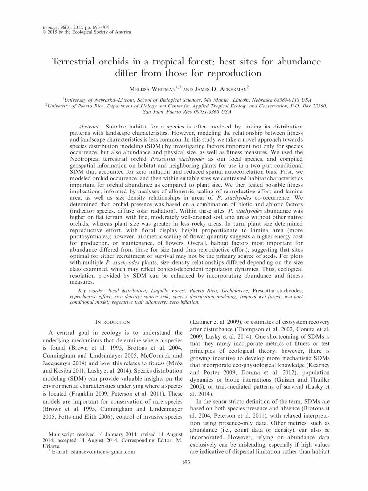
diagram of our SDM process is illustrated in Fig. 1 andAppendix A: Fig. A1.

A priori, we predicted orchid occurrence to be highestin areas with less historic land use disturbance. Orchid

abundance was thought to be indicative of seedgermination or seedling survival; thus, we expected

optimum habitat to have flat, moist terrain (avoidingwashout, yet providing water for protocorms), and

presence of positive indicator species (Dufrene andLegendre 1997, McCune and Mefford 1997). Largerplants were expected on hilltops or slopes with higher

solar radiation, and in less rocky areas. Lamina area wasexpected to determine reproductive effort (based on

energy available from photosynthesis), with isometricscaling. A negative size–density relationship was expect-

ed for co-occurring orchids, similar to observations ofother herbaceous monocots (Weller 1987).

MATERIALS AND METHODS

Species and study site

We chose the terrestrial orchid Prescottia stachyodesas our model species because it is common and non-weedy; co-occuring with both rare (Bergman et al. 2006)

and invasive orchids (Cohen and Ackerman 2009). Therange of P. stachyodes includes forest habitats from mid-

to-high elevations in Brazil, Venezuela, Colombia,Central America, Mexico, and throughout the West

Indies (Ackerman 1995, 2014). Prescottia stachyodes haspersistent foliage, shallow, fleshy roots, and several dark

green elliptical leaves (Ackerman 1995). From Februaryto March, P. stachyodes produces a slender and erect

raceme covered with dozens of small green flowers thatare either self-pollinating or visited by moths (Ackerman

1995, Singer and Sazima 2001). Prescottia stachyodeshas high fruit set, ranging from 52% to 98%, and

produces thousands of small, dust-like, wind-dispersedseeds (Ackerman 1995, Singer and Sazima 2001). To

germinate, orchids rely on external nutrients acquired

MELISSA WHITMAN AND JAMES D. ACKERMAN694 Ecology, Vol. 96, No. 3

FIG. 1. Diagram of the species distribution modeling (SDM) process for a two-part conditional model suitable for zero-inflateddata, with novel incorporation of both abundance and plant size as indicator of fitness. Overall methods include: (1) data collection;(2) assessment of response variable; (3) two-part conditional model starting with a generalized additive model (GAM) of speciespresence–absence, including steps to reduce bias of spatial autocorrelation (smoothing for X, Y coordinates), followed by ageneralized linear model (GLM) for abundance and a linear model (LM) for plant size, with additional steps to assess modelquality; and (4) assessment of fitness measures and testing allometric scaling predictions. Top models were selected using Akaike’sinformation criterion (AIC) and/or Bayesian information criterion (BIC). The overall goal of this SDM process was to understandnot only suitable habitat for species of interest, but also broader fitness implications.

March 2015 695BEST SITES FOR ABUNDANCE OR REPRODUCTION

from mycorrhizal fungi (e.g., Jacquemyn et al. 2007,

Jersakova and Malinova 2007, Gowland et al. 2011,

Bunch et al. 2013, McCormick and Jacquemyn 2014).

Although mycorrhizal surveys have been made of

tropical epiphytic orchids, at present little is known of

the orchid–fungal relationships among tropical terres-

trial species, including P. stachyodes (Otero et al. 2002).

Our study site was the Luquillo Forest Dynamics Plot

(LFDP), a 16-ha grid near the El Verde Field Station,

Puerto Rico (188180 N, 658470 W), in forest dominated

by tabonuco trees (Dacryodes excelsa Vahl) at 350–500

m in elevation. The study area is within the subtropical

wet forest zone (Holdridge Life Zone system; Ewel and

Whitmore 1973) and has a minimum of 200 mm of rain

per month (Brown et al. 1983). Habitat includes mostly

primary forest (with some historical selective logging),

and secondary forest that was once used for grazing,

intensive logging, agriculture, and coffee plantations

(Thompson et al. 2002). Since 1934, human disturbance

has been drastically reduced and has been minimal for

about seven decades; canopy coverage is now ;100%(Thompson et al. 2002).

Recording orchid distribution, abundance, and size

The LFDP grid is divided into 20320 m plots, further

subdivided into 5 3 5 m subplots. We used six 10 3 500

m transect lines containing 1200 subplots spanning areas

with differing ecological characteristics as well as

disturbance history. These subplots were identical to

those used by prior orchid studies (Bergman et al. 2006,

Cohen and Ackerman 2009), but with data collected

independently from those projects.

We recorded P. stachyodes presence–absence, and

abundance, per 5-m2 subplot during the nonflowering

season from June to August 2005; data were then used

as response variables for modeling. All orchids with a

minimum of one leaf were included, with sampling of

plants at all life stages. Spatial patterns of P. stachyodes

were described using Moran’s I (Moran 1950) and the

index of clumping (David and Moore 1954).

Because vegetative traits were highly correlated (log10-

transformed lamina area, number of leaves, petiole

length), we used lamina area as a proxy for overall plant

size (Appendix B: Table B1). We estimated lamina area

using the equation ((0.71 3 width in cm 3 length in cm)

� 0.97), based on photos of leaves (n ¼ 40) measured

using the program ImageJ (Abramoff et al. 2004).

Measures of vegetative traits (proxy for plant size) from

the largest orchid per subplot (expected to be mature

and able to reproduce) were then used as a response

variable for modeling size.

Associations with neighboring species

We anticipated that neighboring species would be

important as a SDM factor because of the indirect

ecological associations between orchids and neighboring

plants, linked via shared facultative relationships with

mycorrhizal fungi (Otero et al. 2002, Jersakova and

Malinova 2007, McCormick and Jacquemyn 2014). To

identify significant positive or negative relationships

between P. stachyodes and other species, we performed

an indicator species analysis (Dufrene and Legendre

1997), using data on the relative abundance and

frequency of 118 woody plant species, analyzed with

the program PC-ORD version 4.0 (McCune and

Mefford 1997). Our methods were identical to those

used by Bergman et al. (2006) with the locally sympatric

orchid Wullschlaegelia calcarata Benth. (an orchid

associated with 32 indicator species), allowing us to

make more direct comparisons between studies and to

promote a deeper understanding of tropical orchid–tree

relationships. Forest data came from the LFDP census

(completed in 2002) of all species .1 cm diameter at

breast height, archived by the Luquillo Experimental

Forest-Long Term Ecological Research (LEF-LTER)

program (available online).4 We also conducted separate

indicator species analyses for subplots with differing

disturbance history. Significance values were based on a

Monte Carlo simulation, where orchid locations were

randomly assigned 1000 times. Second, we categorized

the co-occurrence of indicator species in four ways: (1)

positive indicator species; (2) negative indicator species;

(3) both positive and negative indicator species; or (4) no

indicator species. This simplified indicator species metric

was then used for modeling orchid occurrence, abun-

dance, and size.

Habitat characteristics

Abiotic habitat characteristics per subplot were

derived or interpolated from spatially explicit data using

the geographic information system (GIS), ArcInfo

version 9.3 (ESRI 2004). Geospatial data was provided

by LEF-LTER (URL in footnote 4). Attribute values

were based on where the centroid of each 5 3 5 m

subplot intersected with a geospatial layer of interest.

Geospatial layers for soil characteristics and rockiness

were based on surveys conducted by the U.S. Depart-

ment of Agriculture (Vick and Lynn 1995). To ensure

sufficient sample size for modeling, we used the most

common soil types (Zarzal and Cristal), and grouped

rockiness into two categories: ‘‘less rocky’’ (very

bouldery, extremely bouldery) and ‘‘more rocky’’

(rubbly, very rubbly). We created a topographic position

layer (seat, slope, or top) based on transect notes by E.

Bergman and C. Torres ( personal communication).

Historical land use classes were categorized by Thomp-

son et al. (2002) based on aerial photographs from 1936;

we grouped sites with ,80% canopy cover as ‘‘more

disturbed’’ and sites with .80% canopy cover as ‘‘less

disturbed.’’ We created a digital elevation model (DEM)

raster using ordinary kriging (spherical) of 442 ground-

surveyed elevation points from the corners of each 20-m

plot, extending beyond the LFDP grid to reduce edge

4 http://luq.lternet.edu/data


error. These DEM methods are similar to other Center

for Tropical Forest Science (CTFS) plots (Condit 1998).

Degree slope and diffuse solar radiation rasters were

interpolated using ArcGIS Spatial Analyst Tools (ESRI

2004) and had 5-m spatial resolution that aligned with

the LFDP subplots. Collinearity was noted between

degree slope and diffuse solar radiation; however, these

factors were hypothesized to be biologically important.

Thus, to disentangle unique contributions per factor, we

used the residuals from a linear regression of solar

radiation as a function of degree slope (Graham 2003).

Species distribution models and model section process

To address the zero inflation of our data set, we

adopted a two-part conditional modeling process (Cragg

1971, Barry and Welsh 2002, Cunningham and Linden-

mayer 2005, Potts and Elith 2006). First, we modeled

orchid presence and absence across the 1200 LFDP

subplots using a suite (set) of binomially distributed

generalized additive models (GAM) with a logit link

function suitable for zero-inflated data sets and with the

ability to add, if needed, a smoothing function (for X, Y

coordinates) to reduce (but not explicitly account for)

spatial autocorrelation (Dormann et al. 2007). Other

modeling methods can also be used for zero inflation or

spatial autocorrelation, but most likely these methods

would have produced only a subtle difference in results

(Martin et al. 2005, Latimer et al. 2009). Next, within

sites where P. stachyodes orchids were present, we used a

suite of zero-truncated (positive-Poisson) generalized

linear models (GLM) with a logistic link function for

abundance. As a point of comparison, we also modeled

plant size (normally distributed) using a suite of linear

models (LM) with predictor variables identical to those

of the GLM suite (Fig. 1; Appendix A: Fig. A1,

Appendix C: Tables C2 and C3) and with data spatially

joined by using the same LFDP subplots.

For each SDM suite (GAM, GLM, LM), we included

(1) a null model; (2) simple models with one or two

predictor variables; (3) more complex models based

directly on hypotheses; and (4) a global model of all

possible factors and interactions examined (Anderson

and Burnham 2002). The GAM set included 45 models,

and the GLM and LM set each contained 28 models.

The ‘‘top model’’ selected per suite was based on a

combination of the following: low Akaike’s information

criterion (AIC; Akaike 1974) and Bayesian information

criterion (BIC) scores, model weights (while also

checking for possible over-fitting of data), and constan-

cy of predictor variables included in highly ranked AIC

and BIC models. When two models had similar delta

values, we favored the one with the fewer parameters.

To estimate GAM accuracy, we used receiver operating

characteristics (ROC) area under the curve (AUC)

values (Hanley and McNeil 1982). For model evalua-

tion, we plotted model fit, checked model residuals for

spatial autocorrelation using Moran’s I statistic, tested

for correlation between observed and predicted values

using Spearman’s rank, and calculated root mean square

error (RMSE) and average error (AVEerr), similar to

Potts and Elith (2006). All models were run with R

version 3.1 (R Development Core Team 2013), with the

packages AICcmodavg, countreg, MASS, mgcv, ncf,

spdep, stats (Venables and Ripley 2002, Wood 2011,

Bjornstad 2013, Mazerolle 2013), and script (Dormann

et al. 2007).

For the second step of the modeling process, it was

noted that P. stachyodes abundance and plant size were

correlated (Kendall rank correlation, s ¼ 0.22, P ¼0.008), a situation that we expected at the local scale

(Cornwell and Ackerly 2010). To differentiate which

habitat characteristics most strongly influence each

response variable, we used a novel application of

evidence ratio methods (Appendix A: Fig. A1). First,

we calculated Akaike’s information criterion weights per

model suite (Anderson and Burnham 2002, Wagen-

makers and Farrell 2004). Then we calculated evidence

ratios, with model comparisons within suites informed

by observations of which predictor variables were found

to be the most important for the top model across suites.

This process does not compare AIC values across suites

(Anderson and Burnham 2002); rather it compares those

environmental factors most important per response

variable. Evidence ratios . 10 were regarded as showing

sufficient contrast (Uriarte et al. 2004).

Fitness based on isometric or allometric scaling

The first step toward linking habitat suitability with

fitness is to connect the size of an individual with its

reproductive effort (Niklas and Enquist 2003, Mroz and

Kosiba 2011). Our approach was to test whether there is

a linear relationship between reproductive effort (scape

length in mm; estimated number of flowers) and lamina

area in cm2 (for the largest leaf per individual), based on

measurements sampled from mature P. stachyodes

located near the LFDP plot (n ¼ 30). We expected a

positive, linear relationship, and specifically tested

whether the scaling was isometric, with reproductive

effort proportionate to lamina area (a proxy for energy

available from photosynthesis), or allometric (dispro-

portionate energy cost). Under isometric scaling, scape

length to lamina area has a predicted slope of 1/2,

because length is one-dimensional and lamina area is

two-dimensional; and the estimated number of flowers

to lamina area has a predicted slope of 3/2, assuming

flower arrangement within three-dimensional space.

To gain further perspective on the response variables

used in the SDM, we also examined the relationship

between physical size and abundance, with specific

comparisons between size classes (potential life stages).

Within sites with co-occurring orchids (.1), we selected

the largest (most likely mature), and smallest (most

likely immature) individuals and tested lamina area

(cm2) as a function of orchid density (number of plants/

m2) per subplot. We then tested whether the slope of this

relationship was comparable to the self-thinning rule


(�3/2) used to describe size–density dynamics of trees

(Yoda et al. 1963), or closer to�0.44, as observed with

other herbaceous monocots (Weller 1987). Note that

our metric for size was based on lamina area (cm2)

rather than dry lamina biomass (g), due to restrictions

on removing plant tissue; however, these two metricstend to be highly correlated, with an expected scaling

relationship close to 1 (Niklas et al. 2007). In terms of

known allocation strategy, the majority of P. stachyodes

biomass is composed of leaves, with few roots. We

expected that higher densities of orchids would result in

smaller-sized plants due to competition for resources.

We used the R package SMATR (Warton et al. 2012)

to test whether observed slopes matched predictions

inspired by ecological theory. Slopes (reproductive effort

varying with plant size; plant size varying with density)

were calculated using reduced major axis (RMA)regression, also known as standardized major axis

(SMA) regression (Warton et al. 2006), after log10-

transformation of all data. We chose the RMA method

based on our sample size and assumption of comparable

measurement errors for both the X and Y axis. A

significant difference in scaling (line-fit) was dependent

upon nonoverlap of the predicted slope and the 95%confidence interval for the observed slope (Warton et al.

2006, 2012).

RESULTS

Orchid distribution and indicator species analysis

A total of 218 P. stachyodes were identified in 90 of

1200 (7.5%) of the 5 3 5 m subplots (Appendix D: Fig.D1). The largest leaf per individual had a mean lamina

area of 52.8 6 SE 2.17 cm2 (minimum 1.9 cm2;

maximum 132.8 cm2). The average subplot density was

0.36 plants/m2, with highest density recorded being 18

individuals (3.6 individuals/m2). Orchid presence dis-

played significant spatial autocorrelation (P ¼ 0.001),

with a pattern described as slightly clustered within a

short distance (0–20 m), and then becoming randomover longer distances (.20 m), with Moran’s I statistic¼

0.009 (where�1 is highly dispersed, 0 is random, and 1 is

highly clustered). Smoothing methods (X, Y coordi-

nates) were then used to reduce spatial autocorrelation

for the residuals in the GAM model suite, with the

change resulting in nonsignificant spatial autocorrela-

tion for the null GAM model (Appendix E: Figs. E1 and

E2). Within sites where orchids were present, spatial

autocorrelation was nonsignificant; thus, no changes

were made to the GLM and LM model suite. Orchid

abundance was aggregated (using the index of clumping,

or IC, where ,0 is uniform, 0 is random, and .0 is

clustered), with majority of individuals being restricted

to a few sites for both 535 m subplots (IC¼ 4.5) and 20

3 20 m plots (IC ¼ 8.4). A histogram of orchid

abundance data is shown in Appendix F: Figs. F1 and

F2.

There were relatively few indicator species (nine out of

118 species tested) associated with P. stachyodes

presence relative to the overall plant diversity of the

LFDP plot (Table 1). However, sites with .1 indicator

species accounted for 71% (156 out of 218) of the total

P. stachyodes sampled. Positive relationships were found

with seven species, whereas negative relationships were

found for two (Table 1).

Modeling orchid presence–absence, abundance, and size

The top generalized additive model (GAM) that we

selected (Table 2; Appendix C: Table C1; Appendix G:

Fig. G1) for predicting orchid occurrence included the

following factors: indicator species (especially co-occur-

rence with positive indicator species) and areas with

higher diffuse solar radiation residuals (locations with

greater light availability, attributed to aspect rather than

slope). Alternate top-ranking models (Appendix C:

Table C1) also highlighted the importance of interac-

tions between degree slope and topographic position

(with orchid occurrence associated with the flat terrain

on the tops of hills). The top GAM model selected had

an AUC score of 0.854, where AUC of 0.5 is null (or

random) and 1.0 is excellent (Hanley and McNeil 1983,

TABLE 1. Indicator species analysis for the terrestrial orchid Prescottia stachyodes terrestrial orchid in the Luquillo Forest, PuertoRico.

Family Species Association

P

Entire plot Cover class 1–3 Cover class 4

Malpighiaceae Byrsonima spicata (Cav.) DC. positive � � � 0.025 � � �Salicaceae Casearia arborea (Rich.) Urb. positive 6 0.027 0.005 � � �Boraginaceae Cordia sulcata DC. positive � � � � � � 0.005Myrtaceae Eugenia stahlii (Kiaersk.) Krug and Urb. positive 6 0.03 � � � 0.011Moraceae Ficus citrifolia Mill. positive 0.024 � � � � � �Chrysobalanaceae Hirtella rugosa Pers. positive 6 0.036 � � � � � �Sapindaceae Matayba domingensis (DC.) Radlk. positive 6 0.011 0.001 � � �Salicaceae Casearia sylvestris Sw. negative 6 0.018 0.018 � � �Sapotaceae Manilkara bidentata (A. DC.) A. Chev. negative 0.016 � � � � � �

Notes: Results are based on the presence or absence of P. stachyodes and the basal area of 118 woody plants within the LuquilloForest Dynamics Plot (LFDP). Analyses were conducted with PC-ORD. Significant results (P , 0.05) are shown for the entireLFDP plot, for areas with historic land use disturbance (cover class 1–3), and for the area with the least disturbance (cover class 4).Ellipses indicate that results are not significant. The symbol ‘‘6’’ indicates the same association as the orchid Wullschlaegeliacalcarata (Bergman et al. 2006).


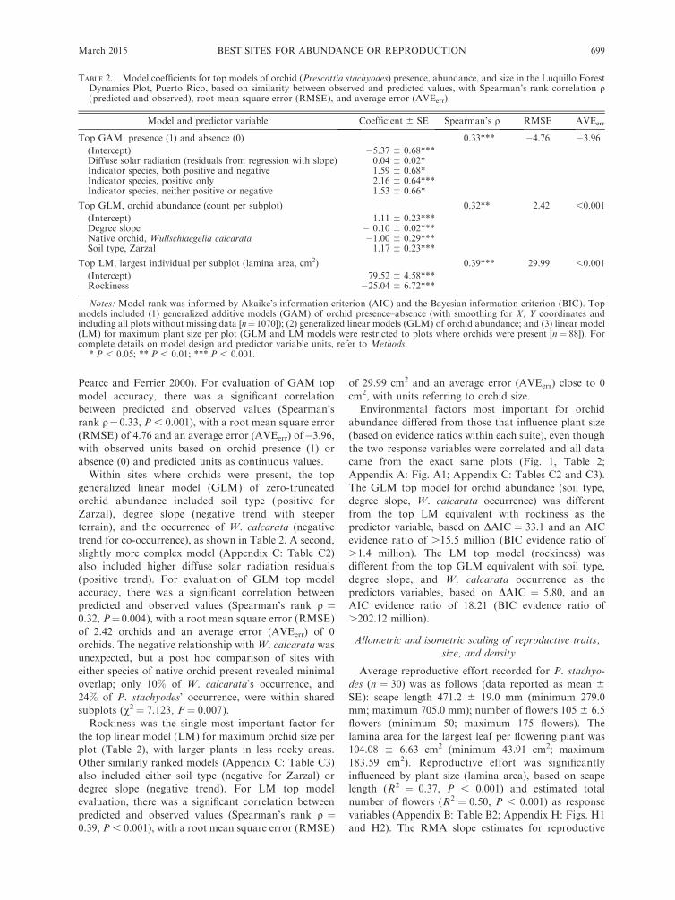
Pearce and Ferrier 2000). For evaluation of GAM top

model accuracy, there was a significant correlation

between predicted and observed values (Spearman’s

rank q¼ 0.33, P , 0.001), with a root mean square error

(RMSE) of 4.76 and an average error (AVEerr) of�3.96,with observed units based on orchid presence (1) or

absence (0) and predicted units as continuous values.

Within sites where orchids were present, the top

generalized linear model (GLM) of zero-truncated

orchid abundance included soil type (positive for

Zarzal), degree slope (negative trend with steeperterrain), and the occurrence of W. calcarata (negative

trend for co-occurrence), as shown in Table 2. A second,

slightly more complex model (Appendix C: Table C2)

also included higher diffuse solar radiation residuals(positive trend). For evaluation of GLM top model

accuracy, there was a significant correlation between

predicted and observed values (Spearman’s rank q ¼0.32, P¼ 0.004), with a root mean square error (RMSE)

of 2.42 orchids and an average error (AVEerr) of 0orchids. The negative relationship with W. calcarata was

unexpected, but a post hoc comparison of sites with

either species of native orchid present revealed minimal

overlap; only 10% of W. calcarata’s occurrence, and

24% of P. stachyodes’ occurrence, were within sharedsubplots (v2 ¼ 7.123, P ¼ 0.007).

Rockiness was the single most important factor for

the top linear model (LM) for maximum orchid size per

plot (Table 2), with larger plants in less rocky areas.

Other similarly ranked models (Appendix C: Table C3)also included either soil type (negative for Zarzal) or

degree slope (negative trend). For LM top model

evaluation, there was a significant correlation between

predicted and observed values (Spearman’s rank q ¼0.39, P , 0.001), with a root mean square error (RMSE)

of 29.99 cm2 and an average error (AVEerr) close to 0

cm2, with units referring to orchid size.

Environmental factors most important for orchid

abundance differed from those that influence plant size

(based on evidence ratios within each suite), even though

the two response variables were correlated and all datacame from the exact same plots (Fig. 1, Table 2;

Appendix A: Fig. A1; Appendix C: Tables C2 and C3).

The GLM top model for orchid abundance (soil type,

degree slope, W. calcarata occurrence) was different

from the top LM equivalent with rockiness as thepredictor variable, based on DAIC ¼ 33.1 and an AIC

evidence ratio of .15.5 million (BIC evidence ratio of

.1.4 million). The LM top model (rockiness) was

different from the top GLM equivalent with soil type,

degree slope, and W. calcarata occurrence as thepredictors variables, based on DAIC ¼ 5.80, and an

AIC evidence ratio of 18.21 (BIC evidence ratio of

.202.12 million).

Allometric and isometric scaling of reproductive traits,

size, and density

Average reproductive effort recorded for P. stachyo-

des (n ¼ 30) was as follows (data reported as mean 6

SE): scape length 471.2 6 19.0 mm (minimum 279.0mm; maximum 705.0 mm); number of flowers 105 6 6.5

flowers (minimum 50; maximum 175 flowers). The

lamina area for the largest leaf per flowering plant was

104.08 6 6.63 cm2 (minimum 43.91 cm2; maximum

183.59 cm2). Reproductive effort was significantlyinfluenced by plant size (lamina area), based on scape

length (R2 ¼ 0.37, P , 0.001) and estimated total

number of flowers (R2 ¼ 0.50, P , 0.001) as response

variables (Appendix B: Table B2; Appendix H: Figs. H1

and H2). The RMA slope estimates for reproductive

TABLE 2. Model coefficients for top models of orchid (Prescottia stachyodes) presence, abundance, and size in the Luquillo ForestDynamics Plot, Puerto Rico, based on similarity between observed and predicted values, with Spearman’s rank correlation q(predicted and observed), root mean square error (RMSE), and average error (AVEerr).

Model and predictor variable Coefficient 6 SE Spearman’s q RMSE AVEerr

Top GAM, presence (1) and absence (0) 0.33*** �4.76 �3.96(Intercept) �5.37 6 0.68***Diffuse solar radiation (residuals from regression with slope) 0.04 6 0.02*Indicator species, both positive and negative 1.59 6 0.68*Indicator species, positive only 2.16 6 0.64***Indicator species, neither positive or negative 1.53 6 0.66*

Top GLM, orchid abundance (count per subplot) 0.32** 2.42 ,0.001

(Intercept) 1.11 6 0.23***Degree slope � 0.10 6 0.02***Native orchid, Wullschlaegelia calcarata �1.00 6 0.29***Soil type, Zarzal 1.17 6 0.23***

Top LM, largest individual per subplot (lamina area, cm2) 0.39*** 29.99 ,0.001

(Intercept) 79.52 6 4.58***Rockiness �25.04 6 6.72***

Notes: Model rank was informed by Akaike’s information criterion (AIC) and the Bayesian information criterion (BIC). Topmodels included (1) generalized additive models (GAM) of orchid presence–absence (with smoothing for X, Y coordinates andincluding all plots without missing data [n¼1070]); (2) generalized linear models (GLM) of orchid abundance; and (3) linear model(LM) for maximum plant size per plot (GLM and LM models were restricted to plots where orchids were present [n ¼ 88]). Forcomplete details on model design and predictor variable units, refer to Methods.

* P , 0.05; ** P , 0.01; *** P , 0.001.


effort varying with plant size (Appendix B: Table B2)

matched our isometric predictions for scape length (P¼0.18), but not for number of flowers (P ¼ 0.003); scape

had a slope of 0.62 (95% CI¼ 0.45, 0.83; 0.5 predicted);

total number of flowers had a slope of 0.98 (95% CI ¼0.75, 1.28; 1.33 predicted).

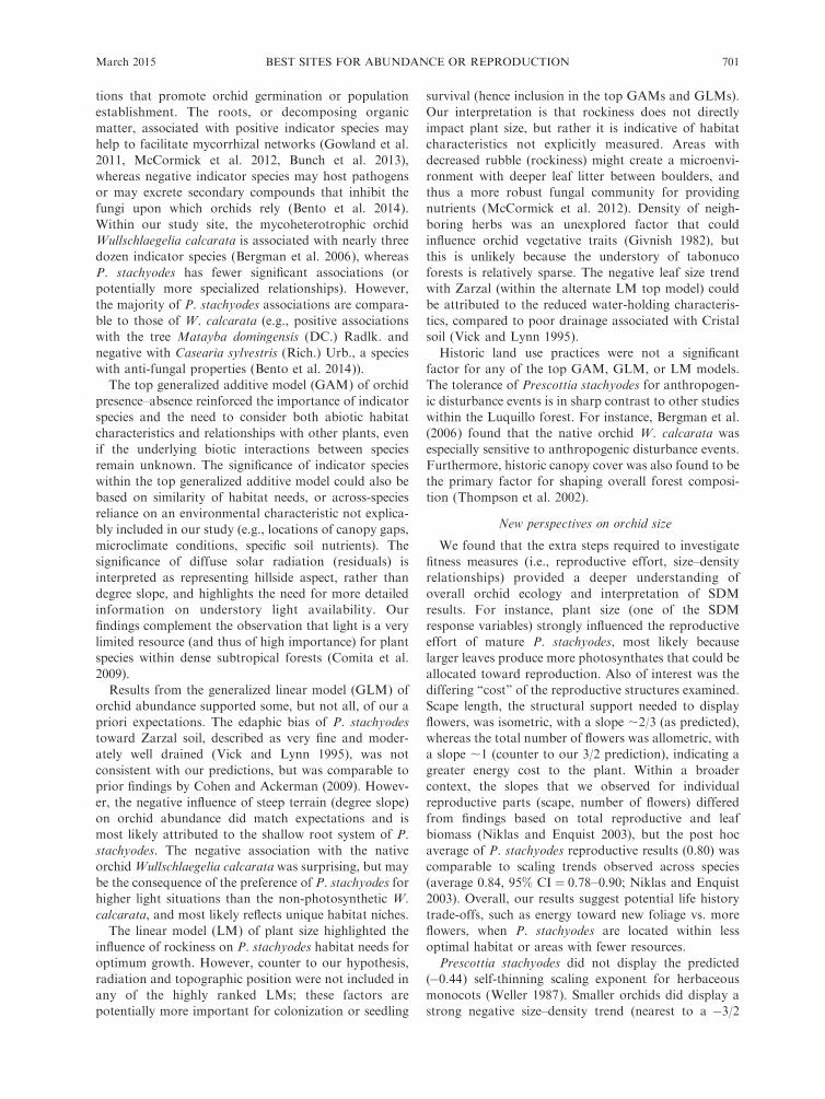
Plant size (lamina area) was influenced by subplot

orchid density for both the smallest (P , 0.001, R2 ¼0.48) and the largest plants (P¼ 0.015, R2¼ 0.13; Fig. 2;

Appendix B: Table B3), but not for the average of co-

occurring individuals (P¼ 0.75). The reduced major axis

(RMA) slope estimates for plant size varying with

density for the smallest individuals was�1.5 (95% CI ¼�1.90, �1.19), and was different from the predicted

�0.44 scaling for herbaceous monocots (P , 0.001), but

not different from the�3/2 self thinning rule (P¼ 0.99).

Counter to expectations, the largest individuals had a

positive slope of 0.67 (95% CI¼ 0.49, 0.90) that was also

significantly different than self-thinning predictions (P¼0.008, P , 0.001). As a post hoc analysis, we found that

the sizes of the largest and smallest individuals were

independent from one another, with no significant

correlation (P ¼ 0.53).

DISCUSSION

To date, the majority of species distribution modeling

(SDM) techniques have focused on the identification of

suitable habitat by using environmental conditions as

predictors for species occurrence or abundance. Al-

though this approach is effective for some applications,

there is growing interest in SDMs that offer a more

mechanistic perspective on distribution patterns of an

organism, often obtained by incorporating eco-physio-

logical responses, biotic interactions, life history stages,

or resource–allocation trade-offs (Guisan and Thuiller

2005, Kearney and Porter 2009, Douma et al. 2012,

Lasky et al. 2014). Our approach to SDMs was to link

habitat suitability with fitness differences via testing of

allometric relationships (reproductive effort varying

with plant size; plant size varying with density).

Additional insights on our focal species were gained by

adopting a two-part conditional modeling approach

(suitable for instances of zero inflation), followed by

informed comparisons of factors most important for

species abundance in contrast to plant size. Thus, while

exploring the local distribution complexities of a single

species of orchid (Prescottia stachyodes), we have

demonstrated novel SDM methods applicable to a

broader audience of ecological researchers.

Insights on the complexity of orchid distribution and

defining ‘‘suitable habitat’’

The spatial distribution patterns of P. stachyodes

(clustered occurrence at short spatial scales shifting to

random occurrence with distance, combined with

clumped abundance) are not surprising, given models

of orchid seed dispersal patterns (Kindlmann et al.

2014), and field observations reported in both temperate

and tropical habitats (e.g., Jacquemyn et al. 2007,

Whitman et al. 2011). These spatial patterns are also

common with tropical tree species (Condit et al. 2000)

and may reflect either dispersal limitation or highly

specific niche requirements (Brown et al. 1995). Overall,

distribution patterns for P. stachyodes occurrence and

abundance suggest that either most seeds are deposited

near maternal plants, resulting in a hotspot for

germination (Jacquemyn et al. 2007, Jersakova and

Malinova 2007), or that sites for population establish-

ment are spatially localized, which may be accompanied

by strong competition for limiting resources (Otero et al.

2007, Bunch et al. 2013). The random patterns of P.

stachyodes occurrence with distance may be due to

chance long-distance dispersal events combined with the

low probability of seeds landing on suitable habitat in a

landscape of high physiographic, and perhaps mycor-

rhizal, heterogeneity. In addition, subpopulation persis-

tence fluctuates through time, especially when mortality

of seedlings and juveniles is high (Ackerman et al. 1996,

Tremblay 1997, Otero et al. 2007).

Orchids are distinct from most other plants in that

they must exploit fungi to successfully germinate. Thus,

their distribution often reflects the extent of below-

ground mycorrhizal fungi networks (Jacquemyn et al.

2007, Jersakova and Malinova 2007, McCormick et al.

2012). Our knowledge of tropical orchid–fungi relation-

ships is limited, but the indicator species analysis results

may provide useful insights on direct and indirect species

interactions, suitable habitat niches, or edaphic condi-

FIG. 2. Plant size as a function of density for the largestand smallest co-occurring orchids per subplot. Plant size wasinfluenced by subplot density for the smallest (P , 0.001, R2¼0.48) and the largest (P¼ 0.015, R2¼ 0.13) plants. Lines showthe reduced major axis (RMA) slope for log10-transformed size(lamina area in cm2) varying with log10-transformed density(number of plants/m2). For the smallest individuals, slope ¼�1.5 (95% CI¼�1.90,�1.19); for the largest individuals, slope¼ 0.67 (95% CI ¼ 0.49, 0.90).


tions that promote orchid germination or population

establishment. The roots, or decomposing organic

matter, associated with positive indicator species may

help to facilitate mycorrhizal networks (Gowland et al.

2011, McCormick et al. 2012, Bunch et al. 2013),

whereas negative indicator species may host pathogens

or may excrete secondary compounds that inhibit the

fungi upon which orchids rely (Bento et al. 2014).

Within our study site, the mycoheterotrophic orchid

Wullschlaegelia calcarata is associated with nearly three

dozen indicator species (Bergman et al. 2006), whereas

P. stachyodes has fewer significant associations (or

potentially more specialized relationships). However,

the majority of P. stachyodes associations are compara-

ble to those of W. calcarata (e.g., positive associations

with the tree Matayba domingensis (DC.) Radlk. and

negative with Casearia sylvestris (Rich.) Urb., a species

with anti-fungal properties (Bento et al. 2014)).

The top generalized additive model (GAM) of orchid

presence–absence reinforced the importance of indicator

species and the need to consider both abiotic habitat

characteristics and relationships with other plants, even

if the underlying biotic interactions between species

remain unknown. The significance of indicator species

within the top generalized additive model could also be

based on similarity of habitat needs, or across-species

reliance on an environmental characteristic not explica-

bly included in our study (e.g., locations of canopy gaps,

microclimate conditions, specific soil nutrients). The

significance of diffuse solar radiation (residuals) is

interpreted as representing hillside aspect, rather than

degree slope, and highlights the need for more detailed

information on understory light availability. Our

findings complement the observation that light is a very

limited resource (and thus of high importance) for plant

species within dense subtropical forests (Comita et al.

2009).

Results from the generalized linear model (GLM) of

orchid abundance supported some, but not all, of our a

priori expectations. The edaphic bias of P. stachyodes

toward Zarzal soil, described as very fine and moder-

ately well drained (Vick and Lynn 1995), was not

consistent with our predictions, but was comparable to

prior findings by Cohen and Ackerman (2009). Howev-

er, the negative influence of steep terrain (degree slope)

on orchid abundance did match expectations and is

most likely attributed to the shallow root system of P.

stachyodes. The negative association with the native

orchidWullschlaegelia calcarata was surprising, but may

be the consequence of the preference of P. stachyodes for

higher light situations than the non-photosynthetic W.

calcarata, and most likely reflects unique habitat niches.

The linear model (LM) of plant size highlighted the

influence of rockiness on P. stachyodes habitat needs for

optimum growth. However, counter to our hypothesis,

radiation and topographic position were not included in

any of the highly ranked LMs; these factors are

potentially more important for colonization or seedling

survival (hence inclusion in the top GAMs and GLMs).

Our interpretation is that rockiness does not directly

impact plant size, but rather it is indicative of habitat

characteristics not explicitly measured. Areas with

decreased rubble (rockiness) might create a microenvi-

ronment with deeper leaf litter between boulders, and

thus a more robust fungal community for providing

nutrients (McCormick et al. 2012). Density of neigh-

boring herbs was an unexplored factor that could

influence orchid vegetative traits (Givnish 1982), but

this is unlikely because the understory of tabonuco

forests is relatively sparse. The negative leaf size trend

with Zarzal (within the alternate LM top model) could

be attributed to the reduced water-holding characteris-

tics, compared to poor drainage associated with Cristal

soil (Vick and Lynn 1995).

Historic land use practices were not a significant

factor for any of the top GAM, GLM, or LM models.

The tolerance of Prescottia stachyodes for anthropogen-

ic disturbance events is in sharp contrast to other studies

within the Luquillo forest. For instance, Bergman et al.

(2006) found that the native orchid W. calcarata was

especially sensitive to anthropogenic disturbance events.

Furthermore, historic canopy cover was also found to be

the primary factor for shaping overall forest composi-

tion (Thompson et al. 2002).

New perspectives on orchid size

We found that the extra steps required to investigate

fitness measures (i.e., reproductive effort, size–density

relationships) provided a deeper understanding of

overall orchid ecology and interpretation of SDM

results. For instance, plant size (one of the SDM

response variables) strongly influenced the reproductive

effort of mature P. stachyodes, most likely because

larger leaves produce more photosynthates that could be

allocated toward reproduction. Also of interest was the

differing ‘‘cost’’ of the reproductive structures examined.

Scape length, the structural support needed to display

flowers, was isometric, with a slope ;2/3 (as predicted),

whereas the total number of flowers was allometric, with

a slope ;1 (counter to our 3/2 prediction), indicating a

greater energy cost to the plant. Within a broader

context, the slopes that we observed for individual

reproductive parts (scape, number of flowers) differed

from findings based on total reproductive and leaf

biomass (Niklas and Enquist 2003), but the post hoc

average of P. stachyodes reproductive results (0.80) was

comparable to scaling trends observed across species

(average 0.84, 95% CI ¼ 0.78–0.90; Niklas and Enquist

2003). Overall, our results suggest potential life history

trade-offs, such as energy toward new foliage vs. more

flowers, when P. stachyodes are located within less

optimal habitat or areas with fewer resources.

Prescottia stachyodes did not display the predicted

(�0.44) self-thinning scaling exponent for herbaceous

monocots (Weller 1987). Smaller orchids did display a

strong negative size–density trend (nearest to a �3/2


slope), but more intriguing was the positive size–density

slope (nearest to a 2/3 slope) for the largest orchids,

combined with the lack of significant interaction

between size classes. One explanation of these differing

context-dependent size–density results is that areas with

the highest orchid densities are distinct subpopulations

(Tremblay et al. 2006) that include mixed age ranges,

and that sites with the lowest orchid densities are older

subpopulations (based on the intercepts; Fig. 2) that

have been reduced to a few larger individuals that

survive longer than smaller plants. When considering

these size–density results under the context of SDMs, it

appears that orchid abundance (density) is more

attributed to habitat specificity (and potentially inter-

specific competition) than to intraspecific competition or

resource partitioning (Goldberg and Barton 1992).

Linking habitat characteristics with possible life

history stages

The overarching results from our study, that factors

most important for orchid occurrence differ from those

linked with abundance or plant size, suggest that the

relevance of specific habitat characteristics may change

over time or with life history stage. Habitat character-

istics that promote larger sized P. stachyodes, and thus

greater reproductive effort and eventual seed output, are

not necessarily the same conditions needed for seedling

establishment or the maintenance of subpopulations.

Disjunction between habitat needs at different life stages

is feasible, given the overall ecological complexity

attributed to this taxonomic group (Givnish 1982,

Jacquemyn et al. 2007, Whitman et al. 2011, Bunch et

al. 2013). For instance, specificity of tree host substrate

was not linked to adult orchid fitness or probability of

flowering, but may be attributed to conditions necessary

for early life stages (Gowland et al. 2011). Having spatial

distribution patterns linked to a broad suite of habitat

characteristics and belowground fungal associations,

rather than governed by a single factor, also explains the

rarity of some orchid species (Jersakova and Malinova

2007, Phillips et al. 2011, Bunch et al. 2013, McCormick

and Jacquemyn 2014) and the potential ecological

mechanisms that underlie distribution patterns of our

model organism.

CONCLUSION

Environmental factors of importance in species

distributions differ depending on how one identifies

‘‘suitable habitat’’ for a species. Had we restricted the

scope of our analyses to more standard response

variables used in species distribution modeling (e.g.,

presence-only data), or relied strictly on abiotic environ-

mental data without exploring species diversity within

this forest type, then we might not have sufficiently

represented the ecological complexity of our model

organism. Analyses of isometric, compared to allometric,

scaling of reproductive effort, and size–density relation-

ships, added valuable perspectives on potential fitness

differences, and possible population dynamics. Appar-

ently, sites that are the source of seeds in Prescottia

stachyodes may not be optimal for establishment. Thus,

we conclude that habitat characteristics influencing

species abundance can differ from conditions that

influence plant size or reproductive effort.

ACKNOWLEDGMENTS

We thank anonymous reviewers, T. Awada, E. Bergman,N. Brokaw, C. Brassil, J. DeLong, J. P. Gibert Cruz, S.Jadeja, C. Leroy, R. Matthews, J. F. McLaughlin, N.Muchhala, J. Philips, A. Ramirez, S. E. Russo, J. Thompson,C. Torres, A. J. Tyre, and J. K. Zimmerman for theirfeedback. This work was supported by the NSF ResearchExperience for Undergraduates program at El Verde FieldStation, University of Puerto Rico (DBI-0552567), A.Ramırez, PI. The LFDP was funded by NSF grants BSR-8811902, DEB-9411973, DEB-0080538, and DEB-0218039 tothe University of Puerto Rico and the International Instituteof Tropical Forestry as part of the Long Term EcologicalResearch program in the Luquillo Experimental Forest. M.Whitman was funded by the NSF Graduate ResearchFellowship.

LITERATURE CITED

Aarssen, L. W., and D. R. Taylor. 1992. Fecundity allocation inherbaceous plants. Oikos 65:225–232.

Abramoff, M. D., P. J. Magalhaes, and S. J. Ram. 2004. Imageprocessing with ImageJ. Biophotonics International 11:36–42.

Ackerman, J. D. 1995. An orchid flora of Puerto Rico and theVirgin Islands. Memoirs of the New York Botanical Garden73:1–208.

Ackerman, J. D. 2014. Orchids of the Greater Antilles.Memoirs of the New York Botanical Garden 109:1–621.

Ackerman, J. D., A. Sabat, and J. K. Zimmerman. 1996.Seedling establishment in an epiphytic orchid: an experimen-tal study of seed limitation. Oecologia 106:192–198.

Akaike, H. 1974. A new look at the statistical modelidentification. IEEE Transactions on Automatic Control19:716–723.

Anderson, D. R., and K. P. Burnham. 2002. Avoiding pitfallswhen using information-theoretic methods. Journal ofWildlife Management 66:912–918.

Barry, S. C., and A. H. Welsh. 2002. Generalized additivemodelling and zero inflated count data. Ecological Modelling157:179–188.

Bento, T. S., L. M. B. Torres, M. B. Fialho, and V. L. R.Bononi. 2014. Growth inhibition and antioxidative responseof wood decay fungi exposed to plant extracts of Caseariaspecies. Letters in Applied Microbiology 58:79–86.

Bergman, E., J. D. Ackerman, J. Thompson, and J. K.Zimmerman. 2006. Land-use history affects the distributionof the saprophytic orchid Wullschlaegelia calcarata in PuertoRico’s tabonuco forest. Biotropica 38:492–499.

Bjornstad, O. N. 2013. ncf: spatial nonparametric covariancefunctions. R package v 1.1-5. R: A language and environ-ment for statistical computing. R Foundation for StatisticalComputing, Vienna, Austria. http://cran.r-project.org/web/packages/ncf/index.html

Bloom, A. J., F. S. Chapin, III, and H. A. Mooney. 1985.Resource limitation in plants—an economic analogy. AnnualReview of Ecology and Systematics 16:363–392.

Brotons, L., W. Thuiller, M. Araujo, and A. Hirzel. 2004.Presence–absence versus presence-only modelling methodsfor predicting bird habitat suitability. Ecography 4:437–448.

Brown, J. H., D. W. Mehlman, and G. C. Stevens. 1995. Spatialvariation in abundance. Ecology 76:2028–2043.


Brown, S., A. E. Lugo, S. Silander, and L. Liegel. 1983.Research history and opportunities in the Luquillo experi-mental forest. General Technical Report SO-44:1–132.USDA Forest Service, Southern Forest Experiment Station,New Orleans, Louisiana, USA.

Bunch, W. D., C. C. Cowden, N. Wurzburger, and R. P.Shefferson. 2013. Geography and soil chemistry drive thedistribution of fungal associations in lady’s slipper orchid,Cypripedium acaule. Botany 91:850–856.

Cohen, I. M., and J. D. Ackerman. 2009. Oeceoclades maculata,an alien tropical orchid in a Caribbean rainforest. Annals ofBotany 104:557–563.

Comita, L. S., M. Uriarte, J. Thompson, I. Jonckheere, C. D.Canham, and J. K. Zimmerman. 2009. Abiotic and bioticdrivers of seedling survival in a hurricane-impacted tropicalforest. Journal of Ecology 97:1346–1359.

Condit, R. 1998. Tropical forest census plots: methods andresults from Barro Colorado Island, Panama and acomparison with other plots. Springer, New York, NewYork, USA.

Condit, R., et al. 2000. Spatial patterns in the distribution oftropical tree species. Science 288:1414–1418.

Cornwell, W. K., and D. D. Ackerly. 2010. A link betweenplant traits and abundance: evidence from coastal Californiawoody plants. Journal of Ecology 98:814–821.

Cragg, J. G. 1971. Some statistical models for limiteddependent variables with application to the demand fordurable goods. Econometrica 39:8829–8844.

Cunningham, R. B., and D. B. Lindenmayer. 2005. Modelingcount data of rare species: some statistical issues. Ecology 86:1135–1142.

David, F. N., and P. G. Moore. 1954. Notes on contagiousdistributions in plant populations. Annals of Botany 18:47–53.

Dormann, C. F., et al. 2007. Methods to account for spatialautocorrelation in the analysis of species distributional data:a review. Ecography 30:609–628.

Douma, J. C., J. M. Witte, R. Aerts, R. P. Bartholomeus, J. C.Ordonez, H. O. Venterink, M. J. Wassen, and P. M. vanBodegom. 2012. Towards a functional basis for predictingvegetation patterns; incorporating plant traits in habitatdistribution models. Ecography 35:294–305.

Dufrene, M., and P. Legendre. 1997. Species assemblages andindicator species: the need for a flexible asymmetricalapproach. Ecological Monographs 67:345–366.

ESRI. 2004. ArcGIS. Environmental Systems Research Insti-tute, Redlands, California, USA.

Ewel, J. J., and J. L. Whitmore. 1973. The ecological life zonesof Puerto Rico and the U.S. Virgin Islands. USDA ForestService Research Paper ITF-18. International Institute forTropical Forestry, Rio Piedras, Puerto Rico, USA.

Franklin, J. 2009. Mapping species distributions: spatialinference and prediction. Cambridge University Press, NewYork, New York, USA.

Givnish, T. J. 1982. On the adaptive significance of leaf heightin forest herbs. American Naturalist 120:353–381.

Goldberg, D. E., and A. M. Barton. 1992. Patterns andconsequences of interspecific competition in natural commu-nities: a review of field experiments with plants. AmericanNaturalist 139:771–801.

Gowland, K. M., J. Wood, M. A. Clements, and A. B. Nicotra.2011. Significant phorophyte (substrate) bias is not explainedby fitness benefits in three epiphytic orchid species. AmericanJournal of Botany 98:197–206.

Graham, M. H. 2003. Confronting multicollinearity in ecolog-ical multiple regression. Ecology 84:2809–2815.

Guisan, A., and W. Thuiller. 2005. Predicting species distribu-tion: offering more than simple habitat models. EcologyLetters 8:993–1009.

Hanley, J. A., and B. J. McNeil. 1982. The meaning and use ofthe area under a receiver operating characteristic (ROC)curve. Radiology 143:29–36.

Hanley, J. A., and B. J. McNeil. 1983. A method of comparingthe areas under receiver operating characteristic curvesderived from the same cases. Radiology 148:839–843.

Jacquemyn, H., R. Brys, K. Vandepitte, O. Honnay, I. Roldan-Ruiz, and T. Wiegand. 2007. A spatially explicit analysis ofseedling recruitment in the terrestrial orchid Orchis purpurea.New Phytologist 176:448–459.

Jersakova, J., and T. Malinova. 2007. Spatial aspects of seeddispersal and seedling recruitment in orchids. New Phytol-ogist 176:237–241.

Kearney, M., and W. Porter. 2009. Mechanistic nichemodelling: combining physiological and spatial data topredict species’ ranges. Ecology Letters 12:334–350.

Kindlmann, P., E. Melendez-Ackerman, and R. L. Tremblay.2014. Disobedient epiphytes: colonization and extinctionrates in a metapopulation contradict theoretical predictionsbased on patch connectivity. Botanical Journal of theLinnean Society 175:598–606.

Lasky, J. R., M. Uriarte, V. K. Boukili, and R. L. Chazdon.2014. Trait-mediated assembly processes predict successionalchanges in community diversity of tropical forests. Proceed-ings of the National Academy of Sciences USA 111:5616–5621.

Latimer, A. M., S. Banerjee, H. Sang, E. S. Mosher, and J. A.Silander. 2009. Hierarchical models facilitate spatial analysisof large data sets: a case study on invasive plant species in thenortheastern United States. Ecology Letters 12:144–154.

Martin, T. G., B. A. Wintle, J. R. Rhodes, P. M. Kuhnert, S. A.Field, S. J. Low-Choy, A. J. Tyre, and H. P. Possingham.2005. Zero tolerance ecology: improving ecological inferenceby modelling the source of zero observations. Ecology Letters8:1235–1246.

Mazerolle, M. J. 2013. AICcmodavg: Model selection andmultimodel inference based on (Q)AIC(c). R package v 1.35.R: A language and environment for statistical computing. RFoundation for Statistical Computing, Vienna, Austria.http://cran.r-project.org/web/packages/AICcmodavg/index.html

McCormick, M. K., and H. Jacquemyn. 2014. What constrainsthe distribution of orchid populations? New Phytologist 202:392–400.

McCormick, M. K., D. Lee Taylor, K. Juhaszova, R. K.Burnett, D. F. Whigham, and J. P. O’Neill. 2012. Limitationson orchid recruitment: not a simple picture. MolecularEcology 21:1511–1523.

McCune, B., and M. J. Mefford. 1997. PC-ORD for Windows.Multivariate analysis of ecological data version 4.0. MjMSoftware Design, Gleneden Beach, Oregon, USA.

Moran, P. A. P. 1950. Notes on continuous stochasticphenomena. Biometrika 37:17–23.

Mroz, L., and P. Kosiba. 2011. Variation in size-dependentfitness components in a terrestrial orchid, Dactylorhizamajalis (Rchb.) Hunt et Summerh., in relation to environ-mental factors. Acta Societatis Botanicorum Poloniae 80:129–138.

Muller, I., B. Schmid, and J. Weiner. 2000. The effect ofnutrient availability on biomass allocation patterns in 27species of herbaceous plants. Perspectives in Plant Ecology,Evolution and Systematics 3:115–127.

Niklas, K. J., E. D. Cobb, U. Niinemets, P. B. Reich, A. Sellin,B. Shipley, and I. J. Wright. 2007. ‘‘Diminishing returns’’ inthe scaling of functional leaf traits across and within speciesgroups. Proceedings of the National Academy of SciencesUSA 104:8891–8896.

Niklas, K. J., and B. J. Enquist. 2003. An allometric model forseed plant reproduction. Evolutionary Ecology Research 5:79–88.


Otero, J. T., J. D. Ackerman, and P. Bayman. 2002. Diversityand host specificity of endophytic Rhizoctonia-like fungi fromtropical orchids. American Journal of Botany 89:1852–1858.

Otero, J. T., S. Aragon, and J. D. Ackerman. 2007. Sitevariation in spatial aggregation and phorophyte preference inPsychilis monensis (Orchidaceae). Biotropica 39:227–231.

Pearce, J., and S. Ferrier. 2000. Evaluating the predictiveperformance of habitat models developed using logisticregression. Ecological Modelling 133:225–245.

Peterson, A. T., J. Soberon, R. G. Pearson, R. P. Anderson, E.Martınez-Meyer, M. Nakamura, and M. B. Araujo. 2011.Ecological niches and geographic distributions. Monographsin Population Biology. Volume 49. Princeton UniversityPress, Princeton, New Jersey, USA.

Phillips, R. D., M. D. Barrett, K. W. Dixon, and S. D. Hopper.2011. Do mycorrhizal symbioses cause rarity in orchids?Journal of Ecology 99:858–869.

Potts, J. M., and J. Elith. 2006. Comparing species abundancemodels. Ecological Modelling 199:153–163.

R Development Core Team. 2013. R version 3.1. R: A languageand environment for statistical computing. R Foundation forStatistical Computing, Vienna, Austria.

Singer, R. B., and M. Sazima. 2001. The pollination mechanismof three sympatric Prescottia (Orchidaceae: Prescottinae)species in southeastern Brazil. Annals of Botany 88:999–1005.

Thompson, J., N. Brokaw, J. K. Zimmerman, R. B. Waide,E. M. Everham III, D. J. Lodge, C. M. Taylor, D. Garcia-Montiel, and M. Fluet. 2002. Land use history, environment,and tree composition in a tropical forest. EcologicalApplications 12:1344–1363.

Tremblay, R. L. 1997. Distribution and dispersion patterns ofindividuals in nine species of Lepanthes (Orchidaceae).Biotropica 29:38–45.

Tremblay, R. L., E. Melendez-Ackerman, and D. Kapan. 2006.Do epiphytic orchids behave as metapopulations? Evidencefrom colonization, extinction rates and asynchronous popu-lation dynamics. Biological Conservation 129:70–81.

Uriarte, M., R. Condit, C. D. Canham, and S. P. Hubbell.2004. A spatially explicit model of sapling growth in atropical forest: does the identity of neighbours matter?Journal of Ecology 92:348–360.

Venables, W. N., and B. D. Ripley. 2002. Modern appliedstatistics with S. Fourth edition. Springer, New York, NewYork, USA.

Vick, R. L., and W. Lynn. 1995. Order 1 soil survey of theLuquillo Long-Term Ecological Research Grid, Puerto Rico.Pages 1–92. United States Department of Agriculture,National Resource Conservation Service, Lincoln, Nebraska,USA.

von Liebig, J. F. 1847. Organic chemistry in its applications toagriculture and physiology. Fourth edition. Taylor andWalton, London, UK.

Wagenmakers, E.-J., and S. Farrell. 2004. AIC model selectionusing Akaike weights. Psychonomic Bulletin and Review 11:192–196.

Warton, D. I., R. A. Duursma, D. S. Falster, and S. Taskinen.2012. smatr 3—an R package for estimation and inferenceabout allometric lines. Methods in Ecology and Evolution 3:257–259.

Warton, D. I., I. J. Wright, D. S. Falster, and M. Westoby.2006. Bivariate line-fitting methods for allometry. BiologicalReviews 81:259–291.

Weller, D. E. 1987. A reevaluation of the �3/2 power rule ofplant self-thinning. Ecological Monographs 57:23–43.

Whitman, M., M. J. Medler, J. J. Randriamanindry, and E.Rabakonandrianina. 2011. Conservation of Madagascar’sgranite outcrop orchids: the influence of fire and moisture.Lankesteriana 11:55–67.

Wood, S. N. 2011. Fast stable restricted maximum likelihoodand marginal likelihood estimation of semiparametricgeneralized linear models. Journal of the Royal StatisticalSociety B 73:3–36.

Yoda, K., T. Kira, H. Ogawa, and K. Hozumi. 1963. Selfthinning in overcrowded pure stands under cultivated andnatural conditions. Journal of Biology, Osaka City Univer-sity 14:107–129.

SUPPLEMENTAL MATERIAL

Ecological Archives

Appendices A–H are available online: http://dx.doi.org/10.1890/14-0104.1.sm


http://dx.doi.org/10.1890/14-0104.1.sm

Habitat suitability for terrestrial orchids in a tropical forest: best sites for survival differ...

Documents

Transcript of Habitat suitability for terrestrial orchids in a tropical forest: best sites for survival differ...