142

Abstract—Life history aspects of larval and, mainly, juvenile spotted seatrout (Cynoscion nebulosus) were studied in Florida Bay, Everglades National Park, Florida. Collections were made in 1994−97, although the majority of juveniles were collected in 1995. The main objective was to obtain life history data to eventually develop a spatially explicit model and provide baseline data to understand how Everglades res­toration plans (i.e. increased freshwater flows) could influence spotted seatrout vital rates. Growth of larvae and juve­niles (<80 mm SL) was best described by the equation loge standard length = –1.31 + 1.2162 (loge age). Growth in length of juveniles (12–80 mm SL) was best described by the equation standard length = –7.50 + 0.8417 (age). Growth in wet weight of juveniles (15–69 mm SL) was best described by the equation loge wet-weight = –4.44 + 0.0748 (age). There were no significant differences in juvenile growth in length of spot­ted seatrout in 1995 between three geographical subdivisions of Florida Bay: central, western, and waters adja­cent to the Gulf of Mexico. We found a significant difference in wet-weight for one of six cohorts categorized by month of hatchdate in 1995, and a significant difference in length for another cohort. Juveniles (i.e. survivors) used to cal­culate weekly hatchdate distributions during 1995 had estimated spawning times that were cyclical and protracted, and there was no correlation between spawning and moon phase. Tem­perature influenced otolith increment widths during certain growth periods in 1995. There was no evidence of a rela­tionship between otolith growth rate and temperature for the first 21 incre­ments. For increments 22–60, otolith growth rates decreased with increas­ing age and the extent of the decrease depended strongly in a quadratic fash­ion on the temperature to which the fish was exposed. For temperatures at the lower and higher range, increment growth rates were highest. We suggest that this quadratic relationship might be influenced by an environmental factor other than temperature. There was insufficient information to obtain reliable inferences on the relationship of increment growth rate to salinity.

Manuscript approved for publication 23 June 2003 by Scientific Editor. Manuscript received 20 October 2003 at NMFS Scientific Publications Office. Fish. Bull. 102:142–155 (2004).

Growth, mortality, and hatchdate distributions of larval and juvenile spotted seatrout (Cynoscion nebulosus) in Florida Bay, Everglades National Park

Allyn B. Powell Robin T. Cheshire Elisabeth H. Laban National Ocean ServiceNational Oceanic and Atmospheric AdministrationCenter for Coastal Fisheries and Habitat Research101 Pivers Island RoadBeaufort, North Carolina 28516E-mail address (for A. B. Powell): allyn.powell@noaa.gov

James Colvocoresses Patrick O’Donnell Florida Fish and Wildlife Commission Florida Marine Research Institute 2796 Overseas Highway, Suite 119 Marathon, Florida 33050

Marie Davidian Room 209, Patterson Hall 2501 Founder’s Drive North Carolina State University Raleigh, North Carolina 27695

The spotted seatrout (Cynoscion nebu- Fakahatchee Bays, and McMichael and losus) is an important recreational fish Peters (1989) described the size distri­in Florida Bay and spends its entire life bution, growth, spawning, and diet of history within Florida Bay (Rutherford spotted seatrout in Tampa Bay. et al.,1989). The biology of adult spotted Information on growth and mortality seatrout in Florida Bay is well known of larval and juvenile spotted seatrout (Rutherford et al., 1982, 1989), as are the in Florida Bay is lacking. Research on distribution and abundance of juveniles these topics would enhance our under-in the bay, including a description of the standing of the entire life history of this juvenile habitats and their diets (Het- valuable species, and in particular aid tler, 1989; Chester and Thayer, 1990; in eventually developing a spatially ex-Thayer et al., 1999; Florida Department plicit model for spotted seatrout that is of Environmental Protection1). The highly desired by the Program Manage-temporal and spatial distribution and ment Committee for the South Florida abundance of larval spotted seatrout in Ecosystem Restoration Prediction and Florida Bay and adjacent waters, and the Modeling Program. In addition, these spatial and temporal spawning habits of life history studies could help clarify ju­these larvae also have been determined venile growth and survival and provide (Powell et al., 1989; Rutherford et al., needed information for the restoration 1989; Powell, 2003).

The early life history of spotted 1 Florida Department of Environmental seatrout in other south Florida estu- Protection. 1996. Fisheries-independent­

aries also has been well documented. monitoring program, 1995 annual report, 58 p. Florida Department of Environmen-Peebles and Tolley (1988) described the tal Protection, Florida Marine Research

distribution, growth, and mortality of Institute, 100 8th Avenue SE, St. Peters-larval spotted seatrout in Naples and burg, FL 33701.

143Powell et al.: Growth, mortality, and hatchdate distributions for Cynoscion nebulosus

of the Everglades, including a return of historic freshwater fl ows into Florida Bay.

Two conceptual frameworks have been advanced to couple the role of growth and mortality in infl uencing cohort dy-namics. Anderson (1988), in a review of hypotheses relating survival of prerecruits to recruitment, advocated a growth-mortality hypothesis as a rational framework for early life history studies that address recruitment variability. This concept predicts that survival of a cohort is directly related to growth rates during the early life stages. The growth-mortality framework, which includes several important in-tegrated components and is based on bioenergetic principles of growth and ecological theory that predict growth rate, is directly related to survival. If it can be demonstrated that survival is a function of growth during the early life stage, then a valuable tool becomes available for examining mecha-nisms infl uencing recruitment of marine fi shes.

Another framework suggests that the mortality rate does not operate alone in determining stage-specifi c survival, but it is the mortality:growth (M:G) ratio (mortality per unit of growth) that determines stage-specifi c survival (see citations in Houde, 1997). Houde (1997) advanced the idea of using the M:G ratio as an estimator of production and potential survivorship especially in early life stages when both mortality and growth are high and variable. This con-cept was partly based on the strong coupling of growth and mortality demonstrated by Ware (1975) who argued that when growth rate is poorer than average, larvae would be exposed to sources of mortality over a longer period and hence their mortality rate would increase. Growth and

mortality values for successive cohorts would tend to form a cluster of points around a regression of mortality on growth based on average values for a particular species.

Our intent is not to test the growth-mortality hypothesis (sensu Hare and Cowen, 1997) as outlined by Anderson (1988), nor fully to develop the M:G ratio concept (Houde, 1997), but rather to use these concepts as a framework for our study. The major goal is to provide information on growth and survival of larval and, mainly, juvenile spotted seatrout that can ultimately be used to develop a spatially explicit model that can be linked to Everglades restoration activities. Therefore, the major objectives of this paper are 1) to determine overall growth rates of larval and juvenile spotted seatrout in Florida Bay; 2) to determine and com-pare juvenile growth rates geographically; 3) to estimate natural mortality rates of juveniles; 4) to estimate hatch-date distributions; 5) to compare cohort growth and mortal-ity rates and G:M ratios for juveniles; and 6) to evaluate the effects of salinity and temperature on otolith growth—a surrogate for somatic growth.

Methods and materials

Field collections

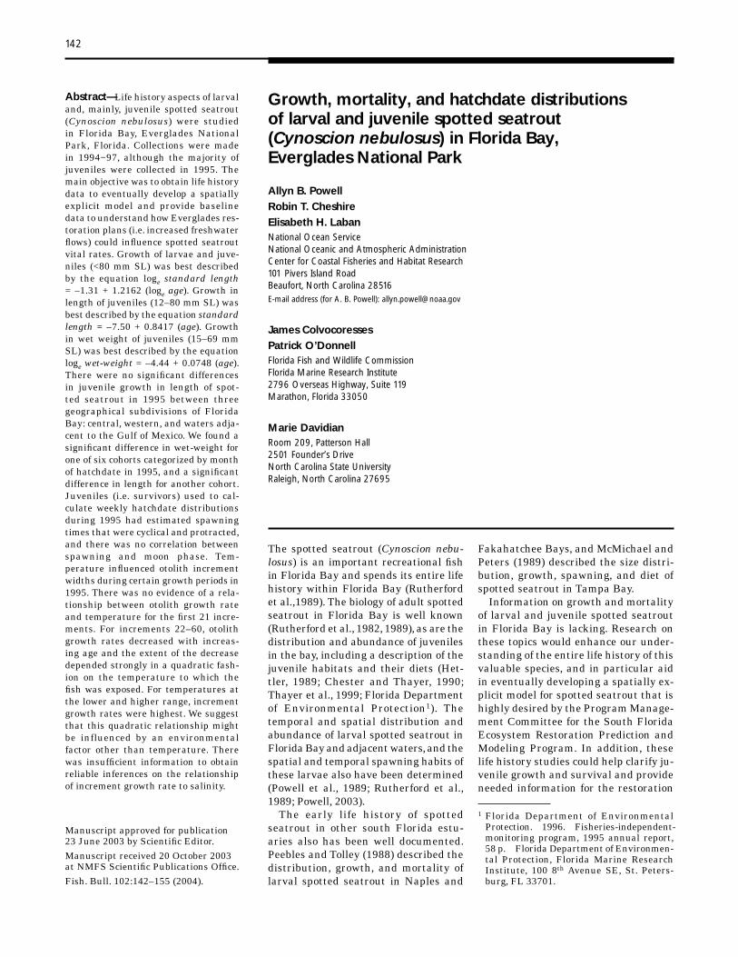
Larval fi sh used for otolith microstructure analysis were collected from September 1994 through July 1997, mainly in the Gulf transition, western, and central subdivisions (Table 1, Fig. 1). These subdivisions designated by the

• ••

••

•

•

• •

•

•

• •

•

•

•

••

•

•

16

45

10

21

9 13

18

1211

148

15

20

17

1 2

619

37

Y

N

•

25o20'

25o10'

25o00'

24o50'

81o00' 80o45' 80o30'

Cape Sable

Flamingo

northern transition

western

central

eastern

Florida Keys

Straits

of Florid

a

Gulf transition

Figure 1Location of sampling sites for spotted seatrout (Cynoscion nebulosus) in Florida Bay, Everglades National Park, Florida, including Florida Bay Subdivisions.

Gulf of Mexico

EvergladesNationalPark Boundary

Atlantic transitio

n

144 Fishery Bulletin 102(1)

Table 1 Florida Bay sampling stations where otoliths from spotted seatrout were collected. Included are numbers (n) of larvae and juveniles used in the otolith microstructure analysis, and subdivisions as defined by the South Florida Ecosystem Restoration Prediction and Modeling Program, Program Management Committee.

Station Longitude Florida Bay Juveniles Larvae number (degrees and minutes) (degrees and minutes) subdivisions Location (n) n)

1 25 06.81 81 05.27 Gulf transition Cape Sable — 4 2 25 06.37 81 01.42 Gulf transition Middle Ground 1 10 3 25 06.40 80 58.58 Gulf transition Conchie Channel — 4 4 25 07.70 80 56.90 Gulf transition Bradley Key 119 — 5 25 07.12 80 56.07 western Murray Key 4 8 6 25 08.11 80 50.95 central Snake Bight 3 — 7 25 09.45 80 53.42 central Snake Bight 4 — 8 25 07.50 80 48.51 central Rankin Lake 12 — 9 25 05.06 80 47.30 central Roscoe Key 20 —

10 25 02.30 81 .1.12 Gulf transition Sandy Key 49 — 11 25 02.90 80 55.00 western Johnson Key Basin 125 — 12 25 06.00 80 52.50 western Palm Key Basin 110 — 13 25 04.50 80 45.15 central Whipray Basin 2 62 14 25 08.00 80 43.20 central Crocodile Point 9 — 15 24 56.70 80 57.20 Gulf transition Schooner Bank 2 — 16 24 54.70 80 56.31 Gulf Transition Sprigger Bank — 8 17 25 00.40 80 47.68 central Sid Key Bank 6 — 18 24 57.03 80 47.52 central Twin Key Basin 6 — 19 25 07.98 80 40.48 eastern Madeira Point 1 — 20 25 11.85 80 37.15 northern Little Madeira Bay 8 — 21 25 13.00 80 27.80 eastern Shell Key 5 —

Latitude (

South Florida Ecosystem Restoration Prediction and Modeling Program, Program Management Committee, were based on modifications of the benthic mollusc com­munity (Turney and Perkins, 1972). In 1994 and 1995, we used 60-cm bongo nets fitted with 0.333-mm mesh fished from the port side of a 5.4-m boat. Beginning in 1996, we used a paired 60-cm bow-mounted push net with 0.333-mm mesh nets similar to that described by Hettler and Chester (1990).

Juvenile spotted seatrout were obtained from monitor­ing programs established by the NOAA Center for Coastal Fisheries and Habitat Research (NOAA) and Florida Ma­rine Research Institute (FMRI). NOAA collections were made from May 1995 through September 1997. Juveniles were collected with an otter trawl towed between two 5-m boats. The otter trawl measured 3.4 m (headrope) and was fitted with a 3.2-mm mesh tailbag with 6-mm mesh. FMRI collections were made in 1995 with a seine and a trawl. The 21.4-m center-bag drag seine was fitted with a 1.8 m Z 1.8 m Z 1.8 m bag of 3.2-mm mesh. The 6.1-m (headrope) otter trawl was fitted with a body of 38.1-mm stretch mesh and a 3.2-mm mesh tailbag. The majority of juveniles (86%) from NOAA and FMRI collections were collected in 1995.

Otolith microstructure analysis

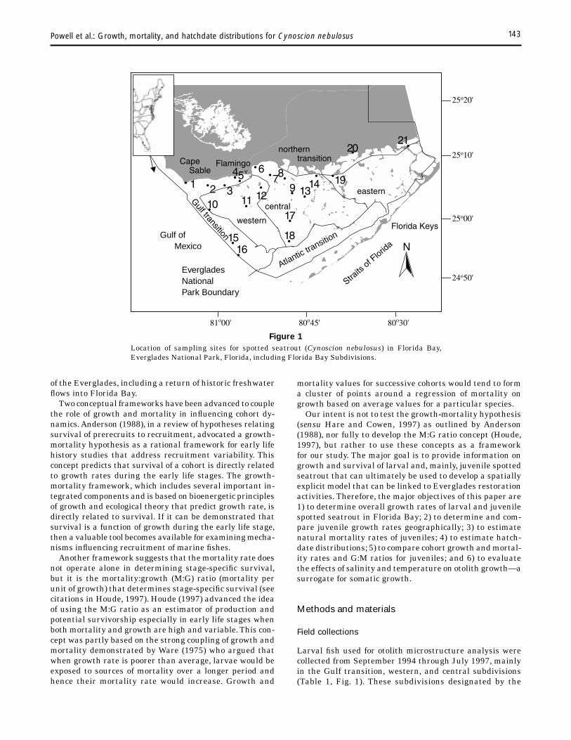
Otolith processing Otolith removal and preparation gen­erally followed the methods of Secor et al. (1991). All oto­

liths, except for the right sagitta, were mounted on a slide with mounting media and archived. The right sagittal oto­lith was embedded for transverse sectioning or polishing (or both).The left sagitta was embedded for transverse sec­tioning if the right was damaged. Sagittae were read with a light microscope at 1000Z magnification under oil immer­sion. The first increment was determined as that following the core increment; which was defined as a well-defined dark increment surrounding the core (Powell et al., 2000). Two blind counts of increments were made by one reader and if the counts differed by more than 5, then the otolith was read again. If the counts were within the acceptable range, the two counts were averaged. Based on a previous validation study (Powell et al., 2000), 2.5 days were added to the increment counts to obtain the daily age. A total of 582 sagittal otoliths were aged. This total included 96 from larval collections from September 1994 through July 1997, 139 juveniles from NOAA collections from June 1995 through September 1997, and 347 from FMRI collections from June 1995 through December 1995.

Increment widths were measured on 347 otoliths from FMRI collections (1995) by using image analysis. The measuring path consisted of two segments: a ventral path from the core to the 21st increment and a ventral-medial path along the sulcus, from the 21st increment to the edge (Fig. 2). The 21st increment was selected as the transition point in these measuring paths by test reading 30 otolith sections representing the entire range of sample fish

Powell et al.: Growth, mortality, and hatchdate distributions for Cynoscion nebulosus 145

Figure 2 Transverse polished section of a spotted seatrout (Cynoscion nebulosus) (18 mm SL; age 48 days) otolith showing the counting paths.

Primordia

10 µm

Sulcus

Ventral Lobe

Medial Edge

Distal Edge

Counting Path 1 (to 21 days)

Counting Path 2

(21 days to capture)

lengths. In all samples, the 21st increment could easily be traced in both measuring paths and in all samples the first 21 increments could be measured within the same image. Increment widths were averaged over a 7-day period. Age estimates were also obtained and we eliminated any oto­lith used to measure increment widths if the difference in total increment count between the two methods (counts ob­tained directly from the microscope versus those attained by image analysis) was greater than 7 days or 10%. On this basis, 117 otoliths were removed from the increment width analysis.

We believed counts obtained directly from the microscope were more accurate than those obtained by summing the number of increments measured on the computer moni­tor with the image analysis system. Counting increments directly through the microscope lens allows the reader to optically section the otolith (by varying the focus), which helps in detecting daily increments. “Frozen” multiple im­ages are a result of using the image analysis; hence optical sectioning is not possible.

Data analysis Data from all years and sources were used for 1) overall growth (i.e. larval and juvenile); 2) juvenile growth; and 3) estimates of juvenile mortality. Data from NOAA larval and juvenile collections were used to estimate a body-length–otolith-radius relationship. Data from 1995 FMRI and NOAA collections, which was the most com­plete data set, were used for growth comparisons between cohorts, and hatchdate distributions. Data from 1995 FMRI collections were used for 1) growth comparisons between geographical subdivisions; 2) estimating a wet-weight−age relationship to compute the ratio of wet-weight specific-

growth to mortality (G:M ratios), which assesses the rela­tive recruitment potential of individual cohorts (Houde, 1996; Rilling and Houde, 1999; Rooker et al., 1999); and 3) determining the influence of temperature on otolith incre­ment width. We used the FMRI data set exclusively for the above analyzes because collections were spatially more localized and wet weights were available.

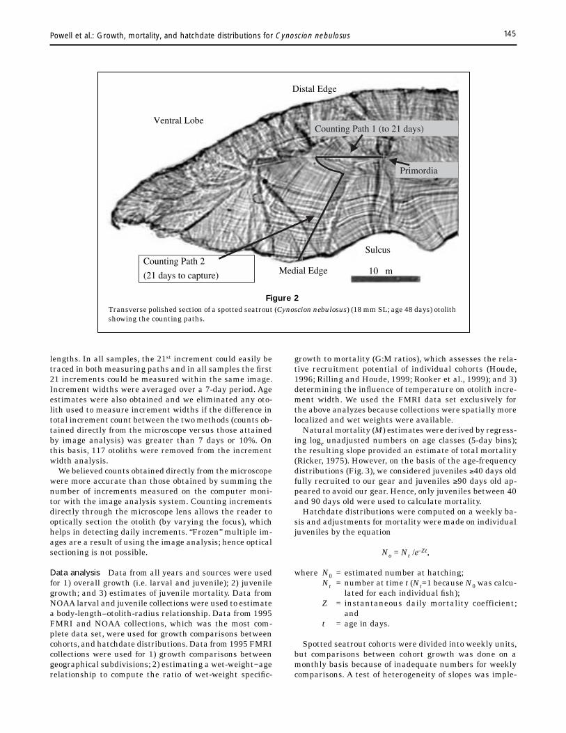
Natural mortality (M) estimates were derived by regress­ing loge unadjusted numbers on age classes (5-day bins); the resulting slope provided an estimate of total mortality (Ricker, 1975). However, on the basis of the age-frequency distributions (Fig. 3), we considered juveniles ≥40 days old fully recruited to our gear and juveniles ≥90 days old ap­peared to avoid our gear. Hence, only juveniles between 40 and 90 days old were used to calculate mortality.

Hatchdate distributions were computed on a weekly ba­sis and adjustments for mortality were made on individual juveniles by the equation

No = Nt /e–Zt,

where N0 = estimated number at hatching; Nt = number at time t (Nt=1 because N0 was calcu­

lated for each individual fish); Z = instantaneous daily mortality coefficient;

and t = age in days.

Spotted seatrout cohorts were divided into weekly units, but comparisons between cohort growth was done on a monthly basis because of inadequate numbers for weekly comparisons. A test of heterogeneity of slopes was imple-

146 Fishery Bulletin 102(1)

Figure 3 Frequency distribution of spotted seatrout (Cynoscion nebulosus) age classes used in deter-mining minimum age at full recruitment to the sampling gear, and mortality.

Age class (days)

<4

90-9

4

80-8

4

70-7

4

60-6

4

50-5

4

40-4

4

30-3

20-2

4

10-1

4

Num

bers

0

20

40

60

80

100

was used to test if spawning was cyclical. Cohorts (1995) were categorized according

to the following hatchdates: cohort A, 29 March–2 May (“April”); cohort B, 3 May–6 June (“May”); cohort C, 7 June–4 July (“June”); cohort D, 5 July–1 August (“July”); cohort E, 2 August–5 September (“August”); cohort F, 6 September–3 October (“September”).

Comparisons of the relative recruitment potential of individual cohorts (G:M ratios) between all cohorts were unresolved. Although cohort mortality estimates could be generated, they were appropriate (by analyzing r2 and P-values from regression analysis) for only three cohorts (cohorts B, D, and F).

A random coefficient model was used to investigate the relationship between growth rate of otoliths with age and

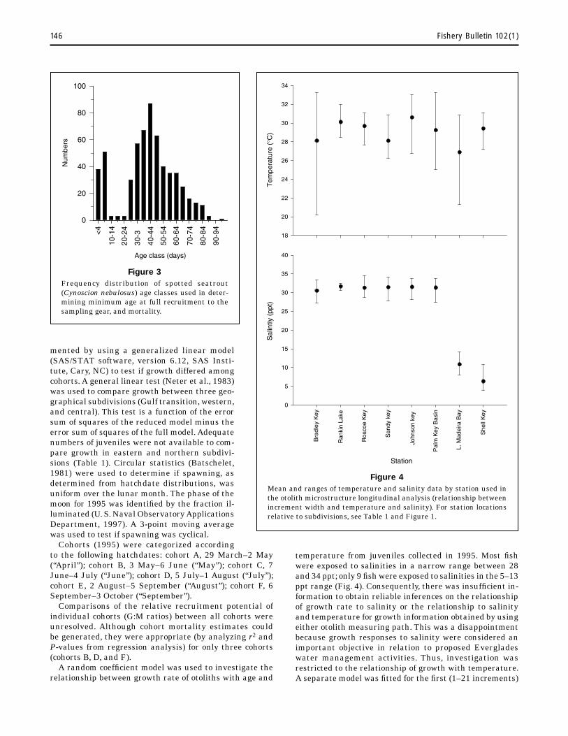
Figure 4 Mean and ranges of temperature and salinity data by station used in the otolith microstructure longitudinal analysis (relationship between increment width and temperature and salinity). For station locations relative to subdivisions, see Table 1 and Figure 1.

Station

Bra

dley

Key

Ran

kin

Lake

Ros

coe

Key

San

dy k

ey

John

son

key

Pal

m K

ey B

asin

L. M

adei

ra B

ay

She

ll K

ey 0

5

10

15

20

25

30

35

40

18

20

22

24

26

28

30

32

34

Tem

pera

ture

(°C

)S

alin

tiy (

ppt)

mented by using a generalized linear model (SAS/STAT software, version 6.12, SAS Insti­tute, Cary, NC) to test if growth differed among cohorts. A general linear test (Neter et al., 1983) was used to compare growth between three geo­graphical subdivisions (Gulf transition, western, and central). This test is a function of the error sum of squares of the reduced model minus the error sum of squares of the full model. Adequate numbers of juveniles were not available to com­pare growth in eastern and northern subdivi­sions (Table 1). Circular statistics (Batschelet, 1981) were used to determine if spawning, as determined from hatchdate distributions, was uniform over the lunar month. The phase of the moon for 1995 was identified by the fraction il­luminated (U. S. Naval Observatory Applications Department, 1997). A 3-point moving average

temperature from juveniles collected in 1995. Most fish were exposed to salinities in a narrow range between 28 and 34 ppt; only 9 fish were exposed to salinities in the 5–13 ppt range (Fig. 4). Consequently, there was insufficient in-formation to obtain reliable inferences on the relationship of growth rate to salinity or the relationship to salinity and temperature for growth information obtained by using either otolith measuring path. This was a disappointment because growth responses to salinity were considered an important objective in relation to proposed Everglades water management activities. Thus, investigation was restricted to the relationship of growth with temperature. A separate model was fitted for the first (1–21 increments)

Powell et al.: Growth, mortality, and hatchdate distributions for Cynoscion nebulosus 147

and second (22–60 increments) measuring paths because otolith increment width changed at a constant (age-inde­pendent) rate for each path. We did not include fish with >60 increments because the relationship past this number was determined for only 10% of the fish and included obvi­ous outliers. Letting Yij be the otolith width measurement for fish i at age αij, where j indexes time, the model for each path was

Yij = α0i + α1iαij + eij,

where α0i and α1i are the fish-specific intercept and slope describing the relationship between increment width and age for fish i, and eij is a normally distributed error term; thus, α1i is the growth rate for fish i over the measuring path.Temperature exhibited only negligible change for any given fish over the measuring path; thus, temperature for fish i was summarized as ti, the average temperature over the path for that fish. To determine an appropriate model for the relationship between intercept and growth rate and temperature, a preliminary analysis was performed in which ordinary least squares estimates of α0i and α1i were obtained separately for each fish i and plotted against tem­perature. For the first measuring path (1–21 increments), the appropriate model was

α0i = β00 + β0iti + b0i, α1i = β10 + β11ti + β12ti 2 + b1i,

where b0i and b1i are normally distributed random effects, allowing growth rates for fish at the same temperature to vary across fish. For the second measuring path (22−60 increments), the appropriate model was,

α0i = β00 + β01ti + β02ti 2 + b0i, α1i = β10 + β11ti + β12ti

2 + b1i.

By substitution, these considerations yielded models 1 and 2 for the first and second paths, respectively:

Yij = (β00 + β01ti) + (β10 + β11ti + β12ti 2) aij + b0i +

b1iaij + eij (1)

Yij = (β00 +β01ti + β02ti2) +

(β10 + β11ti + β12ti 2) aij + b0i + b1iaij + eij (2)

thus representing otolith increment width in each case as having a straight line relationship with age, where the slope (age-independent growth rate) depends on average temperature according to a quadratic relationship. The random effects allow observations on the same fish to be correlated, whereas observations across fish are inde­pendent. Models 1 and 2 were implemented in SAS Proc Mixed (SAS/STAT software, version 6.12, SAS Institute, Cary, NC).

Daily temperature records were obtained from the Unit­ed States Department of Interior’s National Park Service, Florida Bay monitoring stations and averaged over a 7-day period. In 1995, temperature records were available only for Johnson Key Basin (JKB), Whipray Basin (WB), Little Blackwater Sound (LBS), and Little Madeira Bay (LMB), but spotted seatrout were also collected at other sites

(Table 1). Daily temperatures were estimated for Sandy Key (SK) and Roscoe Keys (RK) from values recorded dur­ing sampling trips because both these stations are not in close proximity to National Park Service monitoring sites. Sandy Key values were regressed on JKB values (same dates). Sandy Key temperatures were collected from Janu­ary 1994 through August 1996. The regression model for temperature was SK = 0.76 + 0.9536 JKB [r2=0.89; n=25]. Roscoe Key values were regressed on WB values (same dates). Roscoe Key temperatures were collected from Janu­ary 1994 through August 1996. The regression model for temperature was RK = 5.60 + 0.7976 WB [r2=0.87; n=31). Temperature values were available at Murray Key (MK) in 1997. To attain values for our 1995 analysis we regressed MK on JKB (same dates). The temperature regression model was MK = 0.77 + 0.9680 JKB [r2=0.99; n=342].

We reported measurements in standard length (SL). For preflexion and flexion larvae, standard length was mea­sured from the tip of the snout to the tip of the notochord. For postflexion larvae and juveniles, standard length was measured from the tip of the snout to the base of the hy­pural plate.

Results

Overall growth of larvae and juveniles (<80 mm SL) was best described by the equation loge standard length = –1.31 + 1.2162 (loge age) [n=582; r2=0.97]. Growth in body length of juveniles (12–80 mm SL) was best described by the linear equation standard length = –7.50 + 0.8417 (age) [n=486; r2=0.84]; hence, juveniles between approximately age 20–100 days grew on average 0.84 mm/d. There were no significant differences in juvenile growth in body length among three geographical subdivisions [F4

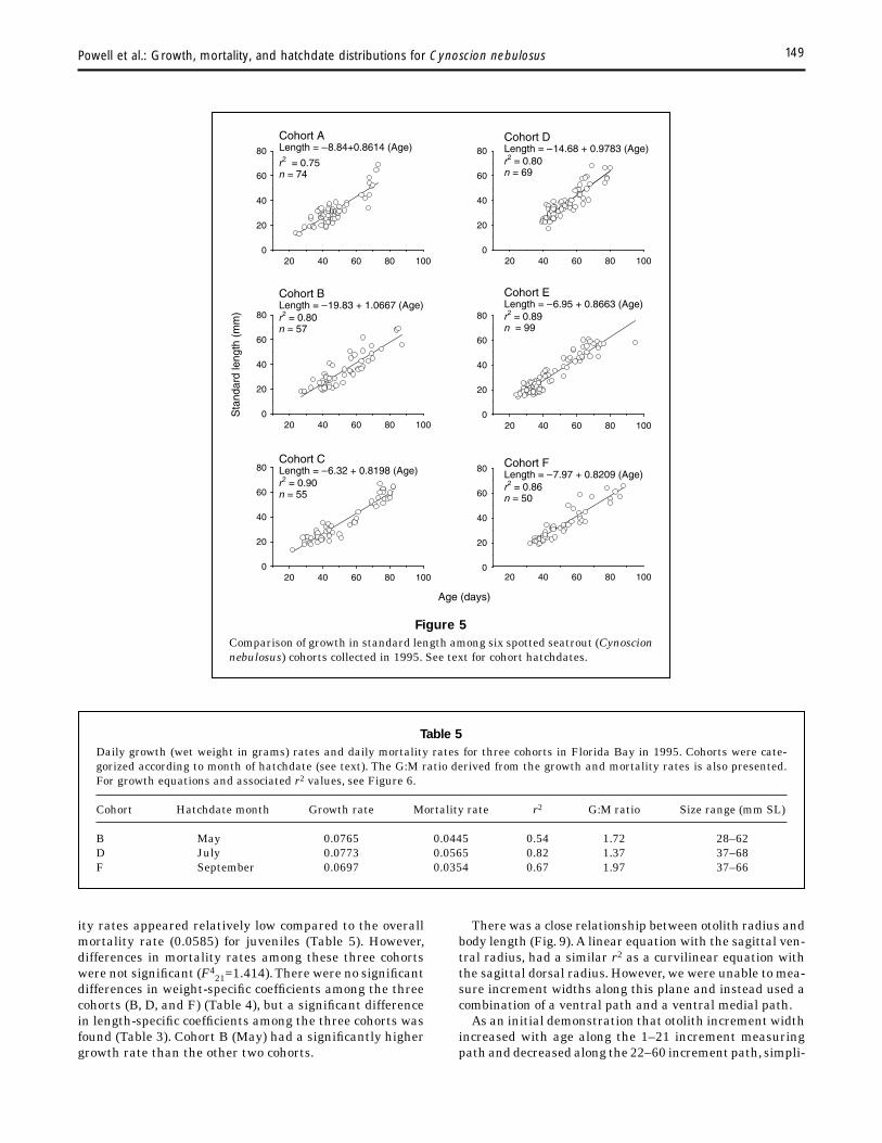
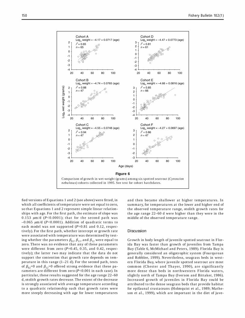
327=0.756; n=333] (Table 2), but there was a significant growth differ­ence in length for one of six 1995 cohorts (Table 3, Fig. 5). Growth in wet weight of juveniles (15–69 mm SL) was best described by the equation loge wet weight = –4.44 + 0.0748 (age) [n=347, r2=0.84]. There was a significant growth dif­ference in wet weight for one cohort (Table 4, Fig. 6).

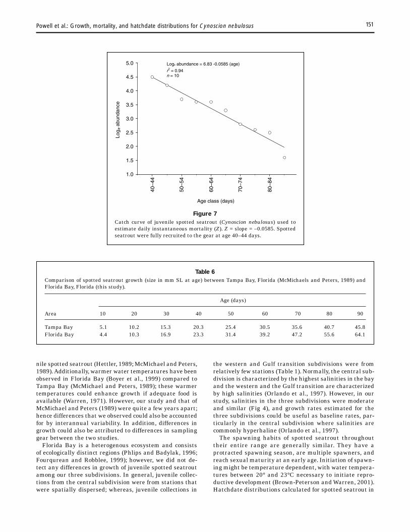
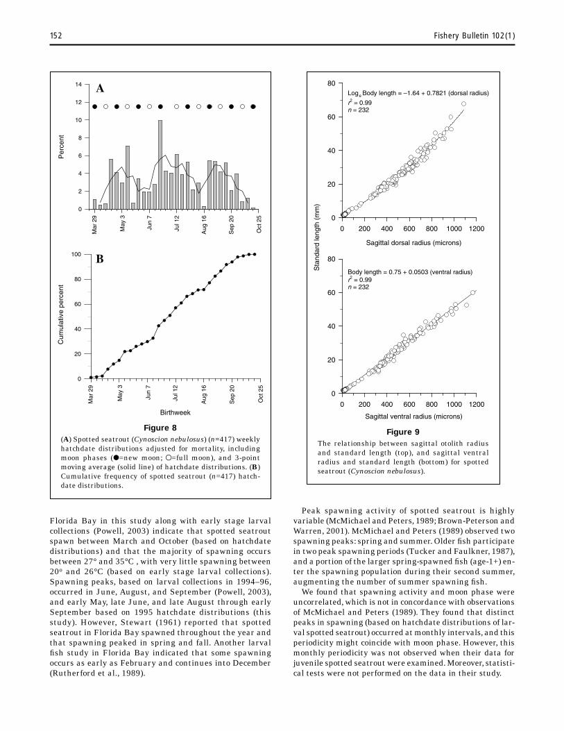
Weekly 1995 hatchdate distributions, determined by us­ing daily instantaneous mortality (0.0585, Fig. 7), indicated juveniles in collections (i.e. survivors) were from spawning that was cyclical and protracted (Fig. 8). The most intense successful spawning occurred during 21–27 June (9.2% of total). Using a 3-point moving average, we observed three similar cycles (Fig. 8). From data on survivors, ~25% of ju­veniles were spawned by late May, 50% by early July, and 75% by late August and from data on cohorts, three cohorts (cohorts C, D, and E; early June–late August) comprised 55% of the total estimated spawn of spotted seatrout.There was no correlation between spawning and moon phase (pe­riodic regression r2=0.019, P=0.754) (Fig. 8).

The relative recruitment potential (G:M ratio) of the 1995 year class estimated from the wet-weight specific growth coefficient (0.0748) and the instantaneous daily mortal­ity rate (0.0585, Fig. 7) was 1.28. The G:M ratio for three cohorts (B, May; D, July; and F, September) was greater than the ratio for the total 1995 year class because mortal-

148 Fishery Bulletin 102(1)

Table 2 Summary of growth data used to compare growth in length of spotted seatrout among three Florida Bay subdivisions. Growth was best described by the linear equation: standard length = a + b (age in days).

Subdivision Slope n r2 Size range (mm SL)

Gulf transition –11.07 0.8914 139 0.86 16 –69 Central 0.9298 49 0.80 15 –63 Western 0.8834 145 0.85 17–69

Intercept

–12.23 –10.56

Table 3 Summary of statistics for a test for heterogeneity of slopes for cohort somatic growth rates of spotted seatrout. Cohorts were catego­rized according to month of hatchdate (see text). The base parameter is cohort F and all parameter estimates are deviations from the base cohort. For growth equations, see Figure 5.

Parameter Standard error t-value P-value

Intercept 3.02829 –2.63 0.0088 Cohort A –0.86811 4.31970 –0.20 0.8408 Cohort B –11.85849 3.91387 –3.03 0.0026 Cohort C 1.65094 3.86470 0.43 0.6695 Cohort D –6.70820 4.74936 –1.41 0.1586 Cohort E 1.02077 3.50931 0.29 0.7713

Slope 0.05613 14.62 <0.001 Cohort A 0.04054 0.08604 0.47 0.6378 Cohort B 0.24578 0.07106 3.46 0.0006 Cohort C −0.00113 0.07091 −0.02 0.9873 Cohort D 0.15741 0.08730 1.80 0.0721 Cohort E 0.04544 0.06821 0.67 0.5058

Estimate

–7.97270

0.82088

Table 4 Summary of statistics for a test for heterogeneity of slopes for cohort wet-weight growth rate of spotted seatrout. Cohorts were categorized according to month of hatch date (see text). The base parameter is cohort F and all parameter estimates are deviations from the base cohort. For growth equations, see Figure 6.

Parameter Standard error t-value P-value

Intercept 0.23763 −17.99 <0.0001 Cohort A 0.10201 0.37014 0.28 0.7830 Cohort B –0.46348 0.34092 –1.36 0.1749 Cohort C –0.27866 0.32116 –0.87 0.3862 Cohort D –0.19540 0.38352 –0.51 0.6108 Cohort E –0.38260 0.29853 –1.28 0.2009

Slope 0.00439 15.88 <0.0001 Cohort A 0.00195 0.00729 0.27 0.7889 Cohort B 0.00679 0.00622 1.09 0.2754 Cohort C 0.00502 0.00575 0.87 0.3835 Cohort D 0.00759 0.00702 1.08 0.2808 Cohort E 0.01188 0.00564 2.11 0.0359

Estimate

–4.27384

0.06974

Powell et al.: Growth, mortality, and hatchdate distributions for Cynoscion nebulosus 149

Figure 5 Comparison of growth in standard length among six spotted seatrout (Cynoscion nebulosus) cohorts collected in 1995. See text for cohort hatchdates.

20 40 60 80 100 0

20

40

60

80

Cohort B Length = –19.83 + 1.0667 (Age) r 2 = 0.80 n = 57

20 40 60 80 100

Sta

ndar

d le

ngth

(m

m)

0

20

40

60

80

Cohort C Length = –6.32 + 0.8198 (Age) r 2 = 0.90 n = 55

20 40 60 80 100 0

20

40

60

80

20 40 60 80 100 0

20

40

60

80

20 40 60 80 100 0

20

40

60

80

20 40 60 80 100 0

20

40

60

80

Cohort A Length = –8.84+0.8614 (Age)

r 2 = 0.75 n = 74

Cohort D Length = –14.68 + 0.9783 (Age) r 2 = 0.80 n = 69

Cohort E Length = –6.95 + 0.8663 (Age) r 2 = 0.89 n = 99

Cohort F Length = –7.97 + 0.8209 (Age) r 2 = 0.86 n = 50

Age (days)

Table 5 Daily growth (wet weight in grams) rates and daily mortality rates for three cohorts in Florida Bay in 1995. Cohorts were cate­gorized according to month of hatchdate (see text). The G:M ratio derived from the growth and mortality rates is also presented. For growth equations and associated r2 values, see Figure 6.

Cohort Hatchdate month Growth rate Mortality rate r2 G:M ratio Size range (mm SL)

B y 0.0765 0.0445 0.54 1.72 28–62 D uly 0.0773 0.0565 0.82 1.37 37–68 F 0.0697 0.0354 0.67 1.97 37–66

MaJSeptember

ity rates appeared relatively low compared to the overall There was a close relationship between otolith radius and mortality rate (0.0585) for juveniles (Table 5). However, body length (Fig. 9). A linear equation with the sagittal ven­differences in mortality rates among these three cohorts tral radius, had a similar r2 as a curvilinear equation with were not significant (F4

21=1.414).There were no significant the sagittal dorsal radius. However, we were unable to mea­differences in weight-specific coefficients among the three sure increment widths along this plane and instead used a cohorts (B, D, and F) (Table 4), but a significant difference combination of a ventral path and a ventral medial path. in length-specific coefficients among the three cohorts was As an initial demonstration that otolith increment width found (Table 3). Cohort B (May) had a significantly higher increased with age along the 1–21 increment measuring growth rate than the other two cohorts. path and decreased along the 22–60 increment path, simpli-

150 Fishery Bulletin 102(1)

Figure 6 Comparison of growth in wet-weight (grams) among six spotted seatrout (Cynoscion nebulosus) cohorts collected in 1995. See text for cohort hatchdates.

20 40 60 80 100 -4

-3

-2

-1

0

1

2

Cohort A Log e weight = –4.17 + 0.0717 (age)

r 2 = 0.65 n = 65

20 40 60 80 100 Log e

wet

wei

ght (

gram

s)

-4

-3

-2

-1

0

1

2

Cohort B Log e weight = –4.74 + 0.0765 (age)

r 2 = 0.88 n = 47

20 40 60 80 100 -4

-3

-2

-1

0

1

2

Cohort C Log e weight = –4.55 + 0.0748 (age)

r 2 = 0.94 n = 47

20 40 60 80 100 -4 -3 -2 -1 0 1 2 3

Cohort D Log e weight = –4.47 + 0.0773 (age)

r 2 = 0.81 n = 61

20 40 60 80 100 -4 -3 -2 -1 0 1 2 3

Cohort E Log e weight = –4.66 + 0.0816 (age)

r 2 = 0.85 n = 66

20 40 60 80 100 -3

-2

-1

0

1

2

3

Cohort F Log e weight = –4.27 + 0.0697 (age)

r 2 = 0.86 n = 47

Age (days)

fied versions of Equations 1 and 2 (see above) were fitted, in which all coefficients of temperature were set equal to zero, so that Equations 1 and 2 represent simple linear relation-ships with age. For the first path, the estimate of slope was 0.153 Hm/d (P<0.0001); that for the second path was –0.065 Hm/d (P<0.0001). Addition of quadratic terms to each model was not supported (P=0.81 and 0.12, respec­tively). For the first path, whether intercept or growth rate were associated with temperature was determined by test­ing whether the parameters β01, β11, and β12 were equal to zero. There was no evidence that any of these parameters were different from zero (P=0.45, 0.35, and 0.42, respec­tively); the latter two may indicate that the data do not support the contention that growth rate depends on tem­perature in this range (1–21 d). For the second path, tests of β02=0 and β12=0 offered strong evidence that these pa­rameters are different from zero (P<0.001 in each case). In particular, these results suggested for the age range 22–60 d, otolith growth rates decrease. The extent of the decrease is strongly associated with average temperature according to a quadratic relationship such that growth rates were more steeply decreasing with age for lower temperatures

and then became shallower at higher temperatures. In summary, for temperatures at the lower and higher end of the observed temperature range, otolith growth rates for the age range 22–60 d were higher than they were in the middle of the observed temperature range.

Discussion

Growth in body length of juvenile spotted seatrout in Flor­ida Bay was faster than growth of juveniles from Tampa Bay (Table 6, McMichael and Peters, 1989). Florida Bay is generally considered an oligotrophic system (Fourqurean and Robblee, 1999). Nevertheless, seagrass beds in west-ern Florida Bay, where juvenile spotted seatrout are most common (Chester and Thayer, 1990), are significantly more dense than beds in northwestern Florida waters, slightly north of Tampa Bay (Iverson and Bittaker, 1986). Increased growth of juveniles in Florida Bay could be attributed to the dense seagrass beds that provide habitat for epifaunal crustaceans (Holmquist et al., 1989; Mathe­son et al., 1999), which are important in the diet of juve-

Powell et al.: Growth, mortality, and hatchdate distributions for Cynoscion nebulosus 151

Figure 7 Catch curve of juvenile spotted seatrout (Cynoscion nebulosus) used to estimate daily instantaneous mortality (Z). Z = slope = –0.0585. Spotted seatrout were fully recruited to the gear at age 40–44 days.

Age class (days)

40–4

4

50–5

4

60–6

4

70–7

4

80–8

4

Log e

abu

ndan

ce

1.0

1.5

2.0

2.5

3.0

3.5

4.0

4.5

5.0 Loge abundance = 6.83 -0.0585 (age)

r 2 = 0.94 n = 10

Table 6 Comparison of spotted seatrout growth (size in mm SL at age) between Tampa Bay, Florida (McMichaels and Peters, 1989) and Florida Bay, Florida (this study).

Age (days)

Area 10 20 60 70 80 90

Tampa Bay 5.1 15.3 20.3 30.5 45.8 Florida Bay 4.4 16.9 23.3 39.2 64.1

50 40 30

10.2 25.4 40.7 35.6 10.3 31.4 55.6 47.2

nile spotted seatrout (Hettler, 1989; McMichael and Peters, 1989).Additionally, warmer water temperatures have been observed in Florida Bay (Boyer et al., 1999) compared to Tampa Bay (McMichael and Peters, 1989); these warmer temperatures could enhance growth if adequate food is available (Warren, 1971). However, our study and that of McMichael and Peters (1989) were quite a few years apart; hence differences that we observed could also be accounted for by interannual variability. In addition, differences in growth could also be attributed to differences in sampling gear between the two studies.

Florida Bay is a heterogenous ecosystem and consists of ecologically distinct regions (Phlips and Badylak, 1996; Fourqurean and Robblee, 1999); however, we did not de­tect any differences in growth of juvenile spotted seatrout among our three subdivisions. In general, juvenile collec­tions from the central subdivision were from stations that were spatially dispersed; whereas, juvenile collections in

the western and Gulf transition subdivisions were from relatively few stations (Table 1). Normally, the central sub-division is characterized by the highest salinities in the bay and the western and the Gulf transition are characterized by high salinities (Orlando et al., 1997). However, in our study, salinities in the three subdivisions were moderate and similar (Fig 4), and growth rates estimated for the three subdivisions could be useful as baseline rates, par­ticularly in the central subdivision where salinities are commonly hyperhaline (Orlando et al., 1997).

The spawning habits of spotted seatrout throughout their entire range are generally similar. They have a protracted spawning season, are multiple spawners, and reach sexual maturity at an early age. Initiation of spawn­ing might be temperature dependent, with water tempera­tures between 20° and 23°C necessary to initiate repro­ductive development (Brown-Peterson and Warren, 2001). Hatchdate distributions calculated for spotted seatrout in

152 Fishery Bulletin 102(1)

Figure 9The relationship between sagittal otolith radius and standard length (top), and sagittal ventral radius and standard length (bottom) for spotted seatrout (Cynoscion nebulosus).

Sagittal dorsal radius (microns)

0 200 400 600 800 1000 1200

Sta

ndar

d le

ngth

(m

m)

0

20

40

60

80

Sagittal ventral radius (microns)

0 200 400 600 800 1000 1200

0

20

40

60

80

Loge Body length = –1.64 + 0.7821 (dorsal radius)

r2 = 0.99n = 232

Body length = 0.75 + 0.0503 (ventral radius)r2 = 0.99n = 232

Figure 8(A) Spotted seatrout (Cynoscion nebulosus) (n=417) weekly hatchdate distributions adjusted for mortality, including moon phases (●=new moon; ●=full moon), and 3-point moving average (solid line) of hatchdate distributions. (B) Cumulative frequency of spotted seatrout (n=417) hatch-date distributions.

Mar

29

May

3

Jun

7

Jul 1

2

Aug

16

Sep

20

Oct

25

Per

cent

0

2

4

6

8

10

12

14

Birthweek

Mar

29

May

3

Jun

7

Jul 1

2

Aug

16

Sep

20

Oct

25

Cum

ulat

ive

perc

ent

0

20

40

60

80

100

A

B

Florida Bay in this study along with early stage larval collections (Powell, 2003) indicate that spotted seatrout spawn between March and October (based on hatchdate distributions) and that the majority of spawning occurs between 27° and 35°C , with very little spawning between 20o and 26°C (based on early stage larval collections). Spawning peaks, based on larval collections in 1994–96, occurred in June, August, and September (Powell, 2003), and early May, late June, and late August through early September based on 1995 hatchdate distributions (this study). However, Stewart (1961) reported that spotted seatrout in Florida Bay spawned throughout the year and that spawning peaked in spring and fall. Another larval fi sh study in Florida Bay indicated that some spawning occurs as early as February and continues into December (Rutherford et al., 1989).

Peak spawning activity of spotted seatrout is highly variable (McMichael and Peters, 1989; Brown-Peterson and Warren, 2001). McMichael and Peters (1989) observed two spawning peaks: spring and summer. Older fi sh participate in two peak spawning periods (Tucker and Faulkner, 1987), and a portion of the larger spring-spawned fi sh (age-1+) en-ter the spawning population during their second summer, augmenting the number of summer spawning fi sh.

We found that spawning activity and moon phase were uncorrelated, which is not in concordance with observations of McMichael and Peters (1989). They found that distinct peaks in spawning (based on hatchdate distributions of lar-val spotted seatrout) occurred at monthly intervals, and this periodicity might coincide with moon phase. However, this monthly periodicity was not observed when their data for juvenile spotted seatrout were examined. Moreover, statisti-cal tests were not performed on the data in their study.

Powell et al.: Growth, mortality, and hatchdate distributions for Cynoscion nebulosus 153

Our inferences, from this study, in relation to spotted seatrout peak spawning are based on hatchdate distribu­tions and should be viewed with caution because hatch-dates are based on survivors. Differential survival for early life history stages can bias results. Hatchdate distributions are valuable when compared to egg or recently hatched lar­val densities and might suggest processes responsible for differential cohort survivorship. Because spotted seatrout undergo a protracted spawning period and because there is high variation associated with icthyoplankton samples (Cyr et al., 1992), intensive and extensive sampling of recently hatched larvae would be required over a long duration to answer these process-oriented mortality questions.

The daily instantaneous mortality rate of juvenile spot­ted seatrout was higher in Florida Bay than those reported from northwestern Florida systems (Nelson and Leffler, 2001). Mortality rates of juvenile spotted seatrout from Florida Bay were 5.7%/d; whereas, for the other systems, rates approximated 3%/d. In general, mortality rates might increase with increasing estuarine temperatures (Houde and Zastrow, 1993). Although we were unable to estimate instantaneous daily mortality rates for larval spotted seat-rout, these data have been estimated for larvae (3.5–6.5 mm) in two southwestern Florida estuaries (Peebles and Tolly, 1988). Highly variable rates were reported between the two Florida estuaries (Naples Bay: 0.70 or 50%/d; and Fakahatchee area: 0.37 or 31%/d). Houde (1996) reported a generalized instantaneous daily mortality rate for marine fish larvae of 0.239 (21%/d). Estimating mortality rates for larval spotted seatrout in Florida Bay will be critical for calculating G:M ratios in order to evaluate stage-specific survival and to develop credible spatially explicit models.

Mortality rates of spotted seatrout cohorts could be cal­culated for only three of six cohorts (B, May; D, July; and F, September) because slopes were significantly different from zero for only these cohorts. Furthermore, mortality rates of two of the three cohorts (B and F) were associated with low r2 values (Table 5); hence the G:M ratios along with the mortality rates for these three cohorts should be considered “rough” estimates. Attaining more accurate mortality estimates for spotted seatrout would be valuable in linking cohort variability with potential recruitment and stage-specific survival. For example, larval cohorts of bay anchovy (Anchoa mitchilli) from Chesapeake Bay, a tem­perate estuary, exhibit growth rates that are temporally variable and mortality rates that are spatially and tem­porally variable (Rilling and Houde, 1999). Temperature, zooplankton prey and gelatinous predators are believed to influence growth and mortality rates of the bay anchovy. For striped bass (Morone saxatilis) in a subestuary of Ches­apeake Bay, cohorts exhibited highly variable seasonal G:M ratios that were strongly influenced by temperature (Houde, 1997). In a subtropical estuary, cohort-specific mortality rates for juvenile red drum varied temporally; early and late season cohorts exhibited the highest mortal­ity rates, which coincided with highest growth rates and G:M ratios for midseason cohorts (Rooker et al., 1999). We agree with Houde (1997) that future research should focus on the variability and causes of variability in growth and mortality, both of which interact to determine stage-spe­

cific survival. The developmental stage or age where G:M variability is greatest, along with the relationship of this variability to recruitment, need to be determined for spot­ted seatrout in Florida Bay. No doubt a relationship exists between G:M ratios and recruitment. Future research should also determine if cohort G:M ratios and somatic growth rates are seasonally or spatially variable. If they are, then a limited spatial and temporal sampling program could be designed to annually evaluate G:M ratios at highly variable stages or ages as an index of year-class strength of spotted seatrout in Florida Bay. Such an index could be verified by examining year-class catch rates on an annual basis or by virtual population analysis.

In our study there was little temporal difference in growth of juvenile spotted seatrout cohorts. Larval growth and mortality, which was not treated adequately in our study, could be influenced by copepod prey—an important dietary component of larval spotted seatrout (McMichael and Peters, 1989). The copepod Acartia tonsa is dominant in Florida Bay, but egg production rates for this species are low in the bay compared to those in other systems (Kleppel et al., 1998). We suspect the “bottleneck” to recruitment of spotted seatrout could occur during the larval stage. Hence, future research should examine mortality and growth of larval and recently settled spotted seatrout; in particular the patterns of larval production potential (G:M ratios). Research in these areas should increase our understand­ing of the degree of variability in stage-specific survival and recruitment of spotted seatrout in Florida Bay (Houde, 1996).

For most species, especially those with protracted spawn­ing habits, it is most informative to analyze cohort growth and mortality. For example, striped bass and bay anchovy cohorts in Chesapeake Bay exhibit highly variable growth rates, mortality rates, and stage durations (Rutherford and Houde, 1995; Rilling and Houde, 1999). This variabil­ity could cause differential survival for cohorts and result in frequency distributions of survivor hatchdates that do not resemble recently hatched larvae or egg-production frequency distributions (e.g. Crecco and Savoy, 1985; Rice et al., 1987).

We are unable to interpret the significance of the abso­lute value of the G:M ratio for juvenile spotted seatrout, because interannual comparisons were not made, but we presented the ratio for future comparisons. Generally, the G:M ratio is <1.0 during the early larval stage, indicating a decline in biomass. However, the G:M ratio of a cohort will eventually exceed 1.0 as a result of a relative decline in mortality as larvae grow (Houde and Zastrow, 1993). Clearly, stage specific analysis of the spotted seatrout from egg through juvenile stage would have been more informa­tive in determining when the maximum G:M ratio occurs (when cohort biomass increases at a maximum rate) and in providing insight into stage-specific dynamics of spotted seatrout (Houde, 1997). A constraint of our study was our inability to estimate larval mortality rates; hence early life history stage dynamics could not be examined.

Size-selective mortality in the juvenile life history stages can have important consequences for recruitment. Sogard (1997) argued that “within-cohort size-selective mortality”

154 Fishery Bulletin 102(1)

is more evident in the juvenile stage than during the egg and larval stages when random mortality independent of fish size is more likely to occur (e.g. dispersal of eggs and larvae away from suitable nursery areas). In addition, vari­ation in size, which provides a “template” for size-selective processes, increases during the juvenile stage as larval size is constrained by egg size. Sogard (1997) cited a number of recent studies that suggest the early juvenile period plays a greater role in determining year-class strength than previously thought.

We were unable to determine if salinity influenced incre­ment width (a surrogate for somatic growth) at early life stages. Understanding the relationship between salinity and growth is critical because Everglades restoration will most likely result in increased freshwater flows to Florida Bay, and during low rainfall periods, salinities in the north central portion of the bay can exceed 45 ppt (Orlando et al., 1997; Boyer et al., 1999). But, salinities were moderate and similar at most stations where juvenile trout were col­lected in the bay during 1995 (Fig. 4). Very few fish were collected at low salinities; in fact, juvenile spotted seatrout are not commonly collected at low-salinity stations (Table 1; Florida Department of Environmental Protection1), and hyperhaline conditions were not observed in 1995. There-fore, we were only able to determine if temperature could influence increment widths. The curvilinear relationship between otolith growth rate and temperature, although a statistically strong relationship, is difficult to explain biologically. Temperature could mask other factors, e.g. temporal variability in prey and predator availability, and optimal temperatures for growth (Rooker et al., 1999). We were able to demonstrate that one cohort grew faster than five other cohorts, possibly indicating differential prey availability in 1995. An individual-based bioenergetics model for spotted seatrout now in preparation (Wuenschel et al.2) should add to our understanding of the effects of salinity and temperature on larval and juvenile spotted seatrout

Acknowledgments

We are especially grateful to Al Crosby, Mike Greene, Mike LaCroix, and other Beaufort staff that participated in the field work.We thank James Waters of the NMFS Southeast Fisheries Science Center for computer programing assis­tance and Jon Hare of our laboratory for performing the circular statistics. We are grateful to Dean Ahrenholz, Jon Hare, Patti Marraro, Joseph Smith, and three anonymous reviewers for their valuable reviews of the manuscript. We also thank Steve Bobko at Old Dominion University for the image analysis macro used to obtain otolith increment widths.

2 Wuenschel, M. J., R. G. Werner, D. E. Hoss, and A. B. Powell. 2001. Bioenergetics of larval spotted seatrout (Cynoscion nebulosus) in Florida Bay. Florida Bay Science Conference, April 23–26, 2001, p. 215–216. Westen Beach Resort, Key Largo, Florida. Abstract. Center for Coastal Fisheries and Habitat Research, Beaufort Laboratory, 101 Pivers Island Road, Beaufort, NC 28516.

Literature cited

Anderson, J. T. 1988. A review of size dependent survival during pre-recruit

stages of fishes in relation to recruitment. J. Northw. Atl. Fish. Sci. 8:55−66.

Batschelet, E. 1981. Circular statistics in biology, 371 p. Academic Press,

New York, NY. Boyer, J. N., J. W. Fourqurean, and R. D. Jones.

1999. Seasonal and long-term trends in the water quality of Florida Bay (1989−1997). Estuaries 22:417−430.

Brown-Peterson, N. J., and J. W. Warren. 2001. The reproductive biology of spotted seatrout, Cyno­

scion nebulosus, along the Mississippi Gulf Coast. Gulf Mexico Sci. 2001:61−73.

Chester, A. J., and G. W. Thayer. 1990. Distribution of spotted seatrout (Cynoscion nebu­

losus) and gray snapper (Lutjanus griseus) juveniles in seagrass habitats of western Florida Bay. Bull. Mar. Sci. 46:345−357.

Crecco, V., and T. Savoy. 1985. Effects of biotic and abiotic factors on growth and

relative survival of young American shad, Alosa sapidis­sima, in the Connecticut River. Can. J. Fish. Aquat. Sci. 42: 1640−1648.

Cyr, H., J. A. Downing, S. Lalonde, S. B. Baines, and M. L. Price. 1992. Sampling larval fish: choice of sample number and

size. Trans. Am. Fish. Soc. 121:356−368. Fourqurean, J. W., and M. B. Robblee.

1999. Florida Bay: a history of recent ecological changes. Estuaries 22:345−357.

Hare, J. A., and R. K. Cowen. 1997. Size, growth, development, and survival of the plank-

tonic larvae of Pomatomus saltatrix (Pisces: Pomatomidae). Ecology 78:2415−2431.

Hettler, W. F., Jr. 1989. Food habits of juveniles of spotted seatrout and

gray snapper in western Florida Bay. Bull. Mar. Sci. 44: 152−165.

Hettler, W. F., and A. J. Chester. 1990. Temporal distribution of ichthyoplankton near

Beaufort Inlet, North Carolina. Mar. Ecol. Prog. Ser. 68: 157−168.

Holmquist, J. G., G. V. N. Powell, and S. M. Sogard. 1989. Decapod and stomatopod communities of seagrass­

covered mud banks in Florida Bay: inter- and intra­bank heterogeneity with special reference to isolated subenvironments. Bull. Mar. Sci. 44:251−262.

Houde, E. D. 1996. Evaluating stage-specific survival during the early life

of fish. In Survival strategies in early life stages of marine resources (Y. Watanabe, Y. Yamashita, and Y. Oozeki, eds.), p. 51−66. Balkema, Brookfield, VT.

1997. Patterns and consequences of selective processes in teleost early life histories. In Early life history and recruit­ment of fish populations (R. C. Chambers and E. A. Trippel, eds.), p. 173−196. Chapman and Hall, London.

Houde, E. D., and C. E. Zastrow. 1993. Ecosystem-and taxon-specific dynamic and energetic

properties of larval fish assemblages. Bull. Mar. Sci. 53: 290−335.

Iverson, R. L., and H. F. Bittaker. 1986. Seagrass distributions and abundances in eastern

Gulf of Mexico coastal waters. Estuar. Coast. Shelf Sci. 1986:577−602.

Powell et al.: Growth, mortality, and hatchdate distributions for Cynoscion nebulosus 155

Kleppel, G. S., C. A. Burkart, L. Houchin, and C. Tomas. 1998. Egg production of the copepod Acartia tonsa in Florida

Bay during summer. 1. The roles of food environment and diet. Estuaries 21:328−339.

Matheson, R. E., Jr., S. M. Sogard, and K. A. Bjorgo. 1999. Changes in seagrass-associated fish and crustacean

communities on Florida Bay mud banks: the effects of recent ecosystem changes? Estuaries 22:534−551.

McMichael, R. H., Jr., and K. M. Peters. 1989. Early life history of spotted seatrout, Cynoscion nebu­

losus (Pisces: Sciaenidae), in Tampa Bay, Florida. Estuar­ies 12:98−110.

Nelson, G. A., and D. Leffler. 2001. Abundance, spatial distribution, and mortality of

young-of-the-year spotted seatrout (Cynoscion nebulosus) along the Gulf Coast of Florida. Gulf Mex. Sci. 19:30−42.

Neter, J., W. Wasserman, and M. H. Kutner. 1983. Applied linear regression models, 547 p. Richard D.

Irwin, Inc., Homewood, IL. Orlando, S. P., Jr., M. B. Robblee, and C. J. Klein.

1997. Salinity characteristics of Florida Bay: a review of the archived data set (1955−1995), 33 p. Office of Ocean Resources Conservation and Assessments, NOAA, Silver Spring, MD.

Peebles, E. B., and S. G. Tolley. 1988. Distribution, growth and mortality of larval spotted

seatrout, Cynoscion nebulosus: a comparison between two adjacent estuarine areas of southwest Florida. Bull. Mar. Sci. 42:397−410.

Phlips, E. J., and S. Badylak. 1996. Spatial variability in phytoplankton standing crop and

composition in a shallow inner-shelf lagoon, Florida Bay, Florida. Bull. Mar. Sci. 58:203−216.

Powell, A. B. 2003. Larval abundance and distribution, and spawning

habits of spotted seatrout, Cynoscion nebulosus, in Florida Bay, Everglades national Park, Florida. Fish. Bull. 101: 704−711.

Powell, A. B., D. E. Hoss, W. F. Hettler, D. S. Peters, and S. Wagner.

1989. Abundance and distribution if ichthyoplankton in Flor­ida Bay and adjacent waters. Bull. Mar. Sci. 44:35−48.

Powell, A. B., E. H. Laban, S. A. Holt, and G. J. Holt. 2000. Validation of age estimates from otoliths of larval and

juvenile spotted seatrout, Cynoscion nebulosus. Fish. Bull. 98:650−654.

Rice, J. A., L. B. Crowder, and M. E. Holey. 1987. Exploration of mechanisms regulating larval survival

in Lake Michigan bloater: a recruitment analysis based on characteristics of individual larvae. Trans. Am. Fish. Soc. 116:481−491.

Ricker, W. E. 1975. Computation and interpretation of biological statistics

of fish populations. Bull. Fish. Res. Board. Can. 191, 382 p. Rilling, G. C., and E. D. Houde.

1999. Regional and temporal variability in growth and mor­

tality of bay anchovy, Anchoa mitchilli, larvae in Chesa­peake Bay. Fish. Bull. 97:555−569.

Rooker, J. R., S. A. Holt, G. J. Holt, and L. A. Fuiman. 1999. Spatial and temporal variability in growth, mortal­

ity, and recruitment potential of postsettlement red drum, Sciaenops ocellatus, in a subtropical estuary. Fish. Bull. 97:581−590.

Rutherford, E. S., and E. D. Houde. 1995. The influence of temperature on cohort-specific growth,

survival, and recruitment of striped bass, Morone saxatilis, larvae in Chesapeake Bay. Fish. Bull. 93:315−332.

Rutherford, E. S., E. B. Thue, and D. G. Buker. 1982. Population characteristics, food habits and spawning

activity of spotted seatrout, Cynoscion nebulosus, in Ever-glades National Park, 48 p. United States Park Service, South Florida Research Center Report T-668, Homestead, Florida.

Rutherford, E. S., T. W. Schmidt, and J. T. Tilmant. 1989. Early life history of spotted seatrout (Cynoscion

nebulosus) and gray snapper (Lutjanus griseus) in Florida Bay, Everglades National Park, Florida. Bull. Mar. Sci. 44:49−64.

Secor, D. H., J. M. Dean, and E. H. Laban. 1991. Manual for otolith removal and preparation for

microstructural analysis, 85 p. Belle W. Baruch Institute for Marine Biology and Coastal Research Technical Publica­tion 1990-01.

Sogard, S. M. 1997. Size-selective mortality in the juvenile stage of teleost

fishes: a review. Bull. Mar. Sci. 60:1129−1157. Stewart, K. W.

1961. Contributions to the biology of the spotted seatrout (Cynoscion nebulosus) in the Everglades National Park, Florida. M.S thesis, 103 p. Univ. Miami, Coral Gables, FL.

Thayer, G. W., A. B. Powell, and D. E. Hoss. 1999. Composition of larval, juvenile and small adult fishes

relative to change in environmental conditions in Florida Bay. Estuaries 22:518−533.

Tucker, J. W., Jr., and B. E Faulkner. 1987. Voluntary spawning patterns of captive spotted

seatrout. Northeast Gulf Sci. 9:59−63. Turney, W. J., and B. F. Perkins.

1972. Molluscan distribution in Florida Bay. Sedimenta III, 37 p. Rosenstiel School of Atmospheric Science, Univ. of Miami, FL.

U. S. Naval Observatory Applications Department. 1997. Fraction of the moon illuminated. [Available at

http//aa.usno.navy.mil/data/docs/Moon Fraction.html.] Last accessed 17 December 2001.

Ware, D. M. 1975. Relation between egg size, growth, and natural mortal­

ity of larval fish. J. Fish. Res. Board Can. 32:2503−2512. Warren, C. E.

1971. Biology and water pollution control, 434 p. W. B. Saunders Company, Philadelphia, PA.