Svensk Kärnbränslehantering ABSwedish Nuclear Fueland Waste Management Co

Box 250, SE-101 24 Stockholm Phone +46 8 459 84 00

R-09-20

CM

Gru

ppen

AB

, Bro

mm

a, 2

010

Groundwater flow modelling of periods with temperate climate conditions – Forsmark

Steven Joyce, Trevor Simpson, Lee Hartley, David Applegate, Jaap Hoek, Peter Jackson, David Swan

Serco Technical Consulting Services

Niko Marsic Kemakta Konsult AB

Sven Follin SF GeoLogic AB

November 2010

R-09-20

Groundw

ater flow m

odelling of periods with tem

perate climate conditions – Forsm

ark

Tänd ett lager: P, R eller TR.

Groundwater flow modelling of periods with temperate climate conditions – Forsmark

Steven Joyce, Trevor Simpson, Lee Hartley, David Applegate, Jaap Hoek, Peter Jackson, David Swan

Serco Technical Consulting Services

Niko Marsic Kemakta Konsult AB

Sven Follin SF GeoLogic AB

November 2010

ISSN 1402-3091

SKB R-09-20

ID 1233543

Updated 2013-08

This report concerns a study which was conducted for SKB. The conclusions and viewpoints presented in the report are those of the authors. SKB may draw modified conclusions, based on additional literature sources and/or expert opinions.

A pdf version of this document can be downloaded from www.skb.se.

Update notice

The original report, dated November 2010, was found to contain both factual and editorial errors which have been corrected in this updated version. The corrected factual errors are presented below.

Updated 2013-08

Location Original text Corrected text

Page 23, Table 2-3 column 4, row 1 (0.038, 2.55) (0.038, 2.50)

Page 23, Table 2-3, column 4, row 2 (0.038, 2.75) (0.038, 2.70)

Page 23, Table 2-3, column 4, row 5 (0.038, 2.42) (0.038, 2.38)

The updated tables show the correct input values used in the modelling presented in the original version of this report; i.e. all results are identical between the original and the up-dated versions of the report.

R-09-20 3

Abstract

As a part of the license application for a final repository for spent nuclear fuel at Forsmark, the Swedish Nuclear Fuel and Waste Management Company (SKB) has undertaken a series of groundwater flow modelling studies. These represent time periods with different climate conditions and the simulations carried out contribute to the overall evaluation of the repository design and long-term radiological safety.

This report concerns the modelling of a repository at the Forsmark site during temperate conditions; i.e. from post-closure and throughout the temperate period up until the receding shoreline leaves the modelling domain at around 12,000 AD. The collation and implementation of onsite hydrogeological and hydrogeochemical data from previous reports are used in the construction of a hydrogeological base case (reference case conceptualisation) and then in an examination of various areas of uncertainty within the current understanding by a series of model variants. The hydrogeological base case models at three different scales, ‘repository’, ‘site’ and ‘regional’, make use of continuous porous medium (CPM), equivalent continuous porous medium (ECPM) and discrete fracture network (DFN) models. The use of hydrogeological models allow for the investigation of the groundwater flow from a deep disposal facility to the biosphere and for the calculation of performance measures that will provide an input to the site performance assessment.

The focus of the study described in this report has been to perform numerical simulations of the hydrogeological system from post-closure and throughout the temperate period. Besides providing quantitative results for the immediate temperate period following post-closure, these results are also intended to give a qualitative indication of the evolution of the groundwater system during future temperate periods within an ongoing cycle of glacial/inter-glacial events.

4 R-09-20

Sammanfattning

Som en del av en ansökan för ett slutförvar för använt kärnbränsle i Forsmark har Svensk Kärn bränsle-hantering AB (SKB) genomfört en serie grundvattenflödesmodelleringsstudier. De olika studierna representerar tidsperioder med olika klimatförhållanden och de utförda simuleringarna bidrar till den övergripande bedömningen av förvarsdesign och långsiktig radiologisk säkerhet.

Föreliggande rapport behandlar en modelleringsstudie av förvaret i Forsmark under tempererade klimat förhållanden, dvs från och med förslutning fram till slutet av den temperarade perioden vid ca år 12 000 AD då strandlinjen har passerat modelldomänen. Ett hydrogeologiskt basfall (referensfalls-konceptualisering) är implementerat baserat på platsspecifik hydrogeologisk och hydrogeokemisk data sammanställd från tidigare rapporter. En undersökning av olika typer av osäkerheter givet nuva-rande förståelse (beskrivning) undersöks med hjälp av en serie modellvarianter. Det hydrogeologiska basfallet, beskrivet på förvars-, plats- och regionalskala, använder kontinuerliga porösa media (CPM), ekvivalenta kontinuerliga porösa media (ECPM) och diskreta spriknätverksmodeller. Användningen av hydrogeologiska modeller gör det möjligt att studera grundvattenflöde från ett djupförvar till biosfär och för att beräkna resultat som går vidare in i säkerhetsanalysen.

Fokus i föreliggande rapport är numeriska simuleringar av det hydrogeologiska systemet från och med förslutning fram till slutet av den tempererade perioden. Förutom kvantitativa resultat för den tempererade period som följer direkt efter förvarets förslutning ger studien kvalitativa indikationer för grundvattensystemets utveckling under kommande tempererade perioder i efterföljande cykler av glacialer och inter-glacialer.

R-09-20 5

Contents

1 Introduction 71.1 Background 71.2 Scope and objectives 81.3 Setting 81.4 This report 12

2 Hydrogeological model of the Forsmark site 132.1 Supporting documents 132.2 Systems approach in the SDM 132.3 Summary of the bedrock hydrogeological model 14

2.3.1 General 142.3.2 Hydraulic characteristics of hydraulic conductor domains (HCD) 152.3.3 Hydraulic characteristics of the hydraulic rock mass domains (HRD) 172.3.4 Hydrogeological characteristics of the target volume 20

2.4 Summary of the regolith hydrogeological model (HSD) 232.5 Groundwater flow modelling and confirmatory testing 26

3 Concepts and methodology 273.1 Conceptual model types 27

3.1.1 Continuous porous medium (CPM) representation 273.1.2 Discrete fracture network (DFN) representation 273.1.3 Equivalent continuous porous medium (ECPM) representation 303.1.4 Embedded CPM/DFN models 323.1.5 Particle tracking 34

3.2 Modelling methodology 353.2.1 Model scales 353.2.2 Representation of deformation zones (DZs) 413.2.3 Variable density groundwater flow and salt transport 433.2.4 Transport calculations 443.2.5 Flow and transport in the repository and EDZ 443.2.6 Calculation of performance measures 453.2.7 Deposition hole rejection criteria (FPC/EFPC) 49

4 Hydrogeological base case model specification 514.1 Regional-scale model 52

4.1.1 Model description 524.1.2 Boundary conditions and initial conditions 554.1.3 Calculation of past and future evolution 554.1.4 Outputs 57

4.2 Site-scale model 574.2.1 Model description 584.2.2 Boundary conditions and initial conditions 614.2.3 Calculations 614.2.4 Outputs 61

4.3 Repository-scale model 614.3.1 Model description 624.3.2 Boundary conditions and initial conditions 654.3.3 Calculations 654.3.4 Outputs 65

5 Model variants 675.1 Alternative DFN transmissivity-size relationships 67

5.1.1 Specification 675.1.2 Representation 67

6 R-09-20

5.2 Inclusion of possible deformation zones 685.2.1 Specification 685.2.2 Representation 68

5.3 Unmodified vertical hydraulic conductivity 695.3.1 Specification 695.3.2 Representation 69

5.4 Extended spatial variability 695.4.1 Specification 695.4.2 Representation 70

5.5 Tunnel variants 715.5.1 Specification 715.5.2 Representation 71

5.6 Effect of boreholes 725.6.1 Specification 725.6.2 Representation 72

5.7 Glacial conditions 745.7.1 Specification 745.7.2 Representation 77

6 Results 796.1 Presentation of results 796.2 Hydrogeological base case model for the temperate period 79

6.2.1 Distribution of reference waters 796.2.2 Evolution of exit locations with time 866.2.3 Evolution of performance measures with time 866.2.4 Spatial distribution of performance measures 886.2.5 Effect of FPC and EFPC 916.2.6 Multiple particles per start point 936.2.7 Multiple realisations 94

6.3 Variant models for the temperate period 996.3.1 Possible deformation zones 996.3.2 Alternative DFN transmissivity-size relationships 1026.3.3 Unmodified vertical hydraulic conductivity 1106.3.4 Extended spatial variability 1106.3.5 Tunnel variants 1116.3.6 Effect of boreholes 114

6.4 Glacial conditions 1166.4.1 Glacial ice front location II 1166.4.2 Glacial ice front location I 1176.4.3 Glacial ice front location II tunnel variants 1216.4.4 Glacial ice front location II and III recharge pathways 124

7 Discussion and conclusions 1297.1 Conclusions for the temperate period 1297.2 Conclusions for the glacial period 130

8 References 131

Appendix A Glossary of abbreviations and symbols 135Appendix B File formats 137Appendix C Changes to palaeo-hydrogeological simulations for

SR-Site Forsmark relative to SDM-Site Forsmark 139Appendix D Derivation of Performance Measure Equations 153Appendix E Performance Measure Plots Attached on CDAppendix F Using analytic expressions to estimate time for fresh

water penetration to repository depths 163Appendix G Effect of Boreholes Results 181

R-09-20 7

1 Introduction

1.1 BackgroundThe Swedish Nuclear Fuel and Waste Management Company (SKB) has conducted site investiga-tions at two different locations, the Forsmark and Laxemar-Simpevarp areas (Figure 1-1), with the objective of siting a final repository for spent nuclear fuel according to the KBS-3 concept. In conjunction with the preparatory work for an application of a final repository for spent high-level nuclear fuel, information from a series of groundwater flow modelling studies is evaluated to serve as a basis for an assessment of the repository’s design and long-term radiological safety premises. The present report is one of a series of three groundwater flow modelling studies, which together handle different periods of the entire lifetime of a final repository at Forsmark. The three modelling studies are:

• Groundwaterflowmodellingoftheexcavationandoperationphases–Forsmark/SvenssonandFollin 2010/.

• Groundwaterflowmodellingofperiodswithtemperateclimateconditions–Forsmark(thisreport).

• Groundwaterflowmodellingofperiodswithperiglacialandglacialclimateconditions–Forsmark/Vidstrandetal.2010/.

Figure 1‑1. Map of Sweden showing the location of the Forsmark and Laxemar-Simpevarp sites, located in the municipalities of Östhammar and Oskarshamn, respectively. (Figure 1-1 in /SKB 2008a/.)

8 R-09-20

1.2 Scope and objectivesThe main objective of the modelling work reported here is to model the hydrogeology of the Fors-mark site during the temperate period from 8000 BC to 12,000 AD and to calculate performance measures for the intended repository. The time period 2000 AD to 12,000 AD represents the interval following the closure, backfilling and saturation of the repository until the next glacial period. The time period 8000 BC to 1000 AD represents the submerged conditions following future periglacial and glacial conditions.

The main items studied in this work are:

• exitlocationsandperformancemeasuresforparticlesreleasedfromthecanisterlocationsintherepository,

• theeffectofstochasticpropertiesinthehydraulicconductordomain(HCD)andhydraulicrockmass domain (HRD),

• theeffectofvaryingtunnelproperties,

• theeffectdifferentfracturestatisticsandpresenceofpossibledeformationzones,

• theeffectofboreholesarisingfromhumanintrusion,

• theeffectofglacialconditionsandtheeffectoftunnelpropertiesunderglacialconditions(thisisadditional work to the primary SR-Site report on glacial conditions, /Vidstrand et al. 2010/).

The modelling work used the ConnectFlow software /Serco 2008a/, which allowed modelling on different scales to be carried out using both continuous porous medium (CPM) and discrete-fracture network (DFN) concepts, including embedded CPM/DFN models. The use of a DFN concept provides more detailed flow and transport modelling of fracture rock, allowing the tails in the distributions of the performance measures to be captured.

1.3 SettingThe Forsmark area is located in northern Uppland within the municipality of Östhammar, about 120 km north of Stockholm (Figure 1-1 and Figure 1-2). The candidate area for site investigation is located along the shoreline of Öregrundsgrepen. It extends from the Forsmark nuclear power plant and the access road to the SFR-facility in the north-west (SFR is a repository for low- and inter-mediate level radioactive waste) to Kallrigafjärden in the south-east (Figure 1-2). It is approximately 6 km long and 2 km wide. The north-western part of the candidate area was selected as the target area for the complete site investigation work /SKB 2005c/ (Figure 1-3).

The Forsmark area consists of crystalline bedrock that belongs to the Fennoscandian Shield, one of the ancient continental nuclei on the Earth. The bedrock at Forsmark in the south-western part of this shield formed between 1.89 and 1.85 billion years ago during the Svecokarelian orogeny /SKB 2005a/. It has been affected by both ductile and brittle deformation. The ductile deformation has resulted in large-scale, ductile high-strain belts and more discrete high-strain zones. Tectonic lenses, in which the bedrock is less affected by ductile deformation, are enclosed between the ductile high strain belts. The candidate area is located in the north-westernmost part of one of these tectonic lenses. This lens extends from north-west of the nuclear power plant south-eastwards to the area around Öregrund (Figure 1-4). The brittle deformation has given rise to reactivation of the ductile zones in the colder, brittle regime and the formation of new fracture zones with variable size.

The current ground surface in the Forsmark region forms a part of the sub-Cambrian peneplain in south-eastern Sweden. This peneplain represents a relatively flat topographic surface with a gentle dip towards the east that formed more than 540 million years ago. The candidate area at Forsmark is characterised by a small-scale topography at low altitude (Figure 1-5). The most elevated areas to the south-west of the candidate area are located at c. 25 m above current sea level (datum RHB 70). The whole area is located below the highest coastline associated with the last glaciation, and large parts of the candidate area emerged from the Baltic Sea only during the last 2,000 years. Both the flat

R-09-20 9

topography and the still ongoing shore level displacement of c. 6 mm per year strongly influence the current landscape (Figure 1-5). Sea bottoms are continuously transformed into new terrestrial areas or freshwater lakes, and lakes and wetlands are successively covered by peat.

The layout and design of the Forsmark repository is described in /SKB 2007/ and /SKB 2010d/.

Figure 1‑2. The red polygon shows the size and location of the Forsmark candidate area for site investiga-tion. The green rectangle indicates the size and location of the associated regional model area. (Figure 1-3 in /SKB 2008a/.)

10 R-09-20

Figure 1‑3. The north-western part of the candidate area was selected as the target area for the complete site investigation work. (Modified after Figure 2-15 in /SKB 2005c/.)

Figure 1‑4. Tectonic lens at Forsmark and areas affected by strong ductile deformation in the area close to Forsmark. (Figure 4-1 in /Stephens et al. 2007/.)

R-09-20 11

Figure 1‑5. Photos from Forsmark showing the flat topography and the low-gradient shoreline with recently isolated bays due to land uplift. (Figure 1-7 in /Follin 2008/.)

12 R-09-20

1.4 This report/Selroos and Follin 2010/ present the data and hydraulic properties from the SDM work as well as the methodology to be used by the three groundwater flow modelling studies that serve as a basis for an assessment of the design and long-term radiological safety of a final repository at Forsmark in the SR-Site project. In the work reported here, we describe the hydrogeological base case models used for carrying out the groundwater flow and transport calculations during the temperate period in Chapter 4. As a background to this, Chapter 2 describes the hydrogeological model of the Forsmark site and Chapter 3 describes the modelling concepts and methodology used. Chapter 2 is shared by all three modelling reports listed in Section 1.1.

Chapter 5 describes the models used for several variants of the hydrogeological base case.

Chapter 6 presents the main results of the modelling and the overall conclusions are given in Chapter 7. The full set of results are presented in Appendix E, apart from the effect of boreholes results, which are given in appendix G.

Appendix A gives a glossary of the abbreviations and symbols used in the report.

Appendix B describes the formats of some of the output files produced.

Appendix C presents the changes in the regional-scale palaeo-hydrogeological modelling relative to SDM-Site Forsmark.

Appendix D gives a derivation of the performance measure equations.

Appendix F is an analysis of the time taken for fresh water to penetrate to repository depths.

R-09-20 13

2 Hydrogeological model of the Forsmark site

2.1 Supporting documentsThree versions of a site descriptive model were completed for Forsmark prior to the final site descriptive model, SDM-Site /SKB 2008a/. Version 0 established the state of knowledge prior to the start of the site investigation programme. Version 1.1 was essentially a training exercise and was completed during 2004. Version 1.2 was a preliminary site description and concluded the initial site investigation work (ISI) in June 2005. The site descriptive modelling resulting in the final site description,SDM-Site,hasinvolvedthreemodellingstages,2.1–2.3.Thefirstmodellingstage,referred to as stage 2.1, included an updated geological model for Forsmark and aimed to provide a feedback from the modelling working group to the site investigation team to enable completion of the site investigation work. The two background reports reported in stage 2.2 are key to repository engineering, one documenting the hydraulic properties of deformation zones and fracture domains /Follin et al. 2007a/ and one the development of a conceptual flow model and the results of numeri-cal implementation and calibration of the flow model /Follin et al. 2007b/. Since the flow model with its calibrated hydraulic properties is also an essential input to the radiological safety assessment, the main findings of the flow modelling in stage 2.2 were revisited in stage 2.3. /Follin et al. 2008/ addressed the impact of parameter heterogeneity on the flow modelling results as well as the impact of the new field data acquired in data freeze 2.3 on the conceptual model development. Table 2-1 shows the cumulative number of boreholes providing hydraulic information about the bedrock at Forsmark. /Follin 2008/ provides the reference numbers of the background reports on bedrock hydrogeology in relation to the three model versions and the three modelling stages carried out in preparation of the SDM-Site report /SKB 2008a/.

Table 2‑1. The cumulative number of cored boreholes (KFM) providing geometrical and hydraulic information about the bedrock at Forsmark at the end of each of the three model versions and three model stages carried out for SDM‑Site. (Modified after Table 1‑2 in /Follin 2008/.)

Initial site investigation (ISI) Complete site investigation (CSI)

Desk top exercise

Training exercise Preliminary SDM Feedback and strategy

Hydrogeological model

Model verification and uncertainty assessment

Version 0 Version 1.1 Version 1.2 Stage 2.1 Stage 2.2 Stage 2.3

0 KFM (0%) S length: 0 km

1 KFM (4%) S length: 1 km

5 KFM (21%) S length: 5 km

9 KFM (38%) S length: 7 km

20 KFM (83%) S length: 15.9 km

25 KFM (100%) S length: 19.4 km

2.2 Systems approach in the SDMFigure 2-1 illustrates schematically the division of the groundwater system into hydraulic domains as used by SKB in the SDM for both Forsmark and Laxemar/Simpevarp. The hydrogeological model consists of three hydraulic domains, HCD, HRD and HSD, where:

• HCD(HydraulicConductorDomain)representsdeformationzones,

• HRD(HydraulicRockmassDomain)representsthelessfracturedbedrockinbetweenthedeformation zones, and

• HSD(HydraulicSoilDomain)representstheregolith(Quaternarydeposits).

14 R-09-20

The division into hydraulic domains constituted the basis for the conceptual modelling, the planning of the site investigations and the groundwater flow modelling carried out in the SDM studies. Besides the three hydraulic domains, the systems approach also encompasses the following three model components:

• adual-porositymodelforthemodellingofsalttransportinthefracturesystem(advectionanddispersion) and in the rock matrix (diffusion),

• initialconditionsforgroundwaterflowandhydrochemistry,and

• boundaryconditionsforgroundwaterflowandhydrochemistry.

2.3 Summary of the bedrock hydrogeological model2.3.1 GeneralThe bedrock in the Forsmark area has been thoroughly characterised with both single-hole and cross-hole (interference) tests. Constant-head injection tests and difference flow logging pump-ing tests have been used in parallel to characterise the fracture properties close to the boreholes, and interference tests have been used for larger-scale studies. The overall experience from these investigations is that spatial variability in the structural geology significantly affects the bedrock hydrogeology and associated hydraulic properties at all depths. There is a substantial depth trend in deformation zone transmissivity and in the conductive fracture frequency in the bedrock between the deformation zones; the uppermost part of the bedrock is found to be significantly more conductive than the deeper parts. In conclusion, the strong contrasts in the structural-hydraulic properties with depth encountered inside the target volume suggest a hydraulic phenomenon that causes shallow penetration depths of the near-surface groundwater flow system. This probably contributes to the observed slow transient evolution of fracture water and porewater hydrochemistry at repository depth, although the slow evolution is mainly due to the low permeability at these depths.

The left picture in Figure 2-2 illustrates the high water yield of boreholes drilled in the uppermost part of the bedrock close to ground surface. The right picture shows a man carrying two unbroken 3 m long drill cores acquired from repository depth. Hundreds of such unbroken drill cores were obtained within the target volume, information that conforms to the low water yields encountered at repository depth. The spatial extent of these two observations, a permeable “shallow bedrock aquifer” on top of a sparsely fractured bedrock of low permeability was hypothesised in modelling stage 2.2. The hypothesis was not falsified by data from the new boreholes, single-hole hydraulic tests and interference tests conducted in modelling stage 2.3. The frequency and the transmissivity of conductive fractures are plotted versus depth in Figure 2-12.

Figure 2‑1. Cartoon showing the division of the crystalline bedrock and the regolith (Quaternary deposits) into three hydraulic domains, HCD, HRD and HSD. (Figure 3-2 in /Rhén et al. 2003/.)

R-09-20 15

2.3.2 Hydraulic characteristics of hydraulic conductor domains (HCD)The hydrogeological model suggested for the deterministically modelled deformation zones (Figure 2-3) has four main characteristics.

• Thedivisionofthedeformationzonesintomajorsetsandsubsetsisusefulfromahydrogeo-logical point of view. Most of these structural entities are steeply dipping and strike WNW-NW, NNW and NNE-NE-ENE; one is gently dipping (G).

• Alldeformationzones,regardlessoforientation(strikeanddip),displayasubstantialdecreasein transmissivity with depth. The data suggest a contrast of c. 20,000 times in the uppermost one kilometre of the bedrock, i.e. more than four orders of magnitude. Hydraulic data below this depth are lacking (Figure 2-4).

• Thelateralheterogeneityintransmissivityisalsosubstantial(afewordersofmagnitude)butmore irregular.

• Thehighesttransmissivitieswithinthecandidatearea,regardlessofdepth,havebeenobservedamong the gently dipping deformation zones. The steeply dipping deformation zones that strike WNW and NW have, relatively speaking, higher mean transmissivities than steeply dipping deformation zones in other directions.

An exponential model for the depth dependency of the in-plane deformation zone transmissivity was simulated in /Follin et al. 2007b/ based on the data shown in Figure 2-4. The depth trend model may be written as:

kzTzT /10)0()( = (2-1)

where T(z) is the deformation zone transmissivity, z is the elevation relative the sea level of year 1970 (RHB 70), T(0) is the expected value of the transmissivity of the deformation zone at zero elevation and k is the depth interval that gives an order of magnitude decrease of the transmissivity. The value of T(0) can be estimated by inserting a measured value [z’, T(z’)] in Eq. (2-1), i.e.:

kzzTT /'10)'()0( −= (2-2)

In the case of several measurements at different locations in the same zone, the geometric mean of the calculated values of T(0) is used as an effective value, Teff (0) in Eq. (3-1). With this approach, the effect of conditioning to a measurement was to extrapolate the conditioned value over the entire

Figure 2‑2. Two key features of the bedrock in the target area at Forsmark. Left: High water yields are often observed in the uppermost c. 150 m of the bedrock. Right: The large number of unbroken drill cores gathered at depth support the observation of few flowing test sections in the deeper bedrock. (Figure 10-1 in /Follin 2008/.)

16 R-09-20

extent of the deformation zone laterally, but not more than 100 m vertically, see Figure 2-5. Lateral heterogeneity was simulated in /Follin et al. 2008/ by adding a log-normal random deviate to the exponent in Eq. (2-1), i.e.:

),0(/ )log(10)0()( TkzTzT σN+= (2-3)

where slog(T) = 0.632. The applied value of slog(T) implies that 95% of the lateral spread in T is assumed to be within 2.5 orders of magnitude. Furthermore, the transmissivity model assumed a nugget covariance model for the lateral spatial variability, which was conditioned on measured transmissivity data. Since the heterogeneity away from the measurement boreholes is undetermined, this required a stochastic approach using several model realisations, see Figure 2-5 for an example. The calibrated deterministic base model realisation derived in /Follin et al. 2007b/ corresponds to case where slog(T) was set to zero.

The kinematic porosity of the deformation zones was not investigated. In the groundwater flow mod-elling, values of the kinematic porosity were calculated from the ratio between the transport aperture and the geological thickness. The transport apertures were calculated from the transmissivities of the deformation zones (see Eq. (2-1) in /Follin 2008/ and Eq. (3-17) in Section 3.2.2) and the values of the geologic thicknesses were provided by /Stephens et al. 2007/.

Figure 2‑3. 3-D visualisation of the regional model domain and the 131 deformation zones modelled deterministically for Forsmark stage 2.2. The steeply dipping deformation zones (107) are shaded in differ-ent colours and labelled with their principal direction of strike. The gently dipping zones (24) are shaded in pale grey and denoted by a G. The border of the candidate area is shown in red and regional and local model domains in black and purple, respectively. The inset in the upper left corner of the figure shows the direction of the main principal stress. (Figure 3-4 in /Follin 2008/.)

R-09-20 17

2.3.3 Hydraulic characteristics of the hydraulic rock mass domains (HRD)The hydrogeological model of the fracture domains, i.e. the fractured bedrock between the deterministically modelled deformation zones (Figure 2-6, Figure 2-7, and Figure 2-8) has four main characteristics:

• The division of the bedrock between the deterministically modelled deformation zones in the candidate area into six fracture domains, FFM01-06, and five fracture sets, NS, NE, NW, EW and HZ, is useful from a hydrogeological point of view.

• The conductive fracture frequency shows very strong variations with depth, and a discrete network model for conductive fractures within the target volume is adopted that is split into three layers; above 200 m depth, between 200 and 400 m depth, and below 400 m depth.

• The hydraulic character of the fracture domains is dominated by the gently dipping HZ fracture set, and with only a small contribution from the steeply dipping NS and possibly NE fracture sets. However, the depth trend in fracture transmissivity for the fracture domains is not as conclusive as for the deformation zones.

• The sparse number of steeply dipping flowing features at depth within the target volume suggests that fractures associated with the gently dipping HZ fracture set may be fairly long (large) in order to form a sufficiently connected network.

For the bedrock outside the candidate area, due to lack of data the discrete fracture network (DFN) approach associated with the fracture domain concept was replaced by a continuous porous medium (CPM) approach in the hydrogeological modelling for the SDM. Approximate values for this rock were taken from hydraulic single-hole tests in deep boreholes at Finnsjön /Andersson et al. 1991/ using the results given for the geometric mean of 3 m double-packer injection tests in the bedrock between deformation zones, see Table 2-2. A depth dependency is suggested by the data, which was simplified in the SDM to a step-wise model consistent with the depth zonations used in FFM01 in the SDM work. Table 2-3 shows the parameter setup of the hydrogeological DFN model used for the target volume in the groundwater flow modelling. r0 and kr are the location parameter and the shape parameter, respectively, of the assumed power-law size-intensity distribution.

Figure 2‑4. Transmissivity data versus depth for the deterministically modelled deformation zones. The transmissivities are coloured with reference to the orientations of the deformation zones, where G means gently dipping. The deformation zones with no measurable flow are assigned an arbitrary low transmissivity value of 1×10–10 m2/s in order to make them visible on the log scale. (Figure 5-1 in /Follin 2008/.)

18 R-09-20

Table 2‑2. Homogeneous and isotropic hydraulic properties used for the HRDs outside the candidate area. (Table 3‑6 in /Follin et al. 2007a/.)

Elevation (m RHB 70) Hydraulic conductivity (m/s) Kinematic porosity (–)

> –200 1×10–7 1×10–5

–200 to –400 1×10–8 1×10–5

< –400 3×10–9 1×10–5

Figure 2‑5. Top: The resulting homogeneous (deterministic) property model of the HCDs using Eq. (3-1). Here, the regional scale deformation zones are coloured to indicate the hydraulic conductivity within the zones and drawn as volumes to show their assigned hydraulic width. Bottom: Example visualisation of a stochastic realisation of the deformation zones that occur inside the local model domain using Eq. (2-3) to define heterogeneous hydraulic properties. (Modified after Figure 6-1 and Figure 6-2 in /Follin 2008/.)

R-09-20 19

Figure 2‑7. Three-dimensional view towards ENE showing the relationship between deformation zone A2 (red) and fracture domain FFM02 (blue). Profile 1 and 2 are shown as cross-sections in Figure 2-8. (Figure 3-11 in /Follin 2008/.)

Figure 2‑6. Three-dimensional view of the fracture domain model, viewed towards ENE. Fracture domains FFM01, FFM02, FFM03 and FFM06 are coloured grey, dark grey, blue and green, respectively. The gently dipping and sub-horizontal zones A2 and F1 as well as the steeply dipping deformation zones ENE0060A and ENE0062A are also shown. (Figure 3-10 in /Follin 2008/.)

20 R-09-20

2.3.4 Hydrogeological characteristics of the target volumeThe cross-section cartoon in Figure 2-9 summarises the key components of the conceptual model of the bedrock hydrogeology in the target volume at Forsmark.

• The flow at repository depth in fracture domains FFM01 and FFM06 is probably channelised in the sparse network of connected fractures, D, which is dominated by two fracture sets, HZ and NE. The HZ fracture set is interpreted to be longer and probably more transmissive than the NE set.

• D connects to A and C, where A represents the steeply dipping NNE-ENE deformation zones, which are abundant but hydraulically heterogeneous, and C represents the intensely fractured fracture domain FFM02, which lies on top of D.

• The groundwater flow in C is dominated by the HZ fracture set, which occurs with a high frequency. More importantly, C is intersected by several extensive, horizontal fractures/sheet joints, B (Figure 2-10), which can be very transmissive (Figure 2-2).

• B and C and the outcropping parts of A probably form a shallow network of flowing fractures. The network is interpreted to be highly anisotropic, structurally and hydraulically. Together with D, which is close to the percolation threshold, the network creates a hydrogeological situation that is referred to as a shallow bedrock aquifer on top of a thicker bedrock segment with aquitard-type properties (Figure 2-11).

Figure 2‑8. Simplified profiles in a NW-SE direction that pass through the target volume. The locations of the profiles are shown in Figure 2-7. The key fracture domains, FFM01, -02 and -06, for a final repository at Forsmark occur in the footwall of zones A2 (gently dipping) and F1 (sub-horizontal). The major steeply dip-ping zones ENE0060A and ENE0062A are also included in the profiles. (Figure 5-4 in /Olofsson et al. 2007/.)

R-09-20 21

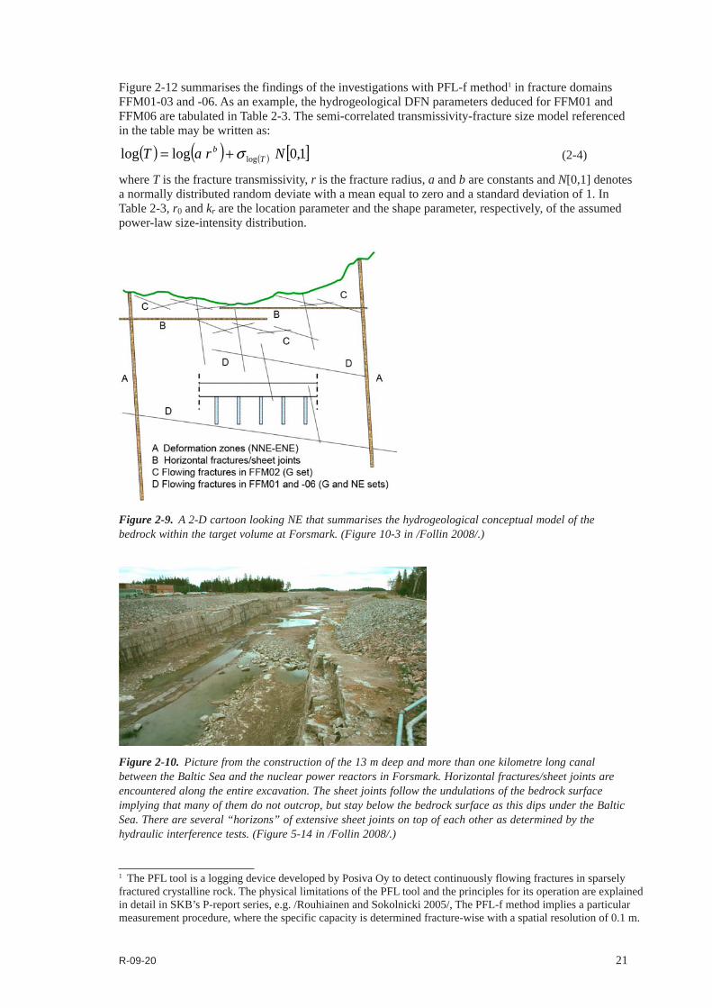
Figure 2-12 summarises the findings of the investigations with PFL-f method1 in fracture domains FFM01-03 and -06. As an example, the hydrogeological DFN parameters deduced for FFM01 and FFM06 are tabulated in Table 2-3. The semi-correlated transmissivity-fracture size model referenced in the table may be written as:

( ) ( ) ( ) [ ]1,0loglog log NraT Tb s+= (2-4)

where T is the fracture transmissivity, r is the fracture radius, a and b are constants and N[0,1] denotes a normally distributed random deviate with a mean equal to zero and a standard deviation of 1. In Table 2-3, r0 and kr are the location parameter and the shape parameter, respectively, of the assumed power-law size-intensity distribution.

1 The PFL tool is a logging device developed by Posiva Oy to detect continuously flowing fractures in sparsely fractured crystalline rock. The physical limitations of the PFL tool and the principles for its operation are explained in detail in SKB’s P-report series, e.g. /Rouhiainen and Sokolnicki 2005/, The PFL-f method implies a particular measurement procedure, where the specific capacity is determined fracture-wise with a spatial resolution of 0.1 m.

Figure 2‑10. Picture from the construction of the 13 m deep and more than one kilometre long canal between the Baltic Sea and the nuclear power reactors in Forsmark. Horizontal fractures/sheet joints are encountered along the entire excavation. The sheet joints follow the undulations of the bedrock surface implying that many of them do not outcrop, but stay below the bedrock surface as this dips under the Baltic Sea. There are several “horizons” of extensive sheet joints on top of each other as determined by the hydraulic interference tests. (Figure 5-14 in /Follin 2008/.)

Figure 2‑9. A 2-D cartoon looking NE that summarises the hydrogeological conceptual model of the bedrock within the target volume at Forsmark. (Figure 10-3 in /Follin 2008/.)

22 R-09-20

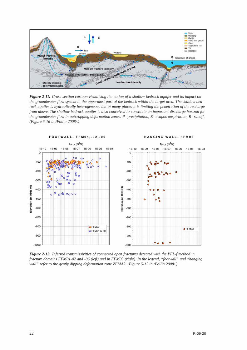
Figure 2‑12. Inferred transmissivities of connected open fractures detected with the PFL-f method in fracture domains FFM01-02 and -06 (left) and in FFM03 (right). In the legend, “footwall” and “hanging wall” refer to the gently dipping deformation zone ZFMA2. (Figure 5-12 in /Follin 2008/.)

Figure 2‑11. Cross-section cartoon visualising the notion of a shallow bedrock aquifer and its impact on the groundwater flow system in the uppermost part of the bedrock within the target area. The shallow bed-rock aquifer is hydraulically heterogeneous but at many places it is limiting the penetration of the recharge from above. The shallow bedrock aquifer is also conceived to constitute an important discharge horizon for the groundwater flow in outcropping deformation zones. P=precipitation, E=evapotranspiration, R=runoff. (Figure 5-16 in /Follin 2008/.)

R-09-20 23

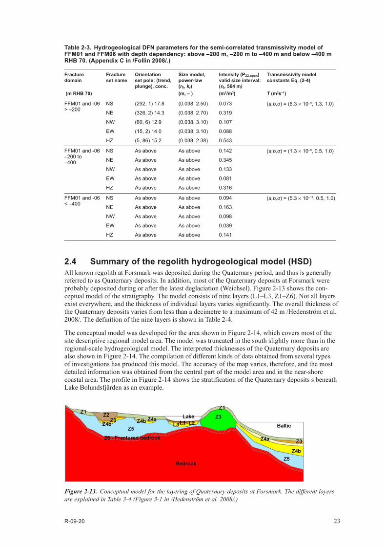
2.4 Summary of the regolith hydrogeological model (HSD)All known regolith at Forsmark was deposited during the Quaternary period, and thus is generally referred to as Quaternary deposits. In addition, most of the Quaternary deposits at Forsmark were probably deposited during or after the latest deglaciation (Weichsel). Figure 2‑13 shows the con‑ceptual model of the stratigraphy. The model consists of nine layers (L1–L3, Z1–Z6). Not all layers exist everywhere, and the thickness of individual layers varies significantly. The overall thickness of the Quaternary deposits varies from less than a decimetre to a maximum of 42 m /Hedenström et al. 2008/. The definition of the nine layers is shown in Table 2‑4.

The conceptual model was developed for the area shown in Figure 2‑14, which covers most of the site descriptive regional model area. The model was truncated in the south slightly more than in the regional‑scale hydrogeological model. The interpreted thicknesses of the Quaternary deposits are also shown in Figure 2‑14. The compilation of different kinds of data obtained from several types of investigations has produced this model. The accuracy of the map varies, therefore, and the most detailed information was obtained from the central part of the model area and in the near‑shore coastal area. The profile in Figure 2‑14 shows the stratification of the Quaternary deposits s beneath Lake Bolundsfjärden as an example.

Table 2‑3. Hydrogeological DFN parameters for the semi‑correlated transmissivity model of FFM01 and FFM06 with depth dependency: above –200 m, –200 m to –400 m and below –400 m RHB 70. (Appendix C in /Follin 2008/.)

Fracture domain

Fracture set name

Orientation set pole: (trend, plunge), conc.

Size model, power‑law (r0, kr)

Intensity (P32,open) valid size interval: (r0, 564 m)

Transmissivity model constants Eq. (2‑4)

(m RHB 70) (m, – ) (m2/m3) T (m2s–1)

FFM01 and -06 > –200

NS (292, 1) 17.8 (0.038, 2.50) 0.073 (a,b,σ) = (6.3 × 10–9, 1.3, 1.0)

NE (326, 2) 14.3 (0.038, 2.70) 0.319

NW (60, 6) 12.9 (0.038, 3.10) 0.107

EW (15, 2) 14.0 (0.038, 3.10) 0.088

HZ (5, 86) 15.2 (0.038, 2.38) 0.543

FFM01 and -06 –200 to –400

NS As above As above 0.142 (a,b,σ) = (1.3 × 10–9, 0.5, 1.0)

NE As above As above 0.345

NW As above As above 0.133

EW As above As above 0.081

HZ As above As above 0.316

FFM01 and -06 < –400

NS As above As above 0.094 (a,b,σ) = (5.3 × 10–11, 0.5, 1.0)

NE As above As above 0.163

NW As above As above 0.098

EW As above As above 0.039

HZ As above As above 0.141

Figure 2‑13. Conceptual model for the layering of Quaternary deposits at Forsmark. The different layers are explained in Table 3-4 (Figure 3-1 in /Hedenström et al. 2008/.)

24 R-09-20

Table 2‑4. Names and definitions of Quaternary deposits (Modified after Table 2‑4 in /Hedenström et al. 2008/.)

Layer Description and comments

L1 Layer consisting of different kinds of gyttja/mud/clay or peat. Interpolated from input data, thickness will therefore vary.L2 Layer consisting of sand and gravel. Interpolated from input data, thickness will therefore vary.L3 Layer consisting of different clays (glacial and postglacial). Interpolated from input data, thickness will therefore vary.Z1 Surface affected layer present all over the model, except where peat is found and under lakes with lenses. Thickness

is 0.10 m on bedrock outcrops, 0.60 m elsewhere. If total regolith thickness is less than 0.60 m, Z1 will have the same thickness as the total, i.e. in those areas only Z1 will exist.

Z2 Surface layer consisting of peat. Zero thickness in the sea. Always overlies by Z3.Z3 Middle layer of sediments. Only found where surface layers are other than till, clay or peat. Z4a Middle layer consisting of postglacial clay. Always overlies by Z4b.Z4b Middle layer of glacial clay. Z5 Corresponds to a layer of till. The bottom of layer Z5 corresponds to the bedrock surface.Z6 Upper part of the bedrock. Fractured rock. Constant thickness of 0.5 m. Calculated as an offset from Z5.

Figure 2‑14. Top left: Extent of the model of the Quaternary deposits in stage 2.2. Top right: Interpreted total thickness of the Quaternary deposits. Bottom: Example cross-section showing the interpreted stratification and thicknesses of the Quaternary deposits beneath Lake Bolundsfjärden. (Based on figures from Appendix 2 of /Hedenström et al. 2008/.)

R-09-20 25

Table 2-5 and Table 2-6 show the parameter values provided for groundwater flow modelling by the surface system group /Bosson et al. 2008/. Most of the values represent so-called ‘best estimates’ based on site-specific data supported by generic data when site-specific data are scarce, cf. /Johansson 2008/.

Table 2‑5. Values of the total porosity and the specific yield of the Quaternary deposits sug‑gested for groundwater flow modelling in SDM stage 2.2. (Modified after Table 2‑4 in /Bosson et al. 2008/.)

Layer Total porosity [–] and specific yield [–] of layers with several types of Quaternary depositsFine till Coarse till Gyttja Clay Sand Peat

L1 – – 0.50 / 0.03 – – 0.60 / 0.20Z1 0.35 / 0.15 0.35 / 0.15 – 0.55 / 0.05 0.35 / 0.20 0.40 / 0.05Z5 0.25 / 0.03 0.25 / 0.05 – – – –

Total porosity [–] and specific yield [–] of layers with one type of Quaternary deposits

L2 0.35 / 0.20L3 0.55 / 0.05Z2 0.40 / 0.05Z3 0.35 / 0.20Z4 0.45 / 0.03

Table 2‑6. Values of the saturated hydraulic conductivity of the Quaternary deposits suggested for groundwater flow modelling in SDM stage 2.2. (Modified after Table 2‑4 in /Bosson et al. 2008/.)

Layer K [m/s] of layers with several types of Quaternary depositsFine till Coarse till Gyttja Clay Sand Peat

L1 – – 3 × 10–7 – – < 0.6 m depth: 1 × 10–6

Z1 3 × 10–5 3 × 10–5 – 1 × 10–6 1.5 × 10–4 > 0.6 m depth: 3 × 10–7

Z5 1 × 10–7 1.5 × 10–6 – – – –

K [m/s] of layers with one type of Quaternary deposits

L2 3 × 10–4

L3 < 0.6 m depth: 1 × 10–6 ; > 0.6 m depth: 1.5 × 10–8

Z2 3 × 10–7

Z3 1.5 × 10–4

Z4 1.5 × 10–8

This complex stratigraphy was handled in different ways in the SDM studies depending on the objectives of the flow modelling and the software used, see /Follin et al. 2007b/ and /Bosson et al. 2008/.In/Follinetal.2007b/,theQuaternarydepositsweresubstitutedbyfourelementlayerseachof constant 1 m thickness. The same equivalent hydraulic conductivity tensor was specified for each vertical stack of four grid elements, but was varied horizontally from element-to-element, and was anisotropic between horizontal and vertical components. The horizontal component of the tensor was based on the arithmetic mean of the hydraulic properties of the original stratigraphy, whereas the vertical component was based on its harmonic mean. The resulting hydraulic conductivity distribu-tion is illustrated in Figure 2-15.

26 R-09-20

2.5 Groundwater flow modelling and confirmatory testingThe main objectives of the groundwater flow modelling carried out for the SDM were to investigate the behaviour of a numerical implementation of the conceptual hydrogeological model and test its performance against three sets of confirmatory data:

• transient, large-scale cross-hole (interference) test responses,

• steady-state, natural (undisturbed) groundwater levels in the uppermost 150 m, and

• hydrochemical observations in deep boreholes.

In general, the behaviour of the numerical flow model was found to be sound and the matching against the confirmatory data sets reasonable. However, it was noted that the performance of the groundwater flow model, which was based on equivalent continuous porous media (ECPM) proper-ties, was slightly improved if the anisotropy of the horizontal to vertical hydraulic conductivity ratios oftheupscaledvaluesforboththeQuaternarydeposits(HSD)andthefracturedomains(HRD)wereincreased compared with the upscaled values derived from the initial structural-hydraulic settings described above. The objective of the multiple simulations carried out in /Follin et al. 2008/ was to address the sensitivity of the resulting calibrated deterministic base model simulation developed in /Follin et al. 2007b/ to parameter uncertainty, e.g. heterogeneity.

Figure 2‑15. Resulting effective hydraulic conductivity for HSD top layer based on Quaternary deposits layer thicknesses and hydraulic properties. Left: E-W horizontal component. Right: vertical component. (Figure 6-10 in /Follin 2008/.)

R-09-20 27

3 Concepts and methodology

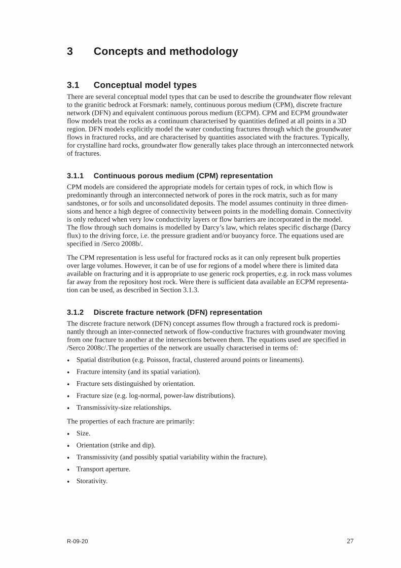
3.1 Conceptual model types There are several conceptual model types that can be used to describe the groundwater flow relevant to the granitic bedrock at Forsmark: namely, continuous porous medium (CPM), discrete fracture network (DFN) and equivalent continuous porous medium (ECPM). CPM and ECPM groundwater flow models treat the rocks as a continuum characterised by quantities defined at all points in a 3D region. DFN models explicitly model the water conducting fractures through which the groundwater flows in fractured rocks, and are characterised by quantities associated with the fractures. Typically, for crystalline hard rocks, groundwater flow generally takes place through an interconnected network of fractures.

3.1.1 Continuous porous medium (CPM) representationCPM models are considered the appropriate models for certain types of rock, in which flow is predominantly through an interconnected network of pores in the rock matrix, such as for many sandstones, or for soils and unconsolidated deposits. The model assumes continuity in three dimen-sions and hence a high degree of connectivity between points in the modelling domain. Connectivity is only reduced when very low conductivity layers or flow barriers are incorporated in the model. The flow through such domains is modelled by Darcy’s law, which relates specific discharge (Darcy flux) to the driving force, i.e. the pressure gradient and/or buoyancy force. The equations used are specified in /Serco 2008b/.

The CPM representation is less useful for fractured rocks as it can only represent bulk properties over large volumes. However, it can be of use for regions of a model where there is limited data available on fracturing and it is appropriate to use generic rock properties, e.g. in rock mass volumes far away from the repository host rock. Were there is sufficient data available an ECPM representa-tion can be used, as described in Section 3.1.3.

3.1.2 Discrete fracture network (DFN) representation The discrete fracture network (DFN) concept assumes flow through a fractured rock is predomi-nantly through an inter-connected network of flow-conductive fractures with groundwater moving from one fracture to another at the intersections between them. The equations used are specified in /Serco 2008c/.The properties of the network are usually characterised in terms of:

• Spatial distribution (e.g. Poisson, fractal, clustered around points or lineaments).

• Fracture intensity (and its spatial variation).

• Fracture sets distinguished by orientation.

• Fracture size (e.g. log-normal, power-law distributions).

• Transmissivity-size relationships.

The properties of each fracture are primarily:

• Size.

• Orientation (strike and dip).

• Transmissivity (and possibly spatial variability within the fracture).

• Transport aperture.

• Storativity.

28 R-09-20

In ConnectFlow, fractures are usually rectangular, but may be right-angled triangles where a complex surface has been triangulated into many pieces. For stochastic fractures, the properties are sampled from probability distribution functions (PDFs) specified for each fracture set. The properties may be sampled independently or correlated with other properties.

The DFN concept is very useful since it naturally reflects the individual flow conduits in fractured rock, and the available field data. However, to model flow and transport on the regional-scale it is often necessary to consider larger-scale bulk properties in the context of an ECPM continuum con-cept. This requires methods (i) to convert the properties of a network of discrete fractures of lengths less than the continuum blocks into equivalent continuous porous medium (ECPM) block properties, known as upscaling, and (ii) to represent larger scale features such as fracture zones by appropriate properties in a series of continuum blocks (the IFZ method). The implementations of the upscaling and IFZ methods in ConnectFlow are described in Sections 3.1.3 and 3.2.2, respectively.

An example of a DFN model generated on the repository-scale for SR-Site is shown in Figure 3-1. It includes both stochastic fractures, each of which is square, combined with deterministic fracture zones that are defined as more complex non-planar surfaces. Horizontal and vertical slices through the fractures are shown in Figure 3-2.

Figure 3‑1. An example of a repository-scale DFN model showing stochastic fractures and higher transmissivity deterministic fracture zones, coloured by log10(transmissivity).

R-09-20 29

Figure 3‑2. Slices through an example of a repository-scale DFN model showing stochastic fractures and higher transmissivity deterministic fracture zones, coloured by log10(transmissivity). Top: horizontal slice at z = –470 m; Bottom: Vertical slice.

30 R-09-20

3.1.3 Equivalent continuous porous medium (ECPM) representationIn order to assess the implications of the DFN model on flow and transport on the regional-scale, it is often necessary for practical reasons to convert the DFN model to an ECPM model with appropri-ate properties. The resulting parameters are a directional hydraulic conductivity tensor, fracture kinematic porosity and other transport properties (such as the fracture surface area per unit volume). In ConnectFlow, a flux-based upscaling method is used that requires several flow calculations through a DFN model in different directions.

Figure 3-3 shows an illustration of how flow is calculated in a DFN model (a 2D network is shown for simplicity). To calculate equivalent hydraulic conductivity for the block shown, the flux through the network is calculated for a linear head gradient in each of the axial directions.

Due to the variety of connections across the network, several flow-paths are possible, and may result in cross-flows non-parallel to the head gradient. Cross-flows are a common characteristic of DFN models and can be approximated in an ECPM by an anisotropic hydraulic conductivity.

In 3D, ConnectFlow uses six directional components to characterise the symmetric hydraulic conductivity tensor. Using the DFN flow simulations, the fluxes through each face of the block are calculated for each head gradient direction. The hydraulic conductivity tensor is then derived by a least-squares fit to these flux responses for the fixed head gradients /Jackson et al. 2000/.

Kinematic porosity, Φ, for each block is calculated as

V

ae ff

t∑=f

(3-1)

where V is the volume of the block, af is the area of each fracture in the block and et is the transport aperture of the fracture, which is related to fracture transmissivity, T, by

Tet 5.0= (3-2)

The coefficient of 0.5 is a rounding of the value of 0.46 used for SDM-Site /Follin 2008/. The sum-mation is over all fractures within the block. As for SDM-Site, the porosity was multiplied by ten to account for the lower limit on the fracture size truncation.

Flow wetted surface per unit volume of rock, ar, is calculated for each block as:

ar = 2P32 (3-3)

where P32 is the fracture area per unit volume within the block, calculated as

P32V

aP f

f∑=32

(3-4)

where V is the volume of the block. The ar value is used in transport calculations to calculate the flow-related transport resistance (F) within the ECPM, as described in Section 3.2.6. The ar values are discussed further in Appendix C.

One refinement of the upscaling methodology is to simulate flow through a slightly larger domain than the block size required for the ECPM properties, but then calculate the flux responses through the correct block size. The reason for this is to avoid over-prediction of hydraulic conductivity from flows through fractures that just cut the corner of the block but that are unrepresentative of flows through the in situ fracture network (Figure 3-4). The area around the block is known as a ‘guard-zone’, and an appropriate choice for its thickness is approximately one fracture radius. The problem is most significant in sparse heterogeneous networks in which the flux through the network of fractures is affected by ‘bottlenecks’ through low transmissivity fractures, and is quite different to the flux through single fractures. A guard zone was not used for the upscaling in SR-Site Forsmark because it hadn’t been implemented in ConnectFlow for unstructured models at the time. However, the use of a guard zone is a refinement of the methodology and its use is unlikely to have significantly affected the upscaling at Forsmark. The effect of a guard zone is discussed in /Rhén et al. 2009/ for Laxemar SDM-Site.

R-09-20 31

Figure 3‑3. 2D illustration of flow through a network of fractures. A random network of fractures with variable length and transmissivity is shown top left (orange fractures are large transmissivity, blue are low). Top right: flow-paths (dotted arrows) for a linear head gradient E-W decreasing along the x-axis. Bottom left: flow-paths through the network for a linear head gradient S-N decreasing along the y-axis.

Figure 3‑4. 2D illustration of how block-scale hydraulic conductivity can be overestimated.

32 R-09-20

3.1.4 Embedded CPM/DFN modelsIn addition to the capability to create distinct models based on the concepts described above, ConnectFlow offers the option to construct embedded models that integrate sub-models of different types. That is, the model can be split into two different domains: one that uses the CPM concept, and one that uses the DFN concept. However, DFN and CPM sub-models have to be exclusive, i.e. the approaches cannot be used simultaneously in any part of the domain. Internal boundary conditions between the domains ensure continuity of pressure and conservation of mass. On the DFN side of the interface, these boundary conditions are defined at nodes that lie along the lines (traces) that make up the intersections between fractures and the interface surface. On the CPM side, the bound-ary conditions are applied to nodes in finite-elements that abut the interface surface. Thus, extra equations are added to the discrete system matrix to link nodes in the DFN model to nodes in the finite-element CPM model, as shown in Figure 3-5. By using equations to ensure both continuity of pressure and continuity of mass, a more rigorous approach to embedding is obtained than by simply interpolating pressures between separate DFN and CPM models. The equations used are specified in /Serco 2008a/.

In order to construct embedded models of the same fractured rock (mixing DFN and CPM sub-models), the data used for the DFN and CPM models should be self-consistent. For example, if a repository-scale DFN model is embedded within an ECPM model, then flow statistics on an appro-priate scale (the size of the elements in the ECPM model) need to be consistent. This is achieved by the fracture upscaling techniques described in Section 3.1.3.

Two quite different examples are included below to illustrate some of the possible models that can be constructed. Figure 3-6 shows an example of a model where a local-scale DFN model is embedded within a larger regional-scale ECPM model. The DFN sub-model is used to provide detailed flow and transport calculations around a repository, while the ECPM sub-model provides a representation of the regional-scale flow patterns that control the boundary conditions on the DFN model. The interface between these two sub-models is on the outer faces of the DFN model.

The converse example is to embed a CPM sub-model within a DFN sub-model as shown in Figure 3-7. In this case, a CPM sub-model is used to represent flow in backfilled main and deposi-tion tunnels, while the surrounding fractured rock is represented by a DFN sub-model. The interface between the two sub-models has a complex geometry corresponding to the outer surface of the tunnel system.

Figure 3‑5. Illustration of embedding between DFN and CPM sub-models. A finite-element CPM mesh is shown on the left. The right hand surface is intersected by a single fracture plane. Extra equations are used to link the DFN to the CPM.

R-09-20 33

Figure 3‑6. An example of an ECPM/DFN ConnectFlow model using a DFN sub-model to represent the detailed fractures around a repository and embedded within a larger regional-scale ECPM sub-model as a slice at z = –470 m.

Figure 3‑7. An example of a DFN/CPM ConnectFlow model using a CPM sub-model of deposition and main tunnels embedded within a DFN sub-model. Some fractures have been removed to reveal the tunnels. Here, the interface between the two sub-models is on the boundary of the CPM model.

34 R-09-20

In summary, embedded models make it possible to represent different regions using different model concepts and then combine the regions into a single model. This is different from the case where discrete fractures co-exist in the same space with a porous medium model of the rock matrix. The interaction between fractures and the rock matrix within the same domain can be represented in ConnectFlow by modelling rock matrix diffusion (RMD) within CPM/ECPM models, but it should be recognised that this is a different situation. It may be noted that RMD of salinity is not represented within the DFN domain, but RMD of radionuclides within the fracture system can be accounted for either in the particle tracking algorithm or later in the far field radionuclide transport calculations.

3.1.5 Particle trackingA particle tracking algorithm is used to represent advective transport of radionuclides. In CPM models, particles are tracked in a deterministic way by moving along a discretised path within the local finite-element velocity-field.

In DFN models, a stochastic ‘pipe’ network type algorithm is used. Particles are moved between pairs of fracture intersections stepping from one intersection to another. At any intersection there may be several possible destinations that the particle may move to, as flow follows different chan-nels through a fracture. A random process weighted by the mass flux between pairs of intersections (connected by a ‘pipe’) is used to select which path is followed for any particular particle. Hence, there is an explicit hydrodynamic dispersion process built into the transport algorithm used in the DFN if more than one particle is released per start point. The time taken to travel between any two intersections, the distance travelled and flow-related transport resistance (described in Section 3.2.6) are calculated for each pipe based on flow rates and geometries.

In an embedded model, particles are traced through both DFN and CPM regions continuously, using the appropriate algorithm for the region currently containing the particle (Figure 3-8). The implica-tion is that particle tracks are deterministic until they enter a DFN sub-model, and are then stochastic afterwards, even if the particle goes back into a CPM sub-model.

Figure 3‑8. Illustration of particle tracking through an embedded DFN/CPM to show the different particle tracking methods in the two regions: deterministic in CPM, stochastic in DFN.

R-09-20 35

3.2 Modelling methodology3.2.1 Model scalesThree different scales of model are used in the SR-Site temperate period modelling. Each scale of model is chosen to focus in on parts of the model of interest, with consideration to what is compu-tationally feasible and which types of calculations are supported by the ConnectFlow software for different model concepts. By considering these three scales of model a comprehensive and robust study can be made of the issues relevant to groundwater flow and transport and some conceptual uncertainties can be quantified. The models are described fully in Chapter 4, but each scale is sum-marised below.

Information on variable values and particle transport is passed between the different model scales. Figure 3-9 shows the relationship between the scales, the embedding of the rock representations that they use and how data is passed between them. Figure 3-10 shows a flowchart that gives the workflow of modelling processes and data transfer. Table 3-1 gives a modelling summary for each scale. Table 3-2 shows how each feature within the models is represented at each scale.

Figure 3-11 shows how the domains of the three different scales of model relate to each other. Figure 3-12 is a close-up view of the local area around the repository, showing the domains of the repository-scale blocks and the site-scale embedded DFN. Note that the site-scale DFN covers the repository structures, but is not required to cover the full domain of the repository-scale blocks. Figure 3-13 shows how the repository structures are represented within the site-scale model. Further details on these models are contained in Chapter 4.

Figure 3‑9. Illustration of the concepts of model scales, embedding, and the transfer of data between scales.

36 R-09-20

Figure 3‑10. Modelling processes. Fracture generation is shown in green, regional-scale processes in pink, site-scale processes in yellow and repository-scale processes in blue. Outputs are shown in peach. Solid arrows indicate the modelling workflow within a scale and dotted arrows indicate a transfer of data between scales.

Table 3‑1. Modelling summary for each scale.

Regional‑scale Site‑scale Repository‑scale

Earliest time simulated 8000 BC 0 AD 2000 ADLatest tme simulated 12,000 AD 12,000 AD 9000 ADFlow model Saturated flow in a porous

medium (ECPM/CPM)Saturated flow at fixed time slices in a porous medium (ECPM/CPM) with an embedded discrete feature network (DFN)

Saturated flow at fixed time slices in a discrete fracture network (DFN) with an embedded CPM representation of the tunnels

Transport model Dual porosity Single porosity Single porosityFluid properties Salinity S(x,y,z,t)

Temperature T(z) Density ρ(S, T) Viscosity μ(T)

Salinity S(x,y,z|t) Temperature T(const.) Density ρ(S) Viscosity μ(const.)

Salinity S(x,y,z|t) Temperature T(const.) Density ρ(S) Viscosity μ(const.)

Modelling procedure 1. Multiple heterogeneous realisations

2. Transient boundary conditions

3. Solve for flow and trans-port of reference waters at each time step

1. Multiple heterogeneous realisations

2. Fixed boundary conditions at different time slices

3. Converging flow at each time slice4. Fixed flow particle tracking at each

time slice

1. Multiple heterogeneous realisa-tions

2. Fixed boundary conditions at different time slices

3. Converging flow at each time slice

4. Fixed flow particle tracking at each time slice

Primary output Fluid pressure and density at different time slices

Flow and particle tracking perfor-mance measures

Flow and particle tracking performance measures

Secondary output Hydrochemistry at different time slices

Particle exit locations at different time slices

Particle exit locations at different time slices

Regional-scale Hydro-DFN Generate HRD fractures

Regional-scale Hydro-DFN Export HRD fractures r > 5.6 m

Regional-scale Hydro-DFN Export all HRD fractures

Regional-scale Upscale DFN Export ECPM properties

Regional-scale Transient solve Hydrochemical evolution

Regional-scale Export pressure, density

Site-scale Steady state flow solve

Site-scale Continuation particle tracking

Repository-scale Steady state flow solve

Repository-scale Particle tracking

Export chemistry

Performance measures

Exit locations

Site-scale Particle tracking

Regional-scale Hydro-DFN Connectivity analysis

Exit locations for biosphere objects

R-09-20 37

Table 3‑2. Representation of model features at each scale.

Feature Regional‑scale Site‑scale Repository‑scale

HCD ECPM Single fracture surfaces Single fracture surfacesHRD ECPM/CPM DFN/ECPM/CPM DFNHSD CPM CPM Not presentMain tunnels Not present Equivalent fractures CPMDeposition tunnels Not present Equivalent fractures CPMDeposition holes Not present Not present CPMOther repository structures Not present Equivalent fractures Equivalent fracturesExcavation damaged zone (EDZ) Not present Equivalent fractures Equivalent fractures

Figure 3‑11. The different scales of model: regional-scale (purple outline); embedded DFN in the site-scale model (black); repository-scale block models (red, green, blue).

38 R-09-20

Figure 3‑13. Representation of tunnels and excavation damaged zone (EDZ) in the site-scale model.

Figure 3‑12. Embedded DFN part of the site-scale model (grey); repository-scale blocks (red, green, blue).

R-09-20 39

The regional-scale model corresponds to the SDM-Site model and covers the same domain. The model uses an ECPM representation where FFMs are defined and a CPM representation elsewhere, including the HSD, as illustrated in Figure 3-14. The deformation zones and sheet joints are represented by IFZ fractures (described in Section 3.2.2). The model is used to calculate the transient evolution of coupled groundwater flow and reference water transport with rock matrix diffusion (RMD) from 8000 BC to 12,000 AD. The calculated pressure and fluid density values are exported from this model for particular times for use by the two other scales.

The site-scale model replaces the part of the regional-scale ECPM model local to the repository area, with an explicit embedded DFN representation of the HRD, as shown in Figure 3-15. The DFN region was chosen to encompass all the repository features and to extend from the bottom of the HSD to a depth of a few hundred metres below the repository. The fractures in this region are identi-cal to the ones used to provide the upscaled properties for the ECPM in the regional-scale model, but with additional smaller-scale fractures added close to the repository structures. These small scale fractures provide more detailed particle tracking for particles released at the repository. Each deformation zone is represented by a single fracture surface with appropriate hydraulic properties, as described in Section 3.2.2. The sheet joints are represented as three fracture surfaces, each at a different depth. Properties were assigned to the sheet joints by interpolation of available site data. Fractures with appropriate hydraulic and transport properties are also used to represent the repository structures. Boundary conditions (pressure) and initial conditions (pressure and density) are imported from the regional-scale model. The density is held fixed and the pressure field consistent with the densities and boundary conditions is calculated to give conservation of mass. The site-scale model is primarily used to continue particles from the repository-scale model, but it is also used track particles from the repository to provide exit locations for biosphere objects.

The repository-scale model uses a CPM representation of the main tunnels, deposition tunnels and deposition holes in the repository. This provides a suitable representation of the tunnel backfill, which is a porous medium, and allows detailed 3D particle tracking within the tunnels. These structures are embedded within a DFN representation of the HRD, including the smaller fractures around the repos-itory structures. These small fractures are on the same scale as the smallest fractures modelled around the boreholes in the calibration to PFL data in SDM-Site. It is not practical to model these fractures everywhere, but they provide transport pathways for particles released from deposition holes.

Figure 3‑14. Schematic illustration of the regional-scale model. An ECPM (upscaled DFN) is contained within a CPM. The HSD in the upper layers of the model is represented as a CPM. The hatched lines represent no flow boundaries. The top surface has flux, q, pressure, p, and concentration, C (reference water mass fractions), boundary conditions that vary with time. The bottom surface has a fixed concentration boundary condition.

40 R-09-20

Figure 3‑16. Schematic illustration of the repository-scale model. A CPM representation of the main tunnels, deposition tunnel and deposition holes is embedded within a DFN representation of the HRD. The external surface boundary conditions use specified pressures, p(x,y,z), imported from the regional-scale model for specified time slices. The top surface elevation corresponds to the bottom of the HSD. The yellow line represents a particle tracked from a single canister location to the boundary of a repository-scale block.

Figure 3‑15. Schematic illustration of the site-scale model. A DFN is embedded within the ECPM of a regional-scale model. The repository location is indicated by the pale green box. The hatched lines rep-resent no flow boundaries. The top surface boundary condition uses specified pressures, p(x,y,z) imported from the regional-scale model for specified time slices. The continuation of a repository-scale particle is shown in yellow. A site-scale only particle tracked from the repository is shown in pale purple.

Other repository structures (transport tunnels, central tunnels, the ramp and shafts) are represented by fractures with appropriate hydraulic and transport properties in the same way as for the site-scale model. The geometries of these structures are more difficult to model as CPM and they are less important for particle tracking due to their distance from the deposition holes and so a fracture representation is more practical. The excavation damaged zone (EDZ), deformation zones and sheet joints are represented as fractures in the same way as in the site-scale model. The repository-scale model is divided into 3 blocks for computational efficiency. Boundary conditions (pressure) and initial conditions (pressure and density) are imported from the regional-scale model. The density is held fixed and the pressure field consistent with the densities and boundary conditions is calculated to give conservation of mass. An illustration of a repository-scale block is shown in Figure 3-16.

R-09-20 41

3.2.2 Representation of deformation zones (DZs)For SR-Site Forsmark, the basic concept is that fractures exist on a continuous range of length scales, which motivates a methodology to generate sub-lineament-scale fractures stochastically on scales between a few metres to about 1 km, and then combine this DFN by superposition with the larger scale deterministic deformation zones (DZs) contained within the HCD. The approach used to represent the DZs was different in DFN and CPM/ECPM models, as described below.

Deformation zones in CPM/ECPM modelsIn CPM and ECPM models the DZs were represented by modifying the hydraulic properties of any finite-elements intersected by one or more zones to incorporate the structural model in terms of the geometry and properties of zones using the Implicit Fracture Zone (IFZ) method in ConnectFlow, as described in /Marsic et al. 2001/. In a CPM model, properties are homogeneous within a set of defined sub-domains prior to superposition of the DZs. Afterwards, the hydraulic properties vary from element to element if intersected by a DZ. In an ECPM model, the methodology is to first create one or more realisations of the stochastic DFN (including the DZs to provide connectivity) on the regional-scale and then, using the upscaling methods described in Section 3.1.3, to convert this to a realisation of the ECPM model, with the DZs removed. The ECPM model properties are then modified to incorporate the effect of the DZs.

The IFZ method identifies which elements are crossed by a fracture zone and combines a hydraulic conductivity tensor associated with the fracture zone with a hydraulic conductivity tensor for the background stochastic network. For each element crossed by the fracture zone the following steps are performed:

1. The volume of intersection between the fracture zone and the element is determined.

2. The hydraulic conductivity tensor of the background rock is calculated in the coordinate system of the fracture zone.

3. The combined conductivity tensor of the background rock and the fracture zone is calculated in the coordinate system of fracture zone.

4. The effective hydraulic conductivity tensor that includes the effect of the fracture zone is determined in the original coordinate system.

The methodology is illustrated in Figure 3-17. In 3D, the resultant hydraulic conductivity is a 6-component symmetric tensor in the Cartesian coordinate system. The tensor can be diagonalised to give the principal components and directions of anisotropy.

Similarly, combined scalar block-scale porosity is calculated for the element, based on combining the deformation zone porosity and the background block-scale porosity using a weighting based either on the relative volume or on relative transmissibility (total channel flow capacity, which is transmissivity times flow length [m3s–1]). The latter weighting was used for the SR-Site modelling and can be suitable for transport since it weights the combined porosity toward the fracture zone porosity if this is of a relatively high hydraulic conductivity.

The result of this process is to produce a spatial distribution of CPM element properties (hydraulic conductivity tensor, porosity and flow wetted surface) that represent the combined influence of both the deterministic fractures zones and background stochastic fractures.

It may be noted the term “background conductivity” here means the equivalent conductivity of the stochastic fracture network. No extra component for matrix conductivity or micro-fracturing is added. However, the stochastic DFN is necessarily truncated in some way, e.g. based on fracture radius which in consequence means that some elements may not include a connected network of fractures or may only be connected in some directions. To avoid this just being a result of the choice of truncation limit and chance, a minimum block conductivity and porosity is set for any elements that have zero properties following the fracture upscaling and IFZ methods. Appropriate minimum properties were derived in the SDM Hydro-DFN studies by calculating the minimum values seen when the DFN is truncated only at very small fractures relative to the block size, and so are essentially free from the truncation effect.

42 R-09-20

Deformation zones in DFN modelsIn DFN models, the deformations zones (DZs) are modelled as surfaces (i.e. no volume) which are composed of many rectangular or triangular planes that discretise the geometry and hydraulic properties. The site descriptive modelling prescribed a depth dependent transmissivity that decreased significantly with depth and also depended on the dip (gently dipping or vertical) of the zone. Therefore, it was necessary to sub-divide the zones into relatively small sub-fractures to represent the property variations (Figure 3-18).

The transport aperture, et, of each fracture that represents a DZ is calculated as

bet f= (3-5)

where Φ is the porosity and b is the thickness of the deformation zone at that point, as specified by the geologists. The transport aperture is then used in transport calculations and used to calculate per-formance measures in the same way as for other fractures in the DFN, as described in Section 3.2.6.

Deformation zones in embedded modelsTo ensure consistency of how larger scale fractures zones are represented when they cross between DFN and CPM models, the fracture zone geometries need to be defined consistently. This is achieved by using the same deformation zone data file for both the DFN and CPM regions of the model. Figure 3-19 illustrates how a large deterministic fracture that crosses between DFN and CPM sub-models can be modelled in such a way as to ensure there is continuity in its representation, and hence in flow between the regions.

A few fractures in the DFN region are shown in red and orange. The red fractures may be stochastic, for example. The orange fracture is a deterministic DZ that crosses the interface. On the DFN side it is shown as a plane, while on the CPM side it is drawn with its actual thickness. The elements crossed by the DZs are coloured yellow. Hydraulic conductivity, porosity and flow wetted surface in these elements will be modified by the IFZ method to represent the effect of the fracture zone on flow and transport.

Figure 3‑17. Schematic illustration of the modification of the hydraulic conductivity tensor by the IFZ method. A finite-element grid crossed obliquely by two fracture zones of different thickness (left).

R-09-20 43

3.2.3 Variable density groundwater flow and salt transportVariations in groundwater composition create variations in groundwater density and hence buoyancy- driven flow that modifies the pattern of groundwater flows. Since gradients in the water table at Forsmark are relatively weak, then buoyancy forces arising from the presence of salt are significant. ConnectFlow has the following capabilities for handling variable-density flow:

1. An option in CPM or ECPM models to simulate flow in a porous medium for groundwater of variable salinity, where the salinity arises from a number of groundwater constituents. This can be modelled either in terms of transport of mass fractions of the basic hydrogeochemical con-stituents (such as chloride, sodium), which are taken to be conservative, or in terms of transport of fractions of selected reference waters. In both cases the transport equations are coupled with the overall mass conservation equation for groundwater flow. In addition, rock matrix diffusion (RMD) is included in the transport of mass fractions of groundwater constituents, or in the transport of fractions of reference waters, respectively.

Figure 3‑18. Deformation zones (DZs) modelled as surfaces in a DFN model with depth dependent transmissivity.

Figure 3‑19. Schematic illustration of continuity of DZs across a CPM/DFN interface in a ConnectFlow model. The DFN region is to the right with a CPM grid to the left.

44 R-09-20

2. An option to calculate groundwater flow for specified spatial variations in groundwater density in DFN models and embedded models. That is, the groundwater density has to be interpolated on to the fracture system from another model, but then the consistent pressure distribution and flow-field is calculated with buoyancy forces included. The groundwater density is typically interpolated from a CPM or ECPM model for a selected time slice. Particle tracking through both DFN and embedded models with the calculated flow field can then be performed.

The RMD capability makes it possible to model diffusion of the reference waters between ground-water flowing in fractures and immobile water in the rock matrix between the fractures. The numeri-cal approach used /Hoch and Jackson 2004/ is based on a method developed by /Carrera et al. 1998/ and enhanced to enable potentially larger time steps to be taken. The approach combines an approxi-mation that is accurate for small times with one that is accurate for long times, to give a representa-tion of the diffusion into the rock matrix that is accurate for all times. At early times, the diffusion is represented in terms of the inverse of the square root of time, and at long times it is represented as a series of decaying exponentials. The main parameter that controls the rate of RMD is the fracture surfaceareaperunitvolume,σ[m2/m3] (see Appendix C).

3.2.4 Transport calculationsA major objective of the SR-Site modelling is to compute groundwater flow-paths from each deposi-tion hole (there are 6,916 in total) to the surface. The approach taken was to track particles moving with the advective flow velocity from release points around the deposition holes until they reach the top surface. In doing this, two key issues that have to be addressed are how to do this when two scales of model are being used, and how to deal with the transient evolution of the flow-field.

The repository-scale models are very detailed around the repository but have limited extent. Vertically,themodelextendsfrom–800melevationtothebottomoftheHSDthatliesontopoftherockhead, but does not extend horizontally far beyond the edge of the repository layout. The vertical path was found to be an important one in the embedded DFN/CPM model, but still some paths exit the vertical sides of the model. The solution is to track particles from the release points to the outer boundary of the repository-scale model, and then restart the particle tracking in the corresponding site-scale model from the points where the particles leave the repository-scale model. Performance measures such as travel-time are calculated as the cumulative travel-time along both legs of the path.

It is possible in ConnectFlow to track particles as they move through a flow-field that evolves with time in a CPM model. However, for a DFN model or an embedded CPM/DFN model, fixed instantaneous flow-fields from selected times must be used to obtain a qualitative assessment of the potential impact of releases at different times. The objective is to establish whether flow-paths are sensitive to the retreat of the shoreline, and if so, whether flow-paths stabilise once the shoreline becomes remote from the site. The release times are chosen carefully to represent different phases when the flow-field appears to be either changing significantly, or when there are periods of relative stability. Hence, for the transport calculations reported here, performance measures are calculated based on fixed flow-fields at several selected times.

For the case where the shoreline is retreating away from the site, such that a major discharge area is getting further away in time, then it is expected that flow-paths and travel-times are getting longer, and hence using the instantaneous flow-field at the release time is considered a conservative approximation for the subsequent evolution. When travel-times become longer than the temperate climate period due to retention (e.g. due to sorption), then one needs to consider transport in the wider context of the climate evolution, which is outside the remit of the study reported here.

3.2.5 Flow and transport in the repository and EDZThe repository is a large hydraulic feature with a potentially significant impact on the local ground-water flow given the low hydraulic conductivity of the bedrock. In order to account for these effects it is necessary to represent the repository appropriately in the model. The potential conduits for flow within the repository are the deposition tunnels, main tunnels, transport tunnels, ramp and shafts, together with the excavation damaged zone (EDZ) around the tunnels created during construction of the repository. The operational and re-saturation phases are not considered here, so it is assumed that

R-09-20 45

we only need consider saturated flow and that all tunnels have been backfilled to give homogeneous properties. For the EDZ, the design premise is that the transmissivity will be 1.0∙10-8 m2/s over a thickness of 0.3 m /SKB 2010a/. Although this is the scenario adopted by the hydrogeological base case as a conservative approach, data suggests that a continuous EDZ would not form at all /SKB 2010a/. Models with different EDZ properties and no EDZ are treated as variants (see Section 5.5).

In terms of safety assessment calculations, three potential paths for radionuclides to leave the canister are considered:

1. Q1, diffusion into the mobile water in fractures surrounding the deposition hole.

2. Q2, diffusion into mobile water in the EDZ.

3. Q3, diffusion into a fracture intersecting the tunnel.

In order to study each of these paths, the detailed repository-scale models have to represent the deposition holes, tunnels and EDZ explicitly, and flow-paths have to be computed for a release at three appropriate positions around each canister. Hence, the performance measures (PMs) defined in Section 3.2.6 are calculated for three paths for each canister. It is possible that the three particles may follow very similar trajectories, such that tr, Lr and Fr are similar, but Ur, UEDZ or Ut will vary, where the subscript r denotes rock and the subscript t denotes the repository structures, primarily tunnels. Further, for each path, the PMs are calculated for portions of the path spent in the rock, tunnels, and EDZ separately. In the work reported here, no retention of radionuclides is assumed within the tunnels and EDZ and so the flow wetted surface (ar) is assigned a zero value in the tunnels and EDZ, and hence FEDZ and Ft are zero, and therefore only tEDZ, LEDZ, tt and Lt are calculated. Figure 3-20 shows the three pathways considered.

3.2.6 Calculation of performance measuresTo provide input to performance assessment (PA) calculations, tables of performance measures are produced for each case using five performance measures (PMs). In a CPM representation these are defined as:

1. Travel-time, ∑=l

r qlt φδ

, where dl is a step length, for example through one finite-element,

along a path of l steps, f is the kinematic porosity, and q is the Darcy flux.

2. Equivalent flux at the release point, Ur, described in more detail below.

3. Equivalentflowrateatthereleasepoint,Qeq, described in more detail below.

Figure 3‑20. Schematic view of the repository design, showing the small hole in the canister and the location of the various possible transport paths into near-field rock.

46 R-09-20

4. Pathlength, ∑=l

r lL d .

5. Flow-related transport resistance, ∑=l

rr q

laF d, where ar is the flow wetted surface per unit

volume. This is a measure of the potential for retention and retardation of radionuclides within the rock.

The subscript “r” indicates that the PM is calculated in the rock. That is, they only represent cumula-tive PMs for those parts of paths within the rock and exclude parts of flow-paths that pass through the EDZ or tunnel backfill. PMs are calculated for legs of paths within the EDZ and tunnels, but are computed as separate PMs for each path and distinguish by an “EDZ” or “t” subscript, respectively.

In a DFN representation the PMs are defined as:

1. Travel-time, ∑=f f

ftfr Q

lwet

δ, where dl is a step length along a path of f steps, each

between a pair of fracture intersections, etf is the fracture transport aperture, wf is the flow width between the pair of intersections, and Qf is the flow rate between the pair of intersections in the fracture.

2. Equivalent flux at the release point, Ur, described in more detail below.

3. Equivalentflowrateatthereleasepoint,Qeq, described in more detail below.

4. Pathlength, ∑=f

r lL d .

5. Flow-related transport resistance, ∑∑ ==f tf

rf

f f

fr e

tQ

lwF

22 δ, where trf is the travel time in a

fracture along the path.

The results from the particle tracking are then used to produce ensemble statistics for the perfor-mance measures, as well as locating the discharge areas. The ensemble is over the set of 6,916 par-ticle start locations, one for each deposition hole and is in total divided over three blocks; block 1 with 1,994 start locations, block 2 with 2,769 start locations and block 3 with the remaining 2,153 start locations (Figure 3-13). Apart from the work done on the repository layout, no further attempt is made to avoid starting particles in either deterministic fracture zones or high transmissivity sto-chastic fractures. In reality, such features are likely to be avoided during repository construction, and hence the model may tend to see particles start in a wider range of possible fracture transmissivities than might be encountered in reality.

To avoid particles becoming stuck in regions of stagnant flow, they are not started if the initial Darcy flux is less than 1∙10–6 m2/yforQ1andQ2and1·10–6m/yforQ3.ThisappliestoQ1,Q2andQ3releases.ForQ1andQ2,initialDarcyflux,qf, in a fracture is defined as

f

ftff a

Qveq == (3-6)

where:

• etf is the transport aperture of the fracture [m],

• v is the initial transport velocity [m/y],

• Qf is the volumetric flow rate in the fracture [m3/y],

• af is the area of the fracture plane [m2].

ForQ3,theinitialDarcyflux,q, is defined as the volumetric flux per unit area at the particle starting location within the CPM.

Equivalent flow rate (Qeq) for input to near‑field modelsThe near-field code COMP23 calculates the non-stationary nuclide transport in the near-field of a repository. The system is divided in to compartments, where the only restriction is that a compart-

R-09-20 47

ment is formed of the same material. The model, which is a very coarsely discretised Integrated Finite Difference Model, embeds analytical solutions at locations where other models require a very fine discretisation, such as entrances and exits from small holes and fractures. In the repository, radionuclides leaking out through a small hole in the canister wall diffuse into the bentonite buffer and may then migrate through various pathways into the flowing water in rock fractures.

For compartments in contact with water flowing in fractures in the rock, the diffusive transport is determined by an equivalent flow-rate, Qeq [m3/y]. This parameter is a fictitious flow-rate of water that carries a concentration equal to that at the compartment interface. It has been derived by solving the equations for diffusive transport to the passing water by using boundary layer theory /Neretnieks 1979/. The value of Qeq is dependent on the geometry of the contact area, the water flux, the flow porosity or fracture aperture and the diffusivity. As part of the SR-97 assessment formulae were derived for a CPM model /Moreno and Gylling 1998/. The formulae are different for a DFN model as detailed below for the three pathways. The derivation of the equations is given in Appendix D.

Q‑equivalent release into the fractured rock (Q1) for a repository‑scale modelPathQ1considersreleaseofradionuclidesintothefracturedrocksurroundingthedepositionhole,and hence the particle starts within a fracture that intersects the wall of the deposition hole. Several fractures may intersect the deposition hole. For reasons of making a conservative assumption, the flux into all fractures that intersect the deposition hole and contribute to advective flow away from the deposition hole are included in the calculation of Qeq. That is, an effective flow-rate is calculated for all fractures that cut the deposition hole and are connected to at least one other fracture. These equivalent flow-rates are summed for the deposition hole to give the total Qeq. The equivalent groundwater flow rate for Qeq1 can be written as:

∑

=

f

wfw

f

feq

tD

a

QQ

π4

1 (3-7)

where ff

tffwf aQ

eLt

⋅=

If there are several fractures intersecting a single deposition hole, then a conservative approach to calculate the equivalent groundwater flow rate requires the flow to be summed across all the fractures, with twf calculated separately for each fracture. Hence, the average equivalent flux, Ur1, for all fractures intersecting the deposition hole is:

∑=f f

f

cr

aQ

wU 1

1 (3-8)

where:

• Dw is the diffusivity in water [m2/y],

• twf is the time the water is in contact with the deposition hole within each fracture [y],

• Lf is the length of the fracture intersection with the wall of the deposition hole [m],

• Ur1 is the equivalent initial flux in the fracture system averaged over the rock volume adjacent to the deposition hole [m/y],

• Qf is the volumetric flow rate in the fracture intersecting the deposition hole [m3/y],

• etf is the transport aperture of the fracture intersecting the deposition hole [m],

• af is the area of the fracture plane intersecting the deposition hole [m2],

• wc is the deposition hole height [m].

Here, Dw was set to 0.0316 m2/y and wc was set to 5 m, although this is strictly the canister height. All other values were determined in the flow simulations.

48 R-09-20

Q‑equivalent release into the EDZ (Q2) for a repository‑scale modelPathQ2considersthereleaseofradionuclidesintotheEDZ.Heretheparticlesarereleasedwithina fracture used to represent the EDZ that surrounds the top of the deposition hole. The equivalent groundwater flow-rate, Qeq2, is calculated from the flow in the EDZ fractures that cut the deposition hole.Theseeffectiveflow-ratesaresummedforthedepositionholetogivethetotalQeq, with twE calculated separately for each fracture. The equivalent groundwater flow-rate, Qeq2, can be written as:

∑

=

E

wEw

E

Eeq

tDa

QQπ

42 (3-9)

where EE

tEEwE aQ

eLt =

The equivalent initial flux, Ur2, for flow in the EDZ is:

∑=E E

E

Er a

Qw

U 12 (3-10)

where:

• Dw is the diffusivity in water [m2/y],

• twE is the time the water is in contact with the deposition hole within each EDZ fracture [y],

• LE is the length of the EDZ fracture intersection with the wall of the deposition hole [m],

• Ur2 is the equivalent initial flux in the EDZ fracture system averaged over the EDZ fracture cross-sectional area [m/y],

• QE is the volumetric flow rate in the EDZ fracture intersecting the deposition hole [m3/y],

• etE is the transport aperture of the EDZ fracture intersecting the deposition hole [m],

• aE is the area of the EDZ fracture plane intersecting the deposition hole [m2],

• wE is the EDZ thickness [m].

Here, Dw was set to 0.0316 m2/y and wE was set to 0.3 m. All other values were determined in the flow simulations.

Q‑equivalent release into the tunnel (Q3) for a repository‑scale modelPathQ3considersthereleaseofradionuclidesintoatunnelandthenintoafracturethatintersectsthetunnel. It is assumed that diffusive equilibrium of radionuclides is achieved in the tunnel backfill and diffusion takes place into the water flowing in fractures surrounding the tunnel. Hence, an equivalent flow-rate, Qeq3, is required for advective flow in the first fracture encountered along the path after a particle is released in the tunnel backfill above the deposition hole. The equivalent groundwater flow-rate, Qeq3 is calculated from the flow-rate in the first fracture the particle enters after leaving the tunnel.

The equivalent groundwater flow-rate, Qeq3, in the first fracture intersecting the tunnel can be written as:

( )π

fftfweq

aQLeDQ

/423 = (3-11)

The initial flux, Ur3, for flow in the first fracture intersecting the tunnel is:

fT

fr aw

QU =3 ( 3-12)

R-09-20 49

where:

• Dw is the diffusivity in water [m2/y],

• Listhehalfcircumferenceofthetunnel[m],

• Qf is the volumetric flow rate in the fracture intersecting the tunnel [m3/y],

• wT is the fracture width intersecting the tunnel [m],

• af is the area of the fracture plane intersecting the tunnel [m2],

• etf is the transport aperture of the fracture intersecting the tunnel [m].

Here, Dw was set to 0.0316 m2/y , L was set to 7 m and wT was set to 2.5 m. All other values were determined in the flow simulations.

Q‑equivalent release into the tunnels (Q1, Q2, Q3) for a site‑scale modelFor the site-scale model, the repository structures are represented by equivalent fractures rather thanasCPM.Therefore,particlesarereleaseddirectlyintofracturesforQ1,Q2andQ3.Sincethetunnels and deposition holes are not represented with a 3D volume, it is not appropriate to sum over all fractures intersecting the deposition hole or tunnel. Therefore, the Qeq and Ur values are only calculated for the single fracture that the particle enters when it leaves the deposition hole or tunnel. The equivalent groundwater flow-rate, Qeq123, is calculated from the flow in the starting fracture for each released particle. The equivalent groundwater flow rate, Qeq123, can be written as:

π0

123

42 Ttfw

eq

ULeDQ = (3-13)

This is equivalent to equations (3-7) and (3-9) for a single fracture, with the factor 2 indicating that flow can be around either side of the deposition hole or tunnel. The equivalent flux, Ur123, for flow in the fracture is:

wUU T 0

123 = (3-14)

where:

• Dw is the diffusivity in water [m2/y],

• Listhehalfcircumferenceofthedepositionhole(Q1andQ2)ortunnel(Q3)[m],

• UT0 is the flow rate in the fracture per unit fracture width [m2/y],

• etf is the transport aperture of the fracture [m],

• w is the deposition hole height or fracture width [m].

Here, Dw was set to 0.0316 m2/y , Lwassetto2.8mforQ1,to2.8mforQ2andto7.0mforQ3,w wassetto5.0mforQ1(althoughthisisstrictlythecanisterheight),to0.3mforQ2andto2.5mforQ3.AllothervaluesweredeterminedintheDFNflowsimulations.Thisisequivalenttoequations(3-8) and (3-10) for a single fracture.

3.2.7 Deposition hole rejection criteria (FPC/EFPC)During construction of the repository some deposition holes may be excluded due to the presence of transmissive fractures. If such fractures are detected then the deposition hole may not be constructed. There are two criteria for deciding whether or not a hole should be excluded:

1. Fullperimetercriteria(FPC)–adepositionholeisexcludedifitisintersectedbythehypotheticalextension of a fracture that intersects the full perimeter of the corresponding deposition tunnel.

2. Extendedfullperimetercriteria(EFPC)–adepositionholeisexcludedifitsfullperimeterisintersected by a fracture that also intersects the full perimeter of four or more neighbouring deposition holes in the same deposition tunnel.

50 R-09-20

An algorithm for analysing the deposition holes according to the FPC and EFPC was implemented in ConnectFlow. This was used to flag deposition holes that may be excluded due to these criteria, but they were not actually excluded in the flow or particle tracking calculations. For the purposes of the algorithms, full-perimeter indicated an intersection between a fracture and all four side edges of a deposition tunnel or a deposition hole. Also, in the implementation of the FPC, the fracture was not hypothetically extended when considering intersections with deposition holes, i.e. the fracture needed to actually intersect the deposition hole as well as the full perimeter of the deposition tunnel. This approximation is unlikely to significantly affect the number of deposition holes fulfilling the FPC.

EDZ fractures were not considered for the FPC or the EFPC. Deformation zone fractures were flagged differently for the FPC. Also recorded was the longest length and highest transmissivity of fractures intersecting each deposition hole. This information, along with the FPC and EFPC results, was made available for safety assessment analyses.

R-09-20 51

4 Hydrogeological base case model specification

The hydrogeological base case was derived from the base case model from SDM-Site, but with the changes given in Appendix C. Note that the base case model simulation in SDM-Site used a homogeneous HCD and a single realisation of the HRD. In SR-Site, the hydrogeological base case has the base model plus 10 realisations:

• HomogeneousHCD+r1ofHRD,• r1ofHCD+r1ofHRD,• r2ofHCD+r2ofHRD,• …• r10ofHCD+r10ofHRD.where rn denotes realisation n.

The hydrogeological base case was implemented as a set of models at three different scales to focus on the quantities of interest at each scale. However, each model scale is a representation of the same hydrogeological base case and each is derived from the same set of properties and fractures. The regional-scale model was concerned with the large scale evolution of pressure and reference water distribution over time from 8000 BC to 12,000 AD. The site-scale model used a DFN to provide a more detailed representation of the site for carrying out particle transport calculations. The repository-scale model used a CPM representation of the main tunnels, deposition tunnels and deposition holes within the site-scale DFN to provide detailed performance measures for the initial portions of the particle transport pathways. Each model scale is described in more detail in the following sections.

Since the HRD and, in some cases, the HCD are based on stochastic properties, the hydrogeological base case was represented as a number of realisations. Each realisation forms part of the hydrogeo-logical base case.

A summary of the hydrogeological base case and the variant cases covered in Chapter 5 is given in Table 4-1.

Table 4‑1. Summary of modelling cases.

Case Description Report section

Scales Times Number of realisations

Hydrogeological base

The hydrogeological base case with a semi-correlated transmissivity-size relationship

4 Regional 8000 BC to 12,000 AD 10Site 0 AD to 12,000 AD 10Repository 2000 AD, 3000 AD,

5000 AD, 9000 AD10

Correlated Uses a fully correlated transmissivity-size relationship

5.1 Regional 8000 BC to 2000 AD 5Site 2000 AD 5Repository 2000 AD 5

Uncorrelated Uses an uncorrelated transmissivity-size relationship

5.1 Regional 8000 BC to 2000 AD 5Site 2000 AD 5Repository 2000 AD 5

Possible deformation zones

Includes possible deformation zones 5.2 Regional 8000 BC to 2000 AD 3Site 2000 AD 3Repository 2000 AD 3

Unmodified vertical hydraulic conductivity

Removes the modification of vertical hydraulic conductivity used in SDM-Site

5.3 Regional 8000 BC to 2000 AD 1Site 2000 AD 1

Extended spatial variability

Extends the ECPM to the whole of the regional-scale model

5.4 Regional 8000 BC to 12,000 AD 1Site 2000 AD, 3000 AD,

5000 AD, 9000 AD 1

Tunnel Modifies tunnel properties due to changes in EDZ transmissivity, removes the EDZ or includes a crown space

5.5 Site 2000 AD 1Repository 2000 AD 1

Boreholes Introduces boreholes 5.6 Site 2000 AD 1Repository 2000 AD 1

Glacial Applies pressures and densities arising from the presence of an ice sheet and also considers the effect on the tunnel variants

5.7 Site Glacial 1Repository Glacial 1

52 R-09-20

4.1 Regional‑scale modelThe regional-scale model used the same representation as the SDM-Site Forsmark model, but with the changes given in Appendix C. Its purpose was to model the evolution of hydrogeology and hydrochemistry from 8000 BC to 2000 AD, and then into the future temperate period up to 12,000 AD. Periglacial climate conditions are expected at Forsmark before the retreating shoreline reaches the boundary of the model domain at around 12,000 AD.

4.1.1 Model descriptionThe regional-scale model was constructed from the following domains:

• Hydraulicconductordomain(HCD):deformationzonesandsheetjointsofgenerallyrelativelyhigh conductivity.

• Hydraulicrockmassdomain(HRD):thebedrockbetweenthedeformationzones.

• Hydraulicsoildomain(HSD):thesurfacehydrologicalunits.

Each domain is described in the following sections.

As in SDM-Site, the model used 20 m horizontal refinement for the elements in the area local to the repository (a 3 km × 2.76 km block). Elsewhere, 100 m horizontal refinement was used. The model extendedfromthegroundsurfacetoanelevationof–1,200m.Theupperlayersofthemodelweremapped to be parallel to the surface topography.

Hydraulic Conductor Domain (HCD)The HCD consists of the deformation zones and sheet joints within the model region. Each deforma-tion zone represents a region of increased fracturing and increased hydraulic conductivity, kinematic porosity and flow-wetted surface area per unit volume of rock. Each deformation zone was included in the regional-scale model as an implicit fracture zone (IFZ), as described in Section 3.2.2. Figure 4-1 shows the IFZs representing the HCD in the hydrogeological base case model. Each IFZ was given depth dependent deterministic properties and conditioned on borehole measurements in the regions around the intersections between boreholes and deformation zones.

Figure 4‑1. The implicit fracture zones used in the regional-scale hydrogeological base case model. The IFZs are coloured by hydraulic conductivity, showing the depth dependency of properties.

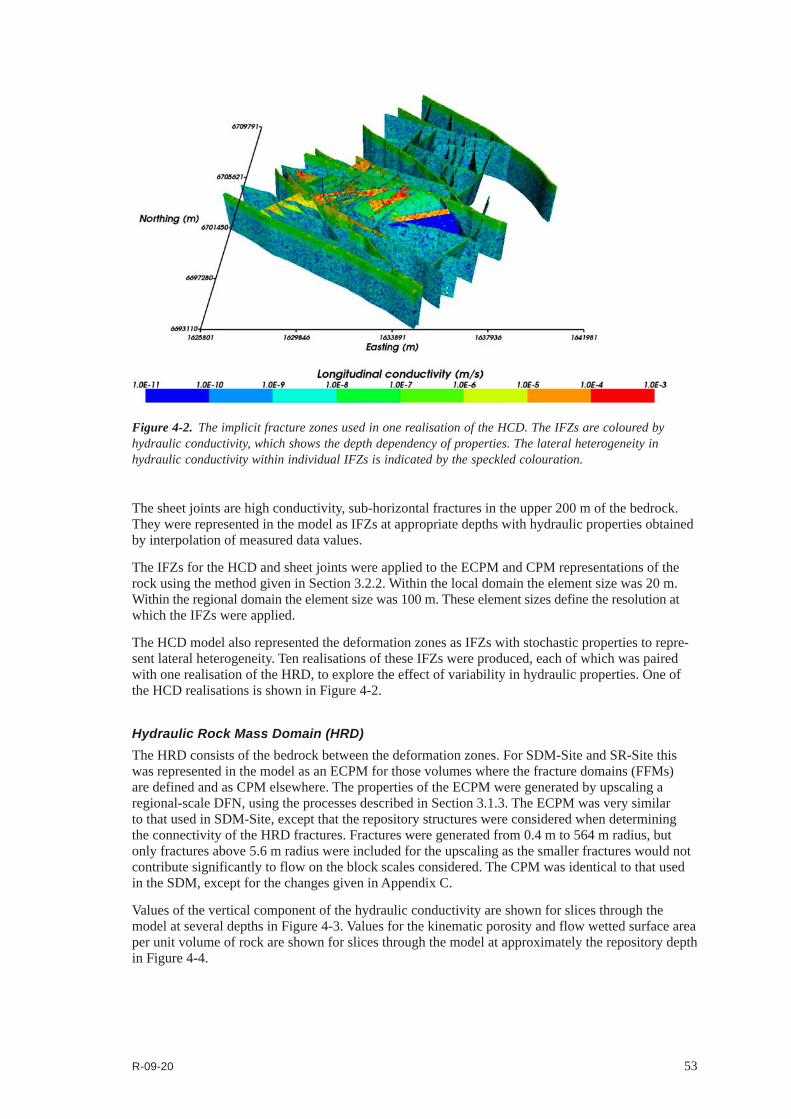
R-09-20 53

The sheet joints are high conductivity, sub-horizontal fractures in the upper 200 m of the bedrock. They were represented in the model as IFZs at appropriate depths with hydraulic properties obtained by interpolation of measured data values.

The IFZs for the HCD and sheet joints were applied to the ECPM and CPM representations of the rock using the method given in Section 3.2.2. Within the local domain the element size was 20 m. Within the regional domain the element size was 100 m. These element sizes define the resolution at which the IFZs were applied.

The HCD model also represented the deformation zones as IFZs with stochastic properties to repre-sent lateral heterogeneity. Ten realisations of these IFZs were produced, each of which was paired with one realisation of the HRD, to explore the effect of variability in hydraulic properties. One of the HCD realisations is shown in Figure 4-2.

Hydraulic Rock Mass Domain (HRD)The HRD consists of the bedrock between the deformation zones. For SDM-Site and SR-Site this was represented in the model as an ECPM for those volumes where the fracture domains (FFMs) are defined and as CPM elsewhere. The properties of the ECPM were generated by upscaling a regional-scale DFN, using the processes described in Section 3.1.3. The ECPM was very similar to that used in SDM-Site, except that the repository structures were considered when determining the connectivity of the HRD fractures. Fractures were generated from 0.4 m to 564 m radius, but only fractures above 5.6 m radius were included for the upscaling as the smaller fractures would not contribute significantly to flow on the block scales considered. The CPM was identical to that used in the SDM, except for the changes given in Appendix C.

Values of the vertical component of the hydraulic conductivity are shown for slices through the model at several depths in Figure 4-3. Values for the kinematic porosity and flow wetted surface area per unit volume of rock are shown for slices through the model at approximately the repository depth in Figure 4-4.

Figure 4‑2. The implicit fracture zones used in one realisation of the HCD. The IFZs are coloured by hydraulic conductivity, which shows the depth dependency of properties. The lateral heterogeneity in hydraulic conductivity within individual IFZs is indicated by the speckled colouration.

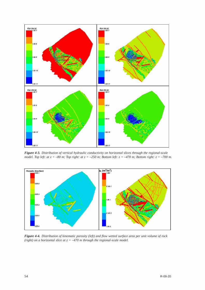
54 R-09-20

Figure 4‑3. Distribution of vertical hydraulic conductivity on horizontal slices through the regional-scale model. Top left: at z = –80 m; Top right: at z = –250 m; Bottom left: z = –470 m; Bottom right: z = –700 m.

Figure 4‑4. Distribution of kinematic porosity (left) and flow wetted surface area per unit volume of rock (right) on a horizontal slice at z = –470 m through the regional-scale model.

R-09-20 55

Hydraulic Soil Domain (HSD)The HSD consists of the surface layers of soil in the top few metres of the regional-scale model. It was identical to the HSD used in SDM-Site.

Multiple realisationsTo explore the effect of variability in the rock properties, 10 realisations of the regional DFN were generated. Each of these realisations was coupled with the corresponding HCD realisation to con-struct a model and carry out calculations. The hydrogeological base case model, with a deterministic HCD, used realisation 1 of the HRD. This means that two of the models used realisation 1 of the HRD, giving 11 models in total.

4.1.2 Boundary conditions and initial conditionsThe boundary conditions used for SR-Site were the same as those used for SDM-Site. They con-sisted of a recharge-discharge boundary condition on the top surface and no flow through the sides and bottom of the model. The bottom of the model also had a hydrochemical boundary condition set to the initial values of the reference water mass fractions. The reference water mass fractions on the top boundary varied with time according to the elevation of shoreline with regard to the topography of the ground surface.

The initial conditions were also the same as those used in SDM-Site, except as noted in Appendix C.

4.1.3 Calculation of past and future evolutionThe past evolution of the regional-scale model was calculated in the same way as for SDM-Site, i.e. the calculation of pressures and reference water mass fractions for a transient evolution in 20 year time steps from 8000 BC to 2000 AD. The future evolution continued these calculations to 12,000 AD. The change in the shoreline due to post-glacial land rise was obtained from the curve shown in Figure 4-5. The salinity of the Baltic Sea was obtained from the blue curve shown in

Figure 4‑5. Evolution of the shoreline /SKB 2010b/.

56 R-09-20

Figure 4-6. Both of these curves match those used for SDM-Site up to 2000 AD. The salinity curve used is not consistent with the final SR-Site curve (red dashed line in Figure 4-6). This is due to the fact that later information has changed the view on salinity development /Lindborg 2010/. The curves match until 500 BC and then are very similar until about 6000 AD. After this, the final SR-Site curve predicts a higher salinity. However, given the uncertainty in future salinity predictions and the distance of the shore from the Forsmark site at later times, these differences are unlikely to have a significant effect on the results.

The location of the shoreline at different times is shown in Figure 4-7. It can be seen that the repository area is under the sea at 0 AD until about 1000 AD and by 12,000 AD the shoreline has reached the edge of the model domain.

For the 10 realisations of the HCD and HRD, the calculations were carried out from 8000 BC to 2000 AD only.

Figure 4‑7. Shoreline location at different times (dark blue=0 AD, light blue=2000 AD, green=3000 AD, orange=5000 AD, red=9000 AD, purple=12,000 AD) presented against the regional-scale domain. The repository structures are shown in black.

Figure 4‑6. Evolution of the salinity of the Baltic Sea. The curve used in this report is shown as a solid blue line /SKB 2010c/ and the final SR-Site curve is shown as a dashed red line /Lindborg 2010/.

R-09-20 57

4.1.4 OutputsThe principal outputs of the regional-scale model were the fluid density distribution and pressure boundary conditions at chosen times for use in the site-scale and repository-scale models.

Also exported were hydraulic conductivity values, salinity values and reference water mass fractions for use in other studies.

4.2 Site‑scale modelThe bedrock at Forsmark is of low hydraulic conductivity and it is thought that the primary hydraulic flow pathways are through a network of connected fractures. In order to better represent this system, a discrete fracture network (DFN) model was used in the local domain around the repository location, embedded within the regional-scale ECPM/CPM model. Thus the extent of the site-scale model is the same as the regional-scale model, but part of the local region has been replaced by an explicit DFN. The local region is the rock volume around the repository where FFMs are defined and extra refinement is used in the regional-scale model. The DFN sub-model is defined within a part of the local region that can be described with a polygon that is fully within the refined region and fully covers the repository structures, as shown by the grey area in Figure 4-8. The use of a DFN has implications for particle transport as it constrains the flow pathways available and hence the discharge locations reached. This effect cannot readily be observed using an ECPM model at the grid resolutions available computationally.

Figure 4‑8. Site-scale model. The DFN domain is the cut-out section in the centre, but only the repository structures are shown. The ECPM is coloured by vertical hydraulic conductivity and the repository structures are coloured black.

58 R-09-20

4.2.1 Model descriptionThe site-scale model was constructed from the following domains:

• Hydraulicconductordomain(HCD):deformationzonesandsheetjointsofgenerallyrelativelyhigh conductivity.

• Hydraulicrockmassdomain(HRD):thebedrockbetweenthedeformationzones.

• Hydraulicsoildomain(HSD):thesurfacehydrologicalunits.

• Repositorystructures.

Each domain is described in the following sections.

Hydraulic Rock Mass Domain (HRD)The site-scale model had the same domain as the regional-scale model, but part of the local model was replaced with an embedded DFN, as shown by the grey area in Figure 4-8. The ECPM/CPM part of the model was the same as the equivalent parts of the regional-scale model, but the grid resolution had been increased from 100 m to 60 m in the regional domain. The purpose of increasing the regional grid resolution was to improve the resolution of particle discharge locations. The DFN was the same as that used to provide the upscaled properties for the regional-scale model, thus ensuring consistency between the two scales. All fractures were included from 0.4 m to 564 m radius. The fractures below 5.6 m in radius were only generated close the repository structures, as shown in Figure 4-9. These additional small fractures may be important in creating local connectivity between the repository structures and the fracture network. Fractures were tessellated to 10 m in length to give a reasonable resolution, i.e. any fracture with a side length larger than 10 m (equivalent to a radius of 5.6m–seeEquation(5-2))wasdividedintosquaresub-fractureswithasidelengthof10m.

Hydraulic Conductor Domain (HCD)The same HCD was used as in the site-scale model, including the sheet joints, as shown in Figure 4-10. In the ECPM/CPM model they were represented implicitly, but in the DFN they were represented as explicit fracture surfaces with appropriate hydraulic properties. The HCD fractures were tessellated to 20 m in length.

Figure 4‑9. Small fractures (0.4 m to 5.64 m radius) around the repository structures in the site-scale model.

R-09-20 59

Hydraulic Soil Domain (HSD)The HSD was identical to that used in the regional-scale model.

Repository StructuresThe repository was represented by fractures with appropriate hydraulic and transport properties. The modelled repository structures were based on a layout that differed in minor details from the final one produced in /SKB 2010d/, specifically the location of some of the halls in the Central Area have been adjusted (maximum 1.3 m in the horizontal direction and maximum 2.2 m in the vertical direc-tion). These discrepancies are unlikely to have a significant impact on results. All tunnels, ramps and shafts were included and were tessellated to 10 m in length. Deposition holes were not represented. Table 4-2 shows the properties of the repository features used in the site-scale and repository-scale models. The hydraulic conductivity and porosity values correspond to the backfill properties that will be used in each structure. The top sealing hydraulic conductivity was applied to those parts of therepositoryfeaturesthatareaboveanelevationof–200m,i.e.theupperpartsoftherampandshafts, which correspond to areas of backfill that could be degraded by permafrost.

Figure 4‑10. Site-scale model. Only the fractures representing the sheet joints and deformation zones are shown. Fractures are coloured by transmissivity and the ECPM is coloured by vertical hydraulic conductivity.

Table 4‑2. Properties of the repository structures used in the site‑scale and repository‑scale models.

Structure Height (m) Width (m) Hydraulic conductivity (m/s)

Porosity

Main tunnel 6.0 10.0 1.0∙10–10 0.45Transport tunnel 6.0 7.0 1.0∙10–10 0.45Deposition tunnel 6.0 4.0 1.0∙10–10 0.45Deposition hole 8.0 1.5 1.0∙10–12 0.41Central area tunnel 6.0 7.0 1.0∙10–5 0.27Ramp 6.0 5.2 1.0∙10–10 0.45Elevator shaft 4.34 4.34 1.0∙10–10 0.45Skip shaft 3.96 3.96 1.0∙10–10 0.45Air intake shaft 3.32 3.32 1.0∙10–10 0.45Air exhaust shaft 2.81 2.81 1.0∙10–10 0.45Deposition area air exhaust shaft 3.07 3.07 1.0∙10–10 0.45Top sealing N/A N/A 1.0∙10–1 N/AEDZ 0.3 N/A 3.333∙10–8 1.0∙10–4

60 R-09-20

An excavation damaged zone (EDZ) was also represented in the site-scale model as a set of fractures orthogonal to the repository structure fractures. In the case of the tunnels and ramp, the EDZ fractures were horizontal and intersected the bottom of the tunnel fractures. In the case of the ramp, the EDZ matched the slope of the ramp. For the shafts, the EDZ fractures intersected the centre of the shaft fractures. There was no EDZ included for the central area tunnels as it would have little effect given the high conductivity of the backfill in those tunnels. The EDZ fractures were tessellated to 6 m in length.

Figure 4-11 shows the representation of the repository structures and EDZ.

Figure 4‑11. Site-scale model. Top: representation of main and deposition tunnels as vertical fractures and the EDZ as horizontal fractures. Bottom: fracture representation of central area tunnels, ramps and shafts. Fractures are coloured by transmissivity.

R-09-20 61

Multiple realisationsTo explore the effect of variability in the rock properties, 10 realisations of the HRD were used. Each of these realisations was coupled with the corresponding HCD realisation to construct a model and carry out calculations. The hydrogeological base case model, with a deterministic HCD, used realisa-tion 1 of the HRD. This means that two of the models used realisation 1 of the HRD.

4.2.2 Boundary conditions and initial conditionsThe pressure boundary condition values on the top surface were imported from the regional-scale model for specified times. No-flow boundary conditions were present on the sides and bottom of the model.

The initial conditions for pressure and fluid density were imported from the regional-scale model for specified times. For the DFN, the pressure and fluid density values were interpolated on to the fracture network. The fluid density values were fixed during the calculations.

4.2.3 CalculationsThe steady state groundwater pressures were calculated consistent with the applied boundary condi-tions and the specified fluid densities. The calculations where carried out for every 1,000 years from 0 AD to 12,000 AD for a single realisation of the HRD and the deterministic HCD (the hydrogeo-logical base case).

The calculations were also carried out for 10 realisations of the HRD and HCD at 2000 AD.

Particle tracking calculations were carried out for the hydrogeological base case using the calculated groundwater flow fields for each of the specified times. Since there were no deposition holes present in the model, particles were started from the closest fracture intersection (weighted by flux) to each of theQ1,Q2andQ3releasepoints.Particlesweretrackeduntiltheyexitedthemodel.Thesecalcula-tions are primarily to provide exit locations for surface modelling. Here the details of the repository representation are less important and the reduced computational cost means that more release times can be considered.

The site-scale model was also used to continue particles from the repository-scale model. Each particle was started from the closest fracture intersection (weighted by flux) to the point it exited the repository-scale model and tracked until it exited the site-scale model. These particle tracking calculations were carried out for each of the times used for the repository-scale model and for each of the 10 realisations of the HRD and HCD at 2000 AD.

4.2.4 OutputsPerformance measures and exit locations were produced from the particle tracking calculations for each of the specified times, both for the site-scale only model and for continuation from the repository-scale model.

For continuation from the repository-scale model, the performance measures and exit locations were also produced for each of the 10 realisations of the HRD and HCD at 2000 AD.

4.3 Repository‑scale modelThe repository-scale model focussed directly on the region around the Forsmark repository tunnels. The main tunnels, deposition tunnels and deposition holes were represented as a continuous porous medium (CPM) in order to better represent the backfill and to model the detailed flow within these features. The other repository features (transport tunnels, central area, ramps and shafts) were represented as deterministic fractures with appropriate hydraulic and transport properties.

In order to be computationally feasible, the repository-scale model was divided into 3 blocks as shown in Figure 4-12. Blocks 2 and 3 contained one main tunnel each. Block 1 contained two main tunnels and included the central area, ramps and shafts. Each block extended from an elevation of –800matthebottomtoatopsurfacemappedtothetopographybelowtheHSDlayers.Therewerewas no HSD present in the repository-scale models.

62 R-09-20

4.3.1 Model descriptionThe repository-scale model was constructed from the following domains:

• Hydraulicconductordomain(HCD):deformationzonesandsheetjointsofgenerallyrelativelyhigh conductivity.

• Hydraulicrockmassdomain(HRD):thebedrockbetweenthedeformationzones.

• Repositorystructures.

Each domain is described in the following sections.

Hydraulic Rock Mass Domain (HRD)The same HRD was used as for the site-scale model. For each block, the parts of the fractures outside the boundaries of that block were removed. As with the site-scale model, fractures were tessellated to 10 m in length.

Hydraulic Conductor Domain (HCD)The same HCD was used as for the site-scale model. For each block, the parts of the HCD fractures outside the boundaries of that block were removed. As with the site-scale model, HCD fractures were tessellated to 20 m in length.

Figure 4‑12. Repository-scale blocks. Block 1 is coloured blue, block 2 is green and block 3 is red.

R-09-20 63

Hydraulic Soil Domain (HSD)There was no HSD included in the repository-scale model. However, the effect of the HSD on particles was considered during their continuation in the site-scale model.

Repository StructuresThe main tunnels, deposition tunnels and deposition holes were represented as a continuous porous medium (CPM) in order to better represent the backfill and to model the detailed flow within these features. The other repository structures (transport tunnels, central area, ramps and shafts) were represented as deterministic fractures with appropriate hydraulic and transport properties. The repository structure fractures were tessellated to 10 m in length. The properties of the repository structures used in the site-scale and repository-scale models are given in Table 4-2 in Section 4.2.

The modelled repository structures were based on a layout that differed in minor details from the final one produced in /SKB 2010d/, specifically the location of some of the halls in the Central Area have been adjusted (maximum 1.3 m in the horizontal direction and maximum 2.2 m in the vertical direction). These discrepancies are unlikely to have a significant impact on results

Figure 4-13 shows the repository structures in each block. The CPM structures are coloured green and the fracture structures are coloured blue. If parts of main tunnels or deposition tunnels from a neighbouring block are included within the domain of a block, then they are represented as fractures with appropriate properties. This ensures the connectivity of repository structures with the bounda-ries of the block where appropriate.

An excavation damaged zone (EDZ) was also represented in the repository-scale model as a set of fractures with appropriate hydraulic and transport properties. In the case of the main and deposition tunnels, the EDZ was represented as a set of horizontal fractures below each tunnel, with a vertical cross fracture present to provide an intersection with the tunnel. For the transport tunnels and ramp, the EDZ fractures were horizontal relative to the structure and intersected the bottom of the tunnel fractures. In the case of the ramp, the EDZ matched the slope of the ramp. For the shafts, the EDZ fractures intersected the centre of the shaft fractures. There was no EDZ included for the central area tunnels as it would have little effect given the high conductivity of the backfill in those tunnels. The EDZ fractures were tessellated to 6 m in length. Figure 4-14 shows the EDZ, coloured red, below a main tunnel and some deposition tunnels.

Multiple realisationsTo explore the effect of variability in the rock properties, 10 realisations of the regional DFN were used. Each of these realisations was coupled with the corresponding HCD realisation to construct a model and carry out calculations. The hydrogeological base case model, with a deterministic HCD, used realisation 1 of the HRD. This means that two of the models used realisation 1 of the HRD.

Multiple particles per start pointMostoftheparticletrackingsimulationsreleasedoneparticleperstartpointforeachoftheQ1,Q2andQ3locations.However,withintheDFNparticlescanfollowdifferentpathwaysaccordingto a flux weighted random selection at each intersection. Therefore if multiple particles per start point are released then they could potentially follow different pathways and thus generate different performance measures. It is assumed that due to the large number of canister locations, sufficient particles are released across the repository to sample the different pathways available to particles in a statistical sense. To test this, a version of the hydrogeological base case was created that released ten particles per start point from the 25% of locations with the highest UrvaluesforQ1,Q2andQ3.The performance measures were then compared with the corresponding starting locations for the standard one particle per start point hydrogeological base case. Note that the 25% of locations with the highest UrvaluesmayrefertodifferentcanisterpositionsforQ1,Q2andQ3.

64 R-09-20

Figure 4‑13. Repository-scale structures. The CPM structures are coloured green and the fracture structures are coloured blue. Top: Block 1. Middle: Block 2: Bottom: Block 3.

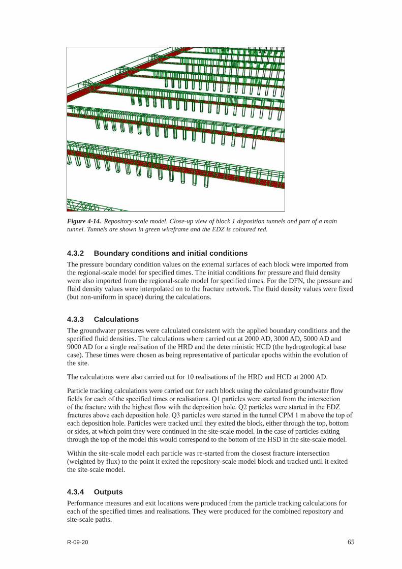
R-09-20 65

4.3.2 Boundary conditions and initial conditionsThe pressure boundary condition values on the external surfaces of each block were imported from the regional-scale model for specified times. The initial conditions for pressure and fluid density were also imported from the regional-scale model for specified times. For the DFN, the pressure and fluid density values were interpolated on to the fracture network. The fluid density values were fixed (but non-uniform in space) during the calculations.

4.3.3 CalculationsThe groundwater pressures were calculated consistent with the applied boundary conditions and the specified fluid densities. The calculations where carried out at 2000 AD, 3000 AD, 5000 AD and 9000 AD for a single realisation of the HRD and the deterministic HCD (the hydrogeological base case). These times were chosen as being representative of particular epochs within the evolution of the site.

The calculations were also carried out for 10 realisations of the HRD and HCD at 2000 AD.

Particle tracking calculations were carried out for each block using the calculated groundwater flow fieldsforeachofthespecifiedtimesorrealisations.Q1particleswerestartedfromtheintersectionofthefracturewiththehighestflowwiththedepositionhole.Q2particleswerestartedintheEDZfracturesaboveeachdepositionhole.Q3particleswerestartedinthetunnelCPM1mabovethetopofeach deposition hole. Particles were tracked until they exited the block, either through the top, bottom or sides, at which point they were continued in the site-scale model. In the case of particles exiting through the top of the model this would correspond to the bottom of the HSD in the site-scale model.

Within the site-scale model each particle was re-started from the closest fracture intersection (weighted by flux) to the point it exited the repository-scale model block and tracked until it exited the site-scale model.

4.3.4 OutputsPerformance measures and exit locations were produced from the particle tracking calculations for each of the specified times and realisations. They were produced for the combined repository and site-scale paths.

Figure 4‑14. Repository-scale model. Close-up view of block 1 deposition tunnels and part of a main tunnel. Tunnels are shown in green wireframe and the EDZ is coloured red.

R-09-20 67

5 Model variants

5.1 Alternative DFN transmissivity‑size relationships5.1.1 Specification It is assumed that there is some correlation between the sizes of fractures and their transmissivity (/Follin 2008/, Appendix C). The hydrogeological base case defines a semi-correlated relationship between fracture size and transmissivity. The variants in this section examine two alternative relationships, fully correlated and uncorrelated.

5.1.2 Representation The hydrogeological base case relates fracture radius, r, to transmissivity, T, according to the relationship in equation (2-4) and repeated in a slightly different form in equation (5-1)

)1,0()log(10 Nar b

T σ+= (5-1)

where a and b are the factor and exponent respectively of the power-law relationship between r and the mean of log10(T), σ is the standard deviation of log10(T), and N(0,1) denotes a normally distrib-uted random deviate with a mean equal to zero and a standard deviation of 1. Since ConnectFlow uses rectangular fractures defined by length rather than circular fractures defined by radius, it is necessary to convert between the two by producing square fractures with side length, L, and equivalent area using equation (5-2).

2rL π= (5-2)

The transmissivity is limited to two standard deviations either side of the mean by resampling values outside of this range. However, this resampling leads to a different random number sequence than that used in the correlated and uncorrelated variants and hence leads to a different realisation of the DFN.

For the uncorrelated variant, there is no relationship between fracture radius and transmissivity. Instead, the transmissivity is based on the log-normal relationship given in equation (5-3).

)1,0(10 NT σµ += (5-3)

where μ is the mean of log10(T), σ is the standard deviation of log10(T), and N(0,1) denotes a nor-mally distributed random deviate with a mean equal to zero and a standard deviation of 1. However, to maintain a realistic range of transmissivities, the maximum values for each fracture set were limited to the maximum deformation zone transmissivities with corresponding inclinations, fracture domains and depth zones, as shown in Table 5-1. Transmissivities greater than the maximum value were resampled from the same distribution until an acceptable value was obtained. Again, this would lead to a different DFN realisation from the semi-correlated or correlated cases.

For the fully correlated variant, the fracture transmissivity is completely determined by its radius according to equation (5-4).

T = ar b (5-4)

where a and b are the factor and exponent, respectively, describing the power-law relationship.

Other than the different relationships between transmissivity and size, the fractures for the two vari-ants are generated in the same way as for the hydrogeological base case and used in the three scales of model in the same way.

The parameters used are the same as in SDM-Site and are given in /Follin 2008/, Appendix C, along with a description of the methodology.

68 R-09-20

5.2 Inclusion of possible deformation zones5.2.1 SpecificationForty-three possible deformation zones (PDZ) were identified in the single-hole geological inter-pretations. /Follin et al. 2007b/ established that only ten of these corresponded with a hydraulic test above the detection limit. Of these, six were found to be gently dipping zones in the top 150 m of bedrock and considered to be near-surface sheet joints, leaving four PDZs above the hydraulic detec-tion limit at or close to repository depth. The deformation zones are one of the main groundwater flow conduits and therefore it is important to investigate the influence of these additional possible deformations zones.

5.2.2 RepresentationThe four possible deformation zones were added to the three scales of model in the same way as the deterministically modelled deformation zones. Three realisations of stochastic properties were gener-ated for the possible deformation zones to represent lateral heterogeneity. These were combined with the corresponding realisations of the HCD and HRD fractures. Figure 5-1 shows the possible deformation zones relative to the repository structures. Some of them intersect the repository structures and may provide potential flow pathways.

Table 5‑1. Maximum transmissivity values for an uncorrelated transmissivity size relationship according to depth zone, inclination and FFM. An inclination of V indicates sub‑vertical deforma‑tion zones and fracture sets, whilst H indicates sub‑horizontal or gently dipping deformation zones and fracture sets.

Depth zone Inclination FFM ln(T) [m2/s]

Above –200 m V 01 or 06 –8.002 to 05 –8.0

H 01 or 06 –7.402 to 05 –6.7

–200 m to –400 m V 01 or 06 –13.502 to 05 –13.5

H 01 or 06 –12.102 to 05 –10.4

Below –400 m V 01 or 06 –14.902 to 05 –14.9

H 01 or 06 –15.402 to 05 –11.9

Figure 5‑1. Realisation 1 of the possible deformation zones in relation to the repository structures.

R-09-20 69

5.3 Unmodified vertical hydraulic conductivity5.3.1 SpecificationDuring the calibration and confirmatory testing of the SDM base model simulation, the vertical conductivityoftheHRDaboveanelevationof–400mwasreducedbyafactorofteninordertoprovide a better fit to chemistry and interference test data. This was also used for the ECPM in the hydrogeological base case for SR-Site. However, no corresponding change was made to the proper-ties of the fractures in the DFN representation of the HRD, leading to a possible inconsistency in flows between the DFN and CPM in the site-scale model.

This variant removes the modification of the vertical conductivity of the ECPM used in the regional and site-scale models.

5.3.2 RepresentationThis variant generated and used the ECPM in exactly the same way as the hydrogeological base case,butwithoutreducingtheverticalconductivityoftheHRDaboveanelevationof–400m.

5.4 Extended spatial variability5.4.1 SpecificationThe hydrogeological base case uses an HRD model from SDM-Site that covers the repository site area, based on the data available. Outside this area, the rock is modelled as a CPM with homogene-ous and isotropic properties for each depth zone. However, this greatly reduces the effect of outcrop-ping sub-vertical deformation zones on particle exit points.

Limited additional data from the ongoing investigations at SFR /Öhman and Follin 2010/ allowed for a tentative parameterisation of a DFN in the area currently modelled as a CPM, as shown in Table 5-2.

Table 5‑2. Hydrogeological DFN parameters for a correlated transmissivity model of the fractures within the former CPM area, based on data from SFR investigations /Öhman and Follin 2010/ with depth dependency.

Fracture domain Fracture set name

Orientation set pole: (trend, plunge), conc.

Size model, power‑law (r0, kr)

Intensity, (P32), valid size interval: (r0, 564 m)

Parameter values for the transmissivity model shown in Eq. (5‑4) (a, b)

(m RHB 70) (m, – ) (m2/m3)

Shallow > –60

EW (2.7, 7.4) 12.6 (0.038, 3.45) 2.598 (6.00×10–9, 1.29)

NW (232.7, 11.9) 13.2 (0.038, 3.10) 1.154 (8.00×10–9, 1.13)

NE (128.3, 8.2) 11.7 (0.038, 3.45) 1.339 (1.00×10–8, 1.25)

Hz (115.9, 84.5) 27.6 (0.038, 2.60) 1.062 (1.41×10–7, 1.43)

Gd (232.2, 85.1) 6.5 (0.038, 2.79) 1.871 (2.11×10–8, 1.09)

Repository –60 to –245

EW (5.0, 12.7) 8.5 (0.038, 3.45) 1.407 (6.00×10–9, 1.29)

NW (234.0, 6.0) 12.3 (0.038, 2.95) 0.856 (8.00×10–9, 1.13)

NE (128.2, 5.5) 11.5 (0.038, 3.45) 1.033 (1.00×10–8, 1.25)

Hz (137.0, 84.3) 42.9 (0.038, 2.55) 0.850 (2.06×10–9, 1.85)

Gd (354.2, 85.4) 7.1 (0.038, 2.72) 1.208 (4.00×10–9, 1.05)

Below ZFM871 < –245

EW (2.5, 19.6) 9.7 (0.038, 3.45) 0.918 (6.00×10–9, 1.29)

NW (233.3, 7.0) 14.9 (0.038, 3.10) 0.867 (8.00×10–9, 1.13)

NE (304.7, 0.1) 11.2 (0.038, 3.45) 1.023 (1.00×10–8, 1.25)

Hz (127.7, 80.9) 27.9 (0.038, 2.75) 0.596 (1.34×10–9, 1.32)

Gd (269.8, 84.5) 6.6 (0.038, 2.70) 1.287 (9.80×10–10, 0.93)

70 R-09-20

5.4.2 RepresentationThis variant keeps the hydrogeological base case DFN but adds fractures, based on the additional data, to cover the area to the boundaries of the regional model. This is used to provide a full ECPM for the regional-scale and site-scale models. In addition, the area of the DFN in the site-scale model was extended northwards beyond the Singö deformation zone, which may provide an important discharge location. Both models retain the existing HSD. The repository-scale model was not used for this variant. Figure 5-2 shows that the spatial variability has been extended into the former CPM part of the regional-scale model. Figure 5-3 shows both the extended spatial variability in the CPM and the extended DFN in the site-scale model. The fractures were generated with a fully correlated transmissivity-size relationship (Equation (5-4)) using the parameters specified in Table 5-2.

For this variant the performance measures both with and without the contribution from the ECPM were produced.

Figure 5‑2. Regional-scale extended spatial variability model, with the ECPM coloured by vertical hydraulic conductivity. The HSD has been removed from the image.

Figure 5‑3. Site-scale extended spatial variability model, with the ECPM coloured by vertical hydraulic conductivity and the DFN coloured by transmissivity. The black line indicates the boundary of the DFN model. The HSD has been removed from the image.

R-09-20 71

5.5 Tunnel variants 5.5.1 SpecificationOnce the repository has been closed, the deposition tunnels will be backfilled with low permeability material, typically bentonite, which may consolidate over a period of time. This settlement of the backfill may leave a crown space between the top of the backfill and the top of the tunnel. The crown space may lead to extra flow in the repository and provide additional transport pathways for particles. A variant considers a case with a crown space included, but it is expected that there will always be a swelling pressure of the backfill such that a crown space will not develop in reality /Åkesson et al. 2010/.

Repository construction can cause local damage in the surrounding rock, known as an excavation damaged zone (EDZ). The hydrogeological base case represented the EDZ as a continuous layer below the tunnels with a thickness of 0.3 m and a transmissivity of 1.0∙10–8 m2/s, consistent with the design premise /SKB 2010a/. However, it was considered justified to consider how transmissive an EDZ would need to be in order to significantly affect performance measures, hence two variants are considered with higher transmissivity values of 1.0∙10–7 m2/s and 1.0∙10–6 m2/s respectively. Evidence actually suggests that repository construction would lead to no continuous EDZ developing at all /SKB 2010a/, and so a third variant is considered with no EDZ present.

The tunnel variant properties are summarised in Table 5-3.

Table 5‑3. Properties of the tunnel variant cases.

Case EDZ transmissivity (m2/s)

Crown space or EDZ thickness (m)

Crown space hydraulic conductivity (m/s)

Crown space or EDZ porosity

Crown 1.0∙10–8 0.1 1.0∙10–3 1.0EDZ T = 1.0∙10–7 1.0∙10–7 0.3 N/A 1.0∙10–4

EDZ T = 1.0∙10–6 1.0∙10–6 0.3 N/A 1.0∙10–4

No EDZ N/A N/A N/A N/A

5.5.2 RepresentationThe crown space variant adds a layer of very high hydraulic conductivity (1.0∙10–3 m/s) and high porosity (1.0) elements to the top of the CPM representation of the main and deposition tunnels in the repository-scale model (Figure 5-4). A crown space is added to the remaining repository structures in the repository-scale model and all the repository structures in the site-scale model by means of a set of connected fractures with equivalent hydraulic properties.

Figure 5‑4. The crown space (red) for the main (green) and deposition (yellow) tunnels in block 1 of the repository-scale model.

72 R-09-20

The hydrogeological base case represented the EDZ as a set of connected fractures below the tunnels and ramp. The two EDZ variants used the same representation, but with higher transmissivity values applied. The case without an EDZ simply removed the EDZ fractures.

Particle tracking was carried out in these variant cases in the same way as for the hydrogeological base case, i.e. with particles starting in the repository-scale model and continuing in the site-scale model, with performance measures calculated as before. However, in the crown space case, particles were released in the crown space above each deposition hole rather than 1 m above the tunnel floor.

5.6 Effect of boreholes5.6.1 SpecificationFuture human intrusion may lead to the creation of abandoned boreholes that could intersect the repository volume. Also boreholes drilled during characterization and construction of the repository could be forogotten or the sealing fail. These boreholes could provide additional flow pathways for particles. The purpose of this variant is to assess the affect on groundwater flow and performance measures of the presence of one or more hypothetical boreholes.

5.6.2 RepresentationThe boreholes were added to the repository-scale model as narrow fractures with a width and thickness of 0.08 m (equivalent to the diameter of a standard Forsmark borehole). Each borehole extendedfromanelevationof–10mtodownto–600m(about130mbelowrepositorydepth)and were tessellated to 6.0 m in length. The hydraulic conductivity was set to 1.0∙10–1 m/s and the porosity was 1.0.

Five types of borehole models were considered, each in one or more separate cases, as shown in Table 5-4. The table shows that there are three cases where the borehole may cause an undesirable effect and two cases where it should have little effect.

The groundwater flow and transport was calculated using steady-state conditions based on a snap-shot of boundary conditions and density at 2000 AD, as for the hydrogeological base case model. A freshwater density was assigned to the entire borehole, which is be a conservative assumption in terms of hydraulic driving forces.

Table 5‑4. Description of modelled borehole cases.

Case type

Description

1 The borehole intersects a deposition tunnel and creates a new flowing pathway to the surface. This is likely to be downstream of where a deformation zone intersects a deposition tunnel, but where the tunnel currently has no significant outflow.

2 The borehole intersects near a deposition tunnel and creates a new flowing path-way to the surface. This could be an intersection with a transmissive fracture that intersects a deposition tunnel, but does not intersect with anything else carrying a significant flow.

3 The borehole intersects a deposition tunnel but does not cause a significant effect on the flow. Perhaps there is no supply of flow in this tunnel or all the flow is already going into a transmissive feature.

4 The borehole intersects near a deposition tunnel but does not cause a significant effect on the flow. Perhaps it does not intersect anything very transmissive or it intersects something that is transmissive but is already carrying a significant flow so that the borehole doesn’t make much difference.

5 The borehole intersects a canister position directly and creates a new flowing pathway to the surface.

R-09-20 73

For each case, particle tracking was carried out and performance measures were calculated in the usual way, i.e. for all canister locations within the modelled repository block. The performance measures were also calculated for just the canister locations where the particles enter the boreholes. The results were then compared to the hydrogeological base case. Particle tracking was only carried out within the repository scale model, i.e. particles were only tracked to the bottom of the HSD or to the block sides. There was no continuation of particles within the site-scale model. The effect of boreholes is likely to be local and so the effects should be most significant at the repository-scale and so particle continuation is not necessary.

Due to the difficulty in identifying borehole locations that match each of the required cases, many candidate boreholes were considered simultaneously in each of the three repository blocks, four in block 1 (ABH1b1 to ABH4b1), nine in block 2 (ABH1b2 to ABH9b2) and six in block 3 (ABH1b3 to ABH6b3), as shown in Figure 5-5. Once boreholes were identified for each case they were subsequently modelled individually to obtain performance measure and flow results. This avoids the potential for coupled effects between multiple boreholes.

Additional boreholes were considered to investigate the effect of having a borehole directly above a canister location (ABH10b2 to ABH13b2 and ABH7b3 to ABH10b3) and also to study the effect of placing a borehole in the area of discharge flow present in the south-west portion of the repository (ABH14b2 to ABH16b2 and ABH11b3 to ABH13b3).

Figure 5‑5. Plan view of the repository with block 1 (red), block 2 (green) and block 3 (blue). The posi-tions of the modelled boreholes are indicated using yellow markers. A horizontal slice through the HCD at elevation –455 m is shown in purple.

74 R-09-20

5.7 Glacial conditions5.7.1 Specification

Although this study focuses on the temperate period between glacial periods, a set of variants are required to consider scenarios in which glacial conditions are introduced to the models. The glacial conditions are represented by a series of ice front locations, as shown in Figure 5-6. Each ice front location corresponds to a set of pressures and densities within the modelled domain.

The data was obtained from the SR-Site groundwater flow modelling of the glacial period described in /Vidstrand et al. 2010/ and corresponds to case (c) in that report. That case considers a NW-SE ice sheet advance, ice profile A (the theoretical reference evolution profile) and a complete ice sheet cycle without permafrost. Figure 5-7 shows the surface elevation and ice sheet thickness for ice front location II (IFL II). Figure 5-8 shows the ice sheet elevation profile. A hydraulic head at the base of the ice sheet equal to 92% of the ice sheet thickness was assumed. Figure 5-9 shows the pressure field at ice front location II. The interface between freshwater and saltwater is pushed downward and forward and some saltwater is flushed out in the periglacial region in front of the ice sheet margin along with the up-coning that occurs. That is, the salinity beneath an advancing, or retreating, ice sheet is altered by the recharge of fresh melt water. Figure 5-10 shows the salinity field at ice front location II.

Figure 5‑6. Map showing the present-day topography at Forsmark and the positions of the studied ice front locations (I-IV). The large polygon in the centre is the regional flow domain used in the groundwater flow modelling for SDM-Site Forsmark /Follin 2008/. The location of the investigated candidate area (small polygon) and the simulated final repository for spent nuclear fuel inside the candidate area are also shown. The y-axis points towards north. (Figure 1-7 in /Vidstrand et al. 2010/.)

R-09-20 75

Figure 5‑7. Visualisation of the ice thickness for case (c) at ice front location II. The present-day elevation of the shoreline was used for all glacial simulations without permafrost although the predicted elevation of the shoreline during a glaciation period is envisaged to be at approximately –28 m RHB 70. In this image, all elevations higher than –28 m are indicated by a turquoise colour, whereas all elevations lower than –28 metres are shown with a blue colour. The y-axis points towards north. (Figure F-1 in /Vidstrand et al. 2010/.)

Figure 5‑8. Theoretical ice sheet elevation profile used in case (c). (From Figure F-2 in /Vidstrand et al. 2010/.)

76 R-09-20

Figure 5‑9. Visualisation of the pressure field for the ice sheet profile addressed in case (c) when the front of the ice sheet is at IFL II. The topography and the ice sheet thickness are displayed as transparent maps. (Figure F-3 in /Vidstrand et al. 2010/).

Figure 5‑10. Visualisation of the salinity when the front of the ice sheet is at IFL II. The ice sheet eleva-tions are shown in terms of light gray lines. The maximum ice sheet thickness in this image is c. 900 m. The topography is displayed as a transparent map. (Figure F-19 in /Vidstrand et al. 2010/).

R-09-20 77

5.7.2 RepresentationThe effect of glacial conditions was represented by a pressure and salinity field imported from /Vidstrand et al. 2010/ for ice front location II. This ice front is located roughly at the centre of the repository location. The salinity field was used to provide a non-uniform density distribution across the site-scale and repository-scale models. The pressure field was applied as a boundary condition to the top surface of the site-scale model and to all boundary surfaces of the repository-scale model. The site-scale model had no flow boundary conditions on the side and bottom surfaces, as in the hydrogeological base case model. Steady state groundwater flow solves for pressure were carried out to produce a consistent set of pressures across the models. Transport calculations were then carried out in the same way as for the hydrogeological base case, i.e. particles were started in the repository-scale model and continued in the site-scale model.

Tunnel variants of this model were also produced, as described in Section 5.5.

A further variant considered a case based on ice front location I. This ice front is located to the northwest of the repository location and considers an alternative pressure profile in the repository location. This variant only used the site-scale model, as a means of assessing the larger scale effects of the ice front location.

A final variant applied glacial ice front location II and ice front location III conditions to the extended spatial heterogeneity case to examine recharge pathways. Particles were released from the Q1locationsinthismodelandbacktrackedtotherechargelocationsatthemodelboundary.Theextended spatial heterogeneity model was chosen as it provides a more detailed description of the regional parts of the model outside the FFMs. The recharge pathways are important for determining whether or not glacial melt water of low salinity will penetrate to the repository during the glacial period, as discussed in Appendix F.

6 Results

6.1 Presentation of resultsThe primary results obtained from this study are particle exit locations and performance measures. When carrying out particle transport calculations, not all released particles successfully reach the top surface of the model. Some are discarded before they start, either because there is no available fractureforthemtostartin(forQ1)orbecausetheinitialDarcyfluxisbelowthestartingthreshold.Some particles fail to reach the model boundary for numerical issues, such as local mass balance problems, and some particles exit from the sides or bottom of the model. The way these unsuccessful particles are handled varies according to the plot used, as described below, but in each case the plot caption will indicate the percentage of particles included. Where several cases are displayed on one plot, either the percentages are given individually or a range is given. The percentages are given separatelyforQ1,Q2andQ3particlereleases.

Unless otherwise stated, segments of particle paths in the ECPM and CPM parts of the model do not contribute to the reported performance measures in the rock, which may be a significant portion of the particle pathways for later times.

Particle start or exit locations are displayed as plots of the points overlaid on a representation of the model domain, with location information such as deformation zones, roads and buildings added to provide context. The points are coloured either to indicate which case they relate to or to represent a property associated with the particle, such as a performance measure. Start point plots relate particle properties to repository location. Exit point plots relate particle properties to discharge location. Both types of plot only include particles that have successfully reached the top surface of the model.

Cumulative distribution plots (CDF) of performance measures show the cumulative fraction of parti-cles as a function of performance measure value. Non-normalised plots consider all particles, but the curves begin (intercept the fraction axis) at the fraction of particles that do not start. In addition, for advective travel time and flow-related transport resistance, the plots end at one minus the fraction of particles that become stuck along the path. Normalised plots filter out particles that do not start and particles that do not reach the top surface of the model and then re-normalise the proportions to the range zero to one.

Bar and whisker plots are used for comparing the median and spread of performance measures for several cases. The cases are shown side by side and each case has its own bar and whiskers. The median is shown as a red line. The 25th and 75th percentiles are the blue bar (or box) and the 5th and 95th percentiles are the black whiskers. For plots of Ur all particles that successfully start are included. For other plots, particles that fail to reach the top surface of the model are excluded.

The main results and discussion are presented in this chapter. The full set of results are given in Appendix E.

6.2 Hydrogeological base case model for the temperate period6.2.1 Distribution of reference waters The simulations considered the evolution of groundwater flow and hydrochemistry for the temperate period from 8000 BC to 12,000 AD. This involved setting an initial condition based on a conceptual model for the hydrochemical evolution at the surface and in groundwater. In the hydrochemical modelling it is suggested that the mixing of several reference waters contribute to the groundwater composition in the Forsmark area /SKB 2005a/. Conceptually, different reference waters together reflect important aspects of the geological evolution. Therefore, the specification of the initial condi-tions is posed in terms of mixtures of the defined reference waters given in Table 6-1 .

80 R-09-20

Table 6‑1. The definitions of the reference waters.

Reference water Description

Deep Saline Strong saline source implies a high chloride content (> 20,000 mg/L)Non-marine origin implies a low magnesium content (< 20 mg/L)Enriched δ18O

Littorina Brackish saline source implies moderate chloride content (max. ~ 5,500 mg/L)(Baltic Sea Water has a present-day chloride content of ~ 3,000 mg/L)Marine origin implies a high magnesium content (max. 250–350 mg/L)Enriched δ18O (> –10‰ SMOW)

Meteoric Non-saline source implies a low chloride content (< 200 mg/L)Non-marine origin implies a low magnesium content (< 50 mg/L)Intermediate δ18O (–12 to –11‰ SMOW)

Glacial Non-saline source implies a low chloride content (< 8 mg/L)Non-marine origin implies a low magnesium content (< 8 mg/L)Significantly depleted δ18O

Old Meteoric Strong saline source implies a high chloride content (> 20,000 mg/L)Non-marine origin implies a low magnesium content (< 50 mg/L)Intermediate δ18O (–12 to –11‰ SMOW)

An initial condition at 8000 BC was assumed to be Deep Saline water at depth, with the less saline groundwater above being a mixture of Deep Saline water, Old Meteoric water and Glacial water. This initial condition assumes that the flushing with Holocene Glacial melt water did not completely replace the pre-existing waters above the Deep Saline water. Prior to Forsmark stage 2.2, Old Meteoric water was not considered in the initial conditions. To implement this new initial condition Old Meteoric water was introduced as an additional fifth reference water, which was assumed to have the same hydrochemical composition as the Present-day Meteoric water, except that the levels of bicarbonate were reduced to those of the ancient Deep Saline water in accordance with low bicarbonatelevelsmeasuredatelevationsbelowabout–200m.

Figure 6-2 to Figure 6-6 shows the evolution of each reference waters with time from 2000 AD to 9000 AD for a vertical slice taken through the regional-scale model. The location of this slice is shown in Figure 6-1. The important deformation zones ZFMA2 and ZFMENE0060 in the region of the repository and the repository structures are also shown for context.

Figure 6‑1. The location of the north west to south east vertical slice used in the fractional distributions plots of various waters for the regional-scale model.

R-09-20 81

Deep Saline In Figure 6-2, as expected, the initial highest concentrations (maximum concentration fraction of 0.8) of Deep Saline are found at the deeper depths. The initial distribution of concentration is comparable to the distribution presented in the Total Dissolved Solids plot in /Follin 2008/ and the concentration plot of Chloride on page 110. The concentrations do not significantly change from 2000 AD through to 9000 AD because as the time progresses throughout the epoch the other reference waters have a lower density and thus typical mix at shallower depths.

Figure 6‑2. Vertical slices (north west to south east) of the fractional distributions of the Deep Saline water for the regional-scale model. From the top: Distributions at 2000 AD, 3000 AD, 5000 AD and 9000 AD.

82 R-09-20

LittorinaIn Figure 6-3 the Littorina water concentrations (maximum concentration fraction of over 0.9) are initially highest immediately above and down gradient of the repository. The initial distribution of concentration is comparable to that found in the SDM vertical slice with the highest concentrations being found at approximately the same elevation as the repository and with lower concentrations being found both above and below. The concentrations decrease steadily from 2000 AD through to 9000 AD.

Figure 6‑3. Vertical slices (north west to south east) of the fractional distributions of the Littorina water for the regional-scale model. From the top: Distributions at 2000 AD, 3000 AD, 5000 AD and 9000 AD.

R-09-20 83

MeteoricIn Figure 6-4 the distribution of concentrations at 2000 AD is comparable to that found in the SDM, with concentrations (maximum concentration fraction of over 0.9) highest at the very top of the slice. The depth of the highest concentrations increases steadily from 2000 AD through to 9000 AD until it reaches the full depth of the model.

Figure 6‑4. Vertical slices (north west to south east) of the fractional distributions of the Meteoric water for the regional-scale model. From the top: Distributions at 2000 AD, 3000 AD, 5000 AD and 9000 AD.

84 R-09-20

Figure 6‑5. Vertical slices (north west to south east) of the fractional distributions of the Glacial water for the regional-scale model. From the top: Distributions at 2000 AD, 3000 AD, 5000 AD and 9000 AD.

GlacialIn Figure 6-5 the highest initial concentrations (maximum concentration fraction of 0.8) is down gra-dient from the repository with slightly lower concentration fractions of 0.6 in the immediate vicinity. The distribution at 2000 AD is not very similar to that produced by the SDM. The concentrations of the Glacial water decrease from 2000 AD through to 9000 AD.

R-09-20 85

Figure 6‑6. Vertical orthogonal slices (north west to south east) of the fractional distributions of the Old Meteoric water for the regional-scale model. From the top: Distributions at 2000 AD, 3000 AD, 5000 AD and 9000 AD.

Old MeteoricIn Figure 6-6 the highest initial concentrations (maximum concentration fraction of 0.7) are found immediately up gradient of the repository. The distribution of concentration at 2000 AD is comparable to that found in the SDM vertical slice with the highest concentrations being found at approximately the same elevation as the repository and with lower concentrations being found both above and below. The concentration then decreases steadily from 2000 AD to 9000 AD.

86 R-09-20

6.2.2 Evolution of exit locations with timeThe distribution of exit points from the site-scale hydrogeological base case model is shown in Figure 6-7 for release times every 1,000 years from 0 AD to 12,000 AD. The exit points released at earlier times, 0 AD (blue), 1000 AD (red) and 2000 (green) are located onshore near the repository and show a very slight migration toward the 2000 AD shoreline with release time. The near-future exit points 3000 AD (magenta), 4000 AD (cyan) and 5000 AD (yellow) follow the retreating shoreline. The far-future exit points 6000 AD through to 12,000 AD congregate on the north-eastern model boundary. This suggests that the model domain should be extended further to the northeast. However, the boundary is consistent with the boundary of the SDM model, which corresponds to a low point in the terrain in this area and so extending it wouldn’t necessarily have an effect. Also, due to the CPM representation, the exit locations may be dominated by the location of the shoreline. For a DFN or ECPM representation the exit locations may be more influenced by outcropping deforma-tion zones or fractures. This latter point will be examined by the extended spatial variability case.

6.2.3 Evolution of performance measures with timeFour time slices were chosen, 2000 AD, 3000 AD, 5000 AD and 9000 AD, for the repository-scale model from the results of the site-scale modelling to give representative exit locations that are progressively distant from the repository as the shoreline recedes.

The normalised CDF plots for Ur and Fr in Figure 6-8 show that Ur is not affected by release time and Fr increases by about a quarter of an order of magnitude in median value from 2000 AD to 9000 AD. As the shoreline retreats it is expected that the groundwater flows will become more lateral. This would lead to more horizontal particle pathways and hence particles would have longer travel times in the rock and give an increase in Fr. However, this effect does not seem to have a significant impact on the magnitudes of the initial fluxes seen in the repository.

Note that time spent in the ECPM and CPM parts of the model does not contribute to Fr, which may be a significant portion of the particle pathways for later times. Figure 6-9 shows the Fr CDF plots with the ECPM and CPM contribution included. The contribution from the ECPM and CPM has little effect at 2000 AD and 3000 AD, but adds about half an order of magnitude to the median Fr values for 5000 AD and 9000 AD because a greater proportion of the particle pathways are in the ECPM and CPM at the later release times due to the increase in lateral flow.

Figure 6‑7. Exit locations for the Q2 particles successfully reaching the top boundary of the site-scale hydro-geological base case model (89%–97%) for releases every 1,000 years from 0 AD to 12,000 AD. The modelling domain is shown in beige. Roads and buildings (black) and 2000 AD shoreline (blue) are also shown.

R-09-20 87

Figure 6‑8. Normalised CDF plots of Ur (top) and Fr (bottom) in the hydrogeological base case models for the Q1 particles successfully reaching the model top boundary (24%).

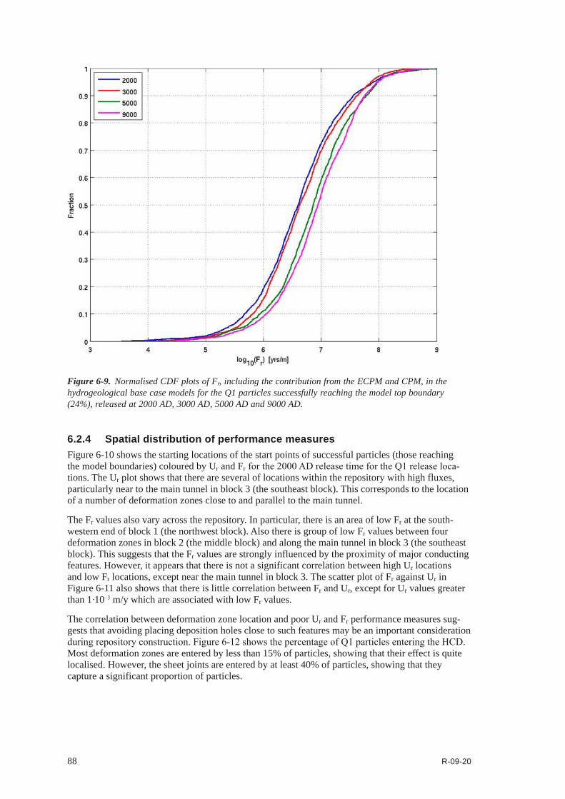
88 R-09-20

6.2.4 Spatial distribution of performance measuresFigure 6-10 shows the starting locations of the start points of successful particles (those reaching the model boundaries) coloured by Ur and Frforthe2000ADreleasetimefortheQ1releaseloca-tions. The Ur plot shows that there are several of locations within the repository with high fluxes, particularly near to the main tunnel in block 3 (the southeast block). This corresponds to the location of a number of deformation zones close to and parallel to the main tunnel.

The Fr values also vary across the repository. In particular, there is an area of low Fr at the south-western end of block 1 (the northwest block). Also there is group of low Fr values between four deformation zones in block 2 (the middle block) and along the main tunnel in block 3 (the southeast block). This suggests that the Fr values are strongly influenced by the proximity of major conducting features. However, it appears that there is not a significant correlation between high Ur locations and low Fr locations, except near the main tunnel in block 3. The scatter plot of Fr against Ur in Figure 6-11 also shows that there is little correlation between Fr and Ur, except for Ur values greater than 1∙10–3 m/y which are associated with low Fr values.

The correlation between deformation zone location and poor Ur and Fr performance measures sug-gests that avoiding placing deposition holes close to such features may be an important consideration duringrepositoryconstruction.Figure6-12showsthepercentageofQ1particlesenteringtheHCD.Most deformation zones are entered by less than 15% of particles, showing that their effect is quite localised. However, the sheet joints are entered by at least 40% of particles, showing that they capture a significant proportion of particles.

Figure 6‑9. Normalised CDF plots of Fr, including the contribution from the ECPM and CPM, in the hydrogeological base case models for the Q1 particles successfully reaching the model top boundary (24%), released at 2000 AD, 3000 AD, 5000 AD and 9000 AD.

R-09-20 89

Figure 6‑10. Starting locations coloured by log10(Ur) (top) and log10(Fr) (bottom) for Q1 particles released at 2000 AD and successfully reaching the top boundary of the hydrogeological base case model (24%). The HCD model at z = –470 m (purple), roads and buildings (black) and 2000 AD shoreline (blue) are also shown.

90 R-09-20

Figure 6‑12. Histogram showing the percentage of particles that enter the HCD for Q1 particles released at 2000 AD and successfully reaching the top boundary of the hydrogeological base case model (24%). The deformation zones are ordered by descending percentage and the top 30 displayed. A particle may enter several deformation zones and so the percentages add up to over 100%.

Figure 6‑11. Scatter plot of Fr against Ur for Q1 particles released at 2000 AD, 3000 AD, 5000 AD and 9000 AD and successfully reaching the top boundary of the hydrogeological base case model (24%).

R-09-20 91

6.2.5 Effect of FPC and EFPCTheparticlestartinglocations(6,916intotal)forQ1,withthoseparticlesnotmeetingFPC(402loca-tions, including 133 that also do not meet EFPC) and EFPC (343 locations, including 133 that also do not meet FPC) removed, are shown in Figure 6-13 and Figure 6-14, coloured by Ur and Fr respectively. These plots show that the FPC and EFPC are quite effective at removing the high Ur particles, but less effective at removing the low Fr particles. The fractures responsible for FPC and EFPC removals are probably larger HRD fractures with high transmissivities. Deformation zones are unlikely to cause FPC and EFPC removals because deposition hole locations are chosen to avoid these features.

Figure 6‑13. Starting locations coloured by log10(Ur) for Q1 particles not excluded by FPC and EFPC, released at 2000 AD and successfully reaching the top boundary of the hydrogeological base case model. The HCD model at z = –470 m (purple), roads and buildings (black) and shoreline (blue) are also shown.

Figure 6‑14. Starting locations coloured by log10(Fr) for Q1 particles not excluded by FPC and EFPC, released at 2000 AD and successfully reaching the top boundary of the hydrogeological base case model. The HCD model at z = –470 m (purple), roads and buildings (black) and shoreline (blue) are also shown.

92 R-09-20

Figure 6‑15. Non-normalised CDF plots of Ur and Fr in the hydrogeological base case model for the 6,916 Q1 particles released at 2000 AD, including FPC and EFPC.

R-09-20 93

Figure 6-15 shows the non-normalised plots of Ur and Fr for the hydrogeological base case model with the FPC and EFPC included. In these plots the intersection with the y-axis on the left hand side represents the proportion of particles that do not get started (blue curve) and/or are excluded by FPC (red curve) or FPC and EFPC (green curve). These plots show that approximately an additional 7% of particles are excluded by FPC and an additional 3% by EFPC. There is little difference in the median values when FPC and EFPC is applied, suggesting that any changes are in the tails of the distributions, particularly for high Ur.

6.2.6 Multiple particles per start pointFigure 6-16 shows the exit locations for the 25% of particles (1,729) with the highest Ur values for theQ2releaseinthehydrogeologicalbasecasemodelat2000AD.Theupperplot(blue)isforarelease of ten particles per start point and the lower plot (red) is for one particle per start point. There appears to be little difference between the two plots, although there are more exit points to the north with ten particles per start point.

There is very little difference in performance measures between the two cases (see CDF plots in Section E.1.4). These results indicate that the number of particles per start point do not affect the performance measures. This suggests that the large number of starting locations provide a sufficient sampling of the available flow pathways or there is very little dispersion of particles along their paths, i.e. the paths may be dominated by relatively few flow channels.

Figure 6‑16. Exit locations for the Q2 particles successfully reaching the top boundary of the model (94%) with ten particles per start point (blue) compared with one particle per start point (red) released at 2000 AD. The particles are released from the Q2 locations with a Ur value in the top 25% in the hydrogeo-logical base case model. Also shown is the HCD at z = –50 m (purple), roads and buildings (black) and the shoreline at 2000 AD (blue) for the repository-scale model.

94 R-09-20

6.2.7 Multiple realisationsTable 6-2 shows the number and percentage of particles successfully reaching the top boundary of themodelfortheQ2releaseforeachrealisation.Thepercentagesareverysimilar,showingthatthere is no bias to the normalised plots caused by a different number of particles being included.

Table 6‑2. The number and percentage of particles from the Q2 release locations at 2000 AD that successfully reached the top surface of the hydrogeological base case model (r0) and for ten stochastic realisations (r1 to r10).

Realisation No. of successful particles

%

r0 5,740 83r1 5,937 83r2 5,836 84r3 5,918 86r4 6,039 87r5 5,648 82r6 5,634 81r7 5,812 84r8 5,726 83r9 5,945 86r10 5,836 84

Figure 6-17 shows the normalised CDF plots of Ur, Fr and trfortheQ1releaselocationsfor10 stochastic realisations of the hydrogeological base case model at 2000 AD. Figure 6-18 shows the corresponding bar and whisker plots. There appears to be little variability in median values between realisations, with up to about half of an order of magnitude in the median values. However, there is more variability in the high end tails of Ur and in the low end tails of Fr and tr. In particular, realisation 9 has particles with significantly higher Ur values and lower Fr and tr values than the other realisations. Realisation 5 also has lower Fr and tr values than other realisations (these are even more apparentintheQ2andQ3plotsgiveninSectionE.1.5).

Advective travel time, tr, depends on the transport apertures of the fractures. In the hydrogeological base case model these vary by fracture transmissivity according to the relationship

et = 0.5T 0.5 (6-1)

where et is transport aperture and T is transmissivity. This was also the relationship used for SDM-Site /Follin 2008/, but with the coefficient rounded from 0.46 to 0.5. However, if a relationship proposed by /Hjerne et al. 2010/, based on a compilation of Swedish tracer test data, is used

et = 0.28T 0.3 (6-2)

then the trvaluesfortheQ1pathsareincreasedbyafactorofbetweenabout2and70.Figure6-19shows the normalised CDF plots of trfortheQ1releaselocationsforthetworelationships.TheHjerne relationship gives about an order of magnitude increase in median tr values compared to the hydrogeological base case.

Examination of the particle pathways show that the low Fr and tr values for realisation 5 are associ-ated with a single large, high transmissivity (about 1.0∙10–3 m2/s) HRD fracture that extends from the surface and intersects several deposition tunnels near the main tunnel, as shown in Figure 6-20. In reality such a feature would have a depth dependent transmissivity which would reduce the flow associated with it at repository depth. However, depth dependency in the transmissivity of individual HRD fractures was not used in the modelling. Also, in practice, such features would be detected and avoided during repository construction. However, it does suggest that performance measures may be sensitive to variations in stochastic geometry and properties between realisations.

R-09-20 95

Figure 6‑17. Normalised CDF plots of Ur (top), Fr (middle) and tr (bottom) in the hydrogeological base case model (r0) and 10 stochastic realisations of the HCD and HRD (r1 to r10) for the Q1 particles successfully reaching the model top boundary (24%–27%), released at 2000 AD.

96 R-09-20

Figure 6‑18. Bar and whisker plots of Ur (top), Fr (middle) and tr (bottom) in the hydrogeological base case model (r0) and 10 stochastic realisations of the HCD and HRD (r1 to r10) for the Q1 particles that successfully started (28%–31%), released at 2000 AD. The statistical measures are the median (red), 25th and 75th percentile (blue bar) and the 5th and 95th percentile (black “whiskers”).

R-09-20 97

Figure 6‑19. Normalised CDF plots of tr in the hydrogeological base case model using the standard et to T relationship and the /Hjerne et al. 2010/ relationship for the Q1 particles successfully reaching the model top boundary (24%), released at 2000 AD.

Figure 6‑20. The fracture (brown) in stochastic realisation 5 responsible for the low tr paths (shown as blue lines). The repository structures for block 2 are also shown.

98 R-09-20

Similarly, many of the high Ur values for realisation 9 are associated with a single large HRD frac-ture, as shown in Figure 6-21. Here the transmissivity is lower at about 2.0∙10–6 m2/s, but the fracture is gently dipping and intersects a large number of deposition holes, one deposition tunnel and a large number of other highly conductive features, such as deformation zones. Because it intersects the depositionholesithasaparticulareffectontheQ1releaselocations.Inpractice,theaffecteddeposi-tion holes would be elimination by the application of the FPC and EFPC due to the large number of adjacent deposition holes intersected by this fracture.

Figure 6-22 shows the distribution of the exit locations for the hydrogeological base case and the ten stochastic realisations. The lower plot just shows realisations 1, 5 and 9, which are those with the most atypical performance measures. The exit locations do not appear to vary significantly between realisations.

Figure 6‑21. The fracture (brown) in stochastic realisation 9 responsible for the high Ur Q1 paths (start points shown as red dots). The repository structures for block 2 are also shown in green.

R-09-20 99

6.3 Variant models for the temperate period6.3.1 Possible deformation zonesThe exit locations for the three PDZ realisations given in Figure 6-23 show little variation between realisations and are similar to those for the hydrogeological base case in Figure 6-22.

Figure 6-24 shows the CDF plots of Ur and Fr for the 3 realisations of the possible deformation zone variant compared to the hydrogeological base case and to the corresponding realisations of thehydrogeologicalbasecasefortheQ2releaselocationsat2000AD.Thepossibledeformationzones seem to have little effect on Ur values or on median Fr, values, but there is a significant low Fr tailforPDZrealisation1.ThistaildoesnotappearfortheQ1releaselocations,butitdoesforQ3(see Section E.1.5). This suggests that one of the PDZs in this realisation is providing a conductive pathwayforparticlestoleavethetunnels(Q3)orEDZ(Q2)butnotadirectpathwayforparticlesleavingdepositionholes(Q1).SomeoftheseparticlepathsareshowninFigure6-25.

Figure 6‑22. Top: Exit locations for the Q2 particles successfully reaching the top boundary of the model (81%–87%) at 2000 AD for all realisations of the hydrogeological base case. Bottom: Exit locations for realisations 1 (83%), 5 (82%) and 9 (86%). Also shown are the HCD at z = –50 m (purple), roads and buildings (black) and the shoreline at 2000 AD (blue).

100 R-09-20

Figure 6‑23. Exit locations for the Q2 particles successfully reaching the top boundary of the model (83%–86%) at 2000 AD for all realisations of the possible deformation zone variant. From the top: realisation 1 (red), realisation 2 (green) and realisation 3 (magenta). Also shown are the HCD at z = –50 m (purple), roads and buildings (black) and the shoreline at 2000 AD (blue).

R-09-20 101

Figure 6‑24. Normalised CDF plots of Ur (top) and Fr (bottom) for 3 realisations of the possible deforma-tion zone model (pdzr1 to pdzr3), the hydrogeological base case model (r0) and 3 stochastic realisations of the hydrogeological base case model (r1 to r3) for Q2 the particles successfully reaching the model top boundary (83%–86%), released at 2000 AD.

102 R-09-20

6.3.2 Alternative DFN transmissivity‑size relationshipsFigure6-26showstheparticlestartpointsforQ1colouredbyUr for each case. The correlated case has more high Ur values than the hydrogeological base case, but they are at a number of discrete locations, presumably associated with large stochastic fractures. For the uncorrelated case, the Ur values are higher than the hydrogeological base case generally, indicating a larger number of smaller fractures with higher transmissivities across the repository.

Figure6-27showstheparticlestartpointsforQ1colouredbyFr for each case. Here there is less variation between cases, with all of them showing low values at a number of discrete locations. This suggests that the low Fr values are dominated by the proximity of deformation zones, which do not vary between cases. However, there are more low values for the uncorrelated case and particularly for the correlated case compared to the hydrogeological base case. This may indicate more flow between the repository structures and the deformation zones in these cases.

Figure 6-28 shows the normalised CDF plots of Ur and FrfortheQ1releaselocationsforrealisation r0 of the correlated and uncorrelated cases compared to the hydrogeological base case (semi-correlated). Realisation r0 indicates deterministic HCD properties and realisation 1 of the HRD. Figure 6-29 and Figure 6-30 shows the normalised CDF plots of Ur and FrfortheQ1releaselocationsforrealisationsofthecorrelatedanduncorrelatedcasesrespectively.TheQ1CDFplotsshowthelargestvariationbetweenthedifferentrelationshipscomparedtoQ2andQ3(giveninAppendix E), with up to about half an order of magnitude variation in median Ur and Fr values betweenvariants.AsQ1representsareleasedirectlyintothefracturenetworktheperformancemeasureswillbedirectlyinfluencedbychangesinfractureproperties.Q2andQ3areparticlereleases into the EDZ and deposition tunnels respectively and so are less influenced by the HRD properties.

Figure 6‑25. Low Fr particles (paths shown in dark blue) associated with a possible deformation zone in realisation 1. The possible deformation zone and repository features are coloured by hydraulic conductivity.

R-09-20 103

Figure 6‑26. Starting locations coloured by log10(Ur) for Q1 particles released at 2000 AD and success-fully reaching the top boundary of the model. Top: correlated case (31%); Middle: hydrogeological base case (24%) Bottom: uncorrelated case (27%). The HCD model at z = –470 m (purple), roads and buildings (black) and shoreline (blue) are also shown.

104 R-09-20

Figure 6‑27. Starting locations coloured by log10(Fr) for Q1 particles released at 2000 AD and successfully reaching the top boundary of the model. Top: correlated case (31%); Middle: hydrogeological base case (24%); Bottom: uncorrelated case (27%). The HCD model at z = –470 m (purple), roads and buildings (black) and shoreline (blue) are also shown.

R-09-20 105

Figure 6‑28. Normalised CDF plots of Ur (top) and Fr (bottom) for realisation r0 of the correlated and uncorrelated transmissivity-size relationships compared to the hydrogeological base case (semi-correlated) for the Q1 particles successfully reaching the model top boundary (24% semi-correlated, 32% correlated, 27% uncorrelated), released at 2000 AD. Realisation r0 indicates a deterministic HCD and realisation 1 of the HRD.

106 R-09-20

Figure 6‑29. Normalised CDF plots of Ur (top) and Fr (bottom) for realisations of the correlated transmissivity-size relationship compared to the hydrogeological base case for the Q1 particles successfully reaching the model top boundary (24% hydrogeological base case, 31%–36% correlated), released at 2000 AD. Realisation r0 indicates a deterministic HCD and realisation 1 of the HRD.

R-09-20 107

Figure 6‑30. Normalised CDF plots of Ur (top) and Fr (bottom) for realisations of the uncorrelated transmissivity-size relationships compared to the hydrogeological base case for the Q1 particles success-fully reaching the model top boundary (24% hydrogeological base case, 26%–30% uncorrelated), released at 2000 AD. Realisation r0 indicates a deterministic HCD and realisation 1 of the HRD.

108 R-09-20

Figure 6‑31. Plots of fracture transmissivity against fracture radius for each transmissivity-size relation-ship at each depth zone for FFM01. Top: above –200 m; Middle; between –200 m and –400 m; Bottom: below –400 m.

R-09-20 109

The highest median UrvaluesforQ1areseenintheuncorrelatedcase.Figure6-31showsplotsoftransmissivity against fracture radius for the three cases for each depth zone. At repository depth (below–400m,bottomplot)itcanbeseenthatthesemi-correlatedcase(hydrogeologicalbasecase)has lower transmissivities than the other two cases for most fracture sizes. This leads to the semi-cor-related case having the lowest Ur values. There is a greater proportion of small fractures at repository depth than large fractures due to the power-law fracture size to intensity relationship (even allowing for the reduced connectivity of small fractures, which is partly compensated for by the extra con-nectivity provided by the repository structures). The uncorrelated case has the highest transmissivity values for small fractures, which is a result of matching observed flow measurements during SDM-Site calibration /Follin 2008/ (i.e. higher flows in small fractures compensate for lower flows in large fractures). This leads to the higher median Ur values seen for the uncorrelated case compared to the other two cases. The correlated case shows a significant high Ur tail, indicating some large, high transmissivity HRD fractures in a few locations. The correlated case will be sensitive to large HRD fractures intersecting the repository as these will always have relatively high transmissivities for this case. Also, because there is no transmissivity depth variation for individual HRD fractures, it is possible for higher transmissivity large fractures from upper depth zones to penetrate to repository depth (for example see Figure 6-20). The transmissivities of these fractures will be highest for the correlatedcase.NotethatthereareveryfewPFLflowsmeasuredbelow–400mandsotherewaslittle data to base the fracture flow calibration on. This means that there is some uncertainty in the calibration and hence in the calculated Ur values for the different correlation models.

The Fr values are a large scale property of the rock and will tend to be determined by the larger struc-tures such as deformation zones and large stochastic fractures. These structures will tend to carry most of the flow in the fracture network as they are the most transmissive (except for the uncor-related case) and most connected structures. Figure 6-31 indicates that the correlated case has the highest transmissivities for large fractures at all depth zones, which is a result of matching observed flows during SDM-Site calibration /Follin 2008/ (i.e. higher flows in large fractures compensate for lower flows in small fractures). This leads to the correlated case having the lowest Fr values.

There is little variation in Ur and Fr between realisations for the correlated and uncorrelated cases, apart from in Ur for realisation 5 of the correlated case. This realisation has a significant proportion of particles with high Ur values, associated with one or more large HRD fractures intersecting the repository, as shown in Figure 6-32. The transmissivity of the illustrated fracture is quite low at about 5.0∙10–8 m2/s, but it is nearly horizontal and intersects a large number of deposition holes and a large number of highly conductive features, such as deformation zones. Because it intersects the depositionholesithasaparticulareffectontheQ1releaselocations,comparedtoQ2orQ3.Inpractice, the affected deposition holes would be elimination by the application of the EFPC due to the large number of adjacent deposition holes intersected by this fracture.

Figure 6‑32. The fracture (brown) in stochastic realisation 5 of the correlated case responsible for the high Ur Q1 paths (start points shown as red dots). The repository structures for block 1 are also shown in green. The central area, ramp and transport tunnels are not included for clarity.

110 R-09-20

6.3.3 Unmodified vertical hydraulic conductivityThe particle exit locations and performance measures (see Section E.2.3) for the unmodified vertical hydraulic conductivity case are very similar to the hydrogeological base case, suggesting that the site-scale model is insensitive to changes in the vertical hydraulic conductivity in the ECPM. There is no change to the hydraulic conductivity in the DFN parts of the model and hence the two cases have essentially the same DFN with different boundary conditions and densities. The performance measures at 2000 AD are predominantly governed by the DFN in the site-scale model and the two cases have very similar values, thus implying that there was not a significant effect on the boundary conditions or densities in the DFN.

6.3.4 Extended spatial variabilityFigure 6-33 shows the particle exit locations for the hydrogeological base case and extended spatial variability case at the selected release times. For the extended spatial variability case there are fewer particles at the north-east boundary and fewer at intermediate locations, although there are some extra locations at the north of the model. The enhanced effect of the deformation zones seems to have caused more particles to exit closer to the repository. This emphasises the important role that deformation zones have in determining exit locations.

Figure 6‑33. Exit locations for the Q2 particles successfully reaching the top boundary of the site-scale model (89%–94%) at 2000 AD, 3000 AD, 5000 AD and 9000 AD. Top: Hydrogeological base case. Bottom: Extended spatial variability case. The HCD model at z = –50 m (purple), roads and buildings (black) and shoreline at 2000 AD (blue) are also shown.

R-09-20 111

The CDF plots of Ur and Fr in Section E.2.3 show that the extended spatial variability has little effect on performance measures. However, the CDF plots for Fr do not include the contribution from the ECPM and CPM. Figure 6-34 shows the corresponding plots with the CPM and ECPM contribution included. The contribution from the ECPM and CPM has little effect at 2000 AD and 3000 AD for both cases, but adds up to about half an order of magnitude to the mean Fr values for 5000 AD and 9000 AD because a greater proportion of the particle pathways are in the ECPM and CPM at the later release times. However, the increase in Fr is not as great for the extended spatial variability case compared to the hydrogeological base case, implying that a lesser proportion of the particle pathways are in the ECPM/CPM than for the hydrogeological base case. This is consistent with exit locations closer to the repository for the extended spatial variability case and suggests that the description of recharge and discharge is dependent on the flow concept, where the DFN approach render more local flow cells.

6.3.5 Tunnel variantsThe UrCDFplotsforQ1at2000ADinFigure6-35forthehydrogeologicalbasecase,crownspacecase, EDZ with T = 1∙10–7 m2/s, EDZ with T = 1∙10–6 m2/s and no EDZ cases are almost identical, suggesting that the EDZ and crown space has little influence on the initial flux in the fractures thatintersectthedepositionhole.ForQ2,thecrownspaceUr CDF plot is almost identical to the hydrogeological base case, indicating that the crown space has little influence on the flux in the EDZ. The case with EDZ T = 1∙10–7 m2/s gives an order of magnitude increase in the median Ur value in theEDZforQ2andthecasewithEDZT=1·10–6 m2/s gives a further order of magnitude increase, asmaybeexpectedgiventheincreasesintransmissivityintheEDZ.ThenoEDZplotforQ2isnotpossible by definition. The median UrvaluesforQ2are:hydrogeologicalbasecase=4.0·10–3 m/y, crown space = 4.0∙10–3 m/y, EDZ T = 1∙10–7 = 2.5∙10–2 m/y and EDZ T = 1∙10–6 = 1.7∙10–1 m/y. For the Q3CDFplots,thecrownspacecausesaboutoneorderofmagnitudeincreaseinthemedianUr value in the first fracture, the case with EDZ T = 1∙10–6 m2/s gives about two orders of magnitude increase and the case with EDZ T = 1∙10–7 m2/s gives about one order of magnitude increase. These cases increase the flux in the first fracture that the particle enters due to their enhanced conductivity relative to the tunnel and EDZ in the hydrogeological base case. The no EDZ case gives about one order of magnitude decrease in median Ur due to the low conductivity of the tunnel relative to the EDZ.

Figure 6‑34. Normalised CDF plots of Fr, including the contribution from the ECPM and CPM, in the extended spatial variability (ext. var.) site-scale and hydrogeological base case (base case) site-scale models for the Q1 particles successfully reaching the model top boundary (67%–70%), released at 2000 AD, 3000 AD, 5000 AD and 9000 AD.

112 R-09-20

Figure 6‑35. Normalised CDF plots of Ur for the hydrogeological base case model, the crown space model, the EDZ T = 1∙10–7 m2/s case, the EDZ T = 1∙10–6 m2/s case and the no EDZ case for the particles successfully reaching the model top boundary, released at 2000 AD. From the top: Q1 (14% no EDZ, 23%–24% others), Q2 (82%–84%) and Q3 (68% hydrogeological base case, 81% crown space, 64% EDZ T = 1∙10–7, 53% EDZ T = 1∙10–6, 52% no EDZ) release locations respectively. The UR axis corresponds to Ur for the Q3 release locations.

R-09-20 113

Figure 6‑36. Normalised CDF plots of Fr for the hydrogeological base case model, the crown space case, the EDZ T = 1∙10–7 m2/s case, the EDZ T = 1∙10–6 m2/s case and the no EDZ case for the particles success-fully reaching the model top boundary, released at 2000 AD. From the top: Q1 (14% no EDZ, 23%–24% others), Q2 (82%–84%) and Q3 (68% hydrogeological base case, 81% crown space, 64% EDZ T = 1∙10–7, 53% EDZ T = 1∙10–6, 52% no EDZ) release locations respectively.

114 R-09-20

Theflow-relatedtransportresistanceCDFplotsforQ1andQ3inFigure6-36showthatthenoEDZcase has significantly higher Fr values than the other cases. The absence of the EDZ potentially removes a significant flow pathway through the repository, leading to particles following slower paths through the rock before they can reach higher flowing features, such as deformation zones. The lower Fr values for the other variants compared to the hydrogeological base case show that the crown space and more transmissive EDZ potentially provide more significant pathways to higher flowing features.ThisismostclearlyseenintheQ3plots,wherethereisroughlyanorderofmagnitudereduction in the median Fr values.

These results indicate the importance of the repository structures in determining performance meas-ures. The values can be quite sensitive, in particular, to the presence of a highly conductive crown space or EDZ. These features can provide long flow pathways to highly transmissive fractures, such as deformation zones, which can then transport particles to the surface.

6.3.6 Effect of boreholesThe full set of results for the borehole cases are given in Appendix G. The results show that the pres-ence of an open borehole has an effect on the flow in the model. In all cases but one, particles are attracted to the borehole. In 16 out of the modelled 33 cases more than 5% of the released particles at some point enter the borehole. Eight cases have more than 10% of the particles entering the borehole and for one case as many as 23% of the released particles enter the borehole.

It may be concluded that it is not difficult to find positions for boreholes, inside or outside deposition tunnels and inside or outside fracture zones, which will have a considerable effect on the number of particles captured by the borehole. In fact, even if the borehole is positioned in the rock outside deposition tunnels and fracture zones, there will still be particles entering the borehole through the fracture network at all elevations.

The statistical analysis of the complete ensemble of the released particles shows that there is little change in performance measures. The change in performance measures generally stays within 20% comparing the borehole case to the hydrogeological base case. The performance measures behave as expected, initial Darcy flux and equivalent flow rate is slightly increased while the travel time, path length and F is somewhat decreased in the borehole cases.

When the statistical analysis is performed on only the particles that enter the boreholes and the results are compared to the same subset of particles in the hydrogeological base case, the effect on the performance measures is larger. However, the changes still remain within a factor of 4 and in the same direction for the different performance measures as before.

Figure 6-37 shows the non-normalised CDF plot of Urforthesub-setofQ3particlesthatenterboreholes and the corresponding particles in the hydrogeological base case. The median fluxes in the first fracture, Ur, are very similar comparing the borehole cases and the hydrogeological base case in all three blocks. The only exception is a slight increase in ABH5b3.

Figure 6-38 shows the non-normalised CDF plot of Frforthesub-setofQ3particlesthatenterboreholes and the corresponding particles in the hydrogeological base case. The results for Fr show decreased values in all boreholes compared to the respective hydrogeological base case paths. The contribution from the borehole is not included in Fr and so the reduction in values is due to the particles entering the borehole and bypassing a portion of the rock.

Thus, it can be concluded that including a borehole in the hydrogeological base case model does not have a major effect on the performance measures even if the groundwater flow pattern is affected and the flow paths of the released particles change.

R-09-20 115

Figure 6‑37. Non-normalised CDF plot of Ur for the repository blocks in the hydrogeological base case model (BC*b1 to BC*b3) and selected borehole cases (ABH*b*), for Q3 particles entering the borehole and successfully reaching the model top boundary, released at 2000 AD. The UR axis corresponds to Ur for the Q3 release locations.

Figure 6‑38. Non-normalised CDF plot of Fr for the repository blocks in the hydrogeological base case model (BC*b1 to BC*b3) and selected borehole cases (ABH*b*), for Q3 particles entering the borehole and successfully reaching the model top boundary, released at 2000 AD.

116 R-09-20

6.4 Glacial conditions6.4.1 Glacial ice front location IIThe CDF plots of Ur and FrfortheQ1releaselocationsinFigure6-39showthatthemedianUr valueforQ1hasincreasedbyanorderofmagnitudefrom1·10–5 m/y to 1∙10–4 m/y for the glacial ice front location II case compared to the 2000 AD hydrogeological base case. The increase is even largerforQ2andQ3(seeSectionE.3.1).Thissuggeststhattheintroductionofglacialconditionsover one-third of the repository area increases the groundwater flow velocities throughout the reposi-tory volume. This is presumably due to an increase in the pressure gradient across the repository.

Figure 6‑39. Normalised CDF plots of Ur (top) and Fr (bottom) for the hydrogeological base case model at 2000 AD and the glacial ice front location II model (Glacial II) for the Q1 particles successfully reaching the model top boundary (24% 2000 AD, 27% Glacial II).

R-09-20 117

The larger increases in UrvaluesforQ2andQ3comparedtoQ1suggestthattheincreasedflowsare greater within the repository structures compared to the fractures that intersect them. This may be because the increased head gradients penetrate less into the sparsely connected fracture system at depth. Some of the pressure may also be dissipated by the highly conductive, horizontal sheet joints in the upper 150 m of the bedrock.

The increased flows seen in the system will also reduce travel times and hence lead to the reduction of over an order of magnitude in Fr values calculated.

6.4.2 Glacial ice front location IThe red areas in Figure 6-40 shows the residual pressures imposed on the top surface of the site-scale model by the glacial conditions for ice front locations I and II. The blue area is offshore and the orange and green areas represent higher elevations of the ground surface. The residual pressure is the pressure that is obtained after subtraction from the total pressure of the hydrostatic pressure due to a freshwater column that extends vertically from to the location where the total pressure is measured to the reference elevation. It is the residual pressure that provides the driving force for the flow of groundwater through the bedrock.

Figure 6‑40. Residual pressure plots of the top surface of the site-scale model for glacial ice front locations I (top) and II (bottom).

118 R-09-20

The highest pressure difference experienced by the repository in the glacial ice front I case, as shown in the left plot of Figure 6-41, is no more than two orders of magnitude, between 1∙106 N/m2 in the west and 1∙104 N/m2 in the east. For the glacial ice front II case, the highest pressure difference is 1∙107 N/m2 in the west and 1∙104 N/m2 in the south east, suggesting that the groundwater flow direc-tion and magnitude will be different for the two cases.

Figure 6-42 shows a plot of pressure as a vertical slice through the repository for the two ice front locations. The repository structures are also shown to indicate where the pressure differences occur.

Figure6-43showstheexitlocationsoftheQ2particlesforthetwoicefrontlocationsandforthehydrogeological base case at 2000 AD. For ice front location I, the exit locations are shifted slightly to the east due to the change in the pressure gradient. For ice front location II, the exit locations have moved to the southeast due to the strong pressure gradient in that direction.

The CDF plots of Ur and Fr in Figure 6-44 show that ice front location II has a much greater effect on the performance measures than ice front location I. The distance of ice front location I from the repository is probably too great for it to exert much influence on the pressure gradient and flows in the repository volume.

Figure 6‑41. Residual pressure plots at repository elevation (z = –470 m) in the site-scale model for ice front locations I (top) and II (bottom).

R-09-20 119

Figure 6‑42. A northwest to southeast vertical slice of residual pressure for glacial ice front location I (top) and glacial ice front location II (bottom) for the site-scale model. The repository structures as also shown coloured by residual pressure.

120 R-09-20

Figure 6‑43. Exit locations for the Q2 particles successfully reaching the top boundary of the site-scale mode (93%–97%). From the top: they hydrogeological base case model at 2000 AD (blue), ice front location I (red) and ice front location II (green). Also shown are the HCD at z = –50 m (purple), roads and buildings (black) and the shoreline at 2000 AD (blue).

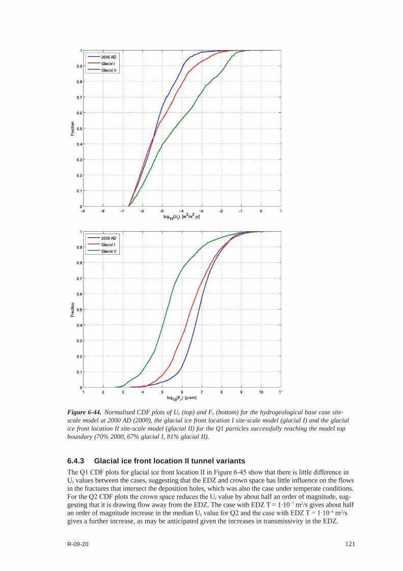
R-09-20 121

Figure 6‑44. Normalised CDF plots of Ur (top) and Fr (bottom) for the hydrogeological base case site-scale model at 2000 AD (2000), the glacial ice front location I site-scale model (glacial I) and the glacial ice front location II site-scale model (glacial II) for the Q1 particles successfully reaching the model top boundary (70% 2000, 67% glacial I, 81% glacial II).

6.4.3 Glacial ice front location II tunnel variantsTheQ1CDFplotsforglacialicefrontlocationIIinFigure6-45showthatthereislittledifferenceinUr values between the cases, suggesting that the EDZ and crown space has little influence on the flows in the fractures that intersect the deposition holes, which was also the case under temperate conditions. FortheQ2CDFplotsthecrownspacereducestheU r value by about half an order of magnitude, sug-gesting that it is drawing flow away from the EDZ. The case with EDZ T = 1∙10–7 m2/s gives about half an order of magnitude increase in the median UrvalueforQ2andthecasewithEDZT=1·10–6 m2/s gives a further increase, as may be anticipated given the increases in transmissivity in the EDZ.

122 R-09-20

Figure 6‑45. Normalised CDF plots of Ur for the glacial ice front location II base case model, the crown space case, the EDZ T = 1∙10–7 m2/s case, the EDZ T = 1∙10–6 m2/s case and the no EDZ case for the parti-cles successfully reaching the model top boundary. From the top: Q1 (18% No EDZ, 25%–27% others), Q2 (85%–89%) and Q3 (81% glacial base case, 86% crown space, 78% EDZ T = 1∙10–7, 73% EDZ T = 1∙10–6, 69% no EDZ) release locations respectively. The UR axis corresponds to Ur for the Q3 release locations.

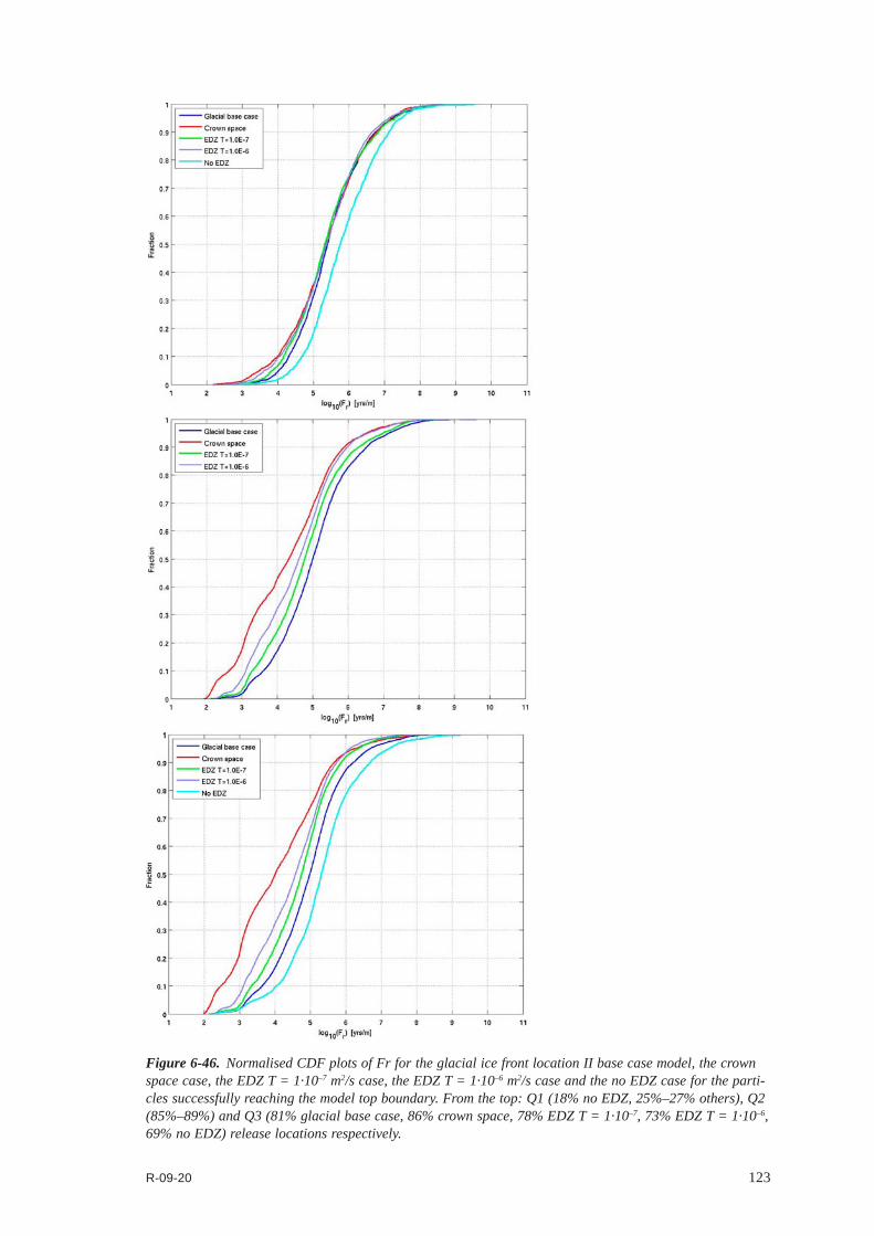
R-09-20 123

Figure 6‑46. Normalised CDF plots of Fr for the glacial ice front location II base case model, the crown space case, the EDZ T = 1∙10–7 m2/s case, the EDZ T = 1∙10–6 m2/s case and the no EDZ case for the parti-cles successfully reaching the model top boundary. From the top: Q1 (18% no EDZ, 25%–27% others), Q2 (85%–89%) and Q3 (81% glacial base case, 86% crown space, 78% EDZ T = 1∙10–7, 73% EDZ T = 1∙10–6, 69% no EDZ) release locations respectively.

124 R-09-20

Again,forQ2thenoEDZplotisnotpossible.FortheQ3CDFplots,thecrownspacecausesabout two orders of magnitude increase in the median Ur value in the first fracture, the case with EDZ T = 1∙10–6 m2/s gives about one order of magnitude increase and the case with EDZ T = 1∙10–7 m2/s gives about half an order of magnitude increase. These cases increase the flux in the first fracture that the particle enters due to their enhanced conductivity relative to the tunnel and EDZ in the hydrogeological base case. The no EDZ case gives about one order of magnitude decrease in median Ur due to the low conductivity of the tunnel relative to the EDZ.

InFigure6-46,theCDFplotsforQ1andQ3indicatethattheFr values for the no EDZ case are significantly greater than for the other variants, as was the case under temperate conditions. Again, the absence of the EDZ may be removing access to the more transmissive flow pathways in the constituent rock, leading to particles following slower paths before they reach higher flowing features,suchasdeformationzones.ThereductionintheQ3Fr values for the other variants show that the crown space and more transmissive EDZ may provide more significant pathways to higher flowing features, but the effect is not as great as in the temperate case. The Fr values are calculated only in the DFN and the relative influence of the crown space and EDZ may be reduced when there are greater flows in the model as a whole.

6.4.4 Glacial ice front location II and III recharge pathwaysTheQ1CDFplotsofUr, Fr and tr for the recharge pathways for the extended spatial variability case with glacial ice front location II and location III conditions are shown in Figure 6-47. The two cases are quite similar, although the ice front location III case has slightly higher Fr and tr values. The Fr and tr values are important for determining whether or not glacial melt water of low salinity will penetrate to the repository during the glacial period, as discussed in Appendix F. In this case around 5% of paths have Fr values of less than 1∙10–4 m/y and around 65% of paths have travel times of less than 10 years for both cases. The U r values are similar to those seen for the forward paths for the glacial II model in Section 6.4.1.

Figure 6-48 and Figure 6-49 show the back paths and recharge locations for the glacial ice front location II and ice front location III extended spatial variability cases respectively. There is little difference between the two cases, with recharge taking place mostly at the north western boundary of the model, with some recharge locations closer to the site. These are similar to the results given in Figure F-4 for the base case glacial ice front location II model.

R-09-20 125

Figure 6‑47. Normalised CDF plots of Ur (top), Fr (middle) and tr (bottom) for the extended spatial vari-ability model at glacial ice front location II (Glacial II ext. var.) and glacial ice front location III (Glacial III ext. var.) for the Q1 particles successfully reaching the model top boundary (23% glacial II, 24% glacial III).

126 R-09-20

Figure 6‑48. Recharge pathways (purple) for the Q1 particles successfully reaching the top boundary of the extended spatial variability model for glacial ice front location II. Top: map view; Bottom: Oblique view from south.

R-09-20 127

Figure 6‑49. Recharge pathways (purple) for the Q1 particles successfully reaching the top boundary of the extended spatial variability model for glacial ice front location III. Top: map view; Bottom: Oblique view from south.

R-09-20 129

7 Discussion and conclusions

7.1 Conclusions for the temperate periodDuring the temperate period, particle exit locations move northeast with release time as the shoreline retreats. For early times, the exit locations are dominated by the DFN features, particularly the deformation zones. Once the particles enter the ECPM and CPM they are more strongly influenced by the shoreline location. The influence of the shoreline is diminished in the extended spatial vari-ability case, showing that the exit locations are affected by how the region outside the repository site is represented. The exit locations are relatively insensitive to stochastic realisation or to variation in repository properties.

Performance measures do not show much variation with release time, although there is a gradual increase in Fr values as the release time increases. There is some variation between stochastic realisa-tions, with one or two showing significant tails at the low Fr end. This may be attributable to a small number of HRD fractures with atypical characteristics. However, this shows that a small number of large stochastic features can have a significant effect on performance measures if they are highly transmissive or well connected. Since there is very little data on flowing fractures at repository depth there is a degree of uncertainty in the properties and distribution of fractures at this depth. Therefore a conservative approach was taken that allows such fractures to occur in the models, even if they are unlikely in reality.

High flows in fractures that intersect deposition holes are undesirable in the repository due to the implications for buffer erosion and canister corrosion. However, it seems that the FPC and EFPC could be effective at removing the deposition holes that would be most affected. The criteria seem to be less effective at removing deposition holes that would lead to low Fr values. In the latter case, proximity to highly transmissive deformation zones appears to be more of a factor.

The transmissivity-size relationship used for HRD fractures can have a significant effect on performance measures. In particular, they can alter the distribution of transmissivity values between fractures of different sizes, which allows the smaller or larger fractures to have more of an influence on the flow pathways. It is thought that the semi-correlated case (i.e. the hydrogeological base case) is the most realistic case, with the other two cases representing extremes of this case. Both the correlated and uncorrelated case lead to poorer performance measures relative to the semi-correlated case (hydrogeological base case). The highest median UrvaluesforQ1areseenintheuncorrelatedcase. This is because higher transmissivities can be observed in the smaller fractures in this variant, many of which are in contact with the repository and can easily connect with the EDZ or nearby larger fractures. This leads to higher flows in the fractures that intersect the deposition holes. The correlated case shows a significant high Ur tail, indicating some large, high transmissivity HRD fractures in a few locations. The correlated case will be sensitive to large HRD fractures intersecting the repository as these will always have high transmissivities. The lowest Fr values are seen for the correlated case. This suggests that the flows are dominated by the larger fractures, which have a cor-respondingly higher transmissivity in the correlated case. For this case these often occur at a number of discrete locations associated with larger fractures that potentially can be filtered out by applying FPC and EFPC. For the uncorrelated case it is more difficult to filter out the poorly performing locations since they are typically caused by smaller fractures. Due to the lack of data at repository depth there is a major degree of uncertainty in the calibration of these cases for the depth zone below –400m.

Possible deformation zones that intersect the repository can have an effect on the performance measures at some canister locations. Depending on the stochastic properties assigned to the zones, they can become large, highly conductive features that provide significant flow pathways for nearby particles. For one realisation, there are a significant number of Fr particles with low Fr values for the Q2andQ3releaselocations,butnotforQ1,suggestingthatoneormoreofthePDZsisprovidingaconductivepathwayforparticlesleavingthetunnels(Q3)orEDZ(Q2)butnotadirectpathwayforparticlesleavingdepositionholes(Q1).SincetheexistenceandpropertiesofthePDZsareuncertainthe results only indicate a possible effect on performance measures.

130 R-09-20

Modifying the tunnel properties, specifically the EDZ transmissivity and the presence of a crown space can have a large effect on performance measures. These features have the potential to deliver significant flows from the repository structures to the more transmissive features, such as deforma-tion zones. The high transmissivity EDZ and crown space cases represent extreme situations that are not expected to occur in reality, but are used to examine the sensitivity of the models to particularly variations. The no EDZ case is probably the most likely in reality /SKB 2010a/, but the hydrogeo-logical base case includes an EDZ as a conservative approach.

The presence of abandoned boreholes can have an effect on the flow patterns and particle trajectories over a significant area. However, in most cases the impact on performance measures is relatively minor, especially when the full ensemble of particles is considered. Some of the boreholes examined are probably in worst case locations in that they were chosen to demonstrate an effect. In reality, boreholes would probably have even less of an effect unless they were located in unfortunate posi-tions. It is possible that the results are also sensitive to the borehole properties considered and other properties could be examined. Also the issue of boreholes carrying freshwater to the repository under glacial conditions could be considered.

7.2 Conclusions for the glacial periodThe results for the glacial ice front location II models show that glacial conditions can have a dramatic effect on both performance measures and exit locations. These changes are driven by the large pressure gradient that can be exerted on the repository volume. However, the position of the ice front is important, as seen for ice front location I, where the effect on performance measures and exit locations is much reduced due to the distance of the ice front from the repository.

The tunnel variants can also have an effect under glacial conditions. However, the size of the relative effect on performance measures can be altered compared to the temperate period. In particular, the effect of changing EDZ properties seems to be reduced, whereas the crown space has more of an influence on Fr values.

One particular concern that arises from the evolution of the climate through temperate and glacial cycles is the possible infiltration of dilute groundwaters to repository depth since this may lead to buffer erosion. This issue is assessed in terms of the ranges of expected dilution times for ground-water surrounding each canister under temperate and various glacial conditions in Appendix F.

The findings are that during the situation when the ice front is over the site about 2% of canister locations might be affected by dilute groundwater, although the period of high flows at a particular location may only last around 10 years, which would bring the proportion affected within that time period to about 0.7% (the other 1.3% have recharge pathways too long to be affected within a 10 year period). The proportion affected under temperate conditions is between about 0.7% and 2.4% depending on duration, and only 0.5% when an ice sheet covers the site. These results are moderately sensitive to the assumed diffusivity into the matrix and dilution factor required for colloid release. The locations where times for dilute recharge are short do not necessarily correlate with locations of very low F or initial flux, although they do tend to cluster around areas of high deformation zone intensity.

R-09-20 131

8 References

SKB’s (Svensk Kärnbränslehantering AB) publications can be found at www.skb.se/publications.

Andersson J-E, Nordqvist R, Nyberg G, Smellie J, Tirén S, 1991. Hydrogeological condi-tions in the Finnsjön area. Compilation of data and conceptual model. SKB TR 91-24. Svensk Kärnbränslehantering AB.

Bosson E, Gustafsson L-G, Sassner M, 2008. Numerical modelling of surface hydrology and near-surface hydrogeology at Forsmark. Site descriptive modelling, SDM-Site Forsmark. SKB R-08-09, Svensk Kärnbränslehantering AB.

Carrera J, Sánchez-Vila X, Benet I, Medina A, Galarza G, Guímerà J, 1998. On matrix diffu-sion:formulations,solutionmethodsandquantitativeeffects.HydrogeologyJournal,6,pp178–190.

Crawford J, 2008. Bedrock transport properties Forsmark. Site descriptive modelling, SDM-Site Forsmark. SKB R-08-48, Svensk Kärnbränslehantering AB.

Follin S, 2008. Bedrock hydrogeology Forsmark. Site descriptive modelling, SDM-Site Forsmark. SKB R-08-95, Svensk Kärnbränslehantering AB.

Follin S, Levén J, Hartley L, Jackson P, Joyce S, Roberts D, Swift B, 2007a. Hydrogeological characterisation and modelling of deformation zones and fracture domains, Forsmark modelling stage 2.2. SKB R-07-48, Svensk Kärnbränslehantering AB.

Follin S, Johansson P-O, Hartley L, Jackson P, Roberts D, Marsic N 2007b. Hydrological con-ceptual model development and numerical modelling using CONNECTFLOW, Forsmark modelling stage 2.2. SKB R-07-49, Svensk Kärnbränslehantering AB.

Follin S, Hartley L, Jackson C P, Roberts D, Marsic N, 2008. Hydrogeological conceptual model development and numerical modelling using CONNECTFLOW, Forsmark modelling stage 2.3. SKB R-08-23, Svensk Kärnbränslehantering AB.

Hartley L, Cox I, Hunter F, Jackson P, Joyce S, Swift B, Gylling B, Marsic N, 2005. RegionalhydrogeologicalsimulationsforForsmark–numericalmodellingusingCONNECTFLOW.PreliminarysitedescriptionForsmarkarea–version1.2.SKBR-05-32,Svensk Kärnbränslehantering AB.

Hartley L, Hunter F, Jackson P, McCarthy R, Gylling B, Marsic N, 2006a. Regional hydrogeo-logicalsimulationsusingCONNECTFLOW.PreliminarysitedescriptionLaxemarsubarea–version1.2. SKB R-06-23, Svensk Kärnbränslehantering AB.

Hartley L, Hoch A, Jackson P, Joyce S, McCarthy R, Rodwell W, Swift B, and Marsic N, 2006b. Groundwater flow and transport modelling during the temperate period for the SR-Can assessment.Forsmarkarea–version1.2.SKBR-06-98,SvenskKärnbränslehanteringAB.

Hartley L, Hoch A, Jackson P, Joyce S, McCarthy R, Swift B, Gylling B, Marsic N, 2006c. Groundwater flow and transport modelling during the temperate period for the SR-Can assessment. Laxemarsubarea–version1.2.SKBR-06-99,SvenskKärnbränslehanteringAB.

Hedenström A, Sohlenius G, Strömgren M, Brydsten L, Nyman H, 2008. Depth and stratigraphy of regolith at Forsmark. Site descriptive modelling, SDM-Site Forsmark. SKB R-08-07. Svensk Kärnbränslehantering AB.

Hjerne C, Nordqvist R, Harrström J, 2010. Compilation and analyses of results from cross-hole tracer tests with conservative tracers. SKB R-09-28, Svensk Kärnbränslehantering AB.

Hoch A R, Jackson C P, 2004. Rock-matrix diffusion in transport of salinity. Implementation in CONNECTFLOW. SKB R-04-78, Svensk Kärnbränslehantering AB.

Jackson C P, Hoch A R, Todman S, 2000. Self-consistency of a heterogeneous continuum porous mediumrepresentationofafracturedmedium.WaterResources.Research,36,pp189–202.

132 R-09-20

Johansson P-O, 2008. Description of surface hydrology and near-surface hydrogeol-ogy at Forsmark. Site descriptive modelling, SDM-Site Forsmark. SKB R-08-08, Svensk Kärnbränslehantering AB.

Lindborg T (ed), 2010. Landscape Forsmark. Indata, methodology and results for SR-Site. SKB TR-10-05, Svensk Kärnbränslehantering AB.

Löfgren M, Vecernik P, Havlova V, 2009. Studying the influence of pore water electrical con-ductivity on the formation factor, as estimated based on electrical methods. SKB R-09-57, Svensk Kärnbränslehantering AB.

Marsic N, Hartley L, Jackson P, Poole M, Morvik A, 2001. Development of hydrogeological modelling tools based on NAMMU. SKB R-01-49, Svensk Kärnbränslehantering AB.

Moreno L, Gylling B, 1998. Equivalent flow rate concept used in near field transport model COMP23 – Proposed values for SR 97. SKB R-98-53, Svensk Kärnbränslehantering AB.

Neretnieks I, 1979. Transport mechanism and rates of transport of radionuclides in the geosphere as related to the Swedish KBS concept. In: Proceedings of a symposium on the underground disposal of radioactive wastes, Otaniemi, Finland, 2–6 July 1979. Vienna: International Atomic Energy Agency, Vol II, pp 315–339.

Olofsson I, Simeonov A, Stephens M, Follin S, Nilsson A-C, Röshoff K, Lindberg U, Lanaro F, Frediksson A, Persson L, 2007. Site descriptive modelling Forsmark, stage 2.2. A fracture domain concept as a basis for the statistical modelling of fractures and minor deformation zones, and interdisciplinary coordination. SKB R-07-15, Svensk Kärnbränslehantering AB.

Öhman J, Follin S, 2010. Site investigation SFR. Hydrogeological modelling of SFR. Model version 0.2. SKB R-10-03, Svensk Kärnbärnslehantering AB.

Rhén I, Follin S, Hermanson J, 2003. Hydrological Site Descriptive Model – a strategy for its development during Site Investigations. SKB R-03-08, Svensk Kärnbärnslehantering AB.

Rhén I, Forsmark T, Hartley L, Joyce S, Roberts D, Gylling B, Marsic N, 2009. Bedrock hydrogeolology. Model testing and synthesis. Site descriptive modelling, SDM-Site Laxemar. SKB R-08-91, Svensk Kärnbärnslehantering AB.

Rouhiainen P, Sokolnicki M, 2005. Difference flow logging in borehole KFM06A. SKB P-05-15. Svensk Kärnbränslehantering AB.

Selroos J-O, Follin S, 2010. SR-Site groundwater flow modelling methodology, setup and results. SKB R-09-22, Svensk Kärnbränslehantering AB.

Serco, 2008a. CONNECTFLOW Release 9.6 Technical Summary Document. Serco Report SA/ENV/CONNECTFLOW/15.

Serco, 2008b. NAMMU Release 9.6 Technical Summary Document. Serco Report SA/ENV/CONNECTFLOW/8.

Serco, 2008c. NAPSAC Release 9.6 Technical Summary Document. Serco Report SA/ENV/CONNECTFLOW/12.

SKB, 2005a. Hydrogeochemical evaluation. Preliminary site description. Forsmark area – version 1.2. SKB R-05-17, Svensk Kärnbränslehantering AB.

SKB, 2005b. Preliminary site description. Forsmark area – version 1.2. SKB R-05-18, Svensk Kärnbränslehantering AB.

SKB, 2005c. Forsmark site investigation. Programme for further investigations of geosphere and biosphere. SKB R-05-14, Svensk Kärnbränslehantering AB.

SKB, 2006a. Site descriptive modelling Forsmark stage 2.1. Feedback for completion of the site investigation including input from safety assessment and repository engineering. SKB R-06-38, Svensk Kärnbränslehantering AB.

SKB, 2006b. Data report for the safety assessment SR-Can. SKB TR-06-25, Svensk Kärnbränsle-hantering AB.

R-09-20 133

SKB, 2007. Final repository facility. Underground design premises/D2. SKB R-07-33, Svensk Kärn bränsle hantering AB.

SKB, 2008a. Site description of Forsmark at completion of the site investigation phase. SDM-Site Forsmark. SKB TR-08-05, Svensk Kärnbränslehantering AB.

SKB, 2010a. Data report for the safety assessment SR-Site. SKB TR-10-52, Svensk Kärn bränsle-hantering AB.

SKB, 2010b. Climate and climate related issues for the safety assessment SR-Site. SKB TR-10-49, Svensk Kärnbränslehantering AB.

SKB, 2010c. BiosphereanalysesforthesafetyassessmentSR-Site–synthesisandsummaryofresults. SKB TR-10-09, Svensk Kärnbränslehantering AB.

SKB, 2010d. Slutförvarsanläggningföranväntkärnbränsle.AnläggningsbeskrivninglayoutD–Forsmark. SKB R-09-12, Svensk Kärnbränslehantering AB (in Swedish).

Stephens M B, Fox A, La Pointe P, Isaksson H, Simeonov A, Hermanson J, Öhman J, 2007. Geology Forsmark. Site descriptive modelling Forsmark stage 2.2. SKB R-07-45, Svensk Kärn-bräns lehantering AB.

Svensson U, Follin S, 2010. Groundwaterflowmodellingoftheexcavationandoperationphases–SR-Site Forsmark. SKB R-09-19, Svensk Kärnbränslehantering AB.

Vidstrand P, Follin S, Zugec N, 2010. Groundwater flow modelling of periods with periglacial and glacialclimateconditions–SR-SiteForsmark.SKBR-09-21,SvenskKärnbränslehanteringAB.

Åkesson M, Kristensson O, Börgesson L, Dueck A, Hernelind J, 2010. THM modelling of buffer, backfill and other system components. Critical processes and scenarios. SKB TR-10-11, Svensk Kärnbränslehantering AB.

R-09-20 135

Appendix A

Glossary of abbreviations and symbols

Abbreviations and notation used are:

ar Fracture surface area per unit volume (2×P32) (m2m-3), used for particle transport

ABH Abandoned borehole CDF Cumulative distribution function CPM Continuous porous medium DFN Discrete fracture network DZ Deformation zone ECPM Equivalent continuous porous medium EDZ Excavation damaged zone EFPC Extended full perimeter criteria et Fracture transport aperture (m) Fa.b Forsmark version a.b, e.g. F1.2 Fr Flow-related transport resistance in the rock (y/m) FFM Fracture Forsmark Model (fracture domain) FPC Full perimeter criteria HCD Hydraulic conductor domain HRD Hydraulic rock mass domain HSD Hydraulic soil domain IFL Ice front location IFZ Implicit fracture zone K Hydraulic conductivity (ms-1) KFM Cored borehole at Forsmark kr Shape parameter in the power-law fracture size-intensity distribution LEDZ Path-length in the EDZ (m) Lr Path-length in the rock (m) Lt Path-length in the tunnel (m) P10 Linear fracture intensity: number of fractures per metre along a borehole (m-1) P10c Linear fracture intensity of connected open fractures: number of connected

fractures per metre along a borehole (m-1) P10corr Terzaghi corrected linear fracture intensity: ‘true’ number of fractures per metre

along a borehole corrected for the bias introduced by the angle of the borehole made with fractures (m-1)

P10PFL Linear fracture intensity of PFL-anomalies: number of PFL anomalies per metre along a borehole (m-1)

P10PFL,corr Terzaghi corrected Linear fracture intensity of PFL-anomalies (m-1) P21 Area fracture intensity: total fracture trace lengths per square metre of outcrop

(m m-2) P32 Volumetric fracture intensity: total fracture surface area per cubic metre of rock

(m2 m-3) P32c Volumetric fracture intensity of connected fractures: total connected fracture

surface area per cubic metre of rock (m2 m-3) PA Performance assessment PDF Probability distribution function

136 R-09-20

PFL Posiva flow-log Φ Kinematic porosity PM Performance measure PSS Pipe-string system Q Groundwater flow rate (m3s-1 or m3y-1) Qeq Equivalent flow rate (m3s-1 or m3y-1) q Darcy flux (m s-1 or m y-1) RMD Rock matrix diffusion r0 Location parameter in the power-law fracture size-intensity distribution (m) rmin Minimum fracture radius used in DFN simulations (m) RHB 70 Shoreline datum level of year 1970 Residual pressure The pressure that is obtained after subtraction from the total pressure of the

hydrostatic pressure due to a freshwater column that extends vertically from the location where the total pressure (not including atmospheric pressure) is measured relative to the reference elevation.

SDM Site descriptive modelling or model SFR A final repository for low- and intermediate level waste at Forsmark σ Standard deviation, or the fracture surface area per unit volume (m2 m-3) for

solute transport SMOW Standard Mean Ocean Water STP Standard temperature and pressure T Fracture transmissivity (m2s-1) tEDZ Advective travel-time in the EDZ (y) tr Advective travel-time in the rock (y) tt Advective travel-time in the tunnel (y) Θ Temperature (K) TDS Total dissolved solids (g/L) Ur Initial equivalent flux in the rock (m/y) z Elevation (m)

R-09-20 137

Appendix B

File formats

B.1 PTABLE File Format The PTABLE file format is used to export summary information on each pathline from a ConnectFlow particle tracking simulation. In the format that follows, text in bold indicates a literal entry in the file, text in italics between <> indicate an entry that is replaced by a number in the file, and other text is descriptive.

Header lines:

# PARAMETER TABLE FILE FROM CONNECTFLOW

#

# NUMBER OF COLUMNS DEFINED

<number of columns>

# NUMBER OF TIMES THEY ARE USED

<number of rows> <number of rows> <number of rows> # HOW MANY TIMES THEY COULD BE USED

<number of rows> <number of rows> <number of rows> # THE PARAMETER TABLE:

Column header:

# POINT XS YS ZS XE YE ZE OKFLAG T0 U0 QEQ TW F L TRAPP TW_TUN L_TUN TW_EDZ L_EDZ UR QEQR LR_TUN TR_TUN

Followed by one line per path each with the following space separated entries:

Entry Description POINT Path number XS X coordinate of start point. YS Y-coordinate of start point. ZS Z-coordinate of start point. XE X coordinate of end point. YE Y-coordinate of end point. ZE Z-coordinate of end point.

138 R-09-20

OKFLAG Indicates whether or not a particle reached the model boundary:

0 = reached the top boundary;

1 = failed to start due to no fracture (Q1 or Q2) or low initial Darcy flux (Q1, Q2 and Q3), as defined in section 3.2.6;

2 = ran out of time steps;

3 = stuck;

4 = oscillating between DFN and CPM;

5 = reached a side boundary or the bottom boundary. T0 Release time (y). U0 Initial equivalent flux (m/y) for Q1 (Ur1 in equation (3-8)) and Q2 (Ur2 in equation

(3-10)). For Q3 this is just the initial Darcy flux (m/y) and UR should be used for radionuclide transport.

QEQ Equivalent groundwater flow rate (m3/y) for Q1 (equation (3-7)) and Q2 (equation (3-9)). QEQR is used for Q3 instead.

TW Travel time in the rock, i.e. the DFN (y). F Flow-related transport resistance for the rock, i.e. the DFN (y/m). L Path length in the rock, i.e. the DFN (m). TRAPP Initial transport aperture (m) in the first fracture for Q1 or Q2, or the porosity for

Q3. TW_TUN Travel time in the tunnels (y). L_TUN Path length in the tunnels (m). TW_EDZ Travel time in the EDZ (y). L_EDZ Path length in the EDZ (m). UR Initial equivalent flux (m/y) in the first fracture for Q3 (equation ( 3-12)), zero for

Q1 or Q2. LR_TUN Path length (m) to the first fracture for Q3, zero for Q1 or Q2. TW_CPM Travel time in the ECPM or CPM, i.e. not in the DFN (y). L_CPM Path length in the ECPM or CPM, i.e. not in the DFN (m). F_CPM Flow-related transport resistance for the ECPM or CPM, i.e. not in the DFN (y/m). TR_TUN Travel time (y) to the first fracture for Q3, zero for Q1 or Q2. QEQR Equivalent groundwater flow rate (m3/y) in the first fracture for Q3 (equation

(3-11)), zero for Q1 or Q2. FPC Whether or not the path is associated with a deposition hole that would be

excluded if the FPC (Section 3.2.7) were applied:

0 = would not be excluded;

1 = excluded due to background fracture;

2 = excluded due to deformation zone fracture. EFPC The largest number of adjacent deposition holes (including this deposition hole)

fully intersected by a fracture that fully intersects this deposition hole. A value of 5 or greater means that the hole would be excluded if the EFPC (Section 3.2.7) were applied.

FLEN The length (m) of the largest fracture intersecting the deposition hole. This is fixed at 1000.0 m for a deformation zone fracture.

R-09-20 139

Appendix C

Changes to palaeo-hydrogeological simulations for SR-Site Forsmark relative to SDM-Site Forsmark

C.1 Background Coupled groundwater flow and salt transport modelling of the temperate period for SR-Site Forsmark (2000 AD to 12,000 AD) is carried out in the same way as the modelling of the palaeo period for SDM-Site Forsmark (8000 BC to 2000 AD). In summary, the migration of salt is modelled by means of a double-porosity model with advection and dispersion processes in the fracture system and a diffusion process in the rock matrix.

The implementation of coupled groundwater flow and salt transport in ConnectFlow is described in /Hoch and Jackson 2004/ and the governing equations are reproduced in Section C.3 below. An implementation of a ‘faster dedicated equation’ option in ConnectFlow for modelling rock matrix diffusion (RMD) was made in Spring 2005, i.e. at the time of the preliminary SDM-Site work. The ‘faster dedicated equation’ was not used during the F1.2 modelling /Hartley et al. 2005/ or the L1.2 modelling /Hartley et al. 2006a/, but was used for some of the palaeo-hydrogeology calculations in SR-Can /Hartley et al. 2006b and Hartley et al. 2006c/.

During the completion of the coupled groundwater flow and salt transport modelling for SDM-Site Laxemar /Rhén et al. 2009/, an error in the flux of solutes into the matrix was discovered at locations in the model where the advection and diffusion processes took place on similar timescales. The problem was found to be due to an incorrect assembly of the ‘faster dedicated equation’ of the RMD process; hence a fix was made in ConnectFlow for SDM-Site Laxemar /Rhén et al. 2009/. Indeed, comparisons between the original and the ‘faster dedicated equation’ assembly of the RMD process were checked for SR-Can Forsmark /Hartley et al. 2006b/ and SR-Can Laxemar /Hartley et al. 2006c/, but these checks clearly were not sensitive enough to show up the problem encountered during the modelling for SDM-Site Laxemar.

C.2 Objectives In view of the fact that the problem with the ‘faster dedicated equation’ was not discovered in time for the palaeo-hydrogeological simulations for SDM-Site Forsmark /SKB 2008a/, the main objective of this appendix is to provide a comparison between the incorrect (‘old’) assembly of the ‘faster dedicated equation’ used for SDM-Site Forsmark /Follin et al. 2007b, Follin et al. 2008/ and the corrected (‘new’) assembly applied in SR-Site Forsmark.

For the sake of clarity, it is noted that a few parameter settings were slightly revised in the palaeo-hydrogeological simulations for SR-Site Forsmark. However, these changes have nothing to do with the incorrect assembly of the ‘faster dedicated equation’ mentioned above, but provide an adaption to the fact that a repository is present in SR-Site and also achieves a better consistency between modelling disciplines with regard to the transport property settings /Crawford 2008, Löfgren et al. 2009/. In summary, the following parameter revisions have been made to the palaeo-hydrogeological simulations for SR-Site Forsmark relative to the simulations for SDM-Site Forsmark:

The effective diffusivity of solutes in the matrix was reduced from 110–13 m2/s to 410–15 m2/s. (It is noted that the chloride ion is the key constituent in the salt transport modelling.)

The specification of the rock matrix diffusion parameters for solute transport has changed, primarily for the specific flow-wetted fracture surface area per unit volume of rock below -200 m elevation in the key hydraulic rock mass domains at Forsmark, FFM01 and FFM06.

The initial conditions for two of the five reference waters used in the palaeo-hydrogeological simulations (Old Meteoric and Glacial) were changed to include a variation with distance from a conductive fracture within the matrix.

140 R-09-20

Grid dispersivities (dispersion lengths) were modified slightly for the region outside the candidate area, i.e. in the part handled as a homogeneous and isotropic continuous porous medium (CPM). The longitudinal dispersion length in the coarser part of the grid was increased from 40 m to 50 m, and the transverse dispersion length in the coarse part of the grid was increased from 5 m to 10 m.

The identification of the connected discrete fracture network on the regional-scale now includes a representation of the repository and smaller-scale fractures down to radius of 0.4 m in a volume surrounding the repository, while fractures with radius greater than 5.6 m are created over the hydraulic rock mass domains covered by the candidate area, FFM01 to FFM06.

The shoreline displacement curve was updated to also include the evolution during the temperate period (2000 AD – 12,000 AD)

Sections C.3 and C.10 are the key sections with regard to the objectives of this appendix, whereas Sections C.4 through C.9 provide further details on the motives behind each of the listed parameter changes made for SR-Site Forsmark.

C.3 Changes to the rock matrix diffusion of solutes implemented in ConnectFlow

The implementation of coupled groundwater flow and salt transport in ConnectFlow is described in /Hoch and Jackson 2004/. The governing equations are reproduced here:

)( gq

Pk (C-1)

0)()(

q

tf (C-2)

0

)()()(

wef

f

wcDcDc

tc

q (C-3)

)()(wcD

wtc

e

(C-4)

where

q is the specific discharge (or Darcy flux ) [LT-1];

k is the effective permeability tensor due to the fractures carrying the flow [L2];

is the groundwater viscosity (which depends on the salinity) [ML-1T-1];

P is the (total) pressure in the groundwater [ML-1T-2];

is the groundwater density (which depends on the salinity) [ML-3];

g is the gravitational acceleration [LT-2];

t is the time [T];

R-09-20 141

f is the effective porosity due to the fractures carrying the flow (which is sometimes referred to as the kinematic porosity) [-];

c is the salinity in the groundwater flowing through the fractures (expressed as a mass fraction) [-];

D is the (effective) dispersion tensor [L2T-1];

eD is the effective diffusion coefficient for diffusion into the rock matrix, [L2T-1];

is the specific flow-wetted fracture surface area, that is the average flow-wetted fracture surface area of the matrix per unit volume of rock [L-1]. For smooth planar fractures, is given by 2 P32,HRD, where P32,HRD is the fracture surface area per unit volume of rock deduced from fracture frequency analyses;

w is a one-dimensional coordinate in the rock matrix [L];

c is the salinity of the groundwater in the rock matrix (expressed as a mass fraction) [-];

is the capacity factor (matrix porosity) of the rock matrix [-]

In ConnectFlow, two parameters are used in parallel to define fracture surface area per unit volume, and ar ; is used for solute transport calculations (cf. the last term in Eq. (C-3)), whereas ar is used for particle transport calculations, i.e. for calculation of F-values along flow paths. Partly this is to provide flexibility, but also for numerical efficiency reasons; is envisaged as a hydraulic rock mass domain (HRD) property, and there may typically be a few tens of hydraulic rock mass domains in a regional flow model, whereas ar is defined for each finite-element, based on calculating the specific fracture surface area within each finite-element, P32,element. In contrast to , ar is treated as a stochastic entity that varies in space in accordance to a particular realisation of an underlying hydrogeological DFN model, i.e.:

zyxPzyxa elementr ,,2,, ,32 (C-5)

The last term in Eq. (C-3) corresponds to the flux of salinity in to the matrix from the fracture system and hence the exchange of solute by rock matrix diffusion (RMD). In the numerical implementation this flux is evaluated at each time step, lt , by writing it in the form (see chapter 4 of /Hoch and Jackson 2004/):

lll

lll

e BttccAw

wcD

)()()0( 1

1

(C-6)

where lc is the salinity at the end of the time step, 1lc is the salinity at the previous time step, 1lt , and lA and lB do not depend on lc . The terms lA and lB have to be evaluated at each time step and for each finite-element. This approach to incorporating the effects of RMD was implemented and verified in ConnectFlow for both transport of salinity and for transport of multiple reference waters (see chapters 6 and 7 of /Hoch and Jackson 2004/).

For large simulations with about one million elements, several reference waters and several hundred time steps, the time taken to assemble the discrete system matrix became very significant using the standard generalised algorithm for assembling the equations in ConnectFlow. To make the calculations more tractable, an algorithm was implemented in ConnectFlow for assembling the specific finite-element equations for coupled groundwater flow and reference water transport for

142 R-09-20

hexahedral elements with nodal quadrature, which was about 4-5 times faster. Unfortunately, Equation (C-6) was implemented incorrectly in this algorithm being coded as:

)()()0( 1

1

ll

lll

ettccBw

wcD (C-7)

The result was a reduction of the solute flux into the matrix, but this error was only noticeable in circumstances where solute transport by advection and RMD took place on similar timescales. This finding was not immediately apparent in the modelling for SDM-Site Forsmark, but it became obvious in the modelling for SDM-Site Laxemar:

In the upper bedrock at Forsmark, i.e. above –200m elevation, the fracture system is both intense and transmissive, thus the transport of salt in the upper bedrock is mainly governed by advective flows. Deeper down, e.g. around repository depth, the conductive fracture frequency is significantly lower (close to the percolation threshold) and the fracture transmissivities are also lower, which evidently imply lower advective flows, but also a significantly smaller specific flow-wetted fracture surface area. Hence, the erratic reduction of the solute flux into the matrix associated with incorrect (‘old’) assembly of the ‘faster dedicated equation’ had negligible effects on the palaeo-hydrogeological results for SDM-Site Forsmark.

At depths around –150m to –650m elevation at Laxemar, the conductive fracture frequency is higher, relatively speaking, which implies a higher specific flow-wetted fracture surface area, i.e. a greater exchange with the matrix (see Equation (C-3)). Hence, the effects of the erratic reduction of the solute flux into the matrix were found to be more important.

The resulting changes for SR-Site Forsmark relative to SDM-Site Forsmark are quantified in Section C.9 of this appendix. In summary, with regard to other types of uncertainties such as the impact of multiple realisations and parameter heterogeneity, the differences in confirmatory testing results between the incorrect assembly of the ‘faster dedicated equation’ used for SDM-Site Forsmark and the correct assembly used for SR-Site Forsmark are considered negligible. The results obtained with the corrected assembly of the ‘faster dedicated equation’ used for SR-Site Forsmark are not in conflict with the palaeo-hydrogeological simulations and the confirmatory testing reported for SDM-Site Forsmark. (For the sake of clarity, it is noted here that the notation used in the report sections describing the palaeo-hydrogeological simulations for SDM-Site Forsmark, e.g. see Table 3-10 of /Follin et al. 2007a/ and Table 3-13 of /Follin et al. 2008/, is not entirely correct. The symbol ar should be replaced by the symbol in these reports.)

C.4 Revision of the effective diffusivity In SKB’s programme, in situ effective diffusivity is usually formulated in terms of the formation factor, fF , and the diffusivity in free-water, wD ,

wfe DFD . (C-8)

Although strictly a geometrical parameter, measurement of the formation factor is influenced by other non-geometrical artefacts such as surface diffusion and anion exclusion effects. The formation factor is calculated using electrical resistivity measurements or through-diffusion experiments /Crawford 2008/. Mainly these are laboratory measurements, although electrical resistivity can also be measured in situ. From the formation factor, approximate effective diffusivities can be calculated for all solutes. The wD is about 10–9 m2/s and laboratory measurements of formation factor are

around 10-4, and hence a value of about 10–13 m2/s was used for eD as a typical value of effective diffusivity into the matrix in SDM-Site Forsmark.

R-09-20 143

In the SR-Can Data report /SKB 2006b/, the formation factor and diffusivity in free solution for Na+ and Cl- are given in Tables A-41 and A-40, respectively. The mean value of the formation factor is given as log10(Ff) = -4.74, corresponding to a formation factor of 1.810-5. The Dw of Cl- and Na+ at 25C is given as 2.010-9 m2/s and 1.310-9 m2/s, respectively. For the in-situ temperature at repository depth, which is presently around 12C, the diffusivities should be reduced by a factor of about 1.5, compared to 25C (/SKB 2010a, section 6.8.5 and Appendix A/). Furthermore, an anion exclusion reduction factor of 10 is suggested in the SR-Can Data report /SKB 2006b, p 193/. Accordingly, the diffusivity of chloride should be reduced by a factor of 10.

When modelling matrix diffusion of salt, the diffusivity of the ion-pair is needed. This requires the use of the harmonic mean of the ions’ individual diffusivities (equations in /SKB 2010a, Appendix A/). If doing this, using the Ff and the Dw of the ion-pair based on the data presented above, the effective diffusivity De becomes 410-15 m2/s, which is the value used in this study.

It should be noted that in SR-Site generally, the data are modified, predominantly on two accounts. Firstly, the best estimate Ff of 1.810-5 for the undisturbed rock and 7.210-5 for the fractured rock surrounding flow paths are suggested (/SKB 2010a, section 6.8.10 and Appendix A/). Secondly, the anion exclusion reduction factor of √10 is suggested, as compared to 10 in SR-Can. Based on this, the effective diffusivity for salt transport is in SR-Site suggested to be within the range of 110-14– 110-13 m2/s, with the best estimate at 410-14 m2/s (cf. justification in /SKB 2010a, Appendix A/).

C.5 Changes to the specification of rock matrix diffusion parameters Apart from effective diffusivity and matrix porosity, the other parameters related to RMD are the specific flow-wetted fracture surface area, σ, in Equation (C-3), that scales the flux into the matrix per unit volume, and a diffusion distance in to the matrix LD. The maximum value appropriate for LD is bounded by half the size of the matrix blocks and so LD is 1/σ for cuboid blocks, although it can be assumed to be smaller if diffusion only into a surface layer is of interest. When σ is small, then to model diffusion into the whole matrix block would require LD to be set to a very large number which would require a lot of terms to be stored to calculate the flux into the matrix accurately /Hoch and Jackson 2004/. Hence, for practical reasons LD has to be set to an appropriate maximum, i.e. a limited penetration depth for diffusion into the matrix. A maximum value of 6.7m was used in SDM-Site Forsmark, as the amount of solute diffusing deeper than 6.7m during Holocene time (c. 10,000 years) was considered negligible. For SDM-Site Forsmark, σ was estimated based on 2 P10,corr for PFL-f fractures, then LD was set to min(1/σ, 6.7m), and σ was changed to be consistent, i.e. 1/LD. The parameterisation of σ and LD were subject to confirmatory testing by the palaeo-hydrogeological testing, and for simplicity uniform values were used within each HRD in case changes were felt necessary for either calibration or sensitivity purposes.

As mentioned above, a specific flow-wetted fracture surface area, ar, is also used for calculating the F-factor in particle tracking calculations in the ECPM model. For this purpose, it was considered more appropriate to use values specific to the underlying stochastic DFN model within each finite-element that particles pass through, and hence ar was calculated from the actual fracture surface area per unit volume of the connected fracture network within each element (cf. Equation (C-5)), see Table C-1 for a summary.

For the purposes of SR-Site Forsmark, it was thought appropriate to use the same basic approach as for SDM-Site Forsmark to parameterise LD and ar, but not to modify σ based on 1/LD, i.e. to keep it as 2 P10,corr, see Table C-2 for a summary. The motivation for this choice was to limit the size of LD to be no more than 6.7 m, otherwise a prohibitively large number of coefficients are required to accurately store the distribution of salinity in the matrix. These changes in themselves were found to not change the resulting palaeo-hydrogeological simulations significantly.

144 R-09-20

C.6 Changes to the initial conditions of some reference waters The initial condition for Old Meteoric and Glacial reference waters in the matrix was changed from SDM-Site Forsmark to include a variation with distance from a conductive fracture within the matrix. The initial condition for the fracture system was unchanged, however. For the matrix system, a spatially varying profile into the matrix was calculated by allowing a diffusion of the fracture initial condition into the matrix initial condition for 1000 years. By allowing an in-diffusion of one reference water into another, a presumably unrealistically sharp interface in the matrix between the two reference waters at the start of the simulation period was avoided. The motive for the adopted profile is driven by the fact that the Forsmark site has been subjected to several glaciations in the past, i.e. before Holocene time.

The adopted profile only affects the initial condition for the Old Meteoric and Glacial reference waters as it was interpreted that the initial condition for these references waters in matrix pore water far from the connected fractures were different to that in the fractures system. The Deep Saline reference water is considered very old, relative to all other reference waters, thus assumed to vary with depth only. In contrast, the Littorina and Altered Meteoric reference waters are not part of the initial conditions at the start of the simulation period (8000 BC). In conclusion, the adopted change only affects predictions of species such as δ18O, i.e. constituents that are characteristic of the Old Meteoric reference water versus the Glacial.

Table C-1. Transport parameters used in the palaeo-hydrogeological simulations in SDM-Site Forsmark for each hydraulic rock mass domain (FFM01-FFM06) as well as for the rock outside FFM01-FFM06. σ is the specific flow-wetted fracture surface area used in the solute transport Equation (C-3), LD is the maximum penetration distance used for matrix diffusion (has to be <1/σ, but truncated to keep the calculation of the flux into the matrix tractable), ar is used in calculating F for particle transport in ECPM models. HRD z > –200m –200m > z > –400m –400m > z σ [m–1] LD [m] ar [m–1] σ [m–1] LD [m] ar [m–1] σ [m–1] LD [m] ar [m–1] FFM01, -06 0.30 3.3 DFN 0.15 6.7 DFN 0.15 6.7 DFN FFM02 0.60 1.7 DFN 0.60 1.7 DFN 0.60 1.7 DFN FFM03, -05 0.15 6.7 DFN 0.15 6.7 DFN 0.15 6.7 DFN FFM04 0.30 3.3 DFN 0.30 3.3 DFN 0.30 3.3 DFN Other 0.60 1.7 0.60 0.30 3.3 0.30 0.30 3.3 0.30

Table C-2. 0Transport parameters used in the palaeo-hydrogeological simulations in SR-Site Forsmark for each hydraulic rock mass domain (FFM01-FFM06) as well as for the rock outside FFM01-FFM06. σ is the specific flow-wetted fracture surface area used in the solute transport Equation (C-3), LD is the maximum penetration distance used for matrix diffusion (has to be <1/σ, but truncated to keep the calculation of the flux into the matrix tractable), ar is used in calculating F for particle transport in ECPM models. HRD z > –200m –200m > z > –400m –400m > z σ [m–1] LD [m] ar [m–1] σ [m–1] LD [m] ar [m–1] σ [m–1] LD [m] ar [m–1] FFM01, -06 0.30 3.3 DFN 0.08 6.5 DFN 0.02 6.7 DFN FFM02 0.66 1.5 DFN 0.66 1.5 DFN 0.66 1.5 DFN FFM03, -05 0.18 5.5 DFN 0.18 5.5 DFN 0.10 6.5 DFN FFM04 0.18 5.5 DFN 0.18 5.5 DFN 0.10 6.5 DFN Other 0.60 1.7 0.60 0.30 3.3 0.30 0.30 3.3 0.30

C.7 Changes to dispersion lengths Some numerical “ripples” in the solute transport were detected in the SDM-Site Forsmark models in a few limited locations arising toward the end of palaeo-hydrogeological simulations around 2000 AD. These showed up as a few elements with mass fractions of reference waters outside the 0-100% range. When the evolution of palaeo-hydrogeology was continued into the future (cf. the extended time span of SR-Site Forsmark), these ripples grew gradually in time as instabilities. The reasons were identified as being caused by the use of slightly small dispersion lengths in the coarsely gridded

R-09-20 145

part of the domain away from the region of interest, i.e., outside the candidate area. Therefore, the longitudinal dispersion length in the coarser part of the grid, with 100 m element size, was increased from 40 m to 50 m, and the transverse dispersion length in the coarse part of the grid was increased from 5 m to 10 m. This had little impact on the hydrochemical results inside the candidate area but eliminated the numerical instabilities observed in the coarsely gridded part of the domain away from the region of interest.

C.8 Changes to fracture network generation and upscaling The palaeo-hydrogeological modelling is performed using an equivalent continuous porous medium (ECPM) approach to describe the hydraulic and transport properties of the bedrock. The description of the hydraulic rock mass domains (HRD) is based on an underlying hydrogeological discrete fracture network (Hydro-DFN) model which is upscaled to the scale of the finite-element regional-scale grid. The steps are as follows:

1. Generate a realisation of the Hydro-DFN on the regional-scale;

2. Perform a connectivity analysis of the regional-scale Hydro-DFN to identify and remove isolated fractures and dead-end fractures;

3. Perform upscaling of the Hydro-DFN to provide ECPM properties for each finite-element in the regional grid;

4. Perform palaeo-hydrogeological simulations using these ECPM properties.

In SDM-Site Forsmark, steps 1-3 were performed with only the stochastic fractures present and no representation of repository features, a representation of the HCD only being introduced in step 4 to modify the properties of elements crossed by one or more deformation zones. In SR-Site Forsmark, the approach was enhanced to include both the HCD and repository structures, represented as equivalent fractures, in the connectivity analysis of step 2. This was to account for a potentially enhanced connectivity around the tunnels. Fractures connected to two or more repository structure surfaces were not removed, even if they were not connected to any other fractures. After identifying the connected fractures in step 2, the HCD and repository features were removed prior to the upscaling calculation of step 3 so as to provide ECPM properties for the HRD separately and then include the hydraulic effects of the HCD in step 4, as for SDM-Site Forsmark. The potential change in hydraulic properties resulting from flows along the repository structures were not included in the palaeo-hydrogeological simulations, although the enhanced connectivity around the tunnels was included as it may have an indirect effect on the equivalent hydraulic conductivity of the fracture network in the vicinity of the repository.

In addition, smaller scale fractures down to a radius of r = 0.4 m were generated in a volume surrounding the repository, while fractures r > 5.6 m were created over the whole volume covered by the hydraulic rock mass domains FFM01-FFM06. Only the stochastic fractures r > 5.6 m were generated in the SDM-Site Forsmark work.

C.9 Shoreline displacement curve A shoreline displacement curve specific to SR-Site Forsmark was delivered that covers the past, from 8000 BC, up to 121,000 AD. The part of the curve prior to 2000 AD is the same as that used in the SDM-Site work although on a coarser time discretisation, 500 years instead of 50 years. ConnectFlow interpolates linearly between provided shoreline displacement points, and so this slight difference does not seem to change the results in any noticeable way.

146 R-09-20

C.10 Comparison between the incorrect and corrected assembly of the ‘faster dedicated equation’ of RMD modelling in ConnectFlow

Before presenting simulation results that demonstrate the effect of a corrected ‘faster dedicated equation’ of RMD modelling in ConnectFlow, we first present the effect of the changes made to the coupled groundwater flow and salt transport modelling during the temperate period for SR-Site Forsmark, see Figure C-1. For the sake of clarity, it is recalled that these changes have nothing to do with the incorrect assembly of the ‘faster dedicated equation’, but were based on the different focus of the simulations for SR-Site compared to the simulations for SDM-Site, i.e. SR-Site handles a situation with a repository present. The figures that follows after Figure C-1, i.e. Figure C-2, Figure C-3 and Figure C-4, provide a condensed, sequential comparison between the incorrect (‘old’) assembly of the ‘faster dedicated equation’ of RMD modelling used for SDM-Site Forsmark /Follin et al. 2007a, Follin et al. 2008/ and the corrected (‘new’) assembly applied for SR-Site Forsmark. It is noted that all of the figures show conditions that are representative for the HRD associated with the target volume in the footwall of zone A2, i.e. fracture domains FFM01, FFM02 and FFM06.

Figure C-1 shows an example visualisation of the difference caused by changing the rock matrix diffusion parameters discussed in Section C.4, the dispersivity lengths discussed in Section C.6 and the Hydro-DFN network generation and upscaling discussed in Section C.7.

Figure C-2 shows an example visualisation of the difference between the ‘old’ and ‘new’ assemblies of the ‘faster dedicated equation’ of RMD modelling. In this plot, the value of the effective diffusivity, eD , is the same as the value used for SDM-Site Forsmark, i.e. 10–13 m2/s.

Figure C-3 shows an example visualisation of the effect of changing the effective diffusivity to 410–15 m2/s in the ‘new’ assembly of the ‘faster dedicated equation’ of RMD modelling discussed in Section C.3. Figure C-3 also shows the effect of altering the initial conditions for Old Meteoric and Glacial references waters in the matrix porewater discussed in Section C.5.

Figure C-4, finally, shows the role of multiple Hydro-DFN realisations, i.e. an assessment of the uncertainty associated with the spatial variability observed in the hydrogeological properties of the HRDs. The plot shown to the left in Figure C-4 represents the ‘old’ assembly of the ‘faster dedicated equation’ of RMD modelling (cf. Figure 7-8 in /Follin et al. 2008/). The plot shown to the right in Figure C-4 represents the ‘new’ assembly of the ‘faster dedicated equation’ of RMD modelling applied for SR-Site Forsmark.

R-09-20 147

Figure C-1. Example visualisation of the difference caused by changing the rock matrix diffusion parameters discussed in Section C.5, the dispersion lengths discussed in Section C.7 and the Hydro-DFN network generation and upscaling discussed in Section C.8.

148 R-09-20

Figure C-2. Example visualisation of the difference between the ‘old’ and ‘new’ assemblies of the ‘faster dedicated equation’ of RMD modelling.

R-09-20 149

Figure C-3. Example visualisation of the effect of changing the effective diffusivity to 410–15 m2/s in the ‘new’ assembly of the ‘faster dedicated equation’ of RMD modelling discussed in Section C.4. The plot also shows the effect of altering the initial conditions for Old Meteoric and Glacial references waters in the matrix porewater discussed in Section C.6.

150 R-09-20

R-09-20 151

C.11 Discussion and conclusions Figure C-1 offers a means to evaluate the effect of the property and methodological changes made to adapt the simulations of the palaeo-hydrogeological evolution during Holocene time to the case with a repository present in the model as implemented for SR-Site Forsmark during the temperate period. The plot shown in Figure C-1 does not suggest that the changes made significantly alter the performance of the coupled groundwater flow and salt transport modelling for SR-Site Forsmark compared to SDM-Site Forsmark.

Figure C-3 shows that the revised parameterisation of the effective diffusivity counteract the difference observed for a single Hydro-DFN realisation between the ‘old’ and ‘new’ assemblies of the ‘faster dedicated equation’ of RMD modelling shown in Figure C-2.

Figure C-4 suggests that the uncertainty associated with the spatial variability observed in the hydrogeological properties of the HRDs at Forsmark is more important for the coupled groundwater flow and salt transport modelling than the differences observed between the ‘old’ and ‘new’ assemblies of the ‘faster dedicated equation’ of RMD modelling.

In conclusion, with regard to other types of uncertainties, such as the impact of multiple realisations and parameter heterogeneity, the differences in confirmatory testing results between the incorrect assembly of the ‘faster dedicated equation’ used for SDM-Site Forsmark and the correct assembly used for SR-Site Forsmark are considered negligible. Hence, the results obtained with the corrected assembly of the ‘faster dedicated equation’ used for SR-Site Forsmark are not in conflict with the interpretation of the palaeo-hydrogeological simulations and the confirmatory testing reported for SDM-Site Forsmark.

R-09-20 153

Appendix D

Derivation of Performance Measure Equations

In COMP23 analytic solutions are used in several cases to give good representations of radionuclide migration in regions with small dimensions without incurring the computational costs of a finely discretised numerical model. One such case is that of radionuclide migration from a bentonite-filled deposition hole or tunnel into a fracture carrying flow that intersects the deposition hole or tunnel. This is represented in terms of the following analytic solution.

Radionuclide migration is considered for constant uniform flow u parallel to the x -axis in the region

fLx 0

fey 0

z0

shown in Figure D-1, which represents a parallel-sided fracture with aperture fe , with the

concentration held at some value 0c on 0z , which represents the interface between the bentonite-filled deposition hole or tunnel, where there is no flow and the water flowing in the fracture.

Figure D-1. Domain for analytic solution.

The equation that represents advection and diffusion of a solute migrating in the domain is

2

2

2

2

2

2

zc

yc

xcD

xcu

tc

w (D-1)

154 R-09-20

where

u is flow,

c is concentration,

t is time,

wD is the diffusion coefficient for the solute.

In the case of interest, the first term on the right-hand side is relatively small and can be neglected and the second term on the right-hand side is zero. Then, for steady state, the equation reduces to

2

2

zcD

xcu w

(D-2)

which is essentially the 1D diffusion equation with ux taking the role of time. The solution to this for the case of interest is well known and is

uxDzerfcccw20 (D-3)

where

0

221 deerfc

is the complementary error function.

The total amount of solute in the water at fLx is

uLDzerfccedz

fwf 20

0

(D-4)

On changing variables to

uLDz

fw2

and integrating by parts, this can be written as

uLDceeduLDceerfcuLDce fw

ffwffwf 2222 00

000

2

(D-5)

R-09-20 155

Hence the flux of solute out of the domain can be expressed as

0cQeq

where

uLD

ueQ fwfeq

4 (D-6)

Various approximations have been made in this. Firstly, the flow has been taken to be independent of y . In reality, there would be a parabolic variation of the flow with y within a fracture. It can be shown that, asymptotically, diffusion in such a flow field approximates to diffusion in the constant flow field with an enhanced diffusion coefficient (this is so-called Taylor dispersion). The flow field has also been taken to be 1D and unaffected by the presence of the deposition hole. The 1D approximation is reasonable provided that the radius of the deposition hole is large compared to the effective distance over which the solute diffuses.

The representation described above has been used for several cases, which are discussed below.

D.1 Qeq for release into fractured rock from a deposition hole (path Q1) for a repository-scale model

The first case is that of path Q1 (in the notation of section 3.2.6) in which several fractures intersect a deposition hole containing a waste package surrounded by bentonite, see Figure D-2. In this case, the approximation is made that the concentration on the interface between the bentonite and the water flowing in the fracture is the same for all fractures. Taking the fractures to be square, with uniform flow aligned with one of the axes, the flow velocity in a fracture is given by

ff

ff ae

Qu (D-7)

where

fQ is the water flux in the fracture [m3/y],

fa is the area of the fracture (and so fa is the length of a side) [m2],

fe is the aperture of the fracture [m].

Then, using the analysis derived above, the total flux of solute into the fractures is given by 0cQeq where

f

fw

f

feq

tDa

QQ

4

1 (D-8)

where

ff

fff aQ

eLt .

156 R-09-20

where fL is the length of the intersection of the deposition hole with the fracture.

The equivalent Darcy flux in the vicinity of the deposition hole is given by

f f

f

cr a

Qw

U 11 (D-9)

where cw is the height of the deposition hole.

Figure D-2. Fractures intersecting a deposition hole.

R-09-20 157

D.2 Qeq for release into the EDZ from a deposition hole (path Q2) for a repository-scale model

The second case to be considered is that of migration of solute into fractures in the EDZ at the top of a deposition hole, path Q2 (in the notation of section 3.2.6), see Figure D-3. The analysis for this is essentially the same as that for the previous case, leading to

E

Ew

E

Eeq

tDa

QQ

42 (D-10)

where

EQ is the water flux in a fracture in the EDZ intersecting the deposition hole [m3/y],

Ea is the area of the fracture (and so Ea is the length of a side) [m2],

Ee is the aperture of the fracture [m].

and

EE

EEE aQ

eLt .

where EL is the length of the intersection of the fracture in the EDZ with the deposition hole.

The equivalent Darcy flux in the EDZ in the vicinity of the deposition hole is given by

E E

E

Er a

Qw

U 12 (D-11)

where

Ew is the thickness of the EDZ [m].

158 R-09-20

Figure D-3. Fracture in EDZ intersecting deposition hole.

D.3 Qeq for release into a fracture from a tunnel (path Q3) for a repository-scale model

The third case of interest is that of solute migration into a fracture intersecting a tunnel, path Q3 (in the notation of section 3.2.6), see Figure D-4. In this case, the fracture is taken to be larger than the tunnel diameter and so the flow in the fracture splits around the intersection with the tunnel. Solutes can then migrate into the flow on both sides. Taking this into account, a similar analysis to that for the previous two cases leads to

3

3

33

42 fw

f

feq

tDa

QQ (D-12)

where

3fQ is the water flux in the fracture intersecting the tunnel [m3/y],

3fa is the area of the fracture (and so Ea is the length of a side) [m2],

3fe is the aperture of the fracture [m].

R-09-20 159

and

33

333

ff

fff aQ

eLt .

where 3fL is half the circumference of the tunnel, assuming the fracture is normal to the tunnel.

The equivalent Darcy flux in the vicinity of the tunnel is given by

3

3

33

1

f

f

fr a

Qw

U (D-13)

where

3fw is the length of the tunnel associated with the fracture in some sense [m],

3fQ is the volumetric flow rate in the fracture intersecting the tunnel [m3/y].

Figure D-4. Fracture intersecting a tunnel.

D.4 Qeq for release into a fracture (paths Q1, Q2 and Q3) for a site-scale model For the site-scale model, the repository structures are represented by equivalent fractures rather than as CPM. Therefore, particles are released directly into fractures for Q1, Q2 and Q3. Since the tunnels and deposition holes are not represented with a 3D volume, it is not appropriate to sum over all fractures intersecting the deposition hole or tunnel. Therefore, the Qeq and Ur values are only calculated for the single fracture that the particle enters when it leaves the deposition hole or tunnel. The equivalent groundwater flow-rate, Qeq123, is calculated from the flow in the starting fracture for each released particle. Allowing for the flow being on either side of a deposition hole or tunnel, Qeq123 can be written as:

0

123

42 Ttfw

eq

ULeDQ (D-14)

160 R-09-20

and an equivalent flux can be determined from

wUU T 0

123

where

L is half the circumference of the deposition hole for paths Q1 and Q2 and half the circumference of the tunnel for path Q3,

0TU is the flow rate per unit width in the fracture [m2/y],

tfe is the transport aperture of the fracture [m],

w is the height of the deposition hole or fracture [m].

Appendix E

Performance Measure Plots

E.1 Hydrogeological base case model for the temperate period E.1.1 Evolution of exit locations with time The locations of exit points from the site-scale hydrogeological base case model are shown in Figure E-1 for release times every 1000 years from 0 AD to 12,000 AD. The exit points released at earlier times, 0 AD (blue), 1000 AD (red) and 2000 (green) are located onshore near the repository and show a very slight migration toward the 2000 AD shoreline with release time. The near-future exit points 3000 AD (magenta), 4000 AD (cyan) and 5000 AD (yellow) follow the retreating shoreline. The far-future exit points 6000 AD through to 12,000 AD congregate on the north-eastern model boundary.

Figure E-1. Exit locations for the Q2 particles successfully reaching the top boundary of the site-scale hydrogeological base case model (89%-97%) for releases every 1000 years from 0 AD to 12,000 AD. The modelling domain is shown in beige.

E.1.2 Evolution of performance measures with time Figure E-2 shows the normalised CDF plots of equivalent flux in the rock, Ur, for each release time in the site-scale hydrogeological base case model. The first three time slices, 0 AD, 1000 AD, 2000 AD have very similar curves whereas the remaining curves have a slight increase in the upper limit values with increasing release time.

Figure E-3 shows the corresponding CDF plots for flow-related transport resistance in the rock, Fr. There is a decrease in Fr values after 1000 AD, but then the values do not vary much with release time.

Figure E-4 shows the normalised CDF plots of Ur for each release time in the hydrogeological base case model (starting in the repository-scale model and continuing in the site-scale model). There is little change with release time. There is also little change with release time in the corresponding plots for Qeqr in Figure E-5.

Figure E-6 shows the normalised CDF plots of Fr for each release time in the hydrogeological base case model. There is a minor increase in Fr values with release time, with about a quarter of an order of magnitude difference in median values between 2000 AD and 9000 AD. Note that time spent in the ECPM and CPM parts of the model does not contribute to Fr, which may be a significant portion of the particle pathways for later times. Figure E-7 shows the corresponding plots with the ECPM and CPM contribution included. The contribution from the ECPM and CPM has little effect at 2000 AD and 3000 AD, but adds about half an order of magnitude to the median Fr values for 5000 AD and 9000 AD because a greater proportion of the particle pathways are in the ECPM and CPM at the later release times.

Figure E-8 shows the normalised CDF plots of tr for each release time in the hydrogeological base case model. As with Fr, there is a minor increase in tr values with release time, with about a quarter of an order of magnitude difference in median values between 2000 AD and 9000 AD. Again, this does not include the contribution from the ECPM or CPM.

Figure E-9 shows the non-normalised plots of Ur for the hydrogeological base case model. Figure E-10 shows the non-normalised plots of Fr for the hydrogeological base case model. The intercept on the y-axis on the left hand side gives the fraction of particles that do not start due to a fracture not being available (Q1) or because the initial Darcy flux is less than the specified threshold, see section 3.2.6. The intercept with the y-axis on the right hand side gives the fraction of particles that either did not start or reached the model top boundary successfully. The difference between this fraction and 1.0 gives the fraction of particles that became stuck due to numerical reasons, such as imperfect mass balance in the model. Both of these plots show similar trends with release time as the corresponding normalised plots.

Figure E-2. Normalised CDF plots of Ur in the site-scale hydrogeological base case model for the particles successfully reaching the model top boundary, released every 1000 years from 0 AD to 12,000 AD. From the top: Q1 (67%-70%), Q2 (89%-94%) and Q3 (85%-90%) release locations respectively.

Figure E-3. Normalised CDF plots of Fr in the site-scale hydrogeological base case model for the particles successfully reaching the model top boundary, released every 1000 years from 0 AD to 12,000 AD. From the top: Q1 (67%-70%), Q2 (89%-94%) and Q3 (85%-90%) release locations respectively.

Figure E-4. Normalised CDF plots of Ur in the hydrogeological base case models for the particles successfully reaching the model top boundary, released at 2000 AD, 3000 AD, 5000 AD and 9000 AD. From the top: Q1 (24%), Q2 (83%) and Q3 (68%) release locations respectively. The UR axis corresponds to Ur for the Q3 release locations.

Figure E-5. Normalised CDF plots of Qeqr in the hydrogeological base case models for the particles successfully reaching the model top boundary, released at 2000 AD, 3000 AD, 5000 AD and 9000 AD. From the top: Q1 (24%), Q2 (83%) and Q3 (68%) release locations respectively. The QeqR axis corresponds to Qeqr for the Q3 release locations.

Figure E-6. Normalised CDF plots of Fr in the hydrogeological base case models for the particles successfully reaching the model top boundary, released at 2000 AD, 3000 AD, 5000 AD and 9000 AD. From the top: Q1 (24%), Q2 (83%) and Q3 (68%) release locations respectively.

Figure E-7. Normalised CDF plots of Fr, including the contribution from the ECPM and CPM, in the hydrogeological base case models for the particles successfully reaching the model top boundary, released at 2000 AD, 3000 AD, 5000 AD and 9000 AD. From the top: Q1 (24%), Q2 (83%) and Q3 (68%) release locations respectively.

Figure E-8. Normalised CDF plots of tr in the hydrogeological base case models for the particles successfully reaching the model top boundary, released at 2000 AD, 3000 AD, 5000 AD and 9000 AD. From the top: Q1 (24%), Q2 (83%) and Q3 (68%) release locations respectively.

Figure E-9. Non-normalised CDF plots of Ur in the hydrogeological base case model for the 6,916 particles released at 2000 AD, 3000 AD, 5000 AD and 9000 AD. From the top: Q1, Q2 and Q3 release locations respectively. The UR axis corresponds to Ur for the Q3 release locations.

Figure E-10. Non-normalised CDF plots of Fr in the hydrogeological base case model for the 6,916 particles released at 2000 AD, 3000 AD, 5000 AD and 9000 AD. From the top: Q1, Q2 and Q3 release locations respectively.

E.1.3 Spatial distribution of performance measures Figure E-11 shows the starting locations of the start points of successful particles (those reaching the model boundaries) coloured by Ur for the 2000 AD release time at the Q1 location. The plot shows that there are a number of locations within the repository with high flows, particularly near to the main tunnel in block 3 (the southeast block)

Figure E-12 shows the starting locations of the start points of successful particles coloured by Fr for the 2000 AD release time at the Q1, Q2 and Q3 release locations. The Fr values are consistent between Q1, Q2 and Q3, but vary across the repository.

Figure E-13 shows the corresponding exit point plot at 2000 AD coloured by Fr. There does not seem to be a strong correlation between exit location and Fr.

Figure E-14 shows scatter plots of Fr against Ur for each release time. There is not much correlation between Fr and Ur, except for Ur values greater than 1·10-3 m/y for the Q1 release locations which are associated with low Fr values.

Figure E-11. Starting locations coloured by log10(Ur) for Q1 particles released at 2000 AD and successfully reaching the top boundary of the hydrogeological base case model. The HCD model at z= -470m (purple), roads and buildings (black) and shoreline (blue) are also shown.

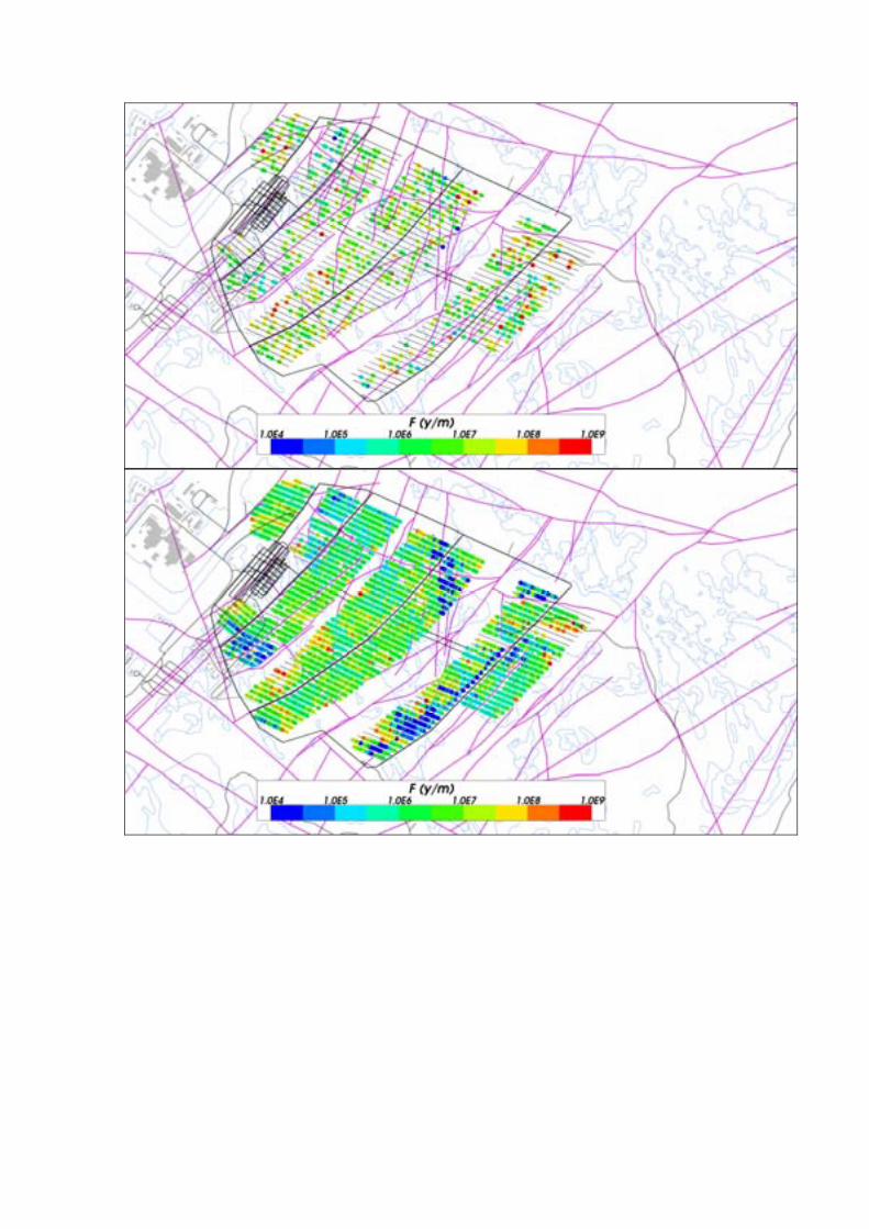
Figure E-12. Starting locations coloured by log10(Fr) for particles released at 2000 AD and successfully reaching the top boundary of the hydrogeological base case model. From the top: Q1 (24%), Q2 (83%) and Q3 (68%) release locations. The HCD model at z= -470m (purple), roads and buildings (black) and shoreline (blue) are also shown.

Figure E-13. Exit locations coloured by log10(Fr) for particles released at 2000 AD and successfully reaching the top boundary of the hydrogeological base case model. From the top: Q1 (24%), Q2 (83%) and Q3 (68%) release locations. The HCD model at z= -50m (purple), roads and buildings (black) and shoreline (blue) are also shown.

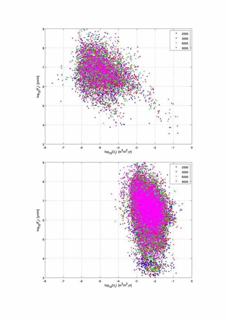
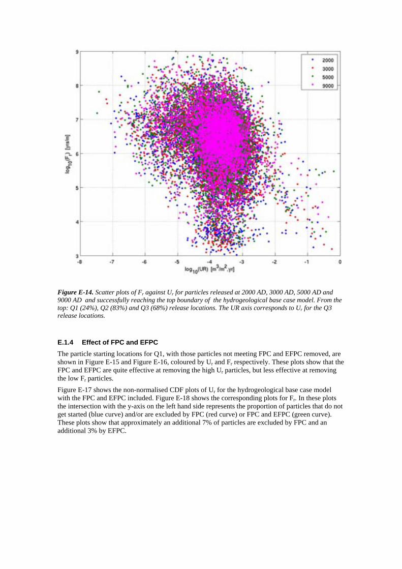
Figure E-14. Scatter plots of Fr against Ur for particles released at 2000 AD, 3000 AD, 5000 AD and 9000 AD and successfully reaching the top boundary of the hydrogeological base case model. From the top: Q1 (24%), Q2 (83%) and Q3 (68%) release locations. The UR axis corresponds to Ur for the Q3 release locations.

E.1.4 Effect of FPC and EFPC The particle starting locations for Q1, with those particles not meeting FPC and EFPC removed, are shown in Figure E-15 and Figure E-16, coloured by Ur and Fr respectively. These plots show that the FPC and EFPC are quite effective at removing the high Ur particles, but less effective at removing the low Fr particles. Figure E-17 shows the non-normalised CDF plots of Ur for the hydrogeological base case model with the FPC and EFPC included. Figure E-18 shows the corresponding plots for Fr. In these plots the intersection with the y-axis on the left hand side represents the proportion of particles that do not get started (blue curve) and/or are excluded by FPC (red curve) or FPC and EFPC (green curve). These plots show that approximately an additional 7% of particles are excluded by FPC and an additional 3% by EFPC.

Figure E-15. Starting locations coloured by log10(Ur) for Q1 particles not excluded by FPC and EFPC, released at 2000 AD and successfully reaching the top boundary of the hydrogeological base case model. The HCD model at z= -470m (purple), roads and buildings (black) and shoreline (blue) are also shown.

Figure E-16. Starting locations coloured by log10(Fr) for Q1 particles not excluded by FPC and EFPC, released at 2000 AD and successfully reaching the top boundary of the hydrogeological base case model. The HCD model at z= -470m (purple), roads and buildings (black) and shoreline (blue) are also shown.

Figure E-17. Non-normalised CDF plots of Ur in the hydrogeological base case model for the 6,916 particles released at 2000 AD, 3000 AD, 5000 AD and 9000 AD, including FPC and EFPC. From the top: Q1, Q2 and Q3 release locations respectively. The UR axis corresponds to Ur for the Q3 release locations.

Figure E-18. Non-normalised CDF plots of Fr in the hydrogeological base case model for the 6,916 particles released at 2000 AD, 3000 AD, 5000 AD and 9000 AD, including FPC and EFPC. From the top: Q1, Q2 and Q3 release locations respectively.

E.1.5 Multiple particles per start point Figure E-19 shows the exit locations for the 25% of particles with the highest Ur values for the Q2 release in the hydrogeological base case model at 2000 AD. The upper plot (blue) is for a release of ten particles per start point and the lower plot (red) is for one particle per start point. There appears to be little difference between the two plots, although there are perhaps more exit points to the north with ten particles per start point.

Figure E-20 shows the normalised CDF plots of Ur for the Q1, Q2 and Q3 release locations. They compare the one particle per start point case and the ten particles per start point case. There is very little difference between the two cases.

Figure E-21 shows the corresponding plots for Fr. Again, there is little difference between them.

Figure E-19. Exit locations for the Q2 particles successfully reaching the top boundary of the model (94%) with ten particles per start point (blue) compared with one particle per start point (red) released at 2000 AD. The particles are released from the Q2 locations with a Ur value in the top 25% in the hydrogeological base case model. Also shown is the HCD at z = -50 m (purple), roads and buildings (black) and the shoreline at 2000 AD (blue) for the repository-scale model.

Figure E-20. Normalised CDF plots for Ur for ten particles per start point (10 particles) compared with one particle per start point (1 particle) released at 2000 AD. The particles are released from the locations with an Ur value in the top 25% in the hydrogeological base case model. From the top: Q1 (83%), Q2 (94%) and Q3 (93%) release locations respectively. The UR axis corresponds to Ur for the Q3 release locations.

Figure E-21. Normalised CDF plots for Fr for ten particles per start point (10 particles) compared with one particle per start point (1 particle) released at 2000 AD. The particles are released from the locations with an Ur value in the top 25% in the hydrogeological base case model. From the top: Q1 (83%), Q2 (94%) and Q3 (93%) release locations respectively.

E.1.6 Multiple realisations Figure E-22 shows the normalised CDF plots of Ur for the Q1, Q2 and Q3 release locations for 10 stochastic realisations of the hydrogeological base case model at 2000 AD. Figure E-23 shows the corresponding bar and whisker plots. There appears to be little variability in Ur values between realisations, with up to about a quarter of an order of magnitude in the median values. However, there is a high Ur tail for realisation 9 with the Q1 release locations. Table E-1 shows the number and percentage of particles successfully reaching the top boundary of the model for the Q2 release for each realisation. The percentages are very similar, showing that there is no bias to the normalised plots caused by a different number of particles being included. Figure E-24 shows the CDF plots for Qeqr with the corresponding bar and whisker plots in Figure E-25. Here there is hardly any variability between realisations, but again there is a high Qeqr value tail for realisation 9 with the Q1 release locations. Figure E-26 shows the CDF plots for Fr with the corresponding bar and whisker plots in Figure E-27. Here there is more variability between realisations, with up to about half an order of magnitude in the median values. Realisation 5 stands out particularly with a tail at the low end of the Fr values. This is even more apparent in the CDF plots of tr in Figure E-28 and the bar and whisker plots in Figure E-29. Figure E-30 shows the distribution of the exit locations for the hydrogeological base case and the ten stochastic realisations. The lower plot just shows realisations 1, 5 and 9, which are those with the most different performance measures. The exit locations do not appear to vary significantly between realisations.

Figure E-22. Normalised CDF plots of Ur in the hydrogeological base case model (r0) and 10 stochastic realisations of the HCD and HRD (r1 to r10) for the particles successfully reaching the model top boundary, released at 2000 AD. From the top: Q1 (24%-27%), Q2 (81%-87%) and Q3 (67%-75%) release locations respectively. The UR axis corresponds to Ur for the Q3 release locations.

Table E-1 The number and percentage of particles from the Q2 release locations at 2000 AD that successfully reached the top surface of the hydrogeological base case model (r0) and for 10 stochastic realisations (r1 to r10). Realisation No. of successful

particles %

r0 5740 83

r1 5937 83

r2 5836 84

r3 5918 86

r4 6039 87

r5 5648 82

r6 5634 81

r7 5812 84

r8 5726 83

r9 5945 86

r10 5836 84

Figure E-23. Bar and whisker plots of Ur in the hydrogeological base case model (r0) and 10 stochastic realisations of the HCD and HRD (r1 to r10) for the particles that successfully started, released at 2000 AD. The statistical measures are the median (red), 25th and 75th percentile (blue bar) and the 5th and 95th percentile (black “whiskers”). From the top: Q1 (28%-31%), Q2 (100%) and Q3 (76%-83%) release locations respectively. The UR axis corresponds to Ur for the Q3 release locations.

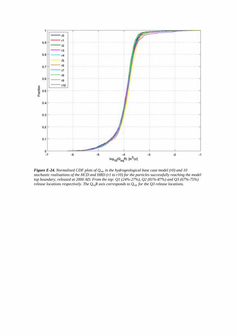
Figure E-24. Normalised CDF plots of Qeqr in the hydrogeological base case model (r0) and 10 stochastic realisations of the HCD and HRD (r1 to r10) for the particles successfully reaching the model top boundary, released at 2000 AD. From the top: Q1 (24%-27%), Q2 (81%-87%) and Q3 (67%-75%) release locations respectively. The QeqR axis corresponds to Qeqr for the Q3 release locations.

Figure E-25. Bar and whisker plots of Qeqr in the hydrogeological base case model (r0) and 10 stochastic realisations of the HCD and HRD (r1 to r10) for the particles that successfully started, released at 2000 AD. The statistical measures are the median (red), 25th and 75th percentile (blue bar) and the 5th and 95th percentile (black “whiskers”). From the top: Q1 (28%-31%), Q2 (100%) and Q3 (76%-83%) release locations respectively. The QeqR axis corresponds to Qeqr for the Q3 release locations.

Figure E-26. Normalised CDF plots of Fr in the hydrogeological base case model (r0) and 10 stochastic realisations of the HCD and HRD (r1 to r10) for the particles successfully reaching the model top boundary, released at 2000 AD. From the top: Q1 (24%-27%), Q2 (81%-87%) and Q3 (67%-75%) release locations respectively.

Figure E-27. Bar and whisker plots of Fr in the hydrogeological base case model (r0) and 10 stochastic realisations of the HCD and HRD (r1 to r10) for the particles successfully reaching the model top boundary, released at 2000 AD. The statistical measures are the median (red), 25th and 75th percentile (blue bar) and the 5th and 95th percentile (black “whiskers”). From the top: Q1 (24%-27%), Q2 (81%-87%) and Q3 (67%-75%) release locations respectively.

Figure E-28. Normalised CDF plots of tr in the hydrogeological base case model (r0) and 10 stochastic realisations of the HCD and HRD (r1 to r10) for the particles successfully reaching the model top boundary, released at 2000 AD. From the top: Q1 (24%-27%), Q2 (81%-87%) and Q3 (67%-75%) release locations respectively.

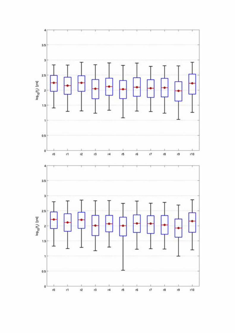
Figure E-29. Bar and whisker plots of tr in the hydrogeological base case model (r0) and 10 stochastic realisations of the HCD and HRD (r1 to r10) for the particles successfully reaching the model top boundary, released at 2000 AD. The statistical measures are the median (red), 25th and 75th percentile (blue bar) and the 5th and 95th percentile (black “whiskers”). From the top: Q1 (24%-27%), Q2 (81%-87%) and Q3 (67%-75%) release locations respectively.

Figure E-30. Top: Exit locations for the Q2 particles successfully reaching the top boundary of the model (81%-87%) at 2000 AD for all realisations of the hydrogeological base case. Bottom: Exit locations for realisations 1 (83%), 5 (82%) and 9 (86%). Also shown are the HCD at z= -50m (purple), roads and buildings (black) and the shoreline at 2000 AD (blue).

E.2 Variant models for the temperate period E.2.1 Possible deformation zones The exit locations for the three PDZ realisations shown in Figure E-31 show little variation between realisations and are similar to those for the hydrogeological base case in Figure E-30.

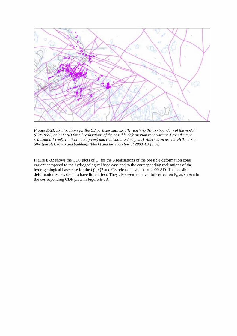
Figure E-31. Exit locations for the Q2 particles successfully reaching the top boundary of the model (83%-86%) at 2000 AD for all realisations of the possible deformation zone variant. From the top: realisation 1 (red), realisation 2 (green) and realisation 3 (magenta). Also shown are the HCD at z= -50m (purple), roads and buildings (black) and the shoreline at 2000 AD (blue).

Figure E-32 shows the CDF plots of Ur for the 3 realisations of the possible deformation zone variant compared to the hydrogeological base case and to the corresponding realisations of the hydrogeological base case for the Q1, Q2 and Q3 release locations at 2000 AD. The possible deformation zones seem to have little effect. They also seem to have little effect on Fr, as shown in the corresponding CDF plots in Figure E-33.

Figure E-32. Normalised CDF plots of Ur for 3 realisations of the possible deformation zone model (pdzr1 to pdzr3), the hydrogeological base case model (r0) and 3 stochastic realisations of the hydrogeological base case model (r1 to r3) for the particles successfully reaching the model top boundary, released at 2000 AD. From the top: Q1 (24%-25%), Q2 (83%-86%) and Q3 (70%-71%) release locations respectively. The UR axis corresponds to Ur for the Q3 release locations.

Figure E-33. Normalised CDF plots of Fr for 3 realisations of the possible deformation zone model (pdzr1 to pdzr3), the hydrogeological base case model (r0) and 3 stochastic realisations of the hydrogeological base case model (r1 to r3) for the particles successfully reaching the model top boundary, released at 2000 AD. From the top: Q1 (24%-25%), Q2 (83%-86%) and Q3 (70%-71%) release locations respectively.

E.2.2 Alternative DFN transmissivity-size relationships Figure E-34 shows the particle start points for Q1 coloured by Ur for each case. The correlated case has a greater number of high Ur values than the hydrogeological base case, but they are at a number of discrete locations, presumably associated with large stochastic fractures. For the uncorrelated case, the Ur values are higher than the hydrogeological base case generally, indicating a larger number of smaller fractures with higher transmissivities across the repository.

Figure E-35 shows the particle start points for Q1 coloured by Fr for each case. Here there is less variation between cases, with all of them showing low values at a number of discrete locations.

Figure E-36 shows the normalised CDF plots of Ur for realisation r0 of the correlated and uncorrelated cases compared to the hydrogeological base case. Realisation r0 indicates a deterministic HCD and realisation 1 of the HRD.

Figure E-37 shows the normalised CDF plots of Fr for realisation r0 of the correlated and uncorrelated cases compared to the hydrogeological base case.

Figure E-38 shows the normalised CDF plots of Ur for realisations of the correlated case compared to the hydrogeological base case.

Figure E-39 shows the normalised CDF plots of Fr for realisations of the correlated case compared to the hydrogeological base case.

Figure E-40 shows the normalised CDF plots of Ur for realisations of the uncorrelated case compared to the hydrogeological base case.

Figure E-41 shows the normalised CDF plots of Fr for realisations of the uncorrelated case compared to the hydrogeological base case.

The Q1 CDF plots show the largest variation between the different relationships compared to Q2 and Q3, with up to about half an order of magnitude variation in median Ur and Fr values between cases. The highest median Ur values for Q1 are seen in the uncorrelated case, but the correlated case has a larger proportion of particles with high Ur values (greater than 1.0·10-3 m/y). The lowest Fr values are seen for the correlated variant. There is little variation in Ur and Fr between realisations for the correlated and uncorrelated cases, apart from in Ur for realisation 5 of the correlated case.

Figure E-34. Starting locations coloured by log10(Ur) for Q1 particles released at 2000 AD and successfully reaching the top boundary of the model. Top: correlated case (31%); Middle: hydrogeological base case (24%); Bottom: uncorrelated case (27%). The HCD model at z= -470m (purple), roads and buildings (black) and shoreline (blue) are also shown.

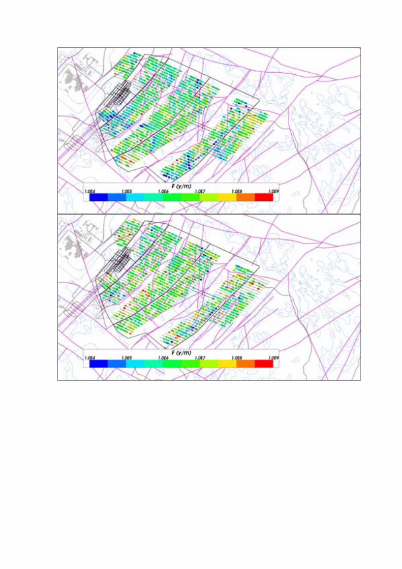
Figure E-35. Starting locations coloured by log10(Fr) for Q1 particles released at 2000 AD and successfully reaching the top boundary of the model. Top: correlated case (31%); Middle: hydrogeological base case (24%); Bottom: uncorrelated case (27%). The HCD model at z= -470m (purple), roads and buildings (black) and shoreline (blue) are also shown.

Figure E-36. Normalised CDF plots of Ur for realisation r0 of the correlated and uncorrelated transmissivity-size relationships compared to the hydrogeological base case (semi-correlated) for the particles successfully reaching the model top boundary, released at 2000 AD. Realisation r0 indicates a deterministic HCD and realisation 1 of the HRD. From the top: Q1 (24% semi-correlated, 32% correlated, 27% uncorrelated), Q2 (83% semi-correlated, 86% correlated, 72% uncorrelated) and Q3 (68% semi-correlated, 78% correlated, 64% uncorrelated) release locations respectively. The UR axis corresponds to Ur for the Q3 release locations.

Figure E-37. Normalised CDF plots of Fr for realisation r0 of the correlated and uncorrelated transmissivity-size relationships compared to the hydrogeological base case (semi-correlated) for the particles successfully reaching the model top boundary, released at 2000 AD. Realisation r0 indicates a deterministic HCD and realisation 1 of the HRD. From the top: Q1 (24% semi-correlated, 32% correlated, 27% uncorrelated), Q2 (83% semi-correlated, 86% correlated, 72% uncorrelated) and Q3 (68% semi-correlated, 78% correlated, 64% uncorrelated) release locations respectively.

Figure E-38. Normalised CDF plots of Ur for realisations of the correlated transmissivity-size relationship compared to the hydrogeological base case for the particles successfully reaching the model top boundary, released at 2000 AD. Realisation r0 indicates a deterministic HCD and realisation 1 of the HRD. From the top: Q1 (24% hydrogeological base case, 31%-36% correlated), Q2 (83% hydrogeological base case, 85%-89% correlated) and Q3 (68% hydrogeological base case, 74%-80% correlated) release locations respectively. The UR axis corresponds to Ur for the Q3 release locations.

Figure E-39. Normalised CDF plots of Fr for realisations of the correlated transmissivity-size relationship compared to the hydrogeological base case for the particles successfully reaching the model top boundary, released at 2000 AD. Realisation r0 indicates a deterministic HCD and realisation 1 of the HRD. From the top: Q1 (24% hydrogeological base case, 31%-36% correlated), Q2 (83% hydrogeological base case, 85%-89% correlated) and Q3 (68% hydrogeological base case, 74%-80% correlated) release locations respectively.

Figure E-40. Normalised CDF plots of Ur for realisations of the uncorrelated transmissivity-size relationship compared to the hydrogeological base case for the particles successfully reaching the model top boundary, released at 2000 AD. Realisation r0 indicates a deterministic HCD and realisation 1 of the HRD. From the top: Q1 (24% hydrogeological base case, 26%-30% uncorrelated), Q2 (83% hydrogeological base case, 72%-80% uncorrelated) and Q3 (68% hydrogeological base case, 64%-72% uncorrelated) release locations respectively. The UR axis corresponds to Ur for the Q3 release locations.

Figure E-41. Normalised CDF plots of Fr for realisations of the uncorrelated transmissivity-size relationship compared to the hydrogeological base case for the particles successfully reaching the model top boundary, released at 2000 AD. Realisation r0 indicates a deterministic HCD and realisation 1 of the HRD. From the top: Q1 (24% hydrogeological base case, 26%-30% uncorrelated), Q2 (83% hydrogeological base case, 72%-80% uncorrelated) and Q3 (68% hydrogeological base case, 64%-72% uncorrelated) release locations respectively.

E.2.3 Unmodified vertical hydraulic conductivity The particle exit locations, shown in Figure E-42, for both the hydrogeological base case and the unmodified vertical hydraulic conductivity case for the site-scale model at 2000 AD show similar distributions. The CDF plots of Ur and Fr, shown in Figure E-43 and Figure E-44 respectively, are very similar.

Figure E-42. Exit locations for the Q2 particles successfully reaching the top boundary of the site-scale model (94%) at 2000 AD for the hydrogeological base case (blue) and the unmodified vertical hydraulic conductivity case (red). Also shown are the HCD at z= -50m (purple), roads and buildings (black) and the shoreline at 2000 AD (blue).

Figure E-43. Normalised CDF plots of Ur for the hydrogeological base case site-scale model and the unmodified vertical hydraulic conductivity site-scale model (Unmodified) for the particles successfully reaching the model top boundary, released at 2000 AD. From the top: Q1 (70%), Q2 (94%) and Q3 (91%) release locations respectively.

Figure E-44. Normalised CDF plots of Fr for the hydrogeological base case site-scale model and the unmodified vertical hydraulic conductivity site-scale model (Unmodified) for the particles successfully reaching the model top boundary, released at 2000 AD. From the top: Q1 (70%), Q2 (94%) and Q3 (91%) release locations respectively.

E.2.4 Extended spatial variability Figure E-45 shows the particle exit locations for the hydrogeological base case and extended spatial variability case at the selected release times. For the extended spatial variability case there are fewer particles at the north-east boundary and fewer at intermediate locations, although there are some extra locations at the north of the model.

The CDF plots of Ur in Figure E-46 and Fr in Figure E-47 show that the extended spatial variability has little effect on performance measures. However, the CDF plots for Fr do not include the contribution from the ECPM and CPM. Figure E-48 shows the corresponding plots with the CPM and ECPM contribution included. The contribution from the ECPM and CPM has little effect at 2000 AD and 3000 AD for both cases, but adds up to about half an order of magnitude to the mean Fr values for 5000 AD and 9000 AD because a greater proportion of the particle pathways are in the ECPM and CPM at the later release times. However, the increase in Fr is not as great for the extended spatial variability case, implying that a lesser proportion of the particle pathways are in the ECPM/CPM than for the hydrogeological base case.

Figure E-45. Exit locations for the Q2 particles successfully reaching the top boundary of the site-scale model (89%-94%) at 2000 AD, 3000 AD, 5000 AD and 9000 AD. Top: Hydrogeological base case. Bottom: Extended spatial variability case. The HCD model at z= -50m (purple), roads and buildings (black) and shoreline at 2000 AD (blue) are also shown.

• 2000 AD• 3000 AD• 5000 AD• 9000 AD

• 2000 AD• 3000 AD• 5000 AD• 9000 AD

Figure E-46. Normalised CDF plots of Ur in the extended spatial variability (ext. var.) site-scale and hydrogeological base case (base case) site-scale models for the particles successfully reaching the model top boundary, released at 2000 AD, 3000 AD, 5000 AD and 9000 AD. From the top: Q1 (67%-70%), Q2 (88%-94%) and Q3 (85%-90%) release locations respectively.

Figure E-47. Normalised CDF plots of Fr in the extended spatial variation (ext. var.) site-scale and hydrogeological base case (base case) site-scale models for the particles successfully reaching the model top boundary, released at 2000 AD, 3000 AD, 5000 AD and 9000 AD. From the top: Q1 (67%-70%), Q2 (88%-94%) and Q3 (85%-90%) release locations respectively.

Figure E-48. Normalised CDF plots of Fr, including the contribution from the ECPM and CPM, in the extended spatial variability (ext. var.) site-scale and hydrogeological base case (base case) site-scale models for the particles successfully reaching the model top boundary, released at 2000 AD, 3000 AD, 5000 AD and 9000 AD. From the top: Q1 (67%-70%), Q2 (88%-94%) and Q3 (85%-90%) release locations respectively.

E.2.5 Tunnel variants The Ur CDF plots for Q1 at 2000 AD in Figure E-49 for the hydrogeological base case, crown space case, EDZ with T=1·10-7 m2/s, EDZ with T=1·10-6 m2/s and no EDZ cases are almost identical. For Q2, the crown space Ur CDF plot is almost identical to the hydrogeological base case. The case with EDZ T=1·10-7 m2/s gives an order of magnitude increase in the median Ur value in the EDZ for Q2 and the case with EDZ T=1·10-6 m2/s gives a further order of magnitude increase. The no EDZ plot for Q2 is not possible by definition. The median Ur values for Q2 are: hydrogeological base case = 4.0·10-3 m/y, crown space = 4.0·10-3 m/y, EDZ T=1·10-7 = 2.5·10-2 m/y and EDZ T=1·10-6 = 1.7·10-1 m/y. For the Q3 CDF plots, the crown space causes about one order of magnitude increase in the median Ur value in the first fracture, the case with EDZ T=1·10-6 m2/s gives about two orders of magnitude increase, the case with EDZ T=1·10-7 m2/s gives about one order of magnitude increase and the no EDZ case gives about one order of magnitude decrease. The flow-related transport resistance CDF plots for Q1and Q3 in Figure E-50 show that the no EDZ case has significantly higher Fr than the other cases.

Figure E-49. Normalised CDF plots of Ur for the hydrogeological base case model, the crown space case, the EDZ T=1·10-7 m2/s case, the EDZ T=1·10-6 m2/s case and the no EDZ case for the particles successfully reaching the model top boundary, released at 2000 AD. From the top: Q1 (14% no EDZ, 23%-24% others), Q2 (82%-84%) and Q3 (68% hydrogeological base case, 81% crown space, 64% EDZ T=1·10-7, 53% EDZ T=1·10-6, 52% no EDZ) release locations respectively. The UR axis corresponds to Ur for the Q3 release locations.

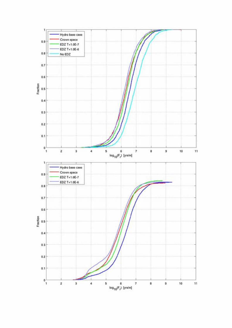
Figure E-50. Normalised CDF plots of Fr for the hydrogeological base case model, the crown space case, the EDZ T=1·10-7 m2/s case, the EDZ T=1·10-6 m2/s case and the no EDZ case for the particles successfully reaching the model top boundary, released at 2000 AD. From the top: Q1 (14% no EDZ, 23%-24% others), Q2 (82%-84%) and Q3 (68% hydrogeological base case, 81% crown space, 64% EDZ T=1·10-7, 53% EDZ T=1·10-6, 52% no EDZ) release locations respectively.

E.2.6 Effect of boreholes These results are presented in Appendix G.

E.3 Glacial conditions E.3.1 Glacial ice front location II The CDF plots of Ur in Figure E-51 show that the median Ur value for Q1 has increased by an order of magnitude from 1·10-5 m/y to 1·10-4 m/y for the glacial ice front location II case compared to the 2000 AD hydrogeological base case, whereas the median Ur value for Q2 has increased over two orders of magnitude from 3·10-1 m/y to 5·10-3 m/y and the median flux for Q3 has also increased by approximately two orders of magnitude from 8·10-6 m/y to 4·10-4 m/y.

A reduction of over an order of magnitude in median Fr values can be seen in Figure E-52.

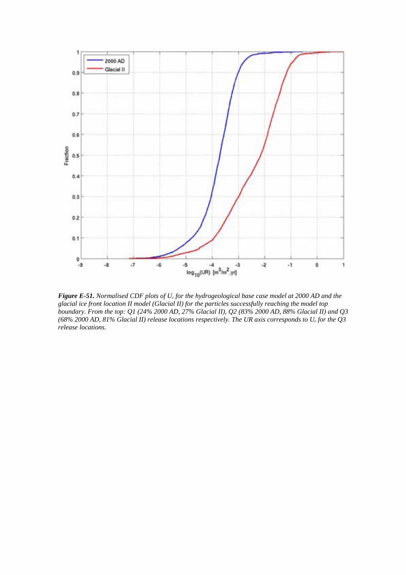
Figure E-51. Normalised CDF plots of Ur for the hydrogeological base case model at 2000 AD and the glacial ice front location II model (Glacial II) for the particles successfully reaching the model top boundary. From the top: Q1 (24% 2000 AD, 27% Glacial II), Q2 (83% 2000 AD, 88% Glacial II) and Q3 (68% 2000 AD, 81% Glacial II) release locations respectively. The UR axis corresponds to Ur for the Q3 release locations.

Figure E-52. Normalised CDF plots of Fr for the hydrogeological base case model at 2000 AD and the glacial ice front location II model (Glacial II) for the particles successfully reaching the model top boundary. From the top: Q1 (24% 2000 AD, 27% Glacial II), Q2 (83% 2000 AD, 88% Glacial II) and Q3 (68% 2000 AD, 81% Glacial II) release locations respectively.

E.3.2 Glacial ice front location I Figure E-53 shows the exit locations of the Q2 particles for the two ice front locations and for the hydrogeological base case site-scale model at 2000 AD. For ice front location I, the exit locations are shifted slightly to the east due to the change in the pressure gradient. For ice front location II, the exit locations have moved to the southeast due to the strong pressure gradient in that direction.

The CDF plots of Ur in Figure E-54 and Fr in Figure E-55 show that ice front location II has a much greater effect on the performance measures than ice front location I.

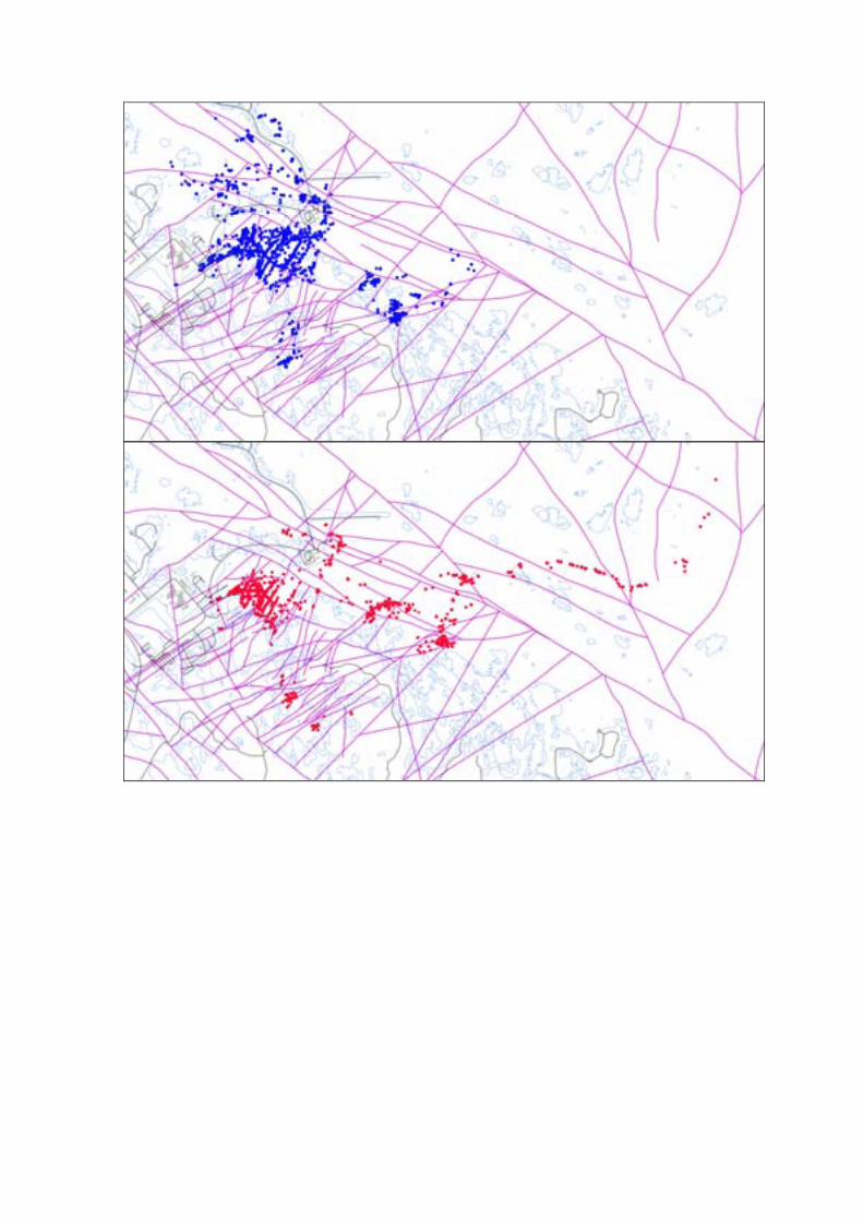
Figure E-53. Exit locations for the Q2 particles successfully reaching the top boundary of the site-scale mode (93%-97%). From the top: they hydrogeological base case model at 2000 AD (blue), ice front location I (red) and ice front location II (green). Also shown are the HCD at z= -50m (purple), roads and buildings (black) and the shoreline at 2000 AD (blue).

Figure E-54. Normalised CDF plots of Ur for the hydrogeological base case site-scale model at 2000 AD, the ice front location I site-scale model (Glacial I) and the ice front location II site-scale model (Glacial II) for the particles successfully reaching the model top boundary. From the top: Q1 (70% 2000 AD, 67% Glacial I, 81% Glacial II), Q2 (94% 2000 AD, 93% Glacial I, 97% Glacial II) and Q3 (90% 2000 AD, 89% Glacial I, 95% Glacial II) release locations respectively.

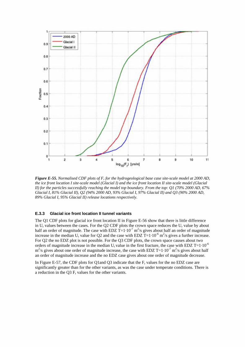
Figure E-55. Normalised CDF plots of Fr for the hydrogeological base case site-scale model at 2000 AD, the ice front location I site-scale model (Glacial I) and the ice front location II site-scale model (Glacial II) for the particles successfully reaching the model top boundary. From the top: Q1 (70% 2000 AD, 67% Glacial I, 81% Glacial II), Q2 (94% 2000 AD, 93% Glacial I, 97% Glacial II) and Q3 (90% 2000 AD, 89% Glacial I, 95% Glacial II) release locations respectively.

E.3.3 Glacial ice front location II tunnel variants The Q1 CDF plots for glacial ice front location II in Figure E-56 show that there is little difference in Ur values between the cases. For the Q2 CDF plots the crown space reduces the Ur value by about half an order of magnitude. The case with EDZ T=1·10-7 m2/s gives about half an order of magnitude increase in the median Ur value for Q2 and the case with EDZ T=1·10-6 m2/s gives a further increase. For Q2 the no EDZ plot is not possible. For the Q3 CDF plots, the crown space causes about two orders of magnitude increase in the median Ur value in the first fracture, the case with EDZ T=1·10-6 m2/s gives about one order of magnitude increase, the case with EDZ T=1·10-7 m2/s gives about half an order of magnitude increase and the no EDZ case gives about one order of magnitude decrease. In Figure E-57, the CDF plots for Q1and Q3 indicate that the Fr values for the no EDZ case are significantly greater than for the other variants, as was the case under temperate conditions. There is a reduction in the Q3 Fr values for the other variants.

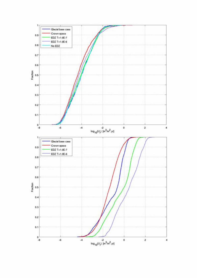
Figure E-56. Normalised CDF plots of Ur for the glacial ice front location II base case model, the crown space case, the EDZ T=1·10-7 m2/s case, the EDZ T=1·10-6 m2/s case and the no EDZ case for the particles successfully reaching the model top boundary. From the top: Q1 (18% no EDZ, 25%-27% others), Q2 (85%-89%) and Q3 (81% glacial base case, 86% crown space, 78% EDZ T=1·10-7, 73% EDZ T=1·10-6, 69% no EDZ) release locations respectively. The UR axis corresponds to Ur for the Q3 release locations.

Figure E-57. Normalised CDF plots of Fr for the glacial ice front location II base case model, the crown space case, the EDZ T=1·10-7 m2/s case, the EDZ T=1·10-6 m2/s case and the no EDZ case for the particles successfully reaching the model top boundary. From the top: Q1 (18% no EDZ, 25%-27% others), Q2 (85%-89%) and Q3 (81% glacial base case, 86% crown space, 78% EDZ T=1·10-7, 73% EDZ T=1·10-6, 69% no EDZ) release locations respectively.

E.3.4 Glacial ice front location II and III recharge pathways The Q1 CDF plots of Ur, Fr and tr for the recharge pathways for the extended spatial variability case with glacial ice front location II and location III conditions are shown in Figure E-58. The two cases are quite similar, although the ice front location III case has slightly higher Fr and tr values. Figure E-59 and Figure E-60 show the back paths and recharge locations for the glacial ice front location II and ice front location III extended spatial variability cases respectively. There is little difference between the two cases, with recharge taking place mostly at the north western boundary of the model, with some recharge locations closer to the site. These are similar to the results given in Figure F-4 for the base case glacial ice front location II model.

Figure E-58. Normalised CDF plots of Ur (top), Fr (middle) and tr (bottom) for the extended spatial variability model at glacial ice front location II (Glacial II ext. var.) and glacial ice front location III (Glacial III ext. var.) for the Q1 particles successfully reaching the model top boundary (23% glacial II, 24% glacial III).

Figure E-59. Recharge pathways (purple) for the Q1 particles successfully reaching the top boundary of the extended spatial variability model for glacial ice front location II. Top: map view; Bottom: Oblique view from south.

Figure E-60. Recharge pathways (purple) for the Q1 particles successfully reaching the top boundary of the extended spatial variability model for glacial ice front location III. Top: map view; Bottom: Oblique view from south.

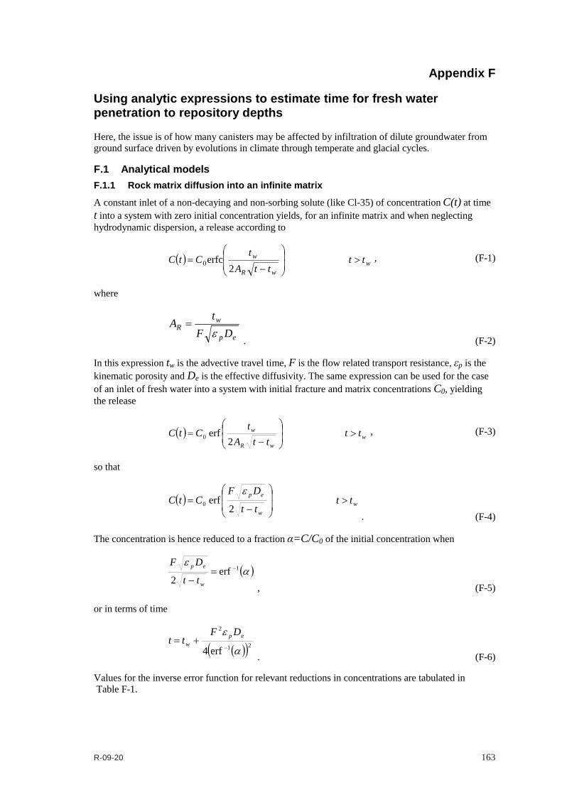
R-09-20 163

Appendix F

Using analytic expressions to estimate time for fresh water penetration to repository depths

Here, the issue is of how many canisters may be affected by infiltration of dilute groundwater from ground surface driven by evolutions in climate through temperate and glacial cycles.

F.1 Analytical models F.1.1 Rock matrix diffusion into an infinite matrix

A constant inlet of a non-decaying and non-sorbing solute (like Cl-35) of concentration C(t) at time t into a system with zero initial concentration yields, for an infinite matrix and when neglecting hydrodynamic dispersion, a release according to

wwR

w ttttA

tCtC

2erfc0 , (F-1)

where

ep

wR DF

tA

. (F-2)

In this expression tw is the advective travel time, F is the flow related transport resistance, εp is the kinematic porosity and De is the effective diffusivity. The same expression can be used for the case of an inlet of fresh water into a system with initial fracture and matrix concentrations C0, yielding the release

wwR

w ttttA

tCtC

2erf0

, (F-3)

so that

ww

ep tttt

DFCtC

2erf0

. (F-4)

The concentration is hence reduced to a fraction α=C/C0 of the initial concentration when

1erf2

w

ep

tt

DF

, (F-5)

or in terms of time

21

2

erf4

epw

DFtt

. (F-6)

Values for the inverse error function for relevant reductions in concentrations are tabulated in Table F-1.

164 R-09-20

Table F-1 Tabulated values of the inverse of the error function for relevant values of α. α erf-1(α) 0.1 0.088856 0.01 0.008863 0.001 0.000886 0.0001 0.000089

F.1.2 Equilibrium transport conditions for a finite matrix Alternatively, the effects of retardation by rock matrix diffusion into a finite matrix can be considered. Assuming advection is sufficiently slow to allow equilibrium transport conditions to apply then the retardation factor for the advance of a mixing front can be written as

Ftt mpw

, (F-7)

where δm is the average half size of matrix blocks, i.e. half the flowing fracture spacing.

Combining these two formulae an estimate of the breakthrough of dilute groundwater to a canister location can then be estimated as

F

DFtt mp

epw

,

erf4min

21

2

(F-8)

Equation (F-6) gives the smaller retardation times for low values of F less than about 3 105 y/m, and Equation (F-7) gives the smaller retardation times at larger F values when the assumption of a finite matrix becomes important.

F.2 Application to transport of dilute surface water to repository depth The above formulae can be used to estimate the timescale for dilute groundwater to penetrate from ground surface to repository depth for each deposition hole given the advective travel time and F for the pathway between the top surface and the deposition hole. These can be calculated by performing backward pathlines (i.e. following the upstream trajectory rather than usual downstream trajectory) with a particle released into any fractures surrounding the deposition hole. Dilute groundwater can infiltrate the bedrock during any of the three main climate situations given in Table F-2, and hence groundwater flow conditions and associated transport pathways have to be evaluated for each of these three cases. Dilute groundwater is judged to have reached the repository if the transport time predicted by Equation (F-8) is less than the duration for which the associated conditions persist.

In summary, the approach used is as follows:

Consider each climate situation separately;

Calculate steady-state flow for fixed but spatially variable-density field;

Calculate backward (recharge) pathlines to identify tw and F for the recharge pathway to each canister;

Calculate forward (discharge) pathlines to calculate tw, U0 and F for discharge paths;

R-09-20 165

Calculate retardation times for dilute groundwater based on Equation (F-8) using tw and F for backward pathway, and compare these times with the duration of the climate situation ;

Consider F for the forward (discharge) pathways from those locations with dilute water breakthrough times less than the epoch duration.

Table F-2 The three climate situations considered during which dilute groundwaters may penetrate to repository depth. Climate situation Duration Comments

Temperate 10,000 to 60,000 y 60,000 y is a global warming scenario. Use situation at 2,000 AD Injection of meteoric water of zero salinity.

Ice front over site 20 – 100 y Ice sheet advance 50 m/y, retreat 300 m/y. Use Glacial II situation. Injection of glacial melt water of zero salinity at high velocities for short duration. Calculate duration based on time for ice front to move 5 km across the site, although highest velocities at a particular location probably only last 5-20 y.

Ice sheet over site 20,000 – 100,000 y Lasts about 20,000 y in /Vidstrand et al. 2010/. Glaciations in the Pleistocene may have lasted ~ 100,000 y Use Glacial V situation. Injection of glacial melt water of zero salinity at low velocities for long duration.

Other notes:

The hydrogeological base case (as specified in Section 4) and glacial variants (as specified in Section 5.7) are used to determine recharge/discharge pathways;

The hydrogeological base case and glacial variants are used to derive tw, F, FPC, and EFPC for each deposition hole;

The calculated travel times and F used are for transport within fracture domains FFM01-FFM06 that are represented by an explicit DFN model. Travel time and retention in the CPM outside of this have not been included. Also, to be conservative, no retardation in tunnels is included, although this could be large;

Only the hydrogeological base case semi-correlated model is considered.

166 R-09-20

F.2.1 Groundwater flows during the different climate situations Temperate

Figure F-1 and Figure F-2 show hydrogeological base case simulations of regional flow paths under temperate conditions. There are a few paths that recharge just above the site, some recharge in the valley to the south around the Forsmark deformation zone, while the majority recharge on the high ground to the south with flow circulating to the full depth of the model.

Figure F-1. Simulations of discharge points (orange) and recharge points (purple) for a release from all deposition holes in the flow field under temperate conditions at 2000 AD.

R-09-20 167

Figure F-2. Simulations of discharge pathways (orange) and recharge pathways (purple) for a release from all deposition holes in the flow field under temperate conditions at 2000 AD. Top: map view; Bottom: Oblique view from south.

168 R-09-20

Ice front over site

Figure F-3 and Figure F-4 show forward and backward paths for Glacial position II when the ice front is above the western most main tunnel. Discharge occurs just southeast of the repository area while recharge takes place mainly on the western boundary of the model. Again, recharge paths generally circulate to depth with upward flow just ahead of the ice front.

Figure F-3. Simulations of discharge points (orange) and recharge points (purple) for a release from all deposition holes in the flow field for the ice front over the site conditions (Glacial II position).

R-09-20 169

Figure F-4. Simulations of discharge pathways (orange) and recharge pathways (purple) for a release from all deposition holes in the flow field for the ice front over the site conditions (Glacial II position). Top: map view; Bottom: Oblique view from south.

170 R-09-20

Ice sheet over site

Figure F-5 and Figure F-6 show the recharge and discharge pathways for flow under conditions of ice front location V. Discharge occurs to the southeast, some on the top surface, but a majority on the eastern boundary of the model. Some recharge comes from the top surface to the northwest, but the majority comes from the western boundary of the model. Recharge pathways generally circulate to depth. Discharge pathways are more distributed between upward shallow paths and deep circulating paths.

In summary, for all three climate situations, recharge pathways are generally longer than discharge paths, and recharge to the repository area is often upward. This suggests under many conditions the repository area may be replenished by old brackish water possibly mixed with dilute groundwater from the surface. Such deep circulating water would suggest the predominant situation is that the repository is recharged by a mixture of old brackish water and more recent surface derived meteoric or glacial melt water. There are exceptions though under all three climate situations where recharge is from the surface and relatively close to the site. Hence, the focus of the analysis below is on these restricted set of canister locations where the recharge pathway originates close to the surface. Recharge points above -300 m were used to discern recharge pathways of shallow origin (possibly starting on the model sides), bringing dilute groundwater down, from recharge from depth of presumably more saline water.

Both forward and backward paths were performed using the detailed repository-scale DFN models and site-scale DFN models to give realistic estimates of tw and F.

Figure F-5. Simulations of discharge points (orange) and recharge points (purple) for a release from all deposition holes in the flow field for the ice sheet over the site conditions (Glacial V position).

R-09-20 171

Figure F-6. Simulations of discharge pathways (orange) and recharge pathways (purple) for a release from all deposition holes in the flow field for ice sheet over the site conditions (Glacial V position). Top: map view; Bottom: Oblique view from south.

172 R-09-20

F.2.2 Evaluation of dilute groundwater mixing times The following lists the parameters used to estimate the time for groundwater to dilute the deposition holes.

General parameters

• Use De=4 10-14 m2/s, or 1.26 10-6 m2/y, based on recommendations for NaCl given in Appendix C (similar values are also appropriate for cations);

• Use εp= 3.7 10-3 as used in the palaeo-hydrogeology simulations ;

• Use δm = 12.5 m, the approximate spacing of PFLs (Based on Terzaghi corrected spacing of flowing features 1/(2·P10PFL,corr) from Table 10-22 to Table 10-24 /Follin et al. 2007a/ for depths between -200m and -400m);

• erf-1(0.1)=0.089, i.e. α=0.1.

where α represents the dilution factor. The salinity criterion for buffer erosion is 0.3 g/L, which represents the dilute conditions with the potential for buffer erosion to occur. The present day salinity (TDS) at repository depth is about 10 g/L and the initial salinity before the onset of the glacial period is estimated to be 3 g/L. As an illustration, two values of α were considered. An α of 0.1 would give a dilution to about 1 g/L TDS at repository depth for the temperate period, which is above the criterion of 0.3 g/L and so could be viewed as a conservative estimate. An α of 0.1 would give a dilution to about 0.3 g/L TDS at repository depth for the glacial period, which matches the salinity criterion for potential buffer erosion. An α of 0.02 would give a dilution to about 0.2 g/L TDS at repository depth for the temperate period and 0.06 g/L for the glacial period, which is below the salinity criterion and provides a sensitivity measure.

In equating δm with the spacing of PFLs there is an implicit assumption that infiltrating water from the surface equilibrates between the fractures and surrounding matrix at least along pathways between the surface and repository depth. There is some data available from the site to suggest that the fracture and matrix waters are in equilibrium, at least in the upper bedrock above about -300 m, that is relevant to recharge between the surface and repository depth, see Figure F-7 for chloride in KFM01D. The uncertainty associated with oxygen isotope measurements in porewater are much larger than chloride making it difficult to assess whether glacial related tracers are in equilibrium. Therefore, it is concluded that there is some field evidence to support equilibrium conditions between fracture and matrix water in mid depths around -200 m to -400 m where the flow conductive fracture spacing is about 12.5 m, and hence it seems reasonable to use this as an estimate for the diffusion depth for water percolating between the surface and the repository.

A summary of the specific assumptions made in analysing each of the three climate states are given below.

R-09-20 173

KFM01DCl, 2000AD

-1000

-900

-800

-700

-600

-500

-400

-300

-200

-100

00 5000 10000 15000 20000 25000

Cl (mg/L)

Elev

atio

n (m

)Cl mg/L KFM01D

Cl mg/L KFM01D Porewater

Possible DZ, 6m

Possible DZ, 7m

ZFMENE0061, 21m

Possible DZ, 6m

Figure F-7. Comparison of Chloride concentrations in groundwater samples from fractures (squares) and porewater (open circles) for KFM01D.

Temperate

Used hydrogeological base case model;

Only use backward paths with OKFLAG=0 (complete path);

Eliminate FPC+EFPC positions;

663 positions remain for backward paths;

Cf. 1169 paths for forward paths.

Ice front over site

Used hydrogeological variant model based on Ice front location II;

Only use backward paths with OKFLAG=0 (complete path);

Eliminate FPC+EFPC positions;

174 R-09-20

983 positions remain for backward paths;

Cf. 1400 paths for forward paths.

Ice sheet over site

Used hydrogeological variant model based on Ice front location V;

Only use backward paths with OKFLAG=0;

Eliminate FPC+EFPC positions;

589 positions remain for backward paths;

Cf. 741 paths for forward paths.

Results

Table F-3 gives estimates of the numbers of deposition holes that become critically diluted by the end of each climate situation. The sensitivity to the duration of the climate situation and the critical dilution factor are quantified. The largest number of positions at risk from dilute groundwater comes from the case when the ice sheet moves directly over the site, followed by the temperate situation. The situation when the ice sheet is over the site gives the fewest positions at risk despite it having the longest duration.

Figure F-8 shows the cumulative distribution of transport times for dilute water to reach the canister positions under temperate conditions. If this epoch lasts only 10,000 years then 52 positions are effected. If the epoch lasts 60,000 years, then 166 positions are effected. The question then is whether these small proportion of positions correlate with low F values for discharge pathways. This is evaluated in Figure F-9 as a cross-plot of F values for forward and backward paths. 11 of these locations have F values below 105 y/m, and none have a F value below 104 y/m.

The equivalent plots for conditions with an ice front at the western end of the repository are shown in Figure F-10 and Figure F-11. There are 77 locations with dilute groundwater after 20 years and 147 after 100 years. F values for the discharge pathways from these locations are higher, with 18 <104 y/m.

The equivalent plots for conditions with an ice sheet completely over the site are shown in Figure F-12 and Figure F-13. There are 37 locations with dilute groundwater after 20,000 years and 157 after 100,000 years. One of these locations has F values below 105 y/m.

The positions of deposition holes at risk from dilute groundwater are shown in Figure F-14. Interestingly, these positions usually tend to cluster close to areas of high deformation zone intensity, and some are consistent under all three climate situations (circled).

Table F-3. Estimates of numbers of deposition holes that become critically diluted by the end of each climate situation. Sensitivities to the duration of the climate situation and critical dilution factor are considered. Duration Dilution factor=0.1 Dilution factor=0.02 Temperate 10,000 y 52 42 60,000 y 166 166

Ice front over site 20 y 77 16 100 y 147 32

Ice sheet over site 20,000 y 37 37 100,000 y 157 157

R-09-20 175

0.00

0.02

0.04

0.06

0.08

0.10

0.12

0.14

0.16

0.18

0.20

1 10 100 1,000 10,000 100,000 1,000,000 10,000,000 100,000,000

Time for dilute water penetration (y)

Frac

tion

Flow at 2000 AD

Base case~10,000 yGlobal warming~60,000 y

Figure F-8. Estimates of time for penetration of dilute groundwater under temperate conditions based on Equation (F-8) for backward paths. The vertical lines indicate the duration of the initial temperate period: Base case~10,000 years (purple), Global warming variant~60,000 years (green).

1.0E+00

1.0E+01

1.0E+02

1.0E+03

1.0E+04

1.0E+05

1.0E+06

1.0E+07

1.0E+08

1.0E+09

1.0E+00 1.0E+01 1.0E+02 1.0E+03 1.0E+04 1.0E+05 1.0E+06 1.0E+07 1.0E+08

F for backward path (y/m)

F fo

r for

war

d pa

th (y

/m)

Dilute before 10,000 y

Dilute before 60,000 y

Figure F-9. Cross-plot of F for the forward (discharge) pathway and backward (recharge) pathway under temperate conditions for canister positions with times to dilution less than the epoch duration.

176 R-09-20

0.00

0.02

0.04

0.06

0.08

0.10

0.12

0.14

0.16

0.18

0.20

1 10 100 1,000 10,000 100,000 1,000,000 10,000,000 100,000,000

Time for dilute water penetration (y)

Frac

tion

Flow at ice location II

Retreat~20 yAdvance~100 y

Figure F-10. Estimates of time for penetration of dilute groundwater under Glacial II conditions based on Equation (F-8) for backward paths. The vertical lines indicate the duration of the ice advance/retreat periods.

1.0E+00

1.0E+01

1.0E+02

1.0E+03

1.0E+04

1.0E+05

1.0E+06

1.0E+07

1.0E+08

1.0E+09

1.0E+00 1.0E+01 1.0E+02 1.0E+03 1.0E+04 1.0E+05 1.0E+06 1.0E+07 1.0E+08

F for backward path (y/m)

F fo

r for

war

d pa

th (y

/m)

Dilute before 20 y

Dilute before 100 y

Figure F-11. Cross-plot of F for the forward (discharge) pathway and backward (recharge) pathway under Glacial II conditions for canister positions with times to dilution less than the epoch duration.

R-09-20 177

0.00

0.02

0.04

0.06

0.08

0.10

0.12

0.14

0.16

0.18

0.20

1 10 100 1,000 10,000 100,000 1,000,000 10,000,000 100,000,000

Time for dilute water penetration (y)

Frac

tion

Flow at ice location V

Ice sheet~20,000 yIce sheet~100,000 y

Figure F-12. Estimates of time for penetration of dilute groundwater under Glacial V conditions based on Equation (F-8) for backward paths. The vertical lines indicate the duration of the ice advance/retreat periods.

1.0E+00

1.0E+01

1.0E+02

1.0E+03

1.0E+04

1.0E+05

1.0E+06

1.0E+07

1.0E+08

1.0E+09

1.0E+00 1.0E+01 1.0E+02 1.0E+03 1.0E+04 1.0E+05 1.0E+06 1.0E+07 1.0E+08

F for backward path (y/m)

F fo

r for

war

d pa

th (y

/m)

Dilute before 20,000 y

Dilute before100,000 y

Figure F-13. Cross-plot of F for the forward (discharge) pathway and backward (recharge) pathway under Glacial V conditions for canister positions with times to dilution less than the epoch duration.

178 R-09-20

Figure F-14. Deposition holes at risk from dilute groundwater infiltration. Holes at risk during the temperate period are coloured green; holes at risk during the Ice front (Glacial II) period are coloured red; holes at risk during the Ice sheet (Glacial V) period are coloured blue. The deformation zones at -470 m are shown in purple. Areas with several holes at risk under all 3 situations are circled.

Extended spatial variability

The recharge and discharge particle pathways for the glacial ice front location II and III cases were also calculated using the extended spatial variability model. The performance measures and particle pathways for these cases are given in sections 6.4.4 and E.3.4. An analysis of dilute water penetration for a dilution factor of 0.1 was also carried out for the extended spatial variability case with ice front location II and compared to the hydrogeological base case with ice front location II.

Table F-4 gives estimates of the numbers of deposition holes that become critically diluted by the end of the glacial ice front location II climate situation for the two models. There is a reduction of 30-40% in the number of deposition holes affected when the extra F from the recharge pathway through the extended DFN is included.

Figure F-15 shows the cumulative distribution of transport times for dilute water to reach the canister positions under glacial ice front location II conditions for the extended spatial variability case.

R-09-20 179

Table F-4 Estimates of numbers of deposition holes that become critically diluted by the end of the glacial ice front location II climate situation for the hydrogeological base case model and the extended spatial variability model. Duration Dilution factor=0.1 Hydrogeological base case 20 y 77 100 y 147

Extended spatial variability 20 y 44 100 y 99

0.00

0.02

0.04

0.06

0.08

0.10

0.12

0.14

0.16

0.18

0.20

1 10 100 1,000 10,000 100,000 1,000,000 10,000,000 100,000,000

Time for dilute water penetration (y)

Frac

tion

Flow at ice location II

Retreat~20yAdvance~100y

Figure F-15. Estimates of time for penetration of dilute groundwater under Glacial II conditions for the extended spatial variability case based on Equation (F-8) for backward paths. The vertical lines indicate the duration of the ice advance/retreat periods.

F.3 Conclusions During the situation when the ice front is over the site about 2% of canister locations might be recharged by dilute groundwater, although the period of high flows at a particular location may only last around 10 years, which would bring the proportion affected to about 0.7%. For the extended spatial heterogeneity model under the same conditions the proportion of canisters affected is between 0.6% and 1.4%, depending on duration. The proportion affected under temperate conditions is between about 0.7% and 2.4%, depending on duration, and only 0.5% when an ice sheet covers the site. These results are moderately sensitive to the assumed diffusivity into the matrix and dilution factor.

The locations where times for dilute recharge are short do not necessarily correlate with locations of very low F or initial flux, although they do tend to cluster around areas of high deformation zone intensity.

R-09-20 181

Appendix G

Effect of Boreholes Results

G.1 Effect on flow In Table G-1 a summary of the modelled borehole cases is shown. Together with the case name and block where the borehole is placed, a brief description of the model environment in the vicinity of the borehole is given for each case. The case type refers to a borehole type described in Table 5-4. The columns “No. of PART Q* in BH” show the number of particles that enter the borehole when releasing particles from the Q1, Q2 and Q3 release locations respectively. The column “Total no. of PART” shows the total number of released particles for the particular case. The column “Q3 PART in BH/Tot. PART [%]” shows the ratio of particles from the Q3 release location entering the borehole to the total number of released particles for the case of interest as a percentage.

It is clear that the presence of an open borehole has an effect on the flow in the model. In all cases but one, ABH2b3, particles are attracted to the borehole. These results take into account all unique particles that enter the boreholes even if the path length along the borehole is short. Even so, in 16 out of the modelled 33 cases more than 5% of the released particles at some point enter the borehole. Eight cases have more than 10% of the particles entering the borehole and ABH3b2 has 23% of the released particles entering the borehole. It is not possible to draw any conclusion about the sensitivity to boreholes for the different blocks based on the results in Table 5-4 since the frequency and locations of boreholes vary between the blocks. However, one can conclude that it is not difficult to find positions for boreholes, inside or outside deposition tunnels and inside or outside fracture zones, which will have a considerable effect on the number of particles captured by the borehole. In fact, even if the borehole is drilled in the rock outside deposition tunnels and fracture zones, there will still be particles entering the borehole through the fracture network at all elevations.

Figure G-1 shows particle trajectories for starting positions 39 and 40 in case ABH3b2. The released particles find their way through the model, passing through several deposition tunnels and fractures zones. They enter the borehole just above the repository and then follow the vertical borehole until they reach the sheet joints in the upper bedrock. They then follow the sheet joints and exit through the model top surface further away from the borehole.

Figure G-2 shows more trajectories for case ABH3b2. This borehole takes a lot of paths because it intercepts ZSMNNE2293 near the deposition tunnels, which is difficult to visualise in 2D. ZSMNNE2293 is a significant transport route and the borehole provides a bypass from flow in this zone at about -400 m to the sheet joints in the upper bedrock.

Figure G-3 shows a trajectory example from path 1134 in case ABH9b2. These figures show that there are still substantial paths in the bedrock near the start and at the end, but the borehole provides a shortcut between the main transport pathways at depth and the sheet joints.

182 R-09-20

Table G-1 Summary of modelled borehole cases. Case name Block Model environment Case

type No. of Q1 PART in BH

No. of Q2 PART in BH

No. of Q3 PART in BH

Total no. of PART

Q3 PART in BH / Tot PART [%]

ABH1b1 1 single fracture zone / deposition tunnel 1, 3 45 108 114 1994 5.7

ABH2b1 1 fracture zone intersection 2, 4 78 211 197 1994 9.9

ABH3b1 1 fracture zone intersection / deposition tunnel 1, 3 91 218 218 1994 10.9

ABH4b1 1 fracture zone intersection / deposition tunnel 1, 3 101 228 228 1994 11.4

ABH1b2 2 deposition tunnel 1, 3 57 162 156 2769 5.6

ABH2b2 2 deposition tunnel 1, 3 69 167 159 2769 5.7

ABH3b2 2 single fracture zone 2, 4 227 631 639 2769 23.1

ABH4b2 2 fracture zone intersection 2, 4 136 382 389 2769 14.0

ABH5b2 2 fracture zone intersection 2, 4 105 308 318 2769 11.5

ABH6b2 2 deposition tunnel 1, 3 26 83 87 2769 3.1

ABH7b2 2 deposition tunnel 1, 3 77 156 156 2769 5.6

ABH8b2 2 fracture zone intersection 2, 4 18 21 25 2769 0.9

ABH9b2 2 rock 2, 4 84 209 216 2769 7.8

ABH10b2 2 canister location 794 5 4 16 13 2769 0.5

ABH11b2 2 canister location 1500 5 126 404 403 2769 14.6

ABH12b2 2 canister location 1900 5 65 149 186 2769 6.7

ABH13b2 2 canister location 2200 5 43 87 94 2769 3.4

ABH14b2 2 deposition tunnel s-w area 1, 3 19 56 60 2769 2.2

ABH15b2 2 deposition tunnel s-w area 1, 3 13 22 25 2769 0.9

ABH16b2 2 rock s-w area 2, 4 12 39 46 2769 1.7

ABH1b3 3 rock 2, 4 1 2 7 2153 0.3

ABH2b3 3 fracture zone intersection 2, 4 0 0 0 2153 0.0

ABH3b3 3 fracture zone intersection / deposition tunnel 1, 3 19 45 52 2153 2.4

ABH4b3 3 rock 2, 4 9 21 14 2153 0.7

ABH5b3 3 single fracture zone 2, 4 110 284 280 2153 13.0

ABH6b3 3 single fracture zone / deposition tunnel 1, 3 74 155 146 2153 6.8

ABH7b3 3 canister location 111 5 11 28 24 2153 1.1

ABH8b3 3 canister location 600 5 31 87 90 2153 4.2

ABH9b3 3 canister location 1200 5 143 350 352 2153 16.3

ABH10b3 3 canister location 1700 5 38 99 100 2153 4.6

ABH11b3 3 single fracture zone / deposition tunnel s/w area

1, 3 1 6 4 2153 0.2

ABH12b3 3 rock s/w area 2, 4 14 23 25 2153 1.2

ABH13b3 3 deposition tunnel s/w area 1, 3 42 101 98 2153 4.6

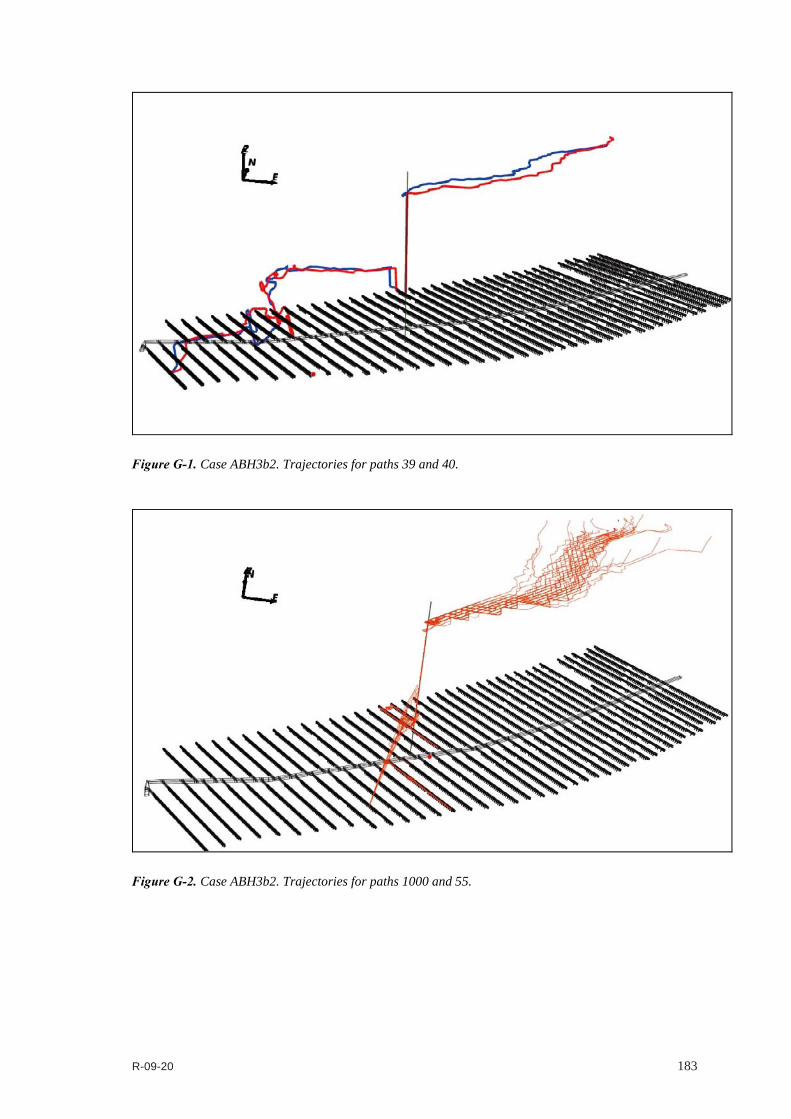
R-09-20 183

Figure G-1. Case ABH3b2. Trajectories for paths 39 and 40.

Figure G-2. Case ABH3b2. Trajectories for paths 1000 and 55.

184 R-09-20

Figure G-3. Case ABH9b2. Trajectory for path 1134.

G.2 Performance measures A set of five borehole cases were chosen for a more detailed statistical analysis, see Table G-2, Table G-3 and Table G-6 and Figure G-4 to Figure G-25. These cases were selected such that all three repository blocks were represented and the case with the highest ratio of particles entering the borehole was selected for each block (ABH4b1, ABH3b2 and ABH9b3). Also, all different types of borehole model environments were represented (fracture zone, deposition tunnel, rock and canister). These five cases were then compared to the corresponding results from the hydrogeological base case, see Table G-4 and Figure G-4 to Figure G-14. Since the total number of released particles is quite high, there is a risk that the effect the boreholes have on the ensemble performance measures might be hidden, depending on the number of particles that enter the boreholes and how the performance measures vary for these particles. Therefore, in addition to the analysis of the full ensemble of particles, only particles that enter a borehole were analysed, see Table G-3 and Figure G-15 to Figure G-25. Since the Q3 release locations show the greatest effect on performance measures due to the contact with or proximity of the boreholes to the deposition tunnels, the results for Q1 and Q2 are not given. The Q1 and Q2 results show the same general trends as Q3, but with a reduced magnitude.

Table G-2 shows a statistical summary of the ensemble medians for various performance measures for the five different borehole cases ABH4b1, ABH3b2, ABH9b2, ABH5b3 and ABH9b3. The particles were released at 2000 AD from the Q3 release locations. The statistics are based on the full ensemble of released particles and no separation was made between particles entering the borehole and particles that do not. The “Fraction OK” column gives the proportion of particles successfully reaching the top boundary of the model.

Table G-3 shows a statistical summary of medians of various performance measures only for particles entering the borehole for five different borehole cases corresponding to Table G-2.

Table G-4 shows a statistical summary of the ensemble medians for various performance measures for each repository block in the hydrogeological base case model BCb1, BCb2 and BCb3. The particles were released at 2000 AD from the Q3 release locations. These results are shown for comparison with the borehole cases in Table G-2. The comparison should be made on a block by block basis. Hence, for block 1, BCb1 should be compared with ABH4b1, for block 2, BCb2 should

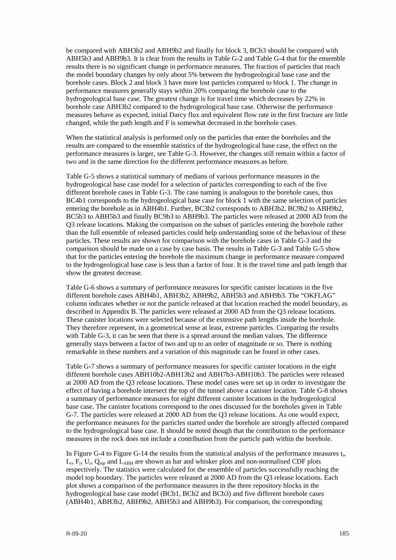
R-09-20 185

be compared with ABH3b2 and ABH9b2 and finally for block 3, BCb3 should be compared with ABH5b3 and ABH9b3. It is clear from the results in Table G-2 and Table G-4 that for the ensemble results there is no significant change in performance measures. The fraction of particles that reach the model boundary changes by only about 5% between the hydrogeological base case and the borehole cases. Block 2 and block 3 have more lost particles compared to block 1. The change in performance measures generally stays within 20% comparing the borehole case to the hydrogeological base case. The greatest change is for travel time which decreases by 22% in borehole case ABH3b2 compared to the hydrogeological base case. Otherwise the performance measures behave as expected, initial Darcy flux and equivalent flow rate in the first fracture are little changed, while the path length and F is somewhat decreased in the borehole cases.

When the statistical analysis is performed only on the particles that enter the boreholes and the results are compared to the ensemble statistics of the hydrogeological base case, the effect on the performance measures is larger, see Table G-3. However, the changes still remain within a factor of two and in the same direction for the different performance measures as before.

Table G-5 shows a statistical summary of medians of various performance measures in the hydrogeological base case model for a selection of particles corresponding to each of the five different borehole cases in Table G-3. The case naming is analogous to the borehole cases, thus BC4b1 corresponds to the hydrogeological base case for block 1 with the same selection of particles entering the borehole as in ABH4b1. Further, BC3b2 corresponds to ABH3b2, BC9b2 to ABH9b2, BC5b3 to ABH5b3 and finally BC9b3 to ABH9b3. The particles were released at 2000 AD from the Q3 release locations. Making the comparison on the subset of particles entering the borehole rather than the full ensemble of released particles could help understanding some of the behaviour of these particles. These results are shown for comparison with the borehole cases in Table G-3 and the comparison should be made on a case by case basis. The results in Table G-3 and Table G-5 show that for the particles entering the borehole the maximum change in performance measure compared to the hydrogeological base case is less than a factor of four. It is the travel time and path length that show the greatest decrease.

Table G-6 shows a summary of performance measures for specific canister locations in the five different borehole cases ABH4b1, ABH3b2, ABH9b2, ABH5b3 and ABH9b3. The “OKFLAG” column indicates whether or not the particle released at that location reached the model boundary, as described in Appendix B. The particles were released at 2000 AD from the Q3 release locations. These canister locations were selected because of the extensive path lengths inside the borehole. They therefore represent, in a geometrical sense at least, extreme particles. Comparing the results with Table G-3, it can be seen that there is a spread around the median values. The difference generally stays between a factor of two and up to an order of magnitude or so. There is nothing remarkable in these numbers and a variation of this magnitude can be found in other cases.

Table G-7 shows a summary of performance measures for specific canister locations in the eight different borehole cases ABH10b2-ABH13b2 and ABH7b3-ABH10b3. The particles were released at 2000 AD from the Q3 release locations. These model cases were set up in order to investigate the effect of having a borehole intersect the top of the tunnel above a canister location. Table G-8 shows a summary of performance measures for eight different canister locations in the hydrogeological base case. The canister locations correspond to the ones discussed for the boreholes given in Table G-7. The particles were released at 2000 AD from the Q3 release locations. As one would expect, the performance measures for the particles started under the borehole are strongly affected compared to the hydrogeological base case. It should be noted though that the contribution to the performance measures in the rock does not include a contribution from the particle path within the borehole.

In Figure G-4 to Figure G-14 the results from the statistical analysis of the performance measures tr, Lr, Fr, Ur, Qeqr and LABH are shown as bar and whisker plots and non-normalised CDF plots respectively. The statistics were calculated for the ensemble of particles successfully reaching the model top boundary. The particles were released at 2000 AD from the Q3 release locations. Each plot shows a comparison of the performance measures in the three repository blocks in the hydrogeological base case model (BCb1, BCb2 and BCb3) and five different borehole cases (ABH4b1, ABH3b2, ABH9b2, ABH5b3 and ABH9b3). For comparison, the corresponding

186 R-09-20

statistical analyses only for the subset of particles entering the borehole are shown in Figure G-15 to Figure G-25. Note that the results for the hydrogeological base case remain unchanged between the two sets of figures.

Figure G-4 and Figure G-5 show the bar and whisker plot and the non-normalised CDF plot of tr respectively. Block 1 shows very similar results when comparing the hydrogeological base case and ABH4b1. For block 2, ABH9b2 shows similar results compared to the hydrogeological base case, BCb2, whilst a decrease in travel time can be observed for ABH3b2 suggesting that particles find faster paths through the introduced borehole compared to the hydrogeological base case. For block 3 both ABH5b3 and ABH9b3 show slightly lower travel times compared to the hydrogeological base case, BCb3. Within each block there is little difference between the curves for different cases apart from ABH3b2 in block 2 which shows a clear divergence from the hydrogeological base case.

Figure G-6 and Figure G-7 show the bar and whisker plot and the non-normalised CDF plot of Lr respectively. In block 1 the path lengths do not differ much between the hydrogeological base case and the borehole case, ABH4b1. For block 2 the results are a bit different. Here both cases with boreholes, ABH3b2 and ABH9b2, show shorter paths compared to the hydrogeological base case. This indicates that a significant number of released particles enter the borehole and have a shorter way through the model. In block 3 a similar, but less pronounced, behaviour can be seen.

Figure G-8 and Figure G-9 show the bar and whisker plot and the non-normalised CDF plot of Fr respectively. The results for Fr show the same behaviour as for tr, i.e. very similar results for block 1 when comparing the hydrogeological base case and ABH4b1. For block 2, a decrease in Fr can be observed for ABH3b2 compared to the hydrogeological base case, BCb2. For block 3 both ABH5b3 and ABH9b3 show slightly lower Fr compared to the hydrogeological base case, BCb3.

Figure G-10 and Figure G-11 show the bar and whisker plot and the non-normalised CDF plot of Ur respectively. The three blocks show very similar results when comparing the hydrogeological base case and the borehole cases within each block separately. ABH3b2 and ABH5b3 stand out by showing a slight increase in Ur.

Figure G-12 and Figure G-13 show the bar and whisker plot and the non-normalised CDF plot of Qeqr respectively. The three blocks show very similar results when comparing the hydrogeological base case and the borehole cases within each block separately. ABH3b2 and ABH5b3 show a minor increase in Qeqr.

In Figure G-14 a non-normalised CDF plot of the path length inside the borehole, LABH, is shown. The median values are between 20-50 m showing that for most of the particles the path along the borehole is very short. Instead particles tend to prefer other ways through the fracture network and many particles never even enter the borehole. For a smaller fraction of the particles the path lengths inside the boreholes go up to 300-400 m. However, it should be remembered that these results are based on analysis of all particles and that the path length along the borehole for particles that actually enter the borehole is expected to be longer.

In order to extract the effect from the included borehole on the flow field and performance measures, only the subset of particles that entered the boreholes were selected for statistical analysis. In order to make the comparison as relevant as possible, the same selection of particles was made in the corresponding hydrogeological base case model. Due to a limited available space in the figures the case notation had to be shortened. Each borehole case has a corresponding selection of particles in the hydrogeological base case such that BC4b1 corresponds to ABH4b1, BC3b2 to ABH3b2, BC9b2 to ABH9b2, BC5b3 to ABH5b3 and finally BC9b3 to ABH9b3. The graphical results are shown in Figure G-15 to Figure G-25 and the corresponding statistical summaries for the five different borehole cases and the hydrogeological base case are shown in Table G-3 and Table G-5.

Figure G-15 and Figure G-16 show the bar and whisker plot and the non-normalised CDF plot of tr respectively. In block 1, a decrease in travel time is shown when comparing the hydrogeological base case and ABH4b1. For block 2, the effect is even greater. ABH3b2 and ABH9b2 both show about half a an order of magnitude lower travel times compared to the hydrogeological base case,

R-09-20 187

BCb2. In block 3, both ABH5b3 and ABH9b3 show a decrease compared to the hydrogeological base case, BC5b3 and BC9b3 respectively.

Figure G-17 and Figure G-18 show the bar and whisker plot and the non-normalised CDF plot of Lr respectively. As expected, all five borehole cases show lower path lengths compared to their respective hydrogeological base case. This shows that the boreholes provide shorter paths for the released particles through the model compared to the hydrogeological base case.

Figure G-19 and Figure G-20 show the bar and whisker plot and the non-normalised CDF plot of Fr respectively. The results for Fr show decreased values for all borehole cases compared to the respective hydrogeological base case paths.

Figure G-21 and Figure G-22 show the bar and whisker plot and the non-normalised CDF plot of Ur respectively. The median fluxes in the first fracture, Ur, are very similar comparing the borehole cases and the hydrogeological base case in all three blocks. The only exception is a slight increase in ABH5b3.

Figure G-23 and Figure G-24 show the bar and whisker plot and the non-normalised CDF plot of Qeqr respectively. The results for Qeqr are very similar to those for Ur, i.e. overall small differences between the cases apart from ABH5b3 which shows a slightly increased median value compared to the hydrogeological base case.

In Figure G-25 a non-normalised CDF plot of the path length inside the borehole, LABH, is shown. The median values are between 200-400 m showing that for the subset of released particles that enter the borehole the path length increases about one order of magnitude. It can also be noted that the distribution is much tighter around the median compared to when all particles are included, as would be expected.

Table G-2. Summary of ensemble medians for performance measures for selected borehole cases. Particles released at 2000 AD for the Q3 release locations.

Case Fraction OK tr [y] Ur [m/y] Lr [m] Fr [y/m] Qeqr [m3/y]

ABH4b1 0.775 1.60E+02 2.84E-04 1.53E+03 1.51E+06 8.77E-01

ABH3b2 0.610 1.42E+02 2.14E-04 1.94E+03 2.41E+06 7.61E-01

ABH9b2 0.622 1.72E+02 1.98E-04 2.17E+03 3.00E+06 7.27E-01

ABH5b3 0.570 6.94E+01 1.52E-04 1.29E+03 7.25E+05 6.47E-01

ABH9b3 0.550 7.29E+01 1.43E-04 1.28E+03 7.24E+05 6.27E-01

Table G-3. Summary of medians of performance measures only for particles entering the borehole for five different borehole cases. Particles released at 2000 AD for the Q3 release locations.

Case Fraction OK tr [y] Ur [m/y] Lr [m] Fr [y/m] Qeqr [m3/y]

ABH4b1 0.899 1.01E+02 2.17E-04 1.08E+03 6.63E+05 7.63E-01

ABH3b2 0.845 7.87E+01 2.20E-04 1.68E+03 1.41E+06 7.66E-01

ABH9b2 0.903 7.20E+01 1.16E-04 8.52E+02 3.22E+06 5.47E-01

ABH5b3 0.796 4.43E+01 1.71E-04 1.03E+03 5.30E+05 6.74E-01

ABH9b3 0.776 7.69E+01 1.38E-04 1.49E+03 5.78E+05 6.14E-01

188 R-09-20

Table G-4. Summary of ensemble medians for performance measures for each repository block in the hydrogeological base case model. Particles released at 2000 AD for the Q3 release locations.

Case Fraction OK tr [y] Ur [m/y] Lr [m] Fr [y/m] Qeqr [m3/y]

BCb1 0.772 1.61E+02 2.87E-04 1.56E+03 1.53E+06 8.80E-01

BCb2 0.591 1.82E+02 1.86E-04 2.37E+03 2.86E+06 7.09E-01

BCb3 0.545 8.36E+01 1.41E-04 1.45E+03 7.79E+05 6.23E-01

Table G-5. Summary of medians for performance measures only for particles entering the borehole in the corresponding borehole case for each repository block in the hydrogeological base case model. Particles released at 2000 AD for the Q3 release locations.

Case Fraction OK tr [y] Ur [m/y] Lr [m] Fr [y/m] Qeqr [m3/y]

BC4b1 0.851 1.31E+02 2.15E-04 1.44E+03 9.09E+05 7.52E-01

BC3b2 0.674 1.90E+02 1.77E-04 2.81E+03 3.06E+06 6.83E-01

BC9b2 0.630 2.64E+02 1.26E-04 3.09E+03 6.28E+06 5.80E-01

BC5b3 0.575 1.26E+02 8.62E-05 1.74E+03 7.97E+05 4.79E-01

BC9b3 0.705 1.28E+02 1.32E-04 1.77E+03 7.68E+05 6.18E-01

Table G-6. Summary of performance measures for specific canister locations for selected borehole cases. Particles released at 2000 AD for the Q3 release locations. Canister locations selected for particles with extensive path lengths inside the borehole.

Case Canister OKFLAG tr [y] Ur [m/y] Lr [m] Fr [y/m] Qeqr [m3/y]

ABH4b1 1799 0 4.16E+01 2.17E-04 2.88E+02 1.16E+05 7.60E-01

ABH3b2 608 0 2.89E+02 7.90E-05 2.07E+03 4.53E+07 4.59E-01

ABH9b2 1352 0 1.68E+01 7.02E-05 4.83E+02 2.64E+06 4.32E-01

ABH5b3 1093 0 1.02E+02 6.07E-05 1.99E+03 1.32E+05 4.02E-01

ABH9b3 1198 0 1.93E-01 6.24E-02 6.16E+01 3.31E+01 6.66E+02

Table G-7. Summary of performance measures for specific canister locations for selected borehole cases. Particles released at 2000 AD for the Q3 release locations. Canister locations selected that are immediately below a borehole intersecting a deposition tunnel.

Case Canister OKFLAG tr [y] Ur [m/y] Lr [m] Fr [y/m] Qeqr [m3/y]

ABH10b2 794 0 9.17E-01 2.28E-03 1.38E+02 2.18E+01 2.46E+00

ABH11b2 1500 5 2.23E+00 9.22E-02 1.29E+03 7.07E+02 8.09E+02

ABH12b2 1900 0 3.88E+00 1.73E-01 1.26E+03 1.10E+03 1.11E+03

ABH13b2 2200 0 1.36E+00 1.05E-01 8.78E+02 7.27E+02 8.65E+02

ABH7b3 111 0 1.92E+01 4.54E-02 1.25E+03 9.35E+04 5.68E+02

ABH8b3 600 0 6.50E-02 1.72E-01 8.70E+01 6.21E+00 1.10E+03

ABH9b3 1200 0 1.91E-01 6.24E-02 6.56E+01 2.69E+01 6.66E+02

ABH10b3 1700 0 2.30E+00 4.23E-02 6.30E+02 7.34E+01 5.48E+02

R-09-20 189

Table G-8. Summary of performance measures for selected canister locations in the hydrogeological base case. Particles released at 2000 AD for the Q3 release locations. Canister locations selected corresponding to Table G-7.

Case Canister OKFLAG tr [y] Ur [m/y] Lr [m] Fr [y/m] Qeqr [m3/y]

BCb2 794 0 3.26E+02 9.70E-04 2.89E+03 6.57E+06 1.61E+00

BCb2 1500 0 1.59E+02 6.75E-04 1.33E+03 3.71E+06 1.34E+00

BCb2 1900 1 6.42E+02 7.63E-06 2.21E+03 3.27E+06 1.43E-01

BCb2 2200 5 1.47E+02 9.21E-04 1.50E+03 1.41E+07 1.57E+00

BCb3 111 1 1.26E+03 1.71E-03 1.19E+03 1.21E+08 2.14E+00

BCb3 600 0 2.45E+01 6.57E-07 1.50E+03 2.67E+05 1.23E-02

BCb3 1200 1 7.99E+01 8.86E-04 1.85E+03 1.87E+06 1.54E+00

BCb3 1700 1 4.09E+01 4.73E-06 7.33E+00 1.95E+07 1.12E-01

Figure G-4. Bar and whisker plot of tr for the repository blocks in the hydrogeological base case model (BCb to BCb3) and selected borehole cases (ABH*b*), for all Q3 particles successfully reaching the model top boundary, released at 2000 AD. The statistical measures are the median (red), 25th and 75th percentile (blue bar) and the 5th and 95th percentile (black “whiskers”).

190 R-09-20

Figure G-5. Non-normalised CDF plot of tr for the repository blocks in the hydrogeological base case model (BCb1 to BCb3) and selected borehole cases (ABH*b*), for all Q3 particles successfully reaching the model top boundary, released at 2000 AD.

R-09-20 191

Figure G-6. Bar and whisker plot of Lr for the repository blocks in the hydrogeological base case model (BCb1 to BCb3) and selected borehole cases (ABH*b*), for all Q3 particles successfully reaching the model top boundary. The statistical measures are the median (red), 25th and 75th percentile (blue bar) and the 5th and 95th percentile (black “whiskers”).

192 R-09-20

Figure G-7. Non-normalised CDF plot of Lr for the repository blocks in the hydrogeological base case model (BCb1 to BCb3) and selected borehole cases (ABH*b*), for all Q3 particles successfully reaching the model top boundary.

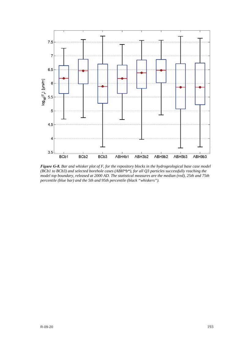
R-09-20 193

Figure G-8. Bar and whisker plot of Fr for the repository blocks in the hydrogeological base case model (BCb1 to BCb3) and selected borehole cases (ABH*b*), for all Q3 particles successfully reaching the model top boundary, released at 2000 AD. The statistical measures are the median (red), 25th and 75th percentile (blue bar) and the 5th and 95th percentile (black “whiskers”).

194 R-09-20

Figure G-9. Non-normalised CDF plot of Fr for the repository blocks in the hydrogeological base case model (BCb1 to BCb3) and selected borehole cases (ABH*b*), for all Q3 particles successfully reaching the model top boundary, released at 2000 AD.

R-09-20 195

Figure G-10. Bar and whisker plot of Ur for the repository blocks in the hydrogeological base case model (BCb1 to BCb3) and selected borehole cases (ABH*b*), for all Q3 particles successfully reaching the model top boundary, released at 2000 AD. The statistical measures are the median (red), 25th and 75th percentile (blue bar) and the 5th and 95th percentile (black “whiskers”). The UR axis corresponds to Ur for the Q3 release locations.

196 R-09-20

Figure G-11. Non-normalised CDF plot of Ur for the repository blocks in the hydrogeological base case model (BCb1 to BCb3) and selected borehole cases (ABH*b*), for all Q3 particles successfully reaching the model top boundary, released at 2000 AD. The UR axis corresponds to Ur for the Q3 release locations.

R-09-20 197

Figure G-12. Bar and whisker plot of Qeqr for the repository blocks in the hydrogeological base case model (BCb1 to BCb3) and selected borehole cases (ABH*b*), for all Q3 particles successfully reaching the model top boundary, released at 2000 AD. The statistical measures are the median (red), 25th and 75th percentile (blue bar) and the 5th and 95th percentile (black “whiskers”). The QeqR axis corresponds to Qeqr for the Q3 release locations.

198 R-09-20

Figure G-13. Non-normalised CDF plot of Qeqr for the repository blocks in the hydrogeological base case model (BCb1 to BCb3) and selected borehole cases (ABH*b*), for all particles successfully reaching the model top boundary, released at 2000 AD.

R-09-20 199

Figure G-14. Non-normalised CDF plot of LABH for selected borehole cases (ABH*b*), for all Q3 particles successfully reaching the model top boundary, released at 2000 AD.

200 R-09-20

Figure G-15. Bar and whisker plot of tr for the repository blocks in the hydrogeological base case model (BC*b1 to BC*b3) and selected borehole cases (ABH*b*), for Q3 particles entering the borehole and successfully reaching the model top boundary, released at 2000 AD. The statistical measures are the median (red), 25th and 75th percentile (blue bar) and the 5th and 95th percentile (black “whiskers”).

R-09-20 201

Figure G-16. Non-normalised CDF plot of tr for the repository blocks in the hydrogeological base case model (BC*b1 to BC*b3) and selected borehole cases (ABH*b*), for Q3 particles entering the borehole and successfully reaching the model top boundary, released at 2000 AD.

202 R-09-20

Figure G-17. Bar and whisker plot of Lr for the repository blocks in the hydrogeological base case model (BC*b1 to BC*b3) and selected borehole cases (ABH*b*), for Q3 particles entering the borehole and successfully reaching the model top boundary, released at 2000 AD. The statistical measures are the median (red), 25th and 75th percentile (blue bar) and the 5th and 95th percentile (black “whiskers”).

R-09-20 203

Figure G-18. Non-normalised CDF plot of Lr for the repository blocks in the hydrogeological base case model (BC*b1 to BC*b3) and selected borehole cases (ABH*b*), for Q3 particles entering the borehole and successfully reaching the model top boundary, released at 2000 AD.

204 R-09-20

Figure G-19. Bar and whisker plot of Fr for the repository blocks in the hydrogeological base case model (BC*b1 to BC*b3) and selected borehole cases (ABH*b*), for Q3 particles entering the borehole and successfully reaching the model top boundary, released at 2000 AD. The statistical measures are the median (red), 25th and 75th percentile (blue bar) and the 5th and 95th percentile (black “whiskers”).

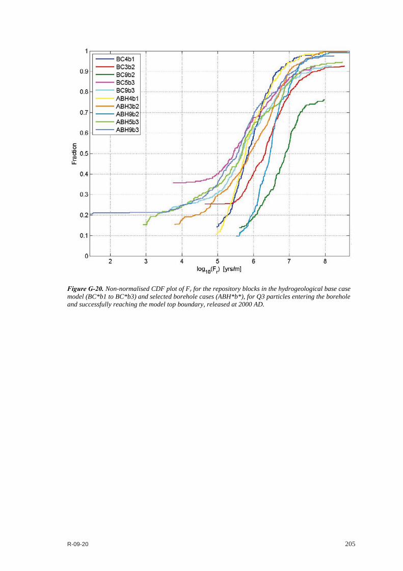
R-09-20 205

Figure G-20. Non-normalised CDF plot of Fr for the repository blocks in the hydrogeological base case model (BC*b1 to BC*b3) and selected borehole cases (ABH*b*), for Q3 particles entering the borehole and successfully reaching the model top boundary, released at 2000 AD.

206 R-09-20

Figure G-21. Bar and whisker plot of Ur for the repository blocks in the hydrogeological base case model (BC*b1 to BC*b3) and selected borehole cases (ABH*b*), for Q3 particles entering the borehole and successfully reaching the model top boundary, released at 2000 AD. The statistical measures are the median (red), 25th and 75th percentile (blue bar) and the 5th and 95th percentile (black “whiskers”). The UR axis corresponds to Ur for the Q3 release locations.

R-09-20 207

Figure G-22. Non-normalised CDF plot of Ur for the repository blocks in the hydrogeological base case model (BC*b1 to BC*b3) and selected borehole cases (ABH*b*), for Q3 particles entering the borehole and successfully reaching the model top boundary, released at 2000 AD. The UR axis corresponds to Ur for the Q3 release locations.

208 R-09-20

Figure G-23. Bar and whisker plot of Qeqr for the repository blocks in the hydrogeological base case model (BC*b1 to BC*b3) and selected borehole cases (ABH*b*), for Q3 particles entering the borehole and successfully reaching the model top boundary, released at 2000 AD. The statistical measures are the median (red), 25th and 75th percentile (blue bar) and the 5th and 95th percentile (black “whiskers”). The QeqR axis corresponds to Qeqr for the Q3 release locations.

R-09-20 209

Figure G-24. Non-normalised CDF plot of Qeqr for the repository blocks in the hydrogeological base case model (BC*b1 to BC*b3) and selected borehole cases (ABH*b*), for Q3 particles entering the borehole and successfully reaching the model top boundary, released at 2000 AD. The QeqR axis corresponds to Qeqr for the Q3 release locations.

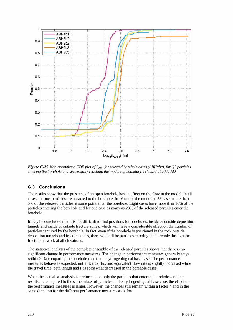
210 R-09-20

Figure G-25. Non-normalised CDF plot of LABH for selected borehole cases (ABH*b*), for Q3 particles entering the borehole and successfully reaching the model top boundary, released at 2000 AD.

G.3 Conclusions The results show that the presence of an open borehole has an effect on the flow in the model. In all cases but one, particles are attracted to the borehole. In 16 out of the modelled 33 cases more than 5% of the released particles at some point enter the borehole. Eight cases have more than 10% of the particles entering the borehole and for one case as many as 23% of the released particles enter the borehole.

It may be concluded that it is not difficult to find positions for boreholes, inside or outside deposition tunnels and inside or outside fracture zones, which will have a considerable effect on the number of particles captured by the borehole. In fact, even if the borehole is positioned in the rock outside deposition tunnels and fracture zones, there will still be particles entering the borehole through the fracture network at all elevations.

The statistical analysis of the complete ensemble of the released particles shows that there is no significant change in performance measures. The change in performance measures generally stays within 20% comparing the borehole case to the hydrogeological base case. The performance measures behave as expected, initial Darcy flux and equivalent flow rate is slightly increased while the travel time, path length and F is somewhat decreased in the borehole cases.

When the statistical analysis is performed on only the particles that enter the boreholes and the results are compared to the same subset of particles in the hydrogeological base case, the effect on the performance measures is larger. However, the changes still remain within a factor 4 and in the same direction for the different performance measures as before.

R-09-20 211

Thus, it can be concluded that including a borehole in the hydrogeological base case model does not have a significant effect on the performance measures even if the groundwater flow pattern is affected and the flow paths of the released particles change.

The presented comparison of borehole cases and the hydrogeological base case has been performed on a repository block by block basis. Potentially a borehole could have an effect on the other parts of the repository which would not be captured in these models. However, it is not believed that this would change the statistical results significantly.

In the study, the boreholes were assigned geometrical and physical (conductivity and porosity) properties that were chosen in order to make a good enough numerical representation of a borehole. The exact values of the parameters are hard to define and a sensitivity study of these parameter settings could be performed in order to investigate the effect of different selections. Also, a freshwater density was assigned to the entire borehole, which should be a conservative assumption in terms of hydraulic driving forces.