GMSmith MA Thesis 2012

HIGHLAND HUNTERS: PREHISTORIC RESOURCE USE IN THE YUKON-TANANA UPLANDS

By

Gerad M. Smith

RECOMMENDED: _______________________________________

_______________________________________

_______________________________________

Advisory Committee Chair

_______________________________________

Chair, Department of Anthropology

APPROVED: ____________________________________

Interim Dean, College of Liberal Arts

____________________________________

Dean of the Graduate School

____________________________________

Date

HIGHLAND HUNTERS: PREHISTORIC RESOURCE USE IN THE YUKON-TANANA UPLANDS

A

THESIS

Presented to the Faculty

Of the University of Alaska Fairbanks

In Partial Fulfillment of the Requirements for the Degree of

MASTER OF ARTS

By

Gerad M. Smith, B.A.

Fairbanks, Alaska

May 2012

2012 Gerad M. Smith

iii

Abstract

The purpose of this study was to conduct a first approximation of explorations and excavations

throughout the White Mountain and Steese Conservation areas during the summer field seasons of 2010

and 2011 in the Yukon Tanana Uplands. An analysis of the lithic artifacts from five site excavations (the

Big Bend, Bachelor Creek, Bear Creek, US Creek and Cripple Creek) was then undertaken. These

assemblages were then examined and modeled using risk-assessments, optimal resource use, and behavior

processes in order to explore the interdependence of environment, ecology, and material culture that drove

prehistoric subsistence cycles in this area. This archaeological research will supplement ethnographies to

indicate patterns of change in landscape value, trade networks, and local economic strategies.

iv

Table of Contents Page

Signature Page ................................................................................................................................................. i

Title Page ....................................................................................................................................................... ii

Abstract ......................................................................................................................................................... iii

Table of Contents .......................................................................................................................................... iv

List of Figures ................................................................................................................................. ix

List of Tables ................................................................................................................................ xiii

List of Appendices .......................................................................................................................... xv

Acknowledgments ....................................................................................................................................... xvi

1 Introduction ..................................................................................................................................................1

1.1 History of Research in the Interior ..............................................................................................2

1.2 Research Summary ....................................................................................................................4

2 Theoretical Approaches and Methodology ...................................................................................................6

2.1 Assumptions, Organization, and Structure of Behavioral Ecology .............................................6

2.2 Models.........................................................................................................................................8

2.2 Large, Medium, and Small Scale Analysis .................................................................................9

2.3.1 The Diet Breadth Model .......................................................................................... 10

2.3.2 The Direct vs. Embedded Procurement Model ........................................................ 10

2.3.3 The Site Occupation Duration Model ...................................................................... 10

2.3.4 The Field Processing Model .................................................................................... 12

2.4 Large Scale Specific Methods ................................................................................................... 12

2.5 Large and Medium Scale Analysis: The Technological Investment Model .............................. 16

2.6 Medium Scale Analysis: The Logistic and Residential Mobility Model .................................. 17

2.7 Medium and Small Scale Analysis: The Patch Choice Model .................................................. 17

2.8 Small Scale Analysis ................................................................................................................. 17

2.8.1 The Ideal Free Distribution Model .......................................................................... 17

2.8.2 The Central Place Foraging Model .......................................................................... 18

2.9 Application and Expectations to Subarctic Alaska ................................................................... 19

3 Modeling the Prehistory of Alaska ............................................................................................................. 21

3.1 Siberian Origins and the Colonization of Beringia ................................................................... 21

3.2 Late Pleistocene and Early Holocene Eastern Beringia ............................................................ 22

3.3 Mid-Holocene Alaska ............................................................................................................... 26

3.4 Discussion ................................................................................................................................. 27

4 Modeling Optimizing Behaviors Across the Yukon Tanana Uplands........................................................ 29

4.1 Land Evaluation ........................................................................................................................ 31

v

4.2 Construction of Economic Models of Land Use From Ethnographic and Historic Data .......... 31

4.2.1 The Han ................................................................................................................... 32

4.2.2 The Gwich’in ........................................................................................................... 33

4.2.3 The Tanana .............................................................................................................. 35

4.3 Methods..................................................................................................................................... 36

4.3.1 The Diet Breadth Model .......................................................................................... 37

4.3.2 Dependent Variables ................................................................................................ 38

4.3.2.1 Site Locations ......................................................................................... 38

4.3.2.2 Boundaries .............................................................................................. 40

4.3.3 Independent Variables ............................................................................................. 40

4.3.3.1 Elevation ................................................................................................. 40

4.3.3.2 Vegetation .............................................................................................. 40

4.3.3.3 Hydrography and Anadromous Streams ................................................. 40

4.3.3.4 Mammal/Waterfowl Distribution ........................................................... 40

4.4 Model Results ........................................................................................................................... 41

4.4.1 Spring ....................................................................................................................... 41

4.4.2 Summer .................................................................................................................... 42

4.4.3 Fall ........................................................................................................................... 42

4.4.4 Winter ...................................................................................................................... 43

4.5 Discussion ................................................................................................................................. 44

5 Ridgetop Site Assemblage Variability ....................................................................................................... 46

5.1 Bachelor Creek Lookout Introduction ....................................................................................... 47

5.1.1 Lithic Analysis ......................................................................................................... 51

5.1.2 Raw Material Analysis ............................................................................................. 51

5.1.3 Debitage Attributes .................................................................................................. 53

5.1.4 Reduction Strategies ................................................................................................ 54

5.1.5 Formal Tool Attributes ............................................................................................ 54

5.1.6 Informal Tool Attributes .......................................................................................... 55

5.2 Big Bend Overlook Introduction ............................................................................................... 56

5.2.1 Big Bend Overlook Artifacts ................................................................................... 59

5.2.2 Raw Material Analysis ............................................................................................. 61

5.2.3 Debitage Attributes .................................................................................................. 61

5.2.4 Reduction Strategies ................................................................................................ 67

5.2.5 Core Attributes ......................................................................................................... 67

5.2.6 Formal Tool Attributes ............................................................................................ 68

vi

5.2.7 Informal Tool Attributes .......................................................................................... 69

6 Valley Floor Site Assemblage Variability .................................................................................................. 71

6.1 Introduction to the US Creek and Cripple Creek sites .............................................................. 72

6.2 Early Excavations ..................................................................................................................... 72

6.3 Cripple Creek Introduction ....................................................................................................... 73

6.3.1 Excavation Methods and Collection Practices ......................................................... 76

6.3.2 Stratigraphic Description ......................................................................................... 76

6.3.2.1 Block 1 Stratigraphy (N470-470 E512-515) .......................................... 78




6.3.3 1978 Excavation Location ....................................................................................... 87

6.3.4 Cripple Creek Cultural Features .............................................................................. 89

6.3.4.1 Feature 1 ................................................................................................. 89

6.3.4.2 Feature 2 ................................................................................................. 91

6.3.4.3 Feature 3 ................................................................................................. 92

6.3.4.4 Feature 4 ................................................................................................. 94

6.3.4.5 Feature 5 ................................................................................................. 95

6.3.4.6 1978 Hearth Feature ............................................................................... 97

6.3.4.7 Discussion .............................................................................................. 97

6.3.5 Faunal Analysis Summary ....................................................................................... 97

6.3.6 Block 1 Discussion .................................................................................................. 99

6.3.7 Cripple Creek Lithic Artifacts ............................................................................... 100

6.3.8 Raw Material Analysis ........................................................................................... 101

6.3.9 Debitage Attributes ................................................................................................ 103

6.3.10 Microblade Attributes .......................................................................................... 104

6.3.11 Reduction Strategies ............................................................................................ 105

6.3.12 Flake Core Attributes ........................................................................................... 105

6.3.13 Formal Tool Attributes ........................................................................................ 106

6.3.14 Informal Tool Attributes ...................................................................................... 109

6.3.15 Ceramic Analysis ................................................................................................. 109

6.4 US Creek Introduction ............................................................................................................ 112

6.4.1 Stratigraphy ............................................................................................................ 115

6.4.2 Cultural Features .................................................................................................... 115

6.4.2.1 Feature 1 ............................................................................................... 115

vii

6.4.2.2 Feature 2 ............................................................................................... 115

6.4.2.3 Feature 3 ............................................................................................... 115

6.4.2.4 Feature 11 ............................................................................................. 115

6.4.2.5 Feature 12 ............................................................................................. 116

6.4.2.6 Feature 13 ............................................................................................. 116

6.4.2.7 Feature 14 ............................................................................................. 117

6.4.2.8 Features 16 and 17 ................................................................................ 117

6.4.2.9 Feature 18 ............................................................................................. 117

6.4.2.10 Discussion........................................................................................... 117

6.4.3 Faunal Analysis Summary ..................................................................................... 117

6.4.4 US Creek Lithic Artifacts ...................................................................................... 118



6.4.7 Microblade Attributes ............................................................................................ 123

6.4.8 Reduction Strategies .............................................................................................. 126

6.4.9 Flake Core Attributes ............................................................................................. 126

6.4.10 Formal Tool Attributes ........................................................................................ 127

6.4.11 Informal Tool Attributes ...................................................................................... 129

6.4.12 Spatial Analysis and Site Structure ...................................................................... 129

6.4.13 US Creek Cultural Zone 1 and Cultural Zone 2 ................................................... 129

6.4.14 Additional Artifacts ............................................................................................. 135

6.5 Bear Creek Introduction .......................................................................................................... 135

6.5.1 Bear Creek Artifacts .............................................................................................. 137



6.5.4 Reduction Strategies .............................................................................................. 140

6.5.5 Core Attributes ....................................................................................................... 141

6.5.6 Microblade Core Tab Attributes ............................................................................ 141

6.5.7 Formal Tool Attributes .......................................................................................... 142

6.5.8 Informal Tool Attributes ........................................................................................ 142

7 Modeling Site Structure Behaviors in the Yukon-Tanana Uplands.......................................................... 144

7.1 Technological Organization .................................................................................................... 145

7.1.1 The Technological Investment Model ................................................................... 145

7.2 Mobility................................................................................................................................... 150

7.2.1 The Diet Breadth Model ........................................................................................ 154

viii

7.3 Social Organization ................................................................................................................. 155

8 Conclusions .............................................................................................................................................. 159

8.1 Regional Model Summary ...................................................................................................... 159

8.2 Assemblage Overview ............................................................................................................ 159

8.3 Sampling and Taphonomy ...................................................................................................... 160

8.4 Technological Patterns ............................................................................................................ 161

References ................................................................................................................................................... 162

ix

List of Figures Page

Figure 1.1 Locations of the five prehistoric sites referenced in this study ......................................................3

Figure 2.1 Graphic illustrations of the four main HBE models discussed in the text ......................................9

Figure 3.1 Map of Beringia and the Alaskan glaciers at their greatest extent during

the LGM .......................................................................................................................................... 24

Figure 4.1 Ethnographically attested band territories ca1890 A.D. ............................................................... 32

Figure 4.2 The model boundary (red) and all prehistoric sites according to the

AHRS 2010 database ...................................................................................................................... 39

Figure 4.3 Prehistoric site locations within the YTU in relation to modern

infrastructure and major federal landholdings................................................................................. 39

Figure 4.4 Graphic representations of seasonal caloric value patches ........................................................... 41

Figure 4.5 Cumulative percent of actual sites vs. cumulative percent of random

points vs. cumulative percent of acres within each value patch ...................................................... 43

Figure 5.1 Location of the two ridgetop sites discussed in this chapter ........................................................ 46

Figure 5.2 The Bachelor Creek site, located around the knob at the top of the bluff .................................... 48

Figure 5.3 Bachelor Creek overview, showing the grid and flagged artifacts ............................................... 48

Figure 5.4 Bachelor Creek site map of all artifacts (blue) ............................................................................. 49

Figure 5.5 Typical stratigraphy near the prominent knob on the site ............................................................ 50

Figure 5.6 Outline denotes ash feature located in test pit N510 E505 ........................................................... 50

Figure 5.7 Raw material debitage weight variability..................................................................................... 51

Figure 5.8 Lithic artifact isopleths ................................................................................................................. 52

Figure 5.9 Raw material debitage size class weight % and count ................................................................. 53

Figure 5.10 Bachelor Creek tools .................................................................................................................. 55

Figure 5.11 Bachelor Creek microblades and bifaces ................................................................................... 56

Figure 5.12 Big Bend .................................................................................................................................... 58

Figure 5.13 Big Bend .................................................................................................................................... 58

Figure 5.14 Stratigraphy at Big Bend ............................................................................................................ 59

Figure 5.15 Big Bend site map of all artifacts ............................................................................................... 60

Figure 5.16 Local/nonlocal raw material distribution, and spatial distributions of tools .............................. 62

Figure 5.17 Chalcedony, chert, siltstone, and Batza Tena obsidian distributions ......................................... 63

Figure 5.18 Upper levels of Big Bend total raw material weight variability ................................................. 64

Figure 5.19 Lower levels of Big Bend total raw material weight variability ................................................ 65

Figure 5.20 Raw material weight by size class ............................................................................................. 66

Figure 5.21 Flake core size class by weight .................................................................................................. 68

Figure 5.22 Big Bend early-stage bifaces and wedge-shaped gray chert core .............................................. 68

x

Figure 5.23 Big Bend microblades and late-stage bifaces ............................................................................. 70

Figure 6.1 Location of sites discussed in this chapter ................................................................................... 71

Figure 6.2 US Creek and Cripple Creek sites ................................................................................................ 72

Figure 6.3 Cripple Creek site ........................................................................................................................ 74

Figure 6.4 Feature 1, cache pit ...................................................................................................................... 75

Figure 6.5 The southern part of the slope of Cripple Creek .......................................................................... 75

Figure 6.6 Harris Matrix for Cripple Creek ................................................................................................... 77

Figure 6.7 South excavation (Block 1) .......................................................................................................... 78

Figure 6.8 Block 1 North wall generalized stratigraphy ................................................................................ 79

Figure 6.9 Block 2 excavation units .............................................................................................................. 80

Figure 6.10 Block 2 East wall generalized stratigraphy ................................................................................ 81

Figure 6.11 Block 3 Stratigraphy .................................................................................................................. 82

Figure 6.12 Block 3 stratigraphy ................................................................................................................... 83

Figure 6.13 Feature 1 cross section, Excavation Block 3 .............................................................................. 83

Figure 6.14 Block 3 west wall generalized stratigraphy ................................................................................ 84

Figure 6.15 Block 4 east wall stratigraphy .................................................................................................... 85

Figure 6.16 Block 4 generalized stratigraphy ................................................................................................ 86

Figure 6.17 Old test unit from 1978 .............................................................................................................. 87

Figure 6.18 Cripple Creek map ..................................................................................................................... 88

Figure 6.19 Organic artifact spatial distributions .......................................................................................... 89

Figure 6.20 Birch bark in situ within Feature 1 ............................................................................................. 90

Figure 6.21 Feature 1 birch bark, after the soil had been removed ............................................................... 91

Figure 6.22 Feature 2 hearth. Pink toothpicks denote boundaries of this feature .......................................... 92

Figure 6.23 Feature 3 cross section ............................................................................................................... 93

Figure 6.24 Features 4 and 5 ......................................................................................................................... 94

Figure 6.25 Features 3, 4, and 5 .................................................................................................................... 95

Figure 6.26 Feature 3 and 5 ........................................................................................................................... 96

Figure 6.27 Two broken unidentified long bone fragments that had unworked

lithics embedded within them ......................................................................................................... 98

Figure 6.28 A gray chert flake found in situ within a fractured long bone element ...................................... 99

Figure 6.29 Block 1. Fire cracked rock, faunal, and charcoal weight distributions..................................... 100

Figure 6.30 Raw material quantities by total count/weight percent ............................................................ 101

Figure 6.31 Local/Nonlocal raw material and fire cracked rock density maps ........................................... 102

Figure 6.32 Raw material densities ............................................................................................................. 103

Figure 6.33 Raw material debitage weight variability ................................................................................. 104

xi

Figure 6.34 Flake cores by size class and weight ........................................................................................ 105

Figure 6.35 Cripple Creek artifacts ............................................................................................................. 107

Figure 6.36 Tool distributions at Cripple Creek in relation to charcoal densities ....................................... 108

Figure 6.37 Ceramic and birch bark weight densities ................................................................................. 110

Figure 6.38 Ceramics recovered from Feature 3 ......................................................................................... 111

Figure 6.39 Artifact distribution at the US Creek Site ................................................................................ 112

Figure 6.40 US Creek site plan ................................................................................................................... 113

Figure 6.41 US Creek view toward the southwest ...................................................................................... 114

Figure 6.42 Typical US Creek stratigraphy, away from the hearth features ............................................... 114

Figure 6.43 US Creek Feature 11 hearth cross section ................................................................................ 116

Figure 6.44 Faunal elements being recovered at US Creek in 2004 ............................................................ 118

Figure 6.45 Raw material debitage weight diversity ................................................................................... 119

Figure 6.46 US Creek raw material distribution .......................................................................................... 120

Figure 6.47 Obsidian distributions at US Creek .......................................................................................... 121

Figure 6.48 Chert size class weights ........................................................................................................... 122

Figure 6.49 Raw material size class weights ............................................................................................... 122

Figure 6.50 US Creek microblades ............................................................................................................. 124

Figure 6.51 US Creek microblade core tablets ............................................................................................ 125

Figure 6.52 US Creek microblade cores ...................................................................................................... 125

Figure 6.53 US Creek flake core size class weights .................................................................................... 126

Figure 6.54 A sample of US creek bifaces .................................................................................................. 127

Figure 6.55 Tool distributions at US Creek ................................................................................................. 128

Figure 6.56 US Creek prehistoric cultural zones ......................................................................................... 129

Figure 6.57 Level 2 tools and features associated with CZ1 ....................................................................... 130

Figure 6.58 Nonlocal raw material distributions associated with artifacts only

associated with CZ1 features ........................................................................................................ 131

Figure 6.59 All core and blade technology in relation to CZ2 Features 14 and 18 ..................................... 133

Figure 6.60 Nonlocal raw material distributions associated with artifacts only

associated with CZ2 features ........................................................................................................ 134

Figure 6.61 Cultural Zone 1 raw material size class weights ...................................................................... 135

Figure 6.62 Cultural Zone 2 raw material size class weights ...................................................................... 135

Figure 6.63 Bear Creek site aerial photograph ............................................................................................ 136

Figure 6.64 Bear Creek site overview ......................................................................................................... 136

Figure 6.65 Bear Creek site map ................................................................................................................. 137

Figure 6.66 Raw material variability ........................................................................................................... 138

xii

Figure 6.67 Raw material distributions at Bear Creek ................................................................................ 139

Figure 6.68 Raw material size class weights ............................................................................................... 140

Figure 6.69 Bear Creek tool isopleths ......................................................................................................... 141

Figure 6.70 Bear Creek artifacts .................................................................................................................. 143

Figure 7.1 The five main sites focused on in this research .......................................................................... 144

Figure 7.2 Arrow shaft and several types of stone and bone projectile points ............................................ 148

Figure 7.3 Composite spear ......................................................................................................................... 148

Figure 7.4 Obsidian sources ........................................................................................................................ 151

Figure 7.5 Local vs nonlocal materials by topographic zone ...................................................................... 152

Figure 7.6 Local vs. nonlocal materials by site, topographic zone and cultural period .............................. 153

Figure 7.7 Artifact diversity by site, topographic zone, and cultural period ............................................... 156

Figure 7.8 Artifact diversity by topographic zone ....................................................................................... 157

Figure 7.9 Raw material diversity by topographic zone .............................................................................. 157

Figure A-1 Anadromous stream riparian habitats ....................................................................................... 175

Figure A-2. Vegetation patches in the region .............................................................................................. 176

Figure A-3. Spring ungulate patches ........................................................................................................... 177

Figure A-4. Fall ungulate patches ............................................................................................................... 178

Figure A-5 Ungulate winter patches ............................................................................................................ 179

xiii

List of Tables Page

Table A-1 Diet Breadth model for the YTU ................................................................................................ 180

Table A-2 Statistic results for each season .................................................................................................. 180

Table A-3 GIS data sets and sources used ................................................................................................... 181

Table A-4 Site location occurrences within calculated seasonal weighted patches .................................... 182

Table B-1 Bachelor Creek raw material type by stratigraphic level ............................................................ 183

Table B-2 Bachelor Creek artifact types by stratigraphic level ................................................................... 183

Table B-3 Bachelor Creek lithic raw material summaries ........................................................................... 184

Table B-4 Bachelor Creek Sullivan and Rosen summary ........................................................................... 185

Table B-5 Bachelor Creek White cortex summary ...................................................................................... 186

Table B-6 Bachelor Creek cortex type summary ........................................................................................ 186

Table B-7 Bachelor Creek artifact type by size class .................................................................................. 186

Table B-8 Bachelor Creek microblade platform type and segment by size class ........................................ 187

Table B-9 Bachelor Creek debitage material types associated reduction strategies by

platform type ................................................................................................................................. 187

Table B-10 Bachelor Creek debitage material types associated with reduction strategies

by dorsal scars ............................................................................................................................... 188

Table B-11 Bachelor Creek artifact type by raw material type ................................................................... 189

Table B-12 Big Bend artifact summary by stratigraphic depth ................................................................... 189

Table B-13 Big Bend raw material summary by stratigraphic depth .......................................................... 190

Table B-14 Big Bend lithic raw material summaries .................................................................................. 190

Table B-15 Big Bend Sullivan and Rosen summary ................................................................................... 192

Table B-16 Big Bend White cortex summary ............................................................................................. 194

Table B-17 Big Bend cortex type summary ................................................................................................ 195

Table B-18 Big Bend microblade depth and size class summary ................................................................ 197

Table B-19 Big Bend artifact type by raw material type ............................................................................. 198

Table B-20 Big Bend debitage platform type .............................................................................................. 198

Table B-21 Big Bend debitage reduction strategies by dorsal scars ............................................................ 199

Table B-22 Cripple Creek artifact type by stratigraphic level ..................................................................... 201

Table B-23 Cripple Creek raw material summaries .................................................................................... 202

Table B-24 Cripple Creek artifact type by raw material type ...................................................................... 203

Table B-25 Cripple Creek Sullivan and Rosen summary ............................................................................ 204

Table B-26 Cripple Creek White cortex summary ...................................................................................... 204

Table B-27 Cripple Creek artifact type size classes .................................................................................... 205

Table B-28 Cripple Creek microblade portion summary ............................................................................ 205

xiv

Table B-29 Cripple Creek microblade platform type and size class summary ............................................ 205

Table B-30 Cripple Creek microblade depth summary ............................................................................... 205

Table B-31 Cripple Creek cortex type summary ......................................................................................... 206

Table B-32 Cripple Creek debitage raw material types and reduction strategy summary

by platform type ............................................................................................................................ 206

Table B-33 Cripple Creek debitage raw material types and reduction strategy summary

by dorsal scars ............................................................................................................................... 207

Table B-34 Cripple Creek biface hafting style by depth summary ............................................................. 207

Table B-35 US Creek Artifact type by stratigraphic level........................................................................... 208

Table B-36 US Creek lithic raw material summaries .................................................................................. 209

Table B-37 US Creek artifact type level code by cultural zone .................................................................. 210

Table B-38 US Creek artifact type by cultural zone .................................................................................... 210

Table B-39 US Creek raw material type by cultural zone ........................................................................... 211

Table B-40 Bear Creek artifact raw material summary ............................................................................... 212

Table B-41 Bear Creek raw material summaries ......................................................................................... 213

Table B-42 Bear Creek Sullivan and Rosen summary ................................................................................ 213

Table B-43 Bear Creek White cortex summary .......................................................................................... 214

Table B-44 Bear Creek artifact type size classes......................................................................................... 214

Table B-45 Bear Creek raw material reduction strategies by platform types .............................................. 215

Table B-46 Bear Creek raw material reduction strategies by dorsal scars .................................................. 215

Table B-47 Bear Creek artifact type use wear summary ............................................................................. 216

Table C-1 Percent of debitage linked to reduction strategies by site ........................................................... 217

Table C-2 Total microblade artifacts by site ............................................................................................... 217

Table C-3 Total microblade artifacts by topographic zone ......................................................................... 217

Table C-4 T-tests of artifact type, raw material type, and local/nonlocal groups

by topographic zone ...................................................................................................................... 217

xv

List of Appendices Page

Appendix A GIS Layers and sources and diet breadth model utilized for patch weight calculations 175

Appendix B Data summaries for site assemblages 183

Appendix C Combined site assemblage summaries 217

xvi

Acknowledgments

I would first of all like to thank the members of my committee, Ben A. Potter, Joel D. Irish, and

Patrick Plattet for their help and assistance throughout this work. Foremost is my advisor, Ben Potter, who

pushed my thinking beyond models and into integrated systems. Next to Patrick Plattet whose

conversations on cultural transmission were very insightful. Finally, Joel Irish whose help with the human

remains was greatly appreciated. Additionally, I would like to thank Loukas Barton, who provided

immense help teaching and discussing the methodology and shortcomings of Human Behavioral Ecology

theory.

This project would not have been possible without the help and support of the US Bureau of Land

Management, who provided the funding for this project, as well as two field seasons of work within the

region. Special thanks to Robin Mills (US BLM archaeologist) who provided help on the project outline,

provided access to the US Creek data and artifacts, as well as help and assistance for the excavations of the

Big Bend, Bachelor Creek, and Cripple Creek sites. Thanks to my coworkers Steve Lanford, Jess Peterson,

and Tiffany Curtis. The helicopters, boats, floods, and one persistent bear provided us with years of stories.

Thanks especially to Mary Ann Sweeney, who conducted the faunal analysis for Cripple Creek.

Many thanks to the University of Alaska Museum of the North and the archaeology department

personnel for providing time and space for study of collections there. I would also like to thank everyone

on the field crews of 2010 and 2011 who donated time and muscle exploring and excavating these sites and

areas in the Yukon Tanana Uplands. Special thanks goes out to my lab partner Katie Antal, whose help

sorting and cataloguing bones, lithics, and charcoal, was very much appreciated. Thanks also to Mike

Kenyhercz for his help with identifying and analyzing the human remains.

Finally, my fellow students have been a pillar of support through this period. Thanks to my family

for always being a phone-call away. Laura, Nicki, and KC, thank you for saving my sanity through this

project. And to the members of the field crew of the Montana Yellowstone Archaeological Project 2008

where the original idea for this work was birthed: Seth Bates, Robert Peltier, and Justin Ferryman, may

your trowels be ever sharp in your hands.

1

1 Introduction

This thesis focuses on the mechanisms of cultural adaptation and change in response to resource

optimization and risk mitigation during the late Holocene in the Yukon Tanana Uplands (YTU).

Archaeological assemblages in this geographic region (encompassing over 18 million square acres) are

generally small lithic scatters in shallow deposition. These types of settings are often considered less

tractable than large sites in solid, deep stratigraphy, whose features are more likely to be established in

temporal context. When sites are interpreted using landscape-based inferences, patterns of assemblage

variability become apparent.

This work will largely focus on inferences from assemblage variability and debitage

characteristics, rather than traditional formal tool form and reduction techniques. These latter two points are

important approaches, and will be discussed in proper context. This investigation is carried out primarily

through models derived from Human Behavioral Ecology (HBE), a system of theory that has been rarely

applied to this area. This theoretical framework was chosen for its robust linking of behaviors and

economics in real-world anthropological contexts, and therefore can be heuristically applied to the past

material cultural record in order test variety of optimization-based hypotheses. Optimizing models are not

unique to Optimal Foraging Theory. Optimization has been utilized productively in making sense of

assemblage variability in many archaeological contexts (Schiffer 1976). Therefore, while HBE provides

several useful models of exploring the empirical record, other models outside this theoretical framework

will be utilized as well.

The eastern Alaskan interior represents one of the longest continuously occupied zones of

demonstrated human habitation on the two American continents, lasting roughly 14,000 years. Due to a

lack of local infrastructure, short field seasons, remote locations of sites, and expense of travel to these

locations, it remains relatively understudied. This region was inhabited by small bands of hunter-gatherers,

whose foraging strategies were constructed around the acquisition of large ungulates and summer salmon.

The relationship between those two very different resources and their changing importance to prehistoric

people remains unclear.

The prehistoric inhabitants in central Alaska utilized several weapon strategies throughout their

prehistoric occupation. A tradition of core-and-blade composite weapons exists throughout most of human

occupation of the Interior. Several formal bifacial reduction strategies have been demonstrated to be

associated with the Nenana/Chindadn complex, Denali complex, and the Northern Archaic tradition

(~5000-1000 BP). These are argued to be isolated by time from each other. Other informal projectile point

strategies have been informally categorized as of “lanceolate” in form (Esdale 2008, Goebel et al. 1991,

Holmes 2008).

The last 1000 years is also one of importance to archaeologists at it represents a time of many

changes to the ancient prehistoric systems. Microblade composite weaponry, a Pleistocene strategy that had

2

survived in Alaska throughout the entire Holocene was lost. Bow and arrow technology appears to have

replaced earlier atlatl-thrown darts in the Interior, adopted likely from the coastal Eskimo (Hare et al.

2004). The fur trade with Euro-American traders beginning 400-300 BP also probably had an impact on

ancient trade routes, changing the value of prestige items, as well as targeted prey in ways which we can

largely only guess at now (Simeone 1982).

The reasons for the rise in popularity of specific technological strategies as a response to local

ecological and seasonal patterns has only just begun to be studied in this region during the last decade (see

Potter 2005, 2008a and 2008b, Holmes 2008). The bulk of this work has focused on the late Pleistocene

and early Holocene, focusing on the Tanana Valley region. The regional archaeological record has been

studied far more in the Alaska Range and the Brooks Range in the far north at the expense of the YTU, the

highlands that lie between them. The lack of research in the YTU has spurred this project, which was

originally conceived by Robin Mills and Ben Potter in 2008. The scope of this project was established

before and during the field seasons of 2009 and 2010. This study primarily focuses on the lithic debitage

and tools, with reference to the associated faunal assemblages. This material is used to answer the primary

question: can lithic variability be explained as a response mechanism to energy optimization of perceived

risk management, and can we identify relationships among assemblage variables and modeled, seasonally

available districts of potential resources? This main research question is further divided into four sub

questions: (1) why are several weapon strategies used simultaneously on the landscape?, (2) how are both

logistic and residential mobility strategies articulated simultaneously in the same region?, (3) What were

the implications of caching resources?, and (4) does a relationship between mobility patterns, weapon

strategies, and caching behaviors exist?, and (5) How do these change through time?

1.1 History of Research in the Interior

This section will briefly cover the theoretical approaches that have characterized the basis of

Alaskan archaeological studies. The early decades of Alaskan archaeology focused along the coasts,

studying Eskimo prehistory where the material culture was considered to be far richer than that of the

interior. Archaeology in the Interior got its jump-start when wedge-shaped cores that had been dislodged in

a field at the University of Alaska Fairbanks were noted to be strongly similar to cores from the Gobi desert

(Nelson 1935). The Campus Site spurred interest into the prehistoric record of the Interior. Rainey (1939)

produced some early descriptions of artifacts and sites in the Tanana Valley. These early writings are

primarily descriptive in nature. In the early development of Americanist archaeology, collections of

artifacts were examined inductively to produce or reveal patterns in the archaeological record. This became

the Cultural Historical approach, which primarily focused on recognizing artifact types whose spatial and

temporal relationships were constrained.

3

The culmination of this approach was hypothesized cultural sequences (Dixon 1985). West (1967)

and Dumond (1969) both produced early formative works on Alaskan prehistory through these theoretical

paradigms. The Denali complex was hypothesized to be a Terminal Pleistocene core-and-blade culture that

spanned Beringia. Dumond hypothesizing that changes in the material cultural record from the Denali

complex to the Northern Archaic side-notched bifacial points could be explained through actual migration,

contact, and diffusion. Cook and Workman both produced regional cultural chronologies. Cooks’ work

focused on Healy Lake, where he established a record of temporal technological change (1969). Workman

produced a similar work in southwestern Yukon (1978). Both of these were seminal works describing the

continuity and change of artifact types in regional context.

Various large-scale infrastructure projects such as the Trans-Alaska Pipeline Survey (Cook 1977),

the Fort Wainwright Archaeological Survey (Dixon et al. 1980), the Susitna Hydroelectric Project (Dixon

et al. 1981, 1983), helped to amass archaeological data on a regional basis. The 1980’s saw archaeologists

recognizing the long-term continuity of artifact types; the Denali Complex was first split into an early and

late phase, then later recognized as existing throughout the Holocene (West 1996). The Northern Archaic

Tradition was established as beginning in the mid-Holocene (5000-6000 BP) (Dixon 1985) and lasting to

the Athabascan Period, which began about 1000 BP and lasted to the Historic Period.

Figure 1.1 Locations of the five prehistoric sites referenced in this study (the Yukon-Tanana Uplands are

bounded in white).

4

1.2 Research Summary

Various frameworks of Traditions and Complexes have been set forth explaining continuity and

change in the record (see West 1996, Powers and Hoffecker 1989, Goebel et al. 1991 and Holmes 2008).

The purpose of this work is to not revisit these methodologies, but to build upon them by explaining

regional differences in the context of localized geography and resource distribution.

The primary assemblages for this study come from the Cripple Creek (CIR-003), Big Bend

Overlook (LIV-500), and Bachelor Creek Lookout (CIR-191), the US Creek site (CIR-029) and Bear Creek

site (CIR-166) (Figure 1.1). This research will reference several well-known assemblages throughout the

Tanana Valley.

Site-based analyses provide limited opportunities to explore broader questions. Once established,

these are often then hypothesized over a temporal/regional basis. This is often why large sites in good

stratigraphic context are sought. Small sites by definition should only provide a glimpse at a few specific

behaviors, and are therefore less likely to be informative at a regional level. However, studying several

assemblages within the context of each other can mitigate this. In this way, assemblage similarities and

differences can be observed at the local and regional scale, quantified, and compared against each other.

This investigation will provide several benefits to Interior archaeology. First, it will provide

important, additional information about Athabascan adaptive strategies. Second, it will investigate changes

in technological strategies as optimized responses to local and regional environmental conditions, and

provide insights into material culture change. As summarized above, this is a complex problem, and this

study can provide alternative frames of reference. However, if the evidence suggests that if technological

change can be adequately explained as an optimization or risk-management response, it will support the

hypothesis that present day Athabascans and their successful survival strategies unique to Central Alaska

and Yukon are embedded in deep time.

As understanding of the material record improves, it will provide archaeologists with the

opportunity to consider the behavioral responses of lithic technology to biotic change on the landscape. By

using the general framework of HBE structured application of additional formal and informal models is

possible. This will provide useful information of processes of cultural change in the Interior. The intent of

this study is to interpret the contents of Interior Alaskan assemblage variability through a different body of

archaeological theory (beyond Cultural History and Processual approaches), and compare the outcome with

that of previous research. Its ultimate goal is to apply optimality models derived from HBE to specific

assemblage contents in order to determine optimal behaviors that would result in the assemblage patterns.

The study is based upon over 3000 artifacts from five mid to late Holocene (~3000 – 100 BP)

archaeological sites in central Alaska falling within the Yukon Tanana Uplands (YTU).

This study will focus on strategies in the YTU, and how they changed through time. This will test

predictions of tool strategies being a function of mobility, which is in turn a function of prey density. If

5

weapon strategies are strongly dependent upon habitat quality, this may indicate reasons for projectile point

type abandonment, and/or adoption through time, as well as the continued use of core and blade technology

for roughly 14,000 years in the region. Additionally, it will add explanations for the switch from atlatl to

bow technology and the acceptance of caching behaviors. Metric and spatial data from all artifacts will

need to be recorded, as well as soils and stratigraphy and hearth-related radiocarbon samples.

This study will also provide understanding of the utility gained from applying optimizing models

to high latitude archaeology. There is a growing body of literature on the application of optimality models

to lithic assemblages, and this study will provide additional insight into the applicability and limitations of

this body of theory to the regional problems.

Chapter 2 focuses upon the methods and models that build the theoretical framework of this

project. Chapter 3 then provides a descriptive summary of the prehistory of Alaska from an archaeological

perspective with problem domains and areas of interest focused upon. Focusing on the study region,

Chapter 4 is a small-scale spatial analysis of seasonal prey distributions throughout the YTU. This is used

to interpret known site locations on the landscape through optimal use of those resources. Concentrating on

the sites used within the study region, Chapter 5 provides detailed intrasite analysis of ridgetop site

assemblages, while Chapter 6 concentrates on the assemblages located in the valley bottoms. Chapter 7

then integrates the assemblage patterns and interpreted behaviors between the two locales. Conclusions are

presented in Chapter 8.

6

2 Theoretical Approaches and Methodology

This study employs a theoretical framework based upon Human Behavioral Ecology, Behavioral

ecology falls under the theoretical approach of evolutionary ecology, which studies behavioral traits of

animals as being shaped by natural selection. Traits are described as adaptations to certain ecological

conditions (Winterhalder and Smith 1992, 2000). HBE applies models of behavioral ecology to the

anthropological study of humans. HBE uses simple economic models and concepts that account for basic

behavioral responses to environmental conditions. HBE extends this logic to the study of humans in order

to move beyond the use of analogy to explain the past. HBE models provide a comparative framework to

identify and study relationships between humans and their ecological constraints (Bettinger 1991; Kelly

1995).

2.1 Assumptions, Organization, and Structure of Behavioral Ecology

The concepts of optimization (e.g. energy and time) is embedded in a variety of processual

approaches (Kuhn 1994, Andrefsky 1999). In this approach, adaptations are analyzed in their ecological

contexts. Decision theory plays a strong role in the application of models, along with aspects of

evolutionary genetics and sociobiology (Smith 1992). As opposed to studying behavior as influenced by

culture, HBE studies behavior as influenced by environment that will then produce culture as a by-product

(Borgerhoff Mulder 1991).

Darwin stated after years of observation that certain traits were favored in individuals over other

traits, which ultimately enabled individuals to succeed in passing on those traits to their offspring. From

this, Darwin wrote three postulates: (1) supply is limited, not everyone or everything can survive, (2)

variation allows individuals to survive, and (3) variation is heritable (1859). Since Darwin’s time, genetic

evolution has superseded his original theory in biology. However, we still do not know precisely how

behaviors are influenced by genetic loci. HBE assumes that certain decision rules or strategies have been

favored by natural selection over others to create adaptive phenotypes, known as the ‘phenotypic gambit’

(Smith and Winterhalder 1992). The phenotypic gambit is used to model or predict behavioral strategies

and their outcomes. Behavior is measured directly by testing predictions about fitness outcomes.

As opposed to biology and anthropology, archaeologists are severely handicapped in their lack of

ability to directly observe the populations and individuals from which they attempt to create a general

system of theory. Dynamic social behaviors are often difficult to directly link with artifact-level data. The

research strategy will integrate empirical artifact data with theoretical models, directly measuring the

technological organization of specific sites, and deriving explanations for their patterning through

contingency models.

Contingency models often pit risk and energy against each other with a decision variable used as a

determining factor where the specific strategy being employed will decide the give and take in the risk vs.

7

energy continuum. HBE explanations are functional in form, implying cause and effect. The explanatory

mechanism for such functions is justified through observations both in controlled and natural environments

that are used as arguments. Natural selection is considered the mechanism, which in turn influences the

individual. Behaviors are a response to specific ecological situations. Just as the ecological world adapts

and evolves responses to chemical forces inflicted upon it, behaviors, being adaptive, also evolve through

responses, or natural selection. Behaviors that are more optimal than others will have a greater chance of

being reproduced within a system (Bettinger 1991, Smith and Winterhalder 1992).

Individuals are assumed to behave in a rational, optimal way that benefits their present situation.

Behavioral rationality is measured in terms of fitness bearing “currencies” (energy), with fitness being

measured as reproductive success (Kelly 1995, Smith and Winterhalder 1992). Not every behavior is

optimal, and situations exist where cultural variables will impose or produce sub-optimal behavior systems.

Behaviors can be manifested in ways not immediately recognizable (Gould and Lewontin 1979). However,

optimality is assumed to take place at some decisive level, despite less than optimal constraints, cultural or

otherwise.

Behaviors that optimize time, energy, and nutrition in regards to an individual and their offspring

are assumed to be favored through natural selection for the simple reason that the chances for survival of

those offspring have increased. Despite this logic, this assumption is a generalization that overlooks the

possible retention of past adaptations that are retained but no longer beneficial. Resource optimization can

lead to immediate reproductive success, but could in turn be maladaptive in the long term. Natural

Selection is considered the main, but not the only, means of adaptation. Behaviors can become fixed in an

individual in spite of optimization and natural selection. New behaviors also can have a small chance of

being accepted into a population, even if they are more optimal. These problems are addressed through

comparison of predicted optimality and actual optimality (Kelly 1995, Smith and Winterhalder 1992).

Specific situations are modeled through the framework of an actor, strategy, currency, constraints, and goal.

The outcome is tested against models to judge if optimal behavior can be predicted.

The next stage of research utilizes specific models. Models represent abstract, simplified structure

of hypothesized or observed relationships. They are of specific use to archaeology because the subject

matter is complex and they can be utilized to determine a balance between empirical field observations and

the explanatory power of abstract ideas. Specifically, models help to bring order and structure to analytical

efforts and universal understanding among researchers (Winterhalder 2002).

In the 1960’s, evolutionary ecologists began to focus on adaptive design. Fieldwork was problem

oriented, using hypothetico-deductive methods that stated natural selection should optimize to the point of

stabilization of specific ecological variables (i.e. feeding efficiency, or niche optimization) at the level of

the individual. Directly out of these studies grew HBE and the application of their models to humans.

The models used here are heuristic in nature. Fundamentally, they will explore the implications of

8

basic Darwinian Theory and archaeological assemblages. In other words, the models will additionally

facilitate the exploration of the relationship between behavior and natural selection. These models can be

empirical in nature, based upon direct observation and able to generalize beyond those observations. They

will exhibit components that are static (no temporal component), dynamic (time-dependent), stochastic

(unpredictable values), and mathematical.

Due to the fact that empirical archaeological research in Alaska can in no way be determined

exhaustive, the normative application of models to our problems is used. Using this approach, a model is

considered to be applicable to a given situation because of its past merit, regardless of immediate empirical

observation.

“If a model has been tested and found to fit the case, it can serve its normative role, mainly that of reassurance, with high confidence: not only is behavior x observed when predicted, it is the behavior that should be observed. However, even if x is not observed, there may remain reason to assign a model a normative role. Although individuals are doing otherwise, x is what they should do if they are to most effectively realize their goals” (Winterhalder 2002:209).

The models assume optimal behavior. They are then used either to test if the data is the product of

optimal behavior, or to predict an optimal behavior. Behaviors are not ultimately controlled by genes, but

are rather the culmination of the interaction of thousands of genes and numerous environmental variables

(Waguespack et al. 2009). Behaviors are then assumed to be a phenotypic, rather than cultural (as long as

culture is not considered part of the human phenotype), adaptation that works toward maximizing a

successful life geared towards reproduction.

2.2 Models

Application of HBE in this study will test models of mobility and weapon strategies used by

inhabitants of the YTU. Ethnographic models of seasonal land use will be tested against models of raw

material patterns in assemblages to test mobility strategies. The use of local resources is indicative of

mobility patterns. Prior models argue that toolkits represent risk and time minimizing tactics, the

characteristics of which change depending on prey density. The resulting mobility pattern models will be

tested against weapon strategy models to see if a correlation exists. The resulting interplay of these models

will the relationship of mobility with weapon choice, resource availability and technological change.

Winterhalder and Smith (1992) defined the basic components which are shared between HBE

models as consisting of the hypothetical actor, who must choose between alternative strategies, the strategy

sets which define the range of options that are available, the currency by which costs and benefits of

outcomes are weighed against each other, the constraints within which the strategies must be played out

according to feasibility and a final goal, or the behavioral outcome.

The following models are structured under a parametric environment, defined as aggregations of

9

characteristics of the actors and their interactions with the environment. The interactions between the actor

and environment are replicated through optimality models. Models (Figure 2.1) provide expectations given

specific optimality goals within certain environmental conditions. These expectations provide a frame of

reference to evaluate archaeological patterning.

Figure 2.1 Graphic illustrations of the four main HBE models discussed in the text.

2.3 Large, Medium, and Small Scale Analysis

The models and methods are grouped according to their utility to this study. Certain models are

only applicable at certain analytical levels. Large-scale analyses focus on the assemblages themselves, and

therefore are the most robust for deriving local behavioral inferences. Medium-scale analyses focus on

inter-site comparisons within topographic areas, drawing inferences from the similarities and differences

between related assemblages. Large-scale analyses focus on the landscape as an integrated land use system.

Models used at this level are not as robust as those at the small-scale; however, they are useful for a broad

10

interpretation as to how the landscape resources were valued as a whole. It is important to integrate models

to provide more comprehensive explanations of human land use.

2.3.1 The Diet Breadth Model

Four high-utility models are developed in this study that are useful at all levels of analysis. The

Diet Breadth Model (Figure 2.1) examines the decision faced by a hunter who has several choices of prey

to search for. The caloric return rate of each animal (measured as kcals) is divided by the units of handling

time needed to collect and process that food type. Food items that give the most return for the least amount

of time is ranked highest, with lesser items ranked in decreasing importance until the caloric returns are no

longer worth the handling time (Bettinger 1991, 2009; Kaplan and Hill 1992:169; Kelly 1995:78; Smith

1991; Winterhalder 1981).

The hunter is assumed to know the energy return of all the possible prey simultaneously available.

Optimally, he will choose to hunt the animal with the most caloric return for the least amount of net energy

input. The model addresses the choice that a hunter will make when faced with the choice more numerous,

“small package” items which are less time consuming to hunt, kill, and process (termed handling time) and

“large package” items which require more time and energy to handle. The model has high utility to this

study and will be used at the large, medium, and small-scale analyses.

This model is, however, limited in its focus on only caloric load of prey items. Hawkes et al.

(1982) first applied this model to procurement practices among the Ache in Peru and !Kung of southern

Africa and concluded that regardless of caloric value, large game will always be a first-ranked resource,

and plant food will rise and fall in relation to large game procurement.

2.3.2 The Direct vs. Embedded Procurement Model

Binford (1979) argued that resource procurement strategies shift between direct and embedded

procurement. Embedded procurement, or the collecting and caching of supplies and food should

characterize central foraging strategies. More residentially mobile patterns will follow direct procurement

patterns. Surovell (2003) modeled separate costs for direct and embedded strategies, predicting that caching

becomes cheaper the more abundant the local materials are. Caching is a function of the ability to acquire a

surplus. Surplus size should increase as a square root function of the ratio of the costs of direct to

embedded procurement. Larger surpluses could imply longer site occupation times. Embedded procurement

rates are a function of lithic raw material sources at a site.

2.3.3 The Site Occupation Duration Model

Kuhn (1994) created a model for site occupation duration based upon the relative ratios of local

and nonlocal lithic raw materials in an assemblage. The probability of discard of artifacts with relatively

11

long use-lives consequently is low for short-term occupations, which increases the longer a site is occupied

(Schiffer 1987:55; Surovell 2003:120-127). Discarded tools at short-term residential sites should be

dominated by non local materials, heavy modification and/or retouching indicative of raw material

conservation. Discarded tools at long term residential camps should be of a higher ratio of local materials,

and a reduced amount of reworking.

The model assumes that when a group of people first occupy a site, the majority of tools and items

they have with them are assumed to have been carried from elsewhere, and therefore the shorter an

occupation is, the higher the ration of nonlocal to local debitage will be left behind. Conversely, the longer

people occupy a site, the more local raw materials will be incorporated, and, due to ease of access, should

eventually dominate the assemblage.

The duration a site was occupied can be modeled by the ratio of non local materials to local

materials in an assemblage Local materials will be constrained to those that can be acquired within a day’s

walk (a round trip of 10-20 km). Non local materials, having been transported upon arrival in the toolkits,

should dominate short-term sites. Local materials should dominate long-term sites.

Local materials would be those considered easy to procure and likely are embedded in everyday

trips. “Nonlocal” are materials that would require specific time-consuming trips to procure. Therefore, the

difference between local and non local raw material becomes a question of accessibility and how that is

expressed empirically. Potter (2005) defined accessibility as a material value quantified by total number of

lithics, total weight, core weight, tool weight, and tool number.

To test mobility models further into the archaeological record with more robust methods, data

must be used directly from site assemblages. As environments become increasingly patchy, fewer

residential moves by hunter-gatherers are argued to be an optimizing solution (Binford 1980; Kelly 1995;

Surovell 2003). The duration of time that a site is occupied is dependent on the frequency (or vice versa) of

residential moves. Long-term occupations translate to low frequencies of relocating home bases. In

principle, accumulated artifacts are therefore a function of occupation span.

Combining this model with Binford’s logistic/residential mobility model, patchy environments

should support a pattern of logistic mobility. Logistic mobility implies fewer moves of the main camp that

can support a larger population, and more numerous small spike camps to acquire specific raw materials,

food, or other resources. Items are likely to be either cached en mass or brought directly back to the main

camp (Bousman 2005; Surovell 2003). In a pattern of environmental degradation, ecosystem diversity will

lessen, having a direct impact on the number and size of available patches. Patches will decrease in number

and therefore present a lower rate of return to the forager, causing an increase in foraging time and

distances needing to fulfill needs. In response to this type of situation, a pattern of logistic mobility should

be adopted, where residential camps become smaller, short term, and supporting fewer people.

12

Several problem domains exist in regards to the issue of radiocarbon dating. The first is a problem

of logistics. Radiocarbon analysis is expensive and time consuming; therefore, samples must ideally be

strongly associated with features or artifacts. The principal investigator must control for questionable

provenience and sample integrity. Another problem domain is the chance of reoccupation of a site, and the

mixing of new radiocarbon in older features. Another is a question of association of the material with the

cultural occupation zone it is conveying a range of dates for. Ideally, several samples from any given

feature or occupation zone will convey a far more robust argument for dating a component.

2.3.4 The Field Processing Model

The Field Processing Model (Figure 2.1) is a variant of the Central Place Foraging Model. The

model predicts that packages are constrained by their size, and therefore the greater the distance one needs

to travel to bring back an item, the more processed the item will be. Quality increases with distance, so

intensity of processing, being a function of travel time, will increase the further one must travel to get the

item (Bettinger 2009).

2.4 Large Scale Specific Methods

The methods described in this section incorporate both the models described above and later in the

chapter with traditional lithic analytical approaches (Ahler 1989, Andrefsky 2005, Kuhn 1994, Sullivan and

Rosen 1985, White 1963). First, a raw material analysis was undertaken. Second, a technological analysis

was undertaken on all debitage to identify reduction stages that took place at the site. Third, a technological

analysis was completed on all informal and formal tools.

The initial lithic analysis of these collections included data collection and basic description,

consisting of five data groups. Descriptive categories consisted of site name, catalogue number, museum

accession number, artifact type, excavation unit, level, excavator, data, cataloger, and photo ID. Raw

material lithology data consisted of describing color, translucency, and crystal/grain size, and material

structure. The third data group focused on formal tools, defined as tools with longer investment times in

their creation, the specific tasks they were likely to have performed, the likelihood of their broader

geographical usefulness. They were generally heavily curated throughout their use-cycle, transported

between sites, and created in long-term anticipation of tasks. The fourth data group focused on informal

tools and debitage, here defined as tools produced for immediate use and discarded as soon as the task at

hand was done. The fifth data set consisted of an elemental signature analysis of obsidian artifacts using a

portable X-Ray Florescence (pXRF) machine in order to quantitatively measure similar patterns with other

obsidian samples for sourcing materials (Cook 1995).

One source of hindrance to a proper raw material analysis in this region is the fact that most

quality toolstone sources remain specifically unknown. In order to circumvent this problem, we need to

13

understand how material types are being treated in the assemblage. Kuhn (1994) makes a good point that as

a site is first occupied, all material utilized will generally be of materials brought by the inhabitants.

Obviously, what materials utilized would be dependent on the tasks to be performed. The statement

assumes that the person has at their disposal several material types of different grades, densities, and

sharpness, and will choose the type they need for its suitability for the task at hand. The best quality

materials are often also the most difficult to procure, as they are often restricted to single quarry sites.

Therefore, in a region where high residential mobility patterns are practiced, and raw material sources are

scarce, better quality material would be of higher value, and therefore curated and conserved far more than

that of a low-quality, abundant material.

With little soil deposition in the region, almost every site should have locally available, poor

quality materials of varying grades. The extent to which these would be utilized would be dependent on 1.

How much good-quality material the inhabitants could have brought with them, and 2. How long those

materials would be projected to need to last. Potter (2005) addressed this problem in his analysis of the

Gerstle River site. Most lithic sources represented in the assemblages were also unknown, and therefore the

relationships between all the sources within and between cultural components needed to be demonstrated in

order to discuss their value.

Classification of raw materials can be highly subjective, and results can vary between researchers.

Due to these problem areas, the visual variables were recorded first. These are: structure, obvious

translucency, and color group. These are then used to determine a raw material type. Thirty-six types were

described for these sites. The pXRF method is a widely recognized, reliable method of analyzing specific

element quantities in different materials. It is non-destructive and quantifies elemental signatures by

sending a steady amount of x-rays through an object, and exciting the electrons within that object. These

are released from within the atoms and counted at a steady rate in order to quantify the elemental

fingerprint. Obsidian is considered an excellent material to source, due to the consistency of elemental

signatures in samples (Glascock et al. 1998). Other raw material types, such as chert, have proven difficult

to source using this method due to the inconsistent nature of element conformity throughout the stone

matrix. This nondestructive analysis was conducted using a portable Bruker Tracer III-V x-ray fluorescence

(XRF) spectrometer. Through this analysis, we were able to quantify the elements potassium (K),

manganese (Mn), iron (Fe), gallium (Ga), thorium (Th), rubidium (Rb), strontium (Sr), yttrium (Y),

zirconium (Zr) and niobium (Nb).

All artifacts were analyzed visually and microscopically. Linear measurements were recorded

using an SPI digiMAX 30-440-2 digital caliper, (0.00 mm). All artifacts were weighed with an Ohaus

Adventurer Pro AV812 digital scale (0.00 g). Attributes that were described for all artifacts were described

by the variables Artifact Type, Thermal Alterations, Grinding, Weight, Raw Material, and Color.

14

Debitage included all collected artifacts that appeared to have been related to core reduction, but

lacked usewear. Visually analyzed variables were thermal alterations (presence/absence), grinding

(presence/absence), platform type, facet number, dorsal flake scar number, flake termination, cortex type,

cortex percent, flake type (White 1963), Sullivan and Rozen (1985, Prentiss 1998) type (SRT), and flake

portion (Surovell 2003). Linear measurements (mm) taken were maximum length, maximum width,

maximum thickness, platform length, and platform width. From this, a maximum dimension was calculated

after Potter (2005), and Ahler (1989). The maximum linear dimension was converted into size classes that

increase by 5 mm increments. Interior platform angle was measured with a goniometer, to the nearest 5°.

Formal tools are artifacts that exhibited more care and time investment in their creation. Visually

analyzed variables were usewear (presence/absence and location), biface portion, retouch, cortex (type and

presence/absence), hafting type, and biface stage (Whittaker 1994). Linear measurements taken were

maximum length, width at three points along the artifact, maximum thickness, blade width, blade length

(sides A and B), neck height (sides A and B) neck width, haft length, base width, base length, and shoulder

to corner (sides A and B).

All flakes were visually analyzed for secondary modification. Secondary modification includes

any type of beveling, chipping, flaking, and grinding appearing likely to have occurred on the artifact after

it was detached from the core, and could be seen visually without the aid of a microscope. The term

“modification” is considered a neutral term which does not imply a mechanism of change to the flake.

Visually analyzed variables of informal tools were usewear (presence/absence and location),

platform type, facet number, dorsal flake scar number, flake termination, and cortex type. Linear

measurements (mm) taken were maximum length, maximum width, maximum thickness, platform length,

and platform width. For the boulder spalls, platform angle, length, width, dorsal flake scar number and

termination was not recorded. The sample number followed the debitage variables. Flake cores included all

artifacts that exhibited irregular flake scars across all faces and no secondary modification.

A higher value is given to materials that are harder to procure than others. Therefore, that material

will not be readily discarded as fast as a local material piece might be. If curation is a function of weight, a

difference should be seen in the relative numbers and weights of discarded raw materials. Heavier, more

relatively numerous materials, typically exhibiting a larger tendency for cortex are classified as

hypothetically local, and lighter, less numerous material types are classified as hypothetically nonlocal.

It is assumed that in reduction assemblages, larger amounts of complete, split, and debris/shatter

flakes will be indicative of core reduction/flake production, and in assemblages where tool production was

the primary purpose, broken flakes will dominate (Sullivan and Rozen 1989, Prentiss 1998). Additionally,

broken flakes can indicate post-depositional disturbances, such as trampling and crushing of artifacts and

will be explored further in the final chapter.

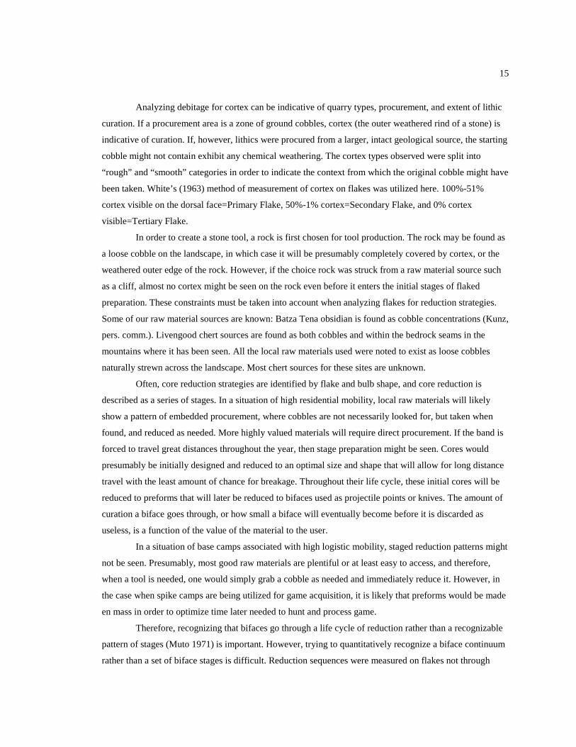
15

Analyzing debitage for cortex can be indicative of quarry types, procurement, and extent of lithic

curation. If a procurement area is a zone of ground cobbles, cortex (the outer weathered rind of a stone) is

indicative of curation. If, however, lithics were procured from a larger, intact geological source, the starting

cobble might not contain exhibit any chemical weathering. The cortex types observed were split into

“rough” and “smooth” categories in order to indicate the context from which the original cobble might have

been taken. White’s (1963) method of measurement of cortex on flakes was utilized here. 100%-51%

cortex visible on the dorsal face=Primary Flake, 50%-1% cortex=Secondary Flake, and 0% cortex

visible=Tertiary Flake.

In order to create a stone tool, a rock is first chosen for tool production. The rock may be found as

a loose cobble on the landscape, in which case it will be presumably completely covered by cortex, or the

weathered outer edge of the rock. However, if the choice rock was struck from a raw material source such

as a cliff, almost no cortex might be seen on the rock even before it enters the initial stages of flaked

preparation. These constraints must be taken into account when analyzing flakes for reduction strategies.

Some of our raw material sources are known: Batza Tena obsidian is found as cobble concentrations (Kunz,

pers. comm.). Livengood chert sources are found as both cobbles and within the bedrock seams in the

mountains where it has been seen. All the local raw materials used were noted to exist as loose cobbles

naturally strewn across the landscape. Most chert sources for these sites are unknown.

Often, core reduction strategies are identified by flake and bulb shape, and core reduction is

described as a series of stages. In a situation of high residential mobility, local raw materials will likely

show a pattern of embedded procurement, where cobbles are not necessarily looked for, but taken when

found, and reduced as needed. More highly valued materials will require direct procurement. If the band is

forced to travel great distances throughout the year, then stage preparation might be seen. Cores would

presumably be initially designed and reduced to an optimal size and shape that will allow for long distance

travel with the least amount of chance for breakage. Throughout their life cycle, these initial cores will be

reduced to preforms that will later be reduced to bifaces used as projectile points or knives. The amount of

curation a biface goes through, or how small a biface will eventually become before it is discarded as

useless, is a function of the value of the material to the user.

In a situation of base camps associated with high logistic mobility, staged reduction patterns might

not be seen. Presumably, most good raw materials are plentiful or at least easy to access, and therefore,

when a tool is needed, one would simply grab a cobble as needed and immediately reduce it. However, in

the case when spike camps are being utilized for game acquisition, it is likely that preforms would be made

en mass in order to optimize time later needed to hunt and process game.

Therefore, recognizing that bifaces go through a life cycle of reduction rather than a recognizable

pattern of stages (Muto 1971) is important. However, trying to quantitatively recognize a biface continuum

rather than a set of biface stages is difficult. Reduction sequences were measured on flakes not through

16

flake shape or bulb prominence but through flake scar count. Surovell (2003) writes that flakes which

exhibit less than three dorsal flake scars are generally associated with initial core reduction or flake

production, where larger flakes are removed, and flakes that exhibit three or more dorsal scars are

associated with bifacial thinning, where smaller flakes are removed with more care.

2.5 Large and Medium Scale Analysis: The Technological Investment Model

The Technological Investment model predicts that tool investment is a function of utility,

manufacturing time, and tool use time. In other words, the more time invested into tool production and use

time must also increase the caloric return from the resource utility. Time is a constraint on this model. If

increasing patchiness of environments increases residential mobility patterns and direct procurement

patterns, tools will be more heavily utilized and reworked. There will be a tradeoff between time spent

hunting and processing food and time spent for raw material acquisition and tool production.

Weapon strategies that increase reliability and maintainability will be more favored over

expediency in less patchy, resource poor situations. In these situations, heavily curated, durable tool

strategies will be optimal. In resource rich environments supporting more raw materials, and a variety of

habitat patches, an embedded procurement strategy will be optimal. Expedient tools should be more

frequently used and strategies that favor rapid weapon replacement should be seen (Bousman 2005, Bright

et al. 2002, Surovell 2003, Ugan et al. 2003). The probability of discard of artifacts with relatively long

use-lives consequently is low for short-term occupations, which increases the longer a site is occupied

(Schiffer 1987:55; Surovell 2003:120-127). Discarded tools at short-term residential sites should be

dominated by non local materials, heavy modification and/or retouching indicative of raw material

conservation. Discarded tools at long term residential camps should be of a higher ratio of local materials,

and a reduced amount of reworking. Centralized residence patterns should result in surplus tools, whereas

residentially mobile patterns should result in consumed tools. The model has high utility to this study, and

will be used at both the large and medium scale of analysis.

This model is constrained by the fact that it requires marginal gains will always be increased with

‘cheaper’ technologies rather than more costly ones. Cheaper technologies will always capture relatively

large marginal returns when compared to more costly ones. Bettinger et al. (2006) addressed this problem

by constraining technologies for comparison to specific categories of structurally related forms, and classes

of all potential technological types that could be applied to a particular subsistence pursuit.

“Formal” tools have been described as having a general, shared mental template among related

peoples in a specific time period, and tools which are premade, and transported between tasks and sites, and

are long lived. While this definition is almost too broad, they are here defined as opposed to tools that show

little to no secondary retouch, and exhibit more time-intensive curatorial practices. “Informal” tools are

ones considered to have been made immediately for a task at hand and generally discarded soon after their

17

purpose was finished.

2.6 Medium Scale Analysis: The Logistic and Residential Mobility Model

Binford (1980) also created a model that explains annual mobility patterns by frequency of moves.

A pattern of Logistic Mobility is recognized by fewer moves of the group. Main camps are often in a

central place, with smaller “spike” camps surrounding this. The model states that smaller camps and forays

are taken into surrounding regions in order to support the main camp. A pattern of Residential Mobility is

recognized by a greater number of moves of the residential camp throughout the year. Adding an HBE

component to the model, an optimizing solution to an increasingly patchy environment should be to adopt a

logistic mobility pattern, where a network of habitats and resources surrounds a central camp, and specific

logistical forays are undertaken from that point to acquire and return with specific resources (Kelly 1995,

Surovell 2003). The duration of time that a site is occupied is dependent on the frequency of residential

moves, or vice versa. Long-term occupations translate to low frequencies of relocating home bases. In

principle, accumulated artifacts are a function of occupation span (Kuhn 1994).

2.7 Medium and Small Scale Analysis: The Patch Choice Model

Some researchers define habitats as being made up of a system of ‘patches’ or “isolated areas of

homogeneous resource opportunities on a scale such that a forager may encounter several to several dozen

in a daily foraging expedition” (Winterhalder and Kennett 2006:16). The Marginal Value Theorem

(Charnov 1976), applied to the Patch Choice Model, assumes that while a predator is within a patch, its

food intake within that patch decreases over time. The Patch Choice Model predicts that a predator knows

and controls that patch it will visit, and will stay within a patch until the food within that patch decreases

below that of an adjacent patch, or the average for the habitat as a whole. Due to the fact that we cannot

directly observe prehistoric patches being chosen, this model is limited in its use and really only has utility

at the small and medium scale analysis in relation to site choice placement. The model assumes that 1)

natural selection will favor behaviors of optimal allocation of time and energy expenditures, 2) in a fine-

grained environment, prey species are located in the proportion in which they occur, and 3) the larger the

variety of acceptable items, the less search time per unit of food (MacArthur and Pianka 1966). The model

is limited as the predator (not patch boundaries) defines prey items. Therefore, defining patch boundaries is

subject to the researchers’ data (Sih 1980).

2.8 Small Scale Analysis

2.8.1 The Ideal Free Distribution Model

Two models are useful at the small-scale analytical level. The Ideal Free Distribution model

18

(Figure 2.1) illustrates that habitats (or unit area or unit resource) are chosen on the basis of fitness quality

within them (suitability). Individuals are assumed to choose to occupy the best habitat available to them,

and to have free access to choose between habitats. Fitness is based upon successful reproduction rates

and/or food intake. The model assumes that the individual has complete information on a habitat (Fretwell

and Lucas 1968; Kennett 2005; Sutherland 1983, 1996; Winterhalder and Kennett 2006:16). An increase in

population size will lead to a decrease in survival and reproduction; therefore, suitability of a habitat

increases as predator/forager population drops to zero. The model will only have use at the level of small-

scale analysis, inferring behavioral choice for groups of site placements on the landscape, and potential

abandonment of one region for another. The model is limited in its assumption of equality of all predators.

It also does not take into account habitat size, as more suitable habitats and patches tend to decrease in size.

Sutherland (1983) applied this model to predator aggregation. Aggregation occurs when chance

encounter with prey increases within a patch. Therefore, residence times will increase in high-density

patches, and disbanding occurring when the patch average return rate falls below that of the habitat return

rate as a whole.

2.8.2 The Central Place Foraging Model

The Central Place Foraging model (Figure 2.1) predicts that the distance an individual will travel

from a camp location to find food is determined by the time spent foraging multiplied by the return rates of

the food. The result is divided by the travel costs for a net result (Kelly 1995, Orians and Pearson 1979).

The model assumes that resources are not itemized in patches, but homogeneously distributed around the

camp location. The predator/forager can search simultaneously for several prey items; however, or one can

be pursued and handled at a time. If some prey types affect subsequent captures more than other types, the

over-all rate of energy capture during a trip may be increased by selecting those prey with minimal adverse

effects on subsequent captures at the beginning of a foraging sequence and only taking other types toward

the end of a sequence when foraging is about to be terminated for other reasons. As distance (traveling

time) from patch to central place is increased, the greater must be the prey energy selected by the predator.

For short traveling times, superiority of prey hinges on energy-per-unit handling times. For long traveling

times, superior prey are those of higher energy, regardless of their handling times. If patch quality remains

constant, optimal load increases with increasing distance of the patch from the central place, a predator

should continue to load even though its rate of loading is dropping. If a partial or full load of small items

will not seriously hamper pursuit and capture of large prey, then small items should be taken when

encountered, providing that handling such items does not seriously detract from search time. If the large

item is rare, it should be taken whenever encountered; but if it is abundant, capture should be postponed

until a full load of small prey is obtained, especially when travel time is great. Predators should, other

things being equal, travel initially to the farthest site to be exploited during a trip and then forage while

19

moving in the general direction of the central place. However, factors may reverse this. The model can be

used qualitatively to assume the placement and relative duration of occupation of a site based upon the

resources available.

Applying these models to the research area will allow us to explore potential decisions by which

hunter gatherers chose to move and camp across the landscape. Ethnographic research in the region is very

limited in the data available to operationalize the models to prehistoric lifeways adequately. Additionally, a

lack of organic preservation and stratigraphic integrity further complicates the process of identifying site

behaviors.

2.9 Application and Expectations to Subarctic Alaska

In the Alaskan Interior, several prehistoric weapon-manufacturing techniques have been

recognized. Researchers have argued that specific technologies are constrained by time, space, and

environment. However, when seasonal rounds (annual migrations throughout a group’s territory) are

modeled, it becomes apparent that weapon choice likely varied between seasonal availability of prey as

well. Hypotheses from behavioral responses to geography and prey choice can be tested against

expectations of HBE to understand the mechanisms for stasis and change. The research hypothesis is that

resource availability could also have been a constraint on weapon strategy. The disappearance of an

acquisition system (a behavior), or a weapon strategy (a material correlate), from the record can be

explained as loss or abandonment of an ecological niche to which a specific tool was adapted.

This research proposes to examine technological stability and change in Central Alaska from an

HBE theoretical construct. Much previous research has partly depended upon the cultural-historical

paradigm, explaining tool form as a cultural identifier. More recent research has begun identifying tool

forms as possibly indicative of seasonal strategies (Potter 2008b, Wygal 2009). This study assumes that

humans in the past exploited resources in a given area according to a least-cost principle; that the visible

combination of environmental variables and human behavior patterns creates a specific recognizable

pattern, that the economic system therein is consistent throughout time despite distinct archaeological

periods, and that a relationship exists between site density and prehistoric land use.

If weapon form is dependent on prey choice, then mobility patterns may potentially be inferred. If

raw material is an indicator of mobility patterns, short-term occupation sites should be dominated by non

local raw material, and local materials should dominate long-term occupation sites. If weapons were a

function of seasonal weather, composite weapons would dominate winter assemblages, and point/shaft

weapons a function of warmer months. If weapon strategies are a function of season, they should be patch-

specific. If technological strategies were constrained specifically to ecological niches that were exploited

on a seasonal basis, then changes within these systems/technologies are a function of ecological change. If,

at multiple occupation sites, a correlation exists between environmental conditions and tool occurrence,

20

then tool strategy can be said to be a behavioral function of the environment. If ecological constraints

favored certain technologies to be more useful than others in specific habitats, then individuals may have

used a strategy that utilized specific weapon technologies in ecological conditions that were constrained by

space and season. If increasing patchiness of environments increases residential mobility patterns and direct

procurement patterns, tools will be more heavily utilized and reworked. If weapon strategies are strongly

dependent upon habitat quality, this may suggest reasons for projectile point type abandonment, and/or

adoption through time, as well as the conservation of microblade technology throughout the Holocene and

suggest some reasons for the loss of this technology around ~1300-800 BP.

The following chapter incorporates these methods, models, and hypotheses into the prehistoric

archaeological record as we presently understand it. Chapter 4 will incorporate them into a spatial model of

resources at a landscape level in order to reveal seasonal behavior and mobility patterns as constrained by

potential prey choice and availability, and Chapter 7 will incorporate them into an intersite analysis.

21

3 Modeling the Prehistory of Alaska

3.1 Siberian Origins and the Colonization of Beringia

This chapter summarizes the prehistoric origins and developments that set the stage for the

Athabascan Period in Alaska and the Yukon. At the time of the LGM, Asia extended as a continuous

landmass into North America. At their lowest point, sea levels had dropped roughly 120 meters below

present levels, with water being locked away into the continental ice sheets. Northeastern Asia extended

east as a sub-continental sized peninsula known as Beringia. The area was also broken by localized ice

sheets in the mountainous areas and bounded by the Laurentide and Cordilleran Ice Sheets in the east.

Vegetation was dominated by a mosaic pattern grasses, sedges, and forbs uniquely adapted to the harsh,

arid Pleistocene climes (Ager and Brubaker 1985). Beringia likely never exhibited a continuous ecosystem;

from the fossil record, not all terrestrial Pleistocene fauna known in northeastern Asia migrated into Alaska.

Only select species whose behaviors were adapted to successfully moving between mosaics of ecological

niches successfully adapted to this harsh arctic landscape.

Archaeological assemblages that can be attributed to modern humans existing in northeastern Asia

before the onset of the Last Glacial Maximum (LGM) show a remarkable uniformity with each other.

Throughout Siberia, the technocomplex known as the Diuktai culture, possibly extending as far back as 35

cal BP shows artifact continuity expanding either out of the Aldan Basin (Mochanov and Fedoseeva 1986)

and/or south-central Siberia (Kuzmin 2007). The complex included various sized bifaces, wedge-shaped

cores and associated blades, as well as a few surviving bone and ivory projectile points (Mochanov and

Fedoseeva 1996). These tools appear to be an integral strategy that allowed humans to successfully expand

throughout Siberia and into Beringia.

The Early Upper Paleolithic (EUP) complexes accompanied, and perhaps enabled humans to

spread throughout Siberia into the Russian Far East (Brantingham et al. 2004, Goebel 1999, 2002, 2004).

The widespread artifact continuity disappears from the record at 22.8 cal BP. While the classic EUP

technological markers disappear from northeastern Asia (22.8 cal BP), it appears humans continued to

inhabit northern China (Barton et al. 2007), the Korean peninsula (Bae and Kim 2003), the Japanese

Archipelago (Nakazawa et al. 2005), and southern Siberia (Kuzmin and Keates 2005), however in apparent

less density. Interior continental deserts (the Gobi and the Mu Us) expanded south with the onset of the

LGM, pushing grass steppe-lands even further south, leading to an apparent abandonment of the

continental interior above the 41st parallel (Barton et al. 2007).

A strategy that was likely adopted in response to these ecological restrictions was the development

of microblade technology. The appearance of microblades and associated cores, are assumed to have been

an integral part of a composite weapon comprising small stone blades inset into the sides of a bone

projectile point, hafted onto a wood shaft. At this stage in the research, microblade technology appears in

22

China as early as 31 cal BP (Chen and Wang 1989), slightly later in Siberia at 30 cal BP (Derev’anko and

Markin 1998), existing sporadically until 25 cal BP, when it appears to be a strong component of

northeastern Asian systems, spreading into the Korean peninsula and Japanese archipelago around 24 cal

BP (Nakazawa et al., 2005, Bae and Kim, 2003; Ikawa-Smith, 2004).

Rapidly deteriorating conditions of weather patterns associated with the LGM, drastic floral

changes, and regional extirpation of key prey species are likely key reasons for the technological change

(microlithization or abandonment) seen in northeastern Asia. At this time, it does not appear any

representatives of the EUP migrated east into North America. The rapid reduction of viable prey would

have placed such a demand on human behaviors dependent upon those species key to group survival that

required adaptive behaviors led to dramatic loss in human populations (Brantingham et al. 2004).

Immediate responses to a drop in prey density would include increased mobility on the landscape,

resulting in more short-term, smaller campsites (less visible archaeologically), expansion of diet breadth

(adding more prey items to the diet which would not have originally considered worthwhile to harvest),

adopting innovative weapon strategies, and altering food storage practices. Other coordinated responses,

requiring widespread acceptance and cooperation would be adopting strategies of resource exchange,

territorial rights, expansion of kinship, and divisions of labor. These risk minimization strategies are

inferred upon prehistoric individuals and bands through the demonstration and interpretation of patterns

and key interruptions of those systems.

Humans who continued to inhabit the cold grass steppe of northeastern Asia during the LGM

likely adapted to herd movements and migrations of the large Pleistocene ungulates. Reducing risk likely

meant increased mobility, which likely meant reduced band size, and targeting harvesting resources near

the reduced number of lakes and rivers that would have drawn or funneled game to fewer, specific, and

predictable locales.

3.2 Late Pleistocene and Early Holocene Eastern Beringia

Around 14,000-13,000 BP, warmer temperatures are indicated by the expansion of birch and shrub

tundra into the area of Central Alaska. The warming trend was followed by another period of climactic

deterioration, the Younger Dryas (13-11,300 BP) characterized by birch, willow, grasses and sedges

(Bigelow and Powers 2001).

In the Alaskan Interior, mammoths appear to become locally extirpated around 12,000 cal BP. Elk

were absent from the region between 18,000 and 13,000 cal BP after which they rapidly recolonized the

Interior (Guthrie 2006). Moose also disappear at 18,000 BP, recolonizing eastern Beringia around 12,500

BP. Both species move in from Asia, followed closely by humans. Bison seem to have marginally survived

the LGM in the region, and substantially increase in numbers around 12,000 BP. After a period of

continued decrease in body size, the horse population crashes around 11,800 cal BP (Guthrie 2003,

23

Grayson 2007). DNA evidence suggests that mammoth and horse both persisted in Alaska, at least

marginally, until 10,500 cal BP (Haile et al. 2009). The existence of these various species that represent

both grazers and browsers, along with the lack of proof of simultaneous cross-species extirpation suggests

not a uniform ecosystem, but rather a complex environment, conducive to human predation, adaptation, and

survival.

Around 13,000 cal BP, the Ice Free Corridor opened between the Cordilleran and Laurentide ice

sheets, permitting access between Beringia and central North America. Along the western North American

coast, evidence of sunken forests suggests a series of coastal refugia existed throughout the LGM (Dixon

1993). However, evidence is as yet only circumstantial as to which route the first Americans took to arrive

south of the ice sheets.

The terminal Pleistocene was a highly fluctuating environment, with marked periods of warming

and cooling. Eastern Beringia was marked by the ever-changing mosaic patchwork of sandy deserts and

grassy steppes. The continuous changing diversity of large game would have required strategies that were

able to adapt to these fluctuations. Assuming that technology is a function of diet breadth, in an

environment lacking long-term continuity, risk would be higher, and we should expect to see less specific

tool curation. Time and investment in specific weapon systems is predicted to increase when diet breadth

narrows, and alternatively decrease when diet breadth broadens. Therefore, we should see less toolkit

conformity during the initial phases of the LGM colonization, and increased toolkit conformity as local

fauna establishes itself over long periods of time.

The Holocene Thermal Maximum (HTM) occurred between 10,000 and 9,000 cal BP (Kaufman et

al. 2004). The HTM period saw the final inundation of central Beringia. At Birch Lake in the upper Tanana

valley, Bigelow (1997) identifies a landscape parkland dominated by poplar and willow from 8100 to 6900

BP, transitioning to spruce dominated by 5300 cal BP (Magoun and Dean 2000, Viereck et al. 1992).

Bison and elk seem to have thrived in the Interior to about 9000 cal BP (Yesner 2001); after this

date bison population numbers drop, eventually becoming locally extinct between 1000 - 400 yBP

(Stephenson et al. 2001). The persistence of elk is not well documented, as the bones may often be

misidentified as those of moose (Potter 2005). DNA evidence from muskox shows a considerable loss of

genetic diversity from the LGM into the mid Holocene, when their population rebounded, expanding even

into eastern Asia (MacPhee and Greenwood 2007). Caribou from Alaska and the Yukon appear to be

genetically diverse enough from other North American populations that researchers argue for their isolation

within Alaska during the Wisconsin Glaciation and continued population persistence throughout the

Holocene (Harding 2003). Dall sheep also continued to survive in the Interior.

The actual landscape probably existed as a patchwork of ancient steppelands surviving at higher

altitudes and latitudes, with the parklands dominating the majority of the habitable landscape below the

perennial icefields, and the slowly encroaching boreal forests. As these habitats alternately expanded and

24

contracted throughout the early to mid-Holocene, ungulate herds specifically adapted to local niches also

responded.

The landscape appears to have become increasingly forested, which had a negative effect on the

success of most species of large ungulates in the Interior (Mason and Bigelow 2008). The loss of grazing

ecozones seems to have affected horse and mammoth herds first, with bison and wapiti surviving later. By

the time the next cooling/drying event occurred about 8200 cal BP (Powers and Hoffecker 1989), the boreal

forest dominated the landscape. The loss of ungulate diversity could have increased the importance of

salmon in the diet and the increased focus on summer harvesting of anadromous fish.

Figure 3.1 Map of Beringia and the Alaskan glaciers at their greatest extent during the LGM (20 cal BP).

Sea levels have been set at approximately 120 meters below present levels. Sites projected are not

necessarily contemporaneous with each other or dry land and glacial extent.

In Eastern Beringia, the Diuktai microblade toolkit along with transverse and dihedral burins is

represented in Swan Point Cultural Zone 4, c. 14,000 cal BP (Holmes 2008). Technology represented at the

Ushki Lake site (Figure 3.1) lacks microblades in the earliest occupations; however they are represented in

25

the later Diuktai-like assemblages (Dikov 1993). Aside from the technological continuity suggesting

cultural continuity across Siberia at the end of the LGM, the seminal work of Edward Vajda (2010)

establishing the genetic links between the North American Na-Dene language family and the central

Siberian Yeneseian languages adds another line of evidence of the antiquity and cultural connections of

Pleistocene human migrations.

Projectile point weapon technologies appear to be focused on the acquisition of medium to large

sized game, and may change morphology depending on the species being hunted. In eastern Beringia,

triangular bifaces appears to develop regionally. The technology was first described by John Cook (1969)

at the earliest occupations at Healy Lake (Figure 3.1). Called Chindadn or Nenana (Goebel and Slobodin

1999) these bifaces are highly variable and likely represent a multiuse tool.

Terminal Pleistocene diet breadth in the Alaskan Interior can only be adequately demonstrated

through multiple sites across a wide variety of geographical settings. A formal model of diet breadth for

this time period cannot yet be demonstrated, however, we do have several sites that have preserved a good

sample of prey utilized by humans. Dry Creek component I yielded faunal elements consistent with wapiti

and mountain sheep, and a lithic assemblage of bifacial knives and projectile points. The later component II

yielded faunal elements of bison and mountain sheep, with distinct clusters of lithic remains consistent with

both bifacial reduction and microblade production strategies, by which the researchers concluded that the

site represented a fall/winter residential hunting camp (Powers et al. 1983). Bison, being grazers, prefer low

lying grassy plains, mountain sheep prefer upland settings, and wapiti, also grazers, can be found in all

sorts of environs.

Across the northern slopes of the Alaska Range, important sites exist likely as a response to the

habitat boundaries. The diet breadth from Dry Creek component I and II (Powers and Hoffecker 1989),

Teklanika West CZ2 (Coffman 2011) and north of the Tanana River at Gerstle River (CZ3) (Potter 2005)

(Figure 3.1) indicate specific hunting behaviors targeting large ungulates. This suggests that the diet was

supplemented by continued use of salmon and migratory fowl as seen in Swan Point CZ 4 (Figure 3.1)

(Holmes et al. 1996) and Broken Mammoth CZ 3 and 4 (Yesner 1994, 1996, 2001)

At Teklanika West, Component I bison elements (10,920 +-50 BP and 11,080 +- 50 BP) are

associated with debitage consistent with bifacial reduction (Coffman 2011), and may represent tools only

consistent with meat processing and not prey killing. At the Upward Sun River Site (Figure 3.1), a hearth

feature that contained the cremated remains of a young child (11,620-11,280 cal BP) also contained the

bones of salmon, marmot, hare, squirrel, ptarmigan and passerine (Potter et al. 2011). The contents led

researchers to conclude the hearth and associated house feature represented a summer/late summer

encampment (compare with Carlo Creek, also interpreted as a likely summer camp (Bowers 1980)).

Component 1 at Gerstle River (9893+-35 BP) contains some possible bird elements, with unidentifiable

mammalian bones of various sized animals (Potter 2005:341-342). The lithic assemblage lacked

26

microblade production.

Throughout the Terminal Pleistocene and early Holocene, microblades are found in high

association with bison, wapiti/moose, while bifacial technology tends to be associated with mountain sheep

and caribou. Potter (2011) has shown that this correlation suggests two weapon strategies employed

simultaneously, but separated by seasonal context. Sites which exhibit both technologies may possibly

represent residential camps where one technology (Strategy A) was being implemented for prey acquisition

while the other (Strategy B) was being utilized to gear up for the upcoming season focusing on hunting

animals in a different ecological context. Potter has also shown that microblades tend to be found in

lowland contexts, and bifaces in upland contexts (2008a). From this, it appears that humans employed

annual migration patterns throughout the late Pleistocene and early Holocene, which focused on

intercepting large ungulate spring and fall migrations, and winter ranges in the uplands, while summers

were in lowland context focused on harvesting fish and small mammals in river and lake patch

environments. Tools in these latter contexts were likely organic implements and have not survived.

Throughout the Pleistocene-Holocene transition, the cultural record suggests a wide variety of

weapons that were available to their users. These included lanceolate point-tipped darts, designed to be

lightweight, thrown great distances, and transported easily. These were likely used in situations where

close-encounter kill opportunities were limited. Composite weapons, associated microblade technology,

were more durable, and could have been utilized in close-encounter kills, where game was placed in

disadvantaged situations, including being driven into bodies of water, snares, or down cliffs or steep slopes.

There is much debate concerning the role microblade technology played to the people who utilized them.

As the climate fluctuated and various targeted game expanded, contracted, or were extirpated across the

landscape probably had a direct effect on the variability and visibility of tool types in the archaeological

record.

3.3 Mid-Holocene Alaska

During the mid-Holocene, bison and wapiti continue to decline in abundance as salmon and

caribou become more common in archaeological assemblages. These two mainstays were likely

supplemented by a wide variety of edible items of less caloric return, if the ethnographic and historic record

can be used as a reliable proxy. The loss of big game diversity, may have been accelerated by several large

scale, widespread volcanic events in South-central Alaska (the Oshetna tephra, 6750-5850 cal BP (Dixon

1993). The Hays series of eruptions between 4200-3800 cal BP (Beget et al. 1991) likely also played a

negative role in habitat/patch diversity and local predator and prey population levels. Another

cooling/drying event occurred at 3800 cal BP and again at 2900 cal BP (Brigham-Grette 2001). It is very

likely that this system of warming and cooling events, compiled with devastating ash/tephra falls in the

higher elevations, and the persistence of widespread spruce forests contributed to the continued decline of

27

game diversity, and thereby the carrying capacity of human population levels in the Interior.

Two additional main volcanic events characterize the late Holocene in central Alaska. The first

White River Ash fall occurred ca 1800 cal BP and the second 1140 cal BP. Between these another cooling

event, the Medieval glacial advance 1500-1300 cal BP occurred (Calkin et al. 2001), followed by the final

one, the Little Ice Age, lasting ca 900-200 BP. The warming events between them have been linked to

drastic effects on populations across northern Europe and Asia, which is beyond the scope of the paper, but

we can make similar inferences for the American subarctic. While the volcanic events likely had short-term

effects on local demographics, the climate warming events probably are the culprit for any sustained

ethnographic change.

After 6000 cal BP, side-notched points, associated with the Northern Archaic Tradition appear in

the archaeological record throughout Alaska. The Northern Archaic Tradition is thought by many to

indicate human adaptation to a Taiga forest environment (Mason and Bigelow 2008). These points vary

extensively in morphology, perhaps indicating that the shape and size of the point were of lesser

importance to the hafting procedure. It is important to note that microblade technology continues

throughout this time.

Some researchers (Anderson 1968, Dumond 1969, Derry 1975) explain technological changes in

the Interior as being due to migrations into central Alaska. Others (Morrison 1987) explain this change as

rather a diffusion of technology across groups, while Dumond (1987) searches for a compromise between

the two, positing an amalgamation. The apparent lack of an available nutrient load to attract immigrant

movement in the first place argues against this. Successful population movements would need adequate

information on raw material locations and seasonal prey locations. The chances of opportunistically finding

these at levels that would sustain band survival in the face of likely hostile opposition from local

established groups add to the unlikelihood of successful migrations due to single-point-in-time events.

Rather, if large scale population displacements did indeed occur in eastern Beringia (coastal regions

excluded), it was more likely due to prolonged environmental change which forced a continued

demographic shift in the face of social collapse.

3.4 Discussion

Previous research has drawn connections between changes in technology and possibly changes in

either conditioning facts and/or normative cultural templates. This research focuses on decision variables

that are tractable in the empirical record. In general, normative models of artifact change are difficult to

test.

The Late Prehistoric, or Athabascan Period (~1000-100 cal BP) is one of pronounced

technological change. This period is marked by the increased importance of organic tools, food caching

behaviors, and the use of hammered copper (Workman 1978, Shinkwin 1979, Cooper 2007). Holmes

28

(2008) notes that this period is marked by an increase in diversity of projectile point forms. The Athabascan

Period is marked by the introduction of the bow and arrow, largely supplanting the older atlatl and dart

strategy, likely adopted from the coastal Eskimo. The new technology seems to be linked to the loss of

composite weapon strategies as well. Bow hunting allows the hunter to kill prey from farther away, and

also lessens the need for a group to make successful kills. Microblades are largely lost from the record.

Potter (2008) provides a strong summary for expectations of microblade and biface use across the

landscape.

Ice patch finds in the southern Yukon, where hafted implements have been preserved, indicate that

the transition between atlatl darts and bow and arrows occurred between 1200-1100 cal BP (Hare et al.

2004). Ice patch hunting is a specific strategy, however. The YTU has been unglaciated since the

Hypsithermal. Permanent ice patches do not exist in the region today. While bows were likely favored

throughout the year, certain hunting strategies in the region may have favored composite weaponry to

linger in the region longer than elsewhere in the subarctic.

Composite weapons as heavy-duty thrusting spears are optimal in conditions where multiple uses

and durability of the same tool is needed. These conditions would be useful in periods of logistic behaviors,

such as during the fall caribou hunts. In the YTU, caribou fences of trees, deadfalls, snares, humans, and

Inuksuk were all utilized for the fall migration hunt. Mass quantities of caribou were slaughtered,

butchered, and stored for the long winter months. At a single point in time, where hundreds of caribou are

being caught and killed, a few multi-use weapons might be optimal over shooting many one-time-use

arrows. In this sense, microblade technology could be hypothesized to exist alongside bow technology.

Another strategy of durability and multi-use tools however, also spread in popularity during this

time: the native copper industry. The industry seems to have risen simultaneously on the west and east

sides of the Wrangell Mountains in southeastern Alaska and southwestern Yukon (Cooper 2007).

Hammered copper implements spread throughout the interior via trade routes, and were highly sought after

items for many tools and decorative objects. Copper knives and projectile points might have actually met

the desire for a durable tool when this was needed. The ultimate loss of the core and blade technology by

the historic period might have been due to the interplay of both bow and arrow and copper implements. In

this light, microblade technology would have lingered in resource-poor regions, where the value of copper

as a trade item might have exceeded the desire to acquire it. The late occurrence of a specific technology

could occur in instances of neighboring group hostility, or a lack of a reciprocal trade item of equal worth.

This problem will be explored throughout the rest of this work, primarily in Chapter 7. The Athabascan

Period will be discussed more in depth in the following chapter.

29

4 Modeling Optimizing Behaviors Across the Yukon Tanana Uplands

The Athabascan, or Late Prehistoric Period is generalized as the last one thousand years until the

historic period of direct contact with Euro-Americans. The main problem facing research is that we only

know broadly what foraging choices were being made during this time period. Connecting this broad data

reported in the ethnographic record to archaeological assemblage variability will help demonstrate

assemblage behavioral choices. This chapter incorporates all regionally known prehistoric sites, modern

resource data, and an ethnographically informed model in order to recreate recent foraging events. If

migrations of new people with new technology did indeed replace older populations in this region, it is

unlikely their resource use patterns would mirror their predecessors. If the human population is held

constant through time, and their weapon system was replaced through adoption of another, resource

patterns again should shift through time. If, however, the human population held constant, and likely did

not change through migration between the Northern Archaic and Athabascan periods, and their toolkit

changed over a long period of centuries rather than a relatively fast event, resource-use patterns might be

affected indicating a more successful prey-acquisition strategy change. If strong correlations exist between

these frames of reference, then patterns of land use can demonstrated to exist through the past. Most of the

prehistoric sites in the region remain undated, and therefore, we cannot test Northern Archaic sites against

Athabascan sites for differences in regional resource use. However, if weak correlations between land use

patterns and site placement are encountered, then the resource patterns can be said to have changed

throughout time, suggesting population replacement or large-scale hunting weapon replacement. The model

presented in this chapter assumes that humans in the past exploited resources in the area according to a

least-cost principle; that the visible combination of environmental variables and human behavior patterns

creates a specific recognizable pattern, that the economic system is consistent throughout time despite

distinct archaeological periods, and that a relationship exists between site density and prehistoric land use.

This stage in the analysis is necessary as a coarse-grained first approximation of linking different

datasets in order to draw broad inferences in site placement choice. Once enough of a sample of the

prehistoric record is known, and the patterns within those assemblages have been adequately described,

inferences drawn from those records can be used to model greater expected behavioral patterns. The

research focuses on the little known mountainous region between the Yukon and Tanana rivers, defined as

the Yukon Tanana Uplands (YTU) (Wahrhaftig 1965).

The YTU are sparsely populated today, with the majority of local infrastructure resulting from on-

going gold mining activities. The archaeological knowledge of this region tends to be oriented towards

exploring areas of infrastructure development such as roads, trails, and mining claims. Areas that are more

difficult to reach, due to distance, topography, and other environmental factors are overlooked in favor of

places that are easier to access due to logistical factors, such as time, cost, and effort. As a result,

archaeological sites are clustered near areas of modern infrastructure, creating patterns of prehistoric

30

activity that are likely a biased, misrepresentation of the actual regional archaeological record.

In an attempt to counteract the effect of this misrepresentation and to help streamline future

research into the remote country of these highlands, relationships between existing sites and variables on

the landscape that would have been considered of value to prehistoric inhabitants need to be clearly

distinguished. The next step is to project these variables regionally in order to highlight areas on the

landscape that hold a higher potential for prehistoric site preservation.

In the Alaskan interior, interpreting material culture and how it relates to human behavior over

space is critical in explaining human habitat and exploitation of the local environment (Andrews 1977,

Derry 1975, Hoffecker et al. 1993, Holmes 2008, Mason and Bigelow 2008, Potter 2006, 2008a, 2008b,

Shinkwin et al. 1980). The period of cultural contact between the Natives of this area and the Euro-

Americans was highly destructive to ancient behavioral patterns. Already before actual historic contact,

new trade goods had changed previous Athabascan lifeways, causing bands to alter their camps, villages

and hunting cycles to facilitate trade ultimately with the Lebedev-Lastochkin Company, the Russian

American Company and the Hudson Bay Company (McKennan 1959, Osgood 1936 and 1971, Pierce 1995,

Simeone 1982).

There were few people present to make a written record of the changes, which were swift, and

therefore the extent of them can only be estimated. Information is derived from Native memories, various

memoirs recorded by whites, and the little ethnographic work done in the following decades. For the

purposes of the model, it is assumed that this information is an accurate portrayal of pre-contact native life

in the area. It is also assumed that the basic economic system in this area was held constant through time,

and that all prehistoric sites within its boundaries reflect this one broad system of exploiting the landscape.

The same basic foraging equipment is assumed to be held constant through time. Further assumptions are

that climate, faunal, and floral data have also remained constant since at least the mid Holocene. This scale

of analysis is useful in exploring the relationships between site placement and seasonal resource

availability. Relationships may be completely spurious and while seemingly apparent, in reality might be

non-existent.

An ethnographic study was independently undertaken to resolve the best understanding of the

distribution, abundance, and the economic costs and benefits of natural systems through the territories of

the Han, Tanana, and Gwich’in. The seasonal rounds discussed in this chapter fall into what Binford (1980)

would describe as behavior indicative of “collectors”, involving storage of food for part of the year and

logistically-organized groups or bands specifically structured for food procurement. Collector groups are

characterized as setting out to specifically procure certain resources, and thus, these goals will be apparent

in site formation, features, and artifacts.

Certain sites will be large and highly visible large due to the amount of food being processed.

Other sites could be characterized as caches and observation stations. The placement of certain sites may be

31

a combination of any of these three types. Certain materials in the area will be largely available throughout

the region, while others are only available in specific regions and sites oriented at or near them can be

interpreted as sharing a relationship with that material.

The purpose of this chapter is to test known Northern Archaic and Athabascan settlement patterns

and cultural systems against optimization models. To do this, an ethnographic model, followed by Optimal

Foraging, Diet Breadth, and the Patch Choice models, and finally a geospatial model using ArcGIS will be

implemented. The hypothesis here is: if significant site patterns can be demonstrated by applying optimal

foraging models to this area, then further, more robust hypotheses of seasonal use of this montane region

can be investigated.

Optimal Foraging theory assumes that if specific behaviors have been selected against other

behaviors to optimize reproductive success, then models can be produced that predict the optimal pattern of

behavior within given constraints. Foraging behaviors that make choices that yield the biggest payoff will

be naturally selected for. Therefore, hunter-gatherers decide when and what to forage for based upon

consideration of the relative value of simultaneously available resources. Foraging decisions, when given

the context of technology and environment, can be predicted according to the Optimal Foraging assumption

that net energy capture rates serves to model relative values of resources.

4.1 Land Evaluation

Kamermans (2006) points out that land evaluation from an archaeological perspective is done

through an inductive approach, where one incorporates known site attributes, historical, ethnographic, and

landscape information, which is then used to predict site location. A deductive approach would build a

model based on historical, ethnographic knowledge and landscape information, and would then use existing

archaeological information to evaluate the strength and validity of the model. For reasons pointed out in the

introduction, current accumulated archaeological knowledge in the YTU is considered biased, and therefore

a deductive approach is used as a first approximation.

4.2 Construction of Economic Models of Land Use From Ethnographic and Historic Data

Multiple ethnographically attested groups peripherally used the YTU, primarily utilizing the

lowlands. Three to four matrilocal bands of the Han used the easternmost regions of these highlands,

between the Yukon River in the North to the Tanana in the South. North of them bordered the Gwich’in, a

people thought to have originally inhabited a range that included the whole southern slopes of the Brooks

Range. By the 1850’s they were being pushed eastward and southward by Eskimo groups. At the turn of

the century, one group was noted as living on the southern banks of the Yukon, the Birch Creek Kutchin.

The Lower Tanana and Middle Tanana Athabascans are territorially linked to the Tanana River

and its north and south tributaries. They exploited the southern drainages of the Yukon-Tanana uplands. By

32

the turn of the century, these groups were using the south-flowing creeks and rivers from this area, and

likely pushed north occasionally as the need presented itself. The Koyukon Athabascans inhabited the

Minto Flats area to the west, where the conflux of the Yukon and Tanana Rivers is located. It is also not

known if they exploited the White Mountains in any way, but they are thought to have come late to the

area, pushing east during the 1800’s (Andrews 1975, 1977, Crow and Obley 1981, Fathauer 1942, Hosley

1981a, 1981b, McFadyen 1981, McKennan 1959, 1981, Osgood, 1936, 1971, Simeone 1982 and Will

1984).

Figure 4.1 Ethnographically attested band territories ca1890 A.D. (red bounds the project area, with all

prehistoric sites known in yellow). Boundaries were likely very fluid through time, and shifted often.

4.2.1 The Han

Osgood records that the Han Athabascans are thought to have numbered about 1000 individuals at

the time of contact in 1898 (1971). He recorded three known matrilineal clans. Bands tended to consist of

one or several families (Crow and Obley 1981).

The territory of the Han (Figure 4.1) centered on the Yukon River, between the tributaries of the

33

Klondike and Kandik rivers on the northeast bank and the Fortymile and Charley Rivers on the southwest

bank. Andrews estimates their territory as extending 16,900 square miles. Three main camps are noted in

the late 19th century: Charley’s Village, near the mouth of the Kandik River, and Johnny’s Village and

David’s Camp, located near present day Eagle (Andrews 1977).

Fish was considered the staple of their diet (Osgood 1971). Spring would find the Han migrating

to areas along the Yukon and these other rivers in anticipation of the salmon run. The migration would be

undertaken before breakup and while the ground was still frozen, in order to facilitate movement.

The villages of the Han appear to have been more or less semi-permanent settlements. The

structures in the villages consisted of semi-subterranean houses, built of split, upright spruce poles and

insulated with moss. While traveling, small domed tents of caribou hide were utilized. The log/moss houses

were used during all seasons for long encampments (Crow and Obley 1981).

Spring involved repairing the moss houses, repairing and building canoes which were built of

birch bark or moose hide), nets, and fish weirs. While preparing for the salmon run, caribou, moose, small

game, and other fish were hunted, using the bow with several types of arrows, spears, and snares. Blunt

arrows were used for hunting waterfowl.

During the summer salmon run (July-September), focus was entirely turned to capturing as many

fish as possible and drying and storing them for the winter. When the run ceased, the groups broke into

small familial bands for about a month, spreading out into the surrounding countryside. Men tended to

spend their time hunting and the women, children, and elders continued fishing and repairing the caribou

impounds for the winter. During this time extra meat was cached, which was returned for usually around

mid-January. Around October, the bands would recongregate at the river camps. Snowshoes and clothing

were then prepared for the winter.

Winter was spent in the river camps, with a trip to bring in cached meat occurring in January. Mid-

February to mid-March was focused on the caribou hunt. The caribou hunt was a communal activity, with

bands congregating together to participate. Animals were driven into large caribou fences, which were long

systems of felled and somewhat cultivated trees. One of these was reported to have stretched over thirty

miles in length. The game would become entangled with hidden snares, and then dispatched by bow, spear,

and occasionally by knife. The caribou hunt provided meat that was cached and sustained the bands until

the salmon runs. The use of small corrals formed by wood or humans to capture and kill the animals has

been reported also. To a lesser extent, moose, bear, and sheep were also hunted. Spruce roots were used to

weave baskets for cooking, which were dug into the ground and filled with hot rocks for boiling (Osgood

1971, Crow and Obley 1981).

4.2.2 The Gwich’in

The Gwich’in were a widespread Athabascan group whose territory originally extended across the

34

entire south flanks of the Brooks Range. During the 19th century, they were pushed to the east by the

Eskimo, and at contact, their bands range from the Mackenzie River in the east to the headwaters of the

Koyukuk River in the west. Until the Eskimos pushed them south, they ranged the north slope of the

eastern Brooks. In the Yukon, they exploited as far south as the tributaries of the Peel River. They bordered

the northern territory of the Han (Figure 4.1). One regional band (the Birch Creek Kutchin (older colloquial

rendering of Gwich’in)) of several families exploited the northern reaches of Birch Creek, and two families

were reported to exploit Beaver Creek, but it is unknown how far south they pushed into the White

Mountains (Slobodin 1981).

The Gwich’in are generalized as a caribou-hunting/oriented people; however, the people of the

Yukon Flats looked more to the river for their sustenance. Post-and-withe weirs were used for fishing in the

summers, and dip nets, gill nets, leisters, and hooks used throughout the year. Blunt arrows and snares were

used against birds in the summers.

Osgood gives a haunting picture of the impact of contact with the whites. “Within twenty-five

years of their first discovery, the Birch Creek Kutchin was annihilated by an epidemic of scarlet fever”

(1936). William Schneider interviewed an informant called ‘Birch Creek Jimmy’ at the Village of Birch

Creek in 1974. Originally from the Black River area, his family was living and exploiting the lower reaches

of Birch Creek by 1900. It is not known if his family was considered originally part of the Birch Creek clan

or not. However, he reports that they mostly kept to the flats, rarely moving beyond the lower reaches of

the Birch and Beaver Creeks (Will 1984).

Traditionally, the Gwich’in south of the Yukon seem to have considered the northern White

Mountains and Crazy Mountains as part of their territory (Caulfield 1983). David James, the son of Birch

Creek Jimmy, recounted in another interview that “the original Dendu Gwich’in were “mountain people”

who lived principally in the foothills of the White Mountains and utilized primarily caribou and sheep. The

Gwit’ee Gwich’in were said to be the band who lived along Birch Creek and their name meant “people

living under” and, perhaps refers to the fact that the band lived at the base of the White Mountains. The

name Dendu Gwich’in translates to mean “people of the other side” and is apparently a name assigned to

the band by another group – not traditionally used by the band to describe itself” (Will 1984).

Simione presents a hand drawn map of main prehistoric trade routes that existed in Alaska at the

turn of the century. One of these ran from Cook Inlet, passed near present day Fairbanks, and north

following Beaver Creek ending near Fort Yukon. That specific trade route would have passed through and

been facilitated by the Gwich’in people south of the Yukon (Simione 1982).

In general, the Gwich’in of the Flats spent July and August harvesting the salmon runs. Following

this, moose, muskrat, and to a lesser extent caribou were hunted in the fall until freeze-up. During winter,

the scarcity of game decided the distance to which bands would scatter. Osgood’s informants told him that

the people of the Yukon Flats disliked the taste of caribou, indicating their unfamiliarity with the meat; this

35

may be a reflection of changing harvest patterns in the historical period, indicating the winter hunts in the

highlands had ceased for these people (1936a).

The Chandalar Gwich’in are reported to have hunted caribou in surrounds, or by driving them into

bodies of water for dispatch or down steep slopes. They hunted sheep by approaching the animals from

above, as they tended to look for predators toward the valley floors. Both these characteristics can probably

be attributed the inhabitants of the White Mountains (Osgood 1936).

4.2.3 The Tanana

The native groups that utilized the region of the Tanana River are called by the same name, and

are ethnographically split into three main groups, the Tanana (sometimes referred to as the Lower Tanana,

Tanacross, and Upper Tanana (Figure 4.1). McKennan uses the term Lower Tanana to distinguish the

bands living west of Goodpaster River from the overall term that describes the three main groups, and for

clarity, his definition will be used here as well.

McKennan recognizes five regional bands of the Lower Tanana, stretching from the lower reaches

of the river to the Canadian border. The Minto (one band), Chena (one band), and Salcha (two bands)

groups, speaking regional dialects grouped together as “Tanana” by Krauss (McKennan 1981) inhabited the

Tolovana, Chena, and Salcha Rivers that flow south and west into the Tanana River from the Yukon-

Tanana Uplands.

The Healy River-Josef and Mansfield-Kechumstuck groups represented the Tanacross in the

project area. The Tetlin-Last Tetlin, the Lower Nabesna and Scottie Creek groups represented the Upper

Tanana in the project area. These groups exploited the area of the north forks of the Fortymile River jointly

with the Han, illustrating the arbitrariness of concepts of distinct territory boundaries in the region

(McKennan 1959).

The fall caribou hunt was of extreme importance to the Tanana bands. They migrated into the

highlands for the winter months, congregating into small camps or “villages”. The migration and hunt

began in late August and utilized caribou fences, (sometimes one set with snares or two parallel fences with

a corral at one end) which sometimes extended for miles. The hunt was intended to bring in enough meat to

sustain the bands throughout the entire winter. Before breakup, the bands would make use of the snow for

ease of travel, migrating nearer to the Tanana River for fishing and moose hunting. Caribou hunting

continued in the flats, along with hunts for small mammals and waterfowl.

Weirs, fish traps, and dip nets were utilized for the whitefish and salmon runs. Following the fish

runs, men would make a sheep hunt into the mountains, following which the annual cycle returned the

bands to the caribou fences (McKennan 1981).

Despite cultural and linguistic boundaries, each of these groups similarly utilized the resources

that the local environment provided. Birch bark was used for baskets and canoes and bows were fashioned

36

from the wood that was used also to make snowshoes. Spruce roots were woven into cooking baskets, and

willow was also used for the construction of snowshoes. Bone and antler were used to fashion projectile

points, and copper knives and points were traded from the south. Red ochre or hematite was used for

coloring and also contained a spiritual element (Slobodin 1981, Crow and Obley 1981, Hosley 1981a,

1981b, McKennan 1981).

4.3 Methods

The YTU is characterized by hills rising 1500-3500 feet in elevation. The western portions of

these uplands are surrounded by extensive bottomlands (the Yukon Flats, Minto Flats, and Tanana Valley).

Mixed stands of white and black spruce, birch, aspen and some willow characterize these mountains. The

flats are characterized as muskeg, with tussocks extending up the gradual slopes, making travel through the

country extremely difficult during the summer months. The YTU divides the watersheds of the Yukon

River to the north and the Tanana River to the south.

The model area is restricted to the highlands and expanded it to encompass the entire Yukon

Tanana Terrane from the Canadian border to the conflux on the Yukon and Tanana rivers. As previously

stated, this model restricts the boundaries of the study area to only montane areas. The landmass of the

model includes regions currently managed by the US Bureau of Land Management (BLM), Park Service,

state, native, local agencies, and private holdings.

The YTU encompasses over 18 million square acres. Within this area, only 353 prehistoric sites

have been described. This area is marginal at best for site preservation processes. Little soil formation has

been observed in association with many known sites. Additionally, most sites are described as small,

ephemeral lithic scatters, possessing little stratigraphic integrity, distinct lack of faunal preservation, and

usable radiocarbon samples.

The ethnographic data from this region is very limited as to adequate information that the Optimal

Foraging models require. Therefore, Bruce Winterhalder’s study of the Cree (1981); another primarily-

based Boreal Forest adapted culture, along with David Zeanah et al. (1995) study of land use in the Carson

Desert of the Great Basin will be utilized as proxies for the model in this region.

The diet breadth model makes use of three specific predictions: 1) Hunter-gatherers will pursue

the highest ranked resources they encounter. 2) The capture of lower ranked resources depends upon their

abundance compared to higher ranked resources. 3) Fluctuations in the abundance of higher ranked

resources will resolve choices of including or excluding lower ranked resources into the diet (Schoener

1971).

Using these predictions, we can predict preferred resource patches of the region, and model

cultural exploitations of them. The first step is to estimate the net caloric return rate of food items within

37

the model area and then rank the resources. Major resource use is known from ethnographic and narrative

accounts (Andrews 1975, Osgood 1936, McKennan 1959, Slobodin 1981).

As a proxy, Winterhalder’s study of the Cree (1981) is used to generalize caloric return of the

entire boreal forest. These rates are based on averages. Modern technology (guns, snowmobiles, traps) was

used in their procurement. Therefore, actual kcal rates are not used in the final model, but are only used to

help rank the resource (Raven and Elston 1989, Zeanah et al. 1995), which is in turn used to generate the

model.


The diet breadth model illustrates a hunter/gatherer faced with simultaneous habitats, or patches;

many of which overlap each other. They must then decide which prey item to primarily search for, which

other prey items are worth taking when encountered while searching for the main prey, and which will be

passed by. The rational is, is that the hunter will decide on prey items with the highest rate of calorie return.

Caloric return rates differ for species throughout the year, as shown by Winterhalder. Additionally, not all

highest ranked resources are available throughout the year.

This study also incorporates the patch choice model. The model posits that resources are unevenly

distributed throughout the environment. Food is concentrated in “patches’, which are depleted as they are

exploited. Foragers will leave patches when their rate of caloric return falls below that of another patch.

Foragers are predicted by the patch choice model to prefer the most energetically profitable patch.

Disruptions in the net caloric return rate can alter a hunter’s choice of patches.

In order to make the best use of the optimal foraging models, variables are constrained by their

appropriate seasons, following Zeanah et al.’s (1995) study in the Great Basin. Seasons were factored into

the model in order to enhance understanding of settlement strategies and subsistence exploitation, and

improve the reality and accuracy of the predictive power of the model.

Patterns of patch availability are controlled by temporal accessibility. These are split into four

arbitrary “seasons”; Calving season (spring), salmon season (summer), and the rut/forty mile caribou herd

migration season (fall), and winter. These seasons are known from ethnographies and other historical

accounts to be the main seasonal rounds by which Native peoples structured their movements. The diet

breadth model can only predict hunter-gatherer behavior among resources that are simultaneously

available, which is why resource patches must be analyzed temporally.

For each season, Winterhalder (1981) and Zeanah et al. (1995) caloric rates of returns and

rankings are used along with the historically known resources used in order to build the model. It is

essential to create a simplistic model. A problem that is faced with geospatial analysis is that the bigger the

model area is, the more generalized the findings will be. Another problem faced in optimal foraging models

38

is that the more resources one tries to calculate, the more “noise” is encountered mathematically, and the

models become cumbersome.

Different amounts of ranked resources were encountered each season in the model area. Winter is

the lowest, with four species split into two ranks. Spring and summer and fall each have six separately

ranked resources (Table A-1).

For each species considered, a geospatial layer was used to delineate its patch within the

boundary. Seasonal layer weights were calculated by the ratios of each rank to each other. Following this,

the 353 site locations (Figure 4.2) were calculated against 1992 randomly generated points (Figure A-1) in

relation to the final weighted calculation with a Mann-Whitney U test (Table A-2) in order to identify

statistically significant differences between sites and random pseudo-nonsite points in relation to the

seasonal patches. The test is appropriate for analyses when randomality cannot be assumed.

4.3.2 Dependent Variables

4.3.2.1 Site Locations

Following the creation of this model, maps generated would indicate potential for site location

according to weights attributed in this paper. Naturally, since the weights are arbitrarily assigned, they may

not accurately or remotely represent reality; therefore the next step beyond the deductive methodology

outlined here would be to inductively test each variable against the existing known site database of the

Alaska Heritage Resources Survey, and generate a set of random pseudo-nonsite points across the

landscape. Probabilities of relationships can then be calculated between the sites and points in relation to

the independent variables in order to see if a relationship exists between each variable and known site

locations.

From a prehistoric perspective, site placement was dependent on availability of local food, shelter,

protection, defensibility, and both visibility of prey and concealment from them. From an environmental

perspective, site preservation is dependent on sediment burial, artifact assemblages left behind, preservation

of faunal materials, and lack of disturbance. From a modern discovery perspective, sites are rediscovered

according to their proximity to local infrastructure (Figure 4.3), and resources available for site discovery

and description. Within the YTU, two areas in particular are over-represented in known site locations in

relation to other areas: these are the Yukon-Charley National Preserve and the Fairbanks-Northstar

Borough. The Salcha River drainage is completely devoid of site locations, not because they are not there,

but due to the fact that access to this drainage is restricted to Eielson Air Force Base military personnel

only, and no attempt at utilizing this area in a way that would require the creation of modern infrastructure

has been made. Other modern biases include site locations near navigable rivers, the pipeline, and

highways, where exploration is more cost effective.

39

Figure 4.2 The model boundary (red) and all prehistoric sites according to the AHRS 2010 database.

Figure 4.3 Prehistoric site locations within the YTU in relation to modern infrastructure and major federal

landholdings.

40

4.3.2.2 Boundaries

The boundaries of this model will be the U.S.-Canadian border in the east, and the confines of the

YTU, as defined by the US Geological Survey (Figure 4.2) (See Table A-3 for data sets and sources used).

4.3.3 Independent Variables

Weighting variables according to their diet breadth rank creates too great of a value range in the

final model calculation. To compensate this problem, once the ranked prey choices have been made, each

prey item is simply ranked equally according to presence/absence on the landscape.

4.3.3.1 Elevation

Slope is calculated as a percent, with intervals marked at every 5°. Slopes greater than 20° would

be weighted as (0), with increasing intervals: 20°-16° (+1), 15°-11° (+2), 10°-6° (+3), 5°-0° (+4). Digital

Elevation Models (DEMs) are used, and the modeling DEM resolution level is set at 30 meters.

4.3.3.2 Vegetation

Vegetation is difficult to weight, as most floral resources seem to have been used in one way or

another. Plants known for food, medicine and tool use would be given a weight of (+1), and others

negatively weighted, but these may end up covering much of the region area, and turn out to be nonspecific

in regards to site location. See Figure A-2 in Appendix A for a graphic representation of vegetation

variables used

4.3.3.3 Hydrography and Anadromous Streams

Anadromous streams were significant for salmon procurement as well as other fish species and

small mammals, and as winter trail systems. Therefore, they would be given a higher weight (+3). A buffer

of 250 meters will be included to account for riparian habitat important for resource exploitation and travel.

Other waterways are important simply for water procurement, however, are not weighted. Beyond the

boundary, areas will be negatively weighted (-1).

4.3.3.4 Mammal/Waterfowl Distribution

In the YTU, the Fortymile Caribou Herd is active and was a primary focus of food at specific

times of the year. Weights for this resource are set according to generalized regions that the animals are

found in throughout the year. Wintering range would be weighted as (+1) and areas outside this boundary

considered neutral (0). Sheep range exists in highland areas, and these generalized maps would be weighted

as presence (+1) or absence (-1). Waterfowl would also be considered as a generalized distribution, with

presence weighted as (+1) and absence (-1). Moose are weighted as presence (+1) and absence (-1). Small

41

mammals are left out of this variable weight and are considered in the weighting of waterways discussed

above. See Figures A-4 - A-6 in Appendix A for graphic representations of these patches.

Figure 4.4 Graphic representations of seasonal caloric value patches.

4.4 Model Results

4.4.1 Spring

Before breakup, the bands would make use of the snow for ease of travel, migrating nearer to the

anadromous rivers for fishing and moose hunting. Caribou and sheep were also hunted, along with small

mammals and waterfowl. The final habitats calculated pattern showed the strongest difference between site

locations and the random pseudo-nonsite points for all four seasons. With winter caches depleted, people

were moving about the landscape much more. These hunts sustained families and small bands until they re-

congregated for the summer fishing.

The model (Figure 4.4) shows high probability patches occurring in riparian habitats, as well as

highland areas shared by caribou and sheep. There was a distinct difference in sites vs. random pseudo-

nonsite points (Figure 4.5) in the lower probability patches, and a large jump in the high probability

patches, all of which were statistically significant (Table A-4).

42

This seasonal model also confirms that spring was a time of resource stress in this region. Diet

breadth increases during this season, indicated by an increase in mobility patterns, high altitude patch

return-rate increase, and site placement across the landscape.

4.4.2 Summer

During the summer salmon run (July-September), focus was entirely turned to capturing as many

fish as possible and drying and storing them for the winter. Weirs, fish traps, and dip nets were all utilized

for the whitefish and salmon runs. Muskrat, beaver, waterfowl and blueberries were taken between runs.

High value patches for the summer are found in those areas, and we see a 10% rise in site placement vs.

random point placement in those high value patches (Figures 4.4, 4.5), a statistically significant difference

(Table A-4).

The patch return rate is indicated here to increase in the valley bottoms, and decrease in the higher

altitudes. There is a significant difference seen between site points and the random pseudo-nonsite points in

relation to “High” ranked patches (Figure 4.4). The model strengthens the idea that summer was a time of

relative resource plenty and decreased diet breadth.

4.4.3 Fall

When the salmon run ceased, the groups broke into small familial bands for about a month,

spreading out into the surrounding countryside. Men spent their time hunting moose and sheep, depending

on the area, and the women, children, and elders continued fishing and repairing the caribou impounds for

the winter. Following this, the bands returned to the caribou fences (McKennan 1981) where this prey item

was captured en masse and processed. Surplus meat was cached, and returned for usually around mid-

January.

In the model, we see a lesser focus on riparian habitats, with moose rutting habitats gaining

importance (Figure 4.4). The model predicts that behaviors should turn away from the central highlands.

There is a statistically significant jump in the patches ranked and medium-to-high and high (Figure 4.5,

Table A-4). When compared against the spring model, this model is probably not as strong due to

centralizing behaviors that the caribou migration imposed upon the bands.

The model suggests a return rate increase in the middle altitudes. The highest altitudes are still

considered too low to be utilized. Diet breadth and mobility patterns should reflect this broadening return

rate and increase as well. Resource stress is again on the rise; however, this is exacerbated by the

construction and maintenance of caribou fences.

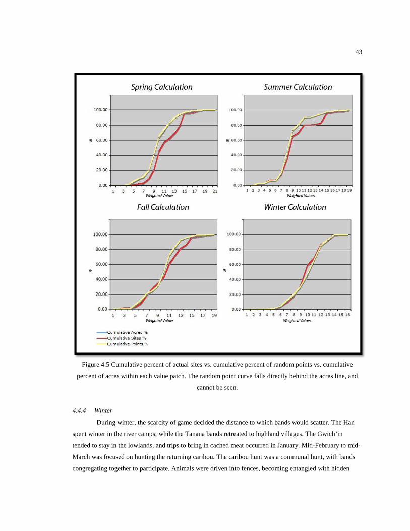
43

Figure 4.5 Cumulative percent of actual sites vs. cumulative percent of random points vs. cumulative

percent of acres within each value patch. The random point curve falls directly behind the acres line, and

cannot be seen.

4.4.4 Winter

During winter, the scarcity of game decided the distance to which bands would scatter. The Han

spent winter in the river camps, while the Tanana bands retreated to highland villages. The Gwich’in

tended to stay in the lowlands, and trips to bring in cached meat occurred in January. Mid-February to mid-

March was focused on hunting the returning caribou. The caribou hunt was a communal hunt, with bands

congregating together to participate. Animals were driven into fences, becoming entangled with hidden

44

snares, and then dispatched by bow, spear, and occasionally by knife. The use of small corrals and human

corrals to capture and kill the animals has been reported also. To a lesser extent, moose, bear, and sheep

were also hunted. However, when these patches were analyzed by site location vs. random pseudo-nonsite

points, no statistical difference was seen (Figure 4.5, Table A-4). The lack of a pattern suggests severe

limitations that the harsh winter environment imposed upon the inhabitants, and therefore site formation

processes was likely restricted during these months.

The model suggests that return rates increase in forested lowlands (Figure 4.4). High altitudes and

river bottoms decrease in return rates in the region. The pattern suggests a period of heightened resource

stress. Responses to this included aggregation of groups and use of summer and fall food caches, which

cannot be modeled here. Winter potlatches may have been (among many other things) a risk-mitigation

strategy for people with dwindling resources to acquire more for survival during this time from others who

had an abundance of resources. The potlatch allowed for ritual wealth resource redistribution from the

wealthiest members of the tribe to all others, without the requirement for immediate material reciprocal

repayment. Potlatch reciprocity was conceptualized as a long-term investment: he who could give more

increased in respect and stature among his peers. These two concepts were accepted as valid immediate

repayment for material goods.

4.5 Discussion

Most inductive models use aspects of geology in order to predict site location and preservation.

Geological models are not used here, in order to highlight and allow focus upon the dietary reasons that

may underlie known site locations. The restriction allows these inferences to be made largely free of site

preservation constraints. The assumption, however, limits the applicability of this stage of analysis to small

scale. The systems that become apparent are dependent on the data used to produce them, and are not tied

directly to the empirical record. Small-scale analysis makes use of layered assumptions and must then be

interpreted through use of medium and large-scale analysis that focuses on the actual material cultural

record in order to demonstrate its applicability and relevance to the prehistoric record. These GIS models

indicate that the majority of the sites in the area are associated with hunting-related behaviors. These are

further clustered by the seasonal availability of acceptable prey items.

These models indicate that most sites conform to spring and fall prey patches, when resource

return rates increased and expanded from the valley bottoms into the highlands. Diet breadth and mobility

increased during these months. During the summer, patch return rates increase dramatically again in the

valley bottoms, constraining mobility to these areas only, and a reduction of diet breadth to only the highest

ranked resources. The winter model suggests a large-scale reduction of return rates, and likely a general

abandonment of the YTU during this time.

45

This also illustrates that resource patches do not exist as single entities, but rather as a matrix of

changing resources that increase and decrease in return rates in a seasonal-specific pattern. The Central

Place Foraging model suggests that an occupation site will be placed where travel costs are minimized by

proximity to the highest resource returns.

Using the ethnographic, optimal foraging, diet breadth, and patch choice models to interpret

seasonality of site locations suggests that people were most widely moving about the YTU during the

spring and early summer months. The pattern is seen again for the fall months, but is restricted by

behaviors that caused people to congregate near patches that facilitated intercepting migrating caribou.

Summer patches indicate that people confined themselves to riparian habitats, in close proximity to the

salmon runs. The winter model suggests several things. The cold season posed the most difficult situations

to human survival, and was punctuated by low food resources and periods of starvation. Food was cached

during the salmon and caribou harvests specifically for this time. When these ran out, many resources were

considered as viable food options that would not have been at other times of the year. It also could indicate

that the region was largely devoid of people during the coldest months.

It is assumed here for the sake of the model that the patches delineated here extend at least as far

back as the White River Ash volcanic events, and possibly at far back as with the establishment of the

boreal forests (~6000 cal BP). This model also suggests that hunting and procurement behaviors, which

Osgood, McKennan and others recorded, can be inferred to extend deeply back through the cultural history

of the region. The model suggests that no large-scale resource use shift occurred between the Northern

Archaic and Athabascan periods in this region. The seasonal models indicate that a strong difference exists

between resources found in valley floors and ones located at higher elevations. This model of optimal

seasonal land use can be now applied to site assemblages. Due to the topographic difference demonstrated

here between resources, sites will be split into two locales: Valley Floors and Ridgetops. Assemblages will

be compared against each other for debitage differences, discarded expedient tool and formal tool

differences in patches by seasons. The next two chapters switch focus from the small-scale regional

analysis to a large-scale examination of sites at an intensive, assemblage-specific basis.

46

5 Ridgetop Site Assemblage Variability

Two assemblages from the YTU, the Big Bend Overlook and Bachelor Creek Lookout sites

(Figure 5.1) were chosen based on their respective locations as representative assemblages for this stage in

the analysis. Both are important as they are situated at high altitudes on ridges splitting major river

drainages, and are assumed to have been occupied by people moving between these drainages. The

geographical setting also restricts their likely seasonal occupation. From the ethnographic record, fall

would most likely be the time of occupation, with spring and winter as alternate possibilities.

Resources in the YTU are spatially clustered and separated by long distances on the landscape,

and often only available at certain times of the year. The lack of consistent availability greatly reduced the

chances for opportunistic resupplying, and required farsighted logistical planning in order to carry out a

successful hunt. In addition to needing reliable logistical supply points, the technological system that was

transported between sites had to be equally reliable and long-lived.

Figure 5.1 Location of the two ridgetop sites discussed in this chapter.

47

The sites in these upland settings generally consist of the stone debitage left over from tool

production and maintenance. Other types of sites are quarrying sites, such as those found at Rosebud Knob,

or Tolovana sites described by David Derry during the Alyeska survey (Cook 1977, Aigner and Gannon

1980, 1981a, 1981b). Further site types are kill sites, butchering sites. The possibility of long term camp

sites can not be ruled out in the uplands, but their likelihood is greatly reduced the further one retreats from

the Yukon River, Tanana river, and associated lakes in the flats. Each of these site types represent a specific

picture of the overall economic system required for a successful life in the prehistoric subarctic.

5.1 Bachelor Creek Lookout Introduction

The Bachelor Creek Overlook site is situated on a prominent knob in the middle of a high saddle

(Figure 5.2) between Homestake and Bachelor Creeks at an elevation of about 3350 feet above sea level.

The site is a surface/subsurface lithic scatter and comprised mostly of chert and diorite debitage, measuring

approximately 40m x 75m.

The field methods employed focused on collecting the total number of prehistoric artifacts that lay

exposed on the surface (Figure 5.3), as well as collecting a systematic sample of artifacts from 18 shovel

test pits placed across the site (Figure 5.4). Based upon the fact that little soil formation could be observed

at the site, (other than within an area of about 5m2 in the center of the site) this was treated as a highly

disturbed site. No surface features were observed.

Three stratigraphic levels (Figure 5.5) were identified in the field. Layer 1 was an organic root

mat, on average about 5 cm thick. Underlying this was Layer 2, a brown silty loess. Below this was Layer

3, gray silty loess, ranging from 10-40 cm thick, and was in turn underlined with culturally sterile, broken

bedrock. A possible hearth feature (Figure 5.6) was encountered in one test pit, but no artifacts were

recovered from within the ash layer. For the purposes of this analysis, it is assumed that the subsurface

artifacts represent an accurate sample of the remaining subsurface component.

48

Figure 5.2 The Bachelor Creek site, located around the knob at the top of the bluff.

Figure 5.3 Bachelor Creek overview, showing the grid and flagged artifacts.

49

Figure 5.4 Bachelor Creek site map of all artifacts (blue). Test pits are marked in red. Isopleths are set at 1

item per 0.25 meter. Topography contours set at 1-foot intervals.

50

Figure 5.5 Typical stratigraphy near the prominent knob on the site.

Figure 5.6 Outline denotes ash feature located in test pit N510 E505.

51

5.1.1 Lithic Analysis

Three hundred thirty six lithic artifacts were recovered from the site. Seven of these were bifaces

(2.08%), eight were microblades (2.4%), five were retouched flakes (1.5%), two were utilized flakes

(0.6%) and the remainder (92.9%) was debitage. See Table B-1 (Appendix B) for a summary of raw

material counts recovered by stratigraphic level, and Table B-2 (Appendix B) for artifact type counts

recovered by stratigraphic level. Four material types were found in quantities greater than 30 artifacts.

These were tested using a χ2 test to observe if a significant difference could be demonstrated to exist

between the surface and subsurface assemblage of these artifacts. No significant difference was found

among both artifact type and strata and raw material type and strata, the site was then assumed to represent

a single cultural component.

Figure 5.7 Raw material debitage weight variability.

5.1.2 Raw Material Analysis

Six material types would be considered to be local (Figures 5.7, 5.8, 5.9, Table B-3 Appendix B).

Clear/black mottled chalcedony is known to exist in raw form throughout the Livengood area. This type,

along with dark gray chert, clusters strongly in both quantity and weight along with the local types. The

trend would be expected to appear in the others if there was, in fact, an easy-access quarry nearby, and is

likely to be a function of the fact that the site assemblage is very small, and likely represents a short-term

occupation. Another reason for this overrepresentation might be that this site represents an early stop along

a seasonal round that encompassed hundreds of miles and many months. These materials might still have

52

Figure 5.8 Lithic artifact isopleths (set at 1 item per 0.25 meter).

53

been in plentiful numbers in the toolkits. Another reason might have been an anticipated soon arrival at a

raw material procurement source. All obsidian artifacts were sourced to Batza Tena.

Figure 5.9 Raw material debitage size class weight percent and count.

5.1.3 Debitage Attributes

Using Sullivan and Rozen’s (1985) typology, 46.2% of the debitage assemblage consisted of

complete flakes, 40.4% consisted of broken flakes, 6.7% of split flakes, 6.1% of flake fragments, and 0.6%

of debris (Table B-4 Appendix B). According to experiments done by Tomka (1989), tool production

should result in higher quantities of complete flakes, while core reduction should result in higher quantities

of broken and split flakes. Using White’s (1963) typology of cortex amount, 0.6% of the flakes were

primary, 1.9% was secondary, and 97.4% were tertiary (Table B-5 Appendix B). The low percentage of

cortex suggests the site did not function as a primary reduction area, but where already prepared cores were

further reduced and tools resharpened. Cortex was also equally represented between rough and smooth

types, indicating a variety of procurement sources (Table B-6 Appendix B).

When size class was compared against weight percent, a slight underrepresentation of SC4 was

seen, and by default a possible overrepresentation of SC3. The low representation of SC4 could indicate a

preference for use of those flakes. Interestingly, a correlation is seen with four retouched flakes being

represented in SC3 and only one in SC4. The assemblage was dominated by debitage in SC2 and 3. Chert

and diorite are the dominant raw material types both by weight and number in the smaller classes (Table B-

7 Appendix B).

Microblades are also not represented in SC4 but are in SC2, SC3, and one in SC5. The lack of

SC4 artifacts could indicate a preference for that size microblades as prime use for retooling. The majority

of flaking patterns consisted of faceted (28.6%) platforms and flat (49.7%) platforms. Empirically, SC 3

54

shows the strongest representation in the assemblage, and the one microblade, which exhibited usewear,

was a proximal obsidian blade of this size (Table B-8 Appendix B).

5.1.4 Reduction Strategies

No cores were recovered from this site; however, as utilized flakes, microblades and bifaces were

among the artifacts, all three reduction strategies were potentially utilized here. According to Surovell’s

model (2003), obsidian, all types of siltstone, and presumably cherts (despite their low numbers) are

associated only with bifacial thinning, while the rest are associated with both initial core reduction and

bifacial thinning. Microblade are associated with obsidian, white and greenish gray siltstone, clear/black

mottled chalcedony, and dark gray chart, so these material types are also linked to microblade core

reduction (Table B-9 Appendix B).

Cortex was observed 2.7% of the debitage. Different raw materials respond in their own individual

ways to reduction mechanics. To the experienced flintknapper, the ultimate purpose of reducing a core will

be dependent on both the fracture mechanics of the material and the tool needed to be produced. Andrefsky

provides an excellent explanation of platform type associations (2005). Cortical platforms are associated

with initial core or flake production. None were seen at this site. Flat and less complex platforms are often

associated with nonbifacial thinning. In this assemblage, flat and dihedral platforms were observed on

54.6% of the assemblage. If the material types associated with the microblades are removed and assumed to

only have association with their respective reduction strategy 7.6% of the debitage may be associated only

with microblade technology (Table B-9 Appendix B). Using the dorsal scar count, 7.6% of the remaining

debitage is associated with initial core and flake production, and 49.5% with late-stage biface production.

The remaining two material types are associated with both bifaces and microblades. As much as 13.1%

could be associated with early stage biface reduction, and 22.2% might be late stage reduction, but some of

this is likely due to microblade production as well (Table B-10 Appendix B).

5.1.5 Formal Tool Attributes

Formal tools at Bachelor Creek consisted of bifaces (n=7) and microblades (n=10) (Table B-11

Appendix B). No thermal alterations were noted on any artifacts. Six microblades were proximal ends: two

had faceted platforms and four had flat platforms. Two microblades were distal, one of these being a distal

fragment, and one being a complete, unsnapped microblade. The remaining three were medial sections, all

of which exhibited usewear, and one (obsidian) that exhibited retouched sides.

The complete bifaces and biface fragments (n=7) consisted of stages 2, 3, 4, and 5. In these

assemblages, hafting seems to occur with both stage 4 and stage 5 bifaces. Retouching was not noted,

however, three of the bifaces were late stage broken distal ends, perhaps a function of use. Edge angles

ranged from 39° to 77°. See Figure 5.10 for spatial distributions, and Figure 5.11 for artifacts.

55

The first biface appears to like a classic stage 4 Northern Archaic stemmed expanding point. The

artifact, of local dark gray diorite (UA2010-118-121) measured 27.4mm long, 22.3mm wide, 7.3mm thick,

and weighed 4.5g.

UA2010-118-45 was a clear/black mottled chalcedony stage 4 convex lanceolate point that had

been retouched from a flake. Part of the base had been snapped off. It measured 21.4mm long, 10.8mm

wide, 2.5mm thick, and weighed .62g.

UA2010-118-12 was a complete, stage 3 worn bifacially flaked object. It was of gray/black-

banded chert and measured 23.6mm long, 18.1mm wide, 7.3mm thick and weighed 4.71g.

UA2010-118-52 was a small stage 5 broken proximal convex lanceolate point of dark gray chert.

It measured 7.2mm long, 9.2mm wide, 3.2mm thick, and weighed 0.24g.

UA2010-118-91 was a broken proximal irregular-edged stage 2, convex lanceolate, bifacially

flaked object of dark gray chert. It measured 29.2mm long, 15.9mm long, 7mm thick and weighed 4.58g.

UA2010-118-108 was a broken distal end of a stage 5 biface. It was made of clear/black-mottled

chalcedony, measuring 19.7mm long, 11.5mm wide, 2.5mm thick, and weighed 0.56g.

UA2010-118-120 was a broken distal end of a stage 4 biface. It was of clear/black-mottled

chalcedony, measuring 10.9mm long, 9.7mm wide, 3.4mm thick, and weighed 0.54g.

Figure 5.10 Bachelor Creek tools. Orange=biface locations (n=7), Black=microblade locations (n=10), and

blue=modified flake locations (n=5). Isopleths set at 1 item per 0.25 meter.

5.1.6 Informal Tool Attributes

In the analysis, unretouched utilized flakes (n=2) and retouched flakes (n=5) were lumped together

as “modified flakes” and assumed to be expediently made (Figure 5.11). If it can be assumed that the

56

assemblage is a representative sample of the site, it would appear that a preference existed here for formal

tools (n=14) over expedient ones (n=7). Retouched flakes tended to be unifacially worked.

Figure 5.11 Bachelor Creek microblades and bifaces.

5.2 Big Bend Overlook Introduction

This Big Bend Overlook site is a surface/subsurface lithic scatter located along the SSE facing

bluff edge and knob that accentuates the southwestern corner of a large plateau. It overlooks the Big Bend

of Beaver Creek to the east (Figure 5.12) and the Tatalina River drainage to the southwest. The site

measures approximately 130 meters x 20 meters, with artifacts tending to concentrate in three major

surface clusters.

57

Near the westernmost point of the site, adjacent to a modern moose hunting camp (Figure 5.13),

an area of about 5m² was observed to have 30-40 cm of soil deposition. In 2004, a wildfire had burned over

part of the site, traces of which could still be seen. The fire had removed the vegetation and burned the

organic soil, leaving some areas of the site stripped to the underlying mineral soil and broken bedrock. For

most of the site, the original depth provenience of artifacts could not be trusted, due to processes of

cryoturbation and bioturbation.

Forty 50cm x 50cm shovel test pits were placed on a systematic sampling plan for the site.

Twenty-five of these were placed around the top of the knob, where surface artifacts were noticed to be the

densest. In order to eliminate bias in test pit placement, these were individually spaced at five meters apart.

Additionally, one 1 x 1 meter excavation unit was also placed in at the top of the knob.

Soil formation has accrued highest along the top of the knob. An organic mat (A Horizon) exists

on average for about 5 cm thick, and is underlined by a possible hearth feature (Figure 5.14), a layer of ash

which was noted in several test pits as well as the excavation unit. The ash was noted to be about 2-4 cm

thick, and was in turn underlined by a poorly mixed layer of sandy loess, about 10-40 cm in thickness (C-

Horizon). Under this was weathered bedrock. It is questionable as to whether or not the ash originated from

a hearth feature or from natural processes. A sample was recovered for analysis. Charcoal flakes were

noted in this ash layer, and several samples were also separately collected.

As the bluff dropped off toward the east, soil formation lessened to a few centimeters in thickness

to exposed poorly mixed loess and bedrock. Some of this was due to fire destruction of the soil from the

2004 burn. Artifacts were noted in the organic and ash feature, as well as the top 5-10 cm of the C Horizon.

58

Figure 5.12 Big Bend, viewing down the grid east-west line through the site towards the Big Bend of

Beaver Creek.

Figure 5.13 Big Bend, view from the top of the hill looking northeast.

59

Figure 5.14 Stratigraphy at Big Bend. The gray lens was interpreted to be an ash feature, possibly a hearth.

5.2.1 Big Bend Overlook Artifacts

One thousand, seven hundred fifty nine lithic artifacts were recovered from the site (See Figure

5.15 for spatial distribution). Nine of these were bifaces (0.5%), forty-one were microblades (2.3%), five

were retouched flakes (0.3%), one was a tchi-tho (0.06%), sixteen were flake cores (0.9%) and the

remainder (95.9%) was debitage (Table B-11 and B-12 Appendix B).

Here, there is the possibility that a separate subsurface component might be seen in the site. No

sterile layers in the stratigraphy separate any cultural components. However, there is a difference among

the spatial position of microblades and bifaces in relation to the strata. The majority of microblades were

recovered in subsurface context, while the majority of bifaces were recovered from the surface. Six raw

material types were found in quantities greater than 30 artifacts. These were tested using a χ2 test to

observe if a significant difference could be demonstrated to exist between the surface and subsurface

assemblage of these artifacts. No significant difference was found among both artifact type and strata and

raw material type and strata, the site was then assumed to represent a single cultural component. The null

hypothesis of no difference between artifact type and strata and raw material type and strata is accepted.

However, due to the difference between artifact types by stratigraphy (artifact numbers were not large

enough to test for statistical significance), the possibility for cultural reoccupation is real, and the amount of

surface artifacts versus only the sample of subsurface artifacts might be causing a false negative correlation

60

to appear. Due to the fact that no cultural separation could be seen spatially in the field, this suggests a

heavy amount of post-depositional artifact mixing has occurred at the site. Very few material types are

solely represented by one stratum: therefore, definite cultural components cannot be demonstrated. Cultural

zones will be described according to the strata defined in the field. These were Layer 1: Surface, Layer 2:

Brown Loess, Layer 3: Gray Loess, and the hearth feature, located between Layer 2 and 3 (Table B-13

Appendix B).

Figure 5.15 Big Bend site map of all artifacts. Test pits are in red. Isopleths are set at 1 item per 0.25 meter.

Topographic contour levels are set at 5 feet.

61


Throughout the site as a whole, seventeen lithic raw material types were described. Diorite stands

out immediately as a local material (See Figure 5.16 for spatial distribution). All colors of this were seen in

the natural cobbles scattered throughout the site and surrounding area. Quartz was also noted in isolated

locales throughout the surrounding hills, yet this material type was not expressed in the assemblage at the

same level as other local material types. White/gray mottled chalcedony is also not known in the area, and

was overrepresented due to the presence of a large, discarded core (Table B-14 Appendix B).


Of the surface artifacts, 41.5 % of the debitage assemblage consisted of complete flakes, 37.3% of

broken flakes, 17.5% of split flakes, and 3.6% of flake fragments. In Level 2, 46.8% were complete flakes,

32.3% were broken flakes, 13.5% were split flakes, and 7.4% were flake fragments. In Level 3, 55.6% were

complete flakes, 28.8% were broken flakes, 9.4% were split flakes, and 6.3% were flake fragments. In the

hearth feature, 56.7% were complete flakes, 25.8% were broken flakes, 11.3% were split flakes, and 6.2%

were flake fragments. No artifacts were classified as debris/shatter (Table B-15 Appendix B). Complete

flakes were higher in the lower two components as opposed to the two upper ones, indicating a stronger

preference for tool production in the lower strata.


Throughout the site as a whole, seventeen lithic raw material types were described. Diorite stands

out immediately as a local material (See Figure 5.16 for spatial distribution). All colors of this were seen in

the natural cobbles scattered throughout the site and surrounding area. Quartz was also noted in isolated

locales throughout the surrounding hills, yet this material type was not expressed in the assemblage at the

same level as other local material types. White/gray mottled chalcedony is also not known in the area, and

was overrepresented due to the presence of a large, discarded core (Table B-14 Appendix B).

The debitage was then analyzed for cortex (White 1963). Of the surface artifacts, 2.8% of the

flakes exhibited primary cortex, 4.3% was secondary, and 92.9% were tertiary. Of the Level 2 assemblage,

0.5% was primary, 0.5% was secondary, and 99% were tertiary. Of the Level 3 assemblage, 1.6% was

primary, 0.2% was secondary, and 98.2% were tertiary. Of the hearth assemblage, 3.1% were primary,

3.1% were secondary, and 93.8% were tertiary (Table B-16 Appendix B). Of cortex types (Table B-17

Appendix B), the surface assemblage was overrepresented by the presence of rough cortex represented by

the local raw materials, suggesting local procurement. The subsurface components showed closer numbers

of rough and smooth types, suggesting more variety of procurement areas. All three types of local diorite

dominated the four cultural strata assemblages. Chalcedony dominates the remainder of the surface

assemblage. Chalcedony and chert are found in roughly equivalent frequencies the Level 2 assemblage,

62

while siltstone dominates the bottom Gray Loess Level 3, followed closely by chert and chalcedony. In the

hearth feature, chert is the most prevalent nonlocal material (Figures 5.17–5.20).

Figure 5.16 Local/nonlocal raw material distribution, and spatial distributions of tools. Red=local raw

material distribution, blue=nonlocal raw material distribution. Spatial distributions of tools:

blue=microblades, red=flake cores, green=retouched flakes, black=bifaces. Isopleths are set at 1 item per

0.25 meter.

63

Figure 5.17 Chalcedony, chert, siltstone, and Batza Tena obsidian distributions. Chalcedony is the most

widely spread out material type. All types of chert, siltstone, and Batza Tena obsidian were found in the

vicinity of the ash feature. Isopleths are set at 1 item per 0.25 meter.

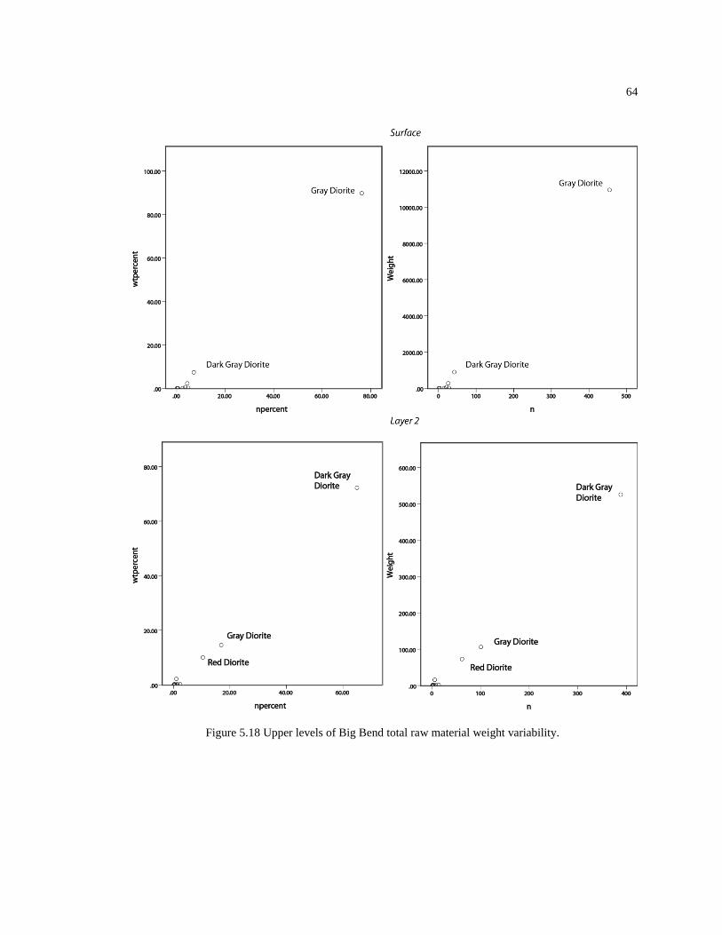
64

Figure 5.18 Upper levels of Big Bend total raw material weight variability.

65

Figure 5.19 Lower levels of Big Bend total raw material weight variability.

66

Figure 5.20 Raw material weight by size class.

67

No microblade cores or tabs were recovered from the site. (Note: one microblade was lost before

linear measurements were taken). Three proximal microblades were recovered from the surface. One distal,

two medial, and four proximal microblades were recovered from Level 2. One complete, three medial, and

three proximal microblades were recovered from Level 3. From the hearth feature, one complete, one

medial, and one proximal microblade were recovered (Table B-18 Appendix B). By far, the majority

recovered were proximal blades (n=13), six of which were in SC2. Medial and distal blades of this size

class are underrepresented. The underrepresentation is suggestive of their choice for inset into weapons, or

is possibly due to sampling error due to the low numbers of recovered artifacts (Table B-19 Appendix B).


Modified flakes, microblade debitage, and bifaces in several stages of completion were all

recovered from this site, indicating at least three reduction strategies were utilized here. According to

Surovell’s model (2003), no material types can be completely attached to any one type of early or late stage

biface reduction. Microblades are associated with grayish brown siltstone, greenish gray siltstone, gray

siltstone, white/black mottled chalcedony, pale brown chert, and yellow chert. Two material types,

white/gray mottled chalcedony and dark gray chert were associated with both bifaces and microblades. The

others will be assumed to be linked only to microblade core reduction (Table B-20 Appendix B).

Assuming flat and dihedral platforms are associated with initial biface reduction/flake production,

70.2% of the surface assemblage, 78.3% of Level 2, 69.4% of Level 3, and 68.1% of the Hearth could be

categorized as associated with early stage flake reduction. If the material types associated only with

microblades are removed and assumed to be only associated with microblade core reduction, 2.8% of the

surface debitage assemblage, 1.3% of the Level 2 assemblage, 10.7% of the Level 3 assemblage, and 9.9%

of the Hearth is associated with microblade technology. Using dorsal scar count, 54.9% of the surface

assemblage, 67.6% of Level 2, 60.5% of Level 3, and 61.9% of the Hearth debitage are associated with

initial core reduction. 40.8% of the Surface assemblage, 30.9% of Level 2, 28.1% of Level 3, and 25.8% of

the Hearth with late-stage biface production (Table B-21 Appendix B).

5.2.5 Core Attributes

At the site, 11 flake cores were of local, dark gray diorite, one of gray diorite, one of clear/black

mottled chalcedony, one of pale brown chert, and one of yellow chert. One large wedge-shaped blade core

of white/gray-mottled chalcedony was also included in this stage of analysis. Flake cores were first

analyzed according to 5mm size class and weight, indicating most had been exhausted before discard

(Figure 5.21). Flake cores are represented in the assemblage against bifaces by a ratio of almost 2.1. The

majority of the cores (n=13) were found in surface context. One was recovered in the Brown Loess (Level

2) and 2 from the Hearth feature. No cores were recovered from the lowest level.

68

Figure 5.21 Flake core size class by weight. Blue=Surface, red=Level 2, green=Hearth.

Figure 5.22 Big Bend early-stage bifaces and wedge-shaped gray chert core (far right).


Formal tools at Big Bend consisted of bifaces (n=9), and microblades (n=21) (Figures 5.22-5.23).

Thermal alterations were noted on one microblade. Thirteen microblades were proximal ends: two

exhibited a faceted platform, ten had a flat platform, and one had been sheared off. Three microblades were

distal ends. The remainders, five, were medial sections, one of which exhibited retouch.

0.00500.00

1000.001500.002000.002500.003000.003500.004000.004500.005000.00

0 10 20 30 40

Wei

ght (

g)

Size Class

69

The complete bifaces and biface fragments (n=9) consisted of stages 1, 3, 4, and 5. Three of these

bifaces, all early stage (Figure 5.22), were very large and struck from local diorite, one (stage 3) weighed

336 grams, another (stage 1) 651 grams, and the third (stage 1) 811 grams. Due to their size, it is very likely

none of these were intended for hafting. The remaining bifaces were late-stage lanceolate-based tools,

except for two that were broken.

UA2010-116-0026 was the broken, distal end of a stage 4 biface made of clear/black-mottled

chalcedony. It measured 15.8mm long, 18.5mm wide, 4.7mm thick, and weighed 1.6g.

UA2010-116-0054 was the broken distal end of a stage 4 biface made of clear/black-mottled

chalcedony. It measured 14.5mm long, 46.5mm wide, 5.1mm thick, and weighed 2.84g.

UA2010-116-0056 was a complete, stage 5, flat-based lanceolate point knapped from dark gray

chert. It measured 60.7mm long, 30.5mm wide, 7.5mm thick, and weighed 15.49g.

UA2010-116-0083 was a large, stage 1 biface of local dark gray diorite. It measured 165.2mm

long, 109.7mm wide, 50.3mm thick, and weighed 811.1g.





UA2010-116-0116 was a broken, proximal end of a stage 5 convex lanceolate biface. It was

knapped from white/gray mottled chalcedony, and measured 14.7mm long, 22mm wide, 3.9mm thick, and

weighed 1.26g.


knapped from clear/black mottled chalcedony and measured 13.7mm long, 17.1mm wide, 5.4 mm thick,

and weighed 1.35g.


knapped from local dark gray diorite, and measured 20.1mm long, 26.3mm wide, 6.8mm thick, and

weighed 3.48g.


In the analysis, unretouched, utilized flakes (n=18), tchi-thos (n=1) and retouched flakes (n=5)

were lumped together as “modified flakes” and were assumed to be expediently made, and all other tools

considered to be “formally” made. If we assume the assemblage constitutes a representative sample of the

site, there was a small preference for formal tools here. Retouched flakes tended to be unifacially worked.

Two of the large, early stage bifaces exhibited cortex.

70

Figure 5.23 Big Bend microblades and late-stage bifaces.

71

6 Valley Floor Site Assemblage Variability

In this section, three different assemblages from the YTU, the Bear Creek, the US Creek, and the

Cripple Creek sites (Figure 6.1) will be discussed. Each of these sites are situated in similar settings at the

toes of hills near confluences of smaller and larger streams. The geographical setting (far inside the

uplands) also restricts their likely seasonal occupation. From the ethnographic record, autumn would most

likely be the time of occupation, with spring and winter as alternate possibilities, due to their distance from

prime salmon harvesting areas. To call these sites “lowland” would be misleading as that usually refers to

sites associated with the widespread Tanana Flats, a different system of ecological patches altogether. From

the spatial resource modeling, these sites are expected to be in settings with a wider variety of available

resources, longer residence times, and therefore they should exhibit greater material variability.

Figure 6.1 Location of sites discussed in this chapter.

6.1 Introduction to the US Creek and Cripple Creek sites

The US Creek (CIR-029) and Cripple Creek (CIR-003) sites are similar in both proximity and

local geographic setting (Figure 6.2). Both sites are within five kilometers of each other, situated on the low

72

toes of hills at the confluences of the small creeks that bear their names and the Chatanika River. Both

exhibited food caching behaviors, and have radiocarbon-dated components falling solidly within the last

1000 years, an important period of time of material cultural change throughout the whole Alaskan

archaeological record. In the Interior, this period of time is termed both the Late Prehistoric, and the

Athabascan Period, the latter term connecting the cultural record to ethnographic groups that were

described at the turn of the Historic Period in the 1890’s. Both of these sites had formal excavations carried

out, as opposed to the three previous sites, whose subsurface context was only tested.

Figure 6.2 US Creek and Cripple Creek sites. View to the NNE, showing both sites situated along the north

banks of the Chatanika River (photo courtesy of Robin Mills ca. 2003).

6.2 Early Excavations

In 1976, a team of archaeologists from the Office of History and Archaeology (OHA), Alaska

Division of Parks conducted a reconnaissance survey along the Steese Highway, which had been built in

the 1920’s in response to heavy mining activity throughout the area between Fairbanks and Central, Alaska.

The only records from this early exploration are from a journal by Dr. Charles Holmes (1976; available

73

upon request from the Office of History and Archaeology), who described Cripple Creek as a series of

cache pits along a ridge north of the highway and on the south side of the highway. Subsurface testing

occurred along the ridgetop, which produced fire-cracked rock, numerous caribou bones, and a single chert

flake. No record exists of how many test pits were dug in this particular year, or where they were located.

However, Holmes remembers placing at least one inside a cache pit along the ridgetop (Holmes pers.

comm. 2011), in which numerous caribou bones were found. There is no record of artifacts from the 1976

testing being taken from the field or accessioned to the University of Alaska Museum of the North.

In 1978, a second team of OHA archaeologists revisited the area under the supervision of Timothy

Dilliplane. Planned improvements along the Steese Highway between mileposts 43.8 and 66 prompted this

cultural resource survey in order to locate and identify sites eligible for the National Register of Historic

Places. During this survey, T. Dilliplane, Robert Mack, and M. Dean Pittenger further explored the ridgetop

component of Cripple Creek. Seventeen 50cm x 50cm test pits were dug, thirteen of which was described

as containing cultural remains. These test units were mapped and tied into a centerline survey stake

associated with the road construction. However, this stake has long since disappeared, and there was no

description of local topographic features in relation to any of the test units, so tying this excavation in with

the later 2011 excavation was problematic (Dilliplane 1980). Artifacts recovered from this year included

lithics, faunal remains, and soil samples, accessioned to the Museum of the North under UA80-304.

6.3 Cripple Creek Introduction

Several questions remained unanswered as of early 2011 in regards to the US Creek site,

pertaining to the problematic association of the microblade component with the dated features at the site.

The site had been completely destroyed by road construction in 2006, so revisiting it was impossible.

However, nearby was a site similar to US Creek in proximity, geographical setting, age (Robin Mills (US

BLM archaeologist) had submitted a faunal element from an earlier excavation at Cripple Creek for

radiocarbon dating), cache pit features, and core and blade technology in stratigraphic context with the

dated element (130+-30 cal BP).

Therefore, this site presented an excellent opportunity to potentially revisit these problems in

connection with the Late Prehistoric period. The site was chosen in order to better answer questions

remaining from the nearby US Creek site. No physical remains of the 1978 excavation units, other than a

single 50cm2 test pit ‘footprint’ were located. A pit feature (interpreted as one of the cache pits recorded

during the 1976 test at the site was found (Holmes 1976, personal communication 2011).

A complete examination of the ground surface was conducted at the site (Figure 6.3). No surface

artifacts were located. One surface feature, the cache pit, was re-located (Figure 6.4). In the reports from

the 1970’s, ridgeline cache pits are always referred to in the plural (but never with a specific number);

however only one is now visibly present. The southwestern part of the slope has been cut away due to the

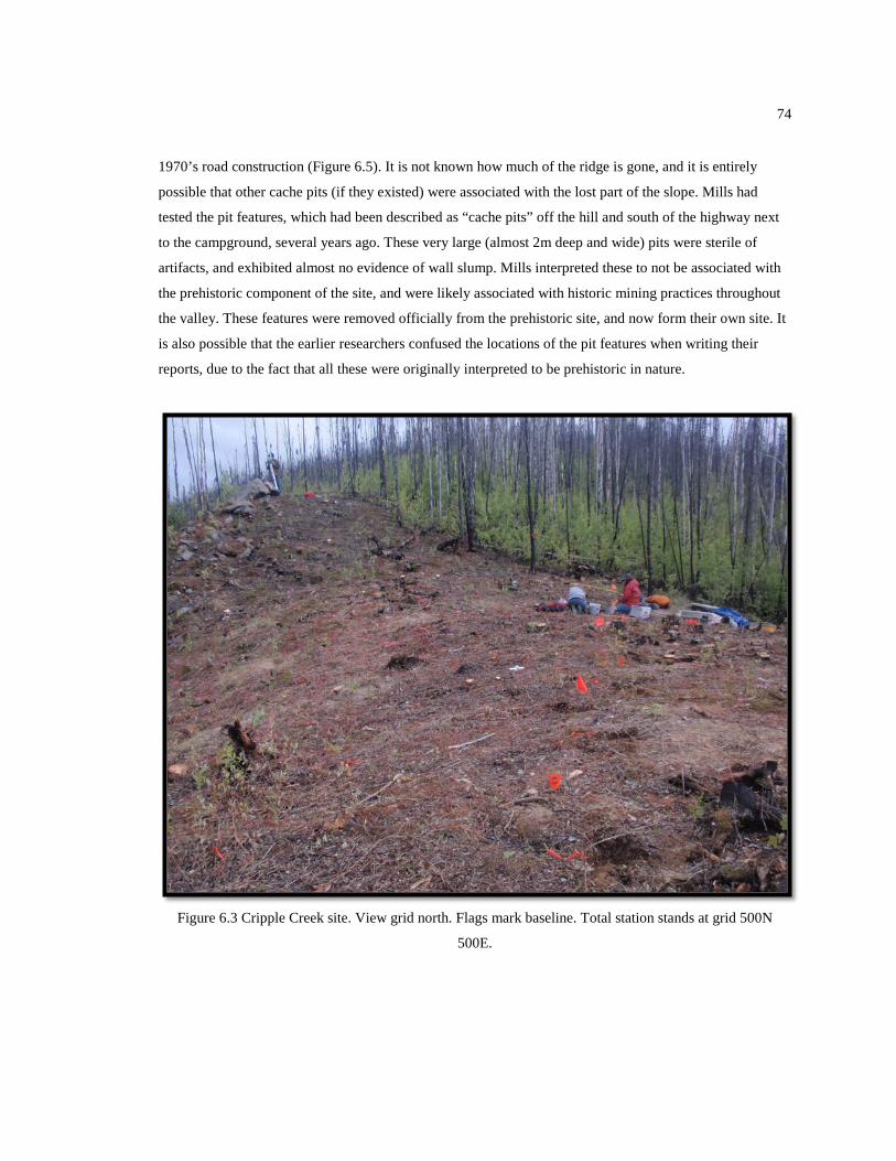
74

1970’s road construction (Figure 6.5). It is not known how much of the ridge is gone, and it is entirely

possible that other cache pits (if they existed) were associated with the lost part of the slope. Mills had

tested the pit features, which had been described as “cache pits” off the hill and south of the highway next

to the campground, several years ago. These very large (almost 2m deep and wide) pits were sterile of

artifacts, and exhibited almost no evidence of wall slump. Mills interpreted these to not be associated with

the prehistoric component of the site, and were likely associated with historic mining practices throughout

the valley. These features were removed officially from the prehistoric site, and now form their own site. It

is also possible that the earlier researchers confused the locations of the pit features when writing their

reports, due to the fact that all these were originally interpreted to be prehistoric in nature.

Figure 6.3 Cripple Creek site. View grid north. Flags mark baseline. Total station stands at grid 500N

500E.

75

Figure 6.4 Feature 1, cache pit (view north).

Figure 6.5 The southern part of the slope Cripple Creek is located on, which has been removed due to road

construction (view northeast).

76

6.3.1 Excavation Methods and Collection Practices

Prior to more-precise test excavations, 14 shovel test pits were deliberately placed to the southeast

of each two meter-spaced spike along the baseline. The purpose of the shovel tests was to determine

potential artifact densities across the site. The shovel tests were stopped when artifacts were recovered (i.e.,

they were not dug to bedrock). Artifacts from shovel test pits were collected by type lot. All of the material

excavated from the test pits was screened using 1/8th inch steel mesh. Nine 1x1 meter excavation units and

two 50x50 centimeter excavation units were dug down to bedrock across the site, in four locations, marked

Blocks 1, 2, 3, and 4 in the field notes.

The methods employed focused on collecting the total number of prehistoric artifacts throughout

the excavated portion of the site (e.g., lithic artifacts; faunal material and other ecofacts). A sampling of

charcoal was collected for species identification and dating purposes. Generally, 40-50 centimeters of soil

formation was observed across the site above the bedrock. No surface artifacts were recovered.

6.3.2 Stratigraphic Description

Three of the excavation blocks were placed near shovel test pits that had yielded the most artifacts.

One block was placed through the pit (Feature 1). In 1978, Ty Dilliplane recognized four stratigraphic

levels. During the 2011 excavation, 23 were recognized. Many of these layers were associated with features

in Block 3. Due to the complicated relationship among all of these layers, a Harris Matrix was developed

for each block (Figure 6.6). From this matrix, each observed layer was given a number in order of

superposition, 1 being the lowest level, and 23 being the uppermost.

77

Figure 6.6 Harris Matrix for Cripple Creek.

78

6.3.2.1 Block 1 Stratigraphy (N470-470 E512-515)

These three 1 x 1 m excavation units were dug to a depth of 35-40 cm, to weathered bedrock

(Figures 6.7 and 6.8). On top of the bedrock extended a layer of grey loess upwards 20-30 cm. On top of

this a layer of orange grey mottled loess extended 5-15 cm. Several pockets of burnt soil and ash seemed to

be intermixed within this layer. A 3-7 cm thick dark brown layer overlies these orange grey layer and

pockets. The layer contained numerous charcoal flecks and most of the artifacts from this block. On top of

this, a black organic rich loess extended 2-5 cm thick.

Figure 6.7 South excavation (Block 1).

79

Figure 6.8 Block 1 North wall generalized stratigraphy.

80


This excavation block includes two 50x50 cm excavation units dug directly to the NE of the main

1x1 m unit (Figures 6.9 and 6.10). These units were dug to weathered bedrock at a depth between 35 and

45 cm. A grey, clayey loess extends upwards from this 20-25 cm. Overlying this, is a layer of orange and

grey mottled loess, about 5 cm thick throughout most of the main unit and the northeastern-most 50x50 cm

unit. In the northeastern quad of the 1x1 m unit and the adjacent 50x50 cm unit, a burnt red loess overlies

the grey loess for a depth of 3 cm. The burnt red layer is overlaid directly by a layer of ash and loess mixed

with calcined bone. The layer is interpreted as a hearth (Feature 2). Above the orange grey mottled loess, is

a dark brown loess, about 3 cm thick, mixed with numerous charcoal flecks. Most of the artifacts in this

block were found within the dark brown. A black organic rich loess layer, about 3 cm thick, overlays the

dark brown loess. Little-to-no surface vegetation was present owing to a wildfire that swept across the site

in 2004.

Figure 6.9 Block 2 excavation units (view southwest).

81

Figure 6.10 Block 2 East wall generalized stratigraphy.


The purpose of this block was to transect Feature 1, the surface pit, and the associated low

sediment mound that surrounded it (Figures 6.11, 6.12, 6.13, and 6.14). The pit feature was about 30 cm

deep. Holmes, who was a part of the team in 1976 that discovered and tested the site, reported that a test

unit had been sunk within a cache pit, but could not remember if the test pit had been backfilled (personal

communication, 2011). The stratigraphy associated with the cache pit is complex; therefore each of the four

excavation units associated with Block 3 will be discussed separately. As above, little-to-no surface

vegetation was present in the block owing to a wildfire that swept across the site in 2004.

The southern-most unit, N484 E513 was dug to a depth of 45 cm, where broken bedrock was

encountered. A grey layer of loess extended up from this 20-25 cm. On top of this, a grey orange mottled

layer extended 3-7 cm. A dark brown layer extended over this about 10-15 cm. numerous charcoal flecks

and most of the artifacts from this unit were found within this layer. On top of this, a black organic rich

layer extended 5-10 cm.

Excavation unit N485 E513 extended just beyond the center of the bottom of the pit feature. Under

the center of the pit, a mass of birch bark was found just above the weathered bedrock 15 cm to the south of

the bark. A grey clayey loess extended up the length of the birch bark and nearly 30 cm at the south wall.

Over the top of this grey layer, an orange grey mottled loess layer extended to the top of the birch bark

mass. On top of this, a dark brown loess, containing most of the artifacts from this unit, extended up from

the birch bark mass 10 cm at the south wall. On top of this, a sterile grey loess extended 10-15 cm thick,

and overlaid the birch bark mass.

Excavation unit N486 E513 was dug to a depth of 80 cm at the north wall to the weathered

bedrock. The cultural birch bark mass at the bottom of the pit feature was located in the southwest quadrant

of the unit. A grey clayey loess extended up from the bedrock 60 cm at the north wall, and tapered to about

15 cm thick in the southwest quad. Within this layer, an isolated dark brown lens was present through both

the northern quads. The lens was variably 1-3 cm thick, and was tentatively identified as Feature 3 as its

82

association with Feature 1 was questionable. Charcoal and scorch marks were noted associated with this

lens, which was about 10 cm above the bedrock, which sloped downward to the north. On top of the grey

loess, an orange layer extended about 3 cm thick. A black charcoal stained loess, about 1 cm thick was on

top of the orange layer. A thick dark brown matrix of loess, charcoal, bones, and calcined bone extended

about 10 cm thick on top of this, identified as Feature 4. Overlying this, a sterile layer of grey loess

extended up 10-30 cm, overlain by a thin surface moss layer.

Excavation unit N487 E513 was dug to weathered bedrock at a depth of about 80 cm. A grey,

clayey loess extended up from this about 60 cm. An orange grey mottled loess lay on top of this, about 3-8

cm. On top of this layer, in the southwest quad, a mixed burned and ashy loess was about 1 cm thick. On

top of that was a 5 cm thick layer of ash, calcined bone, charcoal, and is interpreted as a hearth (Feature 5).

On top of this, the dark brown matrix mix of charcoal, loess and bone seen in N486 E513 extended about 5

cm thick. Patches of grey, sterile loess seemed intermixed with old organic rich layers, and may be a result

of back dirt from the 1976 test pit. On top of this, a thick root mat extended almost 10 cm.

Figure 6.11 Block 3 Stratigraphy (N 490-491 E 513-514) (view southwest).

83

Figure 6.12 Block 3 stratigraphy (view to the northwest).

Figure 6.13 Feature 1 cross section, Excavation Block 3 (view west).

84

Figure 6.14 Block 3 west wall generalized stratigraphy.

85


This excavation block was dug to a depth of 30-40 cm, where broken, weathered bedrock was

encountered (Figures 6.15 and 6.16). Above the bedrock, a grey clayey loess extended upwards to about 10

cm below surface. On top of this, an orange and grey mottled loess was noted in several locations,

extending about one cm thick. On top of this, a dark brown loess extended about 7 cm thick, and was noted

to contain numerous charcoal flecks, and the majority of the artifacts from this block were found in this

layer. On top of this was the uppermost layer, a black organic loess, about 2 cm thick. Little-to-no surface

vegetation was present owing to a wildfire that swept across the site in 2004.

Figure 6.15 Block 4 east wall stratigraphy.

86

Figure 6.16 Block 4 generalized stratigraphy.

87

6.3.3 1978 Excavation Location

While Dilliplane’s published site map (1980) is excellently triangulated off of an old highway

construction survey point, no reference is given on it or in the text to any natural feature on the local

landscape. To add to this confusion of the old excavation location, only one old test unit “footprint” was

located. The hill and ridgeline are of an area that confines the possible location of the old test units to a

small area. Based upon these two facts, the location of the old excavation was calculated. It was determined

in the field that the footprint was most likely that of Dilliplane’s “Test Unit D” (Figure 6.17 and 6.18).

Figure 6.17 Old test unit from 1978.

88

Figure 6.18 Cripple Creek map. Red denoted 2011 excavation units, blue, the hypothetical location of the

1978 excavation.

89

Figure 6.19 Organic artifact spatial distributions (Isopleths are denoted by 50g weight intervals).

6.3.4 Cripple Creek Cultural Features

6.3.4.1 Feature 1

Feature 1 (Figure 6.19) was the visible pit, interpreted to be a cache pit. The pit was roughly oval

in shape, surrounded by a low mound of possible backfill either from prehistoric diggings, or the 1976

testing. It measured roughly two meters NE-SW x one meter NW- SE, and about 40cm deep. Half of this

90

feature was excavated in 2011, (EU N486 E513 and EU N487 E513) and at the time of writing, the other

half remains in situ.

Directly associated with the pit was a thick layer of birch bark (Figure 6.20). A total of 766.86g of

this were removed from just below (3cm at the shallowest point) the pit feature (Figure 6.21). Once the

birch bark layer had been found, all soil remaining in situ above the bark was removed in bulk and taken

back to the UAF archaeology lab, where it was sifted through a 1/16inch sieve. However, no other faunal

remains were recovered. All birch bark was removed in sections with their associated soils. No other

artifacts were recovered. A sample of bark was submitted to Beta analytic for radiocarbon dating.

Directly below the birch bark, the soil was an orange and gray mottled loess, (noted everywhere

on the site). There were several large pieces of charcoal and two bone fragments associated with this layer.

None of the birch bark exhibited any scorch marks, except for some that had been burned from the 2004

fire. The charcoal is therefore interpreted to be related to an event prior to the layer of bark being placed in

this feature. One specific layer of orange and gray mottled loess extended throughout all the excavation

units at the site. The layer melds directly into the birch bark layer and disappears: specifically, not above

the bark, but directly into the outside edge of the bark, and disappears. A sample of this birch bark was

submitted to Beta Analytic for AMS analysis (Beta-315705) and returned a calibrated date of 80+-30 BP or

139 +-98 cal BP using CalPal.

Figure 6.20 Birch bark in situ within Feature 1.

91

Figure 6.21 Feature 1 birch bark, after the soil had been removed.

6.3.4.2 Feature 2

Feature 2 (northeast quadrant of EU N482-483 E513-514) (Figure 6.19) consisted of a distinct ash

lens with burned and calcined large ungulate bones, below which was a layer of dark red burnt loess

(Figure 6.22). Directly below the burnt red layer was the layer of orange and gray mottled loess. The ash

layer was distinctly confined to a small oval shaped area about 1m NE-SW x 40cm NW-SE. Two small

50cm2 excavation units were dug to further explore this feature, confirming it as a cultural hearth. Due to

time constraints, this could not be excavated further, and parts of this feature remain in situ. Very few

faunal specimens from this feature were of quality preferred for ideal AMS dating. However, two samples

that exhibited the least amount of burning and mineralization were submitted to Beta Analytic for analysis.

However, no collagen could be extracted for dating purposes. Considering the tight stratigraphic sequence

demonstrated at the site and similarity in artifact distribution, it is highly likely that this feature is closely

associated with the others in its vicinity.

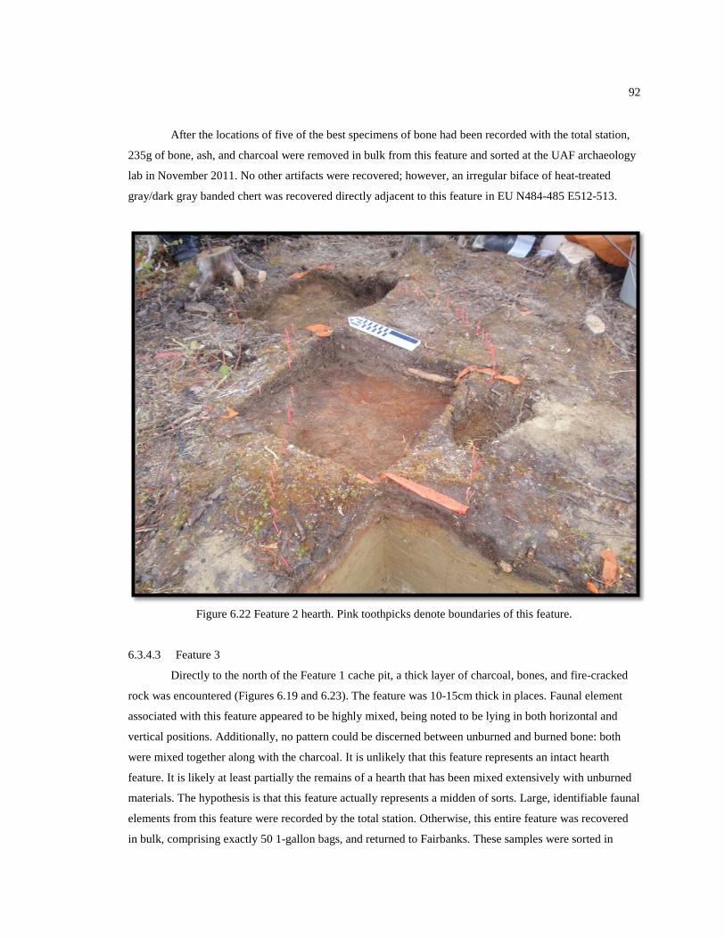
92

After the locations of five of the best specimens of bone had been recorded with the total station,

235g of bone, ash, and charcoal were removed in bulk from this feature and sorted at the UAF archaeology

lab in November 2011. No other artifacts were recovered; however, an irregular biface of heat-treated

gray/dark gray banded chert was recovered directly adjacent to this feature in EU N484-485 E512-513.

Figure 6.22 Feature 2 hearth. Pink toothpicks denote boundaries of this feature.

6.3.4.3 Feature 3

Directly to the north of the Feature 1 cache pit, a thick layer of charcoal, bones, and fire-cracked

rock was encountered (Figures 6.19 and 6.23). The feature was 10-15cm thick in places. Faunal element

associated with this feature appeared to be highly mixed, being noted to be lying in both horizontal and

vertical positions. Additionally, no pattern could be discerned between unburned and burned bone: both

were mixed together along with the charcoal. It is unlikely that this feature represents an intact hearth

feature. It is likely at least partially the remains of a hearth that has been mixed extensively with unburned

materials. The hypothesis is that this feature actually represents a midden of sorts. Large, identifiable faunal

elements from this feature were recorded by the total station. Otherwise, this entire feature was recovered

in bulk, comprising exactly 50 1-gallon bags, and returned to Fairbanks. These samples were sorted in

93

September 2011 using a hand pumped water screen, which removed most of the associated loess. During

this time, nine pieces of broken ceramics, rare in the Interior, were recovered from this matrix.

Figure 6.23 Feature 3 cross section (view west).

The southern extent of the feature ends abruptly 30cm below to northern edge of the cache pit. A

thick layer of gray loess extends over the top of this layer. In profile, Feature 3 extends directly into what is

interpreted as the original cache pit floor. It does not appear, above the cache pit layer, or below it, but ends

directly in association with the cache pit. In profile, it appears that the southern edge of feature 3 might

have been dug through during the placement of the birch bark event in the pit.

Ethnographic evidence suggests cache pits were dug out with wooden “shovels”. Fires were used

also, especially if permafrost was encountered high up. Fire also was used to “clean” old cache pits and

ready them for reuse, which is possibly what is indicated here by the relationship between these two

features. The layer of orange and gray mottled loess lies directly under this feature.

94

6.3.4.4 Feature 4

In excavation unit N486-487 E512-513, directly below Feature 3 (20cm below at the southern

point, and 50cm below at the northern point), a unique lens was found. It was a very dark brown color;

however did not resemble a paleosol. It lay directly at the same level as the Feature 1 birch bark to the

south, and nearly came into contact with it (the closest point was 2cm) (Figures 6.24 and 6.25). There was a

distinct difference between the two: while the bark was in excellent condition with almost no

decomposition noted, there was almost no intact organics noted with Feature 4. It was filled with organic

fibrous elements, some of which were collected. Several scorch marks and charcoal was also noted. The

gray loess immediately and easily separated from this feature during excavation, allowing for relatively

easy removal. No artifacts were found in association with this feature, therefore at this point it cannot be

culturally associated with the site, and will not be discussed further.

Figure 6.24 Features 4 and 5 N486 E513 NW and SW quads.

95

Figure 6.25 Features 3, 4, and 5. Northwest corner of EU N486 E513.

6.3.4.5 Feature 5

Feature 5 was recognized during the final two days of excavation. It was an ash feature that

extended at most 10cm into the western excavation unit N487-488 E512-513 (Figure 6.26). The ash lens

appears to be the edge of an intact hearth lying directly below feature 3 and directly above the orange and

gray mottled loess layer. At its thickest point, this feature is nearly 10cm thick; however, we only

excavated the very edge of this, it is likely that as much as 90-95% of this feature still exists in situ. A wall

10cm thick had been left intact between this excavation unit and the one directly to the south of it. The

feature extended east about 10cm into this wall and was removed the afternoon of the last field day and

taken back to the UAF archaeology lab in order to sort and identify the associated faunal elements.

This feature was the final bulk sample to be sorted in November 2011. While sorting the faunal

remains from feature 3, a small broken tooth was recovered. Joel Irish (UAF) identified this tooth as being

a juvenile lower left lateral incisor from a human child. The top of the tooth exhibited usewear. No

reabsorption of the root enamel had yet begun to occur, and Irish estimated the child to have been about 3

years old when the tooth loss occurred. When it was established that a human element existed at the site,

we took extensive care with the entire faunal assemblage. Teeth can be lost naturally, and so this artifact

96

did not yet fall under the Native American Graves Repatriation Act (NAGPRA). However, the potential for

this was now real.

Figure 6.26 Feature 3 and 5, southwest corner of N487 E513.

Most of the faunal elements associated with feature 3 had been sorted and taken to the BLM

archaeology lab, where MaryAnn Sweeney was conducting the faunal analysis. She was immediately noted

of the potential for further human remains. None were found in association with Feature 3. Immediately,

the faunal elements associated with Feature 5 for closer scrutiny. Five calcined bone fragments were

identified as possibly human. Mike Kenyhercz who had specific past experience in identifying cremated,

fragmented, human remains was invited to try and identify if these fragments, and any others, had a human

origin. Kenyhercz confirmed that the fragments were very indicative of the human skull. In addition, he

noted that the diploe was just beginning to form in places, a process that begins in the third year of a child’s

life, adding strength to the connection of the tooth in Feature 3 to the bone fragments in Feature 5.

Further, Kenyhercz observed that the breakage pattern of the root was consistent with burning,

rather than a forced snap. Charring was noted inside the root, along with a pattern of charring and stepping,

which occurs as the tooth enamel, dentin, and root absorb and react to extreme heat at different rates.

97

Additionally, a few endocranial scratches were noted on one of the parietal fragments. One of

these is deep and likely post-mortem, possibly indicative of stoking. The number of human remains (n=5)

at this site limits the conclusions that can be made about this individual. Child mortality rates are high in

hunter-gatherer populations, an unfortunate fact that is often forgotten in our age known for its remarkable

strides in the medical field. The bones themselves were highly calcined, indicating burning temperatures of

600-700 degrees, consistent with cremation temperatures. A sample of charcoal that lay directly at the

horizon between this hearth feature and the loess below was submitted to Beta Analytic for AMS dating

(Beta-315707), returning a date of 50 +-30 BP, calibrated using CalPal to 54+-80 cal BP.

6.3.4.6 1978 Hearth Feature

Dilliplane (1980) described one ash feature as a hearth. The ash lens lay on top of a layer

described by Dilliplane as Level III “reddish orange clay”, this is very likely the same layer described in the

field (2011) as the orange and gray mottled loess, and below a layer he described as Level II “dark loess”.

Level II appears to be consistent with our “10YR3/2 Brown Loess” layer, which extended throughout the

site. The hearth feature was large, extending throughout both of the largest 1978 excavation units.

Assuming the placement of the old excavation units is correct, this hearth feature lies about 1 meter (closest

point) southwest of the Feature 1 cache pit.

A broken distal femoral section from a “large mammal” (likely a caribou) that had been partially

burned (UA80-304-20) was found in association with this hearth. In 2005, Dr. Mills submitted this sample

to Beta Analytic for AMS analysis. Half was used for the analysis, and the other half of the sample (Beta-

203881) was returned to the UA Museum of the North. The sample returned a date of 30+-40 radiocarbon

years BP. Using INTCAL98, this date was calibrated to 130+-30 years BP.

6.3.4.7 Discussion

Of the cultural features described, Feature 2 and the 1978 hearth feature appear to be roughly

strategraphically contemporaneous. Both of these features are likely the oldest cultural features so far

described. Both of these are overlain by the Brown Loess (11) layer, which appeared throughout the site

and was recognized in the field as the main artifact-bearing layer. Feature 5, the cremation, appears to be

above this Brown Loess layer. It in turn is surrounded and covered by the large Feature 3 midden. The

feature appears to have been cut through in its southern end by the cache pit, or at least the final use of the

cache pit.

6.3.5 Faunal Analysis Summary

It is beyond the scope of this project to describe the faunal component of this site, other than a

quick summary and relevant references to those artifacts. A faunal analysis and identification of elements

98

(over 3000) was undertaken by MaryAnn Sweeney during the fall of 2011. A quick summary suggests most

bones were the remains of caribou, as well as some medium and small mammals. The bones from the 1978

excavation were identified previously by museum personnel, who also identified some fetal caribou

elements that hint at a winter/spring occupation of the site. We plan to eventually publish a paper that

describes in depth the results of this stage of analysis. Briefly, most elements were discarded broken

marrow-bearing bones. Densities are displayed not by artifact count, but rather by artifact weight, due to

the fragmentary nature of most of the artifacts. A quick summary of the findings suggests an assemblage

dominated by broken long bones, similar to US Creek, suggesting that neither site likely functioned as a kill

site or initial butchery site; rather, animals were killed and the elements brought here for further processing,

storage, and consumption. See Figures 6.27 and 6.28 for in situ examples of faunal remains.

Figure 6.27 Two broken unidentified long bone fragments that had unworked lithics embedded within

them.

99

Figure 6.28 A gray chert flake found in situ within a fractured long bone element.

6.3.6 Block 1 Discussion

Between Block 1 and Block 2 (separated by 12 meters), almost no artifacts were recovered in the

test units. Within Block 1, however, several charcoal lenses were found in addition to patches of burnt

loess. These could not be definitively described as cultural features, but are drawn into the stratigraphic

profiles. Numerous shattered caribou bone fragments were recovered in direct association with fire-cracked

rock (Figure 6.29). The only modified lithic artifacts recovered here were quartz debitage. The area may be

indicative of a separate activity area and merits further exploration in order to demonstrate if this is indeed

separate from the activity areas associated with the cache pit, and if cultural features can be demonstrated.

100

Figure 6.29 Block 1. Orange=fire cracked rock weight distribution, green=faunal weight distribution, and

black=charcoal distribution (isopleths set at 50g weight intervals).

6.3.7 Cripple Creek Lithic Artifacts

After all the bulk samples taken from the summer’s excavation had been sorted and catalogued, a

complete analysis was undertaken on all lithic artifacts, which included the same variables used on all

previous collections discussed in this work. The analysis was conducted between November 29 and

December 16, 2011 (UA2011-084 collection lithics: n=231). In addition, the lithic artifacts collected in

1978 (UA80-304 collection lithics: n=18) were analyzed on December 12, 2011. The analysis will

encompass all the lithics recovered during both excavations.

Two hundred forty nine lithic artifacts were recovered from the site. Five (2%) of these were

bifaces, 4 (1.6%) were microblades, 2 (0.8%) were retouched flakes, 7 (2.8%) were flake cores, 1 (0.4%)

was a microblade core tab, 2 (0.8%) were utilized flakes, and the rest (228, 91.6.8%) were flake debitage

(Table B-22 Appendix B).

101


Sixteen raw material types were described for this site (Table B-23 and B-24 Appendix B). Using

Dr. Potter’s model (2005), two material types immediately stand out in heavier quantities, indicating less

need for curation, and represent local material types (Figure 6.30 and 6.31). These are both found in natural

occurrence throughout the site: quartz and mica-schist.

All fire-cracked rock recovered was collected and brought back to the laboratory for cataloguing

by weight and provenience. These artifacts were not accessioned to the museum. FCR density is mapped by

weight, rather than number (Figure 6.31). Rocks were an important aspect in prehistoric cooking. They

were often heated in fires, then removed from those fires and placed in birch bark baskets; the heat transfer

from the stones serving to cook food placed in the baskets (Rainey 1939). The discard of these stones likely

did not occur far from where the cooking actually took place. Therefore, weight densities were measured in

order to indicate potential placement of these activities.

The four main grouped nonlocal material types (Figure 6.32) were chert, chalcedony, siltstone and

obsidian. All formed distinct spatial patterning, with obsidian and siltstone associated with the cache pit

and chert associated with the 1978 hearth feature. All obsidian artifacts recovered (n=16) were taken to the

UA Museum of the North for pXRF analysis and entry into the Alaska Obsidian Project Database. Twelve

samples were large enough for quantitative measurement, and all registered a signature strongly grouping

with others of the Batza Tena source. It is assumed that the four smaller samples are of the same source.

Figure 6.30 Total raw material weight variability.

102

Figure 6.31 Local/Nonlocal raw material and fire cracked rock density maps (raw material isopleths are set

at 1 item per 0.25 meter, FCR isopleths set at 200g weight intervals).

103

Figure 6.32 Raw material densities (isopleths are set at 1 item per 0.25 meter).


All debitage was classified according to Sullivan and Rozen’s 1985 typology. 67.5% of the

debitage assemblage consisted of complete flakes, 15.4% consisted of broken flakes, 12.3% consisted of

split flakes, and 4.8% consisted of flake fragments. No artifacts were classed as debris (Table B-25

104

Appendix B). The percentage of complete flakes is stronger here than at the ridgetop sites, suggesting a

greater preference for tool production over core reduction. When debitage was analyzed for cortex (White

1963), 0.9% of flakes exhibited primary cortex, 2.2% secondary decortication, and 96.9% were tertiary


Next, all flakes were subdivided in size class increments of 5mm according to the longest linear

measurement (Ahler 1989, Potter 2005) (Figure 6.33). SC 3 is slightly underrepresented, but this might be

due to sampling error. While it appears that SC7 and 8 are very underrepresented, this is likely due to

overall low numbers of artifacts over SC6, and not indicative of site behaviors (Table B-27 Appendix B).

Figure 6.33 Raw material debitage weight variability.

6.3.10 Microblade Attributes

Four microblades are in this assemblage. One of these was recovered and recorded with the total

station in 2011, and the other three were recovered in 1978. All were proximal sections (Table B-28 and B-

29 Appendix B). Each was also of a different material type.

One microblade tab was recovered during the 1978 excavation (UA80-304-25). The artifact

measured 47mm long, 28.9mm wide, 8.1mm thick, and weighed 12.6g. It was knapped from yellowish-

gray chert, a different material type than shared by any of the microblades. Dilliplane described this artifact

as being found in “Level II, Dark Loess” which is likely synonymous with our Level 11 Brown Loess, the

main artifact-bearing layer throughout the site. It was found above the 1978 hearth feature (130 cal BP).

One question this excavation had hoped to shed more light on was directly related to the date and this

artifact. If the two are indeed associated, this is an anomalously late date for this type of artifact. However,

only one microblade was recovered in 2011. Three of the four microblades recognized all come from the

Orange/Gray mottled loess (Layer 6) (Table B-30). While this number is too low to run any statistical

significance tests, it might indicate that the microblade component at the site is associated with this layer,

and the tab has simply moved due to some type of soil disturbance.

105


Utilized flakes, microblade debitage, and bifaces in several stages of completion were all


Surovell’s model (2003), a few material types seem to be attached to one stage or the other, but both dorsal

scar count groups represent most. Microblades are associated with 14 raw material types: of these, four

types are also associated with bifaces: greenish gray siltstone, gray/dark gray chalcedony, pale brown chert,

and yellow chert, and so is excluded here. The others will be assumed to be linked only to microblade core

reduction.

Cortex was observed on 6.4% of the debitage (Table B-31 Appendix B). Assuming flat and

dihedral platforms are associated with initial biface reduction/flake production, 78.1% of the assemblage

could be categorized as associated with early stage reduction (Table B-32 Appendix B). If the material

types associated only with microblades are removed and assumed to be only associated with microblade

core reduction, 8.6% of the debitage assemblage is associated with core and blade technology, 57.1% with

initial core reduction (as per dorsal scar count), and 31.8% with late-stage biface production. Dark gray

chert, utilized in both microblade production and biface reduction, constitutes the remaining 2.5% of the

debitage assemblage (Table B-33 Appendix B).

6.3.12 Flake Core Attributes

At the site, four flake cores were of locally available quartz, two of Batza Tena obsidian, and one

of green-gray chert. These show a general trend, with one SC11 quartz core appearing as an outlier (Figure

6.34). Flake cores are represented in the assemblage against bifaces by a ratio of almost 3:2.

Figure 6.34 Flake cores by size class and weight.

0.00

20.00

40.00

60.00

80.00

100.00

120.00

0 5 10 15 20

Wei

ght (

g)

Size Class

106


Five bifaces were recovered at the Cripple Creek site (Table B-34 Appendix B). One was a distal

section, one was a broken medial section, and 3 were complete. Three were classed as in the early Stage 1

reduction sequence, and two (both projectile points) were classed as late Stage 5 (Figure 6.35 and 6.36).

UA2011-084-1005 was a broken distal section of shale. One edge was bifacially worked.

Additionally, both faces of this piece exhibited multiple scratches, all running roughly parallel to each

other. The piece measured 63.9mm long, 49.7mm wide, 6.4mm thick, and weighed 20.19g. It was found in

the top of Layer 2: gray loess, EU N484 E513 NE quad, and therefore possibly associated with Feature 2

hearth, but strategraphically lower than it.

UA2011-084-0959 was a small broken proximal section, bifacially worked, of green gray

siltstone. It measured 4.9mm long, 4.1mm wide, 4.9mm thick, and weighed 0.13g. The artifact was also

recovered from Layer 2: gray loess, EU N484 E513 NW quad, and therefore possibly associated with

Feature 2 hearth but strategraphically lower than it.

UA2011-084-0976 was a large, irregularly shaped, unhafted, and bifacially worked section of dark

gray chert. It measured 77.5mm long, 52.2mm wide, 9.1mm thick, and weighed 36.08g. The artifact was

recovered from Layer 6: the orange/gray mottled loess, EU N484 E513 SE quad, about midway between

Feature 2 hearth and Feature 1 cache pit, but strategraphically below both.

UA2011-084-0977 was a complete, stemmed contacting, stage 5 biface, strongly resembling a

Kavik point, of dark gray chert. It measured 23.9mm long, 15.5mm wide, 4.4mm thick, and weighed 1.22g.

It was recovered in Layer 11, Brown Loess, the main artifact-bearing layer across the site. It was found in

EU N485 E513 NE quad. It is in stratigraphic sequence between the Feature 2 hearth and Feature 5

cremation, and very close to the cache pit.

UA80-304-24 was a complete, stemmed contracting, stage 5 biface, also resembling a Kavik

point. However, this biface of medium gray chert does not exhibit the pronounced shoulders of UA2011-

084-0977. The biface was recovered during the 1978 excavation in Layer 2: gray loess.

107

Figure 6.35 Cripple Creek artifatcs. A: microblade core tablet, B: microblades, C: irregular biface, D:

Kavik projectile points.

108

Figure 6.36 Tool distributions at Cripple Creek in relation to charcoal densities (gray to black isopleths).

109


In this assemblage, unretouched, utilized flakes (n=2), and retouched flakes (n=2) were described

as expedient tools, with the rest being formal tools. While the overall numbers of tool artifacts is low across

the site, there is a preference for formal tools over informal tools by a ratio of close to 2:1.

6.3.15 Ceramic Analysis

In addition to the other artifacts, several broken shards of ceramics (n=10) were also recovered

from the site (Figures 6.37 and 6.38). Despite the fact that two of these shards were relatively large (~27g

and 39g, respectively) they had not been recognized as such in the field. As opposed to the coasts, ceramic

ware is rare in the Alaskan Interior, likely due to the lack of suitable clay deposits. Most of these shards had

been placed in fire-cracked rock lot bags, which they had likely been mistaken for in the field. FCR is not

generally collected in the field; it is generally counted, noted for provenience and discarded. If the FCR lots

to take back to the lab for weight analysis, these shards would not have been recovered.

While new pottery is easy to discern from the average rock, in its decomposing form, it can

become very hard to recognize without previous experience. The pieces are nearly identical in color and

shape to many of the FCR pieces themselves. One reason why ceramic ware might not be being observed in

the interior could be due to the fact that they are mistaken for broken rock or FCR.

Of the 225 lithic artifacts recovered in the 2011 field season, 104 (46.2%) were recovered in situ

and their provenience recorded with the total station. These included many artifacts in size classes 1 and 2,

and strongly suggests that the reason the ceramics were not recognized in the field was not due to shoddy

excavation practices but simply a lack of recognition.

Ceramic studies formed some of the earliest cohesive body of archaeological theory on the North

American continent. Early Americanist culture historical approaches were created from observations that

pottery often exhibited stylistic patterns that were unique spatially and temporally (Kidder and Kidder

1917). These spatial/temporal patterns are often interpreted as a passive or active reflection of ethnic

identity (Peelo 2011). There is not space here to introduce a complete discussion on the theoretical

arguments and structural studies, other than to say that elsewhere on the continent, studies in ceramics are

light-years ahead of central Alaska. The shards from Cripple Creek do not exhibit any visual sign of outer

decoration; therefore, a background in this theoretical approach is not needed at this time.

While the development of ceramic technology was likely hampered in the Interior due to a lack of

good quality clay deposits, other factors at play would have included climate, available tempering

materials, and the conscious choice of individuals to actively incorporate ceramic production and possibly

trade into their behavioral patterns (Lechtman 1977).

Interior pottery making was first described by Rainey (1939). While researching the area of

Rampart Rapids, “Several Indians of the Lower Tanana River told me of pottery-making somewhere in the

110

vicinity of Rampart Rapids on the Yukon and described a trade in clay vessels which, in prehistoric times,

extended up the Tanana to the Delta, a distance of four hundred and twenty-five miles” (376). He was

directed by a man called Chief Matthew to a place near that location where clay had been obtained before

the historic period began, by digging open pits through 1.5 meters of overburden to the clay deposits. The

Chief further told Rainey that inhabitants of both the Yukon and Tanana valleys apparently travelled to this

location to obtain the material. “The clay was mixed with chopped bear’s hair, moulded by hand into large

semi-spherical vessels, and baked in an open fire” (376-377).

Rainey performed an excavation at the site in 1937, recovering a number of shards, which he

described as “crude, poorly fired, dark gray pottery, tempered with coarse bits of quartz and schist”

(1939:377). The temper was the same seen in the Cripple Creek shards. Large grains of quartz can be seen

in the broken edges.

Figure 6.37 Ceramic weight densities (green) in relation to Feature 1, denoted by bark weight densities

(brown) (isopleths set at 50g intervals).

111

Figure 6.38 Ceramics recovered from Feature 3.

112

6.4 US Creek Introduction

During a 1978 survey, the US Creek site was also located and described (Dilliplane 1980). Two

cache pit features were discovered and tested. Lithic artifacts were recovered only from “Cache Pit 1”;

“Cache Pit 2” was tested but no artifacts were recovered. Several test probes were also placed at various

locations around the site, yet nothing further was found (Dilliplane 1980). Further excavations at both sites

were carried out over the last 12 years at both sites, and will now be discussed separately.

This site was not revisited until September 22, 1999, again in response to a road realignment

project along the US Creek Road. Bureau of Land Management archaeologists relocated the cache pits.

“Cache Pit 1” was renamed “Feature 2” and “Cache Pit 2” was renamed “Feature 1”. The work done at US

Creek will only be summarized here. A complete site monograph is currently being prepared, which will be

available for further research (Mills 2000, 2004a-e, Mills and Greene 2003).

Mills undertook further investigations at the site between 2003 and 2005 (Figure 6.39, 6.40, and

6.41). The site also had a historic component to it, associated with the Davidson Ditch, which flows nearby

through a large diversion culvert. Eighteen features were ultimately described for the entire site. Features 1,

2, 3, 11, 12, 13, 14, 16, 17, and 18 were identified with the prehistoric component, and the remaining with

the historic component, which will not be discussed here.

Ultimately, the road was realigned from the west side of US Creek to the east side, placing the

prehistoric component directly in the middle of the construction. After the final excavations were

undertaken in 2005, the toe of the hill was completely bulldozed in order to make way for the access road.

No part of the described prehistoric component remains today.

Figure 6.39 Artifact distribution (blue) at the US Creek Site (isopleths set at 1).

113

Figure 6.40 US Creek site plan. Features indicated by charcoal weight isopleths (g).

114

Figure 6.41 US Creek view toward the southwest. Robin Mills stands at the screen in the background

(courtesy of Robin Mills).

Figure 6.42 Typical US Creek stratigraphy, away from the hearth features (courtesy of Robin Mills

(6/9/2004)).

115

6.4.1 Stratigraphy

Dr. Mills described five natural stratigraphic layers in the field. At this point in the analysis, no

illustrated soil profiles were available for this work. Five natural stratigraphic layers were recognized.

Layer I was the vegetation mat, ranging from 10-18 cm thick, and present across the whole excavation.

Layer II was a yellowish brown silt, culturally sterile, located in only the southern part of the excavation.

Layer III was a dark brown fine sandy silt, culturally sterile, and ranged from 13-20 cm thick. Layer IV, an

ashy silt, was interpreted as a discontinuous cultural burn layer present throughout the site, and ranged from

2-4 cm thick. Layer V was a fine yellowish brown sand, recognized as the bottom layer, and was culturally

sterile (Mills 2004d) (Figure 6.42).

6.4.2 Cultural Features

6.4.2.1 Feature 1

Feature 1, Dilliplane’s “Cache Pit 2”, is the westernmost feature ion the site. The pit was reported

by Mills (2004d) to be roughly rectangular in shape, measure 120 cm north-south, and 80 cm east-west at

the bottom of the pit. Forty cm below the surface, two large flat stones were recovered, overlying a layer of

large ungulate bones, which was 7-8cm thick. No artifacts were found below this layer. A radiocarbon date

was returned of 195 +-95 cal BP.

6.4.2.2 Feature 2

Feature 2 was identified as Dilliplane’s “Cache Pit 1”. No dating has been done on any artifacts

recovered from this feature, nor is there any other description in Mills’ reports which he has made available

for research. It is assumed here to be roughly contemporaneous with Features 1 and 3.

6.4.2.3 Feature 3

This feature is another cache pit feature, the easternmost of the three, and closest to the main

excavation block. No description of this feature or its contents is in any of the current notes. However,

artifact proveniences for Features 2 and 3 are known, and will be discussed later.

6.4.2.4 Feature 11

Feature 11 was an oval-shaped hearth, excavated between 2003 and 2004. The main ash lens

measured at most 5-6cm thick, bounded below and above by a charcoal lens, measured 13 cm thick

including the charcoal lenses, and measured 1.75m long x 1.0m wide. The feature was directly associated

with a large unspecified amount of fire cracked rock. A charcoal sample from the lens was submitted for

116

accelerator mass spectrometry (AMS) radiocarbon dating (Beta-183107) and returned a date of 190+-30

uncal BP (Figure 6.43).

Figure 6.43 US Creek Feature 11 hearth cross section (courtesy of Robin Mills (2004)).

6.4.2.5 Feature 12

Feature 12 is a small hearth ash lens, 1-2cm thick, with about 2 cm of dark charcoal above it and

burnt red loess (7cm thick) below, measuring 55cm in diameter. Very few fire-cracked rocks were found

associated with this feature. A charcoal sample submitted for AMS analysis (Beta-193822) returned a date

of 340+-40 uncal BP.

6.4.2.6 Feature 13

Feature 13 was another small hearth ash lens, about 1-2cm thick, and was overlain by a thin

charcoal rich lens (1-2cm thick). There was an unspecified quantity of fire-cracked rock just to the

southwest and west of this feature. A charcoal sample from the lens was submitted for AMS analysis (Beta-

195308) returned a date of 440+-40 uncal BP.

117

6.4.2.7 Feature 14

Feature 14, another hearth lens, was situated just off the flat portion of the ridge on the south

slope. The main ash lens measured about 3cm thick, 50cm in diameter, and surrounded by a discontinuous

layer of charcoal 1-2 cm thick. A charcoal sample from the lens was submitted for AMS dating (Beta-

195309), and returned a date of 820+-40 uncal BP, the oldest date returned from the site.

6.4.2.8 Features 16 and 17

No notes on Features 16 and 17 were available. Both are large hearth features. Feature 17 remains

undated, while Feature 16 returned a date less than 100 years BP, and was dismissed by Mills as likely

caused by modern contamination.

6.4.2.9 Feature 18

Feature 18 was the last hearth feature excavated in 2005. A description of the feature was

unavailable; however, a sample of charcoal was submitted for AMS analysis, and returned a date of 710+-

40 uncal BP, well within the range of Feature 14.

6.4.2.10 Discussion

While only single dates were obtained for each feature at this site, they still present an interesting

picture. At one standard deviation, the calibrated dates indicate 3 possible occupations, one (Features 11

and 1) within the last 293 years cal BP, another (Features 3, 12, and 13) between 480 and 314 cal BP, and

the earliest features, 14 and 18 are separated by 17 years cal BP. At two standard deviations, the youngest

two groups cluster together, while the oldest two features (14 and 18) still cluster separately.

Two analytical approaches will be undertaken here. Undoubtedly, if the site does indeed represent

several occupations, there has been artifact mixing throughout the surface geology, and no clear

stratigraphic separation can be demonstrated among components. Artifacts only associated with the dated

features will be focused upon.

6.4.3 Faunal Analysis Summary

A detailed faunal analysis of cache pit materials was completed as an unfinished master’s thesis by

Lisa Slayton, a copy of which is currently held by the BLM. A summary indicated almost all elements were

caribou, including some fetal elements that suggest a winter/spring occupation of the site (Figure 6.44).

118

Figure 6.44 Faunal elements being recovered at US Creek in 2004 (courtesy of Robin Mills).

6.4.4 US Creek Lithic Artifacts

An initial lithic analysis was conducted by Julie Esdale (Esdale 2005, 2006). All basic catalogue

information, provenience, raw material type, color and weight were used from her database. The analyzed

variable list was expanded by myself to include actual measurements, platform type, number of platform

facets, number of dorsal flake scars, and percent of cortex presence and type, in order to be able to compare

the assemblage with the other collections. The obsidian pieces were submitted in 2007 to the Smithsonian

Institution’s Museum Conservation Unit for instrumental neutron activation (INA) and PXRF analysis for

use in determining their sources (Slobodina and Speakman 2008). At the request of the principle

investigator, complete artifact summary tables will not be reproduced here, except in specific cases, and

will be reproduced in full in the published site monograph.

The majority of obsidian artifacts (n=42) recovered contained a chemical signature consistent with

obsidian from the Batza Tena source, two were sourced to the Mt. Edziza source in Kluane National Park,

British Columbia, and one to Wiki Peak in Wrangell-St. Elias National Park on the border between Alaska

and Yukon. One piece was assigned to Group A’ now thought to be a variant of Batza Tena. Seven artifacts

were sourced to Group AA. At this date, no other artifacts analyzed as part of the Alaska Obsidian

Database Project have matched the Group AA chemical signature. The artifacts were reanalyzed in

119

December at the University of Alaska Museum of the North using the PXRF method. The result solidly

matched the signature of other artifacts since having been described from the Mt. Hoodoo source in Kluane

National Park, British Columbia, roughly thirty miles west from Mt. Edziza. At this time, these pieces

represent the furthest extent west that artifacts from this source have traveled (Rasic, pers. comm. 2012).

Six hundred fifty three lithic artifacts were recovered from the site. Eight (1.2%) of these were

bifaces, thirty four (6%) were microblades, sixteen were retouched flakes (2.5%), two were tchi-thos

(0.3%), five were flake cores (0.7%), eight were microblade core tabs (1.2%), three were abraders (0.5%),

six were wedge-shaped microblade cores (0.9%), nine were utilized flakes (1.4%), and the remainder (562,

86%) was debitage (Table B-35 Appendix B).


Twenty-seven raw material types were described for this site. Four raw materials immediately

stand out in heavier quantities, indicating less desire for curation, and probably represent local raw

materials (Figure 6.45). These include mica-schist, quartz, basalt, and dark gray diorite (Table B-36

Appendix B). See Figures 6.46 and 6.47 for raw material group densities across the site.

Figure 6.45 Raw material debitage weight diversity.

120

Figure 6.46 US Creek raw material distribution (isopleths are set at 1 item per 0.25 meter).

121

Figure 6.47 Obsidian distributions at US Creek (isopleths are set at 1 item per 0.25 meter).

122


All debitage was classified according to Sullivan and Rozen’s 1985 typology. 54.8% of the

debitage assemblage consisted of complete flakes, 29.5% consisted of broken flakes, 9.8% of split flakes,

and 5.9% of flake fragments. No artifacts were classed as debris. These rates are similar to the Big Bend

lower components. When debitage was analyzed for cortex (White 1963), 0.7% of flakes exhibited primary

cortex, 2.7% secondary decortication, and 96.6% were tertiary.

All flakes were subdivided in size class increments of 5mm according to the longest linear

measurement (Ahler 1989, Potter 2005). SC 2 is remarkably overrepresented in the assemblage in

comparison against the other size classes. While a little variation exists among the larger size classes, the

smaller ones (SC2 excluded) are fairly uniform. It is more likely that this discrepancy is not due to certain

sizes of flakes being chosen for working tasks, but is probably a function of late-stage knapping behaviors,

where only fine flaking techniques are involved (Figures 6.48 and 6.49)

Figure 6.48 Chert size class weights.

Figure 6.49 Raw material size class weights.

123

6.4.7 Microblade Attributes

Twenty-three microblades were in the assemblage. Eighteen exhibited flat platforms, and five

exhibited faceted. Six of these were complete, unsnapped microblades, eighteen were proximal ends, two

were distal ends, and the remaining eight were medial sections. Fourteen material types at this site

represented Microblades. Out of a total population of 34, this is remarkable. Only two raw material types

are represented in quantities greater than 3: Batza Tena obsidian (n=6) and dark gray chert (n=7).

Microblade size classes exhibit an even distribution (Figure 6.50).

Eight microblade core tablets were in the assemblage. Four were of dark gray chert, two of green

gray siltstone, one of gray siltstone, and the last of yellow chert.

The largest of these was a gray siltstone tab (UA2005-051-0328); it measured 27.7mm long,

19.9mm wide, 11mm thick, and weighed 7.34g.

UA2005-051-0501 was of green-gray siltstone, 19.6mm long, 12.2mm wide, 4.7mm thick, and

weighed 1.05g.

UA2005-051-0526 was also of green-gray siltstone, measured 12.9mm long, 12.3mm wide,

0.95mm thick, and weighed 0.19g.

UA2005-051-0548 was of dark gray chert, measured 12.8mm long, 9.5mm long, 2.6mm thick and

weighed 0.45g.

UA2005-051-0559 was of dark gray chert, measured 10.3mm long, 10.2mm wide, 3.7mm thick,

and weighed 0.99g.

UA2005-051-0576 was of yellow chert, measured 14.9mm long, 14.7mm thick, 3.8mm thick, and

weighed 0.69g.

UA2005-051-0884 was of dark gray chert, measured 26.6mm long, 17.2mm wide, 1.55mm thick,

and weighed 2.91g.

UA2005-051-1147 was of dark gray chert, measured 28.2mm long, 24mm wide, 7.4mm thick, and

weighed 5.22g.

No tablets refit to each other. All except UA2005-051-1147 were related to wedge-shaped

microblade core reduction. These ranged in variation from 28.2-10.3mm long (a difference of 17.9mm), 24-

9.5mm wide (a difference of 14.5mm), 11-2.6mm thick (a difference of 8.4mm), and 7.34-0.19g (a

difference of 7.15g) (Figure 6.51).

Six wedge-shaped microblade cores were recovered from the site. UA2005-051-0529 was of

yellow chert, measured 25.9mm long, 18.7mm wide, 9.9mm thick, and weighed 5.46g. UA2005-051-0546

was of dark gray chert, measured 20.4mm long, 11.8mm wide, 7.8mm thick, and weighed 1.62g. UA2005-

051-0549 was of gray/dark gray chalcedony, measured 32.7mm long, 21.8mm wide, 12.9mm thick, and

weighed 11.61g. UA2005-051-0551 was of yellow chert, measured 23.4mm long, 19.5mm wide, 9.9mm

thick, and weighed 5.21g. UA2005-051-0553 was of dark gray chert, measured 21.6mm long, 20.4mm

124

wide, 9.3mm thick, and weighed 4.43g. UA2005-051-0771 was of yellow chert, measured 40.6mm long,

18.3mm wide, 12.1mm thick, and weighed 9.91g. These ranged in variation from 25.9-19.5mm long (a

difference of 6.4mm), 20.4-11.8mm wide (a difference of 8.6mm), 11.8-6mm thick (a difference of

5.8mm), and 11.61-1.62g (a difference of 9.99g) (Figure 6.52).

Figure 6.50 US Creek microblades

125

Figure 6.51 US Creek microblade core tablets

Figure 6.52 US Creek microblade cores

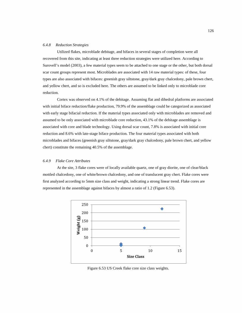
126




Surovell’s model (2003), a few material types seem to be attached to one stage or the other, but both dorsal

scar count groups represent most. Microblades are associated with 14 raw material types: of these, four

types are also associated with bifaces: greenish gray siltstone, gray/dark gray chalcedony, pale brown chert,

and yellow chert, and so is excluded here. The others are assumed to be linked only to microblade core

reduction.

Cortex was observed on 4.1% of the debitage. Assuming flat and dihedral platforms are associated

with initial biface reduction/flake production, 79.9% of the assemblage could be categorized as associated

with early stage bifacial reduction. If the material types associated only with microblades are removed and

assumed to be only associated with microblade core reduction, 43.1% of the debitage assemblage is

associated with core and blade technology. Using dorsal scar count, 7.8% is associated with initial core

reduction and 8.6% with late-stage biface production. The four material types associated with both

microblades and bifaces (greenish gray siltstone, gray/dark gray chalcedony, pale brown chert, and yellow

chert) constitute the remaining 40.5% of the assemblage.

6.4.9 Flake Core Attributes

At the site, 3 flake cores were of locally available quartz, one of gray diorite, one of clear/black

mottled chalcedony, one of white/brown chalcedony, and one of translucent gray chert. Flake cores were

first analyzed according to 5mm size class and weight, indicating a strong linear trend. Flake cores are

represented in the assemblage against bifaces by almost a ratio of 1.2 (Figure 6.53).

Figure 6.53 US Creek flake core size class weights.

0

50

100

150

200

250

0 5 10 15

Wei

ght (

g)

Size Class

127


In addition to the microblade technology, eight bifaces were recovered at US Creek. Five of these

were broken sections, two were proximal sections (a stemmed lanceolate piece and a convex lanceolate

piece), and only one was complete, a Northern Archaic stemmed expanding point. All were in late stage

production: five were stage 4 and three were stage 5 (Figure 6.54). See Figure 6.55 for tool distributions

across the site.

UA2005-051-0378 was a broken, proximal, stage 5, convex lanceolate biface made of green gray

siltstone. It measured 14mm long, 15.8mm wide, 5.5mm thick, and weighed 0.97g.

UA2005-051-0532 was a broken, proximal, stage 5 stemmed lanceolate biface made of yellow

chert. It measured 52mm long, 22.9mm wide, 8.7mm thick, and weighed 9.92g.

UA2005-051-0535 was a stage 4 broken edge biface fragment, made of red chert. It measured

18.3mm long, 12.7mm wide, 4.6mm thick, and weighed 1.04g.

UA2005-051-0974 was a complete, Northern Archaic stemmed expanding stage 5 biface. It

exhibited heavy use wear along one blade, and was likely last used a cutting implement. It was made from

gray/dark gray chalcedony, and measured 40.1mm long, 28.8mm wide, 12.2mm thick, and weighed 8.13g.

UA2005-051-0550 was a broken stage 4 medial biface section. It was made from pale brown

chert, and measured 25mm long, 27.3mm wide, 10mm thick, and weighed 9.17g. It refits to UA 220-051-

0556, a broken stage 4 medial biface section. It was of pale brown chert, measured 13.2mm long, 25.9mm

wide, 8.6mm thick and weighed 3.53g.

UA2005-051-0554 was a broken stage 4 medial biface section. It was of yellow chert, measured

27.9mm long, 23.1mm wide, 10.3mm thick, and weighed 8.38g. It refits to UA2005-051-0600, a broken

stage 4 medial biface section. It was of a different color, pale brown chert, indicating a lack of actual

difference between the two material types. It measured 14.4 mm long, 22.9mm wide, 10mm thick, and

weighed 4.48g.

Figure 6.54 A sample of US creek bifaces.

128

Figure 6.55 Tool distributions at US Creek (isopleths are set at 1 item per 0.25 meter).

129


In this assemblage, unretouched, utilized flakes (n=9), tchi-thos (n=2), retouched flakes (n=16)

were described as expedient tools, with the rest being formal tools. There was a strong preference for

formal tools over informal tools at this site, exhibiting a ratio of almost 2:1.

6.4.12 Spatial Analysis and Site Structure

In this section, the possibility of reoccupation of this site will be discussed, and the probability of a

conservative estimate of two cultural components existing at the US Creek Site, as indicated by the

radiocarbon-dated features. Cultural Zone (CZ) 1 will encompass the younger dated features 1, 3, 11, 12,

and 13. CZ2 will encompass the older two features 14 and 18, and will only discuss the artifacts that were

in direct association with these two groups of features (Figure 6.56).

Figure 6.56 US Creek prehistoric cultural zones.

6.4.13 US Creek Cultural Zone 1 and Cultural Zone 2

Features associated with the younger CZ1 (Figure 6.57) include 1 (cache pit 195+-98 cal BP), 3

(cache pit (372+-58 cal BP), 11 (hearth 154+-124 cal BP), 12 (hearth (400+-61 cal BP), and 13 (hearth

440+-40 cal BP). Several of these features had eight lithic raw material types in direct association with

them (Figure 6.58). These included basalt, quartz, Batza Tena obsidian, dark gray chert, light gray chert,

red chert, translucent gray/black mottled chalcedony, and white/brown mottled chalcedony. Three of these

material types, basalt, quartz, and dark gray chert were also found in direct association with the older CZ2

hearth features. The representation of these three material types in both cultural zones might be due to the

130

Figure 6.57 Level 2 tools and features associated with CZ1, indicated by charcoal density isopleths.

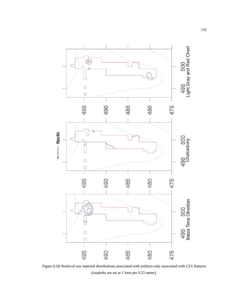
131

Figure 6.58 Nonlocal raw material distributions associated with artifacts only associated with CZ1 features

(isopleths are set at 1 item per 0.25 meter).

132

material types actually having been utilized by people from both components as well as the possibility of

artifact mixing between components. Feature 11 is also partway between both older features 14 and 18, and

will make the argument for spatial integrity problematic.

The two hearth features associated with CZ2 (Figure 6.59) are 14 (740 +-35 cal BP) and 18 (640+-

48 cal BP). These two features also had eight raw materials in direct association (Figure 6.60). These were

basalt, quartz, gray-brown siltstone, clear/black mottled chalcedony, dark gray chert, translucent gray chert,

and yellow chert.

When analyzed with an independent samples t- test to see if there was a significant difference

among artifact types according to this model of cultural zones, no significance was seen among artifact

types or raw materials between cultural zones. This is likely due to the factors of shared material types

between zones.

In order to add a level of strength to formal and informal tool association and features, four

categories were added: Level 1 is tools found in direct association with the dated CZ features, and whose

raw material types are also only directly associated with those features. Level 2 is tools not found in direct

association with dated CZ features, but are of the same material type as debitage found in direct association

with features of only that specific CZ. Level 3 is tools directly found in association with dated features of

only one CZ, but whose respective material types are found in direct association with both Cultural Zones,

and therefore the relationship is ambiguous. Level 4 is tools not found in direct association with any dated

features, but whose respective material types are found in association with features of both Cultural Zones


No Level 1 or Level 3 tools were described for CZ1. Level 2 artifacts, or tools not in direct

association with dated features but whose respective raw materials were only found in direct association

with CZ1 features included 1 biface, 7 microblades, 2 retouched flakes, 1 tchi-tho, 1 flake core, and 2

utilized flakes. In CZ2, Level 1 tools included 3 microblades, 2 retouched flakes, and 1 utilized flake. Level

2 tools included 3 bifaces, 7 microblades, 6 retouched flakes, 1 flake core, 1 microblade core tab, 4 wedge-

shaped microblade cores, and one utilized flake (Table B-38 Appendix B). CZ 1 is dominated by dark gray

chert and quartz debitage (Figure 6.61), while CZ 2 is dominated by clear/black chalcedony, dark gray

chert, and quartz (Figure 6.62).

In regards to the core and blade technology demonstrated at this site, this model of two cultural

components and four levels of artifact strength ties this technology strongly to the earlier component (CZ2)

as opposed to the later one. See Table B-39 (Appendix B) for a summary of artifact types by cultural zone,

and Table B-40 (Appendix B) for a summary of raw material types by cultural zone.

133

Figure 6.59 All core and blade technology in relation to CZ2 Features 14 and 18. Green=microblades,

Blue=microblade core tabs, red=microblade cores. US Creek Features associated with Cultural Zone 2

Level 1 and 2 tools (isopleths are set at 1 item per 0.25 meter).

134

Figure 6.60 Nonlocal raw material distributions associated with artifacts only associated with CZ2 features

(isopleths are set at 1 item per 0.25 meter).

135

Figure 6.61 Cultural Zone 1 raw material size class weights.

Figure 6.62 Cultural Zone 2 raw material size class weights.

6.4.14 Additional Artifacts

In addition, a single piece of red ochre was recovered, weighing 3.02g, worn on one end.

6.5 Bear Creek Introduction

The Bear Creek prehistoric site was discovered in 2005 by BLM archaeologists. The lithic scatter

was situated along a bluff overlooking the cabin and the confluence of a small-unnamed creek and Bear

Creek (Figures 6.63, 6.64 and 6.65). An ash layer was located within one of the test pits placed at the site;

however, it remains unclear if this is related to a hearth feature or a result of natural processes. All artifacts

136

were recovered from the surface of the site. An initial lithic analysis was conducted by Esdale (2010), the

same variables were used and added as in the case with the US Creek analysis.

Figure 6.63 Bear Creek site aerial photograph (courtesy of Robin Mills).

Figure 6.64 Bear Creek site overview (courtesy of Robin Mills).

137

Figure 6.65 Bear Creek site map. Test pits are marked in red (isopleths are set at 1 item per 0.25 meter).

6.5.1 Bear Creek Artifacts

Ninety-nine lithic artifacts and one piece of fire-cracked rock were recovered from the site. The

fire-cracked rock was not included in the analysis. Two (2%) were bifaces, four (4%) were irregular

bimarginally worked flakes, six (6.1%) were tchi-thos, four (4%) were microblades, six (6.1%) were flake

cores, three (3.% were microblade core tabs, one (1.%) was a notched cobble, four (4.%) were retouched

flakes, and the remainder (n=70, 70.7%) were flake debitage.

138


Eleven raw material types were observed at the site (Table B-41 Appendix B). These are:

andesite, basalt, quartz, dark gray chert, translucent gray chert, light gray chert, clear/black mottled

chalcedony, gray/dark gray chalcedony, translucent gray/black mottled chalcedony, obsidian, and white

siltstone. In this analysis, fifteen obsidian artifacts were analyzed for element signatures. Three pieces were

too small to be analyzed1. These were assigned to the Batza Tena source. Three raw materials stand out

compared by cumulative weight percent to the rest and would be considered local. There is a clear definite

break between cumulative weight percents between two groups, being interpreted here as local and

nonlocal (Figure 6.66, Table B-42 Appendix B). See Figure 6.67 for raw material group distributions across

the site.

Figure 6.66 Raw materials 1, 2, and 3, (local) compared to cumulative weight percent of nonlocal materials.

1 One was unrecognized and given an “Unassigned” source (Slobodina and Speakman 2008). In

her analysis, one discrepancy was made. Table 3 (pp. 11) one obsidian flake is assigned to Wiki Peak.

However, referencing Table 1 (pp. 5), a cumulative report on all artifacts submitted, both samples are

indicated to be from US Creek (discussed later) and EAG-597. All artifact bags submitted to the Museum

of the North had the obsidian source written on the bags, and none of them referenced Wiki Peak. It is

assumed to be a typo in the report, as in Table 3, no artifacts are listed from Wiki Peak for US Creek,

whereas one from that assemblage is known to come from that source. For the sake of quantification, the

single unassigned obsidian piece and the three unsourced pieces will be assumed to come from Batza Tena.

139

Figure 6.67 Raw material distributions at Bear Creek (isopleths are set at 1 item per 0.25 meter).


All debitage was classified according to Sullivan and Rozen’s 1985 typology. In this assemblage,

55.6% of flakes were classified as complete, 25.4% were broken, and 19% were split. No artifacts were

classed as flake fragments or debris (Table B-44). These rates were similar to both the US Creek artifacts

140

and Big Bend lower strata. When the debitage was analyzed for cortex (White 1963) 4.8% exhibited

primary decortication, 4.8% were secondary, and 90.5% were tertiary Table B-44 Appendix B). Cortex was

largely confined to the local raw material types. When flakes were divided into 5mm size class increments

(Ahler 1989, Potter 2005) flake size class was compared against cumulative weight percent, no real

difference is seen in size classes (Figure 6.68, Table B-45 Appendix B).

No microblade cores were recovered from the site. However, three microblade core tabs, or

platform rejuvenation flakes, were. Each was of a different material type. One was an obsidian piece

sourced to Batza Tena, another was of grey/dark gray chalcedony, and the third was of clear/black-mottled

chalcedony. Four microblades were in the assemblage. All exhibited flat platforms; three of these were

complete, unsnapped microblades, and the remaining was a proximal end. All four were of Batza Tena

obsidian, and likely related to the single obsidian core tab.

Figure 6.68 Raw material size class weights.



recovered from this site, indicating at least three reduction strategies were utilized here. Microblades are

associated with obsidian, gray/dark gray/chalcedony, and clear/black mottled chalcedony. These material

types were not empirically associated with any other artifact type and are assumed to have been only

utilized for microblade production.

Cortex was observed on 21.2% of the artifacts. Assuming flat and dihedral platforms are

associated with initial biface reduction/flake production, 70% of the assemblage could be categorized as

associated with early stage reduction (Table B-46 Appendix B). If the material types associated only with

microblades are removed, 18% of the debitage assemblage is associated with core and blade technology.

Using dorsal scar count 26.9% is associated with early stage reduction, and 41.6% with late stage biface

thinning (Table B-47 Appendix B). The remaining 13.5% belongs to clear/black mottled chalcedony,

141

utilized for both microblade and biface strategies.

Figure 6.69 Bear Creek tool isopleths (set at 1 item per 0.25 meter). Bifaces=blue, retouched flakes, utilized

flakes, and flake cores=orange, tchi-thos=brown, microblades and microblade core tabs=green.

6.5.5 Core Attributes

One flake core was of local quartz, and the other was of nonlocal dark gray chert. The three

remaining core fragments were recognized as microblade core tabs. Flake cores (n=2) were recovered in

equal amounts to bifaces (n=2). See Figure 6.69 for artifact locations.

6.5.6 Microblade Core Tab Attributes

One microblade core tab (UA2007-072-0011) was of gray/dark gray chalcedony. It was unbroken,

52.88mm long, 36.32mm wide, 14.39mm thick, and weighed 25.88g. It had a faceted platform angled at 75

degrees. The obsidian core tab (UA2007-072-0031) was unbroken, 26.47mm long, 23.01mm wide, 7.47mm

thick, and weighed 5.09g. It had a complex platform, from which an angle measurement could not be taken,

as no distinguishing angle could be seen. The third, of clear/black-mottled chalcedony (UA2007-072-

0055), may also have been reused as a scraper. The platform had been broken off, and the remaining

portion measured 30.18mm long, 26.51mm wide, 7.41mm thick and weighed 5.35g. The range in variation

142

on these discarded tabs was 52.88-26.47mm long (a difference of 26.41mm), 36.32-23.01mm wide (a

difference of 13.31mm), 14.39-7.41mm thick (a difference of 6.98mm), and 25.88-5.09g (a difference of

20.79g). While three artifacts is too small a number to run any relevant statistical tests of significance on

this, one can see that the first artifact is much larger than the last two, which are similar in size (Figure

6.70). See Figure 6.69 for artifact locations.


Formal tools at Bear Creek consist of bifaces (n=2), a notched cobble (n=1), and microblades

(n=4). One microblade was a proximal end which exhibited retouch, while three were complete, unsnapped

microblades. Regarding the two bifaces, one was a large green andesite early stage 1 preform. The artifact

resembled a tchi-tho that had been bifacially reduced. The artifact measured 172.25mm long, 97.7mm

wide, 26.9mm thick and weighed 474.83g. The other was a flat-based lanceolate stage 4 biface of dark gray

chert, which had the tip broken off. It measured 68.9mm long, 24.12mm wide, 10mm thick, and

weighed16.26g (Figure 6.70). See Figure 6.69 for artifact locations.


Unretouched utilized flakes (n=7), retouched flakes (n=4), and tchi-thos (n=6) were assumed to be

expediently made. There was a significant difference in favor of expedient tools at this site. “Retouched

flakes” were flakes that had been unifacially worked, as opposed to “bifacially worked flakes”. Artifacts in

this second category tended to retain their irregular shape, not having been reworked into a regular or

rounded shape. The ratio of informal tools to formal tools at this site is strongly in favor of the former, at a

ratio of exactly 3:1. In the assemblage, 19.2% of artifacts retained cortex, again indicating both early and

late stage core reduction occurred here. See Figure 6.69 for artifact locations, and Table B-48 (Appendix B)

for a artifact usewear summary.

143

Figure 6.70 Bear Creek artifacts. A: microblades, B: microblade core tablets, C: notched cobble, D: biface.

144

7 Modeling Site Structure Behaviors in the Yukon-Tanana Uplands

This chapter presents an analysis of the patterns introduced and discussed in the previous chapters

and sections. The course-grained seasonal resource models presented in Chapter 4 were built in order to

help inform us about the lithic variability expectations the sites should present. This thesis has built upon

the work of previous archaeologists who have directly contributed years of field research in this research

area. These have included John Cook, David Derry, Susan Will, Robin Mills, Ben Potter, Steve Lanford,

and Carol Gelvin-Reymiller.

Previous landscape-based models (Gelvin-Reymiller and Potter 2009) have noted different

resource-use patterns existed between the large Yukon Valley and Tanana Valley flatlands, and the

highlands. The seasonal modeling presented earlier further breaks differences of resource use patterns

within the highlands of the YTU into higher and lower topographic regions. The five sites were then

grouped by Ridgetop and Valley Floor topographic zones (Figure 7.1). This chapter will test the site data

from these groups with optimality and mobility models to draw out further conclusions about behavioral

patterns in this area.

Figure 7.1 The five main sites focused on in this research.

145

7.1 Technological Organization

Within the YUT, ethnographic records indicate that during late winter to early spring as well as

early fall, bands split into small groups, moving throughout an expanded foraging territory. Summer

salmon runs and the autumn caribou migration drew groups back together for mass harvesting of these two

resources. During winter, people relied primarily on cached salmon and caribou for food (Osgood 1936 and

1971, McKennan 1959). Several different major food-acquisition strategies are indicated here to have been

utilized throughout the year. A technology specialized to salmon fishing included leisters, nets, and fish

traps (Osgood 1936) existed along side one specialized for mass caribou hunts that involved large fences,

snares, and corrals (Osgood 1971). Both these strategies involved successfully preparing and storing food

in caches for winter use. Other strategies were adapted to encounter-based forest hunting (Osgood 1936),

likely high altitude snow patch hunting (Hare et al. 2004), and the possible use of hunting blinds, all

focused on large ungulate capture. Further strategies were adapted to small game and waterfowl

(McKennan 1959).

The use of the atlatl dart technology, between 14,000 – 1500 cal BP is only inferred to have

existed in the Interior from the archaeological record. This technology is argued to have been abruptly

replaced by the bow around 1500 cal BP (Hare et al. 2004). From the ethnographic record, arrows, darts,

and/or spears were tipped with stone, organic, or copper points. The process of adoption of the bow and

abandonment of the atlatl in Alaska is not well understood. This process of replacement may have occurred

at different rates depending on the region. Two hypotheses include, (1) atlatls were rapidly replaced by the

bow (i.e. within a generation), or (2) atlatls and bows were utilized together over multiple generations.

7.1.1 The Technological Investment Model

The Technological Investment Model focuses on the creation and maintenance of technology.

Weapons of any type require a certain amount of time investment. The investment must have a payoff that

is inversely related. In other words, a tool requiring large amounts of time, energy, and expensive resources

will not be used to acquire food items with low return. Expedient tools would be ideal in most situations, as

they would provide the biggest payoff. However, in a situation where a tool is costly to make but relatively

easy to maintain thus allowing for multiple uses, intensive tool curation would provide a bigger prey payoff

than multiple, expedient tools.

The problem with modeling this technological investment is that direct observation of tool

investment cannot be made except through experimental replication. This method is problematic because

replication processes were largely reinvented without ethnographically informed guidance. While the final

product may look identical to past artifacts, it is impossible to test that the process that brought the artifact

to completion is identical. Therefore, like the diet breadth model, this must be implemented heuristically.

146

On an x-intercept line (Figure 2.1, Chapter 2), relative tool investment times would mark the

starting point of functional use of the item. Return rates then increase to a peak (the functional

achievement). The peak could be increased through intensification/reuse of the weapon to a point; however

the point will come when benefits will be outweighed by the investment costs. The threshold marks the

ideal moment when an old tool would be replaced by a new one (Bettinger et al. 2006).

Most weapon systems are considered composite (i.e. they are composed of several elements):

some parts considered expendable and other parts crucial. Damage is designed to occur in the expendable

portions, leaving the crucial elements largely untouched. With bow technology, the expendable portion is

the projectile point, and to a lesser extent, the arrow shaft, with the bow itself being the crucial element.

Most time will be invested into the creation of the bow, less to the arrow shafts, and the least to the

arrowheads themselves (Waguespack et al. 2009).

In regards to the atlatl, the dart point is expendable, and the shaft and spear-throwing arm is

crucial. Between the crucial elements, the bow is more costly to make than the spear thrower. The stone

bifacial tip costs would be the same. Atlatl dart shafts were more costly, however, than arrow shafts due to

their doubled length over arrows, adding weight and consuming crucial travel space. Here the benefits of

switching to bow technology are demonstrable even before the use benefits are introduced. By investing

more time into the crucial bow element, which can be used far longer than the expendable tips, time

investments into the shafts are lessened. Further benefits include less time and predator movement between

reloading arrows rather than atlatl darts, and may have also inversely affected hunting practices, lessening

the need for larger hunting parties and increasing the success rates of smaller or even single individual

hunts (Churchill 2002). The same trend is easily demonstrated with the adoption of firearms: costly, long-

term use rifles and cheap expendable bullets replace the bow in Alaska almost immediately upon contact,

further increasing hunting success, and decreasing search time.

The Technological Investment Model suggests that the bows’ success was a clear advantage over

the atlatl in general use. Was the bow a clear advantage over the atlatl in all situations? If not, there exists

the possibility for an opportunity to use both technologies simultaneously. Bettinger et al. (2006) explored

this problem of approaching the weapon technology as a whole as compared to each other. Due to the fact

that the atlatl was both less costly to make and simultaneously generated less net energy returns, the bow

would be chosen over the atlatl. However, in situations where low returns were specifically sought (i.e.

opportunistic foraging), then the atlatl becomes viable for continued use.

Not all technological innovation occurs with the discard of an entire system and the adoption of a

new one; others are simply a matter of small innovations to an existing system. The next section focuses on

the decision variables that affect the shaft, haft, and projectile point choices.

Several types of projectile points were used in the Interior. Composite bone/antler with inset

microblades was one successful strategy that may have been used for both thrusting spears and atlatl darts.

147

Single-piece stone bifaces as projectile points was another strategy that existed both as itself (hafted

directly to the shaft), and also possibly as part of the blade-and-bone points. Projectile points were also

crafted from bone, antler, and wood and hafted directly to a shaft with no indication stone was a part of the

system. Hammered copper points hafted directly to a shaft were also a viable option during the Athabascan

Period (Figures 7.2 and 7.3).

Flaked stone points are brittle and can fail (either unintentionally or by design) during use.

Optimally, this failure is designed to occur within the prey animal, facilitating internal hemorrhaging. An

additional risk exists for failure by striking trees, rocks, and the ground (Knecht 1997, Ellis 1997). Another

risk in the subarctic is that stone becomes brittle and easily damaged in extreme cold temperatures (Elston

and Brantingham 2002).

Faunal-derived points are more durable than stone and solve the brittleness problem. However,

they are not as sharp, or as lethal as their tensile strength is far higher than stone (Waguespack et al. 2009).

Copper points also solve the brittleness problem. However, they do not hold an edge as long, nor the

sharpness, nor the lethality of a stone tool. Stone points will however likely outlast the faunal points in

overall use. Copper points also solve the brittleness problem. However, being a soft metal, they do not hold

an edge as long as a stone tool, decreasing their lethality. They will also, however, likely outlast the faunal

and stone points in use.

Mixing specific elements of each of these can make for a composite point that could be utilized in

multiple contexts: however, the increased cost in time and materials to make the composite points would

have to guarantee a situation where the net return is also increased over the return of a lesser-cost point.

Of the configurations presented above, the highest-cost point would be the composite, which

would be utilized most effectively in situations of guaranteed high net energy returns, such as fall big game

hunts centered around the caribou migration. The durability and engineering properties of these types of

points also cause it to become heavier, and therefore more effective in close range kills, likely where the

prey animal has been placed in a disadvantaged situation (Churchill 2002). The high-cost technology might

be then limited to mass killing hunts, associated with large ungulate migrations. In winter, where the

durable point would be an advantage over the brittle point, a lighter weapon would be needed. Mass kills

are far less likely, and when hunting situations were viable, these usually consisted of stalking single or

small groups of animals, and a weapon with an extended effective killing distance would mitigate the risk

of losing food. In this situation, an organic or copper point would be more optimal over a heavy composite

or a brittle stone point. During the spring months, when hunts were not focused on migration exploitation,

stone-tipped projectile weapons could be favored over copper/organics (See also Wygal 2009).

These hypotheses are also driven by resource availability for weapon creation. If a high-quality

lithic toolstone source is readily available, and copper is only available through trade with a potentially

hostile band, stone might be chosen over copper where copper would be ideal. Lithic materials are also

148

Figure 7.2 Arrow shaft and several types of stone (left) and bone (right) projectile points.

Figure 7.3 Composite spear modeled after bison rib artifacts (early Holocene) recovered by Ben Potter

from Gerstle River Component 3, 2011 (Artwork by Zerah Turbitt).

only available during the warmer months, requiring either their caching, or extended periods of tooling up

during the autumn in preparation of winter. It has also been hypothesized that microblades are a raw

material-maximizing strategy for either cold, months, or for the use of large, resource-stressed areas

149

(Flenniken 1987). During the winter, they are either largely hidden by snow or frozen in and to the ground.

These situational driven ideas, however, are more difficult to test (Elston and Brantingham 2002).

In the YTU, no known copper sources exist, and any copper traded would have likely been part of

a long-distance exchange system. Already it has been observed that obsidian at US Creek possibly passed

through this valley, allowing for the possibility of copper to pass along these same trade routes. Copper, as

with any regionally-isolated resource, likely increased in relative rarity and value the greater the distance

from its original source. Therefore, in a resource-poor region such as the YTU, far removed from copper

sources, the value of metal implements might have prevented their discard.

If, over time, microblades were increasingly associated with composite weapons that were

increasingly isolated to mass-procurement caribou hunts, the sustained regional collapse of a migrating

herd could create a situation where composite microblade weapons were dropped in favor of lighter

weapons more suitable for encounter-based hunting. If this situation was widespread over a region and

sustained long enough, the technology could be lost entirely, especially given that the different cost-benefit

ratios between copper, faunal, and lithic bifaces.

The regional small-scale models (Chapter 4) suggest that winter hunting was not a widespread

activity in the YTU, and most sites conform to the spring model, and to a lesser extent the fall resource

model. Therefore, the record should indicate a preference for stone biface points in spring-related hunting

camps, and biface and microblade-composite preferences in fall-related camps.

The assemblages with more microblade artifacts include Bear Creek and US Creek (CZ2). The US

Creek assemblage shows a very low percentage of debitage linked to late-stage biface production, possibly

indicating that this site was associated directly with a mass-hunt using composite weaponry. Bear Creek

shows a preference for both strategies. Bachelor Creek, Big Bend, and Cripple Creek all show similar

smaller amounts of microblade-related debitage. Bachelor Creek shows the largest amount of debitage

associated with late-stage biface production, indicating a situation where this system was preferred,

possibly hinting at a spring occupation. Big Bend and Cripple Creek have less late-stage biface material

byproducts in favor of flake production, indicating other activities beyond tool manufacture/repair were

also occurring.

In regards to core and blade technology patterns, significant patterns exist both at the locale level

and at the site specific level. Microblades are in greatest number at US Creek; however, both ridgetop sites

hold a far greater number of these artifacts than the other two remaining valley floor sites. Core tabs and

discarded cores, however, are only found at the valley floor sites. These patterns indicate that primary

composite weapon retooling likely was focused in the valley bottoms, and only secondary repair occurred

on the ridgetops.

Reduction strategy patterns indicate that microblade production is highest at US Creek and Bear

Creek. Flake production is highest at Big Bend and Cripple Creek. Biface production is highest at both

150

Bachelor Creek and Bear Creek (Table C-1 Appendix C). While microblade production seems to dominate

the low sites as opposed to the high sites (Table C-2 Appendix C), biface and flake production is not as

clear-cut, suggesting that these two strategies occurred more opportunistically than did composite tool

repair (Table C-3 Appendix C).

The question of technological investment can also be applied to the use of ceramic bowls and

birch bark containers. Ceramic bowls are certainly more costly; they require specific trips to procure the

materials, time to manufacture and fire the bowls, and the risk of transporting them between sites and

remaining intact. Birch bark containers are less costly to procure and make, and far more durable in regards

to transportation. The cost of a ceramic bowl, however, would eventually be returned by its far greater

resistance to heat damage, increased nutritional benefits of ceramic-cooked food as opposed to raw, or meat

cooked directly over flames. In a situation of high residential mobility, birch bark bowls would likely be

favored over ceramics, whose weight and brittleness would add a far greater increased risk of loss and

damage during transport. In situations of longer residence times, ceramic utensils would be favored for

their longer use life and added increased nutritional value of food (Ugan et al. 2003).

This cost-benefit model suggests that ceramics should only be found in residential sites, and then

only in situations where logistic mobility strategies are favored over residential mobility strategies. As

stated previously, ceramics have only been recovered from the Cripple Creek site where a wide variety of

behavior patterns are indicating a longer residence time in relation to other sites in the region.

7.2 Mobility

Recreating mobility patterns within the YTU poses a daunting problem. From the ethnographic

and historical records, several major prehistoric trade routes crossed the YTU, utilizing both river systems

and ridgetops. Simeone (1982) indicates that within the immediate region of the five sites discussed here, at

least one major route passed up the Chatanika River, and another passed north from there along Beaver

Creek. Within the traditional territories (Figure 4.1, Chapter 4), bands moved by the seasons (Osgood 1936

and 1971, McKennan 1959). Rainey (1939), when investigating ceramic production at Rampart on the

Yukon River reports an informant reporting natives of both the Tanana basin and Yukon basin travelling to

that location to procure clay and produce the containers.

Within the site assemblages, all obsidian artifacts, with the exception of US Creek came from the

Batza Tena source. US Creek, in addition to most of its obsidian coming from Batza Tena, also had element

signatures indicating pieces traveling from Wiki Peak, on the border between Alaska and Yukon, and

further from Hoodoo Mountain and Mt. Edziza in northern British Columbia (Figure 7.4).

Throughout the Livengood region, in the northwestern portion of the YTU, numerous chert

formations are found. While these can be highly variable in color, one type of chert is considered to be

sourced to that area (termed colloquially as “Livenengood Chert”). Visibly, this appears as an opaque black

151

mottled with clear, uncolored bands. In the initial lithic analysis, this was termed here as “black/clear

mottled chalcedony” due to its very fine, almost invisible particulate structure. This type was one of the

more numerous chert types found in each assemblage.

Figure 7.4 Obsidian sources.

The heavy presence of Livengood chert and Batza Tena obsidian in all the assemblages (as well as

the ceramics from Cripple Creek) suggest a migratory movements to and from these sites and the

northwest, into the Livengood mountains, Rampart on the Yukon beyond that, and possibly further west to

Batza Tena. These materials could also have been acquired through trade instead of direct procurement.

The obsidian from Wiki Peak, Mt. Hoodoo, and Mt. Kluane almost certainly arrived at US Creek through

long-distance trade networks.

Raw materials, were treated significantly differently throughout all five sites, and is likely a

function of the statistically significant difference between the treatment of local and nonlocal raw material

groups. The difference is possibly explained by occupation duration at each site. According to Kuhn (1994)

local and nonlocal raw material density is a function of occupation time. When a group first arrives on a

152

site, presumably all their materials they have with them have been carried from elsewhere. The longer the

site is occupied, the further the exotic materials will be curated and the more local materials will be

integrated into the assemblage.

Known good toolstone quarries in the YTU exist in only a few places. Therefore, obtaining their

materials would require a specific, high cost trip, at the expense of important food acquisition. In order to

mitigate this, strategies may have included planned, annual or seasonal stops at these locations during

residential moves, and preparation of these materials on site into preforms that optimize travel wear,

weight, and potential tool use longevity. In a situation of direct procurement of a resource, opportunity

costs are increased due to opportunities lost for acquiring a separate, different resource. In a situation of

embedded procurement, combining the acquisition of several resources to a single event mitigates this

opportunity cost.

The high quality materials are nonlocal in all these sites, indicating specific trips were required for

their procurement. The low quality materials are always local in the assemblages, indicating they were

acquired through an embedded system (i.e. they were gathered in the immediate site vicinity as they were

needed). There is an interesting trend in the treatment of local and nonlocal raw material groups. The

percentages are nearly opposite for the two locales (Figure 7.5).

Figure 7.5 Local (blue) vs nonlocal (green) materials by topographic zone.

153

Figure 7.6 Local vs. nonlocal materials by site, topographic zone and cultural period. Local (white) vs.

nonlocal (gray) raw materials by site, topographic zone and cultural period.

154

At the ridgetops, almost 80% of the combined lithics from both the Bachelor Creek and Big Bend

assemblages are local. In the valley floor sites, nearly 80% of the combined assemblages are nonlocal

material types (Figure 7.6). This suggests that a system of embedded, low cost procurement was used more

often in the ridgetop locations, and a system of direct, high cost procurement were used in relation to the

valley bottom sites. These patterns could indicate that the valley bottom patches were the first occupation

areas after trips to procure these better quality materials. The caloric return rates in the valley bottoms were

high enough to allow for time to be allocated for specific high-quality toolstone acquisition. When caloric

return rates had dropped enough that the higher altitudes and ridgetops became promising food acquisition

patches, search time seems to have increased to the point that a low cost procurement pattern was needed,

resulting in assemblages dominated by local, lesser quality material types, likely a search-time mitigation

strategy. Viewing this as a continuum (Bousman 1993) valley bottom sites indicate resource-maximizing

behaviors, and ridgetop sites indicate patterns of time-minimizing behaviors.

The use of nonlocal material types is more prevalent in the valley bottoms, which would indicate

shorter time-span use of those sites in relation to the upland sites. The trend is likely dominated by the US

Creek and Big Bend sites, both contributing the bulk of artifacts in this study. Using Kuhn’s (1994) model

and Surovell’s (2003) operization of this model, both US Creek cultural zones would indicate the shortest

occupation spans, followed by Bear Creek and Bachelor Creek. The Cripple Creek, and Big Bend sites

would have the longest relative occupation length.


In the contexts discussed throughout this research, tone tools were created primarily to capture and

process food. The lithic tools can either be utilized directly against prey items, such as in the case of

projectile points, knives, and tchi-thos, or they can be used to enhance other food processing items such as

burins, hammer stones, and grinding stones. The variety of prey that is considered at any one time to be

available, viable food is expected to be reflected in the variety of tools needed to procure and process those

items. If only a few prey items are needed for comfortable survival, then food-related technological

variability should reflect this lack of variety.

The Diet Breadth Model determines prey profitability by size, density, distribution, and

technology utilized to exploit them. Assuming an optimal response, prey ranked with the highest caloric

return will be exploited first. Expansion of the diet breadth to include additional lower-ranked items will

increase prey encounter rate and decrease overall search time. However, handling time/costs will increase.

The balance between the rising handling time and decreasing search time is the decision point where the

optimal diet is made.

Bousman (1993, 2005) hypothesizes that diet breadth expansion is also directly affected by

technological cost. Handling costs are decreased by less time-consuming technologies, (expedient tools)

155

and easily obtained raw materials. In situations where expensive, less diverse technological strategies, and

more harder-to-obtain raw materials are used, handling costs are immediately increased and therefore diet

breadth decreases, reflecting use of only the highest ranked prey. When the highest ranked resources in a

region are not enough to sustain a group, lower ranked resources with less caloric return must be utilized in

order to facilitate survival. In such a situation, the expansion of the diet breadth should be reflected by a

greater variety of tools needed to process different items. The devotion of more time to these low-ranked

resources detracts from available time for locating good toolstone, therefore a higher amount of less quality

toolstone is expected to also be seen.

These analyses indicate that on the ridgetop sites, less tool diversity is seen than in the valley

bottom sites (Figure 7.7 and 7.8). If we assume tool diversity increase = diet breadth decrease (with focus

only upon the highest ranked resources), as Bousman does, then the technological diversity matrix here

suggests that a wider variety of prey were being sought after in the valley floor zones where tool diversity

is higher. At the ridgetop zones where the tool diversity is lower, the diet breadth model suggests that this is

indicative of fewer, high ranked resources being captured. These relationships suggest that a wider variety

of prey were utilized in the valley floors. Conversely, the ridgetop zones were utilized only for specific

prey items.

When tested by topographic zone with a t-test, artifact type, raw material type, and local/nonlocal

groups all vary at significant levels (Table C-4). Artifact variability is far stronger in the valley bottom sites

than at the ridgetops, and suggests a greater variation in internal site behaviors at the low sites than the high

ones. We can infer then, that the ridgetop sites were likely utilized directly for relatively few specific

objectives, then abandoned, and vice versa in the valley bottom sites. Raw material diversity is also greater

in the valley bottoms than at the ridgetops (Figure 7.9). The US Creek assemblage suggests usage of high

quality material (the obsidian, chert, and chalcedony diversity). The Big Bend site represents an opposite

trend: an assemblage dominated by the use of local materials, suggesting that, in the YTU, diet breadth is

decreased when ridgetop sites are used, and increased when valley floor sites are inhabited.

7.3 Social Organization

Throughout the YTU, ethnographic evidence from Osgood (1936, 1971), McKennan (1959) and

Slobodin (1981) report that prehistoric bands were small, and centered around 1-3 nuclear families. Bands

came together in larger groups in order to harvest summer salmon and autumn fish runs as well as to target

migrating caribou. Winter was also a season of band congregations, and potlaches also provided motivation

to come together. In other situations, such as early fall, early winter, late winter, spring, and early summer,

resources were not as predictable and bands split into small groups, spreading out across the landscape.

156

Figure 7.7 Artifact diversity by site, topographic zone, and cultural period.

157

Figure 7.8 Artifact diversity by topographic zone.

Figure 7.9 Raw material diversity by topographic zone.

This was likely a risk minimizing strategy, as prey tended to be hunted according to an encounter-based

approach.

The ethnographic and historic accounts indicate that when the Lower Tanana and Gwich’in groups

broke up into smaller foraging bands, the nuclear family did not separate (McKennan 1981, Osgood 1936),

but travelled together. In these situations, the reports indicate that stalking and killing practices was

coordinated by adult males while other members focused upon the butchering and storage. Osgood (1971)

reports that early fall was a time when all-male foraging parties left Han groups between the summer

salmon runs and fall caribou migrations. Osgood also reports that winter Han foraging bands were

occasionally composed of young males who would spend as long as a week rounding up small groups of

caribou to drive back to the village, where the remaining male and female members would dispatch the

animals.

158

A sexual or gender separation of hunting practices is not suggested in the literature with regards to

the caribou migration or salmon and fish runs. Where wood fences and snares were utilized to catch the

caribou, every-able bodied member of the group helped to dispatch and butcher the animals. This tended to

hold true for the fish runs as well (Osgood 1936, 1971, McKennan 1981, Slobodin 1981).

Multiple wives sharing one man was a rare practice, and multiple husbands sharing one woman

was rarer still, however, not unheard of. The practice of polygamy suggests the probability that large game

hunting may have been practiced by women as well. It is likely that the all-male hunting parties, when this

was considered a viable practice, served as a demonstration of prowess in order to gain a desirable mate

(Zeanah 2004).

Before the adoption of bow technology, which favored both smaller hunting bands and individual

hunting success, the atlatl has been suggested to have had the greatest return when utilized in group-hunting

strategies (Bettinger et al. 2006). In the Northern Archaic period, when this technology seemed to dominate

ungulate hunting strategies, group hunting may have favored a greater number of individuals working

together. In encounter-based foraging situations, this may have favored a greater foraging gender division,

than was seen in the Athabascan period.

Hunting technology is associated with all five sites. The notched cobble at Bear Creek suggests

fishing practices as well. The high presence of local flake production at Big Bend suggests the presence of

butchering. The best evidence for the presence of a nuclear family comes from Cripple Creek, where

domestic artifacts are indicated by the presence of ceramics. Finally, the cremation and burial of the child at

Cripple Creek presents the strongest evidence for the presence of a family.

159

8 Conclusions

This regional analysis was conducted through formal methods of archaeology (with analysis

focusing on lithic, geoarchaeology, radiocarbon, and ceramics) anthropology (applying ethnographic,

historical, and behavioral ecology models) and geospatial analysis to investigate the use of the Yukon

Tanana Uplands by its prehistoric inhabitants. This approach examined contexts of environment, economy,

and cultural change that played important roles in successful prey-capturing strategies in this area. The

primary objectives of this research were to (1) provide a contextual discussion of the seasonal relationship

between humans and their regional prey, and (2) explore how topography, seasons, and weapon choice

affected the human interaction within this region.

8.1 Regional Model Summary

The seasonal models provide a course-grained first-approximation look at site location patters

within the YTU. The resource models were built using modern floral and faunal distribution data, and

prehistoric sites were for the sake of the model assumed to represent cultural stasis. Despite these data

shortcomings and site preservation and location biases, patterns were demonstrated to exist between site

placement and seasonal resources. From these relationships, mobility patterns were inferred, with spring

representing the time period of highest mobility, followed by autumn, with summer suggesting low

landscape mobility, and winter showing no correlation between mobility and resources.

These patterns are consistent with what is known from the ethnographic and historical literature.

From these geospatial patterns and the ethnographic evidence, two topographic zones of resource

acquisition within the YTU were drawn. These were the lower valley floors and the mid-range altitude

ridge and hilltop zones. The differences between these ecozones were hypothesized to require differing

prey acquisition strategies which would result in differences in toolstone acquisition and weapon

production and maintenance.

8.2 Assemblage Overview

The ridgetop sites appear culturally contemporaneous. Based on the formal artifact assemblage

from Bachelor Creek, this assemblage is associated with the Northern Archaic tradition. Both microblades

and bifaces were found in mixed association, although of differing material types, suggesting a spring

occupation of the site.. The formal artifact assemblage from Big Bend indicates also a Northern Archaic

association. The Hearth and Level 3 share closer association than Level 2 and the Surface. The assemblage

was split into two components for the purposes of Chapter 7. The lower component favored microblade

production, while the upper component favored biface production. This suggests a difference in

procurement strategies between the components, possibly further indicating either a seasonal change (with

the lower component suggesting an autumn occupation, and the upper component suggesting a spring

160

occupation), or the noted abandonment of microblades from the regional toolkit during the Athabascan

period.

The Bear Creek formal artifact assemblage shares tools found throughout both the Northern

Archaic and Athabascan periods. No diagnostic forms of either cultural period was found, and therefore

this assemblage was placed in the “Transitional” phase, which is used here as a cultural placeholder

between both formally recognized periods. The mix of artifact types suggest a late spring or early autumn

occupation, when fishing would have been a viable option.

The US Creek Cultural Zone 2, dating between 800 and 600 cal BP, also was placed in the

“Transitional” phase. While the dates, place it in what is traditionally understood as the Athabascan period

(Dixon 1985), the presence of a microblade component suggests that these artifacts were not suddenly

abandoned within this region, but were retained, seemingly later in time after their abandonment in other

Athabascan regions. The heavy representation of microblades, and microblade related lithics, suggest an

autumn occupation focused upon the caribou migration.

The US Creek Cultural Zone 1 (~500-30 cal BP) represents Athabascan food caching and short

term occupation behaviors. Nearby, the Cripple Creek (~200-50 cal BP) also represents Athabascan food

caching, however, this is found in association with long-term occupation behaviors. Both of these

assemblages have a questionable microblade-bearing components; further data is not present to adequately

explore their problematic relationship. The faunal assemblages indicate an occupation ranging between late

autumn and early spring.

8.3 Sampling and Taphonomy

The Bear Creek assemblage is the only assemblage apparently collected in full. The US Creek

assemblage is estimated to include as much as 80% of the original site assemblage prior to destruction

(Mills personal communication). The Cripple Creek collection likely only represents 10-20% of the

remaining assemblage. Big Bend and Bachelor Creek were both collected in similar fashion: a complete

surface collection followed by subsurface systematic shovel testing. This results in patterns dominated by

the surface artifacts, which can skew data results. Additional intensive sampling and block excavations can

provide rigorous tests of the patterns and relationships identified here.

The Sullivan and Rosen summaries indicate similar patterns of flake breakage patterns across the

sites, never within any category having artifact types range beyond 10% of each other. These similarities

across topographic and ecological zones suggest that none of the assemblages were subjected to any great

amount of post-depositional disturbance.

161

8.4 Technological Patterns

The US Creek assemblages suggest a late occurrence of microblade technology at least within the

upper Chatanika River valley, well into the beginning of the Athabascan Period. If an actual population

difference existed between the Northern Archaic people and Athabascans, this suggests the area was a

region where the descendants of Northern Archaic peoples were able to retain (for a time) culturally-

distinct implements while surrounding Athabascan-related bands successfully expanded into a landscape

with technology that favored organic tools.

If, however, the loss of microblades is related to a shift of behavioral hunting strategies, then this

region suggests local factors were present to favor the use of this ancient strategy and perhaps the gradual

abandonment of it over the course of several generations. This latter interpretation is favored here over the

former, due to the apparent lack of evidence beyond technological change for cultural replacement.

The valley floor sites exhibited greater raw material type variability than did the ridgetop sites,

The lower altitude sites also exhibited a greater range of tool types than did the higher altitude sites. The

high altitude sites also tended to have more local material types incorporated into their assembalges. These

three indicators suggest that (1) the ridgetop sites were not the initial sites to be utilized after primary lithic

acquisition trips had occurred, (2) less activities are represented in the ridgetop assemblages than the valley

floor assemblages, and (3) While less activities are present in the ridgetop sites, the higher presence of local

debitage suggests longer occupation times based upon the apparent lack of high-quality toolstone. Finally,

long-term storage sites are only found in the later-dated, valley floor components. This suggests the lower

elevation sites were considered better locations for these behaviors.

The White River Ash Fall, (ca 1800 cal BP) certainly had a devastating effect in the eastern YTU.

Kuhn et al. (2010) have demonstrated through DNA evidence that caribou herds throughout the southwest

Yukon have recently undergone a partial DNA replacement around 1000 years ago, suggesting population

collapse and recolonization. The collapse of such an important food resource could certainly cause the

abandonment of a region by human predators, if replacement resources were not enough to sustain bands

and individuals. However, it has not been demonstrated in such an abandonment occurred, and if that

further resulted in recolonization of the area by the same people later on armed with new technology, or by

entirely new people and new technology altogether. The apparent retention of microblades into the early

Athabascan period, and their argued gradual loss, coupled with the similar mobility patters, resource uses,

and similar other tool artifacts, suggests human population continuity in the western YTU, with gradual

cultural and behavioral modifications from the late Northern Archaic period until the historic period of

contact

162

References Ager, T. A. and L. B. Brubaker

1985 Quaternary Palynology and Vegetational History of Alaska. In Records of Late Quaternary North American Sediments, edited by B. Vaughn, Jr., and F. Holloway, pp. 353-384. American Association of Stratigraphic Palynologists, Dallas.

Ahler, S. A.

1989 Experimental Knapping with KRF and Midcontinent Cherts: Overview and Applications. In Experiments in Lithic Technology, edited by D. S. Amick and R. P. Mauldin, pp. 199-234. BAR International Series 528, Oxford.

Aigner, J. S. and B. L. Gannon

1980 Historic and Prehistoric Land Use in Interior Alaska: Delta North to Prudhoe Bay. Background report for archaeological survey along the proposed natural gas pipeline from Delta Junction to Prudhoe Bay. Fluor Engineers and Constructors, Irvine, California. University of Alaska, Fairbanks. 1981a Archaeological Survey in Interior Alaska: Final Report on the 1980 Archaeological Survey Along the Northwest Alaska Pipeline Company Proposed Natural Gas Pipeline Corridor from Prudhoe Bay to Delta Junction, With Additional Work to the South. November 1981. Anthropology Program and Institute of Arctic Biology, University of Alaska, Fairbanks. 1981b Archaeological Survey in Interior Alaska: Final Report on the 1981 Archaeological Survey Along the Northwest Alaska Pipeline Company Proposed Natural Gas Pipeline Corridor from Prudhoe Bay to Delta Junction, With Additional Work to the South. December 1981. Anthropology Program and Institute of Arctic Biology, University of Alaska, Fairbanks.

AHRS

2010 Alaska Heritage Resource Survey, Office of History and Archaeology, State Historic Preservation Officer. State of Alaska, Anchorage.

Anderson, D. D. 1968 A Stone Age Campsite at the Gateway to America. Scientific American 218(6):24-33. Andrefsky, W.

1999 The Analysis of Stone Tool Procurement, Production, and Maintenance. Journal of Archaeological Research, 17:65-103. 2005 Lithics: Macroscopic Approaches to Analysis, 2nd Edition. Cambridge University Press, New York.

Andrews, E. F.

1975 Salcha: An Athabascan Band of the Tanana River and Its Culture. Master’s Thesis, University of Alaska, Fairbanks. 1977 Report on the Cultural Resources of the Doyon Region, Central Alaska. Anthropology and Historic Preservation Cooperative Park Studies Unit Occasional Paper 5, Vol. 1 and 2. University of Alaska, Fairbanks.

Bae, K. and J. C. Kim

2003 Radiocarbon chronology of the Palaeolithic complexes and the transition to the Neolithic in Korea. The Review of Archaeology 24, 46–49.

163

Barton, L., P. J. Brantingham, and D. Ji 2007 Late Pleistocene climate change and Paleolithic cultural evolution in Northern China: Implications from the Last Glacial Maximum. In Developments in Quaternary Sciences, Vol. 9.

Beget, J. E., R. D. Reger, D. Pinney, T. Gillispie, and K. Campbell

1991 Correlation of the Holocene Jarvis Creek, Tangle Lake, Cantwell and Hayes Tephras in Southcentral and Central Alaska. Quaternary Research 35:174-189.

Bettinger, R. L.

1991 Hunter-Gatherers: Archaeological and Evolutionary Theory. Plenum Press, Newy and London. 2009 Hunter-Gatherer Foraging: Five Simple Models. Eliot Werner Publications, Inc. New York.

Bettinger, R. L., B. Winterhalder, and R. McElreath

2006 A simple model of technological intensification. Journal of Archaeological Science 33:538-545

Bigelow, N. H.

1997 Late Quaternary Vegetation and Lake Level Changes in Central Alaska. PhD Dissertation, Department of Anthropology, University of Alaska Fairbanks.

Bigelow, N. H. and W. R. Powers

2001 Climate, Vegetation, and Archaeology 14,000-9000 cal yr B.P. in Central Alaska. Arctic Anthropology 38(2):171-195.

Binford, L. R.

1979 Organization and Formation Processes: Looking at Curated Technologies. Journal of Anthropological Research, 35(3):255-273. 1980 Willow Smoke and Dogs’ Tails: Hunter-Gatherer Settlement Systems and Archaeological Site Formation. American Antiquity, 45(1):4-21.

Borgerhoff Mulder, M.

1991 Human Behavioral Ecology. In: Behavioral Ecology: an Evolutionary Approach. Ed. J. R. Krebs and N. B. Davies. Oxford: Blackwell Scientific Publications.

Bousman, C. B.

1993 Hunter-Gatherer Adaptations, Economic Risk and Tool Design. Lithic Technology 18(1&2):59-86. 2005 Coping With Risk: Later Stone Age Technological Strategies at Blydefontein Rock Shelter, South Africa. Journal of Anthropological Archaeology 24:193–226.

Bowers, P. M.

1980 The Carlo Creek Site: Geology and Archaeology of an Early Holocene Site in the Central Alaska Range. Anthropology and Historical Preservation Cooperative Park Studies Unit. University of Alaska Fairbanks, Alaska.

Brantingham, P. J., K. W. Kerry, A. I. Krivoshapkin, and Y. V. Kuzmin

2004 Time-space dynamics in the early upper Paleolithic of Northeast Asia. In: Madsen, D.B., (Ed.), Entering America: Northeast Asia and Beringia before the Last Glacial Maximum. The University of Utah Press, Salt Lake City, pp. 255–284.

164

Brigham-Grette, J. 2001 New Perspectives on Beringian Quaternary Paleogeography, Stratigraphy, and Glacial History. Quaternary Science Reviews. 20:15-24.

Bright, J., A Ugan, and L. Hunsaker

2002 The Effect of Handling Time on Subsistence Technology. World Archaeology. 34(1):164-181.

Calkin, P. E., G. C. Wiles, and D. J. Barclay

2001 Holocene Coastal Glaciation of Alaska. Quaternary Science Reviews 20:449-461. CalPal

2006 University of Cologne Radiocarbon Calibration and Paleoclimatic Research Package, May edition.

Caulfield, R. A.

1983 Subsistence Land Use in Upper Yukon-Porcupine Communities, Alaska. Alaska Department of Fish and Game Division of Subsistence Technical Paper Number 16. Fairbanks, Alaska.

Charnov, E. L.

1976 Optimal Foraging, the Marginal Value Theorem. Theoretical Population Biology 9(2):129-136.

Chen, C. and X.-Q. Wang

1989 Upper Paleolithic microblade industries in North China and their relationships with northeast Asia and North America. Arctic Anthropology 26:127-156.

Churchill, S. E.

2002 Weapon Technology, Prey Size Selection, and Hunting Methods in Modern Hunter-Gatherers: Implications for Hunting in the Palaeolithic and Mesolithic. In Hunting and Animal Exploitation in the Later Palaeolithic and Mesolithic of Eurasia, edited by G. L. Peterkin, H. M. Bricker, and P Mellars, pp. 11-24.

Coffman, S. C.

2011 Archaeology at Teklanika West (HEA-001): An Upland Archaeological Site, Central Alaska. M.A. Thesis, University of Alaska, Fairbanks.

Cook, J. P.

1969 The early prehistory of Healy Lake, Alaska [PhD dissertation]. Madison: University of Wisconsin. 1995 Characterization and distribution of obsidian in Alaska. Arctic Anthropology 32:92-100.

Cook, J. P. (editor)

1977 Pipeline Archaeology. University of Alaska Institute of Arctic Biology, Fairbanks. Cooper, H. K.

2007 The Anthropology of Native Copper Technology and Social Complexity in Alaska and the Yukon Territory: An Analysis Using Archaeology, Archaeometry, and Ethnohistory. Ph.D. Dissertation, Department of Anthropology, University of Alberta, Edmonton.

165

Crow, J. R. and P. R. Obley 1981 Han. In Handbook of North American Indians, Volume 6: Subarctic, edited by June Helm. Smithsonian Institution, Washington, D. C.

Darwin, C.

1859 The origin of species by means of natural selection, or, The preservation of favored races in the struggle for life. New York: Modern Library. 18th ed. 1998.

Derev’anko, A. P. and S. Markin

1998 The Middle and Upper Paleolithic of Western and Central Siberia. In The Paleolithic of Siberia: New Discoveries and Interpretations, edited by A. P. Derev’anko, pp. 79-84. University of Illinois Press, Urbana.

Derry, D. E.

1975 Later Athapaskan prehistory: A migration hypothesis. Western Canadian Journal of Anthropology 5(3–4):134– 147.

Dikov, N.

1993 Paleolit Kamchatki i Chukotki v Sviazi s Problemoi Pervonachal’nogo Zaseleniia Ameriki. Rossiiskaia Akademia Nauk, Dal’nevostochnoe Otdelenie Severo-Vostochnyi Kompleksnyi Nauchno-Issledovatel’skii Institut, Magadan (in Russian).

Dilliplane, T. L.

1980 Cultural resource investigation along the Steese Highway: miles 43.8-66. In: Archaeological Survey Project, 1978, Miscellaneous Publications History and Archaeology Series No. 22. Edited by: T.L. Dilliplane. Office of History and Archaeology, Alaska Division of Parks, Anchorage, pp. 77-96.

Dixon, E. J.

1985 Cultural Chronology of Central Interior Alaska. Arctic Anthropology, 22(1):47-66. 1993 Quest for the Origin of the First Americans. University of New Mexico Press. Albuquerque.

Dixon, E. J., G. S. Smith, and D. C. Plaskett

1980 Archaeological Survey and Inventory of Cultural Resources, Fort Wainwright, Alaska. Final Report. Submitted to the Department of the Army, Alaska District, Corps of engineers, Contract No. DACA-78-C-0047. Copy on file, University of Alaska Museum, Fairbanks.

Dixon, E. J., G. S. Smith, R. M. Thorson, and R. C. Betts

1981 Annual Report. Sub-task 7. 06 Cultural Resources Investigation for the Susitna Hydroelectric project. Submitted to the Alaska Power Authority, Anchorage, Alaska. copy on fi1e, University of Alaska Museum, Fairbanks. 1983 Field Season Cultural Resource Investigation of the Susitna Hydroelectric Project. Submitted to the Alaska Power Authority, Anchorage, Alaska. Copy on fi1e, University of Alaska Museum, Fairbanks.

Dumond, D. E.

1969 Toward A Prehistory of the Na-Dene, With a General Comment on Population Movements Among Nomadic Hunters. American Anthropologist 71(5):857-863. 1987 The Eskimos and Aleuts, Thames and Hudson, London.

166

Ellis, C. J., 1997 Factors influencing the use of stone projectile tips: an ethnographic perspective. In: Projectile Technology. Edited by H. Kecht. Plenum Press, New York, pp. 37–74.

Elston, R. G. and P. J. Brantingham

2002 Microlithic Technology in Northern Asia: A Risk-Minimizing Strategy of the Late Paleolithic and Early Holocene. In Thinking Small: Global Perspectives on Microlithization. Edited by R. G. Elston and S. L. Kuhn. Pp 103-116. Archaeological Papers of the American Anthropological Association, 12, Arlington.

Esdale, J.

2005 Series of reports on the lithic analysis of the U.S. Creek Site (CIR-00029). Manuscript of file, Bureau of Land Management, Fairbanks District Office, Fairbanks, Alaska. 2006 The US Creek Prehistoric Site: 2005 Lithic Analysis. Manuscript of file, Bureau of Land Management, Fairbanks District Office, Fairbanks, Alaska.

2008 A Current Synthesis of the Northern Archaic. Arctic Anthropology, 45(2):3-38. 2010 Bear Creek (CIR-00161) Surface Assemblage Lithic Analysis. Manuscript of file, Bureau of Land Management, Fairbanks District Office, Fairbanks, Alaska.

Fathauer, G. H.

1942 Social Organization and Kinship of the Northern Athabascan Indians. Master’s Dissertation, University of Chicago, Chicago, Illinois.

Flenniken, J. J.

1987 The Paleolithic Dyuktai Pressure Blade Technique of Siberia. Arctic Anthropology, 24(2):117-132.

Fretwell, S. D. and H. L. Lucas, Jr.

1968 On Territorial Behavior and other factors influencing habitat distribution in Birds, I. Theoretical Development. Acta Biotheoretica XIX:16-36.

Gelvin-Reymiller, C. and B. A. Potter

2009 Site Location Model and Survey Strategy for Cultural Resources in the White Mountain National Recreation Area and Steese National Conservation Areas. Report prepared for the Fairbanks District Office Bureau of Land Management.

Glascock, M. D., G. E. Braswell, and R. H. Cobean

1998 A Systematic Approach to Obsidian Source Characterization. In Archaeological Obsidian Studies: Method and Theory, edited by M. S. Shackley, pp. 15-65. Plenum Press, New York and London.

Goebel, T.

1999 Pleistocene human colonization of Siberia and the peopling of the Americas: An ecological approach. Evolutionary Anthropology 8, 208–227. 2002 The ‘‘Microblade Adaptation’’ and recolonization of Siberia during the late upper Paleolithic. In: Elston, R.G., Kuhn, S.L., (Eds.), Thinking Small: Global Perspectives on Microlithization. Archaeological Papers, Number 12. American Anthropological Association, Washington, D.C, pp. 117–131. 2004 The search for a Clovis progenitor in subarctic Siberia. In: Madsen, D.B., (Ed.), Entering America: Northeast Asia and Beringia Before the Last Glacial Maximum. University of Utah Press, Salt Lake City, pp. 311–358.

167

Goebel, T., R. Powers, and N. Bigelow 1991 The Nenana Complex of Alaska and Clovis Origins. In Clovis: Origins and Adaptations, Edited by: Robson Bonnichsen and Karen L. Turnmire, Peopling of the Americas Publications, Corvallis Oregon, pp 49-79.

Gould, S. J. and R. C. Lewontin

1979 The Spandrels of San Marco and the Panglossian Paradigm: A Critique of the Adaptationist Paradigm. Proceedings of the Royal Society of London. Series B, Biological Sciences, 205(1161). The evolution of Adaptation by Natural Selection, 581-598.

Goebel, T. and S. B. Slobodin

1999 The colonization of western Beringia: Technology, ecology, and adaptations. In Ice Age People of North America: Environments, Origins, and Adaptations, ed. by R. Bonnichsen and K. L. Turnmire, pp. 104-155. Corvallis: Oregon State University.

Grayson, D. K.

2007 Deciphering North American Pleistocene Extinctions. Journal of Anthropological Research, 63(2):185-213.

Guthrie, R. D.

2003 Rapid body size decline in Alaskan Pleistocene horses before extinction. Nature 429:169-171. 2006 New Carbon Dates link climactic change with human colonization and Pleistocene extinctions. Nature 441:207-209

Haile, J., D. G. Froese, R. D. E. MacPhee, R. G. Roberts, L. J. Arnold, A. V. Reyes, M. Rasmussen, R. Nielsen, B. W. Brook, S. Robinson, M. Demuro, M. Thomas, P. Gilbert, K. Munch, J. J. Austin, A. Cooper, I. Barnes, P. Moller, and E. Willerslev

2009 Ancient DNA reveals late survival of mammoth and horse in interior Alaska. Proceedings of the National Academy of Sciences 106(52):22352-22357.

Harding, L. E.

2003 Distribution of Caribou in North America. Proceedings from the Caribou Genetics and Relationships Workshop edited by Keri McFarlane, Anne Gunn, and Curtis Strobeck Department of Natural Resources and Environment Government of the Northwest Territories (published 2009), Edmonton, Alberta, March 8-9, 2003.

Hare, P. G., S. Greer, R. Gotthardt, R. Farnell, V. Bowyer, and C. Schweger

2004 Ethnographic and Archaeological Investigations of Alpine Ice Patches in Southwestern Yukon, Canada. Arctic 57(3):260-272.

Hawkes, K., K. Hill, and J. F. O’Connell

1982 Why Hunters Gather: Optimal Foraging and the Ache of Eastern Paraguay. American Ethnologist 9(2, Economics and Ecological Processes in Society and Culture):379-398.

Hoffecker, J. F., W. R. Powers, and T. Goebel

1993 The Colonization of Beringia and the Peopling of the New World. Science, 259(5091):46-53.

Holmes, C. E.

1976 Office of History and Archaeology Field Notes. Office of History and Archaeology, Anchorage, Alaska.

168

2008 The Taiga Period: Holocene Archaeology of the Northern Boreal Forest, Alaska. Alaska Journal of Anthropology, 6(1):69-81.

Holmes, C. E., R. VanderHoek, and T. E. Dilley

1996 Swan Point. In American Beginnings, edited by F. H. West. University of Chicago Press. Hosley, E. H.

1981a Environment and Change in the Alaska Plateau. In Handbook of North American Indians, Volume 6: Subarctic, edited by June Helm. Smithsonian Institution, Washington, D. C. 1981b Intercultural Relations and Cultural Change in the Alaska Plateau. In Handbook of North American Indians, Volume 6: Subarctic, edited by June Helm. Smithsonian Institution, Washington, D. C.

Ikawa-Smith, F.

2004 Humans along the Pacific margin of Northeast Asia before the Last Glacial Maximum. In: Madsen, D. B., (Ed), Entering America: Northeast Asia and Beringia before the Last Glacial Maximum. The University of Utah Press, Salt Lake City, pp. 285-309.

Kamermans, H.

2006 Problems in Paleolithic Land evaluation: A Cautionary Tale. In GIS and Archaeological Site Location Modeling. Ed by Mehrer and Wescott. 97-122.

Kaplan, H. and K. Hill

1992 The Evolutionary Ecology of Food Acquisition. In Evolutionary Ecology and Human Behavior, edited by Eric Alden Smith and Bruce Winterhalder, pp. 167-201. Aldine De Gruyter, New York.

Kaufman, D. S., T. A. Ager, N. J. Anderson, P. M. Anderson, J. T. Andrews, P. J. Bartlein, L. B. Brubaker, L. L. Coats, L. C. Cwynar, M. L. Duvall, A. S. Dyke, M. E. Edwards, W. R. Eisner, K. Gajawski, A. Geirsdottir, F. S. Hu, A. E. Jennings, M. R. Kaplan, M. W. Oswald, B. L. Otto-Bliesner, D. F. Porinchu, K. Ruhland, J. P. Smol, E. J. Steig, and B. B. Wolfe

2004 Holocene Thermal Maximum in the Western Arctic (0-180°W). Quaternary Science Reviews: 529-560.

Kelly, R. L.

1995 The Foraging Spectrum: Diversity in Hunter-Gatherer Lifeways. Smithsonian Institution Press, Washington and London.

Kennett, D. J.

2005 The Island Chumash: Behavioral Ecology of a Maritime Society. University of California Press, Berkeley, Los Angeles.

Kidder, M. A. and A. V. Kidder

1917 Notes on the Pottery of Pecos. American Anthropologist 19:325-360. Knecht, H.

1997 Projectile Points of Bone, Antler, and Stone: Experimental Explorations of Manufacture and Use. In Projectile Technology edited by Heidi Knecht pp. 191-212, Plenum Press, New York.

Kuhn, S. L.

1994 A formal approach to the design and assembly of mobile toolkits. American Antiquity 59:426-442.

169

Kuhn, T., K. McFarlane, P. Groves, A. Mooers, and B. Shapiro 2010 Modern and ancient DNA reveal recent partial replacement of caribou in the southwest Yukon. Molecular Ecology 2010.

Kuzmin, Y. V.

2007 Geoarchaeological aspects of the origin and spread of microblade technology in northern and central Asia. Ed. by Y. V. Kuzmin, S. G. Keates, and C. Shen, pp. 115-124. Burnaby: Simon Fraser University Archaeology Press.

Kuzmin, Y.V. and S. G. Keates

2005 Dates are not just data: Paleolithic settlement patterns in Siberia derived from radiocarbon records. American Antiquity 70, 773–789.

Lechtman, H.

1977 Style in Technology: Some Early Thoughts. In Material Culture: Styles, Organization, and Dynamics of Technology edited by R. Merrill and H. L. Merrill. West Publishing, St. Paul, Minnesota.

MacArthur, R. H. and E. R. Pianka

1966 On Optimal Use Of A Patchy Environment. The American Naturalist 100(916):603-609. MacPhee, R. D. E. and A. D. Greenwood

2007 Continuity and Change in the extinction dynamics of Late Quaternary Muskox (Ovibos): Genetic and Radiometric evidence. Bulletin of Carnegie Museum of Natural History 39:203-212.

Magoun, A. J. and F. C. Dean

2000 Floodplain Forests along the Tanana River, Interior Alaska: Terrestrial ecosystem Dynamics and Management Considerations. Alaska Boreal Forest Council Miscellaneous Publications No. 3.

Mason, O. K. and N. H. Bigelow

2008 The Crucible of Early to Mid-Holocene Climate in Northern Alaska: Does Northern Archaic Represent the People of the Spreading Forest? Arctic Anthropology, 45(2):39-70.

McFadyen, C. A.

1981 Koyukon. In Handbook of North American Indians, Volume 6: Subarctic, edited by June Helm. Smithsonian Institution, Washington, D. C.

McKennan, R. A.

1959 The Upper Tanana Indians. Yale University Publications in Anthropology 55. 1981 Tanana. In Handbook of North American Indians, Volume 6, Subarctic, edited by June Helm. 562-575. Smithsonian Institution Press, Washington, D. C.

Mills, R. O.

2000 Field Trip Letter Report: U.S. Creek Road site (CIR-00029). Manuscript on file, Bureau of Land Management, Fairbanks District Office, Fairbanks, Alaska. 2004a Feature Descriptions. Manuscript on file, Bureau of Land Management, Fairbanks District Office, Fairbanks, Alaska. 2004b History of Investigations. Manuscript on file, Bureau of Land Management, Fairbanks District Office, Fairbanks, Alaska. 2004c Methods. Manuscript on file, Bureau of Land Management, Fairbanks District Office, Fairbanks, Alaska.

170

2004d Prehistoric Feature Descriptions. Manuscript on file, Bureau of Land Management, Fairbanks District Office, Fairbanks, Alaska. 2004e U.S. Creek Site (CIR-00029) Archaeological Excavations, 2004. Manuscript on file, Bureau of Land Management, Fairbanks District Office, Fairbanks, Alaska.

Mills, R. O. and T. R. Greene

2003 U.S. Creek Site (CIR-00029) Test Excavations, 2003. Manuscript of file, Bureau of Land Management, Fairbanks District Office, Fairbanks, Alaska.

Mochanov, Y. A. and S. A. Fedoseeva 1986 Main periods in the ancient history of northeast Asia. In Beringia in the Cenozoic Era

(Russian Translation Series 28) ed. by V. L. Kontrimavichus, pp. 669-693. Rotterdam: A. A. Balkema.

1996 Dyuktai Cave. In American Beginnings: The Prehistory and Paleoecology of Beringia, edited by F. H. West, pp. 164–174, University of Chicago Press, Chicago.

Morrison, D. A. 1987 The Middle Prehistoric Period and the Archaic Concept in the Mackenzie Valley.

Canadian Journal of Archaeology 11:49-74. Muto, G. R.

1971 A Technological Analysis of the early stages in the manufacture of chipped stone implements. M. A. thesis, Idaho State University.

Nakazawa, Y., M. Izuho, J. Takakura, and S. Yamada

2005 Toward an understanding of technological variability in microblade assemblages in Hokkaido, Japan. Asian Perspectives 44:276–292.

Nelson, N.

1935 Early Migration of Man to America. Natural History 35(4):356. Orians, G. H. and N. E. Pearson

1979 On the theory of central place foraging. In Analysis of Ecological Systems, edited by D. J. Horn, G. R. Stairs, and R. D. Mitchell, pp. 155-177. Ohio State University, Columbus.

Osgood, C.

1936 Contributions to the Ethnography of the Kutchin. Yale University Publications in Anthropology 14. Yale University Press, New Haven. 1971 The Han Indians: A compilation of ethnographic and historical data on the Alaska-Yukon boundary area. Yale University Publications in Anthropology 74. Department of Anthropology, Yale University, New Haven.

Peelo, S.

2011 Pottery-Making in Spanish California. American Antiquity 76(4):642-666. Peirce, J. C. Jr.

1995 Reconstruction of Neets’aii Gwich’in Land Use: A Methodological Study. Master’s Thesis. University of Alaska, Fairbanks, Alaska.

Prentiss, W. C.

1998 The Reliability and Validity of a Lithic Debitage Typology: Implications for Archaeological Interpretation. American Antiquity 63(4):635-650.

171

Potter, B. A. 2005 Site Structure and Organization in Central Alaska. PhD dissertation, University of Alaska, Fairbanks, Department of Anthropology. 2006 Site Location Model and Survey Strategy for Cultural Resources in the Alaska Railroad Northern Rail Extension Project Area. Prepared for ICF Consulting Services, LLC, by Northern Land Use Research, Inc., Fairbanks. 2008a Exploratory Models of Intersite Variability in Mid to Late Holocene Central Alaska. Arctic 61(4): 407-425. 2008b A First Approximation of Inter-Assemblage Variability in Central Alaska. Arctic Anthropology. 45(1):89-113. 2011 Later Pleistocene and Early Holocene Assemblage Variability in Central Alaska. In From the Yenisei to the Yukon: Interpreting Lithic Assemblage Variability in Late Pleistocene/Early Holocene Beringia. Edited by Ted Goebel and Ian Buvit. Texas A&M University Press, College Station.

Potter, B. A., J. D. Irish, J. D. Reuther, C. Gelvin-Reymiller, and V. T. Holliday

2011 A Terminal Pleistocene Child Cremation and Residential Structure from Eastern Beringia. Science. 331:1058-1062.

Powers, W. R. and J. F. Hoffecker

1989 Late Pleistocene Settlement in the Nenana Valley, Central Alaska. American Antiquity 54:263-287.

Powers, W. R., R. D. Guthrie, and J. F. Hoffecker

1983 Dry Creek: Archaeology and Paleoecology of a Late Pleistocene Alaskan Hunting Camp. Report Submitted to the National Park Service.

Rainey, F. G.

1939 Archaeology in Central Alaska. Anthropology Papers of the American Museum of Natural History 36(4):355-405.

Raven, C. and R. G. Elston

1989 Prehistoric Human Geography in the Carson Desert: Part I: A Predictive Model of Land Use in the Stillwater Management Area. U. S. Fish and Wildlife Service Cultural Resource Series, No. 3. Portland.

Schiffer, M. B. 1976 Behavioral Archaeology. Academic Press. New York.

1987 Formation Processes of the Archaeological Record. University of New Mexico Press, Albuquerque.

Schneider, W.

1974 Manuscript of Interview with Birch Creek Jimmy on 2/27, 2/28, and 3/01/74. Schoener, T. W.

1971 Theory of Feeding Strategies. Annual Review of ecological Systems, 2:369-404.

Shinkwin, A. D. 1979 Dakah De’nin’s Village and the Dixthada Site: A Contribution to Northern Alaskan Prehistory. National Museum of Man Mercury Series No. 91.

172

Shinkwin, A. D., J. S. Aigner, and E. Andrews. 1980 Land Use Patterns in the Upper Tanana Valley, Alaska. Anthropological Papers of the University of Alaska 19(2): 43-53.

Sih, A.

1980 Optimal Foraging: Partial Consumption of Prey. The American Naturalist 116(2):281-290.

Simione, W. E.

1982 A History of Alaskan Athabascans. Alaska Historical Commission, Anchorage, Alaska. Slobodin, R.

1981 Kutchin. In Handbook of North American Indians, Volume 6: Subarctic, edited by June Helm. Smithsonian Institution, Washington, D. C.

Slobodina, N. S. and R. J. Speakman

2008 Source Determination of Obsidian Artifacts from CIR-00029, CIR-00166, and EAG-00597. Report Prepared for Robin Mills, BLM Open File Report. Manuscript on file, Bureau of Land Management, Fairbanks District Office, Fairbanks, Alaska.

Smith, E. A.

1991 Inujjuamiut Foraging Strategies: Evolutionary Ecology of an Arctic Hunting Economy. Aldine De Gruyter, New York. 1992 Human Behavioral Ecology: I. Evolutionary Anthropology. 20-25.

Smith, E. A. and B. Winterhalder

1992 Natural Selection and Decision-Making: Some Fundamental Principles. In Evolutionary Ecology and Human Behavior, edited by Eric Alden Smith and Bruce Winterhalder, pp. 25-60. Aldine De Gruyter, New York.

Stephenson, R. O., S. C. Gerlach, R. D. Guthrie, C. R. Harington, R. O. Mills, and G. Hare

2001 Wood Bison in Late Holocene Alaska and Adjacent Canada: Paleontological, Archaeological and Historical Records. In People and Wildlife in Northern North America: Essays in Honor of R. Dale Guthrie, edited by S. C. Gerlach and M. S. Murray, pp. 124-158. BAR International Series 944. British Archaeological Reports, Oxford.

Sullivan, A. P. and K. C. Rozen

1985 Debitage Analysis and Archaeological Interpretation. American Antiquity 50(4):755-779. 1989 Measurement, Method, and Meaning in Lithic Analysis: Problems with Amick and Mauldin’s Middle-Range Approach. American Antiquity 54(1):169-175.

Surovell, T.

2003 The Behavioral Ecology of Fulsom Lithic Technology. Ph.D. Dissertation, University of Arizona.

Sutherland, W. J.

1983 Aggregation and the ‘Ideal Free’ Distribution. Journal of Animal ecology 52(3):821-828. 1996 From Individual Behavior to Population Ecology. Oxford University Press, Oxford.

Tomka, S. A.

1989 Differentiating lithic reduction techniques: an experimental approach. In Experiments in Lithic Technology, ed. D. S Amick and R. P. Mauldin, pp. 137-162. BAR International Series 528. Oxford: BAR.

173

Ugan, A., J. Bright, and A. Rogers

2003 When is technology worth the trouble? Journal of Archaeological Science 30:1315-1329. Vajda, E.

2010 A Siberian Link with Na-Dene Languages. In The Dene-Yeneseian Connection. Anthropological Papers of the University of Alaska. New Series, 5(1-2):33-99.

Viereck, L. A., C. T. Dyness, A. R. Batten, and K. J. Wenzlick

1992 The Alaska Vegetation Classification. General Technical Report PNW-GTR-286. U.S. Department of Agriculture, Forest Service, Pacific Northwest Research Station, Portland, OR.

Waguespack, N. M., T. A. Surovell, A. Denoyer, A. Dallow, A. Savage, J. Hyneman, and D. Tapster 2009 Making a point: wood- versus stone-tipped projectiles. Antiquity 83:786-800.

Wahrhaftig, C.

1965 Physiographic Divisions of Alaska. United States Geological Survey Professional Paper, 482. United States Government Printing Office, Washington, D. C.

West, F. H.

1967 The Donnelly Ridge Site and the Definition of an early Core and Blade Complex in Central Alaska. American Antiquity 32(3):360-382. 1996 Beringia and New World Origins II. The Archaeological Evidence. In American Beginnings: The Prehistory and Palaeoecology of Beringia . Frederick Hadleigh West, ed. pp. 537–559. Chicago: University of Chicago Press.

White, A. M.

1963 Analytic Description of the Chipped Stone Industry from the Snyders Site, Calhoun County, Illinois. In Miscellaneous Studies in Typology and Classification, by A. M. White, L. R. Binford, and M. L. Papworth, pp. 1-70. Anthropological Papers No. 19, Museum of Anthropology, University of Michigan, Ann Arbor.

Whittaker, J. C.

1994 Flintknapping: Making and Understanding Stone Tools. Austin: University of Texas Press.

Will, S.

1984 Beaver Creek National Wild River Cultural Resources Class I Inventory. BLM Open File Report, Bureau of Land Management, Fairbanks District Office, Fairbanks Alaska.

Winterhalder, B.

1981 Foraging strategies in the boreal forest: An analysis of Cree hunting and Gathering. In Hunter-gatherer foraging strategies, edited by B. Winterhalder and E. A. Smith. University of Chicago Press, pp 66-98.

Winterhalder, B. and D. J. Kennett

2006 Behavioral Ecology and the Transition from Hunting and Gathering to Agriculture. In Behavioral Ecology and the Transition to Agriculture, edited by Douglas J. Kennett and Bruce Winterhalder, pp.1-21. University of California Press, Berkeley, Los Angeles, London.

Winterhalder, B. and E. A. Smith

1981 Optimal Foraging Strategies and Hunter-Gatherer Research in Anthropology: Theory and Models. In Hunter-Gatherer Foraging Strategies: Ethnographic and Archeological Analyses, edited by Bruce Winterhalder and Eric Alden Smith, pp. 13-35. University of Chicago Press,

174

Chicago, London. 1992 Evolutionary Ecology and the Social Sciences. In Evolutionary Ecology and Human Behavior, edited by Eric Alden Smith and Bruce Winterhalder, pp. 3-23. Aldine De Gruyter, New York. 2000 Analyzing Adaptive Strategies: Evolutionary Ecology at Twenty-Five. Evolutionary Anthropology 9(2):51-72. 2002 Models. In Darwin and Archaeology: a handbook of key concepts. Eds. J. P. Hart and J. Terrell. Westport, CT. Bergin and Garvey, pp 201-223.

Workman, W. B.

1978 Prehistory of the Aishihik-Kluane Area, Southwest Yukon Territory. Mercury Series, National Museum of Man, Ottawa, pp. 414-430.

Wygal, B. T.

2009 Prehistoric Colonization of Southcentral Alaska: Human Adaptations in a Post Glacial World. Ph.D. dissertation, Department of Anthropology, University of Nevada, Reno.

Yesner, D. R.

1994 Subsistence Diversity and Hunter-Gatherer Strategies in Late Pleistocene/Early Holocene Beringia: Evidence from the Broken Mammoth Site, Big Delta, Alaska. Current Research in the Pleistocene 11:154-156. 1996 Human Adaptation at the Pleistocene-Holocene Boundary (Circa 13,000 to 8,000 BP) in Eastern Beringia. In Humans at the End of the Ice Age: The Archaeology of the Pleistocene-Holocene Transition, edited by L. G. Strauss, B. V. Eriksen, J. M. Erlandson, and D. R. Yesner, pp. 255-276. Plenum, New York. 2001 Human dispersal into Interior Alaska: antecedent conditions, mode of colonization, and adaptations. Quaternary Science Reviews 20(2001):315-327.

Zeanah, D. W.

2004 Sexual division of labor and central place foraging: a model for the Carson Desert of Western Nevada. Journal of Anthropological Archaeology 23:1-32.

Zeanah, D. W., J. A. Carter, D. P. Dugas, R. G. Elston, and J. E. Hammett

1995 An Optimal Foraging Model of Hunter-Gatherer Land Use in the Carson Desert. Silver City, NV: U. S. Fish and Wildlife Service, U. S. Department of the Navy, and Intermountain Research.

175

Appendix A

GIS Layers and sources and diet breadth model utilized for patch weight calculations

Figure A-1 Anadromous streams were held as a constant for riparian habitats throughout spring, summer,

and fall.

176

Figure A-2. Vegetation patches in the region.

177

Figure A-3. Spring ungulate patches. These variables were also held as a proxy for summer patches.

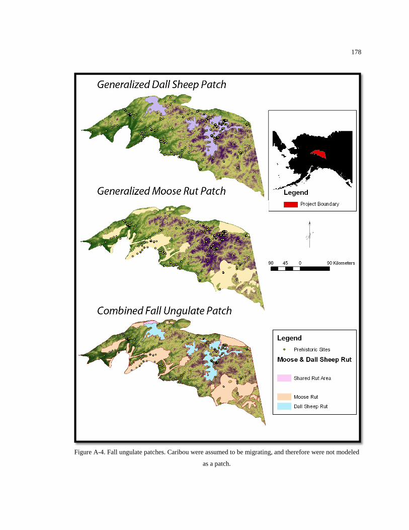
178

Figure A-4. Fall ungulate patches. Caribou were assumed to be migrating, and therefore were not modeled

as a patch.

179

Figure A-5 Ungulate winter patches.

180

Table A-1 Diet Breadth model for the YTU

Rank Season Resource Caloric Mean Data Source 1 Spring Caribou 11950 Winterhalder 1977,1981 1 Spring Moose 11950 Winterhalder 1977,1981 2 Spring Fish 6430 Winterhalder 1977,1981 3 Spring Beaver 3460 Winterhalder 1977,1981 4 Spring Hare 1900 Winterhalder 1977,1981 5 Spring Muskrat 1375 Winterhalder 1977,1981 6 Spring Waterfowl 720 Winterhalder 1977,1981 1 Summer Muskrat 3825 Winterhalder 1977,1981 2 Summer Fish 3790 Winterhalder 1977,1981 3 Summer Beaver 3460 Winterhalder 1977,1981 4 Summer Waterfowl 1980 Winterhalder 1977,1981 5 Summer Hare 1900 Winterhalder 1977,1981 6 Summer Blueberries 250 Winterhalder 1977,1981 1 Fall Caribou 11280 Winterhalder 1977,1981 1 Fall Moose 11280 Winterhalder 1977,1981 1 Fall Sheep 11280 (Ranked equal to deer; Zeanah, et al., 1995) 2 Fall Muskrat 3825 Winterhalder 1977,1981 3 Fall Beaver 3460 Winterhalder 1977,1981 4 Fall Hare 1900 Winterhalder 1977,1981 1 Winter Caribou 6050 Winterhalder 1977,1981 1 Winter Moose 6050 Winterhalder 1977,1981 1 Winter Sheep 6050 (Ranked equal to deer; Zeanah, et al., 1995) 2 Winter Hare 1900 Winterhalder 1977,1981

Table A-2 Statistic results for each season

Spring Summer Fall Winter Mann-Whitney U 236938.5 297576.5 305490.5 329876.5 Z -9.517 -4.25 -3.496 -1.361 Asymp. Sig. (2-tailed) 0.0 0.0 0.0 0.173

181

Table A-3 GIS data sets and sources used

Dataset Source Scale Source Location

Digital Elevation Models

Alaska Geospatial Data Clearinghouse 15 Minute

http://agdc.usgs.gov/data/usgs/geodata/dem/63K/demlist_A.html

Digital Raster Graphics-tif

Alaska Geospatial Data Clearinghouse 1:250,000

http://agdc.usgs.gov/data/usgs/geodata/drg/temp/drglist_A.html

Digital Raster Graphics-tfw



Vegetation Class

Alaska Geospatial Data Clearinghouse

1 km resolution http://agdc.usgs.gov/data/projects/hlct/hlct.html#K

Slope



Hydraulic Regions



Anadromous Waters

Alaska Department of Fish and Game

http://www.sf.adfg.state.ak.us/SARR/AWC/index.cfm/FA/data.GISData

hydrography


http://agdc.usgs.gov/data/usgs/geodata/dlg/63K/hydrography_B.html





http://agdc.usgs.gov/data/projects/hlct/hlct.html#K

http://agdc.usgs.gov/data/projects/hlct/hlct.html#K





182

Table A-4 Site location occurrences within calculated seasonal weighted patches

Season

Patch Probability Rank

Percent of Sites

Percent of Random Points

Cumulative % of Sites

Cumulative % of Random Points

Spring

Low 8.78 20.38 8.78 20.38 Med/Low 11.61 21.44 20.4 41.82 Med 24.65 23.19 45.04 65.01 Med/High 17.28 18.57 62.32 83.58 High 37.68 25.4 100 100

Summer


Fall

Low 34.56 31.43 34.56 31.43 Med/Low 7.93 17.87 42.49 49.3 Med 18.41 23.64 60.91 72.94 Med/High 37 10.54 71.39 83.48 High 28.61 16.52 100 100

Winter


183

Appendix B

Data summaries for site assemblages

Table B-1 Bachelor Creek raw material type by stratigraphic level

Raw Material

Depth

Total Surface

Layer 1: Root/

Vegetation Mat

Layer 2: Brown Loess

Layer 3: Gray Loess

Dark Gray Diorite 63 12 8 0 83 Clear/Black Mottled Chalcedony 57 6 9 8 80 Dark Gray Chert 32 7 1 1 41 Red Diorite 16 13 2 0 31 Gray Diorite 21 0 0 0 21 White/Gray Mottled Chalcedony 20 0 0 0 20 Quartz 17 0 0 0 17 Batza Tena Obsidian 8 8 0 0 16 Gray Siltstone 7 0 0 1 8 White Siltstone 6 0 0 0 6 Greenish Gray Siltstone 2 0 1 0 3 Gray/Dark Gray Chalcedony 2 0 0 0 2 White Chert 2 0 0 0 2 Rhyolite 1 0 0 0 1 Red Siltstone 0 0 0 1 1 Greenish Gray Chert 0 0 1 0 1 Light Gray Chert 1 0 0 0 1 Translucent Gray Chert 0 0 0 1 1 Red Chert 1 0 0 0 1 Total 256 46 22 12 336

Table B-2 Bachelor Creek artifact types by stratigraphic level

Artifact

Depth

Total Surface Layer 1: Root/ Vegetation

Mat Layer 2: Brown

Loess

Layer 3: Gray Loess

Flakes 234 45 21 12 312 Microblades 8 1 1 0 10 Bifaces 7 0 0 0 7 Modified Flakes 7 0 0 0 7 Total 256 46 22 12 336

184

Table B-3 Bachelor Creek lithic raw material summaries

Hypothetical Placement Material Type

Total n Total wt. n% wt.%

Debitage wt. Tool wt.

Local Dark Gray Diorite 83 38.2 24.7 34.1 5.6 Local Gray Diorite 21 12.8 6.3 11.4 44.6 0.6 Local Red Diorite 31 7.9 9.2 7.0 7.9 Local Quartz 17 7.0 5.1 6.2 5.4 1.6

Nonlocal

Clear/Black Mottled Chalcedony 80 18.2 23.8 16.3 15.8 2.4

Nonlocal* Dark Gray Chert 43 17.2 12.8 15.4 6.8 10.4 Nonlocal* White Siltstone 6 2.6 1.8 2.3 2.5 0.1

Nonlocal Batza Tena Obsidian 16 2.5 4.8 2.3 1.1 1.4

Nonlocal*

White/Gray Mottled Chalcedony 20 2.2 6.0 2.0 2.2

Nonlocal* Gray Siltstone 8 1.6 2.4 1.4 1.6

Nonlocal* Green-Gray Siltstone 3 0.8 0.9 0.7 0.5 0.4

Nonlocal* White Chert 2 0.4 0.6 0.3 0.1 0.3 Nonlocal* Rhyolite 1 0.3 0.3 0.3 0.3 Nonlocal* Light Gray Chert 1 0.1 0.3 0.1 0.1 Nonlocal* Red Chert 1 0.1 0.3 0.1 0.1 Nonlocal* Green-Gray Chert 1 0.1 0.3 0.1 0.1 Nonlocal* Red Siltstone 1 0.03 0.3 0.03 0.03

Nonlocal* Translucent Gray Chert 1 0.02 0.3 0.02 0.02

*hypothetical placement

185

Table B-4 Bachelor Creek Sullivan and Rosen summary

Raw material

Sullivan and Rozen Typology

Total Complete

Flake Broken Flake

Split Flake

Flake Fragment

Debris/ Shatter

Dark Gray Diorite 30 43 7 2 0 82 Clear/Black Mottled Chalcedony

45 22 2 5 0 74

Dark Gray Chert 18 15 1 2 0 36 Red Diorite 11 13 3 4 0 31 Gray Diorite 7 10 3 1 0 21 White/Gray Mottled Chalcedony

9 8 1 2 0 20

Quartz 9 4 0 1 1 15 Batza Tena Obsidian 4 5 1 1 0 11 Gray Siltstone 2 4 1 1 0 8 White Siltstone 3 2 0 0 0 5 Rhyolite 0 0 0 0 1 1 Greenish Gray Siltstone 1 0 0 0 0 1 Red Siltstone 1 0 0 0 0 1 Gray/Dark Gray Chalcedony

1 0 0 0 0 1

Greenish Gray Chert 0 0 1 0 0 1 Light Gray Chert 1 0 0 0 0 1 Translucent Gray Chert 1 0 0 0 0 1 Red Chert 1 0 0 0 0 1 White Chert 0 0 1 0 0 1 Total 144 126 21 19 2 312

186

Table B-5 Bachelor Creek White cortex summary

Raw Material Flake Type

Total Primary Secondary Tertiary Dark Gray Diorite 0 0 82 82 Clear/Black Mottled Chalcedony 0 1 73 74 Dark Gray Chert 1 1 34 36 Red Diorite 0 0 31 31 Gray Diorite 0 1 20 21 White/Gray Mottled Chalcedony 0 0 20 20 Quartz 1 0 14 15 Batza Tena Obsidian 0 1 10 11 Gray Siltstone 0 1 7 8 White Siltstone 0 0 5 5 Rhyolite 0 1 0 1 Greenish Gray Siltstone 0 0 1 1 Red Siltstone 0 0 1 1 Gray/Dark Gray Chalcedony 0 0 1 1 Greenish Gray Chert 0 0 1 1 Light Gray Chert 0 0 1 1 Translucent Gray Chert 0 0 1 1 Red Chert 0 0 1 1 White Chert 0 0 1 1 Total 2 6 304 312

Table B-6 Bachelor Creek cortex type summary

Artifact Cortex Type

Total None Rough Smooth Flakes 304 4 4 312 Microblades 10 0 0 10 Bifaces 6 0 1 7 Modified Flakes 7 0 0 7 Total 327 4 5 336

Table B-7 Bachelor Creek artifact type by size class

Artifact Size Class

Total 1 2 3 4 5 6 7 Microblades 0 3 6 0 1 0 0 10 Flakes 36 144 92 22 14 3 1 312 Total 36 147 98 22 15 3 1 322

187

Table B-8 Bachelor Creek microblade platform type and segment by size class

Microblade Size Class

Total 2 3 5 Platform Type Faceted 1 1 0 2

Flat 1 2 1 4 Total 2 3 1 6 Portion Complete 0 1 1 2

Medial 1 3 0 4 Proximal 2 2 0 4

Total 3 6 1 10

Table B-9 Bachelor Creek debitage material types associated reduction strategies by platform type

Reduction Strategy Raw material

Platform Type

Total Complex Crushed Dihedral Faceted Fla

t Sheared Biface and Microblade strategies

Clear/Black Mottled Chalcedony

1 1 5 19 26 17 69

Dark Gray Chert

0 0 2 12 16 4 34

Total 1 1 7 31 42 21 103 Microblade strategies only

Batza Tena Obsidian

0 1 0 4 3 2 10

White Siltstone

0 0 0 1 3 1 5

Greenish Gray Siltstone

0 0 0 1 0 0 1

Total 0 1 0 6 6 3 16 Other debitage

Dark Gray Diorite

1 1 5 27 43 3 80

Red Diorite 0 0 0 5 23 1 29 Gray Diorite 1 0 2 5 10 2 20 White/Gray Mottled Chalcedony

0 2 2 7 7 0 18

Quartz 0 4 1 1 5 3 14 Gray Siltstone

1 0 0 3 3 0 7

Rhyolite 0 0 0 0 1 0 1 Red Siltstone 0 0 0 0 1 0 1 Gray/Dark Gray Chalcedony

0 0 0 0 1 0 1

Greenish Gray Chert

0 0 0 0 1 0 1

Light Gray Chert

0 0 0 1 0 0 1

188

Translucent Gray Chert

0 0 0 0 0 1 1

Red Chert 0 0 0 0 1 0 1 White Chert 1 0 0 0 0 0 1 Total 4 7 10 49 96 10 176

Table B-10 Bachelor Creek debitage material types associated with reduction strategies by dorsal scars

Reduction Strategy Raw Material <3 dorsal

scars >=3 dorsal

scars Total % Total Biface and Microblade strategies


31 46 77

66.4 Dark Gray Chert 12 27 39 33.6 Total 43 73 116 100

Microblade strategies only

Batza Tena Obsidian

4 12 16 64

White Siltstone 1 5 6 24 Greenish Gray Siltstone

0 3 3 12

Total 5 20 25 100 Other debitage Dark Gray Diorite 43 39 82 43.6

Red Diorite 17 14 31 16.5 Gray Diorite 10 11 21 11.2 White/Gray Mottled Chalcedony

7 13 20 10.6

Quartz 9 8 17 9 Gray Siltstone 1 7 8 4.3 White Chert 0 2 2 1.1 Rhyolite 1 0 1 0.5 Red Siltstone 1 0 1 0.5 Gray/Dark Gray Chalcedony

0 1 1 0.5

Greenish Gray Chert

0 1 1 0.5

Light Gray Chert 0 1 1 0.5 Translucent Gray Chert

1 0 1 0.5

Red Chert 0 1 1 0.5 Total 90 98 188 100

189

Table B-11 Bachelor Creek artifact type by raw material type

Raw Materials

Artifact Type

Total Bifaces Microblades Modified

Flakes Flakes Dark Gray Diorite 1 0 0 82 83 Clear/Black Mottled Chalcedony 3 1 2 74 80 Dark Gray Chert 2 2 1 36 41 Red Diorite 0 0 0 31 31 Gray Diorite 0 0 0 21 21 White/Gray Mottled Chalcedony 0 0 0 20 20 Quartz 0 0 2 15 17 Batza Tena Obsidian 0 5 0 11 16 Gray Siltstone 0 0 0 8 8 White Siltstone 0 1 0 5 6 Greenish Gray Siltstone 0 1 1 1 3 Gray/Dark Gray Chalcedony 1 0 0 1 2 White Chert 0 0 1 1 2 Rhyolite 0 0 0 1 1 Red Siltstone 0 0 0 1 1 Greenish Gray Chert 0 0 0 1 1 Light Gray Chert 0 0 0 1 1 Translucent Gray Chert 0 0 0 1 1 Red Chert 0 0 0 1 1 Total 7 10 7 312 336

Table B-12 Big Bend artifact summary by stratigraphic depth

Artifact

Depth

Total

Layer 1:

Surface Layer 2:

Brown Loess Layer 3: Gray

Loess Feature 1: Ashy Loess

(Hearth?) Flakes 558 585 449 97 1689 Modified Flakes 14 2 7 0 23 Microblades 3 7 8 3 21 Flake Cores 13 1 0 2 16 Bifaces 7 2 0 0 9 Tchi-Tho 1 0 0 0 1 Total 596 597 464 102 1759

190

Table B-13 Big Bend raw material summary by stratigraphic depth

Depth

Total

Layer 1:

Surface


Layer 3: Gray Loess

Feature 1: Ashy Loess (Hearth?)

Dark Gray Diorite 455 388 182 39 1064 Gray Diorite 42 101 96 25 264 Red Diorite 21 61 84 0 166 Clear/Black Mottled Chalcedony 28 14 13 1 56 Greenish Gray Siltstone 1 5 37 11 54 White/Gray Mottled Chalcedony 26 2 2 0 30 Dark Gray Chert 3 6 14 4 27 Yellow Chert 0 0 11 12 23 Quartz 15 3 0 1 19 Pale Brown Chert 0 8 6 5 19 Grayish Brown Siltstone 0 3 12 2 17 Gray Siltstone 0 3 5 0 8 Gray/Dark Gray Chalcedony 1 0 1 2 4 White/Black Mottled Chalcedony 3 0 0 0 3 Light Gray Chert 0 2 0 0 2 Batza Tena Obsidian 0 1 1 0 2 White Siltstone 1 0 0 0 1 Total 596 597 464 102 1759

Table B-14 Big Bend lithic raw material summaries

Strati-graphic Position

Hypo-thetical Placement

Material Type

Total n Total wt. n% wt.%

Core wt.

Debitage wt.

Tool wt.

Layer 1: Surface Local

Dark Gray Diorite 455

10947.55

76.34 89.7 6408 2196.6

2342.95

Local Gray Diorite 42 895.88 7.05 7.34 0.62 247.19 648.07

Nonlocal*

White/Gray Mottled Chalcedony 26 274.47 4.36 2.25

265.6 6.98 1.89

Local Red Diorite 21 59.26 3.52 0.49 59.26

Nonlocal

Clear/Black Mottled Chalcedony 28 16.27 4.7 0.13 0.27 11.81 4.19

Local Quartz 15 6.03 2.52 0.05 6.03

Nonlocal*

White/Black Mottled Chalcedony 3 2.72 0.5 0.02 2.34 0.38

Nonlocal*

Gray/Black Mottled Chalcedony 1 2.39 0.17 0.02 2.39

191

Nonlocal* Dark Gray Chert 3 0.23 0.5 0.002 0.23

Nonlocal* Gray Siltstone 1 0.09 0.17 0.001 0.09

Nonlocal* White Siltstone 1 0.02 0.17

0.0002 0.02


Local Dark Gray Diorite 388 525.04

64.99 72.23 7.87 513.58 3.59

Local Gray Diorite 101 105.88 16.9

2 14.56 105.88

Local Red Diorite 62 72.84 10.3

9 10.02 72.84

Nonlocal* Dark Gray Chert 6 15.65 1.01 2.15 0.11 15.54

Nonlocal* Brown Chert 8 1.63 1.34 0.22 1.63

Nonlocal* Light Gray Chert 2 1.54 0.34 0.21 1.54

Nonlocal*


Nonlocal

Clear/Black Mottled Chalcedony 14 1.47 2.35 0.2 3

Nonlocal* Gray Siltstone 3 0.63 0.5 0.09 0.02 0.61

Nonlocal* Green Gray Siltstone 5 0.32 0.84 0.04 0.17 0.15

Nonlocal* Brown Siltstone 3 0.23 0.5 0.03 0.21 0.02

Nonlocal Quartz 2 0.13 0.34 0.02 0.13

Nonlocal Batza Tena Obsidian 1 0.06 0.17 0.01 0.06

Layer 3: Gray Loess


39.22 70.91 466.32 411.88


9 20.33 117.96 133.8 Local Red Diorite 84 88.48 18.1 7.14 87.98 0.5

Nonlocal* Brown Siltstone 12 5.72 2.59 0.46 5.72

Nonlocal* Green Gray Siltstone 37 3.45 7.97 0.28 3.14 0.31

Nonlocal Clear/Black Chalcedony 13 2.66 2.8 0.21 2.66

Nonlocal* Yellow Chert 11 2.29 2.37 0.18 2.1 0.19

Nonlocal*


Nonlocal Batza Tena Obsidian 1 1.8 0.22 0.15 1.8

Nonlocal* Dark Gray Chert 14 1.21 3.02 0.1 1.21

192

Nonlocal*

Light Gray/Dark Gray Mottled Chalcedony 1 0.36 0.22 0.03 0.36

Nonlocal* Brown Chert 6 0.33 1.29 0.03 1.47 0.07

Nonlocal* Gray Siltstone 5 0.26 1.08 0.02 0.11 0.15

Layer 4:Hearth


38.24 58.57 68.68


1 29.41 34.49

Nonlocal* Yellow Chert 12 6.86

11.76 5.85 0.84 5.75 0.44

Nonlocal* Brown Chert 5 3.98 4.9 3.39 3.68 0.3

Nonlocal* Dark Gray Chert 4 1.27 3.92 1.08 1.11 0.16

Nonlocal* Green Gray Siltstone 11 0.73

10.78 0.62 0.73

Nonlocal* Brown Siltstone 2 0.73 1.96 0.62 0.73

Nonlocal*

Light Gray/Dark Gray Mottled Chalcedony 2 0.31 1.96 0.26 0.31

Nonlocal

Clear/Black Mottled Chalcedony 1 0.14 0.98 0.12 0.14

Local Quartz 1 0.07 0.98 0.06 0.07 *hypothetical placement

Table B-15 Big Bend Sullivan and Rosen summary

Level Raw Material

SRT

Total Complete Flake

Broken Flake

Split Flake

Flake Fragment

Surface Dark Gray Diorite 189 162 81 10 442 Gray Diorite 15 17 8 1 41

White/Gray Mottled Chalcedony 7 7 2 8 24

Clear/Black Mottled Chalcedony 14 10 0 0 24

Red Diorite 8 7 6 0 21 Quartz 5 6 3 1 15

White/Black Mottled Chalcedony 0 2 0 1 3

Dark Gray Chert 1 2 0 0 3

193

White Siltstone 0 1 0 0 1

Greenish Gray Siltstone 0 1 0 0 1

Gray/Dark Gray Chalcedony 0 0 1 0 1

Level 2 Dark Gray Diorite 185 124 44 31 384 Gray Diorite 37 43 16 5 101 Red Diorite 34 16 8 3 61


Pale Brown Chert 4 2 2 0 8 Dark Gray Chert 2 0 1 1 4 Quartz 2 1 0 0 3

Grayish Brown Siltstone 0 0 1 1 2



Light Gray Chert 1 0 1 0 2

Batza Tena Obsidian 0 1 0 0 1

Gray Siltstone 1 0 0 0 1 Level 3 Dark Gray Diorite 92 54 17 13 176 Gray Diorite 70 19 6 0 95 Red Diorite 30 35 10 8 83


Dark Gray Chert 11 2 1 0 14



Yellow Chert 3 3 1 2 9 Pale Brown Chert 2 3 0 0 5 Gray Siltstone 2 0 0 1 3


Batza Tena Obsidian 0 1 0 0 1


Hearth Dark Gray Diorite 22 12 4 1 39 Gray Diorite 14 6 3 2 25


194

Yellow Chert 2 3 2 2 9 Pale Brown Chert 4 0 0 0 4 Dark Gray Chert 1 1 0 1 3



Quartz 0 1 0 0 1


Table B-16 Big Bend White cortex summary

Level Raw Material Flake Type

Total Primary Secondary Tertiary Surface Dark Gray Diorite 14 20 408 442 Gray Diorite 2 3 36 41

White/Gray Mottled Chalcedony 0 0 24 24

Clear/Black Mottled Chalcedony 0 0 24 24

Red Diorite 0 1 20 21 Quartz 0 1 14 15

White/Black Mottled Chalcedony 0 0 3 3

Dark Gray Chert 0 0 3 3 White Siltstone 0 0 1 1

Greenish Gray Siltstone 0 0 1 1

Gray/Dark Gray Chalcedony 0 0 1 1

Total 16 25 535 576 Level 2 Dark Gray Diorite 2 3 379 384 Gray Diorite 0 0 101 101 Red Diorite 0 0 61 61


Pale Brown Chert 0 0 8 8 Dark Gray Chert 0 0 4 4 Quartz 1 0 2 3

Grayish Brown Siltstone 0 0 2 2



Light Gray Chert 0 0 2 2 Batza Tena Obsidian 0 0 1 1

195

Gray Siltstone 0 0 1 1 Total 3 3 579 585 Level 3 Dark Gray Diorite 2 1 173 176 Gray Diorite 2 0 93 95 Red Diorite 2 0 81 83


Dark Gray Chert 0 0 14 14



Yellow Chert 0 0 9 9 Pale Brown Chert 0 0 5 5 Gray Siltstone 0 0 3 3


Batza Tena Obsidian 0 0 1 1


Total 7 1 440 448 Hearth Dark Gray Diorite 0 1 38 39 Gray Diorite 3 2 20 25


Yellow Chert 0 0 9 9 Pale Brown Chert 0 0 4 4 Dark Gray Chert 0 0 3 3



Quartz 0 0 1 1


Total 3 3 91 97

Table B-17 Big Bend cortex type summary

Level Raw Material Cortex Type

Total None Rough Smooth Surface Dark Gray Diorite 420 31 4 455 Gray Diorite 37 4 1 42



Red Diorite 20 0 1 21 Quartz 14 1 0 15

196

White/Black Mottled Chalcedony 3 0 0 3

Dark Gray Chert 3 0 0 3 White Siltstone 1 0 0 1



Total 554 36 6 596 Level 2 Quartz 3 0 0 3 Dark Gray Diorite 380 1 3 384 Gray Diorite 101 0 0 101 Red Diorite 61 0 0 61 Batza Tena Obsidian 1 0 0 1



Gray Siltstone 1 0 0 1



Pale Brown Chert 8 0 0 8 Dark Gray Chert 4 0 0 4 Light Gray Chert 2 0 0 2 Total 581 1 3 585 Level 3 Dark Gray Diorite 175 2 0 177 Gray Diorite 94 0 1 95 Red Diorite 82 0 1 83


Dark Gray Chert 14 0 0 14



Yellow Chert 9 0 0 9 Pale Brown Chert 5 0 0 5 Gray Siltstone 3 0 0 3


Batza Tena Obsidian 1 0 0 1


Total 444 3 2 449 Hearth Dark Gray Diorite 38 1 0 39 Gray Diorite 20 0 5 25 Greenish Gray 11 0 0 11

197

Siltstone Yellow Chert 9 0 0 9 Pale Brown Chert 4 0 0 4 Dark Gray Chert 3 0 0 3



Quartz 1 0 0 1


Total 91 1 5 97

Table B-18 Big Bend microblade depth and size class summary

Level Section Microblade Size Class

Total 2 3 4 5 Surface Proximal 0 1 1 1 3 Total 0 1 1 1 3 Level 2 Distal 1 0 0 0 1 Medial 1 1 0 0 2 Proximal 3 1 0 0 4 Total 5 2 0 0 7 Level 3 Complete 0 0 0 1 1 Medial 1 1 1 0 3 Proximal 2 0 1 0 3 Total 3 1 2 1 7 Hearth Complete 0 0 0 1 1 Medial 0 1 0 0 1 Proximal 1 0 0 0 1 Total 1 1 0 1 3

198

Table B-19 Big Bend artifact type by raw material type

Level Artifact Size Class (>SC10 excluded) Tota

l 1 2 3 4 5 6 7 8 9 10

Surface Micro-blade 0 0 1 1 1 0 0 0 0 0 3

Flake 2 95 128 95 75 38 30 31 14 10 518 Total 2 95 129 96 76 38 30 31 14 10 521

Level 2 Micro-blade 0 5 2 0 0 0 0 0 0 0 7

Flake 8 161 166 97 72 35 25 5 8 2 579 Total 8 166 168 97 72 35 25 5 8 2 586

Level 3 Micro-blade 0 3 1 2 1 0 0 0 0 0 7

Flake 18 174 127 51 29 12 8 10 7 3 449 Total 18 177 128 53 30 12 8 10 7 3 456

Hearth Micro-blade 0 1 1 0 1 0 0 0 0 0 3

Flake 2 33 30 12 6 6 3 4 0 0 96 Total 2 34 31 12 7 6 3 4 0 0 100

Table B-20 big Bend debitage platform type

Level Raw Material Platform Type

Total Complex Crushed Dihedral Faceted Flat Sheared Surface Quartz 0 1 0 4 7 1 13 Dark Gray Diorite 1 2 3 97 305 8 416 Gray Diorite 0 1 0 6 30 0 37 Red Diorite 0 0 0 6 13 1 20 White Siltstone 0 0 0 1 0 0 1

Greenish Gray Siltstone 0 0 0 0 1 0 1

Gray/Dark Gray Chalcedony 0 0 0 0 1 0 1

Clear/Black Mottled Chalcedony 0 0 1 5 11 7 24

Dark Gray Chert 0 0 0 1 1 1 3 Total 1 4 4 120 369 18 516 Level 2 Quartz 0 0 0 1 2 0 3 Dark Gray Diorite 0 7 3 67 274 4 355 Gray Diorite 0 0 3 18 75 0 96 Red Diorite 0 0 2 7 49 0 58 Batza Tena Obsidian 0 0 0 0 1 0 1

White/Gray Mottled Chalcedony 0 0 0 0 0 1 1


Pale Brown Chert 0 0 0 2 5 1 8 Light Gray Chert 0 0 0 0 2 0 2

199

Total 0 7 8 98 418 6 537 Level 3 Dark Gray Diorite 0 1 1 38 123 2 165 Gray Diorite 0 0 1 18 73 3 95 Red Diorite 0 1 1 9 64 0 75 Batza Tena Obsidian 0 0 0 1 0 0 1

Grayish Brown Siltstone 0 1 0 5 6 0 12

White/Gray Mottled Chalcedony 0 0 0 0 2 0 2



Dark Gray Chert 0 0 0 1 13 0 14 Total 0 3 3 75 290 6 377 Hearth Dark Gray Diorite 1 0 0 8 29 0 38 Gray Diorite 0 0 0 5 18 0 23

Greenish Gray Siltstone 0 0 0 3 8 0 11

Pale Brown Chert 0 0 0 1 3 0 4

Grayish Brown Siltstone 2 0 0 0 0 0 2


Quartz 0 0 0 0 1 0 1


Total 3 0 0 17 62 0 82

Table B-21 Big Bend debitage reduction strategies by dorsal scars

Reduction Strategy Level Raw Material

Dorsal Scars

Total <3 dorsal scars

>=3 dorsal scars

Biface and microblade

Surface White/Gray Mottled Chalcedony 12 10 22 Total 12 10 22

Level 2 Dark Gray Chert 4 0 4 Total 4 0 4

Microblade Surface White/Black Mottled Chalcedony 0 2 2 Total 0 2 2

Level 2 Grayish Brown Siltstone 2 0 2 Greenish Gray Siltstone 2 0 2 Gray Siltstone 1 0 1 Total 5 0 5

Level 3 Greenish Gray 22 12 34

200

Siltstone Gray Siltstone 2 1 3 Pale Brown Chert 2 3 5 Yellow Chert 5 4 9 Total 31 20 51

Hearth Yellow Chert 1 8 9 Dark Gray Chert 1 2 3 Total 2 10 12

Other Surface Dark Gray Diorite 255 175 430 Gray Diorite 25 13 38 Clear/Black Mottled Chalcedony 2 22 24 Red Diorite 14 7 21 Quartz 10 4 14 Dark Gray Chert 0 3 3 White Siltstone 0 1 1 Greenish Gray Siltstone 0 1 1 Gray/Dark Gray Chalcedony 0 1 1 Total 306 227 533

Level 2 Dark Gray Diorite 253 129 382 Gray Diorite 76 25 101 Red Diorite 48 13 61 Clear/Black Mottled Chalcedony 8 6 14 Pale Brown Chert 5 3 8 Quartz 3 0 3 White/Gray Mottled Chalcedony 0 2 2 Light Gray Chert 0 2 2 Batza Tena Obsidian 1 0 1 Total 394 180 574

Level 3 Dark Gray Diorite 137 39 176 Gray Diorite 65 30 95 Red Diorite 51 32 83 Batza Tena Obsidian 0 1 1 Grayish Brown Siltstone 6 6 12 White/Gray Mottled Chalcedony 0 2 2 Gray/Dark Gray Chalcedony 1 0 1 Clear/Black Mottled Chalcedony 4 9 13 Dark Gray Chert 7 7 14 Total 271 126 397

Hearth Dark Gray Diorite 30 9 39

201

Gray Diorite 18 7 25 Greenish Gray Siltstone 7 4 11 Pale Brown Chert 3 1 4 Grayish Brown Siltstone 0 2 2 Gray/Dark Gray Chalcedony 1 1 2 Quartz 1 0 1 Clear/Black Mottled Chalcedony 0 1 1 Total 60 25 85

Table B-22 Cripple Creek artifact type by stratigraphic level

Stratigraphic Layer

Artifact Type

Total Biface Micro-

blade Modified

Flake Flake Flake Core

Micro-blade Core Tab

Layer 23, 21, & 20: Root/Vegetation Mat 0 1 0 6 0 0 7

Layer 17: Feature 3: Midden/Hearth 0 0 0 43 1 0 44

Layer 11: Brown Loess 1 0 2 54 1 1 59 Layer 9: Feature 2: Hearth 0 0 0 1 1 0 2 Layer 7: Burnt Loess (Beneath Feature 2) 0 0 0 2 0 0 2

Layer 6: Orange/Gray Mottled Loess 1 3 0 64 3 0 71

Layer 2: Gray Loess 3 0 2 58 1 0 64 Total 5 4 4 228 7 1 249

202

Table B-23 Cripple Creek raw material summaries

Hypothetical Type Material Type

Total n

Total wt. n% wt.%

Core wt.

Debitage wt.

Tool wt.

Local Quartz 125 291.2

3 50.20 51.88 240.8

7 50.21 0.15

Local Mica-Schist 2 162.5

2 0.80 28.95 13.42 149.1

Nonlocal* Dark Gray Chert 9 40.33

5 3.61 7.18 2.34 37.99

5 Nonlocal* Shale 2 20.21 0.80 3.60 0.02 20.19 Nonlocal Batza Tena Obsidian 16 14.27 6.43 2.54 11.83 1.36 1.08 Nonlocal* Yellow Chert 1 12.6 0.40 2.24 12.6 Nonlocal* Granite 2 5.39 0.80 0.96 0.45 4.94 Nonlocal* Green-Gray Chert 13 4.305 5.22 0.77 0.28 3.51 0.515 Nonlocal* Light Gray Chert 3 4.2 1.20 0.75 0.365 3.835 Nonlocal* Green-Gray Siltstone 52 2.95 20.88 0.53 2.63 0.32 Nonlocal* Gray Siltstone 5 0.63 2.01 0.11 0.18 0.45 Nonlocal* Red Chert 3 0.37 1.20 0.07 0.23 0.14

Nonlocal Clear/Black Mottled Chalcedony 7 0.32 2.81 0.06 0.31 0.01

Nonlocal* Gray/Dark Gray Chalcedony 1 0.14 0.40 0.02 0.14

Nonlocal* White/Gray Mottled Chalcedony 1 0.09 0.40 0.02 0.09

Nonlocal* Basalt 7 1.83 2.81 0.33 1.83 *hypothetical placement

203

Table B-24 Cripple Creek artifact type by raw material type

Raw Material Artifact Type

Total Biface Micro-

blade Modified

Flake Flake Flake Core

Microblade Core Tab

Quartz 0 0 0 121 4 0 125 Greenish Gray Siltstone 1 0 1 50 0 0 52

Batza Tena Obsidian 0 0 1 13 2 0 16

Greenish Gray Chert 0 1 0 11 1 0 13

Dark Gray Chert 2 1 0 6 0 0 9 Basalt 0 0 0 7 0 0 7 Clear/Black Mottled Chalcedony

0 0 0 7 0 0 7

Gray Siltstone 0 1 0 4 0 0 5 Light Gray Chert 1 0 0 2 0 0 3

Red Chert 0 1 0 2 0 0 3 Granite 0 0 1 1 0 0 2 Mica-Schist 0 0 1 1 0 0 2 Shale 1 0 0 1 0 0 2 Gray/Dark Gray Chalcedony 0 0 0 1 0 0 1

White/Black Mottled Chalcedony

0 0 0 1 0 0 1

Yellow Chert 0 0 0 0 0 1 1 Total 5 4 4 228 7 1 249

204

Table B-25 Cripple Creek Sullivan and Rosen summary

Raw Material SRT


Broken Flake

Split Flake

Flake Fragment

Quartz 87 15 19 0 121 Greenish Gray Siltstone 31 9 4 6 50 Batza Tena Obsidian 11 2 0 0 13 Greenish Gray Chert 8 1 2 0 11 Basalt 6 0 1 0 7 Clear/Black Mottled Chalcedony 4 2 1 0 7 Dark Gray Chert 2 2 1 1 6 Gray Siltstone 1 1 0 2 4 Light Gray Chert 1 1 0 0 2 Red Chert 0 1 0 1 2 Granite 0 1 0 0 1 Mica-Schist 1 0 0 0 1 Shale 1 0 0 0 1 Gray/Dark Gray Chalcedony 1 0 0 0 1 White/Black Mottled Chalcedony 0 0 0 1 1 Total 154 35 28 11 228

Table B-26 Cripple Creek White cortex summary


Total Primary Secondary Tertiary

Quartz 2 0 119 121 Greenish Gray Siltstone 0 1 49 50 Batza Tena Obsidian 0 3 10 13 Greenish Gray Chert 0 0 11 11 Basalt 0 0 7 7 Clear/Black Mottled Chalcedony 0 0 7 7 Dark Gray Chert 0 0 6 6 Gray Siltstone 0 0 4 4 Light Gray Chert 0 0 2 2 Red Chert 0 1 1 2 Granite 0 0 1 1 Mica-Schist 0 0 1 1 Shale 0 0 1 1 Gray/Dark Gray Chalcedony 0 0 1 1 White/Black Mottled Chalcedony 0 0 1 1 Total 2 5 221 228

205

Table B-27 Cripple Creek artifact type size classes

Size Class Artifact Type

Total Microblade Modified Flake Flake 1 0 0 12 12 2 2 0 135 137 3 1 1 43 45 4 1 0 25 26 5 0 0 9 9 6 0 2 1 3 7 0 0 1 1 8 0 0 1 1

12 0 0 1 1 26 0 1 0 1

Total 4 4 228 236

Table B-28 Cripple Creek microblade portion summary

Raw Material Microblade Portion

Total Proximal

Gray Siltstone 1 1 Dark Gray Chert 1 1 Greenish Gray Chert 1 1 Red Chert 1 1 Total 4 4

Table B-29 Cripple Creek microblade platform type and size class summary

Microblade Platform Type

Size Class Total 2 3 4

Faceted 1 0 1 2 Flat 1 1 0 2 Total 2 1 1 4

Table B-30 Cripple Creek microblade depth summary

Stratigraphic Layer Microblade Size Class

Total 2 3 4

Layer 23, 21, & 20: Root/Vegetation Mat 1 0 0 1 Layer 6: Orange/Gray Mottled Loess 1 1 1 3 Total 2 1 1 4

206

Table B-31 Cripple Creek cortex type summary

Artifact Type Cortex Type

Total None Rough Smooth

Flake 221 3 4 228 Flake Core 3 3 1 7 Biface 2 3 0 5 Microblade 4 0 0 4 Modified Flake 2 1 1 4 Microblade Core Tab 1 0 0 1 Total 233 10 6 249

Table B-32 Cripple Creek debitage raw material types and reduction strategy summary by platform type

Reduction Strategy Raw Material

Platform Type Total Crushed Dihedral Faceted Flat Sheared

Microblade Greenish Gray Chert

0 0 3 9 0 12

Gray Siltstone 0 0 2 1 0 3 Red Chert 0 0 1 1 0 2 Total 0 0 6 11 0 17

Biface and Microblade

Dark Gray Chert

0 0 2 2 1 5

Other Quartz 5 0 9 105 2 121 Greenish Gray Siltstone

1 0 7 33 4 45

Batza Tena Obsidian

0 1 6 7 0 14

Basalt 0 0 0 7 0 7 Clear/Black Mottled Chalcedony

0 0 1 5 1 7

Granite 0 0 0 2 0 2 Mica-Schist 1 0 1 0 0 2 Light Gray Chert

0 0 2 0 0 2

Shale 0 0 0 1 0 1 Gray/Dark Gray Chalcedony

0 0 0 1 0 1

Total 7 1 26 161 7 202

207

Table B-33 Cripple Creek debitage raw material types and reduction strategy summary by dorsal scars


Dorsal Scars Total <3 >=3

Microblade Greenish Gray Chert 3 9 12 Gray Siltstone 3 2 5 Red Chert 2 1 3 Total 8 12 20

Biface and Microblade

Dark Gray Chert 3 3 6

Other Quartz 83 38 121 Greenish Gray Siltstone 25 24 49 Batza Tena Obsidian 7 7 14 Basalt 5 2 7 Clear/Black Mottled Chalcedony

6 1 7

Granite 2 0 2 Mica-Schist 1 1 2 Light Gray Chert 2 0 2 Shale 1 0 1 Gray/Dark Gray Chalcedony

0 1 1

White/Black Mottled Chalcedony

0 1 1

Total 132 75 207

Table B-34 Cripple Creek biface hafting style by depth summary

Hafting Type

Depth

Total Layer 11: Brown

Loess

Layer 6: Orange/Gray

Mottled Loess Layer 2: Gray

Loess None 0 1 1 2 Stemmed Contracting

1 0 1 2

Broken 0 0 1 1 Total 1 1 3 5

208

Table B-35 US Creek Artifact type by stratigraphic level

Feature

Artifact Type

Total Biface Micro

-blade

Modi-fied Flake

Flake Tchi-Tho

Flake Core

Micro-blade Core Tab

Abrad-er

Wedge-Shaped Micro-blade Core

Layer 4:Ashy/ Gray Brown Loess

4 9 7 214 0 0 2 1 3 240


1 11 6 148 2 3 1 1 0 173

Layer 3: Dark Brown Loess

2 8 3 132 0 1 3 0 2 151

Layer 1: Root/ Vegetation Mat

1 2 3 18 0 1 2 1 1 29

Feature 3: Cache Pit 372+-58 calBP

0 0 1 26 0 0 0 0 0 27

Feature 18: Hearth 640+-48 calBP

0 0 1 10 0 0 0 0 0 11

Feature 14: Hearth 740+-35 calBP

0 4 1 5 0 0 0 0 0 10

Feature 16: Hearth (modern contam.)

0 0 2 6 0 0 0 0 0 8

Feature 1: Cache Pit 195+-98 calBP

0 0 1 3 0 0 0 0 0 4

Total 8 34 25 562 2 5 8 3 6 653

209

Table B-36 US Creek lithic raw material summaries

Local/Nonlocal Material Type

Total n

Total wt. n% wt.%

Core wt.

Debitage wt.

Tool wt.

Local Mica-Schist 5 591.14 0.77 30.21 0.05 591.09 Local Quartz 26 571.74 3.98 29.22 342.88 228.86 Local* Basalt 25 160.29 3.83 8.19 14.29 146 Local Dark Gray Diorite 4 122.11 0.61 6.24 9.38 112.73

Nonlocal* Gray/Dark Gray Chalcedony 31 76.995 4.75 3.93 11.61 11.16 65.84

Nonlocal* Dark Gray Chert 116 75.59 17.76 3.86 15.62 42.81 17.16

Nonlocal Clear/Black Mottled Chalcedony 110 55.22 16.85 2.82 26.77 28.45

Nonlocal* Yellow Chert 39 49.62 5.97 2.54 21.27 8.94 19.41 Nonlocal* Light Gray Chert 21 47.895 3.22 2.45 6.875 41.02 Nonlocal Batza Tena Obsidian 42 44.86 6.43 2.29 8.76 36.1

Nonlocal* Translucent Gray Chert 40 43.15 6.13 2.21 4.61 22.46 16.08

Nonlocal* Pale Brown Chert 33 31.66 5.05 1.62 6.41 25.25 Nonlocal* Red Chert 29 17.79 4.44 0.91 16.09 1.7 Nonlocal* Gray Siltstone 62 14.95 9.49 0.76 7.34 7.1 0.51

Nonlocal* White/Gray Mottled Chalcedony 8 14.14 1.23 0.72 14.14

Nonlocal* Sandstone 2 13.86 0.31 0.71 0.07 13.79 Nonlocal* Green Gray Siltstone 20 7.89 3.06 0.40 1.24 5.28 1.37

Nonlocal* Gray Brown Siltstone 15 6 2.30 0.31 2.65 3.35

Nonlocal* White/Black Mottled Chalcedony 3 3.42 0.46 0.17 3.3 0.12

Nonlocal* Red Ocher 1 3.02 0.15 0.15 3.02

Nonlocal* White/Brown Chalcedony 5 2.71 0.77 0.14 1.66 0.83 0.22

Nonlocal Mt Hoodoo Obsidian 7 1.64 1.07 0.08 1.33 0.31

Nonlocal*

Translucent Gray/Black Mottled Chalcedony 4 0.73 0.61 0.04 0.73

Nonlocal Mt Edziza Obsidian 2 0.24 0.31 0.01 0.11 0.13 Nonlocal* White Siltstone 2 0.16 0.31 0.01 0.16 Nonlocal Wiki Peak Obsidian 1 0.09 0.15 0.00 0.09

*hypothetical placement

210

Table B-37 US Creek artifact type level code by cultural zone

Artifact Type CZ Level Code

Total Level 1 Tools Level 2 Tools Cultural Zone 1 Microblade 0 7 7

Modified Flake 0 4 4 Biface 0 1 1 Tchi-Tho 0 1 1 Flake Core 0 1 1 Total 0 14 14

Cultural Zone 2 Microblade 3 7 10 Retouched Flake 2 6 8 Wedge-Shaped Microblade Core

0 4 4

Biface 0 3 3 Utilized Flake 1 1 2 Flake Core 0 1 1 Microblade Core Tab 0 1 1 Total 6 23 29

Table B-38 US Creek artifact type by cultural zone

Artifact Type Cultural Zone

Total Cultural Zone 1

Cultural Zone 2

Cultural Zones 1 & 2 Unassigned

Flake 87 206 143 126 562 Microblade 7 10 7 10 34 Modified Flake 4 10 7 3 25 Biface 1 3 0 4 8 Microblade Core Tab 0 1 4 3 8 Wedge-Shaped Microblade Core 0 4 2 0 6

Flake Core 1 1 3 0 5 Abrader 0 0 0 3 3 Tchi-Tho 1 0 0 1 2 Total 101 235 167 150 653

211

Table B-39 US Creek raw material type by cultural zone

Raw Material Cultural Zone

Total Cultural Zone 1

Cultural Zone 2

Cultural Zones 1&2 Unassigned

Batza Tena Obsidian 42 42 Red Chert 29 29 Light Gray Chert 21 21 White/Brown Chalcedony 5 5 Translucent Gray/Black Mottled Chalcedony 4 4

Clear/Black Mottled Chalcedony 110 110 Translucent Gray Chert 40 40 Yellow Chert 40 40 Gray/Dark Gray Chalcedony 30 30 Grayish Brown Siltstone 15 15 Dark Gray Chert 116 116 Quartz 26 26 Basalt 25 25 Gray Siltstone 62 62 Pale Brown Chert 33 33 Greenish Gray Siltstone 20 20 White/Gray Mottled Chalcedony 8 8 Hoodoo Mountain Obsidian 7 7 Mica-Schist 5 5 Dark Gray Diorite 4 4 White/Black Mottled Chalcedony 3 3 Sandstone 2 2 Mount Edziza Obsidian 2 2 White Siltstone 2 2 Red Ochre 1 1 Wiki Peak Obsidian 1 1 Total 101 235 167 150 653

212

Table B-40 Bear Creek artifact raw material summary

Raw material Artifact Type

Total Bifaces Microblades Modified

Flakes Flakes Fire Cracked Rocks

Quartz 0 0 0 15 0 15 Batza Tena Obsidian 0 4 1 9 0 14 Dark Gray Chert 1 0 4 6 0 11 Clear/Black Mottled Chalcedony 0 0 1 10 0 11

Translucent Gray Chert 0 0 0 11 0 11

Andesite 1 0 3 0 0 4 Translucent Gray/Black Mottled Chalcedony

0 0 0 6 0 6

Basalt 0 0 1 1 0 2 Light Gray Chert 0 0 1 2 0 3 White Siltstone 0 0 0 2 0 2 Gray/Dark Gray Chalcedony 0 0 0 1 0 1

Granite 0 0 0 0 1 1 Total 2 4 11 63 1 81

Tchi-Thos Flake Cores Microblade

Core Tabs Notched Cobble

Bifacially Worked Flakes

Quartz 2 3 0 0 3 8 Batza Tena Obsidian 0 0 1 0 0 1 Dark Gray Chert 0 2 0 0 1 3 Clear/Black Mottled Chalcedony 0 0 1 0 0 1

Translucent Gray Chert 0 0 0 0 0 0

Andesite 3 0 0 0 0 3 Translucent Gray/Black Mottled Chalcedony

0 0 0 0 0 0

Basalt 1 0 0 1 0 2 Light Gray Chert 0 0 0 0 0 0 White Siltstone 0 0 0 0 0 0 Gray/Dark Gray Chalcedony 0 0 1 0 0 1

Granite 0 0 0 0 0 0 Total 6 5 3 1 4 19

213

Table B-41 Bear Creek raw material summaries

Hypothetical Placement Material Type

Total n

Total wt. n% wt.%

Core wt.

Debitage wt.

Tool wt.

Local* Andesite 7 1374.0

6 7.07 37.06 1374.0

6

Local* Basalt 4 1312.8 4.04 35.41 2.77 1310.0

3 Local Quartz 23 827.18 23.23 22.31 119.26 60.88 647.07 Nonlocal* Dark gray chert 14 98.73 14.14 2.66 26.6 19.08 53.05

Nonlocal

Clear/black mottled chalcedony 12 26.77 12.12 0.72 5.35 13.34 8.08

Nonlocal* Gray/dark gray chalcedony 2 26.48 2.02 0.71 25.88 0.6

Nonlocal* Translucent gray chert 11 15.6 11.11 0.42 15.6

Nonlocal Batza Tena Obsidian 15 10.49 15.15 0.28 5.09 4.76 0.51

Nonlocal* Light gray chert 3 9.94 3.03 0.27 5.15 4.79

Nonlocal*

Translucent gray/black mottled chalcedony 6 4.99 6.06 0.13 4.99

Nonlocal* White siltstone 2 0.13 2.02 0.00 0.13 *hypothetical placement

Table B-42 Bear Creek Sullivan and Rosen summary

Raw Material SRT


Broken Flake

Split Flake

Quartz 9 3 3 15 Translucent Gray Chert 6 4 1 11 Clear/Black Mottled Chalcedony 6 1 3 10 Batza Tena Obsidian 5 3 1 9 Translucent Gray/Black Mottled Chalcedony 4 1 1 6 Dark Gray Chert 2 2 2 6 White Siltstone 0 2 0 2 Light Gray Chert 2 0 0 2 Basalt 1 0 0 1 Gray/Dark Gray Chalcedony 0 0 1 1 Total 35 16 12 63

214

Table B-43 Bear Creek White cortex summary


Total Primary Secondary Tertiary

Quartz 1 1 13 15 Translucent Gray Chert 0 0 11 11 Clear/Black Mottled Chalcedony 0 0 10 10 Batza Tena Obsidian 0 0 9 9 Translucent Gray/Black Mottled Chalcedony 0 0 6 6 Dark Gray Chert 2 1 3 6 White Siltstone 0 0 2 2 Light Gray Chert 0 1 1 2 Basalt 0 0 1 1 Gray/Dark Gray Chalcedony 0 0 1 1 Total 3 3 57 63

Table B-44 Bear Creek artifact type size classes

Artifact Type Size Class (>SC10 excluded)

Total 2 3 4 5 6 7 8 9 10

Flakes 11 19 7 8 7 5 4 1 1 63 Modified Flakes 0 1 0 0 2 1 1 1 0 11

Tchi-Tho 0 0 0 0 0 0 0 0 0 6 Microblades 0 4 0 0 0 0 0 0 0 4 Bifacially Worked Flakes 0 0 0 0 0 2 0 0 0 4

Total 11 24 7 8 9 8 5 2 1 88

215

Table B-45 Bear Creek raw material reduction strategies by platform types

Reduction Strategy

Raw Material

Platform Type Total Complex Crushed Dihedral Faceted Flat Cortical

Microblades Batza Tena Obsidian

0 0 0 0 8 1 9

Gray/Dark Gray Chalcedony

0 0 0 0 1 0 1

Microblades and Bifaces


0 0 0 2 8 0 10

Other Quartz 0 1 1 0 13 0 15 Translucent Gray Chert

0 0 0 6 5 0 11

Translucent Gray/Black Mottled Chalcedony

0 0 0 2 4 0 6

Dark Gray Chert

1 0 0 2 3 0 6

White Siltstone

0 0 0 1 1 0 2

Light Gray Chert

0 0 0 1 1 0 2

Basalt 0 0 0 1 0 0 1 Total 1 1 1 13 27 0 43

Table B-46 Bear Creek raw material reduction strategies by dorsal scars


Dorsal Scars

Total <3 >=3 Microblades Batza Tena Obsidian 3 11 14

Gray/Dark Gray Chalcedony 1 1 2 Microblades and Bifaces

Clear/Black Mottled Chalcedony 2 10 12

Other Quartz 9 11 20 Dark Gray Chert 6 5 11 Translucent Gray Chert 3 7 11 Andesite 1 5 6 Translucent Gray/Black Mottled Chalcedony 0 6 6 Basalt 3 0 3 White Siltstone 1 1 2 Light Gray Chert 0 2 2 Total 23 37 61

216

Table B-47 Bear Creek artifact type use wear summary

Artifact Type Usewear

Total Yes No

Flakes 0 63 63 Modified Flakes 11 0 11 Tchi-Thos 3 3 6 Flake Cores 0 5 5 Microblades 1 3 4 Bifacially Worked Flakes 3 1 4 Microblade Core Tabs 3 0 3 Bifaces 0 2 2 Notched Cobble 0 1 1 Total 21 78 99

217

Appendix C

Combined site assemblage summaries

Table C-1 Percent of debitage linked to reduction strategies by site

Reduction Strategy Bachelor Creek Big Bend Bear Creek US Creek Cripple Creek

Microblade Core Reduction 7.6 7.1 18 43.1 8.6 Flake Production 7.6 58.4 26.9 7.8 57.1 Late-Stage Biface Reduction 49.5 23.3 41.6 8.6 31.8 Untypable 35.3 11.2 13.5 40.5 2.5

Table C-2 Total microblade artifacts by site

Artifact Type

Site Name

Total "Bachelor

Creek" "Big

Bend" "Bear

Creek" "US

Creek" "Cripple Creek"

Microblade 10 21 4 34 4 73 Microblade Core Tab 0 0 3 8 1 12 Wedge-Shaped Microblade Core

0 0 0 6 0 6

Total 10 21 7 48 5 91

Table C-3 Total microblade artifacts by topographic zone

Artifact Type

Locale

Total Ridgetop Valley Bottom

Microblades 31 42 73 Microblade Core Tabs 0 12 12 Wedge-Shaped Microblade Cores 0 6 6 Total 31 60 91

Table C-4 T- tests of artifact type, raw material type, and local/nonlocal groups by topographic zone

Variable Levene's Test for Equality of

Variances t-test for Equality of Means

F Sig. t df Sig. (2-tailed)

Artifact Type 115.913 0.00 -3.486 3094 0.00

-2.943 1351.541 0.003

Raw Material 511.507 0.00 -24.259 3094 0.00

-20.775 1388.036 0.00

Local Nonlocal 7.293 0.007 -37.278 3094 0.00

-36.788 1904.487 0.00

GMSmith MA Thesis 2012

Documents

Transcript of GMSmith MA Thesis 2012