2011. Acoustic correlates of lenis and fortis stops in Saulteaux-Ojibwe. MA thesis, University of...

Acoustic Correlates of Lenis and Fortis Stops in Manitoba Saulteaux

by

Adam J.R. Tallman

A Thesis submitted to the Faculty of Graduate Studies of

The University of Manitoba

in partial fulfilment of the requirements of the degree of

MASTER OF ARTS

Department of Linguistics

University of Manitoba

Winnipeg

Copyright © 2011 by Adam J.R. Tallman

i

Abstract

This study investigated some of the acoustic correlates of lenis-fortis contrast in

Saulteaux Ojibwe based on speech from six speakers in Manitoba. Four acoustic correlates of

lenis and fortis stops in intervocalic position were measured; consonant duration, postaspiration,

preaspiration and sonority level. It was assumed that although the speakers displayed much

variation in terms of what correlates marked the contrast overall the contrast would be

maintained with a similar degree of robustness across the speakers. It was hypothesized that

despite the ubiquitous variation, the speakers would trade off acoustic correlates in order to

maintain the contrast. Bias-reduced multiple logistic regression models were used in order to

assess the (non)importance of each correlate by speaker. Multi-model inference was used in

order to choose the best model for each speaker based on their speech. Some trading relations

between the correlates were discovered across the speakers, however, the precise quantitative

weightings between them were difficult to assess for a number of reasons. The relevance of the

current study for Ojibwe dialectology is discussed.

ii

Acknowledgements

This thesis was written with the enthusiastic help of influence of many individuals. I would like

to start off by thanking my supervisor Kevin Russell. He is responsible for shaping my views of

phonology and phonetics and helping guide me through some profound and exciting intellectual

revolutions. The other committee members deserve thanks as well. I have profited from many

stimulating and inspiring discussions with Rob Hagiwara on phonology and phonetics. H.C.

Wolfart continues to be a role model for me in terms of his unconditional love for knowledge. He

also taught me how to write when I was an undergraduate. My conversations with Jim Hare have

been few but have introduced me to the importance of interdisciplinary and broader ethological

perspectives on my own field. Although David H. Pentland was not on my thesis committee, I

wish to thank him for originally keeping my interest in the field as an undergraduate. He also

introduced me to Algonquian linguistics generally.

Much thanks also go out to Roger Roulette my original Saulteaux teacher here at the University

of Manitoba for sharing his language with me with such enthusiasm and jest. I would also like to

thank the people at ALM for letting me use recordings from their library for this project.

Much thanks go out to the anthropologist Maureen Matthews for giving a broader context to my

work and helping procure additional recordings.

Bill Tredway has been such a good friend to me throughout the writing of this thesis it is difficult

for me to express. His deep compassion and commitment to the Ojibwe language has been a

huge source of inspiration. He is also a fountain of polymathematical knowledge that still amazes

even after hours of conversations over tea.

iii

This thesis is dedicated to my linguistic consultant, Ojibwe teacher and friend Boo Bumble (Ron

Hobson) from Long Plain reservation. I have truly enjoyed the company and conversation of

such a biting and clever person who has taught me things that will always be between him and

myself and that cannot be mentioned here for many reasons. Gichi-miigwech for your time and

incredible patience with me.

Thanks go out to my friends who have supported me throughout and got me through this process

emotionally; Jesse Stewart for standing in solidarity with me in being perpetually confused about

statistics; Nedja Lucena for being there for me even though far away; Ana Paula Brandão for

being a close friend to me during the isolating period of thesis writing, listening to my

complaints, and even reading drafts of my thesis from continents away; thanks go out to my

Winnipeg friends Conrad Sweatman, Lasha Mowchun and Kelci Stephenson for much emotional

support.

This thesis would also not have been possible without the loving support of my parents, Ross and

Barbara Tallman who have gone through so much on my behalf.

Acoustic Correlates of Lenis and Fortis Stops in Manitoba Saulteaux

by

Adam J.R. Tallman

Contents

1. Introduction

2. Phonological Grammar

2.1. Evolution

2.2. Morphophononological Correspondences

2.3. Discussion

3. Theoretical Framework: Probabilistic Phonology

4. Phonetic Encoding I: Methodology

4.1. Speakers and Data

4.2. Measurement

4.2.1. Consonant Duration

4.2.2. Postaspiration

4.2.3. Preaspiration

4.2.4. Voicing

4.3. Probability Models

4.3.1. Phonetic Contrast as a Logit Function

4.3.2. Separation

5. Phonetic Encoding II: Places of Articulation

5.1. Bilabials




5.1.4. Voicing

5.1.5. Loglinear Models I: Factors

5.1.6. Loglinear Models II: Multiple Regression

5.2. Dentals/Alveolars




5.2.4. Voicing



5.3. Velars




5.3.4. Voicing



6. Discussion and Summary

Figures

1a. Density distributions for /d/-/t/ on the consonant duration parameter (Boo). 1b. Density distributions for /d/-/t/ on the postaspiration parameter (Boo). 2a. Density distributions for /d/ on the consonant duration and postaspiration parameter (Boo). 2b. Density distributions for /t/ on the consonant duration and postaspiraiton parameter (Boo). 3a. Hypothetical density distributions with means 40 and 80 and standard deviations 10 each. 3b. Hypothetical density distributions with means 40 an 80 and standard deviations 20 each. 4. Ojibwe Dialects. 5. Saulteaux speakers from Manitoba used in this study. 6. Spectrogram and waveform of apabiyin 'seat'. 7. Spectrogram and waveform of dabaziiwag 'they flee'. 8. Spectrogram and waveform of aagaskoonsag 'little prairie chickens'. 9. Spectrogram and waveform of bekaa 'wait'.

10. Spectrogram and waveform of odikoon 'branch'. 11. Spectrogram and waveform of akawe 'first'. 12. Spectrogram and waveform of obakitewaan 'He hits him'. 13. Spectrogram and waveform of odaabaan 'car'. 14. Spectrogram and waveform of waabooz 'rabbit'. 15. Spectrogram and waveform of anishinaabe 'Indian'. 16. Spectrogram and waveform of gi-gii-diba`igem 'You guys payed it.' 17. Spectrogram and waveform of dagwaagig 'it is autumn'. 18. Density distributions for /b/-/p/ on the consonant duration for MR. 19. Loglinear curve for Pr(/p/) on consonant duration for MR. 20a. Hypothetical example of quasi-separate data structure. 20b. Hypothetical example of completely-separate data structure. 21. Consonant duration of /b/-/p/ by speaker. 22. Postaspiration duration of /b/-/p/ by speaker. 23. Quantile-quantile plots for postaspiration in /p/ by speaker. 24. Quantile-quantile plots for preaspiration in /p/ by speaker. 25. Histograms for sonority values in /b/s by speaker. 26a. Categories for /b/ and /p/ on consonant duration for JB. 26b. Categories for /b/ and /p/ on consonant duration for WM. 27a. Loglinear curve of Pr(/p/) on postaspiration for JB. 27b. Loglinear curve of Pr(/p/) on postaspiration for SF. 28a. Histograms for /b/s according to sonority values for Boo (left) and JB (right). 28b. Loglinear curves of Pr(/p/) on sonority for Boo (dotted) and JB (solid). 29a. Loglinear curve for Pr(/p/) on sonority for JB's best model. 29b. Loglinear curve for Pr(/p/) on consonant duration for MR's best model. 30a. Loglinear curves for Pr(/p/) on consonant duration with sonority at 1 (solid) and 0 (dotted) for Boo's best model. 30b. Loglinear curves for Pr(/p/) on sonority with consonant duration at 59 (dotted) and 102 (solid) for Boo's best model. 31. Consonant duration of /d/-/t/ by speaker. 32. Postaspiration of /d/-/t/ by speaker. 33. Quantile-quantile plots for preaspiration in /t/ by speaker. 34. Duration of preaspiration in ms before long vs. short vowels by speaker. 35. Spectrogram and waveform of mitigoog 'trees'. 36. Histograms for the density of /d/s falling in each sonority value by speaker. 37. Loglinear curves for Pr(/t/) on consonant duration with postaspiration at 0, preaspiration at 0 and sonority at 0 for Boo (solid) and SF (dashed). 38. Loglinear curves for Pr(/t/) on postaspiration with consonant duration at 80 ms, preaspiration at 0 ms and sonority at 0. 39a. Loglinear curves for Pr(/t/) on consonant duration with postaspiration and preaspiration at 0 for WM (solid) and MR (dashed). 39b. Loglinear curves for Pr(/t/) on preaspiration with consonant duration at 90 ms and 0 postaspiration for WM (solid) and MR (dashed). 40. Quantile-quantile plots for consonant duration in /g/ by speaker.

41. Spectrogram and waveform of mashkode-bizhikiwan 'black cow' produced by SF. 42. Spectrogram and waveform of ako EMPH produced by MR. 43. Consonant duration of /g/-/k/ by speaker. 44. Postaspiration of /g/-/k/ by speaker. 45. Quantile-quantile plots for postaspiration in /g/ by speaker. 46. Quantile-quantile plots for preaspiration in /k/ by speaker. 47. Preaspiration before short and long vowels for /k/ by speaker. 48. Histograms for sonority values in /g/s by speaker. 49a. Density distributions for /g/ and /k/ on consonant duration for JB. 49b. Density distributions for /g/ and /k/ on consonant duration for NT. 50. Density distributions for /k/ on postaspiration for MR (solid), SF (dotted) and JB (dashed). 51. Loglinear curves for /g/-/k/ contrast on postaspiration for MR (solid), SF (dotted) and JB (dashed). 52a. Loglinear curves for /g/-/k/ contrast on consonant duration for WM (solid) and MR (dashed). 52b. Loglinear curves for /g/-/k/ contrast on consonant duration for WM (solid) and MR (dashed) with preaspiration at 0 ms and postaspiration a 30 ms for MR. 53. Density distributions for /k/ on preaspiration for JB (solid) and MR (dashed).

Tables 16. Mean, standard deviation and consonant duration ratios for /b/-/p/ by speaker. 17. Mean, standard deviation, proportions, and duration ratios of postaspiration for /b/-/p/ by speaker. 18. Mean, standard deviation and proportion of preaspiration duration and proportion of preaspirated /p/s by speaker. 19. Proportions of /b/ falling in each sonority value by speaker. 20. Measures of contrast precision for /b/ vs. /p/ on consonant duration by speaker. 21. Rankings of speakers by measure of contrast precision in (20). 22. Measures of contrast precision for /b/ vs. /p/ on postaspiration by speaker. 23. Rankings of speakers by measure of contrast precision in (22). 24. Measures of contrast precision for /b/ vs. /p/ on preaspiration by speaker. 25. Rankings of speakers by measure of contrast precision in (24). 26. Measures of contrast precision for /b/ vs. /p/ on sonority by speaker. 27. Rankings of speakers by measure of contrast precision in (26). 28. Token counts for bilabials. 29. Basic model for Boo: /b/-/p/ 30. Best model for Boo: /b/-/p/ 31. Basic model for JB: /b/-/p/ 32. Best model for JB: /b/-/p/ 33. Basic model for WM: /b/-/p/ 34. Best model for WM: /b/-/p/ 35. Alternative model for WM: /b/-/p/ 36. Basic model for MR: /b/-/p/ 37. Best model for MR: /b/-/p/

38. Overview of /b/ vs. /p/ as complex categories. 39. Accuracy for /b/-/p/ contrast by speaker (rows) and dimensional or multidimensional space (columns). 40. Mean, standard deviation and duration ratios for /d/-/t/ on consonant duration by speaker. 41. Mean, standard deviation, proportions and duration ratios for /d/-/t/ on postaspiration by speaker. 42. Proportions of /d/ falling in each sonority value by speaker. 43. Measures of contrast precision for /d/ vs. /t/ on consonant duration by speaker. 44. Rankings of speakers by measure of contrast precision in (43). 45. Measures of of contrast precision for /d/ vs. /t/ on postaspiration by speaker. 46. Rankings of speakers by measure of contrast precision in (45). 47. Meaures of contrast precision for /d/ vs. /t/ on preaspiration by speaker. 48. Rankings of speakers by measure of contrast precision in (47). 49. Measures of contrast precision for /d/ vs. /t/ on sonority by speaker. 50. Rankings of speakers by meassure of contrast precision in (49). 51. Token counts for dental/alveolars. 52. Basic model for NT: /d/-/t/ 53. Best model for NT: /d/-/t/ 54. Basic model for Boo: /d/-/t/ 55. Basic model for SF: /d/-/t/ 56. Basic model for JB: /d/-/t/ 57. Best model for JB: /d/-/t/ 58. Basic model for WM: /d/-/t/ 59. Best model for WM: /d/-/t/ 60. Basic model for MR: /d/-/t/ 61. Best model for MR: /d/-/t/ 62. Overview of /d/ vs. /t/ as complex categories. 63. Accuracy for /d/-/t/ contrast by speaker (rows) on multidimensional space (columns). 64. Example sentence from Stan Flett. 65. Mean, standard deviation and duration ratios for /g/-/k/ on consonant duration by speaker (all data). 66. Mean, standard deviation and duration ratios for /g/-/k/ on consonant duration by speaker (no zeros). 67. Mean, standard deviation, proportions and duration ratios of postaspiration for /g/-/k/ by speaker. 68. Means, standard deviation and proportions of preaspiration for /g/-/k/ by speaker. 69. Tokens and proportions of preaspirated /k/s in relation to vowel length by speaker. 70. Proportions of /g/ falling in each sonority value by speaker. 71. Measures of contrast precision for /g/ vs. /k/ on consonant duration by speaker. 72. Rankings of speakers by measure of contrast precision in (71). 73. Measures of contrast precision for /g/ vs. /k/ on postaspiration by speaker. 74. Rankings of speakers by measure of contrast precision in (73). 75. Measures of contrast precision for /g/ vs. /k/ on preaspiration by speaker. 76. Rankings of speakers by measure of contrast precision in (75). 77. Measures of sonority for /g/ vs. /k/ on sonority by speaker. 78. Rankings of speakers by measure of contrast precision in (77). 79. Token counts for velars. 80. Basic model for NT: /g/-/k/ 81. Basic model for Boo: /g/-/k/

82. Best model for Boo: /g/-/k/ 83. Basic model for SF: /g/-/k/ 84. Best model for SF: /g/-/k/ 85. Basic model for JB: /g/-/k/ 86. Best model for JB: /g/-/k/ 87. Basic model for WM: /g/-/k/ 88. Best model for WM: /g/-/k/ 89. Basic model for MR: /g/-/k/ 90. Best model for MR: /g/-/k/ 91. Overview of /g/ vs. /k/ as complex categories. 92. Accuracy for /g/-/k/ contrast by speaker (rows) on multidimensional space (columns).

1

1. Introduction

This thesis describes some of the acoustic correlates of the lenis-fortis contrast in

Saulteaux. Saulteaux is a dialect of Ojibwe spoken from western Ontario through Manitoba and

Saskatchewan to Alberta (Rhodes & Todd 1981, Valentine 1994). Historically the speakers of

this dialect are thought to have migrated from the Great Lakes area (Bishop 1974, 2002, Peers

1994). What is termed "Saulteaux" in the linguistic literature overlaps with what are considered

two distinct cultural groups in the anthropological literature (Steinberg 1981, Albers 2001).

Ojibwe is an Algonquian language which extends from eastern Quebec to Alberta and

southward into Michigan (Rhodes & Todd 1981). It has often been designated as a central

Algonquian language (along with Cree, Menominee and Fox (e.g. Bloomfield 1925)), however,

the general consensus in Algonquian linguistics is that the central languages do not constitute a

genetic subgroup (e.g. Pentland 1979, Goddard 1981).

Despite the fact that this thesis compares the acoustic correlates of the lenis-fortis contrast

in what might be termed "subdialects" of Saulteaux, since the speakers are from different

communities, I make no claims about dialect classification in Ojibwe. The scope is purely

descriptive, statements about "phonetic distance" are not meant to imply anything with regards to

dialect categories, isoglosses and the like. A brief and cursory discussion of the relevance of the

current study for Ojibwe dialectology will be given in the final discussion.

2

Two main intellectual pursuits have motivated this study. The first is the empirical

findings and concomitant methodological reorientation of Laboratory Phonology that attempts to

articulate the relationship between phonology and phonetics (cf. Pierrehumbert, Beckman &

Ladd 2000). Close attention to phonetic detail and micro-variation is an important

methodological value in this paradigm (e.g. Docherty 1992). The other field of study which has

motivated the writing of this thesis is Ojibwe dialectology (cf. Valentine 1994, 1996). This thesis

attempts to catalogue and describe in greater depth a parameter of phonological variation in

Ojibwe for the Saulteaux dialect. Ojibwe dialects are thought to vary according to the

subphonemic content of the lenis-fortis classes (Valentine 1994). Laboratory Phonology and

Ojibwe Dialectology converge towards the same goal when one attempts to describe the phonetic

content of the natural classes, lenis and fortis obstruents, in Ojibwe, the topic of this thesis.

This thesis is structured as follows. In chapter 2, I review the phonological and

impressionistic phonetic literature of the lenis-fortis contrast in Ojibwe. Attention will be given

to the evolution of the contrast with reference to the literature on Algonquian historical

phonology. Some of the morphophonemic phenomena that relate specifically to the lenis-fortis

contrast will be reviewed. This chapter is meant only to summarize the descriptive facts reported

to date as they pertain to phonotactic distributions and phonological alternations in Ojibwe.

Although The latter can inform what one looks for in the phonetics. The primary concern of this

thesis is with the phonetic content of the natural classes lenis and fortis. Chapter 3 describes the

basic outlines of the theory of phonology and phonetic used in this thesis. The specific

hypothesis investigated in this thesis is whether the robustness (or phonetic distance) between

lenis and fortis stops is approximately the same when the relevant factors are considered in

3

tandem, despite each stop differing from one another quite strikingly in terms of the phonetic

coding along each parameter taken individually. I suggest that using loglinear regressions is a

useful tool for investigating this hypothesis. I propose various ways of corroborating the

hypothesis, all of which nonetheless have some problems associated with them. Chapter 4

contains the main content of this thesis. Here I describe the methodology used in the instrumental

studies. I then compare the lenis-fortis contrast in speakers separated by place of articulation

(henceforth POA). This is in part an arbitrary decision. I could have equally well described each

speaker and had POAs as subsections for each speaker. The reason I chose this format was so

that speakers could be compared throughout the discussion. This will help us in considering the

hypothesis investigated in this thesis.

The final chapter summarizes the results; contextualizes them with respect to the phonetic

realization of lenis-fortis consonants cross-linguistically, i.e. for phonological typology

(Lindblom & Maddieson 1986) and gives a brief discussion of the relevance of the present study

for Ojibwe dialectology. Finally I emphasize the limitations in scope of the present study and

highlight the need for future research.

2. Phonological Grammar

This section gives phonological context to the acoustic investigation undertaken in

chapters 5 and 6. I assess the phonological evidence that fortis consonants are underlying

consonant clusters. Despite this, at a surface level lenis and fortis consonants have been

described as falling into distinct natural classes. Three types of phenomena are generally thought

to require the use of natural classes/distinctive features in order to account for them (Hall 2001:

4

4). The first is the need to account for natural classes in the phonological inventory of the

language. The second is the particular phonological processes or distributional constraints that

need to make reference to one of these classes. The third is the need to capture natural classes

cross-linguistically. This chapter is focused on describing the lenis/fortis consonants with

reference to the first two of the aforementioned phenomena described above. The historical

development of the contrast, and the morphophonemic rules that might make reference to it,

provide us with clues to what phonetic attributes might encode the lenis-fortis contrast

irrespective of the theoretical framework adopted (cf. Pierrehumbert 2001b).

A number of different orthographies are used for Ojibwe. For the section on phonology, we use

the orthography from Bloomfield (1956) and Nichols (1980) since it is better able to capture the

relationship between Ojibwe and other Algonquian languages (e.g. Bloomfield 1946, Pentland

1979). The lenis and fortis obstruents of Ojibwe are written as follows.

(1) The lenis and fortis consonant in Ojibwe (Bloomfield 1956, Nichols 1980, et al.)

lenis fortis

p pp

t tt

k kk

s ss

š šš c/č cc/čč

The notation that represents fortis consonants as geminates or double lenis consonants reflects

their historical development from consonant clusters (cf. 2.1.). <š> represents a postalveolar

fricative [検], and <c> represents a postalveolar affricate [t検]. In the section on phonetics I switch

5

to a different orthography from Nichols & Nyholm (1991) for reasons discussed below.1 We now

review the historical development of the lenis-fortis contrast in Ojibwe and its relationships to its

synchronic phonology.

2.1. Evolution

This section describes the diachronic development of lenis and fortis consonants in

Ojibwe with reference to some of the explanatory principles of Evolutionary Phonology (cf.

Blevins 2004), specifically how this theory explains geminate inventories. The first premise of

Evolutionary Phonology is that in order to understand the phonology of a language it needs to be

contextualized with respect to its historical development. As we will see, this approach also

motivates the phonetic correlates investigated in this study. The reason for this is that, apart from

serving as the basis for phonological change itself, the phonetic content of phonological contrasts

often has a partly evolutionary basis (cf. Labov 1994, Blevins 2004, Bermúdez-Otero 2007).

In Blevins' approach to phonology, the phonetic basis of sound change is considered one of the

main driving forces behind the development of phonological structure. The phonetic encoding of

phonological systems is systemic enough to maintain contrast between their combinatorial

primes (phonemes, gestures, syllables etc…) for a generation of speakers, and yet flexible due to

the inherent phonetic variability that arises from the tug-of-war between perceptual and

articulatory drives (Lindblom 1990, Boersma 1998). The variability encodes the potential for

1 It has often been noted that in some dialects of Saulteaux the s~ss and š~šš distinction is being lost due to contact

with Plains Cree, which lost this distinction (Valentine 1994, Goddard 2001). This is a serious research question that deserves instrumental investigation, though it is not addressed in the current study because the acoustic analysis is limited to stops.

6

phonological change. While recurrent sound patterns could be due to a number of factors2,

Evolutionary Phonology attempts to account for these as much as possible with reference to

"parallel evolution in the form of parallel phonetically motivated sound change" (Blevins 2006:

120) rather than assuming that these are prima facie attributable to innate aspects of phonological

structure, requiring hypothetico-deductive models.3

Blevins (2004, 2005) has recently discussed the typology of geminates in terms of their

various patterns of convergence. She identifies seven different pathways of development given in

(2).

(2) General pathways in the evolution of consonant length contrasts (Blevins 2004: 170)

(a) assimilation in consonant clusters

(b) assimilation between consonant and adjacent vowel/glides

(c) vowel syncope

(d) lengthening under stress (including expressive lengthening)

(e) boundary lengthening

2 According to Blevins (2006: 120) these are; "(i) inheritance from a mother tongue; (ii) parallel evolution in the

form of parallel evolution in the form of parallel motivated sound change; (iii) physical constraints on form & function, in particular, innate aspects of speech perception & production, and potential phonological universals; (iv) 'non-natural' or external factors (e.g. language contact, prescriptive norms, literacy, second-language learning); (v) or mere chance." 3 This is not to say that generative models did not understand that many of the rules they posited had a phonetic

basis in sound change (cf. Belvins 2006 for details). The statement above should be regarded as indicative of a methodological shift, with consequences for how we explain the relevant empirical phenomena, i.e. what theories we posit (cf. Lauden 1977). Blevins describes this reorientation succinctly: "The premise is that principled extra-phonological explanations for sound patterns have priority over competing phonological explanations unless independent evidence demonstrates that a purely phonological account is warranted… this means that similar sound patters which are directly inherited from a mother tongue (a), the consequence of recurrent natural phonetically motivated sound change (b), the result of language contact, prescriptive norms or literacy (d), or due to chance (e), should not be attributed to innate linguistic phonological knowledge (c)." (Blevins 2006: 124) See Lindblom et al. 1984 for an earlier formulation of this methodological standpoint.

7

(f) reinterpretation of a voicing contrast

(g) reanalysis of identical C+C sequences

Certain facts about phonological inventories can be understood with reference to the

historical origin of these contrasts. For instance (a) will tend to create relatively smaller

inventories of geminates compared to (c). The reason for this is that consonant inventories

derived from (a) will only have geminates from assimilating clusters. There may have been

distributional constraints that prevented such consonant clusters in the lexicon. Geminates

developed from (c) are more likely to produce all of the combinations, i.e. have a geminate for

every singleton. For example, Palaun and Wichita have two and three geminates from syncope

between identical consonants and have a nearly full geminate inventory (Blevins 2008).

Distributional facts are predictable from the pathways stated in (2) as well. Many

languages have constraints whereby geminates cannot occur word-initially. When we think about

allophony in relation to word position, this has a rather obvious phonetic explanation. It is often

impossible to parse the length of a plosive that appears word-initially because there is no way to

discern the onset of the closure (Blevins 2004): 181-3). In terms of the distribution of phonemic

contrasts, the distribution of geminates in a language will be predictable from the distribution of

consonant clusters in the protolanguage. For instance geminates in Nhanda are restricted to

intervocalic position. In Proto-Pama Nyungan and Pre-Nhanda consonant clusters were restricted

to word-medial position (Blevins 2001).

8

Fortis consonants in Ojibwe have roots in pathway (2a), assimilation of consonant

clusters.4 Ojibwe is perhaps a typological outlier compared to the 73 languages surveyed by

Blevins (2010), since the consonants in (1) represent 12 out of the 16 consonant in the entire

inventory and thus have close to a "full" geminate inventory in Blevins' sense, despite having

their evolutionary origins in (a). As noted repeatedly in the literature (e.g. Piggott 1980,

Valentine 1994, et al.), fortis consonants in Ojibwe do not occur word initially because of a

constraint in Proto-Algonquian that disallowed consonant clusters in this position.5 Bloomfield

(1925, 1946) reconstructed the Proto-Algonquian phonological inventory using primarily

Ojibwe, Cree, Menominee and Fox (but cf. n5).

Cognate by cognate comparisons demonstrate that fortis consonants in Ojibwe are comparable

with consonant clusters in other central Algonquian languages. An example of this is given in

(3). Here the Ojibwe geminate consonant /pp/ reconstructs to Proto-Algonquian */čp/ based on

its correspondences with other Algonquian languages.

(3) PA *noočpinatamwa “he pursues it”: Cree noospinatam, Ojibwe nooppinatank:

Menominee noočpenооhtaw. (Bloomfield 1946: 88)

4 A rich literature on the historical phonology of Algonquian languages has developed since the pioneering work of Bloomfield (e.g. Bloomfield 1925, 1946, Goddard 1979, 1990, Michelson 1935, Pentland 1979, Siebert 1941, et al.). The reconstruction is essentially undisputed except for minor adjustments. 5 It should be noted, however, that certain Ojibwe dialects may be creating additional geminates through vowel

syncope. Eastern dialects of Ojibwe undergo various syncopation processes (Piggott 1980, Valentine 2001). Syncopation occurs in other Ojibwe dialects as well but to a lesser degree than in Odawa (Valentine 1994). Vowel syncopation in fast speech does occur in Saulteaux but I have not observed that its presence is so ubiquitous to conclude that this dialect is undergoing geminate formation from vowel syncope. I have one example from a speaker from Sandy Bay (KL), taken from conversation where two homorganic lenis consonants concatenate through syncopation to produce what seems to be a fortis consonant in terms of being voiceless, with a long aspiration. This does not, however, appear to be a particularly common phenomenon.

9

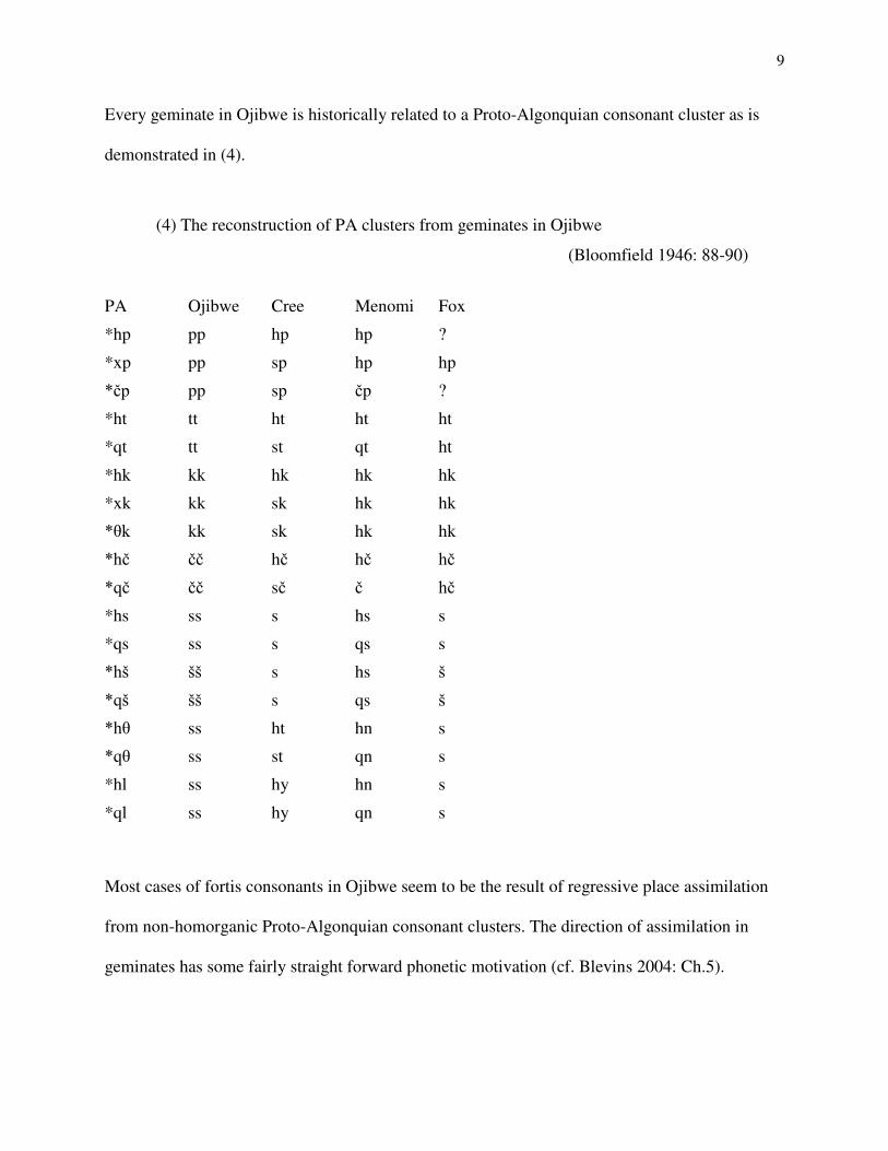
Every geminate in Ojibwe is historically related to a Proto-Algonquian consonant cluster as is

demonstrated in (4).

(4) The reconstruction of PA clusters from geminates in Ojibwe

(Bloomfield 1946: 88-90)

Most cases of fortis consonants in Ojibwe seem to be the result of regressive place assimilation

from non-homorganic Proto-Algonquian consonant clusters. The direction of assimilation in

geminates has some fairly straight forward phonetic motivation (cf. Blevins 2004: Ch.5).

PA Ojibwe Cree Menomi Fox

*hp pp hp hp ?

*xp pp sp hp hp

*čp pp sp čp ?

*ht tt ht ht ht

*qt tt st qt ht

*hk kk hk hk hk

*xk kk sk hk hk

*しk kk sk hk hk

*hč čč hč hč hč

*qč čč sč č hč

*hs ss s hs s

*qs ss s qs s

*hš šš s hs š

*qš šš s qs š

*hし ss ht hn s

*qし ss st qn s

*hl ss hy hn s

*ql ss hy qn s

10

Rhodes (2006) posited that in "Proto-Ojibwe" (or Old Ojibwe) fortis consonants went through an

intermediate hC stage (e.g. xk s hk s kk, qt s ht s tt). This is presumably based on the fact

that in some dialects of Ojibwe fortis consonants are described as preaspirated (e.g. Valentine

1994), and thus the most economic explanation of the current state of affairs is that the northern

dialects reflect the more conservative variant (more on this later). In Blevins' typology of sound

changes6 (Blevins 2004, 2006) the first stage (C1C2 s hC2 where subscripts indicate POA

identity) is an instance of what is termed CHANGE whereby "The phonetic signal is

misperceived by the listener due to: acoustic similarities between the utterance and the perceived

utterance; and biases of human perceptual system" (Blevins 2006: 126). Experimental results

consistently show that CV transitions provide more prominent place cues than VC transitions

(e.g. Repp 1978, Fujimora et al. 1978, Ohala 1990). Thus, the preconsonantal C1 in the cluster

C1C2 is perceptually weaker with regards to its place features.7 This explains why C1C2 clusters

in (4) all underwent regressive and not progressive place assimilation.

The second stage of the development (hC2 s C2C2) would have been an instance of CHOICE in

Blevins' (2004, 2006) model; "Multiple phonetic variants of a single phonological form are

accurately perceived by the listener. The listener (a) acquires a proto-type or best exemplar

which differs from that of the speaker; and/or (b) associates a phonological form in the speaker's

6 The typology consists of three types of sound change, two of which are described above. The other is "CHANCE: The phonetic signal is accurately perceived by the listener but is intrinsically phonologically ambiguous. The listener associates a phonological form with the utterance which differs from the phonological form in the speaker's grammar." (Blevins 2006: 126). 7 Actually according to this account it is unlikely that all consonant clusters took this path. Only those with preconsonantal fricatives would have an intermediate stage of hC clusters. The preaspiration in clusters derived from stop-stop combinations in Proto-Algonquian probably received preaspiration (as a segment or correlate) through structural analogy (roughly in Blevins 2006: 128 sense). The PA fricative-stop clusters PA thus went through the process C1C2 s hC2 s C2C2 where identical subscripts equal identical POAs. The PA stop-stop clusters most likely went through C1C2 s C2C2. In the case of northern dialects the first set may have analogized to the second in its second stage thus making all segments hC2.

11

grammar." (Blevins 2006: 126). In some speech registers (e.g. hypospeech (cf. Lindblom 1992))

the preconsonantal glottal friction associated with preaspiration, i.e. the /h/ segment, would likely

drop out. This percept could easily be transformed into the articulatory domain through laryngeal

retiming. In some dialects (e.g. "southern"), the onset of the voiceless laryngeal gesture,

previously realized as glottal frication preceding the stop, would align its onset with the onset of

the supralaryngeal place feature associated with C2 (cf. Blevins 2004: Ch.5). As we will see, this

crude account is an oversimplification since preaspiration in Saulteaux is variable, implying that

there is no discrete transition from hC2 to C2C2 clusters.8, 9

In addition to the distributional facts passed on from Proto-Algonquian, the apparent phonetic

basis underlying the development of the lenis-fortis contrast will motivate our phonetic studies.

We will discuss the relevance of the diachronic development of the lenis-fortis contrast for the

the phonetic encoding of the lenis-fortis contrast in 2.4.

2.2. Morphophonological Correspondences

In this section I review the synchronic phonological data that have led researchers to

suggest that fortis consonants are underlying consonant clusters, possibly lenis-lenis (e.g. Piggott

1980). Most of the empirical facts reviewed here are discussed in Piggott (1980) and the papers

8 It is not clear what the phonetic grounds are for distinguishing between /hk/ and /hkk/ in the apparent diachronic

process /hk/ s /hkk/ where the h superscript represents glottal frication before the closure. The difference (perhaps) hinges on whether in /hk/ sequences the /h/ is obligatory whereas in /hkk/ the preaspiration correlate is only optional, contingent on the weighting of other factors in the signal. Instrumental phonetic studies on the synchronic state of preaspiration (e.g. Helgason 2002) suggest that the process is gradual. There cannot be any simple threshhold whereby a /hk/ becomes /hkk/. 9 Furthermore, where it has been investigated preaspiration seems to persist as breathy voice (H1-H2) in the

preceding vowel (e.g. Blankenship 1997, Gobl & Ní Chasaide 1999). Thus in addition to the variable realization of preaspiration there is never a discrete point at which we can say that modal voicing has stopped and glottal frication has begun, rather they overlap (cf. also Hoole, Gobl & Ní Chasaide 1999).

12

from the Odawa Language Project (Kaye et al. 1971, Piggott & Kaye 1973) described in an SPE

framework (Chomsky & Halle 1968). Piggott's primary concern was with the necessity for

abstract representation and rule-ordering, not with phonetic interpretation. Only the evidence as

it pertains to the phonological nature of fortis consonants is presented here, however. Phonetic

motivation for the phonological processes based on Jun's (2004) account of consonant

assimilation is given. Despite the fact that almost all of these data are also presented in Piggott

(1980), I use data from my own field data from Saulteaux.

The phonological alternations that give evidence for the lenis-fortis distinction in Ojibwe

can be separated according to the level of morphological derivation they make reference to;

either inflectional or derivational boundaries. The inflectional processes are cases of regressive

assimilation that occur at a morpheme boundary. A fortis consonant derives from two underlying

lenis consonants. One occurs with the AI and TA10 verb paradigms with the third person

conjunct marker lenis coronal stop -t (5a). When the preterit suffix -pan (5b) is concatenated this

produces a fortis /pp/ (5c) (Piggott 1980: 133).

(5) t+p s pp (a) mii appii kaa=maačaat

mii appii kaa=maačaa-t EMPH when C-leave.AI-3.C

„That‟s when he left.‟ (b) nii=waapamaapan

ni-wii=waapam-aa-pany 1-DES=see.TA-DIR-PRET

„I was going to see him... (c) mii appii waa=wiintamawaappan

mii appii waa=wiintamaw-aa-t-pany

10

AI refers to an intransitive verb which takes an animate subject. TA refers to a transitive verb with an animate object (cf. Bloomfield 1962 for the relevant terminology).

13

EMPH when DES.C=tell.TA-DIR-3.C-PRET

„That‟s when he was going to tell him.‟

The other strengthening process occurs when a stem final lenis /t/ (6a) precedes the inanimate

intransitive (II) verb singular conjunct marker -k (6b) at a morpheme boundary. Regressive

assimilation produces a word final /k/ (6c) (cf. Piggott 1980: 135).

(6) t+k > kk (a) sanakat be.difficult.II

„It‟s difficult.‟ (b) nkikkentaan miskwaak n-kikkent-aa-n miskwaa-k 1-know.TI-DIR-0 be.big.II-0.C

„I know it‟s big.‟ (c) nkikkentaan sanakakk n-kikkent-aa-n sanakat-k 1-know.TI-DIR-0 be.difficult.II-0.C

„I know it‟s difficult.‟

Thus, both cases of strengthening involve the lenis coronal stop /t/. Another phonological

alternation occurs when the derivational suffix -toon is added to a TA verb to derive a TI verb. A

TA verb ending in /h/ or /顕/ (7a), depending on the dialect (Valentine 1994: 122), with the TI

forming -toon (7b) creates a /tt/ (7c) at a morpheme boundary. We represent the derivational

stem boundary with + in the parse (cf. Piggott 1980: 132).

(7) h/蔀+t >tt (a) nkii=nači蔀aa n-kii=nači蔀-aa 1-PAST-abandon.TA-DIR

„I abandon him.‟ (b) nkii=piitoon n-kii=pii+ toon 1-PAST-bring+TI

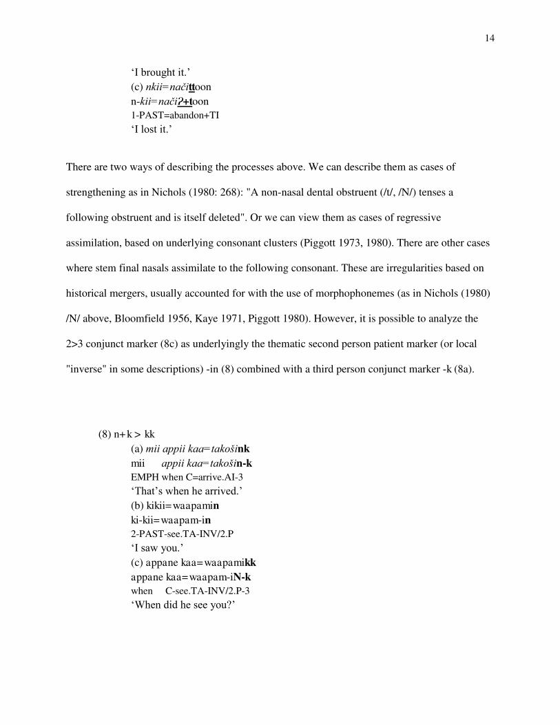
14

„I brought it.‟ (c) nkii=načittoon n-kii=nači蔀+toon 1-PAST=abandon+TI

„I lost it.‟

There are two ways of describing the processes above. We can describe them as cases of

strengthening as in Nichols (1980: 268): "A non-nasal dental obstruent (/t/, /N/) tenses a

following obstruent and is itself deleted". Or we can view them as cases of regressive

assimilation, based on underlying consonant clusters (Piggott 1973, 1980). There are other cases

where stem final nasals assimilate to the following consonant. These are irregularities based on

historical mergers, usually accounted for with the use of morphophonemes (as in Nichols (1980)

/N/ above, Bloomfield 1956, Kaye 1971, Piggott 1980). However, it is possible to analyze the

2>3 conjunct marker (8c) as underlyingly the thematic second person patient marker (or local

"inverse" in some descriptions) -in (8) combined with a third person conjunct marker -k (8a).

(8) n+k > kk (a) mii appii kaa=takošink mii appii kaa=takošin-k EMPH when C=arrive.AI-3

„That‟s when he arrived.‟ (b) kikii=waapamin ki-kii=waapam-in 2-PAST-see.TA-INV/2.P

„I saw you.‟ (c) appane kaa=waapamikk appane kaa=waapam-iN-k when C-see.TA-INV/2.P-3

„When did he see you?‟

15

Bloomfield (1946: 102) reconstructs the second person theme sign of Proto-Algonquian as -eし.

The PA equivalent of the 2>3 -ikk suffix in Ojibwe is accordingly -eしk. In Ojibwe short */i/ and

short */e/ merged to /i/. There is synchronic evidence of this in certain asymmetrical patterns of

palatalization, not taken up here (cf. Piggott 1980, Nichols 1980, et al.). Recall from (4) that PA

/*しk/ changed to fortis /k/ in Ojibwe. PA /*し/ and /*n/ merged to /n/ in Ojibwe. This explains the

morphophonemic asymmetries in (8).11 Synchronically these phenomena have been accounted

for with morphophonemes that undergo absolute neutralization in the phonetic component.

(Piggott (1980: 173) for example chooses to regard /n/s that undergo this process as underlying

/l/s, which never surface phonetically).

There is one case where a fortis consonant turns into a lenis consonant. When the negative suffix

–ssii (9) is concatenated with a nasal at a morpheme boundary it is transformed to –sii [zi:] (10).

Thus, the voicing feature assimilates to the fortis consonant from the previous nasal. In Saulteaux

it appears that the nasal stop is deleted completely.

(10) n+ss> ns [nz] (a) gaawn nkii=kanoonaassii gaawn n-kii=kanoon-aa-ssii NEG 1-PAST-speak.TA-DIR-NEG

„I didn‟t speak to him.‟ (b) gaawn nkii=noontaasii gaawn n-kii=noont-aa-n-ssii NEG 1-PAST-hear.TA-DIR-0-NEG

„I didn‟t hear it.‟

11

In Berens and Northern Ojibwe, the stems of II verbs ending in /t/ have been reanalyzed as ending in /n/. Thus, the same morphophonemic alternation would occur in my example in (6) as well.

16

Regressive coronal place assimilation as in the examples in (5-6) is common cross-linguistically

(Jun 2004). In a general sense it mirrors the evolutionary process that created geminates to begin

with.12

Coronal assimilation is typologically well-attested. There is a phonetic basis for this in the

inertial motor properties of coronals as they relate to their place cues as opposed to other

obstruents (Jun 2004). Recall that there are stronger place cues after the release of a consonant

than before it (Fujimura et al. 1978). There are no place cues for oral stops during the closure and

only weak place cues for the nasal stop (Repp & Svastikula 1988). The typological asymmetry of

greater coronal assimilation for stops is based on differences in articulatory timing and how this

relates to the place cues present in the surrounding vowels. Bilabials and velars have more

sluggish articulations compared to coronals. The former have more salient place cues because

they have a substantial effect through a longer portion of the vowel. The difference can be

represented in (12b) where C1 is a coronal and C2 is a bilabial or a velar. The C2 gesture even has

observable effects on the prevocalic place cues of C1 thus further obscuring the perceptual cues

to /t/ in consonant clusters (cf. Dilley & Pitt 2007). (12a) represents a case where both of the

gestures have similar trajectories before and after their targets.

12 Another consonant mutation occurs at the boundary between stem and –toon; nittoon ‗kill it‟ from niss „kill him‟. I am uncertain as to the origins of this word, but it is the only case where the consonant mutation is not necessarily analyzable as underlyingly two lenis consonants, the example in (b) is from pedagogical material produced by Black River First Nation. ss+ t> tt (a) okii=nissaan o-kii=niss-aa-n 3.ERG=kill.TA-DIR-0 „He killed him.‟ (b) aaniin ke=iši=antawenčikeyaan, kekoo či-nittoowaan kemaa ke=iši=pimaači蔀owaan? aaniin ke=iši=antawenčike-yaan,kekoo či-niss-too-waan kemaa ke=iši=pimaači蔀-owaan how FUT.C=thus=hunt.AI-1.C thing C-kill.TA+TI-1.C pc FUT.C=thus=provide.AI-1.C „Then how can I hunt, kill my game, or make my living.‟ (Black River First Nation 2005)

17

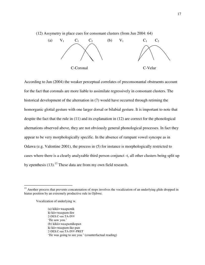
(12) Assymetry in place cues for consonant clusters (from Jun 2004: 64)

(a) V1 C1 C2 (b) V1 C1 C2

C-Coronal C-Velar

According to Jun (2004) the weaker perceptual correlates of preconsonantal obstruents account

for the fact that coronals are more liable to assimilate regressively in consonant clusters. The

historical development of the alternation in (7) would have occurred through retiming the

homorganic glottal gesture with one larger dorsal or bilabial gesture. It is important to note that

despite the fact that the rule in (11) and its explanation in (12) are correct for the phonological

alternations observed above, they are not obviously general phonological processes. In fact they

appear to be very morphologically specific. In the absence of rampant vowel syncope as in

Odawa (e.g. Valentine 2001), the process in (5) for instance is morphologically restricted to

cases where there is a clearly analyzable third person conjunct -t, all other clusters being split up

by epenthesis (13).13 These data are from my own field research.

13 Another process that prevents concatenation of stops involves the vocalization of an underlying glide dropped in hiatus position by an extremely productive rule in Ojibwe. Vocalization of underlying w. (a) kikii=waapamik ki-kii=waapam-ikw 2-DES.C-see.TA-INV „He saw you.‟ (b) kikii=waapamikopan ki-kii=waapam-iko-pan 2-DES.C-see.TA-INV-PRET „He was going to see you.‟ (counterfactual reading)

18

(13) Epenthesis beside coronal /t/ at a morpheme boundary: t+p> tip.14

(a) mii appii waa=waapamatipan mii appii waa=waapam-at-pan EMPH when C=see.TA-2>3-PRET

„That‟s when you saw him.‟ (b) mii appii waa=waapamankitipan mii appii waa=waapam-ankit-pan EMPH when C-see.TA-1.PL>3-PRET

„That‟s when we saw him.‟

Whatever the analysis, the fact remains that these rules of place assimilation are quite

morphologically restricted. There are no general phonological rules which account for more than

a few processes (in Saulteaux), and other mechanisms (e.g. morphophonemes, morpheme

specific constraints, allomorph listing) must be adopted in order to account for discrepancies

between (5) and (13). The relevance of these studies for phonetics is that processes such as (5-7)

provide evidence for fortis consonants as underlying concatenations of lenis consonants. These

assimilatory processes have their phonetic roots in regressively retiming a supralaryngeal gesture

to line up with the voiceless laryngeal gesture of a previous consonant. The most obvious way

this process might occur would be through lengthening the supralaryngeal gesture. Thus, we

would expect closure duration to be a correlate of the lenis-fortis contrast. If we consider the

process in (10), we observe a case of voicing assimilation, since it is triggered by nasals. We

would expect voicing to be a correlate at least in fricatives. Although this investigation is limited

to stop contrasts, feature economy predicts voicing to be an important correlate across the board

(but cf. Jessen 1998 for the difference in featural content between lax-tense stops and fricatives

in Standard German).

14 Bloomfield (1956: 54) noted that “-pan [is] added to –t without connective”. In his account allomorph –ipan is used elsewhere.

19

2.3. A Note on Orthographies

There are two types of orthographies used for Ojibwe; roman and syllabic. Only the

roman alphabets are reviewed here since the syllabic does not differentiate between lenis and

fortis consonants. Valentine (1994: 164) states that "…Roman orthographies reflect a regional

variation in the nature of the fortis-lenis contrast, the Northern orthography representing this

contrast as one of preaspiration, or a sequence of h followed by a consonant, and the Southern

orthography representing it as a voiced contrast". The "Southern orthography", used in

publications by John Nichols and others, is represented as a voicing difference (e.g. Nichols &

Nyholm 1991, Kegg 1991). Some of the different orthographies from the main dialect divisions

are given below. Recall we have been using Bloomfield's (1956) system till now.

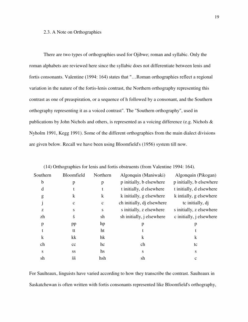
(14) Orthographies for lenis and fortis obstruents (from Valentine 1994: 164).

Southern Bloomfield Northern Algonquin (Maniwaki) Algonquin (Pikogan)

b p p p initially, b elsewhere p initially, b elsewhere

d t t t initially, d elsewhere t initially, d elsewhere

g k k k initially, g elsewhere k intially, g elsewhere

j c c ch initially, dj elsewhere tc initially, dj

z s s s initially, z elsewhere s initially, z elsewhere

zh š sh sh initially, j elsewhere c initially, j elsewhere

p pp hp p p

t tt ht t t

k kk hk k k

ch cc hc ch tc

s ss hs s s

sh šš hsh sh c

For Saulteaux, linguists have varied according to how they transcribe the contrast. Saulteaux in

Saskatchewan is often written with fortis consonants represented like Bloomfield's orthography,

20

but with an <h> instead of the first consonant in the Northern orthography in CC clusters (e.g.

Cote 1984, Scott et al. 1995, Logan 2001). This may tell us nothing about the phonetics since,

according to Logan (2001), fortis consonants are phonetically long in Saskatchewan Saulteaux

(e.g. [p:]). In a pedagogical grammar based on Saulteaux dialects in Manitoba by Voorhis et al.

(1976) the distinction is marked with double consonants as in Bloomfield. I myself took

introductory and intermediate Ojibwe classes with a speaker from McGregor, Manitoba (Roger

Roulette). Nichols' orthography (e.g. b/p…) was used throughout, and we were explicitly taught

that the difference was one of voicing. Generally in Manitoba, out of the Roman alphabets15, the

"Southern" orthography seems to be the most widely adopted. It is present in every piece of

Ojibwe language material based out of Manitoba since the 1990s that I have been able to find

(e.g. Fox 2005, Roulette 1997, Ningewance 2004).

It is not correct, however, that preaspiration is not present at all in the Saulteaux spoken in

Manitoba as the adoption of the "Southern" orthography and Valentine's (1994: 164) statement

above would suggest. Rhodes & Todd (1981) for instance describe preaspiration as occurring in

"some Saulteaux".16 It is unclear whether this should be taken to mean some speakers or some

dialects; but the current study suggests that it occurs some of the time for every speaker but to

different degrees (cf. Helgason 2002 for a similar situation with some languages of northern

Europe, and DiCanio (2008: 114-5) for San Martín Itanyuso Trique, Zapotec). Valentine

(1994:123) states that in the dialects of "northwestern Ontario, and western Saulteaux" fortis

obstruents are realized as [hC], and even [lp], [st], [xk], that is a stop preceded by a constriction

approximating that of a homorganic fricative". There have been no published instrumental

15 Syllabics are used in some parts of Manitoba as well (Roger Roulette p.c.). 16 Hardly any Saulteaux communities were surveyed in Rhodes & Todd‟s (1981) study.

21

investigations, besides the present that have attempted to describe or document the state of

preaspiration in any Ojibwe dialect (cf. Tallman 2010a for a pilot study with some subdialects of

Berens and Saulteaux).

2.4. Discussion

This chapter has reviewed some of the evidence that some linguists have used to argue

that fortis consonants are underlyingly consonant clusters at some level of representation. Two

types of phenomenon seem to support this idea. First, Ojibwe fortis consonants pattern with

consonant clusters phonotactically. This reflects the fact that they are derived from consonant

clusters in Proto-Algonquian. Second, phonological alternations that produce fortis consonants

involve the assimilation of a preceding segment to the place features of the second lenis

consonant in a C1C2 cluster. This pattern is either morphologically conditioned in some fashion

(as in the third person conjunct -t with the preterit), or else it is extremely morphologically

restricted (/t/ final II verbs with the inanimate conjunct marker -k). The fact that mostly coronals

regressively assimilate, although most likely categorical, may have a phonetic basis in the

inertial motor properties of these consonants in relation to their place cues in flanking vowels.

Another phonological alternation occurs at a derivational word boundary and involves the

assimilation of a glottal stop to the supralaryngeal place features of the /t/ in the suffix -toon.

Despite the lack of detailed instrumental studies, the historical basis of the lenis-fortis contrast

(2.1.), the phonological alternations that imply segmental differences (2.2.) and the auditory

impressions of various investigators, can give us an idea of what parameters of phonetic

22

encoding are important for making the lenis-fortis contrast in Ojibwe, and hence how our

phonetic investigation should proceed.

It is often noted, especially in early missionary descriptions (e.g. Baraga 1850 for Chippewa,

Dumouchel & Brachet 1942 for Saulteaux), that fortis consonants are in some sense "strong".

Dumouchel and Brachet describe the situation with some fortis consonants (cf. a similar

statement in Baraga (1850: P. II, cited in Nichols (1992: xii)):

"Il arrive souvent que P, K, T aient un son dur. Leur prononciation est difficile à rendre

par écrit. Tout ce que nous pouvons indiquer ici, c'est que souvent la prononciation pour

P est entre celle du P et du B; celle du K est entre celle du K et du G; celle du T est entre

celle du T et du D… Le seul moyen de trouver la prononciation exacte de ces consonnes

est d'écouter attentivement les Indiens les prononcer" (Dumouchel & Brachet 1942: 5).

Unlike the lay grammarians mentioned above, Bloomfield was able to correctly capture the

phonological distribution of lenis and fortis consonants. Adhering to his phonemic principle

(Bloomfield 1926) allowed him to achieve a greater degree of precision than the missionary

grammarians that preceded him with repect to the phonemics, however, the phonetics of the

contrast still evade precise description:17

17 In fact Bloomfield seems to implicitly relegate phonetic detail to another field of inquiry completely: "… the physiological and acoustic description of acts of speech belongs to other sciences than ours" (Bloomfield 1926: 153). Compare this to the position of contemporary Laboratory Phonology: "Probably the single most important auxiliary theory in our field is the acoustic theory of speech production. This theory relates critical aspects of speech articulation to eigenvalues of the vocal tract, which can in turn be related to peaks in the spectrum…" (Pierrehumbert, Beckman & Ladd 2000: 281).

23

"The fortes are voiceless, vigorously articulated, and often rather long. The stops pp, tt,

kk, cc are often preceded by a slight aspiration: eto:ppuwin 'table'. The sibilants ss, šš are

often weakened between the vigorous onset and the vigorous opening, with a clear

division into to syllables: ni:ssa:ntuwe: 'he climbs down, descends" (Bloomfield 1956:

8).

Hockett (1939:1) similarly noted that fortis consonants in Potawatomi were "strongly

enunciated".18 Piggott (1980: 57) states that lenis consonants are "basically voiceless and

unaspirated, but become voiced, or fortis aspirated, under certain conditions". Piggott does not

explicitly discuss the phonetics of fortis consonants, referring to this series as "fortis aspirated"

or "phonetically fortis". Nichols (1991: xxvii) transcribes fortis consonants as phonetically long

(as in [k:] for k) in his pronunciation guide. In a pedagogical grammar of Manitoba Saulteaux,

Voorhis et al. (1976: 4-4) considers fortis consonants "double [lenis] consonants" and states that

they "always have the voiceless sound" (Voorhis et al. 1976: 3-3) and are "somewhat extended or

longer than the single consonants" (1976: 4-4). He notes that lenis consonants are voiceless word

initially and voiced intervocallically and before nasals, but that this varies according to rate of

speech. Word-finally the only thing that distinguishes lenis from fortis is the length of the fortis

consonant (Voorhis et al. 1976: 4-4). Valentine (1994: 123-4) states that the lenis stops are only

consistently voiced in Algonquin and in other dialects "at least partially voiced in all

environments". Fortis are "typically both voiceless and more or less geminate" (Valentine 1994:

124). 18 Potawatomi is not considered a dialect of Ojibwe by some authors (e.g. Valentine 1994). Valentine (1994: 100) describes the difference as it pertains to lenis and fortis obstruents: "Reflexes of various PA clusters which show up as fortis obstruents in Ojibwe alternate between fortis and lenis in Potawatomi, the latter occurring in utterance initial positions e.g., nwapma k:we 'I see the woman', but kwe nwapma initially. Also word final fortis obstruents only show up as fortis before a consonantal sonorant (n, m, w, y), e.g. muk niwapma 'I see the beaver.' vs.niwapma muk."

24

There is nothing wrong with using the terms lenis and fortis to make reference to a descriptive

class whose covariates cover a range of various phonetic features (Malécot 1970, Sils 1970,

Kohler 1984, Docherty 1992). However, as a descriptive label that accounts for the details of

phonetic implementation in a particular language, the notion of lenis and fortis has been

discredited (Catford 1977, Ladefoged & Maddieson 1996).19, 20

The only instrumental phonetic study of the lenis-fortis contrast in Ojibwe concluded that it is

not one of gemination as the consonant cluster analysis described above would suggest

(Swierzbin 2003). This was based on the fact that the difference in closure duration between

lenis and fortis consonants in Border Lakes Ojibwe patterned closer to English than languages

normally analyzed as consisting of geminates. It was found that so-called Ojibwe geminates are

only 1.2-1.4 times as long as their lenis counterparts, closer to the differences between voiced

and voiceless consonants in English (1:1.4) and French (1:1.2) (Suen & Beddoes 1974,

19 This is not to say that there are no interesting theories of "strength", which describe for allophonic variation (Lavoie 2001), or the inertial motor factors involved in sound change (Kirchner 1998). The latter authors approach the problem from the perspective of the different categorical and gradient processes which effect these consonants both synchronically and diachronically (Kirchner 1998, Lavoie 2001). These are not mutually exclusive approaches but rather methodological starting points for addressing what is very similar and in some cases identical phenomena (cf. Lavoie 2001). Lavoie (2001) bases her theory of strength on a typological survey of languages which she attempts to back up with synchronic phonetic evidence. Kirchner (1998) provides a cross-linguistic survey of lenition processes and attempts to explain these based on a principle of effortfulness formalized as the constraint [LAZY] in an optimality theoretic approach (Prince and Smolensky 1993). Given that the contrast itself is based on different constraint rankings (Kircher 1998) the theory implicitly makes predictions concerning the phonetic correlates to the contrast in question. The difference arises in the overlapping empirical phenomena that these approaches address. Where as the lenition approaches focus on strength as a phonetic process dependent on many features of phonological contrast and their interrelations, feature-correlate approaches start from the goal of characterizing the nature of an entire natural class. Lenition in the latter case is highly correlated with one of these natural classes (the 'lenis' consonants), but not limited to it. 20 Note that this principle, about the nonuniversality of the phonetic encoding of labels in phonological descriptions, does not just apply to the lenis-fortis contrast, it applies across the board to all phonological categories: "categories [the phonetic correlates to phonological contrast], defined as relations between a discrete level and a parametric level, cannot be universal. That is the picture of human phonetic resources as pegs in an IPA-like phonetic pegboard cannot be sustained." (Pierrehumbert 2003b: 127).

25

O'Shaughnessy 1981 respectively, cited in Swierzbin (2003: 346)). Languages with real

geminates have ratios of between 1:2 (Esposito & Benedetto (1999) for Italian, Lahiri &

Hankamer (1988) for Bengali) and 1:3 (Lahiri & Hankamer (1988) for Turkish). Swierzbin

(2003: 346) concludes that "based on these comparisons, it seems that the main difference

between fortis and lenis consonants in Border Lakes Ojibwe is that of voicing and not duration".

Lenis consonants are "usually voiced when they occur between two vowels and voiceless

otherwise" (Swierzbin 2003: 345). However, the degree and type of voicing that marks

consonants contrasts varies in systematic ways from language to language (e.g. Keating 1984 for

English, French and Polish). This is also the case for consonant duration as well; so-called fortis

consonants are 1.5 to 3 times as long as their lenis counterparts (Ladefoged 1996: 91-2), with no

discrete break between languages that code a voiced/voiceless contrast or languages that

distinguish primarily according to some other correlate. Thus, informal descriptive labels such as

lenis-fortis, voiced-voiceless, singleton-geminate etc… do not solve the problem of contrast, they

only put it in another domain, even if informed by some instrumental phonetic data.

Hence, previous approaches have not formulated the issue of contrast directly, too readily giving

special empirical status to labels which describe only the fact that there is a contrast- not how the

contrast is made. Despite this, previous investigations can inform what correlates we consider

important for marking the lenis-fortis contrast in Ojibwe. We can be reasonably sure that

consonant duration will be a correlate. This hypothesis is based on considerable impressionistic

observation and the fact that fortis consonants historically come from consonant clusters.

Continued vocal fold vibration during the closure may also be a correlate, since investigators

have frequently described the contrast as one based on "voicing" on analogy with the category in

26

English phonological descriptions, i.e. [+/-voice] (e.g. Kingston et al. 2008 and references cited

therein). Every description makes reference to lenis consonants being voiced in certain

circumstances compared to fortis consonants which are always voiceless. Postaspiration (Jessen

1998), VOT (Lisker & Abramson 1964) or mVOT (cf. Helgason 2002) are most likely correlates

as well, as it is a cross-linguistically common way of distinguishing so-called lenis-fortis sets.

Postaspiration is associated with longer voiceless consonant duration for physical reasons as

well, in that these consonants have longer intraoral air pressure build up (cf. Stevens 1998).

Piggott (1980) also refers to fortis consonants as aspirated in some circumstances as we saw

above. Preaspiration has been reported to exist in some Saulteaux (Rhodes & Todd 1981: 58). It

is usually described as being obligatory in Berens Ojibwe (e.g. Valentine 1994), but it is

generally not thought to be particularly prevalent elsewhere. However, as Helgason (2002) notes,

preaspiration can often be fairly subtle and undetectable without instrumental study. It is likely

that its cross-linguistic prevalence has been underdescribed.

We might also keep in mind the relevance of the historical development of fortis consonants for

understanding the contemporary structure. There is no distinction between lenis and fortis

consonants word initially (without syncopation (cf. Valentine 20010)) because there was a

constraint in Proto-Algonquian that disallowed consonant clusters in this position. Since there is

no lenis-fortis contrast word initially, it makes no sense to analyse contrast in this position.

Piggott (1980) posited a rule that turns lenis consonants "phonetically fortis" word initially.

However, from the perspective of phonetic interfacing, what we should ask is the extent to which

initial consonants pattern with lenis or fortis in terms of their phonetic correlates. It is for this

reason that initial consonants are not pooled with lenis or fortis consonants in this study. Only

27

intervocalic lenis and fortis consonants are compared. Word final fortis consonants are extremely

rare in corpus data. They are outside the scope of this study.

The rest of this thesis attempts to give a first approximation of some of the quantitative aspects

of the correlates of the Saulteaux Ojibwe lenis-fortis contrast with reference to the relationship

these correlates share with each other between speakers and places of articulation in some of the

Saulteaux dialects of Manitoba. First we describe the theoretical framework that motivates the

descriptive parameters used in this study.

3. Theoretical Framework: Probabilistic Phonology

In this section we describe the main hypothesis of this thesis and its relationships to the

theoretical framework adopted. This will be important for understanding the modelling choices

used in the results section (4.1.3.). We adopt the model phonological structure recently

articulated by Pierrehumbert (Pierrehumbert 2001a, 2001b, 2003a, 2003b). Some mention is

made of exemplar theory in relation to the theory adopted here.

In this framework phonology is a cognitive architecture that consists of multiple levels of

representation. Following Pierrehumbert (2003b: 116) these levels include at least (1)

Parametric phonetics: A quantitative map of acoustic and articulatory dimensions over which

some notion of proximity and distance can be defined. (2) Phonetic encoding: Categories and

category systems that relate linguistic elements (phonemes, distinctive feature, syllables,

morphemes etc…) to a k-dimensional phonetic space. (3) The lexicon: Lexical representation of

28

morphemes, wherein lies the symbolic relations between form and meaning. (4) The

phonological grammar: General constraints on morphemes in the lexicon based on the

combinatorial elements that are encoded at level (2). (5) Morphophonological correspondences:

Phonological relationships between classes of morphological forms and processes.

The empirical phenomena related to the lenis-fortis contrast in Saulteaux Ojibwe for the levels

(4) and (5) were described in the previous chapter. The main structure of this thesis is on how the

contrast is structured at level (2), that of phonetic encoding. The following specific technical

definitions of the following concepts are necessary for understanding the discussion below (cf.

Pierrehumbert 2003c, Luce 1963):

Category: This defines a density distribution over a particular dimension of the parametric level.

It relates an abstract variable to a probability region over some phonetic continuum. Multiple

categories can exist on a single phonetic continuum and their statistical properties and

relationships can be used to make linguistically relevant distinctions.

For example in a study conducted by Maye & Gerken (2000), English speaking subjects were

exposed to various examples along the VOT continuum in a set of experiments. They created

synthetic phonetic continuum between /d/ and unaspirated /t/ which are not phonemically distinct

in English in the position they examined. One group was exposed to a unimodal frequency

distribution and the others a bimodal frequency distribution over the continuum. Subjects'

responses in a discrimination test echoed the frequency distributions they were exposed to.

Subjects exposed to bimodal distributions had higher discrimination near the boundaries of the

29

distributions they were exposed to, while subjects exposed to unimodal distributions did not. In

the terminology we are developing here, the former group acquired two categories and the latter

acquired only one on the VOT dimension.

A frequency distribution of VOT values a speaker associates with a particular phoneme is an

example of a category. An example of categories encoded along the same dimensions is given

from my own data from Saulteaux in figure 1a and 1b. The data are from the dental/alveolar lenis

and fortis stops of the speaker Boo from Long Plain. The following plots demonstrate four

categories associated with two different phonetic continua. A and B are each separate density

distributions over the closure duration parameter (figure 1a) and C and D are each separate

density distributions over the postaspiration (or mVOT, cf. 4.1.2.2. below) parameter (figure 1b),

despite the fact that they overlap. A category refers to regions in these dimensions not individual

points.

Figure 1. a. Consonant duration in ms for the speaker Boo from Long Plain. A is a density distribution for the values associated with lenis /d/. B is a density distribution for the values associated with fortis /t/. b. Postaspiration in ms for the speaker Boo from Long Plain. C is a density distribution for the values associated with lenis /d/ and D is a density distribution for the values associated with fortis /t/.

30

Category System: I use the term category system to refer specifically to a label that defines a set

of categories or distributions.21 Thus, because phonemes encode multiple phonetic dimensions

they are examples of category systems. Elaborating on the tutorial plots above, a category system

could define the set of categories {A, C}, another {B, D}. Category systems define regions in a

k-dimensional phonetic space rather than along just one parameter as in simple categories. Hence

the category systems for the sets {A, C} and {B, D} have two dimensions associated with them.

This situation is represented in the following figures 2a and 2b. Specifically the figure 2a could

represent /d/ and the figure to the right fortis /t/ given closure duration and postaspiration

assuming these are the only correlates to these phonemes.

Figure 1a (left). Two density distributions for the phoneme /d/ on the closure duration and postaspiration parameter. 1b (right). Two density distributions for the phoneme /t/ on the closure duration and postaspiration parameter.

21 In much of the categorization literature it is customary to refer to what I call a "category system" as a "category" (e.g. Rosch & Mervis 1975, Pothos & Close 2008) with multiple dimensions.

31

The tutorial plots above belie the fact that phonemes are never composed of just two dimensions.

Many more correlates have been shown to be used by speakers to distinguish phonemes even in

minimal pairs (Lisker 1986). The actual phonetic space of a particular unit of phonetic encoding

can never be displayed graphically because it is too high-dimensional. These units map onto

regions in a k-dimensional phonetic space (Pierrehumbert 2001b, 2003b).

Contrast Precision:22 This refers to how well a particular density distribution (category) is able

to predict a particular category system in contrast to others with reference to one or more

dimensions of phonetic space. Intuitively contrast precision increases as the density distributions

on a particular parameter get further apart and/or overlap less. As categories get closer together

their contrast precision for a particular complex category decreases (cf. Pierrehumbert 2001a,

Kirby 2011). Informally the contrast precision of category A for the category system {A, C} in

the figures above is defined by how much overlap it has with B in the consonant duration

dimension. If the category systems {A, C} and {B, D} were placed on the same plot contrast

precision would extend to this case as well. Thus, it can be viewed both as a property of

categories in isolation and category systems as a whole. It is important to point out that contrast

precision cannot be equated with the distance between particular points. It is difficult to explain

this aspect of contrast precision with reference to the figures above, so we use the invented

categories below.

22 This term is not used by Pierrehumbert (2001b, 2003b). It is borrowed from Kirby (2011), although he does not give it an explicit definition. For Pierrehumbert (2001, 2003c), and most likely for exemplar theorists in general, this concept would be subsumed under the relationship between statistical choice rules in relation to complex categories in perception (Luce 1963, Krushke 1992) and in production (Pierrehumbert 2001b).

32

Figure 3a (left). Hypothetical density distributions with mean 40 and 80 and standard deviations 10 each. 3b (right). Hypothetical density distributions with mean 40 and 80 and standard deviations of 20 each.

All of the density distributions in figures 3a and 3b have the same means (40 for the left, 80 for

the right) but different standard deviations (a=10, b=20). The distance between the means of the

categories on each dimension is the same but the degree to which the categories overlap is

different. In figure 3b the categories overlap more than in figure 3a. We, therefore, want our

measure of contrast precision to capture this difference. That is, contrast precision should

quantify the separation of categories in relation to their width (Pierrehumbert 2001b: 208).

Generally literature on phonetic typology has demonstrated that where contrast precision is

diminished in one dimension it is increased in another (Pierrehumbert 2003b, Kirby 2011). For

example, Engstrand & Krull (1994) demonstrated that Swedish and English vowels show more

broad and overlapped phonetic distributions for length than Finnish vowels. This can be

attributed to the fact that in Swedish and English vowel quality and vowel length function

together in a system of vowel categories, whereas Finnish has a pure length distinction with

0 20 40 60 80 100 120 0 20 40 60 80 100 120

33

extremely little impact on vowel quality. Swedish and English have category precision dispersed

along three parameters for the relevant contrast, but for Finnish vowel duration has higher

category precision to the detriment of other parameters.

Another example is from the aspirated-lenis obstruent contrast in Korean. In Korean VOT was

identified as the most reliable correlate of the contrast between aspirated and lenis stops, with

aspirated stops consistently having a higher VOT value (e.g. Han & Weizman 1970). F0 (pitch)

covaried with the distinction, but was not described as the primary cue to the lenis-aspirated

contrast. In a recent study done with a younger generation of speakers, Kang and Guion (2008)

found that VOT was nondistinctive, and F0 was a better covariate to the pair. Thus, heightened

category precision along the F0 dimension corresponded to a lowering of precision on the VOT

dimension for the younger generation of Korean speakers (cf. Kirby 2011 for an "enhancement"

model that accounts for this change).

In this thesis I attempt to quantify/model contrast precision between lenis and fortis stops along

certain dimensions of the quantitative parametric phonetic space. A hypothesis that this thesis

attempts to corroborate, on the general lines of the studies described above, is that although the

contrast precision along each particular parameter may vary from speaker to speaker, the contrast

precision between category systems as some function of all their dimensions considered together

should be approximately the same. Framed with reference to our topic, although Saulteaux

speakers vary in terms of how they use acoustic correlates to mark the lenis-fortis contrast,

overall the contrast has close to the same degree of robustness from speaker to speaker.

34

In this study we are able to quantify contrast precision for the lenis-fortis distinction by inferring

density distributions from frequency distributions in the database.23 Thus, a simplifying

assumption is made in this thesis in order to investigate precision contrast. We assume that the

frequency distributions of the acoustic correlates found in our corpus data for lenis and fortis

stops can adequately represent the density distributions in the phonetic encoding of these

consonants for each speaker. The phonetic encoding of a contrast is not just used for production,

however, it is also used for perception. Obviously a speaker's ability to weigh perceptual cues,

however, need not be completely a function of their production; in fact it is clearly not this

simple (Foulkes & Docherty 2006). Ideally a study such as this should be supplemented by data

from perceptual studies centred on the relevant acoustic correlates in relation to the

categorization of lenis-fortis stops. We tentatively assume that the supposition that frequency

distributions from production are adequate for describing phonetic encoding is justified by the

success of exemplar theory. Exemplar theory claims that categories are maintained and updated

by incremental updates based on exemplar tokens of those categories (Johnson 1997,

Pierrehumbert 2001b, 2003b). Pierrehumbert (2003b: 186) explains the relationship between

phonetic encoding, perception and production based off this theory:

"Once a label is selected (presumably through a decision to say a word that involves that

label), a production goal is established by sampling the empirical distribution for that

label. Specifically, an averaged neighbourhood around a randomly-sampled point in the

distribution serves as a production goal."

23 A number of methods are used for this (cf. 4.1.3.)

35

Thus, the statistical distributions serve as the primary data for the phonetic encoding of category

systems for the language learner. Analogously, we hope that these statistical distributions in

corpus data can serve as the primary data for the linguist attempting to understand this system.

4. Phonetic Encoding I: Methodology

Section 4.1. describes the speakers and data collection method for this study. The next

section 4.2., describes how the acoustic correlates were measured with reference to spectrograms

and wave forms. Problems with the methodology and how I attempted to cope with them are

noted in each section. The final section describes the probability models used to quantify the

concept of contrast precision defined in the previous chapter.

4.1. Speakers and Data

Ojibwe is spoken throughout a wide geographical area extending from western Quebec

into Alberta (figure 4). The speakers for this study were all from Manitoba and thus fall within

the Saulteaux dialect, according to classifications in the literature (e.g. Rhodes & Todd 1981,

Valentine 1994, 1996).24 The six Saulteaux speakers represented in this study are from Fairford,

Lake St. Martin, Brokenhead, Peguis, Sandy Bay and Long Plain (figure 5). The exact age of all

24 However, it appears that dialects in northeastern Manitoba closer to the Ontario border should be regarded as different dialects. Voorhis et al. (1976: vi) states that "the language spoken around Island Lake and Red Sucker Lake in Manitoba, and in adjacent parts of Ontario, though often called Saulteaux or Ojibwa, and just as often called Cree, is really different enough from all of these [Saulteaux dialects of Manitoba] that is is hard for both neighbouring Saulteaux and Cree speakers to understand it" (cf. Wolfart 1977, Wolfart & Shofel 1977).

36

the speakers is not known, although from the stories they tell it sounds as if they are

approximately middle age.25 All the speakers in this study are fluent in Saulteaux.

The data for this study came from three different sources. The first was from elicitation with a

speaker from Long Plain. The data obtained this way are naturally more controlled. Recordings

were made in Portage la Prairie Manitoba. Data for the speakers from Fairford, Sandy Bay, Lake

St. Martin and Brokenhead all came from recordings from the Treaty #1 Oral History Video

Project.26 The data from the speaker from Peguis were obtained from Rand Valentine's Ojibwe

website (Valentine 2010). The data obtained from Valentine‟s website were recorded in 1983.

The data obtained from the Aboriginal Languages of Manitoba Cultural Centre (henceforth

ALM) consists of interviews that Roger Roulette conducted in the 1990s with various speakers

of Ojibwe for the Treaty #1 Oral History Video Project (Roulette 1997). These were recorded on

video by Roger Roulette and then converted to wav files by the current researcher. The

interviews are fairly informal. Permission to use these recordings was obtained from ALM.

Sometimes English words are used for place names or in certain expressions, but generally the

use of English is negligible. Transcripts were all written by Roger Roulette, using the Fiero

orthography. Mistakes in the transcription were corrected by the present researcher, although this

was fairly rare. The recordings vary in terms of their quality. Interviews that contained

predictable background noise (some feedback, refrigerator etc...), that did not seem to interfere

with the measurements were used.

25 Joseph Bealieau (Sandy Bay) tells a story from the 1940s for instance: Twenty eight days imaa ngii-anokii bwaashka`iganing, aazha four dollars a day gii-diba`igem. That was, aazha thirty years old iwapii. Ngoji iidog, 1941, 42 ngoji imaa. 26 Much thanks go out to Aboriginal Languages of Manitoba for allowing me to use these recordings.

37

Figure 4. Ojibwe dialects (from Valentine 2010)

38

Figure 5. Rough location of Saulteaux speakers in Manitoba used in this study.

I obtained the data from Long Plain through elicitation. Two word lists were constructed. One

was meant to elicit general phonological attributes present in the dialects. This was based on

material presented in Valentine (1996). Another word list was constructed to obtain controlled

tokens of lenis and fortis stops. 27

27 The construction of a word list was a fairly complex process. The reason for this was that the word list was constructed out of dictionaries from all the dialects (Baraga 1886, Rhodes 1985, Nichols & Nyholm 1991, et al.). It was expected that many of the words would be infrequent or nonexistent in my consultant‟s dialect, so the word lists had to be large in order to account for this. Also it is difficult to not confound affects from phonological environment and morpheme specific phonetics in agglutinating languages such as Ojibwe. The phonological environment controlled for in the database was all words where these stops occurred between low front vowels (a_a, aa_a, a_aa, aa_aa). A pilot study was done using an online Ojibwe dictionary found that this was the environment where the most of the lenis and fortis stops could be compared (Tallman 2010c). A preliminary database was then constructed which encoded phonological specifications (surrounding vowels and consonants, number of syllables, stress position) and information about morphological decomposition. The idea was that one could use such a database to construct word lists with comparable phonological environments whilst controlling for morphology. Controlling for morphological decomposition was felt to be necessary because derivational morphology is extremely productive in Ojibwe (e.g. Rhodes 1976). Thus, morphological structure ought to be

39

The consultant preferred to use words in elicited sentences rather than in carrier phrases. The

process was repeated 5-10 times with each word. Sometimes, the consultant produced some

tokens at an abnormally slow pace to help the current investigator hear what he was saying

during some sessions. These tokens were removed from the database.

Thus, the data were obtained from different sources with different methods of collection. This

should be kept in mind during the presentation of the acoustic data. The distinction between the

corpus data and noncorpus data will probably be reflected in differences in hypo to hyper

articulated speech (cf. Lindblom 1990). In the latter case (hyper speech) the acoustic correlates

might be exaggerated. Moon and Lindblom (1994) for instance found that vowel undershoot was

much less prevalent in citation-form speech. The information on speakers and recordings is

summarized in (15).

controlled for to avoid confounding contextual allophony with morpheme/word specific phonetics (Hay 2000, Pierrehumbert 2002). Although this was not obvious to the present researcher at the time, it seems that such a problem is much more difficult to resolve in Saulteaux Ojibwe than in nonagglutinating languages. The reason for this is that there is such a tight relationship between phonological environment (at least in terms of surrounding vowels and consonants) and morpheme in Ojibwe. In consequence, specifying subsets of phonological environments in the database was often no different from asking for all the words that contained a particular morpheme (90% of /at/ sequences come from the final –batoo „run‟) (Tallman 2010d, 2010e). These problems aside, word lists were still constructed, although their degree of control came down to specifying the quality and length of the previous vowel. In the end all tokens of lenis and fortis consonants from elicitation were used. Information about phonological environments was specified directly in the database with the acoustic measurements. In principle, a degree of control could be achieved through sheer sample size and subsetting. One can specify subsets of data by referring to the database which contained the acoustic measurements directly. For example if one wanted to only compare the length of a previous vowel with /a/, then one could specify a subset of the data that contained only tokens that met that criterion. In this case we still have to check to see if there is enough tokens for the statistical models to be meaningful and whether there might be confounding effects involved (such as phonological environment and morphological context symmetry).

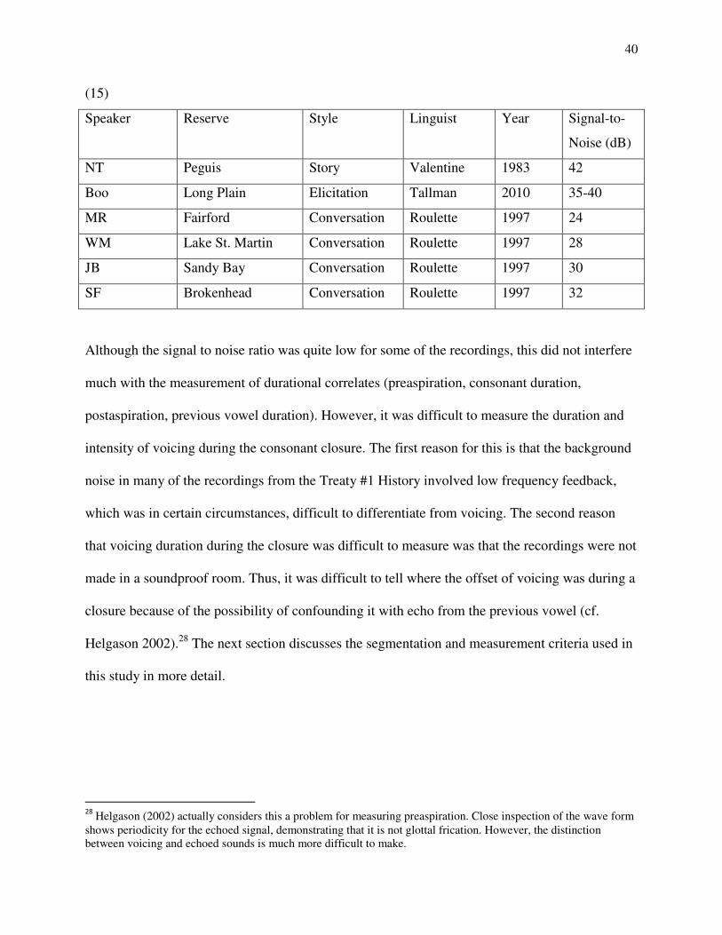
40

(15)

Speaker Reserve Style Linguist Year Signal-to-

Noise (dB)

NT Peguis Story Valentine 1983 42

Boo Long Plain Elicitation Tallman 2010 35-40

MR Fairford Conversation Roulette 1997 24

WM Lake St. Martin Conversation Roulette 1997 28

JB Sandy Bay Conversation Roulette 1997 30

SF Brokenhead Conversation Roulette 1997 32

Although the signal to noise ratio was quite low for some of the recordings, this did not interfere

much with the measurement of durational correlates (preaspiration, consonant duration,

postaspiration, previous vowel duration). However, it was difficult to measure the duration and

intensity of voicing during the consonant closure. The first reason for this is that the background

noise in many of the recordings from the Treaty #1 History involved low frequency feedback,

which was in certain circumstances, difficult to differentiate from voicing. The second reason

that voicing duration during the closure was difficult to measure was that the recordings were not

made in a soundproof room. Thus, it was difficult to tell where the offset of voicing was during a

closure because of the possibility of confounding it with echo from the previous vowel (cf.

Helgason 2002).28 The next section discusses the segmentation and measurement criteria used in

this study in more detail.

28

Helgason (2002) actually considers this a problem for measuring preaspiration. Close inspection of the wave form shows periodicity for the echoed signal, demonstrating that it is not glottal frication. However, the distinction between voicing and echoed sounds is much more difficult to make.

41

4.2. Measurement

This section describes the methodology employed in measuring the acoustic correlates

analysed in this study: Consonant duration (4.2.1), postaspiration (4.2.2), preaspiration (4.2.3),

and voicing (4.2.4). In the latter case an ordinal value was obtained from inspection of the

waveform.

Only intervocalic lenis and fortis stops were measured in this study. The criterion for deciding

whether a consonant was lenis or fortis was based on its transcription. In cases where I suspected

there might be a mistake the transcription was checked against its spelling in an Ojibwe

dictionary (Rhodes 1985, Nichols & Nyholm 1992, Ningewance 2010, et al.). This practice was

justified because, with respect to phonology, Ojibwe dialects are thought to vary mostly

subphonemically (Valentine 1994). The only case where there was any confusion regarding the

transcription was with the word baapaase 'wood pecker', which had been variously transcribed

as baabaase or baapaase. The reason for this might be due to occasional vocal fold vibration

(voicing) seeping into fortis bilabials, which are generally voiceless. Cases where the class of the

stop could not be determined were removed.

All acoustic measurements were made in Praat (Boersma & Weenink 2007) from wav files. The

segmentation was done by hand using some of the criteria from Olive, Greenwood & Coleman

(1993). For the spectrograms the dynamic range was 35 dB throughout the analysis and the

window length was set at 0.005 s.

42


In this study consonant duration refers to the length of the steady state period produced by an

occlusion in the vocal tract. In the case of unaspirated stops this occlusion is measured as the

period of silence between two periodic waves or stages of glottal frication. The majority of fortis

consonants displayed this characteristic (figure 6).

Figure 6. Spectrogram and waveform of the word apabiyin ‗seat‘ produced by Boo (B.0496) from Long Plain. The closure duration of the fortis /p/ is approximately 75 ms.

It is not uncommon for some periodic energy (voicing) to seep into fortis consonants, however

(cf. Stevens 2000: 333, for a description of this phenomena in voiceless stops). This voicing is

generally much weaker in amplitude than in stops described as "voiced", and so in this case the

segmentation criteria are based more on spectral discontinuity rather than period of silence per

se. Sometimes it was difficult to tell whether a periodic wave during the closure was periodic

voicing continuing from the previous vowel or echo from the previous vowel. The latter problem

can only be completely resolved if recordings are made in a soundproof room, however the

difference is often obvious when we inspect the shape of the wave (echo is a smaller amplitude

43

version of the previous vowel whereas voicing during a closure has other attributes associated

with the resonators involved).

Ojibwe lenis consonants are often described as "voiced" intervocalically (Bloomfield

1946, Swierzbin 2003). The F2 onset, offset and inflection points were used for segmenting

boundaries between periodic vowels and voiced/lenis consonants, as well as sharp discontinuities

marked by the amplitude of the wave form surrounding the intervocalic stops. For bilabials and

dentals this criterion was almost always reliable. F2 is only weakly visible during the closure

period. Segmentation of a segment with vocal fold vibration during the closure is given in figure

7.

Figure 7. Spectrogram and waveform of the word dabaziiwag ‗they flee‘ produced by Boo (B.0401) from Long Plain. The closure duration of intervocalic lenis /b/ is approximately 67 ms.

There is one consonant in this study that is not always easily measurable using the criteria

described above. The velar lenis stop /g/ is often undershot so much that the spectral

discontinuities between it and its flanking vowels become more subtle. It is often only

44

distinguishable from its flanking vowels by slight drops in intensity, changes in the shape of the

periodic wave and 'velar pinch' (Olive et al. 1997: 85). Thus, lenis velar /g/ often has visible

formant structure a sign that it is becoming more like an approximant in certain contexts (Lavoie

2001: 81), at least in the hypospeech of some Saulteaux. An example of this is given in figure 8.

Figure 8. Spectrogram and waveform of the word aagaskoonsag ‗little prairie chickens‘ produced by Boo (B.0333) from Long Plain. The closure duration of intervocalic lenis /g/ is approximately 34 ms. The reduction of voiced lenis /g/ to an approximant velar [血] is a cross-linguistically common

direction of lenition (Lavoie 2001: 36-7). In many cases /g/ is so undershot that there is no

discernible boundary between it and the flanking vowels, either because the FFT is unable to

notice any differences, or I am unable to observe any spectral discontinuity. In such situations

the closure duration was recorded as 0 ms. Lenis velar undershoot in hypospeech is particularly

prevalent in the speakers from Sandy Bay, Long Plain and Brokenhead, and especially in the

latter two because the measurements were made from conversation. Details are discussed in the

section on velar contrasts (5.3.).

45


In this study postaspiration refers to the duration of glottal frication produced after the

release of the stop. Voice onset time (VOT) appears to be the most common measurement for

aspiration after the release of the closure. It is measured as the time between the release of the

closure and the onset of periodic voicing (Lisker & Abramson 1964). VOT can receive a

negative value if voicing begins or persists before the release of the closure. There are a few

other measurement criteria used in the literature for obtaining aspiration duration values more

directly. One can measure the beginning of F2 after the release of the consonant (e.g. Jessen

1998: 76). A distinction is sometimes made between voice onset time (VOT) and modal voice

onset time (mVOT). There is often a period of breathy voice in the transition between the

aspiration burst and the onset of modal voicing (Helgason 2002: 109). Thus, one can measure the

duration of glottal frication produced after the release (figure 9). In many cases there is no

difference between VOT and mVOT. It is important to note, however, that they can potentially

represent different dimensions of the phonetic hyperspace. In Hindi, the difference between

aspirated and breathy stops is primarily a difference in VOT and mVOT (Dixit 1987). In this

study we measure mVOT, since it was found that significant and consistent release bursts were

made after some voiced lenis consonants in certain contexts. Also it is more comparable with

preaspiration because this measurement almost always includes a certain degree of breathy voice

(cf. Helgason 2002).

46

Figure 9. Spectrogram and waveform for the word bekaa ‗wait‘ produced by Boo (B.0276) from Long Plain. The duration of the aspiration is approximately 50 ms.

So called fortis consonants tend to be described as having longer postaspiration than their lenis

counterparts cross-linguistically (Cho & Ladefoged 1999).29 It is essentially unproblematic to

measure, unless the following vowel is syncopated. Figure 10 below emphasizes the fact that we

are measuring the duration of glottal frication as opposed to the duration of voicelessness. Lenis

alveolar/dental /d/ is aspirated in a fair number of contexts even when it is voiced (cf. 5.2. for

more details).

29

Excepting of course Korean, where fortis stops are contrasted with aspirated stops in a three way opposition between fortis, aspirated and lenis (e.g. Kim et al. 2010).

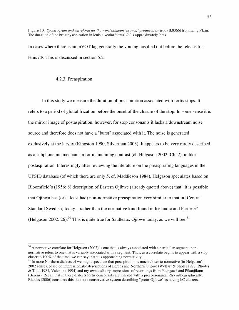
47

Figure 10. Spectrogram and waveform for the word odikoon ‗branch‘ produced by Boo (B.0366) from Long Plain. The duration of the breathy aspiration in lenis alveolar/dental /d/ is approximately 9 ms.

In cases where there is an mVOT lag generally the voicing has died out before the release for

lenis /d/. This is discussed in section 5.2.


In this study we measure the duration of preaspiration associated with fortis stops. It

refers to a period of glottal frication before the onset of the closure of the stop. In some sense it is

the mirror image of postaspiration, however, for stop consonants it lacks a downstream noise

source and therefore does not have a "burst" associated with it. The noise is generated

exclusively at the larynx (Kingston 1990, Silverman 2003). It appears to be very rarely described

as a subphonemic mechanism for maintaining contrast (cf. Helgason 2002: Ch. 2), unlike

postaspiration. Interestingly after reviewing the literature on the preaspirating languages in the

UPSID database (of which there are only 5, cf. Maddieson 1984), Helgason speculates based on

Bloomfield‟s (1956: 8) description of Eastern Ojibwe (already quoted above) that “it is possible

that Ojibwa has (or at least had) non-normative preaspiration very similar to that in [Central

Standard Swedish] today... rather than the normative kind found in Icelandic and Faroese”

(Helgason 2002: 26).30 This is quite true for Saulteaux Ojibwe today, as we will see.31

30

A normative correlate for Helgason (2002) is one that is always associated with a particular segment, non-normative refers to one that is variably associated with a segment. Thus, as a correlate begins to appear with a stop closer to 100% of the time, we can say that it is approaching normativity. 31

In more Northern dialects of we might speculate that preaspiration is much closer to normative (in Helgason's 2002 sense), based on impressionistic descriptions of Berens and Northern Ojibwe (Wolfart & Shofel 1977, Rhodes & Todd 1981, Valentine 1994) and my own auditory impressions of recordings from Paungaasi and Pikanjikum (Berens). Recall that in these dialects fortis consonants are marked with a preconsonantal <h> orthographically. Rhodes (2006) considers this the more conservative system describing "proto-Ojibwe" as having hC clusters.

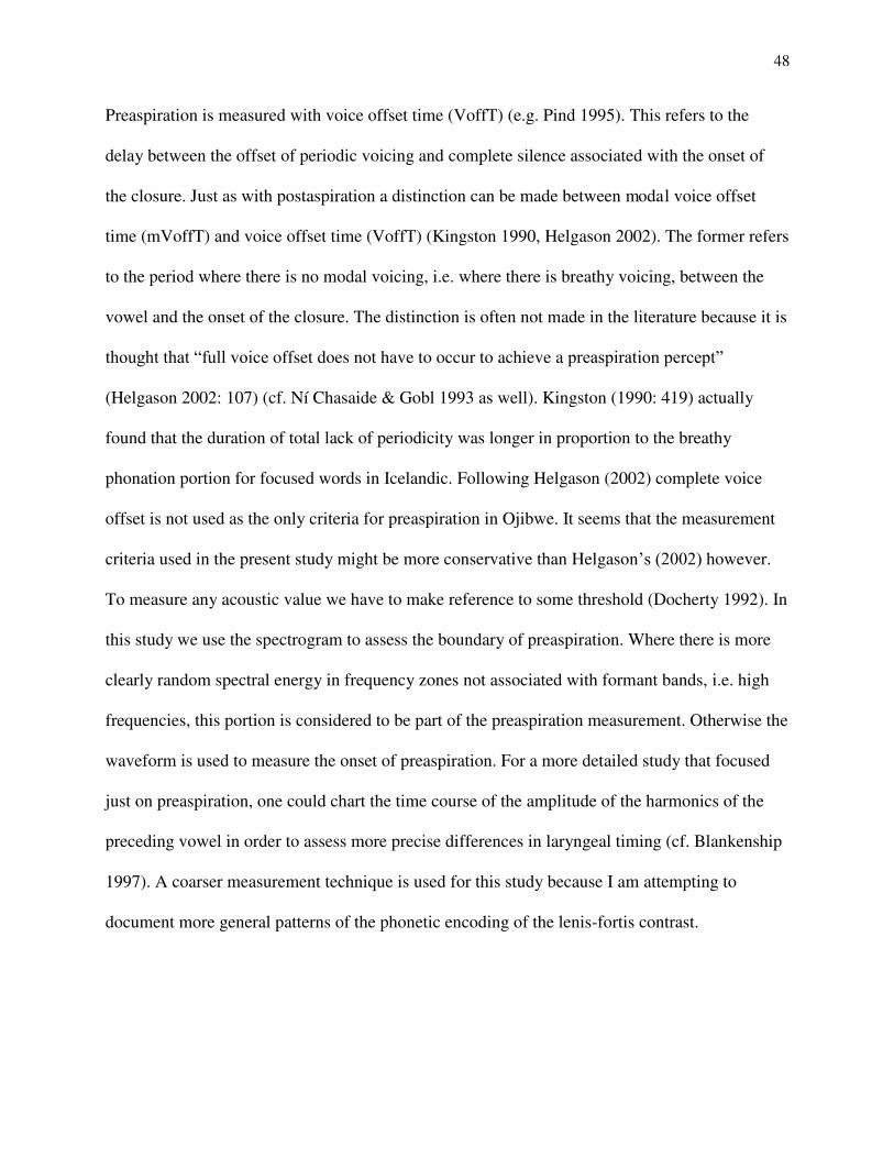
48

Preaspiration is measured with voice offset time (VoffT) (e.g. Pind 1995). This refers to the

delay between the offset of periodic voicing and complete silence associated with the onset of

the closure. Just as with postaspiration a distinction can be made between modal voice offset

time (mVoffT) and voice offset time (VoffT) (Kingston 1990, Helgason 2002). The former refers

to the period where there is no modal voicing, i.e. where there is breathy voicing, between the

vowel and the onset of the closure. The distinction is often not made in the literature because it is

thought that “full voice offset does not have to occur to achieve a preaspiration percept”

(Helgason 2002: 107) (cf. Ní Chasaide & Gobl 1993 as well). Kingston (1990: 419) actually

found that the duration of total lack of periodicity was longer in proportion to the breathy

phonation portion for focused words in Icelandic. Following Helgason (2002) complete voice

offset is not used as the only criteria for preaspiration in Ojibwe. It seems that the measurement

criteria used in the present study might be more conservative than Helgason‟s (2002) however.

To measure any acoustic value we have to make reference to some threshold (Docherty 1992). In

this study we use the spectrogram to assess the boundary of preaspiration. Where there is more

clearly random spectral energy in frequency zones not associated with formant bands, i.e. high

frequencies, this portion is considered to be part of the preaspiration measurement. Otherwise the

waveform is used to measure the onset of preaspiration. For a more detailed study that focused

just on preaspiration, one could chart the time course of the amplitude of the harmonics of the

preceding vowel in order to assess more precise differences in laryngeal timing (cf. Blankenship

1997). A coarser measurement technique is used for this study because I am attempting to

document more general patterns of the phonetic encoding of the lenis-fortis contrast.

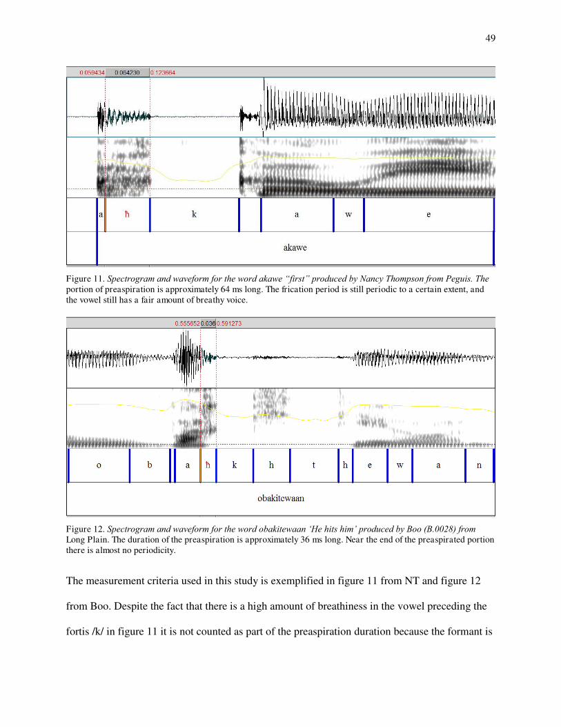
49

Figure 11. Spectrogram and waveform for the word akawe ―first‖ produced by Nancy Thompson from Peguis. The portion of preaspiration is approximately 64 ms long. The frication period is still periodic to a certain extent, and the vowel still has a fair amount of breathy voice.

Figure 12. Spectrogram and waveform for the word obakitewaan ‗He hits him‘ produced by Boo (B.0028) from Long Plain. The duration of the preaspiration is approximately 36 ms long. Near the end of the preaspirated portion there is almost no periodicity.

The measurement criteria used in this study is exemplified in figure 11 from NT and figure 12

from Boo. Despite the fact that there is a high amount of breathiness in the vowel preceding the

fortis /k/ in figure 11 it is not counted as part of the preaspiration duration because the formant is

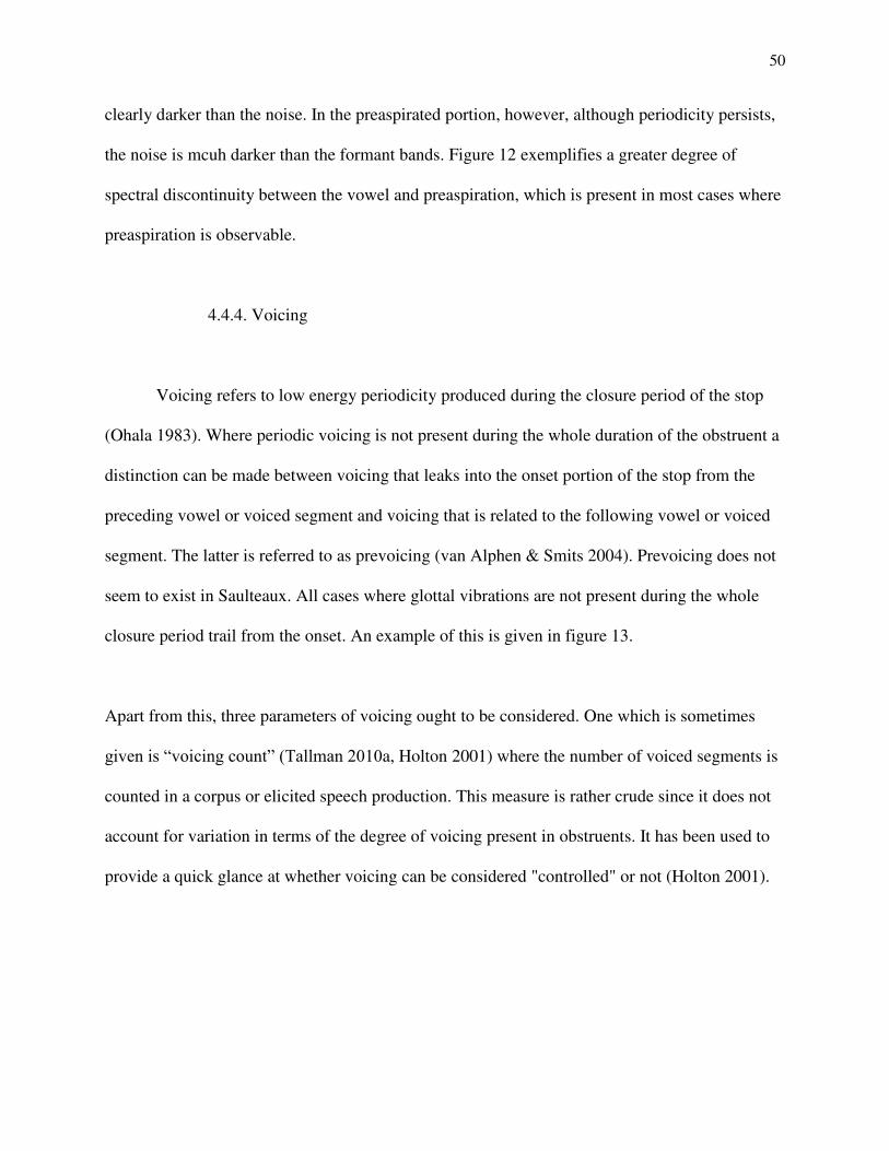
50

clearly darker than the noise. In the preaspirated portion, however, although periodicity persists,

the noise is mcuh darker than the formant bands. Figure 12 exemplifies a greater degree of

spectral discontinuity between the vowel and preaspiration, which is present in most cases where

preaspiration is observable.

4.4.4. Voicing

Voicing refers to low energy periodicity produced during the closure period of the stop

(Ohala 1983). Where periodic voicing is not present during the whole duration of the obstruent a

distinction can be made between voicing that leaks into the onset portion of the stop from the

preceding vowel or voiced segment and voicing that is related to the following vowel or voiced

segment. The latter is referred to as prevoicing (van Alphen & Smits 2004). Prevoicing does not

seem to exist in Saulteaux. All cases where glottal vibrations are not present during the whole

closure period trail from the onset. An example of this is given in figure 13.

Apart from this, three parameters of voicing ought to be considered. One which is sometimes

given is “voicing count” (Tallman 2010a, Holton 2001) where the number of voiced segments is

counted in a corpus or elicited speech production. This measure is rather crude since it does not

account for variation in terms of the degree of voicing present in obstruents. It has been used to

provide a quick glance at whether voicing can be considered "controlled" or not (Holton 2001).

51

Figure 13. Spectrogram and waveform for the word odaabaan ‗car‘ produced by Boo (B.0100) from Long Plain. The voicing for /d/ trails off near the end of the consonant. The duration of the voicing during the closure period is 61 ms.

Other measurements that quantify the physical realization of voicing are its length in

proportion to the closure duration and its intensity. In the former case we can measure the length

of the voicing portion starting from the onset of the closure. For example in figure 13 the closure

duration of /d/ is 84 ms, hence the consonant would be assigned the value 0.73 for voicing

duration.32

Intensity is measured in decibels. In terms of the lenis-fortis distinction it is practically

irrelevant for obstruent consonants, because fortis consonant are generally completely

voiceless.33 A less accurate but quicker way to measure voicing intensity is by measuring the

32

It is interesting to note, that despite voicing being described as present or not in more contemporary work, Bloomfield actually described them as "partly or wholly voiced" (1956: 8) the most accurate statement in the literature up until now. 33Leander (2008) found that in Ozolotepec Zapotec there was no significant difference in terms of intensity between laterals and only a slight difference (2 decibels) between lenis and fortis nasals in word final position, which came out as barely significant (p=.039). For Cypriot Greek lenis and fortis sonorants did show some slight differences but not always in the expected direction (Arvaniti & Tserdanelis 2000).

52

trough of the intensity contour during the consonant closure and comparing it to the intensity of

the flanking vowels.

Measuring the voicing duration and intensity are clearly preferable to the voicing count

technique, however they were not used for all speakers in this study. Voicing duration was not

recorded for any of the speakers from the Treaty #1 Oral History because these recordings

contained low amplitude (but predictable) periodic background noise, which was difficult to

distinguish from voicing in cases where the consonant was shorter than approximately 60 ms.

While it was easy to tell whether voicing was generally present or not, the background noise

introduced an intolerable level of inaccuracy to these measurements, and so there was a concern

that interspeaker comparisons would be confounded by differences in signal to noise ratio. The

other reason was that low amplitude periodic voicing can be confused with echo from the

previous vowel if recordings are not done in a sound proof room. The reason intensity was not

recorded was because the different degrees of background noise would make it difficult to

compare intensity levels across speakers.

A compromise between the crude method of voicing count and the quantitative

measurements of voicing parameters was used in this study. We assigned an ordinal value of

voicing from 0 to 5 based on visual observations of the spectrogram and waveform in relation to

its flanking vowels (henceforth “Sonority” value). That we had to use this technique is

unfortunate since we are potentially losing much rich quantitative data, but it is far superior to

the voicing count, in the sense that if there are gross differences in the degree of voicing between

speakers and POAs we can get a first approximation. (16) describes the measurement criteria and

refers the reader to spectrogram and waveform examples. The levels above 0 are perfectly

53

ordinal when applied to the data and imply increasing levels of periodic energy based on a

number of acoustic attributes.

(16) Measurement criteria for the Sonority value.

0: Assigned if the stop has no voicing or the duration of the voicing is less than

half of the duration of the closure; ~1…

1: Voicing is present for more than half of the duration of the closure; ~0, ~2….

(figure 14).

2: 1 is true and the intensity of the waveform appears to be half or more the size of

its flanking vowels; ~0, 1, ~3… (figure 15).

3: The intensity of voicing appears to be the same as its flanking vowels (the

boundaries between stop and vowel are only observable based on spectral

discontinuities, such as a change in the shape of the periodic wave instead of its

size); ~0, 1, 2, ~4… (figure 16).

4: There is no discernible boundary between the flanking vowels and the stop, but

the it can still be heard by the investigator; 3, ~5… (figure 17).

5: Assigned when the stop appears to be completely syncopated, i.e. the

researcher cannot see it in the spectrogram nor hear it; ~4.

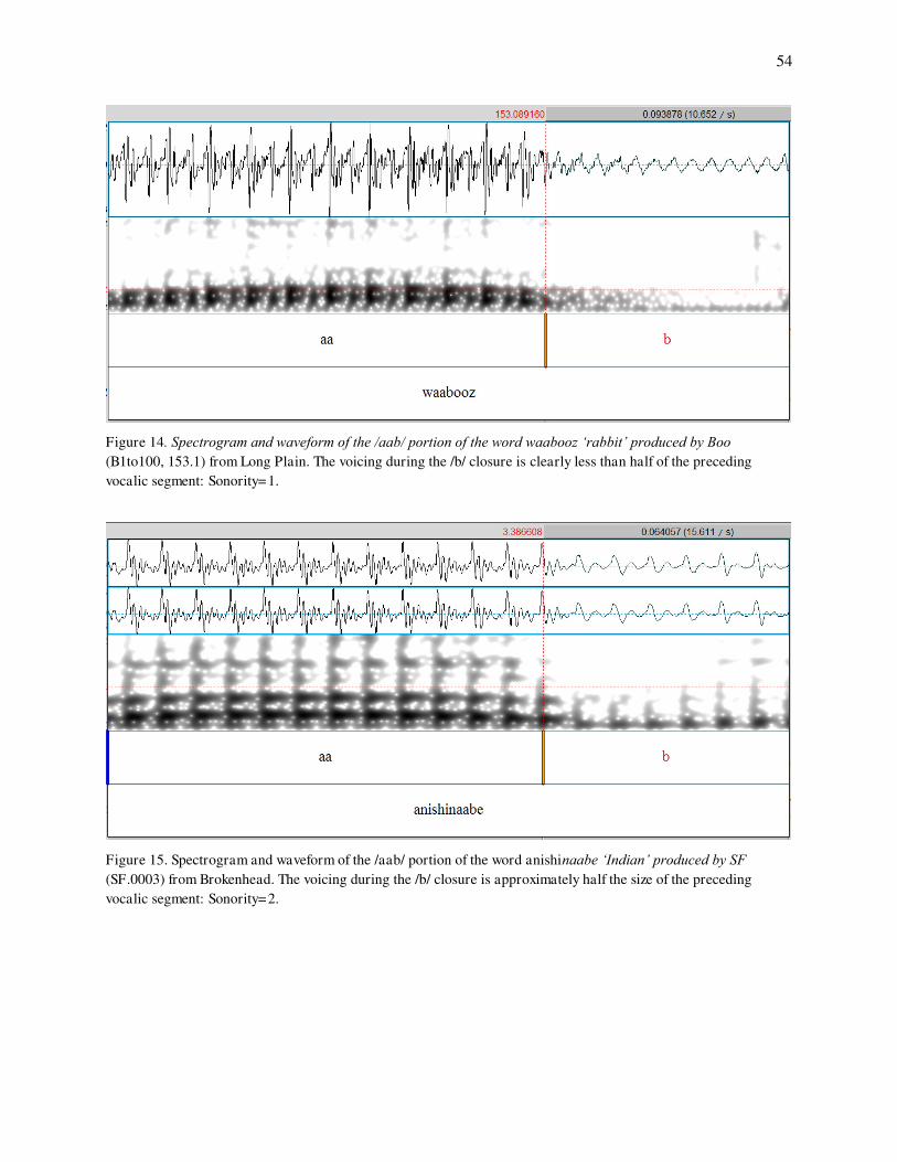
54

Figure 14. Spectrogram and waveform of the /aab/ portion of the word waabooz ‗rabbit‘ produced by Boo (B1to100, 153.1) from Long Plain. The voicing during the /b/ closure is clearly less than half of the preceding vocalic segment: Sonority=1.

Figure 15. Spectrogram and waveform of the /aab/ portion of the word anishinaabe ‗Indian‘ produced by SF (SF.0003) from Brokenhead. The voicing during the /b/ closure is approximately half the size of the preceding vocalic segment: Sonority=2.

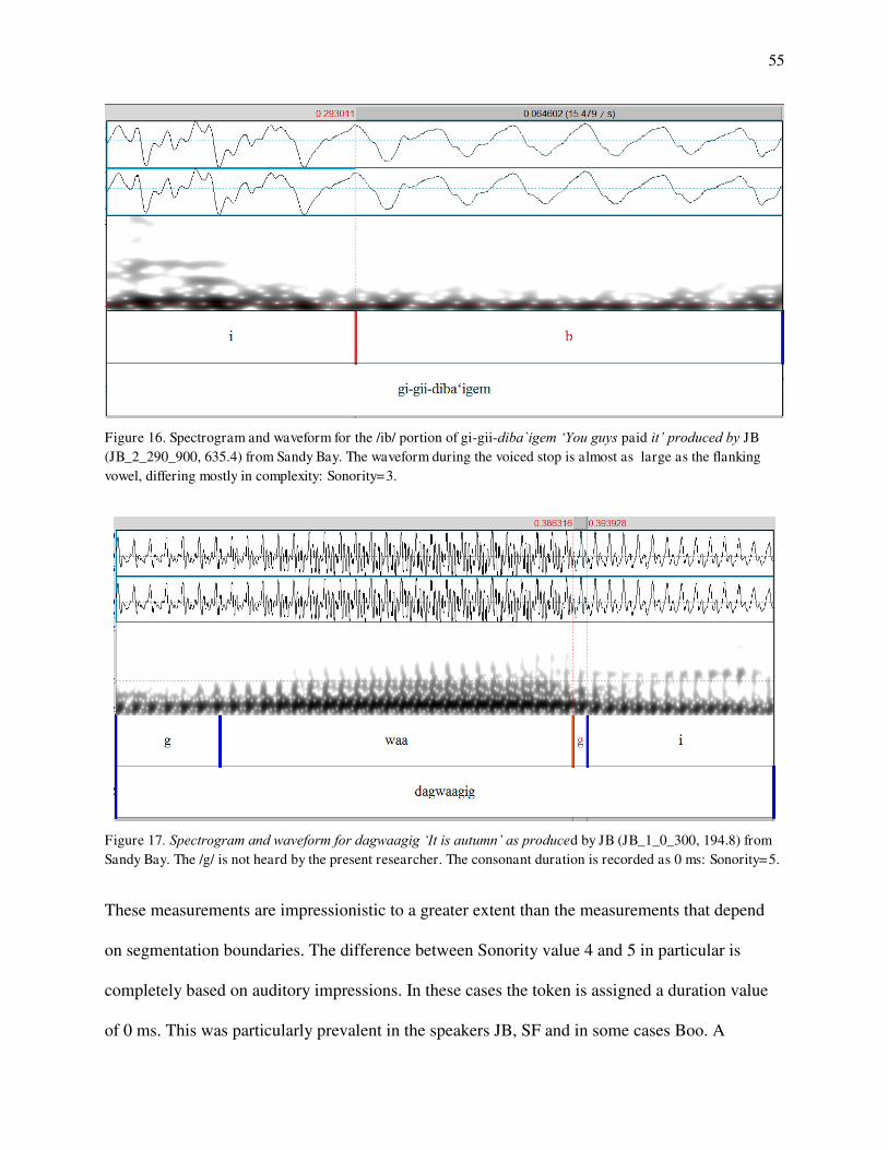
55

Figure 16. Spectrogram and waveform for the /ib/ portion of gi-gii-diba`igem ‗You guys paid it‘ produced by JB (JB_2_290_900, 635.4) from Sandy Bay. The waveform during the voiced stop is almost as large as the flanking vowel, differing mostly in complexity: Sonority=3.

Figure 17. Spectrogram and waveform for dagwaagig ‗It is autumn‘ as produced by JB (JB_1_0_300, 194.8) from Sandy Bay. The /g/ is not heard by the present researcher. The consonant duration is recorded as 0 ms: Sonority=5.

These measurements are impressionistic to a greater extent than the measurements that depend

on segmentation boundaries. The difference between Sonority value 4 and 5 in particular is

completely based on auditory impressions. In these cases the token is assigned a duration value

of 0 ms. This was particularly prevalent in the speakers JB, SF and in some cases Boo. A

56

question that needs to be addressed is whether the tokens which are essentially unrecordable in

terms of consonant duration should be included in the statistical description. This level of

undershoot is ubiquitous for some speakers. The question will be addressed in the section on

velars, since only /g/ reaches this level of undershoot.

More precise measurements of voicing were made for a few of the speakers. For Boo, the

voicing duration during the closure was recorded as in figure 13. For Boo and NT the voicing

intensity during the closure was measured at trough of the intensity curve during the closure

against the peak of the intensity curve in the flanking vowels. These data are presented, but

because they were only made with one or two speakers they are extremely tentative.

4.3. Probability Models: Description and Technical Problems

Probability models can be used to model the probability of an event occurring given a set

of factors (Liao 1994). In this section we explain how we use probability models in this study to

quantify the notion of contrast precision described in chapter 3 (4.3.1.). These probability models

entail some technical problems with data structures due to their computational complexity. My

corpus contains such data structures, and thus brief mention is given to the method adopted to

cope with the technical problems (4.3.2.).

4.3.1. Contrast Precision as a Logit Function

57

Recall in chapter three that we described phonemes as category systems, adopting

Pierrehumbert's (2001b, 2003b) terminology. This means that they encode multiple categories,

which are density distributions over a particular parameter of a multidimensional phonetic

hyperspace. To these categories we can assign a certain value of contrast precision associated

with how important a particular dimension is for predicting one phoneme (category system) over

another. This will be a function of how much overlap there is between the density distributions

on this parameter and how far apart they are. In order to quantify contrast precision as it is

defined here we use probability models.

Probability models can assess the likelihood of an event occurring given a set of factors (Liao

1994). Taking instances of lenis or fortis stops as events and their phonetic correlates as factors,

we can model the probability of a token stop being fortis as opposed to lenis (fortis= Pr(1),

lenis=Pr(0)) given a set of values associated with those phonetic correlates. These models can

tell us how important a particular density distribution (inferred from instances of phonetic

correlates) is for predicting that a stop is fortis instead of lenis. In other words, we can model

contrast precision over a particular dimension for a category of interest.

The particular probability model that we use in this thesis is the loglinear model. This model

transforms a normal regression line into an S-shaped curve that represents the change in

probability along a particular dimension as the value for that dimension increases. The values of

the dimension are modelled as the predictor variable and the probability of fortis (Y=1) over lenis

(Y=0) is modelled as the response variable. To take an example from my own data, the density

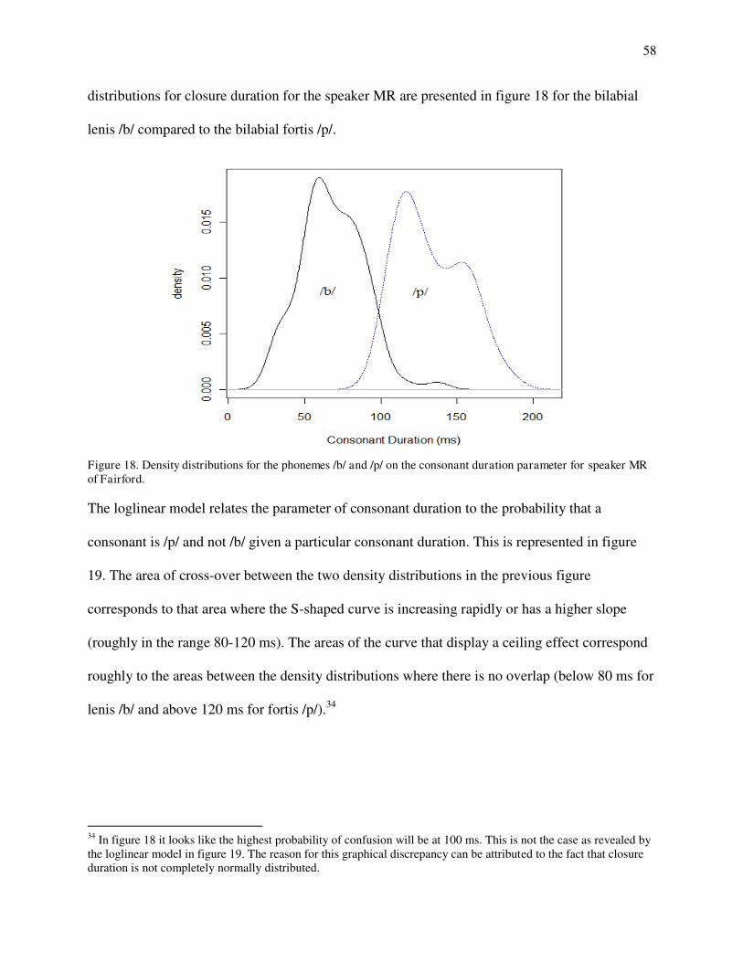
58

distributions for closure duration for the speaker MR are presented in figure 18 for the bilabial

lenis /b/ compared to the bilabial fortis /p/.

Figure 18. Density distributions for the phonemes /b/ and /p/ on the consonant duration parameter for speaker MR of Fairford. The loglinear model relates the parameter of consonant duration to the probability that a

consonant is /p/ and not /b/ given a particular consonant duration. This is represented in figure

19. The area of cross-over between the two density distributions in the previous figure

corresponds to that area where the S-shaped curve is increasing rapidly or has a higher slope

(roughly in the range 80-120 ms). The areas of the curve that display a ceiling effect correspond

roughly to the areas between the density distributions where there is no overlap (below 80 ms for

lenis /b/ and above 120 ms for fortis /p/).34

34 In figure 18 it looks like the highest probability of confusion will be at 100 ms. This is not the case as revealed by the loglinear model in figure 19. The reason for this graphical discrepancy can be attributed to the fact that closure duration is not completely normally distributed.

59

Figure 19. Loglinear curve for the /b/-/p/ contrast on the consonant duration parameter for MR of Fairford. A particular point on the curve represents the probability that a particular bilabial is /p/ and not /b/ given a particular consonant duration.

Before we describe how we can quantify contrast precision we need to first consider the

complexities involved in looking at more than one factor at a time in the model described above.

When we consider phonemes as multidimensional category systems (instead of their encoding

along just one parameter as in figure 18) we are considering how the probability increases in

relation to increases or decreases on all of its parameters (instead of one parameter at a time as in

figure 19). In this case the predictability of one parameter might be subsumed under its

relationship to another. Framing this in terms of perception, a listener may only actually need to

pay attention to one or two dimensions at a time to decide whether a stop is fortis or lenis

although other cues might be present in the signal (cf. Pothos & Close 2008). With respect to

60

production data this situation is called "multicollinearity". This occurs when two or more

predictor variables are correlated with each other with respect to a particular multiple regression

model (Baayen 2008). It implies that contrast precision between two category systems is not

necessarily an additive function of contrast precision along each of their parameters taken

individually.

Although covarying predictors may not play as strong a part in maintaining contrast

between two units they are still (by definition and/or theoretical inclination) part of the phonetic

encoding of a category system. Let us consider the example of ongoing phonetic change in

Korean (cf. Kirby 2011). In Korean the older generation, which relied mostly on VOT to make

the distinction between aspirated and lenis stops, was still encoding higher F0 associated with the

aspirated set even though in terms of making the relevant contrast it is predictable from VOT.

The new generation reversed this relationship. F0 became the primary predictor of the contrast

(Kang & Guion 2008). This would not have been possible if the older generation had not been

encoding F0 in their aspirated stops.35 Just because a correlate need not play a part in making a

contrast at some point in time does not mean it is not encoded in the category systems of the

contrasting elements. This situation implies that there is rarely a simple relationship between

contrast precision at a particular dimension in isolation (contrast between categories) and the

contrast precision of multiple factors taken at once (contrast between category systems).

One can consider either situation when one quantifies contrast precision. Although, a concern for

the latter will help us focus on what is important for speakers making the contrast between lenis

35 The reason this took place was because longer VOT is associated with higher F0 for physiological reasons (Solé 2007).

61

and fortis stops synchronically, the former case is important because those redundant parameters

have the potential to usurp the position of the main predictors. In this thesis therefore I describe

contrast precision along each parameter for the lenis-fortis pairs in isolation, in addition to

modelling contrast precision associated with the complex categories of the lenis and fortis stops.

The parameters taken in isolation are discussed in the Loglinear I section associated with each of

the contrasts grouped by place of articulation (/b/ vs. /p/, /d/ vs. /t/, /g/ vs. /k/). In Loglinear II I

discuss the parameters as multiple and potentially interacting factors in a multiple logistic

regression model.

To quantify this notion of contrast precision it necessary to give some sort of numerical

summary of the loglinear model exemplified in figure 19. There are a number of ways of doing

this (Pampel 2001). In the sections on loglinear models we use various measures to summarize

different aspects of the relationship defined by loglinear models. These act as different measures

of contrast precision. They are defined and justified below. The first three are different types of

measures that are based on the predicted probabilities of the loglinear models (using the predict()

function in R (cf. Chambers & Hastie 1992)) and the fourth is based on the coefficient associated

the predictor variable (cf. Pampel 2001, Gelman & Hill 2007).

R2: This is a measure of association between the dummy variables (lenis: Y=0, fortis: Y=1) and

the predicted probabilities of the logistic regression model. There are various ways of measuring

R2 but the method adopted here is fairly simplistic and specific to our purposes (Lewis-Beck

1980, Berry 1993). Our only interest is that we want to know how close the predicted

probabilities for lenis stops are to 0 and how close the fortis stops are to 1. We measure this by

62

taking the mean of the predicted probabilities associated with 0 and the mean of the predicted

probabilities associated with 1 and then subtracting the latter from the former. This method thus

tells us how close each token of a lenis/fortis stop was to perfect prediction overall.

k: This is also a measure of association between the dummy variables (lenis: Y=0, fortis: Y=1)

and the predicted probabilities of the logistic regression model. Kendall's k is a rank correlation

that measures concordance in relation to discordance (Kendall & Gibbons 1990). The coefficient

will be higher the less discordance there is. Rank correlations are often used to summarize

logistic regression models (e.g. Baayen 2008). They are advantageous because we do not commit

a specification error when using them on data which are not normally distributed, as opposed to

R2 (Lewis-Beck 1980, Berry 1993). They oversimplify the relationship by not telling us how

close the predicted probabilities are to perfect prediction (0 in the case of lenis stops, 1 in the

case of fortis stops). They are also only concerned with whether the variables increase or

decrease together, not where the increase or decrease takes place.

Accuracy: This is a measure of the proportion of lenis/fortis tokens that were classified correctly

based on their predicted probabilities in relation to some threshold (cf. van Rijsbergen 1979). In

this study we let the threshold be Pr(0.5) corresponding to the highest probability of confusion. If

the predicted probability of a lenis falls below 0.5 then it is classified correctly, otherwise not. If

the predicted probability of a fortis is above 0.5 then it classified correctly, otherwise not. Then

we calculate at the proportion of lenis and fortis tokens classified correctly in relation to the total

amount of tokens for each group. Then, we add these two classification percentages together and

63

divide by two. The latter method is used because we do not have equal proportions of lenis to

fortis stops for each POA and speaker.

Slope: This is a measure of the slope of the loglinear regression line at the highest probability of

confusion for a given predictor. It cannot summarize models with more than one factor but it can

give us a good idea of how sharp the category boundary between two density distributions is for

a given parameter. It corresponds more directly to how much two density distributions overlap.

Although it is interesting to look at when we compare speakers in terms of their contrast

precision along a particular parameter, it is difficult to use as a measure of contrast precision for

comparing correlates that have different variances and density functions (e.g. skewed as opposed

to normally distributed). We use it to describe contrast precision on one dimension at a time

(Pampel 2001, Gelman & Hill 2007). It becomes a useful measure of contrast precision when the

variables are standardized, otherwise it is difficult to interpret.

Two other statistical terms will be used throughout this thesis. In the second loglinear

regression subsection of each main section in the following chapter we use multiple regression

models to help us understand contrast as it manifests itself on a multidimensional category

system level. The following technical terms will be important for understanding that section.

Interaction: This refers generically to cases where the combined effects of two variables is not a

simple sum of their separate effects in a regression model (Dodge 2003). With respect to

complex categories this usually implies that two categories are predicting the contrast

redundantly to a certain extent. This aspect of complex categories is important because it means

64

that categories that participate in making a contrast do not operate in perfect trading relations

with each other all the time, where the absence or loss of the contrast precision of one category

implies the increase of another. In the chapters which follow there are some cases, where models

for contrasting category systems will include interaction terms to account for multicollinearity

between factors (cf. Jaccard 2001).

Akaike Information Criterion (AIC): The AIC is based on the concept of information entropy.

Basically it measures the amount of information loss associated with applying a particular model

to explain data. This is used to assess the best fitted model for each speaker in the relevant

section. Ideally it could be used as a measurement of contrast precision (preferably with other

information-theoretic criteria (cf. Anderson 2008)). However we have different sample sizes

according to speaker in many cases. Since the AIC is based on information loss this makes it an

unreliable measure of contrast precision for comparing speakers. We use it here to select the best

model in each speaker for the relevant contrast. The lowest AIC corresponds to the best model.

The measurements of contrast precision based on predicted probabilities (R2, k, Accuracy

described above) are then selected from the best model (cf. Anderson 2008, Burnham &

Anderson 2002).

4.3.2. Separation

There is a technical problem associated with applying loglinear models to certain data

structures. Separation occurs when the data between two frequency distributions do not overlap.

Observe the following the figure 20a and 20b.

65

Figure 20a (left). Hypothetical example of quasi-separate data structure. Figure 20b (right). Hypothetical example of completely-separate data structure.

There are two types; Quasi-separation occurs when they overlap on one unit of the predictor

variable but do not cross. Complete separation occurs when the frequency distributions do not

overlap at all. Quasi-separation and complete separation are exemplified in the diagrams above.

In figure 20a the frequency distributions of the variables y1 and y2 are overlapping on one unit.

In figure 20b the frequency distributions are completely separated from each other. Both of these

situations are problematic for the algorithm that estimates coefficients in logistic regression

models. Models that attempt to estimate parameters with data with this type of structure do not

converge (Allison 2004, 2008).36

36 Consider the formula for a loglinear regression below. ln (P i / P i - 1)= g + く1x1 + く2x2 ..... くnxn

The actual values for P i in this formula are attained through maximum likelihood estimation. For the logistic model an algorithm produces the く coefficients that produce P i values that maximize the logged likelihood function (lnLF) in the following formula.

ln LF = ∑ [Yi * lnP i] + [ (1 – Yi) * ln(1 – P i)] . (Pampel 2001: 43) The Newton-Raphston algorithm solves the equation by selecting coefficients that make this function the largest (cf. Allison 2004, 2008). The process is repeated until the maximum modification for each parameter estimate from one iteration to the next is smaller than some criterion, considered the convergence point of the algorithm. However, there are certain types of data for which the algorithm does not converge. For instance, if we consider a case where

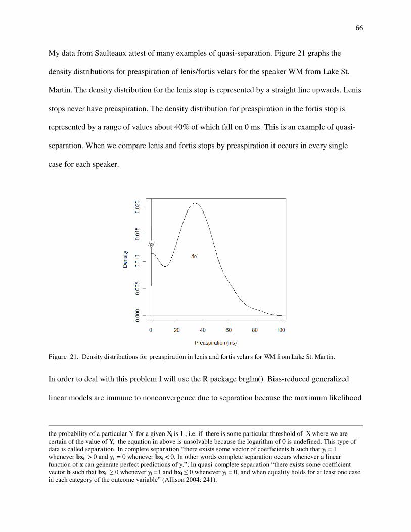
66

My data from Saulteaux attest of many examples of quasi-separation. Figure 21 graphs the

density distributions for preaspiration of lenis/fortis velars for the speaker WM from Lake St.

Martin. The density distribution for the lenis stop is represented by a straight line upwards. Lenis

stops never have preaspiration. The density distribution for preaspiration in the fortis stop is

represented by a range of values about 40% of which fall on 0 ms. This is an example of quasi-

separation. When we compare lenis and fortis stops by preaspiration it occurs in every single

case for each speaker.

Figure 21. Density distributions for preaspiration in lenis and fortis velars for WM from Lake St. Martin.

In order to deal with this problem I will use the R package brglm(). Bias-reduced generalized

linear models are immune to nonconvergence due to separation because the maximum likelihood

the probability of a particular Yi for a given Xi is 1 , i.e. if there is some particular threshold of X where we are certain of the value of Y, the equation in above is unsolvable because the logarithm of 0 is undefined. This type of data is called separation. In complete separation “there exists some vector of coefficients b such that yi = 1 whenever bxi > 0 and yi = 0 whenever bxi < 0. In other words complete separation occurs whenever a linear function of x can generate perfect predictions of y.”; In quasi-complete separation “there exists some coefficient vector b such that bxi ≥ 0 whenever yi =1 and bxi ≤ 0 whenever yi = 0, and when equality holds for at least one case in each category of the outcome variable” (Allison 2004: 241).

67

estimation is always reached (Kosmidis 2011, cf. n37 above). It has recently been applied

successfully to a number of fields that model data using loglinear or similar models (e.g. Heinze

& Schemper 2004). Bias-reduction is used in this study because of the ubiquity of separation in

my data (in preaspiration, in the Sonority value, and at times in postaspiration).

5. Phonetic Encoding II: Places of Articulation

This chapter describes the acoustic correlates of lenis and fortis stops taking one place of

articulation at a time. From this point on when I say that a particular correlate comes out as

(non)significant, I mean specifically that it is (non)significant in a loglinear model where lenis

and fortis tokens are modelled as the dummy response variables (lenis: Y=0, fortis: Y=1). The

loglinear model subsections for each POA section discuss the different measures of contrast

precision described in the previous chapter for each correlate taken individually.

5.1. Bilabials: /b/-/p/

This section describes the acoustic correlates of the lenis-fortis contrast in intervocalic

bilabials as represented in the elicitation and corpus data. I assess the effect of each correlate

individually. We give the means, standard deviations and proportional differences as measured

from the means of the frequency distributions between lenis and fortis stops along each of the

parameters: Consonant duration (5.1.1), postaspiration (5.1.2), preaspiration (5.1.3) and voicing

(5.1.4). Then we describe the contrast precision measures from our loglinear regression models

68

for each parameter comparing the extent to which these parameters correspond (5.1.5).37 The

second loglinear section discusses the contrast when lenis and fortis stops are viewed as category

systems containing all the aforementioned dimensions simultaneously (5.1.6). I choose the best

model for each speaker.

One problem needs to be mentioned before we display the results. Fortis bilabials are by far the

most infrequent of the stop consonants discussed in this study. This is a problem for models that

include more than one factor. The data from NT for example should be looked upon with more

scepticism. It is generally recommended that we have ten events per independent variable for

logistic regression (e.g. Agresti 2007). This benchmark is not met with NT. Through her whole

story there are only 9 tokens of intervocalic fortis /p/ and 30 tokens of /b/ or /p/ in total. The data

from SF is also problematic in this regard. There are only 21 tokens of fortis /p/ in 35 minutes of

conversation and many of them are from high frequency particles (81 tokens of lenis /b/ were

gathered). The conclusions based on the data from NT and SF are much more tentative than the

data from other speakers. Multiple regression models are not applied to data from these speakers

for bilabials.

37 One might argue that this discussion is unnecessary because we should only be interested in contrast precision between whole category systems, since these are the real linguistic elements of contrast. We are more generally interested in the contrast between phonemes not a hypothetical contrast between the phonetic dimensions of a phoneme. Dimensions which do not seem to be operative in terms of contrasts between category systems are still part of the phonetic encoding of those category systems, however. In fact, in certain circumstances they form the basis of phonetic change. One dimension where the contrast is encoded redundantly can supersede the main effect eventually and become the primary correlate of the contrast. This is essentially what has been described for Korean ( Kirby 2011, cf. chapter 3 of this thesis). Thus, proper description of redundant phonetic encoding is necessary if we are to document processes of phonetic change.

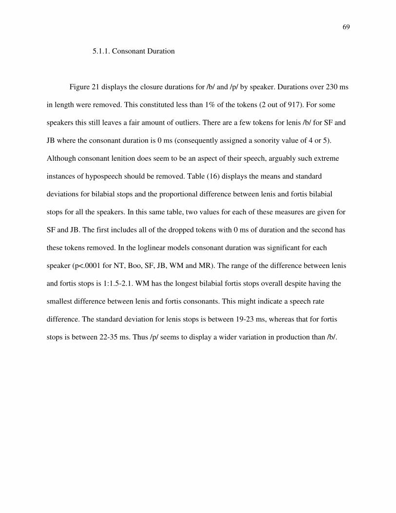
69


Figure 21 displays the closure durations for /b/ and /p/ by speaker. Durations over 230 ms

in length were removed. This constituted less than 1% of the tokens (2 out of 917). For some

speakers this still leaves a fair amount of outliers. There are a few tokens for lenis /b/ for SF and

JB where the consonant duration is 0 ms (consequently assigned a sonority value of 4 or 5).

Although consonant lenition does seem to be an aspect of their speech, arguably such extreme

instances of hypospeech should be removed. Table (16) displays the means and standard

deviations for bilabial stops and the proportional difference between lenis and fortis bilabial

stops for all the speakers. In this same table, two values for each of these measures are given for

SF and JB. The first includes all of the dropped tokens with 0 ms of duration and the second has

these tokens removed. In the loglinear models consonant duration was significant for each

speaker (p<.0001 for NT, Boo, SF, JB, WM and MR). The range of the difference between lenis

and fortis stops is 1:1.5-2.1. WM has the longest bilabial fortis stops overall despite having the

smallest difference between lenis and fortis consonants. This might indicate a speech rate

difference. The standard deviation for lenis stops is between 19-23 ms, whereas that for fortis

stops is between 22-35 ms. Thus /p/ seems to display a wider variation in production than /b/.

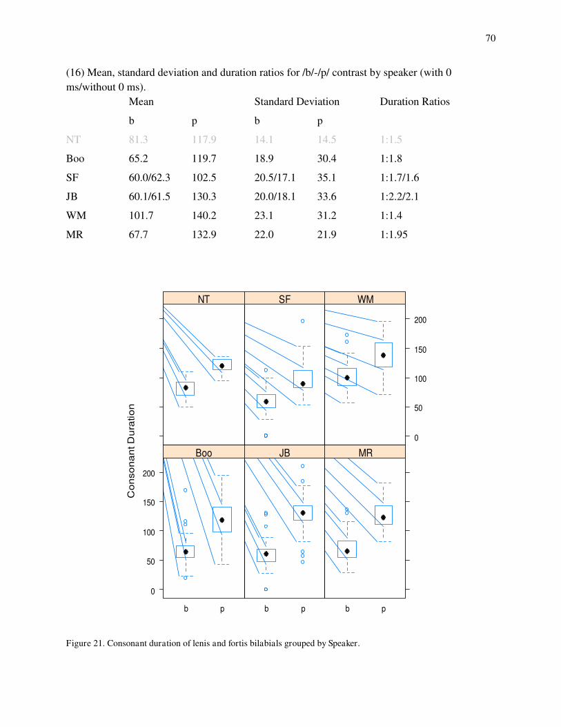
70

(16) Mean, standard deviation and duration ratios for /b/-/p/ contrast by speaker (with 0 ms/without 0 ms). Mean Standard Deviation Duration Ratios

b p b p

NT 81.3 117.9 14.1 14.5 1:1.5

Boo 65.2 119.7 18.9 30.4 1:1.8

SF 60.0/62.3 102.5 20.5/17.1 35.1 1:1.7/1.6

JB 60.1/61.5 130.3 20.0/18.1 33.6 1:2.2/2.1

WM 101.7 140.2 23.1 31.2 1:1.4

MR 67.7 132.9 22.0 21.9 1:1.95

Figure 21. Consonant duration of lenis and fortis bilabials grouped by Speaker.

Co

nso

na

nt D

ura

tio

n

0

50

100

150

200

b p

Boo

b p

JB

b p

MR

NT SF

0

50

100

150

200

WM

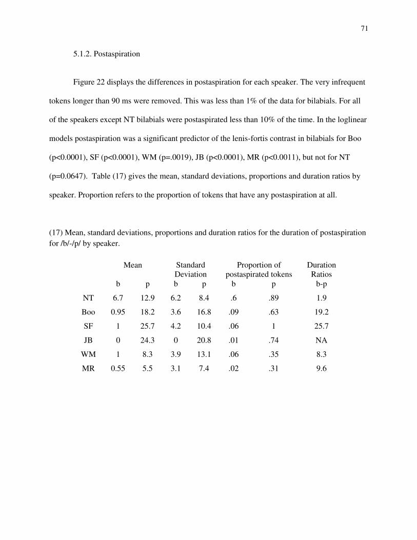
71


Figure 22 displays the differences in postaspiration for each speaker. The very infrequent

tokens longer than 90 ms were removed. This was less than 1% of the data for bilabials. For all

of the speakers except NT bilabials were postaspirated less than 10% of the time. In the loglinear

models postaspiration was a significant predictor of the lenis-fortis contrast in bilabials for Boo

(p<0.0001), SF (p<0.0001), WM (p=.0019), JB (p<0.0001), MR (p<0.0011), but not for NT

(p=0.0647). Table (17) gives the mean, standard deviations, proportions and duration ratios by

speaker. Proportion refers to the proportion of tokens that have any postaspiration at all.

(17) Mean, standard deviations, proportions and duration ratios for the duration of postaspiration for /b/-/p/ by speaker.

Mean Standard Deviation

Proportion of postaspirated tokens

Duration Ratios

b p b p b p b-p

NT 6.7 12.9 6.2 8.4 .6 .89 1.9

Boo 0.95 18.2 3.6 16.8 .09 .63 19.2

SF 1 25.7 4.2 10.4 .06 1 25.7

JB 0 24.3 0 20.8 .01 .74 NA

WM 1 8.3 3.9 13.1 .06 .35 8.3

MR 0.55 5.5 3.1 7.4 .02 .31 9.6

72

Figure 22. Postaspiration duration by lenis and fortis bilabials grouped by Speaker.

Postaspiration appears to be more important for Boo, JB and SF, than for the other speakers. The

consistency with which a speaker uses postaspiration to make the contrast can generally be

gleaned from observing a quantile-quantile plot of postaspiration in fortis bilabials (figure 23).

The more tokens clustered around 0 ms the speaker has the less important postaspiration is for

the speaker. There is quite a bit of variation between speakers in terms of the degree normativity

(in Helgason's 2002 sense).

Po

st A

sp

ira

tio

n

0

20

40

60

b p

Boo

b p

JB

b p

MR

NT SF

0

20

40

60

WM

73

Figure 23. Quantile-quantile plots for postaspiration duration in fortis /p/s grouped by Speaker.


Preaspiration is a non-normative acoustic correlate for bilabial fortis stops.38 It does not

consistently mark fortis stops and it never occurs with the lenis set. Quantile-quantiles plots for

preaspiration duration in /p/s by speaker are given in figure 24. demonstrates that in the majority

of cases there is no preaspiration on fortis bilabial stops, but that this varies from speaker to

speaker. (18) gives mean, and standard deviation values for preaspiration. It also gives the

38 A particular correlate is normative where it is marked consistently on a particular phoneme or phoneme class (cf. Helgason 2002). Cross-linguistically preaspiration is often non-normative in this sense. It clearly distinguishes one class from another but is not always present. Itanyuso Trique (Zapotec) is an exception (DiCanio 2008). Some lenis consonants in Itanyuso Trique are preaspirated.

qnorm

Po

sta

sp

ira

tio

n D

ura

tio

n

0

20

40

60

-2 -1 0 1 2

Boo JB

-2 -1 0 1 2

MR

NT

-2 -1 0 1 2

SF

0

20

40

60

WM

74

proportion of fortis bilabials that have any preaspiration at all for each speaker. In the logistic

regression models only WM came out as significant for preaspiration (p=0.0048). The rest of the

speakers' models were not significant.

Figure 24. Quantile-quantile plot of preaspiration in fortis bilabials grouped by Speaker.

qnorm

Fre

qu

en

cy: P

rea

sp

ira

tio

n

0

50

100

150

-2 -1 0 1 2

Boo JB

-2 -1 0 1 2

MR

NT

-2 -1 0 1 2

SF

0

50

100

150

WM

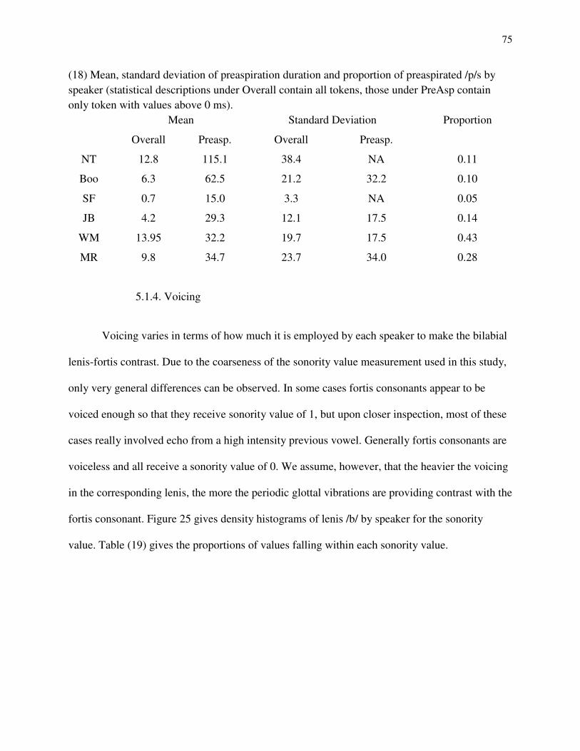
75

(18) Mean, standard deviation of preaspiration duration and proportion of preaspirated /p/s by speaker (statistical descriptions under Overall contain all tokens, those under PreAsp contain only token with values above 0 ms).

Mean Standard Deviation Proportion

Overall Preasp. Overall Preasp.

NT 12.8 115.1 38.4 NA 0.11

Boo 6.3 62.5 21.2 32.2 0.10

SF 0.7 15.0 3.3 NA 0.05

JB 4.2 29.3 12.1 17.5 0.14

WM 13.95 32.2 19.7 17.5 0.43

MR 9.8 34.7 23.7 34.0 0.28

5.1.4. Voicing

Voicing varies in terms of how much it is employed by each speaker to make the bilabial

lenis-fortis contrast. Due to the coarseness of the sonority value measurement used in this study,

only very general differences can be observed. In some cases fortis consonants appear to be

voiced enough so that they receive sonority value of 1, but upon closer inspection, most of these

cases really involved echo from a high intensity previous vowel. Generally fortis consonants are

voiceless and all receive a sonority value of 0. We assume, however, that the heavier the voicing

in the corresponding lenis, the more the periodic glottal vibrations are providing contrast with the

fortis consonant. Figure 25 gives density histograms of lenis /b/ by speaker for the sonority

value. Table (19) gives the proportions of values falling within each sonority value.

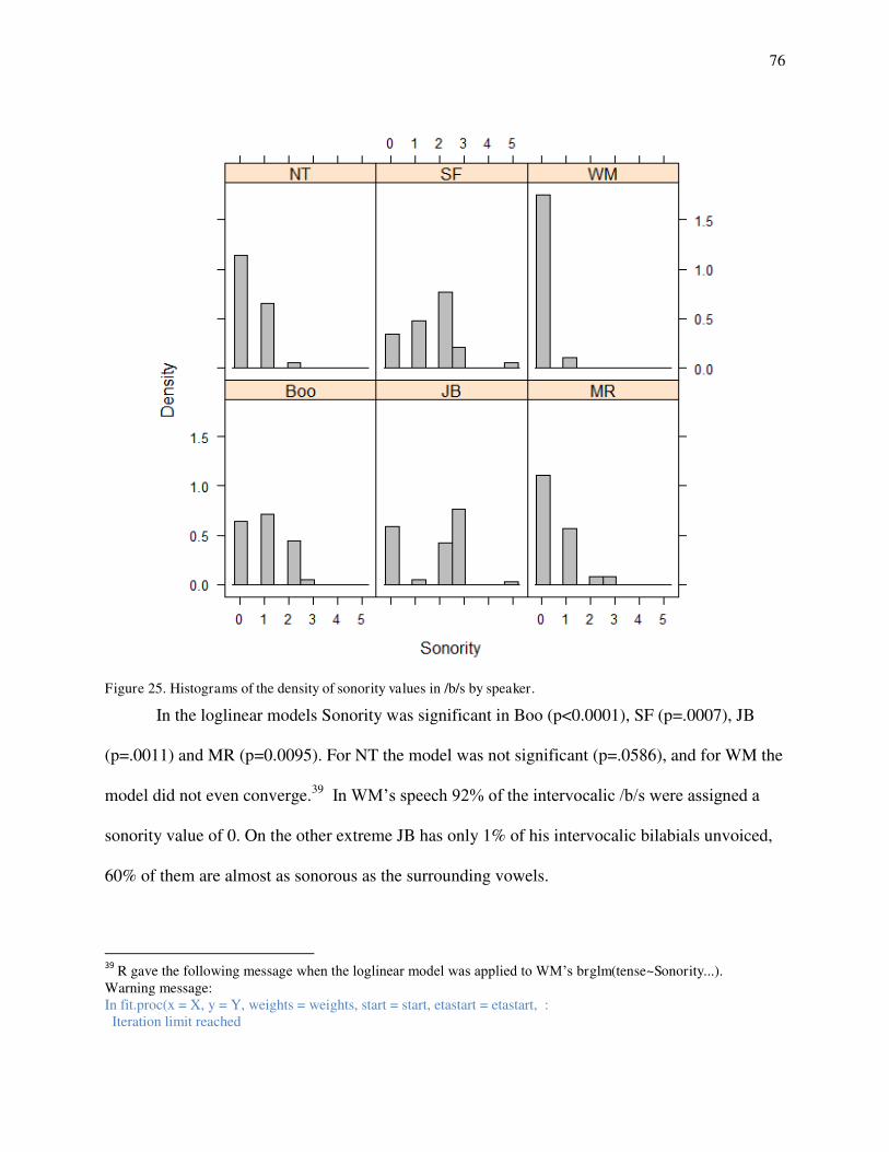
76

Figure 25. Histograms of the density of sonority values in /b/s by speaker.

In the loglinear models Sonority was significant in Boo (p<0.0001), SF (p=.0007), JB

(p=.0011) and MR (p=0.0095). For NT the model was not significant (p=.0586), and for WM the

model did not even converge.39 In WM‟s speech 92% of the intervocalic /b/s were assigned a

sonority value of 0. On the other extreme JB has only 1% of his intervocalic bilabials unvoiced,

60% of them are almost as sonorous as the surrounding vowels.

39

R gave the following message when the loglinear model was applied to WM‟s brglm(tense~Sonority...). Warning message: In fit.proc(x = X, y = Y, weights = weights, start = start, etastart = etastart, : Iteration limit reached

77

(19) Sonority value proportions of /b/ by speaker.

0 1 2 3 4 5

NT 0.5 0.46 0.04 0 0 0

Boo 0.03 0.57 0.37 0.04 0 0

SF 0.04 0.31 0.48 0.14 0 0.04

JB 0.01 0.04 0.33 0.60 0 0.02

WM 0.92 0.8 0 0 0 0

MR 0.49 0.40 0.06 0.06 0 0

Notice also that these differences correspond roughly to the consonant duration differences noted

in 5.1.1. For example, JB has the greatest difference in voicing and the greatest in consonant

duration differences (1:2.1). WM has the least difference in voicing and the least difference in

consonant durations (1:1.4). There are physical reasons for expecting this difference, since it is

harder to maintain voicing beyond certain closure durations (Ohala 1983).

Values were measured for voicing intensity when there was not a large amount of background

noise for NT and Boo. For these speakers the voicing intensity measurements correspond to the

sonority value differences. For the voicing intensity ratios Boo had a mean of 0.8533

(sd=0.0522) and NT had a mean of 0.6160 (sd=0.1542) .


In this section we compare the different measures of contrast precision along each of the

phonetic dimensions described above for the contrast between /b/-/p/. We rank the speakers in

terms of the importance of each correlate based on these measures of contrast precision seeing to

what degree these rankings correspond with the more basic statistical descriptions given above

78

(e.g., proportional difference between means, proportions of preaspirated segments, etc…) and

with each other. Where we see noncorrespondences between these different measures we try to

explain them based on the statistical structure of the relevant category at each parameter.

Although overall the patterns correspond, there is often much discordance between the rankings

because the variation between speakers can be fairly subtle. We limit our scope to discussing the

speakers with the worst and best models for a given correlate in the particular rankings of

contrast precision. When rankings of these speakers do not correspond we attempt to explain

why. NT is presented in the charts but should not be taken too seriously because of the small

sample size in bilabials for this speaker.

5.1.5.1. Consonant Duration

The measures of contrast precision are given in (20) and the rankings of the speakers in (21).

(20) Measures of contrast precision for /b/ vs. /p/ on consonant duration by speaker.

Proportional difference

R2 k Slope Accuracy

NT 1:1.5 .6860 .6062 .0346 .8681

Boo 1:1.8 .6170 .5953 .0209 .7464

SF 1:1.7/1.6 .3967 .4247 .02095 .6877

JB 1:2.2/2.1 .7217 .5929 .0197 .9124

WM 1:1.4 .3580 .4457 .0128 .7260

MR 1:1.95 .8283 .5919 .0357 .9481

79

(21) Rankings of speakers by measure of contrast precision in (20).

Ratio from

means

R2 k Slope Accuracy

WORST WM WM SF WM SF

NT SF WM JB WM

SF Boo JB Boo Boo

Boo NT Boo SF NT

MR JB MR NT JB

BEST JB MR NT MR MR

Closure duration is the worst predictor for WM compared to the other speakers in all measures

except for k coefficient and Accuracy. k measures discordance against concordance in a ranking

of the tokens without consideration for distance between the tokens. Thus, k descends faster than

any other measure as the category distributions overlap more, which accounts for this difference.

Thus, we can see that SF is worse than WM because SF has large standard deviations in relation

to the mean for the contrasting distributions (by measuring sd/mean for each category). For SF

this is .34 for /b/ and /p/ and for WM this ratio is .23 and .22.

Closure duration is the best predictor for MR compared to the other speakers. JB's proportional

differences, however, are greater than those for MR. Contrast precision is worse for JB on this

parameter because his categories overlap more in relation to their distance.40 This can be seen by

comparing the categories of JB in figure 26a and 26b for the categories of MR on the consonant

duration parameter. The ratios of standard deviation to mean are .33 and .26 for JB and .32 and

.16 for MR. This difference corresponds to JBs lower slope compared to the other speakers in

40 In fact from the density distributions in figures 26a and 26b it looks as if JB's category encoded with /p/ on the closure duration parameter might have multimodal structure. This implies that there may be hard interactions with other factors in JBs complex category.

80

general (ranking second). The probability that a particular stop token gets recognized as fortis

based on closure duration rises by 3.5% for every 1 ms of difference at the highest probability of

confusion. For JB it rises slower near the overlapping distributions, at 1% per 1 ms.

Figure 26a (left). Categories for /b/ and /p/ on consonant duration for WM. Figure 26b (right). Categories for /b/ and /p/ on consonant duration for WM.

5.1.5.2. Postaspiration

The measures of contrast precision are given in (22) and the rankings of the speakers by

measurement in (23). The difference in proportions is measured by taking the proportion of

postaspirated fortis tokens minus the proportion of postaspirated lenis tokens.

(22) Measures of contrast precision for /b/ vs./p/ on postaspiration by speaker.

Difference in proportions

R2 k Slope Accuracy

NT .29 .141 .317 .0292 .5347

Boo .54 .413 .573 .0395 .7966

SF .94 .763 .827 .0664 .9210

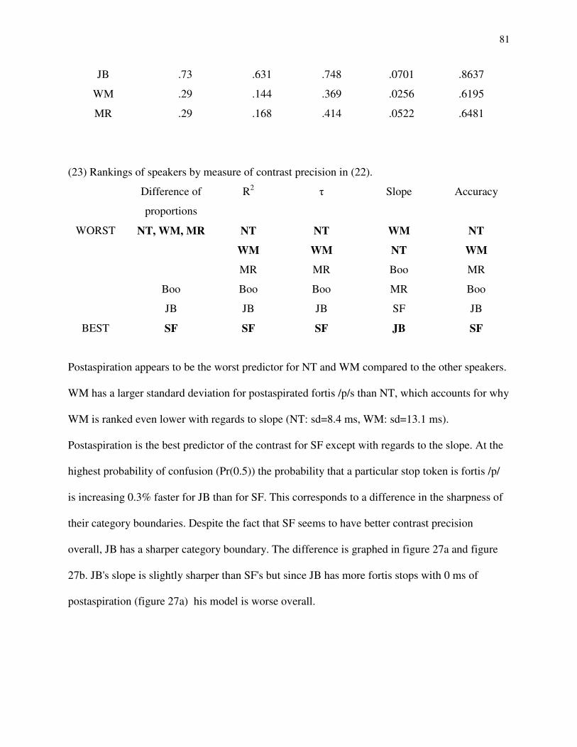
81

JB .73 .631 .748 .0701 .8637

WM .29 .144 .369 .0256 .6195

MR .29 .168 .414 .0522 .6481


Difference of

proportions

R2 k Slope Accuracy

WORST NT, WM, MR NT NT WM NT

WM WM NT WM

MR MR Boo MR

Boo Boo Boo MR Boo

JB JB JB SF JB

BEST SF SF SF JB SF

Postaspiration appears to be the worst predictor for NT and WM compared to the other speakers.

WM has a larger standard deviation for postaspirated fortis /p/s than NT, which accounts for why

WM is ranked even lower with regards to slope (NT: sd=8.4 ms, WM: sd=13.1 ms).

Postaspiration is the best predictor of the contrast for SF except with regards to the slope. At the

highest probability of confusion (Pr(0.5)) the probability that a particular stop token is fortis /p/

is increasing 0.3% faster for JB than for SF. This corresponds to a difference in the sharpness of

their category boundaries. Despite the fact that SF seems to have better contrast precision

overall, JB has a sharper category boundary. The difference is graphed in figure 27a and figure

27b. JB's slope is slightly sharper than SF's but since JB has more fortis stops with 0 ms of

postaspiration (figure 27a) his model is worse overall.

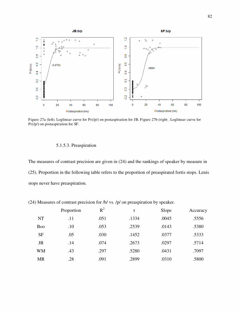
82

Figure 27a (left). Loglinear curve for Pr(/p/) on postaspiration for JB. Figure 27b (right . Loglinear curve for Pr(/p/) on postaspiration for SF.

5.1.5.3. Preaspiration

The measures of contrast precision are given in (24) and the rankings of speaker by measure in

(25). Proportion in the following table refers to the proportion of preaspirated fortis stops. Lenis

stops never have preaspiration.

(24) Measures of contrast precision for /b/ vs. /p/ on preaspiration by speaker.

Proportion R2 k Slope Accuracy

NT .11 .051 .1334 .0045 .5556

Boo .10 .053 .2539 .0143 .5380

SF .05 .030 .1452 .0377 .5333

JB .14 .074 .2673 .0297 .5714

WM .43 .297 .5280 .0431 .7097

MR .28 .091 .2899 .0310 .5800

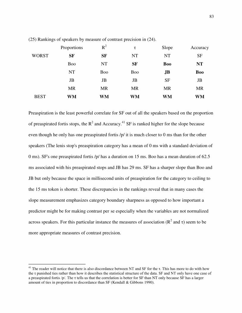
83


Proportions R2 k Slope Accuracy

WORST SF SF NT NT SF

Boo NT SF Boo NT

NT Boo Boo JB Boo

JB JB JB SF JB

MR MR MR MR MR

BEST WM WM WM WM WM

Preaspiration is the least powerful correlate for SF out of all the speakers based on the proportion

of preaspirated fortis stops, the R2 and Accuracy.41 SF is ranked higher for the slope because

even though he only has one preaspirated fortis /p/ it is much closer to 0 ms than for the other

speakers (The lenis stop's preaspiration category has a mean of 0 ms with a standard deviation of

0 ms). SF's one preaspirated fortis /p/ has a duration on 15 ms. Boo has a mean duration of 62.5

ms associated with his preaspirated stops and JB has 29 ms. SF has a sharper slope than Boo and

JB but only because the space in millisecond units of preaspiration for the category to ceiling to

the 15 ms token is shorter. These discrepancies in the rankings reveal that in many cases the

slope measurement emphasizes category boundary sharpness as opposed to how important a

predictor might be for making contrast per se especially when the variables are not normalized

across speakers. For this particular instance the measures of association (R2 and k) seem to be

more appropriate measures of contrast precision.

41 The reader will notice that there is also discordance between NT and SF for the k. This has more to do with how the k punished ties rather than how it describes the statistical structure of the data. SF and NT only have one case of a preaspirated fortis /p/. The k tells us that the correlation is better for SF than NT only because SF has a larger amount of ties in proportion to discordance than SF (Kendall & Gibbons 1990).

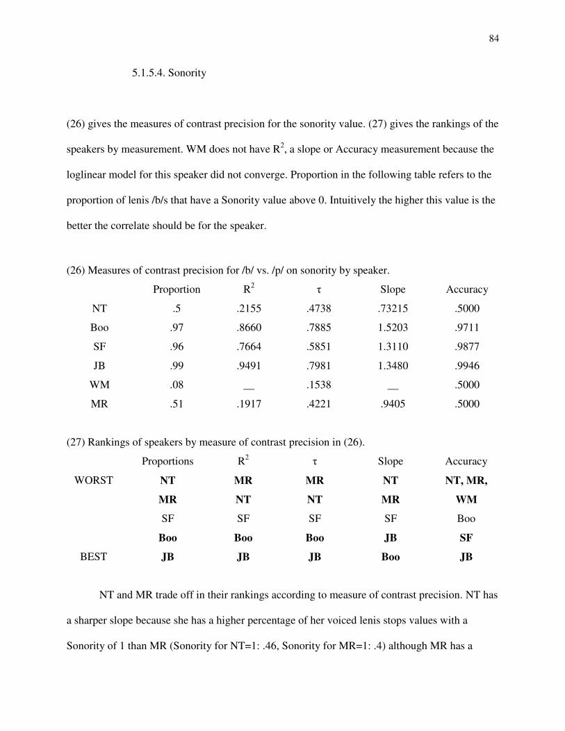
84

5.1.5.4. Sonority

(26) gives the measures of contrast precision for the sonority value. (27) gives the rankings of the

speakers by measurement. WM does not have R2, a slope or Accuracy measurement because the

loglinear model for this speaker did not converge. Proportion in the following table refers to the

proportion of lenis /b/s that have a Sonority value above 0. Intuitively the higher this value is the

better the correlate should be for the speaker.

(26) Measures of contrast precision for /b/ vs. /p/ on sonority by speaker.


NT .5 .2155 .4738 .73215 .5000

Boo .97 .8660 .7885 1.5203 .9711

SF .96 .7664 .5851 1.3110 .9877

JB .99 .9491 .7981 1.3480 .9946

WM .08 __ .1538 __ .5000

MR .51 .1917 .4221 .9405 .5000



WORST NT MR MR NT NT, MR,

WM MR NT NT MR

SF SF SF SF Boo

Boo Boo Boo JB SF

BEST JB JB JB Boo JB

NT and MR trade off in their rankings according to measure of contrast precision. NT has

a sharper slope because she has a higher percentage of her voiced lenis stops values with a

Sonority of 1 than MR (Sonority for NT=1: .46, Sonority for MR=1: .4) although MR has a

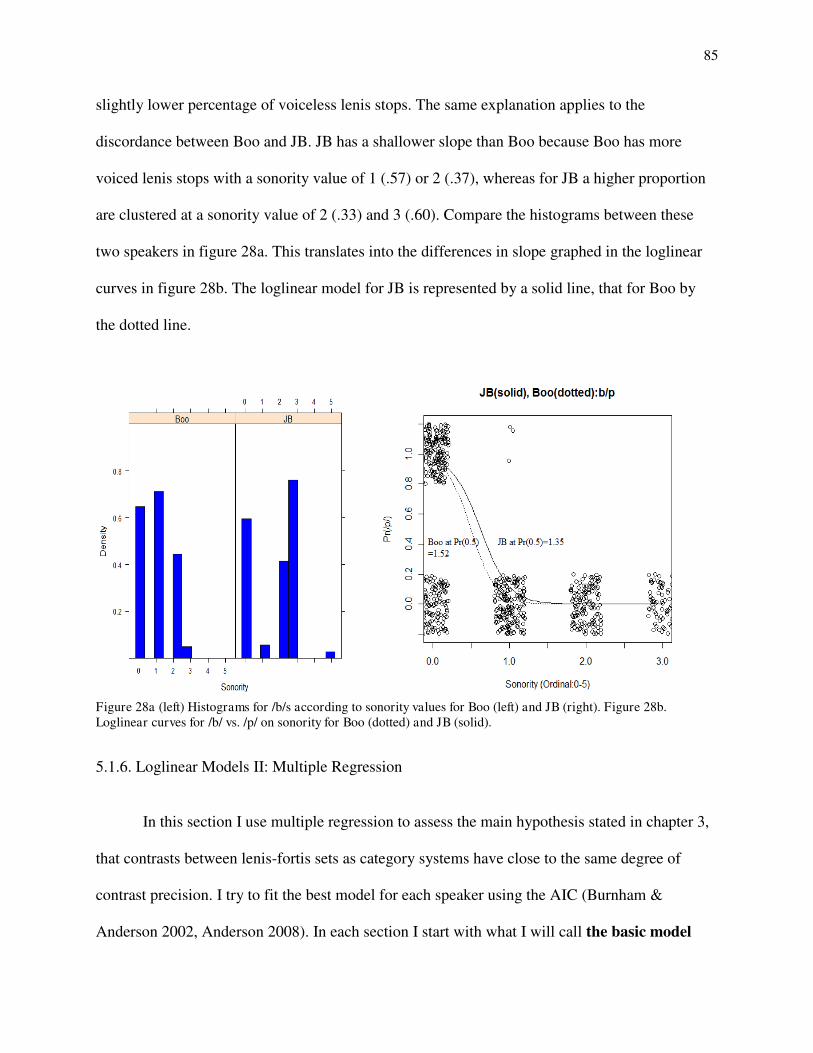
85

slightly lower percentage of voiceless lenis stops. The same explanation applies to the

discordance between Boo and JB. JB has a shallower slope than Boo because Boo has more

voiced lenis stops with a sonority value of 1 (.57) or 2 (.37), whereas for JB a higher proportion

are clustered at a sonority value of 2 (.33) and 3 (.60). Compare the histograms between these

two speakers in figure 28a. This translates into the differences in slope graphed in the loglinear

curves in figure 28b. The loglinear model for JB is represented by a solid line, that for Boo by

the dotted line.

Figure 28a (left) Histograms for /b/s according to sonority values for Boo (left) and JB (right). Figure 28b. Loglinear curves for /b/ vs. /p/ on sonority for Boo (dotted) and JB (solid).


In this section I use multiple regression to assess the main hypothesis stated in chapter 3,

that contrasts between lenis-fortis sets as category systems have close to the same degree of

contrast precision. I try to fit the best model for each speaker using the AIC (Burnham &

Anderson 2002, Anderson 2008). In each section I start with what I will call the basic model

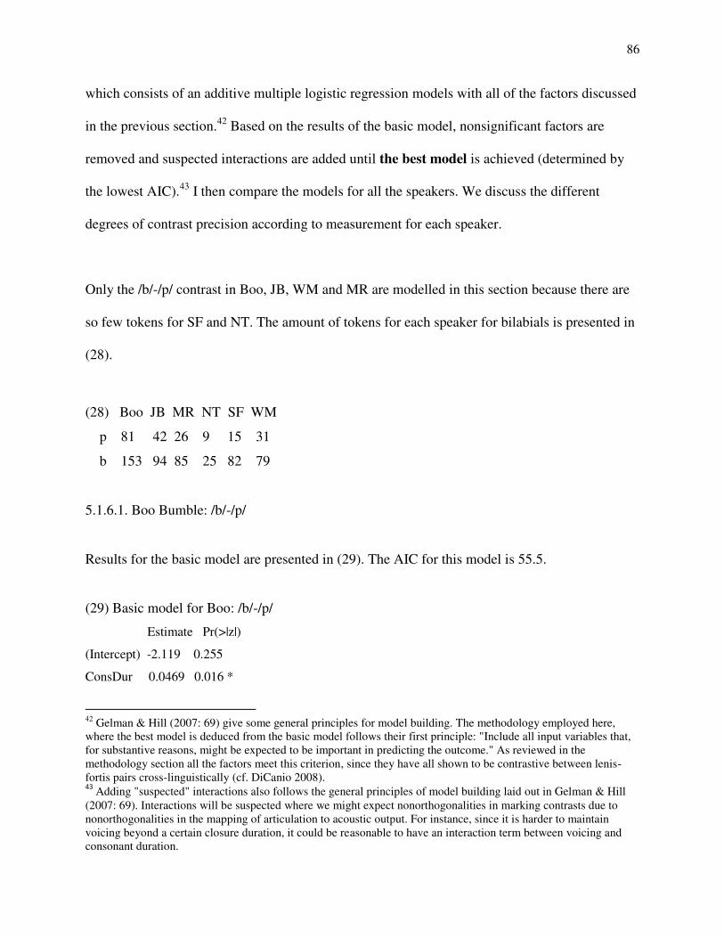
86

which consists of an additive multiple logistic regression models with all of the factors discussed

in the previous section.42 Based on the results of the basic model, nonsignificant factors are

removed and suspected interactions are added until the best model is achieved (determined by

the lowest AIC).43 I then compare the models for all the speakers. We discuss the different

degrees of contrast precision according to measurement for each speaker.

Only the /b/-/p/ contrast in Boo, JB, WM and MR are modelled in this section because there are

so few tokens for SF and NT. The amount of tokens for each speaker for bilabials is presented in

(28).

(28) Boo JB MR NT SF WM

p 81 42 26 9 15 31

b 153 94 85 25 82 79

5.1.6.1. Boo Bumble: /b/-/p/

Results for the basic model are presented in (29). The AIC for this model is 55.5.

(29) Basic model for Boo: /b/-/p/

Estimate Pr(>|z|)

(Intercept) -2.119 0.255

ConsDur 0.0469 0.016 *

42 Gelman & Hill (2007: 69) give some general principles for model building. The methodology employed here, where the best model is deduced from the basic model follows their first principle: "Include all input variables that, for substantive reasons, might be expected to be important in predicting the outcome." As reviewed in the methodology section all the factors meet this criterion, since they have all shown to be contrastive between lenis-fortis pairs cross-linguistically (cf. DiCanio 2008). 43

Adding "suspected" interactions also follows the general principles of model building laid out in Gelman & Hill (2007: 69). Interactions will be suspected where we might expect nonorthogonalities in marking contrasts due to nonorthogonalities in the mapping of articulation to acoustic output. For instance, since it is harder to maintain voicing beyond a certain closure duration, it could be reasonable to have an interaction term between voicing and consonant duration.

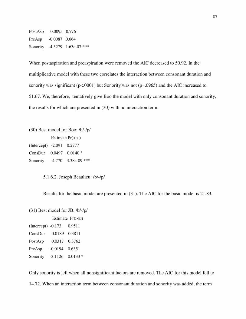
87

PostAsp 0.0095 0.776

PreAsp -0.0087 0.664

Sonority -4.5279 1.63e-07 ***

When postaspiration and preaspiration were removed the AIC decreased to 50.92. In the

multiplicative model with these two correlates the interaction between consonant duration and

sonority was significant (p<.0001) but Sonority was not (p=.0965) and the AIC increased to

51.67. We, therefore, tentatively give Boo the model with only consonant duration and sonority,

the results for which are presented in (30) with no interaction term.

(30) Best model for Boo: /b/-/p/

Estimate Pr(>|z|)

(Intercept) -2.091 0.2777

ConsDur 0.0497 0.0140 *

Sonority -4.770 3.38e-09 ***

5.1.6.2. Joseph Beaulieu: /b/-/p/

Results for the basic model are presented in (31). The AIC for the basic model is 21.83.

(31) Best model for JB: /b/-/p/

Estimate Pr(>|z|)

(Intercept) -0.173 0.9511

ConsDur 0.0189 0.3811

PostAsp 0.0317 0.3762

PreAsp -0.0194 0.6351

Sonority -3.1126 0.0133 *

Only sonority is left when all nonsignificant factors are removed. The AIC for this model fell to

14.72. When an interaction term between consonant duration and sonority was added, the term

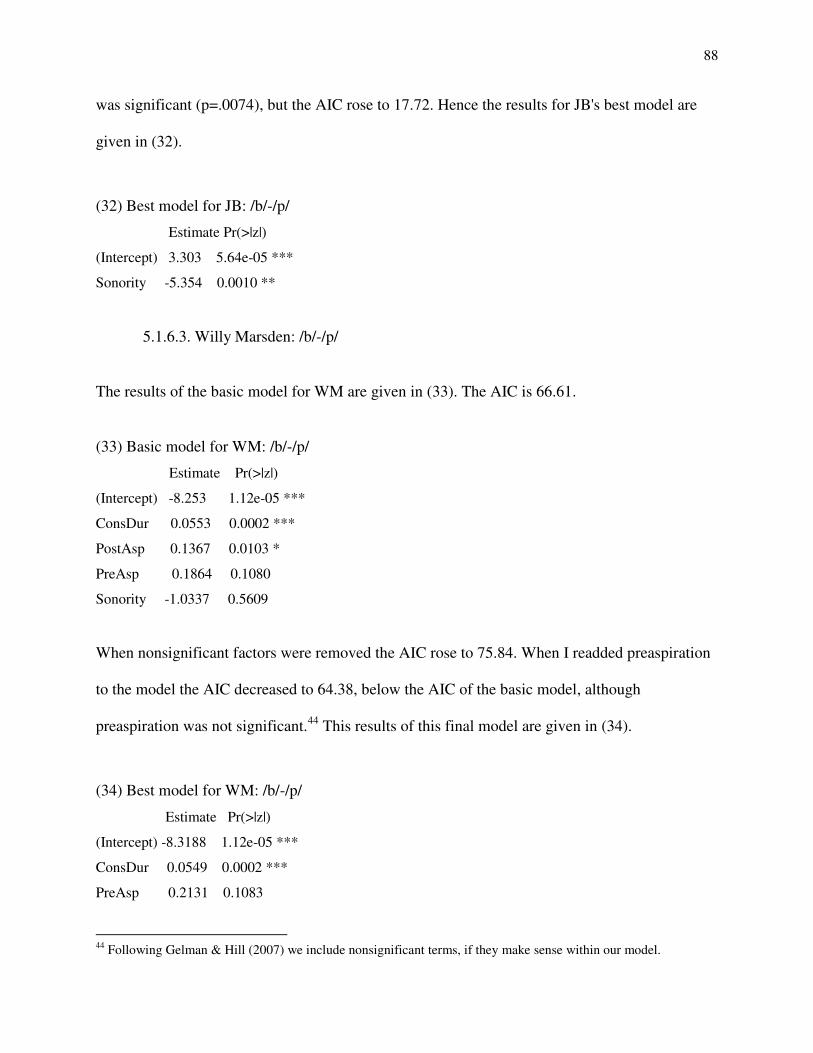
88

was significant (p=.0074), but the AIC rose to 17.72. Hence the results for JB's best model are

given in (32).

(32) Best model for JB: /b/-/p/

Estimate Pr(>|z|)

(Intercept) 3.303 5.64e-05 ***

Sonority -5.354 0.0010 **

5.1.6.3. Willy Marsden: /b/-/p/

The results of the basic model for WM are given in (33). The AIC is 66.61.

(33) Basic model for WM: /b/-/p/

Estimate Pr(>|z|)

(Intercept) -8.253 1.12e-05 ***

ConsDur 0.0553 0.0002 ***

PostAsp 0.1367 0.0103 *

PreAsp 0.1864 0.1080

Sonority -1.0337 0.5609

When nonsignificant factors were removed the AIC rose to 75.84. When I readded preaspiration

to the model the AIC decreased to 64.38, below the AIC of the basic model, although

preaspiration was not significant.44 This results of this final model are given in (34).

(34) Best model for WM: /b/-/p/

Estimate Pr(>|z|)

(Intercept) -8.3188 1.12e-05 ***

ConsDur 0.0549 0.0002 ***

PreAsp 0.2131 0.1083

44 Following Gelman & Hill (2007) we include nonsignificant terms, if they make sense within our model.

89

PostAsp 0.1433 0.0079 **

Another model which makes sense and is only slightly worse in terms of the AIC is one with an

interaction term between consonant duration and postaspiration and only consonant duration and

preaspiration terms as main effects.45 The AIC for this model is 64.47. It is given below.

(35) Alternative model for WM: /b/-/p/

Estimate Pr(>|z|)

(Intercept) -8.0301 1.39e-05 ***

ConsDur 0.0528 0.0003 ***

PreAsp 0.1770 0.0823 .

ConsDur:PostAsp 0.0014 0.0198 *

5.1.6.4. Mary Ryle: /b/-/p/

The basic model for MR is presented in (36). The AIC of this model is 35.01.

(36) Basic model for MR: /b/-/p/

Estimate Pr(>|z|)

(Intercept) -13.3811 0.0001 ***

ConsDur 0.1205 0.0002 ***

PostAsp 0.1157 0.3747

PreAsp -0.0032 0.9661

Sonority 0.9644 0.4395

45 ConsDur:PostAsp is not technically an interaction term, it is really a data manipulation of consonant duration based on postaspiration since postaspiration is not a main effect. Whether this term is theoretically motivated or not is unclear to me at this point.

90

When nonsignificant factors were removed the AIC decreased to 29.38. No significant two way

interactions were found with consonant duration and any other potential predictor. The results of

the best model which contains only consonant duration are given in (37).

(37) Best model for MR:/b/-/p/

Estimate Pr(>|z|)

(Intercept) -15.3547 4.40e-05 ***

ConsDur 0.1425 6.49e-05 ***

5.1.6.4. Overview: /b/-/p/ as Complex Categories

In this section we compare the speakers in terms of the contrast between their complex

categories. In the previous section we chose the best model for each speaker. None of the

speakers had the exact same model. This is summarized in (38).

(38) Overview of the best models for the /b/-/p/ contrast with standardized coefficients by speaker.

ConsDur PostAsp PreAsp Sonority

Boo 1.730 -3.974

JB -7.234

WM 1.808 1.182 2.555

MR 5.310

Note that in many cases a correlate is omitted from a particular speaker's model even though

when it is isolated it is significant and appears strong. A good example is consonant duration for

JB where the proportional difference between lenis-fortis stops was the greatest (1:2.1). Despite

this consonant duration is essentially predictable from sonority and thus not enough is added to

the model by including it as a factor (without the risk of over fitting). However, it is still

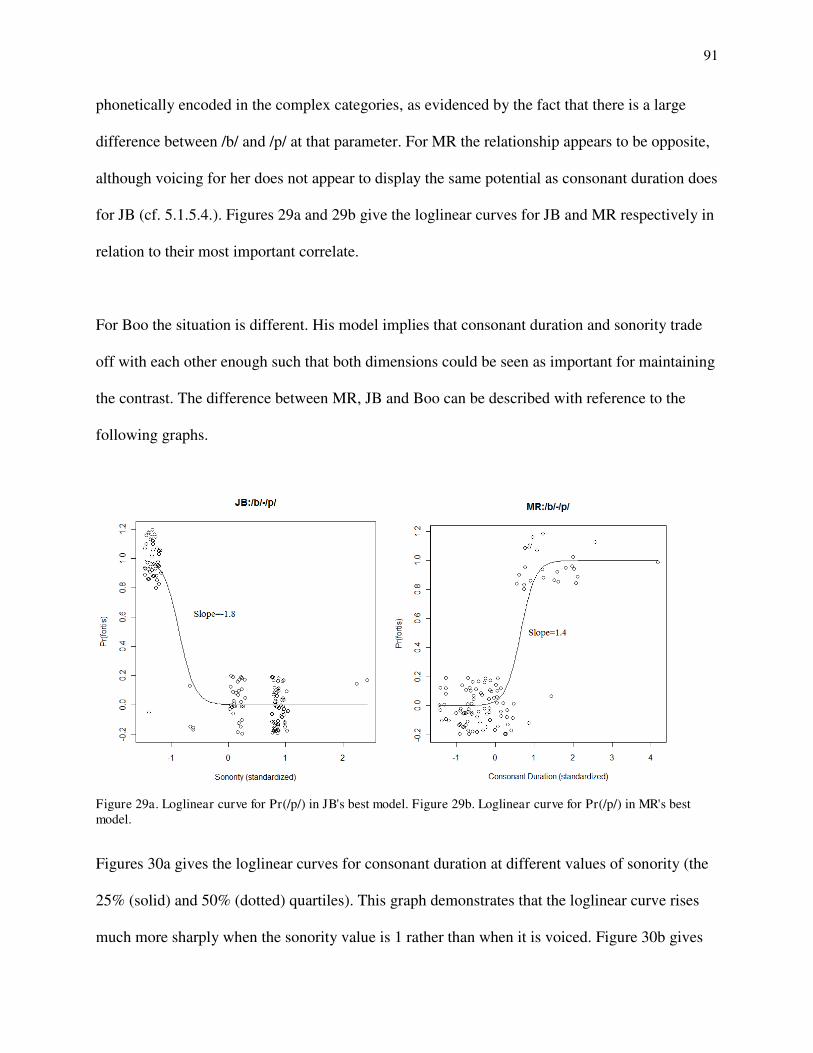
91

phonetically encoded in the complex categories, as evidenced by the fact that there is a large

difference between /b/ and /p/ at that parameter. For MR the relationship appears to be opposite,

although voicing for her does not appear to display the same potential as consonant duration does

for JB (cf. 5.1.5.4.). Figures 29a and 29b give the loglinear curves for JB and MR respectively in

relation to their most important correlate.

For Boo the situation is different. His model implies that consonant duration and sonority trade

off with each other enough such that both dimensions could be seen as important for maintaining

the contrast. The difference between MR, JB and Boo can be described with reference to the

following graphs.

Figure 29a. Loglinear curve for Pr(/p/) in JB's best model. Figure 29b. Loglinear curve for Pr(/p/) in MR's best model.

Figures 30a gives the loglinear curves for consonant duration at different values of sonority (the

25% (solid) and 50% (dotted) quartiles). This graph demonstrates that the loglinear curve rises

much more sharply when the sonority value is 1 rather than when it is voiced. Figure 30b gives

92

the loglinear curves for the sonority value with different levels of consonant duration (at the 25%

(dotted) and 75% (solid) quartile). These graphs demonstrate that in Boo's /b/-/p/ model as the

importance of one correlate increases the other decreases, and vice versa. To a certain extent

these correlates operate in a kind of trading relation with each other in production. That said,

they are not completely orthogonal. The model which was constructed that contained an

interaction term between the two correlates demonstrated that these two correlates do interact,

however, indicating that the predictors are not completely additive. The interaction term was not

large enough compared to the main effects, however, for us to use in this study according to the

information-theoretic criterion that we adhere to. Even if consonant duration and voicing trade

off to a certain degree it would be odd to find a case where they were totally nonorthogonal

unless they were in radically different phonological positions (cf. Pierrehumbert 2000a, 2000b)46.

Increases in glottal vibrations during the closure should tend to correlate with a decrease in

consonant duration as vocal fold vibration becomes more difficult beyond certain closure

durations (Ohala 1983).

46 We might also expect that consonant duration and voicing would be more orthogonal in languages described as using voicing [+/- voice] and consonant duration [+/-long] distinctively such as Arabic which has a singleton-geminate contrast in addition to a voicing contrast.

93

Figure 30a. Loglinear curves for Pr(/p/) on consonant duration with Sonority at 1 (solid) and 0 (dotted) for Boo. Figure 30b. Loglinear curves for Pr(/p/) on sonority with consonant duration at 59 (dotted) and 102 (solid) for Boo.

The following tables compare the measures of contrast precision between the parameters taken in

isolation and the best model by speaker. Accuracy measurements for contrast precision by

speaker are given in (39). The column with Best is the contrast between category systems

irrespective of the amount and type of dimension involved.

(39) Accuracy for /b/-/p/ contrast by speaker (rows) and dimensional or multidimensional space (columns).

ConsDur PostAsp PreAsp Sonority Best

Boo .7464 .7966 .5380 .9711 .9744

JB .9124 .8637 .5714 .9946 .9946

WM .7260 .6195 .7097 .5000 .8098

MR .9481 .6481 .5800 .5000 .9481

Range .72-.94 .53-.86 .56-.71 .50-.99 .81-.99

A theme in much of the literature on phonetic typology is that languages cut up the parametric

phonetic space in different ways in the formation of language specific phonological categories

94

(cf. Pierrehumbert 2003b). The differential importance of phonetic correlates by speaker

indicates that we may have found this type of pattern within the production of the Saulteaux

spoken in Manitoba as well. At this point we cannot assess the sociolinguistic variables that

might be involved because each of the speakers are from different communities. However, all

Ojibwe speakers (we assume) have approximately the same phonological inventories (the same

oppositions are made between lenis and fortis stops). Based on this we might assume that they all

have the same functional drive to maintain the lenis-fortis contrast. It is therefore reasonable to

assume that they have approximately the same degrees of contrast precision between phonemes

when they are described as category systems the differential use of phonetic correlates

notwithstanding. As can be seen from (39) to a certain extent we have corroborated this thesis

even based only on the four correlates I investigated in this study. The range of variation seems

to be greater between the contrast precisions of speakers at individual parameters than it is

between the /b/-/p/ phonemes as category systems and the speakers vary according to the weight

of each correlate and or whether they use a particular correlate at all to mark a contrast.

However, WM has a much lower Accuracy measurement than the other speakers for his best

model. It may be the case that in fact the lenis-fortis contrast is less robust for WM, but there are

a number of possible correlates that were not investigated in this study that could also be

participating in the /b/-/p/ contrast for WM. Dozens of additional correlates have been noted to

covary with the lenis-fortis contrast cross-linguistically; F0 or F0 flexion (e.g. Löfqvist et al.

1989, Kingston et al. 2008; cf. Abramson 2003 for Pattani-Malay and Muller 2001 for Chukese),

F1 or F2 flexion (cf. Debrock 1977 for Dutch and French, Moreton 2004 for English, Leander

2008 for Ozolotepec Zapotec), breathy-stiff phonation in flanking vowels47 (cf. Cho &

47 For Seoul Korean and Cheju, Cho and Ladefoged (2001) found that so-called lenis stops were more breathy than fortis stops. For Standard German, Jessen (1998) found the opposite trend for what are considered "lenis" and

95

Ladefoged 2000 for Seoul Korean and Cheju and Jessen 1998 for Standard German), among

others (cf. Lisker 1986).

Despite these problems, the statistical summaries of the /b/-/p/ contrast across speakers indicate

that correlates in production are being used with different weights attached to them by speaker.

Whether this implies that the contrast between /b/ and /p/ as category systems has the same

degree of contrast precision between speakers awaits further research (e.g. investigation of more

correlates). We also need some way of deciding whether in fact we should expect the same level

of contrast precision to exist for each speaker and what factors might condition these potential

differences (e.g. relative position on hypo-hyperspeech continuum, functional load associated

with the relevant phonemic opposition, interactions between sociolinguistc variables, etc…) .48

Until such issues are addressed and integrated into our framework it is difficult to come up with

clear answers to the more complex questions about the structure of system-wide phonemic

oppositions (such as the lenis-fortis distinction) in relation to phonetic variation, within a

speaker, between speakers and between dialects.

"fortis" (or "lax" and "tense" if the reader wishes) in the literature on German phonetics. The direction in which the correlate covaries is irrelevant, however. If we find that correlates tend to covary in the same direction cross-linguistically it can be related to nonorthogonal mappings between articulation and acoustic output (cf. Pierrehumbert 2000 on this point on the acoustic correlate to vowel distinctions). Longer voiceless laryngeal gestures will in general produce longer postaspiration because greater intraoral pressure will cause a more intense noise burst after the release (Stevens 2000). Shorter closure durations will tend to be correlated with more and stronger vocal fold vibrations because it is difficult to maintain voicing beyond a certain closure duration (Ohala 1983) 48 Perhaps certain speakers expect that their interlocutor is relying on more top-down processing than others (cf. McClelland & Elman 1986). In this situation we would expect that contrast precision would diminish as a function of the hypo-hyper speech continuum (Moon Lindblom 1994). Perhaps the lenis-fortis contrast bears differential degrees of functional load (cf. Hockett 1967) depending on which speakers are involved in the linguistic exchange. The higher the functional load the higher we would expect the overall contrast precision to be.

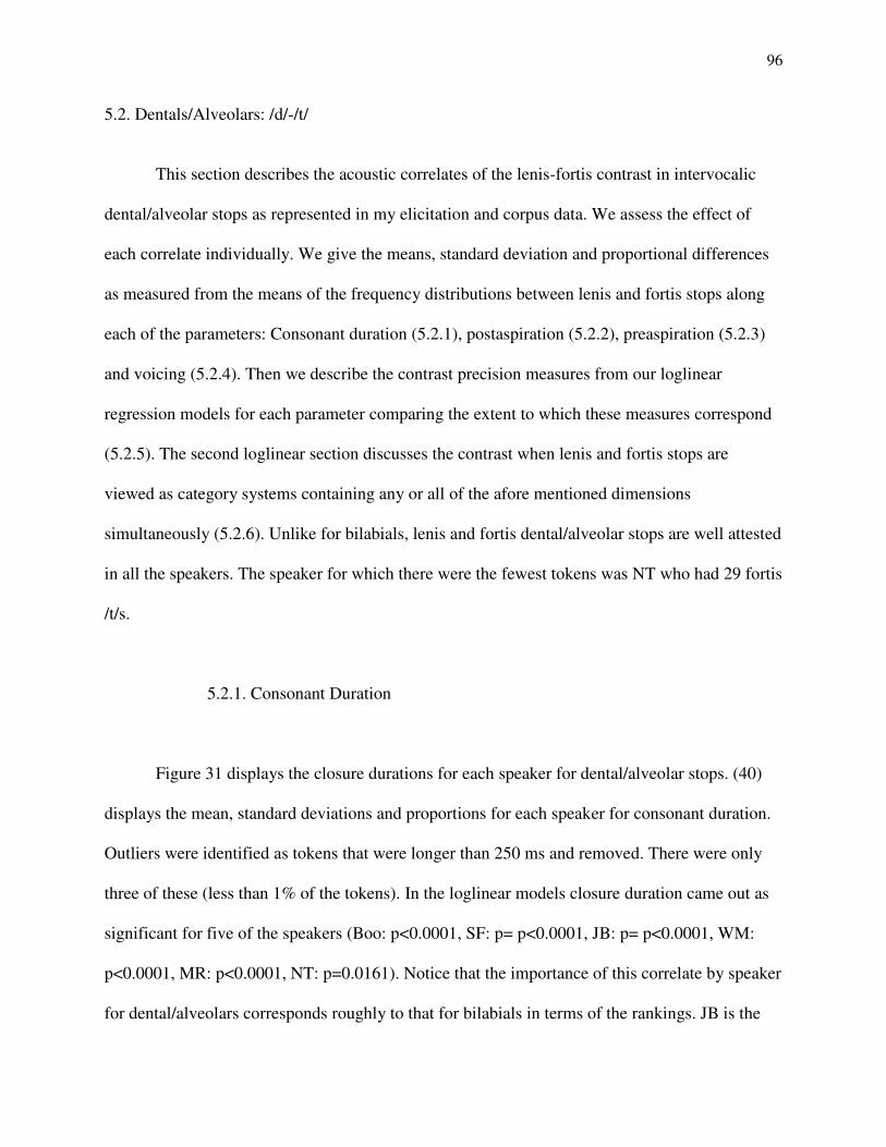
96

5.2. Dentals/Alveolars: /d/-/t/


dental/alveolar stops as represented in my elicitation and corpus data. We assess the effect of

each correlate individually. We give the means, standard deviation and proportional differences

as measured from the means of the frequency distributions between lenis and fortis stops along

each of the parameters: Consonant duration (5.2.1), postaspiration (5.2.2), preaspiration (5.2.3)

and voicing (5.2.4). Then we describe the contrast precision measures from our loglinear

regression models for each parameter comparing the extent to which these measures correspond

(5.2.5). The second loglinear section discusses the contrast when lenis and fortis stops are

viewed as category systems containing any or all of the afore mentioned dimensions

simultaneously (5.2.6). Unlike for bilabials, lenis and fortis dental/alveolar stops are well attested

in all the speakers. The speaker for which there were the fewest tokens was NT who had 29 fortis

/t/s.


Figure 31 displays the closure durations for each speaker for dental/alveolar stops. (40)

displays the mean, standard deviations and proportions for each speaker for consonant duration.

Outliers were identified as tokens that were longer than 250 ms and removed. There were only

three of these (less than 1% of the tokens). In the loglinear models closure duration came out as

significant for five of the speakers (Boo: p<0.0001, SF: p= p<0.0001, JB: p= p<0.0001, WM:

p<0.0001, MR: p<0.0001, NT: p=0.0161). Notice that the importance of this correlate by speaker

for dental/alveolars corresponds roughly to that for bilabials in terms of the rankings. JB is the

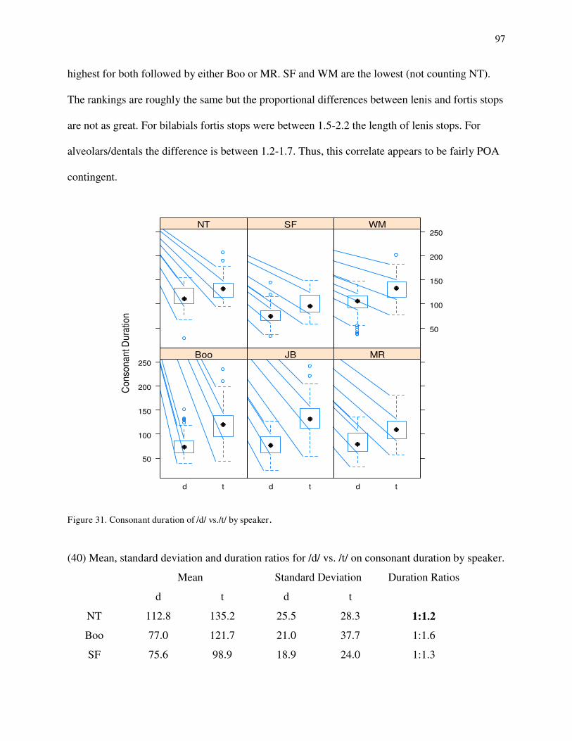
97

highest for both followed by either Boo or MR. SF and WM are the lowest (not counting NT).

The rankings are roughly the same but the proportional differences between lenis and fortis stops

are not as great. For bilabials fortis stops were between 1.5-2.2 the length of lenis stops. For

alveolars/dentals the difference is between 1.2-1.7. Thus, this correlate appears to be fairly POA

contingent.

Figure 31. Consonant duration of /d/ vs./t/ by speaker.

(40) Mean, standard deviation and duration ratios for /d/ vs. /t/ on consonant duration by speaker.

Mean Standard Deviation Duration Ratios

d t d t

NT 112.8 135.2 25.5 28.3 1:1.2

Boo 77.0 121.7 21.0 37.7 1:1.6

SF 75.6 98.9 18.9 24.0 1:1.3

Co

nso

na

nt D

ura

tion

50

100

150

200

250

d t

Boo

d t

JB

d t

MR

NT SF

50

100

150

200

250WM

98

JB 76.6 132.0 23.4 37.4 1:1.7

WM 101.0 132.2 26.8 25.5 1:1.3

MR 80.7 109.5 24.9 24.0 1:1.4


Figure 32 displays the postaspiration differences by Speaker. (41) gives the mean,

standard deviations, proportions and durational ratios for /d/ and /t/. Outliers above 60 ms were

removed. This was less than 1% of the data (1/773). The standard deviations for lenis consonants

remained large nevertheless.

Although the postaspiration of fortis consonants are all higher in terms of duration and overall

amount of postaspirated segments than those for lenis stops, the difference is slight. The logistic

regression model with postaspiration was significant Boo (p<0.0001), SF (p=0.0017) and MR

(p=0.0214). Postaspiration was a nonsignificant predictor of the contrast for NT (p=0.457) and

JB (p=0.1467). The model did not converge for WM.

99

Figure 32. Postaspiration duration (ms) of /d/ vs. /t/ by speaker.

(41) Mean, standard deviation, proportions and duration ratios for postaspiration of /d/ vs. /t/ by speaker. Proportion refers to the proportion of tokens (lenis or fortis) which have any postaspiration at all).

Mean Standard

Deviation

Proportions Duration ratios

d:t

d t d t d t

NT 16.9 18.0 3.9 5.2 1 1 1:1.1

Boo 11.4 26.3 7.7 9.5 .78 1 1:2.3

SF 21.9 30.0 14.0 10.2 .86 1 1:1.4

JB 21.9 24.8 23.4 37.4 .88 .98 1:1.1

WM 17.7 20.2 6.7 4.5 .95 1 1:1.1

MR 10.3 13.7 7.6 6.6 .73 .94 1:1.3

Po

sta

sp

ira

tio

n

0

10

20

30

40

50

60

d t

Boo

d t

JB

d t

MR

NT SF

0

10

20

30

40

50

60

WM

100

As noted before lenis /d/ is peculiar in that it typically has some postaspiration in intervocalic

position. This is not the case with bilabials, nor with velars. There does not seem to be a

description of lenis /d/s in Ojibwe as having breathy voiced aspiration in the literature, however.

Relative duration of postaspiration does not seem to be contrastive for the dental/alveolar lenis-

fortis stops (except for NT and JB).

Despite the fact that postaspiration seems to be a weak predictor because lenis /d/ often has a

substantial amount of postaspiration associated with it, there may be other acoustic differences

between the postaspiration in /d/ and /t/ that are not strictly durational. Although this question

could not be addressed in this thesis it appears that the postaspiration of the /t/s has more high

frequency frication associated with it, whereas with /d/, the duration reflects VOT lag whether

breathy or not. This topic requires future research, if this correlate is contrastive it surely goes

against the grain of feature economy. Long postaspiration might be contrastive for bilabials and

velars but for dental/alveolars the contrast might be between aspiration and breathy voice

aspiration a phonetic feature usually reserved for languages with more than just a two way

contrast between stops at a particular POA such as Hindi (e.g. Dixit 1987).


Preaspiration is a non-normative correlate of the lenis-fortis contrast in dental/alveolar

stops. It does not occur with every fortis token (some /t/'s have 0 ms preaspiration). Lenis /d/s

never have preaspiration, and thus the data structure is quasi-separate. The quantile-quantile plots

in figure 33 give an idea of the differences in preaspiration between speakers. These display

101

fortis stops so that the reader can get an idea of how many of the fortis stops surface with or

without preaspiration. All tokens were left in. (42) gives the mean, standard deviations and

proportions associated with preaspirated stops. In the former case we give the mean and standard

deviations with and without 0 ms tokens. Overall in (42) refers to a data set where all the 0 ms

tokens are left in whereas Preasp. refers to the mean and standard deviations of preaspiration

where 0 ms tokens are removed. In the loglinear models preaspiration was a significant predictor

for every speaker (NT: p=0.0317, Boo: p<0.0001, SF: p=0.0208, JB: p=0.0065, WM: p=0.0041,

MR: p=0.0049).

Figure 41. Quantile-quantile plot of preaspiration in fortis alveolar stops by Speaker

(42) Mean, standard deviation, and proportions for /d/ vs. /t/ on preaspiration by speaker. (Statistical descriptions under the column Overall contain all fortis tokens, those under the column PreAsp. contain only fortis tokens with preaspiration above 0 ms.)


qnorm

Pre

asp

ira

tio

n

0

20

40

60

80

-2 -1 0 1 2

Boo JB

-2 -1 0 1 2

MR

NT

-2 -1 0 1 2

SF

0

20

40

60

80

WM

102


NT 19.7 38.9 26.2 25.7 0.50

Boo 13.8 28.1 18.2 16.1 0.49

SF 8.8 32.1 16.9 17.1 0.27

JB 7.8 29.9 14.9 13.6 0.26

WM 15.3 27.6 16.0 10.8 0.56

MR 16.6 34.4 21.6 18.6 0.48

We might attribute some of the variance associated with preaspiration to other sources. Ojibwe

has a distinction between short and long vowels. In the literature a distinction is sometimes made

between vowels that devoice before fortis consonants in certain circumstances and preaspiration

associated with the fortis consonants (e.g. Valentine 1994). No such distinction has been made in

this study, and it is difficult to see how it could be done in principle. Preaspiration may, in

certain circumstances, be a form of previous vowel reduction. The literature has often noted that

only short vowels undergo this reduction and that long vowels are always stressed (e.g. Piggott

1980, Valentine 2001, Swierzbin 2003). In figure 34 it looks as if preaspiration is much more

prevalent for fortis stops which follow short vowels rather than long vowels, and that for all the

speakers, except WM where preaspiration approaches normativity (in Helgason's 2002 sense) the

median value is higher before short vowels.

For all of the speakers together 49.5% of the fortis stops with previous short vowels receive

preaspiration whereas the percentage of fortis stops with preceding long vowels that receive

preaspiration is 22%. An example of this breathy voice or devoicing before fortis consonants is

given in figure 35 from the speaker SF from Brokenhead.

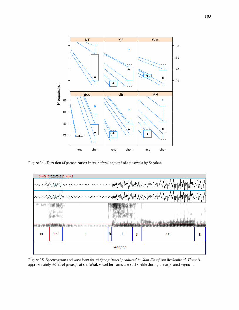
103

Figure 34 . Duration of preaspiration in ms before long and short vowels by Speaker.

Figure 35. Spectrogram and waveform for mitigoog ‗trees‘ produced by Stan Flett from Brokenhead. There is approximately 38 ms of preaspiration. Weak vowel formants are still visible during the aspirated segment.

Pre

asp

ira

tio

n

20

40

60

80

long short

Boo

long short

JB

long short

MR

NT SF

20

40

60

80

WM

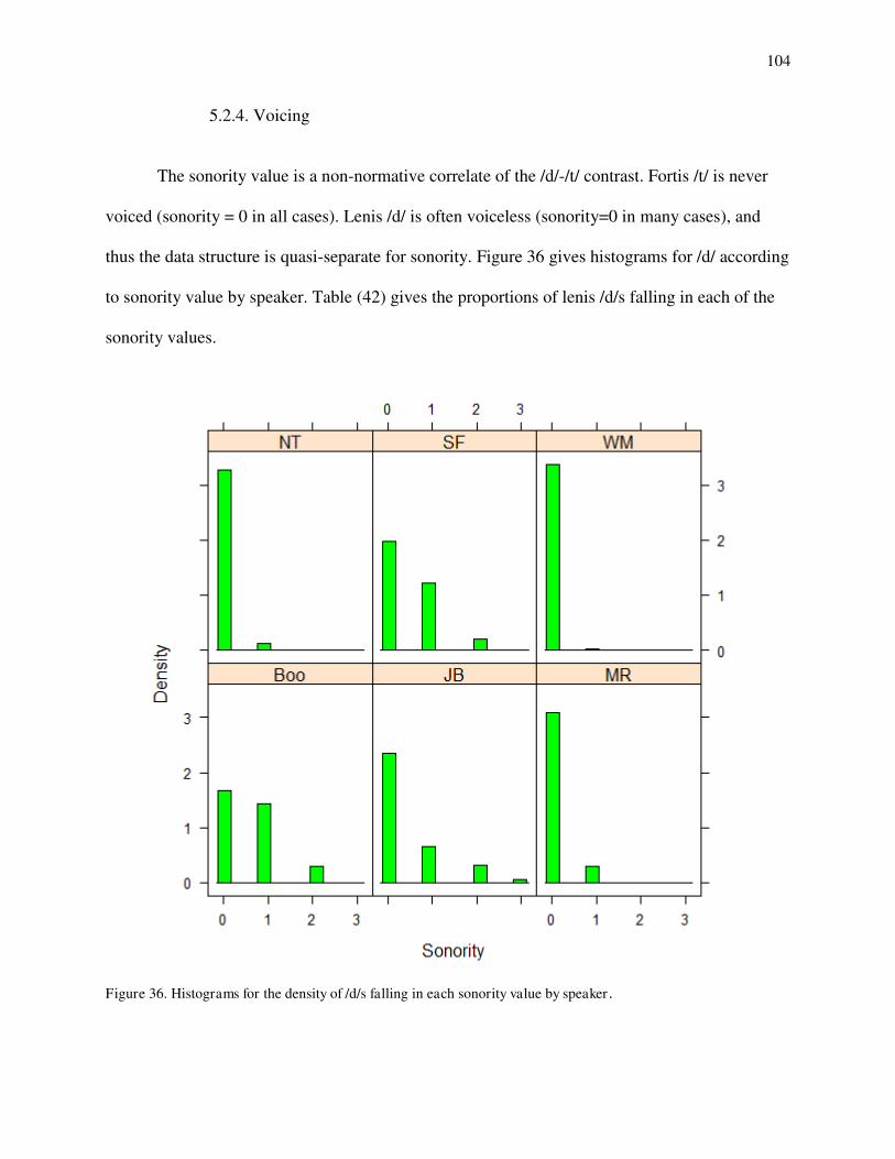
104

5.2.4. Voicing

The sonority value is a non-normative correlate of the /d/-/t/ contrast. Fortis /t/ is never

voiced (sonority = 0 in all cases). Lenis /d/ is often voiceless (sonority=0 in many cases), and

thus the data structure is quasi-separate for sonority. Figure 36 gives histograms for /d/ according

to sonority value by speaker. Table (42) gives the proportions of lenis /d/s falling in each of the

sonority values.

Figure 36. Histograms for the density of /d/s falling in each sonority value by speaker .

105

(42) Proportions of /d/ falling in each sonority value by speaker.

0 1 2 3 4 5

NT .93 .07 0 0 0 0

Boo .19 .67 .14 0 0 0

SF .35 .55 .095 0 0 0

JB .54 .29 .135 .03 0 0

WM .985 .015 0 0 0 0

MR .86 .14 0 0 0 0

Based on these data it appears that sonority is the best correlate for the /d/-/t/ contrast for Boo.

For Boo a substantial amount of /d/ tokens have a sonority value above 0 (81%). On the other

extreme for WM almost every single /d/ token has a sonority value of 0, the same as every /t/

token. If we compare this to figure 25 (pg. 65) for the sonority values of lenis /b/ it is obvious

that voicing is not as good a predictor for the /d/-/t/ contrast as it is for the /b/-/p/ contrast. In

general a larger proportion of lenis /d/s have a sonority value of 0 compared to /b/s. Only Boo

has lenis /d/s with a substantial amount of voicing on lenis /d/s. Note also that JB's sonority value

was an extremely strong predictor for the /b/-/p/ contrast. Here most of his lenis /d/ tokens fall in

the 0 sonority range.

Loglinear models did not even converge for NT or WM. In the loglinear models Sonority came

out as significant for Boo (p<0.0001), SF (p=.0005) and JB (p=.0049). It came out as barely

nonsignificant for MR (p=.0588).

106

The sonority value is an overly coarse measurement. In most cases even for speakers where there

are almost no fully voiced /d/s, periodic glottal vibrations seep into the the stop from the

preceding vowel. Intuitively, however, the voicing measurement intensities correspond to the

difference in sonority values at least for the two speakers for whom it was measurable. For Boo

the mean intensity is .777 (sd=.0667) and for NT it is lower at .4479 (sd=.0742).



relevant parameters for the /d/-/t/ contrast. We rank the speakers in terms of the importance of

each correlate based on these measures of contrast precision investigating to what degree these

rankings correspond with the more basic statistical descriptions given above (e.g. proportional

difference between means, proportions of preaspirated segments, etc…) and with each other.

Where we see noncorrespondences between these different measurements we try to explain them

based on the statistical structure of the categories for each speaker. Although overall the patterns

correspond, there is often much discordance between the rankings because the variation between

certain speakers can be quite subtle. We limit our scope to discussing the speakers with the worst

and best models for a given correlate in the particular rankings on contrast precision. When the

rankings of these speakers do not correspond we attempt to explain why this is the case.


107

The measurements of contrast precision for dental/alveolar stops on the consonant

duration parameter are given in (43). The rankings of speaker by measurement are given in (44).

(43) Measures of contrast precision for /d/ vs. /t/ on consonant duration by speaker.


R2 k Slope Accuracy

NT 1:1.2 .1163 .2709 .0080 .5500

Boo 1:1.6 .4100 .5188 .0139 .7635

SF 1:1.3 .2289 .3698 .0126 .6434

JB 1:1.7 .5046 .5335 .0164 .8412

WM 1:1.3 .2562 .4074 .0134 .6909

MR 1:1.4 .2180 .3712 .0111 .6571



WORST NT NT NT NT NT

MR MR SF MR SF

SF SF MR SF MR

WM WM WM WM WM

Boo Boo Boo Boo Boo

BEST JB JB JB JB JB

The measurements of contrast precision all correspond with regards to the ranking of the worst

and the best predictors.49 The ranking is still not perfect however. SF has a lower k coefficient

than MR. The consonant duration for MR's /d/ has a larger standard deviation in relation to its

49 Noteworthy is the fact that MR had consonant duration as one of the best predictors for bilabial stops, but is now one of the ranked second worst for this correlate in dental/alveolar stops. WM was ranked worst for bilabials but is now third best. These POA asymmetries are briefly discussed in the final discussion.

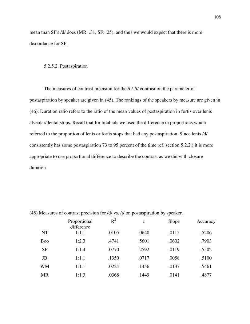
108

mean than SF's /d/ does (MR: .31, SF: .25), and thus we would expect that there is more

discordance for SF.


The measures of contrast precision for the /d/-/t/ contrast on the parameter of

postaspiration by speaker are given in (45). The rankings of the speakers by measure are given in

(46). Duration ratio refers to the ratio of the mean values of postaspiration in fortis over lenis

alveolar/dental stops. Recall that for bilabials we used the difference in proportions which

referred to the proportion of lenis or fortis stops that had any postaspiration. Since lenis /d/

consistently has some postaspiration 73 to 95 percent of the time (cf. section 5.2.2.) it is more

appropriate to use proportional difference to describe the contrast as we did with closure

duration.

(45) Measures of contrast precision for /d/ vs. /t/ on postaspiration by speaker.


R2 k Slope Accuracy

NT 1:1.1 .0105 .0640 .0115 .5286

Boo 1:2.3 .4741 .5601 .0602 .7903

SF 1:1.4 .0770 .2592 .0119 .5502

JB 1:1.1 .1350 .0717 .0058 .5100

WM 1:1.1 .0224 .1456 .0137 .5461

MR 1:1.3 .0368 .1449 .0141 .4877

109

(46) Rankings of speakers by measure of contrast precision.


WORST NT NT NT JB NT

JB WM JB NT WM

WM MR MR SF MR

MR SF WM WM SF

SF JB SF MR JB

BEST Boo Boo Boo Boo Boo

Postaspiration was the worst predictor of the contrast for NT compared to the other speakers,

except for slope where JB had an even less successful model. We can attribute this to the fact

that JB's categories overlap more because the standard deviations of postaspiration are 23.4 ms

for /d/ and 37.4 for his fortis. For NT the standard deviations were much smaller at 3.9 ms for /d/

and 5.2 ms for /t/. Boo has the highest contrast precision on the postaspiration parameter out of

all the speakers.


(47) gives the measurements of contrast precision for the /d/-/t/ contrast on the preaspiration

parameter. (48) give the rankings of speakers by measure. Proportion in the following chart

refers to the proportion of preaspirated fortis /t/. Lenis stops never have preaspiration.

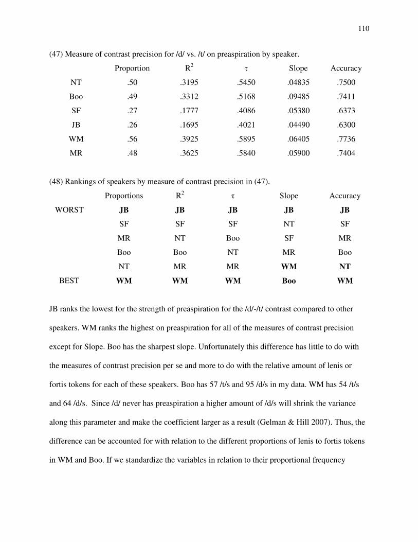
110

(47) Measure of contrast precision for /d/ vs. /t/ on preaspiration by speaker.


NT .50 .3195 .5450 .04835 .7500

Boo .49 .3312 .5168 .09485 .7411

SF .27 .1777 .4086 .05380 .6373

JB .26 .1695 .4021 .04490 .6300

WM .56 .3925 .5895 .06405 .7736

MR .48 .3625 .5840 .05900 .7404



WORST JB JB JB JB JB

SF SF SF NT SF

MR NT Boo SF MR

Boo Boo NT MR Boo

NT MR MR WM NT

BEST WM WM WM Boo WM

JB ranks the lowest for the strength of preaspiration for the /d/-/t/ contrast compared to other

speakers. WM ranks the highest on preaspiration for all of the measures of contrast precision

except for Slope. Boo has the sharpest slope. Unfortunately this difference has little to do with

the measures of contrast precision per se and more to do with the relative amount of lenis or

fortis tokens for each of these speakers. Boo has 57 /t/s and 95 /d/s in my data. WM has 54 /t/s

and 64 /d/s. Since /d/ never has preaspiration a higher amount of /d/s will shrink the variance

along this parameter and make the coefficient larger as a result (Gelman & Hill 2007). Thus, the

difference can be accounted for with relation to the different proportions of lenis to fortis tokens

in WM and Boo. If we standardize the variables in relation to their proportional frequency

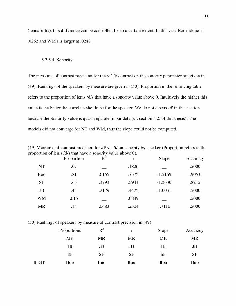
111

(lenis/fortis), this difference can be controlled for to a certain extent. In this case Boo's slope is

.0262 and WM's is larger at .0288.

5.2.5.4. Sonority

The measures of contrast precision for the /d/-/t/ contrast on the sonority parameter are given in

(49). Rankings of the speakers by measure are given in (50). Proportion in the following table

refers to the proportion of lenis /d/s that have a sonority value above 0. Intuitively the higher this

value is the better the correlate should be for the speaker. We do not discuss d' in this section

because the Sonority value is quasi-separate in our data (cf. section 4.2. of this thesis). The

models did not converge for NT and WM, thus the slope could not be computed.

(49) Measures of contrast precision for /d/ vs. /t/ on sonority by speaker (Proportion refers to the proportion of lenis /d/s that have a sonority value above 0). Proportion R2 k Slope Accuracy

NT .07 __ .1826 __ .5000

Boo .81 .6155 .7375 -1.5169 .9053

SF .65 .3793 .5944 -1.2630 .8245

JB .44 .2129 .4425 -1.0031 .5000

WM .015 __ .0849 __ .5000

MR .14 .0483 .2304 -.7110 .5000



MR MR MR MR MR

JB JB JB JB JB

SF SF SF SF SF


112

The models did not converge for NT and WM. All of the measures of contrast precision

correspond exactly in this case in terms of the rankings in (50).





Anderson 2002, Anderson 2008). In each section I start with what I will call "the basic model"

which consists of an additive multiple logistic regression model with all of the factors discussed

in the previous section. Based on the results of the basic model, nonsignificant factors are

removed and suspected interactions are added until the best model is achieved (according to the

lowest AIC). I then compare the models for all the speakers and discuss the different degrees of

contrast precision according to measure for each speaker. The counts of tokens for

dental/alveolar stops by speaker are given in (51).


t 57 50 52 28 51 54

d 95 103 95 30 94 64

5.2.6.1. NT: /d/-/t/

Results for the basic model for NT's /d/-/t/ contrast are given in (52). The AIC is 62.52.

(52) Basic model for NT: /d/-/t/

Estimate Pr(>|z|)

113

(Intercept) -4.3043 0.0775

ConsDur 0.0154 0.3008

PostAsp 0.0998 0.2598

PreAsp 0.1584 0.0475 *

Sonority -0.5233 0.7890

A model where all nonsignificant factors are removed has an AIC of 60.14. This is the best

model, presented in (53).

(53) Best model for NT: /d/-/t/

Estimate Pr(>|z|)

(Intercept) -0.7346 0.0223 *

PreAsp 0.1934 0.0317 *

5.2.6.2. Boo:/d/-/t/

The basic model for the /d/-/t/ contrast in Boo is presented in (54). The AIC is 35.936.

(54) Basic model for Boo: /d/-/t/

Estimate Pr(>|z|)

(Intercept) -8.9126 0.0002 ***

ConsDur 0.0544 0.0009 ***

PostAsp 0.1897 0.0056 **

PreAsp 0.1632 0.0719

Sonority -4.0344 0.0108 *

After preaspiration was removed the AIC rose to 42.52. A two way interaction between

consonant duration and postaspiration was not significant (p=.3663). Another two way

interaction between consonant duration and sonority was not significant (p=.6847). Thus, the

basic model is the best model for Boo. An alternative model which has an AIC of 35.937 (.001

114

higher than the basic model) does not contain preaspiration, instead it has a nonsignificant

interaction term between consonant duration and preaspiration. The results of this alternative

model are presented in (55). We still use the basic/best model for Boo, however.

(55) Alternative model for Boo: /d/-/t/

Estimate Pr(>|z|)

(Intercept) -8.9618 0.0001 ***

ConsDur 0.0538 0.0009 ***

PostAsp 0.1956 0.0047 **

Sonority -4.0166 0.0110*

ConsDur:PreAsp 0.0019 0.0867

5.2.6.3. SF: /d/-/t/

The basic model for the /d/-/t/ contrast for SF is given in (55). The AIC for this model is 92.73.

(55) Basic model for SF: /d/-/t/

Estimate Pr(>|z|)

(Intercept) -5.1559 0.0008 ***

ConsDur 0.0362 0.0049 **

PostAsp 0.0683 0.0039 **

PreAsp 0.1279 0.0386 *

Sonority -4.2342 0.0057 **

If we remove any of these factors the AIC increases. No significant two way interactions were

found for SF. Thus, we accept the basic model as the best for this speaker.

5.2.6.4. JB: /d/-/t/

The basic model for the /d/-/t/ contrast for JB is given in (). The AIC for this model is 87.27.

115

(56) Basic model for JB.

Estimate Pr(>|z|)

(Intercept) -6.2145 1.63e-05 ***

ConsDur 0.0604 1.34e-06 ***

PostAsp -0.0252 0.3502

PreAsp 0.1481 0.0178 *

Sonority -2.6784 0.0616

When nonsignificant factors are removed the AIC increases to 93.41. When Sonority is readded

the AIC is smaller than the basic model's at 87.27. No two way interaction terms were

significant, and adding interaction terms increased the AIC.

(57) Best model for JB: /d/-/t/

Estimate Pr(>|z|)

(Intercept) -6.8531 6.88e-07 ***

ConsDur 0.0608 1.47e-06 ***

PreAsp 0.1423 0.0210 *

Sonority -2.5777 0.0790

5.2.6.5. WM: /d/-/t/

The basic model for the /d/-/t/ contrast for WM did not converge. Recall that a model that just

contained sonority did not converge either. The basic model without sonority is presented in

(58). The AIC is 80.24.

(58) Best model for WM: /d/-/t/

Estimate Pr(>|z|)

(Intercept) -11.3728 1.64e-05 ***

ConsDur 0.0764 2.03e-05 ***

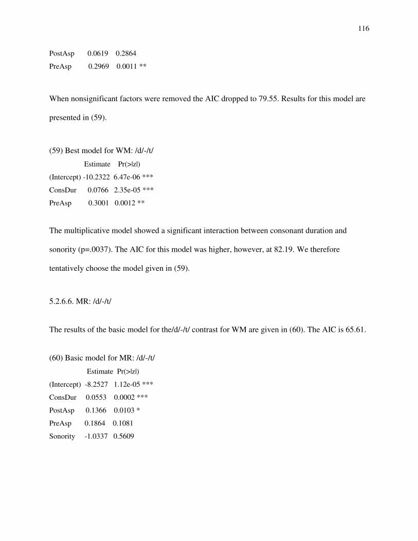
116

PostAsp 0.0619 0.2864

PreAsp 0.2969 0.0011 **

When nonsignificant factors were removed the AIC dropped to 79.55. Results for this model are

presented in (59).

(59) Best model for WM: /d/-/t/

Estimate Pr(>|z|)

(Intercept) -10.2322 6.47e-06 ***

ConsDur 0.0766 2.35e-05 ***

PreAsp 0.3001 0.0012 **

The multiplicative model showed a significant interaction between consonant duration and

sonority (p=.0037). The AIC for this model was higher, however, at 82.19. We therefore

tentatively choose the model given in (59).

5.2.6.6. MR: /d/-/t/

The results of the basic model for the/d/-/t/ contrast for WM are given in (60). The AIC is 65.61.

(60) Basic model for MR: /d/-/t/

Estimate Pr(>|z|)

(Intercept) -8.2527 1.12e-05 ***

ConsDur 0.0553 0.0002 ***

PostAsp 0.1366 0.0103 *

PreAsp 0.1864 0.1081

Sonority -1.0337 0.5609

117

When nonsignificant factors are removed the AIC increased to 75.84. When preaspiration was

readded the AIC decreased to 64.38. The results for this model are presented in (61). This was

the best model. No significant interactions were found.

(61) Best model for MR: /d/-/t/

Estimate Pr(>|z|)

(Intercept) -8.3188 1.12e-05 ***

ConsDur 0.0549 0.0002 ***

PostAsp 0.1433 0.0079 **

PreAsp 0.2131 0.1083

5.2.6.7. Summary: Contrast Precision between Complex Categories: /d/-/t/

In this section we compare the speakers in terms of the contrast between /d/ and /t/ as

complex categories. An overview of the most important predictors for each speaker is given in

(62). The numbers in each of the cells represents the coefficient for the predictor with all the

variables standardized (the mean subtracted from the value divided by the standard deviation).

Recall we cannot compare the AIC between speakers directly. Each speaker has a different count

of /d/s and /t/s. The AIC value depends on information entropy (i.e. how much information is

lost be the model), and thus it is contingent on sample size.

The table in (62) contains coefficients associated with each factor involved in the model with

each variable standardized. The coefficients for the predictors represent the values when all of

the other predictors are at their mean. The units are also standardized so it is easier to compare

their relative importance in a particular speaker's model. However, since the variables do not

have all of the same distributional structures (when compared to each other and possibly when

118

compared across speakers) the coefficients do not directly represent the relative importance of

each cue in each speaker's model. The coefficients are too contingent on their relationship to

other variables.

(62) Overview of /d/ vs. /t/ as complex categories by speaker.

ConsDur PostAsp PreAsp Sonority

NT 4.022

Boo 2.175 2.088 2.069 -2.574

SF .8555 .9096 1.380 -2.594

JB 2.332 1.309 -1.912

WM 1.856 3.806

MR 1.455 .6187 3.715

There are two senses in which the speakers have different models for predicting the /d/-/t/

contrast. First, the best model contains different acoustic correlates as factors depending on the

speaker. For example, WM's best model contains only consonant duration and preaspiration

whereas MR's best model contains these factors in addition to postaspiration. Second, the

strength of each predictor for making the contrast between /d/-/t/ varies from speaker to speaker.

Boo and SF have the same model in the first sense but different models in the second sense. This

is not attributable to differential weighting of acoustic cues. Boo had a higher contrast precision

than SF for every correlate when the dimensions were considered individually. This seems to be

reflected in the coefficients for the multivariate analysis as well. Recall that Boo's data were

from elicitation and SF's were from conversation. Unless there are other predictors which I did

not investigate which are stronger for SF than for Boo, the difference between these speakers

correspond with the general findings of H & H theory (Lindblom 1992, Moon & Lindblom

1994). In elicitation Boo is using hyperspeech and thus has stronger acoustic correlates to the /d/-

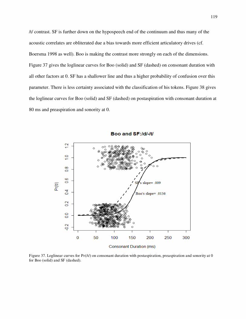
119

/t/ contrast. SF is further down on the hypospeech end of the continuum and thus many of the

acoustic correlates are obliterated due a bias towards more efficient articulatory drives (cf.

Boersma 1998 as well). Boo is making the contrast more strongly on each of the dimensions.

Figure 37 gives the loglinear curves for Boo (solid) and SF (dashed) on consonant duration with

all other factors at 0. SF has a shallower line and thus a higher probability of confusion over this

parameter. There is less certainty associated with the classification of his tokens. Figure 38 gives

the loglinear curves for Boo (solid) and SF (dashed) on postaspiration with consonant duration at

80 ms and preaspiration and sonority at 0.

Figure 37. Loglinear curves for Pr(/t/) on consonant duration with postaspiration, preaspiration and sonority at 0 for Boo (solid) and SF (dashed).

120

Figure 38. Loglinear curves for Pr(/t/) on postaspiration with consonant duration at 80 ms, preaspiration at 0 ms and sonority at 0.

A comparison between Boo and SF who appear to use the same dimensions in marking the /d/-/t/

contrast shows that there is an obvious difference in robustness according to speech style. Boo

naturally uses more hyperspeech, and SF more hypospeech. A comparison of MR and WM

potentially shows a different situation. Based on the standardized coefficients it looks as if MR

uses postaspiration to the detriment of her other correlates. WM's consonant duration and

preaspiration coefficients are larger than MR's, suggesting that he is relying more on just these

two dimensions. Figure 39a gives the loglinear curves for WM and MR on consonant duration

when postaspiration and preaspiration are 0. Figure 39b gives the loglinear curves for WM and

MR on preaspiration when postaspiration is 0 ms and consonant duration is 90 ms. In both cases

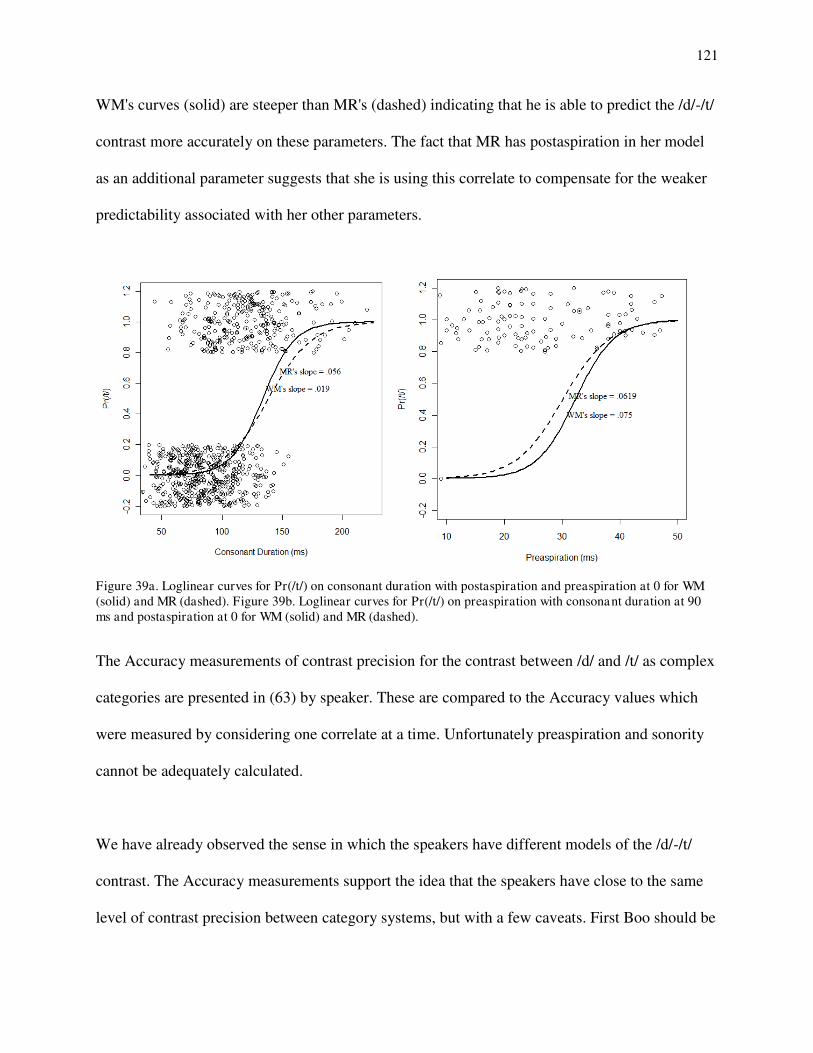
121

WM's curves (solid) are steeper than MR's (dashed) indicating that he is able to predict the /d/-/t/

contrast more accurately on these parameters. The fact that MR has postaspiration in her model

as an additional parameter suggests that she is using this correlate to compensate for the weaker

predictability associated with her other parameters.

Figure 39a. Loglinear curves for Pr(/t/) on consonant duration with postaspiration and preaspiration at 0 for WM (solid) and MR (dashed). Figure 39b. Loglinear curves for Pr(/t/) on preaspiration with consonant duration at 90 ms and postaspiration at 0 for WM (solid) and MR (dashed).

The Accuracy measurements of contrast precision for the contrast between /d/ and /t/ as complex

categories are presented in (63) by speaker. These are compared to the Accuracy values which

were measured by considering one correlate at a time. Unfortunately preaspiration and sonority

cannot be adequately calculated.

We have already observed the sense in which the speakers have different models of the /d/-/t/

contrast. The Accuracy measurements support the idea that the speakers have close to the same

level of contrast precision between category systems, but with a few caveats. First Boo should be

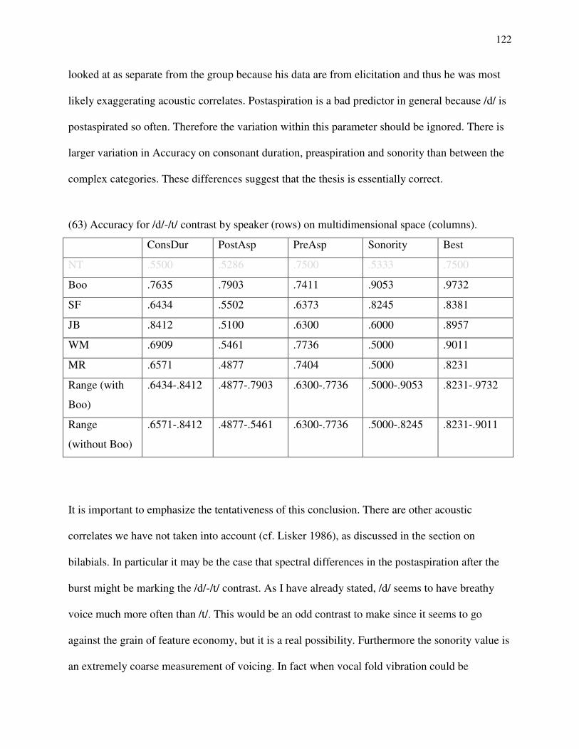
122

looked at as separate from the group because his data are from elicitation and thus he was most

likely exaggerating acoustic correlates. Postaspiration is a bad predictor in general because /d/ is

postaspirated so often. Therefore the variation within this parameter should be ignored. There is

larger variation in Accuracy on consonant duration, preaspiration and sonority than between the

complex categories. These differences suggest that the thesis is essentially correct.

(63) Accuracy for /d/-/t/ contrast by speaker (rows) on multidimensional space (columns).

ConsDur PostAsp PreAsp Sonority Best

NT .5500 .5286 .7500 .5333 .7500

Boo .7635 .7903 .7411 .9053 .9732

SF .6434 .5502 .6373 .8245 .8381

JB .8412 .5100 .6300 .6000 .8957

WM .6909 .5461 .7736 .5000 .9011

MR .6571 .4877 .7404 .5000 .8231

Range (with

Boo)

.6434-.8412 .4877-.7903 .6300-.7736 .5000-.9053 .8231-.9732

Range

(without Boo)

.6571-.8412 .4877-.5461 .6300-.7736 .5000-.8245 .8231-.9011

It is important to emphasize the tentativeness of this conclusion. There are other acoustic

correlates we have not taken into account (cf. Lisker 1986), as discussed in the section on

bilabials. In particular it may be the case that spectral differences in the postaspiration after the

burst might be marking the /d/-/t/ contrast. As I have already stated, /d/ seems to have breathy

voice much more often than /t/. This would be an odd contrast to make since it seems to go

against the grain of feature economy, but it is a real possibility. Furthermore the sonority value is

an extremely coarse measurement of voicing. In fact when vocal fold vibration could be

123

measured during the closure, the measurements were made. In this case we can measure the ratio

of vocal fold vibration to the closure duration. Voicing ratio was significant in a loglinear model

with all the speakers pooled (p<.0001). Speakers might be using the glottal vibrations that seep

into /d/s to mark the contrast.

5.3. Velars: /g/-/k/


velar stops as represented in my elicitation and corpus data. We assess the effect of each

correlate individually. I give the means, standard deviation and proportional differences as

measured from the means of the frequency distributions between lenis and fortis stops along each

of the parameters for each speaker: Consonant duration (5.3.1), postaspiration (5.3.2),

preaspiration (5.3.3) and voicing (5.3.4). Then we describe the contrast precision measures from

our loglinear regression models for each parameter examining the extent to which these

parameters correspond (5.3.5). The second loglinear section discussed the contrast when lenis

and fortis stops are viewed as category systems containing all the afore mentioned dimensions

simultaneously (5.3.6). I choose the best model for each speaker.


As noted in section 4.2.4 some consonant tokens are assigned a consonant duration of 0

ms. This corresponds to a Sonority level of 4 or 5. In these cases I was unable to detect any

discernible boundary between the consonant and the flanking vowels (Sonority=4), in some

cases I was unable to even hear the consonant (Sonority=5). This phenomenon never occurs with

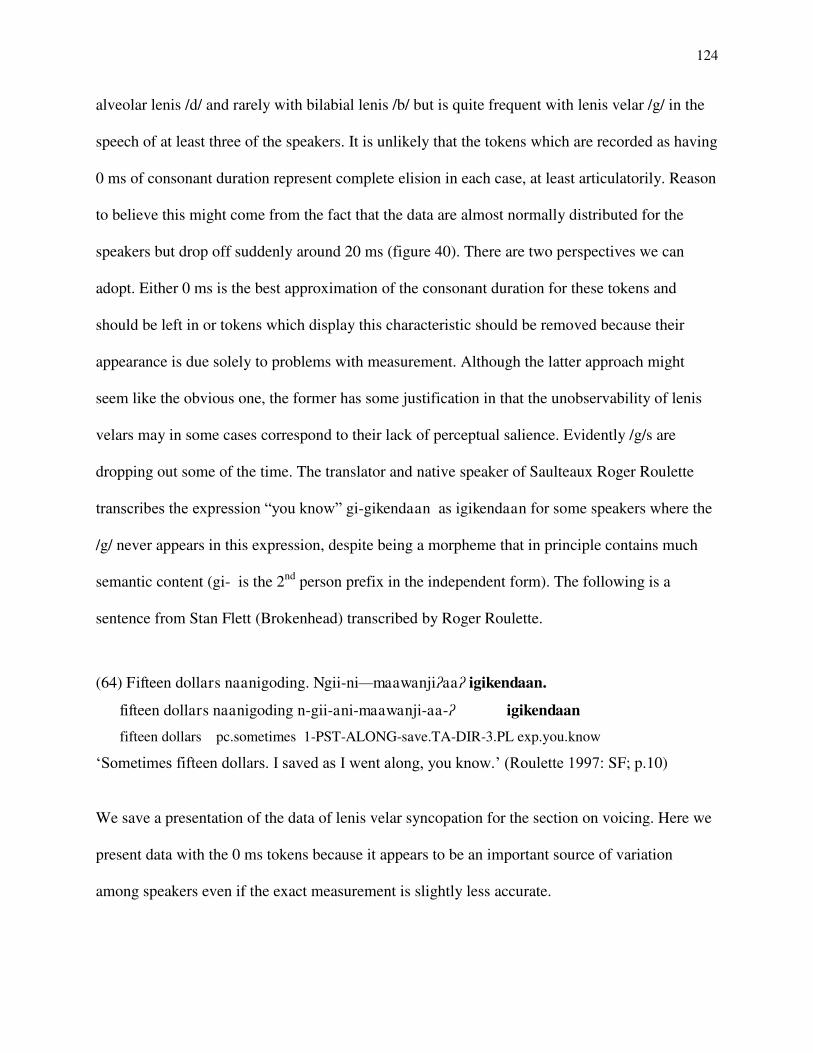
124

alveolar lenis /d/ and rarely with bilabial lenis /b/ but is quite frequent with lenis velar /g/ in the

speech of at least three of the speakers. It is unlikely that the tokens which are recorded as having

0 ms of consonant duration represent complete elision in each case, at least articulatorily. Reason

to believe this might come from the fact that the data are almost normally distributed for the

speakers but drop off suddenly around 20 ms (figure 40). There are two perspectives we can

adopt. Either 0 ms is the best approximation of the consonant duration for these tokens and

should be left in or tokens which display this characteristic should be removed because their

appearance is due solely to problems with measurement. Although the latter approach might

seem like the obvious one, the former has some justification in that the unobservability of lenis

velars may in some cases correspond to their lack of perceptual salience. Evidently /g/s are

dropping out some of the time. The translator and native speaker of Saulteaux Roger Roulette

transcribes the expression “you know” gi-gikendaan as igikendaan for some speakers where the

/g/ never appears in this expression, despite being a morpheme that in principle contains much

semantic content (gi- is the 2nd person prefix in the independent form). The following is a

sentence from Stan Flett (Brokenhead) transcribed by Roger Roulette.

(64) Fifteen dollars naanigoding. Ngii-ni—maawanji鞍aa鞍 igikendaan.

fifteen dollars naanigoding n-gii-ani-maawanji-aa-鞍 igikendaan

fifteen dollars pc.sometimes 1-PST-ALONG-save.TA-DIR-3.PL exp.you.know

„Sometimes fifteen dollars. I saved as I went along, you know.‟ (Roulette 1997: SF; p.10)

We save a presentation of the data of lenis velar syncopation for the section on voicing. Here we

present data with the 0 ms tokens because it appears to be an important source of variation

among speakers even if the exact measurement is slightly less accurate.

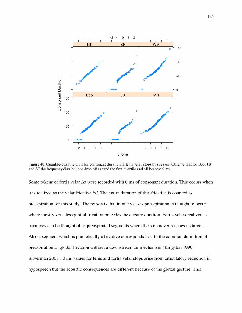
125

Figure 40. Quantile-quantile plots for consonant duration in lenis velar stops by speaker. Observe that for Boo, JB and SF the frequency distributions drop off around the first quartile and all become 0 ms.

Some tokens of fortis velar /k/ were recorded with 0 ms of consonant duration. This occurs when

it is realized as the velar fricative /x/. The entire duration of this fricative is counted as

preaspiration for this study. The reason is that in many cases preaspiration is thought to occur

where mostly voiceless glottal frication precedes the closure duration. Fortis velars realized as

fricatives can be thought of as preaspirated segments where the stop never reaches its target.

Also a segment which is phonetically a fricative corresponds best to the common definition of

preaspiration as glottal frication without a downstream air mechanism (Kingston 1990,

Silverman 2003). 0 ms values for lenis and fortis velar stops arise from articulatory reduction in

hypospeech but the acoustic consequences are different because of the glottal gesture. This

qnorm

Co

nso

na

nt D

ura

tio

n

0

50

100

150

-2 -1 0 1 2

Boo JB

-2 -1 0 1 2

MR

NT

-2 -1 0 1 2

SF

0

50

100

150WM

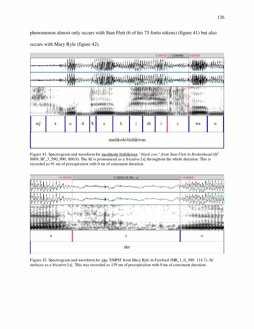
126

phenomenon almost only occurs with Stan Flett (6 of his 75 fortis tokens) (figure 41) but also

occurs with Mary Ryle (figure 42).

Figure 41. Spectrogram and waveform for mashkode-bizhikiwan ―black cow‖ from Stan Flett in Brokenhead (SF. 0009, SF_3_590_900; 860.9). The /k/ is pronounced as a fricative [x] throughout the whole duration. This is recorded as 91 ms of preaspiration with 0 ms of consonant duration.

Figure 42. Spectrogram and waveform for ako 'EMPH' from Mary Ryle in Fairford (MR_1_0_300: 114.7). /k/ surfaces as a fricative [x]. This was recorded as 159 ms of preaspiration with 0 ms of consonant duration.

127

Figure 43 displays the differences in closure duration for velar stops by speaker. (65) gives the

mean, standard deviations and proportional differences by speaker. (66) gives these same values

with all of the 0 ms tokens removed.

Figure 43. Consonant duration of /g/ vs. /k/ by speaker.

(65) Mean, standard deviation and proportional differences for consonant duration (all data).


g k g k

NT 58.6 100.1 18.3 16.5 1:1.7

Boo 46.4 93.1 19.7 29.9 1:2.0

SF 44.3 61.7 22.3 27.7 1:1.4

JB 35.2 102.8 22.9 28.2 1:2.9

WM 68.1 111.2 20.4 37.6 1:1.6

MR 58.4 102.3 18.6 30.5 1:1.75

Co

nso

na

nt D

ura

tio

n

0

50

100

150

200

g k

Boo

g k

JB

g k

MR

NT SF

0

50

100

150

200

WM

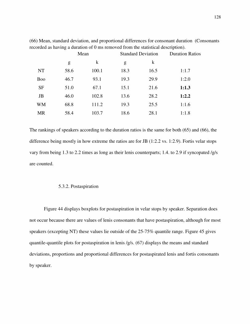
128

(66) Mean, standard deviation, and proportional differences for consonant duration (Consonants recorded as having a duration of 0 ms removed from the statistical description).


g k g k

NT 58.6 100.1 18.3 16.5 1:1.7

Boo 46.7 93.1 19.3 29.9 1:2.0

SF 51.0 67.1 15.1 21.6 1:1.3

JB 46.0 102.8 13.6 28.2 1:2.2

WM 68.8 111.2 19.3 25.5 1:1.6

MR 58.4 103.7 18.6 28.1 1:1.8

The rankings of speakers according to the duration ratios is the same for both (65) and (66), the

difference being mostly in how extreme the ratios are for JB (1:2.2 vs. 1:2.9). Fortis velar stops

vary from being 1.3 to 2.2 times as long as their lenis counterparts; 1.4. to 2.9 if syncopated /g/s

are counted.


Figure 44 displays boxplots for postaspiration in velar stops by speaker. Separation does

not occur because there are values of lenis consonants that have postaspiration, although for most

speakers (excepting NT) these values lie outside of the 25-75% quantile range. Figure 45 gives

quantile-quantile plots for postaspiration in lenis /g/s. (67) displays the means and standard

deviations, proportions and proportional differences for postaspirated lenis and fortis consonants

by speaker.

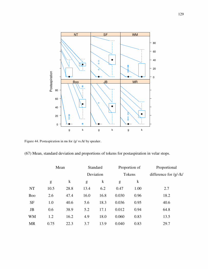
129

Figure 44. Postaspiration in ms for /g/ vs./k/ by speaker.

(67) Mean, standard deviation and proportions of tokens for postaspiration in velar stops.

Mean Standard

Deviation

Proportion of

Tokens

Proportional

difference for /g/-/k/

g k g k g k

NT 10.5 28.8 13.4 6.2 0.47 1.00 2.7

Boo 2.6 47.4 16.0 16.8 0.030 0.96 18.2

SF 1.0 40.6 5.6 18.3 0.036 0.95 40.6

JB 0.6 38.9 5.2 17.1 0.012 0.94 64.8

WM 1.2 16.2 4.9 18.0 0.060 0.83 13.5

MR 0.75 22.3 3.7 13.9 0.040 0.83 29.7

Po

sta

sp

ira

tio

n

0

20

40

60

80

g k

Boo

g k

JB

g k

MR

NT SF

0

20

40

60

80

WM

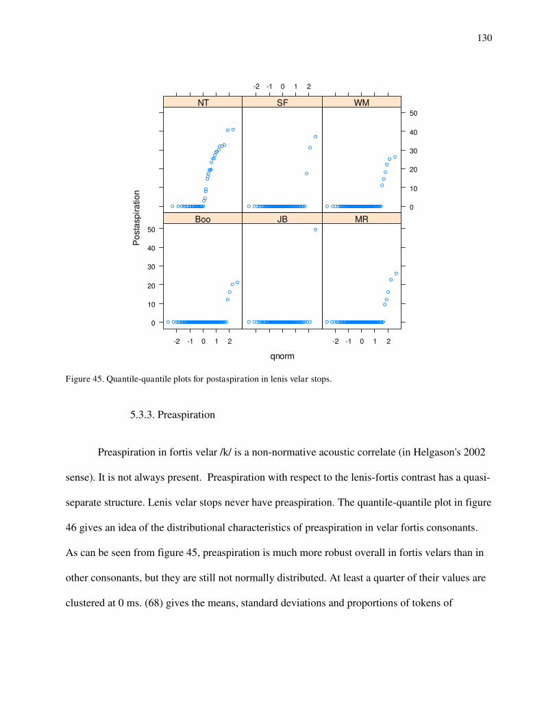
130

Figure 45. Quantile-quantile plots for postaspiration in lenis velar stops.


Preaspiration in fortis velar /k/ is a non-normative acoustic correlate (in Helgason's 2002

sense). It is not always present. Preaspiration with respect to the lenis-fortis contrast has a quasi-

separate structure. Lenis velar stops never have preaspiration. The quantile-quantile plot in figure

46 gives an idea of the distributional characteristics of preaspiration in velar fortis consonants.

As can be seen from figure 45, preaspiration is much more robust overall in fortis velars than in

other consonants, but they are still not normally distributed. At least a quarter of their values are

clustered at 0 ms. (68) gives the means, standard deviations and proportions of tokens of

qnorm

Po

sta

sp

ira

tio

n

0

10

20

30

40

50

-2 -1 0 1 2

Boo JB

-2 -1 0 1 2

MR

NT

-2 -1 0 1 2

SF

0

10

20

30

40

50

WM

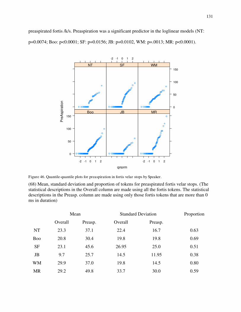
131

preaspirated fortis /k/s. Preaspiration was a significant predictor in the loglinear models (NT:

p=0.0074; Boo: p<0.0001; SF: p=0.0156; JB: p=0.0102, WM: p=.0013; MR: p<0.0001).

Figure 46. Quantile-quantile plots for preaspiration in fortis velar stops by Speaker.

(68) Mean, standard deviation and proportion of tokens for preaspirated fortis velar stops. (The statistical descriptions in the Overall column are made using all the fortis tokens. The statistical descriptions in the Preasp. column are made using only those fortis tokens that are more than 0 ms in duration)



NT 23.3 37.1 22.4 16.7 0.63

Boo 20.8 30.4 19.8 19.8 0.69

SF 23.1 45.6 26.95 25.0 0.51

JB 9.7 25.7 14.5 11.95 0.38

WM 29.9 37.0 19.8 14.5 0.80

MR 29.2 49.8 33.7 30.0 0.59

qnorm

Pre

Asp

ira

tio

n

0

50

100

150

-2 -1 0 1 2

Boo JB

-2 -1 0 1 2

MR

NT

-2 -1 0 1 2

SF

0

50

100

150

WM

132

Recall that there was a difference in the amount of preaspiration that occurred with a

dental/alveolar fortis stop depending on the previous vowel. We attributed this to differential

degrees of reduction of the previous vowel. Figure 47 gives fortis consonants before short and

long vowels in terms of their preaspiration by speaker. Again it looks as if short vowels are more

prone to devoice and cause a preaspirated fortis consonant. This seems to be true for Boo, NT,

MR and SF. Figure 47 is slightly misleading because long vowels before fortis consonants are

much less frequent overall. Nevertheless there are proportional differences between the two

groups, and in every case, except for WM, fortis consonants preaspirate more before short

vowels. This fact makes sense if we consider the literature on Ojibwe stress, which posits that

short vowels are often lenited (Piggott 1980, Valentine 1994, 2001). This could correspond to

articulatory undershoot in terms of the preconsonantal vocalic laryngeal gesture, increasing the

likelihood that voiceless laryngeal coarticulation from the fortis consonant will produce

preaspiration.

The differences are fairly substantial for NT, Boo, SF and MR but not for the other speakers.

Loglinear models where we attempt to predict the vowel length feature based off preaspiration

only come out as significant for Boo (p=.0110), SF (p=.0261) and MR (p=.0274). Models for the

other speakers were not significant (NT: p=.4787, JB: p=.7484, WM: p=.0935).

133

Figure 47. Preaspiration in velar fortis stops before long and short vowels by Speaker.

(46) Token counts and proportions of preaspirated /k/s in relation to vowel length by speaker.

long long short short

preasp./tokens percentage of

preasp.

preasp./tokens percentage of

preasp.

NT 7/17 0.41 15/18 0.83

Boo 13/31 0.42 83/109 0.76

SF 2/17 0.12 36/63 0.57

JB 7/22 0.32 18/44 0.41

WM 6/7 0.86 38/48 0.79

MR 8/19 0.42 36/56 0.64

Pre

asp

ira

tion

0

50

100

150

long short

Boo

long short

JB

long short

MR

NT SF

0

50

100

150

WM

134

5.3.4. Voicing

Sonority has a quasi-separate structure in almost all speakers for velars. For Boo Sonority

has complete separation. The difference between Boo and the other speakers in this regard may

correspond to differences along the hypo-hyper speech continuum (Moon & Lindblom 1994).

Recall that Boo's data was gathered from elicitation, and thus it most likely lies closer to the

hyperspeech end of the continuum rather than the data from the other speakers which is from

conversation (SF, JB, WM, MR) or story telling (NT). On the hyperspeech end of the continuum

acoustic correlates will tend to be exaggerated. Thus, if voicing is an important acoustic correlate

to the contrast for Boo, then he will exaggerate the extent to which it appears in his speech.

There are no substantially voiced fortis /k/s (they all receive a Sonority value of 0). The

proportions for each sonority value for each speaker are given in (70). Figure 48 displays the

Sonority values for lenis velar stops for each speaker. In the loglinear model the Sonority value

was significant for all speakers (NT=.0016; Boo<.0001; SF: p<.0001; JB: p<.0001; WM:

p<.0037; MR: p=.0004).

(70) Proportions of /g/ falling in each sonority value by speaker.

0 1 2 3 4 5

NT .32 .48 .16 .02 .02 0

Boo 0 .135 .49 .32 .05 0

SF .02 .17 .42 .265 .07 .05

JB .01 .06 .13 .56 .10 .13

WM .57 .34 .07 .01 0 0

MR .42 .44 .10 .04 0 0

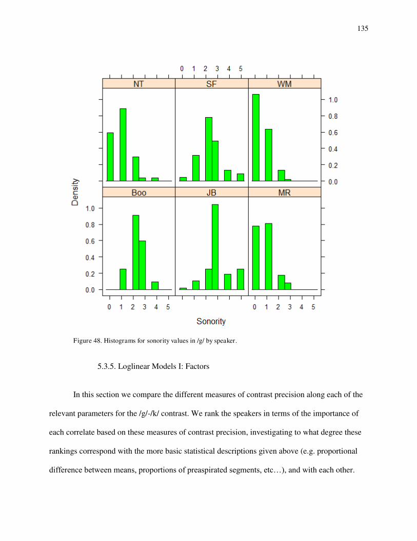
135

Figure 48. Histograms for sonority values in /g/ by speaker.



relevant parameters for the /g/-/k/ contrast. We rank the speakers in terms of the importance of

each correlate based on these measures of contrast precision, investigating to what degree these

rankings correspond with the more basic statistical descriptions given above (e.g. proportional

difference between means, proportions of preaspirated segments, etc…), and with each other.

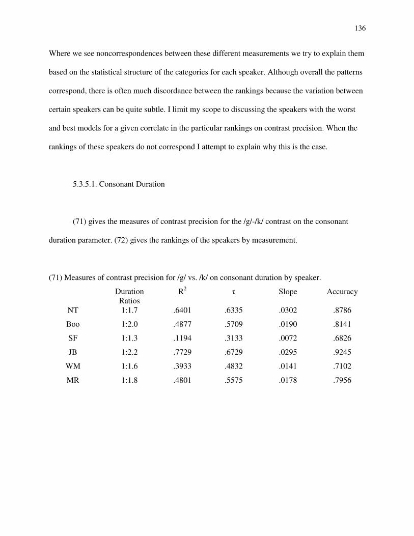
136

Where we see noncorrespondences between these different measurements we try to explain them

based on the statistical structure of the categories for each speaker. Although overall the patterns

correspond, there is often much discordance between the rankings because the variation between

certain speakers can be quite subtle. I limit my scope to discussing the speakers with the worst

and best models for a given correlate in the particular rankings on contrast precision. When the

rankings of these speakers do not correspond I attempt to explain why this is the case.


(71) gives the measures of contrast precision for the /g/-/k/ contrast on the consonant

duration parameter. (72) gives the rankings of the speakers by measurement.

(71) Measures of contrast precision for /g/ vs. /k/ on consonant duration by speaker.

Duration Ratios

R2 k Slope Accuracy

NT 1:1.7 .6401 .6335 .0302 .8786

Boo 1:2.0 .4877 .5709 .0190 .8141

SF 1:1.3 .1194 .3133 .0072 .6826

JB 1:2.2 .7729 .6729 .0295 .9245

WM 1:1.6 .3933 .4832 .0141 .7102

MR 1:1.8 .4801 .5575 .0178 .7956

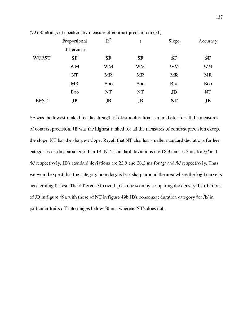
137


Proportional

difference

R2 k Slope Accuracy

WORST SF SF SF SF SF

WM WM WM WM WM

NT MR MR MR MR

MR Boo Boo Boo Boo

Boo NT NT JB NT

BEST JB JB JB NT JB

SF was the lowest ranked for the strength of closure duration as a predictor for all the measures

of contrast precision. JB was the highest ranked for all the measures of contrast precision except

the slope. NT has the sharpest slope. Recall that NT also has smaller standard deviations for her

categories on this parameter than JB. NT's standard deviations are 18.3 and 16.5 ms for /g/ and

/k/ respectively. JB's standard deviations are 22.9 and 28.2 ms for /g/ and /k/ respectively. Thus

we would expect that the category boundary is less sharp around the area where the logit curve is

accelerating fastest. The difference in overlap can be seen by comparing the density distributions

of JB in figure 49a with those of NT in figure 49b JB's consonant duration category for /k/ in

particular trails off into ranges below 50 ms, whereas NT's does not.

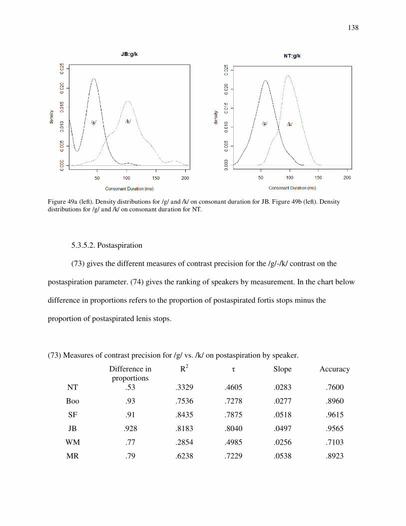
138

Figure 49a (left). Density distributions for /g/ and /k/ on consonant duration for JB. Figure 49b (left). Density distributions for /g/ and /k/ on consonant duration for NT.


(73) gives the different measures of contrast precision for the /g/-/k/ contrast on the

postaspiration parameter. (74) gives the ranking of speakers by measurement. In the chart below

difference in proportions refers to the proportion of postaspirated fortis stops minus the

proportion of postaspirated lenis stops.

(73) Measures of contrast precision for /g/ vs. /k/ on postaspiration by speaker.

Difference in proportions

R2 k Slope Accuracy

NT .53 .3329 .4605 .0283 .7600

Boo .93 .7536 .7278 .0277 .8960

SF .91 .8435 .7875 .0518 .9615

JB .928 .8183 .8040 .0497 .9565

WM .77 .2854 .4985 .0256 .7103

MR .79 .6238 .7229 .0538 .8923

139


Difference in

Proportions

R2 k Slope Accuracy

WORST NT WM NT WM NT

WM NT WM Boo WM

MR MR MR NT MR

SF Boo Boo JB Boo

JB JB SF SF JB

BEST Boo SF JB MR SF

The k and Accuracy measures show that postaspiration for NT has the worst contrast precision.

The R2 and Slope show that WM is the worst on this parameter. NT's k is larger because NT has

the most postaspirated lenis /g/s which means that there is more discordance on this category

space overall. WM's R2 is lower than NT's because his postaspirated fortis stops generally have a

smaller duration of mVOT (a mean of 16.2 ms as opposed to NT`s mean of 28.8 ms). Even when

stops are postaspirated for WM they are very close to the point of the highest probability of

confusion relative to other speakers (Pr(0.5)) which is at 12 ms for WM (it is at 26 ms for NT).

This has the effect of making WM's predicted probabilities further away from their

corresponding dummy variables.

JB has a slightly better k coefficient for postaspiration than SF. This corresponds to slight

differences in the standard deviations of their categories. JB's standard deviation for /k/ is 1 ms

less than that for SF. MR has a higher slope than SF and JB despite only ranking fourth for all

the other measurements. MR's postaspirated fortis stops are closer to 0 ms, where the density

distribution of the postaspiration for lenis /g/ is the highest. Figure 50 displays the density

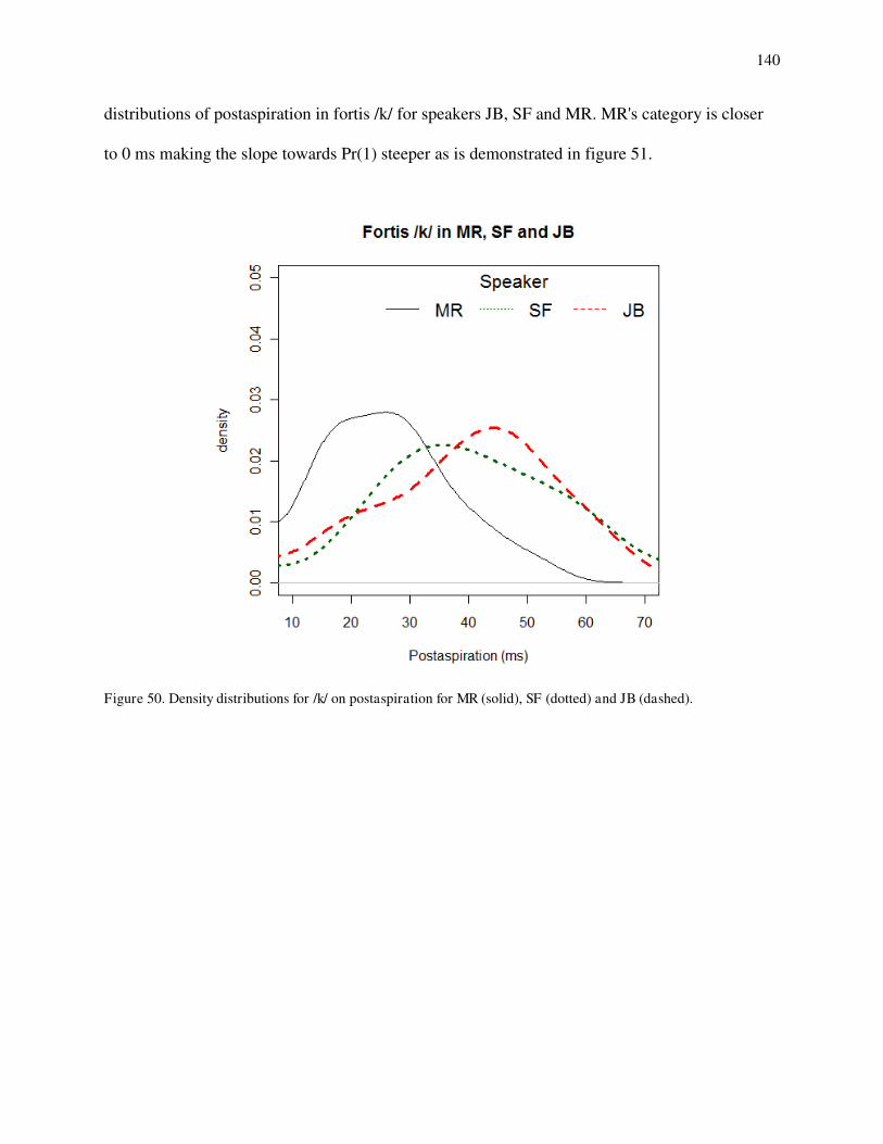
140

distributions of postaspiration in fortis /k/ for speakers JB, SF and MR. MR's category is closer

to 0 ms making the slope towards Pr(1) steeper as is demonstrated in figure 51.

Figure 50. Density distributions for /k/ on postaspiration for MR (solid), SF (dotted) and JB (dashed).

141

Figure 51. Loglinear cuvres for /g/-/k/ contrast on postaspiration for MR (solid), SF (dotted), and JB (dashed).


(75) gives the measures of contrast precision for velars by speaker. (76) gives the

rankings of speaker by measure. In the following chart proportion refers to the proportion of

preaspirated fortis /k/s. Lenis /g/s never have preaspiration.

(75) Measures of contrast precision for /g/ vs. /k/ on preaspiration by speaker.


NT .63 .4799 .6539 .0521 .8143

Boo .69 .4473 .6080 .0462 .8406

SF .51 .3440 .5527 .0500 .7566

JB .38 .2499 .4873 .0667 .6894

WM .80 .7033 .7735 .07135 .9000

MR .59 .4119 .6130 .0353 .7961

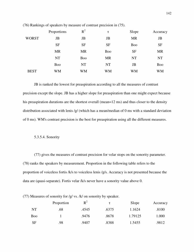
142



WORST JB JB JB MR JB

SF SF SF Boo SF

MR MR Boo SF MR

NT Boo MR NT NT

Boo NT NT JB Boo

BEST WM WM WM WM WM

JB is ranked the lowest for preaspiration according to all the measures of contrast

precision except the slope. JB has a higher slope for preaspiration than one might expect because

his preaspiration durations are the shortest overall (mean=12 ms) and thus closer to the density

distribution associated with lenis /g/ (which has a mean/median of 0 ms with a standard deviation

of 0 ms). WM's contrast precision is the best for preaspiration using all the different measures.

5.3.5.4. Sonority

(77) gives the measures of contrast precision for velar stops on the sonority parameter.

(78) ranks the speakers by measurement. Proportion in the following table refers to the

proportion of voiceless fortis /k/s to voiceless lenis /g/s. Accuracy is not presented because the

data are (quasi-separate). Fortis velar /k/s never have a sonority value above 0.

(77) Measures of sonority for /g/ vs. /k/ on sonority by speaker.


NT .68 .4545 .6375 1.1624 .8100

Boo 1 .9476 .8678 1.79125 1.000

SF .98 .9407 .8388 1.5455 .9812

143

JB .99 .4855 .8023 0.1899 .9662

WM .43 .2085 .4488 1.0493 .5000

MR .48 .3500 .5668 1.2669 .7876



WORST WM WM WM JB NT

MR MR MR WM WM

NT NT NT NT SF

SF JB JB MR MR

JB SF SF SF JB


Sonority is the worst predictor for WM for all the measurements of contrast precision

except for slope. JB's logit curve has a shallower slope than WM's. JB's slope is shallow because

so many of his tokens have a sonority value of 3. His logit curve becomes shallower because its

ceiling effect is reached later in the sonority space. Boo's data for the sonority value display

complete- separation. Sonority is the best predictor for this speaker.





Anderson 2002, Anderson 2008). In each section I start with what I will call "the basic model"

which consists of an additive multiple logistic regression model with all of the factors discussed

in the previous section. Based on the results of the basic model, nonsignificant factors are

144

removed and suspected interactions are added until the best model is achieved (according to the

lowest AIC). I then compare the models for all the speakers and discuss the extent to which the

measures of contrast precision corroborate the main thesis. The count of tokens for velar stops by

speaker are given in (79).


k 138 66 76 35 76 55

g 120 89 113 50 82 96

5.3.6.1. NT: /g/-/k/

The basic model for NT for the /g/-/k/ contrast is presented in (80). The AIC is 32.65.

(80) Basic model for NT: /g/-/k/

Estimate Pr(>|z|)

(Intercept) -9.8446 0.0029 **

ConsDur 0.0894 0.0065 **

PostAsp 0.0994 0.0338 *

PreAsp 0.0600 0.1511

Sonority -2.2123 0.1833

When nonsignificant factors were removed the AIC increased to 38.94. When only

sonority was removed from the basic model the AIC was 33.78. When only sonority was

removed from the basic model the AIC was 34.99. Two-way interaction terms between

consonant duration and postaspiration and consonant duration and sonority were significant

(p=.0126 and p=.03034 respectively) but neither of these models were better fits to the data in

terms of the AIC. Thus the best model is the basic model in (80).

145

5.3.6.2. Boo: /g/-/k/

The basic model for Boo for the lenis-fortis contrast in velars is given in (81). The AIC is

29.69.

(81) Basic model for Boo: /g/-/k/

Estimate Pr(>|z|)

(Intercept) 1.0273 0.6954

ConsDur 0.0084 0.6867

PostAsp 0.0193 0.3940

PreAsp 0.0843 0.1503

Sonority -4.9008 0.0041 **

When nonsignificant terms were removed the AIC decreased to 26.03. This is the best

model for Boo. It is given in (82). When consonant duration was readded in a multiplicative

model the interaction term between consonant duration and sonority is significant (p=.0027) but

the AIC increased to 31.62.

(82) Best model for Boo: /g/-/k

Estimate Pr(>|z|)

(Intercept) 4.0133 3.57e-10 ***

Sonority -7.5038 2.79e-06 ***

5.3.6.3. SF:/g/-/k/

The results of the basic model for SF for the /g/-/k/ contrast is produced in (83). The AIC is

19.25.

(83) Basic model for SF: /g/-/k/

Estimate Pr(>|z|)

146

(Intercept) -1.1114 0.6684

ConsDur 0.0178 0.5952

PostAsp 0.1178 0.0115 *

PreAsp 0.0403 0.3366

Sonority -3.2406 0.0233 *

When nonsignificant factors were removed the AIC decreased to 16.04. In the multiplicative

version of this model, with just preaspiration and sonority, the interaction term was

nonsignificant (p=.976) and the AIC increased to 18.9. Hence the best model is that produced in

(84).

(84) Best model for SF: /g/-/k/

Estimate Pr(>|z|)

(Intercept) 1.1911 0.2192

PostAsp 0.1181 0.0184 *

Sonority -4.8571 0.0006 ***

5.3.6.4. JB: /g/-/k/

The results of the basic model for JB for the /g/-/k/ contrast are given in (85). The AIC is 23.6.

(85) Basic model for JB: /g/-/k/

Estimate Pr(>|z|)

(Intercept) 0.66786 0.759533

ConsDur 0.04318 0.010338 *

PostAsp -0.03568 0.358163

PreAsp 0.02238 0.677798

Son -7.44796 0.000512 ***

When nonsignificant factors were removed the AIC decreased to 20.1. No two way interaction

terms came out as significant. The results for the best model are given in (86).

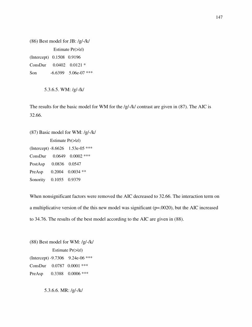
147

(86) Best model for JB: /g/-/k/

Estimate Pr(>|z|)

(Intercept) 0.1508 0.9196

ConsDur 0.0402 0.0121 *

Son -6.6399 5.06e-07 ***

5.3.6.5. WM: /g/-/k/

The results for the basic model for WM for the /g/-/k/ contrast are given in (87). The AIC is

32.66.

(87) Basic model for WM: /g/-/k/

Estimate Pr(>|z|)

(Intercept) -8.6626 1.53e-05 ***

ConsDur 0.0649 0.0002 ***

PostAsp 0.0836 0.0547

PreAsp 0.2004 0.0034 **

Sonority 0.1055 0.9379

When nonsignificant factors were removed the AIC decreased to 32.66. The interaction term on

a multiplicative version of the this new model was significant (p=.0020), but the AIC increased

to 34.76. The results of the best model according to the AIC are given in (88).

(88) Best model for WM: /g/-/k/

Estimate Pr(>|z|)

(Intercept) -9.7306 9.24e-06 ***

ConsDur 0.0787 0.0001 ***

PreAsp 0.3388 0.0006 ***

5.3.6.6. MR: /g/-/k/

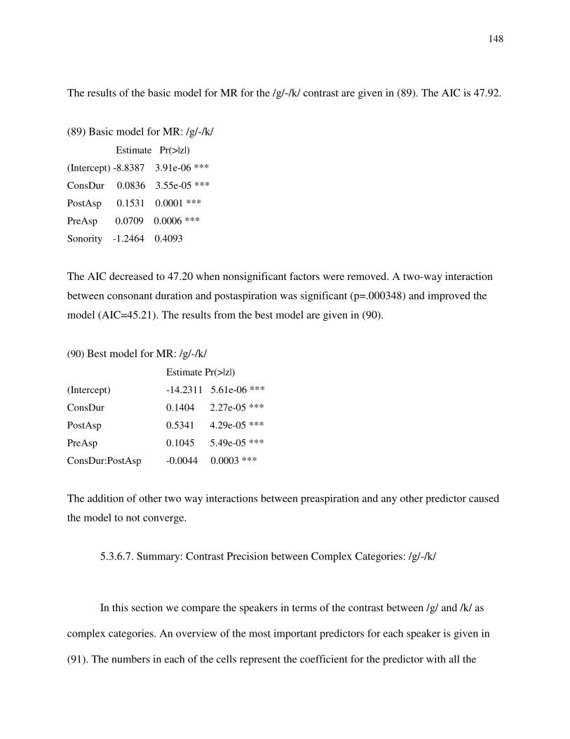
148

The results of the basic model for MR for the /g/-/k/ contrast are given in (89). The AIC is 47.92.

(89) Basic model for MR: /g/-/k/

Estimate Pr(>|z|)

(Intercept) -8.8387 3.91e-06 ***

ConsDur 0.0836 3.55e-05 ***

PostAsp 0.1531 0.0001 ***

PreAsp 0.0709 0.0006 ***

Sonority -1.2464 0.4093

The AIC decreased to 47.20 when nonsignificant factors were removed. A two-way interaction

between consonant duration and postaspiration was significant (p=.000348) and improved the

model (AIC=45.21). The results from the best model are given in (90).

(90) Best model for MR: /g/-/k/

Estimate Pr(>|z|)

(Intercept) -14.2311 5.61e-06 ***

ConsDur 0.1404 2.27e-05 ***

PostAsp 0.5341 4.29e-05 ***

PreAsp 0.1045 5.49e-05 ***

ConsDur:PostAsp -0.0044 0.0003 ***

The addition of other two way interactions between preaspiration and any other predictor caused

the model to not converge.

5.3.6.7. Summary: Contrast Precision between Complex Categories: /g/-/k/

In this section we compare the speakers in terms of the contrast between /g/ and /k/ as

complex categories. An overview of the most important predictors for each speaker is given in

(91). The numbers in each of the cells represent the coefficient for the predictor with all the

149

variables standardized (the mean subtracted from the value divided by the standard deviation).

Recall we cannot compare the AIC between speakers directly. Each speaker has a different

amount of /g/s and /k/s. The AIC value depends on information entropy (i.e. how much

information is lost be the model), which is contingent on sample size.

The table in (91) contains coefficients associated with each factor involved in the model with

each variable standardized. The coefficients for the predictors represent the values when all of

the other predictors are at their mean. The units are also standardized so it is easier to compare

their relative importance in a particular speaker's model. However, since the variables do not

have all of the same distributional structures (when compared to each other and possibly when

compared across speakers) the coefficients do not directly represent the relative importance of

each cue in each speaker's model. The mapping of probability functions onto the parametric

phonetic space is too contingent on relationships between the parameters and the statistical

structure of the density distributions, some of which are highly skewed.

(91) Overview of /g/ vs. /k/ as complex categories.

ConsDur PostAsp PreAsp Sonority Interactions

NT 2.413 1.415 1.103 -1.790

Boo -8.957

SF 1.327 -7.871

JB 1.687 -6.640

WM 2.735 6.294

MR 3.210 2.802 2.672 -1.986 (ConsDur:PostAsp)

150

All of the speakers have different models for the /g/-/k/ contrast based on their production data.

One notable difference is the number of dimensions used by the speakers in making the contrast.

Despite the fact that Boo encodes other dimensions for /g/ and /k/ (Boo's /k/s are twice as long as

his /g/s on consonant duration), a model with only sonority is sufficient for this contrast for him.

/g/-/k/ are always distinguished with using voicing in my data. Generally the other speakers rely

on more dimensions. This difference between Boo and the other speakers corresponds well to the

findings of those phoneticians who have been interested in establishing "invariance" associated

phonetic contrast (e.g. Blumstein 1986, Stevens 2002, et al.).50 One of the recent findings of this

research paradigm has been that invariance is present in controlled speech but obliterated in

natural speech where "substitute" or "secondary" cues are coopted to mark the relevant contrasts

(Stevens & Keyser 2010, cf. Jessen 1998 for definitions of "substitute" and "primary" correlates

etc…). The data in (91) could be seen as supporting this picture since Boo's data were all from

elicitation and the other speaker's data were from more natural speech.51 The difference between

Boo and most of the other speakers also makes sense from the perspective of H & H theory,

which we have already discussed. Boo's speech is closer to the hyperspeech end of the

continuum than the speech of other speakers in this study because his data are from elicitation

which I assume is closer to clear speech (cf. Moon & Lindblom 1994, Picheny et al. 1986).

Acoustic targets are reached more emphatically and consistently, his model can consequently

afford to be less complex. The explanation based on invariance and H & H speech has some

problems, however, notably that there is very little difference between Boo's model and SF's.

50 See the articles in Perkell & Klatt (1986) for issues related to this research paradigm. 51 However, in most studies on invariance subjects are asked to read a word list using a consistent carrier phrase whereas for Boo the words were taken from more naturalistic sentences. In fact in many cases investigators feel that they need to have subjects produce invented words in order to prove that there is "invariance" associated with a contrast (e.g. Kim et al. 2010).

151

The different coefficients associated with each correlate suggest that the speakers are using

different weightings of these correlates in their speech to mark the /g/-/k/ contrast. The first

evidence of this comes from the fact that most of the speakers are using different dimensions in

general to mark the contrast in their production. So as with the /d/-/t/ contrast WM uses

consonant duration and preaspiration whereas MR uses these dimensions in addition to

postaspiration. For the /d/-/t/ contrast WM and MR's models suggested that the former was

marking the contrast more strongly based on the two comparable dimensions (consonant duration

and preaspiration) but that MR was partly compensating for this by using postaspiration.52 In this

case, however, consonant duration appears to be a better predictor for MR. Figure 52 gives

loglinear curves for WM and MR for the /g/-/k/ contrast on consonant duration when all other

factors are held at 0. The slope of MR's loglinear curve is steeper than WM's at the highest

probability of confusion. In addition to this MR uses postaspiration for making the contrast. 83%

of MR's fortis tokens have postaspiration and in these cases the probability of a correctly

choosing a fortis token increases drastically. This can be seen from figure 52 which compares the

loglinear curves of WM and MR on consonant duration when preaspiration is 0 ms and

postaspiration is 30 ms. The fact that the curve ceilings for MR at a very early stage on the

consonant duration space with 30 ms of postaspiration indicates that this correlate is extremely

useful for marking the contrast irrespective of consonant duration. Postaspiration is not in WM's

model for the /g/-/k/ contrast. The reason is because occurrences of postaspiration are predictable

from distinctive values of consonant duration or preaspiration.

52 Partly compensating, because it seems that based on the correlates studied in this investigation MR had a lower contrast precision than WM between /d/ and /t/ according to the Accuracy measure.

152

Figure 52a (left). Loglinear curves for /g/-/k/ contrast on consonant duration for WM (solid) and MR (dashed) with all other factors held at 0 ms. Figure 52b (right). Loglinear curves for /g/-/k/ contrast on consonant duration for WM (solid) and MR (dashed) with preaspiration at 0 ms and postaspiration a 30 ms for MR.

When we compare loglinear curves over consonant duration we are describing a gradual increase

in the probability of /k/ over /g/. If it is worth it for a speaker to use preaspiration in her model

then any token that has preaspiration can instantly be recognized as a fortis stop irrespective of

the values on other parameters. Notice that 80% of WM's fortis stops have preaspiration,

meaning that the other correlates are essentially only relevant in predicting the other 20%. MR

has 59% of her fortis stops preaspirated. The power given to the other correlates in her model

might be seen as accounting for that 11% that it cannot predict with preaspiration.53

Consequently she adds another dimension (postaspiration) and needs consonant duration to be a

more consistent predictor. Again, this situation might suggest that the speakers are using a

53

Of course this is an oversimplification. This angle of description does not take into account that, depending on the speaker, phonetic covariates can have different degrees of multicollinearity with one another. The predictive power we might naively attribute to MR's coefficients does not necessarily take into account that how important they are. If we observe figure 52a, it appears that the probability of a velar stop token being fortis would be close to 1 at approximately 150 ms. The importance of consonant duration in relation to preaspiration really depends on how much this value of consonant duration is associated with no preaspiration. If lower values of consonant duration (say around 120 ms) appeared with no preaspiration it would not matter how good the latter predictor was. This problem is only resolved to a certain extent by standardizing the predictor variables in relation to their mean and standard deviation as is done here.

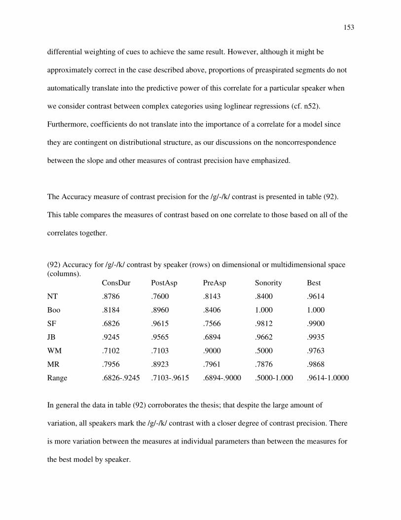
153

differential weighting of cues to achieve the same result. However, although it might be

approximately correct in the case described above, proportions of preaspirated segments do not

automatically translate into the predictive power of this correlate for a particular speaker when

we consider contrast between complex categories using loglinear regressions (cf. n52).

Furthermore, coefficients do not translate into the importance of a correlate for a model since

they are contingent on distributional structure, as our discussions on the noncorrespondence

between the slope and other measures of contrast precision have emphasized.

The Accuracy measure of contrast precision for the /g/-/k/ contrast is presented in table (92).

This table compares the measures of contrast based on one correlate to those based on all of the

correlates together.

(92) Accuracy for /g/-/k/ contrast by speaker (rows) on dimensional or multidimensional space (columns). ConsDur PostAsp PreAsp Sonority Best

NT .8786 .7600 .8143 .8400 .9614

Boo .8184 .8960 .8406 1.000 1.000

SF .6826 .9615 .7566 .9812 .9900

JB .9245 .9565 .6894 .9662 .9935

WM .7102 .7103 .9000 .5000 .9763

MR .7956 .8923 .7961 .7876 .9868

Range .6826-.9245 .7103-.9615 .6894-.9000 .5000-1.000 .9614-1.0000

In general the data in table (92) corroborates the thesis; that despite the large amount of

variation, all speakers mark the /g/-/k/ contrast with a closer degree of contrast precision. There

is more variation between the measures at individual parameters than between the measures for

the best model by speaker.

154

6. Discussion and Summary

Research in phonetic typology has shown that languages encode and contrast phonetic

categories on a high dimensional phonetic space (Pierrehumbert 2003b). Analogous

phonological units are encoded on these phonetic continua in a language specific fashion. This

applies to the descriptive label "lenis/fortis" as it is used in the description of phonological

inventories across languages. The basic distinction between phonemes transcribed as /b/-/p/, /p/-

/pp/ etc., depending on the linguist is actually encoded on a variety of phonetic continua. The

relative weight given to each continuum for the purpose of maintaining this contrast is language

and even dialect specific.

In this thesis I attempted to formalize Pierrehumbert's concept of category and category system

to model the contrast between lenis and fortis stops based on production data from six speakers

of Saulteaux Ojibwe. I developed the notion of contrast precision in relation to categories and

category systems. Based on the results of loglinear models, various measures of contrast

precision were compared. A distinction was made between contrast precision on a particular

phonetic continuum or dimension and contrast precision between category systems on a

multidimensional phonetic space. A hypothesis was formulated in relation to contrast precision

based on findings in phonetic typology (Pierrehumbert 2003b), quoted in (93)

(93) Although speakers/dialects of Saulteaux may vary in terms of how strongly the lenis-fortis

contrast is marked on particular dimensions of obstruent space (i.e. they will have different

155

levels of contrast precision for these dimensions), when the contrast is compared on a k-

dimensional space of phonetic correlates, the differences in contrast precision will become

increasingly small as k increases.

This hypothesis underscores many issues that are complex and extremely contingent since it is

based on relationships between dimensions and the measure of contrast precision employed. It is

also based on the size of k, i.e. how many parameters are involved in the comparison. Still, I

have had various degrees of success in corroborating the hypothesis in (93) in this thesis. It is

worth reviewing why we would expect (93) to be true in the first place.

Oversimplifying for a moment, generally the literature on phonetic typology suggests that an

increase in the importance of one dimension of phonetic encoding for contrast maintenance

between units of phonetic encoding implies a concomitant decrease in the importance of other

dimensions. For example Engstrand & Krull (1994) investigated vowel length in conversational

Swedish, Finnish and Estonian. They found that the density distributions of long and short

vowels in Swedish overlapped more than for Finnish and Estonian. This could be related to the

finding that vowel length distinctions are enhanced by formant structure to a greater extent in

Swedish than in the other languages.

A similar situation was found in Korean but between generations rather than across languages.

Older speakers of Korean produced large differences in VOT between lenis and aspirated stops

(30-35 ms for lenis, 93-108 ms for aspirated). VOT values for these two types did not overlap.

F0 also covaried with the contrast but was considered a redundant correlate (Silva 2006), a by-

156

product of the articulatory configurations used to make the VOT difference. In recent studies

with speakers born after 1965, the VOT values overlap more, but the contrast is reinforced by F0

on the vowels following the stops (Kang & Guion 2008). Thus, contrast precision on VOT was

reduced and replaced by a higher precision on the F0 dimension. Although there are some

complications the current study suggests that speakers that use more voicing on lenis stops (JB

and Boo) use less preaspiration. Speakers that use more preaspiration on fortis stops (WM and

MR) will tend to mark less lenis stops as voiced. SF seems to use preaspiration and voicing

together to mark the contrast, to the detriment of consonant duration compared to this value for

other speakers.

These phenomena have functional explanations. On the one hand a certain amount of acoustic

distance between sounds must be maintained in order for the contrast to be perceived. On the

other hand redundant phonetic attributes are often not maintained in production because they

imply an increase in articulatory effort or complexity. (The interplay between these two forces

has often been used to explain regularities in the structure of phonological inventories (Lindblom

& Maddieson 1986, Boersma 1998).) If we take the example from Korean described above, we

can see that the loss of VOT as an important correlate for the lenis-aspirated contrast was a

consequence of the latter functional drive (minimal articulatory effort) and the concomitant

increase of importance of F0 as a consequence of the former (perceptual distance).

The situation is not as simple as the caricature above would suggest. Redundancies must always

exist in the marking of phonetic contrast for change to occur at all (Blevins 2007). Hence, the

drive towards minimal articulatory effort is only a factor. Thus we should not expect to find

157

perfect trading relations between cues. This redundancy implies that covariates of phonetic

contrast may not be orthogonal. For example, in Korean the F0 was undoubtedly coded by the

older speakers, the younger speakers enhanced the importance the feature rather than inventing

out of thin air (cf. Kirby 2011, Kang & Guion 2008, 2009). Two auxiliary theories can help

explain how this situation comes about; the acoustic theory of speech production and exemplar

theory (Pierrehumbert 2000, Pierrehumbert, Beckman & Ladd 2000).

From the acoustic theory of speech production we know that there are nonorthogonalities in the

mapping of articulation to acoustic output (Pierrehumbert 2000). For instance a longer voiceless

laryngeal gesture generally creates higher intraoral pressure which will tend to produce a longer

and more intense aspiration burst after the release (Fant 1960, Stevens 2000). This explains why

in a two-way obstruent contrast aspiration is typically associated with longer voiceless

consonants. A language that has only a two-way contrast between obstruents will not contrast

[dh] vs. [t:] for example. If aspiration is contrastive it is associated with the longer voiceless set

of consonants.

Voicing is another example. Vocal fold vibrations during a stop consonant become increasingly

harder to maintain beyond a certain closure duration (Ohala 1983). Thus longer consonant

duration will tend to be more voiceless and thus it would be odd for a two way contrast to mark a

longer consonant with more glottal vibrations during the closure (e.g. [d:] vs. [t]). Thus, the

acoustic theory of speech production explains regularities in the direction that a particular

correlate covaries with the lenis-fortis stop. Exemplar theory explains why a speaker would even

encode a phonetic feature that might be redundant in the signal. In exemplar theories repeated

158

associations between covariates in production get stored in speech as probabilistic associations

between exemplar clouds (Johnson 1997, Pierrehumbert 2003b). These associations function as

potential catalysts for phonetic change.

In this thesis I used production data from six Saulteaux speakers of Manitoba to ascertain the

best loglinear models of the lenis-fortis contrast. Choosing the best models meant that redundant

correlates would be removed from the model. Redundant correlates were those that had minimal

significance in terms of predicting the contrast when other potentially more important factors

were considered. I also described the covariates by themselves (one dimension at a time)

because, although redundant, they represent an important repository for potential

phonetic/phonological change and thus need to be documented.54 The models based on multiple

logistic regression can be viewed as the best model a listener would infer based on the

production data recorded in my database for each speaker. The best model was chosen based on

a trade off between simplicity and fit to the data (i.e. information theoretic multimodel inference

(Burnham & Anderson 2002, Anderson 2008)). Analogously, our hypothetical listeners only use

those dimensions that they have good reason to believe are functional for marking the contrast. If

we assume that our speakers have approximately the same functional drive to maintain the lenis-

fortis contrast55 then our hypothetical listeners should construct models based on their production

54 If the F0 of the older speakers of Korean had not been documented, redundant as it was, we would lack understanding of the diachronic process that led to the younger speakers using F0 as contrastive. 55 By "the same functional drive", I mean that it is equally important in communication. This is related to the concept of functional load (Hockett 1967) which gives a metric of how important a contrast is based on the information entropy the loss of that contrast would entail. The idea here is that since the speakers have approximately the same lexicons and the same phonological inventories they should have close to the same functional drive to maintain the contrast. Of course this assumption would not always be legitimate. Western Saulteaux speakers must not have the same drive to maintain the contrast between alveolar and palatal fricatives as other speakers since they are losing this contrast (Valentine 1994).

159

data with approximately similar degrees of contrast precision whatever the relative weighting of

cues in the corpus.

Naturally our models were dependent on sample size. Bilabials may have produced simpler

models in general because there was less reason to think weaker or highly collinear correlates

were not just random. For velars, however, the models were more complex overall. SF and MR

used two dimensions and NT, JB and MR used one dimension. Interestingly for Boo only one

dimension was necessary because the measurement for voicing was completely separate. I

attributed this to the fact that Boo may have been using clearer speech, because his data were

from elicitation.

Although it is obvious that there is much variation between the speakers in terms of the encoding

of lenis and fortis stops, when we attempt to model the contrast using multiple regression

quantifying the relative weight of the factors involved poses some problems. Standardizing the

variables helped to a certain extent but there were still some problems with inter-speaker

comparison. For example from the coefficients in table 91 that JB had a higher coefficient for

preaspiration than MR. An obvious reason for this might be that MR's preaspiration predictor is

collinear (or more collinear) with other predictors. This turned out to not be the case.56 In fact the

reason can be attributed to the difference in the distribution of phonetic values for JB. JB's

preaspirated stops were all closer to the density distribution for lenis /g/ on preaspiration. This

56 Unfortunately any time an interaction term was added to MR's /g/ vs. /k/ model, the model did not converge. Thus, we could not assess the multicollinearity directly with an interaction term A logistic regression of consonant duration as a predictor variable and a binomial response variable for preaspiration (0=no preaspiration, 1= preaspiration above 0 ms) for MR's /k/s came out as significant with a negative sign (p=.00384). If preaspiration was collinear with consonant duration we would expect the opposite relationship. The same trend was found with postaspiration and sonority for MR.

160

increased the slope of the loglinear curve without necessarily implying that JB's preaspiration is

a better predictor than MR's.

Despite these problems I maintain that the approach taken here and the descriptive facts

uncovered by this approach have much to offer Ojibwe dialectology. Investigation of the lenis-

fortis contrast in Ojibwe dialects has been limited by the fact that without statistical tools

differences between dialects can only be described using statements which assume that phonetic

variables such as postaspiration, preaspiration and length are categorical and invariant.57 For

instance, the current study has revealed that there is variation in the amount of fortis consonants

that are preaspirated. This variation can be described statistically and in some cases has a fairly

straightforward explanation. For example if one compares WM and JB one can see that as WM

uses more preaspiration on his fortis stops, JB uses more voicing on his lenis across the POAs.

Figure 57 compares preaspiration between WM and JB. Figure 58 shows that most of WM's

sonority values for lenis stops fall with 0 indicating that there is very little voicing. Figure 59

reveals that JB has a higher proportion of lenis stops falling in sonority values above 0.

57 Whether Ojibwe dialectologists actually believe that phonetic interpretation ought to be described this way is besides the point. In some descriptions it is evident that the linguist is aware of the variation. For example Valentine (1994: 124) explains "In many dialects lenis consonants are at least partially voiced in all environments, but fortis consonants are typically both voiceless and more or less geminate."

161

Figure 57. Preaspiration in fortis stops for JB vs. WM by place of articulation.

Figure 58. Density of sonority values of lenis stops for WM by place of articulation.

162

Figure 59. Density of sonority values of lenis stops for JB by place of articulation.

In contrast, previous literature on this topic has been limited to variation that can be described

using phonetic transcription. For instance tables (94a) and (94b) were used to describe dialect

variation in the realization of obstruents in Rhodes & Todd's (1981) survey of Cree and Ojibwe

dialects. (94a) presents the lenis obstruents and (94b) presents the fortis.

(94a) Obstruent Correspondences among Ojibwe Dialects (Rhodes & Todd 1981: 58)

General Ojibwa lenis obstruents not in clusters p t č k s š

word initial

Algonquin /p/ /t/ /č/ /k/ /s/ /š/

other dialects /b/ /d/ /苦/ /g/ /z/ /ž/

word medial, all dialects /b/ /d/ /苦/ /g/ /z/ /ž/

word final

Ottawa /p/ /t/ /č/ /k/ /s/ /š/

other dialects /b/ /d/ /苦/ /g/ /z/ /ž/

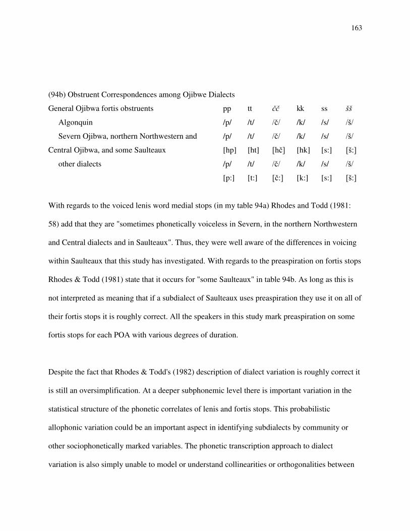
163

(94b) Obstruent Correspondences among Ojibwe Dialects

General Ojibwa fortis obstruents pp tt čč kk ss šš

Algonquin /p/ /t/ /č/ /k/ /s/ /š/

Severn Ojibwa, northern Northwestern and

Central Ojibwa, and some Saulteaux

/p/

[hp]

/t/

[ht]

/č/

[hč]

/k/

[hk]

/s/

[s:]

/š/

[š:]

other dialects /p/

[p:]

/t/

[t:]

/č/

[č:]

/k/

[k:]

/s/

[s:]

/š/

[š:]

With regards to the voiced lenis word medial stops (in my table 94a) Rhodes and Todd (1981:

58) add that they are "sometimes phonetically voiceless in Severn, in the northern Northwestern

and Central dialects and in Saulteaux". Thus, they were well aware of the differences in voicing

within Saulteaux that this study has investigated. With regards to the preaspiration on fortis stops

Rhodes & Todd (1981) state that it occurs for "some Saulteaux" in table 94b. As long as this is

not interpreted as meaning that if a subdialect of Saulteaux uses preaspiration they use it on all of

their fortis stops it is roughly correct. All the speakers in this study mark preaspiration on some

fortis stops for each POA with various degrees of duration.

Despite the fact that Rhodes & Todd's (1982) description of dialect variation is roughly correct it

is still an oversimplification. At a deeper subphonemic level there is important variation in the

statistical structure of the phonetic correlates of lenis and fortis stops. This probabilistic

allophonic variation could be an important aspect in identifying subdialects by community or

other sociophonetically marked variables. The phonetic transcription approach to dialect

variation is also simply unable to model or understand collinearities or orthogonalities between

164

correlates at all. With multiple loglinear models we can assess to what extent preaspiration trades

off with consonant duration in making a contrast or to what extent a difference in closure

duration is predictable from voicing. Describing statistical variation in redundant phonetic

features also gives us the potential to document phonetic change. The extent to which phonetic

change is gradual or discontinuous can only be investigated with adequate descriptions of the

statistical distributions of correlates that encode phonemic oppositions (cf. Pierrehumbert 2001a).

The statistical structure of phonetic encoding is complex and difficult to summarize when

multiple dimensions are considered at once. General summaries of what this investigation has

uncovered about the phonetic encoding of lenis and fortis stops for each speaker are given below.

NT (Peguis): For NT duration ratios between lenis and fortis stops were 1:1.5 for bilabials, 1:1.2

for dental/alveolars, and 1:1.7 for velars. All of these differences were significant. Postaspiration

was only a reliable covariate for the lenis-fortis contrast in velars. It occurred on 100% of /k/s

and 47% of /g/s. The postaspiration on /k/s was significantly different than that for /g/s.

Postaspiration was a nonsignificant predictor for bilabials and dental/alveolars. Preaspiration

occurred on 11% of /p/s, 50% of /t/s and 68% of the /k/s. For velars there was a significant

difference in terms of the occurrence and quantity of preaspiration governed by the length feature

of the previous vowel. Preaspiration durations range from 12-115 ms (not counting fortis stops

that have no preaspiration). Sonority values above 1 occurred on 50% of /b/s, 7% of /d/s and

68% of /g/s. The majority of NT's voiced stops had sonority values of 1 (77%). Only /g/ had

some tokens above this value. No multiple regression model was constructed for NT's bilabials.

For dental/alveolars the best model contained only preaspiration, all other factors being too weak

165

to be considered useful. For velars all of the correlates were used in the best model. Two way

interaction terms between consonant duration and postaspiration and consonant duration and

sonority were significant; however these did not improve the model. Modelling was generally

less effective or informative for NT compared to other speakers due to smaller sample size. From

the model with velars consonant duration appears to be the best predictor with other correlates

having fairly substantial importance (their coefficients were never less than half of the

coefficient for consonant duration for standardized variables).

Boo (Long Plain): For Boo duration ratios between lenis and fortis stops were 1:1.8 for

bilabials, 1:1.6 for dental/alveolars, and 1:2 for velars. All of these differences were significant.

Postaspiration was a reliable correlate for all of the POAs but was not particularly strong for the

/d/-/t/ contrast. Dental/alveolar lenis stops are postaspirated 78% of the time with a mean

duration of 11 ms, while the fortis counterpart /t/ is always postaspirated with a mean of 28 ms.

Preaspiration occurred on 10% of /p/s, 49% of /t/s and 69% of /k/s. The preaspiration ranges

from 8-113 ms. Boo consistently used voicing as a strong correlate for lenis stops. 97% of /b/s,

81% of dentals and 100% of /g/s had sonority values of 0. For Boo, the sample size was the

largest and this gave as the possibility to develop the most complex models. However, Boo's

speech was most likely hyperarticulated compared to the other speakers in this study. This had

the predictable effect of the exageration of certain acoustic cues to the point where the presence

of others was not necessary in the speaker's best model. For example, despite the fact that

consonant duration, postaspiration and preaspiration were all strong predictors when described

individually for the /g/-/k/ contrast only Sonority was necessary in Boo's final model, because it

displayed complete separation. All the other predictors became superfluous. For Boo voicing

166

was the strongest predictor in every case. For dentals consonant duration, postaspiration and

preaspiration could be seen as playing a part in the contrast because a significant amount of /d/s

were voiceless (19%). Still, sonority was the strongest predictor. It would be interesting to see to

what extent this situation would hold in conversational speech (i.e. hypospeech).

SF (Brokenhead): For SF consonant duration ratios were 1:1.6 for bilabials, 1:1.3 for

dental/alveolars, and 1:1.3 for velars. In the latter case the ratio is slightly larger if we include

syncopated velar /g/s (1:1.4). These differences were significant. Postaspiration was a significant

predictor for all the POAs, but for dental/alveolars the difference is not very large. /p/ has

postaspiration 100% of the time, its lenis counterpart 6% of the time. /k/ has postaspiration 95%

of the time, its lenis counterpart 4% of the time. However while /t/ has postaspiration 100% with

a mean duration of 30 ms of the time its lenis counterpart is postaspirated 86% of the time with a

mean duration of 22 ms. Thus postaspiration is a weaker predictor for the /d/-/t/ contrast. In the

multiple logistic regression model with the POAs pooled the interaction between dental/alveolar

place was negative and almost as large as effect of postaspiration on predicting the /b/-/p/

contrast. Preaspiration occurred on 5% of /p/s, 27% of /t/s and 51% of /k/s. The range in duration

of preaspirated fortis stops was 10-93 ms. 96% of /b/s, 65% of /d/s and 98% of /g/s had sonority

values above 0. For bilabials, no model was constructed because I could only find 25 fortis /p/s.

In the multiple loglinear regression for the /d/-/t/ contrast voicing seems to be the best predictor

although consonant duration postaspiration and preaspiration all have minor effects. With the

coefficients based on standardized variables it the largest and when the correlate is taken alone it

has the highest Accuracy score. For the /g/-/k/ postaspiration and sonority were chosen as the

predictors. The sonority value coefficient is much stronger again (7.9 for sonority compared to

167

1.3 for postaspiration). Thus for SF voicing seems to be the best predictor in each case with

postaspiration secondary. Overall SF uses the most postaspiration out of all the speakers to make

the lenis-fortis contrast.

JB (Sandy Bay): For JB consonant duration ratios between lenis and fortis stops were 1:2.1 for

bilabials, 1:1.7 for dental/alveolars, 2:2.2 for velars. In the case of velars the ratio increases to

1:2.9 if all the syncopated /g/s are counted. Postaspiration was a significant predictor for the

bilabial and velar contrasts. Postaspiration on /p/s occurs 74% of the time, on /k/s 94% of the

time and only 1% of the time of these consonant's corresponding lenis stops. For alveolar/dental

stops, however, postaspiration was not a significant predictor. While /t/s are postaspirated 98%

of the time with a mean of 25 ms, /d/s are postaspirated 78% of the time with a mean of 22 ms, a

small difference. Preaspiration occurs on 14% of /p/s, 26% of /t/s and 38% of /k/s. The range in

duration of preaspiration on fortis stops for JB is 9-63 ms. Voicing is a strong predictor of the

lenis-fortis contrast. Sonority values above 0 occur on 99% of /b/s, 46% of /d/s and 99% of /g/s.

Overall voicing seems to be the strongest predictor. It is the only factor in JB's model for the /b/-

/p/ contrast. For velars both consonant duration and sonority are in the best model but sonority is

clearly more important. Its coefficient is larger (6.64 compared to 1.69 for consonant duration)

and its accuracy measurement is stronger when we compare the factors by themselves (.97 for

sonority, .92 for consonant duration). Consonant duration is still a strong predictor, but most of

its ability to predict the contrast can be subsumed under the voicing difference. For

dental/alveolars voicing becomes less important as dental/alveolar /d/ is only voiced 46% of the

time. In the best model for the /d/-/t/ contrast consonant duration was a better predictor by

coefficient (2.3>1.9) and Accuracy measure when considered alone (.84>.50). Thus, voicing

168

appears to be the best correlate for JB but dental/alveolar /d/ is voiceless too often for it to be as

strong a predictor for alveolar/dentals.

WM (Lake St. Martin): For WM consonant duration ratios between lenis and fortis stops are

1:1.4 for bilabials, 1:1.3 for dentals, 1:1.6 for velars. Postaspiration was a significant predictor

for bilabials and velars but not for alveolars. For bilabials there was significantly less

postaspiration than for other speakers. Only 35% of /p/s were postaspirated compared to 83% of

/k/s. All /t/s had some postaspiration but this was not a covariate of contrast for dental/alveolars

because 95% of /d/s had it as well. Preaspiration occurred on 43% of /p/s, 56% of /t/s and 80% of

/k/s. The range of duration of WM's preaspirated stops is 12-148 ms. Voicing is not important for

WM. Only 8% of /b/s and 2% of /d/s have sonority values above 0. 57% of /g/s have a sonority

value above 0, but this is largely predictable from consonant duration.58 In WM's model for the

/b/-/p/ contrast consonant duration, postaspiration and preaspiration all improve the model.

Preaspiration has the strongest coefficient when the variables are standardized. For the /d/-/t/

model only consonant duration and preaspiration are included. Again preaspiration seems to be

the most important predictor. Its coefficient is higher (3.8>1.9) when the variables are

standardized. The Accuracy score for preaspiration is higher than consonant duration's as well

when the dimensions are analyzed separately (.77>.69). For the /g/-/k/ model consonant duration

and preaspiration are the predictors again with preaspiration as the stronger predictor. Generally

for WM preaspiration and higher consonant duration values trade off to mark fortis consonants,

with the former tending to play a more important role. Further evidence that they trade off comes

from the fact that they are negatively correlated with each other for fortis stops (p<.0001, R2 =

58 A linear regression with consonant duration as the response variable and sonority as the predictor variable for /g/s comes out as significant (p<.0001), with an adjusted R2 of .234 and a slope of -14.7.

169

.112). Overall the pattern in WM's speech is that where nondistinctive consonant durations of

fortis stops are produced these are supplemented with more preaspiration.

MR (Fairford): For MR consonant duration ratios between lenis and fortis stops are 1:1.95 for

bilabials, 1:1.4 for dental/alveolars, and 1:1.75 for velars. All of these differences were

significant. Postaspiration was a significant predictor for the lenis fortis contrast in all of the

POAs. Postaspiration occurred on 31% of /p/s (mean: 6 ms), 94% of /t/s (mean 13 ms) and 83%

of /k/s (mean 22 ms). In the case of alveolar/dentals and velars postaspiration was negligible of

the lenis counterpart. It occurred on 73% of /d/s with a mean only 3 ms less than that for /t/.

Voicing was a slightly better predictor of the lenis-fortis contrast for MR than for WM. 51% of

/b/s, 14% of /d/s and 42% of /g/s had sonority values over 0. Still like WM, models for the lenis

fortis contrast by POA were better without sonority as a predictor. MR's best model for the /g/-

/k/ contrast only contained consonant duration. For dental/alveolars preaspiration became much

more important as the distance between /d/ and /t/ on consonant duration is smaller. Lenis /d/ is

longer for all speakers compared to the other lenis stops. Postaspiration and preaspiration were

thus included in the model. Preaspiration was the most important both in terms of its coefficient

from standardized variables (3.7> 1.5 (ConsDur), .6 (PostAsp)) and its Accuracy measure when

the dimensions were considered separately (.74>.66 (ConsDur), .45 (PostAsp)). For velars

consonant duration was an important correlate as well, however on its own postaspiration had a

higher Accuracy measure (.89>.80). A two way interaction term between consonant duration and

postaspiration revealed that these terms were collinear and thus a certain amount of the

postaspiration was redundantly marking the contrast. The interaction term between preaspiration

and consonant duration was nonsignificant. Furthermore these predictors trade off each other just

170

as with WM. More ambiguous consonant durations imply a higher probability of preaspiration.

Evidence for this comes from the fact that consonant duration and preaspiration as negatively

correlated with each other (p<.0001, R2 = .203). Thus postaspiration predicts the contrast but

could be considered less important because it is collinear with consonant duration. Consonant

duration and preaspiration trade off with one another in MR's /g/-/k/ contrast.

Investigation of the acoustic correlates and the relationship between the phonetic

dimensions of the lenis-fortis contrast across these six speakers has revealed that there is much

subdialectal variation in the Saulteaux of Manitoba. The variation is not random, however. It is

governed on the one hand by the need to maintain contrast and on the other by sociophonetic

dimensions. If the strength of one correlate for a particular phonemic contrast diminishes, the

contrast needs to be reinforced by another correlate for it to be maintained. This serves as a

constraint on the variation in the phonetic encoding of complex categories. Sociophonetic

dimensions on the other hand act to maintain the variation between dimensions. Differences in

pronunciation are important sociolinguistic variables and index different social categories within

a speech community (Foulkes & Docherty 2006). Any linguist or anthropologist who has ever

worked with an Ojibwe speaker for a substantial amount of time has undoubtedly been told by

their consultant that he or she is able to tell the community where a particular interlocutor is from

by their speech (at least within a reasonable geographical range). The next step in this project,

apart from documenting more correlates, would be to identify the sociolinguistic variables that

are conditioning the ubiquitous phonetic variation described in this study.

171

References

Abramson, A. S. 1991. Amplitude as a cue to word-initial consonant length: Pattani Malay. Proceedings of the XIIthe International Congress of Phonetic Sciences 3. Aix-en-Province: Université de Provence, 1991. 98-101. Abramson, A. S. 2003. Acoustic Cues to Word-Initial Stop Length in Pattani Malay. Proceedings of the 15th International Congress of Phonetic Sciences, August 3-9, 2003, Barcelona, Spain. 387-390. Albers, P. C. 2001. Plains Ojibwa. Handbook of North American Indians 13. Sturtevant, W. E. ed. 652-661. Allison, P. D. 2004. Convergence Problems in Logistic Regression. Numerical Issues in Statistical Computing for the Social Scientist. Altman, M., J. Gill, M. P. McDonald. eds. John Wesley & Sons. 238-52. Allison, P. D. 2008. Convergence Failures in Logistic Regression. Statistics and Data Analysis. SAS Global Forum 2008, Paper 360-2008. Anderson, D. R. 2008. Model Based Inference in the Life Sciences: A Primer on Evidence. New York: Springer. Arvaniti, A. & Tserdanelis, G. 2000. On the Phonetics of Geminates: Evidence from Cypriot Greek. Proceedings of the 6th International Conference on Spoken Language Processing. 559-562. Beijing, China. Baayen, R. H. 2008. Analyzing Linguistic Data: A Practical Introduction to Statistics using R. Cambridge: Cambridge University Press. Baraga, F. 1850. A Theoretical and Practical Grammar of the Otchipwe Language. Detroit: Ann Arbor Michigan. Benus, S. & Gafos, A. 2007. Articulatory characteristics of Hungarian 'transparent' vowels. Journal of Phonetics 35. 271-300. Bermútez-Otero, R. 2007. Diachronic Phonology. The Cambridge Handbook of Phonology. de Lacy, P. ed. Cambridge: Cambridge University Press. 497-519. Beckman, M. E. & Pierrehumbert, J. Positions, probabilities, and levels of categorization. Keynote address, Eight Australian International Conference on Speech Science and Technology, Canberra, Dec. 4-7, 2000.

172

Berry, W. D. 1993. Understanding Regression Assumptions. Quantitative Applications in the Social Sciences. London: Sage Publications. Bishop, C. A. 1974. The Northern Ojibwa and the fur trade: An historical and ecological study. Toronto: Holt, Rinehart & Winston of Canada. Bishop, C. A. 2002. Northern Ojibwa Emergence: The Migration. Papers of the Thirty-Third Algonquian Conference, H.C. Wolfart, ed. University of Manitoba: Winnipeg. Blackenship, B. 1997. The time course of breathiness and laryngealization in vowels. PhD thesis, University of California. Blevins, J. 2001. Where have all the onsets gone? Initial consonant loss in Aboriginal languages. Forty years on: Ken Hale and Australian languages. Simpson, J., D. Nash, M. Laughren, P. Austin & B. Alpher.eds. Pacific Linguistics 512. Canberra: Research School on Pacific and Asian Studies. 481-92. Blevins, J. 2004. Evolutionary Phonology. Cambridge: Cambridge University Press. Blevins, J. 2005. The typology of geminate inventories: Historical explanations for recurrent sound patterns. Seoul Linguistics Forum 2005. Seoul Language Education Institute, Seoul National University. 121-37. Blevins, J. 2006. A Theoretical Synopsis of Evolutionary Phonology. Theoretical Linguistics 32-2. 117-166. Blevins, J. 2007. Interpreting Misperception: Beauty is in the ear of the beholder. Experimental Approaches to Phonology. Solé, M. J., Beddor, P. S., Ohala, M. 144-54. Oxford: Oxford University Press. Blevins, J. 2010. Explaining Diversity in Consonant Inventories: An Evolutionary Approach. ms, Max Plank Institute for Evolutionary Anthropology. Bloomfield, L. 1925. On the sound-system of Central Algonquian. Language 1. 130-56. Bloomfield, L. 1926. A set of postulates for the science of language. Language 2. 153-64. Bloomfield, L. 1946. Algonquian. Linguistic structures of native america. Hoijer, H. et al. ed. 85-129. Bloomfield, L. 1958. Eastern Ojibwa: grammatical sketch, texts and word list. Ann Arbor: University of Michigan Press. Blumstein, S. E. 1986. On Acoustic Invariance in Speech. Invariance and Variability in Speech Processes. Perkell, J. S. & D. H. Klatt. eds. 176-193.

173

Boersma, P. 1998. Functional Phonology: Formalizing the interactions between articulatory and perceptual drives. PhD, University of Amsterdam,The Hague. Boersma, P. & Weenink, D. 2007. Praat: Doing phonetics by computer (Version 4.3.14) [Computer program]. Retrieved November 2009, from <http://www.praat.org/> Browman, C. P. & Goldstein, L. 1992. Articulatory Phonology: An overview. Phonetica 49. 155-180. Burnham, K. P. & Anderson, D. R. 2002. Model Selection and Multimodel Inference: A Practical Information-Theoretic Approach. New York: Springer. Catford, J. C. 1977. Fundamental Problems in Phonetics. Bloomington: Indiana University Press. Chambers, J. M. & Hastie, T. J. 1992. Statistical Methods in S. Wadsworth & Brooks/Cole. Chomsky, N. & Halle, M. 1968. The Sound Pattern of English. New York: Harper & Row. Chomsky, N. 1995. The Minimalist Program. MIT: MIT Press. Cho, T. & Ladefoged, P. 1999. Variation and universals in VOT: evidence from 18 languages. Journal of Phonetics 27. 207-229. Cho, T. & Ladefoged, P. 2000. An Acoustic and Aerodynamic Study of Consonants in Cheju. Korean Journal of Speech Science 7. 109-141. Cote, M. 1984. Nahkawêwin Saulteaux: Ojibway Dialect of the Plains. Regina: Regents Publishing Co. Debrock, M. 1977. An acoustic correlate of the force of articulation. Journal of Phonetics 5. 61-80. DeMaris, A. 1992. Logit Modeling: Practical Applications. Quantitative Applications in the Social Sciences 86. London: Sage Publications. DeMaris, A.1995. A Tutorial in Logistic Regression. Journal of Marriage and the Family 57. 956-968. DiCanio, C. T. 2008. The Phonetics and Phonology of San Martín Itunyoso Trique. PhD, University of California Berkeley. Dilley, L. C. & Pitt, M. A. 2007. A study of regressive place assimilation in spontaneous speech and its implications for spoken word recognition. Journal of the Acoustical Society of America 122:4. 2340-53. Dixit, R. P. 1987. In defence of the phonetic adequecy of the traditional term “voiced aspirated”. Proceedings of the International Congress of Phonetic Sciences 11, 2. 145-148. Docherty, G. 1992. The Timing of Voicing in British English Obstruents. Berlin: Walter de Gruyter.

174

Dodge, Y. 2003. The Oxford Dictionary of Statstical Terms. Oxford: Oxford University Press. Dumouchel, P. A. & Brachet, J. 1942. Grammaire Saulteause. Saint-Boniface: Province Oblate du Manitoba. Engstrand, O. & Krull, D. 1994. Durational correlates of quantity in Swedish, Finnish, and Estonian: Cross-language evidence for a theory of adaptive dispersion. Phonetica 51. 80-91. Esposito, A. & Di Benedetto, M. G. 1999. Acoustical and perceptual study of gemination in Italian stops. Journal of the Acoustical Society of America 106:4. 2051-62. Fant, G. 1960. Acoustic Theory of Speech Production. The Hague: Mouton. Firth, D.1993. Bias reduction of maximum likelihood estimates. Biometrika 80. 27-38. Foulkes, P. & Docherty, G. 2006. The social life of phonetics and phonology. Journal of Phonetics 34. 409-438. Fox, T. 2005. Aaniin zhigaag wenji-maazhimaagozid. Black River First Nation, Manitoba. Fujimura, O., M. J. Macchi & L.A. Streeter. 1978. Perception of stop consonants with conflicting transitional cues: cross-linguistic study. Language and Speech 21. 337-46. Gelman, A. & Hill, J. 2007. Data Analysis Using Regression and Multilevel/Hierarchical Models. Cambridge: Cambridge University Press. Gobl, C. & Ní Chasaide, A. 1999. Perceptual correlates of source parameters in breathy voice. Proceedings of the XIVth International Congress of Phonetic Sciences, San Francisco. 2437-40. Goddard, I. 1979. Comparative Algonquian. In The languages of Native America: historical and comparative assessment, Campbell, Lyle, Marianne Mithun. eds. Austin: University of Texas Press. Goddard, I. 1981. Against the linguistic evidence claimed for some Algonquian dialect relationships. Anthropological Linguistics 23. 271-297. Goddard, I. 1982. The historical phonology of Munsee. International Journal of American Linguistics 48: 16-48. Goddard, I. 1990. Algonkian linguistic change and reconstruction. Patterns of Change, Change of Patterns: Linguistic Change and Reconstruction Methodology. Baldi, Philip. ed., 99-114. Hall, T.A. 2001. Introduction: Phonological representations and phonetic implementation of distinctive features. Distinctive Feature Theory, Hall, T. A. ed. 1-41.

175

Ham, W. H. 2001. Phonetic and Phonological Aspects of Geminate Timing. New York: Routledge. Han, M. S. & Weizman, R. S. 1970. Acoustic features of /P, T, K/ and /ph, th, kh/. Phonetica 22. 112-128. Hay, J. B. 2000. Causes and consequences of word structure. PhD thesis, Northwestern University. Hayes, B. & Londe, Z. C. 2006. Stochastic phonological knowledge: the case of Hungarian vowel harmony. Phonology 23. 59-104. Helgason, P. 2002. Preaspiration in the Nordic Languages. PhD, Stockholm University. Heinze, G. & Schemper, M. 2004. A solution to the problem of separation in logistic regression. Statistics in Medicine 21. 2409-2419. Hockett, C. F. 1939. Potawatomi I: Phonemics, Morphophonemics, and Morphological Survey. International Journal of American Linguistics 15. 1-10. Hockett, C. F. 1967. The quantification of functional load. Word 23. 320-39. Holton, G. 2001. Fortis and lenis fricatives in Tanacross Athapaskan. International Journal of American Linguistics 67. 396-414. Hombert, J.-M. & Ohala, J. J. & Ewan, W. G. 1979. Phonetic explanations for the development of tones. Language 55. 37-58. Hoole, P. Gobl, C. & Ní Chasaide, A. 1999. Laryngeal coarticulation. Coarticulation: Theory, Data and Techniques. Coarticulation: Theory, Data and Techniques. Hardcastle, W. J. & Hewlett, N. eds. Cambridge: Cambridge University Press. 105-107. Jaccard, J. 2001. Interaction Effects in Logistic Regression. Quantitative Applications in the Social Sciences 135. London: Sage Publications. Jessen, M. 1998. Phonetics and Phonology of Tense and Lax Obstruents in German. Studies in Functional and Structural Linguistics 44. Amsterdam: John Benjamins. Johnson, K. 1997. Speech Perception without Speaker Normalization. Talker Variability in Speech Processing. Johnson, K. & Mullenix, J. eds. 145-165. Jun, J. 2004. Place assimilation. Phonetically Based Phonology. Hayes, B. & R. Kirchner, & D. Steriade.eds. Cambridge: Cambridge University Press. 58-87.

176

Kang, K.-H. & Guion, S. G. 2008. Clear speech production in Korean stops: Changing phonetic targets and enhancement strategies. Journal of the Acoustical Society of America 124: 6. 3909-3917. Kaye, J. D. 1971. A Case of Local Ordering in Ojibwa. Odawa Language Project: First Report. Kaye, J. D., G. L. Piggott & K. Tokaichi. eds. 3-11. Kaye, J. D., Piggot, G. L. & Tokachi, K. eds. 1971. Odawa Language Project: First Report. Anthropological Series No. 9. Toronto: University of Toronto. Keating, P. A. 1984. Phonetic and Phonological Representation of Stop Consonant Voicing. Language 60:2. 286-319. Kegg, M. 1991. Portage Lake: Memories of an Ojibwe Childhood. Nichols, J. ed. Edmonton: University of Alberta Press. Kendall, M. & Gibbons, J. D. 1990. Rank Correlation Methods. New York: Oxford University Press. Kim, H., Maeda, S. & Honda, K. 2010. Invariant articulatory bases of the features [tense] and [spread glottis] in Korean plosives: New stroboscopic cine-MRI data. Journal of Phonetics 38. 90-108. Kirby, J. P. 2011. The role of probablistic enhancement in phonologization. In A. Yu. ed. Origin of Sound Pattern: Approaches to Phonologization. Oxford: Oxford University Press. Kingston, J. 1990. Articulatory binding. Papers in Laboratory Phonology I: Between the Grammar and Physics of Speech. Kingston, J. & M. E. Beckman. eds. Cambridge: Cambridge University Press. Kirchner, R. M. 1998. An Effort-Based Approach to Consonant Lenition. Phd, University of California. Kohler, K. J. 1984. Phonetic explanation in phonology: the feature fortis/lenis. Phonetica 41. 150-174. Kosmidis, I. 2011. Bias-reduction in binomial-response GLMs. R Documentation. http://127.0.0.1:18407/library/brglm/html/brglm.html, downloaded 17/02/2011. Kruschke, J. K. 1992. ALCOVE: An Exemplar-Base Connectionist Model of Category Learning. Psychological Review 99:1. 22-44. Labov, W. 1994. Principles of Linguistic Change: Volume 1, Internal Factors. Oxford: Blackwell. Ladefoged, P. & Maddieson, I. 1996. The Sounds of the World‘s Languages. Cambridge: Blackwell Publishers. Lahiri, A. & Hankamer, J. 1988. The timing of geminate consonants. Journal of Phonetics 16. 327-338. Lahiri, A. & Reetz, H. 2010. Distinctive features: Phonological underspecification in representation and processing. Journal of Phonetics 38. 44-59.

http://127.0.0.1:18407/library/brglm/html/brglm.html

177

Lavoie, L.M. 2001. Consonant Strength: Phonological Patterns and Phonetic Manifestations. New York: Garland Publishing. Laudan, L. 1977. Science and Values: The Aims of Science and Their Role in Scientific Debate. California: University of California Press. Leander, A. J. Acoustic Correlates of Fortis/Lenis in San Francisco Ozolotepec Zapotec. MA, University of North Dakota. Lehiste, I. 1970. Suprasegmentals. Cambridge: The MIT Press. Lewis-Beck, M. S. 1980. Applied Regression: An Introduction. Quantitative Applications in the Social Sciences 22. London: Sage Publications. Liao, T. F. 1994. Interpreting Probability Models: Logit, Probit, and Other Generalized Linear Models. Quantitative Applications in the Social Science 101. London: Sage Publications. Lindblom, B. S. 1990. Explaining phonetic variation: a sketch of the H&H theory. Hardcastle, W. & Marchal, A. eds. Speech production and speech modelling. 403-39. Dordretch: Kluwer. Lindblom, B. S. 1999. Emergent Phonology. ms, http://www.ling.su.se/fon/perilus/1999_14.pdf. Lisker, L. & Abramson, A. S. 1964. A Cross-Language Study of Voicing in Initial Stops: Acoustical Measurements. Word 20. 384-422. Logan, H. J. 2001. A collection of Saulteaux texts with translations and linguistic analyses. MA thesis, University of Regina. Löfqvist, A. Baer, T. McGarr, N. S. & Seider, S. R. 1989. The cricothyroid muscle in voicing control. Journal of the Acoustical Society of America 85. 1314-1321. Luce, R. D. 1963. Detection and recognition. D. R. Bush, E. Galanter. eds. Handbook of Mathematical Psychology. 103-89. New York. John Wiley and Sons, Inc. Malécot, A. 1970. The Lenis-Fortis Opposition: Its Physiological Parameters. Journal of the Acoustical Society of America 47:6. 1588-92. McCarthy, J. 1981. A prosodic theory of nonconcatenative morphology. Linguistic Inquiry 17. 207-263. McCleland, J. L. & Elman, J. L. 1986. The TRACE Model of Speech Perception. Cognitive Psychology 18. 1-86. Michelson, T. 1935. Phonetic Shifts in Algonquian Languages. International Journal of American Linguistics 8. 131-71.

http://www.ling.su.se/fon/perilus/1999_14.pdf

178

Moon, S. & Lindblom, B. 1994. Interaction between duration, context, and speaking style in English stressed vowels. Journal of the Acoustical Society of America 96. 40-55. Moreton, E. 2004. Realization of the English postvocalic [voice] contrast in F1 and F2. Journal of Phonetics 32. 1-33. Muller, J. S. 2001. The Phonology and Phonetics of Word-Initial Geminates. PhD, The Ohio State University. Ní Chasaide, A. & Gobl, C. 1993. Contextual variation of the vowel voice source as a function of adjacent consonants. Language and Speech 36. 303-330. Nichols, J. D. 1980. Ojibwe Morphology. PhD thesis, Harvard University. Nichols, J. D. 1992. Forward to the Reprint Edition. Dictionary of the Ojibway Language. Baraga, F. Minnesota: Minnesota Historical Society. Nichols, J. D. & Nyholm, E. 1991. A Concise Dictionary of Minnesota Ojibwe. Minneapolis: University of Minnesota Press. Ningewance, P. 2004. Anishinaabemodaa: Becoming a Successful Ojibwe Eavesdropper. Winnipeg: Aboriginal Languages of Manitoba. Ningewance, P. 2010. Anishinaabe-ikidowinan: English to Ojibwe Dictionary. ms. Ohala, J.J. 1983. The Origin of Sounds Patterns in Vocal Tract Constraints. The Production of Speech. MacNeilage, P.F. ed. New York: Springer-Verlag. 189-217. Ohala, J. J. 1990. The phonetics and phonology of aspects of assimilation. Papers in Laboratory Phonology I: Between the grammar and physics of speech. Kingston, J. & M. E. Beckman. eds. Cambridge: Cambridge University Press. 258-75. Olive, J. P., Greenwood, A. & Coleman, J. 1993. Acoustics of American English Speech: A Dynamic Approach. New York: Springer. O‟Shaughnessy, D. 1981. A Study of French vowel and consonant durations. Journal of Phonetics 9. 385-406. Pampel, F. C. 2001. Logistic Regression: A Primer. Quantitative Applications in the Social Sciences 123. London: Sage Publications. Peers, L. L. 1994. The Ojibwa of Western Canada, 1780 to 1870. Winnipeg: The University of Manitoba Press.

179

Pentland, D. 1979. Algonquian historical phonology. PhD thesis, University of Toronto. Perkell, J. S. & Klatt, D. H. eds. 1986. Invariance and Variability in Speech Processes. New Jersey: Lawrence Erlbaum Associates. Picheny, M., Durlach, N. & Braida, L. 1986. Speaking clearly for the hard of hearing II: Acoustic characeristics of clear and conversational speech. Journal of Speech and Hearing Research 29. 434-446. Pierrehumbert, J. 1999. What people know about the sounds of language. Studies in the Linguistic Sciences 29:2. 111-120. Pierrrehumbert, J. 2000. The phonetic grounding of phonology. Bulletin de la Communication Parlée 5. 7-23. Pierrehumbert, J. 2001a. Exemplar dynamics: Word frequency, lenition and contrast. Frequency and the Emergence of Linguistic Structure. Bybee, J. & P. Hopper. eds. Philadelphia: John Benjamins. 137-157. Pierrehumbert, J. 2001b. Probabilistic Phonology. Probabilistic Linguistics. Bod, R., J. Hay, S. Jannedy. eds. Cambridge: The MIT Press. 177-228. Pierrehumbert, J. 2002. Word-specific phonetics. Laboratory Phonology VII. Gussenhoven, C. & Warner, N. eds. Berlin: Mouton de Gruyter. 101-140. Pierrehumbert, J. 2003a. The voice of markedness. Paper presented at Markedness and the lexicon: An IAP Workshop. Cambridge, MA:MIT Press, January 24-25. Pierrehumbert, J. 2003b. Phonetic diversity, statistical learning and acquisition of phonology. Language and Speech 46. 115-154. Pierrehumbert, J. 2006. The next toolkit. Journal of Phonetics 34. 516-30. Pierrehumbert, J. Beckman, M. & Ladd, D. R. 2000. Conceptual Foundations of Phonology as a Laboratory Science. Phonological Knowledge. Burton-Roberts, P. Carr, & Docherty, G. eds. Oxford: Oxford University Press. 273-303. Piggot, G. L. On a Rule of Dissimilation in Odawa. Odawa Language Project: Second Report. Piggot, G. L. & J. Kaye. eds. 28-42. Piggot, G. 1980. Aspects of Odawa morphophonemics. Outstanding dissertations in linguistics. Jorge Hankamer. ed. New York: Garland. Piggot, G. L. & Kaye, J. eds. 1973. Odawa Language Project: Second Report. University of Toronto Linguistic Series No.1. Toronto: University of Toronto.

180

Pind, J. 1995. Constancy and normalization in the perception of voice offset time as a cue for preaspiration. Acta Psychologica 89. 53-81. Pothos, E. M. & Close, J. 2008. One or two dimensions in spontaneous classification: A simplicity approach. Cognition 107. 581-602. Prince, A. & Smolensky, P. 2003 [1993]. Optimality Theory. Oxford: Blackwell Press. Repp, B. H. 1978. Perceptual integration and differentiation of spectral cues for intervocalic stop consonants. Perception and Psychophysics 24. 471-85. Repp, B. H. & Liberman, A. M. 1987. Phonetic category boundaries are flexible. Categorical Perception. Harnad, S. ed. Cambridge: Cambridge University Press. 89-113. Repp, B. H. & Svastikula, K. 1988. Perception of the [m]-[n] distinction in VC syllables. Journal of the Acoustical Society of America 83. 238-47. Rhodes, R. A. 1976. The morphosyntax of the Central Ojibwa verd. PhD thesis, University of Michigan. Ann Arbor, Michigan. Rhodes, R. A. 1985. Eastern Ojibwa-Chippewa-Ottawa dictionary. New York: Mouton. Rhodes, R. A. 2006. Ojibwe Language Shift: 1600-present. Language Spread Conference, 12 Aug. 2006. Rhodes, R. A. & Todd, E. M. 1981. Subartic Algonquian Languages. Handbook of North American Indians 6. Sturtevant, W. E. ed. 52-67. van Rijsbergen, C. V. 1979. Information Retrieval. Boston: Butterworth. Ringen, C. 1988. Transparency in Hungarian Vowel Harmony. Phonology 5: 2. 327-342. Ringen, C. & Vago, R. 1998. Hungarian Vowel Harmony in Optimality Theory. Phonology 5:2. 393-416. Rogers, J. H. 1973. Participant Identification and Role Allocation in Ojibwa. PhD thesis, University of Toronto. Rosch, E. & Mervis, B. C. 1975. Family resemblances: Studies in the internal structure of categories. Cognitive Psychology 7. 573-605. Roulette, R. 1997. Oral History of the Treaty #1- Video Project. Dibaajimom gaagii-izhi-bimaadiziwaad Anishinaabeg mewinzha. Winnipeg: Manitoba Indian Cultural Education Centre. Scott, M. E. et a. 1995. The Saulteaux language dictionary. Edmonton, Éditions Duvale, Kinistin First Nation.

181

Siebert, F. T. Jr. 1941. Certain Proto-Algonquian consonant clusters. Language 17. 298-303. Silva, D. J. 2006. Acoustic evidence for the emergence of tonal contrast in contemporary Korean. Phonology 23. 287-308. Silverman, D. 2003. On the Rarity of Pre-Aspirated Stops. Journals of Linguistics 39. 575-598. Slis, I. H. & Cohen, A. 1969. On the complex regulating the voiced-voiceless distinction I. Language and Speech 12: 2. 80-102. Solé, M.-J. 2007. Controlled and mechanical properties of speech. Solé, M.-J., Beddor, P. S., & Ohala, M. eds. Experimental Approaches to Phonology. 302-321. Oxford: Oxford University Press. Steinbring, J. H. 1981. Saulteaux of Lake Winnipeg. Handbook of North American Indians 6. Sturtevant, W. E. ed. 244-56. Stevens, K. N. 2000. Acoustic Phonetics. Cambridge: The MIT Press. Stevens, K. N. 2002. Towards a model for lexical access based on acoustic landmarks and distinctive features. Journal of the Acoustic Society of America 111. 1872-1891. Stevens, K. N. & Keyser, S. J. 2010. Quantal theory, enhancement and overlap. Journal of Phonetics 38. 10-19. Suen, C. Y. & Beddoes, M. P. 1974. The silent interval of stop consonants. Language and Speech 17. 126-134. Swierzbin, B. 2003. Stress in Border Lakes Ojibwe. Papers in the Thirty-Fourth Algonquian Conference. Wolfart, H. C. ed. 341-71. Tallman, A. 2010a. Modelling the Acoustic Correlates of the Lenis-Fortis Contrast in Ojibwe. ms, University of Manitoba. Tallman, A. 2010b. The acoustic correlates of the voiced-voiceless contrast in singletons and geminates in Libyan Arabic. ms, University of Manitoba. Tallman, A. 2010c. The Lenis-Fortis contrast: Methodological and Theoretical Preliminaries. ms, University of Manitoba. Tallman, A. 2010d. Lenis-Fortis in Ojibwe, Progress Report 1: Flanking Vowels. ms, University of Manitoba.

182

Tallman, A. 2010e. Lenis-Fortis in Ojibwe, Progress Report 2: Controlling for Phonological and Morphological Environment in an Algongonquian languages. ms, University of Manitoba. Tallman, A. 2010f. Lenis-Fortis in Ojiwe, Progress Report 3: A Dynamic Word-List. ms, University of Manitoba. Vago, R. 1976. Theoretical Implications of Hungarian Vowel Harmony. Linguistic Inquiry 7:2. 243-263. Valentine, J. R. 1994. Ojibwe Dialect Relationships. PhD thesis, University of Texas at Austin. Valentine, J. R. 1996. Phonological Parameters of Ojibwe Dialect Variation. Papers of the Twenty-Seventh Algonquian Conference. Winnipeg: University of Manitoba Press. 287-324. Valentine, J. R. 2001. Nishnaabemwin Reference Grammar. Toronto: University of Toronto Press. Valentine, J. R. 2010. Anishinaabemowin. http://imp.lss.wisc.edu/~jrvalent/ais301/. van Alphen, P. M. & Smits, R. 2004. Acoustical and perceptual analysis of the voicing distinction in Dutch initial plosives: the role of prevoicing. Journal of the Phonetics 32. 455-491.

Voorhis, P. et al. 1976. A Saulteaux (Ojibwe) phrase book based on the dialects of Manitoba. Brandon: Department of Native Studies, Brandon University. Wolfart, H. C. 1977. Les paradigmes verbaux et la position de dialecte de Severn. Cowan, W. ed. Actes du Huitième Congrès des Algonquinistes. 188-206. Wolfart, H. C. Shrofel, S. M. 1977. Aspects of Cree interference in Island Lake Ojibwa. Cowan, W. ed.

Actes du Huitième Congrès des Algonquinistes. 156-67.

2011. Acoustic correlates of lenis and fortis stops in Saulteaux-Ojibwe. MA thesis, University of...

Documents

Transcript of 2011. Acoustic correlates of lenis and fortis stops in Saulteaux-Ojibwe. MA thesis, University of...