arX

iv:0

910.

0433

v1 [

mat

h.A

P] 2

Oct

200

9

GLOBAL EXISTENCE FOR HIGH DIMENSIONAL QUASILINEAR

WAVE EQUATIONS EXTERIOR TO STAR-SHAPED OBSTACLES

JASON METCALFE AND CHRISTOPHER D. SOGGE

1. Introduction. The purpose of this article is to study long time existence for highdimensional quasilinear wave equations exterior to star-shaped obstacles. In particular,we seek to prove exterior domain analogs of the four dimensional results of [5] wherethe nonlinearity is permitted to depend on the solution not just its first and secondderivatives. Previous proofs in exterior domains omitted this dependence as it did notmesh well with the energy methods in use. The main estimates used in the proof arethe variable coefficient localized energy estimate of [12] as well as a constant coefficientvariant of this estimate which was developed in [1], [3], and [4].

Let us more specifically describe the problem at hand. We fix a bounded set K whichhas smooth boundary and is star-shaped with respect to the origin. Without loss ofgenerality, we shall assume that K ⊂ |x| < 1. We then seek to solve the followingboundary value problem

(1.1)

2u = Q(u, u′, u′′), (t, x) ∈ R+ × Rn\K,

u(t, · )|∂K = 0,

u(0, · ) = f, ∂tu(0, · ) = g

where 2 = ∂2t − ∆ is the d’Alembertian. Here and throughout, we use u′ = (∂tu,∇xu)

to denote the space-time gradient. The nonlinear term Q is smooth in its arguments andhas the form

(1.2) Q(u, u′, u′′) = A(u, u′) +Bαβ(u, u′)∂α∂βu

with the convenient notation ∂0 = ∂t. Throughout this paper, we shall utilize the sum-mation convention where repeated indices are summed. Greek indices α, β, γ are summedfrom 0 to the spatial dimension n, while Latin indices i, j, k are implicitly summed from1 to n. We shall reserve µ, ν, and σ for multiindices. Here A is taken to vanish to secondorder at (u, u′) = (0, 0), and B vanishes to first order at the origin. We also assume thesymmetry condition

(1.3) Bαβ(u, u′) = Bβα(u, u′), 0 ≤ α, β ≤ n.

To solve (1.1), one must assume that the data satisfy some compatibility conditions.These are well known, and we shall only tersely describe them. A more detailed expositionis available in, e.g., [7]. We write Jku = ∂µ

xu : 0 ≤ |µ| ≤ k. For any formalHm solutionu, we can write ∂k

t u(0, · ) = ψk(Jkf, Jk−1g), 0 ≤ k ≤ m for some compatibility functionsψk. The compatibility condition of order m for data (f, g) ∈ Hm×Hm−1 simply requires

The authors were supported in part by the NSF.

1

2 JASON METCALFE AND CHRISTOPHER D. SOGGE

that ψk vanishes on ∂K for 0 ≤ k ≤ m− 1. For (f, g) ∈ C∞, we say that the data satisfythe compatibility condition to infinite order if the above holds for all m.

Under these assumptions, we have small data global existence when n ≥ 5.

Theorem 1.1. Let K ⊂ Rn, n ≥ 5 be a smooth, bounded, star-shaped obstacle, and let

Q(u, u′, u′′) be as above. Assume further that (f, g) ∈ C∞(Rn\K) vanish for |x| > R forfixed R and satisfy the compatibility conditions to infinite order. Then there is a constantε0 and a positive integer N so that if 0 < ε < ε0 and

(1.4)∑

|µ|≤N+1

‖∂µxf‖L2(Rn\K) +

∑

|µ|≤N

‖∂µxg‖L2(Rn\K) ≤ ε,

then (1.1) has a unique global solution u ∈ C∞([0,∞) × Rn\K).

When the Q(u, u′, u′′) = Q(u′, u′′), such global existence results have previously beenestablished in [12, 13] for n ≥ 4. The geometrical restrictions on K in [13] are much lessstrict. When n ≥ 7, the proof in [12] can easily be adapted to prove the theorem. Weshall not discuss the n = 5, 6 result further as it follows from easy modifications of thearguments of [1] or of those in the sequel.

With a general nonlinearity such as above, in dimension 4, one expects almost globalexistence as in Hormander [5] for the boundaryless case, and this was indeed proved in[1]. Similarly, in three dimensions, based on the boundaryless results of Lindblad [10],one expects a lifespan Tε ∼ ε−2, and this was proved for star-shaped obstacles in [2].

The proofs of [5] and [10] for long time existence in the boundaryless case show animproved lifespan in n = 3, 4 if the additional restriction

(1.5) (∂2uA)(0, 0, 0) = 0

is imposed. With this additional restriction, the lifespan bounds which are proved arecomparable to those which were previously available when the nonlinearity was not per-mitted to depend on u. That is, in three dimensions, solutions exist almost globally, andin four dimensions, there is global existence.

The exterior domain analog of this four dimensional global existence is the primaryresult of this article.

Theorem 1.2. Let K ⊂ R4 be a smooth, bounded, star-shaped obstacle, and let Q(u, u′, u′′)

satisfy (1.5) in addition to the assumptions of Theorem 1.1. Assume further that (f, g) ∈C∞(R4\K) vanish for |x| > R for fixed R and satisfy the compatibility conditions toinfinite order. Then there is a constant ε0 and a positive integer N so that if 0 < ε < ε0and

(1.6)∑

|µ|≤N+1

‖∂µxf‖L2(R4\K) +

∑

|µ|≤N

‖∂µxg‖L2(R4\K) ≤ ε,

then (1.1) has a unique global solution u ∈ C∞([0,∞) × R4\K).

While we have only stated Theorem 1.1 and Theorem 1.2 for scalar equations, it isnot difficult to extend these results to systems and even multiple speed systems. We donot expect the restriction to star-shaped obstacles to be optimal but impose this largelyfor simplicity of exposition. One might fully expect similar results to hold in domains

GLOBAL EXISTENCE OF QUASILINEAR WAVE EQUATIONS 3

similar to those addressed in [11], that is, any domain for which there is a sufficientlyrapid decay of local energy.

We also note here that we only examine the case of Dirichlet boundary conditions.While Neumann boundary conditions were permitted in [4], they are more difficult tohandle for quasilinear equations. First of all, even proving energy estimates for smallperturbations of the d’Alembertian in the exterior domain requires additional assump-tions. In particular, one either needs to assume a nonlinear compatibility condition whichis akin to what appears in [14] or more generally take the boundary condition to regardthe conormal derivative as in [9]. Moreover, with Dirichlet boundary conditions and a starshaped obstacle, the boundary terms which appear in the localized energy estimates (seeProposition 3.1 and [12]) have a favorable sign. This is no longer the case with Neumannboundary conditions. By developing techniques that would allow more general obstaclegeometries, it is possible that one may also permit Neumann boundary conditions, butwe do not explore that here.

In hopes of making the arguments more transparent, we shall truncate the nonlinearityat the quadratic level. Since we are dealing with small amplitude solutions, the higherorder terms are better behaved, and it is clear how to alter the proofs in the sequel topermit these terms. With such a truncation, we may now focus on

(1.7) 2u = aαu∂αu+ bαβ∂αu∂βu+Aαβu∂α∂βu+Bαβγ∂αu∂β∂γu

with Dirichlet boundary conditions and small data.

Our proof is based on two key estimates. The first is a localized energy estimate which,beginning with [6], has played a key role in nearly every proof of long time existence forwave equations in exterior domains. In one of its simplest forms, it states

(1.8) ‖〈x〉−1/2−

w′‖L2t,x([0,T ]×Rn) . ‖w′(0, · )‖2 +

∫ T

0

‖2w(s, · )‖2 ds

in R+ × Rn, n ≥ 3. We shall also utilize a version of this for perturbations of the

d’Alembertian which is from [12].

The second of the key estimates is a variant on this. It can be thought of as ageneralization of the main new estimate used in [1]. It is also the p = 2 version of theweighted Strichartz estimates of [3], [4]. In R+ × R

4, this states that

(1.9) ‖|x|−1/2−γw‖L2t,x

. ‖w′(0, · )‖Hγ−1 + ‖|x|−1−γ2w‖L1

t L1rL2

ω, 0 < γ < 1/2.

It is the γ = 0 version of this estimate which was used in [1] to prove almost globalexistence in R

4\K when (1.5) is not assumed. When γ = 0, there is a logarithmic blowup in t in the estimate, and this logarithm corresponds precisely to the exponential inthe lifespan bound.

2. Main estimates on R+ × R4. In this section, we gather the main boundaryless

estimates. These estimates, for the most part, are not new. In the sequel, we shallapply a cutoff which vanishes near the boundary to the solution. What results solves aboundaryless wave equation to which these estimates may be applied.

4 JASON METCALFE AND CHRISTOPHER D. SOGGE

The estimates which we explore here will be for linear wave equations in R+ ×R4. We

let w solve

(2.1)

2w = F, (t, x) ∈ R+ × R4,

w(0, · ) = w0, ∂tw(0, · ) = w1.

The first of these estimates is a localized energy estimate. This has become an increas-ingly standard tool in the study of nonlinear wave equations. In the next section, we shallalso present a version of this estimate which holds for perturbations of the d’Alembertian

Proposition 2.1. Let w be a smooth solution to (2.1) which vanishes for large |x| foreach t. Then, for any T > 0, we have(2.2)

‖〈x〉−1/2−

w′‖L2t,x([0,T ]×R4) + ‖〈x〉

−3/2w‖L2

t,x([0,T ]×R4) . ‖w′(0, · )‖2 +

∫ T

0

‖2w(t, · )‖2 dt

with constant independent of T .

This proposition, in fact, holds in any dimension n ≥ 3, though in n = 3 the secondterm in the left side has a logarithmic divergence in T . A proof can be found in [12],though this estimate did not originate there. The interested reader can see the referencestherein for a more complete history. To prove the estimate, one uses a positive commu-

tator argument with multiplier f(r)∂rw + 32

f(r)r w where f(r) = r

r+R to get the estimatein a torus with radii ≈ R. Summing over such dyadic radii yields the proposition.

The second estimate is from [3] and [4].

Proposition 2.2. Let w be a smooth solution to (2.1). Then, for 0 < γ < 12 , we have

(2.3) ‖|x|−12−γw‖L2

t,x(R+×R4) . ‖w0‖Hγ(R4)+‖w1‖Hγ−1(R4)+‖|x|−1−γF‖L1tL1

rL2ω(R+×R4).

This proposition follows in the homogeneous case by interpolating a trace lemma(on a sphere) and a variant of the localized energy estimate which follows by applyingPlancherel’s theorem in the t-variable. The inhomogeneous estimate follows, in turn, byusing the dual estimate to the trace lemma which was applied. This yields a much widerclass of estimates, which were dubbed weighted Strichartz estimates, for which we haveonly stated the p = 2 case.

The γ = 0 variant of this estimate, which involves a logarithmic blow-up in T whenapplied on [0, T ]×R

4, laid at the heart of the proof of the four dimensional almost globalanalog of Theorem 1.1 in [1]. Here one alters (2.2) by applying it to the Reisz tranformsof the solution. A weighted variant of Sobolev’s lemma is applied to the resulting Sobolevnorm with negative index which contains the forcing term.

To obtain a boundaryless wave equation, one applies a cutoff to the solution in theexterior domain. In order to handle the resulting commutator term, we shall require avariant of these estimates that permits the forcing term to be taken in L2

t provided thatit is compactly supported in the spatial variable, uniformly in t.

Proposition 2.3. Let w be a smooth solution to (2.1) with vanishing data (w0 = w1 = 0).Suppose that F (t, x) = 0 for |x| > 2. Then,

(2.4) ‖〈x〉−1/2−

w‖L2t,x([0,T ]×R4) . ‖F‖L2

t,x([0,T ]×R4).

GLOBAL EXISTENCE OF QUASILINEAR WAVE EQUATIONS 5

This proposition is from [1] and in fact holds for n ≥ 3. The techniques describedbelow, however, only work for n ≥ 4. The n = 3 case was presented in [2] using ideasfrom [6]. When w is replaced by w′ in the left side, this estimate follows from theproof of (2.2) described above. Rather than applying the Schwarz inequality in x andbounding the multiplier term using the energy inequality, one instead applies Schwarzin t and x while appropriately introducing a weight so that the multiplier term can bebootstrapped into the left side of the estimate. In order to obtain (2.4), we apply thisto ∂j(∆

−1∂jw). Applying ∆−1∂j to F does not maintain the compact support, but thekernel is O(|x−y|−3) which remains sufficient to absorb the weight which was introduced.

We will utilize one additional variant of the localized energy estimates. This one isobtained using techniques akin to those which appeared in [5] and [10].

Proposition 2.4. Let v be a smooth solution to

(2.5)

2v =∑4

0 aj∂jG, (t, x) ∈ R+ × R4,

v(0, · ) = ∂tv(0, · ) = 0.

Then,

(2.6) ‖〈x〉−1/2−δv‖L2t,x([0,T ]×R4) . ‖G(0, · )‖Hδ−1 +

∫ T

0

‖G(t, · )‖2 dt

for 0 < δ < 1/2.

Proof. We let v1 solve 2v1 = G with vanishing data, and let v0 solve the homogeneousequation 2v0 = 0 with v0(0, · ) = 0, ∂tv0(0, · ) = G(0, · ). Then,

v =

4∑

0

aj∂jv1 − a0v0.

Thus,

‖〈x〉−1/2−δv‖L2t,x

. ‖〈x〉−1/2−δv′1‖L2t,x

+ ‖〈x〉−1/2−δv0‖L2t,x.

For the first term in the right side, we simply apply (2.2), and to the second term weapply (2.3).

We end this section with our principal source of decay. Here, as was initiated in [6],we use the localized energy estimates so as to obtain long time existence from decayin the |x| variable rather than decay in the t variable, which is more standard in theboundaryless case but much more difficult to prove when there is a boundary. The decaythat we obtain is based on the vector fields that generate translations and rotations. Tothat end, we set

Ω = Ωjk = xj∂k − xk∂j, 1 ≤ j < k ≤ 4

and

Z = ∂α,Ωjk, 0 ≤ α ≤ 4, 1 ≤ j < k ≤ 4.

Lemma 2.5. For h ∈ C∞(R4) and R > 1,

(2.7) ‖h‖L∞(|x|∈[R,2R]) . R−3/2∑

|µ|≤2,j≤1

‖Ωµ∇jrh‖L2(|x|∈[R/2,4R]).

6 JASON METCALFE AND CHRISTOPHER D. SOGGE

This lemma is proved by apply Sobolev embeddings on R × S3 after localizing to theannulus. The decay results from the difference in the volume element for R × S3 versusthat of R

4 in polar coordinates. See [8].

3. Main estimates on R+ × R4\K. The main estimate here is a localized energy

estimate which holds for perturbations of the d’Alembertian. The technique of proofdescribed in the previous section continues to hold. The boundary term that arises dueto the obstacle, thanks to the star-shapedness assumption, has a favorable sign and cansimply be dropped.

In order to handle the highest order terms of the quasilinear equation, it is beneficialto have an analog of the localized energy estimate for perturbations of the d’Alembertian.We suppose that φ ∈ C∞(R+ × R

4\K) solves

(3.1)

2hφ = F, (t, x) ∈ R+ × R4\K,

φ|∂K = 0,

φ(0, · ) = f, ∂tφ(0, · ) = g

where f, g are smooth, supported in |x| < R, and satisfy the smallness condition (1.6).Here

2hφ = (∂2t − ∆)φ+ hαβ(t, x)∂α∂βφ,

and

(3.2) hαβ(t, x) = hβα(t, x)

as well as

(3.3) |h| =4

∑

α,β=0

|hαβ(t, x)| ≤ δ ≪ 1.

We shall also utilize the notation

|∂h| =4

∑

α,β,γ=0

|∂γhαβ(t, x)|

and

SKT = [0, T ]× R

4\K.

For such a φ, we have the following estimates from [12].

Proposition 3.1. Suppose that K ⊂ |x| < 1 is a smooth, bounded, star-shaped ob-stacle as above. Let φ ∈ C∞(R+ × R

4\K) solve (3.1) with data satisfying (1.6) and thecompatibility conditions. Suppose further that

∑

|µ|≤N

‖∂µ2φ(0, · )‖L2(R4\K) ≤ Cε.

GLOBAL EXISTENCE OF QUASILINEAR WAVE EQUATIONS 7

Suppose that hαβ satisfies (3.2) and (3.3) for a sufficiently small choice of δ. Then forany nonnegative integer N and for any T > 0,

(3.4)∑

|µ|≤N

‖〈x〉−1/2−

∂µφ′‖L2(SK

T ) +∑

|µ|≤N

‖〈x〉−3/2

∂µφ‖L2(SK

T ) +∑

|µ|≤N

‖∂µφ′(T, · )‖L2(R4\K)

. ε+∑

j≤N

∫ T

0

‖2h∂jt φ(t, · )‖L2(R4\K) dt+

∑

j≤N

∫ T

0

∥

∥

∥

(

|∂h| +|h|

r

)

|∇∂jt φ|

∥

∥

∥

L2(R4\K)dt

+∑

|µ|≤N−1

‖2∂µφ‖L2(SK

T) +

∑

|µ|≤N−1

‖2∂µφ(T, · )‖L2(R4\K),

and

(3.5)∑

|µ|≤N

‖〈x〉−1/2−

Zµφ′‖L2(SK

T ) +∑

|µ|≤N

‖〈x〉−3/2

Zµφ‖L2(SK

T ) +∑

|µ|≤N

‖Zµφ′(T, · )‖L2(R4\K)

. ε+∑

|µ|≤N

∫ T

0

‖2hZµφ(t, · )‖2 dt+

∑

|µ|≤N

∫ T

0

∥

∥

∥

(

|∂h| +|h|

r

)

|∇Zµφ|∥

∥

∥

L2(R4\K)dt

+∑

|µ|≤N+1

‖∂µxφ

′‖L2([0,T ]×|x|<1).

As stated above, the description of the proof in the previous sections remains validwhen N = 0. For the higher order cases, one uses the fact that ∂t commutes with 2

and preserves the Dirichlet boundary conditions. Then, by using elliptic regularity andrelating the Laplacian to time derivatives via the equation, one can obtain (3.4). Toprove (3.5), one argues as in the N = 0 case and applies a trace theorem to the resultingboundary terms. Here we note that the coefficients of Z are O(1) on ∂K. Also note thatthe last term in (3.5) is controlled by the left side of (3.4).

4. Proof of Theorem 1.2. With the estimates of the previous sections in hand, wenow proceed to the proof of the main long time existence result.

We solve the nonlinear equation via an iteration. We set u0 ≡ 0 and recursively defineul to solve(4.1)

2ul = aαul−1∂αul−1 + bαβ∂αul−1∂βul−1 +Aαβul−1∂α∂βul +Bαβγ∂αul−1∂β∂γul

ul|∂K = 0

ul(0, · ) = f, ∂tul(0, · ) = g.

8 JASON METCALFE AND CHRISTOPHER D. SOGGE

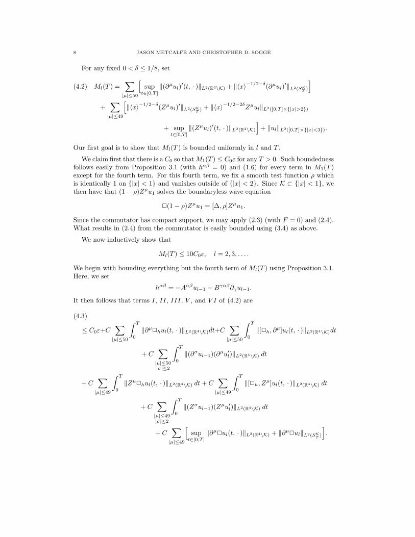
For any fixed 0 < δ ≤ 1/8, set

(4.2) Ml(T ) =∑

|µ|≤50

[

supt∈[0,T ]

‖(∂µul)′(t, · )‖L2(R4\K) + ‖〈x〉−1/2−δ(∂µul)

′‖L2(SK

T)

]

+∑

|µ|≤49

[

‖〈x〉−1/2−δ

(Zµul)′‖L2(SK

T ) + ‖〈x〉−1/2−2δ

Zµul‖L2([0,T ]×|x|>2)

+ supt∈[0,T ]

‖(Zµul)′(t, · )‖L2(R4\K)

]

+ ‖ul‖L2([0,T ]×|x|<3).

Our first goal is to show that Ml(T ) is bounded uniformly in l and T .

We claim first that there is a C0 so thatM1(T ) ≤ C0ε for any T > 0. Such boundednessfollows easily from Proposition 3.1 (with hαβ = 0) and (1.6) for every term in M1(T )except for the fourth term. For this fourth term, we fix a smooth test function ρ whichis identically 1 on |x| < 1 and vanishes outside of |x| < 2. Since K ⊂ |x| < 1, wethen have that (1 − ρ)Zµu1 solves the boundaryless wave equation

2(1 − ρ)Zµu1 = [∆, ρ]Zµu1.

Since the commutator has compact support, we may apply (2.3) (with F = 0) and (2.4).What results in (2.4) from the commutator is easily bounded using (3.4) as above.

We now inductively show that

Ml(T ) ≤ 10C0ε, l = 2, 3, . . . .

We begin with bounding everything but the fourth term of Ml(T ) using Proposition 3.1.Here, we set

hαβ = −Aαβul−1 −Bγαβ∂γul−1.

It then follows that terms I, II, III, V , and V I of (4.2) are

(4.3)

≤ C0ε+C∑

|µ|≤50

∫ T

0

‖∂µ2hul(t, · )‖L2(R4\K)dt+C

∑

|µ|≤50

∫ T

0

‖[2h, ∂µ]ul(t, · )‖L2(R4\K)dt

+ C∑

|µ|≤50|σ|≤2

∫ T

0

‖(∂σul−1)(∂µu′l)‖L2(R4\K) dt

+ C∑

|µ|≤49

∫ T

0

‖Zµ2hul(t, · )‖L2(R4\K) dt+ C

∑

|µ|≤49

∫ T

0

‖[2h, Zµ]ul(t, · )‖L2(R4\K) dt

+ C∑

|µ|≤49|σ|≤2

∫ T

0

‖(Zσul−1)(Zµu′l)‖L2(R4\K) dt

+ C∑

|µ|≤49

[

supt∈[0,T ]

‖∂µ2ul(t, · )‖L2(R4\K) + ‖∂µ

2ul‖L2(SK

T)

]

.

GLOBAL EXISTENCE OF QUASILINEAR WAVE EQUATIONS 9

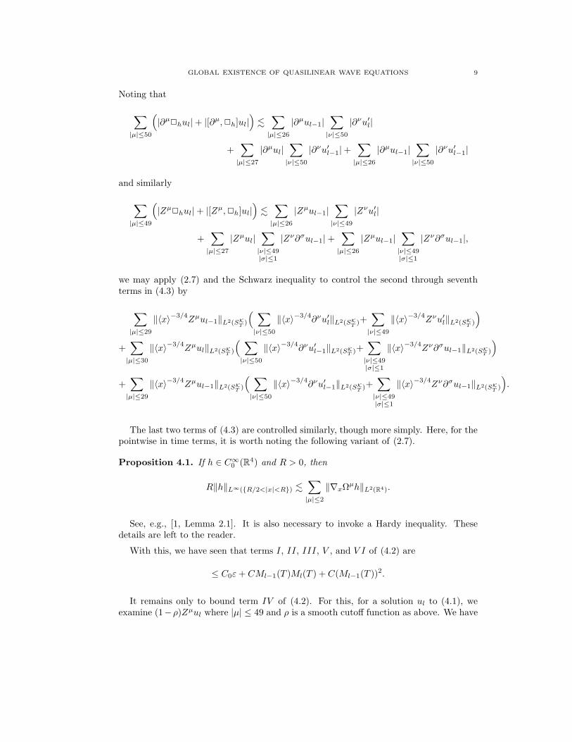
Noting that

∑

|µ|≤50

(

|∂µ2hul| + |[∂µ,2h]ul|

)

.∑

|µ|≤26

|∂µul−1|∑

|ν|≤50

|∂νu′l|

+∑

|µ|≤27

|∂µul|∑

|ν|≤50

|∂νu′l−1| +∑

|µ|≤26

|∂µul−1|∑

|ν|≤50

|∂νu′l−1|

and similarly

∑

|µ|≤49

(

|Zµ2hul| + |[Zµ,2h]ul|

)

.∑

|µ|≤26

|Zµul−1|∑

|ν|≤49

|Zνu′l|

+∑

|µ|≤27

|Zµul|∑

|ν|≤49|σ|≤1

|Zν∂σul−1| +∑

|µ|≤26

|Zµul−1|∑

|ν|≤49|σ|≤1

|Zν∂σul−1|,

we may apply (2.7) and the Schwarz inequality to control the second through seventhterms in (4.3) by

∑

|µ|≤29

‖〈x〉−3/4

Zµul−1‖L2(SK

T)

(

∑

|ν|≤50

‖〈x〉−3/4

∂νu′l‖L2(SK

T)+

∑

|ν|≤49

‖〈x〉−3/4

Zνu′l‖L2(SK

T)

)

+∑

|µ|≤30

‖〈x〉−3/4

Zµul‖L2(SK

T )

(

∑

|ν|≤50

‖〈x〉−3/4

∂νu′l−1‖L2(SK

T )+∑

|ν|≤49|σ|≤1

‖〈x〉−3/4

Zν∂σul−1‖L2(SK

T )

)

+∑

|µ|≤29

‖〈x〉−3/4

Zµul−1‖L2(SK

T )

(

∑

|ν|≤50

‖〈x〉−3/4

∂νu′l−1‖L2(SK

T )+∑

|ν|≤49|σ|≤1

‖〈x〉−3/4

Zν∂σul−1‖L2(SK

T )

)

.

The last two terms of (4.3) are controlled similarly, though more simply. Here, for thepointwise in time terms, it is worth noting the following variant of (2.7).

Proposition 4.1. If h ∈ C∞0 (R4) and R > 0, then

R‖h‖L∞(R/2<|x|<R) .∑

|µ|≤2

‖∇xΩµh‖L2(R4).

See, e.g., [1, Lemma 2.1]. It is also necessary to invoke a Hardy inequality. Thesedetails are left to the reader.

With this, we have seen that terms I, II, III, V , and V I of (4.2) are

≤ C0ε+ CMl−1(T )Ml(T ) + C(Ml−1(T ))2.

It remains only to bound term IV of (4.2). For this, for a solution ul to (4.1), weexamine (1−ρ)Zµul where |µ| ≤ 49 and ρ is a smooth cutoff function as above. We have

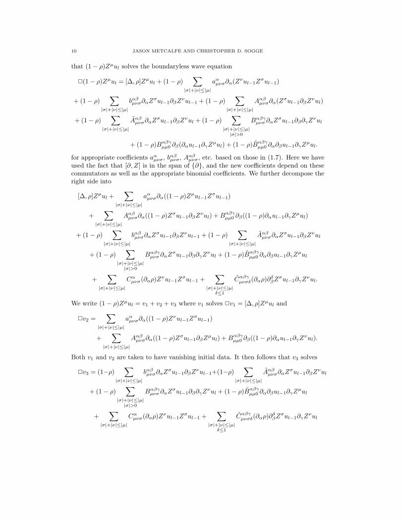
10 JASON METCALFE AND CHRISTOPHER D. SOGGE

that (1 − ρ)Zµul solves the boundaryless wave equation

2(1 − ρ)Zµul = [∆, ρ]Zµul + (1 − ρ)∑

|σ|+|ν|≤|µ|

aαµνσ∂α(Zνul−1Z

σul−1)

+ (1 − ρ)∑

|σ|+|ν|≤|µ|

bαβµνσ∂αZ

σul−1∂βZνul−1 + (1 − ρ)

∑

|σ|+|ν|≤|µ|

Aαβµνσ∂α(Zσul−1∂βZ

νul)

+ (1 − ρ)∑

|σ|+|ν|≤|µ|

Aαβµνσ∂αZ

σul−1∂βZνul + (1 − ρ)

∑

|σ|+|ν|≤|µ||σ|>0

Bαβγµνσ ∂αZ

σul−1∂β∂γZνul

+ (1 − ρ)Bαβγµµ0 ∂β(∂αul−1∂γZ

µul) + (1 − ρ)Bαβγµµ0 ∂α∂βul−1∂γZ

µul.

for appropriate coefficients aαµνσ, bαβ

µνσ, Aαβµνσ , etc. based on those in (1.7). Here we have

used the fact that [∂, Z] is in the span of ∂, and the new coefficients depend on thesecommutators as well as the appropriate binomial coefficients. We further decompose theright side into

[∆, ρ]Zµul +∑

|σ|+|ν|≤|µ|

aαµνσ∂α((1 − ρ)Zµul−1Z

σul−1)

+∑

|σ|+|ν|≤|µ|

Aαβµνσ∂α((1 − ρ)Zσul−1∂βZ

νul) +Bαβγµµ0 ∂β((1 − ρ)∂αul−1∂γZ

µul)

+ (1 − ρ)∑

|σ|+|ν|≤|µ|

bαβµνσ∂αZ

σul−1∂βZνul−1 + (1 − ρ)

∑

|σ|+|ν|≤|µ|

Aαβµνσ∂αZ

σul−1∂βZνul

+ (1 − ρ)∑

|σ|+|ν|≤|µ||σ|>0

Bαβγµνσ ∂αZ

σul−1∂β∂γZνul + (1 − ρ)Bαβγ

µµ0 ∂α∂βul−1∂γZµul

+∑

|σ|+|ν|≤|µ|

Cαµνσ(∂αρ)Z

νul−1Zσul−1 +

∑

|σ|+|ν|≤|µ|δ≤1

Cαβγµνσδ(∂αρ)∂

δβZ

σul−1∂γZνul.

We write (1 − ρ)Zµul = v1 + v2 + v3 where v1 solves 2v1 = [∆, ρ]Zµul and

2v2 =∑

|σ|+|ν|≤|µ|

aαµνσ∂α((1 − ρ)Zνul−1Z

σul−1)

+∑

|σ|+|ν|≤|µ|

Aαβµνσ∂α((1 − ρ)Zσul−1∂βZ

µul) + Bαβγµµ0 ∂β((1 − ρ)∂αul−1∂γZ

νul).

Both v1 and v2 are taken to have vanishing initial data. It then follows that v3 solves

2v3 = (1−ρ)∑

|σ|+|ν|≤|µ|

bαβµνσ∂αZ

σul−1∂βZνul−1+(1−ρ)

∑

|σ|+|ν|≤|µ|

Aαβµνσ∂αZ

σul−1∂βZνul

+ (1 − ρ)∑

|σ|+|ν|≤|µ||σ|>0

Bαβγµνσ ∂αZ

σul−1∂β∂γZνul + (1 − ρ)Bαβγ

µµ0 ∂α∂βul−1∂γZµul

+∑

|σ|+|ν|≤|µ|

Cαµνσ(∂αρ)Z

νul−1Zσul−1 +

∑

|σ|+|ν|≤|µ|δ≤1

Cαβγµνσδ(∂αρ)∂

δβZ

σul−1∂γZνul

GLOBAL EXISTENCE OF QUASILINEAR WAVE EQUATIONS 11

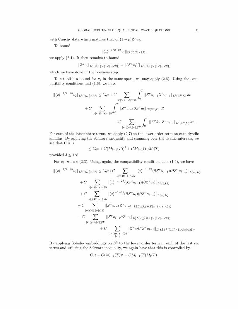
with Cauchy data which matches that of (1 − ρ)Zµul.

To bound

‖〈x〉−1/2−2δv1‖L2([0,T ]×R4),

we apply (2.4). It then remains to bound

‖Zµul‖L2([0,T ]×1<|x|<2) + ‖(Zµul)′‖L2([0,T ]×1<|x|<2)

which we have done in the previous step.

To establish a bound for v2 in the same space, we may apply (2.6). Using the com-patibility conditions and (1.6), we have

‖〈x〉−1/2−2δ

v2‖L2([0,T ]×R4) ≤ C0ε+ C∑

|ν|≤49,|σ|≤25

∫ T

0

‖Zσul−1Zνul−1‖L2(R4\K) dt

+ C∑

|ν|≤49,|σ|≤25

∫ T

0

‖Zσul−1∂Zνul‖L2(R4\K) dt

+ C∑

|ν|≤49,|σ|≤25

∫ T

0

‖Zσ∂ulZνul−1‖L2(R4\K) dt.

For each of the latter three terms, we apply (2.7) to the lower order term on each dyadicannulus. By applying the Schwarz inequality and summing over the dyadic intervals, wesee that this is

≤ C0ε+ C(Ml−1(T ))2 + CMl−1(T )Ml(T )

provided δ ≤ 1/8.

For v3, we use (2.3). Using, again, the compatibility conditions and (1.6), we have

‖〈x〉−1/2−2δ

v3‖L2([0,T ]×R4) ≤ C0ε+C∑

|ν|≤49,|σ|≤25

‖〈x〉−1−2δ

(∂Zσul−1)(∂Zνul−1)‖L1

t L1rL2

ω

+ C∑

|ν|≤49,|σ|≤25

‖〈x〉−1−2δ(∂Zσul−1)(∂Zνul)‖L1

t L1rL2

ω

+ C∑

|ν|≤49,|σ|≤25

‖〈x〉−1−2δ

(∂Zσul)(∂Zνul−1)‖L1

t L1rL2

ω

+ C∑

|ν|≤49,|σ|≤25

‖Zσul−1Zνul−1‖L1

t L1rL2

ω([0,T ]×1<|x|<2)

+ C∑

|ν|≤49,|σ|≤26

‖Zσul−1∂Zνul‖L1

t L1rL2

ω([0,T ]×1<|x|<2)

+ C∑

|ν|≤49,|σ|≤26δ≤1

‖Zσul∂δZνul−1‖L1

tL1rL2

ω([0,T ]×1<|x|<2).

By applying Sobolev embeddings on S3 to the lower order term in each of the last sixterms and utilizing the Schwarz inequality, we again have that this is controlled by

C0ε+ C(Ml−1(T ))2 + CMl−1(T )Ml(T ).

12 JASON METCALFE AND CHRISTOPHER D. SOGGE

By combining the bounds for each of these pieces, we see that

Ml(T ) ≤ 4C0ε+ C(Ml−1(T ))2 + CMl−1(T )Ml(T ).

If we apply the inductive hypothesis Ml−1(T ) ≤ 10C0ε, it indeed follows that

Ml(T ) ≤ 10C0ε

provided that ε is sufficiently small.

It remains to show that ul is a Cauchy sequence in similar spaces. To this end, weset

(4.4)

Al(T ) =∑

|µ|≤49

[

supt∈[0,T ]

‖(∂µ(ul−ul−1))′(t, · )‖L2(R4\K)+‖〈x〉−1/2−δ(∂µ(ul−ul−1))

′‖L2(SK

T)

]

+∑

|µ|≤48

[

‖〈x〉−1/2−δ

(Zµ(ul − ul−1))′‖L2(SK

T ) + ‖〈x〉−1/2−2δ

Zµ(ul − ul−1)‖L2([0,T ]×|x|>2)

+ supt∈[0,T ]

‖(Zµ(ul − ul−1))′(t, · )‖L2(R4\K)

]

+ ‖ul − ul−1‖L2([0,T ]×|x|<3).

Using quite similar arguments and the O(ε) bound on Ml(T ), one can prove

Al(T ) ≤1

2Al−1(T ).

This suffices to show that the sequence converges. Its limit is indeed the solution u, whichcompletes the proof.

References

[1] Y. Du, J. Metcalfe, C. D. Sogge and Y. Zhou: Concerning the Strauss conjecture and almost

global existence for nonlinear Dirichlet-wave equations in 4-dimensions, Comm. Partial DifferentialEquations 33 (2008), 1487–1506.

[2] Y. Du and Y. Zhou: The life span for nonlinear wave equation outside of star-shaped obstacle in

three space dimensions, Comm. Partial Differential Equations 33 (2008), 1455–1486.[3] D. Fang and C. Wang: Weighted Strichartz Estimates with Angular Regularity and their Applica-

tions, arXiv:0802.0058.[4] K. Hidano, J. Metcalfe, H. F. Smith, C. D. Sogge, Y. Zhou: On abstract Strichartz estimates and

the Strauss conjecture for nontrapping obstacles. Trans. Amer. Math. Soc., to appear.[5] L. Hormander: On the fully nonlinear Cauchy problem with small data. II. Microlocal analysis

and nonlinear waves (Minneapolis, MN, 1988–1989), 51–81, IMA Vol. Math. Appl., 30, Springer,New York, 1991.

[6] M. Keel, H. F. Smith, and C. D. Sogge: Almost global existence for some semilinear wave equations,J. Anal. Math. 87 (2002), 265-279.

[7] M. Keel, H. F. Smith, and C. D. Sogge: Global existence for a quasilinear wave equation outside

of star-shaped domains. J. Funct. Anal. 189 (2002), 155–226.[8] S. Klainerman: The null condition and global existence to nonlinear wave equatoins. Lect. Appl.

Math. 23 (1986), 293–326.[9] H. Koch: Mixed problems for fully nonlinear hyperbolic equations. Math. Z. 214 (1993), 9–42.

[10] H. Lindblad: On the lifespan of solutions of nonlinear wave equations with small initial data.Comm. Pure Appl. Math. 43 (1990), 445–472.

[11] J. Metcalfe and C. D. Sogge: Hyperbolic trapped rays and global existence of quasilinear wave

equations. Invent. Math. 159 (2005), 75–117.[12] J. Metcalfe and C. D. Sogge: Long time existence of quasilinear wave equations exterior to star-

shaped obstacles via energy methods. SIAM J. Math. Anal. 38 (2006), 188–209.

GLOBAL EXISTENCE OF QUASILINEAR WAVE EQUATIONS 13

[13] J. Metcalfe and C. D. Sogge: Global existence for Dirichlet-wave equations with quadratic nonlin-

earities in high dimensions. Math. Ann. 336 (2006), 391–420.[14] J. Metcalfe, C. D. Sogge, and A. Stewart: Nonlinear hyperbolic equations in infinite homogeneous

waveguides. Comm. Partial Differential Equations 30 (2005), 643–661.

Department of Mathematics, University of North Carolina, Chapel Hill

E-mail address: metcalfe@email.unc.edu

Department of Mathematics, Johns Hopkins University

E-mail address: sogge@jhu.edu