Glass-Reinforced Plastic Springs for Linear Actuators

Prof. Dr. Fumiya Iida

Semester Project

Supervised by: Author:Prof. Dr. Fumiya Iida Bryan AnastasiadesNandan Maheshwari

Glass-Reinforced PlasticSprings for Linear Actuators

Autumn Term 2011

Contents

Abstract iii

Acknowledgement v

1 Introduction 1

1.1 Motivation . . . . . . . . . . . . . . . . . . . . . . . . . . . . . . . . . . . 1

1.2 Goal of project . . . . . . . . . . . . . . . . . . . . . . . . . . . . . . . . . 1

1.3 Structure of report . . . . . . . . . . . . . . . . . . . . . . . . . . . . . . . 2

2 Introduction to GRP 3

2.1 Structure of GRP . . . . . . . . . . . . . . . . . . . . . . . . . . . . . . . . 3

2.1.1 Material properties . . . . . . . . . . . . . . . . . . . . . . . . . . . 4

2.2 Limitations . . . . . . . . . . . . . . . . . . . . . . . . . . . . . . . . . . . 5

2.3 Applications of GRP in modern mechanical engineering . . . . . . . . . . 6

3 Design of the spring 7

3.1 Linear spring . . . . . . . . . . . . . . . . . . . . . . . . . . . . . . . . . . 7

3.1.1 Computation . . . . . . . . . . . . . . . . . . . . . . . . . . . . . . 7

3.1.2 Counterblock . . . . . . . . . . . . . . . . . . . . . . . . . . . . . . 8

3.1.3 Layer setup . . . . . . . . . . . . . . . . . . . . . . . . . . . . . . . 10

3.1.4 Manufacturing of the spring . . . . . . . . . . . . . . . . . . . . . . 10

3.1.5 Assembly of the spring . . . . . . . . . . . . . . . . . . . . . . . . . 12

3.2 Non-linear spring . . . . . . . . . . . . . . . . . . . . . . . . . . . . . . . . 13

3.2.1 Design idea . . . . . . . . . . . . . . . . . . . . . . . . . . . . . . . 13

3.2.2 Computations . . . . . . . . . . . . . . . . . . . . . . . . . . . . . . 13

3.2.3 Counterblock . . . . . . . . . . . . . . . . . . . . . . . . . . . . . . 13

3.2.4 Manufacturing of the spring . . . . . . . . . . . . . . . . . . . . . . 14

4 Design of the Series Elastic Actuator 15

4.1 General Concept . . . . . . . . . . . . . . . . . . . . . . . . . . . . . . . . 15

4.2 Changes to previous designs . . . . . . . . . . . . . . . . . . . . . . . . . . 16

5 Evaluation 19

5.1 GRP linear spring test . . . . . . . . . . . . . . . . . . . . . . . . . . . . . 19

5.1.1 First prototype . . . . . . . . . . . . . . . . . . . . . . . . . . . . . 20

5.1.2 Second prototype . . . . . . . . . . . . . . . . . . . . . . . . . . . . 22

5.2 GRP non-linear spring test . . . . . . . . . . . . . . . . . . . . . . . . . . 24

5.3 The hopping experiment . . . . . . . . . . . . . . . . . . . . . . . . . . . . 27

6 Conclusion 31

i

7 Future work 337.1 Work on the spring . . . . . . . . . . . . . . . . . . . . . . . . . . . . . . . 337.2 Work on the actuator . . . . . . . . . . . . . . . . . . . . . . . . . . . . . 33

A Calculations 37A.1 Linear and non-linear springs . . . . . . . . . . . . . . . . . . . . . . . . . 37A.2 The hopping experiment . . . . . . . . . . . . . . . . . . . . . . . . . . . . 38

B Ordered Parts 43

C Contact Persons 45

D Step-by-step Instruction 47D.1 Preparation . . . . . . . . . . . . . . . . . . . . . . . . . . . . . . . . . . . 47

D.1.1 Counterblock . . . . . . . . . . . . . . . . . . . . . . . . . . . . . . 47D.1.2 Layer . . . . . . . . . . . . . . . . . . . . . . . . . . . . . . . . . . 47D.1.3 Resin . . . . . . . . . . . . . . . . . . . . . . . . . . . . . . . . . . 47

D.2 Lamination . . . . . . . . . . . . . . . . . . . . . . . . . . . . . . . . . . . 48D.3 Vacuum . . . . . . . . . . . . . . . . . . . . . . . . . . . . . . . . . . . . . 48D.4 Spring connectors . . . . . . . . . . . . . . . . . . . . . . . . . . . . . . . . 49

D.4.1 Pre-steps . . . . . . . . . . . . . . . . . . . . . . . . . . . . . . . . 49D.4.2 Lamination . . . . . . . . . . . . . . . . . . . . . . . . . . . . . . . 49D.4.3 Cutting . . . . . . . . . . . . . . . . . . . . . . . . . . . . . . . . . 49

E Technical drawings 51

Bibliography 59

ii

Abstract

This Project investigates the use of glass reinforced plastic (GRP) leaf springs as areplacement for spiral steel springs. Springs are for example used as an elastic element ina Linear Multi-Modal Actuator (LMMA). They are for instance placed in a knee joint ofa walking robot. This actuators power the leg and allow the robot to walk and jump. Inthis report the development and evaluation of leaf springs with both linear and non-linearprogressive spring characterisitics is presented. Also a hopping experiment was made toevaluate the use of this leaf springs for a jumping robot. For that purpose a series elasticactuator was designed which has a similar operation principle as the LMMA.

iii

Acknowledgement

First of all, we would like to thank Prof. Fumiya Iida for the opportunity to work onthis project but also for his support and understanding during the whole process. Alsomany thanks to Nandan Maheshwari for his help, guidance, doing most of the orderingsand always having the right equipment.A very special thanks we would like to give Fabian Guenther who helped getting startedin this project. Also his support in the developing process of the GRP springs is verymuch appreciated. At this point we would like to thank Dr. Gerald Kress for his helpanalyzing the results from the spring test.Big thanks also to the guys from the workshop, in particular Pascal Wespe and AlessandroRotta. Last but not least we would like to thank all the staff of the BIRL Lab, especiallyDerek Leach for his huge support in the testing phase. We could always come to you andask for assistance. You guys are amazing!

v

Chapter 1

Introduction

1.1 Motivation

In many applications it is interesting to include elastic elements to the structure. Elasticelements provide damping, compliance and more importantly a capability to store andrelease mechanical energy. Building up energy when compressing spring and then releas-ing the spring makes a robot jump very efficiently.Springs are very old mechanical elements. Spiral springs are known since the earlyfifteenth century. When they first appeared in watches. In 1676 a british physician,Robert Hooke, discovered the basic principle for mechanical springs. Hooke’s Law as itwas named from there on, describes the linear correlation between the displacement ofthe spring and the resulting force by

F (x) = k · x

The linear correlation simplifies the computation of the spring in a mechanical envi-ronment. The spring constant k is specific to the material used in the spring and thegeometry of its structure. For example the used material, the thickness of the wire andthe lead of the coil.In some applications it might be more interesting to have a non-linear characteristic. Ifwe look at the properties of natural muscles we find, that they have a non-linear springlike behavior. In bio-inspired robotics we try to mimic biological systems. A spring withnatural properties is therefore of great interest.

1.2 Goal of project

Since the first two prototypes of theLinear Multi-Modal Actuator (LMMA) are very bigand heavy, we decided to look for ways to make it smaller, lighter and also simpler tomanufacturing. The design of the LMMA I and II are well enough for their purpose.But there are some key problems. The massive steel spring is almost 25 % of the overallweight. Also there is systematic problem with spiral formed springs. When compressed,a sprial spring always generates a small turning moment. This turning moment can leadto a jam of the two sliders of our actuator design. The friction increases resulting in amechanism which gets stuck.We then came up with the idea of replacing the sprial steel spring with a lightweightglass reinforced plastic (GRP) or carbon fiber (CF) leaf springs. This leaf spring is notonly light, but it also compresses without the generation of turning moment. It is alsosimpler to mount, as it does not need any complicated connectors. Both GRP and CFare comparable to steel in terms of strength and endurance, but are much lighter. Themajor difference between GRP and CF is that CF is stiffer and even a bit ligther.

1

Chapter 1. Introduction 2

The only problem with CF is that conditioning generates dust which is cancer causingwhen entering the lungs. So for health and simplicity reasons we decided to focus onGRP materials.In this project we focus on the manufacturing and testing of such leaf springs. Are theysuitable replacements of the spiral steel springs? Is there a way how we can design springsfor a specific task? Meaning can we design the characteristic curve of a spring in a linearor even in a non-linear progressive way?

1.3 Structure of report

This report is structured as follows: In chapter 2 a short introduction to GRP materialis provided. In chapter 3 the focus lies on the manufacturing of the springs. In chapter4 we describe the development of the series elastic actuator. In chapter 5 we present theresults for the spring tests as well as from the hopping experiment. In chapter 6 we drawa conclusion about our work. And finally in chapter 7 an outlook on further work on theproject is given.Basic calculations we did are discribed in appendix A. Blue prints of mechanical partsof the series elastic actuator can be found in appendix E.

Chapter 2

Introduction to GRP

This chapter introduces the reader to the composite material which we used for thisreport: Glass Reinforced Plastic (GRP)1. For construction we used the hand lay-up op-eration since we do not have the equipment for other construction methods2. Section 2.1provides a short overview on the structure of the material and basic material properties.In section 2.2 some basic limitations of GRP materials are mentioned. In section 2.3 welist miscellanious applications of GRP materials in modern engineering.

2.1 Structure of GRP

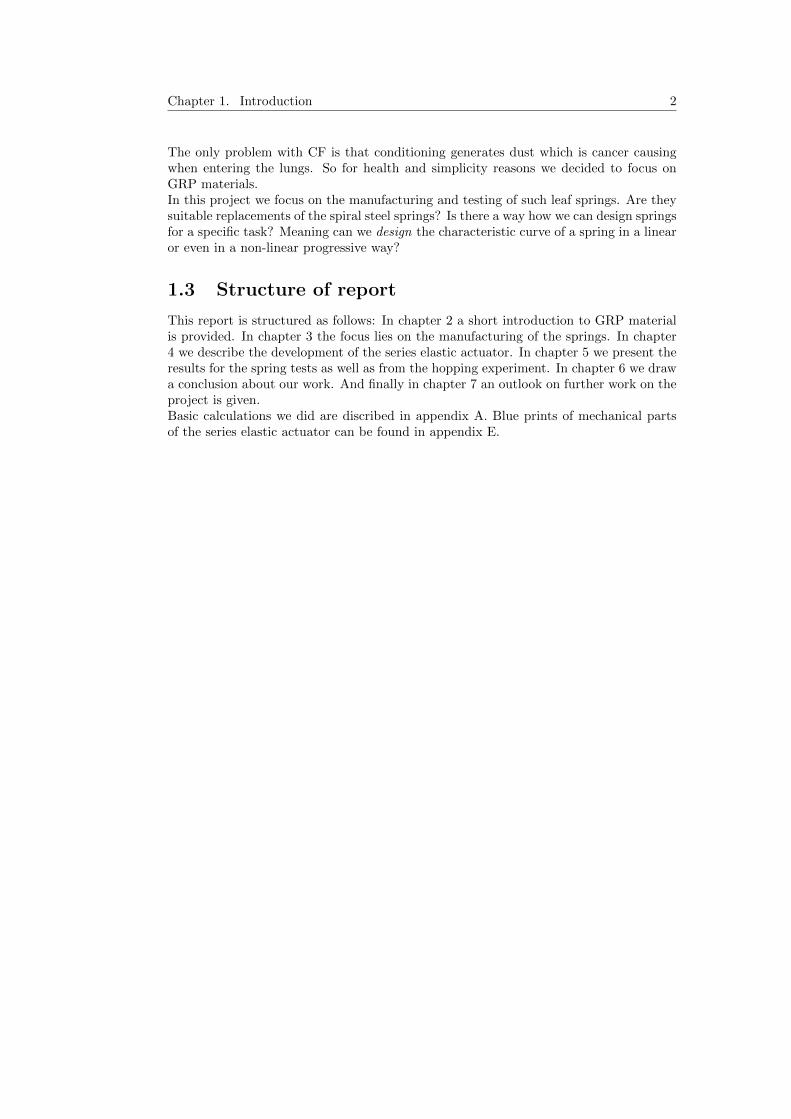
Other than metals like steel and aluminium, GRP does not consist of one (cristaline)matrial structure, but consists of many fibers. This very long and thin fibers are madeof glass. The matrix which holds the fibers together is a polymere resin ([3],[4]). Thematerial can be bought as a pre-made glass fiber fabric of different thickness and struc-ture. The fabric is very cheap compared to steel and aluminium but also compared toother composite materials. Out of the fabric any kind of layers shapes can be cut. Theresin is applied when laminating each layer.We mainly distinguish between unidirectional(UD) and crossbred (CB) kind of fabric.The unidirectional fabric has all the fibers in the same direction. The crossbred fabriccrosses the fibers in different angles. In particular 45 to 90 degree. In figure 2.1 on theleft the a sketch of unidirectional fabric is shown and on the right is the crossbred fabric,which we used for our springs.

1Sometimes also called Glassfiber reinforced Plastic (GFRP)[4]2e.g. spray lay-up, pultrusion

3

Chapter 2. Introduction to GRP 4

Figure 2.1: Left image: Sketch of unidirectional glass fiber laminate. Right image:sketch of crossbred glass fiber laminate with an angle of 90 degree. The resin, displayedin orange, fully covers the fibers and holds them together.

The resin functions as binding material to hold the fibers together. We used epoxyresin for that purpose. Since the resin itself can not hold much weight the strength ofthe material comes from the glass fibers. Since each fiber is long and thin it can onlywithstand strain in direction of the fiber. Therefore the unidirectional fabric is verystrong in one direction but lacks of any strength in direction perpendicular to the glassfibers. The crossbred fabric, however, has fibers in both directions equally. Therefore itcan be stressed in both directions and is assumed to be quasi-isotropic.Drawbacks of UD fabric are the anisotropic material properties due to the directiondependency. The cross fribers do also help in holding fibers straight together. Thereforein practice often CB fabric is used eventhough half of the weight is lost due to thefibers which point in the orthogonal direction without immediate use for strength of thematerial.

2.1.1 Material properties

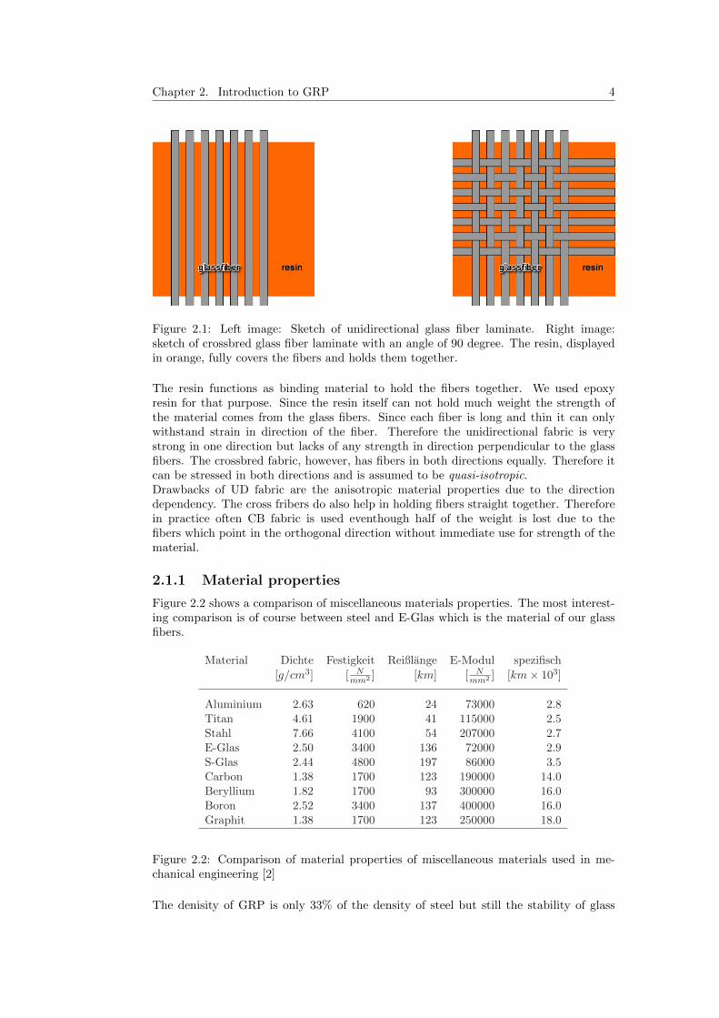
Figure 2.2 shows a comparison of miscellaneous materials properties. The most interest-ing comparison is of course between steel and E-Glas which is the material of our glassfibers.

1.1 Faserverbundwerkstoffe 3

Material Dichte Festigkeit Reißlange E-Modul spezifisch

[g/cm3] [ Nmm2 ] [km] [ N

mm2 ] [km× 103]

Aluminium 2.63 620 24 73000 2.8Titan 4.61 1900 41 115000 2.5Stahl 7.66 4100 54 207000 2.7E-Glas 2.50 3400 136 72000 2.9S-Glas 2.44 4800 197 86000 3.5Carbon 1.38 1700 123 190000 14.0Beryllium 1.82 1700 93 300000 16.0Boron 2.52 3400 137 400000 16.0Graphit 1.38 1700 123 250000 18.0

Tabelle 1.1: Absolute und spezifische Eigenschaften von Materialien in Faserform. Aus [1]

die Reißlange. Diese ist die Lange einer gedachten Stange, Drahtes, oder Faser, die freihangend von einem Material erreicht werden kann, bevor es unter dem eigenen Gewichtzerreißt. Die Reißlange errechnet man in der Einheit Kilometer, indem man den Zahlen-wert der Festigkeit durch denjenigen der Dichte teilt und außerdem berucksichtigt, daßein Gramm im Schwerefeld der Erde auf Hohe des Meeresspiegels 9, 81 × 10−3N wiegt.Die hochsten Werte der Reißlange erzielen Fasern aus Glas, Boron und Graphit.Die gleiche Umrechnung liefert, wenn auch ohne entsprechende anschauliche Bedeutung,die spezifischen E-Moduln in der rechten Spalte von Tabelle 1.1. Vergleicht man hier dieWerte von Stahl und Aluminium, welche bei kompakter Form etwa die selben sind, fragtman sich vielleicht, warum Aluminium gegenuber Stahl im Leichtbau einen Vorteil habensoll. Die Erklarung liegt in der Tatsache, daß eine Struktur aus Aluminium eine hohereWandstarke aufweist als eine gleich schwere aus Stahl und damit erst bei deutlich hoherenLasten beult. Die deswegen mit Aluminium entfallenden Versteifungen bedeuten eineEinsparung an Gewicht. Aber noch bedeutend gunstiger fur den Leichtbau als Aluminiumerscheinen die Fasern aus Graphit, Boron und Beryllium. Der Durchmesser von Fasernaus Carbon oder Graphit ist geringer als der eines menschlichen Haares. Diese Fasernkonnen also leicht gebogen und auch zu Geweben verarbeitet werden. Fasern aus Boronhaben Durchmesser wie Bleistiftminen und lassen sich nicht so flexibel einsetzen.Technisch interessante Faserverbundwerkstoffe bieten beinahe unbegrenzte Moglichkeiten,verschiedene Werkstoffe und Verstarkungsformen zu kombinieren (Abb. 1.3(a), ein hohes

a b c d

Abbildung 1.3: Technisch interessante Aspekte von Faserverbundwerkstoffen

Potential fur den Leichtbau (b), eine Vielzahl interessanter physikalischer Eigenschaften(c) und die Moglichkeit zur Integration funktionaler Elemente und Werkstoffe wahrenddes Herstellungsprozesses (d).

c© ETH Zurich IMES-ST, 10. April 2008

Figure 2.2: Comparison of material properties of miscellaneous materials used in me-chanical engineering [2]

The denisity of GRP is only 33% of the density of steel but still the stability of glass

5 2.2. Limitations

fibers are 83% of steel. So GRP fabric is much lighter but almost as strong as steel.The main difference is the rather different E-modulus. The much lower modulus of GRPmeans that the material is much more flexibel. We can see that fact in the differentbreaking lengths as well.The amount of energy which can be stored in a spring is the area beneath the char-acteristic curve3 of the spring. Therefore for energy storage we are very interested inflexibel materials because the more flexibel the material the higher the displacement.Since the stability is almost the same, the spring made of GRP can hold similar forcewithut breaking. Figure 2.3 illustrates that fact with a sketch of the characteristic curveof a steel and a comparable GRP spring. One can easily see that the area under theGRP spring is bigger.

Figure 2.3: Sketch of characteristic curves of a steel spring and a corresponding GRPspring. The area under the curve is the energy which can be stored in the spring.

Other properties are a high electrical resistance and a strong resistance against corrosion([3],[4]).

2.2 Limitations

Besides the numerous advantages of GRP material over steel, there are also some impor-tant drawbacks. The list is not complete but covers important drawbacks from our pointof view.

• The need for a counterblock. With GRP one can build almost any kind of layerbased shape. Only limitation is the counterblock on which each layer is laminated.Especially sharp corners are very difficult to make. But any kind of gap producesair pockets when laminating. Each air pocket greatly reduce stability. In practicespatula is used to cope with that problem.

• Manufacturing is much more time consuming and equipment for auonomous pro-duction is expensive. GRP products are often hand made which has its own limi-tations (precision, repeatability, costs, ...)

3Force over displacement diagram

Chapter 2. Introduction to GRP 6

2.3 Applications of GRP in modern mechanical engi-neering

GRP is a very versatile material. The material properties and the fact that it is verycheap favored GRP in a variety of applications ([3],[4]).

• Pipes

• Lightweight covers

• (Model) planes

• Lightweight leaf springs for cars

• Rotor blades of wind energy power plants

• Hulk of a boat (e.g. yacht)

Chapter 3

Design of the spring

In this chapter we focus on the design of the springs we used in our actuator. Thedevelopment of the linear spring is described in section 3.1. In section 3.2 we describethe development of the non-linear spring.

3.1 Linear spring

To design a leaf spring there are many different possibilities. One simple approach is theU shape. It allows both compressing and streching of the spring. Both is required fora linear actuator in order to operate in both directions. Also - since a counterblock isrequired - the U shape is simple enough to be manufactered by hand in our own lab.

3.1.1 Computation

The goal was to design a spring that has a similar characteristic curve as the steel springs,namely linear. The force is introduced on the tip of the spring legs. We therefore havea linear increase of the bending moment with respect to the distance from the tip of thespring leg to the back of the spring. Figure 3.1 shows the linear change in thickness weused from the tip of the spring leg to the top of the spring. This allows us to have anequal distribution of the bending moment over the whole spring. We want the back ofthe spring to be rigid and not bend in order to simplify the computation. Therefore thetop has the biggest thickness.

Figure 3.1: Simple CAD concept model of the U shaped leaf spring we designed with alinear decrease in thickness from the top to the tip of the spring leg.

7

Chapter 3. Design of the spring 8

Since the U shape still has bended parts which are difficult to calculate analytically weused a simplified model. In figure 3.2 the simplified model for one spring leg is shown.The rigid back of the spring can be assumed to be a wall. The spring legs then act asbeams with a linear change in thickness.

Figure 3.2: Simple model of one spring leg with linear change in thickness. The rigidback of the spring can be simplified as a wall. The force is applied on the end of thespring leg.

Since the spring is symmetric, calculating one leg is enough. The original steel springwas picked to have maximum displacement at around 100 N Force. Figure 3.3 showsthe bending line of the simplified model when applied 100N force on the beam. Allcalculations were done using a online FEM tool1. The computations are not ment tobe very accurate but they allow us to roughly estimate required thickness of the spring.The thicker the structure the more stiff the spring becomes.

Figure 3.3: Picture of the output of the online FEM tool which we used for estimatingthe required thickness of the spring. Above is the spring leg as we have modeled it. Thelower image shows the bending line of the spring leg when force is applied on the end ofthe bar.

Because this calculations are not very accurate and for testing reasons we then also madesprings with half the thickness and with 50% more material. Those springs are denotedin this report as spring type 1.0 for the original, 0.5 and 1.5 for the alternative springs.

3.1.2 Counterblock

The first counterblock was cut from a block of styrofoam with a hot wire. After grindingit to a good surface and shape we used a plastic tape to seal it. This step is importantin order to prevent the very agressive resin to attack the styrofoam. During the man-ufacturing of the first test spring series we experienced a high increase in termperatureof the hardener-resin mixture. In figure 3.4 the result after removing the vacuum pump

1http://www.tm-interaktiv.de/BT2D/index.html

9 3.1. Linear spring

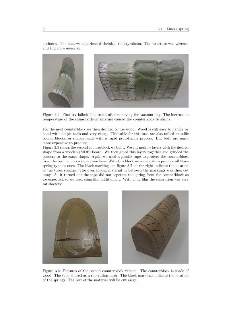
is shown. The heat we experienced shrinked the styrofoam. The structure was wizenedand therefore unusable.

Figure 3.4: First try failed: The result after removing the vacuum bag. The increase intemperature of the resin-hardener mixture caused the counterblock to shrink.

For the next counterblock we then decided to use wood. Wood is still easy to handle byhand with simple tools and very cheap. Thinkable for this task are also milled metalliccounterblocks, or shapes made with a rapid prototyping process. But both are muchmore expensive to produce.Figure 3.5 shows the second counterblock we built. We cut muliple layers with the desiredshape from a wooden (MDF) board. We then glued this layers together and grinded theborders to the exact shape. Again we used a plastic tape to protect the counterblockfrom the resin and as a seperation layer.With this block we were able to produce all threespring type at once. The black markings on figure 3.5 on the right indicate the locationof the three springs. The overlapping material in between the markings was then cutaway. As it turned out the tape did not seperate the spring from the counterblock aswe expected, so we used cling film additionally. With cling film the seperation was verysatisfactory.

Figure 3.5: Pictures of the second counterblock version. The counterblock is made ofwood. The tape is used as a seperation layer. The black markings indicate the locationof the springs. The rest of the material will be cut away.


3.1.3 Layer setup

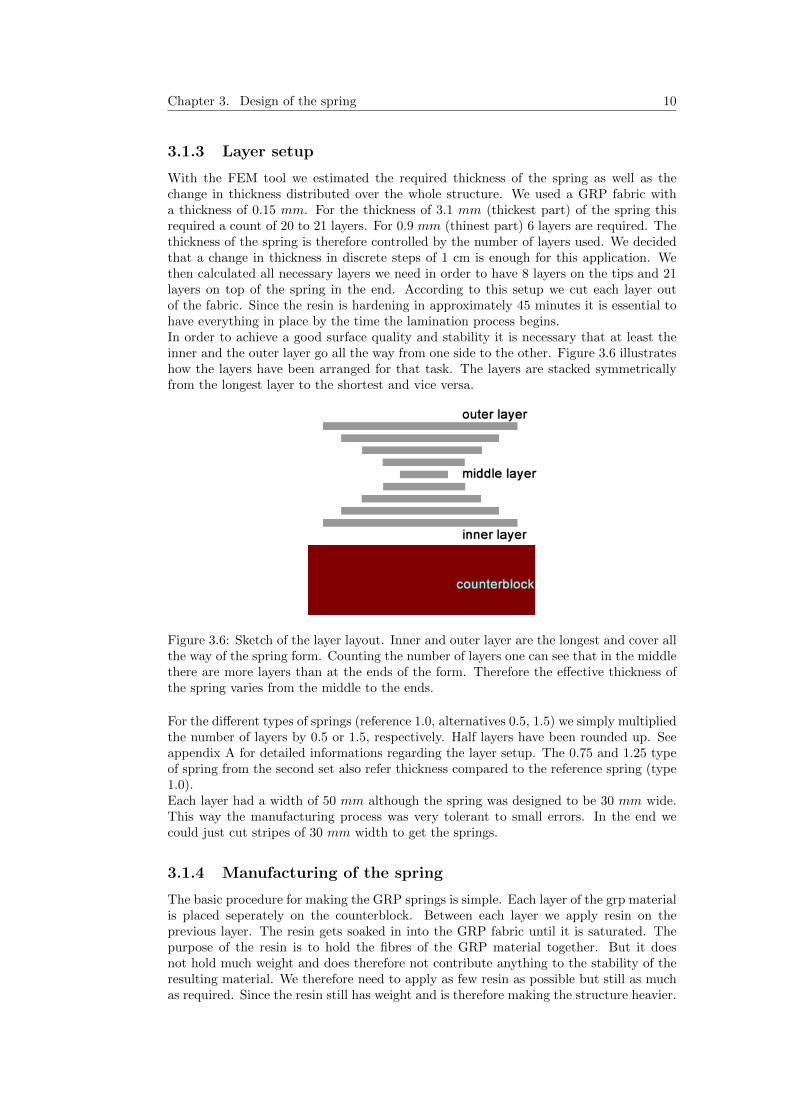
With the FEM tool we estimated the required thickness of the spring as well as thechange in thickness distributed over the whole structure. We used a GRP fabric witha thickness of 0.15 mm. For the thickness of 3.1 mm (thickest part) of the spring thisrequired a count of 20 to 21 layers. For 0.9 mm (thinest part) 6 layers are required. Thethickness of the spring is therefore controlled by the number of layers used. We decidedthat a change in thickness in discrete steps of 1 cm is enough for this application. Wethen calculated all necessary layers we need in order to have 8 layers on the tips and 21layers on top of the spring in the end. According to this setup we cut each layer outof the fabric. Since the resin is hardening in approximately 45 minutes it is essential tohave everything in place by the time the lamination process begins.In order to achieve a good surface quality and stability it is necessary that at least theinner and the outer layer go all the way from one side to the other. Figure 3.6 illustrateshow the layers have been arranged for that task. The layers are stacked symmetricallyfrom the longest layer to the shortest and vice versa.

Figure 3.6: Sketch of the layer layout. Inner and outer layer are the longest and cover allthe way of the spring form. Counting the number of layers one can see that in the middlethere are more layers than at the ends of the form. Therefore the effective thickness ofthe spring varies from the middle to the ends.

For the different types of springs (reference 1.0, alternatives 0.5, 1.5) we simply multipliedthe number of layers by 0.5 or 1.5, respectively. Half layers have been rounded up. Seeappendix A for detailed informations regarding the layer setup. The 0.75 and 1.25 typeof spring from the second set also refer thickness compared to the reference spring (type1.0).Each layer had a width of 50 mm although the spring was designed to be 30 mm wide.This way the manufacturing process was very tolerant to small errors. In the end wecould just cut stripes of 30 mm width to get the springs.

3.1.4 Manufacturing of the spring

The basic procedure for making the GRP springs is simple. Each layer of the grp materialis placed seperately on the counterblock. Between each layer we apply resin on theprevious layer. The resin gets soaked in into the GRP fabric until it is saturated. Thepurpose of the resin is to hold the fibres of the GRP material together. But it doesnot hold much weight and does therefore not contribute anything to the stability of theresulting material. We therefore need to apply as few resin as possible but still as muchas required. Since the resin still has weight and is therefore making the structure heavier.

11 3.1. Linear spring

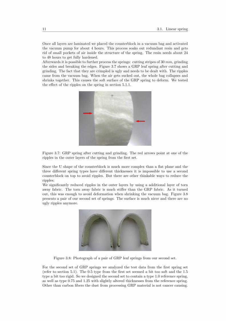
Once all layers are laminated we placed the counterblock in a vacuum bag and activatedthe vacuum pump for about 4 hours. This process soaks out redundant resin and getsrid of small pockets of air inside the structure of the spring. The resin needs about 24to 48 hours to get fully hardened.Afterwards it is possible to further process the springs: cutting stripes of 30 mm, grindingthe sides and breaking the edges. Figure 3.7 shows a GRP leaf spring after cutting andgrinding. The fact that they are crimpled is ugly and needs to be dealt with. The ripplescame from the vacuum bag. When the air gets sucked out, the whole bag collapses andshrinks together. This causes the soft surface of the GRP spring to deform. We testedthe effect of the ripples on the spring in section 5.1.1.

Figure 3.7: GRP spring after cutting and grinding. The red arrows point at one of theripples in the outer layers of the spring from the first set.

Since the U shape of the counterblock is much more complex than a flat plane and thethree different spring types have different thicknesses it is impossible to use a secondcounterblock on top to avoid ripples. But there are other thinkable ways to reduce theripples.We significantly reduced ripples in the outer layers by using a additional layer of tornaway fabric. The torn away fabric is much stiffer than the GRP fabric. As it turnedout, this was enough to avoid deformation when shrinking the vacuum bag. Figure 3.8presents a pair of our second set of springs. The surface is much nicer and there are nougly ripples anymore.

Figure 3.8: Photograph of a pair of GRP leaf springs from our second set.

For the second set of GRP springs we analyzed the test data from the first spring set(refer to section 5.1). The 0.5 type from the first set seemed a bit too soft and the 1.5type a bit too rigid. So we designed the second set to contain a type 1.0 reference spring,as well as type 0.75 and 1.25 with slightly altered thicknesses from the reference spring.Other than carbon fibers the dust from processing GRP material is not cancer causing.


But still it is not recommended to breath in the dust or have too much of it on the skinas it starts to itch really bad. Also breathing in GRP dust can cause Asthma or allergicreactions ([3],[4]).

3.1.5 Assembly of the spring

Now the springs are almost ready to use. A connection interface which allows us toconnect the spring to the structure of the actuator needs t be included. In order to avoidgenerating large moments in the thinest parts of the spring, a free rotating connectionwas implemented. Namely a small tube added to the tip of the spring legs fixed to therest of the actuator with a bolt. The tube has a outer diameter of 4 mm and an innerdiameter of 2.5 to 3 mm. Because the resin tends to resolve glue we fixed the tube witha strong thread.Another problem is the difference in thickness between the spring leg and the tube. Itis almost impossible to laminate GRP layers around the tube and not having a massivepocket of air beneath. To cope with that problem something to stuff the gap is required.In this case fine cotton balls were mixed into resin2. The more cotton the more pasty themixture gets. With this material it is possible to level out the cap between the springleg and the tube. Now it is no problem to laminate additional layers around the tube.For that purpose we used a thiner (only 0.07 mm thickness) GRP fabric because it ismore adaptive to round surfaces. In our first attempt we used nine3 additional layerswith increasing length. So the last layer is again providing a smooth transition to therest of the spring. The length of this additional layers is not very important. Their onlyfunction is to hold the copper tube on the tip of the spring legs. As the forces at the tipsof the spring legs are not very high it is preferable to use as few material as possible. Inour second build we slightly reduced the number of layers to eight4. Figure 3.8 showsthe springs after adding the connectors at the ends of the spring legs.Finally the springs had to be cut at the end of the spring legs so they fit into the springconnectors of the structure of the actuator. This is illustrated with a CAD model in figure3.9 on the left. Figure 3.9 on the right shows the CAD model of the spring mounted onthe connector of the structure of the actuator.

Figure 3.9: Left image: CAD model of the ready-to-use state of the GRP spring. Rightimage: CAD model of the spring mounted on the spring connector.

2Same mixture as for the laminating itself33 small, 3 medium, 3 larger layer42 × 10mm, 2 × 8mm, 2 × 6mm, 2 × 4mm

13 3.2. Non-linear spring

3.2 Non-linear spring

Since we were able to build a GRP leaf spring with a linear characteristic we extendedour objective to non-linear springs with a progressive characteristic. A non-linear pro-gressive spring would imitate the behavior of natural muscles much better since thosehave a non-linear characteristic as well.

3.2.1 Design idea

There is a variety of ideas how to make a structure stiffer the more force is applied. Mostof them are based on sandwich constructions of different materials or thicknesses withdifferent stiffness combined together in a way such that each element works on distinctintervall of applied force. So it is possible to have a non-linear curve at the cost that itchanges at certain points. As a huge drawback a spring design as described above wouldnot have a continuous curve but several discrete steps.We wanted to build a spring with continuous change in stiffness so we took advantage ofa simple observation based on the material we used: Deformations of the GRP materiallead to an increase in stiffness. Or in other words, the more the material bends, thestiffer it becomes.In the U-shape the deformation was not enough since the two legs tend to touch inthe middle. So we designed a spring which is able to deform more and therefore has asignificant increase in stiffness the more force is applied. Of course this only works up toa certain maximum where the force gets too high for the structure of the spring and itbreaks.

3.2.2 Computations

A detailed structural analysis is again out of the scope of this project. To get a easyresult to start with we used the same assumptions and model we did in section 3.1.1 forthe linear spring. Since we are interested in a high deformation we followed the compu-tation of the linear 0.75 and 0.5 type of spring from the first and the second set of linearsprings. We also designed a 1.0 type similar to the 1.0 linear spring type as a reference.It is important to emphasize that all computations here were only ment to give somekind of guidance since the simple model we used for calculation does only apply well forsmall deformations which in our case is contradictory to the operation principle.

3.2.3 Counterblock

The form of the spring was guessed on a trial and error basis. For this purpose wetried to bend paper models, carton sheets and our other GRP springs. We then cameup with a simple extended U shape in order to have a fast verification of the generalprinciple our non-linear spring concept is based on. Figure 3.10 shows a photographsof the counterblock design. The back is longer so there is more room for the springs todeform. Also the opening angle of the spring legs is higher so the deformation is increasedfrom the start. Downside of that fact is that the spring does not behave symmetricallyin pushing and pulling situations. The counterblock itself is made the same way as ourprevious built described in section 3.1.2.


Figure 3.10: Photographs of the counterblock we used to build the non-linear GRPsprings. Left image shows the front view and the right image is an isometric view on thewhole counterblock.

3.2.4 Manufacturing of the spring

The general principle of the layer setup is the same as shown in figure 3.6 for the linearspring. Only difference was that thickest part of the spring was now extended over thewhole back of the spring. Some additional layers on the back of the spring make sure thatthe assumption that this part is rigid part is still valid. The non-linear spring was madethe same way as the linear spring, but with altered length of the layers. For detailedinformation regarding the layer setup please refer to appendix A. Figure 3.11 shows aphotograph of one of the non-linear springs we built. In this picture the tubes we use asconnectors at the end of the spring legs are already attached.

Figure 3.11: Non-linear GRP spring after cutting and grinding. The tubes at the endsof the spring legs are already attached.

There is an air pocket above the copper tube at the left tip of the spring leg. Thisair pocket reduces the stability of the spring connector but the connector is still strongenough not to break apart.

Chapter 4

Design of the Series ElasticActuator

This chapter describes the process of designing the series elastic actuator which we usedto test the grp springs in a hopping environment.

4.1 General Concept

Figure 4.1 illustrates the general concept of the previous actuator designs [1]. It worksas follows:

• A motor drives a ball screw for linear motion.

• Three sliding parts (slider 1, slider 2, slider 3) are mounted on two parallel guides.

• A spring is connecting slider 1 and slider 2.

• The motor is connected to slider 3 while the ball screw nut is connected to slider2.

• Slider 1 and slider 2 have a breaking mechanisms which allows them to hold theirposition on the guides independently.

• The leg of the robot is connected to the guides on one side and on slider 3 on theother side.

Figure 4.1: Sketch of the general concept of the LMMA described in [1]

This concept works well for the application of a knee joint of a walking robot developedat our lab. But we experienced problems with the breaking mechanism and the springs.For this project we decided not to care about the breaking but to find ways to cope withthe spring problem. The improvement of the breaking mechanism is left for a futureproject. In our design we tried to provide an interface on which a breaking mechanismcould be implemented later on without changing all the other parts of the actuator.Another simplification was that we fixed the position of slider 1.

15

Chapter 4. Design of the Series Elastic Actuator 16

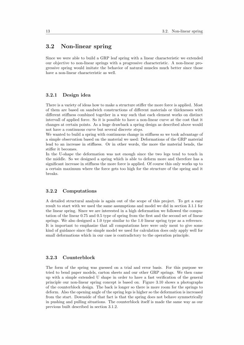
A CAD model of the whole actuator is shown in figure 4.2. The operation principle issimilar to the LMMA. The DC Motor on slider 3 drives the ball screw which is connectedto slider 2. Slider 2 is then connected to slider 1 with a GRP leaf spring. There are nosensors mounted on the actuator but the hall sensor which is already installed in theDC Motor. For a proper control of the actuator at least linear potentiometer for thedisplacement have to be mounted. We suggest that the potentiometer would be installedbetween slider 3 and the guide.

Figure 4.2: CAD model of the series elastic actuator with mounted GRP spring.

4.2 Changes to previous designs

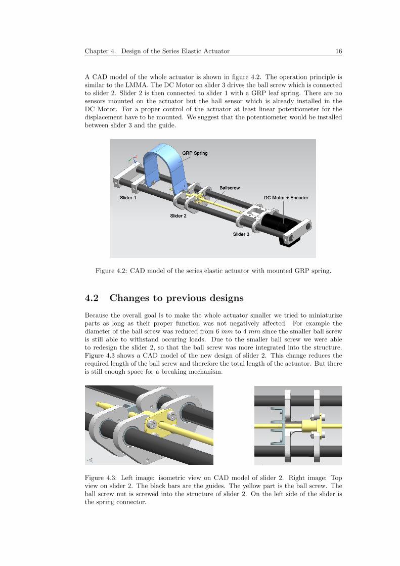
Because the overall goal is to make the whole actuator smaller we tried to miniaturizeparts as long as their proper function was not negatively affected. For example thediameter of the ball screw was reduced from 6 mm to 4 mm since the smaller ball screwis still able to withstand occuring loads. Due to the smaller ball screw we were ableto redesign the slider 2, so that the ball screw was more integrated into the structure.Figure 4.3 shows a CAD model of the new design of slider 2. This change reduces therequired length of the ball screw and therefore the total length of the actuator. But thereis still enough space for a breaking mechanism.

Figure 4.3: Left image: isometric view on CAD model of slider 2. Right image: Topview on slider 2. The black bars are the guides. The yellow part is the ball screw. Theball screw nut is screwed into the structure of slider 2. On the left side of the slider isthe spring connector.

17 4.2. Changes to previous designs

Since we use leaf springs instead of spiral springs we also had to design new connectors forthe spring. Figure 4.4 on the left shows the new slider 1 design with the spring connectorattached. In figure 4.4 on the right the spring is attached to slider 1. As mentionedbefore slider 1 is now fixed to the guides with small bolts on the sides.

Figure 4.4: Left image: CAD model of slider 1 with the new spring connector attached.Right image: CAD model of slider 1 with GRP leaf spring attached.

We designed the connector as simple as possible but it is thinkable to change the designdepending on the requirements of the GRP spring. It is important to mention that theconnection of the spring needs to be either colinear with the guides or with an symmetricoffset. Otherwise there is a resulting reaction force on the slider which could cause theslider to get stuck.With that in mind we can design a connector which can mount multiplesprings. Refer to section 7.2 for additional informations regarding this topic.

Chapter 4. Design of the Series Elastic Actuator 18

Chapter 5

Evaluation

In this chapter we provide results from the spring tests we made. In section 5.1 theresults from testing the first grp linear spring prototype are stated. In section 5.2 arethe results from the first grp non-linear spring prototype and finally in section 5.3 arethe performance measurements of the whole series elastic actuator when placed in thecontext of a hopping leg.

5.1 GRP linear spring test

For this kind of test we built a small test environment were we could mount the springsand apply weight w (and therefore force due to gravitation) to them. Figure 5.1 showsa sketch of the test environment. The operation principle is the same as for the serieselastic actuator. We used guides to prevent the spring to bend in direction perpendicularto the moving direction. For the force generation we used simple weights from dumbbells.With four 500 g and four 1.25 kg weights we could generate forces from 5 N to 70 N .

Figure 5.1: Conceptual sketch of the test environment we used for finding the springcharactersistics. The displacement was measured with a potentiomenter and read outmanually with a multimeter. The results were then transfered into matlab manually.

The friction on the guides can be neglected as we are just interested in the static displace-ment at a given force. This force is acting on the leaf spring colinear to the direction ofthe gravitational force. We then measured the resistance R between the two spring legswith a potentiometer. As the used linear potentiemeter varies the resistance linearlly thedistance between the legs of the spring can be extracted with linear interpolation.

19

Chapter 5. Evaluation 20

d = dmin +dmax − dmin

Rmax −Rmin(R−Rmin)

Where d is the distance measured with the potentiometer translated in milimeter. dmin

in our case is 0 and dmax is the maximal length of the potentiometer in milimeter. Rmin isthe measured resistance at dmin, Rmax at dmax and R is the actual measured resistance.Reduced by the interpolated length of the spring without load d0 that provides thedisplacement of the spring D at a given force level.

D = d− d0

5.1.1 First prototype

Figure 5.2 to 5.4 show the force over the measured displacement diagram for the firstprototype of our GRP leaf springs. Each data point indicates the average out of 5independent measurements. The blue line indicates a quadratic fit of the measured datapoints. The 0.5 type of spring in figure 5.2 had only few data points, since small weights(less than 2 kg) already caused to spring to compress fully1. The graph looks non-linearprogressive, but this is with a lot of uncertainty because of the few data amount. Theother two springs in figure 5.3 and 5.4 also show non-linear characteristics. Namelyprogressive in figure 5.3 but also asymptotic in figure 5.4. This non-linearity is greatlyinfluenced by the ripples the spring has in the outer surface layers.

0 5 10 15 20 25−2

0

2

4

6

8

10

12

displacement [mm]

forc

e [N

]

force over displacement of grp spring

Spring type 0.5 quadratic fit

Figure 5.2: Plot of applied force over measured displacement of the spring type 0.5. Theblue line indicates a quadratic fit of the data points.

1Until the two spring legs touch.

21 5.1. GRP linear spring test

0 5 10 15 20 25 300

5

10

15

20

25

30

displacement [mm]

forc

e [N

]




0 2 4 6 8 10 12 14 160

10

20

30

40

50

60

70

displacement [mm]

forc

e [N

]




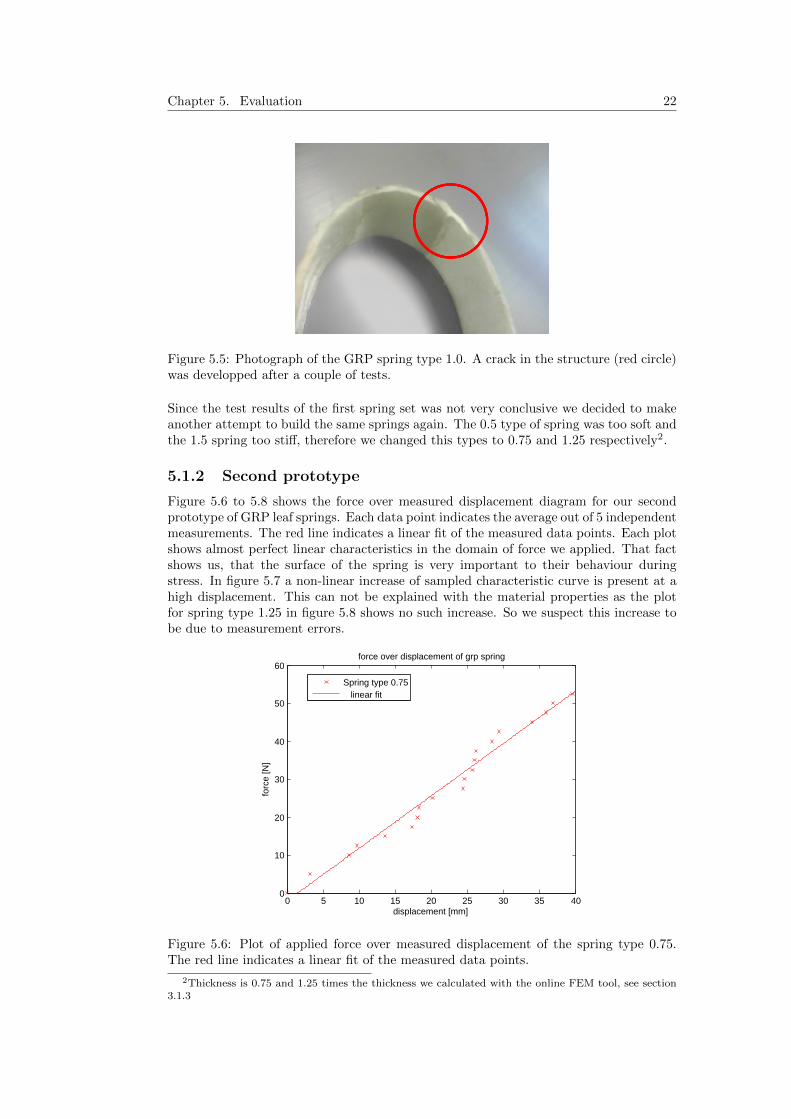
After a couple of test runs the 1.0 type of spring started to crack along a ripple in theouter surface layer. On figure 5.5 this crack is shown in the red circle. A crack reduces thestiffness of the spring drastically but the spring did not break apart. The characteristicsof a broken spring are unpredictable but the spring is still safe and functionable. This isan important aspect regarding the security of an actuator equipped with GRP springs.


Figure 5.5: Photograph of the GRP spring type 1.0. A crack in the structure (red circle)was developped after a couple of tests.

Since the test results of the first spring set was not very conclusive we decided to makeanother attempt to build the same springs again. The 0.5 type of spring was too soft andthe 1.5 spring too stiff, therefore we changed this types to 0.75 and 1.25 respectively2.

5.1.2 Second prototype

Figure 5.6 to 5.8 shows the force over measured displacement diagram for our secondprototype of GRP leaf springs. Each data point indicates the average out of 5 independentmeasurements. The red line indicates a linear fit of the measured data points. Each plotshows almost perfect linear characteristics in the domain of force we applied. That factshows us, that the surface of the spring is very important to their behaviour duringstress. In figure 5.7 a non-linear increase of sampled characteristic curve is present at ahigh displacement. This can not be explained with the material properties as the plotfor spring type 1.25 in figure 5.8 shows no such increase. So we suspect this increase tobe due to measurement errors.

0 5 10 15 20 25 30 35 400

10

20

30

40

50

60

displacement [mm]

forc

e [N

]


Spring type 0.75 linear fit

Figure 5.6: Plot of applied force over measured displacement of the spring type 0.75.The red line indicates a linear fit of the measured data points.

2Thickness is 0.75 and 1.25 times the thickness we calculated with the online FEM tool, see section3.1.3

23 5.1. GRP linear spring test

0 5 10 15 20 25 300

10

20

30

40

50

60

displacement [mm]

forc

e [N

]



Figure 5.7: Plot of applied force over measured displacement of the spring type 1.0. Thered line indicates a linear fit of the measured data points.

0 5 10 15 20 25 30−10

0

10

20

30

40

50

60

70

80

displacement [mm]

forc

e [N

]



Figure 5.8: Plot of applied force over measured displacement of the spring type 1.25.The red line indicates a linear fit of the measured data points.

Spring constant

With a linear spring characteristic curve it is possible to compute the spring constantusing Hooke’s Law. Figure 5.9 shows the result of the computation of the spring constantfor each sample point (crosses in the previous graphs):

ki = Fi/xi

where Fi is the applied force and xi the average of the measured displacements of samplepoint i.


0 5 10 15 20 251

1.2

1.4

1.6

1.8

2

2.2

2.4

2.6

2.8

sample number i

sprin

g co

nsta

nt o

f sam

ple

num

ber

i

spring constant of each sample

Spring type 0.75Spring type 1.0Spring type 1.25

Figure 5.9: Plot of the spring constant computation for each sample. The green linecorresponds to the 1.25 type, the blue to the 1.0 type and the red to the 0.75 type ofspring.

The spring constant is more or less constant (only a small change in magnitude) forall spring types. All the springs show a light increase in stiffness the higher the forcesand therefore the higher the deformation becomes. The material increases the stiffnessas a reaction to the deformation up to a certain level at which the structure starts todelaminate and the spring eventually breaks. This observation lead to the development ofthe non-linear spring. We try to take advantage of this fact by increasing the deformation.For the three spring types we built, the average of the spring constant is:

• Type 0.75: 1.27 N/mm

• Type 1.0: 2.04 N/mm

• Type 1.25: 2.62 N/mm

The spring constant of the steel spring which was used in [1] was 2.27 N/mm. Thisshows that we are in the same range.

5.2 GRP non-linear spring test

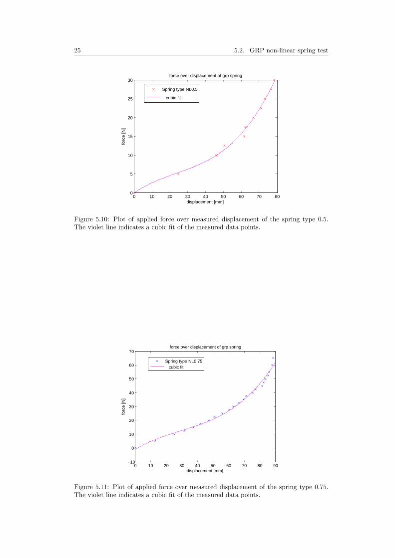
We placed the non-linear spring in the same experimental environment and applied forcethe same way we did for the linear spring. Figure 5.10 to 5.12 show the force over mea-sured displacement for all non-linear spring types. In all plots we can see the almostlinear charactersistic until the deformation gets high enough such that the stiffness in-crease drastically. In figure 5.12 we don’t see the non-linear increase in stiffness. Thisis because the applied force of 70 N was not high enough to deform the spring to thenon-linear area of operation.This results demonstrate that it is possible to design GRP springs with non-linear pro-gressive stiffness only by the design of the shape of the spring and not with the combi-nation of different shapes or materials.

25 5.2. GRP non-linear spring test

0 10 20 30 40 50 60 70 800

5

10

15

20

25

30

displacement [mm]

forc

e [N

]


Spring type NL0.5

cubic fit

Figure 5.10: Plot of applied force over measured displacement of the spring type 0.5.The violet line indicates a cubic fit of the measured data points.

0 10 20 30 40 50 60 70 80 90−10

0

10

20

30

40

50

60

70

displacement [mm]

forc

e [N

]


Spring type NL0.75 cubic fit



0 10 20 30 40 50 60 700

10

20

30

40

50

60

70

displacement [mm]

forc

e [N

]


Spring type NL1.0 cubic fit


Spring parameter

In the case of the non-linear spring characteristic we can no longer have a constantparameter for the spring. The spring parameter changes with respect to the displacement.Therefore k is now a function of x.

F (x) = k(x) · x→ k(x) = F (x)/x

Figure 5.13 shows the distribution of the spring parameter we computed for each samplepoint (crosses from the previous graphs). For the 0.5 and the 0.75 type there is asignificant increase of the spring parameter at higher forces. This increase correspondsto the increase in stiffness of the spring. For the 1.0 type of spring we see a constantdistribution. This also corresponds to the linear characteristic we observed in that rangeof forces.

0 5 10 15 20 250.2

0.3

0.4

0.5

0.6

0.7

0.8

0.9

1

1.1

1.2

sample number i

sprin

g pa

ram

eter

of s

ampl

e nu

mbe

r i

spring parameter of each sample

Spring type 0.5Spring type 0.75Spring type 1.0

Figure 5.13: Plot of the spring parameter distribution for each spring type. The greenline corresponds to the 1.0 type, the blue to the 0.75 type and the red to the 0.5 type ofspring.

27 5.3. The hopping experiment

The ranges of the spring parameter for the three types of non-linear spring we built is:

• Type 0.5: 0.2...0.4 N/mm

• Type 0.75: 0.4...0.8 N/mm

• Type 1.0: 1...1.2 N/mm

The stiffness of all three springs is low. A low stiffness corresponds to a high displacement.A high displacement corresponds to a high deformation. So the increase in stiffness ishigher for springs with a lower stiffness. But the higher the forces on a soft spring thecloser the strain gets to the point where the spring breaks. The solution to this trade-offdepends on the application in which the spring is acting.

5.3 The hopping experiment

After developing both the springs and the series elastic actuator we placed all partstogether to see how they perform in a hopping experiment. The mathematical modellingand related calculations are shown in appendix A.2. We have two possibilities how wecan achieve hopping. The loaded spring and the excited spring hopping.

Loaded spring

Since we have a series elastic actuator we can not load the spring because that wouldrequire a breaking mechanism in the slider connected to the spring. Figure 5.14shows anillustration how the jump was made. We tried to achieve jumping by fixing the motorand manually loading the spring by pressing down the slider. After releasing the sliderthe whole series elastic actuator jumps couple of centimeters.

Figure 5.14: CAD illustration of the series elastic actuator generating the jump. The redarrow represents the manual pushing of the slider. The compression of the spring (greenarrow) causes the jump (blue arrow) after releasing the slider.

Table 5.3 shows the result from few samples. The jumping hight ist depending on thedisplacement of the spring. In each test run we tried to load the spring to its maximumin order to get the maximum jumping hight.


Spring type displacement [mm] jumping hight [mm]non-linear 0.75 80 90linear 0.75 50 60linear 1.0 30 40

Table 5.1: Jump test results with various manually loaded springs.

The resulting jumping hight of all tested springs was larger than the displacement. Thissimple test illustrates how much energy can be stored in GRP leaf springs.

Excited spring

The other approach was to initiate hopping by exciting the spring. Figure 5.15 illustrateshow the spring can be excited. By driving the ball screw in a sinusoidal movement, theDC motor causes the spring to compress and release. At a certain frequency, the naturalfrequency of the damped oscillator, the whole actuator starts to hop.

Figure 5.15: CAD illustration of the series elastic actuator generating the hopping move-ment. The up- and downward movement (red arrows) initiate a compression and releaseof the spring (green arrow). At peak frequency the actuator starts to hop.

Unfortunately we did not succeed in achieving significant hopping hights. For all springtypes we tried driving the motor around the natural frequency since the exact naturalfrequency is hard to estimate. Also we tried different loads3 on the actuator. This wasnot enough to cause the actuator to hop. Only vibrations in the structure of the actuatorwere visible.We suspect the friction in the actuator and the internal damping of the spring to causethe natural frequency to be smeared over many frequencies. Hopping is not possible ifthe resonant peak of the swinging spring is not high enough.Figure 5.16 shows the amplitude gain response of the linear 0.75 type of spring with aload of 3.75 kg. The higher the single resonant peak the higher the actuator is able to

30.5 kg to 3.75 kg

29 5.3. The hopping experiment

hop. In our case the highest peak at around 31 rads was not high enough to lift off the

ground. Also other smaller peaks indicate that there is no unique natural frequency.

101.4 101.5 101.6

100.52

100.56

100.6

Driving Frequency (rad/s)

Gai

n

101.4 101.5 101.6−80

−60

−40

−20

0

Driving Frequency (rad/s)

Phas

e(d

eg)

Figure 5.16: Amplitude response gain of the excited GRP leaf spring type 0.75 with3.75 kg load.

In order to get better results additional tests on this topic have to be made in the future.

Chapter 6

Conclusion

We showed in this project that it is possible to design GRP springs with a linear char-acteristic. The spring constant of such a spring is comparable to spiral steel springsbut with the benefit of a lower weight1 and a much simpler assembly of the actuator.During our work on the project we also discovered that a non-linear progressive springcharacteristic can be achieved without using patchwork or sandwich techniques.By using the basic fact that the material gets stiffer the more it deforms we designed aspring which has a continuous non-linear characteristic. This is a interesting discoveryfor the design of bio-inspired robots because natural muscle also have a non-linear pro-gressive spring behavior.In the hopping experiment we showed that the storable energy in GRP leaf springs isvery high. This allows us to build very efficient walking and jumping robots. We also dis-covered a very high damping property of our spring design. As a drawback this dampingmakes excited spring hopping very difficult. But there is also an upside. High internaldamping is preferable for shock absorbance, e.g. after a jump over an obstacle. Withinternal dampers we can take out energy of an impact without having to insert additionaldamping elements. This makes robot structures ligther and also more resistant to shocksof impacts.The cost of GRP material is very low compared to other composite materials, but also tosteel and aluminium. The big problem here is the manufacturing. Since we still dependon hand-made GRP structures the manufacturing process is expensive and very error-prone. With an automated lamination process that would be solved, but up to now suchequipment is very expensive. Until this problem is adressed, GRP spring are unlikely toendanger the dominance of steel springs. Expecially with regard to mass production.With this project we showed that GRP material has a high potential to replace standardmetallic elements in order to get closer to our biological role models. Therefore for bio-inspired robotics composite spring development may gain importance. But still a lot ofresearch is required to efficiently impose their use in modern robotics in general.

1Weight of GRP springs is around 30 g compared to 90 g of the comparable steel spring.

31

Chapter 6. Conclusion 32

Chapter 7

Future work

Although we found designs of GRP leaf springs which have linear as well as non-linearprogressive characteristic, we are not yet at the point where we can replace all steelsprings by GRP springs. In the following several points are mentioned where we need todo more research before our idea becomes practical.

7.1 Work on the spring

In this section several suggestions regarding the spring design are stated.

Spring design

We only investigated the U shape form of spring. But since almost every shape ispossible, there is maybe a better solution. Also the combination of CF and GRP couldbe interesting to investigate, especially for stiffer springs with higher target forces.

Linear spring

The manufacturing of the spring was very time consuming and required multiple stepswith 24 hours waiting time in between. Probably there are ways to simplify that process.Especially the mounting of the connector tubes could probably be integrated in theproduction of the spring itself. This would save a third of the production time.

Non-linear spring

The design of the non-linear spring is very simple and came straight forward from thedevelopment of the linear spring. Since the whole idea of the non-linear spring is toincrease the deformation while compressing the spring, there could be other shapes howto achieve that.The trade-off mentioned in section 5.2 also needs to be investigated further.

7.2 Work on the actuator

In this section we mention points where future work on the actuator could be done.

Break mechanism

The break mechanism is not implemented in the series elastic actuator presented in thisproject. But since the overall goal is to build a multi mode linear actuator, a breaking

33

Chapter 7. Future work 34

mechanism is required. The breaks should be able to fix the sliders on the guides. In allprevious prototypes this break mechanism was based on friction. By applying pressurethe break shoe is pressing on the guides. This increases the friction. The slider is fixedonce the friction of the breaks is higher than the force acting on the slider.Another important advantage of the friction based breaks is that it is independent fromthe position on the guides. With a form-closed approach this is not necessarly the case.In [1] a mechanism with an ellipse which presses two break shoes symmetrically on theguides is proposed. One challange could be to increase the friction on the break shoe.Figure 7.1 shows a sketch how this could be achieved using cam belts both on the guideand on the break shoe. The bigger the teeth of the belt the closer it gets to a form-closedapproach. A good trade-off is key.

Figure 7.1: Conceptual sketch of the belt idea.

Multiple springs

The effective spring constant can also be changed by adding more springs in parallel.Figure 7.2 shows a sketch of two parallel springs. The resulting spring constant ktot ofparallel springs is

ktot = k1 + k2

with k1 the constant of the first and k2 the constant of the second parallel spring.

Figure 7.2: Two springs in parallel can be simplified to one.

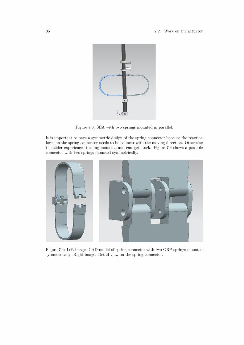
this can be used to change the effective spring constant of the actuator. A conceptualCAD model of the actuator with two mounted springs is shown in figure 7.3.

35 7.2. Work on the actuator

Figure 7.3: SEA with two springs mounted in parallel.

It is important to have a symmetric design of the spring connector because the reactionforce on the spring connector needs to be colinear with the moving direction. Otherwisethe slider experiences turning moments and can get stuck. Figure 7.4 shows a possibleconnector with two springs mounted symmetrically.

Figure 7.4: Left image: CAD model of spring connector with two GRP springs mountedsymmetrically. Right image: Detail view on the spring connector.

Chapter 7. Future work 36

Appendix A

Calculations

A.1 Linear and non-linear springs

For the calculations we assumed isotropic material conditions based on the crossbredfabric. Figure A.1 shows a screenshot of the excel table we used to do some basiccalculations. This was a very iterative process.

Inertia

The width w of the spring we set to 30mm. The thickness d of the back of the spring weassumed to be 3.1mm. Therefore for the inertia we have

Iyback=w · d3

12= 74.8mm4

E-modulus

We started from the E-modulus value we found in [2] for glass fibers. The crossbredfabric (which has the same amount of fibers in horizontal and vertical direction) whichwe used, in practice is only able to use half of the fibers for stability. Therefore we dividedthe modulus by two. Since almost half of the volume of the spring is resin, we dividedthe modulus again by two. So

E =86000

4= 21500

N

mm2

EI value

The EI value which we used to determine the shape of the bar in the online FEM toolwas then

E · Iyback= 1601266.25Nmm2

for the back of the spring. The analogue calculation (thickness d = 0.9mm) leads to theEI value of the second segment, the tip of the spring leg:

E · Iytip= 39183.75Nmm2

37

Appendix A. Calculations 38

Strain distribution

A force f of 100N attacks at the end of the spring legs. Since the spring legs have alength l of 70mm, this leads to a bending moment of Mb = f · l = 7000Nmm. Since thethickness is changing linearlly over the structure of the spring and with the restistancemoment for each segment

Iwback=w · d2

6

we can compute the strain distribution over the whole spring leg. The strain at the backof the spring is therefore

σback =Mb

Iwback

= 145.68N

mm2

This value is lower than the critical strain. In our case that is true for each segment ofthe spring.Figure A.2 show a screenshot of the same considerations for the non-linear spring.

A.2 The hopping experiment

For the hopping experiment we used basic calculations similar to [5]

Mathematical model

The simplified mathematical model of the experiment is shown in figure A.3. The totalmass acting on the slider is denoted as m. This is the combined mass of the structure andthe additional load. The spring constant is denoted as k and d is the internal dampingof the spring combined with the influence of friction on the sliders. The displacement ofthe load is x. This is also the state variable of the system.

Figure A.3: Simplified mathematical model of the jump environment

The equation of motion for a mechanical system like this is

m · x+ d · x+ k · x = 0

Normalized by the mass m this equation becomes

x+d

m· x+

k

m· x = 0

Since this is the equation of a damped oscillator, we see the resonance frequency ω0 ofthe spring is given by

ω0 =

√k

m

39 A.2. The hopping experiment

The damping ratio ζ can then be calculated using

ζ =d

2 ·m · ω0

The problem here is, that the damping of the spring d is hard to estimate. One wayhow to achieve that is by analysing the swing behavior of the spring. For that purposewe need to measure an initial displacement x1 and the displacement after one full swingcycle x2. With this two values we know how much movement the spring absorbed. Thiscorresponds to the damping which can be calculated using

d = ln |x1x2|

The damped natural frequency ωd can then be computed using

ωd = ω0 ·√

1− ζ2


Figure A.1: Excel sheet used to predict the required thickness of the spring

41 A.2. The hopping experiment

Figure A.2: Excel sheet used to predict the required thickness of the spring

Appendix B

Ordered Parts

Legend

• KSS ball screw (KSS): http://http://kssballscrew.com/

• Suter Kunstroffe AG (SK): http://www.swiss-composite.ch

• Maedler GmbH (M): http://www.maedler.ch

• Maxon Motors (MM): http://www.maxonmotor.ch

• igus Bearings (IG): http://www.igus.ch

• Coop: Bau und Hobby (CBH): http://www.coop.ch/bauundhobby

Part listSheet1

Page 1

Part Desc. Order nr. Amount Dealer Price [CHF]Ball screw SRT0401-147R187C10B0X 2 KSS 665

DC Motor + Encoder 333437 1 MM 356EPOS2 3900003 1 MM 395

GRP fabric 163g/qm 190.1158 5m SK 82GRP fabric 81g/qm 190.0070 2m SK 0Torn away fabric 85g/qm 190.1100 2m SK 0Epoxy L resin, work package 100.1101 1 kg SK 0

igus bearring JSM-1012-05 26 IG 40

Ball bearing 624-2Z-SKF 5 M 92coupling steel 60299602 2 M 44

MDF wood N/A 2x (22x10x100) CBH 6tape N/A 1 CBH 6cling film N/A 1 CBH 3alu tubes N/A 1x1m CBH 4copper tubes N/A 1x1m CBH 4thread N/A 1 CBH 5

Figure B.1: List of ordered parts with the ordering number and approx. prices

43

Appendix B. Ordered Parts 44

Appendix C

Contact Persons

Workshop

• Pascal Wespe: Material ordering and manufacturing of partsE-Mail: [email protected]

• Alessandro Rotta: Manufacturing of milled partsE-Mail: [email protected]

Composite Lab

• Thomas Heinrich: Repsonsible for the composite labE-Mail: [email protected]

• Markus ZoggE-Mail: [email protected]

KSS Ballscrew

• Martina Nava from GARNET s.r.lE-Mail: [email protected]

45

Appendix C. Contact Persons 46

Appendix D

Step-by-step Instruction

This chapter is a step-by-step instruction of how to make GRP springs as described inthis report.

D.1 Preparation

D.1.1 Counterblock

1. Build counterblock (CB)

2. Seal CB with tape

3. Mark middle line and position of springs on CB

D.1.2 Layer

1. Cut layers from fabric according to layer setup for all springs (refer to A.1).

2. Mark the center of the layer.

3. Order layers according to their symmetric setup: first layer is on the inside lateron, last layer is the outer layer (see figure 3.6 in section 3.1.3).

4. Prepare torn away fabric:

• One torn away fabric on the inside, one on the ouside of each spring leg.

• Torn away fabric allows us to laminate further layers later on (rough surface)which we need for the small tube connectors.

D.1.3 Resin

1. Make sure the room is supplied with fresh air.

2. Mix resin according to the mix ratio (resin to hardener)

• Volume: 100 to 45

• Mass: 100 to 40

3. Mix thouroughly for approx. 1 min with a wooden stick

Note: Resin-Hardener mixture will start to get hard in 45 min! If the mixture becomeshot, the mix ratio was wrong.

47

Appendix D. Step-by-step Instruction 48

D.2 Lamination

Security Notes

• The resin is irritating, make sure to wear gloves at any time.

• Always make sure that fresh air can enter the room.

• Resin on clothes will stay and can not be washed out!

Procedure

1. Apply small film of resin on counterblock with a brush.

2. Place torn away fabric at the future spring legs.

3. Repeat until all layers are laminated:

• Apply resin on the previous layer with the brush (the less the better, butenough to saturate the previous layer. A darker layer indicates that it hasresin soaked in. Make sure you apply resin by dabing and not by coating toavoid shifting the layers.)

• Place next layer with the center mark aligned with the center line of the CB.

4. Place torn away fabric on the outer layer.

Note: If air pockets occur (paler points), try to work them out by dabing on them withthe brush.

D.3 Vacuum

The following stepts are not required, but we reccomend to use a vacuum bag in order topress the layer together, get rid of redundant resin and reduce the amount of air pockets.

1. Place perforated plastic foil around the spring.

2. Place filter film around the spring.

3. Place package into vacuum bag (VB).

4. Insert valve into the VB.

5. Seal the VB airtight.

6. Connect the vacuum pump and start it slowly.

7. The VB will contract. Four hours in the VB are enough.

8. Make sure to shut down the vacuum pump!

9. Remove the VB and put away the package for at least 24 hours before you removethe filter film and the perforated foil.

Note: If ripples occur in the outer layers, additionally place torn away fabric all theway on the outer surface of the spring before placing in the VB.

49 D.4. Spring connectors

D.4 Spring connectors

Preparation

1. Mark where the springs are on the outer layer.

2. Remove the springs from the counterblock.

3. Cut the springs along the markings (we suggest you use a Dremel).

4. Grind the spring if not even.

5. Cut pieces from the copper tube (or any other small tube you have for the connec-tor) with the same length as the width of the spring. Two pieces for each spring.

6. Remove the torn away fabric from the spring legs (inside and outside).

D.4.1 Pre-steps

1. Glue one tube at the tip of each spring leg.

2. Tie the tubes with a strong thread on the spring leg (as the resin tends to resolvethe glue).

3. Prepare the spatula (mix resin-hardener mixture as for the lamination process butadd cotton balls until micture gets pasty).

4. Clean the spring legs using aceton.

5. Even out the gap between the tube and the spring leg with the spatula.

6. Let the spatula harden out for at least four hours.

D.4.2 Lamination

Preparation

1. Prepare additional layers (thiner fabric):

• For example: 2 x 2cm, 2x 4cm, 2x 6cm, 2x 8cm for each spring leg

Procedure

1. Laminate as described in D.2.

2. Put in VB as described in D.3

D.4.3 Cutting

1. Grind the sides of the springs until they are even.

2. Mark the place which needs to be cut out according to the spring connector.

3. Roughly cut and then grind using a file until the spring fits into the connector.

Appendix D. Step-by-step Instruction 50

Appendix E

Technical drawings

51

Bibliography

[1] Fabian Guenther: Mechanical Design of a Multi Mode Linear Actuator. SemesterProject, ETH Zuerich, 2010.

[2] Gerald Kress: Mechanik der Faserverbundwerkstoffe. Script of lecture, ETHZuerich, 2008.

[3] www.Wikipedia.org: Glasfaserverstaerker Kunststoff.http://de.wikipedia.org/wiki/Glasfaserverstarkter Kunststoff

[4] www.Wikipedia.org: Glassfiber.http://en.wikipedia.org/wiki/Glass-reinforced plastic

[5] www.Wikipedia.org: Harmonic Oscillator.http://en.wikipedia.org/wiki/Harmonic oscillator

59

Glass-Reinforced Plastic Springs for Linear Actuators

Documents

Transcript of Glass-Reinforced Plastic Springs for Linear Actuators