Gilgel Abay, Medium Hydro power Design, Ethiopia, by Endrias Alemayehu Keno, Arbaminch University...
181
CERTIFICATION THIS IS TO CERTIFY THAT THE FINAL YEAR PROJECT WORK ENTITLED ON “GILGEL-ABBAY MEDIUM HYDROPOWER PROJECT” AND HEREBY RECOMMEND FOR ACCEPTANCE BY ARBA MINCH UNIVERSITY DEPARTMENT OF HYDRAULIC AND WATER RESOURCES ENGINEERING. Mr. Gedion Tasew (M.Sc.) ------------------------ Mr. Zerihun Leggesse (M.Sc.) ------------------------
Transcript of Gilgel Abay, Medium Hydro power Design, Ethiopia, by Endrias Alemayehu Keno, Arbaminch University...

CERTIFICATION
THIS IS TO CERTIFY THAT THE FINAL YEAR PROJECT WORK ENTITLED ON
“GILGEL-ABBAY MEDIUM HYDROPOWER PROJECT” AND HEREBY
RECOMMEND FOR ACCEPTANCE BY ARBA MINCH UNIVERSITY DEPARTMENT
OF HYDRAULIC AND WATER RESOURCES ENGINEERING.
Mr. Gedion Tasew (M.Sc.)
------------------------
Mr. Zerihun Leggesse (M.Sc.)
------------------------

DECLARATION
THIS IS TO DECLARE THAT THE PROJECT WORK TITLED “GILGEL-ABBAY
MEDIUM HYDROPOWER PROJECT” IS DONE AND SUBMITTED BY:
1. TALARGEW MEKONEN
2. WONDIMU ZEBERIE
3. KAMIL MOHAMMED
4. AMANUEL TADESSE
5. INDRIAS ALEMAYEHU
6. ALEMINEH ANIMAW
7. NETSANET GIRMA
8. AMIR ABDURAHMAN
9. NEJMUDIN HUSSEN
IN PARTIAL FULFILLMENT OF THE REQUIREMENTS FOR THE AWARD OF
BACHELOR DEGREE IN HYDRAULIC AND WATER RESOURCES ENGINEERING
UNDER GUIDANCE OF:
Mr. Gedion Tasew (M.Sc.)
And
Mr. Zerihun Leggesse (M.Sc.)

i
ACKNOWLEDGEMENT
First and for most Praise, glory, and honor are deserve to almighty God who helped us from
the very beginning of our step to this destination.
We would like to express our wholehearted gratitude to our advisors, Mr.Gedion Tasew
(M.Sc.) and Mr.zerihun Leggesse (M.Sc.) for his priceless support in supervising our work and
providing us with important reference materials including revised all documentations.
And we would like to express our deepest hearted thanks to Arba minch Institute of technology
for giving the chance to prepare this design document. And our thanks are also for our
department hydraulic and water resources for the preparation of advisors to guide us on this
journey.
Our sincere appreciation goes to Arba Minch University library staff, for their active
cooperative and provision of materials whenever necessary.
Finally, we strongly thank our parents and others who helped us either financially, technically
or morally from a very beginning up to this stage.

ii
ABSTRACT
This protect is done on Gilgel- Abbay river in Amhara region West Gojjam zone. The project
is designed for medium hydropower, which serves for power to national grid supply. To design
this hydropower project available hydro metrological data are obtained from Merawi, Bahirdar,
Dangla and Meshenti rainfall stations, for design flood estimation frequency analysis of Log
normal distribution is the nearest fit for the given data. So, for 100 year return period
483.92m3/s is taken as design discharge.
The reservoir is planned by the method of mass curve and elevation area capacity curve
technique. And the sediment volume is approximated by liner regression methods. Due to the
availability of ample rock material and other reasonable factors, in our case Gravity dam is
selected. The dam has a height of 62m with crest width and length of 4.35m and bottom width
of 40m respectively. The selected spillway for this dam ogee type is designed to have an
effective length of 60m and discharge of about 168.92m3/sec.
The conveyance system consists of tower intake, concrete lined tunnel, surge tank, penstock
and concrete lined tail race canal. The diversion of river flow during construction diverted by
cofferdam of height 4m and a diversion tunnel with a diameter of 1.4m have been designed.
The powerhouse proposed in ground surface vertically aligned with installed capacity of the
plant is 134.09Mw with Francis turbines and generators are used for power generation.
Environmental impacts due to the implementation of the project are quoted and mitigation
measures are suggested under the topic.
The cost analysis is roughly done, since there is no enough data obtained for the total economic
analysis of the project. Finally, dam safety and dam instrumentation, the conclusion and
recommendation are included.
iii
TABLE OF CONTENTS
ACKNOWLEDGEMENT .......................................................................................................... i ABSTRACT ............................................................................................................................... ii LIST OF TABLE ..................................................................................................................... vii
LIST OF FIGURES ............................................................................................................... viii ACRONYMS AND ABBREVIATIONS ................................................................................. ix 1 INTRODUCTION ............................................................................................................. 1
1.1 General ........................................................................................................................ 1 1.2 Back ground information ............................................................................................ 1
1.3 Location and access to the project site ........................................................................ 1 1.4 Project Objective ......................................................................................................... 2 1.5 Project Area Description ............................................................................................. 2 1.6 Socio-economic characteristics ................................................................................... 3
1.6.1 Population in the project area .............................................................................. 3
1.6.2 Social and economic services and infrastructure ................................................. 3 2 HYDROLOGY .................................................................................................................. 5
2.1 General ........................................................................................................................ 5
2.2 Catchment Area Parameters ........................................................................................ 5 2.3 Hydro metrological data .............................................................................................. 6 2.4 Estimation of missing data .......................................................................................... 6
2.4.1 Arithmetic Mean Method .................................................................................. 6
2.4.2 Regression Method ............................................................................................ 6 2.4.3 Adequacy ............................................................................................................. 8
2.4.4 Accuracy .............................................................................................................. 8 2.4.5 Consistency .......................................................................................................... 8
2.5 Check for data consistency .......................................................................................... 8
2.5.1 By Graphically ..................................................................................................... 9 2.5.2 Test for outliers: ................................................................................................... 9
2.6 Estimation of annual dependable rainfall .................................................................... 9 2.7 Computation of design rainfall .................................................................................. 11
2.8 Design flood determination method .......................................................................... 12 2.8.1 Maximum Probable flood (PMF)....................................................................... 12
2.8.2 Standard project flood (SPF) ............................................................................. 13 2.9 Selection of Return Period ........................................................................................ 13
2.10 Risk and Reliability ............................................................................................... 14 2.11 DESIGN FLOOD DETERMINATION ................................................................ 14
2.11.1 Unit hydrograph analysis ................................................................................... 15 2.11.2 Flood Frequency Analysis ................................................................................. 15 2.11.3 Parameter Estimator ........................................................................................... 15
2.11.4 Estimation of L-Moment.................................................................................... 16 2.12 Flow Duration Curve (FDC) .................................................................................. 21
2.12.1 Plotting Position ................................................................................................. 21
3 RESERVIOR PLANNING .............................................................................................. 23 3.1 General ...................................................................................................................... 23 3.2 Reservoir site selection criteria ................................................................................. 23 3.3 Physical characteristics of reservoirs ........................................................................ 24
3.4 Reservoir Capacity Determination ............................................................................ 24 3.4.1 Elevation area capacity curve ............................................................................ 24 3.4.2 Mass curve method: ........................................................................................... 27

iv
3.5 Reservoir Losses ....................................................................................................... 29
1. Evaporation losses ................................................................................................. 29 3.5.1 Seepage loss; ...................................................................................................... 32 3.5.2 Absorption and Percolation losses: .................................................................... 32
3.6 Reservoir Sedimentation ........................................................................................... 32
3.7 Storage Zones of a Reservoir .................................................................................... 36 3.7.1 Control of Reservoir sedimentation ................................................................... 36
4 FLOOD ROUTING ......................................................................................................... 37 4.1 General ...................................................................................................................... 37 4.2 Inflow hydrograph ..................................................................................................... 38
4.3 Out Flow Hydrograph ............................................................................................... 40 5 DAM ................................................................................................................................ 44
5.1 General ...................................................................................................................... 44 5.2 Classification of Dams .............................................................................................. 44 5.3 Selection of suitable dam site .................................................................................... 44
5.4 Dam type selection .................................................................................................... 45 5.5 Gravity Dam Designing ............................................................................................ 46
5.5.1 Height of the dam:- ............................................................................................ 46 5.5.2 Free board: - ....................................................................................................... 46
5.5.3 Top width ........................................................................................................... 47 5.5.4 Upstream slope; ................................................................................................. 47
5.5.5 Downstream slope .............................................................................................. 47 5.5.6 Bed width ........................................................................................................... 47
5.6 Load combination and Forces Acting on dam .......................................................... 48
5.6.1 Primary loads: .................................................................................................... 49 5.6.2 Secondary loads: - .............................................................................................. 50
5.6.3 Exceptional loads: .............................................................................................. 52 5.7 Load combination ...................................................................................................... 52 5.8 Forces, moments and structural equilibrium ............................................................. 53
5.9 Joints in the dam ........................................................................................................ 61
5.10 Foundation treatment ............................................................................................. 61 6 SPILLWAY ..................................................................................................................... 63
6.1 General ...................................................................................................................... 63
6.2 Essential Requirements of A Spill Way .................................................................... 63 6.3 Spill Way Capacity.................................................................................................... 64
6.4 Components of Spillway ........................................................................................... 64 6.5 Type of Spillway ....................................................................................................... 65 6.6 Design of Ogee or Over Flow Spillway .................................................................... 66
6.6.1 Crest Shape of ogee Spillway ............................................................................ 66 6.6.2 Designing of ogee spill way crest ...................................................................... 66
6.6.3 Discharge computation for an ogee spillway ..................................................... 67 6.7 Calculation for Ogee Spillway design ....................................................................... 68
6.8 The shape of downstream profile from origin of the coordinates. ............................ 69 6.9 Energy Dissipation .................................................................................................... 71
6.9.1 Energy dissipation process ................................................................................. 71 6.9.2 Factors affecting the design of energy dissipaters ............................................. 71 6.9.3 Hydraulic jump formation.................................................................................. 72
6.9.4 Bucket type energy dissipaters........................................................................... 74 7 DIVERSION WORK ....................................................................................................... 76
7.1 General ...................................................................................................................... 76

v
7.2 Diversion stages ........................................................................................................ 76
7.3 Sequence: The work is normally conducted in the following sequence ................... 77 7.4 Diversion works: ....................................................................................................... 77 7.5 Diversion Tunnel ....................................................................................................... 77 7.6 Coffer Dam ................................................................................................................ 78
7.6.1 Design of Coffer Dam ........................................................................................ 79 7.6.2 Risk of the cofferdam due to the flood .............................................................. 80
8 CONVEYANCE STRUCTURE ...................................................................................... 81 8.1 General ...................................................................................................................... 81 8.2 Intake Structure ......................................................................................................... 81
8.3 Types of intakes ........................................................................................................ 81 8.4 Functions of Intakes .................................................................................................. 81 8.5 Intake selection and design ....................................................................................... 82
8.5.1 Intake Opening/Entrance ................................................................................... 82 8.5.2 Intake Aeration................................................................................................... 83
8.5.3 Gates .................................................................................................................. 84 8.5.4 Design of trash racks .......................................................................................... 84
8.6 Penstock .................................................................................................................... 86 8.6.1 Design criteria for penstock ............................................................................... 87
8.6.2 Material of Fabrication ...................................................................................... 87 8.6.3 Economic Diameter of Penstock ........................................................................ 87
8.6.4 Structural Design of Penstock ............................................................................ 88 8.6.5 Penstock Inlet Aeration ...................................................................................... 89 8.6.6 Capacity of air vent ............................................................................................ 90
8.7 Design of Manifolds .................................................................................................. 90 8.8 Anchor Block and Saddle Support ............................................................................ 91
8.9 Hydraulic Losses ....................................................................................................... 91 8.9.1 Net head ............................................................................................................. 91 8.9.2 Hydraulic Losses of Intake ................................................................................ 92
8.10 Surge Tank ............................................................................................................. 94
8.10.1 Function of Surge Tank ..................................................................................... 94 8.10.2 Design consideration of surge tank .................................................................... 94
9 DESIGN OF HYDRO POWER PLANT AND POWER HOUSE .................................. 98
9.1 General ...................................................................................................................... 98 9.2 Hydraulic Turbines and Electromechanical Equipment’s ......................................... 98
9.2.1 Impulse turbine: ................................................................................................. 98 9.2.2 Reaction turbine: ................................................................................................ 98
9.3 Selection of Turbine Type ......................................................................................... 99
9.3.1 Available Head: ................................................................................................. 99 9.3.2 Specific speed: ................................................................................................... 99
9.3.3 Synchronous speed............................................................................................. 99 9.3.4 Efficiency: ........................................................................................................ 100
9.3.5 Overall cost: ..................................................................................................... 100 9.4 Firm power .............................................................................................................. 100 9.5 Installed Capacity-Pins ............................................................................................. 101 9.6 Determination of turbine parameters....................................................................... 103
9.6.1 Specific speed: ................................................................................................. 103
9.6.2 Turbine speed ................................................................................................... 103 9.6.3 Synchronous speed........................................................................................... 104
9.6.4 Determination of peripheral co-efficient .................................................... 104

vi
9.6.5 Run away speed ............................................................................................... 105
9.7 Turbine Scroll Case ................................................................................................. 106 9.8 Draft Tube ............................................................................................................... 108
9.8.1 Dimensions of elbow type draft tube ............................................................... 108 9.9 Electromechanical equipment’s .............................................................................. 110
9.10 Generators ............................................................................................................ 111 9.10.1 Diameter of generator ...................................................................................... 111 9.10.2 Weight of the generator ................................................................................... 111
9.10.3 Diameter of generator frame ( fD ) ................................................................. 112
9.10.4 Generator pit diameter ..................................................................................... 112 9.11 Power House Planning......................................................................................... 112
9.11.1 Types of Power House Planning ...................................................................... 113 9.11.2 Selection of Site for Power House Planning .................................................... 114
9.11.3 Dimensions of Power House ............................................................................ 114 9.12 Cavitation: ........................................................................................................... 116
9.13 Turbine governor ................................................................................................. 117 9.13.1 Transformer: .................................................................................................... 118 9.13.2 Transmission of electric power ........................................................................ 118 9.13.3 Turbine Blade Arrangements ........................................................................... 118
9.13.4 Tail Race Canal ................................................................................................ 118 10 Environmental Impact Assessment ................................................................................ 120
10.1 General ................................................................................................................. 120 10.2 Why EIA is necessary .......................................................................................... 121 10.3 EIA Process ......................................................................................................... 121
10.4 Impact of the Gilgel-Abbay Hydropower Project on the Environment ............... 122 10.5 Impact mitigation measures ................................................................................. 123
11 Economic Analysis ........................................................................................................ 125 11.1 General ................................................................................................................. 125
11.2 Cost estimation .................................................................................................... 125 11.3 Annual benefit: - .................................................................................................. 125 11.4 Interest rate: - ....................................................................................................... 125 11.5 Financial costs ..................................................................................................... 126
11.6 Costs evaluation of the project ............................................................................ 126 11.7 Bill of quantity of Gilgel abbay hydropower project .......................................... 126 11.8 Camp installation and labor cost (including cost of land) ................................... 128 11.9 Benefits of the project .......................................................................................... 128
11.9.1 Benefits from hydropower development ......................................................... 128
11.10 Economic Analysis .............................................................................................. 128 11.10.1 Cash Flow Diagram ...................................................................................... 129
12 DAM SAFETY, INSTRUMENTATION AND SURVEILLANCE ............................. 130 12.1 Introduction ......................................................................................................... 130 12.2 Surveillance ......................................................................................................... 130
12.3 Instrumentation Application and objectives ........................................................ 131 12.4 Instruments: design principles ............................................................................. 131
13 CONCLUSION AND RECOMMANDATION ............................................................ 133 13.1 CONCLUSION ................................................................................................... 133 13.2 R ECOMMENDATION ...................................................................................... 134
BIBLIOGRAPHY .................................................................................................................. 135 APPENDIX –A ...................................................................................................................... 137

vii
LIST OF TABLE
Table 2.1 Rainfall data with filled missing data ........................................................................ 7 Table 2.2 Computation of the dependable annual rainfall ....................................................... 10 Table 2.3 Mean monthly and annual rainfall for Merawi area ................................................ 10 Table 2.4 Annual max flood of Gigel abbay station ................................................................ 13 Table 2.5 Guideline for selecting the return period ................................................................. 14
Table 2.6 L-moment ratio ........................................................................................................ 17 Table 2.7 Computed value for L=moment graph .................................................................... 18 Table 2.8 Calculation of stream flow values using log normal distribution Function ............. 19 Table 2.9Calculation of stream flow values using log person distribution Function .............. 19 Table 2.10 Annual flows at selected frequency ....................................................................... 22
Table 3.1 Initial areas for integration method .......................................................................... 25 Table 3.2 computation of c using end area method ................................................................. 26 Table 3.3 Estimation of evaporation using evaporimeter ........................................................ 29
Table 3.4 computation of evaporation using penman method ................................................. 31 Table 3.5 Evaporation from Gilgel Abbay reservoir ............................................................... 31 Table 3.6 Observed sediment ................................................................................................... 33
Table 3.7 computation of mean monthly and annually sediment load .................................... 34 Table 4.1 Inflow hydrograph computed value ......................................................................... 40
Table 4.2 Outflow hydrograph computed value ...................................................................... 42 Table 5.1 load combination for different load condition ......................................................... 53 Table 5.2 Forces and moments computation for dam stability analysis .................................. 56
Table 5.3 moment computation for centroid X-----X .............................................................. 56 Table 6.1 The values of K and n are given as follows ............................................................. 67
Table 8.1 The shape of bell mouth elliptical profile ................................................................ 83 Table 8.2 Unsupported length of bar in cm for velocity (m/s) ................................................ 86 Table 9.1 Specific speed for different type of turbines. ......................................................... 102
Table 9.2 various values of HN s ,, and efficiency ( ) for Francis turbines .................... 105
Table 10.1 Mitigation measurement ...................................................................................... 124 Table 11.1 Estimation of the project cost by bill of quantity (BOQ) .................................... 126

viii
LIST OF FIGURES
Figure 2.1 Delineated catchment area ........................................................................................ 5 Figure 2.2 Consistency Graph for Merawi rainfall station ........................................................ 9 Figure 2.3 Temporal variation of mean monthly rainfall in Merawi ....................................... 10 Figure 2.4 L-moment graph to determine best fit distribution................................................. 18 Figure 2.5 Testing for adequacy of Gumble for flood frequency. ........................................... 20
Figure 2.6 Testing adequacy of Log Normal for flood frequency. .......................................... 20 Figure 2.7 Testing for adequacy of Pearson Type III distribution ........................................... 20 Figure 2.8 Flow Duration Curve .............................................................................................. 22 Figure 3.1 Gilgel Abbay Dam and Reservoir site .................................................................... 24 Figure 3.2 Elevation- Area capacity Curve .............................................................................. 27
Figure 3.3 Mass curve and demand curve ............................................................................... 28 Figure 3.4 Longitudinal profile of a reservoir. ........................................................................ 33 Figure 4.1 Inflow hydrograph .................................................................................................. 40
Figure 4.2 Inflow and outflow hydrograph .............................................................................. 42 Figure 5.1 Dam Cross section profile ..................................................................................... 48 Figure 5.2 load distribution on gravity dam ............................................................................. 49
Figure 5.3 Height of the wave and fetch length of reservoir ................................................... 51 Figure 5.4 Conditions of failure on the dam ............................................................................ 54
Figure 6.1 Ogee type Spillway on the dam .............................................................................. 63 Figure 6.2 ogee type spillway with vertical upstream slop ...................................................... 66 Figure 6.3 Ogee spillway profile ............................................................................................. 70
Figure 6.4 Hydraulic jump formation ...................................................................................... 72 Figure 6.5 Solid roller bucket type .......................................................................................... 75
Figure 7.1 Diversion coffer dam with diversion tunnel section profile ................................... 79 Figure 9.1 Spiral casing ......................................................................................................... 108 Figure 9.2 Draft tube dimensions........................................................................................... 110
Figure 9.3 Hydropower plant layout ...................................................................................... 113

ix
ACRONYMS AND ABBREVIATIONS
a.m.s.l Above mean sea level
AVG Average
B/C Benefit cost ratio
BOQ Bill of Quantity
EEPCO Ethiopian Electric Power Corporation
EIA Environmental Impact Assessment
FAO Food and Agricultural Organization
FDC Flow duration curve
FSL Full Supply Level
HFL High Flood Level
HL Head Loss
Km Kilo Meter
M3/S Meter Cubic per Second
MAX Maximum
MFL Maximum Flood Level
MIN Minimum
MM Millimeter
Mm3 million meter cube
MPF Maximum Probable Flood
MPL Minimum pool level
MRL maximum reservoir level
MW Mega Watt
NGO Non-governmental Organization
NLC Normal Load Combination
NPL Normal Pool Level
OM Operation and maintenance cost
PFD Probable Flood Design
PMF Probable Maximum Flood
RBL Reduced Bed Level
SDF Standard Design Flood
TWL Tail Water Level
TWRC Tail water Rating Curve
UH Unit Hydrograph
USBR United States Bureau of Reclamation

GILGEL ABBAY MEDIUM HYDROPOWER FINAL YEAR PROJECT
AMIT DEPARTMENT OF HWRE 1
CHAPTER ONE
1 INTRODUCTION
1.1 General
Ethiopia has significant energy resources that are enough to the present and long term energy
requirement of the country. In Ethiopia, the electricity generation from water came to existence
in the beginning of 1930s, when Aba Samuel hydropower scheme was commissioned in 1932.
This station is capable of generating 6MW of electricity.
Ethiopia has got substantial hydropower potential estimated as 30,000MW. Out of this, less
than 3% has been utilized and the remaining should be developed at small to large scale so that
the source of energy for various uses can be replaced by this more environmentally friendly,
highly efficient and perpetual alternative energy source.
When the hydropower plant that is developed on Gilgel-Abbay project area is implemented, it
will play its own role in solving the electric scarcity problem in rural areas of Region 3 Amhara.
1.2 Back ground information
The livelihood of the people living in the Gilgel-Abbay project area depends on agriculture as
it was found that the valley floor provided drainage would be improved. The lands are hardly
used for agriculture, but extensively used for grazing in the dry season.
During phase 2 of the master plan study, seven project sites have been identified of which the
first one would be inundated by the reservoir of Gilgel- dam, which constitutes a better site
for storing water than Gilgel- .
The data required for the analysis and design of any project may be obtained from nearby
metrological station and gauging stations. For this particular project Merawi station is
available. The rainfall, minimum and maximum temperature data obtained from Merawi station
are used for analysis. This is because Merawi is very near to the project site. The sunshine
duration, relative humidity and wind speed of climatological data are obtained from Bahir Dar
because of its available long years of record.
1.3 Location and access to the project site
Gilgel Abbay hydropower project site is found in Region 3 Amhara, west Gojjam zone. The
left bank of the valley is part of Achefer wereda, with Durbete as administrative center. The
right bank is part of merawi wereda, with merawi as administrative center .Gilgel-Abbay

GILGEL ABBAY MEDIUM HYDROPOWER FINAL YEAR PROJECT
AMIT DEPARTMENT OF HWRE 2
project area is located in the Gilgel-valley between Wetet Abbay and Lake Tana as shown in
the location map Abbay River Master Plan prepared by Ministry of Water Resource. The
project area is located at latitude 37° 02´ 00´´and longitude 11° 22´ 00´´.There are no
agriculture offices in the project area and there is one major road, 15 km along the eastern edge
of both areas from Debre Markos to Bahir Dar.
Roads and tracks poorly serve the valley. During the rainy season, it is impossible to reach the
project sites by vehicles, apart from the site near Chimba. During the dry season the areas in
the valley can only be reached from the main road (Gilgel-2,right bank) and the road from
Durbete to Kunzila ,(left bank).The right bank near Chimba is accessible via all-weather road
leading from Bahir Dar to Gilgel river.
1.4 Project Objective
1. General objective
The main objective of this project is:
To design small scale hydropower project on Gilgel Abbay River, to convert the
potential energy of mass of water, flowing in the river with a certain fall to the turbine
(termed the “head”) into electric energy at the lower end of scheme.
2. Specific objective
The aim of this project is:
For satisfy the supply and demand of power for the community.
It promotes the social development by improving the living condition of the rural
people.
To enhance energy development for rural areas that helps to develop the country’s
enormous hydropower potential.
1.5 Project Area Description
Climate and altitude ;The climate of the valley falls in the traditional Woina Dega climatic
zone and is marked by a wet season from May to September, with monthly rainfalls varying
from 123 mm in May to 430mm in August. The dry season , from October to April has a total
rainfall of about only 10% of the annual rainfall of 1572 mm. Dependable rainfall varies from
less than 50 mm during the dry season to 50-288 mm/month during the period of May to
August, equivalent to 40-80% of the average values. Temperature variations throughout the
year are minor (15.7ºc in January to 18.2ºc in May), whereas humidity values vary between

GILGEL ABBAY MEDIUM HYDROPOWER FINAL YEAR PROJECT
AMIT DEPARTMENT OF HWRE 3
58% in May and 80% in August. Wind speed is low, thus minimizing potential
evapotranspiration values between 95 mm/month in August and 144 mm/month in August
and 144 mm/month in April. Sunshine duration is reduced to 3.6-5.2 hours daily during June
to August; combined with low temperature, this would reduce the potential for growing ice in
the area.
Without dam average flows of Gilgel River which has a catchment of area of 1980 km2 at the
gauging station just upstream of the main road crossing at Wetet Abbay would decrease from
a maximum of 193 m3/s in August to as low as 3.1 m3/s in April. The dry season flows,
exceeded 4 out 5 years reach minimum values 1.7 m3/s.
1.6 Socio-economic characteristics
Gilgel Abbay command area includes at pre-feasibility level survey there are two groups of
project areas: Gilgel-2(Amri Kebele) Gilgel-5(Chimba Woreda) with five project areas in
Merawi wereda and Gilgel-5(Chimba Woreda) with one project area in Achefer Wereda (west
Gojam zone). The unsurvey project areas include no school, no commercial, no private
enterprise nor any credit institution.
1.6.1 Population in the project area
According to the 1994 census, the total population is 24,599 people in 1994 in the 5 project
areas of Gilgel-2,650 people in Chimba project area in Gilgel-5(Chimba Woreda). The
population estimated by the project area chairmen fits exactly to the census figure. By the 1997,
according to the projected growth rate for each wereda, the population in the command area is
estimated at:
4,192 people in Gilgel-2(Amri Kebele), or 968 households and 2,372 active. The sex
ratio is 50% of men.
3,441 people in Gilgel-5, or 948 households and 1,944 active. The sex ratio is 49.1%
of men. The majority of the population belongs to the ethnic group of Amharic.
1.6.2 Social and economic services and infrastructure
a) Education: Although 27% of the heads of the households declare that they send their
Children to school, there is only one school in Gilgel-5, with 270 children enrolled in
education (36.7% of girls), and 5 teachers, and 1 school in Gilgel-2 (555 pupils and 6
teachers). The gross enrollment ratio in primary education is 9.4% in Gilgel-2 and 19.9%

GILGEL ABBAY MEDIUM HYDROPOWER FINAL YEAR PROJECT
AMIT DEPARTMENT OF HWRE 4
in Gilgel-5. The zonal average is 12% for boys and 8.9% for girls, while the region average
is 17.0% and 15.1%.
b) Health and Sanitation: 13% of households paid a visit to the health center in the last
month, but there is no health service in the area. There is one new health post in Gilgel-2,
but not yet functioning till the end of 1997. The first reported disease malaria; after come
typhus and cholera. 20% of the households received some information about family
planning, but none of the surveyed households use any Contraceptive method. Only 37%
of the households have currently, and only 3% have a latrine.
c) Water Supply: According to the project area chairmen, 10% of the households in Gilgel-
5 and 50% in Gilgel-2 have access to a reasonably clean water source (developed springs).
There is no borehole. However, the surveyed households report only 10% on average of
access to “clean” water, while the zonal average (of access to “good water) is 16% only. In
the dry season, the water is at less than 30 minutes of walking distance for 90% of the
households. Only 50% of the people have to go less than three times per day to fetch water.
d) Source of energy: More than 97% of the households use wood as a source of fuel, and
kerosene as a source of light. There is no electricity in the command area.
e) Agricultural inputs: All project areas have access to agricultural inputs, through a trading
operator (Ambassel), and the Ministry of Agriculture. In Gilgel Abbay command area, the
use of agricultural inputs is more common than in most other command areas because there
is no fear of river flooding. 29% of the household expenditures are for agricultural inputs;
this is 2 to 5 times more than in the other command areas surveyed for pre-feasibility studies
in Amhara Region.
f) Credit: The Ministry of Agriculture and one co-operative provides agricultural inputs
through credit in all project areas. When not used for agricultural inputs, the only source of
credit is friends and relatives, or merchants and traders. No credit was obtained through a
bank.
g) Food security: West Gojam is a rich agricultural zone, and food deficit is almost unknown.
h) Accessibility of services: According to the household survey, the church is at distance of
22 minutes walking, the school at 51 minutes, the market at 79 minutes, the cooperative at
85 minutes, the grain mill at 108 minutes (out of the area). Post, telephone, bank and
hospital are almost never used, and out of reach. People must walk 4.5 hours to reach a
health center.

GILGEL ABBAY MEDIUM HYDROPOWER FINAL YEAR PROJECT
AMIT DEPARTMENT OF HWRE 5
CHAPTER TWO
2 HYDROLOGY
2.1 General
The primary objectives of hydrological investigations are mainly connection with the design,
planning, construction and operation of hydraulic structures such as dams, spillways and
reservoirs. The established river flow characteristics are: mean daily and monthly flow, daily
and monthly flow duration curves, firm flows and probable maximum flood. Design flood
corresponding to a certain return period is required to design efficiently and economically
functioning hydraulic structures.
For any water resource project, the hydro metrological data for a reasonable period of time and
their analysis are very important. The data may be obtained from past records at the proposed
site or may be synthesized from other similar catchments, by different approach. It is obvious
that a historical record is more reliable than the synthetic one as this may involve several
assumptions, which may deviate much from actual conditions.
2.2 Catchment Area Parameters
The figure 3.1 below shows the delineated catchment area using GIS computer method from
the top map. The longest length from the remotest point of catchment to the out let point is
66.5km and its straight length (or air distance) is 38.1km. The total catchment area is
1755.71km2
Figure 2.1 Delineated catchment area

GILGEL ABBAY MEDIUM HYDROPOWER FINAL YEAR PROJECT
AMIT DEPARTMENT OF HWRE 6
2.3 Hydro metrological data
Four metrological stations are located around the study area, Merawi, Bahirdar, and Dangla
and Meshenti. Mean daily rainfall from Merawi station and other temperature, wind speed and
relative humidity data from other neighbor stations of each station are given through table
presented in Appendix (A). Also stream flow data’s of Gilgel Abbay River at Merawi gauging
station given on table 2.4 blow.
2.4 Estimation of missing data
Failure of any rain gauge or absence of observer from a station causes short break in the record
of rainfall at the station. These gaps are to be estimated first before we use the rainfall data for
any analysis. To fill those missing data we have malty options method from these in our case
we have one station rainfall data so the arithmetic mean and linear regression method is the
best fits for our case.
2.4.1 Arithmetic Mean Method
This method is suitably applied for a basin where the gauges are uniformly distributed and the
individual gauge catches do not vary much from the mean. This method gives fairly good
results if the topographic influences on precipitation and aerial representativeness are
considered while selecting the gauge site.
)1.2(1...
1
21
n
i
in
av Pnn
PPPP
Where P1, P2 . . . Pn are the precipitation recorded by n number of gauges located within the
basin. The normal annual rainfall of the missing station say x is within 10% of the normal
annual rainfall of the surrounding stations,
2.4.2 Regression Method
If the coefficient of correlation obtained between successive months is greater than 0.6, then
the data obtained by regression is adopted as the representative value of the missing record.
However if the coefficient of correlation is less than 0.6, then the average value of the recorded
data for that respective month is taken as best estimate of the missing value.
The equation for linear regression is:
Y = aX + b − − − − − − − − − − − − − − − − − − − − − − − − − − − − − −(2.2)
Where: X – monthly rainfall of the specific month for which the data is available for the
hydrological year considered

GILGEL ABBAY MEDIUM HYDROPOWER FINAL YEAR PROJECT
AMIT DEPARTMENT OF HWRE 7
Y – Monthly rainfall of the specific month following the month for which the data is available
in which the missing data is going to be determined. And a and b are constants and given b
)3.2(
22
*
1 1
1 1 1
N
i
N
i
N
i
N
i
N
i
XN
YXXYN
a
)4.2(
1
2
1
2
1 1 1 1
2
N
i
N
i
N
i
N
i
N
i
N
i
XXN
YXXY
b
)5.2(2
11
2
2
11
2
1 1 1
N
i
N
i
N
i
N
i
N
i
N
i
N
i
YYNXXN
YXXYN
r
And the correlation coefficient ‘r’ is given by above equation. The values of ‘r’ lies between
0 and 1 as Y can have only positive correlation with rainfall. A value of 0.6 r 1.0 indicate
good correlation. Therefor for our case the recreation method is the best fit for the missing data
given blow.at correlation coefficient ‘r’ is near to unit. For N=number of years with available
data.
Table 2.1 Rainfall data with filled missing data
Year January February March April May June July August September October Nobember December Averag
1981 30.4 15.6 43.0 30.0 137.3 241.4 568.4 482.2 212.1 73.3 29.6 0.0 155.3
1982 19.9 0.0 36.9 11.3 145.0 239.5 287.5 532.2 158.6 93.8 20.8 15.6 130.1
1983 15.6 15.6 31.3 60.3 122.0 284.2 463.0 466.2 243.1 123.8 7.0 0.0 152.7
1984 0.0 0.0 21.1 60.3 143.4 362.3 603.4 299.1 421.2 25.7 0.0 25.3 163.5
1985 0.0 1.2 12.6 28.0 172.4 199.6 424.1 382.3 205.5 101.4 27.7 2.6 129.8
1986 0.0 4.5 4.5 19.4 22.0 380.9 568.2 186.2 364.9 64.7 28.4 0.0 137.0
1987 0.0 0.0 19.0 13.2 320.9 324.7 332.5 307.5 165.8 64.3 0.8 0.0 129.1
1988 11.2 20.3 0.0 0.0 153.3 408.0 508.9 294.9 218.7 193.9 26.3 0.3 153.0
1989 0.0 0.0 46.6 58.9 62.6 211.5 374.9 375.8 151.5 140.5 12.1 17.1 120.9
1990 2.6 0.0 22.1 2.5 63.3 209.1 474.8 573.5 227.2 112.8 29.0 34.8 146.0
1991 0.3 0.0 7.7 131.6 79.0 326.6 589.8 472.0 386.1 131.1 18.1 25.8 180.7
1992 0.0 0.0 3.5 108.4 59.3 273.3 463.9 373.1 171.2 94.4 0.0 0.0 128.9
1994 15.6 17.1 29.0 43.3 165.6 247.5 229.9 369.1 164.1 106.2 37.5 0.0 118.7
1995 0.0 2.0 18.1 37.3 202.3 312.7 332.3 291.5 174.3 59.3 8.7 30.1 122.4
Averag 6.8 5.4 21.1 43.2 132.0 287.2 444.4 386.1 233.1 98.9 17.6 10.8 180.7

GILGEL ABBAY MEDIUM HYDROPOWER FINAL YEAR PROJECT
AMIT DEPARTMENT OF HWRE 8
2.4.3 Adequacy
It refers primarily to the length of record, but scarcity of data collecting stations is often a
problem. The observed record is merely a sample of the total population of floods that have
occurred and may occur again. If the sample is too small the probabilities derived cannot be
expected to be reliable. Available stream flow records are too short to provide an answer to the
question. And mostly it is good to have records more than 30yrs.
2.4.4 Accuracy
This refers primarily to the problem of homogeneity. Most flow records are satisfactory in
terms of intrinsic accuracy, and if they are not, there is little that can be done with them. If the
reported flows are unreliable they are not a satisfactory basis for frequency analysis. Even
though reported flows are accurate, they may be unsuitable for probability analysis if change
in the catchments have caused a change in the hydrologic characteristic i.e. if the record is not
internally homogenous.
2.4.5 Consistency
If the conditions relevant to the recording of a rain gauge station have undergone a significant
change during the period of record, inconsistency would arise in the rainfall data of that station.
2.5 Check for data consistency
Rainfall and stream flow data reported from a station may not be consistent always over the
period of observation of records, there could be checked by graphical and analytic or outlier
test methods.
The given stream flow data of Gilgel Abbay and annual rainfall data for Merawi and is checked
for consistence

GILGEL ABBAY MEDIUM HYDROPOWER FINAL YEAR PROJECT
AMIT DEPARTMENT OF HWRE 9
2.5.1 By Graphically
Figure 2.2 Consistency Graph for Merawi rainfall station
The annual max rainfall recorded in Merawi station is consistent with each other.
2.5.2 Test for outliers:
An outlier is an observation that deviates significantly from the bulk of the data may be due to
errors in data collection, recording, or due to natural causes. Outliers can be identified visually
by plotting the data or by a variety of statistical tests like Grubbs T test.
We use Grubbs T test in order to identify outlying flow observations. The Grubbs T test
statistic is calculated as:
T =|X − X|
S− − − − − − − − − − − − − − − − − − − − − − − − − − − − − − − (2.6)
The value calculated test for outlier is tabulated in appendix (A)
2.6 Estimation of annual dependable rainfall
As there is relatively large amount of rainfall data (14-years data) is available in the Merawi
station and this station is about 16km from the centre of the catchment, the data from this station
is reliable and most suitable for the dam site area. Therefore, the mean annual and the
probability of the annual amount of precipitation for a once in 4 years event (75%
dependability) were computed
0.00
50.00
100.00
150.00
200.00
1980 1982 1984 1986 1988 1990 1992 1994 1996
CONSISTANCY BY GRAPH

GILGEL ABBAY MEDIUM HYDROPOWER FINAL YEAR PROJECT
AMIT DEPARTMENT OF HWRE 10
Table 2.2 Computation of the dependable annual rainfall
yearly mean rainfall Descending order Rank %P
155.27 180.66 1 6.67
130.09 163.47 2 13.33
152.68 155.27 3 20.00
163.47 152.97 4 26.67
129.77 152.68 5 33.33
136.96 145.97 6 40.00
129.05 136.96 7 46.67
152.97 130.09 8 53.33
120.95 129.77 9 60.00
145.97 129.05 10 66.67
180.66 128.92 11 73.33
128.92 122.37 12 80.00
118.74 120.95 13 86.67
122.37 118.74 14 93.33
From table 2.3above the probability of the annual amount of precipitation for a once in 14 years
event (75% dependability) is computed and the value is interpolated between (128.92,73.33)
and (122.37,80.00) is equal to 127.28mm . Summary of the mean monthly and annual
precipitation for the study area is presented in table 2.4 and the temporal variation is shown in
figure 2.2
Table 2.3 Mean monthly and annual rainfall for Merawi area
Jan Feb Mar Apr May June July Aug Sept Oct Nob Dec
6.83 5.45 21.09 43.17 132.02 287.23 444.39 386.10 233.14 98.93 17.56 10.83
Figure 2.3 Temporal variation of mean monthly rainfall in Merawi
0.00
100.00
200.00
300.00
400.00
500.00
Rain
fall
(m
m)
Time (month)
Mean monthly rainfall (mm)

GILGEL ABBAY MEDIUM HYDROPOWER FINAL YEAR PROJECT
AMIT DEPARTMENT OF HWRE 11
The mean annual rainfall of the area (the mean annual rainfall from the Merawi meteorological
station for the period of 14 years, was estimated to be 127.28mm).For estimation of the annual
catchment yield and reservoir storage capacity determination 75% dependable rainfall of the
annual precipitation of the catchment area has been considered
2.7 Computation of design rainfall
The statistical parameters such as mean and standard deviations for the two series are also
required and need to be determined. Important numerical values that are obtained from annual
series are probability of occurrence of each rainfall values.
It is a measure of the expected occurrence of rainfall in the period under consideration. The
accidence probability, occurrences of rainfall with intensity greater than or equal to expected.
The Gumbles distribution function method is selected to determine design rainfall shown blow.
1. Gumbel's distribution function:
Giving the variety XT with the return period T is used as
x x KnT
1
− − − − − − − − − − − − − − − − − − − − − − − − − − − −(2.7)
Where n-1 = standard deviation of the sample
K = frequency factor expressed as
)8.2(
n
nT
S
yyK
In which yT = reduced variety a function of T and is given by
)9.2(1
lnln
T
TyT
Or
)10.2(1
loglog303.2834.0
T
TyT
yn= reduced mean, a function of sample size N and is given in Table 2.5; for N⟹,
yn
⟹0.577.
Sn = reduced standard deviation, a function of sample size N and is given in Table 2.6; for
N⟹, Sn⟹1.2825. Both table located at appendix (A)
For 100 year return period and number of observation (N) =14year

GILGEL ABBAY MEDIUM HYDROPOWER FINAL YEAR PROJECT
AMIT DEPARTMENT OF HWRE 12
Sn =1.0095 and yn
= 0.5100 from above table, X = 140.5 and σn−1 = 18.35 from above
mean annual rainfall.
yT = − (ln (ln (100
100 − 1))) = 4.6
K =4.6 − 0.51
1.0095= 4.052
XT = 140.5 + 4.052 ∗ 18.35 = 214.85mm
Therefore, the design rainfall for selected design period of 100 years is 214.85mm.
2.8 Design flood determination method
A flood may be defined as an overflow coming from some river or from some other body of
water. Various methods, which are generally used, for determining flood flows can be
classified in to the following four classes.
Determination by means of empirical formulae
Determination by envelope curves
Determination by unit hydrograph
Determination by statistical probability method
Some of those methods are often employed together, and value of the design flood is chosen.
Here let we analyze the hydrologic data by unit hydrograph and probability methods. Because
empirical formulae can be safely applied to the place for which they were specifically derived,
but it may give wrong results for other areas. Determination of flood by hydrograph method is
very useful and reliable methods for computing design flood for a project, provided the basin
is small medium size say up to 5000sq.km.In probability method prediction for the future
floods are made on the basis of the available records of the past floods. This method can be
safely used to determine the maximum flood that is expected on the river with a given
frequency, if sufficient past records are available. Depending on the above judgments and
justifications, relatively unit hydrograph and probability methods are best.
2.8.1 Maximum Probable flood (PMF)
The extreme flood that is physically possible in a region as a result of severe most combination
including the combinations of meteorological and hydrological factors. It is used in situations
where the failure of the structure could result in loss of life and catastrophic damage.

GILGEL ABBAY MEDIUM HYDROPOWER FINAL YEAR PROJECT
AMIT DEPARTMENT OF HWRE 13
2.8.2 Standard project flood (SPF)
The flood that would result from a severe combination of metrological factors that are
reasonably applicable to the region and it is also the flood that is likely to be exceeded in
magnitude at rare occasions and thus constitutes standard for design of structures that would
provide enough flood protection. The standard project flood is generally much less than the
probable maximum flood (PMF) that might occur under the most meteorological and
hydrological conditions.
Table 2.4 Annual max flood of Gigel abbay station
Year Annual max Year Annual max Year Annual max
discharge(m3/s) discharge(m3/s) discharge(m3/s)
1959 279.855 1975 380.9 1991 349.6
1960 300.43 1976 341.5 1992 409.6
1961 263.6 1977 346.9 1993 377.8
1962 280.56 1978 312.4 1994 279.5
1963 246 1979 279.5 1995 964
1964 284.5 1980 409.6 1996 360.4
1965 320 1981 513 1997 355
966 283.24 1982 320.2 1998 297
1967 223.7 1983 322.8 1999 298.031
1968 266.99 1984 328 2000 381.915
1969 379.4 1985 650 2001 303.247
1970 279.16 1986 241 2002 303.247
1971 452 1987 253 2003 400.169
1972 284 1988 277 2004 335.66
1973 287 1989 436.3
2.9 Selection of Return Period
Return period (T) is the average interval in year between events when equal or excess to a given
magnitude. It only indicates average frequency occurrence of an event over a long period of
time of years selecting higher return period means the corresponding flood magnitude is also
very high. On the other hand, if a very low discharge corresponding to low return period is
chosen for design, it will results in the failure of the structure causing damage. Subermanya
(1989) and Novak (1972) gave the general guideline for selecting the return period.

GILGEL ABBAY MEDIUM HYDROPOWER FINAL YEAR PROJECT
AMIT DEPARTMENT OF HWRE 14
Table 2.5 Guideline for selecting the return period
Type of structure Return period (year)
Spillways for project with storage more than 60Mm3 1000
Barrage and minor dams with storage less than 60Mm3 100
Spillway of small reservoir dam in considering not
endangering urban residences
10-20
Diversion weir 50-100
In our case we expect the total storage greater than 60Mm3; therefore we have taken the return
period as 1000 years
2.10 Risk and Reliability
The design of a hydraulic structure always faces a nagging doubt about the risk of failure of
structures .This is because of the estimation of the hydrologic design values such as design
flood involves or inbuilt uncertainty and such as hydraulic risk of failure.
Risk (Ř) is the probability of occurrence of an event (X≥ XT) at least once of over a period of
n years, where n is the useful life of the reservoir (1000 years).
Reliability (Re) is the probability of non-occurrence of the events (X≤ XT) in n years.
Ř = 1 − (1 − P)n = 1 − (1 −1
T)
n
− − − − − − − − − − − − − − − − − − − −(2.11)
Re = 1 − Ř = (1 −1
T)
n
− − − − − − − − − − − − − − − − − − − − − − − −(2.12)
Where; P =probability of event (X>XT) =1
T
Re= reliability, Ř= risk, n= expected life of the structure = return period since a useful life of
100 and a return period of 1000 years are considered.
Ř = 1 − (1 −1
1000)
100
= 9.5% Re = 1 − Ř = 90.5%
Thus the possible risk of flood damage by a flood magnitude exceeding the 1000 years
frequency in the assumed life of the reservoir is about 9.5 % with the reliability of confidence
of 90.5%.
2.11 DESIGN FLOOD DETERMINATION
This is a flood selected for the design of a structure. It is selected in such a way that it
accommodates any negative effects that are to be imposed on the structure intended. It is also
sometimes taken as a flood corresponding to a certain desired frequency of occurrence
depending up on economy and practical consideration. Whenever any structure is to be

GILGEL ABBAY MEDIUM HYDROPOWER FINAL YEAR PROJECT
AMIT DEPARTMENT OF HWRE 15
constructed on a river it must be properly planned and designed keeping in mind the damage
to which it is going to create in events of its failure. So, depending up on the above explanation
the design floods can be determined by;
2.11.1 Unit hydrograph analysis
Design flood are often used to compute design hydrograph for reservoir or other water resource
projects. Design flood of more common frequencies are 2 to 100 years recurrence interval as
stated in U.S. America Corps of Engineers.
2.11.2 Flood Frequency Analysis
Flood frequency analysis is a hydrologic term used to describe the probability of occurrence of
a particular hydrologic event (example rainfall, flood drought etc.). Therefore, frequency
analysis is usually needs recorded hydrological data.
In order to estimate the design flood around six flood frequency analysis methods are used
namely:
Gumble’s
Log Pearson
Log normal
Generalized extreme value distribution (GEVD)
Exponential
Uniform distribution
To select and evaluate the parent distribution L-moment, which is the recent method and that
gives efficient result as compared with the others.
The flood-frequency analysis described above is a direct means of estimating the desired flood
based upon the available flood-flow data of the catchment. The results of the frequency analysis
depend upon the length of data. Flood-frequency studies are most reliable in climates that are
uniform from year to year. In such cases a relatively short record gives a reliable picture of the
frequency distribution. Therefor for our case flood frequency analysis method is best choose
for 44 year recorded data so to use this method first determine parameters.
2.11.3 Parameter Estimator
Fitting a distribution to data set provides a compact and smoothed representation of the
frequency distribution revealed by the available data, and leads to a systematic procedure for
extrapolation to frequencies beyond the range of the data sets.

GILGEL ABBAY MEDIUM HYDROPOWER FINAL YEAR PROJECT
AMIT DEPARTMENT OF HWRE 16
General there are three methods available to determine parameters fitting a distribution to data
set provides a compact and smoothed representation of the frequency distribution.
a) The method of moments
b) Method of maximum likely hood
c) The probable weighted moment.
In wide range of hydrologic application L-moments provide simple and reasonable efficient
estimators at the characteristic of hydrology data and of a distribution.
2.11.4 Estimation of L-Moment
L-moments are another way to summarize the statically properties of hydrologic data. The first
data L-moments is the mean;
1 = E x − − − − − − − − − − − − − − − − − − − − − − − − − − − − − − − (2.13)
Let X (i/n) be the ith largest observation in the sample size of n and (i=1 correspond to the largest).
Then for any distribution the second L-moments is a description of scale based on the expected
difference between to randomly selected observation;
2 =1
2 E X (
1
2) – X (
2
2) − − − − − − − − − − − − − − − − − − − − − − − − − (2.14)
Similarly, the third and the fourth L-moments measures of skew ness and kurtosis respectively
as;
3 =1
3EX (
1
3) − 2X (
2
3) + X (
3
3) − − − − − − − − − − − − − − − − − − − −(2.15)
4 =1
4EX (
1
4) − 3X (
2
4) + 3X (
3
4) − X (
4
4) − − − − − − − − − − − − − − − (2.16)
L-moment can be written as a function probability weighted moment (PWMs) which can be
defined as,
βr = E {X [F(X)]r} − − − − − − − − − − − − − − − − − − − − − − − − − − − (2.17)
And unbiased ness is important; one can employ unbiased PWM estimators.
bo = Xm − − − − − − − − − − − − − − − − − − − − − − − − − − − − − − − (2.18)
b1 =∑ (n−j) (Xj)n−1
j=1
n(n−1)− − − − − − − − − − − − − − − − − − − − − − − − − − − −(2.19)
b2 =∑ (n−j)(n−j−1)(Xj)n−2
j=1
n(n−1)(n−2)− − − − − − − − − − − − − − − − − − − − − − − − − − − −(2.20)

GILGEL ABBAY MEDIUM HYDROPOWER FINAL YEAR PROJECT
AMIT DEPARTMENT OF HWRE 17
b3 =∑ (n−j)(n−j−1)(n−j−2)(Xj)n−3
j=1
n(n−1)(n−2)(n−3)− − − − − − − − − − − − − − − − − − − − − − − − − (2.21)
According to the given data the values of L-moment parameters are computed below.
Xm=bo =346.77
b1 = 199.81
b2 =145.72
b3 =116.94
1=bo =346.77
2=2b1-bo =52.85
3=6b2- 6b1+bo =22.27
4=20b3- 30b2+12b1 – b0=17.98
Table 2.6 L-moment ratio
L-coefficient of variation Z2= 2/1 0.152
L-coefficient of skewness Z3= 3/2 0.421
L-coefficient of kurtosis Z4= 4/2 0.340
To select the type of distribution which fit to the given data are computed as follows;
a) Uniform distribution
Z3 = 0 Z4 = 0
b) Exponential distribution
z3 =1
3 Z4 =
1
6
c) Normal distribution
Z3 = 0 Z4 = 0.1226
d) Gumbel distribution
Z3 = 0.1699 Z4 = 0.1504
e) Log normal distribution
Z4 = 0.12282 + 0.77578 (Z3)2 + 0.12279 (Z3)4 − 0.13638(Z3)6 + 0.113638(Z3)8
= 𝟎. 𝟒𝟎𝟐

GILGEL ABBAY MEDIUM HYDROPOWER FINAL YEAR PROJECT
AMIT DEPARTMENT OF HWRE 18
f) General Extreme Value (GEV)
Z4=0.1070+0.1109 (Z3) 2 -0.0669 (Z3)
3 + 0.60567(Z3)
4 - 0.04208(Z3) 5 +0.03763(Z3)
6
= 0.140
g) Pearson distribution
Z4 = 0.1224 + 0.30115 (Z3)2 + 0.95812 (Z3)4 − 0.57488(Z3)6 + 0.19383(Z3)8
=0.203
Table 2.7 Computed value for L=moment graph
Figure 2.4 L-moment graph to determine best fit distribution
Uniform distribution Exponential distributionNormal distribution Gumbel distribution Log normal distributionGeneral Extreme Value (GEV)Pearson distribution
Z3 Z4 Z3 Z4 Z3 Z4 Z3 Z4 Z3 Z4 Z3 Z4 Z3 Z4
0.000 0.000 0.333 0.167 0.000 0.123 0.170 0.150 0.0 0.123 0.0 0.107 0.0 0.122
0.1 0.131 0.1 0.108 0.1 0.126
0.2 0.154 0.2 0.112 0.2 0.136
0.3 0.194 0.3 0.120 0.3 0.157
0.4 0.250 0.4 0.136 0.4 0.193
0.5 0.323 0.5 0.163 0.5 0.249
0.6 0.414 0.6 0.209 0.6 0.331
0.7 0.523 0.7 0.281 0.7 0.444
0.8 0.653 0.8 0.388 0.8 0.589
0.9 0.809 0.9 0.541 0.9 0.773
1.0 1.001 1.0 0.752 1.0 1.001
0.000
0.200
0.400
0.600
0.800
1.000
1.200
0.000 0.200 0.400 0.600 0.800 1.000 1.200
kurt
osi
s
Skwnees
L-moment diagramUniformDistribution
ExponetialDistribution
NormalDistribution
GumbleDistribution
LognormalDistribution
PearsonDistribution
General ExtremeValue (GEV)
Dam site

GILGEL ABBAY MEDIUM HYDROPOWER FINAL YEAR PROJECT
AMIT DEPARTMENT OF HWRE 19
Thus the value of the sample Z4 is almost close to the value of the computed Z4 for Log normal
distribution. Then the best probable parameter distribution for our 44 years stream flow data is
the Log normal distribution method.
2.11.4.1 Log normal distribution function:
Log (XT) = Y + Kt × Sy − − − − − − − − − − − − − − − − − − − − − − − −(2.22)
When 0<= P<= 0.5.
Kt = w −2.515517 + 0.802853w + 0.01032w2
1 + 1.432788w + 0.18926w2 + 0.001308w3− − − − − − − − − − − (2.23)
W = (ln (1
P2))
0.5
− − − − − − − − − − − − − − − − − − − − − − − − − − − −(2.24)
P=exceedence probability
When P>=0.5, 1-p is substituted for p in equation of w and the value of the frequency
Table 2.8 Calculation of stream flow values using log normal distribution Function
Return
period Probability w
Freq. Fact
(Kt) Log XT XT
5 0.2 1.794 0.841 2.568 370.183
10 0.1 2.146 1.282 2.603 400.553
25 0.04 2.537 1.751 2.639 435.676
50 0.02 2.797 2.054 2.663 459.980
100 0.01 3.035 2.327 2.684 482.993
Table 2.9Calculation of stream flow values using log person distribution Function
Return
period Probability Freq. Fact (Kt) Log XT XT
5 0.2 0.841456276 2.548729799 353.777
10 0.1 1.281728963 2.553390726 357.594
25 0.04 1.751077544 2.558359464 361.709
50 0.02 2.054190165 2.561568352 364.392
100 0.01 2.326787435 2.564454191 366.821
From the two methods log Pearson and lognormal makes a relatively good straight line, which
shows best, fit. So, we have to choose one by comparing in above the stream flow values for
different return period. The other calculated value presented in appendix (A)

GILGEL ABBAY MEDIUM HYDROPOWER FINAL YEAR PROJECT
AMIT DEPARTMENT OF HWRE 20
Comparing the stream flow values for longer return periods, lognormal distribution gives a
relatively higher value. There for, the design discharge for a return period of 100 year is
482.993m3/s
Figure 2.5 Testing for adequacy of Gumble for flood frequency.
Figure 2.6 Testing adequacy of Log Normal for flood frequency.
Figure 2.7 Testing for adequacy of Pearson Type III distribution
0
200
400
600
800
-2 -1.5 -1 -0.5 0 0.5 1 1.5 2 2.5 3
GUMBLE
GUMBLE
2.00
2.05
2.10
2.15
2.20
2.25
-2.00 -1.50 -1.00 -0.50 0.00 0.50 1.00 1.50
l0gX
T
friq factor (Kt)
Lognormal
2.51
2.52
2.53
2.54
2.55
2.56
2.57
2.58
-0.2 -0.1 0 0.1 0.2 0.3
log pearson
log pearson

GILGEL ABBAY MEDIUM HYDROPOWER FINAL YEAR PROJECT
AMIT DEPARTMENT OF HWRE 21
2.12 Flow Duration Curve (FDC)
A stream flow varies over a water year. One of the popular methods of studding this stream
flow variability is through flow duration curve. A flow duration curve of a stream is a plot of
discharge against percent of time the flow was equaled or exceeded. It also answers the question
concerning normal flow, the length of the time (duration) that a certain reviver flow is expected
to be exceeded and also to decide whether storage is required or not.
There are two different methods for constructing flow duration curve; namely the
Total year method and
Calendar year method
In total year method, the entire available record is used for drawing the flow duration curve.
All the data are tabulated in descending order starting from the wettest month on the entire
period and ending with the driest month of the period for which the flow record is available.
2.12.1 Plotting Position
When studying stream flow variability through flow duration curve, it requires detail
knowledge of the different plotting position formulae. Numerous methods have been proposed
for the determination of plotting position by different researchers, but most of them are
empirical. A comparative study among different empirical formulae revealed that, on the basis
of theoretical sampling from extreme values and normal distribution the Weibull formula (
m/n+1) provided the estimate that are consistent with the experience
Where Pi = 1n
m× 100 %
Pi = plotting position
m = rank
n = length of records
Since total year method incorporates all the data in the record it gives more correct results than
the calendar year method. Therefore, the total year method is used to plot the flow duration
curve for this particular project. The coordinates of the flow duration curve are given on
appendix. The ordinates of the flow duration curves at selected frequencies are given in table
and other computed value through table in appendix (A).
The flow duration curve for the given Gilgel abbay river stream flow shown in blow figure.

GILGEL ABBAY MEDIUM HYDROPOWER FINAL YEAR PROJECT
AMIT DEPARTMENT OF HWRE 22
Figure 2.8 Flow Duration Curve
Therefor firm flow which is available through the year Q90% discharge is equals to
234.43m3/s and other Q97%and, Q95, Q75% and Q50% are computed from FDC curve listed
in blow table.
Table 2.10 Annual flows at selected frequency
Frequency of Occurrence % of time Flow (m3/s)
97 229.70
95 241.00
90 234.43
75 279.86
50 316.2
0.00
200.00
400.00
600.00
800.00
1000.00
1200.00
0.00 20.00 40.00 60.00 80.00 100.00 120.00An
nu
al m
ax D
isch
rge
(Q
max
)
Percent of Exceedence (%P)
FDC Curve
Flow (m^3/s)
Firm flow Q90%

GILGEL ABBAY MEDIUM HYDROPOWER FINAL YEAR PROJECT
AMIT DEPARTMENT OF HWRE 23
CHAPTER THREE
3 RESERVIOR PLANNING
3.1 General
A reservoir is created behind a dam built across a river or a stream to impound part of the runoff
from the catchments upstream of the dam site. Storage is done during wet season when flow is
in excess of the demand to maintain continuous hydropower generation in addition to meet up
the requirements for various purposes, such as, irrigation and public water supply etc. The
demand is met from the runoff of the river when the flow is in excess of the demand and from
the reservoir storage during loan period. Thus the reservoir is effective in removing the
variation in demand and availability of water resources.
3.2 Reservoir site selection criteria
It is virtually impossible to locate a reservoir site having completely ideal characteristics.
General rules for choice of reservoir sited are:
a) A suitable dam site is available
b) The geological formations of the reservoir should be such that to entail minimum
leakage.
c) The reservoir site must have adequate capacity.
d) Too much silt laid in tributaries should be avoided as much as possible.
e) The reservoir basin should have a deep narrow opening in the valley, so that the
length of the dam is minimum.
f) The geology of the catchment area should be such that to entail minimum water losses
through absorption and percolation. In our case, based on the above facts, a suitable
site for Gilgel Abbay reservoir and Dam is selected by using top map as well as Arc
GIS and it is shown in Fig 3.1

GILGEL ABBAY MEDIUM HYDROPOWER FINAL YEAR PROJECT
AMIT DEPARTMENT OF HWRE 24
Figure 3.1 Gilgel Abbay Dam and Reservoir site
3.3 Physical characteristics of reservoirs
As the primary function of reservoirs is to provide storage, their most important physical
characteristics are storage capacity. The capacity of a reservoir of regular shape can be
compared with the formulas for the volumes of solids, but the capacity of reservoirs on natural
sites must usually be determined from topographic surveys. Because of the flow in Gilgel-
Abbay River is not sufficient during the dry season for large hydropower project, the perception
of dam in order to create a reservoir is necessary for storing the flow in the wet season for the
intended purpose during the dry season.
3.4 Reservoir Capacity Determination
Reservoir capacity determination is performed using historical inflow records in the stream at
the proposed dam site. There are several methods to determine a reservoir storage capacity.
The most common ones are presented below.
3.4.1 Elevation area capacity curve
The objective of an elevation area capacity curve is to obtain the capacity of reservoirs at
different elevation with respect to submergence area. This curve utilizes an input data from
topographic survey on natural sites for its construction.
An area elevation curve is constructed by plan metering the map enclosed with each
contour of the reservoir area.

GILGEL ABBAY MEDIUM HYDROPOWER FINAL YEAR PROJECT
AMIT DEPARTMENT OF HWRE 25
Integration method- it is best because, the capacity of a reservoir by this method can
be determined by surveying only a few contours. The method does not give more
than 3% error, when it is crosschecked with the capacity worked out by surveying
large number of contour contours. This error is not considered much; in the light of
the fact that the areas of contours are, themselves not vary precise figures.
Computation; Taking the starting datum at RL1830 and contour interval 5m, the following
table can be produced to give the information about some counter with area coverage and
contour interval for initial calculation.
Table 3.1 Initial areas for integration method
Elevation(m) area(m^2) h(m)
1830 267300 0
1835 307800 5
1840 324000 10
1845 364500 15
The area for contour interval of 5m starting from RL 1830m is determined using integration
method.
A (h) = α + βh + γh2 + Фh3 − − − − − − − − − − − − − − − − − − − − − −(3.1)
At RL 1830m, A (0) = α + β (0) + γ (0) ² + Ф (0) ³ = 267300
α = 267300
At RL 1835m, A (5) = α + β (5) + γ (5) ² + Ф (5) ³ = 307800
𝛽 + 5𝛾 + 25𝛷 = 8100……………………… ……....(a)
At RL 1840 m, A (10) = α + β (10) + γ (10) ² + Ф (10) ³ = 324000
𝛽 + 10𝛾 + 100𝛷 + 56……………... ……………..….(b)
At RL 1845 m, A (15) = α + β (15) + γ (15) ² + Ф (15) ³ = 364500
𝛼 + 𝛽 (15) + 225(𝛷) = 648……. …………………….(c)
Solving equation (1) and (2) simultaneously, we get
5𝛾 + 75𝛷 = −2430………………….…………………..(d)
Solving again equation (c) and (d) simultaneously, we get,
5𝛾 + 125𝛷 = 810
5𝛾 + 75𝛷 = −2430

GILGEL ABBAY MEDIUM HYDROPOWER FINAL YEAR PROJECT
AMIT DEPARTMENT OF HWRE 26
50 𝛷 = 3240
𝛷 = 64.8
By substituting Φ into equation (d),
𝛾 =810 – 125× 64.8
5
γ = -1458
To find the value of β, substitute γ and Φ in equation (a)
𝛽 + 5 × −1458 + 25 × 64.8 = 8100
β = 13770
Hence, the equation of area-elevation curve is given by
𝐴 (ℎ) = 267300 + 13770ℎ − 1458ℎ2 + 64.8ℎ3 − − − − − − − − − − − − − −(3.2)
Integrating this equation results the storage capacity,
𝑆 (ℎ) = ∫ 𝐴 (ℎ) − − − − − − − − − − − − − − − − − − − − − − − − − − − − − (3.3)
𝑆(ℎ) = ∫ 267300 + 13770ℎ − 1458 ℎ264.8ℎ3
= 267300ℎ + 6885 ℎ2 – 486ℎ3 + 16.2ℎ4 + 𝒄
Where c is the reservoir capacity up to RL 1830m
i.e. c = commutative volume up to 1830 which is calculated using end area method.
Table 3.2 computation of c using end area method
Elevation
Dam
height(m)
Incremental
Area(m2)
Cumulative
area(m2) s(h) in m3
1830 0 267300.00 267300.00 733050
1831 1 279676.80 546976.80 1739810.2
1832 2 289526.40 836503.20 3031351.4
1833 3 297237.60 1133740.80 4616411.6
1834 4 303199.20 1436940.00 6501784.8
1835 5 307800.00 1744740.00 8692709.8
1836 6 311428.80 2056168.80 11193259

GILGEL ABBAY MEDIUM HYDROPOWER FINAL YEAR PROJECT
AMIT DEPARTMENT OF HWRE 27
𝐸𝑛𝑑 𝑎𝑟𝑒𝑎 𝑣𝑜𝑙𝑢𝑚𝑒 = (𝐴𝑖 + 𝐴𝑖 − 1) ×∆ℎ
2
Cumulative volume = S(h)at 1830
Thus, C = 733050
Hence, the equation capacity-elevation curve is
𝑆(ℎ) = 267300ℎ + 6880ℎ2 – 486ℎ3 + 16.2ℎ 4 + 733050 − − − − − − − − − −(3.4)
Figure 3.2 Elevation- Area capacity Curve
3.4.2 Mass curve method:
A mass curve (or mass inflow curve) is a plot of accumulated volume in a stream against time.
As indicated below a mass curve can be prepared from the flow hydrograph of a stream for a
large number of consecutive previous years. Figure 3.3 shows a typical flow volume
hydrograph of a stream for a yearly. A mass curve continuously rises as it shows accumulated
flows volume. The slope of the curve at any point indicates the rate of flow volume at that
particular time. If there is no flow volume during certain period the curve will be horizontal
during that period.
1820.00
1830.00
1840.00
1850.00
1860.00
1870.00
1880.00
1890.00
1900.00
1910.00
0.00500.001000.001500.002000.002500.003000.003500.004000.004500.00Capacity (Mm^3)
Elv
atio
n (
m)
Area (km^2)
Elvation area capacity curve
ElvationCapacitycurve
ElvationAreacurve

GILGEL ABBAY MEDIUM HYDROPOWER FINAL YEAR PROJECT
AMIT DEPARTMENT OF HWRE 28
Figure 3.3 Mass curve and demand curve
A demand curve on the other hand is a plot between accumulated demand and time. If the
demand is at a constant rate so the demand curve is a straight line having its slope equal to the
demand rate. However, if the demand is not constant then the demand will be curved indicating
a variable rate of demand. The reservoir capacity required for a specified yield or demand may
be determined by using mass curve and demand curve using the following steps.
1) A mass curve is prepared from the flow volume hydrograph for a number of
consecutive years selected from the available stream flow record such that it includes
the most critical or the driest period.
2) Corresponding to the given rate of demand, a demand curve is prepared. If the rate
of demand is constant then the corresponding demand curve is a straight line
3) Lines such as the upper curve tangent and lower tangent are drawn parallel to the
demand curve and tangential to the high points the curve of the mass curve (or the
points at the beginning of the dry periods).
4) The maximum vertical intercepts between the tangential lines drawn in step 3 and the
mass curves are measured. The vertical intercepts indicate the volume by which the
total flow in the stream falls short of the demand and hence required to be provided
from the reservoir storage.
5) The largest of the maximum vertical intercepts, determined in step 4 represents the
reservoir capacity required to satisfy the given demand. However, the requirement of
storage so obtained would be the net storage that must be available for utilization and
it must be increased by the amount of water lost by evaporation and seepage.
0.00
100000.00
200000.00
300000.00
400000.00
500000.00
600000.00
0 10 20 30 40 50
Com
mu
lati
ve
volu
m(M
m^
3)
Time (year)
Mass curve
Flow volume curve
Deman curve

GILGEL ABBAY MEDIUM HYDROPOWER FINAL YEAR PROJECT
AMIT DEPARTMENT OF HWRE 29
This graphical solution of the mass method can also be done in tabular calculation easily using
computer spreadsheet programs. From the above analysis the minimum live storage required
is between 383000-330000 equals to 53000 Mm3. So lives storage capacity of 53000 Mm3 is
taken.
3.5 Reservoir Losses
Huge quantity of water is generally lost from an impounding reservoir due to evaporation,
absorption and percolation.
1. Evaporation losses:
These losses depend up on several factors such as water surface area, water depth, humidity,
wind velocity, temperature, atmospheric pressure and quality of water. The amount of water
evaporated from a water surface is estimated by
Evaporimeter data
Penman formula
2. Using Evaporimeter
Evaporimeters are water containing pans which are exposed to the atmosphere and the loss of
water by evaporation measured at regular intervals.
Pan coefficient (Cp) evaporation pans are not exact models of large reservoirs, the evaporation
observed from a pan has to be corrected to get the evaporation from a reservoir under similar
climatic and exposure conditions.
Lake or pond evaporation is = Cp × pan evaporation. In which Cp = pan coefficient for class A
pan, Cp=0.7
In our case evaporation is measured in Bahir dar is taken for this analysis, since there is no data
in the reservoir area as well as in Merawi.
Table 3.3 Estimation of evaporation using evaporimeter
Month Jan Feb Mar Apr May Jun Jul Aug Sep Oct Nov Dec
Ep 150 179 231 239 204 117 69.7 65.8 72.6 116 139 145
0.7×Ep 105 125 161 167 143 81.8 48.8 46.1 50.8 81 97.4 102
3. Penman Open Water Evaporation
There are three major approaches to calculate the evaporation from open water the mass
transfer method, the energy balance approach and a combination of the two. Frome out of the
three for our condition the combination method is the best option to determine E0

GILGEL ABBAY MEDIUM HYDROPOWER FINAL YEAR PROJECT
AMIT DEPARTMENT OF HWRE 30
Combined approach, the Equation of Penman.
Penman (1948) derived a formula which is based on the empirical Dalton equation and the
energy balance approach. This formula, which may be used for estimating the evaporation of
an open water surface, is written as
𝐸0 =𝐶
𝐿
𝑆𝑅𝑁+𝐶𝑃𝜌𝑎(𝑒𝑠−𝑒𝑑)
𝑟𝑎
𝑆+𝛾− − − − − − − − − − − − − − − − − − − − − − − − − −(3.5)
Where
Eo =open water evaporation in mm.d-1
C = constant to convert units from kg.m-2.s-1 to mm.d-1 (C = 86400)
RN =net radiation at the earth's surface in W.m-2
L = latent heat of vaporization (L = 2.45 × 10⁶ J.kg-1)
S =slope of the temperature-saturation vapour pressure curve (kPa.K-1)
Cp = specific heat of air at constant pressure (cp = 1004.6 J.kg-1.K-1)
Da =density of air (Da = 1.2047 kg.m-3 at sea level)
ed = actual vapour pressure of the air at 2 m height in kPa
es = saturation vapour pressure for the air temperature at 2 m height in kPa
𝛾 = Psychometric constant (psychometric constant ( 𝛾= 0.067 kPa.K-1 at sea level)
ra =aerodynamic resistance in s.m-1
𝑅𝑛𝐿 = 𝜎(273 + 𝑇𝑚𝑖𝑛)4 + (273 + 𝑇𝑚𝑎𝑥)4
2(0.34 − 0.139√𝑒𝑑) (0.1 + 0.9
𝑛
𝑁) − − − −(3.6)
Where 𝜎is the Stefan-Boltzmann constant (𝜎 = 5.6745 × 10⁻⁸ W.m-2.K-4 ), ed is the actual
vapour pressure of the air, and Tmin and Tmax are the minimum and maximum temperatures of
the air in 0C, respectively.
Using the above empirical relations the net radiation, RN (W.m-2) may be estimated from
𝑅𝑁 = (1 − 𝑟)𝑅𝑆 − 𝑅𝑛𝐿 − − − − − − − − − − − − − − − − − − − − − − − − − −(3.7)
Where for free surface water body r =0.067 constant from sebremaneiy books
General 𝑅𝑆 = (0.25 + 0.50𝑛
𝑁) 𝑅𝐴 − − − − − − − − − − − − − − − − − − − −(3.8)
Where Short wave radiation RA received at the outer limits of the atmosphere expressed in W.m-2. (RA) from
table foe latitude 11.420 North from table
𝑒𝑠 = 0.6108𝑒17.27𝑇𝑎
237.3+𝑇𝑎 − − − − − − − − − − − − − − − − − − − − − − − − − −(3.9)

GILGEL ABBAY MEDIUM HYDROPOWER FINAL YEAR PROJECT
AMIT DEPARTMENT OF HWRE 31
𝑆 =4098𝑒𝑠
(237.3+𝑇𝑎)2− − − − − − − − − − − − − − − − − − − − − − − − − − − − − (3.10)
𝑒𝑑 = 𝑒𝑠 − 𝛾(𝑇𝑑𝑟𝑦 − 𝑇𝑤𝑒𝑡) − − − − − − − − − − − − − − − − − − − − − − − −(3.11)
Where the saturation vapour pressure, es is obtained from the above equation for Ta = Twet and
is the Psychometric constant, which value depends on the type of instrument and the altitude.
For the widely used Assmann psychomotor with an aspiration of 5 m.s-1, (= 0.067 kPa.oC-1 at
sea level.
𝑟𝑎 =245
0.54𝑈2+0.5− − − − − − − − − − − − − − − − − − − − − − − − − − − − − (3.13)
The formula of Penman has found world-wide application because it has a strong physical
basis. It requires the following standard meteorological data: Tmin, Tmax minimum and
maximum temperature of the air (oC), or if not available, the mean temperature, Ta
RH = relative humidity
U2 = wind speed (m/s)
RN = net radiation (W.m-2) or the relative sunshine duration, n/N
The data refer to 24 hour mean values and apply to a height of 2 m above soil surface.
Table 3.4 computation of evaporation using penman method
Evaporation loss from Gilgel abbay reservoir can be taken the average of the two methods.
Table 3.5 Evaporation from Gilgel Abbay reservoir
Month Tmax Tmin Humiditywind speed sun shine Ta es ed S N RA n/N Rs RnL RN ra E0 (mm/d) E0 (mm)
Jan 28.90 7.20 52.00 0.602 9.70 18.05 2.07 1.34 0.13 11.51 357.91 0.84 240.29 63.05 161.14 296.97 4.28 128.436
Feb 29.80 8.30 47.20 0.546 9.70 19.05 2.20 1.48 0.14 11.73 390.89 0.83 259.34 59.97 182.00 308.18 4.57 137.187
Mar 30.80 11.20 44.50 0.515 9.00 21.00 2.49 1.83 0.15 12.00 419.73 0.75 262.33 50.26 194.50 314.86 4.47 133.998
Apr 30.30 12.40 43.30 0.501 9.30 21.35 2.54 1.94 0.16 12.25 435.00 0.76 273.87 49.09 206.43 317.92 4.62 138.488
May 29.00 12.70 49.20 0.569 8.30 20.85 2.46 1.92 0.15 12.74 411.84 0.65 237.12 43.03 178.20 303.41 4.09 122.809
Jun 26.30 13.20 61.70 0.714 6.90 19.75 2.30 1.86 0.14 12.82 427.12 0.54 221.72 36.71 170.16 276.64 4.04 121.345
Jul 23.80 23.80 74.50 0.862 5.40 23.80 2.95 2.95 0.18 12.73 429.62 0.42 198.53 21.50 163.73 253.72 3.08 92.294
Aug 24.00 12.90 76.30 0.883 4.70 18.45 2.12 1.75 0.13 12.35 429.89 0.38 189.27 28.34 148.26 250.80 3.72 111.534
Sep 25.20 12.60 70.30 0.814 6.60 18.90 2.18 1.76 0.14 12.12 421.44 0.54 220.11 37.91 167.45 260.81 4.12 123.565
Oct 26.30 11.20 11.20 0.130 8.70 18.75 2.16 1.66 0.14 12.00 400.75 0.73 245.46 50.02 178.99 429.82 4.31 129.306
Nov 27.50 9.10 55.00 0.637 9.60 18.30 2.10 1.49 0.13 11.50 367.62 0.83 245.35 59.66 169.24 290.37 4.36 130.790
Dec 27.70 6.80 53.70 0.622 9.70 17.25 1.97 1.27 0.12 11.35 348.48 0.85 236.03 64.71 155.50 293.19 4.26 127.754
Pan (mm) 105.00 125.00 161.00 167.00 143.00 81.80 48.80 46.10 50.80 81.30 97.40 102.00
Eo(mm) 128.44 137.19 134.00 138.49 122.81 121.34 92.29 111.53 123.57 129.31 130.79 127.75
E(avg)(mm) 116.72 131.09 147.50 152.74 132.90 101.57 70.55 78.82 87.18 105.30 114.10 114.88

GILGEL ABBAY MEDIUM HYDROPOWER FINAL YEAR PROJECT
AMIT DEPARTMENT OF HWRE 32
Total yearly evaporation from the proposed reservoir is equal to 1353.35mm
= 1353.535mm×(1m/1000mm)×500km2×1000000m2/1km2 = 67676750m3/year
=67.6767Mm3/year
Where area of reservoir expected to store the water is assumed to be =500km2 the other value
of calculation is to be unite conversion.
3.5.1 Seepage loss;
Seepage from the dam which is taken to be 0.02 l/s per meter of width of dam taken in reservoir
capacity analysis. Initial width of the dam is measured from the top map and found to be
1667m.Therefore the seepage loss from Gigel abbay reservoir is
Seepage loss = 0.02l
sper meter × 1667 = 33.34
l
s= 0.0333
𝑚3
𝑠
3.5.2 Absorption and Percolation losses:
These losses do not play any significant role in planning, since, their amount, though sometimes
large in the beginning, falls considerably as the pores get saturated. They certainly depend up
on the type of soil forming reservoir. Percolation losses: depend on the walls of the reservoir.
There for no considered of absorption and percolation loss for Gilgel abby reservoir area
because of high impervious layer.
3.6 Reservoir Sedimentation
In the design of dam, it is important to assess the magnitude of sediment deposition in the
reservoir. The problem can be assessed for the following question
I. How much sediments enter the reservoir?
II. What is the trap efficiency of the reservoir?
In a detailed study, the sediment size distributions also have to be determined for question one.
Question two may also involve determining the location of the deposits and the concentration
and grain size distribution of the sediments entering the water intakes.
Another question is the location of sediment deposits. Figure 3.6 shows a longitudinal profile
of the reservoir. There is a dead storage below the lowest level the water can be withdrawn.
This storage may be filled with sediments without affecting the operation of the reservoir.

GILGEL ABBAY MEDIUM HYDROPOWER FINAL YEAR PROJECT
AMIT DEPARTMENT OF HWRE 33
Figure 3.4 Longitudinal profile of a reservoir.
HRW is the highest regulated water level. The reservoir volume below LRW is called the dead
storage, as this can be used.
There are several methods for estimating sediment load. The most commonly used are
Sediment sampling at the site
Empirical equation
Survey result of similar existing reservoir.
From the three methods of estimating sediment load, it is difficult to measure the bed load by
sampling. The bed may vary to several times the suspended load, though; more commonly lies
in range of 5 to 25% of the suspended load for the bed load.
Procedure;The mean monthly suspended sediment load of the Gilgel Abbay River is
computed using equation developed from the observed concentration and flow by simply a
scientific calculator.
Table 3.6 Observed sediment
Now, input the above data in a calculating using linear regression technique
Cs (t
d) = 143.79Q – 399.86
Where, Cs = estimated concentration of sediment
Q = mean monthly flow of river
From the equation, we can form a table for the estimated concentration with the corresponding
flow.
Flow(m3/s) 3.589 173.5 2.546
observed concentration(t/d) 54.98 24548.28 26.65

GILGEL ABBAY MEDIUM HYDROPOWER FINAL YEAR PROJECT
AMIT DEPARTMENT OF HWRE 34
Table 3.7 computation of mean monthly and annually sediment load
Sediment load / year = 3133841.703 t/year
Assume bed load is 15% of suspended load;
Total load = suspended load + bed load
= 3136677.804 + 0.15×3136677.804
= 3607179.4746tone/year
Assuming a sediment density of 0.5 t /m3 as per USDA recommendation for reservoir level
maintained high and shrinkage doesn’t take place.
Total silt load/year = 3607179.4746tone
= 3607179.4746/0.5
= 7214358.949m3
Catchment area (of which the hydro-sediment logical data is taken) = 500 km2
Annual total sediment load/year = 7214358.949/500
= 14428.717m3/km2
Month
Mean
Flow(m^3/s)
Sediment
load(t/d)
Sediment
load(t/month)
Jan 5.7101 421.19 12636
Feb 3.9158 163.19 4895.7
Mar 3.6964 131.65 3949.5
Apr 5.7384 425.26 12758
May 13.128 1487.8 44634
June 56.273 7691.6 230748
July 165.44 23389 701669
Aug 221.75 31486 944576
Sept 167.78 23725 711753
Oct 78.945 10952 328548
Nov 25.624 3284.6 98538
Dec 11.853 1304.5 39136
Annual 3133842

GILGEL ABBAY MEDIUM HYDROPOWER FINAL YEAR PROJECT
AMIT DEPARTMENT OF HWRE 35
Rate of silting = 14428.717m3/km2/year
Then, since the life of reservoir is 100 year,
Dead storage = rate of silting × life of reservoir
= 14428.717m3/km2/year × 100 year
=1442871.17 m3/km2
Then from elevation-area-capacity curve (fig 3.2)
The elevation for 1442871.17 m3 = 1.44287 Mm3 volume is about 1831.76m.
Therefore, the height of the dead storage is = 1831.76-1830 = 1.76m take 2 m for safety
Use Full Life of a Reservoir
The life of a reservoir can be expressed under various concepts such as the following
Use full life - It is usually taken as the period through which the capacity occupied by sediment
does not prevent the reservoir from serving its intended primary purpose.
Design life – this is either useful life or shorter of the expected economic life or fixed span of
life of 50/100 yrs. keeping in view of various criteria.
Full life – it is the number of years required for the reservoir capacity to be fully depleted by
sedimentation. For this particular project the use full life is taken to be 100yrs as the storage
capacity is more than 60Mm3.
Computation of Probable Life of Reservoir
Annual average sediment inflow = 1.443 Mm3/yr
Average annual inflow rate = 173.5m3/sec
= 173.5 ×365×24×3600
= 5471.496 Mm3
Total reservoir capacity =live storage +dead storage + net volume evaporation
= 53000Mm3 + 67.67Mm3 +1.443Mm3
= 53069.113Mm3
And live storage=53000Mm3 for trapped efficiency
Reservoir life =Total sediment ent for 100 year
Annual sediment enttrapped=
53069.123
516.49= 102.72year
Since the estimated life is 102.12 years which means that the sediment volume will take 102.12
years to reach the dead storage level, so our reservoir is safe for the 100 years useful life.

GILGEL ABBAY MEDIUM HYDROPOWER FINAL YEAR PROJECT
AMIT DEPARTMENT OF HWRE 36
Therefore, from area elevation capacity curve for a storage capacity of 53069.113Mm3 the
elevation of reservoir = 1885.69m.a.m.s.l.
3.7 Storage Zones of a Reservoir
Normal pool level: is the maximum elevation to which the reservoir water surface
will rise during normal operating conditions. It is equivalent to the elevation of the
spillway gates for most of the cases. (=1887.5m.a.s.l)
Minimum pool level: is the lowest water surface elevation, which has to be kept
under normal operating conditions in a reservoir. This level may be fixed by the
elevation of lowest outlet in the dam or may be guided by the minimum head required
for efficient function of turbines. (=1888.14m asl)
Dead storage: is the water stored in the reservoir below the minimum pool level and
it is not of much use the operation of the reservoirs. (14405 m3)
Useful storage: is the volume of water stored in the reservoir between the minimum
pool and normal pool levels. (53.069 × 10⁸ m3)
Surcharge storage: is the volume of water stored between the normal and the
maximum pool level. Surcharge storage is an uncontrolled storage, and exists till the
flood is in progress and cannot be retained for later use. (8.056 × 10⁴ m3)
3.7.1 Control of Reservoir sedimentation
In order to increase the life of the reservoir, it is necessary to control the deposition of sediment.
The various methods which are adopted to control the deposition of sediment in reservoir are
as follows:
a) Selection of dam site: - The silting depends upon the amount of erosion from the
catchments.
b) Construction of check dams:-The sediment inflow can be controlled by building
check dams across the river stream contributing much sediment load.
c) Construction of under sluice in the dam:-The dam is provided with openings in its
bed, so as to remove the more silted water on downstream side.

GILGEL ABBAY MEDIUM HYDROPOWER FINAL YEAR PROJECT
AMIT DEPARTMENT OF HWRE 37
CHPTER FOUR
4 FLOOD ROUTING
4.1 General
At a river gauging station, the stage and discharge hydrographs represent the passage of waves
of river depth and stream flow during flood, respectively. As this wave moves down the river,
the shape of the wave gets modified due to various factors, such as channel storage, resistance,
lateral addition or withdrawal of flows etc. when a flood wave passes through a reservoir, its
peak is attenuated and the time base is enlarged (translated) due to the effect of storage. Flood
waves passing down a river have their peaks attenuated due to friction if there is no lateral
inflow. In both reservoir and channel conditions the time to peak is delayed, and hence the peak
discharge is translated.
Flood routing is the technique of determining the flood hydrograph at a section of a river by
utilizing the data of flood flow at one or more upstream sections. The hydrologic analysis of
problems such as flood forecasting, flood protection, reservoir and spillway design invariably
include flood routing. In these applications two broad categories of routing can be recognized.
These are:
1) Reservoir routing and
2) Channel routing
In reservoir routing the effect of a flood wave entering a reservoir is studied. Knowing the
volume-elevation characteristics of the reservoir and the out flow elevation relationship for
spillways and other outlet structures in the reservoir; the effect of a flood wave entering the
reservoir is studied to predict the variation of reservoir elevation and out flow discharge with
time. This form of routing is essential
i. In the design of the capacity of spillways and other reservoir outlet structures and
ii. In the location and sizing of the capacity of reservoirs to meet specific requirements.
In channel routing the changes in the shape of a hydrograph as it travels down a channel is
studied. By considering a channel reach and an input hydrograph at the upstream end, this form
of routing aims to predict the flood hydrograph at a various sections of the reach. A variety of
flood routing methods are available and they can be broadly classified in to two categories as:
Hydraulic routing and
Hydrologic routing.

GILGEL ABBAY MEDIUM HYDROPOWER FINAL YEAR PROJECT
AMIT DEPARTMENT OF HWRE 38
Hydrologic routing methods employ essentially the equation of continuity and a storage
function, indicated as lumped routing.
4.2 Inflow hydrograph
It is a graph of inflow versus time. In order to develop an inflow hydrograph
Hourly measured stream flow data or
UH (unit hydrograph) development for the basin
However such information is not available for the Gilgel abbay dam site locations. In order to
construct a unit hydrograph for this project empirical equations of a regional validity, which
relate the salient hydrograph, cross section to the basin are available.
The unit hydrograph derived from such relationships are known as synthetic unit hydrographs.
Synthetic unit hydrograph is one of the Snyder’s methods that are based on the study of large
catchments in United States. The basin characteristics considered by Snyder’s synthetic unit
hydrograph are the area and shapes of the catchments.
The basin lag time tp is given by Vente chow (1985)
)1.4(*3.0
* ctp LLct
But Linsley suggested that the basin lag tp is better correlated with the following catchment’s
parameters.
)2.4(** n
Ctp LLct
Where,
pt = the basin lag time in hours
L =the basin length is measured along the watercourse from the basin divide to the gauging
station in (Km) =66.5km (given data)
cL = Distances along the main water course from the gauging station to a point opposite to the
watershed centroid in (Km) =60%L=0.6×66.5=46.55km
tc =a regional constant representing watershed slope and storage. ( tc =1.2 for mountainous
drainage area)
A typical dimensionless unit hydrograph developed by the US soil conservation services (SCS)
has its ordinate expressed by the ratio of (Q/Qpk) and the abscissa is expressed as a ratio of time

GILGEL ABBAY MEDIUM HYDROPOWER FINAL YEAR PROJECT
AMIT DEPARTMENT OF HWRE 39
to peak (t/tpk). This dimensionless unit hydrograph provides a shape to the unit hydrograph and
these leads to a better result than the synthetic unit hydrograph.
And the shape of the dimensionless unit hydrograph is more agreed with the unit hydrograph
that is likely to occur in nature.
)3.4(2
''
rPpk
ttt
)4.4(4
*22
21
r
pp
ttt
So for our given data the values are as follows
n=0.3 constant adopted from K. SUBRAMANYA (1994)
tc =1.2 for mountainous
L=66.5km and Lc=46.55Km
But, hrLLctn
ctp 48.11^55.46*5.662.1* 3.0
Therefore hrst p 5.11 Again
)(Re09.25.5
5.11
)5.4(5.5
ecessiontimhrs
tt
p
r
tpk=tp’+tr/2
tp’=21/22×tp+tr/2=21/22×11.5+2.09/2=13hr
tpk =13+2.09/2=14hr
But ∆t≤1/6×tpk=1/6×14=2hr
Here we have ∆t=10hr
The time base tb is also given by (USSCS)
hrt
tt
b
pb
6513*5
)6.4(*5
the inflow hydrograph is calculated by multiplying pkt and PKQ with the ratio given by
USCS. For PQ =483m3/s (design flood obtained from flood frequency analysis) and time to
peak pkt calculated above; tpk=69.68hr the following inflow hydrograph table is formulated.

GILGEL ABBAY MEDIUM HYDROPOWER FINAL YEAR PROJECT
AMIT DEPARTMENT OF HWRE 40
Table 4.1 Inflow hydrograph computed value
Figure 4.1 Inflow hydrograph
4.3 Out Flow Hydrograph
There are different techniques that are used in the determination of reservoir routing like trial
and error, modified Pul’s method, and Good rich method.
From these equations the trial and error method is adopted as it is widely used with the help of
computer programming. The equation of continuity used in all the hydrograph routing methods,
t/tpk col.1 Q/Qpk col.2 t=tpk*col.1 Q=Qpk*col.20 0 0.00 0.00
0.1 0.015 1.39 7.25
0.2 0.075 2.79 36.23
0.3 0.16 4.18 77.28
0.4 0.28 5.57 135.24
0.5 0.43 6.97 207.69
0.6 0.6 8.36 289.80
0.7 0.77 9.75 371.91
0.8 0.89 11.15 429.87
0.9 0.97 12.54 468.51
1 1 13.94 483.00
1.1 0.98 15.33 473.34
1.2 0.92 16.72 444.36
1.3 0.84 18.12 405.72
1.4 0.75 19.51 362.25
1.5 0.66 20.90 318.78
1.6 0.56 22.30 270.48
1.8 0.42 25.08 202.86
2 0.32 27.87 154.56
2.2 0.24 30.66 115.92
2.4 0.18 33.44 86.94
2.6 0.13 36.23 62.79
2.8 0.098 39.02 47.33
3 0.075 41.81 36.23
3.5 0.036 48.77 17.39
4 0.018 55.74 8.69
4.5 0.009 62.71 4.35
5 0.004 69.68 1.93
0.00
100.00
200.00
300.00
400.00
500.00
600.00
0.00 10.00 20.00 30.00 40.00 50.00 60.00 70.00 80.00
Qi(m
3/S
)
Time (hr)
Inflow (m3/s)
Inflow(m^3/s)

GILGEL ABBAY MEDIUM HYDROPOWER FINAL YEAR PROJECT
AMIT DEPARTMENT OF HWRE 41
as the primary equation, states that the difference between the inflow equation and out flow
rate is equal to the rate of change of storage
𝐼 − 𝑄 =∆𝑆
∆𝑡− − − − − − − − − − − − − − − − − − − − − − − − − − − − − − − (4.7)
Where I =inflow rate
Q =out flow rate
∆S = storage
∆t = time interval
Alternatively, in a small time interval ∆t, the difference between the total inflow volume and
the total out flow volume is equal to the change in a storage volume. i.e.
𝐼∆𝑡 − 𝑄∆𝑡 = ∆𝑆 − − − − − − − − − − − − − − − − − − − − − − − − − − − − − (4.8)
There fore
)9.4(2
21
II
I avg
)10.4(2
21
Qavg
)11.4(12 SSS
Where the suffixes 1and 2 denote the beginning and the end of the time interval ∆t,
The above equation can be written as:
)12.4(22
122121
SS
QQt
IIt
)13.4(222
221121
Q
t
SQ
t
SII
In order to determine the out flow hydrograph first the inflow hydrograph is divided in to a
number of small intervals; for this project ∆t=5hrs. Then calculate the average inflow for the
time interval.
For the computation of the above steps the storage is determined by assuming a constant
increase in height for the horizontal surface area (normal pool level) at the top, which is
assumed in the routing technique. Therefore;

GILGEL ABBAY MEDIUM HYDROPOWER FINAL YEAR PROJECT
AMIT DEPARTMENT OF HWRE 42
𝑆 = 𝐴 ∗ 𝐻 − − − − − − − − − − − − − − − − − − − − − − − − − − − − − − − (4.14)
Where S=storage (m3)
A=the surface area at normal pool level =175.50km2
H= head of water measured above the crest (normal pool level)
And the routing process is done for overflow spillway and discharge over it is computed by the
general equation.
)15.4(** 5.1 HLCQ
In the determination of the spillway length 60m are taken for the comparison. When the
length of the spillway decreases the height of the outflow above the spillway will increase,
ultimately, it results in increasing the dam height, which in turn increases the dam cost. On
the other hand when the length of the spillway increases it will make the design of the
spillway more costly. For C=2.2 and L=60m
𝑄 = 2.2 × 60 × 𝐻1.5 = 132 × 𝐻1.5
Table 4.2 Outflow hydrograph computed value
Figure 4.2 Inflow and outflow hydrograph
Time I (I1+I2)/2 Q(m3/s) S=Storage S1/∆t-0.5Q S2/∆t+0.5Q Head (m) CELL TARGET
0 0.00 0.00 0.00 0.00 0.00 0.00 0.00 0.00
5 111.47 55.74 1.77 987400.38 54.50 55.74 0.06 55.74
10 382.26 219.00 18.69 4754751.54 260.41 273.50 0.27 273.50
15 475.63 347.31 60.43 10395249.19 565.43 607.73 0.59 607.73
20 346.93 347.12 109.41 15441247.59 835.97 912.55 0.88 912.55
25 204.81 275.97 145.83 18702254.87 1009.85 1111.93 1.07 1111.93
30 122.93 199.45 164.73 20284826.27 1093.99 1209.30 1.16 1209.30
35 73.44 136.44 168.92 20627446.08 1112.18 1230.43 1.18 1230.43
40 43.43 89.94 163.31 20168338.64 1087.80 1202.12 1.15 1202.12
45 27.59 58.76 152.47 19265808.14 1039.83 1146.56 1.10 1146.56
50 15.55 37.16 139.22 18132641.57 979.52 1076.98 1.04 1076.98
55 9.61 23.38 125.52 16922695.77 915.05 1002.91 0.97 1002.91
60 5.30 14.34 112.36 15717794.52 850.74 929.39 0.90 929.39
69.68 1.93 8.14 100.16 14558412.21 788.77 858.88 0.83 858.88
0.00
100.00
200.00
300.00
400.00
500.00
600.00
0.00 20.00 40.00 60.00 80.00
Qi
an
d Q
o (
m^
3/s
)
Time (hr)
Inflow and out flow hydrographyInflow andout flowhydrography
Outflow(m^3/S)

GILGEL ABBAY MEDIUM HYDROPOWER FINAL YEAR PROJECT
AMIT DEPARTMENT OF HWRE 43
Therefore; S=A×H
Where A=the surface area at normal pool level =175.571km2
H= head of water measured above the crest (normal pool level)
And the routing process is done for overflow spillway and discharge over it is computed by the
general equation.
5.1** HLCQ
In the determination of the spillway length 40m, 48m, 50m and 60m are taken for the
comparison. When the length of the spillway decreases the height of the outflow above the
spillway will increase, ultimately, it results in increasing the dam height, which in turn
increases the dam cost. On the other hand when the length of the spillway increases it will make
the design of the spillway more costly. For the Gilgel abbay project of spillway to be 60m.
For C=2.2 and L=60m
Q=2.2×60×H3/2=132×H3/2
From the graph of flood routing the maximum discharge over the spillway,
Qmax =168.92m3/s, and the corresponding height is 1.18m
Therefore, for the design of the spillway Qmax=490.90m3/s at an elevation of (1.18+1888)
=1889.18m.a.m.s.l.

GILGEL ABBAY MEDIUM HYDROPOWER FINAL YEAR PROJECT
AMIT DEPARTMENT OF HWRE 44
CHPTER FIVE
5 DAM
5.1 General
A dam is an obstruction or a barrier built across a stream or a river. At the back of the barrier,
water gets collected forming a pool of water that is termed as up streamside and the other is
the down streamside. The sides on which water gets collected forms the reservoir that has many
applications for hydropower, irrigation and water supply etc.
5.2 Classification of Dams
Dams may be classified in to various ways according to
1. The material used in the construction of dams they can be classified as
Rigid dam-timber, steel arch, solid gravity etc.
Non rigid-rock fills, earth or the combination of both.
2. Hydraulic design
Non over flow and
Over flow dams
3. Function of the dam
Diversion dams
Detention dams
Storage dams
4. Design criteria / stability consideration
Gravity dams
Non-gravity dams
5.3 Selection of suitable dam site
In order to select a suitable site for constructing a dam for hydropower generation the following
points should be considered
1) Suitable foundation
The foundation has to carry the weight of the dam.So as to detect the thickness of the foundation
strata, presence of faults, fissured materials and their permeability, slope and slip etc. should
be checked.

GILGEL ABBAY MEDIUM HYDROPOWER FINAL YEAR PROJECT
AMIT DEPARTMENT OF HWRE 45
2) General bed level
The general bed level of the dam site should be preferably and higher than that of the river
basin and this will reduce the height of the dam and facilitate the drainage problem.
3) Spillway size and location
A suitable site for the spillway should be available in the near vicinity; if the spillway is to be
combined with the dam it is suitable for concert dam and if the material is provided from
earthen and rock fill prepared separately.
4) Construction materials
Materials required for construction should be easily available either locally or in the near
vicinity, so that the cost of transporting them is as low as possible.
5) Other considerations
The length of the dam should be as small as possible and for a given height; it should store the
maximum volume of water. The value of land and property submerged by the proposed
reservoir should be as low as possible. The dam site should be easily accessible so that it can
be economically connected to important towns and cities by rails, roads etc.
5.4 Dam type selection
Various factor for selection of appropriate dam type at a given site depends on the following
physical factors:
Topography
Geology
Foundation condition
Suitable site for spillway
We select concrete gravity dam for Gilgel-Abbay due to the following reasons
1. The height of the dam is greater than 30m which is 62m impossible for embankment
dam while it is adopted for concrete gravity dam.
2. We assume good foundation condition since there is no extensive sub surface
exploration on conformation of site geology.
3. Concrete gravity dam is: suitable to the site topography of wide component rock if
available at shallow depth, Not sensitive for overtopping, can accommodate crest
spillway hence the cost of separate spillway reduced, and outlet pipe works, valves
and other auxiliary works can be provided with in the body of the dam.

GILGEL ABBAY MEDIUM HYDROPOWER FINAL YEAR PROJECT
AMIT DEPARTMENT OF HWRE 46
5.5 Gravity Dam Designing
Gravity dam is a type of concrete dam that depends on self-weight to resist the action of water
stored on the upstream face and other force acting up on opposing its stability. It is constructed
approximately triangular in section to ensure stability and to avoid over turning, sliding and
stressing of a dam or its foundation.
5.5.1 Height of the dam:-
The height of dam should be provided very well to avoid over topped at any time. Thus after
studying wave height, wind set up, likely maximum water elevation etc. the free board varies
between 3 to 5 m is provided depending up on the nature of spillway also the degree of seismic
activity at the proposed site.
For Gilgel abbay project the height of the dam is fixed as 62m from elevation area capacity
curve in such a way that crest level is equal to 1887.5m.a.s.l
The limiting height for whether the dam high or low checked by;
𝐻max =f
γw(SC−C+1)− − − − − − − − − − − − − − − − − − − − − − − − − − − −(5.1)
Where f = allowable stress of dam material =3000KN/m2 for concrete gravity dam
𝛾𝑤 = Unit weighs of water =10KN/m2
Sc Specific gravity of concrete =2.4 from S.k Garg
C When uplift is ignored (USBR) to be on the safe side i.e. C=0 and ignoring uplift
mmKN
mkNH 2.88
)14.2(*/10
/30002
2
max
maxH = 88.2 m
Since in Gilgel abby project dam height Hdam= 62m < 88.2m, hence the dam is low dam
5.5.2 Free board: -
Freeboard is the vertical distance between the top of the dam and the full supply level in the
reservoir; this must provide in order to avoid the possibility of the water spilling over the top
of dam due to wave action and also helps as a safety for unseen flood higher than the design
flood. The free board is generally provided equal to 4.5 % of the dam height. [Ref. Santosh
Kumar Garg -2003]
Free board of Gilgel abbay dam is = 4.5 ×62
100= 2.79 Take 3m

GILGEL ABBAY MEDIUM HYDROPOWER FINAL YEAR PROJECT
AMIT DEPARTMENT OF HWRE 47
5.5.3 Top width
According to Mr. Bligh has given an empirical formula for computing out the thickness of the
top of the dam; (Santosh K.Garg)
b = 0.552 × √𝐻 − − − − − − − − − − − − − − − − − − − − − − − − − − − −(5.2)
Where; H= the height of the dam in meter
b= the top width of the dam in meter.
b=0.552× √62 =4.35m take 4.5m of top width of the proposed dam.
5.5.4 Upstream slope;
The upstream slope of the dam is given by equation for high dam but for low dam upstream
slope recommended between (0.05-0.125) H: 1V so for Gilgel abbay dam we assumed
0.125H:1V
5.5.5 Downstream slope
Gilgel abbay dam is low dam of 62 m therefore it provided as triangular shape soassociated
with a mean downstream slope recommended for low dam between 0.5-0.85H to 1V on S.K
Garg (2003) so for our case we assumed 0.75H: 1V
5.5.6 Bed width
Bed width of the dam is given by
Bb =H
√(𝛾𝑐 − 𝐶)− − − − − − − − − − − − − − − − − − − − − − − − − − − − − (5.3)
Where H = dam height (m)
C =0 for uplift consideration and
ϒc =2.4Nm3
Bb =40m
The upstream face can be kept vertical up to H` to determine who approximate by equation
blow
H′ = 2a√𝛾𝐶 − − − − − − − − − − − − − − − − − − − − − − − − − − − − − − − (5.4)
Where a = top width of the dam,
ϒc=material property =2.4
H’ =10.62m

GILGEL ABBAY MEDIUM HYDROPOWER FINAL YEAR PROJECT
AMIT DEPARTMENT OF HWRE 48
The downstream face can be kept vertical up to Z it is determined by geometrical property of
the section
Z =a
tanϕd =
4.5
tan(36052`11.63``) =6m
The values are done in the design portion. Typical section of the dam is as shown below.
Figure 5.1 Dam Cross section profile
5.6 Load combination and Forces Acting on dam
Loads can be classified in terms of applicability or relative importance as primary loads,
secondary loads, and Exceptional loads.
i) Primary loads: are identified as those of major importance to all dams irrespective of
type. Example self-weight, water and related seepage loads.
ii) Secondary loads: are universally applicable although of lesser magnitude (e.g. Silt
load) or alternatively are of major importance only to certain types of dam (e.g. thermal
effects with in concrete dams).
iii) Exceptional loads: are so designed on the basis of limited general applicability of
occurrence (e.g. tectonic effects, or the inertia loads associated with seismic activity)

GILGEL ABBAY MEDIUM HYDROPOWER FINAL YEAR PROJECT
AMIT DEPARTMENT OF HWRE 49
Gravity dam Loads
The various external forces acting on gravity dam are
Figure 5.2 load distribution on gravity dam
5.6.1 Primary loads:
Are identified as those of major importance to all dams irrespective of type.
a. Water pressure forces: -it is the most major external force acting on such a dam that the
horizontal water pressure exerted by the weight of the water stored on the upstream side on
the dam can be estimated from a rule of hydrostatic pressure distribution which is triangular
in shape. Since Gilgel abbay dam has an up stream vertical face
PH =𝛾𝑤∗H1
2
2 (
KN
m) − − − − − − − − − − − − − − − − − − − − − − − − − − − (5.5)
This acts horizontally at H1/3 from the base of the dam. A resultant vertical force Pwv must
also be accounted for if the upstream face has a silently slopped.
PHv = γw (area AW) (KN
m) − − − − − − − − − − − − − − − − − − − − − − − −(5.6)
This acts vertically at the centroid of water area AW. And the tail water pressure for resultant
and silently slopped is
PHt =(γw ∗ H3
2)
2 (
KN
m) − − − − − − − − − − − − − − − − − − − − − − − − − (5.7)
PHt1 = γw (area AtW) (KN
m) − − − − − − − − − − − − − − − − − − − − − − − (5.8)
This acts horizontally at H3/3 from the base of the dam. But in our case no tail water provided
because Gilgel abbay hydropower project has low dam type.

GILGEL ABBAY MEDIUM HYDROPOWER FINAL YEAR PROJECT
AMIT DEPARTMENT OF HWRE 50
b. Self-weight load: - the weight of the dam body and its foundation is the major resisting
force. In two dimensional analysis of a gravity dam, a unit length of the dam is considered.
The cross section can then be divided in to rectangle and triangle. Then the weight is
determined with an appropriate unit weight of the material 𝛾𝐶 = 3.5𝐾𝑁
𝑚3 from hydraulic
structure P.Novak
𝑃𝑚 = 𝛾𝑐 ∗ 𝐴𝑃 (𝐾𝑁
𝑚) − − − − − − − − − − − − − − − − − − − − − − − − − (5.9)
This acts through the centroid of the cross-sectional area Ap.
c. Up lift pressure:-Uplift load, Pu, is represented by the resultant effective vertical
components of interstitial water pressure Uw. It is referred to as internal uplift if determined
with respect to a horizontal plane through the dam. Pu is a function of the mean pressure
(Uw avg) across a plane and of plane effective area Ah.
PU = Ah(UW avg) (KN
m) − − − − − − − − − − − − − − − − − − − − − − − − − (5.10)
Where 𝐴ℎ = 1 × 𝐵
Uw avg =γ
w(H−H′)
2− − − − − − − − − − − − − − − − − − − − − − − − − − − −(5.11)
Total up lift force on the base of the dam is (PU=average pressure intensity × area)
PU =γ(H − H′)
2∗ (1 ∗ B) − − − − − − − − − − − − − − − − − − − − − − − − − (5.12)
Acts at Z =5H+2H′
3(H+H′)− − − − − − − − − − − − − − − − − − − − − − − − − − − (5.13)
Where H= upstream water level.
H’=0 tail water level because no tail water distribution at downstream face.
B= base width of the dam.
5.6.2 Secondary loads: -
There are universally applicable in spite of lesser magnitude such as:-
1) Wave pressure (hydrodynamic force):- waves are generated on the surface of the
reservoir by the blowing winds, which cause a pressure to wards downstream side. Wave
pressure depends up on the wave height.

GILGEL ABBAY MEDIUM HYDROPOWER FINAL YEAR PROJECT
AMIT DEPARTMENT OF HWRE 51
Hs F
Figure 5.3 Height of the wave and fetch length of reservoir
The wave height is given by the equation
hw = 0.032 + 0.763 − 0.271√𝐹4
− − − − − − − − − − − − − − − − − −(5.14)
If F
hw = 0.032 − − − − − − − − − − − − − − − − − − − − − − − − − − − (5.15)
If F>32 Km
Where, hw= height of the wave
V= wind velocity in Km/hr
F= fetch or straight length of water expanse in Km. hw significant wave height V wind
speed(80-160). Take V=100.
For Gilgel abby F= 12 Km
V=100 Km/hr for normal pool level.
hw= 1.367 m
The maximum pressure intensity due to wave action is
Pwv = 2.4 whw and hence the total force will be
FWV = 2.0 ∗ w (hw)2 − − − − − − − − − − − − − − − − − − − − − − − − − −(5.16)
And acts at the height of 0.375 hw, above the sill water level.
2) Silt pressure the gradual accumulation of significant deposits of fine sediment, notably
silts, against the face of the dam generates a resultant horizontal force, Ps. The magnitude
of Ps, which is additional to water load Pwh, is a function of the sediment depth, Z2, the
VF
Km32
VF

GILGEL ABBAY MEDIUM HYDROPOWER FINAL YEAR PROJECT
AMIT DEPARTMENT OF HWRE 52
submerged unit weight and the active lateral pressure coefficient, Ka, The silt deposited
in the pond exerts pressure on the dam.
Ps =kaγs
′hs2
2− − − − − − − − − − − − − − − − − − − − − − − − − − − − − −(5.17)
And acting at Z2 above the base of the dam.
𝛾𝑠′ = 𝛾𝑠 − 𝛾𝑤 − − − − − − − − − − − − − − − − − − − − − − − − − − − − − (5.18)
𝑘𝑎 =1−𝑠𝑖𝑛𝜙𝑠
1+𝑠𝑖𝑛𝜙𝑠− − − − − − − − − − − − − − − − − − − − − − − − − − − − − (5.19)
Where is angle of shearing resistance of sediment? Values of =18–20KN/m3 and
=30° are representative, since Gilgel abbay uses the unregulated silt water and stream flow
from a medium catchments which needs medium pond age to rise water level, there is
significant silt deposition.
5.6.3 Exceptional loads:
For high dams, or dams in situations where seismicity is considered critical, more sophisticated
procedures are necessary but the Gilgel abbay dam site have low concrete dam and no effect
consideration of Earth quake or seismic effect therefor no need of exceptional load effect
calculation.
5.7 Load combination
Different design authorities have differing load combinations. A concrete dam should be
designed with regard to combination of loads which have a reasonable probability of
simultaneous occurrence.
With probability of simultaneous occurrence of load combination decreases, factor of safety
should also decrease. Generally there are three type of load combination namely normal load
combination (NLC), unusual load combination (NLC) and extreme load combination (ELC)
'
s
s s
s

GILGEL ABBAY MEDIUM HYDROPOWER FINAL YEAR PROJECT
AMIT DEPARTMENT OF HWRE 53
Table 5.1 load combination for different load condition
Load Source Qualification Load Combination
NLC ULC ELC
PRIMARY
Water
Tail water
Self-weight
Uplift
DFL
NML
TWL
Minimum
-------
Drains functioning
Drains inoperative
SECONDARY
Silt
Ice
Concrete
Temperature
Discretionary
Minimum normal
Min. at time of event
EXCEPTIONAL
Seismic
CME (control max. EQ)
i. DFL: Design flood level
NML: Normal maximum level
CME: Control maximum earth quake
ii. ULC should also be investigated for the ‘drains inoperative’ condition
iii. studies and investigations may be appropriate with respect to:
a. Nominated load combinations in relation to foundation stability
b. Any other loading combination which is considered appropriate to analyze for the
dam considered.
5.8 Forces, moments and structural equilibrium
The reactive forces developed in the foundation and/or abutments of the dam in response to
applied loads must also be accounted for to satisfy the conditions for static equilibrium. The
conditions essential to structural equilibrium and stability can be summarized as
ΣH=ΣV =0……………………………………………………………………a
ΣM=0…………………………………………………………………………b

GILGEL ABBAY MEDIUM HYDROPOWER FINAL YEAR PROJECT
AMIT DEPARTMENT OF HWRE 54
In equations ‘a’ and ‘b’ ΣH and ΣV respectively denote the summation of all active and
reactive horizontal and vertical forces, and ΣM represents the summation of the moments of
those forces with respect to any point.
5.8.1.1 Stability analysis requirement of the dam
The gravity dam must be in overall equilibrium (i.e., structurally safe and stable). It should not
move in any direction or rotate about any point. In addition to the overall stability, the internal
stress induced anywhere in the dam must be within the safe limit. The dam may fail in one or
more of the following modes:-
i. Rotation and over turning
ii. Translation and sliding
iii. Over stressed and material failure.
iv. Over turning stability
Figure 5.4 Conditions of failure on the dam

GILGEL ABBAY MEDIUM HYDROPOWER FINAL YEAR PROJECT
AMIT DEPARTMENT OF HWRE 55
5.8.1.2 Rotation and over turning
Factor of safety against overturning, Fo,
FO =∑ M+ve
∑ M−ve− − − − − − − − − − − − − − − − − − − − − − − − − − − − − −(5.20)
Where;
= the total stabilizing moment about the toe.
= the total over turning moment about the toe.
Fo >1.25 may be acceptable, but Fo 1.5 is desirable.
5.8.1.3 Sliding stability
Factor of safety against sliding, Fs, estimated using one of the three definitions;-
i. Sliding factor Fss ,
ii. Shear friction factor, FSF or
iii. Limit equilibrium factor, FLE=FSF for
The resistance to sliding or shearing which can be mobilized across a plane is expressed
through parameters C and tan .
a. Sliding factor Fss:- for the resistance against sliding of purely frictional, and no shear
strength or cohesion is involved.
FSS =∑ H
∑ V− − − − − − − − − − − − − − − − − − − − − − − − − − − − − − − (5.21)
If it has a horizontal plane.
If the foundation plane is inclined at a small angle .
Fss =
∑ H
∑ V−tanα
1+(∑ H
∑ V)tanα
− − − − − − − − − − − − − − − − − − − − − − − − − − − −(5.22)
Where; - Summation of all horizontal loads
- Summation of all vertical loads
- should not permitted to exceed 0.75, but under ELC up to 0.9 is acceptable.
b. Shear friction factor:-FSF is defined as the ratio of total resistance to shear and sliding
which can be mobilized on a plan to the total horizontal load.
veM
veM
0
o
H
V
ssF

GILGEL ABBAY MEDIUM HYDROPOWER FINAL YEAR PROJECT
AMIT DEPARTMENT OF HWRE 56
𝐹𝑠𝐹 =𝑆
∑ 𝐻− − − − − − − − − − − − − − − − − − − − − − − − − − − − − − − (5.23)
Where; S-maximum is shear resistance which can be mobilized. For horizontal plane ( )
S = CAb + ∑ Vtanϕ − − − − − − − − − − − − − − − − − − − − − − − − − − − (5.24)
FSF =CAb + ∑ Vtanϕ
∑ H− − − − − − − − − − − − − − − − − − − − − − − − − −(5.25)
Where; - Internal friction angle of the material
Ab- area of plane of contact or sliding
C- Cohesion of the material at the plane of contact.
5.8.1.4 Force and moment calculation
Table 5.2 Forces and moments computation for dam stability analysis
Table 5.3 moment computation for centroid X-----X
0
ConditionDiscr
iption
Force Area Values(m^2) Height - + - + - +
Load–moment table (all moments are relative to toe)
Moment arm (m) Vertical force (KN) Horzontal force (KN) Moments (KNm)
Values(m)
Load
Pm1 Am1 140.64 42 3305.04 138811.68
Pm2 Am2 279 37.75 6556.5 247507.88
Pm3 Am3 994 23.67 23359 552829.67
33220.54 939149.22
Self-weigh
t
sum at reservoir empity condition vertical force and moment
At MFL Pw Z1 59 19.67 17074.31 335795,, NPL Pw Z1 57.5 19.17 16217.16 310829,, MFL Pwv1 Awv1 72.72 43 713.3832 30675.48
,, NPL Pwv1 Awv1 63.72 43 625.09 26879.01
Pwv2 Awv2 140.64 30.37 1379.68 41905.43Wat
er lo
ad
At MFL Pu Z1 59 1.67 13312 22187
,, NPL Pu Z1 57.5 1.67 12974 21622.9
H' 0
B 46
Silt load Ps Z2 2 0.67 16.38 10.92
Wave force Pwve hw 1.367 0.51 36.66 18.7947
At MFL 13312 35313.60 17127.35 358011 1011730.13 ,, NPL 12974 35225.31 16270.20 332481 1007933.66Sum
Tail water head
Baes width of the DamUpl
ifte fo
rce
Pm1 140.6 3305.04 12.4 40982.496
Pm2 279 6556.50 8.15 53435.475
Pm3 994 23359.00 0 0
33220.54 94417.971
Pwh 59 17074.31 19.6667 335794.67
Pwv1 72.72 713.38 43 30675.478
Pwv2 140.6 1379.68 30.373 41905.432
sedement Ps 2 16.38 0.67 10.92
Wave force Pwve hw=1.37 36.66 13.75 504.08449
336309.67 166998.88sum
Load elem
Horzonal
35313.60 17127.35
HA
Load disc
riptio
n
self weight
water load
Moment arm(m) M*
Vertical - +

GILGEL ABBAY MEDIUM HYDROPOWER FINAL YEAR PROJECT
AMIT DEPARTMENT OF HWRE 57
5.8.1.5 Stress and stability analysis
For the analysis of dam stability, three load combinations are considered.
1) Load combination A-when reservoir is empty
2) Load combination B-at normal pool level
3) Load combination C-at maximum flood level
For load combination A: when reservoir is empty
℮ =∑ 𝑀∗
∑ 𝑉 =
94417.971
33220.54= 2.84𝑚
B/6=46m/6=7.667m
a. Check for tension
Since ℮<B/6, tension will not occur =℮=2.84m<B/6=7.667m……….ok
b. Check for Sliding
Since there is no sliding force, sliding will not occur.
c. Check for Overturning
As there is no overturning moment, check for overturning is not required.
d. Stresses analysis
i) Vertical normal stresses
At toe
𝑓𝑦𝑑 =∑ 𝑉
𝐵(1 −
6℮
𝐵) =
33220.54
46(1 −
6∗(2.847)
46) = 454.66𝐾𝑁/𝑚2 ……..it is ok
At heel 𝑓𝑦𝑢 =∑ 𝑉
𝐵(1 +
6∗℮
𝐵) =
33220.54
46(1 +
6∗(2.84)
46) = 989.71𝐾𝑁/𝑚2 ….it is ok
ii) Principal stresses
At toe,
𝛿𝑑 = 𝑓𝑦𝑑𝑠𝑒𝑐2∅𝑑 = 454.66 ∗ (1 + 0.752) = 710.41𝐾𝑁/𝑚2
At heel, 𝛿𝑢 = 𝑓𝑦𝑢𝑠𝑒𝑐2∅𝑢 = 989.71 ∗ (1 + 0.1252) = 1005.17𝐾𝑁/𝑚2
There for both stress are <3000KN/m2 ………………………………………..it is ok
iii) Shear stresses
At toe, 𝜏𝑑 = 𝑓𝑦𝑑𝑡𝑎𝑛𝜙𝑑 = 454.66 ∗ 0.75 = 340.99𝐾𝑁𝑚……………………..ok
At heel, 𝜏𝑢 = 𝑓𝑦𝑢𝑡𝑎𝑛𝜙𝑢 = 989.71 ∗ 0.125 = 123.71𝐾𝑁𝑚.…………………..ok
For load combination B: at normal pool level
∑ 𝑀+ = 1007933.66𝐾𝑁𝑚 ∑ 𝑉+ = 35225.31𝐾𝑁

GILGEL ABBAY MEDIUM HYDROPOWER FINAL YEAR PROJECT
AMIT DEPARTMENT OF HWRE 58
∑ 𝑀− = 332481𝐾𝑁𝑚 ∑ 𝑉− = 12974𝐾N
∑ 𝑀 = 675452.66𝐾𝑁𝑚 ∑ 𝑉 = 22251.31𝐾𝑁
∑ 𝑀∗+ = 166999𝐾𝑁𝑚 ∑ 𝐻 = 16270.20𝐾𝑁
∑ 𝑀∗− = 336309.67𝐾𝑁𝑚 ∑ 𝑉∗ = 35313.60𝐾𝑁 Without uplift force
∑ 𝑀∗ = −169310.67𝐾𝑁
℮ =∑ 𝑀∗
∑ 𝑉=
−169310.67
35313.60= −4.79𝑚
The negative value of e lies downstream of the centroid.
B/6= 46m/6 =7.67m
a. Check for tension
Since ℮ = −4.79𝑚 <𝐵
6= 7.67𝑚 tension will not occur……………..safe
b. Sliding factor,
𝐹𝑆𝑆 =∑ 𝐻
∑ 𝑉=
16270.20𝐾𝑁
22251.31𝐾𝑁= 0.73
𝐹𝑆𝑆 = 0.73 < 0.75 ……………………………… it is OK
c. Shear friction factor
Where an =1×B
Take unit shear resistance, C=600kNm-2 from hydraulic structure P.NOVAK
𝐹𝑆𝐹 =600 ∗ 46 + 22251.31 ∗ 𝑡𝑎𝑛 (530)
16270.20= 3.51 > 3 … … … … … … … … . 𝑆𝑎𝑓𝑒
d. Check for overturning,
𝐹𝑂 =∑ 𝑀+
∑ 𝑀−=
1007933.66𝐾𝑁𝑚
332481𝐾𝑁𝑚= 3.03 > 1.5 … … … … … … … … … . 𝑆𝑎𝑓𝑒
e. Analysis of stresses
i. Vertical normal stresses
At toe,𝑓𝑦𝑢
𝑓𝑦𝑢 =∑ 𝑉
𝐵(1 −
6℮
𝐵) =
22251.31
46(1 −
6 ∗ 4.79
46) = 181.50𝐾𝑁𝑚−2
< 3000𝐾𝑁𝑚−2 … … … … … … … … … … … … … … … … … … . . . . 𝑜𝑘
ssF
sFF
H
VCAF
n
sF
tan
oF

GILGEL ABBAY MEDIUM HYDROPOWER FINAL YEAR PROJECT
AMIT DEPARTMENT OF HWRE 59
At heel, 𝑓𝑦𝑑
𝑓𝑦𝑑 =∑ 𝑉
𝐵(1 +
6℮
𝐵) =
22251.31
46(1 +
6 ∗ 4.79
46) = 785.95𝐾𝑁𝑚−2
< 3000𝐾𝑁𝑚−2 … … … … … … … … … … … … … … … … … … 𝑜𝑘
ii. Principal stresses
At toe 𝛿𝑑 = 𝑓𝑦𝑑(𝑠𝑒𝑐2𝜙𝑑) = 785.95(1 + 0.752) = 1228.05𝐾𝑁𝑚−2
At heel 𝛿𝑢 = 𝑓𝑦𝑢(1 + 𝑡𝑎𝑛2𝜙𝑢) = 181.50(1 + 0.1252) = 184.33𝐾𝑁𝑚−2
iii. Shear stresses
At toe 𝜏𝑑 = 𝑓𝑦𝑑𝑡𝑎𝑛𝜙𝑑 = 785.95 ∗ 0.75 = 589.46𝐾𝑁𝑚−2
At heel
𝜏𝑢 = −(𝑓𝑦𝑢 − 𝑃𝑤)𝑡𝑎𝑛𝜙𝑢 = −(181.50 − 16270) ∗ 0.125 = 2011.06𝐾𝑁𝑚−2
For load combination C; at maximum flood level.
∑ 𝑀+ = 1011730.13 𝐾𝑁𝑚 ∑ 𝑉+ = 35313.6𝐾𝑁
∑ 𝑀− = 358011𝐾𝑁𝑚 ∑ 𝑉− = 13312𝐾𝑁
∑ 𝑀 = 653719.13𝐾𝑁𝑚 ∑ 𝑉 = 22001.6𝐾𝑁
∑ 𝑀∗+ = 166998.88𝐾𝑁𝑚 ∑ 𝐻 = 17127.35𝐾𝑁
∑ 𝑀∗− = 336309.67𝐾𝑁𝑚 ∑ 𝑉∗ = 35313𝐾𝑁 Without uplift force
∑ 𝑀∗ = −169310.79𝐾𝑁
℮ =∑ 𝑀∗
∑ 𝑉=
−169310.67
22001.60= −0.74𝑚
The negative value of e shows that centre of the dam lies downstream of the centroid.
B/6= 46m/6 =7.67m
a) Check for tension
Since ℮ = −0.74𝑚 <𝐵
6= 7.67𝑚 tension will not occur………………….………...safe
b) Sliding factor,
𝐹𝑆𝑆 =∑ 𝐻
∑ 𝑉=
17127.35𝐾𝑁
22001.6𝐾𝑁= 0.7412
𝐹𝑆𝑆 = 0.7412 < 0.75 ……………………………………… it is OK
ssF

GILGEL ABBAY MEDIUM HYDROPOWER FINAL YEAR PROJECT
AMIT DEPARTMENT OF HWRE 60
c) Shear friction factor
Where an =1×B
Take unit shear resistance, C=600kNm-2 from hydraulic structure P.NOVAK
𝐹𝑆𝐹 =600 ∗ 46 + 22001.6 ∗ 𝑡𝑎𝑛 (530)
17127.35= 3.32 > 3 … … … … … … … . . … . 𝑆𝑎𝑓𝑒
d) Check for overturning,
𝐹𝑂 =∑ 𝑀+
∑ 𝑀−=
1011730.13𝐾𝑁𝑚
358011𝐾𝑁𝑚= 2.83 > 1.5 … … … … … … . . … … … . . 𝑆𝑎𝑓𝑒
e) Analysis of stresses
i. Vertical normal stresses
At toe,𝑓𝑦𝑢
𝑓𝑦𝑢 =∑ 𝑉
𝐵(1 −
6℮
𝐵) =
22001.6
46(1 −
6 ∗ 0.74
46) = 432.13𝐾𝑁𝑚−2
< 3000𝐾𝑁𝑚−2 … … … … … … … … … … … … … … . . 𝑜𝑘
At heel, 𝑓𝑦𝑑
𝑓𝑦𝑑 =∑ 𝑉
𝐵(1 +
6℮
𝐵) =
22001.6
46(1 +
6 ∗ 0.74
46) = 524.46𝐾𝑁𝑚−2
< 3000𝐾𝑁𝑚−2 … … … … … … … … … … … … … … … 𝑜𝑘
ii. Principal stresses
At toe 𝛿𝑑 = 𝑓𝑦𝑑(𝑠𝑒𝑐2𝜙𝑑) = 524.46(1 + 0.752) = 819.47𝐾𝑁𝑚−2
At heel 𝛿𝑢 = 𝑓𝑦𝑢(1 + 𝑡𝑎𝑛2𝜙𝑢) = 432.13(1 + 0.1252) = 438.88𝐾𝑁𝑚−2
iii. Shear stresses
At toe 𝜏𝑑 = 𝑓y𝑑𝑡𝑎𝑛𝜙𝑑 = 524.46 ∗ 0.75 = 393.31𝐾𝑁𝑚−2
At heel
𝜏𝑢 = −(𝑓𝑦𝑢 − 𝑃𝑤)𝑡𝑎𝑛𝜙𝑢 = −(432.13 − 17127.35) ∗ 0.125 = 2086.90𝐾𝑁𝑚−2
sFF
H
VCAF
n
sF
tan
oF

GILGEL ABBAY MEDIUM HYDROPOWER FINAL YEAR PROJECT
AMIT DEPARTMENT OF HWRE 61
5.9 Joints in the dam
Joints are required to be provided in a dam to permit systematic, convenient and economical
construction and to prevent development of tension cracks.
1. Construction joints: -
Are vertical joints provided in the body of the dam to prevent development of cracks? The
crack may be developed in a dam due to tensile stress being developed due to produced when
volumetric changes of concrete are restrained. Cracks cause stress concentration and destroy
the monolithic nature of the structure; adversely affect water tightness, durability and
appearance.
A. Transverse joints:- it is provided normal to dam axis, extend vertically from the
foundation to the top of the dam and are continuous from up to downstream of the dam
face. The joints are usually spaced (15_20) m.
B. Longitudinal joints: -extend vertically from foundation and run between two adjacent
transverse joints. But in now a day temperature control by pre-cooling of concrete
supplemented when necessary by post cooling is better option.
C. Horizontal joints: - Are joints introduced between successive lifts of concrete to provide
sufficient cooling between successive lifts of concrete? A lift is the height by which each
block is raised in one continuous operation of pouring concrete. The concrete of next lift
is placed after sufficient time is allowed for previously placed to cool and attain its initial
set and become hard. For solid gravity dam 1.5m lifts are usually adopted.
5.10 Foundation treatment
A good foundation must have adequate strength to withstand weight of the structure and
prevent sliding, it should be tight enough to prevent excessive leakage and uplift must be
reduced, not be damaged by out flow and inflow discharge.
Commonly adopted foundation treatments are:
1. Surface preparation: - removing of entire loose soil till sound bed rock is exposed without
damaging the underlying rock.
2. Foundation grouting: - process of injecting grout consisting of cementations material in
the foundation of a dam to act as a binder and fill the voids for improving stability and
impermeability of pervious foundation

GILGEL ABBAY MEDIUM HYDROPOWER FINAL YEAR PROJECT
AMIT DEPARTMENT OF HWRE 62
Consolidation grouting
Used to strengthen the rock, to stop water passage through the disintegrated rock, to increase
bearing capacity of the strata and to seal off major crevices. Drilling shallow holes (3 to25m
deep) on a grid pattern at a spacing of 5 to 30m by mixture of cement and water at low pressure
grout not less than 35000kg/m²
Curtain grouting
Curtain against seepage (leakage) through the foundations, and thus reduces the uplift pressure.
Generally only one line of grout holes parallel to the axis of the dam is sufficient.

GILGEL ABBAY MEDIUM HYDROPOWER FINAL YEAR PROJECT
AMIT DEPARTMENT OF HWRE 63
CHAPTER SIX
6 SPILLWAY
6.1 General
A spillway is a structure constructed at or near the dam site, for effective disposal of the surplus
water from the reservoir to the channel downstream. Spillways are provided for all dams as a
safety measure against over topping and the consequent damages and failure. Hence, a spillway
is essentially a safety value for a dam. It must be properly designed and must have adequate
capacity to dispose of the entire surplus water at the time of the arrival of the worst design
flood.
A spillway may be located either with in the body of the dam or at one end of the dam or
entirely away from the dam as an independent structure in a saddle. A separate independent
spillway is generally preferred for earth dams, although due to non-availability of sites a
concrete spillway is sometimes constructed with in or at one of the ends of an earth dam.
Figure 6.1 Ogee type Spillway on the dam
6.2 Essential Requirements of A Spill Way
The essential requirements of spillway are:-
i) The spillway must have sufficient capacity
ii) In must be hydraulically and structurally adequate

GILGEL ABBAY MEDIUM HYDROPOWER FINAL YEAR PROJECT
AMIT DEPARTMENT OF HWRE 64
iii) It must be so located that it provides safe disposal of water, i. e spill way discharge
will not erode or undermine the downstream of the dam.
iv) The bounding surfaces of the spillway must be erosion resistant to with stand the
high scouring velocities by the drop from the reservoir surface to the tail water.
v) Some device will be required for dissipation of energy on the d/s side of the
spillway.
6.3 Spill Way Capacity
The required capacity of a spillway, i.e the maximum out flow rate through the spillway, may
be determined by flood routing and requires the following data.
i) inflow hydrograph( plot of inflow Vs time)
ii) Reservoir capacity curve ( plot of reservoir storage Vs water surface elevation)
iii) discharge curve ( plot of rate of out flow Vs reservoir water surface elevation)
By flood routing corresponding to a particular inflow hydrograph the maximum out flow rate
and maximum rise in the water surface may be determined.
However the required capacity of a spillway depends on the following factors:
i) The inflow flood
ii) The available storage capacity
iii) The discharge capacity of other outlet works
iv) Whether the spillway is gated or un gated
v) The possible damages if a spillway of adequate capacity is not provided
6.4 Components of Spillway
1) Entrance channel: - are required in those types of spillways in which the control structure
is away from the reservoir. The entrance channel draws water from the reservoir and carries
it to the control structure.
2) Control structure: is the most important component of the spillway which regulates and
controls the outflow from the reservoir.
3) Discharge channel (water way or conveyance structure): Its main function is to convey
the water safely from the reservoir down ward to the river. It is located next to the control
structure.

GILGEL ABBAY MEDIUM HYDROPOWER FINAL YEAR PROJECT
AMIT DEPARTMENT OF HWRE 65
4) Terminal structure or energy dissipater:-are provided at the downstream end of the
discharge channel to dissipate the excess energy. Generally a hydraulic jump basin, a roller
bucket, a ski-jump bucket, or some other suitable energy dissipating devices is provided
for the dissipation of excess energy.
5) Exit channel: is provided to convey the spillway discharge from the terminal structure to
the river downstream.
6.5 Type of Spillway
Spillways may be classified into different types based on the various criteria as explained
below.
1) According to their purpose
Main (or service) spillway: - It is designed to pass the design flood and for frequent
use in conveying flood releases from the reservoir to a water course.
Auxiliary spillways: - In some dams, where the site conditions are favorable, an
auxiliary spillway is usually constructed in conjunction with a main spillway. When
the floods exceed the designed capacity of the main spillway, the auxiliary spillway
comes in to operation and the total flood is passed by both the spillways.
Emergency spillways; an emergency spillway is sometimes provided in addition to
the main spillway. It comes in to operation only during an emergency which may
arise at any time during the life of the dam.
2) According to mode of control as:-
Free (or uncontrolled) spillways: - In this case gates are not provided over the crest
to control the out flow from the reservoir.
Gated (or controlled) spill ways: - is one which is provided with the gates over the
crest to control the outflow from the reservoir.
3) According to hydraulic criteria as
1. over flow or ogee spillway
2. Chute or open channel or trough spillway
3. Side channel spillway
4. Siphon spillway
5. Shaft or morning Glory spill way
6. Conduit or tunnel spillway

GILGEL ABBAY MEDIUM HYDROPOWER FINAL YEAR PROJECT
AMIT DEPARTMENT OF HWRE 66
6.6 Design of Ogee or Over Flow Spillway
Ogee spillway is an improvement up on the free fall spillway and widely used with concrete,
masonry, arch and buttress dams. Several earth and rock fill dams are also provided with this
type of spillway as a separate structure.
Where as in the case of an ogee shaped spillway the water flowing over the crest is guided
smoothly over the crest and is made to slide over the downstream face of the spillway.
6.6.1 Crest Shape of ogee Spillway
The shape of the crest or the upper curve of the ogee profile of this spillway is made to conform
closely to the profile of the lower surface of the nappe (or lower nappe) or sheet of water
flowing over a ventilated sharp crested dam when discharging at a head equal to the design
head of the spillway.
6.6.2 Designing of ogee spill way crest
The shape of the ogee shaped spill way depends up on a number of factors such as
1. head over the crest
2. Height of the spill way above the stream bed or the bed of the entrance channel and
3. The inclination of the upstream face of the spill way
The downstream profile can be represented by the equation.
𝑋𝑛 = 𝑘 ∗ 𝐻𝑑𝑛−1 ∗ 𝑦 − − − − − − − − − − − − − − − − − − − − − − − − − − − −(6.1)
Where: (x, y) are the co-ordinates of the points on the crest profile with the origin at the
highest point.
Hd: Design head excluding the head due to velocity of approach
K and n are constants which depend on the inclination of the upstream face.
Figure 6.2 ogee type spillway with vertical upstream slop
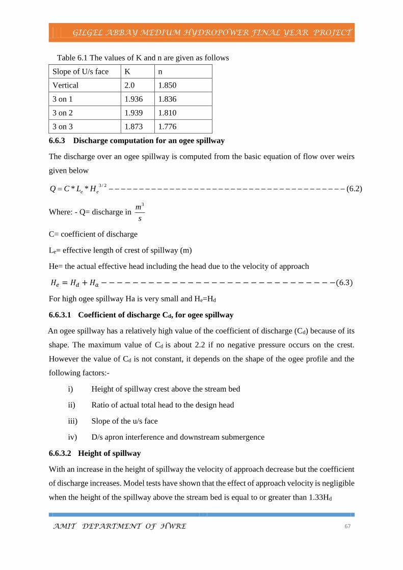
GILGEL ABBAY MEDIUM HYDROPOWER FINAL YEAR PROJECT
AMIT DEPARTMENT OF HWRE 67
Table 6.1 The values of K and n are given as follows
Slope of U/s face K n
Vertical 2.0 1.850
3 on 1 1.936 1.836
3 on 2 1.939 1.810
3 on 3 1.873 1.776
6.6.3 Discharge computation for an ogee spillway
The discharge over an ogee spillway is computed from the basic equation of flow over weirs
given below
)2.6(**2/3
ee HLCQ
Where: - Q= discharge in s
m3
C= coefficient of discharge
Le= effective length of crest of spillway (m)
He= the actual effective head including the head due to the velocity of approach
𝐻𝑒 = 𝐻𝑑 + 𝐻𝑎 − − − − − − − − − − − − − − − − − − − − − − − − − − − − − −(6.3)
For high ogee spillway Ha is very small and He=Hd
6.6.3.1 Coefficient of discharge Cd, for ogee spillway
An ogee spillway has a relatively high value of the coefficient of discharge (Cd) because of its
shape. The maximum value of Cd is about 2.2 if no negative pressure occurs on the crest.
However the value of Cd is not constant, it depends on the shape of the ogee profile and the
following factors:-
i) Height of spillway crest above the stream bed
ii) Ratio of actual total head to the design head
iii) Slope of the u/s face
iv) D/s apron interference and downstream submergence
6.6.3.2 Height of spillway
With an increase in the height of spillway the velocity of approach decrease but the coefficient
of discharge increases. Model tests have shown that the effect of approach velocity is negligible
when the height of the spillway above the stream bed is equal to or greater than 1.33Hd

GILGEL ABBAY MEDIUM HYDROPOWER FINAL YEAR PROJECT
AMIT DEPARTMENT OF HWRE 68
However, in low spillways, with h/Hd<1.33, the approach velocity is having an appreciable
effect. The curve given below can be used in such cases, to evaluate the coefficient of
discharge, using Cd=2.2
6.6.3.3 Effective length of Ogee spillway
The effective length of an overflow spillway is given by
)4.6(2 eape HkNkL
Where: - Le= effective length of crest
L= net length of crest which is equal to the sum of the clear spans of the gate
bays between piers
He= total head on crest including velocity head
N= number of piers
Kp= pier contraction coefficient
Ka= abutment contraction coefficient
Square nose piers with corners rounded on a radius equal to about 0.1 of pier thickness kp=0.02
Square abutment with head wall at 900 to the direction of flow Ka=0.20
6.7 Calculation for Ogee Spillway design
Given data for design of ogee spillway are:-
Spillway crest level =1887.5m.a.s.l
Design discharge (from flood routing) =168.92m3/s
River bed level =1830m.a.s.l
Dam height (H) =62m
Design Procedure;The discharge passing over the ogee spillway is given by:-
Assuming the spillway is the coefficient of discharge may be taken as C = 2.2 and L eL
mLL e 60
Correction due to height of dam
54.5218.1
62
m
m
H
H
d

GILGEL ABBAY MEDIUM HYDROPOWER FINAL YEAR PROJECT
AMIT DEPARTMENT OF HWRE 69
Since dH
P>1.33, the spillway is high and the velocity of approach can be neglected. In such a
case the coefficient of discharge C=Cd has been found to be 2.2.
Correction due to upstream slope
Upstream slope correction is required when the upstream face is sloping at some angle.
However, for Gilgel abby its slope is vertical, hence no need of upstream slope correction.
Correction due to upstream apron interference and submergence effect.
73.4918.1
5.5718.1
e
a
e
e
H
dh
H
HH
Since ,7.1
e
a
H
dhthe discharge coefficient is not affected by tail water condition.
6.8 The shape of downstream profile from origin of the coordinates.
This equation is applicable to positive values of X and Y.
mHd 18.1 , 𝑋1.85 = 2 ∗ (1.18)0.85 ∗ 𝑌
𝑌 = 0.434 ∗ 𝑋1.85 − − − − − − − − − − − − − − − − − − − − − − − − − − − −(6.5)
The slope of the straight portion varies between 1V:0.6H to1V:0.8H.At the end of the sloping
surface a curved bucket is provide to create a smooth transition of flow from the spillway to
the outlet channel or the river on the downstream side and prevent scouring.
For this spillway assume slope is taken as, 1V:0.75H
333.175.0/1804.0tan 85.0 Xd
d
x
y
X0.85=1.333/0.804, X =1.66m and Y=0.434× (1.66)1.85 =1.106m

GILGEL ABBAY MEDIUM HYDROPOWER FINAL YEAR PROJECT
AMIT DEPARTMENT OF HWRE 70
The all computed value for downstream profile shown in appendix (A)
Figure 6.3 Ogee spillway profile
For upstream profile determination shown below
Where: Hd=1.18m
𝑎 = 0.175 ∗ 𝐻𝑑 = 0.207𝑚
𝑏 = 0.282𝐻𝑑 = 0.33276𝑚
𝑅1 = 0.5𝐻𝑑 = 0.59𝑚
𝑅2 = 0.2𝐻𝑑 = 0.236𝑚 Or
According to WES the upstream profile of the ogee spillway for vertical upstream face can be
computed by
)6.6(27.0**4315.0*126.0
*27.0*724.0 625.0375.0
85.0
85.1
ddd
d
d HXHHH
HXY
Where the upstream profile extends up to:
𝑋 = −0.27 dH = −0.32𝑚
𝑌 = 0.126 ∗ dH = 0.15𝑚
625.085.1 )32.0(*46.015.0)32.0(*513.0 XXY
The values of X and Y are taken as positive to words the downstream and negative in the
upstream direction respectively.
After having plotted most of the profile the ogee spillway has a smooth gradual reverse
curvature is provided at the bottom of downstream face which turns the flow in to the apron of

GILGEL ABBAY MEDIUM HYDROPOWER FINAL YEAR PROJECT
AMIT DEPARTMENT OF HWRE 71
stilling basin or in to the spillway discharge channel. Radius of about one-fourth of the spillway
height is satisfactory for this reverse bottom curve.
)7.6(4
H
R
Where H=height of spillway crest above the bed level.
R =57.5
4= 14.375m
6.9 Energy Dissipation
Energy dissipation at dams and weirs is closely associated with spillway design, particularly
with the chosen discharge of the difference between upstream and downstream water level, and
downstream conditions. Without energy dissipation may Large-scale scour can take place on
the down streamside near the toe of the dam and away from it. If this scour is not controlled, it
may endanger the downstream side of the dam and spillway.
The excess kinetic energy possessed by the water can be dissipated by the two most common
methods as shown below.
i. By using different types of buckets i.e. by directing flow of water in to air and then
making it falls away from the toe of the structure.
ii. By converting supercritical flow in to sub critical flow by hydraulic jump.
Bucket type energy dissipaters
Solid roller bucket type
Slotted roller bucket type
Sky jump Bucket type (trajectory or shooting or flip)
6.9.1 Energy dissipation process
Can be achieved in five separate stage some of which may be combined
On the spillway surface
In a free falling jet
At impact into a Downstream pool
In the stilling basin
6.9.2 Factors affecting the design of energy dissipaters
Nature of foundation
Magnitude of flood and their occurrence

GILGEL ABBAY MEDIUM HYDROPOWER FINAL YEAR PROJECT
AMIT DEPARTMENT OF HWRE 72
Velocity of flow
Orientation of flow
Depth discharge and its relationship at the site of structure
6.9.3 Hydraulic jump formation
Basically, hydraulic jump can form in a horizontal rectangular channel when the following
relation is satisfied between pre jump depth (y 1 ) and post jump depth (y 2 ).
)8.6(8112
212 Fr
yy
Here, the point is, neglecting any loss of energy and the head due to velocity approach and
applying Bernoulli’s theorem between upstream water surface and at toe section, respectively,
it is possible to determine the total kinetic energy at downstream for section due to potential
energy at upstream water surface.
Therefore, from the above theorem
Figure 6.4 Hydraulic jump formation
From part A
Energy equation at upstream side is equal to
)9.6(2
1
2
1 yg
VHP d

GILGEL ABBAY MEDIUM HYDROPOWER FINAL YEAR PROJECT
AMIT DEPARTMENT OF HWRE 73
Where, p = Upstream water from river bed level up to spillway crest =57.5m
Hd =Hydraulic head flow over spillway or head above the spillway crest =1.18m
V1 =velocity at section one
Y1 = depth of water at section one
And water way on spillway within piers above spillway crest, also its contraction coefficient
for determination of effective length: N= 5, KP =0.1 and Ka =0.2 are given for square nosed
piers from S.K Garg.
𝐿𝑒 = 𝐿 − 2(𝐾𝑝𝑁 + 𝐾𝑎)𝐻𝑑 − − − − − − − − − − − − − − − − − − − − − − − −(6.10)
𝑞 =𝑄
𝐿𝑒− − − − − − − − − − − − − − − − − − − − − − − − − − − − − − − −(6.11)
𝑞 = 𝑉1 ∗ 𝑌1 = 𝑉2 ∗ 𝑌2 − − − − − − − − − − − − − − − − − − − − − − − − − −(6.12)
𝐹𝑟1 =𝑉1
√𝑔𝑦1− − − − − − − − − − − − − − − − − − − − − − − − − − − − − −(6.13)
Le = 60 − 2(0.1 ∗ 5 + 0.2)1.18 = 58.35m
q =168.92
58.35= 2.89
m3
sm⁄
From (1)
58.68 =(
2.89y1
)
2 ∗ 9.81
2
+ y1 =0.43
y12+ y1 = 58.68
𝑦12 =
0.43
58.68 − 𝑦1
𝑦1 = [0.43
58.68 − 𝑦1]
1/2
By trial and error, Y1=0.086 Therefor,
𝑉1 =2.89
0.086= 33.6
𝑚
𝑠𝑒𝑐 𝑎𝑛𝑑
𝐹𝑟1 =33.6
√9.81 ∗ 0.086= 36.58
Now from Part B,

GILGEL ABBAY MEDIUM HYDROPOWER FINAL YEAR PROJECT
AMIT DEPARTMENT OF HWRE 74
By applying Hydraulic jump
We can find the sequent depth y 2 on the horizontal apron.
my
y
Fry
y
41.4
)58.36(8112
086.0
2,8112
2
2
2
12
When tail water depth "" 2y is too great for the formation of hydraulic jump (i.e when Y2is too
large compared toY1) dissipation of the high energy of flow can be effected by the use of
submerged bracket deflector.
In general, 𝑌1 = 0.086𝑚
Y2 = 4.41m
V1 = 33.6m
s
Fr1 = 36.58
q = 2.86m3
s/m
Q = 168.92m3
s
For desperation of energy, Bucket type energy dissipaters are usually of small size and more
economical than the conventional hydraulic jump stilling basins especially when the fraud
number Fr1 exceeds 10,
In general, the Bucket type of energy dissipater can also be adopted for all tail water conditions
and are commonly used for dissipation of energy below the overflow spillway.
6.9.4 Bucket type energy dissipaters
A bucket type energy dissipaters consists of an upturned bucket provided at the toe of the
spillway. The bucket type energy dissipaters may be used only for ogee or overflow type
spillways. This type of energy dissipation becomes more economical than the method of stilling
basins when the Froude number Fr1 of the incoming flow exceeds 10, because in such cases the
difference between initial and sequent depths being large. Moreover the bucket type energy
dissipaters may be used with any tail water condition. However, this type of energy dissipater
may be used only when the river bed is composed of stiff rock.

GILGEL ABBAY MEDIUM HYDROPOWER FINAL YEAR PROJECT
AMIT DEPARTMENT OF HWRE 75
The solid or slotted roller bucket may be used where the tail water depths are too large as
compared to the sequent depths required for the formation of the hydraulic jump. Both these
buckets remain submerged in tail water and hence these are also termed as submerged bucket
type energy dissipaters. The solid and slotted roller buckets are discussed as under:
(i) Solid roller Bucket
A solid roller bucket consists of a bucket like apron with a concave circular profile of large
radius and a deflector lip as shown. When the water flows over the bucket the entire sheet of
water leaving the bucket is deflected upward by the bucket lip and two elliptical rollers are
developed as shown in the figure 6.1. These drawbacks of the solid roller bucket are removed
in slotted roller bucket Radius of the Bucket:
R = 0.6√(P ∗ Hd) − − − − − − − − − − − − − − − − − − − − − − − − − − − −(6.14)
Where p = fall from crest of spillway to bucket invert in meter.
And Hd =Head over crest in meters
R = 0.6 ∗ √57.5 ∗ 1.18 = 4.94
Figure 6.5 Solid roller bucket type

GILGEL ABBAY MEDIUM HYDROPOWER FINAL YEAR PROJECT
AMIT DEPARTMENT OF HWRE 76
CHPTER SEVEN
7 DIVERSION WORK
7.1 General
The design for a dam which is to be constructed across a stream channel must consider
diversion of the stream flow around or through the dam site during the construction period. The
extent of the diversion problem will vary with the size and flood potential of the river. At some
sites, especially in the case of earth and rock fill dams, diversion may be costly and time
consuming and may affect scheduling of construction activities. However, a diversion problem
exists at all sites except those located off-stream selection of the most appropriate scheme for
handing the flow of the stream during construction is important to the economy of the dam
.The following factors should be considered in a study to determine the best diversion scheme:
Characteristics of stream flow.
Size and frequency of diversion flood.
Methods of diversion.
Specification requirements that is availability of materials at site.
Type of dam and its height.
Location, type and elevation of spilling arrangements.
The diversion works must form part of the overall project design in that:
They must be based on the same hydrological, topographic and geological features
of the site as the main dam;
They may be partially governed by a requirement for early commissioning of the
permanent works under partial heads.
They involve major construction problems that may have considerable impact on
overall construction time and cost.
They may have to take in to account environmental factors.
They may have to be eventually incorporated in the permanent works.
7.2 Diversion stages
Two approaches to the construction of the permanent works in the river channel are feasible:
A) Single - stage diversion. The river diversion and construction may take place in one
single operation. This approach is used chiefly in narrow valleys. In this project due to the

GILGEL ABBAY MEDIUM HYDROPOWER FINAL YEAR PROJECT
AMIT DEPARTMENT OF HWRE 77
narrow valley features of the area at and near the proposed dam site, it is economical to
adopt the single-stage diversion approach
B) Multistage diversion. In this case, two or more coffer dams may be built with the river
being diverted through different passages as different stages of construction proceed. The
multistage technique is suitable for wide river diversion works..
7.3 Sequence: The work is normally conducted in the following sequence
a. Build a partial coffer dam during the low flow season, allowing construction of
diversion tunnels, culverts, channels and control works.
b. Build diversion tunnels, culverts, channels and control works.
c. Divert low season flow through these passages.
d. Build a full size coffer dam competent for the design diversion flood.
e. Build permanent works.
f. Close diversion passages; impoundment begins (full river closure).
7.4 Diversion works:
The main components in the diversion works for the single –stage approach are:
Diversion tunnel, culvert, conduit, canal.
Upstream and downstream coffer dam.
The diversion tunnel or channel passes around the side of the construction area which is itself
protected by the upstream and downstream cofferdams. One or more passages may be
necessary, so frequently both river banks are used.
7.5 Diversion Tunnel
Diversion tunnels by pass around a dam site. For larger design floods, several diversion tunnels
can also run around both sides of valley. Except on smaller rivers, thin tunnels one on each
bank are most usually employed for safety and convenience. Tunnels may be designed for
pressure of free surface flow. Normally they have a free surface flow to divert floating mater
also; In this case, they must not run more than 70% full for the design flood or 80% if the flood
is of very short duration. Tunnel velocities can be the order of 10-20m/s. for excavated tunnels,
the maximum slope is typically 10%due to construction reason. The slope in the tunnel should
satisfy conditions like reduction of cross section for economic reason and prevent tunnel
abrasion and also guided by the inlet and out let elevations.

GILGEL ABBAY MEDIUM HYDROPOWER FINAL YEAR PROJECT
AMIT DEPARTMENT OF HWRE 78
Q = 40.21m3/s, monthly computed design discharge.
)1.7(2* gHACQ d
Where Q = Flood to be passed
Cd= Discharge Coefficient =0.82
A= Cross sectional Area
H = Differential head causing flow
(u/s water level – d/s water level) the depth of flaw
Q = 40.21m3/s, per monthly discharge.
C d =0.82… S.K. GARG (2005)
Where, h is
Hg=NPL-TWL=53.09m
)2..7(2
gHc
QA
d
252.109.53*81.9*2*82.0
21.40mA
mD
mD
A
4.1
52.14
. 22
Therefore, one diversion tunnel having 1.4m is provided for diversion tunnel upstream of the
dam.
7.6 Coffer Dam
A coffer dam is a temporary dam used to divert the stream flow and to enclose the area dry
during construction .The design of an adequate coffer dam involves the problem of construction
economics. The conditions which make the coffer dam favorable or offer great scope for the
general design are:
Easy, observation, maintenance, and reinforcement due to available facilities of
construction organization on site.
Large movements and higher rate of seepage may be accepted though requiring
expensive pump age.
The short life of coffer dams justifies the use of limited materials.

GILGEL ABBAY MEDIUM HYDROPOWER FINAL YEAR PROJECT
AMIT DEPARTMENT OF HWRE 79
There is generally less damage as a result of failure for lower height coffer dams.
A wide variety of designs exists for coffer dams and especially for low head coffer dams as
they need to be adapted to suit local materials and available equipment.
Therefore, the following requirements should be taken in to account in selecting the type and
size of coffer dams and the shape of foundations:
Distance from a coffer dam to the foundation of a structure should be not less than
and, sometimes, in excess of 10m.
Shape of dam foundation, in plan, should allow for suitable placing of roads on the
crest of the coffer dams, access tracks to the dam foundation and a good approach to
haul roads.
Shape of dam foundation should be suitable for locating crones, other construction equipment,
and water lowering and over flow drainage installations
7.6.1 Design of Coffer Dam
For the design of the cofferdam, the height of the coffer dam is taken as sum of the diameter
of the tunnel and some allowance for free board which is taken from 2.5m, (b/n 2 to3). (USBR)
method, and we take average 2.5m for free board.
i.e.= H = D + fb, 1.4 + 2.5 ≈4m so, the upstream cofferdam has 4m height and slope may be
taken as 2H: 1V. Top width =6m and bottom width =25m for safe and stability of the earthen
coffer dam.
Figure 7.1 Diversion coffer dam with diversion tunnel section profile

GILGEL ABBAY MEDIUM HYDROPOWER FINAL YEAR PROJECT
AMIT DEPARTMENT OF HWRE 80
7.6.2 Risk of the cofferdam due to the flood
Assuming 5yrs construction period and 100yrs return period, the risk can be obtained as:
%50495.01)10
11(1
)5(
)100(
,
)3.7()1
1(1
5
Risk
yrsporiodnconstuction
yrsperidreturnT
riskRwher
TRisk n
For this 5% of Risk, the u/s and the d/s force of the cofferdam has to be made concrete facing

GILGEL ABBAY MEDIUM HYDROPOWER FINAL YEAR PROJECT
AMIT DEPARTMENT OF HWRE 81
CHAPTER EIGHT
8 CONVEYANCE STRUCTURE
8.1 General
Intake, head race tunnel, penstocks, outlets, conduits etc. drawing water from reservoir, river
or canal have to be provided with suitable arrangement to draw in required supply in a
satisfactory manner for the production of power. Structures for this purpose are known as water
conveyance structures.
8.2 Intake Structure
The intake is a structure constructed at the entrance of a power canal or pipe through which the
flow diverted from the source such as river or reservoir. It provides smooth easy and turbulent
free flow through the conveyance.
8.3 Types of intakes
The type of intake structure depends up on the type of power plant as well as its layout. There
are six types of intake:
Run-of-river intake
Canal intake
Dam intake
Tower intake
Shaft intake
Intakes of special type
8.4 Functions of Intakes
The main functions of intakes are:
To control flow of water in to the conveyance system
To provide smooth, easy and vortex or turbulence free entry of water in to the
conveyance system
To prevent entry of coarse river born trash matters such as boulders, logs, tree
branches etc…
To exclude heavy sediment load of river, from entering the conveyance system.

GILGEL ABBAY MEDIUM HYDROPOWER FINAL YEAR PROJECT
AMIT DEPARTMENT OF HWRE 82
8.5 Intake selection and design
The basic principles for selection of intake location
Intakes from streams should be located, wherever possible on the concave side of the
bend.
The effectiveness of the intake in preventing sediment entry increase with the
sharpness of the bend
Intakes from the straight reaches can be made favorable by artificially forcing the
water to follow a curved path.
Best position of intake is with the screen at right angles to the spillway so that in
flood seasons the flow carries the debris over its crest.
In order to attain the required discharge capacity the intake must be placed
sufficiently below reservoir level and high enough to prevent entry of sediment.
The design of an intake has to care for
Structural stability
Hydraulic efficiency
Limitation of entrance velocity
Practicability of operation
For this particular project, the appropriate intake type is tower intake with trash rack structure
in front of the horizontal bell mouth inlet, which minimizes the entrance losses and provides
smooth flow.
8.5.1 Intake Opening/Entrance
The entrance of the intake should be properly designed so as to minimize the entrance losses
and to provide smooth flow. This is achieved by using a bell mouth entry governed by the
equation;
The shape of bell mouth is elliptical, as suggested by the equation:
X2
(0.5D)2+
Y2
(0.15D)2= 1 − − − − − − − − − − − − − − − − − − − − − − − − − − − (8.1)
D= 3.6m (diameter of penstock)
Therefore , 0.308𝑥2 + 3.33𝑦2 = 1
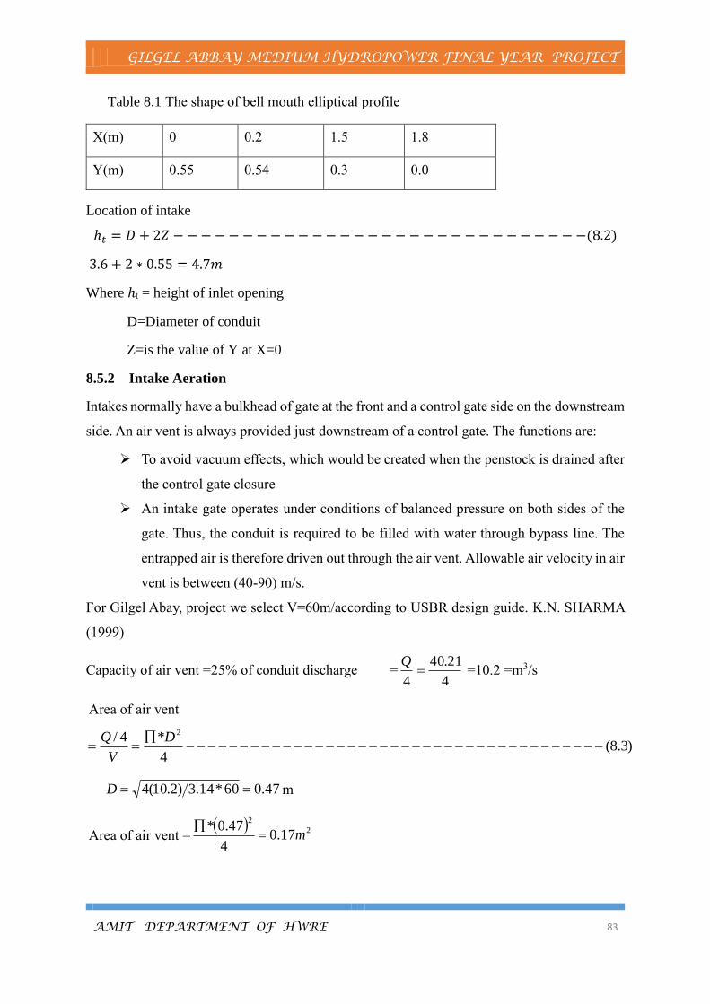
GILGEL ABBAY MEDIUM HYDROPOWER FINAL YEAR PROJECT
AMIT DEPARTMENT OF HWRE 83
Table 8.1 The shape of bell mouth elliptical profile
Location of intake
ℎ𝑡 = 𝐷 + 2𝑍 − − − − − − − − − − − − − − − − − − − − − − − − − − − − − −(8.2)
3.6 + 2 ∗ 0.55 = 4.7𝑚
Where ℎt = height of inlet opening
D=Diameter of conduit
Z=is the value of Y at X=0
8.5.2 Intake Aeration
Intakes normally have a bulkhead of gate at the front and a control gate side on the downstream
side. An air vent is always provided just downstream of a control gate. The functions are:
To avoid vacuum effects, which would be created when the penstock is drained after
the control gate closure
An intake gate operates under conditions of balanced pressure on both sides of the
gate. Thus, the conduit is required to be filled with water through bypass line. The
entrapped air is therefore driven out through the air vent. Allowable air velocity in air
vent is between (40-90) m/s.
For Gilgel Abay, project we select V=60m/according to USBR design guide. K.N. SHARMA
(1999)
Capacity of air vent =25% of conduit discharge =4
Q
4
21.40 =10.2 =m3/s
Area of air vent
)3.8(4
*4/ 2
D
V
Q
47.060*14.3)2.10(4 D m
Area of air vent = 2
2
17.04
47.0*m
X(m) 0 0.2 1.5 1.8
Y(m) 0.55 0.54 0.3 0.0

GILGEL ABBAY MEDIUM HYDROPOWER FINAL YEAR PROJECT
AMIT DEPARTMENT OF HWRE 84
8.5.3 Gates
The form of a reservoir outlet works will vary considerably with the type of dam and the
purpose of the reservoir. The requirements of a high-pressure conduit control are:
A. The outlet should be hydraulically smooth pipe when full open in order to pass the
maximum discharge.
B. When opened partially sufficient air should be admitted to present vibration and cavitation.
C. The whole arrangement should be simple, rigid, and economical and facilitate easy
inspection and maintenance.
Vertical left side gate
Slide gate is a simplest type of vertical left side gate in which the movement of the gate is of
sliding type. This type of gate is known to less prone to vibration. Most intakes are provided
with gate or valve at their entrance. The main function of the gate is to regulate the quality of
flow, which passes through the intake conduit. For the power plant of Gilgel Abay the intake
gates are to be located at the entrance of the penstock operated by vertical gate shaft.
8.5.4 Design of trash racks
Trash rack is one of the most important constituent of intake complex on a hydropower plant.
It checks the entry of floating debris like grass, leaves, trees and bushes, drift timber as of
rolling and floating boulders, at the intake of the water conductor for the plants. In cold areas,
entry of ice sheets is likewise checked. The acceptable size of debris depends up on the type of
turbine being use for power generation and the type of various check values in the complex.
a) General Arrangement
Girders form vertical divisions of trash rack. These divisions are known as panels. The
dimensions of panels are determined by the possible of transport and handling. Each panel
consists of the following.
A system of rigid frame for small grills and the fixing plates for the big areas
A system of vertical bars generally of rectangular section
A series of horizontal pieces, the functions of which is of prime importance
These are intermediate supports for the vertical bars besides distributing the load
It gives protection to the bars against vibration. These are keeping 400mm - 500mm apart.

GILGEL ABBAY MEDIUM HYDROPOWER FINAL YEAR PROJECT
AMIT DEPARTMENT OF HWRE 85
b) Design Head of Trash Rack
Design head for a trash rack depends up on the difference in water levels on the upstream and
downstream sides at the time of maximum clogging i.e. the critical head in the trash rack
structure. The extent of clogging depends up on the intensity of trash inflow, as well as, the
efficiency of racking. Some practices for adoption of design head given below:
E.Mosony: ordinarily 1m to 2m, in exceptional case 4m to5m
US Army corps of engineers: a design head of 3m is enough.
Adoption of higher value of design head will make the structure uneconomical, while its lower
value might make it unsafe.
c) Trash Rack Inclination
The trash rack usually place vertical or near vertical say (0° to 25°) from the vertical, usually
across the water flow in the power channel keeping the trash rack inclined is always a better
practice. For this project, take = 25° for easy cleaning.
d) Permissible velocity through trash rack
Velocity should be sufficiently low to avoid high head loss and should be sufficiently high to
avoid large intake and trash rack cross section. The following are suggested limiting entrance
velocities.
1. Mooneye’s formula to eliminate eddies and vortices
𝑉 = 0.075√2𝑔𝐻 − − − − − − − − − − − − − − − − − − − − − − − − − − − − − (8.4)
Where: g – acceleration due to gravity
2. U.S.B.R’s criterion: permissible velocity in the range of 0.6-1.5m/s. For this project, the
trash rack is designed so that the approach velocity (Va) is in between 0.6 to1.5 m/s. we
take the average of this equals to 1.0 m/s.
e) Racks
Bar thickness; Thickness of bars is usually from 6mm to 25mm.For Gilgel Abay river hydro
project take the bar thickness 25mm.
Length of rack bars; the maximum length of rack bars between lateral supports of stiffeners
is limited by the vibration characteristics related to bar thickness and velocity through the
bars. Table below gives recommendation regarding the lateral unsupported length of bar in
centimeter.

GILGEL ABBAY MEDIUM HYDROPOWER FINAL YEAR PROJECT
AMIT DEPARTMENT OF HWRE 86
Table 8.2 Unsupported length of bar in cm for velocity (m/s)
Thickness
of bar in
mm
Velocity
in
(m/s)
0.6 1 1.5 2 3
6 50 42 32 29 24
10 75 60 47 40 35
12 100 80 63 55 45
20 150 115 100 82 65
25 175 145 125 112 88
For thickness, 25mm and velocity 1.0 m/s calculated above, the length of bars from above table
would be 145cm.
Spacing; Trash rack have usual inter spacing of 100 to 500 mm. The experimental
recommendation is:
𝑏
𝑡≤ 0.7 𝑎𝑛𝑑
𝑏
𝑡≤ 10 − − − − − − − − − − − − − − − − − − − − − − − − − −(8.5)
Where: L= length of bar
t= thickness of bar
b= spacing between two bars
≤ 0. 7 × 145, ≤ 101.5 ≥ 100mm take 100mm
Check for vibration
8.6 Penstock
The water is taken from the fore bay to the power station through the penstocks. These may be
pressure conduits or shafts. The penstocks carry water to the turbines with the least possible
loss of head consistent with the overall economy of the project.
≤ 10 , 10
≤
100
10 ≤ , 10 ≤ 25

GILGEL ABBAY MEDIUM HYDROPOWER FINAL YEAR PROJECT
AMIT DEPARTMENT OF HWRE 87
8.6.1 Design criteria for penstock
The structural design of penstock is same as pressure vessels. Because of the possibilities of
sudden load changes design against water hammer is essential. For relatively short penstock, it
is generally more economical to fore go the protection of surge tank and rely on a heavier pipe
wall and slow closing valve. The penstocks are equipped with head gate at the fore bay, which
can be closed to permit repair of the penstock.
8.6.2 Material of Fabrication
Factors to be considered in choosing the material of penstock on a particular project are:
Design pressure or head to which the penstock is subject.
Topography of the terrain
The discharge to be handled
Weight and ease of installation
Relative cost
Weather condition
Method of joint etc.
Steel penstock have become most common type of installation in hydropower developments
due to simplicity in fabrication strength and assurance that will perform in wide variety of
circumstances hence considering the above mentioned criterion a steel penstock is selected for
out project.
Method of support
A non-buried penstock is selected due to the following main advantages.
Since the terrain is rocky it will be expensive to excavate
It is easy for inspection of faults and maintenance
Stability is ensured with anchorage
8.6.3 Economic Diameter of Penstock
The larger the diameter smaller will be the head losses and greater will be the net head available
to the turbine, resulting in greater power development. On the other hand greater size of
penstock would means less velocity and greater capital investment hence the size which would
give the least annual cost should be choose.
Among the different methods used determine the Economical diameter of penstock the
following empirical formula is adopted.

GILGEL ABBAY MEDIUM HYDROPOWER FINAL YEAR PROJECT
AMIT DEPARTMENT OF HWRE 88
As per USBR empirical formula
1) 𝑉 = 0.125√2𝑔𝐻𝑛𝑒𝑡 − − − − − − − − − − − − − − − − − − − − − − − − − (8.6)
= 0.125√2 ∗ 9.81 ∗ 52 = 4m/s and 𝑉 = 4𝑄 ᴨ𝐷2⁄ from which,
2) 𝐷 = √4𝑄 𝜋𝑉⁄ − − − − − − − − − − − − − − − − − − − − − − − − − − − −(8.7)
= √4 ∗ 40.2 4𝜋⁄ = 3.57m
𝐷 ≅ 3.6𝑚
3) 𝐷 = 3.55[𝑄^2 ⁄ 2𝑔𝐻]0.25 − − − − − − − − − − − − − − − − − − − − − −(8.8)
=𝐷 ≅ 4𝑚
4) G.S Sarkarias formula (1968)
Therefore the economical diameter is the average of the three of them
Dpenstock = 3.6m
A penstock of diameter 3.6 can be adapted and the actual velocity of flow through is
𝑉 = 𝑄 𝐴⁄ =40.2 (𝜋⁄ 4 ∗ 3.62)
= 4 m/s so the value is lies within 3 to 6 OK!!
8.6.4 Structural Design of Penstock
The penstock should have sufficient thickness to resist the static and water hammer pressures.
The maximum pressure head due to water hammer is given by
ℎ𝑤=𝐶𝑉𝑜 𝑔⁄ − − − − − − − − − − − − − − − − − − − − − − − − − − − − − −(8.9)
For gate closure time less than 2𝐿 𝐶⁄
Where VO =velocity of flow in the penstock (m/s)
C=celerity, the velocity of water wave (m/s)
Where H = 53.09m . .
P=horse power transmitted=
P= 0 .62 × 40.2 × 53.09
= 17636
= 0 . 62 .
.
= 0 . 62 × 17636
.
53.09 . = 3.2m

GILGEL ABBAY MEDIUM HYDROPOWER FINAL YEAR PROJECT
AMIT DEPARTMENT OF HWRE 89
C= (k/𝜌)
Where k=bulk modulus of water (=2.18×10⁹KN/S)
𝜌=density of water (=998.2kg/m3)
C= (2.18×10⁹/998.2) =1477.8m/s
ℎ𝑤 =1477.813∗4
9.81= 602.6
The total pressure head immediately after closure is the summation of pressure head due to
water hammer and static head.
𝐻 = 𝐻 + ℎ𝑤 − − − − − − − − − − − − − − − − − − − − − − − − − − − − − (8,10)
=52+602.6 =654.6m
Providing a steel penstock with allowable hoop stress q=150,000𝐾𝑁 𝑚2⁄ , the thickness of
penstock can be determined by the following formula.
𝑡(𝑚𝑚) =𝑝∗𝑟∗1000
𝑞− − − − − − − − − − − − − − − − − − − − − − − − − − − −(8.11)
Where P=internal pressure in 𝐾𝑁 𝑚2⁄
r=radius of penstock in m.
q=allowable hoop stress in 𝐾𝑁 𝑚2⁄
t=thickness of penstock in mm
𝑃 = 𝛾. 𝐻 − − − − − − − − − − − − − − − − − − − − − − − − − − − − − − − −(8.12)
=9.81×654.6=6421.6𝐾𝑁 𝑚2⁄
𝑅 = 𝐷 2⁄ =3.6/2 =1.8m
𝑡 =6421.6∗1.8∗1000
150000= 77𝑚𝑚
8.6.5 Penstock Inlet Aeration
Intakes normally have a bulk-head gate at the front and a control gate inside them. An air vent
is always provided just downstream of the control gate. The main function of air vent pipe is:
Admission of air to nullify the vacuum effect which would be created when the water
in the penstock drains after the intake gate is closed.
The intake gates operate under the function of balanced pressure on both sides. For
this purpose, the conduit is required to be filled through a bypass pipe. The entrapped
air is, therefore, driven out through the air vent pipe.

GILGEL ABBAY MEDIUM HYDROPOWER FINAL YEAR PROJECT
AMIT DEPARTMENT OF HWRE 90
8.6.6 Capacity of air vent
According to U.S.B.R design guide
Capacity of air vent = 25% of conduit discharge
Qa = 0.25× 40.2 = 10.05m3/s
Allowable air velocity, 𝑉𝑎 = 45 to 90 m/s take
𝑉𝑎 = 60 m/s Vent area,
𝑎 = 𝑄𝑎
𝑉𝑎− − − − − − − − − − − − − − − − − − − − − − − − − − − − − − − (8.13)
=10.05
45= 0.167𝑚2
d = √4𝐴
𝜋− − − − − − − − − − − − − − − − − − − − − − − − − − − − − − − −(8.14)
=√4∗0.167
𝜋=𝑑 = 0.46𝑚
Where, s = depth of water above penstock inlet, m
V = velocity through penstock, m/s
D = diameter of penstock, m
8.7 Design of Manifolds
The number of turbine to be feed water through penstock is four; hence the main penstock from
the fore bay is goes to in to pipe.
𝐻1 =𝐹1𝑉2
2𝑔𝑑− − − − − − − − − − − − − − − − − − − − − − − − − − − − − − − (8.15)
Q = 𝜋
4√
2𝑔𝐻1
𝑓1𝐷2.5 − − − − − − − − − − − − − − − − − − − − − − − − − − − −(8.16)
𝑄 𝐷2.5⁄ =constant
Therefore =𝑄 𝐷2.5⁄ = 𝑄1 𝐷12.5⁄
For four manifolds, the discharge through the main penstock is divided into four equal
discharge i.e. 𝑄 = 4𝑄1
𝑄1
𝑄(
𝐷1
𝐷)
2.5
− − − − − − − − − − − − − − − − − − − − − − − − − − − − − − − (8.17)
=1/4

GILGEL ABBAY MEDIUM HYDROPOWER FINAL YEAR PROJECT
AMIT DEPARTMENT OF HWRE 91
Hence 𝐷1 = 𝐷 40.2⁄ , D1=3.6/40.24 =1.24m
Provide four manifolds of diameter=1.24m
8.8 Anchor Block and Saddle Support
Anchors, slide blocks, and trust blocks are used to constraint movement of penstock. They
should be placed on the original soil and not fill. The bearing area must be calculated to support
the pipe line without exceeding the safe bearing load of the soil drainage should be provided
to prevent erosion of the foundations.
Distance between Blocks
Both anchors and slide blocks act to support the penstock. The maximum spacing of blocks is
calculated, so that the pipe line does not collapse between supports when filled with water.
Generally, one sliding support for each pipe length is provided.
8.9 Hydraulic Losses
The gross head is the total head available without subtracting intake and conveyance loss. It is
the elevation difference between the normal pool level and the tail water level.
It is the vertical distance that the water falls through the generating Power that is between
normal pool level and the tailrace level.
𝐻𝑔 = 𝑁𝑃𝐿 − 𝑇𝑊𝐿 − − − − − − − − − − − − − − − − − − − − − − − − − − − −(8.17)
Where;-Hg= Gross head
NPL =Normal pool level =57.5
TWL = Tail water level = 4.41
Hg =53.09m
8.9.1 Net head
It is the head available for power generation and it is the difference between the gross head and
the total loss.
𝐻𝑛 = 𝐻𝑔 = ∑ 𝑙𝑜𝑠𝑠
Where; - Hn =Net head Hg=Gross head

GILGEL ABBAY MEDIUM HYDROPOWER FINAL YEAR PROJECT
AMIT DEPARTMENT OF HWRE 92
8.9.2 Hydraulic Losses of Intake
i. Entranceloss
∆ℎ𝑒 = 𝐾𝑡 ∗𝑉2
2𝑔− − − − − − − − − − − − − − − − − − − − − − − − − −(8.18)
Where: Kt = 0.3 for bell mouth entry.
V =0.075√2𝑔ℎ
V= 2.42m/s
∆ℎ𝑒 = 0.3×2.42^2
2∗9.81 =0.09m
ii. Trash rack loss
There are numerous expressions available for predicting head loss across trash rack. One such
expression (Kirschmer’s) is:
)19.8(sin2
*
23/4
g
V
b
tKh a
tr
Where: t = thickness of bar
b = clear spacing between bars
Va = velocity of flow in front of rack
=angle of bar inclination with horizontal
t =thickness of bar (𝑏
𝑡 = 10 is recommended) in twine Francis; 10cm to 50cm
Take avg. =30cm
t = 30
10 = 3cm
𝑉𝑂 = permissible velocity through trash racks
It is in order of 0.8 to 1m/s for average depth take 𝑉𝑂 = 1m/s
Φ = angle of bars with the horizontal
= 90ᵒ - 25ᵒ=65ᵒ
𝐾𝑡 Is factor depending on bar shapes = 2.42
∆ℎ𝑟 = 2.42 ∗ (330⁄ )
4
3 ∗ (12
2 ∗ 9.81⁄ ) 𝑠𝑖𝑛65 = 0.01m

GILGEL ABBAY MEDIUM HYDROPOWER FINAL YEAR PROJECT
AMIT DEPARTMENT OF HWRE 93
iii. Gate loss
Head loss due to gates is given by:
hl =𝑣^2
2𝑔
2.42^2
2∗9.81 =0.3m ℎ1 =
𝑣2
2𝑔 =
2.422
2∗9.81 = 0.3m
iv. Loss of head at bends
)20.8(2
2
2 g
VKhLb
Where K – Coefficient depends on total angle of bend and on the relative radius of curvature
R/d where R – is the radius of curvature and d- is the diameter of the penstock / tunnel
K =2
∏2(𝑙𝑛𝑅𝑏
𝐷+⍺)
− − − − − − − − − − − − − − − − − − − − − − − − − − − − − (8.21)
⍺= deflection angle = 58ᵒ
Rb =radius of curvature bend
Let Rb = D =3.6m Kb = 2
𝜋2 = 0.20 V=
4𝑄
𝜋𝐷2
9∗50
𝜋∗16 =3.98m/s
ℎ𝐿𝑏 = 0.2(3.982 2 ∗ 9.81⁄ )= 0.32m/s
v. penstock losses
hf =f𝐿
𝐷
𝑉2
2𝑔− − − − − − − − − − − − − − − − − − − − − − − − − − − − − − − −(8.22)
Where f-friction coefficient =0.011 for steel
L=length of penstock 70m
D=diameter of penstock 3.6m
V=velocity through penstock 4m/s
hf = 0.011×150 (4^2/2×9.81×3.6)
= 0.37m
vi. Head loss in the tunnel
)23.8(2
2
gD
fLVh fto
Where, f=Manning’s coefficient =0.018
V=velocity in tunnel =4m/s
D=diameter of tunnel=3.5m

GILGEL ABBAY MEDIUM HYDROPOWER FINAL YEAR PROJECT
AMIT DEPARTMENT OF HWRE 94
L=length of tunnel =80m
ℎ𝑓𝑡𝑜 =𝑓𝐿𝑉2
2𝑔𝐷 =
0.018∗80∗42
2∗9.81∗3.5= 0.3𝑚
Total head loss = 0.09+0.01+0.3+0.37+0.3 = 1.07m
Adding 0.2m for operation losses
HL = 1.32m
Net head = gross head –head loss, Hnet ≈ 52m
8.10 Surge Tank
The surge tank or the surge tower is a structure which forms an essential part of the conveyance
pressure conduit system. Whenever such systems are long surge tanks may be considered
essentially as a fore bay close to a machine. Their primary purpose is protection of long
pressure tunnel in medium and high head plants against high water hammer pressure arising
from sudden rejection or acceptance of load
8.10.1 Function of Surge Tank
Surge tank or expansion is a structure which forms an essential part of the pressure
conduit conveyance system, it may be considered essentially as a fore bay close to
machine.
It can also be considered as safety value to relive the penstock pipe for water hammer
pressure.
Protection of long pressure tunnel in medium and high head plants against water
hammer pressure arising from sudden rejection or acceptance of load.
Convert high frequency,(water hammer) into low frequency of low pressure, mass
oscillation
To store water during load demand
To provide a free reservoir surface lose to the discharge regulating mechanism.
8.10.2 Design consideration of surge tank
The hydraulic design of surge tank concern with two main aspects
1. Cross section of surge tank
2. Height of surge tank

GILGEL ABBAY MEDIUM HYDROPOWER FINAL YEAR PROJECT
AMIT DEPARTMENT OF HWRE 95
I. Design of cross-sectional area
The cross-sectional area of a surge tank is determined based on stability and economic
considerations. Stability considerations of the system were established by Thomas stated that
in order to prevent the development unstable oscillations. The cross-section of the surge tank
should exceed a certain critical value.
Based on Thomas expression:
)24.8(2
2
min tnef
ros
Hgh
LAVA
Where minsA = minimum cross-sectional area of surge tank
Vo- mean velocity in the tunnel
LT-length of tunnel
AT-cross sectional area of a tunnel
Hf-head loss in the tunnel
Hnet-net head on the turbine
But in actual practice the cross sectional area of a surge tank is
Asurge = F. S × Asmin
Where F.S-is a factor of safety and has a value of safety and has a value of 1.5
Therefore; the required minimum one will be
tnef
ros
Hgh
LAVA
2
2
min
Where D- diameter of the tunnel
VO =4∗𝑄
3.14∗𝐷2 =4∗40.2
3.14∗3.52 =4.16m/s
LT=80m
222
6.94
5.3*
4
*m
DAT
Hnet=52m (calculated above)
Therefore, 2
22
min 3.452*33.0*81.9*2
6.9*80*16.4
2m
Hgh
LAVA
tnef
ros

GILGEL ABBAY MEDIUM HYDROPOWER FINAL YEAR PROJECT
AMIT DEPARTMENT OF HWRE 96
Taking factor of safety of 1.5
mD
DA
mAsurg
surg
86.2
4
*
45.6556.2*5.1
2
2
Therefore, for this particular project a surge tank with a diameter of 2.21m is used.
II. Height of surge tank: -
The height of the surge tank is proportional to the maximum upsurge and down surge contained
within the tank. These surges are computed for extreme conditions i.e. the top level of the surge
chamber is governed by the maximum upsurge when the reservoir level is at its tail water level
is at its maximum down surge level.
The maximum surge height (Z max)
Zmax = maximum up surge neglecting friction
Z max = )25.8(* gAs
LAtVo
Where, hf = friction head loss through the tunnel=0.33m
LT = length of the tunnel =80m
AT = cross sectional area of the tunnel =6.45m2
g = acceleration due to gravity
VO = velocity in the tunnel=4.16m/s
As=cross sectional area of surge tank=4.3m2
`Zmax=4.16× √(80 ∗ 6.45)/(9.81 ∗ 4.3) =15m
Jaeger has recommended the following formula for computing up surge and down surge in the
case where friction is taken in to account.
2
max 9
1
3
21 oo
uppp
Z
Z
Where Zup-maximum up surge with friction taken in to account.
Zmax-maximum up surge neglecting friction.
)26.8(max
Z
hP
f
o
, where hf= 0.33m (head loss in the tunnel)

GILGEL ABBAY MEDIUM HYDROPOWER FINAL YEAR PROJECT
AMIT DEPARTMENT OF HWRE 97
)27.8(9
1
3
21
02268.015
33.0
max
2
ZPPZ
m
mPo
ooup
m774.14
15*02268.0*9
102268.0*
3
21 2
)28.8(21 max ZPZ odown
, Where Zdown–is the down surge
mZdown 3.1415*02268.0*21
The height of the surge tank will be determined as follows
𝐻 = 𝑍𝑢𝑝 + 𝑍𝑑𝑜𝑤𝑛 + 𝐻𝑙𝑖𝑣𝑒 𝑠𝑡𝑜𝑟𝑎𝑔𝑒 + 3𝑚 − − − − − − − − − − − − − − − − − − − (8.29)
(For protection of air entry)
=14.774m+14.3+2m+3m =34m

GILGEL ABBAY MEDIUM HYDROPOWER FINAL YEAR PROJECT
AMIT DEPARTMENT OF HWRE 98
CHAPTER NINE
9 DESIGN OF HYDRO POWER PLANT AND POWER HOUSE
9.1 General
Hydropower is extracted from the natural potential of usable water resources, and about one
quarter of the world’s power requirement is at present derived in this way. Waterpower (or
hydropower) is generated by utilizing the energy of water (or hydraulic energy). Hydropower
is obtained from generators coupled with water turbines that convert the hydraulic energy in to
mechanical energy.
9.2 Hydraulic Turbines and Electromechanical Equipment’s
Hydraulic turbines may be considered as hydraulic motors or prime motors or prime movers
of waterpower development, which convert water energy in to mechanical energy (shaft
power). The shaft power developed is used in running electricity generators directly coupled
to the shaft of the turbine, thus producing electrical power.
All types of turbine, basically fall into two categories
Impulse turbine
Reaction turbine
9.2.1 Impulse turbine:
All the available potential energy is converted in to kinetic energy with the help of contracting
nozzles. The water after impinging on the curved vanes or bucket is discharged freely to drown
stream channel, example: peloton wheel.
9.2.2 Reaction turbine:
In this type, the water enters the turbine in a circumferential direction in to the scroll case and
makes in to the runner through a series of guide vanes called wicket gates.
The available energy partly converted to kinetic energy and substantial magnitude remains in
the form of pressure energy example Francis, Kaplan, propeller etc.
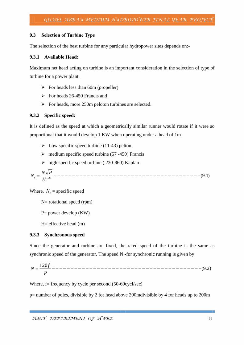
GILGEL ABBAY MEDIUM HYDROPOWER FINAL YEAR PROJECT
AMIT DEPARTMENT OF HWRE 99
9.3 Selection of Turbine Type
The selection of the best turbine for any particular hydropower sites depends on:-
9.3.1 Available Head:
Maximum net head acting on turbine is an important consideration in the selection of type of
turbine for a power plant.
For heads less than 60m (propeller)
For heads 26-450 Francis and
For heads, more 250m peloton turbines are selected.
9.3.2 Specific speed:
It is defined as the speed at which a geometrically similar runner would rotate if it were so
proportional that it would develop 1 KW when operating under a head of 1m.
Low specific speed turbine (11-43) pelton.
medium specific speed turbine (57 -450) Francis
high specific speed turbine ( 230-860) Kaplan
)1.9(25.1
H
PNNs
Where, sN = specific speed
N= rotational speed (rpm)
P= power develop (KW)
H= effective head (m)
9.3.3 Synchronous speed
Since the generator and turbine are fixed, the rated speed of the turbine is the same as
synchronic speed of the generator. The speed N -for synchronic running is given by
)2.9(120
p
fN
Where, f= frequency by cycle per second (50-60cycl/sec)
p= number of poles, divisible by 2 for head above 200mdivisible by 4 for heads up to 200m

GILGEL ABBAY MEDIUM HYDROPOWER FINAL YEAR PROJECT
AMIT DEPARTMENT OF HWRE 100
III. Peripheral Velocity
It is the ratio of the peripheral speed of the bucket or vanes at the minimal diameter, D to the
theoretical velocity of water under the effective head H acting on the turbine. It is given by
)3.9(260
gh
DN
Where D= diameter of the turbine
H= net head in (m)
N=turbine speed (rpm)
9.3.4 Efficiency:
The turbine efficiency varies with power output and head. Francis and propeller turbines have
high fall of efficiency in comparison to pelton and Kaplan.
Load:
The turbine selection is also influenced by the variability of load. The type of turbines dictates
minimum load up to which turbines may be continuously operated without any cavitations and
vibration.
Cavitation:
Cavitation is an important consideration in the selection of turbine for the given head and
specific speed. It is an account of cavitation’s limit that high-speed turbines are not used for
high heads, but low speed turbines can work under high heads.
9.3.5 Overall cost:
It includes initial cost and running cost. As much as possible it should be adopted minimum
overall cost turbine unit.
For this project, considering all the above parameters and using the performance curves,
Francis turbine is selected.
9.4 Firm power
Primary, or ‘firm’, power is the power which is always available, and which corresponds to the
minimum stream flow without consideration of storage. Secondary, or surplus, power is the
remainder and is not available all the time. Secondary power is useful only if it can be absorbed

GILGEL ABBAY MEDIUM HYDROPOWER FINAL YEAR PROJECT
AMIT DEPARTMENT OF HWRE 101
by relieving some other station, thus affecting water saving (in the case of another hydro station
with storage).
𝑃 = 𝜂𝑂 ∗ 𝛾𝑤 ∗ 𝑄𝑓𝑖 ∗ 𝐻𝑛 − − − − − − − − − − − − − − − − − − − − − − − − − −(9.4)
Where,𝑇𝑎𝑘𝑖𝑛𝑔 𝜂𝑜 = 𝑏𝑒𝑡𝑤𝑒𝑒𝑛 (0.90 − 0.94) 𝐹𝑜𝑟 𝐹𝑟𝑎𝑛𝑐𝑖𝑠 𝑡𝑢𝑟𝑏𝑖𝑛𝑒𝑠 (𝑃. 𝑁𝑜𝑣𝑎𝑘)
𝜂𝑜=0.94,
Qfirm=223.70m3/s,
Unit weight of water𝛾𝑤 = 9.81𝑘𝑔/𝑚3
𝑁𝑒𝑡 ℎ𝑒𝑎𝑑 𝑎𝑣𝑖𝑙𝑎𝑏𝑙𝑒 = 𝐻𝑔 − ℎ𝑓 = 53.09 − 1.09 = 52𝑚
Pfir= 0.94*9.81*223.7*52=107267.0134kW=107.27Mw
9.5 Installed Capacity-Pins
The installed capacity of a hydropower plant is the maximum power which can be developed
by the generators at normal head with full flow. The unit of electrical power is the kilowatt,
and that of the electrical energy, defined as the power delivered per unit time, is the kilowatt-
hour (kW h).
Pins= )5.9(*** max HQf
But, power factor, PF = )6.9(INS
frm
P
P
Power factor is in the range of (0.8-.09) ------S.K. GARG 2005
PF=0.8
𝑃𝐹 =𝑃𝑓𝑖𝑟
𝑃𝑖𝑛𝑠⇒ 𝑃𝑖𝑛𝑠 =
𝑃𝑓𝑖𝑟
𝑃𝐹− − − − − − − − − − − − − − − − − − − − − − − − − (9.7)
=107.27
0.8= 𝟏𝟑𝟒. 𝟎𝟗𝑴𝒘
Determination of Number of Units
For a given total plant capacity, total costs will generally increase with an increase in the
number of units. Efficiency of large units is generally higher than the smaller and for uniform
power demand; it is practicable to install large units. Factors such as space limitations by
geological characteristic and difficulty in transportation are sometimes necessary to limit the
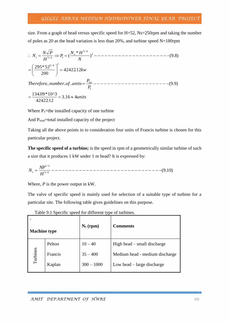
GILGEL ABBAY MEDIUM HYDROPOWER FINAL YEAR PROJECT
AMIT DEPARTMENT OF HWRE 102
size. From a graph of head versus specific speed for H=52, Ns=250rpm and taking the number
of poles as 20 as the head variation is less than 20%, and turbine speed N=180rpm
units
P
PunitsofnumberTherefore
kw
N
HNP
H
PNN
ins
ss
416.312.42422
3^10*09.134
)9.9(.......
12.42422200
52*295
)8.9()*
(
1
24/5
24/5
14/5
Where P1=the installed capacity of one turbine
And Ptotal=total installed capacity of the project
Taking all the above points in to consideration four units of Francis turbine is chosen for this
particular project.
The specific speed of a turbine; is the speed in rpm of a geometrically similar turbine of such
a size that it produces 1 kW under 1 m head? It is expressed by:
)10.9(4/5
2/1
H
NPNs
Where, P is the power output in kW.
The valve of specific speed is mainly used for selection of a suitable type of turbine for a
particular site. The following table gives guidelines on this purpose.
Table 9.1 Specific speed for different type of turbines.
`
Machine type Ns (rpm) Comments
T
urb
ines
Pelton
Francis
Kaplan
10 – 40
35 – 400
300 – 1000
High head – small discharge
Medium head - medium discharge
Low head – large discharge

GILGEL ABBAY MEDIUM HYDROPOWER FINAL YEAR PROJECT
AMIT DEPARTMENT OF HWRE 103
9.6 Determination of turbine parameters
9.6.1 Specific speed:
The specific speed of the unit can be calculated with the help of a number of formulas as shown
below:
1. R.W. Abett’s formula
rpm
HNs
75.23552
1700
)11.9(1700
2. P.C. Nag and K. Modhvan’s formula
rpm
HNs
4.22752
1640
)12.9(1640
3. Moody formula
rpm
HNs
34.4836.8375.952
6780
)13.9(6.8375.9
6780
4. Norwegian turbine factory
rpm
HNs
61.31452
5000
)14.9(5000
7.0
7.0
5. T.L white‘s formula
rpm
HNs
56.21352
1540
)15.9(1540
Taking the average of the above values
NS =294.93rpm ≈295rpm
9.6.2 Turbine speed
)16.9()
45(
1
P
HNN
s

GILGEL ABBAY MEDIUM HYDROPOWER FINAL YEAR PROJECT
AMIT DEPARTMENT OF HWRE 104
20012.42422
)52(295 4/5
N take N=200rp
9.6.3 Synchronous speed
)17.9(120
P
fN
Where f=50 Hz
P = 30200
50*120
P No. of pole =30
TakeP = 28 which are divisible by 4 for H<200m=> P = 30
There for, N= rpmrpmN
f
P
20020030
50*120*120
The new specific speed
)18.9(*
4/5
H
PNNs
NS= 99.29452
12.42422*2004/5
, take295rpm
Therefore NS=295rpm and N=200rpm
9.6.4 Determination of peripheral co-efficient
Kruger’s formula (for Francis turbine)
P.C Nag and K. Modhvan’s formula for Fancies turbine
993.0
)20.9(*036.012/7
SN
D.Zonobelti’s formula
774.0
)21.9(2500
656.0
SN
Taking the average of the above three values = 91.0
96.0
)19.9(09.0*0197.03/2
SN

GILGEL ABBAY MEDIUM HYDROPOWER FINAL YEAR PROJECT
AMIT DEPARTMENT OF HWRE 105
The table below shows various values of HN s ,, and efficiency ( ) for the Francis types of
turbines.
Table 9.2 various values of HN s ,, and efficiency ( ) for Francis turbines
Based on the above parameters, operation head of 52m, generating coefficient 0.91, generating
power of 42.42Mw and the turbine speed of 200rpm makes Francis turbine suitable for this
project.
9.6.5 Run away speed
If the external load on the machine suddenly drops to zero (sudden rejection) and the governing
mechanism fails at the same time, the turbine will tend to race up to the maximum possible
speed, known as runaway speed. This limiting speed under no load, maximum flow must be
considered for safe design. The following formula may also be used to determine proportion
of runaway speed as compared to normal speed.
U.S.B.R. Formula )22.9()(. 21
max d
nH
HNKNr
Where
%8851.1
)145295*1475.0(
)23.9(%)1451475.0(
n
n
Sn
K
K
ageinNK
Hd=Hnet=52m
N=200rpm
38.39552/5.57*200*88.1 N
Hence, the nearest commercially available value is taken.
i.e. rpmNr 400
Runner Discharge diameter; the discharge diameter can be found with help of the
peripheral coefficient . The value of (calculated before), 91.0
Types of runner Ns H (m) Efficiency ( )
Francis 0.6-0.9 40-130
130-350
350-452
25-450
90-94
94
94-93

GILGEL ABBAY MEDIUM HYDROPOWER FINAL YEAR PROJECT
AMIT DEPARTMENT OF HWRE 106
1. Mosonyi’s formula
72.1
)25.9(400
2955.039.1)5.0(
39.1400
52*91.0*6.84
)24.9(*6.84
3
13
1
1
D
N
NsDD
D
N
HD
2. Guthrie Brown’s formula
7.3
400
12.223*90
)26.9(90
3
3/1
3
31
3
D
D
N
QD
3. Zanobetti’s formula
Therefore taking the average values
D1=1.3m; take 1.3m and
D3 =2.71m
Where; D1 = diameter of entering edge of runner blade
D3 = diameter at the discharge end
9.7 Turbine Scroll Case
A scroll case is a conduit directs the water from intake or penstock to the runner. A spiral
shaped scroll case of correct geometry ensures an even distribution of water around the
periphery of the runner with the minimum possible eddy formations. The shape and internal
dimensions are closely related to the design of the turbine. For the Francis turbine of this project
a steel circular spiral case with nose angle 330o is suggested and size proportions take from
recommended dimensions are shown on the detail drawing blow.
m
D
N
HND s
21.1
400
52)295*033.053.57(
)26.9()033.053.57(
1
1

GILGEL ABBAY MEDIUM HYDROPOWER FINAL YEAR PROJECT
AMIT DEPARTMENT OF HWRE 107
Dimension of spiral case; According to F.desiervo and F.deleva, water velocity at spiral case
inlet section for Ns=324.
m
NsDI
m
NsDH
m
NsDG
m
NsDF
m
NsDE
m
NsDD
m
NDC
m
NsDB
m
NDA
sm
NV
s
s
s
79.0295*00065.01.071.2
)36.9()00065.01.0(
89.2295
75.8179.071.2
)35.9()75.81
79.0(
298.3295
5.9689.071.2
)34.9()5.96
89.0(
92.3295
4.131171.2
)33.9()4.131
1(
24.3295
6.6398.071.2
)32.9()6.63
98.0(
51.4295
8.485.171.2
)31.9()8.48
5.1(
03.4295
25.492.171.2
)30.9()25.49
32.1(
76.3295
8.542.171.2
)29.9()8.54
2.1(
07.3295
56.192.171.2
)28.9()56.19
2.1(
/12.69295*844
)27.9(844
3
3
3
3
3
3
3
3
3
44.0
44.0

GILGEL ABBAY MEDIUM HYDROPOWER FINAL YEAR PROJECT
AMIT DEPARTMENT OF HWRE 108
mNsDM
mNsDL
64.1295*000015.06.071.2)000015.06.0(
78.2295*00049.088.071.2)00049.088.0(
3
3
Figure 9.1 Spiral casing
9.8 Draft Tube
A draft tube is a conduit discharging water from the turbine runner to the tailrace. It is employed
in conjunction with reaction type turbines and has two fold purposes.
For this particular project elbow type draft tubes is selected since it has the following
advantages compared to conical type draft tube.
Minimizes the required depth of excavation
Directs the flow in the direction of the tail water flow
Allows the provision of gate at the outlet of the tube
9.8.1 Dimensions of elbow type draft tube
According to F.desiervo and F.deleva have given the formula for draft tube dimensions
V1= water velocity at draft tube inlet section

GILGEL ABBAY MEDIUM HYDROPOWER FINAL YEAR PROJECT
AMIT DEPARTMENT OF HWRE 109
sm
NsV
/58.9295
24874.8
)37.9(248
74.81
m
NsDZ
m
NsDV
m
NDU
m
NsDT
m
NDS
m
NsDR
m
NsDQ
m
NsDP
m
NsDO
S
S
SN
44.7295
8.3363.271.2
)47.9()8.33
63.2(
47.3295
7.531.171.2
)46.9()7.53
1.1(
822.0295*0007.051.071.2
)45.9(0007.051.0
217.4295*00019.05.171.2
)44.9()00019.05.1(
40.1228.9295*25.0
29571.2
)43.9(28.925.0
34.4295
0013.06.171.2
)42.9()0013.0
6.1(
,78.1295
6.2258.071.2
)41.9()6.22
58.0(
265.3295*00056.037.171.2
)40.9()00056.037.1(
54.3295
7.14083.071.2
)39.9()7.140
83.0(
3
3
3
3
3
3
3
3
3

GILGEL ABBAY MEDIUM HYDROPOWER FINAL YEAR PROJECT
AMIT DEPARTMENT OF HWRE 110
Figure 9.2 Draft tube dimensions
9.9 Electromechanical equipment’s
The following items of equipment are considered for planning and dimensioning of the
powerhouse:
1. Hydraulic turbines
Turbines
Gate and Gate valves
Flow measurements
2. Electrical equipment’
Generate
Transformers, pumps, cooling systems, connections, funs and plate forms
3. Switching equipment’s
Switch board panels
Switch board equipment and instruments
4. Miscellaneous equipment
Crane
Work shops
Other facilities (clinic, store, etc)

GILGEL ABBAY MEDIUM HYDROPOWER FINAL YEAR PROJECT
AMIT DEPARTMENT OF HWRE 111
9.10 Generators
Generators transform mechanical energy into electrical energy. They are essentially designed
to suit the characteristics of the turbine to which these are connected. The speed of generator
varies widely as the head on the turbine and its rating. Generators are usually designed for full
runaway speed of the turbine.
9.10.1 Diameter of generator
J.J.Dolands formula
)48.9(119.0 233.0466.0 KPDg
Where Dg=diameter of generator in meter
P=number of poles =30
K=capacity of generator in KN
mD
KN
KNPK
g 3.7)65.53027()30(*119.0
65.530278.0
12.42422
)49.9(8.0
)(
233.0466.0
9.10.2 Weight of the generator
)50.9(85/ NKgWg
Where g=coefficient that varies between 20&32, taking the average =26
tonsWg 36.21485400
65.5302726
Height of the generator
)51.9(3.2' P
DKH
g
g
Where K’ varies from 5.5 to 12.57; take 8
mH g 25.43.230
3.7*8

GILGEL ABBAY MEDIUM HYDROPOWER FINAL YEAR PROJECT
AMIT DEPARTMENT OF HWRE 112
J.H.Walker has given elaborate curves and relations to determine the dimensions of the
generator. If gD' is the gap between poles and stator and this diameter in meter is
)52.9(5.32
62'
k
p
pDg
Where, K=varies from 5to 9(take k=7) mD g 14.1]730
5.32[
62
30'
P=number of poles
9.10.3 Diameter of generator frame ( fD )
𝑫𝒇= 𝑫𝒈′ [
𝟐.𝟏
𝑷+ 𝟏] + 𝟏. 𝟓𝟓 − − − − − − − − − − − − − − − − − − − (𝟗. 𝟓𝟑)
= 𝟏. 𝟏𝟒 [𝟐.𝟏
𝟑𝟎+ 𝟏] + 𝟏. 𝟓𝟓 = 𝟐. 𝟕𝟕𝒎
9.10.4 Generator pit diameter
The generator pit diameter required is given by
m
DD fP
77.4277.2
)54.9(2
Therefore the different dimensions of the generator are
Hg =height of the generator = 4.25m
Wg =weight of the generator = 214.36tons
Dg =diameter of the generator = 7.3m
gD =gap between the poles and the stator =1.14m
Df=diameter of the generator frame =2.77m
Dp =generator pit diameter =4.77m
9.11 Power House Planning
The basic objective of power house planning is to house all the equipment suitably in a
structural complex

GILGEL ABBAY MEDIUM HYDROPOWER FINAL YEAR PROJECT
AMIT DEPARTMENT OF HWRE 113
Figure 9.3 Hydropower plant layout
9.11.1 Types of Power House Planning
The basic requirement of power house planning is a functional efficiency coupled with
aesthetic beauty. A power house can be classified as:
Surface power house:
The power house is located in a building above the ground
Underground power house:
In this type of power house the power house carven, tunnels and shafts for water conduits
system, access tunnels and ventilation shafts are located inside the mountain.
Comparison between surface and underground power house
a) Surface power house planning
The construction period will be delayed due to snow fall and monsoon.
Liable to be damaged by landslides.
b) Underground power house planning
Maintain scientific beauty of the land escape.
Lay out and conduit alignment can be kept nearly straight depending on the
geological strata.
Apart from saving initial cost shorter length means less frictional loss and additional
power production.

GILGEL ABBAY MEDIUM HYDROPOWER FINAL YEAR PROJECT
AMIT DEPARTMENT OF HWRE 114
9.11.2 Selection of Site for Power House Planning
The site selection for the power house is based on the following criteria:
To provide maximum available head.
To minimize cost of construction and excavation.
To get easy access to the power plant.
9.11.3 Dimensions of Power House
The three essential constituents of power house are:
Unit bay
Erector bay
Control bay
Vertical setting is better for multiple units. The size of the erector bay is usually governed by
the size of the generator. Normally, in the case of surface power house, the width of the erector
bay is equal to the machine hall width and the length equals that of one operating bay or center
to center distance of two adjacent units.
The control room and the office may be adjacent to the power house or may be located in
separating buildings located above the ground.
Unit spacing can be determined using the following empirical formula
1. E. Mosonyi’s formula :
Unit spacing = )55.9(*200
5.5 3
D
Ns
= 21.1302.3*200
2255.5
m
. 2. J.J Donald’s formula
Unit spacing=3.5 - 6D3, take 4.75D3(average) ------------------------------------ (9.56)
=4.75*3.02=14.34m
3. N. Venkata Rows formula
Unit spacing = 3.6 to 5D3, take 4.3D3 ------------------------------------------------- (9.57)

GILGEL ABBAY MEDIUM HYDROPOWER FINAL YEAR PROJECT
AMIT DEPARTMENT OF HWRE 115
=4.3*3.02=12.99m
Taking the maximum value, unit spacing = 14.34m
Length; The center-to-center distance between the units, is from (4.5-5) D + (2-3) m for
minimum clearance. Hence the total length
Number of units=11unit+1unit for erection + 1 unit for control room =13 units
L=5D3+2.5--------------------------------------------------------------------------------------- (9.58)
=5*3.02+2.5=17.6m
Ltotal=13*17.6=228.8m take 229m
Width; The width of machine hall can be determined by the size and the clearance space
from the walls needed as a gangway.
Width center-to-center distance of the unit spacing. =17.6m
W = F + C + 2 + 1.85D3 − − − − − − − − − − − − − − − − − − − − − − − − − (9.58)
Where F and C are calculated in the dimensioning of spiral casing
Width=4.784+4.647+2+1.85*3.02=17m
In order to minimize the excavation cost, the lesser value is adopted i.e width=17m
Height: The height of the machine hall is fixed up by the head room requirement of the crane
operation .The hall must have the height which will enable the cranes to lift the
rotors of the generator clear of the floor without any other machine sets forming
obstruction.
Height of power house (H)
Generator capacity =installed capacity
power factor− − − − − − − − − − − − − − − − − −(9.60)
Where P.F=0.8
Installed capacity = 7206952
1441390
Generator capacity = KN75.9008688.0
720695

GILGEL ABBAY MEDIUM HYDROPOWER FINAL YEAR PROJECT
AMIT DEPARTMENT OF HWRE 116
H=Height of generator +clearance (4m)+allowance for free movement of crane (say 2m) +
allowance for crane girders (say 4.5 m)
H =5.74+4+2+4.5
H =16.24m say 17m
H=17m
Therefore the dimensions of the power house are =Length * width *height =229*17*17
For Gilgel-Abbay hydropower plant a vertical alignment of the turbine and generator with 5D
center-to-center distance between the two turbine units is recommended so that the machine
hall length is reduced to some extent. The powerhouse is constructed above ground at elevation
of 1828m.
9.12 Cavitation:
Cavitation is the formation in subsequent collapse of vapor pockets in a region of liquid where
the pressure has been reduced to that of vapor pressure of the liquid. When the pressure in any
part of flow passage reaches the vapor pressure of the flowing liquid it starts vaporizing and
small bobbles of vapor form in large number.
The effects of cavitation’s are:-
Surface of the vanes subjected to intense pressure during the collapse becomes
scored, pitted and even torn.
Cause noise and vibration.
Cavitation’s in a turbine can be avoided by the following measures
A careful stream lined design of the flow passages of the runner as well as that of
draft tube.
The average sub-atmospheric pressure at runner outlet is kept reasonably above the
vapor pressure limit.
Some metals are more resistance to cavitation’s damage than others.
The cavitation’s characters tics of a hydraulic machine is characterized by a cavitation’s
constant called Thomas’s cavitation’s constant б and given by
𝜌𝑐 =𝐻𝑎−𝐻𝑣−𝑌𝑠
𝐻− − − − − − − − − − − − − − − − − − − − − − − − − (9.61)
Where (Ha-Hv) =Barometric pressure which is 10.1m of water

GILGEL ABBAY MEDIUM HYDROPOWER FINAL YEAR PROJECT
AMIT DEPARTMENT OF HWRE 117
H=net head (m)
Ys=static draft head
бc= critical Thomas’s cavitation’s constant=0.0432(Ns/100) 2 for Francis turbine
The value of σc for different turbines may be determined by using the following empirical
relations:-
For the case of Gilgel abbay hydropower project Francis turbine have been selected and the
value is
235.0100
2950432.0
)62.9(100
0432.0
2
2
c
c
Ns
To maximize turbine efficiency
𝑌𝑠𝑚𝑎𝑥= (𝐻𝑎 − 𝐻𝑣) − 𝛿𝑐 ∗ 𝐻 − − − − − − − − − − − − − − − − − − − −(9.63)
= 10.1 − 0.235 ∗ 52 = −2.12𝑚
The turbine unit should be set at 2.12m below tail water level in order to remove formation of
cavitation. Recommended dimensions of the draft tube are given in detail drawing Appendix.
The effects of cavitation can be reduced by-
setting the turbine near the tailrace level using hydraulic calculation
Making the runner blades from especially chosen resistant metals such as stainless
steel and nickel steel.
Spraying thin layers of erosion resistance materials in place where cavitation is most
likely to occur.
9.13 Turbine governor
The governor is a mechanism of controlling the rotational speed of the turbo generator unit;
constant speed must be maintained in order to obtain the A.C supply with constant frequency.
As the turbine and hence its interconnected generator tend to decrease or increase speed as the
load varies, the maintenance of an almost constant speed requires regulation of the amount of
water allowed to flow through the turbine by closing or opening the gates of the turbines
automatically, through the action of a governor.

GILGEL ABBAY MEDIUM HYDROPOWER FINAL YEAR PROJECT
AMIT DEPARTMENT OF HWRE 118
9.13.1 Transformer:
Transformer in a hydroelectric installation is an important piece of equipment for converting
the power of the generator at a relatively low voltage to power for transmitting to a remote
electrical system at a high voltage. Due to the cost of high amperage connection between
generators and transformers, transformer location at surface may only be economically viable
by the shallowest seated powerhouse.
9.13.2 Transmission of electric power
The transmission system delivers bulk power from the power stations to the load centers. The
electrical power may be transmitted by either underground cables or overhead lines. The former
are suited for densely populated areas as these are safer requires less maintenance and do not
influence the appearance the town.
9.13.3 Turbine Blade Arrangements
Where V1and V2are velocity of the jet at inlet and outlet
U1 and U2 are velocity of vanes (blades) at inlet and outlet
Vr1and Vr2 are relative velocity of the jet and the plate at inlet and Outlet
Vf1 and Vf2 are velocity of flow at inlet and outlet
Vw1and Vw2 are velocity of whirl at inlet and outlet
Φ and Ø are vane angles at inlet and outlet.
9.13.4 Tail Race Canal
The powerhouse discharges water in to the tailrace or tail water. The draft conveys the water
from the discharge side of the turbine to the tailrace. The tailrace canal, which is in the vicinity
of the draft tube, must be properly lined; as it may otherwise degrade and cause the lowering
of the tail water elevation.
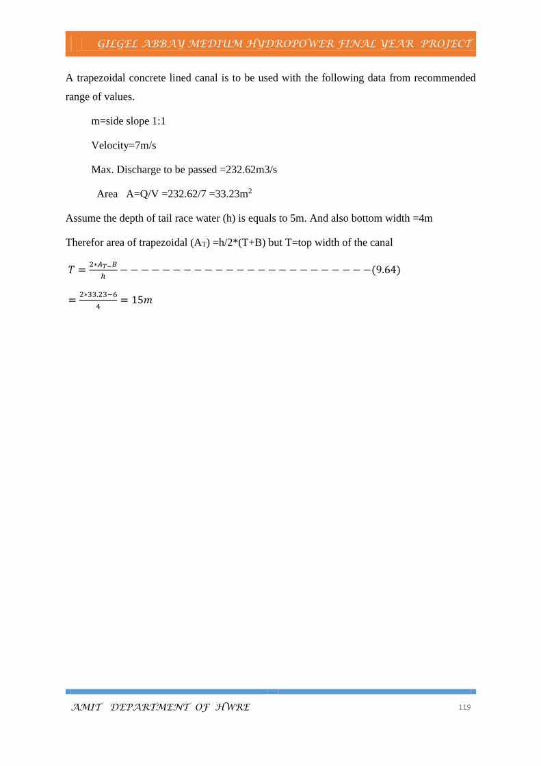
GILGEL ABBAY MEDIUM HYDROPOWER FINAL YEAR PROJECT
AMIT DEPARTMENT OF HWRE 119
A trapezoidal concrete lined canal is to be used with the following data from recommended
range of values.
m=side slope 1:1
Velocity=7m/s
Max. Discharge to be passed =232.62m3/s
Area A=Q/V =232.62/7 =33.23m2
Assume the depth of tail race water (h) is equals to 5m. And also bottom width =4m
Therefor area of trapezoidal (AT) =h/2*(T+B) but T=top width of the canal
𝑇 =2∗𝐴𝑇−𝐵
ℎ− − − − − − − − − − − − − − − − − − − − − − − −(9.64)
=2∗33.23−6
4= 15𝑚

GILGEL ABBAY MEDIUM HYDROPOWER FINAL YEAR PROJECT
AMIT DEPARTMENT OF HWRE 120
CHAPTER TEN
10 Environmental Impact Assessment
10.1 General
Hydropower projects that are intended to produce electric energy, may cause irreversible
environmental changes over a wide geographic area and thus have a potential for significant
impacts. The area of influence of the project extends from the upper limits of the catchments
too far down stream. Therefore hydropower project such as Gilgel abbay are designed to
enhance economic development and bring a better standard of life to people due consideration
should be given to their adverse environmental and social effects. This can be done through
environmental impact assessment, which is a management tool for officials, and manager who
take decision about important development project.
The EIA not only predicts potential problems but also identifies measures to minimize the
problems and out lines ways to improve the project suitability for its proposed environment.
The aim of environmental impact assessments is:
1. To understand the likely environmental consequences of new developments.
2. To understand the amplification of proposed interventions.
3. To identify measures by which the impacts can be mitigated.
4. To present the results in such a way that they can provide answers needed by
stakeholders.
Generally, EIA can be described in short as an instrument used to identify, predict and assess
the environmental consequences of a proposed major development project. Moreover, EIA is
used to plan appropriate measures to reduce adverse effects. EIA encourages the developer to
find ways to lessen the consequences. The purpose of EIA is to establish and describe the direct
and indirect impact of a planned activity or measure on community, flora, fauna, land water,
air, the climate, the landscape, the socio-economic environment and cultural environmental as
well as on sustainable management of land, Water and the biophysical in General In venal, EIA
is a management too, like economic analyis and engineering feasibility studies for official and
managers who must make important decisions about major development projects.

GILGEL ABBAY MEDIUM HYDROPOWER FINAL YEAR PROJECT
AMIT DEPARTMENT OF HWRE 121
10.2 Why EIA is necessary
EIA is under taken for the following reasons
To integrate environmental considerations in development planning.
To ensure the potential negative impacts are foreseen and addressed at early stage in
the planning process.
To identify and enhance positive impacts of the proposed development activities.
To examine the trades offs and the possible alternatives.
To ensure that all affected and interested groups (Grass root communities,
government authorities, developers, NGOs, etc.) in the process.
To promote social and economic equity and the empowerment of the people at grass
root level to participate in decision making.
To provide an eco-friendly and people centered management tool
To set up a machinery to carry out mitigation measures and monitoring.
EIA is as one of environmental management tools that facilitates inclusion of
principle of sustainable development operation well in advance at project planning
stage.
10.3 EIA Process
The EIA process can be divided in to two phases namely; initial inquiries (examination) and
the EIA itself. The various stages involved in EIA include the following.
1. Pre-screening consultation.
2. Project screening
3. Scoping
4. Environmental impact study
5. Mitigation
6. Environmental management and monitoring plan
7. Environmental impact study report
8. Reviewing
9. Environmental Decision making

GILGEL ABBAY MEDIUM HYDROPOWER FINAL YEAR PROJECT
AMIT DEPARTMENT OF HWRE 122
10.4 Impact of the Gilgel-Abbay Hydropower Project on the Environment
The Gilgel-Abbay hydropower project has to be subjected to EIA process according to
Ethiopian context stage by stage since the project may has the following impact on the
surrounding environment.
Hydrological impact; Low flow regime; a reduction in the natural river flow
together with a discharge of low quality discharge water can have severe negative
impacts on downstream users mostly by irrigation scheme.
Operation of dam; a number of diseases hazards are associated with dam operation
some of which can be minimized, others eliminated by careful operation.
a) Impact on water and air quantity
Solute dispersion; the changing of hydrological regime associated with the project
may alter the capacity of the environment to assimilate water soluble pollution
Anaerobic effects; an aerobic condition may occur when water is so polluted that
produces gases such as hydrogen supplied, methane and ammonia all of which are
poisonous and some of which contribute to the greenhouse effect.
b) Erosion and sedimentation impact
Erosion; upstream erosion may result the delivery of fertile sediments to delta areas.
Sedimentation; a major negative impact of erosion and the associated transport of soil
particles is the sedimentation of reservoir which reduce the storage capacity of
reservoir and clog intakes.
c) Impact on river morphology
Channel Structures; degradation of the river bed is likely to threaten the structural
intensity of hydraulic structures. The construction of new structure impacts on nearby
structures by changing local flow condition. Sedimentation; the Gilgel-Abbay
Hydropower project may fail if the sediment load of the stream is higher than the
capacity of the sediment channels to transport sediment.
d) Biological and Ecological impact
Water bodies; the creation of reservoirs and channels provides the possibility of
enhanced aquatic habitats and may also offer favorable habitats for disease
transmitting insects and snails.
Project land; the consequence of the change of land use and water in the project area
affects the land around the project area and on aquatic ecosystems that share the

GILGEL ABBAY MEDIUM HYDROPOWER FINAL YEAR PROJECT
AMIT DEPARTMENT OF HWRE 123
catchment are likely. Biological diversity areas of special interest like scientific,
animal-migration industrial areas are important study areas.
e) Impact on wet lands and plains
The project may have direct impact on wetlands by either changing the hydrological conditions
or by reducing water quality in downstream areas. Seasonally flooded plains or deltas of
specialized important habitats providing grazing for cattle and wild life.
f) Socio economic impact
Population change; the project may encourage population density to increase because
the increased prosperity of the area attracts the population
Income and amenity;
Human migration; due to submergence of the area by the proposed reservoir.
g) Impact on human health
A number of disease hazards may be associated with the project including malaria,
schistosomiasis and river blindness.
Environmentally sound design requires the project adverse impacts on the environment and
natural resource bases are zero or very limited and all reasonable steps have to be taken to
minimize adverse impacts and maximize positive impacts. Mitigation measures have to be
proposed for each environmental problem by EIA study group.
EIA is an ongoing process of review, negation and incremental decision making at various
levels of project cycle, about whether or not the proposal is to proceed, and under what
conditions. The EIA report prepared by the study group will help the government authority to
decide whether the Gilgel-Abbay project is to proceed or not or under what conditions have to
proceed.
10.5 Impact mitigation measures
The purpose of mitigation measures are to minimize adverse impacts and enhance the
benefits of scheme and are summarized in table below.

GILGEL ABBAY MEDIUM HYDROPOWER FINAL YEAR PROJECT
AMIT DEPARTMENT OF HWRE 124
Table 10.1 Mitigation measurement
S.NO
Types of negative potential
Impacts
Recommended mitigation
measures
1 Reduction of soil erosion
and disturbance
Following the completion of
the construction:
Compact soils on slopes or
loose surface.
Agricultural soil packed by
the vehicles and heavy
machinery must be lessened.
2
Reduction of noise Using vehicles, machineries
and equipment with less
noise.
Avoiding or minimizing
blasting of rocks using an
appropriate method.
3 Afforestation Community programmed for
tree replanting
4
Measures concerning
affected population
Reallocation of population
and loss of productive land.
Compensation should be
made for their house and
immovable property.
5 Damage on wild life Preparing conservation
camps.
6
Health problem Establishing appropriate
health care centers and
disease controlling program.

GILGEL ABBAY MEDIUM HYDROPOWER FINAL YEAR PROJECT
AMIT DEPARTMENT OF HWRE 125
CHAPTER ELEVEN
11 Economic Analysis
11.1 General
The main objective of economic analysis in hydropower project is to provide an economic basis
for deciding whether or not to implement a project. And, secondly to examine promising
development alternative in an economic respect to determine which is the most attractive. An
economic analysis is based on the benefits and costs from the point view of the society as a
whole.
11.2 Cost estimation
The economic analysis of the project studies is dependent on orderly and accurate cost
estimation. The type of study, whether a reconnaissance study, a feasibility study or a final
design study, will tend to dictate the precision with which cost estimates are made.
The total cost of the project is estimated as follows depending on the bill of quantities and their
corresponding unit rates.
Parameters:
11.3 Annual benefit: -
All the benefits from various projects are calculated annually on the bases of the prevailing
rates. For hydropower generation the cost per unit and the total units of power generated from
a project gives the annually return from power. For hydropower projects benefit cost analysis
needs careful consideration.
11.4 Interest rate: -
It is simply a reward having made capital available. It depends on:-
The state of the economy.
The risk involved in the loan.
Future expected rate of inflation.
Consideration of a lower rate of interest needs justification for the importance of the project
in the regional and national level as this gives a better cost-benefit ratio.

GILGEL ABBAY MEDIUM HYDROPOWER FINAL YEAR PROJECT
AMIT DEPARTMENT OF HWRE 126
11.5 Financial costs
Annual cost: - it is the sum of;
Annual capital cost.
Annual interest.
Annual operation, maintenance and replacement (OMR) cost which is taken usually
less than 1% of the capital cost.
Depreciation or Amortization
Taxes and insurance
Water right payments for the resource managements
11.6 Costs evaluation of the project
Before economies of an engineering project can be evaluated, it is necessary to reasonably
estimate the various cost and revenue components that describe the project
11.7 Bill of quantity of Gilgel abbay hydropower project
The following is the procedure adopted for estimating the total cost of the project.
Table 11.1 Estimation of the project cost by bill of quantity (BOQ)
S.no Description Unit Unit cost
(Birr)
Quantity Total cost
(MBirr)
1 Access road m 87 1500 1.305
Construction access road km 200,000 8.3 1.66
2 Diversion work
Diversion tunnel (excavation
and lining)
m3 2250 60.1 0.135
Coffer dam m3 43.2 52800 2.28
3 Dam
Borrow excavation m3 135 5520 0.745
Foundation excavation m3 120 11712 1.41
Concrete m3 960 169626 162.84
4 Water conveyance
Power intake excavation m3 130 336.53 0.044
Intake gate _ - -

GILGEL ABBAY MEDIUM HYDROPOWER FINAL YEAR PROJECT
AMIT DEPARTMENT OF HWRE 127
5
Headrace tunnel
excavation(L=34m) m3 2350 327.12 0.77
Shotecrete m3 5400 757 4.088
Penstock(d=3.6) m 32500 70 2.275
Tailrace tunnel
excavation(L=225m)
m3 450 7521.75 3.385
Shotecrete m3 5400 1640 8.87
Surge shaft excavation m3 450 360 0.162
Shotecrete m3 5400 21 0.113
6
Power house
Excavation m 3 450 420 0.189
Concrete lining m3 1800 32.48 0.0585
Masonry work M3 500 37.12 0.01856
7
Electro mechanical
equipments
Turbine governor and turbine
equipments item 28.89×10⁶ 4 115.92
Generator and
generator
equipments item 27.45×10⁶ 4 109.8
Power house crane
Transformer item 558000 2 1.116
Auxiliary mechanical
and electrical
equipments
_ _ _ 4.1
8
Spillway
9
Transmition cost Kw 3285 84300 276.9
Switch yards Kw 450 84300 37.9
Environmental mitigation
measures
sum 1 20,000,000 20
10
TOTAL COST 756.0841
Contingency cost 20% of
the total cost
151.22
11 Engineering and
Administration
15% 113.41
12 Grand sum 1020.72

GILGEL ABBAY MEDIUM HYDROPOWER FINAL YEAR PROJECT
AMIT DEPARTMENT OF HWRE 128
11.8 Camp installation and labor cost (including cost of land)
Assuming 450people for an operation of 5 years and 200persons for one year during the main
concrete works, and assuming an area of 15m2 per person, we need 13500m2 of area. Unit rate
of labor cost assumed as 950birr/month.
Unit cost of installation including water supply, health facility, electric and
others=4,342,803Birrper m2 of area
Total cost of installation and labor cost= 902,592,803Birr
Summing up all the costs, the total project cost will be 1.92B.Birr
OM=1.5% of total project cost =0.0288B.Birr
TOTAL COST=1.9488B.Birr
11.9 Benefits of the project
The main benefit of the project is selling cash electrical power. Actually, there may be some
tangible and intangible benefits, which we didn’t include in this study, since the former is the
main.
11.9.1 Benefits from hydropower development
We have assumed the design period of the structure=100years
Yearly power production=107,270 KWH
The average energy price according to recent (EEPCO) on hydropower is 0.57Birr/Kwhr.
Annual benefit from selling power=107,270×365×24×0.35 = 0.33B.Birr/kwh
11.10 Economic Analysis
Total initial investment costs=1.92B.Birr
Annual benefits = 0.33B.Birr
Annual operation and maintenance cost=0.00492B.Birr
Taking an interest rate of 7% and change the annual benefits and operation and maintenance
cost all in to present worth values

GILGEL ABBAY MEDIUM HYDROPOWER FINAL YEAR PROJECT
AMIT DEPARTMENT OF HWRE 129
)1.10(1
111
n
n
iiiAP
⇒
269.1407.0107.0
1107.01
1
111
100
100
n
n
iii
A
P
11.10.1Cash Flow Diagram
Annual benefit = 0.33B.Birr
Value of all OM costs = 0.41B.Birr
Present value of total cost (initial + OM cost) =2.33B.Birr
Present value of total benefit = 4.71B.Birr
Initial cost=1.92B.Birr Annual OM cost =0.0288B.Birr
Fig 10.1 Cash flow diagram
𝐵𝑒𝑛𝑒𝑓𝑖𝑡
𝑐𝑜𝑠𝑡 𝑟𝑎𝑡𝑖𝑜 =
4.71
2.33= 2.02
Since the B/C ratio of the project is greater than 1.0 the project is economically feasible.
Annual benefit=0.33B.Birr

GILGEL ABBAY MEDIUM HYDROPOWER FINAL YEAR PROJECT
AMIT DEPARTMENT OF HWRE 130
CHPTER TWELVE
12 DAM SAFETY, INSTRUMENTATION AND SURVEILLANCE
12.1 Introduction
Perspective on dam safety
Reservoirs constitute a potential hazard to downstream life and property. The floodplain at risk
in the event of catastrophic breaching may be extensive, densely populated and of considerable
economic importance. In such instances dam failure can result in unacceptable fatalities and
economic damage. Surveys and statistical analyses of failures and other serious incidents have
been published by the International Commission on Large Dams (ICOLD, 1995). Jansen
(1980) provides a more detailed review of a number of major dam disasters.
A particular hazard is represented by tailings dams and storage lagoons. The potential hazard
associated with tailings dams and lagoons is raised very significantly by several factors which
distinguish them from conventional embankment dams and reservoirs
The risk of tailings dams breaching may be much enhanced by inadequate levels of
supervision and surveillance;
The environmental and economic consequences of serious breaching are frequently
heightened by the toxic nature of the outflow;
A tailings dam or lagoon may be discontinued and/or abandoned, and left
unsupervised, following the cessation of active operation.
12.2 Surveillance
Dams of all types require regular surveillance if they are to be maintained in a safe and
operationally efficient state. The primary objective of a surveillance programmer is to minimize
the possibility of catastrophic failure of the dam by the timely detection of design inadequacies
or regressive changes in behavior. A further objective is to assist in the scheduling of routine
maintenance or, when necessary, of major remedial works.
Surveillance embraces the regular and frequent observation and recording of all aspects of the
service performance of a dam and its reservoir. It includes routine observation and inspection,
the monitoring and assessment of seepage and instrumentation data and the recording of all
other relevant information, including hydrological records. Routine inspection should cover all
readily accessible parts of the dam and of its associated components (e.g. spillways, gates,

GILGEL ABBAY MEDIUM HYDROPOWER FINAL YEAR PROJECT
AMIT DEPARTMENT OF HWRE 131
valves and outlet works). Visual inspection should also extend to the area downstream of the
dam, including the miters and abutments, and to any parts of the reservoir perimeter designated
as requiring observation. Additional effort may be directed at particular locations or to specific
signs of some possible deterioration, e.g. sources of suspected seepage or leakage and, in the
case of embankments, localized crest settlement and slope deformation. The inspecting
engineer must be alert to change, whether favorable or unfavorable, between successive visits.
12.3 Instrumentation Application and objectives
The provision of monitoring instruments is accepted good practice for all new dams of any
magnitude. In parallel with this, a basic level of instrumentation is now frequently installed
retrospectively to monitor existing dams. The scope and degree of sophistication of individual
suites of instruments varies greatly. Careful attention to specification, design, and correct
installation of all but the simplest instrument arrays is critical to their satisfactory performance.
Responsibility for the planning and commissioning of monitoring installations is therefore best
retained at an experienced and relatively senior level within an appropriate organization, e.g.
the design agency, owner, or state authority.
Suites of instruments may, for convenience, be classified according to the primary function of
the installation.
1. Construction control: verification of critical design parameters with immediate looped
feedback to design and construction.
2. Post-construction performance: validation of design; determination of initial or datum
behavioral pattern.
3. Service performance/surveillance: reassurance as to structural adequacy; detection of
regressive change in established behavioral pattern; investigation of identified or suspected
problems.
4. Research/development: academic research; equipment proving and development.
12.4 Instruments: design principles
Monitoring instruments are required to function satisfactorily under very harsh environmental
conditions and for essentially indeterminate periods of time, possibly several decades. As
guidelines underwriting sound design it is therefore desirable that instruments be

GILGEL ABBAY MEDIUM HYDROPOWER FINAL YEAR PROJECT
AMIT DEPARTMENT OF HWRE 132
1. As simple in concept as is consistent with their function,
2. Robust and reliable,
3. Durable under adverse environmental and operating conditions and
4. acceptable in terms of ‘through-life’ costs (i.e. the sum of purchase, installation,
support and monitoring costs).
A sound principle is to retain the sophisticated and vulnerable sensing elements, e.g. electronic
components and transducers, above ground level wherever possible. In such instances it may
also be advantageous to make the above-ground elements readily transportable, e.g. by use of
compact portable transducer units to monitor pore water pressures from piezometers.
Additional advantages associated with the use of a transportable sensing element lie in greater
physical security and avoidance of the need to construct large and costly instrument houses for
fixed measuring equipment. Instrument capability has developed significantly over recent
years, and reliable and robust equipment is now readily available. The enhanced capability and
complexity are reflected in high costs and a greater risk of component, and thus system,
malfunction or failure. Such sophistication is therefore generally justifiable only in more
exceptional circumstances. For most dams instrumentation at a relatively unsophisticated and
basic level will prove adequate for routine monitoring and surveillance.

GILGEL ABBAY MEDIUM HYDROPOWER FINAL YEAR PROJECT
AMIT DEPARTMENT OF HWRE 133
13 CONCLUSION AND RECOMMANDATION
13.1 CONCLUSION
The implementation of Gilgel abbay Medium Hydropower Project has an ultimate benefit to
increase the demand of power supply in the country and project area region.to fulfill this benefit
the following designing process occurred in this final year project.
Hydrological data analysed for determination of maximum rainfall probability and
design rain fall of 214.18mm as well as from Gilgel Abbay River recorded stream
flow, the maximum design discharge for a return period of 100 year is 482.993m3/s
determined.
Reservoir planning by using counter elevation and its covering area from given field
survey data to fix the dam height and storage capacity by using elevation area
capacity curve which is done by integration method and mass curve methods.
The reservoir and flood roughing to determine maximum spill out discharge of
168.92m3/s and its corresponding height of 1.18m by using inflow and outflow
hydrograph
Depending up on different criteria which is missioned in the body of this report
Gravity dam is best selection for Gilgel abbay project with 62m height, 4.5 and 63m
top and bottom width respectively. The upstream and downstream slops are
designed as 1.25:1 and 0.75:1 (H: V) respectively. To increase dam stability, to
protect sliding and over stressed by increasing contact area of the dam at both
upstream and downstream. All safety factor of the dam which is tension, sliding and
over turning are checked by determining different load combination such as NLC,
ULC and ELC condition.
Based on the type of dam proposed, ogee spillway is selected on the dam itself with
bucket type energy dissipation structure.
A cofferdam is constructed at the upstream of the dam to divert the river flow for the
purpose of dam construction. And conveyance strictures designed properly.
Gilgel-Abbay Hydropower project will provide an average energy output of 134MW
from this energy some would be107.2MW firm energy (90% reliability).
The powerhouse will be a surface type structure of reinforced concrete and structural
steel construction. The powerhouse accommodates a loading/service bay, four bay
for each of the 4 Francis turbine units.

GILGEL ABBAY MEDIUM HYDROPOWER FINAL YEAR PROJECT
AMIT DEPARTMENT OF HWRE 134
The Gilgel-Abbay hydropower project has many positive impacts especially in
increasing electric power production and providing new employment opportunities
for the local people. However, it has negative impacts primarily related to the loss of
home with a land associated with the development of the dam site.
Gilgel-Abbay hydropower project is economically feasible and has a benefit-cost
ratio of 2.02.
13.2 R ECOMMENDATION
A hydropower design system is a vast task; requires a due attention, effort and lot of experience.
For a complete and in-depth design full, sufficient and actual data is required including variable
on-site observations.
A design based on written information only cannot be sufficient. Actual observation plays
a decisive role for design of hydropower.
These report present scant information which is not sufficient for detailed design. A
detailed information, which is the basis to carry out the design in conformity with the
results of detailed field, laboratory investigations and pilot performance results is not
available.so
In this project, since there is no any suspended sediment data, we make rough
estimation. But, since it has great effect on the design of the hall hydraulic structures,
directly or indirectly, there should be detail and accurate sediment data.
Since the reservoir created by the implementation of the project may facilitate the
spread of the diseases in the area, appropriate heath care services and creation of
awareness for controlling the diseases has to be established with the implementation of
the project. And also appropriate protection measures should be taken for other impacts
of the project as much as possible
The estimated cost is obtained by rough analysis, which need further detail quantity
surveying
To have efficient use of water and to keep the structure in good condition, the owner of
the project should have to manage it appropriately
Afforestation should be seriously done for protection of erosion to protect
sedimentation of the reservoir easily.
Facilitation of fish husbandry and recreational centres should be carried out

GILGEL ABBAY MEDIUM HYDROPOWER FINAL YEAR PROJECT
AMIT DEPARTMENT OF HWRE 135
BIBLIOGRAPHY
1. B.Franzin, R. a. (n.d.). Water resourse engineering (3rd edition ed.).
2. chow, V. T. ((1988)). Applied Hydrology :. Singapore.
3. Dandekar, M. a. (1997). Water power engeenering. New Delhi: Vikas
publishing.
4. Garg, S. (( 2005)). Irrigation Engineering and Hydraulic Structures:. Delhi,
India.
5. Garg, S. ((2000)). Water Supply : . India.
6. Hill, T. M. (2000). Subermanya K.Engeenering Hydrology. New Delhi.
7. K.C, P. (n.d.). Hydrology andwater resource engineering,. NORSA, published.
8. Linsley Ray K, M. A. (1982). Hydrology for engineers. Tokyo: Mc Graw Hill.
9. Michael, A. ((2001)). Irrigation Theory and Practice :. New Delhi.
10. Mutreja, P. K. ((1994 )). Applied Hydrology:. New Delhi, India.
11. Novak. P, A. M. (n.d.). Hydraulic Structures:.
12. Patra, K. (( 2001 )). Hydrology and water resource engineering :. India.
13. Professor Taffa, T. (( 2002)). Soil and water conservation for sustainable :.
Addis Abeba, Ethiopia,.
14. Varshney, R. (1993). Theory and design of irrigation structures Volume II :.
New Chand and Bros: New Chand and Bros.

APPENDIX –A
Table 6.1 Upstream and downstream profile of Spillway from origin coordinates
Downstream profile Upstream Profile
X Y X Y
0 0.000 -0.010 -0.012
0.1 0.006 -0.020 -0.011
0.2 0.022 -0.030 -0.010
0.3 0.047 -0.040 -0.009
0.4 0.080 -0.050 -0.007
0.5 0.120 -0.060 -0.006
0.6 0.169 -0.070 -0.004
0.7 0.224 -0.080 -0.002
0.8 0.287 -0.090 0.000
0.9 0.357 -0.100 0.003
1 0.434 -0.110 0.005
1.1 0.518 -0.120 0.008
1.2 0.608 -0.130 0.011
1.3 0.705 -0.140 0.014
1.4 0.809 -0.150 0.017
1.5 0.919 -0.160 0.021
1.6 1.035 -0.170 0.025
1.66 1.108 -0.180 0.029
-0.190 0.033
-0.200 0.038
-0.210 0.043
-0.220 0.048
-0.230 0.054
-0.240 0.060
-0.250 0.066
-0.260 0.074
-0.270 0.081
-0.280 0.090
-0.290 0.099
-0.300 0.110
-0.310 0.124
-0.320 0.150

Table 1 outlier test computed value by using Grub’s T-test
T-test
year January February March April May June July August September October
Nobem
ber December Xmean S staDeve
1981 30.38 15.62 42.98 30.00 137.30 241.40 568.40 482.20 212.10 73.30 29.60 0.00 155.27 190.35
Tcalcu 0.66 0.73 0.59 0.66 0.09 0.45 2.17 1.72 0.30 0.43 0.66 0.82
Ttest 2.55 2.55 2.55 2.55 2.55 2.55 2.55 2.55 2.55 2.55 2.55 2.55
1982 19.90 0.00 36.90 11.30 145.00 239.50 287.50 532.20 158.60 93.75 20.81 15.62 130.09 158.89
Tcalcu 0.69 0.82 0.59 0.75 0.09 0.69 0.99 2.53 0.18 0.23 0.69 0.72
Ttest 2.55 2.55 2.55 2.55 2.55 2.55 2.55 2.55 2.55 2.55 2.55 2.55
1983 15.62 15.62 31.27 60.30 121.98 284.25 463.04 466.15 243.10 123.80 7.00 0.00 152.68 172.48
Tcalcu 0.79 0.79 0.70 0.54 0.18 0.76 1.80 1.82 0.52 0.17 0.84 0.89
Ttest 2.55 2.55 2.55 2.55 2.55 2.55 2.55 2.55 2.55 2.55 2.55 2.55
1984 0.00 0.00 21.10 60.25 143.43 362.25 603.35 299.12 421.15 25.65 0.00 25.30 163.47 206.13
Tcalcu 0.79 0.79 0.69 0.50 0.10 0.96 2.13 0.66 1.25 0.67 0.79 0.67
Ttest 2.55 2.55 2.55 2.55 2.55 2.55 2.55 2.55 2.55 2.55 2.55 2.55
1985 0.00 1.15 12.60 28.00 172.35 199.55 424.10 382.30 205.50 101.40 27.70 2.60 129.77 150.06
Tcalcu 0.86 0.86 0.78 0.68 0.28 0.47 1.96 1.68 0.50 0.19 0.68 0.85
Ttest 2.55 2.55 2.55 2.55 2.55 2.55 2.55 2.55 2.55 2.55 2.55 2.55
1986 0.00 4.50 4.50 19.40 22.00 380.90 568.15 186.15 364.85 64.70 28.40 0.00 136.96 194.57
Tcalcu 0.70 0.68 0.68 0.60 0.59 1.25 2.22 0.25 1.17 0.37 0.56 0.70
Ttest 2.55 2.55 2.55 2.55 2.55 2.55 2.55 2.55 2.55 2.55 2.55 2.55
1987 0.00 0.00 19.00 13.20 320.90 324.70 332.50 307.45 165.80 64.30 0.80 0.00 129.05 149.48
Tcalcu 1.00 1.00 0.85 0.90 1.49 1.52 1.58 1.38 0.28 0.50 0.99 1.00
Ttest 2.55 2.55 2.55 2.55 2.55 2.55 2.55 2.55 2.55 2.55 2.55 2.55
1988 11.20 20.30 0.00 0.00 153.30 408.00 508.85 294.90 218.65 193.85 26.25 0.30 152.97 176.25
Tcalcu 0.80 0.75 0.87 0.87 0.00 1.45 2.02 0.81 0.37 0.23 0.72 0.87
Ttest 2.55 2.55 2.55 2.55 2.55 2.55 2.55 2.55 2.55 2.55 2.55 2.55
1989 0.00 0.00 46.60 58.85 62.56 211.50 374.90 375.80 151.50 140.45 12.10 17.10 120.95 136.06
Tcalcu 0.89 0.89 0.55 0.46 0.43 0.67 1.87 1.87 0.22 0.14 0.80 0.76
Ttest 2.55 2.55 2.55 2.55 2.55 2.55 2.55 2.55 2.55 2.55 2.55 2.55
1990 2.60 0.00 22.05 2.50 63.30 209.10 474.80 573.50 227.20 112.84 29.01 34.75 145.97 193.83
Tcalcu 0.74 0.75 0.64 0.74 0.43 0.33 1.70 2.21 0.42 0.17 0.60 0.57
Ttest 2.55 2.55 2.55 2.55 2.55 2.55 2.55 2.55 2.55 2.55 2.55 2.55
1991 0.30 0.00 7.70 131.60 79.00 326.60 589.80 471.95 386.05 131.10 18.05 25.80 180.66 208.12
Tcalcu 0.87 0.87 0.83 0.24 0.49 0.70 1.97 1.40 0.99 0.24 0.78 0.74
Ttest 2.55 2.55 2.55 2.55 2.55 2.55 2.55 2.55 2.55 2.55 2.55 2.55
1992 0.00 0.00 3.45 108.40 59.30 273.30 463.90 373.10 171.20 94.37 0.00 0.00 128.92 160.44
Tcalcu 0.80 0.80 0.78 0.13 0.43 0.90 2.09 1.52 0.26 0.22 0.80 0.80
Ttest 2.55 2.55 2.55 2.55 2.55 2.55 2.55 2.55 2.55 2.55 2.55 2.55
1994 15.62 17.10 29.04 43.28 165.60 247.50 229.90 369.10 164.05 106.20 37.50 0.00 118.74 117.33
Tcalcu 0.88 0.87 0.76 0.64 0.40 1.10 0.95 2.13 0.39 0.11 0.69 1.01
Ttest 2.55 2.55 2.55 2.55 2.55 2.55 2.55 2.55 2.55 2.55 2.55 2.55
1995 0.00 2.00 18.10 37.30 202.25 312.70 332.30 291.50 174.25 59.30 8.65 30.10 122.37 131.76
Tcalcu 0.93 0.91 0.79 0.65 0.61 1.44 1.59 1.28 0.39 0.48 0.86 0.70
Ttest 2.55 2.55 2.55 2.55 2.55 2.55 2.55 2.55 2.55 2.55 2.55 2.55

Table 2 computation for maximum rain fall by using frequency distribution (Gumbel’s)
Dicending proability return periodYt kt xt
order Rank
1 1959 279.855 964 1 0.012762078 78.35714 4.354862 2.541069 659.3996
2 1960 300.43 650 2 0.035551504 28.12821 3.318728 1.849852 574.3576
3 1961 263.6 513 3 0.05834093 17.14063 2.811546 1.511505 532.73
4 1962 280.56 452 4 0.081130356 12.32584 2.469691 1.28345 504.6718
5 1963 246 436.3 5 0.103919781 9.622807 2.209775 1.110057 483.3388
6 1964 284.5 409.6 6 0.126709207 7.892086 1.998882 0.969368 466.0295
7 1965 320 409.6 7 0.149498633 6.689024 1.820596 0.850431 451.3965
8 966 283.24 400.169 8 0.172288058 5.804233 1.665532 0.746986 438.6694
9 1967 223.7 381.915 9 0.195077484 5.126168 1.527815 0.655114 427.3661
10 1968 266.99 380.9 10 0.21786691 4.589958 1.40352 0.572195 417.1645
11 1969 379.4 379.4 11 0.240656335 4.155303 1.289891 0.496392 407.8382
12 1970 279.16 377.8 12 0.263445761 3.795848 1.184914 0.42636 399.2221
13 1971 452 360.4 13 0.286235187 3.493631 1.087074 0.36109 391.1917
14 1972 284 355 14 0.309024613 3.235988 0.995196 0.299797 383.6507
15 1973 287 349.6 15 0.331814038 3.013736 0.90835 0.241862 376.5228
16 1975 380.9 346.9 16 0.354603464 2.820051 0.825787 0.186782 369.7463
17 1976 341.5 341.5 17 0.37739289 2.649758 0.746886 0.134147 363.2704
18 1977 346.9 335.66 18 0.400182315 2.498861 0.671132 0.083611 357.0528
19 1978 312.4 328 19 0.422971741 2.364224 0.598084 0.034879 351.0573
20 1979 279.5 322.8 20 0.445761167 2.243354 0.527362 -0.0123 345.2527
21 1980 409.6 320.2 21 0.468550593 2.134241 0.458633 -0.05815 339.6116
22 1981 513 320 22 0.491340018 2.03525 0.391598 -0.10287 334.1097
23 1982 320.2 312.4 23 0.514129444 1.945035 0.325989 -0.14664 328.7247
24 1983 322.8 303.247 24 0.53691887 1.862479 0.261556 -0.18962 323.4363
25 1984 328 303.247 25 0.559708295 1.786645 0.198063 -0.23198 318.2251
26 1985 650 300.43 26 0.582497721 1.716745 0.135287 -0.27386 313.0726
27 1986 241 298.031 27 0.605287147 1.652108 0.073004 -0.31541 307.9607
28 1987 253 297 28 0.628076572 1.592163 0.010993 -0.35678 302.871
29 1988 277 287 29 0.650865998 1.536415 -0.05098 -0.39812 297.7847
30 1989 436.3 284.5 30 0.673655424 1.484438 -0.11315 -0.43959 292.6817
31 1991 349.6 284 31 0.69644485 1.435864 -0.17579 -0.48138 287.5403
32 1992 409.6 283.24 32 0.719234275 1.390368 -0.2392 -0.52368 282.336
33 1993 377.8 280.56 33 0.742023701 1.347666 -0.30372 -0.56672 277.0407
34 1994 279.5 279.855 34 0.764813127 1.307509 -0.36975 -0.61077 271.621
35 1995 964 279.5 35 0.787602552 1.269676 -0.4378 -0.65617 266.0357
36 1996 360.4 279.5 36 0.810391978 1.233971 -0.5085 -0.70334 260.2329
37 1997 355 279.16 37 0.833181404 1.200219 -0.58269 -0.75283 254.1438
38 1998 297 277 38 0.85597083 1.168264 -0.66152 -0.80542 247.6735
39 1999 298.031 266.99 39 0.878760255 1.137967 -0.74668 -0.86223 240.684
40 2000 381.915 263.6 40 0.901549681 1.109201 -0.84079 -0.92501 232.9597
41 2001 303.247 253 41 0.924339107 1.081854 -0.94837 -0.99678 224.1303
42 2002 303.247 246 42 0.947128532 1.055823 -1.07837 -1.0835 213.46
43 2003 400.169 241 43 0.969917958 1.031015 -1.25386 -1.20057 199.057
44 2004 335.66 223.7 44 0.992707384 1.007346 -1.59349 -1.42714 171.1811
No year Annual max

Table 3 computed value of flow duration curve (FDC)
Annual max Dicending Firm
No year discharge(m3/s) order Rank P = m/(n+1)*100 flow
1 1959 279.86 964.00 1 2.22 258.30
2 1960 300.43 650.00 2 4.44 258.30
3 1961 263.60 513.00 3 6.67 258.30
4 1962 280.56 452.00 4 8.89 258.30
5 1963 246.00 436.30 5 11.11 258.30
6 1964 284.50 409.60 6 13.33 258.30
7 1965 320.00 409.60 7 15.56 258.30
8 966 283.24 400.17 8 17.78 258.30
9 1967 223.70 381.92 9 20.00 258.30
10 1968 266.99 380.90 10 22.22 258.30
11 1969 379.40 379.40 11 24.44 258.30
12 1970 279.16 377.80 12 26.67 258.30
13 1971 452.00 360.40 13 28.89 258.30
14 1972 284.00 355.00 14 31.11 258.30
15 1973 287.00 349.60 15 33.33 258.30
16 1975 380.90 346.90 16 35.56 258.30
17 1976 341.50 341.50 17 37.78 258.30
18 1977 346.90 335.66 18 40.00 258.30
19 1978 312.40 328.00 19 42.22 258.30
20 1979 279.50 322.80 20 44.44 258.30
21 1980 409.60 320.20 21 46.67 258.30
22 1981 513.00 320.00 22 48.89 258.30
23 1982 320.20 312.40 23 51.11 258.30
24 1983 322.80 303.25 24 53.33 258.30
25 1984 328.00 303.25 25 55.56 258.30
26 1985 284.50 300.43 26 57.78 258.30
27 1986 241.00 298.03 27 60.00 258.30
28 1987 253.00 297.00 28 62.22 258.30
29 1988 277.00 287.00 29 64.44 258.30
30 1989 436.30 284.50 30 66.67 258.30
31 1991 349.60 284.00 31 68.89 258.30
32 1992 409.60 283.24 32 71.11 258.30
33 1993 377.80 280.56 33 73.33 258.30
34 1994 279.50 279.86 34 75.56 258.30
35 1995 319.95 279.50 35 77.78 258.30
36 1996 360.40 279.50 36 80.00 258.30
37 1997 355.00 279.16 37 82.22 258.30
38 1998 297.00 277.00 38 84.44 258.30
39 1999 298.03 266.99 39 86.67 258.30
40 2000 381.92 263.60 40 88.89 258.30
41 2001 303.25 253.00 41 91.11 258.30
42 2002 303.25 246.00 42 93.33 258.30
43 2003 400.17 241.00 43 95.56 258.30
44 2004 335.66 223.70 44 97.78 258.30

Table 4 Flood frequency analysis by using lognormal distribution
Annual max Dicending
No year discharge(m3/s) order Rank P = m/(n+1)*100 b0 b1 b2 b3 logXT
1 1959 279.86 319.95 1 2.22 346.77 7.27 7.27 7.27 2.505
2 1960 300.43 284.50 2 4.44 346.77 6.32 6.17 6.01 2.454
3 1961 263.60 513.00 3 6.67 346.77 11.12 10.59 10.07 2.710
4 1962 280.56 452.00 4 8.89 346.77 9.56 8.87 8.22 2.655
5 1963 246.00 436.30 5 11.11 346.77 8.99 8.14 7.34 2.640
6 1964 284.50 409.60 6 13.33 346.77 8.23 7.25 6.36 2.612
7 1965 320.00 409.60 7 15.56 346.77 8.01 6.87 5.86 2.612
8 966 283.24 400.17 8 17.78 346.77 7.61 6.35 5.26 2.602
9 1967 223.70 381.92 9 20.00 346.77 7.07 5.72 4.60 2.582
10 1968 266.99 380.90 10 22.22 346.77 6.84 5.38 4.20 2.581
11 1969 379.40 379.40 11 24.44 346.77 6.62 5.04 3.81 2.579
12 1970 279.16 377.80 12 26.67 346.77 6.39 4.72 3.45 2.577
13 1971 452.00 360.40 13 28.89 346.77 5.91 4.22 2.98 2.557
14 1972 284.00 355.00 14 31.11 346.77 5.63 3.89 2.65 2.550
15 1973 287.00 349.60 15 33.33 346.77 5.36 3.57 2.35 2.544
16 1975 380.90 346.90 16 35.56 346.77 5.13 3.30 2.09 2.540
17 1976 341.50 341.50 17 37.78 346.77 4.87 3.02 1.84 2.533
18 1977 346.90 335.66 18 40.00 346.77 4.61 2.75 1.61 2.526
19 1978 312.40 328.00 19 42.22 346.77 4.33 2.48 1.39 2.516
20 1979 279.50 322.80 20 44.44 346.77 4.09 2.24 1.20 2.509
21 1980 409.60 320.20 21 46.67 346.77 3.89 2.04 1.04 2.505
22 1981 513.00 320.00 22 48.89 346.77 3.72 1.86 0.91 2.505
23 1982 320.20 312.40 23 51.11 346.77 3.47 1.65 0.77 2.495
24 1983 322.80 303.25 24 53.33 346.77 3.21 1.45 0.64 2.482
25 1984 328.00 303.25 25 55.56 346.77 3.05 1.31 0.54 2.482
26 1985 284.50 300.43 26 57.78 346.77 2.86 1.16 0.45 2.478
27 1986 241.00 298.03 27 60.00 346.77 2.68 1.02 0.37 2.474
28 1987 253.00 297.00 28 62.22 346.77 2.51 0.90 0.31 2.473
29 1988 277.00 287.00 29 64.44 346.77 2.28 0.76 0.24 2.458
30 1989 436.30 284.50 30 66.67 346.77 2.11 0.65 0.19 2.454
31 1991 349.60 284.00 31 68.89 346.77 1.95 0.56 0.15 2.453
32 1992 409.60 283.24 32 71.11 346.77 1.80 0.47 0.11 2.452
33 1993 377.80 280.56 33 73.33 346.77 1.63 0.39 0.09 2.448
34 1994 279.50 279.86 34 75.56 346.77 1.48 0.32 0.06 2.447
35 1995 319.95 279.50 35 77.78 346.77 1.33 0.25 0.04 2.446
36 1996 360.40 279.50 36 80.00 346.77 1.18 0.20 0.03 2.446
37 1997 355.00 279.16 37 82.22 346.77 1.03 0.15 0.02 2.446
38 1998 297.00 277.00 38 84.44 346.77 0.88 0.10 0.01 2.442
39 1999 298.03 266.99 39 86.67 346.77 0.71 0.07 0.00 2.426
40 2000 381.92 263.60 40 88.89 346.77 0.56 0.04 0.00 2.421
41 2001 303.25 253.00 41 91.11 346.77 0.40 0.02 0.00 2.403
42 2002 303.25 246.00 42 93.33 346.77 0.26 0.01 0.00 2.391
43 2003 400.17 241.00 43 95.56 346.77 0.13 0.00 0.00 2.382
44 2004 335.66 223.70 44 97.78 346.77 0.00 0.00 0.00 2.350

Table 5 mass curve computation for determination of storage
year Discharge Volume (Mm3) Commul volum(Mm3) Demand(Mm3) Commul deman(Mm3)
1 279.86 8837.60 8837.60 10950.59287 10950.59287
2 300.43 9487.34 18324.94 10950.59287 21901.18573
3 263.60 8324.28 26649.21 10950.59287 32851.7786
4 280.56 8859.86 35509.07 10950.59287 43802.37147
5 246.00 7768.48 43277.56 10950.59287 54752.96434
6 284.50 8984.28 52261.84 10950.59287 65703.5572
7 320.00 10105.34 62367.18 10950.59287 76654.15007
8 283.24 8944.49 71311.68 10950.59287 87604.74294
9 223.70 7064.27 78375.94 10950.59287 98555.3358
10 266.99 8431.33 86807.27 10950.59287 109505.9287
11 379.40 11981.15 98788.42 10950.59287 120456.5215
12 279.16 8815.65 107604.07 10950.59287 131407.1144
13 452.00 14273.80 121877.87 10950.59287 142357.7073
14 284.00 8968.49 130846.36 10950.59287 153308.3001
15 287.00 9063.23 139909.59 10950.59287 164258.893
16 380.90 12028.52 151938.11 10950.59287 175209.4859
17 341.50 10784.30 162722.41 10950.59287 186160.0787
18 346.90 10954.82 173677.23 10950.59287 197110.6716
19 312.40 9865.34 183542.57 10950.59287 208061.2645
20 279.50 8826.39 192368.96 10950.59287 219011.8573
21 409.60 12934.84 205303.80 10950.59287 229962.4502
22 513.00 16200.13 221503.93 10950.59287 240913.0431
23 320.20 10111.66 231615.59 10950.59287 251863.6359
24 322.80 10193.77 241809.36 10950.59287 262814.2288
25 328.00 10357.98 252167.33 10950.59287 273764.8217
26 284.50 8984.28 261151.62 10950.59287 284715.4145
27 241.00 7610.59 268762.20 10950.59287 295666.0074
28 253.00 7989.54 276751.74 10950.59287 306616.6003
29 277.00 8747.44 285499.18 10950.59287 317567.1931
30 436.30 13778.00 299277.18 10950.59287 328517.786
31 349.60 11040.09 310317.27 10950.59287 339468.3789
32 409.60 12934.84 323252.11 10950.59287 350418.9718
33 377.80 11930.62 335182.73 10950.59287 361369.5646
34 279.50 8826.39 344009.12 10950.59287 372320.1575
35 319.95 10103.77 354112.89 10950.59287 383270.7504
36 360.40 11381.14 365494.03 10950.59287 394221.3432
37 355.00 11210.62 376704.65 10950.59287 405171.9361
38 297.00 9379.02 386083.67 10950.59287 416122.529
39 298.03 9411.58 395495.25 10950.59287 427073.1218
40 381.92 12060.57 407555.82 10950.59287 438023.7147
41 303.25 9576.30 417132.12 10950.59287 448974.3076
42 303.25 9576.30 426708.41 10950.59287 459924.9004
43 400.17 12637.02 439345.43 10950.59287 470875.4933
44 335.66 10599.87 449945.30 10950.59287 481826.0862

Table 5 maximum design flood computation by using flood frequency analysis
Annual max Dicending probability
No year discharge(m3/s)order Rank P T Kt XT log XT
1 1959 279.855 964 1 0.012692656 78.78571 0.210609 372.6777 2.571333
2 1960 300.43 650 2 0.035358114 28.28205 0.152931 365.5814 2.562984
3 1961 263.6 513 3 0.058023572 17.23438 0.124699 362.1081 2.558838
4 1962 280.56 452 4 0.08068903 12.39326 0.105672 359.7671 2.556021
5 1963 246 436.3 5 0.103354488 9.675439 0.091207 357.9874 2.553868
6 1964 284.5 409.6 6 0.126019946 7.935252 0.07947 356.5434 2.552112
7 1965 320 409.6 7 0.148685403 6.72561 0.06955 355.3229 2.550623
8 966 283.24 400.169 8 0.171350861 5.835979 0.060922 354.2614 2.549324
9 1967 223.7 381.915 9 0.194016319 5.154206 0.05326 353.3187 2.548167
10 1968 266.99 380.9 10 0.216681777 4.615063 0.046346 352.468 2.54712
11 1969 379.4 379.4 11 0.239347235 4.17803 0.040025 351.6904 2.54616
12 1970 279.16 377.8 12 0.262012693 3.816609 0.034187 350.9721 2.545273
13 1971 452 360.4 13 0.28467815 3.512739 0.028746 350.3027 2.544443
14 1972 284 355 14 0.307343608 3.253687 0.023637 349.6741 2.543663
15 1973 287 349.6 15 0.330009066 3.03022 0.018809 349.0801 2.542925
16 1975 380.9 346.9 16 0.352674524 2.835476 0.01422 348.5155 2.542222
17 1976 341.5 341.5 17 0.375339982 2.664251 0.009835 347.976 2.541549
18 1977 346.9 335.66 18 0.39800544 2.512528 0.005625 347.4581 2.540902
19 1978 312.4 328 19 0.420670898 2.377155 0.001567 346.9588 2.540278
20 1979 279.5 322.8 20 0.443336355 2.255624 -0.00236 346.4755 2.539673
21 1980 409.6 320.2 21 0.466001813 2.145914 -0.00618 346.0059 2.539084
22 1981 513 320 22 0.488667271 2.046382 -0.0099 345.5481 2.538508
23 1982 320.2 312.4 23 0.511332729 1.955674 -0.01354 345.1001 2.537945
24 1983 322.8 303.247 24 0.533998187 1.872666 -0.01712 344.6602 2.537391
25 1984 328 303.247 25 0.556663645 1.796417 -0.02064 344.227 2.536845
26 1985 650 300.43 26 0.579329102 1.726135 -0.02412 343.7988 2.536304
27 1986 241 298.031 27 0.60199456 1.661145 -0.02757 343.3741 2.535768
28 1987 253 297 28 0.624660018 1.600871 -0.031 342.9515 2.535233
29 1988 277 287 29 0.647325476 1.544818 -0.03443 342.5295 2.534698
30 1989 436.3 284.5 30 0.669990934 1.492558 -0.03787 342.1063 2.534161
31 1991 349.6 284 31 0.692656392 1.443717 -0.04134 341.6802 2.53362
32 1992 409.6 283.24 32 0.71532185 1.397972 -0.04484 341.2493 2.533072
33 1993 377.8 280.56 33 0.737987307 1.355037 -0.0484 340.8113 2.532514
34 1994 279.5 279.855 34 0.760652765 1.31466 -0.05204 340.3636 2.531943
35 1995 964 279.5 35 0.783318223 1.27662 -0.05578 339.9029 2.531355
36 1996 360.4 279.5 36 0.805983681 1.24072 -0.05967 339.4251 2.530744
37 1997 355 279.16 37 0.828649139 1.206783 -0.06373 338.9249 2.530104
38 1998 297 277 38 0.851314597 1.174654 -0.06804 338.3951 2.529424
39 1999 298.031 266.99 39 0.873980054 1.144191 -0.07267 337.8251 2.528692
40 2000 381.915 263.6 40 0.896645512 1.115268 -0.07776 337.199 2.527886
41 2001 303.247 253 41 0.91931097 1.087771 -0.08352 336.4899 2.526972
42 2002 303.247 246 42 0.941976428 1.061598 -0.09038 335.6467 2.525882
43 2003 400.169 241 43 0.964641886 1.036654 -0.09931 334.5481 2.524459
44 2004 335.66 223.7 44 0.987307344 1.012856 -0.11419 332.7167 2.522075

Table 6 Elevation Area capacity curve computed value by using integrated method
Elevation Dam height(m) Incremental
Area(km2)
Cumulative
area(km2) h
s(h) in
(Mm3)
cum.S(h)
(Mm^3)
1830.00 0.00 2.67 2.67 0 0.00 0.00
1831.00 1.00 2.80 5.47 1 0.73 0.73
1832.00 2.00 2.90 8.37 2 1.01 1.74
1833.00 3.00 2.97 11.34 3 1.29 3.03
1834.00 4.00 3.03 14.37 4 1.59 4.62
1835.00 5.00 3.08 17.45 5 1.89 6.50
1836.00 6.00 3.11 20.56 6 2.19 8.69
1837.00 7.00 3.14 23.71 7 2.50 11.19
1838.00 8.00 3.17 26.88 8 2.81 14.01
1839.00 9.00 3.20 30.08 9 3.13 17.14
1840.00 10.00 3.24 33.32 10 3.45 20.58
1841.00 11.00 3.29 36.61 11 3.77 24.35
1842.00 12.00 3.35 39.96 12 4.10 28.45
1843.00 13.00 3.42 43.38 13 4.43 32.88
1844.00 14.00 3.52 46.90 14 4.77 37.64
1845.00 15.00 3.65 50.54 15 5.11 42.76
1846.00 16.00 3.80 54.34 16 5.47 48.23
1847.00 17.00 3.98 58.33 17 5.84 54.07
1848.00 18.00 4.21 62.53 18 6.23 60.30
1849.00 19.00 4.47 67.00 19 6.64 66.94
1850.00 20.00 4.78 71.78 20 7.07 74.01
1851.00 21.00 5.14 76.92 21 7.54 81.55
1852.00 22.00 5.55 82.46 22 8.03 89.58
1853.00 23.00 6.01 88.48 23 8.56 98.14
1854.00 24.00 6.54 95.01 24 9.14 107.28
1855.00 25.00 7.13 102.14 25 9.77 117.05
1856.00 26.00 7.79 109.93 26 10.45 127.50
1857.00 27.00 8.52 118.44 27 11.19 138.69
1858.00 28.00 9.32 127.77 28 12.01 150.70
1859.00 29.00 10.21 137.98 29 12.90 163.60
1860.00 30.00 11.18 149.15 30 13.88 177.48
1861.00 31.00 12.23 161.39 31 14.94 192.42
1862.00 32.00 13.38 174.77 32 16.11 208.54
1863.00 33.00 14.63 189.40 33 17.39 225.93

1864.00 34.00 15.97 205.37 34 18.79 244.72
1865.00 35.00 17.42 222.78 35 20.32 265.04
1866.00 36.00 18.97 241.75 36 21.99 287.03
1867.00 37.00 20.63 262.38 37 23.81 310.84
1868.00 38.00 22.41 284.79 38 25.79 336.63
1869.00 39.00 24.31 309.10 39 27.94 364.56
1870.00 40.00 26.33 335.42 40 30.27 394.83
1871.00 41.00 28.47 363.89 41 32.80 427.64
1872.00 42.00 30.75 394.64 42 35.54 463.17
1873.00 43.00 33.16 427.79 43 38.50 501.67
1874.00 44.00 35.70 463.50 44 41.69 543.37
1875.00 45.00 38.39 501.89 45 45.13 588.50
1876.00 46.00 41.23 543.12 46 48.84 637.34
1877.00 47.00 44.21 587.34 47 52.82 690.15
1878.00 48.00 47.35 634.69 48 57.09 747.24
1879.00 49.00 50.65 685.34 49 61.66 808.90
1880.00 50.00 54.11 739.45 50 66.56 875.47
1881.00 51.00 57.73 797.18 51 71.80 947.26
1882.00 52.00 61.52 858.70 52 77.39 1024.65
1883.00 53.00 65.49 924.19 53 83.35 1108.00
1884.00 54.00 69.63 993.82 54 89.70 1197.70
1885.00 55.00 73.95 1067.77 55 96.45 1294.15
1886.00 56.00 78.46 1146.23 56 103.63 1397.78
1887.00 57.00 83.16 1229.39 57 111.25 1509.02
1888.00 58.00 88.05 1317.44 58 119.33 1628.35
1889.00 59.00 93.13 1410.57 59 127.88 1756.23
1890.00 60.00 98.42 1508.98 60 136.94 1893.17
1891.00 61.00 103.90 1612.89 61 146.52 2039.69
1892.00 62.00 109.60 1722.49 62 156.63 2196.32
1893.00 63.00 115.51 1838.00 63 167.30 2363.62
1894.00 64.00 121.64 1959.63 64 178.55 2542.17
1895.00 65.00 127.98 2087.61 65 190.41 2732.58
1896.00 66.00 134.55 2222.16 66 202.89 2935.47
1897.00 67.00 141.34 2363.50 67 216.01 3151.48
1898.00 68.00 148.37 2511.88 68 229.80 3381.29
1899.00 69.00 155.63 2667.51 69 244.29 3625.57
1900.00 70.00 163.13 2830.64 70 259.48 3885.06
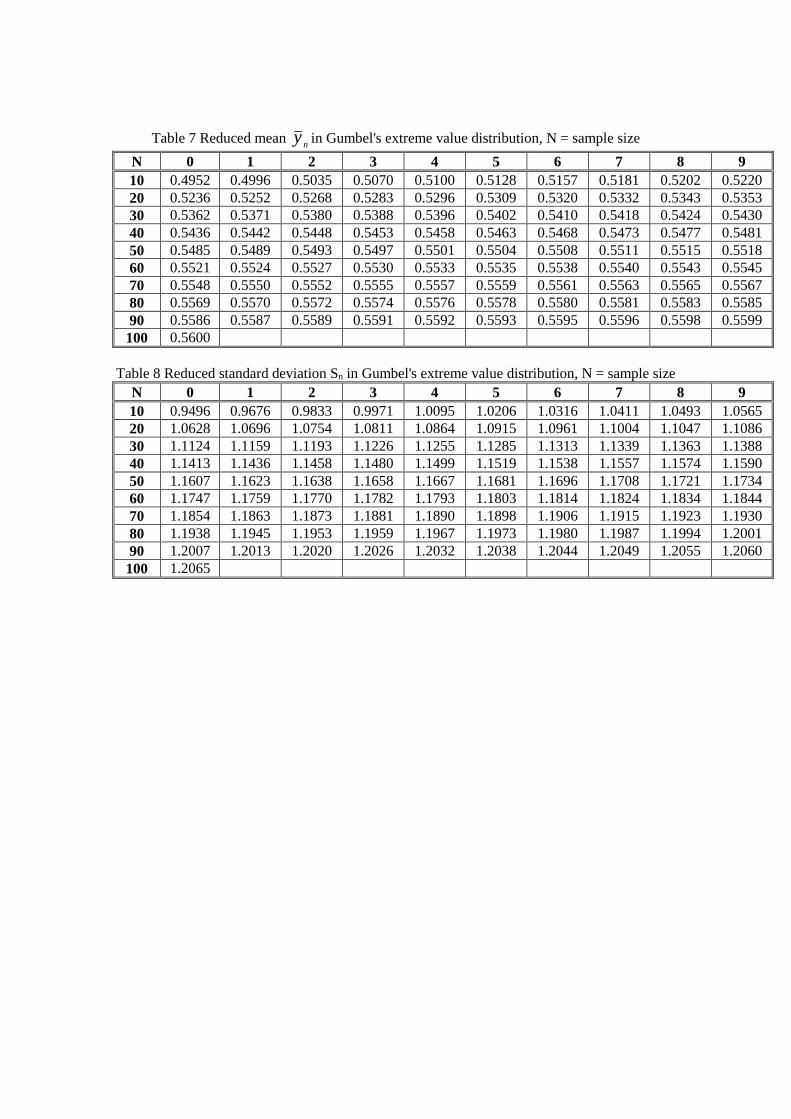
Table 7 Reduced mean yn
in Gumbel's extreme value distribution, N = sample size
N 0 1 2 3 4 5 6 7 8 9
10 0.4952 0.4996 0.5035 0.5070 0.5100 0.5128 0.5157 0.5181 0.5202 0.5220
20 0.5236 0.5252 0.5268 0.5283 0.5296 0.5309 0.5320 0.5332 0.5343 0.5353
30 0.5362 0.5371 0.5380 0.5388 0.5396 0.5402 0.5410 0.5418 0.5424 0.5430
40 0.5436 0.5442 0.5448 0.5453 0.5458 0.5463 0.5468 0.5473 0.5477 0.5481
50 0.5485 0.5489 0.5493 0.5497 0.5501 0.5504 0.5508 0.5511 0.5515 0.5518
60 0.5521 0.5524 0.5527 0.5530 0.5533 0.5535 0.5538 0.5540 0.5543 0.5545
70 0.5548 0.5550 0.5552 0.5555 0.5557 0.5559 0.5561 0.5563 0.5565 0.5567
80 0.5569 0.5570 0.5572 0.5574 0.5576 0.5578 0.5580 0.5581 0.5583 0.5585
90 0.5586 0.5587 0.5589 0.5591 0.5592 0.5593 0.5595 0.5596 0.5598 0.5599
100 0.5600
Table 8 Reduced standard deviation Sn in Gumbel's extreme value distribution, N = sample size
N 0 1 2 3 4 5 6 7 8 9
10 0.9496 0.9676 0.9833 0.9971 1.0095 1.0206 1.0316 1.0411 1.0493 1.0565
20 1.0628 1.0696 1.0754 1.0811 1.0864 1.0915 1.0961 1.1004 1.1047 1.1086
30 1.1124 1.1159 1.1193 1.1226 1.1255 1.1285 1.1313 1.1339 1.1363 1.1388
40 1.1413 1.1436 1.1458 1.1480 1.1499 1.1519 1.1538 1.1557 1.1574 1.1590
50 1.1607 1.1623 1.1638 1.1658 1.1667 1.1681 1.1696 1.1708 1.1721 1.1734
60 1.1747 1.1759 1.1770 1.1782 1.1793 1.1803 1.1814 1.1824 1.1834 1.1844
70 1.1854 1.1863 1.1873 1.1881 1.1890 1.1898 1.1906 1.1915 1.1923 1.1930
80 1.1938 1.1945 1.1953 1.1959 1.1967 1.1973 1.1980 1.1987 1.1994 1.2001
90 1.2007 1.2013 1.2020 1.2026 1.2032 1.2038 1.2044 1.2049 1.2055 1.2060
100 1.2065

Table 9 Give daily rainfall data from Merawi station
NATIONAL METEOROLOGICAL SERVICES AGENCY
STATION:MERIHAWE ELEMENT: Daily
Rainfall YEAR:1981
Date I II III IV V VI VII VIII IX X XI XII
1 0.0 0.0 6.7 15.8 0.5 0.0 7.2 0.0
2 0.0 0.0 9.4 11.5 3.7 13.5 1.9 0.0
3 0.0 0.0 39.7 14.5 0.0 0.0 12.2 0.0
4 0.0 10.5 4.0 0.6 10.2 0.5 0.1 0.0
5 0.0 5.2 7.4 25.6 12.4 9.3 0.0 0.0
6 0.0 0.5 2.2 4.5 0.0 15.2 0.0 0.0
7 4.4 0.0 33.1 12.5 2.8 0.0 0.0 0.0
8 10.1 2.0 35.1 4.7 0.4 12.7 0.0 0.0
9 0.0 6.5 45.6 0.0 1.4 14.2 0.0 0.0
10 0.0 0.0 12.2 0.0 3.0 0.0 0.0 0.0
11 0.0 0.0 11.0 45.2 3.7 0.0 0.0 0.0
12 0.2 23.5 13.5 4.5 50.8 0.0 0.0 0.0
13 6.2 19.8 13.0 0.0 0.0 0.0 0.0 0.0
14 18.7 21.9 5.3 46.4 0.0 0.0 0.0 0.0
15 6.5 14.5 0.6 3.8 30.1 0.0 0.0 0.0
16 1.2 2.1 3.8 2.3 0.0 0.0 0.0 0.0
17 2.0 0.0 33.7 5.7 4.6 0.0 0.0 0.0
18 0.0 2.3 0.0 18.0 17.1 18.1 0.0 0.0 0.0
19 0.0 0.0 40.9 6.5 18.2 2.6 0.0 0.0 0.0
20 10.0 9.0 10.9 8.1 18.7 0.4 0.0 0.0 0.0
21 2.3 26.2 37.9 12.5 13.7 12.8 0.0 0.0 0.0
22 13.6 29.2 18.1 15.1 0.0 7.0 0.0 8.2 0.0
23 2.8 0.0 0.3 26.3 0.0 0.2 0.0 0.0 0.0
24 1.3 10.0 0.0 18.2 19.8 19.7 0.0 0.0 0.0
25 0.0 9.8 0.0 58.1 4.7 14.7 0.0 0.0 0.0
26 0.0 0.0 9.3 0.0 0.0 11.8 0.0 0.0 0.0
27 0.0 0.0 7.5 31.4 5.9 1.2 0.0 0.0 0.0
28 0.0 0.8 0.0 23.1 24.3 0.0 0.0 0.0 0.0
29 0.0 0.2 0.0 59.0 133.4 0.0 0.0 0.0 0.0
30 0.0 0.0 10.0 0.9 13.4 0.0 0.0 0.0 0.0
31 0.5 14.9 15.4 7.9 0.0

Table 10 Give daily rainfall data from Merawi station
NATIONAL METEOROLOGICAL SERVICES AGENCY
STATION:MERIHAWE ELEMENT: Daily Rainfall
YEAR:1982
Date I II III IV V VI VII VIII IX X XI XII
1 0.0 0.0 2.5 0.0 0.0 0.0 0.4 5.5 2.4 6.7
2 0.0 0.0 21.7 0.0 0.0 20.1 5.0 20.0 8.4 5.6
3 0.0 0.0 1.5 0.0 0.0 1.2 14.0 28.2 1.1 7.9
4 0.0 0.0 0.0 0.0 5.3 0.0 32.1 4.6 0.0 6.9
5 0.0 0.0 5.0 0.0 15.2 4.5 2.5 22.2 18.8 1.5
6 0.0 0.0 0.2 0.0 14.2 0.0 3.3 0.6 15.0 1.9
7 0.0 0.0 0.3 0.0 24.1 4.9 2.0 4.6 0.2 4.8
8 0.0 0.0 0.0 0.0 10.6 0.0 5.1 22.9 4.1 0.0
9 14.2 0.0 1.3 0.0 0.6 0.0 2.5 7.2 24.6 0.0
10 5.4 0.0 3.0 0.0 0.0 1.9 21.0 25.0 5.2 0.0
11 0.3 0.0 0.0 0.0 0.0 16.5 1.7 9.9 0.0 3.7
12 0.0 0.0 0.4 0.0 0.0 15.6 0.9 5.0 0.0 0.0
13 0.0 0.0 0.0 0.0 0.0 51.2 0.3 3.0 6.0 10.5
14 0.0 0.0 0.0 0.0 0.0 0.5 3.9 0.5 24.2 2.4
15 0.0 0.0 1.0 0.0 0.0 13.3 11.6 13.7 11.6 0.2
16 0.0 0.0 0.0 0.0 0.0 3.1 22.6 25.9 3.1
17 0.0 0.0 0.0 0.0 0.0 3.3 6.2 10.1 3.6
18 0.0 0.0 0.0 0.0 0.3 2.1 19.0 15.8 5.4
19 0.0 0.0 0.0 0.0 0.1 0.0 14.3 2.7 1.0
20 0.0 0.0 0.0 0.0 0.0 32.5 3.6 23.0 0.0
21 0.0 0.0 0.0 0.0 0.0 12.0 22.6 6.2 0.0
22 0.0 0.0 0.0 0.0 0.0 5.3 9.3 8.4 0.8
23 0.0 0.0 0.0 0.0 0.0 0.0 9.4 1.5 1.7
24 0.0 0.0 0.0 0.0 0.0 3.5 17.4 22.6 7.4
25 0.0 0.0 0.0 0.0 0.0 20.5 2.7 1.9 5.7
26 0.0 0.0 0.0 8.3 0.0 0.1 19.3 0.0 0.0
27 0.0 0.0 0.0 0.0 24.1 0.0 0.4 19.5 4.5
28 0.0 0.0 0.0 0.0 0.0 0.9 18.4 16.4 0.0
29 0.0 0.0 3.0 0.0 19.8 1.2 100.0 0.8
30 0.0 0.0 0.0 20.9 6.7 14.2 100.0 3.0
31 0.0 0.0 29.6 0.6 5.3

Table 11 Give daily rainfall data from Merawi station
NATIONAL METEOROLOGICAL SERVICES AGENCY
STATION:MERAWI(Gojam) Element: Daily Rain fall in mm YEAR:1983
Date I II III IV V VI VII VIII IX X XI XII
1 0.2 0.0 0.0 0.0
2 0.0 0.0 0.0 0.0
3 0.0 0.0 0.0 0.0
4 2.8 0.0 0.0 0.0
5 7.0 0.2 0.0 0.0
6 26.3 0.6 0.0 0.0 0.0
7 33.5 27.2 7.9 1.0 0.0
8 0.3 17.3 0.9 0.0 0.0
9 11.5 18.0 0.0 0.1 0.0
10 0.0 71.0 0.0 0.0 0.0
11 13.9 23.6 0.0 0.0 0.0
12 6.5 2.2 0.0 0.0 0.0
13 12.1 11.6 8.8 0.0 0.0
14 16.0 1.0 9.0 0.0 0.0
15 3.9 6.0 21.6 0.0 0.0
16 17.6 0.3 2.4 1.7 0.0
17 6.0 6.5 21.5 0.7 0.0
18 9.2 1.7 32.4 1.3 0.0
19 29.3 7.8 0.5 2.2 0.0
20 29.0 0.8 7.8 0.0 0.0
21 22.4 0.0 10.8 0.0 0.0
22 19.7 0.2 0.0 0.0 0.0
23 11.9 26.7 0.0 0.0 0.0
24 13.0 0.3 0.0 0.0 0.0
25 29.0 0.0 0.0 0.0 0.0
26 1.0 0.0 0.0 0.0 0.0
27 45.4 0.0 0.0 0.0 0.0
28 2.3 7.7 0.0 0.0 0.0
29 3.2 2.6 0.0 0.0 0.0
30 12.2 0.0 0.0 0.0 0.0
31 12.9 0.0 0.0

Table 12 Give daily rainfall data from Merawi station
NATIONAL METEOROLOGICAL SERVICES AGENCY
STATION:MERAWE ELEMENT: Daily Rainfall
YEAR:1984
Date I II III IV V VI VII VIII IX X XI XII
1 0.0 0.0 0.0 0.0 6.2 22.1 8.0 0.0 0.0
2 0.0 0.0 0.0 0.0 0.6 17.3 9.0 0.0 0.0
3 0.0 0.0 4.0 0.0 22.5 11.7 8.0 0.0 0.0
4 0.0 0.0 0.1 0.0 14.9 34.7 30.1 0.0 0.0
5 0.0 0.0 0.0 0.0 0.1 0.0 T.R 0.0 T.R
6 0.0 0.0 0.0 0.0 17.7 T.R 0.0 0.0
7 0.0 0.0 0.0 0.0 0.0 0.0 0.0 0.0
8 0.0 0.0 0.0 0.0 1.3 T.R 1.9 0.0 0.0
9 0.0 0.0 0.0 0.0 2.0 1.1 18.0 0.0 0.0
10 0.0 0.0 0.0 0.0 0.0 16.0 1.5 0.0 10.3
11 0.0 0.0 0.0 0.0 2.1 79.1 T.R 0.0 0.0 0.0
12 0.0 0.0 0.0 0.0 0.0 11.6 85.0 0.0 0.0 0.0
13 0.0 0.0 0.0 0.0 0.0 26.1 3.7 0.0 0.0 0.0
14 0.0 0.0 0.0 0.0 85.9 6.7 30.0 0.0 0.0 0.0
15 0.0 0.0 0.0 0.0 35.0 14.5 30.0 0.0 0.0 0.0
16 0.0 0.0 0.0 0.0 87.9 43.1 2.3 0.0 0.0 0.0
17 0.0 0.0 0.0 0.0 23.5 0.3 15.0 0.0 0.0 0.0
18 0.0 0.0 0.0 0.0 12.1 7.0 0.0 0.0 0.0 0.0
19 0.0 0.0 11.0 14.5 9.4 0.6 0.2 0.0 0.0 0.0
20 0.0 0.0 5.5 T.R 13.0 173.0 T.R 0.0 0.0 0.0
21 0.0 0.0 0.5 15.6 14.0 8.1 0.0 0.0 0.0 0.0
22 0.0 0.0 0.0 15.1 9.7 27.8 0.0 0.0 0.0 4.3
23 0.0 0.0 0.0 0.0 8.0 6.0 98.0 0.0 0.0 0.0
24 0.0 0.0 0.0 0.0 0.0 46.0 3.0 0.0 0.0 0.0
25 0.0 0.0 0.0 0.0 17.1 11.6 0.0 0.0 0.0 0.0
26 0.0 0.0 0.0 0.0 0.0 18.6 0.0 0.0 0.0 7.5
27 0.0 0.0 0.0 0.0 1.0 1.3 0.0 0.0 0.0 3.2
28 0.0 0.0 0.0 0.0 0.0 11.8 0.0 0.0 0.0 0.0
29 0.0 0.0 0.0 0.0 2.5 3.6 0.0 0.0 0.0 0.0
30 0.0 0.0 0.0 0.0 3.0 7.1 0.0 0.0 0.0 0.0
31 0.0 0.0 0.0 19.8 0.0

Table 13 Give daily rainfall data from Merawi station
NATIONAL METEOROLOGICAL SERVICES AGENCY
STATION:MERAWI Wereda:MECHIA Awraja:BAHRDAR
Region:Gojam
Alt.______ Long.________Lat._________ Element: Daily Rain Fall
YEAR:1985
Date I II III IV V VI VII VIII IX X XI XII
1 0.0 0.0 0.0 0.0 3.6 15.7 15.7 1.8 6.8 0.4 0.0 0.0
2 0.0 0.0 0.0 0.0 0.0 0.6 31.8 24.1 0.0 0.0
3 0.0 0.7 0.0 7.7 16.7 0.0 17.0 16.2 14.0 7.3 0.0 0.0
4 0.0 0.3 0.0 4.7 0.4 0.0 3.1 10.9 13.6 2.2 2.5 1.6
5 0.0 T.R 0.0 1.9 5.4 0.0 19.7 8.6 0.1 0.3 14.6 0.5
6 0.0 0.0 0.0 0.0 0.0 0.0 1.7 6.8 0.7 0.0 0.0 0.0
7 0.0 0.0 0.0 2.1 6.6 2.4 1.4 30.9 1.0 0.0 0.0 0.5
8 0.0 0.0 0.0 0.0 0.0 33.3 3.0 8.9 16.7 5.3 0.0 0.0
9 0.0 0.0 0.0 0.0 0.0 0.0 11.3 5.8 11.8 2.7 0.0 0.0
10 0.0 0.0 0.0 0.0 0.0 0.0 21.3 12.8 3.6 0.0 0.0 0.0
11 0.0 0.0 0.0 0.0 0.0 2.3 20.1 16.3 0.8 0.0 0.0 0.0
12 0.0 0.0 0.0 0.0 22.4 2.8 19.6 10.0 22.5 7.4 0.0 0.0
13 0.0 0.0 0.0 0.0 6.3 0.0 13.5 15.4 0.3 0.7 0.0 0.0
14 0.0 0.0 0.0 0.0 6.6 3.7 1.8 4.5 35.6 0.0 0.0 0.0
15 0.0 0.0 0.0 0.0 9.2 0.6 16.2 5.5 0.0 0.0 0.0 0.0
16 0.0 0.0 0.0 5.6 26.8 3.6 3.5 2.4 0.0 0.0 0.0
17 0.0 0.0 0.0 0.0 0.3 5.1 3.8 11.1 2.0 0.0 10.6 0.0
18 0.0 0.0 0.0 0.0 0.3 3.7 15.0 9.0 9.1 0.0 0.0 0.0
19 0.0 0.0 0.0 0.0 1.6 6.7 56.6 12.7 0.5 0.0 0.0 0.0
20 0.0 0.0 11.5 1.5 2.5 0.0 13.9 17.8 0.0 0.0 0.0 0.0
21 0.0 0.0 0.5 10.1 23.7 11.8 23.8 5.4 6.8 0.0 0.0 0.0
22 0.0 0.0 0.0 0.0 1.4 0.1 6.6 0.1 9.5 0.0 0.0 0.0
23 0.0 0.0 0.0 0.0 3.0 12.1 6.1 31.8 0.0 0.0 0.0 0.0
24 0.0 0.0 0.0 0.0 12.1 5.0 1.3 16.8 0.0 0.0 0.0
25 0.0 0.0 0.6 0.0 6.7 15.5 37.8 8.5 0.0 0.0 0.0 0.0
26 0.0 0.0 0.0 0.0 9.5 1.2 23.5 25.0 9.6 0.0 0.0 0.0
27 0.0 0.0 0.0 0.0 1.5 0.7 8.4 8.6 0.0 0.0 0.0 0.0
28 0.0 0.0 0.0 0.0 3.8 27.5 10.5 6.3 0.0 0.0 0.0 0.0
29 0.0 0.0 0.0 13.1 1.0 24.7 21.3 1.1 0.0 0.0 0.0
30 0.0 0.0 0.0 12.5 6.6 13.0 26.3 9.8 28.5 0.0 0.0
31 0.0 0.0 4.8 5.8 7.4 22.5 0.0

Table 14 Give daily rainfall data from Merawi station
NATIONAL METEOROLOGICAL SERVICES AGENCY
STATION:MERAWI Wereda:MECHIA Awraja:BAHRDAR
Region:Gojam
Alt.______ Long.________Lat._________ Element: Daily Rain Fall
YEAR:1986
Date I II III IV V VI VII VIII IX X XI XII
1 0.0 0.0 0.0 0.1 0.0 5.8 11.6 1.2 12.3 0.0 0.0
2 0.0 0.0 0.0 0.0 0.0 19.2 62.7 10.7 19.5 0.5 0.0 0.0
3 0.0 0.0 0.0 0.5 0.0 0.7 T.R 12.6 1.0 9.9 0.0 0.0
4 0.0 0.0 0.0 1.4 0.0 3.1 29.2 1.4 12.9 7.5 0.0 0.0
5 0.0 0.0 0.0 0.0 0.0 0.0 12.0 0.9 49.3 13.5 0.0 0.0
6 0.0 0.0 0.0 0.0 0.0 0.0 11.6 0.6 45 0.3 0.0 0.0
7 0.0 0.0 0.0 0.0 0.0 1.5 8.0 7.0 23.0 0.0 0.0 0.0
8 0.0 0.0 2.0 0.0 0.0 0.9 13.7 6.0 14.0 0.0 0.0 0.0
9 0.0 0.0 0.0 0.0 0.0 29.0 17.7 6.7 32.1 0.0 0.0 0.0
10 0.0 0.0 0.0 0.0 2.6 14.1 18.2 7.7 1.6 0.0 0.0 0.0
11 0.0 0.0 0.0 0.0 0.0 21.3 8.3 8.7 0.7 0.0 0.0 0.0
12 0.0 0.0 0.0 0.0 0.0 12.0 6.5 3.1 0.3 0.0 0.0 0.0
13 0.0 0.0 0.0 0.0 0.0 15.9 0.0 4.2 4.4 0.0 0.0 0.0
14 0.0 0.0 0.0 0.0 0.0 40.0 13.5 1.8 12.0 0.0 0.0 0.0
15 0.0 0.0 0.0 0.0 0.0 15.0 16.6 0.2 7.2 1.6 0.0 0.0
16 0.0 0.0 0.0 6.0 0.0 17.4 1.1 2.4 0.5 0.0 0.0 0.0
17 0.0 0.0 0.0 0.4 0.0 42.5 1.5 2.9 0.9 0.0 0.0
18 0.0 0.0 0.0 4.3 0.0 29.7 4.1 2.0 0.7 0.0 0.0
19 0.0 0.0 0.0 0.0 0.0 0.3 16.9 5.7 4.4 0.0 28.4 0.0
20 0.0 0.0 0.0 0.0 0.0 7.7 5.7 29.2 7.3 9.7 0.0 0.0
21 0.0 0.0 0.0 0.0 0.0 4.2 30.6 1.6 6.1 1.1 0.0 0.0
22 0.0 0.0 0.0 0.0 0.0 16.2 9.7 6.0 2.0 4.5 0.0 0.0
23 0.0 0.0 0.0 0.0 0.8 0.4 8.7 0.0 0.0 0.0
24 0.0 0.0 0.0 3.4 0.0 10.7 24.8 0.0 0.0 2.2 0.0 0.0
25 0.0 0.0 2.2 3.3 0.0 14.0 14.0 16.1 0.4 0.0 0.0 0.0
26 0.0 0.0 0.0 0.0 0.0 7.4 23.4 15.0 2.5 0.0 0.0 0.0
27 0.0 0.0 0.0 0.0 10.1 11.1 8.7 1.7 8.5 0.0 0.0 0.0
28 0.0 4.5 0.0 0.0 5.5 46.0 21.0 2.1 4.8 0.0 0.0 0.0
29 0.0 0.2 0.0 0.0 2.7 36.0 10.5 23.4 0.0 0.0 0.0
30 0.0 0.0 0.0 3.0 0.4 3.0 11.5 65.7 0.0 0.0 0.0
31 0.0 0.1 0.0 57.8 1.2 0.0 0.0 0.0
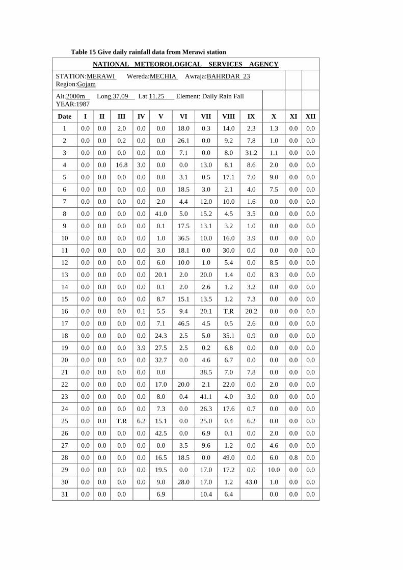
Table 15 Give daily rainfall data from Merawi station
NATIONAL METEOROLOGICAL SERVICES AGENCY
STATION:MERAWI Wereda:MECHIA Awraja:BAHRDAR 23
Region:Gojam
Alt.2000m Long.37.09 Lat.11.25 Element: Daily Rain Fall
YEAR:1987
Date I II III IV V VI VII VIII IX X XI XII
1 0.0 0.0 2.0 0.0 0.0 18.0 0.3 14.0 2.3 1.3 0.0 0.0
2 0.0 0.0 0.2 0.0 0.0 26.1 0.0 9.2 7.8 1.0 0.0 0.0
3 0.0 0.0 0.0 0.0 0.0 7.1 0.0 8.0 31.2 1.1 0.0 0.0
4 0.0 0.0 16.8 3.0 0.0 0.0 13.0 8.1 8.6 2.0 0.0 0.0
5 0.0 0.0 0.0 0.0 0.0 3.1 0.5 17.1 7.0 9.0 0.0 0.0
6 0.0 0.0 0.0 0.0 0.0 18.5 3.0 2.1 4.0 7.5 0.0 0.0
7 0.0 0.0 0.0 0.0 2.0 4.4 12.0 10.0 1.6 0.0 0.0 0.0
8 0.0 0.0 0.0 0.0 41.0 5.0 15.2 4.5 3.5 0.0 0.0 0.0
9 0.0 0.0 0.0 0.0 0.1 17.5 13.1 3.2 1.0 0.0 0.0 0.0
10 0.0 0.0 0.0 0.0 1.0 36.5 10.0 16.0 3.9 0.0 0.0 0.0
11 0.0 0.0 0.0 0.0 3.0 18.1 0.0 30.0 0.0 0.0 0.0 0.0
12 0.0 0.0 0.0 0.0 6.0 10.0 1.0 5.4 0.0 8.5 0.0 0.0
13 0.0 0.0 0.0 0.0 20.1 2.0 20.0 1.4 0.0 8.3 0.0 0.0
14 0.0 0.0 0.0 0.0 0.1 2.0 2.6 1.2 3.2 0.0 0.0 0.0
15 0.0 0.0 0.0 0.0 8.7 15.1 13.5 1.2 7.3 0.0 0.0 0.0
16 0.0 0.0 0.0 0.1 5.5 9.4 20.1 T.R 20.2 0.0 0.0 0.0
17 0.0 0.0 0.0 0.0 7.1 46.5 4.5 0.5 2.6 0.0 0.0 0.0
18 0.0 0.0 0.0 0.0 24.3 2.5 5.0 35.1 0.9 0.0 0.0 0.0
19 0.0 0.0 0.0 3.9 27.5 2.5 0.2 6.8 0.0 0.0 0.0 0.0
20 0.0 0.0 0.0 0.0 32.7 0.0 4.6 6.7 0.0 0.0 0.0 0.0
21 0.0 0.0 0.0 0.0 0.0 38.5 7.0 7.8 0.0 0.0 0.0
22 0.0 0.0 0.0 0.0 17.0 20.0 2.1 22.0 0.0 2.0 0.0 0.0
23 0.0 0.0 0.0 0.0 8.0 0.4 41.1 4.0 3.0 0.0 0.0 0.0
24 0.0 0.0 0.0 0.0 7.3 0.0 26.3 17.6 0.7 0.0 0.0 0.0
25 0.0 0.0 T.R 6.2 15.1 0.0 25.0 0.4 6.2 0.0 0.0 0.0
26 0.0 0.0 0.0 0.0 42.5 0.0 6.9 0.1 0.0 2.0 0.0 0.0
27 0.0 0.0 0.0 0.0 0.0 3.5 9.6 1.2 0.0 4.6 0.0 0.0
28 0.0 0.0 0.0 0.0 16.5 18.5 0.0 49.0 0.0 6.0 0.8 0.0
29 0.0 0.0 0.0 0.0 19.5 0.0 17.0 17.2 0.0 10.0 0.0 0.0
30 0.0 0.0 0.0 0.0 9.0 28.0 17.0 1.2 43.0 1.0 0.0 0.0
31 0.0 0.0 0.0 6.9 10.4 6.4 0.0 0.0 0.0

Table 16 Give daily rainfall data from Merawi station
NATIONAL METEOROLOGICAL SERVICES AGENCY
STATION:MERAWI Wereda:MECHIA Awraja:BAHRDAR
Region:Gojam
Alt.202m Long. Lat._________ Element: Daily Rain
Fall YEAR:1988
Date I II III IV V VI VII VIII IX X XI XII
1 0.0 0.0 0.0 0.0 1.5 0.0 0.0 8.1 TR 0.0 0.0 0.0
2 0.2 0.0 0.0 0.0 4.6 8.8 41.7 14.0 16.0 8.7 0.0 0.0
3 0.0 0.0 0.0 0.0 3.5 25.7 3.1 0.6 28.4 1.5 0.0 0.0
4 0.0 4.3 0.0 0.0 22.0 7.5 3.8 6.3 5.3 20.0 3.0 0.0
5 0.0 5.5 0.0 0.0 26.3 7.3 42.3 20.0 0.0 1.4 0.0 0.0
6 0.0 0.0 0.0 0.0 40.4 0.0 52.0 0.0 8.3 1.5 14.4 0.0
7 0.0 0.0 0.0 0.0 8.6 TR 3.0 7.6 18.6 25.0 0.0 0.0
8 0.0 0.0 0.0 0.0 5.3 11.6 23.6 12.3 22.0 38.0 0.0 0.0
9 0.0 0.0 0.0 0.0 0.0 5.3 21.0 1.0 6.8 2.4 0.0 0.0
10 0.0 0.0 0.0 0.0 0.0 31.0 24.2 3.0 11.0 31.3 0.0 0.0
11 0.0 0.0 0.0 0.0 0.0 0.0 7.6 24.7 0.6 1.5 0.0 0.0
12 0.0 0.0 0.0 0.0 1.5 11.6 2.5 12.0 1.7 3.7 0.0 0.0
13 0.0 0.0 0.0 0.0 0.0 9.5 11.5 22.0 14.2 12.5 0.0 0.0
14 11.0 0.0 0.0 0.0 0.0 8.8 48.6 15.0 0.0 T.R 0.0 0.0
15 0.0 0.0 0.0 0.0 0.0 27.2 5.0 0.0 0.0 11.0 5.9 0.0
16 0.0 0.0 0.0 0.0 0.0 42.7 20.8 16.1 14.8 4.7 0.0
17 0.0 0.0 0.0 0.0 12.3 16.5 25.6 1.5 0.2 6.1 0.0 0.0
18 0.0 0.0 0.0 0.0 3.4 21.0 3.8 12.8 T.R 0.0 0.0 0.0
19 0.0 0.0 0.0 0.0 7.3 0.1 3.3 22.4 4.7 0.0 0.0 0.0
20 0.0 1.6 0.0 0.0 14.3 0.0 15.8 14.5 9.0 0.0 0.0 0.0
21 0.0 0.6 0.0 0.0 2.3 0.3 3.1 0.3 0.0 0.0 0.0
22 0.0 1.4 0.0 0.0 0.0 40.6 2.4 10.4 TR 0.0 0.0 0.0
23 0.0 6.9 0.0 0.0 0.0 7.6 53.5 12.0 0.0 0.0 0.0 0.0
24 0.0 0.0 0.0 0.0 0.0 3.0 8.5 TR 0.0 0.0 0.0 0.0
25 0.0 0.0 0.0 0.0 0.0 0.6 2.1 11.0 0.1 0.0 0.0 0.0
26 0.0 0.0 0.0 0.0 0.0 0.3 39.0 4.3 5.0 2.1 0.0 0.0
27 0.0 0.0 0.0 0.0 0.0 22.2 17.2 8.0 20.8 0.4 0.0 0.0
28 0.0 0.0 0.0 0.0 0.0 28.0 10.0 2.3 X 10.3 0.0 0.0
29 0.0 0.0 0.0 0.0 0.0 30.0 4.0 14.2 0.0 0.0 0.2
30 0.0 0.0 0.0 0.0 0.0 2.1 0.0 0.0 0.0 0.0
31 0.0 0.0 0.0 0.0 0.0 7.1 2.1 0.0 TR

Table 17 Give daily rainfall data from Merawi station
NATIONAL METEOROLOGICAL SERVICES AGENCY
STATION:MERAWI Wereda:MECHIA Awraja:BAHRDAR Region:Gojam
Alt.202m Long.________Lat._________ Element: Daily Rain Fall YEAR:1989
Date I II III IV V VI VII VIII IX X XI XII
1 0.0 0.0 0.0 0.0 1.5 12.5 8.5 0.0 1.6 12.0 0.0
2 0.0 0.0 0.0 0.0 0.5 10.3 0.0 4.0 0.0 0.1 0.0
3 0.0 0.0 0.0 0.0 0.0 14.6 50.3 0 0.0 0.0 0.0
4 0.0 0.0 0.0 0.0 0.0 2.3 6.7 1.3 0.0 0.0 0.0
5 0.0 0.0 0.0 0.0 0.0 1.3 8.7 TR 0.0 0.0 13.6
6 0.0 0.0 0.0 0.0 41.3 11.0 10.0 2.2 0.0 0.0 0.0
7 0.0 0.0 0.0 0.0 0.2 20.0 6.5 0.0 0.0 0.0 0.0
8 0.0 0.0 0.0 0.0 36.4 22.0 12.3 8.3 0.0 0.0 0.0
9 0.0 0.0 0.0 0.0 7.6 5.1 3.5 5.0 9.3 0.0 0.0
10 0.0 0.0 0.0 0.0 9.3 20.1 6.4 8.1 0.0 0.0 0.0
11 0.0 0.0 1.3 0.0 6.6 9.0 31.6 0.0 0.0 0.0 0.0
12 0.0 0.0 3.7 0.0 13.9 0.0 22.4 8.3 0.0 0.0 0.0
13 0.0 0.0 0.1 0.0 2.9 2.2 18.0 7.2 0.0 0.0
14 0.0 0.0 0.2 TR 0.0 18.2 10.0 0.0 0.0 0.0
15 0.0 0.0 TR 0.0 0.2 30.0 0.0 TR 0.0 0.0
16 0.0 0.0 0.0 1.1 21.0 15.6 0.0 1.1 0.0 0.0
17 0.0 0.0 0.0 10.1 0.0 3.5 10.2 12.2 13.4 0.0 0.0
18 0.0 0.0 0.0 5.3 4.1 2.3 10.7 15.5 29.8 0.0 3.5
19 0.0 0.0 0.0 TR 2.0 0.0 0.0 1.2 1.0 0.0 0.0
20 0.0 0.0 0.0 14.2 0.4 18.3 2.0 32.6 0.0 0.0 0.0
21 0.0 0.0 0.0 13.5 19.6 29.1 10.0 0.0 7.3 0.0 0.0
22 0.0 0.0 0.0 0.0 13.2 19.5 10.6 0.0 0.3 0.0 0.0
23 0.0 0.0 0.0 3.0 0.0 0.6 10.7 0.0 26.0 0.0 0.0
24 0.0 0.0 0.0 1.9 0.0 13.2 2.3 0.0 0.0 0.0 0.0
25 0.0 0.0 0.0 0.0 5.1 13.1 20.0 1.6 0.0 0.0 0.0
26 0.0 0.0 10.3 0.0 5.2 19.1 44.5 11.4 0.0 0.0 0.0
27 0.0 0.0 1.2 0.0 0.0 29.5 0.0 15.0 0.0 0.0 0.0
28 0.0 0.0 0.1 0.0 2.2 16.5 10.7 0.0 0.0 TR 0.0
29 0.0 0.0 29.6 0.0 6.3 8.0 42.6 0.0 0.0 0.0 0.0
30 0.0 0.0 0.0 12.0 4.5 4.6 14.2 6.0 0.0 0.0
31 0.0 0.0 0.0 3.5 2.0 TR 0.0

Table 18 Give daily rainfall data from Merawi station
NATIONAL METEOROLOGICAL SERVICES AGENCY
STATION:MERAWI Wereda:MECHIA Awraja:BAHRDAR
Region:Gojam
Alt.______ Long.________Lat._________ Element: Daily Rain Fall
YEAR:1990
Date I II III IV V VI VII VIII IX X XI XII
1 0.0 TR 0.0 0.0 5.6 11.5 41.2 10.6 2.0
2 0.0 0.0 0.0 0.0 9.3 3.0 2.3 11.1 5.2
3 0.0 0.0 0.0 0.0 0.0 18.0 5.9 6.4 6.1
4 0.0 0.0 0.0 0.0 0.0 11.4 39.0 19.7 2.4
5 0.0 0.0 0.0 0.0 0.0 0.3 3.2 38.7 1.3
6 0.0 0.0 0.0 0.0 0.0 0.0 0.6 4.1 40
7 0.0 0.0 0.0 0.0 7.9 0.0 2.5 7.4 6.2
8 0.0 0.0 0.0 0.0 0.1 0.0 34.8 4.3
9 0.0 0.0 0.0 0.0 15.3 0.0 1.0 0.0 0.0
10 0.0 0.0 0.0 0.0 0.0 0.0 7.6 9.3 8.1
11 0.0 0.0 0.0 0.0 15.0 0.0 32.8 0.2 13.7
12 0.0 0.0 0.0 0.0 0.0 0.0 13.0 83.6 7.8
13 0.0 0.0 0.0 0.0 0.0 3.2 5.3 74.5 1.7
14 0.0 0.0 0.0 0.0 0.0 0.0 8.3 13.4 0.0
15 0.0 0.0 3.0 0.0 0.0 3.6 0.0 11.3 0.0
16 0.0 0.0 0.0 0.0 0.0 0.8 6.0 6.9 0.0
17 0.0 0.0 0.0 0.0 0.0 8.0 18.0 40.3 14.3
18 0.0 0.0 0.0 0.0 0.0 37.0 27.0 51.3 13.5
19 0.0 0.0 0.0 0.0 0.0 18.6 2.5 70.4 11.0
20 0.0 0.0 0.0 TR 0.0 1.2 15.0 9.6 9.0
21 0.0 0.0 0.0 0.0 0.0 0.0 23.2 34.2 0.2
22 0.0 0.0 2.0 0.0 0.0 1.0 23.2 3.2 13.2
23 0.0 0.0 2.5 0.0 0.0 0.0 18.4 4.2 4.2
24 0.0 0.0 3.1 0.0 0.0 17.2 1.7 12.2 0.0
25 0.0 0.0 1.4 0.0 0.0 10.3 0.5 5.3 0.1
26 0.0 0.0 2.1 0.0 0.0 17.0 34.2 15.5 26.5
27 0.0 0.0 5.3 0.0 0.0 21.5 18.3 0.2 9.5
28 0.0 0.0 0.0 0.0 0.0 4.3 2.0
29 0.0 0.0 2.5 0.1 19.3 59.8 7.1 8.3
30 2.6 0.0 0.0 0.0 6.2 6.2 14.2 22.3
31 0.0 0.0 10.0 23.3 0.0

Table 19 Give daily rainfall data from Merawi station
NATIONAL METEOROLOGICAL SERVICES AGENCY
STATION:MERAWI Wereda:MECHIA Awraja:BAHRDAR
Region:Gojam
Alt.______ Long.________Lat._________ Element: Daily Rain Fall
YEAR:1991
Date I II III IV V VI VII VIII IX X XI XII
1 0.0 0.0 0.0 0.0 0.0 0.0 83.3 13.0 12.7 10.0 0.0 0.0
2 0.0 0.0 0.0 0.0 0.0 2.0 3.2 0.0 0.0 1.3 11.0 0.0
3 0.0 0.0 0.0 0.0 0.0 1.1 7.7 0.0 35.8 3.4 0.0 0.0
4 0.3 0.0 0.0 0.0 0.0 0.0 0.6 48.3 93.1 7.1 0.0 0.0
5 0.0 0.0 0.0 8.7 11.2 0.0 14.1 1.7 TR 27.3 0.0 0.0
6 0.0 0.0 0.0 15.1 0.0 0.0 15.0 8.1 1.3 30.5 0.0 0.0
7 0.0 0.0 0.0 16.0 4.0 76.3 12.5 2.2 TR 1.5 0.9 25.8
8 0.0 0.0 4.5 0.8 14.5 0.0 11.4 12.4 13.2 0.0 4.1 0.0
9 0.0 0.0 0.0 14.1 0.8 0.0 31.7 23.6 6.6 0.0 TR 0.0
10 0.0 0.0 0.0 6.2 0.0 0.0 11.3 16.0 17.7 24.8 0.0 0.0
11 0.0 0.0 0.0 10.0 0.0 18.5 22.0 44.3 13.6 0.0 0.0 0.0
12 0.0 0.0 0.0 15.0 0.0 15.3 7.3 14.9 42.4 0.0 0.0 0.0
13 0.0 0.0 0.0 7.0 0.0 9.0 32.5 21.2 14.0 0.0 0.0 0.0
14 0.0 0.0 0.0 0.3 0.0 28.2 40.2 6.2 2.7 0.0 0.0 0.0
15 0.0 0.0 0.0 0.2 0.0 8.3 17.3 11.2 4.2 0.0 0.0 0.0
16 0.0 0.0 0.0 0.3 0.0 0.0 10.4 16.0 3.2 0.0 0.0 0.0
17 0.0 0.0 0.0 0.0 0.0 0.0 19.2 TR 9.8 8.2 0.0 0.0
18 0.0 0.0 0.0 13.0 0.0 0.0 30.6 20.0 0.0 0.0 0.0 0.0
19 0.0 0.0 0.0 8.0 0.4 34.7 18.1 20.1 2.0 0.0 0.0 0.0
20 0.0 0.0 0.0 15.7 8.0 6.7 25.0 30.2 0.0 0.0 0.0 0.0
21 0.0 0.0 0.0 1.2 4.9 20.2 7.4 TR 15.5 0.0 0.0 0.0
22 0.0 0.0 0.1 0.0 0.0 3.7 36.4 11.5 0.0 13.2 0.0 0.0
23 0.0 0.0 0.0 0.0 23.5 24.2 26.5 14.6 7.1 0.0 0.0 0.0
24 0.0 0.0 3.1 0.0 0.0 24.2 17.6 TR 20.2 3.8 0.0 0.0
25 0.0 0.0 0.0 0.0 0.0 6.5 8.2 0.0 0.5 0.0 0.0 0.0
26 0.0 0.0 0.0 0.0 0.0 5.3 15.3 12.9 0.0 0.0 0.0 0.0
27 0.0 0.0 0.0 0.0 0.0 2.1 10.0 24.0 0.0 0.0 0.0 0.0
28 0.0 0.0 0.0 0.0 0.0 3.5 12.3 23.7 0.0 0.0 0.0 0.0
29 0.0 0.0 0.0 8.1 19.2 20.6 15.0 5.0 0.0 0.0 0.0
30 0.0 0.0 0.0 1.3 17.6 0.0 10.0 11.0 0.0 0.0 0.0
31 0.0 2.3 22.1 4.7 0.0 0.0

Table 20 Give daily rainfall data from Merawi station
NATIONAL METEOROLOGICAL SERVICES AGENCY
STATION:MERAWI Wereda:MECHIA Awraja:BAHRDAR
Region:Gojam
Alt.______ Long.________Lat._________ Element: Daily Rain Fall
YEAR:1992
Date I II III IV V VI VII VIII IX X XI XII
1 0.0 0.0 0.0 0.0 0.0 0.0 62.5 13.1 12.6
2 0.0 0.0 0.0 0.0 0.0 14.0 11.0 10.0 4.0
3 0.0 0.0 0.0 0.0 0.0 0.0 24.0 41.6 0.0
4 0.0 0.0 0.0 0.0 0.0 0.0 18.0 6.5 0.0
5 0.0 0.0 0.0 0.0 0.0 0.0 12.5 13.5 0.9
6 0.0 0.0 0.0 0.0 0.0 4.5 8..3 10.2 17.3
7 0.0 0.0 0.0 0.0 0.0 1.7 2.6 13.6 8.1
8 0.0 0.0 0.0 0.0 0.0 3.5 0.0 7.5 20.3
9 0.0 0.0 0.0 0.0 2.4 0.5 10.5 1.1 0.5
10 0.0 0.0 0.0 0.0 41.5 0.0 9.0 28.9 2.1
11 0.0 0.0 0.0 0.0 0.0 7.2 0.3 19.4 8.9
12 0.0 0.0 0.0 0.0 0.0 55.8 6.6 0.0 0.0
13 0.0 0.0 2.3 0.0 0.0 31.5 5.7 5.0 4.5
14 0.0 0.0 0.0 0.0 4.2 3.4 17.5 6.0 8.3
15 0.0 0.0 0.0 0.0 1.0 6.0 6.7 6.0 0.0
16 0.0 0.0 0.1 16.6 9.8 0.0 13.9 10.1 0.0
17 0.0 0.0 0.3 0.0 0.0 0.0 15.4 0.4 0.6
18 0.0 0.0 TR 0.8 0.0 6.5 5.0 73.0 13.0
19 0.0 0.0 0.0 7.3 0.0 38.0 3.0 8.3 4.3
20 0.0 0.0 0.0 0.1 0.4 0.0 8.9 11.1 6.7
21 0.0 0.0 0.0 0.0 0.0 0.0 21.4 1.8 0.0
22 0.0 0.0 0.0 0.0 0.0 0.2 12.6 8.3 0.0
23 0.0 0.0 0.0 0.6 0.0 25.3 16.5 5.0 0.0
24 0.0 0.0 0.6 74.6 0.0 0.4 30.8 0.0 1.1
25 0.0 0.0 0.0 2.3 0.0 7.7 23.2 0.2 21.0
26 0.0 0.0 0.0 3.1 0.0 18.0 16.9 3.2 37.0
27 0.0 0.0 0.0 2.0 0.0 15.0 23.3 26.0 0.0
28 0.0 0.0 0.0 TR 0.0 24.2 28.6 7.1 0.0
29 0.0 0.0 0.0 0.0 TR 8.9 30.8 11.0 TR
30 0.0 0.0 0.0 0.0 1.0 5.3 25.2 TR
31 0.0 0.0 0.0 13.1 0.0

Table 21 Give daily rainfall data from Merawi station
NATIONAL METEOROLOGICAL SERVICES AGENCY
STATION:MERAWI Wereda: Awraja: Region:Gojam
Alt.______ Long.________Lat.________ Element: Daily Rain Fall YEAR:1994
Date I II III IV V VI VII VIII IX X XI XII
1 0.1 23 0.0 0.0 0.5 0.0
2 4.8 4.1 12.1 0.0 0.0 0.0
3 14.5 7.6 0.0 0.0 0.0 0.0
4 8.1 7.6 25.5 0.0 0.0 0.0
5 2.5 9.0 0.7 0.1 0.0 0.0
6 19.0 2.1 0.0 0.0 0.0 0.0
7 3.3 2.3 0.8 TR 0.0 0.0
8 2.2 4.6 0.0 33.8 0.0 0.0
9 0.1 16.5 0.0 0.0 0.0 0.0
10 18.6 0.1 TR 27.7 11.0 0.0
11 2.4 7.4 0.0 0.0 TR 0.0
12 2.9 39.0 0.9 0.0 0.0 0.0
13 13.0 1.4 6.5 0.0 0.0 0.0
14 0.0 20.7 1.4 0.0 0.0 0.0
15 3.2 3.7 3.6 0.0 0.0 0.0
16 4.3 0.5 0.0 0.0 0.0 0.0
17 2.4 11.3 7.9 2.1 0.0 0.0
18 2.9 36.0 7.8 16.0 0.0 0.0
19 0.0 4.4 29.1 0.0 0.0 0.0
20 3.0 29.4 5.9 0.0 0.0 0.0
21 10.0 0.0 22.1 0.0 0.0 0.0
22 6.6 0.0 26.3 0.0 9.0 0.0
23 4.8 0.0 1.0 0.0 0.0 0.0
24 13.2 26.1 8.3 0.0 0.0 0.0
25 4.0 6.6 TR 0.0 0.0 0.0
26 0.6 33.0 0.0 0.0 11.5 0.0
27 17.3 28.7 TR 0.0 0.0 0.0
28 10.0 0.0 0.0 0.0 0.0 0.0
29 0.2 5.0 0.0 5.8 0.0 0.0
30 51.5 13.0 0.0 TR 0.0 0.0
31 4.4 26.0 0.6 0.0 0.0

Table 22 Give daily rainfall data from Merawi station
NATIONAL METEOROLOGICAL SERVICES AGENCY
STATION:MERAWI Wereda:MECHIA Awraja:-------
Region:W.Gojam
Alt.______ Long.________Lat._________ Element: Daily Rain Fall
YEAR:1995
Date I II III IV V VI VII VIII IX X XI XII
1 0.0 0.0 0.0 1.1 0.0 TR 3.2 2.4 18.8 7.8 6.4 0.0
2 0.0 0.0 0.0 4.6 26.1 0.1 2.4 4.4 0.0 0.0 0.0
3 0.0 0.0 0.0 0.0 20.5 0.0 2.0 12.7 14.9 0.0 0.0 0.0
4 0.0 0.0 0.0 0.0 1.1 TR 0.0 33.1 4.4 0.0 0.0 0.0
5 0.0 0.0 0.0 0.0 21.5 12.0 8.5 0.1 0.0 12.0 0.0 0.0
6 0.0 0.0 0.0 0.0 1.0 6.2 2.5 21.3 21.0 1.5 0.0 0.0
7 0.0 0.0 0.0 0.0 9.2 2.5 8.2 2.8 6.3 0.0 0.0 0.0
8 0.0 0.0 0.0 0.0 TR 0.0 10.2 4.5 2.3 0.0 0.0 0.0
9 0.0 0.0 0.0 0.0 0.0 TR 7.7 11.0 6.6 0.0 0.0 0.0
10 0.0 0.0 0.0 0.0 51.0 0.0 14.0 0.1 0.5 0.0 0.0 0.0
11 0.0 0.0 0.0 0.0 0.0 34.3 14.1 3.4 0.0 0.0 0.0 0.0
12 0.0 0.0 0.0 0.0 0.0 0.0 14.6 15.8 15.8 2.2 0.0 28.6
13 0.0 0.0 0.0 0.0 0.0 0.0 0.0 12.8 0.3 10.0 1.5 0.0
14 0.0 0.0 0.0 0.0 0.0 1.2 8.0 6.8 11.0 0.0 TR 0.0
15 0.0 0.0 0.0 0.0 0.0 1.0 8.5 11.0 3.4 1.7 0.0 0.0
16 0.0 0.0 0.0 0.0 0.0 7.6 3.8 6.7 TR 5.1 0.0 TR
17 0.0 0.0 1.7 0.0 0.0 13.3 29.1 3.2 12.0 19.0 0.0 1.0
18 0.0 0.0 0.0 0.0 0.0 2.3 14.3 6.8 2.3 0.0 0.0 0.0
19 0.0 0.0 0.0 9.3 0.0 39.6 0.5 3.3 0.0 0.0 0.0 0.0
20 0.0 0.0 1.7 0.0 0.6 6.8 5.4 27.0 7.9 0.0 0.0 0.0
21 0.0 0.0 0.5 3.8 TR 0.0 3.4 17.1 TR 0.0 0.0 0.0
22 0.0 0.0 0.8 0.0 0.0 37.6 13.1 14.7 0.0 0.0 0.0 TR
23 0.0 0.0 0.1 0.0 0.0 3.5 19.5 0.1 3.4 0.0 0.0 0.0
24 0.0 0.0 0.0 11.5 6.6 5.3 0.0 5.8 4.2 0.0 0.0 0.0
25 0.0 2.0 5.0 0.0 0.0 1.1 22.1 41.2 22.2 0.0 0.0 0.0
26 0.0 0.0 TR 0.0 13.7 1.2 16.5 4.2 0.0 0.0 0.0 TR
27 0.0 0.0 0.0 0.0 3.9 17.8 72.5 2.1 0.0 0.0 0.0 0.0
28 0.0 0.0 0.0 0.0 11.3 19.5 7.9 9.1 0.9 0.0 0.0 0.0
29 0.0 0.0 0.0 0.0 31.5 6.5 12.0 0.2 0.0 0.0 0.0 0.0
30 0.0 5.8 7.0 11.7 46.5 4.8 1.3 0.0 0.0 0.0 0.0
31 0.0 0.0 3.5 5.8 8.5 0.0 0.0 0.0

Table 23 Give daily rainfall data from Merawi station
NATIONAL METEOROLOGICAL SERVICES AGENCY
STATION:MERAWI Wereda:…... Awraja:-------
Region:Gojam
Alt.______ Long.________Lat._________ Element: MONTHLY MEAN MAX
TEMP
YEAR I II III IV V VI VII VIII IX X XI XII
1981 x x x 29.7 28.4 27.1 23.1 23.9 24.3 25.9 26.4 27.3
1982 28.3 28.5 29.3 30.2 28.9 26.2 24.5 23.8 25.5 26.0 27.6 XII
1983 x x x x x x x 23.7 25.9 25.9 27.2 27.9
1984 28.6 31.0 32.1 33.3 32.9 25.4 25.0 24.8 26.4 28.2 29.8 28.8
1985 30.5 31.2 32.4 30.9 28.8 26.9 24.5 24.8 25.6 26.8 28.1 28.4
1986 29.8 31.3 31.5 30.1 31.3 26.0 24.0 23.9 24.9 26.2 28.1 28.6
1987 29.5 30.0 30.9 30.5 25.9 25.3 24.6 24.0 25.9 26.2 27.8 28.0
1988 28.0 28.6 31.5 31.8 28.9 25.9 23.0 22.6 24.3 25.0 26.4 26.7
1989 27.1 28.3 28.3 28.2 x 26.6 24.4 23.6 24.9 25.2 27.0 26.4
1990 28.1 27.8 29.3 30.1 29.2 26.9 23.2 23.5 24.2 25.9 x x
1991 28.6 30.0 30.1 27.7 28.7 25.8 22.9 23.1 24.5 25.2 26.5 x
1992 27.6 28.4 30.9 30.0 29.3 27.0 24.5 24.1
1993
1995 29.1 29.8 30.4 30.9 28.5 26.4 23.2 23.8 25.5 27.6 28.5 28.8
1996
1997
2005 27.2 30.1 29.4 29.9 28.4 24.5 23.5 23.9 25.1 25.7 27.1 27.8

Table 24 Give daily rainfall data from Merawi station
STATION:MERAWI Wereda:…... Awraja:-------
Region:Gojam
Alt.______ Long.________Lat._________ Element:MONTHLY MEAN
MIN TEMP
YEAR I II III IV V VI VII VIII IX X XI XII
1981 13.9 13.5 13.1 12.6 12.6 11.3 10.4 9.2 6.3
1982 8.4 8.3 11.1 10.3 12.7 12.5 12.9 13.0 11.9 10.5 8.3
1983 13.0 11.9 10.9 7.7 4.8
1984 5.4 6.6 10.8 12.5 12.3 13.1 12.5 12.3 10.9 9.4 7.7 8.2
1985 6.5 7.1 12.0 11.5 12.9 12.8 12.8 12.6 12.0 10.3 9.1 8.0
1986 5.2 7.7 11.3 11.2 11.5 13.4 12.7 12.8 11.9 11.2 8.5 6.7
1987 6.7 9.2 12.3 11.6 13.2 13.1 12.7 12.9 18.0 11.2 11.5 5.4
1988 9.9 12.2 12.4 13.2 11.6 11.5 12.1 12.3 12.8 12.1 9.2 6.6
1989 6.3 7.0 8.7 9.8 11.9 11.6 11.6 11.0 10.0 7.0 6.2
1990 6.5 7.4 9.3 13.1 13.9 13.1 12.9 12.7 11.6 8.4
1991 8.1 9.9 11.7 13.9 13.9 14.8 14.4 13.4 13.0 12.8 10.2
1992 8.5 8.8 12.4 12.7 14.5 14.1 13.5 13.9
1994 13.5 13.2 13.0 11.5 10.7 8.0
1995 7.3 8.8 9.7 12.9 12.5 13.4 13.9 13.1 12.4 12.1 9.0 8.0
2005 6.2 7.3 10.4 12.6 10.7 12.9 13.4 13.4 12.9 11.8 8.2 4.1

Table 25 Give daily rainfall data from Merawi station
NATIONAL METEOROLOGICAL SERVICES AGENCY
STATION:MERAWI Wereda:MECHIA Awraja:BAHRDAR Region:Gojam
Alt.202m Long.________Lat._________ Element:Daily Rain Fall YEAR:1989
Date I II III IV V VI VII VIII IX X XI XII
1 0.0 0.0 0.0 0.0 1.5 12.5 8.5 0.0 1.6 12.0 0.0
2 0.0 0.0 0.0 0.0 0.5 10.3 0.0 4.0 0.0 0.1 0.0
3 0.0 0.0 0.0 0.0 0.0 14.6 50.3 0 0.0 0.0 0.0
4 0.0 0.0 0.0 0.0 0.0 2.3 6.7 1.3 0.0 0.0 0.0
5 0.0 0.0 0.0 0.0 0.0 1.3 8.7 TR 0.0 0.0 13.6
6 0.0 0.0 0.0 0.0 41.3 11.0 10.0 2.2 0.0 0.0 0.0
7 0.0 0.0 0.0 0.0 0.2 20.0 6.5 0.0 0.0 0.0 0.0
8 0.0 0.0 0.0 0.0 36.4 22.0 12.3 8.3 0.0 0.0 0.0
9 0.0 0.0 0.0 0.0 7.6 5.1 3.5 5.0 9.3 0.0 0.0
10 0.0 0.0 0.0 0.0 9.3 20.1 6.4 8.1 0.0 0.0 0.0
11 0.0 0.0 1.3 0.0 6.6 9.0 31.6 0.0 0.0 0.0 0.0
12 0.0 0.0 3.7 0.0 13.9 0.0 22.4 8.3 0.0 0.0 0.0
13 0.0 0.0 0.1 0.0 2.9 2.2 18.0 7.2 0.0 0.0
14 0.0 0.0 0.2 TR 0.0 18.2 10.0 0.0 0.0 0.0
15 0.0 0.0 TR 0.0 0.2 30.0 0.0 TR 0.0 0.0
16 0.0 0.0 0.0 1.1 21.0 15.6 0.0 1.1 0.0 0.0
17 0.0 0.0 0.0 10.1 0.0 3.5 10.2 12.2 13.4 0.0 0.0
18 0.0 0.0 0.0 5.3 4.1 2.3 10.7 15.5 29.8 0.0 3.5
19 0.0 0.0 0.0 TR 2.0 0.0 0.0 1.2 1.0 0.0 0.0
20 0.0 0.0 0.0 14.2 0.4 18.3 2.0 32.6 0.0 0.0 0.0
21 0.0 0.0 0.0 13.5 19.6 29.1 10.0 0.0 7.3 0.0 0.0
22 0.0 0.0 0.0 0.0 13.2 19.5 10.6 0.0 0.3 0.0 0.0
23 0.0 0.0 0.0 3.0 0.0 0.6 10.7 0.0 26.0 0.0 0.0
24 0.0 0.0 0.0 1.9 0.0 13.2 2.3 0.0 0.0 0.0 0.0
25 0.0 0.0 0.0 0.0 5.1 13.1 20.0 1.6 0.0 0.0 0.0
26 0.0 0.0 10.3 0.0 5.2 19.1 44.5 11.4 0.0 0.0 0.0
27 0.0 0.0 1.2 0.0 0.0 29.5 0.0 15.0 0.0 0.0 0.0
28 0.0 0.0 0.1 0.0 2.2 16.5 10.7 0.0 0.0 TR 0.0
29 0.0 0.0 29.6 0.0 6.3 8.0 42.6 0.0 0.0 0.0 0.0
30 0.0 0.0 0.0 12.0 4.5 4.6 14.2 6.0 0.0 0.0
31 0.0 0.0 0.0 3.5 2.0 TR 0.0

Table 26 Give monthly mean temperature data from Bahirdar station
Station: Bahirdar Wereda: Bahir Dar Awraja: Bahir Dar Region: Gojjam
Alt.1802 M Long. ____________Lat. ____________Element: Monthly mean min. temperature
Year I II III IV V VI VII VIII IX X XI XII
1961 14.2 14.2 12.9 12.2 12.1 9.6
1962 12.2 14.1 13.6 13.0 10.5 10.7 7.8
1963 6.7 7.4 9.7 12.0 13.1 13.4 13.8 14.1 13.1 11.9 12.5 7.2
1964 10.4 8.9 9.1 11.0 13.2 13.0 13.7 13.5 12.7 12.2 8.5 6.6
1965 5.5 7.9 11.4 12.7 12.6 13.1 13.3 13.1 11.9 12.4 11.1 6.0
1966 6.6 9.3 10.9 11.3 13.6 13.3 13.4 13.4 12.6 12.4 10.9 x
1967 3.5 5.8 10.5 10.4 12.3 12.9 16.2 13.5 12.8 11.2 10.2 6.8
1968 4.8 4.8 8.5 10.0 13.7 13.4 13.6 13.9 12.9 12.6 10.2 7.0
1969 8.8 9.4 13.7 14.0 14.6 14.6 14.0 13.5 13.0 11.5 8.8 5.4
1970 4.9 7.9 10.1 13.1 13.1 13.9 13.9 13.4 12.2 12.2 7.4 4.6
1971 5.1 5.8 9.5 11.0 13.7 12.9 12.5 12.5 11.8 12.0 9.4 4.3
1972 6.8 6.0 10.0 11.0 13.1 12.1 13.2 12.0 11.1 10.7 10.0 6.9
1973 5.3 6.7 11.9 13.9 13.3 12.7 12.7 12.2 11.1 10.8 8.5 3.0
1974 5.4 7.8 9.3 10.3 12.3 11.4 11.4 11.8 10.7 10.1 4.5 3.4
1975 4.6 9.8 9.9 9.3 11.0 11.1 11.0 11.6 10.7 9.5 6.8 4.6
1976 3.0 5.9 10.9 9.0 10.8 10.7 11.6 10.9 10.2 9.7 8.0 5.6
1977 3.4 4.9 11.4 7.6 11.6 12.0 11.5 11.2 10.5 11.4 7.4 6.5
1978 4.2 5.4 7.5 11.8 11.2 10.4 8.3 8.4 6.3 7.4 7.3 5.6
1979 4.6 12.8 14.0 13.8 13.1 12.9 9.3 7.8
1980 7.4 11.1 12.9 15.8 16.4 15.4 14.2 14.2 13.3 12.0 10.7 8.2
1981 9.4 9.4 12.8 13.8 14.9 14.6 14.4 13.9 13.4 12.2 10.4 7.6
1982 9.3 9.7 13.8 12.4 14.5 14.9 14.2 14.2 13.5 12.4 10.6 7.7
1983 7.8 9.5 12.4 13.7 16.0 15.1 14.6 14.6 14.0 13.0 10.8 8.4
1984 9.0 8.3 14.1 15.8 14.9 14.8 13.8 13.1 13.0 10.9 10.6 10.2
1985 8.5 9.6 15.0 13.5 14.7 14.3 13.9 13.7 13.2 12.3 11.3 9.7
1986 7.1 9.5 13.3 13.5 14.7 14.8 13.7 13.7 13.6 12.9 10.4 8.3
1987 7.7 10.4 13.6 16.5 16.0 14.9 14.4 14.4 13.5 14.0 10.9 9.9
1988 9.7 11.4 13.5 13.1 16.6 15.0 14.8 13.9 13.7 12.7 9.5 6.7
1989 6.3 7.8 9.9 10.5 13.1 14.2 13.6 13.9 12.9 13.0 9.5 x
1990 10.1 10.6 14.0 14.0 15.5 15.6 14.0 14.0 13.0 12.0 9.8 6.4
1991 6.3 9.8 13.9 14.7 14.2 13.3 13.2 10.9 9.1
1992 8.5 9.2 13.5 14.8 16.2 15.1 14.3 14.5 13.4 14.2 12.5 10.6
1993 8.8 10.1 13.1 15.8 15.4 14.6 14.2 14.2 13.8 13.9 12.3 9.5

1994 9.9 11.7 11.6 16.3 16.0 15.5 15.0 14.8 14.6 13.4 13.0 9.8
1995 9.5 11.5 12.0 16.5 16.7 15.5 14.8 14.7 14.2 13.8 12.3 11.8
1996 9.9 12.3 14.3 16.6 15.9 14.9 14.6 14.5 14.1 13.3 12.0 10.7
1997 10.0 11.2 15.3 15.3 15.9 14.7 15.0 14.9 14.1 14.5 13.6 1.4
1998 6.3 6.3 11.0 12.6 14.5 13.3 14.1 14.2 12.6 13.1 8.6 8.8
1999 9.5 11.0 10.6 15.5 14.8 13.4 13.8 14.3 13.5 13.8 10.9 10.1
2000 9.4 10.7 13.2 14.5 15.4 14.6 14.3 13.8 13.5 13.7 10.9 9.1
2001 6.8 10.4 12.6 4.5 14.5 13.7 12.9 11.9 12.4 14.7 11.8 10.5
2002 10.1 11.7 13.3 15.0 15.8 15.2 14.8 14.7 13.9 14.1 12.6 9.7
2003 8.6 12.6 15.2 14.9 16.7 15.6 14.7 15.0 14.1 13.8 11.7 9.4
2004 9.6 10.8 12.9 15.2 15.1 16.3 14.4 14.5 14.0 12.7 12.8 10.4
2005 7.7 11.3 13.7 16.2 14.2 15.5 14.7 14.9 14.5 14.3 11.1 6.6

Table 27 Give monthly mean temperature data from Bahirdar station
Station: Bahirdar (syn) Wereda: __________ Awraja: __________ Region: Gojjam
Alt. _________ Long. __________ Lat. ___________ Element: Monthly mean max. temperature
Year I II III IV V VI VII VIII IX X XI XII
1961 x x x x x x 22.5 22.1 23.7 25.0 24.7 24.4
1962 24.8 28.1 29.8 29.5 28.1 26.2 24.4 22.7 24.2 25.7 25.3 25.6
1963 25.5 27.2 29.3 27.2 27.1 25.8 23.7 23.3 24.4 25.8 25.2 24.5
1964 25.8 27.5 30.3 29.7 27.9 25.4 22.6 22.7 24.1 24.3 25.0 24.3
1965 25.3 27.8 29.1 29.6 31.1 28.8 24.2 23.4 25.1 25.1 25.4 25.4
1966 26.5 26.9 29.3 29.5 28.6 25.8 24.2 23.8 24.9 25.8 25.3 25.8
1967 26.6 27.8 27.7 28.6 28.2 26.6 22.3 22.2 24.1 24.9 24.2 24
1968 258 24.8 28.3 28.1 28.0 25.1 23.3 23.7 24.8 25.8 25.8 26.1
1969 25.3 26.2 28.4 29.7 29.1 27.3 23.8 23.4 24.8 26.0 27 27.2
1970 25.6 28.2 29.0 29.9 29.8 26.8 23.6 23.4 24.8 25.4 25.7 25.7
1971 25.9 27.9 29.7 30.0 28.4 25.9 23.7 23.6 24.9 26.0 26.5 25.4
1972 27.1 27.8 30.2 29.9 30.1 27.3 24.3 25.6 26.2 28.0 27.9 28.1
1973 28.9 31.2 33.2 32.9 29.3 26.7 23.9 24.0 25.9 27.1 27.6 27.4
1974 28.5 30.8 29.9 32.7 28.5 26.6 23.9 24.5 25.1 23.9 25.6 25.6
1975 26.0 27.3 29.2 28.2 28.8 24.8 23.6 21.6 23.4 25.1 25.4 24.7
1976 25.9 27.2 28.8 28.1 27.1 25.5 23.0 23.5 24.5 26.1 25.1 25.9
1977 25.4 27.1 29.4 29.4 28.1 25.3 23.8 23.5 25.0 25.4 25.6 25.9
1978 26.5 27.1 28.6 29.2 28.3 26.0 22.9 23.9 24.8 24.8 26.2 25.9
1979 25.5 27.2 29.3 29.8 27.8 26.2 24.3 24.1 24.9 26.3 26.5 26.2
1980 27.0 28.2 29.5 29.4 28.9 26.7 23.7 23.9 25.3 26.2 26.5 26.4
1981 27.0 28.5 28.3 29.2 28.1 27.4 23.2 23.9 24.3 26.3 26.4 26.5
1982 26.8 26.4 28.8 29.0 28.6 27.2 24.7 23.6 25.4 25.7 26.0 26.0
1983 26.1 27.2 29.2 29.4 29.4 27.7 25.2 23.9 25.1 25.9 26.3 26.0
1984 26.1 28.8 29.9 31.2 28.5 25.5 24.2 24.3 25.1 26.7 26.7 26.3
1985 26.7 26.8 29.8 28.1 26.1 25.3 23.9 24.0 24.7 26.3 26.4 26.3
1986 26.4 27.9 29.8 28.9 29.8 26.0 23.8 24.1 24.9 26.2 27.1 26.3
1987 26.6 28.7 29.5 31.0 27.6 26.6 25.7 24.8 26.5 27.0 26.9 26.9
1988 28.6 27.7 30.8 32.1 29.6 26.7 23.2 23.5 24.8 26.4 26.4 26.0
1989 25.6 27.0 27.7 28.4 28.2 26.5 24.1 25.3 24.9 28.5 29.3 x
1990 27.0 26.6 28.7 29.8 27.9 24.5 24.7 25.0 26.8 27.0 27.3 x
1991 27.0 27.9 x x x 25.3 23.7 23.8 25.3 26.2 26.1 25.9
1992 25.4 25.9 29.6 29.4 29.1 27.5 24.1 23.1 25.1 25.3 25.1 25.5
1993 25.7 26.5 28.4 28.4 28.3 26.2 24.3 24.5 24.8 25.8 26.9 26.5
1994 27.3 30.3 28.8 30.7 28.8 25.7 23.5 23.4 25.4 26.9 27.1 26.9
1995 27.1 27.8 29.1 30.2 29.2 27.4 24.2 24.2 25.6 27.0 26.7 26.7

1996 26.5 29.2 29.2 29.8 27.3 26.1 25.1 24.7 26.2 27.5 26.8 27.0
1997 27.1 29.3 30.5 29.8 28.2 26.6 25.1 25.7 27.5 27.2 27.5 27.9
1998 28.7 29.7 32.2 33.5 30.9 28.3 23.0 23 25.5 26.9 27.7 26.9
1999 26.9 29.2 29.2 31.2 29.1 27.8 23.3 24.1 25.1 25.2 27.1 25.9
2000 27.2 29.0 30.6 28.0 28.4 27.1 24.7 24.5 25.8 25.8 26.3 26.4
2001 26.0 28.6 28.8 30.7 29.7 25.9 24.5 24.5 26.0 26.9 26.4 26.4
2002 26.8 29.1 29.6 31.2 30.8 27.7 25.8 25.1 26.2 27.8 27.7 26.7
2003 27.5 30.0 31.2 31.6 32.1 27.8 24.7 24.7 25.8 27.7 27.7 27.4
2004 27.3 28.3 30.0 29.3 30.9 27.2 25.5 23.9 25.1 27.1 27.4 27.1
2005 26.2 29.7 29.3 29.5 28.9 27.3 23.3 27.3 24.8 25.8 26.8 26.8

Table 28 Give monthly mean temperature data from Bahirdar station
Station: Bahirdar (Synoptic) Wereda: __________ Awraja: _________ Region: Gojjam
Alt. ________Long. _____________ Lat. ___________ Element: Monthly mean wind speed
Year I II III IV V VI VII VIII IX X XI XII
1980 7.0 9.3 11.8 14.3 11.0 10 7.5 6.6 6.0 6.4 7.2 6.5
1981 7.0 8.4 9.9 11.1 9.5 9.6 7.0 6.4 5.4 6.0 6.1 6.3
1982 6.7 7.3 8.9 9.0 9.5 8.6 6.4 4.7 4.7 5.1 5.3 5.5
1983 5.8 7.6 8.2 8.9 9.3 6.9 5.5 4.7 4.0 4.4 4.6 4.7
1984 6.1 6.9 9.1 18.1 8.2 5.7 4.1 4.6 4.2 4.9 5.1 3.9
1985 0.6 0.6 0.4 0.2 0.2 0.3 0.4 0.4
1986 0.4 0.5 0.6 0.7 0.6 0.6 0.4 0.3 0.2 0.1 0.2 0.4
1987 0.4 0.4 0.6 0.7 0.6 0.5 0.3 0.2 0.3 0.2 0.4 0.2
1990 0.7 0.7 0.7 0.6 0.7
1991 0.8 0.7 0.9 0.9 0.7 0.7 0.8 0.7 0.7
1992 0.6 0.7 0.8 0.8 0.9 1.0 0.8 0.7 0.7 0.7 0.7 0.6
1993 0.7 0.7 0.9 1.0 0.9 0.8 0.7 0.7 0.6 0.7 0.6 0.5
1994 0.5 0.6 0.7 0.8 0.9 0.8 0.6 0.6 0.7 0.7 0.6 0.6
1995 0.5 0.6 0.7 0.8 0.8 0.8 0.7 0.6 0.6 0.7 0.6 0.6
1996 0.5 0.6 0.7 1.0 0.7 0.7 0.7 0.7 0.6 0.6 0.6 0.5
1997 0.5 0.6 0.8 0.7 0.7 0.7 0.6 0.7 0.6 0.7 0.6 0.5
1998 0.4 0.5 0.6 0.6 0.7 0.6 0.6 0.5 0.6 0.6 0.5 0.4
1999 0.5 0.6 0.5 0.8 0.7 0.7 0.6 0.6 0.5 0.6 0.6 0.5
2000 0.4 0.5 0.6 0.8 0.8 0.7 0.6 0.6 0.5 0.6 0.5 0.3
2001 0.7 0.5 0.6 0.7 0.6 0.6 0.5 0.5 0.5 0.5 0.4 0.4
2002 0.3 0.4 0.5 0.7 0.5 0.6 0.5 0.4 0.4 0.3 0.3 0.3
2003 0.2 0.3 0.5 0.5 0.4 0.4 0.4 0.3 0.3 0.6 0.5 0.5
2004 0.4 0.5 0.5 0.6 0.6 0.7 0.7 1.1 1.0 0.7 0.5 0.4
2005 1.1 1.1 1.4 1.5 1.3 1.5 1.1 1.0 1.0 0.9 1.1 1.0

Table 29 Give monthly mean temperature data from Bahirdar station
Station: Bahirdar Wereda:______________ Awraja ___________ Region: Gojjam
Alt.____________ Long. _________ Lat. _________ Element: Daily mean sun shine hours
Year I II III IV V VI VII VIII IX X XI XII
1975 x x 9.4 10.2 9.3 6.0 5.1 3.6 5.6 9.0 9.8 9.5
1976 10.2 9.5 9.1 9.9 8.4 7.6 5.6 5.3 6.4 8.4 8.4 8.8
1977 9.3 9.9 8.7 9.8 7.8 5.8 5.3 4.8 7.2 8.2 10.2 9.1
1978 9.7 9.4 8.9 9.5 9.2 6.8 4.4 6.0 6.7 8.5 9.8 9.0
1979 7.6 10.5 9.3 9.8 7.7 8.0 5.6 6.0 7.0 8.4 10.5 10.2
1980 10.2 8.8 10.0 8.9 7.8 7.4 4.9 4.9 7.4 8.9 9.1 10.1
1981 9.3 9.9 8.8 8.9 8.5 7.9 5.0 4.9 6.0 9.6 9.5 9.8
1982 9.7 8.6 8.8 9.1 8.6 7.1 5.5 4.7 6.8 8.4 9.2 9.8
1983 9.5 x 9.1 9.6 8.0 7.1 6.0 4.1 6.5 8.0 9.3 10.0
1984 9.9 10.4 9.5 9.1 7.4 6.9 x x 6.9 9.7 9.6 8.5
1985 9.8 9.3 9.2 7.8 7.5 7.1 4.6 5.3 6.5 8.6 9.7 8.2
1986 10.0 9.8 9.2 9 9.2 5.8 5.4 4.9 6.5 8.9 9.8 9.7
1987 10.6 9.5 9.3 8.6 5.6 8.2 5.7 4.6 7.6 7.8 9.7 9.8
1988 9.8 8.6 10 9.8 9.0 6.9 x 3.2 6.1 x x 9.8
1989 10.1 9.8 7.3 x x x x x x x x x
1990 9.6 9.4 7.8 9.9 7.9 5.3 9.1 5.9 5.9 9 9.7 9.9
1991 9.6 x x x x x 5.5 4.3 x x 9.3 9.0
1992 8.4 9.3 8.8 8.6 9.1 8.1 5.3 4.0 6.9 7.3 8.2 9.6
1993 x 8.9 x 8.4 8.0 6.8 5.3 5.7 6.2 7.8 9.5 9.6
1994 9.7 9.8 9.8 9.5 8.5 6.3 4.0 4.5 7.1 9.2 9.3 10.4
1995 10.2 9.4 9.7 9.3 8.0 6.9 4.9 4.6 7.1 9.8 9.7 9.2
1996 9.7 10.3 8.9 9.1 7.0 7.2 5.6 4.5 6.8 9.7 x 10.0
1997 9.3 10.3 8.4 8.4 8.0 6.4 5.5 5.6 8.6 7.9 9.1 10.0
1998 9.7 9.7 8.9 9.7 8.8 8.5 3.2 3.8 6.3 8.6 10.2 10.9
1999 9.8 10.8 10.3 9.8 8.2 7.0 5.0 4.9 6.7 7.7 10.5 10.1
2000 10.3 10.4 7.3 6.5 9.0 7.9 5.0 3.9 6.9 7.8 9.6 9.8
2001 10.3 9.8 8.0 9.5 x 5.4 4.3 3.8 6.9 8.2 9.8 9.4
2002 8.7 x 9.2 10.3 10 7.8 6.2 5.3 7.2 9.1 9.6 10.2
2003 10.6 9.3 8.2 9.8 8.5 6.5 3.9 3.8 5.2 9.6 9.3 10.1
2004 9.8 9.8 10.0 8.3 9.6 6.5 5.5 4.5 6.0 8.8 8.9 9.9

Table 30 Give monthly mean temperature data from Bahirdar station
Station: Bahirdar Wereda:______________ Awraja ___________ Region: Gojjam
Alt.__________ Long. __________ Lat. ________ Element: R. Humudity at 1800
Year I II III IV V VI VII VIII IX X XI XII
1961 82 83 77 71 69 69
1962 61 53 49 42 51 62 80 83 74 57 66 59
1963 58 53 46 53 61 71 79 82 75 62 69 54
1964 52 50 42 44 51 71 75 79 74 70 56 57
1965 57 51 45 45 40 55 79 77 71 70 65 58
1966 56 53 47 43 52 70 76 79 77 70 65 59
1967 52 52 52 46 50 62 80 74 67 53 57 59
1968 55 52 45 45 54 72 79 76 73 64 62 57
1969 59 54 48 48 53 56 78 82 72 56 52 54
1970 59 54 49 44 47 57 75 79 72 70 55 56
1971 57 46 46 44 51 65 78 79 72 65 58 55
1972 56 50 47 47 45 64 73 77 71 63 57 57
1973 51 45 42 43 55 63 72 77 75 64 56 55
1974 51 46 48 42 59 70 77 77 74 63 55 58
1975 55 51 43 40 45 64 81 81 76 64 58 57
1976 50 45 47 47 50 64 78 80 75 64 65 58
1977 56 49 48 43 53 66 77 77 73 67 51 56
1978 51 47 45 41 49 61 77 72 75 61 51 56
1979 52 49 43 37 53 63 75 73 69 60 52 51
1980 45 48 41 47 46 59 72 74 63 57 53 49
1981 52 43 41 44 48 58 79 79 72 59 59 57
1982 55 47 45 42 47 55 70 75 66 63 52 56
1983 53 53 45 40 45 58 75 76 68 58 53 52
1984 48 38 43 39 47 56 71 69 66 46 51 55
1985 47 47 46 43 56 58 74 73 66 55 52 54
1986 48 48 40 43 42 59 74 69 72 56 48 47
1987 48 41 42 41 59 61 69 71 64 62 50 52
1988 60 54 42 48 58 72 79 84 75 71 61 67
1989 45 41 42 32 51 56 71 69 62 53 51 56
1990 50 53 41 44 41 48 74 74 68 51 50 52
1992 50 47 46 46 44 57 68 72 63 65
1993 58 48 46 48 49 66 72 75 67 64 56 50

1994 48 47 44 41 47 63 77 76 65 55 50 46
1995 45 42 41 41 46 58 68 75 61 47 48 49
1996 48 39 51 43 55 64 71 74 66 51 55 50
1997 46 39 43 44 67 70 74 57 65 58 51
1998 48 44 45 38 47 59 75 79 69 59 49 45
1999 52 34 33 37 51 57 68 71 96 61 51
2000 42 39 38 51 47 62 69 73 64 66 53 51
2001 44 43 41 39 48 61 70 79 64 59 50
2002 48 44 45 36 39 57 67 71 65 53 50 50
2003 47 42 42 36 37 64 74 79 71 52 51 49
2004 53 43 40 43 36 56 71 84 76 54 55 54
2005 47 44 37 40 38 59 78 75 74 62 48 39