Réseaux de préférences conditionnelles et logique possibiliste
Upload
khangminh22Category
view
2download
0
2018-ENST-0013
EDITE - ED 130
Doctorat ParisTech
T H È S E
pour obtenir le grade de docteur délivré par
TELECOM ParisTech
Spécialité « Communication et Électronique »
présentée et soutenue publiquement par
Konstantinos ALEXANDRISle 9 mars 2018
Gestion de mobilité et de ressources pour des réseaux d’accèsradio de cinquième génération
Directeur de thèse : Navid NIKAEIN
JuryM. Raymond KNOPP, Professeur, EURECOM Président du jury
M. Albert BANCHS, Professeur, Universidad Carlos III de Madrid Rapporteur
M. Olav TIRKKONEN, Professeur, Aalto University Rapporteur
M. Athanasios KORAKIS, Maître de Conférences, University of Thessaly Examinateur
Mme Ingrid MOERMAN, Professeur, Ghent University Examinateur
M. Thrasyvoulos SPYROPOULOS, Maître de Conférences, EURECOM Examinateur
TELECOM ParisTechécole de l’Institut Télécom - membre de ParisTech


DISSERTATION
In Partial Fulfillment of the Requirementsfor the Degree of Doctor of Philosophy
from Telecom ParisTech
Specialization
Communication and Electronics
Ecole doctorale Informatique, Telecommunications et Electronique (Paris)
Presented by
Konstantinos ALEXANDRIS
Mobility Management and Resource Allocation towards 5GRadio Access Networks (RANs)
Defense scheduled on March 9th 2018
before a committee composed of:
Prof. Raymond Knopp President of the JuryProf. Albert Banchs ReporterProf. Olav Tirkkonen ReporterProf. Athanasios Korakis ExaminerProf. Ingrid Moerman ExaminerProf. Thrasyvoulos Spyropoulos ExaminerProf. Navid Nikaein Thesis Supervisor


THESE
presentee pour obtenir le grade deDocteur de
Telecom ParisTech
Specialite
Communication et Electronique
Ecole doctorale Informatique, Telecommunications et Electronique (Paris)
Presentee par
Konstantinos ALEXANDRIS
Gestion de mobilite et de ressources pour des reseaux d’accesradio de cinquieme generation
Soutenance de these prevue le 9 mars 2018
devant le jury compose de:
Prof. Raymond Knopp President du juryProf. Albert Banchs RapporteurProf. Olav Tirkkonen RapporteurProf. Athanasios Korakis ExaminateurProf. Ingrid Moerman ExaminateurProf. Thrasyvoulos Spyropoulos ExaminateurProf. Navid Nikaein Directeur de these


Abstract
Mobility management and resource allocation are the key features of the current and next gen-eration cellular systems that enable the users to change seamlessly their cell associations andmaintain their service continuity with required quality-of-service (QoS). Software-defined net-working (SDN) promises to overcome such adversities in network design by centrally controllingthe behavior of the underlying network via an abstraction layer. These mechanisms are ap-plied on those procedures in 5G mobile communications exploiting the holistic knowledge of thenetwork.
In the first part of the thesis, we develop and examine the performance of the legacy 3GPPX2 handover (HO) using the OpenAirInterface (OAI) platform to understand not only the mo-bility management in 4G but also the interplay of system parameters on triggering the HOprocess towards designing a HO algorithm. As a next step, a load-aware HO decision algorithmfor the next-generation heterogeneous networks (HetNets) is proposed considering the users ser-vice delay and the asymmetrical cells power. Results have shown that the proposed algorithmoutperforms the conventional received signal strength (RSS) and distance-based ones. In addi-tion, an SDN architecture is sketched to manage the system decisions resulting in a centralizednetwork coordination.
In the second part of the thesis, the importance of users QoS in 5G networks turns our atten-tion to radio resource management under the multi-connectivity setting. A utility-based resourceallocation that considers the users QoS requirements is proposed and compared to proportionalfairness schemes. Multi-connectivity use case is shown to outperform the legacy 3GPP single-connectivity in terms of user satisfaction and aggregated network throughput. In that setup,besides the air-interface limitations, we assume local routing among cells allowing to offloadthe backhaul/core network. Subsequently, we introduce backhaul capacity constraints leadingto results that show multi-connectivity is still superior to the legacy one while retaining usersQoS. Finally, we study the performance gain for a multi-connected user under spatio-temporalchannel variability (large and small-scale fading) by exploiting the opportunistic scheduling forloaded and unloaded cell scenarios. Extracted results reveal the benefits of UPF utility functionwith opportunistic scheduling in terms of users QoS.
i

Abstract
ii

Acknowledgements
First of all, I would like to acknowledge my PhD thesis supervisor, Prof. Navid Nikaein, forgiving me the chance to discover a new technology world, choose a challenging dissertationtopic, be part of an exciting work environment and collaborate with esteemed industry expertsall over the world. His guidance, support and patience, both in academic but also in personallevel, made the completion of this work possible.
Also, I would like to express my sincere gratitude to Prof. Thrasyvoulos Spyropoulos. Hisconstructive comments guided me towards the right direction to think creatively and out of thebox. Moreover, I would like to express my strong appreciation to Prof. Raymond Knopp foracting as the president of my PhD committee as well as the committee members who graciouslyagreed to serve.
Special thanks go to Dr. Kostas Katsalis and Dr. Nikolaos Sapountzis for the smoothcollaboration and helpful discussions. In particular, I am most grateful to my research partnerChia-Yu Chang. His precious help was more than crucial from a technical and non-technicalperspective in order to achieve any goal within the limited time constraints.
A PhD is usually considered a solitary journey, where self-discipline needs to be strength-ened. In this regard, I would like to take some time here and thank all my lifelong friends forencouraging and supporting me all these years as well as the ones that came to my life unex-pectedly to change my mindset and make me a well-rounded person. Next, I am thankful to thepeople who created such a good atmosphere in the office and the lab.
Last but not least, I want to dedicate this thesis to my beloved family, without whom myentire studies would not have been possible. Through their deepest love and understanding,they are always present to stand next to me, help me deal better with hard times in life andkeep my faith to carry on.
iii

Acknowledgements
iv

Contents
Abstract . . . . . . . . . . . . . . . . . . . . . . . . . . . . . . . . . . . . . . . . . . . . i
Acknowledgements . . . . . . . . . . . . . . . . . . . . . . . . . . . . . . . . . . . . . . iii
Contents . . . . . . . . . . . . . . . . . . . . . . . . . . . . . . . . . . . . . . . . . . . . v
List of Figures . . . . . . . . . . . . . . . . . . . . . . . . . . . . . . . . . . . . . . . . ix
List of Tables . . . . . . . . . . . . . . . . . . . . . . . . . . . . . . . . . . . . . . . . . xi
Acronyms . . . . . . . . . . . . . . . . . . . . . . . . . . . . . . . . . . . . . . . . . . . xiii
Preface . . . . . . . . . . . . . . . . . . . . . . . . . . . . . . . . . . . . . . . . . . . . xix
1 Introduction 1
1.1 5G Networks and Beyond . . . . . . . . . . . . . . . . . . . . . . . . . . . . . . . 1
1.2 Challenges and Related work . . . . . . . . . . . . . . . . . . . . . . . . . . . . . 2
1.2.1 Problem 1: Mobility management in LTE/LTE-A networks and beyond . 2
1.2.2 Problem 2: Resource allocation under multi-connectivity in 5G networks . 3
1.3 Motivation and Contribution . . . . . . . . . . . . . . . . . . . . . . . . . . . . . 6
1.3.1 Motivation . . . . . . . . . . . . . . . . . . . . . . . . . . . . . . . . . . . 6
1.3.2 Contributions and Outline . . . . . . . . . . . . . . . . . . . . . . . . . . . 9
2 X2 Handover in LTE/LTE-A 11
2.1 Introduction . . . . . . . . . . . . . . . . . . . . . . . . . . . . . . . . . . . . . . . 11
2.2 X2 Handover protocols . . . . . . . . . . . . . . . . . . . . . . . . . . . . . . . . . 12
2.2.1 X2 Application Protocol . . . . . . . . . . . . . . . . . . . . . . . . . . . . 12
2.2.2 Handover Criteria and Parameterization . . . . . . . . . . . . . . . . . . . 16
2.2.3 Handover Delay Analysis . . . . . . . . . . . . . . . . . . . . . . . . . . . 18
2.3 X2 Handover experimentation setup . . . . . . . . . . . . . . . . . . . . . . . . . 18
2.3.1 Network Components . . . . . . . . . . . . . . . . . . . . . . . . . . . . . 19
2.3.2 Network topology and mobility . . . . . . . . . . . . . . . . . . . . . . . . 20
2.4 System performance evaluation in OAI emulator (oaisim) . . . . . . . . . . . . . 20
2.5 Experimental results with OAI X2 HO RF testbed . . . . . . . . . . . . . . . . . 23
2.6 Discussion . . . . . . . . . . . . . . . . . . . . . . . . . . . . . . . . . . . . . . . . 25
2.7 Conclusion . . . . . . . . . . . . . . . . . . . . . . . . . . . . . . . . . . . . . . . 27
3 Load-aware Handover Decision Algorithm in Next-generation HetNets 29
3.1 Introduction . . . . . . . . . . . . . . . . . . . . . . . . . . . . . . . . . . . . . . . 29
3.2 System model and assumptions . . . . . . . . . . . . . . . . . . . . . . . . . . . . 30
3.2.1 Air-interface model . . . . . . . . . . . . . . . . . . . . . . . . . . . . . . . 30
3.2.2 Mobility and Traffic model . . . . . . . . . . . . . . . . . . . . . . . . . . 31
v

CONTENTS
3.3 Handover algorithm . . . . . . . . . . . . . . . . . . . . . . . . . . . . . . . . . . 31
3.4 SDN-based implementation . . . . . . . . . . . . . . . . . . . . . . . . . . . . . . 34
3.5 Simulations . . . . . . . . . . . . . . . . . . . . . . . . . . . . . . . . . . . . . . . 35
3.6 Discussion . . . . . . . . . . . . . . . . . . . . . . . . . . . . . . . . . . . . . . . . 38
3.7 Conclusion . . . . . . . . . . . . . . . . . . . . . . . . . . . . . . . . . . . . . . . 39
4 Utility-Based Resource Allocation under Multi-Connectivity in LTE 41
4.1 Introduction . . . . . . . . . . . . . . . . . . . . . . . . . . . . . . . . . . . . . . . 41
4.2 System model and assumptions . . . . . . . . . . . . . . . . . . . . . . . . . . . . 42
4.2.1 Air-interface model . . . . . . . . . . . . . . . . . . . . . . . . . . . . . . . 42
4.2.2 Connection and Traffic model . . . . . . . . . . . . . . . . . . . . . . . . . 44
4.3 Problem setup . . . . . . . . . . . . . . . . . . . . . . . . . . . . . . . . . . . . . 44
4.3.1 Utility function . . . . . . . . . . . . . . . . . . . . . . . . . . . . . . . . . 45
4.3.1.1 Proportional Fairness (PF) . . . . . . . . . . . . . . . . . . . . . 45
4.3.1.2 Utility Proportional Fairness (UPF) . . . . . . . . . . . . . . . . 45
4.3.2 Problem formulation . . . . . . . . . . . . . . . . . . . . . . . . . . . . . . 46
4.3.3 Problem transformation . . . . . . . . . . . . . . . . . . . . . . . . . . . . 47
4.4 Simulations . . . . . . . . . . . . . . . . . . . . . . . . . . . . . . . . . . . . . . . 48
4.4.1 Comparison: Single-connectivity and Multi-connectivity . . . . . . . . . . 49
4.4.2 Performance analysis of PF & UPF in multi-connectivity . . . . . . . . . 50
4.4.3 Impact of γ on UPF problem . . . . . . . . . . . . . . . . . . . . . . . . . 51
4.5 Discussion . . . . . . . . . . . . . . . . . . . . . . . . . . . . . . . . . . . . . . . . 52
4.6 Conclusion . . . . . . . . . . . . . . . . . . . . . . . . . . . . . . . . . . . . . . . 53
5 Multi-Connectivity Resource Allocation with Limited Backhaul Capacity inEvolved LTE 55
5.1 Introduction . . . . . . . . . . . . . . . . . . . . . . . . . . . . . . . . . . . . . . . 55
5.2 System model and assumptions . . . . . . . . . . . . . . . . . . . . . . . . . . . . 56
5.2.1 Air-interface model . . . . . . . . . . . . . . . . . . . . . . . . . . . . . . . 56
5.2.2 Connection and Traffic model . . . . . . . . . . . . . . . . . . . . . . . . . 57
5.3 Problem setup . . . . . . . . . . . . . . . . . . . . . . . . . . . . . . . . . . . . . 58
5.3.1 Utility function . . . . . . . . . . . . . . . . . . . . . . . . . . . . . . . . . 58
5.3.2 Problem formulation . . . . . . . . . . . . . . . . . . . . . . . . . . . . . . 59
5.4 Simulations . . . . . . . . . . . . . . . . . . . . . . . . . . . . . . . . . . . . . . . 60
5.4.1 Single versus Multi-connectivity . . . . . . . . . . . . . . . . . . . . . . . 61
5.4.2 Fixed backhaul capacity limitations . . . . . . . . . . . . . . . . . . . . . 63
5.4.3 Dynamic backhaul capacity limitations . . . . . . . . . . . . . . . . . . . . 65
5.5 Discussion . . . . . . . . . . . . . . . . . . . . . . . . . . . . . . . . . . . . . . . . 66
5.6 Conclusion . . . . . . . . . . . . . . . . . . . . . . . . . . . . . . . . . . . . . . . 67
6 Utility-based Opportunistic Scheduling under Multi-Connectivity with Lim-ited Backhaul Capacity 69
6.1 Introduction . . . . . . . . . . . . . . . . . . . . . . . . . . . . . . . . . . . . . . . 69
6.2 System model and assumptions . . . . . . . . . . . . . . . . . . . . . . . . . . . . 70
6.2.1 Air-interface model . . . . . . . . . . . . . . . . . . . . . . . . . . . . . . . 70
6.2.2 Connection and Traffic model . . . . . . . . . . . . . . . . . . . . . . . . . 71
vi

CONTENTS
6.3 Problem setup . . . . . . . . . . . . . . . . . . . . . . . . . . . . . . . . . . . . . 71
6.3.1 Utility function . . . . . . . . . . . . . . . . . . . . . . . . . . . . . . . . . 71
6.3.2 Problem formulation . . . . . . . . . . . . . . . . . . . . . . . . . . . . . . 71
6.3.3 Proposed algorithm . . . . . . . . . . . . . . . . . . . . . . . . . . . . . . 72
6.4 Simulations . . . . . . . . . . . . . . . . . . . . . . . . . . . . . . . . . . . . . . . 73
6.5 Discussion . . . . . . . . . . . . . . . . . . . . . . . . . . . . . . . . . . . . . . . . 75
6.6 Conclusion . . . . . . . . . . . . . . . . . . . . . . . . . . . . . . . . . . . . . . . 75
7 Conclusions and Future Work 77
7.1 Conclusions . . . . . . . . . . . . . . . . . . . . . . . . . . . . . . . . . . . . . . . 77
7.2 Future work . . . . . . . . . . . . . . . . . . . . . . . . . . . . . . . . . . . . . . . 78
8 Resume en francais 81
8.1 Reseaux vision 5G . . . . . . . . . . . . . . . . . . . . . . . . . . . . . . . . . . . 81
8.2 Motivation et contribution de la these . . . . . . . . . . . . . . . . . . . . . . . . 82
8.2.1 Probleme 1: Gestion de mobilite dans les reseaux LTE/LTE-A et au-dela 82
8.2.2 Probleme 2: Gestion de ressources en multi-connectivite dans les reseaux5G . . . . . . . . . . . . . . . . . . . . . . . . . . . . . . . . . . . . . . . . 83
8.3 Chapitre 2 - “X2 Handover in LTE/LTE-A” . . . . . . . . . . . . . . . . . 85
8.3.1 Critere de HO 3GPP . . . . . . . . . . . . . . . . . . . . . . . . . . . . . . 85
8.3.2 Resultats d’emulation . . . . . . . . . . . . . . . . . . . . . . . . . . . . . 86
8.3.2.1 Evaluation de la performance du systeme . . . . . . . . . . . . . 86
8.3.2.2 Resultats experimentaux avec OAI X2 RF testbed . . . . . . . . 87
8.4 Chapitre 3 -“Load-aware Handover Decision Algorithm in Next-generationHetNets” . . . . . . . . . . . . . . . . . . . . . . . . . . . . . . . . . . . . . . . . 87
8.4.1 Algorithme de HO sensible a la charge . . . . . . . . . . . . . . . . . . . . 88
8.4.2 Resultats de la simulation . . . . . . . . . . . . . . . . . . . . . . . . . . . 89
8.5 Chapitre 4 -“Utility-Based Resource Allocation under Multi-Connectivityin LTE” . . . . . . . . . . . . . . . . . . . . . . . . . . . . . . . . . . . . . . . . . 91
8.5.1 Modele de systeme et hypotheses de probleme . . . . . . . . . . . . . . . . 91
8.5.2 Fonction d’utilite . . . . . . . . . . . . . . . . . . . . . . . . . . . . . . . . 93
8.5.2.1 Equite proportionnelle (PF) . . . . . . . . . . . . . . . . . . . . 93
8.5.2.2 Utilite par proportions equitables (UPF) . . . . . . . . . . . . . 93
8.5.3 Formulation du probleme . . . . . . . . . . . . . . . . . . . . . . . . . . . 94
8.5.4 Resultats de la simulation . . . . . . . . . . . . . . . . . . . . . . . . . . . 94
8.5.4.1 Comparaison: connectivite unique et multi-connectivite . . . . . 95
8.5.4.2 Impact de γ sur le probleme UPF . . . . . . . . . . . . . . . . . 95
8.6 Chapitre 5 - “Multi-Connectivity Resource Allocation with LimitedBackhaul Capacity in Evolved LTE” . . . . . . . . . . . . . . . . . . . . . . 96
8.6.1 Modele de systeme et hypotheses de probleme . . . . . . . . . . . . . . . . 96
8.6.2 Fonction d’utilite . . . . . . . . . . . . . . . . . . . . . . . . . . . . . . . . 97
8.6.3 Formulation du probleme . . . . . . . . . . . . . . . . . . . . . . . . . . . 98
8.6.4 Resultats de la simulation . . . . . . . . . . . . . . . . . . . . . . . . . . . 99
8.7 Chapitre 6 - “Utility-based Opportunistic Scheduling under Multi-Connectivity with Limited Backhaul Capacity” . . . . . . . . . . . . . . . 101
8.7.1 Modele de systeme et hypotheses de probleme . . . . . . . . . . . . . . . . 101
vii

CONTENTS
8.7.2 Fonction d’utilite . . . . . . . . . . . . . . . . . . . . . . . . . . . . . . . . 1028.7.3 Formulation du probleme . . . . . . . . . . . . . . . . . . . . . . . . . . . 1028.7.4 Resultats de la simulation . . . . . . . . . . . . . . . . . . . . . . . . . . . 103
Appendix A 105A.1 Capacity analysis-I . . . . . . . . . . . . . . . . . . . . . . . . . . . . . . . . . . . 105
A.1.1 Lower bound . . . . . . . . . . . . . . . . . . . . . . . . . . . . . . . . . . 105A.1.2 Upper bound . . . . . . . . . . . . . . . . . . . . . . . . . . . . . . . . . . 106
A.2 Capacity analysis-II . . . . . . . . . . . . . . . . . . . . . . . . . . . . . . . . . . 106A.2.1 Lower bound . . . . . . . . . . . . . . . . . . . . . . . . . . . . . . . . . . 106A.2.2 Upper bound . . . . . . . . . . . . . . . . . . . . . . . . . . . . . . . . . . 107
Appendix B 109B.1 Proof of Lemma 3 . . . . . . . . . . . . . . . . . . . . . . . . . . . . . . . . . . . 109
Appendix C 111C.1 OAI testbed for X2 handover experimentation . . . . . . . . . . . . . . . . . . . . 111
C.1.1 OAI testbed description . . . . . . . . . . . . . . . . . . . . . . . . . . . . 111C.2 OAI X2 experimental setup . . . . . . . . . . . . . . . . . . . . . . . . . . . . . . 112C.3 OAI X2 handover demonstration with OAI emulator (oaisim) . . . . . . . . . . . 113C.4 OAI X2 handover experimental RF testbed demonstration . . . . . . . . . . . . . 114C.5 SDN-based handover control . . . . . . . . . . . . . . . . . . . . . . . . . . . . . . 115
viii

List of Figures
1.1 Heteregeneous networks towards 5G . . . . . . . . . . . . . . . . . . . . . . . . . 3
1.2 Multi-connectivity . . . . . . . . . . . . . . . . . . . . . . . . . . . . . . . . . . . 4
1.3 LTE with SDN control . . . . . . . . . . . . . . . . . . . . . . . . . . . . . . . . . 5
2.1 eNB X2 protocol stack for control-plane and data-plane . . . . . . . . . . . . . . 13
2.2 X2 handover procedure . . . . . . . . . . . . . . . . . . . . . . . . . . . . . . . . 14
2.3 Network topology . . . . . . . . . . . . . . . . . . . . . . . . . . . . . . . . . . . . 20
2.4 X2 handover measurements . . . . . . . . . . . . . . . . . . . . . . . . . . . . . . 22
2.5 RSRP measurements both for source eNB (serving cell) and target eNB (targetcell) for S=2 . . . . . . . . . . . . . . . . . . . . . . . . . . . . . . . . . . . . . . 22
2.6 RSRP measurements both for source eNB (serving cell) and target eNB (targetcell) for S=5 . . . . . . . . . . . . . . . . . . . . . . . . . . . . . . . . . . . . . . 23
2.7 X2 handover measurements . . . . . . . . . . . . . . . . . . . . . . . . . . . . . . 25
2.8 Network information before/after HO . . . . . . . . . . . . . . . . . . . . . . . . 26
2.9 Source/Target eNB RSRP before/after HO . . . . . . . . . . . . . . . . . . . . . 26
2.10 RSRP measurements both for source eNB (serving cell) and target eNB (targetcell) . . . . . . . . . . . . . . . . . . . . . . . . . . . . . . . . . . . . . . . . . . . 27
3.1 Upper and lower bounds of the average capacity for the macrocell and the picocell,as a function of the distance. . . . . . . . . . . . . . . . . . . . . . . . . . . . . . 33
3.2 Network setup and SDN controller. . . . . . . . . . . . . . . . . . . . . . . . . . . 34
3.3 Cell assignment probability (CONV vs LA) for different number of static macro-cell users NSU,m and number of static picocell users NSU,pj = 10. . . . . . . . . . 36
3.4 Average delay in the macrocell/picocell for different number of static macrocellusers NSU,m and number of static picocell users NSU,pj = 10. . . . . . . . . . . . 37
3.5 Picocell assignment probability (CONV vs DIST vs LA) for number of staticmacrocell users NSU,m = 200 and number of static picocell users NSU,pj = 10 fordifferent λ. . . . . . . . . . . . . . . . . . . . . . . . . . . . . . . . . . . . . . . . 38
4.1 Multi-connectivity example . . . . . . . . . . . . . . . . . . . . . . . . . . . . . . 43
4.2 Shape of sigmoid function . . . . . . . . . . . . . . . . . . . . . . . . . . . . . . . 46
4.3 CDF plot of PF/UPF utility functions with different R . . . . . . . . . . . . . . 52
4.4 PDF plot of UPF utility function for several γ . . . . . . . . . . . . . . . . . . . 53
5.1 Multi-connectivity example in LTE network . . . . . . . . . . . . . . . . . . . . . 57
5.2 Aggregated rate of Scenario A . . . . . . . . . . . . . . . . . . . . . . . . . . . . . 62
ix

LIST OF FIGURES
5.3 User satisfaction ratio of Scenario A . . . . . . . . . . . . . . . . . . . . . . . . . 625.4 Aggregated rate of Scenario B . . . . . . . . . . . . . . . . . . . . . . . . . . . . . 635.5 User satisfaction ratio of Scenario B . . . . . . . . . . . . . . . . . . . . . . . . . 635.6 Uplink result of Scenario B with 2/2/2 . . . . . . . . . . . . . . . . . . . . . . . . 645.7 Backhaul capacity impact on average aggregate rate . . . . . . . . . . . . . . . . 645.8 Time-varying backhaul capacity of both scenarios . . . . . . . . . . . . . . . . . . 66
6.1 User satisfaction ratio versus backhaul capacity (0/z/z) . . . . . . . . . . . . . . 746.2 User satisfaction ratio versus backhaul capacity (z/z/z) . . . . . . . . . . . . . . 746.3 Unsatisfied error versus backhaul capacity (z/z/z) . . . . . . . . . . . . . . . . . 75
8.1 Reseaux heterogenes vision 5G . . . . . . . . . . . . . . . . . . . . . . . . . . . . 838.2 Multi-connectivite . . . . . . . . . . . . . . . . . . . . . . . . . . . . . . . . . . . 848.3 Mesures Handover X2 . . . . . . . . . . . . . . . . . . . . . . . . . . . . . . . . . 868.4 Mesures Handover X2 . . . . . . . . . . . . . . . . . . . . . . . . . . . . . . . . . 888.5 Probabilite d’association par picocellule (CONV vs DIST vs LA) pour un nombre
NSU,m = 200 d’utilisateurs statiques en macrocellules et un nombre NSU,pj = 10d’utilisateurs statiques en picocellules pour differents λ. . . . . . . . . . . . . . . 90
8.6 Trace PDF d’UPF pour differents γ . . . . . . . . . . . . . . . . . . . . . . . . . 968.7 Influence de la capacite backhaul sur debit moyen agrege . . . . . . . . . . . . . . 1008.8 Erreur insatisfait par rapport a capacite backhaul (z/z/z) . . . . . . . . . . . . . 104
C.1 OAI testbed portal . . . . . . . . . . . . . . . . . . . . . . . . . . . . . . . . . . . 112C.2 OAI testbed nodes setup . . . . . . . . . . . . . . . . . . . . . . . . . . . . . . . . 113C.3 X2 HO experimental setup schematic . . . . . . . . . . . . . . . . . . . . . . . . . 114C.4 X2 HO experimental setup in the lab . . . . . . . . . . . . . . . . . . . . . . . . . 115C.5 FlexRAN scenario . . . . . . . . . . . . . . . . . . . . . . . . . . . . . . . . . . . 116
x

List of Tables
2.1 Emulation Parameters . . . . . . . . . . . . . . . . . . . . . . . . . . . . . . . . . 212.2 Basic system Parameters . . . . . . . . . . . . . . . . . . . . . . . . . . . . . . . . 232.3 Parameter notation . . . . . . . . . . . . . . . . . . . . . . . . . . . . . . . . . . . 24
3.1 Simulation setup parameters . . . . . . . . . . . . . . . . . . . . . . . . . . . . . 353.2 Delay gain for NSU,m = 200, NSU,pj = 10 and different λ . . . . . . . . . . . . . . 37
4.1 Simulation parameters . . . . . . . . . . . . . . . . . . . . . . . . . . . . . . . . . 494.2 Comparison of Single/Multi-connectivity . . . . . . . . . . . . . . . . . . . . . . . 494.3 QoS metrics comparison of PF and UPF . . . . . . . . . . . . . . . . . . . . . . . 50
5.1 Parameter notation . . . . . . . . . . . . . . . . . . . . . . . . . . . . . . . . . . . 585.2 Simulation parameters . . . . . . . . . . . . . . . . . . . . . . . . . . . . . . . . . 605.3 User satisfaction ratio (%) of different BH capacity . . . . . . . . . . . . . . . . . 655.4 Utilization ratio (%) of time-varying BH capacity . . . . . . . . . . . . . . . . . . 66
6.1 Simulation parameters . . . . . . . . . . . . . . . . . . . . . . . . . . . . . . . . . 72
8.1 Gain en delai pour NSU,m = 200, NSU,pj = 10 et differents λ . . . . . . . . . . . . 908.2 Notation des parametres . . . . . . . . . . . . . . . . . . . . . . . . . . . . . . . . 918.3 Comparaison: connectivite unique et multi-connectivite . . . . . . . . . . . . . . 958.4 Notations additionnelles des parametres . . . . . . . . . . . . . . . . . . . . . . . 978.5 Ratio de satisfaction d’utilisateurs (%) pour differentes capacites backhaul . . . . 100
C.1 ho.yaml file content . . . . . . . . . . . . . . . . . . . . . . . . . . . . . . . . . . . 117
xi

LIST OF TABLES
xii

Acronyms
3GPP 3rd Generation Partnership Project
4G Fourth Generation
5G Fifth Generation
ACK Acknowledgment
ANRF Automatic Neighbor Relation Function
AP Access Point
API Application Programming Interface
AR Augmented Reality
AU Active User
BH Backhaul
BS Base Station
C-RAN Cloud-Radio Access Network
CA Carrier Aggregation
CAPEX Capital Expenses
CDF Cumulative Distribution Function
CLI Control Line Interface
CN Core Network
CoMP Coordinated MultiPoint
CONV Conventional
COTS Commercial-Off-The-Self
D2D Device-to-Device
DC Dual Connectivity
xiii

Acronyms
DIST Distance-based
DL Downlink
DRB Dedicated Radio Bearer
DU Disconnected User
E-UTRAN Evolved Universal Terrestrial Access
EESM Exponential Effective SINR Mapping
EMA Exponential Moving Average
eNB evolved Node B
EPC Evolved Packet Core
EPS Evolved Packet System
FDD Frequency Division Duplexing
GBR Guaranteed Bit Rate
GPRS General Packet Radio Service
GPS Global Positioning System
GTP GPRS Tunneling Protocol
HeNB Home eNB
HetNet Heterogeneous Network
HO Handover
HSPA High Speed Packet Access
HW Hardware
PHY Physical Layer
IoE Internet of Everything
IoT Internet of Things
KPI Key Performance Indicator
LA Load-aware
LTE Long Term Evolution
LTE-A Long Term Evolution-Advanced
M-MTC Massive Massive-Type Communication
xiv

Acronyms
M2M Machine-to-Machine
MAC Medium Access Control
MCS Modulation Coding Scheme
MCC Mobile Country Code
MCN Mobile Network Code
MEC Mobile Edge Computing
MME Mobile Management Entity
MIMO Multiple-Input Multiple-Output
MU Mobile User
mm-wave Milimeter Wave
NAS Non-Access Stratum
NGMN Next Generation Mobile Networks
OAI OpenAirInterface
OFDMA Orthogonal Frequency-Division Multiple Access
OPEX Operational Expenses
oaisim OAI emulator
P2P Point-to-Point
P-GW Packet Gateway
PCI Physical Cell Identity
PDCP Packet Data Convergence Protocol
PDF Probability Density Function
PRACH Physical Random Access Channel
PF Proportional Fairness
PRB Physical Resource Block
PHY Physical Layer
PS Processor Sharing
QoS Quality of Service
QCI QoS Class Identifier
xv

Acronyms
RAB Radio Access Bearer
RACH Radio Access Channel
RAN Radio Access Network
RAT Radio Access Technology
REST Representational State Transfer
RLC Radio Link Control
RN Relay Nodes
RRC Radio Resource Control
RSRP Reference Signal Received Power
RSRQ Reference Signal Received Quality
RSS Received Signal Strength
S-GW Serving Gateway
SC Small Cell
SCTP Stream Control Transmission protocol
SDN Software-Defined Networking
SI Study Item
SIM Subscriber Identity Module
SINR Signal-to-Interference-plus-Noise Ratio
SFN System Frame Number
SN Sequence Number
SNR Signal-to-Noise Ratio
SOM Self-Organizing Map
SON Self-Organizing Network
SRB Signalling Radio Bearer
SU Static User
TA Tracking Area
TCP Transmission Control Protocol
TNL Transport Network Layer
xvi

Acronyms
TTT Time-to-Trigger
U2U User-to-User
U-MTC Ultra-Reliable Machine-Type Communication
UDN Ultra Dense Network
UDP User Datagram Protocol
UE User Equipment
UL Uplink
UMTS Universal Mobile Telecommunications System
UPF Utility Proportional Fairness
USRP Universal Software Radio Peripheral
V2X Vehicular-to-X
VNF Virtual Network Function
VoIP Voice over IP
VRB Virtual Resource Block
X2-AP X2 Application Protocol
Wi-Fi Wireless Fidelity
WiMAX Worldwide Interoperability for Microwave Access
xvii

Acronyms
xviii

Preface
Definitions, theorems, lemmas, propositions and examples share the same index within eachchapter. The symbol � stands for the end of proof of theorem, or lemma.
x a variablex a vectorxT transpose of x1N N × 1 all-ones column vector||x|| the Euclidean distance of a vector xN the set of natural numbersR the set of real numbersR+ the set of positive real numbers|A| cardinality of a set A1(·) denotes the indicator functionmin (a, b) the minimum value of a and bCN
(µ, σ2
)denotes the complex Gaussian distribution of a random variable x with mean µand variance σ2
N(µ, σ2
)denotes the Gaussian distribution of a random variable x with mean µand variance σ2
Log-N(µ, σ2
)denotes the log-normal distribution of a random variable x with parameters µand σ
xix

Preface
xx

Chapter 1
Introduction
1.1 5G Networks and Beyond
Societal changes throughout the world will have an impact on the way mobile and wirelesscommunication systems are used in nowadays. A plethora of services as e-banking, e-health,augmented reality (AR), on-demand entertainment etc., begins to proliferate emerging industryand academia research consortia to define the 5G wireless access capabilities. The ubiquitousaccess to such services comes with the requirements of service continuity, seamless mobility,higher resource efficiency and low energy consumption. On the other hand, the avalanche effectof mobile and wireless traffic volume increment that is followed by the exponential growth inconnected devices targeted not only to human-type communications that dominate the currentnetworks but also to the machine-type ones. A total of 50 billion connected devices is pre-dicted to be prevalent by 2020 [1, 2] with the upcoming technology of internet of things (IoT),massive machine-type communication (M-MTC) and ultra-reliable machine-type communication(U-MTC) promising to make our life and daily chores easier.
The future networks evolution has to support the coexistence of diverse applications withvaried characteristics that impose a wide range of different requirements. To better reflect 5Grequirements, we describe its disruptive capabilities based on the intended goals to achieve sum-marized by the following metrics: a) peak internet mobile (IM) terminal data rate (≥ 10Gbps),b) connections density (≥ 1M IM terminals/km2), c) end-to-end latency (≤ 5ms), d) guaranteeduser data rate (≥ 50Mbps) before channel coding, e) capability of human-oriented terminals(≥ 20B), f) capability of IoT devices (≥ 1T), g) mobility support at speed (≥ 500km/h) forground transportation, h) aggregated service reliability (≥ 99.999%) and i) outdoor terminal lo-cation accuracy (≤ 1m) [3]. By addressing the portraying sustainable development goals, severalkey performance indicators (KPIs) are presented by quantitative mathematical definitions to fa-cilitate the technical solutions design and accomplish the new trend technologies demands [4]. Inaddition, non-quantitative criteria are related to the network management including software-based central architectures, simplified authentication, multi-tenancy and multi-RAT support,satellite communications and robust security and privacy to reduce the CAPEX/OPEX levelswith current technologies.
The design principles to build the next-generation networks infrastructure host new types ofservices, new types of devices and different technologies spanning from the fronthaul to backhaulaccess radio access network (RAN). To this direction, 5G architecture will dramatically change
1

CHAPTER 1. INTRODUCTION
fostering to new radio paradigms. Recent advances towards pre-5G/LTE-Advanced Pro (LTE-APro) transition such small cells [5] lead to Ultra Dense Networks (UDNs) combined with mas-sive multiple-input multiple-output (MIMO) and milimeter wave (mm-wave) radio mechanismspromise to increase capacity, reduce power emission and extend network coverage. Such environ-ments are identified by a mixture of different entities, e.g., human-to-human, human-to-machineand machine-to-machine (M2M) communications. To conclude, operators can choose differentstrategies in network planning dominated by multiple technologies that enable new businessmodels to support both legacy communication services as well as their future enhancements.
1.2 Challenges and Related work
Modern networks are characterized by different technologies interacting with varied type of en-tities. Such heterogeneity forms a new type of networks, the so-called heterogeneous networks(HetNets), including e.g., long term evolution (LTE) cellular base stations (BSs), wireless-fidelity(Wi-Fi) access points (APs), vehicular-to-x (V2X) and device-to-device (D2D) communicationsetc., as depicted in Fig. 1.1. The latter motivates to explore HetNets assymetrical character-istics aligned with the upcoming network architectures. To this direction, the thesis focuseson mobility management that is emerged to be revisited in LTE/LTE-A HetNets introducingnew mechanisms beyond the current standardization schemes. Hence, this radical view of thenetwork creates new radio interfaces ahead point-to-point (P2P) links schemes establishing si-multaneously multiple connections in order to improve reliability. The new feature of introducingmore than one radio interfaces leverages new ways of managing network resources. Tackling theproblem of resource management under multi-connectivity, the thesis provides new solutionsreviewing former techniques in the direction of next-generation mobile networks. To conclude,we turn our attention to such problems and discuss in detail the current system challenges aswell as the design criteria beyond the state-of-the art proposed methodology.
1.2.1 Problem 1: Mobility management in LTE/LTE-A networks and beyond
Mobility is one of the key features of current and next generation cellular systems that en-ables the users to change seamlessly their point of attachment while using their data and voiceservices under dense small cell networks environment regimes. Critical issues are related to thedeployment of new techniques based on spectrum availability, preliminary admission control andquality-of-service (QoS) criteria [6]. Future networks control mechanisms face to solve complexand multi-dimensional decision problems impacting users performance, e.g., throughput, servicedelay etc. during the handover procedure in mobility management.
Handover (HO) decision algorithms development for multiple-macrocell multiple-femtocellscenarios is even more prominent, since dense cell networks become an integral part of the 5Gnetworks. Cell densification is emerged to cope with the tremendous growth of data coming fromubiquitous data hungry devices as mentioned before. Specifically, HetNets composed of differentcells with different levels of power, i.e., different cell sizes, towards new network architecturesadapted to different type of technologies. 3GPP Rel.9 introduces small cells (SC) as Home eNBs(HeNBs) to provide indoors coverage for closed subsriber groups with macro-cell coordination.Later, in 3GPP Rel.10, relay nodes (RNs) are presented as low-power SCs to enhance coverage,i.e., areas without fiber connections, as well as overcome bandwidth limitations that createsinterference from the neighbor cells due to the reuse of the same bands. Current HetNets deploy
2


CHAPTER 1. INTRODUCTION
eNB protocol
stack
SDN controller
Local agent
So
uth
bo
un
d
AP
IApplications N
orth
bo
un
d
AP
I
Local agent
eNB protocol
stack
Control
Protocol
Control
Protocol
Figure 1.3: LTE with SDN control
connection is lost [19].
Hence, the importance of QoS turns our attention to network resource management towards5G networks under the multi-connectivity regime. In general, many types of allocation have beenproposed in literature related to former network technologies. The utility-based proportionalfairness resource allocation criterion is proposed in [20] and achieves fairness in terms of theselected utility functions. Further, several works exploit utility functions as a measurement of theuser application’s QoS performance. In [21], different utility functions are used to formulate theutility proportional-fair optimization problem under good wireless channel conditions. Further,the authors in [22] deal with the power allocations of multi-class traffic in terms of four generaltypes of utility functions: convex, concave, S-shape and inverse S-shaped. A time-variant utilityfunction is introduced in [23] to minimize the delays for various foreground and background trafficdemands. Recently, a few works appear to apply resource allocation with multi-connectivitysupport. The authors in [24] propose a multi-connectivity concept for a cloud radio accessnetwork and apply a simple proportional fair resource allocation showing performance results interms of throughput and radio links failure. In [25], an approximation algorithm is presentedto a user association that is optimal up-to an additive constant for the proportional fairnessutility under the DC regime. Nevertheless, none of these works formally addresses utility-basedproportional fairness schemes in a multi-connectivity wireless environment such as to retain usersQoS.
To sum up, the thesis deals with the mobile and resource management towards 5G RANsby tackling the aforementioned problem challenges. If we refer to the 3GPP protocol stack[26], this type of management is related to the MAC and RRC layers for L2 network control
5

CHAPTER 1. INTRODUCTION
where the scheduling and handover processes mainly take place. To apply, such control canexploit the holistic knowledge of the network implying the existence of a network controllerwithin a centralized architecture framework to acquire the information needed. The networkcontroller can interact with the RAN by taking cross-layer decisions as depicted in Fig. 1.3.To this direction, SDN-based unified control-plane architecture retrieves and reconfigures real-time network control information for its data-plane use case and also consider Virtual NetworkFunctions (VNFs) for the implementation of its components. The latter passes on a frameworkdesign that is open to high-layer application development, considers for easy associated servicesdeployment and defines the relevant communication interfaces (northbound/southbound APIs).Specifically, a network application defines the requested policy to the SDN controller via anorthbound API, e.g., REST API, the SDN controller communicates this policy to the localeNB agent via a southbound API, i.e., OpenFlow like control protocol (see FlexRAN controlprotocol [27]), and finally the policy is applied to each LTE protocol stack layer (in our case theMAC and RRC layer). Throughout this thesis, the process to be followed leads to centralizedschemes implying the support of such systems for network management and monitoring of theunderpin 5G networks by any operator.
1.3 Motivation and Contribution
Based on the previous section, the general requirements of 5G systems are progressively takingshape by raising many questions to the common study problems in the existing literature wherethere is room to improve various performance metrics and examine the design trade-offs.
1.3.1 Motivation
Most of the current studies on the problems presented and discussed in Section 1.2.1 (i) baseon conventional assumptions not adapted to present networks complexity by nature, (ii) isolatenetwork problems ignoring the holistic network view to offer a solution, (iii) neglect the practicalaspects concerning design and implementation issues. In the following of this section, we pointout the weaknesses of the state-of-the art works by emphasizing the need to come up withnew sophisticated algorithms poised to evolve the cutting-edge algorithmic technologies thatlead to the legacy communications systems modernization. Finally, Section 1.3.2 proposes newmethods and techniques that can be applied to future standardization suggesting solutions thatreview older assumptions in network modelling and take into account the upcoming networkarchitectures. In that sense, the goal of this thesis is to combine theoretical and practical insightsso as to provide solutions and bring some answers to emerging network problems adopting arealistic approach. Specifically, the main motivation and incentives of this thesis coming fromprevious studies on mobility management and resource allocation are listed as follows:
Legacy handover performance study: Inspired by Problem 1 statement, as a first step,we focus on the legacy handover algorithm study for our better understanding of mobility man-agement in LTE/LTE-A networks. In more detail, many works have been done comparing theS1 and X2 handover in terms of the EPC signaling load and the results prove that X2 handovercan reduce EPC signaling load more than six times compared with S1 handover. X2 handovercan be a sort of solution to decrease the load impact to the EPC and to increase the reliable in-bound handover [28,29]. In addition, it reveals that the X2 handover triggering time is decreasedwith the increase on the eNB transmission power and vehicle speed using RSRP criterion on the
6

CHAPTER 1. INTRODUCTION
MATLAB platform [30]. Another work models the LTE handover scheme on an open sourceplatform operated on the ns-3 platform; however, it does not compare the impact of differentparameters on the handover delay [31]. Finally, this work uses the ns-3 platform to compare themeasured RSRP and RSRQ level under different parameters: vehicle velocity, eNB transmissionpower and distance between UE and eNB. However, there is no comparison on the handover la-tency on different parameters [32]. An initial study on X2 HO latency can be found in [33] basedon Helsinki’s metropolitan area mobile network measurements. Nevertheless, changing systemparameters in such cases is not feasible, since commercial systems are not open to experimenterscommunity. Towards this direction, after implementing the X2 handover (HO) mechanism inOpenAirInterface (OAI) (open-source) platform, HO performance need to be examined in termsof network delay as well as the impact of system parameters on triggering the HO process.
Heterogeneity in next generation networks: Beyond legacy approach when hetero-geneity comes to the picture, conventionalities related to handover decision algorithms needto be revised as discussed in the following. Denser deployments in HetNets experience highspatio-temporal load variations and thus require more advanced HO algorithms. In addition,power based algorithms (e.g., RSS-based) proposed in the literature cannot be applied, due toasymmetrical transmission powers among macrocells and SCs in the literature. Especially, insuch environments, a UE usually remains connected to a macrocell that offers high transmis-sion power (and is potentially overloaded due to its high number of concurrent users), while isplaced close to one or more underloaded SCs. According to the latter, authors in [34] proposeto scale down macrocell RSS with an appropriate factor to force connection to a SC. This factoris selected optimally based on the maximization of the SC assignment probability. Therefore, itwas left as future work to examine policies that consider user throughput, delay or other usersrequirements etc. To this end, the problem of HO shall be revisited, in the context of future Het-Nets deployments, considering users QoS under transmission power asymmetry regimes beyondthe conventional methods.
Software-defined networking (SDN): SDN promises to overcome network design adver-sities by centrally controlling network functions via an abstraction of the underlaying network.This is achieved by separating the mechanisms that are in charge of making the decisions aboutwhere the data are sent (control plane) from the mechanisms that transfer the data throughthe network (data plane). Software-defined radio access network (SoftRAN) proposes a central-ized design, where a centralized controller is responsible for the global network state while eachindividual radio element handles local control decisions [12]. In [35], authors mention that ex-isting expensive equipment and complex controller plane protocols in cellular wireless networkssparkle interest on research for future SDN architectures including new challenges in controllerapplications. Finally, Softcell architecture in [36] uses a centralized controller for achievingscalability and minimizing core network state via packet classification at the access edge andmulti-dimensional aggregation respectively.
New envisioned SDN architectures claim to reduce energy UE consumption, signaling com-munication overhead and handover delays [37]. Further, distributed algorithmic approaches usedin SONs do not scale well in large-scale networks with a large number of base stations and a cen-tralized approach may meet better the global network needs. A centralized approach is referredin [38], where an SDN framework reduces real-time video freeze events via fast switching amongthe access points (APs) by using a system controller for handover management. Another SDNcontroller is used in OpenRoads [39] for lossless and seamless handover between WiFi-WiMAXin order to provide robustness of the channel via simultaneous transmission of packets over mul-
7

CHAPTER 1. INTRODUCTION
tiple interfaces. In that sense, SDN architecture can be considered as a solution to manage thehandover decisions resulting in a centralized network coordination. The latter calls for proposingnew SDN-based implementations that support HO functionalities combined with an algorithm’ssophistication to better manage mobility in next generation networks. Emerging control frame-works such as FlexRAN [27] with support for both north- and south-bound protocols can beexploited for mobility management via RAN programmability.
Traffic differentiation: Based on Problem 2 statement, we focus on new resource allocationschemes under the multi-connectivity regime with different types of traffic. Most of the currentworks [40, 41] usually focus on one type of traffic while current technologies urge for trafficdifferentiation in next generation mobile networks. That implies joint UL/DL consideration forany link dependencies as well as different constraints arising from link parameters asymmetriesadapted to multiple simultaneous connections traffic flows. The type of considered traffic canbe generally categorized as follows:
• UL/DL: In that type of traffic, we consider uplink flows with direction from the UE to theBS and downlink flows with direction from the BS to the UE, i.e., user-to-network (UL)and network-to-user (DL) traffic. For instance, applications related to social networking(e.g., Facebook), augmented reality (e.g., Google Translate) and video-on-demand/videodissemination/content recommendation (e.g., Netflix) belong to this traffic category. Dueto asymmetry in transmit powers of UEs and BSs, power control needs to be appliedregarding the UL. Further, such traffic can be routed via the backhaul network infrastruc-ture or locally in case a cache-assisted mobile edge computing (MEC) system [42, 43] issupported by intelligent BSs capabilities.
• U2U : In that type of traffic, we consider flows with direction from one UE to anotherUE, i.e., user-to-user (U2U) traffic. For instance, applications related to peer-to-peer (e.g.,Hangout) and public safety (e.g., bSafe) communication networks belong to this type oftraffic. In such scenarios, the traffic routing can be distinguished as: a) 1 hop: a UEsends traffic direct to another UE via D2D communication, b) 2 hop: a UE sends trafficto another UE via local routing by a common BS connection (no backhaul routing), c) 4hop: a UE sends traffic to another UE via Evolved Packet Core (EPC)-based routing inthe backhaul.
Consequently, new multi-connectivity scheduling schemes need to be created based on trafficdifferentiation across multiple connections of one or more RATs such that to improve userperformance and network resource utilization towards 5G era.
Backhaul capacity limitations: As stressed earlier, multi-connectivity can greatly im-prove the system performance and fits well in various traffic flows whereas introduces severaldifferent challenges. Mobile networks appear to tremendously create a traffic data rate incre-ment over the air-interface and it is argued that the major performance bottleneck will be on thebackhaul networks infrastructure [44]. Consequently, some recent works focus on that directionand attempt to jointly consider radio access and backhaul capacity limitations. These are mostlytaken into account in various schemes related to user association [45], energy efficiency resourceallocation [46], power allocation [47], relay cooperative transmissions [48], caching-aware userassociation [49], load-balancing in HetNet [50], cell range extension [51], or multi-cell cooperativeprocessing [52]. Compared to the aforementioned studies, potential backhaul network limita-tions among the end-users and the major network is crucial to be introduced, leading to the need
8

CHAPTER 1. INTRODUCTION
of more sophisticated resource allocation schemes under the multi-connectivity regime. Thoseschemes are significantly important since they directly impact both the overall network systemperformance and the received user QoS, especially when the backhaul capacity limitations comeinto the picture.
Spatio-temporal channel variability: In wireless mobile networks, the channel conditionsare varying in time due to small-scale fading effects. In that sense, different users experiencedifferent channel conditions at a given time. Exploiting such diversity, scheduling mechanisms,the so-called opportunistic, benefit from the favorable channel conditions in assigning time andfrequency slots to the mobile users. To this direction, opportunistic scheduling can be combinedwith multi-connectivity exploiting multiple connections among the users, i.e., different channelconditions based on cell diversity. Many opportunistic schemes have been proposed tackling theissue of scheduling from different aspects [53]. For instance, there are proposals that mainlyfocus on improving network throughput [54] while others aim to provide fairness under usersQoS constraints [55]. Based on such schemes, new opportunistic scheduling techniques need tobe examined under the multi-connectivity regime with network backhaul limitations.
1.3.2 Contributions and Outline
The goal of this thesis is to answer the questions raised by revising Problem 1 and 2 discussedin Section 1.2. In that sense, we provide realistic assumptions applied on the proposed systemmodels to better reflect the network trends of novel architectures towards 5G deployed networks.The current manuscript can be divided into two parts: a) mobility management (Chapter 2 andChapter 3) and b) resource allocation (Chapter 4, Chapter 5 and Chapter 6). Both partscover the practical aspects presenting the implementation difficulties and lesson learnt to anypractitioner as well as the theoretical approaches emphasizing the challenges of mathematicalanalysis to any theorist. Moreover, the analytical tools lie in queuing, probability, convex, non-convex and combinatorial optimization theory leading to results that offer the design insights andreveal the trade-offs involved. Specifically, the chapters of the thesis and the main contributionsin each one of them, are organized as following:
Chapter 2-X2 Handover in LTE/LTE-A: In this chapter, we analyze the performance ofthe X2 handover from the user perspective. Furthermore, the impact of the different parameterson the handover decision algorithm is investigated. Presented results, obtained from the Ope-nAirInterface LTE/LTE-A emulation platform, demonstrate that main delay bottleneck residesin the uplink synchronization of the UE to the target eNB. The work related to this chapter is:
• K. Alexandris, N. Nikaein, R. Knopp, and C. Bonnet,“Analyzing X2 handover in LTE/LTE-A,” in Wireless Networks: Measurements and Experimentation,” WINMEE 2016, May 9,2016, Arizona State University, Tempe, Arizona, USA.
Chapter 3-Load-aware Handover Decision Algorithm in Next-generation Het-Nets: In this chapter, we focus on new algorithms that take into account also the networkperspective, e.g., cell load. Specifically, a load-aware algorithm is proposed considering the ser-vice delay that a user experiences from the network. In addition, an implementable frameworkbased on Software Defined Networking (SDN) architecture is sketched to support the algorithm.The proposed algorithm is compared with the 3GPP legacy (RSS-based) one presented in Chap-ter 2 and a distance-based one. Extracted cell assignment probability and user service delayperformance results show that the load-aware approach outperforms both of them. The workrelated to this chapter is:
9

CHAPTER 1. INTRODUCTION
• K. Alexandris, N. Sapountzis, N. Nikaein, and T. Spyropoulos, “Load-aware handoverdecision algorithm in next-generation HetNets,” in IEEE WCNC 2016, 3-6 April 2016,Doha, Qatar.
Chapter 4-Utility-Based Resource Allocation under Multi-Connectivity in LTE:In this chapter, we examine a resource allocation problem under multi-connectivity in an evolvedLTE network and propose a utility proportional fairness (UPF) resource allocation that supportsQoS in terms of requested rates. We evaluate the proposed policy with the proportional fairness(PF) resource allocation through extensive simulations and characterize performance gain fromboth the user and network perspectives under different conditions. The work related to thischapter is:
• K. Alexandris, C.-Y. Chang, K. Katsalis, N. Nikaein, and T. Spyropoulos, “Utility-BasedResource Allocation under Multi-Connectivity in Evolved LTE,” in IEEE VTC 2017, Sep24-27, 2017, Toronto, Canada.
Chapter 5-Multi-Connectivity Resource Allocation with Limited Backhaul Ca-pacity in Evolved LTE: In this chapter, we examine a UPF resource allocation problem undermulti-connectivity in evolved LTE and propose a utility considering the users QoS with backhaulcapacity limitations compared to Chapter 4 where only the air interface constraints appear. Theproposed policy is compared with PF resource allocation through extensive simulations. Pre-sented results show that multi-connectivity outperforms single connectivity in terms of networkaggregated rate and users QoS satisfaction in different network case studies, i.e., empty andloaded cell scenarios with fixed and variable backhaul capacity. The work related to this chapteris:
• K. Alexandris, C.-Y. Chang, N. Nikaein, and T. Spyropoulos, “Multi-Connectivity Re-source Allocation with Limited Backhaul Capacity in Evolved LTE,” in IEEE WCNC2018, April 15-18, 2018, Barcelona, Spain.
Chapter 6-Utility-based Opportunistic Scheduling under Multi-Connectivity withLimited Backhaul Capacity: In this chapter, we revisit the scenarios discussed in Chapter 5exploiting the impact of spatiotemporal channel variability (large- and small-scale fading) viaopportunistic scheduling. Specifically, we examine an opportunistic resource allocation problemunder multi-connectivity and limited backhaul capacity in evolved LTE using the two afore-mentioned utility functions: PF and UPF. We then propose an efficient algorithm to deal withthe formulated NP-hard problem. Such algorithm is guaranteed to produce a solution with anexplicit bound toward the optimal solution. Finally, the simulation results justify that usingUPF utility function with opportunistic scheduling in multi-connectivity can better satisfy QoSrequirements. The work related to this chapter is:
• K. Alexandris, C.-Y. Chang, N. Nikaein, and T. Spyropoulos, “Utility-based OpportunisticScheduling under Multi-Connectivity with Limited Backhaul Capacity,” in IEEE WirelessCommunications Letters, 2018, submitted, under review.
10

Chapter 2
X2 Handover in LTE/LTE-A
2.1 Introduction
Mobile data continuous growth emerges efficient technologies to satisfy the required quality ofservice (QoS) of the new services. Network mobile users force to change seamlessly their point ofattachments during their service time. Handover in Long Term Evolution (LTE), as in previousgeneration of cellular systems, is a procedure to transfer a user equipment (UE) and its contextfrom a source evolved NodeB (eNB) to a target eNB. It requires efficient handover decisionalgorithms in order to optimize both UE and network performance and quality. Handover is a“UE-assisted network-controlled” process in that the measurement is reported by UE, and thedecision is made by the network, i.e. eNBs and/or Mobility Management Entity (MME).
As explicitly discussed in Chapter 1, X2 handover can be used to reduce EPC signaling load(∼ six times) and ensure system’s validity and reliability [28, 29]. In this chapter, we revisitX2 handover in order to analyze the impact of different system parameters in terms of latencycontrary to other works that focus on measured RSRP/RSRQ level [32]. Finally, experimentsto study the system performance are carried out in OpenAirInterface (OAI) [56] adding value tothis work by using a real world LTE deployment compared to other works that are based on theMATLAB or ns3 platforms [30, 31]. In more detail, this chapter will focus on X2 handover inLTE/LTE-A that happens between eNBs [57]. In all the cases, both source and target eNBs areconnected to the same MME and are located in the same tracking area (TA). The measurementcases cover the handover between two cells supporting the X2 interface between the eNBs. Thechapter contributions can be summarized as follows:
• We discuss and sum up the X2 handover protocol as well as its own characteristics, pa-rameters and further extensions towards 5G network technologies.
• We investigate the impact of the handover parameters such as frequency offsets and hys-teresis that are commonly used in the handover decision algorithms criteria.
• We analyze and characterize the performance of X2 in terms of delay using the OAI emula-tion platform focusing on the Evolved Universal Terrestrial Access Network (E-UTRAN).
• We perform real world OAI X2 handover RF testbed measurements and we compare themwith the OAI emulated results.
11

CHAPTER 2. X2 HANDOVER IN LTE/LTE-A
The remainder of the chapter is organized as follows. Section 2.2 introduces the system de-scription and modeling approach. Section 2.3 presents the system implementation. Section 2.4includes the emulated system evaluation. Section 2.5 shows real-world RF testbed measure-ments. Section 2.6 offers a brief discussion. Finally, Section 2.7 provides concluding remarks.
2.2 X2 Handover protocols
2.2.1 X2 Application Protocol
Handover architecture, deployment and implementation has entirely changed compared to thelegacy 3GPP technologies. Universal Mobile Telecommunications System (UMTS) technologysupported the Radio Network Controller (RNC), a network component that was in charge ofhandling any handover signaling capability. In LTE Evolved Packet System (EPS), RNC hasbeen removed and the intelligence is kept in the eNB side that is responsible for handover. Aconnection has to be established among eNBs in order to signal with each others for handovering.This is managed through X2 interface, using X2 Application Protocol (X2-AP).
X2 interface can be established between one eNB and its neighbors in order to exchangethe intended information. Hence, fully mesh topology is not mandated contrary to S1 interfacewhere a star topology is used. Moreover, the protocol structure over X2 interface containsboth the control and the data plane protocol stack that is the same as over the S1 interfaceas depicted in Fig. 2.1. The X2 topology as well as the X2-AP structure provide advantagesrelated to the data forwarding operation as will be discussed later. In case X2 interface isnot configured or the connection is blocked; handover can be performed via MME using S1interface. The initialization of X2 interface starts with the neighbor identification, i.e., basedon configuration or Automatic Neighbor Relation Function (ANRF) process. Subsequently, theTransport Network Layer (TNL) is set using the TNL address of the neighbor. Once the TNLis established, the X2 setup procedure is ready to run to exchange application level data neededfor two eNBs in order to operate correctly via X2 interface. Specifically, the source eNB (i.e., theinitiating eNB in which the UE is attached) sends the X2 Setup Request to the target eNodeB(i.e., the candidate eNB in which the UE intends to handover). The target eNB replies with theX2 Setup Response.
The X2 handover key features are [58]:
• The whole procedure is directly performed between the two eNBs.
• MME is involved only after the handover procedure is completed for the path switchprocedure contrary to the S1 handover that is MME assisted decreasing the delay and thenetwork signaling overhead.
• The release of source eNB resources is triggered via the target eNB at the end of the pathswitch procedure.
The X2 procedure can be described in five steps, as shown in Fig. 2.2:
1. Before Handover: UE is attached to the source eNB. The Dedicated Radio Bearers(DRBs) and Signalling Radio Bearers (SRBs) are established and UL/DL traffic is trans-mitted between the source eNB and the UE. The UE remains in the Radio Resource
12


CHAPTER 2. X2 HANDOVER IN LTE/LTE-A
and UL/DL traffic is transmitted as in the initial step.
Mobility over X2 can be differentiated in four different modes according to the RAB QoS ClassIdentifier (QCI). The source eNB has to select based on the UE QoS requirements received (e.g.,Guaranteed Bit Rate (GBR)/non-GBR traffic etc.). These modes are described as follows (seealso Fig. 2.1):
• Control plane: Only Stream Control Transmission Protocol (SCTP) connection is es-tablished among the two eNBs for control plane messaging and no data forwarding viaX2 interface is supported. In that case, all the packets that is intended to be transmittedthrough the S1 path or are PDCP processed (i.e., buffered locally, but not yet acknowl-edged by the UE).
• DL data plane: General Packet Radio Service (GPRS) Tunneling Protocol (GTP) tun-nels will be established for downlink data forwarding on per radio access bearer. The X2request message that is sent by the source eNB proposes the GTP tunnel establishment;then the tunnel endpoint is included in the X2 request ACK message if the establishment isaccepted by the target eNB. Thus, the source eNB can start the packet forwarding processin parallel with the HO command transmission to the UE. This type of data forwardingincludes packets arriving over the source S1 path and is known as “seamless handover”. Asan enhancement, packets that are PDCP processed can also be forwarded (PDCP SN isincluded in the GTP extension header). The aforementioned data forwarding is referredas “lossless handover”, since there is no packet loss.
• UL data plane: Uplink forwarding can be similarly handled by taking into accountthe traffic coming from the UE side that is PDCP buffered, non-acknowledged by thesource eNB and consequently non-forwarded through the S1 path. This mode is knownas “selective retransmission”, since the UE can be informed by the target eNB for notre-transmitting those packets accelerating the uplink re-transmission.
• DL & UL data plane: A combination of the above modes can be also performed decreas-ing the overall delay. Accompanied with the control plane messaging assures the overallpacket transmission both for DL/UL retaining the handover procedure seamless to the UEside.
In general, X2 handover can be initiated by the eNB for several reasons:
1. Quality-based handover: The indicated QoS levels included in the measurement reportby the UE are too low and the UE needs to switch to another eNB for enhancing its QoSmetrics.
2. Coverage-based handover: UE is moving from the one cell to another. In general, itcould be intra-LTE or from LTE to UMTS or Global System for Mobile communication(GSM), when the UE moves to an area that is not LTE-covered, i.e., inter-Radio AccessTechnology (inter-RAT).
3. Load-based handover: This is an optimization case concerning the load among differenteNBs. The required information is transferred through the X2 load indication message.Based on the purpose served, the case falls into two categories:
15

CHAPTER 2. X2 HANDOVER IN LTE/LTE-A
3.1. Load balancing: This category handles the load imbalance management betweentwo neighboring cells by taking into account the overall system capacity. The fre-quency exchange of load information is low (i.e., in the order of seconds).
3.2. Interference coordination: This category elaborates Radio Resource Management(RRM) processes optimization such as interference coordination. Using this infor-mation, the target eNB can decide its scheduling policy based on its interferencesensitivity. The frequency exchange of load information is high (i.e., in the order ofmiliseconds).
2.2.2 Handover Criteria and Parameterization
In principle the LTE network setup considers for the deployment of eNBs in hexagonal topology.Let B denote the number of deployed eNBs and let rdBm
i [k] denote the Reference Signal ReceivedPower (RSRP) from each base station (BS) i ∈ I = {1, . . . ,B} at time k 2 in dBm scale.Averaging is performed by an Exponential Moving Average (EMA) filter, i.e., low-pass filter,for smoothing any RSRP abrupt variations and is applied in the radio resource control (RRC)layer [59] (i.e., L3 filtering). High frequency fluctuations are filtered out and can be neglected.The filtered signal is expressed in dBm as follows:
rdBmi [k] , (1− α)rdBm
i [k − 1] + αrdBmi [k], (2.1)
where α , 2−q/4 and q ∈ F 3.
Handover is performed using a set of handover parameters. Here, we refer to their def-initions as well as the fields they belong to in the corresponding RRC layer structures, i.e.,ReportConfigEUTRA, MeasObjectEUTRA, QuantityConfigEUTRA, see also [59]. Specifically,the parameters that could be adjusted are:
• Time to trigger (ttt): Time during which specific criteria for the event needs to be met inorder to trigger a measurement report (time-to-trigger as defined in ReportConfigEUTRA).
• Hysteresis (hys): the hysteresis parameter for this event (i.e., hysteresis as defined inReportConfigEUTRA).
• OFN (ofn): the frequency specific offset of the neighbor cell frequency (i.e., offsetFreq asdefined in MeasObjectEUTRA).
• OCN (ocn): the cell specific offset of the neighbor cell (i.e., cellIndividualOffset corre-sponding to the frequency of the neighbor cell as defined in MeasObjectEUTRA).
• OFS (ofs): the frequency specific offset of the serving cell frequency (i.e., offsetFreq asdefined in MeasObjectEUTRA).
• OCS (ocs): the cell specific offset of the serving cell (i.e., cellIndividualOffset correspondingto the serving frequency as defined in MeasObjectEUTRA).
2The time k corresponds to the discretization of the continuous time t sampling at kTs intervals, where Ts
stands for the measurement sampling period.3The set of integers F is defined in [59, 10.3.7.9]
16

CHAPTER 2. X2 HANDOVER IN LTE/LTE-A
• OFF (off): the offset parameter for this event (i.e., a3-offset as defined within Report-ConfigEUTRA for this event).
• L3 Filtering coefficient RSRP/Reference Signal Received Quality (RSRQ) (q): Parameterfor the EMA filter as defined in Eq. (2.1) (i.e., this parameter is defined within Quantity-ConfigEUTRA).
A well-known handover criterion, commonly used in conventional HO decision algorithmsfor mobile communication systems (also applied in 3GPP LTE), is based on RSRPs comparisonmethod in which hysteresis and handover offsets are included. Specifically, we focus on A3 eventand its condition that is used as a criterion for the cell selection. The criterion is expressed asfollows:
rdBmn [k] + ofn+ ocn > rdBm
s [k] + ofs+ ocs+ hys+ off, (2.2)
where s ∈ I and denotes the serving cell, n ∈ I − s and denotes the neighbor cells. Finally, thehandover parameters that are included in Eq. (2.2) are defined as described above.
The above inequality is interpreted as follows: when the RSRP of a neighbor cell (sum ofthe neighbor’s RSRP and offsets, rdBm
n [k] + ofn+ ocn) becomes greater than that of the RSRPof the serving cell (sum of signal strength and offset, rdBm
s [k] + ofs + ocs) and the differenceis greater than the value of off (referred also as a3-offset), Event A3 is triggered and the UEreports the measurement results to the eNB. Hysteresis (hys) indicates the value of a handovermargin between the source and the target cell. Finally, the inequality can be compressed as:
rdBmn [k] + S > rdBm
s [k], (2.3)
where S = ofn+ ocn− ofs− ocs− hys− off . The S can be determined as a sum of the offsetsincluding all the offset impacts in triggering the handover condition.
Other representative handover algorithms include not only Received Signal Strength (RSS)criteria; a brief description of the non-RSS HO algorithms is given as follows:
• Interference-based: Interference-aware handover decision algorithms enable the shiftingto femtocell communication paradigm in HetNets, where co-tier and cross-tier interferenceis taking into account based on interference level at the cell sites or Received Signal Quality(RSQ) at the UEs [11].
• Speed-based: Speed handover decision algorithms typically compare the UE speed withspecific thresholds to mitigate the HO probability for high speed users (i.e., fast handovercase) decreasing the overall handover signaling cost. Such algorithms can be combinedwith load/traffic-type criteria that are discussed below [10].
• Load-based: To this direction, load-aware handover decision algorithms can be developedconsidering the service delay that a user experiences from the network. In addition, animplementable framework based on Software Defined Networking (SDN) architecture canbe included to support the algorithm, as suggested to be a key enabler for the realizationof 5G networks. This approach overcomes the shortcomings created by only consideringReceived Signal Strength (RSS) criteria in HO decision for HetNets [61] and is thoroughlyanalyzed in Chapter 3.
17

CHAPTER 2. X2 HANDOVER IN LTE/LTE-A
2.2.3 Handover Delay Analysis
Handover delay can be classified into two different main categories: the protocol delay thatcaptures the processing time and handover signaling delay and the transport delay that capturesthe transmission time through the physical medium of the X2 link (wired or wireless). Theaverage delay budget of a handover can be defined as:
DelayHO = TBefore HO + THO Preparation + THO Execution + THO Completion + TMargin︸ ︷︷ ︸
detach time ≤ 65ms
(2.4)
where TBefore Ho represents the time required to search and identify the unknown target cellidentity. This is applicable only to the network-triggered handover (e.g., load-balancing), oth-erwise, it is 0. THO Preparation is the UE transition time from RRC connected state to RRC idlestate where the RRC Connection Reconfiguration message is received from the source eNB (seeFig. 2.2–HO Preparation phase). This delay includes the X2-AP processing and transport. Itis noted that the UE can still send and receive traffic before getting in RRC idle mode. Inaddition, 3GPP has set requirements for the length of the detach time observed by the UE [33].THO Execution represents the time to acquire the random access (contention-free or contention-based) and receiving an uplink resource grant for sending the RRC Connection Reconfigurationcomplete message (see Fig. 2.2–HO execution phase) and it is set to 45 ms for contention-basedrandom access with very small probability of collision. In case of contention-free random access,the C-RNTI generated by the target eNB is sent to the source eNB via the X2 HO request ACKand finally received by the UE as part of MobilityControlInfo field included in the RRCConnec-tionReconfiguration message. THO Completion delay is zero for the UE as the UE is already in theRRC connected state with respect to the target eNB (see Fig. 2.2–HO completion phase). Onthe target eNB side, this delay is non-zero and holds for the time interval till the reception ofRRC Connection Reconfiguration complete message. TMargin is the implementation-dependentmargin time upper bounded to 20 ms. Thus, the length of the detach time is estimated to 65ms [62].
The latter depends on the deployment scenario, for instance in a cloud-RAN (C-RAN) [63],eNBs may share a common memory space, which in turn simplifies the X2 messaging. Thus,the transport delay becomes negligible, since practically there is no physical link presence.
2.3 X2 Handover experimentation setup
OpenAirInterface (OAI) [56] is an open experimentation and prototyping platform initially de-veloped by the Communication Systems Department at EURECOM in order to stress innovationtargeting on cellular technologies such as LTE/LTE-A. OpenAirInterface comprises a highly op-timized C implementation all of the elements of the 3GPP LTE Rel.8.6 and a subset of Rel.10protocol stack for UE and eNB (PHY, MAC, RLC, RRC, PDCP, NAS driver) as well as newfeatures beyond Rel.12 towards 5G as new radio (NR), masssive MIMO, C-RAN, SDN etc. Tosupport real-world LTE RF experimentation, OAI provides software radio frontend based on theExpressMIMO2 PCI Express (PCIe) board 4. Besides ExpressMIMO2, OAI now supports theUHD interface on recent Commercial-Off-The-Shelf (COTS) USRP PC-hosted software radioplatforms such as Ettus USRP B210/X300, Nuand BladeRF and Lime Microsystems LimeSDR.
4http://openairinterface.eurecom.fr/expressmimo2
18

CHAPTER 2. X2 HANDOVER IN LTE/LTE-A
Apart from real-time operation of the software modem on a hardware target, the full protocolstack can be run in emulation.
OpenAirInterface emulation environment (oaisim) [64] allows for virtualization of networknodes within physical machines and distributed deployment on wired Ethernet networks. Nodesin the network communicate via direct-memory transfer when they are part of the same physicalmachine and via multicast IP over Ethernet when they are in different machines. One way toemulate the wireless medium behavior is the full PHY mode that generates real I/Q samplesafter modulation. Specifically, it performs the convolution of these samples with a syntheticchannel to simulate the influence of the RF chains and propagation channel on the signal,instead of sending them to a RF card. The resulting samples are given to the demodulator of thereceiving node. Another way provided in OAI is the PHY abstraction mode that supports bothExponential effective SINR mapping (EESM) and Mutual Information based SINR mapping(MIESM) abstraction techniques [65]. PHY layer includes power and resource allocation to aspecific UE, number of spatial layers, modulation (UL single FDD, DL OFDMA) and differentcoding schemes (MCS), TDD and FDD configuration (5, 10, 20 MHz), UL/DL LTE channels,transmission modes, HARQ support (UL/DL) and mainly channel chracteristics, i.e., path loss,shadowing and stochastic small scale fading (frequency flat/selective channels) parameters. Theremainder of the protocol stack holds the same as in a real full-RF LTE implementation.
OpenAirInterface required parameters for large scale system simulations are highly dynamicand are provided by the specific OAI simulation tools. These tools include openair traffic gener-ator, (e.g., TCP, UDP, VoIP traffic) and openair mobility generator (e.g., trace-based, randomwalk mobility patterns). The handover experiment is conducted based on the OpenAirInterface(OAI) built-in emulation platform [56, 66]. For the PHY layer we used the ”full PHY mode” asdefined above and the full-LTE protocol stack supporting the handover procedure as well as themobility and traffic generator tools. Finally, a brief description of the network components andthe network topology of our experiment is given below based on the OAI tools discussed in thissection.
We conduct several experiments based on the OpenAirInterface (OAI) built-in emulationplatform [56]. This platform implements standard compliant LTE UE and eNB protocol stacksspanning all the protocol layers. As mentioned before, we make use of the “full PHY mode”that generates real I/Q samples after encoding and modulation, but instead of sending themto a radio front-end to produce a RF signal as in a real system, samples are convolved with asynthetic channel to simulate the influence of the RF chains and propagation channel on thesignal. The resulting samples are given to the demodulator of the receiving node.
2.3.1 Network Components
In order to perform handover experimentation, the minimal involved LTE network componentsare a single UE and two eNBs. The number of UE and eNB instances as well as their owncharacteristics can be provided as OAI input. Fig. 2.3 shows the considered network topologyfor the handover experiment and the corresponding coordinates for each network component, abrief description of the experiment’s setup is given as follows:
• 2 eNBs: one source and one target single omnidirectional antenna cell
• 1 UE: single omnidirectional antenna user
19


CHAPTER 2. X2 HANDOVER IN LTE/LTE-A
Table 2.1: Emulation Parameters
Parameter Value Parameter Value
Carrier Freq. 1.9 GHz Max. Tx Pwr (dBm) eNB 15 - UE 0
Bandwidth 5 MHz Max. MCS DL 26 - UL 16
Pathloss at 1km -122dB RLC Mode UM
Pathloss Exp. 3.67 Duplexing FDD
Noise Model AWGN and Rayleigh fading Noise floor (dBm) -105.1
Trans. Mode 1 Antenna Omni 0dBi
source eNB (i.e., UE RRC connected) and sends the Measurement report in order to connect tothe target eNB, until the reception of the RRC Reconfiguration message (i.e., UE RRC idle).The second one includes the time interval between the RRC Reconfiguration message receptionat the UE side and the RRC Reconfiguration complete message reception at the target eNBside after UE synchronization (i.e., UE RRC connected). Based on the experiments extractedstatistics in Fig. 2.4, if we focus on the second delay measurement that represents the lengthof the detach time, it can be noticed that we are within the estimated time interval based onEq. (2.4) (≤ 65ms). The estimation takes into account the average case scenario handoverexecution delay, i.e., ∼ 45 ms as well as additional delays of the the custom implementationrelated to the contention-based random access, i.e., ∼ 20 ms. It is noted that the additionaldelay added by the contention-based procedure can be reduced introducing the contention-freemechanism described in Section 2.2.3 where the UE gets directly the C-RNTI via the RRCConnection Reconfiguration message. Subsequently, the C-RNTI is incorporated in the headerof the RRC Connection Reconfiguration complete message that is sent later to the target eNB inthe HO completion part such that the UE to be distinguished by the target eNB. The support ofthis feature in the implementation phase skips the transmission of PRACH/UL grant messagesthat is the major bottleneck in terms of handover execution delay, especially if the UE signalquality is low that may result in handover execution delay increment or even handover failureand connection re-establishment as well as ping-pong effects.
Fig. 2.5 and Fig. 2.6 depict the filtered RSRP measurements both for the source (servingcell) and the target eNB (target cell) in time during the handover procedure for different valuesof S offset as defined in Eq. (2.3). The two figures include the real signal measurements as wellas the smoothed ones in order to suppress any abrupt variations of the real signal measurementsperformed. At the beginning, the UE is attached to the source eNB. As the UE is movingtowards the target cell, the filtered RSRP of the target eNB, see Eq. (2.1), becomes S times lessthan the source eNB one and the handover criterion of Eq. (2.2) starts to be fulfilled. Whenthe ttt time period passes since the handover condition is continuously satisfied, the UE sendsthe measurement report to the source eNB. The offset values play a crucial role in a successfulhandover process. If S is large, the handover process is triggered too early when the UE is toofar away from the target to send the required signaling for synchronization and the handoverprocess might fail. On the other hand, if the offset value S is small or negative then the handoveris triggered later and it might happen the UE to be closer to the target and far away from thesource eNB that renders the UE unable to send the required signaling (i.e., RRC Reconfiguration
21

CHAPTER 2. X2 HANDOVER IN LTE/LTE-A
10
15
20
25
30
35
40
45
50
55
60
UE (connected to idle) UE (idle to connected)
X2 handover measurements
Dela
y (
ms)
Figure 2.4: X2 handover measurements
0 50 100 150 200 250 300−138
−136
−134
−132
−130
−128
−126
time (ms)
Fil
tered
RS
RP
(d
Bm
)
Filtered RSRP measurements with S=2
eNB0−S=2−real
eNB1−S=2−real
eNB0−S=2−smoothed
eNB1−S=2−smoothed
Serving cell
Target cell
Handover is triggered
Figure 2.5: RSRP measurements both for source eNB (serving cell) and target eNB (target cell)for S=2
complete) to the source cell in order to detach from it. Both of the cases lead to additional delayand connection re-establishment procedure to the nearest cell need to be supported as discussedin the previous paragraph.
Finally, based on the OAI output logs (see OAI logger [66]) we captured the handovertriggered regions across measurements in time. In both of the cases, the handover is triggeredbefore the cross of the two curves, since S > 0. Another impact of the parameters, observingthe OAI logger, is the earlier handover trigger when S = 5 compared to the S = 2 case asexpected, since the criterion in Eq. (2.2) is satisfied faster. To this end, the selection of Sparameter impacts the handover triggering and subsequently the handover execution delay as
22

CHAPTER 2. X2 HANDOVER IN LTE/LTE-A
0 50 100 150 200 250 300−138
−136
−134
−132
−130
−128
−126
time (ms)
Fil
tered
RS
RP
(d
Bm
)
Filtered RSRP measurements with S=5
eNB0−S=5−real
eNB1−S=5−real
eNB0−S=5−smoothed
eNB1−S=5−smoothed
Target cellServing cell
Handover is triggered
Figure 2.6: RSRP measurements both for source eNB (serving cell) and target eNB (target cell)for S=5
Table 2.2: Basic system Parameters
Parameter Value Parameter Value
Carrier Freq. 2.6 GHz (Band 7) Max. Tx Pwr (dBm) eNB 10 - UE 0
Bandwidth 5 MHz Antenna Omni 0dBi
Trans. Mode 1 Duplexing FDD
Max. MCS DL 28 - UL 20 RLC Mode UM
stressed earlier.
2.5 Experimental results with OAI X2 HO RF testbed
As an extension of X2 handover implementation in oaisim, we perform real-world RF measure-ments in the deployed OAI X2 HO experimental testbed presented in Appendix C. The objectiveis to test, study and analyze the OAI X2 handover system performance in a pragmatic testbed.To this direction, similarly to Section 2.4, we focus on the performance of the X2 handoverin terms of handover delay that is the main implementation criticality. Finally, UE networkinformation snapshots as well as RSRP measurements are collected using the Network SignalGuru Android application [67]. A summary of the system parameters is provided in Table 2.2.
Specifically, we perform 4 experiments as the Table 2.3 depicts to examine the X2 HO delayperformance. The experiments are categorized in two basic groups: Experiment 1 & 2 correspondto the scenario of 4 dB difference of channel attenuation between target (Ch1) and source (Ch0)while Experiment 3 & 4 correspond to the scenario of -2 dB difference. In both groups, the
23

CHAPTER 2. X2 HANDOVER IN LTE/LTE-A
Table 2.3: Parameter notation
Experiment Parameter Value Parameter Value
#1 prach config index 0 Channels attenuation Ch0: 12, Ch1:16
#2 prach config index 14 Channels attenuation Ch0: 12, Ch1:16
#3 prach config index 0 Channels attenuation Ch0: 12, Ch1:10
#4 prach config index 14 Channels attenuation Ch0: 12, Ch1:10
PRACH Configuration Index is variable (0 or 14) 5.
Fig. 2.7 describes the performance of the X2 HO in the OAI RAN in terms of delay. Theleft-side bar columns delay measurements include the time that the source eNB receives theRRC Measurement report by the UE in order to connect to the target eNB (i.e., UE RRCconnected) till the reception of the X2 Handover Request ACK message sent by the target eNBto the source eNB 6. The right-side bar columns delay measurements include the time that thesource eNB sends the RRC Connection Reconfiguration message to UE (i.e., UE RRC idle) tillthe reception at the target eNB side of the RRC Connection Reconfiguration Complete mes-sage reception after UE synchronization (i.e., UE RRC connected). Based on the experimentsextracted results in Fig. 2.7, if we compare the left and right-side bar columns delay measure-ments, there is a large difference due to the main bottleneck of the handover process in termsof delay that is the transmission of PRACH/UL grant messages in the HO execution phase.Focusing on such bottleneck, Exp.2 & 4 apply PRACH Configuration Index 14 instead of 0used in Exp.1 & 3 to reduce the delay as it is depicted. That implies more chances in Exp.2 &4 for the target eNB to detect the PRACH message as the transmissions are performed in allsub frames of any SFN by using prach config index=14 compared to Exp.1 & 3. In addition,we examine the channel impact in PRACH reception by the target eNB; in Exp.3 & 4, we ap-ply less attenuation to the target eNB (Ch1>Ch0) compared to Exp.1 & 2 (Ch0>Ch1) usingoctoBoxquadAtten’s programmable attenuator (see Section C.2). Due to wireless environmentvariability, the handover triggering 7, RRC Connection Reconfiguration message detection byUE (more interference introduced by target eNB) and UE synchronization initiation are im-pacted. To this end, in Exp.3 the preamble is detected 1 frame later compared to Exp.1 (SFNneeds to be even number-prach config index=0) and in Exp.4 the preamble is detected one subframe later compared to Exp.2 based on our log files. The latter explains the additional delays,i,e., 10 ms for Exp.1 vs Exp.3 and 1 ms for Exp.2 vs Exp. 4 depicted in Fig. 2.7.
The current RF testbed implementation delay measurements exceed the estimated time in-terval based on Eq. (2.4) (≤ 65ms) presented in Section 2.4 implying further considerations forreal-time system optimization compared to the oaisim emulator results where delay measure-ments were lying within this interval. Finally, contention-free mechanism can be introducedto avoid PRACH/UL grant messages that represent the main handover bottleneck in terms ofdelay.
As follows, Fig. 2.8(a) and Fig. 2.8(b) depict network information as MCC, MCN, SIM
5PRACH Configuration Index determines the prach preamble timing and prach preamble type (see TS36.211-Table 5.7.1-2). PRACH Configuration Index 0 means that UE is allowed to transmit PRACH only at sub framenumber 1 of every even system frame number (SFN) while PRACH Configuration Index 14 means that UE isallowed to transmit PRACH in all sub frame numbers of any SFN.
6The measurements are performed in the eNB side due to no access in the COTS UE signalling log files.7The S parameter expressed in Eq. (2.3) is set to 10.
24

CHAPTER 2. X2 HANDOVER IN LTE/LTE-A
X2 handover measurements
1 2 3 4
Experiments
0
20
40
60
80
100
120D
ela
y (
ms)
UE (connected to idle)
UE (idle to connected)
Figure 2.7: X2 handover measurements
state, TAC, RSRP, RSRQ etc. for both source/target eNB before and after HO. It is criticalto state that the serving/neighbor physical cell id (PCI) is 0/1 before HO while PCI is 1/0after HO showing that HO process was succeeded. Further, Fig. 2.9(a) and Fig. 2.9(b) offerthe source/target RSRP before and after HO. It is observed that the serving cell is superiorin terms of power before HO and the neighbor cell is superior to the source after HO, i.e.,A3 event has been triggered since the neighbor cell becomes an offset better than the servingcell. With the increment of the source eNB and the decrement of the target eNB channelattenuator (Ch0/Ch1), we emulate the UE mobility in order to trigger the handover process. InFig. 2.10, the serving/neighbor cell RSRP is presented across time signifying RSRP variationas described. Handover A3 event is triggered before the two curves cross, i.e., S = 10 > 0in our case. Consequently, the selection of S parameter impacts the handover triggering andsubsequently the handover execution delay as stressed earlier.
2.6 Discussion
Based on the current study, many contingent directions can be followed beyond the 3GPPstandardization handover process. As mentioned earlier, LTE handover is UE assisted butnetwork controlled. In more detail, handover event (e.g., A3 event) is triggered by UE and targeteNB is reported to source eNB; later call admission control is performed by target eNB in orderto accept or reject the UE handover. Subsequently, the centralized network control providedby SDN technologies can enable more sophisticated mobility management mechanisms thatconsider metrics as HO failures, dropped calls, ping-pong ratios, UE interference/speed/delay,cells load etc. To this direction, conventional handover decision rules as the one expressed inEq. (2.3) can be changed introducing new offsets (i.e., S-like parameters) that are based onthe aforementioned HO metrics and are optimized by taking into account the entire network
25

CHAPTER 2. X2 HANDOVER IN LTE/LTE-A
(a) Network information before HO (PCI =0) (b) Network information after HO (PCI =1)
Figure 2.8: Network information before/after HO
(a) Source/Target eNB RSRP before HO (PCI =0) (b) Source/Target eNB RSRP after HO (PCI =1)
Figure 2.9: Source/Target eNB RSRP before/after HO
26

CHAPTER 2. X2 HANDOVER IN LTE/LTE-A
Figure 2.10: RSRP measurements both for source eNB (serving cell) and target eNB (targetcell)
knowledge. In other words, handover triggering can be controlled and adjusted optimally bynetwork operators relying on advanced handover decision schemes. Such schemes consider anynetwork conditions and detect persistent bottlenecks in order to both reduce handover delayor failure and optimize network performance metrics, e.g., throughput, user QoS etc. To thisdirection, a load-aware HO decision algorithm is introduced and analyzed in Chapter 3 inspiredby the concluding remarks of this chapter.
2.7 Conclusion
This chapter presents the details of the LTE/LTE-A X2 handover procedures and parameters.The performance of the X2 handover in terms of transition delay from RRC connected to idlestate with respect to the source eNB, and from RRC idle to connected state for the target eNB areinvestigated. Further, a set of real world experiments were performed to assess the performanceof X2 handover with real applications and radio channels and be compared with the emulatedones. Presented results show that the uplink synchronization procedure obtained through theMedium Access Control (MAC) RACH procedure contributes the most to the total latency, andthat the contention-free preambles are preferred to avoid collision, especially in high load andmobility scenarios. Finally, the impact of the handover parameters on the decision algorithm isstudied thoroughly.
27

CHAPTER 2. X2 HANDOVER IN LTE/LTE-A
28

Chapter 3
Load-aware Handover DecisionAlgorithm in Next-generationHetNets
3.1 Introduction
In Chapter 2, we analyzed the 3GPP legacy X2 HO studying the protocol and transport delayperformance as well as the impact of the system’s HO parameters. The aforementioned studyshows that HO is a costly process in terms of time implying moderation in handover decisions,especially when HO is crucial to happen fast and seamlessly in the network.
HO decision algorithms in heterogeneous networks (HetNets) are emerging with the ex-treme densification and offloading of cellular systems as the key technologies to get 1000x datarate [68]. Many works have been done in HO decision algorithms considering the overall sys-tem performance from the user and network perspective, in the context of long-term evolution(LTE)/LTE–Advanced (LTE–A) networks [6]. Specifically, from the network perspective, ad-vanced self-organizing map (SOM) is examined to suppress handovers in regions that coincidewith many unnecessary HOs [9]; also the HO offset tuning is performed via network load-balancing for assuring handover to possible target cells and no return to their serving cell [69].In addition, a HO algorithm that adapts the hysteresis and the time-to-trigger (TTT) based oncertain network key-metrics (e.g., HO failure or ping-pong ratios) is studied in [8], along withthe self-organising networks (SONs). The main focus so far has been to enhance the systemperformance from the user-perspective as discussed in Chapter 2. The main categories include:(i) received signal strength (RSS), (ii) user speed and (iii) interference-management [10, 11]. Athorough analysis for the selection of the hysteresis parameter based on the minimization of theoutage probability and the probability of handover through dynamic optimization via a hybridsystem is presented in [70].
However as mentioned in Chapter 1, denser deployments in HetNets face high variability inload emerging more advanced HO algorithms that jointly consider user and network perspectives.In addition, RSS-based legacy techniques cannot be applied, due to the assymetrical powercharacteristics among macrocells and picocells (encompassed by SCs) in HetNets. In that sense,UE doesn’t consider underloaded SCs while is nearby and remains attached to the macrocell thatis superior in terms of power. Authors in [34] suggest to scale down the macrocell RSS with an
29

CHAPTER 3. LOAD-AWARE HANDOVER DECISION ALGORITHM INNEXT-GENERATION HETNETS
appropriate factor and allow UEs to connect to other SCs. Hence, no user service requirementsare considered such throughput, delay etc. The latter implies that review of HO proposedalgorithms is needed considering the future HetNets deployment. The chapter contributions canbe summarized as follows:
1) We construct a framework considering both user (i.e., RSS) and network (i.e., cell load)perspectives. Specifically, the service delay of a random flow is analytically derived, as a keyQoS criterion for the HO decision algorithm under the assumption of uneven transmission powerregimes. This approach overcomes the shortcomings created by only considering RSS criteria inHO decision for HetNets.
2) We propose a HO decision algorithm and sketch an implementable framework based onSoftware Defined Networking (SDN) architecture, as suggested to be a key enabler for therealization of 5G networks [71].
3) We investigate the related trade-offs involved, in different load variation scenarios. Further,the proposed algorithm is compared with the (i) one used in traditional LTE systems and (ii) adistance-based algorithm proposed in [34] and significantly outperforms them.
The remainder of this chapter is organized as follows. Section 3.2 provides the problemsetup and system modeling approach. Section 3.3 presents the proposed load-aware HO decisionalgorithm, and Section 3.4 provides its applicability to the software-defined networking (SDN)framework. Simulation results are presented in Section 3.5. Section 3.6 offers a brief discussion.Finally, Section 3.7 provides concluding remarks.
3.2 System model and assumptions
We consider a network consisting of a macrocell and a group of picocells located at given distancesDj from it, where j ∈ {1, . . . ,P} and P is the total number of the picocells. The cells, i.e.,macrocell/picocells, are denoted by m, pj , respectively. In addition, the picocells are assumedcircular on average, regardless of the fading effects presence. Each base station (BS) is consideredto be located in the center of each circular cell i ∈ {m, pj} of a given radius Ri correspondingto the (xi, yi) coordinates. In the following, the system model is presented in more detail:
3.2.1 Air-interface model
A.1-Reference Signal Received Power (RSRP): Let rdBmm [k] and rdBm
pj [k] denote the RSRP
from the macrocell BS and the picocell BS at time k 1 in dBm scale, respectively:
rdBmi [k] , P dBm
Tx,i + P dBL,i (d
ki ) + ψdB
i [k], i ∈ {m, pj}, (3.1)
where P dBmTx,i
denotes the BS transmission power, P dBL,i (d
ki ) denotes the path loss in dB, dki
represents the distance from the BS to the user that is greater than a reference distance drand ψdB
i [k] stands for the shadowing fading in dB for each cell i. The pathloss P dBL,i (d
ki ) ,
10 log10 (K) − 10η log10(dki /dr
), where K is the path loss measured at reference distance dr
and η is the pathloss exponent. The K parameter is given by K , [c0/ (4πfcdr)]2, where c0
is the universal speed of light in vacuum and fc is the carrier frequency. The shadow fading
1k corresponds to the discretization of the continuous time t sampling at kTs intervals, where Ts stands for
the measurement sampling period.
30

CHAPTER 3. LOAD-AWARE HANDOVER DECISION ALGORITHM INNEXT-GENERATION HETNETS
ψdBi [k] ∼ N
(
0, σ2dB,i/ξ2)
and is assumed to be independent across i and k, where ξ , 10/ ln(10).
Averaging is performed by an exponential moving average (EMA) filter, i.e., low-pass filter, forsmoothing any RSRP abrupt variations. High frequency fluctuations (i.e., Rayleigh fading) arefiltered out and can be neglected. Consequently, the output filtered signal is:
rdBmi [k] , (1− α)rdBm
i [k − 1] + αrdBmi [k], (3.2)
where α , 2−q/2 and q ∈ N.
3.2.2 Mobility and Traffic model
B.1-Network users: The users are distinguished in two different categories depending ontheir mobility status: a) Static users (SU): Users that are not moving on average and theydon’t intend to handover. The static users are divided in two subcategories based on their on-going traffic: i) Active users (AU): Users that have already associated with a BS and generatenew flows. ii) Disconnected users (DU): Users that are considered to be switched-off. Thisimplies no association with a specific BS. b) Mobile users (MU): Users that are moving andintend to handover. The users mobility can be described with any mobility model.
The SUs are getting active with probability pri in each cell i at each time k. On that account,the number of the AUs in each cell i at time k, Nk
AU,i, is distributed according to the binomialdistribution with parameters NSU,i and pri , where NSU,i stands for the total number of the staticusers in each cell i. The exact value of Nk
AU,i is considered to be known to the BS at each timek. The MUs are always active and NMU stands for their total number.
B.2-Traffic flows: New flows (all considered as best-effort) by active users are assumed toarrive according to a Poisson process with the total arrival rate in each cell i at time k [72]:
λki = λ(
NkMU,i +Nk
AU,i
)
, (3.3)
where λ denotes the flow arrival rate per user. The flow size follows a general distribution withmean Y . We assume the Processor Sharing (PS) scheduling discipline and adopt the stationaryM/G/1/PS system [72]. Nk
MU,i , 1 (u 6∈ i)+NkMU,i, where 1(·) stands for the indicator function
and becomes one when a mobile user u that intends to handover is not associated with the celli (i.e., u 6∈ i) at time k; Nk
MU,i denotes the total number of mobile user that are associated with
the cell i at time k (i.e., a subset of NMU). NkMU,i is also acquainted by each cell i BS. If the
mobile user u is already associated with the cell i, then 1(·) is zero and u is already includedin Nk
MU,i. Thus, after computing NkMU,i and plug-inning it to Eq. (3.3), we get an estimation of
the total arrival rate after the HO procedure. This is also used for the prediction of the servicedelay, as it will be discussed in Section 3.3.
3.3 Handover algorithm
A well-known criterion, commonly used in conventional HO decision algorithms for mobile com-munication systems (e.g., 3GPP LTE), is based on RSRPs comparison method in which hys-teresis and threshold are included [73]. Specifically, the criterion for the handover scenario isexpressed as:
rdBmpj [k] > rdBm
m [k] + ∆ ∧ rdBmm [k] < rdBm
m,th, (3.4)
31

CHAPTER 3. LOAD-AWARE HANDOVER DECISION ALGORITHM INNEXT-GENERATION HETNETS
Algorithm 1: Handover algorithm
Input : Dkm /* Predicted average delay of the macrocell m */Dkp
j/* Predicted average delay of the picocell p
j*/
rp,th /* Picocell RSRP threshold */Output: User cell association/* Select the picocell with the maximum received power */j∗ ← argmax
jrpj ;
/* User stays within the picocell area */
if(
rpj∗ [k] > rp,th
)
then
/* Handover decision rule */if (rj∗ [k] > rm[k]) then
connect to picocell;
elseconnect to macrocell;
where ∆ denotes the hysteresis and rm,th is the minimum RSRP macrocell threshold value.
There are scenarios where a macrocell is overloaded and it becomes crucial for the user toconnect to a picocell that is underloaded. Due to significant differences in transmission poweramong a macrocell and picocells, there is a huge gap between their received powers at the UEs(i.e., rdBm
m [k] ≫ rdBmpj [k]). Hence, the above criterion does not often hold and the conventional
HO algorithm cannot be triggered to maintain the required QoS (e.g., in terms of rate, delay andthroughput). Thus, load-aware algorithms development are crucial for uneven received powersregimes found in HetNet scenarios.
The proposed load-aware (LA) policy is described in Algorithm 1. The algorithm is appliedonly to the mobile and static active users. The disconnected users are not taken into account,since they are assumed to be switched-off. ri[k] stands for the RSRP from each cell i at time k inlinear scale. The picocell that the user intends to handover is the one with the maximum receivedpower, denoted as pj∗ . After the selection of the pj∗ picocell, the condition rpj∗ [k] > rp,th,with rp,th standing for the picocell RSRP threshold, ensures that the user stays within thepicocell coverage area and the received signal is retained adequately strong. Thus, the algorithmis running only inside the picocell. The latter avoids ping-pong effects due to picocell non-coverage, i.e., cell-edge users are not considered. Subsequently, we define rj∗ [k] , rpj∗ [k] +[
1− f(
Dkm, Dkpj∗
)]
rm[k]. Dki denotes the prediction of the average (service) delay of a new
flow of a cell i at time k that the user experiences when staying in the picocell. An analyticalexpression for Dki is given later in Eq. (3.8). It is noted that the prediction of the average delayDki is performed at time k, but it represents an estimation for the entire time period that theuser is staying within the picocell (i.e., user’s delay assumed to be Dki during this time period).Further, f(·) stands for a continuous function and is constructed properly to force the user toconnect in the picocell pj∗ , iff D
kpj∗≪ Dkm, despite the fact that rm[k]≫ rpj∗ [k]. This approach
meets the user needs that cannot be supported by the congested macrocell and its associationwith a picocell is critical in terms of QoS. The condition that must hold to connect to the picocell
32

CHAPTER 3. LOAD-AWARE HANDOVER DECISION ALGORITHM INNEXT-GENERATION HETNETS
0 200 400 600 800 10000
200
400
600
dm(m)
Cb(dm)(M
bps)
Average Capacity bounds in macrocell
Lower boundUpper bound
0 50 100 150 200100
200
300
400
dpj(m)
Cb(dpj)(M
bps)
Average Capacity bounds in picocell
Lower boundUpper bound
Figure 3.1: Upper and lower bounds of the average capacity for the macrocell and the picocell,as a function of the distance.
is given analytically by the following inequality that applies the above policy:
rj∗ [k] > rm[k]⇔ rpj∗ [k] > f(
Dkm, Dkpj∗
)
rm[k], (3.5)
otherwise the user is connected to the macrocell. Finally, we define the function
f(
Dkm, Dkpj
)
, exp
[
−cDkmDkpj
]
, c ≥ 1 (3.6)
with a co-domain in [0, 1] that provides such a property as intended. Specifically, the exponentialnature of the function provides quick convergence to zero when Dkpj∗ ≪ D
km. This manages to
scale down the received powers asymmetry in order to hold Eq. (3.5) and associate the userwith the underloaded picocell. Finally, the constant c stands for a tuning parameter. Next, wedescribe the computations needed for the prediction of Dki :
The C(dl,i) ,[CL(dl,i) + CU (dl,i)
]/2 is defined as the arithmetic mean of CL(dl,i), CU (dl,i)
that represents the analytical lower and upper bounds of the averaged capacity as a function ofthe lth static active user’s distance, dl,i, from each cell i (see Fig. 3.1). A detailed description oftheir analytical expression is given in Appendix A (see Eq. (A.2), (A.3)). The latter computa-tions are consistent with the prediction of Dki for the entire user’s sojourn within the picocell,since dl,i remains invariant for the static users across time k. For the mobile users, there is noprior knowledge of their future positions, thus their corresponding lower and upper bounds of theaveraged capacity for each cell i, CiL, C
iU , are averaged over all the possible distances, assuming
that the user moves uniformly through all the points within the picocell after multiple visitsduring its staying within it. The uniform distribution of the points as well as the correspondingcapacity analysis are enclosed in Appendix A. Thus, the aforementioned computations are con-sistent also with the prediction of Dki for the total user’s sojourn within the picocell. Finally,their respective arithmetic mean is given by Ci =
(CiL + CiU
)/2.
33

CHAPTER 3. LOAD-AWARE HANDOVER DECISION ALGORITHM INNEXT-GENERATION HETNETS
Figure 3.2: Network setup and SDN controller.
According to the above computations, the expected average rate 2 at time k for each cell iis determined by [74]:
Rki =
NkMU,iCi +
NkAU,i∑
l=1
C (dl,i)
NkMU,i +Nk
AU,i
. (3.7)
Consequently, based on the system assumptions (i.e., stationary M/G/1/PS), the predictionof Dki is given by [72]:
Dki =1
µki − λki
, (3.8)
where µki = Rki /Y stands for the service rate at time k for each cell i.
3.4 SDN-based implementation
The proposed handover algorithm decides whether a mobile user should handover from its (cur-rently) associated BS, to another nearby BS that might potentially promise enhanced QoS. Tomake such a decision, UE should be aware of the cell load or the offered user QoS for both BSs.To this end, a centralized entity determines the service delay of each individual cell based on thereceived measurements and communicates this with the underlying network. SDN architecturefacilitates this procedure, since it offers a centralized programmable control for the underlyingnetwork [71]. Following the SDN outline, we consider three planes as illustrated in Fig. 3.2:Controller tier: Each time k, the controller: a) receives the respective λki and µ
ki from all cells,
b) computes and sends the corresponding delays Dki to all BSs needed (e.g., a certain BS shouldknow not only his corresponding service delay, but also the one from its neighboring BSs).Network tier: Each time k, BSs: a) send the respective λki and µ
ki , b) receive the corresponding
delays Dki , c) send the Dki to the UE.User tier: Each time k, the UE: a) receives the delays Dki , b) triggers the association procedurebased on Algorithm 1.
2The rate considers a priori the user association, as it is used for the predicted delay. Thus, NkMU,i is plug-inned.
34
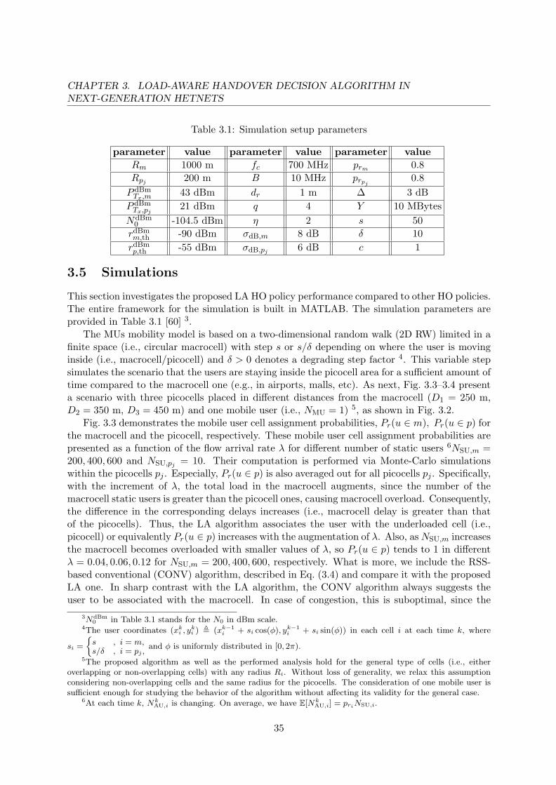
CHAPTER 3. LOAD-AWARE HANDOVER DECISION ALGORITHM INNEXT-GENERATION HETNETS
Table 3.1: Simulation setup parameters
parameter value parameter value parameter value
Rm 1000 m fc 700 MHz prm 0.8
Rpj 200 m B 10 MHz prpj 0.8
P dBmTx,m
43 dBm dr 1 m ∆ 3 dB
P dBmTx,pj
21 dBm q 4 Y 10 MBytes
NdBm0 -104.5 dBm η 2 s 50
rdBmm,th -90 dBm σdB,m 8 dB δ 10
rdBmp,th -55 dBm σdB,pj 6 dB c 1
3.5 Simulations
This section investigates the proposed LA HO policy performance compared to other HO policies.The entire framework for the simulation is built in MATLAB. The simulation parameters areprovided in Table 3.1 [60] 3.
The MUs mobility model is based on a two-dimensional random walk (2D RW) limited in afinite space (i.e., circular macrocell) with step s or s/δ depending on where the user is movinginside (i.e., macrocell/picocell) and δ > 0 denotes a degrading step factor 4. This variable stepsimulates the scenario that the users are staying inside the picocell area for a sufficient amount oftime compared to the macrocell one (e.g., in airports, malls, etc). As next, Fig. 3.3–3.4 presenta scenario with three picocells placed in different distances from the macrocell (D1 = 250 m,D2 = 350 m, D3 = 450 m) and one mobile user (i.e., NMU = 1) 5, as shown in Fig. 3.2.
Fig. 3.3 demonstrates the mobile user cell assignment probabilities, Pr(u ∈ m), Pr(u ∈ p) forthe macrocell and the picocell, respectively. These mobile user cell assignment probabilities arepresented as a function of the flow arrival rate λ for different number of static users 6NSU,m =200, 400, 600 and NSU,pj = 10. Their computation is performed via Monte-Carlo simulationswithin the picocells pj . Especially, Pr(u ∈ p) is also averaged out for all picocells pj . Specifically,with the increment of λ, the total load in the macrocell augments, since the number of themacrocell static users is greater than the picocell ones, causing macrocell overload. Consequently,the difference in the corresponding delays increases (i.e., macrocell delay is greater than thatof the picocells). Thus, the LA algorithm associates the user with the underloaded cell (i.e.,picocell) or equivalently Pr(u ∈ p) increases with the augmentation of λ. Also, asNSU,m increasesthe macrocell becomes overloaded with smaller values of λ, so Pr(u ∈ p) tends to 1 in differentλ = 0.04, 0.06, 0.12 for NSU,m = 200, 400, 600, respectively. What is more, we include the RSS-based conventional (CONV) algorithm, described in Eq. (3.4) and compare it with the proposedLA one. In sharp contrast with the LA algorithm, the CONV algorithm always suggests theuser to be associated with the macrocell. In case of congestion, this is suboptimal, since the
3NdBm0 in Table 3.1 stands for the N0 in dBm scale.
4The user coordinates (xki , y
ki ) , (xk−1
i + si cos(φ), yk−1i + si sin(φ)) in each cell i at each time k, where
si =
{
s , i = m,s/δ , i = pj ,
and φ is uniformly distributed in [0, 2π).
5The proposed algorithm as well as the performed analysis hold for the general type of cells (i.e., eitheroverlapping or non-overlapping cells) with any radius Ri. Without loss of generality, we relax this assumptionconsidering non-overlapping cells and the same radius for the picocells. The consideration of one mobile user issufficient enough for studying the behavior of the algorithm without affecting its validity for the general case.
6At each time k, NkAU,i is changing. On average, we have E[Nk
AU,i] = priNSU,i.
35

CHAPTER 3. LOAD-AWARE HANDOVER DECISION ALGORITHM INNEXT-GENERATION HETNETS
0.01 0.02 0.04 0.06 0.08 0.1 0.120
0.1
0.2
0.3
0.4
0.5
0.6
0.7
0.8
0.9
1
λ
Cellassignmen
tprobability
Algorithms performance for different NSU,m and NSU,pj = 10
LA-Pr(u ∈ p)
LA-Pr(u ∈ m)
CONV-Pr(u ∈ p)
CONV-Pr(u ∈ m)
NSU,m = 600
NSU,m = 400
NSU,m = 200
Figure 3.3: Cell assignment probability (CONV vs LA) for different number of static macrocellusers NSU,m and number of static picocell users NSU,pj = 10.
user is placed close to one or more underloaded cells. Pr(u ∈ m), is also plotted, showing thecomplementary behavior of the algorithm.
Fig. 3.4 shows the predicted delays, Dm, Dp for the macrocell and the picocell, as a function ofthe flow arrival rate λ. Specifically, these are the Dkm, D
kp that are also averaged out across time k.
Their computation is performed via Monte-Carlo simulations for different number of static usersNSU,m = 200, 400, 600 and NSU,pj = 10 within the picocells pj . Especially, Dp is also averagedout for all picocells pj . It is noticed that the average delay, Dm, increases sharper for largervalues of NSU,m and smaller values of λ, according to Eq. (3.8). The latter implies that totalarrival rate becomes faster equal to the system service rate. NSU,m and λ affect Dm incrementand consequently enlarge the difference between Dm, Dp. Hence, when their ratio becomes large(Dm ≫ Dp), f(·) tends to zero and vanishes the gap between the received powers. Thus, theimpact of NSU,m, λ on Dm, Dp ratio exceeds the impact of received powers asymmetry. Thisvalidates the LA algorithm functionality that associates the user with the underloaded picocellsin the case of an overloaded macrocell (Pr(u ∈ p) goes to one), regardless the gap in receivedpowers. On the other hand, HO is not triggered if there is not much difference in Dm, Dp, i.e.,the user QoS is satisfied (Pr(u ∈ p) goes to zero). Consequently, RSS-based HO that maximizesthe instantaneous rate of a user (i.e., the best modulation and coding scheme (MCS) is used),reflects user QoS only when the BS is lightly loaded. However, user performance, in terms ofper flow delay, may be severely affected if the BS offering the best RSS is congested.
In Fig. 3.5, the picocell assignment probability, Pr(u ∈ p), is depicted as a function of theuser’s distance from the macrocell for fixed number of NSU,m = 200 and NSU,pj = 10 in thepicocell. The proposed algorithm is compared with the CONV and a distance-based (DIST)one provided in [34], for different λ. The latter is applied in hierarchical macrocell/SCs networkthat is also our case. The DIST approach associates the user with its closest SC regardlessthe asymmetry in BSs powers. This is achieved using a scale down factor α based on themaximization of the SC assignment probability. Further, some of the system parameters are
36

CHAPTER 3. LOAD-AWARE HANDOVER DECISION ALGORITHM INNEXT-GENERATION HETNETS
0.01 0.02 0.04 0.06 0.08 0.1 0.120
0.1
0.2
0.3
0.4
0.5
λ
Averagedelay(sec)
Average delay for different NSU,m and NSU,pj = 10
Dp
Dm
NSU,m = 400
NSU,m = 200
NSU,m = 600
Figure 3.4: Average delay in the macrocell/picocell for different number of static macrocell usersNSU,m and number of static picocell users NSU,pj = 10.
Table 3.2: Delay gain for NSU,m = 200, NSU,pj = 10 and different λ
λ 0.05 0.08 0.1 0.11 0.12
DLA (sec) 0.0701 0.0992 0.1261 0.1125 0.0621
DDIST (sec) 0.0621 0.0807 0.1109 0.1470 0.2808
DCONV (sec) 0.0743 0.1160 0.1864 0.2708 0.5496
DDIST/DLA 0.8861 0.8141 0.8798 1.3066 4.5235
DCONV/DLA 1.0596 1.1701 1.4790 2.4073 8.8547
changed to adapt the simulated scenario in [34] 7. For the DIST algorithm, Pr(u ∈ p) is close to1 after a specific user’s distance from the picocell despite the fact that the macrocell is overloadedor not. However, with the LA approach, Pr(u ∈ p) increases, depending on the macrocell loadfor different λ, no matter the user’s proximity to the picocell. Thus, if the user is close to apicocell, its association with it may be unnecessary, since its QoS requirements may be alreadymet. Finally, the CONV algorithm does not trigger the HO, due to BSs power assymetry.
The overall delay that the user experiences (i.e., Dm from the macrocell and Dp from thepicocell depending on where it is associated) is presented in Table 3.2. The setup is consideredthe same as in Fig. 3.5. Using the CONV algorithm, it is noted that the overall delay, DCONV,is identical to the delay of the macrocell (see Fig. 3.4 for NSU,m = 200 and NSU,pj = 10), sincethe user is always connected to the macrocell. The DIST algorithm retains the user connectedto the macrocell up to a specific distance threshold and after that it attaches it to the picocell(see Fig. 3.5) with Pr(u ∈ p) close to 1. Thus, the augmentation of the macrocell delay, whenit becomes overloaded, compared to the picocell ones, increases the overall delay, DDist. The
7Specifically, one macrocell and one picocell are considered in distance D1 = 200 m, a∗ = 0.96 as the optimala for the specific D1, ∆ = 0, Rp = 150 m and rp,th = −51 dBm. In addition, the mobility model is changed, sincethe authors in [34] assume that one mobile user moving across a line from the macrocell to the picocell coveragearea.
37

CHAPTER 3. LOAD-AWARE HANDOVER DECISION ALGORITHM INNEXT-GENERATION HETNETS
50 60 80 100 120 140 160 1800
0.1
0.2
0.3
0.4
0.5
0.6
0.7
0.8
0.9
1
dm(m)
Picocellassignmen
tprobability
Algorithms performance for NSU,m = 200 and NSU,pj = 10
LA-λ = 0.05LA-λ = 0.08LA-λ = 0.1LA-λ = 0.11LA-λ = 0.12DISTCONV
Figure 3.5: Picocell assignment probability (CONV vs DIST vs LA) for number of static macro-cell users NSU,m = 200 and number of static picocell users NSU,pj = 10 for different λ.
LA algorithm keeps a conservative policy when the load is low in the macrocell, i.e., the userremains associated with the macrocell. Hence, Pr(u ∈ p) is low even if the user is close to thepicocell. This policy gives slightly higher overall delays when λ ≤ 0.1 compared to the DISTone, since the latter connects the user to the cell with the lower delay (i.e., picocell) earlier.Consequently, unnecessary handovers to the picocell and related signaling overhead are avoidedwith the LA approach. On the other hand, if the load is high in the macrocell, the LA algorithmassociates the user with the underloaded picocell earlier than the DIST algorithm that is load-unaware giving significant performance to the overall delay, DLA. The respective ratios of theCONV/DIST algorithms over the LA algorithm (i.e., DCONV/DLA, DDIST/DLA) overall delaysare demonstrated to show the corresponding gains in Table 3.2. The same trend holds for highervalues of NSU,m, but with different values of λ, as explained in Fig. 3.4. Finally, significantgains are provided in high load scenarios (i.e., ≃ 4 and ≃ 8 compared to the CONV and DISTapproach).
3.6 Discussion
The possible directions beyond the proposed HO load-aware algorithm mainly focus on its ap-plicability to other use cases. Such use cases urge for new handover decision rules correspondingto different functions f (·). For instance, to consider scenarios where picocells are overloadedcompared to macrocell, i.e., Dpj∗ ≫ Dm, a generalization of the current function in Eq. (3.6) isgiven as follows:
f(
Dkm, Dkpj
)
, exp
[
c
(
−DkmDkpj
+DkpjDkm
)]
, c ≥ 1. (3.9)
The new generalized function is defined with a co-domain in [0,+∞]. It is noted thatthe function scales down the power differences following the proposed HO rule, i.e., rpj∗ [k] >
38

CHAPTER 3. LOAD-AWARE HANDOVER DECISION ALGORITHM INNEXT-GENERATION HETNETS
f(
Dkm, Dkpj∗
)
rm[k] and associates the user to the appropriate cell based on the predicted average
delays 8. In more detail, based on that rule, the user is associated to the picocell iff Dm ≫ Dpj∗ ,
i.e., f(
Dkm, Dkpj∗
)
→ 0+ while in the macrocell iff Dm ≪ Dpj∗ , i.e., f(
Dkm, Dkpj∗
)
→ +∞.
Further, similar rules can be used in picocell-to-picocell HO scenarios without loss of generality.Towards this direction, more advanced HO rules can be applied by taking into account transientphenomena that are crucial in mobility scenarios, especially when the sojourn time in a cell(function of UE speed) is not sufficiently enough to provide system stationarity. Subsequently,the prediction of the service delay becomes complicated and switch to transient analysis toolsis required. Finally, paving the path to 5G beyond the HO (RSS-based) legacy presented inChapter 2, this chapter discusses an SDN-based programmable framework to centrally controlthe HO process. It can be noticed that UE receives the predicted delay for each cell by its servingcell in order to trigger the association procedure defined by the load-aware HO algorithm (seeFig. 3.2). Hence, that algorithm can directly run on the SDN controller side that is aware of theusers RSRP such that to send only the cell association results to the interrelated users offloadingthe signaling overhead and bypassing any modifications in the UE protocol stack for the SDNprotocol support.
3.7 Conclusion
This chapter focuses on user-centric HO decision algorithms for HetNets. It was shown that theproposed load-aware algorithm can significantly enhance the system performance by consideringboth user and network perspective in order to improve user QoS. To this end, it was comparedwith a conventional and a distance-based LTE-handover algorithm and we showed that it canoutperform both of them according to the extracted cell assignment probability and user servicedelay performance results.
8Such load-aware scaling can be considered as a dynamic cell range extension showing a delay gain comparedto the DIST/CONV algorithms.
39

CHAPTER 3. LOAD-AWARE HANDOVER DECISION ALGORITHM INNEXT-GENERATION HETNETS
40

Chapter 4
Utility-Based Resource Allocationunder Multi-Connectivity in LTE
4.1 Introduction
In the previous chapters, we cover the topic of mobility management towards next-generationcellular networks. More precisely, we present the analytical insights about the involved trade-offs on handover decision algorithms for next-generation HetNets. The comparisons with theconventional methodologies reveal the new network trends that are met in heterogeneous en-vironments. To this end, 5G communication systems are expected to fulfill the insatiable andheterogeneous service requirements in future deployments.
As stressed in Chapter 1, toward the development of 5G vision, it is expected that the mobilebroadband service will be enhanced to provide a consistent user experience [75]. Consideringthe current cellular technologies, cell edge users and those experiencing high interference sufferfrom poor service, even when coordinated signal processing is applied. Along this direction, thecoordination of multiple connections is expected to be a solution by re-designing radio/networkfunctions [75]. To overcome such limitation, multi-connectivity was introduced in 5G as amechanism of supporting multiple cell connections per end-user basis on several radio accesstechnologies (RAT) or frequency bands [76,77].
The multi-connectivity concept is characterized by effective resource utilization for seam-less user experience [78], enhancement among capacity, coverage and mobility [79], reliablehigh-speed data delivery [80] and acting as a quick fail-over method [19]. In general, the mul-tiple connections can be applied among heterogeneous inter-RAT or intra-RAT [81] or withina single RAT that is viewed as establishing multiple connections to different BSs. The dual-connectivity (DC) concept was introduced in LTE Rel.12 study item (3GPP TR36.842) as thebaseline of multi-connectivity enabling two simultaneous connections across the end-users inan intra-RAT, i.e., transmit/receive data simultaneously from two distinct BSs in uplink (UL)and/or downlink (DL).
Despite its appealing, once of the significant challenge of multi-connectivity is presentedin [24] related to the efficient radio resource utilization. Towards this direction, the current andthe following chapters explore the new problem of resource allocation under multi-connectivity.The resource allocation in multi-connectivity is crucial to enhance the user performance and todeal with the increasing demand of traffic. In general, two types of application traffic exist, (i)
41

CHAPTER 4. UTILITY-BASED RESOURCE ALLOCATION UNDERMULTI-CONNECTIVITY IN LTE
user-to-user such as content/video dissemination sharing, peer-to-peer gaming and public safety,and (ii) user-to-network and network-to-user such as social networking and video-on-demand.Nevertheless, another challenge is related to satisfy the quality of service (QoS) requirement ofeach traffic flow and optimize network throughput across multiple connections.
The work in [82] proposes an hierarchical architecture to control and coordinate multi-connectivity with resource allocation and interference management. In [83], the authors considerresource allocation at the macro node side based on DC enabled downlink (DL) connectionssupported by small cells. While these works focus on resource allocation schemes in multi-connectivity environment, users QoS-aware utility proportional fairness allocation schemes [20]are not proposed. In that sense, this chapter addresses the new problem of resource allocationunder multi-connectivity case with user-to-user traffic and QoS requirement. The contributionsof this chapter are summarized as follows:
1. We introduce the proportional fairness resource allocation problem that aims to maximizenetwork aggregated throughput for multi-connectivity and compare with legacy single-connected case under different scenarios.
2. We propose a utility-based resource allocation that considers the QoS and analyze theperformance gain with aforementioned proportional fairness resource allocation.
3. Finally, we investigate the impact of utility function on QoS satisfaction in terms of itsshape.
The rest of the chapter is organized as follows. Section 4.2 provides the system modeland assumptions used through this chapter. Section 4.3 formulates the optimization problem.Simulation results are discussed in Section 4.4. Section 4.5 offers a brief discussion. Finally,Section 4.6 presents the concluding remarks.
4.2 System model and assumptions
In this section, we describe the system model and the assumptions. We consider an area L ⊂ R2
served by a set of BSs B = {b1, · · · , b|B|} and a set of UEs U = {u1, · · · , u|U|} is distributedin this area. For instance, in Fig. 4.1, an example is presented with B = {b1, b2, b3} and U ={u1, u2, u3, u4}. In following, we examine our model in more detail:
4.2.1 Air-interface model
A.1-Mobility: We assume user mobility, implying that all location related parameters arechanging in time. For simplicity, we skip the time index t throughout the chapter.
A.2-Signal to interference plus noise ratio (SINR): The SINR of the received signalfrom the j-th BS (bj) to the i-th UE (ui) per Physical Resource Block (PRB) along the DLdirection is denoted as:
SINRDbj ,ui
=RSRPD
bj ,ui∑
bk 6=bj
pDbk,uiRSRPDbk,ui
+WDbjN0
. (4.1)
Respectively, the SINR from the i-th UE to the j-th BS in UL direction is denoted as SINRUui,bj
.
42


CHAPTER 4. UTILITY-BASED RESOURCE ALLOCATION UNDERMULTI-CONNECTIVITY IN LTE
where Pmax,dBmui is the maximum transmitted power of the i-th UE. However, in the DL, no power
control algorithm is applied and the transmitted power from each BS to all UEs is denoted asPD,dBmbj ,ui
= PD,dBmbj
. It is noted that the asymmetry in UL/DL transmitted powers due to the
UL power control differentiates the UL/DL SINR values (see assumption A.2).
4.2.2 Connection and Traffic model
B.1-Multi-connectivity: Under multi-connectivity, users can be associated to and com-municate with more than one BSs at the same time. We assume the multi-connectivity ca-pability exists in both DL and UL for all UEs and a UE can be connected to a BS if bothDL and UL SINR is above a pre-defined threshold, i.e., SINRth. Hence, we define a set
E , {(ui, bj) , (bj , ui) : min(
SINRUui,bj
, SINRDbj ,ui
)
> SINRth} that represents all possible con-
nections between UEs and BSs. Further, no connection can be established when the condition
min(
SINRUui,bj
, SINRDbj ,ui
)
> SINRth is not hold for the i-th UE and the j-th BS. Without
loss of generality, asymmetric connection scenarios among UE and BSs, i.e., only UL or DLconnection to one cell, can be allowed, but in such cases multi-cell connectivity can be limited,especially under bi-directional traffic presence.
B.2-Local-routing: In principle, routing in the backhaul network is necessary even for theuser-to-user traffic served by the same BS. To offload the backhaul/core network, the concept oflocal-routing is applied [84] in which the user-to-user traffic is routed directly via intermediateBS, thus offloading the core and backhaul network, and reducing the number of hops taken byIP packets to reach the destination [85]. In this case, traffic is not routed via the core network,e.g., LTE evolved packet core (EPC), but only via the intermediate BS [86]. We focus on theuser-to-user traffic flow that can be locally-routed, i.e., both user are connected to at least onecommon BS2. Such traffic flow is representative of the public safety (e.g., isolated BSs) and closecommunity application (e.g., community-based video sharing) scenarios where content is sharedlocally among UEs. Thus, backhaul-routed case is not considered 3.
B.3-Active users pairs: Based on the minimum SINR requirement defined in B.1, aset that comprises all active user pairs served by the j-th BS is defined as Cbj , {(ui, uq) :(ui, bj) , (bj , uq) ∈ E , ui 6= uq} and the user pair (ui, uq) ∈ Cbj can have user-to-user traffic routed
locally via BS bj . Consequently, a set C ,⋃
bj∈BCbj is formed as the union of all active user
pairs. Lastly, two sets are further defined for each user: Dui , {uq : (ui, uq) ∈ C} comprises alldestined UEs from the i-th UE and Sui , {uq : (uq, ui) ∈ C} comprises all source UEs that cantransport traffic to the i-th UE.
B.4-Traffic flow requested rate: It corresponds to the requested rate Rui,uq determinedas the total rate required by a group of U2U applications running on the top using an end-to-end established connection of user pair (ui, uq), that can go through any intermediate BS vialocal-routing4.
4.3 Problem setup
Based on aforementioned system model, we formulate the optimization problem in this section.
2In Fig.4.1, the traffic from u1 to u2 can be local routed via b1 or b2.3In Fig.4.1, the traffic from u1 to u4 is not considered.4In Fig. 4.1, requested rate Ru1,u2
and Ru2,u1can go through b1 and b2,
44

CHAPTER 4. UTILITY-BASED RESOURCE ALLOCATION UNDERMULTI-CONNECTIVITY IN LTE
4.3.1 Utility function
Our objective here is to allocate optimally the resource to user-to-user traffic based on theapplied utility function. We define xUbj ,(ui,uq), x
Dbj ,(ui,uq)
∈ X as the percentage of allocated PRB
to total PRBs in decimal form along UL/DL direction to transport user-to-user traffic of userpair (ui, uq) through BS bj . It is noted that xUbj ,(ui,uq) = xDbj ,(ui,uq) = 0, if (ui, uq) /∈ Cbj , i.e., no
resource is allocated if such user pair can not be local routed through BS bj . In the following,we introduce two different utility functions: one provides proportional fairness and the otherone extends the proportional fairness by taking QoS into consideration.
4.3.1.1 Proportional Fairness (PF)
As the first utility function, we exploit a logarithmic utility function similar to the one in [87] thatachieves “proportional fair” resource allocation. The “proportional fair” characteristic impliesthat if we select a data rate greater than the optimal one for a given user, then there will be atleast one another data rate that will be decreased in a proportion larger than the proportion ofthe increased user data rate [88]. Such utility function is given as:
Φ (y) = log (y) , (4.5)
4.3.1.2 Utility Proportional Fairness (UPF)
In the former utility function, a significant drawback lies on the lack of QoS consideration. Toincorporate the QoS into the utility function, we use the family of sigmoid functions as:
Φ (y) = log (S (y, γ, β)) = log
(1
1 + e−γ(y−β)
)
, (4.6)
γ > 0, y ≥ 0, where β is the traffic requested rate defined as introduced in B.3 of Section 4.2.The function Φ (y) is the natural logarithm of the sigmoid utility function, S (y, γ, β), commonlyused in literature [89] that preserves the traffic requested rate. In Fig. 4.2(a), the family ofsigmoid function with different γ is compared with the linear increment and step incrementfunction for β = 5 Mbps. If the allocated data rate y is less than the requested rate β, thesigmoid function family provides monotonic increment on its slope as shown in Fig. 4.2(b)whereas its slope is monotonic decreasing when the requested rate is achieved (i.e., y > β).Moreover, the value of γ impacts the shape of sigmoid function to be more like step or linearfunction that reflects the demand degree of requested rate. In other words, it echoes the trade-offbetween the network throughput maximization provided by the “linear” characteristic (better inthe network perspective) and the QoS satisfaction by the “non-linear” characteristic (better inthe user perspective).
Under the multi-connectivity regime assumption (see B.1 of Section 4.2), we can introduceour final objective function based on any utility function Φ (·) presented in Eq. (4.5) or Eq. (4.6)as following:
U(
xUui,uq ,x
Dui,uq
)
, Φ
∑
bj∈B
Q(
xUbj ,(ui,uq), xDbj ,(ui,uq)
)
, (4.7)
where xUui,uq ,
[
xUb1,(ui,uq), · · · , xUb|B|,(ui,uq)
]T, xD
ui,uq ,
[
xDb1,(ui,uq), · · · , xDb|B|,(ui,uq)
]T.
45

CHAPTER 4. UTILITY-BASED RESOURCE ALLOCATION UNDERMULTI-CONNECTIVITY IN LTE
0 1 2 3 4 5 6 7 8 9 10
y 106
0
0.2
0.4
0.6
0.8
1
(a) Sigmoid function
0 1 2 3 4 5 6 7 8 9 10
y 106
0
0.2
0.4
0.6
0.8
110
-6
(b) Slope of sigmoid function
Figure 4.2: Shape of sigmoid function
The Q (·) function stands for the allocated rate of user pair (ui, uq) and is expressed as follows:
Q(
xUbj ,(ui,uq), xDbj ,(ui,uq)
)
, min(
xUbj ,(ui,uq)RUui,bj
, xDbj ,(ui,uq)RDbj ,uq
)
(4.8)
It is noted that the minimum operator guarantees the same allocated rate in both UL/DLdirections for a single user-to-user traffic 5. Specifically, each user cannot send or receive withan allocated rate greater than another user can send or receive. No mechanism support of thisguarantee implies UL/DL buffering that renders the current model more complex introducingqueuing theory analysis tools and is out of the scope of this study. Finally, the argument of Φ (·)in Eq. (4.7) takes the aggregated allocated rate of user pair (ui, uq) over all common BSs (i.e.,∀ bj ∈ B).
4.3.2 Problem formulation
Based on the proposed system model, assumptions and utility functions, we present our problemformulation. The problem falls into the category of the network utility maximization for resourceallocation and is given in Eq. (4.9). A detailed explanation of the proposed optimization problemfollows, presenting both the objective function and constraints.
Objective function: The objective is to allocate the resource xUbj ,(ui,uq), xDbj ,(ui,uq)
∈ X to each
user pair in order to maximize the aggregated network utility function over all user pairs thatexchange traffic. The two aforementioned utility functions can be utilized.
5Neither the user-to-network traffic nor the network-to-user traffic applies such minimum operation.
46

CHAPTER 4. UTILITY-BASED RESOURCE ALLOCATION UNDERMULTI-CONNECTIVITY IN LTE
maxX
∑
(ui,uq)∈C
U(
xUui,uq ,x
Dui,uq
)
s.t.∑
(ui,uq)∈Cbj
xUbj ,(ui,uq) ≤ 1, ∀ bj ,
∑
(ui,uq)∈Cbj
xDbj ,(ui,uq) ≤ 1, ∀ bj ,
∑
bj∈B
∑
uq∈Dui
xUbj ,(ui,uq)BUbj≤ BU
ui , ∀ ui,
∑
bj∈B
∑
uq∈Sui
xDbj ,(uq ,ui)BDbj≤ BD
ui , ∀ ui,
∑
bj∈B
∑
uq∈Dui
xUbj ,(ui,uq)PUui,bj
BUbj≤ Pmax
ui , ∀ ui. (4.9)
Constraints: Here, we present a detailed description for each one of them:
1. The first two constraints ensure that the number of allocated PRBs (expressed as thepercentage in decimal form on total PRBs) at each BS bj to all UEs will not exceed thetotal number of PRBs in both UL/DL.
2. The third and fourth constraints assure that the number of allocated PRBs to each UEamong all connected BSs will not exceed the maximum number of allocated PRBs, BU
ui , BDui ,
in UL/DL of the i-th UE, respectively. Specifically, these constraints take into accountall user-to-user traffic related to the i-th UE as uq ∈ Dui of all destinate UEs in UL anduq ∈ Sui of all source UEs in DL through any intermediate BS (bj ∈ B). Further, theseconstraints lie on the user capability defined as UE-category in 3GPP TS36.306.
3. Finally, the last constraint is related to the power control mechanism introduced in A.4of Section 4.2. It restricts the total transmitted power from the i-th user to all connectedBSs to be within its power limitation as Pmax
ui .
Finally, we note that the objective function contains the minimum operation that is concave butnon-differentiable. Thus, we need to transform the objective function to a differentiable concaveone in order to conclude to a unique tractable global optimal. The following paragraph describessuch procedure.
4.3.3 Problem transformation
To deal with the minimum operation in Eq. (4.8), we replace Q(
xUbj ,(ui,uq), xDbj ,(ui,uq)
)
with
the auxiliary variable zbj ,(ui,uq) ∈ Z and add two extra constraints zbj ,(ui,uq) ≤ xUbj ,(ui,uq)Rui,bj
and zbj ,(ui,uq) ≤ xDbj ,(ui,uq)Rbj ,uq . Then, we define U(zui,uq
), Φ
(∑
bj∈Bzbj ,(ui,uq)
)
, zui,uq ,[
zb1,(ui,uq), · · · , zb|B|,(ui,uq)
]Tand the transformed problem in Eq. (4.10). The objective function
in the transformed optimization problem is strictly concave as the sum of U(zui,uq
)is strictly
concave as proved in the Lemma 1.
47

CHAPTER 4. UTILITY-BASED RESOURCE ALLOCATION UNDERMULTI-CONNECTIVITY IN LTE
maxX ,Z
∑
(ui,uq)∈C
U(zui,uq
)
s.t. zbj ,(ui,uq) ≤ xUbj ,(ui,uq)
RUui,bj
, ∀ bj ,
zbj ,(ui,uq) ≤ xDbj ,(ui,uq)
RDbj ,uq
, ∀ bj ,∑
(ui,uq)∈Cbj
xUbj ,(ui,uq) ≤ 1, ∀ bj ,
∑
(ui,uq)∈Cbj
xDbj ,(ui,uq) ≤ 1, ∀ bj ,
∑
bj∈B
∑
uq∈Dui
xUbj ,(ui,uq)BUbj≤ BU
ui , ∀ ui,
∑
bj∈B
∑
uq∈Sui
xDbj ,(uq ,ui)BDbj≤ BD
ui , ∀ ui,
∑
bj∈B
∑
uq∈Dui
xUbj ,(ui,uq)PUui,bj
BUbj≤ Pmax
ui , ∀ ui (4.10)
Lemma 1. The utility function U(zui,uq
)in the transformed optimization problem is strictly
concave.
Proof. It is noticed that U(zui,uq
)function can be written as:
U(zui,uq) = Φ(
1T|B|zui,uq
)
, (4.11)
and any utility function Φ (·) is strictly concave. The first one is the logarithmic in Eq. (4.5)and the second one in Eq. (4.6) is proved to be strictly concave as the logarithm of the sigmoidfunction based on Lemma III.1 in [89]. It is known that any composition of a concave functionwith an affine function is concave [90]. Thus, as expressed in Eq. (4.11), we conclude thatU(zui,uq) is also concave.
Combined with the linear constraints, the transformed optimization problem is a convexoptimization problem with a unique tractable optimal solution.
4.4 Simulations
In this section, the performance evaluation results are presented for the optimization problemdescribed in Section 4.3. Simulation parameters applied to UEs, BSs and network planning aremostly taken from 3GPP (TR36.814, TR36.942, TR25.942) and NGMN documents [91], andsome important parameters are listed in Table 4.1 6. Moreover, all assumptions introduced in
6Without loss of generality, we assume the (maximum) BS Tx power that corresponds to a macrocell. Hence,the current work is fully applicable for small cells deployment. The same assumption holds for Chapter 5 and 6.
48

CHAPTER 4. UTILITY-BASED RESOURCE ALLOCATION UNDERMULTI-CONNECTIVITY IN LTE
Table 4.1: Simulation parameters
Parameter Value
LTE mode FDD, SISO
Carrier frequency DL: 2.19 GHz; UL: 2.0 GHz
Total PRBs of each BS 100 (20 MHz BW)
Maximum PRBs of each UE 100
Number of BSs 3
Initial UE distribution Uniform of each BS
UE speed Selected from [3, 30, 120] km/h as [91]
UE direction Uniform distributed in [0, 360] degree
UE traffic model Full buffer
SINR threshold -10 dB
BS transmission power 46 dBm
UE maximum transmission power 23 dBm
Power control parameters P dBm0 = -58 dBm, α = 0.8
Thermal noise density -174 dBm/Hz
Table 4.2: Comparison of Single/Multi-connectivity
UE number Performance Single- Multi-in BS b1/b2/b3 metric connected connected
Connected BS 1 2.07Under-loaded Connected UE pairs 6 17.52case: 2/2/2 Aggregated user rate 0.99 Mbps 20.04 Mbps
Connected BS 1 1.34Uneven-loaded Connected UE pairs 34 49.95case: 6/2/2 Aggregated user rate 11.68 Mbps 46.73 Mbps
Connected BS 1 1.45Over-loaded Connected UE pairs 90 162.22case: 6/6/6 Aggregated user rate 55.04 Mbps 57.01 Mbps
Section 4.2 are also held. The whole simulation framework is built in MATLAB 7 and we use theinterior point algorithm to iteratively solve the linear-constrained convex optimization problemof both utility functions: PF and UPF.
4.4.1 Comparison: Single-connectivity and Multi-connectivity
Firstly, we compare the performance of legacy single-connectivity case with the multi-connectivityone using the same PF utility function. The considered legacy single-connected case associateseach UE to only one BS and only allows each UE to communicate with the associated BS in bothUL/DL directions in terms of the best received RSRP. In Table 4.2, we compare them in terms
7Our self-developed MATLAB LTE/LTE-A simulation platform is based on the 3GPP specifications andNGMN documents to provide a system level view of the whole mobile network. It can generate the network mapvia planning several BSs and mobile UEs, emulate the non-idealities of wireless channel model and provide anetwork-wide inspection on the user and network performance. The same simulator is used in Chapter 5 and 6.
49

CHAPTER 4. UTILITY-BASED RESOURCE ALLOCATION UNDERMULTI-CONNECTIVITY IN LTE
Table 4.3: QoS metrics comparison of PF and UPF
Metric Requested rate PF problem UPF problem
0.1Mbps 68.72% 91.39%0.5Mbps 42.07% 58.03%
Satisfaction 1Mbps 25.15% 35.33%ratio 5Mbps 6.42% 23.10%
10Mbps < 1% <1%
0.1Mbps 0.2122 0.0625Unsatisfied 0.5Mbps 0.4131 0.2317normalized 1Mbps 0.5483 0.3906
error 5Mbps 0.7949 0.660710Mbps 0.8833 0.8441
of the average number of connected BS, number of connected user pairs, and aggregated userrate. Three representative scenarios, namely under-loaded, uneven-loaded and over-loaded, arepresented, where the x/y/z notation represents the initially uniformly distributed of x/y/z UEsover each BS. It is noted that the x, y, z variables variation creates the aforementioned scenariosrelated to the network load.
It can be seen from the table that the number of connected BS per UE increases withmulti-connectivity especially for under-loaded scenario. This is because of the induced inter-cell interference is minor for under-loaded scenario. Moreover, we observe a higher number ofconnected user pair in multi-connectivity as each UE is able to transmit and receive traffic toa larger set of UEs through the local routing across different BSs. This advantage becomessignificant of over-loaded scenario that allows more traffic diversity among users. Even thenumber of UEs increases, the core network signaling overhead is reduced benefiting from thelocal-routing adaption of the current network setup.
When comparing the aggregated user rate of all user pairs, we notice that the performancegain is significantly higher in under-loaded scenario followed by the uneven-loaded scenario.This gain is due to schedule UEs across all available BSs, that is indeed one of the expectedmerit of multi-connectivity. To sum up, the multi-connectivity not only has advantage in userperspective (i.e., more UEs can be reached through multiple BSs) but also in the network per-spective (i.e., larger aggregated user rate) in different loading scenarios.
4.4.2 Performance analysis of PF & UPF in multi-connectivity
Then, we present the results of both utility functions with a fixed γ = 10/R in a scenario with 4UEs over each BS (i.e., 4/4/4). Firstly, we define the final allocated rate of the user pair (ui, uq)among all intermediate BSs as
ζui,uq ,∑
bj∈B
Q(
x⋆Ubj ,(ui,uq), x⋆Dbj ,(ui,uq)
)
, (4.12)
where x⋆Ubj ,(ui,uq), x⋆Dbj ,(ui,uq)
are the optimization results of control variables xUbj ,(ui,uq), xDbj ,(ui,uq)
.
Further, in a quantitative comparison on QoS, we define two different metrics: (i) Satisfactionratio that represents the ratio of user pairs which are satisfied with the allocated rate represented
50

CHAPTER 4. UTILITY-BASED RESOURCE ALLOCATION UNDERMULTI-CONNECTIVITY IN LTE
by the CDF 8 in (4.13), and (ii) Unsatisfied normalized error that shows the normalized Euclideandistance between the allocated rate ζui,uq and the requested rate Rui,uq when a user pair (ui, uq)is unsatisfied in (4.14).
Mui,uq = Prob{
ζui,uq ≥ Rui,uq
}
. (4.13)
Eui,uq =
∥∥∥∥
ζui,uq−Rui,uq
Rui,uq
∥∥∥∥, if ζui,uq < Rui,uq ,
0 , o/w.(4.14)
Table 4.3 shows the results of the defined QoS metrics using both PF and UPF utilityfunctions with five different requested rate R = Rui,uq , ∀ (ui, uq) ∈ C. In terms of the satisfaction
ratio, the UPF is much better than the PF one except in R = 10 Mbps case in which bothutility functions satisfy less than 1% of user pairs due to inter-cell interference impact. Further,UPF reduces the unsatisfied normalized error by allocating resources as close as possible to therequested rate. We can see that even the QoS requirement cannot be satisfied for some userpairs mostly in overloaded scenarios, the UPF still provides less error to the requested rate.
In more qualitative comparison, in Fig. 4.3, the CDF plot of the allocated rate to all userpairs with three different requested rates are shown. The ratio of satisfied user pair is higherfor the UPF case in Fig. 4.3(a) and Fig. 4.3(b) and is almost the same of both UPF and PF inFig. 4.3(c) that matches the satisfaction ratio in Table 4.3. For instance, the satisfaction ratioMui,uq = 1 − 0.65 = 0.35 of the UPF case in Fig. 4.3(a); however, Mui,uq = 0.25 of the PFcase (CDF is 0.75 at this point and it means 75% of user pairs are unsatisfied). We observe thatthe PF has the same CDF among different requested rate R (i.e., independent of R) and possessesa longer tail due to the fact that it only maximizes the network throughput without consideringany QoS requirements. In other words, UPF provides less network aggregated rate improvinguser pairs QoS, i.e., shorter tail considering R, compared to PF that targets to maximize thenetwork aggregated rate, i.e., longer tail and unconstrained of R.
4.4.3 Impact of γ on UPF problem
Fig. 4.4 compares the impact of γ on the UPF utility function in terms of the PDF plot ofallocated rate ζui,uq for all user pairs. For simplicity, we only provide the result with R = 1 Mbpsbut the same phenomena can be observed for other requested rates. Firstly, it can be observedthat the tail of PDF plot is longer with smaller γ, i.e., the tail is the longest of the three whenγ = 5/R. That is because the sigmoid function with smaller γ tends to be more linear andmakes the allocated rate exceed the requested rate as shown in Fig. 4.2(a). The latter approachis better from the network perspective.
Moreover, we observe a significant amount of user pairs are with smaller allocated rate (ζui,uq <
0.4 Mbps) when γ is large, γ = 20/R, compared to the case when γ is small, γ = 5/R. This isalso due to the shape of the sigmoid function in Fig. 4.2(a) in which the function with larger γ ismore like the step function and prefers to serve the user pair that is close to the QoS requirement.In that sense, some user pairs that are struggle to achieve the requested rate due to the poorSINR condition will be allocated with a smaller data rate or even be queued (e.g., ζui,uq = 0).
8The term ratio is corresponding to theζui,uq
Rui,uq
related to the eventζui,uq
Rui,uq
≥ 1 that implies satisfaction.
51

CHAPTER 4. UTILITY-BASED RESOURCE ALLOCATION UNDERMULTI-CONNECTIVITY IN LTE
(a) R = 1 Mbps
0 0.2 0.4 0.6 0.8 1 1.2 1.4 1.6 1.8 2 2.2 2.4 2.6
107
0
0.2
0.4
0.6
0.8
1
F(
)
(b) R = 5 Mbps
0 0.2 0.4 0.6 0.8 1 1.2 1.4 1.6 1.8 2 2.2 2.4 2.6
107
0
0.2
0.4
0.6
0.8
1
F(
)
(c) R = 10 Mbps
Figure 4.3: CDF plot of PF/UPF utility functions with different R
The latter approach is better from the user perspective. Consequently, the adjustment of sig-moid function shape based on the γ parameters can impact the allocation policy highlightingthe trade-off of fairness from the user and network perspective.
4.5 Discussion
Based on the current study, extensions of the current multi-connectivity optimization frameworkcan be extracted to improve future network deployments. As stressed earlier, the resourceallocation policy can be adjusted via changing the value of γ of the UPF’s sigmoid function. Asit was shown with the increment of gamma, we have a transition from the linear to non-linear(step function) shape of the sigmoid, i.e., network (PF approach) to user perspective (UPFapproach). Towards this direction, operators can impact the users network performance viaUPF function shape adjustment based on traffic classification.
52

CHAPTER 4. UTILITY-BASED RESOURCE ALLOCATION UNDERMULTI-CONNECTIVITY IN LTE
0 0.2 0.4 0.6 0.8 1 1.2 1.4 1.6 1.8 2 2.2
107
0
0.2
0.4
0.6
0.8
1
f()
10-6
Figure 4.4: PDF plot of UPF utility function for several γ
Specifically, traffic classes can be prioritized based on the predefined QoS class identifier(QCI) such that to be optimized in a sequential way. This sequential optimization method isefficient even when the number of traffic class remains small; however, it needs to pre-definethe priority and minimum quality of each class. Another approach is to perform the resourceallocation for each traffic class in parallel. By doing so, the PRBs need to be abstracted asvirtual resource block (VRB) with infinite resources, which means each utility maximizationproblem of each traffic can be executed in parallel. Then theses VRBs are mapped into physicalPRBs after the optimization following the resource allocation policy and traffic class priority,and then transported from the logical to physical channels. To this end, MAC scheduler canapply different algorithms associated with different MAC layer functions as the ones proposedfor resource allocation using a gamut of utility functions in order to fulfill different networkdemands. These demands can be related to the establishment of different radio bearers (e.g.dedicated bearer and default bearer in LTE) across different RATs that are converged at thehigher layers (e.g. packet data convergent protocol (PDCP) or legacy IP).
Complementarily to this chapter, Chapter 5 introduces the user-to-network and network-to-user traffic, i.e., regular UL/DL traffic to/from remote server, formulating new schedulersmechanisms beyond the scope of U2U traffic. In more detail, even U2U traffic can be routed viaisolated BSs based on local-routing, user-to-network and network-to-user traffic must be routedover the backhaul that appears to be an emergency performance bottleneck bringing out newlimitations as the next chapter examines.
4.6 Conclusion
This chapter examines a resource allocation problem under multi-connectivity in an evolved LTEnetwork. A utility proportional fairness resource allocation is proposed as an extension to theproportional fairness one, which takes into account the QoS requirement in terms of requestedrates. Simulation results reveal that the multi-connectivity can boost the aggregated data rateof user-to-user traffic in under-loaded and uneven-loaded scenarios when compared with thesingle-connectivity case. In addition, UPF is able to fulfill the requested rate and increase thesatisfaction ratio when there are available radio resources among multiple connections. Lastly,the shape of UPF function can be changed in accordance to either user or network perspectives.
53

CHAPTER 4. UTILITY-BASED RESOURCE ALLOCATION UNDERMULTI-CONNECTIVITY IN LTE
54

Chapter 5
Multi-Connectivity ResourceAllocation with Limited BackhaulCapacity in Evolved LTE
5.1 Introduction
In the previous chapter, we focus on the multi-connectivity resource allocation in the radio accesslayer assuming U2U traffic. In more detail, we study the new problem of utility-based resourceallocation under the multi-connectivity regime and we compare the performance of the proposedscheme with the legacy single-connectivity use case. Hence, complementarily to the previouschapter, we focus on the regular UL/DL traffic to/from remote server 1. In addition, while theproposed optimization problem formulated in Chapter 4 supports the constraints arise from atypical wireless environment under multi-connectivity regime, it does not take into account thecore network (CN) restrictions appear with the regural UL/DL traffic routing, since U2U trafficcan be routed via isolated BSs based on local-routing.
As highlighted in Chapter 1, the chance that the backhaul link capacities will not be suffi-cient to support the demand of the RAN, is relatively high. Consequently, as the date rate overthe air-interface is increasing, the capacity over the backhaul network is emerged as a majorperformance bottleneck [45]. The main reasons are connected with (i) the evolution of accessnetwork functionalities, and (ii) the fact that multiple BS might have to share the capacityof a single backhaul link; impacting the backhaul capacities. Due to these reasons, more so-phisticated, backhaul-aware, optimization algorimths need to be considered conforming with thenew network demands, especially in dense heterogeneous deployment in 5G. To this end, in thischapter, we revisit the problem of resource allocation in multi-connectivity including backhaulconstraints by taking into account the UL/DL users QoS. The contributions of this chapter aresummarized as follows:
1. We introduce the system model and assumptions to be used to formulate the utility-based re-source allocation problem for multi-connectivity in LTE that jointly considers the air-interfacelimitation and backhaul capacity constraints.
1In this chapter, we refer to the typical UL/DL users traffic, i.e., social networking etc. Without loss ofgenerality, the current work can be extended to the U2U traffic scenarios.
55

CHAPTER 5. MULTI-CONNECTIVITY RESOURCE ALLOCATION WITH LIMITEDBACKHAUL CAPACITY IN EVOLVED LTE
2. Besides fairness among the users, we apply the utility-based resource allocation that takesinto account the users QoS requirements for the UL and DL directions.
3. Simulation results show that multi-connectivity is superior to the legacy single-connectivityfor different regimes, i.e., empty and loaded cell scenarios with fixed and variable backhaulcapacity, in terms of network aggregated rate as well as users QoS satisfaction.
The rest of the chapter is organized as follows. The system model and applied assumptionsare introduced in Section 5.2. In Section 5.3, we formulate the considered optimization problems.In Section 5.4, we provide the numerical results and give in-depth analysis. In Section 5.5, weoffer a brief discussion. Finally, we conclude the chapter in Section 5.6.
5.2 System model and assumptions
This section describes the system model and the assumptions. We consider a set of BS B ={b1, · · · , b|B|} connected to the core network via backhaul network to serve a set of UE U ={u1, · · · , u|U|}. An example is presented in Fig. 5.1 with B = {b1, b2, b3} and U = {u1, u2, u3, u4}.In Table 5.1, we summarize some applied notations used in this chapter.
5.2.1 Air-interface model
To better elucidate the assumptions of the current chapter in difference with the ones mentionedin Section 4.2, we redefine them in order to point out the new considered system setup:
A.1-Carrier frequency: Multi-connectivity deployments are categorized into two differenttypes: (a) Intra-frequency or (b) Inter-frequency. The inter-frequency deployment stands for thecase where a UE is multi-connected through different carrier frequencies, either from a singleor multi-RAT. While the intra-frequency one refers to transmissions on the same frequencyfrom a single-RAT, where Coordinated Multipoint (CoMP) schemes are required to mitigateinterference [92]. In this chapter, we apply the inter-frequency single RAT deployment anddenotes the DL carrier frequency as fDj for the j-th BS2.
A.2-Physical data rate: Each BS bj can deliver a maximum physical data transmissionrate of RD
j,i to a UE ui (in absence of any other served UE). The physical data rate RDj,i for the
DL in bps is given in Eq. (5.1) based on the Shannon capacity formula:
RDj,i = BD
j WDj log2
(1 + SINRD
j,i
), (5.1)
where BDj is the j-th BS total number of DL PRBs, WD
j is the j-th BS DL bandwidth per PRBin Hz and
SINRDj,i =
RSRPDj,i
∑
bk 6=bj , fDk=fDj
RSRPDk,i +WD
j N0
, (5.2)
stands for the DL signal-to-interference-plus-noise-ratio (SINR) of the received signal from thej-th BS bj to the i-th UE ui. Respectively, the SINR for the UL direction is denoted as SINRU
i,j .
2In the uplink (UL), notation becomes, e.g., fUj , while the same holds for the rest of the system parameters,
and is partially skipped for brevity.
56

CHAPTER 5. MULTI-CONNECTIVITY RESOURCE ALLOCATION WITH LIMITEDBACKHAUL CAPACITY IN EVOLVED LTE
BSs
UEsu1
u3
u2
u4
b1 b3b2
Core network
Internet
Backhaul
links
Figure 5.1: Multi-connectivity example in LTE network
The DL Reference Signal Received Power (RSRP) RSRPDj,i = LD
j,iPDj,iG
Dj,i includes the path
loss and shadowing from the j-th BS to the i-th UE LDj,i, the transmission power of the j-th BS
to the i-th UE PDj,i, and the combined antenna gain of the j-th BS and the i-th UE GD
j,i. The
NdBm0
3 stands for the thermal noise density in dBm per Hz, such that the product WDj N0 is
the DL aggregated noise power per PRB. Finally, fast fading effects are assumed to be filteredand equalized.
A.3-Uplink Power Control: The assumption related to the uplink power control is con-sidered as the one mentioned in Chapter 4 (see assumption A.4 of Section 4.2) and similarly weexpress the transmitted power of each PRB in UL as:
PU,dBmi,j = min
(
Pmax,dBmi , P dBm
0 + α · LU,dBi,j
)
. (5.3)
However, in the DL, no power control algorithm is applied and the transmitted power from eachBS to all UEs is denoted as PD,dBm
j,i = PD,dBmj .
5.2.2 Connection and Traffic model
The multi-connectivity assumption as described in Chapter 4 is considered the same (see as-sumption B.1 in Section 4.2), but new assumptions regarding the backhaul network and theusers traffic need to be discussed:
B.1-Backhaul network: Backhaul connection can either directly go through wired solution(e.g., with star topology) or go through one or more wireless hub cells aggregation points (e.g.,with tree topology) [93]. In our case, we assume that each BS is connected to the gateway ofcore network via a dedicated and direct connection (i.e., star topology), see Fig. 5.1. Finally, wecharacterize the provisioned capacity of the backhaul link from the j-th BS in both UL and DLas CU
h,j , CDh,j respectively.
3The notation dB or dBm is skipped when we refer to the linear scale of any quantities.
57

CHAPTER 5. MULTI-CONNECTIVITY RESOURCE ALLOCATION WITH LIMITEDBACKHAUL CAPACITY IN EVOLVED LTE
Table 5.1: Parameter notation
Parameter Description Direction
RSRPD or Uj,i Reference signal received power DL/UL
SINRD or Uj,i Signal to interference plus noise ratio DL/UL
SINRth Signal to interference plus noise ratio threshold -
BD or Uj Total PRB number of j-th BS DL/UL
MD or Ui Maximum PRB number of i-th UE DL/UL
WD or Uj Bandwidth per PRB in Hz DL/UL
N0 Thermal noise density DL/UL
RD or Uj,i Physical data rate DL/UL
RD or Ui Traffic requested rate DL/UL
PDj,i DL PRB transmission power of BS DL
PUi,j UL PRB transmission power of UE UL
α, P0 Open loop power control parameters UL
Pmaxi Maximum transmission power of i-th UE UL
CD or Uh,j Backhaul link capacity in bps DL/UL
fD or Uj Carrier frequency in Hz DL/UL
B.2-Traffic requested rate: The UEs are assumed to send and receive traffic from bothUL and DL directions. The set of UEs that transmit in UL is defined as S and the set of UEsreceive in DL is defined as D. We denote the traffic requested rate per direction (UL/DL) asthe total rate required by a group of user applications running on the top. This group of userapplications can be mapped to bi-directional traffic flows corresponding to the UL and DL whilethe requested rate can reflect the intended user QoS. Specifically, a user ui sends traffic in theUL by requesting data rate RU
i (UL traffic requested rate) and receives traffic in the DL byrequesting rate RD
i (DL traffic requested rate).
5.3 Problem setup
5.3.1 Utility function
We define xUi,j , xDj,i ∈ X as the percentage in decimals on total PRBs allocated by BS bj to a user
ui to send or receive traffic in UL and DL. Similarly to Chapter 4, we use two different utilityfunctions; one provides proportional fairness (PF) and another one extends the proportional fair-ness by taking into account the users QoS requirements (UPF), expressed in Eq. (4.5)and (4.6).
Based on the system model introduced in Section 5.2, we firstly form 4 vectors as xUi ,
[
xUi,1, · · · , xUi,|B|
]T, xD
q ,
[
xD1,q, · · · , xD|B|,q
]T,RU
i ,
[
RUi,1, · · · , R
Ui,|B|
]TandRD
q ,
[
RD1,q, · · · , R
D|B|,q
]T.
Then, the per-user final objective utility functions of multi-connectivity proposed for ui ∈ S anduq ∈ D and based on any utility function Φ (·) (PF/UPF) are
U1
(xUi
), Φ
((xUi
)T·RU
i
)
= Φ
∑
bj∈B
xUi,jRUi,j
, (5.4)
58

CHAPTER 5. MULTI-CONNECTIVITY RESOURCE ALLOCATION WITH LIMITEDBACKHAUL CAPACITY IN EVOLVED LTE
U2
(xDq
), Φ
((xDq
)T·RD
q
)
= Φ
∑
bj∈B
xDj,qRDj,q
. (5.5)
Note that(xUi
)T·RU
i and(xDq
)T·RD
q include the aggregated rate over all connected BSs in UL
or DL direction for ui and uq. The value of RUi or RD
q is assigned to β in Eq. (4.6) (sigmoidfunction) for UL or DL direction.
5.3.2 Problem formulation
Based on aforementioned system model, assumptions and utility functions, we then formulatethe resource allocation problem. Such problem falls into the category of the network utilitymaximization for resource allocation and is given as:
maxX
∑
ui∈S
U1
(xUi
)+∑
uq∈D
U2
(xDq
)
s.t. C1:∑
ui∈S, (ui,bj)∈E
xUi,j ≤ 1, ∀ bj ∈ B,
C2:∑
uq∈D, (bj ,uq)∈E
xDj,q ≤ 1, ∀ bj ∈ B,
C3:∑
bj∈B, (ui,bj)∈E
xUi,jBUj ≤M
Ui , ∀ ui ∈ U ,
C4:∑
bj∈B, (bj ,uq)∈E
xDj,qBDj ≤M
Dq , ∀ uq ∈ U ,
C5:∑
bj∈B, (ui,bj)∈E
xUi,jBUj P
Ui,j ≤ P
maxi , ∀ ui ∈ U ,
C6:∑
ui∈S, (ui,bj)∈E
xUi,jRUi,j ≤ C
Uh,j , ∀ bj ∈ B,
C7:∑
uq∈D, (bj ,uq)∈E
xDj,qRDj,q ≤ C
Dh,j , ∀ bj ∈ B. (5.6)
A detailed explanation of the proposed optimization problem is offered presenting the objec-tive function as well as all seven constraints:
Objective function: The objective is to allocate optimally the resources xUi,j , xDj,q ∈ X
for each user ui, uq ∈ U to maximize the sum of utility functions of all users via applying theper-user utility functions in Eq.(5.4) and Eq.(5.5).
Constraints: We elaborate all constraints as following:
• C1-C2: These constraints ensure that the number of allocated PRBs (expressed as the per-centage in decimals on total PRBs) of each BS bj to all users shall not exceed the total numberof PRBs in both UL and DL directions.
• C3-C4: These two constraints assure that the total number of allocated PRBs to each useramong all connected BSs will not exceed its maximum number of allocated PRBs, MU
i ,MDq ,
in UL and DL, respectively.
59

CHAPTER 5. MULTI-CONNECTIVITY RESOURCE ALLOCATION WITH LIMITEDBACKHAUL CAPACITY IN EVOLVED LTE
Table 5.2: Simulation parameters
Parameter Value
LTE mode FDD, SISO
Frequency band Band 1 (3×20MHz BW)
Total PRBs of each BS 100 (20 MHz BW)
Maximum PRBs of each UE 100
Number of BSs 3
UE distribution Uniform for each BS
UE traffic model Full buffer
SINR threshold -12 dB
BS transmission power 46 dBm
UE maximum transmission power 23 dBm
Power control parameters P dBm0 = -58 dBm, α = 0.8
Thermal noise density -174 dBm/Hz
Requested rate distribution Uniform between 50 to 150 Mbps
γ of UPF utility function 10/β
• C5: Such constraint is related to the power control mechanism in the uplink and it restrictsthat the total transmission power of the i-th user to all connected BSs can not exceed itspower limitations denoted as Pmax
i .
• C6-C7: These two constraints are related to the backhaul link and they assure that theaggregated rates at each BS bj will not exceed the provisioned backhaul capacities both in theUL and DL directions.
Finally, the convexity of the proposed problem is proved in the following lemma:
Lemma 2. The optimization problem proposed in Eq. (5.6) is convex 4.
Proof. Any of the proposed functions Φ (·) are strictly concave as the first one is the logarithmicand the second one is the logarithm of the sigmoid function 5. It is known that any compositionof a concave function with an affine function is concave [90]. Thus, we conclude that U1
(xUi
)and
U2
(xDq
)are also concave. Consequently, the objective function is concave as a sum of concave
functions U1
(xUi
)and U2
(xDq
). Combined with the linear constraints, the problem is convex
with an unique tractable optimal solution.
5.4 Simulations
In this section, the performance evaluation results are presented for the aforementioned opti-mization problem. Simulation parameters applied to UEs, BSs and network planning are mostlytaken from 3GPP (TR36.814, TR36.942, TR25.942) and NGMN documents, and some impor-tant parameters are listed in Table 5.2. The whole simulation framework is built in MATLABand any optimization results are obtained numerically using the interior point method.
4Convex solvers such as interior-point methods can be utilized to find the global optimal solutions with greatefficiency [90].
5The natural logarithm of the sigmoid function is proved as strictly concave in [89].
60

CHAPTER 5. MULTI-CONNECTIVITY RESOURCE ALLOCATION WITH LIMITEDBACKHAUL CAPACITY IN EVOLVED LTE
Two main simulations scenarios are considered as follows:
• Scenario A-Empty cell: There is 1 BS that serves 0 UEs (i.e., 0% traffic load) while theremaining 2 BSs serve non-zero UEs. The empty cell traffic load is used in the evaluationof 3GPP report (TR 25.927) and characterizes some real-world measurement results. Weuse 0/z/z notation to represent this scenario where z is the number of non-zero servedUEs per BS.
• Scenario B-Loaded cell: All cells serve non-zero UEs and we use z/z/z notation torepresent this scenario. The value of z is 2 or 4 in our simulations.
Further, we define two basic metrics: (a) the network aggregated rate as the sum of totalallocated rate to all users for DL
RD ,∑
uq∈D
∑
bj∈B
(xDj,q)⋆RDj,q (5.7)
where and(
xDj,q
)⋆are the optimization results in DL (same holds for UL), and (b) the user
satisfaction ratio as the percentage of users that are satisfied with the allocated data rate
SD , Prob
∑
bj∈B
(xDj,q)⋆RDj,q ≥ R
Dq
(5.8)
(same holds for UL).Finally, the empty and loaded cell scenarios are used to identify the corresponding lower and
upper bounds of our performance metrics, i.e., best and worst case scenarios.
5.4.1 Single versus Multi-connectivity
Firstly, we compare the performance of single-connectivity and multi-connectivity under the caseof infinite backhaul capacity (i.e., CD
h,j = CUh,j = ∞, ∀j) 6. The considered single-connectivity
mode associates each UE to only one BS and only allows each UE to communicate with thatassociated BS in both UL and DL directions in terms of the best received RSRP. In following,we firstly provide the results of DL direction.
Fig. 5.2 depicts the aggregated rate of Scenario A under single and multi-connectivity forboth PF and UPF case. It can be seen that multi-connectivity outperforms the single one, sinceit utilizes more resources of the empty cell to enhance the aggregated rate. Additionally, it isnoted that PF outperforms UPF as PF aims to boost the aggregated rate while UPF targetsto increase the user satisfaction. Further, the same trend is observed in both cases with 2 and4 UEs per BS, since the applied resource allocation should give the approximately same resultsin terms of aggregated rate, but not per-user rate as shown in the following user satisfactionresults. In Fig. 5.3, the user satisfaction ratio of Scenario A under single and multi-connectivityfor both PF and UPF is shown. Multi-connectivity performs better than the single one as moreresources are in use. Further, we notice that UPF is superior to the PF in both single and
6It is noted that the infinite backhaul scenario UL/DL traffic results are differentiated by the ones presentedin the previous chapter for the U2U traffic, since joint UL/DL was considered. Here, the allocation of UL/DLdirections is independent such that no restrictions come from the UL power control impact the DL allocation.
61

CHAPTER 5. MULTI-CONNECTIVITY RESOURCE ALLOCATION WITH LIMITEDBACKHAUL CAPACITY IN EVOLVED LTE
Single-PF-0/2/2 Multi-PF-0/2/2 Single-UPF-0/2/2 Multi-UPF-0/2/2400
500
600
700
800
900
Da
ta r
ate
(M
bp
s) DL aggregated rate comparison of Scenario A
Single-PF-0/4/4 Multi-PF-0/4/4 Single-UPF-0/4/4 Multi-UPF-0/4/4400
500
600
700
800
900
Da
ta r
ate
(M
bp
s) DL aggregated rate comparison of Scenario A
Figure 5.2: Aggregated rate of Scenario A
Single-PF-0/2/2 Multi-PF-0/2/2 Single-UPF-0/2/2 Multi-UPF-0/2/20
20
40
60
80
100
Pe
rce
nta
ge
(%
) DL user satisfaction ratio comparison of Scenario A
Single-PF-0/4/4 Multi-PF-0/4/4 Single-UPF-0/4/4 Multi-UPF-0/4/40
20
40
60
80
100
Pe
rce
nta
ge
(%
) DL user satisfaction ratio comparison of Scenario A
Figure 5.3: User satisfaction ratio of Scenario A
multi-connectivity (3%-9% gain) for 2 and 4 UEs per BS implying the trade-off between thenetwork aggregated rate and the user satisfaction acquisition. Finally, as the number of usersis increasing, the user satisfaction ratio is decreasing, since the per-user rate is not sufficient tosatisfy the traffic requested rate.
In Fig. 5.4, we examine analogous results for Scenario B. It is noted that there are no signif-icant differences between single and multi-connectivity as no empty cell resources are available,i.e., loaded cell case. It is noted that the aggregated rate is slightly higher compared to ScenarioA due to more uniformly distributed users that are added while their SINRs variate. Further,in Fig. 5.5, we observe that UPF can still increase the user satisfaction when compared to PFin both single and multi-connectivity cases (4%-21% gain) for 2 and 4 UEs per BS. Lastly, theUL resource allocation is similar to the DL ones except for the uplink power control constraintin C5 of Eq. (5.6). This constraint further restricts the number of allocated PRBs to each UEand increases the number of unallocated resources at each BS which can be further exploited inmulti-connectivity. In that sense, the UL results of Scenario B7 in Fig. 5.6 show a higher gain onthe aggregate rate and user satisfaction ratio between single and multi-connectivity case when
7The UL results for Scenario A show the same behavior with the ones in DL and are omitted due to spacelimitations.
62

CHAPTER 5. MULTI-CONNECTIVITY RESOURCE ALLOCATION WITH LIMITEDBACKHAUL CAPACITY IN EVOLVED LTE
Single-PF-2/2/2 Multi-PF-2/2/2 Single-UPF-2/2/2 Multi-UPF-2/2/2600
700
800
900
Da
ta r
ate
(M
bp
s) DL aggregated rate comparison of Scenario B
Singel-PF-4/4/4 Multi-PF-4/4/4 Singel-UPF-4/4/4 Multi-UPF-4/4/4650
750
850
950
Da
ta r
ate
(M
bp
s) DL aggregated rate comparison of Scenario B
Figure 5.4: Aggregated rate of Scenario B
Single-PF-2/2/2 Multi-PF-2/2/2 Single-UPF-2/2/2 Multi-UPF-2/2/20
20
40
60
80
100
Pe
rce
nta
ge
(%
) DL user satisfaction ratio comparison of Scenario B
Single-PF-4/4/4 Multi-PF-4/4/4 Single-UPF-4/4/4 Multi-UPF-4/4/40
20
40
60
80
100
Pe
rce
nta
ge
(%
) DL user satisfaction ratio comparison of Scenario B
Figure 5.5: User satisfaction ratio of Scenario B
compared with the corresponding gain of DL results in Fig. 5.4 and Fig. 5.5.
5.4.2 Fixed backhaul capacity limitations
We demonstrate the results for DL with fixed backhaul capacity considering the same value isapplied to all backhaul links. In Fig. 5.7, the average aggregated rate is shown for Scenario A andB with 2 UEs per BS under single and multi-connectivity as a function of the backhaul capacityfor both UPF and PF. In both empty and loaded scenarios, the aggregated rate convergeswhen backhaul capacity is provisioned to exceed 300 Mbps in both single and multi-connectivitycases. Regarding Scenario A (i.e., empty cell), it can be seen that multi-connectivity outperformsthe single one even with insufficient backhaul capacity, i.e., less than 300 Mbps, via utilizingunallocated backhaul capacity of empty cell. For Scenario B, there are no significant differencesbetween single and multi-connectivity, since in the loaded cell case multi-connectivity cannotutilize more resources than the single one compared to the empty cell case, where additionalresources are available. Nevertheless, the multi-connectivity case can better reflect the trade-off between achieving higher data rate and attaining higher users satisfaction (i.e., PF versusUPF). In other words, more aggregated rate is allocated in multi-connectivity in order to better
63

CHAPTER 5. MULTI-CONNECTIVITY RESOURCE ALLOCATION WITH LIMITEDBACKHAUL CAPACITY IN EVOLVED LTE
Single-PF-2/2/2 Multi-PF-2/2/2 Single-UPF-2/2/2 Multi-UPF-2/2/2500
600
700
800
Da
ta r
ate
(M
bp
s) UL aggregated rate comparison of Scenario B
UL user satisfaction ratio comparison of Scenario B
Single-PF-2/2/2 Multi-PF-2/2/2 Single-UPF-2/2/2 Multi-UPF-2/2/20
20
40
60
80
100
Pe
rce
nta
ge
(%
)
Figure 5.6: Uplink result of Scenario B with 2/2/2
150 200 250 300 350 400
Backhaul Capacity (Mbps)
200
300
400
500
600
700
800
Avg
da
ta r
ate
(M
bp
s)
DL average aggregated rate of Scenario A
Single-PF-0/2/2
Multi-PF-0/2/2
Single-UPF-0/2/2
Multi-UPF-0/2/2
(a) Scenario A: Empty cell
150 200 250 300 350 400
Backhaul Capacity (Mbps)
400
500
600
700
800
Avg d
ata
rate
(M
bps)
DL average aggregated rate of Scenario B
Single-PF-2/2/2
Multi-PF-2/2/2
Single-UPF-2/2/2
Multi-UPF-2/2/2
(b) Scenario B: Loaded cell
Figure 5.7: Backhaul capacity impact on average aggregate rate
satisfy the users requested rate when comparing with the single-connectivity case as shown inthe following Table 5.3.
The user satisfaction ratio results is presented in Table 5.3 of both Scenario A and B andwe observe that the satisfaction ratio can be increased through two manners: (a) apply multi-connectivity (from single to multi-connectivity) where with PF a 3%-31% average gain is ob-served and with UPF a 7%-34% average gain is offered, and (b) use the UPF utility function(from PF to UPF) where in single connectivity a 7%-10% average gain is inspected while in
64

CHAPTER 5. MULTI-CONNECTIVITY RESOURCE ALLOCATION WITH LIMITEDBACKHAUL CAPACITY IN EVOLVED LTE
Table 5.3: User satisfaction ratio (%) of different BH capacity
Backhaul Single Multi Single MultiCapacity PF PF UPF UPF(Mbps) 0/2/2 2/2/2 0/2/2 2/2/2 0/2/2 2/2/2 0/2/2 2/2/2
150 ∼20 ∼20 63 ∼20 ∼20 ∼20 81 ∼20200 49 ∼50 95 ∼50 51 54 100 55
250 72 65 95 68 83 80 100 91
300 81 72 95 73 90 84 100 93
>350 81 72 95 73 90 84 100 93
multi connectivity a 8%-16% average gain is noticed. We highlight that multi-connectivity isbeneficial in the empty cell case where it can boost the user satisfaction rate via exploiting moreunallocated resources. In addition, UPF can be used to accelerate more the intended perfor-mance through redistributing the network resources based on the users requested rate especiallyin the loaded cell case when compared with the PF one.
5.4.3 Dynamic backhaul capacity limitations
Based on the results of fixed backhaul capacity, we further investigate the time-varying backhaulscenarios (i.e., CD
h,j (t) and CUh,j (t) are the backhaul capacity at time t). This scenario matches the
wireless backhaul condition as introduced in Section 5.2 that could be half-duplex in 5G smallcell deployment [94]. In Fig. 5.8(a), we use the time-varying uniformly distributed backhaulcapacity between 150 Mbps and 350 Mbps to evaluate the aggregated rate and user satisfactionratio for both empty and loaded scenarios. We observe that multi-connectivity provides higheraggregated rate for both scenarios (much higher for Scenario A and slightly higher for ScenarioB) compared to single one as expected in empty (additional resources to use) and loaded (noadditional resources to use) scenarios. Further, regarding the user satisfaction ratio resultspresented in Fig. 5.8(b), we compare the multi-connectivity to the single one where PF showsa gain of 28% in Scenario A and 5% in Scenario B while UPF offers a gain of 23% in ScenarioA and 16% in Scenario B. Finally, respecting the case to compare PF with UPF, in single-connectivity we obtain a gain of 7% for both Scenario A and B while in multi-connectivity wesee a gain of 2% for Scenario A and 16% for Scenario B. It can be noticed that the presentedresults closely lie in the range of gains presented with the finite backhaul capacity representingthe anticipated system behavior even with backhaul capacity variability. Table 5.4 summarizesthe resource utilization ratio in terms of (a) the percentage of allocated PRBs on air-interface,and (b) the percentage of allocated data rate on backhaul link. Multi-connectivity utilizes betterthe unallocated resources both in air-interface and backhaul when compared to the single one.It is noticed that the dynamic BH captures the scenario between two cases: a) Unlimited BH:the air-interface resources are fully used (100%) and the BH utilization ratio is < 100 %, b)Limited BH: the air-interface resources are not fully used (< 100 %) and the BH utilizationratio is 100 %. The latter observation clarifies the depicted results that are below 100 % interms of utilization ratio.
65

CHAPTER 5. MULTI-CONNECTIVITY RESOURCE ALLOCATION WITH LIMITEDBACKHAUL CAPACITY IN EVOLVED LTE
Single-PF-0/2/2 Multi-PF-0/2/2 Single-UPF-0/2/2 Multi-UPF-0/2/2200
400
600
800
1000
Da
ta r
ate
(M
bp
s) DL aggregated rate comparison of Scenario A
Single-PF-2/2/2 Multi-PF-2/2/2 Single-UPF-2/2/2 Multi-UPF-2/2/2500
600
700
800
900
Da
ta r
ate
(M
bp
s) DL aggregated rate comparison of Scenario B
(a) Aggregated rate
DL user satisfaction ratio comparison of Scenario A
Single-PF-0/2/2 Multi-PF-0/2/2 Single-UPF-0/2/2 Multi-UPF-0/2/20
20
40
60
80
100
Pe
rce
nta
ge
(%
)
DL user satisfaction ratio comparison of Scenario B
Single-PF-2/2/2 Multi-PF-2/2/2 Single-UPF-2/2/2 Multi-UPF-2/2/20
20
40
60
80
100
Pe
rce
nta
ge
(%
)
(b) User satisfaction ratio
Figure 5.8: Time-varying backhaul capacity of both scenarios
Table 5.4: Utilization ratio (%) of time-varying BH capacity
Utilization Single Multi Single MultiRatio PF PF UPF UPF(%) 0/2/2 2/2/2 0/2/2 2/2/2 0/2/2 2/2/2 0/2/2 2/2/2
Air-interface 57 90 94 98 57 90 93 98
Backhaul 63 92 95 93 63 92 93 91
5.5 Discussion
The current study is focused on multi-connectivity framework for regular UL/DL traffic, i.e.,remote server UL/DL traffic, by taking into account BH that is characterized as the major per-formance criticality between the RAN and the core network. Towards this direction, we revealthe air-interface and BH limitations in multi-connectivity MAC schedulers algorithms design. Asfuture extensions of the current work, one can consider different BH topologies, e..g., tree/meshtopology etc., in order to examine wireless BH solutions existing in small cell infrastructures.Another focal point is to deal with the intra-frequency use case, where interference mitigationschemes need to be incorporated in the presented optimization framework. To this direction,
66

CHAPTER 5. MULTI-CONNECTIVITY RESOURCE ALLOCATION WITH LIMITEDBACKHAUL CAPACITY IN EVOLVED LTE
interference can be managed either with power allocation control variables or precoding-basedinterference alignment solutions under the multi-connectivity regime. That implies further con-siderations to encompass network interference, especially in load cell use cases, where users QoSneeds to be retained.
Hence, the current multi-connectivity schedulers presented in Chapter 4 and 5 do not takeinto account the spatiotemporal channel variations, i.e., small-scale fading effects, that can ame-liorate users QoS performance. Specifically, such technique is known as opportunistic schedulingand can take advantage of the channel fluctuations selecting properly the allocated resourcescorresponding to each UE in order to improve its data rate. Next chapter discusses and analyzesan opportunistic scheduling scheme in multi-connectivity with BH constraints to better exploitnetwork resources under users QoS requirements.
5.6 Conclusion
To conclude, in this chapter, we propose a UPF resource allocation scheme under multi-connectivityconsidering backhaul constraints that targets to enhance users QoS. Presented results show thatmulti-connectivity outperforms single-connectivity in terms of: a) network aggregated rate andb) users QoS satisfaction exploiting better the air-interface and backhaul resources in bothempty and loaded cell scenarios with fixed and variable backhaul capacity for the PF and UPFrespective cases. The proposed scheme can be applied to other RATs beyond LTE with minormodifications on the legacy link schedulers.
67

CHAPTER 5. MULTI-CONNECTIVITY RESOURCE ALLOCATION WITH LIMITEDBACKHAUL CAPACITY IN EVOLVED LTE
68

Chapter 6
Utility-based OpportunisticScheduling under Multi-Connectivitywith Limited Backhaul Capacity
6.1 Introduction
In the former chapters (Chapter 4 and Chapter 5) we studied on the problem of multi-connectivityand examine different scenarios, i.e., loaded/unloaded, including air-interface and backhaul con-straints. As stressed in Chapter 1, multi-connectivity targets for higher throughput, lowerlatency, and improving of capacity coverage and network robustness. The latter imposed inmany works as formely mentioned using the simplest form of multi-connectivity, so-called dualconnectivity (DC), supporting two simultaneous connections across end-users in LTE RAT. Forinstance, the work in [83] considers resource allocation at the macro base station (BS) assistedby DC-enabled downlink (DL) small BSs connections. While authors in [95] study the jointproblem of user association and power allocation in uplink (UL) of a DC-enabled heterogeneousnetwork.
In difference with the aforementioned works, the proposed optimization problems that areformulated in Chapter 4 and Chapter 5 retain QoS satisfaction via a utility-based proportionalfairness scheme. Hence, the former proposed methodologies do not consider channel fluctuations,i.e., small-scale fading that are commonly used in opportunistic scheduling [53]. It is notedthat the opportunistic scheduling can exploit channel variabilities and allow for better QoS-awareness as discussed in [96]. In that sense, the current chapter analyzes the impact of channelvariabilities (hence the term opportunistic) under the multi-connectivity regime with backhaulcapacity limitations. The chapter’s contributions can be summarized as follows:
• We formulate an opportunistic resource allocation problem under multi-connectivity andlimited backhaul capacity in evolved LTE using the two aforementioned utility functions:PF and UPF.
• We provide an efficient algorithm to deal with the formulated NP-hard problem. Suchalgorithm is guaranteed to produce a solution with an explicit bound toward the optimalsolution.
69

CHAPTER 6. UTILITY-BASED OPPORTUNISTIC SCHEDULING UNDERMULTI-CONNECTIVITY WITH LIMITED BACKHAUL CAPACITY
• Simulation results justify that UPF utility function with opportunistic scheduling in multi-connectivity exploit channel variability to further satisfy users QoS requirements comparedto the PF one.
The rest of the chapter is organized as follows. We introduce the considered system modelin Section 6.2, elaborate the formulated problem and proposed algorithm in Section 6.3, andprovide the simulation results in Section 6.4. We offer a brief discussion in Section 6.5. Weconclude the chapter in Section 6.6.
6.2 System model and assumptions
We consider an area served by a set of BSs B = {b1, · · · , b|B|} connected to core network (CN)via the backhaul network and a set of user equipments (UEs) U = {u1, · · · , u|U|} is distributedin this area. The topology is the same with the one in Chapter 5 (see for instance Fig. 5.1).
6.2.1 Air-interface model
The assumption A.1 related to the inter-frequency multi-connectivity deployment as describedin Section 5.2 of Chapter 5 holds the same and some variations on the channel model (i.e., small-scale fading so as to consider channel flunctuations) and physical data rate definitions comparedto Chapter 5 are presented in the following:
A.1-Channel model: In LTE RAT, the DL direction makes use of orthogonal frequencydivision multiple access with the minimum radio resource granularity termed as physical resourceblock (PRB) spanning one single time slot in time domain and one sub-channel (equals to severalsubcarriers) in frequency domain. Hence, a sub-channel set K can be allocated for each BS. Ourconsidered channel model includes both large-scale and small-scale fading. The large-scale fadingincludes both path loss and shadowing as LD
j,i from the j-th BS to the i-th UE, whereas the
small-scale one comprises both multi-path effect and Doppler spread as sDj,k,i (t) from the j-thBS to the i-th UE over the k-th sub-channel at time t. For simplicity, we drop time index t infollowing paragraphs.
A.2-Physical data rate: The physical data rate that the i-th UE can get from the j-th BS
of the k-th sub-channel in bps is RDj,k,i =WD
j,k log2
(
1 + SINRDj,k,i
)
, where WDj,k is the bandwidth
of the k-th sub-channel at the j-th BS in Hz and
SINRDj,k,i =
RSRPDj,k,i
∑
bm 6=bj , fDm=fDj
RSRPDm,k,i +WD
j,kN0
(6.1)
is the DL signal-to-interference-plus-noise-ratio (SINR) of the received signal from the j-th BSto the i-th UE of the k-th sub-channel. The reference signal received power (RSRP) RSRPD
j,k,i =
LDj,is
Dj,k,iP
Dj,k,iG
Dj,i includes large-scale and small-scale fading, the transmission power of the j-th
BS to the i-th UE at the k-th sub-channel as PDj,k,i, and the combined antenna gain at both j-th
BS and i-th UE as GDj,i. Note N
dBm0 is the thermal noise density in dBm per Hz, such that the
product WDj,kN0 represents the aggregated noise power.
70

CHAPTER 6. UTILITY-BASED OPPORTUNISTIC SCHEDULING UNDERMULTI-CONNECTIVITY WITH LIMITED BACKHAUL CAPACITY
6.2.2 Connection and Traffic model
The multi-connectivity regime holds as in Chapter 4 and 5, where the connectivity criteriondescribed in assumption B.1 of Section 4.2 holds the same, the i-th UE can be connected tothe j-th BS if the average SINR SINRD
j,i over all sub-channels is above a threshold, i.e., SINRth,where
SINRDj,i =
1
|K|
∑
k∈K
SINRDj,k,i. (6.2)
Limited capacity assumptions as the one in Section 5.2 (see assumption B.1) are taken intoaccount. We denote the bottleneck backhaul capacity from the CN toward the j-th BS asCDh,j that can potentially limit the achievable user data rate. In addition, the assumption B.2
presented in Section 5.2 related to the users traffic requested rate holds the same.
6.3 Problem setup
6.3.1 Utility function
We define xDj,k,i ∈ {0, 1} as the binary variables representing the allocation or not of the k-th
sub-channel to the i-th UE from the j-th BS. Hence, yDj,k,i = xDj,k,i · RDj,k,i is the corresponding
physical data rate.
Based on the system model introduced in Section 5.2, we firstly form 2 vectors as xDi =
[
xD1,1,i,...,xD1,|K|,i, x
D2,1,i,...,x
D2,|K|,i,...,x
D|B|,1,i,...,x
D|B|,|K|,i
]Tis the vector form of binary allocation
variables andRDi =
[
RD1,1,i,...,R
D1,|K|,i, R
D2,1,i,...,R
D2,|K|,i,...,R
D|B|,1,i,...,R
D|B|,|K|,i
]Trepresents the vec-
torized physical data rate. Then, the network utility function of the i-th UE is U(xDi
),
Φ((
RDi
)T· xD
i
)
, where Φ (·) can be any of the two utility functions presented in Chapter 4 (see
Eq. (4.5)and (4.6). Further, the arguments of both PF and UPF utility functions include theaggregated data rate overall all connected BSs and allocated sub-channels. Finally, UPF utilityfunction assigns RD
i to its β argument (see Eq. (4.6)).
6.3.2 Problem formulation
Optimization Problem: The problem falls into the category of the network utility maximiza-tion for resource allocation and is given as follows:
maxxDi ∈{0,1}|B|×|K|
∑
ui∈U
U(xDi
)(6.3)
s.t. C1:∑
ui∈U
∑
k∈K
xDj,k,i ≤ BDj , ∀ bj ∈ B,
C2:∑
bj∈B
∑
k∈K
xDj,k,i ≤MDi , ∀ ui ∈ U ,
C3:∑
ui∈U
xDj,k,i ≤ 1, ∀ bj ∈ B, k ∈ K. (6.4)
71

CHAPTER 6. UTILITY-BASED OPPORTUNISTIC SCHEDULING UNDERMULTI-CONNECTIVITY WITH LIMITED BACKHAUL CAPACITY
Table 6.1: Simulation parameters
Parameter Value
LTE mode FDD, SISO, Band 1 (3×20 MHz bandwidth)
Total PRBs of each BS 100 (20 MHz bandwidth)
Maximum allocated PRBs of UE 100
Number of BSs 3
UE traffic model Full buffer
SINR threshold -12 dB
BS transmission power 46 dBm
Thermal noise density -174 dBm/Hz
Requested rate distribution Uniform between 10 to 100 Mbps
Objective function: The objective is to allocate optimally the resources xDj,k,i ∈ {0, 1} foreach UE ui ∈ U to maximize the sum of utility functions of all UEs. Both PF/UPF utilityfunctions described in Section 8.5.2 can be applied.
Constraints: In following, we present a detailed description on each constraint; C1: Itensures the number of allocated sub-channels of BS bj to all UEs will not exceed the total numberof available sub-channels at bj , B
Dj ; C2: It assures the total number of allocated sub-channels to
UE ui among all connected BSs will not exceed the maximum allocatable sub-channels towardui, M
Di . It relies on the user capability defined as the UE-category in 3GPP TS36.306; C3: It
ensures each single sub-channel will not be assigned to more than one UE implying sub-channelexclusivity.
6.3.3 Proposed algorithm
The formulated optimization problem is NP-hard. Then, we prove it has a submodular andmonotone objective function and three matroid constraints in Lemma 3.
Lemma 3. The formulated optimization problem is with submodular and monotone objectivefunction (Eq. (6.3)) and three matroid constraints (Eq. (6.4)).
Proof. The proof is given in Appendix B.
Hence, we propose a greedy algorithm in Algorithm 2 with f (·) as the objective functionand I1/I2/I3 as three constraints detailed in Eq. (B.3) and Eq. (B.4) of Appendix B. Suchalgorithm can efficiently solve the problem with polynomial time complexity. Moreover, weshow the outcome provided by the proposed algorithm is with an explicit bound toward theoptimal solution in following theorem 1.
Theorem 3.1. Let OPT be the optimal solution of the formulated problem and S⋆ be the outputof Algorithm 2. Then, it holds that f (S⋆) ≥ 1
4 OPT.
Proof. Define I =⋂Ll=1 Il, where Il is matroid constraints. Even I is not a matroid constraint,
the output of greedy algorithm of Algorithm 2 is guaranteed with f (S⋆) ≥ 1L+1 OPT shown
1The given problem falls in the NP-hard class and a greedy algorithm with an explicit bound on the optimiza-tion problem solution is provided as follows. Such methodology argues sub-modularity with matroid constraintsand solves the problem in the discrete domain coming with guarantees contrarily to common continuous relaxationapproach.
72

CHAPTER 6. UTILITY-BASED OPPORTUNISTIC SCHEDULING UNDERMULTI-CONNECTIVITY WITH LIMITED BACKHAUL CAPACITY
Algorithm 2: Proposed greedy algorithm with complexity: O(
(|B| · |K|)2 · |U|)
Input : RDj,k,i, R
Di , B
Dj , M
Di , ∀ bj ∈ B, k ∈ K, ui ∈ U
Output: S⋆
S0 ← ∅; t← 0; /* Parameter initialization */I ← I1
⋂I2⋂I3; /* Get intersection of three constraints */
while t <∑
bj∈BBD
j dot← t+ 1 ;v ← arg max
l∈I\St−1
f (St−1 ∪ {l}) ; /*v gets largest gain*/
if v 6= ∅ thenSt ← St−1
⋃v ; /*Include v in set St*/
elsebreak;
S⋆ ← St ;
in [97]. As L = 3 (i.e., three matroid constraints) in the formulated problem, we prove Theo-rem 3.1.
Last but not least, to satisfy the backhaul capacity limitation, CDh,j , we further scale the
allocated data rate to the i-th UE as
RDi ,
∑
bj∈B
∑
k∈K
(xDj,k,i
)⋆RDj,k,i ·min
CDh,j
∑
ui∈U
∑
k∈K
(
xDj,k,i
)⋆RDj,k,i
, 1
, (6.5)
where(
xDj,k,i
)⋆are the outcomes of proposed algorithm. In reality, such scaling can be done via
adjusting the modulation and coding scheme but is out of scope of this study.
6.4 Simulations
Two major scenarios are simulated2 using self-developed MATLAB system-level simulator withproposed algorithm: Scenario A-Empty cell: There is 1 BS that serves 0 UEs, i.e, 0% trafficload, whereas the rest 2 BSs serve non-zero UEs. Such empty cell traffic load is used in theevaluation of 3GPP report (TR 25.927) and characterizes some real-world measurements. The0/z/z notation represents such scenario where z is the number of non-zero served UEs per BS.Scenario B-Loaded cell: All cells serve non-zero UEs and we use z/z/z notation to representthis scenario. The value of z is 2 in our simulations3. Then, our considered performance metricsinclude (i) user satisfaction ratio as the percentage of users that are satisfied with the allocateddata rate, i.e., Psat , Prob{RD
i ≥ RDi } and (ii) unsatisfied normalized error as the normalized
2Simulation parameters applied to UEs, BSs and network planning are mostly taken from 3GPP (TR36.814,TR36.942, TR25.942) and NGMN documents, and some important parameters are listed in Table 6.1
3Without loss of generality, we focus on the impact of zero and non-zero cell users and any variation of z cancover this case study.
73

CHAPTER 6. UTILITY-BASED OPPORTUNISTIC SCHEDULING UNDERMULTI-CONNECTIVITY WITH LIMITED BACKHAUL CAPACITY
120 140 160 180 200 220 240 260 280 300
Backhaul Capacity (Mbps)
50
60
70
80
90
100
Avg
use
r sa
tisfa
ctio
n (
%)
PF-Multi with avg 2.21 connections per UE
UPF-Multi with avg 2.49 connections per UE
PF-Single with avg 1.00 connection per UE
UPF-Single with avg 1.00 connection per UE
Figure 6.1: User satisfaction ratio versus backhaul capacity (0/z/z)
120 140 160 180 200 220 240 260 280 300
Backhaul Capacity (Mbps)
50
60
70
80
90
100
Avg
use
r sa
tisfa
ctio
n (
%)
PF-Multi with avg 2.01 connections per UE
UPF-Multi with avg 2.19 connections per UE
PF-Single with avg 1.00 connection per UE
UPF-Single with avg 1.00 connection per UE
Figure 6.2: User satisfaction ratio versus backhaul capacity (z/z/z)
Euclidean distance from the allocated rate to the requested rate formulated as
EDi =
∥∥∥RD
i −RDi
RDi
∥∥∥ , if RD
i < RDi ,
0 , o/w.(6.6)
In Fig. 6.1, empty cell scenario results are shown with several combinations of PF/UPF withsingle/multi-connectivity. We can see that using UPF utility function can boost the satisfactionratio even with single-connectivity; however, some QoS requirements can never be fulfilled evenwe continuously increase the backhaul capacity. It is due to the lack of utilizing unallocatedresources at empty cell and thus multi-connectivity shows its advantage. Further, using UPFwith multi-connectivity can better fulfill QoS requirements even with fewer backhaul capacity.Then, the results of loaded cell scenario are shown in Fig. 6.2. Using multiple connections is notenough to fulfill QoS requirements if only PF is adopted. Such observation is due to there is nounallocated resources from empty cell; hence, we need to efficiently reshuffle allocated resourcesvia using UPF.
Finally, Fig. 6.3 shows the opportunistic scheduling benefits in loaded cell scenario withUPF and multi-connectivity compared to the non-opportunistic one. Note the non-opportunisticscheduling can optimally rely on the average SINR (i.e., SINRD
j,i); however, its worst case is based
on the minimum SINR among all sub-channels (i.e., mink∈K
(
SINRDj,k,i
)
). The opportunistic one
can utilize more connections and provides a smaller error no matter to the best or worst case ofnon-opportunistic scheduling.
74

CHAPTER 6. UTILITY-BASED OPPORTUNISTIC SCHEDULING UNDERMULTI-CONNECTIVITY WITH LIMITED BACKHAUL CAPACITY
100 120 140 160 180 200Backhaul Capacity (Mbps)
0
0.05
0.1
0.15
Avg
un
sa
tisfie
d
no
rm e
rro
r
Non-opportunistic UPF-Multi (Min SINR) (Avg 1.76 connections per UE)
Non-opportunistic UPF-Multi (Avg SINR) (Avg 1.89 connections per UE)
Opportunistic UPF-Multi (Avg 2.19 connections per UE)
Figure 6.3: Unsatisfied error versus backhaul capacity (z/z/z)
6.5 Discussion
The possible directions beyond the proposed opportunistic scheme extend the current schemeto evaluate system performance by taking into account spatio-temporal channel fluctuations inmore complex scenarios aligned with 5G technologies. As stressed earlier, UPF favores usersQoS exploiting the time and frequency variant channel conditions even in load cell scenariosas well as utilizing more connections. The latter calls for further considerations of new oppor-tunistic schemes beyond the current study under the multi-connectivity regime seeking for novelapplications and new challenges.
In more detail, the use of opportunistic scheduling in more complex scenarios introducesmulti-objective QoS schedulers, where different users QoS criteria need to be fulfilled whilefairness is imposed. Further, different clusters among mobile users can be formed based onchannel variability and traffic requirements applied in cooperative schemes, e.g., D2D commu-nications. Towards this direction, a member from each cluster is chosen to convey informationto neighboring users in case of emergency, e.g., disaster management communications, applyinga best-channel scheduling policy as the one presented in this chapter. Hence, flow-level dy-namics based on queuing theory modeling provide a better overview approaching more realisticscenarios for different types of network traffic. To this end, combined schemes as U2U andUL/DL traffic can be jointly scheduled focusing on diverse traffic patterns requirements undermulti-connectivity and network BH limitations.
6.6 Conclusion
In this chapter, we formulate the utility-based opportunistic resource allocation problem undermulti-connectivity and limited backhaul capacity. The proposed greedy algorithm can efficientlysolve the problem with an explicit bound toward the optimal solution. The simulation resultsjustify the benefits of UPF utility function with opportunistic scheduling in terms of QoS satis-faction ratio and unsatisfied normalized error.
75

CHAPTER 6. UTILITY-BASED OPPORTUNISTIC SCHEDULING UNDERMULTI-CONNECTIVITY WITH LIMITED BACKHAUL CAPACITY
76

Chapter 7
Conclusions and Future Work
7.1 Conclusions
Mobility is an important aspect of the current and next generation cellular systems consideringthe aggressive densification of network deployments and the spatio-temporal load variationsoften met in HetNets. Nowdays, users intend to change seamlessly their point of attachmentunder the umbrella of a reliable and consistent mobility management service. SDN promises toovercome such adversities in network design by centrally controlling network functions via anabstraction of the underlaying network. These mechanisms are applied on mobility managementprocedures in 5G mobile communications exploiting the holistic knowledge of the network.
In parallel to mobility management, resource allocation plays a crucial role to meet theinsatiable demands of users services, especially in networks deteriorated by data hungry devicestowards 5G. The current cellular technologies are usually only providing single cell connectivitywhich limits cell edge users performance in terms of QoS when the network resource managementcomes to the picture. In single cell connectivity, the end user is only allowed to transmit andreceive data with only one BS. To this end, multi-connectivity is considered as an efficientapproach supporting simultaneous connections to several technologies or bands providing moreresources to the end-users and exploiting cell diversity.
The overall study aims to suggest new radio functionalities beyond the simplistic approachesfound in conventional networks as well as to pose questions related to the problems arised so as toprovide solutions by better understanding the future network trends and needs. Throughout thethesis chapters, we consider various models and we perform the required analysis by using tools liein queuing, probability, convex, non-convex and combinatorial optimization theory. The derivedexpressions and algorithms are aligned with the 3GPP standardization and can be exploited byany operator for efficient mobility and resource management in future 5G deployments. Ourcontributions are summarized as following:
• In Chapter 2, to better understand mobility, we implement the X2 HO in OAI platformand examine its performance in terms of network delay as well as the impact of systemparameters on triggering the HO process. The analysis creates a detailed view of the HOprocess both in emulated and real world RF testbed environment that shows the main delaybottleneck resides in the UE’s uplink synchronization through the MAC RACH procedureimplying moderation in handover decisions.
77

CHAPTER 7. CONCLUSIONS AND FUTURE WORK
• In Chapter 3, motivated by mobility management challenges in dense network environ-ments as part of future networks, we focus on new handover algorithms beyond the con-ventional legacy ones presented in Chapter 2 considering both the network and user per-spective. Specifically, a load-aware algorithm is proposed and an SDN architecture frame-work is sketched to support the HO functionality. The algorithm intends to alleviate theassymetrical power regime met in HetNets and take into account user QoS criteria asservice delay. The extracted cell assignment probability and the user service delay perfor-mance results shows the load-aware algorithm is superior compared to the legacy RSS anddistance-based schemes.
• In Chapter 4, inspired by multi-connectivity new added feature towards 5G, we examinenew policies in resource allocation problem under multi-connectivity regime in an evolvedLTE network. A UPF resource allocation that takes into account the users requestedrates as QoS criterion is proposed and is compared to the PF allocation policy throughoutsimulations. The gain of multiple connections compared to the single-connectivity caseis characterized in under-loaded and uneven-loaded scenarios. Finally, UPF shows tooutperform PF in terms of users satisfaction, i.e., requested rate is achieved even in highloaded scenarios. It is noted that the shape of UPF can be changed by the correspondingoperator in accordance to either user or network perspective.
• In Chapter 5, based on the previous multi-connectivity study, we investigate the impactof backhaul capacity limitations while in Chapter 4 only the air interface constraints aretaken into account. The UPF policy is compared with the PF common one via extensivesimulations showing that multi-connectivity outperforms single-connectivity in differentnetwork use cases, i.e., empty and loaded cell scenarios under fixed and variable backhaulcapacity constraints. The presented results reveal the gain of multiple connections com-pared to the single one even the network aggregated rate is degraded due to the backhauland the user satisfaction is impacted.
• In Chapter 6, we deepen into the spatiotemporal channel variability (large- and small-scalefading) by exploiting the opportunistic scheduling for loaded and unloaded cell scenariosunder backhaul constraints similar to the ones presented in Chapter 5. In more detail,a utility-based opportunistic resource allocation problem under multi-connectivity andlimited backhaul capacity is formulated. A greedy algorithm is proposed to solve an NP-hard problem and an explicit bound toward the optimal solution is derived. The offeredresults show the benefits of UPF utility function with opportunistic scheduling in termsof QoS satisfaction ratio and unsatisfied normalized error.
7.2 Future work
Towards 5G networks, various problems have been proposed and studied both in radio accessand core network leaving room for many open issues. Consequently, the maximum perfor-mance improvements, the corresponfing trade-offs as well as the arising dependencies betweenthe access-backhaul networks in the context of next generation communications systems are notclear yet. Having proposed concrete mobile management and resource allocation techniqueswithin specific frameworks, the future research directions we are planning to pursue implyingour vision beyond 5G are the following:
78

CHAPTER 7. CONCLUSIONS AND FUTURE WORK
• Joint resource allocation and user association in multi-connectivity: Toward 5G era, devel-oped frameworks related to user association in HetNets can be applied to multi-connectivityscenarios and jointly combined with our resource allocation ones. A tractable and ana-lytical framework for joint access and backhaul network optimization on user associationpresented in [45]. To this direction, such a framework can be extended to support mul-tiple associations under backhaul limitations so as to provide seamless handovers to theintended users and take into account resource allocation policies based on a generalizedutility function aligned with an SDN-based architecture. Such methodologies can offer acentralized optimization framework focusing on users QoS enhancements via a transparentmobility scheme.
• FlexRAN multi-connectivity mobile and resource management API: Based on the abovemulti-connectivity framework, the current FlexRAN API (see Appendix C) can be furtherextended to support the corresponding radio and CN functionalities based on such algo-rithmic scheme decisions. To this direction, new gamut of VNFs related to SDN-aidedmobility and resource management control, i.e., FlexRAN local agent and centralized con-troller APIs, need to be developed as well as the RAN and CN OAI multi-connectivityfeatures need to be supported. This kind of sophistication can leverage new mechanismswrapped up as a 5G prototype to pave the path for next-generation network deployments.
Other future work steps, include the consideration of combined U2U and UL/DL traffic inthe context of co-existence of public safety networks and 5G network deployments.
• Public safety networks under multi-connectivity: 5G is expected to be the next RATfor Public Safety (PS) communications and specifications items have emerged to this re-gard [85]. Beyond 3GPP Rel.14, scenarios include multi-hop communications as part ofself-backhauled LTE mesh networks [98] promise to improve users QoS in autonomous net-working environments. Being aligned with such scenarios, we can further extend our multi-connectivity resource allocation framework to support mixed U2U (2-hop) and UL/DL(4-hop) traffic via local or backhaul routing depending on the network mesh topology. Tothis end, an adaptable SDN framework that offloads the backhaul can be provided whilein parallel can apply a holistic optimization approach that retain users QoS in complexmulti-RAT environments.
79

CHAPTER 7. CONCLUSIONS AND FUTURE WORK
80

Chapter 8
Resume en francais
8.1 Reseaux vision 5G
Les changements societaux a travers le monde auront un impact sur la facon dont les systemes decommunication mobiles et sans fil sont utilises de nos jours. Une plethore de services tels que labanque en ligne, l’e-sante, la realite augmentee, le divertissement a la demande, etc., commence aproliferer dans les consortiums de recherche emergents de l’industrie et des universites a definir lescapacites d’acces sans fil 5G. L’acces permanent a ces services repond aux exigences de continuitede service, de mobilite sans faille, d’efficacite accrue des ressources et de faible consommationd’energie. D’autre part, l’effet d’avalanche de l’augmentation de volume de trafic mobile et sansfil qui est suivie par la croissance exponentielle des dispositifs connectes ciblait non seulementles communications de type humain qui dominent les reseaux actuels mais aussi ceux de typemachine. Un total de 50 milliards d’appareils connectes devrait exister d’ici 2020 [1, 2] avec laprochaine technologie de l’Internet des objets (IoT), la communication massive de type machine(M-MTC) et l’ultra-communication fiable de type machine (U-MTC) promettant de faciliternotre quotidien.
L’evolution future des reseaux doit supporter la coexistence de diverses applications auxcaracteristiques variees qui imposent un large eventail d’exigences differentes. Afin de mieux re-fleter les exigences de la 5G, nous decrivons ses capacites perturbatrices en fonction des objectifsvises, resumes par les mesures suivantes: a) debit Internet maximal au terminal (≥ 10Gbps),b) densite de connexions (≥ 1M terminaux/km2), c) latence de bout en bout (≤ 5ms), d) debitde donnees utilisateur garanti (≥ 50Mbps) avant le codage des canaux, e) capacite des ter-minaux a orientation humaine (≥ 20B), f) capacite des peripheriques IoT (≥ 1T), g) supportde mobilite en deplacement terrestre (≥ 500km/h), h) la fiabilite du service agrege (≥ 99.999%)et i) la precision de l’emplacement du terminal exterieur (≤ 1m) [3]. En visant les objectifsde developpement durable, plusieurs indicateurs cles de performance (KPI) sont presentes pardes definitions mathematiques quantitatives afin de faciliter la conception de solutions tech-niques et d’accomplir les nouvelles demandes de technologies de tendance [4]. En outre, descriteres non quantitatifs sont lies a la gestion du reseau, y compris les architectures centraleslogicielles, l’authentification simplifiee, le support multiclient et multi-RAT, les communicationspar satellite et la securite et la confidentialite pour reduire les niveaux CAPEX/OPEX avec lestechnologies actuelles.
Les principes de conception pour construire l’infrastructure de reseaux de nouvelle generation
81

CHAPTER 8. RESUME EN FRANCAIS
hebergent de nouveaux types de services, de nouveaux types de dispositifs et differentes tech-nologies allant du reseau d’acces radio de liaison de bout en bout a l’acces de backhaul (RAN).Dans ce sens, l’architecture 5G changera radicalement en faveur de nouveaux paradigmes radio.Les recentes avancees vers la transition Pro-5G/LTE-Advanced Pro (LTE-A Pro) telles que lespetites cellules [5] conduisent a des reseaux Ultra Dense (UDN) combines a de multiples sortiesmulti-entrees (MIMO) et des mecanismes de transmission micro-ondes (mm-wave) promettentd’augmenter la capacite, de reduire les emissions de puissance et d’etendre la couverture dureseau. De tels environnements sont identifies par un melange de differentes entites, par ex-emple, des communications d’homme a homme, d’homme a machine et de machine a machine(M2M). En conclusion, les operateurs peuvent choisir differentes strategies dans la planifica-tion de reseau dominee par de multiples technologies qui permettent aux nouveaux modelesd’entreprise de prendre en charge a la fois les services de communication existants et leursameliorations futures.
8.2 Motivation et contribution de la these
Les reseaux modernes sont caracterises par differentes technologies interagissant avec differentstypes d’entites. Une telle heterogeneite forme un nouveau type de reseaux, les reseaux ditsheterogenes (HetNets), incluant par exemple les stations de base (BS) LTE, les points d’accessans fil (Wi-Fi), communications Car-to-x (V2X) et de peripherique a peripherique (D2D) etc.,comme represente sur la figure 8.1. Ce dernier motive a explorer les caracteristiques asymetriquesde HetNets alignees avec les architectures de reseau a venir. Dans cette direction, la these seconcentre sur gestion de mobilite qui est apparue pour etre revisitee dans les HetNets LTE/LTE-A introduisant de nouveaux mecanismes au-dela des schemas de standardisation actuels. Ainsi,cette vision radicale du reseau cree de nouvelles interfaces radio en amont des schemas de lienspoint a point (P2P) etablissant simultanement plusieurs connexions afin d’ameliorer la fiabilite.La nouvelle fonctionnalite de l’introduction de plus d’une interface radio exploite de nouvellesfacons de gerer les ressources du reseau. S’attaquant au probleme de gestion de ressourcesen multi-connectivite, la these fournit de nouvelles solutions en passant en revue les anciennestechniques dans le sens des reseaux mobiles de la prochaine generation. En conclusion, nousportons notre attention sur de tels problemes et discutons en detail les defis du systeme actuel,ainsi que les criteres de conception au-dela de la methodologie de l’etat de l’art proposee.
8.2.1 Probleme 1: Gestion de mobilite dans les reseaux LTE/LTE-A et au-dela
La mobilite est l’une des principales caracteristiques des systemes cellulaires actuels et de laprochaine generation qui permet aux utilisateurs de modifier de facon transparente leur pointde rattachement tout en utilisant leurs services voix et donnees dans des environnements densesa reseaux de petites cellules. Les problemes critiques sont lies au deploiement de nouvelles tech-niques basees sur la disponibilite du spectre, le controle d’admission preliminaire et les criteresde qualite de service (QoS) [6]. Les futurs mecanismes de controle des reseaux sont destinesa resoudre des problemes de decision complexes et multidimensionnels ayant une incidence surle fonctionnement de l’equipement usager (UE), par exemple le debit, le delai de service, etc.pendant la procedure de HO dans la gestion de mobilite.
82


CHAPTER 8. RESUME EN FRANCAIS
tiple pour un reseau de C-RAN et appliquent une allocation proportionnelle juste et equitabledes ressources montrant les resultats de performance en termes de debit et de defaillance desliaisons radio. Dans [25], un algorithme d’approximation est presente a une association d’usagerqui est optimale jusqu’a une constante additive pour l’utilite d’equite proportionnelle sous leregime DC. Neanmoins, aucun de ces travaux n’aborde pas officiellement les schemas d’equiteproportionnelle bases sur les fonctions d’utilite dans un environnement sans fil a connectivitemultiple, par exemple pour conserver la qualite de service des utilisateurs.
Le but de cette these est de repondre aux questions soulevees en revisant les problemes 1 et2 abordes dans la section 1.2. Dans ce sens, nous fournissons des hypotheses realistes appliqueesaux modeles de systeme proposes afin de mieux refleter les tendances de reseau des architecturesnouvelles vers les reseaux deployes 5G. Le manuscrit actuel peut etre divise en deux parties: a)gestion de mobilite (chapitre 2 et chapitre 3) et b) gestion de ressources (chapitre 4, chapitre 5et chapitre 6). Les deux parties couvrent les aspects pratiques presentant les difficultes de miseen œuvre et les lecons apprises a tout praticien ainsi que les approches theoriques soulignantles defis de l’analyse mathematique a tout theoricien. De plus, les outils d’analyse se situentdans la theorie des fils d’attente, des probabilites, de l’optimisation convexe, non-convexe etcombinatoire conduisant a des resultats qui offrent des apercus de conception et revelent lescompromis impliques. Plus precisement, les chapitres de la these et les principales contributionsdans chacun d’entre eux, sont organises comme suit:
8.3 Chapitre 2 - “X2 Handover in LTE/LTE-A”
Dans ce chapitre, nous analysons les performances du handover (HO) X2 du point de vue del’utilisateur. De plus, l’impact des differents parametres sur l’algorithme de decision de HOest etudie. Les resultats presentes, obtenus a partir de la plateforme d’emulation OpenAirIn-terface (OAI) LTE/LTE-A, demontrent que le principal goulot d’etranglement reside dans lasynchronisation de l’UE en montee vers l’eNB cible.
8.3.1 Critere de HO 3GPP
Un critere de HO bien connu, couramment utilise dans les algorithmes de decision HO tradi-tionnels pour les systemes de communication mobiles (egalement applique dans le LTE 3GPP),est base sur la methode de comparaison RSRPs dans laquelle les decalages d’hysteresis et deHO sont inclus. Plus precisement, nous nous concentrons sur l’evenement A3 et son etat qui estutilise comme critere pour la selection des cellules. Le critere est exprime comme suit:
rdBmn [k] + ofn+ ocn > rdBm
s [k] + ofs+ ocs+ hys+ off, (8.1)
ou s ∈ I et indique la cellule de service, n ∈ I − s et indique les cellules voisines. Enfin, lesparametres de HO qui sont inclus dans l’equation (2.2) sont definis comme decrit ci-dessus.
L’inegalite ci-dessus est interpretee comme suit: lorsque le RSRP d’une cellule voisine (sommedes RSRP et offsets du voisin, rdBm
n [k] + ofn + ocn) devient plus grande que celle de la RSRPde la cellule de desserte (somme de l’intensite et de l’offset du signal, rdBm
s [k] + ofs + ocs) etla difference est superieur a la valeur de off (egalement appele decalage a3), l’evenement A3est declenche et l’UE signale les resultats de mesure a l’eNB. Hysteresis (hys) indique la valeurd’une marge de HO entre la source et la cellule cible.
85

CHAPTER 8. RESUME EN FRANCAIS
10
15
20
25
30
35
40
45
50
55
60
UE (connected to idle) UE (idle to connected)
X2 handover measurements
Dela
y (
ms)
Figure 8.3: Mesures Handover X2
8.3.2 Resultats d’emulation
8.3.2.1 Evaluation de la performance du systeme
La figure 8.3 caracterise les performances de l’accomplissement de HO X2 dans le segment RANen termes de delai. La premiere mesure de delai comprend le temps pendant lequel l’UE estconnecte a l’eNB source (c.-a-d., UE RRC connecte) et envoie le rapport de mesure pour seconnecter a l’eNB cible, jusqu’a la reception du message RRC Reconfiguration (c.-a-d., UERRC inactif). La seconde comprend l’intervalle de temps entre la reception du message dereconfiguration RRC du cote UE et la reception du message complet de reconfiguration RRCdu cote eNB cible apres la synchronisation UE (c.-a-d., UE RRC connecte). Sur la base desexperiences extraites des statistiques de la figure 8.3, si nous nous concentrons sur la deuxiememesure de delai qui represente la duree du temps de detachement, on peut remarquer que noussommes dans l’intervalle de temps estime base sur l’equation (2.4) (≤ 65 ms). L’estimationprend en compte le delai d’execution du scenario HO de cas moyen, a savoir ∼ 45 ms, ainsi queles delais supplementaires de l’implementation personnalisee liee a l’acces aleatoire base sur lacontention, a savoir ∼ 20 ms. On notera que le delai supplementaire ajoute par la procedurebasee sur la contention peut etre reduit en introduisant le mecanisme sans contention decritdans la section 2.2.3 ou l’UE obtient directement le C-RNTI via le message de reconfigurationde connexion RRC. Par la suite, le C-RNTI est incorpore dans l’en-tete du message completde reconfiguration de connexion RRC qui est envoye plus tard a l’eNB cible dans la partied’achevement HO de telle sorte que l’UE soit distingue par l’eNB cible. La prise en chargede cette fonctionnalite dans la phase d’implementation ignore la transmission des messagesd’accord PRACH/montee qui constituent le principal goulot d’etranglement en termes de delaid’execution, surtout si la qualite du signal UE est faible.
86

CHAPTER 8. RESUME EN FRANCAIS
8.3.2.2 Resultats experimentaux avec OAI X2 RF testbed
Dans le prolongement de la mise en œuvre de HO intercellulaire X2 dans l’emulateur oaisim [64],nous effectuons des mesures RF dans le monde reel dans le banc d’essai experimental OAI HO X2deploye presente dans l’annexe C. L’objectif est de tester, etudier et analyser les performancesdu systeme de HO OAI X2 dans un banc d’essai reel. Dans ce sens, comme dans la section 2.4,nous nous interessons a la performance de HO X2 en termes de delai de HO qui est le critereprincipal de l’implementation. Enfin, les instantanes d’informations sur le reseau UE ainsi queles mesures RSRP sont collectes a l’aide de l’application Android Network Guru Android [67].Un resume des parametres du systeme est fourni dans le tableau 2.2.
Specifiquement, nous effectuons 4 experiences comme le decrit le tableau 2.3 pour examinerles performances du delai HO X2. Les experiences sont classees en deux groupes de base: Lesexperiences 1 & 2 correspondent au scenario de 4 dB de difference d’attenuation entre la cible(Ch1) et la source (Ch0) tandis que les experiences 3 & 4 correspondent au scenario de -2 dB .Dans les deux groupes, l’index de configuration PRACH est variable (0 ou 14).
La figure 8.4 decrit les performances du HO X2 dans le OAI RAN en termes de delai. Lesmesures de delai des colonnes a barres laterales comprennent le temps pendant lequel l’eNBsource recoit le rapport de mesure RRC par l’UE afin de se connecter au eNB cible (a savoirUE RRC connecte) jusqu’a la reception du message ACK de demande de HO X2 envoye parl’eNB cible a la source eNB 1. Les mesures actuelles de delai d’implementation du banc d’essaiRF depassent l’intervalle de temps estime base sur l’equation (2.4) (≤ 65 ms) presentee dansla section 2.4 impliquant d’autres considerations pour l’optimisation du systeme en temps reelcompare aux resultats de l’emulateur oaisim ou les mesures de delai se situaient dans cet inter-valle. Enfin, un mecanisme sans contention peut etre introduit pour eviter les messages d’accordPRACH/montee qui representent le goulot d’etranglement de HO principal en termes de delai.
Le travail lie a ce chapitre est:
• K. Alexandris, N. Nikaein, R. Knopp, and C. Bonnet,“Analyzing X2 handover in LTE/LTE-A,” in Wireless Networks: Measurements and Experimentation,” WINMEE 2016, May 9,2016, Arizona State University, Tempe, Arizona, USA.
8.4 Chapitre 3 - “Load-aware Handover Decision Algorithm inNext-generation HetNets”
Dans ce chapitre, nous nous interessons aux nouveaux algorithmes qui prennent egalement encompte la perspective reseau, par exemple la charge de cellules. Plus precisement, un algorithmeprenant en charge la charge est propose en tenant compte du delai de service qu’un utilisateurconfronte sur le reseau. En outre, un cadre implementable base sur l’architecture SDN est es-quisse pour prendre en charge l’algorithme. L’algorithme propose est compare a l’heritage 3GPP(base sur RSS) presente dans le chapitre 2 et base sur la distance. La probabilite d’attributionde cellules extraites et les resultats de performance de delai de service utilisateur montrent quel’approche de charge sensible surpasse les deux.
1Les mesures sont effectuees du cote eNB en raison de l’absence d’acces aux journaux de signalisation COTSUE.
87

CHAPTER 8. RESUME EN FRANCAIS
X2 handover measurements
1 2 3 4
Experiments
0
20
40
60
80
100
120D
ela
y (
ms)
UE (connected to idle)
UE (idle to connected)
Figure 8.4: Mesures Handover X2
8.4.1 Algorithme de HO sensible a la charge
La politique de load-aware (LA) proposee est decrite in Algorithm 3. L’algorithme est appliqueuniquement aux utilisateurs actifs mobiles et statiques. Les utilisateurs deconnectes ne sont paspris en compte, car ils sont supposes etre desactives. ri[k] represente le RSRP de chaque cellule ia l’instant k en echelle lineaire. La picocellule que l’utilisateur a l’intention de transferer est celleavec la puissance maximale recue, notee pj∗ . Apres la selection de picocellule pj∗ , la conditionrpj∗ [k] > rp,th, avec rp,th, le seuil de RSRP de picocellule garantit que l’utilisateur reste dansla couverture de la picocellule et que le signal recu reste suffisamment fort. Ainsi, l’algorithmefonctionne uniquement a l’interieur de la picocellule. Ce dernier evite les effets de ping-pong dusa la non-couverture des picocellules, c.-a-d., que les utilisateurs de bord de cellule ne sont pas
pris en compte. Par la suite, nous definissons rj∗ [k] , rpj∗ [k] +[
1− f(
Dkm, Dkpj∗
)]
rm[k]. Dki
indique la prediction du delai moyen (de service) d’un nouveau flux d’une cellule i a l’instantk que l’utilisateur rencontre quand rester in le picocellule. Une expression analytique pour Dkiest donnee par l’equation (3.8). Il est a noter que la prediction du delai moyen Dki est effectueea l’instant k, mais elle represente une estimation pour toute la periode que l’utilisateur restedans la picocellule (c.-a-d., le delai de l’utilisateur suppose etre Dki pendant cette periode). Deplus, f(·) represente une fonction continue et est construit correctement pour forcer l’utilisateura se connecter dans la picocellule pj∗ , ssi D
kpj∗≪ Dkm, malgre le fait que rm[k]≫ rpj∗ [k]. Cette
approche repond aux besoins des utilisateurs qui ne peuvent pas etre pris en charge par lamacrocellule congestionnee et son association avec une picocellule est critique en termes de QoS.La condition qui doit tenir pour se connecter a la picocellule est donnee analytiquement parl’inegalite suivante qui applique la politique ci-dessus:
rj∗ [k] > rm[k]⇔ rpj∗ [k] > f(
Dkm, Dkpj∗
)
rm[k], (8.2)
88

CHAPTER 8. RESUME EN FRANCAIS
Algorithm 3: Algorithme de HO
Entree: Dkm /* Delai moyen prevue de la macrocellule m */Dkp
j/* Delai moyen prevue de la picocellule p
j*/
rp,th /* Seuil RSRP de la picocellule RSRP */Sortie : Association d’utilisateur/* Selectionner la picocellule a la puissance recue maximale */j∗ ← argmax
jrpj ;
/* L’utilisateur reste dans la picocellule */
if(
rpj∗ [k] > rp,th
)
then
/* Regle de decision HO */if (rj∗ [k] > rm[k]) then
connectee a la picocellule;
elseconnectee a la macrocellule;
sinon, l’utilisateur est connecte a la macrocellule. Enfin, nous definissons la fonction
f(
Dkm, Dkpj
)
, exp
[
−cDkmDkpj
]
, c ≥ 1 (8.3)
avec un co-domaine in [0, 1] qui fournit une telle propriete comme prevu. Plus precisement, lanature exponentielle de la fonction fournit une convergence rapide a zero lorsque Dkpj∗ ≪ D
km.
Cela permet de reduire l’asymetrie des puissances recues afin de conserver l’equation (8.2) etd’associer l’utilisateur a la picocellule sous-chargee. Enfin, la constante c represente un parametred’optimisation.
8.4.2 Resultats de la simulation
Dans la figure 8.5, la probabilite d’association de picocellule, Pr(u ∈ p), est representee enfonction de la distance de l’utilisateur de la macrocellule pour un nombre fixe de NSU,m = 200et NSU,pj = 10 dans la picocellule. L’algorithme propose est compare a la CONV et a celui basesur la distance (DIST) fourni dans [34], pour λ different. Ce dernier est applique dans le reseaumacrocellule/SCs hierarchique qui est aussi notre cas. L’approche DIST associe l’utilisateur a sonSC le plus proche, sans tenir compte de l’asymetrie des puissances BS. Ceci est obtenu en utilisantun facteur de reduction d’echelle α base sur la maximisation de la probabilite d’association SC.Pour l’algorithme DIST, Pr(u ∈ p) est proche de 1, apres une distance specifique d’utilisateur dela picocellule, malgre que la macrocellule est surchargee ou non. Cependant avec l’approche LA,Pr(u ∈ p) augmente, suivant la charge de la macrocellule pour λ different, par rapport la distancede l’utilisateur a la picocellule. Par consequent, si l’utilisateur est proche de la picocellule, sonassociation avec elle peut-etre inutile, car ses exigences de qualite sont deja satisfaits. Enfinl’algorithme CONV ne declenche pas le HO, a cause de la puissance asymetrique des stations debase.
Le delai total que l’utilisateur confronte (c.-a-d., Dm de la macrocellule et Dp de la pic-ocellule selon auquelle il est associe) est presente dans 8.1. La configuration est consideree
89
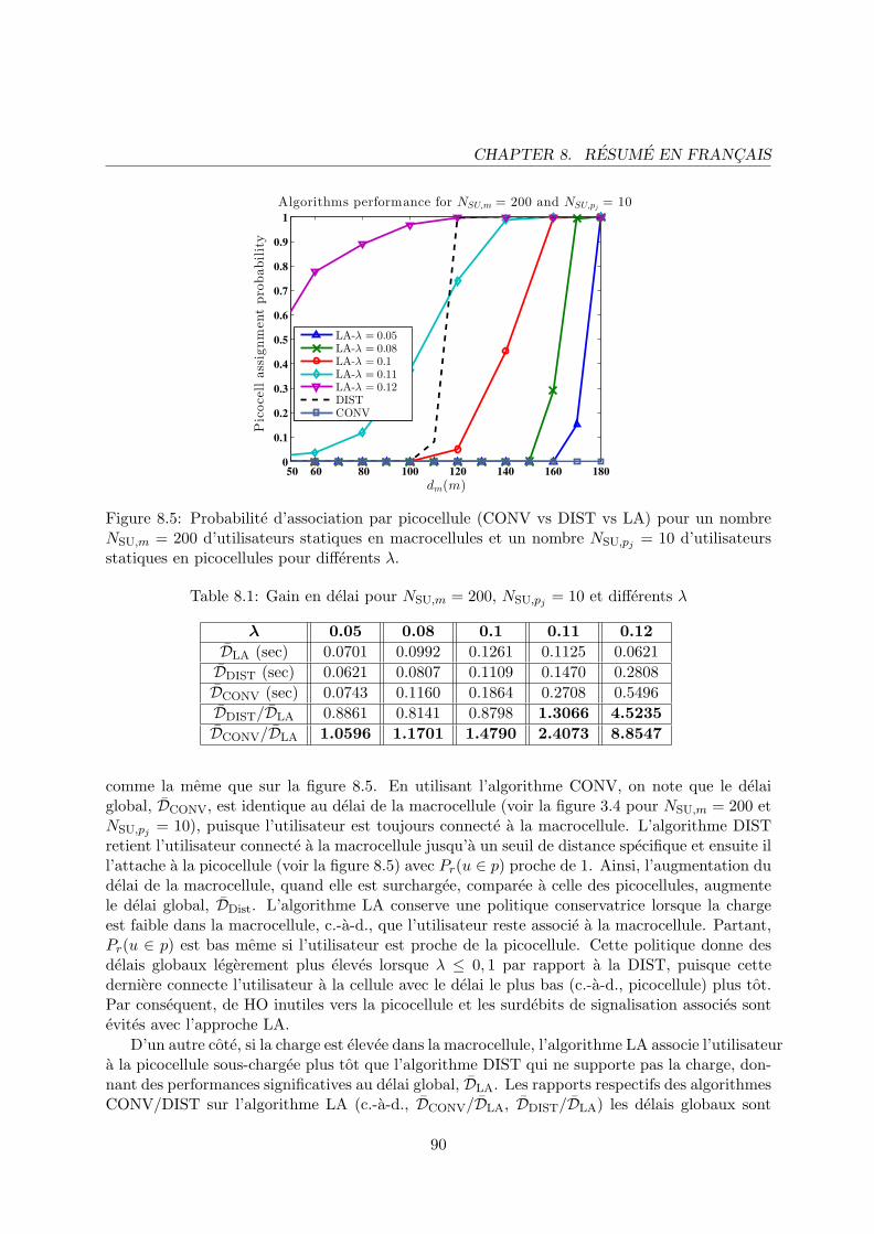
CHAPTER 8. RESUME EN FRANCAIS
50 60 80 100 120 140 160 1800
0.1
0.2
0.3
0.4
0.5
0.6
0.7
0.8
0.9
1
dm(m)
Picocellassignmen
tprobability
Algorithms performance for NSU,m = 200 and NSU,pj = 10
LA-λ = 0.05LA-λ = 0.08LA-λ = 0.1LA-λ = 0.11LA-λ = 0.12DISTCONV
Figure 8.5: Probabilite d’association par picocellule (CONV vs DIST vs LA) pour un nombreNSU,m = 200 d’utilisateurs statiques en macrocellules et un nombre NSU,pj = 10 d’utilisateursstatiques en picocellules pour differents λ.
Table 8.1: Gain en delai pour NSU,m = 200, NSU,pj = 10 et differents λ
λ 0.05 0.08 0.1 0.11 0.12
DLA (sec) 0.0701 0.0992 0.1261 0.1125 0.0621
DDIST (sec) 0.0621 0.0807 0.1109 0.1470 0.2808
DCONV (sec) 0.0743 0.1160 0.1864 0.2708 0.5496
DDIST/DLA 0.8861 0.8141 0.8798 1.3066 4.5235
DCONV/DLA 1.0596 1.1701 1.4790 2.4073 8.8547
comme la meme que sur la figure 8.5. En utilisant l’algorithme CONV, on note que le delaiglobal, DCONV, est identique au delai de la macrocellule (voir la figure 3.4 pour NSU,m = 200 etNSU,pj = 10), puisque l’utilisateur est toujours connecte a la macrocellule. L’algorithme DISTretient l’utilisateur connecte a la macrocellule jusqu’a un seuil de distance specifique et ensuite ill’attache a la picocellule (voir la figure 8.5) avec Pr(u ∈ p) proche de 1. Ainsi, l’augmentation dudelai de la macrocellule, quand elle est surchargee, comparee a celle des picocellules, augmentele delai global, DDist. L’algorithme LA conserve une politique conservatrice lorsque la chargeest faible dans la macrocellule, c.-a-d., que l’utilisateur reste associe a la macrocellule. Partant,Pr(u ∈ p) est bas meme si l’utilisateur est proche de la picocellule. Cette politique donne desdelais globaux legerement plus eleves lorsque λ ≤ 0, 1 par rapport a la DIST, puisque cettederniere connecte l’utilisateur a la cellule avec le delai le plus bas (c.-a-d., picocellule) plus tot.Par consequent, de HO inutiles vers la picocellule et les surdebits de signalisation associes sontevites avec l’approche LA.
D’un autre cote, si la charge est elevee dans la macrocellule, l’algorithme LA associe l’utilisateura la picocellule sous-chargee plus tot que l’algorithme DIST qui ne supporte pas la charge, don-nant des performances significatives au delai global, DLA. Les rapports respectifs des algorithmesCONV/DIST sur l’algorithme LA (c.-a-d., DCONV/DLA, DDIST/DLA) les delais globaux sont
90

CHAPTER 8. RESUME EN FRANCAIS
Table 8.2: Notation des parametres
Parametre Decription Direction
RSRPD or Uj,i Puissance recue de signal de reference descente/montee
SINRD or Uj,i Signal sur interference et bruit descente/montee
SINRth Seuil de signal sur interference et bruit -
BD or Uj Nombre total de PRB pour la j eme BS descente/montee
WD or Uj Bande passante par PRB en Hz descente/montee
N0 Densite de bruit thermique descente/montee
RD or Uj,i Debit du canal physique descente/montee
RD or Ui Debit de trafic demande descente/montee
PDj,i Puissance de transmission de la BS de PRB en descente descente
PUi,j Puissance de transmission de la BS de PRB en montee montee
α, P0 Controle de parametres de puissance en boucle ouverte montee
Pmaxi Puissance maximale de transmission de l’ ieme UE montee
presentes pour montrer le gain correspondant dans le tableau 8.1. La meme tendance vaut pourles valeurs superieures de NSU,m, mais avec des valeurs differentes de λ, comme explique dans lafigure 3.4. Enfin, des gains significatifs sont fournis dans des scenarios de forte charge (c.-a-d.,≃ 4 et ≃ 8 par rapport a l’approche CONV et DIST).
Le travail lie a ce chapitre est:
• K. Alexandris, N. Sapountzis, N. Nikaein, and T. Spyropoulos, “Load-aware handoverdecision algorithm in next-generation HetNets,” in IEEE WCNC 2016, 3-6 April 2016,Doha, Qatar.
8.5 Chapitre 4 -“Utility-Based Resource Allocation under Multi-Connectivity in LTE”
Dans ce chapitre, nous examinons un probleme d’allocation de ressources sous multi-connectivitedans un reseau LTE et proposons une allocation de ressource UPF (utilite par proportionsequitables) qui prend en charge la QoS en termes de debits demandes. Nous evaluons la politiqueproposee avec l’allocation des ressources de l’equite proportionnelle (PF) grace a des simulationsapprofondies et caracterisons le gain de performance tant du point de vue de l’utilisateur quedu reseau dans differentes conditions.
8.5.1 Modele de systeme et hypotheses de probleme
Nous considerons une zone L ⊂ R2 servie par un ensemble de BS B = {b1, · · · , b|B|} et un
ensemble d’UE U = {u1, · · · , u|U|} est distribue dans cette zone. Dans la suite, nous examinonsnotre modele plus en detail: Sur la base du modele de systeme susmentionne, nous formulons leprobleme d’optimisation dans cette section.
A.1-Mobility: Nous assumons la mobilite de l’utilisateur, ce qui implique que tous lesparametres lies a l’emplacement changent dans le temps.
91

CHAPTER 8. RESUME EN FRANCAIS
A.2-Debit de donnees physique: La j eme BS peut delivrer un debit de transmission dedonnees physique maximum RD
bj ,uia un UE. Le debit de donnees physique de la descente en bits
par seconde (bps) est donne dans l’equation (8.4) basee sur la formule de capacite de Shannon:
RDbj ,ui
= BDbjWDbjlog2
(
1 + SINRDbj ,ui
)
, (8.4)
ou BDbj
est le nombre total de PRB en descente de la j eme BS (BUbj
pour montee). En ce qui
concerne le debit de donnees physique de l’ ieme UE a la j eme BS en montee est comme RUui,bj
.
A.3-Controle de puissance: Le controle de puissance en boucle ouverte est applique enmontee et chaque UE compense la perte de chemin LU,dB
ui,bjet effets d’ombrage bases sur les
parametres de controle de puissance (c.-a-d., α, P dBm0 ). Ainsi, la puissance transmise de chaque
PRB de la ieme UE a la j eme BS est:
PU,dBmui,bj
= min(
Pmax,dBmui , P dBm
0 + α · LU,dBui,bj
)
, (8.5)
ou Pmax,dBmui est la puissance maximale transmise de l’ ieme UE. Cependant, en descente, aucun
algorithme de controle de puissance n’est pas applique et la puissance transmise de chaque BS atous les UE est notee PD,dBm
bj ,ui= PD,dBm
bj. On notera que l’asymetrie des puissances transmises en
montee/descente au controle de puissance en montee differencie les valeurs en montee/descentede SINR.
A.4-Multi-connectivite: Dans le cadre de la connectivite multiple, les utilisateurs peuventetre associes et communiquer avec plusieurs BS en meme temps. Nous supposons que la capac-ite de connectivite multiple existe en montee/descente pour tous les UE et qu’un UE peut etreconnecte a une BS si en montee et en descente SINR depassent un seuil predefini, c.-a-d., SINRth.
Par consequent, nous definissons un ensemble E , {(ui, bj) , (bj , ui) : min(
SINRUui,bj
, SINRDbj ,ui
)
>
SINRth} qui represente toutes les connexions possibles entre UE et BS.
A.5-Routage-local: En principe, le routage dans le reseau backhaul est necessaire memepour le trafic d’utilisateur a utilisateur servi par la meme BS. Dans ce cas, le trafic n’est pasroute via le reseau central, par exemple le cœur de reseau (EPC) LTE, mais seulement vial’intermediaire BS [86]. Nous nous concentrons sur le flux de trafic utilisateur-utilisateur quipeut etre route localement, c.-a-d., que les deux utilisateurs sont connectes a au moins un BS.
A.6-Paires d’utilisateurs actifs: Base sur l’exigence SINR minimale definie dans B.1, unensemble qui comprend toutes les paires d’utilisateurs actives desservies par la j eme BS est definicomme Cbj , {(ui, uq) : (ui, bj) , (bj , uq) ∈ E , ui 6= uq} et la paire d’utilisateurs (ui, uq) ∈ Cbjpeut avoir un trafic d’utilisateur a utilisateur achemine localement via BS bj . Par consequent,un ensemble C ,
⋃
bj∈BCbj est forme comme l’union de toutes les paires d’utilisateurs actifs.
Enfin, deux ensembles sont definis pour chaque utilisateur: Dui , {uq : (ui, uq) ∈ C} comprendtous les UEs destines a partir du ieme UE et Sui , {uq : (uq, ui) ∈ C} comprend tous les UEsource qui peuvent transport du trafic vers l’ ieme UE.
A.7-Debit demande pour le flux de trafic: Il correspond au debit demande Rui,uqdetermine comme le debit total requis par un groupe d’applications U2U s’executant en hauten utilisant une connexion etablie de bout en bout de la paire d’utilisateurs (ui, uq), qui peutpasser par n’importe quelle BS intermediaire via local-routing.
92

CHAPTER 8. RESUME EN FRANCAIS
8.5.2 Fonction d’utilite
Notre objectif ici est d’allouer de maniere optimale la ressource au trafic utilisateur-utilisateuren fonction de la fonction d’utilite appliquee. Nous definissons xUbj ,(ui,uq), x
Dbj ,(ui,uq)
∈ X comme
pourcentage du PRB alloue au total des PRB sous forme decimale selon la direction en mon-tee/descente pour transporter le trafic utilisateur-utilisateur de la paire d’utilisateurs (ui, uq) aBS bj . Dans ce qui suit, nous introduisons deux fonctions d’utilite differentes: l’une fournit uneequite proportionnelle et l’autre etend l’equite proportionnelle en tenant compte de la QoS.
8.5.2.1 Equite proportionnelle (PF)
En tant que premiere fonction d’utilite, nous exploitons une fonction d’utilite logarithmiquesimilaire a celle de [87] qui realise une allocation de ressources “proportionnellement equitable”.Cette fonction d’utilite est donnee comme:
Φ (y) = log (y) , (8.6)
8.5.2.2 Utilite par proportions equitables (UPF)
Dans l’ancienne fonction d’utilite, un inconvenient important reside dans l’absence de prise encompte de la qualite de service. Pour incorporer la QoS dans la fonction d’utilite, nous utilisonsla famille des fonctions sigmoıdes comme:
Φ (y) = log (S (y, γ, β)) = log
(1
1 + e−γ(y−β)
)
, (8.7)
γ > 0, y ≥ 0, ou β est le debit demande defini en A.7 de la section 8.5.1. La fonction Φ (y)est le logarithme naturel de la fonction d’utilite sigmoıde, S (y, γ, β), couramment utilise dansla litterature (voir [89]) qui preserve le debit demande.
Sous l’hypothese du regime de multi-connectivite (voir A.4 de la section 8.5.1), nous pouvonsintroduire notre fonction objective finale basee sur toute fonction d’utilite Φ (·) presente a l’equation (8.6) ou a l’ equation (8.7) comme suit:
U(
xUui,uq ,x
Dui,uq
)
, Φ
∑
bj∈B
Q(
xUbj ,(ui,uq), xDbj ,(ui,uq)
)
, (8.8)
ou where xUui,uq ,
[
xUb1,(ui,uq), · · · , xUb|B|,(ui,uq)
]T, xD
ui,uq ,
[
xDb1,(ui,uq), · · · , xDb|B|,(ui,uq)
]T.
La fonction Q (·) represente le debit alloue de la paire d’utilisateurs (ui, uq) et s’exprime commesuit:
Q(
xUbj ,(ui,uq), xDbj ,(ui,uq)
)
, min(
xUbj ,(ui,uq)RUui,bj
, xDbj ,(ui,uq)RDbj ,uq
)
(8.9)
Il est a noter que l’operateur minimum garantit le meme debit alloue en montee et en descentepour un trafic utilisateur a utilisateur.
93

CHAPTER 8. RESUME EN FRANCAIS
8.5.3 Formulation du probleme
Base sur le modele de systeme propose, les hypotheses et les fonctions d’utilite, nous presentonsnotre formulation du probleme. Le probleme tombe dans la categorie de la maximisation del’utilite du reseau pour l’allocation des ressources et est donne dans l’equation (8.10).
Fonction objective: L’objectif est d’allouer la ressource xUbj ,(ui,uq), xDbj ,(ui,uq)
∈ X a chaque
paire d’utilisateurs afin de maximiser la fonction d’utilite reseau agregee sur toutes les pairesd’utilisateurs qui echangent du trafic. Les deux fonctions d’utilite susmentionnees peuvent etreutilisees.
maxX
∑
(ui,uq)∈C
U(
xUui,uq ,x
Dui,uq
)
s.c.∑
(ui,uq)∈Cbj
xUbj ,(ui,uq) ≤ 1, ∀ bj ,
∑
(ui,uq)∈Cbj
xDbj ,(ui,uq) ≤ 1, ∀ bj ,
∑
bj∈B
∑
uq∈Dui
xUbj ,(ui,uq)BUbj≤ BU
ui , ∀ ui,
∑
bj∈B
∑
uq∈Sui
xDbj ,(uq ,ui)BDbj≤ BD
ui , ∀ ui,
∑
bj∈B
∑
uq∈Dui
xUbj ,(ui,uq)PUui,bj
BUbj≤ Pmax
ui , ∀ ui. (8.10)
Contraintes: Ici, nous presentons une description detaillee pour chacun d’entre eux:
1. Les deux premieres contraintes garantissent que le nombre de PRB alloues (exprime sousforme de pourcentage decimal sur le total des PRB) a chaque BS bj pour tous les UE nedepassera pas le nombre total de PRB en montee et en descente.
2. Les troisieme et quatrieme contraintes assurent que le nombre de PRB alloues a chaqueUE parmi toutes les BS connectees ne depassera pas le nombre maximum de PRB al-loues, BU
ui , BDui , du ieme UE, respectivement. Plus precisement, ces contraintes prennent
en compte tout le trafic utilisateur-utilisateur lie au ieme UE comme uq ∈ Dui de tous lesUE destinataires dans montee et uq ∈ Sui de tous les UE source en descente par n’importequelle BS (bj ∈ B). En outre, ces contraintes reposent sur la capacite de l’utilisateur definiecomme categorie UE dans 3GPP TS36.306.
3. Enfin, la derniere contrainte est liee au mecanisme de controle de puissance introduit dansA.3 de la section 8.5.1. Il limite la puissance totale transmise de l’ ieme UE a toutes lesBS connectees pour etre dans sa limite de puissance comme Pmax
ui .
Le probleme propose dans l’equation (8.10) est prouve etre convexe.
8.5.4 Resultats de la simulation
Les principaux resultats de la simulation sont presentes comme suit:
94
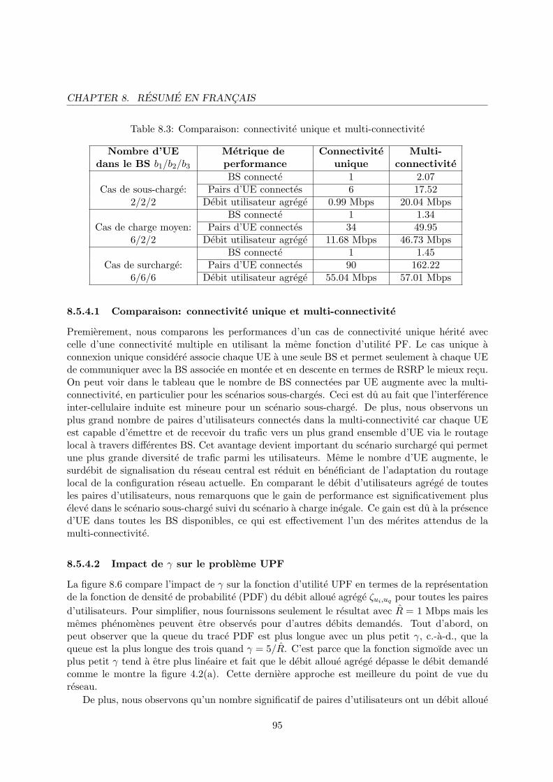
CHAPTER 8. RESUME EN FRANCAIS
Table 8.3: Comparaison: connectivite unique et multi-connectivite
Nombre d’UE Metrique de Connectivite Multi-dans le BS b1/b2/b3 performance unique connectivite
BS connecte 1 2.07Cas de sous-charge: Pairs d’UE connectes 6 17.52
2/2/2 Debit utilisateur agrege 0.99 Mbps 20.04 MbpsBS connecte 1 1.34
Cas de charge moyen: Pairs d’UE connectes 34 49.956/2/2 Debit utilisateur agrege 11.68 Mbps 46.73 Mbps
BS connecte 1 1.45Cas de surcharge: Pairs d’UE connectes 90 162.22
6/6/6 Debit utilisateur agrege 55.04 Mbps 57.01 Mbps
8.5.4.1 Comparaison: connectivite unique et multi-connectivite
Premierement, nous comparons les performances d’un cas de connectivite unique herite aveccelle d’une connectivite multiple en utilisant la meme fonction d’utilite PF. Le cas unique aconnexion unique considere associe chaque UE a une seule BS et permet seulement a chaque UEde communiquer avec la BS associee en montee et en descente en termes de RSRP le mieux recu.On peut voir dans le tableau que le nombre de BS connectees par UE augmente avec la multi-connectivite, en particulier pour les scenarios sous-charges. Ceci est du au fait que l’interferenceinter-cellulaire induite est mineure pour un scenario sous-charge. De plus, nous observons unplus grand nombre de paires d’utilisateurs connectes dans la multi-connectivite car chaque UEest capable d’emettre et de recevoir du trafic vers un plus grand ensemble d’UE via le routagelocal a travers differentes BS. Cet avantage devient important du scenario surcharge qui permetune plus grande diversite de trafic parmi les utilisateurs. Meme le nombre d’UE augmente, lesurdebit de signalisation du reseau central est reduit en beneficiant de l’adaptation du routagelocal de la configuration reseau actuelle. En comparant le debit d’utilisateurs agrege de toutesles paires d’utilisateurs, nous remarquons que le gain de performance est significativement pluseleve dans le scenario sous-charge suivi du scenario a charge inegale. Ce gain est du a la presenced’UE dans toutes les BS disponibles, ce qui est effectivement l’un des merites attendus de lamulti-connectivite.
8.5.4.2 Impact de γ sur le probleme UPF
La figure 8.6 compare l’impact de γ sur la fonction d’utilite UPF en termes de la representationde la fonction de densite de probabilite (PDF) du debit alloue agrege ζui,uq pour toutes les paires
d’utilisateurs. Pour simplifier, nous fournissons seulement le resultat avec R = 1 Mbps mais lesmemes phenomenes peuvent etre observes pour d’autres debits demandes. Tout d’abord, onpeut observer que la queue du trace PDF est plus longue avec un plus petit γ, c.-a-d., que laqueue est la plus longue des trois quand γ = 5/R. C’est parce que la fonction sigmoıde avec unplus petit γ tend a etre plus lineaire et fait que le debit alloue agrege depasse le debit demandecomme le montre la figure 4.2(a). Cette derniere approche est meilleure du point de vue dureseau.
De plus, nous observons qu’un nombre significatif de paires d’utilisateurs ont un debit alloue
95

CHAPTER 8. RESUME EN FRANCAIS
0 0.2 0.4 0.6 0.8 1 1.2 1.4 1.6 1.8 2 2.2
107
0
0.2
0.4
0.6
0.8
1
f()
10-6
Figure 8.6: Trace PDF d’UPF pour differents γ
agrege plus faible (ζui,uq < 0, 4 Mbps) quand γ est grand, γ = 20/R, compare au cas ou γ est
petit, γ = 5/R. Ceci est aussi du a la forme de la fonction sigmoıde dans la figure 4.2(a) danslaquelle la fonction avec un plus grand γ est plus proche de la fonction step et prefere servir lapaire d’utilisateurs proche du QoS exigence. En ce sens, certaines paires d’utilisateurs qui ont dumal a atteindre le debit demande en raison de la mauvaise condition SINR seront allouees avecun debit de donnees agrege plus faible ou meme en file d’attente (par exemple, ζui,uq = 0). Cettederniere approche est meilleure du point de vue de l’utilisateur. Par consequent, l’ajustementde la forme de la fonction sigmoıde sur la base des parametres γ peut avoir un impact surla politique d’allocation mettant en evidence le compromis entre l’equite et la perspective del’utilisateur et du reseau.
Le travail lie a ce chapitre est:
• K. Alexandris, C.-Y. Chang, K. Katsalis, N. Nikaein, and T. Spyropoulos, “Utility-BasedResource Allocation under Multi-Connectivity in Evolved LTE,” in IEEE VTC 2017, Sep24-27, 2017, Toronto, Canada.
8.6 Chapitre 5 - “Multi-Connectivity Resource Allocation withLimited Backhaul Capacity in Evolved LTE”
Dans ce chapitre, nous examinons un probleme d’allocation de ressource UPF sous multi-connectivite en LTE et proposons une utilite considerant la QoS des utilisateurs avec des limita-tions de capacite backhaul par rapport au chapitre 4 ou seules les contraintes radio apparaissent.La politique proposee est comparee a l’allocation des ressources PF par le biais de simulationsapprofondies. Les resultats presentes montrent que la connectivite multiple surpasse la connec-tivite unique en termes de debit agrege du reseau et de QoS des utilisateurs la satisfaction dansdifferentes etudes de cas de reseau, c.-a-d., des scenarios de cellules vides et chargees avec unecapacite de liaison fixe et variable.
8.6.1 Modele de systeme et hypotheses de probleme
Nous considerons un ensemble de BS B = {b1, · · · , b|B|} connecte au reseau central via unreseau backhaul pour servir un ensemble de UE U = {u1, · · · , u|U|}. Pour mieux elucider les
96

CHAPTER 8. RESUME EN FRANCAIS
Table 8.4: Notations additionnelles des parametres
Parametres Description Direction
MD or Ui Nombre de PRB maximal de l’ ieme UE descente/montee
RD or Ui Debit de trafic demande descente/montee
CD or Uh,j Capacite du lien backhaul en bps descente/montee
fD or Uj Frequence de porteuse en Hz descente/montee
hypotheses du chapitre actuel en difference avec celles mentionnees dans la section 8.5.1, nousles redefinissons afin de souligner la nouvelle configuration systeme consideree:
A.1-Frequence de porteuse: Dans ce chapitre, nous appliquons le deploiement RATinter-frequence unique et denote la frequence porteuse en descente comme fDj pour la j eme BS2.
A.2-Reseau Backhaul: Dans notre cas, nous supposons que chaque BS est connectee a lapasserelle du reseau central via une connexion dediee et directe (c.-a-d., topologie en etoile), voirla figure 5.1. Enfin, nous caracterisons la capacite provisionnee de la liaison backhaul a partirde la j eme BS en montee et en descente comme CU
h,j , CDh,j respectivement.
A.3-Debit de trafic demande: Les UE sont supposes envoyer et recevoir du traficprovenant des directions en montee et en descente. L’ensemble des UE qui transmettent enmontee est defini comme S et l’ensemble des UE recus en descente est defini comme D. Plusprecisement, un utilisateur ui envoie du trafic en montee en demandant un debit de donnees RU
i
(debit de trafic demande en montee) et recoit du trafic en descente en demandant un debit RDi
(debit de trafic demande en descente).
8.6.2 Fonction d’utilite
Nous definissons xUi,j , xDj,i ∈ X comme les nombres en decimaux sur le total des PRB alloue par
BS bj a un utilisateur ui pour envoyer ou recevoir du trafic en montee et en descente.
U1
(xUi
), Φ
((xUi
)T·RU
i
)
= Φ
∑
bj∈B
xUi,jRUi,j
, (8.11)
U2
(xDq
), Φ
((xDq
)T·RD
q
)
= Φ
∑
bj∈B
xDj,qRDj,q
. (8.12)
Notez que(xUi
)T· RU
i et(xDq
)T· RD
q incluent le debit agrege sur toutes les BS connectees en
montee ou en descente pour ui et uq. La valeur de RUi ou RD
q est assignee a β dans l’equation (8.7)(fonction sigmoıde) en montee et en descente.
2En montee, la notation devient, par exemple, fUj et la meme regle est appliquee pour le reste des parametres
du systeme.
97

CHAPTER 8. RESUME EN FRANCAIS
8.6.3 Formulation du probleme
Sur la base du modele de systeme susmentionne, des hypotheses et des fonctions d’utilite, nousformulons ensuite le probleme d’allocation des ressources. Un tel probleme tombe dans la cate-gorie de la maximisation de l’utilite du reseau pour l’allocation des ressources et est donnecomme suit:
maxX
∑
ui∈S
U1
(xUi
)+∑
uq∈D
U2
(xDq
)
s.c. C1:∑
ui∈S, (ui,bj)∈E
xUi,j ≤ 1, ∀ bj ∈ B,
C2:∑
uq∈D, (bj ,uq)∈E
xDj,q ≤ 1, ∀ bj ∈ B,
C3:∑
bj∈B, (ui,bj)∈E
xUi,jBUj ≤M
Ui , ∀ ui ∈ U ,
C4:∑
bj∈B, (bj ,uq)∈E
xDj,qBDj ≤M
Dq , ∀ uq ∈ U ,
C5:∑
bj∈B, (ui,bj)∈E
xUi,jBUj P
Ui,j ≤ P
maxi , ∀ ui ∈ U ,
C6:∑
ui∈S, (ui,bj)∈E
xUi,jRUi,j ≤ C
Uh,j , ∀ bj ∈ B,
C7:∑
uq∈D, (bj ,uq)∈E
xDj,qRDj,q ≤ C
Dh,j , ∀ bj ∈ B. (8.13)
Une explication detaillee du probleme d’optimisation propose est donnee presentant la fonctionobjectif ainsi que les sept contraintes:
Fonction objective: L’objectif est d’allouer de maniere optimale les ressources xUi,j , xDj,q ∈ X
pour chaque utilisateur ui, uq ∈ U pour maximiser la somme des fonctions d’utilite de tous lesutilisateurs en appliquant les fonctions d’utilite par utilisateur (voir equation (8.11) et equation(8.12)).
Contraintes: Nous elaborons toutes les contraintes comme suit:
• C1-C2: Ces contraintes garantissent que le nombre de PRB alloues (exprimes en pourcentageen decimales sur le total des PRB) de chaque BS bj a tous les utilisateurs ne depasse pas lenombre total de PRB en montee et en descente.
• C3-C4: Ces deux contraintes assurent que le nombre total de PRB alloues a chaque utilisateurparmi toutes les BS connectees ne depassera pas son nombre maximum de PRB alloues,MUi ,M
Dq , en montee et en descente, respectivement.
• C5: Une telle contrainte est liee au mecanisme de controle de puissance en montee et ellerestreint que la puissance de transmission totale de l’ ieme UE a toutes les BS connectees nepeut pas depasser ses limites de puissance Pmax
i .
• C6-C7: Ces deux contraintes sont liees a la liaison backhaul et elles assurent que les debitsagreges a chaque BS bj ne depasseront pas les capacites backhaul provisionnees dans lesdirections en montee et en descente.
98

CHAPTER 8. RESUME EN FRANCAIS
Le probleme propose dans l’equation (8.13) est prouve d’etre convexe.
8.6.4 Resultats de la simulation
Deux scenarios de simulation principaux sont consideres comme suit:
• Scenario A-Cellule vide: Il y a 1 BS qui ne sert pas d’UE (c.-a-d., charge de trafic0%) tandis que les 2 BS restantes servent un nombre d’UE non-nulle. La charge de traficcellulaire vide est utilisee dans l’evaluation du rapport 3GPP (TR 25.927) et caracterisecertains resultats de mesure dans le monde reel. Nous utilisons la notation 0/z/z pourrepresenter ce scenario ou z est le nombre d’UE desservis par BS non different de zero.
• Scenario B-Cellule chargee: Toutes les cellules servent un nombre d’UE non-nulle etnous utilisons la notation z/z/z pour representer ce scenario. La valeur de z est 2 ou 4dans nos simulations.
En outre, nous definissons deux parametres de base: (a) le debit agrege du reseau en tant quesomme du debit total alloue a tous les utilisateurs en descente
RD ,∑
uq∈D
∑
bj∈B
(xDj,q)⋆RDj,q (8.14)
ou et(
xDj,q
)⋆sont les resultats d’optimisation en descente (meme chose pour montee), et (b) le
ratio de satisfaction d’utilisateurs en pourcentage d’utilisateurs satisfaits du debit alloue
SD , Prob
∑
bj∈B
(xDj,q)⋆RDj,q ≥ R
Dq
(8.15)
(meme chose en montee).Nous demontrons les resultats en descente avec une capacite de backhaul fixe en considerant
la meme valeur est appliquee a tous les liens backhaul. Sur la figure 8.7, le debit agrege moyenest represente pour les scenarios A et B avec 2 UE par BS sous connectivite unique et multi-connectivite en fonction de la capacite backhaul a la fois pour UPF et PF. Dans les scenarios videset charges, le debit agrege converge lorsque la capacite backhaul est provisionnee pour depasser300 Mbit/s dans les cas de connectivite unique et multi-connectivite. En ce qui concerne lescenario A (c.-a-d., cellule vide), on peut voir que la connectivite multiple surpasse la seule memeavec une capacite de liaison insuffisante, c.-a-d., moins de 300 Mbit/s, en utilisant la capacitenon allouee de la cellule vide. Pour le scenario B, il n’y a pas de differences significatives entrela connectivite unique et la connectivite multiple, car dans la cellule chargee, la connectivitemultiple ne peut pas utiliser plus de ressources que la seule par rapport au cas vide, ou desressources supplementaires sont disponibles. Neanmoins, le cas de multi-connectivite peut mieuxrefleter le compromis entre atteindre un debit de donnees plus eleve et atteindre une plus grandesatisfaction des utilisateurs (c.-a-d., PF par rapport a UPF). En d’autres termes, un debitplus agrege est alloue en multi-connectivite afin de mieux satisfaire le debit demande par lesutilisateurs lors de la comparaison avec le cas de connectivite unique, comme indique dans letableau suivant 8.5.
Les resultats du ratio de satisfaction d’ utilisateurs sont presentes dans le tableau 8.5 duscenario A et B et nous observons que le ratio de satisfaction peut etre augmente de deux
99

CHAPTER 8. RESUME EN FRANCAIS
150 200 250 300 350 400
Backhaul Capacity (Mbps)
200
300
400
500
600
700
800
Avg
da
ta r
ate
(M
bp
s)
DL average aggregated rate of Scenario A
Single-PF-0/2/2
Multi-PF-0/2/2
Single-UPF-0/2/2
Multi-UPF-0/2/2
(a) Scenario A: Cellule vide
150 200 250 300 350 400
Backhaul Capacity (Mbps)
400
500
600
700
800
Avg d
ata
rate
(M
bps)
DL average aggregated rate of Scenario B
Single-PF-2/2/2
Multi-PF-2/2/2
Single-UPF-2/2/2
Multi-UPF-2/2/2
(b) Scenario B: Cellule chargee
Figure 8.7: Influence de la capacite backhaul sur debit moyen agrege
Table 8.5: Ratio de satisfaction d’utilisateurs (%) pour differentes capacites backhaul
Backhaul Single Multi Single MultiCapacity PF PF UPF UPF(Mbps) 0/2/2 2/2/2 0/2/2 2/2/2 0/2/2 2/2/2 0/2/2 2/2/2
150 ∼20 ∼20 63 ∼20 ∼20 ∼20 81 ∼20200 49 ∼50 95 ∼50 51 54 100 55
250 72 65 95 68 83 80 100 91
300 81 72 95 73 90 84 100 93
>350 81 72 95 73 90 84 100 93
manieres: (a) appliquer la multi-connectivite (du simple au multi- connectivite) avec PF avec ungain moyen de 3% - 31% et avec un UPF un gain moyen de 7% - 34%, et (b) d’utiliser la fonctiond’utilite UPF (de PF vers UPF) connectivite unique un gain moyen de 7% - 10% est inspectealors qu’en multi connectivite, un gain moyen de 8% - 16% est remarque. Nous soulignons quela multi-connectivite est benefique dans le cas des cellules vides, ou elle peut augmenter le ratiode satisfaction d’ utilisateurs en exploitant davantage de ressources non allouees. En outre,la fonction UPF peut etre utilisee pour accelerer les performances prevues en redistribuant lesressources reseau en fonction du debit demande par les utilisateurs, en particulier dans le cas decellule chargee par rapport a celui de PF.
100

CHAPTER 8. RESUME EN FRANCAIS
Enfin, les scenarios de cellule vide et chargee sont utilises pour identifier les limites inferieureet superieure correspondantes de nos metriques de performance, c.-a-d., les meilleurs et les piresscenarios.
Le travail lie a ce chapitre est:
• K. Alexandris, C.-Y. Chang, N. Nikaein, and T. Spyropoulos, “Multi-Connectivity Re-source Allocation with Limited Backhaul Capacity in Evolved LTE,” in IEEE WCNC2018, April 15-18, 2018, Barcelona, Spain.
8.7 Chapitre 6 - “Utility-based Opportunistic Scheduling underMulti-Connectivity with Limited Backhaul Capacity”
Dans ce chapitre, nous revenons sur les scenarios discutes dans le chapitre 5 exploitant l’impactde la variabilite du canal spatio-temporel (evanouissements a grande et petite echelle) vial’ordonnancement opportuniste. Plus precisement, nous examinons un probleme d’allocationde ressource opportuniste sous multi-connectivite et capacite de liaison limitee dans LTE evolueen utilisant les deux fonctions d’utilite susmentionnees: PF et UPF. Nous proposons ensuite unalgorithme efficace pour traiter le probleme NP-difficile formule. Un tel algorithme est garantipour produire une solution avec une liaison explicite vers la solution optimale. Enfin, les resul-tats de la simulation justifient que l’utilisation de la fonction d’utilite UPF avec une planificationopportuniste dans la multi-connectivite puisse mieux repondre aux exigences de QoS.
8.7.1 Modele de systeme et hypotheses de probleme
Nous considerons une zone desservie par un ensemble de BS B = {b1, · · · , b|B|} connecte au cœurde reseau (CN) via le reseau de backhaul et un ensemble d’UE U = {u1, · · · , u|U|} est distribuedans cette zone. La topologie est la meme avec celle du chapitre 5 et nous nous concentronsuniquement en descente.
L’hypothese A.1 relative au deploiement multi-connectivite inter-frequence comme decritdans la section 8.6.1 contient la meme chose et quelques variations sur le modele de canal (c.-a-d., l’evanouissement a petite echelle afin de prendre en compte les erreurs de canal) et lesdefinitions de debit physique par rapport au chapitre 5 sont presentes comme suit:
A.1-Modele de canal: Dans le RAT LTE, la direction descente utilise l’acces multiple parrepartition orthogonale de la frequence avec la granularite minimale des ressources radio appeleePRB (Physical Resource Block) couvrant une seule tranche de temps dans le domaine temporelet un sous-canal (egal a plusieurs sous-porteuses) domaine. Par consequent, un ensemble desous-canaux K peut etre alloue pour chaque BS. Notre modele de canal considere inclut a lafois les evanouissements a grande echelle et a petite echelle. L’evanouissement a grande echelleinclut a la fois la perte de chemin et l’ombrage comme LD
j,i de la j eme BS au ieme UE , alors que
la petite echelle comprend l’effet multi-chemin et la propagation Doppler comme sDj,k,i (t) de la
j eme BS au ieme UE sur le keme sous-canal au temps t. Pour plus de simplicite, nous laissonstomber l’index de temps t dans les paragraphes suivants.
A.2-Modele de connexion et de trafic: Le regime de multi-connectivite est comme dansle chapitre 4 et 5, ou le critere de connectivite decrit dans l’hypothese A.4 de la section 8.5.1contient la meme chose, l’ ieme UE peut etre connecte a la j eme BS si le SINR moyen SINRD
j,i
101

CHAPTER 8. RESUME EN FRANCAIS
sur tous les sous-canaux est au-dessus d’un seuil, soit SINRth, ou
SINRDj,i =
1
|K|
∑
k∈K
SINRDj,k,i. (8.16)
Les hypotheses de capacite limitee comme celles de la section 8.6.1 (voir l’hypothese A.2) sontprises en compte. Nous notons la capacite de backhaul vers la j eme BS comme CD
h,j qui peutpotentiellement limiter le debit de donnees utilisateur realisable. En outre, l’hypothese A.3presentee dans la section 8.6.1 liee au trafic demande par les utilisateurs est la meme.
8.7.2 Fonction d’utilite
Nous definissons xDj,k,i ∈ {0, 1} comme les variables binaires representant l’allocation ou non du
keme sous-canal au ieme UE a partir de la j eme BS. Par consequent, yDj,k,i = xDj,k,i · RDj,k,i est le
debit physique correspondant.Base sur le modele de systeme introduit dans la section 8.6.1, nous formons d’abord 2
vecteurs xDi =
[
xD1,1,i,...,xD1,|K|,i, x
D2,1,i,...,x
D2,|K|,i,...,x
D|B|,1,i,...,x
D|B|,|K|,i
]Test la forme vectorielle des
variables d’allocation binaire et RDi =
[
RD1,1,i,...,R
D1,|K|,i, R
D2,1,i,...,R
D2,|K|,i,...,R
D|B|,1,i,...,R
D|B|,|K|,i
]T
represente le debit physique vectorise. Ensuite, la fonction d’utilite du reseau de l’ ieme UE est
U(xDi
), Φ
((RDi
)T· xD
i
)
, ou Φ (·) peut etre l’une des deux fonctions d’utilite presentees aux
equations (8.6) et (8.7). En outre, les arguments des fonctions d’utilite PF et UPF incluent ledebit de donnees agrege globalement toutes les BS connectees et les sous-canaux alloues. Enfin,la fonction d’utilite UPF assigne RD
i a son argument β (voir l’equation (8.7)).
8.7.3 Formulation du probleme
Probleme d’optimisation: Le probleme tombe dans la categorie de la maximisation de l’utilitereseau pour l’allocation des ressources et est donne comme suit:
maxxDi ∈{0,1}|B|×|K|
∑
ui∈U
U(xDi
)(8.17)
s.c. C1:∑
ui∈U
∑
k∈K
xDj,k,i ≤ BDj , ∀ bj ∈ B,
C2:∑
bj∈B
∑
k∈K
xDj,k,i ≤MDi , ∀ ui ∈ U ,
C3:∑
ui∈U
xDj,k,i ≤ 1, ∀ bj ∈ B, k ∈ K. (8.18)
Fonction objective: L’objectif est d’allouer de facon optimale les ressources xDj,k,i ∈ {0, 1}pour chaque UE ui ∈ U pour maximiser la sum des fonctions d’utilite de tous les UE. Les deuxfonctions d’utilite PF / UPF decrites dans Section 8.5.2 peuvent etre appliquees.
Contraintes: Dans la suite, nous presentons une description detaillee de chaque contrainte;C1: Il garantit que le nombre de sous-canaux alloues de BS bj a tous les UE ne depassera pasle nombre total de sous-canaux disponibles a bj , B
Dj ; C2: Il assure que le nombre total de
sous-canaux alloues a UE ui parmi toutes les BS connectees ne depassera pas les sous-canaux
102

CHAPTER 8. RESUME EN FRANCAIS
allouables maximum vers ui,MDi . Il repose sur la capacite utilisateur definie comme la categorie
UE dans 3GPP TS36.306; C3: Il garantit que chaque sous-canal unique ne sera pas assigne aplus d’un UE impliquant l’exclusivite du sous-canal.
Le probleme d’optimisation formule est NP-difficile et se revele etre avec une fonction ob-jective submodulaire et monotone et trois contraintes matrioıdes. Enfin, un algorithme gloutonest propose qui peut resoudre efficacement le probleme avec une liaison explicite vers la solutionoptimale.
Dernier point, mais non des moindres, pour satisfaire la limitation de la capacite de backhaul,CDh,j , nous augmentons encore le debit de donnees alloue au ieme UE comme:
RDi ,
∑
bj∈B
∑
k∈K
(xDj,k,i
)⋆RDj,k,i ·min
CDh,j
∑
ui∈U
∑
k∈K
(
xDj,k,i
)⋆RDj,k,i
, 1
, (8.19)
ou(
xDj,k,i
)⋆sont les resultats de l’algorithme propose. En realite, une telle mise a l’echelle peut
etre effectuee en ajustant le schema de modulation et de codage, mais elle sort du cadre de cetteetude.
8.7.4 Resultats de la simulation
Nous nous concentrons sur le scenario B - Cellule chargee: Toutes les cellules servent des UE non-nulles et nous utilisons la notation z/z/z pour representer ce scenario. Ensuite, notre metriquede performance consideree est:
EDi =
∥∥∥RD
i −RDi
RDi
∥∥∥ , if RD
i < RDi ,
0 , o/w.(8.20)
Dans la figure 8.8, les resultats du scenario de cellule vide sont affiches avec plusieurs combi-naisons de PF/UPF avec une connectivite unique/multiple. Nous pouvons voir que l’utilisationde la fonction d’utilite UPF peut augmenter le ratio de satisfaction meme avec une connectiviteunique. Cependant, certaines exigences QoS ne peuvent jamais etre remplies, meme si nousaugmentons continuellement la capacite de backhaul. Cela est du a l’absence d’utilisation deressources non allouees a la cellule vide et donc la multi-connectivite montre son avantage. Enoutre, l’utilisation de la fonction UPF avec une connectivite multiple permet de mieux repondreaux exigences de qualite de service, meme avec une capacite de transport moins importante.Ensuite, les resultats du scenario de cellule chargee sont montres sur la figure 8.8. L’utilisationde plusieurs connexions n’est pas suffisante pour repondre aux exigences de QoS si seulementPF est adopte. Une telle observation est due a l’absence de ressources non allouees provenant decellules vides; par consequent, nous devons reorganiser efficacement les ressources allouees vial’utilisation de la fonction UPF. Enfin, la figure 8.8 montre les avantages de l’ordonnancementopportuniste dans le scenario de cellule chargee avec UPF et multi-connectivite par rapport ala non-opportuniste. Notez que l’ordonnancement non opportuniste peut s’appuyer de faconoptimale sur le SINR moyen (c.-a-d., SINRD
j,i); cependant, son pire cas est base sur le SINR
minimum parmi tous les sous-canaux (c.-a-d., mink∈K
(
SINRDj,k,i
)
). L’opportuniste peut utiliser
plus de connexions et fournit une erreur plus petite, quel que soit le meilleur ou le pire des casd’ordonnancement non opportuniste.
103

CHAPTER 8. RESUME EN FRANCAIS
100 120 140 160 180 200Backhaul Capacity (Mbps)
0
0.05
0.1
0.15
Avg
un
sa
tisfie
d
no
rm e
rro
r
Non-opportunistic UPF-Multi (Min SINR) (Avg 1.76 connections per UE)
Non-opportunistic UPF-Multi (Avg SINR) (Avg 1.89 connections per UE)
Opportunistic UPF-Multi (Avg 2.19 connections per UE)
Figure 8.8: Erreur insatisfait par rapport a capacite backhaul (z/z/z)
Le travail lie a ce chapitre est:
• K. Alexandris, C.-Y. Chang, N. Nikaein, and T. Spyropoulos, “Utility-based OpportunisticScheduling under Multi-Connectivity with Limited Backhaul Capacity,” in IEEE WirelessCommunications Letters, 2018, submitted, under review.
104

Appendix A
A.1 Capacity analysis-I
The average capacity, assuming shadowing and Rayleigh flat fading 1, is expressed as:
C (di) = Eψi,|h|2
[
B log2
(
1 + ρiK (di/dr)−η ψi |h|
2)]
, (A.1)
where ρi , PTx,i/N0 denotes the transmit signal-to-noise ratio (SNR) 2, PTx,i is the transmissionpower in linear scale, di represents the distance from the BS cell i to the user that is greaterthan a reference distance dr, B stands for the available bandwidth, N0 represents the aggregated
noise power over B in linear scale, ψi ∼ Log-N(
0, σ2dB,i/ξ2)
represents the shadowing fading in
linear scale and h ∼ CN (0, 1) defines the Rayleigh flat fading channel coefficient. To the bestof our knowledge, an analytical expression for the averaged capacity does not exist. Therefore,its lower and upper bound, Cb (di), b ∈ {L,U}, can be easily computed, as follows.
A.1.1 Lower bound
Exploiting the concavity of the logarithmic function, an analytical lower bound is given by:
C (di) = Eψi,|h|2
[
B log2
(
1 + ρiK (di/dr)−η ψi |h|
2)]
⇔
C (di) = Eψi
[
E|h|2
[
B log2
(
1 + ρiK (di/dr)−η ψi |h|
2)]]
⇔
C (di) ≥ Eψi
[
E|h|2
[
B log2
(
ρiK (di/dr)−η ψi |h|
2)]]
⇔
C (di) ≥ B{log2
(ρiK (di/dr)
−η)− γ/ ln (2)}
︸ ︷︷ ︸
CL(di)
, (A.2)
where γ denotes the Euler-Mascheroni constant.
1It is noted that the capacity is based on the received signal before the filtering process, thus Rayleigh fadingeffect is taken into account.
2SINR could also be introduced, but would make the analysis complex.
105

APPENDIX A.
A.1.2 Upper bound
Using Jensen’s inequality for concave functions, the upper bound is computed analytically asfollows:
C (di) = Eψi,|h|2
[
B log2
(
1 + ρiK (di/dr)−η ψi |h|
2)]
⇔
C (di) = Eψi
[
E|h|2
[
B log2
(
1 + ρiK (di/dr)−η ψi |h|
2)]]
⇔
C (di) ≤ B log2(1 + ρiK (di/dr)
−η µψi
)
︸ ︷︷ ︸
CU (di)
, (A.3)
where µψi= E [ψi] = exp
[
σ2dB,i/2ξ2]
.
A.2 Capacity analysis-II
The picocell points x, y are distributed uniformly over a circle according to the following distri-bution:
fX,Y (x, y) =
1
π(
R2pj
−d2r
) , dr ≤ r ≤ Rpj ,
0 , o/w,(A.4)
where r =√
(x− xpj )2 + (y − ypj )
2. Average capacity bounds are obtained by averaging over
all the possible distances (i.e., over all the possible points) within the picocell on the respectivelower and upper capacity bound for each cell i. This can be analytically described as:
Cib =
∫
Y
∫
XCb (di (x, y)) fX,Y (x, y) dxdy, b ∈ {L,U}. (A.5)
A.2.1 Lower bound
The average lower bound of the average capacity by applying cartesian to polar coordinatestransformation in Eq. (A.5) is computed as:
CiL =1
π(
R2pj − d
2r
)
∫ 2π
0
∫ Rpj
dr
rCL
(
di (r, θ))
drdθ =
= B
log2 (ρi) +
1
π(
R2pj − d
2r
)
∫ 2π
0
∫ Rpj
dr
r log2
(
K[
di (r, θ) /dr
]−η)
drdθ
︸ ︷︷ ︸
J1
−γ/ ln (2)
.
(A.6)
106

APPENDIX A.
A.2.2 Upper bound
Applying the same methodology used for the lower bound, the corresponding average upperbound is given by:
CiU =1
π(
R2pj − d
2r
)
∫ 2π
0
∫ Rpj
dr
rCU
(
di (r, θ))
drdθ
=B
π(
R2pj − d
2r
) ×
∫ 2π
0
∫ Rpj
dr
r log2
(
1 + ρiK[
di (r, θ) /dr
]−ηµψi
)
drdθ
︸ ︷︷ ︸
J2
. (A.7)
The function di (r, θ) is given by:
di (r, θ) =
{√
[r cos (θ)− x∗]2 + [r sin (θ)− y∗]2 , i = m,
r , i = pj ,(A.8)
where x∗ = xm − xpj and y∗ = ym − ypj .This function represents the user distance from the macrocell and the picocell BS in polar
coordinates, when the user is located within the picocell. Finally, the J1 and J2 integrals arenumerically computed.
107

APPENDIX A.
108
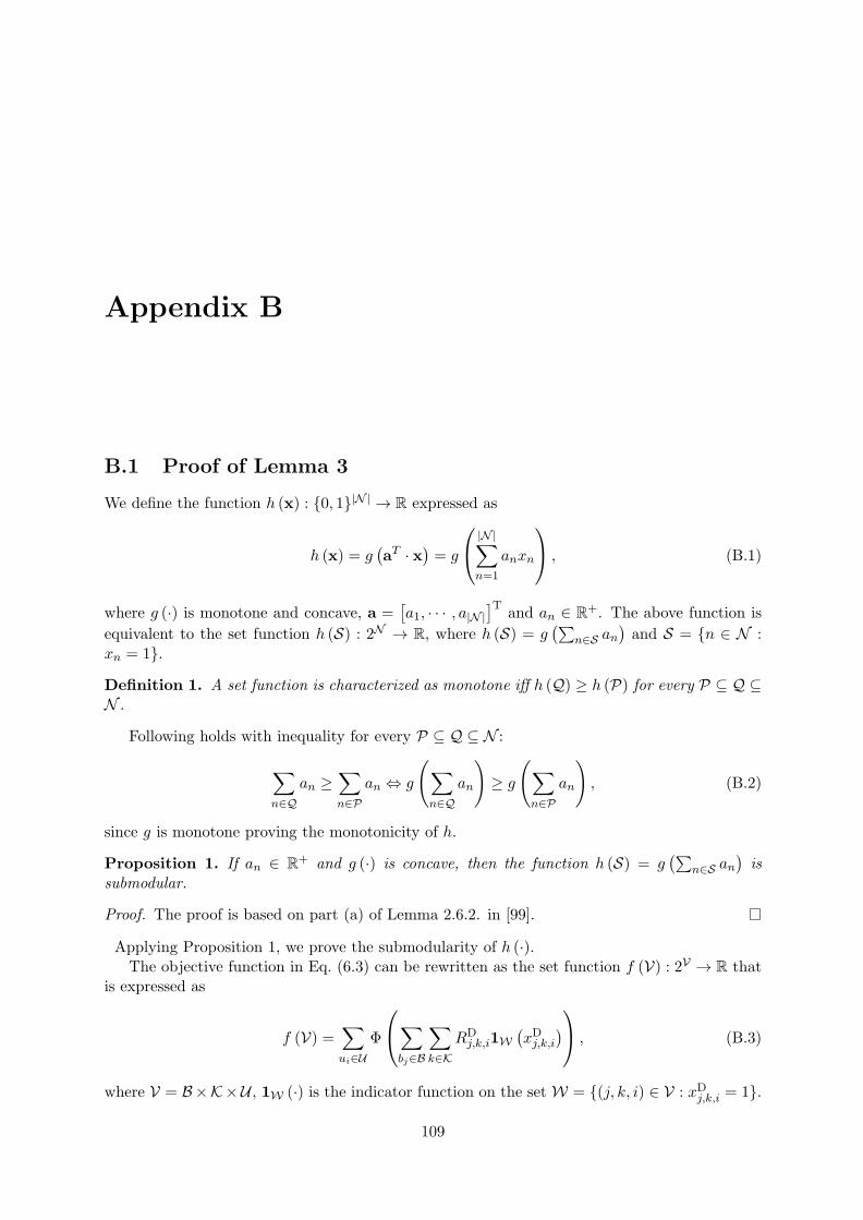
Appendix B
B.1 Proof of Lemma 3
We define the function h (x) : {0, 1}|N | → R expressed as
h (x) = g(aT · x
)= g
|N |∑
n=1
anxn
, (B.1)
where g (·) is monotone and concave, a =[a1, · · · , a|N |
]Tand an ∈ R
+. The above function is
equivalent to the set function h (S) : 2N → R, where h (S) = g(∑
n∈S an)and S = {n ∈ N :
xn = 1}.
Definition 1. A set function is characterized as monotone iff h (Q) ≥ h (P) for every P ⊆ Q ⊆N .
Following holds with inequality for every P ⊆ Q ⊆ N :
∑
n∈Q
an ≥∑
n∈P
an ⇔ g
(∑
n∈Q
an
)
≥ g
(∑
n∈P
an
)
, (B.2)
since g is monotone proving the monotonicity of h.
Proposition 1. If an ∈ R+ and g (·) is concave, then the function h (S) = g
(∑
n∈S an)is
submodular.
Proof. The proof is based on part (a) of Lemma 2.6.2. in [99].
Applying Proposition 1, we prove the submodularity of h (·).The objective function in Eq. (6.3) can be rewritten as the set function f (V) : 2V → R that
is expressed as
f (V) =∑
ui∈U
Φ
∑
bj∈B
∑
k∈K
RDj,k,i1W
(xDj,k,i
)
, (B.3)
where V = B×K×U , 1W (·) is the indicator function on the set W = {(j, k, i) ∈ V : xDj,k,i = 1}.
109

APPENDIX B.
Proposition 2. Φ (·) utility functions are monotone and strictly concave.
Proof. The PF utility function is the logarithmic function and thus is monotone and strictlyconcave. While the UPF takes the natural logarithm of sigmoid function proven as monotoneand strictly concave following Lemma III.1. in [89].
As each term in the summation of objective function f (·) lying on the family of h (·) inEq. (B.1), where Φ (·) ≡ g (·) is monotone and concave, N ≡ B ×K, an ≡ R
Dj,k,i and xn ≡ x
Dj,k,i.
Thus, we conclude that the objective function f (·) is monotone and submodular as it is thesummation of monotone and submodular functions.
Finally, we define three constraints in Eq. (6.4) equivalently as Il, l ∈ {1, 2, 3} in Eq. (B.4)as supersets:
I1 = {S ⊆ 2V : |S ∩ 2{j,K,U}| ≤ Bj , ∀ bj ∈ B}, (B.4a)
I2 = {S ⊆ 2V : |S ∩ 2{B,K,i}| ≤Mi, ∀ ui ∈ U}, (B.4b)
I3 = {S ⊆ 2V : |S ∩ 2{j,k,U}| ≤ 1, ∀ bj ∈ B, k ∈ K}. (B.4c)
To prove these constraints are matroid (see definition in [97]) with V as ground set, two propertiesshall be fulfilled:
(a) For all sets P and Q with P ⊆ Q ⊆ V , if Q ∈ Il, i.e., the sub-channel allocation definedby Q does not violate the constraint Il, then P ∈ Il is held, i.e., the constraint Il is not violatedby sub-channel allocation in P, since P ⊆ Q. All three aforementioned constraints possess suchproperty.
(b) For all sets P,Q ∈ Il and |Q| > |P|, i.e., more sub-channels are allocated in total definedby Q, ∃ e ∈ Q\P such that P ∪ {e} ∈ Il. Since not all sub-channels are allocated definedby P (otherwise, Q will either violate the constraint Il, i.e., Q /∈ Il, or has no more allocatedsub-channels as P, i.e., |Q| ≤ |P|), there is at least one sub-channel that can be further allocatedand will not violate the constraint Il. Hence, such property is held for all three constraints.
Thus, we conclude that Il, ∀ l ∈ {1, 2, 3} are matroid.
110

Appendix C
Towards open-source 4G/5G experimental platforms [100], we are advancing to the OAI testbedimplementation for local or remote access experimentation. The deployed OAI testbed was usedto perform network measurements in order to characterize and analyze the X2 handover systembehavior described in Chapter 2. The supported OAI testbed’s hardware (HW) equipment wasfurther exploited to extend the X2 handover implementation based on the OAI emulator (oaisim)and proceed to its RF-based release for real-time communications prototyping.
C.1 OAI testbed for X2 handover experimentation
In that section, we describe the OAI testbed including the supported nodes, the provided webportal and the offered services. The whole testbed infrastructure is a solution for accessing,managing and monitoring the OAI network resources in a real-time running environment.
C.1.1 OAI testbed description
The remote and local access to the OAI testbed facilities is given via the OAI testbed web por-tal. The NITOS Scheduler [101], a tool that is responsible for managing testbed resources, i.e.,including nodes description, reservation and verification per time slot for a given experiment,was adapted to support the OAI testbed LTE network resources. A detailed description of theOAI testbed portal can be found at https://oailab.eurecom.fr/oai-testbed/, as well asanalytical guidelines on how to access and register to it. The web portal’s user interface isdepicted in Fig. C.1 and the provided OAI testbed LTE nodes with their supported features areshown in Fig. C.2.
The list of nodes is provided as follows:
Node 1: OAI Juju charms, COTS UE (Samsung Galaxy S6), Node 2: OAI eNB (USRP B210),Node 3: LTErf service, Node 4: OAI eNB (USRP B210), Node 5: COTS UE (Huawei e392),OAI HSS, Docker service, Node 6: COTS UE (Huawei e3276), OAI HSS, Docker service, Node7: OAI EPC (MME/SPGW), Node 8: OAI EPC (MME/SPGW).
In more detail, except for the OAI compatible hardware (2 USRP B210) and software (OAIeNB/EPC), we provide a gamut of services, e.g., OAI Juju charms [102], LTErf and Docker.Moreover, the OAI testbed is fully equipped with 3 COTS UEs (Huawei e392/ Huawei e3276/Sam-
111

APPENDIX C.
Figure C.1: OAI testbed portal
sung Galaxy S6) and suitable RF frontend equipment, i.e., antennae, filters, etc. Tutorials forthe experimenters can be found in the following links:
• OAI testbed guidelines:https://oailab.eurecom.fr/oai-testbed/index.php/oai-nodes/lte-testbed
• LTErf guidelines for OAI:https://oailab.eurecom.fr/oai-testbed/index.php/oai-nodes/lterf-guidelines
The provided links include a step by step analytical guide on how an experimenter can accessthe OAI testbed after the registration process. As a second step, we provide the commands thatcan be used to manage and run the OAI LTE network equipment. Last but not least, detailedinstructions for the use of the LTErf service via REST API commands are incorporated to aidthe OAI testbed’s LTE network parameterization during the phase of the experiments.
C.2 OAI X2 experimental setup
The initial implementation of X2 handover was based on the oaisim without including the RFsupport using compatible software/hardware equipment (OAI RF lte-softmodem) as discussedin Chapter 2. Currently, the X2 HO implementation is extended to support the RF functional-ity [103] as well as it is integrated with the OAI testbed.
The E-UTRAN supported messages and functionalities for the X2 HO procedure on the eNBside are described as follows:
112

APPENDIX C.
Figure C.2: OAI testbed nodes setup
PHY/MAC layer API: RAR,RRC layer API: RRC Measurement report, RRC ConnectionReconfiguration, RRC Connection Reconfiguration Complete, X2 API: X2 Setup Request, X2Setup Response, X2 Handover Request, X2 Handover Request ACK.
The experimentation setup is depicted in Fig. C.3 and includes 2 OAI eNBs (2 USRP B210-source/target eNB) synchronised via GPS. In addition, octoBoxquadAtten programmable mod-ules are used as attenuators on both the two eNBs to model UE mobility, e.g., emulate fadingeffects etc. At that instant, UE can send its E-UTRAN RRC Measurement report for triggeringthe HO in the eNB side. Specifically, the selected attenuators offer stable attenuation accuracyvia wide choice of attenuation (63 dB range), frequency ranges (DC to 6000 MHz) and step sizes(0.5 step). In addition, the module can be controlled remotely through Ethernet interface viaan attenuation control unit. For the core network side, a COTS EPC, i.e., Nokia Bell-labs, isused to support the X2 HO functionalities for EPC, e.g., Path switch/Modify Bearer signaling,not currently supported by OAI; this part is included in the HO Execution process (see Fig. 2.2in Chapter 2).
C.3 OAI X2 handover demonstration with OAI emulator (oaisim)
A brief description of the X2 HO intra-frequency oaisim deployment presented in Chapter 2and supported in OAI X2 experimental testbed is discussed as follows. The demonstrationincludes 2 eNBs (one source and one target single omnidirectional antenna cell) and 1 UE (singleomnidirectional antenna user). In addition, one radio chain (Tx/Rx) per UE/eNB wirelesssingle-input single-output (SISO) link in full PHY emulation mode (without radio frontends)
113

APPENDIX C.
Figure C.3: X2 HO experimental setup schematic
is implemented. UE is moving based on a specific mobility pattern (i.e., ping-pong movementpattern) defined by traces that are given as input. The cells are in fixed topology, i.e., placed ina constant position. Before handover, UDP traffic 1 is exchanged between the UE and the sourceeNB (eNB0). Handover procedure is triggered and after handover execution and completion,UDP traffic is exchanged between the UE and the target eNB (eNB1). A youtube video link ofthe demonstration can be found at: https://www.youtube.com/watch?v=PiQxLgY3Gsk.
C.4 OAI X2 handover experimental RF testbed demonstration
As an extension of X2 handover implementation in oaisim, we perform real-world RF mea-surements in the deployed OAI X2 HO experimental testbed. The handover testbed providessmall-cell to small-cell X2 intra-frequency handover functionalities, as described in [57]. Thedemonstration includes 2 OAI eNBs (i.e., 2x USRP B210) and 1 COTS UE (Samsung Galaxy S6).The two eNBs are synchronised via a GPS module as mentioned before and are connected viaEthernet or locally, where SCTP is enabled for communication, i.e., exchanging the required X2
1Additional measurements can be performed using TCP traffic to figure out the impact on HO delay incrementdue to packets retransmission.
114

APPENDIX C.
Figure C.4: X2 HO experimental setup in the lab
signalling, and GTP-U for the user data-plane. This is an initial step for testing the E-UTRANpart including the HO preparation and HO execution steps of X2 HO. For the EPC part; an OAIcompatible (Nokia Bell Labs EPC) is used as descripted in the previous sections. A youtube videolink of the demonstration can be found at: https://www.youtube.com/watch?v=KlwampmhFxw.
C.5 SDN-based handover control
This section describes a Software Defined Network (SDN)-based control and coordination frame-work used for the handover parameters control that it will be released soon for future experi-mentation. In more detail, the supported handover parameters that can be adjusted using theproposed framework are mentioned in Section 2.2.2.
FlexRAN controller/agent: Towards 5G, programmable RAN underlay is essential inorder to facilitate the control and managements procedures. In the LTE domain, SDN controlcan be used to facilitate network agility over the physical or virtualized core network and thebase stations. On the top of the current testbed RAN deployment for X2 handover experi-mentation, an SDN controller is built to provide centrally handover programmability. For theprogrammability of the eNB, emerging control frameworks such as FlexRAN with support forboth northbound and southbound protocols can be used, whose design and implementation canbe found in [27]. A high level representation of the proposed architecture that allows to changethe above parameters on-the-fly is depicted in Fig. C.5. Additional information about FlexRANprogrammability and setup can be found at: https://gitlab.eurecom.fr/FlexRAN/FlexRAN/wikis/FlexRANwithCOTSUE.
Specifically, FlexRAN is composed from two basic entities: a) the FlexRAN controller andb) the FlexRAN agent. The boundary between the network controller and agent is traversed bythe RAN-specific southbound application programming interface (API), the so-called FlexRANagent API. The boundary between the applications and the FlexRAN controller layer is traversedby the northbound API, the so-called FlexRAN application API.
• FlexRAN agent: FlexRAN separates the control from the data plane by detaching the
115

APPENDIX C.
Figure C.5: FlexRAN scenario
L2 protocol logic from the relevant actions and by consolidating all the related control op-erations in a logically centralized controller, which in FlexRAN comprises of the FlexRANmaster controller and the agents interacting via the FlexRAN protocol. In other words,the FlexRAN Agent API constitutes the southbound API. The protocol messages areimplemented using Google protobuf messages; the current implementation supports theRLC/MAC protocol logic and RRC logic is ongoing development related to the handoverparameters control.
• FlexRAN controller: The master controller constitutes the brain of the FlexRAN con-trol plane as it manages the operation of the FlexRAN agent. In more detail, the ap-plications running on top of the FlexRAN master controller make control decisions forthe various functions of the L2. These decisions are manifested in the form of FlexRANprotocol messages that are sent from the master controller to the corresponding FlexRANagent(s). The agents provide a protocol message handler and dispatcher module, thatis responsible to process these messages and to forward them to the L2 control module
116

APPENDIX C.
Table C.1: ho.yaml file content
rrc:
-x2_ho:
parameters:
ttt_ms: :!!int 100
hys: :!!int 0
ofn: :!!int 0
ocn: :!!int 0
ofs: :!!int 0
ocs: :!!int 0
off: :!!int 0
filter_coeff_rsrp: :!!float 0.5
filter_coeff_rsrq: :!!float 0.5
by invoking the proper function of the L2 API. As northbound API, we use the “curl”command-line tool to send by an application via URLs the intended parameter configura-tion.
If an experimenter wants to set/get the handover parameters in order to see their impact inthe network can send a curl command using the northbound API (application-controller) andinvoke the corresponding L2 (RRC layer) getters/setters using the southbound API (controller-agent). An example of the corresponding commands is given in the following:
Set handover parameters:
$ curl -X POST http://localhost:9999/ho_manager/ho.yaml
Get handover parameters:
$ curl -X GET http://localhost:9999/stats_manager/rrc
$ curl -X GET http://localhost:9999/stats_manager/all
The above example shows how the experimenter can set or get the handover parameters val-ues via curl commands invoking the corresponding setters/getters function in L2 layer. Specifi-cally, the experimenter sets the values in the corresponding .yaml files (like the one depicted inTable C.1) or gets the values using the stats manager (returns rrc or all L2 layers parameters).
The centralized network view offered by FlexRAN could enable more sophisticated mobilitymanagement mechanisms that consider additional factors, e.g., the load of cells or use-drivenresource requirements of mobile devices, leading to an optimization of the device-network as-sociations [27]. That kind of sophistication can be devised by the running applications on thetop described in the following. The application layer consists of all the controlling and busi-ness applications running on top of the FlexRAN controller. One of these applications can beconsidered mobility management based on different handover criteria. A well-known handovercriterion supported by OAI RAN platform, commonly used in conventional HO decision algo-rithms (3GPP LTE), is based on RSRPs comparison method in which hysteresis and handoveroffsets are included as described in Chapter 2. As an extension, other representative handoveralgorithms consider not only RSS criteria as the one described in Chapter 3 are planned forfuture development.
117

APPENDIX C.
118

Bibliography
[1] Cisco. Cisco visual networking index forecast projects 18-fold growth in global mobileinternet data traffic from 2011 to 2016. [Online]. Available: http://tinyurl.com/7gn9x9s
[2] Ericsson. 5G radio access: Research and vision. [Online]. Available: http://www.ericsson.com/res/docs/whitepapers/wp-5g.pdf
[3] 5G-PPP–5G Vision. [Online]. Available: https://5g-ppp.eu/wp-content/uploads/2015/02/5G-Vision-Brochure-v1.pdf
[4] A. Osseiran, F. Boccardi, V. Braun, K. Kusume, P. Marsch, M. Maternia, O. Queseth,M. Schellmann, H. D. Schotten, T. Hidekazu, H. M. Tullberg, M. A. Uusitalo, B. Timus,and M. Fallgren, “Scenarios for 5g mobile and wireless communications: the vision of theMETIS project,” IEEE Communications Magazine, vol. 52, no. 5, pp. 26–35, 2014.
[5] Small Cell Forum–Release 10.0. [Online]. Available: http://scf.io/en/documents/newdocuments.php
[6] D. Xenakis, N. Passas, L. Merakos, and C. Verikoukis, “Mobility management for femto-cells in LTE-advanced: Key aspects and survey of handover decision algorithms,” IEEECommunications Surveys Tutorials, 2014.
[7] Nokia, “Ultra Dense Network (udn),”White Paper, 2015.
[8] T. Jansen, I. Balan, J. Turk, I. Moerman, and T. Kurner, “Handover parameter optimiza-tion in LTE self-organizing networks,” in IEEE 72nd Vehicular Technology Conference Fall(VTC 2010-Fall), 2010.
[9] N. Sinclair, D. Harle, I. Glover, J. Irvine, and R. Atkinson, “An advanced som algorithmapplied to handover management within LTE,” IEEE Transactions on Vehicular Technol-ogy, 2013.
[10] H. Zhang, W. Ma, W. Li, W. Zheng, X. Wen, and C. Jiang, “Signalling cost evaluationof handover management schemes in LTE-advanced femtocell,” in IEEE 73rd VehicularTechnology Conference (VTC Spring), 2011.
[11] D. Lopez-Perez, A. Ladanyi, A. Juttner, and J. Zhang, “Ofdma femtocells: Intracell han-dover for interference and handover mitigation in two-tier networks,” in 2010 IEEE Wire-less Communications and Networking Conference (WCNC), 2010.
119

BIBLIOGRAPHY
[12] A. Gudipati, D. Perry, L. E. Li, and S. Katti, “Softran: Software defined radio accessnetwork,” in Proceedings of the Second ACM SIGCOMM Workshop on Hot Topics inSoftware Defined Networking, 2013, pp. 25–30.
[13] 5G PPP Architecture Working Group, “View on 5G architecture,” 2016.
[14] 3GPP, “Study on Small Cell enhancements for E-UTRA and E-UTRAN; Higher layeraspects,” 3rd Generation Partnership Project (3GPP), TR 36.842, Dec 2013.
[15] ——, “Evolved Universal Terrestrial Radio Access Network (eutran);carrier aggregation;base station (bs) radio transmission and reception (release 10),” 3rd Generation Partner-ship Project (3GPP), TR 36.808, Jul 2013.
[16] D. S. Michalopoulos, I. Viering, and L. Du, “User-plane multi-connectivity aspects in 5G,”in 23rd International Conference on Telecommunications (ICT), May 2016, pp. 1–5.
[17] C. Rosa, K. Pedersen, H. Wang, P. H. Michaelsen, S. Barbera, E. Malkamaki, T. Hent-tonen, and B. Sebire, “Dual connectivity for lte small cell evolution: functionality andperformance aspects,” IEEE Communications Magazine, vol. 54, no. 6, pp. 137–143, June2016.
[18] M. Polese, M. Mezzavilla, and M. Zorzi, “Performance comparison of dual connectivityand hard handover for lte-5g tight integration,” in Proceedings of the 9th EAI InternationalConference on Simulation Tools and Techniques, ser. SIMUTOOLS’16, 2016.
[19] Ericsson, “5G radio access,”White Paper, 2014.
[20] W. H. Wang, M. Palaniswami, and S. H. Low, “Application-oriented flow control: funda-mentals, algorithms and fairness,” IEEE/ACM Transactions on Networking, vol. 14, no. 6,pp. 1282–1291, 2006.
[21] G. Tychogiorgos, A. Gkelias, and K. K. Leung, “Utility-proportional fairness in wirelessnetworks,” in IEEE PIMRC 2012, pp. 839–844.
[22] J.-W. Lee and J.-A. Kwon, “Utility-based power allocation for multiclass wireless systems,”IEEE Transactions on Vehicular Technology, vol. 58, no. 7, pp. 3813–3819, 2009.
[23] M. Proebster, M. Kaschub, and S. Valentin, “Context-aware resource allocation to improvethe quality of service of heterogeneous traffic,” in 2011 IEEE International Conference onCommunications (ICC), 2011, pp. 1–6.
[24] F. B. Tesema, A. Awada, I. Viering, M. Simsek, and G. P. Fettweis, “Mobility modelingand performance evaluation of multi-connectivity in 5G intra-frequency networks,” in IEEEGlobecom Workshops, 2015.
[25] N. Prasad and S. Rangarajan, “Exploiting dual connectivity in heterogeneous cellularnetworks,” in 2017 15th International Symposium on Modeling and Optimization in Mobile,Ad Hoc, and Wireless Networks (WiOpt), May 2017, pp. 1–8.
[26] F. Cardoso, F. Pereira de Figueiredo, R. Vilela, and J. Paulo Miranda, “A case study onprotocol stack integration for 3gpp lte evolved node b,” Nov 2014, pp. 1–6.
120

BIBLIOGRAPHY
[27] X. Foukas, N. Nikaein, M. M. Kassem, M. K. Marina, and K. Kontovasilis, “Flexran: Aflexible and programmable platform for software-defined radio access networks,” in Pro-ceedings of the 12th International on Conference on Emerging Networking EXperimentsand Technologies, ser. CoNEXT ’16, 2016, pp. 427–441.
[28] S. Oh, B. Ryu, and Y. Shin, “Epc signaling load impact over s1 and x2 handover onlte-advanced system,” in 2013 Third World Congress on Information and CommunicationTechnologies (WICT), Dec 2013, pp. 183–188.
[29] S. Oh, H. Kim, B. Ryu, and N. Park, “Inbound mobility management on lte-advancedfemtocell topology using x2 interface,” in Proceedings of 20th International Conference onComputer Communications and Networks (ICCCN), July 2011, pp. 1–5.
[30] E. A. Ibrahim, M. R. M. Rizk, and E. F. Badran, “Study of lte-r x2 handover based ona3 event algorithm using matlab,” in 2015 International Conference on Information andCommunication Technology Convergence (ICTC), Oct 2015, pp. 1155–1159.
[31] N. Baldo, M. Requena-Esteso, M. Miozzo, and R. Kwan, “An open source model for thesimulation of lte handover scenarios and algorithms in ns-3,” in Proceedings of the 16thACM International Conference on Modeling, Analysis and Simulation of Wireless andMobile Systems, 2013, pp. 289–298.
[32] M. Assyadzily, A. Suhartomo, and A. Silitonga, “Evaluation of x2-handover performancebased on rsrp measurement with friis path loss using network simulator version 3 (ns-3),” in Information and Communication Technology (ICoICT), 2014 2nd InternationalConference on, May 2014, pp. 436–441.
[33] Atte Helenius, “Performance of handover in long term evolution,” Master Thesis, AaltoUniversity, 2008.
[34] J.-M. Moon and D.-H. Cho,“Novel handoff decision algorithm in hierarchical macro/femto-cell networks,” in 2010 IEEE Wireless Communications and Networking Conference(WCNC), 2010.
[35] L. Li, Z. Mao, and J. Rexford, “Toward software-defined cellular networks,” in 2012 Euro-pean Workshop on Software Defined Networking (EWSDN), Oct 2012, pp. 7–12.
[36] X. Jin, L. E. Li, L. Vanbever, and J. Rexford, “Softcell: Scalable and flexible cellular corenetwork architecture,” in Proceedings of the 9th ACM Conference on Emerging NetworkingExperiments and Technologies, 2013, pp. 163–174.
[37] T. Mahmoodi and S. Seetharaman, “On using a sdn-based control plane in 5G mobilenetworks,” IEEE Vehicular Technology Magazine, vol. 9, no. 3, 2014.
[38] P. Dely, A. Kassler, L. Chow, N. Bambos, N. Bayer, H. Einsiedler, C. Peylo, D. Mellado,and M. Sanchez, “A software-defined networking approach for handover management withreal-time video in wlans,” Journal of Modern Transportation, vol. 21, no. 1, pp. 58–65,2013.
121

BIBLIOGRAPHY
[39] K.-K. Yap, T.-Y. Huang, M. Kobayashi, M. Chan, R. Sherwood, G. Parulkar, and N. McK-eown, “Lossless handover with n-casting between wifi-wimax on openroads,”Mobicom ’09,Sep. 2009.
[40] F. Capozzi, G. Piro, L. Grieco, G. Boggia, and P. Camarda, “Downlink packet schedulingin lte cellular networks: Key design issues and a survey,” IEEE Communication Surveysand Tutorials, 2013.
[41] H. S. Dhillon, M. Kountouris, and J. G. Andrews, “Downlink MIMO hetnets: Modeling,ordering results and performance analysis,” IEEE Transactions on Wireless Communica-tions, 2013.
[42] A. Huang, N. Nikaein, T. Stenbock, A. Ksentini, and C. Bonnet, “Low latency MECframework for SDN-based LTE/LTE-A networks,” in IEEE International Conference onCommunications (ICC), May 2017.
[43] C.-Y. Chang, K. Alexandris, N. Nikaein, K. Katsalis, and T. Spyropoulos, “Mec architec-tural implications for lte/lte-a networks,” in Proceedings of the Workshop on Mobility inthe Evolving Internet Architecture, ser. MobiArch ’16, 2016, pp. 13–18.
[44] S. Tombaz, P. Monti, F. Farias, M. Fiorani, L. Wosinska, and J. Zander, “Is backhaul be-coming a bottleneck for green wireless access networks?” in IEEE International Conferenceon Communications (ICC), 2014, pp. 4029–4035.
[45] N. Sapountzis, T. Spyropoulos, N. Nikaein, and U. Salim, “Optimal downlink and up-link user association in backhaul-limited hetnets,” in the 35th Annual IEEE InternationalConference on Computer Communications (INFOCOM), April 2016, pp. 1–9.
[46] D. W. K. Ng, E. S. Lo, and R. Schober, “Energy-efficient resource allocation in multi-cellofdma systems with limited backhaul capacity,” IEEE Transactions on Wireless Commu-nications, vol. 11, no. 10, pp. 3618–3631, Oct 2012.
[47] S. A. Ahmad and D. Datla, “Distributed power allocations in heterogeneous networks withdual connectivity using backhaul state information,” IEEE Trans. on Wireless Communi-cations, vol. 14, no. 8, pp. 4574–4581, Aug 2015.
[48] O. Somekh, O. Simeone, A. Sanderovich, B. M. Zaidel, and S. Shamai, “On the impact oflimited-capacity backhaul and inter-users links in cooperative multicell networks,” in 42ndAnnual Conference on Information Sciences and Systems, March 2008, pp. 776–780.
[49] F. Pantisano, M. Bennis, W. Saad, and M. Debbah, “Cache-aware user association inbackhaul-constrained small cell networks,” in 12th International Symposium on Modelingand Optimization in Mobile, Ad Hoc, and Wireless Networks (WiOpt), 2014, pp. 37–42.
[50] H. Beyranvand, W. Lim, M. Maier, C. Verikoukis, and J. A. Salehi, “Backhaul-aware userassociation in fiwi enhanced lte-a heterogeneous networks,” IEEE Transactions on WirelessCommunications, vol. 14, no. 6, pp. 2992–3003, 2015.
[51] M. Jaber, M. Imran, R. Tafazolli, and A. Tukmanov, “An adaptive backhaul-aware cellrange extension approach,” in IEEE International Conference on Communication Work-shop (ICCW), 2015, pp. 74–79.
122

BIBLIOGRAPHY
[52] A. Chowdhery, W. Yu, and J. M. Cioffi,“Cooperative wireless multicell ofdma network withbackhaul capacity constraints,” in IEEE International Conference on Communications(ICC), 2011, pp. 1–6.
[53] A. Asadi and V. Mancuso, “A survey on opportunistic scheduling in wireless communi-cations,” IEEE Communications Surveys Tutorials, vol. 15, no. 4, pp. 1671–1688, April2013.
[54] M. Andrews and L. Zhang, “Scheduling algorithms for multicarrier wireless data systems,”IEEE/ACM Transactions on Networking, vol. 19, no. 2, pp. 447–455, April 2011.
[55] S. Shakkottai, “Effective capacity and qos for wireless scheduling,” IEEE Transactions onAutomatic Control, vol. 53, no. 3, pp. 749–761, April 2008.
[56] Openairinterface software alliance. [Online]. Available: http://www.openairinterface.org/
[57] 3GPP. 3rd Generation Partnership Project; Evolved Universal Terrestrial Radio; X2Application Protocol (X2AP) specification (Release 10); Technical Specification TS36.321 v10.7.0. [Online]. Available: http://www.3gpp.org
[58] S. Sesia, I. Toufik, and M. Baker, LTE, The UMTS Long Term Evolution: From Theoryto Practice. Wiley Publishing, 2009.
[59] 3GPP. 3rd Generation Partnership Project; Technical Specification Group Radio AcessNetwork; Radio Resource Control (RRC); Protocol specification (Release 10); TechnicalSpecification TS 36.331 v10.6.0. [Online]. Available: http://www.3gpp.org
[60] ——. 3rd Generation Partnership Project; Technical Specification Group Radio AcessNetwork; Medium Acess Control (MAC); Protocol specification (Release 10); TechnicalSpecification TS 36.321 v10.6.0. [Online]. Available: http://www.3gpp.org
[61] K. Alexandris, N. Sapountzis, N. Nikaein, and T. Spyropoulos, “Load-aware handoverdecision algorithm in next-generation HetNets,” in IEEE Wireless Communications andNetworking Conference (WCNC), 2016.
[62] 3GPP TR 25.912, “Feasibility Study for Evolved Universal Terrestrial Radio Access(UTRA) and Universal Terrestrial Radio Access Network (UTRAN), Version 12.0.0,”Tech.Rep., 2014.
[63] C.-Y. Chang, R. Schiavi, N. Nikaein, T. Spyropoulos, and C. Bonnet, “Impact of pack-etization and functional split on C-RAN fronthaul performance,” in IEEE InternationalConference on Communications (ICC), May 2016.
[64] OAI X2 API oaisim. [Online]. Available: https://gitlab.eurecom.fr/oai/openairinterface5g/tree/feature-39-X2-handover
[65] F. Kaltenberger, I. Latif, and R. Knopp, “On scalability, robustness and accuracy of physi-cal layer abstraction for large-scale system-level evaluations of LTE networks,” in AsilomarConference on Signals, Systems, and Computers, Pacific Grove (ASILOMAR), 2013.
123

BIBLIOGRAPHY
[66] N. Nikaein, R. Knopp, F. Kaltenberger, L. Gauthier, C. Bonnet, D. Nussbaum, andR. Ghaddab, “Demo: Openairinterface: An open lte network in a pc,” in Proceedingsof the 20th Annual International Conference on Mobile Computing and Networking, 2014,pp. 305–308.
[67] Network signal guru. [Online]. Available: https://play.google.com/store/apps/details?id=com.qtrun.QuickTest&hl=fr
[68] J. Andrews, S. Buzzi, W. Choi, S. Hanly, A. Lozano, A. Soong, and J. Zhang, “What will5g be?” IEEE Journal on Selected Areas in Communications, 2014.
[69] A. Lobinger, S. Stefanski, T. Jansen, and I. Balan, “Load balancing in downlink LTE self-optimizing networks,” in IEEE 71st Vehicular Technology Conference (VTC 2010-Spring),2010.
[70] C. Fischione, G. Athanasiou, and F. Santucci, “Dynamic optimization of generalized leastsquares handover algorithms,” IEEE Transactions on Wireless Communications, 2014.
[71] P. Rost, C. Bernardos, A. Domenico, M. Girolamo, M. Lalam, A. Maeder, D. Sabella, andD. Wubben, “Cloud technologies for flexible 5g radio access networks,” IEEE Communi-cations Magazine, 2014.
[72] M. Harchol-Balter, Performance Modeling and Design of Computer Systems. CambridgeUniversity Press, 2010.
[73] G. Pollini, “Trends in handover design,” IEEE Communications Magazine, 1996.
[74] N. Sapountzis, S. Sarantidis, T. Spyropoulos, N. Nikaein, and U. Salim, “Reducing theenergy consumption of small cell networks subject to QoE constraints,” in Proceedings ofthe Global Communications Conference, GLOBECOM 2014, Texas, USA, 2014.
[75] NGMN, “NGMN 5G white paper,” 2015.
[76] E. Dahlman, G. Mildh, S. Parkvall, J. Peisa, J. Sachs, Y. Selen, and J. Skold, “5G wirelessaccess: requirements and realization,” IEEE Communications Magazine, vol. 52, no. 12,pp. 42–47, 2014.
[77] A. Prasad, F. S. Moya, M. Ericson, R. Fantini, and O. Bulakci, “Enabling ran moderationand dynamic traffic steering in 5G,” IEEE VTC-Fall, 2016.
[78] C. L. I, S. Han, Z. Xu, S. Wang, Q. Sun, and Y. Chen, “New paradigm of 5G wirelessInternet,” IEEE Journal on Selected Areas in Communications, 2016.
[79] Nokia, “5G Masterplan - Five keys to create the new communications era,”White Paper,2016.
[80] Huawei, “5G network architecture a high-level view,”White Paper, 2016.
[81] S. Chandrashekar, A. Maeder, C. Sartori, T. Hohne, B. Vejlgaard, and D. Chandramouli,“5G multi-RAT multi-connectivity architecture,” in IEEE ICC workshops, 2016.
124

BIBLIOGRAPHY
[82] J. Deng, O. Tirkkonen, R. Freij-Hollanti, T. Chen, and N. Nikaein, “Resource allocationand interference management for opportunistic relaying in integrated mmwave/sub-6 GHz5G networks,” IEEE Communications Magazine, vol. 55, no. 6, pp. 94–101, 2017.
[83] S. Singh, M. Geraseminko, S. p. Yeh, N. Himayat, and S. Talwar, “Proportional fair traf-fic splitting and aggregation in heterogeneous wireless networks,” IEEE CommunicationsLetters, vol. 20, no. 5, pp. 1010–1013, May 2016.
[84] 3GPP, “Feasibility study for proximity services,” TR 22.803, 2013.
[85] R. Favraud, A. Apostolaras, N. Nikaein, and T. Korakis, “Towards moving public safetynetworks,” IEEE Communications Magazine, vol. 54, no. 3, March 2016.
[86] A. Laya, K. Wang, A. A. Widaa, J. Alonso-Zarate, J. Markendahl, and L. Alonso, “Device-to-device communications and small cells: enabling spectrum reuse for dense networks,”IEEE Wireless Communications, vol. 21, no. 4, pp. 98–105, 2014.
[87] Q. Ye, B. Rong, Y. Chen, M. Al-Shalash, C. Caramanis, and J. G. Andrews, “User as-sociation for load balancing in heterogeneous cellular networks,” IEEE Transactions onWireless Communications, vol. 12, no. 6, pp. 2706–2716, 2013.
[88] S. Shakkottai and R. Srikant, “Network optimization and control,”Foundations and Trendsin Networking, 2008.
[89] A. Abdel-Hadi and C. Clancy, “A utility proportional fairness approach for resource allo-cation in 4G-LTE,” in IEEE ICNC, 2014.
[90] S. Boyd and L. Vandenberghe, Convex Optimization. New York, NY, USA: CambridgeUniversity Press, 2004.
[91] NGMN, “Next generation mobile networks radio access performance evaluation method-ology,” Tech. Rep., 2008.
[92] M. Shariat, D. M. G. Estevez, A. Vijay, K. Safjan, P. Rugeland, I. da Silva, J. Lorca,J. Widmer, M. Fresia, Y. Li, and I. Siaud, “5G radio access above 6 GHz,”Trans. EmergingTelecommunications Technologies, vol. 27, no. 9, pp. 1160–1167, 2016.
[93] A. D. L. Oliva, X. C. Perez, A. Azcorra, A. D. Giglio, F. Cavaliere, D. Tiegelbekkers,J. Lessmann, T. Haustein, A. Mourad, and P. Iovanna, “Xhaul: toward an integratedfronthaul/backhaul architecture in 5G networks,” IEEE Wireless Communications, vol. 22,no. 5, pp. 32–40, 2015.
[94] U. Siddique, H. Tabassum, E. Hossain, and D. I. Kim, “Wireless backhauling of 5G smallcells: Challenges and solution approaches,” IEEE Wireless Communications, vol. 22, no. 5,pp. 22–31, 2015.
[95] Y. Liu, M. Derakhshani, and S. Lambotharan, “Dual Connectivity in Backhaul-limitedMassive-MIMO HetNets: User Association and Power Allocation,” in IEEE Globecom2017.
125

BIBLIOGRAPHY
[96] O. Grøndalen, A. Zanella, K. Mahmood, M. Carpin, J. Rasool, and O. N. Østerbø,“Scheduling Policies in Time and Frequency Domains for LTE Downlink Channel: APerformance Comparison,” IEEE Trans. on Vehicular Technology, vol. 66, no. 4, pp. 3345–3360, April 2017.
[97] A. Krause and D. Golovin, Submodular Function Maximization. Cambridge UniversityPress, 2014, pp. 71–104.
[98] R. Favraud, N. Nikaein, and C.-Y. Chang, “QoS guarantee in self-backhauled LTE meshnetworks,” in IEEE Global Communications Conference (GLOBECOM), Dec 2017.
[99] D. Topkis, Supermodularity and Complementarity, ser. Frontiers of Economic Research.Princeton University Press, 2011.
[100] K. Pechlivanidou, K. Katsalis, I. Igoumenos, D. Katsaros, T. Korakis, and L. Tassiulas,“NITOS testbed: A cloud based wireless experimentation facility,” in 26th InternationalTeletraffic Congress (ITC), Sep 2014, pp. 1–6.
[101] NITOS Scheduler. [Online]. Available: https://github.com/NitLab/NITOS-Scheduler
[102] OAI Juju charms. [Online]. Available: https://jujucharms.com/u/navid-nikaein/
[103] OAI X2 API RF. [Online]. Available: https://gitlab.eurecom.fr/oai/openairinterface5g/tree/x2-ka-test
126
Copyright © 2022 FDOKUMEN