Geologic heterogeneity representation using high-order spatialcumulants for subsurface flow and transport simulations

Hussein Mustapha,1,2 Roussos Dimitrakopoulos,1 and Snehamoy Chatterjee1,3

Received 5 May 2010; revised 24 May 2011; accepted 21 June 2011; published 30 August 2011.

[1] The effects of geological heterogeneity representation on the hydraulic propertiesof two-dimensional flow and transport simulations are studied using various stochasticsimulation algorithms. An alternative multiple-point method (HOSIM) on the basis ofhigh-order spatial cumulants and Legendre polynomials is used and compared to themultiple-point FilterSIM method, and the sequential Gaussian simulation (SGS) method.Conditional realizations of a fluvial reservoir system are generated by HOSIM, FilterSIM,and SGS methods. Then, the simulated hydraulic permeability fields (K) are used in anumerical groundwater flow and solute transport models. Numerical results showed that theHOSIM method created greater connectivity in the reservoir/aquifer (channel) network thanFilterSIM and SGS realizations. The numerical simulations show that in a reservoir/aquifersystem with a strongly connected network of high-K materials, the Gaussian and FilterSIMapproaches are not as effective as HOSIM in reproducing this behavior. The simulationsshowed a good agreement between HOSIM realizations and the exhaustive reference image.

Citation: Mustapha, H., R. Dimitrakopoulos, and S. Chatterjee (2011), Geologic heterogeneity representation using high-order spatial

cumulants for subsurface flow and transport simulations, Water Resour. Res., 47, W08536, doi:10.1029/2010WR009515.

1. Introduction[2] Spatial uncertainty in the representation of geological

heterogeneity and other natural phenomena is frequentlymodeled using stochastic simulation of stationary and er-godic random fields, conditional to available data. Theapplication of geostatistical and stochastic methods formodeling of geologic heterogeneity has become commonpractice because of the complexity of the subsurface and therelative scarcity of data on media properties. Random fieldmodels and stochastic data analysis, termed geostatistics,have long been established as the mainstream approach tomodeling and predicting spatially distributed and location-dependent natural phenomena from limited sets of measure-ments. Theoretical developments and applications exist ina variety of geoscience and engineering fields [Caers, 2005;Chiles and Delfiner, 1999; Cressie, 1993; David, 1977,1988; Goovaerts, 1998; Journel and Huijbregts, 1978;Kitanidis, 1997; Matheron, 1971; Remy et al., 2009; Web-ster and Olivier, 2007]. Despite the considerable work anddevelopments in the field over the past four decades, themainstream modeling paradigm is founded upon both sec-ond-order spatial statistics and the geological information itcontains. Previous investigators have most frequentlyassumed a Gaussian model on basis of the assumption thathydraulic conductivity (K) is distributed multivariate log-normal [Ababou et al., 1989; Ballio and Guadagnini, 2004;

Feyen and Gorelick, 2004; Smith and Schwartz, 1981;Smith and Freeze, 1979a, 1979b; Wagner and Gorelick,1989]. Although second-order statistics are adequate for thecomplete statistical description of Gaussian processes, theyare inadequate for modeling geological phenomena, whichtypically deviate from Gaussianity and exhibit complexnonlinear spatial patterns. These concerns have been articu-lated since the 1990s [Gaurdiano and Srivastava, 1993;Journel 1997; Tjelmeland, 1998]. If the effectiveness ofgeostatistical modeling, particularly in the presence of non-Gaussianity and nonlinearity, is to be enhanced, more spa-tial information needs to be extracted from measurementsand made available. This vital information enhances model-ing applications such as the prediction and quantification ofspatial uncertainty. Enhancing modeling and predictivecapabilities have major applied implications, as demon-strated in reservoirs/aquifers, complex spatial arrangementsof permeable and impermeable units drive the productioncharacteristics of the reservoir/aquifers; and predictionsfrom drilling and seismic data have major economic impli-cations. One can certainly expand this list with examplesfrom environmental modeling, groundwater resources, CO2sequestration in geological formations [Juanes et al., 2009;MacMinn and Juanes, 2009], and so on. Several previousstudies explored the effect of simulation algorithms or het-erogeneity conceptual models on the spatial distribution ofhydrogeologic parameters and consequent flow responses.

[3] A thorough discussion and details are provided byLee et al. [2007], which are briefly reiterated here. Themulti-Gaussian model may produce maximum entropy inspatial pattern as shown by Journel and Deutsch [1993].Comparisons between spatial patterns generated by the vari-ous methods including a multi-Gaussian model, an indicatorsimulation [Alabert et al., 1992; Gomez-Hernandez andWen, 1998; Gotway and Rutherford, 1994; Journel and

1Department of Mining and Materials Engineering, McGill University,Montreal, Canada.

2Schlumberger, United Kingdom.3National Institute of Technology Rourkela, Orissa, India.

Copyright 2011 by the American Geophysical Union.0043-1397/11/2010WR009515

W08536 1 of 16

WATER RESOURCES RESEARCH, VOL. 47, W08536, doi:10.1029/2010WR009515, 2011

Alabert, 1989; Wen and Kung, 1993], a simulated annealingtechnique [Gomez-Hernandez and Wen, 1998; Wen andGomez-Hernandez, 1998], and a Markov chain model[Scheibe and Murray, 1998] show significant differences inspatial distributions [Western et al., 2001; Zinn and Harvey,2003]. Gaussian, truncated Gaussian, and sequential indica-tor simulations methods are used to generate a deep-sea fansystem as in the work of Alabert et al. [1992] and comparedwith respect to the pore volume geometry connection andup-scaled permeability. Alabert et al. [1992] showed that af-ter up-scaling, large-scale permeability distribution was sen-sitive to the geostatistical model.

[4] The previous studies, extensively discussed in thework of Western et al. [2001] and Lee et al. [2007], showthat flow- and transport-response functions are stronglyaffected by the choice of the model. For example, Gomez-Hernandez and Wen [1998] have compared the Gaussianmodel and three alternatives that have the same Gaussianhistogram and covariance function but with different spa-tial continuity for extreme values. The results showed thatdifferent connected patterns in K values are produced byeach alternative. Numerical experiments in different hy-draulic conductivity fields having almost identical lognor-mal distribution and isotropic covariance function, but withdifferent connectivities in extreme values, have been per-formed by Zinn and Harvey [2003]. Three types of uncon-ditional 2-D fields are generated with a multi-Gaussianmodel and two connected patterns of each only high andlow conductivity nodes. Rather than deterministic insertion,the connected low-K patterns were created through absolutevalue transformation and normal score transform of amulti-Gaussian field generated by SGS. Lee et al. [2007]showed significantly different flow simulation results gen-erated with two sets of statistically equivalent geostatisticalconditional simulations in 3-D: one being an indicatormethod that emphasizes fairly strong organization ofhydrofacies, the other being a standard Gaussian randomfield method. The Gaussian field was generated with se-quential Gaussian simulation [Deutsch and Journel, 1998].The geologically structured fields were generated with aMarkov-chain model of transition probability based on in-dicator conditional simulation [Carle and Fogg, 1996,1997]. In the work of Lee et al. [2007], it is shown that im-portant geologic characteristics may not be captured by aspatial covariance model, even if that model is exhaustivelydetermined and closely fits the exponential function.Recently, Michael et al. [2010] presented an aquifer model-ing methodology that combines geologic-process modelswith object-based, multiple-point (MP) approaches, andvariogram-based geostatistics to generate geologically real-istic realizations incorporating geostatistical uncertaintyand conditioned to data. Todays trends, developments, andapplications focus on the so-called multiple point simula-tion algorithms, such as the SNESIM [Strebelle, 2002],FilterSIM [Zhang et al., 2006b; Wu et al., 2008], and Sim-Pat [Arpat and Caers, 2007] algorithms and related exten-sions [Boucher, 2009; Chugunova and Hu, 2008; Mirowskiet al., 2008; Remy et al., 2009]. Additional related newdevelopments include Markov random field based multi-point type approaches [Daly, 2004; Tjelmeland and Eidsvisk,2004], and kernel approaches [Scheidt and Caers, 2009], aswell as multiscale pattern-based simulations based on discrete

wavelet decomposition [Chatterjee et al., 2009; Gloaguenand Dimitrakopoulos, 2009]. Recently, Mustapha and Dimi-trakoupolos [2010a, 2010b, 2010c] introduced an alterna-tive point-based multiple-point method based on high-orderspatial cumulants. The method combines different cumu-lant orders and reproduces multiple-point connectivitiesmuch better than other existing multiple-point methods.The method is used in this paper to study the effects of spa-tial geologic heterogeneity on flow and transport simula-tions, and is also compared to FilterSIM and SGS methods.

2. Simulation of Geologic Heterogeneity2.1. Background

[5] Various methods are used to model heterogeneity incomplex geological systems [Anderson, 1991; de Marsilyet al., 1998; Koltermann and Gorelick, 1996; North, 1996;Lee et al., 2007]. The method developed herein is based onthe HOSIM algorithm developed by Mustapha and Dimi-trakopoulos [2010a, 2010b, 2010c] and uses a sequentialsimulation paradigm [Deutsch and Journel, 1998]. At eachnode x along the random path traversing the simulationgrid, a search template is used to extract the conditioningdata event. The conditional probability density function isestimated using series of Legendre polynomials and coeffi-cients expressed in terms of cumulants.

[6] The Legendre series method is a very-well knownmethod in image analysis and pattern recognition [Liao andPawlak, 1996; Yap and Paramesran, 2005; Hosny, 2007].Mustapha and Dimitrakopoulos [2010b, 2010c] haveextended the Legendre series method to approximate multi-variate distributions. The coefficients of the Legendre se-ries are calculated in terms of high-order cumulants.Cumulants are combinations of statistical moments thatallow the characterization of non-Gaussian random varia-bles [Billinger and Rosenblatt, 1966; Rosenblatt, 1985]. Adefinition of cumulants and an associated calculation arereported in the appendix.

[7] Early work in the frequency domain is presented byShiryaev [1960], Billinger and Rosenblatt [1966], andMende, [1991]. Nikias and Petropulu [1993] provide newdefinitions and terms, in a systematic way, for signal process-ing approaches that are widespread in the signal processingliterature, including the use of high-order multivatiate cumu-lants in nonlinear signal processing [Zhang, 2005]. Anotherknown area for the application of cumulants is astrophysics[e.g., Gaztanaga et al., 2000]. In the field of geostatistics,Matern [1960] refers to the notion of spatial higher-ordermoments without definitions. To our knowledge, there is nodocumented attempt for defining spatial cumulants in thecontext of earth science and engineering problems.

2.2. Method and General Algorithm[8] The development of a high-order framework as an al-

ternative to current models required two key elements : (1)The definitions of spatial cumulants and the understandingof the interrelation of cumulant characteristics and in situbehavior of geological entities or processes [Dimitrakopou-los et al., 2010; Mustapha and Dimitrakopoulos, 2010a];and (2) the development of the related predictive aspects ofrandom field models [Mustapha and Dimitrakopoulos,2010b, 2010c].

W08536 MUSTAPHA ET AL.: MODELING GEOLOGICAL HETEROGENEITY BY HIGH-ORDER CUMULANTS W08536

2 of 16

[9] An important aspect of this new framework, asshown in the above references, is that the specific relationsbetween the order of the spatial cumulants and the lowerorder moments, as it exists in the data set used, are main-tained by the simulated realizations. This makes the simula-tion process consistent over a series of orders, that is, spatialcumulants are not some randomly selected moments. This isalso a main difference with the existing multiple-point meth-ods and leads to realizations where all the lower order statis-tics in a data set are reproduced, something that the existingmultiple-point methods do not ensure; thus, conflicts appearwhen the number of hard data increases [Strebelle, 2002]. Atraining image is not conditional to any local data but mustdepict the relevant patterns that are expected to pertain tothe actual true and unknown image. It was shown that atraining image is best used when the variogram alone failsto capture the important patterns of a given spatial property.For additional details, we refer to Boucher [2009].

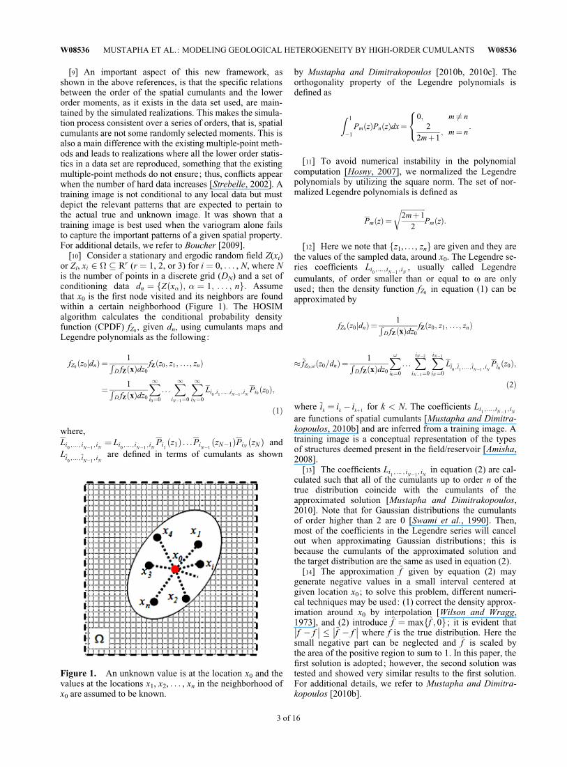
[10] Consider a stationary and ergodic random field Z(xi)or Zi, xi 2 � � Rr (r ¼ 1, 2, or 3) for i ¼ 0, . . . , N, where Nis the number of points in a discrete grid (DN) and a set ofconditioning data dn ¼ fZðx�Þ; � ¼ 1; . . . ; ng. Assumethat x0 is the first node visited and its neighbors are foundwithin a certain neighborhood (Figure 1). The HOSIMalgorithm calculates the conditional probability densityfunction (CPDF) fZ0 , given dn, using cumulants maps andLegendre polynomials as the following:

fZ0ðz0jdnÞ ¼1R

D fZðxÞdz0fZðz0; z1; . . . ; znÞ

¼ 1RD fZðxÞdz0

X1i0¼0

. . .X1

iN�1¼0

X1iN¼0

Li0 ;i1 ; ... ;iN�1 ; iNPi0ðz0Þ;

ð1Þ

where,Li0 ; ... ; iN�1 ; iN

¼ Li0 ; ... ; iN�1 ; iNPi1ðz1Þ . . .PiN�1

ðzN�1ÞPiN ðzN Þ andLi0 ; ... ; iN�1 ; iN

are defined in terms of cumulants as shown

by Mustapha and Dimitrakopoulos [2010b, 2010c]. Theorthogonality property of the Legendre polynomials isdefined as

Z 1

�1PmðzÞPnðzÞdx¼

0; m 6¼ n2

2mþ1; m¼ n

8<: :

[11] To avoid numerical instability in the polynomialcomputation [Hosny, 2007], we normalized the Legendrepolynomials by utilizing the square norm. The set of nor-malized Legendre polynomials is defined as

PmðzÞ ¼ffiffiffiffiffiffiffiffiffiffiffiffiffiffi2mþ1

2

rPmðzÞ:

[12] Here we note that fz1, . . . , zng are given and they arethe values of the sampled data, around x0. The Legendre se-ries coefficients Li0 ; ... ; iN�1 ; iN

, usually called Legendrecumulants, of order smaller than or equal to o are onlyused; then the density function fZ0 in equation (1) can beapproximated by

fZ0ðz0jdnÞ ¼1R

D fZðxÞdz0fZðz0; z1; . . . ; znÞ

� ~fZ0;!ðz0=dnÞ ¼1R

D fZðxÞdz0

X!i0¼0

. . .XiN�2

iN�1¼0

XiN�1

iN¼0

Li0 ; i1 ; ... ; iN�1 ; iNPi0ðz0Þ;

ð2Þ

where ik ¼ ik � ikþ1 for k < N. The coefficients Li1 ; ... ; iN�1 ; iNare functions of spatial cumulants [Mustapha and Dimitra-kopoulos, 2010b] and are inferred from a training image. Atraining image is a conceptual representation of the typesof structures deemed present in the field/reservoir [Amisha,2008].

[13] The coefficients Li1 ; ... ; iN�1 ; iNin equation (2) are cal-

culated such that all of the cumulants up to order n of thetrue distribution coincide with the cumulants of theapproximated solution [Mustapha and Dimitrakopoulos,2010]. Note that for Gaussian distributions the cumulantsof order higher than 2 are 0 [Swami et al., 1990]. Then,most of the coefficients in the Legendre series will cancelout when approximating Gaussian distributions; this isbecause the cumulants of the approximated solution andthe target distribution are the same as used in equation (2).

[14] The approximation ~f given by equation (2) maygenerate negative values in a small interval centered atgiven location x0; to solve this problem, different numeri-cal techniques may be used: (1) correct the density approx-imation around x0 by interpolation [Wilson and Wragg,1973], and (2) introduce f ¼ maxf~f ; 0g ; it is evident thatf � f�� �� � ~f � f

�� �� where f is the true distribution. Here thesmall negative part can be neglected and f is scaled bythe area of the positive region to sum to 1. In this paper, thefirst solution is adopted; however, the second solution wastested and showed very similar results to the first solution.For additional details, we refer to Mustapha and Dimitra-kopoulos [2010b].

Figure 1. An unknown value is at the location x0 and thevalues at the locations x1, x2, . . . , xn in the neighborhood ofx0 are assumed to be known.

W08536 MUSTAPHA ET AL.: MODELING GEOLOGICAL HETEROGENEITY BY HIGH-ORDER CUMULANTS W08536

3 of 16

[15] The main steps of the HOSIM method are asfollows:

[16] 1. Scan the training image and the sample data andstore the spatial cumulants calculated using equation (A2)in a global tree.

[17] 2. Define a random path visiting once all unsamplednodes.

[18] 3. Define the template shape for each unsampledlocation x0 using its neighbors. The conditioning data avail-able within the template are then searched (Figure 1). Thehigh-order spatial cumulants are read from the global treein step 1, and are used to calculate the coefficients of theLegendre series. These coefficient are used to build theCPDF of Z0 using equation (2).

[19] 4. Draw a uniform random value in [0,1] to readfrom the conditional distribution a simulated value, Z(x0),at x0.

[20] 5. Add x0 to the set of sample hard data and the pre-viously simulated values.

[21] 6. Repeat steps 4 and 6 for the next points in the ran-dom path defined in step (3).

[22] 7. Repeat steps 3–7 to generate different realizationsusing different random paths.

[23] The random path defined in step 5 concerns only theunsampled locations. Thus, the final realization obtained inafter step 8 honors the conditioning data.

2.3. Method Characteristics[24] Mustapha and Dimitrakopoulos [2010b] have dis-

cussed the sensitivity of the method developed to the orderof the series in equation (2), the size of the data set as wellas the training image used. Legendre series of orders 6, 12,and 25 are shown to fit complex distributions very well. Inaddition, the Legendre series of orders 12 and 25 are foundto be very close and have provided nearly the same approx-imation. The method developed herein can be coupled witha maximum entropy procedure [Zenkouar et al., 2005] todetermine the optimal order. The process consists of esti-mating the density for different orders and finding the opti-mal one as the one for which the entropy reachesmaximum. The value of o is equal to 6 in this paper.

[25] Despite the advantages shown in past work, simula-tion based on high-order spatial cumulants is computationallydemanding, particularly as the number of dimensions consid-ered increases. This is the area where the work by Mustaphaand Dimitrakopoulos [2010c] contributes by assessing thecontribution of various terms of Legendre polynomials so asto reduce computational needs without the loss of importantinformation, as well as providing a full three-dimensionalalgorithm for the practical use of the method in variousapplications.

[26] The HOSIM method has been demonstrated to becapable of representing 2- and 3-D [Mustapha and Dimitra-kopoulos, 2010b, 2010c] complex non-Gaussian and non-linear patterns. Conceptually, a training image can be usedwith a different, less-complete (i.e., sparser) data set. Inthis case, realizations, which honor the data and their statis-tics, are generated as well. Unconditionally simulated real-izations are generated to better demonstrate the effects ofthe available data. An additional example explores the sen-sitivity of the method developed to the training imagesused. The results show that the newly proposed method ismuch less sensitive to the training images than the existingmultiple-point methods, because of the data-driven approachof the method. The method is shown to (1) generate realiza-tions of complex spatial patterns such as fluvial channels,(2) reproduce bimodal data distributions, (3) data vario-grams and high-order spatial cumulants of the data; theapplications of the method show, as expected, that the (4)hard data available dominate the simulation process andhave a definitive effect on the final simulated realizations,whereas the training images are only used to fill in high-order data relations that are not possible to infer from thedata. Compared to previous MP framework [Strebelle, 2002;Zhang et al., 2006b; Wu et al., 2008; Arpat and Caers,2007], the proposed approach reconstructs (5) data-driven,(6) lower-order spatial complexity, thus using training imagesto borrow information that is not available in data sets used.

3. Data Set[27] The data sets used in this paper are available in the

Stanford V Reservoir data set [Mao and Journel, 1999].

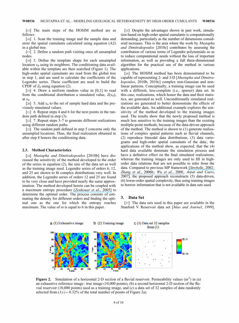
Figure 2. Simulation of a horizontal 2-D section of a fluvial reservoir. Permeability values (m2) in (a)an exhaustive reference image: true image (10,000 points), (b) a second horizontal 2-D section of the flu-vial reservoir (10,000 points) used as a training image, and (c) a data set of 32 samples of data randomlyselected from (1) (¼ 0.32% of the total number of points of Figure 2a).

W08536 MUSTAPHA ET AL.: MODELING GEOLOGICAL HETEROGENEITY BY HIGH-ORDER CUMULANTS W08536

4 of 16

Stanford V is a synthetic fluvial channel classic reservoirdata set. Data on rock porosity and permeability and den-sity are available in the whole reservoir. The Stanford Vreservoir consists of three different layers ; each is dividedinto 100 * 130 * 110 grid cells. In each layer, the channelshave a different thickness and orientation which makes thegeological patterns in the reservoir very complex.

[28] The HOSIM algorithm provides the necessary flexi-bility to simulate such a complex field. Two-dimensionalcross sections from the Stanford V data set are used byMustapha and Dimitrakopoulos [2010b] to demonstrate themain features of the HOSIM method including the sensitiv-ity of the method to the training image used. The full three-dimensional Stanford V is also used by Mustapha andDimitrakopoulos [2010c].

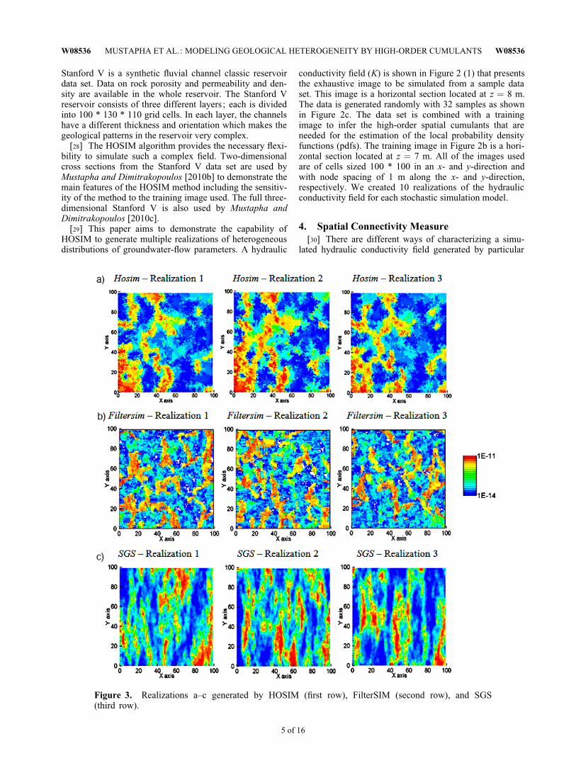
[29] This paper aims to demonstrate the capability ofHOSIM to generate multiple realizations of heterogeneousdistributions of groundwater-flow parameters. A hydraulic

conductivity field (K) is shown in Figure 2 (1) that presentsthe exhaustive image to be simulated from a sample dataset. This image is a horizontal section located at z ¼ 8 m.The data is generated randomly with 32 samples as shownin Figure 2c. The data set is combined with a trainingimage to infer the high-order spatial cumulants that areneeded for the estimation of the local probability densityfunctions (pdfs). The training image in Figure 2b is a hori-zontal section located at z ¼ 7 m. All of the images usedare of cells sized 100 * 100 in an x- and y-direction andwith node spacing of 1 m along the x- and y-direction,respectively. We created 10 realizations of the hydraulicconductivity field for each stochastic simulation model.

4. Spatial Connectivity Measure[30] There are different ways of characterizing a simu-

lated hydraulic conductivity field generated by particular

Figure 3. Realizations a–c generated by HOSIM (first row), FilterSIM (second row), and SGS(third row).

W08536 MUSTAPHA ET AL.: MODELING GEOLOGICAL HETEROGENEITY BY HIGH-ORDER CUMULANTS W08536

5 of 16

simulation algorithms [Zhang et al., 2006; Lee et al.,2007]. One of them consists of measuring connectivity ofspecific facies or K classes, especially when a strong tend-ency of spatial patterns exists in the extreme values.Another method consists of using numerical upscaling tocompute equivalent conductivities of the model units (attwo upscaling scales) [Zhang et al., 2006].

[31] Groundwater flow [Anderson, 1997; Fogg, 1986;Fogg et al., 2000; Jones et al., 1995] and solute transport[Desbarats, 1990; Desbarats and Srivastava, 1991; Morenoand Tsang, 1994; Scheibe and Murray, 1998; Wen andGomez-Hernandez, 1998] in aquifer systems are stronglyaffected by the geometry and connectivity of high perme-ability values [Lee et al., 2007]. On the basis of that, prefer-ential pathways for a solute migration and channeling ofcontaminants can be obtained because of the interconnectedhigh-permeability network.

[32] In this paper, a multiple-point rectilinear connectiv-ity function [Journel and Alaberts, 1989; Strebelle, 2002]is used. This function generalizes the two-point probabilityand statistics. Define the function C [Sunderrajan andJournel, 2004] by:

Cðh;nÞ ¼ EðIðuÞ:Iðuþ hÞ . . . Iðuþ nhÞÞ¼ Prob I uð Þ ¼ 1; I uþ hð Þ ¼ 1; . . . ; I uþ nhð Þ ¼ 1f g;

ð3Þ

where h is a unit vector in any given direction, C(h, n)gives the probability of observing a continuous string of npoints in high-K patterns. The indicator I(u) is 1 if K islarger than a given threshold (i.e., 85% in section 3). In thiscase, I(u) is 1 when K is higher or equal to 0.85 * (maxK �minK) þ minK where minK ¼ min(K) and maxK ¼ max(K).

[33] Note that, the channel proportion is given byC(h, 0), the noncentered indicator covariance by C(h, 1),and the measures of straight rectilinear connectivity byC(h, n).

5. Results and Discussion[34] First, different realizations are generated using the

three methods discussed above. Then, the impact of themethods on underground flow and solute transport simula-tion results is discussed. For that, we consider two differentmodels in this paper. Model 1 consists of a two-phase prob-lem; and a single-phase problem is considered in model 2.Models 1 and 2 are considered in examples 1 and 2, respec-tively. Example 1 consists of solving an incompressibletwo-phase flow problem, while example 2 considers an ad-vective-dispersive-diffusive transport problem. Governingequations for both problems can be found in the work ofBear [1972] and are not repeated here.

5.1. Geological Heterogeneity Simulation andConnectivity

[35] Reproducing of the exhaustive image in Figure 2ausing the training image in Figure 2b, and the data set inFigure 2c is considered herein. During the simulation pro-cess, FilterSIM borrows spatial patterns from the trainingimage, while HOSIM combines both the training imageand data set to infer high-order spatial cumulants. In this

study, the exhaustive image is considered to model semi-variograms for the generation of SGS realizations.

[36] Different realizations are generated using the threemethods as shown in Figure 3. Each squared-area elementor voxel within the gridded area represents a correspondingK value for the simulated realizations. The created hydrau-lic conductivity realizations served as input for a numericalgroundwater flow simulation. The HOSIM realizations(e.g., Figure 3), by better preserving the spatial structureof channels, are more consistent with the data and withthe exhaustive reference image. The FilterSIM realizationsare better than the SGS realizations which lack much of thehigh-K channeling. The HOSIM realizations show that themain channels in the exhaustive image are reproduced.Moreover, the small details in the exhaustive image havebeen reflected by HOSIM realizations as shown in thezones 80 < x < 100 and along the y-direction of Figure 3(first row).

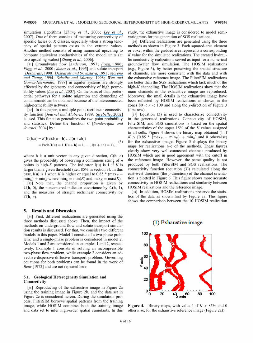
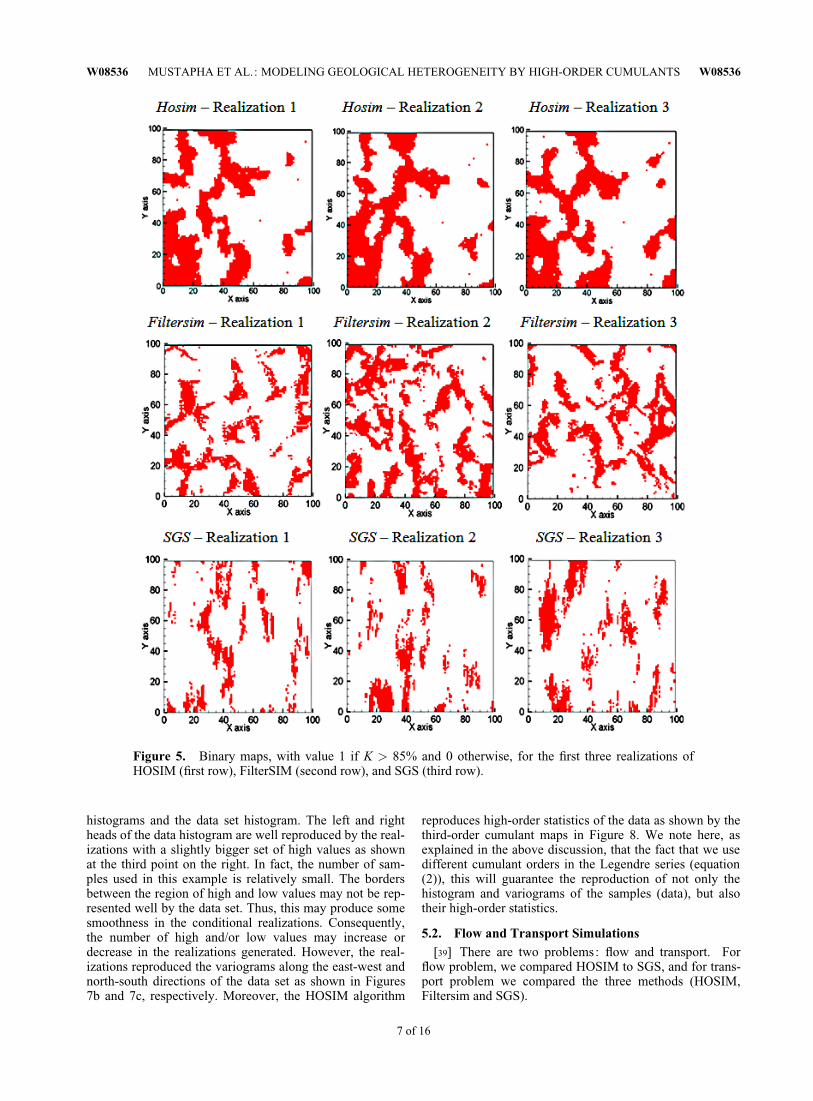
[37] Equation (3) is used to characterize connectivityin the generated realizations. Connectivity of HOSIM,FilterSIM, and SGS simulations is based on the spatialcharacteristics of the upper 15% of the K values assignedto all cells. Figure 4 shows the binary map obtained (1 ifK > [0.85 * fmaxK � minKg þ minK] and 0 otherwise)for the exhaustive image. Figure 5 displays the binarymaps for realizations a–c of the methods. These figuresclearly show very well-connected channels produced byHOSIM which are in good agreement with the cutoff inthe reference image. However, the same quality is notproduced by both FilterSIM and SGS realizations. Theconnectivity function (equation (3)) calculated along theeast-west direction (the y-direction) of the channel orienta-tion is plotted in Figure 6. This figure shows more accurateconnectivity in HOSIM realizations and similarity betweenHOSIM realizations and the reference image.

[38] In addition, HOSIM realizations preserve the statis-tics of the data as shown first by Figure 7a. This figureshows the comparison between the 10 HOSIM realization

Figure 4. Binary maps, with value 1 if K > 85% and 0otherwise, for the exhaustive reference image (Figure 2a)).

W08536 MUSTAPHA ET AL.: MODELING GEOLOGICAL HETEROGENEITY BY HIGH-ORDER CUMULANTS W08536

6 of 16

histograms and the data set histogram. The left and rightheads of the data histogram are well reproduced by the real-izations with a slightly bigger set of high values as shownat the third point on the right. In fact, the number of sam-ples used in this example is relatively small. The bordersbetween the region of high and low values may not be rep-resented well by the data set. Thus, this may produce somesmoothness in the conditional realizations. Consequently,the number of high and/or low values may increase ordecrease in the realizations generated. However, the real-izations reproduced the variograms along the east-west andnorth-south directions of the data set as shown in Figures7b and 7c, respectively. Moreover, the HOSIM algorithm

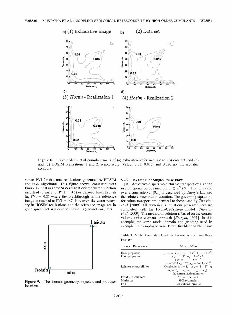
reproduces high-order statistics of the data as shown by thethird-order cumulant maps in Figure 8. We note here, asexplained in the above discussion, that the fact that we usedifferent cumulant orders in the Legendre series (equation(2)), this will guarantee the reproduction of not only thehistogram and variograms of the samples (data), but alsotheir high-order statistics.

5.2. Flow and Transport Simulations[39] There are two problems: flow and transport. For

flow problem, we compared HOSIM to SGS, and for trans-port problem we compared the three methods (HOSIM,Filtersim and SGS).

Figure 5. Binary maps, with value 1 if K > 85% and 0 otherwise, for the first three realizations ofHOSIM (first row), FilterSIM (second row), and SGS (third row).

W08536 MUSTAPHA ET AL.: MODELING GEOLOGICAL HETEROGENEITY BY HIGH-ORDER CUMULANTS W08536

7 of 16

5.2.1. Example 1: Incompressible Two-Phase FlowProblem

[40] Realizations generated from HOSIM and SGS mod-els are used in a numerical model [Mustapha and Dimitra-kopoulos, 2009; Mustapha et al., 2010] of groundwaterflow. The same level of discretization is used for the modeldiscretization and the geostatistical models. We consider a2-D horizontal domain (100 m � 100 m) initially saturatedwith oil (nonwetting phase). Water (wetting phase) isinjected at the upper-right corner to produce oil at the op-posite corner (Figure 9). The injection rate in pore volume(PV) is 0.1 PV yr�1. The capillary pressure and gravity areneglected. The fluid and medium properties are given inTable 1. All runs were performed on a 3.2 Ghz Intel(R)Xeon (TM) PC with 2 GB of RAM.

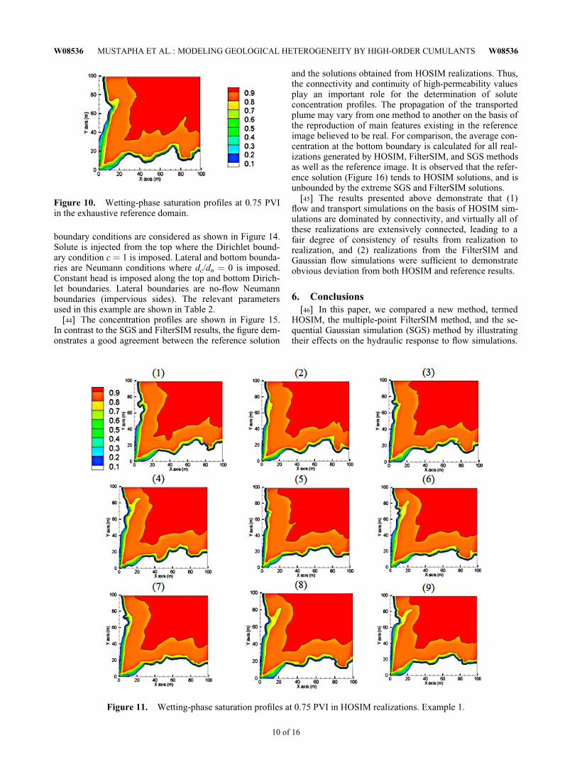
[41] The water saturation profiles in the reference image(Figure 2a) at pore volume injection (PVI) ¼ 0.75 areshown in Figure 10. Figure 11 shows the water saturationprofiles at PVI ¼ 0.75 using the hydraulic permeabilitygenerated by HOSIM realizations. This figure shows approx-imately similar profiles to the reference image. The perme-ability fields generated by the SGS algorithm produced the

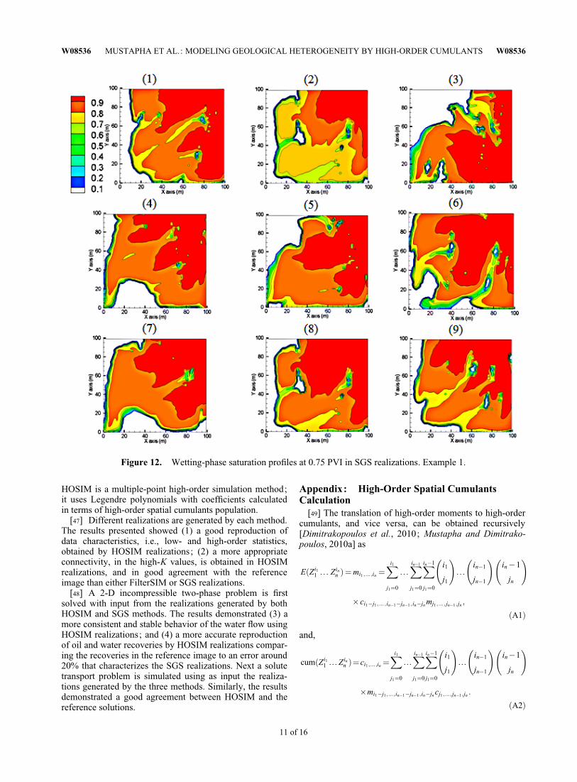
water saturation profiles at PVI ¼ 0.75 in Figure 12. Thisfigure shows some diversity in flow behavior from one real-ization to another. The disorder and weakness of the con-nectivity in low- and high-permeability zones can producesaturation profiles that strongly differ from the true profile.The water injected from the upper-right corner may lead toearly or delayed breakthrough in SGS realizations. The per-meability distribution in Figure 2a shows some continuityand smoothness which may lead to uniform propagation inthe saturation profile as shown in Figure 10. This propertyis preserved in the realizations generated by HOSIM (Fig-ure 11) but not by those generated by SGS; this is becauseof the discontinuity of the permeability field at some loca-tions as shown, for example, at the middle of the domainsin Figure 12.

[42] The oil recovery versus PVI for both HOSIM andSGS realizations are plotted in Figure 13 (first row). Thisfigure shows a good agreement between HOSIM realiza-tions and the reference image. The difference is <5%.However, in some SGS realizations, the oil recovery devi-ates as much as 20% from the oil recovery in the referenceimage. Figure 13 (second row) displays the water recovery

Figure 6. Multiple-point connectivity along the east-west direction. Circles refer to true image, solidlines refer to HOSIM realizations, dashed lines refer to FilterSIM realizations, and dotted lines refer toSGS realizations.

Figure 7. Histograms (a), north-south (b) and east-west (c) variograms of 10 HOSIM realizations. Thecircles refer to the data set and the solid lines refer to the realizations.

W08536 MUSTAPHA ET AL.: MODELING GEOLOGICAL HETEROGENEITY BY HIGH-ORDER CUMULANTS W08536

8 of 16

versus PVI for the same realizations generated by HOSIMand SGS algorithms. This figure shows, consistent withFigure 12, that in some SGS realizations the water injectionmay lead to early (at PVI ¼ 0.5) or delayed breakthrough(at PVI ¼ 0.8) where the breakthrough in the referenceimage is reached at PVI ¼ 0.7. However, the water recov-ery in HOSIM realizations and the reference image are ingood agreement as shown in Figure 13 (second row, left).

5.2.2. Example 2: Single-Phase Flow[43] Advective-dispersive-diffusive transport of a solute

in a polygonal porous medium � � RN (N ¼ 1, 2, or 3) andover a time interval [0,T] is described by Darcy’s law andthe solute concentration equation. The governing equationsfor solute transport are identical to those used by Therrienet al. [2009]. All numerical simulations presented here arecompleted with the HydroGeoSphere model [Therrienet al., 2009]. The method of solution is based on the controlvolume finite element approach [Forsyth, 1991]. In thisexample, the same model domain and gridding used inexample 1 are employed here. Both Dirichlet and Neumann

Figure 8. Third-order spatial cumulant maps of (a) exhaustive reference image, (b) data set, and (c)and (d) HOSIM realizations 1 and 2, respectively. Values 0.01, 0.015, and 0.020 are the isovaluecontours.

Figure 9. The domain geometry, injector, and producerlocations.

Table 1. Model Parameters Used for the Analysis of Two-PhaseProblem

Domain Dimensions 100 m � 100 m

Rock properties � ¼ 0:2; k ¼ 1E� 14 m2; 1E� 11 m2½ �Fluid properties �w ¼ 1 cP; �n ¼ 0:45 cP;

1 cP ¼ 10�3 kg ms�1

�w ¼ 1000 kg m�3 ; �n ¼ 660 kg m�3

Relative permeabilities Quadratic: krw ¼ Se2; krn ¼ (1 � Se)

2);Se ¼ (Sw � Srw)/(1 � Srw � Srn)

the normalized saturationResidual saturations Srw ¼ 0; Srn ¼ 0Mesh size 9801 rectanglesPVI Pore volume injection

W08536 MUSTAPHA ET AL.: MODELING GEOLOGICAL HETEROGENEITY BY HIGH-ORDER CUMULANTS W08536

9 of 16

boundary conditions are considered as shown in Figure 14.Solute is injected from the top where the Dirichlet bound-ary condition c ¼ 1 is imposed. Lateral and bottom bounda-ries are Neumann conditions where dc/dn ¼ 0 is imposed.Constant head is imposed along the top and bottom Dirich-let boundaries. Lateral boundaries are no-flow Neumannboundaries (impervious sides). The relevant parametersused in this example are shown in Table 2.

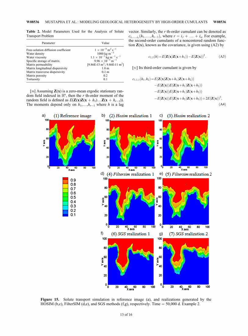
[44] The concentration profiles are shown in Figure 15.In contrast to the SGS and FilterSIM results, the figure dem-onstrates a good agreement between the reference solution

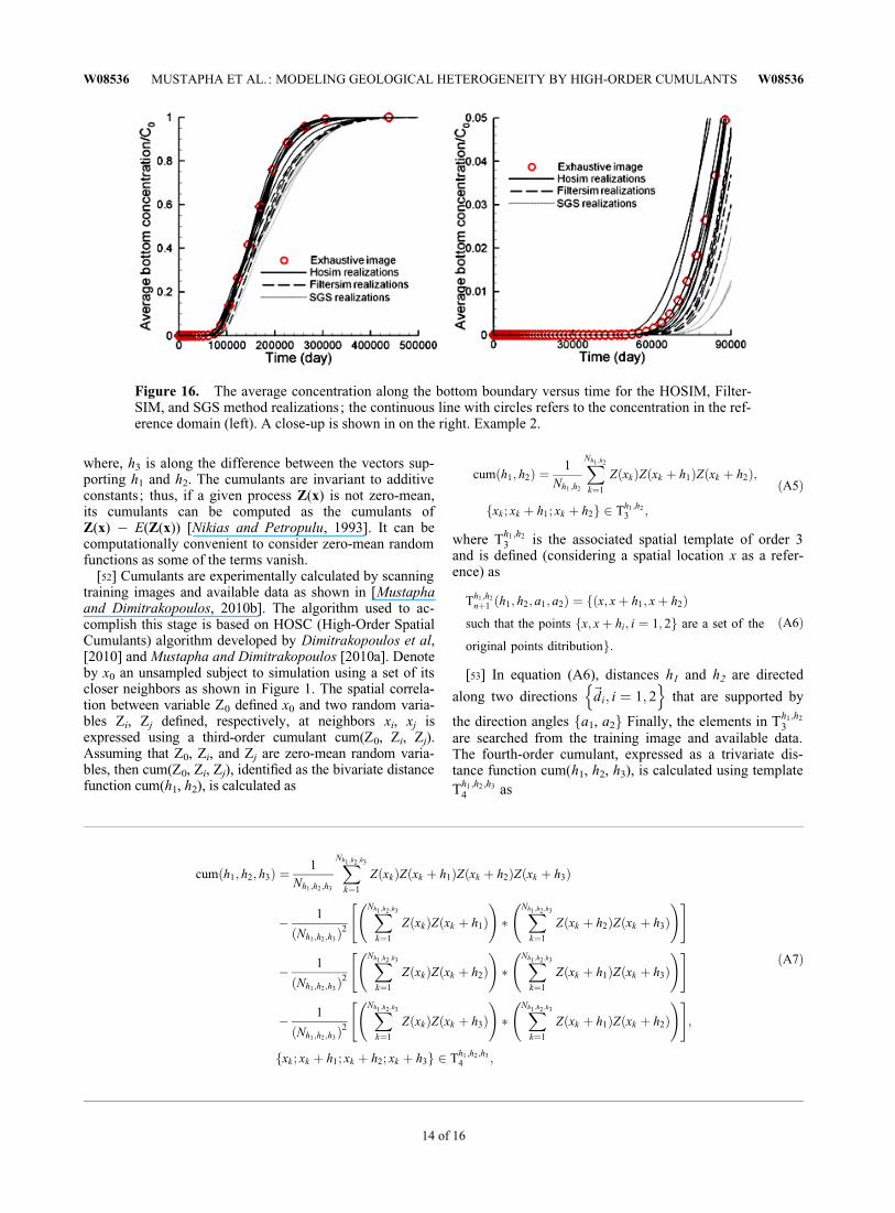
and the solutions obtained from HOSIM realizations. Thus,the connectivity and continuity of high-permeability valuesplay an important role for the determination of soluteconcentration profiles. The propagation of the transportedplume may vary from one method to another on the basis ofthe reproduction of main features existing in the referenceimage believed to be real. For comparison, the average con-centration at the bottom boundary is calculated for all real-izations generated by HOSIM, FilterSIM, and SGS methodsas well as the reference image. It is observed that the refer-ence solution (Figure 16) tends to HOSIM solutions, and isunbounded by the extreme SGS and FilterSIM solutions.

[45] The results presented above demonstrate that (1)flow and transport simulations on the basis of HOSIM sim-ulations are dominated by connectivity, and virtually all ofthese realizations are extensively connected, leading to afair degree of consistency of results from realization torealization, and (2) realizations from the FilterSIM andGaussian flow simulations were sufficient to demonstrateobvious deviation from both HOSIM and reference results.

6. Conclusions[46] In this paper, we compared a new method, termed

HOSIM, the multiple-point FilterSIM method, and the se-quential Gaussian simulation (SGS) method by illustratingtheir effects on the hydraulic response to flow simulations.

Figure 10. Wetting-phase saturation profiles at 0.75 PVIin the exhaustive reference domain.

Figure 11. Wetting-phase saturation profiles at 0.75 PVI in HOSIM realizations. Example 1.

W08536 MUSTAPHA ET AL.: MODELING GEOLOGICAL HETEROGENEITY BY HIGH-ORDER CUMULANTS W08536

10 of 16

HOSIM is a multiple-point high-order simulation method;it uses Legendre polynomials with coefficients calculatedin terms of high-order spatial cumulants population.

[47] Different realizations are generated by each method.The results presented showed (1) a good reproduction ofdata characteristics, i.e., low- and high-order statistics,obtained by HOSIM realizations; (2) a more appropriateconnectivity, in the high-K values, is obtained in HOSIMrealizations, and in good agreement with the referenceimage than either FilterSIM or SGS realizations.

[48] A 2-D incompressible two-phase problem is firstsolved with input from the realizations generated by bothHOSIM and SGS methods. The results demonstrated (3) amore consistent and stable behavior of the water flow usingHOSIM realizations; and (4) a more accurate reproductionof oil and water recoveries by HOSIM realizations compar-ing the recoveries in the reference image to an error around20% that characterizes the SGS realizations. Next a solutetransport problem is simulated using as input the realiza-tions generated by the three methods. Similarly, the resultsdemonstrated a good agreement between HOSIM and thereference solutions.

Appendix: High-Order Spatial CumulantsCalculation

[49] The translation of high-order moments to high-ordercumulants, and vice versa, can be obtained recursively[Dimitrakopoulos et al., 2010; Mustapha and Dimitrako-poulos, 2010a] as

EðZi11 . . . Zin

n Þ¼mi1 ; ... ;in ¼Xi1

j1¼0

. . .Xin�1

j1¼0

Xin�1

j1¼0

i1

j1

!. . .

in�1

jn�1

!in�1

jn

!

�ci1�j1; ... ; in�1�jn�1; in�jn mj1 ; ... ; jn�1; jn ;

ðA1Þ

and,

cumðZi11 ... Zin

n Þ¼ ci1;...;in¼Xi1

j1¼0

...Xin�1

j1¼0

Xin�1

j1¼0

i1

j1

!...

in�1

jn�1

!in�1

jn

!

�mi1�j1;...;in�1�jn�1 ;in�jn cj1;...;jn�1;jn :

ðA2Þ

Figure 12. Wetting-phase saturation profiles at 0.75 PVI in SGS realizations. Example 1.

W08536 MUSTAPHA ET AL.: MODELING GEOLOGICAL HETEROGENEITY BY HIGH-ORDER CUMULANTS W08536

11 of 16

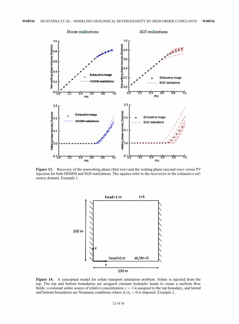
Figure 13. Recovery of the nonwetting phase (first row) and the wetting phase (second row) versus PVinjection for both HOSIM and SGS realizations. The squares refer to the recoveries in the exhaustive ref-erence domain. Example 1.

Figure 14. A conceptual model for solute transport simulation problem. Solute is injected from thetop. The top and bottom boundaries are assigned constant hydraulic heads to create a uniform flowfields; a constant solute source of relative concentration c ¼ 1 is assigned to the top boundary, and lateraland bottom boundaries are Neumann conditions where dc/dn ¼ 0 is imposed. Example 2.

W08536 MUSTAPHA ET AL.: MODELING GEOLOGICAL HETEROGENEITY BY HIGH-ORDER CUMULANTS W08536

12 of 16

[50] Assuming Z(x) is a zero-mean ergodic stationary ran-dom field indexed in Rn, then the r th-order moment of therandom field is defined as E(Z(x)Z(x þ h1)...Z(x þ hr�1)).The moments depend only on h1,...,hr�1 where h is a lag

vector. Similarly, the r th-order cumulant can be denoted asci1;...;inðh1; ...;hr�1Þ, where r ¼ i1 þ ... þ in. For example,the second-order cumulants of a noncentered random func-tion Z(x), known as the covariance, is given using (A2) by

c1;1ðhÞ¼EðZðxÞZðxþh1ÞÞ�EðZðxÞÞ2: ðA3Þ

[51] Its third-order cumulant is given by

c1;1;1ðh1;h2Þ¼EðZðxÞZðxþh1ÞZðxþh2ÞÞ�EðZðxÞÞEðZðxþh1ÞZðxþh2ÞÞ�EðZðxÞÞEðZðxþh1ÞZðxþh3ÞÞ

�EðZðxÞÞEðZðxþh2ÞZðxþh3ÞÞþ2EðZðxÞÞ3;ðA4Þ

Table 2. Model Parameters Used for the Analysis of SoluteTransport Problem

Parameter Value

Free-solution diffusion coefficient 1 � 10�9 m2 s�1

Water density 1000 kg m�3

Water viscosity 1.1 � 10�3 kg m�1 s�1

Specific storage of matrix 9.96 � 10�5 m�1

Matrix permeability [9.86E-13 m2; 9.86E-11 m2]Matrix longitudinal dispersivity 1.0 mMatrix transverse dispersivity 0.1 mMatrix porosity 0.2Tortuosity 0.1

Figure 15. Solute transport simulation in reference image (a), and realizations generated by theHOSIM (b,c), FilterSIM (d,e), and SGS methods (f,g), respectively. Time ¼ 50,000 d. Example 2.

W08536 MUSTAPHA ET AL.: MODELING GEOLOGICAL HETEROGENEITY BY HIGH-ORDER CUMULANTS W08536

13 of 16

where, h3 is along the difference between the vectors sup-porting h1 and h2. The cumulants are invariant to additiveconstants; thus, if a given process Z(x) is not zero-mean,its cumulants can be computed as the cumulants ofZ(x) � E(Z(x)) [Nikias and Petropulu, 1993]. It can becomputationally convenient to consider zero-mean randomfunctions as some of the terms vanish.

[52] Cumulants are experimentally calculated by scanningtraining images and available data as shown in [Mustaphaand Dimitrakopoulos, 2010b]. The algorithm used to ac-complish this stage is based on HOSC (High-Order SpatialCumulants) algorithm developed by Dimitrakopoulos et al,[2010] and Mustapha and Dimitrakopoulos [2010a]. Denoteby x0 an unsampled subject to simulation using a set of itscloser neighbors as shown in Figure 1. The spatial correla-tion between variable Z0 defined x0 and two random varia-bles Zi, Zj defined, respectively, at neighbors xi, xj isexpressed using a third-order cumulant cum(Z0, Zi, Zj).Assuming that Z0, Zi, and Zj are zero-mean random varia-bles, then cum(Z0, Zi, Zj), identified as the bivariate distancefunction cum(h1, h2), is calculated as

cumðh1; h2Þ ¼1

Nh1 ;h2

XNh1 ;h2

k¼1

ZðxkÞZðxk þ h1ÞZðxk þ h2Þ;

fxk ; xk þ h1; xk þ h2g 2 Th1 ;h23 ;

ðA5Þ

where Th1;h23 is the associated spatial template of order 3

and is defined (considering a spatial location x as a refer-ence) as

Th1 ;h2nþ1 ðh1; h2; a1; a2Þ ¼ fðx; xþ h1; xþ h2Þ

such that the points fx; xþ hi; i ¼ 1; 2g are a set of the

original points ditributiong:ðA6Þ

[53] In equation (A6), distances h1 and h2 are directed

along two directions ~di; i ¼ 1; 2n o

that are supported by

the direction angles fa1, a2g Finally, the elements in Th1;h23

are searched from the training image and available data.The fourth-order cumulant, expressed as a trivariate dis-tance function cum(h1, h2, h3), is calculated using templateTh1;h2;h3

4 as

Figure 16. The average concentration along the bottom boundary versus time for the HOSIM, Filter-SIM, and SGS method realizations; the continuous line with circles refers to the concentration in the ref-erence domain (left). A close-up is shown in on the right. Example 2.

cumðh1; h2; h3Þ ¼1

Nh1;h2;h3

XNh1 ;h2 ;h3

k¼1

ZðxkÞZðxk þ h1ÞZðxk þ h2ÞZðxk þ h3Þ

� 1

ðNh1 ;h2;h3Þ2

XNh1 ;h2 ;h3

k¼1

ZðxkÞZðxk þ h1Þ !

XNh1 ;h2 ;h3

k¼1

Zðxk þ h2ÞZðxk þ h3Þ !" #

� 1

ðNh1 ;h2;h3Þ2

XNh1 ;h2 ;h3

k¼1

ZðxkÞZðxk þ h2Þ !

XNh1 ;h2 ;h3

k¼1

Zðxk þ h1ÞZðxk þ h3Þ !" #

� 1

ðNh1 ;h2;h3Þ2

XNh1 ;h2 ;h3

k¼1

ZðxkÞZðxk þ h3Þ !

XNh1 ;h2 ;h3

k¼1

Zðxk þ h1ÞZðxk þ h2Þ !" #

;

fxk ; xk þ h1; xk þ h2; xk þ h3g 2 Th1;h2;h34 ;

ðA7Þ

W08536 MUSTAPHA ET AL.: MODELING GEOLOGICAL HETEROGENEITY BY HIGH-ORDER CUMULANTS W08536

14 of 16

where Nh1;h2 and Nh1;h2;h3 are the number of elements ofTh1;h2

3 and Th1;h2;h24 , respectively. Cumulants of order higher

than four are similarly calculated.

[54] Acknowledgments. We would like to express our deep and sin-cere gratitude to Andre Journel (Stanford) and Dennis McLaughlin (MIT)for their extremely helpful suggestions, technical comments, and criticismsof this work. The work in this paper was funded from NSERC CDR grant335696 and BHP Billiton, as well NSERC Discovery grant 239019.Thanks are in order to Brian Baird, Peter Stone, and Gavin Yates of BHPBilliton, as well as BHP Billiton Diamonds and, in particular, DarrenDyck, for their support, collaboration, as well as technical comments.

ReferencesAbabou, R., D. McLaughlin, L. W. Gelhar, and A. F. B. Tompson (1989),

Numerical simulation of three dimensional saturated flow in randomlyheterogeneous porous media, Transp. Porous Media, 4, 549–566.

Alabert, F. G., E. Aquitaine, and V. Modot (1992), Stochastic models ofreservoir heterogeneity: Impact on connectivity and average permeabil-ities, SPE J., 24893, 355–370.

Amisha, M. (2008), TiGenerator: Object-based training image generator,Comput. Geosci., 34, 1753–1761.

Anderson, M. P. (1991), Universal scaling of hydraulic conductivities anddispersivities in geologic media—comment, Water Resour. Res., 27,1381–1382, doi:10.1029/91WR00574.

Anderson, M. P. (1997), Characterization of geological heterogeneity, InSubsurface Flow and Transport: A Stochastic Approach, pp. 23–43,edited by S. P. Neuman and G. Dagan, Cambridge, Cambridge Univ.Press, Cambridge, U. K.

Arpat, B., and J. Caers (2007), Stochastic simulation with patterns, Math.Geosci., 39, 177–203.

Ballio, F., and A. Guadagnini (2004), Convergence assessment of numeri-cal Monte Carlo simulations in groundwater hydrology, Water Resour.Res., 40(4), W04603, doi:10.1029/2003WR002876.

Bear, J. (1972), Dynamics of fluids in porous media, 784 pp., Elsevier, NewYork.

Billinger, D. R., and M. Rosenblatt (1966), Asymptotic theory of kth-orderspectra, in Spectral Analysis of Time Series, pp., 189–232, edited byB. Harris, Wiley, New York.

Boucher, A. (2009), Considering complex training images with search treepartitioning, Comput. Geosci., 35, 1151–1158.

Caers, J. (2005), Petroleum Geostatistics, Society of Petroleum Enginners,PennWell Books, 104 pp., Tulsa, OK.

Carle, S. F., and G. E. Fogg (1996), Transition probability-based indicatorgeostatistics, Math. Geol. 28, 453–476.

Carle, S. F., and G. E. Fogg (1997), Modeling spatial variability with oneand multidimensional continuous-lag Markov chains, Math. Geol., 29,891–918.

Chatterjee, S., and R. Dimitrakopoulos (2009), Three-dimensional waveletbased conditional co-simulation using training image, COSMO researchreport, 27–57.

Chiles, J. P., and P. Delfiner (1999), Geostatistics: Modeling SpatialUncertainty, 395 pp., Wiley, New York.

Chugunova, T. L., and L. Y. Hu (2008), Multiple-point simulations con-strained by continuous auxiliary data, Math. Geosci., 40, 133–146.

Cressie, N. A. (1993), Statistics for spatial data, Wiley, New York.Daly, C. (2004), Higher order models using entropy, Markov random fields

and sequential simulation, in Geostatistics Banff, pp. 215–225, edited byO. Leuangthong and C. V. Clayton, Springer, New York.

David, M. (1977), Geostatistical Ore Reserve Estimation, 364 pp., Elsevier,Amsterdam.

David, M. (1988), Handbook of Applied Advanced Geostatistical OreReserve Estimation, 216 pp., Elsevier, Amsterdam.

de Marsily, G., F. Delay, F. Teles, and M. T. Schafmeister (1998), Somecurrent methods to represent the heterogeneity of natural media in hydro-geology, Hydrogeol. J., 6, 115–30.

Desbarats, A. J. (1990), Macrodispersion in sand-shale sequences, WaterResour. Res., 26, 153–163, doi:10.1029/WR026i001p00153.

Desbarats, A. J., and R. M. Srivastava (1991), Geostatistical characteriza-tion of groundwater flow parameters in a simulated aquifer, WaterResour. Res., 27, 687–698, doi:10.1029/90WR02705.

Deutsch, C. V., and A. G. Journel (1998), GSLIB Geostatistical SoftwareLibrary and User’s Guide, 369 pp., Oxford Univ. Press, New York.

Dimitrakopoulos, R., H. Mustapha, and E. Gloaguen (2010), High-orderstatistics of spatial random fields: Exploring spatial cumulants for mod-eling complex non-gaussian and non-linear phenomena, Math. Geosci.,42, 65–99.

Feyen, L., and S. Gorelick (2004), Reliable groundwater management inhydroecologically sensitive areas, Water Resour. Res., 40(7), W07408,doi:10.1029/2003WR003003.

Fogg, G. E. (1986), Groundwater flow and sand body interconnectedness ina thick multiple-aquifer system, Water Resour. Res., 22, 679–694,doi:10.1029/WR022i005p00679.

Fogg, G. E., S. F. Carle, and C. Green (2000), Connected-network paradigmfor the alluvial aquifer system, in Theory, Modeling, and Field Investiga-tion in Hydrogeology: A Special Volume in Honor of Shlomo P. Neu-man’s 60th Birthday, pp. 25–42, edited by D. Zhang and C. L. Winter,Geological Society of America Special Paper, Boulder, CO.

Forsyth, P. A. (1991), A control volume finite element approach to NAPLgroundwater contamination, SIAM J. Scientific and Statistical Comput.,12, 1029–1057.

Gaztanaga, E. P., P. Fosalba, and E. Elizalde (2000), Gravitational evolu-tion of the large-scale probability density distribution, Astrophys. J., 539,522–531.

Gloaguen, E., and R. Dimitrakopoulos (2009), Two-dimensional condi-tional simulations based on the wavelet decomposition of trainingimages, Math. Geosci., 41, 679–701.

Gomez-Hernandez, J. J., and X. H. Wen (1998), To be or not to be multi-Gaussian? A reflection on stochastic hydrogeology, Adv. Water Res., 21,47–61.

Goovaerts, P. (1998), Geostatistics for Natural Resources Evaluation, 483pp., Oxford Univ. Press, New York.

Gotway, C. A., and B. M. Rutherford (1994), Stochastic simulation forimaging spatial uncertainty: Comparison and evaluation of availablealgorithms, in Geostatistical Simulation Workshop: Geostatistical Simu-lations:Pproceedings of the Geostatistical Simulation Workshop, Fon-tainebleau, France, pp. 1–21, edited by M. Armstrong and P. A. Dowd,Kluwer Academic, Boston, MA.

Guardiano, J., and R. M. Srivastava (1993), Multivariate geostatistics:Beyond bivariate moments, in Geosatistics Troia ’92, pp. 33–144, editedby A. Soares, Kluwer Academic, Dordrecht, Netherlands.

Hosny, K. M. (2007), Exact Legendre moment computation for gray levelimages, Pattern Recognition, 40, 3597–3605.

Jones, A., J. Doyle, T. Jacobsen, and D. Kjonsvik (1995), Which subseismicheterogeneities influence waterflood performance—a case study of a lownet-to-gross fluvial reservoir, in New Developments in Improved OilRecovery, vol. 84, pp. 5–18, edited by H. J. de Hann, Geological Societyof America Special Publication, Boulder, CO.

Journel, A. G. (1997), Deterministic geostatistics: A new visit, in Geosta-tistics Woolongong, pp. 213–224, edited by E. Baafy and N. Shofield,Kluwer, Dordrecht, Netherlands.

Journel, A. G., and C. V. Deutsch (1993), Entropy and spatial disorder,Math. Geol., 25, 329–55.

Journel, A. G., and F. Alabert (1989), Non-Gaussian data expansion in theearth sciences, TERRA Nova, 1, 123–134.

Journel, A. G., and Ch. J. Huijbregts (1978), Mining Geostatistics, 338 pp.,Academic Press Inc, New York.

Juanes, R., C. W. MacMinn, and M. L. Szulczewski (2009), The footprintof the CO2 plume during carbon dioxide storage in saline aquifers: Stor-age efficiency for capillary trapping at the basin scale, Transp. PorousMedia, 82, 19–30, doi:10.1007/s11242-009-9420-3.

Kitanidis, P. K. (1997), Introduction to geostatistics—Applications inhydrogeology, 271 pp., Cambridge Univ. Press, New York.

Koltermann, C. E., and S. M. Gorelick (1996), Heterogeneity in sedimen-tary deposits—a review of structure-imitating, process-imitating, and de-scriptive approaches, Water Resour. Res., 32, 2617–2658, doi:10.1029/96WR00025.

Lee, S. Y., F. C. Steven, and E. F. Graham (2007), Geologic heterogeneityand a comparison of two geostatistical models: Sequential Gaussian andtransition probability-based geostatistical simulation, Adv. WaterResour., 30, 1914–1932.

Liao, S. X., and M. Pawlak (1996), On image analysis by moments. IEEETrans. Pattern Anal. Machine Intelligence, 18, 254–266.

MacMinn, C. W., and R. Juanes (2009), Post-injection spreading and trap-ping of CO2 in saline aquifers: Impact of the plume shape at the end ofinjection, Comput. Geosci., 13, 483–491, doi:10.1007/s10596-009-9147-9.

Mao, S., and A. G. Journel (1999), Generation of a reference petrophysicaland seismic 3D data set, The Stanford V reservoir, in Stanford Center for

W08536 MUSTAPHA ET AL.: MODELING GEOLOGICAL HETEROGENEITY BY HIGH-ORDER CUMULANTS W08536

15 of 16

Reservoir Forecasting Annual Meeting, SCRF Report, StanfordUniversity.

Matern, B. (1960), Spatial variation—Stochastic models and their applica-tion to some problems in forest surveys and other sampling investigations,Meddelanden fran Statens Skogsforskningsinstitud 49(5) Almaenna,Stockolm.

Matheron, G. (1971), The theory of regionalized variables and its appli-cations, Cahier du Centre de Morphologie Mathematique, No. 5,Fointanebleau.

Mendel, J. M. (1991), Use of high-order statistics (spectra) in signal proc-essing and systems theory: Theoretical results and some applications,IEEE Proc., 79, 279–305.

Michael, H. A., H. Li, A. Boucher, T. Sun, J. Caers, and S. M. Gorelick(2010), Combining geologic-process models and geostatistics for condi-tional simulation of 3-D subsurface heterogeneity, Water Resour. Res.,46, W05527, doi:10.1029/2009WR008414.

Mirowski, P. W., D. M. Trtzlaff, R. C. Davies, D. S. McCormick, N. Wil-liams, and C. Signer (2008), Stationary scores on training images formultipoint geostatistics, Math. Geosci., 41, 447–474.

Moreno, L., and C. F. Tsang (1994), Flow channeling in strongly heteroge-neous porous media—a numerical study, Water Resour. Res., 30, 1421–1430, doi:10.1029/93WR02978.

Mustapha, H., and R. Dimitrakopoulos (2009), Discretizing two-dimen-sional complex fractured fields for incompressible two-phase flow, Int. J.Numer. Methods Fluids, doi:10.1002/fld.2197.

Mustapha, H., and R. Dimitrakopoulos (2010a), A new approach for geo-logical pattern recognition using high-order spatial cumulants, Comput.Geosci., 36, 313–334.

Mustapha, H., and R. Dimitrakopoulos (2010b), High-order stochastic sim-ulation of complex spatially distributed natural phenomena, Math. Geo-sci., 42 (5), 457–485, doi:10.1007/s11004-010-9291-8.

Mustapha, H., and R. Dimitrakopoulos (2010c), HOSIM: A high-order sto-chastic simulation algorithm for generating three-dimensional complexgeological patterns, Comput. Geosci., doi:10.1016/j.cageo.2010.09.007,in press.

Mustapha, H., R. Dimitrakopoulos, T. Graf, and A. Firoozabadi (2010), AnEfficient Method for Discretizing Three-Dimensional Complex DiscreteFractured Fields, Int. J. Numer. Methods Fluids, in press, doi:10.1002/fld.2383.

Nikias, C. L., and A. P. Petropulu (1993), Higher-Order Spectra Analysis:A Nonlinear Signal Processing Framework, 537 pp., PTR Prentice Hall,Upper Saddle River, NJ.

North, C. P. (1996), The prediction and modeling of subsurface fluvial stra-tigraphy, in Advances in Fluvial Dynamics and Strataigraphy, pp. 395–508, edited by P. Carling and M. R. Dawson, John Wiley, New York.

Remy, N., A. Boucher, and J. Wu (2009), Applied geostatistics withSGeMs: A users’s guide, 284 pp., Cambridge Univ. Press, New York.

Rosenblatt, M. (1985), Stationary sequences and random fields, 258 pp.,Birkhaüser, Boston.

Scheibe, T. D., and C. J. Murray (1998), Simulation of geologic patterns:A comparison of stochastic simulation techniques for groundwater trans-port modeling, in Uses of Sedimentologic and Stratigraphic Informationin Predicting Reservoir Heterogeneity, Special Publication of the SEPM(Society for Sedimentary Geology), Tulsa, OK, pp. 107–118, edited byG. S. Fraser and J. M. Davis.

Scheidt, C., and J. Caers (2009), Representing spatial uncertainty using dis-tances and kernels, Math. Geosci., 41, 397–419.

Shiryaev, A. N. (1960), Some problems in the spectral theory of higherorder moments I, Theory of Probability and its Applications, 5, 265–284.

Slough, K., E. Sudicky, and P. Forsyth (1999a), Grid refinement for model-ing multiphase flow in discretely fractured porous media, Adv. WaterRes., 23, 261–269.

Slough, K., E. Sudicky, and P. Forsyth (1999b), Importance of rock matrixentry pressure on DNAPL migration in fractured geologic materials,Ground Water, 37, 237–243.

Slough, K., E. Sudicky, and P. Forsyth (1999c), Numerical simulation ofmultiphase flow and phase partitioning in discretely fractured geologicmedia, Journal of Contaminate Hydrology, 40, 107–136.

Smith, L., and R. A. Freeze (1979a), Stochastic analysis of steady stategroundwater flow in a bounded domain, 1. One-dimensional simulation,Water Resour. Res., 15, 521–528, doi:10.1029/WR015i003p00521.

Smith, L., and R. A. Freeze (1979b), Stochastic analysis of steady stategroundwater flow in a bounded domain, 2. Two-dimensional simulation,Water Resour. Res., 15, 1543–1559, doi:10.1029/WR015i006p01543.

Smith, L., and F. W. Schwartz (1981), Mass transport, 2. Analysis of uncer-tainty in prediction, Water Resour. Res., 17, 351–369, doi:10.1029/WR017i002p00351.

Strebelle, S. (2002), Conditional simulation of complex geological struc-tures using multiple point statistics, Math. Geosci., 34, 1–22.

Sunderrajan, K., and A. G. Journel (2004), Spatial Connectivity: From Var-iograms to Multiple-Point Measures, Math. Geology, 35, 915–925.

Swami, A., G. B. Giannakis, and J. M. Mendel (1990), Linear modeling ofmultidimensional non-Gaussian processes using cumulants source, Mul-tidimensional Systems and Signal Processing, 1, 11–37.

Therrien, R., R. G. McLaren, E. A. Sudicky (2009), HydroGeoSphere—athree-dimensional numerical model describing fully-integrated subsur-face and surface flow and solute transport (Draft ed.). Groundwater Sim-ulations Group, University of Waterloo, Available at http://www.science.uwaterloo.ca/mclaren/public/hydrosphere.pdf.

Tjelmeland, H. (1998), Markov random fields with higher order interac-tions, Scandinavian J. Statistics, 25, 415–433.

Tjelmeland, H., and J. Eidsvik (2004), Directional metropolis: Hastingsupdates for conditionals with nonlinear likelihoods, in GeostatisticsBanff 2004, pp., 95–104, edited by O. Leuangthong and C. V. Clayton,Springer, New York.

Wagner, B. J., and S. M. Gorelick (1989), Reliable aquifer remediation in thepresence of spatial variable hydraulic conductivity: from data to design,Water Resour. Res., 25, 2211–2225, doi:10.1029/WR025i010p02211.

Webster, R., and M. A. Oliver (2007), Geostatistics for Environmental Sci-entists, 304 pp., Wiley, London, UK.

Wen, X. H., and C. Kung (1993), Stochastic simulation of solute transportin heterogeneous formations: a comparison of parametric and nonpara-metric geostatistical approaches, Ground Water, 31, 953–965.

Wen, X. H., and J. Gomez-Hernandez (1998), Numerical modeling ofmacrodispersion in heterogeneous media: a comparison of multi-Gaussian and nonmulti-Gaussian models, J. Contaminant Hydrol., 30,129–56.

Western, A. W., G. Bloschl, and R. B. Grayson (2001), Toward capturinghydrologically significant connectivity in spatial patterns, Water Resour.Res., 37, 83–97, doi:10.1029/2000WR900241.

Wilson, G. A., and A. Wragg (1973), Numerical methods for approximatingcontinuous probability density functions, over [0,þ), using moments,IMA J. Appl. Math., 12, 165–173.

Wu, J., A. Boucher, and T. Zhang (2008), SGeMS code for pattern simula-tion of continuous and categorical variables: FILTERSIM, Comput.Geosci., 34, 1863–1876.

Yap, P. T., and R. Paramesran (2005), An efficient method for the computa-tion of Legendre moments. IEEE Trans. Pattern Anal. Mach. Intell., 27,1996–2002.

Zenkouar, K., H. El Fadili, and H. Qjidaa (2005), Skeletonization of noisyimages via the method of Legendre moments, in, Proceedings of ACIVS:LNCS, pp., 452–459, edited by J. Blanc-Talon.

Zhang, F. (2005), A high order cumulants based multivariate nonlinearblind source separation method source, Machine Learning, 61(1–3),105–127.

Zhang, Y., C. W. Gable, and M. Person (2006a), Equivalent hydraulic con-ductivity of an experimental stratigraphy – implications for basin-scaleflow simulations, Water Resour. Res., 42, W05404, doi:10.1029/2005WR004720.

Zhang, T., P. Switzer, and A. G. Journel (2006b), Filter-based classificationof training image patterns for spatial simulation, Math. Geosci., 38,63–80.

Zinn, B., and C. F. Harvey (2003), When good statistical models of aquiferheterogeneity go bad: A comparison of flow, dispersion, and mass trans-fer in connected and multivariate gaussian hydraulic conductivity fields,Water Resour. Res., 39(3), 1051, doi:10.1029/2001WR001146.

S. Chatterjee, R. Dimitrakopoulos, and H. Mustapha, Department of Min-ing and Materials Engineering, McGill University, 3450 University St.,Montreal, QC, H3A2A7, Canada. (hmustapha@slb.com and hmustapha12@gmail.com)

W08536 MUSTAPHA ET AL.: MODELING GEOLOGICAL HETEROGENEITY BY HIGH-ORDER CUMULANTS W08536

16 of 16