PART OF A SPECIAL ISSUE ON POLLINATOR-DRIVEN SPECIATION

Geographical differentiation in floral traits across the distribution range of thePatagonian oil-secreting Calceolaria polyrhiza: do pollinators matter?

Andrea Cosacov*, Andrea A. Cocucci and Alicia N. Sersic

Laboratorio de Ecologıa Evolutiva y Biologıa Floral, Instituto Multidisciplinario de Biologıa Vegetal (IMBIV),CONICET–Universidad Nacional de Cordoba, Cordoba, Argentina

* For correspondence. Present address: Edificio de Investigaciones Biologicas y Tecnologicas, Ciudad Universitaria, CC 495,CP 5000 Cordoba, Argentina. E-mail andreacosacov@gmail.com

Received: 19 March 2013 Returned for revision: 10 June 2013 Accepted: 30 August 2013 Published electronically: 18 November 2013

† Background and Aims The underlying evolutionary processes of pollinator-driven floral diversification are stillpoorly understood. According to the Grant–Stebbins model speciation begins with adaptive local differentiationin the response to spatial heterogeneity in pollinators. Although this crucial process links the micro- and macroevo-lution of floral adaptation, it has received little attention. In this study geographical phenotypic variation was inves-tigated in Patagonian Calceolaria polyrhiza and its pollinators, two oil-collecting bee species that differ in body sizeand geographical distribution.† Methods Patterns of phenotypic variation were examined together with their relationships with pollinators andabiotic factors. Six floral and seven vegetative traits were measured in 45 populations distributed across the entirespecies range. Climatic and edaphic parameters were determined for 25 selected sites, 2–16 bees per site of themost frequent pollinator species were captured, and a critical flower–bee mechanical fitting trait involved in effectivepollination was measured. Geographical patterns of phenotypic and environmental variation were examined usinguni- and multivariate analyses. Decoupled geographical variation between corolla area and floral traits related tothe mechanical fit of pollinators was explored using a Mantel test.† Key Results The body length of pollinators and the floral traits related to mechanical fit were strongly correlated witheach other. Geographical variation of the mechanical-fit-related traits was decoupled from variation in corolla size;the latter had a geographical pattern consistent with that of the vegetative traits and was mainly affected by climaticgradients.† Conclusions The results are consistent with pollinators playing a key role in shaping floral phenotype at a geograph-ical scale and promoting the differentiation of two floral ecotypes. The relationship between the critical floral-fit-related trait and bee length remained significant even in models that included various environmental variables andan allometric predictor (corolla area). The abiotic environment also has an important role, mainly affecting floralsize. Decoupled geographical variation between floral mechanical-fit-related traits and floral size would representa strategy to maintain plant–pollinator phenotypic matching in this environmentally heterogeneous area.

Key words: Abiotic environmental gradients, bee morphology, Calceolaria, floral ecotypes, geographical range,local adaptation, oil-collecting bees, oil-offering flowers, Patagonia, phenotypic covariance, specialized pollination,speciation, vegetative morphology.

INTRODUCTION

Traditionally the great diversification of animal-pollinatedangiosperms has been proposed to be promoted by divergencein pollinators (Darwin, 1862; Grant and Grant, 1965; Johnson,2010). However, the underlying evolutionary and ecologicalprocesses are still poorly understood, in part because moststudies have focused on floral diversification and pollination rela-tionships in a phylogenetic context or pollinator-mediatedphenotypic selection within populations (reviewed in Herreraet al., 2006; Johnson, 2006). Exploring adaptive intraspecificfloral differentiation in response to pollinator geographical vari-ation is crucial in understanding this macroevolutionary pattern(Gould and Johnston, 1972; Herrera et al., 2006). A conceptualmodel of pollinator-driven speciation first developed by Grantand Grant (1965) and Stebbins (1970) postulated that speciationbegins with adaptation by plants to their most effective pollina-tors at a local scale (see also Johnson, 2006). Thus, given a

geographical mosaic of pollinator availability, one wouldexpect that floral morphology would diverge as plants becomelocally adapted to respective pollinator variants (i.e. ‘pollinationecotypes’; Herrera et al., 2006; Johnson, 2006).

Recent studies of geographical variation of phenotypic traitshave provided insights into the role of pollinators as majordrivers of evolutionary differentiation (e.g. Johnson, 2006;Anderson and Johnson, 2008, 2009; Pauw et al., 2009; Peterand Johnson, 2014; Van der Niet et al., 2014). However, littleis known about the relative contributions of other factors in thegeographical differentiation of floral traits involved in plant–pollinator interactions (Herrera et al., 2006; Kay and Sargent,2009). Several studies of abiotic factors account for the influenceof climate and soil on floral phenotype (e.g. Galen, 1999; Carrollet al., 2001; Herrera, 2005). Moreover, some floral traits involvedin plant–pollinator interaction, particularly those related to at-traction (i.e. corolla size) and floral reward, in general demandlarge amounts of water and nutrients (Galen, 1999), and thus

# The Author 2013. Published by Oxford University Press on behalf of the Annals of Botany Company. All rights reserved.

For Permissions, please email: journals.permissions@oup.com

Annals of Botany 113: 251–266, 2014

doi:10.1093/aob/mct239, available online at www.aob.oxfordjournals.org

at Universidad N

acional de C?rdoba on February 7, 2014

http://aob.oxfordjournals.org/D

ownloaded from

may vary geographically due to resource reallocation understressful conditions (e.g. Jonas and Geber, 1999; Carroll et al.,2001, Herrera, 2005; Strauss and Whittall, 2006). For example,in areas with limited water and soil nutrient availability it is gen-erally advantageous to produce smaller flowers as a strategy toreduce evapotranspiration and decrease the amount of resourcesallocated to corolla tissue (Galen, 1999; Carroll et al., 2001;Herrera, 2005, 2009).

However, few studies that considered floral trait evolution in ageographical context have taken into account the influence ofpollinators concomitantly with abiotic factors (but seeAnderson and Johnson, 2008; Perez-Barrales et al., 2007,2009). Moreover, because vegetative traits play a key role inthe energy and water balance of the plant (e.g. Rico-Gray andPalacios-Rios, 1996; Del Pozo et al., 2002; Roche et al., 2004)and because they are not directly subjected to pollinator-mediated selection (Armbruster et al., 1999; Totland, 2001;Herrera et al., 2002), exploring covariation patterns betweenfloral and vegetative traits might demonstrate that the observedfloral variation pattern could not be attributed directly to selec-tion pressure mediated by pollinators (Herrera, 2005;Lambrecht and Dawson, 2007; Perez-Barrales et al., 2009).Despite these considerations, to our knowledge very fewstudies have included abiotic factors and vegetative charactersin the context of floral evolution at a broad spatial scale (butsee Anderson and Johnson, 2008; Chalcoff et al., 2008).Widely distributed species with specialized pollination systemsprovide the opportunity to investigate the possible role of polli-nators and abiotic factors in shaping floral phenotypes.

In plants with specialized pollination, functionally importanttraits related to plant–pollinator morphological fit are expectedto be under strong selection for accuracy (e.g. Armbrusteret al., 2009). However, this may be in conflict with the generaltendency for size-related traits to covary (e.g. corolla size)along climatic and edaphic gradients (e.g. Lambrecht andDawson, 2007). Decoupling of phenotypic variance betweenmechanical-fit-related traits and other floral traits, such ascorolla size, could be a strategy to facilitate plant–pollinatorphenotypic matching across a variable landscape.

The degree of covariation of population means of differentmorphological characters can be used to assess the degree towhich traits are correlated as a result of evolutionary divergenceof populations (Armbruster 1990, 1991). Consequently, strongcorrelations at inter-population level are likely to reflect theshape of the underlying fitness surface governing floral differen-tiation across the geographical range of a species (Armbrusteret al., 2004). However, traits that are developmentally relatedwould also be correlated and would have evolved as a unit(e.g. Cheverud et al., 1989; Armbruster et al., 2004).Therefore, testing functional and developmental hypotheses isan essential means of providing evidence for the processesacting on character covariation at a geographical scale(Cheverud et al., 1989).

Oil-secreting flowers and oil-collecting bees represent one ofthe most specialized plant–pollinator systems among the angios-perms (e.g. Vogel, 1988; Johnson and Steiner, 2000; Sersic,2004; Pauw, 2006; Cosacov et al., 2008). Flowers offeringfatty oils are only found in ten families of flowering plants(Buchmann, 1987; Neff and Simpson, 2005). These flowers arevisited by highly specialized bees, which constitute only 1.4 %

of the bee species in the world (Buchmann, 1987; Cocucciet al., 2000).

Calceolaria polyrhiza is a xenogamous perennial herb endemicto Patagonia (Molau, 1988; Ehrhart, 2000). Like many of its con-geners, it produces non-volatile oils as floral rewards that attractspecialized oil-collecting solitary bees. Across its distributionrange, C. polyrhiza is exclusively pollinated by two oil-collectingbee species, Chalepogenus caeruleus (Tribe Tapinotaspidini) andCentris cineraria (Tribe Centridini; Simpson and Neff, 1981;Roig-Alsina, 1999, 2000; Sersic, 2004; Cosacov, 2010), whichgreatly differ in their distribution ranges, body length and oil-collecting behaviour (Molau, 1988; Roig-Alsina, 1999, 2000;Sersic, 2004; Cosacov, 2010). Previous studies of the reproductivebiologyofCalceolaria suggestan importantmorphological corres-pondence between flowers and pollinators (Sersic, 2004).Moreover, the relationship between pollinators and floral variationin a phylogenetic context in Calceolaria suggests that plant–pol-linator interaction would be an important factor in genus diversifi-cation (Cosacov et al., 2009).

Here we explore the relationship between pollinator shifts andfloral trait variation in C. polyrhiza across a broad geographicalscale, while simultaneously accounting for variation in climaticand edaphic factors. We ask the following specific questions:(1) What is the extent of environmental variation (i.e. bioticand abiotic factors) among populations? (2) What is the extentof floral and vegetative variation among populations? (3) Whatis the degree of coupling/decoupling between vegetative andfloral traits, and among floral traits? (4) What are the most prob-able drivers of variation (biotic versus abiotic factors) in floraland vegetative attributes? By answering these questions weseek to approach a more fundamental issue: the relative import-ance of pollinators and abiotic factors as drivers of floral diversitypatterns.

MATERIALS AND METHODS

Study species and sites

Calceolaria polyrhiza (Calceolariaceae) is distributed inArgentina from southern Mendoza Province (358S) to southernSanta Cruz Province (528S). It is found from sea level to3000 m a.s.l. and under diverse climatic conditions. In Chile,C. polyrhiza is less abundant and is found in scattered locationsfrom 358 S to 458S. It has hermaphroditic flowers with twostamens and a two-lipped corolla with a distinctive inflatedlower lip bearing a median lobe, the appendage or lap (Sersic,2004). This lip is folded inwards and carries the elaiophore, apatch of oil-secreting trichomes. Like most species in thisgenus, C. polyrhiza provides oils as rewards to pollinators(Vogel, 1974; Molau, 1988; Sersic, 2004). It has a predominantlyoutcrossing mating system and flowers from mid-October toearly December (Cosacov, 2010). Because seeds are dispersedmainly by gravity (Molau, 1988; Fernandez et al., 2002), themode of dispersal is very limited and pollinator movements arespatially confined (,100 m; Sersic, 2004; Michener, 2007),gene flow among populations via seeds and pollen is presumablylimited.

A total of 45 populations of C. polyrhiza were surveyed overfive consecutive flowering seasons (2004–2008). Thirty-eightpopulations were located in Argentina and seven in Chile,

Cosacov et al. — Pollinators as drivers of floral variation in Calceolaria polyrhiza252

at Universidad N

acional de C?rdoba on February 7, 2014

http://aob.oxfordjournals.org/D

ownloaded from

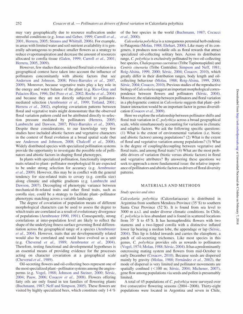
covering the entire species distribution range (a latitudinal exten-sion of 2375 km) and the two main ecological regions where thespecies grows, the arid Patagonian steppe and the understorey ofAndean–Patagonian forests (Fig. 1, Supplementary Data TableS1). The Patagonian steppe is a large (673 000 km2), dry,extra-Andean plain covered by grassland and scrubby vegetationthat extends from the eastern slopes of the southern Andes to theAtlantic coast. The Andean–Patagonian forest is a much smallerarea (248 100 km2) covered by woodlands that extends from 358Sto 558S on the eastern and western slopes of the Andes, reachingthe western edge of the Patagonian steppe to the east.

Floral and vegetative traits measured

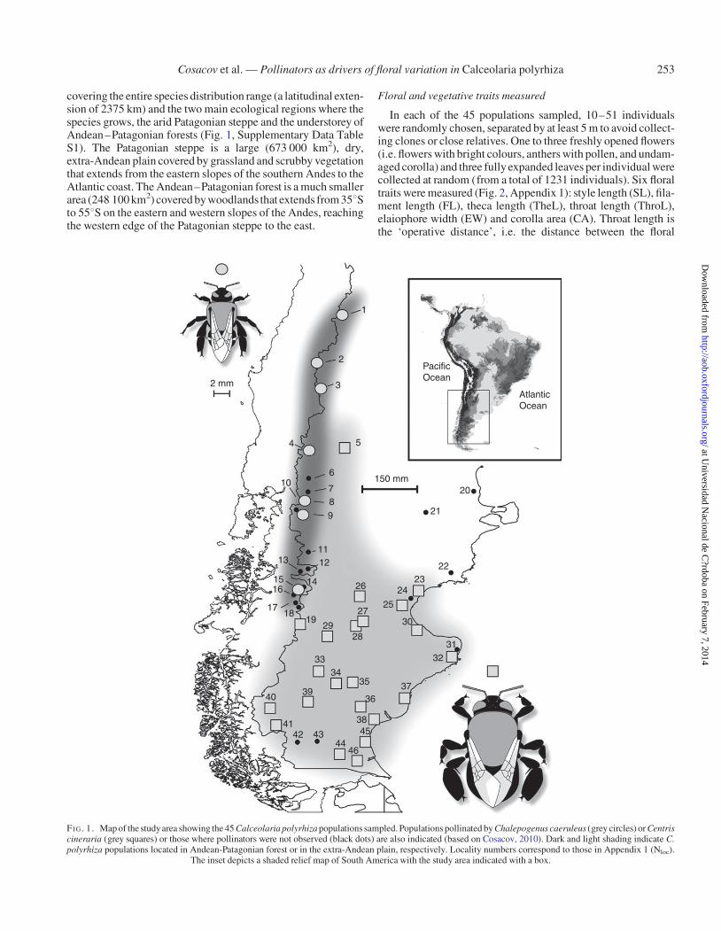
In each of the 45 populations sampled, 10–51 individualswere randomly chosen, separated by at least 5 m to avoid collect-ing clones or close relatives. One to three freshly opened flowers(i.e. flowers with bright colours, anthers with pollen, and undam-aged corolla) and three fully expanded leaves per individual werecollected at random (from a total of 1231 individuals). Six floraltraits were measured (Fig. 2, Appendix 1): style length (SL), fila-ment length (FL), theca length (TheL), throat length (ThroL),elaiophore width (EW) and corolla area (CA). Throat length isthe ‘operative distance’, i.e. the distance between the floral

2 mm

150 mm

2

1

3

54

6

78

9

111213

1516

1718

14

1929

28

27

26

25

2423

22

21

20

PacificOcean

AtlanticOcean

30

3231

3334

3940

4142 43

4446

4538

36

35 37

10

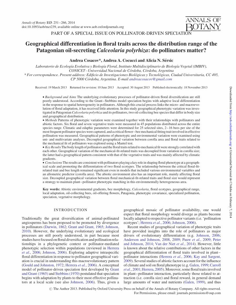
FI G. 1. Map of the studyarea showing the 45 Calceolaria polyrhiza populations sampled. Populations pollinated by Chalepogenus caeruleus (grey circles) or Centriscineraria (grey squares) or those where pollinators were not observed (black dots) are also indicated (based on Cosacov, 2010). Dark and light shading indicate C.polyrhiza populations located in Andean-Patagonian forest or in the extra-Andean plain, respectively. Locality numbers correspond to those in Appendix 1 (Nloc).

The inset depicts a shaded relief map of South America with the study area indicated with a box.

Cosacov et al. — Pollinators as drivers of floral variation in Calceolaria polyrhiza 253

at Universidad N

acional de C?rdoba on February 7, 2014

http://aob.oxfordjournals.org/D

ownloaded from

reward (i.e. the elaiophore) and the fertile parts; therefore, this isthe distance that pollinators have to fit to efficiently transferpollen from the anthers and to deposit it on the stigmas(Fig. 3). Three foliar traits were measured (Fig. 2, Appendix2): total leaf length including petiole (TLL), leaf lamina width(LLW) and leaf lamina length (LLL). We calculated TLL ×LLW as an estimator of total leaf area (TLA), LLL × LLW asan estimator of leaf lamina area (LLA) and LLL/LLW (L/W)as an estimator of leaf shape. Specific leaf area (SLA) was alsocalculated as leaf area per unit of dry mass (Cornelissen et al.,2003). To determine leaf dry mass, leaves were dried at 60 8Cfor 72 h and then weighed to the nearest 0.1 mg using a precisionbalance (Sartorius CP224 S). Three plant attributes were mea-sured in situ (Fig. 2, Appendix 2): plant height (PH), inflores-cence height (IH) and plant area (PA), calculated as theproduct of maximum plant width and perpendicular width. Allmorphometric measurements of flowers (n ¼ 3134) and leaves(n ¼ 3591) were taken from digital images using SigmaScanPro 5.0 software (SPSS). To obtain these images, scaledflowers were placed in a cylindrical case and photographed

Fertile parts

A

C

D

B

ThroL

ThroL

SL

CA

TheL

FL

PH

TLL

LLL

LLW

W1

W2

IH

EW

Elaiophore

(operativedistance)

FI G. 2. Schematic diagram of a flower, leaf and plant of Calceolaria polyrhiza showing linear morphometric measurements. (A) Lateral view of a flower showingfertile parts, elaiophore and the distance between the floral reward (elaiophore) and the fertile parts, i.e. throat length (ThroL). Black dashed line indicates the pointwhere flowers were dissected to obtain parts shown in (B). (B) Floral traits: throat length (ThroL), elaiophore width (EW), corolla area (CA) indicated by the blacksurface, theca length (TheL), filament length (FL) and style length (SL). (C) Vegetative traits: total leaf length (TLL), leaf lamina length (LLL), leaf lamina width

(LLW). (D) Plant traits: inflorescence height (IH), plant height (PH), plant maximum width (W1) and perpendicular width (W2).

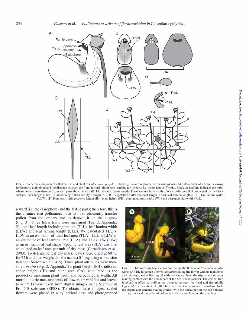
FI G. 3. Oil-collecting bee species pollinating the flowers of Calceolaria poly-rhiza. (A) The large bee Centris cineraria seizing the flower with its mandiblesand mid-legs, and collecting oil with the foreleg. Note the stigma and stamensmaking contact with the dorsal part of the bee’s head (arrow). The critical traitinvolved in effective pollination, distance between the head and the middlelegs (H-ML), is indicated. (B) The small bee Chalepogenus caeruleus. Notethe stigma and stamens making contact with the dorsal part of the bee’s thorax

(arrow) and the pellet of pollen and oils accumulated on the hind legs.

Cosacov et al. — Pollinators as drivers of floral variation in Calceolaria polyrhiza254

at Universidad N

acional de C?rdoba on February 7, 2014

http://aob.oxfordjournals.org/D

ownloaded from

with a Nikon Coolpix 5400 camera, in frontal and lateral views,and dissected as indicated in Fig. 2. Scale leaves were scannedwith 300 d.p.i. resolution.

Climatic and edaphic factors

We recorded geographical coordinates (i.e. latitude and longi-tude) for each population using a GPS system. From this data set,we selected 25 populations representative of the geographicaldistribution of the species. Using information available fromWorldClim database (http://www.worldclim.org/; Hijmanset al., 2005), bioclimatic variables were obtained for each local-ityat a spatial resolution of 1 km2. From the available informationwe selected annual temperature and precipitation averages, tem-perature of the warmest and coldest quarters (i.e. 3-monthseasons), and precipitation of the driest and wettest quarters(Supplementary Data Table S2). These variables correspond toaverage values obtained from interpolations of data observedduring the period between theyears 1950 and 2000. To character-ize edaphic conditions, one soil sample of 500 g was taken fromthe ground surface to a depth of 15 cm at each location. For eachsample, the pH value, organic carbon (C), nitrogen (N), potas-sium (K), phosphorus (P) and total sand/silt content were deter-mined by the soil laboratory of the Consejo Agrario Provincial,Convenio INTA-CAP, Santa Cruz Province, Argentina.

Pollinators

Calceolaria polyrhiza interacts with two pollinator speciesacross its geographical range, Chalepogenus caeruleus, distrib-uted from southern Mendoza Province (35 8 S) to northernChubut Province (43 8S) and inhabiting the northern area ofthe Andean–Patagonian forest, and Centris cineraria, distribu-ted from southern Neuquen Province (40 8 S) to southern SantaCruz Province (51 8S) and inhabiting mainly the Patagoniansteppe ecoregion (Figs 1 and 3; Roig-Alsina, 1999, 2000;Cosacov, 2010). Both are oil-collecting bee species, endemicto Patagonia (Roig-Alsina, 1999, 2000). In the forest ecoregion,C. cineraria was observed in two localities, but records of pollin-ator visits indicated that Ch. caeruleus accounted for .92 % ofthe total visits recorded in each of these two populations(Cosacov, 2010). A previous study indicates that the localitieswhere Ch. caeruleus and C. cineraria are distributed differedin climatic conditions (mean annual temperature and precipita-tion, and mean temperature and precipitation of the warmestquarter) and in edaphic factors (pH value and soil silt content;Cosacov, 2010). To characterize geographical variation in thepollinator functional trait in the 25 C. polyrhiza populationsselected as described in the section Climatic and edaphicfactors, pollinator bees were captured and the distance betweenthe head and the middle legs (HML) was measured under astereomicroscope using a digital calliper (Appendix 3). This isa critical trait involved in effective pollination, because it fitsThroL (Fig. 3). We explored whether HML had a geographicalpattern by using multiple regression models with geographicalcoordinates. To partition the total variance of HML accordingto its differences between bee species, among populationswithin species, and among individuals within populations (thelast level was used as the error term; Sokal and Rohlf, 1995), amixed-effects nested ANOVA was performed for this trait; the

percentage of variance accounted for each level, the componentof variance (CV), was then estimated.

Statistical analyses

Structure of geographical variation in floral and vegetative traits.To partition the total variance of floral and vegetative traitsinto its hierarchical components, a mixed-effects nestedANOVAwas performed for each trait measured. Floral and vege-tative attributes were partitioned according to their differencesamong populations, among individuals within populations, andamong flowers or leaves within individuals (the latter level wasused as the error term; Sokal and Rohlf, 1995). Although notall populations were sampled in the same year, during each flow-ering season we sampled populations representing the entire dis-tribution range of the species. Thus, a possible year effect wasuniformly distributed across the geographical range. In addition,two populations surveyed over 2 years did not show a temporaleffect in morphological variation (P . 0.05; Cosacov, 2010).To assess the presence of distance-based patterns of variationin floral and vegetative phenotypes, a spatial autocorrelation ana-lysis was performed for each floral and vegetative trait.Autocorrelograms were constructed using distance classes of100 km. Significance levels of Moran’s I coefficients of spatialautocorrelation were obtained by Monte Carlo methods with999 simulations. These analyses were performed using thelibrary ncf of the R package (R Development Core Team,2010). Finally, we explored geographical patterns in individualfloral and vegetative traits using simple regression models withgeographical coordinates. Because precipitation and theedaphic gradient follow a non-linear pattern with longitude inthe study area (Paruelo et al., 1998; Cosacov, 2010), we exploredwhether a non-linear adjustment would give a better fit than alinear one.

Coupled/decoupled geographical variation among floral traits. Weused the approach proposed by Cheverud et al. (1989) to evaluatewhether CA was more strongly correlated with vegetative traitsthan with floral ones, and whether floral mechanical-fit-relatedtraits (ThroL, SL, FL) were more closelyassociated among them-selves than with the remaining floral traits, across the geograph-ical range of the studied species. The approach assumes that traitsthat are functionally and/or developmentally related would becorrelated and would have evolved as a unit (e.g. Cheverudet al., 1989). Basically, the approach uses two types of matrix:a hypothetical matrix that describes theoretical relationshipsamong traits, and a matrix containing the empirically derivedmorphometric correlations (Pearson product–moment correla-tions between all pairs of morphological variables using popula-tion mean values of each trait measured). In the simplest case of amatrix of theoretical relationships, characters were identified aslinked (indicated as 0.5) or unlinked (indicated as 0). Thus, weconstructed two hypothetical matrices of developmental (d)and functional (f ) relationships for the whole plant (includingfloral and vegetative traits) and only for flowers (to furtherexplore coupling/decoupling among floral traits). For thewhole plant, we considered two developmental domains (vege-tative and floral); when we considered only flowers, we distin-guished three developmental domains (corolla, androeciumand gynoecium; Supplementary Data Fig. S1). Additionally,

Cosacov et al. — Pollinators as drivers of floral variation in Calceolaria polyrhiza 255

at Universidad N

acional de C?rdoba on February 7, 2014

http://aob.oxfordjournals.org/D

ownloaded from

for the whole plant and for flowers alone, we constructed a morecomplex model: nested hypotheses (n) with hierarchical linkage.In the nested hypotheses two characters were identified as devel-opmentally linked (indicated as 0.5) or unlinked (indicated as 0).Then, if the characters were assumed to be functionally related,an additional linkage value of 0.5 was added to the fundamentaldevelopmental linkage. Thus, if two traits were not linked eitherby development or by function the theoretical relationshipassumed was zero; if two traits were linked only by developmentor function, the relationship assumed was 0.5; and if two traitswere linked only by development and function, the theoretical re-lationship was 1 (Supplementary Data Fig. S1). We then testedwhich of two alternative theoretical matrices best fitted the em-pirical matrix and whether their difference in fit was statisticallysignificant. For this purpose, a Z matrix was obtained from thedifference of the two competing theoretical matrices, after stand-ardizing the elements of both matrices to zero mean and unitystandard deviation. The pattern of similarity between the theor-etical and empirical matrices was subjected to Mantel testswith 999 permutations, implemented in the package Vegan ofthe R 2.15.2 statistical software (R Development Core Team,2010).

Multivariate patterns and possible factors of morphological vari-ation. To analyse the relationship between floral traits and theirassociation with biotic (i.e. pollinator size) and abiotic (climaticand edaphic) factors, a multivariate analysis of redundancy(RDA) was performed using CANOCO (ter Braak andSmilauer, 2002). RDA is a multivariate ordination method inwhich the axes are constructed by a linear combination of envir-onmental variables (ter Braak and Smilauer, 2002). For this ana-lysis, a matrix of population × morphology was analysed inrelation to a corresponding matrix of explanatory environmentalvariables. We included five explanatory factors that werehypothesized to be important determinants of variation inflower morphology: two edaphic, precipitation and temperatureaxes derived from their respective principal component analyses(see Climatic and edaphic factors in the Results section) and thecritical distance measured on captured pollinators (HML). Whennecessary, variables were log-transformed. To avoid using dif-ferent scales and for comparative purposes, the variables werestandardized to zero mean and unity standard deviation. The sig-nificance of the variability explained by each environmentalfactor was analysed by automatic selection of variables using aMonte Carlo test with 999 permutations. In this procedure, thevariable that best fits the data is selected first and then the nextbest fitting variable is added to the model (ter Braak andSmilauer, 2002). We also performed an RDA for the vegetativetrait matrix using the same five explanatory factors (includingbee functional trait and abiotic variables).

Plant–pollinator matching. To further explore plant–pollinatorphenotypic matching, we used multiple regression to analysesimultaneously the effects of biotic (pollinator functional trait)and abiotic (climatic and edaphic parameters) predictor vari-ables on ThroL and the relative importances of these effects.Because ThroL might be explained by allometric relationshipsamong floral traits, we also included CA as a predictor variable.As acontrol test we also performed multiple regression to analysesimultaneously the effects of biotic (pollinator functional trait),

abiotic (climatic and edaphic parameters) and ThroL as predictorvariables on CA and the relative importances of these effects.

RESULTS

Geographical structure of floral and vegetative trait variation

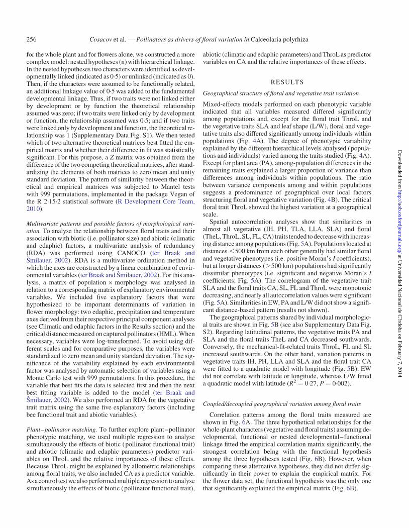
Mixed-effects models performed on each phenotypic variableindicated that all variables measured differed significantlyamong populations and, except for the floral trait ThroL andthe vegetative traits SLA and leaf shape (L/W), floral and vege-tative traits also differed significantly among individuals withinpopulations (Fig. 4A). The degree of phenotypic variabilityexplained by the different hierarchical levels analysed (popula-tions and individuals) varied among the traits studied (Fig. 4A).Except for plant area (PA), among-population differences in theremaining traits explained a larger proportion of variance thandifferences among individuals within populations. The ratiobetween variance components among and within populationssuggests a predominance of geographical over local factorsstructuring floral and vegetative variation (Fig. 4B). The criticalfloral trait ThroL showed the highest variation at a geographicalscale.

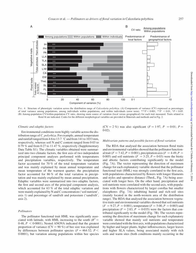
Spatial autocorrelation analyses show that similarities inalmost all vegetative (IH, PH, TLA, LLA, SLA) and floral(TheL, ThroL, SL, FL, CA) traits tended to decreasewith increas-ing distance among populations (Fig. 5A). Populations located atdistances ,500 km from each other generally had similar floraland vegetative phenotypes (i.e. positive Moran’s I coefficients),but at longer distances (.500 km) populations had significantlydissimilar phenotypes (i.e. significant and negative Moran’s Icoefficients; Fig. 5A). The correlogram of the vegetative traitSLA and the floral traits CA, SL, FL and ThroL were monotonicdecreasing, and nearly all autocorrelation values were significant(Fig. 5A). Similarities in EW, PA and L/W did not show a signifi-cant distance-based pattern (results not shown).

The geographical patterns shared by individual morphologic-al traits are shown in Fig. 5B (see also Supplementary Data Fig.S2). Regarding latitudinal patterns, the vegetative traits PA andSLA and the floral traits TheL and CA decreased southwards.Conversely, the mechanical-fit-related traits ThroL, FL and SLincreased southwards. On the other hand, variation patterns invegetative traits IH, PH, LLA and SLA and the floral trait CAwere fitted to a quadratic model with longitude (Fig. 5B). EWdid not correlate with latitude or longitude, whereas L/W fitteda quadratic model with latitude (R2 ¼ 0.27, P ¼ 0.002).

Coupled/decoupled geographical variation among floral traits

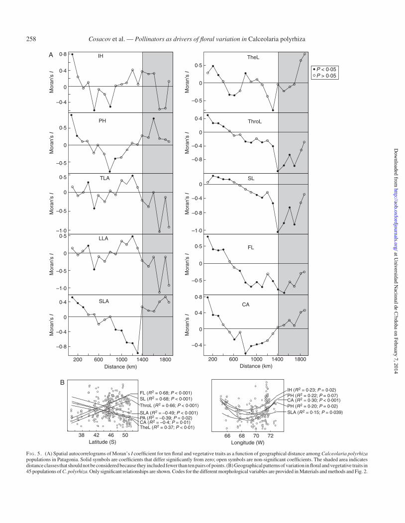
Correlation patterns among the floral traits measured areshown in Fig. 6A. The three hypothetical relationships for thewhole-plant characters (vegetative and floral traits) assuming de-velopmental, functional or nested developmental–functionallinkage fitted the empirical correlation matrix significantly, thestrongest correlation being with the functional hypothesisamong the three hypotheses tested (Fig. 6B). However, whencomparing these alternative hypotheses, they did not differ sig-nificantly in their power to explain the empirical matrix. Forthe flower data set, the functional hypothesis was the only onethat significantly explained the empirical matrix (Fig. 6B).

Cosacov et al. — Pollinators as drivers of floral variation in Calceolaria polyrhiza256

at Universidad N

acional de C?rdoba on February 7, 2014

http://aob.oxfordjournals.org/D

ownloaded from

Climatic and edaphic factors

Environmental conditions were highly variable across the dis-tribution range of C. polyrhiza. For example, annual temperatureand rainfall ranged from 4.6 to 13.7 8C and from 141 to 1033 mm,respectively, whereas soil N and C content ranged from 0.03 to0.79 % and from 0.27 to 11.47 %, respectively (SupplementaryData Table S1). The climatic variables obtained were summar-ized into two climatic factors, the first axis of two independentprincipal component analyses performed with temperaturesand precipitation variables, respectively. The temperaturefactor accounted for 70 % of the total temperature variationand was mainly explained by mean annual temperature andmean temperature of the warmest quarter; the precipitationfactor accounted for 86 % of the total variation in precipi-tation and was mainly explained by mean annual precipitation.Edaphic variables were summarized into two edaphic factors,the first and second axes of the principal component analysis,which accounted for 63 % of the total edaphic variation andwere mainly explained by N and C concentration (‘soil nutrient’,axis 1) and percentage of sand/silt and potassium (‘sand/silt’,axis 2).

Pollinators

The pollinator functional trait HML was significantly asso-ciated with latitude, with HML increasing to the south (R2 ¼0.48, P , 0.0001). Nested ANOVA indicated that the greatestproportion of variance (CV ¼ 90 %) of bee size was explainedby differences between pollinator species (F ¼ 464.32; P ,0.0001), but variation among populations within bee species

(CV ¼ 2 %) was also significant (F ¼ 1.97, P ¼ 0.01; P ¼0.02).

Multivariate patterns and possible factors of floral variation

The RDA that analysed the association between floral traitsand environmental variables showed that the pollinator function-al trait (F ¼ 7.42, P ¼ 0.001), precipitation axis (F ¼ 4.49, P ¼0.005) and soil nutrients (F ¼ 3.25, P ¼ 0.03) were the bioticand abiotic factors contributing significantly to the model(Fig. 7A). The vector representing the direction of maximumchange for each explanatory variable showed that the pollinatorfunctional trait (HML) was strongly correlated to the first axis,with populations characterized by flowers with longer filamentsand styles and operative distance (ThroL, Fig. 7A) being asso-ciated with longer bees. On the other hand, precipitation andsoil nutrients were correlated with the second axis, with popula-tions with flowers characterized by larger corollas but smallerelaiophores (Fig. 7A) inhabiting humid and rich-soil sites(mainly located in the north-western area of the distributionrange). The RDA that analysed the association between vegeta-tive traits and environmental variables showed that soil nutrients(F ¼ 9.27, P ¼ 0.001), temperature (F ¼ 5.00, P ¼ 0.003) andprecipitation (F ¼ 2.83, P ¼ 0.035) were the factors that con-tributed significantly to the model (Fig. 7B). The vectors repre-senting the direction of maximum change for each explanatoryvariable showed that mainly soil nutrients and temperaturewere correlated with the first axis, with populations characterizedby higher and larger plants, higher inflorescences, larger leavesand higher SLA values, being associated mainly with richsoils and warm sites (both conditions mainly occurring in the

IH ***

***

***

***

***

***

***

***

***

******

**

***

PH

PA

LLA

TLA

SLA

L/W

CA

EW

TheL

Flo

ral t

raits

Veg

etat

ive

trai

ts

Among populations

A B

Within populations Within individuals

0·1

CV ratio

Predominance oflocal factors

Predominance ofgeographical factors

Among populationsWithin populations

10

Fol

iar

attr

ibut

esTr

aits

rel

ated

to fl

oral

-fit

Pla

nt a

ttrib

utes

SL

FL

ThroL

0 20 40 60 80 100Component of variance (%)

FI G. 4. Structure of phenotypic variation across the distribution range of Calceolaria polyrhiza. (A) Components of variance (CV) expressed as percentagesof total variance among populations, among individuals within populations, and within individuals (error term). ***P , 0.001, **P , 0.01, *P , 0.05.(B) Among-population CV/within-population CV ratio, showing main source of variation (local versus geographical) for each trait measured. Traits related to

floral fit are indicated. Codes for the different morphological variables are provided in Materials and methods and in Fig. 2.

Cosacov et al. — Pollinators as drivers of floral variation in Calceolaria polyrhiza 257

at Universidad N

acional de C?rdoba on February 7, 2014

http://aob.oxfordjournals.org/D

ownloaded from

0·8A

B

0·4

0

–0·4

0·5

0

–0·5

0·5

0

–0·5

–1·00·5

0

–0·5

–1·0

0·4

0

–0·4

–0·8 –0·4

0

0·4

0·8

–0·5

0

0·5

–1·0

–0·8

–0·4

0

–0·8

–0·4

0

0·4

–0·5

0

0·5

200

38 42 46 50

FL (R2 = 0·68; P < 0·001)IH (R2 = 0·23; P = 0·02)PH (R2 = 0·22; P = 0·07)CA (R2 = 0·30; P < 0·001)PH (R2 = 0·20; P = 0·02)SLA (R2 = 0·15; P = 0·039)

SL (R2 = 0·68; P < 0·001)ThroL (R2 = 0·66; P < 0·001)

SLA (R2 = –0·49; P < 0·001)PA (R2 = –0·39; P = 0·02)CA (R2 = –0·4; P = 0·01)TheL (R2 = 0·37; P < 0·01)

Latitude (S)66 68 70 72

Longitude (W)

600 1000 1400Distance (km)

SLA

LLA

TLA

PH

IH TheL

ThroL

SL

FL

CA

Mor

an’s

IM

oran

’s I

Mor

an’s

IM

oran

’s I

Mor

an’s

I

Mor

an’s

IM

oran

’s I

Mor

an’s

IM

oran

’s I

Mor

an’s

I

1800 200 600 1000 1400Distance (km)

1800

P < 0·05P > 0·05

FI G. 5. (A) Spatial autocorrelograms of Moran’s I coefficient for ten floral and vegetative traits as a function of geographical distance among Calceolaria polyrhizapopulations in Patagonia. Solid symbols are coefficients that differ significantly from zero; open symbols are non-significant coefficients. The shaded area indicatesdistanceclasses that should not be considered because they included fewer than ten pairs of points. (B) Geographical patterns of variation in floral and vegetative traits in45 populations of C. polyrhiza. Only significant relationships are shown. Codes for the different morphological variables are provided in Materials and methods and Fig. 2.

Cosacov et al. — Pollinators as drivers of floral variation in Calceolaria polyrhiza258

at Universidad N

acional de C?rdoba on February 7, 2014

http://aob.oxfordjournals.org/D

ownloaded from

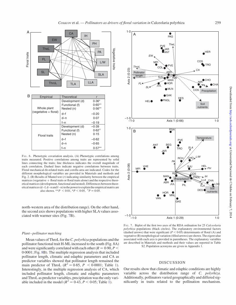
north-western area of the distribution range). On the other hand,the second axis shows populations with higher SLAvalues asso-ciated with warmer sites (Fig. 7B).

Plant–pollinator matching

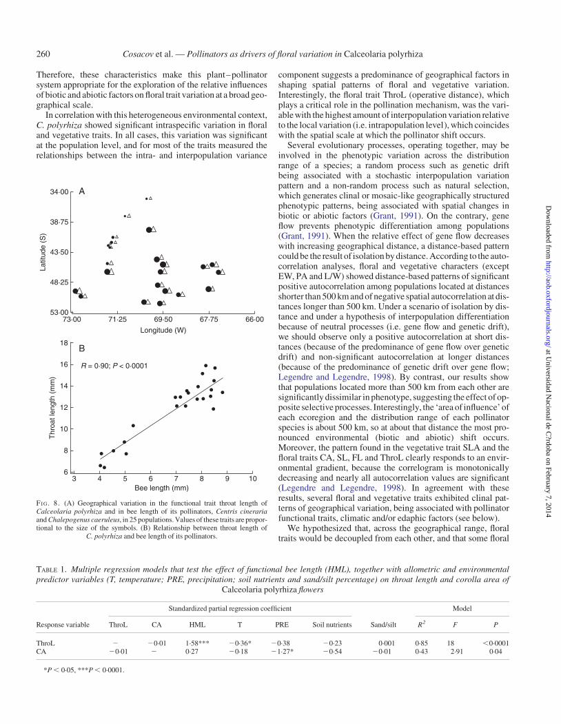
Mean values of ThroL for the C. polyrhiza populations and thepollinator functional trait H-ML increased to the south (Fig. 8A)and were significantly correlated with each other (R ¼ 0.90, P ,0.0001; Fig. 8B). The multiple regression analysis that includedpollinator length, climatic and edaphic parameters and CA aspredictor variables showed that pollinator length remained themain predictor of ThroL (R2 ¼ 0.85, P , 0.0001; Table 1).Interestingly, in the multiple regression analysis of CA, whichincluded pollinator length, climatic and edaphic parametersand ThroL as predictor variables, precipitation was the only vari-able included in the model (R2 ¼ 0.43, P , 0.05; Table 1).

DISCUSSION

Our results show that climatic and edaphic conditions are highlyvariable across the distribution range of C. polyrhiza.Additionally, pollinators varied geographically and differed sig-nificantly in traits related to the pollination mechanism.

EW

CAIH

PH

PA

L/W

SLA

LLATLAThroL

Empirical

Whole plant(vegetative + floral)

Development (d) 0·36*0·60**0·56**

Functional (f)Nested (n)

d–fd–n

f–n

–0·200·07

–0·19Development (d) –0·39

0·62

0·15Functional (f)Nested (n)

d–fd–n

f–n

–0·62–0·65

0·57**

Floral traits

Theoretical r

SL

Flo

ral t

raits

Vegetative traits

FL

TheL

A

B

FI G. 6. Phenotypic covariation analysis. (A) Phenotypic correlations amongtraits measured. Positive correlations among traits are represented by solidlines connecting the traits; line thickness indicates the overall magnitude ofeach correlation. Dashed lines indicate negative correlations between traits.Floral mechanical-fit-related traits and corolla area are indicated. Codes for thedifferent morphological variables are provided in Materials and methods andFig. 2. (B) Results of Mantel test (r) indicating similarity between the empiricalmatrices (vegetative + floral traits or floral traits alone) and the respective theor-etical matrices (development, functional and nested). Differences between theor-etical matrices (d–f, d–n and f–n) in the power to explain the empirical matrix are

also shown. **P , 0.01, *P , 0.05, ^P ¼ 0.05.

PVE

A

B

PAG

JARANT

MPI

COLPVE

ABR

SJUMAN

R26

HOR

MLN

GAK

PNGLHELDES

PGA

Axis 1 (0·66)

Axi

s 2

(0·2

3)

1·0–1·0

Axis 1 (0·29) 1·0–1·0

–1·0

Axi

s 2

(0·0

8)

–1·0

1·0

PVE

TROBEGANT

JAR

RCH CHO

HELSJUVHE

R26

PA

L/W

SLA

SLFL

ThroL

EW

TheL

CA

PH

IHLLA

TLA

Precipitation

Soilnutrients

Soilnutrients

Precipitation

Pollinatorlength

Temperature

MPI

MAN

ABRJUL

HOR

VANMNL

GKE

PIL

DES

CHALOC

PNGLCOS

COS

NIRPIL

CHO

COSTRO

HER

CHAJUL

1·0

FI G. 7. Biplot of the first two axes of the RDA ordination for 25 Calceolariapolyrhiza populations (black circles). The explanatory environmental factors(dashed arrows) that were significant (P , 0.05) determinants of floral (A) andvegetative (B) morphological variation (filled arrows) are shown. The eigenvalueassociated with each axis is provided in parentheses. The explanatory variablesare described in Materials and methods and their values are reported in Table

S2. Population acronyms are given in Appendix 1.

Cosacov et al. — Pollinators as drivers of floral variation in Calceolaria polyrhiza 259

at Universidad N

acional de C?rdoba on February 7, 2014

http://aob.oxfordjournals.org/D

ownloaded from

Therefore, these characteristics make this plant–pollinatorsystem appropriate for the exploration of the relative influencesof biotic and abiotic factors on floral trait variation at a broad geo-graphical scale.

In correlation with this heterogeneous environmental context,C. polyrhiza showed significant intraspecific variation in floraland vegetative traits. In all cases, this variation was significantat the population level, and for most of the traits measured therelationships between the intra- and interpopulation variance

component suggests a predominance of geographical factors inshaping spatial patterns of floral and vegetative variation.Interestingly, the floral trait ThroL (operative distance), whichplays a critical role in the pollination mechanism, was the vari-able with the highest amount of interpopulation variation relativeto the local variation (i.e. intrapopulation level), which coincideswith the spatial scale at which the pollinator shift occurs.

Several evolutionary processes, operating together, may beinvolved in the phenotypic variation across the distributionrange of a species; a random process such as genetic driftbeing associated with a stochastic interpopulation variationpattern and a non-random process such as natural selection,which generates clinal or mosaic-like geographically structuredphenotypic patterns, being associated with spatial changes inbiotic or abiotic factors (Grant, 1991). On the contrary, geneflow prevents phenotypic differentiation among populations(Grant, 1991). When the relative effect of gene flow decreaseswith increasing geographical distance, a distance-based patterncould be the result of isolation by distance. According to the auto-correlation analyses, floral and vegetative characters (exceptEW, PA and L/W) showed distance-based patterns of significantpositive autocorrelation among populations located at distancesshorter than 500 km and of negative spatial autocorrelation at dis-tances longer than 500 km. Under a scenario of isolation by dis-tance and under a hypothesis of interpopulation differentiationbecause of neutral processes (i.e. gene flow and genetic drift),we should observe only a positive autocorrelation at short dis-tances (because of the predominance of gene flow over geneticdrift) and non-significant autocorrelation at longer distances(because of the predominance of genetic drift over gene flow;Legendre and Legendre, 1998). By contrast, our results showthat populations located more than 500 km from each other aresignificantly dissimilar in phenotype, suggesting the effect of op-posite selective processes. Interestingly, the ‘area of influence’ ofeach ecoregion and the distribution range of each pollinatorspecies is about 500 km, so at about that distance the most pro-nounced environmental (biotic and abiotic) shift occurs.Moreover, the pattern found in the vegetative trait SLA and thefloral traits CA, SL, FL and ThroL clearly responds to an envir-onmental gradient, because the correlogram is monotonicallydecreasing and nearly all autocorrelation values are significant(Legendre and Legendre, 1998). In agreement with theseresults, several floral and vegetative traits exhibited clinal pat-terns of geographical variation, being associated with pollinatorfunctional traits, climatic and/or edaphic factors (see below).

We hypothesized that, across the geographical range, floraltraits would be decoupled from each other, and that some floral

34·00 A

B

38·75

43·50

48·25

53·00

18

16

14

12

10

8

63 4 5 6 7 8 9 10

Bee length (mm)

Thr

oat l

engt

h (m

m)

73·00 71·25

R = 0·90; P < 0·0001

69·50 67·75 66·00

Longitude (W)

Latit

ude

(S)

FI G. 8. (A) Geographical variation in the functional trait throat length ofCalceolaria polyrhiza and in bee length of its pollinators, Centris cinerariaand Chalepogenus caeruleus, in 25 populations. Values of these traits are propor-tional to the size of the symbols. (B) Relationship between throat length of

C. polyrhiza and bee length of its pollinators.

TABLE 1. Multiple regression models that test the effect of functional bee length (HML), together with allometric and environmentalpredictor variables (T, temperature; PRE, precipitation; soil nutrients and sand/silt percentage) on throat length and corolla area of

Calceolaria polyrhiza flowers

Response variable

Standardized partial regression coefficient Model

ThroL CA HML T PRE Soil nutrients Sand/silt R2 F P

ThroL 2 20.01 1.58*** 20.36* 20.38 20.23 0.001 0.85 18 ,0.0001CA 20.01 2 0.27 20.18 21.27* 20.54 20.01 0.43 2.91 0.04

*P , 0.05, ***P , 0.0001.

Cosacov et al. — Pollinators as drivers of floral variation in Calceolaria polyrhiza260

at Universidad N

acional de C?rdoba on February 7, 2014

http://aob.oxfordjournals.org/D

ownloaded from

traits would even be coupled to vegetative geographical vari-ation. Previous studies have explored coupling/decouplingbetween vegetative and floral characters at a geographical scale(e.g. Herrera et al., 2002, Lambrecht and Dawson, 2007;Perez-Barrales et al., 2007; Chalcoff et al., 2008), consideringdecoupling as evidence of different selection regimes influen-cing floral and vegetative traits. Probably because of the trad-itional idea that pollinator-mediated selection favourscovariation of the whole floral phenotype (Berg, 1960;Armbruster et al., 1999), the degree of within-flower coupling/decoupling at a geographical scale has been less explored (butsee Rosas-Guerrero et al., 2011). Our results show that throat,filament and style length, which are the critical flower–beefitting traits involved in the pollination mechanism, were signifi-cantly more correlated among each other than with the otherfloral traits, suggesting the existence of one such functional intra-floral module. These traits increased southwards, where popula-tions pollinated by the larger bee (C. cineraria) are located.Interestingly, other floral traits, such as theca length andcorolla area, and the vegetative traits plant area and specificleaf area showed the opposite patterns, decreasing southwards,where C. polyrhiza inhabits sites under stressful moisture andsoil nutrient conditions.

The geographical patterns detected for plant height and area,leaf area, specific leaf area and corolla area were consistentwith previous studies showing a reduction in flower size, leafarea and specific leaf area with increasing aridity (e.g. Jonasand Geber, 1999; Sapir et al., 2002; Herrera, 2005; Lambrechtand Dawson, 2007; Paiaro et al., 2012) and soil nutrient avail-ability (e.g. Frazee and Marquis, 1994; Herrera, 2005; Paiaroet al., 2012). Therefore, the reduction in leaf and flower sizecould be related to strategies for reducing evapotranspirationand reproductive costs in stressful areas, as suggested (e.g.Carroll et al., 2001; Herrera, 2005, 2009). Under certain condi-tions, this transition to smaller flowers could also be associatedwith increasing levels of autogamy, as reported for otherspecies (e.g. Pauw, 2005). We suggest that decoupling amongfloral traits in C. polyrhiza may resolve the conflict between lim-itations in resource allocation to reproductive and vegetativecosts and the demands of fitting to a large pollinator inhabitingstressful localities. Thus, in populations located in stressfulareas (which are pollinated by the larger bee), C. polyrhizawould minimize reproductive costs by reducing floral size (i.e.corolla area) while maintaining covariation patterns amongfit-related floral traits for effective pollination. This suggestedmechanism probably explains why this highly pollinator-specialized species has a wide geographical distribution(Pelabon et al., 2013; Hermant et al., 2013).

Based on RDA results, and in agreement with the geographicalvariation pattern of each trait, both biotic and abiotic factorsshape floral variation at a spatial scale. However, in the multipleregression analysis of ThroL (operative distance), whichincluded all biotic and abiotic factors as predictor variables,the pollinator functional trait remained the main predictor vari-able. Thus, ThroL, which has a critical role for an effective pol-lination mechanism, was strongly associated with bee length,even when other environmental variables were considered sim-ultaneously in the multiple regression models. Interestingly,when this analysis was performed on corolla area, precipitationaxis was the only variable retaining explanatory power in the

model. In systems where the variation induced by pollinatorsand abiotic factors have the same direction, it is difficult to deter-mine the contribution of each factor to the phenotypic variation ata geographical scale, because a better fit to the morphology ofpollinators may just be the result of an increase in flower size(i.e. isometric change) as a consequence of favourable climaticor edaphic conditions (e.g. Anderson and Johnson, 2008;Hodgins and Barrett, 2008). The geographical structure ofbiotic and abiotic variation across the distribution range ofC. polyrhiza provides a scenario in which the expected patternsof either pollinator-driven variation and variation driven bycost–resources trade-offs (Galen, 1999; Herrera, 2005) have op-posite directions. Indeed, our results show the simultaneousinfluences and relative importances of biotic and abioticfactors in the configuration of floral variation at a geographicalscale. While pollinators appear to be the main agents of among-population floral variation influencing mechanical-fit-relatedtraits, precipitation seems to be the most important factor influen-cing corolla area. We consider that geographical studies explor-ing floral variation related to pollinators should include not onlypollination-related traits but also other floral and vegetative vari-ables to thoroughly explore the relative importance of pollinatorsand abiotic factors as drivers of floral diversification.

Our study, which is the first report on an oil–flower/oil–beeinteraction at far southern latitudes in South America, supportsthe Grant–Stebbins model of pollinator-driven divergence(Johnson, 2010; Peter and Johnson, 2014; Sun et al., 2014;Van der Niet et al., 2014). Overall, by covering the entire distri-bution range of C. polyrhiza, we could detect two floral ecotypesmainly differentiated by floral traits related to pollinator fit, withthe pollinator functional trait being the main factor influencingfloral divergence. In this system, local adaptation would resultfrom a variable adaptive landscape determined by geographical-ly differentiated ranges of pollinators. The next step in this studysystem is to analyse the reported floral divergence consideringphylogeographical patterns of C. polyrhiza (Cosacov et al.,2010) to disentangle historical and ecological processes influen-cing floral evolution.

SUPPLEMENTARY DATA

Supplementary data are available online at www.aob.oxford-journals.org and consist of the following. Table S1: number,code, name and geographical co-ordinates of Calceolaria poly-rhiza sampled populations for interpopulation phenotypic vari-ation. Table S2: climatic and edaphic conditions of the 25Calceolaria polyrhiza populations selected in Patagonia. Fig.S1: theoretical development, functional and nested matricesused to analyse coupled/decoupled geographic morphologicalvariation. Fig. S2: geographic patterns of variation of floral andvegetative traits in 45 populations of Calceolaria polyrhiza.

ACKNOWLEDGEMENTS

We thank V. Paiaro, A. Mazzoni, G. Humano, M. E. Vivar andC. Franchini for their field assistance, R. Kofalt for her help inthe logistics of the field trips, C. Romanutti for her help intaking bee measurements, S. Benıtez-Vieyra for his statisticalsuggestions and Jorgelina Brasca for editing the Englishversion of the manuscript. Dr A. Pauw, Dr Y. Sapir and an

Cosacov et al. — Pollinators as drivers of floral variation in Calceolaria polyrhiza 261

at Universidad N

acional de C?rdoba on February 7, 2014

http://aob.oxfordjournals.org/D

ownloaded from

anonymous reviewer provided valuable comments on an earlierversion of this manuscript. We also thank APN Argentina andCONAF Chile for granting permits to work in populationslocated in their parks and reserves. This work was supportedby the National Research Council of Argentina (PIP11220080101264); National Ministry of Science andTechnology (PID 000113/2011, FONCYT-PICT 01-10952,01-33755 and 2011-0709); Myndel Pedersen Foundation andthe Systematics Research Fund.

LITERATURE CITED

Anderson B, Johnson SD. 2008. The geographical mosaic of coevolution in aplant–pollinator mutualism. Evolution 62: 220–225.

Anderson B, Johnson SD. 2009. Geographical covariation and local conver-gence of flower depth in a guild of fly-pollinated plants. New Phytologist182: 533–40.

Armbruster WS. 1990. Estimating and testing adaptive surfaces: the morph-ology and pollination of Dalechampia blossoms. American Naturalist135: 14–31.

Armbruster WS. 1991. Multilevel analysis of morphometric data from naturalplant populations: insights into ontogenetic, genetic, and selective correla-tions in Dalechampia scandens. Evolution 45: 1229–1244.

Armbruster WS, Di Stilio VS, Tuxill JD, Flores TC, Velasquez Runk JL.1999. Covariance and decoupling of floral and vegetative traits in nineNeotropical plants: a re-evaluation of Berg’s correlation-pleiades concept.American Journal of Botany 86: 39–55.

Armbruster WS, Pelabon C, Hansen TF, Mulder CPH. 2004. Floral integra-tion, modularity, and precision: distinguishing complex adaptations fromgenetic constraints. In: Pigliucci M, Preston K. eds. Phenotypic integration:studying the ecology and evolution of complex phenotypes. Oxford: OxfordUniversity Press, 23–49.

Armbruster WS, Hansen TF, Pelabon C, Perez-Barrales R, Maad J. 2009.The adaptive accuracy of flowers: measurement and microevolutionary pat-terns. Annals of Botany 103: 1529–1545.

Berg R. 1960. The ecological significance of correlation pleiades. Evolution 14:171–180.

ter Braak CJF, Smilauer P. 2002. CANOCO reference manual and CanoDrawfor Windows user’s guide: software for canonical community ordination(version 4.5). Ithaca: Microcomputer Power.

Buchmann SL. 1987. The ecologyof oil flowers and their bees. Annual Review ofEcology and Systematics 18: 343–369.

Carroll AB, Pallardy SG, Galen C. 2001. Drought stress, plant water status, andfloral trait expression in fireweed, Epilobium angustifolium (Onagraceae).American Journal of Botany 88: 438–446.

Chalcoff VR, Ezcurra C, Aizen MA. 2008. Uncoupled geographical variationbetween leaves and flowers in a South-Andean Proteaceae. Annals of Botany102: 79–91.

Cheverud JM, Wagner GP, Dow MM. 1989. Methods for the comparative ana-lysis of variation patterns. Systematic Zoology 38: 201–213.

Cocucci AA, Sersic A, Roig-Alsina A. 2000. Oil-collecting structures inTapinotaspidini: their diversity, function and probable origin(Hymenoptera: Apidae). Mitteilungen der Munchner EntomologischenGesellschaft 90: 51–74.

Cornelissen JHC, Lavorel S, Garnier E, et al. 2003. A handbook of protocolsfor standardised and easy measurement of plant functional traits worldwide.Australian Journal of Botany 51:335–380.

Cosacov A. 2010. Patrones de variacion de caracteres fenotıpicos y frecuenciasgenicas en el rango de distribucion de la especie endemica de PatagoniaCalceolaria polyrhiza: su relacion con variables ambientales, poliniza-dores y factores historicos. PhD Thesis, Universidad Nacional deCordoba, Argentina.

Cosacov A, Nattero J, Cocucci AA. 2008. Variation of pollinator assemblagesand pollen limitation in a locally specialized system: the oil-producingNierembergia linariifolia (Solanaceae). Annals of botany 102: 723–734.

Cosacov A, Sersic AN, Sosa V, De-Nova JA, Nylinder S, Cocucci AA. 2009.New insights into the phylogenetic relationships, character evolution, andphytogeographic patterns of Calceolaria (Calceolariaceae). AmericanJournal of Botany, 96: 2240–2255.

Cosacov A, Sersic AN, Sosa V, Johnson LA, Cocucci AA. 2010. Multiple peri-glacial refugia in the Patagonia steppe and post-glacial colonization of theAndes: the phylogeography of Calceolaria polyrhiza. Journal ofBiogeography 37: 1463–1477.

Darwin CR. 1862. The various contrivances by which British and foreignorchids are fertilised by insects. London: Murray.

Ehrhart C. 2000. Die Gattung Calceolaria (Scrophulariaceae) in Chile.Bibliotheca Botanica 153: 1–283.

Fernandez RJ, Golluscio RA, Bisigato AJ, Soriano A. 2002. Gap colonizationin the Patagonian semidesert: seed bank and diaspore morphology.Ecography 25: 336–344.

Frazee JE, Marquis RJ. 1994. Environmental contribution to floral trait vari-ation in Chamaecrista fasciculata (Fabaceae: Caesalpinoideae). AmericanJournal of Botany 81: 206–215.

Galen C. 1999. Why do flowers vary? The functional ecology of variation inflower size and form within natural plant populations. BioScience 49:631–640.

Gould SJ, Johnston RF. 1972. Geographic variation. Annual Review of Ecologyand Systematics 3: 457–498.

Grant V. 1991.The evolutionary process. New York: Columbia University Press.

Grant V, Grant KA. 1965. Flower pollination in the phlox family. New York:Columbia University Press.

Hermant M, Prinzing A, Vernon P, Convey P, Hennion F. 2013. Endemicspecies have highly integrated phenotypes, environmental distributionsand phenotype–environment relationships. Journal of Biogeography 40:1583–1594.

Herrera J. 2005. Flower size variation in Rosmarinus officinalis: individuals,populations and habitats. Annals of Botany 95: 431–437.

Herrera J. 2009. Visibility vs. biomass in flowers: exploring corolla allocation inMediterranean entomophilous plants. Annals of Botany 103: 1119–1127.

Herrera CM, Cerda X, Garcıa BM, et al. 2002. Floral integration, phenotypiccovariance structure and pollinator variation in bumblebee-pollinatedHelleborus foetidus. Journal of Evolutionary Biology 15: 108–121.

Herrera CM, Castellanos MC, Medrano M. 2006. Geographical context offloral evolution: towards an improved research programme in floral diversi-fication. In: Harder LD, Barrett SCH. eds. Ecology and evolution of flowers.Oxford: Oxford University Press, 278–294.

Hijmans RJ, Cameron SE, Parra JL, Jones PG, Jarvis A. 2005. Very highresolution interpolated climate surfaces for global land areas.International Journal of Climatology 25: 1965–1978.

Hodgins KA, Barrett SCH. 2008. Geographic variation in floral morphologyand style-morph ratios in a sexually polymorphic daffodil. AmericanJournal of Botany 95: 185–195.

Johnson SD. 2006. Pollinator-driven speciation in plants. In: Harder LD, BarrettSCH. eds. The ecology and evolution of flowers. Oxford: Oxford UniversityPress, 296–306.

Johnson SD. 2010. The pollination niche and its role in the diversification andmaintenance of the southern African flora. Philosophical Transactions ofthe Royal Society of London B: Biological Sciences 365: 499–516.

Johnson SD, Steiner KE. 2000. Generalization versus specialization in plantpollination systems. Trends in Ecology and Evolution 15: 140–143.

Jonas CS, Geber MA. 1999. Variations among populations of Clarkia unguicu-lata (Onagraceae) along altitudinal and latitudinal gradients. AmericanJournal of Botany 86: 333–343.

Lambrecht SC, Dawson TE. 2007. Correlated variation of floral and leaf traitsalong a moisture availability gradient. Oecologia 151:574–583.

Legendre P, Legendre L. 1998. Numerical ecology, 2nd edn. Amsterdam:Elsevier Science.

Kay KM, Sargent RD. 2009. The role of animal pollination in plant speciation:integrating ecology, geography, and genetics. Annual Review of Ecology,Evolution, and Systematics 40: 637–656.

Michener CD. 2007. The bees of the world, 2nd edn. Baltimore: Johns HopkinsUniversity Press.

Molau U. 1988. Scrophulariaceae—Part I. Calceolariae. Flora NeotropicaMonograph 47. New York: New York Botanical Garden Press.

Neff JL, Simpson BB. 2005. Other rewards: oils, resins, and gums. In: Dafni A,Kevan PG, Husband BC. eds. Practical pollination biology. Cambridge,Ontario: Enviroquest, 314–328.

Van der Niet T, Pirie MD, Shuttleworth A, Johnson SD, Midgley JJ. 2014. Dopollinator distributions underlie the evolution of pollination ecotypes in theCape shrub Erica plukenetii? Annals of Botany 113: 301–315.

Cosacov et al. — Pollinators as drivers of floral variation in Calceolaria polyrhiza262

at Universidad N

acional de C?rdoba on February 7, 2014

http://aob.oxfordjournals.org/D

ownloaded from

Paiaro V, Oliva G, Cocucci AA, Sersic AN. 2012. Geographic patterns and en-vironmental drivers of flower and leaf variation in an endemic legume ofsouthern Patagonia. Plant Ecology and Diversity 5: 13–25.

Paruelo JM, Beltran A, Jobbagy E, Sala OE, Golluscio RA. 1998. The climateof Patagonia: general patterns and control on biotic processes. EcologıaAustral 8: 85–101.

Pauw A. 2005. Inversostyly: a new stylar polymorphism in an oil-secreting plant,Hemimeris racemosa (Scrophulariaceae). American Journal of Botany 92:1878–1886.

Pauw A. 2006. Floral syndromes accurately predict pollination by a specializedoil-collecting bee (Rediviva peringueyi, Melittidae) in a guild of SouthAfrican orchids (Coryciinae). American Journal of Botany 93: 917–926.

Pauw A, Stofberg J, Waterman RJ. 2009. Flies and flowers in Darwin’s race.Evolution 63: 268–279.

Pelabon C, Osler NC, Diekmann M, Graae BJ. 2013. Decoupled phenotypicvariation between floral and vegetative traits: distinguishing between devel-opmental and environmental correlations. Annals of Botany 111: 935–944.

Perez-Barrales R, Arroyo J, Armbruster WS. 2007. Differences in pollinatorfaunas may generate geographic differences in floral morphology and inte-gration in Narcissus papyraceus (Amaryllidaceae). Oikos 116: 1904–1918.

Perez-Barrales R, Pino R, Albaladejo RG, Arroyo J. 2009. Geographic vari-ation of flower traits in Narcissus papyraceus (Amaryllidaceae): do pollina-tors matter? Journal of Biogeography 36: 1411–1422.

Peter CI, Johnson SD. 2014. A pollinator shift explains floral divergence in anorchid species complex in South Africa. Annals of Botany 113: 277–288.

Del Pozo A, Ovalle C, Aronson J, Avendano J. 2002. Ecotypic differentiation inMedicago polymorpha L. along an environmental gradient in centralChile. I. Phenology, biomass production and reproductive patterns. PlantEcology 159: 119–130

R Development Core Team. 2010. The R project for statistical computing. http://www.r-project.org/.

Rico-Gray V, Palacios-Rıos M. 1996. Leaf area variation in Rhizophora mangleL. along a latitudinal gradient in Mexico. Global Ecologyand BiogeographyLetters 5: 23–29.

Roche P, Dıaz-Burlinson N, Gachet S. 2004. Congruency analysis of speciesranking based on leaf traits: which traits are the more reliable? PlantEcology 174: 37–48.

Roig-Alsina A. 1999. Revision de las abejas colectoras de aceites del generoChalepogenus Holmberg (Hymenoptera, Apidae, Tapinotaspidini).Revista del Museo Argentino de Ciencias Naturales 1: 67–101.

Roig-Alsina A. 2000. Claves para las especies argentinas de Centris(Hymenoptera, Apidae) con descripcion de nuevas especies y notas sobresu distribucion. Revista del Museo Argentino de Ciencias Naturales 2:171–193.

Rosas-Guerrero V, Quesada M, Armbruster WS, Perez-Barrales R, DeWittSmith S. 2011. Influence of pollination specialization and breeding systemon floral integration and phenotypic variation in Ipomoea. Evolution 65:350–364.

Sapir Y, Shmida A, Fragnan O, Comes P. 2002. Morphological variation of theOncocyclus irises (Iris: Iridaceae) in the southern Levant. Botanical Journalof the Linnean Society 139: 369–382.

Sersic AN. 2004. Reproductive biology of the genus Calceolaria. Stapfia 82:1–121.

Simpson BB, Neff JL. 1981. Floral rewards: alternatives to pollen and nectar.Annals of the Missouri Botanical Garden 68: 301–22.

Sokal RR, Rohlf FJ. 1995. Biometry. New York: Freeman.Stebbins GL. 1970. Adaptive radiation of reproductive characteristics in angios-

perms, I: pollination mechanisms. Annual Review of Ecology andSystematics 1: 307–326.

Strauss SY, Whittall JB. 2006. Non-pollinatoragents of selection on floral traits.In: Harder LD, Barrett SCH. eds. Ecology and evolution of flowers. Oxford:Oxford University Press, 120–138.

Totland Ø. 2001. Environmental-dependent pollen limitation and selection onfloral traits in an alpine species. Ecology 82: 2233–2244.

Vogel S. 1974. Olblumen und olsammelnde Bienen. Tropische und SubtropischePflanzenwelt 7: 285–547.

Vogel S. 1988. Die Olblumensymbiosen: Parallelismus und andere Aspekte ihrerEntwicklung in Raum und Zeit. Zeitschrift fur Zoologische Systematik undEvolutionsforschung 26: 341–362.

Cosacov et al. — Pollinators as drivers of floral variation in Calceolaria polyrhiza 263

at Universidad N

acional de C?rdoba on February 7, 2014

http://aob.oxfordjournals.org/D

ownloaded from

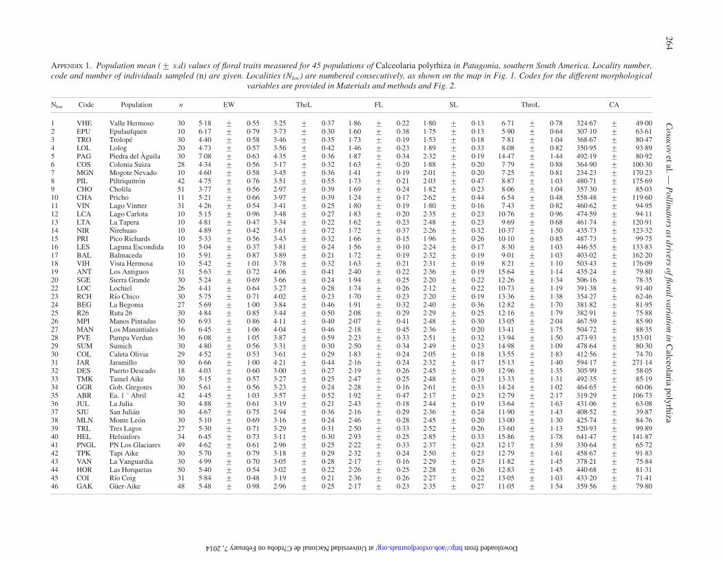
APPENDIX 1. Population mean (+ s.d) values of floral traits measured for 45 populations of Calceolaria polyrhiza in Patagonia, southern South America. Locality number,code and number of individuals sampled (n) are given. Localities (Nloc) are numbered consecutively, as shown on the map in Fig. 1. Codes for the different morphological

variables are provided in Materials and methods and Fig. 2.

Nloc Code Population n EW TheL FL SL ThroL CA

1 VHE Valle Hermoso 30 5.18 + 0.55 3.25 + 0.37 1.86 + 0.22 1.80 + 0.13 6.71 + 0.78 324.67 + 49.002 EPU Epulaufquen 10 6.17 + 0.79 3.73 + 0.30 1.60 + 0.38 1.75 + 0.13 5.90 + 0.64 307.10 + 63.613 TRO Trolope 30 4.40 + 0.58 3.46 + 0.35 1.73 + 0.19 1.53 + 0.18 7.81 + 1.04 368.67 + 80.474 LOL Lolog 20 4.73 + 0.57 3.56 + 0.42 1.46 + 0.23 1.89 + 0.33 8.08 + 0.82 350.95 + 93.895 PAG Piedra del Aguila 30 7.08 + 0.63 4.35 + 0.36 1.87 + 0.34 2.32 + 0.19 14.47 + 1.44 492.19 + 80.926 COS Colonia Suiza 28 4.34 + 0.56 3.17 + 0.32 1.63 + 0.20 1.88 + 0.20 7.79 + 0.88 364.90 + 100.307 MGN Mogote Nevado 10 4.60 + 0.58 3.45 + 0.36 1.41 + 0.19 2.01 + 0.20 7.25 + 0.81 234.23 + 170.238 PIL Piltriquitron 42 4.75 + 0.76 3.51 + 0.55 1.73 + 0.21 2.03 + 0.47 8.87 + 1.03 480.71 + 175.699 CHO Cholila 51 3.77 + 0.56 2.97 + 0.39 1.69 + 0.24 1.82 + 0.23 8.06 + 1.04 357.30 + 85.0310 CHA Pricho 11 5.21 + 0.66 3.97 + 0.39 1.24 + 0.17 2.62 + 0.44 6.54 + 0.48 558.48 + 119.6011 VIN Lago Vintter 31 4.26 + 0.54 3.41 + 0.25 1.80 + 0.19 1.80 + 0.16 7.43 + 0.82 460.62 + 94.9512 LCA Lago Carlota 10 5.15 + 0.96 3.48 + 0.27 1.83 + 0.20 2.35 + 0.23 10.76 + 0.96 474.59 + 94.1113 LTA La Tapera 10 4.81 + 0.47 3.34 + 0.22 1.62 + 0.23 2.48 + 0.23 9.69 + 0.68 461.74 + 120.9114 NIR Nirehuao 10 4.89 + 0.42 3.61 + 0.72 1.72 + 0.37 2.26 + 0.32 10.37 + 1.50 435.73 + 123.3215 PRI Pico Richards 10 5.33 + 0.56 3.43 + 0.32 1.66 + 0.15 1.96 + 0.26 10.10 + 0.85 487.73 + 99.7516 LES Laguna Escondida 10 5.04 + 0.37 3.81 + 0.24 1.56 + 0.10 2.24 + 0.17 8.30 + 1.03 446.55 + 133.8317 BAL Balmaceda 10 5.91 + 0.87 3.89 + 0.21 1.72 + 0.19 2.32 + 0.19 9.01 + 1.03 403.02 + 162.2018 VIH Vista Hermosa 10 5.42 + 1.01 3.78 + 0.32 1.63 + 0.21 2.31 + 0.19 8.21 + 1.10 503.43 + 176.0919 ANT Los Antiguos 31 5.63 + 0.72 4.06 + 0.41 2.40 + 0.22 2.36 + 0.19 15.64 + 1.14 435.24 + 79.8020 SGE Sierra Grande 30 5.24 + 0.69 3.66 + 0.24 1.94 + 0.25 2.20 + 0.22 12.26 + 1.34 506.16 + 78.3522 LOC Lochiel 26 4.41 + 0.64 3.27 + 0.28 1.74 + 0.26 2.12 + 0.22 10.73 + 1.19 391.38 + 91.4023 RCH Rıo Chico 30 5.75 + 0.71 4.02 + 0.23 1.70 + 0.23 2.20 + 0.19 13.36 + 1.38 354.27 + 62.4624 BEG La Begonia 27 5.69 + 1.00 3.84 + 0.46 1.91 + 0.32 2.40 + 0.36 12.82 + 1.70 381.82 + 81.9525 R26 Ruta 26 30 4.84 + 0.85 3.44 + 0.50 2.08 + 0.29 2.29 + 0.25 12.16 + 1.79 382.91 + 75.8826 MPI Manos Pintadas 50 6.93 + 0.86 4.11 + 0.40 2.07 + 0.41 2.48 + 0.30 13.05 + 2.04 467.59 + 85.9027 MAN Los Manantiales 16 6.45 + 1.06 4.04 + 0.46 2.18 + 0.45 2.36 + 0.20 13.41 + 1.75 504.72 + 88.3528 PVE Pampa Verdun 30 6.08 + 1.05 3.87 + 0.59 2.23 + 0.33 2.51 + 0.32 13.94 + 1.50 473.93 + 153.0129 SUM Sumich 30 4.80 + 0.56 3.31 + 0.30 2.50 + 0.34 2.49 + 0.23 14.98 + 1.09 478.64 + 80.3030 COL Caleta Olivia 29 4.52 + 0.53 3.61 + 0.29 1.83 + 0.24 2.05 + 0.18 13.55 + 1.83 412.56 + 74.7031 JAR Jaramillo 30 6.66 + 1.00 4.21 + 0.44 2.16 + 0.24 2.32 + 0.17 15.13 + 1.40 594.17 + 271.1432 DES Puerto Deseado 18 4.03 + 0.60 3.00 + 0.27 2.19 + 0.26 2.45 + 0.39 12.96 + 1.35 305.99 + 58.0533 TMK Tamel Aike 30 5.15 + 0.57 3.27 + 0.25 2.47 + 0.25 2.48 + 0.23 13.33 + 1.31 492.35 + 85.1934 GGR Gob. Gregores 30 5.61 + 0.56 3.23 + 0.24 2.28 + 0.16 2.61 + 0.33 14.24 + 1.02 464.65 + 60.0635 ABR Ea. 1 8 Abril 42 4.45 + 1.03 3.57 + 0.52 1.92 + 0.47 2.17 + 0.23 12.79 + 2.17 319.29 + 106.7336 JUL La Julia 30 4.88 + 0.61 3.19 + 0.21 2.43 + 0.18 2.44 + 0.19 13.64 + 1.63 431.06 + 63.0837 SJU San Julian 30 4.67 + 0.75 2.94 + 0.36 2.16 + 0.29 2.36 + 0.24 11.90 + 1.43 408.52 + 39.8738 MLN Monte Leon 30 5.10 + 0.69 3.16 + 0.24 2.46 + 0.28 2.45 + 0.20 13.00 + 1.30 425.74 + 84.7639 TRL Tres Lagos 27 5.30 + 0.71 3.29 + 0.31 2.50 + 0.33 2.52 + 0.26 13.60 + 1.13 520.93 + 99.8940 HEL Helsinfors 34 6.45 + 0.73 3.11 + 0.30 2.93 + 0.25 2.85 + 0.33 15.86 + 1.78 641.47 + 141.8741 PNGL PN Los Glaciares 49 4.62 + 0.61 2.96 + 0.25 2.22 + 0.33 2.37 + 0.23 12.17 + 1.59 330.64 + 65.7242 TPK Tapi Aike 30 5.70 + 0.79 3.18 + 0.29 2.32 + 0.24 2.50 + 0.23 12.79 + 1.61 458.67 + 91.8343 VAN La Vanguardia 30 4.99 + 0.70 3.05 + 0.28 2.17 + 0.16 2.29 + 0.23 11.82 + 1.45 378.21 + 75.8444 HOR Las Horquetas 50 5.40 + 0.54 3.02 + 0.22 2.26 + 0.25 2.28 + 0.26 12.83 + 1.45 440.68 + 81.3145 COI Rıo Coig 31 5.84 + 0.48 3.19 + 0.21 2.36 + 0.26 2.27 + 0.22 13.05 + 1.03 433.20 + 71.4146 GAK Guer-Aike 48 5.48 + 0.98 2.96 + 0.25 2.17 + 0.23 2.35 + 0.27 11.05 + 1.54 359.56 + 79.80

Co

saco

vet

al.—

Po

llinato

rsa

sd

riverso

ffl

ora

lva

riatio

nin

Calceo

lariap

oly

rhiza

26

4

at Universidad Nacional de C?rdoba on February 7, 2014 http://aob.oxfordjournals.org/ Downloaded from

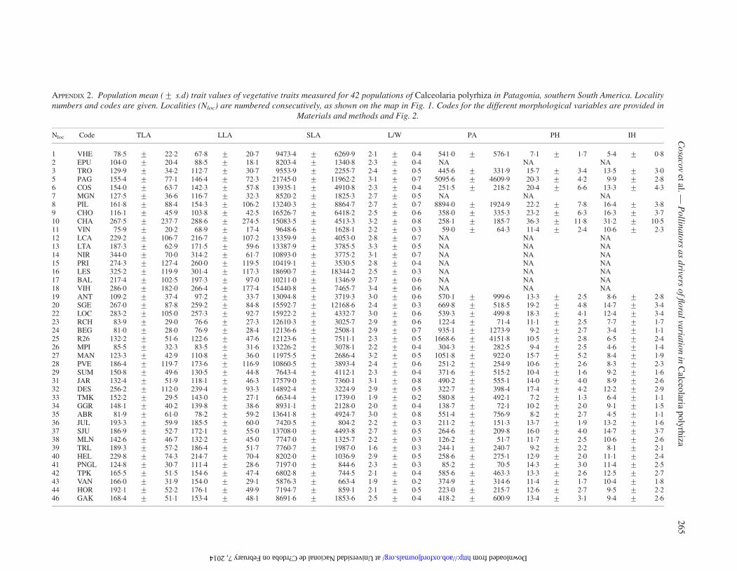
APPENDIX 2. Population mean (+ s.d) trait values of vegetative traits measured for 42 populations of Calceolaria polyrhiza in Patagonia, southern South America. Localitynumbers and codes are given. Localities (Nloc) are numbered consecutively, as shown on the map in Fig. 1. Codes for the different morphological variables are provided in

Materials and methods and Fig. 2.

Nloc Code TLA LLA SLA L/W PA PH IH

1 VHE 78.5 + 22.2 67.8 + 20.7 9473.4 + 6269.9 2.1 + 0.4 541.0 + 576.1 7.1 + 1.7 5.4 + 0.82 EPU 104.0 + 20.4 88.5 + 18.1 8203.4 + 1340.8 2.3 + 0.4 NA NA NA3 TRO 129.9 + 34.2 112.7 + 30.7 9553.9 + 2255.7 2.4 + 0.5 445.6 + 331.9 15.7 + 3.4 13.5 + 3.05 PAG 155.4 + 77.1 146.4 + 72.3 21745.0 + 11962.2 3.1 + 0.7 5095.6 + 4609.9 20.3 + 4.2 9.9 + 2.86 COS 154.0 + 63.7 142.3 + 57.8 13935.1 + 4910.8 2.3 + 0.4 251.5 + 218.2 20.4 + 6.6 13.3 + 4.37 MGN 127.5 + 36.6 116.7 + 32.3 8520.2 + 1825.3 2.7 + 0.5 NA NA NA8 PIL 161.8 + 88.4 154.3 + 106.2 13240.3 + 8864.7 2.7 + 0.7 8894.0 + 1924.9 22.2 + 7.8 16.4 + 3.89 CHO 116.1 + 45.9 103.8 + 42.5 16526.7 + 6418.2 2.5 + 0.6 358.0 + 335.3 23.2 + 6.3 16.3 + 3.710 CHA 267.5 + 237.7 288.6 + 274.5 15083.5 + 4513.3 3.2 + 0.8 258.1 + 185.7 36.3 + 11.8 31.2 + 10.511 VIN 75.9 + 20.2 68.9 + 17.4 9648.6 + 1628.1 2.2 + 0.3 59.0 + 64.3 11.4 + 2.4 10.6 + 2.312 LCA 229.2 + 106.7 216.7 + 107.2 13359.9 + 4053.0 2.8 + 0.7 NA NA NA13 LTA 187.3 + 62.9 171.5 + 59.6 13387.9 + 3785.5 3.3 + 0.5 NA NA NA14 NIR 344.0 + 70.0 314.2 + 61.7 10893.0 + 3775.2 3.1 + 0.7 NA NA NA15 PRI 274.3 + 127.4 260.0 + 119.5 10419.1 + 3530.5 2.8 + 0.4 NA NA NA16 LES 325.2 + 119.9 301.4 + 117.3 18690.7 + 18344.2 2.5 + 0.3 NA NA NA17 BAL 217.4 + 102.5 197.3 + 97.0 10211.0 + 1346.9 2.7 + 0.6 NA NA NA18 VIH 286.0 + 182.0 266.4 + 177.4 15440.8 + 7465.7 3.4 + 0.6 NA NA NA19 ANT 109.2 + 37.4 97.2 + 33.7 13094.8 + 3719.3 3.0 + 0.6 570.1 + 999.6 13.3 + 2.5 8.6 + 2.820 SGE 267.0 + 87.8 259.2 + 84.8 15592.7 + 12168.6 2.4 + 0.3 669.8 + 518.5 19.2 + 4.8 14.7 + 3.422 LOC 283.2 + 105.0 257.3 + 92.7 15922.2 + 4332.7 3.0 + 0.6 539.3 + 499.8 18.3 + 4.1 12.4 + 3.423 RCH 83.9 + 29.0 76.6 + 27.3 12610.3 + 3025.7 2.9 + 0.6 122.4 + 71.4 11.1 + 2.5 7.7 + 1.724 BEG 81.0 + 28.0 76.9 + 28.4 12136.6 + 2508.1 2.9 + 0.7 935.1 + 1273.9 9.2 + 2.7 3.4 + 1.125 R26 132.2 + 51.6 122.6 + 47.6 12123.6 + 7511.1 2.3 + 0.5 1668.6 + 4151.8 10.5 + 2.8 6.5 + 2.426 MPI 85.5 + 32.3 83.5 + 31.6 13226.2 + 3078.1 2.2 + 0.4 304.3 + 282.5 9.4 + 2.5 4.6 + 1.427 MAN 123.3 + 42.9 110.8 + 36.0 11975.5 + 2686.4 3.2 + 0.5 1051.8 + 922.0 15.7 + 5.2 8.4 + 1.928 PVE 186.4 + 119.7 173.6 + 116.9 10860.5 + 3893.4 2.4 + 0.6 251.2 + 254.9 10.6 + 2.6 8.3 + 2.329 SUM 150.8 + 49.6 130.5 + 44.8 7643.4 + 4112.1 2.3 + 0.4 371.6 + 515.2 10.4 + 1.6 9.2 + 1.631 JAR 132.4 + 51.9 118.1 + 46.3 17579.0 + 7360.1 3.1 + 0.8 490.2 + 555.1 14.0 + 4.0 8.9 + 2.632 DES 256.2 + 112.0 239.4 + 93.3 14892.4 + 3224.9 2.9 + 0.5 322.7 + 398.4 17.4 + 4.2 12.2 + 2.933 TMK 152.2 + 29.5 143.0 + 27.1 6634.4 + 1739.0 1.9 + 0.2 580.8 + 492.1 7.2 + 1.3 6.4 + 1.134 GGR 148.1 + 40.2 139.8 + 38.6 8931.1 + 2128.0 2.0 + 0.4 138.7 + 72.1 10.2 + 2.0 9.1 + 1.535 ABR 81.9 + 61.0 78.2 + 59.2 13641.8 + 4924.7 3.0 + 0.8 551.4 + 756.9 8.2 + 2.7 4.5 + 1.136 JUL 193.3 + 59.9 185.5 + 60.0 7420.5 + 804.2 2.2 + 0.3 211.2 + 151.3 13.7 + 1.9 13.2 + 1.637 SJU 186.9 + 52.7 172.1 + 55.0 13708.0 + 4493.8 2.7 + 0.5 264.6 + 209.8 16.0 + 4.0 14.7 + 3.738 MLN 142.6 + 46.7 132.2 + 45.0 7747.0 + 1325.7 2.2 + 0.3 126.2 + 51.7 11.7 + 2.5 10.6 + 2.639 TRL 189.3 + 57.2 186.4 + 51.7 7760.7 + 1987.0 1.6 + 0.3 244.1 + 240.7 9.2 + 2.2 8.1 + 2.140 HEL 229.8 + 74.3 214.7 + 70.4 8202.0 + 1036.9 2.9 + 0.5 258.6 + 275.1 12.9 + 2.0 11.1 + 2.441 PNGL 124.8 + 30.7 111.4 + 28.6 7197.0 + 844.6 2.3 + 0.3 85.2 + 70.5 14.3 + 3.0 11.4 + 2.542 TPK 165.5 + 51.5 154.6 + 47.4 6802.8 + 744.5 2.1 + 0.4 585.6 + 463.3 13.3 + 2.6 12.5 + 2.743 VAN 166.0 + 31.9 154.0 + 29.1 5876.3 + 663.4 1.9 + 0.2 374.9 + 314.6 11.4 + 1.7 10.4 + 1.844 HOR 192.1 + 52.2 176.1 + 49.9 7194.7 + 859.1 2.1 + 0.5 223.0 + 215.7 12.6 + 2.7 9.5 + 2.246 GAK 168.4 + 51.1 153.4 + 48.1 8691.6 + 1853.6 2.5 + 0.4 418.2 + 600.9 13.4 + 3.1 9.4 + 2.6

Co

saco

vet

al.—

Po

llinato

rsa

sd

riverso

ffl

ora

lva

riatio

nin

Calceo

lariap

oly

rhiza

26

5

at Universidad Nacional de C?rdoba on February 7, 2014 http://aob.oxfordjournals.org/ Downloaded from

APPENDIX 3. Population mean (+ s.e) values of functional beelength (HML) measured in Centris cineraria and Chalepogenuscaeruleus. Locality code and number of individuals sampled (N)

are given.

Code Bee species N HML s.e.

ABR C. cineraria 1 8.18 –ANT C. cineraria 2 8.55 + 1.12COL C. cineraria 6 7.47 + 0.53CHA Ch. caeruleus 2 4.65 + 0.43CHO Ch. caeruleus 2 4.65 + 0.43COS Ch. caeruleus 1 5.14 –DES C. cineraria 5 7.03 + 0.71GKE C. cineraria 3 8.26 + 0.68HEL C. cineraria 2 8.2 + 1.77HOR C. cineraria 4 8.1 + 0.75JUL C. cineraria 5 8.41 + 1.32PNGL C. cineraria 3 7.08 + 0.41MAN C. cineraria 2 8.84 + 0.21MLN C. cineraria 4 7.22 + 0.35MPI C. cineraria 2 8.38 + 0.28NIR Ch. caeruleus 1 5.41 –PAG C. cineraria 3 8.51 + 0.98PIL Ch. caeruleus 3 5.07 + 0.87JAR C. cineraria 2 8.07 + 0.54PVE C. cineraria 4 7.9 + 0.53RCH C. cineraria 1 7.53 –R26 C. cineraria 16 7.42 + 0.66SJU C. cineraria 2 8.49 + 1.5TRO Ch. caeruleus 11 4.19 + 0.5VHE Ch. caeruleus 2 4.15 + 0.64

Cosacov et al. — Pollinators as drivers of floral variation in Calceolaria polyrhiza266

at Universidad N

acional de C?rdoba on February 7, 2014

http://aob.oxfordjournals.org/D

ownloaded from