Phylogeography and palaeodistribution modelling ofNassauvia subgenus Strongyloma (Asteraceae): exploringphylogeographical scenarios in the Patagonian steppeMarcela V. Nicola1, Silvana M. Sede1, Ra�ul Pozner1 & Leigh A. Johnson2

1Instituto de Bot�anica Darwinion, C.C. 22, B1642HYD, San Isidro, Provincia de Buenos Aires, Argentina2Department of Biology and Bean Life Science Museum, Brigham Young University, 4102 LSB, Provo, Utah 84602, USA

Keywords

Colonization, fragmentation, glacial refugia,

Patagonian steppe, plant phylogeography,

Pleistocene glaciations, range expansion,

species distribution modelling.

Correspondence

Marcela V. Nicola, Instituto de Bot�anica

Darwinion, C.C. 22, B1642HYD San Isidro,

Prov. de Buenos Aires, Argentina.

Tel: (5411) 4743-4800 int. 125;

Fax: (5411) 4747-4748;

E-mail: mnicola@darwin.edu.ar

Funding Information

NSF-PIRE-OISE 0530267 (USA). CONICET-PIP

11220090100388 (Argentina). ASPT research

grant for graduate students 2010 (USA).

Received: 8 August 2014; Accepted: 4

September 2014

doi: 10.1002/ece3.1268

Abstract

The Patagonian steppe is an immense, cold, arid region, yet phylogeographical-

ly understudied. Nassauvia subgen. Strongyloma is a characteristic element of

the steppe, exhibiting a continuum of morphological variation. This taxon pro-

vides a relevant phylogeographical model not only to understand how past

environmental changes shaped the genetic structure of its populations, but also

to explore phylogeographical scenarios at the large geographical scale of the

Patagonian steppe. Here, we (1) assess demographic processes and historical

events that shaped current geographic patterns of haplotypic diversity; (2) ana-

lyze hypotheses of isolation in refugia, fragmentation of populations, and/or

colonization of available areas during Pleistocene glaciations; and (3) model

extant and palaeoclimatic distributions to support inferred phylogeographical

patterns. Chloroplast intergenic spacers, rpl32–trnL and trnQ–50rps16, were

sequenced for 372 individuals from 63 populations. Nested clade analysis,

analyses of molecular variance, and neutrality tests were performed to assess

genetic structure and range expansion. The present potential distribution was

modelled and projected onto a last glacial maximum (LGM) model. Of 41

haplotypes observed, ten were shared among populations associated with differ-

ent morphological variants. Populations with highest haplotype diversity and

private haplotypes were found in central-western and south-eastern Patagonia,

consistent with long-term persistence in refugia during Pleistocene. Palaeomod-

elling suggested a shift toward the palaeoseashore during LGM; new available

areas over the exposed Atlantic submarine platform were colonized during gla-

ciations with postglacial retraction of populations. A scenario of fragmentation

and posterior range expansion may explain the observed patterns in the center

of the steppe, which is supported by palaeomodelling. Northern Patagonian

populations were isolated from southern populations by the Chubut and the

Deseado river basins during glaciations. Pleistocene glaciations indirectly

impacted the distribution, demography, and diversification of subgen. Strongy-

loma through decreased winter temperatures and water availability in different

areas of its range.

Introduction

Phylogeographical reconstructions along large, extensive

geographic areas are difficult to assess because they ideally

need widely distributed, ubiquitous taxa, present at regio-

nal scale as a characteristic element of different local com-

munities. Nassauvia Comm. ex Juss. subgen. Strongyloma

(DC) Cabrera (Asteraceae) is one of these rare cases; it is

a typical element throughout the immense territory of the

Patagonian steppe.

Cabrera (1982) distinguished five species within sub-

gen. Strongyloma by a taxonomy: Nassauvia axillaris (Lag.

ex Lindl.) D. Don, Nassauvia fuegiana (Speg.) Cabrera,

Nassauvia glomerulosa (Lag. ex Lindl.) D. Don, Nassauvia

maeviae Cabrera, and Nassauvia ulicina (Hook. f.)

Macloskie. The subgenus as a whole is easy to recognize

ª 2014 The Authors. Ecology and Evolution published by John Wiley & Sons Ltd.

This is an open access article under the terms of the Creative Commons Attribution License, which permits use,

distribution and reproduction in any medium, provided the original work is properly cited.

1

in the field: it comprises small shrubs with a tendency to

heteroblasty, with 1–5 white flowers per capitulum, and

hairy cypselas (Cabrera 1982; Freire et al. 1993). Although

Cabrera (1982) suggested wind dispersal, our personal

observations in the field suggest that cypselas are dis-

persed mainly rolling on the ground, because the pappus

is quickly deciduous. Distinguishing species within this

complex is challenging; however, because variation in

morphological traits does not strictly follow species

boundaries as traditionally defined (Nicola et al. 2014).

Maraner et al. (2012) found that subgen. Strongyloma is

polyphyletic based on the ITS region of nuclear ribosomal

DNA, but this appears to be an error in sample or

sequence identity, or the use of divergent sequence para-

logs (Nicola et al. 2014; Nicola, M. V., S. M. Sede, L. A.

Johnson, and R. Pozne in preparation). Morphological

evidence (Cabrera 1982; Freire et al. 1993; Nicola et al.

2014) and molecular data derived from plastid and

nuclear ribosomal DNA regions (Nicola, M. V., S. M.

Sede, L. A. Johnson, and R. Pozner in preparation) indi-

cate subgen. Strongyloma is a well-supported monophy-

letic group with wide and continuous morphological

variation coupled with little genetic divergence. We follow

here the taxonomical decision of Nicola, M. V., S. M.

Sede, L. A. Johnson, and R. Pozner (in preparation) by

considering Nassauvia subgen. Strongyloma as a monospe-

cific taxon. The morphological combinations traditionally

accepted as species (Cabrera 1982; Freire et al. 1993) are

here referred as “morphological variants” (i.e., axillaris,

glomerulosa, fuegiana, maeviae, and ulicina morphologi-

es), just to allow some reference points within the mor-

phological, continuous variation observed in this group

of plants (Nicola et al. 2014).

Nassauvia subgen. Strongyloma has a remarkably wide

distribution, mainly in the Patagonian steppe with a few

enclaves in the Andean region, from sea level to 4560 m

a.s.l., in southern Bolivia (c. 21°S), in Argentina (from

Jujuy Province c. 22°S to northern Tierra del Fuego Prov-

ince c. 54°S), and in Chile (from Valpara�ıso c. 32°S to

Magallanes c. 51°S), including a variety of climatic zones

but mainly adapted to extremely xeric environments

(Cabrera 1982; Nicola et al. 2014). With a particularly

abundant distribution, populations with axillaris and

glomerulosa morphological variants characterized the

Western and the Central Patagonian districts of the Pata-

gonian Phytogeographical Province, respectively (Cabrera

and Willink 1980). Sympatric assemblages of different

combinations of two or three morphological variants of

subgen. Strongyloma are frequent in some areas of Pata-

gonia. With abundant morphologically intermediate indi-

viduals, such areas might represent secondary contact

zones or populations with incomplete sorting of lineages

(Nicola et al. 2014). The fossil record refers the oldest

members of subtribe Nassauviinae back to the Miocene,

when progenitors of this group were expanding in eastern

Patagonia (Barreda et al. 2008). Nassauviinae, together

with Mutisieae, are among the oldest, early branching

groups within Asteraceae, after Onoseridae and Barnade-

sioideae (Funk et al. 2009).

The vast, flat, arid Patagonian steppe ecoregion is lon-

gitudinally placed from the east of the slopes of the

southern Andes to the Atlantic coast, and latitudinally

located from central Mendoza Province (c. 32°S) to

northern Tierra del Fuego Province (c. 54°S) in Argen-

tina, covering a total area of approximately 787,000 km2

(Correa 1998). It was shaped during the Middle–LateMiocene (16–5.3 Ma) mainly by the uplift of the Andes.

This orogeny blocked and filtered moist winds coming

from the Pacific Ocean and produced a substantial rain

shadow to the east, resulting in cold and dry conditions

throughout the steppe, a contraction of the forest, and

the expansion of xerophytic taxa (Barreda and Palazzesi

2007). Major glacial–interglacial cycles in Patagonia began

during the Late Miocene (c. 5–6 Ma), with ice reaching

its maximum development in the Early Pleistocene (c.

1.15 Ma; Ogg et al. 2008; Rabassa et al. 2011). The major

glacial advances in southern South America were the

Great Patagonian Glaciation (GPG; c. 1 Ma) and the Last

Glacial Maximum (LGM; c. 21 Ka). The GPG resulted in

the greatest expansion of ice sheets in the Patagonian

steppe compared with LGM and other Pleistocene glacia-

tions (Rabassa et al. 2011). However, a large part of the

steppe remained free of ice during the glacial episodes,

and climatic conditions were less severe than those occur-

ring in North America (Markgraf et al. 1995).

In Patagonia, Pleistocene glaciations caused several cli-

matic and environmental changes. The sea level lowered,

shifting the coastline about four degrees eastward. Cli-

matic continentality of the surrounding areas enhanced,

with rising extreme temperatures and decreased precipita-

tion. The Argentinean submarine platform was partially

exposed, substantially increasing the space available for

animal and plant colonization (Rabassa 2008). Although

these climatic and environmental changes are thought to

have affected species distribution, the Patagonian steppe

remains poorly phylogeographically studied (S�ersic et al.

2011). Plant studies have focused mainly on the Andean

region (e.g., Muellner et al. 2005; Marchelli and Gallo

2006; Amico and Nickrent 2009; Acosta and Premoli

2010; Vidal-Russell et al. 2011; Segovia et al. 2012; among

others), although interest in understanding the evolution-

ary history and processes of plant diversification in the

Patagonian steppe has increased in recent years (Jakob

et al. 2009; Cosacov et al. 2010, 2013; Sede et al. 2012).

Considering this background, subgen. Strongyloma is a

relevant plant phylogeographical model not only to

2 ª 2014 The Authors. Ecology and Evolution published by John Wiley & Sons Ltd.

Phylogeography of Nassauvia Subgenus Strongyloma M. V. Nicola et al.

understand how recent past environmental changes

shaped the genetic structure of its populations, but also

to explore regional phylogeographical scenarios. Here, we

examine the relative importance of probable historical

events and/or past demographic processes that can

explain the current genetic population structure in sub-

gen. Strongyloma through phylogeographical analyses

using plastid DNA sequences. We also investigate how

palaeoclimatic conditions have influenced the distribution

of this subgenus using distribution modelling (Hijmans

and Graham 2006). We analyze three hypotheses: (1) the

existence of multiple glacial refugia in flanking zones of

the Andes covered by ice followed by postglacial expan-

sion; (2) the expansion of populations over the current

marine platform during the Pleistocene and their succes-

sive, recent retraction to the surroundings of the current

Atlantic coast of Patagonia; and/or (3) the fragmentation

of populations that persisted in areas not reached by the

ice sheet during glacial periods in the center of the steppe

due to past river basins dynamic. Under the first scenario,

population expansion from refugia should leave genetic

signatures of high diversity and private haplotypes in ref-

ugial areas, produced by considerable genome divergence

and reorganization. From the perspective of the second

hypothesis, in recently reduced areas nearby the Atlantic

coast with rapid population retraction, diversity should

be low due to successive bottlenecks on the colonizing

genomes that lead to a loss of alleles. Lastly, if popula-

tions persisted in more or less fragmented areas, then

genetic diversity and unique haplotypes within popula-

tions should be low: during posterior expansions, haplo-

types may spread slowly and more equally (Hewitt 1996).

Finally, we search for significant phylogeographical breaks

consistent with those found previously for other Patago-

nian organisms and consider these breaks with prior

hypotheses (S�ersic et al. 2011; and literature therein; Sede

et al. 2012; Cosacov et al. 2013).

Materials and Methods

Sampling

A total of 372 individuals from 63 populations were sam-

pled in Argentina (excepting Tierra del Fuego), covering

most of the distribution of subgen. Strongyloma and its

wide morphological variation, including axillaris, glomerul-

osa, fuegiana, and ulicina morphological variants (Table 1,

Fig. 1). The maeviae morphological variant is known only

from the type collection, and DNA could not be obtained

from the herbarium voucher. Fresh leaves were sampled

from one to eight individuals at each site, separated by at

least 10 m along a linear transect to minimize the potential

of sibling relationships among samples. Herbarium vouch-

ers were identified following Cabrera (1982) and deposited

at SI (Instituto de Bot�anica Darwinion) or CORD (Museo

Bot�anico, Universidad Nacional de C�ordoba).

DNA isolation, amplification, andsequencing

Genomic DNA was isolated from silica dried leaf tissue

following a modified cetyl trimethyl ammonium bromide

(CTAB) protocol (Doyle and Doyle 1987; Cullings 1992).

The chloroplast intergenic spacers rpl32–trnL (primers

rpL32-F and trnLUAG; Shaw et al. 2007) and trnQ–50rps16(primers trnQUUG and rps16 9 1; Shaw et al. 2007) were

selected as markers because they showed the highest

sequence variability among several surveyed regions.

DNA was amplified and sequenced with a profile con-

sisting of 94°C for 3 min followed by 30 cycles of 94°Cfor 1 min, 50 or 52°C for 1 min for trnQ–50rps16 and

rpl32–trnL, respectively, and 72°C for 1 min. Amplifica-

tion products were purified using PCR96 cleanup plates

(Millipore Corp, Billerica, MA), sequenced with BigDye 3

(Applied Biosystems, Foster City, CA), and purified with

Sephadex (GE Healthcare, Piscataway, NJ) before electro-

phoresis on an AB 3730xl automated sequencer housed in

Brigham Young University’s DNA Sequencing Centre.

Electropherograms were edited and assembled using

SEQUENCHER 4.6 (Gene Codes, Ann Arbor, MI). Sequences

were aligned with CLUSTALX 1.81 (Thompson et al. 1997)

with subsequent manual adjustments using BIOEDIT 5.0.9

(Hall 1999). Indels were coded as binary characters using

simple indel coding (Simmons and Ochoterena 2000) as

implemented in SEQSTATE 1.4 (M€uller 2005). The two

chloroplast regions were concatenated into a single matrix

a priori given their shared ancestry, maternal inheritance,

and extremely rare instances of recombination within the

chloroplast genome. Unique sequences from this com-

bined matrix were identified as haplotypes. All sequences

were deposited in GenBank (rpl32–trnL KM978451–KM978491 and trnQ–50rps16 KM978492–KM978532).

Haplotype network and geographicdistribution

Nested clade analysis (NCA) was performed following Tem-

pleton et al. (1995) and Templeton (2004) using ANECA 1.2

(Panchal 2007). Although NCA has been criticized (Petit

2007; Beaumont and Panchal 2008; Knowles 2008), it has

been validated extensively (Templeton 2008, 2009) and is

used as an exploratory analysis in conjunction with other

population genetic parameters to draw inferences here.

A haplotype network was constructed using TCS 1.21

(Clement et al. 2000) with the default 0.95 probability

connection limit. Ambiguous connections (loops) were

ª 2014 The Authors. Ecology and Evolution published by John Wiley & Sons Ltd. 3

M. V. Nicola et al. Phylogeography of Nassauvia Subgenus Strongyloma

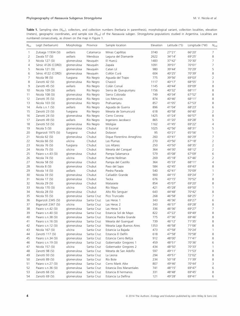
Table 1. Sampling sites (Nloc), collectors, and collection numbers (herbaria in parenthesis), morphological variant, collection localities, elevation

(meters), geographic coordinates, and sample size (Nind) of the Nassauvia subgen. Strongyloma populations studied in Argentina. Localities are

numbered consecutively, as shown on the map in Figure 1.

Nloc Legit (herbarium) Morphology Province Sample location Elevation Latitude (°S) Longitude (°W) Nind

1 Zuloaga 11934 (SI) axillaris Catamarca Minas Capillitas 3740 27°210 66°200 7

2 Zavala 57 (SI) axillaris Mendoza Laguna del Diamante 2622 34°140 69°250 8

3 Nicola 127 (SI) glomerulosa Neuqu�en El Huec�u 1483 37°420 70°300 7

4 S�ersic 4126 (CORD) glomerulosa Neuqu�en Zapala 1091 39°010 70°010 7

5 Nicola 121 (SI) glomerulosa Neuqu�en Catan Lil 980 39°440 70°290 5

6 S�ersic 4122 (CORD) glomerulosa Neuqu�en Coll�on Cur�a 604 40°250 70°390 8

7 Nicola 98 (SI) fuegiana R�ıo Negro Aguada del Trapo 775 39°560 69°030 2

8 Zanotti 42 (SI) glomerulosa R�ıo Negro Chasic�o 1117 40°170 68°550 3

9 Zanotti 45 (SI) axillaris R�ıo Negro Col�an Conu�e 1145 40°440 69°090 8

10 Nicola 109 (SI) axillaris R�ıo Negro Sierra de Queupuniyeu 1156 40°320 68°110 8

11 Nicola 108 (SI) glomerulosa R�ıo Negro Sierra Colorada 749 40°340 67°520 8

12 Zanotti 35 (SI) glomerulosa R�ıo Negro Los Menucos 874 40°460 68°110 8

13 Nicola 103 (SI) glomerulosa R�ıo Negro Prahuaniyeu 857 41°050 67°530 8

14 �Avila s.n.1 (SI) axillaris R�ıo Negro Aguada de Guerra 896 41°040 68°230 6

15 Zanotti 23 (SI) fuegiana R�ıo Negro Meseta de Somuncur�a 618 40°580 66°400 2

16 Zanotti 24 (SI) glomerulosa R�ıo Negro Cerro Corona 1425 41°240 66°570 8

17 Zanotti 49 (SI) axillaris R�ıo Negro Ingeniero Jacobacci 865 41°200 69°280 5

18 Zanotti 53 (SI) glomerulosa R�ıo Negro Molig€ue 1162 41°450 69°220 4

19 Nicola 5 (SI) glomerulosa Chubut El Escorial 1025 42°560 68°310 5

20 Biganzoli 1975 (SI) fuegiana Chubut Dolavon 95 43°210 65°560 1

21 Nicola 62 (SI) glomerulosa Chubut Dique Florentino Ameghino 260 43°410 66°290 7

22 Nicola 66 (SI) ulicina Chubut Las Plumas 270 43°560 67°180 2

23 Nicola 76 (SI) fuegiana Chubut Los Altares 250 43°500 68°350 2

24 Nicola 75 (SI) ulicina Chubut Meseta del Canquel 364 44°300 68°120 2

25 Paiaro s.n.43 (SI) glomerulosa Chubut Pampa Salamanca 579 45°080 67°090 6

26 Nicola 74 (SI) ulicina Chubut Puente Nollman 269 45°180 67°460 2

27 Nicola 58 (SI) glomerulosa Chubut Pampa del Castillo 364 45°330 68°110 4

28 Nicola 8 (SI) glomerulosa Chubut Paso del Sapo 584 42°450 69°430 8

29 Nicola 14 (SI) axillaris Chubut Piedra Parada 540 42°410 70°090 1

30 Nicola 33 (SI) glomerulosa Chubut Ca~nad�on Grande 900 44°150 69°240 7

31 Nicola 17 (SI) glomerulosa Chubut Tecka 676 43°150 70°520 8

32 Nicola 29 (SI) glomerulosa Chubut Matasiete 854 45°070 69°200 8

33 Nicola 170 (SI) ulicina Chubut R�ıo Mayo 421 45°280 69°500 1

34 Nicola 28 (SI) glomerulosa Chubut Alto R�ıo Senguer 643 44°480 70°420 8

35 Nicola 55 (SI) glomerulosa Santa Cruz Pico Truncado 268 46°580 68°250 7

36 Biganzoli 2345 (SI) glomerulosa Santa Cruz Las Heras 1 343 46°360 69°270 6

37 Biganzoli 2347 (SI) ulicina Santa Cruz Las Heras 2 343 46°370 69°280 8

38 Paiaro s.n.42 (SI) glomerulosa Santa Cruz Las Heras 3 336 46°360 69°270 7

39 Paiaro s.n.40 (SI) glomerulosa Santa Cruz Estancia Sol de Mayo 822 47°220 69°490 8

40 Paiaro s.n.38 (SI) glomerulosa Santa Cruz Estancia Piedra Grande 775 47°360 69°460 8

41 Paiaro s.n.16 (SI) glomerulosa Santa Cruz Meseta del Guenguel 739 46°120 71°350 8

42 Paiaro s.n.12 (SI) glomerulosa Santa Cruz Meseta Lago Buenos Aires 1353 46°580 71°060 8

43 Nicola 167 (SI) ulicina Santa Cruz Estancia La Bajada 473 47°580 70°240 1

44 Zanotti 117 (SI) glomerulosa Santa Cruz Estancia El Delf�ın 618 47°580 70°580 8

45 Paiaro s.n.34 (SI) glomerulosa Santa Cruz Estancia Cerro Beltza 912 48°000 71°410 8

46 Paiaro s.n.19 (SI) glomerulosa Santa Cruz Gobernador Gregores 1 459 48°510 70°360 6

47 Nicola 157 (SI) ulicina Santa Cruz Gobernador Gregores 2 434 48°500 70°330 1

48 Zanotti 98 (SI) glomerulosa Santa Cruz Meseta de San Adolfo 597 49°110 71°530 8

49 Zanotti 93 (SI) glomerulosa Santa Cruz La Leona 294 49°510 72°020 8

50 Zanotti 89 (SI) glomerulosa Santa Cruz R�ıo Bote 234 50°180 71°390 8

51 Paiaro s.n.27 (SI) glomerulosa Santa Cruz Cerro Mank Aike 807 49°460 70°440 3

52 Paiaro s.n.36 (SI) glomerulosa Santa Cruz Estancia Dos Manantiales 741 48°150 69°470 6

53 Zanotti 66 (SI) glomerulosa Santa Cruz Estancia 8 hermanos 331 48°480 69°450 8

54 Zanotti 69 (SI) glomerulosa Santa Cruz Estancia La Delfina 121 49°280 69°410 6

4 ª 2014 The Authors. Ecology and Evolution published by John Wiley & Sons Ltd.

Phylogeography of Nassauvia Subgenus Strongyloma M. V. Nicola et al.

resolved using predictions from coalescent theory and

information about sampling according to three criteria:

frequency, network topology, and geography (Crandall

and Templeton 1993).

The resolved haplotype network was converted into a

hierarchical nested design following Templeton et al.

(1987) and Templeton and Sing (1993). Clade (Dc) and

nested clades (Dn) distances were estimated to assess

association between the nested cladogram and geographic

distances among sampled localities (Templeton et al.

1995) using GEODIS 2.6 (Posada et al. 2000). Null distri-

butions (i.e., under a hypothesis of no geographic associa-

tion of clades and nested clades) for permutational

contingency table test comparisons were generated from

10,000 Monte Carlo replications, with a 95% confidence

level. For significant associations, the inference key of

Templeton (2011) was used to recognize probable demo-

graphic processes and/or historical events of the clades.

Population genetic analyses

Haplotype diversity (h; Nei 1987), nucleotide diversity (p;mean number of pairwise differences per site; Nei 1987),

and mean number of pairwise differences (p; Tajima

1983) were calculated for the subgenus as a whole, each

sampling location, and each geographic region, using

DNASP 5.10.01 (Librado and Rozas 2009).

To investigate hierarchical levels of population struc-

ture, two analyses of molecular variance (AMOVA) were

performed that consider genetic distances between haplo-

types and their frequencies using ARLEQUIN 3.5.1.2 (Excof-

fier and Lischer 2010). First, populations were grouped

according to different latitudinal regions, defined by

major rivers: (1) north of Agrio, Neuqu�en, and Negro riv-

ers, c. 38°S; (2) between Agrio, Neuqu�en, and Negro riv-

ers, and Chubut River, c. 38°–43°S; (3) between Chubut

and Deseado rivers, c. 43°–47°S; (4) between Deseado

and Chico rivers, c. 47°–50°S; and (5) south of Chico

River, c. 50°S (Fig. 1). The aim of the second analysis

was to test whether genetic variation was significantly

structured among glaciated and nonglaciated sites during

GPG in populations south of Chubut River (Rabassa

et al. 2011), following a longitudinal transect at c. 71°W.

This region was selected given that eight of the 63 popu-

lations were located within the ice zone (Fig. 1). Estima-

tion of molecular diversity indexes and AMOVAs were

performed considering only populations with four or

more sampled individuals.

Demographic history analyses

To analyze the demographic history of populations in

each geographic area, Tajima’s D (Tajima 1989), Fu’s FS(Fu 1997), and Ramos-Onsins and Rozas’ R2 (Ramos-

Onsins and Rozas 2002) statistics of neutrality were cal-

culated to test for evidence of range expansion. Signifi-

cant negative values of D and FS and small positive

values of R2 indicate an excess of low frequency muta-

tions relative to expectations under the standard neutral

model (i.e., strict selective neutrality of variants, constant

population size, and lack of subdivision and gene flow).

FS and R2 are the most powerful tests used to detect

population growth (Ramos-Onsins and Rozas 2002). Sig-

nificance was evaluated by comparing observed values

with null distributions generated by 10,000 replicates,

using the empirical population sample size and observed

number of segregating sites implemented by DNASP

5.10.01.

Distribution modelling

To validate the phylogeographical analyses, we modelled

the present potential geographic distribution of Nassauvia

subgen. Strongyloma and projected it onto a LGM model

about 21 Ka using point locality information and envi-

ronmental data in DIVA-GIS 7.3 (Hijmans et al. 2001) and

MAXENT 3.3.3, with the maximum entropy machine-

learning algorithm (Phillips et al. 2004).

We recorded latitudinal and longitudinal coordinates

from 224 localities of subgen. Strongyloma, covering its

Table 1. Continued.

Nloc Legit (herbarium) Morphology Province Sample location Elevation Latitude (°S) Longitude (°W) Nind

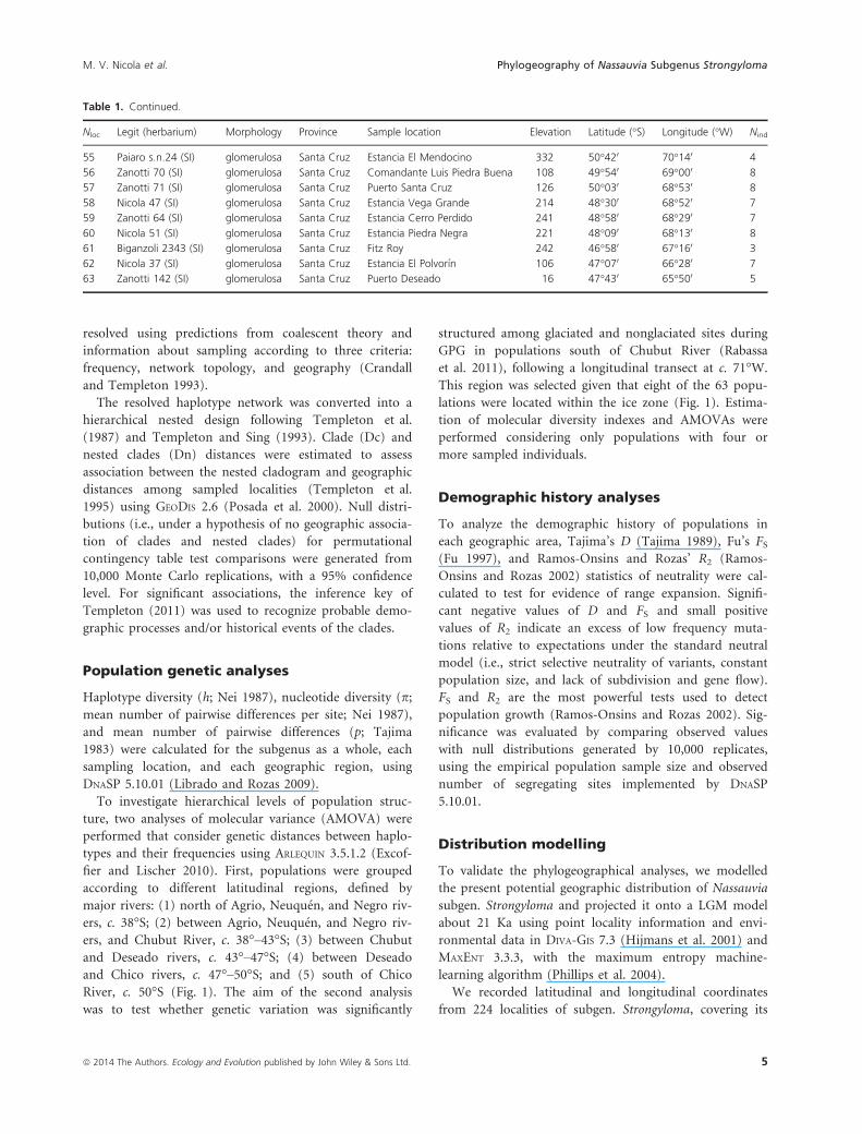
55 Paiaro s.n.24 (SI) glomerulosa Santa Cruz Estancia El Mendocino 332 50°420 70°140 4

56 Zanotti 70 (SI) glomerulosa Santa Cruz Comandante Luis Piedra Buena 108 49°540 69°000 8

57 Zanotti 71 (SI) glomerulosa Santa Cruz Puerto Santa Cruz 126 50°030 68°530 8

58 Nicola 47 (SI) glomerulosa Santa Cruz Estancia Vega Grande 214 48°300 68°520 7

59 Zanotti 64 (SI) glomerulosa Santa Cruz Estancia Cerro Perdido 241 48°580 68°290 7

60 Nicola 51 (SI) glomerulosa Santa Cruz Estancia Piedra Negra 221 48°090 68°130 8

61 Biganzoli 2343 (SI) glomerulosa Santa Cruz Fitz Roy 242 46°580 67°160 3

62 Nicola 37 (SI) glomerulosa Santa Cruz Estancia El Polvor�ın 106 47°070 66°280 7

63 Zanotti 142 (SI) glomerulosa Santa Cruz Puerto Deseado 16 47°430 65°500 5

ª 2014 The Authors. Ecology and Evolution published by John Wiley & Sons Ltd. 5

M. V. Nicola et al. Phylogeography of Nassauvia Subgenus Strongyloma

entire distribution range primarily using a handheld

geographical positioning system (GPS) unit. Only 36

point localities of the total were geo-referenced using

Google Earth (http://www.google.com/earth/index.html).

Environmental data with a resolution of 2.5 arc minutes

(5 km2) for current and past conditions were down-

loaded from the WorldClim database 1.4 (Hijmans et al.

2005) and were represented by 19 bioclimatic variables

derived from the monthly temperature and rainfall

values.

Current conditions are interpolations of observed data

from climate stations around the world, representing a

50-year period from 1950 to 2000. Past conditions for the

LGM are calibrated and statistically downscaled recon-

structions based on the WorldClim data for current con-

ditions. We chose the prediction of one of two global

climate models tested for the LGM, the community cli-

mate system model (CCSM) and the Model for Interdisci-

plinary Research on Climate (MIROC), by evaluating the

MAXENT values of the area under the curve (AUC)

and interpreting the resulting maps of each model in

DIVA-GIS.

We generated 2000 random points from across Argen-

tina, Bolivia, and Chile using GEO Midpoint (http://www.

geomidpoint.com/random/) and extracted environmental

data in DIVA-GIS. To avoid overestimation of climatic data

that can lead to misleading results (Phillips et al. 2004;

Peterson and Nakazawa 2008), we calculated Pearson’s

correlation coefficients (r ≥ 0.75) and performed Princi-

pal Component Analyses in INFOSTAT 2.0 (Di Rienzo et al.

2011) following a similar procedure described by Werneck

et al. (2011) and Sede et al. (2012). We identified highly

correlated variables and selected ten that we considered

more biologically meaningful and directly relevant to sub-

gen. Strongyloma. These were the annual mean tempera-

ture (Bio 1), isothermality (Bio 3), temperature annual

range (Bio 7), mean temperature of the wettest quarter

(Bio 8), mean temperature of the driest quarter (Bio 9),

mean temperature of the coldest quarter (Bio 11), annual

precipitation (Bio 12), precipitation seasonality (Bio 15),

precipitation of the warmest quarter (Bio 18), and precip-

itation of the coldest quarter (Bio 19).

The bioclimatic layers were trimmed to the surround-

ing areas of the known geographic distribution of subgen.

Strongyloma, and then projected over a wider region

from latitude 17°410S to 55°490S and from longitude

57°310W to 75°430O for the present and the LGM in

DIVA-GIS.

MAXENT was run using the following settings for cur-

rent and past models: 10 replicates with auto features,

response curves, jackknife tests, logistic output format,

random seed, random test percentage = 25% (the test

data are a random sample taken from the 100% of the

species presence localities, which allows the program to

do some simple statistical analysis; therefore, the remain-

ing 75% represents the training data), replicate run

type = cross-validate, regularization multiplier = 1, maxi-

mum iterations = 500, convergence threshold = 0.00001,

and maximum number of background points = 10,000.

To determine the threshold value for each prediction, we

used the value of the minimum training presence logistic

threshold. Variable importance was determined compar-

ing percent contribution values and jackknife plots.

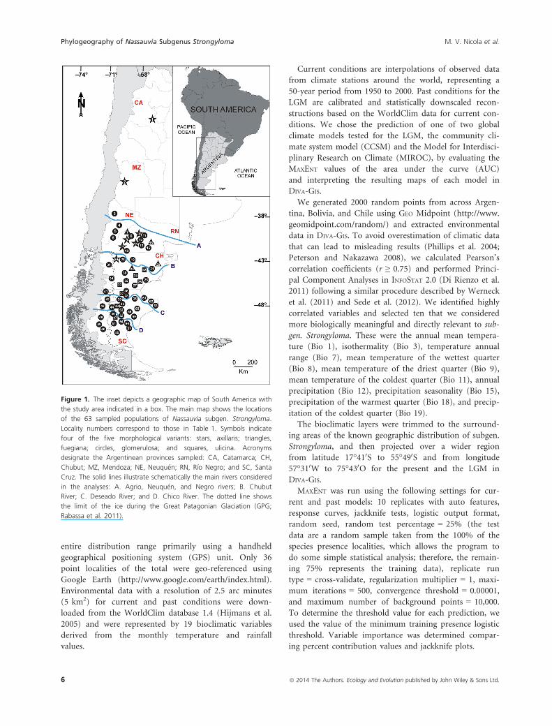
Figure 1. The inset depicts a geographic map of South America with

the study area indicated in a box. The main map shows the locations

of the 63 sampled populations of Nassauvia subgen. Strongyloma.

Locality numbers correspond to those in Table 1. Symbols indicate

four of the five morphological variants: stars, axillaris; triangles,

fuegiana; circles, glomerulosa; and squares, ulicina. Acronyms

designate the Argentinean provinces sampled: CA, Catamarca; CH,

Chubut; MZ, Mendoza; NE, Neuqu�en; RN, R�ıo Negro; and SC, Santa

Cruz. The solid lines illustrate schematically the main rivers considered

in the analyses: A. Agrio, Neuqu�en, and Negro rivers; B. Chubut

River; C. Deseado River; and D. Chico River. The dotted line shows

the limit of the ice during the Great Patagonian Glaciation (GPG;

Rabassa et al. 2011).

6 ª 2014 The Authors. Ecology and Evolution published by John Wiley & Sons Ltd.

Phylogeography of Nassauvia Subgenus Strongyloma M. V. Nicola et al.

Results

DNA data sets

DNA sequences of subgen. Strongyloma ranged from 913

to 928 base pairs (bp) for rpl32–trnL (with two indels of

seven and eight bp) and 916 to 925 bp for trnQ–50rps16(with one indel of nine bp). The three indels were coded

as present or absent and appended to the end of the

matrix. The combined matrix included 1856 characters,

of which 37 were variable.

Haplotype network and geographicdistribution of haplotypes

Statistical parsimony retrieved a well-resolved network in

which three closed loops were resolved unambiguously

(Fig. 2). A total of 41 haplotypes (H) were identified. Ele-

ven haplotypes occurred in interior positions and 30 at

tip positions. Nine additional haplotypes were not

observed in the analyzed individuals and occur only as

inferred intermediates in the network. Four frequent,

widespread haplotypes were found (H25, H1, H18, and

H12; Table 2, Fig. 2).

Among the total observed haplotypes (Table 2), eight

were shared by populations associated with different mor-

phological variant pairs: H41 in axillaris–fuegiana, H9,

H10, and H17 in axillaris–glomerulosa, H1 in axillaris–ulicina, and H18, H25, and H28 in glomerulosa–ulicina.Two additional haplotypes were found in populations

associated with different combinations of three morpho-

logical variants: H12 in axillaris–fuegiana–glomerulosa

and H27 in fuegiana–glomerulosa–ulicina.The nested network resulted in 15 one-step clades,

seven 2-step clades, two 3-step clades, and the total clado-

gram (Fig. 3). Although not strictly nonoverlapping, a lat-

itudinal distribution of the two-step clades was observed

(Figs. 2, 3). Haplotypes in clade 2-1 (HA: high–Andeanregion) were distributed through the Andes north of

38°S, clearly separated from the rest. Haplotypes in clade

2-3 (NP1: northern Patagonia 1 region) included the sec-

ond most frequent, widespread haplotype (H1) and were

distributed between 39° and 47°S, while haplotypes in

clade 2-4 (NP2: northern Patagonia 2 region) included

the fourth most frequent, widespread haplotype (H12)

and were distributed between 40°250 and 44°S. Haplo-

types in clades 2-6 (CP1: central Patagonia 1 region) and

2-5 (CP2: central Patagonia 2 region) were scarce and dis-

tributed between 40° and 43°150S, and 43° and 46°370S,respectively. Haplotypes in clade 2-7 (SP1: southern Pata-

gonia 1 region) included the most frequent, widespread

haplotype (H25) and were distributed mainly south of

43°210S, with one exception further north at 39°440S.

Finally, haplotypes in clade 2-2 (SP2: southern Patagonia

2 region) included the third most frequent, widespread

haplotype (H18) and were distributed south of 45°280S.All geographic regions presented populations with

exclusive haplotypes (Table 2, Fig. 3). The region with

the largest number of exclusive haplotypes was SP1, with

eight exclusive haplotypes distributed in southern Neu-

qu�en (population 5; H38) and mainly in Santa Cruz

(populations 37, 39, 44, 46, 50, 53, and 58; H26, H31,

H37, H36, H32, H30, and H29 respectively). The second

region with the highest number of exclusive haplotypes

was NP1, with six exclusive haplotypes distributed in

southern Neuqu�en (population 5; H7), in central R�ıo

Negro (population 8; H6), and in south-western Chubut

(populations 30, 32, and 34; H2, H3, H4, and H5). The

NP2 region had five exclusive haplotypes distributed in

southern Neuqu�en (population 6; H13), central and cen-

tral-southern R�ıo Negro (populations 10, 17, and 18;

H11, H14, and H16), and central-northern Chubut

(population 28; H15). The SP2 region had four exclusive

haplotypes distributed in Santa Cruz (populations 42, 47,

(A)

(B)

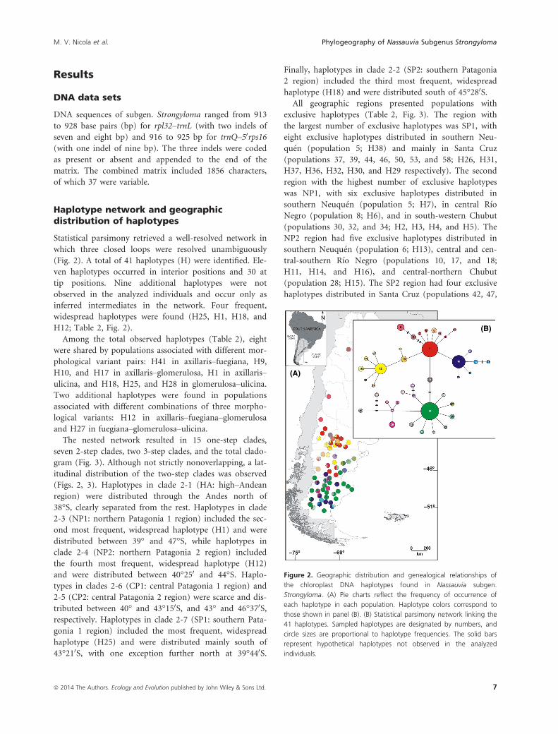
Figure 2. Geographic distribution and genealogical relationships of

the chloroplast DNA haplotypes found in Nassauvia subgen.

Strongyloma. (A) Pie charts reflect the frequency of occurrence of

each haplotype in each population. Haplotype colors correspond to

those shown in panel (B). (B) Statistical parsimony network linking the

41 haplotypes. Sampled haplotypes are designated by numbers, and

circle sizes are proportional to haplotype frequencies. The solid bars

represent hypothetical haplotypes not observed in the analyzed

individuals.

ª 2014 The Authors. Ecology and Evolution published by John Wiley & Sons Ltd. 7

M. V. Nicola et al. Phylogeography of Nassauvia Subgenus Strongyloma

49, and 57; H19, H21, H22, and H23). The CP2 region

presented three exclusive haplotypes distributed in cen-

tral-northern Chubut (population 19; H35) and in cen-

tral-northern Santa Cruz (populations 36 and 37; H33

and H34, respectively). The CP1 region had only one

exclusive haplotype in north-western Chubut (population

31; H40). The HA region possessed only one exclusive

haplotype in Catamarca (population 1; H8). Exclusive

haplotypes were scattered throughout the study area,

although most were located in central-western and south-

eastern Santa Cruz.

Inferences from nested clade analysis

Six one-step clades (1-4, 1-5, 1-7, 1-9, 1-10, and 1-13), all

seven-two-step clades, the two-three-step clades, and the

Table 2. Distribution of haplotypes of Nassauvia subgen. Strongyloma between individuals, populations, morphological variants, Argentinean

provinces, and haploclades.

Haplotype Nind %ind Npop %pop Morphology Distribution Geographic region

1 60 0.161 13 0.127 AXI-ULI NE-RN-CH-SC NP1

2 1 0.003 1 0.010 GLO CH NP1

3 2 0.005 1 0.010 GLO CH NP1

4 2 0.005 1 0.010 GLO CH NP1

5 8 0.022 1 0.010 GLO CH NP1

6 3 0.008 1 0.010 GLO RN NP1

7 2 0.005 1 0.010 GLO SC NP1

8 7 0.019 1 0.010 AXI CA HA

9 15 0.040 2 0.020 AXI-GLO MZ-NE HA

10 11 0.030 3 0.025 AXI-GLO RN NP2

11 1 0.003 1 0.010 AXI RN NP2

12 20 0.054 8 0.067 AXI-FUE-GLO NE-RN-CH NP2

13 2 0.005 1 0.010 GLO NE NP2

14 4 0.011 1 0.010 AXI RN NP2

15 8 0.022 1 0.010 GLO CH NP2

16 1 0.003 1 0.010 GLO RN NP2

17 3 0.008 2 0.020 AXI-GLO CH NP2

18 38 0.102 9 0.075 GLO-ULI CH-SC SP2

19 3 0.008 1 0.010 GLO SC SP2

20 4 0.011 3 0.025 GLO SC SP2

21 3 0.008 1 0.010 GLO SC SP2

22 1 0.003 1 0.010 ULI SC SP2

23 1 0.003 1 0.010 GLO SC SP2

24 7 0.019 2 0.020 GLO CH SP1

25 102 0.274 23 0.192 GLO-ULI CH-SC SP1

26 3 0.008 1 0.010 ULI SC SP1

27 4 0.011 3 0.025 FUE-GLO-ULI CH SP1

28 6 0.016 2 0.020 GLO-ULI CH SP1

29 3 0.008 1 0.010 GLO SC SP1

30 1 0.003 1 0.010 GLO SC SP1

31 4 0.011 1 0.010 GLO SC SP1

32 5 0.013 1 0.010 GLO SC SP1

33 3 0.008 1 0.010 GLO SC CP2

34 4 0.011 1 0.010 ULI SC CP2

35 4 0.011 1 0.010 GLO CH CP2

36 2 0.005 1 0.010 GLO SC SP1

37 3 0.008 1 0.010 GLO SC SP1

38 2 0.005 1 0.010 GLO NE SP1

39 11 0.030 2 0.020 GLO SC SP1

40 4 0.011 1 0.010 GLO CH CP1

41 4 0.011 2 0.020 AXI-FUE RN CP1

Nind, number of individuals per haplotype; %ind, percentage of individuals per haplotype; Npop, number of populations per haplotype; %pop, percent-

age of populations per haplotype; morphological variants: AXI, axillaris; FUE, fuegiana; GLO, glomerulosa; and ULI, ulicina; Distribution: CA, Catamar-

ca; CH, Chubut; MZ, Mendoza; NE, Neuqu�en; RN, R�ıo Negro; and SC, Santa Cruz; Geographic region: CP1, central Patagonia 1; CP2: central

Patagonia 2; HA, high-Andean; NP1, northern Patagonia 1; NP2, northern Patagonia 2; SP1, southern Patagonia 1; SP2, southern Patagonia 2.

8 ª 2014 The Authors. Ecology and Evolution published by John Wiley & Sons Ltd.

Phylogeography of Nassauvia Subgenus Strongyloma M. V. Nicola et al.

total cladogram showed significant levels of geographic

association, while the geographic association hypothesis

was rejected for the remaining nine-one-step clades

(Table 3, Fig. 3).

Historical fragmentation followed by isolation by

distance due to restricted gene flow was inferred for clade

1-4 (most haplotypes of NP2). Processes of restricted gene

flow and/or long-distance dispersal in intermediate areas

not occupied by the species, or gene flow followed by

extinction of intermediate populations were inferred for

clade 1-5 (most haplotypes of NP1). Clades 1-7 (most

haplotypes of SP2) and 3-1 (HA, NP1, NP2, and SP2)

have experienced long-distance colonization and/or frag-

mentation. Processes of restricted gene flow and/or long-

distance dispersal were inferred for clade 1-9 (part of

SP1). Isolation or long-distance dispersal was inferred for

clade 1-10 (most haplotypes of SP1). Clades 2-2 (SP2)

and 2-5 (CP2) have experienced restricted gene flow with

isolation by distance. Finally, range expansion was

inferred for clades 2-4 (NP2) and 3-2 (CP1, CP2, PS1,

and PS2; Table 3, Fig. 3).

Haplotype diversity

Considering all individuals from all 63 sampled popula-

tions, haplotype diversity (h) ranged from 0 to 0.821 with

an average of 0.532, nucleotide diversity (p) ranged from

0 to 0.00218 with an average of 0.00128, and mean num-

ber of pairwise differences among haplotypes within pop-

ulations (p) ranged from 0 and 3.857 with an average of

1.175 (Table 4).

With one exception, the highest values of h were found

in populations of central-western Patagonia (populations

5, 9, 30, 31, 36, 37, 42, 44, and 51; Table 1, Fig. 1),

located from the flanks of the Andes up to 69°W, and

latitudinally from 40°S in southern Neuqu�en to 50°S in

southern Santa Cruz. Population 57 had the highest hap-

lotype diversity and occurs outside this range in south-

eastern Santa Cruz. The highest values of p also occur

in populations of central-western Patagonia, coinciding

with most populations that showed higher haplotype

diversity (populations 5, 9, 31, 37, 48, and 57), and in

one population (24) located in south-eastern Santa Cruz.

The highest values of p similarly occur in populations of

central-western Patagonia, coinciding with most popula-

tions that showed higher haplotype and nucleotide

diversity (populations 5, 9, 31, 37, 48, and 57). Most

populations with high genetic diversity also had exclusive

haplotypes (populations 5, 30, 31, 36, 37, 42, 44, and

57, Table 4).

The same diversity indices were calculated for each

geographic region (Table 5, Fig. 3). The NP2 region

showed the highest value of haplotype diversity

(h = 0.800), followed by the CP2 region, which also

Figure 3. Statistical parsimony network and

resulting nested clade design of the 41

haplotypes found in Nassauvia subgen.

Strongyloma. Haplotypes correspond to those

in Figure 2; solid bars represent hypothetical

haplotypes not observed in the analyzed

individuals. Haplotypes belonging to the same

clade level are boxed. Acronyms associated to

2-step clades indicate the geographic region to

which they belong: CP1, central Patagonia 1;

CP2: central Patagonia 2; HA, high-Andean;

NP1, northern Patagonia 1; NP2, northern

Patagonia 2; SP1, southern Patagonia 1; SP2,

southern Patagonia 2.

ª 2014 The Authors. Ecology and Evolution published by John Wiley & Sons Ltd. 9

M. V. Nicola et al. Phylogeography of Nassauvia Subgenus Strongyloma

showed the highest values of nucleotide diversity and

pairwise differences (h = 0.727; p = 0.00084; p = 1.527),

while the NP1 region showed the lowest values of h, p,and p (h = 0.399; p = 0.00027; p = 0.488).

Population genetic structure

Analyses of molecular variance (AMOVA; Table 6)

showed significant differences among all sources of varia-

tion tested (P < 0.001), with the exception of regions

located inside and outside the boundary of the GPG

(Fig. 1). The AMOVA revealed that genetic variation of

subgen. Strongyloma was best explained by differences

among populations within regions that were glaciated or

nonglaciated during GPG (73.6%, P < 0.001). By dividing

the regions according to major rivers (Fig. 1), the highest

percentage of variation was explained by differences

among populations within each of the regions (50.6%,

P < 0.001).

Past demographic analyses

Recent demographic expansion was evidenced for the

NP1 and the SP1 regions. For the NP1 region, Fu’s FSand Ramos-Onsins and Rozas’ R2 statistics showed a

negative value of �4.18 and a small positive value of

0.0407, respectively. For the SP1 region, Tajima’s D and

Fu’s FS showed negative values of �1.54473 and �7.324,

respectively, while Ramos-Onsins and Rozas’s R2 showed

a small positive value of 0.0353 (Table 5).

Potential Pleistocene geographicdistribution

Present and LGM species distribution models for subgen.

Strongyloma are presented in Figure 4. In predicting the

current distribution, the mean value of the AUC for the

test data of the model for the present was 0.932 � 0.008.

Because the mean value of the AUC for the test data

using the MIROC palaeomodel was 0.836 � 0.075, com-

pared with 0.789 � 0.021 using the CCSM palaeomodel,

the former was selected for projecting the distribution

during the LGM.

The predicted model for the present (Fig. 4A) was a

fairly good representation of the known geographic distri-

bution for subgen. Strongyloma, although some inconsis-

tencies between projected and realized distribution areas

were found. Low probability (0.21–0.30) of suitable con-

ditions was found in the Islas Malvinas/Falkland Islands,

where these plants have never been observed.

Table 3. Population processes and/or historical events affecting genetic structure in Nassauvia subgen. Strongyloma based on nested clade

analysis (NCA). Geographic region, hierarchically nested clades, results of permutation contingency tests with their associated P value, NCA infer-

ence chain and inferred events are shown.

Geographic

region Clade v2 statistic P-value Inference chain Inferred pattern/event

NP2 1-4 119.60 <0.05 1-2-3-4-9-10 NO Geographic sampling inadequate to discriminate between

fragmentation and isolation by distance.

NP1 1-5 222.50 <0.05 1-2-3-5-6-7-8 YES Restricted gene flow/dispersal but with some long-distance

dispersal over intermediate areas not occupied by the species,

or past gene flow followed by extinction of intermediate populations.

SP2 1-7 102.49 <0.05 1-2-3-5-6-13-14 NO Long-distance colonization and/or past fragmentation.

SP1 1-9 42.54 <0.05 1-2-3-5-6-7 YES Restricted gene flow/dispersal but with some long-distance dispersal.

SP1 1-10 464.99 <0.05 1-2-3-5-6-7-8 NO Sampling design inadequate to discriminate between isolation

by distance versus long-distance dispersal.

CP2 1-13 7.00 <0.05 1-19-20 NO Inadequate geographic sampling.

HA 2-1 22.00 <0.05 1-19-20 NO Inadequate geographic sampling.

SP2 2-2 25.33 <0.05 1-2-3-4 NO Restricted gene flow with isolation by distance.

NP1 2-3 54.82 <0.05 – Null hypothesis cannot be rejected.

NP2 2-4 50.00 <0.05 1-2-11-12 NO Contiguous range expansion.

CP2 2-5 11.00 <0.05 1-2-3-4 NO Restricted gene flow with isolation by distance.

CP1 2-6 8.00 <0.05 1-19-20-NO Inadequate geographic sampling.

SP1 2-7 291.46 <0.05 1-2 IO Inconclusive outcome.

HA + NP1 +

NP2 + SP2

3-1 548.03 <0.05 1-2-11-12-13-14 NO Long-distance colonization and/or past fragmentation.

CP1 + CP2

+ SP1

3-2 271.93 <0.05 1-2-11-12 NO Contiguous range expansion.

Total

cladogram

331.13 <0.05 1-2 IO Inconclusive outcome.

10 ª 2014 The Authors. Ecology and Evolution published by John Wiley & Sons Ltd.

Phylogeography of Nassauvia Subgenus Strongyloma M. V. Nicola et al.

Table 4. Diversity indices of sampled Nassauvia subgen. Strongyloma populations: haplotype (h) and nucleotide (p) diversity, and mean number

of pairwise differences (p) with their respective standard deviation (DE).

Nloc Nhap (Nind) h � DE p � DE p � DE

1 H8 (7) 0.00000 0.00000 0.00000

2 H9 (8) 0.00000 0.00000 0.00000

3 H9 (7) 0.00000 0.00000 0.00000

4 H1 (7) 0.00000 0.00000 0.00000

5 H1 (1), H7 (2), H38 (2) 0.80000 � 0.16400 0.00131 � 0.00032 2.40000 � 0.93915

6 H12 (6), H13 (2) 0.42900 � 0.16900 0.00023 � 0.00009 0.42900 � 0.20248

7 H41 (2) 0.00000 0.00000 0.00000

8 H6 (3) 0.00000 0.00000 0.00000

9 H1 (5), H12 (1), H41 (2) 0.60700 � 0.16400 0.00167 � 0.00055 3.07100 � 0.87407

10 H1 (6), H10 (1), H11 (1) 0.46400 � 0.20000 0.00037 � 0.00017 0.67900 � 0.27203

11 H1 (8) 0.00000 0.00000 0.00000

12 H10 (8) 0.00000 0.00000 0.00000

13 H1 (7), H12 (1) 0.25000 � 0.18000 0.00027 � 0.00020 0.50000 � 0.22361

14 H1 (2), H12 (4) 0.53300 � 0.17200 0.00058 � 0.00019 1.06700 � 0.44271

15 H12 (2) 0.00000 0.00000 0.00000

16 H1 (6), H10 (2) 0.42900 � 0.16900 0.00023 � 0.00009 0.42900 � 0.20248

17 H12 (1), H14 (4) 0.40000 � 0.23700 0.00022 � 0.00013 0.40000 � 0.24900

18 H12 (3), H16 (1) 0.50000 � 0.26500 0.00027 � 0.00014 0.50000 � 0.32711

19 H24 (1), H35 (4) 0.40000 � 0.23700 0.00087 � 0.00052 1.60000 � 0.67305

20 H27 (1) – – –

21 H27 (2), H28 (5) 0.47600 � 0.17100 0.00052 � 0.00019 0.95200 � 0.37283

22 H27 (1), H30 (1) – – –

23 H12 (2) 0.00000 0.00000 0.00000

24 H1 (1), H28 (1) – – –

25 H24 (6) 0.00000 0.00000 0.00000

26 H25 (2) 0.00000 0.00000 0.00000

27 H1 (4) 0.00000 0.00000 0.00000

28 H15 (8) 0.00000 0.00000 0.00000

29 H17 (1) – – –

30 H1 (4), H2 (1), H4 (2) 0.66700 � 0.16000 0.00041 � 0.00013 0.76200 � 0.31780

31 H3 (2), H17 (2), H40 (4) 0.71400 � 0.12300 0.00210 � 0.00041 3.85700 � 1.06583

32 H1 (8) 0.00000 0.00000 0.00000

33 H18 (1) – – –

34 H5 (8) 0.00000 0.00000 0.00000

35 H18 (7) 0.00000 0.00000 0.00000

36 H25 (3), H33 (3) 0.60000 � 0.12900 0.00033 � 0.00007 0.60000 � 0.29496

37 H25 (1), H26 (3), H34 (4) 0.67900 � 0.12200 0.00123 � 0.00019 2.25000 � 0.67231

38 H25 (7) 0.00000 0.00000 0.00000

39 H25 (4), H31 (4) 0.57100 � 0.09400 0.00031 � 0.00005 0.57100 � 0.24290

40 H39 (8) 0.00000 0.00000 0.00000

41 H25 (8) 0.00000 0.00000 0.00000

42 H1 (1), H18 (4), H19 (3) 0.67900 � 0.12200 0.00043 � 0.00011 0.78600 � 0.30166

43 H25 (1) – – –

44 H25 (2), H37 (3), H39 (3) 0.75000 � 0.09600 0.00082 � 0.00011 1.50000 � 0.48580

45 H25 (8) 0.00000 0.00000 0.00000

46 H18 (4), H36 (2) 0.53300 � 0.17200 0.00087 � 0.00028 1.60000 � 0.60332

47 H22 (1) – – –

48 H18 (5), H25 (3) 0.53600 � 0.12300 0.00117 � 0.00027 2.14300 � 0.64653

49 H23 (1), H25 (7) 0.25000 � 0.18000 0.00041 � 0.00029 0.75000 � 0.29155

50 H25 (3), H32 (5) 0.53600 � 0.12300 0.00029 � 0.00007 0.53600 � 0.23238

51 H18 (2), H20 (1) 0.66700 � 0.31400 0.00036 � 0.00017 0.66700 � 0.47117

52 H25 (6) 0.00000 0.00000 0.00000

53 H25 (7), H30 (1) 0.25000 � 0.18000 0.00014 � 0.00010 0.25000 � 0.14491

54 H18 (6) 0.00000 0.00000 0.00000

55 H25 (4) 0.00000 0.00000 0.00000

ª 2014 The Authors. Ecology and Evolution published by John Wiley & Sons Ltd. 11

M. V. Nicola et al. Phylogeography of Nassauvia Subgenus Strongyloma

The model of the geographic distribution for the LGM

showed some important differences with the known cur-

rent geographic distribution of the subgenus (Fig. 4B).

Low (0.26–0.5) to null probability of suitable conditions

was found in an area between the Chubut and the Dese-

ado rivers and also in southern Santa Cruz and Tierra del

Fuego. The prediction was overprojected over the current

Atlantic continental shelf, extending approximately

between 45°S (San Jorge Gulf, Chubut) and 51°S (Bah�ıa

Grande, Santa Cruz).

For the training data of the palaeomodel, the highest

contribution and the highest permutation importance

was for the annual mean temperature (Bio1 = 42.8%

and 36.1%, respectively), indicating that this environ-

mental variable contributed most to the construction of

the model. In the jackknife test for the training data, the

mean temperature of the coldest quarter (Bio11) pre-

sented the most useful information when used in isola-

tion to build the model, causing the model to reach the

highest gain and allowing a reasonable adjustment to the

training data. The mean temperature of the wettest quar-

ter (Bio8) contained a substantial amount of useful

information that was not contained in the model when

only the remaining variables were used, since excluding

Bio8 in the model decreased training gain. Jackknife tests

for the gain and for the AUC of the test data yielded

similar results to the jackknife test for the gain of the

training data, suggesting that mean winter temperature

(i.e., the coldest and the wettest quarter) helped MAXENT

achieve a good fit to the training data and also to gener-

alize better, achieving comparatively better results on the

test data.

Discussion

The phylogeographical and palaeomodelling analyses sug-

gest that the genetic diversity and structure found in

Nassauvia subgen. Strongyloma were shaped mainly by

three main different historical events: (1) isolation in

refugia and restricted gene flow during Pleistocene glacial

periods, followed by postglacial range expansions; (2) col-

onization of new available areas during Pleistocene glacia-

tions and postglacial retraction of populations; and (3)

fragmentation of populations in areas not reached by the

ice sheet during Pleistocene glacial periods followed by

postglacial range expansions.

Table 4. Continued.

Nloc Nhap (Nind) h � DE p � DE p � DE

56 H18 (7), H20 (1) 0.25000 � 0.18000 0.00014 � 0.00010 0.25000 � 0.14491

57 H18 (2), H20 (2), H21 (3), H25 (1) 0.82100 � 0.10100 0.00142 � 0.00042 2.60700 � 0.76026

58 H25 (4), H29 (3) 0.57100 � 0.11900 0.00031 � 0.00007 0.57100 � 0.26077

59 H25 (7) 0.00000 0.00000 0.00000

60 H25 (8) 0.00000 0.00000 0.00000

61 H25 (3) 0.00000 0.00000 0.00000

62 H25 (7) 0.00000 0.00000 0.00000

63 H25 (5) 0.00000 0.00000 0.00000

Table 5. Diversity indices and results of demographic analyses used to test range expansion in Nassauvia subgen. Strongyloma for each

geographic area in Argentina. Haplotype (h) and nucleotide (p) diversity, mean number of pairwise differences (p), Tajima’s D, Fu’s FS, and

Ramos-Onsins and Rozas’s R2 are shown.

Geographic region

Diversity indices Demographic analyses

h � SD p � SD p � SD D FS R2

High-Andean 0.45500 � 0.07800 0.00049 � 0.00008 0.90900 � 0.19493 1.48848 2.78400 0.22730

Northern Patagonia 1 0.39900 � 0.06800 0.00027 � 0.00005 0.48800 � 0.07071 �1.40325 �4.18000* 0.04070*

Northern Patagonia 2 0.80000 � 0.03400 0.00064 � 0.00006 1.16800 � 0.16124 �0.73108 �2.54900 0.08250

Central Patagonia 1 0.57100 � 0.09400 0.00124 � 0.00021 2.28600 � 0.68117 2.10118 3.93300 0.28570

Central Patagonia 2 0.72700 � 0.06800 0.00084 � 0.00011 1.52700 � 0.41231 1.68091 1.49100 0.25450

Southern Patagonia 1 0.54600 � 0.04800 0.00050 � 0.00006 0.91600 � 0.07071 �1.54473* �7.32400* 0.03530*

Southern Patagonia 2 0.46300 � 0.07930 0.00041 � 0.00011 0.75500 � 0.11832 �1.18369 �2.04400 0.06530

Total 0.88100 � 0.01100 0.00178 � 0.00005 3.24600 � 0.12247 �1.38638 �20.51400 0.03850

Results consistent with demographic expansion are shown in bold.

*P < 0.05.

12 ª 2014 The Authors. Ecology and Evolution published by John Wiley & Sons Ltd.

Phylogeography of Nassauvia Subgenus Strongyloma M. V. Nicola et al.

Pleistocene refugia in central-western andsouth-eastern Patagonia

Our data suggest that populations of Nassauvia subgen.

Strongyloma may have withstood the extreme cold and

aridity during the Pleistocene glaciations in two kinds of

refugia (Holderegger and Thiel-Egenter 2009): (1) periph-

eral glacial refugia—at least three along the eastern foot-

hills of the Andes— located in south-western Neuqu�en (c.

39°300 S 70°300 W), north-western Chubut (c. 43°S71°W), and north-western Santa Cruz (c. 47°S 71°W);

and (2) lowland glacial refugia—at least four— located

near the Chubut River in central-western Chubut (c. 44°S69°300 W), near the Deseado River in central-northern

Santa Cruz (c. 46°300 S 69°300 W), and near the Chico

River in central-western (c. 48°S 71°W), and south-east-

ern (c. 50°S 69°W) Santa Cruz.

The high diversity and several exclusive haplotypes

found in these populations of subgen. Strongyloma are

consistent with long-term habitation such as would be

expected from Pleistocene refugia (Hewitt 1996; Taberlet

and Cheddadi 2002; Petit et al. 2003; Provan and Bennett

2008). The finding of exclusive haplotypes suggests there

would have been restricted gene flow and that isolation

over time allowed the accumulation of genetic differences

among populations. Most of these populations were

found within the limits of the ice sheet of the GPG.

Moreover, restricted gene flow and posterior range expan-

sion were inferred by NCA and corroborated in most

cases by demographic analyses, indicating that they might

have survived in refugia during glacial periods, as

suggested for other Patagonian organisms in the areas

mentioned above (S�ersic et al. 2011; Sede et al. 2012;

Cosacov et al. 2013). The highest probabilities of occur-

rence projected especially for central-western and south-

eastern Patagonia, both for the current distribution, as

well for the palaeodistribution, reinforce the conclusion

that subgen. Strongyloma probably persisted in refugia in

these areas, without drastic climatic restrictions.

Colonization of eastern Patagonia duringPleistocene glaciations

During Pleistocene glaciations, the current Atlantic sub-

marine platform was partially exposed as a result of the

sea level lowering (c. 100–140 m during full glacial epi-

sodes), allowing for plant colonization (Rabassa 2008).

Palaeomodelling supports that populations of Nassauvia

subgen. Strongyloma could have inhabited that exposed

area of the coast. After glaciations, and as the result of

the sea level rise, populations were forced to retract to

the current Atlantic coast. Low diversity and the absence

of exclusive haplotypes in eastern Patagonia are then

explained by the expansion of populations over the cur-

rent Atlantic coast during Pleistocene glaciations, and

their recent, postglacial retraction, with the consequent

loss of genetic diversity.

Population fragmentation in centralPatagonia and phylogeographical breaks

Latitudinal discontinuities have been previously reported

for other Patagonian organisms, both plants and animals

(S�ersic et al. 2011; Sede et al. 2012; Cosacov et al. 2013).

Dynamics of the river basins, palaeobasins, and coastline

shift during the Pleistocene glacial–interglacial cycles con-stitute factors that may have converted Patagonia into a

highly fragmented landscape (S�ersic et al. 2011). In par-

ticular, the Chubut and the Deseado river basins may

have been important historical barriers that facilitated iso-

lation between populations of different Patagonian species

that persisted north and/or south of these river basins

(e.g., Phyllotis xanthopygus, Kim et al. 1998; Hordeum

spp., Jakob et al. 2009; Mulinum spinosum, Sede et al.

2012; Anarthrophyllum desideratum, Cosacov et al. 2013).

However, adverse climatic conditions such as lower win-

ter temperature and precipitation during glacial periods

have been suggested as a possible reason for plant popula-

tion fragmentation in the same geographic area (Sede

et al. 2012; Cosacov et al. 2013). Our palaeomodelling

results also support a low probability of suitable climatic

conditions for Nassauvia subgen. Strongyloma during the

LGM in the center of the steppe, between the Chubut

(c. 44°S) and the Deseado (c. 47°S) rivers. In fact, the

geographic distribution of this subgenus, as in the steppe

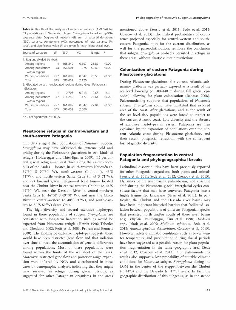
Table 6. Results of the analyses of molecular variance (AMOVA) for

63 populations of Nassauvia subgen. Strongyloma based on cpDNA

sequence data. Degrees of freedom (df), sum of squared deviations

(SSD), variance components (VC), percentage of total variance (%

total), and significance value (P) are given for each hierarchical level.

Source of variation df SSD VC % total P

1. Regions divided by rivers

Among regions 4 168.349 0.507 23.87 <0.001

Among populations

within regions

44 356.604 1.075 50.60 <0.001

Within populations 297 161.099 0.542 25.53 <0.001

Total 345 686.052 2.125

2. Glaciated versus nonglaciated regions during Great Patagonian

Glaciation

Among regions 1 10.703 �0.013 �0.68 n.s.

Among populations

within regions

47 514.250 1.477 73.64 <0.001

Within populations 297 161.099 0.542 27.04 <0.001

Total 345 686.052 2.006

n.s., not significant, P > 0.05.

ª 2014 The Authors. Ecology and Evolution published by John Wiley & Sons Ltd. 13

M. V. Nicola et al. Phylogeography of Nassauvia Subgenus Strongyloma

shrub M. spinosum (Sede et al. 2012), seems to be influ-

enced mainly by the mean temperature of the winter, a

biologically important variable that defines the start of

the growing season (Paruelo et al. 1998). Our findings

also support the traditional water balance hypothesis,

which considers aridization as the main factor affecting

plant population demography and diversification in Pata-

gonia (Cosacov et al. 2013), related to the enlargement

and reduction of the main river basins.

Based on past river basin dynamics and climate condi-

tions cited above, a significant difference could be

expected between northern and southern haplotypes

within subgen. Strongyloma. Nevertheless, there is a close

genetic relation between a few northern and central-

northern lineages with southern lineages distributed in

distant areas. However, a general northern–southern hap-

loclade structure can be supported combining the above

environmental evidence with NCA inferences and demo-

graphic analyses, in two historical steps: (1) both frag-

mentation between northern and southern haploclades,

and isolation with restricted gene flow of one southern

haploclade during Pleistocene glaciations, produced the

split of the original distribution into two groups of popu-

lation, one north of the Chubut river basin, and one

south of the Deseado river basin; and (2) successive range

expansions after the Pleistocene glaciations, mainly

toward warmer and wetter conditions in the center of the

Patagonian steppe. The most likely posterior demographic

expansions would be from both northern and southern

populations toward central-eastern Chubut Province. The

expansion of northern, central, and southern haploclades

could have generated recent contact areas throughout the

entire Patagonian steppe, but mainly between the Chubut

and the Deseado rivers.

Within a general latitudinal geographic structure of

haploclades, other phylogeographical breaks can be distin-

guished related to river basins. On one hand, the high-

Andean haploclade located just north of the Agrio and

Neuqu�en rivers at c. 38°S was clearly separated from the

rest, in accordance with a latitudinal break reported for a

lizard species (Liolaemus elongatus, Morando et al. 2003).

Low diversity and the presence of only one exclusive hap-

lotype in high-Andean populations may be explained by

recent colonization or this was a poor area for the sur-

vival of subgen. Strongyloma during the LGM. However,

these results should be interpreted with caution because

of incomplete sampling of high-Andean region. On the

other hand, the northern limit of one central haploclade

(CP1) coincides with the break at Limay River basin

reported for another lizard species (Liolaemus bibronii,

Morando et al. 2007).

Finally, according to haplotype analyses, the four most

widespread haplotypes and several other interior and tip

haplotypes were shared among populations of different

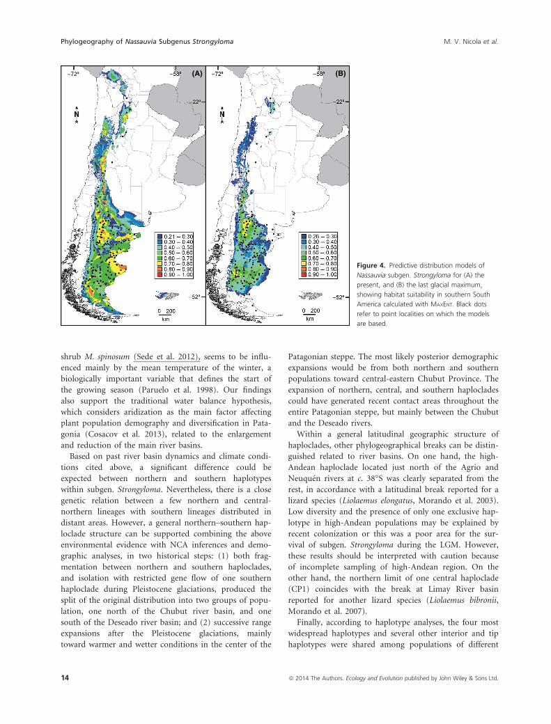
(A) (B)

Figure 4. Predictive distribution models of

Nassauvia subgen. Strongyloma for (A) the

present, and (B) the last glacial maximum,

showing habitat suitability in southern South

America calculated with MAXENT. Black dots

refer to point localities on which the models

are based.

14 ª 2014 The Authors. Ecology and Evolution published by John Wiley & Sons Ltd.

Phylogeography of Nassauvia Subgenus Strongyloma M. V. Nicola et al.

morphological variants, suggesting that there is no strict

relation between morphology and genetic diversity. Fur-

thermore, throughout the entire Patagonian steppe, some

populations have haplotypes from different clades. This

indication of distantly related haplotypes co-occurring

suggests the existence of numerous contact zones (Avise

2000) throughout the steppe: within northern lineages in

central R�ıo Negro; between northern and central clades in

central-western R�ıo Negro; between northern and south-

ern lineages in southern Neuqu�en, north-western Chubut,

and north-western Santa Cruz; between central and

southern clades in central-northern Santa Cruz;

and within southern lineages in central, south-western,

and south-eastern Santa Cruz.

Conclusion

Phylogeographical and palaeomodelling patterns found in

Nassauvia subgen. Strongyloma appear to reflect climatic

fluctuations and landscape changes that occurred during

the Pleistocene having an impact on the distribution,

demography, and diversification of different lineages

within the group. Past events differentially affected areas

within the immense geographic range of these shrubs.

During glaciations, subgen. Strongyloma persisted in

peripheral refugia along the eastern foothills of the Andes,

in lowland refugia in central-western and south-eastern

Patagonia, over the exposed Atlantic submarine platform

toward the east, and in fragmented populations north

and south the Chubut and the Deseado river basins.

Related to those past scenarios, Pleistocene glaciations

indirectly affected the demography of this group of plants

through decreased winter temperatures and water avail-

ability in different areas of its immense geographic range.

Future comparative phylogeographical studies should

consider patterns found in subgen. Strongyloma to better

comprehend the processes that have affected the Patago-

nian biota.

Acknowledgments

We thank L. J. �Avila, F. Biganzoli, M. F. Breitman, A. A.

Cocucci, A. Cosacov, N. Feltrin, M. Kozykarizki, L.

Mart�ınez, M. Morando, M. Olave, V. Paiaro, C. H. F.

P�erez, A. N. S�ersic, C. A. Zanotti, L. Zavala, and F. O,

Zuloaga, for assistance with fieldwork; and F. Fontanella

for help with MAXENT. M. V. Nicola thanks the ASPT

research grant for graduate students 2010. M. V. Nicola

acknowledges the National Research Council of Argentina

(CONICET) as its postdoctoral fellowship holder and R.

Pozner and S. M. Sede as researchers. The overall project

is part of a US NSF-PIRE award (OISE 0530267), sup-

porting collaborative research on Patagonian biodiversity,

granted to the following institutions (alphabetically): Brig-

ham Young University (USA), Centro Nacional Pa-

tag�onico (Argentina), Dalhousie University (Canada),

Instituto de Bot�anica Darwinion (Argentina), Universidad

Austral de Chile (Chile), Universidad de Concepci�on

(Chile), Universidad Nacional del Comahue (Argentina),

Universidad Nacional de C�ordoba (Argentina), and Uni-

versity of Nebraska (USA). Financial support was also

provided by CONICET (PIP 11220090100388).

Conflict of Interest

None declared.

References

Acosta, M. C., and A. C. Premoli. 2010. Evidence of

chloroplast capture in South American Nothofagus

(subgenus Nothofagus, Nothofagaceae). Mol. Phylogenet.

Evol. 54:235–242.

Amico, G. C., and D. L. Nickrent. 2009. Population structure

and phylogeography of the mistletoes Tristerix corymbosus

and T. aphyllus (Loranthaceae) using chloroplast DNA

sequence variation. Am. J. Bot. 96:1571–1580.

Avise, J. C. 2000. Phylogeography: the history and formation

of species. Harvard Univ. Press, Cambridge, U.K.

Barreda, V., and L. Palazzesi. 2007. Patagonian vegetation

turnovers during the Paleogene-Early Neogene: origin of

arid-adapted floras. Bot. Rev. 73:31–50.

Barreda, V., L. Palazzesi, and M. C. Teller�ıa. 2008. Fossil

pollen grains of Asteraceae from the Miocene of Patagonia:

Nassauviinae affinity. Rev. Palaeobot. Palynol. 151:51–58.

Beaumont, M. A., and M. Panchal. 2008. On the validity of

nested clade phylogeographical analysis. Mol. Ecol.

17:2563–2565.

Cabrera, A. L. 1982. Revisi�on del g�enero Nassauvia

(Compositae). Darwiniana 24:283–379.

Cabrera, A. L., and W. Willink. 1980. Biogeograf�ıa de Am�erica

Latina. Serie de Biolog�ıa, Monograf�ıa 13. Ed. 2, corr.

Colecci�on de Monograf�ıas Cient�ıficas de la Secretar�ıa

General de la Organizaci�on de los Estados Americanos.

Programa Regional de Desarrollo Cient�ıfico y Tecnol�ogico,

Washington, DC.

Clement, M., D. Posada, and K. A. Crandall. 2000. TCS: a

computer program to estimate gene genealogies. Mol. Ecol.

9:1657–1999.

Correa, M. N. 1998. Flora Patag�onica, Parte I. Colecci�on

Cient�ıfica del INTA. Instituto Nacional de Tecnolog�ıa

Agropecuaria, Buenos Aires, Argentina.

Cosacov, A., A. N. S�ersic, V. Sosa, L. A. Johnson, and A.

Cocucci. 2010. Multiple periglacial refugia in the Patagonian

steppe and post-glacial colonization of the Andes: the

phylogeography of Calceolaria polyrhiza. J. Biogeogr.

37:1463–1477.

ª 2014 The Authors. Ecology and Evolution published by John Wiley & Sons Ltd. 15

M. V. Nicola et al. Phylogeography of Nassauvia Subgenus Strongyloma

Cosacov, A., L. A. Johnson, V. Paiaro, A. A. Cocucci, F. E.

C�ordoba, and A. N. S�ersic. 2013. Precipitation rather than

temperature influenced the phylogeography of the endemic

shrub Anarthrophyllum desideratum in the Patagonian

steppe. J. Biogeogr. 40:168–182.

Crandall, K. A., and A. R. Templeton. 1993. Empirical tests of

some predictions from coalescent theory with applications

to intraspecific phylogeny reconstruction. Genetics

134:959–969.

Cullings, K. W. 1992. Design and testing of a plant specific

PCR primer for ecological and evolutionary studies. Mol.

Ecol. 1:233–240.

Di Rienzo, J. A., F. Casanoves, M. G. Balzarini, L. Gonz�alez,

M. Tablada, and C. W. Robledo. 2011. InfoStat version

2011. Grupo InfoStat. Facultad de Ciencias Agropecuarias,

Universidad Nacional de C�ordoba, C�ordoba, Argentina.

Available via http://www.infostat.com.ar.

Doyle, J. J., and J. L. Doyle. 1987. A rapid DNA isolation

procedure from small quantities of fresh leaf tissues.

Phytochem. Bull. 19:11–15.

Excoffier, L., and H. E. L. Lischer. 2010. Arlequin suite version

3.5: a new series of programs to perform population

genetics analyses under Linux and Windows. Mol. Ecol.

Resour. 10:564–567.

Freire, S. E., J. V. Crisci, and L. Katinas. 1993. A cladistic

analysis of Nassauvia Comm. ex Juss. (Asteraceae, Mutisieae)

and related genera. Bot. J. Linn. Soc. 112:293–309.

Fu, Y. X. 1997. Statistical tests of neutrality of mutations

against population growth, hitchhiking and background

selection. Genetics 147:915–925.

Funk, V. A., A. Susanna, T. F. Stuessy, and R. J. Bayer. 2009.

Systematics, evolution, and biogeography of Compositae.

American Society of Plant Taxonomy, Vienna, Austria.

Hall, T. A. 1999. BioEdit: a user-friendly biological sequence

alignment editor and analysis program for Windows 95/98/

NT. Nucleic Acids Symp. Ser. 41:95–98.

Hewitt, G. M. 1996. Some genetic consequences of ice ages,

and their role in divergence and speciation. Biol. J. Linn.

Soc. 58:247–276.

Hijmans, R. J., and C. H. Graham. 2006. The ability of climate

envelope models to predict the effect of climate change on

species distributions. Glob. Chang. Biol. 12:2272–2281.

Hijmans, R. J., L. Guarino, M. Cruz, and E. Rojas. 2001.

Computer tools for spatial analysis of plant genetic

resources data: 1. DIVA-GIS. Plant Genet. Resour. Newsl.

127:15–19.

Hijmans, R. J., S. E. Cameron, J. L. Parra, P. G. Jones, and

A. Jarvis. 2005. Very high resolution interpolated climate

surfaces for global land areas. Int. J. Climatol. 25:1965–1978.

Holderegger, R., and C. Thiel-Egenter. 2009. A discussion of

different types of glacial refugia used in mountain

biogeography and phylogeography. J. Biogeogr. 36:476–480.

Jakob, S. S., E. Martinez-Meyer, and F. R. Blattner. 2009.

Phylogeographic analyses and paleodistribution modeling

indicate Pleistocene in situ survival of Hordeum species

(Poaceae) in southern Patagonia without genetic or spatial

restriction. Mol. Biol. Evol. 26:907–923.

Kim, I., C. J. Phillips, J. A. Monjeau, E. C. Birney, K. Noack,

D. E. Pumo, et al. 1998. Habitat islands, genetic diversity,

and gene flow in a Patagonian rodent. Mol. Ecol. 7:667–678.

Knowles, L. L. 2008. Why does a method that fails continue to

be used? Evolution 62:2713–2717.

Librado, P., and J. Rozas. 2009. DnaSP version 5: a software

for comprehensive analysis of DNA polymorphism data.

Bioinformatics 25:1451–1452.

Maraner, F., R. Samuel, T. F. Stuessy, D. J. Crawford, J. V.

Crisci, A. Pandey, et al. 2012. Molecular phylogeny of

Nassauvia (Asteraceae, Mutisieae) based on nrDNA ITS

sequences. Plant Syst. Evol. 298:399–408.

Marchelli, P., and L. A. Gallo. 2006. Multiple ice-age refugia in

a southern beech of South America as evidenced by

chloroplast DNA markers. Conserv. Genet. 7:591–603.

Markgraf, V., M. McGlone, and G. Hope. 1995. Neogene

paleoenvironmental and paleoclimatic change in southern

temperate ecosystems – a southern perspective. Trends Ecol.

Evol. 10:143–147.

Morando, M., L. J. �Avila, and J. W. Sites Jr. 2003. Sampling

strategies for delimiting species: genes, individuals, and

populations in the Liolaemus elongatus-kriegi complex

(Squamata: Liolaemidae) in Andean-Patagonian South

America. Syst. Biol. 52:159–185.

Morando, M., L. J. �Avila, C. R. Turner, and J. W. Sites Jr.

2007. Molecular evidence for a species complex in the

patagonian lizard Liolaemus bibronii and phylogeography of

the closely related Liolaemus gracilis (Squamata: Liolaemini).

Mol. Phylogenet. Evol. 43:952–973.

Muellner, A. N., K. Tremetsberger, T. Stuessy, and C. M.

Baeza. 2005. Pleistocene refugia and recolonization routes in

the southern Andes: insights from Hypochaeris palustris

(Astraceae, Lactuceae). Mol. Ecol. 14:203–212.

M€uller, K. 2005. SeqState: primer design and sequence

statistics for phylogenetic DNA data sets. Appl.

Bioinformatics 4:65–69.

Nei, M. 1987. Molecular evolutionary genetics. Columbia

Univ. Press, New York, NY.

Nicola, M. V., L. A. Johnson, and R. Pozner. 2014. Geographic

variation amongst closely related, highly variable species

with a wide distribution range: the South

Andean-Patagonian Nassauvia subgenus Strongyloma

(Asteraceae, Nassauvieae). Syst. Bot. 39:331–348.

Ogg, J. G., G. M. Ogg, and F. M. Gradstein. 2008. The

Concise Geologic Time scale. Cambridge Univ. Press,

Cambridge, U.K.

Panchal, M. 2007. The automation of nested clade

phylogeographic analysis. Bioinformatics 23:509–510.

Paruelo, J. M., A. Beltr�an, E. Jobb�agy, O. E. Sala, and R. A.

Golluscio. 1998. The climate of Patagonia: general patterns

and controls on biotic processes. Ecol. Austral 8:85–101.

16 ª 2014 The Authors. Ecology and Evolution published by John Wiley & Sons Ltd.

Phylogeography of Nassauvia Subgenus Strongyloma M. V. Nicola et al.

Peterson, A. T., and Y. Nakazawa. 2008. Environmental data

sets matter in ecological niche modelling: an example with

Solenopsis invicta and Solenopsis richteri. Global Ecol.

Biogeogr. 17:135–144.

Petit, R. J. 2007. The coup de grace for the nested clade

phylogeographic analysis? Mol. Ecol. 17:516–518.

Petit, R. J., I. Aguinagalde, J. L. de Beaulieu, C. Bittkau, S.

Brewer, R. Cheddadi, et al. 2003. Glacial refugia: hotspots

but not melting pots of genetic diversity. Science

300:1563–1565.

Phillips, S. J., M. Dud�ık, and R. E. Schapire. 2004. A

maximum entropy approach to species distribution

modeling. Pp. 655–662 in C. E. Brodley, ed. Proceedings of

the Twenty-First International Conference on Machine

Learning. AMC Press, New York, NY.

Posada, D., K. A. Crandall, and A. R. Templeton. 2000.

GeoDis: a program for the cladistic nested analysis of the

geographical distribution of genetic haplotypes. Mol. Ecol.

9:487–488.

Provan, J., and K. D. Bennett. 2008. Phylogeographic insights

into cryptic glacial refugia. Trends Ecol. Evol. 23:564–571.

Rabassa, J. 2008. Late Cenozoic Glaciations in Patagonia and

Tierra del Fuego. Pp. 151–204 in J. Rabassa, ed. The late

Cenozoic of Patagonia and Tierra del Fuego. Elsevier,

Oxford, U.K.

Rabassa, J., A. Coronato, and O. Mart�ınez. 2011. Late

Cenozoic glaciations in Patagonia and Tierra del Fuego: an

updated review. Biol. J. Linn. Soc. 103:316–335.

Ramos-Onsins, S. E., and J. Rozas. 2002. Statistical properties

of new neutrality tests against population growth. Mol. Biol.

Evol. 19:2092–2100.

Sede, S. M., M. V. Nicola, R. Pozner, and L. A. Johnson. 2012.

Phylogeography and palaeodistribution modelling in the

Patagonian steppe: the case of Mulinum spinosum

(Apiaceae). J. Biogeogr. 39:1041–1057.

Segovia, R. A., M. F. P�erez, and L. F. Hinojosa. 2012. Genetic

evidence for glacial refugia of the temperate tree Eucryphia

cordifolia (Cunoniaceae) in southern South America. Am. J.

Bot. 99:121–129.

S�ersic, A. N., A. Cosacov, A. A. Cocucci, L. A. Johnson, R.

Pozner, L. J. �Avila, et al. 2011. Emerging phylogeographic

patterns of plants and terrestrial vertebrates from Patagonia.

Bot. J. Linn. Soc. 103:475–494.

Shaw, J., E. B. Lickey, E. E. Schilling, and R. L. Small. 2007.

Comparison of whole chloroplast genome sequences to

choose noncoding regions for phylogenetic studies in

angiosperms: the tortoise and the hare III. Am. J. Bot.

94:275–288.

Simmons, M. P., and H. Ochoterena. 2000. Gaps as characters in

sequence-based phylogenetic analyses. Syst. Biol. 49:369–381.

Taberlet, P., and R. Cheddadi. 2002. Quaternary refugia and

persistence of biodiversity. Science 297:2009–2010.

Tajima, F. 1983. Evolutionary relationship of DNA sequences

in finite populations. Genetics 105:437–460.

Tajima, F. 1989. The effect of change in population size on

DNA polymorphism. Genetics 123:598–601.

Templeton, A. R. 2004. Statistical phylogeography: methods of

evaluating and minimizing inference errors. Mol. Ecol.

13:789–809.

Templeton, A. R. 2008. Nested clade analysis: an extensively

validated method for strong phylogeographic inference. Mol.

Ecol. 17:1877–1880.

Templeton, A. R. 2009. Why does a method that fails continue

to be used? The answer. Evolution 63:807–812.

Templeton, A. R. 2011. Inference key for the nested haplotype

tree analysis of geographical distances. Available via http://

darwin.uvigo.es/download/geodisKey_06Jan11.pdf. Accessed

22 October 2012.

Templeton, A. R., and C. F. Sing. 1993. A cladistic analysis of

phenotypic associations with haplotypes inferred from

restriction endonuclease mapping. IV. Nested analyses with

cladogram uncertainty and recombination. Genetics

134:659–669.

Templeton, A. R., E. Boerwinkle, and C. F. Sing. 1987. A

cladistic analysis of phenotypic associations with haplotypes

inferred from restriction endonuclease mapping.1. Basic

theory and an analysis of alcohol dehydrogenase activity in

drosophila. Genetics 117:343–351.

Templeton, A. R., E. Routman, and C. A. Phillips. 1995.

Separating population structure from population history: a

cladistic analysis of the geographical distribution of

mitochondrial DNA haplotypes in the tiger salamander,

Ambystoma tigrinum. Genetics 140:767–782.

Thompson, J. D., T. J. Gibson, F. Plewniak, F. Jeanmougin, and

D. G. Higgins. 1997. The CLUSTAL_X windows interface:

flexible strategies for multiple sequence alignment aided by

quality analysis tools. Nucleic Acids Res. 25:4876–4882.

Vidal-Russell, R., C. P. Souto, and A. C. Premoli. 2011.

Multiple Pleistocene refugia in the widespread Patagonian

tree Embothrium coccineum (Proteaceae). Aust. J. Bot.

59:299–314.

Werneck, F. P., G. C. Costa, G. R. Colli, D. E. Prado, and

J. W. Sites Jr. 2011. Revisiting the historical distribution of

seasonally dry tropical forests: new insights based on

palaeodistribution modelling and palynological evidence.

Global Ecol. Biogeogr. 20:272–288.

ª 2014 The Authors. Ecology and Evolution published by John Wiley & Sons Ltd. 17

M. V. Nicola et al. Phylogeography of Nassauvia Subgenus Strongyloma