Genetic parameters related to environmental variability of weight traits in a selection experiment...

Genet. Sel. Evol. 40 (2008) 279–293 Available online at:c© INRA, EDP Sciences, 2008 www.gse-journal.orgDOI: 10.1051/gse:2008003

Original article

Genetic parameters relatedto environmental variability of weight

traits in a selection experiment for weightgain in mice; signs of correlated

canalised response

Noelia Ibanez-Escriche1, Almudena Moreno2, Blanca Nieto3,Pepa Piqueras3, Concepción Salgado3, Juan Pablo Gutierrez3∗

1 Genètica i Millora Animal, IRTA, 25198 Lleida, Spain2 Departamento de Mejora Genética Animal, INIA, 28040 Madrid, Spain

3 Departamento de Producción Animal, Universidad Complutense de Madrid,Av. Puerta de Hierro s/n, 28040 Madrid, Spain

(Received 19 March 2007; accepted 15 November 2007)

Abstract – Data from an experimental mice population selected from 18 generations to in-crease weight gain were used to estimate the genetic parameters associated with environmentalvariability. The analysis involved three traits: weight at 21 days, weight at 42 days and weightgain between 21 and 42 days. A dataset of 5273 records for males was studied. Data were anal-ysed using Bayesian procedures by comparing the Deviance Information Criterion (DIC) valueof two different models: one assuming homogeneous environmental variances and another as-suming them as heterogeneous. The model assuming heterogeneity was better in all cases andalso showed higher additive genetic variances and lower common environmental variances. Theheterogeneity of residual variance was associated with systematic and additive genetic effectsthus making reduction by selection possible. Genetic correlations between the additive geneticeffects on mean and environmental variance of the traits analysed were always negative, rangingfrom −0.19 to −0.38. An increase in the heritability of the traits was found when consideringthe genetic determination of the environmental variability. A suggested correlated canalised re-sponse was found in terms of coefficient of variation but it could be insufficient to compensatefor the scale effect associated with an increase of the mean.

canalisation / environmental variability / mice / weight gain

∗ Corresponding author: [email protected]

Article published by EDP Sciences and available at http://www.gse-journal.org or http://dx.doi.org/10.1051/gse:2008003

http://www.edpsciences.org

http://www.gse-journal.org

http://dx.doi.org/10.1051/gse:2008003

280 N. Ibáñez-Escriche et al.

1. INTRODUCTION

The body weight at a given age and the weight gain at a given period oftime are important economic traits in animal production. Feed efficiency is in-directly evaluated [18, 35] or selected [28] through daily gain. Changes dueto selection have been widely reported in mice and estimation of realisedheritability for post-weaning gain and realised genetic correlations for post-weaning gain and body weight are available [22]. Likewise, several studiesrelate the weight gain to fertility and prolificacy [11, 26]. Moreover, unequalgrowth of contemporary animals creates a competition that results in differen-tial mortality [2, 25].

The models used in animal breeding usually assume homogeneous resid-ual variances. However, there is some evidence of heterogeneity in residualvariance for growth in beef cattle [10], backfat thickness in swine [32], andmilk yield in dairy cattle [21]. Hill [15] and Garrick and van Vleck [9] studiedthe consequences of ignoring heterogeneity in residual variance and found itresults in a loss of expected selection response.

The modelling of heterogeneity is based on the hypothesis of the existenceof a pool of genes controlling the mean of the performance and another poolof genes controlling the homogeneity of the performance when the environ-ment is modified [31]. San Cristobal-Gaudy et al. [29] developed a modelto deal with the genetics of variability together with a way of solving it us-ing an algorithm. This model has been applied to estimate genetic param-eters of variability in different species and traits: litter size in sheep [30],weight at birth in pigs [1, 16, 17] and in rabbits [8]. Recently, Sorensen andWaagepetersen [33] described a Bayesian implementation of this model thathas been applied to analyse litter size in pigs [33], adult growth in snails [27],litter size in mice [14] and uterine capacity in rabbits [19].

These studies provide statistical evidence for the additive genetic control ofenvironmental variation. The presence of genetic variation at the level of theresidual variance suggests the possibility of modifying it by selection. Morehomogeneous production will allow an easier processing of animal products,with a consequent reduction in costs.

A better biological understanding of the genetics of variability is neededbefore carrying out any improvement program at the commercial populationlevel. Some selection experiments involving livestock species have been de-signed and are being carried out [2] to reach this goal, but, in order to reducethe generation interval, selection experiments with laboratory mammals arenecessary [14].

Genetic environmental variability in mice 281

There is also increasing scientific evidence on the existence of a correlatedgenetic response for environmental variability in major production traits inmammals. However, the importance of this response on the mean of the traitsunder selection is still poorly understood. The aim of this paper was to esti-mate the genetic parameters for environmental variability on weight at 21 days(W21), weight at 42 days (W42) and weight gain between 21 and 42 days(WG) in a selection experiment conducted to improve the weight gain in mice.Even though genetic trends were not an objective of this work, exploratorysigns of correlated canalised response were investigated, and the correspond-ing expected consequences of a combined selection with the objective of in-creasing mean values and reducing variance, are addressed.

2. MATERIAL AND METHODS

2.1. Data

The population of mice used in this study came from a previous projectcarried out to compare the response of three different selection methods forWG: (A) the classic selection, choosing animals according to their perfor-mance and randomly mating selected individuals; (B) weighted selection un-balancing the offspring of each animal according to their genetic superiority;and (C) the minimum coancestry method, as in selection method (A) but de-signing mating according to the minimum coancestry criterion. The selectionexperiment was carried out during 18 generations with three replicates per se-lection method [24]. Within each line and replicate, 32 males were evaluatedfor weight gain between 21 and 42 days (WG) and those with the largest WGwere selected. Eight males were individually selected among these 32 evalu-ated males. Each selected male was mated with two females and contributedan equal number of offspring (4 |) to the next generation. The females wereneither evaluated nor selected. At the end of this process, the whole data setconsisted of 5273 records for W21, W42 and WG in males, and 9152 individ-uals in the whole pedigree file.

2.2. Models

Sorensen and Waagepetersen [33] have proposed the use of a Bayesianapproach for canalisation analysis to better manage the model defined bySan Cristobal-Gaudy et al. [29]. This Bayesian approach has previously beenused in a mice population closely related to that analysed here [14].


Under this Bayesian approach two models were fitted:– The homoscedastic model (Model HO) is the classical additive genetic

model, which assumes homogeneity of environmental variation:

yi = x′ib + z′iu + w′ic + ei (1)

where yi is the performance of animal i, b the vector of unknown parametersfor the mixed method-replicate-generation systematic effect with 163 levels(18 generations, 3 selection methods and 3 replicates by method = 18 × 3 × 3,and one level for founder population), u the vector of unknown parameters forthe direct animal genetic effect, c the vector of unknown parameters for littereffect with 2649 levels, xi, zi and wi the incidence vectors for fixed effects,animal effect and litter effect respectively and ei the residual. A maternal effectwas not explicitly fitted in the model. Ignoring such an effect might increasethe genetic variability of the direct genetic effect. However, a previous anal-ysis on performances, fitting together both litter and maternal genetic effects,showed that both effects are confounded and cannot be separated. Thus, ma-ternal influence cannot be considered as ignored in the model, but fitted to alarge extent throughout the litter effect.

Vectors c and u were assumed to be a priori independent and with a normaldistribution, that is: c|σ2

c ∼ N(0, Icσ2c) and u|A, σ2

u ∼ N(0,Aσ2u) , where A is the

known additive relationship matrix.– The heteroscedastic model (Model HE [29]) assumes that the environmen-

tal variance is heterogeneous and partly under genetic control:

yi = x′ib + z′iu + w′ic + e12 (x′ ib∗+z′ iu∗+w′ic∗)εi (2)

where ∗ indicates the parameters associated with environmental variance, b andb∗ are the vectors associated with the systematic effect, u and u∗ the vectorsassociated with the direct genetic effect and c and c∗ the vectors associatedwith the litter effect. Incidence vectors xi, zi and wi have been defined in theprevious HO Model. It must be noted that c and c∗ are fitting the litter effectbut, as previously mentioned, it is assumed that they are also fitting most of thematernal effect.

The genetic effects u and u∗ are assumed to be Gaussian:(

uu∗

)|σ2

u, σ2u∗ ,A, ρ ∼ N

((00

),

(σ2

u ρσuσu∗

ρσuσu∗ σ2u∗

)⊗ A

)(3)

where A is the additive genetic relationship matrix, σ2u is the additive ge-

netic variance of the trait, and σ2u∗ is the additive genetic variance affecting


environmental variance of the trait, ρ is the coefficient of genetic correlationand ⊗ denotes the Kronecker product. The vectors c and c∗ are also assumedto be independent, with c|σ2

c ∼ N(0, Icσ2c) and c∗|σ2

c∗ ∼ N(0, Icσ2c∗) where Ic

is the identity matrix of equal order to the number of females having littersand σ2

c and σ2c∗ are the litter effect variances affecting, respectively, each trait

and its variation. There are several estimations of heritability for the traits un-der this procedure because residual variance varies among levels of the b ef-fects [14, 19, 27]. In this case, the phenotypic variance is the variance of theconditional distribution of yi given b and b∗, and the heritability parameter h2

is the usual ratio of additive to phenotypic variance. Under the heteroscedasticmodel, these parameters are the following:

Var[yi |b, b∗] = σ2u + σ

2c + exp((Xb∗)i + σ

2u∗/2 + σ

2c∗/2) (4)

and

h2i =

σ2u

σ2u + σ

2c + exp((Xb∗)i + σ

2u∗/2 + σ

2c∗/2)

· (5)

It has to be pointed out that under Model HE different ratios for h2i are obtained

for each combination of levels of the systematic effects ((Xb∗)i). Details canbe found in Sorensen and Waagepetersen [33] and Ros et al. [27].

The vectors b and b∗ were assigned bounded uniform prior distributions.Scaled inverted chi-squared (ν = 4 and S = 0.45) distributions were assignedfor variance parameters σ2

u, σ2u∗ and σ2

c , σ2c∗ , and a uniform prior bounded be-

tween −1 and 1 was assigned for ρ.The results for each model were computed by averaging the results obtained

from two independent Markov chain Monte Carlo (MCMC) samples after run-ning 1 000 000 iterations of the MCMC algorithms described by Sorensen andWaagepetersen [33]. Only one sample of each 50 was saved to avoid the highcorrelation between consecutive samples. The effective sample size was evalu-ated using the algorithm of Geyer [13] and Monte Carlo sampling errors werecomputed using time-series procedures described in Geyer [13], which werealways smaller than 0.01. Taking into consideration the Monte Carlo error doesnot change the conclusions of the paper regarding the posterior means. Conver-gence was tested using the criterion given in Geweke [12]. For each variance,a scale parameter (“shrink” factor,

√R) was computed, which involves vari-

ance between and within chains. The shrink factor can be interpreted as thefactor by which the scale of the marginal posterior distribution of each vari-able would be reduced if the chains were run to infinity. It should be closeto 1 to convey convergence. The shrink factor was always between 0.99 and1.15. In order to study the influence of the prior distribution on the posterior


Table I. Genetic parameters obtained using the model of homogeneous variances(Model HO). Ninety-five percent highest posterior density intervals are in squarebrackets: σ2

u additive genetic variance, σ2c environmental permanent variance, σ2

e resid-ual variance, h2 heritability, c2 estimate for litter component, W21 weight at 21 days,W42 weight at 42 days, WG weight gain between 21 and 42 days.

Trait σ2u σ2

c σ2e h2 c2

W21 0.25 0.93 0.60 0.15 0.52[0.19 to 0.31] [0.88 to 0.98] [0.56 to 0.64] [0.12 to 0.18] [0.50 to 0.54]

W42 1.25 2.27 2.39 0.21 0.38[1.06 to 1.44] [2.13 to 2.41] [2.27 to 2.51] [0.18 to 0.24] [0.36 to 0.40]

WG 0.33 1.55 1.79 0.09 0.42[0.24 to 0.42] [1.46 to 1.64] [1.73 to 1.85] [0.06 to 0.12] [0.40 to 0.44]

distributions, the models were analysed using different parameters for the in-verted chi-squared prior distributions; the S parameter of the scaled invertedchi-squared prior distributions was set equal to 0.1 instead of 0.45. The use ofproper priors for the variance components was deliberately chosen in order toavoid improper marginal posterior distributions.

The DIC (Deviance Information Criterion) by Spiegelhalter et al. [34], is acombined measure of model fit and complexity. It has two terms, the first termmeasures the goodness of fit and the second term introduces a penalty factorfor the complexity of the model. Between two models with the same goodnessof fit, the DIC chooses the model with the fewest parameters. This was used totest the second model compared with the first one.

3. RESULTS

Variance components estimated using Model HO are given in Table I for allthe traits. Heritability values ranged from 0.09 for WG, to 0.21 for W42. Vari-ance components for the environmental litter component were higher rangingfrom 0.38 for W42 to 0.52 for W21. The posterior means of variance compo-nents, genetic correlations and their highest posterior density at 95% for thethree traits under Model HE are given in Table II. These correlations assumethat there is a linear association between the additive genetic value affectingthe mean and the additive genetic value affecting the environmental variance.Therefore, the boxplot for posterior MCMC realisations under Model HO ofaveraged squared standardised residuals against groups of additive genetic val-ues ordered according to increasing size were drawn to ensure that they had


Table II. Means of the posterior distribution of variance component estimates and ge-netic correlation (ρ) between mean and variance, using a Bayesian approach under theheteroscedastic model (Model HE). Ninety-five percent highest posterior density inter-vals are in square brackets. σ2

u additive genetic variance, σ2u∗ additive genetic variance

for the environmental variability, σ2c litter variance, σ2

c∗ litter variance for the environ-mental variability, W21 weight at 21 days, W42 weight at 42 days, WG weight gainbetween 21 and 42 days.

Trait σ2u σ2

u∗ ρ σ2c σ2

c∗

W21 0.32 0.12 −0.31 0.90 0.43[0.30 to 0.34] [0.10 to 0.14] [−0.40 to −0.22] [0.86 to 0.94] [0.40 to 0.46]

W42 1.82 0.18 −0.38 2.14 0.74[1.59 to 2.05] [0.14 to 0.22] [−0.53 to −0.23] [1.86 to 2.42] [0.39 to 1.09]

WG 0.99 0.20 −0.19 1.17 1.23[0.90 to 1.08] [0.16 to 0.24] [−0.30 to −0.08] [1.09 to 1.25] [0.97 to 1.49]

Table III. Comparison of models assuming homogeneous (HO) or heterogeneousvariances (HE). Increase in σ2

u (additive genetic variance) and σ2c (litter variance) in

percentage ( Model−He−Model−HoModel−Ho ×100), and in the DIC value (Model−HE – Model−HO).

W21 weight at 21 days, W42 weight at 42 days, WG weight gain between 21 and42 days.

Trait σ2u( Model−He−Model−Ho

Model−Ho × 100) σ2c( Model−He−Model−Ho

Model−Ho × 100) DIC (Model−HE – Model−HO)

W21 28% −3% −803

W42 46% −6% −1430

WG 200% −25% −716

an approximate linear trend [27]. In both models HO and HE, the litter compo-nent was more important than the additive genetic component, and the highestvalue was found for trait W21. Under Model HE, genetic correlation betweentraits and environmental variance, was negative for the three traits (−0.19 to−0.38).

In Table III, Model HO is compared with Model HE, for percentage changeof the main variance components, and for differences in the Deviance Infor-mation Criterion (DIC). The DIC favours Model HE for all the traits. UnderModel HE, genetic additive variance increased for all traits, particularly forthe trait with the lowest heritability (WG) which had a 200% increase in valuecompared to Model HO. These increases in genetic additive variance were ac-companied by a decrease in the variance of the litter variance also for all thetraits. This change was also more important for WG (−25%).


Under Model HE, heritability was estimated for each level of the method-replicate-generation effect, which was the only fixed effect in the model. Her-itabilities estimated in each replicate were averaged within selection methodand generation and further plotted in Figure 1 for the three traits analysed. Her-itability estimated using Model HE, compared to heritability estimated underModel HO (which is illustrated in Fig. 1 as a dotted horizontal line), reachedin general, higher values, particularly for WG. Additional information in Fig-ure 1 shows the (linear) trends of the heritabilities estimated using Model HE;they all decreased with generation regardless of the selection method and trait.Note that since these different estimations of the ratio h2

i are based on differentlevels of the fixed effect for the variability, these trends may be understood asnon genetic.

4. DISCUSSION

Heritability estimated using Model HO (Tab. I) for W21 (0.15) was lowerthan that for W42 (0.21), which was in agreement with the results reported byEisen and Prasetyo [5] and, in a seminal paper, by Falconer [6]. Estimated her-itabilities for these two traits were also in close agreement with those reportedby Fernández et al. [7] for litter weight using DFREML [23] on the same micepopulation as analysed here. Heritability estimated using Model HO for WG(0.09) was clearly lower than that for the other traits, but it was in close agree-ment with the one found for another trait such as litter weight in a similar pop-ulation [14]. The litter component was much more important than the additivegenetic component, ranging from 0.38 for W42 to 0.52 for W21, and substan-tially higher than that of 0.14 reported by Fernández et al. [7] and by Gutiérrezet al. [14]. According to Gutiérrez et al. [14], traits with a strong second ran-dom component, are expected to benefit from the use of models consideringa decomposition of the environmental variability (Model HE). This was espe-cially true here for WG, which was the trait with the lowest additive geneticcomponent estimated under Model HO.

The results from Model HE (Tab. II) show an important increase in the ad-ditive genetic variance when compared to Model HO (28%, 46% and 200% ofthe original values, respectively for W21, W42 and WG). These increases wereaccompanied by a much less important decrease of the variance of the littercomponent (3%, 6% and 25% of the original values under Model HO, respec-tively for W21, W42 and WG). This might confirm that Model HE capturesthe genetic variance of the additive genes concerning phenotypic variabilityfrom the permanent environmental component [14]. Additionally, differences


between variance components of a given trait substantially decreased whenModel HO and Model HE were compared, especially for WG which is thetrait with the lowest additive genetic component estimated under Model HO(Tab. III). Furthermore, Model HE had a better fit than Model HO for all thetraits when using DIC value to compare between them (Tab. III).

Gutiérrez et al. [14] observed parallel lines in the evolution of the heritabili-ties estimated over three generations under panmixia in mice for litter size, lit-ter weight and mean individual weight, thus showing that the residual varianceequally increased or decreased for the three traits from one generation to thenext. Some similar behaviour could be argued from Figure 1 for the traits anal-ysed, but it is difficult to draw any conclusions from this. To carry out such ananalysis, heritabilities for the three replicates were averaged within generation,selection method and trait. Then, we computed all the 9 × 9 correlations be-tween the increases from one generation to the next one in the ratios h2

i . Thesecorrelations ranged from a minimum of 0.08 to a maximum of 0.85, whichwere always positive. This seems to confirm that the changes in the residualvariability tend to have the same explanation for all the traits. On the contrary,the observed trend for the ratio h2

i estimated across generations (Fig. 1), hada negative slope regardless of the traits analysed. This was especially true forW42, which had a high genetic correlation with the selection criterion (WG),but also the highest heritability, and the highest correlation between mean andvariance. It is important to remember that this ratio must not be interpreted asheritability in the classical way, and it is only the part of the additive geneticvariability in the total variability, which cannot be expressed without envi-ronmental references. Moreover, each h2

i assumes different residual variancesdepending on the estimated level of the fixed effect b∗, but it assumes the sameadditive genetic variance, which is in fact that estimated for the founder pop-ulation. Thus, this is a non genetic trend, and there is no easy explanation forthese trends. Apart from drift or response variability, other possible unknowncauses could be influencing their trend.

The negative correlation found between the estimated posterior means ofadditive values affecting mean and variance (Tab. II) were consistent with theresults reported by Garreau et al. [8] for body weight at birth and its vari-ability in rabbits. However, Ibáñez-Escriche et al. [20] found no correlationfor slaughter weight at 175 days in pigs while Gutiérrez et al. [14] found ex-treme positive and negative correlations depending on the trait, and Damgaardet al. [4] and Huby et al. [17] found positive genetic correlations between meanand variability for weight in pigs. Moreover, Zhang et al. [36] found in the lit-erature a wide range of values for correlations between mean and variability.


10%

14%

18%

22%

0 1 2 3 4 5 6 7 8 9 10 11 12 13 14 15 16 17 18

a) Average heritability of weight at 21 days within replicates

Method A Method B Method C Model Ho

Linear (A) Linear (B) Linear (C)

Heritability

Generation

11%

19%

27%

35%

0 1 2 3 4 5 6 7 8 9 10 11 12 13 14 15 16 17 18

b) Average heritability of weight at 42 days within replicates



Heritability Generation

6%

12%

18%

24%

30%

36%

0 1 2 3 4 5 6 7 8 9 10 11 12 13 14 15 16 17 18

c) Average heritability of weight gain within replicates



Heritability

Generation

Figure 1. Heritabilities of a) weight at 21 days (W21), b) weight at 42 days (W42)and c) weight gain between 21 and 42 days (WG), plotted by generation of selectionusing the heteroscedastic model (HE). Horizontal dotted line is the heritability underModel HO. Other dotted lines are fitted linear trends.


The negative correlation between mean and environmental variance (−0.19)for WG, means that we should expect the environmental variance for this traitto decrease in an experiment conducted to increase the mean of the trait. More-over, the genetic correlations estimated between WG and the other two traitsanalysed here, were high, 0.68 at W21 and 0.94 at W42 [24], and the ge-netic correlation between mean and environmental variance for these traits washigher than that for WG (−0.31 for W21 and −0.38 for W42). Given the neg-ative genetic correlations between mean and environmental variances foundhere, it is expected that environmental variance will decrease throughout thegenerations as a consequence of a correlated decrease in the environmentalvariability. However, these changes in the environmental variance depend onthe functional relationship between mean and variance [27]. In our model wepostulate a linear, stochastic relationship between mean and log-variance, andan incorrect choice of functional relationship could give the wrong results forthe genetic correlation between mean and log environmental variance [27].

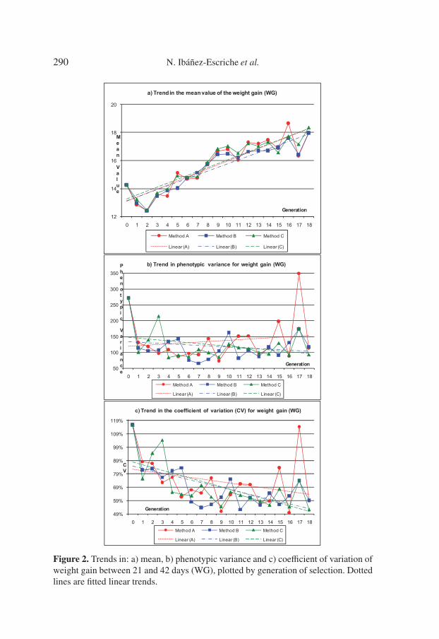
In order to visually check the observed evolution of the variability acrossgenerations, we plotted the trend in phenotypic mean of WG, the phenotypicvariance of WG computed directly from the data, and the coefficient of vari-ation for WG (Fig. 2). Mean WG seems to have increased with generationas a consequence of the selection process. However, the phenotypic variancedid not decrease as would be expected as a correlated response. On the con-trary, the trends corresponding to the coefficient of variation seem to have beennegative and showed that a correlated canalised response may have effectivelybeen achieved. However, this correlated canalised response seems to be insuf-ficient to affect the sign of the trends in phenotypic variances over generations,even though there could be several reasons acting on the phenotypic variabil-ity, for example the Bulmer effect [3] at the beginning of the experiment, theinbreeding, the drift or the response variability. Since the mean of the traitincreased across generations and the coefficient of variation decreased, whilethe phenotypic variance did not decrease, a scale effect seems to have actedon the variance, somehow compensating for the correlated canalised response.However, these trends are only exploratory signs and should be confirmed byestimating genetic trends from BLUP values of animals.

The present analysis confirms the existence of additive genetic control ofthe environmental variability, which has been widely reported by other au-thors [1, 4, 8, 14, 16, 17, 20, 27] for different species and traits. If the environ-mental variability is computed for the upper and the lower limits of the 95%highest posterior density interval of u∗, a ratio of 4 to 6 is found between thecorresponding environmental variability depending on the trait.


12

14

16

18

20

0 1 2 3 4 5 6 7 8 9 10 11 12 13 14 15 16 17 18

a) Trend in the mean value of the weight gain (WG)

Method A Method B Method C


Generation

Mean

Value

50

100

150

200

250

300

350

0 1 2 3 4 5 6 7 8 9 10 11 12 13 14 15 16 17 18

b) Trend in phenotypic variance for weight gain (WG)



Generation

Phenotypic

Variance

49%

59%

69%

79%

89%

99%

109%

119%

0 1 2 3 4 5 6 7 8 9 10 11 12 13 14 15 16 17 18

c) Trend in the coefficient of variation (CV) for weight gain (WG)



Generation

CV

Figure 2. Trends in: a) mean, b) phenotypic variance and c) coefficient of variation ofweight gain between 21 and 42 days (WG), plotted by generation of selection. Dottedlines are fitted linear trends.


Additive genetic component controlling environmental variability was es-timated on the residual variance. Even though, canalised correlated responseis likely to decrease the environmental variance, other factors without geneticcontrol can induce an increase in this variance thus preventing a phenotypicresponse of a reduction of the variability of the selected trait. San Cristobal-Gaudy et al. [29] suggested the possibility of defining a selection index com-bining breeding values for the mean and environmental variance of a giventrait in order to optimise a selection program. Our results suggest that beforeimplementing such a selection index, further studies are required to understandthe functional relationship between mean and variance and their influence onthe expected correlated response. Thus, it would be desirable to explore othermodels [36] with different relationships between mean and variance. Anotherpossibility would be to validate the models by comparing their expected re-sponse to selection with a selection experiment for variability.

ACKNOWLEDGEMENTS

The authors are highly grateful to Loys Bodin and Magali San Cristobalfor their encouragement and help at the beginning of this research line. Thisresearch was partially funded by CCG06-UCM/SAL-1153 from the UniversityComplutense of Madrid. We thank Dr. Félix Goyache for comments on themanuscript.

REFERENCES

[1] Bodin L., Robert-Granié C., Larzul C., Allain D., Bollet G., Elsen J.M., GarreauH., Rochambeau H., Ross M., San Cristobal M., Twelve remarks on canalisa-tion in livestock Production, in: Proceedings of 7th World Congress on GeneticsApplied to Livestock Production, 19–23 August 2002, Montpellier, France,pp. 413–416.

[2] Bolet G., Garreau H., Joly T., Theau-Clement M., Falieres J., Hurtaud J.,Bodin L., Genetic homogenisation of birth weight in rabbits: Indirect selectionresponse for uterine horn characteristics, Livest. Sci. 111 (2007) 28–32.

[3] Bulmer M.G., The Mathematical Theory of Quantitative Genetics, ClarendonPress, Oxford, UK, 1985.

[4] Damgaard L.H., Rydhmer L., Lovendahl P., Grandinson K., Genetic parametersof within litter variation in piglet weight at birth and at three weeks of age inlitters born of Swedish Yorkshire sow, in: Proceedings of the EAAP 52nd AnnualMeeting, 2001, Budapest, Hungary, p. 54.

[5] Eisen E.J., Prasetyo H., Estimates of genetic parameters and predicted selectionresponses for growth, fat and lean traits in mice, J. Anim. Sci. 66 (1988) 1153–1165.


[6] Falconer D.S., Selection for large and small size in mice, J. Genet. 51 (1953)470–501.

[7] Fernández J., Moreno A., Gutiérrez J.P., Nieto B., Piqueras P., Salgado C., Directand correlated selection response for litter size and litter weight at birth in thefirst parity in mice, Livest. Prod. Sci. 53 (1998) 217–237.

[8] Garreau H., Bolet G., Hurtaud J., Larzul C., Robert-Granié C., Ros M., SaleilG., San Cristobal M., Bodin L., Homogeneización genética de un carácter.Resultados preliminares de una selección canalizante sobre el peso al nacimientode los gazapos, in: Proceedings of the XII Reunión Nacional de Mejora GenéticaAnimal, 2004, Las Palmas.

[9] Garrick D.J., van Vleck L.D., Aspects of selection for performance in severalenvironments with heterogeneous variances, J. Anim. Sci. 65 (1987) 409–421.

[10] Garrick D.J., Polak E.J., Quaas R.L., Variance heterogeneity in direct and ma-ternal weight traits by sex and percent purebred for Simmental sired calves, J.Anim. Sci. 67 (1989) 2515–2528.

[11] Gaskins C.T., Snowder G.D., Westman M.K., Evans M., Influence of bodyweight, age, and weight gain on fertility and prolificacy in four breeds of ewelambs, J. Anim. Sci. 83 (2005) 1680–1689.

[12] Geweke J., Evaluating the accuracy of sampling-based approaches to the cal-culation of posterior moments, in: Bernardo J.M., Berger J.O., Dawid A.P.,Smith A.F.M. (Eds.), Bayesian Statistics 4, Oxford University Press, Oxford,UK, 1992, pp. 169–193.

[13] Geyer C.J., Practical Markov chain Monte Carlo, Stat. Sci. 7 (1992) 473–511.[14] Gutiérrez J.P., Nieto B., Piqueras P., Ibáñez N., Salgado C., Genetic parameters

for canalisation analysis of litter size and litter weight traits at birth in mice,Genet. Sel. Evol. 38 (2006) 445–462.

[15] Hill W.G., On selection among groups with heterogeneous variance, Anim. Prod.39 (1984) 473–477.

[16] Högberg A., Rydhmer L., A genetic study of piglet growth and survival, ActaAgric. Scand. Sect. A, Anim. Sci. 50 (2000) 300–303.

[17] Huby M., Gogué J., Maignel L., Bidanel J.P., Corrélations génétiques entre lescaractéristiques numériques et pondérales de la portée, la variabilité du poids desporcelets et leur survie entre la naissance et le sevrage, J. Rech. Porc. 35 (2003)293–300.

[18] Hutjens F., Revisiting feed efficiency and its economic impact, Newsletter (IlliniDairyNet), 6-6-05, 2005.

[19] Ibáñez-Escriche N., Models for residual variance in quantitative genetics, an ap-plication to rabbit uterine capacity, Tesis Doctoral, Univ. Valencia, 2006.

[20] Ibáñez-Escriche N., Varona L., Sorensen D., Noguera J.L., A study of hetero-geneity of environmental variance for slaughter weight in pig, Animal 2 (2008)19–26.

[21] Jaffrézic F., White I.M.S., Thompson R., Hill W.G., A link function approach tomodel heterogeneity of residuals variances over time in lactation curve analyses,J. Dairy Sci. 83 (2000) 1089–1093.

[22] Malik R.C., Genetic and physiological aspects of growth body composition andfeed efficiency in mice: A review, J. Anim. Sci. 58 (1984) 577–590.


[23] Meyer K., 1998, DFREML – version 3.0 B – User Notes,http://agbu.une.edu.au/∼kmeyer/dfreml.html [consulted: 24 August 2006].

[24] Moreno A., Optimización de la respuesta a la selección en “Mus musculus” conconsaguinidad restringida, Tesis Doctoral, UCM, T22287, 1998.

[25] Poignier J., Szendrö Z.S., Levai A., Radnai I., Biro-Nemeth E., Effect of birthweight and litter size at suckling age on reproductive performance in does asadults, World Rabbit Sci. 8 (2000) 103–109.

[26] Ríos J.G., Nielsen M.K., Dickerson G.E., Selection for postweaning gain in rats:II. Correlated response in reproductive performance, J. Anim. Sci. 63 (1986)46–53.

[27] Ros M., Sorensen D., Waagepetersen R., Dupont-Nivet M., San Cristobal M.,Bonnet J.C., Mallard J., Evidence for genetic control of adult weight plasticityin the snail Helix aspersa, Genetics 168 (2004) 2089–2097.

[28] Sánchez J.P., Baselga M., Silvestre M.A., Sahuquillo J., Direct and correlatedresponses to selection for daily gain in rabbits, in: Proceedings of the 8th WorldRabbits Congress, 2004, Puebla-México, pp. 169–174.

[29] San Cristobal-Gaudy M., Elsen J.M., Bodin L., Chevalet C., Prediction of theresponse to a selection for canalisation of a continuous trait in animal breeding,Genet. Sel. Evol. 30 (1998) 423–451.

[30] San Cristobal-Gaudy M., Bodin L., Elsen J.M., Chevalet C., Genetic componentsof litter size variability in sheep, Genet. Sel. Evol. 33 (2001) 249–271.

[31] Schneiner S.M., Lyman R.F., The genetics of phenotypic plasticity. II. Responseto selection, J. Evol. Biol. 4 (1991) 23–50.

[32] See M.T., Heterogeneity of (Co) variance among herds for backfat measures ofswine, J. Anim. Sci. 76 (1998) 2568–2574.

[33] Sorensen D., Waagepetersen R., Normal linear models with genetically struc-tured variance heterogeneity: A case study, Genet. Res. 82 (2003) 207–222.

[34] Spiegelhalter D.J., Best N.G., Carlin B.P., van derLinde A., Bayesian measuresof model complexity and fit, J. R. Statist. Soc. Series B 64 (2002) 583–639.

[35] Vergara Martín J.M., Fernández-Palacios H., Robaina L., Jauncei K.,De la Higuera M., Izquierdo M., The effects of varying dietary protein levelon the growth, feed efficiency, protein utilization body composition of giltheadsea bream fry, Fish. Sci. 62 (1996) 620–623.

[36] Zhang X.-S., Wang J., Hill W.G., Evolution of the environmental component ofthe phenotypic variance: stabilizing selection in changing environments and thecost of homogeneity, Evolution 59 (2005) 1237–1244.

Genetic parameters related to environmental variability of weight traits in a selection experiment...

Documents

Transcript of Genetic parameters related to environmental variability of weight traits in a selection experiment...