Generalized ellipsoids and anisotropic filtering for segmentation improvement in 3D medical imaging

Generalized ellipsoids and anisotropic filtering for segmentation

improvement in 3D medical imaging

R. Dosil*, X.M. Pardo

Departamento de Electronica e Computacion, Universidade de Santiago de Compostela, Monte de condesa, Campus Sur,

Santiago de Compostela 15782, Spain

Received 6 August 2001; received in revised form 8 November 2002; accepted 14 January 2003

Abstract

Deformable models have demonstrated to be very useful techniques for image segmentation. However, they present several weak points.

Two of the main problems with deformable models are the following: (1) results are often dependent on the initial model location, and (2) the

generation of image potentials is very sensitive to noise. Modeling and preprocessing methods presented in this paper contribute to solve

these problems. We propose an initialization tool to obtain a good approximation to global shape and location of a given object into a 3D

image. We also introduce a novel technique for corner preserving anisotropic diffusion filtering to improve contrast and corner measures.

This is useful for both guiding initialization (global shape) and subsequent deformation for fine tuning (local shape).

q 2003 Elsevier Science B.V. All rights reserved.

Keywords: Registration; Deformable models; Segmentation; Anisotropic diffusion; Surface patch saliency; 3D medical images

1. Introduction

A deformable model [12] is an energy minimization

method, where the energy functional is defined in terms of

intrinsic shape attributes (internal energy) and desired

image features (external potential), such as gradient and

curvature. The external potential originates forces that

attract the model to specific image features while the

internal energy causes stress forces that try to maintain

model continuity and smoothness. When forces are

balanced, the model reaches equilibrium, and the geometric

deformation finishes. Therefore, the model deforms itself

from its initial location to approach the nearest energy

minimum, which maybe does not correspond to the target

object surface. Deformable matching can efficiently deal

with small and local shape changes, but fails if global

misalignment is too large. It is very important that the

starting model location and the object boundary are near

enough, so a good initialization method should be valuable.

When deformable models are applied to 3D medical

data, two kinds of segmentation are possible: 2 12

D (slice by

slice) and 3D. Initialization is simpler for 2 12

D segmenta-

tion, since it is applied just to the first slice. Each slice is

initialized with the result of the previous one. Manual

edition of initial 3D surfaces is very laborious, and the

automatic or semiautomatic initialization is usually more

complex than the 2D counterpart. As a counterweight to the

low robustness due to the usual low accuracy in initializa-

tion, deformable surface models have the power to ensure

smoothness and coherence in 3D shapes.

In deformable model literature, we can find different

approaches to cope with the initialization problem in 3D.

Some approaches are based on the incorporation of

balloon forces to overcome potential minima. McInerney

and Terzopoulos [16], for example, used a balloon model

to initialize the ventricle tracking in MRI data. The main

difficulty with this scheme is concerned with the inherent

trade-off in the choice of the inflation/deflation force.

Other approaches are based on the manual or semiauto-

matic selection of anchor points. Among them is the

imposition of interactive constraints in the form of springs

and volcanos [12], and more recently the method of

Neuenschwander et al. [20], that allows the user to fix a set

0262-8856/03/$ - see front matter q 2003 Elsevier Science B.V. All rights reserved.

doi:10.1016/S0262-8856(03)00006-4

Image and Vision Computing 21 (2003) 325–343

www.elsevier.com/locate/imavis

* Corresponding author. Fax: þ34-981-528012.

E-mail addresses: [email protected] (R. Dosil), [email protected] (X.M.

Pardo).

http://www.elsevier.com/locate/imavis

of seed points and their normal vectors, which cannot be

changed during deformation.

Some authors propose multiple initialization through

several seed models. During the deformation process,

several initial models will merge and the superfluous ones

should be removed. This solution was used, among others,

by Tek and Kimia [30] and Leonardis et al. [14]. Important

decisions have to do with: (1) the number and location of

initial seed models, (2) the stopping criteria of the seed

growing process, and (3) choosing one result among the

final models.

Fully automatic initialization can be achieved by

matching the object in the image with a prototype, as

done by Bajcsy and Kovacic [1] who used brain atlases in

their specific-purpose initialization techniques. There are

several problems with the deformable atlas approach. The

technique is sensitive to initial positioning of the atlas and

the presence of neighboring features may cause matching

problems. One solution is to use image preprocessing in

conjunction with the deformable atlas; Sandor and Leahy

[25] used this approach.

Several researchers, as Cootes et al. [6], and Staib et al.

[29], augmented snake-like models with prior information

about typical mean shapes and normal variations. A number

or researchers have incorporated knowledge about object

shape using deformable shape templates. Among them,

super-quadrics have gained popularity in medical image

research [11,17,31].

The segmentation of human organs from CT or MR

images is a good example where model-based reconstruc-

tion can be applied. The model-based reconstruction

problem can be stated in two (no necessarily disjoint)

phases [7]: registration and free form deformation. On the

one hand, registration describes a transformation with far

less degrees of freedom than the free form deformations.

Therefore, their ability to represent shape variations is less

important than the free form deformation. On the other

hand, because of their restricted degrees of freedom, they

tend to be more robust than free form deformations.

Therefore, the first is better for describing global shape

and location and the second is better in detecting fine details.

In this work, we propose a fully automatic initialization

method (registration) based on matching 3D data with

models that comprise global shape and high level feature

information. The main idea is to perform the initialization

phase not taking into account the relevance of individual

point features, but the properties and global saliency of

connected point features (surface patches in 3D). The

method includes the construction of a priori models from

test images. Both shape model construction from test

images and matching with a new image are achieved by

means of fitting a parametric surface to a cloud of points

belonging to the object boundary. This parametric surface is

represented by a generalized ellipsoid scheme. Boundary

points are extracted from the image, grouped in patches and

finally selected according to high level properties. In this

way, we try to extend to 3D the ideas developed in a

previous paper [21] where a priori knowledge on contour

segments was used in order to obtain an improved

initialization of 2D deformable models.

Extraction of boundary points is not a critical step

because the relevance of the point feature depends on all the

neighbors in the same surface patch, and matching with

global shape models is very robust. However, accuracy in

boundary detection has certain influence in the size of

detected surface patches and contributes to eliminate noise

influence.

Noise elimination and boundary detection can be

achieved simultaneously using the derivative of Gaussian

filter, but this presents several drawbacks, such as false

negatives and dislocation of gradient maxima at great

scales, and false positives at low scales. Non-linear diffusion

methods [32] permit noise elimination while preserve

meaningful structures. They simulate a heat-spreading

phenomenon in which diffusivity depends on local proper-

ties of the image. Perona and Malik [22] introduced a

gradient dependent diffusion coefficient to stop diffusion at

boundary points, eliminating boundary blurring but also

maintaining noise at boundary points. Weickert [33]

proposed a non linear anisotropic diffusion method to

smooth surfaces just along the tangent plane at boundary

points, reducing noise also at boundaries without blurring.

The shortcoming of Weickert’s approach to anisotropic

diffusion is that it causes a rounding effect on corners.

Anisotropic diffusion has been frequently used in

medical image processing [10,13,26]. In particular, Krissian

et al. [13] have already applied it to surface extraction

successfully. They developed a directional anisotropic

diffusion technique to enhance surface extraction on vessel

images, obtaining better results than the ones provided by

Gaussian filtering. In their approach, diffusivity in the

maximum curvature direction is annulated to reduce the

rounding problem. This is made at the expense of noise

reduction in the aforementioned direction. The second

contribution of the present work is to introduce a corner-

preserving anisotropic diffusion method, as a preprocessing

tool to improve gradient and corner measure and detection.

This is achieved by defining curvature dependent diffusion

coefficients. The incorporation of the preprocessing step

represents an incoming for both initialization, improving

surface detection, and deformation too, since false minima

elimination and correct placement of boundaries and

corners improves the external potential definition. More-

over, the curvature-based approach proposed in this paper

leads to a better location of gradient potential minima and

enhancement of the curvature based potential, as the

rounding problem is avoided.

The paper is organized as follows. In Section 2, an

overview of the complete initialization methodology is

described. In Section 3, the generalized ellipsoid model is

defined. Section 4 presents the optimization technique used

for model construction and matching. In Section 5 all

R.D. Lago, X.M. Pardo / Image and Vision Computing 21 (2003) 325–343326

the preprocessing steps are described. These are, image

denoising, boundary surface patch detection and patch

classification. Finally, in Section 6 efficacy of the whole

process is studied, paying special attention to its robustness

in the presence of noise and loss of information caused by

contrast variations over surfaces.

2. Initialization methodology

The goal of 3D reconstruction methods is to obtain a

detailed description of objects present in a volume data. To

this end, deformable models are a good choice, because they

possess great flexibility and guarantee certain smoothness

and continuity properties. The problem with deformable

models is that they interact locally with image features. It is

necessary to define a good starting geometric configuration

to ensure the success of the deformation process. The initial

surface must be close to the boundary of the object of

interest, which implies to determine position, orientation

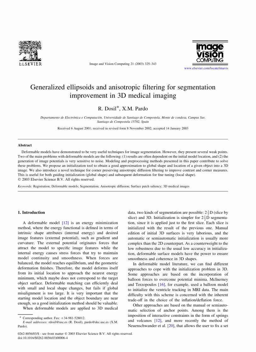
and global structure of that object in the 3D domain. Fig. 1

shows the initialization process proposed in this paper.

The attainment of a high level description of certain

object is separated in two stages: (1) modeling of global

shape of the object class and (2) matching the class model

with the instance object. The first stage is performed off-line

over a set of sample shapes of the same object class (Fig. 1,

step 1). The resulting class model is called the a priori

model. The sample images are segmented manually to avoid

typical automatic segmentation problems and then a surface

prototype is extracted from them. Afterwards, global shape

of the object surface prototype is determined by fitting

a mathematical model to it. To represent global shape we

have chosen the generalized ellipsoid model, also called

superquadric.

Once an a priori model is available, position, orientation

and scale of an instance object in a new image is determined

by a matching technique. To perform matching it is

necessary to extract some feature from the image that

describes the object surface properly and to find the

transformations that lead to a correspondence between

image features and model surface. In this work surface

points are used as image features (Fig. 1, step 2). The

extraction of such low level features from gradient

information is not robust. Again, the use of prior knowledge

is needed to distinguish the target object surface points from

others present in the image as, for example, points

belonging to structures other that the one under study or

noise artifacts. To this end, points are not considered

individually, but they are grouped in patches. Resulting

patches are characterized by some of their average proper-

ties as, for example, area, contrast or shape descriptors, and

these are used in a selection process to exclude undesired

patches (Fig. 1, step 3). The starting surface for deformation

is obtained after matching between model and object (Fig. 1,

step 4). This is done by finding the parameters of the rigid

transformation that minimizes an error function related to

the distances from selected image points to the parametric

surface.

In short, what is presented here is a method that takes

advantage from both bottom-up and top-down processes.

Initialization is accomplished by obtaining higher and

higher level descriptions of image contents: from volume

points with associated gray levels, to boundary point

Fig. 1. Sequence of steps to achieve the starting configuration for the deformable model.

R.D. Lago, X.M. Pardo / Image and Vision Computing 21 (2003) 325–343 327

representation, from boundary points to surface patches,

featured by local and global descriptors that allow

discriminating between desired and spurious patches, and

from surface patches to a global surface model with the help

of prior knowledge. The next stage, not described here,

would walk the inverse way. Starting from the coarse

representation of the surface resulting from initialization,

the deformation process introduces local degrees of freedom

to reach a detailed description of the surface object. Thus,

the conflicting goals of high robustness and high resolution

can be achieved.

3. Global shape models

An initial model must capture the most important

structural aspects of the object to be reconstructed. In this

way, the global energy minimum is accessible from the

starting configuration. In the one hand, a priori models must

be represented using a scheme that ranges all possible

shapes in certain application. In the other hand, the shape

model should depict structural information to get robust-

ness. As a trade-off between these goals, the generalized

ellipsoid model is chosen for this application.

3.1. Generalized ellipsoids

Generalized ellipsoids [11,27] are represented by a

family of parametric surfaces. A set of few parameters

offers a high level description of surface shape. Despite their

simplicity, they bring high flexibility. Their explicit

equations are

x ¼ a1 cos11ðuÞcos12ðfÞ; y ¼ a2 cos11ðuÞsen12ðfÞ;

z ¼ a3 sen11ðuÞ; with2p=2 # 0 , p=2

2p # f , p

(ð1Þ

They can be expressed in implicit form

f ðr;qÞ ¼ ½ðx=a1Þ2=12 þ ðy=a2Þ

2=12�12=11 þ ðz=a3Þ2=11 ¼ 1 ð2Þ

where q is the parameter vector and r a point over the

surface. For the surface to be defined in the whole range of u

and w; the power operation has been redefined to be

u1 U signðuÞlul1 ð3Þ

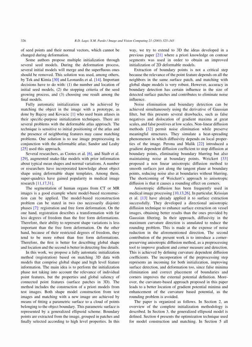
Sizes of the super-quadric in the coordinate directions are

represented by parameters a1; a2 and a3; while 11 and 12 are

the squareness parameters in the latitude and longitude

planes, respectively. Fig. 2 shows some shapes that can be

obtained with this representation for different values of the

squareness parameters.

In Eqs. (1) and (2) the center of the ellipsoid is

considered to be placed in the origin of coordinates and

its principal axes along the coordinate axis. The incorpor-

ation of rigid transformation parameters permits arbitrary

positioning and orientation in space. Translation T and

rotation R transformations imply adding six extra par-

ameters, three displacements in the coordinate directions

and three Euler angles. The expression of a transformed

surface point r0 is given by

r0 ¼ TRr ¼ Rr þ t ð4Þ

where t is the translation vector.

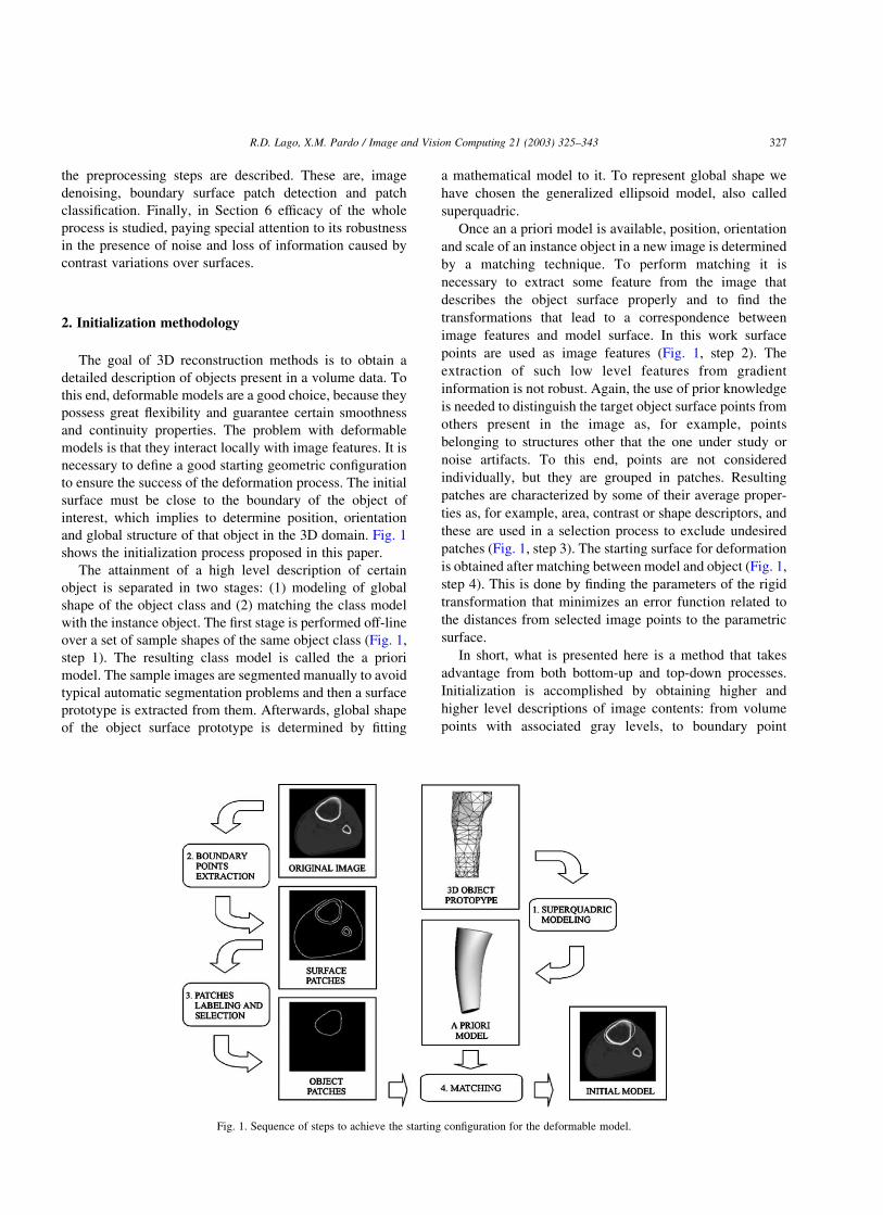
3.2. Global deformations

Even though superquadric representation is very flexible

in relation to its number of parameters, it is not enough for

many applications because is limited to symmetric shapes.

The variety of possible shapes can be extended applying

global deformations, as tapering, twisting and bending

transformations.

Tapering involves a linear transformation of the

transverse section along z axis (Fig. 3a). If the variation

rates along x and y axis are Cx and Cy; respectively, the

expression of a transformed point is

x0 ¼ ðCxz=a3 þ 1Þx; y0 ¼ ðCyz=a3 þ 1Þy; z0 ¼ z;

with 2 1 # Cx; Cy # 1

ð5Þ

Twisting (Fig. 3b) of the transverse section along z axis is

described by a parameter u that represents twisted angle per

Fig. 2. Superquadric surfaces for different 11 and 12 values.

Fig. 3. Global deformations.


z unit. Surface points are transformed as follows

x0 ¼ x cosðzuÞ2 y senðzuÞ;

y0 ¼ x senðzuÞ þ y cosðzuÞ; z0 ¼ z

ð6Þ

When bending is applied, z axis is transformed into an arc of

circumference with curvature k (Fig. 3c). If w is the angle

between the x axis and the line that connects the center of

the superquadric and the circumference, then

x0 ¼ x þ cosðwÞðr0 2 rÞ; y0 ¼ y þ senðwÞðr0 2 rÞ;

z0 ¼ senðgÞð1=k 2 rÞ

ð7Þ

where

r ¼ cosðw2 arctanðy=xÞÞ

ffiffiffiffiffiffiffiffiffix2 þ y2

q;

r0 ¼ 1=k 2 cosðgÞð1=k 2 rÞ; g ¼ zk

ð8Þ

These transformations are not commutative, so it is

necessary to specify an order of application. Next sequence

has been taken in this work

r0 ¼ Translation+Rotation+Tappering+Twisting+BendingðrÞ

according to the criterion followed in Refs. [15,27].

4. Shape matching

To represent a surface with the generalized ellipsoid

model is necessary to determine a parameter vector with 16

components

q ¼ ða1; a2; a3; 11; 12; t1; t2; t3;a;b; g;Cx;Cy; u; k;wÞ

Matching involves finding the parameter vector that best fits

the extracted surface patches. In the matching process, only

translation and rotation parameters are to be determined to

put the object prototype into correspondence with surface

data. In addition, a scale parameter a0 must be included to

account for the relative size of the object in the image.

To accomplish registration it is necessary to define a

measure of parameter vector fitness or an error function that

measures the difference between the model surface and the

object surface patches. Here, error function minimization in

the least squares sense has been adopted as the optimization

criterion. The error function E is constructed from the

individual distances D between each image feature location

and the surface model,

E2ðqÞ ¼XNi¼1

D2ðri;qÞ ð9Þ

where q is the parameter vector, ri is an image point

belonging to the object boundary, and N is the total number

of image points.

4.1. Error functions

Direct calculus of the distance between a point and an

implicit surface is computationally expensive. For that

reason, it is convenient to replace it with an approximation.

Most commonly used approaches derive from the fact that

the implicit function f ðr;qÞ is a monotonic function of the

radial distance d; i.e. distance taken over the line that

connects the point r and the superquadric center. Function f

verifies the next properties

f ðr;qÞ ¼ 1 when r is on the surface

f ðr;qÞ . 1 when r is outside the surface

f ðr;qÞ , 1 when r is inside the surface.

The following are some approximations to the distance

function

D1 ¼ f ðr;qÞ2 1 ð10Þ

D2 ¼ f 11ðr;qÞ2 1 ð11Þ

D3 ¼ ða1a2a3Þ1=2{f 11ðr;qÞ2 1} ð12Þ

D4 ¼ d ¼ k~rk{1 2 1=f 11ðr; qÞ} ð13Þ

D5 ¼ lf 11=2ðr;qÞ2 1l=k7f 11=2ðr; qÞk ð14Þ

Whaite and Ferrie [34] realized an analysis of the behavior

of error functions D1; D2; D3 and D4: They concluded that

D1 and D2 are not satisfactory error metrics, because they

bring biased results. Function D5 [1] requires the calculus of

the gradient of the implicit surface, which is computation-

ally expensive. In this work, error function D4 [27] has been

chosen to be used in the optimization stage.

4.2. Genetic algorithm

Optimization of the quadratic error function has been

performed using a genetic algorithm (GA) [8]. GAs have

been already employed in generalized ellipsoids optim-

ization in the work of Linares et al. [15]. The principal

benefits brought by the use of this technique are: (1) it

ensures convergence to the optimal solution, (2) it is not

necessary to make an initial estimation of the solution,

(3) it is very stable in relation to the selected error

function, (4) it permits to explore wide regions in the

space of solutions, (5) constraints are very easy to

manage, (6) it is suitable for complex error functions, as

no function analysis is to be made, and (7) it is

appropriate for functions defined in spaces with high

dimensionality.

On the contrary, GAs have an important shortcoming:

slow convergence. This problem can be alleviated exploit-

ing its intrinsic parallelism. The fact that the range of some

parameters can be bounded reduces the convergence time as

well. Furthermore, some parameters can be easily initialized

[1,27]. It is especially important to reduce the space of

solutions in the matching process, because the modeling


stage is done off-line. The translation vector can be taken to

be the center of gravity of the surface, assigning unit mass to

each point. Euler angles can be obtained from the rotation

matrix that aligns the coordinate axis with the principal

inertia axis. Scale parameter bounds can be defined in terms

of image size. In this way, probability of fast convergence is

increased. Nevertheless, any other minimization algorithm

could be employed for this task [2,4].

5. Feature extraction for matching

In general, localizing image features correspondent to

interest objects automatically is a difficult problem. Low

level vision algorithms offer detectors for features such

as edges, ridges, lines, and corners, but robust corre-

spondence between low level features and objects is still

necessary. Higher level features are more difficult to

detect reliably and more limited in number. As in 2D

[21], we propose to use ‘intermediate level features’

where the relevance of point features are not individually

computed, but it depends on features of the surface

patches they belong to.

The feature extraction stage consists of a sequence of

several steps. The image is first denoised and then a

boundary operator is applied. Afterwards, connected points

are grouped in a set of surface patches. Patches are classified

according to descriptors such as area, contrast or shape.

Those ones belonging to the target object can be selected

using prior knowledge about object class properties. Prior

knowledge is introduced in the form of selection rules.

These rules are defined as a function of descriptor values,

i.e., one must know a priori which are the expected

descriptor values associated to the object surface class

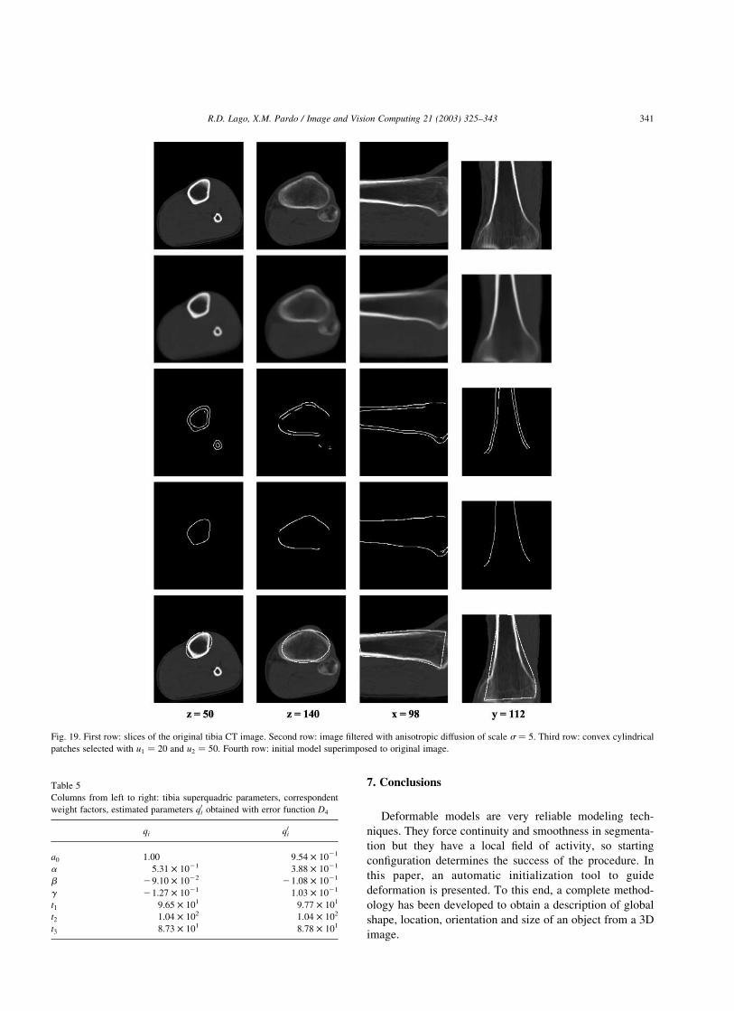
under study. For instance, results presented in the fourth row

of Fig. 19 have been obtained by selecting patches with high

area, high contrast and convex cylindrical morphology,

corresponding to the known characteristics of images from

the external surface of the tibia cortical bone. If this

selection is not realized, other structures appear, as can be

seen in the third row of Fig. 19.

Both boundary detection and calculus of shape descrip-

tors, based on curvature measures, require the computation

of directional derivatives of gray level values. The

derivative of Gaussian operator performs differentiation

and smoothing simultaneously [18,19], but it modifies

gradient maxima position, dislocating surfaces. Moreover,

small structures can be eliminated. Non-linear anisotropic

filters offer better results [3,10,13,22,24,26,32,33].

In this work, a corner preserving an isotropic filter has

been developed to smooth 3D images without alter gradient

and curvature values neither misplacing boundaries nor

rounding corners. After image denoising, derivatives are

approximated by central differences. Next subsections

describe the main steps in feature extraction: anisotropic

smoothing, boundary detection, and surface patch selection.

5.1. Anisotropic diffusion

Let us introduce the general method for diffusion filtering

in 3D proposed by Weickert [33]. Let V be a 3D image

domain and ›V its boundary. Given an image Iðx; y; zÞ; its

filtered version uðx; y; z; tÞ is obtained by the next

expression, with reflecting boundary conditions

›tuðx; y; z; tÞ ¼ 7ðCðk7ukÞ7uðx; y; z; tÞÞ on V £ ð0;1Þ;

uðx; y; z; t ¼ 0Þ ¼ Iðx; y; zÞ on V;

kC7uðx; y; z; tÞ;nl ¼ 0 on ›V £ ð0;1Þ

ð15Þ

where n is the outer normal, k·; ·l; is the inner product and

subscripts stand for partial derivatives. In the isotropic case,

the diffusion coefficient C is a scalar magnitude. Usually, it

is a decreasing function of k7uk with values belonging to the

interval [0,1]. In this way, diffusion is stopped in the

presence of boundaries.

Previous expression is often related to the energy

minimization formulation. The energy functional EðuÞ is

defined as the integral over the image of a potential Fðk7ukÞ:Eq. (15) is obtained by applying the gradient descent

method to minimize the energy functional. Both approaches

are related by

Cðk7ukÞ ¼ F0ðk7ukÞ=k7uk ð16Þ

Using this relation and operating with Eq. (15), next

expression for non linear isotropic diffusion can be obtained

ut ¼ F00ujj þ ðF0=k7ukÞðDu 2 ujjÞ ð17Þ

where ujj stands for the second derivative of u in the normal

direction j: A possible choice for the potential function is

the one proposed by Green [9]

FðsÞ ¼ ða2=2Þlog coshðsÞ ð18Þ

where a represents the gradient threshold at which

diffusivity stops growing. Other approaches were stated by

Perona and Malik [22] and Charbonnier et al. [5] among

others.

A diffusion process is called anisotropic when diffusivity

takes different values {l1;l2;l3} in different directions {e1,

e2, e3} of space. As a result, diffusivity is a tensorial

magnitude, and then, the flux vector C7u is not parallel to

the gradient direction. In the reference frame defined by the

basis {e1, e2, e3}, diffusivity turns into a diagonal tensor

D ¼ diagðl1;l2;l3Þ: The expression for the diffusion tensor

C in a general frame is C ¼ TDTT where T is the matrix

formed by the column basis vectors.

Another way of constructing an anisotropic filer is

generalizing Eq. (17), allowing independent diffusion

coefficients for each term, as done by Krissian et al. [13].

The alternative expression is attained by taking the tensorial

approach and setting the diffusivity eigenvalues such that

li ¼ Fiðk7ukÞ=k7uk; with i ¼ 1; 2, 3, and applying some


mathematical relations, obtaining

ut ¼ F001ujj þ ðF0

2=k7ukÞuh1h1þ ðF0

3=k7ukÞuh2h2ð19Þ

Using this approach to filter an image for a given time t is

faster than using the tensorial approach, because the

second derivatives of u in the extreme curvature directions

can be computed directly without calculating the Hessian

eigenvectors, using the next relation

uh1h1¼ 2k7ukk1 uh2h2

¼ 2k7ukk2 ð20Þ

where k1 and k2 are the maximum and minimum curvatures,

respectively.

A typical scheme for anisotropic diffusion is con-

structed by setting diffusivities associated to tangent

directions to constant values, while taking a decreasing

function of k7uk in the gradient direction. Thus, diffusion

is stopped in the presence of boundaries only in the normal

direction but not in the tangent plane, eliminating noise

also at surfaces.

5.1.1. Corner preserving diffusion

Smoothing in the tangent directions lessens curvature

values as the system evolves. This effect eliminates noise by

flattening surfaces, but also alters the shape of objects,

eliminating small details and rounding corners. One way to

prevent rounding is avoiding diffusion in the maximum

curvature direction. In this way, the highest curvature value

is not modified but, consequently, noise is maintained in the

correspondent direction too.

A better choice would be reducing diffusion only in

the presence of corners, while keeping it at flat regions

or surfaces where the tangent vectors variation is smooth.

In this work, we propose such a diffusion method. To

this aim, diffusivity in the maximum curvature direction

has been modified in relation to the isotropic approach to

introduce a dependency on a certain corner measure c:

This diffusion coefficient is expected to be high in the

absence of corners and decrease as the corner measure

grows. This behavior can be modeled with the Green

function presented for contrast preserving filtering, just

by changing the boundary detector by a corner detector

and the gradient threshold by a corner threshold b:

Therefore, diffusion coefficients in Eq. (19) are

F001 ¼ cosh22ðk7uk=aÞ F0

2=k7uk ¼ tanhðlc=bÞb=c

F03=k7uk ¼ 1

ð21Þ

The corner detector is related to the local principal

curvatures of the image. Curvature measures the variation

of the tangent vector with the arc length in some

direction, but it cannot be considered as a corner detector

itself, because high curvature values can be originated by

noise. To distinguish between real features and noise

artifacts, curvature is usually multiplied by some power

of the gradient magnitude. Different approaches for

a corner detector with these characteristics are studied

and compared by Sporring et al. [28]. Among the various

possibilities discussed there, here it has been selected

next

c ¼ k7uk·lkmaxl ð22Þ

As a result, an image point is considered a corner when

both its gradient modulus and its maximum curvature

have high values. Higher order powers of the gradient

modulus can reject corners from structures with low

contrast.

The selection of the threshold values a and b is crucial in

the accuracy of the obtained results, since they establish

whether a feature must be smoothed or preserved. To obtain

automatic parameter estimation, a tool from robust statistics

[3,23] is employed. The median absolute deviation about the

median, MAD, is taken as a measure of the robust scale se

of some magnitude. If medianI is the median of some

magnitude computed from all points belonging to image I;

then the robust scale for gradient is

se ¼ MADðk7IkÞ=0:6745

¼ medianI½k7Ik2 medianIðk7IkÞ�=0:6745 ð23Þ

The constant 0.6745 is the MAD of a zero-mean normal

distribution with unit variance. Scale se is the contrast value

at which flux must stop growing. If the stopping criterion is

to reach a certain fraction x of the asymptotic limit of the

isotropic flux function f1; parameter a can be related to se

by f ðk7Ik ¼ se;aÞ ¼ x·f1: For the Green function f1 ¼ a;

so the threshold parameter is

a ¼ se=atanhðxÞ ð24Þ

Here, it has been taken x ¼ tanhð1Þ ¼ 0:7619; so that a ¼

se: The same estimation can be done for b; computing

MADIðcÞ:

5.2. Boundary detection

Once the image is smoothed, directional derivatives can

be computed using a central finite differences scheme. An

image point is considered a surface point if it is a local

maximum of the gradient modulus. Monga and Benayoun

[18] accomplish gradient maxima detection by comparing

the modulus magnitude of each point r only with values

correspondent to previous and next points in the gradient

direction 7uðrÞ; represented by rþ and r2 and calculated by

r^ ¼ r ^ 7uðrÞ=k7uðrÞk ð25Þ

When

k7uðrÞk . {k7uðrþÞk; k7uðr2Þk} ð26Þ

r is a gradient maximum. If rþ or r2 do not coincide with an

image position, gradient modulus is approximated by

trilinear interpolation in a vicinity of r.


5.3. Surface patches selection

After gradient maxima detection, image contents are

described by a set of candidate boundary points. Now, it is

necessary to determine what points are to be used in the

fitting process. To this end, a collection of surface points is

not an appropriate description of image objects, since points

do not carry information about which object they belong to

and what is the global aspect of that object. Simple

thresholding of individual point attributes, as gradient

modulus or curvatures, can cause discontinuities on relevant

surfaces due to local fluctuations. Furthermore, not only

structures under study are recovered, but also undesired

surfaces or noise artifacts can appear.

For those reasons, boundary point representation of

image objects is replaced by a higher level description.

Extending the idea pointed by Pardo and Cabello [21] from

2D to 3D, gradient maxima are grouped in connected

components to obtain surface patches. Global information

about objects can be extracted from this new description as,

for example, area, contrast or shape. These global features

are used to determine the value of one unique label for each

point that indicates whether it belongs to the object surface

or not. In a more general case this label may represent the

degree in which that point can be said to belong to the

surface object. This is, each point ri belonging to certain

surface patch Pj is characterized by a label value determined

by a labeling function L such that LðriÞ ¼ LðPjÞ; ;ri [ Pj;

or what is the same, all points in a patch have the same label

value and this value is determined from the contributions of

all individual points. Labeling function dependency on

surface patch attributes is determined according to prior

knowledge about image contents. L must show great values

for patches with global descriptor values similar to the ones

expected a priori for that object class and low values for any

other patch. Therefore, an expression for L must be

constructed from those a priori descriptor values for each

object class.

To accomplish grouping, a 26-connectivity criterion is

used. Many of the points detected as gradient maxima do

not correspond to surfaces of the desired objects in the

image, but they are noise artifacts. When grouping

boundary points to construct surface patches, those points

must not be considered. Simple thresholding is not a

good technique to distinguish noise artifacts from real

surface points, as contrast, in general, is not uniform over

the object surface. Here, hysteresis thresholding is used.

Hysteresis involves defining two threshold levels. The

lowest threshold level determines whether a point

belongs to a surface. If this level is chosen appropriately,

surface fragmentation is reduced. In addition, each

connected component must have, at least, a number n

of points with gradient greater or equal to the other

threshold level. This is supposed to exclude surface

patches originated by noise. Here, minimum number of

points over the highest threshold level has been taken

n ¼ 1:

Our goal is to construct a representation of the image that

emphasizes salient locations. We seek to associate a

measure of saliency, denoted by the labeling function, to

each surface patch. A property that seems to play an

important role in boundary saliency is the combination of

size, global and/or local (smoothness) shape, and contrast. A

labeling function that would account for our working

examples is one that favors long, smooth shape and high

gradient surface patches. In our proposal, smoothness is

related to curvature type or curvature variations.

The exact formulation of L can be adapted to the specific

application domain. Here, working hypotheses are that true

surfaces have higher area and higher average gradient level

than noise artifacts. In addition, they can be useful to

discriminate among various anatomical structures with

known properties. For example, cortical bone tissue in CT

images is characterized by its high contrast in relation to

muscle and trabecular bone tissues. Relative sizes of objects

are also known in general. Shape descriptors are used to

discriminate anatomical structures with different mor-

phologies. In this work Gaussian curvature K and mean

curvature H are used as shape descriptors

H ¼ ðkþ þ k2Þ=2 K ¼ kþ·k2 ð27Þ

where kþ and k2 are the extreme curvature values at each

point. Using their values, next classification of points can be

made:

H . 0 H ¼ 0 H , 0

K . 0 Concave elliptic – Convex ellipticK ¼ 0 Concave cylindrical Plane Convex cylindricalK , 0 Concave hyperbolic Saddle point Convex hyperbolic

Surface patch descriptors can be obtained from point

descriptors by averaging their values. However, the error

committed in the calculus of K is the product of the errors

correspondent to kþ and k2: As curvature values are very

sensitive to noise, results obtained for K are not very

reliable. Better results should be obtained by averaging

extreme curvatures and then using resulting values in Eq.

(27), at least for the Gaussian curvature sign, despite

meanðkþ·k2Þ – meanðkþÞ·meanðk2Þ:

Average Gaussian and mean curvature signs classify

surfaces in a very rough manner. Their utility is limited to

simple objects. If maximum and minimum curvature signs

vary strongly over the surface, average measures are no

longer descriptive of surface shape. Let us think, for

example, in the shape of a vertebra. In these cases, the

curvature variations along the surface patch can be used as a

measure of smoothness.

Labeling function must depend on those patch attributes

in such a manner that target surfaces have high label values

while the remainder patches have low values. Labels can be

used in several ways to decide how the fitting process is to

be done. A general method involves considering labels as


weighting factors in the calculus of the error function,

modulating the contribution of each surface point to the total

error. Then, the error function can be redefined in the next

way

E2ðqÞ ¼XNi¼1

LðriÞD2ðri;qÞ ð28Þ

Then, if a point belongs to a salient patch, its contribution to

the accumulated distance is decisive in the result. As label

value decreases, the influence of all points on the patch is

reduced.

6. Results

Performance of the whole methodology depends on three

aspects: the capability of the chosen model to represent

objects in an appropriate manner in certain field of

application, the efficiency of the optimization method and

the effectiveness of the preprocessing technique in surface

patches extraction. In this section, the initialization method

is tested taking all these points into account.

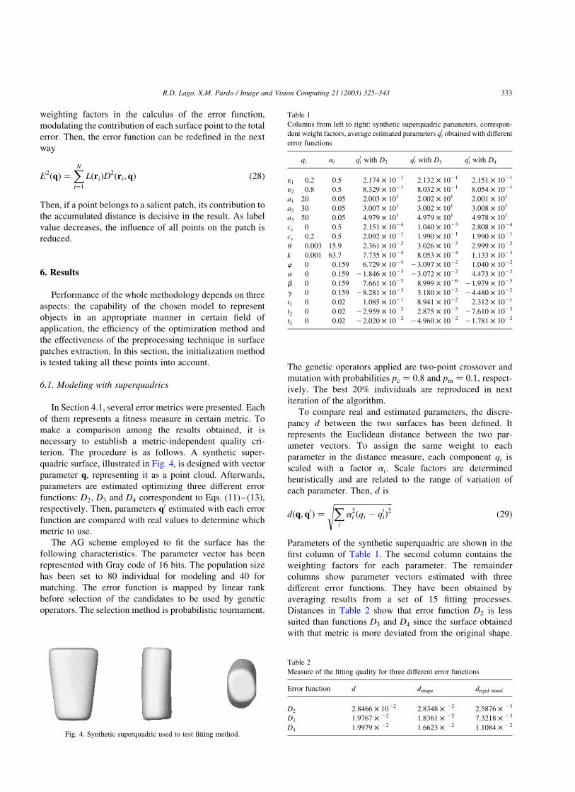
6.1. Modeling with superquadrics

In Section 4.1, several error metrics were presented. Each

of them represents a fitness measure in certain metric. To

make a comparison among the results obtained, it is

necessary to establish a metric-independent quality cri-

terion. The procedure is as follows. A synthetic super-

quadric surface, illustrated in Fig. 4, is designed with vector

parameter q, representing it as a point cloud. Afterwards,

parameters are estimated optimizing three different error

functions: D2; D3 and D4 correspondent to Eqs. (11)–(13),

respectively. Then, parameters q0 estimated with each error

function are compared with real values to determine which

metric to use.

The AG scheme employed to fit the surface has the

following characteristics. The parameter vector has been

represented with Gray code of 16 bits. The population size

has been set to 80 individual for modeling and 40 for

matching. The error function is mapped by linear rank

before selection of the candidates to be used by genetic

operators. The selection method is probabilistic tournament.

The genetic operators applied are two-point crossover and

mutation with probabilities pc ¼ 0:8 and pm ¼ 0:1, respect-

ively. The best 20% individuals are reproduced in next

iteration of the algorithm.

To compare real and estimated parameters, the discre-

pancy d between the two surfaces has been defined. It

represents the Euclidean distance between the two par-

ameter vectors. To assign the same weight to each

parameter in the distance measure, each component qi is

scaled with a factor ai: Scale factors are determined

heuristically and are related to the range of variation of

each parameter. Then, d is

dðq; q0Þ ¼

ffiffiffiffiffiffiffiffiffiffiffiffiffiffiffiffiffiffiffiXi

a2i ðqi 2 q0

iÞ2

sð29Þ

Parameters of the synthetic superquadric are shown in the

first column of Table 1. The second column contains the

weighting factors for each parameter. The remainder

columns show parameter vectors estimated with three

different error functions. They have been obtained by

averaging results from a set of 15 fitting processes.

Distances in Table 2 show that error function D2 is less

suited than functions D3 and D4 since the surface obtained

with that metric is more deviated from the original shape.

Fig. 4. Synthetic superquadric used to test fitting method.

Table 1

Columns from left to right: synthetic superquadric parameters, correspon-

dent weight factors, average estimated parameters q0i obtained with different

error functions

qi ai q0i with D2 q0i with D3 q0i with D4

11 0.2 0.5 2.174 £ 1021 2.132 £ 1021 2.151 £ 1021

12 0.8 0.5 8.329 £ 1021 8.032 £ 1021 8.054 £ 1021

a1 20 0.05 2.003 £ 101 2.002 £ 101 2.001 £ 101

a2 30 0.05 3.007 £ 101 3.002 £ 101 3.008 £ 101

a3 50 0.05 4.979 £ 101 4.979 £ 101 4.978 £ 101

cx 0 0.5 2.151 £ 1024 1.040 £ 1023 2.808 £ 1024

cy 0.2 0.5 2.092 £ 1021 1.990 £ 1021 1.990 £ 1021

u 0.003 15.9 2.361 £ 1023 3.026 £ 1023 2.999 £ 1023

k 0.001 63.7 7.735 £ 1024 8.053 £ 1024 1.133 £ 1023

w 0 0.159 6.729 £ 1024 23.097 £ 1022 1.040 £ 1022

a 0 0.159 21.846 £ 1023 23.072 £ 1022 4.473 £ 1022

b 0 0.159 7.661 £ 1025 8.999 £ 1026 21.979 £ 1025

g 0 0.159 28.281 £ 1023 3.180 £ 1022 24.480 £ 1022

t1 0 0.02 1.085 £ 1021 8.941 £ 1022 2.312 £ 1021

t2 0 0.02 22.959 £ 1023 2.875 £ 1023 27.610 £ 1023

t3 0 0.02 22.020 £ 1022 24.960 £ 1022 21.781 £ 1022

Table 2

Measure of the fitting quality for three different error functions

Error function d dshape drigid transf:

D2 2.8466 £ 1022 2.8348 £ 22 2.5876 £ 23

D3 1.9767 £ 22 1.8361 £ 22 7.3218 £ 23

D4 1.9979 £ 22 1.6623 £ 22 1.1084 £ 22


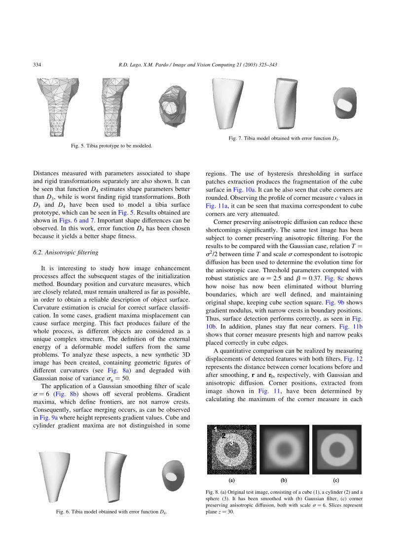
Distances measured with parameters associated to shape

and rigid transformations separately are also shown. It can

be seen that function D4 estimates shape parameters better

than D3; while is worst finding rigid transformations. Both

D3 and D4 have been used to model a tibia surface

prototype, which can be seen in Fig. 5. Results obtained are

shown in Figs. 6 and 7. Important shape differences can be

observed. In this work, error function D4 has been chosen

because it yields a better shape fitness.

6.2. Anisotropic filtering

It is interesting to study how image enhancement

processes affect the subsequent stages of the initialization

method. Boundary position and curvature measures, which

are closely related, must remain unaltered as far as possible,

in order to obtain a reliable description of object surface.

Curvature estimation is crucial for correct surface classifi-

cation. In some cases, gradient maxima misplacement can

cause surface merging. This fact produces failure of the

whole process, as different objects are considered as a

unique complex structure. The definition of the external

energy of a deformable model suffers from the same

problems. To analyze these aspects, a new synthetic 3D

image has been created, containing geometric figures of

different curvatures (see Fig. 8a) and degraded with

Gaussian noise of variance sn ¼ 50:

The application of a Gaussian smoothing filter of scale

s ¼ 6 (Fig. 8b) shows off several problems. Gradient

maxima, which define frontiers, are not narrow crests.

Consequently, surface merging occurs, as can be observed

in Fig. 9a where height represents gradient values. Cube and

cylinder gradient maxima are not distinguished in some

regions. The use of hysteresis thresholding in surface

patches extraction produces the fragmentation of the cube

surface in Fig. 10a. It can be also seen that cube corners are

rounded. Observing the profile of corner measure c values in

Fig. 11a, it can be seen that maxima correspondent to cube

corners are very attenuated.

Corner preserving anisotropic diffusion can reduce these

shortcomings significantly. The same test image has been

subject to corner preserving anisotropic filtering. For the

results to be compared with the Gaussian case, relation T ¼

s2=2 between time T and scale s correspondent to isotropic

diffusion has been used to determine the evolution time for

the anisotropic case. Threshold parameters computed with

robust statistics are a ¼ 2:5 and b ¼ 0:37: Fig. 8c shows

how noise has now been eliminated without blurring

boundaries, which are well defined, and maintaining

original shape, keeping cube section square. Fig. 9b shows

gradient modulus, with narrow crests in boundary positions.

Thus, surface detection performs correctly, as seen in Fig.

10b. In addition, planes stay flat near corners. Fig. 11b

shows that corner measure presents high and narrow peaks

placed correctly in cube edges.

A quantitative comparison can be realized by measuring

displacements of detected features with both filters. Fig. 12

represents the distance between corner locations before and

after smoothing, r and r0, respectively, with Gaussian and

anisotropic diffusion. Corner positions, extracted from

image shown in Fig. 11, have been determined by

calculating the maximum of the corner measure in each

Fig. 5. Tibia prototype to be modeled.

Fig. 6. Tibia model obtained with error function D4:

Fig. 7. Tibia model obtained with error function D3:

Fig. 8. (a) Original test image, consisting of a cube (1), a cylinder (2) and a

sphere (3). It has been smoothed with (b) Gaussian filter, (c) corner

preserving anisotropic diffusion, both with scale s ¼ 6: Slices represent

plane z ¼ 30:


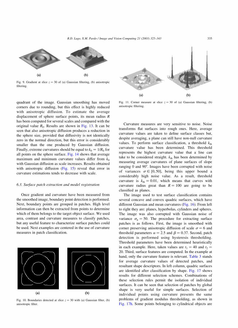
quadrant of the image. Gaussian smoothing has moved

corners due to rounding, but this effect is highly reduced

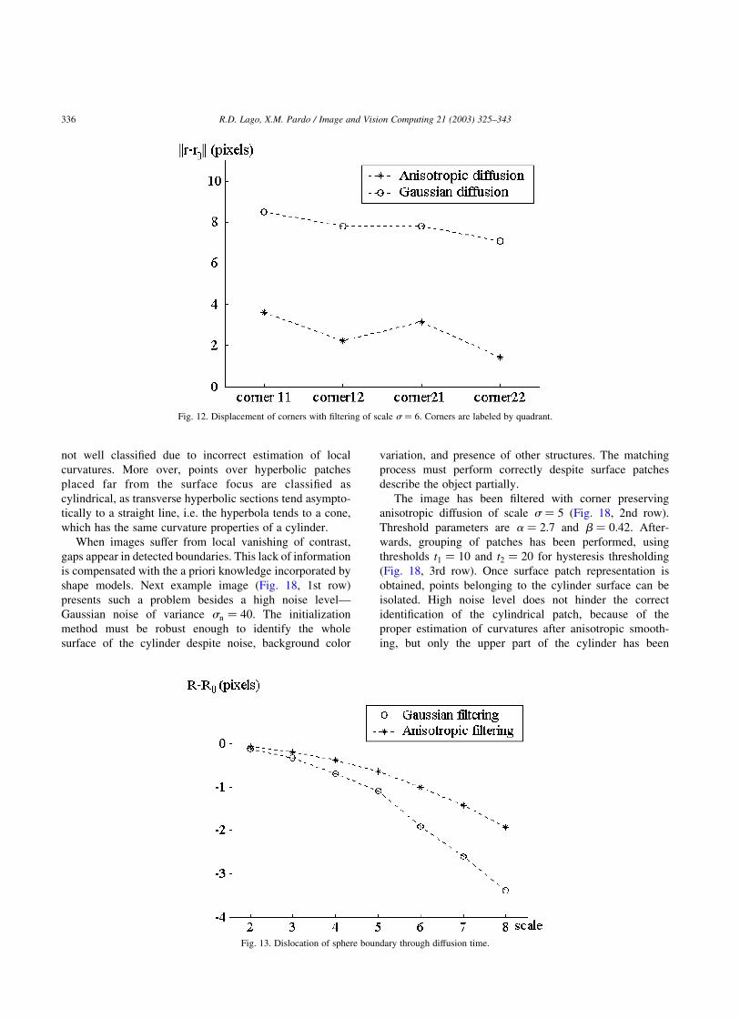
with anisotropic diffusion. To estimate the average

displacement of sphere surface points, its mean radius R

has been computed for several scales and compared with the

original value R0: Results are shown in Fig. 13. It can be

seen that also anisotropic diffusion produces a reduction in

the sphere size, provided that diffusivity is not identically

zero in the normal direction, but this error is considerably

smaller than the one produced by Gaussian diffusion.

Finally, extreme curvatures should be equal to k0 ¼ 1=R0 for

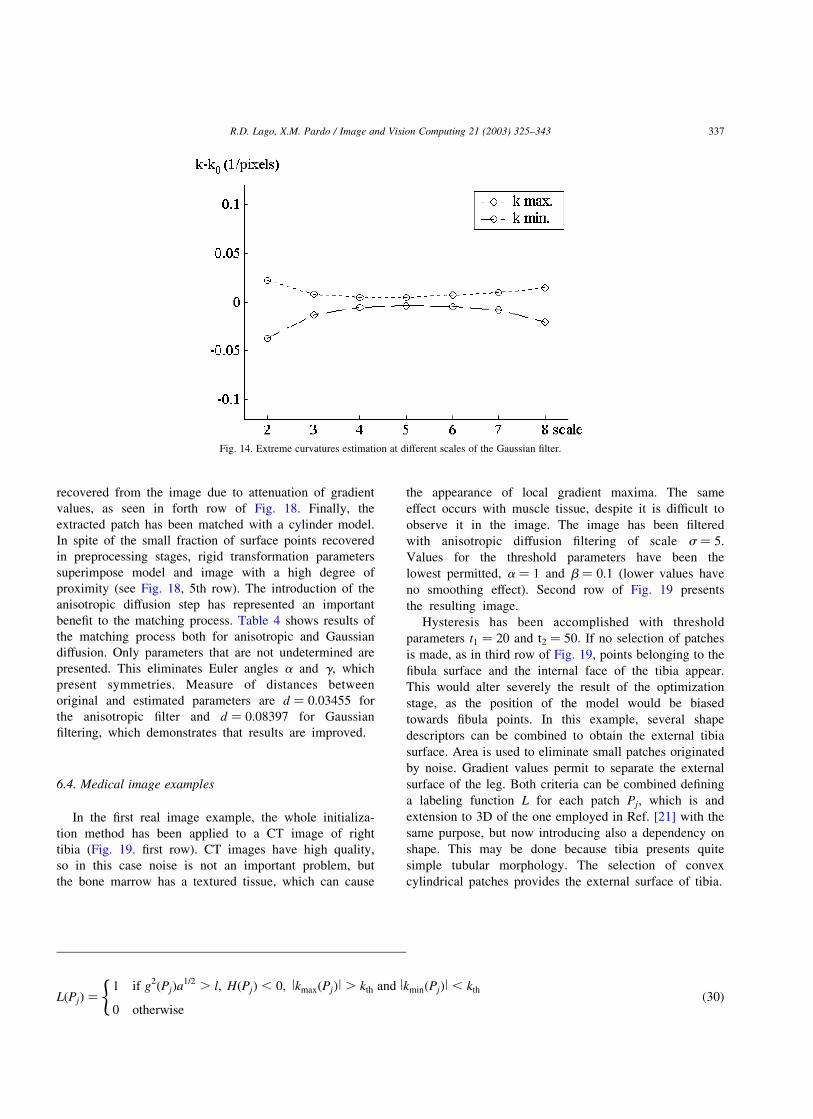
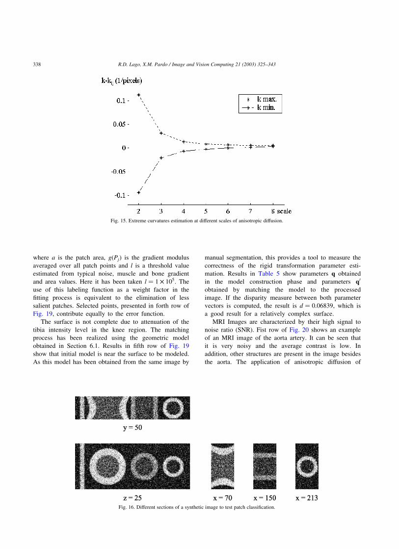
all points on the sphere surface. Fig. 14 shows that average

maximum and minimum curvature values differ from k0

with Gaussian diffusion as scale increases. Results obtained

with anisotropic diffusion (Fig. 15) reveal that error in

curvature estimations tends to decrease with scale.

6.3. Surface patch extraction and model registration

Once gradient and curvature have been measured from

the smoothed image, boundary point detection is performed.

Next, boundary points are grouped in patches. High level

information can then be extracted from points to determine

which of them belongs to the target object surface. We used

area, contrast and curvature measures to classify patches,

but any useful feature to characterize surface patches could

be used. Next examples are centered in the use of curvature

measures in patch classification.

Curvature measures are very sensitive to noise. Noise

transforms flat surfaces into rough ones. Here, average

curvature values are taken to define surface classes but,

despite averaging, a plane can still have non-null curvature

values. To perform surface classification, a threshold kth

curvature value has been determined. This threshold

represents the highest curvature value that a line can

take to be considered straight. kth has been determined by

measuring average curvatures of plane surfaces of slope

ranging 0 and 908. Images have been corrupted with noise

of variances s [ ½0; 50�; being this upper bound a

considerably high noise value. As a result, threshold

curvature is kth ¼ 0:01; which means that curves with

curvature radius great than R ¼ 100 are going to be

classified as planes.

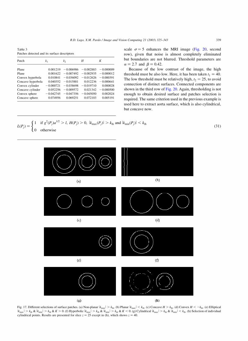
The image used to test surface classification contains

several concave and convex quadric surfaces, which have

different Gaussian and mean curvatures (Fig. 16). From left

to right they are: planes, hyperbolas, cylinders and spheres.

The image was also corrupted with Gaussian noise of

variance sn ¼ 50: The procedure for extracting surface

patches is as follows. First, the image is smoothed with

corner preserving anisotropic diffusion of scale s ¼ 6 and

threshold parameters a ¼ 2:5 and b ¼ 0:37: Second, patch

detection is performed using hysteresis thresholding.

Threshold parameters have been determined heuristically

in each example. Here, taken values are t1 ¼ 40 and t2 ¼

20: Third, surface features are computed. In the example at

hand, only the curvature feature is relevant. Table 3 stands

for average curvature values of detected patches, and

resultant shape descriptors. In left column, quadric surfaces

are identified after classification by shape. Fig. 17 shows

results for different selection schemes. Combinations of

these selection rules permit the isolation of individual

surfaces. It can be seen that selection of patches by global

shape is very useful for simple surfaces. Selection of

individual points using curvature presents the same

problems of gradient modulus thresholding, as shown in

Fig. 17h. Some points belonging to cylindrical objects are

Fig. 9. Gradient at slice z ¼ 30 of (a) Gaussian filtering, (b) anisotropic

filtering.

Fig. 10. Boundaries detected at slice z ¼ 30 with (a) Gaussian filter, (b)

anisotropic filter.

Fig. 11. Corner measure at slice z ¼ 30 of (a) Gaussian filtering, (b)

anisotropic filtering.


not well classified due to incorrect estimation of local

curvatures. More over, points over hyperbolic patches

placed far from the surface focus are classified as

cylindrical, as transverse hyperbolic sections tend asympto-

tically to a straight line, i.e. the hyperbola tends to a cone,

which has the same curvature properties of a cylinder.

When images suffer from local vanishing of contrast,

gaps appear in detected boundaries. This lack of information

is compensated with the a priori knowledge incorporated by

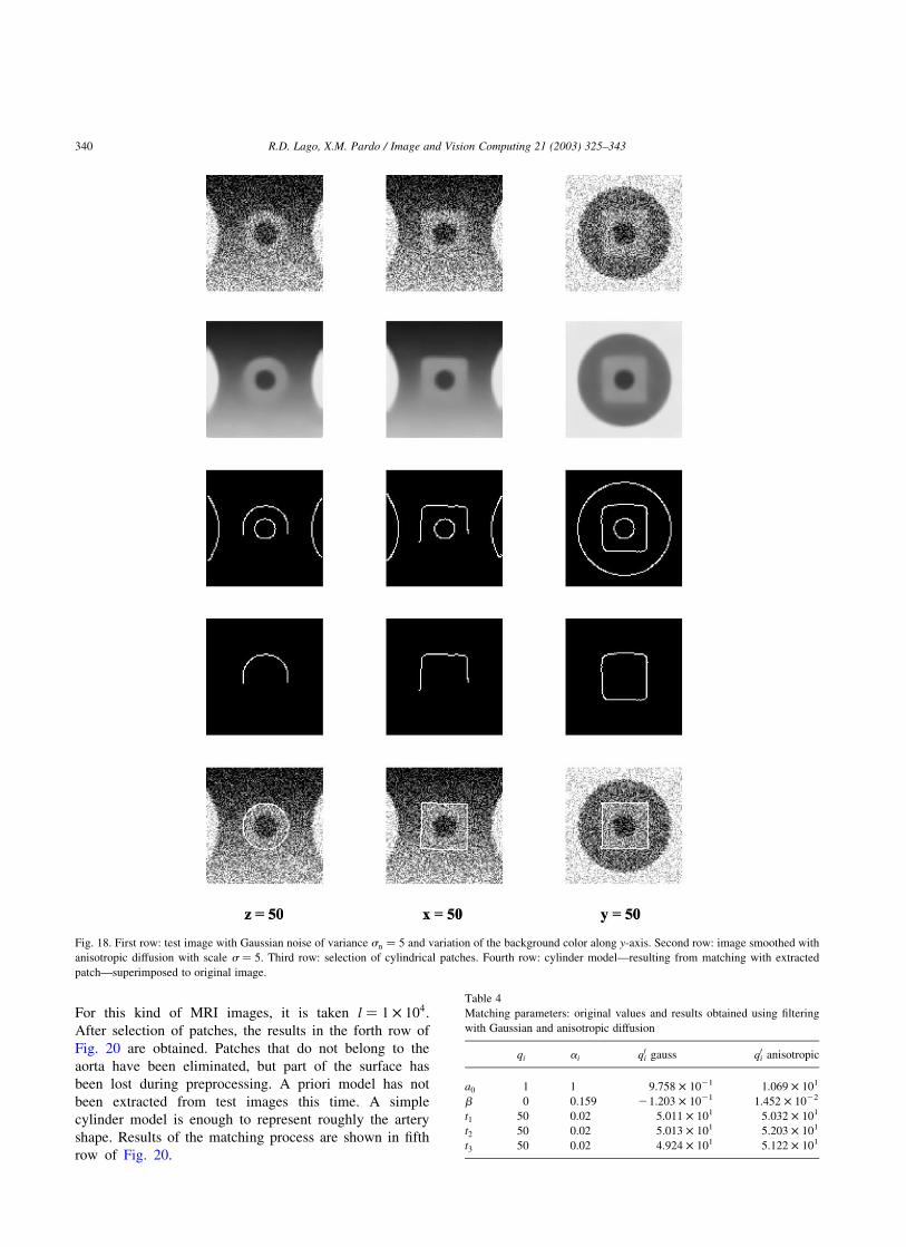
shape models. Next example image (Fig. 18, 1st row)

presents such a problem besides a high noise level—

Gaussian noise of variance sn ¼ 40: The initialization

method must be robust enough to identify the whole

surface of the cylinder despite noise, background color

variation, and presence of other structures. The matching

process must perform correctly despite surface patches

describe the object partially.

The image has been filtered with corner preserving

anisotropic diffusion of scale s ¼ 5 (Fig. 18, 2nd row).

Threshold parameters are a ¼ 2:7 and b ¼ 0:42: After-

wards, grouping of patches has been performed, using

thresholds t1 ¼ 10 and t2 ¼ 20 for hysteresis thresholding

(Fig. 18, 3rd row). Once surface patch representation is

obtained, points belonging to the cylinder surface can be

isolated. High noise level does not hinder the correct

identification of the cylindrical patch, because of the

proper estimation of curvatures after anisotropic smooth-

ing, but only the upper part of the cylinder has been

Fig. 12. Displacement of corners with filtering of scale s ¼ 6: Corners are labeled by quadrant.

Fig. 13. Dislocation of sphere boundary through diffusion time.


recovered from the image due to attenuation of gradient

values, as seen in forth row of Fig. 18. Finally, the

extracted patch has been matched with a cylinder model.

In spite of the small fraction of surface points recovered

in preprocessing stages, rigid transformation parameters

superimpose model and image with a high degree of

proximity (see Fig. 18, 5th row). The introduction of the

anisotropic diffusion step has represented an important

benefit to the matching process. Table 4 shows results of

the matching process both for anisotropic and Gaussian

diffusion. Only parameters that are not undetermined are

presented. This eliminates Euler angles a and g; which

present symmetries. Measure of distances between

original and estimated parameters are d ¼ 0:03455 for

the anisotropic filter and d ¼ 0:08397 for Gaussian

filtering, which demonstrates that results are improved.

6.4. Medical image examples

In the first real image example, the whole initializa-

tion method has been applied to a CT image of right

tibia (Fig. 19. first row). CT images have high quality,

so in this case noise is not an important problem, but

the bone marrow has a textured tissue, which can cause

the appearance of local gradient maxima. The same

effect occurs with muscle tissue, despite it is difficult to

observe it in the image. The image has been filtered

with anisotropic diffusion filtering of scale s ¼ 5:

Values for the threshold parameters have been the

lowest permitted, a ¼ 1 and b ¼ 0:1 (lower values have

no smoothing effect). Second row of Fig. 19 presents

the resulting image.

Hysteresis has been accomplished with threshold

parameters t1 ¼ 20 and t2 ¼ 50. If no selection of patches

is made, as in third row of Fig. 19, points belonging to the

fibula surface and the internal face of the tibia appear.

This would alter severely the result of the optimization

stage, as the position of the model would be biased

towards fibula points. In this example, several shape

descriptors can be combined to obtain the external tibia

surface. Area is used to eliminate small patches originated

by noise. Gradient values permit to separate the external

surface of the leg. Both criteria can be combined defining

a labeling function L for each patch Pj; which is and

extension to 3D of the one employed in Ref. [21] with the

same purpose, but now introducing also a dependency on

shape. This may be done because tibia presents quite

simple tubular morphology. The selection of convex

cylindrical patches provides the external surface of tibia.

LðPjÞ ¼1 if g2ðPjÞa

1=2 . l; HðPjÞ , 0; lkmaxðPjÞl . kth and lkminðPjÞl , kth

0 otherwise

(ð30Þ

Fig. 14. Extreme curvatures estimation at different scales of the Gaussian filter.


where a is the patch area, gðPjÞ is the gradient modulus

averaged over all patch points and l is a threshold value

estimated from typical noise, muscle and bone gradient

and area values. Here it has been taken l ¼ 1 £ 105: The

use of this labeling function as a weight factor in the

fitting process is equivalent to the elimination of less

salient patches. Selected points, presented in forth row of

Fig. 19, contribute equally to the error function.

The surface is not complete due to attenuation of the

tibia intensity level in the knee region. The matching

process has been realized using the geometric model

obtained in Section 6.1. Results in fifth row of Fig. 19

show that initial model is near the surface to be modeled.

As this model has been obtained from the same image by

manual segmentation, this provides a tool to measure the

correctness of the rigid transformation parameter esti-

mation. Results in Table 5 show parameters q obtained

in the model construction phase and parameters q0

obtained by matching the model to the processed

image. If the disparity measure between both parameter

vectors is computed, the result is d ¼ 0:06839; which is

a good result for a relatively complex surface.

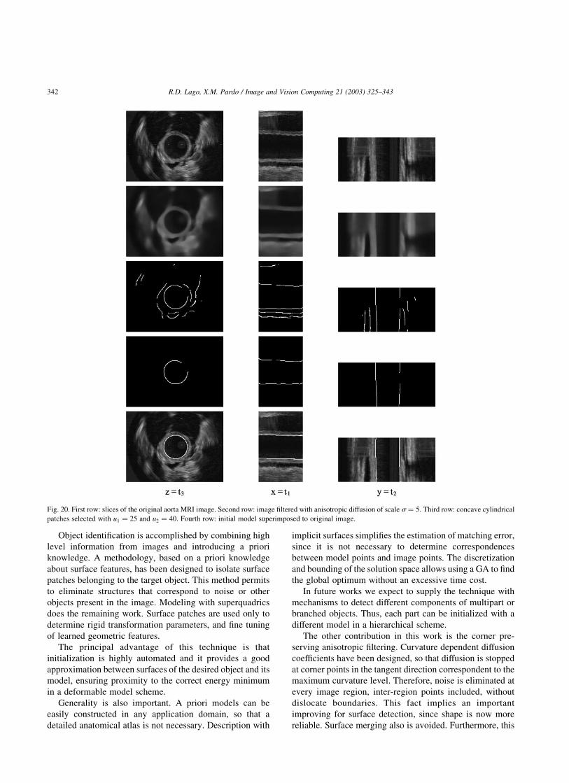
MRI Images are characterized by their high signal to

noise ratio (SNR). Fist row of Fig. 20 shows an example

of an MRI image of the aorta artery. It can be seen that

it is very noisy and the average contrast is low. In

addition, other structures are present in the image besides

the aorta. The application of anisotropic diffusion of

Fig. 15. Extreme curvatures estimation at different scales of anisotropic diffusion.

Fig. 16. Different sections of a synthetic image to test patch classification.


scale s ¼ 5 enhances the MRI image (Fig. 20, second

row), given that noise is almost completely eliminated

but boundaries are not blurred. Threshold parameters are

a ¼ 2:7 and b ¼ 0:42:

Because of the low contrast of the image, the high

threshold must be also low. Here, it has been taken t1 ¼ 40.

The low threshold must be relatively high, t2 ¼ 25; to avoid

connection of distinct surfaces. Connected components are

shown in the third row of Fig. 20. Again, thresholding is not

enough to obtain desired surface and patches selection is

required. The same criterion used in the previous example is

used here to extract aorta surface, which is also cylindrical,

but concave now.

Fig. 17. Different selections of surface patches. (a) Non-planar lkmaxl . kth: (b) Planar lkmaxl , kth: (c) Concave H . kth: (d) Convex H , 2kth: (e) Elliptical

lkmaxl . kth & lkminl . kth & K . 0: (f) Hyperbolic lkmaxl . kth & lkminl . kth & K , 0: (g) Cylindrical lkmaxl . kth & lkminl , kth: (h) Selection of individual

cylindrical points. Results are presented for slice z ¼ 25 except in (h), which shows z ¼ 40:

Table 3

Patches detected and its surface descriptors

Patch k1 k2 H K

Plane 0.001219 20.006986 20.002883 20.000009

Plane 0.001622 20.007492 20.002935 20.000012

Convex hyperbola 0.010841 20.036092 20.012626 20.000391

Concave hyperbola 0.040352 20.015881 0.012236 20.000641

Convex cylinder 20.000721 20.038698 20.019710 0.000028

Concave cylinder 0.052256 20.009572 0.021342 20.000500

Convex sphere 20.042745 20.047356 20.045050 0.002024

Concave sphere 0.074956 0.069251 0.072103 0.005191

LðPjÞ ¼1 if g2ðPjÞa

1=2 . l; HðPjÞ . 0; lkmaxðPjÞl . kth and lkminðPjÞl , kth

0 otherwise

(ð31Þ


For this kind of MRI images, it is taken l ¼ 1 £ 104:

After selection of patches, the results in the forth row of

Fig. 20 are obtained. Patches that do not belong to the

aorta have been eliminated, but part of the surface has

been lost during preprocessing. A priori model has not

been extracted from test images this time. A simple

cylinder model is enough to represent roughly the artery

shape. Results of the matching process are shown in fifth

row of Fig. 20.

Fig. 18. First row: test image with Gaussian noise of variance sn ¼ 5 and variation of the background color along y-axis. Second row: image smoothed with

anisotropic diffusion with scale s ¼ 5: Third row: selection of cylindrical patches. Fourth row: cylinder model—resulting from matching with extracted

patch—superimposed to original image.

Table 4

Matching parameters: original values and results obtained using filtering

with Gaussian and anisotropic diffusion

qi ai q0i gauss q0i anisotropic

a0 1 1 9.758 £ 1021 1.069 £ 101

b 0 0.159 21.203 £ 1021 1.452 £ 1022

t1 50 0.02 5.011 £ 101 5.032 £ 101

t2 50 0.02 5.013 £ 101 5.203 £ 101

t3 50 0.02 4.924 £ 101 5.122 £ 101


7. Conclusions

Deformable models are very reliable modeling tech-

niques. They force continuity and smoothness in segmenta-

tion but they have a local field of activity, so starting

configuration determines the success of the procedure. In

this paper, an automatic initialization tool to guide

deformation is presented. To this end, a complete method-

ology has been developed to obtain a description of global

shape, location, orientation and size of an object from a 3D

image.

Fig. 19. First row: slices of the original tibia CT image. Second row: image filtered with anisotropic diffusion of scale s ¼ 5: Third row: convex cylindrical

patches selected with u1 ¼ 20 and u2 ¼ 50: Fourth row: initial model superimposed to original image.

Table 5

Columns from left to right: tibia superquadric parameters, correspondent

weight factors, estimated parameters q0i obtained with error function D4

qi q0i

a0 1.00 9.54 £ 1021

a 5.31 £ 1021 3.88 £ 1021

b 29.10 £ 1022 21.08 £ 1021

g 21.27 £ 1021 1.03 £ 1021

t1 9.65 £ 101 9.77 £ 101

t2 1.04 £ 102 1.04 £ 102

t3 8.73 £ 101 8.78 £ 101


Object identification is accomplished by combining high

level information from images and introducing a priori

knowledge. A methodology, based on a priori knowledge

about surface features, has been designed to isolate surface

patches belonging to the target object. This method permits

to eliminate structures that correspond to noise or other

objects present in the image. Modeling with superquadrics

does the remaining work. Surface patches are used only to

determine rigid transformation parameters, and fine tuning

of learned geometric features.

The principal advantage of this technique is that

initialization is highly automated and it provides a good

approximation between surfaces of the desired object and its

model, ensuring proximity to the correct energy minimum

in a deformable model scheme.

Generality is also important. A priori models can be

easily constructed in any application domain, so that a

detailed anatomical atlas is not necessary. Description with

implicit surfaces simplifies the estimation of matching error,

since it is not necessary to determine correspondences

between model points and image points. The discretization

and bounding of the solution space allows using a GA to find

the global optimum without an excessive time cost.

In future works we expect to supply the technique with

mechanisms to detect different components of multipart or

branched objects. Thus, each part can be initialized with a

different model in a hierarchical scheme.

The other contribution in this work is the corner pre-

serving anisotropic filtering. Curvature dependent diffusion

coefficients have been designed, so that diffusion is stopped

at corner points in the tangent direction correspondent to the

maximum curvature level. Therefore, noise is eliminated at

every image region, inter-region points included, without

dislocate boundaries. This fact implies an important

improving for surface detection, since shape is now more

reliable. Surface merging also is avoided. Furthermore, this

Fig. 20. First row: slices of the original aorta MRI image. Second row: image filtered with anisotropic diffusion of scale s ¼ 5: Third row: concave cylindrical

patches selected with u1 ¼ 25 and u2 ¼ 40: Fourth row: initial model superimposed to original image.


processing technique is expected to improve the measures for

the external energy of the deformable model.

Results presented show that both gradient and corner

detectors offer better responses after anisotropic filtering in

comparison with Gaussian blurring. The effect of the defini-

tion of the threshold parameters is very relevant for this ap-

plication. The automatic setting of these parameters provides

a useful tool to find a compromise between smoothing and

boundary or corner preserving. However, there are cases in

which the definition of global thresholds is insufficient.

Variations on the background intensity level, attenuation of

the features intensity or the presence of structures of different

intensities can be the reason of important loss of informa-

tion. To solve the problem, the threshold parameters should

be estimated locally on a vicinity of each point. This is a

proposal for future works, where viability of the approach

must be studied in terms of computational efficiency.

Acknowledgements

This work was supported by the Spanish Government

and the Xunta de Galicia by projects TIC2000-0399-C02-02

and PGIDT99PXI20606B, respectively.

References

[1] R. Bajcsy, S. Kovacic, Multiresolution elastic matching, Computer

Vision, Graphics, and Image Processing 46 (1989) 1–21.

[2] E. Bardinet, L.D. Cohen, N. Ayache, A parametric deformable model

to fit unstructured 3D data, report no. 2617, INRIA, Sophia-Antipolis,

France, 1995.

[3] M. Black, G. Sapiro, D. Marimont, D. Heeger, Robust anisotropic

diffusion, Transactions on Image Processing 7 (3) (1998) 421–432.

[4] R.M. Bolle, B.C. Vemuri, On three-dimensional surface reconstruc-

tion methods, IEEE Transactions on Pattern Analysis and Machine

Intelligence 13 (1) (1991) 1–13.

[5] P. Charbonnier, G. Aubert, M. Blanc-Feraud, M. Barlaud, Two

deterministic half-quadratic regularization algorithms for computed

imaging, IEEE International Conference on Image Processing, Austin,

Texas (1994) 168–172.

[6] T. Cootes, A. Hill, C. Taylor, J. Haslam, The use of active shape

models for locating structures in medical images, in: H.H. Barrett,

A.F. Gmitro (Eds.), Information Processing Medical Imaging, LNCS

687, Springer, Berlin, 1993, pp. 33–47.

[7] H. Delingette, J. Montagnat, General deformable model approach for

model-based reconstruction, Proceedings of the IEEE International

Workshop on Model-Bases 3D Image Analysis, Bombay, India

(1998).

[8] D.E. Goldberg, Genetic algorithms in search, optimization and

machine learning, Addison-Wesley, Reading, MA, 1999.

[9] P.J. Green, Bayesian reconstruction from emission tomography data

using a modified EM algorithm, IEEE Transactions on Medical

Imaging 9 (1990) 84–93.

[10] G. Gerig, O. Kubler, R. Kikinis, A. Jolesz, Nonlinear anisotropic

filtering of MRI data, IEEE Transactions on Medical Imaging 11 (2)

(1992) 221–231.

[11] A. Jaklic, A. Leonardis, F. Solina, Segmentation and Recovery of

Superquadrics, Computational Imaging and Vision, vol. 20, Kluwer,

Dordrecht, 2000.

[12] M. Kass, A. Witkin, D. Terzopoulos, Snakes: active contour models,

International Journal of Computer Vision 1 (4) (1988) 321–331.

[13] K. Krissian, G. Malandain, N. Ayache, Directional anisotropic

diffusion applied to segmentation of vessels in 3D images, report

no. 3064, INRIA, Sophia-Antipolis, France, 1995.

[14] A. Leonardis, A. Jaklic, F. Solina, Superquadrics for segmenting and

modeling range data, IEEE Transactions on Pattern Analysis and

Machine Intelligence 19 (11) (1997) 1289–1295.

[15] P. Linares, L. Rodrıguez, G. Montilla, Genetic algorithms fitting of

deformable superquadrics applied to left ventricle visualization,

Computers in Cardiology 25 (1998) 657–660.

[16] T. McInerney, D. Terzopoulos, A finite-element model for 3D shape

reconstruction and nonrigid motion tracking, ICCV’93 (1993)

518–523.

[17] T. McInerney, D. Terzopoulos, Deformable models in medical image

analysis: a survey, Medical Image Analysis 1 (2) (1996).

[18] O. Monga, S. Benayoun, Using partial derivatives of 3D images to

extract typical surface features, report no. 1599, INRIA, Rocquen-

court, France, 1989.

[19] O. Monga, R. Deriche, G. Malandain, J.-P. Cocquerez, Recursive

filtering and edge closing: two primary tools for 3D edge detection,

report no. 1103, INRIA, Rocquencourt, France, 1989.

[20] W. Neuenschwander, P. Fua, G. Szekely, O. Kubler, Velcro surfaces:

fast initialization of deformable models, Computer Vision and Image

Understanding 65 (2) (1997) 237–245.

[21] X.M. Pardo, D. Cabello, Biomedical active segmentation guided by

edge saliency, Pattern Recognition Letters 21 (2000) 559–572.

[22] P. Perona, J. Malik, Scale-space and edge detection using anisotropic

diffusion, IEEE Transactions on Pattern Analysis and Machine

Intelligence 12 (7) (1990).

[23] P.J. Rousseeuw, A.M. Leroy, Robust Regression and Outlier

Detection, Wiley, New York, 1987.

[24] P. Saint-Marc, J.-S. Chen, G. Medioni, Adaptive smoothing: a general

tool for early vision, IEEE Transactions on Pattern Analysis and

Machine Intelligence 13 (6) (1991) 514–529.

[25] S. Sandor, R. Leahy, Surface-based labeling of cortical anatomy using

a deformable atlas, Medical Image 16 (1) (1997) 41–54.

[26] F. Sole, S.-C. Ngan, G. Sapiro, X. Hu, A. Lopez, Anisotropic 2D and

3D averaging of fMRI signals, IEEE Transactions on Medical

Imaging 20 (2) (2001) 86–93.

[27] F. Solina, R. Bajcsy, Recovery of parametric models from range

images: the case for superquadrics with global and local deformations,

IEEE Transactions on PAMI 12 (2) (1990) 131–146.

[28] J. Sporring, M. Nielsen, J. Weickert, O.F. Olsen, A Note on

Differential Corner Measures, Proceedings of the 14th International

Conference on Pattern Recognition, vol. 1, IEEE Computer Society

Press, Los Alamitos, 1998, pp. 652–654.

[29] L.H. Staib, A. Chakraborty, J.S. Duncan, An integrated approach for

locating neuroanatomical structure from MRI, International Journal of

Pattern Recognition and Artificial Intelligence 11 (8) (1997)

1247–1269.

[30] H. Tek, B.B. Kimia, Volumetric segmentation of medical images by

three-dimensional bubbles, Computer Vision and Image Under-

standing 65 (2) (1997) 246–258.

[31] D. Terzopoulos, D. Metaxas, Dynamic 3D models with local and

global deformations: deformable superquadrics, IEEE Transactions

on Pattern Analysis and Machine Intelligence 13 (7) (1991) 703–714.

[32] J. Weickert, A review of nonlinear diffusion filtering, in: B. ter Haar

Romeny, L. Florack, J. Koenderink, M. Viergever (Eds.), Scale-Space

Theory in Computer Vision, Lecture Notes in Computer Science, vol.

1252, Springer, Berlin, 1997, pp. 3–28.

[33] J. Weickert, Scale-space properties of nonlinear diffusion filtering

with a diffusion tensor, report no. 110, Laboratory of Technomathe-

matics, University of Kaiserslautern, Germany, 1994.

[34] P. Whaite, F.P. Ferrie, From uncertainty to visual exploration, IEEE

Transactions on Pattern Analysis and Machine Intelligence 13 (10)

(1991) 1038–1049.


Generalized ellipsoids and anisotropic filtering for segmentation improvement in 3D medical imaging

Documents

Transcript of Generalized ellipsoids and anisotropic filtering for segmentation improvement in 3D medical imaging