GENERAL THEORY OF THREE-DIMENSIONAL CONSOLIDATION

THE ERNEST KEMPTON ADAMS FbND FOR PHYSICAL RESEARCH

OF COLUMBIA UNM3R!XI’Y

REPRINT SERIES

GENERAL THEORY OF THREE-DIMENSIONAL

CONSOLIDATION

BY

MAURICE A. BIOT

Reprinted from JOURNAL OF APPLIED PEYSICS, Vol. 12, No. 2, pp. 155-164, February, 1941

Reprinted from JOURNAL OF APPLIED PHYSICS, Vol. 12, No. 2, 155-164, February, 1941 Copyright 1941 by the American Institute of Physics

Printed in U. S. A.

General Theory of Three-Dimensional Consolidation*

MAURICE A. BIOT

Columbia Univcrsdy, New York, New York

(Received October 2.5, 1940)

The settlement of soils under load is caused by a phenomenon called consolidation, whose mechanism is known to be in many cases identical with the process of squeezing water out of an elastic porous medium. The mathematical physical consequences of this viewpoint are established in the present paper. The number of physical constants necessary to determine the properties of the soil is derived along with the general equations for the prediction of settle- ments and stresses in three-dimensional problems. Simple applications are treated as examples. The operational calculus is shown to be a powerful method of solution of consolidation problems.

INTRODUCTION

I

T is well known to engineering practice that a soil under load does not assume an instan-

taneous deflection under that load, but settles gradually at a variable rate. Such settlement is very apparent in clays and sands saturated with water. The settlement is caused by a gradual adaptation of the soil to the load variation. This process is known as soil consolidation. A simple mechanism to explain this phenomenon was first proposed by K. Terzaghi.’ He assumes that the grains or particles constituting the soil are more or less bound together by certain molecular forces and constitute a porous material with elastic properties. The voids of the elastic skeleton are filled with water. A good example of such a model is a rubber sponge saturated with water. A load applied to this system will produce a gradual settlement, depending on the rate at which the water is being squeezed out of the voids. Terzaghi applied these concepts to the analysis of the settlement of a column of soil under a constant load and prevented from lateral expansion. The remarkable success of this theory in predicting the settlement for many types of soils has been one of the strongest incentives in the creation of a science of soil mechanics.

Terzaghi’s treatment, however, is restricted to the one-dimensional problem of a column under a constant load. From the viewpoint of mathematical physics two generalizations of this are

* Publication assisted by the Ernest Kempton Adams Fund for Physical Research of Columbia University.

1 K. Terzaghi, Erdbaumechanik auf Boden~hysikabischer Grundlage CLeipzig F. Deuticke, 1925); “Principle of soil mechanics,” Eng. News Record (1925), a series of articles.

VOLUME 12, FEBRUARY, 1941

possible : the extension to the three-dimensional case, and the establishment of equations valid for any arbitrary load variable with time. The theory was first presented by the author in rather abstract form in a previous publication.2 The present paper gives a more rigorous and complete treatment of the theory which leads to results more general than those obtained in the previous paper.

The following basic properties of the soil are assumed : (1) isotropy of the material, (2) reversibility of stress-strain relations under final equilibrium conditions, (3) linearity of stress- strain relations, (4) small strains, (5) the water contained in the pores is incompressible, (6) the water may contain air bubbles, (7) the water flows through the porous skeleton according to Darcy’s law.

Of these basic assumptions (2) and (3) are most subject to criticism. However, we should keep in mind that they also constitute the basis of Terzaghi’s theory, which has been found quite satisfactory for the practical requirements of engineering. In fact it can be imagined that the grains composing the soil are held together in a certain pattern by surface tension forces and tend to assume a configuration of minimum potential energy. This would especially be true for the colloidal particles constituting clay. It seems reasonable to assume that for small strains, when the grain pattern is not too much disturbed, the assumption of reversibility will be applicable.

The assumption of isotropy is not essential and

* M. A. Biot, “Le probkme de la Consolidation des Mat&-es argileuses sous une charge,” Ann. Sot. Sci. Bruxelles B55, 110-113 (1935).

15.5

anisotropy can easily be introduced as a refinement. Another refinement which might be of practical importance is the influence, upon the stress distribution and the settlement, of the state of initial stress in the soil before application of the load. It was shown by the present author3 that this influence is greater for materials of low elastic modulus. Both refinements will be left out of the present theory in order to avoid undue heaviness of presentation.

The first and second sections deal mainly with the mathematical formulation of the physical properties of the soil and the number of constants necessary to describe these properties. The number of these constants including Darcy’s permeability coefficient is found equal to five in the most general case. Section 3 gives a dis- cussion of the physical interpretation of these various constants. In Sections 4 and 5 are established the fundamental equations for the consolidation and an application is made to the one-dimensional problem corresponding to a standard soil test. Section 6 gives the simplified

same time small enough, compared to the scale of the macroscopic phenomena in which we are interested, so that it may be considered as infinitesimal in the mathematical treatment.

The average stress condition in the soil is then represented by forces distributed uniformly on the faces of this cubic element. The corresponding stress components are denoted by

They must satisfy the well-known equilibrium conditions of a stress field.

(1.2)

theory for the case most important in practice of a soil completely saturated with water. The

Physically we may think of these stresses as

equations for this case coincide with those of the composed of two parts ; one which is caused by

previous publication.2 In the last section is the hydrostatic pressure of the water filling the

shown how the mathematical tool known as the pores, the other caused by the average stress in

operational calculus can be applied most con- the skeleton. In this sense the stresses in the soil

veniently for the calculation of the settlement are said to be carried partly by the water and

without having to calculate any stress or water partly by the solid constituent.

pressure distribution inside the soil. This method of attack constitutes a major simplification and proves to be of high value in the solution of the more complex two- and three-dimensional problems. In the present paper applications are restricted to one-dimensional examples. A series of applications to practical cases of two-dimensional consolidation will be the object of subsequent papers.

1. SOIL STRESSES

Consider a small cubic element of the con- solidating soil, its sides being parallel with the coordinate axes. This element is taken to be large enough compared to the size of the pores so that it may be treated as homogeneous, and at the

2. STRAIN RELATED TO STRESS AND WATER PRESSURE

We now call our attention to the strain in the soil. Denoting by u, V, zet the components of the displacement of the soil and assuming the strain to be small, the values of the strain components are

du a~ av ez=-

ax’ r.T=-+-_,

ay a2

av a24 aw e,=--, -YII=-+-, (2.1)

ay a2 ax

aw av a24 ez=-

az' -yz=-+-.

ax ay

*M. A. Biot, “Nonlinear theory of elasticity and the In order to describe completely the macroscopic linearized case for a body under initial stress.” condition of the soil we must consider an addi-

156 JOURNAL OF APPLIED PHYSICS

tional variable giving the amount of water in the pores. We therefore denote by 0 the increment of water volume per unit volume of soil and call this quantity the zJariation in water content. The increment’of water pressure will be denoted by u.

Let us consider a cubic element of soil. The water pressure in the pores may be considered as uniform throughout, provided either the size of the element is small enough or, if this is not the case, provided the changes occur at sufficiently slow rate to render the pressure differences negligible.

It is clear that if we assume the changes in the soil to occur by reversible processes the macroscopic condition of the soil must be a definite function of the stresses and the water pressure i.e., the seven variables

e, ey e, Yx YU YE. 8

must be definite functions of the variables:

uz Qu UE 7, i-g 7, CT.

Furthermore if we assume the strains and the variations in water content to be small quantities, the relation between these two sets of variables may be taken as linear in first approximation. We first consider these functional relations for the particular case where u= 0. The six com- ponentsof strain are then functions only of the six stress components cI uy uZ rZ ry 7,. Assuming the soil to have isotropic properties these relations must reduce to the well-known expressions of Hooke’s law for an isotropic elastic body in the theory of eIasticity ; we have

e,=~-~(uz+uu),

~z = rz/G,

mu= 7,/G,

yz= rz/G.

(2.2)

In these relations the constants E, G, v may be interpreted, respectively, as Young’s modulus,

the shear modulus and Poisson’s ratio for the solid skeleton. There are only two distinct constants because of the relation

E G=-.

v+v1 (2.3)

Suppose now that the effect of the water pressure u is introduced. First it cannot produce any shearing strain by reason of the assumed isotropy of the soil; second for the same reason its effect must be the same on all three components of strain e, e, e,. Hence taking into account the influence of u relations (2.2) become

e.=~-~(uv+u,,+i 3H

~z = i-z/G,

Y?/ = r,lG,

yz= TJG,

where H is an additional physical constant. These relations express the six strain components of the soil as a function of the stresses in the soil and the pressure of the water in the pores. We still have to consider the dependence of the increment of water content 0 on these same variables. The most general relation is

6 = aiuo+a2uy+a3ur+a4r2 +a6ry+a67,+a7u. (2.5)

Now because of the isotropy of the material a change in sign of r2 ry rZ cannot affect the water content, therefore a4=aL=a6=0 and the effect of the shear stress components on 0 vanishes. Furthermore all three directions x, y, z must have equivalent properties al = a2 = a3. Therefore relation (2.5) may be written in the form

s=-&-(u~+u,+uz)+~, (2.6) 1

where HI and R are two physical constants.

VOLUME 12, FEBRUARY, 1941 157

Relations (2.4) and (2.6) contain five distinct physical constants. We are now going to prove that this number may be reduced to four; in fact that H=Hl if we introduce the assumption of the existence of a potential energy of the soil. This assumption means that if the changes occur at an infinitely slow rate, the work done to bring the soil from the initial condition to its final state of strain and water content, is independent of the way by which the final state is reached and is a definite function of the six strain components and the water content. This assumption follows quite naturally from that of reversibility introduced above, since the absence of a potential energy would then imply that an indefinite amount of energy could be drawn out of the soil by loading and unloading along a closed cycle.

The potential energy of the soil per unit volume is

U=~(uoez+uy~y+u~~o.+7z~z +ry~y+r.yz+~@. (2.7)

In order to prove that H=Hl let us consider a particular condition of stress such that

Then the potential energy becomes

lJ=$(ure+u0) with E=e,+ey+er

and Eqs. (2.4) and (2.6)

3(1-2~) u t=

E uI+~, e=u~/H~+ulR. (2.8)

The quantity t represents the volume increase of the soil per unit initial volume. Solving for ul and u

e e #J1=-----

RA HA’

--E +3(1 -2V)e u=&A EA ’

(2.9)

3(1-2~) 1 A= --.

ER HH1

The potential energy in this case may be con-

158

sidered as a function of the two variables E, B. Now we must have

Hence

or

au au -=u1, -=u. de de

aal au -=- de de

1 1

Ha==

We have thus proved that H=Hl and we may write

(2.10)

Relations (2.4) and (2.10) are the fundamental relations describing completely in first approximation the properties of the soil, for strain and water content, under equilibrium conditions. They contain four distinct physical constants G, v, H and R. For further use it is convenient to express the stresses as functions of the strain and the water pressure u. Solving Eq. (2.4) with respect to the stresses we find

u,=ZG( eg+fi) --au,

u,=2G( ez+fi) -cyu, (2.11)

7, = GYP,

it, = Grv,

with TZ=GYZ

2(I+v) G CY=

3(1--2~) 5’

In the same way we may express the variation in water content as

where e=ffe+u/Q, (2.12)

1 1 a! -=---. QRH

JOURNAL OF APPLIED PHYSICS

3. PHYSICAL INTERPRETATION OF THE SOIL CONSTANTS

The constants E, G and v have the same meaning as Young’s modulus the shear modulus and the Poisson ratio in the theory of elasticity provided time has been allowed for the excess water to squeeze out. These quantities may be considered as the average elastic constants of the sohd skeleton. There are only two distinct such constants since they must satisfy relation (2.3). Assume, for example, that a column of soil supports an axial load po= -ur while allowed to expand freely laterally. If the load has been applied long enough so that a final state of settlement is reached, i.e., all the excess water has been squeezed out and u = 0 then the axial strain is, according to (2.4),

PO ez= --

E (3.1)

and the lateral strain

VP0 ez=ey=-= -vez.

E . (3.2)

The coefficient v measures the ratio of the lateral bulging to the vertical strain under final equilibrium conditions.

To interpret the constants H and R consider a sample of soil enclosed in a thin rubber bag so that the stresses applied to the soil be zero. Let us drain the water from this soil through a thin tube passing through the walls of the bag. If a negative pressure -u is applied to the tube a certain amount of water will be sucked out. This amount is given by (2.10)

fy= -“. R

(3.3) The coefficient

The corresponding volume change of the soil is given by (2.4)

(3.4)

The coefficient l/H is a measure of the compressibility of the soil for a change in water pressure, while l/R measures the change in water content for a given change in water pres-

sure. The two elastic constants and the constants H and R are the four distinct constants which under our assumption define completely the physical proportions of an isotropic soil in the equilibrium conditions.

Other constants have been derived from these four. For instance Q! is a coefficient defined as

2(l+v) G Cl!=

3(1-22) E (3.5)

According to (2.12) it measures the ratio of the water volume squeezed out to the volume change of the soil if the latter is compressed while allowing the water to .escape (a=O). The coefficient l/Q defined as

1 1 CY -_=---_

QRH (3.6)

is a measure of the amount of water which can be forced into the soil under pressure while the volume of the soil is kept constant. It is quite obvious that the constants (Y and Q will be of significance for a soil not completely saturated with water and containing air bubbles. In that case the constants a and Q can take values depending on the degree of saturation of the soil.

The standard soil test suggests the derivation of additional constants. A column of soil supports a load p. = - ul and is confined laterally in a rigid sheath so that no lateral expansion can occur. The water is allowed to escape for instance by applying the load through a porous slab. When all the excess water has been squeezed out the axial strain is given by relations (2.11) in which we put u=O. We write

er= - pea.

l-2v

(3.7)

l7,=

2G(l- v) (3.8)

will be called the final compressibility. If we measure the axial strain just after the

load has been applied so that the water has not had time to ilow out, we must put B=O in relation (2.12). We deduce the value of the water pressure

u = - aQe&. (3.9)


substituting this value in (2.11) we write

er= -parri. (3.10) The coefficient

a aa=

1 +a2aQ (3.11)

will be called the instantaneous compressibility. The physical constants considered above refer

to the properties of the soil for the state of equilibrium when the water pressure is uniform throughout. We shall see hereafter that in order to study the transient state we must add to the four distinct constants above the so-called coeficient of permeability of the soil.

4. GENERAL EQUATIONS GOVERNING CONSOLIDATION

We now proceed to establish the differential equations for the transient phenomenon of consolidation, i.e., those equations governing the distribution of stress, water content, and settlement as a function of time in a soil under given loads.

Substituting expression (2.11) for the stresses into the equilibrium conditions (1.2) we find

G de aa GV2~+--- -- (Y--o,

l-2vax ax

G de da Gv%~-l---- -- ff--0.

l--2vay dy (4.1) \ I

G ae da GV2wS -.--L,_=O,

l-2vdz dz

v2 =a2/aX2+d2/ay2+a2/a22.

There are three equations with four unknowns u, v, w, 6. In order to have a complete system we need one more equation. This is done by intro- ducing Darcy’s law governing the flow of water in a porous medium. We consider again an elementary cube of soil and call V, the volume of water flowing per second and unit area through the face of this cube perpendicular to the x axis. In the same way we define V, and Vl. According to Darcy’s law these three components of the rate of flow are related to the water pressure by the relations

V,= -k;, V,= -$, V,= -Pt. (4.2)

The physical constant k is called the coeficient of permeability of the soil. On the other hand, if we assume the water to be incompressible the rate of water content of an element of soil must be equal to the volume of water entering per second through the surface of the element, hence

de av, av, av, -=-----7 at‘ ax ay a2

(4.3)

Combining Eqs. (2.2) (4.2) and (4.3) we obtain

de 1 an kV2a = a~---+- -.

at Q at (4.4)

The four differential Eqs. (4.1) and (4.4) are the basic equations satisfied by the four unknowns u, 21, w, c.

5. APPLICATION TO A STANDARD SOIL TEST

Let us examine the particular case of a column of soil supporting a load PO= - cz and confined laterally in a rigid sheath so that no lateral expansion can occur. It is assumed also that no water can escape laterally or through the bottom while it is free to escape at the upper surface by applying the load through a very porous slab.

Take the z axis positive downward; the only component of displacement in this case will be w. Both w and the water pressure u will depend only on the coordinate z and the time t. The differential Eqs. (4.1) and (4.4) become

i a2w aw --- w-=0, (5.1) a a22 a2

160

ka2u-C;a2W 1 ’ au a.22 azat Qat’

(5.2)

JOURNAL OF APPLIED PHYSICS

where a is the final compressibility defined by (3.8). The stress (TV throughout the loaded column is a constant. From (2.11) we have

1 aw PO= -az= ---+cia (5.3)

a dz and from (2.12)

dw a e=a-+--.

da Q Note that Eq. (5.3) implies (5.1) and that

1 PW da

adzat=%. This relation carried into (5.2) gives

Pa 1 aa -=--, dz2 c at

(5.4)

with * 1 al -=a”+-_.

k Qk (5.5)

c

The constant c is called the consolidation constant. Equation (5.4) shows the important result that the water pressure satisfies the well-known equation of heat conduction. This equation along with the boundary and the initial conditions leads to a complete solution of the problem of consolidation.

Taking the height of the soil column to be h and z=O at the top we have the boundary conditions

a=0 for z=O,

da -=0 for z=h. az

(5.6)

The first condition expresses that the pressure of the water under the load is zero because the permeability of the slab through which the load is applied is assumed to be large with respect to that of the soil. The second condition expresses that no water escapes through the bottom.

The initial condition is that the change of water content is zero when the load is applied because the water must escape with a finite velocity. Hence from (2.12)

aw a ~=cP--+--0 for t=O.

az Q Carrying this into (5.3) we derive the initial value of the water pressure

az*,/(A+Ck!) fort=0 or a=yP0, (5.7)

where a, and a are the instantaneous and final compressibility coefficients defined by (3.8) and (3.11). The solution of the differential equation (5.4) with the boundary conditions (5.6) and the initial

condition (5.7) may be written in the form of a series

4 a-ai a=----~0~exp[-(~)z~t]sin~+~exp[-(~)2~t]sin~+~~~). (5.8)

.X ffa

The settlement may be found from relation (5.3). We have

aw -=&a-ape. dz

(5.9)


The total settlement is

s hdW

wo= - -ak = (5.10) 0 az

--$(u-ui)hpo 5 l 0 (2n+1)2

exp ( -[(Znzl’n]z Ct ] +Uhpo.

Immediately after loading (t=O), the deflection is

Taking into account that

WC= a,hp,, (5.11)

which checks with the result (3.10) above. The final deflection for t = 00 is

wc., = ahpo. (5.12)

It is of interest to find a simplified expression for the law of settlement in the period of time immediately after loading. To do this we first eliminate the initial deflection wi by considering

(5.13)

This expresses that part of the deflection which is caused by consolidation. We then consider the rate of settlement.

dw, 2c(a-ai) m

dt= h p0 T exp ( -[(2”i1)r-J&}. (5.14)

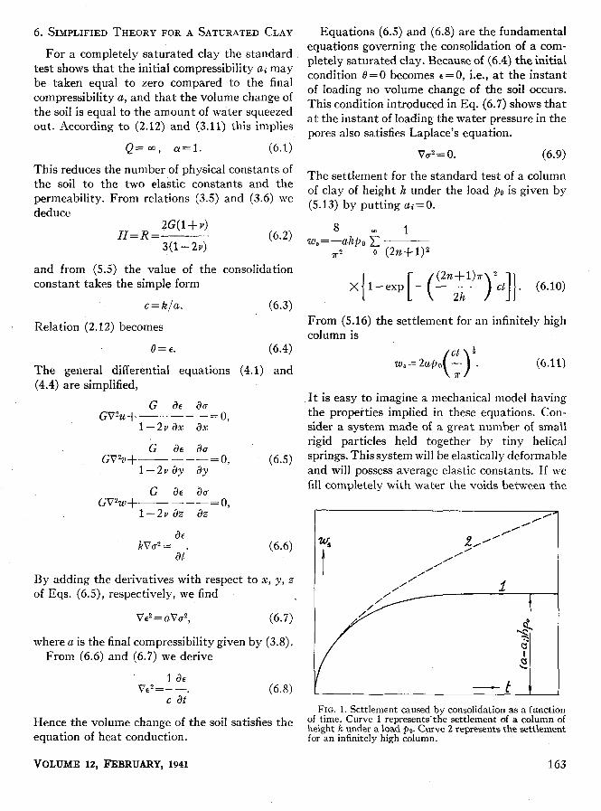
For t =0 this series does not converge; which means that at the first instant of loading the rate of settlement is infinite. Hence the curve representing the settlement w, as a function of time starts with a vertical slope and tends asymptotically toward the value (a-ud)hpl as shown in Fig. 1 (curve 1). It is obvious that during the initial period of settlement the height h of the column cannot have any influence on the phenomenon because the water pressure at the depth z=h has not yet had time to change. Therefore in order to find the nature of the settlement curve in the vicinity of t = 0 it is enough to consider the case where h = w. In this case we put

and write (5.14) as n/h= & l/h=Al

dw, z= 2c(u-U&O 5 exp [ -a2(E+$A~)2ct]A,$

0

,,for h= 60,. The rate of settlement becomes the integral

dw, 00

-=2c(u-uai)po S

exp (- r2E2ct)dE= c(a-UJPO

dt 0 (Tct); .

The value of the settlement is obtained by integration

S t dw,

w*= -dt=2(u-u&o o dt

It follows a parabolic curve as a function of time (curve 2 in Fig. 1).

(5.15)

(5.16)

162 i

/ JOURNAL OF APPLIED PHYSICS i

6. SIMPLIFIED THEORY FOR A SATURATED CLAY

For a completely saturated clay the standard test shows that the initial compressibility ai may be taken equal to zero compared to the final compressibility a, and that the volume change of the soil is equal to the amount of water squeezed out. According to (2.12) and (3.11) this implies

Q=w, cr=l. (6.1)

This reduces the number of physical constants of the soil to the two elastic constants and the permeability. From relations (3.5) and (3.6) we deduce

H=R= 2GO+v)

3(1--2~) (6.2)

and from (5.5) the value of the consolidation constant takes the simple form

c = k/a. (6.3)

Relation (2.12) becomes

6= e. (6.4)

The general differential equations (4.1) and (4.4) are simplified,

G de &s GV2u+-------=Q,

1-2va~ ax

G ae au Gvzv+--- ---=0,

i-2vay ay (6.5)

G ae au GV2w+------=O,

1-2v a2 a2

By adding the derivatives with respect to x, y, z of Eqs. (6.5), respectively, we find

Ve2 = aV$, (6.7)

where a is the final compressibility given by (3.8). From (6.6) and (6.7) we derive

Vc2=! I? c at’

(6.8)

Hence the volume change of the soil satisfies the equation of heat conduction.

Equations (6.5) and (6.8) are the fundamental equations governing the consolidation of a completely saturated clay. Because of (6.4) the initial condition 8=0 becomes e=O, i.e., at the instant of loading no volume change of the soil occurs. This condition introduced in Eq. (6.7) shows that at the instant of loading the water pressure in the pores also satisfies Laplace’s equation.

Va2 = 0. (6.9)

The settlement for the standard test of a column of clay of height h under the load ~0 is given by (5.13) by putting ai=O.

8 w,=-ahp, 5

1

7r2 0 (2nfl)Z

X[ l-e~p[-((2fl~1)n)2&]}. (6.10)

From (5.16) the settlement for an infinitely high column is

ct 3 w,=2apo - . 0 n-

(6.11)

It is easy to imagine a mechanical model having the propel-ties implied in these equations. Con- sider a system made of a great number of small rigid particles held together by tiny helical springs. This system will be elastically deformable and will possess average elastic constants. If we fill completely with water the voids between the

I

FIG. 1. Settlement caused by consolidation as a function of time. Curve 1 represents-the settlement of a column of height h under a load ~0. Curve 2 represents the settlement for an infinitely high column.


particles, we shall have a model of a completely saturated clay.

Obviously such a system is incompressible if no water is allowed to be squeezed out (this corresponds to the condition Q= a) and the change of volume is equal to the volume of water squeezed out (this corresponds to the condition LY = 1). If the systems contained air bubbles this would not be the case and we would have to consider the general case where Q is finite and a#l.

Eqs. (5.1) become

i ak aa a% aw --=-, kaz,=pdz. a a.22 a2

(7.1)

A solution of these equations which vanishes at infinity is

WC c,p(Plc)t (7.2)

1 P + a=&-- -

0 Cle-“‘P/“’ ?

a c

Whether this model represents schematically the actual constitution of soils is uncertain. It is quite possible, however, that the soil particles are held together by capillary forces which behave in pretty much the same way as the springs of the model.

The boundary conditions are for z=O

i aw gz=-l=--, a=O.

a a.2 Hence

c + Cl=a - , C2=l. 0 P

7. OPERATIONAL CALCULUS APPLIED TO CONSOLIDATION

The settlement w. at the top (z = 0) caused by the sudden application of a unit load is

The calculation of settlement under a suddenly applied load leads naturally to the application of operational methods, developed by Heaviside for the analysis of transients in electric circuits. As an illustration of the power and simplicity introduced by the operational calculus in the treatment of consolidation problem we shall derive by this procedure the settlement of a completely saturated clay column already calcu- lated in the previous section. In subsequent articles the operational method will be used extensively for the solution of various consolidation problems. We consider the case of a clay column infinitely high and take as before the top to be the origin of the vertical coordinate z. For a completely saturated clay (Y = 1, Q = 00 and with the operational notations, replacing a/at by p,

c + w,=a - 0 . 1 (t).

P The meaning of this symbolic expression is derived from the operational equation4

(7.3)

The settlement as a function of load PO is therefore

time under the

ct + w*=2apo - . 0 T

(7.4)

This coincides with the value (6.11) above.

4 V. Bush, Operational Circuit Analysis (John Wiley, New York, 1929), p. 192.

164 JOURNAL OF APPLIED PHYSICS

GENERAL THEORY OF THREE-DIMENSIONAL CONSOLIDATION

Documents

Transcript of GENERAL THEORY OF THREE-DIMENSIONAL CONSOLIDATION