University of Nebraska - Lincoln University of Nebraska - Lincoln

DigitalCommons@University of Nebraska - Lincoln DigitalCommons@University of Nebraska - Lincoln

Industrial and Management Systems Engineering -- Dissertations and Student Research

Industrial and Management Systems Engineering

12-2012

Three-Dimensional Indoor RFID Localization System Three-Dimensional Indoor RFID Localization System

Jiaqing Wu University of Nebraska-Lincoln, wujiaqing@huskers.unl.edu

Follow this and additional works at: https://digitalcommons.unl.edu/imsediss

Part of the Industrial Engineering Commons, and the Other Electrical and Computer Engineering

Commons

Wu, Jiaqing, "Three-Dimensional Indoor RFID Localization System" (2012). Industrial and Management Systems Engineering -- Dissertations and Student Research. 36. https://digitalcommons.unl.edu/imsediss/36

This Article is brought to you for free and open access by the Industrial and Management Systems Engineering at DigitalCommons@University of Nebraska - Lincoln. It has been accepted for inclusion in Industrial and Management Systems Engineering -- Dissertations and Student Research by an authorized administrator of DigitalCommons@University of Nebraska - Lincoln.

THREE-DIMENSIONAL INDOOR RFID LOCALIZATION SYSTEM

by

Jiaqing Wu

A DISSERTATION

Presented to the Faculty of

The Graduate College at the University of Nebraska

In Partial Fulfillment of Requirements

For the Degree of Doctor of Philosophy

Major: Engineering

(Industrial, Management Systems, and Manufacturing Engineering)

Under the Supervision of Professor Robert E. Williams

Lincoln, Nebraska

December, 2012

THREE-DIMENSIONAL INDOOR RFID LOCALIZATION SYSTEM

Jiaqing Wu, Ph.D.

University of Nebraska, 2012

Adviser: Robert E. Williams

Radio Frequency Identification (RFID) is an information exchange technology

based on radio waves communication. It is also a possible solution to indoor localization.

Due to multipath propagation and anisotropic interference in the indoor environment,

theoretical propagation models are generally not sufficient for RFID-based localization.

In fact, the radio frequency (RF) signal distribution may not even be monotonic and this

makes range-based localization algorithms less accurate. On the other hand, range free

localization algorithms, such as k Nearest-Neighbor (kNN), require reference tags to be

spread throughout the whole three-dimensional (3D) space which is simply not practical.

In this work, a hybrid real-time localization algorithm that combines reference tags with

Received Signal Strength Indicator (RSSI) ranging is introduced to improve RFID-based

3D localization in high-complexity indoor environments. The experiments demonstrate

that the proposed system is more accurate than traditional algorithms under real world

constraints. The active RFID system includes 4 readers and 24 reference tags deployed in

a fully furnished room. The localization algorithm is implemented in MATLAB and is

synchronized with RF signal data collection in real-time. The results show that the novel

hybrid algorithm achieves an average 3D localization error of 1.08m which represents a

significant improvement over kNN and RSSI algorithms under the same circumstance. A

battery-assisted passive RFID system was deployed side-by-side to the active system for

comparison. Furthermore, the reader and tag performance was evaluated in both high-

complexity laboratory environment and International Space Station (ISS) mock-up with

high-reflection interior surface. In addition, theoretical models on minimum number of

required reference tags and localization error prediction were introduced.

iv

Acknowledgements

I wish to thank my advisor Dr. Robert E. Williams for his constant guidance, help,

and support. His dedication to research has been a real inspiration.

I am sincerely thankful to Dr. Kamlakar P. Rajurkar, Dr. Michael W. Riley, and

Dr. Lance C. Pérez for serving on my Ph.D. committee and providing valuable

suggestions and comments to the original manuscript.

The dissertation experimentation would not have been possible without the

gracious use of the facilities of Dr. Lance C. Pérez, the MC2 laboratory in the department

of Electrical Engineering. I want to thank Lianlin Zhao, Marques L. King and all

associates who were so friendly and helpful to my research there.

I would like to thank all faculty and staff members in the IMSE department and

then the MME department since August 2011. Their kindness made my study at UNL

much more comfortable.

I also would like to thank my beautiful wife, Bijia, for her love, caring, courage,

and support during this research.

Finally, I dedicate this dissertation to my parents, Shuliang Wu and Zhenyun Cao,

and to my sister, Jiawei Wu. They had a great influence on my career path and academic

motivation and pursuits.

v

Table of Contents

Abstract............................................................................................................................... ii

Acknowledgements ............................................................................................................ iv

Table of Contents ................................................................................................................ v

List of Figures .................................................................................................................... ix

List of Tables .................................................................................................................... xii

Nomenclature and Abbreviations .................................................................................... xiv

Chapter 1 Introduction ........................................................................................................ 1

1.1 Radio Frequency Identification (RFID) ............................................................... 1

1.2 Real-Time Localization System (RTLS).............................................................. 2

1.3 Purpose of Research ............................................................................................. 3

1.4 Dissertation Organization ..................................................................................... 4

Chapter 2 Literature Review ............................................................................................... 5

2.1 Radio Frequency Identification (RFID) ............................................................... 5

2.1.1 Tags ............................................................................................................... 8

2.1.2 Readers ........................................................................................................ 11

2.2 Real-Time Localization System (RTLS)............................................................ 12

2.2.1 Global Positioning System (GPS) and A-GPS (Assisted GPS) .................. 14

2.2.2 Wireless Local Area Network (WLAN) and Wireless Sensor Network

(WSN) ....................................................................................................................... 14

vi

2.2.3 Radio Frequency Identification (RFID) ...................................................... 15

2.2.4 Ultra Wide Band (UWB) ............................................................................ 16

2.2.5 Non RF-based ............................................................................................. 17

2.2.6 Summary ..................................................................................................... 18

2.3 RFID-RTLS ........................................................................................................ 19

2.3.1 Schemes ...................................................................................................... 19

2.3.2 Algorithms .................................................................................................. 20

2.3.3 Range-based Localization ........................................................................... 21

2.3.4 Range-free Localization .............................................................................. 27

2.3.5 Summary ..................................................................................................... 29

Chapter 3 Theoretical Modeling ....................................................................................... 31

3.1 Introduction ........................................................................................................ 31

3.2 Assumptions ....................................................................................................... 32

3.3 Ranging .............................................................................................................. 35

3.4 Localization ........................................................................................................ 38

3.5 Experiments ........................................................................................................ 42

3.6 Summary ............................................................................................................ 45

Chapter 4 System and Experimental Designs ................................................................... 47

4.1 Fundamental Tests for Active System ............................................................... 47

4.1.1 Reader Test ................................................................................................. 47

4.1.2 Tag Test ...................................................................................................... 50

4.1.3 Ranging Test ............................................................................................... 53

vii

4.2 Localization Test for Active System .................................................................. 55

4.2.1 System Setup ............................................................................................... 55

4.2.2 Software Development................................................................................ 58

4.2.3 Localization Algorithm ............................................................................... 63

4.2.4 Experimental Design ................................................................................... 67

4.3 Additional Tests for Battery-assisted Passive System ....................................... 69

4.3.1 System Setup ............................................................................................... 69

4.3.2 Software Development................................................................................ 72

4.3.3 Experimental Design ................................................................................... 74

4.4 Localization Tests for Battery-assisted Passive System .................................... 75

4.5 Summary ............................................................................................................ 76

Chapter 5 Results and Analysis ........................................................................................ 77

5.1 Fundamental Tests for Active System ............................................................... 77

5.1.1 Reader Test ................................................................................................. 77

5.1.2 Tag Test ...................................................................................................... 81

5.1.3 Ranging Test ............................................................................................... 84

5.2 Localization Test for Active System .................................................................. 86

5.3 Additional Tests for Battery-assisted Passive System ....................................... 93

5.3.1 Battery-assisted Passive System ................................................................. 93

5.3.2 Active versus Battery-assisted Passive System .......................................... 99

5.3.3 Lab versus Mock-up ................................................................................. 101

5.4 Localization Test for Battery-assisted Passive System .................................... 104

viii

Chapter 6 Conclusions and Recommendations ............................................................... 106

6.1 Conclusions ...................................................................................................... 106

6.1.1 Theoretical Prediction ............................................................................... 106

6.1.2 Localization Performance ......................................................................... 107

6.1.3 Environmental Impacts ............................................................................. 107

6.2 Recommendations ............................................................................................ 108

References ....................................................................................................................... 109

Appendix A Programming Interface ............................................................................... 114

A.1 JSON ................................................................................................................ 114

A.2 XML ................................................................................................................. 120

Appendix B Matlab Implementation .............................................................................. 127

B.1 Welcome Window ............................................................................................ 127

B.2 RSSI Reading ................................................................................................... 128

B.3 Localization ...................................................................................................... 138

Appendix C Data Sheets ................................................................................................. 169

C.1 Reader Test Data Sheet .................................................................................... 169

C.2 Tag Test Data Sheet ......................................................................................... 171

C.3 Ranging Test Data Sheet .................................................................................. 173

C.4 Localization Test Data Sheet............................................................................ 175

C.5 Battery-assisted Passive System Test Data Sheet ............................................ 177

ix

List of Figures

Figure 2-1: Typical frequency bands used for RFID .......................................................... 6

Figure 2-2: Communication models between RFID tags and readers ................................ 7

Figure 2-3: Active RFID tag structure ................................................................................ 8

Figure 2-4: Two common RTLS schemes ........................................................................ 20

Figure 2-5: RSSI with fingerprinting ................................................................................ 22

Figure 2-6: Triangulation for AOA................................................................................... 23

Figure 2-7: Cycle intersection for TOA ............................................................................ 24

Figure 2-8: First step of multilateration for TDOA .......................................................... 25

Figure 2-9: Multilateration for APM ................................................................................ 26

Figure 2-10: kNN .............................................................................................................. 27

Figure 2-11: Proximity ...................................................................................................... 28

Figure 3-1: Reader layout scheme .................................................................................... 34

Figure 3-2: Tag layout scheme ......................................................................................... 34

Figure 3-3: Tag layout scheme (more).............................................................................. 42

Figure 4-1: Layout scheme of reader test ......................................................................... 49

Figure 4-2: Layout scheme of tag test............................................................................... 52

Figure 4-3: Layout scheme of ranging test ....................................................................... 54

Figure 4-4: RF Code readers and tags............................................................................... 55

Figure 4-5: Reader layout in room environment............................................................... 56

x

Figure 4-6: Reference tag layout in room environment .................................................... 57

Figure 4-7: Network and software structure of the RF Code system ............................... 60

Figure 4-8: RSSI reading GUI .......................................................................................... 61

Figure 4-9: Localization GUI............................................................................................ 62

Figure 4-10: 2D algorithm ................................................................................................ 64

Figure 4-11: Intersection point and surrounding reference tags ....................................... 66

Figure 4-12: Intelleflex readers and tags .......................................................................... 70

Figure 4-13: International space station mock-up ............................................................ 71

Figure 4-14: Network and software structure of the Intelleflex system ........................... 72

Figure 4-15: Network and software structure of both systems ......................................... 73

Figure 5-1: Main effects plot for reader test ..................................................................... 78

Figure 5-2: Interference caused by human activities nearby ............................................ 79

Figure 5-3: Main effects plot for tag test .......................................................................... 81

Figure 5-4: Interaction plot for tag test ............................................................................. 82

Figure 5-5: Main effects plot for ranging test ................................................................... 84

Figure 5-6: Linear regression of ranging test .................................................................... 85

Figure 5-7: Localization error histogram with fit ............................................................. 88

Figure 5-8: Localization error comparison ....................................................................... 90

Figure 5-9: Main effects plot for mean ............................................................................. 94

Figure 5-10: Main effects plot for standard deviation ...................................................... 96

Figure 5-11: Linear regression of ranging test (battery-assisted passive system) ............ 97

Figure 5-12: Active versus battery-assisted passive system ........................................... 100

xi

Figure 5-13: Lab versus Mock-up................................................................................... 102

xii

List of Tables

Table 2-1: RTLS products list........................................................................................... 13

Table 2-2: Indoor RTLS comparison based on different frequency bands being used .... 18

Table 2-3: Summary of localization algorithms in RFID-RTLS ...................................... 29

Table 3-1: Design of experiment #1 ................................................................................. 43

Table 3-2: Design of experiment #2 ................................................................................. 44

Table 4-1: Main factors of reader test ............................................................................... 48

Table 4-2: Main factors of tag test .................................................................................... 51

Table 4-3: Reference tags ID and positions ...................................................................... 58

Table 4-4: Main factors of localization test ...................................................................... 67

Table 4-5: Tag position definition .................................................................................... 67

Table 4-6: Main factors of battery-assisted passive tag test ............................................. 74

Table 4-7: Main factors of localization test (battery-assisted passive sytem) .................. 75

Table 5-1: Localization error distribution for all orientations .......................................... 87

Table 5-2: Localization error distribution for orientation same as reference tags only .... 88

Table 5-3: Localization error comparison....................................................................... 104

Table C-1: Reader test data sheet.................................................................................... 169

Table C-2: Tag test data sheet ......................................................................................... 171

Table C-3: Ranging test data sheet ................................................................................. 173

Table C-4: Localization test data sheet ........................................................................... 175

xiii

Table C-5: Battery-assisted passive system test data sheet ............................................ 177

xiv

Nomenclature and Abbreviations

2D Two-dimensional

3D Three-dimensional

A-GPS Assisted-GPS

AOA Angle of Arrival

APM Adaptive Power Multilateration

COTS Commercial off-the-shelf

dBm Ratio of measured power decibels (dB) to one milliwatt (mW)

EM Electromagnetic

EPC Electronic Product Code

Gbps Giga-bits-per-second

Gen 2 EPCglobal UHF Class 1 Generation 2

GPS Global Positioning System

GUI Graphic User Interface

HF High Frequency, 13.56 MHz

IC Integrated Circuit

IR Infrared, 300 GHz to 405 THz

ISS International Space Station

JSON JavaScript Object Notation

kNN k Nearest-Neighbor

xv

LF Low Frequency, 120–150 kHz

LOS Line-of-Sight

LSQ Least Squares Quadratic

MW Microwave Frequency, 2.4–5.8 GHz

PI Prediction Interval

QoS Quality of Service

RF Radio Frequency, 3 kHz to 300 GHz

RFID Radio Frequency Identification

RSSI Received Signal Strength Indication (unit: dBm)

RTLS Real-Time Localization System

TDOA Time Difference of Arrival

TOA Time of Arrival

UHF Ultra High Frequency, 433MHz, 868-870 MHz, and 902-928 MHz

UPC Universal Product Code

UWB Ultra Wide Band

WiFi Wireless Fidelity

WLAN Wireless Local Area Network

WSN Wireless Sensor Network

XML Extensible Markup Language

1

Chapter 1

Introduction

1.1 Radio Frequency Identification (RFID)

Radio Frequency Identification (RFID) is a radio wave transmission process

between an interrogator and a transponder, also known as a reader and a tag. The tag is

identified by responding to the information stored in its internal memory or from the

attached sensors. The reader is usually connected to a computer with a database for

further processing of received information or sensor data. RFID technology is widely

applied in transportation payments, asset management, supply chains, logistics, animal

tracking, libraries, and securities [1].

Based on their working mechanism, RFID tags can be categorized as active tags,

passive tags and semi-passive tags. The active tags are self-powered and broadcast

signals at preset intervals. They usually provide a larger read range. The passive tags and

semi-passive tags are only activated by the querying signal from the reader. The semi-

passive tags use internal battery power to enhance the broadcasting signal strength, while

the passive tags are much cheaper and smaller. The operating frequency bands used for

RFID tags vary from kHz, MHz to GHz, which leads to different radio wave coupling

modes and performance.

2

1.2 Real-Time Localization System (RTLS)

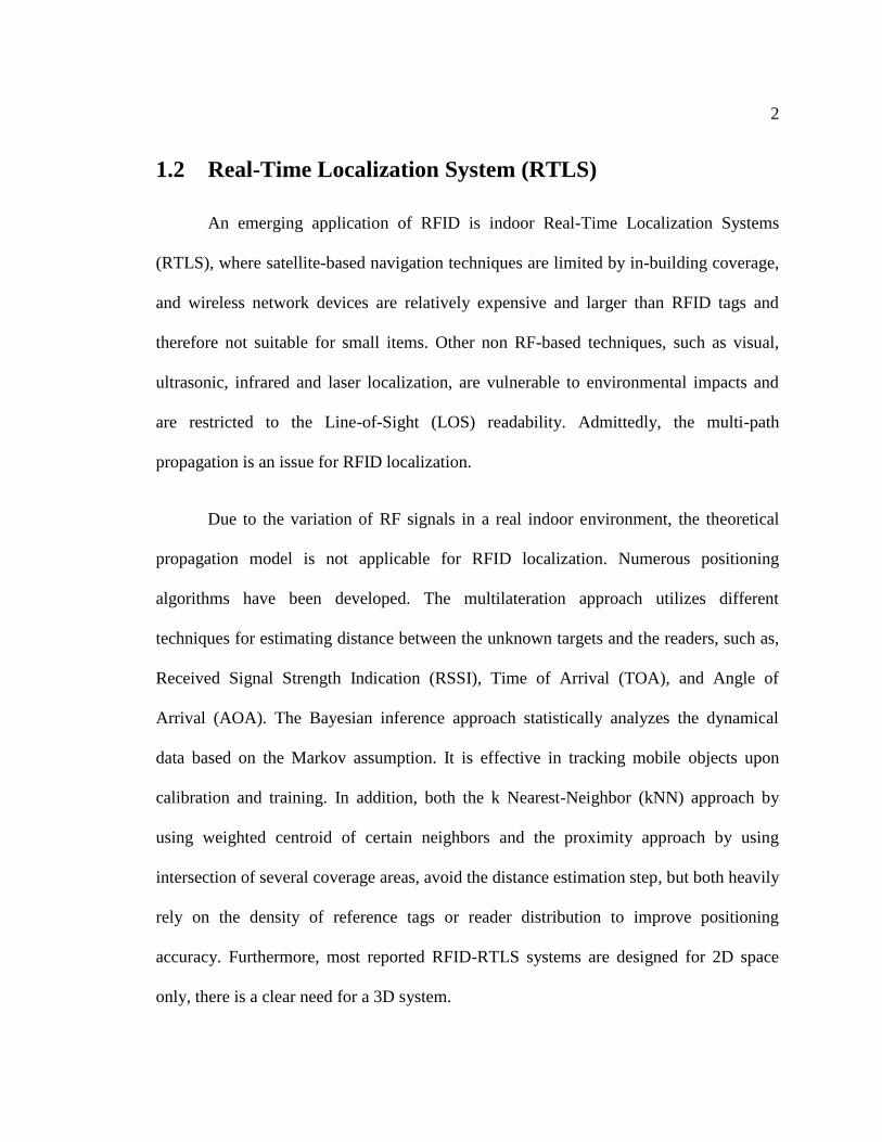
An emerging application of RFID is indoor Real-Time Localization Systems

(RTLS), where satellite-based navigation techniques are limited by in-building coverage,

and wireless network devices are relatively expensive and larger than RFID tags and

therefore not suitable for small items. Other non RF-based techniques, such as visual,

ultrasonic, infrared and laser localization, are vulnerable to environmental impacts and

are restricted to the Line-of-Sight (LOS) readability. Admittedly, the multi-path

propagation is an issue for RFID localization.

Due to the variation of RF signals in a real indoor environment, the theoretical

propagation model is not applicable for RFID localization. Numerous positioning

algorithms have been developed. The multilateration approach utilizes different

techniques for estimating distance between the unknown targets and the readers, such as,

Received Signal Strength Indication (RSSI), Time of Arrival (TOA), and Angle of

Arrival (AOA). The Bayesian inference approach statistically analyzes the dynamical

data based on the Markov assumption. It is effective in tracking mobile objects upon

calibration and training. In addition, both the k Nearest-Neighbor (kNN) approach by

using weighted centroid of certain neighbors and the proximity approach by using

intersection of several coverage areas, avoid the distance estimation step, but both heavily

rely on the density of reference tags or reader distribution to improve positioning

accuracy. Furthermore, most reported RFID-RTLS systems are designed for 2D space

only, there is a clear need for a 3D system.

3

1.3 Purpose of Research

Due to multipath propagation and interference in the indoor environment,

theoretical propagation models are generally not sufficient for RFID-based localization.

In fact, the RF signal distribution may not even be monotonic and this makes range-based

localization algorithms less accurate. On the other hand, range-free localization

algorithms, such as kNN, require reference tags to be deployed throughout the whole 3D

space which is simply not practical. Besides, the anisotropic environmental impacts in

real 3D application are significant and not neglectable.

The first objective of this study is to model the theoretical minimum number of

reference tags needed in a localization system. The modeling process is also helpful on

identifying the major factor affecting the localization accuracy.

The second objective of this research, therefore, is to build an indoor RFID-based

RTLS capable of positioning objects in 3D space in real-time. An active RFID system

and a power-assisted passive RFID system were built side-by-side for easy comparison.

The systems were deployed in a high-complexity laboratory room to reflect real

environmental impacts.

The third objective of this dissertation is to investigate the RFID tag performance

difference between the regular laboratory environment and the ISS mock-up. The high-

reflection interior surface would be a big challenge for RF signal stability. The

investigation result may be valuable for further system design.

4

1.4 Dissertation Organization

Chapter 2 consists of a literature review describing the background regarding

RFID and RTLS technologies, their applications, and common system designs.

Chapter 3 presents a theoretical analysis about the minimum number of reference

tags needed in a localization system.

Chapter 4 describes the proposed 3D localization system designs in the high-

complexity environment and the localization algorithm being evaluated. The experiment

designs of several fundamental tests are mentioned as well.

Chapter 5 contains the results and analysis of the fundamental tests and

localization experiments. It also includes a tag performance comparison between active

tags versus battery-assisted passive tags in both laboratory and mock-up environments.

Chapter 6 summarizes the conclusions and recommendations.

The appendices include the programming interface to the two types of readers, the

Matlab codes used for controlling the whole system, and the data sheets for all

experiments.

5

Chapter 2

Literature Review

2.1 Radio Frequency Identification (RFID)

Radio Frequency Identification (RFID) is a popular information exchange

technology widely applied in electronic passport [2], animal tracking [3], supply chains

[4], industrial automation [5], mining securities [6], hospital [7], asset management [8],

and pharmaceuticals [9]. There are numerous RFID applications, and cannot be listed

here completely. More examples may be found in the RFID Journal and RFID handbook

[1, 10].

A simplest RFID system consists of two major components: a tag and a reader.

The tag and the reader communicate via radio waves. The radio frequency (RF) bands

commonly used in RFID include 120-150 kHz at Low Frequency (LF), 13.56 MHz at

High Frequency (HF), 433MHz, 868-870 MHz, and 902-928 MHz at Ultra High

Frequency (UHF), and 2.4-5.8 GHz at Microwave Frequency (MW) [10]. The RFID

systems with operating frequency at LF and HF work based on inductive coupling. By

contrast, the systems in the range of UHF and MW are coupled using electromagnetic

(EM) fields, which brings a significantly higher read range than inductive systems.

6

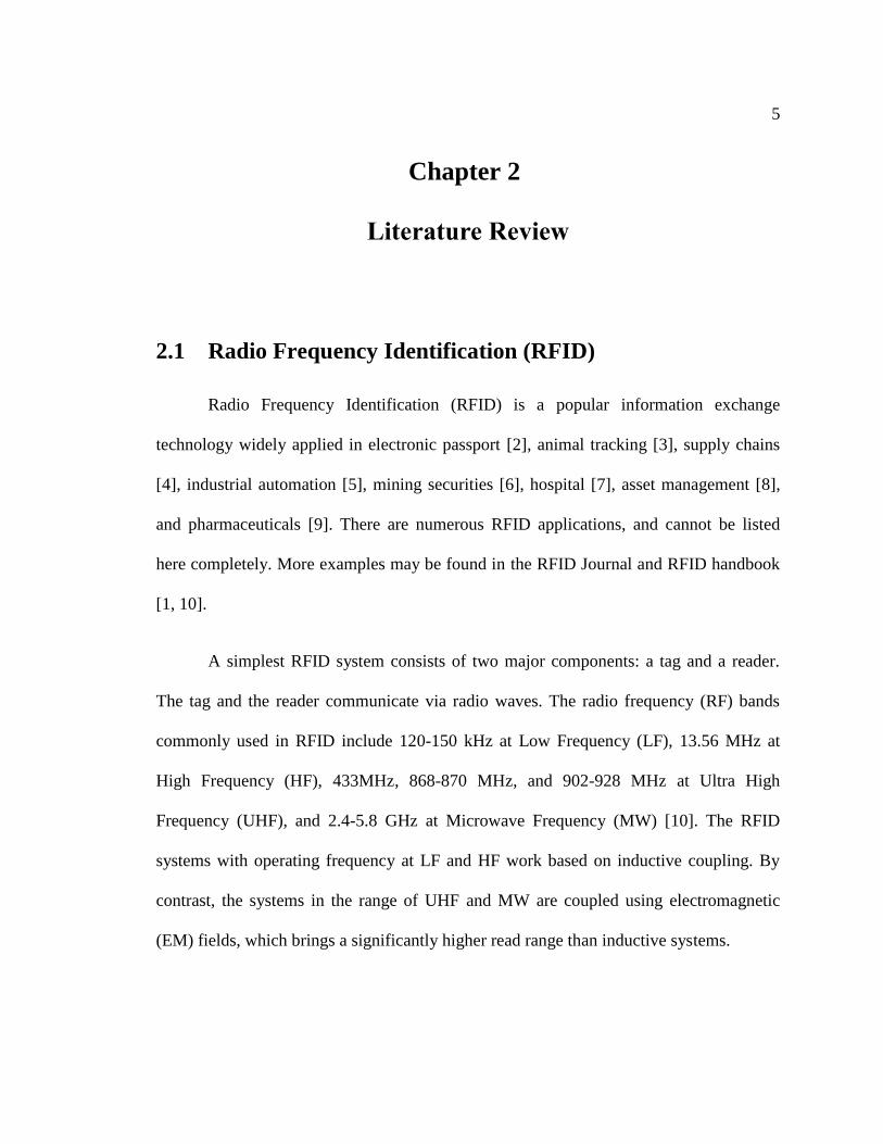
These typical frequency bands used in RFID are summarized in Figure 2-1. The

433 MHz UHF and MW tags are usually used for active tags. In addition, the MW tags

can be designed to be compatible with existing WiFi systems via the IEEE 802.11

protocols. For common passive RFID applications, the LF and HF tags can be used

without license globally, while the UHF frequency bands are restricted by various

regulations in different countries. These passive tags are most likely bonded with an

Electronic Product Code (EPC), which is designed to enhance the traditional Universal

Product Code (UPC) electronically. The international standardization of EPC is mostly

led by EPCGlobal, an organization aiming to standardize and promote EPC technology

worldwide. According to the latest standard [11], which is also adopted as part of ISO-

18000, 868-870 MHz and 902-928 MHz readers and tags communicate using the

EPCglobal UHF Class 1 Generation 2 (Gen 2) interface. The new protocol address some

problems experienced from previous one used for LF and HF tags, namely Gen 1 tags.

Figure 2-1: Typical frequency bands used for RFID

Low Frequency

(LF)

High Frequency

(HF)

Ultra High

Frequency

(UHF)

Microwave

Frequency (MW)

125-134 kHz 13.56 MHz 433MHz,

868-870 MHz and

902-928 MHz

2.4-5.8 GHz

Near-field

inductive

coupling

Far-field

electromagnetic

coupling

Gen 2

Compatible

with WiFi

7

Normally, a reader initiates an inquiry or update process, as shown in Figure 2-2

part (a). Then, a tag receiving the command carries the order and replies the execution

result to the reader. As shown in Figure 2-2 part (b), the self-powered active tag can be

programmed to broadcast data periodically, regardless of whether any reader actually

exists or not. The basic information reported by a RFID tag may include serial number,

manufacturing date, vendor name, asset information, and other customized data [11].

Such static data is stored in the internal memory of the tag. For tags with rewritable

memory, the data can be updated upon request. By integrating certain sensors to the tag,

some additional information, such as motion status, air pressure, temperature, and

humidity can be detected and reported by the tag as well.

Figure 2-2: Communication models between RFID tags and readers

Reader

Tag

Inquiry/Update

Response

Reader

Tag Broadcast

(a) Inquiry/Update process

(b) Broadcast process

8

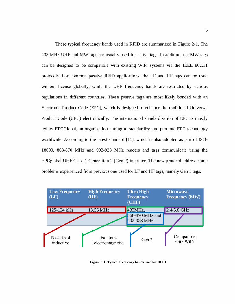
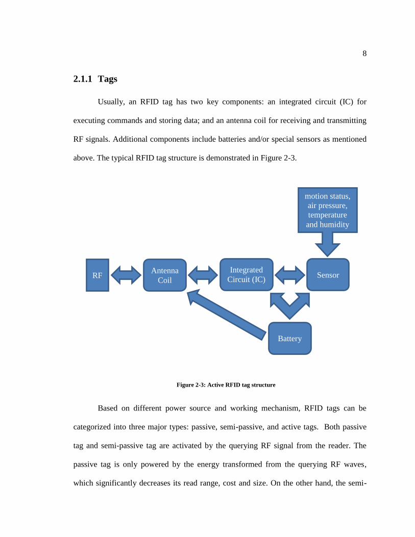
2.1.1 Tags

Usually, an RFID tag has two key components: an integrated circuit (IC) for

executing commands and storing data; and an antenna coil for receiving and transmitting

RF signals. Additional components include batteries and/or special sensors as mentioned

above. The typical RFID tag structure is demonstrated in Figure 2-3.

Figure 2-3: Active RFID tag structure

Based on different power source and working mechanism, RFID tags can be

categorized into three major types: passive, semi-passive, and active tags. Both passive

tag and semi-passive tag are activated by the querying RF signal from the reader. The

passive tag is only powered by the energy transformed from the querying RF waves,

which significantly decreases its read range, cost and size. On the other hand, the semi-

Antenna

Coil

Integrated

Circuit (IC)

Battery

Sensor

motion status,

air pressure,

temperature

and humidity

RF

9

passive tag uses internal battery power to drive the circuits and any existing sensors, and

the signal transmission is still powered by the incoming RF waves. An active tag is self-

powered and broadcasts signals at preset intervals. It usually provides a larger read range.

All types of tags are used in RFID-based RTLS. Systems using active tags are

more commonly reported than passive tag systems due to the larger read range and

continuously working ability. On the other hand, the passive tags and semi-passive tags

have advantages on security and interference issues, owing to their silent characteristics.

2.1.1.1 Passive Tags

A passive RFID tag has neither battery nor sensor. The RF waves propagated by

the reader’s antennas are inducted to provide power for the passive tag. It appears to be

dormant most of the time, and becomes active after an interrogation from a reader is

received. The inquiry/response process limits the passive tag to communicate with only

one reader at a time.

Typical operating frequency bands for passive tags are 120-150 kHz and 13.56

MHz. In this case, near-field communication, where the distance traveled in space of the

RF signal is much less than its wavelength, acts as the major technology to drive the tag.

A relatively larger coil, therefore, is required for the passive tag to generate enough

power by inductive coupling. Since the RF signal strength decays along the distance

rapidly, the read range of traditional passive tags is limited to 1 to 3 meters, varying by

the operating frequency [12]. Due to the reflective characteristics of electromagnetic

waves on metal and liquid surfaces, the readability of passive tags is severely affected

10

under such circumstances. The Gen 2 passive tags use 868-870 MHz and 902-928 MHz

as operating frequency bands and are able to work in the dual mode of near-field and far-

field communication, which improves the overall performance significantly. For instance,

the read range can be extended to 10 meters [13].

Lack of a battery and a sensor definitely bring some limitations to passive RFID

tags. But it also reduces the cost and size of RFID tags significantly.

2.1.1.2 Semi-passive Tags

A semi-passive RFID tag is essentially a passive tag with additional battery and/or

sensor. It is an enhanced edition of a passive tag, but not a silent edition of an active tag.

The additional power supply is used to power the circuits and sensors only. In this way,

all the power received via the RF waves can be used for RF communication with the

reader. It marginally increases the read range since no more power in the received RF

signal is shared to drive circuits the way passive tags do. As long as the inquiry signal can

be received, the response can be sent back with full strength.

2.1.1.3 Active Tags

With an additional battery as power supply, an active RFID tag has the ability to

broadcast its identification information or sensor data actively and periodically. Therefore,

active tags are able to communicate with multiple readers concurrently. Additionally,

they have the larger read range between 50 to 100 meters as higher frequencies are used

and broadcasting RF signal strength is enhanced with the extra battery [14].

11

Typical operating frequency bands for active tags are 433 MHz and 2.4 – 5.8 GHz,

at which the RFID system works in the far-field region where the distance traveled in

space of the RF signal is much greater than its wavelength. In such cases, using higher

frequency (such as 2.4 GHz) leads to higher data transmitting bandwidth and rate.

Therefore, new functionalities, such as tag-to-tag communication and integration to WiFi

network, become possible.

The battery life of an active RFID tag is usually around 3 to 5 years. Thus, battery

monitoring and maintenance are required. Moreover, the additional battery and related

circuits increase both the cost and size of active tags significantly, comparing to passive

tags.

2.1.2 Readers

A RFID reader is a device modulating and demodulating RF signals to

communicate with supported RFID tags via one or several antennas. Most readers are

compatible with either active tags or passive tags of certain operating frequency; only a

few are able to work in dual mode. A database for managing all readers and tags, and

some complicated control logics, such as noise threshold setting, antennas balance, and

active history, may be deployed on the computer connected to the readers.

12

2.2 Real-Time Localization System (RTLS)

An emerging application of RFID is indoor Real-Time Localization System

(RTLS), where the Global Positioning System (GPS) technique is limited by in-building

coverage, Wireless Local Area Network (WLAN) devices are relatively expensive and

larger than RFID tags and therefore not suitable for small items, and Ultra Wide Band

(UWB) systems have a potential interference with some radar systems by sharing a wide

range of bandwidth. Other non RF-based techniques, such as ultrasonic, infrared (IR) and

laser localization, are vulnerable to environmental impacts and are restricted to the Line-

of-Sight (LOS) readability. Admittedly, the multi-path propagation is an issue for RFID

localization.

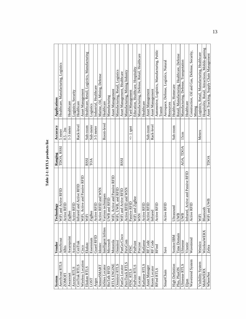
RTLS, especially indoor RTLS, has widespread applications in many areas. Most

current systems provide room-level or sub-room level resolution. Low cost rack-level or

item-level solution is desired. An uncompleted list of up-to-date RTLS products and their

major applications is listed in Table 2-1. All information is collected from the product

description available on their official websites.

13

Tab

le 2

-1:

RT

LS

pro

du

cts

list

Sy

stem

V

en

do

r

Tec

hn

olo

gy

R

an

gin

g

Acc

ura

cy

Ap

pli

cati

on

s

Aer

oS

cou

t R

TL

S

Aer

oS

cou

t W

iFi

and

Act

ive

RF

ID

TD

OA

, R

SS

I 5

met

er

Hea

lth

care

, M

anu

fact

uri

ng,

Lo

gis

tics

ZO

MO

FI

Alb

is

Act

ive

RF

ID

0

.5 -

2m

Aw

aren

et

Aw

arep

oin

t Z

igB

ee

1

-3 m

eter

H

ealt

hca

re

Axce

ss R

TL

S

Axce

ss

Act

ive

RF

ID

Lo

gis

tics

, S

ecu

rity

Cen

Tra

k R

TL

S

Cen

Tra

k

Infr

ared

an

d A

ctiv

e R

FID

Rac

k-l

evel

H

ealt

hca

re

Wir

eles

s L

oca

tio

n

Cis

co

WiF

i, A

ctiv

e an

d P

assi

ve

RF

ID

Ass

et M

anag

emen

t

Ekak

au R

TL

S

Ekak

au

WiF

i R

SS

I S

ub

-ro

om

H

ealt

hca

re,

Ret

ail,

Lo

gic

tics

, M

anu

fact

uri

ng

LO

ST

E

ssen

siu

m

Zig

Bee

T

OA

S

ub

-met

er

Lo

gis

tics

Arg

us

Gu

ard

RF

ID

Act

ive

RF

ID

3

-5 m

eter

In

du

stri

al,

Hea

lth

care

Sen

sorS

MA

RT

Id

ente

c A

ctiv

e R

FID

an

d W

SN

M

arin

e, O

il, M

inin

g,

Def

ense

InS

ites

Lo

cato

r In

tell

igen

t In

Sit

es

Var

iou

s te

chniq

ues

Ro

om

-lev

el

Hea

lth

care

Biz

Tal

k R

FID

M

icro

soft

U

WB

an

d R

FID

M

anu

fact

uri

ng

RT

LS

EN

GIN

E

Mo

toro

la

WiF

i, A

ctiv

e an

d P

assi

ve

RF

ID

Ass

et M

anag

emen

t

Om

nit

rol

RT

LS

O

mn

itro

l W

iFi,

UW

B,

and

RF

ID

Man

ufa

ctu

rin

g,

Ret

ail,

Lo

gis

tics

Pan

Go

Lo

cato

r P

anG

o/C

isco

W

iFi

and

Act

ive

RF

ID

RS

SI

A

sset

Man

agem

ent,

Hea

lth

care

Per

vT

rack

RT

LS

P

ervC

om

A

ctiv

e R

FID

an

d W

SN

M

anu

fact

uri

ng,

Min

ing I

ndu

stry

PIN

C R

TL

S

PIN

C

Pas

sive

RF

ID

+

/- 1

spo

t Y

ard

Man

agem

ent

Pin

Po

int

RT

LS

P

inP

oin

t W

iFi

and

Zig

Bee

E

du

cati

on

, H

ealt

hca

re,

Ho

spit

alit

y

iLo

cate

P

recy

se

WS

N

Man

ufa

ctu

rin

g,

Def

ense

, R

etai

l, H

ealt

hca

re

Rad

ian

se R

TL

S

Rad

ian

se

Act

ive

RF

ID

Hea

lth

care

Ass

et M

anag

er

RF

Co

de

Act

ive

RF

ID

S

ub

-ro

om

A

sset

Man

agem

ent

Ro

om

Lo

cato

r R

F C

od

e In

frar

ed

R

ack-l

evel

A

sset

Man

agem

ent

RF

ind R

TL

S

RF

ind

Act

ive

RF

ID

Au

tom

oti

ve,

Lo

gis

tics

, M

anu

fact

uri

ng, P

ubli

c

Tra

nsi

t

Sm

artC

hai

n

Sav

i A

ctiv

e R

FID

A

ero

spac

e, D

efen

se,

Lo

gis

tics

, N

atu

ral

Res

ou

rces

Hig

h D

efin

itio

n

So

nit

or/

IBM

U

ltra

sou

nd

S

ub

-ro

om

H

ealt

hca

re,

Ho

mec

are

Plu

s, P

lusO

N

Tim

e D

om

ain

U

WB

R

etai

l, M

anu

fact

uri

ng,

Hea

lth

care

, D

efen

se

Ub

isen

se R

TL

S

Ub

isen

se

UW

B

AO

A,

TD

OA

1

5cm

M

anu

fact

uri

ng,

Def

ense

, T

ran

spota

tio

n

Elp

as

Vis

on

ic

Infr

ared

, A

ctiv

e an

d P

assi

ve

RF

ID

Hea

lth

care

Wav

etre

nd

Syst

em

Wav

etre

nd

A

ctiv

e R

FID

C

on

stru

ctio

n,

Oil

an

d G

as,

Def

ense

, S

ecu

rity

,

Min

ing

Vis

ibil

ity S

yst

em

Wes

tico

W

iFi

M

eter

s L

ogis

tics

, R

etai

l, M

anu

fact

uri

ng, H

ealt

hca

re

Mo

biW

ER

X

Wir

eles

sWE

RX

B

luet

ooth

H

osp

ital

ity,

Ret

ail,

Att

ract

ion

s, M

ob

ile-

gam

ing

Wh

ereN

et

Zeb

ra

WiF

i an

d U

WB

T

DO

A

A

sset

Tra

ckin

g,

Su

pp

ly C

hai

n M

anag

emen

t

14

2.2.1 Global Positioning System (GPS) and A-GPS (Assisted GPS)

The Global Positioning System (GPS) is a well-known satellites-based outdoor

localization system operated by the U.S. Other similar systems in use include:

GLONASS by Russia, Beidou by China, and Galileo by Europe. Assisted GPS (A-GPS)

is a GPS application which uses cellular network resources to improve the startup and

locating performance of a receiver. By measuring the time difference of arrivals from

four or more satellites at the same time, the GPS receiver is able to calculate its three-

dimensional (3D) position based on the multilateration approach. For civil applications,

the positioning resolution is about 10 meters for outdoor usage [15]. However, neither

GPS nor A-GPS is suitable for indoor applications due to weak signals. Furthermore,

high energy consuming and expensive receivers limit the GPS or A-GPS to be used for a

large scale deployment.

2.2.2 Wireless Local Area Network (WLAN) and Wireless Sensor

Network (WSN)

The Wireless Local Area Network (WLAN) technique is used for indoor

localization due to several advantages against GPS/A-GPS. First, the Wireless Fidelity

(WiFi) devices are relatively inexpensive and have low power consumption. Second,

WiFi network become an increasingly common infrastructure in many buildings, which

help to reduce the deployment cycle and overall cost of a WiFi-based indoor localization

system. Nevertheless, the size, cost and power consumption of traditional WLAN devices

are still not comparative to RFID tags due to different purpose of use. A technique called

15

Wireless Sensor Network (WSN) was developed to address such issues. The idea of

WSN is to limit the computational power and signal bandwidth of a WSN node to a low

level so that the overall performance is just enough for environmental monitoring

applications. Then, a new problem emerges. WSN nodes may be interfered by WLAN

devices which usually have stronger signals. ZigBee and WiFi are two most important

protocols used in WSN. One of WSN’s major advantages is inter-communication

capability among nodes. The positioning accuracy of the WiFi-based localization systems

varies from sub-meter to several meters for different algorithms and deployment densities

[16]. According to latest research results, the accuracy could achieve 0.04 meters for 2D

and around 0.1 meters for 3D applications [17, 18].

2.2.3 Radio Frequency Identification (RFID)

The biggest advantages of passive or semi-passive RFID tags are the extremely

low price and ultra-small size. However, the RTLS applications based on Gen 1

passive/semi-passive RFID tags are limited by the low read range. Dense deployment is

required to provide enough coverage. The typical resolution of such a RTLS is at the sub-

meter level and highly depends on the density of tag deployment. A system may benefit

from the larger read range of Gen 2 passive tags. For all kinds of passive tags, the tag

orientation affects the signal reading significantly [19]. A common solution is to fix all

tags, both reference tags and target tags, on the same plane (ceiling, floor, or wall) with

the same orientation [20, 21]. This certainly causes some limitations in real applications.

16

Active RFID is similar to WSN but differs in that it has lower operation frequency

(except for WiFi-based RFID, which will be discussed later) and lacks tag-to-tag

communication feature. Due to similar mechanism, most deployment schemes and

positioning algorithms work in almost the same way for both active RFID and WSN

localization systems. Consequently, they share the localization resolution from sub-meter

to sub-room level as well. The 433 MHz RFID system has a potential to be interfered in

real applications because this frequency band is open for amateur radio [10]. The term,

WiFi-based RFID particularly refers to a RFID system operates at the frequency of 2.4

GHz and is embedded into or able to communicate with any existing WiFi systems. In

this way, the RFID system can be easily deployed and managed. Though, interference

and traffic control between RFID signals and regular WiFi signals requires additional

Quality of Service (QoS) configuration on the network server [22].

2.2.4 Ultra Wide Band (UWB)

As a totally different approach, Ultra Wide Band (UWB) is a radio technique

which has high volume data rate (up to 1 Gbps) as the result of using ultra-short pulses

(up to 1-2 giga-pulses per second) over a wide range of frequency spectrum (from 3.1 to

10.6 GHz) [23]. In general, the positioning resolution of a UWB-based localization

system can achieve decimeter level, via LOS measurement and multilateration

approximation [12]. Some particular algorithms may result in even more accurate

resolution, less than 0.04 meters [23]. The pulse radio transmission style ensures UWB

have no interference with other narrow-banded wave radio transmissions in the same

17

frequency bands. However, it may be interfered in some environments where air traffic

control radio beacon system, airport or maritime surveillance radar, and GPS receivers,

are in use [24]. Another concern is that various regulations on this wide spectrum are

permitted in different countries [25], because the pulse-based radio technique is originally

reserved for military usage, such as radar and satellite systems. This leads to high R&D

cost and, therefore, high price for UWB chips.

2.2.5 Non RF-based

Other than the above mentioned radio-based solutions, those non RF-based

techniques, such as ultrasonic, infrared (IR) and laser localization, have long been applied

in positioning systems and are mature [14]. However, restricted to the Line-of-Sight

(LOS) readability, these techniques are vulnerable to environmental impacts, for instance,

obstacles and irregular room shapes. On the other hand, such LOS characteristic ensures

item-level accuracy, given the tag is detected. Nevertheless, the overall locating

resolution is highly determined by the density of reader/antenna deployment, which leads

to significantly increased cost of the whole system.

18

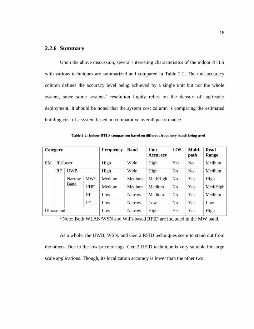
2.2.6 Summary

Upon the above discussion, several interesting characteristics of the indoor RTLS

with various techniques are summarized and compared in Table 2-2. The unit accuracy

column defines the accuracy level being achieved by a single unit but not the whole

system, since some systems’ resolution highly relies on the density of tag/reader

deployment. It should be noted that the system cost column is comparing the estimated

building cost of a system based on comparative overall performance.

Table 2-2: Indoor RTLS comparison based on different frequency bands being used

Category Frequency Band Unit

Accuracy

LOS Multi-

path

Read

Range

EM IR/Laser High Wide High Yes No Medium

RF UWB High Wide High No No Medium

Narrow

Band

MW* Medium Medium Med/High No Yes High

UHF Medium Medium Medium No Yes Med/High

HF Low Narrow Medium No Yes Medium

LF Low Narrow Low No Yes Low

Ultrasound Low Narrow High Yes Yes High

*Note: Both WLAN/WSN and WiFi-based RFID are included in the MW band.

As a whole, the UWB, WSN, and Gen 2 RFID techniques seem to stand out from

the others. Due to the low price of tags, Gen 2 RFID technique is very suitable for large

scale applications. Though, its localization accuracy is lower than the other two.

19

2.3 RFID-RTLS

Despite the difference caused by various types of RFID tags, the fundamental

system structure, or scheme of RFID-RTLS varies. Also, different positioning logics,

namely algorithms, have been reported.

2.3.1 Schemes

RFID-based localization can be classified as fixed-tag localization and fixed-

reader/antenna localization, in accordance with different roles of tags and

readers/antennas [26], as illustrated in Figure 2-4. In the fixed-tag scheme, the tags are

deployed on the ceiling or floor with some rules while the readers/antennas are usually

attached to mobile objects. This is cost effective when the objects to be tracked are

relatively large, few in numbers, and usually move in a 2D plane or on a certain route.

The major application is an auto guided vehicle or robot [27, 28]. In the fixed-

reader/antenna scheme, the readers/antennas and tags are placed in an opposite way to the

fixed-tag scheme. The readers/antennas are installed at fixed positions while the tags are

attached to the items to be tracked. It is useful for most applications where a lot of items

need to be tracked and located at the same time because the tags are much cheaper and

smaller than the readers/antennas. The following work will be based on this scheme.

20

(a) Fixed-tag scheme (b) Fixed-reader scheme

Figure 2-4: Two common RTLS schemes

2.3.2 Algorithms

In a real indoor environment, fading, absorbing, reflection, and interference are

major issues affecting the RF waves’ strength, direction, and distribution. This make the

variation of the RF signal propagation not easily modeled. Since the theoretical model is

not applicable, numerous positioning algorithms have been developed. Several major

types are summarized and introduced as follows, while many varieties exist. The two

largest groups are determined by whether the algorithm ranges the RF signal to an

estimated distance or not.

The range-based localization algorithms require two steps of work. First, the

elementary range results are obtained in several ways: Received Signal Strength

Reader

Tag

Tag

Tag

Tag Tag

Reader

Reader

Reader

Reader

21

Indication (RSSI), Angle of Arrival (AOA), Time of Arrival (TOA), Time Difference of

Arrival (TDOA), or Adaptive Power Multilateration (APM). Then, various approaches on

geographical calculations, such as triangulation, trilateration, and multilateration, are

applied to estimate the final position.

Both the k Nearest-Neighbor (kNN) approach by using centroid of certain

neighbors and the proximity approach by using intersection of several coverage areas

avoid the distance estimation step in range-based localization approaches. However, they

heavily rely on the density of reference tags or reader/antenna distribution to improve

positioning accuracy.

2.3.3 Range-based Localization

2.3.3.1 Received Signal Strength Indicator (RSSI)

Received Signal Strength Indicator (RSSI) is considered the simplest approach for

ranging since almost no additional cost is needed to collect the RSSI data which is

provided by most systems [29]. It is a measurement of received radio signal power in

terms of the ratio of measured power decibels (dB) to one milliwatt (mW). However, it is

also a less accurate way due to complicated environmental impacts to the RF signals

propagation [30]. No theoretical or empirical model can be applied as a universal solution.

Therefore, the RSSI map, which is used to translate the signal strength into distance

estimation, should be calibrated for every single antenna to achieve better results. The

initial solution is to measure the RSSI values at all possible points with predefined

density and renew the mapping periodically. It is not practical to maintain such a system.

22

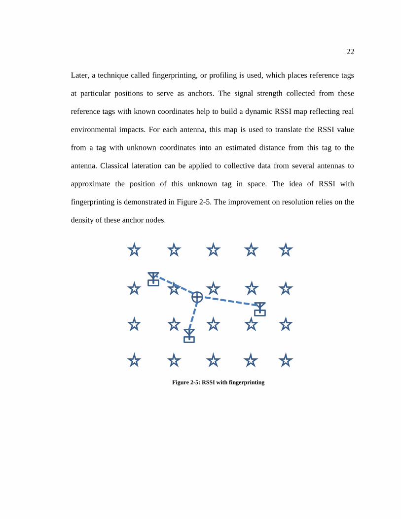
Later, a technique called fingerprinting, or profiling is used, which places reference tags

at particular positions to serve as anchors. The signal strength collected from these

reference tags with known coordinates help to build a dynamic RSSI map reflecting real

environmental impacts. For each antenna, this map is used to translate the RSSI value

from a tag with unknown coordinates into an estimated distance from this tag to the

antenna. Classical lateration can be applied to collective data from several antennas to

approximate the position of this unknown tag in space. The idea of RSSI with

fingerprinting is demonstrated in Figure 2-5. The improvement on resolution relies on the

density of these anchor nodes.

Figure 2-5: RSSI with fingerprinting

23

2.3.3.2 Angle of Arrival (AOA)

The basic idea of Angle of Arrival (AOA) is simple. Consider a triangle for

example. Given the coordinates of any two points are known, the third one can be located

if and only if the angles from these two known points to the unknown point are provided.

This method is known as triangulation, as illustrated in Figure 2-6. The concept can be

extended to 3D space easily. This approach requires customized RF signal

modulating/demodulating units which are add-ons to the overall cost. Therefore, precise

calibration is needed before use. The LOS requirement is another limitation for

applications. The measured angle accuracy is less than 1.7° in a small experimental space,

and decreases for larger angles and longer distance between the tag and the antennas [31].

The overall resolution is approximately sub-meter level for a regular room size space, and

depends on the density of reader/antenna deployment.

Figure 2-6: Triangulation for AOA

Two angles

Known distance

24

2.3.3.3 Time of Arrival (TOA)

The Time of Arrival (TOA) method is based on a theoretical propagation model

of an RF signal. The distance between two points can be determined if the travel time of

the signal between them is measurable. Then, the location of an unknown tag can be

determined using such measurements from various antennas. Cycle intersection, as

shown in Figure 2-7, and nonlinear least-squares approaches are commonly used to get

optimal results with minimum errors. However, the velocity of the EM wave is so high

that the typical travel time within a room is on the scale of nanoseconds. Hence, the TOA

method requires all readers and tags to be strictly precisely synchronized, and all signals

to be time-stamped [29]. The theoretical accuracy can be very high. But with affordable

commercial synchronizing unit, the system resolution is usually about 1 to 2 meters [32].

Moreover, LOS is required to reduce interference caused by multi-path effects.

Figure 2-7: Cycle intersection for TOA

25

2.3.3.4 Time Difference of Arrival (TDOA)

Similar to TOA, the Time Difference of Arrival (TDOA) approach also relies on

precisely synchronized readers and tags. But it uses a different methodology to determine

the location of the unknown point [33]. For each pair of antennas, given the time

difference of the RF signals from them to the tag to be tracked is known, all the possible

locations of this tag must fall into one half of a hyperbola in 2D space, as shown in

Figure 2-8, or a hyperboloid in 3D space. Then, the tag’s location is determined as the

intersection of the hyperbolas or hyperboloids generated by all pairs of antennas. The

TDOA method has same limitations and drawbacks as TOA.

Figure 2-8: First step of multilateration for TDOA

26

2.3.3.5 Adaptive Power Multilateration (APM)

Another approach is called Adaptive Power Multilateration (APM), which

measures the estimated distance from the reader to the tag by reducing or increasing the

reader transmission power until the tag disappears or appears, as shown in Figure 2-9.

The corresponding power level is then translated into distance based on a pre-calibrated

chart. At last, the tag’s position is determined using the multilateration method on

distances estimated from all readers. The accuracy of APM heavily relays on two things.

One is the edge tolerance of the power circle. A perfect clear cut at the edge may not

exist. The other one is the environmental impacts. The pre-calibrated chart may not be

valid under complex circumstance. Some attempts were reported to improve this method

by using reader rotating and some statistical analysis [34, 35].

Figure 2-9: Multilateration for APM

27

2.3.4 Range-free Localization

2.3.4.1 k Nearest-Neighbor (kNN)

The fingerprinting technique applied in the improved RSSI approach is also used

in the k Nearest-Neighbor (kNN) method but without ranging. Similarly, the reference

anchors are deployed in cells. The Eucledian distances between the RSSI values from the

unknown tag and all anchors are calculated. Subsequently, the k anchors with lowest

distances to this tag are selected as its k nearest neighbors. The coordinates of this tag can

be estimated using the centroid of these anchors, as illustrated in Figure 2-10. An

enhanced method call weighted kNN further applies the Eucledian distances from the

unknown tag to its k nearest neighbors as weights to improve the approximation [7].

Overall, the kNN approach is suitable for complex non-isotropic and varying

environments.

Figure 2-10: kNN

28

2.3.4.2 Proximity

In the proximity approach [14], each antenna has a predefined coverage area,

which may be an approximation or calibrated result. If the unknown tag is detected by

more than one antenna, the location of this tag can be estimated by the intersection of the

coverage areas of these antennas, as shown in Figure 2-11. The density of antenna

deployment heavily affects the system resolution. Furthermore, the coverage area may be

difficult to be clearly defined since the RF signals fade away gradually at the edge and

the theoretical propagation model may not be an appropriate simulation for real indoor

environments.

Figure 2-11: Proximity

29

2.3.5 Summary

Pros and cons of different types of localization algorithms most commonly used

in RFID-RTLS are summarized in Table 2-3. Reported localization errors for several

systems using these algorithms are also listed.

Table 2-3: Summary of localization algorithms in RFID-RTLS

Algorithms Pros Cons Accuracy

Range-

based

RSSI Low cost; supported by

most systems; enhanced

with profiling

Low accuracy level; relies on

dense deployment of reference

tags

0.5 m [36],

simulated;

0.72 m [37],

measured

AOA High accuracy level High cost for customized

hardware; LOS measurement

required; pre-calibration need

N/A

TOA High accuracy level High cost for synchronized

devices; LOS measurement

required

N/A

TDOA High accuracy level High cost for synchronized

devices; LOS measurement

required

0.2 m [38],

measured

APM Low cost; no reference

tags needed

Low accuracy level; relies on

pre-calibrated power versus

distance chart; not suitable in

complex environments

0.32 m [35],

simulated;

0.6 m [34],

measured

Range-

free

kNN Low cost; suitable for

complex non-isotropic

and varying environments

Low accuracy level; relies on

dense deployment of reference

tags

0.6 m [7],

measured

Proximity Low cost; easily deployed Low accuracy level; relies on

dense deployment of readers

or antennas, coverage areas

may not be clearly defined in

complex environments

N/A

30

Overall, the RSSI and kNN approaches are mostly cost effective and reliable for

indoor environments. Actually, these two methods are very similar in that they share the

fundamental step of fingerprinting the reference tags. They are only different in the final

stage for estimating the position of the unknown tag.

31

Chapter 3

Theoretical Modeling

3.1 Introduction

It is of interest whether there is any statistically significant minimum number of

reference tags needed for an indoor, real time localization system based on Gen 2 RFID

with battery-assisted passive tags or other active tags. This problem may be solved in two

steps.

First, find out a theoretical solution (at least approximation) based on a series of

assumptions and experimental data from various sources.

Second, design an experiment which is able to determine the relationship between

accuracy level and number of reference tags, and compare the result to the value

estimated in first step.

Furthermore, the trend of localization error as the system dimension increases

from 1D to 2D and then to 3D is investigated. It may be useful on predicting the 3D

localization error based on previous 2D or 1D system performance.

32

3.2 Assumptions

The following are the assumptions used in this modeling section.

Room size. To simplify the question, the test bed is assumed to be located in a

room with the dimension of 3x3x3 meters. In this way, all readers and tags can be

deployed symmetrically and evenly in the 3D space. Such deployment policy in

2D is reported to be an optimum solution in terms of maximizing accuracy [39].

Furthermore, 3*√5=6.7 meter (the maximum distance within a 3x3x3 cube) is a

safe distance to cover the read range of common Gen 2 RFID passive tags [40].

Larger room size may require either more readers or higher class tags to ensure

the RSSI in a stable range. Either option leads to increased overall system cost.

Environment. In reality, a complex environment is very difficult to be modeled.

So, the room is assumed to be absent of large obstructions. All environmental

effects, such as radio wave reflection, absorption, and possible interference, are

assumed to be isotropic and consistent.

Reader. The amount of readers (and/or extended antennas, which will also be

treated as reader for the sake of conciseness) and their deployment will affect the

localization algorithm and accuracy. Nevertheless, such variation/optimization is

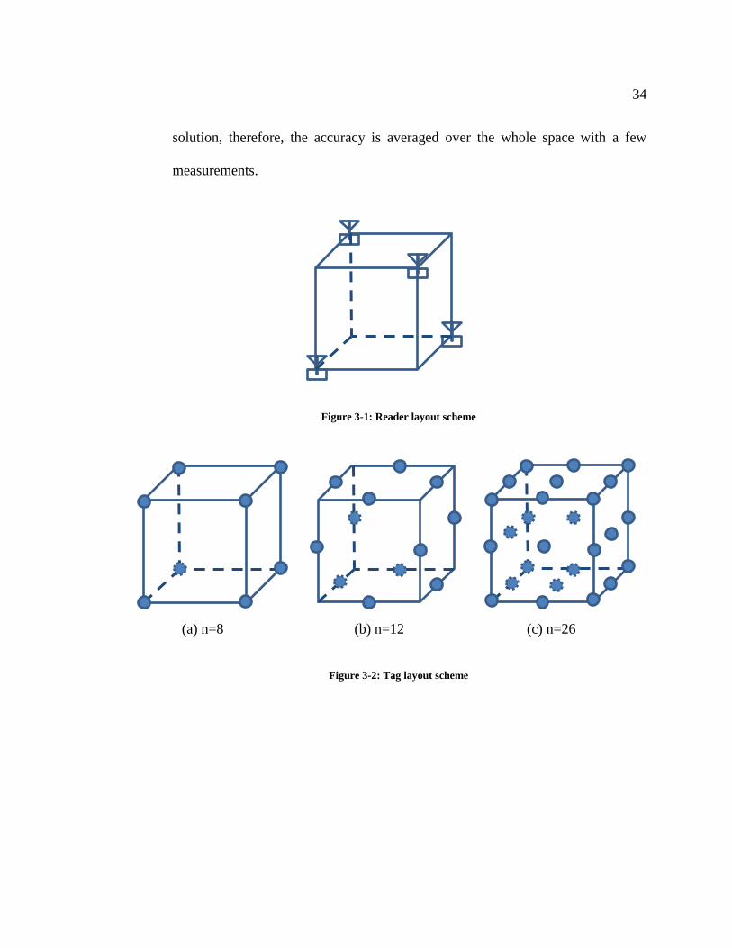
out of the scope of this question. Let’s assume that four readers are placed at the

four opposite corners of the room and none of them are located on the same edge

33

of the cube, as illustrated in Figure 3-1. This is one of the symmetric layouts with

minimum amount of readers required in a 3D space RTLS system.

Tag. All reference tags are placed evenly and symmetrically on the six faces of

the cube. None of them is placed in the inner space of the cube, as this is not

practical in any real application. So, the total amount of all reference tags with

such criteria cannot be any possible integer. Only certain numbers of tags are

possible. Therefore, the minimum amount is 6 for one on each face center.

Several possible layouts are illustrated in Figure 3-2. Scheme (a) has one

reference tag on each corner point. Scheme (b) has one reference tag on each edge

center. Scheme (c) has one reference tag on each corner point, edge center, and

face center. More tag layout schemes will be discussed later.

Algorithm. To simplify the solution, the basic RSSI ranging approach is applied

to each reader. The RSSI map (based on all reference tags) for each reader is

constructed and assumed to be isotropic in 3D space. The distances from the

target tag to four readers are then estimated. The Trilateration method is used to

determine the final position of the target tag.

Measurement. The accuracy is defined as the distance from the real position and

the estimated position of a target tag. Theoretically, the accuracy is not the same

everywhere since there is no reference tag in the middle of the room. So, it is best

to place the target tag at any random position within the room to calculate the

accuracy. However, this may involve complex modeling and simulation. In this

34

solution, therefore, the accuracy is averaged over the whole space with a few

measurements.

Figure 3-1: Reader layout scheme

Figure 3-2: Tag layout scheme

(a) n=8 (b) n=12 (c) n=26

35

3.3 Ranging

The theoretical propagation model used most extensively for RSSI ranging is

called log-normal propagation model [12], which is valid with previous environmental

assumptions. The model is given in Equation (3-1).

[ ] ( )

(3-1)

where PL(d0) is the path loss value for a reference distance d0 (commonly 1.0 meter), η is

the path loss exponent, and Xσ is a Gaussian random variable with zero mean and

variance, σ2, that models the random variation of the RSSI value.

According to previous research [41], the RSSI values are approximately linear

within a range of 4 meters in the anechoic chamber and to a range of 10 meters in the

clear hallway. Therefore, the propagation model in this question may be simplified into

Equation (3-2).

[ ] ( ) (3-2)

where is the slope coefficient for distance, which is a value estimated from the linear

regression of measured RSSI for a given distance. It is a Gaussian random variable with

mean β and variance σβ2

(∑

) (∑ ( )

)⁄ that models the random

variation due to regression estimation. Obviously, more reference tags (larger n) lead to

smaller σβ2 and hence more precise estimation of β. It should be noted that, by definition,

the residual is also a Gaussian random variable with zero mean and variance σ2 which

36

is same as Xσ. Similarly, ( ) is the intercept coefficient with variance

(

∑

).

In order to predict distance with given RSSI, the Equation (3-2) is transformed

into Equation (3-3).

( ) [ ]

(3-3)

where [ ] contains possible measurement error. Then, we have Equation (3-4).

(

( ) [ ]

) (3-4)

This can be further calculated via the following equations, referred from [42, 43].

( ) ( ) ( ) ( ) (3-5)

( ) [ ( )] ( ) [ ( )] ( ) ( ) ( ) (3-6)

(

) [

( )

( )]

{ ( )

[ ( )] ( )

[ ( )] ( )

( ) ( )}

(3-7)

The close form solution of may be too complicated to be easily interpreted. So,

pilot experiment results should be used for further evaluation. The values may vary for

different systems and environments, but the derivation steps are the same. For example,

based on the experiment results on active RFID tags in 2D space, the estimated

regression function (with 9 reference tags) is d = -9.560 - 0.234PRX. The varies from

0.126 to 0.430 (average 0.278) within the range of 4 meters. The corresponding 95%

prediction interval (PI) for ranging varies from 1.858 to 2.690 meters (average 2.274).

37

A close investigation into the relationship between and n reveals that

( ) ( ) ( ) ( ) ( ) ( ) (3-8)

where Var(regression) is the variance generated from linear regression approximation

process, Var(nature) in the variance inherited from RSSI variation and measurement

error, Cov(r,n) is the covariance between them, and α(n), β(n), and γ(n) are corresponding

coefficients for the three terms, respectively. The three coefficients are functions of n.

A proposed hypothesis of as a function of n is that

will decrease to a certain

level as n increases. After that, Var(nature) becomes dominant, and will keep nearly

constant. We may design a series of experiments with various amounts of reference tags

to see whether we are able to fit a model to predict such trend or not. If it is found, then

the maximum possible RSSI ranging error can be estimated for any given amount of

reference tags.

38

3.4 Localization

After the approximated distances from the target tag to four readers are obtained,

the relationship among them may be present in Equation (3-9).

{

( )

( ) ( )

( ) ( )

( )

( ) ( )

( )

( ) ( )

( )

(3-9)

where ( ) is the target tag coordinate to be estimated, ( ) is the position of

four readers, and ri are the predicted distance from the target tag to the four readers. This

group of nonlinear functions can be solved via traditional nonlinear least squares

approach, iterative arithmetic method, or some other algorithms [44]. The fundamental

idea is to find the best solution of ( ) which minimizes the sum of squared

differences between the ri’s and their corresponding modeled values.

The final localization error, e, between the approximated position ( ) and the

real position ( ) of the target tag is defined in Equation (3-10).

( ) ( ) ( ) (3-10)

According to the performance analysis presented in [44], the variance of the

position estimation error is proportional to the square of ranging error, and can be

modeled in Equation (3-11).

(3-11)

39

where is the random error inherited from the RSSI ranging process, , , and

are geometric indices expressing the non-isotropic effect of the system, which can be

calculated with the following functions of Equation (3-12).

(3-12)

By assuming isotropic everywhere in previous statement, the variances in three

axes are identical, and are equal to the ranging variance . Therefore, the geometric

indices , , and are all equal to √2. By further assuming no covariance among the

variances in three axes, the overall variance of position estimation error can be

determined by Equation (3-13).

(3-13)

Similarly, the expected value of the localization error, namely bias, is also proved

to be proportional to the square of ranging error, and can be modeled by Equation (3-14).

(3-14)

where , , and are geometric factors expressing the nonlinearity effect of the

system, which may be defined as the coefficients ratio of the second and first order terms

of the nonlinear distribution equation. By assuming linearity everywhere in previous

statement, the second order terms are negligible for all three axes. Therefore, the

geometric factors , , and and corresponding expected values of position

estimation error for all three axes are equal to zero. This means the overall estimation is

unbiased, as shown in Equation (3-15).

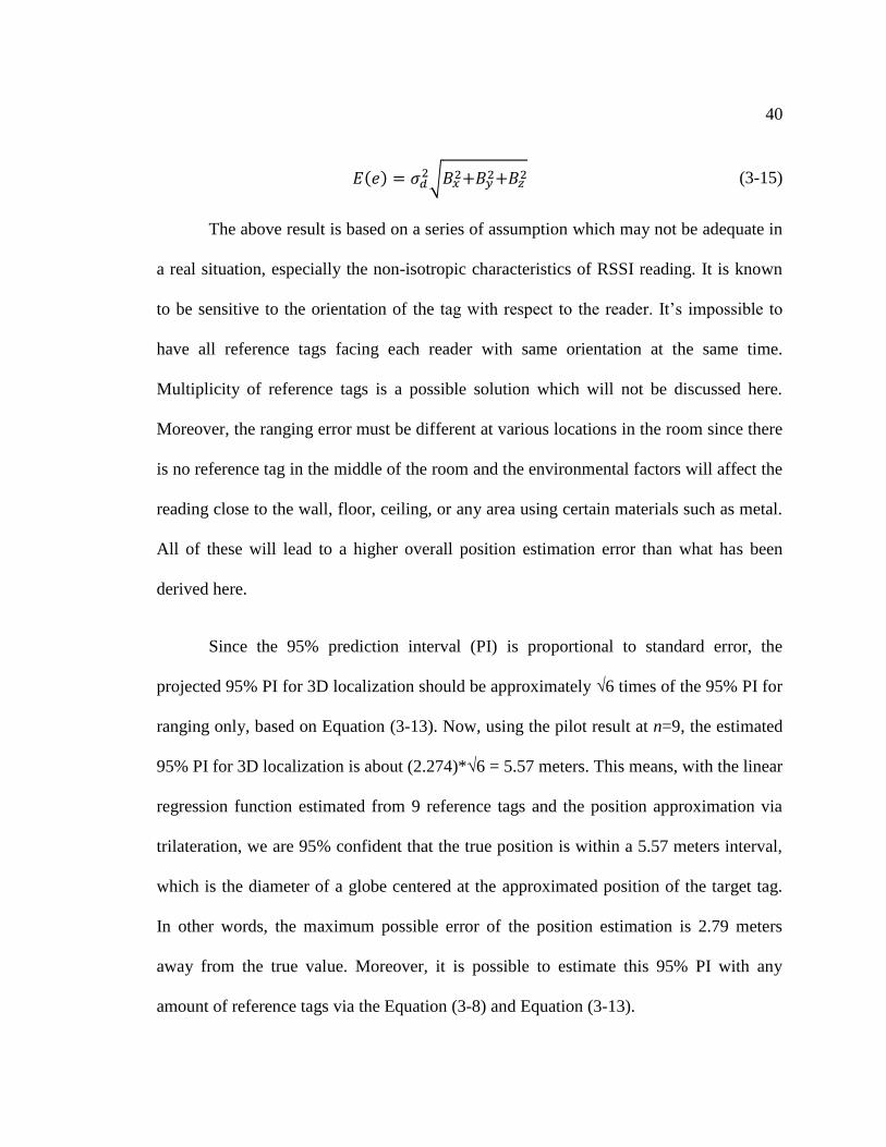
40

( ) √ (3-15)

The above result is based on a series of assumption which may not be adequate in

a real situation, especially the non-isotropic characteristics of RSSI reading. It is known

to be sensitive to the orientation of the tag with respect to the reader. It’s impossible to

have all reference tags facing each reader with same orientation at the same time.

Multiplicity of reference tags is a possible solution which will not be discussed here.

Moreover, the ranging error must be different at various locations in the room since there

is no reference tag in the middle of the room and the environmental factors will affect the

reading close to the wall, floor, ceiling, or any area using certain materials such as metal.

All of these will lead to a higher overall position estimation error than what has been

derived here.

Since the 95% prediction interval (PI) is proportional to standard error, the

projected 95% PI for 3D localization should be approximately √6 times of the 95% PI for

ranging only, based on Equation (3-13). Now, using the pilot result at n=9, the estimated

95% PI for 3D localization is about (2.274)*√6 = 5.57 meters. This means, with the linear

regression function estimated from 9 reference tags and the position approximation via

trilateration, we are 95% confident that the true position is within a 5.57 meters interval,

which is the diameter of a globe centered at the approximated position of the target tag.

In other words, the maximum possible error of the position estimation is 2.79 meters

away from the true value. Moreover, it is possible to estimate this 95% PI with any

amount of reference tags via the Equation (3-8) and Equation (3-13).

41

Please note that this is maximum possible error. It is different from the usually

defined average error. Theoretically, the average localization error, e, can be calculated

based on the definition in Equation (3-10) and its expected value √ ⁄ by assuming a

normal distribution, as shown in Equation (3-16).

√ ⁄ √ ⁄ (√ ) √ ⁄ (3-16)

The estimated error for 3D localization, , is then approximately 2 times of the

ranging standard deviation, . Since the definition of 95% PI is [μ-1.96σ, μ+1.96σ], or

approximately [μ-2σ, μ+2σ], Equation (3-16) can be further expressed in terms of 95% PI

for ranging only, as shown in Equation (3-17).

(3-17)

Using pilot result at n=9, the estimated localization error for 3D is about

(2.274)*0.5=1.137 meters, which is expected to be close to the measured one, e. Though,

it is higher than the accuracy assumption of 0.5 meters, which means more reference tags

may be desired to increase the accuracy level.

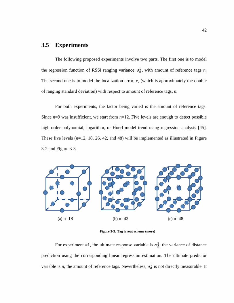
42

3.5 Experiments

The following proposed experiments involve two parts. The first one is to model

the regression function of RSSI ranging variance, , with amount of reference tags n.

The second one is to model the localization error, e, (which is approximately the double

of ranging standard deviation) with respect to amount of reference tags, n.

For both experiments, the factor being varied is the amount of reference tags.

Since n=9 was insufficient, we start from n=12. Five levels are enough to detect possible

high-order polynomial, logarithm, or Hoerl model trend using regression analysis [45].

These five levels (n=12, 18, 26, 42, and 48) will be implemented as illustrated in Figure

3-2 and Figure 3-3.

Figure 3-3: Tag layout scheme (more)

For experiment #1, the ultimate response variable is , the variance of distance

prediction using the corresponding linear regression estimation. The ultimate predictor

variable is n, the amount of reference tags. Nevertheless, is not directly measurable. It

(a) n=18 (b) n=42 (c) n=48

43

should be estimated from the regression process, which is conducted by reader, a block

factor B. For each reader of a given scheme (with certain level of n), the RSSI value and

distance from every reference tag to the corresponding reader are measured to fit a

regression model (assumed to be linear). The for the four blocks are then averaged for

this level of n. By repeating this process for all schemes, we are able to fit the ultimate

regression model between and n for the purpose of predicting

using arbitrary n.

The design structure of experiment #1 is summarized in Table 3-1.

Table 3-1: Design of experiment #1

Objective To fit the best model of ( )

Distance = f(RSSI) ↘ n=12 n=18 n=26 n=42 n=48

B=1

B=2

B=3

B=4

Average

For experiment #2, the ultimate response variable is the localization error, e. The

regression function of ( ) is easy to model. Though, it is of more interest whether

the relationship described in the Equation (3-13) is valid or not. The design structure of

experiment #2 is summarized in Table 3-2. Please note that the total number of replicates

(by putting target tags at different locations) is designed to be able to catch any sample

variation less than or equal to with the power of 80%.

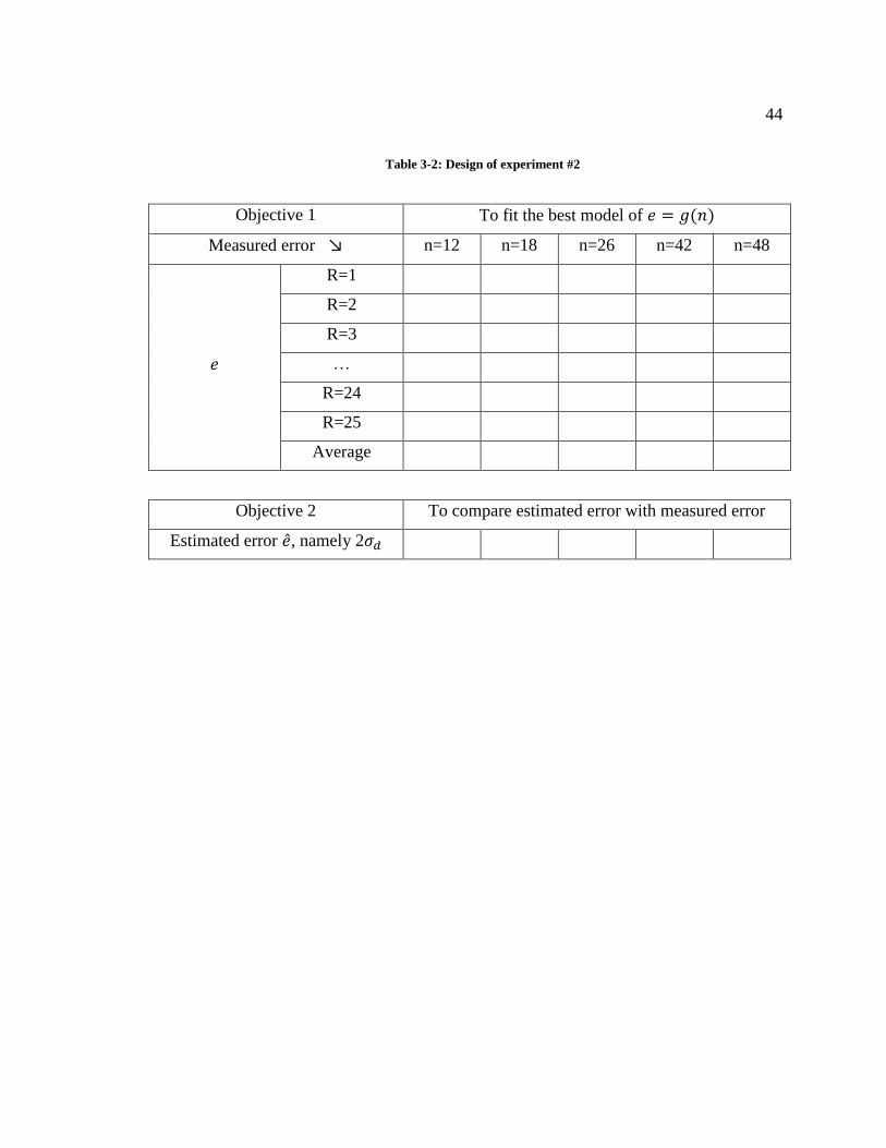
44

Table 3-2: Design of experiment #2

Objective 1 To fit the best model of ( )

Measured error ↘ n=12 n=18 n=26 n=42 n=48

R=1

R=2

R=3

…

R=24

R=25

Average

Objective 2 To compare estimated error with measured error

Estimated error , namely 2

45

3.6 Summary

Both theoretical analysis and experimental design are presented to demonstrate

the idea of evaluating the statistically confident accuracy as a function of the amount of

reference tags for an indoor RTLS with numerous assumptions. Therefore, the

statistically significant minimum number of reference tags needed may be obtained in a

reverse way. The theoretical model also indicates that a lower-bound of the accuracy

level for any given system may exist, due to the natural variation of RFID signal strength.

Improved system design and ingenious localization algorithm may help make this lower-

bound even smaller.

The experimental results could differ a lot from the theoretical function due to

violation of those assumptions or restrictions of the test environment. Revised prediction

model is expected to include more variables, rather than the number of reference tags

only. Despite these, there are several important conclusions which may benefit further

research.

The ranging accuracy is affected by both the regression analysis and the RSSI

variation, as shown in Equation (3-8). At some point, the increase in the number of

reference tags does not bring any further improvement to the overall accuracy, as the

variance from measured RSSI variation becomes dominant, which is the natural

characteristic that belongs to a particular RFID system. The estimated localization error

for 3D applications is approximately equal to half of the 95% PI for 1D ranging only.

46

Moreover, from the whole process, it is clear that the estimated localization error

is expected to be larger in 3D systems than in 2D or 1D systems. According to the

geometric indices defined in Equation (3-12), the theoretical ratio is √6 : √2 : 1, or

approximately 2.45 : 1.4 : 1. The ratio will be even larger when the environmental factors,

such as non-isotropic and non-linear distribution of RF signals are taken into account.

Lastly, the proposed experiments were not actually conducted for several reasons.

Though, a reasonable and relatively safe number of reference tags being used in the

following experiments could be set to 24, as it is not too small or too large.

47

Chapter 4

System and Experimental Designs

4.1 Fundamental Tests for Active System

Some early-stage experiments were conducted to evaluate the active 433 MHz RF

Code reader and tag characteristics. These tests are described as follows.

4.1.1 Reader Test

The purpose of the reader test is to evaluate the effects of reader position and

antenna orientation. The whole system was setup in room W107 Nebraska Hall, which is

a conference room with approximate size of 6.3 by 4.8 by 2.7 meters.

A lot of factors may affect the RSSI reading of a RFID system. To serve the

purpose of this experiment, only reader related variables were investigated. According to

previous research [41], the distance from reader to ground, the distance from reader to

wall, and the antenna orientation may have significant effects on RSSI reading. So, these

three factors were chosen to be evaluated in this experiment. In addition, four readers

were included as a block factor to separate any potential reader bias. Furthermore, three

tags were randomly selected from the 25 tags we have available to serve as non-reader-

related replicates. Both reader and tag effects were contained in the evaluation as well. A

detailed treatment design is listed in Table 4-1.

48

Table 4-1: Main factors of reader test

Symbol Factor Levels Comments

A reader readers #1 IP address: 192.168.1.101

readers #2 IP address: 192.168.1.102

readers #3 IP address: 192.168.1.103

readers #4 IP address: 192.168.1.104

B height 0.4 m Close to the ground

1.2 m Far away from either the ground or the ceiling

2 m Close to the ceiling

C depth 0.2 m Close to the wall

0.6 m Neither too close nor too far away to the wall

1 m Far away from the wall

D antenna [\ /] Antenna A (the left one when facing the reader) and

antenna B (the right one when facing the reader) are

both in the vertical plane with 45 degrees to the ground

and 90 degrees in between;

[|_] Antenna A and B are both in the vertical plane with A

in the vertical direction and B in the horizontal

direction;

[. |] Antenna A is in the horizontal plane and pointing

straight forward, while antenna B is in the vertical

plane and in the vertical direction as well.

E tag tag #1 Tag ID: LOCATE00016492

tag #2 Tag ID: LOCATE00016488

tag #3 Tag ID: LOCATE00016502

The reader and tag deployment is demonstrated in Figure 4-1, where reader has

3x3=9 possible positions while tag position was set at a fixed location (1.2 m from the

ground, and 2 m from the wall).

49

Figure 4-1: Layout scheme of reader test

The desired experimental unit is each possible treatment combination. However,

this may be impractical. Overall, the number of all possible treatment and replicate

combinations is 4*3*3*3*3=324, which is too large for a preliminary experiment. So, a

trade-off was made between the ability to test 2nd order or higher order interactions and

the significantly reduced number of total runs to be conducted. The final design consists

of 56 runs (only certain treatment and replicate combinations were selected) with the

power equal to 0.917 which is judged to be acceptable to test the main effects of each

factor. The 56 runs were randomized within each block of readers.

Thirty continuous RSSI data points, with 2 second intervals, were collected for

each run; then the following responses, namely dependent variables, were calculated:

Height from the ground (m)

Depth from the wall (m) 0.2 0.6 1

0.4

1.2

2

2

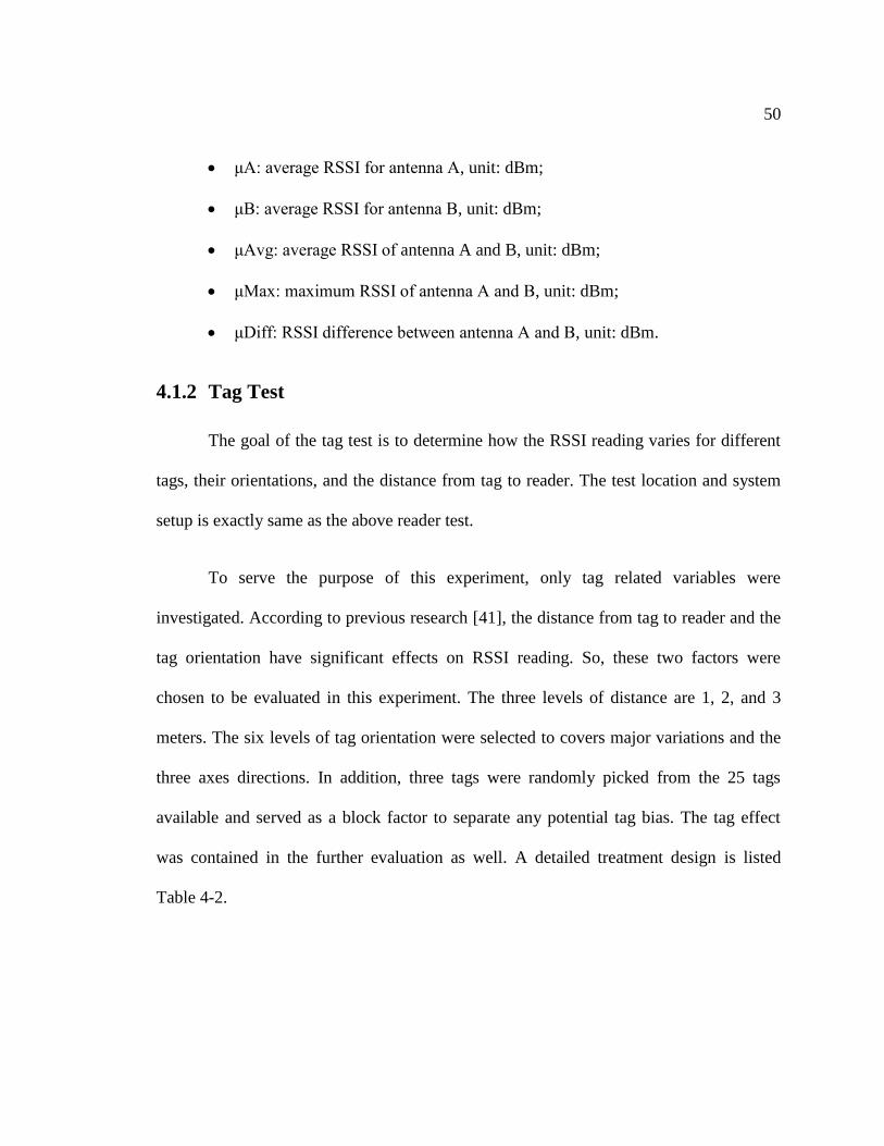
50

μA: average RSSI for antenna A, unit: dBm;

μB: average RSSI for antenna B, unit: dBm;

μAvg: average RSSI of antenna A and B, unit: dBm;

μMax: maximum RSSI of antenna A and B, unit: dBm;

μDiff: RSSI difference between antenna A and B, unit: dBm.

4.1.2 Tag Test

The goal of the tag test is to determine how the RSSI reading varies for different

tags, their orientations, and the distance from tag to reader. The test location and system

setup is exactly same as the above reader test.

To serve the purpose of this experiment, only tag related variables were

investigated. According to previous research [41], the distance from tag to reader and the

tag orientation have significant effects on RSSI reading. So, these two factors were

chosen to be evaluated in this experiment. The three levels of distance are 1, 2, and 3

meters. The six levels of tag orientation were selected to covers major variations and the

three axes directions. In addition, three tags were randomly picked from the 25 tags

available and served as a block factor to separate any potential tag bias. The tag effect

was contained in the further evaluation as well. A detailed treatment design is listed

Table 4-2.

51

Table 4-2: Main factors of tag test

Symbol Factor Levels Comments

A tag tag #1 Tag ID: LOCATE00016492

tag #2 Tag ID: LOCATE00016488

tag #3 Tag ID: LOCATE00016502

B distance 1 m Near distance comparing to room size

2 m Medium distance comparing to room size

3 m Far distance comparing to room size

C orientation Level 1: > The tag is placed facing the ceiling with its long edge

perpendicular to the line connecting reader and tag;

Level 2: ^ The tag is placed facing the ceiling with its short

edge perpendicular to the line connecting reader and

tag;

Level 3: _ The tag is placed sitting on one of its long edges and

facing against the reader;

Level 4: - The tag is placed sitting on one of its short edges and

facing against the reader;

Level 5: | The tag is placed sitting on one of its long edges with

the facing direction 90 degree different from level 3;

Level 6: . The tag is placed sitting on one of its short edges

with the facing direction 90 degree different from

level 4.

The reader was placed at a fixed position (1.2m from the ground, and 0.6m from

the wall). The antenna orientation was setup at the level 2 configuration as used in the

previous reader test, that is, antenna A and B are both in the vertical plane with A in the

vertical direction and B in the horizontal direction. The reader and tag deployment is

illustrated in Figure 4-2.

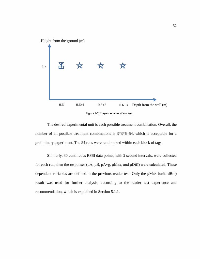
52

Figure 4-2: Layout scheme of tag test

The desired experimental unit is each possible treatment combination. Overall, the

number of all possible treatment combinations is 3*3*6=54, which is acceptable for a

preliminary experiment. The 54 runs were randomized within each block of tags.

Similarly, 30 continuous RSSI data points, with 2 second intervals, were collected

for each run; then the responses (μA, μB, μAvg, μMax, and μDiff) were calculated. These

dependent variables are defined in the previous reader test. Only the μMax (unit: dBm)

result was used for further analysis, according to the reader test experience and

recommendation, which is explained in Section 5.1.1.

Height from the ground (m)

Depth from the wall (m) 0.6+1 0.6 0.6+2

1.2

0.6+3

53

4.1.3 Ranging Test

As a supplement of the above tag test, this ranging test is designed to investigate

the relationship between the RSSI and distance from the tag to the reader in more detail.

The whole system was setup in room 329B Scott Engineering Center, with approximate

size of 4.34 by 8.74 by 2.82 meters.

Only one factor, the distance from the tag to the reader, was used in this

experiment. It includes 10 levels, ranging from 0.5m to 5m with a 0.5m interval. Five

tags were randomly selected as replicates for each distance level.

The reader was setup at a fixed position, at least 2m away from all walls and

exactly 1m from the ground. The antenna orientation was kept in a consistent posture

throughout the whole experiment with the left antenna pointing to the ceiling and the

right antenna pointing to the wall. The tag was placed at the same height of the reader

with the front side facing the reader in a straight line for all distance levels, as illustrated

in Figure 4-3.

The basic experiment unit is a single tag with certain distance to the reader. 30

data points with 2 seconds interval were recorded for each run. The results were naturally

blocked by 5 randomly selected tags. The total number of all treatment combinations is

10*5=50 runs. They are completely randomized. Still, μMax (unit: dBm) is chosen as the

response for analysis as recommended before.

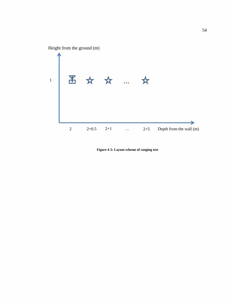
54

Figure 4-3: Layout scheme of ranging test

Height from the ground (m)

Depth from the wall (m) 2+0.5 2 2+1

1

2+5 …

…

55

4.2 Localization Test for Active System

4.2.1 System Setup

In order to evaluate the performance under realistic conditions, the proposed

system was deployed in an experimental environment consisting of a 4x9x3m high-

complexity room, furnished with a bed, a sofa, several tables and chairs, and other

common household items. The system included 4 active 433 MHz RFID readers

deployed at the four edges of the ceiling and 24 reference tags placed on the walls,

ceiling and floor, with an average spacing of 1.5m. The readers and tags are all

commercial off-the-shelf (COTS) products, as shown in Figure 4-4.

Figure 4-4: RF Code readers and tags

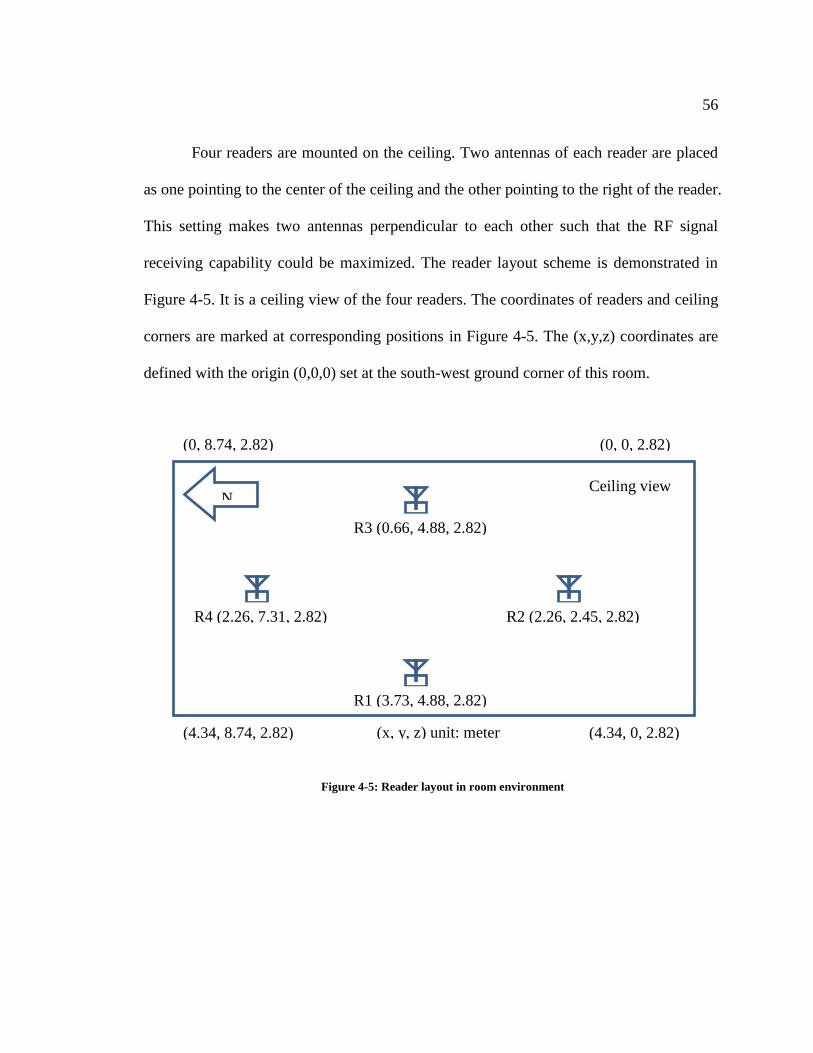
56

Four readers are mounted on the ceiling. Two antennas of each reader are placed

as one pointing to the center of the ceiling and the other pointing to the right of the reader.

This setting makes two antennas perpendicular to each other such that the RF signal

receiving capability could be maximized. The reader layout scheme is demonstrated in

Figure 4-5. It is a ceiling view of the four readers. The coordinates of readers and ceiling

corners are marked at corresponding positions in Figure 4-5. The (x,y,z) coordinates are

defined with the origin (0,0,0) set at the south-west ground corner of this room.

Figure 4-5: Reader layout in room environment

(0, 8.74, 2.82) (0, 0, 2.82)

(4.34, 0, 2.82) (4.34, 8.74, 2.82)

R3 (0.66, 4.88, 2.82)

R1 (3.73, 4.88, 2.82)

R4 (2.26, 7.31, 2.82) R2 (2.26, 2.45, 2.82)

N Ceiling view

(x, y, z) unit: meter

57

The 24 reference tags are grouped into different layers along each of the x, y and

z axes, resulting in 4 layers in the x dimension, 3 layers in the y dimension, and 4 layers

in the z dimension. All tags are placed with its front side facing the positive x direction.

The tag layout scheme is demonstrated in Figure 4-6. The coordinates of these reference

tags are listed in Table 4-3.

Figure 4-6: Reference tag layout in room environment

58

Table 4-3: Reference tags ID and positions

# ID (x,y,z) # ID (x,y,z)

1 LOCATE00016485 [1.32,6.71,2.82] 2 LOCATE00016486 [3.12,6.71,2.82]

3 LOCATE00016487 [1.32,4.88,2.82] 4 LOCATE00016488 [3.12,4.88,2.82]

5 LOCATE00016489 [1.32,3.05,2.82] 6 LOCATE00016490 [3.12,3.05,2.82]

7 LOCATE00016491 [0.00,6.71,1.82] 8 LOCATE00016492 [0,6.71,1.00]

9 LOCATE00016493 [0.00,4.88,1.82] 10 LOCATE00016494 [0,4.88,1.00]

11 LOCATE00016495 [0.00,3.05,1.82] 12 LOCATE00016496 [0,3.05,1.00]

13 LOCATE00016497 [4.34,6.71,1.82] 14 LOCATE00016498 [4.34,6.71,1.00]

15 LOCATE00016499 [4.34,4.88,1.82] 16 LOCATE00016500 [4.34,4.88,1.00]

17 LOCATE00016501 [4.34,3.05,1.82] 18 LOCATE00016502 [4.34,3.05,1.00]

19 LOCATE00016503 [1.32,6.71,0.00] 20 LOCATE00016504 [3.12,6.71,0.00]

21 LOCATE00016505 [1.32,4.88,0.00] 22 LOCATE00016506 [3.12,4.88,0.00]

23 LOCATE00016507 [1.32,3.05,0.00] 24 LOCATE00016508 [3.12,3.05,0.00]

4.2.2 Software Development

The four RF Code readers were initialized using the Reader Configuration Utility

downloaded from the RF Code support website. The reader can be connected to a

computer via either Ethernet port or serial port (recommended for first time initialization).

The basic parameters of these readers were set to the following values.

IP address: 192.168.1.101, 192.68.1.102, 192.168.1.103, and 192.168.1.104;

Subnet mask: 255.255.255.0;

Gateway: 192.168.1.1; and

Others settings were kept at factory default.

59

The control package, Zone Manager, was also downloaded from the official

support website. It was installed on the laptop to work as the center node of the RF Code

system. Both readers and tags information were configured in the Zone Manager. The

package has a web portal which is accessible either from local computer or remote place.

The login information is given below.

Local: http://localhost:6580/rfcode_zonemgr/

Remote: http://<public_ip_address>:6580/rfcode_zonemgr/

It should be noted that, due to different network security policy, some work may

need to be done to setup the correct network and firewall configuration before the remote

access feature works.

After being configured in the Zone Manager, the system is ready for use now. Tag

information is able to be read from the web portal. It is broadcasted periodically (10

seconds by default, 2 second in motion). The tag freezes at last update and eventually

disappears from the list several minutes later after the reader loses track of it. So, there

must be a database to support the web portal to provide buffered information. A system

scheme is demonstrated in Figure 4-7 to make the whole structure clearer. The database

is inaccessible to the end user directly, which makes collecting data over time difficult.

So, additional programming using Matlab has to be done to achieve this automatically

such that real-time algorithm becomes possible. JavaScript Object Notation (JSON) was

used as the programing interface to the RF Code system in Matlab. This is described in

Appendix A.1 in details.

60

Figure 4-7: Network and software structure of the RF Code system

Based on these preparations, a Matlab package was coded to read and collect RF

Code tag information continuously. See Appendix B.2 for codes. This is mainly used in

fundamental tests, including the reader test, tag test and ranging test.

The readers and tags are detected and listed when loading the Graphic User

Interface (GUI), as illustrated in Figure 4-8. Any of them can be chosen to be included in

further evaluation or not. Different channel mode is available to specify the working

mechanism of two antennas. The Read SSI button performs a single request of RSSI

information of selected tags through selected readers.

Reader Reader Reader Reader

Portal/API

Database

Matlab with

JSON

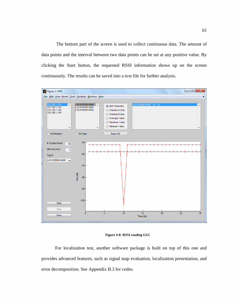
61

The bottom part of the screen is used to collect continuous data. The amount of

data points and the interval between two data points can be set at any positive value. By

clicking the Start button, the requested RSSI information shows up on the screen

continuously. The results can be saved into a text file for further analysis.

Figure 4-8: RSSI reading GUI

For localization test, another software package is built on top of this one and

provides advanced features, such as signal map evaluation, localization presentation, and

error decomposition. See Appendix B.3 for codes.

62

The screen snapshot of the localization GUI is illustrated in Figure 4-9. It mainly

shows the real-time estimated (x,y,z) coordinates and localization error versus time.

Figure 4-9: Localization GUI

The coordinates of all readers, reference tags and other tags can be modified in

pop-up windows by clicking the corresponding buttons. The proposed target tags are

listed in the Selected targets area, which can be modified in the All available tags pop-up

window. Single selection can be made by clicking on the tag ID. Multiple selection can

be made by clicking on the tag ID while pressing the Ctrl or Shift key. The coordinates of

the current selected target tag can be revised in the x/y/z zone. Locate single target

63

perform a one-time localization process. To make a continuous localization, the amount

of data points, the interval between two data points, and the visible length of the time axis

should be defined first. After that, by clicking the Track single target button or the Track

multiple targets button, the real-time estimated x/y/z values and localization errors are

plotted. To switch targets for multiple tracking, simply click the desired target

identification. The Show decomposed signals checkbox allows localization error

decomposition based on various algorithms, as shown in the above snapshot. Though, the

save data feature is currently not available due to data complexity.

4.2.3 Localization Algorithm

The proposed localization algorithm is a hybrid approach by taking both range-

free estimation and range-based measurement into account. This is an improvement based

on a 2D solution previously proposed by other student [46], and has been presented as a

poster in [47]. The scheme of the 2D algorithm is illustrated in Figure 4-10. It can be

broken down into four steps.

Side detection;

RSSI ranging;

Quadrant filtering; and

Final estimation.

64

First, the target tag’s RSSI values obtained from each reader are compared to all

reference tags’ RSSI values. Estimation is then made on which side of the room and

quadrant the target is expected to be in.

Second, based on the side information (two adjacent sides connected to the

estimated quadrant), linear RSSI ranging is conducted using reference tags for each side.

This is repeated for all readers. So far, the total number of ranging estimations for the

target tag is 2 times the number of readers.

Next, the ranges are filtered out if they do not cross over the estimated quadrant or

are totally outside of the room. The rest of them are valid for the next step.

At last, Least Squares Quadratic (LSQ) estimates based on remaining ranges and

their intersections points within the estimated quadrant are then averaged to find the

single final point estimation.

Figure 4-10: 2D algorithm

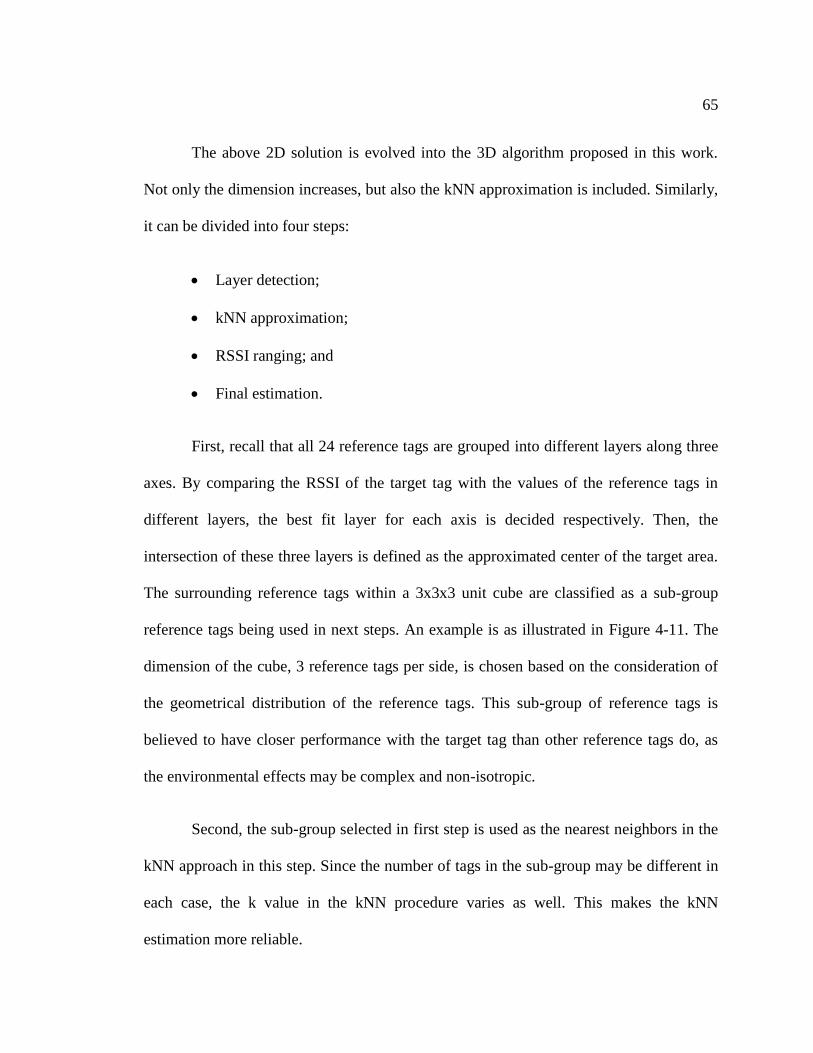
65

The above 2D solution is evolved into the 3D algorithm proposed in this work.

Not only the dimension increases, but also the kNN approximation is included. Similarly,

it can be divided into four steps:

Layer detection;

kNN approximation;

RSSI ranging; and

Final estimation.

First, recall that all 24 reference tags are grouped into different layers along three

axes. By comparing the RSSI of the target tag with the values of the reference tags in

different layers, the best fit layer for each axis is decided respectively. Then, the

intersection of these three layers is defined as the approximated center of the target area.

The surrounding reference tags within a 3x3x3 unit cube are classified as a sub-group

reference tags being used in next steps. An example is as illustrated in Figure 4-11. The

dimension of the cube, 3 reference tags per side, is chosen based on the consideration of

the geometrical distribution of the reference tags. This sub-group of reference tags is

believed to have closer performance with the target tag than other reference tags do, as

the environmental effects may be complex and non-isotropic.

Second, the sub-group selected in first step is used as the nearest neighbors in the

kNN approach in this step. Since the number of tags in the sub-group may be different in

each case, the k value in the kNN procedure varies as well. This makes the kNN

estimation more reliable.

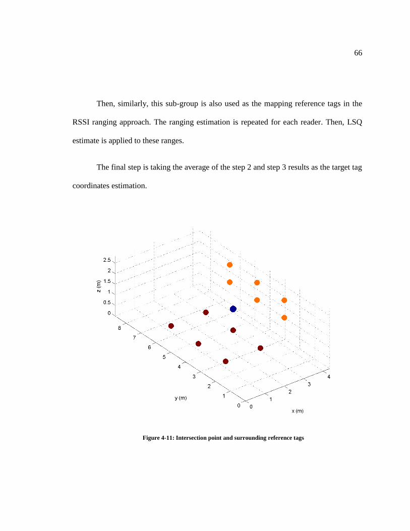
66

Then, similarly, this sub-group is also used as the mapping reference tags in the

RSSI ranging approach. The ranging estimation is repeated for each reader. Then, LSQ

estimate is applied to these ranges.

The final step is taking the average of the step 2 and step 3 results as the target tag

coordinates estimation.

Figure 4-11: Intersection point and surrounding reference tags

67

4.2.4 Experimental Design

The localization experiment is designed to evaluate the performance of the

proposed hybrid algorithm by comparing to the traditional kNN and RSSI algorithms

with various tag position and orientation combinations.

Three factors are location, orientation, and algorithm, as defined as in Table 4-4.

Table 4-4: Main factors of localization test

Factor Level

Position 8 different positions as described as follows

Orientation 3 orientations (X+, Y+, and Z+), defined as putting the tag front

side to the positive direction of the three axes, respectively

Algorithm 3 algorithm (Hybrid, kNN, and RSSI), this is also used as a

blocking factor to simplify the experiment procedure

Table 4-5: Tag position definition

# X (m) Y (m) Z (m)

1 1.32 3.97 0.70

2 1.32 3.97 1.70

3 1.32 5.80 0.70

4 1.32 5.80 1.70

5 3.73 3.97 0.70

6 3.73 3.97 1.70

7 3.73 5.80 0.70

8 3.73 5.80 1.70

X/Y (with Z = 0.70 and 1.70)

Y=

5.80

Y=

3.97

X=1.32 X=3.73

68

The basic experiment unit is a single tag. Thirty data points with 2 seconds

interval are recorded for each run. Three replicates (tags) are used for each treatment. The

total number of all treatment combination is then 8*3*3*3=216 runs. They are

randomized within each block (namely the algorithm).

The response variable is mean localization error, the distance (unit: meter)

between the estimated position and the real position, denoted as e.

The power analysis result shows that, at the confidence level of alpha equal 0.05,

the power of detecting the localization error difference at the same scale of standard

deviation is 0.868, greater than common critical value 0.8. This means the result obtained

from this designed experiment is reliable.

69

4.3 Additional Tests for Battery-assisted Passive System

The above experiment is based on RF Code active tags system and is deployed in

the normal laboratory room environment. Two additional tests are conducted to evaluate

the system performance using Intelleflex battery-assisted passive tags and the effects of

ISS mock-up to the tag characteristics.

4.3.1 System Setup

These additional tests, laboratory environment investigation, were also conducted

in room 329B Scott Engineering Center. Figure 4-12 shows the Intelleflex readers,

antennas and tags. The reader being used in this experiment is Intelleflex FMR6000

Passive RFID Reader. Its operating frequency is 902-928 MHz in North America. One or

two pairs of antennas are used for sending and receiving signals. The tags being used in

this experiment are STT-8000 (general purpose tags) and SMT-8100 (metal environment

tags), labeled as STT and SMT, respectively. They are both battery-powered passive tags.

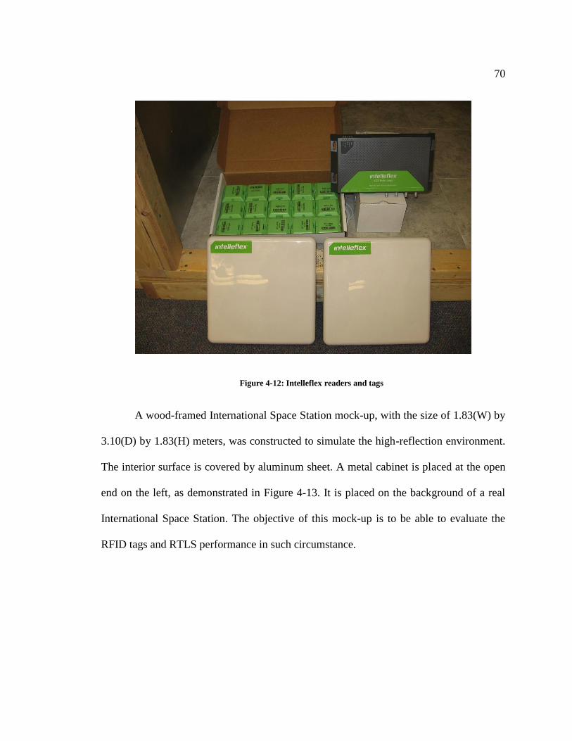
70

Figure 4-12: Intelleflex readers and tags

A wood-framed International Space Station mock-up, with the size of 1.83(W) by

3.10(D) by 1.83(H) meters, was constructed to simulate the high-reflection environment.

The interior surface is covered by aluminum sheet. A metal cabinet is placed at the open

end on the left, as demonstrated in Figure 4-13. It is placed on the background of a real

International Space Station. The objective of this mock-up is to be able to evaluate the

RFID tags and RTLS performance in such circumstance.

71

Figure 4-13: International space station mock-up

The performance of the battery-assisted passive tags in both the regular laboratory

environment and such high-reflection mock-up is of interest. Two types of tags (general

purpose tags and metal environment tags) are evaluated to see if they have similar

characteristics.

72

4.3.2 Software Development

The basic parameters of the Intelleflex readers were set to the following values.

IP address: 192.168.1.11, and 192.68.1.12;

Subnet mask: 255.255.255.0;

Gateway: 192.168.1.1; and

Others settings were kept at factory default.

There is no bundled software provided along with the system. The tag reading

functionality of the reader could be verified via a demo webpage by accessing reader

directly using its IP address. Also, the readability is not guaranteed since there is no

database. The request has to be fulfilled upon real tag feedback every time. This makes

the querying time much longer than RF Code system. The system structure is

demonstrated in Figure 4-14. Extensible Markup Language (XML) was used as the

programing interface to the Intelleflex system in Matlab. See Appendix A.2 for details.

Figure 4-14: Network and software structure of the Intelleflex system

Reader

Portal/API

Reader

Portal/API

Matlab with

XML

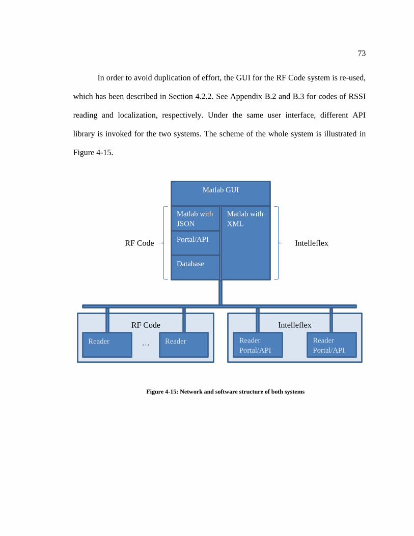
73

In order to avoid duplication of effort, the GUI for the RF Code system is re-used,

which has been described in Section 4.2.2. See Appendix B.2 and B.3 for codes of RSSI

reading and localization, respectively. Under the same user interface, different API

library is invoked for the two systems. The scheme of the whole system is illustrated in

Figure 4-15.

Figure 4-15: Network and software structure of both systems

Reader Reader Reader

Portal/API

Reader

Portal/API

Portal/API

Database

Matlab with

JSON

RF Code

…

Intelleflex

Matlab GUI

Matlab with

XML

RF Code Intelleflex

74

4.3.3 Experimental Design

Four factors are used in this experiment, as described in the following table.

Table 4-6: Main factors of battery-assisted passive tag test

Factor Level

Location Laboratory room (Lab) environment and ISS mock-up (Mockup)

Group General purpose tags (STT) and metal environment tags (MTT)

Orientation 3 orientations (X+, Y+, and Z+), defined as putting the tag front

side to the positive direction of the three axes, respectively

Distance 10 levels from 0.5 meters to 5 meters with 0.5 meters interval in

the laboratory room environment; 6 levels from 0.5 meters to 3

meters with 0.5 meters interval in the ISS mock-up

The basic experiment unit is a single tag. Thirty data points with 2 seconds

interval are recorded for each run. Three replicates (tags) are used for each treatment. The

total number of all treatment combination is then 2*3*(6+10)*3=288 runs. They are

completely randomized.

No blocking is designed. The response variable is the mean RSSI value (unit:

dBm) during each run. The corresponding standard deviation is investigated as well.

75

4.4 Localization Tests for Battery-assisted Passive System

In order to investigate the performance of battery-assisted passive tag in the

proposed localization system, a brief localization test for the battery-assisted passive

system was duplicated based on the localization test for the active system.

Due to space limitation, the Intelleflex readers and antennas are placed at different

positions. And only two pairs of antennas are used in the localization procedure. Their

coordinates are (3.12, 7.71, 1.41) and (1.32, 2.05, 1.41). All reference tags are placed

exactly at the same positions as the RF Code reference tags. The treatment design is listed

in Table 4-7. Most of them are same as the passive system experiment design, except for

the elimination of the factor orientation. The target tags are placed with same orientation

as reference tags since the localization test on passive tags shows that this optimizes the

localization accuracy. Though, the number of replicates (tags) increases from 3 to 5 such

that the power is still higher than 0.8.

Table 4-7: Main factors of localization test (battery-assisted passive sytem)

Factor Level

Position 8 different positions as described in Table 4-5

Algorithm 3 algorithms (Hybrid, kNN, and RSSI), this is also used as a

blocking factor to simplify the experiment procedure

76

4.5 Summary

A localization test bed is built in room 329B Scott Engineering Center. Two RFID

systems, a RF Code active system and an Intelleflex battery-assisted passive system, are

placed side-by-side for comparison. Both use 24 reference tags. There are 4 readers for

the active system, while only one reader plus two separated antennas are used for the

battery-assisted passive system due to implementation restriction. The software package

is developed using Matlab with JSON and XML programming interface to different

readers. It is able to communicate with readers and tags to get RSSI information in real-

time. Certain localization algorithm is then applied to estimate the target tag coordinates

and localization error.

Besides, a series of fundamental tests, such basic reader, tag, and ranging tests,

are designed prior to the formal localization test to help understanding both RFID system

better, such as the reader/antenna placement, tag orientation issue, and measured response

variable selection.

In addition, an International Space Station mock-up is constructed next to the

laboratory environment. Its interior surface is covered by aluminum sheet to simulate the

high-reflection environment. The ranging performance of battery-assisted passive tag in

such a mock-up is compared to regular laboratory results.

77

Chapter 5

Results and Analysis

5.1 Fundamental Tests for Active System

5.1.1 Reader Test

The test results are analyzed for main effect only, which is defined as the effect of

one factor average over all levels of the others for a particular response. The main effects

plot, as shown in Figure 5-1, demonstrates the main effects of the four factors for the two

responses in a matrix. The columns are two selected responses: μAvg and μMax. It was

found that both the average and maximum value of the RSSI from the two antennas are

good candidates as the measurement of RSSI reading for each reader due to the relatively

concentrated standard deviation and few outliers. Therefore, other responses are not

reported here. The rows are four factors: reader, height, depth, and antenna. The tag is not

shown here as it is a replicate factor in this experiment. The individual plot shows how

the response varies with different levels of a factor. The x axes are defined levels for each

factor. The y axes are corresponding RSSI values (unit: dBm) plotted in the same scale

for easier comparison.

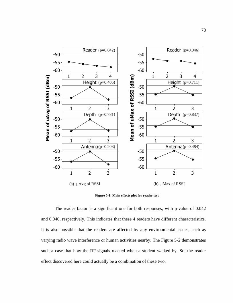
78

(a) μAvg of RSSI (b) μMax of RSSI

Figure 5-1: Main effects plot for reader test

The reader factor is a significant one for both responses, with p-value of 0.042

and 0.046, respectively. This indicates that these 4 readers have different characteristics.

It is also possible that the readers are affected by any environmental issues, such as

varying radio wave interference or human activities nearby. The Figure 5-2 demonstrates

such a case that how the RF signals reacted when a student walked by. So, the reader

effect discovered here could actually be a combination of these two.

Me

an

of

uA

vg

of

RS

SI

(dB

m) 4321

-50

-55

-60

321

-50

-55

-60

321

-50

-55

-60

321

-50

-55

-60

Reader

Height

Depth

Antenna

Me

an

of

uM

ax

of

RS

SI

(dB

m) 4321

-50

-55

-60

321

-50

-55

-60

321

-50

-55

-60

321

-50

-55

-60

Reader

Height

Depth

Antenna

(p=0.042)

(p=0.405)

(p=0.781)

(p=0.208)

(p=0.046)

(p=0.711)

(p=0.837)

(p=0.484)

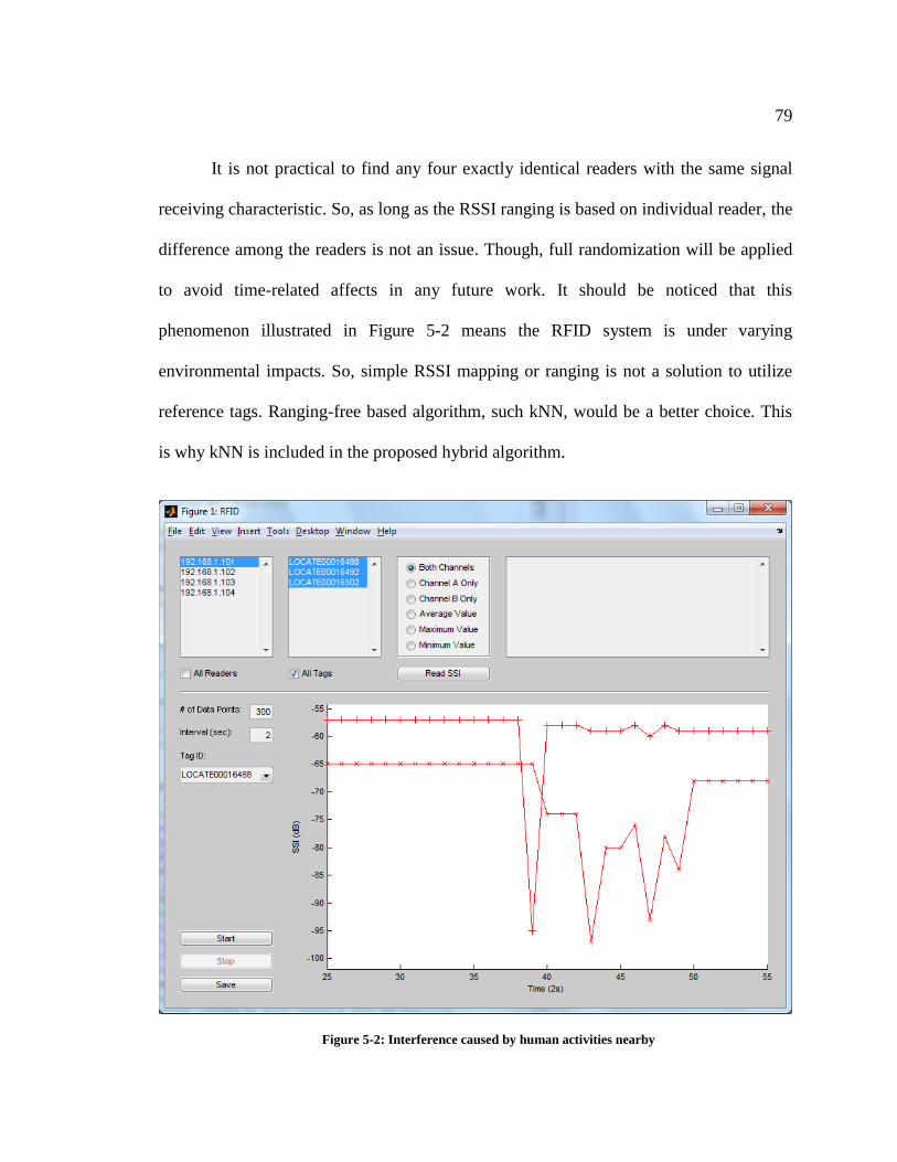
79

It is not practical to find any four exactly identical readers with the same signal

receiving characteristic. So, as long as the RSSI ranging is based on individual reader, the

difference among the readers is not an issue. Though, full randomization will be applied

to avoid time-related affects in any future work. It should be noticed that this

phenomenon illustrated in Figure 5-2 means the RFID system is under varying

environmental impacts. So, simple RSSI mapping or ranging is not a solution to utilize

reference tags. Ranging-free based algorithm, such kNN, would be a better choice. This

is why kNN is included in the proposed hybrid algorithm.

Figure 5-2: Interference caused by human activities nearby

80

Referring to the height and depth columns, the RSSI values are lower when the

reader was placed close to the ground, the ceiling, or the wall. However, as long as this

effect is consistent, it is acceptable. So, it is experimentally justified to mount all readers

on the ceiling in formal experiments.

Having two antennas perpendicular to each other (one is horizontal and the other

is vertical) is provides stable signal receiving, which is also recommended by the manual.

So, the two perpendicular antennas design is applied in the research effort.

Furthermore, the maximum value of RSSI is preferred as a response of RSSI

evaluation rather than the average value in future work. The experimental experience

shows that the maximum value makes the final RSSI ranging estimation more robust and

stable as the RF signals may disappear occasionally.

In summary, the reader test leads to the following conclusions.

The 4 readers may have different RF signal receiving characteristics. Though,

environmental interference could be confounded with the reader effect.

Placing reader close to the edges of the room (especially the wall and the

ceiling) does affect the RSSI reading, but not unpredictably.

Setting one antenna horizontally and the other one vertically is the

recommended antennas placement.

The maximum value of RSSI of two antennas’ measurement presents the

desired information best.

81

5.1.2 Tag Test

The main effects plot is shown in Figure 5-3. Overall, these tags have very similar

performances (with p-value 0.571), which mean the assumption of no significant bias

among the RSSI reading from different tags is acceptable. As distance increases from 1

meter to 3 meters, the RSSI reading decreases almost linearly. The tag orientation has an

extremely significant affect (p=0.000). It is also noticed that some orientations have

similar performance and may be grouped together to reduce levels being used in further

experiments. For example, these 6 orientations may be grouped by the direction of three

axes (level 1 and 2 for z, level 3 and 4 for y, and level 5 and 6 for x). The plot shows that

such grouping is not perfect but reasonable. Then, only 3 levels are needed.

Figure 5-3: Main effects plot for tag test

Me

an

of

uM

ax f

or

RS

SI

(dB

m)

321

-48

-51

-54

-57

321

654321

-48

-51

-54

-57

Tag Distance

Orientation

Main Effects Plot (data means) for uMax

(p=0.571) (p=0.021)

(p=0.000)

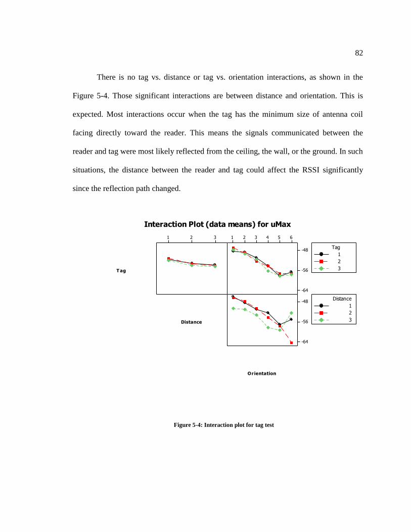
82

There is no tag vs. distance or tag vs. orientation interactions, as shown in the

Figure 5-4. Those significant interactions are between distance and orientation. This is

expected. Most interactions occur when the tag has the minimum size of antenna coil

facing directly toward the reader. This means the signals communicated between the

reader and tag were most likely reflected from the ceiling, the wall, or the ground. In such

situations, the distance between the reader and tag could affect the RSSI significantly

since the reflection path changed.

Figure 5-4: Interaction plot for tag test

T ag

321 654321

-48

-56

-64

Distance

-48

-56

-64

Orientation

Tag

3

1

2

Distance

3

1

2

Interaction Plot (data means) for uMax

83

In summary, the tag test leads to the following conclusions.

Different tags have similar characteristics in this test. So, it is acceptable to

pick any of them as replicates in future tests.

The distance has an approximately negative linear relationship with RSSI in

this 2D experiment, which is expected as normal RF characteristic. Though,

smaller intervals and larger range should be investigated further.

The orientation of any tag is a significant factor and can be further grouped

into 3 levels (facing the x, y, and z direction). Therefore, the tag orientation is

definitely a must-have factor in further experiment design.

Interactions mostly occur when the reader and tag are not directly facing each

other. However, this may not be easily avoided in a 3D application.

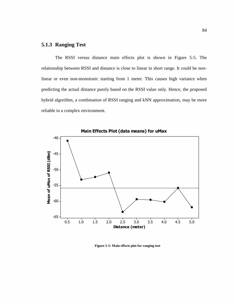
84

5.1.3 Ranging Test

The RSSI versus distance main effects plot is shown in Figure 5-5. The

relationship between RSSI and distance is close to linear in short range. It could be non-

linear or even non-monotonic starting from 1 meter. This causes high variance when

predicting the actual distance purely based on the RSSI value only. Hence, the proposed

hybrid algorithm, a combination of RSSI ranging and kNN approximation, may be more

reliable in a complex environment.

Figure 5-5: Main effects plot for ranging test

Distance (meter)

Me

an

of

uM

ax o

f R

SS

I (d

Bm

)

5.04.54.03.53.02.52.01.51.00.5

-40

-45

-50

-55

-60

-65

Main Effects Plot (data means) for uMax

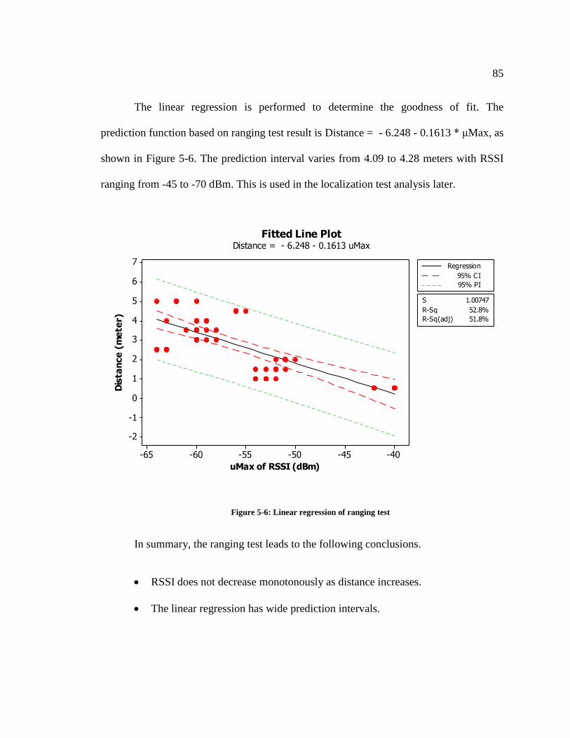
85

The linear regression is performed to determine the goodness of fit. The

prediction function based on ranging test result is Distance = - 6.248 - 0.1613 * μMax, as

shown in Figure 5-6. The prediction interval varies from 4.09 to 4.28 meters with RSSI

ranging from -45 to -70 dBm. This is used in the localization test analysis later.

Figure 5-6: Linear regression of ranging test

In summary, the ranging test leads to the following conclusions.

RSSI does not decrease monotonously as distance increases.

The linear regression has wide prediction intervals.

uMax of RSSI (dBm)

Dis

tan

ce

(m

ete

r)

-40-45-50-55-60-65

7

6

5

4

3

2

1

0

-1

-2

S 1.00747

R-Sq 52.8%

R-Sq(adj) 51.8%

Regression

95% CI

95% PI

Fitted Line PlotDistance = - 6.248 - 0.1613 uMax

86

5.2 Localization Test for Active System

The proposed system was evaluated by taking measurements at 8 different

locations within the room with 3 different tag orientations and 3 different target tags used

at each location, as described in Section 4.2.

As shown in Table 5-1, the experiments resulted in mean localization errors of

1.37, 1.67, and 1.69 meters for the hybrid, kNN, and RSSI ranging algorithms,

respectively. The corresponding standard deviations are 0.65, 0.84, and 0.46 meters,

respectively. The localization error distribution is listed based on error ranges with 0.5

meter intervals. The mean values and standard deviations for each algorithm are

presented at the bottom of the table. Statistics test results for comparing these three

algorithms are also listed.

The hybrid approach performs better than the other two methods in both aspects

of mean and standard deviation. The p-values for mean comparison of the Hybrid method

versus kNN approximation and the Hybrid method versus RSSI ranging are 0.003 and

0.000, respectively. And the p-values for standard deviation comparison are 0.030 and

0.010, respectively. Recall that all three different orientations are included here. With

mixed orientations, the kNN and RSSI approaches have similar performance in terms of

mean localization error.

87

Table 5-1: Localization error distribution for all orientations

Error Range Hybrid kNN RSSI

0m < E ≤ 0.5m 5.56% 0.00% 0.00%

0.5m < E ≤ 1m 26.39% 29.17% 8.33%

1m < E ≤ 1.5m 36.11% 15.28% 25.00%

1.5m < E ≤ 2m 9.72% 25.00% 34.72%

2m < E ≤ 2.5m 18.06% 9.72% 30.56%

E > 2.5m 4.17% 20.83% 1.39%

Mean (m) 1.37 1.67 1.69

P-value for Mean Comparison N/A 0.003 0.000

Stdev (m) 0.65 0.84 0.46

P-value for Stdev Comparison N/A 0.030 0.010

If only the results with same orientation as reference tags are evaluated, the mean

localization errors decrease to 1.08, 1.10, and 1.56 meters for the hybrid, kNN, and RSSI

ranging algorithms, respectively, as listed in Table 5-2. The corresponding standard

deviations are 0.36, 0.58, and 0.50 meters, respectively. The hybrid approach is not a

dominantly best solution this time. But it is significantly better than kNN with smaller

standard deviation (p=0.025), and is significantly better than RSSI with smaller mean

error (p=0.002). Overall, with smallest mean and standard deviation, the hybrid approach

performs significantly better than the other two methods. This is also illustrated

graphically in Figure 5-7. Furthermore, the localization accuracy is much better than

using all target tag orientations. This means for the active tag system, the tag orientation

makes a difference in signal receiving.

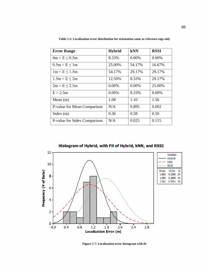
88

Table 5-2: Localization error distribution for orientation same as reference tags only

Error Range Hybrid kNN RSSI

0m < E ≤ 0.5m 8.33% 0.00% 0.00%

0.5m < E ≤ 1m 25.00% 54.17% 16.67%

1m < E ≤ 1.5m 54.17% 29.17% 29.17%

1.5m < E ≤ 2m 12.50% 8.33% 29.17%

2m < E ≤ 2.5m 0.00% 0.00% 25.00%

E > 2.5m 0.00% 8.33% 0.00%

Mean (m) 1.08 1.10 1.56

P-value for Mean Comparison N/A 0.895 0.002

Stdev (m) 0.36 0.58 0.50

P-value for Stdev Comparison N/A 0.025 0.115

Figure 5-7: Localization error histogram with fit

89

Recall that, in 2D, RFID-based RTLSs achieve an accuracy of around 1 meter in

high-complexity indoor environments [41, 46]. Accuracies of less than 1 meter, around

half meter, can be achieved with a higher density of reference tags and/or more

complicated hardware [14]. There is also a clear need for RFID-based 3D indoor RTLSs

[48]. And as summarized in Section 3.6, theoretical results predict that the localization

error in 3D will be at least 1.7 times that in 2D, if isotropic RF propagation and

environmental impacts are accounted for [44]. Therefore, the performance of the

proposed 3D RTLS is aligned with theoretical prediction and is competitive with other

current 2D systems when taking the dimension difference into account.

A localization error comparison chart among various reported RFID-based RTLS

is illustrated in Figure 5-8. The matrix at the bottom shows the localization errors based

on several major algorithms, kNN, RSSI, TDOA, and APM. The results for 3D, 2D, and

simulation are separated in different columns. The simulation results are listed here for

reference only, and are discussed in details. In the second column, the significantly large

value of 3 meters by using RSSI algorithm in 3D is not the focus either. As this is the

very initial attempt at 3D RFID localization, a lot of improvements developed later were

applied to 2D applications but not 3D applications. It should also be noticed that, all

TDOA systems use microware frequency bands, which is an intersection of RFID and

WSN. Their high accuracy error levels were benefited from complicated time

synchronization mechanism of the devices.

90

Figure 5-8: Localization error comparison

First, the RSSI and TDOA rows of the first (UNL 3D) and the third (UNL 2D)

columns are compared. These systems were developed in the same high-complexity

laboratory room at UNL. So, the comparison between the 2D versus 3D relationship is

seen. For RSSI, the ratio of localization error in 3D application versus 2D is 1.56 : 1.03,

or equivalently 1.515 : 1. Similarly, the ratio for TDOA is 0.1 : 0.04, or equivalently 2.5 :

1. Recall that the theoretical ratio is √6 : √2, or equivalently 1.732 : 1, as discussed in

Chapter 3. Thus the theoretical prediction is reasonable, and could be used for further

evaluation.

UNL 3D Other 3D UNL 2D Other 2D Simulated

Hybrid 1.08

kNN 1.1 0.6

RSSI 1.56 3 1.03 0.72 0.5

TDOA 0.1 0.04 0.2

APM 0.6 0.32

0

0.5

1

1.5

2

2.5

3

3.5Lo

caliz

atio

n e

rro

r (m

)

[47]

[47] [7]

[47] [30] [46] [37] [36]

[18] [18] [38]

[34] [35]

91

Now, if this ratio is applied to the 2D systems reported in the fourth column, the

best possible 3D results could be predicted. For kNN, the 3D accuracy prediction is 1.732

* 0.6 = 1.04 meters. The UNL 3D result is 1.1 meters. And for RSSI, the 3D accuracy

prediction is 1.732 * 0.72 = 1.25 meters. Though, the UNL 3D result, 1.56 meters, is 25%

higher than this prediction. It may be caused by the reference tags deployment strategy.

As in other 2D applications, the reference tags are usually placed evenly on the plane

being investigated. However, in the UNL 3D system, all reference tags are attached to the

walls, ceiling, and floor. There is no reference tag in the middle of the room to reflect real

restriction. The proposed hybrid algorithm reduces the localization error to 1.08 meters,

even closer to the prediction than the kNN approach. It also brings significantly smaller

standard deviation, as mentioned in earlier part of this section. So, this 3D system is a

successful attempt. Admittedly, it may be further improved.

In addition, the relationship between the ranging error and localization error was

also evaluated to see if it fit the theoretical prediction as expressed in Equation (3-16).

The typical RSSI values range from -45 to -70 dBm in this localization test. Therefore,

the PI varies from 4.09 to 4.28 meters, as discussed in Section 5.1.3. According to the

prediction formula, Equation (3-17) developed in Section 3.4, the theoretical localization

error using RSSI ranging in 3D applications should be from 2.05 to 2.14 meters. The

actual error measured in this test using RSSI ranging is 1.56 meters, which is smaller than

the prediction values. Due to the time constraint, the proposed experiment in Section 3.5

was not conducted in a full set. The above verification is considered a sample value only.

This may be completed in future work.

92

In summary, based on commercial off-the-shelf (COTS) RFID readers and tags

and using a novel software based localization algorithm, the proposed system achieves a

mean localization error of 1.08 meters, which fits previous theoretical prediction. The

proposed hybrid algorithm offers significantly enhanced localization performance

compared to other existing algorithms.

93

5.3 Additional Tests for Battery-assisted Passive System

5.3.1 Battery-assisted Passive System

A similar tag test as conducted with the RF Code active tags was repeated to

evaluate the performance of two different types of Intelleflex battery-powered passive

Gen 2 RFID tags with different test conditions, as described in Section 4.3.

In order to compare the location effect, all data points measured with distance no

higher than 3 meters are taken as a subset of the whole dataset, due to the dimension

limitation of the mock-up. The main effects plot for the mean of measured signal strength

is illustrated in Figure 5-9.

The two levels of the Location factor are significantly different (p=0.000). Overall,

the signal strength in Lab is higher than in Mockup, which represents different

environmental impacts. The high-reflection effect of the all-metal-surrounded mock-up

causes significant interference to the RF signal propagation, which could lead to lower

signal strength.

In general, STT tags have significant higher signal strength than SMT tags

(p=0.000). The trend is consistent in all other conditions, including different locations. It

may because the additional metal shell of SMT tags act as a protection shield, which

seems to be designed to filter RF signals or moderate interference in high-reflection

environment. Similar component is not found in STT tags.

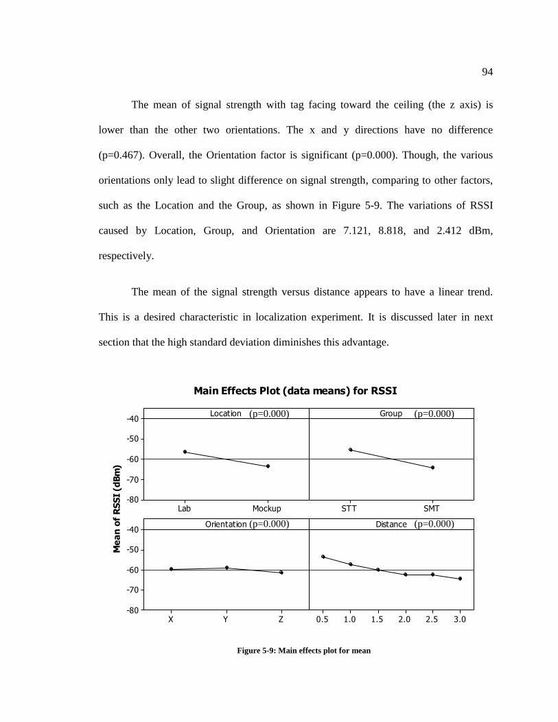
94

The mean of signal strength with tag facing toward the ceiling (the z axis) is

lower than the other two orientations. The x and y directions have no difference

(p=0.467). Overall, the Orientation factor is significant (p=0.000). Though, the various

orientations only lead to slight difference on signal strength, comparing to other factors,

such as the Location and the Group, as shown in Figure 5-9. The variations of RSSI

caused by Location, Group, and Orientation are 7.121, 8.818, and 2.412 dBm,

respectively.

The mean of the signal strength versus distance appears to have a linear trend.

This is a desired characteristic in localization experiment. It is discussed later in next

section that the high standard deviation diminishes this advantage.

Figure 5-9: Main effects plot for mean

Me

an

of

RS

SI

(dB

m)

MockupLab

-40

-50

-60

-70

-80SMTSTT

ZYX

-40

-50

-60

-70

-803.02.52.01.51.00.5

Location Group

Orientation Distance

Main Effects Plot (data means) for RSSI

(p=0.000) (p=0.000)

(p=0.000) (p=0.000)

95

The standard deviation of the signal strength is also investigated. The main effects

plot is shown in Figure 5-10.

The Location factor causes significant difference of signal strength over various

levels (p=0.000). The mock-up environment leads to higher standard deviation, which is

expected in high-reflection space due to signal interference.

The SMT tags have no better performance than STT tags in terms of the standard

deviation of signal strength. The standard deviations for two types of tags are almost

identical (p=0.913). The test result does not fully meet the design purpose of SMT tags.

The additional metal shell could be helpful when the tag is trying to catch signals from

the reader in a metal environment with high signal interference. It may also have a side

effect of partially blocking the signal strength broadcasted from the tag. This could cause

relatively lower signal strength mean for the SMT tags, as discussed above. But it cannot

determine how well the response signal is received by the reader, which means the

standard deviation of the signals is not related to the type of the tag. So, only STT tags

are used in further in laboratory tests.

The standard deviation of signal strength with tag facing toward the antenna (the

y axis) is higher than the other two orientations. The x and z directions have no difference

(p=0.555). Overall, orientation is still a significant factor (p=0.000). Though, it leads to

less variation than the Location does (1.397 versus 4.086 dBm), as shown in Figure 5-10.

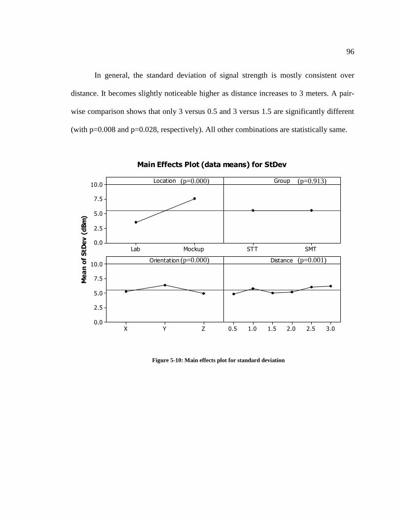
96

In general, the standard deviation of signal strength is mostly consistent over

distance. It becomes slightly noticeable higher as distance increases to 3 meters. A pair-

wise comparison shows that only 3 versus 0.5 and 3 versus 1.5 are significantly different

(with p=0.008 and p=0.028, respectively). All other combinations are statistically same.

Figure 5-10: Main effects plot for standard deviation

Me

an

of

StD

ev

(d

Bm

)

MockupLab

10.0

7.5

5.0

2.5

0.0SMTSTT

ZYX

10.0

7.5

5.0

2.5

0.03.02.52.01.51.00.5

Location Group

Orientation Distance

Main Effects Plot (data means) for StDev

(p=0.000) (p=0.913)

(p=0.000) (p=0.001)

97

Similarly, a linear regression was performed to the ranging data measured in the

laboratory with STT tags, as shown in Figure 5-11. The prediction function based on

ranging test result is Distance = - 7.302 - 0.1779 * RSSI, with R2 equal to 78.7%, which

is acceptable. The prediction interval varies from 2.68 to 2.77 meters with RSSI ranging

from -40 to -75 dBm. This is used in the localization test analysis later. Even with

doubled standard deviation, the PI of the battery-assisted passive system is narrower than

the active system (2.68 to 2.77 versus 4.09 to 4.28 meters) due to the stable linear trend

of the data (R2: 78.7% versus 52.8%).

Figure 5-11: Linear regression of ranging test (battery-assisted passive system)

RSSI (dBm)

Dis

tan

ce

(m

ete

r)

-40-45-50-55-60-65-70-75

7

6

5

4

3

2

1

0

-1

-2

S 0.670287

R-Sq 78.7%

R-Sq(adj) 78.5%

Regression

95% CI

95% PI

Fitted Line PlotDistance = - 7.302 - 0.1779 RSSI

98

In summary, the battery-assisted passive tag test leads to the following

conclusions.

The mock-up leads to lower RSSI and higher deviation than in the laboratory

environment. The signal interference caused by metal reflection is the

expected major reason.

SMT tags have lower RSSI values than STT tags, but they have no difference

in terms of standard deviation. This is probably due to the metal shell design

of the SMT tags. Though, it should be noted that the SMT tags may have

enhanced capability on receiving unstable signals in metal environment, but

the response signals being sent out may not benefit from this.

The Intelleflex tags are not orientation sensitive at all directions in terms of

either mean or standard deviation. The orientation causes 2/3 less variation

than other factors. The possible reason is the enlarged antenna coil size, which

increase broadcasting response signals.

The signal strength versus distance regression appears to have a linear trend.

Though, the high standard deviation makes this advantage less valuable. This

is explained in the next section.

99

5.3.2 Active versus Battery-assisted Passive System

The main effect plots of the signal strength and its deviation versus distance are

compared to the RF Code active tags results in Figure 5-12. Overall, Intelleflex tags are

better on RSSI linearity but have higher and inconsistent standard deviation.

In part (a) comparison, although the average signal strength of the battery-assisted

passive system is lower (-57.15 versus -60.94 dBm, p=0.000), the linear trend is more

obvious than with the active system. In addition, the average signal strength of the active

system does not even monotonously decrease versus distance in most cases.

In part (b) comparison, the signal strength deviation for the battery-assisted

passive system is almost four times higher than the active system, 4.04 versus 1.11 dBm

(p=0.000). This makes the RSSI ranging almost impossible in regular room-size space.

The boxplot comparison in part (c) combines the mean and variation information

together to present different characteristics of these two systems. The active system has

precise RSSI reading at particular locations but is impacted by the environment. The

RSSI measured in the active system does not follow a linear, quadratic, or log trend. It is

not even monotonic, which makes RSSI regression less accurate. The RSSI reading of the

battery-assisted passive system is distance dependent but less stable at any particular

position. As discussed in Chapter 3, such ranging variance is inherited and amplified to

final localization error later. So, neither of these two patterns is desired for the purpose of

RSSI ranging.

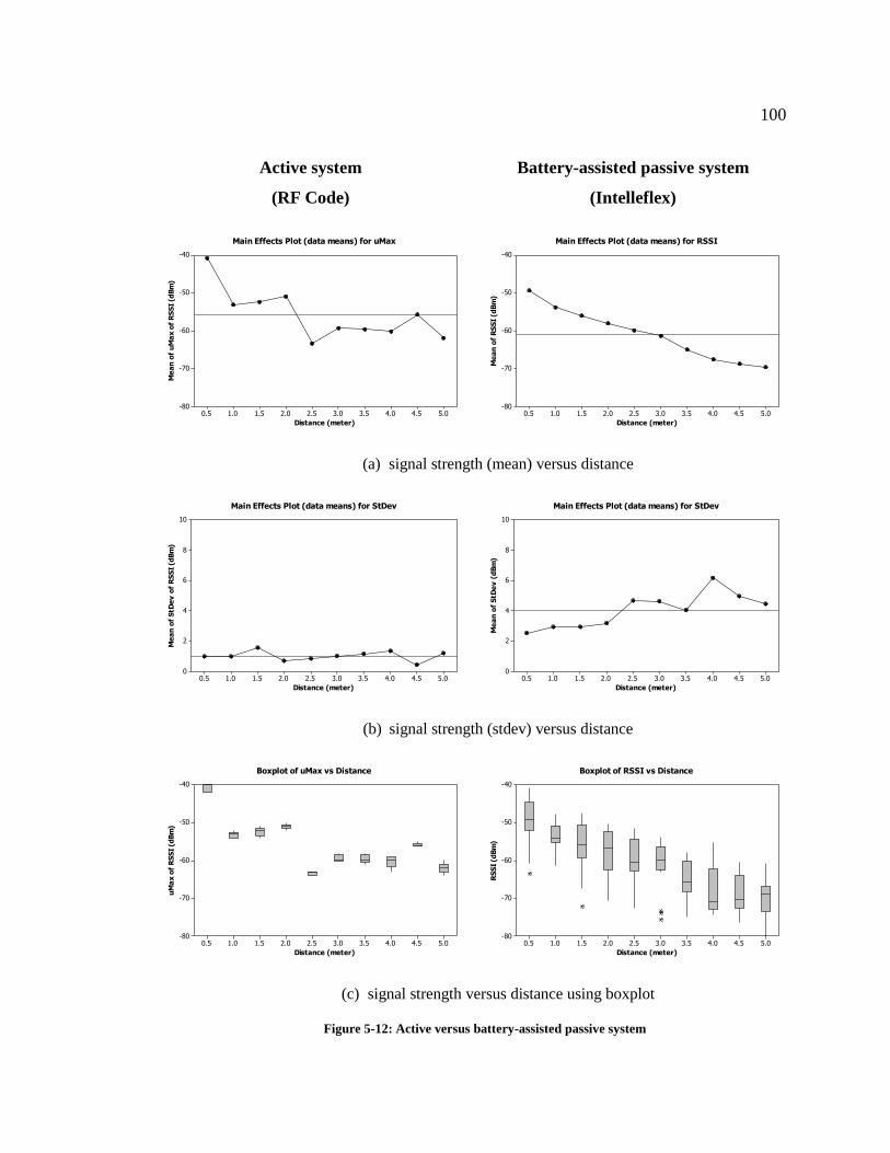
100

Active system

(RF Code)

Battery-assisted passive system

(Intelleflex)

(a) signal strength (mean) versus distance

(b) signal strength (stdev) versus distance

(c) signal strength versus distance using boxplot

Figure 5-12: Active versus battery-assisted passive system

Distance (meter)

Me

an

of

uM

ax o

f R

SS

I (d

Bm

)

5.04.54.03.53.02.52.01.51.00.5

-40

-50

-60

-70

-80

Main Effects Plot (data means) for uMax

Distance (meter)

Me

an

of

RS

SI

(dB

m)

5.04.54.03.53.02.52.01.51.00.5

-40

-50

-60

-70

-80

Main Effects Plot (data means) for RSSI

Distance (meter)

Me

an

of

StD

ev

of

RS

SI

(dB

m)

5.04.54.03.53.02.52.01.51.00.5

10

8

6

4

2

0

Main Effects Plot (data means) for StDev

Distance (meter)

Me

an

of

StD

ev

(d

Bm

)

5.04.54.03.53.02.52.01.51.00.5

10

8

6

4

2

0

Main Effects Plot (data means) for StDev

Distance (meter)

uM

ax o

f R

SS

I (d

Bm

)

5.04.54.03.53.02.52.01.51.00.5

-40

-50

-60

-70

-80

Boxplot of uMax vs Distance

Distance (meter)

RS

SI

(dB

m)

5.04.54.03.53.02.52.01.51.00.5

-40

-50

-60

-70

-80

Boxplot of RSSI vs Distance

101

One possible solution to reduce the signal variance of the battery-assisted passive

system is to use two pairs of antennas at the same position, just like the active system.

Only the maximum value of two antennas measurements is recorded as the official RSSI

reading. In this way, the signal variance may decrease. The size of the antennas of the

battery-assisted passive system may be an issue. Two panels of a single pair of the

antennas, or the two pair of the antennas, require certain space to operate properly.

According to the Intelleflex FMR6000 user manual, at least 1 or 2 feet distance is

recommended, which is not neglectable to be qualified as the same position.

5.3.3 Lab versus Mock-up

The Intelleflex battery-assisted passive system performed differently in the

regular laboratory environment and in the ISS mock-up. The main effect plots of signal

strength versus distance, and its standard deviation versus distance, are compared to the

Lab results within 3 meters, as shown in Figure 5-13. Overall, the RSSI in the laboratory

has higher value and lower standard deviation than in the mock-up.

In part (a) comparison, the average signal strength in the mock-up is even lower

than in the laboratory, -63.540 versus -56.419 dBm, with p-value 0.000.

In part (b) comparison, the signal strength deviation in the mock-up is

significantly higher than in the laboratory, 7.56 versus 3.48 dBm, with p-value 0.000.

Recall that the value for the active system is only 1.10 dBm. The high-reflection

environment makes the signal receiving satiability even worse for the passive system.

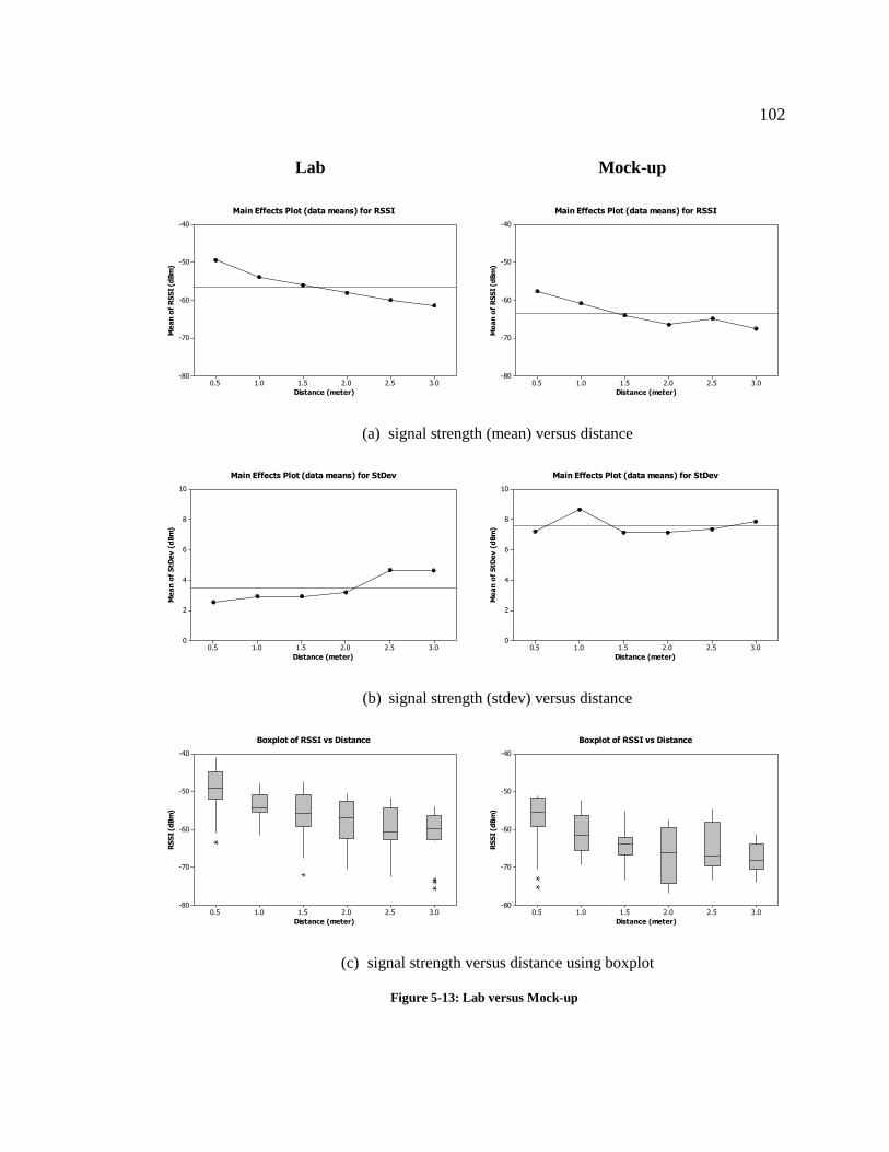
102

Lab Mock-up

(a) signal strength (mean) versus distance

(b) signal strength (stdev) versus distance

(c) signal strength versus distance using boxplot

Figure 5-13: Lab versus Mock-up

Distance (meter)

Me

an

of

RS

SI

(dB

m)

3.02.52.01.51.00.5

-40

-50

-60

-70

-80

Main Effects Plot (data means) for RSSI

Distance (meter)

Me

an

of

RS

SI

(dB

m)

3.02.52.01.51.00.5

-40

-50

-60

-70

-80

Main Effects Plot (data means) for RSSI

Distance (meter)

Me

an

of

StD

ev

(d

Bm

)

3.02.52.01.51.00.5

10

8

6

4

2

0

Main Effects Plot (data means) for StDev

Distance (meter)

Me

an

of

StD

ev

(d

Bm

)

3.02.52.01.51.00.5

10

8

6

4

2

0

Main Effects Plot (data means) for StDev

Distance (meter)

RS

SI

(dB

m)

3.02.52.01.51.00.5

-40

-50

-60

-70

-80

Boxplot of RSSI vs Distance

Distance (meter)

RS

SI

(dB

m)

3.02.52.01.51.00.5

-40

-50

-60

-70

-80

Boxplot of RSSI vs Distance

103

The boxplot comparison in part (c) combines the mean and variation information

together to present different performance in the two environments. The RSSI reading in

the mock-up is more unpredictable than in the laboratory. This means pure RSSI ranging

is not reliable in the mock-up. Therefore, range-free algorithms, such as kNN, should be

highlighted in future localization tests in the mock-up. For the hybrid algorithm, more

weights may be assigned to kNN rather than simple average of kNN and RSSI results in

current approach. Moreover, probabilistic modeling may be another candidate.

104

5.4 Localization Test for Battery-assisted Passive System

As shown in the right column of Table 5-3, this preliminary localization

experiment for the battery-assisted passive system resulted in mean localization errors of

2.06, 2.34, and 2.49 meters for the hybrid, kNN, and RSSI ranging algorithms,

respectively. The active system results are listed in the left column for comparison. It is

very obvious that current battery-assisted passive system produce higher localization

error than the active system. Though, the RSSI prediction shows opposite result, which

may indicate possible improvement space via further system optimization.

Table 5-3: Localization error comparison

Active system

(RF Code)

Battery-assisted Passive System

(Intelleflex)

Hybrid 1.08 m 2.06 m

kNN 1.10 m 2.34 m

RSSI 1.56 m 2.49 m

RSSI prediction 2.05 m – 2.14 m 1.34 m – 1.39 m

The localization error prediction was conducted based on RSSI ranging error of

both the active system and the battery-assisted passive system based on the Equation

(3-17) developed in Section 3.4. Recall that the PIs vary from 4.09 to 4.28 meters and

from 2.68 to 2.77 meters for the two systems. This brings the RSSI prediction of 2.05 to

2.14 meters and 1.34 to 1.39 meters, respectively.

105

For the active system, the real localization error based on RSSI ranging is 1.56

meter, which is around 25% smaller than prediction. This may benefit from the selected

reference tags method, which eliminates those reference tags far away from the target tag.

In this way, the regression approach is more accurate.

However, for the battery-assisted passive system, the current measured result,

2.49 meter, is over 80% larger than the prediction. Recall that this is only one sample

measurement of a whole set of the proposed experiment in Chapter 3. It is possible that

current measurement happens to deviate from the predicted mean value. So, it may

indicate that the current battery-assisted passive system still has high potential to have its

performance improved. One possible solution, mentioned at the end of Section 5.3.2, is to

make dual pairs of antennas at the same position.

106

Chapter 6

Conclusions and Recommendations

6.1 Conclusions

According to the research purpose of this dissertation, the conclusions are

summarized in accordance with three objectives: theoretical prediction on minimum

number of reference tags and localization error, performance evaluation of 3D RFID

systems, and high-reflection environmental impacts.

6.1.1 Theoretical Prediction

Based on a series of assumptions and theoretical interpretation, two experiments

were designed to evaluate the minimum possible number of reference tags that should be

used in a RFID localization test. These experiments per se were not conducted due to a

time restraint. However, a localization error prediction function using prediction interval

on ranging measurement is developed. That is, for

3D applications. And the ratio of localization errors for 3D, 2D and 1D ranging only are:

√6 : √2 : 1. The measured results in Section 5.2 fit these predictions well. The results

from another system, as discussed in Section 5.4, deviated from the prediction. This may

be caused by poor design of the second system. Or, it is just a single sample event. Full

justification may require more experiments.

107

6.1.2 Localization Performance

The proposed 3D indoor RFID localization system was built with two types of

commercial off-the-shelf (COTS) products. One is the RF Code active system. The other

one is the Intelleflex battery-assisted passive system. A hybrid algorithm is developed

based upon kNN and RSSI ranging approaches.

For the active system, a mean localization error of 1.08 meters is achieved, which

fits previous theoretical prediction, and is better than using kNN or RSSI only. The

system is a successful trial on RFID 3D localization. Its performance may be further

improved by rearranging reference tags and reader positions.

For the battery-assisted passive system, the mean localization error is 2.06 meters,

which is 50% higher than predicted result using RSSI ranging only. However, it is still

better than using kNN or RSSI only. Due to space restriction, less readers and antennas

than the active system were used in the current system. This may be a major reason

causing worse performance than expected.

6.1.3 Environmental Impacts

An ISS mock-up was built to evaluate the RFID performance in a high-reflection

environment. It was found that the mock-up did lead to average 7.2 dBm lower RSSI and

double the standard deviation of RSSI than in the laboratory environment. The RF signal

interference is aggravated in the mock-up. Therefore, RSSI ranging may not be

applicable in such environment. The range-free approach may be a better choice.

108

6.2 Recommendations

Based on the above conclusions, a few recommendations for future work are

proposed.

A complete set of experiments should be conducted to fully justify the

conclusion of the theoretical prediction.

Based on the above experiment results, better reference tags and readers

deployment could be assigned to the current system, which may bring better

localization performance.

More readers and antennas should be added to the battery-assisted passive

system. Admittedly, certain deployment restrictions may need to be overcome.

Higher order regressions may be investigated in both the theoretical analysis

and the localization algorithm.

The kNN part of the hybrid algorithm may be emphasized to reduce the

impact of strong signal interference in the metal-surrounded ISS mock-up.

Probabilistic modeling may be another candidate.

109

References

[1] RFID Journal, "RFID Business Applications,"

Http://www.Rfidjournal.com/article/view/1334, 2012(10/9) .

[2] RFID Journal, "US Government Issues 300 RFID Passports,"

Http://www.Rfidjournal.com/article/view/6290, 2006(3/14) .

[3] RFID Journal, "RFID used in Advanced Cattle Tracking System,"

Http://www.Rfidjournal.com/article/view/6133, 2005(2/1) .

[4] RFID Journal, "Wal-Mart Details RFID Requirement,"

Http://www.Rfidjournal.com/article/view/642, 2003(11/6) .

[5] RFID Journal, "RFID Drives into Auto Manufacturing,"

Http://www.Rfidjournal.com/article/view/6454, 2006(3/21) .

[6] Zhang, S., and Yuan, F., 2006, "RFID Technique and its Application in Safety

Management System for People and Vehicle in Mine Shafts," Southern Metals, 2006(1)

pp. 12-14.

[7] Shetty, A., 2010, "Weighted K-Nearest Neighbor Algorithm as an Object Localization

Technique using Passive RFID Tags," M.S. Thesis, Rutgers University, New Brunswick,

NJ.

[8] Jones, E., Riley, M., Franca, R., 2007, "Case Study: The Engineering Economics of

RFID in Specialized Manufacturing," The Engineering Economist, 52(3) pp. 285-303.

[9] Jones E., Cochran D., Frailey T., 2010, "RFID Pharmaceutical Tracking: From

Manufacturer through in Vivo Drug Delivery," ASME Journal of Medical Devices,

Transactions of the ASME, 4(1) pp. 015001-1.

[10] Finkenzeller, K., 2010, "RFID Handbook : Fundamentals and Applications in

Contactless Smart Cards, Radio Frequency Identification and Near-Field

Communication,"Wiley, Chichester, West Sussex; Hoboken, NJ, pp. 155-178.

[11] EPCglobal, "EPCglobal Standards," Http://www.gs1.org/gsmp/kc/epcglobal,

2011(9/17) .

110

[12] Malik, A., 2009, "RTLS for Dummies," For Dummies; John Wiley, Hoboken, N.J.;

Chichester.

[13] SkyRFID, "RFID Gen 2," Http://www.Skyrfid.com/RFID_Gen_2_What_is_it.Php,

2011(9/17) .

[14] Zhou J., and Shi J., 2009, "RFID Localization Algorithms and Applications-A

Review," Journal of Intelligent Manufacturing, 20(6) pp. 695-707.

[15] Anonymous, "Global Positioning System," Http://en.Wikipedia.org/wiki/GPS,

2011(9/17) .

[16] Zhong, Z., 2010, "Range-Free Localization and Tracking in Wireless Sensor

Networks," Ph.D. Dissertation, University of Minnesota, Minneapolis, MN.

[17] Priyantha, N. B., 2005, "The Cricket Indoor Location System," Ph.D. Dissertation,

Massachusetts Institute of Technology, Cambridge, MA.

[18] Mittek, M. M., "3D Indoor Localization Experiments Based on the Cricket System,"

Ph.D. Dissertation (In Process), University of Nebraska-Lincoln, Lincoln, NE.

[19] Rahmati, A., Lin Zhong, Hiltunen, M., 2007, "Reliability Techniques for RFID-

Based Object Tracking Applications," 37th Annual IEEE/IFIP International Conference

on Dependable Systems and Networks, Edinburgh, UK, June 25-28, T. Anderson, ed. pp.

113-118.

[20] Jingwangsa, T., Soonjun, S., and Cherntanomwong, P., 2010, "Comparison Between

Innovative Approaches of RFID Based Localization Using Fingerprinting Techniques for

Outdoor and Indoor Environments," 12th International Conference on Advanced

Communication Technology (ICACT), Phoenix Park, Korea, February 7-10, Y. Park, ed.

2, pp. 1511-1515.

[21] Pathanawongthum, N., and Cherntanomwong, P., 2010, "RFID Based Localization

Techniques for Indoor Environment," 12th International Conference on Advanced

Communication Technology (ICACT), Phoenix Park, Korea, February 7-10, Y. Park, ed.

2, pp. 1418-1421.

[22] Cisco, "Cisco 2700 Series Wireless Location Appliance,"

Http://www.Cisco.com/en/US/products/ps6398/index.Html, 2011(9/17) .

[23] Zhao, L., 2007, "Design and Performance of Ultra-Wideband Localization Systems,"

M.S. Thesis, University of Nebraska-Lincoln, Lincoln, NE.

111

[24] Wiggins, L., "Ultra-Wideband Technology: The Revolution is Here,"

Http://hosteddocs.Ittoolbox.com/LW010807.Pdf, 2011(9/15) .

[25] "Ultra-Wideband," Http://en.Wikipedia.org/wiki/Ultra-Wideband, 2011(9/15) .

[26] Sanpechuda, T., and Kovavisaruch, L., 2008, "A Review of RFID Localization:

Applications and Techniques," IEEE 5th International Conference on Electrical

Engineering/Electronics, Computer, Telecommunications and Information Technology,

(ECTI-CON), Krabi, Thailand, May 14-17, 2, pp. 769-772.

[27] Yeh, L., Hsu, M., Lee, Y., 2009, "Indoor Localization: Automatically Constructing

Today's Radio Map by iRobot and RFIDs," IEEE Sensors, Christchurch, New Zealand,

Octorber 25-28, S. C. Mukhopadhyay, ed. pp. 1463-1466.

[28] Seo, D., Won, D., Yang, G., 2005, "A Probabilistic Approach for Mobile Robot

Localization under RFID Tag Infrastructures," International Conference on Control,

Automation, and Systems (ICCAS), Gyeonggi-do, Korea, June 2-5, pp. 1797-1801.

[29] Bouet, M., and dos Santos, A. L., 2008, "RFID Tags: Positioning Principles and

Pocalization Techniques," 1st IFIP Wireless Days, Dubai, United Arab Emirates,

November 24-27, pp. 1-5.

[30] Hightower, J., Want, R., and Borriello, G., 2000, "SpotON: An Indoor 3D Location

Sensing Technology Based on RF Signal Strength," UW CSE Technical Report #2000-

02-02, University of Washington, Department of Computer Science and Engineering,

Seattle, WA.

[31] Junru Zhou, Hongjian Zhang, and Lingfei Mo, 2011, "Two-Dimension Localization

of Passive RFID Tags Using AOA Estimation," Instrumentation and Measurement

Technology Conference, IEEE, Hangzhou, China, May 10-12, pp. 1-5.

[32] CSL, "Active RTLS RFID Products,"

Http://convergence.Com.hk/products_cat.Php?id=1, 2011(9/15) .

[33] "Multilateration," Http://en.Wikipedia.org/wiki/TDOA, 2011(9/15) .

[34] Alippi, C., Cogliati, D., and Vanini, G., 2006, "A Statistical Approach to Localize

Passive RFIDs," Proceedings of IEEE International Symposium on Circuits and Systems,

Island of Kos, Greece, May 21-24, T. Stouraitis, ed. pp. 769-772.

[35] Almaaitah, A., Ali, K., Hassanein, H. S., 2010, "3D Passive Tag Localization

Schemes for Indoor RFID Applications," IEEE International Conference on

Communications (ICC), Cape Town, South Africa, May 23-27, F. Takawira and W.

Leuschner, eds. pp. 1-5.

112

[36] Bekkali, A., Sanson, H., and Matsumoto, M., 2007, "RFID Indoor Positioning Based

on Probabilistic RFID Map and Kalman Filtering," Third IEEE International Conference

on Wireless and Mobile Computing, Networking and Communications, White Plains, NY,

Octorber 8-10, pp. 21-27.

[37] Jin, G., Lu, X., and Park, M., 2006, "An Indoor Localization Mechanism Using

Active RFID Tag," IEEE International Conference on Sensor Networks, Ubiquitous, and

Trustworthy Computing, Taichung, Taiwan, June 5-7, 1, pp. 4-7.

[38] Bechteler, T. F., and Yenigun, H., 2003, "2-D Localization and Identification Based

on SAW ID-Tags at 2.5 GHz," IEEE Transactions on Microwave Theory and Techniques,

51(5) pp. 1584-1590.

[39] Zhou, J., and Shi, J., 2009, "Effect of Facility Geometry on RFID Localization

Accuracy," ASME Conference Proceedings, International Manufacturing Science and

Engineering Conference, West Lafayette, IN, October 4-7, (43611) pp. 267-275.

[40] SimplyRFiD, 2008, "RFID Read Range,"

Http://www.Simplyrfid.com/blog/2008/7/12/rfid-Read-Range-just-how-Far-can-Rfid-

Track-Something.Html, 2011(11/9) .

[41] Brchan, J. L., 2009, "Indoor Localization in an Active RFID System with Multiple

Propagation Models," M.S. Thesis, University of Nebraska-Lincoln, Lincoln, NE.

[42] Kottegoda, N.T., and Rosso, R., 1997, "Statistics, Probability, and Reliability for

Civil and Environmental Engineers," McGraw-Hill, New York, NY.

[43] Soong, T.T., 1981, "Probabilistic Modeling and Analysis in Science and

Engineering," Wiley, New York, NY.

[44] Manolakis, D. E., 1996, "Efficient Solution and Performance Analysis of 3-D

Position Estimation by Trilateration," Aerospace and Electronic Systems, IEEE

Transactions, 32(4) pp. 1239-1248.

[45] Milliken, G.A., and Johnson, D.E., 2009, "Analysis of Messy Data," CRC Press,

Boca Raton.

[46] Brchan, J. L., Zhao, L., Wu, J., Williams, R. E., and Pérez, L. C., 2012, "A Real-

Time RFID Localization Experiment Using Propagation Models," 6th Annual IEEE

International Conference on RFID, Orlando, FL, April 3-5, pp. 141-148.

[47] Wu, J., Zhao, L., Pérez, L. C., and Williams, R. E., 2012, "RFID-Based 3D Indoor

Real-Time Localization System," ASME Conference Proceedings, International

Manufacturing Science and Engineering Conference, Notre Dame, IN, June 4-8.

113

[48] Jones, E. C., 2005, "RFID Technology for Tracking Inventory in the Space Shuttle,"

Proceedings of the Annual Meeting of the Nebraska Academy of Sciences, Aeronautics

& Space Science, Lincoln, NE, April 22.

114

Appendix A

Programming Interface

A.1 JSON

JSON (JavaScript Object Notation) is a text-based web standard specially

designed for data interchange. It is human-readable, and is simpler than XML (Extensible

Markup Language), another text-based web standard especially suitable for information

exchange, which will be introduced in the Intelleflex section later. The format of JSON

makes it easy to be used in various programming languages and applications. Here is an

example message of tag information in JSON format.

{

“tag_id”: “LOCATE00016484”,

“tag_links”: [

{“channelid”: 1,

“ssi”: -56},

{“channelid”: 2,

“ssi”: -54}

]

}

A simple Matlab package, parse_json, contributed by François Glineur in the

Matlab Community File Exchange makes the work of parsing JSON message into

structure format data much easier.

Most commonly used commands for RF Code (in format of URLs) are:

List all available readers

o http://localhost:6580/rfcode_zonemgr/zonemgr/api/readerlist.json

List all available tags

o http://localhost:6580/rfcode_zonemgr/zonemgr/api/taglist.json

115

List information of one particular tag

o http://localhost:6580/rfcode_zonemgr/zonemgr/api/tagprint.json?tagid

0=<id>

The login information is same as normal web portal access method. Though,

special URL reading function should be constructed since Matlab does not support URL

authorization. Thanks for Matlab Community again: the urlread_auth and base64encode

packages solve this problem. Please note that the urlread_auth must be placed under the

“toolbox\matlab\iofun” folder, and the Matlab library cache may need to be re-hashed for

the changes to take effect.

The JSON related functions coded for this research are shown as follows for

reference. They are pretty much self-explained.

function [base_url,login]=zonemgr_portal(hostname,port,username,password) % generate base_url and login for rfcode zonemgr web portal % all inputs are optional, default values will be applied if not given % created by Jiaqing Wu, 3/18/2011

% check inputs and outputs error(nargchk(0,4,nargin)); error(nargoutchk(2,2,nargout)); % default rfid zonemgr web portal information if (nargin==0), hostname='rfidlab-pc'; end if (nargin<=1), port='6580'; end if (nargin<=2), username='user'; password='user'; end if (nargin==3), password=username; end % define a short url base_url=['http://',hostname,':',port,'/rfcode_zonemgr/zonemgr/api']; % combine username and password to login if ~isempty(username) && ~isempty(password) login=[username,':',password]; else error('zonemgr_portal:InvalidLogin','Missing login information.'); end end

function [reader_status,reader_name,reader_ip]=check_reader(reader_id) % check whether queried reader(s) are available or not % the input reader_id is optional, but must be a cell array if used % all readers will be queried, if reader_id is not given % the output reader_status is a vector of (size of reader_id) by 1 % 1 for online, 0 for offline % the output reader_name is a cell array of (# of all readers) by 1 % the output reader_ip is a cell array of (# of all readers) by 1 % both of them include all available readers reported by the system % created by Jiaqing Wu, 3/18/2011

% check inputs and outputs error(nargchk(0,1,nargin));

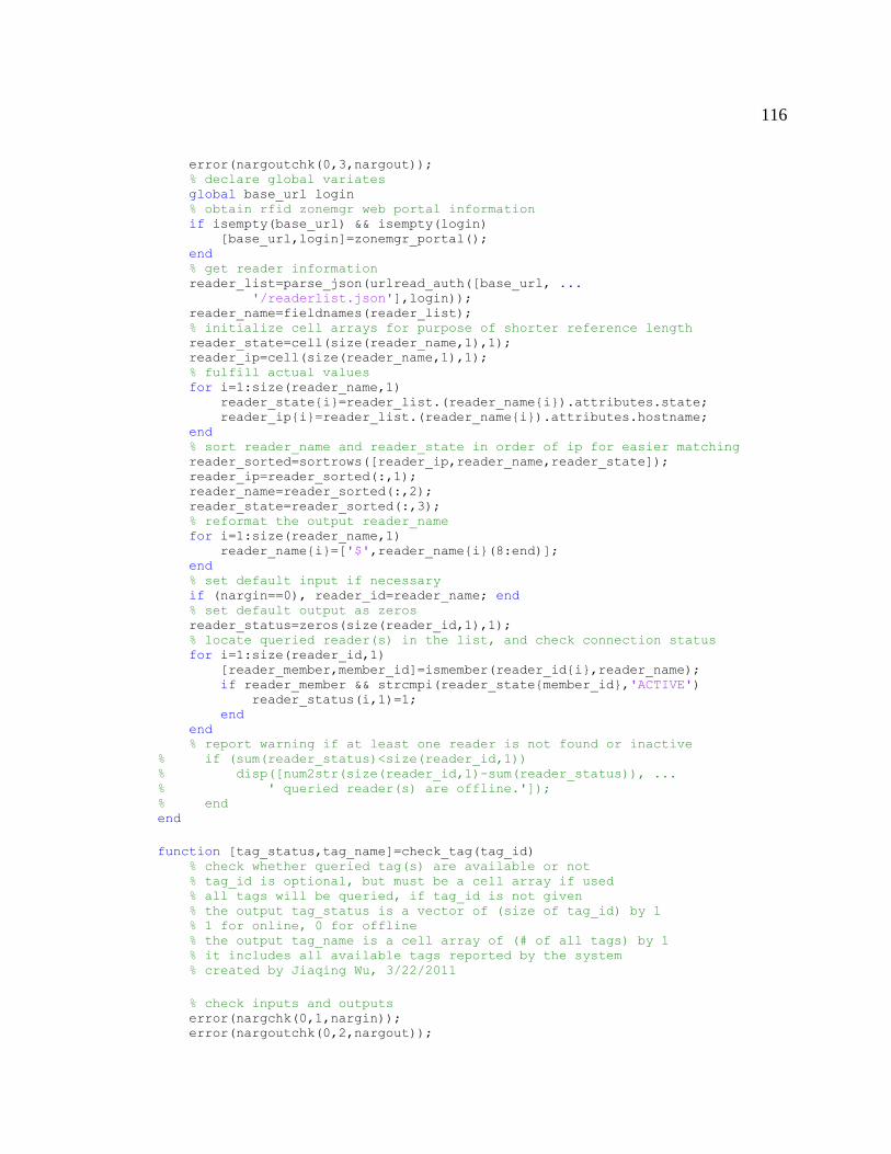
116

error(nargoutchk(0,3,nargout)); % declare global variates global base_url login % obtain rfid zonemgr web portal information if isempty(base_url) && isempty(login) [base_url,login]=zonemgr_portal(); end % get reader information reader_list=parse_json(urlread_auth([base_url, ... '/readerlist.json'],login)); reader_name=fieldnames(reader_list); % initialize cell arrays for purpose of shorter reference length reader_state=cell(size(reader_name,1),1); reader_ip=cell(size(reader_name,1),1); % fulfill actual values for i=1:size(reader_name,1) reader_state{i}=reader_list.(reader_name{i}).attributes.state; reader_ip{i}=reader_list.(reader_name{i}).attributes.hostname; end % sort reader_name and reader_state in order of ip for easier matching reader_sorted=sortrows([reader_ip,reader_name,reader_state]); reader_ip=reader_sorted(:,1); reader_name=reader_sorted(:,2); reader_state=reader_sorted(:,3); % reformat the output reader_name for i=1:size(reader_name,1) reader_name{i}=['$',reader_name{i}(8:end)]; end % set default input if necessary if (nargin==0), reader_id=reader_name; end % set default output as zeros reader_status=zeros(size(reader_id,1),1); % locate queried reader(s) in the list, and check connection status for i=1:size(reader_id,1) [reader_member,member_id]=ismember(reader_id{i},reader_name); if reader_member && strcmpi(reader_state{member_id},'ACTIVE') reader_status(i,1)=1; end end % report warning if at least one reader is not found or inactive % if (sum(reader_status)<size(reader_id,1)) % disp([num2str(size(reader_id,1)-sum(reader_status)), ... % ' queried reader(s) are offline.']); % end end

function [tag_status,tag_name]=check_tag(tag_id) % check whether queried tag(s) are available or not % tag_id is optional, but must be a cell array if used % all tags will be queried, if tag_id is not given % the output tag_status is a vector of (size of tag_id) by 1 % 1 for online, 0 for offline % the output tag_name is a cell array of (# of all tags) by 1 % it includes all available tags reported by the system % created by Jiaqing Wu, 3/22/2011

% check inputs and outputs error(nargchk(0,1,nargin)); error(nargoutchk(0,2,nargout));

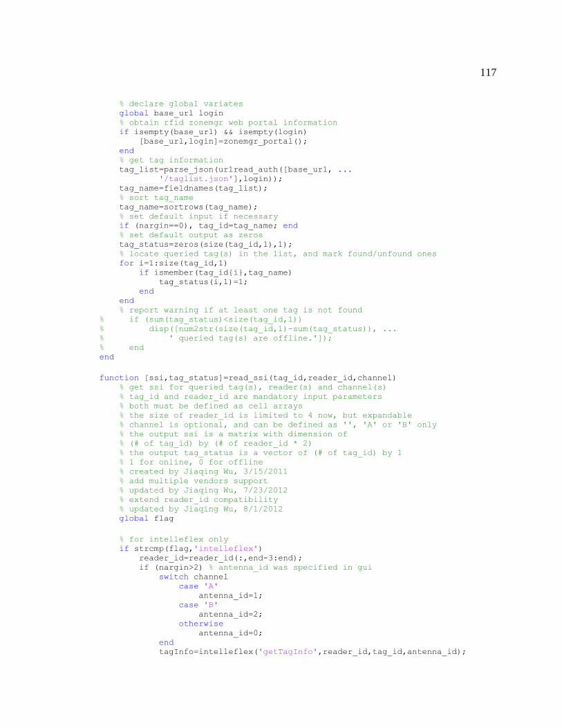
117

% declare global variates global base_url login % obtain rfid zonemgr web portal information if isempty(base_url) && isempty(login) [base_url,login]=zonemgr_portal(); end % get tag information tag_list=parse_json(urlread_auth([base_url, ... '/taglist.json'],login)); tag_name=fieldnames(tag_list); % sort tag_name tag_name=sortrows(tag_name); % set default input if necessary if (nargin==0), tag_id=tag_name; end % set default output as zeros tag_status=zeros(size(tag_id,1),1); % locate queried tag(s) in the list, and mark found/unfound ones for i=1:size(tag_id,1) if ismember(tag_id{i},tag_name) tag_status(i,1)=1; end end % report warning if at least one tag is not found % if (sum(tag_status)<size(tag_id,1)) % disp([num2str(size(tag_id,1)-sum(tag_status)), ... % ' queried tag(s) are offline.']); % end end

function [ssi,tag_status]=read_ssi(tag_id,reader_id,channel) % get ssi for queried tag(s), reader(s) and channel(s) % tag_id and reader_id are mandatory input parameters % both must be defined as cell arrays % the size of reader_id is limited to 4 now, but expandable % channel is optional, and can be defined as '', 'A' or 'B' only % the output ssi is a matrix with dimension of % (# of tag_id) by (# of reader_id * 2) % the output tag_status is a vector of (# of tag_id) by 1 % 1 for online, 0 for offline % created by Jiaqing Wu, 3/15/2011 % add multiple vendors support % updated by Jiaqing Wu, 7/23/2012 % extend reader_id compatibility % updated by Jiaqing Wu, 8/1/2012 global flag

% for intelleflex only if strcmp(flag,'intelleflex') reader_id=reader_id(:,end-3:end); if (nargin>2) % antenna_id was specified in gui switch channel case 'A' antenna_id=1; case 'B' antenna_id=2; otherwise antenna_id=0; end tagInfo=intelleflex('getTagInfo',reader_id,tag_id,antenna_id);

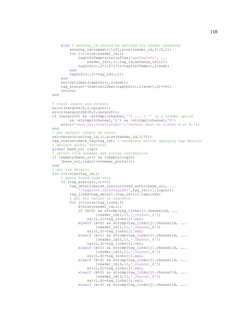
118

else % antenna_id should be defined via reader sequence antenna_id=repmat([1;2],size(reader_id,1)/2,1); for i=1:size(reader_id,1) tagInfoTemp=intelleflex('getTagInfo', ... reader_id(i,:),tag_id,antenna_id(i)); tagInfo(:,2*i:2*i+1)=tagInfoTemp(:,2:end); end tagInfo(:,1)=tag_id(:,1); end ssi=cell2mat(tagInfo(:,2:end)); tag_status=~(sum(cell2mat(tagInfo(:,2:end)),2)==0); return; end

% check inputs and outputs error(nargchk(2,3,nargin)); error(nargoutchk(0,2,nargout)); if (nargin>2) && ~strcmpi(channel,'') ... % '' is a hidden option && ~strcmpi(channel,'A') && ~strcmpi(channel,'B') error('read_ssi:InvalidInput','Channel must be either A or B.'); end % set default output as zeros ssi=zeros(size(tag_id,1),size(reader_id,1)*2); tag_status=check_tag(tag_id); % necessary before querying tag details % declare global variates global base_url login % obtain rfid zonemgr web portal information if isempty(base_url) && isempty(login) [base_url,login]=zonemgr_portal(); end % get tag details for i=1:size(tag_id,1) % query found tags only if (tag_status(i,1)==1) tag_detail=parse_json(urlread_auth([base_url, ... '/tagprint.json?tagid0=',tag_id{i}],login)); tag_links=tag_detail.(tag_id{i}).taglinks; % put ssi values in sequence for j=1:size(tag_links,2) k=size(reader_id,1); if (k>0) && strcmp(tag_links{j}.channelid, ... [reader_id{1,1},'_channel_A']) ssi(i,1)=tag_links{j}.ssi; elseif (k>0) && strcmp(tag_links{j}.channelid, ... [reader_id{1,1},'_channel_B']) ssi(i,2)=tag_links{j}.ssi; elseif (k>1) && strcmp(tag_links{j}.channelid, ... [reader_id{2,1},'_channel_A']) ssi(i,3)=tag_links{j}.ssi; elseif (k>1) && strcmp(tag_links{j}.channelid, ... [reader_id{2,1},'_channel_B']) ssi(i,4)=tag_links{j}.ssi; elseif (k>2) && strcmp(tag_links{j}.channelid, ... [reader_id{3,1},'_channel_A']) ssi(i,5)=tag_links{j}.ssi; elseif (k>2) && strcmp(tag_links{j}.channelid, ... [reader_id{3,1},'_channel_B']) ssi(i,6)=tag_links{j}.ssi; elseif (k>3) && strcmp(tag_links{j}.channelid, ...

119

[reader_id{4,1},'_channel_A']) ssi(i,7)=tag_links{j}.ssi; elseif (k>3) && strcmp(tag_links{j}.channelid, ... [reader_id{4,1},'_channel_B']) ssi(i,8)=tag_links{j}.ssi; else % more information may be detected % duplicate/revise the above code for expansion end end end end % report values on queried channel only % channel = '', given defined in inputs, is treated as both channels if (nargin>2) && strcmpi(channel,'A') ssi(:,2:2:end)=0; elseif (nargin>2) && strcmpi(channel,'B') ssi(:,1:2:end)=0; end end

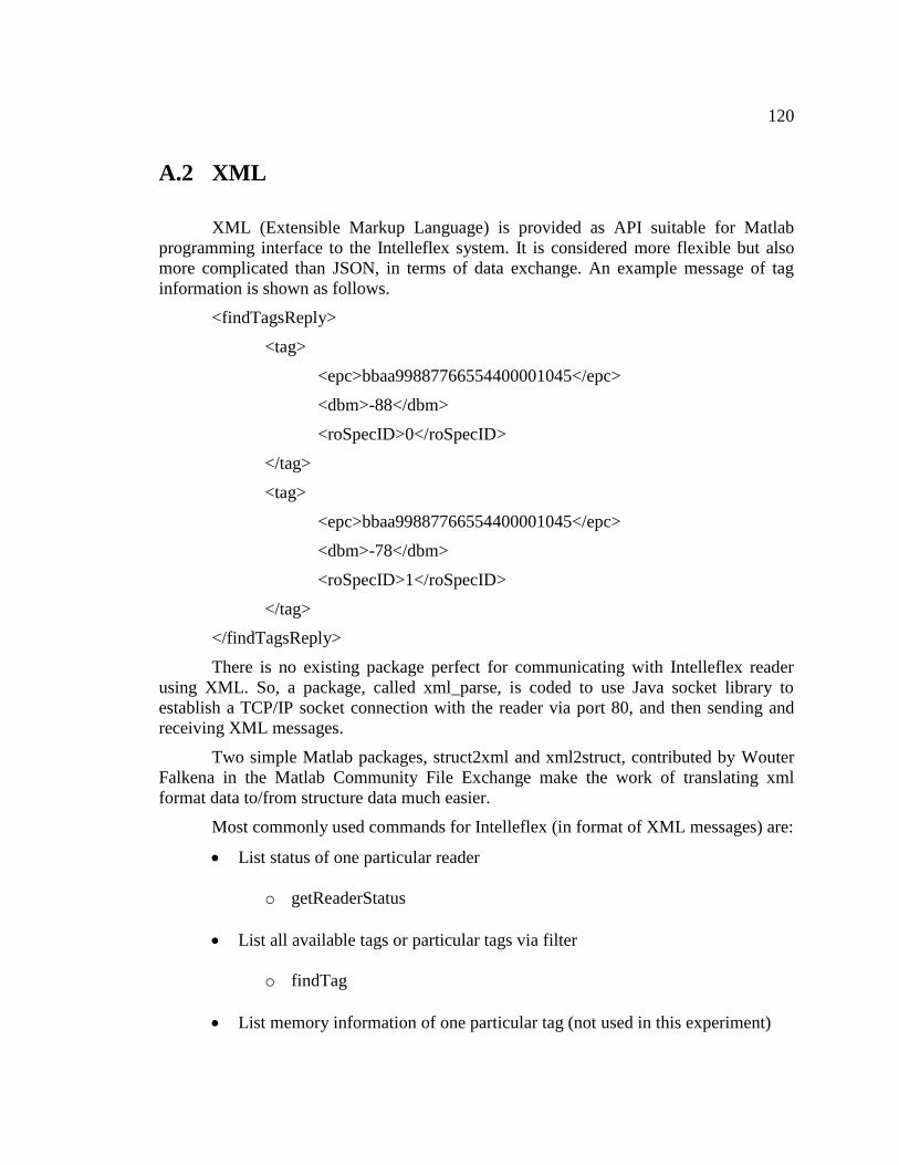
120

A.2 XML

XML (Extensible Markup Language) is provided as API suitable for Matlab

programming interface to the Intelleflex system. It is considered more flexible but also

more complicated than JSON, in terms of data exchange. An example message of tag

information is shown as follows.

<findTagsReply>

<tag>

<epc>bbaa99887766554400001045</epc>

<dbm>-88</dbm>

<roSpecID>0</roSpecID>

</tag>

<tag>

<epc>bbaa99887766554400001045</epc>

<dbm>-78</dbm>

<roSpecID>1</roSpecID>

</tag>

</findTagsReply>

There is no existing package perfect for communicating with Intelleflex reader

using XML. So, a package, called xml_parse, is coded to use Java socket library to

establish a TCP/IP socket connection with the reader via port 80, and then sending and

receiving XML messages.

Two simple Matlab packages, struct2xml and xml2struct, contributed by Wouter

Falkena in the Matlab Community File Exchange make the work of translating xml

format data to/from structure data much easier.

Most commonly used commands for Intelleflex (in format of XML messages) are:

List status of one particular reader

o getReaderStatus

List all available tags or particular tags via filter

o findTag

List memory information of one particular tag (not used in this experiment)

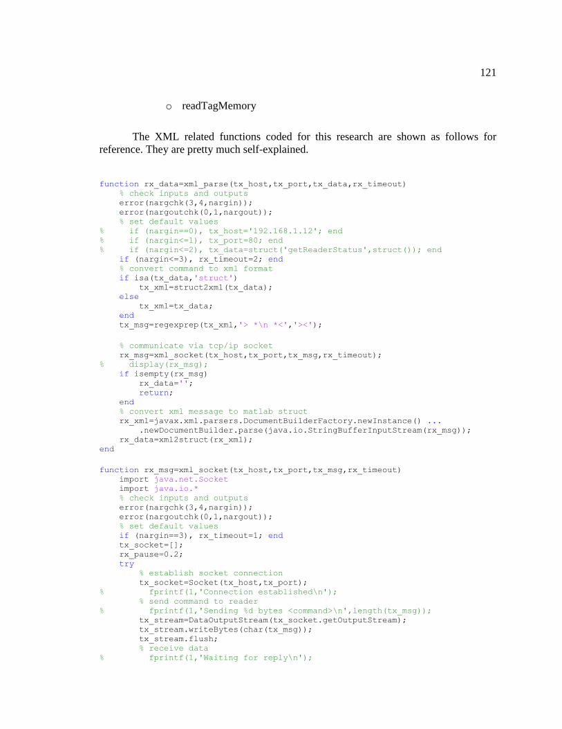
121

o readTagMemory

The XML related functions coded for this research are shown as follows for

reference. They are pretty much self-explained.

function rx_data=xml_parse(tx_host,tx_port,tx_data,rx_timeout) % check inputs and outputs error(nargchk(3,4,nargin)); error(nargoutchk(0,1,nargout)); % set default values % if (nargin==0), tx_host='192.168.1.12'; end % if (nargin<=1), tx_port=80; end % if (nargin<=2), tx_data=struct('getReaderStatus',struct()); end if (nargin<=3), rx_timeout=2; end % convert command to xml format if isa(tx_data,'struct') tx_xml=struct2xml(tx_data); else tx_xml=tx_data; end tx_msg=regexprep(tx_xml,'> *\n *<','><');

% communicate via tcp/ip socket rx_msg=xml_socket(tx_host,tx_port,tx_msg,rx_timeout); % display(rx_msg); if isempty(rx_msg) rx_data=''; return; end % convert xml message to matlab struct rx_xml=javax.xml.parsers.DocumentBuilderFactory.newInstance() ... .newDocumentBuilder.parse(java.io.StringBufferInputStream(rx_msg)); rx_data=xml2struct(rx_xml); end

function rx_msg=xml_socket(tx_host,tx_port,tx_msg,rx_timeout) import java.net.Socket import java.io.* % check inputs and outputs error(nargchk(3,4,nargin)); error(nargoutchk(0,1,nargout)); % set default values if (nargin==3), rx_timeout=1; end tx_socket=[]; rx_pause=0.2; try % establish socket connection tx_socket=Socket(tx_host,tx_port); % fprintf(1,'Connection established\n'); % send command to reader % fprintf(1,'Sending %d bytes <command>\n',length(tx_msg)); tx_stream=DataOutputStream(tx_socket.getOutputStream); tx_stream.writeBytes(char(tx_msg)); tx_stream.flush; % receive data % fprintf(1,'Waiting for reply\n');

122

rx_stream=DataInputStream(tx_socket.getInputStream); bytes_available=0; tic; while (bytes_available~=rx_stream.available)||(bytes_available==0) bytes_available=rx_stream.available; pause(rx_pause); if toc>=rx_timeout fprintf(1,'Timeout after %5.2f second(s)\n\n', ... rx_timeout); break; end end % read response from reader rx_buffer=zeros(1,bytes_available,'uint8'); for i=1:bytes_available rx_buffer(i)=rx_stream.readByte; end if bytes_available>=8092 while ~strcmp(char(rx_buffer(end-5:end)),'Reply>') i=i+1; rx_buffer(i)=rx_stream.readByte; end end % fprintf(1,'Receiving %d bytes <response>\n',length(rx_buffer)); % fprintf(1,'Completed in %5.2f second(s)\n',toc); rx_msg=char(rx_buffer); % close socket connection tx_socket.close; % fprintf(1,'Connection closed\n\n'); catch if ~isempty(tx_socket) tx_socket.close end fprintf(1,'Connection terminated\n\n'); end end

function returnInfo=intelleflex(cmd,readerID,tagID,antennaID,n,t) % check inputs and outputs error(nargchk(0,5,nargin)); error(nargoutchk(0,1,nargout)); % set default values if (nargin<=0), cmd='getReaderInfo'; end if (nargin<=1), readerID={'192.168.1.11',80;'192.168.1.12',80}; end if (nargin<=2), tagID={}; end if (nargin<=3), antennaID=0; end if (nargin<=4), n=5; end if (nargin<=5), t=2; end % choose command to be sent switch cmd case 'getReaderInfo' returnInfo=getReaderInfo(readerID); case 'getTagInfo' returnInfo=getTagInfo(readerID,tagID,antennaID); case 'getTagInfoWithTimer' returnInfo=getTagInfo(readerID,tagID,antennaID,n,t); otherwise returnInfo=getReaderInfo(readerID); end

123

end

function tagData=findTags(readerID,tagID,antennaID,loop) % check inputs and outputs error(nargchk(1,4,nargin)); error(nargoutchk(0,1,nargout)); % set default values if (nargin<=1) tagID={}; selectCmd=''; Qval=6; else if (size(tagID,1)==1) selectCmd=['<select>', ... '<mask>',tagID{1,1},'</mask>', ... '</select>']; else selectCmd=''; end Qval=ceil(log(size(tagID,1)+1)/log(2)); if isempty(tagID), Qval=6; end end if Qval>8 RFProfile=1; rx_timeout=90; elseif Qval>4 RFProfile=2; rx_timeout=30; else RFProfile=3; rx_timeout=10; end if (nargin<=2), antennaID=0; end if (antennaID==1)||(antennaID==2) roSpecCmd=['<roSpec>', ... '<id>',num2str(antennaID-1),'</id>', ... '<Qval>',num2str(Qval),'</Qval>', ... '<txAnt>',num2str(antennaID),'</txAnt>', ... '<RFProfile>',num2str(RFProfile),'</RFProfile>', ... '</roSpec>']; else roSpecCmd1=['<roSpec>', ... '<id>0</id>', ... '<Qval>',num2str(Qval),'</Qval>', ... '<txAnt>1</txAnt>', ... '<RFProfile>',num2str(RFProfile),'</RFProfile>', ... '</roSpec>']; roSpecCmd2=['<roSpec>', ... '<id>1</id>', ... '<Qval>',num2str(Qval),'</Qval>', ... '<txAnt>2</txAnt>', ... '<RFProfile>',num2str(RFProfile),'</RFProfile>', ... '</roSpec>']; roSpecCmd=[roSpecCmd1,roSpecCmd2]; end if (nargin<=3) loop=0; loopCmd=''; else

124

if (loop>1), loop=1; end loopCmd=['<loop>',num2str(loop),'</loop>']; end % construct command tx_data=['<findTags>', ... loopCmd, ... selectCmd, ... roSpecCmd, ... '</findTags>']; try rx_data=xml_parse(readerID{1},readerID{2},tx_data,rx_timeout); tagCount=size(rx_data.findTagsReply.tag,2); catch rx_data=''; tagCount=0; end % stop looping if did if loop==1 xml_parse(readerID{1},readerID{2},struct('stopLooping',struct())); end % decode response if isempty(tagID) tagID=cell(tagCount,1); for i=1:tagCount tagID{i}=rx_data.findTagsReply.tag{i}.epc.Text; end sortrows(tagID); end tagData=[tagID,num2cell(zeros(size(tagID,1),2))]; if isempty(rx_data) return; elseif ~isfield(rx_data.findTagsReply,'tag') return; end for i=1:tagCount if tagCount==1 currentTag=rx_data.findTagsReply.tag; else currentTag=rx_data.findTagsReply.tag{i}; end [tf,loc]=ismember(currentTag.epc.Text,tagID); if tf tagData{loc,str2double(currentTag.roSpecID.Text)+2}= ... str2double(currentTag.dbm.Text); % currentTag.rssi.Text end end % tagData=[tagID,num2cell(-100*rand(size(tagID,1),2))]; end

function tagInfo=getTagInfo(readerID,tagID,antennaID) % check inputs and outputs error(nargchk(1,3,nargin)); error(nargoutchk(0,1,nargout)); % set default values if (nargin<=1), tagID={}; end if (nargin<=2), antennaID=0; end % add column(s) tagInfo=[tagID,num2cell(zeros(size(tagID,1),2*size(readerID,1)))];

125

% check reader status validation if (size(readerID,2)<=2) readerInfo=getReaderInfo(readerID); else readerInfo=readerID; end % acquire tag information for i=1:size(readerInfo,1) if strcmp(readerInfo{i,3},'NOT found') tagData=[tagID,num2cell(zeros(size(tagID,1),2))]; else tagData=findTags(readerInfo(i,:),tagID,antennaID); end if ~isempty(tagData) if ~isempty(tagID) tagInfo(:,i*2:i*2+1)=tagData(:,2:3); else tagInfo=[tagInfo,num2cell(zeros(size(tagInfo,1),2)); ... tagData(:,1), ... num2cell(zeros(size(tagData,1),i*2-2)), ... tagData(:,2:3)]; end end end % refine output if isempty(tagID) tagInfo=sortrows(tagInfo); for k=size(tagInfo,1):-1:2 if (tagInfo{k,1}==tagInfo{k-1,1}) tagInfo(k-1,2:end)=num2cell(cell2mat(tagInfo(k,2:end))+ ... cell2mat(tagInfo(k-1,2:end))); tagInfo(k,:)=[]; end end end end

function tagInfo=getTagInfoWithTimer(readerInfo,tagID,antennaID,n,t) % check inputs and outputs error(nargchk(5,5,nargin)); error(nargoutchk(0,1,nargout)); % set default values tagInfo=[tagID,num2cell(zeros(size(tagID,1),2*size(readerInfo,1)))]; tagInfo=repmat(tagInfo,[1,1,n]); % collect data for n periods for i=1:n tic; % start the stopwatch timer tagInfo(:,:,i)=getTagInfo(readerInfo,tagID,antennaID); pause(t-toc); % pause t seconds between intervals end end

function readerData=getReaderStatus(readerID) % check inputs and outputs error(nargchk(1,1,nargin)); error(nargoutchk(0,1,nargout)); % construct command tx_data='<getReaderStatus></getReaderStatus>'; % send command

126

try rx_data=xml_parse(readerID{1},readerID{2},tx_data); readerName=rx_data.getReaderStatusReply.info.name.Text; readerStatus=1; catch readerName='NOT found'; readerStatus=0; end readerData=[readerID,{readerName,readerStatus}]; end

function readerInfo=getReaderInfo(readerID) % check inputs and outputs error(nargchk(1,1,nargin)); error(nargoutchk(0,1,nargout)); % add column(s) readerInfo=[readerID,cell(size(readerID,1),2)]; % acquire reader information for i=1:size(readerID,1) readerData=getReaderStatus(readerID(i,:)); readerName=readerData{1,3}; readerStatus=readerData{1,4}; readerInfo(i,3:4)={readerName,readerStatus}; % display(['Reader ',readerID{i,1},' is ',readerName,'.']); end end

127

Appendix B

Matlab Implementation

B.1 Welcome Window

function rfcode() % access rfcode m200 reader via zonemgr api % created by Jiaqing Wu, 3/15/2011 % add intelleflex fmr6000 reader access via xml interface % updated by Jiaqing Wu, 7/23/2012

global flag choice=questdlg('Please choose a system','System Menu', ... 'RF Code M200','Intelleflex FMR6000','None of them', ... 'Intelleflex FMR6000'); switch choice case 'RF Code M200' flag='rfcode'; case 'Intelleflex FMR6000' flag='intelleflex'; case 'None of them' return; otherwise return; end switch flag case 'rfcode' % declare global variates, and initialize global base_url login base_url=''; login=''; % obtain rfid zonemgr web portal information if isempty(base_url) && isempty(login) % the blank inputs are default for intranet usage only [base_url,login]=zonemgr_portal(); % the ip address or host name is for internet usage only % [base_url,login]=zonemgr_portal('<ip_address or host_name>'); end case 'intelleflex' % readerID={'192.168.1.11',80;'192.168.1.12',80}; % tagID={'330c4de2611002c000160754';'330c4de26110030000124619'}; otherwise display('The vendor is not recognized.'); return; end

% load ui for visual presentation of xyz coordinates load_gui_xyz(); % clear global variates declaration, better not used for gui % clear global end

128

B.2 RSSI Reading

function load_gui_ssi() % load gui for monitoring ssi and system debug % created by Jiaqing Wu, 3/24/2011 % add multiple vendors support % updated by Jiaqing Wu, 7/23/2012 global flag

% create and hide the gui figure as it is being constructed fig_main=figure('visible','off','position',[100,100,800,600], ... 'MenuBar','none','Resize','off','WindowStyle','modal'); % list all available readers reader_title=uicontrol('style','checkbox','string','All Readers', ... 'position',[20,420,120,20],'callback',@reader_title_callback, ... 'BackgroundColor',get(fig_main,'color')); switch flag case 'rfcode' [reader_status_all,reader_name_all,reader_ip_all]= ... check_reader(); case 'intelleflex' readerID={'192.168.1.11',80;'192.168.1.12',80}; readerID=readerID(1,:); readerInfo=intelleflex('getReaderInfo',readerID); reader_name_all=readerInfo(:,3); reader_ip_all=readerInfo(:,1); end reader_list_all=uicontrol('style','listbox','string',reader_ip_all, ... 'position',[20,450,120,130], ... 'min',0,'max',size(reader_ip_all,1), ... 'callback',@reader_list_all_callback); % list all available tags tag_title=uicontrol('style','checkbox','string','All Tags', ... 'position',[160,420,120,20],'callback',@tag_title_callback, ... 'BackgroundColor',get(fig_main,'color')); switch flag case 'rfcode' [tag_status_all,tag_name_all]=check_tag(); case 'intelleflex' tagInfo=intelleflex('getTagInfo',readerInfo); tag_name_all=tagInfo(:,1); end tag_list_all=uicontrol('style','listbox','string',tag_name_all, ... 'position',[160,450,120,130], ... 'min',0,'max',size(tag_name_all,1), ... 'callback',@tag_list_all_callback); % initialize radio button group for channel channel_group=uibuttongroup('visible','off','units','pixels', ... 'position',[300,450,120,130]); channel_both=uicontrol('style','radiobutton','string', ... 'Both Channels','parent',channel_group, ... 'HandleVisibility','off','position',[10,105,100,20]); channel_a_only=uicontrol('style','radiobutton','string', ... 'Channel A Only','parent',channel_group, ... 'HandleVisibility','off','position',[10,85,100,20]); channel_b_only=uicontrol('style','radiobutton','string', ... 'Channel B Only','parent',channel_group, ...

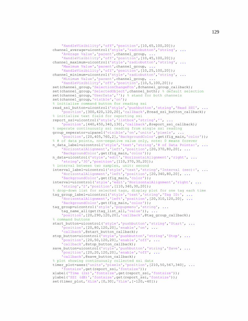
129

'HandleVisibility','off','position',[10,65,100,20]); channel_average=uicontrol('style','radiobutton','string', ... 'Average Value','parent',channel_group, ... 'HandleVisibility','off','position',[10,45,100,20]); channel_maximum=uicontrol('style','radiobutton','string', ... 'Maximum Value','parent',channel_group, ... 'HandleVisibility','off','position',[10,25,100,20]); channel_minimum=uicontrol('style','radiobutton','string', ... 'Minimum Value','parent',channel_group, ... 'HandleVisibility','off','position',[10,5,100,20]); set(channel_group,'SelectionChangeFcn',@channel_group_callback); set(channel_group,'SelectedObject',channel_both); % default selection set(channel_group,'UserData',''); % stand for both channels set(channel_group,'visible','on'); % initialize command button for reading ssi read_ssi_button=uicontrol('style','pushbutton','string','Read SSI', ... 'position',[300,420,120,20],'callback',@read_ssi_button_callback); % initialize text field for reporting ssi report_ssi=uicontrol('style','listbox','string','', ... 'position',[440,450,340,130],'callback',@report_ssi_callback); % seperate continuously ssi reading from single ssi reading group_seperator=uipanel('visible','on','units','pixels', ... 'position',[20,405,760,2],'BackgroundColor',get(fig_main,'color')); % # of data points, non-negative value only, note: 0 means forever n_data_label=uicontrol('style','text','string','# of Data Points:', ... 'HorizontalAlignment','left','position',[20,370,80,20], ... 'BackgroundColor',get(fig_main,'color')); n_data=uicontrol('style','edit','HorizontalAlignment','right', ... 'string','30','position',[110,370,30,20]); % interval between two samples, unit: second interval_label=uicontrol('style','text','string','Interval (sec):', ... 'HorizontalAlignment','left','position',[20,340,80,20], ... 'BackgroundColor',get(fig_main,'color')); interval=uicontrol('style','edit','HorizontalAlignment','right', ... 'string','2','position',[110,340,30,20]); % drop-down list for selected tags, display plot for one tag each time tag_group_label=uicontrol('style','text','string','Tag ID:', ... 'HorizontalAlignment','left','position',[20,310,120,20], ... 'BackgroundColor',get(fig_main,'color')); tag_group=uicontrol('style','popupmenu','string', ... tag_name_all(get(tag_list_all,'value')), ... 'position',[20,290,120,20],'callback',@tag_group_callback); % command buttons start_button=uicontrol('style','pushbutton','string','Start', ... 'position',[20,80,120,20],'enable','on', ... 'callback',@start_button_callback); stop_button=uicontrol('style','pushbutton','string','Stop', ... 'position',[20,50,120,20],'enable','off', ... 'callback',@stop_button_callback); save_button=uicontrol('style','pushbutton','string','Save', ... 'position',[20,20,120,20],'enable','off', ... 'callback',@save_button_callback); % plot showing continuously collected ssi data timer_plot=axes('units','pixels','position',[210,50,567,340], ... 'fontsize',get(report_ssi,'fontsize')); xlabel('Time (2s)','fontsize',get(report_ssi,'fontsize')); ylabel('SSI (dB)','fontsize',get(report_ssi,'fontsize')); set(timer_plot,'XLim',[0,30],'YLim',[-120,-40]);

130

% change units to normalized so components resize automatically set([fig_main,reader_title,reader_list_all,tag_title,tag_list_all, ... channel_group,channel_both,channel_a_only,channel_b_only, ... channel_average,channel_maximum,channel_minimum, ... read_ssi_button,report_ssi,timer_plot,group_seperator,... n_data_label,n_data,interval_label,interval, ... tag_group_label,tag_group, ... start_button,stop_button,save_button], ... 'units','normalized'); switch flag case 'rfcode' fig_main_title='RF Code M200 System - Monitoring GUI'; case 'intelleflex' fig_main_title='Intelleflex FMR6000 System - Monitoring GUI'; end set(fig_main,'numbertitle','off','name',fig_main_title); % rename movegui(fig_main,'center'); % centralize set(fig_main,'visible','on'); % make the GUI visible

% select-all function for readers function reader_title_callback(hObject,eventdata,handles) if (get(reader_title,'value')==get(reader_title,'max')) % checkbox is checked, select all readers set(reader_list_all,'UserData',get(reader_list_all,'value')); set(reader_list_all,'value',(1:1:get(reader_list_all,'max'))); else % checkbox is unchecked, unselect all readers old_value=get(reader_list_all,'UserData'); if isempty(old_value) set(reader_list_all,'value',1); else set(reader_list_all,'value',old_value) end end end

% clear the select all checkbox as selection changes function reader_list_all_callback(hObject,eventdata,handles) if (get(reader_title,'value')==get(reader_title,'max')) set(reader_title,'value',get(reader_title,'min')); end end

% select-all function for tags function tag_title_callback(hObject,eventdata,handles) if (get(tag_title,'value')==get(tag_title,'max')) % checkbox is checked, select all readers set(tag_list_all,'UserData',get(tag_list_all,'value')); set(tag_list_all,'value',(1:1:get(tag_list_all,'max'))); else % checkbox is unchecked, unselect all readers old_value=get(tag_list_all,'UserData'); if isempty(old_value) set(tag_list_all,'value',1); else set(tag_list_all,'value',old_value) end end % also change tag group list

131

tag_group_update(); end

% clear the select all checkbox as selection changes function tag_list_all_callback(hObject,eventdata,handles) if (get(tag_title,'value')==get(tag_title,'max')) set(tag_title,'value',get(tag_title,'min')); end % also change tag group list tag_group_update(); end

% change tag group list as selection changes function tag_group_update() set(tag_group,'string',tag_name_all(get(tag_list_all,'value'))); set(tag_group,'value',1); % choose the first one as default % clear current axe and reset x/y axis cla; set(timer_plot,'XLim',[0,30],'YLim',[-120,-40]); % clear temp storage to avoid mismatching plots if ~isempty(getappdata(timer_plot,'ssi_read_temp')) rmappdata(timer_plot,'ssi_read_temp'); rmappdata(timer_plot,'line_spec_temp'); rmappdata(timer_plot,'x_max_temp'); rmappdata(timer_plot,'i_temp'); end end

% select channel for ssi reporting function channel_group_callback(hObject,eventdata,handles) switch get(get(channel_group,'SelectedObject'),'string') case 'Both Channels' set(channel_group,'UserData',''); case 'Channel A Only' set(channel_group,'UserData','A'); case 'Channel B Only' set(channel_group,'UserData','B'); case 'Average Value' set(channel_group,'UserData','avg'); case 'Maximum Value' set(channel_group,'UserData','max'); case 'Minimum Value' set(channel_group,'UserData','min'); end end

% read ssi for selected reader(s), tag(s) and channel(s) function read_ssi_button_callback(hObject,eventdata,handles) % shorten reference tag_index=get(tag_list_all,'value'); reader_index=get(reader_list_all,'value'); channel_option=get(channel_group,'UserData'); if strcmpi(channel_option,'avg') ... || strcmpi(channel_option,'max') ... || strcmpi(channel_option,'min') channel=''; else channel=channel_option; end

132

% get ssi information switch flag case 'rfcode' ssi=read_ssi(tag_name_all(tag_index), ... reader_name_all(reader_index),channel); case 'intelleflex' ssi=read_ssi(tag_name_all(tag_index), ... readerInfo(reader_index,:),channel); end % revise ssi information ssi=revise_ssi(ssi,channel_option); % organize data for the text field ssi_text=cell(size(ssi,1),1); for i=1:size(ssi,1) for j=1:size(ssi,2) % try to padleft all ssi values k=length(num2str(min(ssi(:,j))))-length(num2str(ssi(i,j))); ssi_text{i}=[ssi_text{i},blanks(2+k), ... num2str(ssi(i,j))]; end end report_text=cell(size(tag_index,2),1); for i=1:size(tag_index,2) report_text{i}=[tag_name_all{(tag_index(i))}, ... ':',ssi_text{i}]; end % locate tag being selected last time in new index [tf,idx]=ismember(get(report_ssi,'UserData'),tag_index); if tf set(report_ssi,'value',idx); else set(report_ssi,'value',1); end % save tag being selected this time based on new index set(read_ssi_button,'UserData',tag_index); set(report_ssi,'UserData',tag_index(get(report_ssi,'value'))); % display ssi information set(report_ssi,'string',report_text); end

% save information function report_ssi_callback(hObject,eventdata,handles) % save tag being selected based on old index tag_index_save=get(read_ssi_button,'UserData'); set(report_ssi,'UserData',tag_index_save(get(report_ssi,'value'))); end

% switch plots for different tags function tag_group_callback(hObject,eventdata,handles) % initialize parameters from temp storage ssi_read=getappdata(timer_plot,'ssi_read_temp'); line_spec_trim=getappdata(timer_plot,'line_spec_temp'); x_max=getappdata(timer_plot,'x_max_temp'); i=getappdata(timer_plot,'i_temp'); % get currently selected tag tag_index=get(tag_group,'value'); % clear current axe and reset x/y axis cla; set(timer_plot,'XLim',[0,30],'YLim',[-120,-40]);

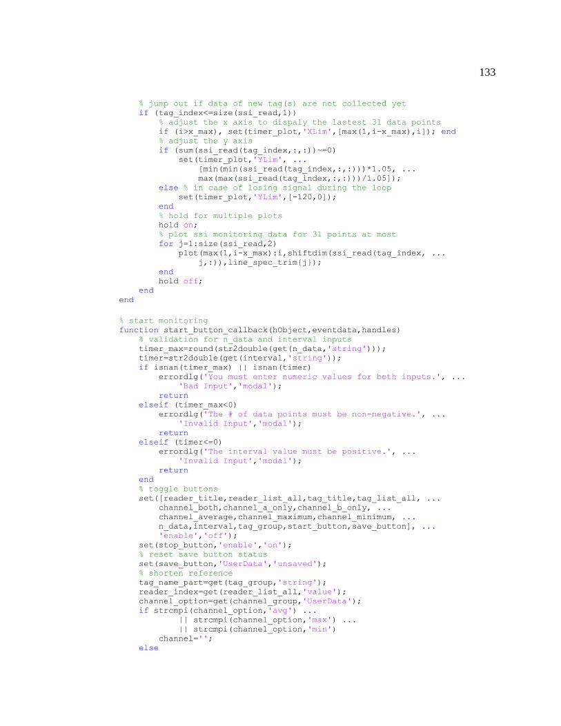
133

% jump out if data of new tag(s) are not collected yet if (tag_index<=size(ssi_read,1)) % adjust the x axis to dispaly the lastest 31 data points if (i>x_max), set(timer_plot,'XLim',[max(1,i-x_max),i]); end % adjust the y axis if (sum(ssi_read(tag_index,:,:))~=0) set(timer_plot,'YLim', ... [min(min(ssi_read(tag_index,:,:)))*1.05, ... max(max(ssi_read(tag_index,:,:)))/1.05]); else % in case of losing signal during the loop set(timer_plot,'YLim',[-120,0]); end % hold for multiple plots hold on; % plot ssi monitoring data for 31 points at most for j=1:size(ssi_read,2) plot(max(1,i-x_max):i,shiftdim(ssi_read(tag_index, ... j,:)),line_spec_trim{j}); end hold off; end end

% start monitoring function start_button_callback(hObject,eventdata,handles) % validation for n_data and interval inputs timer_max=round(str2double(get(n_data,'string'))); timer=str2double(get(interval,'string')); if isnan(timer_max) || isnan(timer) errordlg('You must enter numeric values for both inputs.', ... 'Bad Input','modal'); return elseif (timer_max<0) errordlg('The # of data points must be non-negative.', ... 'Invalid Input','modal'); return elseif (timer<=0) errordlg('The interval value must be positive.', ... 'Invalid Input','modal'); return end % toggle buttons set([reader_title,reader_list_all,tag_title,tag_list_all, ... channel_both,channel_a_only,channel_b_only, ... channel_average,channel_maximum,channel_minimum, ... n_data,interval,tag_group,start_button,save_button], ... 'enable','off'); set(stop_button,'enable','on'); % reset save button status set(save_button,'UserData','unsaved'); % shorten reference tag_name_part=get(tag_group,'string'); reader_index=get(reader_list_all,'value'); channel_option=get(channel_group,'UserData'); if strcmpi(channel_option,'avg') ... || strcmpi(channel_option,'max') ... || strcmpi(channel_option,'min') channel=''; else

134

channel=channel_option; end % define different linespec for each lines line_spec={'-+r';'-xr';'--ob';'--*b';':sm';':dm';'-.pk';'-.hk'}; % keep monitoring forever if # of data points is not given if (timer_max==0), timer_max=inf; end % reset current axe and x/y axis cla reset; xlabel(['Time (',get(interval,'string'),'s)'], ... 'fontsize',get(report_ssi,'fontsize')); ylabel('SSI (dB)','fontsize',get(report_ssi,'fontsize')); set(timer_plot,'XLim',[0,30],'YLim',[-120,-40]); % get ssi information, and plot for i=1:timer_max tic; % start the stopwatch timer % jump out from the loop for interruption if strcmpi(get(stop_button,'enable'),'off'), break; end switch flag case 'rfcode' ssi=read_ssi(tag_name_part, ... reader_name_all(reader_index),channel); case 'intelleflex' ssi=read_ssi(tag_name_part, ... readerInfo(reader_index,:),channel); end

% revise ssi information ssi=revise_ssi(ssi,channel_option); % trim ssi monitoring data ssi_full(:,:,i)=ssi; set(timer_plot,'UserData',ssi_full); x_max=30; % self-defined if (i>x_max) % take the lastest 31 points ssi_trim=ssi_full(:,:,i-x_max:i); else ssi_trim=ssi_full; end % skip zero values if single channel requested if strcmpi(channel,'A') ssi_read=ssi_trim(:,1:2:end,:); line_spec_trim=line_spec(1:2:end,:); elseif strcmpi(channel,'B') ssi_read=ssi_trim(:,2:2:end,:); line_spec_trim=line_spec(2:2:end,:); else ssi_read=ssi_trim; line_spec_trim=line_spec; end % save data for external call setappdata(timer_plot,'ssi_read_temp',ssi_read) setappdata(timer_plot,'line_spec_temp',line_spec_trim); setappdata(timer_plot,'x_max_temp',x_max); setappdata(timer_plot,'i_temp',i); % suspend the tag_index drop-down menu and get current value set(tag_group,'enable','off'); tag_index=get(tag_group,'value'); % adjust the x axis to dispaly the lastest 31 data points if (i>x_max), set(timer_plot,'XLim',[max(1,i-x_max),i]); end % adjust the y axis

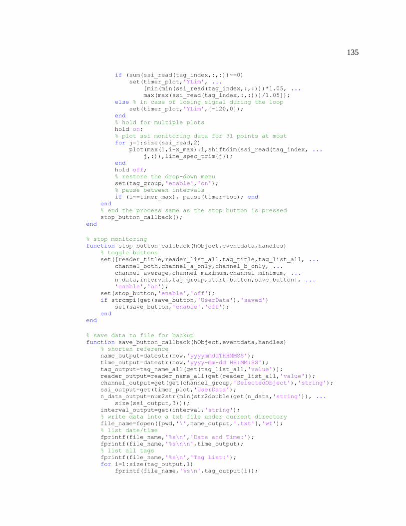
135

if (sum(ssi_read(tag_index,:,:))~=0) set(timer_plot,'YLim', ... [min(min(ssi_read(tag_index,:,:)))*1.05, ... max(max(ssi_read(tag_index,:,:)))/1.05]); else % in case of losing signal during the loop set(timer_plot,'YLim',[-120,0]); end % hold for multiple plots hold on; % plot ssi monitoring data for 31 points at most for j=1:size(ssi_read,2) plot(max(1,i-x_max):i,shiftdim(ssi_read(tag_index, ... j,:)),line_spec_trim{j}); end hold off; % restore the drop-down menu set(tag_group,'enable','on'); % pause between intervals if (i~=timer_max), pause(timer-toc); end end % end the process same as the stop button is pressed stop_button_callback(); end

% stop monitoring function stop_button_callback(hObject,eventdata,handles) % toggle buttons set([reader_title,reader_list_all,tag_title,tag_list_all, ... channel_both,channel_a_only,channel_b_only, ... channel_average,channel_maximum,channel_minimum, ... n_data,interval,tag_group,start_button,save_button], ... 'enable','on'); set(stop_button,'enable','off'); if strcmpi(get(save_button,'UserData'),'saved') set(save_button,'enable','off'); end end

% save data to file for backup function save_button_callback(hObject,eventdata,handles) % shorten reference name_output=datestr(now,'yyyymmddTHHMMSS'); time_output=datestr(now,'yyyy-mm-dd HH:MM:SS'); tag_output=tag_name_all(get(tag_list_all,'value')); reader_output=reader_name_all(get(reader_list_all,'value')); channel_output=get(get(channel_group,'SelectedObject'),'string'); ssi_output=get(timer_plot,'UserData'); n_data_output=num2str(min(str2double(get(n_data,'string')), ... size(ssi_output,3))); interval_output=get(interval,'string'); % write data into a txt file under current directory file_name=fopen([pwd,'\',name_output,'.txt'],'wt'); % list date/time fprintf(file_name,'%s\n','Date and Time:'); fprintf(file_name,'%s\n\n',time_output); % list all tags fprintf(file_name,'%s\n','Tag List:'); for i=1:size(tag_output,1) fprintf(file_name,'%s\n',tag_output{i});

136

end fprintf(file_name,'\n'); % list all readers fprintf(file_name,'%s\n','Reader List:'); for i=1:size(reader_output,1) fprintf(file_name,'%s\n',reader_output{i}); end fprintf(file_name,'\n'); % list channel option fprintf(file_name,'%s\n','Channel Option:'); fprintf(file_name,'%s\n\n',channel_output); % list # of data points fprintf(file_name,'%s\n','# of data points:'); fprintf(file_name,'%s\n\n',n_data_output); % list interval fprintf(file_name,'%s\n','Interval (sec):'); fprintf(file_name,'%s\n\n',interval_output); % list recorded ssi information [m,n,p]=size(ssi_output); for i=1:m fprintf(file_name,'%s\n',['SSI Matrix #',num2str(i),':']); for k=1:p for j=1:n if (j==n) fprintf(file_name,'%4d\n',ssi_output(i,j,k)); else fprintf(file_name,'%4d\t',ssi_output(i,j,k)); end end end % seperator fprintf(file_name,'%s\n','Mean Value:'); % mean value for each channel for j=1:n if (j==n) fprintf(file_name,'%4.1f\n',mean(ssi_output(i,j,:))); else fprintf(file_name,'%4.1f\t',mean(ssi_output(i,j,:))); end

end % seperator fprintf(file_name,'%s\n','Standard Deviation:'); % standard deviation for each channel for j=1:n if (j==n) fprintf(file_name,'%4.2f\n',std(ssi_output(i,j,:))); else fprintf(file_name,'%4.2f\t',std(ssi_output(i,j,:))); end end % seperator fprintf(file_name,'%s\n','Mean and Std for AVG(A+B):'); for j=1:2:n if (j==n-1) fprintf(file_name,'%4.1f\t', ... mean(mean([ssi_output(i,j,:), ... ssi_output(i,j+1,:)]))); fprintf(file_name,'%4.1f\n', ...

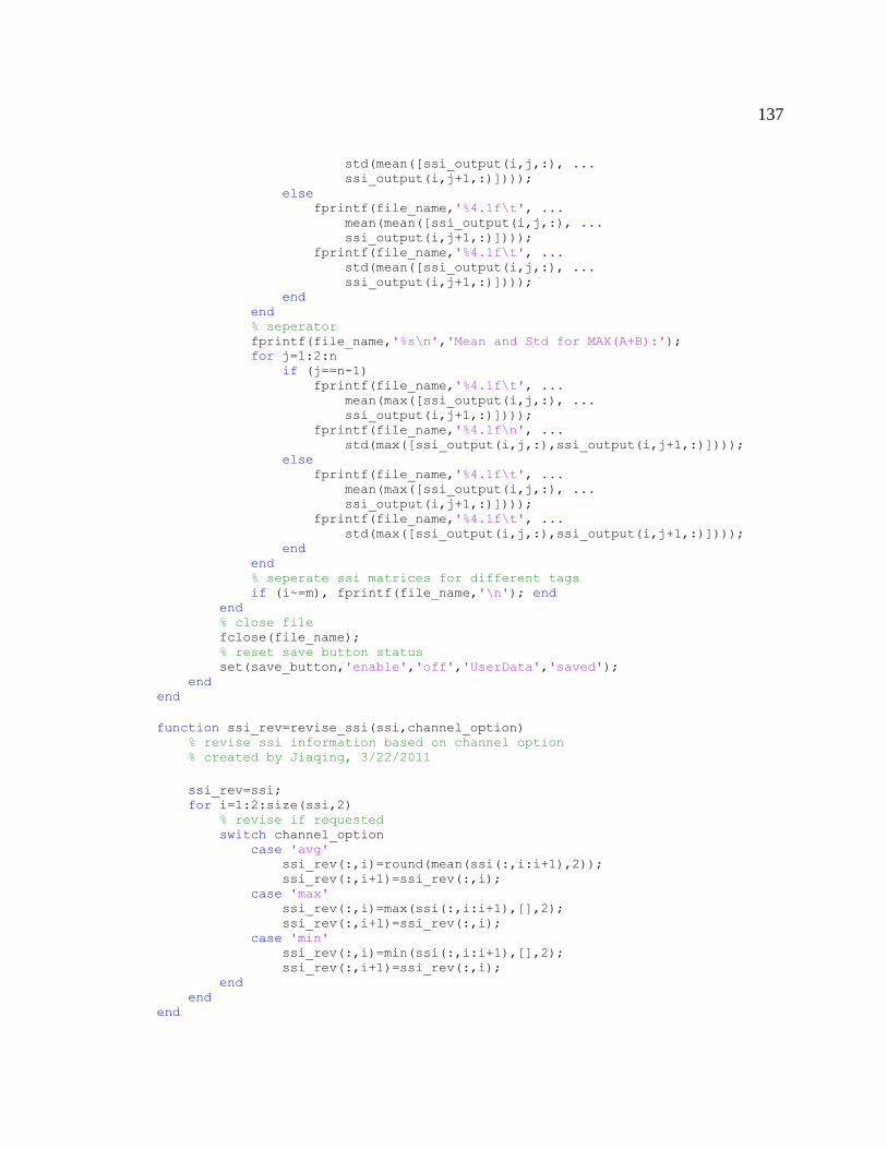
137

std(mean([ssi_output(i,j,:), ... ssi_output(i,j+1,:)]))); else fprintf(file_name,'%4.1f\t', ... mean(mean([ssi_output(i,j,:), ... ssi_output(i,j+1,:)]))); fprintf(file_name,'%4.1f\t', ... std(mean([ssi_output(i,j,:), ... ssi_output(i,j+1,:)]))); end end % seperator fprintf(file_name,'%s\n','Mean and Std for MAX(A+B):'); for j=1:2:n if (j==n-1) fprintf(file_name,'%4.1f\t', ... mean(max([ssi_output(i,j,:), ... ssi_output(i,j+1,:)]))); fprintf(file_name,'%4.1f\n', ... std(max([ssi_output(i,j,:),ssi_output(i,j+1,:)]))); else fprintf(file_name,'%4.1f\t', ... mean(max([ssi_output(i,j,:), ... ssi_output(i,j+1,:)]))); fprintf(file_name,'%4.1f\t', ... std(max([ssi_output(i,j,:),ssi_output(i,j+1,:)]))); end end % seperate ssi matrices for different tags if (i~=m), fprintf(file_name,'\n'); end end % close file fclose(file_name); % reset save button status set(save_button,'enable','off','UserData','saved'); end end

function ssi_rev=revise_ssi(ssi,channel_option) % revise ssi information based on channel option % created by Jiaqing, 3/22/2011

ssi_rev=ssi; for i=1:2:size(ssi,2) % revise if requested switch channel_option case 'avg' ssi_rev(:,i)=round(mean(ssi(:,i:i+1),2)); ssi_rev(:,i+1)=ssi_rev(:,i); case 'max' ssi_rev(:,i)=max(ssi(:,i:i+1),[],2); ssi_rev(:,i+1)=ssi_rev(:,i); case 'min' ssi_rev(:,i)=min(ssi(:,i:i+1),[],2); ssi_rev(:,i+1)=ssi_rev(:,i); end end end

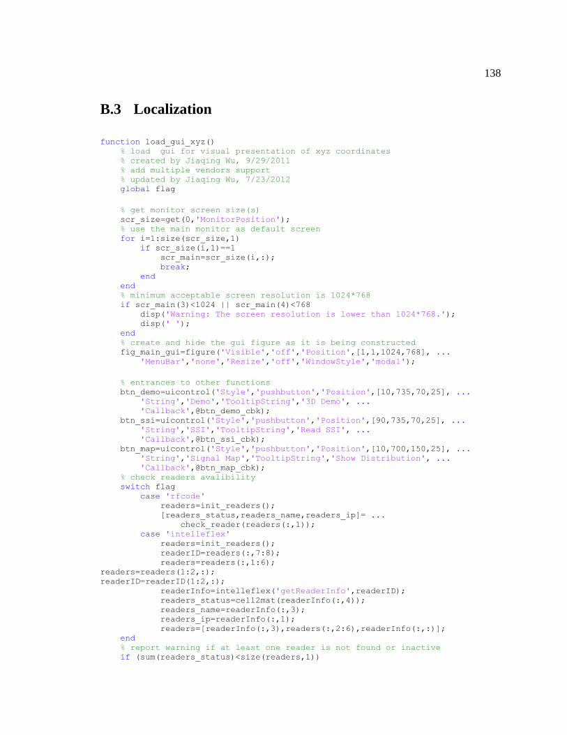
138

B.3 Localization

function load_gui_xyz() % load gui for visual presentation of xyz coordinates % created by Jiaqing Wu, 9/29/2011 % add multiple vendors support % updated by Jiaqing Wu, 7/23/2012 global flag

% get monitor screen size(s) scr_size=get(0,'MonitorPosition'); % use the main monitor as default screen for i=1:size(scr_size,1) if scr_size(i,1)==1 scr_main=scr_size(i,:); break; end end % minimum acceptable screen resolution is 1024*768 if scr_main(3)<1024 || scr_main(4)<768 disp('Warning: The screen resolution is lower than 1024*768.'); disp(' '); end % create and hide the gui figure as it is being constructed fig_main_gui=figure('Visible','off','Position',[1,1,1024,768], ... 'MenuBar','none','Resize','off','WindowStyle','modal');

% entrances to other functions btn_demo=uicontrol('Style','pushbutton','Position',[10,735,70,25], ... 'String','Demo','TooltipString','3D Demo', ... 'Callback',@btn_demo_cbk); btn_ssi=uicontrol('Style','pushbutton','Position',[90,735,70,25], ... 'String','SSI','TooltipString','Read SSI', ... 'Callback',@btn_ssi_cbk); btn_map=uicontrol('Style','pushbutton','Position',[10,700,150,25], ... 'String','Signal Map','TooltipString','Show Distribution', ... 'Callback',@btn_map_cbk); % check readers avalibility switch flag case 'rfcode' readers=init_readers(); [readers_status,readers_name,readers_ip]= ... check_reader(readers(:,1)); case 'intelleflex' readers=init_readers(); readerID=readers(:,7:8); readers=readers(:,1:6); readers=readers(1:2,:); readerID=readerID(1:2,:); readerInfo=intelleflex('getReaderInfo',readerID); readers_status=cell2mat(readerInfo(:,4)); readers_name=readerInfo(:,3); readers_ip=readerInfo(:,1); readers=[readerInfo(:,3),readers(:,2:6),readerInfo(:,:)]; end % report warning if at least one reader is not found or inactive if (sum(readers_status)<size(readers,1))

139

disp(['Warning: ', ... num2str(size(readers,1)-sum(readers_status)), ... ' designated reader(s) are offline.']); disp(' '); end btn_readers=uicontrol('Style','pushbutton', ... 'Position',[10,665,150,25], ... 'String',['Avaliable readers: ',num2str(sum(readers_status)), ... ' of ',num2str(size(readers,1))], ... 'TooltipString','Click for more details', ... 'Callback',@btn_readers_cbk); % check reference tags avalibility switch flag case 'rfcode' ref_tags=init_ref_tags(); ref_tags_group=init_ref_tags_group(ref_tags); [ref_tags_status,ref_tags_name]=check_tag(ref_tags); case 'intelleflex' ref_tags=init_ref_tags(); ref_tags_group=init_ref_tags_group(ref_tags); tagID=ref_tags(:,1); tagInfo=intelleflex('getTagInfo',readerInfo,tagID); ref_tags_status=~(sum(cell2mat(tagInfo(:,2:end)),2)==0); ref_tags_name=tagInfo(:,1); end % report warning if at least one reference tag is not detected if (sum(ref_tags_status)<size(ref_tags,1)) disp(['Warning: ', ... num2str(size(ref_tags,1)-sum(ref_tags_status)), ... ' designated reference tag(s) are offline.']); disp(' '); end btn_ref_tags=uicontrol('Style','pushbutton', ... 'Position',[10,630,150,25], ... 'String',['Avaliable ref_tags: ',num2str(sum(ref_tags_status)), ... ' of ',num2str(size(ref_tags,1))], ... 'TooltipString','Click for more details', ... 'Callback',@btn_ref_tags_cbk); % list all availabe tags switch flag case 'rfcode' [tags_status,tags_name]=check_tag(); [tags,tags_flag]=init_tags(tags_name); case 'intelleflex' tagInfo=intelleflex('getTagInfo',readerID); tags_status=~(sum(cell2mat(tagInfo(:,2:end)),2)==0); tags_name=tagInfo(:,1); [tags,tags_flag]=init_tags(tags_name); end btn_tags=uicontrol('Style','pushbutton', ... 'Position',[10,595,150,25], ... 'String',['All available tags: ', ... num2str(sum(cell2mat(tags_flag),1)), ... ' of ',num2str(size(tags,1))], ... 'TooltipString','Click for more details', ... 'Callback',@btn_tags_cbk);

% real xyz for precision evaluation tbl_real_xyz=uitable('Position',[10,270,150,41],'Enable','off');

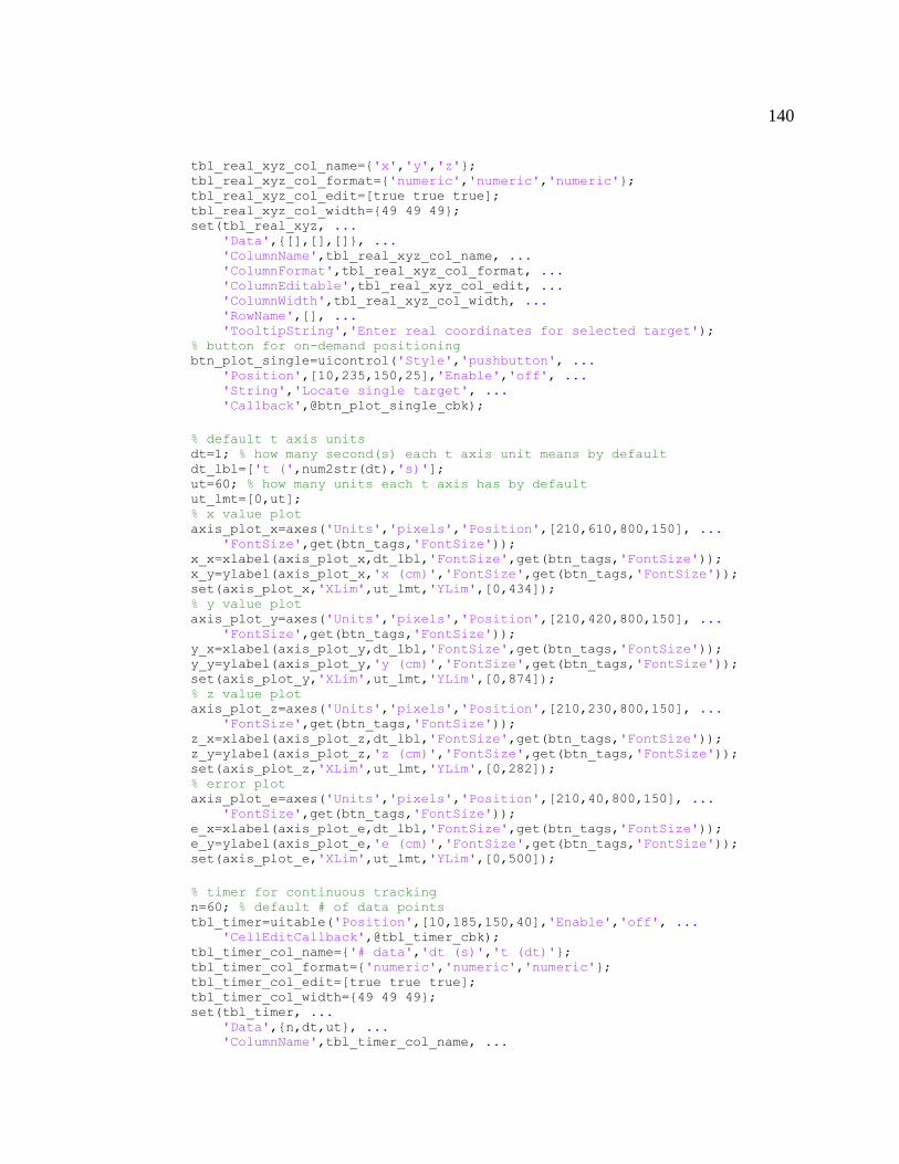
140

tbl_real_xyz_col_name={'x','y','z'}; tbl_real_xyz_col_format={'numeric','numeric','numeric'}; tbl_real_xyz_col_edit=[true true true]; tbl_real_xyz_col_width={49 49 49}; set(tbl_real_xyz, ... 'Data',{[],[],[]}, ... 'ColumnName',tbl_real_xyz_col_name, ... 'ColumnFormat',tbl_real_xyz_col_format, ... 'ColumnEditable',tbl_real_xyz_col_edit, ... 'ColumnWidth',tbl_real_xyz_col_width, ... 'RowName',[], ... 'TooltipString','Enter real coordinates for selected target'); % button for on-demand positioning btn_plot_single=uicontrol('Style','pushbutton', ... 'Position',[10,235,150,25],'Enable','off', ... 'String','Locate single target', ... 'Callback',@btn_plot_single_cbk);

% default t axis units dt=1; % how many second(s) each t axis unit means by default dt_lbl=['t (',num2str(dt),'s)']; ut=60; % how many units each t axis has by default ut_lmt=[0,ut]; % x value plot axis_plot_x=axes('Units','pixels','Position',[210,610,800,150], ... 'FontSize',get(btn_tags,'FontSize')); x_x=xlabel(axis_plot_x,dt_lbl,'FontSize',get(btn_tags,'FontSize')); x_y=ylabel(axis_plot_x,'x (cm)','FontSize',get(btn_tags,'FontSize')); set(axis_plot_x,'XLim',ut_lmt,'YLim',[0,434]); % y value plot axis_plot_y=axes('Units','pixels','Position',[210,420,800,150], ... 'FontSize',get(btn_tags,'FontSize')); y_x=xlabel(axis_plot_y,dt_lbl,'FontSize',get(btn_tags,'FontSize')); y_y=ylabel(axis_plot_y,'y (cm)','FontSize',get(btn_tags,'FontSize')); set(axis_plot_y,'XLim',ut_lmt,'YLim',[0,874]); % z value plot axis_plot_z=axes('Units','pixels','Position',[210,230,800,150], ... 'FontSize',get(btn_tags,'FontSize')); z_x=xlabel(axis_plot_z,dt_lbl,'FontSize',get(btn_tags,'FontSize')); z_y=ylabel(axis_plot_z,'z (cm)','FontSize',get(btn_tags,'FontSize')); set(axis_plot_z,'XLim',ut_lmt,'YLim',[0,282]); % error plot axis_plot_e=axes('Units','pixels','Position',[210,40,800,150], ... 'FontSize',get(btn_tags,'FontSize')); e_x=xlabel(axis_plot_e,dt_lbl,'FontSize',get(btn_tags,'FontSize')); e_y=ylabel(axis_plot_e,'e (cm)','FontSize',get(btn_tags,'FontSize')); set(axis_plot_e,'XLim',ut_lmt,'YLim',[0,500]);

% timer for continuous tracking n=60; % default # of data points tbl_timer=uitable('Position',[10,185,150,40],'Enable','off', ... 'CellEditCallback',@tbl_timer_cbk); tbl_timer_col_name={'# data','dt (s)','t (dt)'}; tbl_timer_col_format={'numeric','numeric','numeric'}; tbl_timer_col_edit=[true true true]; tbl_timer_col_width={49 49 49}; set(tbl_timer, ... 'Data',{n,dt,ut}, ... 'ColumnName',tbl_timer_col_name, ...

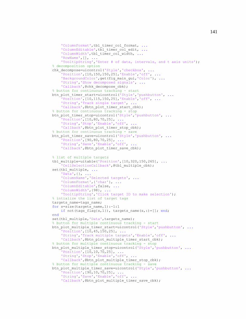
141

'ColumnFormat',tbl_timer_col_format, ... 'ColumnEditable',tbl_timer_col_edit, ... 'ColumnWidth',tbl_timer_col_width, ... 'RowName',[], ... 'TooltipString','Enter # of data, intervals, and t axis units'); % decomposition option chk_decompose=uicontrol('Style','checkbox', ... 'Position',[10,150,150,25],'Enable','off', ... 'BackgroundColor',get(fig_main_gui,'Color'), ... 'String','Show decomposed signals', ... 'Callback',@chk_decompose_cbk); % button for continuous tracking - start btn_plot_timer_start=uicontrol('Style','pushbutton', ... 'Position',[10,115,150,25],'Enable','off', ... 'String','Track single target', ... 'Callback',@btn_plot_timer_start_cbk); % button for continuous tracking - stop btn_plot_timer_stop=uicontrol('Style','pushbutton', ... 'Position',[10,80,70,25], ... 'String','Stop','Enable','off', ... 'Callback',@btn_plot_timer_stop_cbk); % button for continuous tracking - save btn_plot_timer_save=uicontrol('Style','pushbutton', ... 'Position',[90,80,70,25], ... 'String','Save','Enable','off', ... 'Callback',@btn_plot_timer_save_cbk);

% list of multiple targets tbl_multiple=uitable('Position',[10,320,150,265], ... 'CellSelectionCallback',@tbl_multiple_cbk); set(tbl_multiple, ... 'Data',{}, ... 'ColumnName','Selected targets', ... 'ColumnFormat',{'char'}, ... 'ColumnEditable',false, ... 'ColumnWidth',{98}, ... 'TooltipString','Click target ID to make selection'); % intialize the list of target tags targets_name=tags_name; for s=size(targets_name,1):-1:1 if not(tags_flag{s,1}), targets_name(s,:)=[]; end; end set(tbl_multiple,'Data',targets_name); % button for multiple continuous tracking - start btn_plot_multiple_timer_start=uicontrol('Style','pushbutton', ... 'Position',[10,45,150,25], ... 'String','Track multiple targets','Enable','off', ... 'Callback',@btn_plot_multiple_timer_start_cbk); % button for multiple continuous tracking - stop btn_plot_multiple_timer_stop=uicontrol('Style','pushbutton', ... 'Position',[10,10,70,25], ... 'String','Stop','Enable','off', ... 'Callback',@btn_plot_multiple_timer_stop_cbk); % button for multiple continuous tracking - save btn_plot_multiple_timer_save=uicontrol('Style','pushbutton', ... 'Position',[90,10,70,25], ... 'String','Save','Enable','off', ... 'Callback',@btn_plot_multiple_timer_save_cbk);

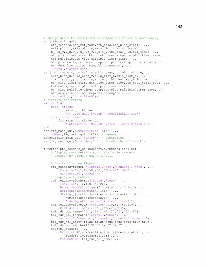
142

% change units to normalized so components resize automatically set([fig_main_gui, ... btn_readers,btn_ref_tags,btn_tags,btn_plot_single, ... axis_plot_x,axis_plot_y,axis_plot_z,axis_plot_e, ... x_x,x_y,y_x,y_y,z_x,z_y,e_x,e_y,tbl_real_xyz,tbl_timer, ... btn_plot_timer_start,btn_plot_timer_stop,btn_plot_timer_save, ... tbl_multiple,btn_plot_multiple_timer_start, ... btn_plot_multiple_timer_stop,btn_plot_multiple_timer_save, ... btn_demo,btn_ssi,btn_map,chk_decompose], ... 'Units','normalized'); set([btn_readers,btn_ref_tags,btn_tags,btn_plot_single, ... axis_plot_x,axis_plot_y,axis_plot_z,axis_plot_e, ... x_x,x_y,y_x,y_y,z_x,z_y,e_x,e_y,tbl_real_xyz,tbl_timer, ... btn_plot_timer_start,btn_plot_timer_stop,btn_plot_timer_save, ... tbl_multiple,btn_plot_multiple_timer_start, ... btn_plot_multiple_timer_stop,btn_plot_multiple_timer_save, ... btn_demo,btn_ssi,btn_map,chk_decompose], ... 'FontUnits','normalized'); % finalize the figure switch flag case 'rfcode' fig_main_gui_title= ... 'RF Code M200 System - Localization GUI'; case 'intelleflex' fig_main_gui_title= ... 'Intelleflex FMR6000 System - Localization GUI'; end set(fig_main_gui,'NumberTitle','off', ... 'Name',fig_main_gui_title); % rename movegui(fig_main_gui,'center'); % centralize set(fig_main_gui,'Visible','on'); % make the GUI visible

function btn_readers_cbk(hObject,eventdata,handles) % Display more details about available readers % Created by Jiaqing Wu, 9/30/2011

% Construct a new figure fig_readers=figure('Visible','off','MenuBar','none', ... 'Position',[1,1,350,200],'Resize','off', ... 'WindowStyle','modal'); % display all readers lbl_readers=uicontrol('Style','text', ... 'Position',[10,180,340,20], ... 'BackgroundColor',get(fig_main_gui,'Color'), ... 'HorizontalAlignment','left', ... 'String',[num2str(sum(readers_status)),' of ', ... num2str(size(readers,1)), ... ' designated reader(s) are online.']); tbl_readers=uitable('Position',[10,65,340,110], ... 'CellEditCallback',@tbl_readers_cbk); tbl_rdr_col_name={'ON','IP','X','Y','Z','A','B'}; tbl_rdr_col_format={'logical','char', ... 'numeric','numeric','numeric','numeric','numeric'}; tbl_rdr_col_edit=[false false true true true true true]; tbl_rdr_col_width={40 90 32 32 32 32 32}; set(tbl_readers, ... 'Data',cat(2,num2cell(logical(readers_status)), ... readers_ip,readers(:,2:6)), ... 'ColumnName',tbl_rdr_col_name, ...

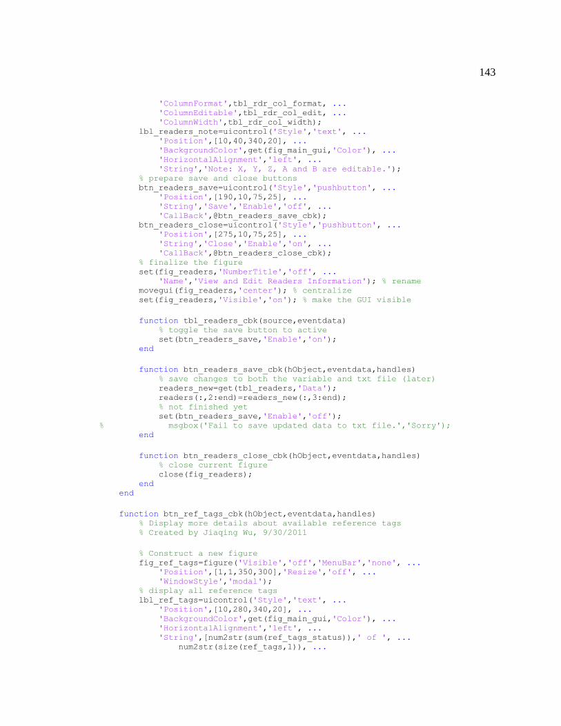
143

'ColumnFormat',tbl_rdr_col_format, ... 'ColumnEditable',tbl_rdr_col_edit, ... 'ColumnWidth',tbl_rdr_col_width); lbl_readers_note=uicontrol('Style','text', ... 'Position',[10,40,340,20], ... 'BackgroundColor',get(fig_main_gui,'Color'), ... 'HorizontalAlignment','left', ... 'String','Note: X, Y, Z, A and B are editable.'); % prepare save and close buttons btn_readers_save=uicontrol('Style','pushbutton', ... 'Position',[190,10,75,25], ... 'String','Save','Enable','off', ... 'CallBack',@btn_readers_save_cbk); btn_readers_close=uicontrol('Style','pushbutton', ... 'Position',[275,10,75,25], ... 'String','Close','Enable','on', ... 'CallBack',@btn_readers_close_cbk); % finalize the figure set(fig_readers,'NumberTitle','off', ... 'Name','View and Edit Readers Information'); % rename movegui(fig_readers,'center'); % centralize set(fig_readers,'Visible','on'); % make the GUI visible

function tbl_readers_cbk(source,eventdata) % toggle the save button to active set(btn_readers_save,'Enable','on'); end

function btn_readers_save_cbk(hObject,eventdata,handles) % save changes to both the variable and txt file (later) readers_new=get(tbl_readers,'Data'); readers(:,2:end)=readers_new(:,3:end); % not finished yet set(btn_readers_save,'Enable','off'); % msgbox('Fail to save updated data to txt file.','Sorry'); end

function btn_readers_close_cbk(hObject,eventdata,handles) % close current figure close(fig_readers); end end

function btn_ref_tags_cbk(hObject,eventdata,handles) % Display more details about available reference tags % Created by Jiaqing Wu, 9/30/2011

% Construct a new figure fig_ref_tags=figure('Visible','off','MenuBar','none', ... 'Position',[1,1,350,300],'Resize','off', ... 'WindowStyle','modal'); % display all reference tags lbl_ref_tags=uicontrol('Style','text', ... 'Position',[10,280,340,20], ... 'BackgroundColor',get(fig_main_gui,'Color'), ... 'HorizontalAlignment','left', ... 'String',[num2str(sum(ref_tags_status)),' of ', ... num2str(size(ref_tags,1)), ...

144

' designated reference tag(s) are online.']); tbl_ref_tags=uitable('Position',[10,65,340,210], ... 'CellEditCallback',@tbl_ref_tags_cbk); tbl_rtg_col_name={'ON','ID','X','Y','Z','O'}; tbl_rtg_col_format={'logical','char', ... 'numeric','numeric','numeric','numeric'}; tbl_rtg_col_edit=[false false true true true true]; tbl_rtg_col_width={40 120 32 32 32 32}; set(tbl_ref_tags, ... 'Data',cat(2,num2cell(logical(ref_tags_status)),ref_tags), ... 'ColumnName',tbl_rtg_col_name, ... 'ColumnFormat',tbl_rtg_col_format, ... 'ColumnEditable',tbl_rtg_col_edit, ... 'ColumnWidth',tbl_rtg_col_width); lbl_ref_tags_note=uicontrol('Style','text', ... 'Position',[10,40,340,20], ... 'BackgroundColor',get(fig_main_gui,'Color'), ... 'HorizontalAlignment','left', ... 'String','Note: X, Y, Z, and O are editable.'); % prepare save and close buttons btn_ref_tags_save=uicontrol('Style','pushbutton', ... 'Position',[190,10,75,25], ... 'String','Save','Enable','off', ... 'CallBack',@btn_ref_tags_save_cbk); btn_ref_tags_close=uicontrol('Style','pushbutton', ... 'Position',[275,10,75,25], ... 'String','Close','Enable','on', ... 'CallBack',@btn_ref_tags_close_cbk); % finalize the figure set(fig_ref_tags,'NumberTitle','off', ... 'Name','View and Edit Reference Tags Information'); % rename movegui(fig_ref_tags,'center'); % centralize set(fig_ref_tags,'Visible','on'); % make the GUI visible

function tbl_ref_tags_cbk(source,eventdata) % toggle the save button to active set(btn_ref_tags_save,'Enable','on'); end

function btn_ref_tags_save_cbk(hObject,eventdata,handles) % save changes to both the variable and txt file (later) ref_tags_new=get(tbl_ref_tags,'Data'); ref_tags(:,:)=ref_tags_new(:,2:end); % not finished yet set(btn_ref_tags_save,'Enable','off'); % msgbox('Fail to save updated data to txt file.','Sorry'); end

function btn_ref_tags_close_cbk(hObject,eventdata,handles) % close current figure close(fig_ref_tags); end end

function btn_tags_cbk(hObject,eventdata,handles) % Display more details about all available tags % Created by Jiaqing Wu, 10/2/2011

145

% Construct a new figure fig_tags=figure('Visible','off','MenuBar','none', ... 'Position',[1,1,350,300],'Resize','off', ... 'WindowStyle','modal'); % display all tags lbl_tags=uicontrol('Style','text', ... 'Position',[10,280,340,20], ... 'BackgroundColor',get(fig_main_gui,'Color'), ... 'HorizontalAlignment','left', ... 'String',[num2str(sum(cell2mat(tags_flag),1)),' of ', ... num2str(size(tags,1)), ... ' available tag(s) are selected.']); tbl_tags=uitable('Position',[10,65,340,210], ... 'CellEditCallback',@tbl_tags_cbk); tbl_tags_col_name={'ON','ID','X','Y','Z','O'}; tbl_tags_col_format={'logical','char', ... 'numeric','numeric','numeric','numeric'}; tbl_tags_col_edit=[true false true true true true]; tbl_tags_col_width={40 120 32 32 32 32}; set(tbl_tags, ... 'Data',cat(2,tags_flag,tags), ... 'ColumnName',tbl_tags_col_name, ... 'ColumnFormat',tbl_tags_col_format, ... 'ColumnEditable',tbl_tags_col_edit, ... 'ColumnWidth',tbl_tags_col_width); lbl_tags_note=uicontrol('Style','text', ... 'Position',[10,40,340,20], ... 'BackgroundColor',get(fig_main_gui,'Color'), ... 'HorizontalAlignment','left', ... 'String','Note: X, Y, Z, and O are editable.'); % prepare save and close buttons btn_tags_save=uicontrol('Style','pushbutton', ... 'Position',[190,10,75,25], ... 'String','Save','Enable','off', ... 'CallBack',@btn_tags_save_cbk); btn_tags_close=uicontrol('Style','pushbutton', ... 'Position',[275,10,75,25], ... 'String','Close','Enable','on', ... 'CallBack',@btn_tags_close_cbk); % finalize the figure set(fig_tags,'NumberTitle','off', ... 'Name','View and Edit All Tags Information'); % rename movegui(fig_tags,'center'); % centralize set(fig_tags,'Visible','on'); % make the GUI visible

function tbl_tags_cbk(source,eventdata) % toggle the save button to active set(btn_tags_save,'Enable','on'); tags_temp=get(tbl_tags,'Data'); set(lbl_tags,'String', ... [num2str(sum(cell2mat(tags_temp(:,1)),1)), ... ' of ',num2str(size(tags,1)), ... ' available tag(s) are selected.']); end

function btn_tags_save_cbk(hObject,eventdata,handles) % save changes to both the variable and txt file (later) tags_new=get(tbl_tags,'Data'); tags_flag=tags_new(:,1);

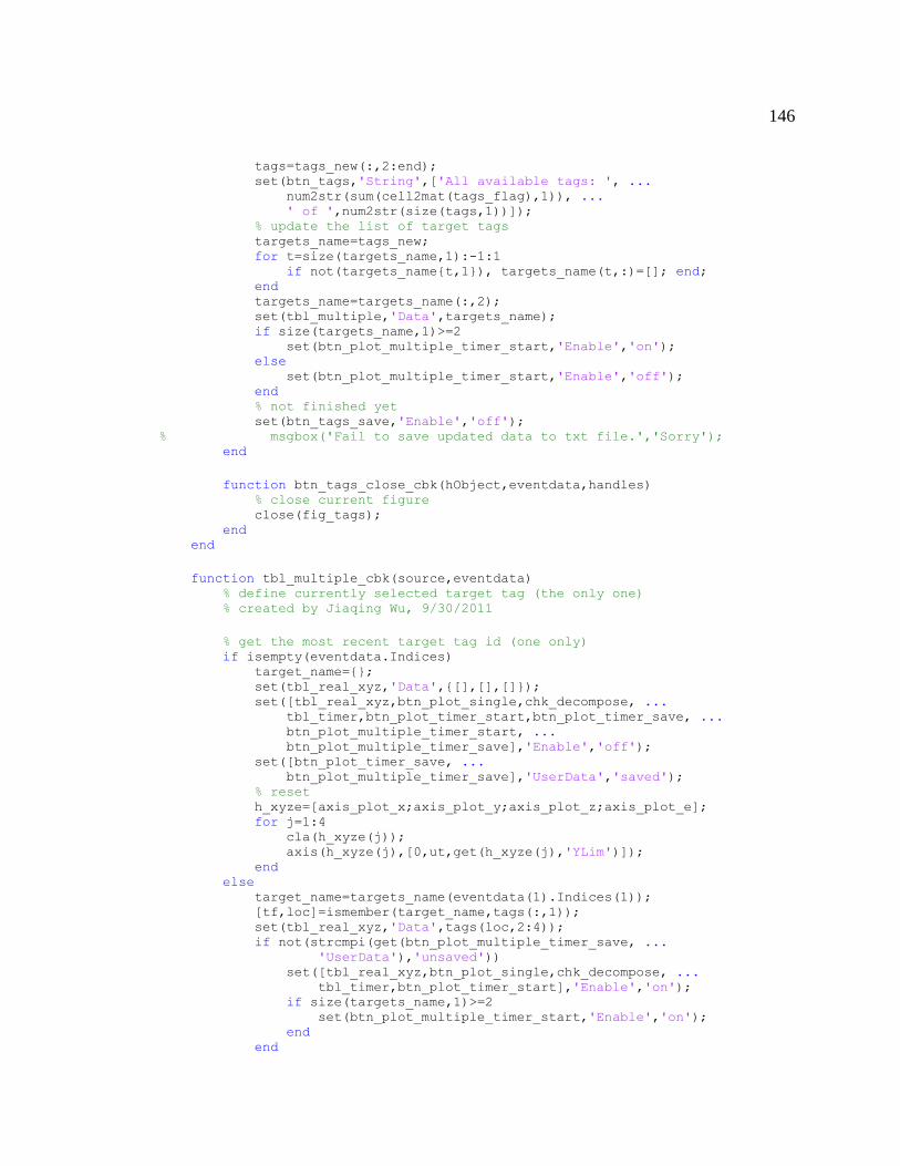
146

tags=tags_new(:,2:end); set(btn_tags,'String',['All available tags: ', ... num2str(sum(cell2mat(tags_flag),1)), ... ' of ',num2str(size(tags,1))]); % update the list of target tags targets_name=tags_new; for t=size(targets_name,1):-1:1 if not(targets_name{t,1}), targets_name(t,:)=[]; end; end targets_name=targets_name(:,2); set(tbl_multiple,'Data',targets_name); if size(targets_name,1)>=2 set(btn_plot_multiple_timer_start,'Enable','on'); else set(btn_plot_multiple_timer_start,'Enable','off'); end % not finished yet set(btn_tags_save,'Enable','off'); % msgbox('Fail to save updated data to txt file.','Sorry'); end

function btn_tags_close_cbk(hObject,eventdata,handles) % close current figure close(fig_tags); end end

function tbl_multiple_cbk(source,eventdata) % define currently selected target tag (the only one) % created by Jiaqing Wu, 9/30/2011

% get the most recent target tag id (one only) if isempty(eventdata.Indices) target_name={}; set(tbl_real_xyz,'Data',{[],[],[]}); set([tbl_real_xyz,btn_plot_single,chk_decompose, ... tbl_timer,btn_plot_timer_start,btn_plot_timer_save, ... btn_plot_multiple_timer_start, ... btn_plot_multiple_timer_save],'Enable','off'); set([btn_plot_timer_save, ... btn_plot_multiple_timer_save],'UserData','saved'); % reset h_xyze=[axis_plot_x;axis_plot_y;axis_plot_z;axis_plot_e]; for j=1:4 cla(h_xyze(j)); axis(h_xyze(j),[0,ut,get(h_xyze(j),'YLim')]); end else target_name=targets_name(eventdata(1).Indices(1)); [tf,loc]=ismember(target_name,tags(:,1)); set(tbl_real_xyz,'Data',tags(loc,2:4)); if not(strcmpi(get(btn_plot_multiple_timer_save, ... 'UserData'),'unsaved')) set([tbl_real_xyz,btn_plot_single,chk_decompose, ... tbl_timer,btn_plot_timer_start],'Enable','on'); if size(targets_name,1)>=2 set(btn_plot_multiple_timer_start,'Enable','on'); end end

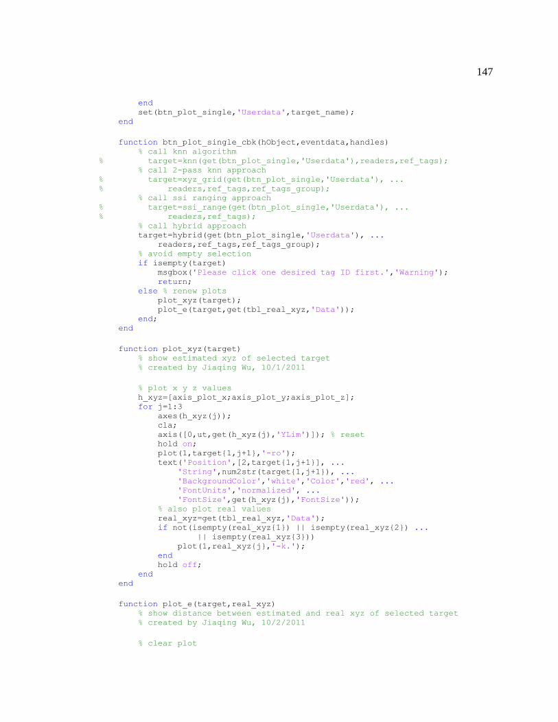
147

end set(btn_plot_single,'Userdata',target_name); end

function btn_plot_single_cbk(hObject,eventdata,handles) % call knn algorithm % target=knn(get(btn_plot_single,'Userdata'),readers,ref_tags); % call 2-pass knn approach % target=xyz_grid(get(btn_plot_single,'Userdata'), ... % readers,ref_tags,ref_tags_group); % call ssi ranging approach % target=ssi_range(get(btn_plot_single,'Userdata'), ... % readers,ref_tags); % call hybrid approach target=hybrid(get(btn_plot_single,'Userdata'), ... readers,ref_tags,ref_tags_group); % avoid empty selection if isempty(target) msgbox('Please click one desired tag ID first.','Warning'); return; else % renew plots plot_xyz(target); plot_e(target,get(tbl_real_xyz,'Data')); end; end

function plot_xyz(target) % show estimated xyz of selected target % created by Jiaqing Wu, 10/1/2011

% plot x y z values h_xyz=[axis_plot_x;axis_plot_y;axis_plot_z]; for j=1:3 axes(h_xyz(j)); cla; axis([0,ut,get(h_xyz(j),'YLim')]); % reset hold on; plot(1,target{1,j+1},'-ro'); text('Position',[2,target{1,j+1}], ... 'String',num2str(target{1,j+1}), ... 'BackgroundColor','white','Color','red', ... 'FontUnits','normalized', ... 'FontSize',get(h_xyz(j),'FontSize')); % also plot real values real_xyz=get(tbl_real_xyz,'Data'); if not(isempty(real_xyz{1}) || isempty(real_xyz{2}) ... || isempty(real_xyz{3})) plot(1,real_xyz{j},'-k.'); end hold off; end end

function plot_e(target,real_xyz) % show distance between estimated and real xyz of selected target % created by Jiaqing Wu, 10/2/2011

% clear plot

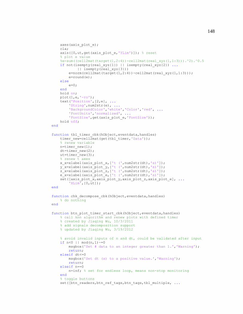
148

axes(axis_plot_e); cla; axis([0,ut,get(axis_plot_e,'YLim')]); % reset % plot e value %e=sum((cell2mat(target(1,2:4))-cell2mat(real_xyz(1,1:3))).^2).^0.5 if not(isempty(real_xyz{1}) || isempty(real_xyz{2}) ... || isempty(real_xyz{3})) e=norm(cell2mat(target(1,2:4))-cell2mat(real_xyz(1,1:3))); e=round(e); else e=0; end hold on; plot(1,e,'-ro'); text('Position',[2,e], ... 'String',num2str(e), ... 'BackgroundColor','white','Color','red', ... 'FontUnits','normalized', ... 'FontSize',get(axis_plot_e,'FontSize')); hold off; end

function tbl_timer_cbk(hObject,eventdata,handles) timer_new=cell2mat(get(tbl_timer,'Data')); % renew variable n=timer_new(1); dt=timer_new(2); ut=timer_new(3); % renew t axes x_x=xlabel(axis_plot_x,['t (',num2str(dt),'s)']); y_x=xlabel(axis_plot_y,['t (',num2str(dt),'s)']); z_x=xlabel(axis_plot_z,['t (',num2str(dt),'s)']); e_x=xlabel(axis_plot_e,['t (',num2str(dt),'s)']); set([axis_plot_x,axis_plot_y,axis_plot_z,axis_plot_e], ... 'XLim',[0,ut]); end

function chk_decompose_cbk(hObject,eventdata,handles) % do nothing end

function btn_plot_timer_start_cbk(hObject,eventdata,handles) % call knn algorithm and renew plots with defined timer % created by Jiaqing Wu, 10/3/2011 % add signals decomposition support % updated by Jiaqing Wu, 3/19/2012

% avoid invalid inputs of n and dt, could be validated after input if n<0 || mod(n,1)~=0 msgbox('Set # data to an integer greater than 1.','Warning'); return; elseif dt<=0 msgbox('Set dt (s) to a positive value.','Warning'); return; elseif n==0 n=inf; % set for endless loop, means non-stop monitoring end % toggle buttons set([btn_readers,btn_ref_tags,btn_tags,tbl_multiple, ...

149

tbl_real_xyz,btn_plot_single,tbl_timer, ... btn_plot_timer_start,btn_plot_timer_save, ... btn_plot_multiple_timer_start, ... btn_plot_multiple_timer_save, ... btn_demo,btn_ssi,btn_map,chk_decompose], ... 'Enable','off'); set(btn_plot_timer_stop,'Enable','on'); set(btn_plot_timer_save,'UserData','unsaved'); % initialize target_timer and e_timer array target_timer=cell(1,4,n); target_dc=zeros(4,3,n); e_timer=cell(1,1,n); e_dc=zeros(4,1,n); % timer for t=1:n tic; % start the stopwatch timer % jump out from the loop for interruption if strcmpi(get(btn_plot_timer_stop,'Enable'),'off'), break; end % call knn algorithm % target_t=knn(get(btn_plot_single,'Userdata'),readers,ref_tags); % call 2-pass knn approach % target_t=xyz_grid(get(btn_plot_single,'Userdata'), ... % readers,ref_tags,ref_tags_group); % call ssi ranging approach % target_t=ssi_range(get(btn_plot_single,'Userdata'), ... % readers,ref_tags); % call hybrid approach [target_t,target_d]=hybrid(get(btn_plot_single,'Userdata'), ... readers,ref_tags,ref_tags_group); % exclude outliers target_t=check_outlier(target_timer,target_t,t); target_d=check_outlier( ... [cat(3,repmat(target_t(:,1),[4,1,t-1]),cell(4,1,n-t+1)), ... num2cell(target_dc)], ... [repmat(target_t(:,1),[4,1,1]),num2cell(target_d)],t); target_d=cell2mat(target_d(:,2:end)); target_timer(:,:,t)=target_t; target_dc(:,:,t)=target_d; % estimate error real_xyz=get(tbl_real_xyz,'Data'); if not(isempty(real_xyz{1}) || isempty(real_xyz{2}) ... || isempty(real_xyz{3})) e_timer(1,:,t)={round(norm(cell2mat( ... target_timer(1,2:4,t))- ... cell2mat(real_xyz(1,1:3))))}; for r=1:4 e_dc(r,:,t)=round(norm(target_dc(r,1:3,t)- ... cell2mat(real_xyz(1,1:3)))); end else e_timer(1,:,t)={0}; e_dc(:,:,t)=zeros(4,1); end % plot decomposed signals or not if get(chk_decompose,'Value')==get(chk_decompose,'Max') plot_xyz_timer(target_timer,t,target_dc); plot_e_timer(e_timer,t,e_dc); else plot_xyz_timer(target_timer,t); plot_e_timer(e_timer,t);

150

end % pause between intervals if (t~=n), pause(dt-toc); end end % end the process same as the stop button is pressed btn_plot_timer_stop_cbk(); % output localizaiton errors for different algorithms combinations print_summary(target_timer,target_dc,real_xyz); end

function btn_plot_timer_stop_cbk(hObject,eventdata,handles) % toggle buttons set([btn_readers,btn_ref_tags,btn_tags,tbl_multiple, ... tbl_real_xyz,btn_plot_single,tbl_timer, ... btn_plot_timer_start,btn_plot_timer_save, ... btn_demo,btn_ssi,btn_map,chk_decompose], ... 'Enable','on'); if size(targets_name,1)>=2 set([btn_plot_multiple_timer_start, ... btn_plot_multiple_timer_save],'Enable','on'); end set(btn_plot_timer_stop,'Enable','off'); % make sure there is data need to be saved if not(strcmpi(get(btn_plot_timer_save,'UserData'),'unsaved')) set(btn_plot_timer_save,'Enable','off'); end if not(strcmpi(get(btn_plot_multiple_timer_save,'UserData'), ... 'unsaved')) set(btn_plot_multiple_timer_save,'Enable','off'); end end

function btn_plot_timer_save_cbk(hObject,eventdata,handles) % save data to txt file (to be finished later)

% reset button status set(btn_plot_timer_save,'Enable','off','UserData','saved'); end

function plot_xyz_timer(target_timer,t,target_dc) % show estimated xyz of selected target over time % created by Jiaqing Wu, 10/3/2011 % add signals decomposition support % updated by Jiaqing Wu, 3/19/2012

% plot x y z values h_xyz=[axis_plot_x;axis_plot_y;axis_plot_z]; for j=1:3 axes(h_xyz(j)); cla; hold on; % adjust the x axis to dispaly lastest data points % if (t>ut), set(h_xyz,'XLim',[max(0,t-ut),t]); end p=get(h_xyz(j),'XLim'); q=get(h_xyz(j),'YLim'); axis([max(0,t-ut),max(t,ut),q]); plot(max(1,t-ut):t, ... squeeze(cell2mat(target_timer(1,j+1,max(1,t-ut):t))), ...

151

'-ro'); % also plot decomposition if (nargin==3) % plot(max(1,t-ut):t, ... % squeeze(target_dc(1,j,max(1,t-ut):t)), ... % 'Line',':','Color',[0.4,0.4,0.4],'Marker','*'); plot(max(1,t-ut):t, ... squeeze(target_dc(1,j,max(1,t-ut):t)), ... 'Line',':','Color',[0,0,0.9],'Marker','+'); plot(max(1,t-ut):t, ... squeeze(target_dc(2,j,max(1,t-ut):t)), ... 'Line',':','Color',[1,0.6,0],'Marker','x'); plot(max(1,t-ut):t, ... squeeze(target_dc(3,j,max(1,t-ut):t)), ... 'Line',':','Color',[0,0.9,0],'Marker','s'); plot(max(1,t-ut):t, ... squeeze(target_dc(4,j,max(1,t-ut):t)), ... 'Line',':','Color',[0.6,0,1],'Marker','d'); end % also plot real values real_xyz=get(tbl_real_xyz,'Data'); if not(isempty(real_xyz{1}) || isempty(real_xyz{2}) ... || isempty(real_xyz{3})) plot(max(1,t-ut):t, ... repmat(real_xyz{j},t-max(1,t-ut)+1),':k.'); end % real-time value, average and s.d. text('Position',[max(1,t-ut+1),q(2)*0.9], ... 'String',['Now: ',num2str(target_timer{1,j+1,t})], ... 'BackgroundColor','white','Color','red', ... 'FontUnits','normalized', ... 'FontSize',get(h_xyz(j),'FontSize')); text('Position',[max(1,t-ut+1),q(2)*0.8], ... 'String',['Avg: ',num2str(round(mean(squeeze(cell2mat( ... target_timer(1,j+1,:))))))], ... 'BackgroundColor','white','Color','red', ... 'FontUnits','normalized', ... 'FontSize',get(h_xyz(j),'FontSize')); text('Position',[max(1,t-ut+1),q(2)*0.7], ... 'String',['Std: ',num2str(round(std(squeeze(cell2mat( ... target_timer(1,j+1,:))))))], ... 'BackgroundColor','white','Color','red', ... 'FontUnits','normalized', ... 'FontSize',get(h_xyz(j),'FontSize')); hold off; end end

function plot_e_timer(e_timer,t,e_dc) % show distance between estimated and real xyz of selected target % created by Jiaqing Wu, 10/2/2011 % add signals decomposition support % updated by Jiaqing Wu, 3/19/2012

% clear plot axes(axis_plot_e); cla; % adjust the x axis to dispaly lastest data points % if (t>ut), set(axis_plot_e,'XLim',[max(0,t-ut),t]); end

152

axis([max(0,t-ut),max(t,ut),get(axis_plot_e,'YLim')]); % plot e value % real_xyz=get(tbl_real_xyz,'Data'); % if not(isempty(real_xyz{1}) || isempty(real_xyz{2}) ... % || isempty(real_xyz{3})) hold on; plot(max(1,t-ut):t, ... squeeze(cell2mat(e_timer(1,1,max(1,t-ut):t))), ... '-ro'); if (nargin==3) % plot(max(1,t-ut):t,squeeze(e_dc(1,1,max(1,t-ut):t)), ... % 'Line',':','Color',[0.4,0.4,0.4],'Marker','*'); plot(max(1,t-ut):t,squeeze(e_dc(1,1,max(1,t-ut):t)), ... 'Line',':','Color',[0,0,0.9],'Marker','+'); plot(max(1,t-ut):t,squeeze(e_dc(2,1,max(1,t-ut):t)), ... 'Line',':','Color',[1,0.6,0],'Marker','x'); plot(max(1,t-ut):t,squeeze(e_dc(3,1,max(1,t-ut):t)), ... 'Line',':','Color',[0,0.9,0],'Marker','s'); plot(max(1,t-ut):t,squeeze(e_dc(4,1,max(1,t-ut):t)), ... 'Line',':','Color',[0.6,0,1],'Marker','d'); end p=get(axis_plot_e,'XLim'); q=get(axis_plot_e,'YLim'); text('Position',[p(2)*0.75,q(2)*0.9], ... 'String', ['Red circle: final estimate, [', ... num2str(round(mean(squeeze(cell2mat( ... e_timer(1,1,:)))))),'/', ... num2str(round(std(squeeze(cell2mat( ... e_timer(1,1,:)))))),']'], ... 'BackgroundColor','white','Color','red', ... 'FontUnits','normalized', ... 'FontSize',get(axis_plot_e,'FontSize')); text('Position',[p(2)*0.75,q(2)*0.8], ... 'String', 'Black dot: real position', ... 'BackgroundColor','white','Color','black', ... 'FontUnits','normalized', ... 'FontSize',get(axis_plot_e,'FontSize')); if (nargin==3) % text('Position',[p(2)*0.75,q(2)*0.7], ... % 'String', ['Gray star: original kNN, [', ... % num2str(round(mean(squeeze(e_dc(1,1,1:t))))),'/', ... % num2str(round(std(squeeze(e_dc(1,1,1:t))))),']'], ... % 'BackgroundColor','white','Color',[0.4,0.4,0.4], ... % 'FontUnits','normalized', ... % 'FontSize',get(axis_plot_e,'FontSize')); text('Position',[p(2)*0.75,q(2)*0.6], ... 'String', ['Blue plus: original kNN, [', ... num2str(round(mean(squeeze(e_dc(1,1,1:t))))),'/', ... num2str(round(std(squeeze(e_dc(1,1,1:t))))),']'], ... 'BackgroundColor','white','Color',[0,0,0.9], ... 'FontUnits','normalized', ... 'FontSize',get(axis_plot_e,'FontSize')); text('Position',[p(2)*0.75,q(2)*0.5], ... 'String', ['Orange cross: kNN with grid, [', ... num2str(round(mean(squeeze(e_dc(2,1,1:t))))),'/', ... num2str(round(std(squeeze(e_dc(2,1,1:t))))),']'], ... 'BackgroundColor','white','Color',[1,0.6,0], ... 'FontUnits','normalized', ... 'FontSize',get(axis_plot_e,'FontSize')); text('Position',[p(2)*0.75,q(2)*0.4], ...

153

'String', ['Green square: original RSSI, [', ... num2str(round(mean(squeeze(e_dc(3,1,1:t))))),'/', ... num2str(round(std(squeeze(e_dc(3,1,1:t))))),']'], ... 'BackgroundColor','white','Color',[0,0.9,0], ... 'FontUnits','normalized', ... 'FontSize',get(axis_plot_e,'FontSize')); text('Position',[p(2)*0.75,q(2)*0.3], ... 'String',['Purple diamond: RSSI with grid, [', ... num2str(round(mean(squeeze(e_dc(4,1,1:t))))),'/', ... num2str(round(std(squeeze(e_dc(4,1,1:t))))),']'], ... 'BackgroundColor','white','Color',[0.6,0,1], ... 'FontUnits','normalized', ... 'FontSize',get(axis_plot_e,'FontSize')); end text('Position',[max(1,t-ut+1),q(2)*0.9], ... 'String',['Now: ',num2str(e_timer{1,1,t})], ... 'BackgroundColor','white','Color','red', ... 'FontUnits','normalized', ... 'FontSize',get(axis_plot_e,'FontSize')); text('Position',[max(1,t-ut+1),q(2)*0.8], ... 'String',['Avg: ',num2str(round(mean(squeeze(cell2mat( ... e_timer(1,1,:))))))], ... 'BackgroundColor','white','Color','red', ... 'FontUnits','normalized', ... 'FontSize',get(axis_plot_e,'FontSize')); text('Position',[max(1,t-ut+1),q(2)*0.7], ... 'String',['Std: ',num2str(round(std(squeeze(cell2mat( ... e_timer(1,1,:))))))], ... 'BackgroundColor','white','Color','red', ... 'FontUnits','normalized', ... 'FontSize',get(axis_plot_e,'FontSize')); hold off; % end end

function btn_plot_multiple_timer_start_cbk(hObject,eventdata,handles) % call knn algorithm and renew plots with defined timer % created by Jiaqing Wu, 10/3/2011

% avoid invalid inputs of n and dt, could be validated after input if n<0 || mod(n,1)~=0 msgbox('Set # data to an integer greater than 1.','Warning'); return; elseif dt<=0 msgbox('Set dt (s) to a positive value.','Warning'); return; elseif n==0 n=inf; % set for endless loop, means non-stop monitoring end % toggle buttons set([btn_readers,btn_ref_tags,btn_tags,tbl_multiple, ... tbl_real_xyz,btn_plot_single,tbl_timer, ... btn_plot_timer_start,btn_plot_timer_save, ... btn_plot_multiple_timer_start, ... btn_plot_multiple_timer_save, ... btn_demo,btn_ssi,btn_map,chk_decompose], ... 'Enable','off'); set(btn_plot_multiple_timer_stop,'Enable','on'); set(btn_plot_multiple_timer_save,'UserData','unsaved');

154

set(tbl_multiple,'Enable','on', ... 'TooltipString','Click target ID to switch plots'); % initialize targets_timer and es_timer array m=size(targets_name,1); targets_timer=cell(m,4,n); es_timer=cell(m,1,n); % timer for t=1:n tic; % start the stopwatch timer % jump out from the loop for interruption if strcmpi(get(btn_plot_multiple_timer_stop,'Enable'),'off') break; end % call knn algorithm to get latest xyz target_name=get(btn_plot_single,'Userdata'); [tf,loc]=ismember(target_name,targets_name); % targets_t=knn(targets_name,readers,ref_tags); % call 2-pass knn approach % targets_t=xyz_grid(targets_name, ... % readers,ref_tags,ref_tags_group); % call ssi ranging approach % targets_t=ssi_range(targets_name,readers,ref_tags); % call hybrid approach targets_t=hybrid(targets_name, ... readers,ref_tags,ref_tags_group); % exclude outliers targets_t=check_outlier(targets_timer,targets_t,t); targets_timer(:,:,t)=targets_t; plot_xyz_timer(targets_timer(loc,:,:),t); for r=1:m [tf,l]=ismember(targets_name(r),tags(:,1)); real_xyz=tags(l,2:4); if not(isempty(real_xyz{1}) || isempty(real_xyz{2}) ... || isempty(real_xyz{3})) es_timer(r,:,t)={round(norm(cell2mat( ... targets_timer(r,2:4,t))- ... cell2mat(real_xyz(1,1:3))))}; else es_timer(r,:,t)={0}; end end % target_name=get(btn_plot_single,'Userdata'); % [tf,loc]=ismember(target_name,targets_name); plot_e_timer(es_timer(loc,:,:),t); % pause between intervals if (t~=n), pause(dt-toc); end end % end the process same as the stop button is pressed btn_plot_multiple_timer_stop_cbk(); end

function btn_plot_multiple_timer_stop_cbk(hObject,eventdata,handles) % toggle buttons set([btn_readers,btn_ref_tags,btn_tags,tbl_multiple, ... tbl_real_xyz,btn_plot_single,tbl_timer, ... btn_plot_timer_start,btn_plot_timer_save, ... btn_plot_multiple_timer_start, ... btn_plot_multiple_timer_save, ... btn_demo,btn_ssi,btn_map,chk_decompose], ...

155

'Enable','on'); set(btn_plot_multiple_timer_stop,'Enable','off'); set(tbl_multiple,'TooltipString', ... 'Click target ID to make selection'); % make sure there is data need to be saved if not(strcmpi(get(btn_plot_timer_save,'UserData'),'unsaved')) set(btn_plot_timer_save,'Enable','off'); end if not(strcmpi(get(btn_plot_multiple_timer_save,'UserData'), ... 'unsaved')) set(btn_plot_multiple_timer_save,'Enable','off'); end end

function btn_plot_multiple_timer_save_cbk(hObject,eventdata,handles) % save data to txt file (to be finished later)

% reset button status set(btn_plot_multiple_timer_save, ... 'Enable','off','UserData','saved'); end

function btn_demo_cbk(hObject,eventdata,handles) % construct a 3d model for demostration demo_3d(); end

function btn_ssi_cbk(hObject,eventdata,handles) % load gui for monitoring ssi and system debug load_gui_ssi(); end

function btn_map_cbk(hObject,eventdata,handles) % construct a 3d map of signal distribution map_3d(); end end

function readers=init_readers() % initialize readers information % created by Jiaqing Wu, 9/29/2011 % add intelleflex readers information % updated by Jiaqing Wu, 8/7/2012 global flag

% designated # of readers n_readers=4; % 6 columns for id, 3d coordinates (x,y,z), and antenna orientation % antenna orientation is defined by its direction along which axis % 1: x; 2: y; 3: z; -1: -x; -2: -y; -3: -z readers=cell(n_readers,6); % enter information for each reader % may be loaded from txt file for easier configuration (later) if strcmp(flag,'rfcode') readers(1,1)={'$zReaderM200_89dec2ea'}; readers(1,2:4)=num2cell([373,488,282]); readers(1,5)=num2cell(2); readers(1,6)=num2cell(-1);

156

readers(2,1)={'$zReaderM200_a15c7b43'}; readers(2,2:4)=num2cell([226,245,282]); readers(2,5)=num2cell(1); readers(2,6)=num2cell(2); readers(3,1)={'$zReaderM200_f5afb811'}; readers(3,2:4)=num2cell([66,548,282]); readers(3,5)=num2cell(-2); readers(3,6)=num2cell(1); readers(4,1)={'$zReaderM200_d81e664b'}; readers(4,2:4)=num2cell([226,731,282]); readers(4,5)=num2cell(-1); readers(4,6)=num2cell(-2); % readers % read information of all readers else readers(1,1)={'Reader #1 Antenna #1'}; readers(1,2:4)=num2cell([312,771,141]); readers(1,5)=num2cell(2); readers(1,6)=num2cell(-1); readers(2,1)={'Reader #1 Antenna #2'}; readers(2,2:4)=num2cell([132,205,141]); readers(2,5)=num2cell(1); readers(2,6)=num2cell(2); readers(3,1)={'Reader #2 Antenna #1'}; readers(3,2:4)=num2cell([0,0,0]); readers(3,5)=num2cell(-2); readers(3,6)=num2cell(1); readers(4,1)={'Reader #2 Antenna #2'}; readers(4,2:4)=num2cell([0,0,0]); readers(4,5)=num2cell(-1); readers(4,6)=num2cell(-2); readers=cat(2,readers,{'192.168.1.11',80;'192.168.1.11',80; ... '192.168.1.12',80;'192.168.1.12',80}); readers=cat(2,readers,{'',0;'',0;'',0;'',0}); end end

function ref_tags=init_ref_tags() % intialize reference tags information % created by Jiaqing Wu, 9/29/2011 % add intelleflex readers information % updated by Jiaqing Wu, 8/7/2012 global flag

% designated # of reference tags n_ref_tags=24; % 6*3 so far, => 6*4 now % 5 columns for id, 3d coordinates (x,y,z), and tag orientation % tag orientation is defined by the facing side to the x-y plane % 1: front/back; 2: top/bottom; 3: left/right ref_tags=cell(n_ref_tags,5); % enter information for each reference tag % may be loaded from txt file for easier configuration (later) if strcmp(flag,'rfcode') ref_tags(1,1)={'LOCATE00016485'}; ref_tags(1,2:4)=num2cell([132,671,282]); ref_tags(1,5)=num2cell(2); ref_tags(2,1)={'LOCATE00016486'}; ref_tags(2,2:4)=num2cell([312,671,282]); ref_tags(2,5)=num2cell(2); ref_tags(3,1)={'LOCATE00016487'};

157

ref_tags(3,2:4)=num2cell([132,488,282]); ref_tags(3,5)=num2cell(2); ref_tags(4,1)={'LOCATE00016488'}; ref_tags(4,2:4)=num2cell([312,488,282]); ref_tags(4,5)=num2cell(2); ref_tags(5,1)={'LOCATE00016489'}; ref_tags(5,2:4)=num2cell([132,305,282]); ref_tags(5,5)=num2cell(2); ref_tags(6,1)={'LOCATE00016490'}; ref_tags(6,2:4)=num2cell([312,305,282]); ref_tags(6,5)=num2cell(2); ref_tags(7,1)={'LOCATE00016491'}; ref_tags(7,2:4)=num2cell([0,671,182]); ref_tags(7,5)=num2cell(2); ref_tags(8,1)={'LOCATE00016492'}; ref_tags(8,2:4)=num2cell([0,671,100]); ref_tags(8,5)=num2cell(2); ref_tags(9,1)={'LOCATE00016493'}; ref_tags(9,2:4)=num2cell([0,488,182]); ref_tags(9,5)=num2cell(2); ref_tags(10,1)={'LOCATE00016494'}; ref_tags(10,2:4)=num2cell([0,488,100]); ref_tags(10,5)=num2cell(2); ref_tags(11,1)={'LOCATE00016495'}; ref_tags(11,2:4)=num2cell([0,305,182]); ref_tags(11,5)=num2cell(2); ref_tags(12,1)={'LOCATE00016496'}; ref_tags(12,2:4)=num2cell([0,305,100]); ref_tags(12,5)=num2cell(2); ref_tags(13,1)={'LOCATE00016497'}; ref_tags(13,2:4)=num2cell([434,671,182]); ref_tags(13,5)=num2cell(2); ref_tags(14,1)={'LOCATE00016498'}; ref_tags(14,2:4)=num2cell([434,671,100]); ref_tags(14,5)=num2cell(2); ref_tags(15,1)={'LOCATE00016499'}; ref_tags(15,2:4)=num2cell([434,488,182]); ref_tags(15,5)=num2cell(2); ref_tags(16,1)={'LOCATE00016500'}; ref_tags(16,2:4)=num2cell([434,488,100]); ref_tags(16,5)=num2cell(2); ref_tags(17,1)={'LOCATE00016501'}; ref_tags(17,2:4)=num2cell([434,305,182]); ref_tags(17,5)=num2cell(2); ref_tags(18,1)={'LOCATE00016502'}; ref_tags(18,2:4)=num2cell([434,305,100]); ref_tags(18,5)=num2cell(2); ref_tags(19,1)={'LOCATE00016503'}; ref_tags(19,2:4)=num2cell([132,671,0]); ref_tags(19,5)=num2cell(2); ref_tags(20,1)={'LOCATE00016504'}; ref_tags(20,2:4)=num2cell([312,671,0]); ref_tags(20,5)=num2cell(2); ref_tags(21,1)={'LOCATE00016505'}; ref_tags(21,2:4)=num2cell([132,488,0]); ref_tags(21,5)=num2cell(2); ref_tags(22,1)={'LOCATE00016506'}; ref_tags(22,2:4)=num2cell([312,488,0]); ref_tags(22,5)=num2cell(2); ref_tags(23,1)={'LOCATE00016507'};

158

ref_tags(23,2:4)=num2cell([132,305,0]); ref_tags(23,5)=num2cell(2); ref_tags(24,1)={'LOCATE00016508'}; ref_tags(24,2:4)=num2cell([312,305,0]); ref_tags(24,5)=num2cell(2); % ref_tags % read information of all tags else ref_tags(1,1)={'330c4de2611002c000155500'}; ref_tags(1,2:4)=num2cell([132,671,282]); ref_tags(1,5)=num2cell(2); ref_tags(2,1)={'330c4de2611002c000174688'}; ref_tags(2,2:4)=num2cell([312,671,282]); ref_tags(2,5)=num2cell(2); ref_tags(3,1)={'330c4de2611002c000165000'}; ref_tags(3,2:4)=num2cell([132,488,282]); ref_tags(3,5)=num2cell(2); ref_tags(4,1)={'330c4de2611002c000141474'}; ref_tags(4,2:4)=num2cell([312,488,282]); ref_tags(4,5)=num2cell(2); ref_tags(5,1)={'330c4de2611002c000158778'}; ref_tags(5,2:4)=num2cell([132,305,282]); ref_tags(5,5)=num2cell(2); ref_tags(6,1)={'330c4de2611002c000167962'}; ref_tags(6,2:4)=num2cell([312,305,282]); ref_tags(6,5)=num2cell(2); ref_tags(7,1)={'330c4de2611002c000155498'}; ref_tags(7,2:4)=num2cell([0,671,182]); ref_tags(7,5)=num2cell(2); ref_tags(8,1)={'330c4de2611002c000163328'}; ref_tags(8,2:4)=num2cell([0,671,100]); ref_tags(8,5)=num2cell(2); ref_tags(9,1)={'330c4de2611002c000160756'}; ref_tags(9,2:4)=num2cell([0,488,182]); ref_tags(9,5)=num2cell(2); ref_tags(10,1)={'330c4de2611002c000160752'}; ref_tags(10,2:4)=num2cell([0,488,100]); ref_tags(10,5)=num2cell(2); ref_tags(11,1)={'330c4de2611002c000160266'}; ref_tags(11,2:4)=num2cell([0,305,182]); ref_tags(11,5)=num2cell(2); ref_tags(12,1)={'330c4de2611002c000159980'}; ref_tags(12,2:4)=num2cell([0,305,100]); ref_tags(12,5)=num2cell(2); ref_tags(13,1)={'330c4de2611002c000155528'}; ref_tags(13,2:4)=num2cell([434,671,182]); ref_tags(13,5)=num2cell(2); ref_tags(14,1)={'330c4de2611002c000157170'}; ref_tags(14,2:4)=num2cell([434,671,100]); ref_tags(14,5)=num2cell(2); ref_tags(15,1)={'330c4de2611002c000160738'}; ref_tags(15,2:4)=num2cell([434,488,182]); ref_tags(15,5)=num2cell(2); ref_tags(16,1)={'330c4de2611002c000169764'}; ref_tags(16,2:4)=num2cell([434,488,100]); ref_tags(16,5)=num2cell(2); ref_tags(17,1)={'330c4de2611002c000160216'}; ref_tags(17,2:4)=num2cell([434,305,182]); ref_tags(17,5)=num2cell(2); ref_tags(18,1)={'330c4de2611002c000161148'}; ref_tags(18,2:4)=num2cell([434,305,100]);

159

ref_tags(18,5)=num2cell(2); ref_tags(19,1)={'330c4de2611002c000160510'}; ref_tags(19,2:4)=num2cell([132,671,0]); ref_tags(19,5)=num2cell(2); ref_tags(20,1)={'330c4de2611002c000160888'}; ref_tags(20,2:4)=num2cell([312,671,0]); ref_tags(20,5)=num2cell(2); ref_tags(21,1)={'330c4de2611002c000160736'}; ref_tags(21,2:4)=num2cell([132,488,0]); ref_tags(21,5)=num2cell(2); ref_tags(22,1)={'330c4de2611002c000147520'}; ref_tags(22,2:4)=num2cell([312,488,0]); ref_tags(22,5)=num2cell(2); ref_tags(23,1)={'330c4de2611002c000169766'}; ref_tags(23,2:4)=num2cell([132,305,0]); ref_tags(23,5)=num2cell(2); ref_tags(24,1)={'330c4de2611002c000159236'}; ref_tags(24,2:4)=num2cell([312,305,0]); ref_tags(24,5)=num2cell(2); end end

function ref_tags_group=init_ref_tags_group(ref_tags) % devide all ref_tags into groups along the x, y, and z axes % created by Jiaqing Wu, 10/5/2011

% designed group information: 4 groups for x and z, 5 for y % add xyz group info to each ref_tag ref_tags_group=cat(2,ref_tags(:,1),cell(size(ref_tags,1),3)); ref_tags_group(1,2:4)=num2cell([2,3,4]); ref_tags_group(2,2:4)=num2cell([3,3,4]); ref_tags_group(3,2:4)=num2cell([2,2,4]); ref_tags_group(4,2:4)=num2cell([3,2,4]); ref_tags_group(5,2:4)=num2cell([2,1,4]); ref_tags_group(6,2:4)=num2cell([3,1,4]); ref_tags_group(7,2:4)=num2cell([1,3,3]); ref_tags_group(8,2:4)=num2cell([1,3,2]); ref_tags_group(9,2:4)=num2cell([1,2,3]); ref_tags_group(10,2:4)=num2cell([1,2,2]); ref_tags_group(11,2:4)=num2cell([1,1,3]); ref_tags_group(12,2:4)=num2cell([1,1,2]); ref_tags_group(13,2:4)=num2cell([4,3,3]); ref_tags_group(14,2:4)=num2cell([4,3,2]); ref_tags_group(15,2:4)=num2cell([4,2,3]); ref_tags_group(16,2:4)=num2cell([4,2,2]); ref_tags_group(17,2:4)=num2cell([4,1,3]); ref_tags_group(18,2:4)=num2cell([4,1,2]); ref_tags_group(19,2:4)=num2cell([2,3,1]); ref_tags_group(20,2:4)=num2cell([3,3,1]); ref_tags_group(21,2:4)=num2cell([2,2,1]); ref_tags_group(22,2:4)=num2cell([3,2,1]); ref_tags_group(23,2:4)=num2cell([2,1,1]); ref_tags_group(24,2:4)=num2cell([3,1,1]); end

function [tags,tags_flag]=init_tags(tags_name) % intialize tags information % created by Jiaqing Wu, 9/29/2011 % add intelleflex readers information

160

% updated by Jiaqing Wu, 8/7/2012 global flag

% 5 columns for id, 3d coordinates (x,y,z), tag orientation % tag orientation is defined by the facing side to the x-y plane % 1: front/back; 2: top/bottom; 3: left/right s=size(tags_name,1); % may be loaded from txt file for easier configuration (later) tags=cat(2,tags_name,cell(s,4)); % default empty % flag is a indicator of whether the tag is selected or not tags_flag=num2cell(false(s,1)); % default selection % for test only for t=1:s if strcmp(flag,'rfcode') if strcmp(tags_name{t},'LOCATE00009559') tags(t,2:4)=num2cell([89,671,76]); tags_flag(t)=num2cell(true); elseif strcmp(tags_name{t},'LOCATE00009560') tags(t,2:4)=num2cell([89,412,76]); tags_flag(t)=num2cell(true); elseif strcmp(tags_name{t},'LOCATE00016484') tags(t,2:4)=num2cell([363,529,76]); tags_flag(t)=num2cell(true); end else if strcmp(tags_name{t},'bbaa99887760030400093417') tags(t,2:4)=num2cell([0,0,0]); tags_flag(t)=num2cell(true); elseif strcmp(tags_name{t},'330c4de2611002c000147514') tags(t,2:4)=num2cell([0,0,0]); tags_flag(t)=num2cell(true); elseif strcmp(tags_name{t},'330c4de2611002c000155598') tags(t,2:4)=num2cell([0,0,0]); tags_flag(t)=num2cell(true); elseif strcmp(tags_name{t},'330c4de2611002c000160202') tags(t,2:4)=num2cell([0,0,0]); tags_flag(t)=num2cell(true); elseif strcmp(tags_name{t},'330c4de2611002c000161154') tags(t,2:4)=num2cell([0,0,0]); tags_flag(t)=num2cell(true); elseif strcmp(tags_name{t},'330c4de2611002c000174664') tags(t,2:4)=num2cell([0,0,0]); tags_flag(t)=num2cell(true); else tags(t,2:4)=num2cell([0,0,0]); tags_flag(t)=num2cell(false); end end end end

function targets_t=check_outlier(targets_timer,targets_t,t,n,l) % exclude outliers which are n_sigma away from the mean value % created by Jiaqing Wu, 10/19/2011

% check inputs and outputs error(nargchk(3,5,nargin)); error(nargoutchk(1,1,nargout)); if (nargin==4), l=10; end % moving average of previous 10 data points

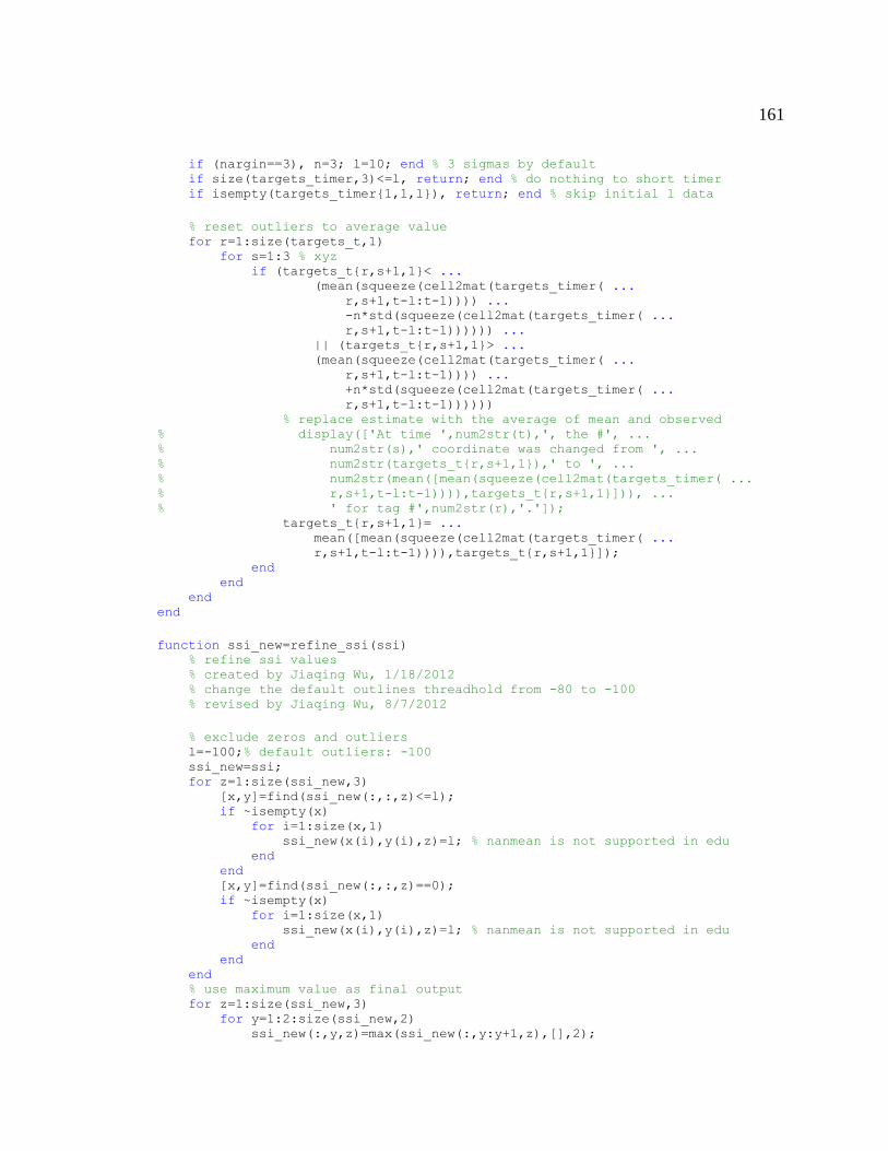
161

if (nargin==3), n=3; l=10; end % 3 sigmas by default if size(targets_timer,3)<=l, return; end % do nothing to short timer if isempty(targets_timer{1,1,l}), return; end % skip initial l data

% reset outliers to average value for r=1:size(targets_t,1) for s=1:3 % xyz if (targets_t{r,s+1,1}< ... (mean(squeeze(cell2mat(targets_timer( ... r,s+1,t-l:t-1)))) ... -n*std(squeeze(cell2mat(targets_timer( ... r,s+1,t-l:t-1)))))) ... || (targets_t{r,s+1,1}> ... (mean(squeeze(cell2mat(targets_timer( ... r,s+1,t-l:t-1)))) ... +n*std(squeeze(cell2mat(targets_timer( ... r,s+1,t-l:t-1)))))) % replace estimate with the average of mean and observed % display(['At time ',num2str(t),', the #', ... % num2str(s),' coordinate was changed from ', ... % num2str(targets_t{r,s+1,1}),' to ', ... % num2str(mean([mean(squeeze(cell2mat(targets_timer( ... % r,s+1,t-l:t-1)))),targets_t{r,s+1,1}])), ... % ' for tag #',num2str(r),'.']); targets_t{r,s+1,1}= ... mean([mean(squeeze(cell2mat(targets_timer( ... r,s+1,t-l:t-1)))),targets_t{r,s+1,1}]); end end end end

function ssi_new=refine_ssi(ssi) % refine ssi values % created by Jiaqing Wu, 1/18/2012 % change the default outlines threadhold from -80 to -100 % revised by Jiaqing Wu, 8/7/2012

% exclude zeros and outliers l=-100;% default outliers: -100 ssi_new=ssi; for z=1:size(ssi_new,3) [x,y]=find(ssi_new(:,:,z)<=l); if ~isempty(x) for i=1:size(x,1) ssi_new(x(i),y(i),z)=l; % nanmean is not supported in edu end end [x,y]=find(ssi_new(:,:,z)==0); if ~isempty(x) for i=1:size(x,1) ssi_new(x(i),y(i),z)=l; % nanmean is not supported in edu end end end % use maximum value as final output for z=1:size(ssi_new,3) for y=1:2:size(ssi_new,2) ssi_new(:,y,z)=max(ssi_new(:,y:y+1,z),[],2);

162

ssi_new(:,y+1,z)=ssi_new(:,y,z); end end % average over time if ssi with timer ssi_new=round(mean(ssi_new,3)); % delete duplicated columns for y=size(ssi_new,2):-2:2 ssi_new(:,y)=[]; end end

function [targets,ref_tags_knn]=knn(targets_name,readers,ref_tags,k) % use kNN algorithm to estimate the location of target tags % created by Jiaqing Wu, 9/30/2011 % unsolved bug: inappropriate for multiple targets with different grids % commented by Jiaqing Wu, 2/23/2012 % add refine_ssi step to use max only % revised by Jiaqing Wu, 3/20/2012 % add ref_tags_knn output % updated by Jiaqing Wu, 3/27/2012

% check inputs and outputs error(nargchk(3,4,nargin)); error(nargoutchk(0,2,nargout)); % default k value if (nargin==3), k=4; end % initialize target tags coordinates targets_xyz=num2cell(zeros(size(targets_name,1),3)); % read ssi targets_ssi=read_ssi(targets_name,readers); % readers(:,1) ref_tags_ssi=read_ssi(ref_tags(:,1),readers); % readers(:,1) % refine ssi targets_ssi=refine_ssi(targets_ssi); ref_tags_ssi=refine_ssi(ref_tags_ssi); % find kNN based on smallest k Euclidean distance (2-norm distance) k_ed=zeros(size(ref_tags,1),size(targets_name,1)); k_ssi=k_ed; k_idx=k_ed; for j=1:size(targets_name,1) for i=1:size(ref_tags,1) k_ed(i,j)=norm(targets_ssi(j,:)-ref_tags_ssi(i,:)); end [k_ssi(:,j),k_idx(:,j)]=sort(k_ed(:,j),1); end k_ssi=k_ssi(1:k,:); k_idx=k_idx(1:k,:); ref_tags_knn=ref_tags(k_idx,:); % calculate weighted centroid of the kNN ref_tags for j=1:size(targets_name,1) % convert Euclidean distances to weights k_ssi(:,j)=sum(k_ssi(:,j))./k_ssi(:,j); if sum(isinf(k_ssi(:,j)))==0 targets_xyz(j,:)=num2cell(round(k_ssi(:,j)'* ... cell2mat(ref_tags(k_idx(:,j),2:4))/sum(k_ssi(:,j)))); else % the target ssi is exactly same with one reference tag for i=1:k if isinf(k_ssi(i,j)) targets_xyz(j,:)=ref_tags(k_idx(i,j),2:4); % display(ref_tags{k_idx(i,j),1}); % verification

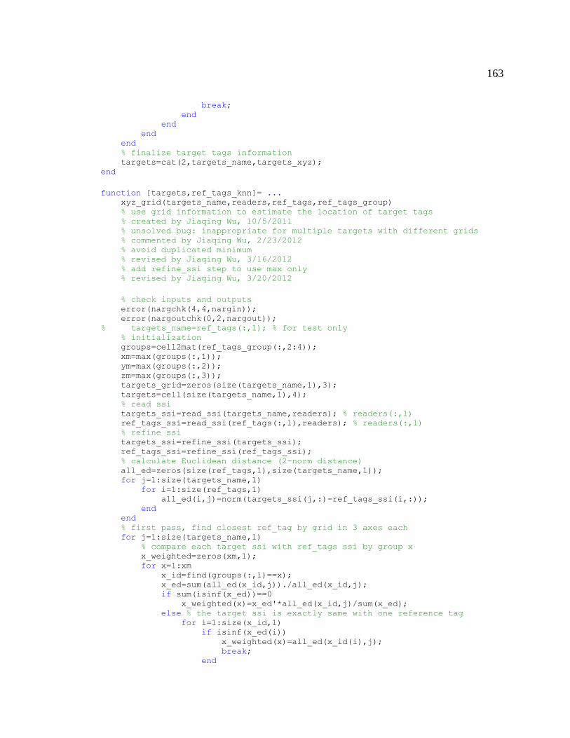
163

break; end end end end % finalize target tags information targets=cat(2,targets_name,targets_xyz); end

function [targets,ref_tags_knn]= ... xyz_grid(targets_name,readers,ref_tags,ref_tags_group) % use grid information to estimate the location of target tags % created by Jiaqing Wu, 10/5/2011 % unsolved bug: inappropriate for multiple targets with different grids % commented by Jiaqing Wu, 2/23/2012 % avoid duplicated minimum % revised by Jiaqing Wu, 3/16/2012 % add refine_ssi step to use max only % revised by Jiaqing Wu, 3/20/2012

% check inputs and outputs error(nargchk(4,4,nargin)); error(nargoutchk(0,2,nargout)); % targets_name=ref_tags(:,1); % for test only % initialization groups=cell2mat(ref_tags_group(:,2:4)); xm=max(groups(:,1)); ym=max(groups(:,2)); zm=max(groups(:,3)); targets_grid=zeros(size(targets_name,1),3); targets=cell(size(targets_name,1),4); % read ssi targets_ssi=read_ssi(targets_name,readers); % readers(:,1) ref_tags_ssi=read_ssi(ref_tags(:,1),readers); % readers(:,1) % refine ssi targets_ssi=refine_ssi(targets_ssi); ref_tags_ssi=refine_ssi(ref_tags_ssi); % calculate Euclidean distance (2-norm distance) all_ed=zeros(size(ref_tags,1),size(targets_name,1)); for j=1:size(targets_name,1) for i=1:size(ref_tags,1) all_ed(i,j)=norm(targets_ssi(j,:)-ref_tags_ssi(i,:)); end end % first pass, find closest ref_tag by grid in 3 axes each for j=1:size(targets_name,1) % compare each target ssi with ref_tags ssi by group x x_weighted=zeros(xm,1); for x=1:xm x_id=find(groups(:,1)==x); x_ed=sum(all_ed(x_id,j))./all_ed(x_id,j); if sum(isinf(x_ed))==0 x_weighted(x)=x_ed'*all_ed(x_id,j)/sum(x_ed); else % the target ssi is exactly same with one reference tag for i=1:size(x_id,1) if isinf(x_ed(i)) x_weighted(x)=all_ed(x_id(i),j); break; end

164

end end end x_grid=find(x_weighted==min(x_weighted)); % compare each target ssi with ref_tags ssi by group y y_weighted=zeros(ym,1); for y=1:ym y_id=find(groups(:,2)==y); y_ed=sum(all_ed(y_id,j))./all_ed(y_id,j); if sum(isinf(y_ed))==0 y_weighted(y)=y_ed'*all_ed(y_id,j)/sum(y_ed); else % the target ssi is exactly same with one reference tag for i=1:size(y_id,1) if isinf(y_ed(i)) y_weighted(y)=all_ed(y_id(i),j); break; end end end end y_grid=find(y_weighted==min(y_weighted)); % compare each target ssi with ref_tags ssi by group z z_weighted=zeros(zm,1); for z=1:zm z_id=find(groups(:,3)==z); z_ed=sum(all_ed(z_id,j))./all_ed(z_id,j); if sum(isinf(z_ed))==0 z_weighted(z)=z_ed'*all_ed(z_id,j)/sum(z_ed); else % the target ssi is exactly same with one reference tag for i=1:size(z_id,1) if isinf(z_ed(i)) z_weighted(z)=all_ed(z_id(i),j); break; end end end end z_grid=find(z_weighted==min(z_weighted)); % avoid duplicated minimum, use first one only targets_grid(j,:)=[x_grid(1),y_grid(1),z_grid(1)]; end % second pass, use ref_tags nearby as k nearest neighbors for j=1:size(targets_name,1) % extend to neighbors within 2 blocks away (not work very well) % knn_grid=zeros(15,3); % knn_grid(1:5,:)=[(targets_grid(j,1)-2:targets_grid(j,1)+2)', ... % repmat(targets_grid(j,2:3),5,1)]; % knn_grid(6:10,:)=[repmat(targets_grid(j,1),5,1), ... % (targets_grid(j,2)-2:targets_grid(j,2)+2)', ... % repmat(targets_grid(j,3),5,1)]; % knn_grid(11:15,:)=[repmat(targets_grid(j,1:2),5,1), ... % (targets_grid(j,3)-2:targets_grid(j,3)+2)']; % extend to neighbors within a 3^3 cube knn_grid=zeros(27,3); knn_grid(:,1)=[repmat(targets_grid(j,1)-1,9,1); ... repmat(targets_grid(j,1),9,1); ... repmat(targets_grid(j,1)+1,9,1)]; knn_grid(:,2)=repmat([repmat(targets_grid(j,2)-1,3,1); ... repmat(targets_grid(j,2),3,1); ... repmat(targets_grid(j,2)+1,3,1)],3,1);

165

knn_grid(:,3)=repmat([targets_grid(j,3)-1; ... targets_grid(j,3);targets_grid(j,3)+1],9,1); % match possible grid to existing ref_tags [tf,loc]=ismember(knn_grid,cell2mat(ref_tags_group(:,2:4)),'rows'); knn_id=unique(loc(any(loc,2)),'rows'); ref_tags_knn=ref_tags(knn_id,:); % finalize target tags information targets(j,:)= ... knn(targets_name(j),readers,ref_tags_knn,size(knn_id,1)); end end

function [targets,targets_range]= ... ssi_range(targets_name,readers,ref_tags,op) % use ssi information to estimate the location of target tags % created by Jiaqing Wu, 1/18/2012 % add targets_range output for further estimation purpose % updated by Jiaqing Wu, 2/21/2012 % unsolved bug: inappropriate for multiple targets with different grids % commented by Jiaqing Wu, 2/23/2012 % add refine_ssi step to use max only % revised by Jiaqing Wu, 3/20/2012 % exclude -40db as origin point % revised by Jiaqing Wu, 3/27/2012 % include 2 readers and 4 readers scenarios % updated by Jiaqing Wu, 7/23/2012 % limit y values to real range % updated by Jiaqing Wu, 8/18/2012

% check inputs and outputs error(nargchk(3,4,nargin)); error(nargoutchk(0,2,nargout)); % initialization if nargin==3, op=0; end % include origin point by default xm=434; ym=874; zm=282; % maximum values of x, y, and z y1=305; y2=671; % real range of y readers_xyz=cell2mat(readers(:,2:4)); ref_tags_xyz=cell2mat(ref_tags(:,2:4)); targets=cell(size(targets_name,1),4); targets_xyz=zeros(size(targets_name,1),3); % read ssi targets_ssi=read_ssi(targets_name,readers); % readers(:,1) ref_tags_ssi=read_ssi(ref_tags(:,1),readers); % readers(:,1) % refine ssi targets_ssi=refine_ssi(targets_ssi); ref_tags_ssi=refine_ssi(ref_tags_ssi); % check ssi if any(any(isnan(targets_ssi))) || any(any(isnan(ref_tags_ssi))) return; end % calculate distance dis=zeros(size(ref_tags_xyz,1),size(readers_xyz,1)); for i=1:size(ref_tags_xyz,1) for j=1:size(readers_xyz,1) dis(i,j)=sqrt(sum((ref_tags_xyz(i,:)-readers_xyz(j,:)).^2)); end end ref_tags_dis=round(dis); % regression analysis

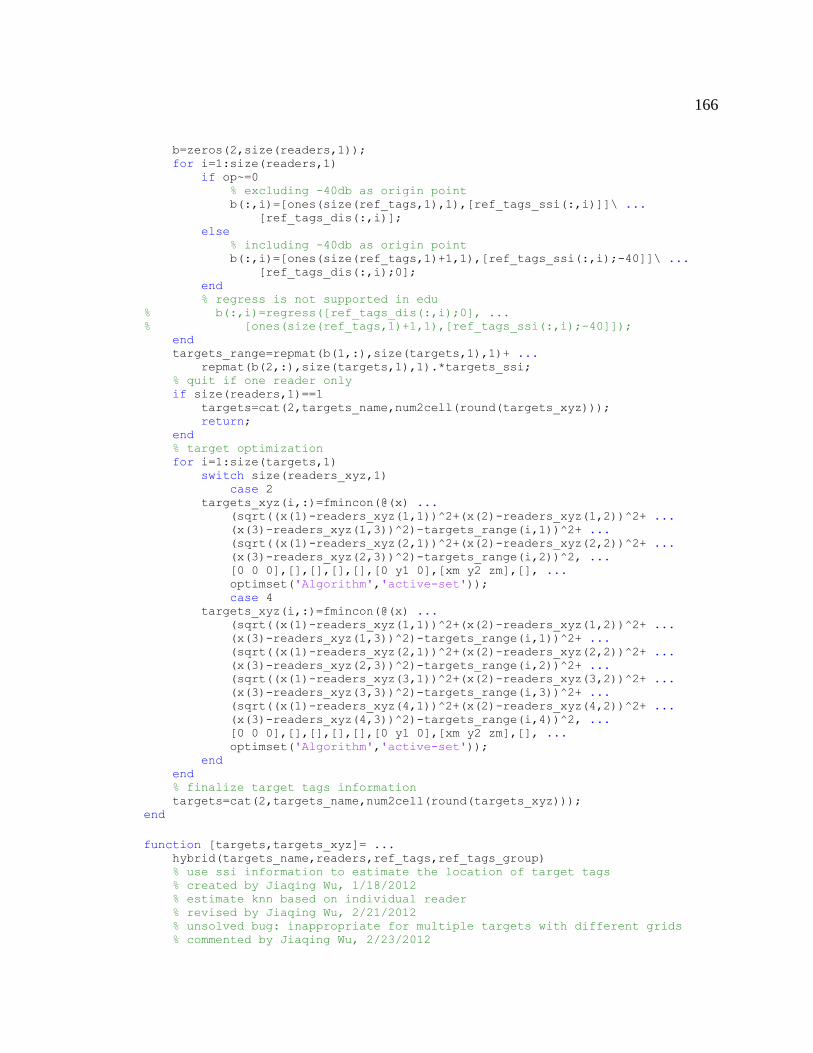
166

b=zeros(2,size(readers,1)); for i=1:size(readers,1) if op~=0 % excluding -40db as origin point b(:,i)=[ones(size(ref_tags,1),1),[ref_tags_ssi(:,i)]]\ ... [ref_tags_dis(:,i)]; else % including -40db as origin point b(:,i)=[ones(size(ref_tags,1)+1,1),[ref_tags_ssi(:,i);-40]]\ ... [ref_tags_dis(:,i);0]; end % regress is not supported in edu % b(:,i)=regress([ref_tags_dis(:,i);0], ... % [ones(size(ref_tags,1)+1,1),[ref_tags_ssi(:,i);-40]]); end targets_range=repmat(b(1,:),size(targets,1),1)+ ... repmat(b(2,:),size(targets,1),1).*targets_ssi; % quit if one reader only if size(readers,1)==1 targets=cat(2,targets_name,num2cell(round(targets_xyz))); return; end % target optimization for i=1:size(targets,1) switch size(readers_xyz,1) case 2 targets_xyz(i,:)=fmincon(@(x) ... (sqrt((x(1)-readers_xyz(1,1))^2+(x(2)-readers_xyz(1,2))^2+ ... (x(3)-readers_xyz(1,3))^2)-targets_range(i,1))^2+ ... (sqrt((x(1)-readers_xyz(2,1))^2+(x(2)-readers_xyz(2,2))^2+ ... (x(3)-readers_xyz(2,3))^2)-targets_range(i,2))^2, ... [0 0 0],[],[],[],[],[0 y1 0],[xm y2 zm],[], ... optimset('Algorithm','active-set')); case 4 targets_xyz(i,:)=fmincon(@(x) ... (sqrt((x(1)-readers_xyz(1,1))^2+(x(2)-readers_xyz(1,2))^2+ ... (x(3)-readers_xyz(1,3))^2)-targets_range(i,1))^2+ ... (sqrt((x(1)-readers_xyz(2,1))^2+(x(2)-readers_xyz(2,2))^2+ ... (x(3)-readers_xyz(2,3))^2)-targets_range(i,2))^2+ ... (sqrt((x(1)-readers_xyz(3,1))^2+(x(2)-readers_xyz(3,2))^2+ ... (x(3)-readers_xyz(3,3))^2)-targets_range(i,3))^2+ ... (sqrt((x(1)-readers_xyz(4,1))^2+(x(2)-readers_xyz(4,2))^2+ ... (x(3)-readers_xyz(4,3))^2)-targets_range(i,4))^2, ... [0 0 0],[],[],[],[],[0 y1 0],[xm y2 zm],[], ... optimset('Algorithm','active-set')); end end % finalize target tags information targets=cat(2,targets_name,num2cell(round(targets_xyz))); end

function [targets,targets_xyz]= ... hybrid(targets_name,readers,ref_tags,ref_tags_group) % use ssi information to estimate the location of target tags % created by Jiaqing Wu, 1/18/2012 % estimate knn based on individual reader % revised by Jiaqing Wu, 2/21/2012 % unsolved bug: inappropriate for multiple targets with different grids % commented by Jiaqing Wu, 2/23/2012

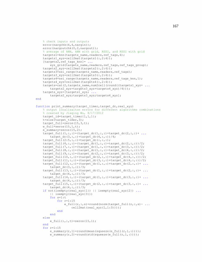
167

% check inputs and outputs error(nargchk(4,4,nargin)); error(nargoutchk(0,2,nargout)); % average of kNN, kNN with grid, RSSI, and RSSI with grid targets1=knn(targets_name,readers,ref_tags,6); targets1_xyz=cell2mat(targets1(:,2:4)); [targets2,ref_tags_knn]= ... xyz_grid(targets_name,readers,ref_tags,ref_tags_group); targets2_xyz=cell2mat(targets2(:,2:4)); targets3=ssi_range(targets_name,readers,ref_tags); targets3_xyz=cell2mat(targets3(:,2:4)); targets4=ssi_range(targets_name,readers,ref_tags_knn,1); targets4_xyz=cell2mat(targets4(:,2:4)); targets=cat(2,targets_name,num2cell(round((targets1_xyz+ ... targets2_xyz+targets3_xyz+targets4_xyz)/4))); targets_xyz=[targets1_xyz; ... targets2_xyz;targets3_xyz;targets4_xyz]; end

function print_summary(target_timer,target_dc,real_xyz) % output localizaiton errors for different algorithms combinations % created by Jiaqing Wu, 8/17/2012 target_id=target_timer{1,1,1}; t=size(target_timer,3); target_full=zeros(15,3,t); e_full=zeros(15,1,t); e_summary=zeros(15,2); target_full(1,:,:)=(target_dc(1,:,:)+target_dc(2,:,:)+ ... target_dc(3,:,:)+target_dc(4,:,:))/4; target_full(2:5,:,:)=target_dc(:,:,:); target_full(6,:,:)=(target_dc(1,:,:)+target_dc(2,:,:))/2; target_full(7,:,:)=(target_dc(1,:,:)+target_dc(3,:,:))/2; target_full(8,:,:)=(target_dc(1,:,:)+target_dc(4,:,:))/2; target_full(9,:,:)=(target_dc(2,:,:)+target_dc(3,:,:))/2; target_full(10,:,:)=(target_dc(2,:,:)+target_dc(4,:,:))/2; target_full(11,:,:)=(target_dc(3,:,:)+target_dc(4,:,:))/2; target_full(12,:,:)=(target_dc(1,:,:)+target_dc(2,:,:)+ ... target_dc(3,:,:))/3; target_full(13,:,:)=(target_dc(1,:,:)+target_dc(2,:,:)+ ... target_dc(4,:,:))/3; target_full(14,:,:)=(target_dc(1,:,:)+target_dc(3,:,:)+ ... target_dc(4,:,:))/3; target_full(15,:,:)=(target_dc(2,:,:)+target_dc(3,:,:)+ ... target_dc(4,:,:))/3; if not(isempty(real_xyz{1}) || isempty(real_xyz{2}) ... || isempty(real_xyz{3})) for s=1:t for r=1:15 e_full(r,:,s)=round(norm(target_full(r,:,s)- ... cell2mat(real_xyz(1,1:3)))); end end else e_full(:,:,t)=zeros(15,1); end for r=1:15 e_summary(r,1)=round(mean(squeeze(e_full(r,1,:)))); e_summary(r,2)=round(std(squeeze(e_full(r,1,:))));

168

end e_summary_all=cat(2,repmat(' ',15,5), ... ['ABCD';'A___';'_B__';'__C_';'___D'; ... 'AB__';'A_C_';'A__D';'_BC_';'_B_D';'__CD'; ... 'ABC_';'AB_D';'A_CD';'_BCD'],repmat(' ',15,15), ... num2str(e_summary)); save_option=questdlg(e_summary_all,target_id(end-5:end), ... 'save','exit','save'); switch save_option case 'save' % disp('save'); m_file=fopen([pwd,'\mean.txt'],'at'); s_file=fopen([pwd,'\std.txt'],'at'); fprintf(m_file,'%s\n',[datestr(now,'yyyy-mm-dd HH:MM:SS'), ... ' <',target_id,'> ',num2str(e_summary(:,1)')]); fprintf(s_file,'%s\n',[datestr(now,'yyyy-mm-dd HH:MM:SS'), ... ' <',target_id,'> ',num2str(e_summary(:,2)')]); fclose(m_file); fclose(s_file); case 'exit' % disp('exit'); return; otherwise % disp('exit'); return; end end

169

Appendix C

Data Sheets

C.1 Reader Test Data Sheet

Table C-1: Reader test data sheet

StdOrder RunOrder Reader Height Depth Antenna Tag uMax

42 1 3 2 2 2 2 -51

37 2 3 1 1 1 3 -50

29 3 3 3 1 3 1 -55

31 4 3 1 3 3 1 -56

36 5 3 1 1 3 3 -53

40 6 3 1 1 1 1 -52

41 7 3 2 2 2 2 -48

30 8 3 3 3 1 3 -53

35 9 3 1 3 3 3 -56

33 10 3 3 3 1 3 -53

38 11 3 3 1 1 1 -62

39 12 3 1 3 1 1 -55

34 13 3 3 3 3 1 -55

32 14 3 3 1 3 3 -57

45 15 4 1 3 3 1 -57

48 16 4 3 3 3 1 -58

50 17 4 1 1 3 3 -56

53 18 4 1 3 1 1 -61

54 19 4 1 1 1 1 -54

46 20 4 3 1 3 3 -57

52 21 4 3 1 1 1 -60

51 22 4 1 1 1 3 -52

55 23 4 2 2 2 2 -51

44 24 4 3 3 1 3 -54

49 25 4 1 3 3 3 -59

47 26 4 3 3 1 3 -53

56 27 4 2 2 2 2 -53

43 28 4 3 1 3 1 -53

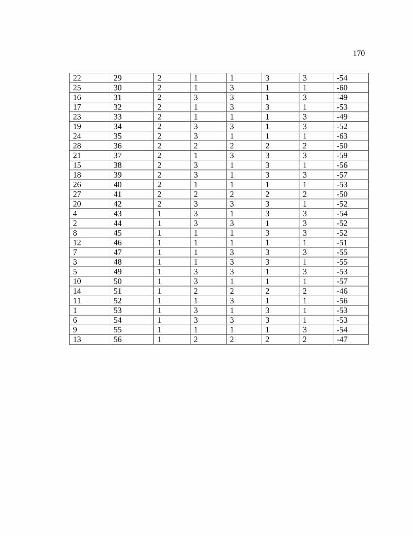
170

22 29 2 1 1 3 3 -54

25 30 2 1 3 1 1 -60

16 31 2 3 3 1 3 -49

17 32 2 1 3 3 1 -53

23 33 2 1 1 1 3 -49

19 34 2 3 3 1 3 -52

24 35 2 3 1 1 1 -63

28 36 2 2 2 2 2 -50

21 37 2 1 3 3 3 -59

15 38 2 3 1 3 1 -56

18 39 2 3 1 3 3 -57

26 40 2 1 1 1 1 -53

27 41 2 2 2 2 2 -50

20 42 2 3 3 3 1 -52

4 43 1 3 1 3 3 -54

2 44 1 3 3 1 3 -52

8 45 1 1 1 3 3 -52

12 46 1 1 1 1 1 -51

7 47 1 1 3 3 3 -55

3 48 1 1 3 3 1 -55

5 49 1 3 3 1 3 -53

10 50 1 3 1 1 1 -57

14 51 1 2 2 2 2 -46

11 52 1 1 3 1 1 -56

1 53 1 3 1 3 1 -53

6 54 1 3 3 3 1 -53

9 55 1 1 1 1 3 -54

13 56 1 2 2 2 2 -47

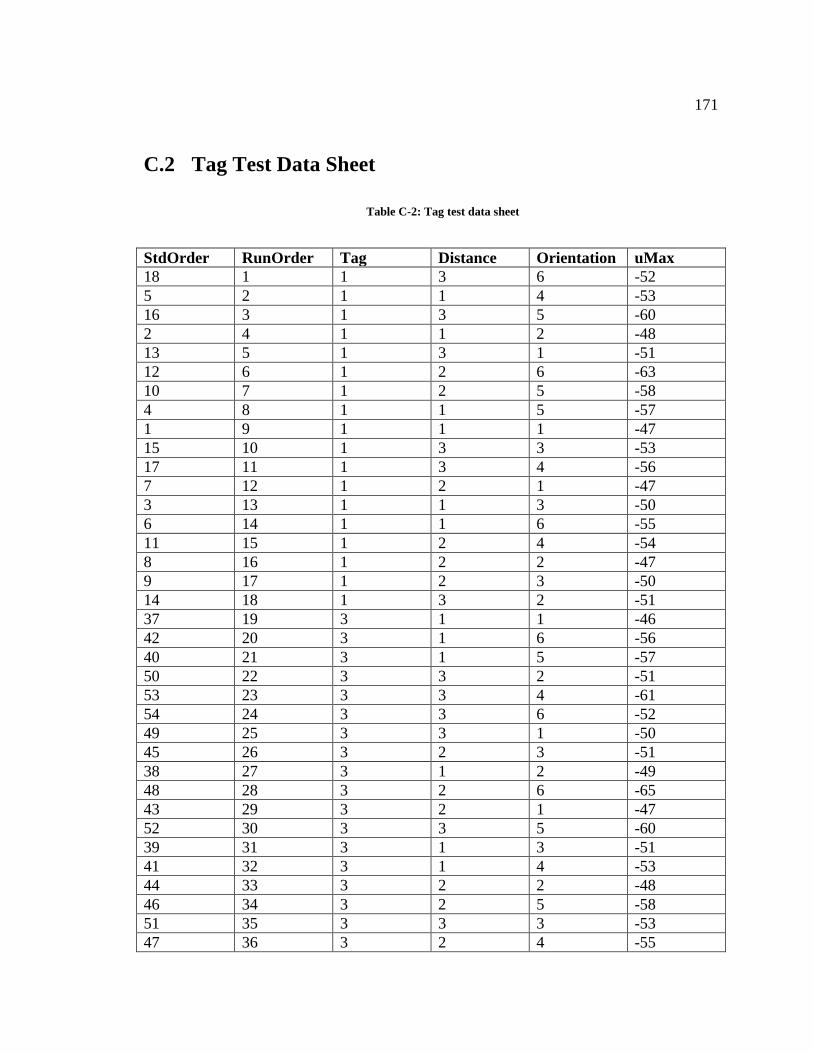
171

C.2 Tag Test Data Sheet

Table C-2: Tag test data sheet

StdOrder RunOrder Tag Distance Orientation uMax

18 1 1 3 6 -52

5 2 1 1 4 -53

16 3 1 3 5 -60

2 4 1 1 2 -48

13 5 1 3 1 -51

12 6 1 2 6 -63

10 7 1 2 5 -58

4 8 1 1 5 -57

1 9 1 1 1 -47

15 10 1 3 3 -53

17 11 1 3 4 -56

7 12 1 2 1 -47

3 13 1 1 3 -50

6 14 1 1 6 -55

11 15 1 2 4 -54

8 16 1 2 2 -47

9 17 1 2 3 -50

14 18 1 3 2 -51

37 19 3 1 1 -46

42 20 3 1 6 -56

40 21 3 1 5 -57

50 22 3 3 2 -51

53 23 3 3 4 -61

54 24 3 3 6 -52

49 25 3 3 1 -50

45 26 3 2 3 -51

38 27 3 1 2 -49

48 28 3 2 6 -65

43 29 3 2 1 -47

52 30 3 3 5 -60

39 31 3 1 3 -51

41 32 3 1 4 -53

44 33 3 2 2 -48

46 34 3 2 5 -58

51 35 3 3 3 -53

47 36 3 2 4 -55

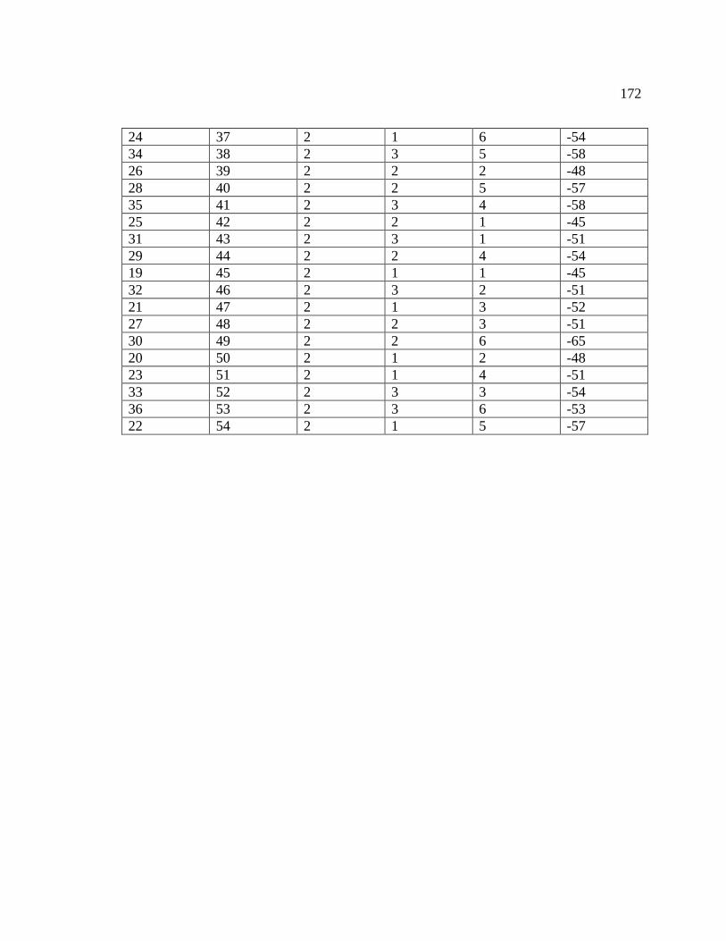
172

24 37 2 1 6 -54

34 38 2 3 5 -58

26 39 2 2 2 -48

28 40 2 2 5 -57

35 41 2 3 4 -58

25 42 2 2 1 -45

31 43 2 3 1 -51

29 44 2 2 4 -54

19 45 2 1 1 -45

32 46 2 3 2 -51

21 47 2 1 3 -52

27 48 2 2 3 -51

30 49 2 2 6 -65

20 50 2 1 2 -48

23 51 2 1 4 -51

33 52 2 3 3 -54

36 53 2 3 6 -53

22 54 2 1 5 -57

173

C.3 Ranging Test Data Sheet

Table C-3: Ranging test data sheet

StdOrder RunOrder Tag Distance uMax

11 1 2 0.5 -49

13 2 2 1.5 -62

18 3 2 4 -61

31 4 4 0.5 -51

14 5 2 2 -54

37 6 4 3.5 -59

4 7 1 2 -54

35 8 4 2.5 -54

33 9 4 1.5 -60

32 10 4 1 -55

5 11 1 2.5 -54

28 12 3 4 -61

9 13 1 4.5 -66.5

24 14 3 2 -54

44 15 5 2 -54

21 16 3 0.5 -51

22 17 3 1 -55

42 18 5 1 -58

38 19 4 4 -63

36 20 4 3 -60

45 21 5 2.5 -55

26 22 3 3 -61

20 23 2 5 -62.1

46 24 5 3 -61

3 25 1 1.5 -60

8 26 1 4 -61

47 27 5 3.5 -60

2 28 1 1 -55

41 29 5 0.5 -52

34 30 4 2 -52

29 31 3 4.5 -64

25 32 3 2.5 -56

30 33 3 5 -59.9

39 34 4 4.5 -66

17 35 2 3.5 -59

48 36 5 4 -61

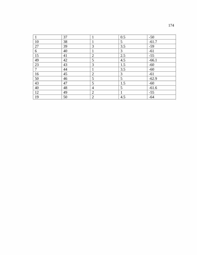
174

1 37 1 0.5 -50

10 38 1 5 -61.7

27 39 3 3.5 -59

6 40 1 3 -61

15 41 2 2.5 -55

49 42 5 4.5 -66.1

23 43 3 1.5 -60

7 44 1 3.5 -60

16 45 2 3 -61

50 46 5 5 -62.9

43 47 5 1.5 -60

40 48 4 5 -61.6

12 49 2 1 -55

19 50 2 4.5 -64

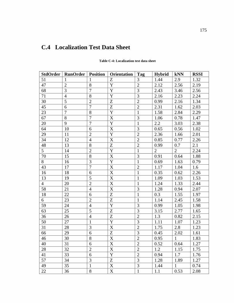
175

C.4 Localization Test Data Sheet

Table C-4: Localization test data sheet

StdOrder RunOrder Position Orientation Tag Hybrid kNN RSSI

51 1 1 Z 3 1.44 2.9 1.32

47 2 8 Y 2 2.12 2.56 2.19

68 3 7 Y 3 2.43 3.46 2.56

71 4 8 Y 3 2.16 2.23 2.24

30 5 2 Z 2 0.99 2.16 1.34

45 6 7 Z 2 2.31 1.62 2.03

23 7 8 Y 1 1.58 2.84 2.29

67 8 7 X 3 1.06 0.78 1.47

20 9 7 Y 1 2.2 3.03 2.38

64 10 6 X 3 0.65 0.56 1.02

29 11 2 Y 2 2.36 1.66 2.01

34 12 4 X 2 0.85 0.77 2.26

48 13 8 Z 2 0.99 0.7 2.1

5 14 2 Y 1 2 2 2.24

70 15 8 X 3 0.91 0.64 1.88

8 16 3 Y 1 0.69 1.63 0.79

43 17 7 X 2 1.17 1.04 1.6

16 18 6 X 1 0.35 0.62 2.26

13 19 5 X 1 1.09 1.03 1.53

4 20 2 X 1 1.24 1.33 2.44

58 21 4 X 3 1.28 0.94 2.07

18 22 6 Z 1 0.3 1.55 1.97

6 23 2 Z 1 1.14 2.45 1.58

59 24 4 Y 3 0.99 1.05 1.98

63 25 5 Z 3 3.15 2.77 1.65

36 26 4 Z 2 1.3 0.82 2.15

50 27 1 Y 3 1.11 1.07 1.23

31 28 3 X 2 1.75 2.8 1.23

66 29 6 Z 3 0.45 2.02 1.61

46 30 8 X 2 0.95 1 1.83

40 31 6 X 2 0.52 0.64 1.27

28 32 2 X 2 1.2 1.15 1.75

41 33 6 Y 2 0.94 1.7 1.76

57 34 3 Z 3 1.28 1.89 1.27

49 35 1 X 3 1.44 1 0.74

22 36 8 X 1 1.1 0.53 2.08

176

42 37 6 Z 2 0.75 1.87 1.33

62 38 5 Y 3 1.04 3.09 1.65

32 39 3 Y 2 0.62 1.55 1.18

56 40 3 Y 3 0.72 1.66 0.57

65 41 6 Y 3 0.72 1.89 1.72

33 42 3 Z 2 1.17 1.83 1.28

25 43 1 X 2 1.07 1.1 0.76

3 44 1 Z 1 2.12 2.75 1.4

60 45 4 Z 3 1.37 0.84 1.52

61 46 5 X 3 1.18 1.28 1.39

37 47 5 X 2 1.28 0.84 1.55

19 48 7 X 1 1.72 0.52 1.49

21 49 7 Z 1 2.03 1.54 2.08

53 50 2 Y 3 2.17 2.17 2.06

72 51 8 Z 3 2.47 0.66 2.07

54 52 2 Z 3 1.81 2.6 1.59

11 53 4 Y 1 1.21 1.06 2.46

17 54 6 Y 1 1.23 2.15 1.84

9 55 3 Z 1 1.08 1.82 1.29

69 56 7 Z 3 2.21 1.29 1.95

24 57 8 Z 1 1.63 0.77 2.14

2 58 1 Y 1 0.73 1.62 1.69

27 59 1 Z 2 2.35 3.14 1.16

10 60 4 X 1 0.96 1.07 2.16

52 61 2 X 3 0.44 2.62 1.78

12 62 4 Z 1 1.15 0.96 1.9

15 63 5 Z 1 2.84 1.97 1.86

14 64 5 Y 1 1.29 3.31 1.52

35 65 4 Y 2 0.96 1 2.06

38 66 5 Y 2 1 3.33 1.55

1 67 1 X 1 1.04 0.93 0.85

39 68 5 Z 2 2.87 2.32 1.77

7 69 3 X 1 1.6 1.56 1.14

26 70 1 Y 2 0.82 0.92 1.45

44 71 7 Y 2 2.25 3.46 2.32

55 72 3 X 3 1.13 1.63 0.97

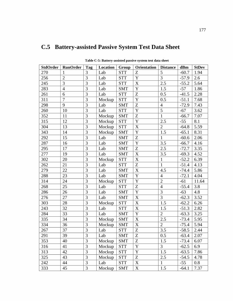
177

C.5 Battery-assisted Passive System Test Data Sheet

Table C-5: Battery-assisted passive system test data sheet

StdOrder RunOrder Tag Location Group Orientation Distance dBm StDev

270 1 3 Lab STT Z 5 -60.7 1.94

256 2 3 Lab STT Y 3 -57.9 2.6

245 3 3 Lab STT X 2.5 -55.2 5.64

283 4 3 Lab SMT Y 1.5 -57 1.86

261 6 3 Lab STT Z 0.5 -41.5 2.28

311 7 3 Mockup STT Y 0.5 -51.1 7.68

298 9 3 Lab SMT Z 4 -72.9 7.43

260 10 3 Lab STT Y 5 -67 3.62

352 11 3 Mockup SMT Z 1 -66.7 7.07

315 12 3 Mockup STT Y 2.5 -55 8.1

304 13 3 Mockup STT X 2 -64.8 5.59

343 14 3 Mockup SMT Y 1.5 -65.1 8.31

292 15 3 Lab SMT Z 1 -60.6 2.06

287 16 3 Lab SMT Y 3.5 -66.7 4.16

295 17 3 Lab SMT Z 2.5 -72.7 3.35

277 19 3 Lab SMT X 3.5 -69.3 4.52

302 20 3 Mockup STT X 1 -52.2 6.39

262 21 3 Lab STT Z 1 -51.4 4.13

279 22 3 Lab SMT X 4.5 -74.4 5.86

288 23 3 Lab SMT Y 4 -72.1 4.04

314 24 3 Mockup STT Y 2 -61 11.64

268 25 3 Lab STT Z 4 -55.4 3.8

286 26 3 Lab SMT Y 3 -63 4.8

276 27 3 Lab SMT X 3 -62.3 3.52

303 28 3 Mockup STT X 1.5 -62.2 6.26

243 32 3 Lab STT X 1.5 -51.3 2.82

284 33 3 Lab SMT Y 2 -63.3 3.25

335 34 3 Mockup SMT X 2.5 -73.4 5.95

334 36 3 Mockup SMT X 2 -75.4 5.94

267 37 3 Lab STT Z 3.5 -58.5 2.44

291 39 3 Lab SMT Z 0.5 -63.4 2.07

353 40 3 Mockup SMT Z 1.5 -73.4 6.07

316 41 3 Mockup STT Y 3 -62.5 6.9

313 42 3 Mockup STT Y 1.5 -63.5 7.86

325 43 3 Mockup STT Z 2.5 -54.5 4.78

242 44 3 Lab STT X 1 -55 0.8

333 45 3 Mockup SMT X 1.5 -64.1 7.37

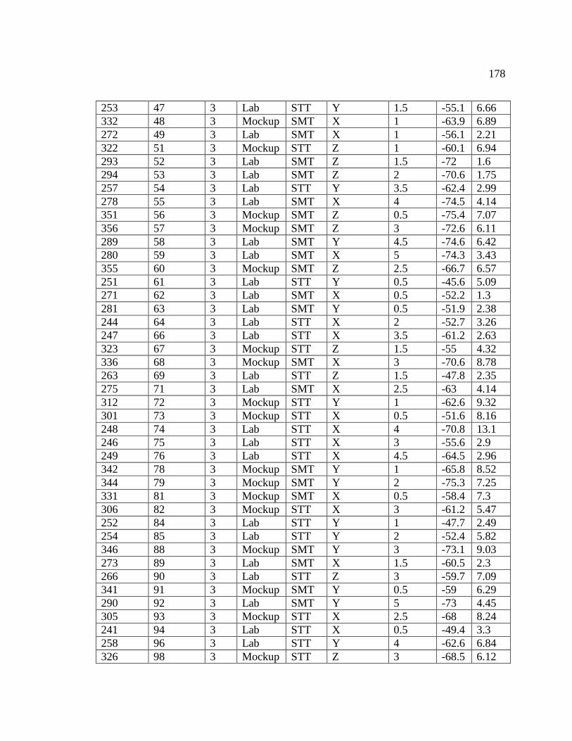
178

253 47 3 Lab STT Y 1.5 -55.1 6.66

332 48 3 Mockup SMT X 1 -63.9 6.89

272 49 3 Lab SMT X 1 -56.1 2.21

322 51 3 Mockup STT Z 1 -60.1 6.94

293 52 3 Lab SMT Z 1.5 -72 1.6

294 53 3 Lab SMT Z 2 -70.6 1.75

257 54 3 Lab STT Y 3.5 -62.4 2.99

278 55 3 Lab SMT X 4 -74.5 4.14

351 56 3 Mockup SMT Z 0.5 -75.4 7.07

356 57 3 Mockup SMT Z 3 -72.6 6.11

289 58 3 Lab SMT Y 4.5 -74.6 6.42

280 59 3 Lab SMT X 5 -74.3 3.43

355 60 3 Mockup SMT Z 2.5 -66.7 6.57

251 61 3 Lab STT Y 0.5 -45.6 5.09

271 62 3 Lab SMT X 0.5 -52.2 1.3

281 63 3 Lab SMT Y 0.5 -51.9 2.38

244 64 3 Lab STT X 2 -52.7 3.26

247 66 3 Lab STT X 3.5 -61.2 2.63

323 67 3 Mockup STT Z 1.5 -55 4.32

336 68 3 Mockup SMT X 3 -70.6 8.78

263 69 3 Lab STT Z 1.5 -47.8 2.35

275 71 3 Lab SMT X 2.5 -63 4.14

312 72 3 Mockup STT Y 1 -62.6 9.32

301 73 3 Mockup STT X 0.5 -51.6 8.16

248 74 3 Lab STT X 4 -70.8 13.1

246 75 3 Lab STT X 3 -55.6 2.9

249 76 3 Lab STT X 4.5 -64.5 2.96

342 78 3 Mockup SMT Y 1 -65.8 8.52

344 79 3 Mockup SMT Y 2 -75.3 7.25

331 81 3 Mockup SMT X 0.5 -58.4 7.3

306 82 3 Mockup STT X 3 -61.2 5.47

252 84 3 Lab STT Y 1 -47.7 2.49

254 85 3 Lab STT Y 2 -52.4 5.82

346 88 3 Mockup SMT Y 3 -73.1 9.03

273 89 3 Lab SMT X 1.5 -60.5 2.3

266 90 3 Lab STT Z 3 -59.7 7.09

341 91 3 Mockup SMT Y 0.5 -59 6.29

290 92 3 Lab SMT Y 5 -73 4.45

305 93 3 Mockup STT X 2.5 -68 8.24

241 94 3 Lab STT X 0.5 -49.4 3.3

258 96 3 Lab STT Y 4 -62.6 6.84

326 98 3 Mockup STT Z 3 -68.5 6.12

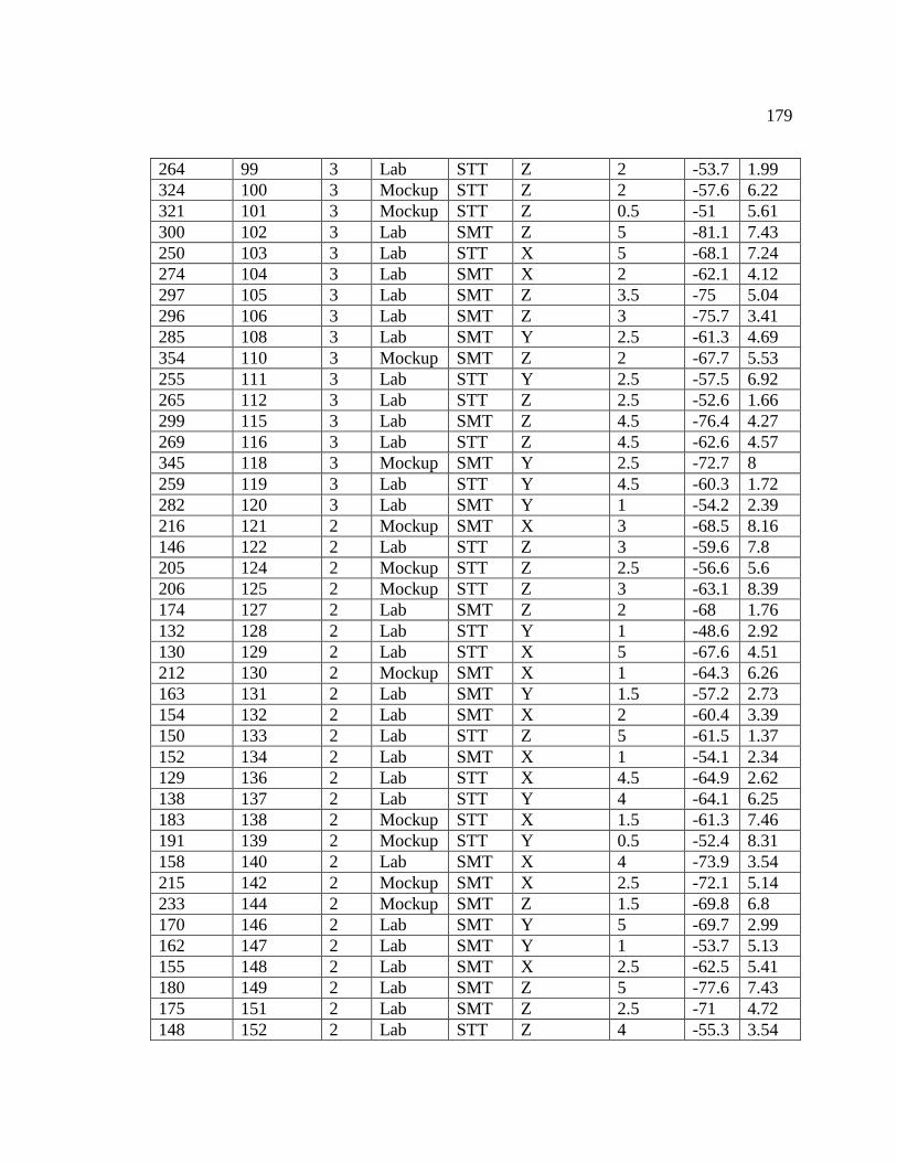
179

264 99 3 Lab STT Z 2 -53.7 1.99

324 100 3 Mockup STT Z 2 -57.6 6.22

321 101 3 Mockup STT Z 0.5 -51 5.61

300 102 3 Lab SMT Z 5 -81.1 7.43

250 103 3 Lab STT X 5 -68.1 7.24

274 104 3 Lab SMT X 2 -62.1 4.12

297 105 3 Lab SMT Z 3.5 -75 5.04

296 106 3 Lab SMT Z 3 -75.7 3.41

285 108 3 Lab SMT Y 2.5 -61.3 4.69

354 110 3 Mockup SMT Z 2 -67.7 5.53

255 111 3 Lab STT Y 2.5 -57.5 6.92

265 112 3 Lab STT Z 2.5 -52.6 1.66

299 115 3 Lab SMT Z 4.5 -76.4 4.27

269 116 3 Lab STT Z 4.5 -62.6 4.57

345 118 3 Mockup SMT Y 2.5 -72.7 8

259 119 3 Lab STT Y 4.5 -60.3 1.72

282 120 3 Lab SMT Y 1 -54.2 2.39

216 121 2 Mockup SMT X 3 -68.5 8.16

146 122 2 Lab STT Z 3 -59.6 7.8

205 124 2 Mockup STT Z 2.5 -56.6 5.6

206 125 2 Mockup STT Z 3 -63.1 8.39

174 127 2 Lab SMT Z 2 -68 1.76

132 128 2 Lab STT Y 1 -48.6 2.92

130 129 2 Lab STT X 5 -67.6 4.51

212 130 2 Mockup SMT X 1 -64.3 6.26

163 131 2 Lab SMT Y 1.5 -57.2 2.73

154 132 2 Lab SMT X 2 -60.4 3.39

150 133 2 Lab STT Z 5 -61.5 1.37

152 134 2 Lab SMT X 1 -54.1 2.34

129 136 2 Lab STT X 4.5 -64.9 2.62

138 137 2 Lab STT Y 4 -64.1 6.25

183 138 2 Mockup STT X 1.5 -61.3 7.46

191 139 2 Mockup STT Y 0.5 -52.4 8.31

158 140 2 Lab SMT X 4 -73.9 3.54

215 142 2 Mockup SMT X 2.5 -72.1 5.14

233 144 2 Mockup SMT Z 1.5 -69.8 6.8

170 146 2 Lab SMT Y 5 -69.7 2.99

162 147 2 Lab SMT Y 1 -53.7 5.13

155 148 2 Lab SMT X 2.5 -62.5 5.41

180 149 2 Lab SMT Z 5 -77.6 7.43

175 151 2 Lab SMT Z 2.5 -71 4.72

148 152 2 Lab STT Z 4 -55.3 3.54

180

142 153 2 Lab STT Z 1 -48.8 4.65

124 154 2 Lab STT X 2 -50.4 3.87

145 155 2 Lab STT Z 2.5 -51.5 1.54

121 156 2 Lab STT X 0.5 -49.1 2.63

186 157 2 Mockup STT X 3 -70.5 8.09

127 158 2 Lab STT X 3.5 -61.8 2.28

234 160 2 Mockup SMT Z 2 -66.6 5.91

164 161 2 Lab SMT Y 2 -59.7 2.79

147 162 2 Lab STT Z 3.5 -57.8 2.22

226 163 2 Mockup SMT Y 3 -69.5 7.29

160 164 2 Lab SMT X 5 -71.5 4.57

223 165 2 Mockup SMT Y 1.5 -67.4 8.28

131 166 2 Lab STT Y 0.5 -44.5 3.89

236 167 2 Mockup SMT Z 3 -73.9 6.91

196 168 2 Mockup STT Y 3 -67.6 9.29

181 169 2 Mockup STT X 0.5 -51.3 6.26

172 172 2 Lab SMT Z 1 -58.9 3.18

211 173 2 Mockup SMT X 0.5 -57.5 7.19

221 174 2 Mockup SMT Y 0.5 -59.7 6.25

151 176 2 Lab SMT X 0.5 -49.3 1.95

179 177 2 Lab SMT Z 4.5 -72.2 4.21

224 179 2 Mockup SMT Y 2 -74.1 7.37

125 180 2 Lab STT X 2.5 -54.5 4.46

165 181 2 Lab SMT Y 2.5 -61.1 4.7

231 182 2 Mockup SMT Z 0.5 -70.6 6.98

144 183 2 Lab STT Z 2 -53.3 1.71

167 185 2 Lab SMT Y 3.5 -67.7 5.24

193 186 2 Mockup STT Y 1.5 -62.6 5.76

178 187 2 Lab SMT Z 4 -73.3 8.43

126 188 2 Lab STT X 3 -56.2 3.43

137 189 2 Lab STT Y 3.5 -64.9 4.17

122 190 2 Lab STT X 1 -54.8 0.96

173 191 2 Lab SMT Z 1.5 -67.5 1.95

168 192 2 Lab SMT Y 4 -70.2 4.95

235 193 2 Mockup SMT Z 2.5 -64.6 6.56

201 195 2 Mockup STT Z 0.5 -51.3 6.25

139 196 2 Lab STT Y 4.5 -71.9 5.4

136 197 2 Lab STT Y 3 -56.3 3.02

161 198 2 Lab SMT Y 0.5 -48.7 1.25

204 199 2 Mockup STT Z 2 -59.6 8.76

194 200 2 Mockup STT Y 2 -58 10.04

166 201 2 Lab SMT Y 3 -60.1 3.91

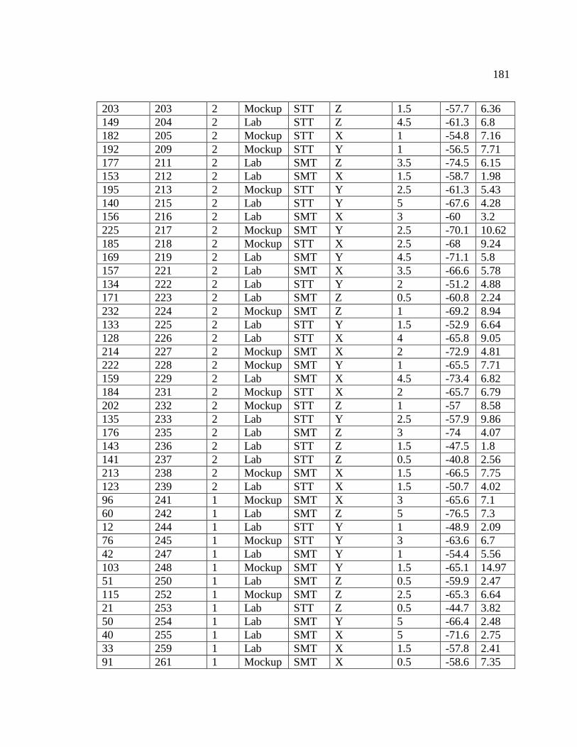
181

203 203 2 Mockup STT Z 1.5 -57.7 6.36

149 204 2 Lab STT Z 4.5 -61.3 6.8

182 205 2 Mockup STT X 1 -54.8 7.16

192 209 2 Mockup STT Y 1 -56.5 7.71

177 211 2 Lab SMT Z 3.5 -74.5 6.15

153 212 2 Lab SMT X 1.5 -58.7 1.98

195 213 2 Mockup STT Y 2.5 -61.3 5.43

140 215 2 Lab STT Y 5 -67.6 4.28

156 216 2 Lab SMT X 3 -60 3.2

225 217 2 Mockup SMT Y 2.5 -70.1 10.62

185 218 2 Mockup STT X 2.5 -68 9.24

169 219 2 Lab SMT Y 4.5 -71.1 5.8

157 221 2 Lab SMT X 3.5 -66.6 5.78

134 222 2 Lab STT Y 2 -51.2 4.88

171 223 2 Lab SMT Z 0.5 -60.8 2.24

232 224 2 Mockup SMT Z 1 -69.2 8.94

133 225 2 Lab STT Y 1.5 -52.9 6.64

128 226 2 Lab STT X 4 -65.8 9.05

214 227 2 Mockup SMT X 2 -72.9 4.81

222 228 2 Mockup SMT Y 1 -65.5 7.71

159 229 2 Lab SMT X 4.5 -73.4 6.82

184 231 2 Mockup STT X 2 -65.7 6.79

202 232 2 Mockup STT Z 1 -57 8.58

135 233 2 Lab STT Y 2.5 -57.9 9.86

176 235 2 Lab SMT Z 3 -74 4.07

143 236 2 Lab STT Z 1.5 -47.5 1.8

141 237 2 Lab STT Z 0.5 -40.8 2.56

213 238 2 Mockup SMT X 1.5 -66.5 7.75

123 239 2 Lab STT X 1.5 -50.7 4.02

96 241 1 Mockup SMT X 3 -65.6 7.1

60 242 1 Lab SMT Z 5 -76.5 7.3

12 244 1 Lab STT Y 1 -48.9 2.09

76 245 1 Mockup STT Y 3 -63.6 6.7

42 247 1 Lab SMT Y 1 -54.4 5.56

103 248 1 Mockup SMT Y 1.5 -65.1 14.97

51 250 1 Lab SMT Z 0.5 -59.9 2.47

115 252 1 Mockup SMT Z 2.5 -65.3 6.64

21 253 1 Lab STT Z 0.5 -44.7 3.82

50 254 1 Lab SMT Y 5 -66.4 2.48

40 255 1 Lab SMT X 5 -71.6 2.75

33 259 1 Lab SMT X 1.5 -57.8 2.41

91 261 1 Mockup SMT X 0.5 -58.6 7.35

182

106 262 1 Mockup SMT Y 3 -66.3 14.96

41 264 1 Lab SMT Y 0.5 -46.3 1.46

101 265 1 Mockup SMT Y 0.5 -58.3 6.69

73 266 1 Mockup STT Y 1.5 -62.5 6.44

71 267 1 Mockup STT Y 0.5 -52.3 8.6

16 268 1 Lab STT Y 3 -55.2 3.17

24 269 1 Lab STT Z 2 -53.2 2.46

5 270 1 Lab STT X 2.5 -53.8 5.09

112 273 1 Mockup SMT Z 1 -69.2 11.25

52 274 1 Lab SMT Z 1 -61.4 5.15

34 275 1 Lab SMT X 2 -60.3 2.61

22 276 1 Lab STT Z 1 -52.7 3.2

13 277 1 Lab STT Y 1.5 -50.7 5.22

10 278 1 Lab STT X 5 -69.5 7.12

30 279 1 Lab STT Z 5 -61.3 1.94

20 280 1 Lab STT Y 5 -68.1 5.04

82 281 1 Mockup STT Z 1 -55.1 8.44

1 282 1 Lab STT X 0.5 -49 2.76

105 283 1 Mockup SMT Y 2.5 -69.7 10.35

43 284 1 Lab SMT Y 1.5 -56.3 2.08

111 285 1 Mockup SMT Z 0.5 -73.1 8.92

7 286 1 Lab STT X 3.5 -60.4 1.62

72 288 1 Mockup STT Y 1 -53.8 6.9

45 289 1 Lab SMT Y 2.5 -60.9 3.67

39 290 1 Lab SMT X 4.5 -70.3 6.73

32 291 1 Lab SMT X 1 -52.6 1.62

18 293 1 Lab STT Y 4 -61 5.69

53 294 1 Lab SMT Z 1.5 -67.1 2.45

61 295 1 Mockup STT X 0.5 -53.3 9.08

74 296 1 Mockup STT Y 2 -59.1 9.85

113 297 1 Mockup SMT Z 1.5 -70 6.81

23 298 1 Lab STT Z 1.5 -47.3 1.34

17 299 1 Lab STT Y 3.5 -59.1 3.14

49 300 1 Lab SMT Y 4.5 -70 6.25

58 301 1 Lab SMT Z 4 -72.4 8.75

102 302 1 Mockup SMT Y 1 -63.7 11.27

36 303 1 Lab SMT X 3 -61.9 4.2

94 304 1 Mockup SMT X 2 -75.5 6.78

63 306 1 Mockup STT X 1.5 -62.3 6.76

84 307 1 Mockup STT Z 2 -57.5 6.66

31 308 1 Lab SMT X 0.5 -49.4 2.14

44 309 1 Lab SMT Y 2 -59.8 3.72

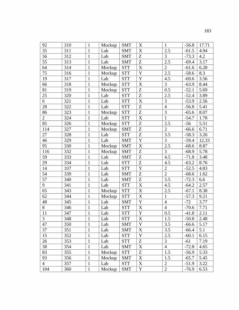
183

92 310 1 Mockup SMT X 1 -56.8 17.71

35 311 1 Lab SMT X 2.5 -61.5 4.94

56 312 1 Lab SMT Z 3 -73.3 4.2

55 313 1 Lab SMT Z 2.5 -69.4 3.17

64 314 1 Mockup STT X 2 -61.6 6.28

75 316 1 Mockup STT Y 2.5 -58.6 8.3

19 317 1 Lab STT Y 4.5 -69.6 3.56

66 318 1 Mockup STT X 3 -63.9 8.44

81 319 1 Mockup STT Z 0.5 -52.1 5.69

25 320 1 Lab STT Z 2.5 -52.4 3.89

6 321 1 Lab STT X 3 -53.9 2.56

28 322 1 Lab STT Z 4 -56.8 5.41

86 323 1 Mockup STT Z 3 -65.6 8.07

2 324 1 Lab STT X 1 -54.7 1.78

85 326 1 Mockup STT Z 2.5 -56 5.51

114 327 1 Mockup SMT Z 2 -66.6 6.71

27 328 1 Lab STT Z 3.5 -58.3 3.26

46 329 1 Lab SMT Y 3 -59.4 12.33

95 330 1 Mockup SMT X 2.5 -68.6 8.87

116 332 1 Mockup SMT Z 3 -68.9 5.78

59 333 1 Lab SMT Z 4.5 -71.8 3.48

29 334 1 Lab STT Z 4.5 -63.2 8.76

14 337 1 Lab STT Y 2 -52.5 4.83

54 339 1 Lab SMT Z 2 -68.6 1.62

57 340 1 Lab SMT Z 3.5 -72.3 6.6

9 341 1 Lab STT X 4.5 -64.2 2.57

65 343 1 Mockup STT X 2.5 -67.1 8.38

62 344 1 Mockup STT X 1 -57.3 9.21

48 345 1 Lab SMT Y 4 -72 3.77

8 346 1 Lab STT X 4 -70.6 7.71

11 347 1 Lab STT Y 0.5 -41.8 2.11

3 348 1 Lab STT X 1.5 -50.8 2.48

47 350 1 Lab SMT Y 3.5 -66.6 5.17

37 351 1 Lab SMT X 3.5 -66.4 5.1

15 352 1 Lab STT Y 2.5 -60.1 6.15

26 353 1 Lab STT Z 3 -61 7.19

38 354 1 Lab SMT X 4 -72.8 4.65

83 355 1 Mockup STT Z 1.5 -56.9 5.33

93 356 1 Mockup SMT X 1.5 -65.7 5.45

4 357 1 Lab STT X 2 -51.9 3.22

104 360 1 Mockup SMT Y 2 -76.9 6.53